FORMAL ANALYSIS OF KEY EXCHANGE PROTOCOLS AND ...

DISS. ETH NO. 20856

FORMAL ANALYSIS OF KEY

EXCHANGE PROTOCOLS AND

PHYSICAL PROTOCOLS

A dissertation submitted toETH ZURICHfor the degree ofDoctor of Sciences

presented byBENEDIKT SCHMIDT

Dipl.-Inf., Universität Karlsruhe (TH), Germanyborn May 1st, 1980Citizen of Germany

accepted on the recommendation ofProf. Dr. David Basin, examiner

Prof. Dr. Srdjan Capkun, co-examinerProf. Dr. Ralf Küsters, co-examiner

2012

AbstractA security protocol is a distributed program that might be executed on a network controlledby an adversary. Even in such a setting, the protocol should satisfy the desired securityproperty. Since it is hard to consider all possible executions when designing a protocol,formal methods are often used to ensure the correctness of a protocol with respect toa model of the protocol and the adversary. Many such formal models use a symbolicabstraction of cryptographic operators by terms in a term algebra. The properties of theseoperators can then be modeled by equations. In this setting, we make the following con-tributions:

1. We present a general approach for the automated symbolic analysis of security proto-cols that use Diffie-Hellman exponentiation and bilinear pairings to achieve advancedsecurity properties. We model protocols as multiset rewriting systems and securityproperties as first-order formulas. We analyze them using a novel constraint-solvingalgorithm that supports both falsification and verification, even in the presence of anunbounded number of protocol sessions. The algorithm exploits the finite variant prop-erty and builds on ideas from strand spaces and proof normal forms. We demonstratethe scope and the effectiveness of our algorithm on non-trivial case studies. For example,the algorithm successfully verifies the NAXOS protocol with respect to a symbolicversion of the eCK security model.

2. We examine the general question of when two agents can create a shared secret. Namely,given an equational theory describing the cryptographic operators available, is there aprotocol that allows the agents to establish a shared secret? We examine this questionin several settings. First, we provide necessary and sufficient conditions for secret estab-lishment using subterm-convergent theories. This yields a decision procedure for thisproblem. As a consequence, we obtain impossibility results for symmetric encryption.Second, we use algebraic methods to prove impossibility results for monoidal theoriesincluding XOR and abelian groups. Third, we develop a general combination result thatenables modular impossibility proofs. For example, the results for symmetric encryptionand XOR can be combined to obtain impossibility for the joint theory.

3. We develop a framework for the interactive analysis of protocols that establish andrely on properties of the physical world. Our model extends standard, inductive, trace-based, symbolic approaches with location, time, and communication. In particular,communication is subject to physical constraints, for example, message transmissiontakes time determined by the communication medium used and the distance betweennodes. All agents, including intruders, are subject to these constraints and this resultsin a distributed intruder with restricted, but more realistic, communication capabilitiesthan those of the standard Dolev-Yao intruder. Building on our message theory thatincludes XOR, we also account for the possibility of overshadowing of message parts.We have formalized our model in Isabelle/HOL and have used it to verify protocolsfor authenticated ranging, secure time synchronization, and distance bounding. Theanalysis of distance bounding attacks accounts for overshadowing and distance hijackingattacks.

3

Zusammenfassung

Sicherheitsprotokolle sind verteilte Algorithmen die in einem Netzwerk ausgeführtwerden können, das von einem Angreifer kontrolliert wird. Dabei sollen die gewün-schten Sicherheitseigenschaften des Protokolls in allen solchen Szenarien gewährleistetsein. Da es schwierig ist während des Protokoll-Entwurfs alle möglichen Ausführungenzu berücksichtigen werden oft formale Methoden eingesetzt, um die Korrektheit eines Pro-tokolls sicherzustellen. Dabei wird ein formales Modell des Protokols und aller möglichenAngreifer genutzt, in dem die kryptographischen Operationen mit Hilfe von Term-Algebrensymbolisch modelliert werden. In diesem Zusammenhang präsentieren wir drei Beiträge.

1. Wir präsentieren eine allgemeine Methode für die automatische symbolische Analysevon Sicherheitsprotokollen die Diffie-Hellman Exponentiation und bilineare Pairingsbenutzen um Sicherheitseigenschaften zu erreichen. Wir modellieren Protokolle alsMultiset Rewriting Systeme und Sicherheitseigenschaften als First-Order Formeln.Unser Algorithmus zur automatischen Analyse solcher Protokolle basiert auf Con-straint Solving und nutzt Ideen aus der Beweistheorie und von Strand Spaces. Wirdemonstrieren die Anwendbarkeit unseres Algorithmus anhand von nicht-trivialen Fall-studien.

2. Wir betrachten die allgemeine Fragestellung ob zwei Agenten ein gemeinsamesGeheimnis erzeugen können. Dabei gehen wir davon aus, dass die verfügbarenOperationen durch eine Term-Algebra und Gleichungen beschrieben werden. Wirbeweisen mehrere Unmöglichkeitsresultate. Unter anderem beweisen wir Resultatefür symmetrische Verschlüsselung, für XOR und ein Kombinationsresultat, mit demUnmöglichkeitsresultate modular bewiesen werden können.

3. Wir entwickeln ein System zur interaktiven Analyse von Protokollen, die physikalischeEigenschaften der Umgebung in der sie ausgeführt werden nutzen und sicherstellen.Unser zugrundeliegendes Modell erweitert Standard-Modelle mit den Konzepten vonOrt, Zeit, und Netzwerk-Kommunikation. Dabei ist die Netzwerk-Kommunikationeingeschänkt, so dass physikalische Gesetze nicht verletzt werden. Wir haben unserModell in dem interaktiven Beweis-Assistenten Isabelle/HOL formalisiert und dieFormalisierung benutzt um die Sicherheit von Authenticated Ranging, Secure Time-Synchronization, und Distance Bounding Protokollen zu analysieren.

5

Acknowledgements

First, I would like to thank my supervisor David Basin for providing me with the opportu-nity to perform research in such a great environment. I am also grateful for all his supportand advice in developing ideas and presenting them. I also want to thank my coauthorsPatrick Schaller, Srdjan Capkun, Simon Meier, Cas Cremers, and Kasper Bonne Rasmussenfor the wonderful cooperations. It was a pleasure to interact with you, at work and outsideof work. Next, I want to thank Ralf Kuesters for his willingness be a co-examiner andvaluable comments on the thesis.

I would also like to thank all members of the Information Security Institute at ETH for aproductive and fun workplace. There were many people that provided valuable discussions,insights, and ideas. In particular, I would like to thank Thanh Binh Nguyen, MichèleFeltz, Mario Frank, Simone Frau, Matus Harvan, Felix Klaedtke, Robert Künnemann,Ognjen Maric, Srdan Marinovic, Bruno Conchinha Montalto, Sasa Radomirovic, Ralf Sasse,Matthias Schmalz, Christoph Sprenger, Nils Ole Tippenhauer, Mohammad Torabi Dashti,and Eugen Zalinescu for feedback on the content of this thesis.

For helping me to find the right balance between work and play, I would like to thankmy friends in Zürich and Trier. Most importantly, I would like to thank my parents andmy two brothers for their patience and for supporting me all the way from the beginningto the end of this journey.

7

Table of contents

Abstract . . . . . . . . . . . . . . . . . . . . . . . . . . . . . . . . . . . . . . . . . . . . . . . . 3

Zusammenfassung . . . . . . . . . . . . . . . . . . . . . . . . . . . . . . . . . . . . . . . . . 5

Acknowledgements . . . . . . . . . . . . . . . . . . . . . . . . . . . . . . . . . . . . . . . . 7

1 Introduction . . . . . . . . . . . . . . . . . . . . . . . . . . . . . . . . . . . . . . . . . . . 13

1.1 Problems . . . . . . . . . . . . . . . . . . . . . . . . . . . . . . . . . . . . . . . . . . . . . 141.1.1 Key Exchange Protocols and Compromising Adversaries . . . . . . . . . . . . 151.1.2 Impossibility of Key Establishment . . . . . . . . . . . . . . . . . . . . . . . . . 171.1.3 Physical Protocols . . . . . . . . . . . . . . . . . . . . . . . . . . . . . . . . . . . . 18

1.2 Contributions . . . . . . . . . . . . . . . . . . . . . . . . . . . . . . . . . . . . . . . . . . 191.2.1 Automated Protocol Analysis . . . . . . . . . . . . . . . . . . . . . . . . . . . . . 191.2.2 Impossibility Results for Key Establishment . . . . . . . . . . . . . . . . . . . . 201.2.3 Interactive Analysis of Physical Protocols . . . . . . . . . . . . . . . . . . . . . 21

1.3 Outline . . . . . . . . . . . . . . . . . . . . . . . . . . . . . . . . . . . . . . . . . . . . . . 23

2 Background . . . . . . . . . . . . . . . . . . . . . . . . . . . . . . . . . . . . . . . . . . . 25

2.1 Security Protocols . . . . . . . . . . . . . . . . . . . . . . . . . . . . . . . . . . . . . . . . 252.1.1 Classical Security Protocols and the Dolev-Yao Adversary . . . . . . . . . . . 252.1.2 Key Exchange Protocols and Compromising Adversaries . . . . . . . . . . . . 272.1.3 Tripartite and Identity-Based Key Exchange Protocols . . . . . . . . . . . . . 312.1.4 Physical Protocols . . . . . . . . . . . . . . . . . . . . . . . . . . . . . . . . . . . . 33

2.2 Notational Preliminaries . . . . . . . . . . . . . . . . . . . . . . . . . . . . . . . . . . . . 352.3 Term Rewriting . . . . . . . . . . . . . . . . . . . . . . . . . . . . . . . . . . . . . . . . . 36

2.3.1 Standard Notions . . . . . . . . . . . . . . . . . . . . . . . . . . . . . . . . . . . . . 362.3.2 Rewriting Modulo and Finite Variants . . . . . . . . . . . . . . . . . . . . . . . 372.3.3 Ordered Completion . . . . . . . . . . . . . . . . . . . . . . . . . . . . . . . . . . . 39

2.4 Isabelle/HOL and the Inductive Approach . . . . . . . . . . . . . . . . . . . . . . . . 39

3 Automated Protocol Analysis . . . . . . . . . . . . . . . . . . . . . . . . . . . . . . 41

3.1 Security Protocol Model . . . . . . . . . . . . . . . . . . . . . . . . . . . . . . . . . . . . 413.1.1 Cryptographic Messages . . . . . . . . . . . . . . . . . . . . . . . . . . . . . . . . 413.1.2 Labeled Multiset Rewriting with Fresh Names . . . . . . . . . . . . . . . . . . 433.1.3 Protocol and Adversary Specification . . . . . . . . . . . . . . . . . . . . . . . . 443.1.4 Trace Formulas . . . . . . . . . . . . . . . . . . . . . . . . . . . . . . . . . . . . . . 463.1.5 Formalization of the one-pass UM Protocol . . . . . . . . . . . . . . . . . . . . 48

3.2 Verification Theory . . . . . . . . . . . . . . . . . . . . . . . . . . . . . . . . . . . . . . . 50

9

3.2.1 Dependency Graphs . . . . . . . . . . . . . . . . . . . . . . . . . . . . . . . . . . . 503.2.2 Dependency Graphs Modulo AC . . . . . . . . . . . . . . . . . . . . . . . . . . . 523.2.3 Normal Message Deduction Rules . . . . . . . . . . . . . . . . . . . . . . . . . . 533.2.4 Normal Dependency Graphs . . . . . . . . . . . . . . . . . . . . . . . . . . . . . . 573.2.5 Guarded Trace Formulas . . . . . . . . . . . . . . . . . . . . . . . . . . . . . . . . 60

3.3 Constraint Solving . . . . . . . . . . . . . . . . . . . . . . . . . . . . . . . . . . . . . . . 623.3.1 Syntax and Semantics of Constraints . . . . . . . . . . . . . . . . . . . . . . . . 623.3.2 Constraint Solving Algorithm . . . . . . . . . . . . . . . . . . . . . . . . . . . . . 633.3.3 Constraint Solving Rules . . . . . . . . . . . . . . . . . . . . . . . . . . . . . . . . 643.3.4 Optimizations for Constraint Solving . . . . . . . . . . . . . . . . . . . . . . . . 743.3.5 One-pass UM: Security proof . . . . . . . . . . . . . . . . . . . . . . . . . . . . . 80

3.4 Extension with Bilinear Pairings and AC operators . . . . . . . . . . . . . . . . . . . 843.4.1 Security Protocol Model . . . . . . . . . . . . . . . . . . . . . . . . . . . . . . . . 843.4.2 Formalization of the Joux Protocol . . . . . . . . . . . . . . . . . . . . . . . . . 853.4.3 Verification Theory . . . . . . . . . . . . . . . . . . . . . . . . . . . . . . . . . . . 853.4.4 Constraint Solving . . . . . . . . . . . . . . . . . . . . . . . . . . . . . . . . . . . . 89

3.5 Implementation and Case Studies . . . . . . . . . . . . . . . . . . . . . . . . . . . . . . 923.5.1 The Tamarin prover . . . . . . . . . . . . . . . . . . . . . . . . . . . . . . . . . . 923.5.2 Security of NAXOS in the eCK Model . . . . . . . . . . . . . . . . . . . . . . . 943.5.3 wPFS Security of RYY . . . . . . . . . . . . . . . . . . . . . . . . . . . . . . . . . 983.5.4 Experimental Results . . . . . . . . . . . . . . . . . . . . . . . . . . . . . . . . . . 993.5.5 Limitations and Extensions . . . . . . . . . . . . . . . . . . . . . . . . . . . . . 102

4 Impossibility Results for Key Establishment . . . . . . . . . . . . . . . . . . . 105

4.1 Preliminaries . . . . . . . . . . . . . . . . . . . . . . . . . . . . . . . . . . . . . . . . . . 1054.2 Traces and Deducibility . . . . . . . . . . . . . . . . . . . . . . . . . . . . . . . . . . . 105

4.2.1 Messages, Frames, and Deducibility . . . . . . . . . . . . . . . . . . . . . . . . 1064.2.2 Derivation Traces . . . . . . . . . . . . . . . . . . . . . . . . . . . . . . . . . . . . 1074.2.3 Shared Secrets and Deducibility . . . . . . . . . . . . . . . . . . . . . . . . . . 1074.2.4 Relating Protocols and Derivation Traces . . . . . . . . . . . . . . . . . . . . 110

4.3 Symmetric Encryption and Subterm-Convergent Theories . . . . . . . . . . . . . 1104.3.1 Symmetric Encryption . . . . . . . . . . . . . . . . . . . . . . . . . . . . . . . . 1104.3.2 Subterm-Convergent Theories . . . . . . . . . . . . . . . . . . . . . . . . . . . . 112

4.4 Monoidal Theories . . . . . . . . . . . . . . . . . . . . . . . . . . . . . . . . . . . . . . 1154.4.1 Impossibility for Group Theories . . . . . . . . . . . . . . . . . . . . . . . . . . 1184.4.2 Protocol for ACU . . . . . . . . . . . . . . . . . . . . . . . . . . . . . . . . . . . 1194.4.3 Impossibility for ACUI and ACUIh . . . . . . . . . . . . . . . . . . . . . . . . 119

4.5 Combination Results for Impossibility . . . . . . . . . . . . . . . . . . . . . . . . . . 1204.5.1 Factors, Interface Subterms, Normalization . . . . . . . . . . . . . . . . . . . 1214.5.2 Combination Result . . . . . . . . . . . . . . . . . . . . . . . . . . . . . . . . . . 122

4.6 Summary . . . . . . . . . . . . . . . . . . . . . . . . . . . . . . . . . . . . . . . . . . . . 123

5 Analysis of Physical Protocols . . . . . . . . . . . . . . . . . . . . . . . . . . . . . 125

5.1 Formal Model . . . . . . . . . . . . . . . . . . . . . . . . . . . . . . . . . . . . . . . . . 1255.1.1 Modeled Concepts . . . . . . . . . . . . . . . . . . . . . . . . . . . . . . . . . . . 1255.1.2 Agents and Transmitters . . . . . . . . . . . . . . . . . . . . . . . . . . . . . . . 126

Table of contents

10

5.1.3 Physical and Communication Distance . . . . . . . . . . . . . . . . . . . . . . 1275.1.4 Messages . . . . . . . . . . . . . . . . . . . . . . . . . . . . . . . . . . . . . . . . . 1285.1.5 Events and Traces . . . . . . . . . . . . . . . . . . . . . . . . . . . . . . . . . . . 1295.1.6 Network, Intruder, and Protocols . . . . . . . . . . . . . . . . . . . . . . . . . . 1305.1.7 Protocol-Independent Results . . . . . . . . . . . . . . . . . . . . . . . . . . . . 132

5.2 Case Studies . . . . . . . . . . . . . . . . . . . . . . . . . . . . . . . . . . . . . . . . . . 1345.2.1 Authenticated Ranging . . . . . . . . . . . . . . . . . . . . . . . . . . . . . . . . 1345.2.2 Ultrasound Distance Bounding . . . . . . . . . . . . . . . . . . . . . . . . . . . 1365.2.3 Secure Time Synchronization . . . . . . . . . . . . . . . . . . . . . . . . . . . . 139

5.3 Extended Model with Xor and Overshadowing . . . . . . . . . . . . . . . . . . . . 1435.3.1 Message Theory for Xor . . . . . . . . . . . . . . . . . . . . . . . . . . . . . . . 1435.3.2 Network Rule with Overshadowing . . . . . . . . . . . . . . . . . . . . . . . . . 146

5.4 Case Study: The Brands-Chaum Protocol . . . . . . . . . . . . . . . . . . . . . . . . 1475.4.1 Security Analysis . . . . . . . . . . . . . . . . . . . . . . . . . . . . . . . . . . . . 1505.4.2 Distance Hijacking Attack on Wrongly Fixed Version . . . . . . . . . . . . . 1515.4.3 Security of Version with Explicit Binding . . . . . . . . . . . . . . . . . . . . . 1535.4.4 Security of Version with Implicit Binding . . . . . . . . . . . . . . . . . . . . . 154

5.5 Isabelle Formalization . . . . . . . . . . . . . . . . . . . . . . . . . . . . . . . . . . . . 155

6 Related Work . . . . . . . . . . . . . . . . . . . . . . . . . . . . . . . . . . . . . . . . . 159

6.1 Security Protocol Analysis . . . . . . . . . . . . . . . . . . . . . . . . . . . . . . . . . 1596.1.1 Cryptographic Messages . . . . . . . . . . . . . . . . . . . . . . . . . . . . . . . 1596.1.2 Protocol Specification and Execution . . . . . . . . . . . . . . . . . . . . . . . 1616.1.3 Property Specification Languages . . . . . . . . . . . . . . . . . . . . . . . . . 1616.1.4 ProVerif . . . . . . . . . . . . . . . . . . . . . . . . . . . . . . . . . . . . . . . . . 1626.1.5 Maude-NPA . . . . . . . . . . . . . . . . . . . . . . . . . . . . . . . . . . . . . . . 1636.1.6 Athena, CPSA, Scyther . . . . . . . . . . . . . . . . . . . . . . . . . . . . . . . . 163

6.2 Impossibility Results . . . . . . . . . . . . . . . . . . . . . . . . . . . . . . . . . . . . . 1636.2.1 Impossibility Results and Bounds for Protocols . . . . . . . . . . . . . . . . . 1646.2.2 Impossibility Results in Cryptography . . . . . . . . . . . . . . . . . . . . . . 1646.2.3 Formal Models of Security Relations . . . . . . . . . . . . . . . . . . . . . . . . 164

6.3 Protocol Analysis with Time, Network Topology, and Location . . . . . . . . . . 164

7 Conclusion . . . . . . . . . . . . . . . . . . . . . . . . . . . . . . . . . . . . . . . . . . . 167

Appendix A Proofs for Chapter 3 . . . . . . . . . . . . . . . . . . . . . . . . . . . . 171

A.1 Proofs for Verification Theory . . . . . . . . . . . . . . . . . . . . . . . . . . . . . . . 171A.1.1 Proofs for Multiplication . . . . . . . . . . . . . . . . . . . . . . . . . . . . . . . 171A.1.2 Proofs for Normal Dependency Graphs . . . . . . . . . . . . . . . . . . . . . . 179A.1.3 Proofs for Formulas . . . . . . . . . . . . . . . . . . . . . . . . . . . . . . . . . . 184

A.2 Proofs for Constraint Solving . . . . . . . . . . . . . . . . . . . . . . . . . . . . . . . 187

Bibliography . . . . . . . . . . . . . . . . . . . . . . . . . . . . . . . . . . . . . . . . . . . . 191

A.2 Proofs for Constraint Solving

11

Chapter 1

Introduction

In the last decade, our reliance on security protocols has increased significantly. The mainreasons are the increased usage of the Internet and the ubiquity of wireless networks anddevices. On the Internet, security protocols are often used to ensure privacy of personal dataor to secure transactions, e.g., in electronic commerce or electronic banking. While wirelessdevices are also used for similar purposes, new application areas for wireless devices haveemerged which require new types of security protocols. For example, car manufacturershave started to replace physical keys with contactless car entry systems. Here, the car doorunlocks automatically if the electronic key for the car is sufficiently close.

While these electronic versions of services or processes are often much more convenientthan their traditional counterparts, obtaining comparable security is often a challenge. Themain problem is that the employed security protocols must achieve their goals even in thepresence of adversaries that interfere with their execution. For example, the security ofprotocols that use the Internet to communicate should not rely on the trustworthiness ofthe service provider who controls the network infrastructure. Hence, most security protocolsemploy cryptographic primitives such as hash functions, digital signatures, and encryptionto remove the need to trust the communication medium. The remaining challenge for thesecurity protocol designer consists of choosing the right primitives and using the primitivescorrectly in the protocol. This is a hard problem since the designer has to balance efficiency,simplicity, and different security goals. Therefore, a large number of security protocolsis proposed each year and many of them contain flaws. This includes newly publishedprotocols [57], standardized protocols [42, 23], and protocols with large-scale deployment[82, 12, 167]. In practice, protocol design is therefore often an iterative process where newattacks are discovered and the protocol is then modified to resist these attacks.

As shown by Lowe [115] who discovered an attack on the Needham-Schroeder pro-tocol [134] that was unknown for 10 years, it is often unclear if all possible attacks havebeen considered. It is therefore desirable to perform the following steps:

1. Make all assumptions about the capabilities of the adversary explicit and give a com-plete specification of the protocol and the desired security property.

2. Prove that the specified protocol achieves the specified security property as long as theassumptions on the adversary hold.

This allows the protocol designer to obtain a guarantee that the protocol is correct withrespect to the given specification and assumptions . Following this idea, two branches ofresearch, adopted by the cryptographic community and the formal methods community,have emerged.

13

The computational (or cryptographic) model represents messages by bitstrings and for-malizes the protocol as a probabilistic polynomial-time Turing machine. The security of theprotocol is then defined in terms of a game, where an arbitrary probabilistic polynomial-time Turing machine, which models the adversary, interacts with the protocol. The protocolis secure if the probability of winning this game is negligible for all such adversaries.Usually, the proof is performed by reduction to a problem that is assumed to be hard suchas factoring large composite integers. If there is an adversary that attacks the protocol withnon-negligible probability, then the adversary can be used to construct an efficient solver forthe hard problem, which was assumed to be infeasible. These proofs are usually long andintricate and many published proofs are incomplete or do not make all assumptions explicit[113, 103, 127, 98]. Recently, machine-support for performing proofs in the computationalmodel has been developed [19, 29], but the fully automated construction of such proofs forsecurity protocols is still out of reach.

The symbolic (or formal) model introduced by Dolev and Yao [69] models messages byterms in a term algebra and the possible operations on messages by message deductionrules. For example, enc(m, k) represents the encryption of the message represented bythe term m with the key represented by the term k. This term can then be used asfollows to deduce new messages. It can be paired with other known messages, encryptedwith known keys, or, if the key k is known, m can be extracted. The assumption that anencryption cannot be used in any other way is called the perfect cryptography assumption.In symbolic models, different formalisms are used to specify protocols and to define theirpossible executions. Usually, these formalisms use terms to denote the messages that aprotocol receives and sends on the network. Given a protocol, its executions are definedas the possible interactions with an adversary that controls the network and deduces newmessages by applying message deduction rules. A protocol satisfies a security property,such as secrecy of a certain message, if all its executions satisfy the property.

Compared to the computational model, the symbolic model abstracts away from manydetails. On the one hand, this means that the symbolic model may miss attacks capturedby the computational model. On the other hand, the symbolic model is considerably simplerand many practically relevant attacks are still captured by the symbolic model. Because ofthe relative simplicity of the model, there are several tools [28, 62, 77] that perform fullyautomated security proofs for a wide range of security protocols. Some of them also providecounterexamples when the proof fails. The symbolic model is also a good fit for obtainingmeta-theoretical results about security protocols. Finally, it is also considerably simplerto mechanize symbolic security proofs in a theorem prover to obtain machine-checkedproofs since no reasoning about bitstrings, computational complexity, and probabilities isrequired.

1.1 Problems

Even though symbolic models models have been successfully applied to many differentapplication areas, there are still several types of security protocols that are outside thescope of existing approaches. In this thesis, we focus on two such types of protocols. First,there is no method that supports the fully automated, unbounded analysis of many recentauthenticated key exchange protocols with respect to their intended adversary models.

Introduction

14

Second, there is no general formal model (computational or symbolic) that supports rea-soning about protocols that utilize and establish physical properties of nodes and theirenvironment. As an example of such a protocol, consider the protocol executed between anelectronic key and a car to establish the distance between the two. Moreover, we investigatea third question in the symbolic setting: Which operations are required to allow two agentsto establish a key using an authentic (but not secret) channel?

1.1.1 Key Exchange Protocols and Compromising Adversaries

Authenticated key exchange (AKE) protocols are widely used components in modern net-work infrastructures. They are often based on public-key infrastructures and their goal is toauthenticate the communication partners and to establish a shared symmetric session keythat can be used to secure further communication. Recent protocols are designed to achievethese goals even in the presence of strong adversaries who can, under certain conditions,reveal session keys, long-term private keys, and the randomness used by the participants.For example, the NAXOS protocol [111] is designed to be secure in the extended Canetti-Krawzyk (eCK) model [111] where only those combinations of reveals are forbidden thatdirectly lead to an attack on this protocol.

The main building block for most AKE protocols is Diffie-Hellman (DH) exponentiationin a cyclic groupG of prime order p generated by a group element g, i.e.,G=gn|n∈N andgp=1. AKE protocols exploit equalities such as (gn)m=(gm)n that hold in all such groupsand that allow the participants to compute the same key in different ways. For instance,in the Diffie-Hellman protocol [68], the participant A knows his private exponent a andthe public group element gb of the other participant B. Similarly, B knows b and ga. Thenboth can compute gab as (gb)a and (ga)b. Attacks on AKE protocols also exploit equalitiesthat hold in such DH groups. Interestingly, many attacks are generic in the following sense.They only use operations and equalities that hold in all DH groups and therefore workindependently of the concrete group used by the protocol.

AKE protocols and their adversary models are an active area of research [42, 59, 43,58, 166]. Many protocols are proposed together with a pen and paper proof in the com-putational model with respect to an adversary model adapted for the protocol underconsideration. The proofs are either just proof sketches or long and complicated and itis hard to check if such a proof is correct or can be adapted to a modified adversarymodel. Hence, it would be useful to have a tool that takes a specification of a protocoland an adversary model and performs a fully automated search for a proof or a coun-terexample in the symbolic model. Of course, the existence of a symbolic proof does notrule out all attacks captured by the computational model. But with the right symbolicmodel, a symbolic proof is still meaningful since it rules out a well-defined and relevantclass of attacks. Furthermore, a symbolic attack is also a computational attack and mighthelp to discover flawed computational proofs or help to fix the protocol or adversary modelbefore attempting a computational proof.

To perform automated symbolic analysis of such AKE protocols, we identify the followingrequirements on the employed method:

1. The message theory must capture the required operations in DH groups and theiralgebraic properties. This means at least exponentiation and the previously mentionedequalities required to establish the shared key in the DH protocol must be captured.

1.1 Problems

15

Additionally, it would be nice to handle inverses of exponents, which are used by someprotocols such as MTI/C0 [119]. Support for the addition of exponents and multiplica-tion of DH group elements would further extend the scope to more protocols [113, 103].Note that if more operations and equations are modeled, then more attacks are cap-tured. This might be relevant even if the protocol under consideration does not employthese operations directly.

2. To support the analysis of modern tripartite and identity-based AKE protocols, themessage theory should also support bilinear pairings.

3. Since the adversary models are defined by stateful queries such as“SessionKeyReveal(s): If the session is completed, but unexpired, thenM obtainsthe corresponding session key” [42],

it would be desirable if the method directly supports the modeling of state and reasoningabout state such as the status of a session.

4. Since the winning conditions for the adversary that capture the adversary model oftencontain logical formulas with temporal statements such as

“[there must be a] Long-Term Key Reveal(B) before completion of the session” [110],it would be desirable for the specification language to support such (temporal) formulas.

5. The method should support attack finding and proofs with respect to an unboundednumber of protocol sessions.

Requirements 1.–4. apply to the specification languages for protocol and property and tothe execution model. The usual way to support 1. and 2. is to represent cryptographicmessages by terms modulo an equational theory E that captures the required algebraicproperties. Requirement 5. applies to the method that is used to analyze protocols withrespect to an execution model that satisfies the other requirements. Since secrecy for anunbounded number of sessions is already undecidable for simpler execution models [72],the best we can hope for is to find proofs or attacks for many relevant examples. Givenrequirement 5., we evaluate existing approaches for the automated unbounded analysisof security protocols with respect to these requirements. The approaches can be roughlyassigned to three different groups which we consider separately.

The Horn-theory based approach [168] implemented in ProVerif [28] was originallyrestricted to secrecy and similar properties that can be encoded as derivability in Horntheories. Blanchet [30] extends the approach to support correspondence properties, whichcan be used to formalize authentication properties such as injective agreement. Blanchetet al. [31] also show how to support a restricted set of equational theories that doesnot include associative and commutative operators. For DH, this approach supports amodel that captures exactly the equality (gx)y = (gy)x, but does not account for inversesof exponents. Together, these extensions have been used in [1] to analyze AKE protocolswith respect to adversary models that account for session key compromise and long-termkey compromise. This work combines correspondence properties with ProVerif’s support forphases and distinguishing between compromised and uncompromised sessions. It is unclearhow well this approach generalizes to more advanced adversary models such as eCK (withperfect forward secrecy) because of the limited support for temporal statements in corre-spondence properties and the limited support for non-monotonic state in ProVerif. Küstersand Truderung [108, 109] later lift the previously described restriction on equational theo-ries and show how ProVerif can be used to verify protocols with respect to XOR and a modelof Diffie-Hellman exponentiation with inverses. Pankova and Laud [138] have recently

Introduction

16

extended this approach with support for bilinear pairings. Unfortunately, these exten-sions are not compatible with the support for correspondence properties and are thereforerestricted to authentication properties that can be encoded as derivability in Horn theories.

Maude-NPA [77] is based on backwards narrowing modulo an equational theory. Proto-cols can be specified by linear role scripts and properties can be specified by characterizingthe attack states by symbolic terms. The backwards narrowing approach is very generalwith respect to the supported equational theories and only requires an implementationof equational unification to work. To achieve termination in bounded and unboundedscenarios, the tool employs various state-space reduction techniques [78] that have to beadapted for different equational theories. In [76], the Diffie-Hellman protocol is analyzedwith respect to the standard Dolev-Yao adversary and an equational theory that does notaccount for inverses. We are not aware of any case studies that consider an equationaltheory with inverses or advanced adversary models.

The Athena [162], Scyther [62], and CPSA [150] tools are all based on similar ideas. Theyperform a complete search for attacks by representing attack states symbolically by the setof events that must have occurred and the causal dependencies between these events. Thecausal dependencies capture, for example, that a message must be known by the adversarybefore it is received by the protocol. The search can terminate for two different reasons.First, if all causal dependencies are satisfied, a ground attack trace (or bundle) can beextracted from the symbolic state. Second, if some dependency cannot be satisfied, thenthe attack state is not reachable and the security of the protocol has been proved. All threetools only support linear role scripts and do not support equational theories. The tools allsupport security properties of the form ∀xR .ϕ ∃yR .ψ where ϕ is a conjunction of eventsand ψ is a disjunction of events. Scyther has been extended [22] with support for numerouscompromising adversary models, but these are hardcoded and cannot be specified by theuser. We refer to Chapter 6 for a detailed discussion of existing approaches.

1.1.2 Impossibility of Key Establishment

Consider a pair (or more generally a group) of honest agents who have no shared secret,but who can communicate over a public channel in the presence of a passive adversary.Furthermore, assume that each agent can generate unguessable nonces, has access to publicinformation, and may use different cryptographic operators. Is it possible for these agentsto establish a shared secret?

There are of course many ways to answers this question positively. For example, if thecryptographic operators include a public-key cryptosystem, an agent may simply send hispublic key over the public channel. Any other agent could then encrypt a secret with thepublic key that can be decrypted only by the agent holding the corresponding private key.Similarly, if a multiplicative group is given for which the so called Diffie-Hellman problemis hard, agents can use the Diffie-Hellman protocol to establish a shared secret. Thereare also negative answers if the set of cryptographic operators is sufficiently restricted. Inparticular, there is a folk theorem that no protocol exists if only symmetric encryption canbe used. However, to the best of our knowledge, no formal proof of this folk theorem haspreviously been given.

Establishing impossibility results and developing related proof methods are of funda-mental theoretical importance as they explain what cannot be achieved using cryptographicoperators, specified equationally. Practically, impossibility results delineate the solution

1.1 Problems

17

space in protocol design and enable a more systematic approach to protocol developmentby guiding the choice of cryptographic operators. This is especially relevant in resourceconstrained scenarios, like with smartcards or sensor networks, where operations like public-key cryptography are sometimes considered too expensive and should be avoided, wherepossible.

1.1.3 Physical Protocols

The shrinking size of microprocessors combined with the ubiquity of wireless networksand devices has led to new application areas for networked systems with novel securityrequirements for the employed protocols. Whereas traditional security protocols are mainlyconcerned with message secrecy or variants of authentication, new application areas oftencall for new protocols that securely establish properties of the network environment. Exam-ples include:

Physical Proximity. One node must prove to another node that a given value is a reliableupper bound on the physical distance between them. Such protocols may use authenti-cation patterns along with assumptions about the underlying communication medium[34, 38, 92, 123, 151]. An important use-case for such protocols are contactless car entrysystems.

Secure Localization. A node must determine its true location in an adversarial settingor make verifiable statements about its location by executing protocols with other nodes[40, 105, 114, 156]. Secure localization and physical proximity verification protocols,and attacks on them, have been implemented on RFID, smart cards, and Ultra-WideBand platforms [71, 153, 151].

Secure Time Synchronization. A node must securely synchronize its clock to the clockof another trusted node in an adversarial setting [84, 164].

Secure Neighbor Discovery or Verification. A node must determine or verify itsdirect communication partners within a communication network [139]. Reliable infor-mation about the topology of a network is essential for all routing protocols.

What these examples have in common is that they all concern physical properties of thecommunication medium or the environment in which the nodes live. Furthermore, standardsymbolic protocol models based on the Dolev-Yao intruder lack the required features toformalize these protocols:

1. They do not model global time and local clocks that can be accessed by nodes anddeviate from the global time.

2. They do not reflect the location of nodes and the distance between nodes induced bytheir locations.

3. They do not reflect the network topology which characterizes possible communicationbetween nodes and lower bounds on message transmission times.

4. They do not support a distributed intruder. If location and communication abilitiesof individual nodes are reflected in a model, then this implies certain bounds on theexchange of information between nodes. Since these bounds should also apply to theintruder, e.g., the intruder cannot transfer knowledge instantaneously from one locationto another, we cannot collapse all intruders into one intruder.

Introduction

18

There are some models that account for one of these aspects, but none that capture all ofthem. Again, we refer to Chapter 6 for a detailed discussion of existing approaches.

1.2 Contributions

To address the three problems described in the previous section this thesis presents thefollowing contributions.

1.2.1 Automated Protocol Analysis

Starting with an expressive and general security protocol model where protocol and adver-sary are specified as multiset rewriting rules, security properties are specified as first-ordertrace-formulas, and executions are defined by multiset rewriting modulo an equationaltheory, we present four contributions. First, we demonstrate that such a model is well-suited for the formalization of AKE protocols and their adversary models. Second, we givea verification theory based on an alternative representation of executions that reduces thesearch space and allows for a compact symbolic representation of executions by constraints.Third, we give a sound and complete constraint solving algorithm for the falsification andunbounded verification of protocols with respect to our model. Fourth, we implemented ouralgorithm in a tool, the Tamarin prover [126], and validated its effectiveness on a numberof case studies.

Our security protocol model uses an equational theory E to specify the considered crypto-graphic operators, their properties, and the message deduction capabilities of the adversary.We support the disjoint combination of a subterm-convergent theory and a theory thatmodels DH exponentiation with inverses, and bilinear pairings. To specify the protocoland adversary capabilities, we use a labeled multiset rewriting system S with support forfresh name generation and persistent facts. The traces are then defined by labeled multisetrewriting modulo E with S. In our setting, a trace is a sequence of sets of facts. Tracesthat satisfy a given security property are then characterized by first-order formulas builtover the predicate symbols f@ i (fact f occurs in the trace at position i), i≺ j (timepointi is smaller than timepoint j), and t≈ s ( t=E s for terms t and s). We support arbitrarynesting of quantifiers and quantification over messages and timepoints, but all quantifiedvariables must be guarded by atoms [7].

We show that our model allows for a natural formalization of a wide range of protocolsand adversary models. For example, we present models for NAXOS [111] security in theeCK model [111], perfect forward secrecy of the Joux tripartite key exchange protocol [97],and security of the RYY protocol [155] under session key reveals and long-term key reveals.

The main result of our verification theory is that instead of defining executions viamultiset rewriting modulo E with S, we can use an alternative definition based on Eand S that reduces the search space and simplifies the symbolic representation of oursearch-state by constraints. To arrive at this alternative definition, we perform a series ofreduction steps which preserves the set of traces. First, we switch from multiset rewritingderivations to dependency graphs, a representation that uses sequences of multiset rewritingrule instances and causal dependencies between generated and consumed facts, similar tostrand spaces [83]. Second, we decompose E into a rewrite system R and an equationaltheoryAX (that contains no cancellation rules) such thatR,AX has the finite variant prop-

1.2 Contributions

19

erty. This allows us to replace S by its set of R,AX -variants and use dependency graphsmodulo AX . Third, we partition the message deduction rules into deconstruction andconstruction rules, which is possible since we now use R,AX -variants, to apply the notionof normal proofs [146, 48] to message deduction in dependency graphs. After extendingthis notion from proof trees to proof graphs and from the standard Dolev-Yao operators toDH exponentiation and bilinear pairings, we show that we can restrict ourselves to normaldependency graphs in our search since normal message deduction is complete.

Our constraint solving algorithm takes a security property ϕ and a protocol P and per-forms a complete search for counterexamples to ϕ that are also traces of P . Our algorithmexploits the results from our verification theory and searches for normal dependency graphsmodulo AX . We give a full proof of soundness and completeness of the constraint solvingrules and also show that we can extract an attack if we reach a solved constraint system.

We show that despite the undecidability of the problem, Tamarin performs well: Fornon-trivial AKE protocols and adversary models from the literature, it terminates in thevast majority of cases. For most 2-round AKE protocols and their intended adversarymodels, the times for falsification and unbounded verification are in the range of a fewseconds. For more complicated models including multi-protocol scenarios, tripartite AKEprotocols, and identity-based AKE protocols, Tamarin terminates in under two minutes.

1.2.2 Impossibility Results for Key Establishment

We present a formal framework to prove impossibility results for secret establishmentfor arbitrary cryptographic operators in the symbolic setting. We model messages andoperations by equational theories and communication by traces of events as is standard insymbolic protocol analysis. The initial question of whether it is possible for two agents toestablish a shared secret therefore reduces to the question: Is there a valid trace where twoagents end up sharing a message that cannot be deduced from the exchanged messages?

We start by applying our framework to the equational theory that models symmetricencryption and prove the folk theorem that secret establishment is impossible in this set-ting. It turns out that symmetric encryption is actually an instance of the more general casewhere the properties of the involved operators can be described by a subterm-convergenttheory. For this general class of equational theories, we present a necessary and sufficientcondition for the possibility of secret establishment based on labelings of the equations.This directly yields a decision procedure that either returns a labeling that corresponds toa trace where two agents establish a shared secret or returns “impossible” if there is none.For an equational theory that models a public-key cryptosystem, the labeling returnedcorresponds to the message exchange previously mentioned where the secret is encryptedusing the public key previously exchanged. Afterwards, we consider monoidal theories.First, we show that secret establishment is impossible for the subset of group theorieswhich includes theories that model XOR and abelian groups. For the remaining monoidaltheories that are usually considered in the setting of security protocol analysis, we eitherexhibit a protocol from the literature that can be used to establish a shared secret or givea separate proof that secret establishment is impossible. This includes theories that modelmultisets and sets. Monoidal theories are not subterm-convergent since they define asso-ciative and commutative operators. Therefore, we use algebraic methods that exploit theisomorphisms between the term algebras modulo the equational theory and the standardalgebraic structure of a (semi)ring.

Introduction

20

The above results are for theories in isolation. We also investigate the problem of com-bining theories and prove a combination result for disjoint theories: Secret establishmentin the combination of the theories is possible if and only if it is already possible for oneof the individual theories alone. This allows for modular proofs where separate resultsare combined. For example, we prove this way that secret establishment is impossible forsymmetric encryption together with XOR.

1.2.3 Interactive Analysis of Physical Protocols

We present a formal model for reasoning about security guarantees of physical protocolslike those listed earlier. Our model builds on standard symbolic approaches and accountsfor physical properties like time, the location of network nodes, and properties of thecommunication medium. Honest agents and the intruder are modeled as network nodes.The intruder, in particular, is not modeled as a single entity but rather as a distributed oneand therefore corresponds to a set of nodes. The ability of the nodes to communicate andthe speed of communication are determined by nodes’ locations and by the propagationdelays of the communication technologies they use. As a consequence, nodes (both honestand those controlled by the intruder) require time to share their knowledge and informationthat they exchange cannot travel between nodes at speeds faster than the speed of light.The intruder and honest agents are therefore subject to physical restrictions. This resultsin a distributed intruder with communication abilities that are restricted, but more realisticthan those of the classical Dolev-Yao intruder.

Our model bridges the gap between informal approaches used to analyze physical proto-cols for wireless networks and the formal approaches taken for security protocol analysis.Informal approaches typically demonstrate the absence of a given set of attacks, ratherthan proving that the protocol works correctly in the presence of an active adversarytaking arbitrary actions. In contrast, existing formal approaches fail to capture the detailsnecessary to model physical protocols and their intended properties. To bridge this gap, ourmodel formalizes an operational, trace-based semantics of security protocols that accountsfor time, location, network topology, and distributed intruders. To model cryptographicoperators and message derivability, we reuse Paulson’s [140] message theory based on theperfect cryptography assumption and extend it with XOR.

In what follows, we explain our contributions in more detail. First, we give a noveloperational semantics that captures the essential physical properties of space and time andthereby supports natural formalizations of many physical protocols and their correspondingsecurity properties. For example, properties may be stated in terms of the relative distancebetween nodes, the locations of nodes, and the times associated with the occurrence ofevents. Moreover, protocols can compute with, and base decisions upon, these quantities.To obtain a realistic model of the communication technology used, for example, by distancebounding protocols, our operational semantics accounts for the modification of messagesthat are in transmission. More precisely, we account for the following concrete scenarios.We allow the intruder to overshadow individual components of a concatenation by knownmessages. Additionally, we account for the non-negligible probability of flipping a lownumber of bits in an unknown message m by randomly sending data. This allows theadversary to modify the original message m into a close message m′, with respect to theHamming-distance.

1.2 Contributions

21

Second, despite its expressiveness, our operational semantics is still simple and abstractenough to allow its complete formalization. We have formalized our model in Isabelle/HOLand used it to formally derive both protocol-independent and protocol-specific properties,directly from the semantics. Protocol-independent properties formalize properties of com-munication and cryptography, independent of any given protocol. For example, it followsfrom our operational semantics that there are no collisions for randomly chosen nonces andthat communication cannot travel faster than the speed of light. This allows us to prove ina protocol-independent way a lower bound on the time until an adversary learns a noncedepending on his distance to the node generating the nonce. We use these properties, inturn, to prove protocols correct or to uncover weaknesses or missing assumptions throughunprovable subgoals.

Third, we show that our approach is viable for the mechanized analysis of a rangeof wireless protocols. We demonstrate this by providing four case studies that highlightdifferent features of the model:

• Our formalization of an authenticated ranging protocol shows how time-of-flight mea-surements of signals relate to physical distances between nodes. Additionally, the modelhas to account for local computation times which are included in protocol messages.

• Our formalization of an ultrasound distance bounding protocol demonstrates how themodel accounts for transceivers that employ different communication technologies andtheir interaction. Furthermore, the example shows how our notion of location can beused to formalize private space assumptions.

• Our formalization of a secure time synchronization protocol illustrates how we canmodel relations between local clock offsets of different nodes. It also shows how boundson the message transmission time can be specified.

• Our formalization of the Brands-Chaum distance bounding protocol [34] demonstratesthe usage of XOR and why the model accounts for overshadowing. We present an attackon the protocol and various flawed and successful fixes.

Finally, we discuss how our security property for distance bounding protocols capturesa new class of attacks that is relevant in practical scenarios, but has previously beenoverlooked by informal approaches. Consequently, we were the first to discover such anattack on a distance bounding protocol by Meadows et al. [123].

Introduction

22

1.3 Outline

Chapter 2. Presents background on security protocols, some mathematical preliminaries,and background on term rewriting.

Chapter 3. Describes the theory and implementation of the Tamarin prover. Thechapter is based on joint work and extends it with support for bilinear pairings andassociative and commutative operators. The joint work has been published in:

Automated analysis of Diffie-Hellman protocols and advanced security properties.With Simon Meier, Cas Cremers and David A. Basin.In Proceedings of the 25rd IEEE Computer Security Foundations Symposium, CSF2012 , pages 78–94. IEEE Computer Society, 2012.

Chapter 4. Describes the impossibility results for key establishment. The chapter is basedon joint work and generalizes the impossibility results for XOR and abelian groups to(monoidal) group theories. The joint work has been published in:

Impossibility results for secret establishment.With Patrick Schaller and David Basin.In Proceedings of the 23rd IEEE Computer Security Foundations Symposium, CSF2010 , pages 261–273. IEEE Computer Society, 2010.

Chapter 5. Describes the framework for physical protocols and the case studies. This isjoint work that has been published in:

Modeling and verifying physical properties of security protocols for wireless networks.With Patrick Schaller, David Basin, and Srdjan Capkun.In Proceedings of the 22nd IEEE Computer Security Foundations Symposium, CSF2009 , pages 109–123. IEEE Computer Society, 2009.

Let’s get physical: models and methods for real-world security protocols.With David Basin, Srdjan Capkun, and Patrick Schaller.In Theorem Proving in Higher Order Logics (TPHOLs), pages 1–22. 2009 (invitedpaper).

Formal reasoning about physical properties of security protocols.With David Basin, Srdjan Capkun, and Patrick Schaller.In ACM Transactions on Information and System Security (TISSEC), 14(2):16, 2011.

Distance Hijacking Attacks on distance bounding protocols.With Cas Cremers, Kasper B. Rasmussen, and Srdjan Capkun.In 33rd IEEE Symposium on Security and Privacy, S&P 2012 , pages 113–127. IEEEComputer Society, May 2012.

Chapter 6. Summarizes the related work and compares it to the contributions of thisthesis.

Chapter 7. Presents the conclusion and discusses future work.

1.3 Outline

23

Chapter 2

Background

In this chapter, we present background on security protocols and technical background. Forsecurity protocols, we focus on authenticated key exchange protocols and physical proto-cols. The technical background consists of the mathematical preliminaries, a short introduc-tion to term rewriting, and a short introduction to Isabelle/HOL [136] and Paulson’sinductive approach to protocol verification [140].

2.1 Security Protocols

In this section, we first introduce the classical Dolev-Yao model for security protocols. Thenwe present key exchange protocols based on Diffie-Hellman exponentiation and bilinearpairings and their desired security properties. Finally, we introduce physical protocols suchas authenticated ranging and distance bounding protocols.

2.1.1 Classical Security Protocols and the Dolev-Yao Adversary

A security protocol is a distributed program that is executed by different entities calledagents that exchange messages. The goal of a security protocol is to achieve a certainobjective, even in the presence of external or internal attackers that do not follow therules of the protocol. For example, the goal of a security protocol could be to enablethe participants to agree on a secret without revealing it to non-participants. A securityprotocol is usually split into multiple roles such as initiator and responder. Each rolespecifies the actions of the agent executing the role. The set of possible actions usuallyincludes sampling random values, applying cryptographic operators, sending messages, andreceiving messages.

As an example, consider the simple challenge-response protocol given in Figure 2.1. Theprotocol consists of two roles A and B whose actions are given on the left and right sideof the figure. The arrows in the middle depict the exchanged messages. Note that we usethe roles A and B as placeholders for the agents executing the roles in the specification ofthe messages. An agent A executing an instance of the role A that intends to execute theprotocol with an agent B executing role B proceeds as follows. First, he chooses a freshnonce na and encrypts the nonce with B’s public key sending the result to B. Then, hewaits for a response by B. If the response is equal to the hash of na, he successfully finishesthe protocol. Otherwise, the protocol execution fails. An agent B executing an instanceof the role B receives a message from A and tries to decrypt the message with his secretkey skB. If the decryption succeeds, he applies a hash function to the resulting cleartextand sends this message back to A. We call an instance of a protocol role executed by someagent a session . We call the intended communication partner of a session the peer .

25

A B

choose fresh nonce na

c7 encpkB(na)

c

x7 decskB(c)

r7 h(x)

r

check that r= h(na)

Figure 2.1. A simple challenge-response protocol.

Even though the figure suggests that the message exchange betweenA and B is authentic,protocols are often analyzed in an open network where this is not the case. For example,many symbolic approaches analyze security protocols with respect to the so called Dolev-Yao model [69] which is based on the following three assumptions:

1. Each agent can simultaneously execute an arbitrary number of sessions of the protocolunder consideration, possibly executing different roles with different parameters at thesame time.

2. The perfect cryptography assumption is employed. This means that cryptographic oper-ators are modeled by a term algebra and only a fixed set of operations can be used todeduce new messages from known messages. For example, given a ciphertext, the onlyway to recover the plaintext is to perform decryption with the right key. Furthermore,the set of agents is partitioned into honest agents and dishonest agents. The long-termkeys of honest agents are assumed to be secret and the long-term keys of dishonestagents are known to the adversary.

3. With respect to the network, the strongest possible adversary is assumed. The Dolev-Yao model identifies the network and the adversary. This means the adversary receivesall messages sent by other agents and agents can only receive messages from the adver-sary. Here, the adversary is allowed to send any message that is deducible from receivedmessages and from his initial knowledge.

Session 1 (R1)actor C1

peer D1

Session 2 (R2)actor C2

peer D2

Session k (Rk)actor Ckpeer Dk

↑↓ ↑↓ ↑↓

Adversary

Figure 2.2. Protocol execution in the Dolev-Yao model.

Figure 2.2 depicts a protocol execution in the Dolev-Yao model. Different protocol ses-sions receive messages from the adversary and send messages to the adversary. There isno guarantee that the sessions match up, i.e., that the communication patterns correspondto the desired ones. The adversary can delete, modify, replay, and forward messages fromdifferent sessions. The goal of a security protocol is often to prevent such undesired behav-

Background

26

iors. An authentication property ensures that if a protocol session finishes successfully undercertain conditions, then there is another session that agrees on certain parameters suchas the participants and the exchanged messages. Authentication properties are often usedtogether with secrecy properties that guarantee that the adversary cannot learn certainprotocol data.

Consider the simple challenge-response protocol from Figure 2.1. Here, an honest agent Aexecuting role A with an honest peer B obtains two guarantees after successfully finishingthe protocol. First, B executes a session of the role B that sends the response after A sentthe challenge and before A receives the response. Second, the nonce na is known to B andnot known to any other agents. From the perspective of B, there are no useful guaranteessince the adversary can always fake the message encpkB

(na).

2.1.2 Key Exchange Protocols and Compromising Adversaries

In this section, we discuss the mathematical primitives employed by most authenticatedkey exchange (AKE) protocols, the signed Diffie-Hellman protocol, the Unified Model (UM)protocol, and the extended Canetti-Krawczyk adversary model for AKE protocols.

2.1.2.1 Diffie-Hellman Exponentiation

In the following, we consider a cyclic group G = 〈g〉 of prime order p. For n ∈ N, gn

denotes the n-fold product∏

i=1

ng of g. Since gp = 1, we can consider the exponents as

elements of Zp, the integers modulo p. We are interested in such groups, where, given gn

and gm for randomly chosen n and m, it is hard to compute gnm. This problem is calledthe computational Diffie-Hellman (CDH) problem . The hardness of the CDH problemimplies the hardness of the discrete logarithm (DL) problem, which states that it is hardto compute n from gn for a random n. In the following, we call a group as described abovea Diffie-Hellman (DH) group. It is easy to see that the equality (gn)m= gnm=(gm)n holdsin all DH groups. This equality states that exponentiation with n and exponentiation withm commute and it is the basis of the Diffie-Hellman Key Exchange protocol.

2.1.2.2 Diffie-Hellman Key Exchange Protocol

The basic DH protocol proposed by Diffie and Hellman [68] in 1976 is the first realistic pro-tocol that allows two agents to establish a shared secret over an authentic (not confidential)channel without sharing any information beforehand. In Figure 2.3, we show a variant ofthe DH protocol that establishes a shared key between two agents. The SIGDH protocoluses signatures to support insecure channels. We assume that before starting the protocol,A knows his own signing key skA and B’s signature verification key pkB and we haveanalogous assumptions on B’s knowledge. To initiate the protocol, A chooses the responderB and a random exponent x ∈ Zp. This exponent is often called the ephemeral privatekey of the given session. The group element gx which is sent to B is the correspondingephemeral public key . To proceed, A signs the concatenation of B’s identity and gx with hissigning key and sends the resulting message to B. When B receives the message from A,he verifies the signature and stores the received ephemeral public key X. Then, he choosesa random exponent y ∈ Zp and replies with the concatenation of gy and a signature onthe concatenation of A’s identity and gy. A verifies the signature and stores the receivedgroup element as Y . Now, both can compute the shared key h(gxy) as h(Y x) and h(X y).The value gxy is often called ephemeral DH key .


27

A Bsignature keys: (skA, pkA) signature keys: (skB, pkB)choose random exponent x

X7 gx, σA: =sigskA(〈B ,X 〉)

〈X,σA〉check signature σAchoose random exponent yY 7 gy, σB7 sigskB

(〈A, Y 〉)

check signature σB

〈Y ,σB〉

compute key h(Y x) compute key h(X y)

Figure 2.3. The SIGDH protocol.

In the classical Dolev-Yao model, the protocol satisfies the following security property:If both the actor and the peer are honest and successfully execute the protocol, then theyagree on the participants and the key. Additionally, the key is secret. We can also includethe roles in the signatures to enforce agreement on the roles.

In many settings, it makes sense to consider a stronger adversary. For example, anadversary may learn the long-term secrets of one or both participants after the session isfinished. It may also be possible for an adversary to learn the ephemeral secret keys of somesessions, e.g., by performing side-channel attacks during the computation of the ephemeralpublic key or because the random generator of a participant is broken. It is also importantto consider the loss of unrelated session keys. These considerations have led to severaladditional security requirements. The main objective in the design of AKE protocols is toobtain protocols that are resilient to such threats while achieving good performance andremaining simple to understand and analyze.

At first, the following additional attacks and requirements have been considered in addi-tion to the security property described above.

Unknown Key Share (UKS) Attack. An agent A establishes a key with an honestagent B, but B thinks that he shares this key with a (possibly dishonest) C A.

Key Compromise Impersonation (KCI) Resilience. Even if the long-term key of Ahas leaked, the adversary cannot impersonate an honest agent B to A.

Perfect Forward Secrecy (PFS). If the long-term keys of both participants leak afterthe session key is established, the session key still remains secret.

The SIGDH protocol is resilient against UKS and KCI attacks and also provides PFS.But if one ephemeral private key x of A leaks, the adversary can reuse the signature andestablish a key with an arbitrary B impersonating A repeatedly. In Section 2.1.2.4, we willpresent a game-based security definition that unifies all these scenarios and also impliesresistance against other types of attacks.

2.1.2.3 The UM protocol

The Unified Model (UM ) protocol [93] has been designed as an improved version of theoriginal Diffie-Hellman protocol. The protocol does not use signatures and provides implicitkey authentication. This means that if A assumes that he shares a key k with B and theadversary did not learn any forbidden secrets, then B is the only agent who can computethe key k.

Background

28

Before starting the UM protocol, the agents A and B know their own long-term private

key a (respectively b) and the other agent’s long-term public key B = gb (respectivelyA= ga). In the first step, A chooses his ephemeral private key x and sends gx to B. Then,B receives the message from A as X and chooses his own ephemeral private key y. Hethen sends gy to A and computes his key. A receives the message from B as Y and alsocomputes the key. The shared key is h(gab, gxy ,A,B,X , Y ), i.e., the hash of the static DHkey, the ephemeral DH key, the identities of both participants, and the exchanged messages.

A B

long-term key pair:(

a, A = ga)


b, B = gb)

choose random exponent x

X7 gx

X

choose random exponent yY 7 gy

Y

compute key h(

Ba, Y x,A,B ,X , Y

)

compute key h(

Ab, X y ,A,B ,X , Y

)

Figure 2.4. The UM protocol.

Note that the UM protocol provides resilience against leakage of ephemeral keys incertain scenarios where the SIGDH protocol does not. For example, even if x and y arerevealed, the adversary cannot compute gab which is required as input to the hash function.As the SIGDH protocol, the UM protocol is resilient against UKS attacks. This is ensuredby including the identities as inputs to the hash function. Unlike the SIGDH protocol, theUM protocol is not resilient against KCI attacks and does not provide PFS. To attack KCI,an adversary can use a to compute gab from B’s public key and impersonate B to A. Toattack PFS, the adversary can send gz to B and reveal b after B has accepted the sessionkey h(gab, gyz ,A,B,X ,Y ). Then, the adversary can compute the session key using A, Y , b,and z. A similar generic attack which works for all two-round protocols that do not use thelong-term private keys in the computation of the ephemeral public keys has been describedin [103]. This attack can be prevented for UM by key confirmation messages where bothparticipants prove that they can compute the session key and agree on it. The resultingprotocol has three rounds instead of two. Note that the original UM protocol does notinclude the exchanged messages and identities in the key derivation function. But addingthese is a common protocol transformation to achieve resistance against certain types ofattacks, see [26, 95, 96, 128]. We use a one-pass version of the UM protocol as a runningexample in Chapter 3 and analyze the security properties achieved by the UM protocol inits different versions with our Tamarin tool in Section 3.5.

2.1.2.4 The eCK Model

The eCK security model [111] is defined in terms of a game played between the adversaryand a challenger. The adversary is given access to a finite number of protocol oracles Πt

indexed by integers t which we call the (external) session identifiers. We assume that eachoracle Πt models a protocol execution by an actor A chosen from a fixed set of agents A.We denote the actor of the session t with tactor. We use trole∈A,B,⊥ to denote t’s role,


29

tpeer ∈ A ∪ ⊥ to denote t’s peer, and tsent, treceived ∈ (0, 1∗)∗ to denote t’s exchangedmessages. The ⊥ is used to denote that the corresponding value is not determined yet. Inaddition to the protocol oracles, the challenger also maintains a mapping from identitiesto long-term keys that is used by the protocol oracles.

Queries. The adversary can perform the following queries on the challenger:

− Start(t, R, B): The oracle Πt starts role R with peer B. The execution proceeds untilΠt waits for a message, fails, or accepts a session key. This query returns all messagessent by the session in the activation and a value that denotes if the session waits foranother message, failed, or accepted a session key.

− Send(t,m): If Πt waits for the reception of a message, then the message m is deliveredto Πt. The execution then proceeds until Πt waits for a message, fails, or accepts asession key. This query returns all messages sent by the session in the activation and avalue that denotes if the session waits for another message, failed, or accepted a sessionkey.

− RevealEphk(t): This query returns the ephemeral private key of Πt.

− RevealSessk(t): If t has accepted a session key k, this query returns k. Otherwise, it fails.

− RevealLtk(A): This query returns the long-term private key of agent A.

− Test(t): This query designates the session t as the test session. If t has accepted asession key k, then the challenger flips a bit bC and returns k if bC = 0 and a randombitstring of the right length otherwise. If t has not accepted or there is already a testsession, the query fails.

We also assume that the adversary can query the challenger for the public keys of agents.

Clean sessions. For a given test session t, certain queries are forbidden to the adversary.To define the forbidden queries, we first define matching sessions. A session t matches asession t

′

if trole, trole′ = A, B and (tactor, tpeer, tsent, treceived) = (tpeer

′ , tactor′ , treceived

′ , tsent′ ).

A session t is clean if none of the following happened.

1. The adversary has performed RevealSessk(t).

2. The adversary has performed RevealLtk(tactor) and RevealEphk(t).

3. There is a matching session t′ and

a) the adversary has performed RevealSessk(t′), or

b) the adversary has performed RevealLtk(tactor′ ) and RevealEphk(t′).

4. There is no matching session and the adversary has performed RevealLtk(tpeer).

Game and Advantage. The eCK game is defined such that the adversary interacts withthe challenger and outputs a bit bA. The adversary wins if he successfully issued the queryTest(t), the test session t is clean, and bC = bA. The advantage for a given adversaryM is

defined as Adv eCKΠ (M) =

∣

∣Pr [M wins the game]− 1

2

∣

∣ where the probability is taken over

the random choices of the challenger and M. The advantage denotes how much betterM is than an adversary that simply guesses bC. A protocol Π is defined as eCK-secure ifmatching sessions compute the same key and the advantage for all adversaries is negligiblein the security parameter k. The first condition ensures that if the adversary is passive,then the participants compute the same key. The second condition formalizes the secrecyof the session key. There is no way for the adversary to distinguish the real session keyfrom a random session key.

Background

30

Discussion. The eCK model captures UKS attacks, i.e., all protocols that are secure inthe eCK model are resilient against UKS attacks as defined earlier. To see why this holds,consider the case where A thinks he is sharing a key k with B and B thinks he shares thesame key k with C A. Then these sessions are not matching and the adversary can chooseA’s session as the test session and reveal the session key of B’s session to win the game.KCI attacks are also captured since the long-term key of the test session’s actor can berevealed as long as the ephemeral key is not revealed. The eCK model does not capture PFSsince secrecy of the test session’s key in the case where both long-term keys are revealed isonly guaranteed for the case captured by (3.), but not for case captured by (4.). If there isno matching session, i.e., if the adversary was not passive with respect to the test session,the long-term key of the peer can never be revealed. This notion is often called weak PFS(wPFS). If PFS is desired, the strengthened variant eCKPFS [110] of the eCK model canbe obtained by replacing (4.) with the following condition.

4. There is no matching session and the adversary has performed RevealLtk(tpeer) beforethe session t has accepted.

Here, PFS is captured since in both cases (3.) and (4.), the long-term keys of the testsession’s actor and peer can be revealed after the test session has accepted the session key.

The first protocol proved secure in the eCK model was the NAXOS protocol [111]. Weformalize NAXOS security in a symbolic version of the eCK model in Section 3.5.2 and useTamarin to obtain an unbounded security proof. We also use Tamarin to find an attackon NAXOS in the eCKPFS model.

2.1.3 Tripartite and Identity-Based Key Exchange Protocols

In this section, we first present the mathematical primitives employed by many tripartiteand identity-based key exchange protocols. Then, we consider the Joux protocol and theRYY protocol as examples of such protocols.

2.1.3.1 Bilinear Pairings

We assume given two DH groupsG1=〈P 〉 andG2= 〈g〉 of the same prime order p. We writeG1 as an additive group andG2 as a multiplicative group. All elements ofG1 can be writtenas [n]P and all elements ofG2 can be written as gn where n∈Zp in both cases. Here, [n]Pdenotes the n-fold sum Σi=1

n P of P . The additive groupG1 is usually an elliptic curve groupand [n]P is also called multiplication of the point P with the scalar n. The multiplicativegroup G2 is usually a subgroup of the multiplicative group of a finite field Fql for a prime q.

We assume that there is a map e :G1×G1→G2 such that e([n]P , [m]P ) = e(P , P )nm,i.e., it is bilinear. Note that this implies that e(R, S) = e(S, R) for all R, S ∈ G1.We also assume that the map is non-degenerate, i.e., e(P , P ) is a generator of G2. Wecall such a map a bilinear pairing. Such maps have proved very useful in the design ofcryptographic primitives and key exchange protocols. For example, the first identity-basedencryption scheme was based on bilinear pairings. In the design of key agreement protocols,bilinear pairings are mostly used for tripartite key exchange protocols and identity-basedkey exchange protocols.

2.1.3.2 Tripartite Key Agreement and the Joux Protocol

The goal of a tripartite key exchange protocol is to establish a key that is shared betweenthree agents. There have been several protocols based on DH groups as shown before, but


31

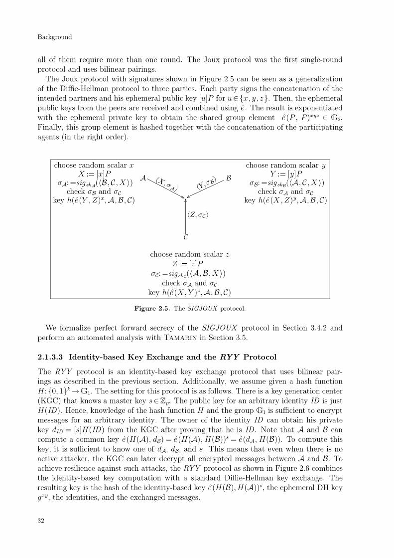
all of them require more than one round. The Joux protocol was the first single-roundprotocol and uses bilinear pairings.

The Joux protocol with signatures shown in Figure 2.5 can be seen as a generalizationof the Diffie-Hellman protocol to three parties. Each party signs the concatenation of theintended partners and his ephemeral public key [u]P for u∈x, y, z. Then, the ephemeralpublic keys from the peers are received and combined using e . The result is exponentiatedwith the ephemeral private key to obtain the shared group element e(P , P )xyz ∈ G2.Finally, this group element is hashed together with the concatenation of the participatingagents (in the right order).

choose random scalar x

〈X,σA 〉〈Y, σ

B〉

〈Z, σC〉

A B

C

choose random scalar yX7 [x]P Y 7 [y]P

σA: =sigskA(〈B, C ,X 〉) σB: =sigskB

(〈A, C ,X 〉)check σB and σC check σA and σC

key h(e(Y ,Z)x,A,B, C) key h(e(X,Z)y,A,B , C)

choose random scalar zZ7 [z]P

σC: =sigskC(〈A,B ,X 〉)

check σA and σCkey h(e(X,Y )z,A,B , C)

Figure 2.5. The SIGJOUX protocol.

We formalize perfect forward secrecy of the SIGJOUX protocol in Section 3.4.2 andperform an automated analysis with Tamarin in Section 3.5.

2.1.3.3 Identity-based Key Exchange and the RYY Protocol

The RYY protocol is an identity-based key exchange protocol that uses bilinear pair-ings as described in the previous section. Additionally, we assume given a hash functionH : 0, 1k→G1. The setting for this protocol is as follows. There is a key generation center(KGC) that knows a master key s∈Zp. The public key for an arbitrary identity ID is justH(ID). Hence, knowledge of the hash function H and the group G1 is sufficient to encryptmessages for an arbitrary identity. The owner of the identity ID can obtain his privatekey dID = [s]H(ID) from the KGC after proving that he is ID . Note that A and B cancompute a common key e(H(A), dB) = e(H(A), H(B))s = e(dA, H(B)). To compute thiskey, it is sufficient to know one of dA, dB, and s. This means that even when there is noactive attacker, the KGC can later decrypt all encrypted messages between A and B. Toachieve resilience against such attacks, the RYY protocol as shown in Figure 2.6 combinesthe identity-based key computation with a standard Diffie-Hellman key exchange. Theresulting key is the hash of the identity-based key e(H(B),H(A))s, the ephemeral DH keygxy, the identities, and the exchanged messages.

Background

32

A Blong-term secret: dA = [s]H(A) long-term secret: dB = [s]H(B)choose random exponent x

X7 gx

X

choose random exponent y

YY 7 gy

key h(Y x, e(dA, H(B)),A,B ,X , Y ) key h(X y , e(H(A), dB),A,B ,X , Y )

Figure 2.6. The RYY protocol with key derivation.

The RYY protocol can be considered an identity-based version of the UM protocol. Weformalize weak perfect forward secrecy of RYY and perform an automated analysis withTamarin in Section 3.5.

2.1.4 Physical Protocols

In this section, we describe two scenarios where physical properties of the environmentmust be established securely. We then describe protocols to achieve these desired goals.

2.1.4.1 Scenario: Contactless Car Entry Systems

Modern cars commonly use contactless entry systems. The car doors are unlocked wheneverthe corresponding key is sufficiently close to the car. The protocol executed between thecar and key establishes two facts. First, the protocol ensures that the car communicateswith the right key. This is a classical authentication property, which is usually ensuredby executing a protocol that uses a shared secret or public key cryptography. Second, theprotocol ensures that the key is sufficiently close to the car. Here, car manufacturers reliedon the limited communication range of the keys. The car can only communicate with thekey if it is sufficiently close. As shown in [82], such a protocol can be attacked by employinga fake key that is close to the car and a leech that is close to the real key. The fake keycan initiate the protocol and relay all challenges from the car to the leech who queries thereal key for the responses.

Relay with cable and antennas.

Distance from 10 to 100 meters.

fake key

leech

Figure 2.7. Relay attack on contactless car entry system.


33

This type of attack was first considered in [66] under the name Mafia fraud. In [34], anattack scenario with fake ATMs is described. Here, a man-in-the-middle attack is employedto forward the messages back and forth between the real ATM and the real card that isinserted into the fake ATM.

2.1.4.2 Authenticated Ranging Protocols

To establish the required facts for a contactless car entry system, an authenticated rangingprotocol can be used. An authenticated ranging protocol is executed between a verifier Vand a prover P . The goal of the protocol is for the verifier V to establish an upper boundon the distance to an honest prover P . Most protocols that achieve authenticated rangingare based on roundtrip-time measurements by the verifier. In the previous example, the carwould be the verifier and the key would be the prover. After establishing an upper boundon the distance to the key, the car would decide if the key is close enough to unlock thedoor. Figure 2.8 shows an example protocol. Here, V send a fresh nonce nv as a challenge

at time tSV. The prover P notes the time tR

P when he received the challenge and decides ona time tS

P when to send the response, based on the required computation time. Then, Pcomputes a signature on the challenge nv and the computation delay tS

P− tRP, which he sends

back to V at time tSP. V notes the reception time tR

V , checks the signature, and computesthe upper bound on the distance as (tR

V − tSV− δ)∗ c

2, where c is the speed of light. Since the

adversary can delay the transmissions, but not speed up the transmissions with respect tothe assumed line-of-sight transmission with speed of light, the computed value is an upperbound on the distance.

V (Verifier) P (Prover)

choose fresh nonce nv

tSV7 readClock()

nvtRP7 readClock()

set δ7 tSP− tR

P

compute sig(〈nv , δ〉, skP)

tRV7 readClock()

sig(〈nv ,δ〉,skP)send at tS

P

check signature

Conclude that |locV− locP| ≤ (tRV − tS

V− δ)∗ c2

Figure 2.8. Authenticated Ranging Protocol.

2.1.4.3 Scenario: Location-Based Access Control

Consider now a slightly different scenario where wireless access to sensitive data is con-trolled by the following access control policy. First, the user, identified by a shared secret oras the holder of a certain private key, must be allowed to access the data. Second, the usermust be located in a certain building to access the data. Access to the building is securedby guards who check the identity of the user. In contrast to an access control policy thatonly takes the first condition into account, this policy also tolerates the loss of key materialto outsiders that cannot gain access to the building. This is the main difference to theprevious scenario where the owner of the real key (material) is always assumed to be honest.

Background

34

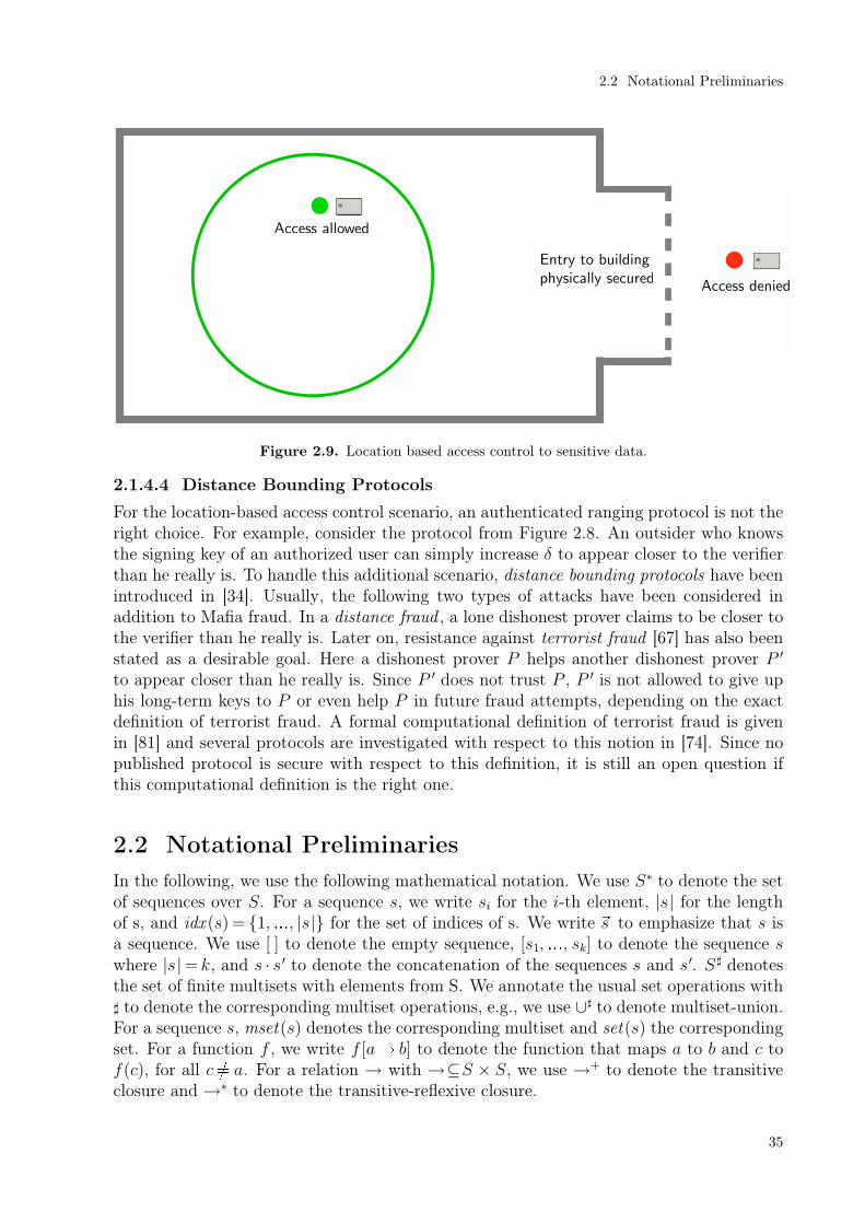
Access allowed

Access denied

Entry to building

physically secured

Figure 2.9. Location based access control to sensitive data.

2.1.4.4 Distance Bounding Protocols

For the location-based access control scenario, an authenticated ranging protocol is not theright choice. For example, consider the protocol from Figure 2.8. An outsider who knowsthe signing key of an authorized user can simply increase δ to appear closer to the verifierthan he really is. To handle this additional scenario, distance bounding protocols have beenintroduced in [34]. Usually, the following two types of attacks have been considered inaddition to Mafia fraud. In a distance fraud , a lone dishonest prover claims to be closer tothe verifier than he really is. Later on, resistance against terrorist fraud [67] has also beenstated as a desirable goal. Here a dishonest prover P helps another dishonest prover P ′

to appear closer than he really is. Since P ′ does not trust P , P ′ is not allowed to give uphis long-term keys to P or even help P in future fraud attempts, depending on the exactdefinition of terrorist fraud. A formal computational definition of terrorist fraud is givenin [81] and several protocols are investigated with respect to this notion in [74]. Since nopublished protocol is secure with respect to this definition, it is still an open question ifthis computational definition is the right one.

2.2 Notational Preliminaries

In the following, we use the following mathematical notation. We use S∗ to denote the setof sequences over S. For a sequence s, we write si for the i-th element, |s| for the lengthof s, and idx (s) = 1, , |s| for the set of indices of s. We write sR to emphasize that s isa sequence. We use [ ] to denote the empty sequence, [s1, , sk] to denote the sequence swhere |s|= k, and s · s′ to denote the concatenation of the sequences s and s′. S ♯ denotesthe set of finite multisets with elements from S. We annotate the usual set operations with♯ to denote the corresponding multiset operations, e.g., we use ∪♯ to denote multiset-union.For a sequence s, mset(s) denotes the corresponding multiset and set(s) the correspondingset. For a function f , we write f [a b] to denote the function that maps a to b and c tof(c), for all c a. For a relation → with →⊆S × S, we use →+ to denote the transitiveclosure and →∗ to denote the transitive-reflexive closure.

2.2 Notational Preliminaries

35

2.3 Term Rewriting

As previously stated, we abstract cryptographic messages and operations on them by termsand the properties of these operations by equations. This naturally allows us to use variablesto reason symbolically about sets of messages. Most methods for this approach come fromthe area of term rewriting. We therefore recall some standard notions from term rewritingfollowing [65], [86], and [79].

2.3.1 Standard Notions

Order sorted term algebras. An order-sorted signature Σ=(S,≤,Σ) consists of a setof sorts S, a partial order ≤ on S, and a set Σ of function symbols associated with sortswith the following two properties. First, for every s∈S, the connected component C of sin (S,≤) has a top sort denoted top(s) such that c≤ top(s) for all c∈C . Second, for everyf : s1× × sk→ s in Σ with k ≥ 1, there is an f : top(s1)× × top(sk)→ s in Σ called thetop sort overloading of f . If the sort hierarchy is clear from the context, we often use Σinstead of Σ.

If there is only one sort, we say the corresponding signature is unsorted and we write Σk

to denote all k-ary function symbols in Σ. We assume that there are countably infinite setsof variables Vs for all sorts s ∈ S and define V =

⊎

s∈SVs. We use x:s to denote variables

from Vs. For a signature Σ and an arbitrary subset V ′⊆V, TΣ(V ′)s denotes the set of well-sorted terms of sort s constructed over Σ∪V ′. We use TΣ(V ′) to denote the set of all well-sorted terms. For a set of constants C, we also use TΣ(V ′∪C) to denote TΣ∪C(V ′).

Positions, subterms, vars, and contexts. A position is a sequence of natural numbers.For a term t and a position p, we denote the subterm of t at position p with t|p. Formally,t|p is defined as (a) t if p=[ ], (b) ti|p′ if p= [i] · p′ and t= f(t1, , tk) for 1≤ i≤ k, and (c)undefined otherwise. We say p is a valid position in t if t|p is defined. For two positions pand p′, p is above p′ if p is a proper prefix of p′. In this case, p′ is below p. If p is unequalto p′ and neither above nor below p ′, then both positions are incomparable . We say p andp′ are siblings if |p|= |p′|, pi= pi

′ for 1≤ i < |p|, and p|p| p|p|′ .

Furthermore, we use t[s]p to denote the term t where the occurrence of the subterm t|pat position p has been replaced by s. We use root(t) to denote f if t= f(t1, , tk) for somef ∈ Σ and t itself otherwise. The set St(t) of syntactic subterms of a term t is defined inthe usual way as t|p |p valid position in t. For a term t, we define vars(t) = St(t) ∩ V.A term t is ground if vars(t)=∅. We use fvars(ϕ) to denote the free variables in a formula ϕ.

A context C is a term with holes. Holes are distinct variables xi that occur exactlyonce in C. We use the notation C[x1, , xn] to indicate that C has the holes x1, , xn andC[t1, , tn] to denote the term where the holes have been replaced by the terms ti.

Substitutions and replacements. A substitution σ is a well-sorted function from V toTΣ(V) that corresponds to the identity function except on a finite set of variables which wedenote with dom(σ). We use range(σ) to denote the image of dom(σ) under σ and definevrange(σ) = vars(range(σ)). We identify σ with its usual extension to an endomorphismon TΣ(V) and use the notation tσ for the application of σ to the term t. Furthermore, wedenote the substitution σ with dom(σ)= x1, , xk and xiσ= ti by t1/x1, , tk/xk. Weuse id to denote the identity substitution.

Background

36

A replacement ρ is a function from a finite set of terms to TΣ(V) such that dom(ρ) ∩St(range(ρ)) = ∅. For a term t, we define tρ as the unique term where all occurrences ofsubterms s= t|p of t, with s ∈ dom(ρ) such that there is no position p ′ above p with t|p′in dom(ρ) are replaced by ρ(s).

Equations and equational theories. An equation over a signature Σ is an unorderedpair s, t of terms t, s∈TΣ(V) denoted s≃ t. An equational presentation is a tuple (Σ,E)where Σ is a signature and E is a set of equations. Given an equational presentationE = (Σ, E), we define the equational theory =E as the smallest Σ-congruence containingall instances of equations of E. We often identify the equational presentation E and thecorresponding equational theory =E. An equation s≃ t is regular if vars(s) = vars(t) andsort-preserving if for all substitutions σ, it holds that sσ∈TΣ(V)s if and only if tσ∈TΣ(V)s.An equational presentation is regular (respectively sort-preserving) if all its equations are.

Unification and matching. An E-unifier of two terms s and t is a substitution σ such

that sσ =E tσ. For W ⊆ V, we use unif EW(s, t) to denote an E-unification algorithm that

returns a set of unifiers of s and t such that for all σ∈unif EW(s, t), vrange(σ)∩W =∅. The

unification algorithm is complete if for all E-unifiers σ of s and t, there is a τ ∈unif EW(s, t)

and a substitution θ such that for all x∈ vars(s, t), (xτ )θ=E xσ. The unification algorithmis finitary if for all s and t, it terminates and returns a finite set of unifiers.

An E-matcher of two terms t and p is a substitution σ such that t=E pσ. The notions ofcomplete and finitary coincide with those for E-unification. We use matchE(t, p) to denotea finitary and complete E-matching algorithm.

Rewriting. A rewrite rule over a signature Σ is an ordered pair of terms (l, r) withl, r ∈TΣ(V) denoted l→ r. A rewrite system R is a set of rewrite rules. R defines a rewriterelation →R with s→R t if there is a position p in s, a rule l→ r ∈R , and a substitutionσ such that s|p=lσ and s[rσ]p= t. A rewrite system R is terminating if there is no infinitesequence (ti )i∈N of terms with ti→R ti+1. A rewrite system R is confluent if for all terms t,s1, s2 with t→R

∗ s1 and t→R∗ s2, there is a term t′ such that s1→R

∗ t ′ and s2→R∗ t′. A rewrite

system R is convergent if it is terminating and confluent. In this case, we use t↓R to denotethe unique normal form of t, i.e., t↓R is the unique term t ′ such that t→R

∗ t ′ and there isno term t′′ with t′→R t

′′. A rewriting rule l→ r is sort-decreasing if for all substitutions σ,rσ ∈TΣ(C)s implies lσ ∈TΣ(C)s. A rewrite system is sort-decreasing if all its rules are.

A rewrite system R is subterm-convergent if it is convergent and for each rule l→ r∈R,r is either a proper subterm of l or r is ground and in normal form with respect to R. Wesay a function symbol f is irreducible with respect to such a rewriting system R if thereis no l→ r ∈R with root(l) = f . We use R≃ to denote the set of equations obtained froma rewrite system by replacing → with ≃ in the rewrite rules.

2.3.2 Rewriting Modulo and Finite Variants

Rewriting modulo. Rewriting is often used to reason about equality modulo an equa-tional theory E . If the equations in E can be oriented to obtain a convergent rewritingsystem R, then R can be used to check equality since t=E s if and only if t↓R = s↓R. Tocope with equational theories containing equations that cannot be oriented such as commu-tativity, the notion of R,AX-rewriting for a rewrite systemR and an equational theory AX

2.3 Term Rewriting

37

has been introduced in [142]. The rewriting relation→R,AX is defined as s→R,AX t if thereis a position p in s, a rewriting rule l→ r ∈R, and a substitution σ such that s|p =AX lσ

and s[rσ]p= t. If AX -matching is decidable, then the relation→R,AX is also decidable. Touse rewriting to reason about equality modulo E , the following properties are required.

Coherence and decomposition. We say R,AX is convergent if the relation →R,AX isconvergent. In this case, we denote the unique normal form of t with respect to R,AX -rewriting by t↓R,AX . We sayR,AX is coherent if for all t1, t2, and t3, it holds that t1→R,AX t2and t1=AX t3 implies that there are t4 and t5 such that t2→R,AX

∗ t4, t3→R,AX+ t5, and t4=AX t5.

If (Σ,R∪AX ) is an equational presentation of =E and R,AX is convergent and coherent,then t=E s if and only if t↓R,AX = s↓R,AX . See [142, 94] for details.

We call (Σ,R,AX ) a decomposition of E if the following holds:

1. (Σ,R≃∪AX ) is an equational presentation of =E.

2. AX is regular, sort-preserving and all equations contain only variables of top-sort.

3.R is sort-decreasing and R,AX is convergent and coherent.

4. There is a complete and finitary AX -unification algorithm.

Example 2.1. Consider the unsorted equational theory ACUN that models Xor withΣACUN = 0, + and EACUN =AC ∪x + 0≃x, x + x≃ 0 for AC = (x + y) + z≃x + (y + z),x+ y≃ y +x. The last two equations in EACUN can be oriented to obtain RACUN =x+0→x, x + x→ 0 and RACUN,AC is convergent. It is easy to see that x + (x + y)=ACUN y, but

(x + (x + y))↓RACUN ,AC = (x + (x + y))AC y= y↓RACUN ,AC .

The problem is that RACUN,AC is not coherent and the relation ↔RACUN ,AC∗ is therefore

strictly smaller than =ACUN . It is possible to complete RACUN with the missing rewrite rulex + (x + y)→ y to obtain RACUN

′ . Then (Σ,RACUN′ ,AC ) is a decomposition of ACUN .

Finite variants. For an equational theory E , we define the E-instances of a term t asinstsE(t)= t′|∃σ.tσ=E t

′. We use ginstsE(t) to denote the set of ground E-instances of t.To reason about E-instances using a decomposition (Σ, R, AX ) of E , the finite variantproperty is often useful.

A decomposition (Σ,R,AX ) of an equational theory E has the finite variant property iffor all terms t, there is a finite set of substitutions τ1, , τk with dom(τi)⊆ vars(t) suchthat for all substitutions σ, there is a substitution θ and i∈1, , k with

1. (tσ)↓R,AX =AX (tτi)↓R,AXθ and

2. xσ↓R,AX =AX (xτi)↓R,AXθ for all x∈ vars(t).

We call such a set of substitutions a complete set of R,AX-variants of t. For a decomposi-tion with the finite variant property, we can use folding variant narrowing [79] to computea complete and minimal set of R,AX -variants of a term.

Example 2.2. Consider the equational theory E = (Σ, E) with Σ = g/2, a/0 andE = g(x, a)≃ a. Then (Σ,R, ∅) is a decomposition with the finite variant property forR = g(x, a)→ a. Consider the term t = g(x, y). The set id , a/y is a complete setof R,∅-variants of t. Let t ′ and σ arbitrary such that t ′ = t′↓R and t′ =E tσ, i.e., t

′ is anirreducible E-instance of t. Since id , a/y is a complete set of R,∅-variants of t, t ′ is

Background

38

either an instance of t (i.e. t′∈ insts∅((t)id)) or an instance of ta/y↓R= a, i.e., equal to a.This is already ensured by requirement (1) for a complete set of variants. Requirement (2)additionally ensures that σ factorizes through id in the first case and through a/y inthe second case. If we would drop requirement (2), then id , a/x, a/y would also be acomplete set of variants, even though σ = a/y would not factorize through a/x, a/y.If complete sets of variants are used to perform E-unification [79], both requirements arenecessary.

2.3.3 Ordered Completion

We use ordered completion [65] to define the normalization of ground terms with respect toan arbitrary equational theory E . In Chapter 4, we use this notion in our combination prooffor impossibility. This technique has been used in similar contexts to prove the correctnessof combination results for unification [15] and deducibility [46, 56]. In the following, weassumed an unsorted signature Σ and a set of constant symbols N different from Σ0

called names. Let ≻ be a total simplification order on ground terms, i.e., for ground termss1 and s2 and a nonempty context C, we have that (i) s1 ≻ s2 or s2 ≻ s1, (ii) C[s1] ≻ s1,and (iii) s1≻ s2 implies C[s1]≻ C[s2]. Additionally, we assume for all n ∈N , c ∈ Σ0, andt ∈ TΣ(N ) \ (N ∪ Σ0) that c≻ n and t≻ c. We then use nmin to denote the minimum for≻, which is a name. The lexicographic path ordering constructed from a total ordering onN ∪ Σ , where names are smaller than constants from Σ0 and constants are smaller thannon-constant function symbols, always has these properties (see [65]).

For a given equational theory E and a total simplification ordering on ground terms ≻,we define the ordered rewrite relation→(≻,E) as follows: t→(≻,E) t

′ if there is a position p of

t, an equation l≃ r in E , and a substitution σ such that t|p=lσ, t′ = t[rσ]p, and t≻ t′. Weuse ordered completion for a given equational theory E to obtain a (possibly infinite) setof equations OE such that =OE

equals =E and →(≻,OE) is convergent on ground terms. Fora ground term t, we use t↓E

≻ to denote the normal form of t with respect to →(≻,OE).

2.4 Isabelle/HOL and the Inductive Approach

In Chapter 5, we use the theorem prover Isabelle [136]. Moreover, we build on the inductiveapproach to protocol verification by Paulson [140] to reason about physical protocols. Thefollowing paragraphs provide a small summary of Isabelle/HOL and the inductive approach.

Isabelle/HOL. Isabelle is a generic theorem prover with a specialization for higher-orderlogic (HOL). We will avoid Isabelle-specific details as much as possible or explain themin context as needed. Here we limit ourselves to few comments on typing. A function f

from type α to β is denoted f :α→ β and fx≡ t defines the function f with parameter xas the term t. We write α× β for the product type of α and β. We use the predefined listtype α list where xs.x denotes the list xs extended by the element x. Algebraic data typesare defined using the datatype declaration. Central to our work is the ability to define(parameterized) inductively defined sets. These sets are defined by sets of rules and denotethe least set closed under the rules. Given an inductive definition, Isabelle generates a rulefor proof by induction.

2.4 Isabelle/HOL and the Inductive Approach

39

Inductive Approach. Paulson has introduced an inductive approach to security protocolverification. The approach is based on a trace-based interleaving semantics, which givesa semantics to distributed systems as the set of traces describing all possible interleavedevents executed by the involved agents. In particular, protocols are modeled by rulesdescribing the protocol steps executed by honest agents and possible intruder actions.The rules constitute an inductive definition that defines the protocol’s semantics as aninfinite set of communication traces, each trace being a finite list of communication events.Security properties are specified as predicates on traces. Protocol security is then proved byinduction on traces using an induction principle derived from the protocol rules. Paulsonformalized his approach within higher-order logic in the Isabelle/HOL system and used itto prove security properties for a wide range of security protocols.

Background

40

Chapter 3

Automated Protocol Analysis

In this chapter, we present a method to analyze security protocols that use DH exponen-tiation and bilinear pairings without bounding the number of protocol sessions. We haveimplemented the method in a tool, called the Tamarin prover, and demonstrated its effec-tiveness in numerous case studies from the area of key exchange protocols, tripartite groupkey exchange protocols, and identity-based key exchange protocols. Given a specificationof the protocol and the adversary model, Tamarin automatically searches for a proof thatthe protocol is secure in the given model with respect to an unbounded number of sessions.If Tamarin terminates without succeeding in the proof, it provides a counterexample, i.e.,an attack on the protocol with respect to the given adversary model.

In the following, we first define our security protocol model based on multiset rewritingand many-sorted first-order logic. Then, we present our verification theory, which simplifiesreasoning about the security protocol model. Next, we present the constraint solving rulesthat we use to analyze protocols. Then, we extend the previously introduced approachfrom DH exponentiation to bilinear pairings and AC operators. Finally, we describe theTamarin tool and the case studies.

3.1 Security Protocol Model

We model the execution of a security protocol in the context of an adversary as a labeledtransition system, whose state consists of the adversary’s knowledge, the messages on thenetwork, information about freshly generated values, and the protocol’s state. The adver-sary and the protocol interact by updating network messages and freshness information.Adversary capabilities and protocols are specified jointly as a (labeled) multiset rewritingsystem. Security properties are modeled as trace properties of the transition system. Inthe following, we first describe cryptographic messages. Then, we define how protocols arespecified and executed. Finally, we define our property specification language and illustrateour protocol model with an example.

3.1.1 Cryptographic Messages

To model cryptographic messages, we use an order-sorted term algebra and an equationaltheory. The function symbols in the signature model the algorithms that can be applied tomessages such as encryption or decryption and the equational theory models the propertiesof the algorithms. We use the set of sorts consisting of the top sort msg and two incompa-rable subsorts fr and pub for fresh and public names. We assume there are two countablyinfinite sets FN and PN of fresh and public names . We use fresh names to model random

41

messages such as keys or nonces and public names to model known constants such as agentidentities. To model DH exponentiation, we define the unsorted signature

ΣDH = _ˆ_ ,_∗_ , 1,_−1

where all function symbols are of sort msg × ×msg→msg . Here, gâ denotes exponen-tiation of the message g with the exponent a. The remaining function symbols model theexponents as an abelian group. The algebraic properties of DH exponentiation are modeledby the equations

EDH =

(xˆy)ˆz≃xˆ(y∗z) xˆ1≃x x∗y≃ y∗x

x∗(y∗z)≃ (x∗y)∗z x∗1≃x x∗x−1≃ 1

which capture that repeated exponentiation in a DH group corresponds to multiplicationof the exponents, exponentiation with 1 is the identity, and the exponents form an abeliangroup. We define the equational theory for DH as DH=(ΣDH, EDH).

For additional cryptographic operators, we assume given an unsorted signature ΣST

disjoint from ΣDH and a subterm-convergent rewrite system RST over ΣST . We define thecombined signature ΣDHe

= ΣST ∪ ΣDH and use T to denote TΣDHe∪FN∪PN(V) and M todenote the ground terms in T which we call messages . We define the combined equationaltheory as DHe = (ΣDH ∪ ΣST , EDH ∪RST

≃ ). In the remainder of this chapter, we use g todenote a public name that is used as a fixed generator of a DH group and a, b, c, and k todenote fresh names.

Example 3.1. Consider the term ((gâ)ˆb)â−1, which results from exponentiating g

with a, followed by b, followed by a inverse. This is equal to gˆ((a∗b)∗a−1) and can befurther simplified to gˆb.

Note that our equational theory does not support protocols that perform multiplicationin the DH group G. To define such protocols, an additional function symbol · denotingmultiplication in G is required. The function symbol ∗ denotes multiplication in the groupof exponents, which is a different operation. For example, the equality (gâ · gˆb)ˆc =(gâ)ˆc · (gˆb)ˆc holds in all DH groups, but does usually not hold if we replace · by ∗. Wefurther discuss our choice of the equational theory DH in Section 6.1.1.

Example 3.2. As an example of a subterm-convergent theory that can be used, considerDY = (ΣDY,RDY) defined by

ΣDY =

〈_,_〉 fst(_) snd(_)pk(_) enc(_,_) dec(_,_)true sig(_,_) verify(_,_) h(_)

and

RDY =

fst(〈x, y〉)→ x snd(〈x, y〉)→ y

dec(enc(x, pk(y)), y)→ x

verify(sig(x, y), x, pk(y))→ true

.

This theory models pairing and projection, public key encryption, message-hiding signa-tures, and a hash function. Note that we often use 〈t1, t2 , tk−1, tk〉 as an abbreviation for〈t1, 〈t2, 〈tk−1, tk〉〉〉 and h(t1, , tk) as an abbreviation for h(〈t1, , tk〉).


42

3.1.2 Labeled Multiset Rewriting with Fresh Names

We use multiset rewriting to specify the concurrent execution of protocol and adversary.Multiset rewriting is commonly used to model concurrent systems since it naturally sup-ports independent transitions. If two rewriting steps rewrite the state at positions that donot overlap, then they can be applied in parallel. Multiset rewriting has been used in thecontext of security protocol verification by Cervesato et al. [41] and in Maude-NPA [77].Like these two approaches, we extend standard multiset rewriting with support for creatingfresh names. Additionally, we introduce persistent facts and enrich rewriting rules withactions to obtain labeled transition systems. Note that it is possible to give a translationfrom processes in the applied pi calculus as, for example, used in ProVerif [28] into ourdialect of multiset rewriting.

State

We model the states of our transition system as finite multisets of facts. Facts are builtfrom terms over a fact signature. Formally, we assume given an unsorted signature ΣF

partitioned into linear and persistent fact symbols. We define the set of facts as the set Fconsisting of all facts F (t1, , tk) such that ti∈T and F ∈ΣF

k . We denote the set of groundfacts by G. We say that a fact F (t1, , tk) is linear if F is linear and persistent if F ispersistent. Linear facts model resources that can only be consumed once, whereas persistentfacts model inexhaustible resources that can be consumed arbitrarily often. We assumethat the linear fact symbol Fr is included in ΣF

1 . The semantics of Fr is fixed and the factFr(n) denotes that the fresh name n is freshly generated. The semantics of the remainingfact symbols are defined by the multiset rewriting rules that generate and consume them.In our examples, we prefix all persistent protocol fact symbols with !.

Rules

We use labeled multiset rewriting to define the possible transitions of our transition system.A labeled multiset rewriting rule is a triple (l, a, r) with l, a, r ∈F∗, denoted l−[a]→ r. Weoften use inference rule notation for rules, i.e., we use

l1 lkr1 rn

[a1 am] orl1 lkr1 rn

if a is empty.

For ru = l−[a]→ r, we define the premises as prems(ru)= l, the actions as acts(ru) = a, andthe conclusions as concs(ru)= r. We call a set of labeled multiset rewriting rules a labeledmultiset rewriting system . In the following, we often drop the “labeled” qualifier.

To deal with fresh name generation, we define the rule

Fresh= []−[]→ [Fr(x:fr)],

which is the only rule that produces Fr facts. In the operational semantics, we ensure thatapplications of this rule are unique and that the same fresh name is never generated twice.

Labeled Operational Semantics

To define the labeled operational semantics of a multiset rewrite system R, we first definethe labeled transition relation steps(R)⊆ G ♯× (ginstsDHe

(R∪Fresh))× G ♯ as

l−[a]→ r ∈ ginstsDHe(R∪Fresh) S ′ =(S \♯ lfacts(l))∪♯mset(r)

lfacts(l)⊆♯S set(pfacts(l))⊆ set(S)

(S, l−[a]→ r, S ′)∈ steps(R),


43

where lfacts(l) and pfacts(l) denote the multisets of linear and persistent facts in l, respec-tively, and each transition is labeled with the applied rule instance.

A transition rewrites the state S with a ground instance of Fresh or a rule from R.Since we perform multiset rewriting modulo DHe, any applicable ground DHe-instance ofa rule in R∪Fresh can be used. An instance l−[a]→ r is applicable to S if the multisetof linear facts in l is included in S with respect to multiset inclusion (⊆♯) and the set ofpersistent facts in l is included in S with respect to set inclusion. To obtain the successorstate S ′, the consumed linear facts are removed and the generated facts are added.

Definition 3.3. An execution of R is an alternating sequence

e= [S0, (l1−[a1]→ r1), S1, , Sk−1, (lk−[ak]→ rk), Sk]

of states and multiset rewriting rule instances such that the following conditions hold:

E1. S0 = ∅♯

E2. For all i∈1, , k, (Si−1, (li−[ai]→ ri), Si)∈ steps(R).

E3. For all i, j ∈1, , k and n∈FN where (li−[ai]→ ri)= (lj−[aj]→ rj)= ([ ]−[ ]→ Fr(n)),it holds that i= j.

We denote the set of executions of R with execs(R). We define the trace of such anexecution e as trace(e)= [set(a1), , set(ak)], i.e., the trace is the sequence of sets of actionsof the multiset rewriting rule instances. We define the observable trace tr of a trace tr asthe subsequence of all actions in tr that are not equal to ∅.

The Conditions E1 and E2 ensure that an execution starts with the empty multiset andeach step is valid. The Condition E3 ensures that the same fresh name is never generatedtwice. To ensure that fresh name generation works as intended, we will restrict ourselvesto multiset rewriting systems R where rules do not introduce Fr-facts or create fresh namesthemselves. To formally define what it means to “create a fresh name”, we define the stablefresh names of a term t as

fnamesst(t)=⋂

t=DHe t′

(St(t ′)∩FN )

The definition of fnamesst accounts for the fact that a term can contain spurious freshnames if it is not reduced with respect to the cancellation equations in DHe. For example,the term a∗b∗b−1 contains the name b, but fnamesst(a∗b∗b−1)=a since b does not occurin all terms that are equal to a∗b∗b−1 modulo DHe. We say a multiset rewriting system R

does not create fresh names if for all (S, ri ,S ′)∈ steps(R), either ri is an instance of Freshor fnamesst(S

′)⊆ fnamesst(S) considering states as terms.

3.1.3 Protocol and Adversary Specification

To define the protocol and message deduction rules, we assume that ΣF consists of Fr, anarbitrary number of protocol-specific fact symbols to describe the protocol state, and thefollowing special fact symbols. A persistent fact K(m) denotes that m is known to theadversary. A linear fact Out(m) denotes that the protocol has sent the message m, whichcan be received by the adversary. A linear fact In(m) denotes that the adversary has sentthe message m, which can be received by the protocol.


44

Protocol Rules

We now define our formal notion of a protocol which encompasses both the rules executedby the honest participants and the adversary’s capabilities, like revealing long-term keys.

Definition 3.4. A protocol rule is a multiset rewriting rule l−[a]→ r such that

P1. l, a, and r do not contain fresh names,

P2. l does not contain K and Out facts,

P3. r does not contain K, In, and Fr facts,

P4. the argument of an Fr-fact is always of sort fr ,

P5. r does not contain the function symbol ∗, and

P6. l −[a]→ r satisfies (a) vars(r) ⊆ vars(l) ∪ Vpub and (b) l only contains irreduciblefunction symbols from ΣST or it is an instance of a rule that satisfies (a) and (b).

A protocol is a finite set of protocol rules.

ConditionP1 prevents protocol rules from directly using fresh names. ConditionsP2 andP3 prevent protocol rules from using the special facts in unintended ways. Condition P4simplifies later definitions and is not a restriction since Fr-facts in reachable states alwayshave a fresh name as argument. Condition P5 ensures that multiplication is not directlyused and simplifies reasoning about products since protocol rules introduce new productsonly as exponents. Condition P6 is a syntactic criterion ensuring together with P1 thatprotocols do not create fresh names, i.e., all fresh names originate from instances of theFresh rule. Note that condition P5 is similar to those of previous work such as [108]and [45] and is not a restriction in practice. Protocols that use multiplication in the group ofexponents such as MTI/C0 [119] can usually be specified by using repeated exponentiation.Moreover, protocols that use multiplication in the DH group, such as MQV [113], cannot bespecified anyway since ∗ denotes multiplication in the group of exponents.

Example 3.5. There are several kinds of rules that are forbidden by P1–P6. For example,[In(x)] −[]→ [Out(y)] is forbidden since y is neither of sort pub nor does it occur in thepremises. We do not allow this rule since it can send arbitrary terms. This is problematicsince those terms can contain fresh names that are identical to fresh names chosen lateron. The rule [In(fst(〈z, y〉))]−[]→ [Out(y)] is equivalent to this rule and demonstrates theproblem with allowing reducible function symbols in the premises.

Another forbidden rule is [In(x), Fr(y:fr)] −[]→ [Out(x∗(y:fr))] which contains ∗. We donot allow this rules since it violates P5. The rule [In(x), Fr(y:fr)] −[]→ [Out(gˆ(x∗(y:fr)))]is also forbidden, but the equivalent rule [In(x),Fr(y:fr)]−[]→ [Out((gˆx)ˆ(y:fr))] is allowed.Finally, the rule [In(gˆ(y:fr)), St(y:fr, x)] −[]→ [Out((gˆ(y:fr))ˆx)] is allowed since it is aninstance of [In(z),St(y:fr, x)]−[]→ [Out(zˆx)].

Message Deduction Rules

The set of messages deduction rules is defined as

MD =

Out(x)

K(x)

K(x)

In(x)[K(x)]

Fr(x:fr)

K(x:fr) K(x:pub)

K(x1) K(xk)

K(f(x1, xk))for all f ∈ΣDHe

k

.


45

The rules in the first line allow the adversary to receive messages from the protocol andsend messages to the protocol. The K(x) action in the second rule makes the messagessent by the adversary observable in a protocol’s trace. We exploit this to specify secrecyproperties. The rules in the second line allow the adversary to learn public names andfreshly generated names. The remaining rules allow the adversary to apply functions fromΣDHe

to known messages. Note that MD does not create fresh names.

Example 3.6. Consider the protocol

PMsg =

Fr(x:fr) Fr(y:fr)

St(x) Out(〈(gˆx)ˆy, y−1〉)[Start()],

St(x) In(gˆx)[Fin()]

.

which encodes the message deducibility problem “is gˆx deducible from 〈(gˆx)ˆy, y−1〉 forfresh names x and y “. This problem has a solution if and only if the protocol has the trace[Start(), K(m), Fin()] for some message m. In this and the following examples, wenever use the same variable name for variables of different sorts in a rule and thereforeinclude the sort annotation only for the first occurrence of a variable.

The protocol has the execution shown in Figure 3.1 with the observable trace [Start(),K(gˆa),Fin()]. We show the states on the right and the DHe-instances of the rules usedto rewrite the state on the left. The first rule applications add fresh facts which are con-sumed by the first protocol rule instance ru3. This is the first observable step. Rule instanceru4 models the reception of the message sent by the protocol and ru5, ru6, and ru7 denotemessage deduction steps. Here, we chose those DHe-instances of the rules that simplifythe terms in the conclusion. For instance, ru5 is a DHe-instance of K(x)−[]→K(fst(x)) andru7 is a DHe-instance of [K(x1), K(x2)] −[]→ K(x1ˆx2). The last two rule instances modelthe sending of the deduced message gˆa by the adversary and the execution of the secondprotocol step.

Note that the sequence of rule instances is already sufficient to characterize the executionsince the trace and the sequence of states can be reconstructed from it. To denote thecausal dependencies between transitions, the figure contains grey arrows from conclusions topremises of rule instances. Such an arrow denotes that the corresponding fact is generatedby the conclusion that is the source of the arrow and consumed by the premise that isthe target of the arrow. The causal dependencies allow us to find permutations of thesequence of rule instances that correspond to valid executions of PMsg. More precisely, anypermutation of the rule instances that respects the causal dependencies corresponds to avalid execution of PMsg. We can therefore represent a set of executions by a sequence ofrule instances and their causal dependencies. We take advantage of these observations inthe next section when we define dependency graphs as sequences of rule instances togetherwith their causal dependencies.

3.1.4 Trace Formulas

We use many-sorted first-order logic with a sort for timepoints [47] to specify securityproperties. This logic supports quantification over both messages and timepoints. We thusintroduce the sort temp for timepoints and write Vtemp for the set of temporal variables.In the following, we use i and j for temporal variables, f for facts, and t1, t2 for terms.

A trace atom is either a term equality t1 ≈ t2, a timepoint ordering i ≺ j, a timepointequality i≈ j, or an action f@ i. A trace formula is a first-order formula over trace atoms.In the following, we also use a fact f as a formula to abbreviate the formula ∃i.f@ i.


46

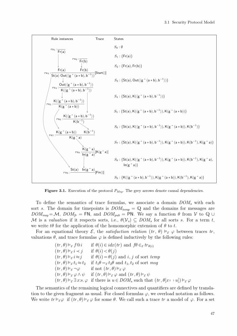
ru1 :Fr(a)

ru2 :Fr(b)

ru4 :Out(〈g ˆ (a ∗ b), b−1〉)

K(〈g ˆ (a ∗ b), b−1〉)

ru3 :Fr(a) Fr(b)

St(a) Out(〈g ˆ (a ∗ b), b−1〉)[Start()]

ru5 :K(〈g ˆ (a ∗ b), b−1〉)

K(g ˆ (a ∗ b))

ru6 :K(〈g ˆ (a ∗ b), b−1〉)

K(b−1)

ru7 :K(g ˆ (a ∗ b)) K(b−1)

K(g ˆ a)

ru8 :K(g ˆ a)

In(g ˆ a)[K(g ˆ a)]

ru9 :St(a) In(g ˆ a)

[Fin()]

S1 : Fr(a)

S0 : ∅

S2 : Fr(a),Fr(b)

S3 : St(a),Out(〈g ˆ (a ∗ b), b−1〉)

S5 : St(a),K(〈g ˆ (a ∗ b), b−1〉),K(g ˆ (a ∗ b))

S4 : St(a),K(〈g ˆ (a ∗ b), b−1〉)

S6 : St(a),K(〈g ˆ (a ∗ b), b−1〉),K(g ˆ (a ∗ b)),K(b−1)

S7 : St(a),K(〈g ˆ (a ∗ b), b−1〉),K(g ˆ (a ∗ b)),K(b−1),K(g ˆ a)

S8 : St(a),K(〈g ˆ (a ∗ b), b−1〉),K(g ˆ (a ∗ b)),K(b−1),K(g ˆ a),

In(g ˆ a)

S9 : K(〈g ˆ (a ∗ b), b−1〉),K(g ˆ (a ∗ b)),K(b−1),K(g ˆ a)

StatesRule instances Trace

Figure 3.1. Execution of the protocol PMsg. The grey arrows denote causal dependencies.

To define the semantics of trace formulas, we associate a domain DOMs with eachsort s. The domain for timepoints is DOMtemp = Q and the domains for messages areDOMmsg =M, DOMfr = FN, and DOMpub = PN. We say a function θ from V to Q ∪M is a valuation if it respects sorts, i.e., θ(Vs) ⊆ DOMs for all sorts s. For a term t,we write tθ for the application of the homomorphic extension of θ to t.

For an equational theory E , the satisfaction relation (tr , θ) E ϕ between traces tr ,valuations θ, and trace formulas ϕ is defined inductively by the following rules:

(tr , θ)E f@ i if θ(i)∈ idx (tr) and fθ ∈E tr θ(i)(tr , θ)E i≺ j if θ(i)<θ(j)(tr , θ)E i≈j if θ(i) = θ(j) and i, j of sort temp(tr , θ)E t1≈ t2 if t1θ=E t2θ and t1, t2 of sort msg(tr , θ)E ¬ϕ if not (tr , θ)E ϕ(tr , θ)E ϕ∧ ψ if (tr , θ)E ϕ and (tr , θ)E ψ(tr , θ)E ∃x:s.ϕ if there is u∈DOMs such that (tr , θ[x u])E ϕ

The semantics of the remaining logical connectives and quantifiers are defined by transla-tion to the given fragment as usual. For closed formulas ϕ, we overload notation as follows.We write tr Eϕ if (tr , θ)E ϕ for some θ. We call such a trace tr a model of ϕ. For a set


47

of traces Tr , we write Tr E ϕ if tr E ϕ for all tr ∈Tr . We say that ϕ is P,E-valid , writtenP E ϕ, if trace(execs(P ∪MD))E ϕ. We say that a formula ϕ is P,E-satisfiable if there istr ∈ trace(execs(P ∪MD)) such that tr E ϕ. Note that a closed formula ϕ is P ,E-valid ifand only if ¬ϕ is not P ,E-satisfiable.

We use the rationals instead of the natural numbers as the domain for temporal variablesto achieve the following property for the satisfaction of formulas by traces.

Lemma 3.7. For all trace formulas ϕ and all traces tr 1 and tr 2 with tr 1 = tr 2 , it holdsthat tr 1E ϕ if and only if tr 2E ϕ.

The lemma holds because Q is dense which makes it impossible to formalize the next-operator in our logic. Therefore, a formula cannot distinguish between traces that onlydiffer in the number of silent steps between two observable steps. We give a full proof ofthis Lemma in [157].

3.1.5 Formalization of the one-pass UM Protocol

As a running example, we use the one-pass UM protocol and an adversary model with long-term and ephemeral key reveals, but no session key reveals. In Section 3.5.2, we will presenta formalization of NAXOS with respect to the full eCK model. The rules for the protocolare given in Figure 3.2. The protocol can be obtained from the two-pass UM protocol givenin Figure 2.4 by leaving out the message from the responder to the initiator and using theresponder’s long-term public key as his ephemeral public key.

Key Generation:Fr(a:fr)

!Ltk(A:pub, a) !Pk(A:pub, gâ) Out(gâ)

Initiator:Fr(x:fr) !Ltk(A:pub, a:fr) !Pk(B:pub, B )

Out(X) !Ephk(sid , x)[Accept(sid , key) ]

where B = gˆ(b:fr)X = gˆxsid = 〈A,B,X, I〉key = h(B ˆx, B â, A,B,X)

Responder:In(X) !Pk(A:pub , A) !Ltk(B:pub, b:fr)

[Accept(sid , key) ]

where A = gˆ(a:fr)sid = 〈B,A,X,R〉key = h(Xˆb, A ˆb, A,B,X)

Long-Term reveal:!Ltk(A, a)

Out(a)[RevealLtk(A) ]

Ephemeral reveal:!Ephk(sid , x)

Out(x)[RevealEphk(sid) ]

Figure 3.2. Rules PUM defining the one-pass UM protocol.


48

To model the protocol, we use the subterm-convergent theory DY as ST . We use thepublic name g to denote the generator of the DH group and the public names I and R todenote the two roles in the session identifier.

The first rule models the generation of keys. A fresh name a is chosen and used as thelong-term private key of an agent A. The corresponding public long-term key is gˆa. Therule generates !Ltk and !Pk facts that can be used to look up the private and the public keyof an agent. Additionally, the public key is sent on the network and can be received by theadversary. We do not model key registration by the adversary in this example; all keys arehonestly generated. Note that an agent can have more than one key pair. The second rulemodels the initiator’s actions. He generates a fresh name x that is used as his ephemeralprivate key, he looks up his own long-term private key a, and B’s public key B . Then hecomputes his public ephemeral key X and sends it. He also provides his ephemeral keyfor reveals. Finally, he accepts the session key key with the session id sid . Note that thepattern matching on the !Ltk and !Pk facts exploits that if such a fact is included in thestate, then the arguments always have a certain form. For example, the second argumentof !Ltk is always of sort fr . The third rule models the responder’s actions. The responderreceives a message X , looks up the required keys, and computes the session key. The lasttwo rules model key reveals by the adversary. These reveals can be executed wheneverthe corresponding long-term or ephemeral private key exists, but they are observable. Thesecurity property can therefore restrict reveals for certain agents and sessions.

ϕUM-exec

=

∃A B X key .// An initiator session and a matching responder session accept key ,Accept(〈A,B,X, I〉, key)∧Accept(〈B,A,X,R〉, key)∧// the initiator accepts before the responder, andi≺ j ∧// the adversary did not perform any reveals.¬(∃C.RevealLtk(C))∧¬(∃ sid .RevealEphk(sid))

ϕUM-sec

=

∀ABX key msid .// If the key of a responder test session with matching sessionmsid isknown,Accept(〈B,A,X,R〉, key)∧K(key)∧msid ≈〈A,B,X,I〉// then the session is not clean, i.e., one of the following happened: (// 1. B’s long-term key was revealed.

RevealLtk(B)

// 2. There is a long-term key reveal for the peer of the test session// and an ephemeral key reveal for a matching session.∨ (RevealLtk(A)∧RevealEphk(msid))

// 3. There is no matching session and a long-term key reveal for the// peer of the responder session.∨ (¬(∃key ′.Accept(msid , key ′))∧RevealLtk(A)))

Figure 3.3. Properties for the PUM protocol.


49

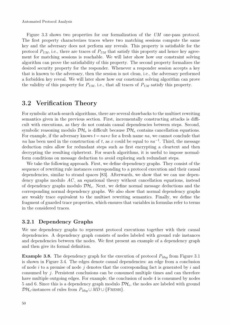
Figure 3.3 shows two properties for our formalization of the UM one-pass protocol.The first property characterizes traces where two matching sessions compute the samekey and the adversary does not perform any reveals. This property is satisfiable for theprotocol PUM, i.e., there are traces of PUM that satisfy this property and hence key agree-ment for matching sessions is reachable. We will later show how our constraint solvingalgorithm can prove the satisfiability of this property. The second property formalizes thedesired security property for the responder. Whenever a responder session accepts a keythat is known to the adversary, then the session is not clean, i.e., the adversary performeda forbidden key reveal. We will later show how our constraint solving algorithm can provethe validity of this property for PUM, i.e., that all traces of PUM satisfy this property.

3.2 Verification Theory

For symbolic attack-search algorithms, there are several drawbacks to the multiset rewritingsemantics given in the previous section. First, incrementally constructing attacks is diffi-cult with executions, as they do not contain causal dependencies between steps. Second,symbolic reasoning modulo DHe is difficult because DHe contains cancellation equations.For example, if the adversary knows t=na∗x for a fresh name na, we cannot conclude thatna has been used in the construction of t, as x could be equal to na−1. Third, the messagededuction rules allow for redundant steps such as first encrypting a cleartext and thendecrypting the resulting ciphertext. For search algorithms, it is useful to impose normal-form conditions on message deduction to avoid exploring such redundant steps.

We take the following approach. First, we define dependency graphs. They consist of thesequence of rewriting rule instances corresponding to a protocol execution and their causaldependencies, similar to strand spaces [83]. Afterwards, we show that we can use depen-dency graphs modulo AC , an equational theory without cancellation equations, insteadof dependency graphs modulo DHe. Next, we define normal message deductions and thecorresponding normal dependency graphs. We also show that normal dependency graphsare weakly trace equivalent to the multiset rewriting semantics. Finally, we define thefragment of guarded trace properties, which ensures that variables in formulas refer to termsin the considered traces.

3.2.1 Dependency Graphs

We use dependency graphs to represent protocol executions together with their causaldependencies. A dependency graph consists of nodes labeled with ground rule instancesand dependencies between the nodes. We first present an example of a dependency graphand then give its formal definition.

Example 3.8. The dependency graph for the execution of protocol PMsg from Figure 3.1is shown in Figure 3.4. The edges denote causal dependencies: an edge from a conclusionof node i to a premise of node j denotes that the corresponding fact is generated by i andconsumed by j. Persistent conclusions can be consumed multiple times and can thereforehave multiple outgoing edges. For example, the conclusion of node 4 is consumed by nodes5 and 6. Since this is a dependency graph modulo DHe, the nodes are labeled with groundDHe-instances of rules from PMsg∪MD ∪Fresh.


50

3 :Fr(a) Fr(b)


1 :Fr(a)

2 :Fr(b)

9 :St(a) In(g ˆ a)

[Fin]

4 :Out(〈g ˆ (a ∗ b), b−1〉)

K(〈g ˆ (a ∗ b), b−1〉)

5 :K(〈g ˆ (a ∗ b), b−1〉)

K(g ˆ (a ∗ b))6 :

K(〈g ˆ (a ∗ b), b−1〉)

K(b−1)

7 :K(g ˆ (a ∗ b)) K(b−1)

K(g ˆ a)

8 :K(g ˆ a)


Figure 3.4. Dependency graph for the execution from Example 3.6.

Definition 3.9. Let E be an equational theory and R be a set of labeled multisetrewriting rules. We say that the pair dg = (I , D) is a dependency graph modulo E for Rif I ∈ ginstsE(R∪Fresh)∗, D ∈N2×N2, and dg satisfies the Conditions DG1–4 listedbelow. To state these conditions, we introduce the following definitions. We call idx (I)the nodes of dg and D the edges of dg . We write (i, u) (j , v) for the edge ((i, u), (j , v)).A conclusion of dg is a pair (i, u) such that i is a node of dg and u∈ idx (concs(Ii)).The corresponding conclusion fact is (concs(Ii))u. A premise of dg is a pair (i, u) such thati is a node of dg and u∈ idx (prems(Ii)). The corresponding premise fact is (prems(Ii))u.A conclusion or premise is linear if its fact is linear.

DG1. For every edge (i, u) (j , v)∈D, it holds that i< j and the conclusion fact of (i, u)is syntactically equal to the premise fact of (j , v).

DG2. Every premise of dg has exactly one incoming edge.

DG3. Every linear conclusion of dg has at most one outgoing edge.

DG4. The Fresh instances are unique.

We denote the set of all dependency graphs modulo E for R by dgraphsE(R).

Let dg = (I ,D) and I = [l1−[a1]→ r1, , lk−[ak]→ rk], overloading notation, we define thetrace of dg as trace(dg) = [set(a1), , set(ak)]. We can show that the multiset rewritingsemantics given in Section 3.1 and the dependency graphs are trace equivalent in thefollowing sense

Lemma 3.10. For all protocols P, trace(execs(P ∪MD))= trace(dgraphsDHe(P ∪MD)).

Proof. We prove by induction that the sequences of rule instances of executions anddependency graphs coincide. Since the traces are determined by the sequences of ruleinstances, this completes the proof.


51

3.2.2 Dependency Graphs Modulo AC

We now switch to a semantics based on dependency graphs modulo associativity andcommutativity. To achieve this, we define the set of equations AC as

AC = x∗(y∗z)≃ (x∗y)∗z, x∗y≃ y∗x

and the rewriting system RDH as

RDH=

(xˆy)ˆz→ xˆ(y∗z) xˆ1→ x

(x−1∗y)−1→x∗y−1 1−1→ 1 x−1∗y−1→ (x∗y)−1

x∗(x∗y)−1→ y−1 x∗1→x (x−1)−1→x

x−1∗(y−1∗z)→ (x∗y)−1∗z x∗(x−1∗y)→ y x∗x−1→ 1(x∗y)−1∗(y∗z)→x−1∗z

.

We define RDHe=RDH∪RST . Then (ΣDHe,RDHe,AC ) is a decomposition of DHe with

the finite variant property for the following reasons. First, (ΣDHe, RDHe

≃ ∪ AC ) is anequational presentation of =DHe

. Second, AC is regular, sort-preserving, and all variablesare of sort msg . Third, RDHe is sort-decreasing and RDHe,AC -rewriting is convergentand coherent. SinceRDH and ST have disjoint signatures and neither contains duplicatingrules [35], it suffices to consider both rewrite systems individually. Since ST is a subterm-convergent theory, both properties easily follow. For RDH,AC -rewriting, we have used theAProVE termination tool [85] and the Maude Church-Rosser and Coherence Checker [73]to verify both properties. Fourth, there is a complete and finitary AC -unification algorithm.Finally, the finite variant property can be established individually for RDH,AC and ST ,which has been done in [51].

Given a term t, we therefore have a unique normal form with respect to RDHe,AC -rewriting, which we denote with t↓RDHe

. We use folding variant narrowing to compute acomplete set of RDHe,AC -variants, which we denote by ⌈t⌉substs

RDHe. We use ⌈t⌉instsRDHe to denote

the set (tτ)↓RDHe|τ ∈ ⌈t⌉substs

RDHe of normalized instances corresponding to the variants.We say that t is ↓RDHe

-normal if t =AC t↓RDHe. We say a dependency graph dg = (I , D)

is ↓RDHe-normal if all rule instances in I are. It is straightforward to extend the notion

of RDHe,AC -variants to multiset rewriting rules by considering rules as terms and therequired new function symbols as free. We can then show that we can take the RDHe,AC -variants of the multiset rewriting rules and use dependency graphs modulo AC .

Lemma 3.11. For all sets of multiset rewriting rules R,

dgraphsDHe(R)↓RDHe

=AC dg | dg ∈ dgraphsAC(⌈R⌉instsRDHe)∧ dg ↓RDHe

-normal .

Proof. The lemma is a consequence of the fact that all ↓RDHe-normal DHe-instances of

rules in R are ↓RDHe-normal AC -instances of rules in ⌈R⌉insts

RDHe.

Example 3.12. The dependency graph from Figure 3.4 is already an element of

dgraphsAC(⌈PMsg∪MD ⌉instsRDHe) and ↓RDHe

-normal. For example, the label of node 5 is ↓RDHe-

normal and an AC -instance of the second rule in the set

⌈K(x)−[]→K(fst(x))⌉instsRDHe = K(x)−[]→K(fst(x)),K(〈y, z 〉)−[]→K(y).


52

As another example, consider the label of node 7 which is ↓RDHe-normal and an AC -instance

of the third rule rule in the set

⌈K(x),K(y)−[]→K(xˆy)⌉instsRDHe =

K(x),K(y)−[]→K(xˆy)K(uˆv),K(v−1)−[]→K(u)K(uˆ(v∗w)),K(w−1)−[]→K(uˆv) 44 other variants

.

The rule for exponentiation has 47 RDHe,AC -variants that cover all ↓RDHe-normal-forms

of xˆy for instantiations of x and y with arbitrary terms. To compute the set of variants,we have used Tamarin, which implements folding variant narrowing.

Note that the rewriting system resulting from orienting the non-AC equations in EDH

from left to right is not coherent for similar reasons as the rewrite system from Example 2.1.After completion, the equations containing the inverse operator are usually oriented suchthat the inverse operator is pushed inwards, e.g., (x∗y)−1→ x−1∗y−1. The problem withthis orientation is that there is no finite set of variants for the term x−1 since for all k, thenormal form of (a1∗ ∗ak)

−1 is a1−1∗ ∗ak

−1. In RDH, we therefore use an orientation dueto Lankford which solves this problem by pushing the inverse operator outwards.

3.2.3 Normal Message Deduction Rules

In dependency graphs modulo AC , we use K-facts and ground AC -instances of ⌈MD ⌉instsRDHe

to model message deduction by the adversary. In the following, we introduce new factsymbols and a new set of rules to model normal message deduction. The new rules aresound and complete with respect to the old rules and enforce restrictions that are similarto those for normal natural deduction proofs [146]. In the setting of message deduction,there are several works that take a similar approach such as [48], [165], and [52]. We firstfocus on the deduction of products, then we show the rules for communication and ΣDH,and finally, we show how to handle the rules for ΣST .

Multiplication

Conditions P1–P6 from Definition 3.4 ensure that protocol rules do not build new productsin extractable positions. More precisely, we define the non-inverse factors of a term t as

nifactors(t)=

nifactors(a)∪ nifactors(b) if t= a∗bnifactors(s) if t= s−1

t otherwise

and prove in Lemma A.4 in the Appendix that for all products t that can be extracted frommessages sent by the protocol, the adversary can already deduce nifactors(t) before themessage is sent. Intuitively, this means that all extractable products are simple variationsof products constructed by the adversary himself. For example, the adversary can senda−1∗b to a protocol that inverts received messages. The protocol replies with a∗b−1, whichis a different product, but has the same non-inverse factors.


53

Rules for Communication and DH

Let us first assume that ΣST = ∅. Then we can partition the rules in ⌈MD ⌉instsRDHe into five

subsets: communication rules for sending and receiving messages, deconstruction rules thatextract a subterm from an argument, exponentiation rules that modify an exponentiationby adding and removing (some, but not all) exponents, construction rules that apply a func-tion symbol from ΣDH to arguments, and multiplication rules consisting of all RDHe,AC -variants of the rule for multiplication. Note that the set of exponentiation rules consists ofall RDHe,AC -variants of the rule [K(x),K(y)]−[]→K(xˆy) that are neither deconstructionnor construction rules.

We want to enforce normal message deductions , which satisfy the following normal-form condition. All messages are deduced by extracting subterms from messages sent bythe protocol, optionally modifying the exponent of extracted exponentiations, and finallyapplying function symbols to these messages. This allows us to search for message deduc-tions by applying deconstruction and exponentiation rules to messages sent by the protocoltop-down and applying construction rules to messages received by the protocol bottom-upuntil both meet in the middle.

To achieve this, we introduce three new fact symbols. K⇓d(m) denotes that m has been

extracted from a message sent by the protocol. K⇓e(m) denotes that m has been deducedby modifying the exponent of an extracted message. We call a rule instance with conclusion

K⇓d(m) or K⇓e(m) a deconstruction of m. Finally, K⇑(m) denotes that m has been deducedusing a normal message deduction. We call a rule instance with conclusion K⇑(m) a normaldeduction of m.

Figure 3.5 shows the normal message deduction rules ND that have been obtained byreplacing each K-fact in the previously defined sets of rules with the appropriate new fact

symbol. The Recv rule generates a K⇓d-fact, which captures that a message sent by theprotocol can be extracted. The Send rule allows the adversary to send a message that hasa normal deduction to the protocol. The deconstruction rules allow to extract a subtermfrom a message that has been extracted itself. This extraction might require an additionalmessage. For example, the second deconstruction rule requires the inverse of the exponent

to extract the base of an exponentiation. For these additional premises, we use K⇑-facts.The exponentiation rules allow us to modify the exponent of an extracted message and

use a K⇓e-fact for the conclusion. The Coerce rule reflects that both extracted subtermsthemselves and extracted subterms with modified exponent have a normal deduction. Theresulting K⇑-fact of this rule can then be used by construction rules or Send. The con-struction rules use K⇑ for both premises and conclusions. There are construction rulesfor all function symbols, for fresh names, and for public names. Note that we replaceall multiplication rules with n,l-ary construction rules for multiplication. This is possiblebecause we can construct all deducible products from their non-inverse factors.

Example 3.13. Figure 3.6 shows three message deduction subgraphs for exponentiation.Subfigure (a) shows a message deduction where aˆb is first constructed from a and b,and immediately afterwards, a is extracted. This is not a normal deduction because, as

Subfigure (b) shows, a deconstruction rule for exponentiation cannot be applied to K⇑(aˆb).Subfigure (c) shows that the ND rules also forbid repeated exponentiations. The deduction

in (c) can be replaced by the single rule instance K⇓d(aˆb),K⇑(b−1∗d)−[]→K⇓e(aˆd). Notethat the deduction in (c) includes the term c which occurs neither in the conclusion of i2


54

Communication rules: RecvOut(x)

K⇓d(x)Send

K⇑(x)

In(x)

Deconstruction rules:

K⇓d(x−1)

K⇓d(x)

K⇓d(xˆy) K⇑(y−1)

K⇓d(x)

K⇓d(xˆ(y−1)) K⇑(y)

K⇓d(x)

K⇓d(xˆ(y∗z−1)) K⇑(y−1∗z)

K⇓d(x)

Exponentiation rules:

K⇓d(xˆy) K⇑(z)

K⇓e(xˆ(y∗z))

K⇓d(xˆy) K⇑(y−1∗z)

K⇓e(xˆz)

K⇓d(xˆ(y1∗y2−1)) K⇑(z1∗z2

−1)

K⇓e(xˆ(y1∗z1∗(y2∗z2)−1))

Coerce rule : CoerceK⇓y

(x)

K⇑(x)

Construction rules:

K⇑(x)

K⇑(x−1)

K⇑(x) K⇑(y)

K⇑(xˆy) K⇑(1)

K⇑(x1) K⇑(xn) K⇑(xn+1) K⇑(xl)

K⇑((x1∗ ∗xn)∗(xn+1∗ xl)−1)

Fr(x:fr)

K⇑(x:fr) K⇑(x:pub)

Figure 3.5. The normal message deduction rules ND . We use y in the Coerce to denote thateither K

⇓d(x) or K⇓e(x) can be used as premise. There are construction rules for multiplication

for all n and l such that n> 0 and l > 1. There are 42 exponentiation rules computed from the 47RDHe,AC -variants of the exponentiation rule in MD . The remaining 5 variants correspond to theconstruction rule for exponentiation, the 3 deconstruction rules for exponentiation, and the variantwhere the exponent is 1 for which no message deduction rule is required.

nor in the first premise of i1. Also note that it is possible to extend the deduction in (c)by adding an unbounded number of additional steps that remove the previously addedexponent and add a new exponent. Since our search algorithm exploits locality of messagedeductions [121], it is important to exclude this redundancy.

i1 :K(a) K(b)

K(a ˆ b)

i2 :K(a ˆ b) K(b−1)

K(a)

i1 :K⇑(a) K⇑(b)

K⇑(a ˆ b)

i2 :K⇓d

(a ˆ b) K⇑(b)

K⇓e

(a)

(a) (b) (c)i1 :

K⇓d

(a ˆ b) K⇑(b−1 ∗ c)

K⇓e

(a ˆ c)

i2 :K⇓d

(a ˆ c) K⇑(c−1 ∗ d)

K⇓e

(a ˆ d)

Figure 3.6. Message deduction subgraphs for exponentiation. The crossed edges are not allowedsince source and target are not equal.

Rules for ST

To explain how the normal message deduction rules for ΣST are computed, we first showthe rules for a simple theory. Then we explain the general case.


55

Example 3.14. Consider the subterm theory DY defined in Example 3.2. This theory hasthe construction rules

K⇑(x) K⇑(y)

K⇑(〈x, y〉)

K⇑(x)

K⇑(fst(x))

K⇑(x)

K⇑(snd(x))

K⇑(x)

K⇑(pk(x))

K⇑(x) K⇑(y)

K⇑(enc(x, y))

K⇑(x) K⇑(y)

K⇑(dec(x, y)) K⇑(true)

K⇑(x) K⇑(y)

K⇑(sig(x, y))

K⇑(x) K⇑(y)

K⇑(verify(x, y))

K⇑(x)

K⇑(h(x))

and the deconstruction rules

K⇓d(〈x, y〉)

K⇓d(x)

K⇓d(〈x, y〉)

K⇓d(y)

K⇓d(enc(x, pk(y))) K⇑(y)

K⇓d(x).

For this theory, the deconstruction rules can be computed by taking the non-trivialRDHe,AC -variants of the message deduction rules and replacing the K-facts such thatthe conclusion and the premise that contains the conclusion-message as a subterm useK⇓d-facts and the remaining premises use K⇑-facts. For example, the only non-trivialRDHe,AC -variant of the rule for dec is [K(enc(x, pk(y))), K(y)] −[]→ K(x) and replacingthe fact symbols as described above yields the given destruction rule.

For arbitrary rewrite rules, the set of deconstruction rules computed as described aboveis unfortunately not complete. For example, consider the rewrite theory

ST =(f(_,_), g(_), e(_,_), f(g(e(x1, x2)), x2)→x1).

Note that given e(a, b) and b, the fresh name a is deducible for this theory since we canfirst apply g to e(a,b) and then apply f to the result and b to obtain f(g(e(a, b)), b), whichreduces to a. Using the method described above to compute the normal message deduction

rules ND , we obtain the single deconstruction rule[

K⇓d(g(e(x1, x2))),K⇑(x2)

]

−[]→K⇓d(x1)

for f and construction rules for f , g, and e. These rules are not sufficient to deduce K⇑(a)

from K⇓d(e(a, b)) and K⇓d(b). To apply the deconstruction rule, the fact K⇓d(g(e(a, b)))is required. Using the construction rule for g and Coerce, it is only possible to deduce

K⇑(g(e(a,b))), which cannot be used with the deconstruction rule for f . We therefore needanother deconstruction rule K⇓d(e(x1, x2)),K

⇑(x2)−[]→K⇓d(x1) which performs the requiredconstruction and deconstruction in one step.

We therefore compute the normal message deduction rules for ST as follows. For eachn-ary function symbol f ∈ΣST , the construction rule is

[K⇑(x1), ,K⇑(xn)]−[]→K⇑(f(x1, , xn)).

We compute the destruction rules from the rewriting system RST . For each rewriting rulel→r∈RST , we distinguish two cases. If r is ground, then we do not require a deconstructionrule for this rewriting rule since r can be directly deduced using only construction rules.If there is a position p with l |p =r, then we use the function drules to compute thecorresponding deconstruction rules

drules(l, p)=([

K⇓d(l|p′)]

· cprems(l, p′))

−[]→[

K⇓d(l|p)]

|p′ strictly above p and p′ [ ]

.

Intuitively, drules returns one deconstruction rule for each subterm of l that containsthe position p except for l|p and l itself. The drules function uses the function cprems to


56

compute the required K⇑-premises. We use the function seq that converts sets into sequencesto define cprems as

cprems(l, p)= seq(K⇑(l |p′) |p′ [ ]∧ p′ has sibling that is above or equal to p).

The rules returned by drules(l, p) express that the adversary can deduce an instance m ofl to extract the corresponding subterm m|p.

Example 3.15. To see how the computation of the deconstruction rules works, considerdrules(l, [1, 1]) for l= dec(enc(x, pk(y)), y). The only position p′ [ ] strictly above [1, 1]

is [1]. We therefore obtain the only rule[

K⇓d(enc(x, pk(y)))]

· [K⇑(y)] −[]→ K⇓d(y). Thesecond premise is equal to cprems(l, [1]) since l |[2]=y and the position [2] is the only siblingof the position [1] or of a position above [1] that is not equal to [ ].

Example 3.16. We can now turn to the problematic case described earlier. The right-handside of the rewrite rule f(g(e(x1, x2)), x2)→x1 occurs at position [1, 1, 1]. We compute thedeconstruction rule for this rewrite rule with drules(l, [1, 1, 1]) for l= f(g(e(x1, x2)), x2).There are two positions p′ [ ] strictly above [1, 1, 1], namely [1, 1] and [1]. We thereforeobtain the two deconstruction rules

([

K⇓d(g(e(x1, x2)))]

· cprems(l, [1]))

−[]→[

K⇓d(x1)]

and([

K⇓d(e(x1, x2))]

· cprems(l, [1, 1]))

−[]→[

K⇓d(x1)]

where the remaining K⇑-premises are computed by cprems(l, [1]) and cprems(l, [1, 1]). Thefirst case captures that the adversary extracts x1 by applying f to g(e(x1, x2)) and theremaining arguments computed by cprems . The second case captures that the adversaryextracts x1 by applying g to e(x1, x2) and f to the result. Here, cprems computes therequired arguments for both the application of g and the application of f . For the first

rule, cprems(l, [1]) returns the sequence [K⇑(x2)] since l|[2]=x2 and [2] is the position of thethe required second argument for the application of f . For the second rule, cprems(l, [1, 1])

also returns the sequence [K⇑(x2)] since [1, 1] has no siblings in l. This reflects that theapplication of g performed by this rule does not require any arguments except for e(x1, x2).Intuitively, cprems(l, p) starts at the position p and traverses l upwards and collects all sib-lings, which correspond to the required arguments for the performed function applications.

Example 3.17. Figure 3.7 shows four message deduction subgraphs. In (a), the adversarydecrypts a message that he earlier encrypted himself. Instead of performing these deduc-tions, the adversary can directly use the conclusion K(a) that is used by i1. The deductionfrom (a) is not possible with the normal message deduction rules ND as depicted in (b).

Subfigures (c) and (d) show two different ways to deduce K⇑(〈a, b〉) from K⇓d(〈a, b〉). Wewill later introduce an additional normal form condition that forbids deduction (c).

3.2.4 Normal Dependency Graphs

We now define normal dependency graphs. They use normal message deductionrules and enforce further normal-form conditions. To state the normal-form condi-tions, we first define the subset of invertible function symbols. An n-ary function


57

i2 :K(enc(a, pk(b))) K(b)

K(a)

i1 :K(a) K(pk(b))

K(enc(a, pk(b)))

i2 :K⇓d

(enc(a, pk(b))) K⇑(b)

K⇓d

(a)

i1 :K⇑(a) K⇑(pk(b))

K⇑(enc(a, pk(b)))

(a)

(b)

(c) (d)i1 :

Out(〈a, b〉)

K⇓d

(〈a, b〉)

i1 :Out(〈a, b〉)

K⇓d

(〈a, b〉)

i4 :K⇓d

(a)

K⇑(a)i5 :

K⇓d

(b)

K⇑(b)

i2 :K⇓d

(〈a, b〉)

K⇓d

(a)i3 :

K⇓d

(〈a, b〉)

K⇓d

(b)

i6 :K⇑(a) K⇑(b)

K⇑(〈a, b〉)

i2 :K⇓d

(〈a, b〉)

K⇑(〈a, b〉)

Figure 3.7. Message deduction subgraphs for DY . The crossed edge is not allowed since sourceand target are not equal.

symbol f ∈ΣST ∪ΣDH is invertible if for arbitrary terms ti and for all 1 ≤ i ≤ n,

K⇓d(f(t1, , tn))−[]→K⇓d(ti)∈ ginstsAC(ND), i.e., there is an AC -instance of a deconstruc-tion rule that extracts ti. For DH, the function symbol _−1 is the only invertible functionsymbol and for the DY theory, 〈_, _〉 is the only invertible function symbol. A mes-sage where the outermost function symbol is invertible can always be deduced by applyingthe corresponding construction rule.

Definition 3.18. A normal dependency graph for a protocol P is a dependency graph dg

such that dg ∈ dgraphsAC(⌈P ⌉instsRDHe∪ND) and the following conditions are satisfied.

N1. The dependency graph dg is ↓RDHe-normal.

N2. There is no multiplication rule that has a premise fact of the form K⇑(s∗t) and allconclusion facts of the form Kd(s∗t) are conclusions of a multiplication rule.

N3. If there are two conclusions c and c′ with conclusion facts Kd(m) and Kd′

(m′) suchthat m=AC m

′ and either d= d′=⇑ or d=⇓y and d′=⇓y′

for y, y ′∈d, e, then c= c′.

N4. All conclusion facts K⇑(f(t1, , tn)) where f is an invertible function symbol areconclusions of the construction rule for f .

N5. If a node i has a conclusion K⇓y(m) for y∈d,e and a node j has a conclusion K⇑(m′)

with m=AC m′, then i< j and either root(m) is invertible or the node j is an instance

of Coerce.

N6. There is no node[

K⇓d(a), K⇑(b)]

−[]→ K⇓e(cˆd) where c does not contain any fresh

names and nifactors(d)⊆AC nifactors(b).

We denote the set of all normal dependency graphs for P with ndgraphs(P ).

Condition N1 ensures that all rule instances are ↓RDHe-normal. Condition N2 formalizes

that the adversary constructs all products directly by multiplying their components. Con-

dition N3 ensures that the same message never has multiple K⇓d, K⇓e, or K⇑ deductions.


58

Condition N4 ensures that terms m where root(m) is invertible are never deduced byCoerce. Condition N5 forbids two types of redundancies. First, if there is already anormal deduction for a message, then there is no need for a later deconstruction of thesame message. Second, if there is already a deconstruction of a message, then the Coercerule should be used to create a normal deduction unless it is forbidden by condition N4.Condition N6 forbids instances of exponentiation rules that can be directly replaced bythe construction rule for exponentiation.

Note that normal dependency graphs have the same observable traces as dependencygraphs modulo AC using the message deduction rules MD .

Lemma 3.19. For all protocols P,

trace(dg) | dg ∈ dgraphsAC(⌈P ∪MD ⌉instsRDHe)∧ dg ↓RDHe

-normal = trace(ndgraphs(P )).

In Appendix A, we prove Lemma A.12, which is an extended version of this lemma forbilinear pairings and AC operators, which we will introduce later on. Combining this resultwith Lemma 3.10 and Lemma 3.11, we conclude that normal dependency graphs have thesame observable traces as our multiset rewriting semantics.

Corollary 3.20. For all protocols P, trace(execs(P ∪MD))↓RDHe=AC trace(ndgraphs(P )) .

Example 3.21. The dependency graph from Figure 3.4 can be converted into the normaldependency graph depicted in Figure 3.8 as follows. First, the rules for message deductionare replaced by the corresponding rules from ND where possible. This requires a a Coercenode between Node 10 and 12 in the normal dependency graph. Between the conclusionof Node 6 and the second premise of Node 10 in the normal dependency graph, we cannotsimply add a Coerce node because of condition N4. We therefore add the deconstructionrule for the inverse followed byCoerce and the construction rule for inverse. This is similarto the deductions (c) and (d) in Figure 3.7 where only deduction (d) is allowed.

Properties of Normal Dependency Graphs

We prove a property of normal dependency graphs that is crucial for our constraint solving

algorithm. It states that every K⇓y(t)-premise is deduced using a chain of deconstruction

rules from a received message. We use here the extended set of deconstruction rules NDdecon

that consists of the deconstruction and exponentiation rules from Figure 3.5 and the decon-struction rules for ST .

Definition 3.22. Let dg =(I ,D) be a normal dependency graph for P . Its deconstructionchain relation ։dg is the smallest relation such that i։dg p if (i, 1) is a K⇓y

-conclusionin dg for y ∈ d, e and (a) (i, 1) p ∈ D or (b) there is a premise (j , 1) such that(i, 1) (j , 1)∈D and j։dg p.

Our algorithm exploits the following lemma to reason about the possible origins of K⇓y-

premises.


59

13 :St(a) In(g ˆ a)

[Fin()]

3 :Fr(a) Fr(b)


4 :Out(〈g ˆ (a ∗ b), b−1〉)

K⇓d

(〈g ˆ (a ∗ b), b−1〉)

5 :K⇓d

(〈g ˆ (a ∗ b), b−1〉)

K⇓d

(g ˆ (a ∗ b))6 :

K⇓d

(〈g ˆ (a ∗ b), b−1〉)

K⇓d

(b−1)

10 :K⇓d

(g ˆ (a ∗ b)) K⇑(b−1)

K⇓e

(g ˆ a)

12 :K⇑(g ˆ a)


11 :

K⇓e

(g ˆ a)

K⇑(g ˆ a)

8 :K⇓d

(b)

K⇑(b)

9 :K⇑(b)

K⇑(b−1)

7 :K⇓d

(b−1)

K⇓d

(b)

1 :Fr(a)

2 :Fr(b)

Figure 3.8. Normal dependency graph for PMsg.

Lemma 3.23. Let dg be a normal dependency graph. For every premise p of dg withfact K⇓y

(m) for y∈d,e, there is a node i in dg such that Ii∈ ginstsAC(Recv) and i։dg p.

The lemma follows from the structure of the rules in ND . The only rule in ND that has aK⇓y

-conclusion, but no K⇓y-premise is Recv.

Example 3.24. For example, in the dependency graph dg from Figure 3.8, 4։dg (11, 1),

5։dg (11, 1), and 5։dg (10, 1), but not 6։dg (11, 1) since conclusion (8, 1) is a K⇑-fact.

3.2.5 Guarded Trace Formulas

In the following, let f range over facts and i, j over temporal variables. A trace formula ϕis in negation normal form if it is built such that negation is only applied to trace atomsand ⊥ and all other logical operators are ∧, ∨, ∀, and ∃.


60

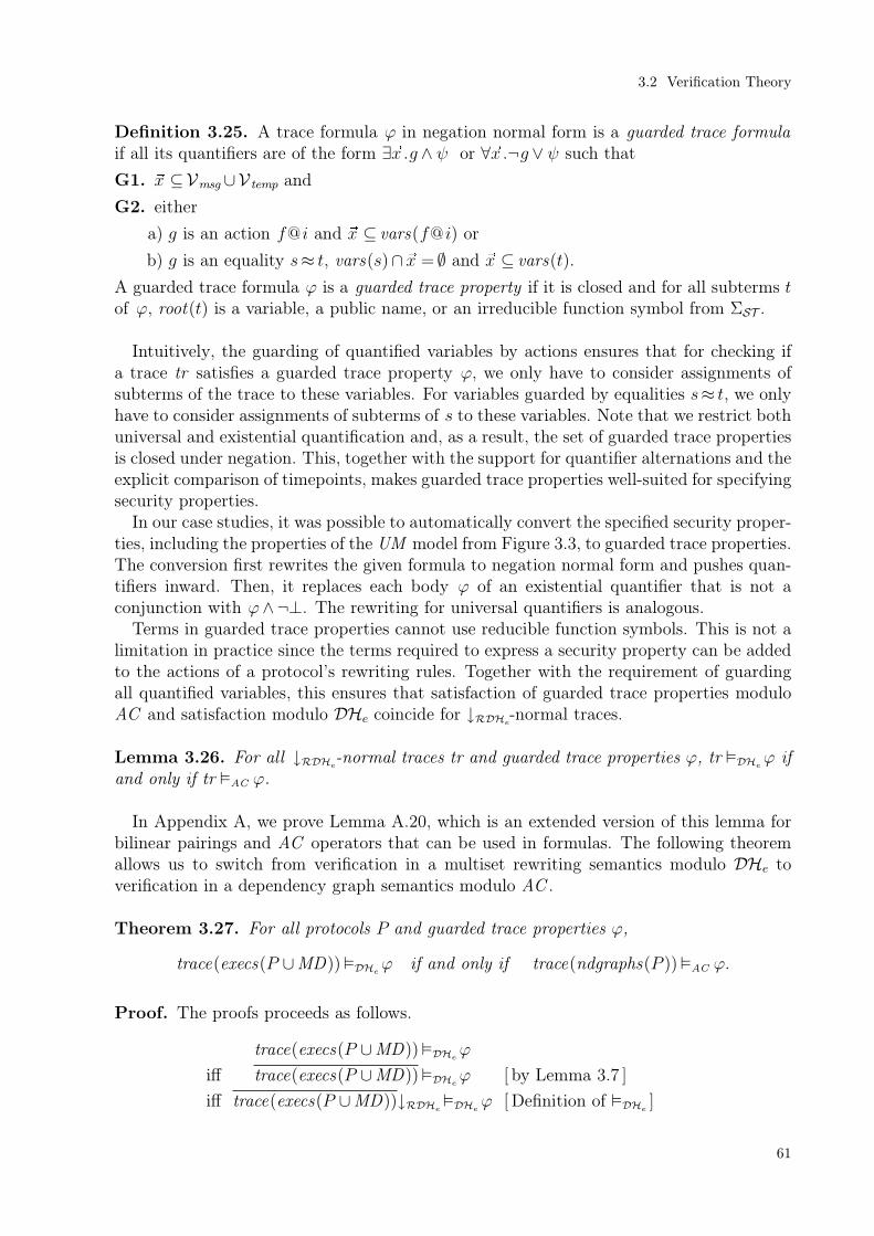
Definition 3.25. A trace formula ϕ in negation normal form is a guarded trace formulaif all its quantifiers are of the form ∃xR .g ∧ ψ or ∀xR .¬g∨ ψ such that

G1. xR ⊆Vmsg∪V temp and

G2. either

a) g is an action f@i and xR ⊆ vars(f@ i) or

b) g is an equality s≈ t, vars(s)∩xR = ∅ and xR ⊆ vars(t).

A guarded trace formula ϕ is a guarded trace property if it is closed and for all subterms tof ϕ, root(t) is a variable, a public name, or an irreducible function symbol from ΣST .

Intuitively, the guarding of quantified variables by actions ensures that for checking ifa trace tr satisfies a guarded trace property ϕ, we only have to consider assignments ofsubterms of the trace to these variables. For variables guarded by equalities s≈ t, we onlyhave to consider assignments of subterms of s to these variables. Note that we restrict bothuniversal and existential quantification and, as a result, the set of guarded trace propertiesis closed under negation. This, together with the support for quantifier alternations and theexplicit comparison of timepoints, makes guarded trace properties well-suited for specifyingsecurity properties.

In our case studies, it was possible to automatically convert the specified security proper-ties, including the properties of the UM model from Figure 3.3, to guarded trace properties.The conversion first rewrites the given formula to negation normal form and pushes quan-tifiers inward. Then, it replaces each body ϕ of an existential quantifier that is not aconjunction with ϕ∧¬⊥. The rewriting for universal quantifiers is analogous.

Terms in guarded trace properties cannot use reducible function symbols. This is not alimitation in practice since the terms required to express a security property can be addedto the actions of a protocol’s rewriting rules. Together with the requirement of guardingall quantified variables, this ensures that satisfaction of guarded trace properties moduloAC and satisfaction modulo DHe coincide for ↓RDHe

-normal traces.

Lemma 3.26. For all ↓RDHe-normal traces tr and guarded trace properties ϕ, tr DHe

ϕ ifand only if tr AC ϕ.

In Appendix A, we prove Lemma A.20, which is an extended version of this lemma forbilinear pairings and AC operators that can be used in formulas. The following theoremallows us to switch from verification in a multiset rewriting semantics modulo DHe toverification in a dependency graph semantics modulo AC .

Theorem 3.27. For all protocols P and guarded trace properties ϕ,

trace(execs(P ∪MD))DHeϕ if and only if trace(ndgraphs(P ))AC ϕ.

Proof. The proofs proceeds as follows.

trace(execs(P ∪MD))DHeϕ

iff trace(execs(P ∪MD))DHeϕ [by Lemma 3.7 ]

iff trace(execs(P ∪MD))↓RDHeDHe

ϕ [Definition of DHe]


61

iff trace(ndgraphs(P ))DHeϕ [by Corollary 3.20 ]

iff trace(ndgraphs(P ))AC ϕ [by Lemma 3.7 and 3.26 ]

Note that the last step exploits that ϕ is a guarded trace property.

3.3 Constraint Solving

In this section, we give an algorithm that determines for a guarded trace property ϕ anda protocol P if ϕ is P ,DHe-satisfiable. Our algorithm uses constraint solving to search fortraces of P that are models of ϕ. If it terminates, it has either found such a trace or, sincethe search is complete, it has proved that ϕ is unsatisfiable by traces of P . To analyze if alltraces of a protocol satisfy a property ϕ, we must check for validity instead of satisfiability.Since these notions are dual, we can determine if ϕ is P ,DHe-valid by using our algorithmto check if ¬ϕ is P ,DHe-satisfiable. If we find a trace, then this a counterexample to thevalidity of ϕ, i.e., there is an attack. Both problems are undecidable and our algorithmdoes not always terminate. Nevertheless, it terminates for many relevant protocols andproperties. In the following, we define the syntax and semantics of constraints. Afterwards,we give our constraint solving algorithm and rules, explain two optimizations, and presentseveral examples.

3.3.1 Syntax and Semantics of Constraints

In the remainder of this section, let ri and ru range over multiset rewriting rules, u andv and w over natural numbers, and ϕ over guarded trace formulas. A graph constraint iseither a node i: ri , an edge (i, u) (j , v), a deconstruction chain i։ (j , v), or a providesi ⊲ f which denotes that f is the first conclusion of the node i. A constraint is a graphconstraint or a guarded trace formula.

A structure is a tuple (dg , θ) of a dependency graph dg = (I , D) and a valuation θ.We denote the application of the homomorphic extension of θ to a rule ru by ruθ. Thesatisfaction relation between structures and constraints is inductively defined by thefollowing rules:

(dg , θ) i: ri if θ(i)∈ idx (I) and ri θ=AC Iθ(i)

(dg , θ) (i, u) (j , v) if (θ(i), u) (θ(j), v)∈D

(dg , θ) i։ (j , v) if θ(i)։dg (θ(j), v)

(dg , θ) i⊲ f if θ(i)∈ idx (I) and (concs(Iθ(i)))1 =AC fθ

(dg , θ) ϕ if (trace(dg), θ)AC ϕ

A constraint system Γ is a finite set of constraints. The structure (dg , θ) satisfies Γ, written(dg , θ) Γ, if (dg , θ) satisfies each constraint in Γ. We say that (dg , θ) is a P -solution of Γ,if dg is a normal dependency graph for P and (dg , θ) Γ. A P -model of Γ is a normaldependency graph dg for P such that there is a valuation θ with (dg , θ) Γ. Note that thefree variables of a constraint system are therefore considered as existentially quantified. Weuse modelsP(Γ) to denote the set of all P -models of Γ.


62

Example 3.28. The dependency graph from Figure 3.8 satisfies the constraints

• i:K⇓d(x),K⇑(b−1)−[]→K⇓e(gˆa) for all valuations θ with θ(i)= 10 and θ(x)=AC gˆ(a∗b),

• (j , 1) (k, 2) for θ with θ(j)= 2 and θ(k)= 3,

• i։ (l, 1) for θ with θ(i)= 10 and θ(l) = 11,

• i⊲K⇑(b) for θ with θ(i)= 8, and

• ∀i y.¬K(h(y))@ i∨⊥ since there is no K-action whose argument is a hash.

3.3.2 Constraint Solving Algorithm

As mentioned before, validity can be reduced to satisfiability. Moreover, Theorem 3.27allows us to use normal dependency graphs and satisfaction modulo AC . Given a guardedtrace property ϕ and a protocol P , we can therefore focus on the problem of finding normaldependency graphs dg ∈ ndgraphs(P ) such that trace(dg)AC ϕ. This is equivalent to theproblem of finding P -models for the constraint system ϕ. To achieve this, we define aconstraint solving relation P that reduces a constraint system to a finite set of constraintsystems by inferring new constraints and performing case splits. The relation P is soundand complete in the following sense: whenever Γ P Γ1, ,Γk, then the set of P -modelsof Γ is equal to the union of the sets of P -models of the Γi. We overload notation anddefine the reflexive-transitive closure P

∗ of P as the least relation such that Γ P∗ ∆

if (a) ∆ = Γ or (b) Γ P Γ1, , Γk, Γi P∗ ∆i, and ∆ =

⋃

i=1

k∆i. We call Γ P

∗ ∆ aconstraint reduction .

The relation P∗ can be used to check P ,DHe-satisfiability of ϕ as follows. We search

for a constraint reduction ϕ P∗ ∅ or a constraint reduction ϕ P

∗ ∆ such that thereis a constraint system Γ∈∆ for which we can directly confirm that it has a P -model. Inthe first case, we have proved that ϕ is not satisfiable. In the second case, we can extracta P -model dg of ϕ from Γ. We call such a constraint system solved and will later formallydefine this notion.

To check P ,DHe-validity of ϕ, we first rewrite ¬ϕ into a guarded trace property ϕ,which is always possible since ϕ is a guarded trace property. Then, a constraint reductionϕ P

∗ ∅ proves the validity of ϕ and a constraint reduction ϕ P∗ ∆, where at least

one constraint system in ∆ is solved, provides a counterexample to ϕ.An algorithm based on P can therefore use the following approach. To check satisfi-

ability of the constraint system Γ= ϕ, it maintains a set ∆ of constraint systems as itsstate. The algorithm starts with the initial state ∆ 7 Γ and maintains the invariantthat Γ P

∗ ∆. In each step, it checks first if ∆ = ∅ and otherwise checks if ∆ contains asolved constraint system. If the first check succeeds, the algorithm has proved that ϕ isnot satisfiable for P . If the second check succeeds, the algorithm has proved that ϕ issatisfiable for P and can construct a P -model of ϕ. If both checks fail, the algorithm canchoose a ∆ ∈∆ and a constraint solving step ∆ P ∆′. Then, it can update its state to∆7 (∆ \∆)∪∆′ and proceed with the next step. This is a standard approach to obtaina constraint solving algorithm from a constraint solving relation by providing a specificcontrol that chooses one of many possible steps. We will provide intuition for devising asensible control strategy in the examples in this section. In Section 3.5.1, we will sketchthe control strategy used in our implementation of the algorithm in the Tamarin proverand explain the interactive mode where the user can provide the control strategy.


63

3.3.3 Constraint Solving Rules

We will now define the constraint solving relation P in three steps. First, we introducenotation and definitions required to formalize the constraint solving rules. Then, we presentall the constraint solving rules except those for handling message deduction and show anexample constraint reduction to provide intuition. Finally, we present the constraint solvingrules for message deduction, properties of the constraint solving relation, and an example.

We first define auxiliary functions on constraint systems. The actions of a constraintsystem Γ are defined as

as(Γ)= f@ i|∃i ri .i: ri ∈Γ∧ f ∈ acts(ri).

The implicit ordering of a constraint system Γ is defined as

≺Γ = (i, j)|(∃uv.( i, u) (j , v)∈Γ)∨ (∃v.i։ (j , v)∈Γ)∨ (i≺ j ∈Γ)+.

We define P as the least relation closed under the rules given in Figures 3.9, 3.10, 3.15, and3.16. In our presentation of the constraint solving relation, we use the following notation.For constraints c and constraint systems Γ, we write c,Γ to denote c∪Γ. We distinguishbetween two types of rules, Insertion rules where

c1, , cl∆1| |∆k

I denotes that Γ P Γ∪∆1, ,Γ∪∆k if c1, , c⊆AC Γ

and modification rules where

Γ

Γ1′ | |Γk

′ M denotes that Γ P Γ1′ , ,Γk

′ .

We assume that all sets of multiset rewriting rules that are used in the side conditions ofrules are renamed away from Γ and freshly chosen variables. For some of the rules, we usethe overloaded notation a ≈ b for facts, natural numbers, or rule instances a and b. Thisdenotes the equality constraint resulting from encoding a and b as terms. In our constraints,

we also use a binary fact symbol K⇓_(_) instead of K⇓e(_) and K⇓d(_). This allows us toencode e and d as terms and use a variable of sort msg to represent both alternatives.

Basic Constraint Solving Rules

The first set of rules given in Figure 3.9 deals with guarded formulas. Note that the insertionrules can be applied repeatedly without yielding any new constraints and we will later definea notion of redundancy. The rule S@ solves a constraint f@ i by performing a case split overall rules and their actions that might be equal to f . In each case, a node constraint j: ru ifor a freshly chosen temporal variable j and a freshly renamed instance ru i of a variantof a protocol rule or Send is added. Additionally, an equality constraint between f andone of the actions of ru i is added. The rule S≈ solves equality constraints by performingunification. Since AC -unification is not unitary, this might result in case splits. Note thatthe rule can also be used to solve timepoint equalities. The rule S∃ insert the body of anexistential quantification and replaces the bound variables with freshly chosen variables.The rule S∀,@ solves a ∀-quantification that is guarded by an action. The bound variables inϕ and f@ i are instantiated by σ such that (f@i)σ holds in Γ and ϕσ is then added to theconstraint system. The rule S∀,≈ solves a ∀-quantification that is guarded by an equality.The bound variables in t and ϕ are instantiated by σ such that the equality holds and ϕσ


64

S@:f@ i

i: ru1, g1≈ f | |i: ru l, gl≈ fI

if (ru1, g1), , (ru l, gl)=

(ru , g) | ru ∈⌈P ⌉instsRDHe∪Send∧ g ∈ acts(ru)

S≈:s≈ t,Γ

Γσ1 | |ΓσlM if σ1, , σl= unif AC

fvars(Γ)(s, t)

S∃:∃xR .ϕϕyR /xR

Iif yR freshly chosen variables such that|xR |= |yR | and xi and yi have the same sort.

S∀,@:∀xR .¬(f@i)∨ ϕ

ϕσI

if g@ j ∈ as(Γ), σ ∈matchAC(g@ j , f@ i),and dom(σ)⊆ xR

S∀,≈:∀xR .¬(s≈ t)∨ ϕ

ϕσI if σ ∈matchAC(s, t) and dom(σ)⊆xR

S∨:ϕ

1∨ ϕ

2

ϕ1|ϕ

2

I S∧:ϕ

1∧ ϕ

2

ϕ1, ϕ

2

I

S≈:¬(t≈ t)⊥

I S⊥:⊥,Γ

M(the result is the emptyset of constraint systems)

S¬@:¬(f@i),Γ

⊥M if f@i∈AC as(Γ)

Figure 3.9. Constraint solving rules for guarded formulas.

is then added to the constraint system. The rule S∨ performs a case distinctions on whichdisjunct is true. The rule S∧ adds both conjuncts to the constraint system. The rule S⊥replaces ⊥ with the empty case distinction. The remaining rules deal with negated atomsthat cannot be false such as ¬(t≈ t).

The second set of rules given in Figure 3.10 enforces several properties of normal depen-dency graphs by adding the corresponding constraints. The constraint solving rule SPrem

solves a non-Kd and non-Fr premise of a node constraint by performing a case distinctionover all rules and their conclusion indices that can provide such a conclusion. It adds a nodeconstraint with a fresh temporal variable, a fresh instance of the rule, and an edge fromthe conclusion to the premise. S can then be used to enforce that the target and sourceof the edge are equal by adding the corresponding equality. Usually, S≈ is then directlyused to solve this equality. In this case, all cases where the premise fact and the conclusionfact have no unifier disappear and a most general unifier of the two facts is applied to theconstraint system in the other cases. SUSrc ensures that each premise has at most oneincoming edge. SUTgt ensures that there is only one outgoing edge for linear conclusions.SULabel ensures that each node has a unique rule instance as its label. SAcyc ensures thatthe nodes can be linearly ordered without violating any constraints. SUFresh exploits theuniqueness of Fresh rules and ensures that the same Fr-premises is only used once. S↓ensures that the rule instances are ↓RDHe

-normal. So far, we have not shown the rules thatdeal with message deduction and the remaining conditions on normal dependency graphs.Before showing these, we will present an example constraint solving sequence where messagededuction is not required.


65

SPrem:i: ri

j: ru1, (j , v1) (i, u)| | j: ru l, (j , vl) (i, u)

I if u∈ idx (prems(ri)),

(prems(ri))u not Kd or Fr-fact, and(ru1, v1), , (ru l, vl)=

(ru , v) |ru ∈⌈P ⌉instsRDHe∪Send

∧v ∈ idx (concs(ru),and j freshly chosen

S:i: ri , j: ru , (i, u) (j , v)

(concs(ri))u≈ (prems(ru))vI SUSrc:

(i, u) p, (j , v) p

i≈ j , u≈ vI

SUTgt:(i, u) (j , v), (i, u) (k,w), i: ri

j≈ k, v≈wI if (concs(ri))u linear

SULabel:i: ri , i: ru

ri ≈ ruI SAcyc:

Γ

⊥M if i≺Γ i for some i

SUFresh:i: ri , j: ru

i≈ j , u≈ vI if (prem(ri))u= (prem(ru))v=Fr(m)

S↓:i: ri

⊥I if ri not ↓RDHe

-normal

Figure 3.10. Constraint solving rules that ensure DG1–4 and N1.

Note that most rules do not remove constraints and it is easy to see that rules such asS@ can be applied a second time without yielding any useful new constraints. We thereforedefine the following notion of redundancy.

Definition 3.29. An application of a constraint solving rule is redundant if it does not addany new constraints except for trivial equalities t≈ t′ where t=AC t

′ or one of the followingholds:

• The rule is S@ and f@ i∈AC as(Γ).

• The rule is S∃ and there are terms tR such that ϕ

tR /xR

∈AC Γ.

• The rule is S∨ and ϕ1∈AC Γ or ϕ

2∈AC Γ.

• The rule is SPrem and there is an edge c (i, u) for some c.

A constraint system is solved if all rule applications are redundant. We also call a constraintsolved if all rule applications using the constraint are redundant.

Example 3.30. We will analyze a modified version of the protocol PUM from Figure 3.2that uses a private channel between participants. The modified version PUM ′ can beobtained by replacing the Out(X) fact in the initiator rule and the In(X) fact in theresponder rule with PChan(X). We analyze if

ϕUM-exec ′

=∃i j A B X key . Accept(〈A,B,X, I〉, key)@i∧Accept(〈B,A,X,R〉, key)@ j

is satisfiable for PUM′. We first compute ⌈ru ⌉instsRDHe for all ru ∈ PUM′. The responder rule

has the six variants shown in Figure 3.11. For all other rules, ⌈ru ⌉instsRDHe = ru↓RDHe

. To


66

1. τ1 = id 2. τ2 = uˆv/X

PChan(X)!Pk(A:pub, gˆ(a:fr))!Ltk(B:pub, b:fr)

[Accept(sid , key)]

PChan(uˆv)!Pk(A:pub, gˆ(a:fr))!Ltk(B:pub, b:fr)

[Accept(sid , key)]

where sid = 〈B,A,X,R〉 where sid = 〈B,A, uˆv,R〉key = h(Xˆb, gˆ(a∗b), A,B,X) key =h(uˆ(v∗b), gˆ(a∗b), A,B,X)

3. τ3 = uˆ(b−1)/X 4. τ4 = uˆ(b−1∗v)/X

PChan(uˆ(b−1))

[Accept(sid , key)]

PChan(uˆ(b−1∗v))

[Accept(sid , key)]

where sid = 〈B,A, uˆ(b−1),R〉 where sid = 〈B,A, uˆ(b−1∗v),R〉key = h(u, gˆ(a∗b), A, B,X) key =h(uˆv, gˆ(a∗b), A, B,X)

5. τ5 = uˆ((b∗v)−1)/X 6. τ6 = uˆ((b ∗v)−1∗w)/X

PChan(uˆ((b∗v)−1))

[Accept(sid , key)]

PChan(uˆ((b∗v)−1∗w))

[Accept(sid , key)]

where sid = 〈B,A, uˆ((b ∗v)−1),R〉 where sid = 〈B,A, uˆ((b∗v)−1∗w),R〉key = h(uˆv−1, gˆ(a∗b), A, B,X) key =h(uˆ(v−1∗w), gˆ(a∗b), A,B,X)

Figure 3.11. Variant substitutions and normalized instances for the responder rule of PUM ′. Wesuppress the second and third premise in Variants 3–6 since they remain unchanged from Variant 1.

define the initial constraint system, we convert ϕUM-exec ′

into the guarded trace property

ϕ= ∃ i A B X key .Accept(〈A,B,X, I〉, key)@i∧ (∃ j.Accept(〈B,A,X,R〉, key)@ j ∧¬⊥).

We start with the constraint system Γ0 = ϕ and apply S∃ and S∧ to obtain

Γ1 =

ϕ Accept(〈A,B,X, I〉, key)@ i∧ (∃ j.Accept(〈B,A,X,R〉, key)@ j ∧¬⊥)Accept(〈A,B,X, I〉, key)@i ∃ j. Accept(〈B,A,X,R〉, key)@ j ∧¬⊥

Accept(〈B,A,X,R〉, key)@ j ¬⊥

.

Figure 3.12 shows the constraint reduction Γ1 P∗ Γ1.1.1.1.1.1.1 resulting in the single

solved constraint system Γ1.1.1.1.1.1.1. We use grey arrows labeled with constraint solvingrules to denote the successor(s) of a constraint system after applying the given rules,possibly multiple times. If such a grey arrow points to ⋄, this means that applying theconstraint solving rule results in the empty set of constraint systems. We use edges betweenconclusions and premises of node constraints to denote edge constraints. We use a greybackground to emphasize constraints that have been added or modified in the last step anda light-blue background as a hint that the next constraint solving step applies a rule to thegiven constraint. In some cases, we suppress solved constraints such as f ≈ f or ϕ in Γ1.

Applying S@ to the first Accept-fact yields nine constraint systems of the form

Γ1, i: ru , (act(ru))1≈Accept(〈A,B,X, I〉, key)@i,


67

one for each non-silent rule. We only show the complete constraint system Γ1.1 for theinitiator rule since the other constraint systems for the long-term reveal rule, the ephemeralreveal rule, and the variants of the responder rule can be shown to be contradictoryby applying S≈ to the added fact-equality. For Γ1.1, there is only one unifier for thefact-equality and the result of applying S≈ is the constraint system Γ1.1.1. Note that theequality has been removed and the constraint Accept(SI ,K)@ i is solved since it is alreadyin as(Γ1.1.1).

Next, we solve the second and the third premise of the node i in three steps each. First,we use SPrem to add the node that provides the conclusion and the edge between conclusionand premise. Then we use S to introduce the equality between source and target ofthe edge. Finally, we use S≈ to solve the equality. This results in the only constraintsystem Γ1.1.1.1.

We now solve Accept(SR ,K)@ j with S@ followed by S≈. This results in two intermediateconstraint systems which we do not show. One where the first variant of the responderrule is added and one where the second variant is added. In both cases, the X in the ruleis instantiated with gˆ(x:fr). In the first case, the node constraint contains the term

key =h((gˆ(x:fr))ˆb, gˆ(a∗b), A,B, gˆ(x:fr)),

which is not ↓RDHe-normal. This case is therefore contradictory by S↓. This reflects that the

first variant is reserved for the case whereX is not an exponentiation. In the second case, wecontinue by solving the third premise of the newly added responder node to obtain Γ1.1.1.1.1.

In this constraint system, the nodes m and l have the same Fr-premise. We therefore useSUFresh to obtain l≈m followed by S≈ and SULabel to obtain Γ1.1.1.1.1.1. Finally, we solvethe remaining open premises and merge the new key generation nodes with the existingones using SUFresh to obtain the solved constraint system Γ1.1.1.1.1.1.1.

It is straightforward to obtain a P -model from this constraint system. For example,Figure 3.13 depicts one such model. We instantiate the fresh variables with distinct freshnames and the public variables with distinct public names. Then, we order the existingnodes such that the resulting sequence is compatible with ≺ Γ1.1.1.1.1.1.1. This is possible sinceSAcyc is not applicable and the ordering relation is acyclic. Then, only Fr-premises do nothave incoming edges. We therefore add the required Fresh instances immediately beforethe respective consumers. Finally, we instantiate node variables with the position in thesequence.

2 :

Fr(a)

!Ltk(A, a) !Pk(A, g ˆ a) Out(g ˆ a)

6 :Fr(x) !Ltk(A, a) !Pk(B, g ˆ b)

PChan(g ˆ x) !Ephk(SI, x)[Accept(SI,K )]

1 :Fr(a)

4 :Fr(b)

!Ltk(A, b) !Pk(A, g ˆ b) Out(g ˆ b)

3 :Fr(b)

5 :Fr(x)

7 :PChan(g ˆ x) !Pk(A, g ˆ a) !Ltk(B, b)

[Accept(SR,K)]

Abbreviations: K := h(gˆ(b∗x), gˆ(b∗a),A,B, gˆx),SI := 〈A,B, gˆx, I〉,SR := 〈B,A, gˆx,R〉

Figure 3.13. Extracted model from Γ1.1.1.1.1.1.1 for a, b, x∈FN and A,B, g, I ,R∈PN.


68

m :Fr(b)

!Ltk(B, b) !Pk(B, g ˆ b) Out(g ˆ b)

i :Fr(x : fr) !Ltk(A : pub, a : fr) !Pk(B : pub, g ˆ b : fr)

PChan(g ˆ x) !Ephk(SI ′, x : fr)[Accept(SI ′,K ′)]

Γ1.1

Accept(SI ′,K ′) ≈ Accept(〈A,B,X, I〉, key)

Γ1.2 Γ1.3 Γ1.4

RevealLtk(..) ≈ Accept(..) RevealEphk(..) ≈ Accept(..) Accept(〈..,R〉, ..) ≈ Accept(〈.., I〉, ..)

S@

S≈

S≈

K′ := h(g ˆ (b ∗ x), g ˆ (b ∗ a), A, B, g ˆ x)

K := h(g ˆ (b ∗ x), g ˆ (b ∗ a), A,B, g ˆ x)

Γ1.1.1

SPrem,S,S≈

Γ1.1.1.1

Γ1

. . .

k :Fr(a)

!Ltk(A, a) !Pk(A, g ˆ a) Out(g ˆ a)m :

Fr(b)



PChan(g ˆ x) !Ephk(SI, x : fr)[Accept(SI,K )]

SI′ := 〈A, B, g ˆ x, I〉

SI := 〈A,B, g ˆ x, I〉

j :PChan(g ˆ x) !Pk(A, g ˆ a) !Ltk(B, b)

[Accept(SR,K)]

k :Fr(a)




l :Fr(b)




k :Fr(a)


Fr(b)



[Accept(SR,K)]

SR := 〈B,A, g ˆ x,R〉

Γ1.1.1.1.1

Γ1.1.1.1.1.1

Γ1.1.1.1.1.1.1

Abbreviations for Γ1.1:

Abbreviations for Γ1.1.1–Γ1.1.1.1.1.1.1:


[Accept(SR,K)]



k :Fr(a)


Fr(b)


Accept(〈A,B,X, I〉, key)@i Accept(〈B,A,X,R〉, key)@j ϕ ¬⊥

Accept(SR,K)@j

S@,S≈,S↓,SPrem,S

SUFresh,S≈,SULabel

SPrem,S,S≈,SUFresh,SULabel

Accept(SR,K)@j

. . .. . .. . .

S≈ S≈

Accept(〈A,B,X, I〉, key)@i Accept(〈B,A,X,R〉, key)@j

⋄ ⋄ ⋄



Figure 3.12. Constraint reduction for PUM ’.


69

Constraint Solving Rules for Message Deduction

To handle message deduction, we require specialized rules to solve K⇑-premises andK⇓y

-premises. Using SPrem for these would often result in nontermination, even for simplecases. We illustrate this in the following example.

Example 3.31. Consider the protocol

PMsgSimp =

Fr(x:fr)

Out(h(x))[Secret(x)]

.

For ST = DY , we want to show that ∀ix.Secret(x)@ i¬(∃j.K(x)@ j) is valid forPMsgSimp. This is equivalent to showing that ∃i jx.Secret(x)@ i∧K(x)@ j is not satisfiablefor PMsgSimp. After some constraint solving steps where we use SPrem also for K⇑-premises,

we obtain the constraint system Γ1.1.1 depicted in Figure 3.14. If we solve the K⇓y-premise of

j with SPrem, one of the resulting cases is shown in Γ1.1.1.1. Again, we solve the K⇓d-premise

of l with SPrem and get a constraint system with another unsolved K⇓d-premise with alarger pair. We can proceed indefinitely this way without obtaining a contradiction. Theproblem is that using only a backwards/bottom-up search, we do not take the messagessent by the protocol into account. Here, we can see that the protocol never sends a pairand we can therefore never deduce a fact of the form K⇓d(〈s, t〉).

Γ1.1.1

j :K⇑(x : fr)

In(x : fr)[K(x : fr)]

i :Fr(x : fr)

Out(h(x : fr))[Secret(x : fr)]

k :K⇓y

(x : fr)

K⇑(x : fr)

l :K⇓d

(〈x, z1〉)

K⇓d

(x)

m :K⇓d

(〈〈x, z1〉, z2〉)

K⇓d

(〈x, z1〉)

j :K⇑(x : fr)


i :Fr(x : fr)

Out(h(x : fr))[Secret(x : fr)] i :

Fr(x : fr)


Γ1.1.1.1Γ1.1.1.1.1

l :K⇓d

(〈x, z1〉)

K⇓d

(x)

j :K⇑(x : fr)


. . .

. . . . . .

. . .

. . .

k :K⇓d

(x : fr)

K⇑(x : fr)k :

K⇓d

(x : fr)

K⇑(x : fr). . . . . .

Figure 3.14. Looping constraint solving for message deduction.

To prevent the problem explained in Example 3.31, we exploit the properties of normalmessage deduction. We solve bottom-up from messages received by the protocol withconstruction rules and top-down from messages sent by the protocol with deconstructionrules until the two meet in the middle with Coerce.

This strategy is formalized by the constraint solving rules given in Figure 3.15. First,note that message deduction usually arises from solving an action K(t)@i or a premisefact In(t). Both are solved by adding the corresponding instance of Recv. Then, the

message deduction starts by solving the premise K⇑(t) of Recv. The corresponding rule

is SPrem,K⇑, which adds the provides constraint j⊲K⇑(t) and the ordering constraint j≺ i


70

SPrem,K⇑:

i: ri

j⊲K⇑(m), j≺ iI if (prems(ri))u=K⇑(m) for

some u and j freshly chosen

S⊲,K

⇑:

i⊲K⇑(m)

i: [K⇑(t1), ,K⇑(tk)]−[]→K⇑(m)

| i:K⇓y(m)−[]→K⇑(m)

I if m= f(t1, , tk),f not invertible, f ∗,and y freshly chosen

S⊲,fr:

i⊲K⇑(m)

i:Fr(m)−[]→K⇑(m)

| i:K⇓y(m)−[]→K⇑(m)

I if m of sort frand y freshly chosen

S⊲,inv:i⊲K⇑(m)

i: [K⇑(t1), ,K⇑(tk)]−[]→K⇑(m)

Iif m= f(t1, , tk)and f invertible

S⊲,∗:i⊲K⇑(m)

j⊲K⇑(t), j≺ iI

if root(m) = ∗,t∈nifactors(m) \Vmsg,and j freshly chosen

SPrem,K⇓y:

i: ri

j։ (i, u), j:Out(z)−[]→K⇓d(z)I

if (prems(ri))u=K⇓y(m)

for some u and y andj, z freshly chosen

S։:

i։ (k, w), i: ri ,Γ

i: ri ,(i, 1) (k, w),Γ| i: ri ,(i, 1) (j , 1), j: ru1, j։ (k, w),Γ||i: ri ,(i, 1) (j , 1), j: ru l, j։ (k,w),Γ

M if ru1, , ru l=NDdecon,

(concs(ri))1 K⇓d(x) for allx∈Vmsg, and j freshlychosen

Figure 3.15. Constraint solving rules for message deduction.

for a fresh temporal variable j, i.e., there must be an earlier node j that provides K⇑(t).We use provides constraints since we do not represent all construction rules explicitly witha node constraint. For example, we never introduce node constraints for multiplicationrules. Then, we have four rules to solve constraints of the form i⊲K⇑(m) for different typesof messages m. First, S

⊲,K⇑ handles the case where m is a function application such that

the outermost function symbol f is neither invertible nor equal to ∗. The rule performs acase distinction, K⇑(m) is either the conclusion of the construction rule for f or it is theconclusion of Coerce. In the second case, we use the variable y to represent both e and d.Second, S⊲,fr handles the case where m is of sort fr with a similar case distinction. Third,S⊲,inv handles the case where the outermost function symbol is invertible. Here, we exploitthat m must be the conclusion of the construction rule for f because of N4. Finally, S⊲,∗

handles products. We know that i must be a multiplication construction rule becauseof N2. Hence, the premises of i are the non-inverse factors of a ground instance of m inall models. We therefore add new provides constraints for all non-inverse factors of m thatcannot be instantiated with products or inverses. Note that if m ∈ Vmsg, then no rule isapplicable. These constraints can be delayed until m is further instantiated, and they aredelayed indefinitely if this never happens.


71

SN3,⇓:i: ps −[]→K⇓y

(m), j: ps ′−[]→K⇓y ′

(m)

i≈ jI SN3,⇑:

i⊲K⇑(m), j⊲K⇑(m)

i≈ jI

SN5,1:i: ps −[]→K⇓y

(m), j⊲K⇑(m)

i≺ jI

SN5,2:i: ps −[]→K⇓y

(m), j⊲K⇑(m)

j:K⇓y(m)−[]→K⇑(m)

Iif root(m) not invertibleand m Vmsg

SN6:i:[

K⇓d(a),K⇑(b)]

−[]→K⇓e(cˆd)

⊥I

if nifactors(d)⊆ nifactors(b),vars(c)⊆Vpub, and St(c)∩FN= ∅

Figure 3.16. Constraint solving rules that ensure N3–6.

The remaining two rules handle the top-down reasoning from sent messages. The rule

SPrem,K⇓y introduces a chain constraint to solve a K⇓y

(m) premise. The rule S։ solves

chain constraints by performing a case distinction: (a) there is an edge from the source ofthe chain to the target of the chain or (b) there is an edge from the source of the chain tothe first premise of some deconstruction rule and a chain from the deconstruction rule tothe target of the original chain.

The rules in Figure 3.16 enforce conditions N3–6. The first two rules ensure uniqueness

of K⇓y-facts and K⇑-facts. The next two rules ensure condition N5 by adding the required

ordering constraint and ensuring that i is an instance of Coerce if the outermost functionsymbol is not invertible. The last rule enforces N6, i.e., exponentiation rules are onlyallowed if they cannot be directly replaced by the construction rule for exponentiation.

It is not hard to see that all constraint solving rules reduce a constraint system to afinite number of constraint systems because all case distinctions are finite. Consider forexample S≈, then there is one case for each unifier and the set of AC -unifiers of two terms isalways finite. Additionally, given a constraint system Γ, there is a finite number of possibleconstraint solving steps Γ P Γ1, ,Γk modulo renaming of freshly introduced variables.

Example 3.32. We can now prove that ∀ix.Secret(x)@ i¬(∃j.K(x)@ j) is valid forPMsgSimp from Example 3.31. We prove that the guarded trace property

ϕ=∃ix.Secret(x)@i∧ (∃j.K(x)@ j ∧¬⊥)

is not satisfiable for PMsgSimp. We start with the constraint system Γ0 = ϕ and obtain Γ1

as shown in Figure 3.17 after simplifying the formula. Note that we overload notation and

use edges between K⇑-conclusions and premises to denote ordering constraints i≺ j betweenthe corresponding nodes. To obtain Γ1.1 from Γ1, we solve the two actions. Next, we solve

the premise K⇑(x:fr) which results in two cases. The first case is depicted in Γ1.1.1 where thepremise is provided by an instance of the construction rule for fresh names. Here, i and khave the same Fr-premise and we can therefore obtain i≈ k using SUFresh which we solvewith S≈. Then we use SULabel to obtain a contradiction since the two rule instances have nounifier. The second case is depicted in Γ1.1.2 where K

⇑(x:fr) is the conclusion of a Coerce

instance with premise K⇓y(x:fr). We proceed by solving this premise with SPrem,K

⇓y which

adds a fresh instance l:Out(z)−[]→K⇓d(z) of Recv and a chain constraint from l to (k, 1).


72

Γ1 . . . Secret(x)@i K (x)@j

Γ1.1

i :Fr(x : fr)


j :K⇑(x : fr)


Γ1.1.1

i :Fr(x : fr)


j :K⇑(x : fr)


i :Fr(x : fr)


Γ1.1.2.1

n :Fr(y : fr)

Out(h(y : fr))[Secret(y : fr)]

Γ1.1.2.1.1

k :Fr(x : fr)

K⇑(x : fr)

k :K⇓y

(x : fr)

K⇑(x : fr)

i :Fr(x : fr)


j :K⇑(x : fr)


Γ1.1.2

S@,S≈

SPrem,K⇑ ,S⊲,fr

SUFresh,S≈,SULabel

S,S

≈

SPrem

,K⇓y,S

Prem,S

,S

≈

S։

j :K⇑(x : fr)


k :K⇓y

(x : fr)

K⇑(x : fr)

l :Out(h(y))

K⇓d

(h(y))

i :Fr(x : fr)


n :Fr(y : fr)


j :K⇑(x : fr)


k :K⇓y

(x : fr)

K⇑(x : fr)

l :Out(h(y))

K⇓d

(h(y))

i :Fr(x : fr)


n :Fr(y : fr)


j :K⇑(x : fr)


k :K⇓y

(x : fr)

K⇑(x : fr)

m :K

⇓d

(〈z1, z2〉)

K⇓d

(z1)

SPrem

,K⇑,S

⊲,fr

S,S

≈

. . .

Γ1.1.2.1.2

l :Out(h(y))

K⇓d

(h(y))⋄

⋄

⋄

Analogous cases to Γ1.1.2.1.2 where

m is a different deconstruction rule.

a. . .

⋄ ⋄

S,S≈

Figure 3.17. Constraint reduction that proves the validity of ∀ix.Secret(x)@ i¬(∃j.K(x)@ j)for PMsgSimp.

Solving the Out-premise of l yields the one case shown in Γ1.1.2.1. Next, we solve the chainconstraint. This results in the constraint system Γ1.1.2.1.1 for the case where there is an edgebetween (l, 1) and (k, 1), constraint system Γ1.1.2.1.2 for the case where the deconstruction

rule for fst is applied to K⇓d(h(y)), and additional cases for the other deconstruction rules.In all cases, we can use S and S≈ to show that these constraint systems are contradictory.For Γ1.1.2.1.1, there is no unifier for h(y) and x:fr. For Γ1.1.2.1.2, there is no unifier for h(y)and 〈z1, z2〉. For the remaining constraint systems, there is no unifier for h(y) and themessage of the first premise of the added deconstruction rule. By reducing ϕ to theempty set of constraint systems, we have proved that ϕ is not satisfiable for PMsgSimp.

Properties of the Constraint Solving Relation

We now formally state and prove two important properties of P . First, the relation issound and complete, which means that the set of P -models does not change when we solveconstraints. Second, under certain well-formedness conditions, we can extract a P -modelfrom a solved constraint system. Note that all constraint systems that occur during analysisare well-formed.

Theorem 3.33. The constraint solving relation P is sound and complete, i.e., for every

Γ P Γ1, ,Γk, modelsP(Γ) =⋃

i=1

kmodelsP(Γi).


73

The proof of this theorem can be found in Appendix A.2. We extend the notion ofredundant to the constraint solving rules from Figure 3.15 and 3.16 as follows.

Definition 3.34. An application of a constraint solving rule is redundant if it satisfiesDefinition 3.29 or one of the following holds:

• The rule is S⊲,K

⇑, S⊲,fr, or S⊲,inv and there is a node constraint i: ps −[]→K⇑(m).

• The rule is SN5,2 and the conclusion is already in Γ for y= e or y= d.

We now define well-formed constraint systems. Well-formedness is required for theextraction of models. For a guarded trace property ϕ, the constraint system ϕ is well-formed and all constraint solving steps preserve well-formedness.

Definition 3.35. A constraint system is well-formed for a protocol P if the followingconditions hold.

WF1. All node constraints are AC -instances of rules from ⌈P ⌉instsRDHe or rules from ND

except for the multiplication rules.

WF2. For all node constraints of the form i: ps −[]→ K⇑(m), there is also a providesconstraint i⊲K⇑(m′) with m=AC m

′.

WF3. All provides constraints are of the form i⊲K⇑(m).

WF4. For all edge constraints (i, u) (j , v), there are node constraints i: ri and j: ru suchthat u and v are valid conclusion and premise indices, respectively.

WF5. For all chain constraints i։ (j , v), there are node constraints i: ri and j: ru suchthat (concs(ri))1 and (prems(ru))v are of the form K⇓y

(t) for some y and t.

WF6. There are no fresh names in Γ.

Theorem 3.36. Every well-formed constraint system Γ for P that is solved with respectto P has at least one P-model.

Proof. (Sketch) The model extraction follows the method described in Example 3.30.Note that for message deduction, there are constraints i ⊲ K⇑(x) for x ∈ Vmsg such thatthere is no node constraint for i. We solve these by instantiating message variables withdistinct fresh names and adding the corresponding instances of the construction rule forfresh names. A full proof for the model extraction for a slightly modified set of rules canbe found in [157].

3.3.4 Optimizations for Constraint Solving

There are two cases where directly using the constraint solving rules leads to unnecessarycase distinctions. First, the SPrem rule introduces one case for each variant of a protocolrule. In many proofs, these case distinctions are not required at all or can be delayedsince the variants are similar enough to jointly deal with all cases. To prevent these casedistinctions, we encode the variants of a rule as a pair of a single rule and a disjunction ofequalities. This allows us to delay the case distinctions stemming from the different variants.Second, the constraint solving rules are not specialized for the protocol that is analyzed.This often leads to situations where the same constraint solving sequence is repeatedly used.


74

As an example, consider the protocol PMsgSimp which sends only terms of the form h(t).Solving constraints i⊲ K⇑(x:fr) with S⊲,fr results in two cases. One where the conclusionis provided by the construction rule for fresh names and another where it is provided byCoerce. It is easy to see that the Coerce case always leads to a contradiction sinceit is impossible to extract a name from a hash. For PMsgSimp, the rule S⊲,fr can thereforebe specialized by removing the Coerce case. To achieve this, we use constraint solvingto compute derived constraint rewriting rules for a protocol P . When analyzing P , wecan then use these derived constraint rewriting rules to save work. We explain these twooptimizations in the following subsections.

Lazy Case Distinctions for Variants

We use the following technique to delay the case distinctions stemming from differentvariants of the same protocol rule. We say a pair (ru ′, ψ) of a rule ru ′ and a formula ψ isa complete RDHe,AC-variant-formula of a rule ru if

ginstsDHe(ru)↓RDHe

=AC ri |∃θ.ri =AC ru ′θ∧ ([ ], θ)AC ψ ∧ ri ↓RDHe-normal.

This means that the rule ru ′ and the formula ψ characterize all ↓RDHe-normal

DHe-instances of ru. We can compute a complete variant-formula (ru ′, ψ) of a rule ru as fol-lows. Let t1, , tk denote the set of terms that occur as direct subterms of facts in ru and

⌈〈t1, , tk〉⌉instsRDHe = 〈s1

1, sk1〉, , 〈s1

n, skn〉.

Then, we obtain ru ′ from ru by replacing all terms ti with distinct variables xi and definethe formula as

ψ=∨

j=1

n

(∃ yjR .x1≈ s1j ∧ ∧xk≈ sk

j) ,

where yjR = vars(s1j , sk

j). Afterwards, we can simplify ru ′ and ψ. For example, if xi≈ t isincluded in all disjuncts, we can instantiate xi with t in ru ′ and remove the equality.

To take advantage of variant-formulas, we define a modified constraint solving rule SPrem′

that uses variant-formulas instead of variants. To define this rule, we assume given analgorithm cvf that computes a complete RDHe,AC -variant-formula of a rule ru. Themodified rule SPrem′ and a similarly modified rule S@ ′ are then defined as follows.

SPrem′:

i: ri

j: ru1, ψ1, (j , v1) (i, u)| | j: ru l, ψl, (j , vl) (i, u)

I

if u∈ idx (prems(ri)),

(prems(ri))u not Kd or Fr fact,(ru1, ψ1, v1), , (ru l, ψl, vl)=(ru ′, ψ, v) |ru ∈P ∪Send

∧(ru ′, ψ) = cvf (ru)∧v ∈ idx (concs(ru ′),

and j freshly chosen

S@ ′:f@ i

i: ru1, g1≈ f , ψ1| |i: ru l, gl≈ f , ψlI

if (ru1, g1, ψi), , (ru l, gl, ψl)=(ru ′, g, ψ) | ru ∈P ∪Send

∧(ru ′, ψ) = cvf (ru)∧g ∈ acts(ru ′)


75

Note that the formula ψ is not always a guarded trace formula since it can contain quan-tification over variables of sorts other than msg . We introduced the restriction to supportmodel extraction, but it is only required for universally quantified variables and can bedropped for existentially quantified variables. The second issue is that si

j can contain arbi-trary function symbols. This is not a problem since the restriction is only required forswitching from satisfaction with respect to DHe

to satisfaction with respect to AC . It isirrelevant for formulas that occur in constraint systems since already uses AC to defineformula semantics.

Example 3.37. As an example, consider the rule In(z)−[]→Out(h(fst(z))). Then

(In(x1)−[]→Out(x2), ((∃z.x1≈ z ∧x2≈ h(fst(z)))∨ (∃uv.x1≈ 〈u, v〉 ∧x2≈h(u))))

is a complete RDHe,AC -variant-formula of the original rule. Since x2≈ h(t1) in the firstdisjunct and x2≈ h(t2) in the second disjunct, we can simplify the rule and formula to

(In(x1)−[]→Out(h(x2)), ((∃z.x1≈ z ∧x2≈ fst(z))∨ (∃uv.x1≈〈u, v〉 ∧x2≈u))).

It is easy to see that using SPrem is equivalent to using SPrem′ followed by S∨, S∃, and S≈.Since the node constraint added by SPrem′ often contains enough information to continuewithout solving the added disjunction, the additional control offered by SPrem′ often allowsto delay the use of S∨.

Example 3.38. For PUM, cvf (ru) = (ru↓RDHe, ¬⊥) for all rules except for the responder

rule. For the responder rule, we obtain (ru ′, ψ) for

ru ′=In(X) !Pk(A:pub, gˆ(a:fr)) !Ltk(B:pub, b:fr)

[Accept(sid , key)]

where sid = 〈B,A,X,R〉key = h(z, gˆ(a∗b), A, B,X)

and

ψ= (z≈Xˆb)

∨(∃ uv.X ≈uˆv∧ z≈uˆ(v∗b))

∨(∃ u.X ≈uˆ(b−1)∧ z≈ u)

∨(∃u v.X ≈uˆ(b−1∗v)∧ z≈ uˆv)

∨(∃ uv.X ≈uˆ(b∗v)−1∧ z≈uˆ(v−1))

∨(∃ uvw.X ≈uˆ((b∗v)−1∗w)∧ z≈uˆ(v−1∗w)).

In Example 3.30, solving Γ1 with S@ ′ results in one case for the responder instead of sixcases, and this case can be shown to be contradictory with S≈ without applying S∨ to thevariant-formula.

Derived Constraint Rewriting Rules

A constraint rewriting rule is a pair (Ω, ∆) written Ω ∆ where Ω is a constraintsystem and ∆ is a set of constraint systems. We say a constraint rewriting ruleΩ ∆ is context-sound and context-complete for the protocol P if for all Γ such thatvars(Γ)∩ (vars(∆) \ vars(Ω)) = ∅, it holds that modelsP(Ω∪Γ)=

⋃

∆∈∆modelsP(∆∪Γ).

Informally, this means that the constraint rewriting rule is sound and complete for allcontexts Γ whose variables do not clash with freshly chosen variables in the rule.


76

A constraint rewriting rule Ω∆ can be applied to a constraint system Γ by performingthe following steps.

1. Rename Ω ∆ away from Γ to obtain Ω′ ∆′.

2. Find a substitution σ with dom(σ)⊆ vars(Ω′) such that Γ =AC (Ω′σ ∪ Γ′) for some Γ′,e.g., using matching modulo AC and the equational theory for sets.

3. Compute the result of the rule application as ∆σ∪Γ′|∆∈∆′.

We call the pair (Γ, ∆σ ∪ Γ ′|∆ ∈ ∆′) an application of Ω ∆ to Γ. Intuitively, weperform set rewriting of Γ with the rule Ω∆ and ensure that the freshly chosen variablesin ∆ do not clash with the variables in Γ.

Lemma 3.39. Let Ω ∆ be an arbitrary constraint rewriting rule that is context-soundand context-complete for P and (Γ,Θ) an application of this rule to Γ. Then

modelsP(Γ)=⋃

Θ∈Θ

modelsP(Θ).

Example 3.40. The constraint rewriting rule

i⊲K⇑(x:fr) i⊲K⇑(x:fr), i: Fr(x:fr)−[]→K⇑(x:fr)

is context-sound and context-complete for PMsgSimp and can be applied to the constraintsystem

Γ= k⊲K⇑(y:fr), j: Fr(y:fr)−[Secret(y:fr)]→Out(h(y:fr))

as follows. First note that the constraint rewriting rule is already renamed away from Γ.For the substitution σ= y:fr/x:fr, k/i and Γ′= j:Fr(y:fr)−[Secret(y:fr)]→Out(h(y:fr)),

Γ =AC (i⊲K⇑(x:fr)σ ∪Γ′). The result of the rule application is therefore

k⊲K⇑(y:fr), k:Fr(y:fr)−[]→K⇑(y:fr), j:Fr(y:fr)−[Secret(y:fr)]→Out(h(y:fr)).

By using the constraint rewriting rule for i ⊲ K⇑(x:fr), we have replaced most of thereasoning from Figure 3.17 with one step. This shows that derived constraint rewritingrules simplify constraint solving considerably. This is similar to using lemmas in proofs.

We have now seen how to use a context-sound and context-complete constraint rewritingrule. The remaining question is how to compute such a rule for a given constraint system Ω.We know P is sound and complete for P . But what about context-soundness and context-completeness for P ? For all constraint solving rules except for S≈, it not hard to see thatΩ P ∆ implies that Ω∆ is a context-sound and context-complete constraint rewritingrule for P . This also holds for P

∗ if the constraint reduction does not use applicationsof S≈. To see why S≈ does not have this property, consider the following example.

Example 3.41. Let a be a fresh name and x ∈ Vmsg. Then x ≈ a P a ≈ a, butx≈ a a≈ a is not context-sound for P . Consider the context x≈ b where b is apublic name different from a. Then

∅=modelsP(x≈ a, x≈ b) modelsP(a≈ a, x≈ b).


77

The problem is that the link between the variable x in the initial constraint system and itsinstantiation a gets lost when applying S≈.

We obtain a constraint solving relation Pctx such that Ω P

ctx∗ ∆ implies that Ω ∆is context-sound and context-complete for P in two steps.

First, we define the constraint solving rule S≈′ which keeps track of all substitutionapplications by adding the corresponding equalities. To define this rule, we use eqs(σ) todenote the set x1≈σ(x1), , xk≈σ(xk) where x1, , xk= dom(σ).

S≈′:s≈ t,Γ

Γσ1, eqs(σ1) | |Γσl, eqs(σl)M if σ1, , σl= unif AC

vars(Γ)(s, t)

The added equalities keep track of the instantiations of variables that occur in the initialconstraint system Ω and prevent the described problem.

Second, we define Pctx as the result of replacing S≈ by S≈′ in P . Note that constraint

rewriting rules resulting from Pctx∗ also maintain the well-formedness of constraint sys-

tems.

Example 3.42. For the protocol PUM, we use Pctx∗ to compute constraint rewriting rules

for the initial constraint systems i⊲K⇑(h(u)), i⊲K⇑(x:fr), and i⊲K⇑(uˆv), where

u, v ∈ Vmsg. For i⊲K⇑(h(u)), we first apply S⊲,K

⇑ to i⊲K⇑(h(u)), which results in two

cases: K⇑(h(u)) is the conclusion of the construction rule for h or the conclusion of Coerce.In the first case, the resulting constraint system is already solved. In the second case, we

proceed by solving the K⇓y(h(u)) premise of Coerce. This introduces a chain constraint

starting at a fresh instance of the Recv rule. By solving the Out-premise of Recv andrepeatedly solving the chain constraint, we can show that this case is contradictory. Thiswas expected since no protocol rule sends a term that contains a hash and it is thereforeimpossible to extract a hash from a sent message. The result of the computation is hence

Rhash= i⊲K⇑(h(u)) i⊲K⇑(h(u)), i:K⇑(u)−[]→K⇑(h(u)).

In this case, it was possible to obtain only solved or contradictory constraint systems.In general, we often stop the computation when the initial constraint and all introducedchain constraints are solved. Continuing further might lead to nontermination or constraintrewriting rules with too many cases. Note that it might not always be possible to get ridof all chain constraints, e.g., for protocols that act like decryption oracles. We discuss thisissue in Section 3.5.5.

For exponentiations, we compute the rule

Rexp= i⊲K⇑(uˆv) ∆1,∆2,∆3,∆4,∆5

depicted in Figure 3.18. This rule states that there are five ways to deduce an expo-nentiation for the adversary. First, he can learn the ephemeral public key of a protocolsession. Second, he can learn the long-term public key of an agent. Third, he can addadditional exponents to the ephemeral public key of a protocol session. Fourth, he can addadditional exponents to the long-term public key of an agent. Finally, he can constructan exponentiation uˆv himself. Here, u cannot be instantiated with an exponentiationsince the resulting term would not be ↓RDHe

-normal and S↓ would be applicable. Repeated


78

∆5

∆1

∆3

∆2

∆4

Γ3

Γ1 Γ2

i :K⇑(u) K⇑(v)

K⇑(u ˆ v)

i :K⇓d

(g ˆ x)

K⇑(g ˆ x)u ≈ g

j :Out(g ˆ x)

K⇓d

(g ˆ x)

v ≈ x : fr

k :Fr(x : fr) !Ltk(a : fr, A : pub) !Pk(g ˆ b : fr, B : pub)

Out(g ˆ x : fr) !Ephk(S, x : fr)[Accept(S,K)]

i :K⇓d

(g ˆ a)

K⇑(g ˆ a)

j :Out(g ˆ a)

K⇓d

(g ˆ a)

k :Fr(a : fr)

!Ltk(A : pub, a) !Pk(A, g ˆ a) Out(g ˆ a)

v ≈ a : fru ≈ g

i :K⇓e

(g ˆ (x : fr ∗ z))

K⇑(g ˆ (x : fr ∗ z))

k :Fr(x : fr) !Ltk(a : fr, A : pub) !Pk(g ˆ b : fr, B : pub)


j :Out(g ˆ x)

K⇓d

(g ˆ x)

l :K⇓d

(g ˆ x) K⇑(z)

K⇓e

(g ˆ (x ∗ z))l :K⇓d

(g ˆ a) K⇑(z)

K⇓e

(g ˆ (a ∗ z))

j :Out(g ˆ a)

K⇓d

(g ˆ a)

k :Fr(a : fr)

!Ltk(A : pub, a) !Pk(A, g ˆ a) Out(g ˆ a)

i :K⇓e

(g ˆ (a : fr ∗ z))

K⇑(g ˆ (a : fr ∗ z))

i :Fr(x : fr)

K⇑(x : fr)

i :K⇓d

(x : fr)

K⇑(x : fr)

k :Fr(a : fr)

!Ltk(A : pub, a) !Pk(A, g ˆ a) Out(g ˆ a)k :

Fr(x : fr) !Ltk(a : fr, A : pub) !Pk(g ˆ b : fr, B : pub)


i :!Ltk(A, a)

Out(a)[RevealLtk(A)]

x : fr ≈ a : fr

k :!Ephk(S, x)

Out(x)[RevealEphk(S)]

Abbreviations:

K := h(g ˆ (b ∗ x), g ˆ (b ∗ a), A,B, g ˆ x)S = 〈A,B, g ˆ x, I〉

j :Out(x)

K⇓d

(x)j :

Out(a)

K⇓d

(a)

u ≈ gu ≈ gv ≈ a : fr ∗ zv ≈ x : fr ∗ z

i :K⇓d

(a : fr)

K⇑(a : fr)

i ⊲ K⇑(u ˆ v)→→i ⊲ K⇑(x : fr)

Figure 3.18. Constraint rewriting rules from Example 3.42.

exponentiation by the adversary is modeled by instantiating v with a product. In this case,the adversary knows all (non-inverse) factors of the exponent, which can exploited by S⊲,∗during constraint solving.

For fresh names, we compute the rule

Rfresh= i⊲K⇑(x:fr) Γ1,Γ2,Γ3

depicted in Figure 3.18. This rule states that the adversary can deduce a fresh name byusing ephemeral key reveal, long-term key reveal, or constructing a fresh name himself.


79

3.3.5 One-pass UM: Security proof

We now demonstrate how the constraint solving relation and the optimizations can beused to prove the security of UM. We want to verify that ϕ

UM-secfrom Figure 3.3 is valid

for PUM from Figure 3.2. To achieve this, we check whether ¬ϕUM-sec

is satisfiable usingconstraint solving. We therefore start with the constraint system Γ0 = ϕ where ϕ is theresult of rewriting ¬ϕ

UM-secinto a guarded trace property, i.e.,

ϕ = ∃iABX key .

Accept(〈B,A,X,R〉, key)@i∧ (∃j.K(key)@ j ∧¬⊥)

∧(∀k.¬RevealLtk(B)@k ∨⊥)

∧(∀k.¬RevealLtk(A)@k ∨ (∀l.¬RevealEphk(〈A,B,X, I〉)@ l∨⊥))

∧((∃kkey ′.Accept(〈A,B,X,I 〉, key ′)@k ∧¬⊥)∨ (∀k.¬RevealLtk(A)@k∨⊥)) .

After simplifying the formula and ignoring solved formulas, we obtain the constraint system

Γ1 =

Accept(〈B,A,X,R〉, key)@i K(key)@ j∀k.¬RevealLtk(B)@k ∨⊥(∀k.¬RevealLtk(A)@k)∨ (∀l.¬RevealEphk(〈A,B,X,I〉)@ l∨⊥)(∃kkey ′.Accept(〈A,B,X, I〉, key ′)@k ∧¬⊥)∨ (∀k.¬RevealLtk(A)@k ∨⊥)

.

In the first step, we apply S∨ to the last formula, simplify the result, and obtain

Γ1.1=Γ1∪Accept(〈A,B,X,I〉, key ′)@k and

Γ1.2= Γ1∪∀k.¬RevealLtk(A)@k∨⊥.

The constraint system Γ1.1 captures the case where the test session 〈B, A, X, R〉 hasa matching initiator session and Γ1.2 captures the case where such a session might notexist. Then, a long-term key reveal for A, the peer of the test session, is forbidden. In thefollowing, we show how to reduce Γ1.1 and Γ1.2 to the empty set of constraint systems.

To obtain Γ1.1.1 shown in Figure 3.19, we solve both Accept-actions, the K-action, andthe premises of the added responder rule. We also solve the variant formula ψvariants (seeFigure 3.21) which has been added with the responder rule. To achieve this, we use S∨,S∃, S≈, and S↓. All disjuncts except for the second one are contradictory since X has beeninstantiated with gˆ(x:fr) by the initiator rule. Note that since we allow an agent to registermore than one long-term key, the key KEY of the test session might differ from the keyKEY ′ of its matching session.

In the next step, we solve the premise K⇑(KEY ) using SPrem,K⇑, the previously computed

constraint rewriting rule Rhash, and S≈. Afterwards, we solve the resulting K⇑-premises forpairs using SPrem,K

⇑ and S⊲,inv to obtain Γ1.1.1.1. To save space, we use “ ” to denote the

unchanged constraints from the previous constraint system without new edges.Γ1.1.1.1 contains the two unsolved constraints j3⊲ gˆ(b∗x) and j5⊲ gˆ(b∗a). Intuitively,

the adversary cannot deduce these messages since this would require either b or x and a. Toprove this formally, we solve j5⊲ gˆ(b∗a) using the constraint rewriting rule Rexp and S≈,which results in three cases. In the case Γ1.1.1.1.2, which results from ∆5 in Rexp, j5 is aconstruction rule for exponentiation with the unsolved premise K⇑(b∗a). We use SPrem,K

⇑

and S⊲,∗ to obtain constraints denoting that b and a are known to the adversary. Sincethe constraint system contains a formula denoting that RevealLtk(B) is not allowed in thetrace, we obtain a contradiction by solving j7⊲ b.


80

Γ1.1.1

Γ1.1.1.1

Γ1.1.1.1.2 Γ1.1.1.1.3

i1 :Fr(a : fr)

!Ltk(A : pub, a) !Pk(A, g ˆ a) Out(g ˆ a)i2 :

Fr(b : fr)

!Ltk(B : pub, b) !Pk(B, g ˆ b) Out(g ˆ b)

j :K⇑(KEY )

In(KEY )[K(KEY )]

k :Fr(x : fr) !Ltk(A, a′) !Pk(B, g ˆ b′)

Out(g ˆ x) !Ephk(〈A,B, g ˆ x, I〉, x)[Accept(〈A,B, g ˆ x, I〉,KEY

′)]

i :In(g ˆ x) !Pk(A, g ˆ a) !Ltk(B, b)

[Accept(〈B,A, g ˆ x,R,KEY )]

j :K⇑(KEY )

In(KEY )[K(KEY )]

j1 :K⇑(〈g ˆ (b ∗ x), g ˆ (b ∗ a), A,B, g ˆ x〉)

K⇑(KEY )

j2 :K⇑(g ˆ (b ∗ x)) K⇑(〈g ˆ (b ∗ a), A,B, g ˆ x〉)

K⇑(. . .)

j4 :K⇑(g ˆ (b ∗ a)) K⇑(〈A,B, g ˆ x〉)

K⇑(. . .)

j5 ⊲ g ˆ (b ∗ a)

j3 ⊲ g ˆ (b ∗ x)

SPrem,K⇑ ,Rhash,S≈,S⊲,inv

j4 :K⇑(g ˆ (b ∗ a)) K⇑(〈A,B, g ˆ x〉)

K⇑(. . .)

j5 :K⇑(g) K⇑(b ∗ a)

K⇑(. . .)

j7 ⊲ b j8 ⊲ a

Rexp,S≈,SUFresh,SULabel,SPrem,K⇑

j4 :K⇑(g ˆ (b ∗ a)) K⇑(〈A,B, g ˆ x〉)

K⇑(. . .)

j5 :K⇓e

(. . .)

K⇑(. . .)

j6 :K

⇓d

(g ˆ a) K⇑(b)

K⇓e

(g ˆ (b ∗ a))

j8 ⊲ bj7 :

Out(g ˆ a)

K⇓d

(g ˆ a)

j4 :K⇑(g ˆ (b ∗ a)) K⇑(〈A,B, g ˆ x〉)

K⇑(. . .)

j5 :K⇓e

(. . .)

K⇑(. . .)

j6 :K⇓d

(g ˆ b) K⇑(a)

K⇓e

(g ˆ (b ∗ a))

j8 ⊲ aj7 :

Out(g ˆ b)

K⇓d

(g ˆ b)

Γ1.1.1.1.1

∀k.¬(RevealLtk(B)@k) ∨ ⊥

∀k.¬(RevealLtk(A)@k) ∨ ∀l.¬(RevealEphk(〈A,B, g ˆ x, I〉) ∨ ⊥

Abbreviations:

KEY = h(g ˆ (b ∗ x), g ˆ (b ∗ a), A,B, g ˆ x)KEY

′ = h(g ˆ (b′ ∗ x), g ˆ (b′ ∗ a′), A,B, g ˆ x)

Rfresh,S≈,SULabel,SUFresh,S∀,@,S⊥Rfresh,S≈,SULabel,SUFresh,S∀,@,S⊥ Rfresh,S≈,SULabel,SUFresh,S∀,@

Γ1.1.1.1.3.1 (see next page)

Rexp,S≈,SPrem,K⇑ ,S⊲,∗ Rexp,S≈,SUFresh,SULabel,SPrem,K⇑

i2 :Fr(b : fr)

!Ltk(B, b) !Pk(B, g ˆ b) Out(g ˆ b)i1 :

Fr(a : fr)


j6 ⊲ b ∗ a

. . .

. . .. . . . . .

⋄ ⋄

Figure 3.19. Constraint reduction for Γ1.1.

In Γ1.1.1.1.2, which results from ∆4 in Rexp, j6 is an exponentiation rule applied to thepublic key gˆ(a:fr) of A. Again, b is known to the adversary and we can derive a contra-diction in a similar way. In Γ1.1.1.1.3, which also results from ∆4 in Rexp for another AC -unifier, j6 is an exponentiation rule applied to the public key gˆ(b:fr) of B. Here, a mustbe be known to the adversary. After solving a, we obtain the new case Γ1.1.1.1.3.1 shown inFigure 3.20 where the adversary learns a by performing a long-term key reveal on A. Sincethis is allowed if there is no ephemeral key reveal for the matching session, applying S∀,@does not directly yield a contradiction. Instead, we obtain a new constraint denoting thatephemeral key reveals for the session 〈A,B, gˆ(x:fr), I〉 are forbidden.


81

Γ1.1.1.1.3.1.1

Γ1.1.1.1.3.1.3

Γ1.1.1.1.3.1.2

i1 :Fr(a : fr)


Fr(b : fr)


j :K⇑(KEY )

In(KEY )[K(KEY )]

i :In(g ˆ x) !Pk(A, g ˆ a) !Ltk(B, b)

[Accept(〈B,A, g ˆ x,R,KEY )]


∀k.¬(RevealLtk(A)@k) ∨ ∀l.¬(RevealEphk(〈A,B, g ˆ x, I〉) ∨ ⊥

Γ1.1.1.1.3.1

∀l.¬(RevealEphk(〈A,B, g ˆ x, I〉) ∨ ⊥

j4 :K⇑(g ˆ (b ∗ a)) K⇑(〈A,B, g ˆ x〉)

K⇑(. . .)

j5 :K⇓e

(. . .)

K⇑(. . .)

j6 :K⇓d

(g ˆ b) K⇑(a)

K⇓e

(g ˆ (b ∗ a))

j7 :Out(g ˆ b)

K⇓d

(g ˆ b)

j1 :K⇑(〈g ˆ (b ∗ x), g ˆ (b ∗ a), A,B, g ˆ x〉)

K⇑(KEY )


K⇑(. . .)

j3 ⊲ g ˆ (b ∗ x)

j10 :!Ltk(A, a)


j9 :Out(a)

K⇓d

(a)

j8 :K⇓d

(a)

K⇑(a)


K⇑(. . .)

j11 :K⇓d

(g ˆ b) K⇑(x)

K⇓e

(g ˆ (b ∗ x))

j12 :Out(g ˆ b)

K⇓d

(g ˆ b)

i2 :Fr(b : fr)



K⇑(. . .)

j13 ⊲ x

j3 :K⇑(g) K⇑(b ∗ x)

K⇑(g ˆ ∗b ∗ x))

j12 ⊲ b j13 ⊲ x


K⇑(. . .)

j11 :K⇓d

(g ˆ x) K⇑(b)

K⇓e

(g ˆ (b ∗ x))

j12 :Out(g ˆ x)

K⇓d

(g ˆ x)



′)]



′)]

j13 ⊲ b

Abbreviations:

KEY = h(g ˆ (b ∗ x), g ˆ (b ∗ a), A,B, g ˆ x)KEY

′ = h(g ˆ (b′ ∗ x), g ˆ (b′ ∗ a′), A,B, g ˆ x)

Rfresh,S≈,SULabel,SUFresh,S∀,@,S⊥ Rfresh,S≈,SULabel,SUFresh,S∀,@,S⊥

Rfresh ,S

≈,S

ULabel ,S

UFresh,S

∀,@,S

⊥

Rexp,S≈,SULabel,SUFresh,SPrem,K⇑

j3 :K⇓e

(. . .)

K⇑(. . .)j3 :K⇓e

(. . .)

K⇑(. . .)

Rexp,S≈,SULabel,SUFresh,SPrem,K⇑

Rexp ,S

≈,S

Prem

,K⇑S⊲,∗

j11 ⊲ b ∗ x . . .

. . .. . .

⋄ ⋄

⋄

Figure 3.20. Constraint reduction for Γ1.1 continued.

In Γ1.1.1.1.3.1, we can now solve j3⊲gˆ(b∗x) similarly to how we solved j5⊲gˆ(b∗a) earlier.In all of the cases, b or x must be known. Since the adversary can learn b only after a long-term key reveal for B, which is forbidden, the corresponding cases are contradictory. Thesame holds for the remaining cases since the adversary can learn x only after an ephemeralkey reveal for the matching session 〈A,B, gˆx,I〉, which is also forbidden.


82

i1 :Fr(a : fr)


Fr(b : fr)


j :K⇑(KEY )

In(KEY )[K(KEY )]


∀k.¬(RevealLtk(A)@k ∨ ⊥

Γ1.2.1

Abbreviations:

KEY = h(z, g ˆ (b ∗ a), A,B,X)

i :In(X) !Pk(A, g ˆ a) !Ltk(B, b)

[Accept(〈B,A,X,R,KEY )]

j :K⇑(KEY )

In(KEY )[K(KEY )]


∀k.¬(RevealLtk(A)@k ∨ ⊥

Γ1.2.1.1

ψvariants = (z ≈ X ˆ b)

∨(∃uv.X ≈ u ˆ v ∧ z ≈ u ˆ (b ∗ v))

∨(∃u.X ≈ u ˆ b−1 ∧ z ≈ u)

∨(∃u v .X ≈ u ˆ b−1 ∗ v ∧ z ≈ u ˆ v)

∨(∃u v .X ≈ u ˆ (b ∗ v)−1 ∧ z ≈ u ˆ (v−1))

∨(∃u v w.X ≈ u ˆ (b ∗ v)−1 ∗ w ∧ z ≈ u ˆ (v−1 ∗ w))

j3 :K⇑(g ˆ (b ∗ a)) K⇑(〈A,B, g ˆ x〉)

K⇑(. . .)

j2 :K⇑(z) K⇑(〈g ˆ (b ∗ a), A,B, Y 〉)

K⇑(. . .)

j1 :K⇑(〈z, g ˆ (b ∗ a), A,B, Y 〉)

K⇑(KEY )

j4 ⊲ g ˆ (b ∗ a)

j4 :K⇑(g ˆ (b ∗ a)) K⇑(〈A,B, g ˆ x〉)

K⇑(. . .)j4 :

K⇑(g ˆ (b ∗ a)) K⇑(〈A,B, g ˆ x〉)

K⇑(. . .)j4 :

K⇑(g ˆ (b ∗ a)) K⇑(〈A,B, g ˆ x〉)

K⇑(. . .)

j7 :Out(g ˆ b)

K⇓d

(g ˆ b)

j6 :K⇓d

(g ˆ b) K⇑(a)

K⇓e

(g ˆ (b ∗ a))

j8 ⊲ a j7 :Out(g ˆ b)

K⇓d

(g ˆ b)j8 ⊲ b

j6 :K⇓d

(g ˆ b) K⇑(a)

K⇓e

(g ˆ (b ∗ a))

j5 :K⇓e

(. . .)

K⇑(. . .)j5 :

K⇓e

(. . .)

K⇑(. . .)

Γ1.2.1.1.1 Γ1.2.1.1.2 Γ1.2.1.1.3

j7 ⊲ b j8 ⊲ a

j5 :K⇑(g) K⇑(b ∗ a)

K⇑(g ˆ (b ∗ a))

i2 :Fr(b : fr)

!Ltk(B, b) !Pk(B, g ˆ b) Out(g ˆ b)i1 :

Fr(a : fr)


i1 :Fr(a : fr)


Fr(b : fr)


i :In(X) !Pk(A, g ˆ a) !Ltk(B, b)

[Accept(〈B,A,X,R,KEY )]

ψvariants

ψvariants

SPrem,K⇑ ,S≈,Rhash,S⊲,inv

Rexp,S≈,SULabel,SUFresh,SPrem,K⇑ Rexp,S≈,SULabel,SUFresh,SPrem,K⇑ Rexp,S≈,SPrem,K⇑ ,S⊲,∗

Rfresh,S≈,SULabel,SUFresh,S∀,@,S⊥ Rfresh,S≈,SULabel,SUFresh,S∀,@,S⊥ Rfresh,S≈,SULabel,SUFresh,S∀,@,S⊥

j6 ⊲ b ∗ a. . . . . . . . .

⋄ ⋄ ⋄

Figure 3.21. Constraint reduction for Γ1.2.

The constraint reduction for Γ1.2 shown in Figure 3.21 is similar to the one for Γ1.1. Theconstraint system Γ1.2.1 shows the result of solving the K-action, the Accept-action for theresponder, and the resulting unsolved premises of the responder rule. In contrast to Γ1.1.1,we know that there is no long-term key reveal for A. We delay solving ψvariants since we donot know the structure of the received message X. Nevertheless, we know that KEY is ahash and the only unknown component is the first input to the hash function, the variablez constrained by ψvariants. We therefore continue as previously until we obtain Γ1.2.1.1 wheregˆ(b∗a) is known to the adversary. Solving the corresponding constraint j4⊲gˆ(b∗a) resultsin three contradictory cases where either a or b is known, even though long-term key revealsfor both A and B are forbidden.


83

Note that both optimizations helped to decrease the size of the proof considerably.Without lazy case distinctions for variants, we would have to repeat the constraint reduc-tion sequence for Γ1.2 for each of the six variants of the responder rule, even though thesteps are independent of the concrete instantiation of z. The precomputed constraintrewriting rules allow us to perform the reasoning about extractable messages once and forall before starting with the actual proof. In the actual proof, there is no need to use therules SPrem,K

⇓y and S։. Still, working out the constraint reductions manually is tedious

and error-prone. That is why we implemented the Tamarin prover.

3.4 Extension with Bilinear Pairings and AC operators

In this section, we show how to extend the method presented in the previous sections withsupport for bilinear pairings and an AC operator. This allows us to analyze tripartite andidentity-based key exchange protocols as described in Section 2.1.3.2. The support for anAC operator, which we also allow in guarded trace properties, considerably simplifies thespecification of tripartite key exchange protocols since we can directly model the multisetof participants. The structure of this section mirrors that of the previous sections since welist the modifications and additions required for the extension.

3.4.1 Security Protocol Model

First, we adapt the definition of cryptographic messages and protocols. Afterwards, weextend the set of message deduction rules.

Cryptographic Messages. To support the new cryptographic operators, we use theequational theory BP = (ΣBP, EBP) instead of DH. We define the signature as

ΣBP = e(_,_), [_]_,_♯_∪ΣDH

and the equations as

EBP =

[z]([y]x)≃ [z∗y]x [1]x≃x

e(x, y)≃ e(y, x) e([z]x, y)≃ e(x, y)ˆz

x♯(y♯z)≃ (x♯y)♯z x♯y≃ y♯x

∪EDH.

As for DH, we use BPe to denote the combined equational theory of BP and ST andΣBPe

to denote the combined signature. To model the setup described in Section 2.1.3.1,we can use a fixed public name P and use terms [s]P to model elements of the group G1.The bilinear map then sends two terms [s]P and [t]P to e([s]P, [t]P)=BP e(P,P)ˆ(s∗t). Theelements of the group G2 are therefore modeled as terms e(P,P)ˆu. We use the ♯ operatorto model non-empty multisets. For example, A♯B♯C models the multiset that consists ofthe three given agents. To encode such a message as a bitstring, a sorted list could be used.

Protocol Rules. We modify P6 from Definition 3.4 on page ? such that ♯ can be usedin the premises l of a protocol rule. The other conditions remain unchanged.


84

Message Deduction Rules. Note that the extended signature ΣBP yields additionalmessage deduction rules for constructing multisets and performing scalar multiplicationand bilinear pairings. To allow the adversary to extract elements from multisets, we extendthe set of message deduction rules MD defined on page ? with the rule K(x♯y)−[]→K(x).

3.4.2 Formalization of the Joux Protocol

We can now formalize the signed Joux protocol from Section 2.1.3.2. The multiset rewritingrules formalizing the protocol, and the security property, are given in Figures 3.22 and 3.23.

In the first step, an agent A chooses his private ephemeral key x and two peers B and C .Then, he uses his signing key a to sign his own identity, the multiset of peers, and his publicephemeral key [x]P. The protocol state fact St(x,A,B ♯C) denotes that a session with thegiven protocol parameters has executed the first step. In the second step, A waits for thesigned messages from the peers, checks their signatures, extracts their ephemeral publickeys Y and Z, and computes the shared key as e(Y , Z)ˆx. The Accept-fact denotes thatA has accepted the given key as shared with the given multiset of peers.

The property captures perfect forward secrecy of the session key under long-term keyreveals. If the key was accepted by A with peers B and C at timepoint i and is known to theadversary, then there must be a long-term key reveal for one of the involved agents before i.

Note that we use pattern matching for the signature check for convenience. We canalso check if verify(s , 〈B, A♯C, Y 〉, pk(b)) =BPe

true for the signature s by extending thesecond step with the action Eq(verify(s , 〈B, A♯C, Y 〉, pk(b)), true) and modifying thesecurity property to (∀kxy. Eq(x, y)@k x ≈ y) ϕSigJoux. This reflects that weverify the property under the additional assumption that all equality checks performed bythe protocol, encoded as Eq-actions, are successful. The same technique can be used tomodel inequality checks and uniqueness of events. For example, we could enforce that theparticipating agents are distinct or that each agent has only one registered key. For thefirst example, we can use InEq-actions and the assumption ¬(∃kx.InEq(x, x)@k). For thesecond example, we can use actions of the form Once(〈keyreg, A〉) and the assumption∀ijx.Once(x)@ i∧Once(x)@ j i≈ j.

∀iABC key .// If the key key has been accepted and is known to the adversary,

Accept(A,B♯C, key)@ i∧K(key)

// then the long-term signing key of one of the participants must have// been revealed before the session key was accepted. (∃l.RevealLtk(A)@ l∧ l≺ i)∨ (∃l.RevealLtk(B)@ l∧ l≺ i)∨ (∃l.RevealLtk(C)@ l∧ l≺ i)

Figure 3.23. Security property for the SIGJOUX protocol.

3.4.3 Verification Theory

We extend parts of the verification theory as follows. First, we adapt the switch to depen-dency graphs modulo AC to account for the new equations in BPe. Then, we extend theset of normal messages deduction rules to account for the new cryptographic operators.


85

Key Registration:Fr(a:fr)

!Ltk(A:pub, a) !Pk(A:pub, pk(a)) Out(pk(a))

First Step:Fr(x:fr) !Ltk(A:pub, a:fr)

Out(〈[x]P, sig(〈A, (B:pub)♯(C:pub), [x]P〉, a)〉)St(x,A,B ♯C)

Second Step:

St(x,A,B ♯C)In(〈Y , sig(〈B,A♯C, Y 〉, b)〉)In(〈Z, sig(〈C,A♯B,Z 〉, c)〉)!Pk(B, pk(b)) !Pk(C, pk(c))

[Accept(A,B♯C, e(Y , Z)ˆx) ]

Long-termkey reveal:

!Ltk(A, a)


Figure 3.22. Rules defining the SIGJOUX protocol.

Finally, we introduce new normal-form conditions to account for the new normal messagededuction rules and relax the definition of guarded trace properties

Dependency Graphs modulo ACC

We first define the set of equations ACC as

ACC = x♯(y♯z)≃ (x♯y)♯z x♯y≃ y♯x e(x, y)≃ e(y, x) ∪AC

and the rewriting system RBP as

RBP = [z]([y]x)→ [z∗y]x [1]x→x e([y]x, z)→ e(x, z)ˆy ∪RDH.

We define RBPe=RBP ∪ST . Then (ΣBPe,RBPe,ACC ) is a decomposition of BPe with

the finite variant property. The arguments are similar to the ones for RDHe and we haveagain used the AProVE termination tool [85] and the Maude Church-Rosser and CoherenceChecker [73] to verify termination, confluence, and coherence.

Normal Message deduction

To define the new message deduction rules, we extend the meaning of K⇓d-facts as follows.K⇓d(m) means that m is an extracted subterm or the result of applying e to at least oneextracted subterm. We also extend the meaning of K⇓e to include that the correspondingmessage can be the result of changing the scalar in an extracted scalar multiplication.

The normal message deduction rules NDBP for bilinear pairing and ♯ are given inFigure 3.24. They extend the originally defined set ND . Scalar multiplication is treatedsimilarly to exponentiation, i.e., there is a construction rule, there are deconstruction rules,

and scalar multiplication rules which use the fact symbol K⇓e in the conclusion. For thebilinear pairing, there is a construction rule and there are bilinear pairing rules corre-sponding to the non-trivial variants of e(x, y). They cover all the different possibilitieshow to normalize the product of the scalars from the two scalar multiplications givenas arguments to e . The message in the conclusion of a bilinear pairing rule is always


86

Construction rules:

K⇑(x) K⇑(y)

K⇑([y]x)

K⇑(x) K⇑(y)

K⇑(e(x, y))

K⇑(x1) K⇑(xk)

K⇑(x1♯ ♯xk)

Deconstruction rules:

K⇓d([y]x) K⇑(y−1)

K⇓d(x)

K⇓d([y−1]x) K⇑(y)

K⇓d(x)

K⇓d([(y∗z−1)]x) K⇑(y−1∗z)

K⇓d(x)

K⇓d(x♯y)

K⇓d(x)

Scalar multiplication rules:

K⇓d([y]x) K⇑(z)

K⇓e([y∗z]x)

K⇓d([y]x) K⇑(y−1∗z)

K⇓e([z]x)

K⇓d([y1∗y2]x) K⇑(z1∗z2−1)

K⇓e([y1∗z1∗(y2∗z2)−1)]x)

Bilinear pairing rules:

K⇓d([z]x) K⇑(y)

K⇓d(e(x, y)ˆz)

K⇓d([z1]x) K⇓d([z2]y)

K⇓d(e(x, y)ˆ(z1∗z2))

K⇓d([y1∗y2−1]x1) K⇓d([z1∗z2

−1]x2)

K⇓d(e(x1, x2)ˆ(y1∗z1∗(y2∗z2)−1))

Figure 3.24. The normal message deduction rules NDBP for bilinear pairing. There are construc-tion rules for ♯ for all k > 1. There are 42 scalar multiplication rules and 28 bilinear pairing rulescomputed from the RBPe,ACC -variants of the corresponding rules.

an exponentiation and can therefore only be used by Coerce, an exponentiation rule,or a deconstruction rule for exponentiation. Note that for the first bilinear pairing rule,the first premise is a scalar multiplication and uses K⇓d and the second premises usesK⇑ and cannot be a scalar multiplication if the instance is in normal form. For all remainingbilinear pairing rules, both premises are scalar multiplications and use K⇓d-facts. Figure 3.25shows the main idea why this choice does not make the rules incomplete.

i2:K ([a]P) K ([b]P)

K (e(P,P) ˆ (a ∗ b))

i1:K(P) K(b)

K([b]P)

i2:K⇓d

([a]P) K⇑(P)

K⇓d

(e(P,P) ˆ a)

i2:K⇓d

([a]P) K⇓d

([b]P)

K⇓d

(e(P,P) ˆ (a ∗ b))

i1:K⇑(P) K⇑(b)

K⇑([b]P)

i3:K⇓d

(e(P,P) ˆ a) K⇑(b)

K⇓e

(e(P,P) ˆ (a ∗ b))

(c)(a) (b)

Figure 3.25. Message deduction (a) is not possible using the normal message deduction rulesbecause the crossed edge shown in (b) is not allowed. It can be replaced by the normal messagededuction (c).

Normal Dependency Graphs

We introduce five new normal-form conditions. To state the conditions, we require thefollowing definitions. A node i labeled with an instance of a protocol rule is the send-nodeof the premise (j , u) in dg if there is a node k labeled with an instance of Recv such that


87

there is an edge (i, v) (k, 1) for some v and a chain k։ (j , u). Intuitively, the send-node

of a premise K⇓y(m) is the protocol rule that sends the message from which m is extracted.

We denote the sequence of fact symbols occurring in a multiset rewriting rule ru withfsyms(ru). We also assume given a total order <fs on sequences of fact symbols.

N7. There is no construction rule for ♯ that has a premise of the form K⇑(s♯t) and allconclusion facts of the form K⇑(s♯t) are conclusions of a construction rule for ♯.

N8. The conclusion of a deconstruction rule for ♯ is never of the form K⇓d(s♯t).


K⇓d(a),K⇑(b)]

−[]→K⇓e([d]c) such that c does not contain any fresh

names and nifactors(d)⊆ACC nifactors(b).

N10. There is no node i labeled with[

K⇓d([t1]p),K⇓d([t2]q)

]

−[]→K⇓d(e(p, q)ˆc) such

that there is a node j labeled with[

K⇓d(e(p, q)ˆc),K⇑(d)]

−[]→K⇓d(e(p, q)ˆe), an edge

(i, 1) (j , 1), nifactors(ti) ⊆ACC nifactors(d) for i = 1 or i = 2, and e(p, q) doesnot contain any fresh names.


K⇓d([a]p),K⇓d([b]q)]

−[]→K⇓d(e(p, q)ˆ(a∗b)) such that the

send-nodes of the first and second premise are labeled with ru1 and ru2 andfsyms(ru2)<fs fsyms(ru1).

The condition N7 is similar to condition N2 for multiplication, but deals with ♯ instead.The condition N8 ensures that the deconstruction rule for ♯ never extracts a multiset.Together with N7, this enforces that multisets are completely deconstructed and thenconstructed from scratch. The condition N9 directly corresponds to condition N6 forexponentiation and forbids unnecessary uses of scalar multiplication rules.The condition N10 prevents deductions where an exponentiation rule is applied to theresult of a bilinear pairing rule such that the deduction can be replaced by a simpler one.Figure 3.26 (a) shows one case prevented by this condition and (b) shows a simpler alter-native to deduce the same message that is allowed. The condition N11 prevents redundantcases resulting from the commutativity of e where two dependency graphs only differ in theorder of premises of a bilinear pairing rule. This is especially problematic for the secondbilinear pairing rule in Figure 3.24 which is symmetric and used very often. We thereforeenforce that the send-node of the second premise cannot be smaller than the send-node ofthe first premise. Since we want to evaluate this condition on constraint systems, which aresymbolic, we choose a very simple partial order on rule instances that considers only thefact symbols. Figure 3.26 (c) shows a violation of N11, swapping the premises of i5 yieldsa node that is allowed and has the same conclusion (modulo ACC ).

i1:Fr(b)

Out([b]P) B(b)i2:

Fr(a)

Out([a]P) A(a)

i5:K⇓d

([b]P) K⇓d

([a]P)

K⇓d

(e(P,P) ˆ (b ∗ a))

i3:Out([b]P)

K⇓d

([b]P)i4:

Out([a]P)

K⇓d

([a]P)

i2:K⇓d

([a]P) K⇓d

([b]P)

K⇓d

(e(P,P) ˆ (a ∗ b))

i3:K⇓d

(e(P,P) ˆ (a ∗ b)) K⇑(b−1 ∗ c)

K⇓e

(e(P,P) ˆ (a ∗ c))i3:

K⇓d

(e(P,P) ˆ a) K⇑(c)

K⇓e

(e(P,P) ˆ (a ∗ c))

i2:K⇓d

([a]P) K⇑(P)

K⇓d

(e(P,P) ˆ a)

(a) (b) (c)

Figure 3.26. Message deduction (a) is forbidden by Condition N10, (b) can be used instead.(c) is forbidden by Condition N11 if [Fr,Out, B]>fs [Fr,Out, A].


88

S⊲,♯:i⊲K⇑(m)

j⊲K⇑(t), j≺ iI

if root(m) = ♯, j freshly chosen,and t∈ elems(m) \ Vmsg

S։,♯:

i։ (k, w), i: ru ,Γ

i: ru , (i, 1) (j , 1), j: ru1, j։ (k,w),Γ||i: ru , (i, 1) (j , 1), j: ru l, j։ (k,w),Γ

M

if (concs(ri))1 =K⇓d(t)

and t= a♯b for some a and b,elems(t)∩Vmsg⊆ knownΓ

≺ (i),ru1, , ru l=

K⇓d(t)−[]→K⇓d(m)

|m∈ elems(t) \Vmsg,and j freshly chosen

Figure 3.27. Constraint solving rules for message deduction with respect to ♯.

Guarded Trace Properties

We relax the definition of guarded trace property to allow for subterms t with root(t) = ♯

in addition to variables, public names, and irreducible function symbols from ΣST . Thisenables the usage of ♯ in security properties as already demonstrated for the Joux protocol.

3.4.4 Constraint Solving

In this section, we first present five new constraint solving rules required for ♯ and bilinearpairing. Then, we discuss constraint solving for the signed Joux protocol.

Constraint solving rules for message deduction

Before showing the new constraint solving rules, we present the required definitions. Themessages known before i in Γ are defined as

knownΓ≺ (i)= m|∃j.j≺Γ i∧ j⊲K⇑(m).

The set of elements of a term t is defined as

elems(t) =

elems(a)∪ elems(b) if t= a♯b

elems(t) otherwise.

The new constraint solving rules for ♯ are shown in Figure 3.27. The rule S⊲,♯ is analogousto S⊲,∗ and directly introduces provides constraint for the premises of the construction rulefor ♯ instead of introducing a node constraint for the rule itself. The rule S։,♯ solves chains

that start at conclusions K⇓d(a♯b). We therefore modify S։ by adding the additional side

condition that (concs(ri))1 K⇓d(a♯b) for all terms a and b. The new rule S։,♯ handlesthis case by adding one case for every element of a♯b that is not a message variable. Therule is only applicable if all elements of a♯b that are message variables are known before.The rule exploits three normal form conditions. Condition N5 allows us to ignore all caseswhere a message that is already K⇑-known is extracted. Condition N7 allows us to ignore

the Coerce case since K⇑(a♯b) is never the conclusion of Coerce. Finally, condition N8allows us to ignore all cases where a term of the form a♯b is extracted. The constraint solving


89

SN9:i:[

K⇓d(a),K⇑(b)]

−[]→K⇓e([d]c)

⊥I

if vars(c)⊆Vpub,St(c)∩FN= ∅, andnifactors(d)⊆ nifactors(b)

SN10:

(j , 1) (i, 1),

i:[

K⇓d([t1]p),K⇓d([t2]q)

]

−[]→K⇓e(e(p, q)ˆc),

j:[

K⇓d(e(p, q)ˆc),K⇑(d)]

−[]→K⇓e(e(p, q)ˆe)

⊥I

if vars(p, q)⊆Vpub,St(p, q)∩FN= ∅, andnifactors(ti)⊆ nifactors(d)for i=1 or i= 2.

SN11:

j:[

K⇓d([a]p),K⇓d([b]q)]

−[]→K⇓e(e(p, q)ˆ(a∗b)),k1: ri1, k2: ri2,i1: ru1, (i1, u1) (k1, 1), k1։ (j , 1),i2: ru2, (i2, u2) (k2, 1), k2։ (j , 2)

⊥I

if ri1 and ri2 areinstances of Recv andfsyms(ru2)>fs fsyms(ru2)

Figure 3.28. Constraint solving rules that ensure N9–11.

rules ensuring the new normal form conditions are shown in Figure 3.28. The other normalform conditions are maintained as invariants. The resulting constraint solving relation issound and complete, which we prove in Appendix A.2, and we can still obtain P -modelsfrom solved constraint systems.

Analyzing the Joux protocol

The key computation in our Joux model applies e to two message variables and exponen-tiates the result. Since the rewriting system RBPe is also more complicated than RDHe,it is not surprising that the rules for Joux have more variants than the rules for UM. Moreprecisely, the responder rule of the UM protocol has 6 variants while the second step ofthe Joux protocol has 160 variants. Nevertheless, the derived constraint rewriting rule forexponentiation given in Figure 3.29 is comparable to the one for UM. The rule states thatthere are five ways to deduce an exponentiation for the adversary captured by the cases ∆i.

1. He can construct the exponentiation himself if he knows the base u, which cannot bean exponentiation itself, and all non-inverse factors of the exponent v.

2. He can apply the bilinear map e to a scalar multiplication [x:fr]P, extracted from themessage sent in the first protocol step, and an arbitrary message q that is not a scalarmultiplication. If q is a scalar multiplication [a]b, then the result e(P, [a]b)ˆ(x:fr) ofapplying e is not ↓RBPe

-normal.

3. He can extract the scalar multiplications [x:fr]P and [y:fr]P from two protocol sendsand apply the bilinear map e to both.

4. He can perform the same steps as in 2 and then use an exponentiation rule to multiplythe exponent of the message deduced in 2 with z.

5. He can perform the same steps as in 3 and then use an exponentiation rule to multiplythe exponent of the message deduced in 3 with z.


90

∆1

∆2

∆3

∆4

∆5

j1 :Fr(x : fr) !Ltk(A : pub, a : fr)

Out(〈[x]P,SIG〉) S(x,A, (B : pub)♯(C : pub))

j2 :Fr(y : fr) !Ltk(D : pub, d : fr)

Out(〈[y]P,SIG〉) S(y,D, (E : pub)♯(F : pub))


Out(〈[x]P,SIG〉) S(x,A, (B : pub)♯(C : pub))i :K⇑(u) K⇑(v)

K⇑(u ˆ v)

j4 :K⇓d

([x]P) K⇑(q)

K⇓d

(e(P, q) ˆ x)

j2 :Out(〈[x]P,SIG〉)

K⇓d

(〈[x]P,SIG〉)

i :K⇓y

(e(P, q) ˆ (x : fr))

K⇑(e(P, q) ˆ (x : fr))

j3 :K⇓d

(〈[x]P,SIG〉)

K⇓d

([x]P)


K⇓d

(〈[x]P,SIG〉)j4 :

Out(〈[y]P,SIG ′〉)

K⇓d

(〈[y]P,SIG ′〉)

j5 :K⇓d

(〈[x]P,SIG〉)

K⇓d

([x]P)j6 :

K⇓d

(〈[y]P,SIG ′〉)

K⇓d

([y]P)

j7 :K⇓d

([x]P) K⇓d

([y]P)

K⇓d

(e(P,P) ˆ (x ∗ y))

i :K⇓y

(e(P,P) ˆ ((x : fr) ∗ (y : fr)))

K⇑(e(P,P) ˆ ((x : fr) ∗ (y : fr)))



j4 :K⇓d

([x]P) K⇑(q)

K⇓d

(e(P, q) ˆ x)


K⇓d

(〈[x]P,SIG〉)

j3 :K⇓d

(〈[x]P,SIG〉)

K⇓d

([x]P)

j5 :K⇓d

(e(P, q) ˆ x) K⇑(z)

K⇓e

(e(P, q) ˆ (x ∗ z))

i :K⇓y

(e(P, q) ˆ ((x : fr) ∗ z))

K⇑(e(P, q) ˆ ((x : fr) ∗ z))

j2 :Fr(y : fr) !Ltk(D : pub, d : fr)

Out(〈[y]P,SIG〉) S(y,D, (E : pub)♯(F : pub))




K⇓d

(〈[x]P,SIG〉)j4 :

Out(〈[y]P,SIG ′〉)

K⇓d

(〈[y]P,SIG ′〉)

j5 :K⇓d

(〈[x]P,SIG〉)

K⇓d

([x]P)j6 :

K⇓d

(〈[y]P,SIG ′〉)

K⇓d

([y]P)

j7 :K⇓d

([x]P) K⇓d

([y]P)

K⇓d

(e(P,P) ˆ (x ∗ y))

i :K⇓y

(e(P,P) ˆ ((x : fr) ∗ (y : fr) ∗ z))

K⇑(e(P,P) ˆ ((x : fr) ∗ (y : fr) ∗ z))

j8 :K⇓d

(e(P, q) ˆ (x ∗ y)) K⇑(z)

K⇓e

(e(P, q) ˆ (x ∗ y ∗ z))

Abbreviations:

SIG = sig(〈A,B♯C, g ˆ x〉, a)SIG ′ = sig(〈D,E♯F, g ˆ y〉, d)

u ≈ e(P, q)v ≈ x : fr

u ≈ e(P, q)v ≈ ((x : fr) ∗ z)

u ≈ e(P,P)v ≈ ((x : fr) ∗ (y : fr))

u ≈ e(P,P)v ≈ ((x : fr) ∗ (y : fr) ∗ z)

i ⊲ K⇑(u ˆ v)→

Figure 3.29. Constraint rewriting rules for SIGJOUX .

We will present the results and runtimes for the automated verification with theTamarin prover in the next section. The automated analysis roughly proceeds as follows.First, the signatures are used to deduce that the session key of the test session has the form

e(P,P)ˆ((x:fr)∗(y:fr)∗(z:fr)).

Then, the above constraint rewriting rule is used to reason about all possible ways to deducethis exponentiation. To finish the proof, all resulting cases are shown to be contradictory.For example, in the first case corresponding to ∆1, the adversary performs an exponentia-tion with base e(P,P) and exponent (x:fr)∗(y:fr)∗(z:fr). Hence, he must know x, y, and z,which is shown to be impossible.


91

3.5 Implementation and Case Studies

In this section, we first describe our implementation of the constraint solving algorithm ina tool called the Tamarin prover. Then, we describe two additional case studies in detail:the security of NAXOS with respect to the eCK model and the security of the RYY protocolwith respect to a model of wPFS with session key reveals and long-term key reveals. Finally,we present an evaluation of the Tamarin prover on numerous protocols.

3.5.1 The Tamarin prover

The Tamarin prover implements a constraint solving algorithm based on P to analyzesecurity protocols. Figure 3.30 depicts Tamarin’s workflow for proving the validity ofsecurity properties. The octagons denote computations and the rectangles denote inputs,outputs, and intermediate values of the algorithm. We use edges to denote the argumentsand results of computations, but leave some arguments implicit, e.g., the equational theoryis used by all computations.

Tamarin takes the following inputs:

1. An equational theory E that is specified by giving (a) function symbols and subterm-convergent equations for ST and (b) boolean flags to denote whether the (built-in)function symbols and equations for Diffie-Hellman exponentiation, bilinear pairing, andmultiset union should be included

2. A protocol P specified as a set of multiset rewriting rules.

3. A sequence ψR of axioms specified as guarded trace properties.

4. A sequence ϕR of security properties that the user wants to prove specified as guardedtrace properties.

Then Tamarin checks whether

trace(execsE(P ∪MDE))E

∧

i=1

∣

∣ψR∣

∣

ψi

(

∧

j=1

|ϕR |

ϕj

)

holds, where MDE denotes the message deduction rules for E , execsE(P ∪ MDE) denotesthe executions for P ∪MDE defined via multiset rewriting modulo E , and E denotes thesemantics of trace formulas modulo E . If Tamarin terminates, it either returns a proof ora counterexample.

To achieve this, Tamarin performs the following steps:

1. It computes a finite variant decomposition R,AX from the given specification of E .Then, it uses folding variant narrowing to compute the complete R,AX -variant-for-mulas for the protocol rules in P . It also computes the normal message deductionrules NDE from E . The normal message deduction rules for Diffie-Hellman and bilinearpairing are usually precomputed and loaded from disk.

2. It uses constraint solving with Pctx to precompute constraint rewriting rules for pro-

tocol facts, the provides constraint i⊲ (x:fr), and provides constraints i⊲ g(x1, , xk)

for all function symbols g. Here, the axioms ψR are already taken into account and thepreviously computed variant-formulas for P are used. This precomputation of constraint


92

Equational theory :builtins: bilinear-pairing, multiset

functions: h/1, pair/2, fst/1, snd/1

equations: fst(pair(x,y)) = x, snd(pair(x,y)) = y

Protocol : rule Register_pk:

[ Fr(ltk:fr) ] --[ ]->

[ !Ltk(A:pub,ltk:fr), !Pk(A:pub,pk(ltk:fr)) ]

...

Folding variant

narrowing

Constraint Solving:reduction steps chosen

by heuristic (terminating)

Constraint Solving:reduction steps chosen by

heuristic or interactively in GUI(heuristics might not terminate)

Proof:solve (Accept(<A,B,X>,key)@i)

case Init_1

...qed

Attack:displays solved constraint system and visualizes the dependency graph for attack

Axioms :axiom InEq: "not (Ex i x. InEq(x,x)@i)"

...

Security Properties :lemma SessionKeySecret:

"All A B C key i j.

Accept(A, B#C, key)@i &

...

Variant formulas

for Protocol

Derived constraint

rewriting rules

E

P

!ψ

!ϕ

Figure 3.30. Tamarin workflow for proving validity of security properties.

rewriting rules is carefully designed to prevent nontermination or an explosion of cases,while still yielding useful constraint rewriting rules.

3. For each ϕj, it uses constraint solving with P and the precomputed constraintrewriting rules to search for a P -model of the constraint system

Γ07

∧

i=1

∣

∣ψR∣

∣

ψi

∧ gf (¬ϕj)

,

where gf denotes a function that rewrites a given formula into a guarded trace formula.If the search fails, the tree of constraint solving steps constitutes a proof of ϕj. Tosearch for P -models, it uses the approach described in Section 3.3.2 extended with someadditional bookkeeping. In the following, we call applications of both the constraint


93

solving rules from P and the precomputed constraint rewriting rules constraint solvingsteps. If the state of the algorithm is the set of constraint systems Γ1, ,Γk wherenone of the constraint systems is solved, then it must make two choices to determinethe next step.

a) It must choose the constraint system Γi which will be reduced next. This choice ismostly relevant if ϕj is not valid since it is possible to stop when the first solvedconstraint system is encountered. To obtain a proof of ϕj, the algorithm must reduceall constraint system to the empty set of constraint systems.

b) Given a constraint system Γi, the algorithm must choose one of the applicable con-straint solving steps. Here, the main goal is to make progress and to add constraintsthat eventually lead to a contradiction. Another goal is to prevent duplicated workby delaying case distinctions if possible .

Tamarin provides an automated mode where this choice is performed by a heuristic andan interactive mode where a GUI (depicted in Figure 3.31) presents the possible choices tothe user. For both modes, trivial constraint solving steps that directly lead to contradictionsor simplify constraint systems without leading to multiple cases are applied eagerly.

For choosing between non-trivial steps, our heuristic takes both previously describedgoals into account. For example, provides constraints i⊲K⇑(m) are delayed if the messagem is earlier sent by the protocol since solving such constraints rarely leads to contradictions.

On the other hand, provides constraints i⊲K⇑(k) for secret keys k are usually solved earlyon since they often lead to contradictions.

Even though we will demonstrate in Section 3.5.4 that the heuristics usually performswell and we could, ignoring efficiency, use iterative deepening to explore all constraintreductions up to a given size, the GUI is still very useful. First, we can perform automatedproof search in the GUI and explore the resulting constraint reduction tree, includingattacks, if there are any. Second, if the automated proof search takes too long or does notterminate, we can use the GUI to investigate the reason or to override the heuristics.

For more details about Tamarin, we refer to its documentation, the included casestudies, and Meier’s thesis [124], which describes the computation of constraint rewritingrules and the heuristics employed by Tamarin in more detail. Note that the initial versionof the GUI was developed by Staub and is described in his Bachelor thesis [163]. In Sec-tion 3.5.5, we will discuss limitations of the method. In this context, we will describe twoextensions developed by Meier [124] that allow Tamarin to handle protocols with loopsand protocols that perform blind forwarding of messages received in encryptions.

3.5.2 Security of NAXOS in the eCK Model

The NAXOS protocol [111] depicted in Figure 3.32 has been designed to be secure in theeCK [111] model. Before starting the NAXOS protocol, the agents A and B know theirown private long-term key a and b and the other agent’s long-term public key B = gb andA = ga, respectively. Then, they generate ephemeral private keys x and y and combinethem with their long-term private keys to compute the ephemeral public keys gh1(x,a)

and gh1(y,b). After exchanging these ephemeral public keys, both agents can compute the

shared secret h2(gah1(y,b), gbh1(x,a), gh1(y,b)h1(x,a), A, B). The basic idea for the security is

that if the adversary was passive and the key is computed as expected, then either x and a


94

Figure 3.31. Tamarin visualizes a proof attempt of the security of PUM . The visited constraintsystems and applied constraint solving steps are shown in the tree on the left which can also beused for navigation. The currently considered constraint system which corresponds to Γ1.1.1.1 inFigure 3.19 is shown on the right. On top, the applicable constraint solving steps are displayed.In this case, we can choose method 3 to show that the current constraint system is contradictory.


95

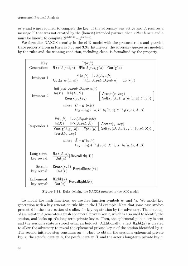
or y and b are required to compute the key. If the adversary was active and A receives amessage Y that was not created by the (honest) intended partner, then either b or x and a

must be known to compute Bh1(x,a) = gbh1(x,a).We formalize NAXOS security in the eCK model with the protocol rules and guarded

trace property given in Figures 3.33 and 3.34. Intuitively, the adversary queries are modeledby the rules and the winning condition, including clean, is formalized by the property.

KeyGeneration:

Fr(a:fr)

!Ltk(A:pub, a) !Pk(A:pub, gâ) Out(gâ)

Initiator 1:Fr(x:fr) !Ltk(A, a:fr)

Out(gˆh1(x, a)) Init(x,A:pub, B:pub, a) !Ephk(x)

Initiator 2:

Init(x:fr, A:pub, B:pub, a:fr)

In(Y ) !Pk(B, B )

!Sessk(x, key)

[

Accept(x, key)Sid(x, 〈A,B, gˆh1(x, a), Y ,I〉)

]

where B = gˆ(b:fr)

key = h2(Y â, B ˆh1(x, a), Y ˆh1(x, a), A, B)

Responder 1:

Fr(y:fr) !Ltk(B:pub, b:fr)

In(X) !Pk(A:pub, A )

Out(gˆh1(y, b)) !Ephk(y)!Sessk(y, key)

[

Accept(y, key)Sid(y, 〈B,A,X, gˆh1(y, b),R〉)

]

where A = gˆ(a:fr)

key = h2(A ˆh1(y, b), Xˆb,Xˆh1(y, b), A, B)

Long-termkey reveal:

!Ltk(A, a)


Sessionkey reveal:

!Sessk(s, k)

Out(k)[RevealSessk(s) ]

Ephemeralkey reveal:

!Ephk(x)

Out(x)[RevealEphk(x) ]

Figure 3.33. Rules defining the NAXOS protocol in the eCK model.

To model the hash functions, we use free function symbols h1 and h2. We model keygeneration with a key generation rule like in the UM example. Note that some case studiespresented in the next section also allow for key registration by the adversary. The first stepof an initiator A generates a fresh ephemeral private key x, which is also used to identify thesession, and looks up A’s long-term private key a. Then, the ephemeral public key is sentand the session’s state is stored using an Init-fact. Additionally, a fact !Ephk(x) is createdto allow the adversary to reveal the ephemeral private key x of the session identified by x.The second initiator step consumes an Init-fact to obtain the session’s ephemeral privatekey x, the actor’s identity A, the peer’s identity B, and the actor’s long-term private key a.


96

A B


a, A = ga)


b, B = gb)

choose random exponent x

X7 gh1(x,a)

Xchoose random exponent y

YY 7 gh1(y,b)

compute h2

(

Y a, Bh1(x,a), Y h1(x,a),A,B)

compute h2

(

Ah1(y,b),Xb, Xh1(y,b),A,B)

Figure 3.32. The NAXOS protocol.

Additionally, it receives the message Y and looks up B’s long-term public key B . Usingthese, the session computes the session key, creates a !Sessk-fact for session key reveals,denotes that it accepted a key using an Accept-action, and associates the session identifier xwith the given session string using an Sid-action. The responder rule is defined analogously.The remaining three rules model long-term key reveal, session key reveal, and ephemeralkey reveal.

∀ key test A B X Y R.

// If there is a test session test whose session key is known to the adversary,Accept(test , key)∧K(key)∧ Sid(test , 〈A,B,X, Y , R〉)

// then one of the followingmust have happened: ( // 1. The adversary revealed test ’s session key.

RevealSessk(test)

// 2. The adversary revealed the long-term key of test ’s actor and// test ’s ephemeral key.∨ (RevealLtk(A)∧RevealEphk(test))

// 3. There is a matching session match and the adversary revealed∨ (∃match R ′.Sid(match , 〈B,A, Y ,X ,R ′〉)∧¬(R≈R ′)∧ (// (a) match ’s session key, or

RevealSessk(match)

// (b) the long-term key of test ’s peer and match’s ephemeral key.∨RevealLtk(B)∧RevealEphk(match)))

// 4. There is no matching session and the adversary revealed∨ (¬(∃match R ′.Sid(match , 〈B,A, Y ,X,R ′〉)∧¬(R≈R ′))

// the long-term key of test ’s peer.∧RevealLtk(B)))

Figure 3.34. eCK security property for the NAXOS protocol.

The security property states that whenever the adversary knows the key of a session test ,then the session is not clean. The definition of clean is a direct translation of the definitionin Section 2.1.2.4. Note that in contrast to the computational definition, our symbolic modelcaptures computability of the session key instead of indistinguishability.


97

3.5.3 wPFS Security of RYY

The formalization of RYY given in Figures 3.35 and 3.36 follows the description in Sec-tion 2.1.3.3. We use the free function symbol H to model the hash function that hashes intoG1 and the free function symbol h to model the hash function used as the key derivationfunction. The rules in the first line model a key generation center that first creates a freshmaster secret key msk and then allows owners of identities to obtain their long-term privatekeys. Since the public key for an identity A is just H(A), there is no need for public keydistribution. The first step of the initiator sends the ephemeral public key gˆx. The secondstep of the initiator receives the ephemeral public key of the responder and computes thesession key by combining the ephemeral DH key and the static identity-based key. We alsoinclude the exchanged messages and the identities of the participants in the input to thehash function. We use Accept-actions and Sid-actions to denote the accepted key and thesession string. The responder rule is defined analogously. The remaining rules handle long-term key reveal, session key reveal, and master key reveal.

Key Generation Center:Fr(msk :fr)

!Msk(msk)

!Msk(msk)

!Ltk(ID : pub , [msk ]H(ID))

Initiator step 1:Fr(x:fr)

Out(gˆx) Init(x,A:pub, B:pub)

Initiator step 2:

Init(x,A:pub, B:pub)In(Y ) !Ltk(A, skA)

!Sessk(x, key)

[

Accept(x, key)Sid(x, 〈A,B, gˆx, Y ,A〉)

]

where key =h(Y ˆx, e(H(B), skA), A,B, gˆx, Y )

Responder step 1:

Fr(y:fr) In(X)!Ltk(B:pub, skB)

Out(gˆy) !Sessk(y, key)

[

Accept(y, key)Sid(y, 〈B,A,X, gˆy,B〉)

]

where key =h(Xˆy, e(H(A), skB), A,B,X, gˆy)

Long-Term key reveal:!Ltk(A, a)


Session key reveal:!Ltk(s, k)

Out(k)[RevealSessk(s) ]

Master key reveal:!Ltk(A, a)

Out(a)[RevealMsk() ]

Figure 3.35. Rules defining the RYY protocol.

The adversary model formalized by the security property allows the adversary to revealsession keys of unrelated sessions, to reveal long-term keys of the participants (or themaster-key) after the test session has accepted the key if he was passive, and to reveal long-term keys of other agents. As we will demonstrate in the next section, Tamarin finds anattack if we add ephemeral key reveals to this model.


98

∀i key test A B X Y R.

// If there is a test session test whose session key is known to the adversary,Accept(test , key)@i∧K(key)∧ Sid(test , 〈A,B,X, Y , R〉)

// then one of the followingmust have happened. // 1. The adversary revealed test ’s session key.

RevealSessk(test)

// 2. There is a matching session match and the adversary revealed∨ (∃match R ′.Sid(match , 〈B,A, Y ,X ,R ′〉)∧¬(R≈R ′)∧ ( // (a) match ’s session key, or

RevealSessk(match)

// (b) the long-term key of test ’s peer before i, or∨ (∃m.RevealLtk(B)@m∧m≺ i)

// (c) the long-term key of test ’s actor before i, or∨ (∃m.RevealLtk(A)@m∧m≺ i)

// (d) the master key before i.∨ (∃m.RevealMsk()@m∧m≺ i)))

// 3. There is no matching session and the adversary revealed∨ (¬(∃l match R ′.Sid(match , 〈B,A, Y ,X ,R ′〉)@ l∧¬(R≈R ′))∧ // the long-term key of test ’s peer, of test ’s actor, or the master key.

(RevealLtk(B)∨RevealLtk(A)∨RevealMsk() ))

Figure 3.36. Security property for the RYY protocol

3.5.4 Experimental Results

We applied Tamarin to three type of case studies. First, we analyzed a number of two-pass AKE protocols with respect to different adversary models. The results, obtained on alaptop with a 2.9 Ghz Intel Core i7 processor, are listed in Table 3.1. For each protocol, weformalized its intended and related adversary models and analyzed them using Tamarin.We analyzed NAXOS with respect to the formalization in Section 3.5.2. For a modifiedadversary model that accounts for Perfect Forward Secrecy (PFS), Tamarin discoveredan attack. We modeled NIST’s KAS1 and KAS2 protocols [102] and the related DH2protocol by Chatterjee et al. [43] which uses inverses. For these protocols, our analysisconfirms the security proofs and the informal statements made in [43]. We also analyzedthe SIGDH protocol from Section 2.1.2 and the KEA+ protocol [112] and obtained theexpected results. To verify Key Independence (KI) for KEA+ and STS, we model that theadversary can reveal certain keys. For STS, we additionally allow the adversary to registerarbitrary public keys for corrupted agents. In this setting, we find the UKS attack reportedin [27]. We model and successfully verify both fixes from [27]. The first fix is to require aProof-of-Possession of the private key for key registration and the second fix is to includethe identities of the participants in the signatures. We also analyzed the TS1, TS2, andTS3 protocols from [95] and their updated versions [96].


99

Protocol Adversary Model Result Time [s]

1. NAXOS eCK proof 4.1

2. NAXOS eCKPFS attack 3.4

3. KAS1 KI+KCI proof 0.7

4. KAS2 weakened eCK proof 5.5

5. KAS2 eCK attack 3.6

6. DH2 weakened eCK proof 21.7

7. SIGDH PFS proof 0.6

8. SIGDH eCK attack 9.4

9. KEA+ KI+KCI proof 0.7

10. KEA+ KI+KCI+wPFS attack 1.0

11. STS-MAC KI, reg-PK UKS-attack 4.1

12. STS-MAC-fix1 KI, reg-PK (with PoP) proof 9.2

13. STS-MAC-fix2 KI, reg-PK proof 2

14. TS1-2004 KI UKS-attack 0.3

15. TS1-2008 KI proof 0.3

16. TS2-2004 KI+wPFS attack 0.5

17. TS2-2008 KI+wPFS proof 1.2

18. TS3-2004/2008 KI+wPFS non-termination -

Table 3.1. Verification Results for two-pass Diffie-Hellman protocols.

Second, we analyzed the one-pass and three-pass versions of the UM protocol with respectto different adversary models. We also analyzed these and other protocols in combinedmodels where multiple protocols are executed jointly sharing static key material. Theresults are shown in Table 3.2. We analyzed our formalization of the one-pass UM pro-tocol [137] from Figures 3.2 and 3.3 which models a weakened version of the eCK model.Since we obtained the description of the one-pass UM protocol from [42], we then modeledone-pass UM in their adversary model, which is based on the CK-model [37], and Tamarinautomatically discovered the attack depicted in Figure 3.37.

In the attack, the test session is a responder session with actor B and peer A thatreceives g1. After a long-term key reveal for A, the adversary can compute the session keyh(gb, gba, A, B) of the test session. There is also a second responder session with peer A andactor B that receives g1. In our model, this is not an attack since a long-term key revealfor the test session’s peer is only allowed if there is a matching session for the test session.Since two responder sessions are never matching sessions in our model, this is not the casefor this execution.

In the model from [42], the adversary is only allowed to reveal the long-term key of thetest session’s peer if there is a matching session, like in our model. Unlike our model, theirmodel does not include the role in the session identifier and the second responder sessionis a matching session of the test session in their model. They define the session identifierof the test session as (A, B, g1), the session identifier of the second session as (B, A, g1),and the two are matching in their model since the actor of the first session is the peerof the second session, the actor of the second session is the peer of the first session, andthe messages are equal. We checked the security proof in [42] and discovered that a casecorresponding to our attack is missing. The proof assumes that the matching session of


100

a responder is always an initiator session. We then modified our formalization to includethe role in the matching session definition and successfully verified this fix with Tamarin.Following the analysis in [42] and [129] we also modeled the three-pass UM protocol andanalyzed the one-pass and the three-pass versions of UM in a joint model where agentsuse the same long-term keys for both protocols. Our results confirm the attack and thefix from [129]. Finally, we verify three-pass variants of the KEA+ and NAXOS protocolsfrom [129] in a joint eCKPFS [110] model with partially matching sessions [129] where theadversary can register arbitrary public keys for corrupted agents.


19. UM-one-pass weakened eCK proof 0.4

20. UM-one-pass CK-like attack* 3.4

21. UM-one-pass CK-likea proof 2.6

22. UM-C+UM-one-pass CK-likea attack 27.4

23. UM-Ca+UM-one-passb CK-likea proof 41

24. NAXOS-C+DHKEA eCKPFSc,reg-PK proof 107

a added role to session identifier

b added protocol identifier to key string

c with partially matching sessions

Table 3.2. Verification Results for one-pass and three-pass Diffie-Hellman protocols. We use * todenote attacks that contradict result proved in the respective papers.

Third, we analyzed tripartite group key exchange protocols and identity-based AKEprotocols that employ bilinear pairings. The results are listed in Table 3.3. For the signedJoux protocol [97], we confirmed that it provides PFS. If we add ephemeral key reveals,then Tamarin discovers an attack. For this protocol, it takes 76 seconds to compute the160 variants of the second protocol step, which is a substantial amount of the total analysistime. For the TAK1 protocol [5], our adversary model distinguishes between two cases. Ifthe adversary was passive with respect to the test session test , then he can reveal eitherthe long-term keys of test ’s actor and test ’s peers or the ephemeral keys of test and thematching sessions, but not both. If the adversary was active, then revealing long-termkeys of test ’s actor or test ’s peers is forbidden. Next, we verify the security of the RYYprotocol [155] with respect to wPFS and confirm an attack after adding ephemeral keyreveals. For the Scott protocol [159], we obtain a similar result. Finally, we model theChen-Kudla protocol [44], which uses point addition. We do not support this operation andthe required equalities like [c]([a]P + [b]Q) = ([c a]P + [c b]Q) in our model and thereforeapproximate the point addition with the associative and commutative operator ♯. Since theChen-Kudla protocol still works if point addition is replaced by sorted concatenation, ourmodel includes the required equalities to execute the protocol. We verify the security ofthe Chen-Kudla protocol in an eCK-like model where, in addition to the usual restrictions,the adversary is not allowed to reveal the ephemeral keys of the test session and thematching session, even if the adversary performs no long-term key reveals. If we removethis restriction, then Tamarin discovers an attack.


101


25. SIGJOUX (tripartite) PFS proof 90.7

26. SIGJOUX (tripartite) PFS,eph-reveal attack 99.8

27. TAK1 (tripartite) weakened eCK-like proof 56.8

28. TAK1 (tripartite) eCK-like attack 77.2

29. RYY (ID-based) wPFS proof 8.3

30. RYY (ID-based) wPFS,eph-reveal attack 7.9

31. Scott (ID-based) wPFS proof 19.3

32. Scott (ID-based) wPFS+eph-reveal attack 26.2

33. Chen-Kudlad (ID-based) eCK-like proof 61

34. Chen-Kudlad (ID-based) eCK attack 45.3

d we use sorted concatenation instead of point addition

Table 3.3. Verification Results for protocols that use bilinear pairing.

3.5.5 Limitations and Extensions

There are two main causes for non-termination. First, non-termination occurs when theprotocol contains loops and the search has to explore the loops to analyze the desiredproperty. For example, it is impossible to prove that ϕ=∀i x.St(x)@i x≈ 1 holds for

PLoop=

St(1)[ St(1) ]

St(x)

St(x)[ St(x) ]

using our constraint solving algorithm. To solve this problem, Meier [124] extends theapproach with induction. First, he checks if ϕ is valid for the empty trace, which is alwayspossible. Then, he encodes the induction hypothesis “ϕ is valid for all prefixes of tr ” in aformula ϕIH. Since this formula is also a guarded trace property, constraint solving canthen be used to check if ϕIH ϕ is valid. This is equivalent to checking if ϕIH ∧¬ϕ issatisfiable, i.e., is there a trace that violates ϕ such that all prefixes satisfy ϕ.

Second, we have seen that enforcing normal message deductions and using a searchstrategy based on the chain property is critical to achieve termination in many cases. Sincewe apply these techniques only to message deduction rules, protocol rules that provide verygeneral message deduction steps are still problematic. For example, the described constraintsolving algorithm does not handle protocols that provide decryption rules such as

In(enc(x, pk(k))) !Ltk(A, k)

Out(x)

where x is a message variable well. The problem is that if we do not know anything aboutthe possible instantiations for x, then any message can be extracted from the sent message.To deal with such protocols, Meier [124] proposes type assertions which are invariantssimilar to “the variable x in the protocol step i is either instantiated with a nonce or alreadyknown to the adversary before i”. Given this invariant, it suffices to consider the case wherethe extracted message is a nonce since the adversary is not allowed to extract a messagethat is already known in the other cases. To prove such invariants, induction is used.


102

Figure 3.37. Tamarin visualizes the attack on the UM-one-pass protocol in the CK-like modelfrom [42] after automatically finding it. The test session is displayed on the left and its matchingsession, which is also a responder session, is shown on the right. On the far right below the matchingsession, a long-term key reveal for its actor is displayed. In the bottom half, the message deductionsfor computing the session key are displayed. Note that A’s long-term key is ∼x and B’s long-termkey is ∼eb where ∼ is used to denote the sort annotation :fr.


103

Meier [124] and Künnemann and Steel [107] have successfully applied the two exten-sions described above to verify protocols with loops and unbounded mutable state such asTESLA [145], the envelope protocol [63], and the Yubikey security token [170].


104

Chapter 4

Impossibility Results for Key Establish-ment

In Chapter 2, we presented the Diffie-Hellman protocol, which was the first protocolto “enable private communication without ever relying on private channels“ (Katz andLindell [106]). The main insight in the development of the protocol was the usage ofDH groups where exponentiation is efficient, repeated exponentiation commutes, and takingthe discrete logarithm is hard. In this chapter, we investigate if it is possible to achievethe above goal also with operations that are simpler than exponentiation in a DH group.More precisely, we model cryptographic operators and their algebraic properties abstractlyby equational theories, as we did in Chapter 3. Then, we consider the question if a givenequational theory, modeling for example XOR, symmetric encryption, or hashing, allowsthe establishment of a secret using only public (but authentic) channels.

In the following, we first state some preliminaries and define our formal model of secretestablishment. Then, we consider symmetric encryption and subterm-convergent theories.Next, we consider monoidal theories such as XOR and abelian groups. Finally, we considerthe disjoint combination of equational theories and summarize our results.

4.1 Preliminaries

In this chapter, we use unsorted term algebras and a single set of names N . We alsoassume that all considered equational theories are consistent, i.e., for two different names nand n ′, it never holds that n=E n

′. For a sequence a= [a1, , ak], we use σ[a] to denote thesubstitution

⋃

i=1

k ai/xi. Note that all equational theories are stable under replacementof names by terms, i.e., if ρ is a replacement of names by terms and s=E t, then s

ρ=E tρ.

4.2 Traces and Deducibility

In this section, we define formally what it means to establish a shared secret. We firstdefine messages, frames, and deducibility. Then, we define the set of derivation traces thatdenotes the possible executions where agents construct messages and exchange messagesover a public channel. Afterwards, we define the notion of shared secret for such a traceand relate derivation traces and protocols.

105

4.2.1 Messages, Frames, and Deducibility

As is common practice in symbolic protocol analysis, we abstract away from concreteimplementations where messages are encoded and manipulated as bitstrings. Given anequational theory E = (Σ, E), we define the set of messages asMΣ = TΣ(N ). We use theset of names N to model atomic messages such as nonces and agent names. The functionsymbols in Σ model cryptographic operations on abstract messages, where the operations’semantics is given by the set of equations E.

We next define a notion of deducibility on a set of messages. Consider, for example, thecase where an adversary has overheard communication between honest agents and has seenthe messages m1, , mk. Given these messages, we are interested in the set of messagesthat the adversary can deduce by applying cryptographic operations. Here, we have toaccount for nonces, keys, and other randomly chosen messages, which the adversary cannotconstruct. We therefore define the notion of a frame, as it has been introduced in theapplied pi calculus [3]. A frame is a pair (n , σ) written as ν n.σ such that:

• n is a finite set of restricted names. Intuitively, this is a set of fresh names and modelsunguessable messages created by honest agents. Although it might be possible for theadversary to deduce restricted names, the adversary cannot create them directly.

• σ is a substitution m1/x1, , mk/xk. This allows the adversary to use the observedmessages m1, ,mk when constructing new ones.

Constn∈N \ nν n.σ ⊢E n

Knowx∈ dom(σ)

ν n.σ ⊢E xσ

Applyν n.σ ⊢Em1 ν n.σ ⊢Emk f ∈Σk

ν n.σ ⊢E f(m1, , mk)Equal

ν n.σ ⊢Em m=Em′

ν n.σ ⊢Em′

Figure 4.1. The deducibility relation ⊢E is inductively defined by these rules.

Based on the notion of a frame, we define the deducibility relation ⊢E between frames andmessages for an equational theory E . The corresponding rules are presented in Figure 4.1and model that the adversary can take any of the following actions.

• Const: The adversary can deduce any name, except the restricted ones in the set n.

• Know: The adversary can deduce all message in the range of σ.

• Apply: The adversary can apply function symbols in Σ to deducible messages.

• Equal: The adversary can deduce messages that are equivalent to deducible messagesmodulo the equational theory E .

The relation ⊢E can be equivalently defined as follows.

Lemma 4.1. For all finite sets of names n, substitutions σ, and terms m, ν n.σ ⊢E m ifand only if there is a term ζ ∈ TΣ(dom(σ)∪ (N \ n)) such that ζσ =E m. We call such aterm ζ a recipe for m.

For theories that contain a nullary function symbol, we can always find a recipe thatdoes not contain unrelated names.

Lemma 4.2. If E is a theory with a nullary function symbol c, names(range(σ)∪m)⊆ n,then ν n.σ ⊢Em if and only if there is recipe ζ ∈TΣ(dom(σ)).

Impossibility Results for Key Establishment

106

Proof. We can just take an arbitrary recipe and replace all names n∈names(ζ)with c. Theresult is still a recipe since all names in m and range(σ) are restricted and cannot occurin ζ. Since E is stable under replacement of names by terms, we have ζ ρσ=E (ζσ)ρ=Em

ρ=m

for a replacement ρ that maps all n∈ names(ζ) to c.

Note that the notion of frames and the deducibility relation ⊢E can also be used for termsthat are not ground, which we exploit in Section 4.3.2.

4.2.2 Derivation Traces

In the following, let A be the set of agents and let E = (Σ, E) describe the cryptographicoperators under consideration and their relevant properties. An event either denotes thatan agent sends a message or learns a message. Events are therefore associated with thecorresponding agent’s identity. A learn event is additionally tagged with the rule R thatdescribes how the agent learned the message.

Event< =Send(A,MΣ)|LearnR(A,MΣ)

The steps taken to construct and communicate messages are modeled by traces, where atrace is a list of events. The set of valid traces TRE is inductively defined by the rules inFigure 4.2. We use restricted(tr)=n|∃A.LearnFresh(A,n) to denote the restricted namesin the trace and LearnR to denote Learn-events with arbitrary rule-tags. The rules modelthe following actions.

• Send: An agent A sends a previously learned message m on the public channel.

• Recv: An agent A receives a message m that has been previously sent by B.

• Fresh: An agent A creates a fresh name n. Note that the minimal name nmin underthe ordering ≻ used for ordered completion cannot be used here or in the Public rule.

• Public: An agent A uses a public value p.

• App: An agent A applies a k-ary function symbol f to the previously learned messagesm1, ,mk. Here we use the fact that every message has a unique normal form moduloE with respect to →(≻,OE).

4.2.3 Shared Secrets and Deducibility

Clearly, we must restrict the initial knowledge of agents to prove impossibility results forsecret establishment. Some restrictions are necessary to prevent initial knowledge distribu-tions that allow the creation of a shared secret, but require the previous existence of secretchannels, e.g., shared secret keys distributed by a third party. We enforce this restriction byrequiring that every derivation starts with the empty trace, which corresponds to the emptyinitial knowledge for the involved agents. However, in our model, we do not distinguishbetween the setup phase and the execution phase. Therefore, any prefix of a derivation tracecan be interpreted as a setup phase where agents establish private and public knowledge inthe presence of the attacker. This covers precisely the initial knowledge distributions that donot require secret channels and include all messages involved in establishing the knowledge.


107

Empty[ ]∈TRE

Sendtr ∈TRE LearnR(A,m)∈ tr

tr ·Send(A,m)∈TRE

Recvtr ∈TRE Send(B,m)∈ trtr ·LearnRecv(A,m)∈TRE

Freshtr ∈TRE n∈N \ (names(tr)∪nmin)

tr ·LearnFresh(A,n)∈TRE

Publictr ∈TRE p∈N \ (restricted(tr)∪nmin)

tr ·LearnPublic(A, p)∈TRE

App

tr ∈TRE f ∈Σk

LearnR1(A,m1)∈ tr LearnRk

(A,mk)∈ tr

tr ·LearnApp(f(m1, ,mk))(A, f(m1, ,mk)↓E≻)∈TRE

Figure 4.2. The set TRE is inductively defined by these rules.

We are interested in impossibility results. An impossibility result for a class of adver-saries implies impossibility for any larger class. As a consequence, we reason about weakadversaries, namely passive adversaries who are restricted to eavesdropping communicationon the public channel. This models an adversary who is not involved in the derivationprocess. For a given trace tr , we therefore define the corresponding frame φtr as follows.Let sent(tr) denote the list of messages [m1, , mk] that have been sent in tr , then φtr isdefined as φtr = ν restricted(tr).σ[sent(tr)].

Note that we combine the deduction rules for honest agents with the rules for exchangingmessages in the definition of TRE. However, the deduction rules formalize deduction capa-bilities that are equivalent to the relation ⊢E. The only difference is that the messages inderivation traces are always in normal form and we therefore do not need an Equal rule.

We now define what it means to share a secret.

Definition 4.3. A term s is a shared secret between A and B in a trace tr if A B,LearnR1

(A, s)∈ tr, LearnR2(B, s)∈ tr, and φtr ⊢Es.

To simplify subsequent proofs, we first show that we can restrict ourselves to a pair ofagents.

Lemma 4.4. If there is a trace that establishes a secret between the distinct agents A andB involving an arbitrary number of agents, then there is also a trace where only A and Bparticipate.


108

Proof. We translate the trace with an arbitrary number of agents to a trace with onlyA and B. The translation maps all events executed by an agent C A, B to thecorresponding event executed by A. It is easy to check that this translation yields a validtrace.

In the following, we therefore fix A = A, B, where A and B are distinct agents. Todefine the notion of minimal traces, we require the following definition.

Definition 4.5. We say that an agent A constructs a message m in tr, if A first learnsm in a LearnR-event for R Recv. We say A freely constructs m in tr if no reductionof the message occurs in the event where A first learns m, i.e., R= Fresh, R= Public, orR=App(m).

We now introduce the notion of minimal trace.

Definition 4.6. A trace tr ∈TRE is a minimal trace if each of the following conditions hold.

1. There is at most one shared secret s. This shared secret is learned by B in the last event,which is a LearnApp-event.

2. There are no LearnPublic-events in the trace, i.e., all names are restricted.

3. There are no duplicate events and every message except for s is constructed only once.

4. The secret s is freely constructed at most once.

We denote the subset of minimal traces by TREmin.

We can now prove that the conditions on minimal traces do not prohibit secret estab-lishment if it is otherwise possible.

Lemma 4.7. If there is a trace tr ∈TRE that establishes a shared secret, then there is also

a minimal trace tr ∈TREmin that establishes a shared secret.

Proof. We first prove by induction that a trace tr ∈TRE without a shared secret can betransformed into a minimal trace without changing names(tr), the deducible messages forthe adversary, and the messages known byA andB. The empty trace [ ] is already minimal.

Assume that the trace tr can be transformed into the minimal trace tr . If tr is extendedwith a Send -event by the Send rule, then we extend tr with the same Send -event, providedit is not a duplicate event. If tr is extended with an event LearnRecv(A,m) by the Recv

rule, then we extend tr with the same event, provided m is not already known to A. If tr is

extended by the Fresh rule, then we extend tr with the same event, which is allowed sincenames(tr)=names(tr ). If tr is extended with an event LearnPublic(A, p) by Public, thenp is deducible by the adversary and we distinguish three cases. If p is already known to A,

we do not extend tr . If p is not known to A, but to some other agent B, we extend tr withthe events Send(B, p) (if required) and LearnRecv(A, p). If p is not known to any agent,

then p names(tr ) and we extend tr with LearnFresh(A, p) and Send(A, p). Finally, if tr isextended with an event ev =LearnApp(f(m1, ,mk))(A,m) by App, we again distinguish three

cases. If m is already known to A, then we do not extend tr . If m is only known to another

agent B, we extend tr with the required Send and LearnRecv events. This is possible becausewe only consider traces tr ·ev which contain no shared secrets. Sincem is shared knowledge,

it cannot be secret. Finally, if m is not known to any agent in tr , then we extend tr with ev .


109

To transform a trace tr ∈TRE with shared secrets into a minimal trace that establishesexactly one shared secret, we first take the shortest prefix trp · ev of tr that establishes ashared secret. Since an agent cannot establish a secret with a Send or LearnR event forR ∈ Recv , Public , Fresh, the last event ev must be a LearnApp-event, where an agentC learns some secret s. Without loss of generality, we assume C = B. We can transformtrp into a minimal trace trp using the previously described transformation since it does

not contain a shared secret. Then trp · ev ∈ TREmin since ev can be added to trp without

violating properties 1.–4. Properties 1.–3. are obvious. To see that 4. holds, assume that sis freely constructed by bothA and B. Then s= f(m1, ,mk) for some f ∈Σk and messagesmi and there are LearnApp(s)(C, s) events for C = A and C = B. Then all mi are sharedknowledge and since s is the only secret, all mi are deducible by the adversary. Hence,s= f(m1, , mk) is also deducible by applying f .

4.2.4 Relating Protocols and Derivation Traces

Above we have reduced the question whether it is possible to establish a shared secretusing an equational theory E to the question of whether there is a derivation trace tr ∈TRE

that establishes a shared secret. This is closely related to the question of whether there isa protocol that establishes a shared secret in a given symbolic protocol model.

The existence of a protocol implies that there is a successful protocol execution wherethe involved agents establish a shared secret. For all reasonable protocol models that usethe same notion of deducibility as we do, a successful protocol execution directly yields acorresponding derivation trace that establishes a shared secret. An impossibility result forsome equational theory E in our model thus directly implies the corresponding impossibilityresult for protocols in such a symbolic model. A concrete example of a protocol model wherethis relationship holds is the applied pi calculus with equational theory E where agents areonly allowed to communicate over public channels.

4.3 Symmetric Encryption and Subterm-ConvergentTheories

In this section, we prove the folk theorem that it is impossible to establish a shared secretusing only symmetric encryption and public channels. We then present a necessary andsufficient condition for impossibility for the more general case of subterm-convergent the-ories. This condition can be used to automatically decide wether it is possible to create ashared secret for a given subterm-convergent theory. We have implemented a decision pro-cedure that checks this condition and illustrate its application to the theory of symmetricencryption. Afterwards, we show how our procedure finds a derivation trace that establishesa shared secret for the theory of public-key encryption.

4.3.1 Symmetric Encryption

We use the equational theory Sym =(ΣSym,ESym) to model symmetric encryption, pairing,a hash function, decryption, and projections on pairs.

ΣSym = enc(_,_), 〈_,_〉, h(_), dec(_,_), π1(_), π2(_)

ESym = dec(enc(m,k), k)≃m, π1(〈m1,m2〉)≃m1, π2(〈m1, m2〉)≃m2


110

Since the rewriting system RSym obtained from ESym by orienting the equations from leftto right is subterm-convergent, we directly use →RSym

to normalize terms in the App ruleand do not require ordered completion. In the following, we say an equational theory issubterm-convergent if the equations can be oriented such that the corresponding rewritesystem is subterm-convergent and we denote the normal form with respect to this rewritesystem with t↓E. The following lemma holds for all subterm-convergent theories and willbe used in Section 4.3.2 as well.

Lemma 4.8. Let E = (Σ, E) be a subterm-convergent theory and tr ∈ TRE. For everyevent LearnR(A, m) ∈ tr and m′ ∈ St(m) such that names(m′) ∅, m′ has been freelyconstructed by some agent C. More precisely, if m′ is a name, then LearnFresh(C,m

′)∈ tror LearnPublic(C, m

′) ∈ tr. Otherwise, there exist m1, , mk and an f ∈ Σk, such thatm′= f(m1, , mk) and LearnApp(m ′)(C,m

′)∈tr.

Proof. The proof is straightforward using rule induction on TRE. The rules Emptyand Send are trivial since they do not add any Learn-events. The Fresh and Publicrules are also trivial since they only add (atomic) names. The Recv rule adds anevent LearnRecv(A,m), but there must be a corresponding LearnR(B, m) by thesender B. We can therefore apply the induction hypothesis. The App-rule adds an eventLearnApp(f(m1, ,mk))(A, m), where m = f(m1, , mk)↓E. We must show that the lemma’sstatement holds for all subterms of m that contain names. Since the equational theoryis subterm-convergent, we have either m = g for some g ∈ TΣ(∅), m = f(m1, , mk),or m is a proper subterm of f(m1, , mk). In the first case, the statement follows triv-ially, since no term in St(g) contains names. In the second case, a subterm of m is either mitself and the statement trivially holds or a subterm of some mi and the statement holdsby the induction hypothesis since there is an event LearnR(A,mi) in the trace. The samereasoning applies to the final case since m and all its subterms are subterms of some mi.

Theorem 4.9. There is no derivation trace for Sym that establishes a shared secret.Namely, if tr ∈TRSym , LearnR1

(A, s)∈ tr, and LearnR2(B, s)∈ tr, then φtr ⊢Sym s.

Proof. We prove the theorem by contradiction. Assume that there is a trace in TRSym

that establishes a shared secret. Then, there is also a trace tr ∈TRSymmin that establishes a

shared secret s and the last event of tr is of the form ev = LearnApp(f(m1, ,ml))(B, s) fors = f(m1, , ml)↓Sym. Thus LearnR(A, s) ∈ tr and we show that φtr ⊢Sym s to obtain acontradiction. We distinguish two cases.

1. If s= f(m1, , ml) then Lemma 4.8 can be applied to LearnR(A, s) and the prefix ofthe trace up to this event. Thus there are two free construction events for s whichcontradicts minimality of tr .

2. If f(m1, ,ml) is not in normal form, then we must consider two more cases.

a) Assume that f(m1, ,ml)=πi(〈t1, t2〉) for some messages ti. Then s= ti and 〈t1, t2〉has been freely constructed by A by Lemma 4.8. Since the pair is known to bothA and B and s is the only secret in tr , the pair is deducible by the adversary andtherefore s is also deducible.

b) Assume that f(m1, ,ml)= enc(m,k) for some messages m and k. Then s=m andenc(m, k) has been freely constructed by A by Lemma 4.8. Then k and enc(m, k)are known to both A and B and are therefore deducible by the adversary. Hence,s is also deducible.

4.3 Symmetric Encryption and Subterm-Convergent Theories

111

Note that the only parts in the proof that are specific to Sym and do not hold for allsubterm-convergent theories are the cases 2.a) and 2.b) for the different rules in RSym. Here,a rule l→ r is applied to the result of the function application in the App-rule and we proveimpossibility by showing that there is no way for A and B to build an instance of l suchthat the corresponding instance of r is not deducible by the adversary. We will show inthe next section that this proof method works with arbitrary subterm-convergent theories.

4.3.2 Subterm-Convergent Theories

We now generalize the previous proof method to a necessary and sufficient condition forthe possibility of secret establishment for a subterm-convergent theory E = (Σ, E). Sincethe condition can be automatically checked, we thereby obtain a decision procedure. Themain idea is that if there is a derivation trace where a secret is established, then thereis also a minimal trace with exactly one reduction step that establishes a secret, i.e., allconstructions except for one are free. We can decide if such a minimal trace exists byconsidering all equations in E individually and enumerating all possible ways to jointlyconstruct a reducible term. Finally, we check if this construction leads to a shared secret.

In the rest of this section, we assume that E is a subterm-convergent equational theory.Note that we can assume without loss of generality that the right-hand sides of the rules inthe corresponding rewrite system are normalized. To prove our main result of this section,we require the following lemma about deducibility in subterm-convergent theories.

Lemma 4.10. For all substitutions σ with range(σ)⊆TΣ(V), s∈TΣ(V), and τ an arbitrarysubstitution, if ν ∅.σ ⊢E s, then ν n. (σ τ)⊢E sτ for n= names(range(τ)).

Proof. Let σ, s, τ , and n as defined above. If ν ∅.σ ⊢E s then there is a recipe ζ such thatnames(ζ)∩ n= ∅ and ζσ=E s. Thus ζ(σ τ) = (ζσ)τ =E sτ and hence ν n. (σ τ)⊢E sτ .

We also require the notion of reduction events.

Definition 4.11. A reduction event is an event of the form LearnApp(f(m1, ,mk))(C, m)

where f(m1, ,mk) is not ↓E-normal, i.e., f(m1, , mk) f(m1, ,mk)↓E =m.

We now show that we can restrict ourselves to a subset of the minimal traces in the caseof subterm-convergent theories.

Lemma 4.12. If there is a trace tr ∈TRE that establishes a shared secret between A and B,then there is also a minimal trace tr ∈TRE

min that establishes a shared secret s between A

and B such that s is freely constructed by A and the last event is the only reduction eventin tr.

Proof. Assume that there is a trace that establishes a shared secret. Then there is aminimal trace tr ∈ TRE

min that establishes the shared secret s, where the last event is ofthe form LearnApp(f(m1, ,mk))(B, s). This event must be a reduction event. Otherwise,

s= f(m1, ,mk) and Lemma 4.8 can be applied to LearnR(A, s). Then there must be twoevents LearnApp(s)(C, s), for C = A and C = B, which contradicts the minimality of tr .Note also that A must have freely constructed s by Lemma 4.8, since it is new to B.


112

We now show that all other reduction events in tr can be replaced by non-reduction-events. A reduction event has the form LearnApp(f(m1, ,mk))(C, m) such that m ∈ TΣ(∅)and ↓E-normal or m is a subterm of some mi. In the first case, the reduction-events canbe replaced by LearnApp-events to construct m where subterms that are already knownby the other agent are transmitted. Since all these subterms do not contain any names,they are deducible by the adversary. In the second case, the other agent must have freelyconstructed m by Lemma 4.8. Hence, m is constructed twice which contradicts minimalityof tr since m is not a shared secret.

Lemma 4.12 implies that we can consider the equations in E separately, since we onlyhave to consider traces with a single reduction step. To enumerate all different ways ofbuilding a reducible term that establishes a shared secret, we introduce labelings of terms.A labeling of a term t is a function from St(t) to A, B and captures which agent hasconstructed which subterm. For such a labeling lt of a term t, the minsent function returnsthe minimal set of exchanged terms that corresponds to lt. It captures that if A uses aterm created by B or vice versa, it must have been sent.

Definition 4.13. We define the minimal set of sent terms of as term t with labeling lt asminsent(t, lt)=

(∪1≤i≤kminsent(ti, lt))∪ti|1≤ i≤ k ∧ lt(t) lt(ti) if t= f(t1, , tk)∅ otherwise

.

Using the notion of labeling and the function minsent , we obtain the following conditionto decide impossibility.

Theorem 4.14. There is a derivation trace tr ∈TRE that establishes a shared secret if andonly if there is an equation t≃ s in E where s is a proper subterm of t and a labeling lt oft such that

1. lt(t) =B,

2. lt(c)=A for all c∈ St(t)∩Σ0,

3. lt(s)=A, and

4. ν ∅.σ[minsent(t,lt)]⊢E s.

Proof. ⇒: Assume there is a trace that establishes a shared secret. Then there is also aminimal trace tr ∈TRE

min where B learns the secret s in the last event, which is the onlyreduction event by Lemma 4.12. Consider the term t= f(m1, , mk) where s is extractedusing the rule t′ → s′ in the last step. Then s′ is a proper subterm of t′ and there is asubstitution τ such that t ′τ = t and s′τ = s.

We can extract a labeling lt from the trace by labeling t with B, all constants in t

with A and all proper subterms of t that are not constants with the agent who freelyconstructed the term. Note that every subterm of t that is not a constant must have beenfreely constructed by exactly one of the agents because of Lemma 4.8 and minimalityof tr . The labeling lt can be translated to a labeling lt ′ of t

′ by defining lt′(u)7 lt(uτ) foru ∈ St(t ′). Then lt ′ obviously has properties 1.–2. It has property 3. because s′τ = s andA freely constructs s in tr . We know that minsent(t′, lt′)τ ⊆minsent(t, lt)⊆ sent(tr) and

φtr ⊢Es. Thus we have ν restricted(tr). (σ[minsent(t ′,lt′)] · τ)⊢E s′τ . By Lemma 4.12, we obtain

ν ∅.σ[minsent(t′,lt′)]⊢E s′.

4.3 Symmetric Encryption and Subterm-Convergent Theories

113

⇐: Given a term t ∈ TΣ(V), we show that for all substitutions τ that instantiate thevariables in t with distinct names, and for all labelings lt of t, we can obtain a tracetr ∈TRE such that: (1) all names are restricted, (2) sent(tr)=(minsent(t, lt)τ)↓, and (3) forall u ∈ St(t), the agent lt(u) learns uτ in tr . We prove this by induction over the term t.First, if t=x for a variable x and τ and lt as stated above, then tr =[LearnFresh(lt(x), xτ)]

is in TRE and satisfies (1)–(3). Next, if t = f(t1, , tk) for f ∈ Σk and terms ti, τ and ltas stated above, then there are traces tr i for ti, τ , and lt with the expected propertiesby the induction hypothesis. Let tr denote the concatenation of the tr i, where duplicate

events are removed, keeping only the first occurrence of an event. Then tr ∈TRE and wecan extend tr with events Send(lt(ti), (tiτ)↓E) and LearnRecv(lt(t), (tiτ )↓E) for all i wherelt(t) lt(ti). Then, we add the event LearnApp(m ′)(lt(t),m) with m′= f((t1τ )↓E, , (tkτ )↓E)and m= f(t1τ , , tkτ )↓E to obtain the trace tr ∈TRE with the desired properties. If thereis an equation t ≃ s where s is a proper subterm of t in E and 1.–4. hold for the givenlabeling, then this trace establishes the shared secret sτ between A and B.

Based on this theorem, we define a decision procedure Find-Derivation-Traces thatchecks the theorem’s conditions for a given theory. Our procedure takes a subterm-con-vergent theory E =(ΣE, EE) as input and either returns Impossible if there is no labelingthat allows secret establishment for a rule in EE or a list of derivation traces if there is alabeling of a rule in EE that satisfies the conditions of Theorem 4.14.

Find-Derivation-Traces(E)1 traces ← [ ]2 for (t≃ s) in EE

3 for lt in Labelings(t)4 if ¬ (Minsent(t, lt)⊢E s) ∧ s∈ St(t) then5 traces ← traces·LabelToTrace(t, lt, s)6 if (traces = [ ]) then return Impossible7 else return traces

Figure 4.3. The pseudocode for the decision procedure Find-Derivation-Traces.

The procedure uses four subroutines. The subroutine Labelings returns all labelingsfor a rule that satisfy conditions (1)–(3). Minsent returns the minimal set of sent termsfor a labeling. The subroutine for ⊢E implements the procedure described in [2] to checkdeducibility. Finally, LabelToTrace converts a labeling to a trace. Note that by The-orem 4.14 we can consider all rules individually. However, we must check deducibility forthe whole equational theory E .

We have implemented our decision procedure in Haskell. Although the number of label-ings grows exponentially in the size of the equations, the procedure returns the resultimmediately for the examples we considered. Typically, the rules are small and mostlabels are already predetermined by the conditions of Theorem 4.14. We can further opti-mize Labelings by taking into account that properties (3) and (4) imply lt(u) = A

for all u ∈ St(t) that have s as immediate subterm. This is because s would otherwisebe in minsent(t, lt) and therefore be trivially deducible. We have applied our implemen-tation of the decision procedure to the theory Sym from the previous section. We havethereby obtained an automated confirmation of the pen-and-paper proof of Theorem 4.9.We use Sym and a theory that models public-key encryption below to illustrate our deci-sion procedure.


114

Example 4.15. The procedure considers the three following reduction rules individually.

1. π1(〈x, y〉)→ x: The only possible labelings are π1(〈xA, yC 〉A)B for C = A and C = B.For both labelings, 〈x, y〉 is in the minimal set of sent terms and x is therefore deducible.

2. π2(〈x, y〉)→ y: Analogous to previous rule.

3. dec(enc(m, k), k) → m: The only possible labelings are dec(enc(mA, kC)A, kC)B forC = A and C = B. For both choices of C, k is used by both A and B and thus musthave been sent. Similarly, enc(m, k) must have been sent in both case. Therefore, mis deducible by the intruder.

Thus Minsent(t, lt)⊢Sym s for all labelings and the procedure returns Impossible.

Example 4.16. Consider the theory ASym =(ΣSym, ESym) with

ΣASym = aenc(_,_), pk(_), adec(_,_) and

EASym = adec(aenc(m, pk(k)))≃m.

For this theory, our procedure returns the labeling adec(aenc(mB,pk(kA)A)B, kA)A andthe following derivation trace that establishes the secret s.

[ LearnFresh(A, k),LearnApp(pk(k))(A, pk(k)),Send(A, pk(k)),LearnRecv(B, pk(k)),

LearnFresh(B, s),LearnApp(aenc(s,pk(k)))(B, aenc(s, pk(k))),Send(B, aenc(s, pk(k))),

LearnRecv(A, aenc(s, pk(k))),LearnApp(adec(aenc(s,pk(k)),k))(A, s) ]

Note that Theorem 4.14 uses the notion of secret establishment introduced in Definition 4.3.Therefore, the existence of a trace that establishes a shared secret according to Theorem4.14 does not guarantee that secret establishment is possible in the presence of activeadversaries.

We also use our implementation to obtain new impossibility results. For example, ourimplementation returns Impossible for the theory describing pairing, signatures, and sym-metric cryptography and thereby proves the following theorem.

Theorem 4.17. Secret establishment is impossible for the combined equational theory(ΣSym∪ΣSig, ESym∪ESig), where the theory for signatures is defined as

ΣSig = sig(_,_), extr(_), verify(_,_), pk(_)

ESig = extr(sig(m,k))≃m, verify(sig(m,k), pk(k)))≃m.

We will later prove a combination result that allows us to consider the two theoriesseparately.

4.4 Monoidal Theories

In this section we will investigate impossibility of secret establishment for monoidal the-ories. We will exploit that each monoidal theory E has an associated semiring SE anddeducibility can be reduced to equation-solving in this algebraic structure. We mostly followthe presentation of [56] and [135] for basic facts about monoidal theories and deducibilityin such theories.


115

Definition 4.18. An equational theory is monoidal if it has an equational presentationE =(Σ, E) such that the following holds.

1. Σ consists of the binary function symbol +, the constant 0, and an arbitrary number ofunary function symbols.

2. The function symbol + is associative and commutative and the constant 0 is a unitfor + . Formally, this means the equations (x+ y)+ z≃x + (y + z) (A), x + y≃ y + z (C),and x + 0= x (U) are in E.

3. All unary function symbols h are homomorphisms with respect to + and 0, i.e., theequations h(x + y)≃h(x) +h(y) and h(0)≃ 0 are in E.

If for all terms t, there is a term s such that t + s=E 0, then the theory is a group theory .

Example 4.19. The following theories are monoidal:

• ACU : The signature Σ is 0, + and E consists of A, C, and U . This theory can beused to model multisets with the empty multiset and multiset union.

• ACUI : The signature Σ is 0, + and E consists of A, C , U , and x + x≃ x (I). Thistheory can be be used to model sets with the empty set and set union, which is idem-potent.

• ACUN : The signature Σ is 0, + and E consists of A, C, U , and x + x≃ 0 (N). Thistheory can be be used to model the XOR operation, which is nilpotent.

• AG : The signature Σ is 0, + ,- and E consists of A, C , U , and x + (-x)≃0. This theorycan be be used to model abelian groups. The unary homomorphism -models the inverseoperation and the equations characterizing that - is homomorphic are consequences ofthe other equations.

• ACUh, ACUIh , ACUNh , AGh : These theories can be obtained by extending the corre-sponding above theories with a homomorphism h and the required equations h(0) = 0

and h(x + y)≃h(x) + h(y).

Except for ACU , ACUh, ACUI , and ACUIh , all of these are group theories.

Definition 4.20. A semiring S is a tuple (S,+, 0, ·, 1) such that S is a set, +:S ×S→S,0∈S, · :S ×S→S, 1∈S, and the following holds:

1. (S,+, 0) is a commutative monoid, i.e., + is associative and commutative and 0 is aunit for +.

2. (S, ·, 1) is a monoid, i.e., · is associative and 1 is a unit for ·.

3. For all a, b, c∈S, (a+ b) · c= a · c+ b · c and a · (b+ c) = a · b+ a · c.

For each monoidal theory E , there is an associated semiring SE.

Definition 4.21. Given a monoidal theory E = (Σ, E), the semiring SEis defined as

(SE,+, 0, ·, 1) where SE=TΣ(1)/=E for a variable 1, and +, 0, ·, and 1 are defined asfollows.

1. [s]E +[t]E =[s + t]E , i.e., given a, b∈SE , first choose s, t∈TΣ(1) such that a=[s]E andb= [t]E. Then take the equivalence class of the term s + t.

2. 0= [0]E , i.e., the equivalence class of the constant 0.

3. 1= [1]E , i.e., the equivalence class of the variable 1.


116

4. [s]E · [t]E =[st/1]E , i.e., the equivalence class of the term that results from replacingevery occurrence of 1 in s with t.

If E is a group theory, then SE is a ring because (SE, +, 0) is a abelian group. If Ehas commuting homomorphisms, then (SE, ·, 1) is a commutative monoid. We use ψb todenote the function that maps a term t∈TΣ(b) to [t[b1]]E ∈SE, i.e., ψb first replaces alloccurrences of b in t by 1 and then takes the equivalence class with respect to E .

Example 4.22. The semirings for ACU , ACUI , ACUN , and AG are isomorphic to thenatural numbers N, the semiring (∅,A,∪, ∅,∩,A) where A is a nonempty set, the ringZ/2Z (which is a finite field), and the integers Z. Note that the semiring (∅,A,∪,∅,∩,A)is isomorphic to the boolean semiringB=(T ,F ,∨,F ,∧,T ). For ACUh, ACUIh , ACUNh ,and AGh , the corresponding semirings are the polynomials N[h], the polynomials B[h], thepolynomials (Z/2Z)[h], and the polynomials Z[h].

For a fixed base B = [b1, , bk] of names or variables bi, we define the function ψB thatmaps a term t∈TΣ(b1, , bn) to a vector v∈ (S

E)n as follows. Write the term t as a sum

t1 + + tk such that ti∈TΣ(bi). This is always possible and the ti are unique modulo E .Then, ψB(t) = (ψb1(t1), , ψbk(tk)). It is not hard to verify that ψB is an isomorphismbetween TΣ(B)/=E and (S

E)n. We use ψB

−1(a) to denote t with ψB(t) = a, which is uniquemodulo E . We now define the required operations to obtain a left SE-module, an algebraicstructure which is similar to a vector-space, but over a semiring instead of a field.

Theorem 4.23. The structure(

(SE)n,+, 0R , ·

)

is a left SE-module for +: (SE)n× (SE)

n→(SE)

n defined as component-wise addition, · :SE × (SE)n→ (SE)

n defined as s · (t1, , tk) =

(s · t1, , s · tk), and 0R = (0, , 0). For a, b ∈SE and cR , eR ∈ (SE)n, these operations satisfy

the following equations required for left SE-modules:

1. (a · b) · cR = a · (b · cR ) 2. (a+ b) · cR = a · cR + b · cR a

3. a · (cR + eR )= a · cR + a · eR 4. a · 0R =0R

5. 1 · cR = cR 6. 0 · cR = 0R

We will now give an algebraic characterization of deducibility for monoidal theories.

Theorem 4.24. Let E = (Σ, E) be a monoidal theory, n = n1, , nk ⊆ N, m ∈ TΣ(n),

and ν n.σ a frame such that names(range(σ))⊆ n. Let B = [n1, , nk], dR = ψB(m), andciR = ψB(xiσ) for dom(σ)= x1, , xl. Then ν n.σ ⊢Em if and only if there are ai∈SE for

1≤ i≤ l such that a1 · c1R + + al · clR = dR.

Proof. ⇒: Let ν n.σ ⊢E m, then there is a recipe ζ ∈ TΣ(dom(σ)) such that ζσ =E m byLemma 4.1 and Lemma 4.2. We can write ζ= ζ1+ + ζl with ζi∈TΣ(xi). For ai=ψxi

(ζ),we have a1 · c1R + + al · clR = dR .

a1 · c1R + + al · clR =ψx1(ζ1) · ψB(xiσ)+ + ψx1

(ζ1) · ψB(xiσ)

=ψB(ζ1σ)+ + ψB(ζlσ)

=ψB(ζ1σ + + ζlσ)

=ψB(ζσ)

=ψB(m)

= dR


117

(⇐): Let a1 · c1R + + al · clR = d, then for ζi= ψxi

−1(ai) and ζ = ζ1 + + ζl ∈TΣ(dom(σ)), wehave ζσ=Em.

ζσ =E ζ1(σ |x1) + + ζl(σ |xl)

=E ψx1

−1(a1)(σ |x1) + + ψxl

−1(al)(σ |x1l)

=E ψB−1(a1 · c1R ) + + ψB

−1(al · clR )

=E ψB−1(a1 · c1R + + al · clR )

=E ψB−1(

dR)

=Em

It is not hard to see that the side conditions m ∈ TΣ(n) and names(range(σ)) ⊆ n arealways satisfied for ν n.σ ⊢E m if ν n.σ = φtr for some minimal trace tr and m has beenlearned in tr .

We will first prove impossibility for group theories, then consider the remaining theoriesfrom Example 4.19 separately. We will provide an example protocol for ACU and showimpossibility for ACUI and ACUIh .

4.4.1 Impossibility for Group Theories

We now consider group theories. Let E =(Σ, E) be a monoidal theory such that for everyterm t, there is a term s with t + s=E 0. For example, s= t is such a term for the theoryACUN and s=−t is such a term for the theory AG . For such theories E , the associatedsemiring SE is a ring and (SE, +, 0) is an abelian group. For each a ∈ SE, we denote theunique element b with a+b=0 with −a. We also use −vR to denote the inverse of a vector vR .

Theorem 4.25. There is no derivation trace using the equational theory E that establishesa shared secret. If tr ∈TRE , Learn(A, m)∈ tr, and Learn(B, m)∈ tr, then φtr ⊢Em.

Proof. Let m1, ,mk be the sequence of transmitted messages, NA=na1, ,na |NA| andNB = nb1, , nb |NB| the set of names created by A and B, and m a shared secret. Weassume that this sequence is of minimal length, i.e., it is not possible to establish a sharedsecret with fewer exchanged messages. We also assume that A sends the last message.

We fix the base B = [na1, , na |NA|, nb1, , nb |NB|] and let eR = ψB(m), and ciR = ψB(mi).

Since m is known by A and B, there are ai, bi ∈ SE for 1≤ i ≤ k and uR , vR ∈ (SE)|B | such

that (uR )j is 0 for all j > |NA|, (vR )j is 0 for all j ≤ |NA| and

a1 · c1R + + ak · ckR +uR = eR (1)

b1 · c1R + + bk · ckR + vR = eR (2) .

Since eR is a (shared) secret, eR − bk · ckR must also be a shared secret: It is deducible by A

since we can replace ak by ak− bk in (1), it is deducible by B since we can replace bk by 0in (2), and eR − bk · ckR is secret since eR is secret. If the adversary can deduce eR − bk · ckR ,then he can also deduce eR by adding bk · ckR which is deducible. But this contradicts ourassumption that it is impossible to establish a shared secret with fewer than k exchangedmessages. A can learn eR − bk · ckR without ck since this message is sent by A himself. B doesnot use ck to learn eR − bk · ckR since eR − bk · ckR =b1 · cR1 + + bk−1 · cRk−1 + vR .


118

4.4.2 Protocol for ACU

In this section, we present a protocol proposed by Rabi and Sherman [148] which uses anassociative hash function. We will show that the protocol is also secure in the symbolicmodel with the equational theory ACU , i.e., with an associative and commutative function.As mentioned before, the semiring SACU is isomorphic to N. For a base B=[n1, , nk], theS

ACU-module ((S

ACU)k, +, 0, ·) is therefore isomorphic to (B ♯, ∪♯, ∅♯, ·), where B ♯ denotes

the set of multisets over B and · is defined as the n-fold multiset union.

Example 4.26. For the base B = [n1, n2, n3], the term n1 + n2 + n1 corresponds to thevector (2, 1,0)∈N3 and the operations in the associated N-module are vector addition andscalar multiplication. Alternatively, we can interpret each vector (a1, a2, a3) as the multisetwhere ni occurs ai times, e.g., (2,1,0) corresponds to n1,n1,n2♯. Then, the vector additioncorresponds to multiset union and the scalar multiplication s ·m corresponds to the s-foldmultiset union m∪♯

∪♯m.

In the following, we use multiset notation for ACU and the associated semiring andmodule.

A B

choose fresh names na and nb

na,nb♯

nb♯

choose fresh name nc

nb,nc♯

compute secret na ,nb , nc♯ compute secret na ,nb , nc♯

Figure 4.4. Protocol from [148] for ACU .

It is not hard to see that

ν na , nb ,nc. na , nb♯/x1, nb♯/x2, nb ,nc♯/x3⊢ACUna , nb ,nc♯

using Theorem 4.24. If not, there are a1, a2, a3∈N such that

a1 · na ,nb♯ + a2 · nb♯ + a3 · nb ,nc♯ = na , nb ,nc♯ .

Since na and nc are included in the multiset on the right-hand-side, a1≥ 1 and a2≥1. Butthen, nb occurs twice on the left-hand-side. Note that the protocol can also be used withthe theories A (an associative hash function as originally proposed), AC , and ACUh.

4.4.3 Impossibility for ACUI and ACUIh

The semiring SACUI is isomorphic to the boolean semiring (F , T ,∨, F ,∧, T ). For a baseB = [n1, , nk], the SACUI-module ((S

ACU)k,+, 0, ·) is isomorphic to (P(B), ∪, ∅, ·) where

P(B) denotes the set of subsets of B and · is defined such that T ·S=S and F ·S = ∅.

Theorem 4.27. There is no derivation trace using the equational theory ACUI that estab-lishes a shared secret. If tr ∈ TRACUI , Learn(A, m) ∈ tr, and Learn(B, m) ∈ tr, thenφtr ⊢ACUI m.


119

Proof. Let m1, , mk be the sequence of exchanged messages and NA and NB the set ofnames created by A and B. Then all messages m known by A can be written as

m=mi1∪ ∪mil∪nA

such that iv is a subsequence of 1, , k and nA⊆NA. Analogously, all messages m knownby B can be written as

m=mj1∪ ∪mju∪nB

such that jv is a subsequence of 1, , k and nB ⊆ NB. Hence, we have m ∩ NA =mi1∪ ∪mil∪mj1∪ ∪mju, m∩NB=mi1∪ ∪mil∪mj1∪ ∪mju, and therefore

m= (m∩NA)∪ (m∩NB)=mi1∪ ∪mil∪mj1∪ ∪mju .

Therefore, m is deducible from the exchanged messages.

Theorem 4.28. There is no derivation trace using the equational theory ACUIh thatestablishes a shared secret. If tr ∈TRACUIh , Learn(A, m)∈ tr, and Learn(B, m)∈ tr, thenφtr ⊢ACUIhm.

Proof. The proof for ACUI can be generalized to ACUIh. For a base B = [n1, , nk],the S

ACUIh-module is isomorphic to the set P(hk(n)|k ∈ N, n ∈ B). In addition to the

operations from the ACUI theory, the homomorphism h can be applied to a set m1, ,mkto deduce hk(m1, , mk) = hk(m1), , h

k(mk). Let m1, , mk be the sequence ofexchanged messages and NA and NB the set of names created by A and B. All messagesm known by A can written as

m=he1(mi1)∪ ∪hel(mil)∪nA

such that iv is a subsequence of 1, k, ev∈N, and nA⊆hk(n)|k∈N, n∈NA. Analogously,all messages m known by B can be written as

m= hf1(mj1)∪ ∪hfu(mju)∪nB

such that jv is a subsequence of 1, k, fv ∈N, and nB⊆ hk(n)|k ∈N, n∈NB. Then bythe same argument as in the previous proof, m is deducible from the exchanged messagessince m=he1(mi1)∪ ∪h

el(mil)∪hf1(mj1)∪ ∪h

fu(mju).

4.5 Combination Results for Impossibility

In Section 4.3.2, we have presented an automated method for deciding impossibility forsubterm-convergent theories. Unfortunately, not all theories in cryptography are subterm-convergent. However, many relevant theories can be presented as the disjoint union of asubterm-convergent theory, such as Sym or ASym, and another theory that is not subterm-convergent, such as ACUN .

In this section, we consider an equational theory E =(Σ, E) that is the disjoint union oftwo equational theories E1 =(Σ1, E1) and E2 = (Σ2, E2), i.e., E=E1⊎E2 and Σ = Σ1⊎Σ2,where Ei only contains equations over Σi. We prove that secret establishment for sucha theory E is possible if and only if it is possible in either E1 or E2. This allows us,for example, to combine our automatic method for a subterm-convergent subtheory withalgebraic methods for the other subtheories.


120

4.5.1 Factors, Interface Subterms, Normalization

We now define the notions of sign , alien subterm, factor , and interface subterm for sucha theory. These definitions are adopted from earlier work [56] and [46] on combinationresults for deducibility. Let t∈TΣ(V ∪N ), then sign(t)= i if t= f(t1, , tk) for f ∈Σi andsign(t)= 0 if t∈V ∪N . A subterm u of t is alien if sign(u) sign(t).

If we say a term is in normal-from, then we mean with respect to ↓E≻.

Definition 4.29. The factors of a term are its maximal alien subterms. We denote theset of factors of the term t with Fct(t). The interface subterms of a term are the subtermswhere a sign change occurs, i.e.,

ISt(t) = t∪⋃

s∈Fct(t)

ISt(s)

Note that the ordered completion OE of E corresponds to the disjoint union of theordered completions OE1

and OE2. See [15] for details. We adopt the following three lemmas

from [56] without providing our own proofs. These lemmas characterize the interactionbetween normalization, replacements, and deducibility.

Lemma 4.30. If all factors of a message m are in normal form, then either sign(m) =sign(m↓E

≻) and Fct(m↓E≻)⊆Fct(m)∪nmin or m↓E

≻∈Fct(m)∪nmin

The intuition behind this lemma is that if all factors of a term are normalized, then thenormalization of the term does not affect its factors, i.e., either the factors of the normalizedterm are a subset of the original factors or the normalized term is a factor. Note that inboth cases we must account for the case where free variables in the equations introduce nmin.

Lemma 4.31. Let m = ζ[f1, , fk] be a message with factors fi such that fi = fi↓E≻.

Let ρ be a bijective replacement that replaces the factors in m with fresh names. Then(m↓E

≻)ρ=(ζ[f1ρ, , fk

ρ])↓E≻.

This lemma states that normalization commutes with the replacement of normalizedfactors by fresh names. The proof is based on Lemma 4.30 and the fact that we considerconsistent theories where names are in normal form. The next lemma states that deductionin the theory E1 is not affected by replacing interface subterms whose sign is 2 by freshnames. Of course, the lemma is also valid for swapped theory indices 1 and 2.

Lemma 4.32. Let ν n1.σ be a frame and m in TΣ(N ) such that m and all terms in range(σ)are in normal-form. Let F2 = u|u ∈ ISt(range(σ) ∪ m) ∧ sign(u) = 2. Let n2 be a setof names not occurring in ν n1.σ and m such that |F2|= |n2|. Let ρ:F2→n2 be a bijectivereplacement. Then ν n1.σ ⊢E1

m if and only if ν (n1∪ n2 ).σρ⊢E1mρ.

To illustrate theses definitions and results, consider the equational theory E=(Σ, E) forΣ = ΣACUN ∪ΣSym and E =EACUN ∪ESym.

Example 4.33. The factors of m = enc(〈n1, n2〉 + n2, n3) are 〈n1, n2〉 + n2 and n3. Theset of interface subterms of ISt(m) is m, 〈n1, n2〉+n2, n3, 〈n1, n2〉, n1, n2. An example ofthe first case in Lemma 4.30 is enc(dec(enc(n1 + n2, k), k), k

′)↓E≻ = enc(n1 + n2, k) and an

example of the second case is dec(enc(n1 +n2, k), k)↓E≻=n1 +n2.

4.5 Combination Results for Impossibility

121

4.5.2 Combination Result

We first prove two lemmas that are required for our main result. The first lemma is similarto Lemma 4.8 and states that all interface subterms of learned messages that are not equalto nmin must have been learned by one of the agents.

Lemma 4.34. Let tr ∈ TRE , A ∈ A, and m, u ∈ MΣ such that Learn(A, m) ∈ tr andu∈ ISt(m) \ nmin. Then there is a B ∈A that constructs u in tr.

Proof. We prove the lemma by induction over TRE. For every rule except App, thestatement of the lemma directly follows from the induction hypothesis. So let tr ∈ TRE

such that for all Learn(A,m)∈ tr and u∈ ISt(m) \nmin, there is a B ∈A that constructsu in tr . Now consider the trace tr · LearnApp(f(m1, ,mk))(A, m) with f(m1, ,mk)↓E

≻=m.

Then we consider two cases separately. First, if sign(m)= sign(f), then

Fct(m)⊆Fct(f(m1, , mk))∪nmin

by Lemma 4.30. Hence ISt(m) ⊆ m, nmin ∪ ISt(m1, , mk). For u = m, there is aconstruction event. For u ∈ ISt(mi), we can apply the induction hypothesis since there isan event Learn(A,mi) in tr . Second, if sign(m) sign(f), then

m∈Fct(f(m1, , mk))∪nmin⊆m1, , mk, nmin∪Fct(m1, , mk).

Hence, ISt(m) ⊆ m1, , mk, nmin ∪ ISt(m1, , mk) and we can therefore apply theinduction hypothesis.

Lemma 4.35. Let tr ∈TRE , then nmin is not learned in tr.

Proof. If there is a trace tr where one of the agents learns nmin, then there must be aterm t ∈ TΣ(N \nmin) with t =E nmin. The term t can be obtained from the trace trby considering the LearnFresh-events and LearnApp-events that are used to construct t.Since E is stable under replacement of names by terms, we obtain t =E n for some namen names(t)∪nmin. But this implies n =E nmin by transitivity which contradicts ourassumption that E is consistent.

Using these lemmas, we now prove our combination result for impossibility.

Theorem 4.36. Let E=(E,Σ) be the disjoint union of the equational theories E1=(Σ1,E1)and E2 =(Σ2, E2). If there is tr ∈TRE that establishes a secret, then there is either a tracetr ∈TRE1

or a trace tr ∈TRE2that establishes a secret.

Proof. If there is a trace in TRE that establishes a shared secret, then there is alsoa minimal trace tr ∈ TRE

min that establishes a shared secret s. The last event in tr isLearnApp(f(m1, ,mk))(B, s) for f ∈ Σ and mi ∈MΣ. We assume without loss of generalitythat f ∈Σ1. We show that there is a trace tr ρ∈TRE1

min that establishes a translated secret sρ.

We first prove for a given minimal trace tr ∈ TREmin , we can find an injective replace-

ment ρ from a|a ∈ ISt(tr) ∧ sign(a) = 2 to N \ (names(tr) ∪ nmin) and a translatedtrace tr ρ ∈ TRE1

min such that tr ρ can be obtained from tr by replacing every event

LearnApp(f(m1, ,mk))(A, m) where sign(m) = 2 with LearnFresh(A, mρ) and every other

event Ev(A,m) with Ev(A,mρ).


122

We prove this by induction on TREmin . The statement obviously holds for the empty trace.

Assume that for a given minimal trace tr , there are ρ and tr ρ with the desired properties.We now consider the rules to extend tr .

Public. A minimal trace does not contain LearnPublic-events.

Recv. The event LearnRecv(A,m) is added to tr . tr ρ ·LearnRecv(A,mρ)∈TRE1

min since therequired Send -event must be in tr and the translated Send -event in tr ρ.

Send. The event Send(A,m) is added to tr . tr ρ ·Send(A,mρ)∈TRE1

min since the requiredLearn-event must be in tr and the translated Learn-event in tr ρ.

Fresh. The event LearnFresh(A, n) is added to the trace tr . If n range(ρ), thentr ρ · LearnFresh(A,n) ∈ TRE1

min has the desired properties since dom(ρ) ∩ N = ∅.If there is m with ρ(m) = n, then we have to modify ρ. Let n′ ∈ N \ (names(tr ρ) ∪nmin ∪ range(ρ)) and ρ′ = ρ[m n ′]. Then ρ′ and tr ρ′ have the desired prop-erties and tr ρ′ ·LearnFresh(A,n)∈TRE1

min .

App. The event LearnApp(f(m1, ,mk))(A,m) is added to tr . We distinguish two case. First,if sign(f)= 1, then tr ρ ·LearnApp(f(m

1

ρ, ,mk

ρ))(A,mρ)∈TRE1

min since

mρ= (f(m1, ,mk)↓E≻)ρ= f(m1,

ρ ,mk

ρ)↓E≻

by Lemma 4.31. Second, if sign(f) = 2, then sign(m) = 2. Otherwise, it holdsthat m∈Fct(f(m1, , mk))∪nmin. Since m = nmin is impossible by Lemma 4.35,m ∈ ISt(m1, , mk) and there must be already a construction event for m in trby Lemma 4.34. Hence, there are two construction events for m in the extended trace.This is only possible if m is the shared secret. But this contradicts our assumptionthat the shared secret is learned by applying f with sign(f) = 1. We therefore choosea fresh name n (names(tr) ∪ range(ρ)) and define ρ′ = p[m n]. Then ρ′ and

tr ρ′ ·LearnFresh(A,mρ ′)∈TRE1

min have the desired properties.

This implies that for for every tr ∈ TREmin where the shared secret s is established using

f ∈ Σ1 in the last event, we can find a replacement ρ such that tr ρ ∈ TRE1

min and tr ρestablishes the shared secret sρ. Since tr ρ has been obtained from tr by applying ρ toall messages, sent(tr ρ) = sent(tr)ρ and the same holds the knowledge of A and B in

the two traces. Hence, both know sρ. Since, ν restricted(tr).σ[sent(tr)] ⊢E s which implies

ν restricted(tr).σ[sent(tr)]⊢E1s and restricted(tr) ∪ range(ρ) = restricted(tr ρ), we can use

Lemma 4.32 to obtain ν restricted(tr ρ).σ[sent(trρ)]⊢E1sρ.

4.6 Summary

We have collected all impossibility results from this paper in Table 4.1. Moreover, wehave augmented the table with possibility results from the literature, thereby providingan overview of existing results. Note that there are theories where, to the best of ourknowledge, the problem is still open. For example, there are no such results for the theoryof (nonabelian) groups, blind signatures, and homomorphic encryption.

4.6 Summary

123

The results presented are for minimal disjoint theories, in the sense that they cannotsensibly be further decomposed. For disjoint equational theories where secret establishmentis impossible, we can apply Theorem 4.36 to obtain an impossibility result for the unionof the two theories. For example, secret establishment using the equational theory Symthat models symmetric encryption, pairing, and a hash function combined with the theoryACUN for XOR is impossible. Here, our combination result allows us to use different proofmethods for the subtheories. Namely, our decision procedure for the subterm-convergenttheory Sym and the proof for group theories for ACUN . Note that neither of these methodscan be used for the union of the two theories. Another application of our combination resultis that we can further optimize the decision procedure from Section 4.3.2. Namely, we cansplit a subterm-convergent theory into disjoint subtheories that can be checked separately.For example, as presented in the table, the theory Sym can be split into the theories forE1 for pairing, E2 for symmetric encryption, and E3 for the theory for the free functionsymbol h. We can then call Find-Derivation-Traces for each of the subtheories andneed only check deducibility for ⊢Ei

in the given call.

Theory Possible? Protocols/Proof technique

Free function symbols No Subterm-convergent(e.g. a hash function h)Pairing No Subterm-convergentSymmetric encryption No Subterm-convergentSignatures No Subterm-convergentPublic-key encryption Yes Key transport in [154]A, AC , ACU , ACUh Yes Key agreement in [148]ACUN ,ACUNh , AG , AGh No Group theoriesACUI , ACUIh No Proof for these monoidal theoriesDH-exponentiation Yes Key agreement [68] and

Key transport [143]

Table 4.1. Impossibility Results and Protocols.


124

Chapter 5

Analysis of Physical ProtocolsIn this chapter, we describe our framework for the interactive analysis of physical proto-cols. The underlying Isabelle/HOL formalization, which contains proofs for all lemmasand theorems in this chapter, can be found at [158]. We first motivate and describe ourformal model excluding XOR and overshadowing. Then, we present three case studies.Afterwards, we present our extension with XOR and overshadowing. Finally, we applythe extended framework to the Brands-Chaum distance bounding protocol, modeling therapid bit-exchange phase by single challenge and response messages.

5.1 Formal Model

In this section, we present our formal model for analyzing physical protocols. First, welist the modeled concepts and our modeling assumptions. Then, we present our modeland sketch its formalization in Isabelle/HOL. We start by formalizing agents and trans-mitters. Then we formalize physical and communication distance, messages, and eventsand traces. Next, we formalize the network, intruders, and the protocol. Finally, we provesome protocol-independent properties of our formalization. Some technical details of ourformalization are described in Section 5.5 and the remaining details can be found in theIsabelle/HOL theory files.

5.1.1 Modeled Concepts

Agents. We consider a set of communicating agents, consisting of honest and dishonestagents. Honest agents follow the protocol rules, whereas dishonest agents (also calledintruders) can deviate arbitrarily from the protocol. Each agent has a fixed location anda set of transmitters and receivers. Agents possess initial knowledge, such as their ownprivate keys and the public keys of other agents, which they can use to construct newmessages or to analyze received messages.

Network. We model an unreliable network connecting agents’ transmitters and receiversas a communication matrix. The matrix describes the connectivity between transmittersand receivers. An agent Alice can send messages directly to an agent Bob if and only if thereis a corresponding entry in the communication matrix. The matrix entries express the lowerbounds on the signal propagation time from a transmitter to a receiver. They thereforecapture not only whether direct communication is possible, but also the different commu-nication technologies with different signal propagation speeds, e.g., radio and ultrasoundtechnologies. Modeling an unreliable network allows us to capture message deletion (jam-ming) and transmission failures. Our model distinguishes between the topology associatedwith the agents’ locations and the topology associated with the network. Whereas the phys-ical distance corresponds to the Euclidean distance, the network topology describes signalpaths not necessarily corresponding to the line-of-sight paths between senders and receivers.

125

For example, consider network cable rolls or signal reflections. However, to accurately modelreality, the communication model must be consistent with basic physical laws. In particular,the smallest transmission time possible between transmitters and receivers corresponds tothe time required for line-of-sight transmission. Since these laws are universal, our modelapplies to any kind of network where the network topology can be described by a fixedcommunication matrix.

Time. Protocols, such as the authenticated ranging example from Section 2.1.4.2, measuretime to make statements about distances. As a result, our model must correctly describetemporal dependencies between related events, such as a send event preceding a receiveevent and agents must be able to access clocks to associate events with time. We achievethis by tagging every event with a corresponding timestamp. We use rules that account forarbitrary offsets of local clocks to model temporal dependencies and clock access by agents

Intruder Model. In order to reason formally about properties of security protocols,we must precisely define the capabilities of the intruder. We therefore need to specify theintruder’s capabilities in terms of network control and cryptographic capabilities. The mostprominent and most widely used intruder model is the so called Dolev-Yao model [69]. Inthis model, an intruder completely controls the communication network in the sense that hecan overhear, remove, and delay any message sent by honest agents. Additionally, he caninsert any message that he is able to construct according to his cryptographic capabilities.In terms of cryptographic capabilities, the Dolev-Yao intruder implements the so calledperfect cryptography assumption.

In our model, the intruder’s cryptographic capabilities correspond to those of the Dolev-Yao intruder. However, in terms of network control, our communication model is subjectto physical restrictions, such as transmission time and network topology. These constraintson communication apply both to honest agents and intruders. An individual intruder cantherefore only intercept messages at his location. Moreover, colluding intruders cannotinstantaneously exchange known messages. The message exchange between intruders isalso subject to limitations incurred by the network topology which is formalized by thecommunication matrix. This models reality, where the attackers’ ability to observe andcommunicate messages is determined by their locations, mutual distances, and by theirtransmitters and receivers. Note that these extensions are essential for modeling protocolsthat involve physical properties of the environment such as time and location. Such pro-tocols fall outside the scope of standard symbolic protocol models based on the Dolev-Yaointruder. This is understandable: the Dolev-Yao model was developed for classical securityprotocols which do not rely on properties of the physical environment. In Section 5.3, wewill extend this model to account for partial overshadowing of messages.

5.1.2 Agents and Transmitters

Agents are either honest or intruders. We model infinitely many agents of each kind byusing the set of natural numbers N as agent identifiers.

datatype agent =Honest N | Intruder N

We refer to agents using capital letters like A and B. We also write HA and HB for honestagents and IA and IB for intruders, when we require this distinction. Each agent has a setof transmitters and receivers.

datatype transmitter =Tx agent N

Analysis of Physical Protocols

126

Given an agent A and an index i, the constructor Tx returns a transmitter denoted TxAi .

The number of usable transmitters can be restricted by specifying that some transmitterscannot communicate with any receivers. Receivers are formalized analogously.

datatype receiver =Rx agent N

We use RxAi to denote A’s receiver with index i.

5.1.3 Physical and Communication Distance

The function loc assigns to each agent A a location locA∈R3. Using the euclidian metricon R3, we define the physical distance between two agents A and B as |locA− locB|.

The line-of-sight distance between two agents A and B is the shortest path, taken, forexample, by electromagnetic waves when there are no obstacles. We define the line-of-sightcommunication distance as the time it takes for a radio signal to travel this path usingspeed of light c, i.e.,

cdistLoS(A,B)=|locA− locB|

c.

The value cdistLoS(A,B) only depends on A and B’s locations and is independent of the net-work topology. We model the network topology using the function cdistNet : transmitter ×receiver → R≥0 ∪ ⊥. Its value reflects the communication medium used by thegiven transceivers, obstacles between the transceivers, and other environmental factors.

cdistNet(TxAi , RxB

j ) = ⊥ denotes that RxBj cannot receive transmissions from TxA

i . In

contrast, cdistNet(TxAi , Rx B

j ) = t, where t ∈ R≥0, denotes that RxBj can receive trans-

missions from TxAi after a minimum delay of t time units. Since we assume that information

cannot propagate faster than with the speed of light, we require that for all A, B, i, and j,

cdistLoS(A,B)≤ cdistNet(TxAi ,RxB

j ) .

In Isabelle/HOL, we model loc as an uninterpreted function. That is, we give loc a type, butdo not provide a concrete interpretation. Similarly, cdistNet is uninterpreted, but we restrictthe class of possible interpretations by additionally requiring the previously mentionedproperty: faster-than-light communication is impossible. Further assumptions about theagents’ locations and the network topology required for analyzing protocols can be addedas local assumptions in security proofs. As an example of such an additional assumption,consider the ultrasound distance bounding protocol and its security properties describedin Section 5.2.2. For the protocol to have the expected security property, we must assumethat there is no adversary in a given area (the so called private space) around an honestagent. This is therefore modeled as an additional assumption in the corresponding securityproof. Hence, our results apply to all possible locations of agents and network topologiesthat fulfill the corresponding assumptions.

Example 5.1. The following example relates the communication distance and the physicaldistance. The left side of Figure 5.1 illustrates the nodes and their environment. Here, edgesdenote line-of-sight connections which correspond to shortest paths in Euclidean space andare labeled with the corresponding values of the cdistLoS function. Note that cdistLoS isdefined in terms of the physical location of nodes and neither depends on communicationobstacles nor physical properties of the communication medium. Also note that cdistLoS issymmetric.

5.1 Formal Model

127

A B

C

1/c

1/c√2/c

A B

C

1/c

1/s

2/c

Figure 5.1. Physical (left) and network topology (right).

The right side of Figure 5.1 illustrates the communication distance associated with thenetwork topology, where A possesses only a radio transmitter, B possesses a radio receiverand an ultrasound transmitter, and C possesses a radio receiver and an ultrasound receiver.The dashed line represents the ultrasonic link, where signals travel at the speed of sound s.The diagonal wall in the middle prevents line-of-sight communication from A to C. How-ever, reflections off the wall in the upper left corner enable C to receive the signal. So thetwo notions of distance only coincide for the link from A to B, which uses line-of-sightcommunication at the speed of light c.

5.1.4 Messages

Amessage is either atomic or composed. Atomic messages are agent names, times, numbers,nonces, and keys represented by natural numbers. Composed messages are hashes, pairs,and encrypted messages.

datatype msg =Agent agent |Time R |Number N |Nonce agent N

| Key key |Hash msg |Pair msg msg |Crypt key msg

Nonces model random unguessable bitstrings and are tagged with the name of the agentwho created them and a unique index. Tagging nonces with the creator’s name ensuresthat nonces created by different agents never collide. Indeed, even colluding intrudersmust communicate to share a nonce. To ensure that nonces created by the same agentdo not collide, the used function introduced below is used. Similar to nonces, keys aretagged with a unique value of type key , which is a type synonym for N. The set of keys ispartitioned into those used for signing, asymmetric encryption, and symmetric encryption.An inverse operator (_)−1 is defined for the three key types. It is the identity functionon symmetric keys. The constructor Crypt denotes signing, asymmetric encryption, orsymmetric encryption, depending on the key used. We write mk for Crypt k m, 〈m,n〉 forPair m n and mack(m) for 〈m,Hash 〈k,m〉〉. If sk is a signing key, we also write sig(m, sk)instead of msk.

Given a set of messages, an agent can deduce new messages by decomposing and com-posing given messages. We formalize this message deduction capability with the inductivelydefined operator DM : agent → msg set → msg set . The rules defining DM are given inFigure 5.2 and specify hashing, projection on pairs, pairing, encryption, message decryp-tion, and the generation of agent names, nonces, times, and numbers. For example, theDec-rule states that if an agent A can deduce the ciphertext mk and the decryption key(Key k)−1, then he can also deduce the cleartext m.


128

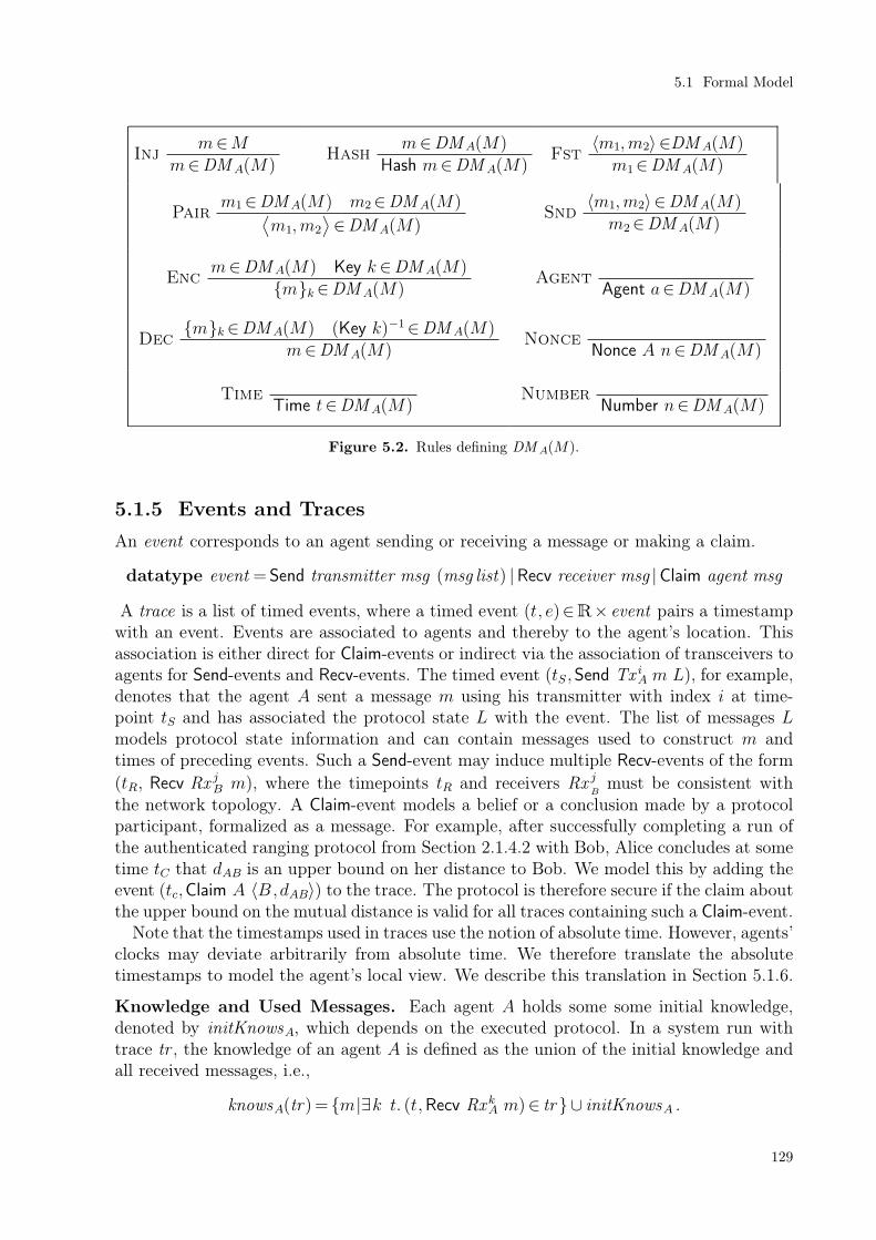
Injm∈M

m∈DMA(M )Hash

m∈DMA(M)

Hash m∈DM A(M)Fst

〈m1,m2〉 ∈DM A(M)

m1∈DM A(M)

Pairm1∈DMA(M ) m2∈DMA(M)

⟨

m1, m2

⟩

∈DMA(M)Snd

〈m1, m2〉 ∈DMA(M)

m2∈DMA(M)

Encm∈DMA(M ) Key k ∈DM A(M)

mk∈DMA(M)Agent

Agent a∈DM A(M)

Decmk∈DMA(M) (Key k)−1∈DM A(M)

m∈DM A(M)Nonce

Nonce A n∈DMA(M)

TimeTime t∈DMA(M)

NumberNumber n∈DMA(M)

Figure 5.2. Rules defining DMA(M).

5.1.5 Events and Traces

An event corresponds to an agent sending or receiving a message or making a claim.

datatype event = Send transmitter msg (msg list) |Recv receiver msg |Claim agent msg

A trace is a list of timed events, where a timed event (t, e)∈R× event pairs a timestampwith an event. Events are associated to agents and thereby to the agent’s location. Thisassociation is either direct for Claim-events or indirect via the association of transceivers toagents for Send-events and Recv-events. The timed event (tS ,Send TxA

i m L), for example,denotes that the agent A sent a message m using his transmitter with index i at time-point tS and has associated the protocol state L with the event. The list of messages Lmodels protocol state information and can contain messages used to construct m andtimes of preceding events. Such a Send-event may induce multiple Recv-events of the form

(tR, Recv RxBj m), where the timepoints tR and receivers Rx

B

j must be consistent withthe network topology. A Claim-event models a belief or a conclusion made by a protocolparticipant, formalized as a message. For example, after successfully completing a run ofthe authenticated ranging protocol from Section 2.1.4.2 with Bob, Alice concludes at sometime tC that dAB is an upper bound on her distance to Bob. We model this by adding theevent (tc,Claim A 〈B,dAB〉) to the trace. The protocol is therefore secure if the claim aboutthe upper bound on the mutual distance is valid for all traces containing such a Claim-event.

Note that the timestamps used in traces use the notion of absolute time. However, agents’clocks may deviate arbitrarily from absolute time. We therefore translate the absolutetimestamps to model the agent’s local view. We describe this translation in Section 5.1.6.

Knowledge and Used Messages. Each agent A holds some some initial knowledge,denoted by initKnowsA, which depends on the executed protocol. In a system run withtrace tr , the knowledge of an agent A is defined as the union of the initial knowledge andall received messages, i.e.,

knowsA(tr) = m|∃k t. (t,Recv RxAk m)∈ tr ∪ initKnowsA .

5.1 Formal Model

129

From the known messages, A can deduce all messages in DMA(knowsA(tr)). For a giventerm m, the set of (extractable) parts and the set of (syntactic) subterms are definedinductively by the rules in Figure 5.3.

m∈ subterms(m)

〈m1,m2〉 ∈ subterms(m)

mi∈ subterms(m)

Hash c∈ subterms(m)

c∈ subterms(m)

ck∈ subterms(m)

c∈ subterms(m)

ck∈ subterms(m)

k ∈ subterms(m)

m∈ parts(m)

〈m1, m2〉 ∈ parts(m)

mi∈ parts(m)

ck∈ parts(m)

c∈ parts(m)

Figure 5.3. Rules defining subterms and parts .

We use subterms to define the set of messages appearing in a trace tr .

used(tr)= n|∃A k t m. (t, Send TxA

k m)∈ tr ∧n∈ subterms(m)

5.1.6 Network, Intruder, and Protocols

We now describe our rules that inductively define the set of traces Tr(proto) for theexecution of a protocol proto together with arbitrary intruders sharing a network. The basecase, modeled by the Nil-rule in Figure 5.4 states that the empty trace is a valid trace forall protocols. The other rules describe how valid traces can be extended. The rules modelthe network behavior, the possible actions of the intruder, and the actions taken by honestagents executing the protocol.

Net

tr ∈Tr(proto) tR≥maxtime(tr)

(tS ,Send TxAi m L)∈ tr

cdistNet

(

TxAi ,RxB

j)

= tAB

tAB ⊥ tR≥ tS + tAB

tr · (tR,Recv Rx Bj m)∈Tr(proto)

Nil[ ]∈Tr(proto)

Fake

tr ∈Tr(proto) t≥maxtime(tr)m∈DM IA(knowsIA(tr))

tr · (t,Send Tx IAi m [ ])

Proto

tr ∈Tr(proto) t≥maxtime(tr) step ∈ proto(act , m)∈ step(view(HA, tr), HA, ctime(HA, t)) m∈DMHA(knowsHA(tr))

tr · (t, translateEv(HA, act , m))

Figure 5.4. Rules defining Tr(proto).

Network Rule. The Net-rule models message transmission from transmitters toreceivers, constrained by the network topology. A Send-event from a transmitter mayinduce a Recv-event at a receiver only if the receiver can receive messages from the trans-mitter. The time between these events is bounded below by the communication distancebetween the transmitter and the receiver. If there is a Send-event in the trace tr and theNet-rule’s premises are fulfilled, a corresponding Recv-event is appended to the trace. The


130

restriction on connectivity and transmission delay are ensured by tAB ⊥ and tR≥ tS + tAB.Here, tAB is the communication distance between the receiver and transmitter, tS is thesending time, and tR is the receiving time.

Note that one Send-event can result in multiple Recv-events at the same receiver atdifferent times. This is allowed because cdistNet models the minimal communication dis-tance and messages may also arrive later, for example due to the reflection of the signalcarrying the message. Moreover, a Send-event can result in multiple Recv-events at differentreceivers, modeling for example broadcast communication. Finally, note that transmissionfailures and jamming by an intruder, resulting in message loss, are modeled by traces wherethe Net-rule is not applied for a given Send-event and receiver, even though all premisesare fulfilled.

The timestamps associated with Send-events and Recv-events denote the starting timesof message transmission and reception. Thus, our network rule captures the latency oflinks, but not the message-transmission-time, which also depends on the message’s size andthe transmission speed of the transmitter and the receiver. Some implementation-specificattacks, such as those described in [156] and [49] are therefore not captured in our model.Also note that we do not capture partial overshadowing of messages by the adversary. InSection 5.3, we will adapt the Net-rule to account for this.

The premise t ≥ maxtime(tr), where t denotes the timestamp associated with the newevent and maxtime(tr) denotes the latest timestamp in the trace tr , is included in everyrule except Nil. It ensures that timestamps increase monotonically within each traceand thereby guarantees that the partial order on events induced by their timestamps isconsistent with the order of events in the trace. However, events can happen at the sametime.

Intruder Rule. The Fake-rule in Figure 5.4 captures the intruders’ behavior. Anintruder can send any message m deducible from his knowledge. We are not required tomodel the internal state of the intruders since they behave arbitrarily. We use explicit Send-events and Recv-events to model the exchange of information between colluding intruders.With an appropriate cdistNet function, it is possible to model an environment where theintruders are connected by high-speed links, allowing them to carry out wormhole attacks.Restrictions on the degree of cooperation between intruders can be modeled as predi-cates on traces. Internal and external attackers are both captured since they differ onlyin their initial knowledge or associated transceivers.

Protocols. In contrast to intruders who can send arbitrary deducible messages, honestagents follow the protocol. A protocol is defined by a set of protocol step functions. Eachstep function takes the local view and time of an agent as input and returns all possibleactions consistent with the protocol specification.

There are two types of possible actions. An agent can either send a message using atransmitter with a given id and store the associated protocol data or make a claim.

datatype action =SendA N (msg list) |ClaimA

An action associated with an agent A and a message m can be translated into the corre-sponding event with the translateEv function.

translateEv(A,SendA k L,m)= Send TxAk m L

translateEv(A,ClaimA, m) =Claim A m

5.1 Formal Model

131

Note that there is no Recv-action since message reception by honest agents is alreadymodeled by the Net-rule. A protocol step function is therefore of type agent × trace×R→(action×msg) set . Since the actions of an agent A only depend on his own previous actionsand observations, we define A’s view of a trace tr as the projection of tr on those eventsinvolving A.

view(A, tr)= [(ctime(A, t), ev)| (t, ev)← tr ∧ occursAt(ev) =A]

The view function uses the function occursAt , which maps events to associated agents.For instance, occursAt(Send TxA

i m L) = A. Since the timestamps of trace events referto absolute time, the view function accounts for the offset of A’s clock by translatingtimes using the ctime function. Given an agent and a global timestamp, the uninterpretedfunction ctime : agent ×R→R returns the corresponding local timestamp for the agent’sclock. The clock offset of A at global time t is given by ctime(A, t)− t. Using the abovedefinitions, we define the Proto-rule in in Figure 5.4. For a given protocol, specified as a setof the step functions, the Proto-rule describes all possible actions of honest agents, giventheir local views of a valid trace tr at a given time t. If all premises are met, the Proto-rule appends the translated event to the trace. Note that agents’ behavior, modeled bythe function step, is based only on the local clocks of the agents, i.e., agents cannot accessthe global time. Moreover, the restriction that all messages must be in DMHA

(knowsA(tr))ensures that agents only send messages deducible from their knowledge.

5.1.7 Protocol-Independent Results

Since the set of traces Tr(proto) is parameterized by the protocol description proto, ourframework allows us to establish protocol-independent results that hold for all protocolsor certain classes of protocols. In this section, we present four lemmas about the origin ofmessages that we will use later when we analyze concrete protocols. The proofs presentedin this section follow the formal proofs of the corresponding lemmas as they can be foundin our Isabelle/HOL formalization.

Our first lemma specifies a lower bound on the time between when an agent first uses anonce and another agent later uses the same nonce. The lemma holds whenever the initialknowledge of all agents does not contain any nonces. Note that according to the Nonce-rule in Figure 5.2, agents can only derive nonces tagged with their own identity and allother nonces must be received over the network.

Lemma 5.2. Let A be an arbitrary (honest or dishonest) agent and let the event(tSA, Send TxA

i mA LA) ∈ tr be the first event in the trace tr with n ∈ subterms(mA) forthe nonce n. If there is another event (tS

B , Send TxBj mB LB) ∈ tr with A B such

that n∈ subterms(mB), then tSB− tS

A≥ cdistLoS(A,B).

Proof. We prove this by induction on Tr(proto). The statement obviously holds for Niland Net since these rules do not add Send-events. We now consider the two remainingrules. Let tr ∈ Tr(proto) and (tS

A, Send TxAi mA LA) ∈ tr be the first event that contains

the nonce n as a subterm.

Fake. The event (tSI , Send Tx I

k mI [ ]) is appended to tr . The only interesting casesoccur when A I and n∈ subterms(mI). From the premises of the rule, we know thatmI ∈DM I(knowsI(tr)). Since I cannot guess a nonce created by another agent A, theintruder I must have received a message m containing n at some time tR

I with receiver


132

Rx Ih, where tR

I ≤ tSI . Every Recv-event in tr is preceded by a corresponding Send-event. So

there must be(

tSC ,Send TxC

u mLC)

∈ tr such that tRI − tS

C≥cdistNet(TxCu ,Rx I

h). If C=A,

then tSC ≥ tS

A since n is first used at time tAS and we have tS

I − tSA≥ cdistLoS(A, I) since

faster-than-light communication is impossible and cdistNet(TxAi ,Rx I

h)≥ cdistLoS(A, I).

If C A, we can apply the induction hypothesis to the event(

tSC ,Send TxC

u m LC)

and

obtain tSC − tS

A≥ cdistLoS(A,C). Together with tRI − tS

C ≥ cdistLoS(C, I) and tRI ≤ tS

I , weobtain tS

I − tSA≥ cdistLoS(A, I) using the triangle inequality for physical distances.

Proto. The event (tSB, translateEv(B, act , mB)) is appended to tr . Only the case where

translateEv(B, act , mB) = SendA i LB, B A, and n ∈ subterms(mB) is interesting.From the premises of the Proto-rule, we have mB ∈ DM B(knowsB(tr)) like in theFake-case. We can therefore proceed analogously.

The next lemma is similar to Lemma 5.2 and concerns the earliest time when an agentcan receive a nonce.

Lemma 5.3. Let A be an arbitrary (honest or dishonest) agent and let (tSA,Send TxA

i mA

LA) ∈ tr be the first event in the trace tr with n ∈ subterms(mA) for the nonce n. If thereis another event (tR

B, Recv RxBj mB) ∈ tr with A B such that n ∈ subterms(mB), then

tRB− tS

A≥ cdistLoS(A,B).

Proof. We prove this lemma by induction over Tr(proto). Except for the Net-case, thestatement trivially follows from the induction hypothesis since no Recv-events are added.For Net, assume that (tS

A,Send TxAi mA LA)∈ tr is the first event that contains the nonce n

and tr is extended with (tRB , Recv RxB

j mB) ∈ tr such that A B and n ∈ subterms(mB).

Then there must be an earlier Send-event (tSC , Send TxC

k mB LC) such that tRB − tS

C ≥cdistNet(TxC

k ,Rx Bj ). From Lemma 5.2, we know that tS

C− tSA≥ cdistLoS(C,A). Since faster-

than-light communication is impossible, we obtain cdistLoS(C, B) ≤ cdistNet(TxCk , Rx B

j ).Combining the inequalities, we obtain tR

B − tSC + tS

C − tSA≥ cdistLoS(B,C) + cdistLoS(A, C).

We can now apply the triangle inequality for physical distances to obtain the inequalitytRB− tS

A≥ cdistLoS(A,B).

The next lemma concerns signatures and their creation time.

Lemma 5.4. Let A be an honest agent and let (tSB, Send TxB

i mB LB) ∈ tr such thatsig(m, skA)∈ subterms(mB), where skA denotes the signing key of A and m is an arbitrary

message. Then there is (tSA, Send TxA

j mA LA) ∈ tr such that sig(m, skA) ∈ subterms(mA)and tS

B− tSA≥ cdistLoS(A,B).

This lemma only holds if the initial knowledge of every agent does not contain signingkeys of other agents or signatures created by using the signing keys of other agents. Addi-tionally we must assume that protocol messages never contain signing keys of agents asextractable subterms. We formalize such assumptions as predicates on protocols and theinitial knowledge.

Proof. (Sketch) The proof is analogous to the proof of Lemma 5.2, but additionally usesthe fact that agents other than A cannot sign messages on behalf of A if the signing keynever leaks.

A similar lemma also holds for MACs.

5.1 Formal Model

133

Lemma 5.5. Let A and B be honest agents and C a different, possibly dishonest, agent.Furthermore, let (tS

C , Send TxCi mC LC)∈ tr such that mac

kAB(m)∈ subterms(mC), where

kAB denotes the shared key of A and B and m is an arbitrary message. Then there is(tSE , Send TxE

j mE LE) ∈ tr such that E ∈ A, B, mackAB(m) ∈ subterms(mE) and

tSC − tS

E ≥ cdistLoS(E,C).

5.2 Case StudiesIn this section, we use our model to analyze the security properties of three protocols: anauthenticated ranging protocol, an ultrasonic distance-bounding protocol, and a securetime synchronization protocol. Each protocol uses cryptographic primitives as well as phys-ical characteristics of the communication technology, environment, or network topology, toprovide security guarantees. Since the first two protocols estimate distance based on round-trip measurements and bounds on the propagation speed of signals, variable clock offsetscan trivially lead to wrong results. Therefore, we only consider those ctime functions thatmodel a constant clock error. In the third example, we also restrict ourselves to constantclock errors.

5.2.1 Authenticated Ranging

To define the set of traces for the authenticated ranging protocol from Figure 5.5 explainedin Section 2.1.4.2, we formalize the set of protocol steps protoAR = ar 1, ar 2, ar 3. Eachstep function ar i(tr , A, t) yields the possible actions of the agent A executing the protocolstep i for his view of the trace tr at time t. We have formalized the steps in Isabelle/HOLusing set comprehension, but present the steps here using rule notation for readability. For afixed tr , A, and t, ar i(tr ,A, t) is defined as the least set closed under the corresponding rule.

1. An honest verifier V can start a protocol run by sending a fresh nonce as a challenge.We use the index r to denote radio transmitters and receivers of honest agents.

(Nonce V i) used(tr)

(SendA r [ ],Nonce V i)∈ ar 1(tr , V , tSV )

2. An honest prover P that receives a challenge may send the corresponding response.Note that we use a typed receive for the nonce, but we do not restrict the creator V ′

of the nonce in any way

(tRP ,Recv RxP

r (Nonce V ′ i))∈ tr

(SendA r [ ], sig(〈Nonce V ′ i, tSP − tR

P 〉, skP))∈ ar 2(tr , P , tSP)

3. The last step introduces a Claim-event. It models the conclusion of a verifier V whoreceived a response to his initial challenge.

(tSV ,Send TxV

r (Nonce V i) [ ])∈ tr

(tRV ,Recv RxV

r sig(〈Nonce V i, δ〉, skP))∈ tr(

ClaimA,⟨

P , (tRV − tS

V − δ)∗ c2

⟩)

∈ ar 3(tr , V , tCV )

The premises state that V has initiated a protocol run and received a response from P .V therefore believes that (tR

V − tSV − δ)∗ c

2is an upper bound on his distance to P .

For this protocol, we define the initial knowledge of each agent A to be her own signingkey skA and the public keys pkB of all other agents B.


134



tSV7 readClock()

nvtRP7 readClock()

set δ7 tSP− tR

P

compute sig(〈nv , δ〉, skP)

tRV7 readClock()

sig(〈nv ,δ〉,skP)send at tS

P

check signature


V− δ)∗ c2

Figure 5.5. Authenticated Ranging Protocol.

Security Analysis. As explained in Section 2.1.4.2, the protocol should compute a reli-able upper on the physical distance between prover and verifier whenever the intendedprover is honest. We therefore state the following theorem.

Theorem 5.6. Let V and P be honest agents, tr ∈Tr(protoAR) and (t,Claim V 〈P ,d〉)∈ tr,then d≥ |locV − locP |.

The theorem states that whenever the authenticated ranging protocol successfully ter-minates for an honest prover and verifier, then the computed distance is an upper boundon the physical distance between the two. Remember that a dishonest prover can shortenthe computed distance by lying about δ and considering a dishonest verifier does not makesense since the prover does not obtain any guarantees.

For our proof, we use three of the protocol-independent lemmas about message origina-tion and the fact that the δ sent in the second protocol message is always equal to tS

P − tRP ,

the delay between the Recv-event and the Send-event, provided that P is honest. Thisfollows directly from the definition of ar 2.

Proof. Since only the step ar 3 adds events of the form (tCV ,Claim V 〈P ,d〉), we do not have

to consider the other protocol steps and rules defining Tr(protoAR). From the premisesof ar 3 and the definitions of ar 2 and ar 3, we know (tS

V , Send TxVr (Nonce V i) [ ]) is the

first event where this nonce is used in tr , (tRV ,Recv RxV

r sig(〈Nonce V i, δ〉, skP))∈ tr , andd= (tR

V − tSV − δ)∗ c

2. Even though we use global timestamps tR

V and tSV in contrast to ar 3

where local times for V are used, the equation for d still holds since we assume constantclock offsets.

We know there must be a Send-event (tSC , Send Tx C

j sig(〈Nonce V i, δ〉, skP)) by some

(possibly dishonest) agent C with tRV − tS

C≥ cdistLoS(C,V ). We can now apply Lemma 5.4,to obtain a Send-event (tS

P ,Send TxPr sig(〈Nonce V i, δ〉, skP)) where P sends the signature

with tSC − tS

P ≥ cdistLoS(P , C). From the definition of ar 2, we know that there must aRecv-event (tR

P , Recv RxPr Nonce V i) such that δ = tS

P − tRP . For this event, we can apply

Lemma 5.3 to obtain tRP − tS

V ≥ cdistLoS(V , P ). Combining the (in)equalities and using thetriangle inequality, we obtain the following.

tRV − tS

V − δ= tRV − tS

V − tSP + tR

P

= tRV − tS

C + tSC − tS

P + tRP − tS

V

≥ cdistLoS(C, V )+ cdistLoS(P ,C)+ cdistLoS(V , P )

5.2 Case Studies

135

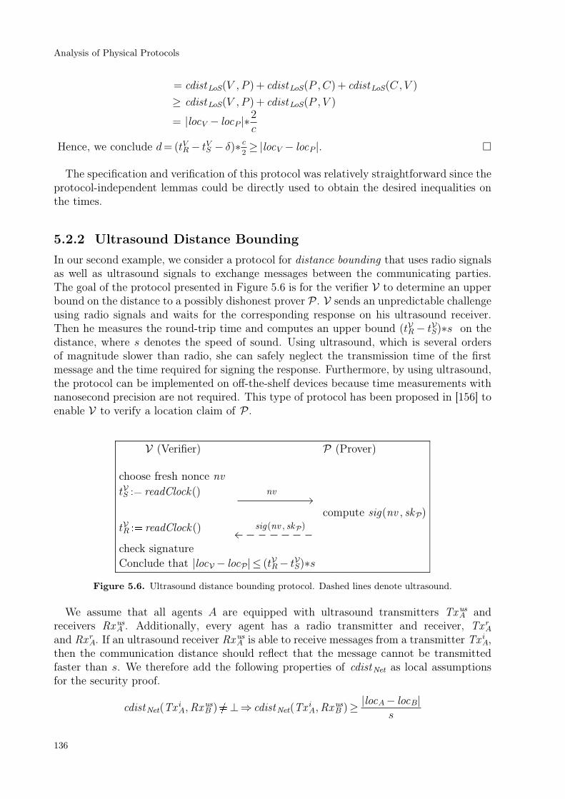
= cdistLoS(V , P ) + cdistLoS(P ,C)+ cdistLoS(C, V )

≥ cdistLoS(V , P ) + cdistLoS(P , V )

= |locV − locP |∗2

c

Hence, we conclude d= (tRV − tS

V − δ)∗ c2≥ |locV − locP |.

The specification and verification of this protocol was relatively straightforward since theprotocol-independent lemmas could be directly used to obtain the desired inequalities onthe times.

5.2.2 Ultrasound Distance Bounding

In our second example, we consider a protocol for distance bounding that uses radio signalsas well as ultrasound signals to exchange messages between the communicating parties.The goal of the protocol presented in Figure 5.6 is for the verifier V to determine an upperbound on the distance to a possibly dishonest prover P. V sends an unpredictable challengeusing radio signals and waits for the corresponding response on his ultrasound receiver.Then he measures the round-trip time and computes an upper bound (tR

V − tSV)∗s on the

distance, where s denotes the speed of sound. Using ultrasound, which is several ordersof magnitude slower than radio, she can safely neglect the transmission time of the firstmessage and the time required for signing the response. Furthermore, by using ultrasound,the protocol can be implemented on off-the-shelf devices because time measurements withnanosecond precision are not required. This type of protocol has been proposed in [156] toenable V to verify a location claim of P .



tSV7 readClock() nv

compute sig(nv , skP)

tRV7 readClock() sig(nv , skP)

check signature


V)∗s

Figure 5.6. Ultrasound distance bounding protocol. Dashed lines denote ultrasound.

We assume that all agents A are equipped with ultrasound transmitters TxAus and

receivers RxAus. Additionally, every agent has a radio transmitter and receiver, TxA

r

and RxAr . If an ultrasound receiver RxA

us is able to receive messages from a transmitter TxAi ,

then the communication distance should reflect that the message cannot be transmittedfaster than s. We therefore add the following properties of cdistNet as local assumptionsfor the security proof.

cdistNet(TxAi ,RxB

us) ⊥⇒ cdistNet(TxAi ,RxB

us)≥|locA− locB|

s


136

The same applies to messages transmitted by ultrasound transmitters TxAus and received

by receivers RxBi .

cdistNet(TxAus,RxB

i ) ⊥⇒ cdistNet(TxAus,RxB

i )≥|locA− locB|

s

Note that it has recently been shown in [152] that radio signals may induce a current inaudio receiver circuits. More precisely, the authors of that paper demonstrated that thistechnique allows to successfully trigger receive events on ultrasound receivers using radiosignals. This would enable trivial attacks against the protocol under consideration. Thefact that we need this explicit additional assumption in our model to successfully prove thesecurity of the protocol shows that our model accounts for subtle problems of this kind.However, we shall assume from now on that the countermeasures described in [152] havebeen implemented and we can keep the assumption.

We now give the set of step functions protoUDB = udb1, udb2, udb3 that defines theultrasound distance bounding protocol.

1. In the start step udb1, the verifier initiates a protocol run.

(Nonce V i) used(tr)

(SendA r [ ],Nonce V i)∈ udb1(V , tr , tSV )

2. The reply step udb2 formalizes the behavior of a prover that responds to an initialchallenge. Note that the ultrasound transmitter TxB

us is used for the response.

(tRP ,Recv RxP

r (Nonce V ′ i))∈ tr(SendA us [ ], sig(Nonce V ′ i, skP))∈ udb2(P , tr , tS

P)

3. The final step udb3 introduces a Claim-event when a verifier V receives a response tohis initial challenge on his ultrasound receiver RxA

us.

(tSV ,Send TxV

r (Nonce V i))∈ tr

(tRV ,Recv RxV

us sig(Nonce V i, skP))∈ tr

(ClaimA, 〈P , (tRV − tS

V )∗s〉)∈ udb3(V , tr , tCV )

This models what V concludes from a signal that apparently traveled from P to V

using the speed of sound s in fewer than tRV − tS

V time units. Namely, V concludes that

(tRV − tS

V ) ∗s is a reliable upper bound on the distance to P .

Security Analysis. The desired security property of the distance bounding protocol issimilar to the property of the authenticated ranging protocol proved in Theorem 5.6. Sincethe prover’s computation time is not used for computing the distance, the protocol does notrequire the prover to be honest. We would therefore expect a statement like the followingto hold.

Proposition 5.7. Let V be an honest agent and P an arbitrary agent. Furthermore, con-sider a valid trace tr ∈ Tr(protoUDB), where (t, Claim V 〈P , d〉) ∈ tr. Then it holdsthat d≥ |locV − locP |, i.e., the distance computed by the verifier is an upper bound on thephysical distance between the involved agents.

5.2 Case Studies

137

However, as shown in [160], this proposition is false without any further assumptions. Anattack involving two colluding intruders is shown in Figure 5.7. We use PS (V ) to denotethe private space of V , which is defined as the largest circle centered at V such that Vcan ensure that no intruder is inside. To mount the attack, ID is placed close to P andreceives P ’s reply over ultrasound. ID then uses a fast radio link to forward it to the secondintruder IC who is close to V . IC finally delivers the message to V using ultrasound. Wehave proven in our Isabelle/HOL formalization that this attack is captured in our modelby showing that the corresponding attack trace is a valid trace. The inequality involvingthe communication distances necessary for such an attack to work is

|locV − locP |s

> cdistNet(TxVr ,RxP

r )+ cdistNet(TxPus,Rx ID

us )+

cdistNet(Tx IDr ,Rx IC

r )+ cdistNet(Tx ICus,RxV

us) .

If the inequality holds, intruders connected by a fast radio link can speed up ultrasoundcommunication between V and P using their radio link, such that the computed distanceis smaller than the real distance between V and P . This attack has been discovered andimplemented in [160].

V

PS(V )

P

ICID

nv

sig(nv , skP )

sig(nv , skP )

sig(nv , skP )

Figure 5.7. Attack on the ultrasound distance bounding protocol.

In light of the above, we prove Proposition 5.7 under an additional assumption: Theverifier V can ensure that the prover P is in his private space. The same assumption is usedin other protocols, e.g., [156] and [39] for location-based access control and device pairing.It holds, for example, in environments where V can visually verify the absence of nearbyintruders. The following inequality ensures that no intruder is closer to the verifier V thanthe possibly dishonest prover P :

∀D. |locV − locID| ≥ |locV − locP |.

Note that this assumption thwarts Mafia frauds as well as Terrorist frauds (as definedin [34]). Remember that a mafia fraud is an attack where an intruder plays man-in-the-middle between a verifier and an honest prover. Since there is no intruder closer to theprover V than the verifier P , this kind of attack is impossible in our setting. Similarly, aterrorist fraud is an attack where an attacker plays man-in-the-middle between a verifierand a dishonest prover. This would require a second attacker being located closer to theverifier than the dishonest prover P . This setup also trivially violates the private spaceassumption of the verifier V . Note that Proposition 5.7 also allows for another attackwhere a dishonest prover IC hands over all key material to another dishonest prover IDthat is closer to V . Then IC can execute the protocol claiming to be ID which results in aninvalid upper bound. We will present an adapted definition that accounts for this problemin Section 5.4.


138

We now restate Proposition 5.7, adding the additional private space assumption, andprove the result.

Theorem 5.8. Let V be an honest agent and P an arbitrary agent such that ∀D. |locV −locID| ≥ |locV − locP |. Furthermore, consider a valid trace tr ∈ Tr(protoUDB), where(t,Claim V 〈P , d〉)∈ tr. Then d≥ |locV − locP |.

Proof. We prove this by induction over Tr(protoUDB). Since only the step udb3 adds

events of the form (tCV ,Claim V 〈P ,d〉), we do not have to consider the other protocol steps

and rules defining Tr(protoUDB). From the premises of udb3 and the definitions of udb2

and udb3, we conclude that (tSV ,Send TxV

r (Nonce V i) [ ]) is the first event where this nonceis used in tr , (tR

V ,Recv RxVus sig(Nonce V i, skP))∈ tr , and d=(tR

V − tSV )∗s. Even though we

use global timestamps tRV and tS

V in contrast to udb3 where local times for V are used, theequation for d still holds since we assume constant clock offsets.

We know there must be a Send-event (tSC ,Send Tx C

j sig(Nonce A i, skB)) by some possiblydishonest agent C with tR

V − tSC ≥ cdistNet(TxC

i ,RxVus)≥ |locV − locC|/s. We also know that

tSC ≥ tS

V by Lemma 5.2. We therefore have d= (tRV − tS

V )∗s≥ (tRV − tS

C)∗s≥ |locA− locC|. IfC =P , then this concludes the proof. If C P , then C must be dishonest and we are alsodone because |locV − locC| ≥ |locV − locP | since P is assumed to be located in PS (V ).

Note that our proof does not use the fact that the second protocol message is authen-ticated by P . Correctness is guaranteed because V ensures that P is in his private space.Therefore even a simplified version of the protocol, where the second message is replacedwith Hash 〈Nonce V i, P 〉, would be secure under the private-space assumption.

5.2.3 Secure Time Synchronization

As a final example, we formalize a secure time synchronization protocol presented in [84].The Enhanced Secure Pairwise Synchronization (E-SPS) protocol achieves pairwise clocksynchronization between two honest nodes in the presence of external attackers by com-puting the relative clock offset between the two nodes. We analyze this protocol under thefollowing assumptions.

Constant clock offset. We assume constant clock offsets for each agent’s clock duringthe execution of the protocol. Namely, for each agent A there is a offset δA such thatctime(A, t) = t+ δA.

Lower bound on message transmission time. We assume a maximal bandwidth forthe connecting network. As a consequence, there is a lower bound dmin on the messagetransmission time for any message that contains a nonce. Even in the case of a mali-cious sender, it is impossible for honest agents to complete reception of a nonce beforetstart + dmin, where tstart is the start time of the reception.

Upper bound on end-to-end delay. Finally, we assume that there is a maximal end-to-end delay when receiving a message expected by the protocol. The maximal delaydmax consists of (1) the time for media access, (2) the time-of-flight, and (3) the message

5.2 Case Studies

139

transmission time. In terms of media access, we assume that the hardware is capable ofobtaining and inserting timestamps of reception and send events. Therefore we do nothave to account for (1) since it does not affect the measurements. We obtain a boundfor (2) by assuming a maximal distance between nodes. However, in most cases (2) isnegligible compared to (3). For (3), it is possible to define a minimal transmission rateand to use the corresponding maximal delay. A detailed breakdown of the times canbe found in [84].

Figure 5.8 depicts the E-SPS protocol as an Alice-and-Bob style sequence diagram,where time passes from left to right. The protocol securely computes an approxi-mation δAB of the relative clock offset δA − δB. To prove that dmax − dmin is upperbound of the approximation, we formalize the protocol as the set of step functionsprotoESPS =esps1, esps2, esps3, esps4. Recall that step functions involve only local timesof agents, i.e., timestamps associated with trace events are translated to the local timeof the corresponding agent.

Alice

Bob

global time

〈A,B,NA〉

〈A,B,NA〉 NB

NB

mac

mac

t1 t2 t3 t4

d1 d2

clock Alice

clock Bobt1 + δA t4 + δA

t3 + δBt2 + δB

If d≤ dmax, Alice accepts the last message and concludes that δAB is an approxima-tion of the relative clock offset such that |δAB− (δA− δB)| ≤ dmax − dmin, where

tiC = ti+ δC

mac = mackAB(B,A,NA, NB , t2

B, t3B)

d=((t2

B− t1A) + (t4

A− t3B))

2

δAB =((t2

B− t1A)− (t4

A− t3B))

2.

Figure 5.8. Enhanced secure time synchronization (E-SPS) protocol.

1. The first step esps1 models an initiator A sending a challenge. Here t1A denotes the local

time measured by A, corresponding to the global time t1A− δA.

(Nonce A i) used(tr)

(SendA r [ ], 〈A,B,Nonce A i〉)∈ esps1(A, tr , t1A)


140

2. The second step esps2 models an agent B responding to an initial challenge.

(Nonce B k) used(tr)

t3B≥ t2

B t2B≥ t2,start

B + dmin

(t2,startB ,Recv B 〈A,B,Nonce A ′ i′〉)

(SendA r [A,Nonce A ′ i′, t2B],Nonce B k)∈ esps2(B, tr , t3

B)

Reception of the challenge starts at t2,startB and ends at t2

B, which is least dmin time units

later. B associates the protocol data [A,Nonce A′ i′,t2B] with the resulting Send-event.

3. The third step esps3 models B sending the MAC.

(t3B ,Send TxB

r (Nonce B k) [A,Nonce A ′ i′, t2B])∈ tr

(SendA r [ ],mackAB(B,A,Nonce A ′ i′,Nonce B k, t2

B , t3B))∈ esps3(B, tr , tB)

Besides the exchanged nonces, B includes the times t2B and t3

B, which denote when thereception of A’s challenge ended and when B started sending his response.

4. Finally, step esps4 models A’s reception of the responses.

(t1A,Send TxA

r 〈A,B,Nonce A i〉 [ ])∈ tr

(t4,startA ,Recv RxA

r (Nonce B ′ j ′))∈ tr

(t5A,Recv RxA

r mackAB(B,A,Nonce A i,Nonce B ′ j ′, t2B , t3

B))∈ tr

t4A≥ t4,start

A + dmin d≤ dmax tA≥ t4A

d= ((t2B− t1

A)+ (t4A− t3

B))∗1

2

δAB =((t2B− t1

A)− (t4A− t3

B))∗1

2

(ClaimA, 〈B, δAB〉)∈ esps4(A, tr , tA)

If A concludes a clock-offset δAB, A must have received the first response and thecorresponding MAC according to the protocol specification. A then computes the delayd and the offset δAB using his own time measurements and the timestamps received inthe messages from B (see Figure 5.8). Finally, A completes the protocol only if d≤dmax .Otherwise, the end-to-end delay for the relevant transmissions took too long, whichwould result in an unreliable estimation of the clock offset.

First note that if neither the challenge nor the response is delayed by an intruder or by theenvironment, then d1≈ d2 for the two transmission delays (see Figure 5.8) and

d=((d1 + δB− δA)+ (d2 + δA− δB))

2=d1 + d2

2≤ dmax .

In this case, Alice computes the relative clock offset

δAB =((d1− d2)+ 2∗δB− 2∗δA)

2≈ δB− δA .

The upper bound dmax bounds the error that the adversary can introduce by delaying eitherthe challenge or the response. We first show that if there is a Claim-event, then there arefour corresponding times that satisfy the following (in)equalities.

5.2 Case Studies

141

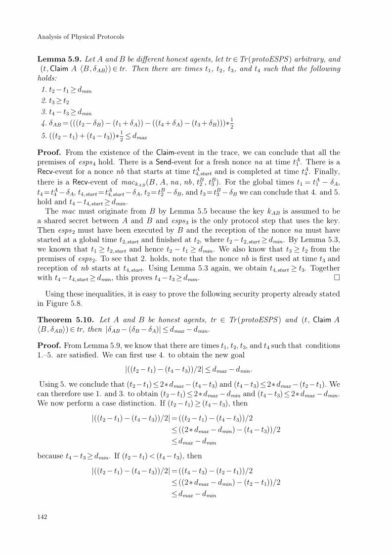
Lemma 5.9. Let A and B be different honest agents, let tr ∈Tr(protoESPS ) arbitrary, and(t,Claim A 〈B, δAB〉)∈ tr. Then there are times t1, t2, t3, and t4 such that the followingholds:

1. t2− t1≥ dmin

2. t3≥ t23. t4− t3≥ dmin

4. δAB =(((t2− δB)− (t1 + δA))− ((t4 + δA)− (t3 + δB)))∗1

2

5. ((t2− t1)+ (t4− t3))∗1

2≤ dmax

Proof. From the existence of the Claim-event in the trace, we can conclude that all thepremises of esps4 hold. There is a Send-event for a fresh nonce na at time t1

A. There is aRecv-event for a nonce nb that starts at time t4,start

A and is completed at time t4A. Finally,

there is a Recv-event of mackAB(B, A, na , nb , t2

B , t3B). For the global times t1 = t1

A − δA,

t4= t4A− δA, t4,start = t4,start

A −δA, t2= t2B− δB, and t3= t3

B− δB we can conclude that 4. and 5.hold and t4− t4,start≥ dmin.

The mac must originate from B by Lemma 5.5 because the key kAB is assumed to bea shared secret between A and B and esps3 is the only protocol step that uses the key.Then esps2 must have been executed by B and the reception of the nonce na must havestarted at a global time t2,start and finished at t2, where t2− t2,start≥ dmin. By Lemma 5.3,we known that t1 ≥ t2,start and hence t2 − t1 ≥ dmin. We also know that t3 ≥ t2 from thepremises of esps2. To see that 2. holds, note that the nonce nb is first used at time t3 andreception of nb starts at t4,start. Using Lemma 5.3 again, we obtain t4,start ≥ t3. Togetherwith t4− t4,start≥ dmin, this proves t4− t3≥ dmin.

Using these inequalities, it is easy to prove the following security property already statedin Figure 5.8.

Theorem 5.10. Let A and B be honest agents, tr ∈ Tr(protoESPS ) and (t, Claim A

〈B, δAB〉)∈ tr, then |δAB− (δB− δA)| ≤ dmax − dmin.

Proof. From Lemma 5.9, we know that there are times t1, t2, t3, and t4 such that conditions1.–5. are satisfied. We can first use 4. to obtain the new goal

|((t2− t1)− (t4− t3))/2| ≤ dmax − dmin.

Using 5. we conclude that (t2− t1)≤2∗dmax− (t4− t3) and (t4− t3)≤2∗dmax− (t2− t1). Wecan therefore use 1. and 3. to obtain (t2− t1)≤2∗dmax−dmin and (t4− t3)≤2∗dmax−dmin.We now perform a case distinction. If (t2− t1)≥ (t4− t3), then

|((t2− t1)− (t4− t3))/2|=((t2− t1)− (t4− t3))/2

≤ ((2∗ dmax − dmin)− (t4− t3))/2

≤dmax − dmin

because t4− t3≥ dmin. If (t2− t1)< (t4− t3), then

|((t2− t1)− (t4− t3))/2|=((t4− t3)− (t2− t1))/2

≤ ((2∗ dmax − dmin)− (t2− t1))/2

≤dmax − dmin


142

because t2− t1≥ dmin.

Note that this is a tighter bound on the error than we proved in [21], where the boundwas 2∗(dmax − dmin). Aside from the reasoning about the creation of MACs, which iscovered by our protocol independent lemmas, most of the theorem-proving work concernsestablishing the desired inequalities between the times of the different events. Most of theseinequalities stem from the relation between the different clock offsets of the two nodes.

5.3 Extended Model with Xor and Overshadowing

So far, we have analyzed an authenticated ranging protocol and an ultrasound distancebounding protocol. For both protocols, the time required by the prover to compute theresponse is not critical. For the authenticated ranging protocol, the prover is assumed tobe honest and the computation time is subtracted to obtain the time-of-flight. For theultrasound distance bounding protocol, the computation time is included in the time-of-flight measured by the verifier, but since the reply travels with the speed of sound, it isnegligible. In this section, we analyze distance bounding protocols that exclusively useradio transmission. In this case, the computation time is included in the measured time-of-flight and can cause a significant enlargement of the computed distance. To minimize thiserror, the computation of the response from the challenge must be fast. For this reason,many distance bounding protocols use XOR. Another advantage of using XOR is that thechallenge-response phase can be performed bitwise, i.e., the verifier sends the i-th bit ofthe challenge and waits for the i-th bit of the response before sending the next bit. Thiscan be used as a countermeasure against some implementation specific attacks as describedby [156, 49].

To support such protocols, we extend our framework with support for Xor . To capturepractically relevant attacks, we also extend our model to account for (partial) over-shadowing of messages that are in transmission. We do not model all the details of overshad-owing in our symbolic model, but enough to discover new attacks and rule out a largeclass of attack for fixed version of the considered protocols.

5.3.1 Message Theory for Xor

We now extend the framework presented in the previous sections with support for Xor . Toachieve this, we continue as follows. First, we define the type fmsg of free messages. Theinhabitants of this type are elements of the free term algebra built over atomic messages andthe cryptographic operators including Xor . Second, we define the equivalence relation =Xor

on fmsg that models the equalities that hold for Xor . Third, we define a normal-form withrespect to =Xor using a normalization function. Fourth, we define a new (abstract) typemsgthat is represented by the normal-form messages in fmsg . This type is bijective to thequotient type fmsg/=Xor

. We then lift the functions for message construction and messagededuction from fmsg to msg . Finally, we define the notions of parts and subterms on msg .


143

Free Messages and =Xor . The type fmsg of free messages is defined as

datatype fmsg =AGENT agent |TIME R |NUMBER N |NONCE agent N

|KEY key |HASH fmsg |PAIR fmsg fmsg |CRYPT key fmsg

| fmsg ⊞ fmsg |ZERO .

We use uppercase constructors and ⊞ because we want to use the usual operator namesfor msg . The equivalence relation =Xor: fmsg × fmsg → bool is defined as the equationaltheory generated by the following equations.

(x⊞ y)⊞ z≃x⊞ (y⊞ z) (A) x⊞ y≃ y⊞x (C)

x⊞ZERO≃x (U) x⊞x≃ZERO (N)

Normal-form and normalization function. We define the function (_)↓: fmsg→ fmsgthat returns the normal-form of the given term. Our normal-form is defined such that nei-ther (U) nor (N) are applicable from left to right and all applications of ⊞ are nested to theright and sorted with respect to a total order on fmsg . To define the normalization function,we first define two helper functions. The helper function _⊕?_: fmsg × fmsg→ fmsg isdefined as a⊕?b=(if b=ZERO then a else a⊞ b). It applies the ⊞ operator, but ensures thatthe message a⊞ZERO, which is not in normal-form, is never created. The helper function_⊕↓_: fmsg × fmsg→ fmsg is defined in Figure 5.9 and also applies ⊞ to its arguments. Itensures that the resulting message is in normal-form whenever its arguments are alreadyin normal-form.

x⊕↓ZERO=x

ZERO⊕↓x=x

(a1⊞ a2)⊕↓ (b1⊞ b2)= if a1 = b1 then a2⊕↓ b2

else if a1<b1 then a1⊕? (a2⊕↓ (b1⊞ b2))

else b1⊕? ((a1⊞ a2)⊕↓ b2)

(a1⊞ a2)⊕↓ b= if a1 = b then a2

else if a1<b then a1⊕? (a2⊕↓ b)else b⊞ (a1⊞ a2)

a⊕↓ (b1⊞ b2)=(b1⊞ b2)⊕↓ a

a⊕↓ b= if a= b then ZERO else if a< b then a⊞ b else b⊞ a

Figure 5.9. The ⊕↓ function.

Using these definitions, we can now define ↓ as follows.

(HASH m)↓= HASH (m↓)

(PAIR m1 m2)↓= PAIR (m1↓) (m2↓)

(CRYPT k m)↓= CRYPT k (m↓)

(a⊞ b)↓= (a↓)⊕↓ (b↓)

x↓= x

We have proved that ↓ is sound and complete with respect to =Xor in the following sense.

Lemma 5.11. For all s, t∈ fmsg, s=Xor t if and only if s↓= t↓.


144

Since we define the normalization function ↓ directly, we can use Isabelle’s automatictermination prover and the message m↓ is obviously unique. The direction s↓= t↓ impliess=Xor t of Lemma 5.11 follows from the intermediate result s=Xor s↓ and is not that hardto prove. The other direction is much harder to prove and requires several intermediatedefinitions and lemmas. For example, it was useful to inductively define a predicate nfthat characterizes normal-form messages and show that nf (a) if and only if a= a↓. Thisallowed us to use the automatically derived induction principle for nf for all messages a↓.

An alternative approach would be to to use ordered rewriting or rewriting modulo ACand to define ↓ as the fixpoint of the one-step rewriting relation. This would requiremanual confluence and termination proofs for the rewriting relation. On the other hand, thedirection s=Xor t implies s↓= t↓ in Lemma 5.11 would follow immediately from confluence.

The msg Type, DM , parts, and subterms. We use the declaration

typedef msg = m∈ fmsg |m↓=m

to define the abstract type msg that is represented by the subset of normal-form messagesin fmsg . The typedef declaration also defines two functions Absmsg: fmsg → msg andRepmsg :msg→ fmsg and axioms that state that Absmsg is a bijection from the representingset m|m↓=m to msg and Repmsg is a bijection from msg to m|m↓=m. For m withm↓ m, Absmsg(m) is unspecified. Using these functions, we can lift the constructors fromfmsg to msg as follows.

Nonce a i=Absmsg(NONCE a i)

Pair m1 m2 =Absmsg(PAIR (Repmsg(m1)) (Repmsg(m2)))

Hash m=Absmsg(HASH (Repmsg(m)))

Xor a b=Absmsg((Repmsg(a)⊞Repmsg(b))↓)

Zero=Absmsg(ZERO)

Note that except for the definition of Xor , the argument to Absmsg is already in normalform since all constructors except for ⊞ are free with respect to =Xor. For Xor , we use↓ to ensure that the argument to Absmsg is in normal-form because the result would beunspecified otherwise. The definitions for Agent, Int, Real, and Key are analogous to Nonce.In the following, we write a⊕ b for (Xor a b) and 0 for Zero.

We can now define the message deduction function DM : agent→msg set→msg set . Ascan be seen in Figure 5.10, the definition is analogous to the definition for the free messagealgebra without Xor . Note that the Xor-rule uses the Xor constructor for the type msgof normal-form messages.

Injm∈M

m∈DMA(M)

NumberNumber n∈DMA(M)

Xora∈DM A(M) b∈DMA(M )

a⊕ b∈DM A(M)Zero

0∈DM A(M)

Figure 5.10. Message deduction function DM for Xor . The missing rules are equal to Figure 5.2.


145

To define the subterms and parts functions on msg , we first extend the definitions fromFigure 5.3 to account for ⊞ to obtain the functions fsubterms and fparts on fmsg . Forexample, (NONCE A i)∈ fparts((NONCE A i)⊞ (NONCE A i)). Then, we define parts as

parts(m) = Absmsg(a)|a∈ fparts(Repmsg(m)).

The function subterms is defined analogously. To illustrate these definitions, we considerthe message m=(Nonce A i)⊕ (Nonce A i). Unfolding the definition of ⊕, which is anabbreviation for Xor , we see that

m=Absmsg((Repmsg(Nonce A i)⊞Repmsg(Nonce A i))↓) =Absmsg(ZERO)= 0.

Hence, parts(m) = parts(0) = 0. This is exactly the definition that we want because weare only interested in the parts of the normal form of a message. For non-Xor messages,we know that those must have been used in the construction of the message.

5.3.2 Network Rule with Overshadowing

Our Fake and Net rules allow the intruder to receive, delete, and send messages. Ignoringthe aspects of timing and network connectivity, giving the intruder the additional capabilityto modify messages that are in transmission is not necessary since he can always receiveand delete such a message m, deduce a new message m′ using m and other known mes-sages, and finally send the message m′. Since our model captures both timing and networkconnectivity, this reasoning does not apply. We therefore extend our model in this sectionto account for various modifications of messages in transmission.

Message Manipulations on the Wireless Channel. As shown in [147], if no crypto-graphic integrity protection is employed, it is possible for an adversary to perform symbolflipping and partial overshadowing of messages sent by honest agents. To perform thesemodifications, it is not necessary for the adversary to known the original messagem. He justhas to send the right modification signal at the right time. Then the receiver receives thesuperposition of the modification signal and the original signal that encodes the messagem,which results in the reception of a message m′. We will consider two types of messagemodification. First, the intruder can completely overshadow the component of a pair with aknown message, even if the remaining components are not known. For example, if an honestagent sends 〈nv , P 〉, then the adversary can overshadow the P and cause the receptionof 〈nv , I 〉, even if he does not know nv . Second, the intruder can modify an unknownmessage m into an unknown message m′ such that the Hamming-distance between m andm′ is low. For example, if the identities P and I differ only in a few positions, then theadversary can use symbol flipping or overshadowing to modify nv ⊕P to nv ⊕ I, even if hedoes not know nv . To achieve this, he computes the positions i where P and P ′ differ, thenhe guesses nv i for these positions, and finally overshadows these positions with nv i ⊕ Pi

′.We will later show in Figure 5.15 how this can capability can lead to attacks.

Formalization of Message Manipulations. To formalize these message manipulationcapabilities, we require two definitions. We define the components of a message m as

components(m) =

components(m1)∪ components(m2) ifm= 〈m1,m2〉m otherwise

.

We define the set LHW of messages that might have have a low Hamming-weight as theleast set closed under the rules in Figure 5.11.


146

Agent A∈LHW Number n∈LHW Time t∈LHW

m1∈LHW m2∈LHWm1⊕m2∈LHW 0∈LHW

Figure 5.11. The set LHW is the least set closed under these rules.

This definition captures that constants and the Xor of constants might have a lowHamming-weight. For nonces, hashes, encryptions, or the Xor of such messages where theydo not cancel out, we assume the probability of a low Hamming-weight is negligible. Notethat two messages m1 and m2 have a small Hamming-distance if m1⊕m2∈ LHW . Usingthese definitions, we define the extended network rule ExtNet in Figure 5.12.

∀u∈ components(m).∃tS A L m′ v.

v ∈ components(m′)

tr ∈Tr(proto) ∧(

tS, Send TxAjm′ L

)

∈ tr∧u⊕ v ∈LHW

∧ cdistNet

(

TxAj,RxB

i)

⊥

∧tR− tS ≥ cdistNet

(

TxAj,RxB

i)

tr ·(

tR,Recv RxBi

m)

∈Tr(proto)

Figure 5.12. The extended network rule that allows for partial overshadowing of messages.

The timing constraints are similar to the original Net rule, but we do not require thatthere is one corresponding Send-event for the received message m. We require that for eachcomponent u of m, there is a corresponding Send-event for a message m′ with component vsuch that the Hamming-distance between u and v is small. This reflects that a message thatcontains v can be received as u if both messages are close with respect to the Hamming-distance. Note that we do not require any intruder sends for such low Hamming-distancemodifications. An alternative viewpoint is that we allow for a small number of bit-errorsin the transmission.

5.4 Case Study: The Brands-Chaum Protocol

In this section, we apply our framework with Xor and the network rule that accounts forovershadowing to the Brands-Chaum distance bounding protocol. We first formalize theprotocol and define the desired security notion. Then we show that there is an attack,discuss various fixes, and prove the security of the fixed variants.

The Brands-Chaum protocol was the first proposed distance bounding protocol. Itsgoal is to prevent Mafia fraud and distance fraud as defined in Section 2.1.4.3. The pro-tocol is given in Figure 5.13 and proceeds as follows. First, the prover commits to a freshnonce np. After receiving the commitment, the verifier starts a rapid bit-exchange phasewhere he sends a single challenge bit nv i of his freshly chosen nonce nv . The prover respondswith nv i ⊕ npi and the verifier measures the roundtrip time. Since only a single bit istransmitted and the computation on the prover’s side is cheap, delays that do not stem from


147

the traveling times of the two signals are minimized. After the rapid bit-exchange phaseis completed, the prover sends an authentication message that consists of the opening ofthe commitment and a signature on nv and the response nv ⊕ np. Finally, after receivingthe authentication messages, the verifier computes the upper bound on the distance as themaximal roundtrip time from the rapid bit-exchange multiplied by c divided by 2.


choose fresh nonce np

c(c, o)7 commit(np)


Rapid bit exchange for i7 1 to |nv |

tS,iV7 readClock()

nvi

mi7 nv i⊕ npi

tR,iV7 readClock()

mi

verify signature (o,sig(〈nv ,m〉,skP))

np7 open(c, o)check m=nv ⊕ np

conclude that |locV− locP| ≤c

2∗max(tR,i

V − tS,iV )|1≤ i≤ |nv |

Figure 5.13. The Brands-Chaum distance bounding protocol.

Since our non-probabilistic model cannot deal with the exchange of single random bits,we abstract away from the rapid bit-exchange and formalize this phase as the exchangeof a single challenge and a single response. Note that for this protocol, the k-th bit of thechallenge and response is completely independent of the earlier bits exchanged in the rapidbit-exchange phase. Hence, it seems reasonable to assume that we do not miss attacks byforcing the adversary to come up with the whole challenge or response at once if he wantsto interfere with the challenge-response phase.

We formalize the protocol as the set protoBS = bs1, bs2, bs3, bs4, bs5 of protocol steps.

1. The first step bs1 formalizes the commitment by the prover. We use a hash functionh(m) to model the bit commitment scheme, i.e., commit(m) = (h(m),m).

(Nonce P i) used(tr)

(SendA r [P1,Nonce P i],Hash (Nonce P i))∈ bs1(P , tr , t)

The step sends the hash of a fresh nonce and stores the protocol state [P1,Nonce P i],which denotes that the first step of the prover was executed with the given nonce.

2. The second step bs2 formalizes the reception of the commitment and the sending of thechallenge by the verifier.

(tRV ,Recv RxV

r com)∈ tr(Nonce V j) used(tr)

(SendA r [V1,Nonce V j, com],Nonce V j)∈ bs2(V , tr , t)

Similarly to the first step, the new event is associated with the protocol state denotingthat the first step of the verifier was executed with the given nonce and commitment.


148

3. The third step bs3 formalizes the response to the challenge by the prover.

(tRP ,Recv RxP

r nv)∈ tr

(tSP ,Send TxP

r com [P1, np])∈ tr

(SendA r [P2, np ,nv ],nv ⊕ np)∈ bs3(P , tr , t)

Note that in contrast to the earlier protocol formalizations without Xor , we use anuntyped receive of the nonce nv . This captures more attacks and is also a more realisticassumption with Xor . Even if type tags are used to distinguish messages of differenttypes, the Xor of a nonce and two identities usually has the same type tag as a nonce.

4. The fourth step bs4 formalizes the delayed authentication of the response by the prover.

(tSP ,Send TxP

r resp [P2, np ,nv ])∈ tr

(SendA r [P3,np , nv ], sig(〈nv , nv ⊕ np 〉, skP))∈ bs4(P , tr , t)

5. The fifth step bs5 formalizes the claim by the receiver after receiving both the responseto the challenge and the authentication message.

(tSV ,Send TxV

r nv [V1, nv , com])∈ tr

(tRespV ,Recv RxV

r m)∈ tr

(tAuthV ,Recv RxV

r sig(〈nv ,m〉, skP))∈ trnp =m⊕ nv com =Hash np

(

ClaimA,⟨

P , (tRespV − tS

V )∗ c2

⟩)

∈ bs5(V , tr , t)

Given the responsem and his own nonce nv , the verifier can compute the prover’s noncenp as m⊕ nv and check the correctness of the commitment com.

We now define the desired security property of distance bounding protocols.

Definition 5.12. Let proto be a distance bounding protocol, V an honest agent, andP an arbitrary agent. Furthermore, consider a valid trace tr ∈ Tr(proto), where(t,Claim V 〈P , d〉)∈ tr. The protocol proto is honest-prover-secure (hp-secure) if P honestimplies d ≥ |locV − locP |. It is dishonest-honest-prover-secure (dp-secure) if P dishonestimplies that there is a dishonest agent P ′ with d≥ |locV − loc

P′|.

If P is honest, the theorem guarantees that the distance computed by the verifier is anupper bound on the physical distance between the involved agents. If P is dishonest, weobtain only the weaker guarantee that the computed distance is an upper bound on thedistance between the verifier and some dishonest prover.

By adapting the definition in the dishonest prover case, we account for the possibilitythat a dishonest agent P provides another dishonest agent P ′ with his key material andthereby allows P ′ to execute the distance bounding protocol posing as P . This allows Pto claim the distance between P ′ and V .

We do not consider a scenario where collusion between dishonest agents is limited, e.g.,provers that cooperate once, but do not want to give away long-term key material or helpother provers with future attacks. In such a scenario, it might be possible to achieve astronger security property where a dishonest prover cannot claim the distance of anotherdishonest prover. The security of a protocol in such a setting is called resistance againstTerrorist fraud. See Section 2.1.4.4 for a discussion of this issue.


149

5.4.1 Security Analysis

We now analyze the security of the Brands-Chaum distance bounding protocol. Note thatleaving out the commitment allows for a simple distance fraud attack where a dishonestprover jumps the gun and sends some reply m before receiving nv . The nonce np canbe later computed as m ⊕ nv . Also note that if the verifier can receive a reflection of hisown challenge nv as a response, there is another distance fraud attack where a dishonestprover P commits to 0 and the verifier accepts his own challenge nv =nv ⊕0 as a responsefrom P . More generally, the prover P can commit on a message l with low Hamming-weightand use message modification to cause the reception of nv ⊕ l at the verifier. To preventthese attacks, we assume from now on that no radio transceiver can receive its own signal,i.e., for all A, cdistNet(TxA

r ,RxAr ) =⊥.

Theorem 5.13. The protocol protoBS is hp-secure, but not dp-secure.

Proof. (Sketch) If there is a an event Claim V 〈P ,d〉 for an honest prover P , then V must

have sent the challenge Nonce V j at some time tSV and received a response (Nonce V j)⊕np

at time tRV . Since V also receives a signature on the challenge and response by P , we know

that np=Nonce P k for some k. From the protocol rules, we know that P must have receivedNonce V j at some time tR

P and sent the response m=(Nonce V j)⊕ (Nonce P k) at some

later time tSP . Using Lemma 5.3, we obtain tR

P − tSV ≥ cdistLoS(V , P ) since Nonce V j is not

used before tSV . We also know that the response m is the first message with Nonce P k ∈

parts(m) since the nonce is only used in the commitment earlier on, where it is protectedby the hash. We have proved a lemma similar to Lemma 5.3, but with parts insteadof subterms . Using this lemma, we obtain tR

V − tSP ≥ cdistLoS(P , V ). Combining the two

inequalities and tSP ≥ tR

P , we obtain the desired result.

To see that the protocol is not dp-secure, consider the attack shown in Figure 5.14. Here,a dishonest prover hijacks the RBE phase of an honest prover. We coin such an attack adistance hijacking attack [60]. This type of attack is not covered by the three classes ofattacks usually considered, but it is not hard to see that in scenarios such as the location-based access control system described in Section 2.1.4.3, it is a valid threat that a distancebounding protocol should prevent.

V (Verifier) P (Prover) I (Intruder)

c

Rapid bit exchange for i7 1 to |nv |

nvi

mi

(o,sig(〈nv ,m〉,skI))

Figure 5.14. Distance Hijacking attack on Brands-Chaum protocol.


150

For the attack to work, we assume that the intruder I can either compute the opening ofrom the commit c and the messages exchanged in the rapid bit-exchange phase or overhearsthe authentication message from P , but ensures that it does not arrive at V.

Assuming that the distances between V and P , V and I, and P and I are 5, 6, and 1respectively, the attack is captured by the following trace in Tr(protoBS ).

[ (0, Send TxPr (Hash (Nonce P 0)) [P1,Nonce P 0]),

(5,Recv RxVr (Hash (Nonce P 0))),

(6, Send TxVr (Nonce V 0) [V1,Nonce V 0,Hash (Nonce P 0)]),

(11,Recv RxPr (Nonce V 0)),

(11, Send TxPr ((Nonce P 0)⊕ (Nonce V 0)) [P2,Nonce P 0,Nonce V 0]),

(12,Recv Rx Ir (Nonce V 0)),

(12,Recv Rx Ir ((Nonce P 0)⊕ (Nonce V 0))),

(16,Recv RxVr ((Nonce P 0)⊕ (Nonce V 0))),

(17, Send Tx Ir sig(〈Nonce V 0, (Nonce P 0)⊕ (Nonce V 0)〉, skI) [ ]),

(23,Recv RxVr sig(〈Nonce V 0, (Nonce P 0)⊕ (Nonce V 0)〉, skI)),

(

0,Claim V⟨

I , (16− 6)∗ c2

⟩)

]

The security property for distance bounding protocols that we use here and that capturesdistance hijacking, Mafia fraud, and distance fraud was introduced in [20]. The first distancehijacking attacks where independently published by the author together with Schaller,Capkun, and Basin in [20] and Malladi in [118]. In [20], the attack on a distance boundingprotocol proposed by Meadows et al. in [123] was called an impersonation attack. It wasjointly discovered with Cas Cremers while the author was working on formalizing theprotocol in this framework. Cremers then discovered later on [60] that similar attacksalso apply to the CRCS protocol and the Brands-Chaum protocol. The class of distancehijacking attacks was defined and explored in [60].

5.4.2 Distance Hijacking Attack on Wrongly Fixed Version

One possible way to prevent the distance hijacking attack on the Brands-Chaum protocolis to incorporate the prover’s identity P into the rapid bit-exchange phase. A cheap wayto achieve this is to modify the response to nv ⊕ np ⊕ P . Since V knows nv and receivesa commitment to np beforehand, he can compare the identities in the response and thesignature.

The described changes yield the protocol protoBSwf =

bs1, bs2, bs3wf , bs4

wf , bs5wf

where

the first two steps remain unchanged and the final three steps are defined as follows.

3. In the fast response of the prover, we use ⊕ to combine the identity with the two nonces.

(tRP ,Recv RxP

r nv)∈ tr

(tSP ,Send TxP

r com [P1, np])∈ tr

(SendA r [P2,np , nv ],nv ⊕ np ⊕P )∈ bswf 3(P , tr , t)

4. In the authenticated response of the prover, we have to account for the modified fast-


151

response.

(tSP ,Send TxP

r resp [P2,np , nv ])∈ tr

(SendA r [P3,np , nv ], sig(〈nv , nv ⊕ np ⊕P 〉, skP))∈ bs4wf (P , tr , t)

5. In the final step of the verifier, we also account for the modified fast-response.

(tSV , Send TxV

r nv [V1,nv , com])∈ tr

(tRespV ,Recv RxV

r m)∈ tr

(tAuthV ,Recv RxV

r sig(〈nv , m〉, skP))∈ trnp =m⊕ nv ⊕P com =Hash np

(

ClaimA,⟨

P , (tRespV − tS

V )∗ c2

⟩)

∈ bs5wf (V , tr , t)

The protocol is still hp-secure and the changes prevent the concrete attack fromFigure 5.14. Nevertheless, the protocol does not provide dp-security. Assume that theidentities of P and a dishonest prover I only differ in the k-th bit. Then the distancehijacking attack given in Figure 5.15 is possible. It is clear that the attack works when-ever the Hamming-distance between P and I is small enough such that it is possibleto guess the required number of bits.

V (Verifier) P (Prover) I (Intruder)

c

Rapid bit exchange for i7 1 to k− 1

nvi

mi

nvk

nvk⊕npk⊕Ikguess nv k⊕ npk

|mk

Rapid bit exchange for i7 k+ 1 to |nv |

nvi

mi

(o,sig(〈nv ,m〉,skI))

Figure 5.15. Distance Hijacking attack on wrongly fixed version of Brands-Chaum.

Assuming that the distances between V and P , V and I, and P and I are 5, 6, and 1respectively, the attack is captured by the following trace in Tr(protoBS ).


152

[ (0, Send TxPr (Hash (Nonce P 0)) [P1,Nonce P 0]),

(5,Recv RxVr (Hash (Nonce P 0))),

(6, Send TxVr (Nonce V 0) [V1,Nonce V 0,Hash (Nonce P 0)]),

(11,Recv RxPr (Nonce V 0)),

(11, Send TxPr ((Nonce P 0)⊕ (Nonce V 0)⊕P) [P2,Nonce P 0,Nonce V 0]),

(12,Recv Rx Ir (Nonce V 0)),

(12,Recv Rx Ir ((Nonce P 0)⊕ (Nonce V 0))),

(16,Recv RxVr ((Nonce P 0)⊕ (Nonce V 0)⊕I)),

(17, Send Tx Ir sig(〈Nonce V 0, (Nonce P 0)⊕ (Nonce V 0)⊕I〉, skI) [ ]),

(23,Recv RxVr sig(〈Nonce V 0, (Nonce P 0)⊕ (Nonce V 0)⊕I〉, skI)),

(

0,Claim V⟨

I , (16− 6)∗ c2

⟩)

]

Note that even though the message nv ⊕np⊕P is transmitted by the prover at time 11,the verifier receives the different message nv ⊕np⊕I at time 16. This is possible since theHamming-distance between the two messages might be small, i.e.,

nv ⊕ np ⊕P ⊕nv ⊕ np ⊕I =P ⊕I ∈LHW.

5.4.3 Security of Version with Explicit Binding

The approach to bind the rapid bit-exchange phase to the prover’s identity is valid. Theproblem with the previous fix is the use of Xor to achieve this binding. We therefore use ahash function and replace the response nv ⊕np from the original protocol by nv ⊕h(np ,P).The previous attack is not possible anymore since even if the Hamming-distance betweenP and I is small, the Hamming-distance between h(np , P) and h(np , I) is not small ingeneral. Note that we can now drop the commitment without becoming susceptible to thedistance fraud attack described earlier. If I jumps the gun and sends some response mbefore receiving nv , then he has to find some np such that m=nv ⊕h(np ,I). This is notpossible for a non-invertible hash function.

We therefore define the protocol as protoBS expl =

bs1expl, bs2

expl, bs3expl, bs4

expl

.

1. There is no commitment, the first step bs1 formalizes the sending of the challenge bythe verifier.

(Nonce V j) used(tr)

(SendA r [V1,Nonce V j],Nonce V j)∈ bs1expl(V , tr , t)

The new event is associated with the protocol state denoting that the first step of theverifier has been executed with the given nonce.

2. The second step bs2 formalizes the response to the challenge by the prover.


(tRP ,Recv RxP

r nv)∈ tr

(SendA r [P1,Nonce P i, nv ],nv ⊕Hash 〈Nonce P i, P 〉)∈ bs2expl(P , tr , t)

Instead of sending the Xor of the verifier and prover nonces, the prover sends the Xorof the verifier’s nonce and the hash of the prover’s nonce and the prover’s identity.


153

3. The third step bs3 formalizes the delayed authentication of the response by the prover.

(tSP ,Send TxP

r resp [P1,np , nv ])∈ tr

(SendA r [P2, np ,nv ], sig(〈nv ,np 〉, skP))∈ bs3expl(P , tr , t)

The prover signs np instead of the response for this variant of the protocol since thereis no way to compute np from nv ⊕ h(np , P ).

4. The fourth step bs4 formalizes the claim by the receiver after receiving both the responseto the challenge and the authentication message.

(tSV , Send TxV

r nv [V1,nv ])∈ tr

(tRespV ,Recv RxV

r m)∈ tr

(tAuthV ,Recv RxV

r sig(〈nv ,np 〉, skP))∈ trm= nv⊕Hash 〈np , P 〉

(

ClaimA,⟨

P , (tRespV − tS

V )∗ c2

⟩)

∈ bs4expl(V , tr , t)

The commitment check is replaced by a check that the fast response is the Xor of nvand the hash.

Theorem 5.14. The protocol protoBS impl is hp-secure and dp-secure.

Proof. (Sketch) The proof of hp-security is similar to the proof for the original Brands-Chaum protocol. For dp-security we proceed as follows. If there is a an event Claim V 〈I , d〉for a dishonest prover I, then V must have sent the challenge Nonce V j at some timetSV and received a response (Nonce V j) ⊕ (Hash 〈np , I 〉) at time tR

V . There must besome agent C who performs the corresponding send of a message containing the com-ponent m′ = (Nonce V j) ⊕ (Hash 〈np , I 〉) ⊕ l with l ∈ LHW at time tS

C such that

tRV − tS

C ≥ cdistLoS(C, V ). By Lemma 5.2, we also know that tSC − tS

V ≥ cdistLoS(V , C) and

hence tRV − tS

V ≥ cdistLoS(C, V )∗2. We now perform a case distinction on C . If C is honest,

then only step bs2expl send a message nv ⊕ (Hash 〈Nonce C j, C 〉) that might match this

message. Since Hash 〈Nonce C j,C 〉 can not appear in nv since the nonce is fresh, we haveHash 〈Nonce C j,C 〉∈ parts(m′) which is impossible. C must therefore be a dishonest agent

and we can conclude from tRV − tS

V ≥ cdistLoS(C, V )∗2 that (tRV − tS

V )∗ c2≥ |locV − locC|.

Note that for this variant, we did not require the assumption that a radio transceivercan never receive its own transmitted signal since h(x, y) never has low Hamming-weight.

5.4.4 Security of Version with Implicit Binding

Instead of including P ’s identity in the rapid bit-exchange phase, it is also possible toinclude the identity in the commitment message. Instead of commit(np), the prover sendscommit(np , P). Since the commitment is hiding, nobody else can commit on np and adifferent identity before the rapid bit-exchange starts. The resulting protocol protoBS impl=

bs1impl, bs2, bs3, bs4, bs5

impl

is identical to the original protocol except for the first and laststep.

1. In the commit step of the prover, we include the identity P in the hash.


(SendA r [P1,Nonce P i],Hash 〈Nonce P i, P 〉)∈ bs1impl(P , tr , t)


154

5. In the final step of the verifier, we adapt the check of the commitment.

(tSV ,Send TxV

r nv [V1, nv , com])∈ tr

(tRespV ,Recv RxV

r m)∈ tr

(tAuthV ,Recv RxV

r sig(〈nv ,m〉, skP))∈ trnp =m⊕ nv com =Hash 〈np , P 〉

(

ClaimA,⟨

P , (tRespV − tS

V )∗ c2

⟩)

∈ bs5impl(V , tr , t)

Theorem 5.15. The protocol protoBS impl is hp-secure and dp-secure.

Proof. (Sketch) The proof of hp-security is similar to the proof for the original Brands-Chaum protocol. For dp-security we proceed as follows. If there is a an event Claim V 〈I , d〉for a dishonest prover I, then V must have sent the challenge Nonce V j at some timetSV and received a response m = (Nonce V j) ⊕ np at time tR

V . V must also have receiveda commitment Hash 〈np , I 〉 before tR

V . Since the commitment on np is received beforeNonce V j is first used, we know that Nonce V j∈parts(m). There must be some agentC who performs the corresponding send of a message containing the component m′ =(Nonce V j) ⊕ np ⊕ l with l ∈ LHW at time tS

C such that tRV − tS

C ≥ cdistLoS(C, V ). If Cis dishonest, then we can finish the proof analogously to the proof for the version withexplicit binding. If C is honest, then m′ can be either sent in the challenge step or inthe response step. If it is sent in the challenge step and C = V , then this contradictsour assumption that no agent can receive a radio signal that he transmitted himself. IfC V , then m′ =Nonce C k cannot contain Nonce V j. If m′ is sent in the response step,then it is of the form nv ⊕ (Nonce C k) and (Nonce C k) ∈ parts(m′) since nv cannotcontain this nonce such that it cancels out. Since m=m′⊕ l and the nonce is not of lowHamming-weight, we know that (Nonce C k) ∈ parts(np) and (Nonce V j) ∈ parts(nv).

Hence tSC ≥ tS

V and I must have committed to np before tCS where Nonce C k was first

used outside of Hash 〈Nonce C k, C 〉. Since it is impossible to obtain Hash 〈np , I 〉 fromHash 〈Nonce C k,C 〉 such that Nonce C k ∈ parts(np), this is a contradiction.

5.5 Isabelle Formalization

We briefly survey our Isabelle/HOL formalization [158]. Our framework consists of thefollowing theories, depicted in Figure 5.16 along with their dependencies.

Message Theory. Our message theory models a free term algebra and is based onPaulson’s work [140]. For the analysis of distance bounding protocols, we have extendedthe theory with support for XOR.

Geometric Properties of R3. Since agent’s locations are vectors in R3, we use the for-malization of real numbers provided in Isabelle’s standard library.

Parameterized Communication Systems. Rules describe the network properties,possible intruder actions, and the protocol steps. Together, these inductively definethe possible set of traces.


155

Protocol Formalizations. These are given by sets of step functions, formalizing theactions taken by agents running the protocol. For a given protocol, we instantiate theinductive rules with the corresponding step functions to obtain all possible executiontraces. Security properties of the protocol are then proved by induction or using theinherited protocol-independent properties, where possible.

Protocol Independent Properties. Parameterizing the set of possible traces by pro-tocol step functions allows us to prove protocol independent system properties.

Message Theory

Extension with XOR

Parameterized Communication

Systems

Protocol Independent PropertiesAuthenticated

Ranging

Ultrasound Distance Bounding

Secure Time Synchronization

Geometric Properties

of F R3

Brands Chaum (Attack)

Brands Chaum Fix-XOR (Attack)

Brands Chaum Fix-Explicit

Brands Chaum Fix-Implicit

Figure 5.16. Theories and Dependencies of our Isabelle Formalization.

Most of our formalization consists of general results applicable to arbitrary protocols. Forthe basic version without XOR, the security proofs of the concrete protocols are thereforecomparably small. For the case studies with XOR, we could not reuse so many protocolindependent results and reasoning about message deduction for XOR was considerablyharder than for the free algebra. Table 5.1 compares the sizes of the different parts of theformalization.


156

Theory Lines of Code Lemmas Definitions Pages

Message Theory 2221 229 18 43(Extension with XOR) 3668 238 21 137Geometric Properties of R3 272 13 6 6Parameterized Communication Systems 633 51 4 12Protocol Independent Properties 2342 57 4 39

Authenticated Ranging 489 57 6 11Ultrasound Distance Bounding 681 15 6 15Secure Time Synchronization 961 20 10 22

Brands Chaum (Attack) 635 7 10 6Brands Chaum Fix-XOR (Attack) 662 7 10 6Brands Chaum Fix-Explicit 1389 16 9 30Brands Chaum Fix-Implicit 2407 35 9 41

Total 16360 745 113 368

Table 5.1. Statistics about our Isabelle Formalization.


157

Chapter 6

Related Work

In this chapter, we discuss related work. First, we discuss related work for Chapter 3 andcompare our approach to existing approaches for security protocol analysis. Then, wediscuss related work for our impossibility results from Chapter 4. Finally, we discuss relatedwork to our framework for the analysis of physical protocols from Chapter 5.

6.1 Security Protocol Analysis

In the following we compare existing approaches to security protocol analysis with respectto three different aspects. First, we compare the different formalisms to define crypto-graphic operators, their properties, and the message deduction capabilities of the adversary.We focus on the equational theories used to model DH exponentiation and bilinear pairings.Second, we compare the different formalisms to specify protocols and define their execu-tions. Third, we compare the different formalism to specify security properties. Afterwardswe compare three existing approaches for the unbounded analysis of security protocols inmore detail: ProVerif [28], Maude-NPA [77], and approaches based on backwards searchsuch as Athena [162], CPSA [150], and Scyther [62].

6.1.1 Cryptographic Messages

Existing models for cryptographic messages can be roughly partitioned into those with andwithout explicit destructors . In models without explicit destructors, there are no functionsymbols for decryption and projection and these operations are captured by message deduc-tion rules. Protocol steps use pattern matching to denote that a message is decrypted or asignature is checked. Since there are no function symbols for destructors, these approachescan use the free algebra. Models with explicit destructors represent operations that decon-struct messages by function symbols and equations. These approaches use terms modulothe equational theory generated by the equations for the destructors. The message deduc-tion capabilities of the adversary correspond to applying function symbols modulo thisequational theory. In Chapter 5, we use a model without explicit destructors. In Chapter 3and Chapter 4, we use explicit destructors. We also show that by computing the variantsof protocol and message deduction rules, we can get rid of the equational theory inducedby a subterm-convergent rewriting system.

159

Equational Theories for Diffie-Hellman

Existing symbolic approaches that support Diffie-Hellman exponentiation differ in the sup-ported operations and the equations that are taken into account. The simplest equationaltheory uses a fixed base g and is generated by the equation (gˆx)ˆy≃ (gˆy)ˆx. This theoryis used by Goubault-Larrecq [90] who uses resolution modulo theories such as this one toverify DH protocols. The theory is also used by Blanchet et al. [31] in ProVerif. As a nextstep, the restriction to a fixed base can be lifted by replacing g with a variable:

(gˆx)ˆy≃ (gˆy)ˆx (DH1).

This theory accounts for arbitrary nestings of exponentiations, for instance, it holdsthat ((gˆa)ˆb)ˆc≈ ((gˆc)ˆa)ˆb. This theory is used in Maude-NPA [76] and in the reduc-tion results by Meadows and Lynch [117] and Mödersheim [132] who show that reasoningmodulo this theory can be reduced to syntactic reasoning for restricted classes of protocols.

By adding the function symbol _−1 for inverses of exponents and the equations

(xˆy)ˆ(y−1)≃x (DH2) and (x−1)−1≃x (DH3),

we obtain the equational theory used by Küsters and Truderung [108]. An alternativeapproach is to model the exponents as an abelian group with the operations (∗,_−1, 1) andto combine the equational theory AG for abelian groups with

(gˆx)ˆy≃ gˆ(x∗y) (DH1’) and gˆ1≃ g (DH2’).

This is the equational theory that we use in Chapter 3 and the same equational theory isalso used in the decidability results for secrecy with respect to a bounded number of pro-tocol sessions by Shmatikov [131] and Chevalier et al. [45]. In their works, Shmatikov doesnot allow the adversary to multiply exponentiations and Chevalier et al. allow productsonly in exponents. With the restriction of Chevalier et al., Küsters and Truderung [108]show that the adversary for the equational theory generated by AG , DH1’, and DH2’ isequally powerful to the adversary for the equational theory generated by DH1–3. For allof the theories mentioned so far, unification is decidable, see for example Meadows andNarendran [122].

For theories that go beyond the previously mentioned ones, for example by modelingmultiplication of DH group elements and the equation

(g1∗g2)ˆx≃(g1ˆx)∗(g2ˆx) (M1),

the situation is different. For many theories that includeM1 andDH1 orDH1’, it has beenshown by Kapur et al. [100, 99, 101] that unification is undecidable. Furthermore, there isis no such theory for which a unification algorithm is known to exist. To circumvent theproblems with unification, Dougherty and Guttman [70] propose an alternative approachto perform manual security proofs. Their proof technique abstracts away from concreteexponentiations and reasons about vectors of integers that characterize how many timessecret values occur in exponents. Their approach uses an order-sorted term algebra andmodels the exponents as a field.

Equational Theories for Bilinear Pairings

Intuitively an equational theory for bilinear pairings models two DH groups G1 and G2

and a bilinear map e : G1 × G1→ G2. If the equational theory does not fix the bases ofthe DH groups, then multiple generators of the same group G1 can be used. This is, for

Related Work

160

example, used by identity-based key exchange protocols, which use hashes of identities asgenerators. Symbolic approaches where the base is not fixed usually also allow to modelfamilies e i:G1

i ×G1i→G2

i of bilinear maps and DH groups. The main difference betweenthe symbolic models of bilinear pairings used in existing approaches is the model of theDH groups. The equational theory used by Pankova and Laud [138] extends the equationaltheory for DH exponentiation used by Küsters and Truderung [108] and is generated by

DH1–3 for the groups G2i , similar equations for the groups G1

i , and the two equations

e(x, y)≃ e(y, x) and e([z]x, y)≃ e(y, x)ˆz

to model the properties of the bilinear map e . They do not fix the base and support bothmultiple generators and families of bilinear pairings. Our treatment of bilinear pairings issimilar to theirs. The main difference is that we use a representation of DH exponentiationwhere products of exponents are represented as terms. This is useful in our search since thesymbolic term gˆx, where x can be instantiated with a product of arbitrary size, cannot berepresented as a term in their term algebra. Kremer et al. [104] consider static equivalencefor bilinear pairings and use a theory with fixed bases for G1 and G2, but model additionof exponents and multiplication in G1 and G2. Note that their method does not rely onunification.

6.1.2 Protocol Specification and Execution

Most classical security protocols have a simple control flow and can be specified by finitesequences of receive-steps and send-steps. Even though many approaches use such a pro-tocol specification language, there are many different ways to define the correspondingprotocol executions. For example, Cremers [61] defines a trace-based operational semantics,Maude-NPA [77] uses multiset rewriting modulo E to define the underlying semantics, andstrand spaces [83] use a partially ordered semantics.

To support protocols that have a more complicated control flow or utilize mutable globalstate, there are three popular approaches. First, set rewriting or multiset rewriting focuseson the state changes performed by protocol steps. This approach is used, for example, byAvispa [10] and Cervesato et al. [41]. Guttman [91] proposes an extension of the strandspace model with multiset rewriting to model state that is shared between different protocolsessions. Second, process calculi such as the applied pi calculus [3] focus on processes andtheir communication. Although there are encodings of mutable global state for such processcalculi, direct support is more convenient in some settings. Hence, extensions of the appliedpi calculus with mutable state have been proposed by Arapinis et al. [9]. Third, protocolimplementations in C or F# can be used directly as specifications. This approach has beenfollowed for example by Goubault-Larrecq and Parrennes [89] and Bhargavan et al. [25].

6.1.3 Property Specification Languages

The standard properties considered in security protocol analysis often fall into the class ofsecrecy properties or authentication properties [116]. There are different ways to specifythese. For example, bad states can specified by symbolic terms [77, 10, 150] or by for-mulas [30, 162]. To handle authentication properties, support for inequalities or negation isusually required. Additionally, some methods provide support for temporal operators. For

6.1 Security Protocol Analysis

161

example, Corin et al. [54] and Armado et al. [11] propose methods that support proposi-tional, linear temporal logics with past operators for analyzing protocols with respect to abounded number of sessions.

6.1.4 ProVerif

Horn theory based approaches [168] such as ProVerif [28] were originally designed to reasonabout secrecy and similar properties that can be encoded as derivability in Horn theories.The approach is based on the following idea. Given a Horn theory T that encodes the initialknowledge of the adversary, the message deduction rules, and the protocol, the message sis secret if the fact K(s) denoting that the message s is known to the adversary is notderivable in T . To obtain such a theory T , the following steps are performed. First, theinitial knowledge of the adversary is encoded by facts K(m). Second, the message deductionrules available to the adversary are encoded by clauses of the form

K(m1), ,K(mk)→K(m),

which model that m is deducible from m1, , mk. Third, the protocol is modeled byadditional message deduction clauses, abstracting away from the protocol state. Forexample, the clause K(enc(x, kAB))→K(h(x)) models a protocol step that receives a mes-sage encrypted with the fixed symmetric key kAB and replies with the hash of the plaintext.The abstraction employed for protocols is sound for secrecy, but can introduce false attackssince the protocol clause can be applied multiple times, even if the corresponding stepcan be only executed once. Based on this approach and various extensions [30, 31], ProVerifcan analyze protocols specified in the applied pi calculus, authentication properties spec-ified as correspondence properties, and also supports some equational theories that donot include associative and commutative operators.

Küsters and Truderung lifted this restriction and developed support for XOR [109] and atheory of DH exponentiation [108] that includes inverses (see Section 6.1.1). Their approachis based on the transformation of Horn theories. More precisely, they reduce derivability ofa fact F in a Horn theory T modulo an equational theory for XOR (respectively DH) tosyntactic derivability of a fact F ′ in a Horn theory T ′. To analyze syntactic derivability,they can then use ProVerif. For DH exponentiation, their reduction is restricted to expo-nent-ground Horn theories. A Horn theory is exponent-ground, if (roughly) no variablesoccur in exponents. Because of this restriction, only authentication properties that can bestated as reachability properties can be analyzed. Using standard (sound) techniques forHorn theory based protocol analysis like nonce-abstraction and considering only a fixednumber of agents [50], they analyze a wide range of AKE protocols with respect to secrecyand Unknown Key Share (UKS) Attacks. Pankova and Laud [138] have recently extendedthis approach with support for bilinear pairings. Their approach inherits the restriction toexponent-ground theories and authentication properties that can be stated as reachabilityproperties. The reduction from derivability modulo a theory modeling DH to syntacticderivability roughly corresponds to our usage of the finite variant property to switch fromreasoning modulo DH to reasoning modulo AC .

Proverif has also been extended [31] to support the verification of properties that cannotbe formalized as trace properties such as voting privacy, security against offline guessing,and strong secrecy. For these, reasoning about observational equivalence between differentprocesses is required.

Related Work

162

6.1.5 Maude-NPA

The Maude-NPA tool [77] is based on backwards narrowing modulo an equational theory E .In contrast to our search, which is based on causal dependencies and allows us to representdifferent interleavings with a single constraint system, backwards narrowing representsexecutions by (sequences of) symbolic states. Since considering all interleavings wouldbe too expensive, Maude-NPA employs various state space reduction techniques [78] toignore some interleavings. The backwards narrowing employed by Maude-NPA supportsall equational theories E with a finite variant decomposition (Σ,R,AX ) where AX is oneof AC , ACI , or C. For backwards narrowing, Maude-NPA uses folding variant narrowing toperform equational unification modulo E . While the backwards narrowing is very general,some of the state space reduction techniques, such as grammar generation, have to beadapted for new equational theories E . This is roughly similar to our approach, wheresupport for new theories E that have a finite variant decomposition still requires the devel-opment of normal message deduction rules and normal-form conditions. Erbatur et al. [75]present a variation of backwards narrowing modulo E where certain parts of the symbolicstate have to remain irreducible. This is similar to our usage of R,AX -variants of rulesand our pruning of constraint systems that contain reducible node constraints with N1.

6.1.6 Athena, CPSA, Scyther

Athena [162], CPSA [150], Scyther [62], and its proof-generating version scyther-proof [125]are closest to our approach. The main difference is that our property specification languageis more expressive and they are restricted to linear role scripts and the free algebra. In ourterminology, they all start with an initial constraint system that characterizes all possibleattacks and search for models of the constraint system that are also executions of theconsidered protocol. In the search, they exploit causal dependencies and add protocol stepsthat must have been executed and messages that must have been deduced. The reasoningabout protocol steps and their ordering is similar to ours. The main difference here isthat in Scyther and Athena, different protocol threads can never be identified later on inthe search, which is possible in CPSA, scyther-proof, and Tamarin. For reasoning aboutmessage deduction, the differences between these approaches are more pronounced. CPSAuses authentication tests, which focus on the origination of nonces and encryptions includedin messages. Like Tamarin, Athena, Scyther, and scyther-proof use a mixed forwardand backward search and enforce that the same message is never learned twice. The maindifference between these approaches and Tamarin is that Tamarin represents the prooftree for message deduction explicitly because the restriction that the same message is neverlearned twice is not sufficient for equational theories such as DH. Note that Scyther has beenextended with support for a large [22], but fixed number of compromising adversary models.

6.2 Impossibility Results

We first summarize impossibility results for protocols. Then, we list some impossibilityresults for cryptography. Finally, we discuss related work on security relations.

6.2 Impossibility Results

163

6.2.1 Impossibility Results and Bounds for Protocols

There are few existing impossibility results for security protocols. Pereira andQuisquater [141] prove the generic insecurity for a class of authenticated group key agree-ment protocols. Micciancio and Panjwani [130] consider the related question of lowerbounds on the communication complexity of security protocols. They establish a lowerbound on the communication complexity for a class of multicast key distribution pro-tocols. Closest to our work is the result by Muniz and Laud [87] that proves that it isimpossible to devise perennial message recognition protocols using XOR and hashing alone.

6.2.2 Impossibility Results in Cryptography

Canetti and Fischlin [36] prove the impossibility of constructing two party bit commitmentprotocols in the (plain) UC model. Backes et al. [17] show that it is impossible to obtaincryptographic soundness results in the sense of Blackbox Reactive Simulatability (RSIM)or Universal Composability (UC) for standard symbolic models of hash functions as freefunction symbols. Backes and Pfitzmann [16] also show a similar result for modeling XOR.

6.2.3 Formal Models of Security Relations

Several authors have investigated sufficient conditions for establishing security relationsbetween agents based on knowledge and properties of cryptographic operators. Maurerand Schmid [120] present a channel calculus that describes how an insecure channel canbe transformed into a channel providing security guarantees. The transformations relyon other channels with given properties that are used in combination with cryptographicoperators. Boyd [33] presents a formal model using the language Z. His model builds onthe abstract types users and keys , where communication channels are modeled as relationson the set of users and security properties of channels are predicates on the distribution ofkeys. Boyd then defines a similar set of secure channel transformations to those presentedby Maurer and Schmid [120]. In terms of impossibility, both papers propose that any securechannel transformation must be based on a previously existing security relation, i.e., youcannot get security from nothing. Whereas Maurer and Schmid [120] propose this as anaxiom, Boyd [33] proves that it is a property of his abstract model.

6.3 Protocol Analysis with Time, Network Topology,and Location

We now summarize formal approaches that address aspects of time, network topology, andlocation. Whereas the related works are restricted to specific types of protocols and addressat most one or two of these aspects, our model combines all three aspects and is thereforeapplicable to a wider range of protocols. For example, there has been, to the best of ourknowledge, no formal analysis of an ultrasound distance bounding protocol before. Suchan analysis obviously requires a model that takes into account time, nodes’ locations, anda network topology that reflects properties of different communication media.

Related Work

164

Time

Most approaches formalizing time like Delzanno and Ganty [64] or Evans and Schneider [80]focus on timestamps, which are used to reason about key-expiration, e.g., in protocolslike Kerberos. These models are based on discrete time, whereas Sharp and Hansen [161]use dense time in their extension of Strand Spaces with time. Corin et al. [53] use timedautomata [6] to model timing attacks and timing issues like timeouts and retransmissionsin security protocols. Gorrieri et al. [88] use a real-time process algebra to model andanalyze µ-TESLA. The protocol is proved to achieve a time-dependent form of integrityfor the messages sent by the broadcast source, abstracting away from the network and thetopology.

Network Topology

Network topology has been considered in formal approaches for analyzing routing protocolsin ad-hoc networks. In Acs et al. [4], a mathematical framework for the analysis of routingprotocols is proposed. Nanz and Hankin [133] present a process calculus with broadcastcommunication that accounts for network connectivity and analyze route consistency forad-hoc routing protocols. Arnaud and Cortier [13] use a related process calculus and devisea decision procedure for analyzing routing protocols with respect to a bounded numberof sessions and a fixed network topology. Cortier et al. [55] prove that it is sufficient toconsider four node topologies for certain types of properties. Yang and Baras [169] presenta semi-decision procedure that is used to find attacks on route stability.

Closely related is the notion of secure neighbor discovery (see for example [139]). In thissetting, a node must detect its direct communication partners, for example, as a basis fortopology information used for routing. It has been shown by Poturalski et al. [144] thatunder certain assumptions, there is no protocol that can achieve this objective.

Location and Distance

Node location has, to our knowledge, only been used in informal proofs. For example, Sastryet al. [156] propose a protocol for verifying location claims based on ultrasonic communica-tion and provide an informal proof of its security and reliability. Avoine et al. [14] presenta framework for classifying different attack scenarios for distance bounding protocols. Otherapproaches only formalize the related notion of relative distance. In Meadows et al. [123],an authentication logic is extended to handle relative distance and is used to prove thesecurity of a newly proposed distance bounding protocol. Here, the distance between twonodes is axiomatically defined as the minimal time-of-flight of a message from the verifierto the prover and back. Different signal propagation speeds are not captured in the model.Dürholz et al. [74] have developed a computational model to analyze RFID distance-bounding protocols in the single-prover single-verifier setting. Malladi [118] extends existingconstraint solving techniques to discover attacks on distance bounding protocols consid-ering a fixed number of sessions.

6.3 Protocol Analysis with Time, Network Topology, and Location

165

Chapter 7

Conclusion

This thesis consists of three parts and we discuss conclusions and possible future work foreach part separately.


For our approach, we have used a security protocol model based on multiset rewritingmodulo an equational theory E and two-sorted first-order logic [47] as a starting point. Todevelop our constraint solving algorithm for falsification and unbounded verification, thefollowing ingredients where key. The switch to dependency graphs allowed us to obtaina joint representation of protocol steps and proof trees for message deduction. In oursearch, this allowed us to represent sets of dependency graphs symbolically by constraints.In the search, we use temporal variables and ordering constraints to represent multipleinterleavings at once. For message deduction, the dependency graphs contain proof graphswhere sharing of subproofs is explicit and message deduction for all deduced messages isconsidered jointly. This, and the switch from DH-instances to AC -instances of messagededuction rules using a finite variant decomposition of E , allowed us to develop a prooftheory for message deduction in our setting. The proof theory allows us to ignore non-normal proofs in the search.

We have implemented our algorithm and demonstrated that it works well for AKEprotocols, tripartite group key exchange protocols, and identity-based AKE protocols. Else-where [124, 107], it has been shown that it works well for classical security protocolsand protocols with loops and global mutable state. In the future, we plan to evaluateour approach with additional case studies from different areas such as website authoriza-tion [18].

Unfortunately, we do not have any formal results about the termination behavior of thealgorithm yet. It would be worthwhile to investigate two questions. First, we believe thealgorithm can be used to decide secrecy for a bounded number of sessions with respect tothe equational theories considered in this thesis. Using formulas that ensure the uniquenessof protocol steps, it is straightforward to encode bounded session scenarios in our approach.Second, it might be possible to prove termination with respect to an unbounded number ofprotocol sessions for restricted classes of protocols such as [149, 8, 32]. This might requireadapting the search strategy employed for message deduction.

An obvious next step is adding support for more equational theories E . Here, we candistinguish two different types of theories.

1. Equational theories E that have a finite variant decomposition R,AX , e.g., the theoryfor XOR or a theory that models blind signatures.

167

2. Equational theories E that do not have a finite variant decomposition. Since we have toreason about symbolic equality, this would still require an E-unification algorithm or atleast an algorithm that works for those unification problems that occur during protocolanalysis. As an example for such theories, consider a theory modeling homomorphicencryption or a theory that models DH exponentiation with multiplication of groupelements.

For 1., we can investigate the R,AX -variants of the message deduction rules and definenormal forms for message deduction proofs. For 2., we must use E-unification instead ofAX -unification and we have to investigate the E-instances of message deduction rules todefine normal forms. To use E-unification, it might be necessary to identify unificationproblems that occur in protocol analysis and develop special purpose unification algorithmsfor these cases if E-unification is undecidable in general.

We think multiset rewriting is a good way to reason about security protocols in ourapproach, similar to how ProVerif uses Horn clauses during protocol analysis. It is also con-venient to specify access to global mutable state and (asynchronous) communication usingmultiset rewriting. For sequential computations with local state, the multiset rewritingapproach can be cumbersome. Two alternatives would be to add support for a processcalculus as an input language or to provide translators from source-code, e.g., in C or afunctional language, to our dialect of multiset rewriting.

Our approach is currently limited to trace properties. To widen the scope to privacy-type properties, it would be interesting to investigate if our techniques can be applied toequivalences such as observational equivalence or trace equivalence.

Impossibility Results

We have initiated the systematic study of impossibility results for secret establishmentprotocols. We have presented three different kinds of results. First, we gave a formalmodel for proving impossibility results for secret establishment for cryptographic operationsdescribed by equational theories. We used this model to give the first formal impossibilityproof for symmetric encryption in the symbolic setting. Afterwards, we generalized thisresult to necessary and sufficient conditions for the impossibility of secret establishment forany subterm-convergent theory. This directly yields a decision procedure and constitutesa first step towards machine assisted analysis of impossibility. Second, we adapt algebraicmethods to prove the impossibility of secret establishment for group theories includingXOR and abelian groups. Finally, we proved a combination result that enables modularimpossibility proofs.

As future work, we plan to investigate other equational theories where the impossibilityquestion is still open. We would also like to investigate other security properties, such asauthentication and perfect forward secrecy, as well as different adversary models. Anotherinteresting question is whether our labeling technique and decision procedure could be usedfor protocol synthesis. Finally, we would like to investigate interpretations of our resultsin a computational setting. Here, the cryptographic faithfulness [24] of equational theorieswith respect to computational algebras seems like a good starting point.

Physical Protocols

We have presented a formal approach to modeling and verifying security protocols involvingphysical properties. Our model captures dense time, agent locations, and physical proper-ties of the communication network. To our knowledge, this is the first formal model that

Conclusion

168

combines these aspects. This model has enabled us to formalize protocols, security proper-ties, and environmental assumptions that are not amenable to formal analysis using otherexisting approaches. We have used our model to verify security properties of four differentprotocols and showed that our model captures relay attacks by distributed intruders anddistance hijacking attacks.

There are several directions for future work. First, we could specialize our model to theanalysis of distance bounding protocols and prove that attacks in our model imply theexistence of attacks in simpler models with fewer details. Given such a simplified model,it might be possible to perform automated analysis of distance bounding protocols, forexample withTamarin. Second, to extend the scope to distance bounding protocols similarto the Hancke-Kuhn [92] protocol, where the rapid bit-exchange phase uses precomputedanswer-bits for the possible challenge-bits instead of XOR, we could search for equationaltheories that would allow us to model this. Third, we could extend our model to handleTerrorist fraud. Finally, it would be worthwhile to investigate if and how our model couldbe adapted to the computational setting.

6.3 Protocol Analysis with Time, Network Topology, and Location

169

Appendix A

Proofs for Chapter 3

In this appendix, we present the missing proofs from Chapter 3. Note that we perform theproofs with respect to the extension with bilinear pairings and AC operators.

A.1 Proofs for Verification Theory

We present proofs for properties of multiplication, of normal dependency graphs, and for-mulas.

A.1.1 Proofs for Multiplication

Conditions P1–P6 from Definition 3.4 were introduced to restrict protocols from creatingnew products that can be extracted by the adversary. We will now precisely define thenotion of “creating new products” and prove that protocol rules satisfy this requirement.To achieve this, we define the following notion of factors.

factors(t)=

factors(a)∪ factors(b) if t= a∗bfactors(s) if t= s−1

t, t−1 otherwise

Since we cannot forbid all occurrences of products in rules, we first define a set of positionswhere no term can be extracted from. In the following, we use exp , smult , and inv todenote (infix versions of) the function symbols _ˆ_, [_]_, and _−1 for exponentiation,scalar multiplication, and inversion.

Definition A.1. A position p is an inaccesssible in t if there is p ′ such that eitherroot(t|p′) = exp and p′ · [2] is above or equal to p or root(t|p′) = smult and p′ · [1]is above or equal to p. We extend this definition to facts, sequences of facts, and multisetrewriting rules in the expected way. We say a position is accessible if it is not inaccessible.

Definition A.2. An accessible product position in a term t is an accessible position p int such that t|p is a product. We use app(t) to denote this set of positions. The accessiblefactors of a term t are then defined as afactors(t) =

⋃

p∈app(t)factors(t|p). Analogously,

we define the accessible variable positions p in t such that t|p∈Vmsg and denote them withavp(t). The accessible variables of a term t are then defined as avars(t)=

⋃

p∈avp(t)t|p. We

extend these notions to facts, sequences of facts, and multiset rewrite rules in the expectedway.

171

We can now define the required condition on multiset rewriting rules that do not “con-struct accessible products”. Note that since we want to allow unrestricted usage of exponen-tiation, scalar multiplication, bilinear maps, and inversion, the condition is slightly weakerand only ensures that such rules do not create accessible products with new factors. Thisis exactly the property we require to simplify the message deduction.

Definition A.3. A multiset rewriting rule l −[a]→ r is factor-restricted if for all ↓RBPe-

normal substitutions σ,

afactors((rσ)↓RBPe)⊆ACC afactors((lσ)↓RBPe

).

A protocol P is factor-restricted if all l−[a]→ r ∈P are factor-restricted.

Since the definition of factor-restricted contains an universal quantification over all sub-stitutions, it is hard to check in practice. We therefore prove that our syntactic restrictionson protocols imply factor-restricted.

Lemma A.4. All protocols P are factor-restricted.

Before we can prove this lemma, we have to prove some auxiliary results about theinteraction of avars , factors , and afactors with normalization and instantiation.

Definition A.5. We define the set of products as

Prod = inv k(a∗b)|k ∈N∧ a, b∈T .

Lemma A.6. For all terms t, either t∈Prod and factors(t)↓RBPe⊆ACC afactors(t)↓RBPe

or

t Prod and factors(t)↓RBPe⊆ACC t, t−1↓RBPe

. Hence factors(t)↓RBPe⊆ACC t, t−1↓RBPe

∪afactors(t)↓RBPe

.

Proof. Let t′ such that t = inv k(t′) and root(t ′) inv . We perform a case distinction onroot(t ′). If t= a∗b, then t∈Prod and

factors(t)= factors(a)∪ factors(b)⊆ afactors(t).

If root(t′) ∗, inv , then t Prod and

factors(t)↓RBPe=ACC

t′, t′−1↓RBPe

=ACC t, t−1↓RBPe.

The next lemma charaterizes the new factors that can be introduced by a rewrite step.

Lemma A.7. For all terms t and t′ such that t→RBPe,ACC t′, it holds that

factors(t ′)↓RBPe⊆ACC factors(t)↓RBPe

∪ afactors(t)↓RBPe∪1.

Proof. We prove this by induction over terms. First, note that the base cases for variablesand names hold since no rewrite rule is applicable.

• t = inv(s): If t is rewritten below the root position, then t′ = inv(s′) for some s ′ suchthat s→RBPe,ACC s

′ and we can conclude the case as follows.

factors(t′)↓RBPe

=ACC factors(s′)↓RBPe[ since t ′= inv(s′) ]

⊆ACC factors(s)↓RBPe∪ afactors(s)↓RBPe

∪1 [ by IH ]

=ACC factors(t)↓RBPe∪ afactors(t)↓RBPe

∪1 [ since t= inv(s) ]


172

If t is rewritten at the root position, then we have to consider the applicable rules fromRBPe, which are all included in RDH. For all rewriting steps t→RBPe,ACC t

′ that applyone of these rules at the root position, it is easy to see that factors(t′)=ACC factors(t).

• t= g(s1, sk) for g inv , ∗, ♯, exp , smult : If t is rewritten below the root position,then root(t ′)= g, t, t′ Prod and therefore


=ACC


=ACC t, t−1↓RBPe

=ACC factors(t)↓RBPe.

If t is rewritten at the root position, then there is a substitution σ and a rewritingrule l → r from ST such that t =ACC lσ and t ′ =ACC rσ. We have to consider twocases. First, r is a ground term built over ΣST . Then t, t′ Prod and the samereasoning as in the previous case applies. Second, r is a proper subterm of l andt′ = t|p for some accessible position p. To see that p is accessible, first note that noposition strictly above p is a variable position in l, l does not contain ∗ or ♯, and p isa valid position in l. Hence, all positions p strictly above p are valid positions in l androot(t|p) = root(l |p) exp , smult for all such positions and therefore p accessible.If t ∈ Prod , then factors(t′)↓RBPe

⊆ACC afactors(t ′)↓RBPe⊆ACC afactors(t)↓RBPe

byLemma A.6. If t Prod, then

factors(t′)↓RBPe=ACC


=ACC t, t−1↓RBPe=ACC factors(t)↓RBPe

.

• t= a♯b: Since there is no rewriting rule applicable at the root position, we can assumewithout loss of generality that t ′ = a′♯b such that a→RBPe,ACC a

′. Then, the reasoningis analogous to the previous case where t is rewritten below the root position.

• t= e(a, b): If t is rewritten below the root position, then the reasoning is analogous tothe previous cases. Otherwise, a= [u]v and t′ = e(v, b)ˆu. Then


=ACC




• t = aˆb: There are three possibilities, either t is rewritten below the root position, atthe root position with the rule (xˆy)ˆz→xˆ(y∗z), or at the root position with the rulexˆ1→x. For the the first two cases and the third case with a not a product, t′ Prod and


=ACC




For the third case with a∈Prod , we have t′ = a and

factors(a)↓RBPe⊆ACC afactors(a)↓RBPe

⊆ACC afactors(t)↓RBPe

since a accessible in t.


173

• t= [b]a: Analogous to the previous case.

• t = s1∗s2: If t is rewritten below the root position, then we assume without loss ofgenerality that t′ =ACC s1

′∗s2 for some s1′ with s1→RBPe,ACC s1

′ . Then we can concludethe case as follows.


=ACC factors(s1′)↓RBPe

∪ factors(s2)↓RBPe[ t′ = s1

′∗s2 ]

⊆ACC factors(s1)↓RBPe∪ afactors(s1)↓RBPe

∪1∪ factors(s2)↓RBPe[ by IH ]

⊆ACC factors(t)↓RBPe∪ afactors(t)↓RBPe

∪1 [ t= s1∗s2 ]

If t is rewritten at the root position, then we have to consider the applicable rules inRDH. For all rewriting steps t→RBPe,ACC t

′ that apply one of these rules at the rootposition, it is easy to see that factors(t′)⊆ACC factors(t)∪1.

Lemma A.8. For all terms t and t′ such that t→RBPe,ACC t′, it holds that

afactors(t′)↓RBPe⊆ACC afactors(t)↓RBPe

∪1.

Proof. We prove this by induction over terms. First, note that the base cases for variablesand names hold since no rewrite rule is applicable.

• t = inv(s): If t is rewritten below the root position, then t′ = inv(s′) for some s ′ suchthat s→RBPe,ACC s

′ and we can conclude the case as follows.

afactors(t ′)↓RBPe

=ACC afactors(s′)↓RBPe[ since t′ = inv(s′) ]

⊆ACC afactors(s)↓RBPe∪1 [by IH ]

=ACC afactors(t)↓RBPe∪1 [ since t= inv(s) ]

If t is rewritten at the root position, then we have to consider the applicable rules fromRBPe, which are all included in RDH. For all rewriting steps t→RBPe,ACC t

′ that applyone of these rules at the root position, it is easy to see that afactors(t′)=ACC afactors(t).

• t= g(s1, sk) for g inv , ∗, ♯, exp , smult : If t is rewritten below the root position,then t ′= g(s1

′ , , sk′ ) such that there is i with si→RBPe,ACC si

′ and sj=ACC sj′ for all i j.

We can prove this case as follows.


=ACC

⋃

i=1

k

afactors(si′)↓RBPe

[ since t ′= g(s1′ , , sk

′ ) ]

=ACC

⋃

i=1

k

afactors(si)↓RBPe∪1 [ by IH ]

=ACC afactors(t)↓RDHe∪1 [ since t= g(s1, , sk) ]

If t is rewritten at the root position, then then there is a substitution σ and a rewritingrule l→ r from ST such that t=ACC lσ and t′=ACC rσ. We distinguish two cases. If r isground, then afactors(t ′) = ∅. Otherwise, r is a proper subterm of l and t′ = t|p for anaccessible position p in t such that no position strictly above p has the root symbol ∗in t. Hence afactors(t′)↓RBPe

⊆ACC afactors(t)↓RBPe∪1.


174

• t= a♯b: Since there is no rewriting rule applicable at the root position, we can assumewithout loss of generality that t ′ = a′♯b such that a→RBPe,ACC a

′. Then, the reasoningis analogous to the previous case where t is rewritten below the root position.

• t= e(a, b): If t is rewritten below the root position, then the reasoning is analogous tothe previous cases. Otherwise, a= [u]v and t′ = e(v, b)ˆu. Then


=ACC afactors(v)↓RBPe∪ afactors(b)↓RBPe

[ since t′= e(v, b)ˆu and u not accessible ]

=ACC afactors(t)↓RDHe. [ since t= e([u]v, b) and u not accessible ]

• t=aˆb: If t is rewritten below the root position, then we distinguish two cases. First, ifb is rewritten, then afactors(t)=afactors(a)=afactors(t ′) implies the desired inclusion.Second, if t′= a′ˆb, then we can apply the induction hypothesis similar to the previouscases.

If it is rewritten at the root position, then it is either rewritten with the rule xˆ1→x

or the rule (xˆy)ˆz→xˆ(y∗z). In the first case, afactors(t)= afactors(a)= afactors(t′)since t′ = a. In the second case, a = gˆc for some g and c and t ′ = gˆ(c∗b). We canconclude this case as follows.

afactors(t′)↓RBPe

=ACC afactors(g)↓RBPe[ since c∗b not accessible in gˆ(c∗b) ]

=ACC afactors(t)↓RDHe. [ since c and b not accessible in (gˆc)ˆb ]

• t= [b]a: Analogous to the previous case.

• t = s1∗s2: If t is rewritten below the root position, then we assume without loss ofgenerality that t′ =ACC s1

′∗s2 for some s1′ with s1→RBPe,ACC s1

′ . Then we can concludethe case as follows.


=ACC afactors(s1′ )↓RBPe

∪ afactors(s2)↓RBPe∪ [ t′ = s1

′∗s2 ]

factors(s1′ )↓RBPe

∪ factors(s2)↓RBPe

⊆ACC afactors(s1)↓RBPe∪ afactors(s2)↓RBPe

∪ [ by IH ]

factors(s1′ )↓RBPe

∪ factors(s2)↓RBPe∪1

⊆ACC afactors(s1)↓RBPe∪ afactors(s2)↓RBPe

∪ [ by Lemma A.7 ]

factors(s1)↓RBPe∪ factors(s2)↓RBPe

∪1

⊆ACC afactors(t)↓RBPe∪1 [ t= s1∗s2 ]

If t is rewritten at the root position, then we have to consider the applicable rules inRDH. For all rewriting steps t→RBPe,ACC t

′ that apply one of these rules at the rootposition. It is easy to see that afactors(t′)⊆ACC afactors(t)∪1.

Lemma A.9. For all terms t, it holds that

afactors(t↓RBPe)⊆ACC afactors(t)↓RBPe

.

Proof. Directly follows from t ↓RBPe-normal or t→RBPe,ACC

+ t↓RBPeusing Lemma A.8 and

the fact that for a product s that is ↓RBPe-normal 1 factors(s).


175

Lemma A.10. For all terms t, it holds that

factors(t↓RBPe)⊆ACC factors(t)↓RBPe

∪ afactors(t)↓RBPe∪1.

Proof. We prove this by induction over the length of the rewriting sequence

t1→RBPe,ACC →RBPe,ACC tk

where tk ↓RBPe-normal.

The base case clearly holds and assuming the hypothesis for k− 1, we conclude with

factors(tk)

⊆ACC factors(t2)↓RBPe∪ afactors(t2)↓RBPe

∪1 [ by IH ]

⊆ACC factors(t1)↓RBPe∪ afactors(t1)↓RBPe

∪1. [Lemma A.7 andLemmaA.8 ]

Lemma A.11. For all terms t and ↓RBPe–normal substitutions σ, it holds that

afactors(tσ)↓RBPe=ACC (afactors(t)σ \Prod)↓RBPe

∪

(

⋃

x∈avars(t)

afactors(xσ)↓RBPe

)

.

Proof. Let σ arbitrary and

Ft= (afactors(t)σ \Prod)↓RBPe∪

(

⋃

x∈avars(t)


)

.

Note that

⋃

i=1

k

afactors(si) =ACC afactors(t) and

⋃

i=1

k

avars(si) =ACC avars(t)

implies⋃

i=1

k

Fsi =ACC Ft (1)

We prove afactors(tσ)↓RBPe=ACC Ft by induction on t.

• t = x for x ∈ Vmsg: Since afactors(x) = ∅ and avars(x) = x, we have Fx =afactors(xσ)↓RBPe

.

• t=x for x∈Vpub∪V fr: Both sides are equal to the empty set since σ well-sorted.

• t∈PN∪FN: Both sides are equal to the empty set.

• t= inv(s):

afactors(tσ)↓RBPe=ACC afactors(sσ)↓RBPe

=ACC Fs [ IH ]

=ACC Ft . [ (1) ]


176

• t= g(s1, , sk) for g ∗, exp , inv , smult :

afactors(tσ)↓RBPe=ACC

(

⋃

i=1

k

afactors(siσ)↓RBPe

)

=ACC

(

⋃

i=1

k

Fsi

)

[ IH ]

=ACC Ft. [ (1) ]

• t= aˆb:

afactors(tσ)↓RBPe=ACC afactors(aσ)↓RBPe

=ACC Fa [ IH ]

=ACC Ft. [ (1) ]

• t= [b]a: Analogous to previous case.

• t= s1∗s2: Let J ⊆1, 2 such that j ∈ J iff siσ Prod . We first show that

Fs1∪Fs2∪

(

⋃

j∈J

sjσ, (sjσ)−1↓RBPe

)

=ACC Ft (2)

”⊆”: If J = ∅, then we are done since avars(s1)∪avars(s2)⊆avars(t), afactors(s1)∪afactors(s2) ⊆ afactors(t) and therefore Fs1 ∪ Fs2 ⊆ Ft. Now let j ∈ J arbitrary.Then sjσ Prod and hence sj Prod . Then there are k and u such that sj =

inv k(u) and root(u) inv , ∗. Note that uσ Prod and u−1σ Prod . Thereforeu, u−1= factors(sj)⊆ afactors(t) and

sjσ, (sjσ)−1↓RBPe=ACC uσ, u−1σ↓RBPe

⊆ACC (afactors(t)σ \Prod)↓RBPe

⊆ACC Ft .

”⊇”: Since

Ft=ACC (afactors(t)σ \Prod)↓RBPe∪

(

⋃

x∈avars(t)


)

=ACC

(

⋃

i=1

2

(afactors(si)σ \Prod)↓RBPe

)

∪

(

⋃

i=1

2

(factors(si)σ \Prod)↓RBPe

)

∪

⋃

i=1

2 (⋃

x∈avars(si)


)

,

we have to show that for i∈1, 2

(factors(si)σ \Prod)↓RBPe⊆ACC Fs1∪Fs2∪

(

⋃

j∈J


)

.


177

Let i ∈ 1, 2 arbitrary. We distinguish two cases. First, if si ∈ Prod , thenfactors(si)⊆ afactors(si) and hence (factors(si)σ \Prod)↓RBPe

⊆ACC Fsi.Second, if si Prod , then there are k and u such that si = inv k(u) and

root(u) ∗, inv . Hence factors(si) = u, u−1 and either uσ ∈ Prod or not. If

uσ ∈ Prod , then u−1σ ∈ Prod and hence (factors(si)σ \ Prod)↓RBPe= ∅. If uσ

Prod , then siσ Prod and hence i∈ J . Then we can conclude the case with

(factors(si)σ \Prod)↓RBPe=ACC uσ, u−1σ↓RDHe

=ACC siσ, (siσ)−1↓RDHe

=ACC Fs1∪Fs2∪

(

⋃

j∈J


)

.

Using the previous result, we can now concluded the proof as follows.

afactors(tσ)↓RBPe

=ACC

⋃

i=1

2

(afactors(siσ)↓RBPe∪ factors(siσ)↓RBPe

) [ t= s1∗s2 ]

⊆ACC

⋃

i=1

2

(afactors(siσ)↓RBPe)∪

(

⋃

j∈J


)

[ by Lemma A.6 ]

⊆ACC Fs1∪Fs2∪

(

⋃

j∈J


)

[by IH ]

⊆ACC Ft [ (2) ]

Proof. (of Lemma A.4) Let l−[a]→ r be an arbitrary protocol rule and σ an arbi-trary ↓RBPe

-normal substitution. Then, the following holds and l−[a]→ r is therefore factor-restricted.

afactors((rσ)↓RBPe)

⊆ACC afactors(rσ)↓RBPe[by Lemma A.9 ]

=ACC (afactors(r)σ \Prod)↓RBPe∪

(

⋃

x∈avars(r)


)

[by Lemma A.11 ]

⊆ACC (afactors(l)σ \Prod)↓RBPe∪

(

⋃

x∈avars(r)


)

[no ∗ in l−[a]→ r ]

⊆ACC (afactors(l)σ \Prod)↓RBPe∪

(

⋃

x∈avars(l)


)

[ (∗) ]

=ACC afactors(lσ)↓RBPe[by Lemma A.11 ]

=ACC afactors((lσ)↓RBPe) [ since (lσ)↓RBPe

=

lσ ]

(*) Since l−[a]→ r is a protocol rule, it holds that vars(r) ⊆ vars(l) ∪ Vpub and l doesnot contain smult or exp , or l−[a]→ r is an instance of such a rule. Then, avars(r) ⊆vars(l)∩Vmsg = avars(l) since l does not contain smult or exp .


178

A.1.2 Proofs for Normal Dependency Graphs

In this section we prove an extended version of Lemma 3.19 for bilinear pairing and ACoperators.

Lemma A.12. For all protocols P,

trace(dg) | dg ∈ dgraphsAC(⌈P ∪MD ⌉instsRBPe)∧ dg ↓RBPe

-normal = trace(ndgraphs(P )).

Definition A.13. We define the known messages of a dependency graph dg as

known(dg) = m| exists conclusion fact K(m) in dg .

We define the d-known messages of a normal dependency graph ndg as

knownd(ndg)= m| exists conclusion fact Kd(m) in ndg

for d∈⇑,⇓d,⇓e.We define the known messages for a normal dependency graph ndg as

knownm(ndg) = known⇑(ndg)∪ known⇓d

(ndg)∪ known⇓e

(ndg).

We define the available state-conclusions of a dependency graph dg as

stfacts(dg)= f ∈ cfacts(dg)|∀md.f K(m)∧ f Kd(m)

where cfacts(dg) denotes the consumable facts in dg . We define the created messages of adependency graph dg as

created(dg) = n| exists conclusion fact Fr(n) in dg .

A normal dependency graph ndg ′ = (I ′, D ′) is a deduction extension of ndg = (I , D) ifI is a prefix of I ′, D ⊆ D ′, trace(ndg) = trace(ndg ′), stfacts(ndg) = stfacts(ndg ′), andcreated(ndg) = created(ndg ′). If there is a deduction extension such that a message m isknown, we write m is deducible.

In the following, we use F⇓ and F⇑ to denote the construction and deconstructionrules for the corresponding function symbols. For example, we use Fst⇓ to denote thedeconstruction rule for fst .

Lemma A.14. For all ndg ∈ndgraphs(P ), conclusions (i, u) in ndg with conclusion fact fand terms t ∈ afactors(f), there is a conclusion (j , v) in ndg with j < i and conclusionfact Kd(m) such that m∈ACC t, (t−1)↓RBPe

Proof. We prove by induction on normal dependency graphs that the property holds. Theproperty obviously holds for ([ ], ∅). Let ndg = (I , D) ∈ ndgraphs(P ) arbitrary, l −[a]→ r

↓RBPe-normal, and D ′ such that ndg ′=(I · l−[a]→ r,D⊎D ′)∈ndgraphs(P ). We perform a

case distinction on l−[a]→ r.

• If l−[a]→ r∈ ginstsACC(Fresh), then there is nothing to show since f =Fr(n) for a freshname n and factors(n)= ∅.


179

• If l −[a]→ r ∈ ginstsACC(⌈P ⌉instsRBPe), then there is a substitution σ that is grounding for

some l ′−[a ′]→ r ′ in P such that l−[ a ]→ r=ACC ((l ′−[a′]→ r ′)σ)↓RBPe. Since P is factor-

restricted,

afactors(r) =ACC afactors((r ′σ)↓RBPe)

⊆ACC afactors((l ′σ)↓RBPe)=ACC afactors(l).

Hence, for all j∈ idx (r) and t∈afactors(rj), there is k∈ idx (l) such that t∈afactors(lk).Because the dependency must be satisfied by some conclusion in ndg , there is a con-clusion c with a conclusion fact that is equal to lk. We can therefore use the inductionhypothesis

• If l −[a]→ r ∈ ginstsACC(ND), then all rules except for the multiplication rule, Send,Recv, Coerce, the construction rules for fresh and public names, and the multiplica-tion rules are of the form [F1(m1), , Fk(mk)]−[]→ [F (f(m1, , mk)↓RBPe

)] with f ∗and mi ↓RBPe

-normal. We can use Lemma A.9 to obtain

afactors(f(m1, ,mk)↓RBPe)⊆ACC afactors(f(m1, , mk))↓RBPe

⊆ACC

⋃

i=1

k

afactors(mi)

and use the induction hypothesis. For the multiplication case, note that the onlynew afactors are the inputs and their inverses and we can therefore use the induc-tion hypothesis too. For the remaining rules, either afactors(l) =ACC afactors(r) orafactors(r)= ∅.

Lemma A.15. For all ndg ∈ ndgraphs(P ) and conclusion facts K⇓y(m), there is a deduc-

tion extension ndg ′ that contains a conclusion fact K⇑(m′) with m=ACC m′.

Proof. We have to consider two cases. First, if there is a conclusion fact K⇑(m′) withm=ACC m

′ in ndg , then we do not have to extend ndg . If there is no such conclusion c′ inndg , we use induction on m.

• If root(m) is not invertible and not equal to ♯, we can use Coerce directly. Note thatbecause of N2, m is not a product.

• If root(m) = ♯, then we can extract all s ∈ elems(m) using the deconstruction rule for♯, convert the s by the induction hypothesis, and then use the construction rule ♯ tobuild m.

• If root(m) invertible, we can proceed as in the previous case.

Lemma A.16. Let ndg ∈ndgraphs(P ), m∈knownm(ndg), m ↓RBPe-normal, and m Prod,

then there is a deduction extension ndg ′ of ndg with (m)−1↓RBPe∈ACC knownm(ndg ′).

Proof. We distinguish wetherm is an inverse or not. If m is an inverse, then there is t suchthat m= t−1 and t is not a product. Hence, (m−1)↓RBPe

=ACC t and t−1∈ACC known⇓(ndg)

or t−1 ∈ACC known⇑(ndg). In the first case, we can use Inv⇓ to deduce t since t is not aproduct. In the second case, t−1 must be the conclusion of an Inv⇑ rule, which implies thatt∈ knownm(ndg).


180

If m is no inverse, then (m−1)↓RBPe=ACC m

−1, as m is no product. Due to Lemma A.15,there is an extension ndg ′ of ndg such that m∈ known⇑(ndg ′). Hence, we can use Inv⇑ todeduce m−1

Lemma A.17. Let ndg ∈ ndgraphs(P ), t ↓RBPe-normal, and for all m ∈ factors(t),

m∈ACC knownm(ndg ′) or (m−1)↓RBPe∈ACC knownm(ndg ′), then there is a deduction exten-

sion ndg ′ of ndg with t∈ACC knownm(ndg ′).

Proof. We prove the lemma by induction over t.

• t∈FN∪PN: Since factors(t)= t, t−1, we can use Lemma A.16 to obtain ndg ′.

• t= f(u1, , uk) for f inv , ∗: The reasoning is the same as in the previous case.

• t=u−1: Since factors(t)= factors(u), we can use the induction hypothesis to obtain ndg ′

such that u is known. We can therefore use Lemma A.15 to deduce K⇑(u) (if required)and then deduce u−1 by applying Inv⇑.

• t=(u1∗ ∗uk)∗(uk+1∗ ∗uk+l)−1: Since factors(t)=ui|1≤ i≤k+ l, either ui or ui

−1 is

known in ndg for all i. If only ui−1 is known, we can deduce ui by Lemma A.16. Hence,

we can apply the corresponding multiplication rule to the ui to deduce t.

Lemma A.18. For all ndg ∈ ndgraphs(P ) and s, t ∈ knownm(ndg), there is a deductionextension ndg ′ of ndg with (s∗t)↓RBPe

∈ACC knownm(ndg ′).

Proof. By Lemma A.17, it is sufficient to show that for allm∈ factors((s∗t)↓RBPe), there is

a deduction extension of ndg where m or (m−1)↓RBPeknown. First, note that the following

holds for factors((s∗t)↓RBPe).

factors((s∗t)↓RBPe)

⊆ACC 1∪ factors(s∗t)↓RBPe∪ afactors(s∗t)↓RBPe

[ by Lemma A.10 ]

⊆ACC 1∪ factors(s)∪ factors(t)∪ afactors(s)∪ afactors(t) [ simplify ]

⊆ACC 1∪ s, (s−1)↓RBPe∪ t, (t−1)↓RBPe

[ by Lemma A.6 ]

∪ afactors(s)∪ afactors(t)

Since 1, s, (s−1)↓RBPe, t, (t−1)↓RBPe

, afactors(s), and afactors(t) are already known ordeducible, this means all elements of factors((s∗t)↓RBPe

) are deducible.

We will now prove a lemma that will be used to show that drules includes all requireddeconstruction rules for the rewrite rules in ST .

Lemma A.19. For all ndg ∈ndgraphs(P ), t∈knownm(ndg) and valid positions p in t suchthat root(t|p′) ∗ for all p′ above or equal to p, either

a) there is a position p [] strictly above p such that t|p∈ACC known⇓(ndg) andt|p′∈ACC knownm(ndg) for all valid positions p′ in t that have a sibling above or equalto p, or

b) t|p∈ACC knownm(ndg) and t|p′∈ACCknownm(ndg) for all valid positions p′ in t that havea sibling above or equal to p.


181

Proof. Let ndg and t arbitrary. We prove the statement by induction over positions psuch that root(t|p′) ∗ for all positions p′. For the empty position [], b) clearly holds sincet|[] =t and [] has no siblings. For the induction step, we first assume that a) holds for theposition p. Then a) also holds for all valid positions p′= p · [i] in t. Now assume that b) holdsfor p. If t|p is ⇑-known and not ⇓-known, then it cannot be the conclusion of the Coercerule and must be the conclusion of a construction rule. Then t|p is either the conclusion of

a multiplication or a construction rule of the form [K⇑(s1), ,K⇑(sk)]−[]→ [K⇑(f(s1, , sk))].

In the first case, root(t|p) = ∗, which contradicts our assumptions. In the second case, b)also holds for all p′= p · [i] with 1≤ i≤k because t|p·[i]=si∈ACC knownm(ndg) and the terms

at sibling positions of p′ are also known. If t|p is ⇓-known and p satisifies b), then for allvalid positions p′ = p · [i] in t, p′ satisifies a).

Proof. (Proof of Lemma A.12) We prove both inclusions separately.⊆ACC : We show by induction over dependency graphs that for all dg ∈

dgraphsACC(⌈P ∪MD ⌉instsRBPe) with dg ↓RBPe

-normal, there is ndg ∈ndgraphs(P ) such that

known(dg)⊆ACC knownm(ndg) (1)

stfacts(dg)⊆ACC♯ stfacts(ndg) (2)

created(dg)=ACC created(ndg) (3)

trace(dg)=ACC trace(ndg). (4)

This clearly holds for dg = ([], ∅). Let dg = (I , D) ∈ dgraphsACC(⌈P ∪ MD ⌉instsRBPe)

with dg ↓RBPe-normal, and ndg =

(

I , D)

∈ ndgraphs(P ) such that (1)–(4) hold. Let

ri ∈ ginstsACC(⌈P ∪MD ⌉instsRBPe∪Fresh) arbitrary such that dg ′ = (I · ri , D ⊎ D ′) ∈

dgraphsACC(⌈P ∪ MD ⌉instsRBPe). Then we have to show that there is an ndg ′ ∈ ndgraphs(P )

that satisfies (1)–(4) with respect to dg ′. We perform a case distinction on ri .

• ri ∈ ginstsACC(Fresh): Condition (3) for dg and ndg ensures that we can extend I withri to obtain ndg ′ without violating unique Fresh instances (DG4).

• ri ∈ ginstsACC(⌈P ⌉instsRBPe): We append ri to I and extend D with the required depen-

dencies to obtain ndg ′, which is possible because of condition (2) for dg and ndg .

• ri ∈ ginstsACC(⌈MD ⌉instsRBPe): Let ri = l−[a]→ r. For all rules except for the adversary

receive, send, fresh name, and public name rules, we have l= [K(m1), ,K(mn)], a=[],and r=[K(m)]. If m= f(m1, ,mn), then we say the instance is a trivial variant of therule. Otherwise it is nontrivial. We must show that there is a deduction extension ndg ′

of ndg such that m∈ACC knownm(ndg ′). We can assume that m ACC knownm(ndg) andmi ∈ACC known⇑(ndg) for 1≤ i ≤ n because of Lemma A.15. If m is a product, thenwe just have to show that m is accessible in one of the premise facts. Then, we can useLemma A.14 to show that all factors or their inverses are known. Hence m is deducibleby Lemma A.17.

− Out(m)−[]→K(m): We can use Recv if m is not a product. If m is a product, thenwe can deduce m since it is accessible in Out(m).

− K(m)−[K(m)]→ In(m): We can use Send.

− Fr(n)−[]→K(m): We can use the construction rule for fresh names.

− −[]→K(c) for c∈PN∪1: We can use the corresponding construction rules.

− Trivial variants [K(m1), ,K(mn)]−[]→ [K(f(m1, , mn))] for f ∈ΣST ∪ inv : Wecan use the the corresponding construction rule since mi∈ACC known⇑(ndg ′).


182

− K(m−1)−[]→K(m): We can deduce m by Lemma A.16.

− [K(m1), , K(mk)] −[]→ [K(m)] for f ∈ ΣST , m = f(m1, , mk)↓RBPe, such that

m ACC f(m1, , mk). Then, there is l→ r in ST such that f(m1, , mk) is aninstance of l and either m = r ∈ TΣST

(∅) and in normal form or there are p and j

such that m = mj |p. In the first case, we can use construction rules to build m.In the second case, mi ∈ACC knownm(ndg) and p satisfies all the conditions fromLemma A.19. Since we assume that m ACC knownm(ndg), case a) must hold andwe can use the corresponding rule from drules(l, p) to deduce m.

− [K(m1), K(m2)] −[]→ [K((m1∗m2)↓RBPe)]: Since m1 and m2 are known, we can use

Lemma A.18.

− trivial variant of exp : First note that the base cannot be an exponentiation sincethe result would not be in normal-form otherwise. We can therefore just use theconstruction rule for exponentiation.

− nontrivial variant of exp : The rule must be equal to [K(aˆc),K(d)]−[]→ [K(m)] form= ((aˆc)ˆd)↓RBPe

. Since a cannot be an exponentiation and must be in normal-form, m= aˆ((c∗d)↓RBPe

). The term aˆc must be known and d must be ⇑-known.If aˆc is only ⇑-known in ndg , then it must be the result of an exponentiationconstruction rule. Then a and c are also ⇑-known and we can deduce (c∗d)↓RBPe

by

Lemma A.18. Therefore, we deduce m with [K⇑(a),K⇑((c∗d)↓RBPe)]−[]→ [K⇑(m)].

If aˆc is ⇓d-known in ndg , then we can use the corresponding exponentiation ruleunless this would violate N6 or N10.

If this would violate N6, then a does not contain any fresh names andnifactors((c∗d)↓RBPe

)⊆ACC nifactors(d). Hence factors((c∗d)↓RBPe)⊆ACC factors(d)

and therefore factors((c∗d)↓RBPe) (or their inverses) known by Lemma A.14 and

(c∗d)↓RBPededucible by Lemma A.17. Since a also deducible because it does not

contain fresh names, we can use the construction rule for exponentiation as before.If the exponentiation rule would violate N10, then aˆc= e(p, q)ˆc for some

terms p and q that do not contain any fresh names, e(p, q)ˆc is the result

of a deconstruction rule for e with input K⇓d([t1]p) and K⇓d([t2]q) such thatnifactors(ti) ⊆ACC nifactors(d) for i = 1 or i = 2. Note that this implies thatc = (t1∗t2)↓RBPe

and m = e(p, q)ˆ((t1∗t2∗d)↓RBPe). We assume without loss of

generality that i = 2. Then, we can replace the deconstruction rule for e with[

K⇓d([t1]p), K⇑(q)

]

−[]→[

K⇓d(e(p, q)ˆt1)]

since q does not contain fresh names.

Since nifactors(t2)⊆ACC nifactors(d) and d known, we can deduce (t2∗d)↓RBPeand

then deduce m with the exponentiation rule[

K⇓d(e(p, q)ˆt1),K⇑((t2∗d)↓RBPe

)]

−[]→ [K⇓e(m)].

If aˆc is only ⇓e-known, it must be the conclusion of an exponentiationrule and there must be e and f such that aˆc = aˆ((e∗f)↓RBPe

), aˆe is⇓-known, and f is known. Then m = aˆ((e∗f∗c)↓RBPe

) and we can use[

K⇓d(aˆe),K⇑((f∗c)↓RBPe)]

−[]→ [K⇓e(m)] unless this violates N6 or N10 which canbe handled like in the previous cases.

− variants of smult : These case are analogous to exp

− trivial variant of e : We can use the construction rule for e . The restriction N11 isonly concerned with deconstruction rules for e .


183

− non-trivial variant of e : The rule must be equal to [K([a]p),K([b]q)]−[]→ [K(m)] form= e(p, q)ˆ((a∗b)↓RBPe

) or equal to [K([a]p),K(q)]−[]→ [K(e(p, q)ˆa)]. We begin byconsidering the first case. Note that if the variant used matches the one in N11,then the premises have to be ordered in the right way. The bilinear pairing rulesrequire both messages to be ⇓-known. If one of the messages is not ⇓-known, e.g.,[a]p, then it must be the result of the construction rule for scalar multiplication andboth a and p must be known. We can then use a bilinear pairing rule with inputp and modify the exponent to include a by applying an exponentiation rule to theresult. If the rule is equal to [K([a]p),K(q)]−[]→ [K(e(p, q)ˆa)], where q is not a scalarmultiplication, and [a]p is not ⇓-known, we can apply the construction rule for e to pand q followed by applying the construction rule for exponentiation to e(p, q) and a.

− [K(u1♯ ♯uk),K(w1♯ ♯wl)]−[]→ [K(u1♯ ♯uk♯w1♯ ♯wl)]: We can deduce ui and wi usingthe deconstruction rule for ♯ (if required) and use the following rule to deduce the

desired term: [K⇑(u1), ,K⇑(ul),K

⇑(wl), ,K⇑(wl)]−[]→ [K(u1♯ ♯uk♯w1♯ ♯wl)].

− [K(u1♯ ♯uk)]−[]→ [K(ui1♯ ♯uil)]: We can first deduce the uij and then use the con-struction rule for ♯ to deduce the desired term.

⊇ACC : We show by induction over dependency graphs that for all ndg ∈ ndgraphs(P ),there is dg ∈ dgraphsACC(⌈P ∪MD ⌉insts

RBPe) with dg ↓RBPe-normal such that

knownm(ndg)⊆ACC known(dg) (1)

stfacts(ndg)⊆ACC♯ stfacts(dg) (2)

created(ndg) =ACC created(dg) (3)

trace(ndg) =ACC trace(dg). (4)

This clearly holds for ndg = ([], ∅). Let ndg = (I , D) ∈ ndgraphs(P ) and dg =(

I ,

D)

∈ dgraphsACC(⌈P ∪ MD ⌉instsRBPe) with dg ↓RBPe

-normal such that (1)–(4) hold. Let

ri ∈ ginstsACC(⌈P ⌉instsRBPe∪Fresh∪ND) arbitrary such that ndg ′ = (I · ri , D ⊎ D ′) ∈

ndgraphs(P ). Then we have to show that there is an dg ′ ∈ dgraphsACC(⌈P ∪ MD ⌉instsRBPe)

that satisfies (1)–(4) with respect to ndg ′. We perform a case distinction on ri .

• ri ∈ ginstsACC(Fresh): Analogous to other inclusion.

• ri ∈ ginstsACC(⌈P ⌉instsRBPe): Analogous to other inclusion.

• ri ∈ ginstsACC(ND): Except for some deconstruction rules for ΣST and the n-ary rulesfor multiplication and ♯, there is a corresponding rule in ⌈MD⌉insts

RBPe. For a rewriting rulef(t1, , tk)−[]→ ti|p from ST , all corresponding deconstruction rules can be simulatedwith trivial variants of rules for function symbols that occur in ti and the variant[K(t1), ,K(tk)]−[]→ [K(ti|p)]. The n-ary rules for multiplication and ♯ can be simulatedby the variants of the binary rules for ∗ and ♯.

A.1.3 Proofs for Formulas

We prove Lemma 3.26 directly for the equational theory with bilinear pairings and ACoperators. Remember that we have adapted the definition of guarded trace property asfollows. A guarded trace formula ϕ is a guarded trace property if it is closed and for allsubterms t of ϕ, root(t) is a variable, a public name, equal to ♯, or an irreducible functionsymbol from ΣST . We adapt Lemma 3.26 as follows.


184

Lemma A.20. For all ↓RBPe-normal traces tr and guarded trace properties ϕ,

tr BPeϕ if and only if tr ACC ϕ.

For the following proofs, we define the allowed function symbols as

Σallowed = f ∈ΣST |f irreducible∪ ♯∪PN.

We first prove the following lemma.

Lemma A.21. For all formulas ϕ, traces tr , tr ′ with tr =E tr′, and valuations θ, θ ′ with

θ(x) =E θ′(x) for all x∈ fvars(φ),

(tr , θ)E ϕ if and only if (tr ′, θ ′)E ϕ.

Proof. The proof proceeds by structural induction over formulas.

To prove Lemma A.20, we require the following definition.

Definition A.22. Let tr be an arbitrary trace and X a set of variables. Two valuationsθ1 and θ2 are equivalent for tr and X ⊆ Vmsg ∪ Vtemp, written θ1 ≡tr ,X θ2 if the followingconditions hold:

1. There is a substitution σ such that θ1|X and θ2|X are instances of σ, dom(σ)=X, andrange(σ)⊆TΣallowed

(vrange(σ)).

2. For the unique substitutions τ1 and τ2 with θi(x)=x(σ ξi) for i∈1, 2 and all x∈X,the following holds for all y ′, y ∈ vrange(σ) and i∈1, 2.

a) root(ξi(y))∈ (ΣBPe\Σallowed)∪FN .

b) ξi(y)ACC ξi(y′) for y y ′.

c) ξ1(y)∈ACC St(tr) if and only if ξ2(y)∈ACC St(tr).

d) ξ1(y)∈ACC St(tr) implies ξ1(y)= ξ2(y).

3. Both valuations agree on temporal variables, i.e., it holds that θ1|Vtemp=θ2|Vtemp

.

Note that the previous definition allows us to modify valuations by consistently replacingsubterms that do not occur in the trace and whose root symbols are not in Σallowed.

Lemma A.23. Let ϕ be an arbitrary formula such that all subterms only contain rootsymbols from Vmsg ∪ Vtemp ∪ Σallowed. Then, for all traces tr and all valuations θ1, θ2 suchthat θ1≡tr ,fvars(ϕ) θ2, it holds that (tr , θ1)ACC ϕ if and only if (tr , θ2)ACC ϕ.

Proof. We prove this by induction over formulas where, without loss of generality,all actions are of the form F (x1, , xk)@ i. This can be achieved by replacing actionsF (t1, , tk)@ i with the formula ∃x1 xk.F (x1, , xk)@ i ∧ x1 ≈ t1 ∧ ∧ xk ≈ tk. Lettr be arbitrary and θ1, θ2 arbitrary such that θ1 ≡tr ,fvars(ϕ) θ2. Let σ and ξ1, ξ2 denotethe substitutions that witness that θ1 and θ2 are equivalent.

i≺ j, i≈ j. Holds because of 3.

F (x1, , xk)@i. (tr , θ1) ACC F (x1, , xk)@ i implies that F (x1, , xk)θ1 ∈ACC tr θ1(i).Hence xiθ1 ∈ACC St(tr) and by 2 c) and d), we have xiθ1 = xiθ2. Together with 3., wetherefore have F (x1, , xk)θ2∈ACC tr θ2(i) and (tr , θ2)ACC F (x1, , xk)@i.


185

¬ψ. By the induction hypothesis, we have that (tr , θ1)ACC ψ if and only if (tr , θ2)ACC ψ

since θ1 ≡tr ,fvars(ψ) θ2 because fvars(ψ) = fvars(¬ψ) = fvars(ϕ). We therefore have

(tr , θ1)ACC ¬ψ if and only if (tr , θ2)ACC ¬ψ.

ψ1 ∧ ψ2. We can use the induction hypothesis on ψ1 and ψ2 and combine the results.

s≈ t. We must show that

sθ1 =(sσ)ξ1 =ACC (tσ)ξ1 = tθ1 (1)

if and only if

sθ2 = (sσ)ξ2 =ACC (tσ)ξ2 = tθ2. (2)

To achieve this, we prove that (1) implies that sσ=ACC tσ, which implies (2). The otherdirection can then be proved analogously. More precisely, we prove that for all termsu,w ∈TΣallowed

(V), it holds that uξ1 =ACC wξ1 implies u=ACC w. The proof proceeds byinduction over u.

For the base case of the induction, let u = y for a variable y. Then root(ξ1(y)) =root(wξ1) and w must therefore also be a variable z because of 2 a). Furthermore,ξ1(y) =ACC ξ1(z) implies y = z because of 2 b), i.e., u =ACC w. In the first step case,we assume that u = f(r1, , rk) for f ∈ Σallowed. Hence t = f(q1, , qk) for someterms qi because of 2 a). Therefore, it holds that riξ1 =ACC qiξ1 and by the inductionhypothesis, it holds that ri =ACC qi and therefore u =ACC w. In the next step case,we assume that u= r1♯ ♯rk and root(ri) ♯. Then w = q1♯ ♯qk for some qi such thatroot(qi) ♯ and riξ1 =ACC qiξ1 by 2 a). We can use the induction hypothesis on the rito obtain ri=ACC qi, which yields u=ACC w.

∃x:s.ψ. From (tr , θ1) ACC ∃x:s. ψ, it follows that there is u of sort s such that(tr , θ1[x u])ACC ψ. To use the induction hypothesis, we have to find u′ suchthat θ1[x u]≡tr ,fvars(ϕ)∪x θ2[x u′]. Then, (tr , θ2[x u′])ACC ψ, which implies

(tr , θ2)ACC ∃x:s.ψ. If x is a temporal variable, then we can set u′ = u and it isnot hard to see that θ1[x u]≡tr ,fvars(ϕ)∪x θ2[x u].

Otherwise, we proceed as follows. Let θ1′7 θ1[x u] and σ ′ and ξ1

′ such thatdom(σ ′) = fvars(ϕ) ∪ x, range(σ ′) ⊆ TΣallowed

(vrange(σ ′)), θ1′(z) = z(σ ′ ξ1

′) for allz∈dom(σ ′), and ξ1

′ satisfies 2. a) and 2. b). We can choose σ ′ such that σ ′ =σ ∪w/xand we can choose ξ1

′ such that ξ1′ = ξ1∪qR /yR for yR =vars(w)\vrange(σ) and terms qR .

To complete the proof, we have to choose rR such that σ ′, ξ1′ and ξ2

′: =ξ2∪rR /yR witnessthat θ1

′ ≡tr ,fvars(ϕ)∪x θ2[x wξ2′], i.e., we set u′ = wξ2

′. Note that conditions 1. and 3.are satisfied independently of the choice of rR . To satisfy 2. a)–d), we distinguish twocases for each 1≤ i≤ |qR |. If qi∈St(tr), we set ri= qi because of c) and d). Otherwise,we set qi to a new fresh name because of a) and b).

Proof. (of Lemma A.20) We prove for all trace formulas ϕ such that all subterms onlycontain root symbols from Vtemp∪Vmsg∪Σallowed and for all for all ↓RBPe

-normal traces trand valuations θ, it holds that (tr , θ)BPe

ϕ if and only if (tr , θ)ACC ϕ. Our proof proceedsby induction over formulas. Let tr be an arbitrary ↓RBPe

-normal trace and θ be an arbitrary↓RBPe

-normal valuation.

i≺ j, i≈ j. Same semantics in BPeand ACC .


186

F (t1, , tk)@i. F (t1, , tk)θ ∈BPetr θ(i) iff F (t1, , tk)θ ∈ACC tr θ(i) since tr and

F (t1, , tk)θ are ↓RBPe-normal because ti only contains allowed function symbols and

θ is ↓RBPe-normal.

¬ψ. Follows immediately from induction hypothesis.

ψ1 ∧ ψ2. Follows immediately from induction hypothesis.

t1 ≈ t2. t1θ=BPet2θ iff t1θ=ACC t2θ since tiθ is ↓RBPe

–normal for i= 1 and i= 2 because tionly contains allowed function symbols and θ is ↓RBPe

-normal.

∃x.ψ. We prove both directions separately.

(tr , θ)BPe∃x.ψ

implies existsu such that (tr , θ[x u])BPeψ

implies exists u′ such that (tr , θ[x u′])BPeψ and u′ ↓RBPe

-normal [u′=u↓RBPe]

implies exists u′ such that (tr , θ[x u′])ACC ψ and u′ ↓RBPe-normal [ IH ]

implies (tr , θ)ACC ∃x.ψ

(tr , θ)ACC ∃x.ψ

implies existsu such that (tr , θ[x u])ACC ψ

implies exists u′ such that (tr , θ[x u′])ACC ψ and u′ ↓RBPe-normal [ (∗) ]

implies exists u′ such that (tr , θ[x u])BPeψ and u′ ↓RBPe

-normal [ IH ]

implies (tr , θ)BPe∃x.ψ

(∗): Here, we use Lemma A.23 and show that there is a term u′ such thatθ[x u]≡tr ,fvars(ψ) θ[x u′] and u′ is ↓RBPe

-normal. The proof that such an u′ existsthat is also ↓RBPe

-normal is analogous to the last case in the proof of Lemma A.23.


We prove the soundness and completeness of all constraint solving rules including those forbilinear pairings and AC operators.

Proof. (of Theorem 3.33) We first consider the completeness of rules. If Γ P Γ1, ,Γkfor the given rule and (dg , θ) Γ for an arbitrary dependency graph dg and valuation θ,then there must be θ ′ and i such that (dg , θ ′) Γi.

S@. Since (dg , θ) f@ i, it holds that fθ∈ACC trace(dg)θ(i). Therefore, θ(i) must be labeledwith some non-silent rule ri and fθ must be equal to one of the actions of ri . Henceθ(i) must be an instance of a variant of a rule in P or an instance of the Recv rule.Hence for one of the cases i:ru j , gj≈ f , where ru j contains only freshly chosen variables,θ can be extended to θ ′ such that (dg , θ ′) i: ru j , gj≈ f ,Γ.

S≈. Since (dg , θ) s ≈ t, it holds that sθ =ACC tθ. Hence, the valuation θ (restricted to

vars(s, t)) is an AC -unifier of s and t and therefore an instance of a σ ∈ unif ACCfvars(Γ)(s, t),

i.e., there is a valuation θ ′ such that θ |fvars(Γ)=(θ ′ σ)|fvars(Γ). We therefore have(dg , θ ′) Γσ.


187

S∃. By the ACC-semantics of ∃, there is a sequence of terms and timepoints uR suchthat (trace(dg), θ[yR uR ])ACC ϕyR /x. Since we use freshly chosen variables yR ,(dg , θ[yR uR ]) still satisfies the other constraints.

S∀,@. Since (dg , θ) ∀xR .¬(f@ i) ∨ ϕ and (dg , θ) (f@i)σ, where σ instantiates allvariables from xR with terms built using variables from fvars(Γ), (dg , θ) ϕσ since(¬(f@i)∨ ϕ)σ ∧ (f@ i)σ is logically equivalent to ϕσ.

S∀,≈. This case is analogous to the previous one.

S∨, S∧, S⊥. Directly follow from ACC-semantics of ∨, ∧, and ⊥.

S≈. Since (dg , θ) ¬(t≈ t), it holds that tθACC tθ, which is a contradiction. This meansmodelsP(Γ)= ∅=modelsP(⊥).

S¬@. Since (dg , θ) ¬(f@ i), it holds that fθ∈ACC

trace(dg)θ(i). But some other constraint

(from as(Γ)) implies that fθ ∈ACC trace(dg)θ(i), which is a contradiction. This meansmodelsP(Γ)= ∅=modelsP(⊥).

SPrem. The node θ(i) is labeled with riθ in dg . It has a non-Kd and non-Fr premise withindex u. Hence, there must be an edge starting at some node and some conclusionindex vj of this node because of DG2. This node must be labeled with an instance ofa variant of a protocol rule or an instance of Send since all other rules only have Kd

and Fr conclusions.

S. The source and targets must be syntactically equal by DG1. Since constraints areunderstood modulo ACC , we can use ≈ here.

SUSrc. There is exactly one incoming edge for each premise by DG2. Hence, the sourceof both edge constraints with the same target must be equal.

SUTgt. There is at most one outgoing edge for each linear conclusion because of DG3.Hence, the target of both edge constraints with the same source must be equal.

SULabel. The label of each node must be unique.

SAcyc. For each i≺ Γj, it must hold that θ(i)≺ θ(j). Hence, it cannot hold that i≺ Γ i andθ(i)≺ θ(i).

SUFresh. By DG4, Fresh instances are unique in a dependency graph. Note that Fr-factsare only provided by Fresh instances and Fr-facts are linear and can therefore have atmost one outgoing edge. Hence, Fr-premises are also unique.

S↓. In a normal dependency graph, labels ri must be ↓RBPe-normal. Since ri not ↓RBPe

-normal implies that riθ not ↓RBPe

-normal for all valuations θ, there is no normal depen-dency graph that can satisfy a node constraint i: ri for an ri that is not ↓RBPe

-normal.

SPrem,K⇑. If θ(i) has a K⇑-premise, then there must be some earlier node that provides this

premise.

S⊲,K

⇑. If a node θ(i) provides a premise K⇑(mθ) such that root(mθ) is a function symbol

that is not equal to ∗ or invertible, then θ(i) must be an instance of Coerce or theconstruction rule for f .

S⊲,fr . If a node θ(i) provides a premise K⇑(mθ) such that mθ ∈FN, then θ(i) must be aninstance of Coerce or the construction rule for fresh names.

S⊲,inv . If a node θ(i) provides a premise K⇑(mθ) such that root(mθ) is an invertiblefunction symbol, then θ(i) must be an instance of the construction rule for f by N4.


188

S⊲,∗. If a node θ(i) provides a premise K⇑(mθ) such that root(mθ) = ∗ and a ∈

nifactors(mθ), then there must be an earlier rule that provides K⇑(a) because θ(i)is an instance of a multiplication rule whose premises are nifactors(mθ). We knowthat if t∈ nifactors(m) and t is not a message variable, then tθ ∈ nifactors(mθ).

SPrem,K⇓y. If θ(i) has a K⇓y

-premise, then there must be a chain that starts at an instance

of a Recv node that provides this premises by Lemma 3.23.

S։. If there is a chain from θ(i) to (θ(k),w), then there is either a direct edge (first case) orthere is an intermediate deconstruction node, an edge from (θ(i), 1) to the first premiseof this node, and a chain from this node to (θ(k), w) (remaining cases).

SN3,⇓, SN3,⇑. These rules enforce N3 by identifying nodes with the same knowledge con-clusion.

SN5,1, SN5,2. These rules enforce N3.

SN6. This rule detects exponentiation rule instance that are forbidden by N6.

S⊲,♯. The reasoning for this rule is similar to the one for S⊲,∗.

S։,♯. This rule specializes the solving of ։-constraint to chains that end in multisets.Because of N8, we do not have to consider cases where a message that is already K⇑-known is extracted or where the extracted message has the form a♯b.

SN9. This rule detects scalar multiplication rule instance that are forbidden by N9.

SN10. This rule detects exponentation rule instances that are forbidden by N10.

SN11. This rule detects e rule instances where the order of premises is wrong accordingto N11.

We now consider the soundness of rules. For all I-rules, the soundness is immediate sincewe only add new constraints without modifying or removing any old constraints. For theremaining rules, we have to show the following. If Γ P Γ1, ,Γk for the given rule and(dg , θ) Γi for an arbitrary dependency graph dg and valuation θ and index 1≤ i≤k, thenthere must be θ ′ such that (dg , θ ′) Γ.

S≈. The constraints Γ are instantiated by σ and the equality (t ≈ s)σ =ACC (tσ ≈ tσ) isremove. Therefore, θ ′7 θ σ is a valuation such that (dg , θ ′) Γ.

S⊥. For this rule, k is always equal to 0 and there is nothing to show.

S¬@. There is no (dg , θ) that satisfies ⊥.

S։, S։,♯. Both rules only remove the chain constraint, which is implied by the newlyadded constraints in all cases.


189

Bibliography

[1] M. Abadi, B. Blanchet and C. Fournet. Just fast keying in the pi calculus. Programming Languagesand Systems , :340–354, 2004.

[2] M. Abadi and V. Cortier. Deciding knowledge in security protocols under equational theories. Theo-retical Computer Science, 367(1-2):2–32, 2006.

[3] M. Abadi and C. Fournet. Mobile values, new names, and secure communication. Proceedings of the28th ACM SIGPLAN-SIGACT symposium on principles of programming languages , , 2001.

[4] G. Acs, L. Buttyan and I. Vajda. Provably Secure On-Demand Source Routing in Mobile Ad HocNetworks. IEEE Transactions on Mobile Computing , 5(11):1533–1546, 2006.

[5] S. Al-Riyami and K. Paterson. Tripartite authenticated key agreement protocols from pairings. Cryp-tography and Coding , :332–359, 2003.

[6] R. Alur and D.L. Dill. A Theory of Timed Automata. Theoretical Computer Science, 126(2):183–235,1994.

[7] H. Andréka, I. Németi and J. van Benthem. Modal languages and bounded fragments of predicatelogic. Journal of Philosophical Logic, 27:217–274, 1998.

[8] M. Arapinis and M. Duflot. Bounding messages for free in security protocols. FSTTCS 2007: Foun-dations of Software Technology and Theoretical Computer Science, :376–387, 2007.

[9] M. Arapinis, E. Ritter and M.D. Ryan. Statverif: verification of stateful processes. In ComputerSecurity Foundations Symposium (CSF), 2011 IEEE 24th, pages 33–47. IEEE, 2011.

[10] A. Armando, D. Basin, Y. Boichut., Y. Chevalier, Compagna. L., J. Cuellar, P. H. Drielsma, P.C. Heám, O. Kouchnarenko, J. Mantovani, S. Mödersheim, D von Oheimb, M. Rusinowitch, J. San-tiago, M. Turuani, L. Viganò and L. Vigneron. The AVISPA tool for the automated validation ofinternet security protocols and applications. In Proceedings of CAV’2005 , LNCS 3576, pages 281–285. Springer-Verlag, 2005.

[11] A. Armando, R. Carbone and L. Compagna. LTL model checking for security protocols. In csf2010 ,pages 385–396. 2007.

[12] A. Armando, R. Carbone, L. Compagna, J. Cuellar, G. Pellegrino and A. Sorniotti. An authenticationflaw in browser-based single sign-on protocols: impact and remediations. Computers & Security , ,2012.

[13] M. Arnaud, V. Cortier and S. Delaune. Modeling and verifying ad hoc routing protocols. ComputerSecurity Foundations Symposium, IEEE , 0:59–74, 2010.

[14] G. Avoine, M. A. Bingöl, S. Kardaş, C. Lauradoux and B. Martin. A framework for analyzing RFIDdistance bounding protocols. Journal of Computer Security – Special Issue on RFID System Security ,, 2010.

[15] F. Baader and K. Schulz. Unification in the union of disjoint equational theories: combining decisionprocedures. Journal of Symbolic Computation, , 1996.

[16] M. Backes and B. Pfitzmann. Limits of the brsim/uc soundness of dolev–yao-style xor. InternationalJournal of Information Security , 7(1):33–54, 2008.

[17] M. Backes, B. Pfitzmann and M. Waidner. Limits of the brsim/uc soundness of dolev-yao modelswith hashes. Pages 404–423. Springer, 2006.

[18] C. Bansal, K. Bhargavan and S. Maffeis. Discovering concrete attacks on website authorization byformal analysis. In Computer Security Foundations Symposium (CSF), 2012 IEEE 25th, pages 247–262. IEEE, 2012.

191

[19] G. Barthe, B. Grégoire, S. Heraud and S. Zanella Béguelin. Computer-aided security proofs for theworking cryptographer. In Advances in Cryptology – CRYPTO 2011 , volume 6841 of Lecture Notesin Computer Science, pages 71–90. Springer, 2011.

[20] D. Basin, S. Capkun, P. Schaller and B. Schmidt. Let’s get physical: models and methods for real-world security protocols. In TPHOLs , pages 1–22. 2009.

[21] D. Basin, S. Capkun, P. Schaller and B. Schmidt. Formal reasoning about physical properties ofsecurity protocols. ACM Transactions on Information and System Security (TISSEC), 14(2):16, 2011.

[22] D. Basin and C. Cremers. Modeling and analyzing security in the presence of compromising adver-saries. In Computer Security - ESORICS 2010 , volume 6345 of lncs , pages 340–356. Sv, 2010.

[23] D. Basin, C. Cremers and S. Meier. Provably repairing the iso/iec 9798 standard for entity authen-tication. Principles of Security and Trust , :129–148, 2012.

[24] M. Baudet, V. Cortier and S. Kremer. Computationally sound implementations of equational theoriesagainst passive adversaries. Information and Computation, 207(4):496–520, 2009.

[25] K. Bhargavan, C. Fournet, A.D. Gordon and S. Tse. Verified interoperable implementations of secu-rity protocols. ACM Transactions on Programming Languages and Systems (TOPLAS), 31(1):5, 2008.

[26] S. Blake-Wilson, D. Johnson and A. Menezes. Key agreement protocols and their security analysis.Crytography and Coding , :30–45, 1997.

[27] S. Blake-Wilson and A. Menezes. Unknown Key-Share Attacks on the Station-to-Station (STS)Protocol. In Proceedings of the 2nd International Workshop on Practice and Theory in Public KeyCryptography, pages 154–170. Sv, 1999.

[28] B. Blanchet. An efficient cryptographic protocol verifier based on prolog rules. In CSFW , pages 82–96. 2001.

[29] B. Blanchet. A computationally sound mechanized prover for security protocols. In Security andPrivacy, 2006 IEEE Symposium on, page 15. IEEE, 2006.

[30] B. Blanchet. Automatic verification of correspondences for security protocols. Journal of ComputerSecurity , 17(4):363–434, 2009.

[31] B. Blanchet, M. Abadi and C. Fournet. Automated verification of selected equivalences for securityprotocols. Journal of Logic and Algebraic Programming , 75(1):3–51, 2008.

[32] B. Blanchet and A. Podelski. Verification of cryptographic protocols: tagging enforces termination.In Foundations of Software Science and Computation Structures , pages 136–152. Springer, 2003.

[33] C. Boyd. Security architectures using formal methods. Selected Areas in Communications, IEEEJournal on, 11(5):694–701, Jun 1993.

[34] S. Brands and D. Chaum. Distance-bounding protocols. In EUROCRYPT ’93: Workshop on theTheory and Application of Cryptographic Techniques on Advances in Cryptology , pages 344–359.Springer-Verlag New York, Inc., 1994.

[35] F. Baader and T. Nipkow. Term rewriting and all that . Cambridge University Press, 1999.

[36] R. Canetti and M. Fischlin. Universally composable commitments. In Advances in Cryptology-Crypto2001 , pages 19–40. Springer, 2001.

[37] R. Canetti and H. Krawczyk. Analysis of key-exchange protocols and their use for building securechannels. In EUROCRYPT , volume 2045 of lncs , pages 453–474. Sv, 2001.

[38] S. Capkun, L. Buttyan and J.-P. Hubaux. SECTOR: secure tracking of node encounters in multi-hop wireless networks. In SASN ’03: Proceedings of the 1st ACM Workshop on Security of Ad Hocand Sensor Networks, pages 21–32. New York, NY, USA, 2003. ACM Press.

[39] S. Capkun and M. Cagalj. Integrity regions: authentication through presence in wireless networks. InWiSe ’06: Proceedings of the 5th ACM Workshop on Wireless Security , pages 1–10. New York, NY,USA, 2006. ACM Press.

[40] S. Capkun and J.P. Hubaux. Secure positioning in wireless networks. IEEE Journal on Selected Areasin Communications , 24(2):221–232, 2006.

[41] I. Cervesato, N.A. Durgin, P.D. Lincoln, J.C. Mitchell and A. Scedrov. A meta-notation for protocolanalysis. In Proceedings of CSFW 1999 , pages 55–69. IEEE, 1999.

Bibliography

192

[42] S. Chatterjee, A. Menezes and B. Ustaoglu. Combined security analysis of the one-and three-passunified model key agreement protocols. Progress in Cryptology-INDOCRYPT 2010 , :49–68, 2010.

[43] S. Chatterjee, A. Menezes and B. Ustaoglu. A generic variant of NIST’s KAS2 key agreementprotocol. In Proceedings of the 16th Australasian conference on Information security and privacy(ACISP’11), pages 353–370. Sv, 2011.

[44] L. Chen and C. Kudla. Identity based authenticated key agreement protocols from pairings. InComputer Security Foundations Workshop, 2003. Proceedings. 16th IEEE , pages 219–233. IEEE,2003.

[45] Y. Chevalier, R. Küsters, M. Rusinowitch and M. Turuani. Complexity results for security protocolswith diffie-hellman exponentiation and commuting public key encryption. ACM Transactions onComputational Logic (TOCL), 9(4):24, 2008.

[46] Y. Chevalier and M. Rusinowitch. Combining intruder theories. In ICALP , pages 639–651. Springer,2005.

[47] J. Chomicki and D. Toman. Temporal databases. Foundations of Artificial Intelligence, 1:429–467,2005.

[48] E.M. Clarke, S. Jha and W. Marrero. Verifying security protocols with Brutus. ACM Trans. Softw.Eng. Methodol., 9(4):443–487, 2000.

[49] J. Clulow, G. P. Hancke, M. G. Kuhn and T. Moore. So near and yet so far: distance-boundingattacks in wireless networks. In Security and Privacy in Ad-hoc and Sensor Networks , pages 83–97.Springer, 2006.

[50] H. Comon-Lundh and V. Cortier. Security properties: two agents are sufficient. In Proceedings of the12th European conference on Programming , ESOP’03, pages 99–113. Berlin, Heidelberg, 2003. Sv.

[51] H. Comon-Lundh and S. Delaune. The finite variant property: How to get rid of some algebraicproperties. Term Rewriting and Applications , :294–307, 2005.

[52] H. Comon-Lundh, S. Delaune and J. Millen. Constraint solving techniques and enriching the modelwith equational theories. Formal Models and Techniques for Analyzing Security Protocols , 5:35–61,2010.

[53] R. Corin, S. Etalle, PH Hartel and A. Mader. Timed analysis of security protocols. Journal ofComputer Security , 15(6):619–645, 2007.

[54] R. Corin, A. Saptawijaya and Sandro Etalle. A logic for constraint-based security protocol analysis.In Proceedings of IEEE Symposium on Security and Privacy, S&P 2006 , pages 155–168. 2006.

[55] V. Cortier, J. Degrieck and S. Delaune. Analysing routing protocols: four nodes topologies are suffi-cient. Principles of Security and Trust , :30–50, 2012.

[56] V. Cortier and S. Delaune. Decidability and combination results for two notions of knowledge insecurity protocols. Pages 1–47. Springer, 2012.

[57] C. Cremers. Session-StateReveal is stronger than eCK’s EphemeralKeyReveal: using automatic anal-ysis to attack the NAXOS protocol. International Journal of Applied Cryptography (IJACT), 2:83–99, 2010.

[58] C. Cremers. Examining indistinguishability-based security models for key exchange protocols: thecase of CK, CK-HMQV, and eCK. In Proceedings of the 6th ACM Symposium on Information,Computer and Communications Security , pages 80–91. ACM, 2011.

[59] C. Cremers and M. Feltz. Beyond eck: perfect forward secrecy under actor compromise andephemeral-key reveal. Computer Security–ESORICS 2012 , :734–751, 2012.

[60] C. Cremers, K. B. Rasmussen, B. Schmidt and S. Čapkun. Distance Hijacking Attacks on DistanceBounding Protocols. In 33rd IEEE Symposium on Security and Privacy, S&P 2012 , pages 113–127.IEEE Computer Society, may 2012.

[61] C.J.F. Cremers. Scyther - Semantics and Verification of Security Protocols . Ph.D. dissertation, Eind-hoven University of Technology, 2006.

[62] C.J.F. Cremers. The Scyther Tool: verification, falsification, and analysis of security protocols. InComputer Aided Verification, 20th International Conference, CAV 2008, Princeton, USA, Proc.,volume 5123/2008 of Lecture Notes in Computer Science, pages 414–418. Springer, 2008.


193

[63] S. Delaune, S. Kremer, M.D. Ryan and G. Steel. Formal analysis of protocols based on tpm stateregisters. In Computer Security Foundations Symposium (CSF), 2011 IEEE 24th, pages 66–80. IEEE,2011.

[64] G. Delzanno and P. Ganty. Automatic Verification of Time Sensitive Cryptographic Protocols.TACAS ’04: Proceedings of the 10th International Conference on Tools and Algorithms for the Con-struction and Analysis of Systems , , 2004.

[65] N. Dershowitz and J.P. Jouannaud. Rewrite systems, Handbook of theoretical computer science (vol.B): formal models and semantics. 1991.

[66] Y. Desmedt, C. Goutier and S. Bengio. Special uses and abuses of the fiat-shamir passport protocol.In Advances in Cryptology-CRYPTO’87 , pages 21–39. Springer, 2006.

[67] Y. Desmedt, C. Goutier and S. Bengio. Special uses and abuses of the fiat-shamir passport protocol.In Advances in Cryptology-CRYPTO’87 , pages 21–39. Springer, 2006.

[68] W. Diffie and M.E. Hellman. New directions in cryptography. IEEE Transactions on InformationTheory , IT-22(6):644–654, 1976.

[69] D. Dolev and A. Yao. On the Security of Public Key Protocols. IEEE Transactions on InformationTheory , 29(2):198–208, 1983.

[70] D.J. Dougherty and J.D. Guttman. Symbolic protocol analysis for diffie-hellman. ArXiv preprintarXiv:1202.2168 , , 2012.

[71] S. Drimer and S. J. Murdoch. Keep your enemies close: distance bounding against smartcard relayattacks. In Usenix ’07: Proceedings of 16th USENIX Security Symposium , pages 1–16. Berkeley, CA,USA, 2007. USENIX Association.

[72] N. Durgin, P. Lincoln, J. Mitchell and A. Scedrov. Multiset rewriting and the complexity of boundedsecurity protocols. Journal of Computer Security, 12(2):247–311, 2004.

[73] F. Durán and J. Meseguer. A church-rosser checker tool for conditional order-sorted equational maudespecifications. Rewriting Logic and Its Applications , :69–85, 2010.

[74] U. Dürholz, M. Fischlin, M. Kasper and C. Onete. A formal approach to distance-bounding rfidprotocols. Information Security , :47–62, 2011.

[75] S. Erbatur, S. Escobar, D. Kapur, Z. Liu, C. Lynch, C. Meadows, J. Meseguer, P. Narendran,S. Santiago and R. Sasse. Effective symbolic protocol analysis via equational irreducibility conditions.Computer Security–ESORICS 2012 , :73–90, 2012.

[76] S. Escobar, J. Hendrix, C. Meadows and J. Meseguer. Diffie-Hellman cryptographic reasoning in theMaude-NRL protocol analyzer. 2007. Informal proceedings.

[77] S. Escobar, C. Meadows and J. Meseguer. A rewriting-based inference system for the NRL protocolanalyzer and its meta-logical properties. Theor. Comput. Sci., 367:162–202, 2006.

[78] S. Escobar, C. Meadows and J. Meseguer. State space reduction in the Maude-NRL protocol analyzer.In Computer Security - ESORICS 2008 , volume 5283 of lncs , pages 548–562. Sv, 2008.

[79] S. Escobar, R. Sasse and J. Meseguer. Folding variant narrowing and optimal variant termination.Journal of Logic and Algebraic Programming , , 2012.

[80] N. Evans and S. Schneider. Analysing Time Dependent Security Properties in CSP Using PVS. InESORICS ’00: Proceedings of the 6th European Symposium on Research in Computer Security , pages222–237. London, UK, 2000. Springer-Verlag.

[81] M. Fischlin and C. Onete. Provably secure distance-bounding: an analysis of prominent protocols.Technical Report, Cryptology ePrint Archive, Report 2012/128, 2012.

[82] A. Francillion, B. Danev and S. Capkun. Relay attacks on passive keyless entry and start systems inmodern cars. In Cryptology ePrint Archive: Report 2010/332 . 2010.

[83] F.J.T. Fábrega. Strand spaces: proving security protocols correct. Journal of Computer Security,7(2):191–230, 1999.

[84] S. Ganeriwal, C. Pöpper, S. Capkun and M.B. Srivastava. Secure time synchronization in sensornetworks. ACM Transactions on Information and System Security , 11(4):23, 2008.

[85] J. Giesl, P. Schneider-Kamp and R. Thiemann. Aprove 1.2: automatic termination proofs in thedependency pair framework. Automated Reasoning, :281–286, 2006.

Bibliography

194

[86] Joseph A. Goguen. Order-sorted algebra I: equational deduction for multiple inheritance, overloading,exceptions and partial operations. TCS , 105:217–273, 1992.

[87] M. González Muñiz and P. Laud. On the (im) possibility of perennial message recognition protocolswithout public-key cryptography. In Proceedings of the 2011 ACM Symposium on Applied Computing ,pages 1510–1515. ACM, 2011.

[88] R. Gorrieri, F. Martinelli, M. Petrocchi and A. Vaccarelli. Formal analysis of some timed securityproperties in wireless protocols. In FMOODS ’03: Proceedings of the 6th IFIP Workshop on FormalMethods for Open Object-based Distributed Systems, pages 139–154. 2003.

[89] J. Goubault-Larrecq and F. Parrennes. Cryptographic protocol analysis on real c code. In Verifica-tion, Model Checking, and Abstract Interpretation, pages 363–379. Springer, 2005.

[90] J. Goubault-Larrecq, M. Roger and K.N. Verma. Abstraction and resolution modulo AC: how toverify Diffie-Hellman-like protocols automatically. Journal of Logic and Algebraic Programming ,64(2):219–251, 2005.

[91] J.D. Guttman. State and progress in strand spaces: proving fair exchange. Journal of AutomatedReasoning , :1–37, 2011.

[92] G. P. Hancke and M. G. Kuhn. An RFID distance bounding protocol. In SECURECOMM ’05:Proceedings of the 1st International Conference on Security and Privacy for Emerging Areas in Com-munications Networks , pages 67–73. Washington, DC, USA, 2005. IEEE Computer Society.

[93] American National Standards Institute. ANSI X9.42. Public Key Cryptography for the FinancialServices Industry: Agreement of Symmetric Keys Using Discrete Logarithm Cryptography. , , 2003.

[94] P. Jouannaud J and H. Kirchner. Completion of a set of rules modulo a set of equations. 1986.

[95] I. R. Jeong, J. Katz and D.H. Lee. One-round protocols for two-party authenticated key exchange.In Applied Cryptography and Network Security, pages 220–232. Springer, 2004.

[96] I. R. Jeong, J. Katz and D.H. Lee. One-round protocols for two-party authenticated key exchange(full). 2008. Http://www.cs.umd.edu/.

[97] A. Joux. A one round protocol for tripartite diffie–hellman. Algorithmic number theory , :385–393,2000.

[98] B.S. Kaliski Jr. An unknown key-share attack on the mqv key agreement protocol. ACM Transactionson Information and System Security (TISSEC), 4(3):275–288, 2001.

[99] D. Kapur, P. Narendran and L. Wang. An E-unification algorithm for analyzing protocols that usemodular exponentiation. In Rewriting Techniques and Applications , pages 165–179. Sv, 2003.

[100] D. Kapur, P. Narendran and L. Wang. Undecidability of unification over two theories of modularexponentiation. In Seventeenth International Workshop on Unification (UNIF-2003), Valencia, Spain .2003.

[101] D. Kapur, P. Narendran and L. Wang. A unification algorithm for analysis of protocols with blindedsignatures. Pages 433–451. Springer, 2005.

[102] National Institute of Standards and Technology. SP 800-56B, Special Publication 800-56B, Rec-ommendation for Pair-Wise Key Establishment Schemes using Integer Factorization Cryptography .National Institute of Standards and Technology, August 2009.

[103] H. Krawczyk. HMQV: a high-performance secure Diffie-Hellman protocol. In Advances in Cryp-tology–CRYPTO 2005 , volume 3621 of lncs , pages 546–566. Sv, 2005.

[104] S. Kremer, A. Mercier and R. Treinen. Reducing equational theories for the decision of staticequivalence. Advances in Computer Science-ASIAN 2009. Information Security and Privacy , :94–108, 2009.

[105] M.G. Kuhn. An Asymmetric Security Mechanism for Navigation Signals. IH 2004: 6th InternationalWorkshop on Information Hiding, Revised Selected Papers , , 2004.

[106] J. Katz and Y. Lindell. Introduction to modern cryptography . Chapman Hall , 2008.

[107] R. Künnemann and G. Steel. YubiSecure? formal security analysis results for the Yubikey andYubiHSM. In Audun Jøsang and Pierangela Samarati, editors, Preliminary Proceedings of the 8thWorkshop on Security and Trust Management (STM’12). Pisa, Italy, sep 2012.


195

[108] R. Küsters and T. Truderung. Using ProVerif to analyze protocols with Diffie-Hellman exponenti-ation. In csf2009 , pages 157–171. IEEE Computer Society, 2009.

[109] R. Küsters and T. Truderung. Reducing protocol analysis with xor to the xor-free case in the horntheory based approach. Journal of Automated Reasoning, 46(3):325–352, 2011.

[110] B.A. LaMacchia, K. Lauter and A. Mityagin. Stronger security of authenticated key exchange(eprint). IACR eprint , 073, 2006.

[111] B.A. LaMacchia, K. Lauter and A. Mityagin. Stronger security of authenticated key exchange. InProvable Security , volume 4784 of lncs, pages 1–16. Sv, 2007.

[112] K. Lauter and A. Mityagin. Security analysis of KEA authenticated key exchange protocol. In PKC2006 , volume 3958 of lncs, pages 378–394. Sv, 2006.

[113] L. Law, A. Menezes, M. Qu, J. Solinas and S. Vanstone. An efficient protocol for authenticated keyagreement. Designs, Codes and Cryptography , 28:119–134, 2003.

[114] L. Lazos, R. Poovendran and S. Capkun. ROPE: robust position estimation in wireless sensornetworks. IPSN 2005: Proceedings of the 4th International Symposium on Information Processing inSensor Networks, 2005 , :324–331, 2005.

[115] G. Lowe. Breaking and fixing the needham-schroeder public-key protocol using fdr. Tools andAlgorithms for the Construction and Analysis of Systems , :147–166, 1996.

[116] G. Lowe. A hierarchy of authentication specifications. In CSFW ’97: Proceedings of the 10th Com-puter Security Foundations Workshop (CSFW ’97), page 31. Washington, DC, USA, 1997. IEEEComputer Society.

[117] C. Lynch and C. Meadows. Sound approximations to Diffie-Hellman using rewrite rules. In Infor-mation and Communications Security , volume 3269 of lncs , pages 65–70. Sv, 2004.

[118] S. Malladi, B. Bruhadeshwar and K. Kothapalli. Automatic analysis of distance bounding protocols.ArXiv preprint arXiv:1003.5383 , , 2010.

[119] T. Matsumoto and Y. Takashima. On seeking smart public-key-distribution systems. IEICETRANSACTIONS (1976-1990), 69(2):99–106, 1986.

[120] U. Maurer and P. Schmid. A calculus for security bootstrapping in distributed systems. Journal ofComputer Security , 4(1):55–80, 1996.

[121] D.A. McAllester. Automatic recognition of tractability in inference relations. Journal of the ACM(JACM), 40(2):284–303, 1993.

[122] C. Meadows and P. Narendran. A unification algorithm for the Group Diffie-Hellman protocol. InProc. of WITS 2002 . 2002.

[123] C. Meadows, R. Poovendran, D. Pavlovic, L. Chang and P. Syverson. Distance bounding protocols:authentication logic analysis and collusion attacks. Secure Localization and Time Synchronization forWireless Sensor and Ad Hoc Networks , :279–298, 2006.

[124] S. Meier. Advancing Automated Security Protocol Verification. Ph.D. dissertation, ETH Zurich,2012. Available http://www.infsec.ethz.ch/research/software#TAMARIN.

[125] S. Meier, C. Cremers and D. Basin. Strong invariants for the efficient construction of machine-checked protocol security proofs. In csf2010 , pages 231–245. IEEE Computer Society, 2010.

[126] S. Meier and B. Schmidt. The Tamarin Prover: source code and case studies. April 2012. Availablehttp://hackage.haskell.org/package/tamarin-prover-0.4.0.0.

[127] A. Menezes. Another look at hmqv. Mathematical Cryptology JMC , 1(1):47–64, 2007.[128] A. Menezes and B. Ustaoglu. Security arguments for the um key agreement protocol in the nist

sp 800-56a standard. In Proceedings of the 2008 ACM symposium on Information, computer andcommunications security, pages 261–270. ACM, 2008.

[129] A. Menezes and B. Ustaoglu. On reusing ephemeral keys in diffie-hellman key agreement protocols.International Journal of Applied Cryptography , 2(2):154–158, 2010.

[130] D. Micciancio and S. Panjwani. Optimal communication complexity of generic multicast key distri-bution. IEEE/ACM Transactions on Networking (TON), 16(4):803–813, 2008.

[131] J. Millen and V. Shmatikov. Symbolic protocol analysis with an abelian group operator or diffie-hellman exponentiation. Journal of Computer Security , 13(3):515–564, 2005.

Bibliography

196

[132] S. Mödersheim. Diffie-Hellman without difficulty. In Proceedings of the 8th International Workshopon Formal Aspects of Security & Trust (FAST). 2011.

[133] S. Nanz and C. Hankin. A framework for security analysis of mobile wireless networks. TheoreticalComputer Science, 367(1):203–227, 2006.

[134] R.M. Needham and M.D. Schroeder. Using encryption for authentication in large networks of com-puters. Communications of the ACM , 21(12):993–999, 1978.

[135] W. Nutt. Unification in monoidal theories. In Proceedings of the 10th international conference onautomated deduction , volume 449, pages 618–632. Springer, 1990.

[136] T. Nipkow, L.C. Paulson and M. Wenzel. Isabelle/Hol: A Proof Assistant for Higher-Order Logic.Springer, 2002.

[137] National Institute of Standards and Technology. SP 800-56A. Special Publication 800-56A, Recom-mendation for Pair-Wise Key Establishment Schemes Using Discrete Logarithm Cryptography. 2006.

[138] A. Pankova and P. Laud. Symbolic analysis of cryptographic protocols containing bilinear pairings.In Computer Security Foundations Symposium (CSF), 2012 IEEE 25th, pages 63–77. IEEE, 2012.

[139] P. Papadimitratos, M. Poturalski, P. Schaller, P. Lafourcade, D. Basin, S. Capkun and J.P. Hubaux.Secure neighborhood discovery: a fundamental element for mobile ad hoc networking. Communica-tions Magazine, IEEE , 46(2):132–139, 2008.

[140] L. C. Paulson. The inductive approach to verifying cryptographic protocols. Journal of ComputerSecurity , 6:85–128, 1998.

[141] O. Pereira and J.J. Quisquater. On the impossibility of building secure cliques-type authenticatedgroup key agreement protocols. Journal of Computer Security , 14(2):197–246, 2006.

[142] G.E. Peterson and M.E. Stickel. Complete sets of reductions for some equational theories. Journalof the ACM (JACM), 28(2):233–264, 1981.

[143] S. Pohlig and M. Hellman. An improved algorithm for computing logarithms over gf (p) and itscryptographic significance. IEEE Transactions on information Theory , , Jan 1978.

[144] M. Poturalski, P. Papadimitratos and J.-P. Hubaux. Secure neighbor discovery in wireless networks:formal investigation of possibility. In ASIACCS ’08: Proceedings of the 3rd ACM Symposium onInformation, Computer, and Communications Security , pages 189–200. ACM, 2008.

[145] Adrian Perrig and J. D. Tygar. Secure Broadcast Communication in Wired and Wireless Networks .Kluwer Academic Publishers, Norwell, MA, USA, 2002.

[146] D. Prawitz. Natural deduction. Almqvist & Wiksell, 1965.[147] C. Pöpper, N. Tippenhauer, B. Danev and S. Capkun. Investigation of signal and message manip-

ulations on the wireless channel. Computer Security–ESORICS 2011 , :40–59, 2011.[148] M. Rabi and A.T. Sherman. Associative one-way functions: a new paradigm for secret-key agreement

and digital signatures. University of Maryland at College Park, MD, USA, :13, 1993.[149] R. Ramanujam and S. Suresh. Tagging makes secrecy decidable with unbounded nonces as well. FST

TCS 2003: Foundations of Software Technology and Theoretical Computer Science, :363–374, 2003.[150] J.D. Ramsdell and J.D. Guttman. Cpsa: a cryptographic protocol shapes analyzer. Hackage. The

MITRE Corporation, 2(009), 2009.[151] K. B. Rasmussen and S. Capkun. Realization of RF distance bounding. In Proceedings of the

USENIX Security Symposium . 2010.[152] K. B. Rasmussen, C. Castelluccia, T. S. Heydt-Benjamin and S. Capkun. Proximity-based access

control for implantable medical devices. In CCS ’09: Proceedings of the 16th ACM conference onComputer and communications security . ACM, 2009.

[153] J. Reid, J. M. Gonzalez Nieto, T. Tang and B. Senadji. Detecting relay attacks with timing-basedprotocols. In ASIACCS ’07: Proceedings of the 2nd ACM Symposium on Information, Computer andCommunications Security , pages 204–213. ACM, 2007.

[154] R. Rivest, A. Shamir and L. Adleman. A method for obtaining digital signatures and public-keycryptosystems. Communications of the ACM , , Jan 1978.

[155] E.K. Ryu, E.J. Yoon and K.Y. Yoo. An efficient id-based authenticated key agreement protocolfrom pairings. Pages 1458–1463. Springer, 2004.


197

[156] N. Sastry, U. Shankar and D. Wagner. Secure verification of location claims. In WiSe ’03: Proceed-ings of the 2003 ACM workshop on Wireless security , pages 1–10. New York, NY, USA, 2003. ACMPress.

[157] B. Schmidt, S. Meier, C. Cremers and D. Basin. Automated Analysis of Diffie-HellmanProtocols and Advanced Security Properties (Extended Version). April 2012. Availablehttp://www.infsec.ethz.ch/research/software#TAMARIN.

[158] B. Schmidt and P. Schaller. Isabelle Theory Files: Formal Reasoning about Physical Propertiesof Security Protocols. 2010. Available http://www.infsec.ethz.ch/research/software/protove-riphy.

[159] M. Scott. Authenticated id-based key exchange and remote log-in with simple token and pin number.IACR eprint , 164, 2002.

[160] S. Sedihpour, S. Capkun, S. Ganeriwal and M. Srivastava. Implementation of attacks on ultrasonicranging systems (demo). Proceedings of the ACM Conference on Networked Sensor Systems (SenSys),, 2005.

[161] R. Sharp and M.R. Hansen. Timed Traces and Strand Spaces. Proceedings of the 16th NordicWorkshop on Programming Theory , :96–98, 2004.

[162] D. Song, S. Berezin and A. Perrig. Athena: a novel approach to efficient automatic security protocolanalysis. Journal of Computer Security , 9:47–74, 2001.

[163] C. Staub. A user interface for interactive protocol design. 2011. Availablehttp://www.infsec.ethz.ch/research/software#TAMARIN.

[164] K. Sun, P. Ning and C. Wang. TinySeRSync: secure and resilient time synchronization in wirelesssensor networks. CCS ’06: Proceedings of the 13th ACM conference on Computer and Communica-tions Security, :264–277, 2006.

[165] A. Tiu and R. Goré. A proof theoretic analysis of intruder theories. In Rewriting Techniques andApplications , pages 103–117. Springer, 2009.

[166] B. Ustaoglu. Comparing session state reveal and ephemeral key reveal for Diffie-Hellman protocols.Provable Security , :183–197, 2009.

[167] R. Wang, S. Chen, X.F. Wang and S. Qadeer. How to shop for free online–security analysis ofcashier-as-a-service based web stores. In Security and Privacy (SP), 2011 IEEE Symposium on , pages465–480. IEEE, 2011.

[168] C. Weidenbach. Towards an automatic analysis of security protocols in first-order logic. AutomatedDeduction CADE-16 , :70–70, 1999.

[169] S. Yang and J.S. Baras. Modeling vulnerabilities of ad hoc routing protocols. In SASN ’03: Pro-ceedings of the 1st ACM Workshop on Security of Ad Hoc and Sensor Networks , pages 12–20. NewYork, NY, USA, 2003. ACM.

[170] Yubikey USB-key. Http://www.yubico.com/yubikey.

Bibliography

198

FORMAL ANALYSIS OF KEY EXCHANGE PROTOCOLS AND ...

Documents

Transcript of FORMAL ANALYSIS OF KEY EXCHANGE PROTOCOLS AND ...