Discussion PaperDeutsche BundesbankNo 20/2022

Foreign exchange interventions and their impact on expectations: Evidence from the USD/ILS options market

Markus Hertrich(Deutsche Bundesbank)

Daniel Nathan(Bank of Israel)

Discussion Papers represent the authors‘ personal opinions and do notnecessarily reflect the views of the Deutsche Bundesbank or the Eurosystem.

Editorial Board: Daniel Foos Stephan Jank Thomas Kick Martin Kliem Malte Knüppel Christoph Memmel Panagiota Tzamourani

Deutsche Bundesbank, Wilhelm-Epstein-Straße 14, 60431 Frankfurt am Main, Postfach 10 06 02, 60006 Frankfurt am Main

Tel +49 69 9566-0

Please address all orders in writing to: Deutsche Bundesbank, Press and Public Relations Division, at the above address or via fax +49 69 9566-3077

Internet http://www.bundesbank.de

Reproduction permitted only if source is stated.

ISBN 978–3–95729–888–1ISSN 2749–2958

Non-technical summary

Research question

We analyze how the intervention activity of the Bank of Israel (BOI) in the USD/Israeli

new shekel (ILS) spot market has affected the foreign value of the ILS and the USD/ILS

options market from 2013 to 2019. We are particularly interested in the response of ex-

pectations about the future value of the ILS and its future risk characteristics as reflected

in the USD/ILS options market, as the effect of foreign exchange (FX) interventions on

spot FX rates might be short-lived, if expectations do not respond as intended.

Contribution

(1) This is one of the few studies analyzing how FX interventions affect expectations about

the future foreign value of a currency and the associated option-implied higher moments

of the risk-neutral probability distribution (RND). To gain a better understanding of the

persistence of the effect that FX interventions have on FX options, we explore a whole

range of option maturities. (2) We provide new evidence on the effect of FX interventions

on the spot FX market. In view of the changes that the FX market has undergone in the

last decade (e.g. in response to technological innovations) and the historically exceptional

period of sustained low interest rates in the last decade, it is important to have more

recent empirical analyses on this topic, as the results documented in older studies may no

longer be representative for the effect of FX market interventions. (3) Our paper is the first

academic contribution that empirically quantifies the effect that FX interventions have on

the deviations from covered interest rate parity (CIP), also known as the cross-currency

basis.

Results

We find that interventions amounting to USD 1 billion are on average associated with

an appreciation of the USD vis-a-vis the ILS by 0.85%, which is at the upper bound

of the estimated impact in other studies. The (indirect) effect on the forward rate is

smaller – the BOI’s USD purchases have widened the negative deviation from CIP. The

higher moments of the RND of future exchange rates proxied by the scaled price quotes

of USD/ILS options, on the contrary, are unaffected. The USD purchases simply shift the

whole RND towards higher USD/ILS values. Crash risk, for instance, is unaffected. We

also find that the USD/ILS options market anticipates intervention episodes and prices

them in before they occur.

Nichttechnische Zusammenfassung

Fragestellung

Wir analysieren, wie sich die Devisenmarktinterventionen der Bank of Israel (BOI) im US-

Dollar/Israeli New Shekel (USD/ILS) Kassamarkt von 2013 bis 2019 auf den Außenwert des ILS und auf den USD/ILS-Optionsmarkt ausgewirkt haben. Wir sind insbesondere an der Reaktion der Erwartungen uber den zukunftigen Wert des ILS und seine zukunftigen Risikomerkmale interessiert, wie sie sich im USD/ILS-Optionsmarkt widerspiegeln, da die Auswirkungen von Devisenmarktinterventionen auf die Kassakurse nur von kurzer Dauer sind, wenn die Erwartungen nicht wie beabsichtigt reagieren.

Beitrag

(1) Unsere Arbeit ist eine der wenigen Studien, die analysieren, wie sich Devisenmarktin-

terventionen auf die Erwartungen uber den zukunftigen Außenwert einer Wahrung und die damit verbundenen hoheren Momente der risikoneutralen Wahrscheinlichkeitsverteilung (risk-neutral density - RND) auswirken. Um ein besseres Verstandnis uber die Persistenz der Auswirkung von Devisenmarktinterventionen auf Devisenoptionen zu gewinnen, un-

tersuchen wir viele verschiedene Optionslaufzeiten. (2) Wir liefern Erkenntnisse uber die Auswirkungen von Devisenmarktinterventionen auf den Kassamarkt, die auf dem Umfeld anhaltend niedriger Zinsen beruhen. Die in alteren Studien dokumentierten Ergebnisse sind moglicherweise nicht reprasentativ fur die Wirkung von Devisenmarktinterventionen in diesem Umfeld. (3) Unsere Arbeit ist der erste wissenschaftliche Beitrag, der empirisch die Auswirkungen von Devisenmarktinterventionen auf die Abweichungen von der gedeckten Zinsparitat quantifiziert.

Ergebnisse

Interventionen in Hohe von 1 Mrd. USD sind im Durchschnitt mit einer Aufwertung des USD gegenuber dem ILS um 0,85% verbunden, was an der oberen Grenze der geschatzten Auswirkungen in anderen Studien liegt. Der (indirekte) Effekt auf den Terminkurs ist geringer – die USD-Kaufe der BOI haben die negative Abweichung von der gedeckten Zinsparitat vergroßert. Die hoheren Momente der RND zukunftiger Wechselkurse blei-

ben dagegen unverandert. Die USD-Kaufe verschieben einfach die gesamte RND in Rich-

tung hoherer USD/ILS-Werte. So reagiert also zum Beispiel die aus der RND abgeleitete Crash-Gefahr nicht auf USD-Kaufe der BOI. Diese Ergebnisse deuten darauf hin, dass der Optionsmarkt Interventionsepisoden zu antizipieren und einzupreisen scheint.

Foreign Exchange Interventions and their Impacton Expectations: Evidence from the

USD/ILS Options Market

Markus HertrichDeutsche Bundesbank1, 3

Daniel NathanBank of Israel2, 3

April 28, 2022

Abstract

Using confidential daily data, we analyse how the intervention episode of the Bankof Israel (BOI) from 2013 to 2019 has affected the foreign value of the Israeli newshekel (ILS) and the expectations about its future value. We find that interventionsamounting to US dollar (USD) 1 billion are on average associated with a depreciationof the ILS by 0.82%–0.85%, which is at the upper bound of the estimated impactin other studies. The (indirect) effect on the forward rate is smaller – the BOI’sUSD purchases have widened the negative deviation from covered interest parity.The higher moments of the risk-neutral probability distribution of future exchangerates proxied by the scaled price quotes of USD/ILS options, on the contrary, areunaffected. The USD purchases simply shift the whole distribution towards higherUSD/ILS values. Crash risk, for instance, is unaffected. We also find that theUSD/ILS options market anticipates intervention episodes and prices them in beforethey occur.

JEL classification: E52, E58, E65, F31, G14, G15.

Keywords: Exchange rate, expectations, central bank intervention, Israeli newshekel, reaction function.

1Markus Hertrich, Deutsche Bundesbank (Directorate General Economics), Wilhelm-Epstein-Straße 14, 60431 Frankfurt am Main. E-mail: markus.hertrich@bundesbank.de. Markus Hertrichis also affiliated as a research fellow to the Department of Finance, University of Basel (E-mail:markus.hertrich@unibas.ch).

2Daniel Nathan, Bank of Israel (Monetary Department), St. Kiryat Ben Gurion, 91007 Jerusalem.E-mail: daniel.nathan@boi.org.il.

3We would like to thank Meni Abudy, Nadav Ben-Zeev, Jacob Boudoukh, Itamar Caspi, ChristophFischer, Amit Friedman, Dan Galai, Ulrich Grosch, Boris Hofmann, Malte Knuppel, Iris Nelißen, Peter Raupach, Sigal Ribon, Amir Yaron, and other seminar participants at the BOI and the Deutsche Bun-desbank for helpful comments. The views expressed in this paper are those of the authors and do not necessarily coincide with the views of the Bank of Israel, the Deutsche Bundesbank or the Eurosystem. Additional information with respect to the analysis conducted in this paper is available in an online appendix, which can be found here.

Bundesbank Discussion Paper No 20/2022

1 Introduction

Since the Great Financial Crisis (GFC), many central banks have adopted an interven-

tion regime in the foreign exchange (FX) market as part of their monetary policy toolkit.1

While the literature on FX interventions has intensively studied the effect of different in-

tervention regimes on spot FX markets, much less is known about its impact in shaping

market expectations as reflected in FX derivatives markets. The few papers that have

researched this topic2 have found only a weak relation between interventions in spot FX

markets and their effect on FX derivatives markets. However, if interventions are associ-

ated with a significant spot FX rate response, as the literature suggests,3 the derivative

market’s perception of the uncertainty concerning the future spot FX rate4 may also

change, as the price of an option is connected to the price of the underlying FX rate.

The apparent disconnect between the spot and derivative markets may also be at odds

with the well-known informational efficiency of derivative markets in rapidly incorporating

news into prices. For example, Hattori, Schrimpf, and Sushko (2016) analyse the response

of the tails of the risk-neutral probability density (RND) function extracted from S&P 500

index options to unconventional monetary policy announcements, focusing on quantitative

easing (QE) policies. They find that these announcements significantly reduce option-

implied equity market crash risk. This finding and the fact that both QE policies and

direct FX interventions significantly affect FX rates in theory and empirically5 suggest

that FX interventions may similarly reduce crash risk in FX option markets.

In this paper, we use Israel as a case study to analyse the effect of the Bank of Israel’s

(BOI) daily intervention activity – which is confidential data – in the USD/Israeli new

shekel (ILS) spot market on the foreign value of the ILS and the USD/ILS options market.

In March 2008, the BOI started intervening in the FX market for the first time since 19976

by purchasing USD on a frequent basis and sterilising these purchases in the fixed-income

market to neutralize the effect that the FX interventions might have on money market

rates.7 As a result of this monetary policy regime switch, the BOI accumulated USD 89.2

1See, for instance, Borio and Disyatat (2010) and Domanski, Kohlscheen, and Moreno (2016).2See, for instance, Galati, Melick, and Micu (2005) and Galati, Higgins, Humpage, and Melick (2007).3For example, in a recent meta-analysis Arango-Lozano, Menkhoff, Rodrıguez-Novoa, and Villamizar-

Villegas (2020) find that a net purchase of USD 1 billion is associated with a contemporaneous depreciationof the domestic currency by 1%.

4As reflected in the higher moments (e.g., the variance, skewness and kurtosis) of the risk-neutralprobability density of the underlying exchange rate.

5See Jarrow and Li (2015) and Dedola, Georgiadis, Grab, and Mehl (2021) for evidence on the impactof QE policies on FX rates.

6The intervention activity that started in 2008 constitutes the first intervention episode of the BOIsince the ILS was allowed to float freely from mid-1997 onwards (Elkayam, 2003).

7With sterilized interventions, interventions can affect exchange rates via the portfolio and the signal-ing channel (see Sarno and Taylor (2001) and Villamizar-Villegas and Perez-Reyna (2017)). The former

1

billion from March 2008 until December 2019, around 23% of Israeli GDP in 2019.

After more than a decade of USD purchases, the question arises of how effective the

intervention activity by the BOI has been. We are particularly interested in the response

of financial market participants’ expectations about the future value of the ILS and its

future risk characteristics as reflected in the USD/ILS options market, as the effect of FX

interventions on spot FX rates might be short-lived, if expectations do not respond to

FX interventions in the intended direction (Miyajima, 2013).8 Using options market data

distinguishes our paper from the work of Ribon (2017) and Caspi, Friedman, and Ribon

(2018) who both analyzed how the BOI’s USD purchases have affected the foreign value of

the ILS in the spot market, while remaining silent about the reaction of the corresponding

forward and options market.

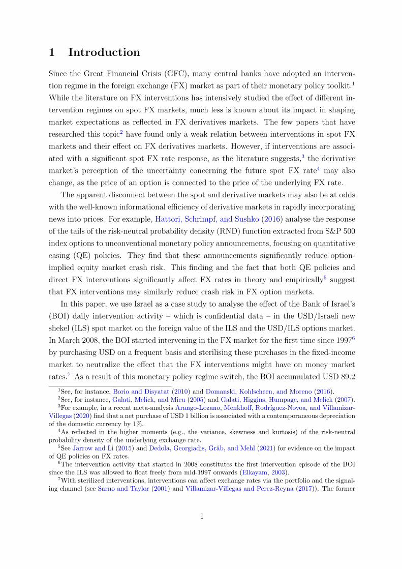
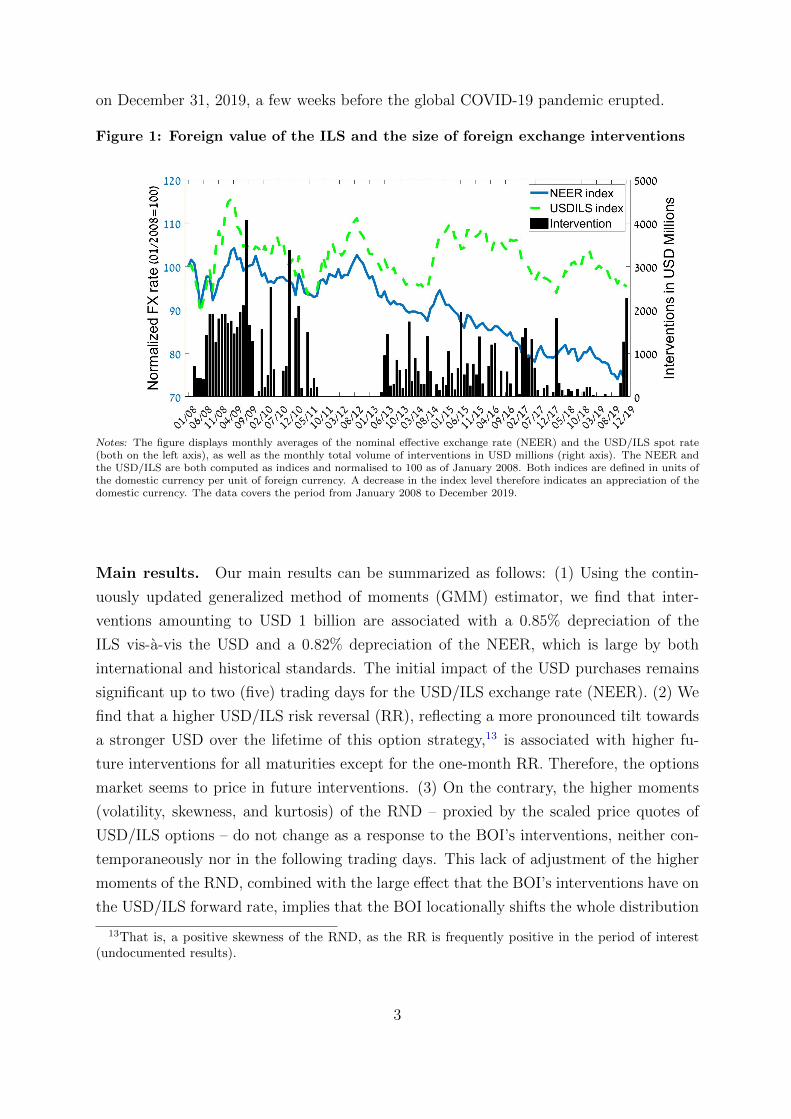
To motivate our paper, Figure 1 displays the monthly volume of FX interventions,

which is published on a monthly basis, the nominal effective exchange rate (NEER)9 of

the ILS and the USD/ILS exchange rate from January 2008 to December 2019.10 The

figure shows a steep appreciation of the ILS by almost 30% from 2008 until the end of our

sample according to the NEER and a 10% appreciation vis-a-vis the USD.11 In tandem,

the bank intervened in the USD/ILS spot market, particularly during periods of strong

appreciation pressure. In the period displayed in Figure 1, however, the BOI changed its

intervention strategy several times. The BOI even stopped intervening in July 2011 for

the following two and a half years. For interested readers, we provide an overview of the

six different regimes since 2008 in online Appendix A.

In the present paper, we focus on the intervention regime that was in place from

January 2013 until January, 14 202112 and was characterized by secret and fully sterilized

USD purchases in the USD/ILS spot market. However, we opt to end our sample period

works through the effect of interventions on expected asset returns that may trigger adjustments in thecomposition of financial market participants’ investment portfolios (“portfolio re-balancing”). The lat-ter works through the information and intent that interventions reveal to financial market participantsabout future changes in the stance of monetary policy. Fanelli and Straub (2021) develop a theory of FXinterventions with FX forward guidance where the effect of these two channels is not disentangled.

8Dominguez (1986) already emphasized the role of expectations for the determination of FX rates inthe aftermath of the Bretton Woods era. The seminal work of Engel and West (2005) develops an assetpricing formula, where the spot FX rate is a function of current and expected future fundamentals, whichhighlights the prominent role of expectations in affecting spot FX rates.

9This index is measured as the geometric average of the ILS exchange rate vis-a-vis 24 currenciesrepresenting 31 countries, Israel’s major trading partners by proportion of trade (Friedman and Galo(2015) and https://www.boi.org.il/en/Markets/ExchangeRates/Pages/efectinf.aspx).

10Note that both exchange rates are displayed as an index for the ease of comparison.11Both exchange rates equal the price of one unit of foreign currency (or a basket of foreign currencies)

in units of the domestic currency: an increase indicates a depreciation of the domestic currency.12On January 14, 2021, the BOI changed its strategy by announcing the total amount of USD that

it planned to buy in 2021. The BOI was, however, silent about the timing of these USD purchases anddid not declare how much USD it planned to buy on any given day. See: https://www.boi.org.il/en/NewsAndPublications/PressReleases/Pages/14-1-21.aspx.

2

on December 31, 2019, a few weeks before the global COVID-19 pandemic erupted.

Figure 1: Foreign value of the ILS and the size of foreign exchange interventions

Notes: The figure displays monthly averages of the nominal effective exchange rate (NEER) and the USD/ILS spot rate(both on the left axis), as well as the monthly total volume of interventions in USD millions (right axis). The NEER andthe USD/ILS are both computed as indices and normalised to 100 as of January 2008. Both indices are defined in units ofthe domestic currency per unit of foreign currency. A decrease in the index level therefore indicates an appreciation of thedomestic currency. The data covers the period from January 2008 to December 2019.

Main results. Our main results can be summarized as follows: (1) Using the contin-

uously updated generalized method of moments (GMM) estimator, we find that inter-

ventions amounting to USD 1 billion are associated with a 0.85% depreciation of the

ILS vis-a-vis the USD and a 0.82% depreciation of the NEER, which is large by both

international and historical standards. The initial impact of the USD purchases remains

significant up to two (five) trading days for the USD/ILS exchange rate (NEER). (2) We

find that a higher USD/ILS risk reversal (RR), reflecting a more pronounced tilt towards

a stronger USD over the lifetime of this option strategy,13 is associated with higher fu-

ture interventions for all maturities except for the one-month RR. Therefore, the options

market seems to price in future interventions. (3) On the contrary, the higher moments

(volatility, skewness, and kurtosis) of the RND – proxied by the scaled price quotes of

USD/ILS options – do not change as a response to the BOI’s interventions, neither con-

temporaneously nor in the following trading days. This lack of adjustment of the higher

moments of the RND, combined with the large effect that the BOI’s interventions have on

the USD/ILS forward rate, implies that the BOI locationally shifts the whole distribution

13That is, a positive skewness of the RND, as the RR is frequently positive in the period of interest(undocumented results).

3

towards higher USD/ILS values without affecting the options market view on the higher-

order risks. Crash risk, for instance, is unaffected. The options market seems to price in

future interventions (see result (2)), while the price quotes are not adjusted when these

interventions are actually carried out. We interpret the adjustment behavior as evidence

that the BOI is successful in shaping market expectations in the intended direction. (4)

We also examine the effect that interventions have on the USD/ILS forward rates, the

first moment of the RND. We find that interventions increase the price of the USD/ILS

3-month forward rate by 0.72%, which is less than the effect on the two spot rates that

we consider. The lower effect implies that the intervention activity makes the deviations

from covered interest rate parity (CIP) – usually referred to as the cross-currency basis –

more negative. This finding is in line with the theoretical predictions of Amador, Bianchi,

Bocola, and Perri (2020), who propose a framework to study the problem of a central

bank that pursues an exchange rate policy (e.g., to stimulate labor demand) that leads

to a violation of interest parity when the zero lower bound binds.

Price discovery in option markets. The question naturally arises as to why the

information of an upcoming intervention is priced in the options market but not in the

spot market,14 as both markets are connected by put-call parity, unless there are arbi-

trage opportunities to exploit.15 Two potential answers come to mind: (1) limits to

arbitrage. Papers such as Duffie (2010), Gromb and Vayanos (2010) and Du, Tepper,

and Verdelhan (2018) show that balance-sheet constraints may prevent arbitrageurs (e.g.

banks) from eliminating arbitrage opportunities. In the case of FX markets, Menkhoff,

Sarno, Schmeling, and Schrimpf (2012) argue that limits to arbitrage help explain the

profitability of momentum strategies. The argument for constrained arbitrageurs seems

particularly relevant in our case, as we find that a one standard deviation increase in

the daily change of the RR for all the maturities that we examine is associated with an

increase of the expected size of interventions amounting to only USD 4 million (USD).

Assuming a USD 1 billion intervention, which is associated with a 0.85% appreciation

of the USD/ILS spot rate according to our empirical results, implies that the options

market is anticipating a mere mUSD 4 × 0.85% = 0.0034% depreciation, which is less

than 1% of the standard deviation of the daily USD/ILS returns. Therefore, the costs for

arbitrageurs may potentially outweigh their expected profits. (2) Derivative’s market

sophistication. Market participants in the derivatives market may be more sophisti-

14The fact that the USD/ILS options market does not significantly adjust its prices when interventionsare carried out, while the USD/ILS spot rate significantly changes suggests that the impact of futureintervention episodes on the future spot exchange rate is priced in the former case.

15See, for instance, Cox and Hobson (2005) and Heston, Loewenstein, and Willard (2007) who demon-strate that this parity breaks down when the martingale property is lost for a financial security.

4

cated than in the spot market. Empirically, price discovery analyses indeed suggest that

FX derivative markets lead spot FX markets in pricing in news, see Tse, Xiang, and Fung

(2006) and Rosenberg and Traub (2009).

Related literature and our contributions. We contribute to the strand of literature

on FX interventions in at least three dimensions. First, there are only few studies that

analyze how FX interventions affect market expectations about the future foreign value of

a currency and its risk characteristics as reflected in the options market (i.e. captured by

the option-implied volatility (IV), skewness, and kurtosis of the RND).16 The results of

these papers are rather mixed; they usually do not find a statistically significant relation

between interventions and the price quotes of these option contracts (or the higher-order

risk-neutral moments extracted from these options). Contrary to these papers, however,

we do not limit ourselves to analyzing options with a specific maturity, but explore options

with maturities ranging from one to twelve months. This part of our empirical analysis is

relevant for monetary policymakers, as they can learn about the persistence of the effect

that spot FX market interventions have on FX options.

The second strand of literature that we contribute to is the literature that estimates

the effect that FX interventions have on the spot FX market.17 In a recent contribution,

Adler et al. (2019), analyzing a panel of 52 countries (13 developed (including Israel)

and 39 emerging market countries) from 1996 to 2013, find that purchases of foreign

currency amounting to 1% of GDP cause a depreciation of the nominal exchange rate

in the range of 1.7% to 2.0%. A recent meta-analysis by Arango-Lozano et al. (2020)

covers 74 empirical studies that have analyzed FX interventions in 19 countries across

five decades, including both emerging and industrialized countries. They find that a net

purchase of USD 1 billion is associated with a depreciation of the domestic currency by 1%.

The authors emphasize, however, that they find evidence of a weak positive publication

bias. Their estimate is therefore modestly upward biased. How do these findings compare

with our results? Our estimated coefficient, re-scaled such that it reflects a volume of

USD purchases amounting to 1 percent of Israeli GDP, is approximately equal to 2.7%

(NEER: 2.6%).18 The BOI’s impact is consequently larger than the upper bound of other

relevant studies. A shortcoming of this strand of literature is the fact that most of the

16See, for instance, Castren (2004), Fratzscher (2005), Galati et al. (2005), Galati et al. (2007), Disyatatand Galati (2007), Morel and Teıletche (2008), Marins, Araujo, and Vicente (2017).

17See, for instance, Sarno and Taylor (2001), Neely (2005), Fratzscher (2005), Egert and Komarek(2006), Disyatat and Galati (2007), Fatum (2015), Ribon (2017), Caspi et al. (2018), Adler, Lisack, andMano (2019), Nedeljkovic and Saborowski (2019)) and Arango-Lozano et al. (2020).

18To get the volume of USD purchases amounting to 1% of domestic GDP, we calculate the averageof the annual nominal GDP of Israel in the period 2013-2019 (denominated in USD) and multiply thisaverage by 1%. We divide the resulting 1% of GDP estimate by USD 1 billion. The resulting factor of3.2 is multiplied by our estimated coefficients.

5

existing contributions cover the years before the GFC. Given the historically exceptional

period of sustained low interest rates in the aftermath of the GFC and the changes that

the FX market has undergone in the last decade in response to technological innovations

and the endorsement of a set of voluntary standards within the “Global Code of Conduct”

regulatory framework,19 it is important to have more recent empirical analyses on this

topic, as the results documented in older studies may no longer be representative for how

interventions affect spot FX markets.

The third strand of literature that we contribute to is the recently revived literature

attempting to explain deviations from CIP (i.e., a non-zero cross-currency basis).20 It can

be shown that these CIP deviations are a direct proxy for the costs of FX interventions

(Amador et al., 2020). To the best of our knowledge, our paper is the first to empirically

quantify the effect that FX interventions have on the cross-currency basis. We find that

FX interventions widen this metric, as predicted by the Amador et al. (2020) model.21

Note that previous academic contributions have erroneously used deviations from uncov-

ered interest parity to proxy for the costs of FX interventions instead (Amador et al.,

2020), which reinforces our view that our work is the first academic contribution that

directly links FX interventions to the dynamics of the cross-currency basis.

This paper is structured as follows. In Section 2 we describe our methodology, our

estimation strategy and the data that we use. Section 3 presents and discusses our main

results, while Section 4 presents our conclusions.

2 Methodology, estimation strategy and data

2.1 Generalized Method of Moments

To assess the impact that the BOI’s FX interventions have on the foreign value of the

ILS and on the USD/ILS options market, we first run simple OLS regressions. We ignore

potential endogeneity biases for now caused, for instance, by the hard to disentangle simul-

taneity of FX interventions and spot FX rate movements that trigger these interventions

(hint: “leaning against the wind”).22 Notice, however, that using daily data significantly

19See, for example, McGeever (2017) and Szalay (2020) for details about the global FX rigging scandalthat initiated the reforms that have led to the creation of voluntary standards.

20See Du et al. (2018), Avdjiev, Du, Koch, and Shin (2019) and Du and Schreger (2021), among others.21In their empirical exercise, Amador et al. (2020) assess the relationship between deviations from CIP

and monthly foreign reserves as a proxy for the actual size of interventions. Foreign reserves, however, areonly a crude proxy for the latter (Neely, 2000), especially if used on a monthly basis, where macroeconomicfactors and news affect the domestic value and the size of these reserves, which may bias their empiricalresults.

22See Section 2 in Neely (2005), subsection 3.2 in Fratzscher (2005) and Section 3 in Tashu (2014) fordetails.

6

reduces the risk that reverse causality and confounding factors may bias our estimated

coefficients (Menkhoff, Rieth, and Stohr, 2021). In addition, this exercise allows us to get

a feeling about how sizable these biases are.

In a second step, we run GMM regressions – allowing us to control for endogeneity23

– and include additional controls to shield against omitted variables bias. The GMM

procedure has four additional advantages. First, this procedure requires no distributional

assumptions. Second, many econometric models can be estimated with this procedure, as

they often are simply special cases of the GMM procedure (Cochrane, 2005). Third and

fourth, the GMM procedure is also general in the sense that it allows for heteroskedasticity

of unknown form and that it can be used when serial correlation cannot be precluded ex

ante. In this case, the effect on the estimated standard errors can be accounted for by

using a heteroskedasticity and autocorrelation (HAC) consistent covariance matrix.

Expressing the model of interest as:24

E [f(wt, zt, θ)] = 0, (1)

where f represents a vector of R population moment conditions, wt denotes a vector of ob-

servable (endogenous or exogenous) variables, zt is a vector of predetermined instruments

and θ a vector containing the K unknown parameters that we are interested in.

Replace the expectation in Equation (1) with its sample counterpart to get an expres-

sion that allows us to estimate the entries of the parameter vector θ:

gT (θ) ≡ 1

T

T∑t=1

f(wt, zt, θ), (2)

with T and gT (·) equal to the number of periods and the sample means of the deviation

of the R sample moment conditions from their population counterparts, respectively.

When we have less sample moment conditions than unknown parameters (i.e. R < K),

the parameter vector θ is unidentified. When the number of sample moment conditions

equals the number of unknown parameters (i.e. R = K), we have a system of R = K

moment conditions with K unknowns. Hence, the parameter vector θ can be exactly

identified by simply setting the R = K elements in Equation (2) equal to zero. Finally,

when the number of moment conditions exceeds the number of parameters (i.e. R > K),

the GMM estimator θGMM is chosen such that it minimizes a quadratic form of gT (θGMM)

23The empirical literature mainly uses either GMM regressions or instrumental variable-panel ap-proaches to shield against potential biases due to simultaneity (see e.g. Adler and Tovar (2011) andAdler et al. (2019)).

24The following exposition follows Chapter 11 in Cochrane (2005) and Chapters 1 and 3 in Hall (2005).

7

in combination with a symmetric, positive definite weighting matrix WT :

argminθGMM

QT (θGMM) = argminθGMM

gT (θGMM)′WTgT (θGMM). (3)

It can be shown that the asymptotically efficient GMM estimator of this quadratic form

is asymptotically normally distributed:

√T(θGMM − θ

)a−→ N (0, V ), (4)

with V representing the asymptotic covariance matrix.

Continuously updated GMM estimator. Notice that the estimated parameters de-

pend on the weighting matrix WT . Hansen, Heaton, and Yaron (1996) have proposed a

GMM estimator that in small samples often exhibits better properties compared to the

two-step (or iterated) GMM estimator. The proposed estimator is known as the contin-

uously updated GMM estimator (CU-GMM), as it uses a covariance matrix WT that is

updated in each step of the GMM algorithm until it converges. To assess the robustness

of our results, we use this GMM estimator in the empirical section in addition to simple

OLS regressions.

2.2 Data

2.2.1 Foreign exchange interventions data

Table 1 includes selected descriptive statistics of the monthly average of the FXI data from

the BOI for the period from January 2013 to December 2019 analyzed in the empirical

section. The descriptive statistics indicate that, on average, the BOI purchased mUSD 594

per month, with a minimum of mUSD 2 and a maximum of USD 2.27 billion. The monthly

intervention volumes are relatively volatile, as reflected in the standard deviation. In total,

we have 69 out of 84 months with at least one trading day, where the BOI intervened

in the USD/ILS spot market. The table also suggests that the distribution of the FXI

data might be right-skewed, as the mean is larger than the median. In other words, the

distribution seems to exhibit a long tail in the positive direction of the number line. In

essence, there are a few observations that are large compared to all other FX intervention

data, which is confirmed in an untabulated histogram of the monthly FX intervention

data.

To give a better sense of the magnitude of FX interventions relative to some other

metrics and in terms of calendar time, Table 2 includes information about the average

size of FX interventions relative to Israeli GDP and the daily USD/ILS spot market

8

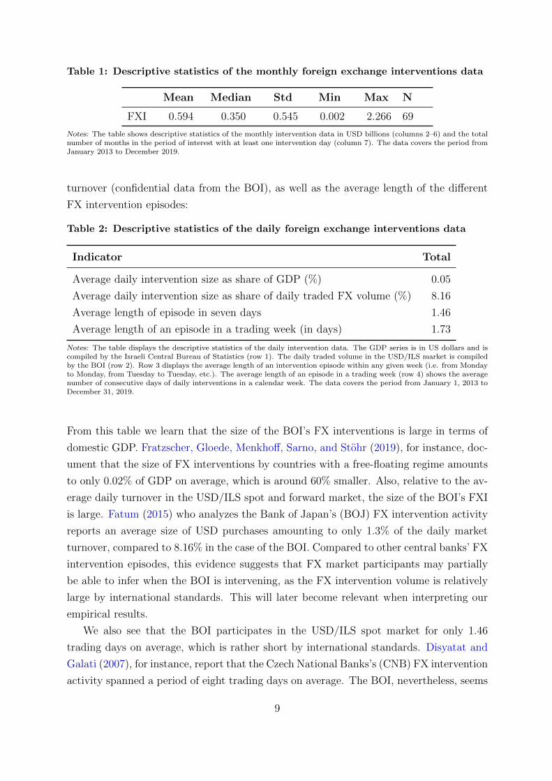
Table 1: Descriptive statistics of the monthly foreign exchange interventions data

Mean Median Std Min Max N

FXI 0.594 0.350 0.545 0.002 2.266 69

Notes: The table shows descriptive statistics of the monthly intervention data in USD billions (columns 2–6) and the totalnumber of months in the period of interest with at least one intervention day (column 7). The data covers the period fromJanuary 2013 to December 2019.

turnover (confidential data from the BOI), as well as the average length of the different

FX intervention episodes:

Table 2: Descriptive statistics of the daily foreign exchange interventions data

Indicator Total

Average daily intervention size as share of GDP (%) 0.05

Average daily intervention size as share of daily traded FX volume (%) 8.16

Average length of episode in seven days 1.46

Average length of an episode in a trading week (in days) 1.73

Notes: The table displays the descriptive statistics of the daily intervention data. The GDP series is in US dollars and iscompiled by the Israeli Central Bureau of Statistics (row 1). The daily traded volume in the USD/ILS market is compiledby the BOI (row 2). Row 3 displays the average length of an intervention episode within any given week (i.e. from Mondayto Monday, from Tuesday to Tuesday, etc.). The average length of an episode in a trading week (row 4) shows the averagenumber of consecutive days of daily interventions in a calendar week. The data covers the period from January 1, 2013 toDecember 31, 2019.

From this table we learn that the size of the BOI’s FX interventions is large in terms of

domestic GDP. Fratzscher, Gloede, Menkhoff, Sarno, and Stohr (2019), for instance, doc-

ument that the size of FX interventions by countries with a free-floating regime amounts

to only 0.02% of GDP on average, which is around 60% smaller. Also, relative to the av-

erage daily turnover in the USD/ILS spot and forward market, the size of the BOI’s FXI

is large. Fatum (2015) who analyzes the Bank of Japan’s (BOJ) FX intervention activity

reports an average size of USD purchases amounting to only 1.3% of the daily market

turnover, compared to 8.16% in the case of the BOI. Compared to other central banks’ FX

intervention episodes, this evidence suggests that FX market participants may partially

be able to infer when the BOI is intervening, as the FX intervention volume is relatively

large by international standards. This will later become relevant when interpreting our

empirical results.

We also see that the BOI participates in the USD/ILS spot market for only 1.46

trading days on average, which is rather short by international standards. Disyatat and

Galati (2007), for instance, report that the Czech National Banks’s (CNB) FX intervention

activity spanned a period of eight trading days on average. The BOI, nevertheless, seems

9

to intervene on more than one trading day in a given trading week (for instance, at

the beginning and at the end of a trading week). As explained in Miyajima (2013),

FX interventions which are also aimed at affecting market expectations should combine

intervention episodes with days of no activity to allow FX derivatives market participants

to evaluate the effect of these interventions over longer horizons – the BOI apparently

follows this advice.

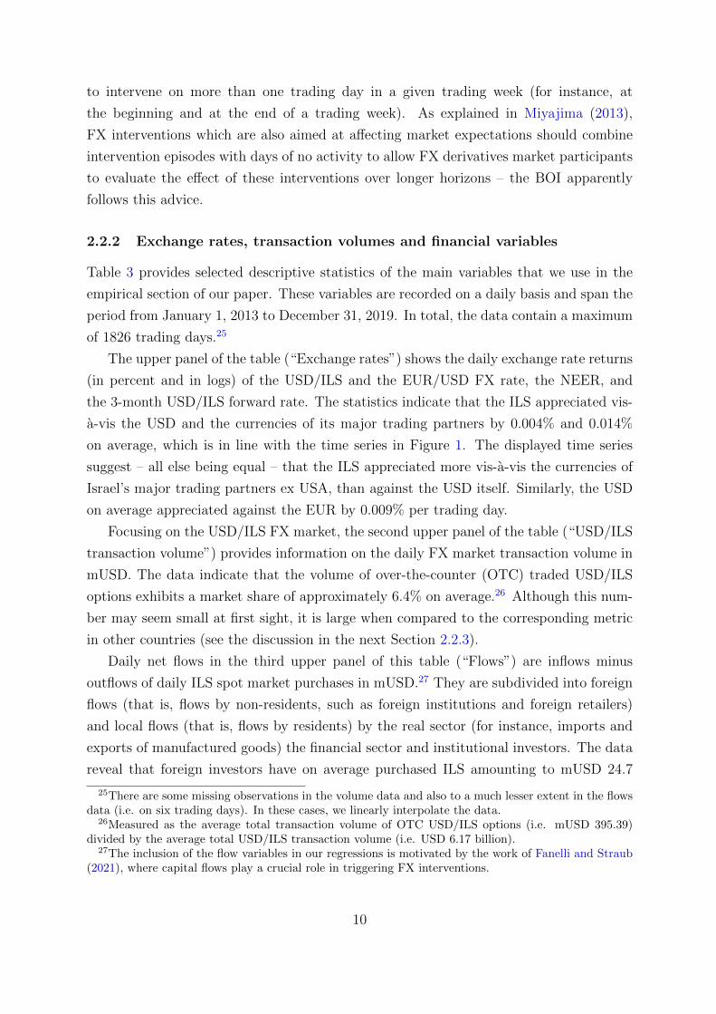
2.2.2 Exchange rates, transaction volumes and financial variables

Table 3 provides selected descriptive statistics of the main variables that we use in the

empirical section of our paper. These variables are recorded on a daily basis and span the

period from January 1, 2013 to December 31, 2019. In total, the data contain a maximum

of 1826 trading days.25

The upper panel of the table (“Exchange rates”) shows the daily exchange rate returns

(in percent and in logs) of the USD/ILS and the EUR/USD FX rate, the NEER, and

the 3-month USD/ILS forward rate. The statistics indicate that the ILS appreciated vis-

a-vis the USD and the currencies of its major trading partners by 0.004% and 0.014%

on average, which is in line with the time series in Figure 1. The displayed time series

suggest – all else being equal – that the ILS appreciated more vis-a-vis the currencies of

Israel’s major trading partners ex USA, than against the USD itself. Similarly, the USD

on average appreciated against the EUR by 0.009% per trading day.

Focusing on the USD/ILS FX market, the second upper panel of the table (“USD/ILS

transaction volume”) provides information on the daily FX market transaction volume in

mUSD. The data indicate that the volume of over-the-counter (OTC) traded USD/ILS

options exhibits a market share of approximately 6.4% on average.26 Although this num-

ber may seem small at first sight, it is large when compared to the corresponding metric

in other countries (see the discussion in the next Section 2.2.3).

Daily net flows in the third upper panel of this table (“Flows”) are inflows minus

outflows of daily ILS spot market purchases in mUSD.27 They are subdivided into foreign

flows (that is, flows by non-residents, such as foreign institutions and foreign retailers)

and local flows (that is, flows by residents) by the real sector (for instance, imports and

exports of manufactured goods) the financial sector and institutional investors. The data

reveal that foreign investors have on average purchased ILS amounting to mUSD 24.7

25There are some missing observations in the volume data and also to a much lesser extent in the flowsdata (i.e. on six trading days). In these cases, we linearly interpolate the data.

26Measured as the average total transaction volume of OTC USD/ILS options (i.e. mUSD 395.39)divided by the average total USD/ILS transaction volume (i.e. USD 6.17 billion).

27The inclusion of the flow variables in our regressions is motivated by the work of Fanelli and Straub(2021), where capital flows play a crucial role in triggering FX interventions.

10

per day. On a net basis, mUSD 18.7 ILS have been purchased by residents, mainly by

residents from the real sector. This sector has therefore been responsible for the major

increase in Israel’s current account balance in the period under review.

Table 3: Descriptive statistics of the main variables

Mean Median Std Min Max AR(1) N

Exchange rates (in logs and in %):

∆USD/ILS =0.004 0.00 0.38 =2.32 2.41 =0.01 1826

∆EUR/USD =0.009 0.01 0.47 =2.30 2.95 0.01 1826

∆NEER =0.014 =0.02 0.32 =2.02 2.34 0.02 1826

∆Forward 3m =0.005 =0.02 0.37 =2.29 1.59 0.05 1826

USD/ILS transaction volume (in mUSD):

Spot and forward 1660.34 1643.89 875.37 0.04 6399.10 0.10 1769

Swap 4109.50 4118.74 1853.63 0.00 11623.51 0.18 1749

OTC options 395.39 277.84 419.14 0.00 5354.98 0.23 1744

Net flows (in mUSD):

Foreign flows – total =24.74 =14.51 157.26 =646.42 736.51 0.36 1820

Local flows – real sector 17.13 10.97 113.66 =552.53 547.44 0.26 1820

Local flows – financial sector 5.60 4.79 80.30 =691.88 578.90 0.03 1820

Local flows – inst. investors =4.06 0.00 86.26 =563.37 734.31 0.23 1820

Misc (in %):

5-year Israeli CDS 0.80 0.74 0.20 0.48 1.52 0.9952 1826

TELBOR 0.38 0.10 0.47 0.10 1.75 0.9995 1826

USD LIBOR 0.82 0.41 0.82 0.08 2.40 0.9997 1826

VIX 14.86 13.89 3.81 9.14 40.74 0.9281 1763

Notes: The table presents descriptive statistics of the main variables. The data is recorded on a daily basis and spans theperiod from January 1, 2013 to December 31, 2019. There are a maximum of 1826 trading days. The FX rates are expressedin log changes and in percent. Both FX rates (USD/ILS and EUR/USD), the 5-year Israeli CDS spread and the one-monthUSD LIBOR are retrieved from Bloomberg. The NEER series is constructed such that it is synchronized with the USD/ILStrading time (see online Appendix B for more information). Forward 3m is the three-month USD/ILS forward rate retrievedfrom Bloomberg. The daily transaction volume in the USD/ILS spot, forward, swap and OTC options market are compiledby the BOI and denominated in millions of USD (“mUSD”). Daily net flows are computed as inflows minus outflows of USDin exchange for ILS in mUSD. The flows are sub-divided into foreign flows, which are net flows by non-residents (foreigninstitutions, retailers, etc.) and local net flows by the real sector (i.e. importers and exporters), the financial sector andinstitutional investors. TELBOR is the one-month Israeli interbank rate published by the BOI. We linearly interpolatemissing TELBOR rates (due to Israeli holidays). VIX measures the implied volatility from S&P 500 index options at USclosing time and is provided by the CBOE. It has less trading days than the other variables due to US holidays.

The table also displays descriptive statistics in the lower panel (“Misc”) for the 5-year

Israeli CDS spread. On average, the CDS spread equaled 80 basis points (bps) in the

period of interest, which is low by international standards and in line with Israel’s high

(investment grade) credit rating.28 The table also shows that the one-month USD LIBOR

has been larger on average than the one-month TELBOR (0.82% vs. 0.38%). Hence, by

CIP, the USD should depreciate vis-a-vis the ILS on average, thereby putting appreciation

28Israel’s credit rating was last set at A1 by Moody’s with a stable outlook on April 24, 2020 (as ofthe date of writing the paper). This credit rating has remained unchanged since May 6, 2006.

11

pressure on the ILS. The last row displays the descriptive statistics for the VIX as a proxy

measure of global uncertainty.

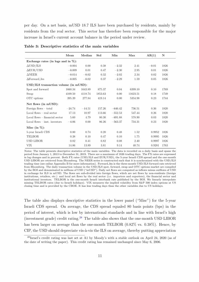
2.2.3 The USD/ILS options market

In this subsection, we concentrate on the USD/ILS options data that we use in the empir-

ical section. The data is retrieved from Bloomberg. Table 4 displays selected descriptive

statistics of the main USD/ILS option trading strategies. The data is recorded on a

daily basis and spans the period from January 1, 2013, to December 31, 2019. The data

include 10-∆ and 25-∆29 RRs (upper panel), 10-∆ and 25-∆ butterfly (BF) spreads30

(middle panel) and at-the-money implied volatilities (ATMV)31 (lower panel) for six ma-

turities, ranging from one week (“1w”) to twelve months (“12m”).32 The price quotes are

measured in implied volatilities and displayed in percent, following the options markets’

quoting convention.33

Notice that the price quotes of these option strategies are highly persistent (column

“AR(1)”). Therefore, we use them in first differences throughout our analysis. Untabu-

lated results show that the first difference eliminates the high persistence in these price

quotes. We also note that only the price quotes of the one-week BF spreads for both

option deltas exhibit lower persistence compared to the other price quotes. This is also

true, but to a much lesser extent, for the one-week RRs (also for both option deltas) and

the one-week ATMV.34 The lower persistence of these five price quotes might indicate

stale prices and a lack of liquidity, which brings us to our next topic.

As we use options data extensively in our paper, we assess how liquid the Israeli FX

option market is by international standards. To this end, we look at the most recent data

from the BIS triennial central bank survey that covers 54 countries and includes collected

data from close to 1300 banks and other dealers on FX turnover, amongst others. The

29For instance, a 10-∆ call (put) corresponds to a Garman and Kohlhagen (1983) option delta of 0.1(-0.1), as FX options are quoted in terms of the GK model by market convention.

30See online Appendix C for details on risk reversals and butterfly spreads.31The ATMV isn’t an option strategy, but we call it a strategy to be consistent with the RRs and the

BF spreads.32Online Appendix D displays the coefficients of the cross-correlation between the log returns of these

three option strategies (Tables C.2, C.3 and C.4). The cross-correlations indicate that the three strategiesare highly correlated with each other, and even more so for strategies with the same option delta. Wealso include in these three tables the correlation between the log returns of these option strategies andthe daily change of the USD/ILS exchange rate. The results show that the former is positively correlatedwith the RRs, reflecting a kind of momentum. This contemporaneous relationship between RRs and spotFX rates was first documented in McCauley and Melick (1996), Malz (1997) and Campa, Chang, andReider (1998) and implies that investors assign a more pronounced (risk-neutral) tilt towards a furtherdepreciation of the ILS vis-a-vis the USD (i.e. a higher RR), when the ILS has already weakened (i.e. ahigher USD/ILS exchange rate).

33For details, see Reiswich and Wystup (2010).34That is, the price quotes of the USD/ILS option strategies with the shortest maturities.

12

Table 4: Descriptive statistics of three USD/ILS option strategies

Mean Median Std Min Max AR(1) N

Risk reversals:10-∆:RR101w 0.658 0.60 0.43 -0.42 2.77 0.95 1826RR101m 1.088 0.93 0.67 -0.12 3.33 0.99 1826RR103m 1.438 1.14 0.87 -0.05 3.58 0.997 1826RR106m 1.649 1.31 0.98 0.00 3.76 0.998 1826RR109m 1.750 1.41 1.05 0.16 4.12 0.998 1826RR1012m 1.950 1.67 1.09 0.26 4.30 0.998 182625-∆RR251w 0.396 0.37 0.26 -0.12 1.49 0.976 1826RR251m 0.597 0.5 0.37 -0.07 1.83 0.994 1826RR253m 0.782 0.61 0.47 -0.02 1.92 0.998 1826RR256m 0.892 0.70 0.53 0.01 1.99 0.998 1826RR259m 0.949 0.78 0.57 0.10 2.13 0.999 1826RR2512m 1.045 0.88 0.58 0.18 2.24 0.999 1826

Butterfly spreads:10-∆:BF101w 0.794 0.90 0.44 -1.67 1.92 0.429 1826BF101m 0.738 0.73 0.12 0.46 1.12 0.918 1826BF103m 1.008 0.98 0.21 0.59 1.45 0.976 1826BF106m 1.186 1.14 0.25 0.65 1.73 0.982 1826BF109m 1.269 1.19 0.29 0.69 1.92 0.983 1826BF1012m 1.452 1.41 0.32 0.78 2.20 0.985 182625-∆:BF251w 0.136 0.20 0.30 -2.45 1.20 -0.052 1826BF251m 0.236 0.23 0.04 0.14 0.37 0.945 1826BF253m 0.327 0.31 0.07 0.19 0.50 0.984 1826BF256m 0.384 0.37 0.08 0.21 0.59 0.986 1826BF259m 0.419 0.39 0.10 0.22 0.63 0.990 1826BF2512m 0.474 0.46 0.11 0.25 0.71 0.990 1826

At-the-money implied volatilities:ATMV1w 6.63 6.35 1.49 3.54 11.43 0.947 1826ATMV1m 6.56 6.35 1.29 3.96 10.33 0.994 1826ATMV3m 6.64 6.47 1.14 4.29 9.72 0.997 1826ATMV6m 6.73 6.54 1.05 4.76 9.41 0.998 1826ATMV9m 6.81 6.61 1.00 5.07 9.21 0.999 1826ATMV12m 6.86 6.67 0.96 5.18 9.05 0.999 1826

Notes: The table displays descriptive statistics for the daily USD/ILS option strategies quoted in implied volatilities andin percent (except columns “AR(1)” and “N”) for the period from January 1, 2013 to December 31, 2019, a total of 1826trading days. The data includes 10-delta and 25-delta risk reversals (“RR10” and “RR25”), 10-delta and 25-delta butterflyspreads (“BF10” and “BF25”) and at-the-money implied volatilities (“ATMV”). In each case the data is available for sixdifferent maturities, ranging from one week (“1w”) to twelve months (“12m”). Data source: Bloomberg.

survey begins in April 2007.35 Our calculations (see Table E.1 in online Appendix E) reveal

that the ratio of OTC-traded FX option volume to the total FX transaction volume36 in

Israel equaled 6.2% in 2019, which is large by international standards. Indeed, Israel is

35Source: https://www.bis.org/statistics/rpfx19.htm.36Including transactions in the FX spot, FX forward, FX option and FX swap market.

13

consistently ranked in the top five of all surveyed countries in terms of the ratio of total FX

options transaction volume to total FX transaction volume since April 2007 (untabulated

results).

The results in Tables E.2-E.4 in online Appendix E add further support to our ar-

gument. The figures show the box plots of the bid-ask spreads (BAS) divided by the

mid-quote of the three USD/ILS option strategies that we use in our paper for 28 cur-

rency pairs across six maturities.37 We note two things: (1) The relative BAS is generally

higher for the one-week contracts. We will therefore omit these contracts in our analysis.

(2) The results show that the relative BAS for the three option strategies are consistently

ranked in the interquartile range, which makes us confident that our option market data is

not significantly affected by low liquidity. This finding indicates that valuable information

can be extracted from the price quotes of USD/ILS options.

3 Results

As described in Section 1, the empirical evidence to date indicates that FX interventions

significantly affect the targeted FX spot rate in the desired direction. We hypothesize that

FX interventions may also affect the market’s perception of the uncertainty associated

with the future FX spot rate, as reflected in the FX options market. Before we assess to

what extent FX interventions in the USD/ILS spot market affect price quotes (and the

herewith associated option-implied higher moments of the extracted RND) in the options

market, we first confirm that FX interventions indeed depreciate the the foreign value of

the ILS in the period under review.

3.1 Effect of interventions on the foreign value of the ILS

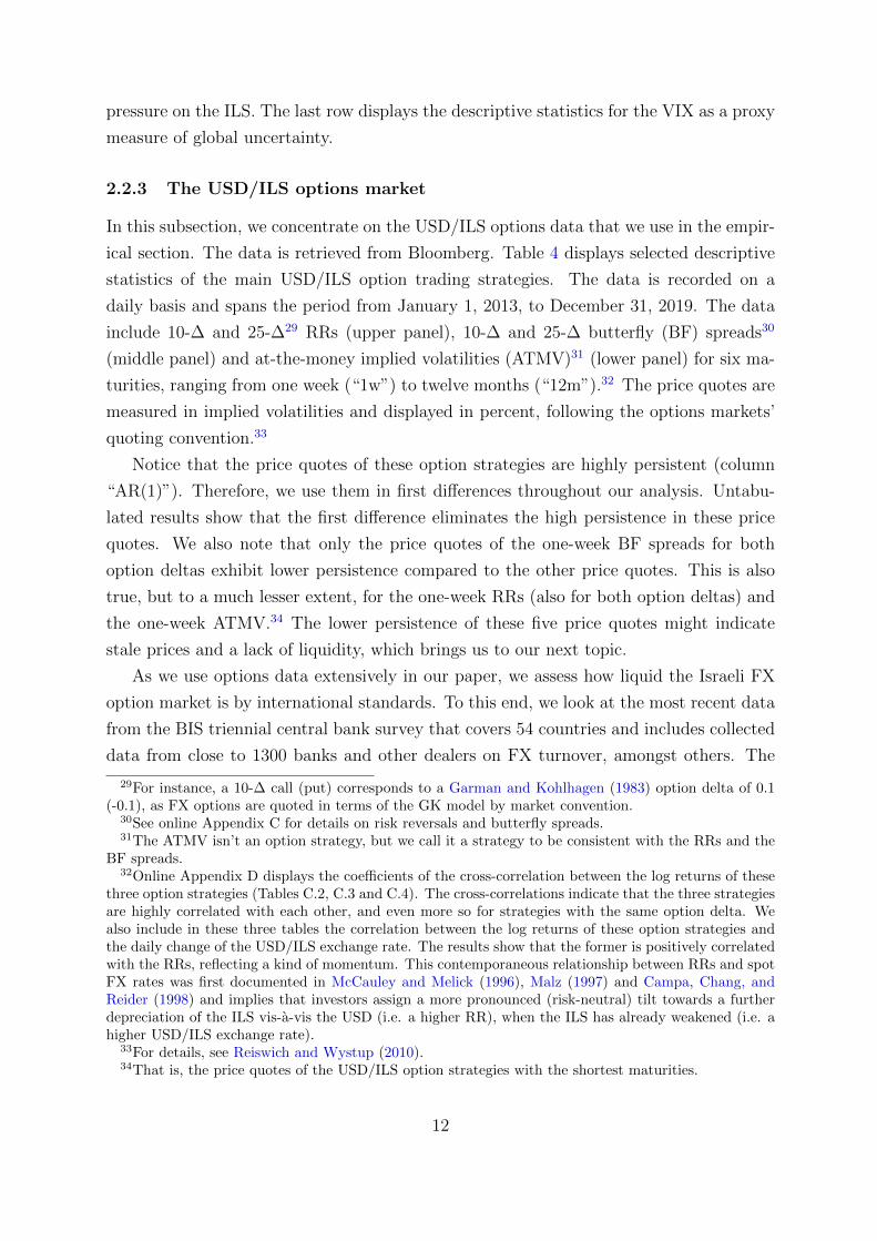
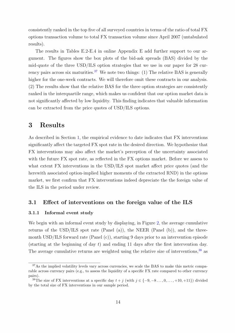
3.1.1 Informal event study

We begin with an informal event study by displaying, in Figure 2, the average cumulative

returns of the USD/ILS spot rate (Panel (a)), the NEER (Panel (b)), and the three-

month USD/ILS forward rate (Panel (c)), starting 9 days prior to an intervention episode

(starting at the beginning of day t) and ending 11 days after the first intervention day.

The average cumulative returns are weighted using the relative size of interventions,38 as

37As the implied volatility levels vary across currencies, we scale the BAS to make this metric compa-rable across currency pairs (e.g., to assess the liquidity of a specific FX rate compared to other currencypairs).

38The size of FX interventions at a specific day t + j (with j ∈ {−9,−8 . . . , 0, . . . ,+10,+11}) dividedby the total size of FX interventions in our sample period.

14

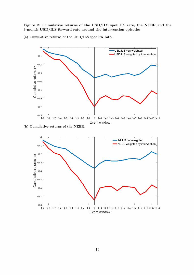
Figure 2: Cumulative returns of the USD/ILS spot FX rate, the NEER and the3-month USD/ILS forward rate around the intervention episodes

(a) Cumulative returns of the USD/ILS spot FX rate.

(b) Cumulative returns of the NEER.

15

(c) Cumulative returns of the 3-month USD/ILS forward rate.

Notes: The figure shows the average cumulative returns of the USD/ILS exchange rate and the NEER (both in percent),and the three-month USD/ILS forward at time t− 9 to t+ 11 on a daily basis, where t reflects the beginning of the tradingday when the first intervention was carried out. The red line displays the cumulative returns weighted by the relative sizeof interventions, while the blue line shows this metric using equal weights for each intervention episode.

we have learned from Table 1 (and the herewith associated following discussion) that

the distribution of FX interventions is right-skewed. For ease of comparison, we also

display the cumulative returns assigning equal weights to each FX intervention episode,

irrespective of the actual size of USD purchases. Equally weighting the FX intervention

episodes tilts the results in favour of those episodes where the size of FX interventions

was relatively small.39

We see that the BOI’s FX interventions contain the appreciation trend of the foreign

value of the ILS (both in the FX spot and the FX forward market) and create a de-

preciation of the ILS by the end of the first FX intervention day. There is also a slight

continuation of this “trend reversal” on day t+1,40 which may reflect a second intervention

day in some cases. The figures also show that weighting the returns by the intervention

volumes results in more pronounced appreciation and depreciation trends prior to and

after day t, respectively. The result implies that the BOI seems to intervene more heav-

ily when there is a more pronounced (or steeper) appreciation trend prior to the first

intervention day t. All in all, these figures imply that the bank is successful in creating

a lasting depreciation in the USD/ILS FX market according to the success “event” and

39As a by-product, this also allows us to learn about the reaction function of the BOI.40That is, the ILS continues to depreciate on the first trading day after the first intervention day.

16

“direction” criterion in the FX intervention strand of literature.41 In the next sections,

we examine the effect of the BOI’s intervention activity more rigorously, while controlling

for the inherent endogeneity and other factors.

3.1.2 Econometric assessment of the contemporaneous effect

As previous research has shown, estimating the causal effect of FX interventions on the

FX spot rate using OLS results in downward-biased estimates. The bias arises because

of the endogeneity caused by the “stylized fact” that central banks typically intervene to

respond to adverse spot rate movements, thereby “leaning against the wind”.

First-stage regression. To circumvent the endogeneity, we follow the standard ap-

proach in the literature and adopt instruments in the GMM framework that are correlated

with the intervention data but not with the shocks that affect the FX rate on the days

when the BOI intervenes.42 Specifically, we use instruments that are commonly used in

the FX literature and are defined in online Appendix B. Our instruments include the one-

day lagged daily intervention volume, a dummy variable that equals one if there has been

an intervention in the previous calendar week, the one-day lagged three-month return of

the USD/ILS spot rate, the one-day lagged two-day return of the NEER, the three-day

lagged two-week return of the NEER, the one-day lagged one-month change in the 5-year

Israeli CDS spread, and the one-day lagged two-week change in the US VIX to proxy

for changes in global uncertainty. As controls, we use contemporaneous explanatory vari-

ables. Specifically, we use the one-day change of the EUR/USD spot rate, the one-week

change in the VIX and the one-week change of the one-month USD LIBOR. We chose

the lags of the instruments based on adjusted R2 criteria (i.e., selecting the specifications

with the highest R2).

The result of the first-stage regression are displayed in Table 5. We see that most

estimated coefficients have the expected sign, pointing to a “leaning against the wind”

intervention activity. Our results are in line with the results in Ribon (2017), although

her results are for monthly data.

Because we use all the instruments of this first-stage regression specification as in-

struments for our CU-GMM estimation, we also include the Kleibergen and Paap (2006)

Wald F-statistic. The test statistic significantly exceeds the Stock and Yogo (2005) critical

value. We can therefore reject the null hypothesis that the instruments have insufficient

explanatory power (that is, our instruments pass the weak identification test) – the test

41See Humpage (1999), Fatum and Hutchison (2003), Fratzscher (2005), Fatum and Hutchison (2006),Galati et al. (2007), Fatum (2008), Fratzscher (2008) and Fratzscher et al. (2019).

42One can also take a different approach to identifying the causal effect of interventions on the FX spotrate by using intra-day intervention data, see for example Caspi et al. (2018).

17

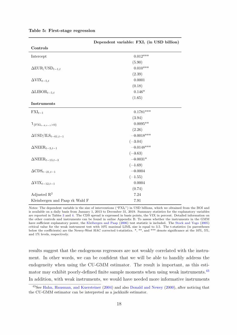
Table 5: First-stage regression

Dependent variable: FXIt (in USD billion)

Controls

Intercept 0.012***

(5.90)

∆EUR/USDt−1,t 0.010***

(2.39)

∆VIXt−5,t 0.0001

(0.18)

∆LIBORt−5,t 0.146*

(1.65)

Instruments

FXIt−1 0.1781***

(3.94)

1{FXIt−6,t−1>0} 0.0095**

(2.26)

∆USD/ILSt−61,t−1 =0.0018***

(=3.04)

∆NEERt−3,t−1 =0.0148***

(=3.63)

∆NEERt−13,t−3 =0.0031*

(=1.69)

∆CDSt−21,t−1 =0.0004

(=1.55)

∆VIXt−12,t−1 0.0004

(0.74)

Adjusted R2 7.24

Kleinbergen and Paap rk Wald F 7.91

Notes: The dependent variable is the size of interventions (“FXIt”) in USD billions, which we obtained from the BOI andis available on a daily basis from January 1, 2013 to December 31, 2019. Summary statistics for the explanatory variablesare reported in Tables 3 and 4. The CDS spread is expressed in basis points, the VIX in percent. Detailed information onthe other controls and instruments can be found in online Appendix B. To assess whether the instruments in the GMMhave sufficient explanatory power, the Kleibergen and Paap (2006) test statistic is included. The Stock and Yogo (2005)critical value for the weak instrument test with 10% maximal LIML size is equal to 3.5. The t-statistics (in parenthesesbelow the coefficients) are the Newey-West HAC corrected t-statistics. *, **, and *** denote significance at the 10%, 5%,and 1% levels, respectively.

results suggest that the endogenous regressors are not weakly correlated with the instru-

ment. In other words, we can be confident that we will be able to handily address the

endogeneity when using the CU-GMM estimator. The result is important, as this esti-

mator may exhibit poorly-defined finite sample moments when using weak instruments.43

In addition, with weak instruments, we would have needed more informative instruments

43See Hahn, Hausman, and Kuersteiner (2004) and also Donald and Newey (2000), after noticing thatthe CU-GMM estimator can be interpreted as a jackknife estimator.

18

or we would have been forced to use an estimator that is less susceptible to biases due to

endogeneity.

In Appendix A, we compare the estimated coefficients and the statistical significance

across several first-stage regression specifications.44 From that “sensitivity analysis” we

learn that the estimated coefficients are both qualitatively and quantitatively similar.

We therefore feel confident about our first-stage regression specification. The adjusted

coefficient of determination R2 is nevertheless lower than in previous studies that have

estimated comparable first-stage regressions.45 Note, however, that our purpose is not to

estimate the BOI’s actual reaction function. Our first-stage regression is just a means

to effectively control for the inherent endogeneity of FX interventions when running the

CU-GMM algorithm, thereby allowing us to get an unbiased estimate of the effect of FX

interventions on the FX spot rate. Consequently, the low R2 is a minor issue.

Contemporaneous effect. Table 6 displays the results of regressing the daily log return

(in percent) of the USD/ILS exchange rate (Panel A), the NEER (Panel B) and the three-

month USD/ILS forward rate46 (Panel C) on an intercept, the intervention variable (in

billions of USD), the daily log return of the EUR/USD spot rate (in percent), the one-week

change in the VIX (in percentage points) and the one-week change of the USD LIBOR

(in percentage points). Column 2 presents the results when running a standard OLS

regression, while column 3 displays the results when using the CU-GMM estimator. As a

robustness check, we also report the results of a two-stage least squares (2SLS) estimation

in the fourth column. The control variables and instruments are the same as in Table 5.

We see that the estimated coefficient associated with the intervention variable is highly

statistically significant in all regressions, even when ignoring the potential bias caused

by simultaneity and simply using standard OLS - consistent with the fact that using

daily intervention data reduces potential endogeneity concerns (Menkhoff et al., 2021).

Using the CU-GMM estimator, the estimated coefficients are statistically significant and

comparable in size for the two spot rates, equaling 0.85% for the USD/ILS rate (panel

A) and 0.82% for the NEER (panel B). The empirical finding is in line with the broad

appreciation trends of the ILS vis-a-vis the USD and vis-a-vis the exchange rates that

constitute the NEER, which is comparable in both cases, as evidenced in Figure 1.

44Also including additional instruments.45See Table 2 in Galati et al. (2005) who obtain an R2 of 0.1 and 0.09 for the case of the BOJ and

the Federal Reserve, respectively; Table 2 in Disyatat and Galati (2007) with an R2 of 0.18 for the CNB;Tables 6 and 9 in Galati et al. (2007) who report an R2 of 0.19 for the JPY sales activity of the BOJ.Ito and Yabu (2007) estimate a reaction function for the BOJ that even explains 30.9% of the variation,using an indicator of interventions instead of the actual size of interventions.

46The results for the USD/ILS forward contracts with other maturities are almost identical, so we omitthem for the sake of brevity.

19

Table 6: Contemporaneous exchange rate regressions

(a) Panel A

Dependent variable: ∆ ln(USDILSt) (in %)

[1]: OLS [2]: CU-GMM [3]: 2SLS

Intercept =0.0203*** =0.0273*** =0.0259***

(=2.57) (=2.16) (=2.11)

FXIt 0.55*** 0.85*** 0.84***

(4.75) (2.10) (2.04)

∆EUR/USDt−1,t =0.41*** =0.41*** =0.41***

(=23.51) (=21.69) (=21.43)

∆VIXt−5,t 0.01*** 0.01*** 0.01***

(4.31) (3.45) (3.50)

∆LIBORt−5,t 0.01 =0.01 =0.02

(0.02) (=0.03) (=0.07)

Hansen J-statistic 1.79

Hansen J-statistic p-value 0.94

(b) Panel B

Dependent variable: ∆ ln(NEERt) (in %)

[1]: OLS [2]: CU-GMM [3]: 2SLS

Intercept =0.0260*** =0.033*** =0.0310***

(=3.19) (=2.67) (=2.48)

FXIt 0.55*** 0.82** 0.77*

(4.43) (2.02) (1.88)

∆EUR/USDt−1,t 0.01 0.01 0.01

(0.74) (0.64) (0.53)

∆VIXt−5,t 0.01*** 0.005* 0.01***

(2.17) (1.69) (2.05)

∆LIBORt−5,t =0.04 =0.073 =0.07

(=0.12) (=0.14) (=0.13)

Hansen J-statistic 7.32

Hansen J-statistic p-value 0.29

20

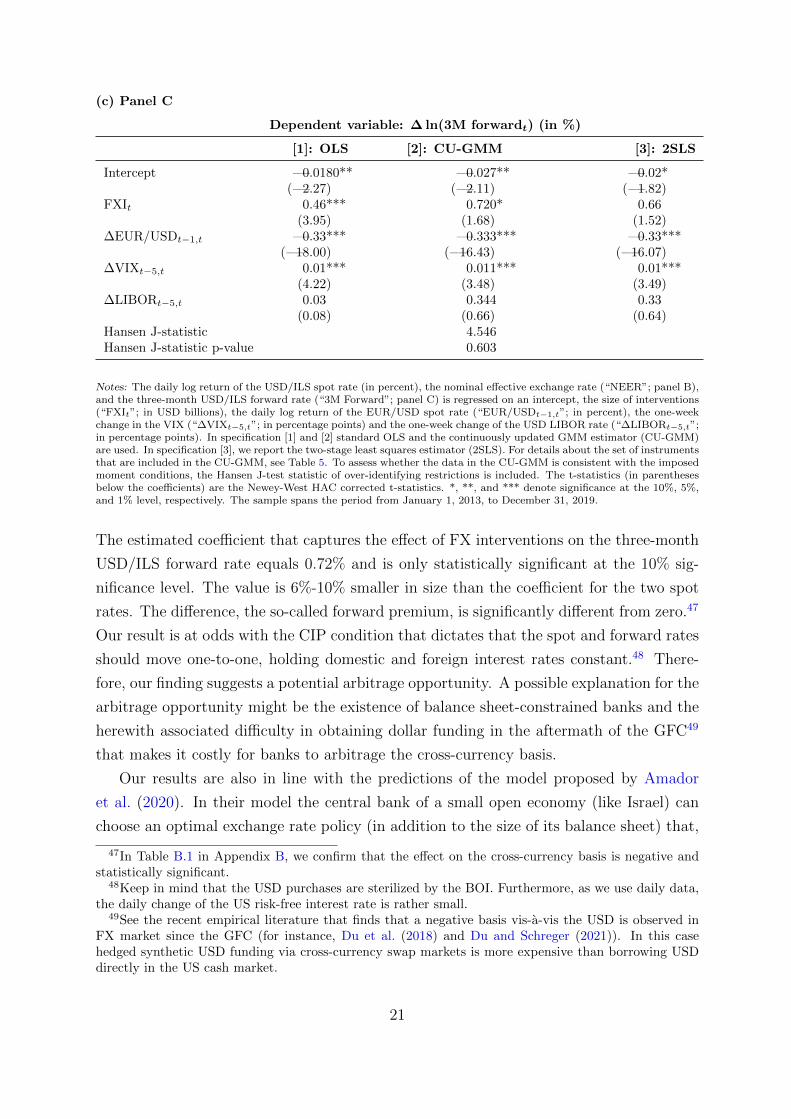
(c) Panel C

Dependent variable: ∆ ln(3M forwardt) (in %)

[1]: OLS [2]: CU-GMM [3]: 2SLS

Intercept =0.0180** =0.027** =0.02*(=2.27) (=2.11) (=1.82)

FXIt 0.46*** 0.720* 0.66(3.95) (1.68) (1.52)

∆EUR/USDt−1,t =0.33*** =0.333*** =0.33***(=18.00) (=16.43) (=16.07)

∆VIXt−5,t 0.01*** 0.011*** 0.01***(4.22) (3.48) (3.49)

∆LIBORt−5,t 0.03 0.344 0.33(0.08) (0.66) (0.64)

Hansen J-statistic 4.546Hansen J-statistic p-value 0.603

Notes: The daily log return of the USD/ILS spot rate (in percent), the nominal effective exchange rate (“NEER”; panel B),and the three-month USD/ILS forward rate (“3M Forward”; panel C) is regressed on an intercept, the size of interventions(“FXIt”; in USD billions), the daily log return of the EUR/USD spot rate (“EUR/USDt−1,t”; in percent), the one-weekchange in the VIX (“∆VIXt−5,t”; in percentage points) and the one-week change of the USD LIBOR rate (“∆LIBORt−5,t”;in percentage points). In specification [1] and [2] standard OLS and the continuously updated GMM estimator (CU-GMM)are used. In specification [3], we report the two-stage least squares estimator (2SLS). For details about the set of instrumentsthat are included in the CU-GMM, see Table 5. To assess whether the data in the CU-GMM is consistent with the imposedmoment conditions, the Hansen J-test statistic of over-identifying restrictions is included. The t-statistics (in parenthesesbelow the coefficients) are the Newey-West HAC corrected t-statistics. *, **, and *** denote significance at the 10%, 5%,and 1% level, respectively. The sample spans the period from January 1, 2013, to December 31, 2019.

The estimated coefficient that captures the effect of FX interventions on the three-month

USD/ILS forward rate equals 0.72% and is only statistically significant at the 10% sig-

nificance level. The value is 6%-10% smaller in size than the coefficient for the two spot

rates. The difference, the so-called forward premium, is significantly different from zero.47

Our result is at odds with the CIP condition that dictates that the spot and forward rates

should move one-to-one, holding domestic and foreign interest rates constant.48 There-

fore, our finding suggests a potential arbitrage opportunity. A possible explanation for the

arbitrage opportunity might be the existence of balance sheet-constrained banks and the

herewith associated difficulty in obtaining dollar funding in the aftermath of the GFC49

that makes it costly for banks to arbitrage the cross-currency basis.

Our results are also in line with the predictions of the model proposed by Amador

et al. (2020). In their model the central bank of a small open economy (like Israel) can

choose an optimal exchange rate policy (in addition to the size of its balance sheet) that,

47In Table B.1 in Appendix B, we confirm that the effect on the cross-currency basis is negative andstatistically significant.

48Keep in mind that the USD purchases are sterilized by the BOI. Furthermore, as we use daily data,the daily change of the US risk-free interest rate is rather small.

49See the recent empirical literature that finds that a negative basis vis-a-vis the USD is observed inFX market since the GFC (for instance, Du et al. (2018) and Du and Schreger (2021)). In this casehedged synthetic USD funding via cross-currency swap markets is more expensive than borrowing USDdirectly in the US cash market.

21

nevertheless, leads to a violation of interest parity when the zero lower bound binds.

In such a situation, they show that a central bank optimally sets interest rates to zero

and carry out FXI in the spot FX market. All else equal, the implementation of this

policy then generates the expectation of an appreciation of the domestic currency in the

future. To see this and following Du et al. (2018), we include the market convention of

the cross-currency basis, adjusting the label of the variables that compose this basis to

the intervention regime that we analyze:

CCBt = rUSt −[rILt − (ft − st)

], (5)

where rUSt denotes the log of (1 + 3-month USD LIBOR), rILt the log of (1 + 3-month

TELBOR), ft the log of the 3-month USD/ILS forward rate and st the log of the 3-month

USD/ILS spot rate.

According to the asset market approach to exchange rate determination, sterilized

interventions imply that both interest rates rUSt and rILt remain unchanged (Villamizar-

Villegas and Perez-Reyna, 2017). Therefore, the CCB can be expressed as

CCBt ≈ ft − st. (6)

As postulated by the Amador et al. (2020) model, the BOI’s interventions will all else

equal raise st and make the cross-currency basis more negative (positive in Amador et al.

(2020), as they use the cross-currency basis with the opposite sign50). In our case, also the

USD/ILS forward rate increases, but by a smaller amount. Hence, the BOI’s intervention

activity on average has widened the cross-currency basis, despite also affecting market

expectations in the intended direction.

How do our estimated coefficients that quantify the effect of FX interventions on the

spot rate compare to the estimates in other recent papers? Ribon (2017) has also analyzed

the BOI’s most recent intervention regime. Using monthly FX intervention data, she finds

that interventions amounting to mUSD 830 contribute to a depreciation of the NEER that

is larger on average by 0.6% compared to a trading day with no intervention activities.

Re-scaling the size of interventions to make her results comparable to ours, her estimated

coefficient corresponds to an estimated coefficient of 0.74, which is ≈ 10% lower than

our estimate of 0.82 for the case of the NEER in Table 6. We note, however, that she

examined a different period (2009–2015) than our study.

Compared to other papers that have analyzed the intervention activity of other central

banks (see Section 1 for details), we find that our estimate of 0.85% and 0.82% is at the

50There are other papers that also use this alternative definition, see Du and Schreger (2016), Du, Im,and Schreger (2018) and Dedola et al. (2021), amongst others.

22

upper bound of other papers, reflecting a high effectiveness of the BOI’s FX intervention

activity in affecting the foreign value of the ILS in the desired direction by both historical

and international standards. We hypothesize that the BOI’s effectiveness may be due

to the large size of the USD purchases in the period of interest. A comparison of the

average size of FX interventions relative to domestic GDP indicates that this ratio is large

by international standards. For instance, Table 2 in Fratzscher et al. (2019) indicates

that countries that de jure have a free floating regime in place intervene by 0.02% of

GDP on average per event day vs. 0.05% of GDP in the case of the BOI (see Table

2). The number increases to 0.03% and 0.05% for countries with pegs and broad or

narrow bands, respectively. Our conjecture is further supported by the stylized facts

about FX interventions and the determinants that explain their effectiveness, as identified

by e.g. Fratzscher et al. (2019). Using a sample of daily data covering 33 countries from

1995 to 2011, these authors find that a key determinant of success is a large size of

FX interventions (for instance in terms of domestic GDP). Last but not least, the more

pronounced estimated coefficient in our study may partially also be related to the higher

frequency of our data than in many previous studies, which better shields our results

against the effect of confounding factors and/or reverse causality (Menkhoff et al., 2021).

When comparing the estimated coefficients using OLS versus CU-GMM, we see that

these are larger in the latter case. The finding suggests that the inclusion of instruments

is important to mitigate the potential negative bias in the estimated coefficients caused

by endogeneity. As explained in Fratzscher (2005) and similar to our findings in Table 5,

central banks usually intervene to “lean against the wind,” that is to revert or contain a

sustained trend of the foreign value of the domestic currency vis-a-vis a specific foreign

currency.51 Under these circumstances, endogeneity causes a downward bias in the es-

timated coefficients and OLS regressions tend to underestimate the actual effect of FX

interventions.

Finally, note that the Hansen J-test statistic of over-identifying restrictions is statisti-

cally insignificant. This indicates that our GMM model is well specified, that is, the data

that we use is consistent with the imposed moment conditions.

3.1.3 Econometric assessment of the longer-term effect

The empirical evidence on FX interventions carried out by other central banks shows that

the effect of FX interventions on FX spot rates is rather short-lived.52,53 Therefore, we

51And sometimes also to stabilize the targeted spot rate by dampening its volatility.52See Galati et al. (2005) and the survey in Villamizar-Villegas and Perez-Reyna (2015).53From the previously cited discussion in Miyajima (2013) we know that one possible explanation for

this short-lived effect may be that central banks intervene too often, thereby not allowing financial marketparticipants to effectively learn about the intervention activity.

23

now assess how persistent the effect of the BOI’s intervention activity on the foreign value

of the ILS is.54 To this end, we analyze the relation between the size of the USD purchases

and following exchange rate returns using long-horizon regressions for the USD/ILS spot

rate, the NEER, and the three-month USD/ILS forward rate. Specifically, we regress

their log-returns from t to to t + h on the intervention on day t, where h – the length of

the forecast horizon – ranges from one up to ten trading days.55 As we have overlapping

data, we use the correction suggested by Hjalmarsson (2011)56 and divide the standard

t-statistic by the square root of the corresponding forecast horizon. We also correct

for the potential bias in the estimated coefficients when running long-horizon predictive

regressions, as suggested in a recent paper by Boudoukh et al. (2021). As controls, we

use the variables that we used in Table 5, but adjust the changes in the controls for the

different lengths of the forecast horizon. The results are displayed in Table 7.

The results suggest that the effect persists in the NEER, the USD/ILS, and the three-

month forward rate for at least two days. However, only in the NEER we do find per-

sistence for up to five trading days. We also see that the point estimates stay relatively

high even at the tenth trading day after the first intervention (and in untabulated results,

the point estimates remain high for longer trading days). But, the large noise in the FX

market doesn’t enable us to say anything about the persistence beyond five days in the

NEER. Our results therefore differ from the findings in Caspi et al. (2018) who analyze

the effect of FX intervention shocks (i.e. the surprise component of FX interventions) and

document that their impulse response functions (displaying the cumulative change in the

NEER) become insignificant only after about two calendar months.

Regarding the results of the forward rates, as we remarked in Table 6, the forward rate

reacts less than the NEER and the USD/ILS to an intervention by the BOI. The long-run

regressions in Table 7 do not indicate that the subdued reaction is due to a “sluggish”

adjustment in the forward rate. Therefore, the BOI’s intervention activity indeed makes

the cross-currency basis more negative.

54See online Appendix F, where we explain to what extent our long-horizon regression captures thelonger-term effect of the size of interventions on day t.

55We acknowledge that we could have used the local projection IV methodology (e.g., the local pro-jection IV (LP-IV) approach in Ramey and Zubairy (2018)) to mitigate possible attenuation bias in ourregressions. However, the results in Table 6 show that there is a significant increase in the standarderrors of the effect of intervention when using the CU-GMM estimator and the 2SLS, compared to theOLS estimator. Given the fact that long-horizon regressions add noise, it would be hard to statisticallydetect whether the effect of intervention persists using the LP-IV approach (which we also confirm inuntabulated results). Therefore, we use the standard OLS approach which is probably more conservative.

56Also recommended by Boudoukh, Israel, and Richardson (2021) due its superior finite sample prop-erties compared to alternative adjustments. For instance, the widely used Newey-West HAC standarderrors inflate the t-statistics. Our results are thus more conservative than papers that use these type ofadjustments.

24

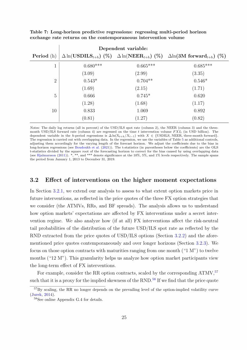
Table 7: Long-horizon predictive regressions: regressing multi-period horizonexchange rate returns on the contemporaneous intervention volume

Dependent variable:

Period (h) ∆ ln(USDILSt+h) (%) ∆ ln(NEERt+h) (%) ∆ln(3M forwardt+h) (%)

1 0.680*** 0.665*** 0.685***

(3.09) (2.99) (3.35)

2 0.543* 0.704** 0.546*

(1.69) (2.15) (1.71)

5 0.666 0.745* 0.620

(1.28) (1.68) (1.17)

10 0.833 1.069 0.892

(0.81) (1.27) (0.82)

Notes: The daily log returns (all in percent) of the USD/ILS spot rate (column 2), the NEER (column 3) and the three-month USD/ILS forward rate (column 4) are regressed on the time t intervention volume FXIt (in USD billion). Thedependent variable in the h-period regressions is ∆ ln(Xt+h/Xt−1) with X ∈ {USDILS, NEER, three-month forward}.The regression is carried out with overlapping data. In the regression, we use the variables of Table 5 as additional controls,adjusting them accordingly for the varying length of the forecast horizon. We adjust the coefficients due to the bias inlong-horizon regressions (see Boudoukh et al. (2021)). The t-statistics (in parentheses below the coefficients) are the OLSt-statistics divided by the square root of the forecasting horizon to correct for the bias caused by using overlapping data(see Hjalmarsson (2011)). *, **, and *** denote significance at the 10%, 5%, and 1% levels respectively. The sample spansthe period from January 1, 2013 to December 31, 2019.

3.2 Effect of interventions on the higher moment expectations

In Section 3.2.1, we extend our analysis to assess to what extent option markets price in

future interventions, as reflected in the price quotes of the three FX option strategies that

we consider (the ATMVs, RRs, and BF spreads). The analysis allows us to understand

how option markets’ expectations are affected by FX interventions under a secret inter-

vention regime. We also analyze how (if at all) FX interventions affect the risk-neutral

tail probabilities of the distribution of the future USD/ILS spot rate as reflected by the

RND extracted from the price quotes of USD/ILS options (Section 3.2.2) and the afore-

mentioned price quotes contemporaneously and over longer horizons (Section 3.2.3). We

focus on those option contracts with maturities ranging from one month (“1 M”) to twelve

months (“12 M”). This granularity helps us analyze how option market participants view

the long-term effect of FX interventions.

For example, consider the RR option contracts, scaled by the corresponding ATMV,57

such that it is a proxy for the implied skewness of the RND.58 If we find that the price quote

57By scaling, the RR no longer depends on the prevailing level of the option-implied volatility curve(Jurek, 2014).

58See online Appendix G.4 for details.

25

of the scaled one-month RR is adjusted upward, while the contracts with longer maturities

are not, it suggests that financial markets believe that the BOI’s intervention activity has

no impact on the option-implied skewness of the future USD/ILS exchange rate59 beyond

the one-month horizon. However, before running these analyses, we will discuss the role of

option markets in providing information beyond what is already reflected in spot markets

in the next section.

Informational externalities. The FX spot rate is equal to the discounted value of its

future fundamental value according to the asset pricing model of FX rates (Engel and

West, 2005), which implies that the spot rate is forward-looking, similar to option con-

tracts. Moreover, ruling out arbitrage opportunities means that the information content

of FX options is equal to the information content of the underlying exchange rate, as

a riskless hedging portfolio replicates the former. In this case, what information do we

expect to gain by analyzing options data beyond the information that is already priced in

the spot rate? The seminal work of Grossman (1988) shows (when applied to the FX mar-

ket) that option prices reveal information about the share of financial market participants

that would potentially sell (or buy) a specific currency in the case of unexpected large

spot FX rate movements, for example, when currency crash risks (random jump risks)

materialize (which are risks that can be insured by entering a risk reversal (BF spread60)

contract). Therefore, from a theoretical perspective, we know that looking at option

markets allows us to learn about the financial market’s perceived (preference-weighted)

uncertainty concerning the future spot exchange rate and how this uncertainty changes

when the BOI intervenes.

Market imperfections. In addition, with limits to arbitrage (e.g. due to balance-sheet

constrained banks), derivatives are no longer redundant assets. In this case, the RND

extracted from FX options reflects risk premia and expectations about the higher-order

moments of the distribution of the future FX spot rate. Options then help to complete

the market (Figlewski, 2018). Another source that may lead to market incompleteness

is due to even more practical limitations (e.g., the existence of trading costs) that do

not allow option writers to fully remove their risk exposures (e.g., delta exposures when

delta hedging these risks). As recently shown by Tian and Wu (2021), option writers

cannot fully hedge their risk exposures for U.S. stocks in practice and therefore demand a

premium for bearing these risks. Specifically, Tian and Wu (2021) identify three relevant

59And its risk characteristics as reflected in the higher moments of the RND.60Alternatively, the (scaled) risk reversals can be used to shield against jump risks. In line herewith, in

the lottery-preference literature, ex ante skewness is used as a proxy for the “lottery-like characteristicsof options”, see e.g. Boyer and Vorkink (2014).

26

risk components, where one is the premium demanded for bearing random jump risk. In

the case of the BOI, market participants may consider FXI as random jump risks, as the

BOI intervenes secretly and they may have learned over time that the BOI’s FXI are

associated with a relatively large USD/ILS spot rate response (e.g., due to the findings in

Ribon (2017)). Have in mind that RRs provide insurance against jump risks. Therefore,

central banks may affect option markets by affecting the market’s perception about jump

risks. We will later see that this is indeed the case for the USD/ILS risk reversals that

increase in anticipation of future FXI. This also suggests that understanding to what

extent FXI affect the option-implied skewness and kurtosis is of interest for FX risk

managers and FX option writers.

To conclude this section, looking at the options market can provide a better under-

standing of the source of the changes in the RND and, thereby, of the source of changes

in the USD/ILS spot rate due to changes in higher moment expectations. Questions that

we can answer by looking at the USD/ILS options market include, for instance: on the

days the BOI intervenes (and, as we showed, causes a depreciation), does it also affect

the price of insurance against FX crash risk? Did the RND become more left-skewed over

time due to the BOI’s continuous intervention activity? Are there fat tails? These are

questions that can only be answered by examining the options market.

3.2.1 Relationship between the three option strategies and future interven-

tions

We begin by assessing the adequacy of using ATMVs, RRs, and BF spreads as additional

explanatory variables to help explain the variation in the size of future FX interventions.

Formally, we regress the FX intervention data on the one-day lagged61 two-week change

of the equally weighted mean of the scaled 10- and 25-∆ RR (“∆RRt−11,t−1”), the scaled62

BF spreads (“∆BFt−11,t−1”) and the ATMV (“∆ATMVt−11,t−1”) as controls. We control

for the contemporaneous change in the spot rate to control for the aforementioned “sys-

tematic” positive correlation between changes in the USD/ILS exchange rate and changes

in the quoted prices of the RRs and BF spreads that is observed in practice.63 In other

words, we want to make sure that the options market has information beyond the con-

temporaneous change that is due to changes of the spot rate. The results are displayed in

61We lag the regressors to remove the contemporaneous effect that the BOI’s USD purchases have onthe USD/ILS exchange rate.

62By scaling, the quoted prices of these two option strategies are proportional to the implied skewnessand excess kurtosis of the USD/ILS RND, see online Appendix G.4 for details.

63See footnote 41. In theory, if interventions do not affect the at-the-money volatility level and theexpected skewness (excess kurtosis) of the distribution of the future FX spot rate, the price quotes of theRRs (BFs) should not change between two following trading days, as the moneyness of the options thatconstitute these strategies should not change from one day to the other (see online Appendix G.3).

27

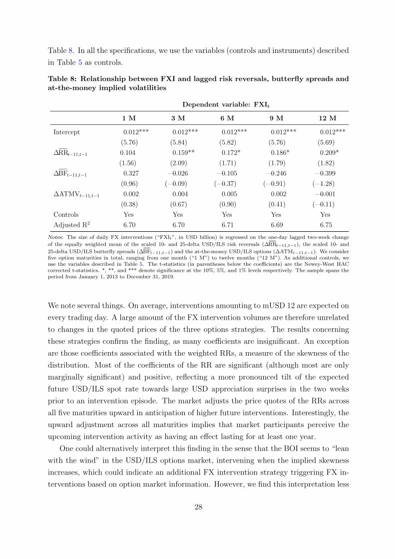
Table 8. In all the specifications, we use the variables (controls and instruments) described

in Table 5 as controls.

Table 8: Relationship between FXI and lagged risk reversals, butterfly spreads andat-the-money implied volatilities

Dependent variable: FXIt

1 M 3 M 6 M 9 M 12 M

Intercept 0.012*** 0.012*** 0.012*** 0.012*** 0.012***

(5.76) (5.84) (5.82) (5.76) (5.69)

∆RRt−11,t−1 0.104 0.159** 0.172* 0.186* 0.209*

(1.56) (2.09) (1.71) (1.79) (1.82)

∆BFt−11,t−1 0.327 =0.026 =0.105 =0.246 =0.399

(0.96) (=0.09) (=0.37) (=0.91) (=1.28)

∆ATMVt−11,t−1 0.002 0.004 0.005 0.002 =0.001

(0.38) (0.67) (0.90) (0.41) (=0.11)

Controls Yes Yes Yes Yes Yes

Adjusted R2 6.70 6.70 6.71 6.69 6.75

Notes: The size of daily FX interventions (“FXIt”, in USD billion) is regressed on the one-day lagged two-week change

of the equally weighted mean of the scaled 10- and 25-delta USD/ILS risk reversals (∆RRt−11,t−1), the scaled 10- and

25-delta USD/ILS butterfly spreads (∆BFt−11,t−1) and the at-the-money USD/ILS options (∆ATMt−11,t−1). We considerfive option maturities in total, ranging from one month (“1 M”) to twelve months (“12 M”). As additional controls, weuse the variables described in Table 5. The t-statistics (in parentheses below the coefficients) are the Newey-West HACcorrected t-statistics. *, **, and *** denote significance at the 10%, 5%, and 1% levels respectively. The sample spans theperiod from January 1, 2013 to December 31, 2019.

We note several things. On average, interventions amounting to mUSD 12 are expected on

every trading day. A large amount of the FX intervention volumes are therefore unrelated

to changes in the quoted prices of the three options strategies. The results concerning

these strategies confirm the finding, as many coefficients are insignificant. An exception

are those coefficients associated with the weighted RRs, a measure of the skewness of the

distribution. Most of the coefficients of the RR are significant (although most are only

marginally significant) and positive, reflecting a more pronounced tilt of the expected

future USD/ILS spot rate towards large USD appreciation surprises in the two weeks

prior to an intervention episode. The market adjusts the price quotes of the RRs across

all five maturities upward in anticipation of higher future interventions. Interestingly, the

upward adjustment across all maturities implies that market participants perceive the

upcoming intervention activity as having an effect lasting for at least one year.

One could alternatively interpret this finding in the sense that the BOI seems to “lean

with the wind” in the USD/ILS options market, intervening when the implied skewness

increases, which could indicate an additional FX intervention strategy triggering FX in-

terventions based on option market information. However, we find this interpretation less

28

convincing, as such a strategy would be hard to implement: notice that the coefficient

on the RR reflects the marginal increase of the RR after controlling for changes in the

USD/ILS spot rate. That is, we’d need to believe that the BOI monitors the prices of

RRs controlling for the effect that FX interventions have on the USD/ILS spot rate.

Regarding the magnitude of the effect, an increase of the RR by one percentage point

is associated with a FX intervention volume which is larger by between mUSD 104 (“1

M”) and mUSD 209 (“12 M”). The finding that the size of the estimated coefficients (i.e.,

reflecting the anticipation of future FXI) increases with option maturities is in line with

the simulation results in Figlewski (1989) who shows that the potential price impact of

market imperfections increases with option maturities. However, the standard deviation

of the adjusted RRs is decreasing with option maturities. An increase of the one- to

twelve-month RRs by one standard deviation is associated with FX interventions which

are only mUSD 4 larger. As expected, the marginal information in the RRs is relatively

small but significant, which indicates the sophistication of the option market.

To conclude this section: while the coefficients associated with the RRs are significant,

this is not true for the BF spreads and the ATMV. Therefore, option market participants

seem to only price crash-risks related to a large USD appreciation (“unidirectional crash

risk”) – the BOI therefore succeeds in affecting higher moment market expectations in

the intended direction.

3.2.2 Risk-neutral tail probabilities and future interventions

This section analyzes the relation between the tails of the USD/ILS RND and future

interventions. Estimating the tail probabilities (or crash-risk probabilities) serves two

purposes: 1. In the previous section, we found a positive relation between the option-

implied skewness of the RND and following interventions, after controlling for the effect

of these interventions on the USD/ILS spot rate. The RR can also be considered as

the difference between the risk-neutral probability of a large depreciation minus the risk-

neutral probability of a large appreciation, where both probabilities are weighted by the

corresponding intrinsic values that compose this option strategy. Therefore, disentangling

the RND components will help us to understand the source of the relation between the RR

and future interventions. 2. Probabilities are more intuitive to understand than changes

in option prices or option-implied higher moments.

We therefore extract the USD/ILS RND for each trading day and for each of the five

maturities that we examine. To this end, we use the methodology suggested by Figlewski

(2009), which we modify so that we can apply it to FX options, see online Appendix

H for details. As we have five different maturities, we have to be careful about the

representativeness of the thresholds that we use to determine the tails of the RND. For

29

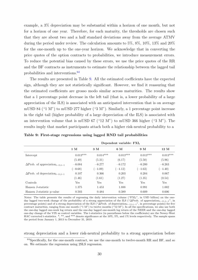
example, a 3% depreciation may be substantial within a horizon of one month, but not

for a horizon of one year. Therefore, for each maturity, the thresholds are chosen such

that they are about two and a half standard deviations away from the average ATMV

during the period under review. The calculation amounts to 5%, 8%, 10%, 13% and 20%

for the one-month up to the one-year horizon. We acknowledge that in converting the

price quotes of the option contracts to probabilities, we introduce measurement errors.

To reduce the potential bias caused by these errors, we use the price quotes of the RR

and the BF contracts as instruments to estimate the relationship between the lagged tail

probabilities and interventions.64

The results are presented in Table 9. All the estimated coefficients have the expected

sign, although they are not statistically significant. However, we find it reassuring that

the estimated coefficients are grosso modo similar across maturities. The results show

that a 1 percentage point decrease in the left tail (that is, a lower probability of a large

appreciation of the ILS) is associated with an anticipated intervention that is on average

mUSD 84 (“1 M”) to mUSD 277 higher (“3 M”). Similarly, a 1 percentage point increase

in the right tail (higher probability of a large depreciation of the ILS) is associated with

an intervention volume that is mUSD 67 (“12 M”) to mUSD 366 higher (“3 M”). The

results imply that market participants attach both a higher risk-neutral probability to a

Table 9: First-stage regressions using lagged RND tail probabilities

Dependent variable: FXIt

1 M 3 M 6 M 9 M 12 M

Intercept 0.013*** 0.014*** 0.013*** 0.013*** 0.013***

(5.49) (5.31) (6.17) (5.50) (5.96)

∆Prob. of appreciationt−11,t−1 =0.084 =0.277 =0.172 =0.200 =0.263

(=0.68) (=1.09) (=1.12) (=1.63) (=1.40)

∆Prob. of depreciationt−11,t−1 0.107 0.366 0.203 0.204 0.067

(1.46) (1.61) (1.27) (1.35) (0.54)

Controls Yes Yes Yes Yes Yes

Hansen J-statistic 1.375 1.453 1.888 0.991 1.002

Hansen J-statistic p-value 0.503 0.484 0.389 0.609 0.606

Notes: The table presents the results of regressing the daily intervention volume (“FXIt”, in USD billion) on the one-day lagged two-week change of the probability of a strong appreciation of the ILS (“∆Prob. of appreciationt−11,t−1”, inpercentage points) and of a strong depreciation of the ILS (“∆Prob. of depreciationt−11,t−1”, in percentage points) for fivecontract maturities, ranging from one month (“1 M”) to twelve months (“12 M”). In all the specifications, we also use boththe one-day lagged one-week log return and the one-day lagged one-month log return of the NEER and the one-day laggedone-day change of the VIX as control variables. The t-statistics (in parentheses below the coefficients) are the Newey-WestHAC corrected t-statistics. *, **, and *** denote significance at the 10%, 5%, and 1% levels respectively. The sample spansthe period from January 1, 2013 to December 31, 2019.

strong depreciation and a lower risk-neutral probability to a strong appreciation before

64Specifically, for the one-month contract, we use the one-month to twelve-month RR and BF, and soon. We estimate the regression using 2SLS regression.

30

the BOI intervenes.

3.2.3 Relationship between option strategies and contemporaneous and fu-

ture interventions

In the previous two sections, we have analyzed the relationship between the price quotes

of the scaled USD/ILS option strategies, their implied crash-risk probabilities, and future

interventions. This section examines how the BOI’s interventions affect the price quotes

of these option strategies contemporaneously or with a lag, running long-horizon OLS

regressions. The regression allows us to understand how the expected higher moments

of the distribution of future USD/ILS spot rates adjust over more extended periods as a

response to the BOI’s intervention activity.

The results are presented in Table 10, where we control again for the contemporaneous

correlation between the option price quotes and the spot exchange rate (see footnote 32

for the motivation). Otherwise, our results might be affected by this correlation, which

is unrelated to FX interventions. Our results indicate that there is no contemporaneous

relation between the size of FX interventions and the price quotes of the scaled option

strategies at the 5% significance level. Examining the different horizons, we find no

significant relation between the size of contemporaneous FX interventions and future

intervention volumes. This finding is in line with most papers in this strand of literature.

How should we interpret these results? We argue that the results do not imply that

the BOI’s intervention has no effect on market expectations after they happen. Recall

that we report in our empirical analysis that there is a large depreciation of the ILS in

both the USD/ILS spot and the USD/ILS forward market on those days when the BOI

intervenes, with no signs of a following reversal of this initial effect. The fact that we don’t

find any change in the higher moments of the USD/ILS RND therefore implies that this

distribution is only locationally shifted to the right (that is, in the direction of higher fu-

ture USD/ILS spot rates), leaving all other option-implied moments unchanged. In other

words, the market’s perceived uncertainty with respect to the future spot exchange rate is

unaffected. Also recall that the price quotes of the scaled USD/ILS option strategies are

adjusted in advance, reflecting the market’s perception of higher future intervention vol-

umes (Section 3.2.1), while these price quotes are not adjusted when these interventions

are actually carried out (this section). We interpret this “asymmetry” (or the statistically

significant anticipation of future intervention volumes) as evidence that the BOI is suc-

cessful in shaping market expectations. This finding may also be related to the fact that

the BOI publishes each month the previous month’s intervention volumes in the USD/ILS

spot market, which allows market participants to estimate a time series model to predict

the expected intervention volumes for the following months and quarters. This finding

31

may also be the mirror image of the BOI’s intensive intervention activity that allows op-

tion market participants to learn over time that the BOI’s commitment to intervene in the

USD/ILS spot market is credible. We conjecture that the fact that the BOI’s intervention

activity to date has been accompanied by monthly updates on the actual total monthly

intervention volumes that allows financial market participants to calibrate a time series

model that allows them to predict the expected size of FX interventions may in part

explain why previous studies have found only a weak relation between interventions in

spot FX markets and their effect on FX derivatives markets.

Table 10: Multi-period change in the price quotes of the risk reversals, butterflyspreads and at-the-money implied volatility options regressed on interventions

(a) Panel A

Dependent variable: ∆(ATMVt+h)

Period (h) 1 M 3 M 6 M 9 M 12 M

0 0.0436 0.0256 0.0143 =0.0028 0.0036

(0.89) (0.86) (0.68) (=0.15) (0.20)

1 0.0932 0.0481 0.0291 =0.0001 =0.0072

(1.00) (0.85) (0.72) (0.00) (=0.26)

5 0.1104 0.0824 0.0556 0.0286 0.0072

(0.55) (0.63) (0.62) (0.39) (0.11)

10 0.1929 0.1975 0.1364 0.1164 0.0899

(0.43) (0.70) (0.69) (0.72) (0.64)

(b) Panel B

Dependent variable: ∆(RRt+h)

Period (h) 1 M 3 M 6 M 9 M 12 M

0 =0.0024 =0.0005 0.0002 =0.0002 0.0009

(=0.95) (=0.19) (0.08) (=0.05) (0.32)

1 =0.0027 =0.0003 0.0003 0.0002 0.0002

(=0.59) (=0.06) (0.08) (0.04) (0.04)

5 =0.0023 0.0020 0.0018 0.0015 0.0025

(=0.20) (0.21) (0.21) (0.14) (0.32)

10 0.0146 0.0171 0.0154 0.0099 0.0154

(0.73) (0.85) (0.82) (0.57) (0.86)

32

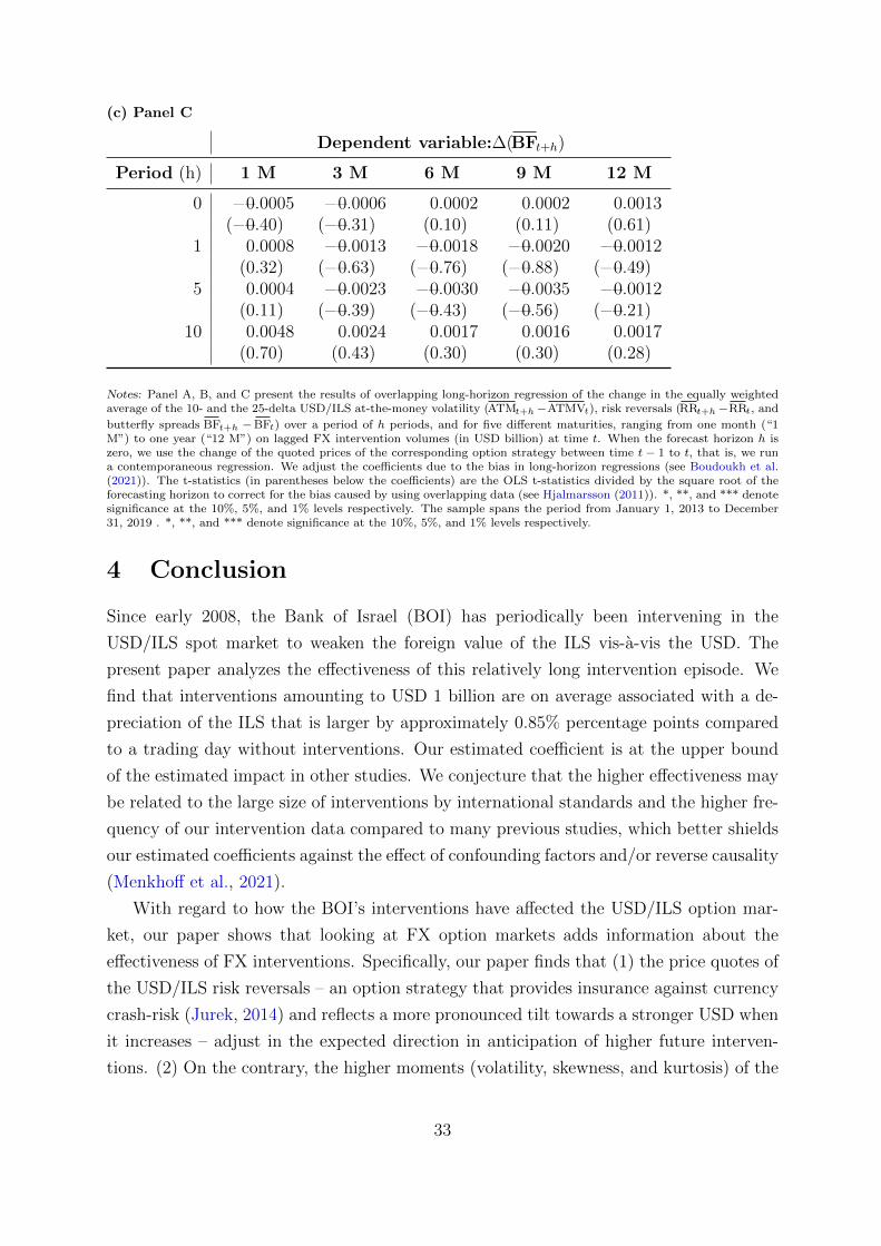
(c) Panel C

Dependent variable:∆(BFt+h)

Period (h) 1 M 3 M 6 M 9 M 12 M

0 =0.0005 =0.0006 0.0002 0.0002 0.0013(=0.40) (=0.31) (0.10) (0.11) (0.61)

1 0.0008 =0.0013 =0.0018 =0.0020 =0.0012(0.32) (=0.63) (=0.76) (=0.88) (=0.49)

5 0.0004 =0.0023 =0.0030 =0.0035 =0.0012(0.11) (=0.39) (=0.43) (=0.56) (=0.21)

10 0.0048 0.0024 0.0017 0.0016 0.0017(0.70) (0.43) (0.30) (0.30) (0.28)

Notes: Panel A, B, and C present the results of overlapping long-horizon regression of the change in the equally weightedaverage of the 10- and the 25-delta USD/ILS at-the-money volatility (ATMt+h−ATMVt), risk reversals (RRt+h−RRt, and

butterfly spreads BFt+h −BFt) over a period of h periods, and for five different maturities, ranging from one month (“1M”) to one year (“12 M”) on lagged FX intervention volumes (in USD billion) at time t. When the forecast horizon h iszero, we use the change of the quoted prices of the corresponding option strategy between time t − 1 to t, that is, we runa contemporaneous regression. We adjust the coefficients due to the bias in long-horizon regressions (see Boudoukh et al.(2021)). The t-statistics (in parentheses below the coefficients) are the OLS t-statistics divided by the square root of theforecasting horizon to correct for the bias caused by using overlapping data (see Hjalmarsson (2011)). *, **, and *** denotesignificance at the 10%, 5%, and 1% levels respectively. The sample spans the period from January 1, 2013 to December31, 2019 . *, **, and *** denote significance at the 10%, 5%, and 1% levels respectively.

4 Conclusion

Since early 2008, the Bank of Israel (BOI) has periodically been intervening in the

USD/ILS spot market to weaken the foreign value of the ILS vis-a-vis the USD. The

present paper analyzes the effectiveness of this relatively long intervention episode. We

find that interventions amounting to USD 1 billion are on average associated with a de-

preciation of the ILS that is larger by approximately 0.85% percentage points compared

to a trading day without interventions. Our estimated coefficient is at the upper bound

of the estimated impact in other studies. We conjecture that the higher effectiveness may

be related to the large size of interventions by international standards and the higher fre-

quency of our intervention data compared to many previous studies, which better shields

our estimated coefficients against the effect of confounding factors and/or reverse causality

(Menkhoff et al., 2021).

With regard to how the BOI’s interventions have affected the USD/ILS option mar-

ket, our paper shows that looking at FX option markets adds information about the

effectiveness of FX interventions. Specifically, our paper finds that (1) the price quotes of

the USD/ILS risk reversals – an option strategy that provides insurance against currency

crash-risk (Jurek, 2014) and reflects a more pronounced tilt towards a stronger USD when

it increases – adjust in the expected direction in anticipation of higher future interven-

tions. (2) On the contrary, the higher moments (volatility, skewness, and kurtosis) of the

33

risk-neutral density (RND) – proxied by the scaled price quotes of USD/ILS options – do

not change as a response to the BOI’s interventions. This lack of adjustment of the higher

moments of the RND, combined with the large effect that the BOI’s interventions have on

the USD/ILS forward rate, implies that the BOI locationally shifts the whole distribution

towards higher USD/ILS values without affecting the options market view on the higher-

order risks. Crash risk, for instance, is unaffected. The options market seems to price in

future interventions (see result (1)), while the price quotes are not adjusted when these

interventions are actually carried out. It appears that the BOI’s intensive intervention

activity has permitted option markets to learn over time that the BOI’s commitment to

its intervention regime is highly credible, which has allowed the BOI to shape market

expectations in the intended direction.

We also examine the effect that interventions have on the USD/ILS forward rates, the

first moment of the RND. We find that interventions increase the price of the USD/ILS

3-month forward rate by 0.72%, which is less than the effect on the USD/ILS spot rate.

The lower effect implies that the intervention activity widens the cross-currency basis.

To the best of our knowledge and as explained in the main body of the paper, there are

reasons to believe that we are the first to empirically show that FX interventions indeed

widen the deviation from covered interest, as predicted by Amador et al. (2020), who

propose a framework to study the problem of a central bank in a small open economy

that pursues an exchange rate policy that leads to a violation of interest parity when the

zero lower bound binds. We thereby contribute to the recently revived strand of literature

that examines deviations from covered interest rate parity.

34

References

Adler, G., N. Lisack, and R. C. Mano (2019). Unveiling the effects of foreign exchange

intervention: A panel approach. Emerging Markets Review 40, 100620.

Adler, G. and C. E. Tovar (2011). Foreign exchange intervention: A shield against appre-

ciation winds? IMF Working Paper 11/165, 1–29.

Amador, M., J. Bianchi, L. Bocola, and F. Perri (2020). Exchange rate policies at the

zero lower bound. Review of Economic Studies 87 (4), 1605–1645.

Arango-Lozano, L., L. Menkhoff, D. Rodrıguez-Novoa, and M. Villamizar-Villegas (2020).

The effectiveness of FX interventions: A meta-analysis. Journal of Financial Stability ,

100794.

Avdjiev, S., W. Du, C. Koch, and H. S. Shin (2019). The dollar, bank leverage, and

deviations from covered interest parity. American Economic Review: Insights 1 (2),

193–208.

Borio, C. and P. Disyatat (2010). Unconventional monetary policies: An appraisal.

Manchester School supplement 2010, 53–89.

Boudoukh, J., R. Israel, and M. Richardson (2021). Biases in long-horizon predictive

regressions. Journal of Financial Economics , 1–33.

Boyer, B. H. and K. Vorkink (2014). Stock options as lotteries. Journal of Finance 69 (4),

1485–1527.

Campa, J. M., P. H. K. Chang, and R. L. Reider (1998). Implied exchange rate dis-

tributions: Evidence from OTC option markets. Journal of International Money and

Finance 17 (1), 117–160.

Caspi, I., A. Friedman, and S. Ribon (2018). The immediate impact and persistent effect

of fx purchases on the exchange rate. Bank of Israel Discussion Paper 2018 (04), 1–29.

Castren, O. (2004). Do options-implied RND functions on G3 currencies move around

the times of interventions on the JPY/USD exchange rate? ECB Working Paper

Series 410, 1–61.

Cochrane, J. H. (2005). Asset Pricing. 2nd ed., Princeton University Press.

Cox, A. M. G. and D. G. Hobson (2005). Local martingales, bubbles and option prices.

Finance and Stochastics 9 (4), 477–492.

35

Dedola, L., G. Georgiadis, J. Grab, and A. Mehl (2021). Does a big bazooka matter?

Quantitative easing policies and exchange rates. Journal of Monetary Economics 117,

489–506.

Disyatat, P. and G. Galati (2007). The effectiveness of foreign exchange intervention in

emerging market countries: Evidence from the Czech koruna. Journal of International

Money and Finance 26 (3), 383–402.

Domanski, D., E. Kohlscheen, and R. Moreno (2016). Foreign exchange market interven-

tion in EMEs: what has changed? BIS Quarterly Review , 65–79.

Dominguez, K. M. (1986). Are foreign exchange forecasts rational? New evidence from

survey data. Economics Letters 21 (3), 277–281.

Donald, S. G. and W. K. Newey (2000). A jackknife interpretation of the continuous

updating estimator. Economics Letters 67 (3), 239–243.

Du, W., J. Im, and J. Schreger (2018). The U.S. Treasury premium. Journal of Interna-

tional Economics 112, 167–181.

Du, W. and J. Schreger (2016). Local currency sovereign risk. Journal of Finance 71 (3),

1027–1070.

Du, W. and J. Schreger (2021). CIP deviations, the dollar, and frictions in international

capital markets. National Bureau of Economic Research w28777, 1–68.

Du, W., A. Tepper, and A. Verdelhan (2018). Deviations from covered interest rate parity.

Journal of Finance 73 (3), 915–957.

Duffie, D. (2010). Presidential address: Asset price dynamics with slow-moving capital.

Journal of Finance 65 (4), 1237–1267.

Egert, B. and L. Komarek (2006). Foreign exchange interventions and interest rate policy

in the Czech Republic: Hand in glove? Economic Systems 30 (2), 121–140.

Elkayam, D. (2003). The long road from adjustable peg to flexible exchange rate regimes:

The case of Israel. Bank of Israel Discussion Paper 2003 (04), 1–33.

Engel, C. and K. D. West (2005). Exchange rates and fundamentals. Journal of Political

Economy 113 (3), 485–517.

Fanelli, S. and L. Straub (2021). A theory of foreign exchange interventions. Review of

Economic Studies 88 (6), 2857–2885.

36

Fatum, R. (2008). Daily effects of foreign exchange intervention: Evidence from official

Bank of Canada data. Journal of International Money and Finance 27, 438–454.

Fatum, R. (2015). Foreign exchange intervention when interest rates are zero: Does

the portfolio balance channel matter after all? Journal of International Money and

Finance 57, 185–199.

Fatum, R. and M. Hutchison (2003). Is sterilised foreign exchange intervention effective

after all? An event study approach. Economic Journal 113 (487), 390–411.

Fatum, R. and M. Hutchison (2006). Effectiveness of official daily foreign exchange market

intervention operations in Japan. Journal of International Money and Finance 25 (2),

199–219.

Figlewski, S. (1989). Options arbitrage in imperfect markets. Journal of Finance 44 (5),

1289–1311.

Figlewski, S. (2009). Estimating the implied risk neutral density for the U.S. market

portfolio. In T. Bollerslev, {Jeffrey R.}. Russell, and M. Watson (Eds.), Volatility and

Time Series Econometrics, pp. 323–353.

Figlewski, S. (2018). Risk-neutral densities: A review. Annual Review of Financial

Economics 10, 329–359.

Fratzscher, M. (2005). How successful are exchange rate communication and interven-

tions? Evidence from time-series and event-study approaches. European Central Bank

Working Paper 528, 1–55.

Fratzscher, M. (2008). Oral interventions versus actual interventions in FX markets: An

event-study approach. Economic Journal 118 (530), 1079–1106.

Fratzscher, M., O. Gloede, L. Menkhoff, L. Sarno, and T. Stohr (2019). When is for-

eign exchange intervention effective? Evidence from 33 countries. American Economic

Journal: Macroeconomics 11 (1), 132–156.

Friedman, A. and L. Galo (2015). The effective exchange rate in Israel. Bank of Israel

Press Release, 1–10.

Galati, G., P. Higgins, O. Humpage, and W. Melick (2007). Option prices, exchange

market intervention, and the higher moment expectations channel: A user’s guide.

International Journal of Finance and Economics 12 (2), 225–247.

37

Galati, G., W. Melick, and M. Micu (2005). Foreign exchange market intervention and

expectations: The yen/dollar exchange rate. Journal of International Money and Fi-

nance 24 (6), 982–1011.

Garman, M. B. and S. W. Kohlhagen (1983). Foreign currency option values. Journal of

International Money and Finance 2 (3), 231–237.

Gromb, D. and D. Vayanos (2010). Limits of arbitrage. Annual Review of Financial

Economics 2 (1), 251–275.

Grossman, S. J. (1988). An analysis of the implications for stock and futures price volatil-

ity of program trading and dynamic hedging strategies. Journal of Business 61 (3),

275–298.

Hahn, J., J. Hausman, and G. Kuersteiner (2004). Estimation with weak instruments:

Accuracy of higher-order bias and MSE approximations. Econometrics Journal 7 (1),

272–306.

Hall, A. R. (2005). Generalized Method of Moments (1st edition). Oxford University

Press.

Hansen, L. P., J. Heaton, and A. Yaron (1996). Finite-sample properties of some alter-

native GMM estimators. Journal of Business & Economic Statistics 14 (3), 262–280.

Hattori, M., A. Schrimpf, and V. Sushko (2016). The response of tail risk perceptions to

unconventional monetary policy. American Economic Journal: Macroeconomics 8 (2),

111–136.

Heston, S. L., M. Loewenstein, and G. A. Willard (2007). Options and bubbles. Review

of Financial Studies 20 (2), 359–390.

Hjalmarsson, E. (2011). New methods for inference in long-horizon regressions. Journal

of Financial and Quantitative Analysis 46 (3), 815–839.

Humpage, O. F. (1999). U.S. intervention: Assessing the probability of success. Journal

of Money, Credit and Banking 31 (4), 731–747.

Ito, T. and T. Yabu (2007). What prompts Japan to intervene in the forex market? A

New approach to a reaction function. Journal of International Money and Finance 26,

193–212.

Jarrow, R. and H. Li (2015). The impact of a central bank’s bond market intervention

on foreign exchange rates. Quarterly Journal of Finance 5 (1), 1550009 (34 pages).

38

Jurek, J. W. (2014). Crash-neutral currency carry trades. Journal of Financial Eco-

nomics 113 (3), 325–347.

Kleibergen, F. and R. Paap (2006). Generalized reduced rank tests using the singular

value decomposition. Journal of Econometrics 133 (1), 97–126.

Malz, A. M. (1997). Estimating the probability distribution of the future exchange rate

from option prices. Journal of Derivatives 5 (2), 18–36.

Marins, J. T. M., G. S. Araujo, and J. V. M. Vicente (2017). Do central bank foreign

exchange interventions affect market expectations? Applied Economics 49 (31), 3017–

3031.

McCauley, R. and W. R. Melick (1996). Risk reversal risk. Risk 9 (11), 54–57.

McGeever, J. (2017). TIMELINE – The global FX rigging scandal.

Menkhoff, L., M. Rieth, and T. Stohr (2021). The dynamic impact of FX interventions

on financial markets. Review of Economics and Statistics 103 (5), 1–15.

Menkhoff, L., L. Sarno, M. Schmeling, and A. Schrimpf (2012). Carry trades and global

foreign exchange volatility. Journal of Finance 67 (2), 681–718.

Miyajima, K. (2013). Foreign exchange intervention and expectation in emerging

economies. Bank for International Settlements Working Papers 414, 1–23.

Morel, C. and J. Teıletche (2008). Do interventions in foreign exchange markets modify

investors’ expectations? The experience of Japan between 1992 and 2004. Journal of

Empirical Finance 15, 211–231.

Nedeljkovic, M. and C. Saborowski (2019). The relative effectiveness of spot and

derivatives-based intervention. Journal of Money, Credit and Banking 51 (6), 1455–

1490.

Neely, C. J. (2000). Are changes in foreign exchange reserves well correlated with official

intervention? Review – Federal Reserve Bank of St. Louis 82 (5), 17–32.

Neely, C. J. (2005). An analysis of recent studies of the effect of foreign exchange inter-

vention. Federal Reserve Bank of St. Louis Working Paper (2005-030B), 1–42.

Ramey, V. and S. Zubairy (2018). Government spending multipliers in good times and in

bad: Evidence from US historical data. Journal of Political Economy 126 (2), 850–901.

39

Reiswich, D. and U. Wystup (2010). A guide to FX options quoting conventions. Journal

of Derivatives 18 (2), 58–68.

Ribon, S. (2017). Why the Bank of Israel intervenes in the foreign exchange market, and

what happens to the exchange rate. Bank of Israel Research Department Discussion

Paper 2017 (04), 1–45.

Rosenberg, J. V. and L. G. Traub (2009). Price discovery in the foreign currency futures

and spot market. Journal of Derivatives 17 (2), 7–25.

Sarno, L. and M. P. Taylor (2001). Official intervention in the foreign exchange market:

Is it effective and, if so, how does it work? Journal of Economic Literature 39 (3),

839–868.

Stock, J. H. and M. Yogo (2005). Testing for weak instruments in linear IV regression.

In D. W. Andrews (Ed.), Identification and Inference for Econometric Models Essays

in Honor of Thomas Rothenberg, pp. 80–108. Cambridge University Press.

Szalay, E. (2020). Dispute brews between EU and currency traders on Mifid reform.

Tashu, M. (2014). Motives and effectiveness of forex interventions: evidence from Peru.

IMF Working Paper 14 (217), 1–30.

Tian, M. and L. Wu (2021). Limits of arbitrage and primary risk taking in derivative

securities. Available at SSRN 3779350, 1–57.

Tse, Y., J. Xiang, and J. K. W. Fung (2006). Price discovery in the foreign exchange

futures market. Journal of Futures Markets: Futures, Options, and Other Derivative

Products 26 (11), 1131–1143.

Villamizar-Villegas, M. and D. Perez-Reyna (2015). A survey on the effects of sterilized

foreign exchange intervention. Borradores de Economıa (862), 1–28.

Villamizar-Villegas, M. and D. Perez-Reyna (2017). A theoretical approach to sterilized

foreign exchange intervention. Journal of Economic Surveys 31 (1), 343–365.

40

Appendix

A Specification analysis of first-stage regression

This appendix shows the results of the first-stage regression with different specifications

in Table A.1. Specification [1] shows that the one-day lagged daily FXI is significant,

but not the two-day lag. In specification [2], we add a dummy that equals one if the

BOI intervened in the past week. We also add log two-day, two weeks, and three months

returns of the USD/ILS FX rate with different lag structures and ∆MA(USD/ILS)t−1,

which is defined as the difference between the USD/ILS rate and its one-year moving

average. The results reveal that the latter doesn’t have any explanatory power, unlike

the log USD/ILS returns series.

Specification [3], however, shows that a model with a higher explanatory power in

terms of the adjusted coefficient of determination is possible when using the lagged NEER

instead of the USD/ILS FX rate – the higher explanatory power is due to the higher signif-

icance of the one-day lagged quarterly NEER return. In specification [4], the specification

we use in the paper, we add the net ILS spot market purchases by non-residents and do-

mestic institutional investors, the change in the 5-year CDS, and the VIX. With regards to

flows by domestic and institutional investors, these two sectors have recently received sig-

nificant attention from the BOI65 and have been jointly identified as one of the “culprits”

for the sustained appreciation trend of the ILS in the last years. The results suggest that

a higher net demand for ILS – if these two sectors sell foreign currencies to buy ILS on a

net basis, this variable is negative – is associated with higher FX interventions. However,

the coefficient is numerically small while being statistically insignificant. With regards to

the CDS and the VIX, although insignificant, untabulated results show that they increase

the adjusted R-squared significantly.

Last, specification [5] reveals that the weekly change in the one-month USD LIBOR

rate and the one-month TELBOR rates is not statistically significant.

65See e.g. Chapter 3 in the Bank of Israel yearly report 2020 and the Bank of Israel Financial StabilityReport for the second half of 2020.

41

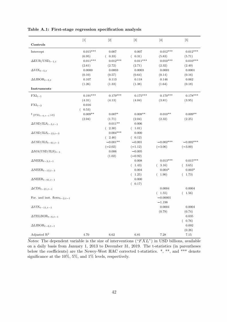
Table A.1: First-stage regression specification analysis

[1] [2] [3] [4] [5]

Controls

Intercept 0.015*** =0.007 =0.007 0.012*** 0.012***

(6.95) (=0.33) (=0.31) (5.83) (5.71)

∆EUR/USDt−1,t 0.011*** 0.012*** 0.011*** 0.010*** 0.010***

(2.61) (2.72) (2.71) (2.32) (2.40)

∆VIXt−5,t 0.0000 0.0003 0.0003 0.0001 0.0001

(0.10) (0.57) (0.64) (0.14) (0.16)

∆LIBORt−5,t 0.107 0.113 0.118 0.146 0.062

(1.26) (1.33) (1.38) (1.64) (0.18)

Instruments

FXIt−1 0.191*** 0.179*** 0.175*** 0.170*** 0.178***

(4.31) (4.13) (4.04) (3.81) (3.95)

FXIt−2 =0.016

(=0.53)

1{FXIt−6,t−1>0} 0.009** 0.007* 0.008** 0.010** 0.009**

(2.04) (1.71) (2.04) (2.32) (2.25)

∆USD/ILSt−3,t−1 =0.011** =0.006

(=2.30) (=1.01)

∆USD/ILSt−13,t−3 =0.004*** 0.000

(=2.46) (=0.12)

∆USD/ILSt−61,t−1 =0.001** =0.001 =0.002*** =0.002***

(=2.02) (=1.12) (=3.06) (=3.00)

∆MA(USD/ILS)t−1 0.006 =0.005

(1.02) (=0.92)

∆NEERt−3,t−1 =0.008 =0.013*** =0.015***

(=1.43) (=3.16) (=3.65)

∆NEERt−13,t−3 =0.004 =0.004* =0.003*

(=1.25) (=1.90) (=1.73)

∆NEERt−61,t−1 0.000

(=0.17)

∆CDSt−21,t−1 =0.0004 =0.0004

(=1.55) (=1.56)

For. and inst. flowst−2,t−1 =0.00001

=1.198

∆VIXt−11,t−1 0.0004 0.0004

(0.79) (0.74)

∆TELBORt−6,t−1 =0.035

(=0.76)

∆LIBORt−6,t−1 0.092

(0.26)

Adjusted R2 4.70 6.62 6.81 7.28 7.15

Notes: The dependent variable is the size of interventions (“FXIt”) in USD billions, availableon a daily basis from January 1, 2013 to December 31, 2019. The t-statistics (in parenthesesbelow the coefficients) are the Newey-West HAC corrected t-statistics. *, **, and *** denotesignificance at the 10%, 5%, and 1% levels, respectively.

42

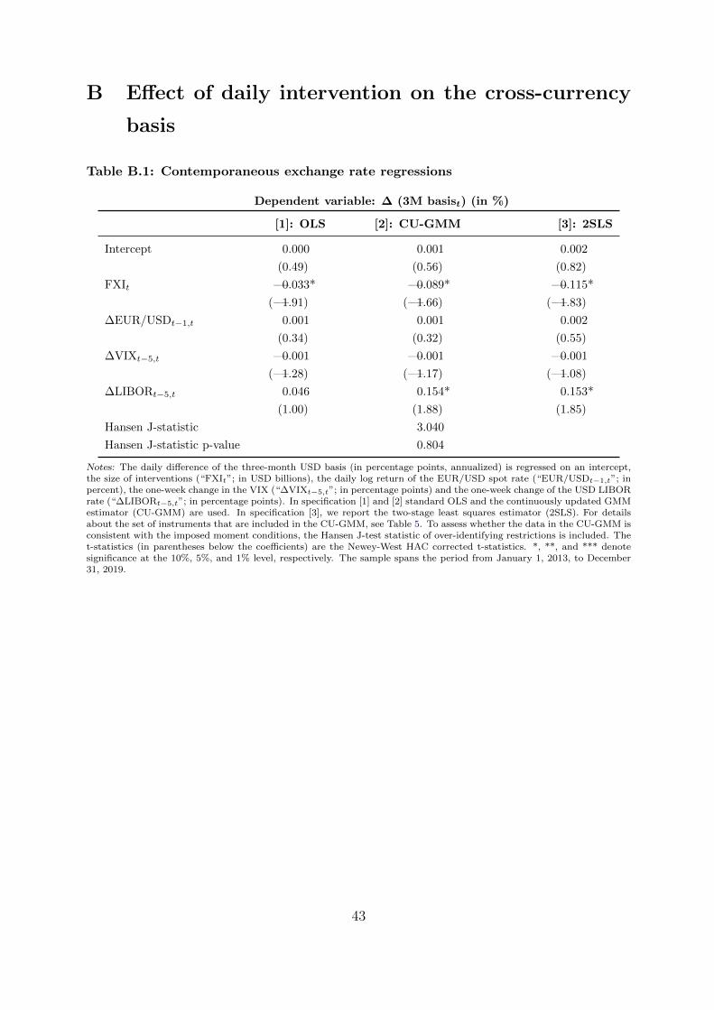
B Effect of daily intervention on the cross-currency

basis

Table B.1: Contemporaneous exchange rate regressions

Dependent variable: ∆ (3M basist) (in %)

[1]: OLS [2]: CU-GMM [3]: 2SLS

Intercept 0.000 0.001 0.002

(0.49) (0.56) (0.82)

FXIt =0.033* =0.089* =0.115*

(=1.91) (=1.66) (=1.83)

∆EUR/USDt−1,t 0.001 0.001 0.002

(0.34) (0.32) (0.55)

∆VIXt−5,t =0.001 =0.001 =0.001

(=1.28) (=1.17) (=1.08)

∆LIBORt−5,t 0.046 0.154* 0.153*

(1.00) (1.88) (1.85)

Hansen J-statistic 3.040

Hansen J-statistic p-value 0.804

Notes: The daily difference of the three-month USD basis (in percentage points, annualized) is regressed on an intercept,the size of interventions (“FXIt”; in USD billions), the daily log return of the EUR/USD spot rate (“EUR/USDt−1,t”; inpercent), the one-week change in the VIX (“∆VIXt−5,t”; in percentage points) and the one-week change of the USD LIBORrate (“∆LIBORt−5,t”; in percentage points). In specification [1] and [2] standard OLS and the continuously updated GMMestimator (CU-GMM) are used. In specification [3], we report the two-stage least squares estimator (2SLS). For detailsabout the set of instruments that are included in the CU-GMM, see Table 5. To assess whether the data in the CU-GMM isconsistent with the imposed moment conditions, the Hansen J-test statistic of over-identifying restrictions is included. Thet-statistics (in parentheses below the coefficients) are the Newey-West HAC corrected t-statistics. *, **, and *** denotesignificance at the 10%, 5%, and 1% level, respectively. The sample spans the period from January 1, 2013, to December31, 2019.

43