money demand and foreign exchange risk in nigeria - IIUM ...

IIUM Journal of Economics and Management 18, no. 1 (2010): 45-72© 2010 by The International Islamic University Malaysia

ABSTRACT

The paper estimates the money demand function that incorporates a foreignexchange risk variable for Nigeria using annual time series data (1970-2006).The applied technique of cointegration analysis is the bounds test whichinvolves autoregressive distributed lags (ARDL). Consistent with economicpostulates, it is found that (a) the demand for money in the log-run iscointegrated with real income, exchange rate variability, interest rate andinflation; (b) the short-run income elasticity is less than one but greater thanzero; (c) inflation is more significant than real income in the money demandfunction; and (d) the real money demand function is stable.

JEL Classification: C13, C22, E41, E52, F31.

Key words: Bounds test, Money demand, Foreign exchange risk,Autoregressive distributed lags (ARDL), Inflation targeting, Nigeria.

MONEY DEMAND AND FOREIGN EXCHANGE RISKIN NIGERIA: A COINTEGRATION ANALYSIS USING

AN ARDL BOUNDS TEST

Douglason G. Y. Omotor

Department of Economics, Delta State University, Abraka, Nigeria.(Email: [email protected])

1. INTRODUCTION

In a not too recent paper, Omotor and Orubu (2003) investigated theNigerian money demand function using annual data from 1970 to 1998.The specifications extended the model of Akhtar and Putnam (1980)1

by introducing distributed lags and slope dummy effects of exchangerate regimes. According to the results, exchange rate variability is not asignificant determinant of money demand and that exchange ratederegulation as captured by the slope dummy in the equation is importantin influencing real money demand.

IIUM Journal of Economics & Management 18, no.1 (2010)46

The empirical results of Omotor and Orubu (2003) are based onstandard regression methods that totally ignore the time series propertiesof the variables (such as testing for unit roots and cointegration); whichmay lead to model mis-specification and spurious regression results(Granger and Newbold, 1974). Expectedly, the results of such statisticalinference may, thus, be misleading. In more modern literature on moneydemand (e.g., Choi and Oxley, 2004), it has been recognized that thepersistence observed in the kind of variables included in the models islikely to be brought about by unit roots, and the analysis is typicallybased on cointegration methods, taking the potential non-stationarity ofthe time series into account. As further amplified by Juselius (2000),macroeconomic variables are mostly found to be non-stationary, and assuch, standard regression methods are not feasible from an econometricpoint of view for their analyses. Rather, the most obvious choice shouldbe cointegration analysis.

Consequent upon the above, the general objective of this study is tore-estimate the Nigerian money demand function integrating a foreignexchange risk variable for the period 1970 to 2006. The study furtherapplies a more robust recently-developed estimation method—thebounds test—first proposed and applied by Pesaran, Shin and Smith(2001), built on the unrestricted error-correction model (UECM). ThePesaran, Shin and Smith (2001) approach also has an added value inthe estimation of cointegration analysis involving autoregressivedistributed lags (ARDL). The ARDL approach, as it should be noted,equally de-emphasizes the pre-testing of orders of integration. This givesfurther impetus for the present study, as the model specified by Omotorand Orubu (2003) incorporates distributed lags in order to derive speedof adjustment.

The UECM, which incorporates the bounds testing approachtogether with the ARDL modeling approach to cointegration analysis(Pesaran and Shin, 1998), according to Mah (2000), has some majoradvantages over the conventional cointegration approach2 of Engle-Granger (1987) and Johansen-Juselius (1990). The bounds test, as theliterature has it, can be applied to series, irrespective of whether theexplanatory variables are I(0) or I(1), provided the endogenous variableis I(1). Secondly, the technique is found effective for small samples, (asis the case of the present study) and, thus, it avoids the uncertaintyabout variable exogeneity, provided that the model is sufficientlyaugmented and allows for estimation of both the long-run (equilibrium)and short-run (dynamic) relationships among variables (Odhiambo, 2007).

Money Demand and Foreign Exchange Risk in Nigeria 47

Nigeria provides an interesting venue of this study for severalreasons. First, Nigeria has achieved some economic progress in thelast few years. This has been associated with the various economicreform programs particularly in the financial sector. Nigeria’s annualeconomic growth rate over the last five years is 7.4% (2003-2007)with a 2007 estimated GDP (purchasing power parity) of USD296.1billion.3 Second, Nigeria in recent years has experienced some reasonableimprovements and growth in her external reserves. Nigeria’s stock offoreign exchange reserves reached USD64.8 billion in August 2008,which could finance about 16 months’ worth of imports. This phenomenalgrowth attributable to the nation’s favorable trade balance mainly drivenby oil and non-oil exports (Abubaka, 2008) is unprecedented in the lasttwo decades. Third, the naira exchange rate has experienced peaksand troughs; it has been relatively stable since late 2007. The exchangerate stood at about N116/USD as at end of September 2008 comparedto N81.25/USD in 1996 and N133.66/USD in 2005. Some reasons thathave been canvassed for the recent stability are the probability of majoreconomies of the world slumping into recession and the recent bankingsector reforms since mid-2000. There is, however, likelihood that abacklash of this may spill over into the Nigerian economy, since it is ahighly import-dependent one. Lastly, Nigeria liberalized its economicinstitutions in the mid-1980s; thus providing a relatively sufficient amountof data (given the bounds test approach used in the study) to evaluatethe impact of the policy shift on the economy.

Specifically, the objectives of this paper are three-fold. In the firstplace, the study seeks to determine the time-series properties of somevariables during the period 1970-2006, particularly that of the regressand.This is to avoid the problem of spurious regression results, although asearlier mentioned, ARDL de-emphasizes the pre-testing of orders ofintegration. Secondly, the study examines the existence of a long-runrelationship between Nigeria’s real money demand and its determinantsusing the bounds tests methodology. This has some implications forpolicy formulation. Thirdly, the study also investigates the effect ofNigeria’s foreign exchange variability on its real money demandbalances. Variability in foreign exchange rate may invoke volatility whichis detrimental in some ways to economic policy formulation. Accordingto Maskus (1990, 85) foreign exchange rate volatility reduces the volumeof international trade since it creates uncertainty over expected profits.In addition, volatility or instability has a consequence of increasing pricesof internationally traded goods given the uncertainty that surrounds its


anticipated behavior. In addition to the application of bounds testmethodology for cointegration, the study shall also estimate an errorcorrection specification that allows for determining the impact of theshort- and long-run exchange rate variability on money demand to beclearly distinguished.

The remainder of the paper is organized as follows. Section 2provides the model and describes the study’s methodology. Section 3presents the data used, while Section 4 discusses the empirical findingsand provides some policy implications. Section 5 concludes the study.

2. A MODEL OF THE MONEY DEMAND FUNCTIONAND THE METHODOLOGY OF THE STUDY

In modeling the money demand function for Nigeria, we simply followthe lead by Omotor and Orubu (2003) which extends the Akhtar andPutnam (A-P) (1980) model. According to the A-P hypothesis, changesassociated with foreign exchange risk may have direct and indirecteffects on the demand for domestic money. The direct effect is howagents of transactions respond to increase in risk associated withcurrency values with a tendency to diversify and hold smaller amountsof domestic money, while increasing their holding of foreign monies.On the other hand, the indirect effect impacts on the volume ofinternational transactions as uncertainty increases cost of trade. It shouldbe noted that the exact direction of the indirect effect has been a matterof debate. As enunciated further by Akhtar and Putnam (1980, 788):

“. . . if the increase in the cost of international transactionsreduces the volume of international transactions below what itotherwise would have been, then the demand for real balances isalso reduced.”

The implication of the estimated A-P results is that exchange risk tendsnot only to reduce demand for domestic money; it is also an importantexplanatory variable in money demand behavior.

The A-P model thus, demonstrates the importance of includingforeign exchange risk in the money demand specifications given theview that increase in the risk associated with foreign exchange tendsto decrease the demand for domestic money. Two critical issues raisedin the study are the choice of variable to proxy foreign exchange risk


and the specification of the money demand function (Akhtar and Putnam,1980).

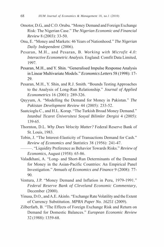
The two basic versions of the money demand functions investigatedby the A-P model are:

(1) 143210 )ln()ln()/ln()ln( uPaVRaRaPYaaM +++++=

(1a) 23210 )ln()/ln()/ln( uVRbRbPYbbPM ++++=

where, M is currency in hands of the public and sight deposits, Y isnominal income, R is interest rate, VR is exchange rate risk or thestandard deviation of daily $/DM spot rates, P is general rise level, andu1 and u2 are the error terms. The variability variable (VR) in equation(1) is the extension and contribution by Akhtar and Putnam (1980) tothe core monetary theory formulation. Further extension to the A-Pmodel by Omotor and Orubu (2003), which they label as ‘a distributedlag-augmented Akhtar and Putnam (DLAP)4 model, is specified as:

;,...,2,1

, (2)1

1543210

ni

MPVRRYMn

tidtttttdt

=

++++++= ∑=

− εββββββ

where Mdt is real money balances for period t, Yt is real gross domesticproduct (GDP) used as a measure of real income in period t, Pt is nowinflation rate for period t and ε1 is the error term. Mdt-i is the distributedlags of the money demand variable. The justification for the incorporationof a distributed lag scheme according to Omotor and Orubu (2003) isthat it enables the determination of the speed (coefficient) at whichdesired levels of money demand adjust to actual levels. This hasimplication for monetary policy formulation and implementation.

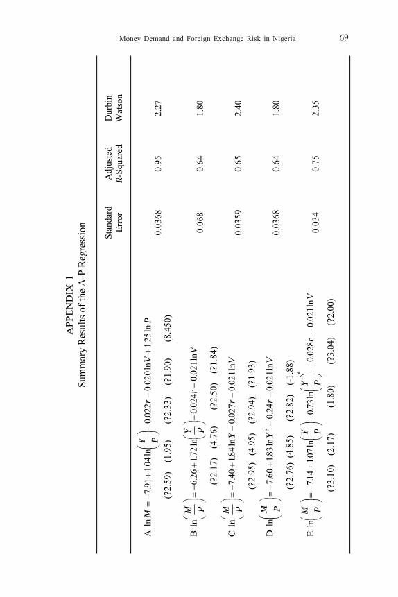
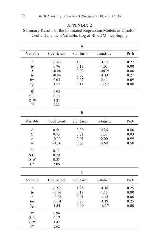
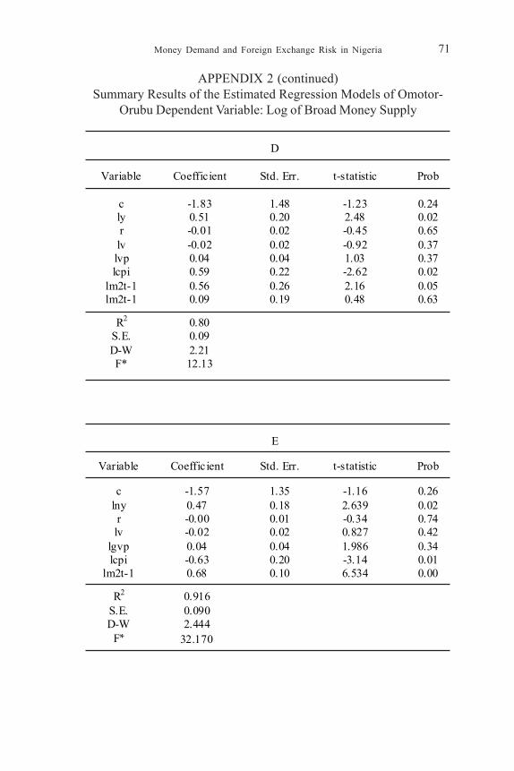
The results of Omotor and Orubu (2003) using Nigerian data,contradicted the A-P findings (using German data) that exchange ratevariability is significant in the behavior of money demand. However,Omotor and Orubu support and confirm the traditional postulate andprevious studies on the Nigerian experience that real income, interestrate and inflation are significant in the money demand function. Inaddition, the adjustment process as captured by the distributed lagsgets support. The results of Omotor and Orubu, (2003) furtherencapsulate that the fixed exchange regime exerts some impact on the


demand for real balances in Nigeria. The summary regression resultsof both Akhtar and Putnam (1980) and Omotor and Orubu (2003) arepresented in Appendices 1 and 2, respectively.

The present study modifies the Omotor and Orubu (2003) modelspecification via the application of an unrestricted error correction model(UECM) specification; à la autoregressive distributed lag (ARDL)methodology. The UECM methodology is briefly summarized in sub-section 2.2.

2.1 STUDIES ON VOLATILITY MEASURES IN MONEY DEMANDSPECIFICATIONS

There exist a plethora of studies that have incorporated various measuresof risks in the money demand functions. These studies for estimationpurpose ascribe the motives of money demand to two behavioralassumptions—the transactions and asset or portfolio balance approaches(Saatcioglu and Korap, 2005). The transactions motive specify money’srole as a medium of exchange. Money by this approach is viewedessentially as an inventory held for transaction purposes. The transactioncost of switching between money and other liquid financial assets justifyholding such inventories, despite that other liquid assets may offer higheryields (Judd and Scadding, 1982; cited in Saatcioglu and Korap, 2005).Earlier popular studies that apply this approach are Baumol (1952) andTobin (1956). Succinctly put, what this approach means is that thedemand for money balances increase proportionally with the volume oftransactions in the economy and decreases with the increase of returnsin the alternative costs of holding money.

The portfolio balance approach explains that people hold money asa store of value, and money is just one of the various assets amongwhich people distribute their wealth. These assets when held for alonger period in relation to the transaction motives possess expectedrate of return whose probable ratio of returns against each other changeover time. This is the risk factor that people take into cognizance intheir distribution of wealth. The basic contribution of the portfolio balanceapproach as Branson (1989) argues is to enter the risk considerationsexplicitly into the determination of the demand for money function (seeSaatcioglu and Korap, 2005). Some elegant empirical studies which inearlier times emphasize the importance of the risk factor in portfoliodecision for the demand for money balances are Tobin (1958) andFriedman (1959).


The money demand function incorporates the risk factor in variousforms, e.g., interest rate volatility, inflation uncertainty and exchangerate volatility. Interest rate uncertainty enters the money demand theorythrough the financial asset motive for holding money. An increase inthe volatility of interest rates increases the risk of holding fixed-terminterest paying securities. To reduce this risk, firms and householdsmay thus wish to hold larger money balances (Garner, 1986).

Some empirical literature that incorporates the risk factor in thedemand for money function focuses on several aspects of howindividuals respond to uncertainty about inflation. Uncertainty raisesthe demand for money by increasing precautionary demand (Klein,1977; and Blejer, 1979). If savers are interested in the real returns onassets, then the proposition that money is a safe asset is invalidatedwhen uncertainty about inflation exist (Apergis, 1999). In the theory,inflation uncertainty affects the demand for money by weakening thepower of money as a store of value as well as a unit of account.

How does foreign exchange risk impact on the demand for money?According to Akhtar and Putnam (1980), riskiness of currency valueshas a tendency to affect people’s action to hold smaller amounts ofdomestic money. When this happens, money no longer serves as anoptimal store of value for a given level of transaction, as the previousinformation content concerning international transactions is eroded.Maskus (1990) highlights that volatility in exchange rate reduces thevolume of international trade as it creates uncertainty over expectedprofits. Foreign exchange volatility may also reduce foreign directinvestment (FDI) as traders for fear of unanticipated exchange ratevolatility would want to add a risk premium to the prices of internationallytraded goods.

Several examples of studies that have incorporated the variousform of risks in the traditional money demand balances are; Tobin (1958);Akhtar and Putnam (1980); Zilberfarb (1988); Apergis (1999), Bahmani-Oskooee and Ng (2002), Omotor and Orubu (2003); Saatcioglu andKorap (2005); and Yinusa and Akinlo (2009).

2.2 THE UNRESTRICTED ERROR CORRECTION MODEL (UECM)OR BOUNDS TESTS AS APPLIED TO THE MODEL

The autoregressive distributed lag (ARDL) model adopted in this paperis aimed at examining the existence of short- and long-run relationshipsbetween money demand and foreign exchange risk. Following Pesaran,


Shin and Smith (2001) as applied in Keong, Yusop and Sen (2005), weconstructed a vector autoregressive (VAR) of order q, denoted asVAR(q), for the following money demand function:

; (3)1

1∑=

− ++=q

ittit ww εβμ

where wt is the vector of both xt and yt, yt is the dependent variabledefined as real money demand and xt = [Yt, Rt, VRt, Pt]’ is the vectormatrix which represents the set of explanatory variables as previouslydefined, μ = [μy, μx], t is a time or trend variable, and βi is a matrix ofVAR parameters for lag i. As noted by Pesaran, Shin and Smith (2001),yt must be I(1) but the explanatory variables can be either I(0) or I(1).A vector error-correction model (VECM) is developed as:

tt

q

oiit

q

iittt xYYw ελαμ y w )4( 1

1-

1-

1-

11- +Δ+Δ+++=Δ −

==∑∑

Δ is the first-difference operator. The long-run multiplier matrix λ ispartitioned as:

⎥⎦

⎤⎢⎣

⎡=

xxxyyxyy

λλλλ

λ

The elements of the diagonal matrix, if unrestricted, implies that theselected series can be either I(0) or I(1).5

The estimated model follows the assumptions made by Pesaran,Shin and Smith (2001) in case III, that is, unrestricted intercepts and notrends.6 The unrestricted error correction model (UECM) of the moneydemand-foreign exchange risk function can thus be stated followingthe imposition of the restrictions λxy = 0, μ ≠ 0 and α = 0 as:

∑

∑∑∑∑

=−

−=

−=

−=

−−−−−

+Δ+

Δ+Δ+Δ+Δ+

+++++=Δ

w

tt

t

v

tt

s

tt

q

tt

p

t

dtttttdt

Md

PVRRY

MPVRRYM

11110

11-

91-1

811

711

6

1514131211o

)5(

ηβ

ββββ

ββββββ

where η1 is a white-noise disturbance term and all other variables areas previously defined and expressed in natural logarithms. Equation (5)


as an ARDL of order (p, q, s, v, w,) implies that if money demand tendsto be influenced and explained by its past values, then it should involveother disturbances or shocks. Consequent upon this, a variant of equation(5) which incorporates a dummy variable (DUM) is re-specified inorder to track and absorb some economic shocks, for example thepolicy shift of deregulation and reforms since 1986. The dummy variablewith the value of zero before the implementation of the StructuralAdjustment Program (SAP) in 1986 and the value of one then andafter is included in equation (6) to measure the impact of the policyshift:

∑

∑ ∑∑∑

=−

= =−−−

=−

=

−−−−−

++Δ+

Δ+Δ+Δ+Δ+

+++++=Δ

w

ttt

s

t

v

tttt

q

tt

p

t

tttttdt

DUMMd

PVRRY

MdPVRRYM

12110

1 119181

171

16

1514131211o

)6(

ηφβ

ββββ

ββββββ

The structural lags of equation 6 will be determined by using theHannan-Quinn criterion. On estimation of equation (6), the Wald statistic(F-statistic) is computed for the purpose of comparison with its criticalvalues in order to infer the long-run relationship among the variables.One way of computing the Wald test according to Keong, Yusop andSen (2005), is by imposing restrictions on the estimated long-runcoefficients of real money balances, interest rates and exchange raterisk among others. The null hypothesis H0: β1 = β2 = β3 = β4 = β5 = 0 (nolong-run relationship) is tested against the alternative HA: β1 ≠ β2≠β3≠ β4≠ β5≠ 0 (a long-run relationship exists) by means of the F-test.

The asymptotic distribution of the F-statistic is non-standard underthe null hypothesis, which means that the assumption of no cointegrationcan be examined whether the explanatory variables are I(0) or I(1),provided the regressand is I(1) as noted earlier. Pesaran, Shin and Smith(2001) provide two sets of asymptotic critical values tabulated in theirTable C1(iii). One set assumes that all the variables are I(0) and theother assumes they are I(1). For a given significance level of á forinstance, if the F-statistic falls below the lower bound, the null of nocointegration cannot be rejected. If it falls above the upper bound criticalvalue, then the null of no cointegration is rejected and we conclude thatthere is a long-run relationship. Finally, should the sample test statistic


falls in-between these two bounds (upper and lower bound values), theresult is interpreted as inconclusive. A confirmation of cointegrationpermits us to go into the next stage of estimating the long-run coefficientsof the money demand function and the related ARDL error correctionmodels. Other processes followed in the estimation exercise arediscussed with the empirical results in Section 4.

2.3 IMPACT OF FOREIGN EXCHANGE REGIMES

Since one basic objective of this paper is to also estimate the impact ofthe foreign exchange regimes on the money demand function, equation(7) is estimated by the use of the foreign exchange slope dummyapproach; rather than disentangling the effects of the foreign exchangerate liberalization dummy. Equation (7) is the estimable form of theslope dummy effects:

3432o . )7( ηγγγγγ +Δ+Δ+Δ+Δ+=Δ DUMEXREXRRYM ttttdt

where EXR.DUM is the exchange rate slope dummy, other variablesas previously defined and the error term η3 ~ (0, σ2). By this, if theattached slope dummy coefficient is found to be significant statistically,it indicates that the foreign exchange regime exerts a stronger effecton the demand for money during the period the dummy assumes thevalue of unity (see Orubu, 2002; Omotor and Orubu, 2003). It is worthyof note that the implementation of the Structural Adjustment Program(SAP) in 1986 deregulated the foreign exchange rate and made it marketdetermined.

For purpose of analysis and derivation of policy implications for thestudy, equations (1), (5), (6) and (7) constitute the conditional models ofestimation interest for the study.

3. THE DATA

Data definition adopted in this paper is as follows. Y is measured asreal (2000 prices) expenditure on gross domestic product (GDP) andits implicit price deflator is the price variable P. The general price levelis proxied by the consumer price index (CPI). The 90-day Treasury billrate measures the opportunity cost of holding money, R. Money demandMdt is M2, defined as currency outside banks plus demand depositswith commercial banks and the Central Bank and quasi money (saving


and time deposits with commercial banks plus total deposit liabilities).The monthly average standard deviation of the nominal effective nairaexchange rate indices for Nigeria (trade weighted; 1985 = 100) isconstructed as the exchange rate risk (VR), which is the variabilityvariable.

All variables are transformed to natural logarithms. Logtransformation reduces the problem of heteroskedasticity because itcompresses the scale in which the variables are measured. As furtherenunciated by Gujarati (1995), the log transformation reduces the scalevariable a tenfold difference between two values to a twofold difference(cited in Keong, Yusop and Sen, 2005). The data are annual other thanthe foreign exchange risk variable constructed from average monthlyvalues on annual basis and the standard deviation of CPI. The dataused are obtained from the Central Bank of Nigeria, Statistical Bulletin(2007).

4. RESULTS AND DISCUSSIONS

The estimations were all carried out using Microfit 4.1; an econometricsoftware. This software has appropriate templates for the expectedestimation exercises, e.g., structural lags, ARDL, Wald test and otherdiagnostic tests.

Conceptually, the ARDL estimation procedure involves two stages.The first stage tests the model of interest for existence of long-runrelationships between the variables by computing the Wald or F-statistic.The computed F-statistic tests for the significance of the lagged levelsof the variables in the error correction form of the underlying ARDLmodel (Pesaran and Pesaran, 1997, 304). The second stage of theanalysis is predicated on satisfying the first stage that the long-runrelationship between the variables being estimated is not spurious.However, in this paper, we shall adopt three stages in a sequentialorder predicated on satisfying conditions set out in the precedingsequence.

Although the ARDL technique can be applied irrespective ofwhether the regressors are I(0) or I(1), thus avoiding the pre-testingproblems associated with standard cointegration analysis, we shallproceed by first carrying out a pre-test on the regressand, Mdt, in orderto determine whether it is I(1) or I(0). The reason for embarking onthis first stage unlike previous ARDL studies which assumed it away;is that ARDL inherently allows for this pre-test since its application is


also predicated on the condition that the regressand must be I(1). Onthe satisfaction of this first condition, we proceed to the second stage,which ought to be the original first step—computing the Wald orF-statistic, in that order.

4.1 STATIONARITY OF THE REGRESSAND

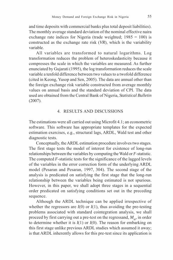
First, the ADF unit test is applied on the regressand, Mdt for stationarity.The test is applied to both the original series (in log form) at level, andto the first difference. The results reported in Table 1 indicate that Mdtis non-stationary at level; that it is a random walk series. Mdt becomesstationary after employing difference operator of degree one. Thismeans that the series is integrated of order one, I(1).

4.1.1 DISCUSSIONS

Having satisfied this first stage that the regressand is an I(1) series, weproceed to the second stage of testing for the existence of long-runrelationship between the variables by computing the Wald or F-statistic.

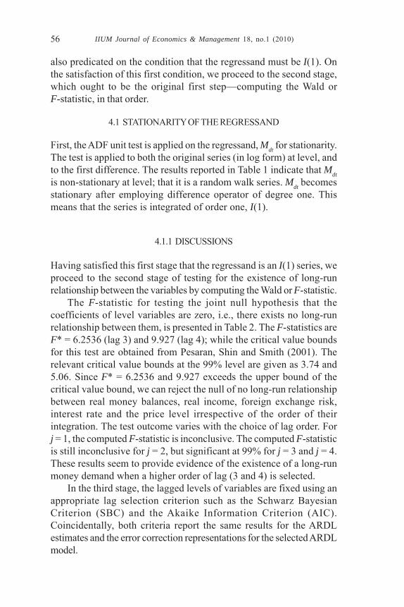
The F-statistic for testing the joint null hypothesis that thecoefficients of level variables are zero, i.e., there exists no long-runrelationship between them, is presented in Table 2. The F-statistics areF* = 6.2536 (lag 3) and 9.927 (lag 4); while the critical value boundsfor this test are obtained from Pesaran, Shin and Smith (2001). Therelevant critical value bounds at the 99% level are given as 3.74 and5.06. Since F* = 6.2536 and 9.927 exceeds the upper bound of thecritical value bound, we can reject the null of no long-run relationshipbetween real money balances, real income, foreign exchange risk,interest rate and the price level irrespective of the order of theirintegration. The test outcome varies with the choice of lag order. Forj = 1, the computed F-statistic is inconclusive. The computed F-statisticis still inconclusive for j = 2, but significant at 99% for j = 3 and j = 4.These results seem to provide evidence of the existence of a long-runmoney demand when a higher order of lag (3 and 4) is selected.

In the third stage, the lagged levels of variables are fixed using anappropriate lag selection criterion such as the Schwarz BayesianCriterion (SBC) and the Akaike Information Criterion (AIC).Coincidentally, both criteria report the same results for the ARDLestimates and the error correction representations for the selected ARDLmodel.


The long-run coefficient estimates are reported in Table 3. It shouldalso be noted that the estimated coefficients obtained from all threemodel selection criteria (SBC, AIC and the Hannan-Quinn Criterion;HQC) are similar. Although the scale variable (income) is rightly signed,all the regressors are not statistically significant in Equation (1).Consequently, we proceeded to estimate Equations (5) and (6).

TABLE 2F-Statistics for Testing the Existence of a Long-Run

Money Demand Equation

Notes: The relevant critical value bounds are given in Table 1.iii (with an unrestrictedintercept and no trend; number of regressors = 4), Pesaran, Shin and Smith(2001). They are 2.86 and 4.01 at the 95% significance level and 3.74 and 5.06at the 99% significance level.*denotes that the F-statistic falls above the 99% upper bound.

Order of lag F-statistic 1 2.0068

2 3.1157

3 6.2536*

4 9.9270*

TABLE 1Augmented Dickey-Fuller (ADF) Test of Stationarity of Mdt

Notes: Regression includes an intercept but not a trend.The 95% critical value for the augmented Dickey-Fuller statistic = -2.9627.Δ shows first difference.

Lag Variable Test Statistic Variable Lag Test

Statistic

DF Mdt -1.2514 ΔMdt DF -3.4861

ADF(1) Mdt -1.9483 ΔMdt ADF(1) -3.5883


Dep

ende

nt V

aria

ble

is M

dt

M

odel

with

out d

umm

y va

riabl

e M

odel

with

dum

my

varia

ble

Re

gres

sor

Coef

ficie

nt

t-rat

io

(Pro

b)C

oeff

icie

nt

t-rat

io

(Pro

b)

Y

1.53

50

1.23

67

(0.2

28)

0.54

95

0.59

78

(0.5

55)

VR

- 0

.021

8 - 0

.982

7 (0

.335

)- 0

.014

8 - 0

.729

8 (0

.472

)

R 0.

2213

0.

4593

(0

.650

)0.

255

0.48

66

(0.6

31)

P

- 0.0

633

- 0.3

944

(0.6

97)

0.09

76

0.66

69

(0.5

11)

IN

PT

- 2.0

898

- 0.5

741

(0.5

71)

0.53

39

0.19

33

(0.8

48)

D

- 0

.279

0 - 1

.066

9

(0.2

961)

TAB

LE 3

Estim

ated

Lon

g-R

un C

oeff

icie

nts u

sing

the A

RD

L A

ppro

ach

AR

DL

(2, 1

, 0, 0

, 1) s

elec

ted

base

d on

Han

nan-

Qui

nn C

riter

ion

(Equ

atio

n 1)


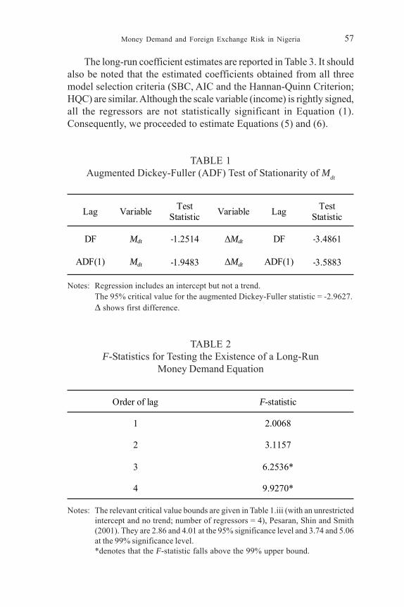
Dependent variable is ΔMdt

Model without dummy Model with dummy

Regressor Coefficient t-ratio (Prob)

Coefficient t-ratio (Prob)

ΔMdt-1 0.2734 1.7334

(0.094) 0.3347 2.018

(0.054)

ΔY - 0.0506 - 0.0576 (0.054)

- 0.0913 2.002 (0.06)

ΔVR - 0.0034 - 1.3769

(0.180) - 0.0025 - 0.938

(0.357)

ΔR 0.0345 0.4701 (0.642)

0.0424 0.481 (0.634)

ΔP - 0.4850 - 2.6891

(0.012) - 0.3747 - 2.087

(0.047)

INPT - 0.3260 - 0.6420 (0.526)

0.0887 0.188 (0.853)

D - 0.4633 - 0.998

(0.327)

ECM(-1) - 0.1560 -2.2827 (0.031)

- 0.1661 - 2.192 (0.038)

Diagnostic statistics

DW-statistic 2.0331 2.1585

Adj-R2 0.4386 0.3897

F-Statistic 5.6311 (0.001)

4.1533 (0.003)

AIC 49.4126 47.9919

SBC 42.5439 41.1233

TABLE 4Error Correction Representation for the Selected ARDL Model

ARDL (2, 1, 0, 0, 1) selected based on Hannan-Quinn


The estimates of Equations (5) and (6), which are the error-correction representations selected by AIC and SBC (with a maximumlag order set at 3) are presented in Table 4. Some of the major findingsof this paper which can augment our understanding of money demandin Nigeria are summarized below. First, it is plausible to imply thatceteris paribus the short-run income elasticity is significantly greaterthan zero in both models but less than unity, consistent with economictheory. An income elasticity of less than unity has some implicationsfor monetary policy. As cited in Valadkhani (2008:80), Ball (2001:36)concludes that such β1 < 1, will make the Friedman rule pseudo-optimaland therefore the supply of money should grow more sluggishly thanoutput in order to achieve the goal of price stability. Second, inflationhas an immediate and relatively larger effect on the demand for moneyin the short-run. The inflation variable is significant and negatively signedas expected a priori. Rising inflation, ceteris paribus, encourages agentsto diversify their portfolios in the economy by acquiring real assets(Valadkhani, 2008), other financial assets and maybe foreign currenciesas substitutes.

The foreign exchange rate variability variable which is a measureof foreign exchange risk enters insignificantly into the equation withthe estimated parameter negatively signed. This may imply that foreignexchange risk is probably not an important determinant in the explanationof real money demand behavior in the case of Nigeria. This resultfurther confirms the Omotor and Orubu (2003) study using standardregression methods which equally do not take into cognizance the timeseries properties of the variables. The Nigerian case on the role ofexchange rate risk in money demand determination is at variance withthe German experience as hypothesized by Akhtar and Putnam (1980).

The long-run coefficients reported in Table 3 are used to generatethe error correction terms. The adjusted coefficients of determinationfor the two models—Equations (5) and (6), respectively—at 0.44 and0.39 are fairly high which may suggest fair fit error correction modelsof the data. The computed F-statistics clearly reject the null hypothesesthat all the regressors have zero coefficients for all cases. Significantas well is the error correction coefficient which carried an expectednegative sign and highly significant at over 95% level in both cases.This reinforces the finding of cointegration relationship in the long-runmodel for money demand. The larger the error correction coefficient(in absolute value) the faster is the economy’s return to its equilibrium


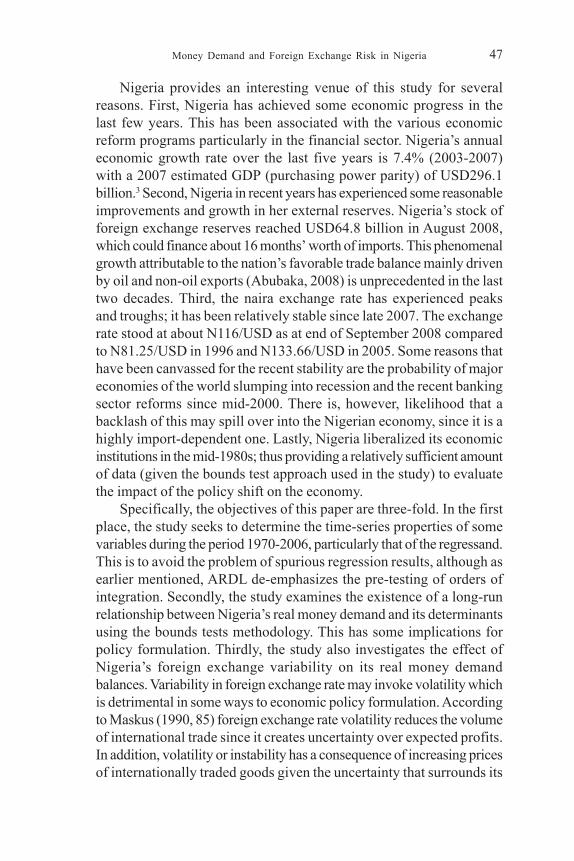
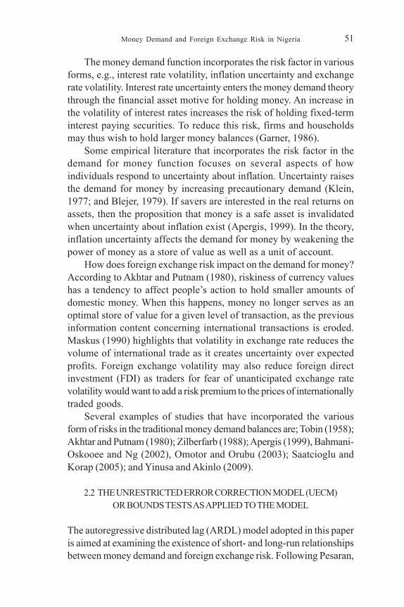
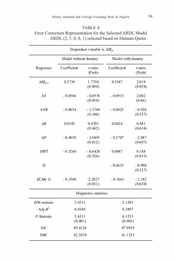
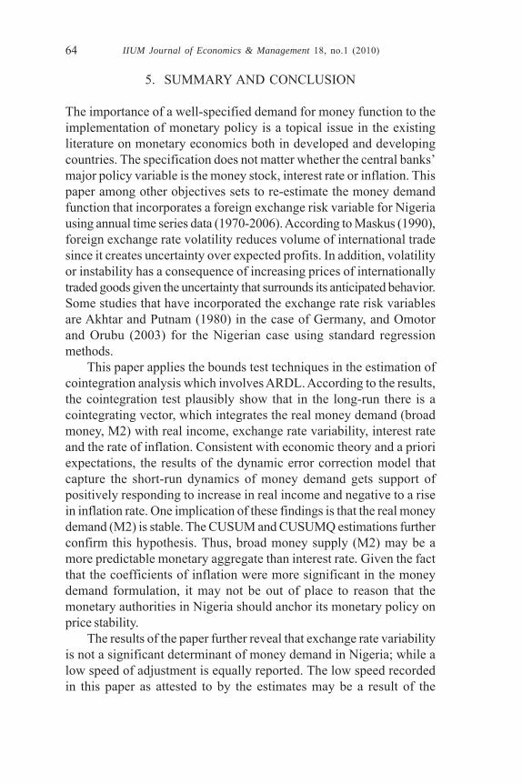
The straight lines represent critical bounds at 5% significance level

-5 -10 -15

0 5

10 15

1973 1978 1983 1988 1993 1998 2003 2006

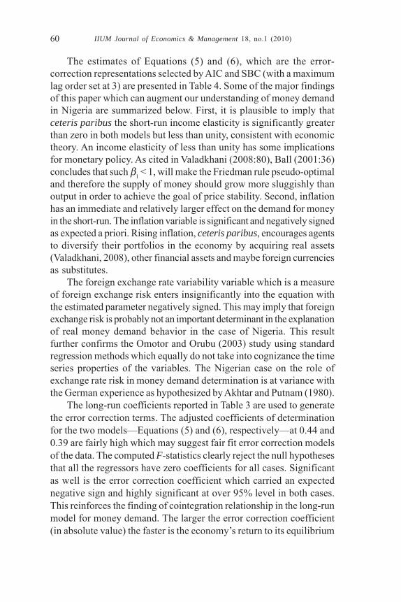
FIGURE 1CUSUM for the model without the SAP dummy

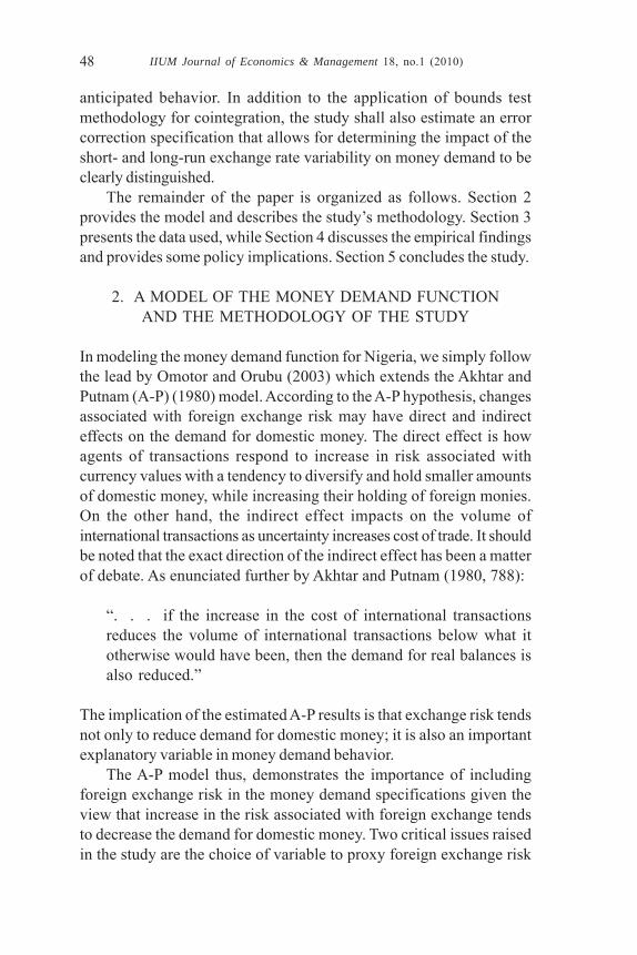
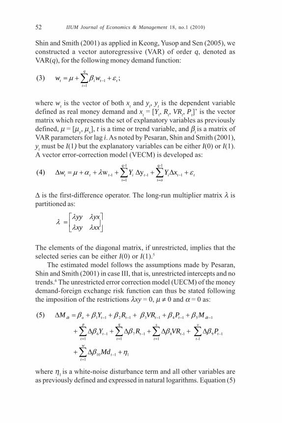
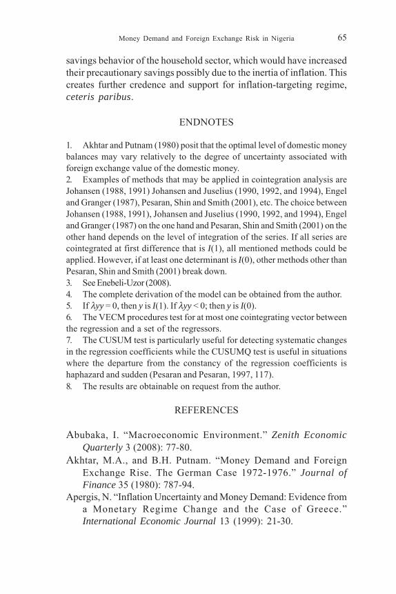
The straight lines represent critical bounds at 5% significance level -0.5 0.0 0.5 1.0 1.5

1973 1978 1983 1988 1993 1998 2003 2006

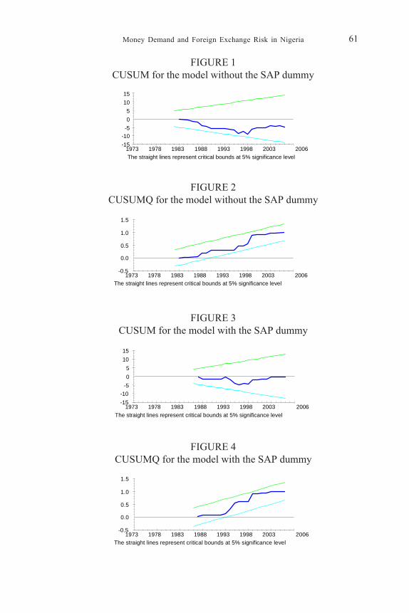
FIGURE 2CUSUMQ for the model without the SAP dummy

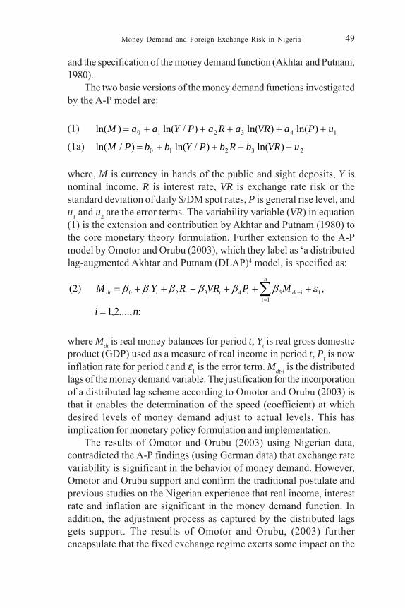
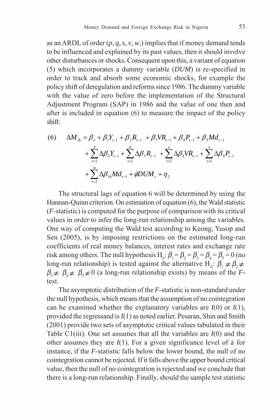
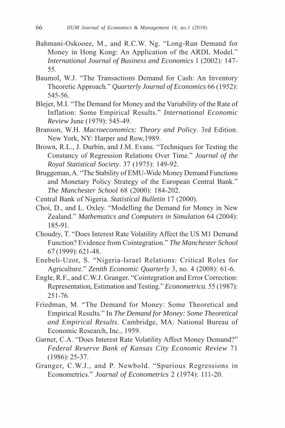
The straight lines represent critical bounds at 5% significance level

-5 -10 -15

0 5

10 15

1973 1978 1983 1988 1993 1998 2003 2006

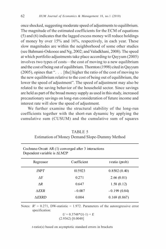
FIGURE 3CUSUM for the model with the SAP dummy

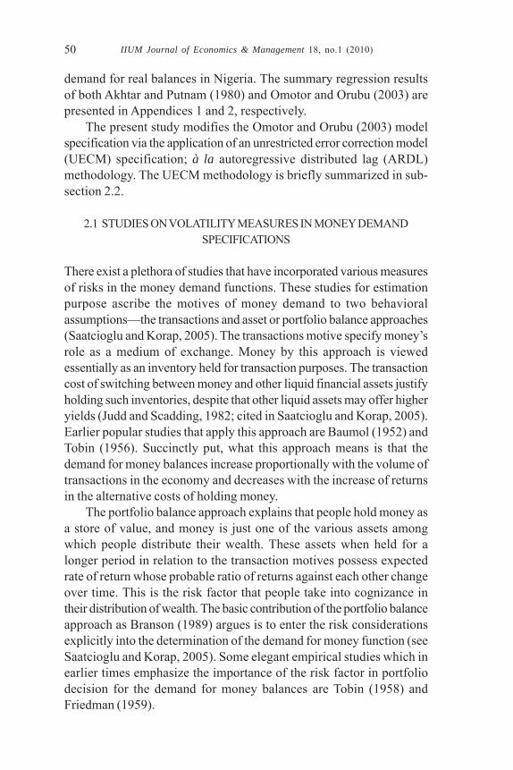
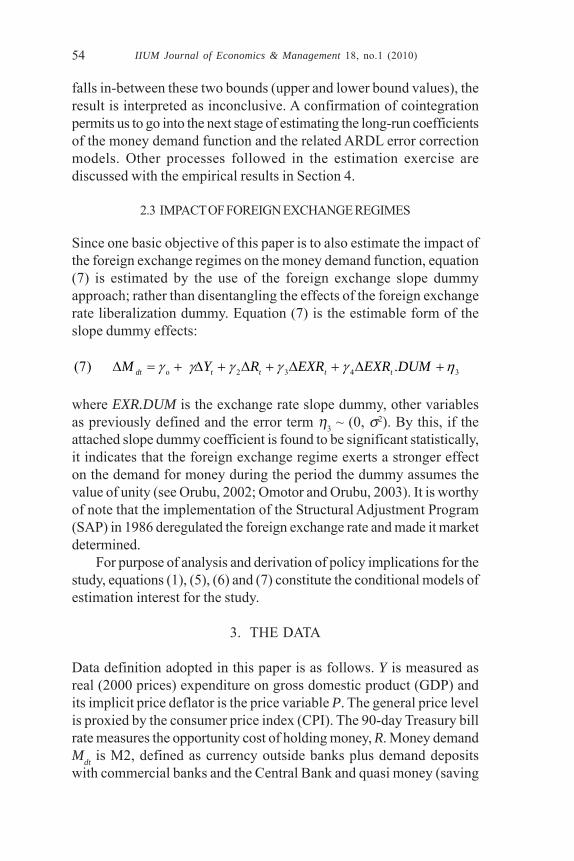
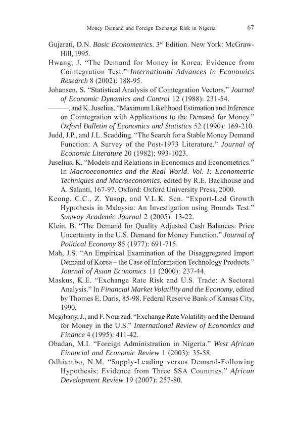
The straight lines represent critical bounds at 5% significance level -0.5 0.0 0.5 1.0 1.5

1973 1978 1983 1988 1993 1998 2003 2006

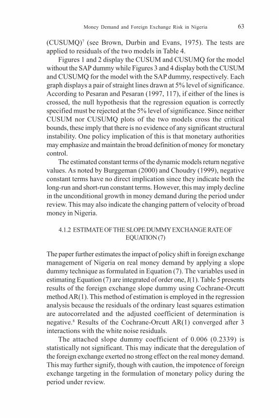
FIGURE 4CUSUMQ for the model with the SAP dummy


once shocked, suggesting moderate speed of adjustments to equilibrium.The magnitude of the estimated coefficients for the ECM of equations(5) and (6) indicates that the lagged excess money will reduce holdingsof money by over 15% and 16%, respectively, in each year. Theseslow magnitudes are within the neighborhood of some other studies(see Bahmani-Oskooee and Ng, 2002; and Valadkhani, 2008). The speedat which portfolio adjustments take place according to Qayyum (2005)involves two types of costs—the cost of moving to a new equilibriumand the cost of being out of equilibrium. Thornton (1998) cited in Qayyum(2005), opines that “. . . [the] higher the ratio of the cost of moving tothe new equilibrium relative to the cost of being out of equilibrium, thelower the speed of adjustment”. The speed of adjustment may also berelated to the saving behavior of the household sector. Since savingsare held as part of the broad money supply as used in this study, increasedprecautionary savings on long-run consideration of future income andinterest rate will slow the speed of adjustment.

We further examine the structural stability of the long-runcoefficients together with the short-run dynamic by applying thecumulative sum (CUSUM) and the cumulative sum of squares

Cochrane-Orcutt AR (1) converged after 3 interactions Dependent variable is ΔLM2P

Regressor Coefficient t-ratio (prob)

INPT 015923 0.8502 (0.40)

ΔY 0.271 2.66 (0.01)

ΔR 0.647 1.58 (0.12)

ΔEXR - 0.007 - 0.199 (0.84)

ΔEXRD 0.004 0.169 (0.867)

TABLE 5Estimation of Money Demand Slope-Dummy Method

Notes: R2 = 0.271, DW-statistic = 1.972. Parameters of the autoregressive errorspecification:

U = 0.3748*U(-1) + E (2.9362) [0.0048]

t-ratio(s) based on asymptotic standard errors in brackets


(CUSUMQ)7 (see Brown, Durbin and Evans, 1975). The tests areapplied to residuals of the two models in Table 4.

Figures 1 and 2 display the CUSUM and CUSUMQ for the modelwithout the SAP dummy while Figures 3 and 4 display both the CUSUMand CUSUMQ for the model with the SAP dummy, respectively. Eachgraph displays a pair of straight lines drawn at 5% level of significance.According to Pesaran and Pesaran (1997, 117), if either of the lines iscrossed, the null hypothesis that the regression equation is correctlyspecified must be rejected at the 5% level of significance. Since neitherCUSUM nor CUSUMQ plots of the two models cross the criticalbounds, these imply that there is no evidence of any significant structuralinstability. One policy implication of this is that monetary authoritiesmay emphasize and maintain the broad definition of money for monetarycontrol.

The estimated constant terms of the dynamic models return negativevalues. As noted by Burggeman (2000) and Choudry (1999), negativeconstant terms have no direct implication since they indicate both thelong-run and short-run constant terms. However, this may imply declinein the unconditional growth in money demand during the period underreview. This may also indicate the changing pattern of velocity of broadmoney in Nigeria.

4.1.2 ESTIMATE OF THE SLOPE DUMMY EXCHANGE RATE OFEQUATION (7)

The paper further estimates the impact of policy shift in foreign exchangemanagement of Nigeria on real money demand by applying a slopedummy technique as formulated in Equation (7). The variables used inestimating Equation (7) are integrated of order one, I(1). Table 5 presentsresults of the foreign exchange slope dummy using Cochrane-Orcuttmethod AR(1). This method of estimation is employed in the regressionanalysis because the residuals of the ordinary least squares estimationare autocorrelated and the adjusted coefficient of determination isnegative.8 Results of the Cochrane-Orcutt AR(1) converged after 3interactions with the white noise residuals.

The attached slope dummy coefficient of 0.006 (0.2339) isstatistically not significant. This may indicate that the deregulation ofthe foreign exchange exerted no strong effect on the real money demand.This may further signify, though with caution, the impotence of foreignexchange targeting in the formulation of monetary policy during theperiod under review.


5. SUMMARY AND CONCLUSION

The importance of a well-specified demand for money function to theimplementation of monetary policy is a topical issue in the existingliterature on monetary economics both in developed and developingcountries. The specification does not matter whether the central banks’major policy variable is the money stock, interest rate or inflation. Thispaper among other objectives sets to re-estimate the money demandfunction that incorporates a foreign exchange risk variable for Nigeriausing annual time series data (1970-2006). According to Maskus (1990),foreign exchange rate volatility reduces volume of international tradesince it creates uncertainty over expected profits. In addition, volatilityor instability has a consequence of increasing prices of internationallytraded goods given the uncertainty that surrounds its anticipated behavior.Some studies that have incorporated the exchange rate risk variablesare Akhtar and Putnam (1980) in the case of Germany, and Omotorand Orubu (2003) for the Nigerian case using standard regressionmethods.

This paper applies the bounds test techniques in the estimation ofcointegration analysis which involves ARDL. According to the results,the cointegration test plausibly show that in the long-run there is acointegrating vector, which integrates the real money demand (broadmoney, M2) with real income, exchange rate variability, interest rateand the rate of inflation. Consistent with economic theory and a prioriexpectations, the results of the dynamic error correction model thatcapture the short-run dynamics of money demand gets support ofpositively responding to increase in real income and negative to a risein inflation rate. One implication of these findings is that the real moneydemand (M2) is stable. The CUSUM and CUSUMQ estimations furtherconfirm this hypothesis. Thus, broad money supply (M2) may be amore predictable monetary aggregate than interest rate. Given the factthat the coefficients of inflation were more significant in the moneydemand formulation, it may not be out of place to reason that themonetary authorities in Nigeria should anchor its monetary policy onprice stability.

The results of the paper further reveal that exchange rate variabilityis not a significant determinant of money demand in Nigeria; while alow speed of adjustment is equally reported. The low speed recordedin this paper as attested to by the estimates may be a result of the


savings behavior of the household sector, which would have increasedtheir precautionary savings possibly due to the inertia of inflation. Thiscreates further credence and support for inflation-targeting regime,ceteris paribus.

ENDNOTES

1. Akhtar and Putnam (1980) posit that the optimal level of domestic moneybalances may vary relatively to the degree of uncertainty associated withforeign exchange value of the domestic money.2. Examples of methods that may be applied in cointegration analysis areJohansen (1988, 1991) Johansen and Juselius (1990, 1992, and 1994), Engeland Granger (1987), Pesaran, Shin and Smith (2001), etc. The choice betweenJohansen (1988, 1991), Johansen and Juselius (1990, 1992, and 1994), Engeland Granger (1987) on the one hand and Pesaran, Shin and Smith (2001) on theother hand depends on the level of integration of the series. If all series arecointegrated at first difference that is I(1), all mentioned methods could beapplied. However, if at least one determinant is I(0), other methods other thanPesaran, Shin and Smith (2001) break down.3. See Enebeli-Uzor (2008).4. The complete derivation of the model can be obtained from the author.5. If λyy = 0, then y is I(1). If λyy < 0; then y is I(0).6. The VECM procedures test for at most one cointegrating vector betweenthe regression and a set of the regressors.7. The CUSUM test is particularly useful for detecting systematic changesin the regression coefficients while the CUSUMQ test is useful in situationswhere the departure from the constancy of the regression coefficients ishaphazard and sudden (Pesaran and Pesaran, 1997, 117).8. The results are obtainable on request from the author.

REFERENCES

Abubaka, I. “Macroeconomic Environment.” Zenith EconomicQuarterly 3 (2008): 77-80.

Akhtar, M.A., and B.H. Putnam. “Money Demand and ForeignExchange Rise. The German Case 1972-1976.” Journal ofFinance 35 (1980): 787-94.

Apergis, N. “Inflation Uncertainty and Money Demand: Evidence froma Monetary Regime Change and the Case of Greece.”International Economic Journal 13 (1999): 21-30.


Bahmani-Oskooee, M., and R.C.W. Ng. “Long-Run Demand forMoney in Hong Kong: An Application of the ARDL Model.”International Journal of Business and Economics 1 (2002): 147-55.

Baumol, W.J. “The Transactions Demand for Cash: An InventoryTheoretic Approach.” Quarterly Journal of Economics 66 (1952):545-56.

Blejer, M.I. “The Demand for Money and the Variability of the Rate ofInflation: Some Empirical Results.” International EconomicReview June (1979): 545-49.

Branson, W.H. Macroeconomics: Theory and Policy. 3rd Edition.New York, NY: Harper and Row,1989.

Brown, R.L., J. Durbin, and J.M. Evans. “Techniques for Testing theConstancy of Regression Relations Over Time.” Journal of theRoyal Statistical Society. 37 (1975): 149-92.

Bruggeman, A. “The Stability of EMU-Wide Money Demand Functionsand Monetary Policy Strategy of the European Central Bank.”The Manchester School 68 (2000): 184-202.

Central Bank of Nigeria. Statistical Bulletin 17 (2000).Choi, D., and L. Oxley. “Modelling the Demand for Money in New

Zealand.” Mathematics and Computers in Simulation 64 (2004):185-91.

Choudry, T. “Does Interest Rate Volatility Affect the US M1 DemandFunction? Evidence from Cointegration.” The Manchester School67 (1999): 621-48.

Enebeli-Uzor, S. “Nigeria-Israel Relations: Critical Roles forAgriculture.” Zenith Economic Quarterly 3, no. 4 (2008): 61-6.

Engle, R.F., and C.W.J. Granger. “Cointegration and Error Correction:Representation, Estimation and Testing.” Econometrica. 55 (1987):251-76.

Friedman, M. “The Demand for Money: Some Theoretical andEmpirical Results.” In The Demand for Money: Some Theoreticaland Empirical Results. Cambridge, MA: National Bureau ofEconomic Research, Inc., 1959.

Garner, C.A. “Does Interest Rate Volatility Affect Money Demand?”Federal Reserve Bank of Kansas City Economic Review 71(1986): 25-37.

Granger, C.W.J., and P. Newbold. “Spurious Regressions inEconometrics.” Journal of Econometrics 2 (1974): 111-20.


Gujarati, D.N. Basic Econometrics. 3rd Edition. New York: McGraw-Hill, 1995.

Hwang, J. “The Demand for Money in Korea: Evidence fromCointegration Test.” International Advances in EconomicsResearch 8 (2002): 188-95.

Johansen, S. “Statistical Analysis of Cointegration Vectors.” Journalof Economic Dynamics and Control 12 (1988): 231-54.

———, and K. Juselius. “Maximum Likelihood Estimation and Inferenceon Cointegration with Applications to the Demand for Money.”Oxford Bulletin of Economics and Statistics 52 (1990): 169-210.

Judd, J.P., and J.L. Scadding. “The Search for a Stable Money DemandFunction: A Survey of the Post-1973 Literature.” Journal ofEconomic Literature 20 (1982): 993-1023.

Juselius, K. “Models and Relations in Economics and Econometrics.”In Macroeconomics and the Real World. Vol. I: EconometricTechniques and Macroeconomics, edited by R.E. Backhouse andA. Salanti, 167-97. Oxford: Oxford University Press, 2000.

Keong, C.C., Z. Yusop, and V.L.K. Sen. “Export-Led GrowthHypothesis in Malaysia: An Investigation using Bounds Test.”Sunway Academic Journal 2 (2005): 13-22.

Klein, B. “The Demand for Quality Adjusted Cash Balances: PriceUncertainty in the U.S. Demand for Money Function.” Journal ofPolitical Economy 85 (1977): 691-715.

Mah, J.S. “An Empirical Examination of the Disaggregated ImportDemand of Korea – the Case of Information Technology Products.”Journal of Asian Economics 11 (2000): 237-44.

Maskus, K.E. “Exchange Rate Risk and U.S. Trade: A SectoralAnalysis.” In Financial Market Volatility and the Economy, editedby Thomes E. Daris, 85-98. Federal Reserve Bank of Kansas City,1990.

Mcgibany, J., and F. Nourzad. “Exchange Rate Volatility and the Demandfor Money in the U.S.” International Review of Economics andFinance 4 (1995): 411-42.

Obadan, M.I. “Foreign Administration in Nigeria.” West AfricanFinancial and Economic Review 1 (2003): 35-58.

Odhiambo, N.M. “Supply-Leading versus Demand-FollowingHypothesis: Evidence from Three SSA Countries.” AfricanDevelopment Review 19 (2007): 257-80.


Omotor, D.G., and C.O. Orubu. “Money Demand and Foreign ExchangeRisk: The Nigerian Case.” The Nigerian Economic and FinancialReview 8 (2003): 33-50.

Onu, E. “Money and Markets: 46 Years of Nationhood.” The NigerianDaily Independent (2006).

Pesaran, M.H., and Pesaran, B. Working with Microfit 4.0:Interactive Econometric Analysis. England: Comfit Data Limited,1997.

Pesaran, M.H., and Y. Shin. “Generalised Impulse Response Analysisin Linear Multivariate Models.” Economics Letters 58 (1998): 17-29.

Pesaran, M.H., Y. Shin, and R.J. Smith. “Bounds Testing Approachesto the Analysis of Long-Run Relationship.” Journal of AppliedEconometrics 16 (2001): 289-326.

Qayyum, A. “Modelling the Demand for Money in Pakistan.” ThePakistan Development Review 44 (2005): 233-52.

Saatcioglu C., and H.L. Korap. “The Turkish Broad Money Demand.”Istanbul Ticaret Üniversitesi Sosyal Bilimler Dergisi 4 (2005):139-65.

Thornton, D.L. Why Does Velocity Matter? Federal Reserve Bank ofSt. Louis, 1983.

Tobin, J. “The Interest-Elasticity of Transactions Demand for Cash.”Review of Economics and Statistics 38 (1956): 241-47.

———. “Liquidity Preference as Behavior Towards Risks.” Review ofEconomics, August (1958): 65-86.

Valadkhani, A. “Long- and Short-Run Determinants of the Demandfor Money in the Asian-Pacific Countries: An Empirical PanelInvestigation.” Annuals of Economics and Finance 9 (2008): 77-90.

Ventura, J.P. “Money Demand and Inflation in Peru, 1979-1991.”Federal Reserve Bank of Cleveland Economic Commentary,December (2000).

Yinusa, D.O., and A.E. Akinlo. “Exchange Rate Volatility and the Extentof Currency Substitution. MPRA Paper No. 16251 (2009).

Zilberfarb, B. “The Effects of Foreign Exchange Risk and Return onDemand for Domestic Balances.” European Economic Review32 (1988): 1359-68.


APP

END

IX 1

Sum

mar

y R

esul

ts o

f the

A-P

Reg

ress

ion

St

anda

rd

Erro

r A

djus

ted

R-Sq

uare

d D

urbi

n W

atso

n

P.

V.

r.

PY.

.M

ln

251ln

020

002

20

ln041

917

lnA

+−

− ⎟ ⎠⎞⎜ ⎝⎛

+−

=

(?2

.59)

(1

.95)

(?2.

33)

(?

1.90

)

(8.

450)

0.

0368

0.

95

2.27

V.

r.

PY.

.PM

ln

021

002

40

ln721

266

lnB

−− ⎟ ⎠⎞

⎜ ⎝⎛+

−=

⎟ ⎠⎞⎜ ⎝⎛

(?2

.17)

(4

.76)

(?2.

50)

(?1

.84)

0.

068

0.64

1.

80

V.

r.

Y.

.PM

ln

021

002

70

ln841

407

lnC

−−

+−

=⎟ ⎠⎞

⎜ ⎝⎛

(?

2.95

) (4

.95)

(?

2.94

) (?1

.93)

0.

0359

0.

65

2.40

V.

r.

Y.

.PM

e

ln02

10

240

ln831

607

lnD

−−

+−

=⎟ ⎠⎞

⎜ ⎝⎛

(?

2.76

) (4

.85)

(?2.

82)

(-1

.88)

0.

0368

0.

64

1.80

V.

r .

PY.

PY.

.PM

ln

021

002

80

ln73

0ln

071147

lnE

*

−−

⎟ ⎠⎞⎜ ⎝⎛

+ ⎟ ⎠⎞⎜ ⎝⎛

+−

=⎟ ⎠⎞

⎜ ⎝⎛

(?3

.10)

(2

.17)

(

1.80

)

(?

3.04

)

(?2.

00)

0.03

4 0.

75

2.35


APPENDIX 2Summary Results of the Estimated Regression Models of Omotor-

Orubu Dependent Variable: Log of Broad Money Supply

A

Variable Coefficient Std. Error t-statistic Prob c -1.43 1.33 -1.07 0.27 ly 0.76 0.18 4.03 0.00 t -0.06 0.02 -4079 0.00

lv -0.04 0.03 -1.13 0.27 lvp 0.03 0.07 0.41 0.69 lcpi 1.52 0.11 13.52 0.00

R2 0.98

S.E. 0.17 D-W 1.31 F* 222

B

Variable Coefficient Std. Error t-statistic Prob c 0.54 2.09 0.26 0.80 ly 0.73 0.31 2.31 0.03 r -0.00 0.01 0.00 0.99 w -0.04 0.05 0.68 0.50

R2 0.13 S.E. 0.29 D-W 0.35 F* 2.06

C

Variable Coefficient Std. Error t-statistic Prob c -1.52 1.28 -1.18 0.25 ly - 0.76 0.18 4.13 0.00 r - 0.06 0.01 -4.45 0.00

lgv - 0.04 0.03 -1.19 0.25 lcpi 1.54 0.09 16.37 0.00

R2 0.98

S.E. 0.17 D-W 1.42 F* 292


APPENDIX 2 (continued)Summary Results of the Estimated Regression Models of Omotor-


D

Variable Coefficient Std. Err. t-statistic Prob c -1.83 1.48 -1.23 0.24 ly 0.51 0.20 2.48 0.02 r -0.01 0.02 -0.45 0.65 lv -0.02 0.02 -0.92 0.37 lvp 0.04 0.04 1.03 0.37 lcpi 0.59 0.22 -2.62 0.02

lm2t-1 0.56 0.26 2.16 0.05 lm2t-1 0.09 0.19 0.48 0.63

R2 0.80

S.E. 0.09 D-W 2.21 F* 12.13

E

Variable Coefficient Std. Err. t-statistic Prob c -1.57 1.35 -1.16 0.26

lny 0.47 0.18 2.639 0.02 r -0.00 0.01 -0.34 0.74 lv -0.02 0.02 0.827 0.42

lgvp 0.04 0.04 1.986 0.34 lcpi -0.63 0.20 -3.14 0.01

lm2t-1 0.68 0.10 6.534 0.00

R2 0.916 S.E. 0.090 D-W 2.444

F* 32.170


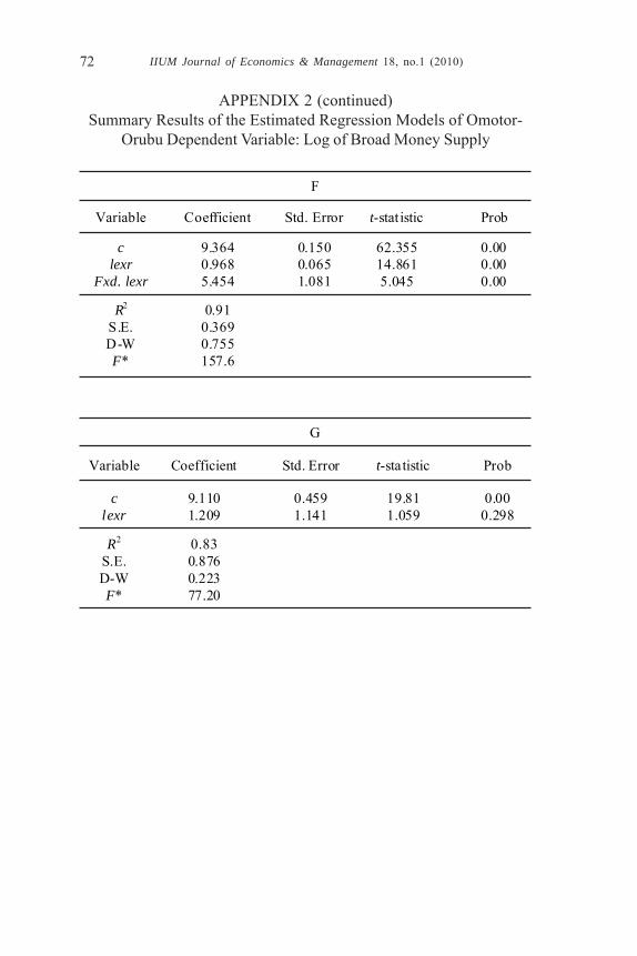
APPENDIX 2 (continued)Summary Results of the Estimated Regression Models of Omotor-


F

Variable Coefficient Std. Error t-stat istic Prob

c 9.364 0.150 62.355 0.00 lexr 0.968 0.065 14.861 0.00

Fxd. lexr 5.454 1.081 5.045 0.00

R2 0.91 S.E. 0.369 D-W 0.755 F* 157.6

G

Variable Coefficient Std. Error t-statistic Prob c 9.110 0.459 19.81 0.00

lexr 1.209 1.141 1.059 0.298

R2 0.83 S.E. 0.876 D-W 0.223 F* 77.20

money demand and foreign exchange risk in nigeria - IIUM ...

Documents

Transcript of money demand and foreign exchange risk in nigeria - IIUM ...