Flux Corrected Method: An accurate approach to fluid flow ...

Retrospective Theses and Dissertations

1997

Flux Corrected Method: An accurate approach tofluid flow modelingSutikno WirogoIowa State University

Follow this and additional works at: http://lib.dr.iastate.edu/rtd

Part of the Aerospace Engineering Commons

This Dissertation is brought to you for free and open access by Digital Repository @ Iowa State University. It has been accepted for inclusion inRetrospective Theses and Dissertations by an authorized administrator of Digital Repository @ Iowa State University. For more information, pleasecontact [email protected].

Recommended CitationWirogo, Sutikno, "Flux Corrected Method: An accurate approach to fluid flow modeling " (1997). Retrospective Theses andDissertations. Paper 12257.

http://lib.dr.iastate.edu/?utm_source=lib.dr.iastate.edu%2Frtd%2F12257&utm_medium=PDF&utm_campaign=PDFCoverPages

http://lib.dr.iastate.edu/?utm_source=lib.dr.iastate.edu%2Frtd%2F12257&utm_medium=PDF&utm_campaign=PDFCoverPages

http://lib.dr.iastate.edu/rtd?utm_source=lib.dr.iastate.edu%2Frtd%2F12257&utm_medium=PDF&utm_campaign=PDFCoverPages

http://lib.dr.iastate.edu/rtd?utm_source=lib.dr.iastate.edu%2Frtd%2F12257&utm_medium=PDF&utm_campaign=PDFCoverPages

http://network.bepress.com/hgg/discipline/218?utm_source=lib.dr.iastate.edu%2Frtd%2F12257&utm_medium=PDF&utm_campaign=PDFCoverPages

http://lib.dr.iastate.edu/rtd/12257?utm_source=lib.dr.iastate.edu%2Frtd%2F12257&utm_medium=PDF&utm_campaign=PDFCoverPages

mailto:[email protected]

INFORMATION TO USERS

This manuscript has been reproduced from the microfihn master. UMI

films the text directly from the original or copy submitted. Thus, some

thesis and dissertation copies are in typewriter &ce, while others may be

from ai^ of computer printer.

The quality of this reproduction is dependent upon the quality of the

copy submitted. Broken or indistinct print, colored or poor quality

illustrations and photographs, print bleedthrough, substandard margins,

and improper alignment can adversely afreet reproductioiL

In the unlikely event that the author did not send UMI a complete

manuscript and there are missing pages, these will be noted. Also, if

unauthorized copyright material had to be removed, a note will indicate

the deletion.

Oversize materials (e.g., m^s, drawings, charts) are reproduced by

sectioning the original, beginning at the upper left-hand comer and

continuing from left to right in equal sections with small overiaps. Each

original is also photographed in one exposure and is included in reduced

form at the back of the book.

Photographs included in the original manuscript have been reproduced

xerographically in this copy. Higher quality 6" x 9" black and white

photographic prints are available for any photographs or illustrations

appearing m this copy for an additional charge. Contact UMI directly to

order.

UMI A BeU & Howell Infonnation Company

300 North Zed) Road, Axm Aibor MI 48106-1346 USA 313/761-4700 800/521-0600

Flux Corrected Method:

An accurate approach to fluid flow modeling

by

Sutikno Wirogo

A dissertation submitted to the graduate faculty

in partial fulfillment of the requirements for the degree of

DOCTOR OF PHILOSOPHY

Major: Aerospace Engineering

Major Professor: Ganesh Rajagopalan

Iowa State University

Ames, Iowa

1997

Copyright © Sutikno Wirogo, 1997. All rights reserved.

DMI Number; 9737770

Copyright 1997 by Wirogo, Sutikno

All rights reserved.

UMI Microform 9737770 Copyright 1997, by UMI Company. All rights reserved.

This microform edition is protected against miauthorized copying mider Title 17, United States Code.

UMI 300 North Zeeb Road Ann Arbor, MI 48103

11

Graduate College Iowa State University

This is to certify that the Doctoral dissertation of

Sutikno Wirogo

has met the dissertation requirements of Iowa State University

For the Graduate CoUege

Signature was redacted for privacy.



iii

TABLE OF CONTENTS

NOMENCLATURE xvi

ACKNOWLEDGEMENTS xvii

1 INTRODUCTION 1

1.1 Convection and Diffusion Transport Mechanisms 1

1.2 Previous Approaches in the Modeling of Convection and Diffusion .... .3

1.2.1 Central-Difference 3

1.2.2 Upwind Scheme 4

1.2.3 Skew Upwind Differencing Scheme 6

1.2.4 Third Order Upstream Weighted Scheme (QUICK) 7

1.2.5 ExponentiaJ Difference Scheme (EDS) 11

1.2.6 Locally Analytic Differencing Scheme (LOADS) 15

1.2.7 Flux Spline Scheme 16

1.3 Modeling of Convection Diffusion Problem 17

1.3.1 High Convection Flow Oblique to the Grid 19

1.3.2 High Cross-flow Gradient 21

1.3.3 Unsteady and Source Influence 22

1.3.4 Previous Approaches to the Overall Balance Principle 22

1.4 Current Work: Flux Corrected Method 23

2 THEORETICAL FORMULATION AND SOLUTION PROCEDURE 25

2.1 Governing Equations 25

iv

2.2 Methods for Solving Incompressible Flow Equations 2

2.3 Conservation Equations in Cartesiaji Coordinates 2

2.4 Integral Balance of Conservation Equations 3

2.4.1 Control Volume Approach 3

2.4.2 Time Integration

2.4.3 Integral Balance of Continuity Equation 3

2.4.4 Integral Balance of General Trainsport Equation 3

2.5 Modeling of the Convection and Diffusion Transport 3

2.5.1 Review of Basic Qualitative Characteristics 3

2.5.2 Steady One-dimensionai Convection Diffusion with Source .... 3

2.6 Flux Corrected Method: Application of Steady One-dimensional Con

vection Diffusion with Source to Two- and Three-dimensional Transport

Modeling 4

2.6.1 Discretization of General Transport Equation 4

2.6.2 Discretization of the x- and y-momentum Equations 4

2.7 Staggered Grid Arrangement 5

2.8 SIMPLER Algorithm 5

2.8.1 Pressure Equation 5

2.8.2 Correction Equations 51

2.8.3 Velocity Correction 59

2.8.4 Pressure Correction Equation 59

2.8.5 Solution Procedure for the Discretized Equations 60

2.8.6 SIMPLER Algorithm Summary 61

HANDLING THE SOURCE TERM 63

3.1 Effect of Pressure Gradients (Group B) 66

3.2 Effect of the Derivatives of the Non-directional TotaJ-fluxes (Group C) . 69

V

3.3 Effect of the Derivatives of the Directional Total-fluxes (Group D) . . . 72

3.4 Combined Effect of the Individual Source Components 72

3.5 Effect of Correction on Boundary Cells 76

3.6 Effect of Linear Source Profile 85

4 DEVELOPMENT OF GENERAL BOUNDARY FORMULATION

FOR PRESSURE EQUATION 91

4.1 Background 91

4.2 General Pressure Boundary Condition 95

4.2.1 Development of Genercil Pressure Boundary Equations 96

4.2.2 Case 1: Prescribed Boundary Normal Velocity with No Reference

Pressure 101

4.2.3 Case 2; Prescribed Boundary Normal Velocity with Reference

Pressure 109

4.2.4 Case 3: Prescribed Boundary Pressure 110

4.3 Implementation of General Pressure Boimdary in FCM 115

5 NUMERICAL VERIFICATION AND TESTING OF THE ALGO

RITHM 117

5.1 Two-dimensional Lid-Driven Cavity Flow IIS

5.1.1 Calculations for /?e=100 119

5.1.2 Calculations for /2e=400 122

0.1.3 Calculations for /?e=10G0 129

5.1.4 Calculations for i?e=10000 139

5.2 Grid Stretching 146

5.3 Convergence Characteristics and CPU Requirement 150

5.4 Unsteady Impulsively Started Lid-Driven Cavity 155

5.5 MultiGrid Technique on FCM 157

vi

5.6 Three-dimensional Lid-Driven Cavity Flow 164

5.7 Flow Over a Backward-Facing Step 166

5.8 Numerical Determination of the Accuracy of the Scheme 183

6 CONCLUSIONS AND RECOMMENDATIONS 190

APPENDIX A POWER LAW APPROXIMATION OF EXPONEN-

TLA.L SCHEME 194

APPENDIX B TABULATED VELOCITY COMPONENTS AND PRES

SURE DATA FOR THE LID-DRIVEN CAVITY PROBLEM. . . . 195

APPENDIX C TABULATED SEPARATION LENGTHS AND LO

CATIONS FOR THE LAMINAR BACKWARD-FACING STEP

FLOW 209

BIBLIOGRAPHY 211

vii

Table 5.1

Table B.l

Table B.2

Table B.3

Table B.4

Table B.5

Table B.6

Table B.7

Table B.8

Table B.9

Table B.IO

Table C.l

Table C.2

Table C.3

Table C.4

LIST OF TABLES

Multigrid performance of the Power Law scheme and FCM. . . . 163

Vertical centerline data for i2e=100 using 22x22 uniform grid. . . 195

Horizontal centerline data for i2e=100 using 22x22 uniform grid. 196

Vertical centerline data for /2e=400 using 22x22 uniform grid. . . 197

Horizontal centerline data for i?e=400 using 22x22 uniform grid. 198

Vertical centerline data for /?e=400 using 32x32 uniform grid. . . 199


Vertical centerline data for Re=1000 using 42x42 uniform grid. . 201


Vertical centerline data for /?e=1000 using 52x52 uniform grid. . 205

Horizontcd centerline data for i2e=1000 using 52x52 uniform grid. 207

Separation lengths and locations using FCM with 102x22 uniform

grid 209


grid 209


grid 210

Separation lengths and locations using Power Law with 102x42

uniform grid 210

viii

LIST OF FIGURES

Figure 1.1 QUICK three node parabolic profile S

Figure 1.2 One-dimensional convection-diffusion profile 12

Figure 1.3 Variation of A(Pe) as a function of Pe 13

Figure 1.4 Two-dimensional discretized domain IS

Figure 1.5 Diagram for possible approximation of <p6 20

Figure 2.1 Two-dimensional X-Y control-volume 33

Figure 2.2 Domain for one-dimensional convection-diffusion equation 37

Figure 2.3 Profile of 0 with 5ci=0 and different Peclet numbers 40

Figure 2.4 Profile of with Scd = 0.5 and different |Pe| 41

Figure 2.5 Middle interface value of </> as function of |Pe| 42

Figure 2.6 Profile of 4> with fixed |Pe| and different Scd 43

Figure 2.7 Variation of A{Pe) and B{Pe) as function of Pe 44

Figure 2.8 Staggered x-control-volume 56

Figure 3.1 Two-dimensional lid-driven cavity 65

Figure 3.2 Driven Cavity Re=400. Effect of using source Group B on the

vertical centerline u profile 67

Figure 3.3 Driven Cavity /2e=400. Effect of using source Group B on the

horizontal centerline v profile 67

Figure 3.4 Driven Cavity Re=400. Effect of using source Group B on the

vertical centerline P profile 68

ix

Figiire 3.5 Driven Cavity i?e=400. Effect of using source Group B on the

horizontal centerline P profile 68

Figure 3.6 Driven Cavity i2e=400. Effect of using source Group C on the

vertical centerline u profile 70

Figure 3.7 Driven Cavity i?e=400. Effect of using source Group C on the






Figure 3.10 Driven Cavity /?e=400. Effect of using source Group D on the

vertical u centerline profile 73

Figure 3.11 Driven Cavity /?e=400. Effect of using source Group D on the


Figure 3.12 Driven Cavity /2e=400. Effect of using source Group D on the


Figure 3.13 Driven Cavity /2e=400. Effect of using source Group D on the


Figure 3.14 Driven Cavity i?e=400. Effect of using combined source Group

B+C on the vertical centerline u profile 77

Figure 3.15 Driven Cavity /2e=400. Effect of using combined source Group

B+D on the vertical centerline u profile 77

Figure 3.16 Driven Cavity /?e=400. Effect of using combined source Group

B+C-f-D on the vertical centerline u profile 78


B+C on the horizontal centerline v profile 78

X


B+D on the horizontal centerline v profile 79

Figure 3.19 Driven Cavity i2e=400. Effect of using combined source Group

B+C+D on the horizontal centerline v profile 79

Figure 3.20 Driven Cavity Re=400. Effect of using combined source Group

B+C on the vertical centerline P profile 80

Figure 3.21 Driven Cavity i?e=400. Effect of using combined source Group

B+D on the vertical centerline P profile 80


B+C+D on the vertical centerline P profile 81


B+C on the horizontal centerline P profile 81

Figure 3.24 Driven Cavity /?e=400. Effect of using combined source Group

B+D on the horizontal centerline P profile 82


B+C+D on the horizontal centerline P profile 82

Figure 3.26 Driven Cavity Re=400. Effects of boundary cell corrections on

the vertical centerline u profile 87

Figure 3.27 Driven Cavity /2e=400. Effects of boundary cell corrections on

the horizontal centerline v profile 87

Figure 3.28 Driven Cavity i2e=400. Effects of boimdary cell corrections on

the vertical centerline P profile 88

Figure 3.29 Driven Cavity i2e=400. Effects of boundary cell corrections on

the horizontal centerline P profile 88

Figure 3.30 Driven Cavity i?e=400. Effects of linear source on the vertical

centerline u profile 89

xi

Figure 3.31 Driven Cavity /2e=400. Effects of linear source on the horizontal

centerline v profile 89

Figure 3.32 Driven Cavity i2e=400. Effects of linear source on the vertical

centerline P profile 90

Figure 3.33 Driven Cavity i?e=400. Effects of linear source on the horizontal

centerline P profile 90

Figure 4.1 X-direction grid with main and staggered control-volumes. ... 92

Figure 4.2 Two-dimensional channel flow with prescribed inlet velocity profile. 94

Figure 4.3 X-direction grid with shaded haJf-left boundary cell 96

Figure 4.4 Driven Cavity /?e=400 using 22x22 grid. Comparison of vertical

centerline pressure profile between original and general pressure

boundary formulation 106

Figure 4.5 Driven Cavity i?e=400 using 42x42 grid. Comparison of vertical

centerline pressure profile between original and general pressure


Figure 4.6 Driven Cavity Re=AQO using 22x22 grid. Comparison of cen

terline u and V profiles between original and general pressure


Figure 4.7 Driven Cavity Re=400 using 22x22 grid. Comparison of mass

convergence history between original and general pressure bound

ary formulation 107

Figure 4.8 Driven Cavity Re=400 using 22x22 grid. Comparison of x-momentum


ary formulation 108

xii

Figure 4.9 Driven Cavity i?e=400 using 22x22 grid. Comparison of u-velocity


ary formulation 108

Figure 4.10 Two-dimensional channel flow with prescribed inlet and outlet

pressure profiles 110

Figure 4.11 Comparison between exact and numerical u-velocity profile for

two-dimensional channel flow with i2e=100 and channel-width

W=l 113

Figure 4.12 Pressure distribution for two-dimensional channel flow with /2e=100

and channel-width W=1 113

Figure 4.13 Convergence history of velocity components for two-dimensional

channel flow with i?e=100 and channel-width W=l 114

Figure 4.14 Velocity vector plot for two-dimensional channel flow with Re=lOO

and channel-width 1^=1 114

Figure 4.15 Driven Cavity /?e=400 using 22x22 grid. Comparison between

original and general pressure boundary formulation applied to

FCM with boundary cell correction 116

Figure 5.1 Vertical centerline u-velocity profile for i?e=100 120

Figure 5.2 Horizontal centerline u-velocity profile for /2e=100 120

Figure 5.3 Vertical centerline pressure profile for /2e=100 121

Figure 5.4 Horizontal centerline pressure profile for i2e=100 121

Figure 5.5 Vertical centerline u-velocity profile for Re=400 123

Figure 5.6 Vertical centerline u-velocity profile for /2e=400 using finer grid. 123


Figure 5.8 Horizontal centerline u-velocity profile for i?e=400 using finer grid. 124

Figure 5.9 Vertical centerline pressure profile for /?e=400 125

xiii

Figiire 5.10 Horizontal centerline pressiire profile for i?e=400 125

Figure 5.11 Power Law grid independent study for i?e=400 126

Figure 5.12 FCM grid independent study for i?e=400 126

Figure 5.13 Streamline contours using 102x102 grid and Power Law scheme

for Re=m 127

Figure 5.14 Streamline contours using 32x32 grid and FCM for /?e=400. . . 127

Figure 5.15 Vertical centerline u-velocity using FCM and Spectral method

for /2e=400 128

Figure 5.16 Vertical centerline u-velocity profile for i?e=10G0 130

Figure 5.17 Vertical centerline u-velocity profile for /2e=1000 130

Figure 5.18 Horizontal centerline u-velocity profile for i?e=1000 131

Figure 5.19 Horizontal centerline u-velocity profile for /?e=1000 131

Figure 5.20 Streamline contours using 162x162 grid and Power Law scheme

for /?e=1000 132

Figure 5.21 Streamline contours using 42x42 grid and FCM for /?e=1000. . . 132

Figure 5.22 FCM and QUICK vertical centerline u-velocity profiles for

i2e=1000 133

Figure 5.23 FCM and QUICK horizontal centerline u-velocity profiles for

/2e=1000 133

Figure 5.24 Fine grid vertical centerline u-velocity profile for i?e=1000. . . . 135

Figure 5.25 Fine grid horizontal centerline u-velocity profile for /?e=1000. . . 135

Figure 5.26 Power Law grid independent study using vertical centerline u-

velocity profile for /?e=1000 136

Figure 5.27 Central-difference grid independent study using vertical center-

line u-velocity profile for i?e=1000 136

Figure 5.28 FCM grid independent study using vertical centerline u-velocity

profile for /?e=1000 137

xiv

Figure 5.29 Power Law fine grid vertical centerline u-velocity profile for

/2e=1000 137

Figure 5.30 Streamfunction at cavity center for /2e=1000 138

Figirre 5.31 Vertical centerline u-velocity profile for i?e=10000 141


Figure 5.33 Time history of the u-velocity at four specific locations inside the

cavity for /?e=10000 and /?e=1000 computed using PCM with

322x322 grid 144

Figure 5.34 Time history of the u-velocity at four specific locations inside the

cavity for Re=10000 and /ie=1000 computed using FCM with

322x322 grid 145

Figure 5.35 Effects of moderate grid stretching on vertical centerline u-velocity

profile for Re = 400 147

Figure 5.36 Effects of high grid stretching on vertical centerline u-velocity


Figure 5.37 Effects of extreme grid stretching on vertical centerline u-velocity


Figure 5.38 Convergence of the residuals for i2e=400 152

Figiire 5.39 Convergence of the residuals for i2e=1000 153

Figure 5.40 Ratio of CPU usage versus number of grid points 155

Figure 5.41 Time history of center u-velocity for /?e=1000 156

Figure 5.42 Time history of center u-velocity for /2e=1000 156

Figure 5.43 Multigrid convergence for /?e=400 159

Figure 5.44 Single grid and multigrid convergence using Power Law 160

Figure 5.45 Single grid and multigrid convergence using FCM 160

Figure 5.46 322x322 single grid and multigrid convergence for i2e=1000. . . . 162

XV

Figure 5.47 Vertical centerline u-velocity profile at the symmetry plane for

the 3-D cavity problem for i2e=400 165

Figure 5.48 Vertical centerline u-velocity profile at the symmetry plane for

the 3-D cavity problem for ile=1000 165

Figure 5.49 Two-dimensional backward-facing step 167

Figiire 5.50 Experimental results for size and location of the recirculating

regions (taken from Armaly et al.) 168

Figure 5.51 Primary separation length versus Reynolds number.

FCM grid independent study 171


Experimental and numerical results 172


Experimental and corrected numerical results 173

Figure 5.54 FCM unsteady development part 1 for /?e=800 179

Figure 5.55 FCM unsteady development part 2 for Re=80Q ISO

Figure 5.56 FCM unsteady development part 5 for i?e=800 181

Figure 5.57 Power Law unsteady development for /2e=800 182

Figure 5.58 Power Law and FCM steady-state solutions for /2e=800 184

Figure 5.59 Cross channel profile at x=7 185

Figure 5.60 Cross channel profile at x=15 185

Figure 5.61 Numerical order of accuracy using lid-driven cavity for /?e=400. 189

Figure A.l Power Law approximation of the exact exponential expression

A(P.) = -p^ 194

XVI

NOMENCLATURE

{ x , y ) Two-dimensional Cartesian coordinates

t Time variable

u x-direction velocity component

V y-direction velocity component

V Velocity

P Pressure

P Density

Viscosity

u Kinematic viscosity

Re Reynolds number

(t> General flow dependent variable

r Diffusion parameter present in the general transport equation

Pe Local grid Reynolds number

s Source present in the multi-dimensional transport equation

Scd One-dimensionai convection-diffusion source

F Convection flux

D Diffusion flux

J Total-flux expression

xvii

ACKNOWLEDGEMENTS

I would like to express my deepest and foremost gratitude to the Lord God Almighty

whose unfailing love and guidajice h«is enabled me to complete my studies. Many thanks

and deep gratitude are due to my major professor, Dr. R. G. Rajagopalan, for his

guidance and encouragement throughout my graduate studies. Thanks are also due to

the members and research review committee, Dr. J.M. Vogel, Dr. A.K. Mitra, Dr. T.J.

McDaniel, and Dr. P.E. Sacks.

I am deeply indebted to my parents for their continued moral and financial support.

This degree is certainly achieved with them and for them. Special gratitude is due to

my girl friend, Susien Sugeng, whose love ajid patience sustained me in all the difficult

times experienced. I also wish to express my gratitude to my sisters and all of my family

members for their support and prayers.

1 would also like to thank Dr. A.J. Zori for his friendship and cheerful encouragement.

His technical and nontechnical suggestions are deeply appreciated. Thanks are also due

to the other members of my reseaxch group, S. Ochs and Michael Maresca. Thanks to

J.H. Miller for helpful technical discussions. Last but not least, I would like to thank the

Indonesian Christiaji Fellowship in Ames. Their encouragement, prayers, and fellowship

have brightened my years here in Ames, Iowa.

Local computing support for this work was provided by the Iowa State University

Computational Center and the AEEM department.

1

1 INTRODUCTION

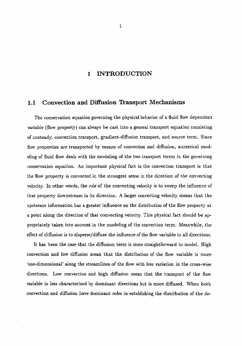
1.1 Convection and Diffusion Transport Mechanisms

The conservation equation governing the physical behavior of a fluid flow dependent

variable (flow property) can always be cast into a general transport equation consisting

of unsteady, convection transport, gradient-diffusion transport, and source term. Since

flow properties axe transported by meaxis of convection and diffusion, numerical mod

eling of fluid flow deals with the modeling of the two transport terms in the governing

conservation equation. An important physical fact in the convection transport is that

the flow property is convected in the strongest sense in the direction of the convecting

velocity. In other words, the role of the convecting velocity is to sweep the influence of

that property downstream in its direction. A laxger convecting velocity means that the

upstream information has a greater influence on the distribution of the flow property at

a point along the direction of that convecting velocity. This physical fact should be ap

propriately taken into account in the modeling of the convection term. Meanwhile, the

effect of diffusion is to disperse/diffuse the influence of the flow variable in all directions.

It has been the case that the diflfusion term is more straightforward to model. High

convection and low diffusion mean that the distribution of the flow variable is more

'one-dimensional' along the streamlines of the flow with less variation in the cross-wise

directions. Low convection and high diffusion mean that the transport of the flow

variable is less characterized by dominant directions but is more diffused. When both

convection and diffusion have dominant roles in establishing the distribution of the de

2

pendent variable, as in the case of recirculating flows, it is expected that the transport

of the flow variable is significant in the cross-wise directions normal to the streamlines of

the flow. This latter flow situation underscores the importance of maintaining compa

rable accuracy in the diflerencing of both the convection and diffusion terms since it is

only in very specialized flow problems that either convection or diffusion is the dominant

transport throughout the flow domain. Moreover, a successful approach to the model

ing of fluid flow must also reflect a balance/interdependence between the two transport

mechanisms in the considered multi-dimensional realm. In a domain discretized by a

structured mesh, it is important to realize that accurate modeling of the convection and

diffusion terms in a certain coordinate direction must take into account the effects of

the cross-wise convection and diffusion.

The governing conservation equation also explicitly states the dependence of the

convection and diffusion transports on the unsteady term and source term in order to

maintain the overall conservation of the dependent variable. This particular dependence

is often overlooked, or in many cases, is only indirectly taken into consideration in the

approximation of the convection and diffusion flux (total-flux) at the control-volume

interfaces. In a paper introducing the Skew Upwind Differencing Scheme (SUDS) [1],

Raithby addressed the fact that SUDS and its variants have not considered the com

plete effect of transient and source terms and thus are not suitable for problems with

a large transient gradient and/or a large source. In a more recent paper, Leonard [2]

also explicitly stated that significant numerical diffusion may result if the effect of the

transient and source terms are not taken into account appropriately.

3

1.2 Previous Approaches in the Modeling of Convection and

Diffusion

1.2.1 Central-Difference

In the eaxly period of CFD, classical central-difference appeared to offer a logical and

natural approach to the approximation of the dependent variable (convection) and its

derivative (diffusion) at the interfaces. In this formulation, both the dependent variable

and its derivative at an interface in a given coordinate direction are approximated by

using a piecewise linear profile (of the dependent Amiable) involving two neighboring

points. Central-difference formulation is the natural outcome of a Taylor-series formu

lation and can be shown to have second-order formal accuracy. This formulation gives

fairly accurate solutions for a class of low Reynolds number problems under specific con

ditions. However, Roache [3], Leonard [4], Patankar [5], and many other researchers have

shown in great detail that central-differencing may lead to unphysical oscillatory behav

ior for an implicit solution or to disastrous non-convergence in an explicit computation

in regions where convection strongly dominates diffusion. Patankar has shown that in

the case of central-difference formulation, when the Peclet number (local grid Reynolds

number) exceeds the value of two, violation of the positive coefficient rule [5] (and thus

violation of the Scarborough criterion) becomes possible with consequent unstable nu

merical iteration. For this reason, all the early attempts to solve convection-dominated

problems by the central-difference scheme were limited to low Reynolds number flows.

Although theoretically it is possible to keep the Peclet number below two by refining the

grid, this approach is neither economical nor practical. Previous work by Khosla and

Rubin [6], and more recent work by Ghia [7], Hayase [8], and Leonard [2] have shown

that it is possible to write the central-difference formulation in a form similax to the so

called 'deferred-correction method'. In this form, the value of the dependent variable at

4

an interface is approximated by an upwind value plus a correction term. Significantly

enhanced stability has been observed when the central-difference scheme is written in

this form.

Higher order central-difference schemes involving wider stencils have been developed

and tested with some success. While it is true that the formal order of accuracy is higher

using this strategy, the oscillatory and stability problems of the classical second-order

scheme are retained. Leonard [4] showed that in the case of central-differencing methods

(of any order), there is no convective feedback sensitivity, so that under high convection

conditions (large Peclet number), stability problems and numerical oscillations are likely

to occur.

In recent years, the so called High Order Essentially Non-Oscillatory schemes (ENO) [9]

have been introduced in an attempt to reduce the oscillation and stability problems in

herent in classical central-difference schemes. These schemes were originally designed

for compressible flow and in general for hyperbolic conservation law but have recently

been applied to incompressible Navier-Stokes equations. It Weis concluded that when it

is either impossible or too costly to fully resolve the flow, ENO can be used on a coarse

grid to obtain at least some partial information about the flow.

1.2.2 Upwind Scheme

Central-difference formulation is second-order accurate in both convection and diffu

sion. For a low Peclet number, the piecewise linear variation of the dependent variable

is generally acceptable. In this condition, both the upstream and downstream values

exert linear influence on the interface value. However, for high convection flow, this

approximation is less than physical. For a high Peclet number flow, it is known that

the upstream value has more influence on the interface variable than the downstream

value. Numerical instabilities can be traced to the non-consideration of this physics in

the convection modeling.

5

The first-order upwind scheme is an attempt to remedy this deficiency in the convec

tion modeling. The interface variable is approximated solely by using the immediate up

stream value (thus earning the name 'donor-cell technique' [10]) while central-difference

is used to evaluate the first derivative. Thus, it is first-order representation for the con

vection and second-order representation for the diffusion. The resulting scheme removes

the oscillatory and stability problems associated with the central-difference scheme and

gives acceptable solutions when it is convection that is mainly responsible for establish

ing the streamwise distribution of the dependent variable [4]. However, if the Peclet

number (based on grid dimension in the flow direction) is less than or equal to five

in magnitude (Peclet number restriction), and additionally, if the flow is significantly

oblique to the grid, large numerical diffusion is observed. This makes the first-order

upwind scheme highly unsuitable for the modeling of recirculating flows. The diffusive

nature of the first-order upwind scheme can be understood by a reference to the one-

dimensional convection-diffusion process outlined by Patankar [5]. It is known that for

low Peclet numbers, the variation of the dependent variable is largely linear between the

two neighboring values (a concept captured correctly by the central-difference scheme).

Neglecting the downstream information is certainly non-physical for this low convection

flow.

In an attempt to reduce the presence of large numerical diffusion inherent in the

first-order upwind scheme, a second-order upwind scheme (original idea traced to Price

et al. [11]) has been proposed which uses one more node in the upwind direction for

evaluating the convective term. There are many variants of the second-order upwind

scheme for estimating the mass flux across the interface of a computational cell, with

the common theme that the value of the dependent variable at a local node is connected

to two upstream values rather than just one, while central-difference is used to evaluate

the diffusion term. This scheme can be shown to have second-order accuracy in both the

convection and diffusion terms. Many researchers have investigated this scheme over the

6

years, but the findings axe not necessaxily consistent among the different studies. Atial

et al. [12] have used this scheme to study the lid-driven cavity flow and the problem of

impinging jet on a normal flat plate in conjunction with the streamfunction vorticity

approach. Wilkes and Thompson [13] have applied this scheme in the numerical study of

laminar ajid turbulent flow in sudden expansions and contractions. Shyy and Correa [14]

have used this scheme for the laminar lid-driven cavity problem. These researchers

have concluded that for the evaluated test problems, second-order upwind schemes have

been shown to give less numerical diffusion and thus a better accuracy than their first-

order predecessor. On the other hand, Vanka [15] foimd that second-order upwind

schemes do not yield satisfactory performance, both in terms of numerical accuracy

and computational stability, in solving the two-dimensional lid-driven cavity flows for

a range of Reynolds numbers. These conflicting findings prompted a more systematic

and thorough study of this scheme by Shyy [16]. The different variants of second-order

upwind schemes were investigated for the two-dimensional lid-driven cavity problem. It

has been concluded that even though all the variants of this scheme have formal second-

order accuracy, they all have different characteristics. It has been found that the scheme

which performs the best is the one which conforms most closely to the principles of

finite-volume formulation and is strictly conservative.

It should be noted that the dependence of convection and diflfusion processes on the

transient and source terms has not been addressed in the formulation of classical upwind

schemes. It was not until the introduction of the QUICKEST scheme by Leonard that

the transient term was taken into account.

1.2.3 Skew Upwind Differencing Scheme

The Skew Upwind Differencing Scheme (SUDS) of Raithby [1] has also been suggested

as an improved alternative to the first-order upwind scheme. As mentioned earlier, the

first-order upwind scheme is known to produce unacceptably large numerical diffusion

I

when the flow is oblique to the grid, rendering the scheme too expensive for recirculating

flow problems. This is because the first-order upwind approximation of the dependent

variable at the interface in a given coordinate direction is satisfactory only when the

flow is aligned to the grid. When the flow is skewed to the grid, the component-wise

upwind direction does not follow the 'true' direction of the convecting velocity, result

ing in significant numerical diffusion. The idea behind SUDS is to use the first-order

upwind scheme applied along the skewed streamline passing through the interface to be

evaluated. The upwinding is then used in a vector sense rather than component-wise

along the coordinate directions. As in the previous case of an upwind scheme, central-

difference is used to approximate the diffusion term. This scheme has been shown to

significantly reduce numerical diffusion which arises when the flow cuts across the grid

at a large angle. This is expected since theoretically it is in direct agreement with the

observed physics of the flow. However, the 'Peclet number restriction' associated with

the first-order upwind scheme is not removed. A slightly more complicated yet more

accurate variant of SUDS is also proposed by Raithby. This scheme is called Skew Up

wind Weighted Differencing Scheme (SUWDS), and as its name suggests, downstream

information is taken into consideration in the differencing stencil, thus removing the

restriction on the grid Peclet number. In his paper, Raithby also noted that the effects

of transient and source terms have not yet been considered, and thus the scheme may

produce numerical diffusion in the presence of high transient gradient and source term,

as is the caise with the previous upwind formulation.

1.2.4 Third Order Upstream Weighted Scheme (QUICK)

Not long after the publication of Raithby's Skew Upwind differencing scheme, Leonard

introduced a different approach in the modeling of the convection term [4], called the

QUICK (Quadratic Upstream Interpolation for Convective Kinematics) scheme. Over

the years, the QUICK scheme hcis proven to be highly successful in solving a wide variety

8

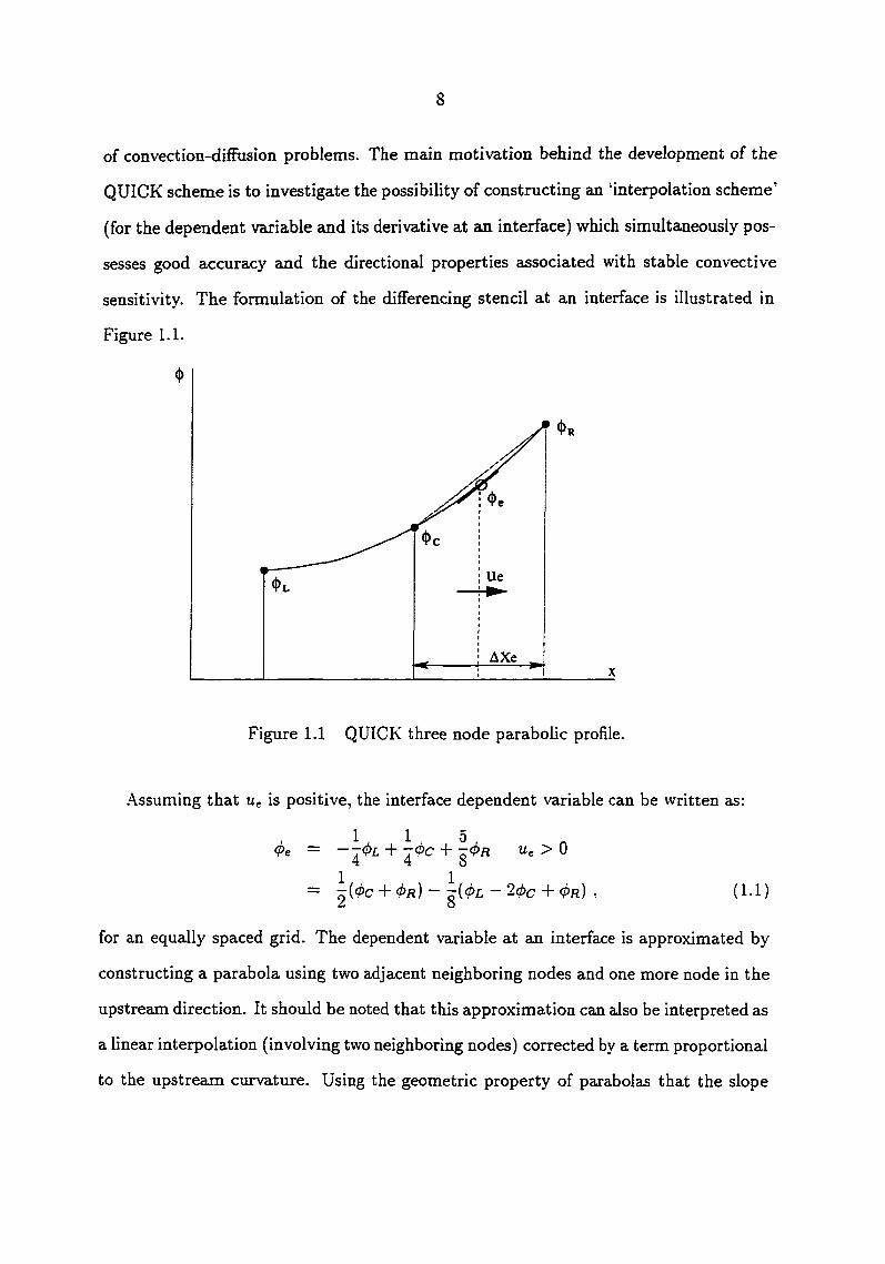
of convection-diffusion problems. The main motivation behind the development of the

QUICK scheme is to investigate the possibility of constructing an 'interpolation scheme'

(for the dependent variable and its derivative at an interface) which simultaneously pos

sesses good accuracy and the directional properties associated with stable convective

sensitivity. The formulation of the differencing stencil at an interface is illustrated in

Figure 1.1.

' <t>R

X.

y'/

<l>e

Ue

AXe ^ X

Figure 1.1 QUICK three node parabolic profile.

.A.ssuming that Ue is positive, the interface dependent variable can be written as:

1 - 1 . 5, ( P e = — + 7 0

4 4 8

= ^(<pc + 0r) — g(OL - 20c + <PH) , (1.1)

for an equally spaced grid. The dependent variable at an interface is approximated by

constructing a parabola using two adjacent neighboring nodes and one more node in the

upstream direction. It should be noted that this approximation can also be interpreted as

a linear interpolation (involving two neighboring nodes) corrected by a term proportional

to the upstream curvature. Using the geometric property of parabolas that the slope

9

halfway between two points is equal to that of the chord joining the points, the gradient

at the interface is given by: d(t> _ <f)R — (t>c / , . p v

dx ~ AXe ' ^

which is identical to the central-difference formula. Leonard has shown that this pro

cedure has greater formal accuracy than the central-difference scheme but retains the

basic stable convective sensitivity property that is characteristic of upstream weighted

schemes. Moreover, since the downstream information is taken into account, the Peciet

number restriction associated with the first-order upwind scheme is removed. Soon after

Leonard's publication of the QUICK scheme, severaJ researchers (Leschziner [17]. Han et

al. [18], Pollard and Siu [19], Freitas et al. [20], Perng and Street [21], Hayase et al. [8])

addressed the implementational details and testing of the scheme in two- and three-

dimensional flows more complex than those originally inspected by Leonard. Higher

order results using this scheme have been consistently reported for a wide range of flow

problems. Besides its upwind characteristics, another reason that the QUICK scheme is

able to capture the effects of source and cross-wise transports relatively well is the wider

stencil involved. The presence of both source and cross-wise transport indirectly influ

ences the value of the dependent variable at the interface by chajiging the node values

used in the construction of the parabolic profile. In other words, a better mathematical

profile is used to take into consideration the effects of source and cross-wise transport.

High order upwind-weighted methods are potentially quite stable. But because of the

wide-stencil involved, care is needed when applying traditional tridiagonal matrix-solver

techniques. Simply casting the outlying values into the source term can evidently lead

to slow convergence or even divergence. Among the various QUICK schemes developed

over the years, the 'Consistent QUICK' formulation by Hayase et al. [8] seems to posses

the best convergence property. Systematic study of the performance of the various

QUICK schemes applied to the two-dimensional lid-driven cavity problem by Hayzise

10

cleaxly shows that while the converged solutions of the schemes axe identical since they

are all derived from Leonard's formulation, their respective stability characteristics show

different behaviors. It is noted in this study that the particxilar formulation by Pollard

and Siu [19] consistently requires more iterations for the range of the Reynolds numbers

investigated. Hayeise's formulation requires that the finite-difference approximation of

the profile of the dependent variable at the interface satisfy Patankar's well-known 'Four

Rules', ensuring stable convergence. Adherence to these convergent rules dictates that

the value of the interface variable be written as the sum of a first-order upwind estimation

and a correction term. The correction term is deferred or lagged from the previous vcdues

and is eventually lumped into the source term. This method is often referred to as the

'Deferred Correction' method and has been proven to enhance stability.

Another inherent difficulty with the high-order upwind scheme is the formulation of

the scheme for the cells adjacent to the wall. Depending on the flow direction, the scheme

may require a value outside the calculation domain. Leonard's subsequent paper [22]

gave the modification of the QUICK scheme for the cells near the boundary. However,

because a third-order boundary-treatment sometimes causes instabilities, a second-order

boundary is often used to avoid potential stability problems. Hayase's formulation shows

that Leonard's third-order boundary formulation can also be written as the sum of

the upwind evaluation plus the correction term, consistent with his proposed QUICK

scheme. The main motivation for retaining third-order boundary treatment is to preserve

the continuity of the third-order truncation error throughout the computational domain.

As shown by Hayase, the use of a lower order boundary in conjunction with the higher

order scheme has been proven to degrade the overall accuracy of the solution. This is

especially true in elliptic problems.

It is known that the high order upwind scheme heis the tendency to generate un-

physical overshoots neax sharp transitions. This means that a typical step>-Iike profile

which should be sharp and monotonic will be computed with an overshoot on one side

11

or the other, or both. This is particularly true with the QUICK scheme. In his recent

paper [2], Leonard proposed the use of a flux limiter to ctirb possible overshoots. In the

first strategy, the Universal Limiter for Tight Resolution and Accuracy (ULTRA) ([23]

and [24]) is used with the QUICK scheme. In the second strategy, a combination of the

ULTRA method and Leonard's Simple High Accuracy Resolution Program (SHARP) is

also proposed. It was concluded that while the ULTRA-QUICK strategy eliminates the

overshoot problems (for the test case considered), numerical diflfusion is also introduced

to some extent. On the other hand, the ULTRA-SHARP strategy hcis been shown to

eliminate the overshoot without introducing additional numerical diffusion.

Modification of the QUICK scheme for unsteady flows is known as the QUICKEST

scheme [4]. Initial testing of the QUICKEST on the simulation of the complex hydrody

namics and salinity transport of a large estuary by Leonard showed that the QUICKEST

scheme does not introduce any appreciable numerical diffusion for highly unsteady prob

lems. However, since its introduction, there have not been many published results for

the application of this scheme to a wide range of unsteady problems.

1-2.5 Exponential Difference Scheme (EDS)

The past two decades have witnessed the popularity of this class of schemes which

is often referred to as the Exponential Differencing Scheme (EDS). The first variant of

these schemes is called the exponential scheme, developed by Allen and Southwell [25].

The exponential scheme models the convection-diffusion transport process by focusing

on each grid-wise component of that process. That is, the dependent variable and its

derivative at the interface in a given coordinate direction are approximated by using the

exact solution of the one-dimensional, constant-coefficients, and source free convection-

diffusion equation along that coordinate direction, resulting in an exponential profile.

Since the present work relies heavily on an understanding of the EDS, a detailed discus

sion of its advantages and disadvantages is presented.

12

interface

(pu) = constant r = constant

Figure 1.2 One-dimensional convection-difFusion profile.

With the aid of Figure 1.2, the convection-difFusion transport in the x-direction is

modelled by solving:

= (1.3)

where {pu)=constant and { r =constant) across the cell considered. This means that the

x-direction totai-flux (Jr) is always constant across that cell, and its analytic expression,

subject to known boundary conditions Oi-i and (^{, is given by:

r Jx = — A4>i) = constant ,

0

where A and B are a function of the Peclet number only and are given by:

^ — 1

B = A + P ^

{pu)5

(1.4)

(1.5)

P. = = Peclet number

The dependence of the total-flux on the Peclet number is shown in Figure 1.3.

Over the years, motivated by the relatively expensive exponential calculations in

volved, several researchers have independently developed variants of the exponential

scheme. The most notable of these convection-difFusion methods axe the hybrid scheme

of Spalding [26] (also known as the high lateral flux modification) and the Power Law

13

A(Pe)

Exponential

Hybrid scheme

Exponential scheme Exact solution

Pe

-2 2 A = 0

Figure 1.3 Vaxiation of A(Pe) as a function of Pe

scheme of Patankar [5]. The hybrid scheme tries to approximate the exponential func

tion A{Pe) by using a three-line piecewise approximation to the exact curve. It should

be noted that the hybrid scheme is identical to the centraJ-difference scheme for a Peclet

number range of —2 <Pe< 2, and outside this range, it reduces to the upwind scheme in

which the diffusion has been set equal to zero. It has been discussed previously that the

second-order central-difference scheme is stable for |Pe|< 2 but is potentially unstable

for a higher Peclet number. On the other hand, the upwind scheme performs better

for a higher Peclet number but is diffusive for a low Peclet number case. Hence, zis its

name suggests, the hybrid scheme is a combination of the central and upwind schemes,

using the better option between the two schemes for each Peclet number case. A better

approximation to the exact curve is given by the Power Law scheme. The Power Law

expression is not particularly expensive to compute but provides an extremely good rep

resentation of the exponential behavior. For this reason, a reference to the exponential

scheme will be used interchangebly with the Power Law scheme.

The exponential Differencing Scheme started to gain popularity with the introduction

14

of the SIMPLE solver [5]. The combination of these procedures resulted in the so-

called TEACH code [27] developed at Imperial College, giving a robust, general purpose

elliptic equation solver suitable for solving steady-state Navier-Stokes equations and the

associated heat and mass transfer problems. In the past decade, hybrid and Power Law

schemes have been widely used for solving a wide class of problems. Their popularity

stems from good convective stability and 'relatively accurate' solutions (compared with

the first-order upwind scheme).

However, in the intervening period, researchers have also shown that for a high-

frequency transient, multidimensional transport process with a significant source, EDS

results in solutions which are marred by unacceptably large numerical diffusion. Many

researchers, including Huang [28], Patel [29], and Leonard [2], have shown that, as is

the case with the first-order upwind scheme, the numerical solution of the EDS scheme

for general flow problems can be significantly inaccurate for coarse grids. Considerable

grid refinement may be needed to produce acceptable results. Careful observation of the

characteristics of EDS shows that EDS can be considered to be a variant of the first-

order upstream weighted scheme with the weighting coefficients obtained from solving

a one-dimensional, source free convection-diffusion equation. These weighting coeffi

cients are such that when the Peclet number is relatively small (i.e. |Pe|< 2), both the

upstream and downstream nodes have 'linear' influence on the interface profile. How

ever, as the Peclet number increases in magnitude, the influence of the upstream node

grows in significance while the effect of the downstream node diminishes. Thus, the

inherent diffusive characteristic of the first-order upwind scheme is also shared to some

extent by EDS (and first order upwind schemes in general). Leonard has shown that

for large Peclet numbers, EDS is equivalent to first-order upwinding for the convection

with physical diffusion neglected [2], which results in the introduction of numerical dif

fusion in the cross-wise direction. However, perhaps the most serious misapplication

of EDS is to multidimensional problems involving high-speed flow oblique or skewed

15

to the grid [2]. In this case, more than one component of the grid Reynolds number

(Peclet number) is large at any given control-volume. Thus, the components of the

convection-diffusion process in each coordinate direction have 'equal' influence on the

values of the dependent variable at the interface. Recall that for a given coordinate di

rection. EDS approximates the dependent variable and its derivative at the interface by

solving the one-dimensional, source free convection-diffusion equation in that direction.

Thus, the influence of the cross-wise components of the convection-diffusion process is

neglected. Cross-wise transports only influence the interface profile indirectly by chang

ing the values of the dependent variables at the two nodes surrounding the interface.

This simplification means that EDS is most effective for solving flow situations which

are steady and quasi-one-dimensional (dominant streamwise transport), provided that

the convecting velocity is nearly aligned with one of the grid coordinate directions.

1,2,6 Locally Analytic Differencing Scheme (LOADS)

At about the same time Patankar introduced the Power Law scheme, an extension

to the exponential scheme, named LO.A.DS, which takes into account the multidimen-

sionality of the flow, was introduced by Raithby [30]. LOADS realizes that unless a

sufficiently fine grid is used, the use of a conventional locally exact one-dimensional

solution (i.e. exponential scheme) cannot be expected to give accurate solutions for

strongly multidimensional problems, such as when the flow is skewed to the grid. A lo

cally one-dimensional solution can be a viable approximation only if the lateral transport

and source terms are taken into account in the determination of the one-dimensional pro

file. This can be done by rewriting the conservation equation (equation 1.8 to be given

later) as a one-dimensional convection-diffusion process in a grid direction with the rest

of the terms combined as one source term. An analytical expression is then used to ap

proximate the exponential solution of the modified one-dimensionaJ transport process.

Referring to the stencil used previously to explain the QUICK profile (Figure 1.1), the

16

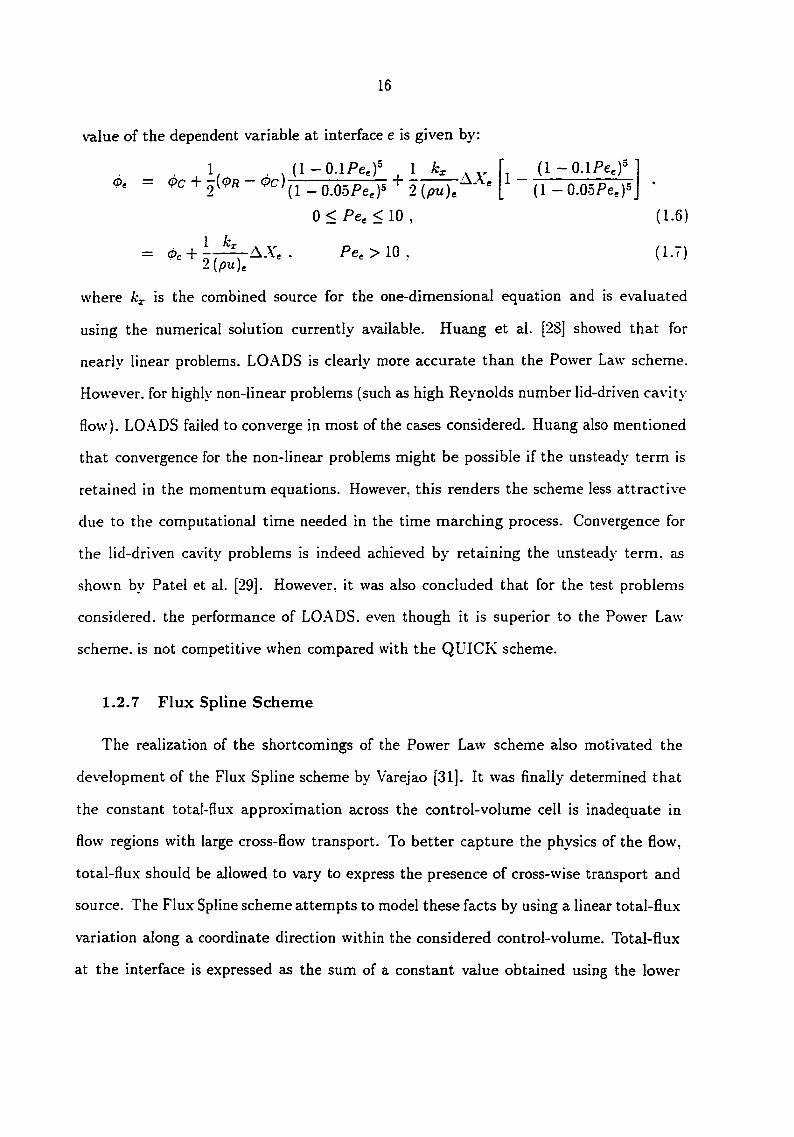
value of the dependent variable at interface e is given by:

, , 1, , , (1-O.lPeef . 1 (1-O.lPe,)^ (1 — O.OoPej)=

0<Pe,<lO, (1.6)

= Oc + . Pe, > 10 , (1.7) 2{pu)^

where kj. is the combined source for the one-dimensional equation and is evaluated

using the numerical solution currently available. Huang et al. [28] showed that for

nearly linear problems, LOADS is clearly more accurate than the Power Law scheme.

However, for highly non-linear problems (such as high Reynolds number lid-driven cavity

flow). LO.A.DS failed to converge in most of the cases considered. Huang also mentioned

that convergence for the non-linear problems might be possible if the unsteady term is

retained in the momentum equations. However, this renders the scheme less attractive

due to the computational time needed in the time marching process. Convergence for

the lid-driven cavitj' problems is indeed achieved by retaining the unsteady term, as

shown by Patel et al. [29]. However, it was also concluded that for the test problems

considered, the performance of LO.A.DS. even though it is superior to the Power Law

scheme, is not competitive when compared with the QUICK scheme.

1.2.7 Flux Spline Scheme

The realization of the shortcomings of the Power Law scheme also motivated the

development of the Flux Spline scheme by Varejao [31]. It was finally determined that

the constant total-flux approximation across the control-volume cell is inadequate in

flow regions with large cross-flow transport. To better capture the physics of the flow,

total-flux should be allowed to vary to express the presence of cross-wise transport and

source. The Flux Spline scheme attempts to model these facts by using a linear total-flux

variation along a coordinate direction within the considered control-volume. Total-flux

at the interface is expressed as the sum of a constant value obtained using the lower

17

order Power Law scheme plus an extra term. It is then clear that the extra term is

intended as the means by which source and flow multidimensionality are captured.

The Flux Spline scheme has been applied to several two- and three-dimensional flow

problems [32] and was reported to be more accurate than the Power Law scheme. To

get the same level of accuracy, the Flux Spline scheme requires a fewer number of grid

points. However, little research has been reported on the use of flux-spline on a wide

variety of problems.

QUICK and Flux spline schemes represent a further step in the realization that a

successful approach to the modeling of convection and diffusion processes must take into

account the presence of the cross-wise transport, the source, and the unsteady term.

Failure to account for these three factors could result in the generation of unwanted

numerical diffusion and/or numerical instabilities.

1.3 Modeling of Convection Diffusion Problem

The general transport equation which governs the physical behavior of the dependent

variable o in two-dimensions is given by:

It should be noted that the convection and diffusion processes have been represented

component-wise in each coordinate direction. Observation of the above equation con

firms the previous qualitative conclusion that the convection-diffusion process in one co

ordinate direction is directly balanced by the unsteady term, source term, and transport

processes in the remaining coordinate directions. Thus, smaller y-direction transport

can mean larger x-direction transport and vice versa. The influence of the unsteady

term and source also works in the same way.

The first step in the discretization process is to integrate equation 1.8 over time and

over the considered control-volume cell given in Figure 1.4. Then, an approximation

(1-S)

18

• • N

n

•

•W^

V

\J ¥ ) e •E

•

A •S •

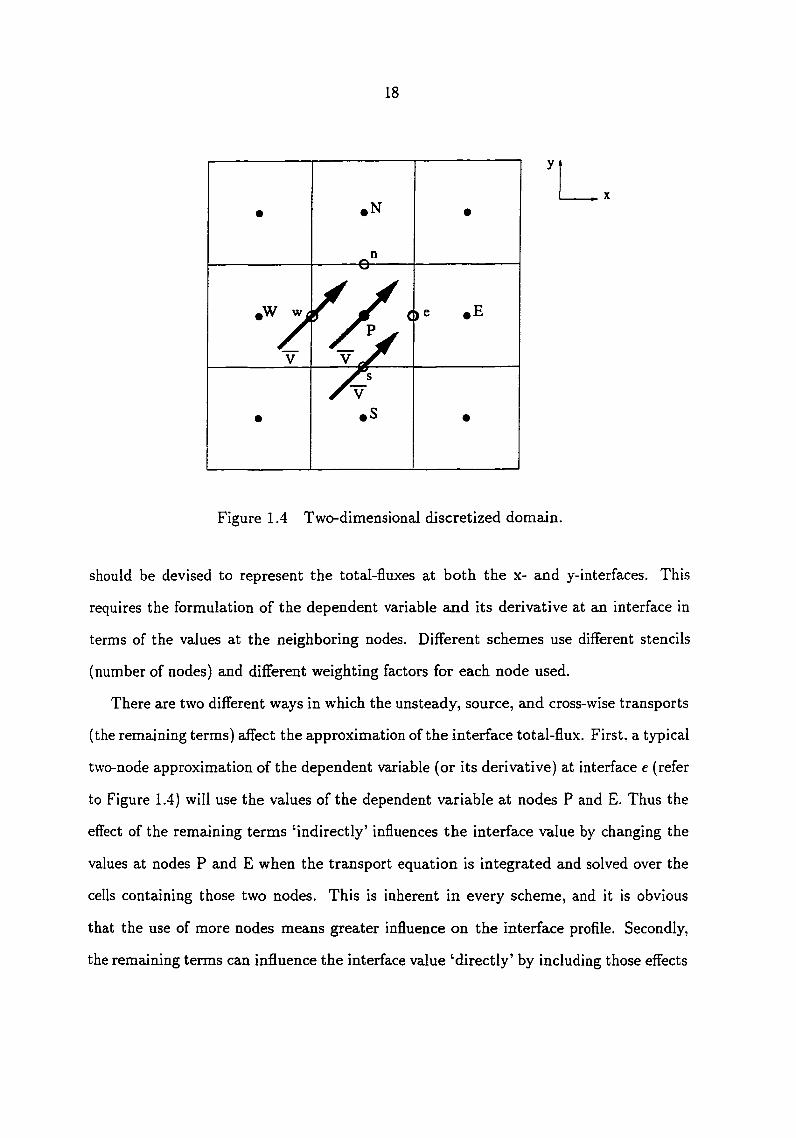
Figure 1.4 Two-dimensional discretized domain.

should be devised to represent the total-fluxes at both the x- aad y-interfaces. This

requires the formulation of the dependent variable and its derivative at an interface in

terms of the values at the neighboring nodes. Different schemes use different stencils

(number of nodes) and different weighting factors for each node used.

There are two different ways in which the unsteady, source, and cross-wise transports

(the remaining terms) affect the approximation of the interface total-flux. First, a typical

two-node approximation of the dependent variable (or its derivative) at interface e (refer

to Figure 1.4) will use the values of the dependent variable at nodes P and E. Thus the

effect of the remaining terms 'indirectly' influences the interface value by changing the

values at nodes P and E when the transport equation is integrated and solved over the

cells containing those two nodes. This is inherent in every scheme, and it is obvious

that the use of more nodes means greater influence on the interface profile. Secondly,

the remaining terms can influence the interface value 'directly' by including those effects

19

directly in the profile approximation. The potential of the latter approach should be

immediately apparent.

1.3.1 High Convection Flow Oblique to the Grid

Accurate modeling of complex flows is at best difficult. Most flow problems involve

situations where the flow has more than one dominant direction throughout the region

of interest. Therefore, it is very difficult, if not impossible, to have a grid structure which

is mostly aligned to the streamlines of the flow. Regardless of the type of grid chosen.

there will always be regions where the flow is significantly oblique or skewed to the grid.

It is often stated that flows oblique to the grid may cause significant numerical

diffusion if the numerical scheme is not properly formulated. The following discussion

attempts to clarify both the characteristics of flow oblique to the grid and the way in

which the previously discussed schemes handle this situation.

First, it is helpful to state the following observation:

[n the convection transport of variable (p, the scalar <p at a given location will be convected in the direction of the convecting velocity V at that location. The larger the magnitude of the convecting velocity, the greater is the influence of the upstream value on the downstream distribution.

This observation is then used as a guide to study the various approximations of the

value of Ob given below.

Case A .Approximating (i>b by a linear interpolation of 4)^ and ©/is accurate when

jV'l is of moderate value. But for larger Pe, this approximation may result

in overshoots or undershoots since linear profile does not taJce into account

the direction of the flow. This approximation is used by the central-difference

scheme and has second-order truncation error.

Case B Approximating b by <f>e (first-order truncation error) has some virtues, but

it does not take into account the aforementioned observation properly if 9 is

20

6 is large - 45

Figure 1.5 Diagram for possible approximation of (Ph-

Case C

Case D

Case E

large. This appro.ximation is acceptable only if V' is nearly aligned with X.

and the approximation is more accurate with larger |V''| restriction). This

is the approach of the first-order upwind scheme.

Approximating cij by a linear profile using (t>d and <pe (second-order trunca

tion error) improves the accuracy considerably when compared to Case B.

However, the shortcomings of Case B are also shared to some extent. This

approach is used by the second-order upwind scheme.

.Approximating Ob by (pa takes into account the above observation better than

Case B, but still has the first-order truncation error and Peclet number

restriction. If </)c is also used, then the Peclet number restriction is removed.

A slight stencil modification of this approach is used by the Skew Upwind and

Skew Upwind Weighted schemes.

Approximating oi, by a parabolic profile using (i>e, and <?!>/ can be shown

21

to have a third-order truncation error. Since approximate downstream infor

mation is considered, the Peclet number restriction is removed. This approx

imation is theoretically better than any of the previous approximations and

is known as the QUICK scheme eis discussed previously. The basic idea of

this scheme is to use a stencil which recognizes both the upwind and more

eUiptic nature of the flow (depending on the P^) and fits a polynomial profile

appropriate to the stencil used.

The exponential scheme uses the same stencil employed by the central-difference

scheme, but instead of using linear-interpolation, a first-order upwind biased profile

obtained by solving a one-dimensional, source free convection-diffusion equation is used.

It is therefore a better approximation than the first-order upwind scheme, but is still

very diffusive if the flow is skewed to the grid.

Mathematically, high convection flow oblique to the grid means that the convection in

the other coordinate directions (refer to equation l.S) are large and should be accounted

for in the approximation of the convection and diffusion processes in all the coordinate

directions considered. The failure of the first-order upwind scheme to recognize this

results in the generation of unacceptably large numerical diffusion for flows oblique to

the grid.

1.3.2 High Cross-flow Gradient

A high cross-flow gradient means that there is a steep variation in the dependent

variable in the cross-wise grid directions. Mathematically, referring to equation 1.8, this

means that the first-derivative term of the total-flux (diffusion term) is large in one

or all grid directions, depending on how the flow angles with the grid. If the flow is

mostly aligned with a grid direction, then the approximation of the dependent variable

along that direction should take into account the rate of variation of that variable in

the mutually perpendicular grid directions. If the flow is skewed to the grid, then the

formulation in each direction should take into account the variation rate in the other

normal directions.

1.3.3 Unsteady and Source Influence

It is clear from equation 1.8 that unsteady and source terms directly influence the

convection and diffusion transports of 4>. If the conservation of the dependent variable is

to be properly maintained, then both terms must be considered in the modeling of the

convection and diffusion terms. This is especially importajit for solving high gradient

transient problems and for modeling of the effects of rotating bodies through source term

additions, such as a rotating helicopter rotor [33].

1.3.4 Previous Approaches to the Overall Balemce Principle

In conclusion, in the pursuit of a stable, highly accurate scheme for general flow

problems, the modeling of convection and diffusion transports in a grid direction should

properly reflect a balance of the overall conservation of the dependent variable. Among

the different mainstream approaches considered thus far, only the Locally Analytic Dif

ferencing Scheme (LOADS) by Raithby comes close to applying this overall conservation

idea. Unfortunately, an improper approach in the implementation of this concept leads

to disastrous non-convergence of LOADS for many non-linear problems. A distinctly

different and widely popular approach is to realize the upwind nature of the flow for

a higher Peclet number and its more elliptic characteristics for a lower Peclet number.

Thus, at a given interface, it is logical to use more than one node in the upstream di

rection while using fewer (though at least one) nodes in the downstream direction. This

wider stencil also shows a greater ability to capture cross-wise transport and source.

This is the approach used by the other schemes discussed previously. The most success

23

ful scheme to date from this fajnily is the QUICK scheme, which uses a parabolic profile

fitted to two upstream and one downstreaxn nodes.

1.4 Current Work: Flux Corrected Method

The Flux Corrected Method (FCM), introduced in this work, attempts to model the

convection and diffusion processes at an interface along a grid direction by conserving

the whole transport equation. This is done by solving a one-dimensionaJ convection-

diffusion equation with a source. The unsteady, cross-wise transport, and source terms

are all lumped together with the original source to form one new source used in the

one-dimensional equation. Thus, the unsteady multi-dimensional problem is treated as

a steady, source driven, one-dimensional problem. FCM is a straightforward extension

of the Power Law scheme since all the correction terms fall conveniently into the source

of the discretized equation.

FCM has been tested on two- and three-dimensional standard test problems involving

high convection flows oblique to the grid and high frequency transient problems. In all

the cases considered, FCM has consistently given very accurate results without the need

to use cm excessively fine grid. Qualitative comparisons using the published results

in the literature show that FCM is at least as accurate as the well-known QUICK

scheme. Limited comparison with the spectral method has shown that FCM performs

very competitively.

Detailed development of this research is presented in the following chapters. Chap

ter 2 introduces the governing conservation equations, the discretization process, the

FCM approach for modeling the convection-diffusion transport, and the modified SIM

PLER algorithm. Chapter 3 presents the possible choices of the convection-diffusion

sources and the combined effects of those possible sources on the solution accuracy. In

Chapter 4, the detailed development of the general pressure boundary implementation

24

is presented. Chapter 5 presents the verification of FCM using two standard test prob

lems commonly used in CFD. Finally, in Chapter 6, the conclusions drawn from this

research and recommendations for future research in FCM development <ire suggested.

25

2 THEORETICAL FORMULATION AND SOLUTION

PROCEDURE

2.1 Governing Equations

The mass, momentum, ajid energy conservation equations applied to a fluid passing

through an infinitesimal, fixed control-volume can be written in divergence form as:

Continuitv Equation: dp

+ V . ( p V ) = 0 , ( 2 . 1 )

Momentum Equation:

^(pV) + V . (pW) = + V . , (2.2)

where pi is the body force per unit volume and V • Hy is the surface force per unit

volume due to external forces on the fluid element. The stress tensor fly consists of

both the normal and shearing viscous stresses and its divergence is given by:

= - V P - V ( V . / ) + V # f . ( 2 . 3 )

The second term V(V • /) vanishes for orthogonal coordinate systems and hence can be

neglected in the current formulation.

For Newtonian fluid, the stress at a point is lineaxly proportional to the rate of strain

of the fluid, and the shear component of the stress tensor is given by:

r = /i \T 2 . VV + (VV)^ _ IV • V/ o

(2.4)

26

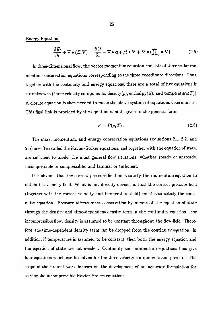
Energy Equation:

^ + V.(£,V) = -V.q + f.V + V.(n...V) (2.5)

In three-dimensional flow, the vector momentum equation consists of three scalar mo-

mentimi conservation equations corresponding to the three coordinate directions. Thus,

together with the continuity and energy equations, there axe a total of five equations in

six unknowns (three velocity components, density(/9), enthalpy(h), and temperaturefT)).

A closure equation is then needed to make the above system of equations deterministic.

This final link is provided by the equation of state given in the general form:

P = P { p S ) . (2.6)

The mass, momentum, and energy conservation equations (equations 2.1. 2.2, and

2.5) are often called the Navier-Stokes equations, and together with the equation of state,

are sufficient to model the most general flow situations, whether steady or unsteady,

incompressible or compressible, and laminar or turbulent.

It is obvious that the correct pressure field must satisfy the momentum equation to

obtain the velocity field. What is not directly obvious is that the correct pressure field

(together with the correct velocity axid temperature field) must also satisfy the conti

nuity equation. Pressure affects mass conservation by means of the equation of state

through the density and time-dependent density term in the continuity equation. For

incompressible flow, density is assumed to be constant throughout the flow-field. There

fore, the time-dependent density term can be dropped from the continuity equation. In

addition, if temperature is assumed to be constant, then both the energy equation and

the equation of state are not needed. Continuity and momentiim equations thus give

four equations which can be solved for the three velocity components and pressure. The

scope of the present work focuses on the development of aji accurate formulation for

solving the incompressible Navier-Stokes equations.

27

2.2 Methods for Solving Incompressible Flow Equations

Even though the complexity due to the coupling of the energy equation (through

the equation of state) to the mass and momentum conservation equations no longer

exists, solving the incompressible Navier-Stokes equations does not prove to be much

simpler than solving the compressible counterpaxts. The real difficulty in solving the

incompressible flow equations lies in the methodology used to determine the pressure

field during the iterative process. The pressure gradient forms a paxt of the source term

of the momentum equation. Given a pressure field, there is no particular difficulty in

solving the momentum equation for the velocity field. However, there is no obvious

equation for obtaining the pressure field. Moreover, there no longer exists a 'direct'

means by which pressure can affect mass conservation and vice versa. The pressure field

is only 'indirectly' specified through the continuity equation. When the correct pressure

field is used to solve the momentum equations, the resulting velocity field also satisfies

the mass conservation.

For two-dimensional situations, it is possible to eliminate the pressure terms by

cross-differencing and then substituting the two components of the momentum equation.

Using the definition of streamfunction (for steady and two-dimensions) and vorticity.

the resulting combined equation is transformed into what is often referred to as the

vorticity-transport equation. Similarly, the continuity equation can also be expressed

in terms of the streamfunction. The resulting two equations can then be solved for

the two dependent variables (streamfunction and vorticity). Upon convergence of the

iterative process, pressure can be obtained separately by solving a Poisson equation.

This approach is known as the vorticity/streamfunction method, and its wide usage has

been limited to two-dimensional flow problems only.

Another approach used for solving the incompressible Navier-Stokes equations is

known zis the primitive variable formulation, wherein the primitive vaxiables V and P

28

axe directly solved. A method based on the primitive variable technique is the artifi

cial compressibility method which was first proposed by Chorin [34]. This method was

originally formulated for steady flows cind has recently been extended to time-accurate

solutions by Kwak et al. [35] and Merkle and Athavale [36]. In this method, a pseudo-

time derivative of pressure is added to the continuity equation, and this provides the

coupling between the velocity and the pressure field. At a given time level, the equa

tions are advanced in pseudo-time by subiterations until a divergent-free velocity field

is obtained at the next time level.

The most common primitive variable approach is introduced by Harlow and Welch

[37]. This method tries to provide the velocity-pressure coupling by using an iterative

procedure which alternately solves for the velocity field and pressure field. Given an

initial pressure distribution, the momentum equation is solved to determine the velocity

field. This velocity field does not necessarily satisfy the continuity equation (unless the

correct pressure field is used) and thus needs to be corrected to preserve mass conserva

tion. This is done via a correction to the pressure field by solving the Poisson equation

for pressure, which is derived from the meiss conservation equation. The subiteration is

continued until convergence is achieved for that time level. A popular derivative of this

method is the SIMPLER scheme of Patankar [5].

2.3 Conservation Equations in Cartesian Coordinates

For simplicity of development, the governing incompressible flow equations axe ex

pressed in two-dimensional Cartesian coordinates:

Continuity Equation:

" • (2.7)

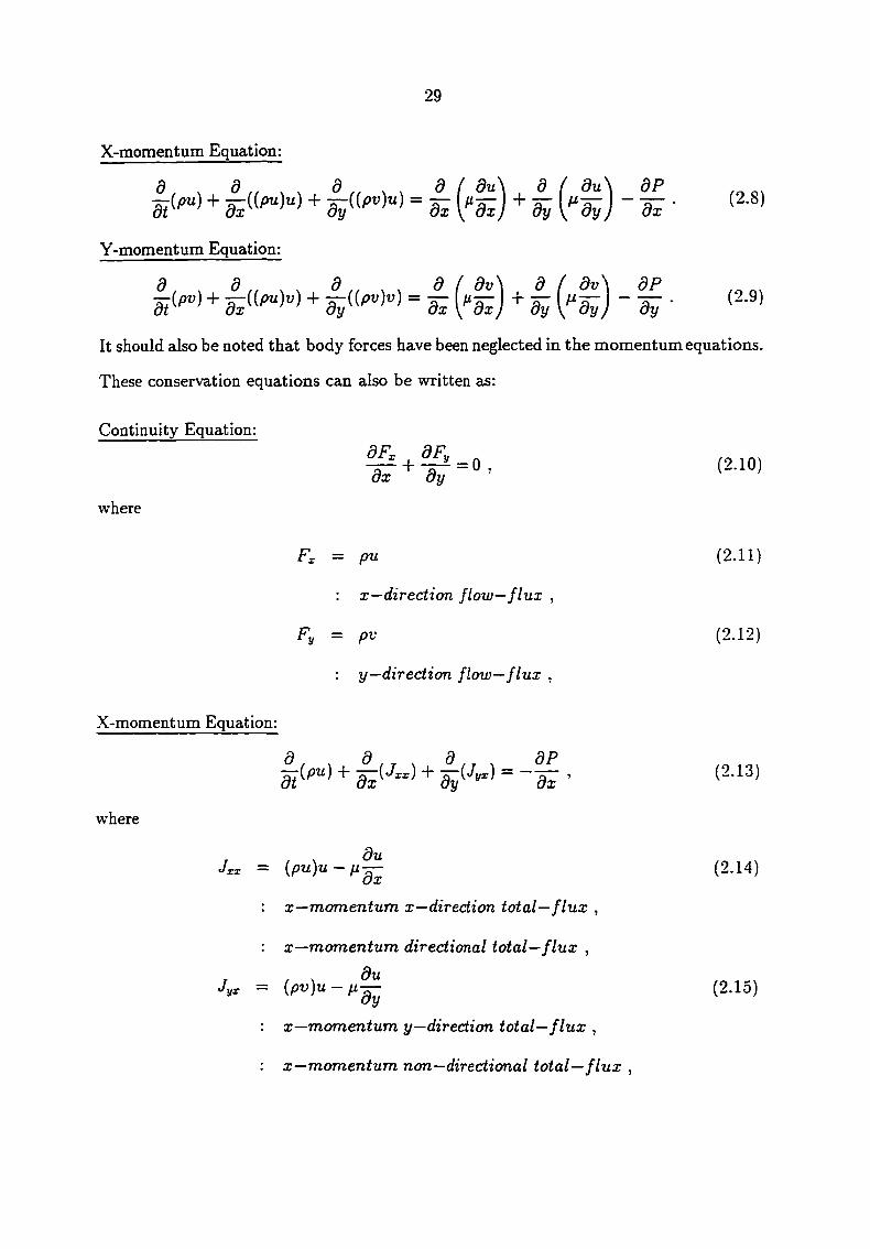
29

X-momentum Equation:

+ ^apu)u) + A((^v)«) = ^ - ~ . (2.8)

Y-momentum Equation:

d , . 9 . . . . ^ f f \ \ ^ ^ / o n \ g^(^v) + (Mv) + •^((pv)v) = g- - — . (2.9)

It should also be noted that body forces have been neglected in the momentum equations.

These conservation equations can also be written as:

Continuity Equation:

dx dy

where

dF„ + -3- = 0, (2.10)

Fx = pu (2.11)

: X—direction flow—flux ,

Fy = pv (2.12)

: y—direction flow—flux ,

X-momentum Equation:

where

du Jrr = {pu)u-H— (2.14)

: X—momentum x—direction total—flux ,

X—momentum directional total—flux ,

du Jyr = { p v ) u - n — (2.15)

: X—momentum y—direction total—flux ,

: X—momentum non—directional total—flux ,

30

Y-momentum Equation:

(2.16)

where

(2.17)

: y—momentum x—direction total—flux .

: y—momentum non—directional total—flux .

(2.1S)

: y—momentum y—direction total—flux .

: y—momentum directional total—flux ,

Note that the second subscript indicates which momentum equation the total-flux

belongs to. and the first subscript, when used in conjunction with the second subscript,

indicates whether it is directional or non-directional. Careful observation of the x- and

y-momentum equations (equations 2.S and 2.9) shows that the scalar momentum equa

tion in a given coordinate direction is basically a transport equation for the velocity

component in that coordinate direction. Both equations also posses similar form and

thus can be written in a generic differential transport equation. It can also be shown

that other conservation principles can always be written in the same generic form. For

this recison, a generic scalar differential transport equation will be used to represent the

flow conservation principles. This will avoid unnecessary repetition and allows the de

velopment of a numerical scheme for any general conservation variable. If the dependent

variable is denoted by 6, the general transport equation is given by:

where F is the diffusion coefficient and S is the source term. The quantities P and S are

specific to a particular meaning of 4>. The four terms in the general transport equation are

—{p0) -t- V • ipY) = V . (rV0) -h 5 , (2.19)

31

the unsteady, convection, gradient driven diffusion, and source terms. Not all diffusion

fluxes axe governed by the gradient of the relevant variable. However, whatever cannot

be cast into this 'nominal' diffusion term can always be expressed as part of the source

term. In Cartesian coordinates, equation 2.19 will take the form;

dt iP't:) + (r|j) + ) + S . (2-20)

which is the same eis equation 1.8. The corresponding conservation form is given by:

+ (2.21)

where

J, = (2.22)

: X—direction total—flux ,

J, = (;av)^-r|2 (2.23)

: y—direct ion total—flux .

Note that in the conservation form, the convection and diffusion terms in a coordi

nate direction are grouped together to form the total-flux in that direction. This is an

important property which will be used in the subsequent development of this work.

2.4 Integral Balance of Conservation Equations

2.4.1 Control Volume Approach

Equation 2.21 implies a continuous distribution of the dependent variable (j) over an

arbitrary domain. In the real, finite world, the domain of interest must be divided into

smaller, non-overlapping subdomains (control-volumes) over each of which the conserva

tion principle is applied. For the scheme to be consistent, it is important to impose the

condition that the flux leaving a portion of the boundary enclosing a control-volume is the

32

same eis the flux entering the adjacent control-volume sharing that same boimdary por

tion. Moreover, the summation of the total influx and outflux of ail the control-volumes

must reflect the overall conservation of <f> applied over the whole domain considered.

This control-volume approach for discretizing the governing equations ensures that the

final discretized equation conserves the dependent variable locally and globally and thus

will help suppress any production of non-physical sources or sinks which are not part of

the original differential equation.

2.4.2 Time Integration

Time variation of a general variable (t> is given by a generalized formula

= + (2.24)

where d" is the value at time t, and o is the value at time t -t- A<. For the rest of this

work, a variable with the superscript ° represents a variable at the old timestep, and a

variable without the superscript ° represents a variable at the new timestep.

For certain specific values of the weighting factor/, the discretization equation reduces

to one of the well-known schemes for parabolic differential equations. In particular, /=0

leads to an explicit scheme, J=0.o leads to the Crank-Nicholson scheme, and /=1 leads

to a fully implicit scheme.

2.4.3 Integral Balance of Continuity Equation

Integrating the mass conservation equation (equation 2.10) over the two-dimensional

control-volume (Figure 2.1) results in the following mass integral balance:

r /J +£ r ° where the order of the integration is chosen according to the flux direction. Evaluation

of the integrals yields the discretized continuity equation:

- Fil'f = 0 , (2.26)

33

X

• •N

n

•

AY

' r

e • £

•

s

• s •

AX

Figure 2.1 Two-dimensional X-Y control-volume

34

where

= I" dy = Ay (2.27)

: integrated x—direction flow—flux at

i n t e r f a c e e , w ,

Fi-l, = ['f,— = (2.28) Jw

: integrated y—direction flow—flux at

i n t e r f a c e n ^ s .

The expressions for the flow-flux in the x- and y-directions are given in equations 2.11

and 2.12.

2.4.4 Integral Balance of General Transport Equation

Similarly, the general transport equation (equation 2.21) is integrated over the control

volume (Figure 2.1) and over the time interv'al from f to i + At. Assuming that the grid

point value of <f) (grid point P) prevails throughout the control-volume, the following

discretized equation is obtained:

[{p(p)p - (P<^)pj AxAyAz

At "*•

/(4-f - 4-^ + 4-^ - 4-!) +

(1 - mrJT' - JUT + JUn' - JUT') =

/ 5 ' " ' ^ - l - ( l , ( 2 . 2 9 )

where

^ dy = Jr-e,w Ay (2.30)

: integrated x—direction total—flux at

i n t e r f a c e e , w ,

35

= f Jy-n^ dx = Lx (2.31) Jw

: integrated y—direction total—flux at

interface n, s ,

Sintg _ f F dxdy = SAxAy . J s J w

The expressions for the total-flux in the x- and y-directions are given in equations 2.22

and 2.23. The next step toward the formulation of the discretized form of the transport

equation is to decide how to evaluate the total-fluxes at the control-volume faces.

2.5 Modeling of the Convection and Diffusion Transport

2.5.1 Review of Basic Qualitative Characteristics

The expression for the total-flux in a coordinate direction consists of the convection

and diffusion transport terms in that direction. For convenience, the equation for the

total-flux in the x-direction (equation 2.22) is repeated below:

J, = {pu)4. - (2.32)

where

{pu)(t> : Convection flux ,

r : Diffusion flux . ox

Throughout the first chapter, the nature of convection and diffusion processes has been

discussed rather extensively. However, a short summary of the queJitative characteristics

of both transport mechanisms is helpful in the development of a physically consistent

and accurate numerical scheme.

Convection transports the dependent variable in the direction of the velocity. The

larger the magnitude of the velocity, the more prominent is the influence of the upstream

36

information. With the help of Spalding's concept of one-way and twcnway coordinates,

it caji be said that convection exhibits more of a one-way nature in the presence of a

large flow-rate. On the other hand, diffusion always has two-way influences. It is true

that when the flow-rate is large, convection overpowers diffusion and thus makes the

space coordinates nearly one-way. Unfortunately, most practical flow situations have

a dominant one-way nature in certain regions and a strong two-way influence in other

regions. Emphasizing one or the other in the modeling of the transport terms will

result in a numericeJ scheme which is inferior in other situations. The differences in the

modeling of the convection and diffusion fluxes at the control-volume faces contributes

to the different characteristics and accuracy of the various schemes in existence.

2.5.2 Steady One-dimensional Convection Diffusion with Source

A convenient way to model the profile of the dependent variable <?i) and its deriva

tive at a control-volume face in a given coordinate direction is to use the steady, one-

dimensional, convection-diffusion equation given by:

^ {{pu)4> - r|| j , 0 < X < L , (2.33)

where

{ p u ) = c o n s t a n t , (2.34)

r = constant , (2.35)

Scd = constant . (2.36)

The corresponding domain of interest is given in Figure 2.2 and the boundary conditions

are defined by equations 2.37 and 2.3S.

4> = <f>o at X = 0 ,

4> = (f>L at X = L .

(2.37)

(2.38)

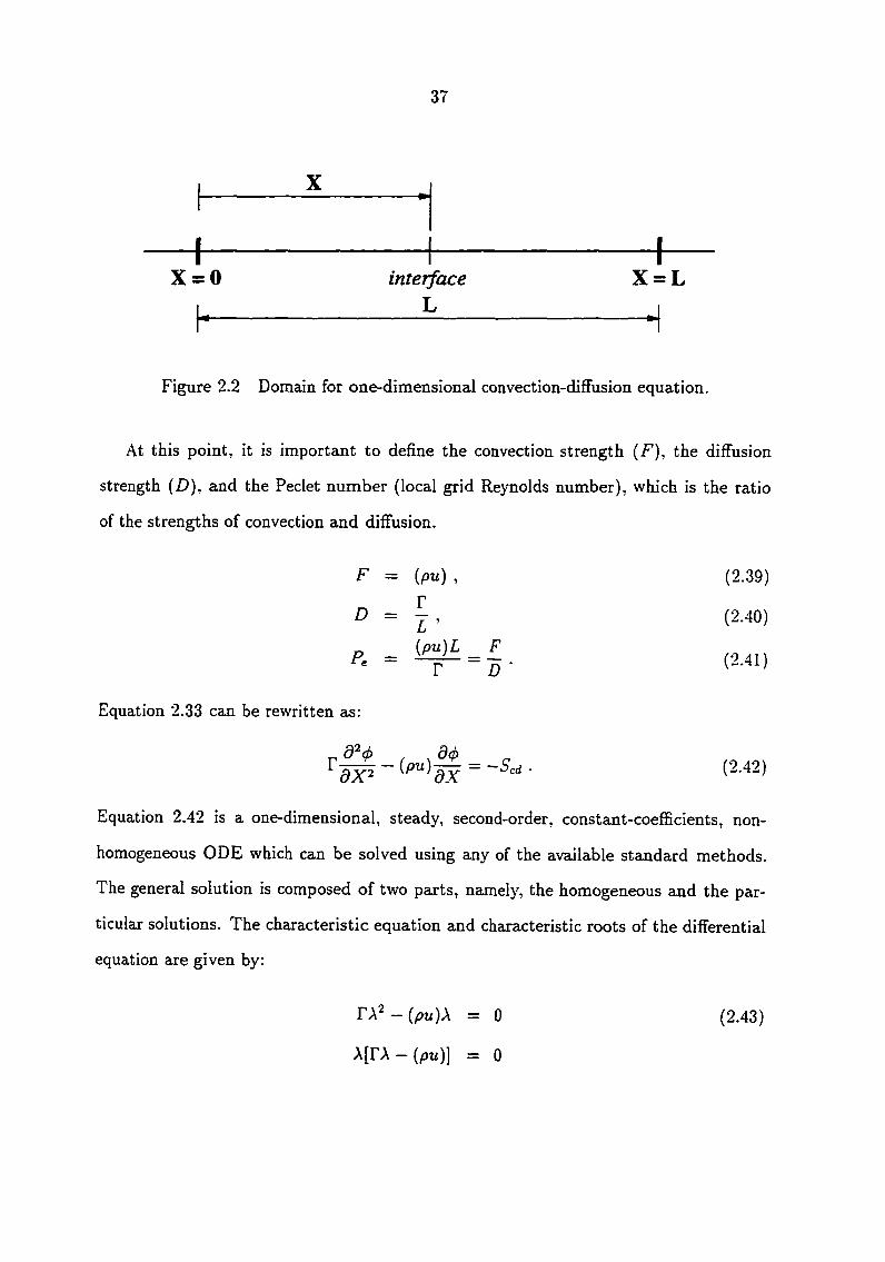
37

+ X = 0 interface X = L

L H

Figure 2.2 Domain for one-dimensional convection-diffusion equation.

At this point, it is importajit to define the convection strength (F), the diffusion

strength (D), and the Peclet number (local grid Reynolds number), which is the ratio

of the strengths of convection and diffusion.

F = { p u ) , (2.39)

JO = ^ , (2.40)

_ {P'^)L F P ' = - V ^ D -

Equation 2.33 can be rewritten as:

T-i d^ / (2.42)

Equation 2.42 is a one-dimensional, steady, second-order, constant-coefficients, non-

homogeneous ODE which can be solved using any of the available standard methods.

The general solution is composed of two parts, namely, the homogeneous and the par

ticular solutions. The characteristic equation and characteristic roots of the differential

equation are given by:

rA2-(^z/)A = 0 (2.43)

X [ r X - { p u ) ] = 0

38

and

A i = 0 ,

. (pti) A2 = — .

The homogeneous solution is obtained as:

4>h{X) = ,

(2.44)

(2.45)

(2.46)

and the particular solution is given by:

M X ) = { p u )

(2.47)

The sum of the homogeneous and particular solutions gives the general solution:

<t>{X) = H{X) + MX)

= c. + ^ + C3 . [ p u )

(2.48)

(2.49)

Applying the left and right boundary conditions (equations 2.37 and 2.38) results in the

following expressions for the constants Ci and Cj:

(<pL - o) - {ScdL)l{pu) Ci =

C2 =

e'P' - 1 — 0 L + [ S c d L ) l { p u )

(2.50)

(2.51) 6 "= — 1

Substituting the above constants into equation 2.49 results in the profile of the dependent

variable 6 d& z. function of the interface distance X:

\P . {X /L) _ <^(-^) — <^0 + oPt — 1 (<PL — 0o) + 4>3{.X) ,

where

U X ) = -

•gP.(A-/L) _ I

(2.52)

(2.53) e <= — 1

Note that 4>s{X) is the correction to the homogeneous solution due to the presence of

source Scd- If Scd is set to zero, then 4>s{X) vanishes, and (f>{X) recovers the exponential

scheme for one-dimensional, convection-diffusion, without source [5].

39

The profile of the first derivative of <f> can then be obtained as:

d(l) fPe

dX

where

= (f) eP^(XlL)

e « — 1 {<f>L - <Po) + , (2.54)

^ _ (^cdL\ dx \ r J

'eP'^x/L) + 7^ • (2.55)

[ p u ) — 1

Again, vanishing Scd means that the source-induced first-derivative term becomes zero,

and only the homogeneous term remains.

To better understand the nature of the profile of 4> obtained from solving the convection-

diffusion equation considered previously, two complementing cases are investigated. In

the first case, the effect of source Scd is neglected and the homogeneous solution of o

along A' is plotted for different values of the Peclet number (Figure 2.3).

It is observed that the profile of <j) is far from linear except for small values of |Fe|.

For small |Pe| (small convection and/or large diffusion), the influences of 4>o and (pi on

the middle interface value are equally dominant. For large \Pe\ (large convection and/or

small diffusion), the interface value is predominantly influenced by the upstream value.

This is consistent with the physics. The role of the boundary conditions, in this case, is

to establish a difference in the boundary (j) values so that the effect of different Peclet

numbers can be established.

In the second case, the boundary values are set to equal value, leaving only the

source induced part of the general solution. As expected, both the Peclet number and

the source level have a profound influence on the profile of (b. The effect of varying the

Peclet number while fixing Scd is given in Figure 2.4. For a given source level, as |Pe|

increases, the peak of the profile decreases in magnitude and is shifted more toward the

downstream direction. Recall that the upstream and downstream are defined relative

to the flow direction. Maximum peak occurs at Pe=0. Thus it can be concluded that

maiximum correction to the homogeneous profile happens at the middle of the domain for

small values of the Peclet number. The plot of the percentage of the ratio of peak value

40

Pe «-1

Pe = -1

Pe = 0

Pe = l

P e » l

O

Figure 2.3 Profile of o witti 5'c<i=0 and different Peclet numbers.

at a given Peclet number to tlie maximum peak value as the Peclet number increases is

given in Figure 2.5. The curve is identical for different source levels. This plot reveals

that the correction is significant until |Pe|«20. At higher |Pe|, the curve is very slowly

assymptoting to 0 as Pe—¥oo. In essence, this says that for a very high convection flow

aligned to a grid direction, the homogeneous solution is nearly sufficient to model the

interface value of cp. Recall that this is the ideal condition for the application of the

Power Law scheme.

The profile of the particular solution as the Peclet number is fixed and the source level

is varied is given in Figure 2.6. It is observed that for a given Peclet number, different

source levels give different peak values but the same peak location. In this analysis, all

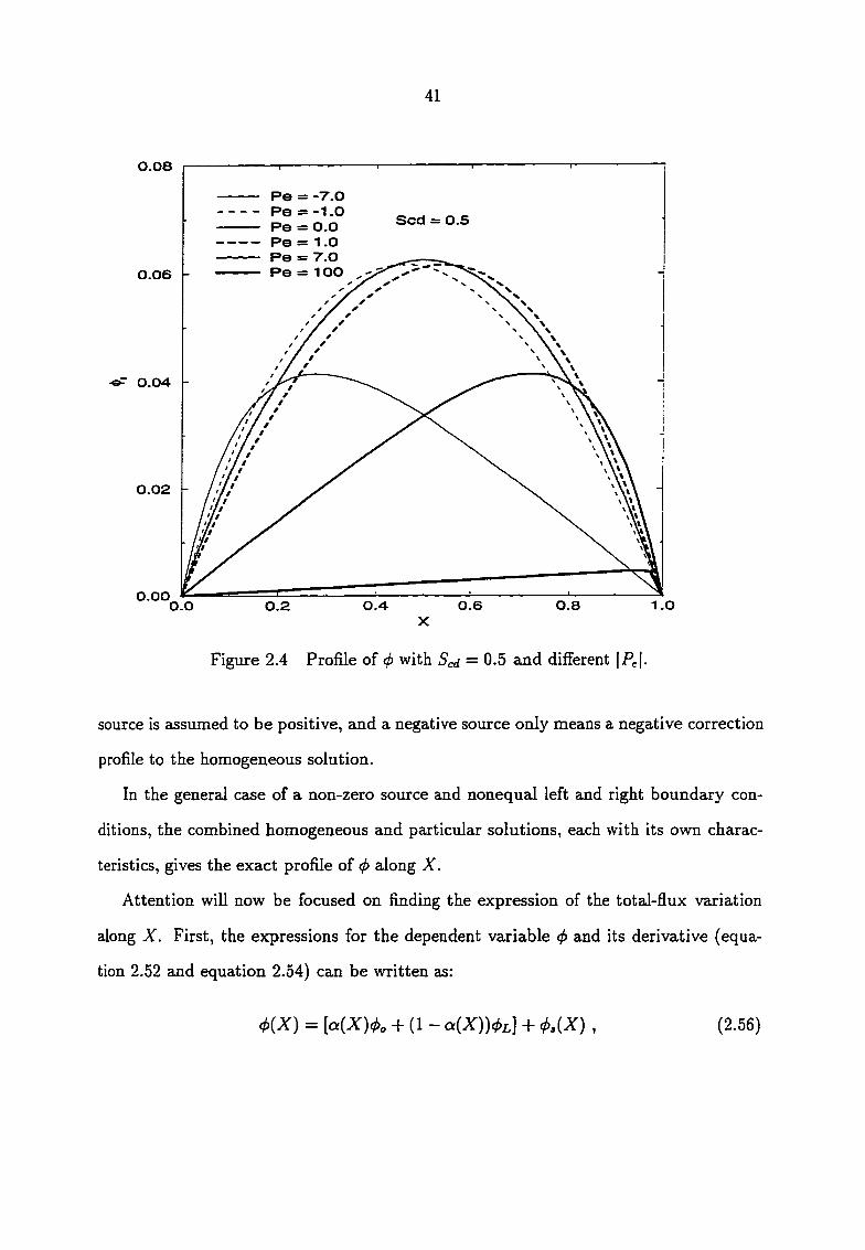
41

0.08

Pe = -7.0 Pe = -1.0 Pe = O.O Pe = 1.0 Pe = 7-.0 Pe = 10O

Scd = 0.5

0.06

0.04

0.02

O.OO 0.6 0.8 1 . 0 O.O 0.2

X

Figure 2.4 Profile of (j) with Scd = 0-5 and different |Pe|.

source is assumed to be positive, ajid a negative source only means a negative correction

profile to the homogeneous solution.

In the general case of a non-zero source and nonequal left and right boundary con

ditions, the combined homogeneous and particular solutions, each with its own charac

teristics, gives the exact profile of 4> along x.

Attention will now be focused on finding the expression of the total-flux variation

along x. First, the expressions for the dependent variable cf) and its derivative (equa

tion 2.52 and equation 2.54) can be written as:

0(X) = [a{x)<f>o + {1- aix))l] mx) , (2.56)

42

100.0

a> CO

CO a> a. X CO

o a>

CO CD d.

"co CC a>

o <D CT> i5 "H o

(X> Q_

80.0

60.0 -

40.0 -

20.0

0.0 0.0 20.0 40.0 60.0

Peclet number 80.0 100.0

Figure 2.5 Middle interface value of as function of |Pe|.

where

and

where

a i X ) = ep' -

— 1

^ ( x ) = /3(X)(,At - ^

/3m = '(puy ep'ixil)

eP' - 1

(2.57)

(2.58)

(2.59)

An intermediate variable Jl will now be defined as:

j ; { X ) = m x )

D = m x ) [ y )

= ((p„)^(x)-r|(X))(^)

(2.60)

43

0.08

0.06

0.04

0.02

O.OO

S_ = 0.30 = 0.50

Scd = = 0.90

O.O 1.0

Figure 2.6 Profile of (p with fixed |Fe| and different Scd-

dd) = p,4>{x) - l^{x) .

Substituting equation 2.56 and 2.58 into the above equation results in:

j;{x) = [b{pc)o - A(Pe)0L] + jsl , (2.61)

where

and

A{P.) =

B{P.) =

pc e^<= - 1 ' p,e^'

e p ' - l '

js; = pmx) - l^{x)

(2.62)

(2.63)

(2.64)

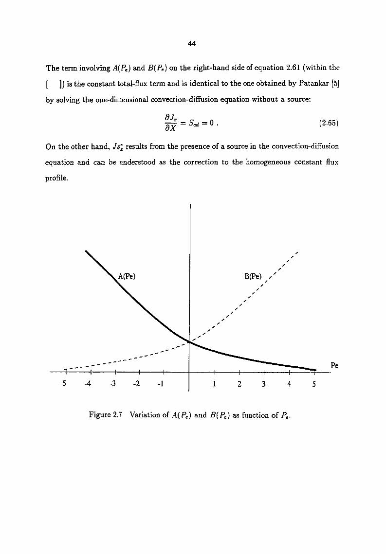
44

The tenn involving A(Pe) and B{Pe) on the right-hand side of equation 2.61 (within the

[ ]) is the constant total-flux term and is identical to the one obtained by Patankar [5]

by solving the one-dimensional convection-diffusion equation without a source:

^ = S^ = 0. (2.60)

On the other hand, Jsl results from the presence of a source in the convection-diffusion

equation and can be understood as the correction to the homogeneous constant flux

profile.

A(Pe) B(Pe)

Figure 2.7 Variation of A{Pe) and B{Pe) as function of Pg.

45

The variation of A{Pe) and B{Pe) as a function of the Peclet number is given in

Figure 2.7. Patankar edso showed that A(Pe) and B{Pe) posses certain mathematical

characteristics. First, subracting A(Fe) from B{Pe) results in:

5(Fe) = A(P,) + Pe. (2.66)

Secondly, careful observation of Figure 2.7 shows that there exists a certain kind of

symmetry between the two curves. Rotating the verticed axis such that Pe becomes —Pg

will result in the two functions interchanging their roles. Thus, A{Pe) and B{Pe) must

be related by:

A(-Pe) = 5(P,), (2.67)

B { - P , ) = A { P g ) . (2.68)

Consequently, A{Pe) axid B{Pe) can be rewritten as:

A{Pg) = A(|P,|) + |-P„OE , (2.69)

B{Pg) = A(|Pe|) + ttP.,OE. (2.70)

Substituting equation 2.66 into equation 2.61 and then using equation 2.69 gives the

following equation:

J : { X ) = P g c j ) , + { A { \ P g \ ) + I-Pe, O]]}(0o - 0l) + J s ; , (2.71)

where | , , ]] means the largest of the quantities contained within it. Similarly, using

equations 2.66, 2.61, and 2.70 results in the second equation for J*(A'):

j ; (X ) = + Js ; . (2.72)

It can be ezisily verified that equation 2.71 and equation 2.72 axe identical. The purpose

of writing Jx[X) in these two forms will be evident in the section to follow.

46

Attention will now be focused on the Substituting equation 2.53 and equa

tion 2.55 into equation 2.64 yields:

J s l ( X ) = - ( y

£2

Scd

Scd

= (

_ 1 e^"= — 1

ep'{xil)

X L „ + -p-'^cd +

e^<= — 1

1

{ p u )

— 1.

1

X L „ ( L \ \ 1 + p 5e</ Saij X

11 eP' - 1 PJ

(2.73)

(2.74)

= yw{p.) + x]scd,

where is a function of the Peclet number only and is given by:

p — + 1 qw = -fprrpt •

Note that Q{Pe) is singular for Pe=0; however, taking the limit cis Pg-^O, yields Q{Pe)—^—^.

Finally, using equations 2.71, 2.72, and 2.73, the expression for the total-flux profile

caxi be written as;

m x ) = j:ix)d = j: Q = + { D A { \ P , \ ) + (I-F,0]]}(<?i„ - 0l) + J s , { X ) (2.75)

= F<l>L + {DA[\P,\) + lFM}{o-<l>L) + Js,{X) , (2.76)

where

J s , { X ) = [ L Q { P , ) + X ] S , i (2.77)

An important observation concerning the above equation is that the total-flux at a given

X-location now consists of a term which multiplies the difference in the boundary values

of . Note that the total-flux correction Jsx{X) is directly driven by the strength of

the source and is not monotonous but varies across the domain considered. Again,

in the absence of a source, the total-flux correction vanishes and the total-flux profile

47

Jx becomes a constant profile resulting from solving the convection-diffusion equation

without a source.

2.6 Flux Corrected Method: Application of Steady One-di-

mensional Convection Diffusion with Source to Two- and

Three-dimensional Transport Modeling

2.6.1 Discretization of General Trsinsport Equation

Recall the general conservation equation given previously in equation 2.20:

d { p 4 > )

d t + | ( M ^ _ r g + A ( M ^ - r | ) = s , ( 2 . 7 8 )

The above equation represents a conservation of the dependent variable 4> with terms

representing the unsteady term, x-direction transport (convection and diffusion), y-

direction transport, axid a source. An increase or decrease in one or more of these

four terms will result in changes in the other terms such that the overall balance of

equation 2.78 is still maintained. Integration of equation 2.79 over time and over a two-

dimensional control-volume (Figure 2.1) is given in equation 2.29 and is quoted here for

convenience: [ { p < f > ) p - AxAy

A< "*•

f( , j intg _ jintg\ , j Wr—c 12/ *1" n '

(1 - =

fgiM, ^ (2.80)

Having decided on how to model the convection-diffusion transport, it is now possible

to take the next step toward the formulation of the discretized equation, which is to

4S

express the totai-flux at a control-volume face in a coordinate direction in terms of

the neighboring (p values in that direction. Consider for example the ic-interface in

Figure 2.1. Flux Corrected Method (FCM) realizes that the expression of the total-flux

at the i£7-interface is actually governed by the same transport equation 2.78 applied to

the main control-volume containing that interface. Thus, a natural way to evaluate the

x-direction total-flux is to use the conservation principle itself, which is rewritten in the

form:

= (5.W • (2.81)

Equation 2.81 is the convection-diffusion equation with source whose solution and char

acteristics have been discussed extensively in the previous section. It is also assumed

that ipu), r, and (5x)ci are constant throughout the control-volume considered. The

left and right boundary conditions are given by Ovv and <f>p. Then, using equation 2.76.

the total-flux in the x-direction at the lu-interface can be written in terms of the bound

ary values (pw and Op. Similarly, the total-flux expression at the e-interface and at the

interfaces at the other coordinate directions can also be expressed in terms of the neigh

boring values of the dependent variable 0 in that coordinate direction. In this way. the

integrated transport equation (equation 2.80) is transformed into the discretized form.

The distinguishing mark of this approach is that the full conservation equation is not

only satisfied at the control-volume over which it is integrated, but is also fully conserved

in the determination of the total-fluxes at the interfaces. Thus, the unsteady term, the

cross-wise total-fluxes, and the source term have a direct way to influence the total-flux

profile in a coordinate direction. The idea behind FCM and its subsequent development

is motivated by the failure of the exponential scheme to take into account the multidi-

mensionaJity and the presence of transient and source terms in the interface total-flux

calculation. Since the exponential scheme (and its derivatives, ie: hybrid and Power

49

Law schemes) is based on the solution of steady, one-dimensional, convection-diffusion

without source, the resulting toted-flux profile is constant throughout the control-volume

considered. What FCM does is to taJce this constajit profile as the baseline profile and

add a non-monotonous correction profile to account for the presence of Scd- This ap

proach is appropriately reflected in the name 'Flux Corrected Method'.

2.6.2 Discretization of the x- and y-momentum Equations

The previous modeling concept for the general multi-dimensional convection-diffusion

transport will now be applied to obtain the discretized x-momentum equation. The

conservative form of the x-momentum equation (equation 2.13) is quoted below for

convenience:

Integration of equation 2.83 over time and over the two-dimensional control-volume

(Figure 2.1) results in the following integral balance of the x-momentum equation:

dy) '

(2.83)

(2.82)

f\( fO intg , jo intg jo intg\ /A*'xr—e w * *^yx—3 ) —

(2.84)

where

(2.87)

(2.86)

(2.85)

50

Note that the time integration of the pressure term is treated implicitly.

Since mass must also be conserved at each timestep, the integral balance of the

continuity equation (equation 2.26) can be rewritten as:

+

(1 - - Ftll'' + - F°JT') = 0 . (2.88)

By multiplying the above equation with up and then substituting the Taylor series

expansion for up about time t:

up = u ? , + ( ^ | A f + 0 ( A t ^ ) . d t j p

= u°p + u°pAt + 0{At^) (2.89)

in the previous integrated mass-conservation equation, one obtains:

/(Fi:L'f - + fil'^ - fi'unup +

ar^f T^o intg po intg , rpo intg rpo intg\ o J )\"x—e ^x-w "I "y—n "y—s /"P

-(1 - - F°J:'n<P^t • (2.90)

Subtracting equation 2.90 from equation 2.84 yields:

( u p - u ° p ) p ° p A x A y

At +

) - <•&„ - ft-tup) +

(- fi'j!up) 1 +

(1 - /)[(4?i, - - (jsx - Fiiwr +

- f-l'^up)' - (42'j. - i =

(pm., _ pmlj) ^

(1 - mki'f - fiztr + (f^-n - f;-/)°KpAi. (2.91)

51

Note that the last term of equation 2.91 vanishes due to mass conservation at the previous

timestep. The next step in the discretization process is to express the totd-fluxes at

the interfaces in terms of the neighboring u values. Considering for example the e- and

u;-interfaces, the total-fluxes at these interfaces eixe obtained by solving the x-direction,

one-dimensionzil, convection-diffusion with source over the x-intervals containing those

interfaces:

^(4x-e.u,) = Sr.-c,u; , (2.92)

and similarly, the total-flux at the n- and 5-interfaces are obtained by solving;

q •^(Jyx-n,s} = Syr-n,3 , (2.93)

over the y-intervaJs containing the n- and s-interfaces. The convention used for the first

and second subscripts of the above sources is the same as that used to differentiate the

momentum total-fluxes. Although the appropriate choice for Sxx~e,w and Syx-n,3 should

be obvious based on the discussion of the general transport formulation in the previous

subsection, let the two convection-diffusion sources represent a general source expression

which will be specified in the next chapter. The combined flux at the tu-interface can

be written as:

J*xx-w ~ = combined flux at w—interface

— [jxi—m pi—w^p\^y

— \Px—w^P "t" :x—tul) "I" U-^x—0]]}(^W ^p) "I" Jxxa—-ui Fx—m^p\^y

= [{^x-u;'4(|Pex-u;|) + 1I^i-u/,0]]}(uh'— Up) + Jxis-v/jAy , (2.94)

where equation 2.76 has been substituted for Jxx-w Referring to Figure 2.2, it should

also be obvious that:

" A x , '

p fx-. fx-^ay

Dx.^ d^X, ~ Dx-u,ay •

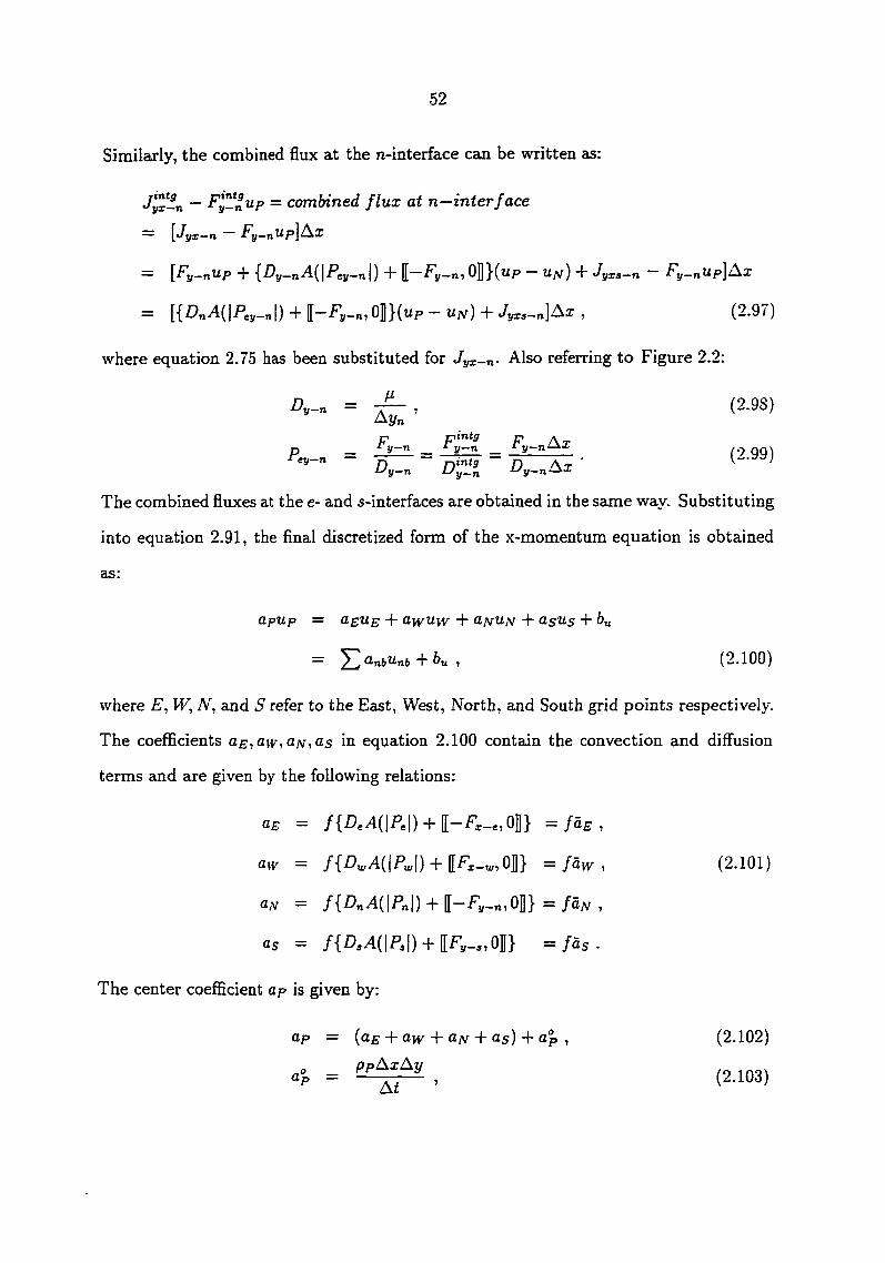
52

Similaxly, the combined flux at the n-interface can be written as:

« ^ r - n — = C o m b i n e d f l u x a t n — i n t e r f a c e

— \Jyx—n Fy—n'^p\^^

— \Fy—n'^p + {Z?y_n Ad/'ey—n 0 "I" [[ -^y—n? 0]]}(up Ujv) + Jyxs—n fy—n'^p]^^

= [{Z}„A(|P,,_„|) + [[-F„_„,0]l}(up - un) + Jyxs-n] A x , (2.97)

where equation 2.75 has been substituted for Jyx-n- Also referring to Figure 2.2:

(2.98) Ay„

— . Dy.„ Dy.^^X- ^

The combined fluxes at the e- and 5-interfaces are obtained in the same way. Substituting

into equation 2.91, the final discretized form of the x-momentum equation is obtained

as:

apup = a£UE + awuw + ai\fU,w + asus + 6u

= 5^a„6U„6 + 6u, (2.100)

where E, W, N, and S refer to the East, West, North, and South grid points respectively.

The coeflScients aEiawidNiUs in equation 2.100 contain the convection and diffusion

terms and are given by the following relations:

o-e = /{^e^d^d) + j—-^x-co]]} = fag ,

<^\v = /{jDu,A((P„[) + [[Fx_^, Oj} = f a w , (2.101)

an = f{DnA{\Pn\) + [[-Fj,_„,0]]} = fa^ ,

as = /{DjAdP,!) + [ [ Fj,_3,01} = f c i s .

The center coefficient ap is given by:

a p = { a E + a w + O ' N + a s ) + d p , (2.102)

. (2.103)

53

and is composed of the sum of the neighboring coefficients and the terms due to the

unsteady integration ap. Similarly, the source term is given by:

6„ = (P.-Pu,)Ay + 6„, + 6^ (2.104)

bus ~ y["^xxa—e *fxxs—w\^y f\,'^yi3—n • (2.10o)

6 ° = a ° p u ° p — { I - f ) [ a E i u p - ue T + a l y { u p - u w ) ° +

a % { u p - u ^ w Y + a ° s { u p - u s ) " ] +

(1 - f)[Jxxs-. - Jxxs-w^^y + (1 - f)[Jyxs-n " . (2.106)

where bus is the collection of the total-flux corrections at the interfaces, and 6° is the

source term due to the unsteady integration.

Observation of equation 2.102 shows that the neighboring coefficients contain the

term .4(|Pe|), which is an exponential function given by equation 2.62. Although the

exponential expression is bcised on the exact solution of the one-dimensional convection-

diffusion equation considered, it is not recommended for use because (1) exponentials

are relatively expensive to compute, and (2) for an NxN two-dimensional grid, the term

.4(1 Pel) must be computed 2x;V^ times. An alternative to computing .4(|Pe|) is to use

the Power Law expression given by Patankar [5]:

.4(|P,|)« 10,(1-0.1|Pe|)'l . (2.107)

The above function is a curve fit to the exponential expression and has been shown to

be sufficiently accurate for all practical purposes. Graphical comparison between the

exponential and Power Law functions can be found in Appendix A.

Careful observation of the above final discretized form also shows that Patankar's

•pour Basic Rules' necessary for convergence eind for physically realistic solutions [5]

are preserved. The total-flux corrections are all collected as an additional source. No

change is introduced to the other coefficients. This property makes FCM very attractive

for established codes based on the exponential scheme (or its variants).

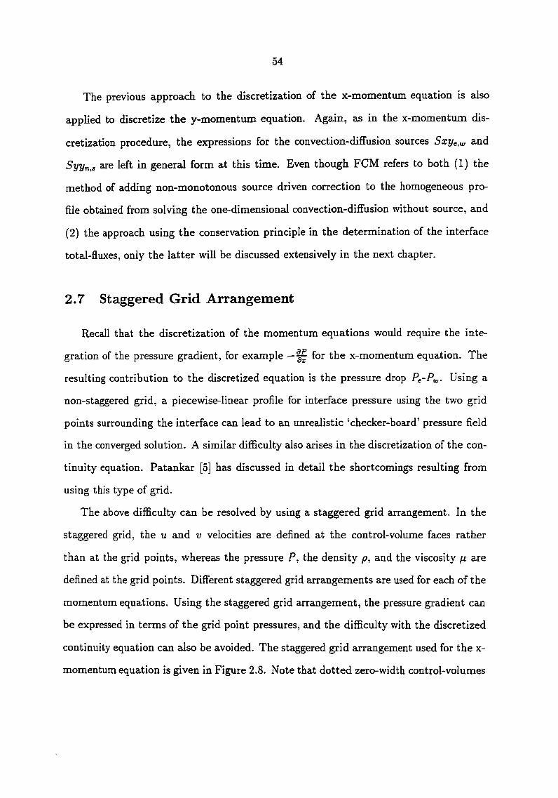
54

The previous approach to the discretization of the x-momentum equation is also

applied to discretize the y-momentum equation. Again, as in the x-momentum dis

cretization procedure, the expressions for the convection-diffusion sources Sxye,^ and

Syyn,s are left in general form at this time. Even though FCM refers to both (1) the

method of adding non-monotonous source driven correction to the homogeneous pro

file obtained from solving the one-dimensional convection-diffusion without source, and

(2) the approach using the conservation principle in the determination of the interface

total-fluxes, only the latter will be discussed extensively in the next chapter.

2.7 Staggered Grid Arrangement

Recall that the discretization of the momentum equations would require the inte

gration of the pressure gradient, for example — for the x-momentum equation. The

resulting contribution to the discretized equation is the pressure drop Pe-Pw Using a

non-staggered grid, a piecewise-linear profile for interface pressure using the two grid

points surrounding the interface can lead to an unrealistic 'checker-board' pressure field

in the converged solution. A similar difficulty also arises in the discretization of the con

tinuity equation. Patankar [5] has discussed in detail the shortcomings resulting from

using this type of grid.

The above difficulty can be resolved by using a staggered grid arrangement. In the

staggered grid, the u and v velocities are defined at the control-volume faces rather

than at the grid points, whereas the pressure P, the density p, and the viscosity // are

defined at the grid points. Different staggered grid arrangements are used for each of the

momentum equations. Using the staggered grid arrangement, the pressure gradient can

be expressed in terms of the grid point pressures, and the difficulty with the discretized

continuity equation can also be avoided. The staggered grid arrangement used for the x-

momentum equation is given in Figure 2.8. Note that dotted zero-width control-volumes

are used to enclose the boundary grid points. The use of zero-width control-volumes

maJces it easier to keep track of the indexing used for the velocity components. From this

point on, distinctions will be made among the terms "main control-volume", "staggered

x-control-volume", cind "staggered y-control-volume".

The discretized momentum equations, each written using its corresponding staggered

grid arrangement, axe :

OeUe = ^ a„6U„6 + {Pp — + K ' (2.108)

anVn = anbVnb + {Pp " /'iv)Ax + + 6° . (2.109)

Since each momentum equation is written based on its own staggered grid arrangement,

the coefficients are different for different momentum equations.

The staggered grid arrangement was first used by Harlow and Welch [37] in the MAC

method. It also forms the basis of the SIV.A procedure of Caretto, Curr, and Spalding

[38] and the SIMPLER procedure of Patankar [5] used in the present work.

The use of a staggered grid also necessitates the establishment of a subscript/indexing

convention to allow quick and convenient reference to a grid-point or a control-volume

face. The x-direction indexing is given in Figure 2.8 where ig is used to denote the grid

index and if is used to denote the control-volume face index. The j-'mdex is defined

trivially. Thus an i subscript to u means an if subscript, and an i subscript to pressure

means an ig subscript. Grid face is then defined as the face which passes through a grid

point, and its indexing convention follows the one used for grid point. The grid and

control-volume face indexes in the y-direction are defined in the same way.

2.8 SIMPLER Algorithm

Early in this chapter, it was mentioned that one approach to solving the incom

pressible flow equations is to use an iterative procedure which alternately solves for the

Figure 2.8 Staggered x-control-volume

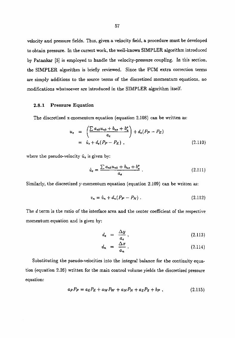
57

velocity and pressure fields. Thus, given a velocity field, a procedure must be developed

to obtain pressure. In the current work, the well-known SIMPLER aJgorithm introduced

by Patankar [5] is employed to handle the velocity-pressure coupling. In this section,

the SIMPLER algorithm is briefly reviewed. Since the FCM extra correction terms

are simply additions to the source terms of the discretized momentum equations, no

modifications whatsoever are introduced in the SIMPLER aJgorithm itself.

2.8.1 Pressure Equation

The discretized x-momentum equation (equation 2.108) can be written as:

Ue = + + + 4(Pp _ p^)

= u,-\-d,{Pp-PE) , (2.110)

where the pseudo-velocity Ue is given by:

IZ "1" ^us "t" /.-> i 7 i i Ue = . (2.111) <Xe

Similarly, the discretized y-momentum equation (equation 2.109) can be written as:

Un = Un + dr ,[Pp - Pn ) • (2.112)

The d term is the ratio of the interface area and the center coefficient of the respective

momentum equation and is given by:

4 = ^, (2.113)

Ax dn = . (2.114)

an

Substituting the pseudo-velocities into the integral balance for the continuity equa

tion (equation 2.26) written for the main control volume yields the discretized pressure

equation:

apPp = oePe + dwPw + clnPn + o-sPs + bp , (2.115)

58

where the coefficients axe given by:

ue = ipd)eay ,

(i]y — i^p^w^y 1

ai^ = (pd)sax (2.116)

as = (pd)nax ,

o.p = 0.E + O.W + Oiv + as ,

and the source term is given by:

bp = -[(/>«)= - (p")u,]Ay - [(/Ju)„ - (/>u),]Ax . (2.117)

2.8.2 Correction Equations

In order to get a converged solution of the velocity field at a given timestep, the

coefficients of the momentum equations are lagged or calculated either by using the ve

locity field obtained from the previous iteration or from the converged velocity field of

the previous timestep in the case of the first iteration within a time-loop. The same

principle is also applied to any source term which is a function of the velocity compo

nents. However, a different treatment is used for the pressure gradient. The pressure

gradient terms are not estimated using the values from the previous iteration, but are

determined directly from the velocity field of the previous iteration using the pressure

equation derived in the previous subsection. The discretized momentum equations can

then be solved for the current iteration to obtain a new velocity field. However, unless

convergence has been achieved, this newly computed velocity field may not satisfy the

continuity equation since the pressure field calculated from the previous iteration of the

velocity field may not have converged yet. Thus a procedure is needed to correct the

pressure field. The corrected pressure field can then be used to correct the velocity field

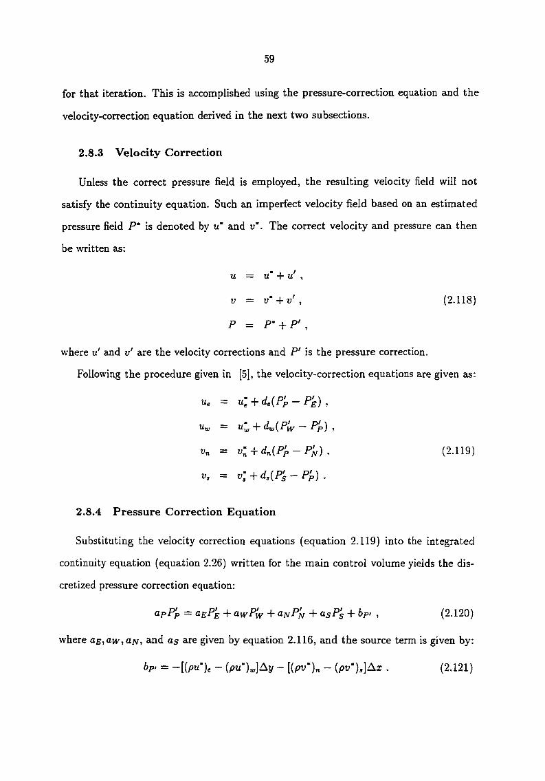
59

for that iteration. This is accomplished using the pressure-correction equation and the

velocity-correction equation derived in the next two subsections.

2.8.3 Velocity Correction

Unless the correct pressure field is employed, the resulting velocity field will not

satisfy the continuity equation. Such an imperfect velocity field based on an estimated

pressure field P' is denoted by u" and u*. The correct velocity and pressure can then

be written as:

u = u' + u' ,

V = v - + v ' , ( 2 . 1 1 8 )

P = P' + P' ,

where u' and v' are the velocity corrections and P' is the pressure correction.

Following the procedure given in [5], the velocity-correction equations are given as:

y-e — y-'e "'t d.e{pp ~ p'e) 1

~ dxu{P\Y — P'p) ,

= v', + dn{P'p-P'f,), (2.119)

Vs = uj 4- ds{P^ — Pp) .

2.8.4 Pressure Correction Equation

Substituting the velocity correction equations (equation 2.119) into the integrated

continuity equation (equation 2.26) written for the main control volume yields the dis-

cretized pressure correction equation:

dpP'p = o,epe "I" ^wPw "I" ^np'n + sP's + ^p' 1 (2.120)

where ae,aw,a]\f, and as are given by equation 2.116, and the source term is given by:

h' = -[(P^'*)e - (/?u')^]Ay - [(^u')„ - (/>u'),]Ax . (2.121)

60

Note that from the above equation, bp> represents a measure of how well the mass

conservation at the main control-volume is satisfied at each iteration. Thus, this quan

tity is often used as the indicator for convergence of the numerical solution. However,

this condition is to be used in conjunction with the convergence of the residual of the

momentum-conservation and with the residual of the velocity components. It has been

observed that for high Reynolds number flow problems, it is possible to see convergence

of the mass conservation to an acceptable level while the residuals of the other two

criterias are still not satisfied.

2.8.5 Solution Procedure for the Discretized Equations

The governing equations for the flow-field are non-linear. Even though the discretized

equations have been cast into a linear form, the coefficients and the source terms are

functions of the dependent variables. In the present work the discretized equations are

solved independently and sequentially (also known as the 'segregated' approach). For

a given timestep and at each iteration, the coefficients and the source terms are lagged

using the flow-field obtained from the previous iteration. Iterations are repeated until

convergence is achieved for that timestep.

Writing the discretized equations for all the control volumes in the flow domain

yields a tridiagonal system of simultaneous algebraic equations. This algebraic system

of equations is solved using the Successive Line Over-Relaxation (SLOR) method. The

SLOR method proceeds by sweeping the two-dimensional computational space, line by

line, in both directions. The TriDiagonal Matrix Algorithm (TDMA) is used for each

line sweep. .A.n under-relaxation is used between each TDMA update to prevent the

solution from diverging.

61

2.8.6 SIMPLER Algorithm Summary

The sequence of steps for the unsteady SIMPLER algorithm modified for FCM im

plementation caji be simimarized as follows:

1. Start with a given initial flowfield.

2. Calculate the unsteady portion of the center coefficients (for the x-momentum.

calculate a°p given by equation 2.103).

3. Calculate the unsteady portion of the source terms (for the x-momentum, calculate

K given by equation 2.106).

4. Calculate the totaJ-flux corrections and add to the source of the momentum equa

tions (for the x-momentum, calculate b^s given by equation 2.105).

5. Calculate the coefficients for the momentum equations and the pseudo-velocities

(equation 2.111 for pseudo u—velocity).

6. Using the calculated pseudo-velocities, calculate the source term for the pressure

equation (equation 2.117).

7. Calculate the coefficients (equation 2.116) and solve the pressure equation (equa

tion 2.115) to obtain the pressure field.

8. Using the calculated pressure field, solve the momentum equations (equation 2.100

for x-momentmn) to get the velocity field.

9. Calculate the source term of the pressure-correction equations (equation 2.121)

and solve for the pressure corrections (equation 2.120).

10. Correct the velocities using the velocity-correction equations (equation 2.119).

62

11. Return to step 4 and repeat until convergence.

12. Staxt with a new time level.

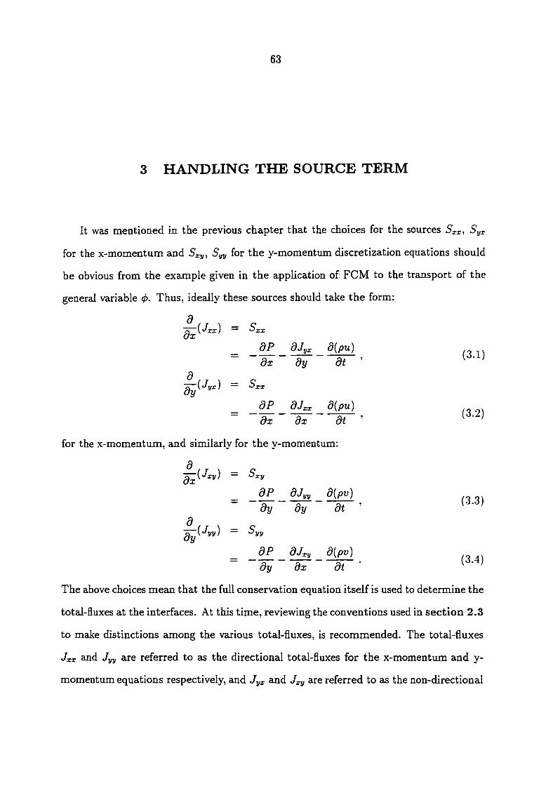
63

3 HANDLING THE SOURCE TERM

It was mentioned in the previous chapter that the choices for the sources Sxxi Syx

for the x-momentum and Sxy, Syy for the y-momentum discretization equations should

be obvious from the example given in the application of FCM to the transport of the

general variable (j). Thus, ideally these sources should take the form:

d — ^xx

dP dJyx d{pu)

dx dy d t

•^{jyx) = sxx

_ dP dJxx d{pu) dx dx d t

for the x-momentimi, and similarly for the y-momentum:

d

(3.1)

(3.2)

dP dJyy d{pv )

dy dy d t (3.3)

dP dJxy d{pv) (3.4)

dy dx d t

The above choices mean that the full conservation equation itself is used to determine the

total-fluxes at the interfaces. At this time, reviewing the conventions used in section 2.3

to maJce distinctions among the various total-fluxes, is recommended. The total-fluxes

Jxx and Jyy are referred to as the directional total-fluxes for the x-momentum and y-

momentum equations respectively, and Jyx and Jxy are referred to as the non-directional

64

total-fluxes for the respective momentum equations. Similarly, Sxx and Syy axe defined

as the directional discretized convection-diffusion sources for the x-momentum and y-

momentum equations respectively, ajid Syx and Sxy are referred to as the non-directional

discretized convection-diffusion sources for the x-momentum and y-momentum equa

tions. The second subscript always refers to the considered momentum equation and

the first subscript gives the coordinate direction of the transport of the flux or source

considered.

At this point in the development of FCM, a thorough study is initiated to investigate

the effects of the various components of the above sources individually before combining

them into the appropriate groups. Note that the convection-diffusion sources for the

x-momentum discretization concept can be categorized as the following:

Group A Unsteady term present in both Sxx and Syx-

Group B Pressure gradient term present in both Sxx and Syx-

Group C Derivative of the non-directional total-flux present in Sxx-

Group D Derivative of the directional total-flux present in Syx -

The y-momentum convection-diffusion sources axe classified in the same way.

The inclusion of the unsteady term is relatively straightforward to implement and

will not be specifically investigated in this chapter. Although only limited testings

on moderately unsteady problems will be done in the subsequent chapter due to time

constraints, it is expected that FCM will perform well for highly unsteady problems. The

mechanism to account for the driving unsteady force has been included in the discretized

equations. In this chapter, attention will focus on the effects of pressure gradients and

derivatives of the totai-fluxes on the numerical accuracy of steady problems. In the

following sections, the individual and combined effects of all the source components

axe investigated. For simplicity, only the total-fluxes at the staggered control-volume

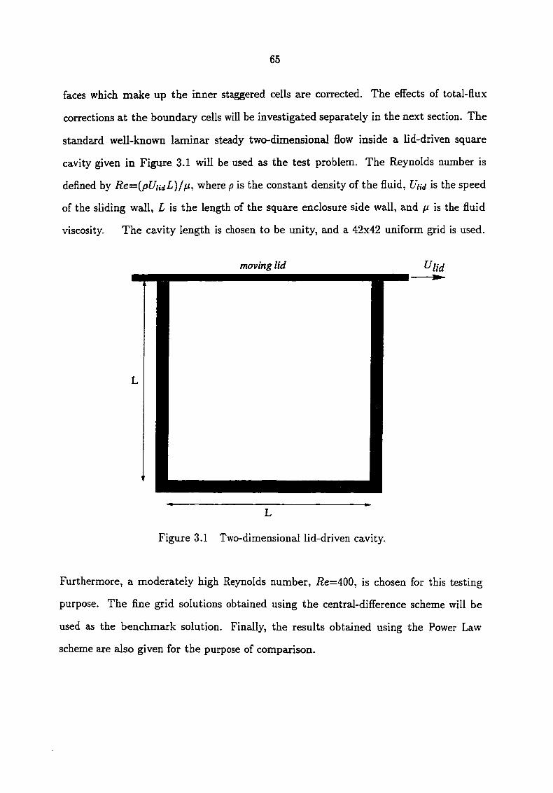
65

faces which make up the inner staggered cells are corrected. The effects of total-flux

corrections at the boundary cells will be investigated separately in the next section. The

standard well-known laminar steady two-dimensional flow inside a lid-driven squcure

cavity given in Figure 3.1 will be used as the test problem. The Reynolds number is

defined by Re={pUiidL)/fji, where p is the constant density of the fluid, Uud is the speed

of the sliding wall, L is the length of the square enclosure side wall, eind fi is the fluid

viscosity. The cavity length is chosen to be imity, and a 42x42 imiform grid is used.

moving lid U

L

Figure 3.1 Two-dimensional lid-driven cavity.

Furthermore, a moderately high Reynolds number, /?e=400, is chosen for this testing

purpose. The fine grid solutions obtained using the central-difference scheme will be

used as the benchmark solution. Finally, the results obtained using the Power Law

scheme are also given for the purpose of comparison.

66

3.1 Effect of Pressure Gradients (Group B)

In this section, the eflfects of the pressure gradients as part of the overall sources used

in the one-dimensionaJ convection-diffusion process axe investigated. The convection-

diffusion sources then can be written as:

dP Srr = (3.5)

ox

S,r = (3.6)

5^ = (3.7)

. (3.8)

Along the vertical centerline (x=0.5), the u-velocity is the dominajit component, and

along the horizontal centerline (i/=0.5), the u-velocity is the dominant component.

Therefore, the accuracy with which the formulation caji model these dominant velocity

components, each in its respective centerline, will be analyzed.

The plots of the velocity components and pressures along the centerlines cire given

in Figure 3.2 to Figure 3.5. Observations of the u- and u-velocity components along the

vertical and horizontal centerlines respectively show that slight overshoots are observed

in some regions, while in regions of high flow gradients, the corrected profiles still fail

short of the benchmark solutions. The effects of the flux-correction can be seen much

more clearly on the pressure profiles along the centerlines. It is quite obvious from

Figures 3.4 and 3.5 that the corrected solution can handle shaxp turning profiles much

better than the original Power Law scheme. Overall, it can be concluded that even

though the inclusion of pressure gradients in the convection-diffusion sources does not

reproduce the benchmark solution, significant improvement is observed.

67

1.0

0.9

0.8

0.7

0.6

>- 0.5

Benchmark 142x142 Power Law 42x42 FCM (Group B) 42x42

0.4

0.3

0.2

O.I

O.O 1.0 0.5 O.O -0.5

u-veloclty

Figure 3.2 Driven Cavity i2e=400. Effect of using source Group B on vertical centerline u profile.

0.4

0.3

0.2

0.1

o.o

-0.1

-0.2

Benchmark 142x142 Power Law 42x42 FCM (Group B) 42x42 -0.3

-0.4

-0.5

-0.6 O.O 0.1 0.2 0.3 0.4 0.5 0.6 0.7 0.8 0.9 1.0

X

Figure 3.3 Driven Cavity i2e=400. Effect of using source Group B on horizontal centerline v profile.

68

1.0

0.9

0.8

Benchmark 142x142 Power Law 42x42 FCM (Group B) 42x42

0.7

0.6

>- 0.5

0.4

0.3

0.2

0.1

0.0 I— 0.90 0.95 1,05 1.00

P

Figure 3.4 Driven Cavity i2e=400. Effect of using source Group B on vertical centerline p profile.

1.01

— Benchmark 142x142 - - Power Law 42x42

FCM (Group B) 42x42 1.00

0.99

0.98

Q. 0.97

0.96

0.95

0.94

0.93

0.92 0.0 O.I 0.2 0.3 0.4 0.5 0.6 0.7 0.8 0.9 1.0

X

Figure 3.5 Driven Cavity /?e=400. Effect of using source Group B on horizontal centerline p profile.

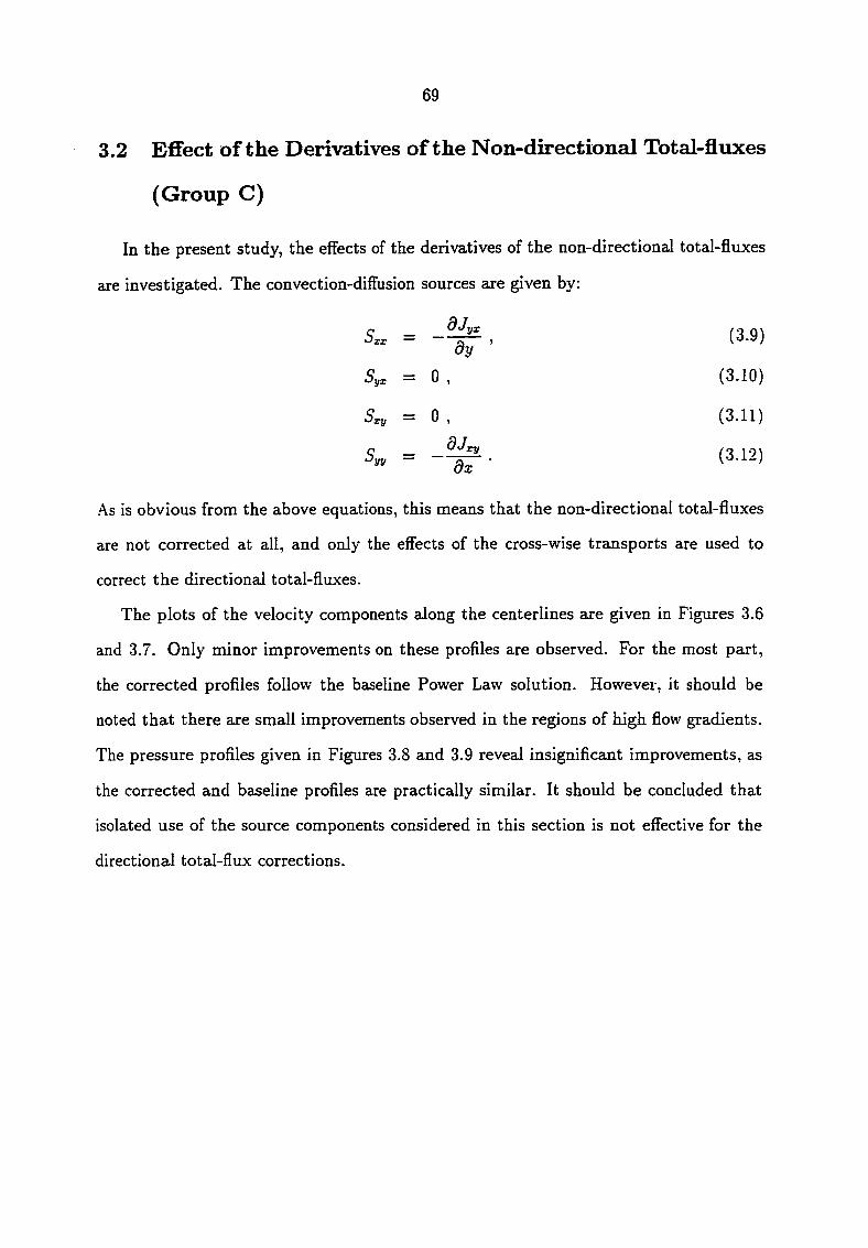
69

3.2 Effect of the Derivatives of the Non-directional Total-fluxes

(Group C)

In the present study, the effects of the derivatives of the non-directional total-fluxes

are investigated. The convection-diffusion sources are given by:

(3.9)

(3.10)

(3.11)

(3.12)

As is obvious from the above equations, this means that the non-directional total-fluxes

are not corrected at all, and only the effects of the cross-wise transports are used to

correct the directional total-fluxes.

The plots of the velocity components along the centerlines axe given in Figures 3.6

and 3.7. Only minor improvements on these profiles are observed. For the most part,

the corrected profiles follow the baseline Power Law solution. However, it should be

noted that there axe small improvements observed in the regions of high flow gradients.

The pressure profiles given in Figures 3.8 and 3.9 reveal insignificaxit improvements, as

the corrected and baseline profiles are practically similar. It should be concluded that

isolated use of the source components considered in this section is not effective for the

directional total-flux corrections.

^ djyx ~ dy '

Syx = 0 ,

Sxy = 0 ,

c _ djry ~ dx •

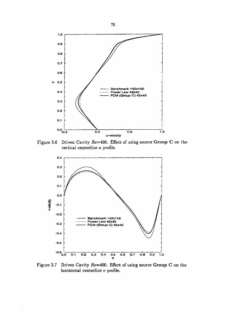
70

1.0

0.9

0.8

0.7

0.6

>- 0.5


FCM (Group C) 42x42 0.4

0.3

0.2

0.1

0.0 1.0 0.5 0.0 -0.5

u-velocity

Figure 3.6 Driven Cavity /2e=400. Effect of using source Group C on the vertical centerline u profile.

0.4

0.3

0.2

0.1

0.0

ts o a> :>

-0.1

-0.2

Benchmark 142x142 Power Law 42x42 FCM (Group C) 42x42 -0.3

-0.4

-0.5

-0.6 0.0 0.1 0.2 0.3 0.4 0.5 0.6 0.7 0.8 0.9 1.0

X

Figiire 3.7 Driven Cavity /2e=400. Effect of using source Group C on the horizontal centerline v profile.

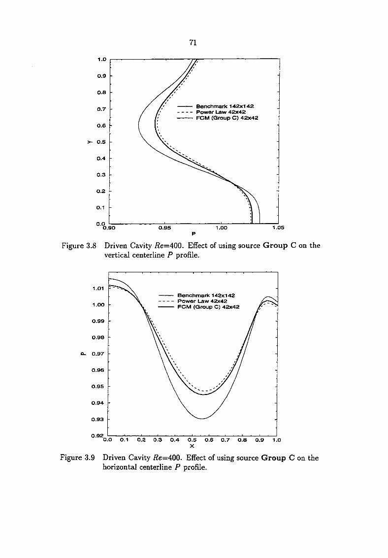
71

1.0

0.9

0.8


FCM (Group C) 42x42

0.7

0.6

>- 0.5

0.4

0.3

0.2

0.1

0.0 — 0.90 1.05 0.95 1.00

P

Figure 3.8 Driven Cavity i?e=400. Effect of using source Group C on vertical centerline p profile.

1.01 Benchmark 142x142 Power Law 42x42 FCM (Group C) 42x42 1.00

0.99

0.98

Q. 0.97

0.96

0.95

0.94

0.93

0.92 0.0 0.1 0.2 0.3 0.4 0.5 0.6 0.7 0.8 0.9 1.0

X

Figure 3.9 Driven Cavity Re=400. Effect of using source Group C on horizontal centerline P profile.

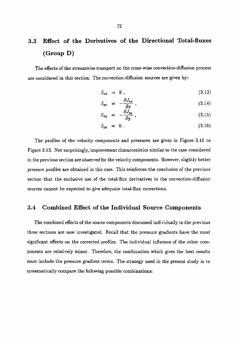
72

3.3 Effect of the Derivatives of the Directional Total-fluxes

(Group D)

The effects of the streamwise transport on the cross-wise convection-diffusion process

are considered in this section. The convection-diffusion sources axe given by:

= 0, (3.13)

dj^

d x ' (3.14)

S. = . (3.10)

= 0 . (3.16)

The profiles of the velocity components and pressures are given in Figure 3.10 to

Figure 3.13. Not surprisingly, improvement characteristics similar to the case considered

in the previous section axe observed for the velocity components. However, slightly better

pressure profiles are obtained in this case. This reinforces the conclusion of the previous

section that the exclusive use of the total-flux derivatives in the convection-diffusion

sources cannot be expected to give adequate total-flux corrections.

3.4 Combined Effect of the Individual Source Components

The combined effects of the source components discussed individually in the previous

three sections axe now investigated. Recall that the pressure gradients have the most

significant effects on the corrected profiles. The individual influence of the other com

ponents are relatively minor. Therefore, the combination which gives the best results

must include the pressure gradient terms. The strategy used in the present study is to

systematically compaxe the following possible combinations:

73

1.0

0.9

0.8

0.7

0.6

>- 0.5

Benchmark 142x142 Power Law 42x42 FCM (Group D) 42x42

0.4

0.3

0.2

0.1

O.O 1 .0 -0.5 O.O 0.5

u-velocity

Figure 3.10 Driven Cavity /?e=400. Effect of using source Group D on the vertical u centerline profile.

0.4

0.3

0.2

0.1

o.o

a a> -0.1

-0.2

Benchmark 142x142 Power Law 42x42 FCM (Group D) 42x42 -0.3

-0.4

-0.5

-0.6 O.O 0.1 0.2 0.3 0.4 0.5 0.6 0.7 0.8 0.9 1.0

X

Figure 3.11 Driven Cavity /?e=400. Effect of using source Group D on the horizontal centerline v profile.

74

1.0

0.9

0.8

Benchmark 142x142 Power Law 42x42 FCM (Group O) 42x42

0.7

0.6

>- 0.5

0.4

0.3

0.2

0.1

0.0 — 0.90 1.05 1.00 0.95

P

Figure 3.12 Driven Cavity /2e=400. Effect of using source Group D on the vertical centerline p profile.

1.01


FCM (Group D) 42x42 1.00

0.99

0.98

Q- 0.97

0.96

0.95

0.94

0.93

0.92 0.0 0.1 0.2 0.3 0.4 0.5 0.6 0.7 0.8 0.9 1.0

X

Figure 3.13 Driven Cavity /2e=400. Effect of using source Group D on the horizontal centerline P profile.

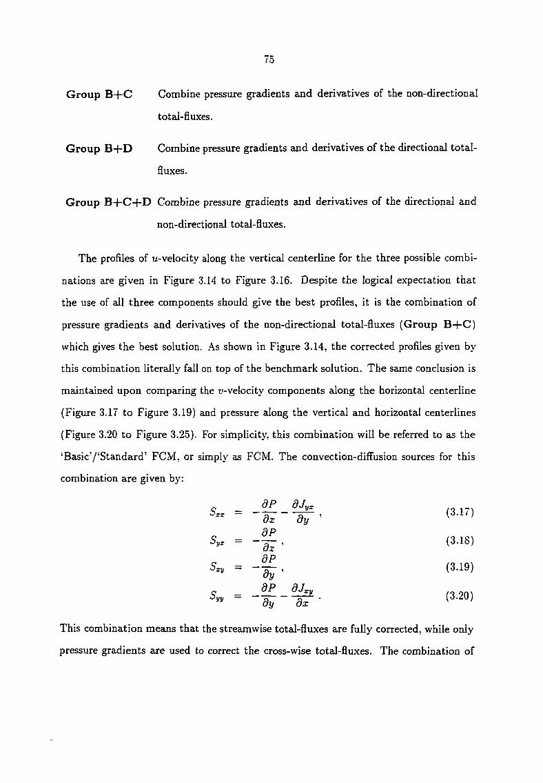
75

Group B-f-C Combine pressure gradients and derivatives of the non-directional

total-fluxes.

Group B-l-D Combine pressure gradients and derivatives of the directional total-

fluxes.

Group B-f-C+D Combine pressure gradients and derivatives of the directional and

non-directional total-fluxes.

The profiles of u-velocity along the vertical centerline for the three possible combi

nations are given in Figure 3.14 to Figure 3.16. Despite the logicai expectation that

the use of ail three components should give the best profiles, it is the combination of

pressure gradients and derivatives of the non-directional total-fluxes (Group B-j-C)

which gives the best solution. As shown in Figure 3.14, the corrected profiles given by

this combination literally fall on top of the benchmark solution. The same conclusion is

maintained upon comparing the u-velocity components along the horizontal centerline

(Figure 3.17 to Figure 3.19) and pressure along the vertical and horizontal centerlines

(Figure 3.20 to Figure 3.25). For simplicity, this combination will be referred to as the

'Basic'/'Standaxd' FCM, or simply as FCM. The convection-diffusion sources for this

combination are given by:

o _ sjy n . - i ~ d x d y ' ' '

V = (3.1S)

Sr, = , (3.19) dy

This combination means that the streamwise total-fluxes are fully corrected, while only

pressure gradients are used to correct the cross-wise total-fluxes. The combination of

76

Group B-j-D, which consists of the pressure gradients and derivatives of the direc

tional total-fluxes, resiilts in slight but non-negligible overshoots and undershoots. Over

correction is obtained when the three source components are used ail together as one

source.

It is not immediately clear why the theoretically better combination of all available

source components gives the worst results. Not only are there overcorrections, but the

slope of the u-velocity at the bottom wall is clearly not correct (Figure 3.16). It is

found that this wall slope cinomaly disappears as the grid is refined. It is the author's

opinion that future work on FCM should include an attempt to further investigate this

unexpected behavior.

3.5 Effect of Correction on Boundary Cells

Up to this point, FCM has been applied only to the inner staggered ceils. In this sec

tion, total-flux corrections are also applied to the staggered control-volume faces which

make up the boundaxy staggered cells. The difficult step in the boundary cell correction

procedure is deciding whether or not it is necessary to correct the boundary totai-fiuxes.

A. closer look at the formulation of boundary total-fluxes is therefore necessary. For the

purpose of convenience, attention will be focused on the left boundary. The total-flux

expression at this boundary is given by:

du Jxx—ig=l — (^^2)^2 • (3.21)

axig=l

Using equation 2.75 and eliminating the total-flux correction term, the left boundary

total-flux can also be written as:

•fix-ig=l — Fx-if=2U2 + {^r-ig=2^(|^e-tff=21) + ([—Fr-,7=25 0ll}(u2 — U3) • (3.22)

77

1.0

0.9

0.8

0.7

0.6

>- 0.5

Benchmark 142x142 Power Law 42x42 FCM (Group B+C) 42x42

0.4

0.3

0.2

0.1

0.0 1.0 -0.5 O.O 0.5

u-velocity

Figure 3.14 Driven Cavity /?e=400. Effect of using combined source Group B+C on the vertical centerline u profile.

1.0

0.9

0.8

0.7

0.6

>- 0.5

— Benchmark 142x142 — - Power Law 42x42 — FCM (Group B+D) 42x42

0.4

0.3

0.2

0.1

0.0 -0.5 0.0 0.5 1.0

u-velocfty

Figure 3.15 Driven Cavity i?e=400. Effect of using combined source Group B+D on the vertical centerline u profile.

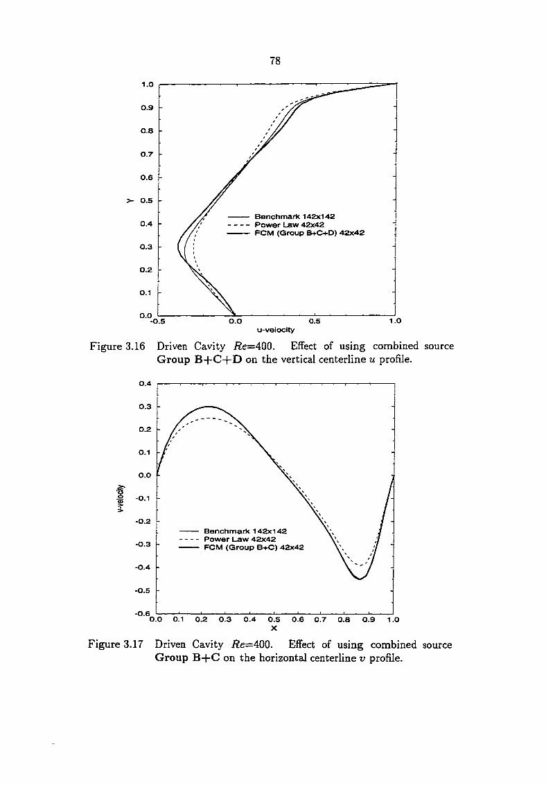
78

1.0

0.9

0.8

0.7

0.6

>- 0.5

Benchmark 142x142 Power Law 42x42 FCM (Group B+C-t-D) 42x42

0.4

0.3

0.2

O.I

0.0 1.0 O.O 0.5 -0.5

u-velocity

Figure 3.16 Driven Cavity /2e=400. Effect of using combined source Group B+C+D on the vertical centerline u profile.

0.4

0.3

0.2

O.I

o.o

a -i -O.I

-0.2

Benchmark 142x142 Power Law 42x42 FCM (Group B+C) 42x42 -0.3

-0.4

-0.5

-0.6 O.O 0.1 0.2 0.3 0.4 0.5 0.6 0.7 0.8 0.9 1.0

X

Figure 3.17 Driven Cavity i?e=400. Effect of using combined source Group B+C on the horizontal centerline v profile.

79

0.4

0.3

0.2

0.1

O.O

TS •i -0.1 >

-0.2

Benchmark 142x142 Power Law 42x42 FCM (Group B-t-D) 42x42 -0.3

-0.5

-0.6 O.O 0.1 0.2 0.3 0.4 0.5 0.6 0.7 0.8 0.9 1.0

X

Figure 3.18 Driven Cavity Re=AOO. Effect of using combined source Group B+D on the horizontal centerline v profile.

0.4

0.3

0.2

0.1

o.o s-o •§ -0.1 :>

-0.2

Benchmark 142x142 Power Law 42x42 FCM (Group B+C+D) 42x42 -0.3

-0.4

-0.5

-0.6 O.O 0.1 0.2 0.3 0.4 0.5 0.6 0.7 0.8 0.9 1.0

X

Figure 3.19 Driven Cavity i2e=400. Effect of using combined source Group B+C+D on the horizontal centerline v profile.

80

1.0

0.9

0.8

— Benchmark 142x142 — - Power Law 42x42 — FCM (Group B+C) 42x42

0.7

0.6

>- 0.5

0.4

0.3

0.2

0.1

0.0 — 0.90 1.05 0.95 1.00

P

Figure 3.20 Driven Cavity /2e=400. Effect of using combined source Group B+C on the vertical centerline p profile.

1.0

0.9

0.8


0.7

0.6

>- 0.5

0.4

0.3

0.2

0.1

0.0 — 0.90 0.9S 1.00 1.05

P

Figure 3.21 Driven Cavity /2e=400. Effect of using combined source Group B+D on the vertical centerline P profile.

81

1.0

0.9

0.8

Benchmark 142x142 Power Law 42x42 FCM (Group B+C-t-D) 42x42

0.7

0.6

>- 0.5

0.4

0.3

0.2

0.1

0.0 — 0.90 1.05 0.95 1.00

P

Figure 3.22 Driven Cavity /2e=400. Effect of using combined source Group B+C+D on the vertical centerline p profile.

1.04

1.03

1.02 — Benchmark 142x142 — - Power Law 42x42 — FCM (Group B+C) 42x42 1.01

1.00

0.99

0.98

OL 0.97

0.96

0.95

0.94

0.93

0.92

0.91

0.90 0.0 O.I 0.2 0.3 0.4 0.5 0.6 0.7 0.8 0.9 1.0

X

Figure 3.23 Driven Cavity i2e=400. Effect of using combined source Group B+C on the horizontal centerline P profile.

82

1.04

1.03


1.02

1.01

1.00

0.99

0.98

Q. 0.97

0.96

0.95

0.94

0.93

0.92

0.91

o.go 0.0 0.1 0.2 0.3 0.4 0.5 0.6 0.7 0.8 0.9 1.0

X

Figure 3.24 Driven Cavity /2e=400. Effect of using combined source Group B+D on the horizontal centerline p profile.

1.04

1.03

1.02 — Benchmark 142x142 — - Power Law 42x42 — FCM (Group B+C+D) 42x42 1.01

1.00

0.99

0.98

Q- 0.97

0.96

0.95

0.94

0.93

0.92

0.91

0.90 0.0 O.I 0.2 0.3 0.4 0.5 0.6 0.7 0.8 0.9 1.0

X

Figure 3.25 Driven Cavity i2e=400. Effect of using combined source Group B+C+D on the horizontal centerline P profile.

83

Realizing that Fr_,7=2=(/fW2)i the following equality is obtained upon comparing the

previous two equations:

01}(U3 - 1^2) . (3.23) OXig=l

The convection term is always known since the normal boundary velocity is either spec

ified or iteratively computed (such as through the application of the mass conservation

principle). Therefore, the acciiracy of the considered boundary total-flux (equation 3.21)

is measured by how well the right-hajid side of equation 3.23 approximates the left-hand

side of the same equation, which is the diffusion flux at the left boundary. For non-zero

convection, it is not possible to judge the accuracy of the approximation. However, it is

known that diffusion is less dominant in the presence of strong convection (as in the case

of the inlet/outlet boimdary). Therefore, it is less relevant to question the accuracy of

the approximating diffusion expression. The worst situation occurs for a wall boundary

where convection vanishes and diffusion is most dominant. For a wall boundary, the

following conditions prevail:

Fr-ij=2 = 0, (3.24)

Pe-ig=2 = ^^^ = 0, (3.25) ^x—ig^2

A(|Pe-.<,=2|) = 1 . (3.26)

Applying the above conditions to equation 3.23, the following results axe obtained:

d u = dr-ig=:2{y-z-u2)

aXig=l

^ (U3 - U2)

=

Ax,"5=2

U3 - "2 (3.27)

Ax,"5=2 J

Note that for a wall boundary, the diffusion flux is represented by a first-order finite-

difference equation. This fact raises questions about whether the high-accuracy nature

84

of FCM will be downgraded by the low order accuracy of the boundeiry total fluxes,

especially when wall conditions exist. However, applying the total-flux correction to the

boundary total-fluxes using the sources which prevail at the boundary main control-

volumes results in overshoots and numerical instabilities. It is observed that if conver

gence can be achieved, these overshoots will eventually disappear with grid refinement.

An attempt was also made to apply the correction only to the diffusion flux since the

convection is known at the boundary, but only an insignificant reduction in overshoots

was observed, while the formulation was still numerically unstable for practical purposes.

Clearly, a different approach must be used if the desired goal is to increeise the formal

order of accuracy of the boundary diff'usion fluxes. One such procedure is to use a higher

order one-sided finite-difference expression for the boundary diffusion term. However, it

should always be remembered that in so doing, it is important to introduce minimum

changes in the main procedure. In the case of left wall boundary, it is proposed that the

left boundary diffusion be written as:

dxl = {Dr-ig=2A.{\Pe-ig=2\) + [[—•f'r-:7=27 0E}("3 " "2) +

OXig=l

U 3 — U 2 d u -fj. h

•^^15=2 oxig^x (3.28)

where the term is to be replaced by the chosen one-sided finite-difference expres

sion. The extra terms in the square bracket should be lagged and grouped together as

part of the source term in the discretized momentum equation. For non-wall bound

ary. the extra term is neglected. This proposed procedure has not been implemented

during the course of the current work due to the limited time available; however, it

is the author's opinion that one of the most important follow-up tasks on the FCM is

to investigate whether improved accuracy is observed with the implementation of the

above procedure. Thus, in the present work, the corrections have been implemented at

the staggered boundary cells, but the original Power Law scheme has been retained for

the boundary total-fluxes.

85

The plots of the velocity components at the centerlines are given in Figiires 3.26 and

3.27. In these figures, the profiles obtained using FCM with and without boundary cells

corrected are compared against each other. The extension -nb will be used to indicate

that boundary cell correction is not implemented. Note that a coarse 22x22 uniform grid

is used to help show the differences. It is observed that definite improvements axe clearly

achieved, especially at regions of high flow gradients. If a 32x32 or finer grid is used

instead, no difference in the profiles can be observed visually. The effects of boundary

correction are most notably observed in the pressure profiles given in Figures 3.28 and

3.29. Excellent agreement between the benchmark solution and FCM^ is observed for

most of the x or y range. However, careful observation of the centerline pressure profiles

reveals that the slope of the corrected profile at the moving lid is cleaxly not correct. It

will be seen later that this rather significant disagreement is the result of the conventional

way the pressure equation is handled at the boundary. This undesirable behavior is one

of the motivating factors for reformulating the procedure used to obtain and solve the

pressure equation at the boundary in the next chapter. It is also found that with a

modest refinement of the grid, the profiles obtained with/without boundary corrections

quickly coalesce into one single profile.

3.6 Effect of Linear Source Profile

The total-flux corrections employed by FCM are based on the solution of one-

dimensionaJ convection-diffusion with a source. Recall that the source is assumed to

be constant (equation 2.36) over the given one-dimensional domain (Figure 2.2). In this

section, the effects of a linear source profile are investigated. The centerline profiles axe

given in Figure 3.30 to Figure 3.33. It can be seen that no improvement over the con

stant source situation is observed for either the velocity-components or pressure profiles.

This confirms the conclusion obtained during the preliminary study of the sensitivity of

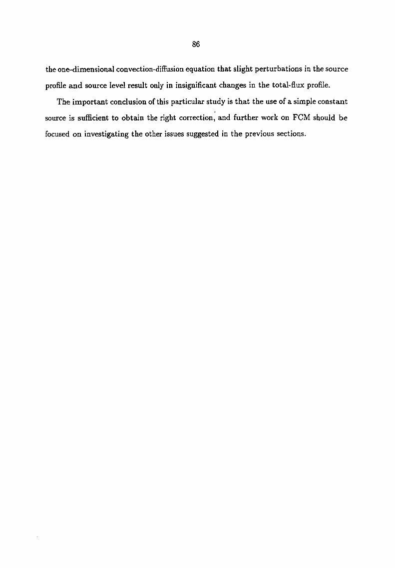
86

the one-dimensional convection-diffusion equation that slight perturbations in the source

profile and source level result only in insignificant chajiges in the total-flux profile.

The important conclusion of this particular study is that the use of a simple constant

source is sufficient to obtain the right correction, and further work on FCM should be

focused on investigating the other issues suggested in the previous sections.

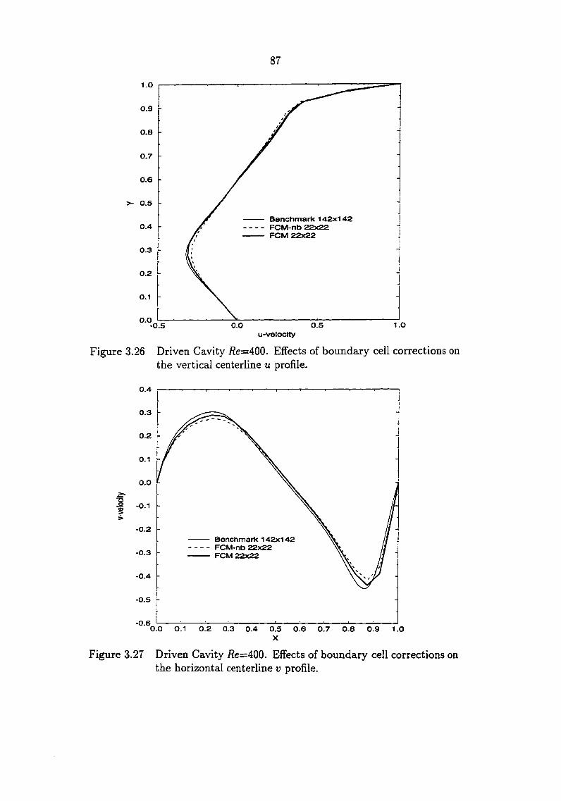
87

1.0

0.9

0.8

0.7

0.6

3- O.S

— Benchmark 142x142 -- FCM-nb 22x22 — FCM 22x22

0.4

0.3

0.2

0.1

0.0 1.0 O.S 0.0 -O.S

Figure 3.26 Driven Cavity /?e=400. Effects of boundary cell corrections on the vertical centerline u profile.

0.4

0.3

0.2

0.1

0.0

2:-•O ^ -0.1 >

-0.2

— Benchmark 142x142 - - FCM-nb 22x22

FCM 22x22 -0.3

-0.4

-0.5

-0.6 0.0 0.1 0.2 0.3 0.4 0.5 0.6 0.7 0.8 0.9 1.0

X

Figure 3.27 Driven Cavity /?e=400. Effects of boundary cell corrections on the horizontal centerline v profile.

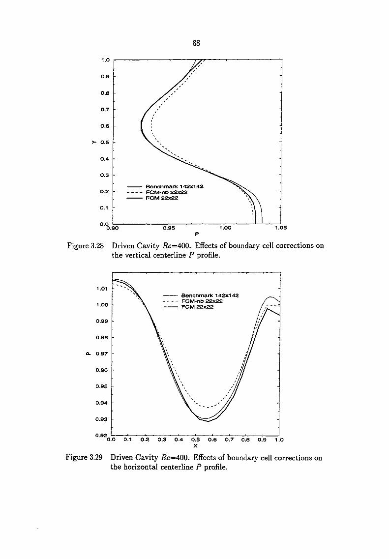
88

1.0

0.9

0.8

0.7

0.6

>- 0.5

0.4

0.3

Benchmark 142x142 FCM-nb 22x22 FCM 22x22

0.2

O.I

O.O 1.0S 1.00 0.90 0.95

P

Figure 3.28 Driven Cavity i?e=400. Effects of boundary cell corrections on the vertical centerline p profile.

1.01

Benchmark 142x142 FCM-nb 22x22 FCM ggygg 1.00

0.99

0.98

Q. 0.97

0.96

0.95

0.94

0.93

0.92 0.0 0.1 0.2 0.3 0.4 0.5 0.6 0.7 0.8 0.9 1.0

X

Figure 3.29 Driven Cavity /2e=400. Effects of boundary cell corrections on the horizontal centerline P profile.

89

1.0

0.9

0.8

0.7

0.6

>- 0.5

0.4 Benchmark 142x142 FCM-nb constant source FCM-nb linear source 0.3

0.2

0.1

0.0 1.0 0.0 0.5 -O.S

u-veloclty

Figure 3.30 Driven Cavity i?e=400. Effects of linear source on the vertical centerline u profile.

0.4

0.3

0.2

O.I

o.o

tS •S -0.1

-0.2

Benchmark 142x142 FCM-nb P?xPP constant source FCM-nb 22x22 linear source

-0.3

-0.4

-0.5

-0.6 O.O 0.1 0.2 0.3 0.4 0.5 0.6 0.7 0.8 0.9 1.0

X

Figure 3.31 Driven Cavity i?e=400. Effects of linear source on the horizontal centerline v profile.

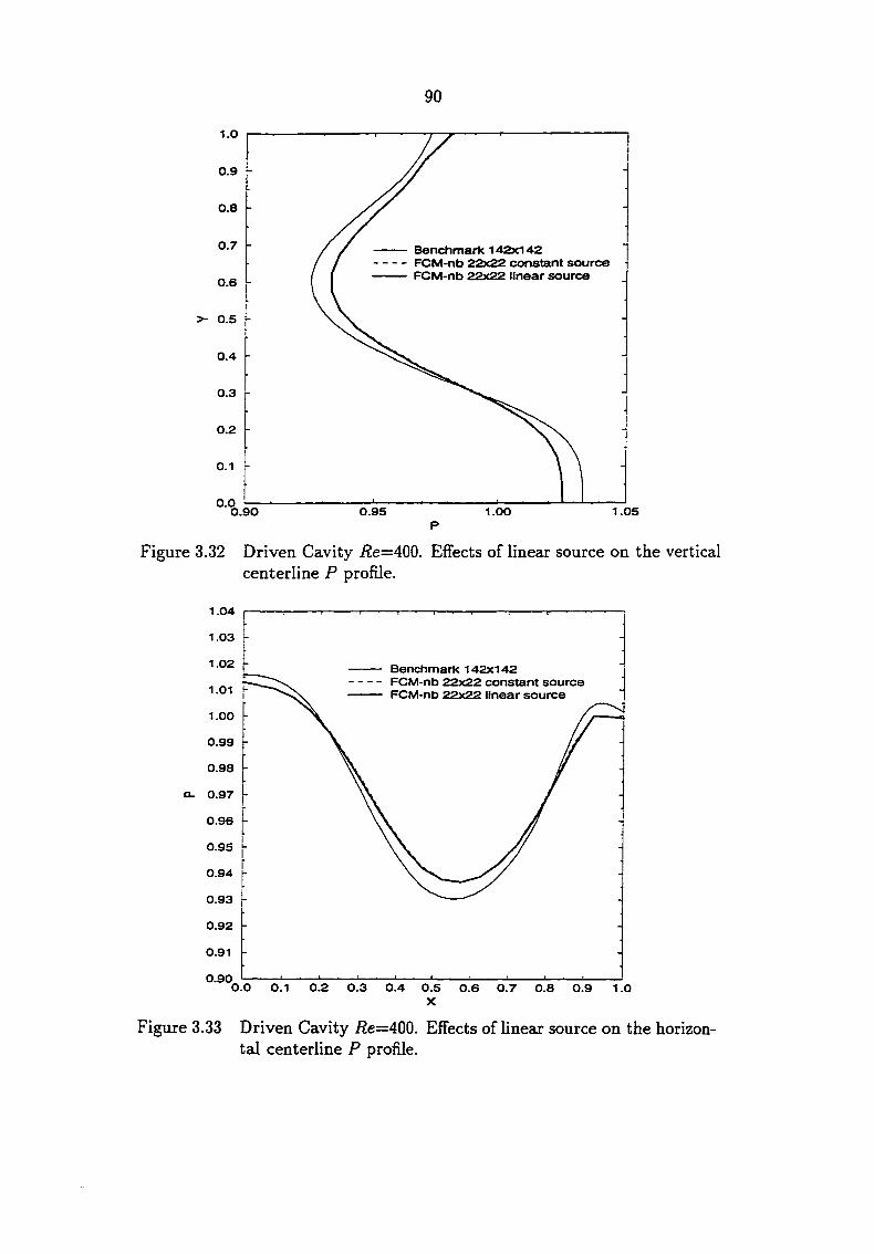
90

1.0

0.9

0.8

0.7 — Benchmark 142x142 — - FCM-nb g?xP2 constant source — FCM-nb linear source

0.6

5- 0.5

0.4

0.3

0.2

0.1

0.0 — 0.90 1.05 0.95 1.00

P

Figure 3.32 Driven Cavity i?e=400. Effects of linear source on the vertical centerline p profile.

1.04

1.03

1.02 Benchmark 142x142 FCM-nb 22x22 constant source FCM-nb 22x22 linear source 1.01

1.00

0.99

0.98

Q- 0.97

0.96

0.95

0.94

0.93

0.92

0.91

0.90 0.0 O.I 0.2 0.3 0.4 0.5 0.6 0.7 0.8 0.9

X

Figure 3.33 Driven Cavity /2e=400. Effects of linear source on the horizontal centerline P profile.

91

4 DEVELOPMENT OF GENERAL BOUNDARY

FORMULATION FOR PRESSURE EQUATION

4.1 Background

Recall the staggered control-volume for the x-momentum given in Figure 2.S. A

complete portion of this grid at a given y-location is presented in Figure 4.1. Note that

dotted control-volumes are used to represent the zero-width boundaxy control-volumes

and that the choice of staggered grid means that ui=u2- Assuming that the boundary is

not periodic {u2^ui) and the boundary values axe prescribed, then (/-3) interior u-values

(u3,... ,u/_i) are to be solved during the iterative process. Recall from equation 2.110

that integrating the x-momentum equation over the staggered u,- control-volume enables

Ui to be written as the sum of the pseudo-velocity ti,- and a term involving the difference

of the pressures at the grid points neighboring u,-, as given by:

Ui = Ui -I- di{Pi-i - Pi) , (4.1)

where di is the area of the face (at which u,- is defined) divided by the center coefficient

multiplying u,-. The above relationship involving u and the neighboring pressures needs

to be established at every main control-volume face and will form the means by which

the pressure equation is formulated.

The choice for the staggered control-volume containing (or u/_i) is not as straight

forward. If the left interface of the left boundaxy cell is made to pass through grid point

ig—2^ then the x-momentum equation is not conserved over the whole computational

92

U,',

1 \

^-1 JPl-1 t 1 1

* f 1 1 IMV • f • i 1 1

• 1 t 1

half left I

boundary cell

staggered M,-

control-volume

< half right

boundary cell

Figure 4.1 X-direction grid with main and staggered control-volumes.

domain. Note that each unknown u-velocity is to be covered by one staggered u-control-

volume, thus the choice for the placement of the left interface of the left boundary

cell means that half of the left boundary is uncovered by the x-momentum since

is assumed to be known. Conservation of the x-momentum equation over the whole

domain can be achieved by letting that left interface pass through grid point ig=l.

Thus effectively control-volume is used for the left boundary. This approach means

that P2 instead of Pi is to be used with P3 to represent the pressure difference across the

left boundary control-volume so that the required relation involving U3, P2, and P3 can

be established. The right boundary staggered control-volume is established in the same

manner. Thus, equation 4.1 can be written for i=3,..., (z — 1). This concept of how the

staggered boundary control-volume is formulated is also used for the integration of the

y-momentum equation over the corresponding staggered grid.

Recall that the pressure equation is obtained by integrating the mass conservation

equation over the main control-volume cells. The integrated equation is then discretized

by substituting equation 4.1 for the u contained in the x-direction mass-flux expression at

the considered main control-volume face. In this way, the dependency of the pressures

at the left, inside, and right side of a main control-volume face is established. The

dependency in the y-direction is obtained by substituting the counterpart of equation 4.1

93

(resulting from the integration of the y-momentum equation) for the v contained in the

y-direction mass-flux expression. The complete discretization of the pressure equation

still requires the establishment of the relationship described in equation 4.1 for 2=2 and

which are the relations at the left and right boundaries respectively. However, no

equation relating U2, A, and P2 for the left boundary is avedlable, and similarly for the

right boundary. One way to work around this problem, as suggested by Patankar [5].

is to realize that the assumption of known normal velocities at a given boundary face

allows equation 4.1 to be written for that face by setting the pseudo-velocity equal

to the known boundary normal velocity and setting the d term, which multiplies the

pressure difference term, to zero. In other words, the mass-flux across that boundary

face should not be expressed in terms of the pseudo-velocity but in terms of the known

prescribed boundary velocity itself. In this way, boundary pressure will not appear in the

discretized form of the pressure equation. This is consistent with the known principle

that at a given boundary, either the normal velocity or the pressure is specified, but

not both simultaneously. Thus, if the normal velocity at a given boundary is known,

the computation of the pressure at that boundary becomes a post-processing procedure

after convergence of the iterative process is achieved. The same principle also applies

for the pressure-correction boundary condition.

Thus, for situations where all the boundary normal velocities are known/prescribed,

boundary pressures have no means of influencing the interior pressures. Consequently,

there are no means by which a unique pressure field can be established. In the intro

duction of the SIMPLER algorithm, Patankar points out that the fact that a unique

absolute pressure field cannot be established does not pose a problem for the constant

density case (no link between density and pressure) as long a^ an iterative solution pro

cedure is used. The absolute pressure field obtained upon convergence depends on the

initial guess used. Adding a consteint to a pressure field which satisfies the momentum

equation does not change the numerical solution. It is the differences in pressure which

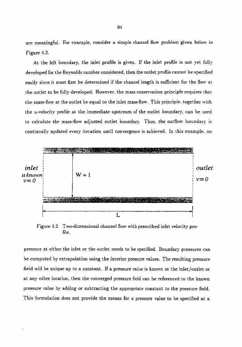
94

are meaningful. For example, consider a simple channel flow problem given below in

Figure 4.2.

At the left boundary, the inlet profile is given. If the inlet profile is not yet fully

developed for the Reynolds number considered, then the outlet profile cannot be specified

easily since it must first be determined if the channel length is sufficient for the flow at

the outlet to be fully developed. However, the mass conservation principle requires that

the mass-flow at the outlet be equal to the inlet mass-flow. This principle, together with

the u-velocity profile at the immediate upstream of the outlet boundary, can be used

to calculate the mass-flow adjusted outlet boundary. Thus, the outflow boundary is

continually updated every iteration until convergence is achieved. In this example, no

inlet U known V = 0

W= I outlet

v = 0

Figure 4.2 Two-dimensional channel flow with prescribed inlet velocitv profile.

pressure at either the inlet or the outlet needs to be specified. Boundary pressures can

be computed by extrapolation using the interior pressure values. The resulting pressure

field will be unique up to a constant. If a pressure value is known at the inlet/outlet or

at any other location, then the converged pressure field can be referenced to the known

pressure value by adding or subtracting the appropriate constant to the pressure field.

This formulation does not provide the means for a pressure value to be specified at a

95

certain boundary eind then allow that reference value to determine the 'level' of the

resulting pressure field automatically during the iterative procedure.

4.2 General Pressure Boundary Condition

Although the previous formulation of the boimdary conditions for the pressure equa

tion offers a simple and powerful procedure when the boundary normal velocities are

known, it is not directly applicable when the pressure rather than the normal velocity

is prescribed at the boundaries. Despite the fact that in the majority of fluid flow sim

ulations it is generally possible to specify the normal velocities at the boundary faces

(either through the known freestream/wall conditions or through iterative mass balance

at an outlet boundary), there exist other flow problems where the pressure at a given

boundary is easily defined but the normal velocity at that boundary is either not known

or not easily approximated, even iteratively. This class of flow problems spurs the need

to modify the existing procedure (discussed in the previous section) so that the resulting

algorithm will be able to handle the general case of pressure boundary conditions. In

particular, the modified formulation should be able to handle the following three cases:

Case 1 The formulation should be able to handle the trivial case of prescribed bound

ary normal velocities just as well as the previous formulation.

Ceise 2 Given the normal velocity at the boundaries and a reference pressure at a

boundary segment, the formulation should be able to establish the level of the

absolute pressure field correctly, b£ised on the given reference value.

Ceise 3 Given pressure values at one or more segments of the boundary, the formu

lation should be able to develop the correct normal velocity profiles at that

boundary segment(s) through the iterative process.

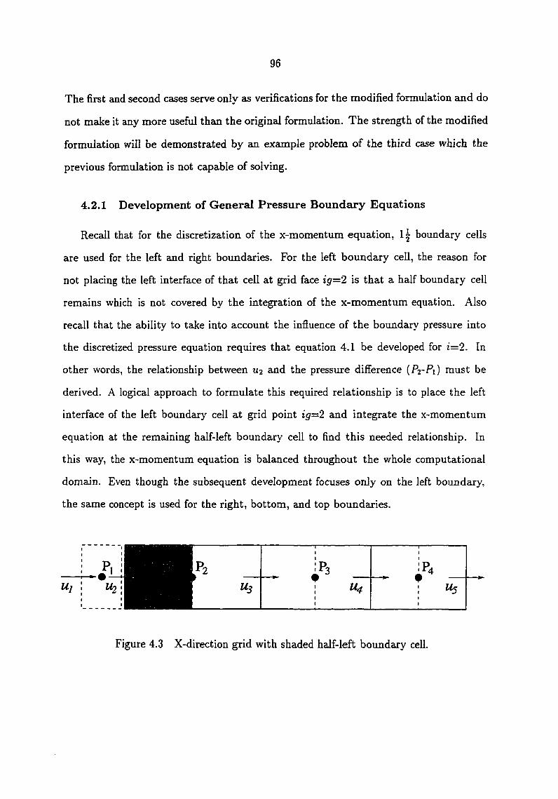
96

The first and second cases serve only as verifications for the modified formulation and do

not make it any more useful than the original formulation. The strength of the modified

formulation will be demonstrated by an example problem of the third case which the

previous formulation is not capable of solving.

4.2.1 Development of General Pressure Boundary Equations

Recall that for the discretization of the x-momentum equation, 11 boundary cells

are used for the left and right boundaries. For the left boundary cell, the reason for

not placing the left interface of that cell at grid face ig=2 is that a half boundary cell

remains which is not covered by the integration of the x-momentum equation. Also

recall that the ability to take into account the influence of the boundary pressure into

the discretized pressure equation requires that equation 4.1 be developed for i=2. In

other words, the relationship between U2 and the pressure diffierence {P2-P1) must be

derived. A logical approach to formulate this required relationship is to place the left

interface of the left boundary cell at grid point ig=2 and integrate the x-momentum

equation at the remaining half-left boundary cell to find this needed relationship. In

this way, the x-momentum equation is balanced throughout the whole computational

domain. Even though the subsequent development focuses only on the left boundary,

the same concept is used for the right, bottom, and top boundaries.

Figure 4.3 X-direction grid with shaded half-left boundary cell.

97

Consider a portion of tlie staggered x-momentum grid involving the left boundary

given in Figure 4.3. Integration of the x-momentum equation 2.13 over time ajid over

the half left boimdaxy cell gives:

\{py-)pi - {p^Yv\

At

r/ rintg fintg , j intg j intg \ , y Wrx—e ' ^yx^n *^yx^a} '

ar\i jo intg jO intg , jO intg jo intg\ //V*'rx—e *Jxx—w i *^yx—n 5 )

pintg _ pintg ^

where the total-fluxes are evaJuated at the appropriate places. The above equation can

be rearranged and written as:

/4xiu, + {Pr'' - Pt') = Sla , (4.3)

where

[{P^)pi - {pu)pi] ^3:Ay bla = +

At ft I r'ifs _ ^ 1

J\"xx—e ' "yx—n "yx—sj "f

e\ ( T° '"'S jo intg , ro intg to intg\ V-'- J )\"XX—e "XX—w "I" "yx—n "yx—s / •

It should be obvious that the purpose of equation 4.3 is to develop a relationship involving

U2 and (Fi-Pa)- The next step is to develop a procedure to evaluate Upi and the total-

fluxes t^xx—'C? *^xx—ti/7 *^yx—nt and tjyx-~s*

Using equation 2.76, the x-momentum x-direction total-flux [ Jxx ) at grid-face ig='2

can be written as:

Jxx-e = Fx-ig=2U3 + {Dx-igz=2-A.{\Pex-ig=2\) + I'fx-ts=2? 0]]}(U2 — U3) . (4.5)

Note that even though the total-flux correction has not been included in the above

equation, the on-going development applies equcdly well to FCM. Also observe that

98

equation 4.5 can either be written as an expression or evaluated numerically. In the

calculation of the West-coefficient of the x-momentum staggered cell ig=Z, equation 4.5

is used as ein expression, while in the current discussion it is evaluated to find a numerical

value for the total-flux Jxx-e- The use of the same equation to represent the total-flux

at grid-face ig=2 must be observed to ensure the conservation of the x-momentum over

the whole computational domain.

Recalling equation 2.14, the x-momentum x-direction toteil-flux at grid-face i^=l can

be written as:

If the velocity component uj (boimdaxy normal velocity) is known, then the formulation

must solve for pressure Pi, and if it is not known, then the boundary pressure Pi is

and can be evaluated in a number of different ways:

• First-order forward-difference.

• Second-order three-point unequal-space one-sided forward-difference.

• One-dimensional convection-diffusion without source applied to the main control-

volume enclosing grid point ig=2.

• One-dimensional convection-diff'usion without source applied to the combination

of control-volumes enclosing grid point ig—2 and ig=Z.

Before the x-momentum y-direction total flux Jyx can be evaluated, it is first neces

sary to evaluate Upi. As in the case of the evaluation of there are several different

ways to do so, which are:

J {pu2)u2 - h (4.6)

specified. In general the term can be written as:

du = C2U2 -f- C4U4 ,

OXig=l (4.7)

99

• First-order linear interpolation using U2 and uz-

• Second-order parabolic interpolation using U2, U3, and U4.

• One-dimensional convection-diffusion without source applied to the main control-

volume enclosing grid point ig=2.

• One-dimensionaJ convection-diffusion without source applied to the combination

of control-volimies enclosing grid point ig=2 and ig='i.

Once Upi has been evaluated for the range of its j-index J), the non-

directional total-flux Jyx can be evaluated as:

Jyx-jj = Fy-jf '^pl-j=jf + {Djf-A{Pe-jf) + I"^pl-j=jf) (4-S)

for j /=2,. . . , J . Now that all the needed components are in place, the term Sla given

in equation 4.4 can be calculated.

Upon substituting equation 4.6 into equation 4.3, the following relation is obtained:

1 Qt

Fx-ig=iU2 — f l{C2U2 + C3U3 -|- C4U4) -t- -jiPl — P2) = J . • (4.9) / f^y

For purposes which will be clear shortly in the discussion, equation 4.9 can also be

written in the second form cis:

1 c/ iFx-ig=l — fJ'C2)'U2 ~ y-{CzUz "h C4U4) -|- -r(Pi — P2) = . . . (4.10)

/ f^y

Isolating U2 and {P1-P2) to one side, the above two equations can be rearranged as:

1 Sla Fx-igz=iU2 -f- y(^l — ^2) = Y^y ^(^2^2 + CzUz + C4U4) , (4.11)

and 1 S la

(Fx-ig=l — fiC2)u2 + ~ 2) = + fi{CzUZ + C4U4) , (4.12)

100

respectively. Equation 4.11 and equation 4.12 can be cast into an intermediate general

form cis:

<iiU2 + "" ^2) = 0.2 • (4-13)

Finally, the needed relationship described in equation 4.1 for i=2 is found as:

U 2 = + T ] w { P l — P 2 ) 7 ( 4 - 1 4 )

where

(4.15) ai

Iw = 7^ • (4.16) j u i

Note that upon comparing the above equation to equation 4.1, it is clear that

and are used to represent U2 and d. At this point, it is important to explain why

for certain situations it is necessary to use equation 4.10 instead of equation 4.9 (or

equation 4.12 instead of equation 4.11). Observe that for the specific situation of Case

1 (prescribed boundary normal velocity and unknown boundary pressure), when the

boundary is wall, if equation 4.11 is used, then the term ai vanishes since Fx-ig-i=0.

This in turn leads to division by zero in the computation of (f„, and t}^. For this situation,

the use of equation 4.12 avoids the division by zero since the term (^Ca) is generally

non-zero. However, it should be noted that in situations where the normal velocity at

the boundary is given and non-zero, it is preferable to use equation 4.11 since this means

that the term is not partially but instead completely lagged, a procedure which

tends to give better stability characteristics. For Case 3 (prescribed boundary pressure

but unknown boundary normal velocity), equation 4.11 should always be used since the

'yet to be solved' normal velocity at the boundary is non-zero in general. Equation 4.14

makes it possible to take into account the influence of Pj. The effect of pressure at

the right boimdaxy is accounted for in the same way. Integration of the y-momentum

101

equation over the heJf bottom and top boimdajies allows equations involving the pressure

at the bottom and top boundaries to be taken into account in the Scime maimer.

Consider the formulation of the discretized pressure equation at the left boundary

main control-volume cell, excluding the left bottom and left upper cells. The left face

of this cell is the left boimdary of the domain considered. Using the procedure outlined

in section 2.8.1, the discretized pressure equation for this cell is obtained as:

apPp = cePE + dwPw + ONPN + asPs + bp , (4-17)

where the coefficients are given by:

OE = {pd)^Ay ,

aw = {pv )wAy, a,\r = {pd) ,Ax ,

a s = {pd)nAx ,

ap = dE + o,w + aitf -t- as ,

and the source term is given by:

i>p = -[(p")e - - [(p")n - (/9ii)5]Ax . (4.19)

The important thing to note is that the standard form of the discretized pressure equa

tion for the inner cells (equation 2.115) is not changed. Similar equations are obtained

for the other boundary and corner cells.

In the following sections, further development of each of the three cases is discussed

separately.

4.2.2 Czise 1: Prescribed Boundary Normal Velocity with No Reference

Pressure

This case is the trivial situation where all the boundary normal velocities are pre

scribed and no reference pressure is given. It has been pointed out previously that the

102

original formulation is able to handle this case by using the known boundeiry normal

velocity itself as the pseudo-velocity eind setting the rf-term to zero in equation 4.1 for

i=2. The effect of the boimdary pressure is neglected in the computation, and its value

is found by extrapolation using the interior values once convergence is achieved. Exam

ples of this class of problems are the confined flow inside a two-dimensional lid-driven

cavity, internal flows with prescribed inlet profile(s) (a simple example is the channel

flow with specified inlet profile as given in Figure 4.2), and external flows where either

the boundary normal velocity or its derivative is given, or the normal velocity can be

iterated using the mass-conservation principle.

In the previous section, a general formulation to account for the influence of boundary

pressure was developed. However, the boundary pressure is unknown for this type of

flow problems. Therefore, an equation relating the pressure at a given boundary to the

immediate interior pressure must be developed. For example, at the left boundary, it is

the relationship between Pi and P2. The purpose of this equation is to close the algebraic

system of equations resvdting from the formulation of the pressure equation. Recall

that the formulation of the discretized pressure equation along the x-direction begins by

integrating the continuity equation over the main control-volume cell for i=2,...,(/—!)

and then substituting the flow-rate with a sum of the pseudo-velocity and the pressure

difference term. This gives (/-2) equations, and there are i unknown pressures. The

relationships between pi and p2 and between F/_i and p[ give the needed two equations

to close the system of equations. The following discussion will focus on finding the

relation between Pi and Pj at the left boundaxy, and as before, the same procedure is

used for the other boimdaries as well.

First, the relation involving uj and (Pi — P2) given in equation 4.14 is repeated below

for convenience:

"2 = + VwiPi - P2) . (4.20)

103

This equation has been used as a means to bring Pi into the discretized pressure equation.

Therefore, trying to find the pressure relationship by substituting the known U2 into the

above equation will cause the system of equations to be indeterminate. It should be

observed that during the development of the above equation, the conservation of meiss

has not been applied to the half left boundaxy cell. Integration of the continuity equation

over this cell gives:

FS - Fil'i + Fi'!' - Fill = 0 . (4.21)

Isolating to one side and then using the definition of Fx, the above equation is

rewritten as:

pintg pintg , pintg _ pintg ti/ ^ r—e • "y—n J5

= fx-way

= {pU2)Ay . (4.22)

Further rearrangement results in:

Finally, by realizing that the common factor U2 present in both equations 4.20 and 4.23

can be eliminated by subtracting one equation from the other, the following relation is

obtained:

p 1 - p 2 - F'i'i - ipu^y] pvw^y

= X L . (4.24)

It is clear that the use of the above equation and its counterpart for the right bound

ary does not cause the considered system of equations to be indeterminate due to the

incorporation of the mass conservation in the set.

The next step in the procedure is to decide how equation 4.24 should be used in

the iterative process. One possibility is to use equation 4,24 to solve for Pi using the

104

previously iterated (lagged) value of P2 at the beginning of each SIMPLER iteration.

This predicted Pi is then used as the Dirichlet boundary condition for the interior

pressures. Thus, in a sense, Pi is solved explicitly. This procedure proves to be unstable

in the current formulation. The other possibility is to rearrange equation 4.24 for Pi

and then use it in equation 4.17 to substitute for Pw- Thus, the following equation is

obtained:

apPp = asPs + (inPN + osPs + 6p , (4.25)

where the coefficients eg, a^v, and as are the same as those given in equation 4.18. The

center-coefficient now becomes the summation of only three neighboring coefficients;

ap = oe + cin + as 1

and the source term has an additional term:

bp = -[(pw)e - - [(p^)n - (/5u)a]Ax + awXL , (4.26)

where again the coefficient aw is the same as that given in equation 4.18. Note that the

boundary pressure P\v does not appear in the discretized equation. However, this does

not mean that the boundary pressure does not influence the interior values. Rather,

the effect of Pw is included implicitly in the source term of the discretized equation.

After solving the interior pressures, the boundary pressure can then be calculated using

equation 4.24. However, before convergence is achieved, it is not necessary to update

the boundary pressure at each iteration unless it is needed for the calculations of other

non-primary flow variables. The above procedure to implicitly account for the pressure

boundary influence has been shown to be quite successful.

The steady two-dimensional lid-driven cavity problem is again used to test the pre

viously discussed formulation. A square cavity of unit length is used, and the moving

lid is chosen to be the top boundary. Both the lid velocity and the density are chosen to

be unity, and thus the Reynolds number is specified by using the appropriate value of

105

the diffusion fi. A Reynolds number of 400 is chosen, and the velocity components ajid

pressure axe initialized to zero and one respectively. Moreover, the Power Law scheme

will be used throughout the verification process of this general boundary pressure for

mulation. Both 22x22 and 42x42 uniform grids are used, and the results obtained using

the original formulation will be plotted against the results obtained using the general

formulation.

The plots of the pressure along the vertical centerline (x=0.5) for both grids axe

given in Figures 4.4 and 4.5. For the purpose of comparison, the results obtained using

the 142x142 fine grid and the original formulation are also plotted. It is important to

mention that the original formulation uses linear interpolation of the interior pressures

to calculate boundary pressures. It is clear from these figures that for most of the y-

range, the original and general formulation give practically the same profile. However,

close observation at the vicinity of the top boundary reveals that the general formulation

gives a more conforming profile to the benchmark solution than the original formulation.

This could be an important factor if the normal pressure gradient at the moving lid is

to be used in the calculation of other variables of interest. From these figures, it can

also be observed that since no reference pressure is specified anywhere in the domain,

a floating pressure field is obtained. Adding a constant to this pressure field does not

change the numerical solution for the velocity components.

In Figure 4.6, the plot of the velocity components along the vertical centerline is

given. No differences between the original and general formulation are observed. Even

though the velocity and pressure profiles along the horizontal centerline are not given,

the same characteristics are observed.

The mass, x-momentum, and u-velocity convergence histories are given in Figure 4.7

through Figure 4.9. The relaxation factor used is 0.4, and only insignificant differences

in the convergence characteristics are observed. This is another important characteristic

of the general formulation.

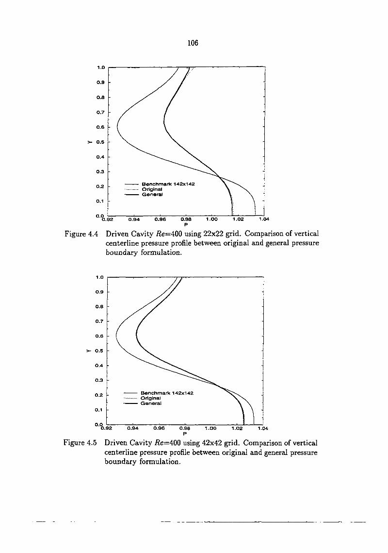
106

1.0

0.9

0.8

0.7

0.6

>- 0.5

0.4

0.3

Benchmark 142x142 Original General

0.2

0.1

0.0 1.04 0.98

P 1.00 1.02 0.96 0.92

Figure 4.4 Driven Cavity i2e=40Q using 22x22 grid. Comparison of vertical centerline pressure profile between original and general pressure boundary formulation.

1.0

0.9

0.8

0.7

0.6

>- 0.5

0.4

0.3

Benchmark 142x142 Original General

0.2

O.I

0.0 — 0.92 0.94 0.96 0.98 1.00 1.02 1.04

P

Figure 4.5 Driven Cavity i2e=400 using 42x42 grid. Compaxison of vertical centerline pressure profile between original and general pressure boundary formulation.

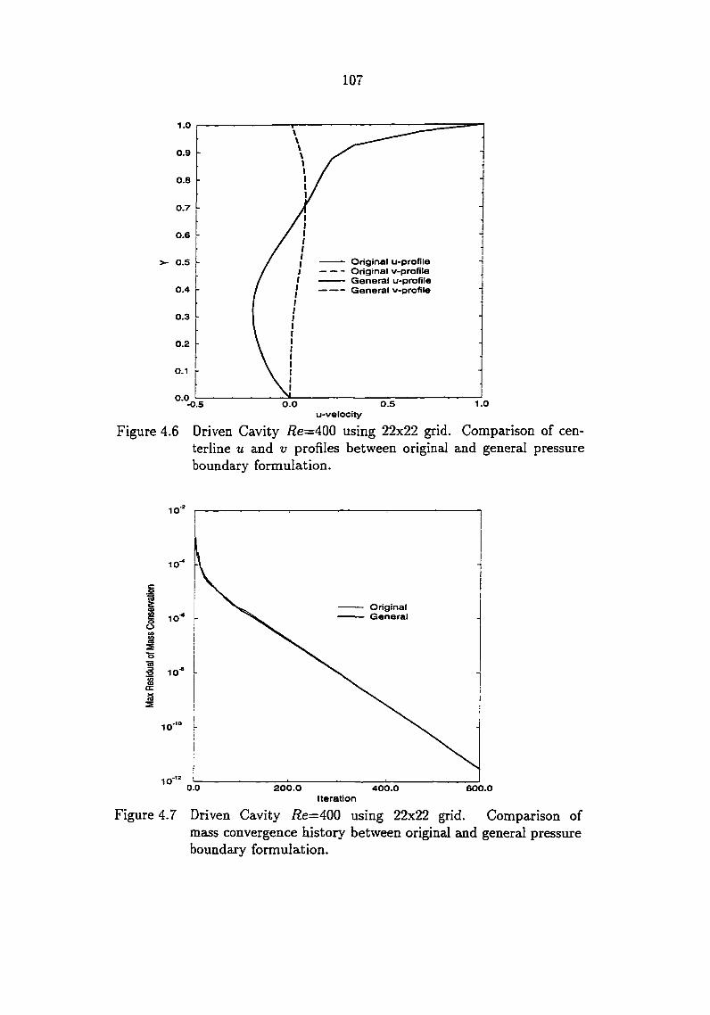
107

1.0

0.9

0.8

0.7

0.6

Original u-profile Original v-profile General u-profile General v-profile

>- 0.S

0.4

0.3

0.2

O.I

O.O 1.0 O.O 0.5 -0.5

Figure 4.6 Driven Cavity i?e=400 using 22x22 grid. Comparison of cen-terline u and v profiles between original and general pressure boundaxy formulation.

io

10"*

Original General 10

o

10 oc

10'

10' 0.0 200.0 400.0 600.0

Iteration

Figure 4.7 Driven Cavity Re—AQQ using 22x22 grid. Comparison of mass convergence history between original and general pressure boundary formulation.

108

Original General o

10-

-to 10

1 0 " 600.0 200.0 400.0 0.0

Iteration

Figure 4.8 Driven Cavity /le=400 using 22x22 grid. Comparison of x-momentum convergence history between original and general pressure boundary formulation.

io"

io^

•$ 10

io^ s

10'

1 0 '

Onginal General

O.O 200.0 400.0 600.0 Iteration

Figure 4.9 Driven Cavity i2e=400 using 22x22 grid. Comparison of u-velocity convergence history between origineil and general pressure boundary formulation.

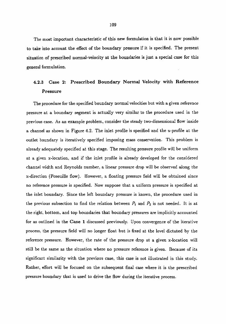
109

The most important characteristic of this new formulation is that it is now possible

to taJce into account the effect of the boundary pressure if it is specified. The present

situation of prescribed normal-velocity at the boundajies is just a special case for this

general formulation.

4.2.3 Case 2: Prescribed Boundary Normal Velocity with Reference

Pressure

The procedure for the specified boundary normal velocities but with a given reference

pressure at a boundary segment is actually very similax to the procedure used in the

previous case. As an example problem, consider the steady two-dimensional flow inside

a channel eis shown in Figure 4.2. The inlet profile is specified and the u-profile at the

outlet boundary is iteratively specified imposing mass conservation. This problem is

already adequately specified at this stage. The resulting pressure profile will be uniform

at a given x-location, and if the inlet profile is already developed for the considered

channel width and Reynolds number, a linear pressure drop will be observed along the

x-direction (Poseuille flow). However, a floating pressure field will be obtained since

no reference pressure is specified. Now suppose that a uniform pressure is specified at

the inlet boundary. Since the left boundary pressure is known, the procedure used in

the previous subsection to find the relation between Pi and P2 is not needed. It is at

the right, bottom, and top boundaries that boundary pressures are implicitly accounted

for as outlined in the Case 1 discussed previously. Upon convergence of the iterative

process, the pressure field will no longer float but is fixed at the level dictated by the

reference pressure. However, the rate of the pressure drop at a given x-location will

still be the same as the situation where no pressure reference is given. Because of its

significant similarity with the previous case, this case is not illustrated in this study.

Rather, effort will be focused on the subsequent final case where it is the prescribed

pressure boundary that is used to drive the flow during the iterative process.

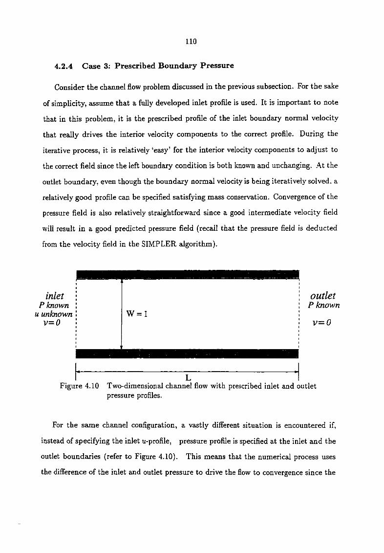
110

4.2.4 Case 3: Prescribed Boundary Pressure

Consider the channel flow problem discussed in the previous subsection. For the sake

of simplicity, assume that a fully developed inlet profile is used. It is important to note

that in this problem, it is the prescribed profile of the inlet boundary normal velocity

that really drives the interior velocity components to the correct profile. During the

iterative process, it is relatively 'easy' for the interior velocity components to adjust to

the correct field since the left boundary condition is both known and unchanging. At the

outlet boundary, even though the boundary normal velocity is being iteratively solved, a

relatively good profile can be specified satisfying mass conservation. Convergence of the

pressure field is also relatively straightforward since a good intermediate velocity field

will result in a good predicted pressure field (recaJl that the pressure field is deducted

from the velocity field in the SIMPLER algorithm).

inlet P known

u unknown V = 0

W= 1

outlet P known

v = 0

Figure 4.10 Two-dimensional channel flow with prescribed inlet and outlet pressure profiles.

For the same channel configuration, a vastly different situation is encountered if,

instead of specifying the inlet u-profile, pressure profile is specified at the inlet and the

outlet boundaries (refer to Figure 4.10). This means that the numerical process uses

the difference of the inlet and outlet pressure to drive the flow to convergence since the

Ill

correct profile of the inlet boundary velocity is not known. The inlet zi-profile must

now be iteratively deducted from the known pressure boundary, while at the outlet

boundary, the predicted profile can be obtained in a similar manner, or the profile at

the immediate interior location to the right boundary can be used. Whichever method is

chosen to obtain the outlet profile, the outlet profile should then be adjusted to preserve

mass conservation. Thus, a much more extensive dependency between pressure and

velocity fields exists. During the iterative process, since the normal velocity boundary

condition is being iteratively developed, a relatively good intermediate velocity field is

no longer available to obtain a good pressure field. In turn, the pressure gradient term

in the momentum equations cannot be accurately calculated.

A procedure must now be developed to calculate the boundary normal velocity given

the boundary pressure. For this example problem, the left boundary is considered. The

first approach is to apply mass conservation to the main control-volume i=2 (refer to

Figure 4.3). Integration of the continuity equation over this cell and then solving for 11-2

gives an equation identical to equation 4.23:

- H-'n • w-2' ) pAy

where the only difference is that the domain of integration of equation 4.23 is over the

half left boundary cell. Note that the above equation does not involve the pressure

difference term at the left boundary, .\nother alternative is to combine equation 4.27

and equation 4.20 to give:

-''') • W-2S)

where now the left boundary pressure difference is taken into account. It is observed in

the current study that the two procedures have virtually identical convergence charac

teristics. Either of them may be chosen, although the former may be preferable due to

its simplicity.

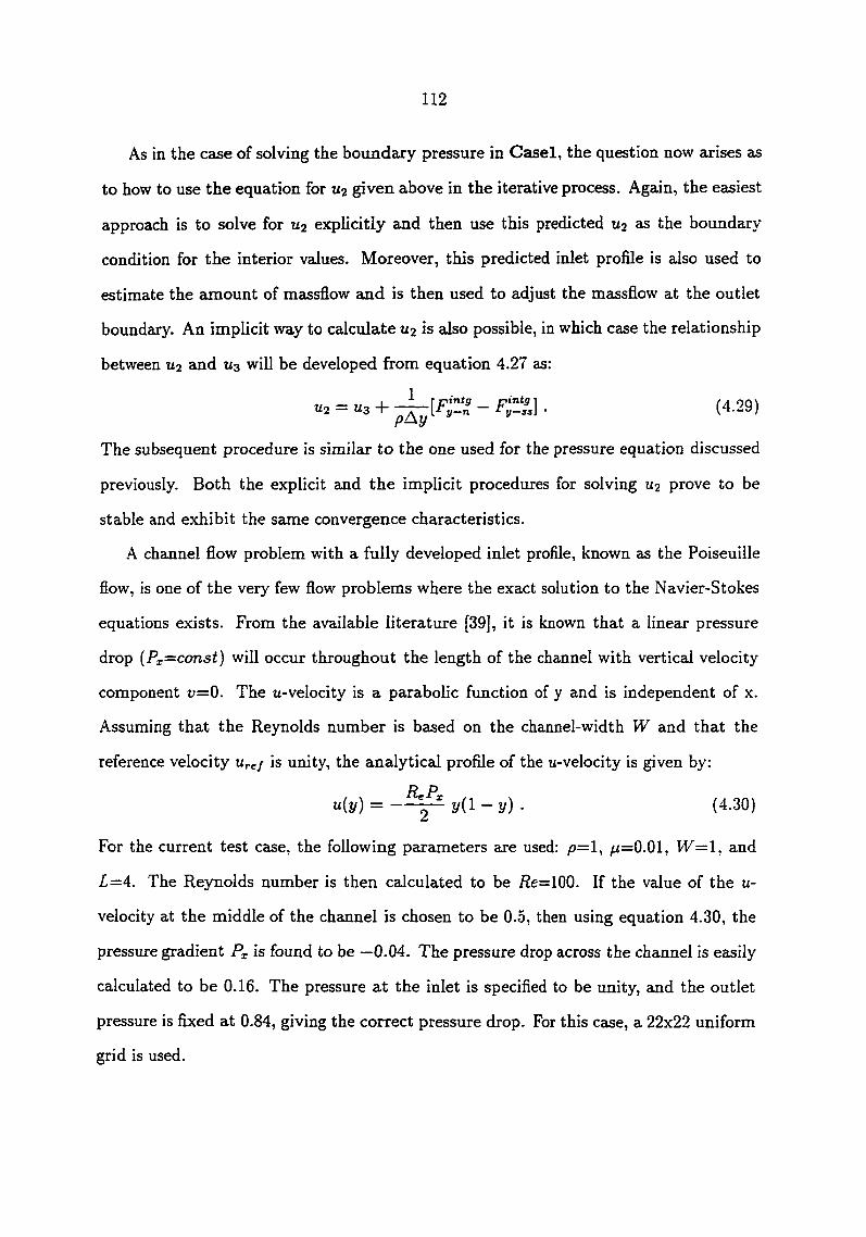
112

As in the case of solving the boundary pressure in Casel, the question now arises as

to how to use the equation for U2 given above in the iterative process. Again, the easiest

approach is to solve for U2 explicitly and then use this predicted U2 as the boundary

condition for the interior values. Moreover, this predicted inlet profile is also used to

estimate the amount of massflow and is then used to adjust the massflow at the outlet

boundary. An implicit way to calculate U2 is aJso possible, in which case the relationship

between U2 and U3 will be developed from equation 4.27 as:

"2 = • (4-29)

The subsequent procedure is similar to the one used for the pressure equation discussed

previously. Both the explicit and the implicit procedures for solving U2 prove to be

stable and exhibit the same convergence characteristics.

A channel flow problem with a fully developed inlet profile, known as the Poiseuille

flow, is one of the very few flow problems where the exact solution to the Navier-Stokes

equations exists. From the available literature [39], it is known that a linear pressure

drop {Px=const) will occur throughout the length of the channel with vertical velocity

component t;=0. The u-velocity is a parabolic function of y and is independent of x.

Assuming that the Reynolds number is based on the channel-width W and that the

reference velocity Ure/ is unity, the analytical profile of the u-velocity is given by:

" ( y ) = y ( i - y ) • ( 4 . 3 0 )

For the current test case, the following parameters are used: /9=1, /i=0.01, 1^=1, and

L=4. The Reynolds number is then calculated to be i?e=100. If the value of the u-

velocity at the middle of the channel is chosen to be 0.5, then using equation 4.30, the

pressure gradient is found to be —0.04. The pressure drop across the channel is easily

calculated to be 0.16. The pressure at the inlet is specified to be unity, and the outlet

pressure is fixed at 0.84, giving the correct pressure drop. For this case, a 22x22 uniform

grid is used.

113

1.0

Numerical solution — Exact solution

0.8

0.6

0.4

O.O 0.00 0.20 0.40 0.50 0.10 0.30

u-velocity

Figure 4.11 Compaxison between exact and numerical u-velocity profile for two-dimensional channel flow with i?e=100 and channel-width w=l.

1.05

1.00

0.95

Q.

0.90

0.85

0.80 O.O 1.0 2.0 3.0 4.0

X

Figure 4.12 Pressure distribution for two-dimensional chaimel flow with /2e=100 and channel-width w=l.

114

10°

lO"

Max residual of u-velocity Max residual of v-veiocity

s •'0-' •n

a> CC

10^

10-

10"' 0.0 2000.0 4000.0 6000.0 8000.0 10000.0

Iteration

Figure 4.13 Convergence history of velocity components for two-dimensional channel flow with i?e=100 and channel-width w=l.

1 . oo 3 . OO » . OO

Figure 4.14 Velocity vector plot for two-dimensional channel flow with i2e=100 and channel-width w=l.

115

The plot of the u-velocity profile as a function of y is given in Figure 4.11. An

excellent comparison with the exact solution is observed. The plot of the pressure

profile cilong the x-direction is given in Figure 4.12. As expected, the pressure drops

very linearly across the length of the channel. Figure 4.13 gives the convergence history

of the maximum residual of both velocity components. The profiles of the u-velocity at

different x-locations along the channel is given in Figure 4.14.

Thus, it can be concluded that the general formulation developed in this section to

account for the influence of boundary pressure has proven to be effective in handling

the three types of boundary specifications discussed previously. Most importantly, the

general formulation is able to solve the type of flow problems such eis Czise C, where

at some given boundary segments, pressure and tangential velocity are specified, and

which is simply unsolvable using the original formulation.

4.3 Implementation of Genercd Pressm*e Boundary in FCM

Even though the current implementation is applied to the Power Law scheme, imple

mentation to the FCM requires no special procedure. Throughout the course of FCM

development, both the original and the general pressure boundary formulation have been

tested and used. Recall the coarse grid (22x22) pressure profile of FCM with boundary

correction for the lid-driven cavity test case (/2e=400) given in Figure 3.28. It was men

tioned before that the corrected pressure profile at the vertical centerline shows excellent

agreement with the benchmark solution. However, significant deviation from the refer

ence solution is observed for the portion of the profile near the lid. It was also observed

in Figures 4.4 and 4.5 that the use of the general pressure boundary formulation results

in an improved pressure profile near the lid for the case of the Power Law scheme. The

vertical centerline pressure profile obtained using this new pressure boundary formula

tion applied to FCM with the boundary correction is given in Figure 4.15. It can be

116

seen that at the region near the lid, the new corrected profile conforms very well to the

reference solution. However, it Ccin also be observed that a slight decrease in accuracy

results from the implementation of the general pressure boimdary procedure. As the

grid is refined to 32x32, the discrepancies disappear.

1.0

0.9

0.8

0.7 Bencfimark 142x142 FCM-b Original pressure boundary FCM-b ggvOT General pressure boundary 0.6

>- 0.5

0.4

0.3

0.2

0.1

O.O — 0.90 0.92 0.94 0.96 0.98 1.00 1.02 1.04

P

Figure 4.15 Driven Cavity /2e=400 using 22x22 grid. Comparison between original and general pressure boundary formulation applied to FCM with boundary cell correction.

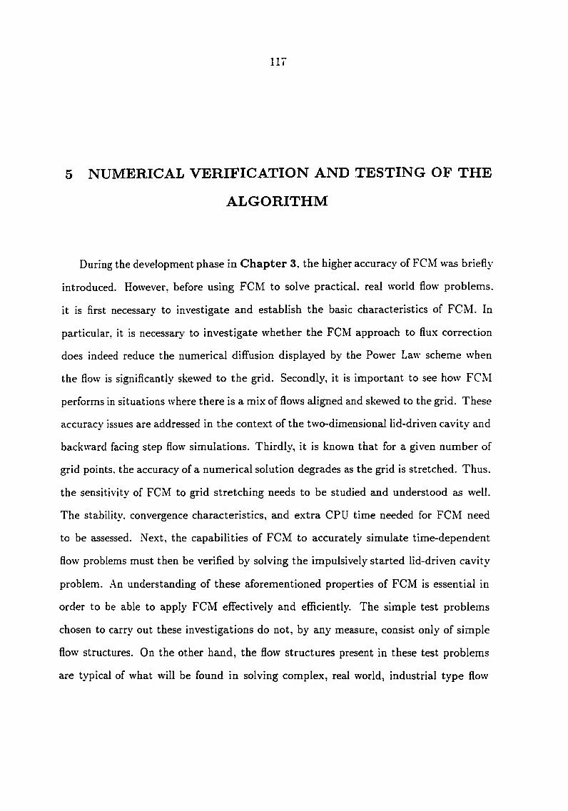
117

5 NUMERICAL VERIFICATION AND TESTING OF THE

ALGORITHM

During the development phase in Chapter 3, the higher accuracy of FCM was briefly

introduced. However, before using FCM to solve practical, real world flow problems,

it is first necessary to investigate and establish the basic characteristics of FCM. In

particular, it is necessary to investigate whether the FCM approach to flux correction

does indeed reduce the numerical diffusion displayed by the Power Law scheme when

the flow is significantly skewed to the grid. Secondly, it is important to see how FCM

performs in situations where there is a mix of flows aligned and skewed to the grid. These

accuracy issues are addressed in the context of the two-dimensional lid-driven cavity and

backward facing step flow simulations. Thirdly, it is known that for a given number of

grid points, the accuracy of a numerical solution degrades as the grid is stretched. Thus,

the sensitivity of FCM to grid stretching needs to be studied and understood as well.

The stability, convergence characteristics, and extra CPU time needed for FCM need

to be assessed. Next, the capabilities of FCM to accurately simulate time-dependent

flow problems must then be verified by solving the impulsively started lid-driven cavity

problem. An understanding of these aforementioned properties of FCM is essential in

order to be able to apply FCM effectively and eflBciently. The simple test problems

chosen to carry out these investigations do not, by any measure, consist only of simple

flow structures. On the other hand, the flow structures present in these test problems

are typical of what will be found in solving complex, real world, industrial type flow

118

problems.

Over the last decade, the muitigrid technique to accelerate the convergence of an

iterative numerical scheme for linear and non-linear problems has been widely adopted

by the CFD conmiunity. The well-known and widely used FAS muitigrid technique has

been used in conjunction with the segregated SIMPLER algorithm by Zori [40] and has

been shown to effectively speed up the convergence of the algorithm. In the current

work, the performance of FCM, when used in conjunction with this muitigrid technique,

is also analyzed.

Having done extensive FCM testing in two-dimensions, a limited testing of FCM for

three-dimensional flow situations is then performed on the standard three-dimensional

lid-driven cavity.

5.1 Two-dimensional Lid-Driven Cavity Flow

In spite of its idealization, the flow inside a lid-driven cavity has been widely ac

knowledged as an excellent test ca^e for evaluating numerical schemes. This is due to

the presence of large streamline to grid skewness over most of the flow domain (on a

rectangulax grid). Moreover, the existence of several relatively large recirculating re

gions, where convection and diffusion are of comparable magnitude, requires that the

difference formulation of the latter be at least as accurate as the former. The steady

flows inside a two-dimensional lid-driven cavity (Figure 3.1) for a range of low, medium,

high, and very high Reynolds numbers (/2e=100,400,1000,10000) have been used to in

vestigate the characteristics of FCM and its performance relative to the Power Law,

central-difference, and QUICK schemes. Constant property laminar flow is assumed,

and the Reynolds number is defined by Re={pUiidL)/fi, where p is the density of the

fluid, Uiid is the speed of the sliding lid, L is the length of the square enclosure side wall,

and p. is the fluid viscosity. Fine grid solutions obtained using the central-difference

119

scheme are used as reference solutions. For /2e=100, 1000, and 10000, fine grid solutions

obtained using the vorticity-stream function formulation with the multigrid method by

Ghia [7] are given as further verifications. Nxmierical solutions of the QUICK scheme

with third-order boundary treatment are taken from published results by Hayase [8].

All calcxilations axe started with a zero velocity field and unit pressure field. For

comparison with standard published results, imiformly spaced grids are used unless

otherwise noted. Each calculation is terminated when the residual e became smaller

than 10~®, where e is defined as the maximum value of the residuals for the mass, x-

momentum, y-momentum, and the difference between the values of u- and r-velocities

between two successive iterations. It is found that it is not necessary to retain the

unsteady terms in the momentum equations (time marching) in order to achieve stable

and converged solutions on all grids for the first three Reynolds numbers considered.

However, for reeisons discussed later in the appropriate subsection, it is necessary to

retain the unsteady terms for the very high /?e=10000 case.

To facilitate future comparisons with other numerical schemes, tabular forms of FCM

solution along the cavity centerlines are given in Appendix B.

5.1.1 Calculations for /2e=100

The velocity profiles for the u- and u-velocities along the vertical and horizontal

centerlines are given in Figures 5.1 and 5.2 respectively. As is obvious, the coarse grid

solutions given by Power Law, Central, FCM, and QUICK are all in close agreement

with the reference solution. This is expected since in general for low Reynolds number

flows, the influence of the flow transport in a coordinate direction is usually too small

to significantly affect the transport profiles in the other coordinate directions. Thus,

the 'one-dimensional' nature of the Power Law scheme is usually sufficient to model the

flow.

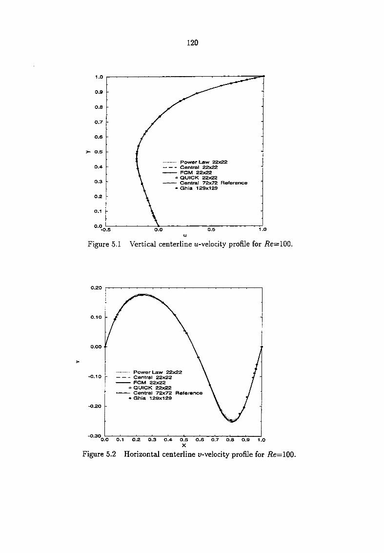
120

1.0

0.9

0.8

0.7

0.6

>- 0.5

Power Law 22x22 Central 22x22 FCM 22x22

o QUICK 22x22 Central 72x72 Reference

• Ghia 129x129

0.4

0.3

0.2

0.1

0.0 0.5 1.0 O.O -0.5

u

Figure 5.1 Vertical centerline li-velocity profile for i2e=100.

0.20

0.10

o.oo

" Power Law 22x22 - Central 22x22 - FCM 22x22 o QUICK 22x22 - Central 72x72 Reference • Ghia 129x129

-0.10

-0.20

-0.30 0.0 0.1 0.2 0.3 0.4 0.5 0.6 0.7 0.8 0.9 1.0

X

Figure 5.2 Horizontal centerline u-velocity profile for i?e=100.

121

1.0

0.9 -- Power Law ?2x?g - Central 22x22 - FCM - FCM 42x42 - Central 72x72 Reference

0.8

0.7

0.6

5- 0.5

0.4

0.3

0.2

0.1

O.O 0.92 0.98

P 0.96 1.00 1.02

Figure 5.3 Vertical centerline pressure profile for i?e=100.

1.020

Power Law 22x22 Central 22x22 FCM 22x22 FCM 42x42 Central 72x72 Reference

1.010

1.000

0.990

0.980

0.970 0.0 0.1 0.2 0.3 0.4 0.5 0.6 0.7 0.8 0.9 1.0

X

Figure 5.4 Horizontal centerline pressure profile for /?e=100.

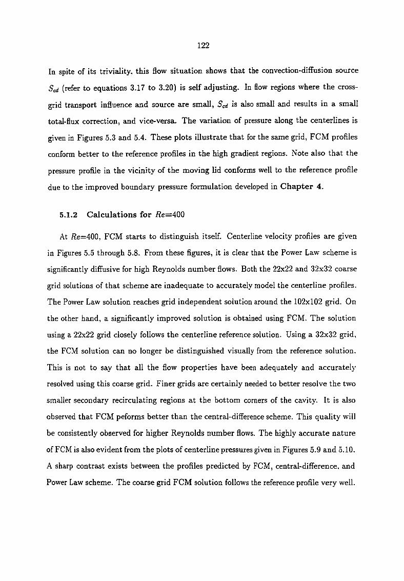
122

In spite of its triviality, this flow situation shows that the convection-difFusion source

Scd (refer to equations 3.17 to 3.20) is self adjusting. In flow regions where the cross-

grid transport influence and source are small, Scd is also small and results in a small

total-flux correction, and vice-versa. The variation of pressure along the centerlines is

given in Figures 5.3 and 5.4. These plots illustrate that for the same grid, FCM profiles

conform better to the reference profiles in the high gradient regions. Note also that the

pressure profile in the vicinity of the moving lid conforms well to the reference profile

due to the improved boimdary pressiire formulation developed in Chapter 4.

5.1.2 Calculations for /?e=400

At /2e=400, FCM starts to distinguish itself. Centerline velocity profiles are given

in Figures 5.5 through 5.8. From these figures, it is clear that the Power Law scheme is

significantly diffusive for high Reynolds number flows. Both the 22x22 and 32x32 coarse

grid solutions of that scheme are inadequate to accurately model the centerline profiles.

The Power Law solution reaches grid independent solution around the 102x102 grid. On

the other hand, a significantly improved solution is obtained using FCM. The solution

using a 22x22 grid closely follows the centerline reference solution. Using a 32x32 grid,

the FCM solution can no longer be distinguished visually from the reference solution.

This is not to say that all the flow properties have been adequately and accurately

resolved using this coarse grid. Finer grids are certainly needed to better resolve the two

smaller secondary recirculating regions at the bottom corners of the cavity. It is also

observed that FCM peforms better than the central-difference scheme. This quality will

be consistently observed for higher Reynolds number flows. The highly accurate nature

of FCM is also evident from the plots of centerline pressures given in Figures 5.9 and 5.10.

A sharp contrast exists between the profiles predicted by FCM, central-difference, and

Power Law scheme. The coarse grid FCM solution follows the reference profile very well.

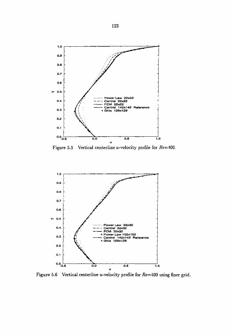
123

1.0

0.9

0.8

0.7

0.6

>- 0.5

Power Law 2Px?P Central Pgx?? FCM 22x22 Central 142x142 Reference

• Ghia 129x129

0.4

0.3

0.2

0.1

0.0 O.O 0.5 1.0 -0.5

u Figure 5.5 Vertical centerline u-velocity profile for /?e=400.

1.0

0.9

0.8

0.7

0.6

s- 0.5

Power Law 32x32 Central 32x32 FCM 32x32

° Power Law 102x102 Central 142x142 Reference

• Ghia 129x129

0.4

0.3

0.2

0.1

0.0 0.0 0.5 -0.5

u

Figure 5.6 Vertical centerline u-velocity profile for /2e=400 using finer grid.

0.4

0.3

0.2

O.I

O.O

-0.1

-0.2

-0.3

-0.4

-O.S 0.0 0.1 0.2 0.3 0.4 O.S 0.6 0.7 0.8 0.9 1.0

X

Figure 5.7 Horizontal centerline u-velocity profile for i2e=400.

0.4

0.3

0.2

0.1

0.0 •

>

' —- Power Law 32x32 Central 32x32 FCM 32x32

' o Power Law 102x102 Central 142x142 Reference

• Ghia 129x129 -0.3 -

-0.4 -

.0.5 1 1 1 1 1 1 0.0 0.1 0.2 0.3 0.4 0.S 0.6 0.7 0.8 0.9 1.0

X

Figure 5.8 Horizontal centerline u-velocity profile for /le=400 using finer grid.

124

—- Power Law 32x32 Central 32x32 FCM 32x32

o Power Law 102x102 Central 142x142 Reference

• Ghia 129x129

125

1.0

0.9

0.8

0.7

0.6

>- 0.5

0.4

0.3 Power Law P2x>?? Central 22x22 FCM 22x22 FCM 32x32 Central 142x142 Reference

0.2

0.1

0.0 1.05 0.95 1.00 0.90

P

Figure 5.9 Vertical centerline pressure profile for /2e=400.

1.04

Power Law P2xPP Central ?Pxg2 FCM FCM 32x32 Central 142x142 Reference

1.02

1.00

a. 0.98

0.96

0.94

0.92 O.O O.I 0.2 0.3 0.4 0.5 0.6 0.7 0.8 0.9

X

Figure 5.10 Horizontal centerline pressure profile for iEe=400.

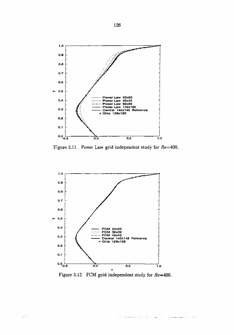
126

1.0

0.9

0.8

0.7

0.6

>- 0.5

Power Law gPxgg Power Law 42x42 Power Law 82x82 Power Law 102x102 Central 142x142 Heference Ghia 129x129

0.4

0.3

0.2

0.1

0.0 0.5 1.0 -O O.O

Figure 5.11 Power Law grid independent study for /2e=400.

1.0

0.9

0.8

0.7

0.6

>- 0.5

0.4 - FCM 22x22 - FCM 32x32 - FCM 42x42 - Central 142x142 Reference • Ghia 129x129

0.3

0.2

0.1

0.0 -0.5 0.0 0.5 1.0

u

Figure 5.12 FCM grid independent study for /?e=400.

127

1.00

0.67

0 . 0 0 1.00 0.67 0 . 0 0 0.33

Figure 5.13 Streamline contours using 102x102 grid and Power Law scheme for i?e=400.

1.00

0.67

0.33

0 .00

0 . 0 0 0.33 0.67 1.00

Figure 5.14 Streamline contours using 32x32 grid and FCM for i?e=400.

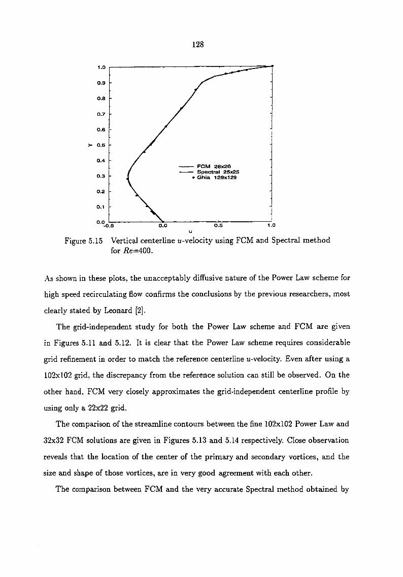
128

1.0

0.9

0.8

0.7

0.6

>- 0.5

0.4 - FCM 26x26 - Spectral 25x25 » Ghia 129x129 0.3

0.2

0.1

0.0 1.0 O.O 0.5 -0.5

u

Figure 5.15 Vertical centerline u-velocity using FCM and Spectral method for /?e=400.

As shown in these plots, the unacceptably diffusive nature of the Power Law scheme for

high speed recirculating flow confirms the conclusions by the previous researchers, most

clearly stated by Leonard [2].

The grid-independent study for both the Power Law scheme and FCM are given

in Figures 5.11 and 5.12. It is clear that the Power Law scheme requires considerable

grid refinement in order to match the reference centerline u-velocity. Even after using a

102x102 grid, the discrepancy from the reference solution can still be observed. On the

other hand, FCM very closely approximates the grid-independent centerline profile by

using only a 22x22 grid.

The comparison of the streamline contours between the fine 102x102 Power Law and

32x32 FCM solutions aire given in Figures 5.13 and 5.14 respectively. Close observation

reveals that the location of the center of the primary and secondaxy vortices, and the

size and shape of those vortices, are in very good agreement with each other.

The comparison between FCM and the very accurate Spectral method obtained by

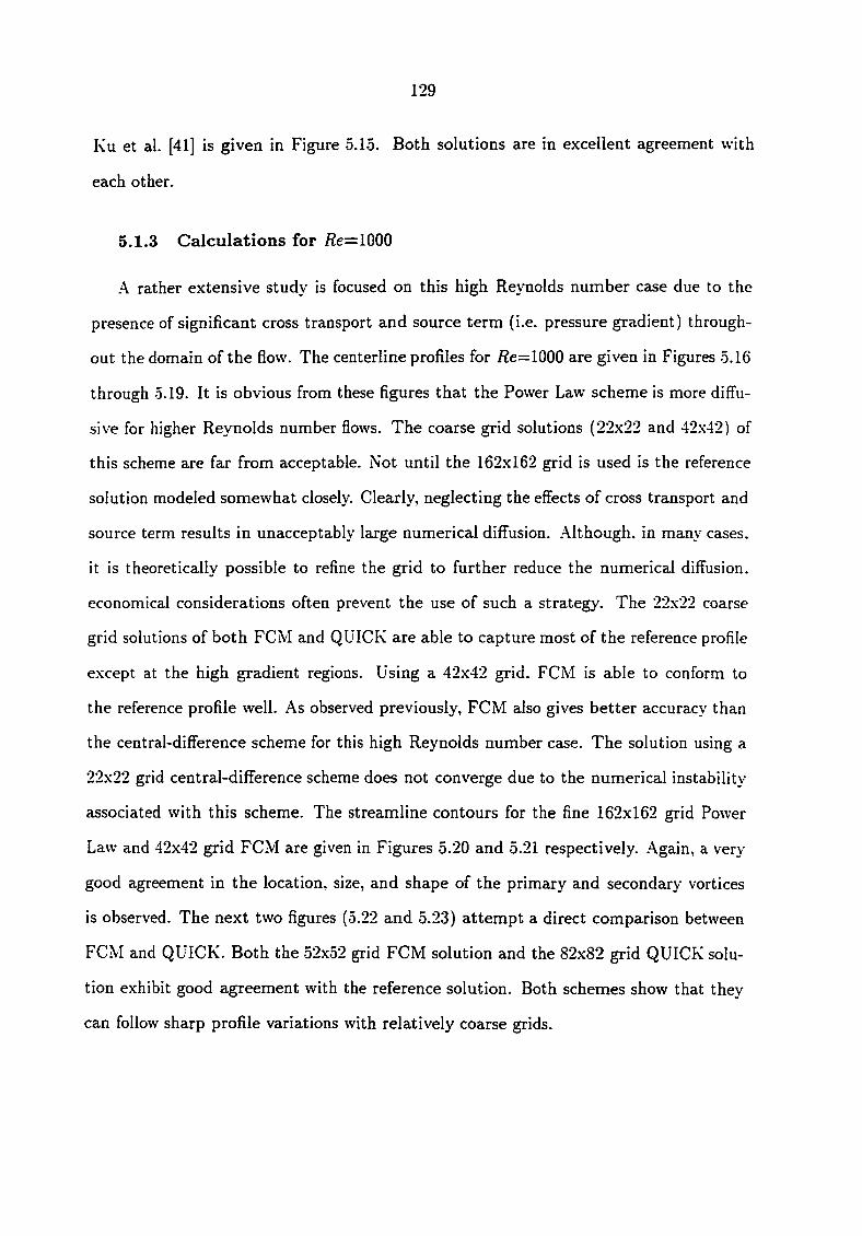
129

Ku et al. [41] is given in Figure 5.15. Both solutions are in excellent agreement with

each other.

5.1.3 Calculations for Re=lOOO

A rather extensive study is focused on this high Reynolds number case due to the

presence of significant cross transport and source term (i.e. pressure gradient) through

out the domain of the flow. The centerline profiles for /?e=1000 are given in Figures 5.16

through 5.19. It is obvious from these figures that the Power Law scheme is more diffu

sive for higher Reynolds number flows. The coarse grid solutions (22x22 and 42x42) of

this scheme are far from acceptable. Not until the 162x162 grid is used is the reference

solution modeled somewhat closely. Clearly, neglecting the effects of cross transport and

source term results in unacceptably large numerical diffusion. .A.lthough. in many cases,

it is theoretically possible to refine the grid to further reduce the numerical diffusion,

economical considerations often prevent the use of such a strategy. The 22x22 coarse

grid solutions of both FCM and QUICK are able to capture most of the reference profile

except at the high gradient regions. Using a 42x42 grid. FCM is able to conform to

the reference profile well. As observed previously, FCM also gives better accuracy than

the central-difference scheme for this high Reynolds number case. The solution using a

22x22 grid central-difference scheme does not converge due to the numerical instability

associated with this scheme. The streamline contours for the fine 162x162 grid Power

Law and 42x42 grid FCM are given in Figures 5.20 and 5.21 respectively. .A.gain, a very

good agreement in the location, size, and shape of the primary and secondary vortices

is observed. The next two figures (5.22 and 5.23) attempt a direct comparison between

FCM and QUICK. Both the 52x52 grid FCM solution and the 82x82 grid QUICK solu

tion exhibit good agreement with the reference solution. Both schemes show that they

can follow sharp profile variations with relatively coarse grids.

130

1.0

0.9

0.8

0.7

0.6

5- 0.5

0.4 Power Law ??xP?

- FCM 22x22 o QUICK 22x22 - Central 202x202 Reference • Ghia 129x129

0.3

0.2

0.1

0.0 O.O 0.5 -0.5 1.0

u Figure 5.16 Vertical centerline u-velocity profile for /2e=1000.

1.0

0.9

0.8

0.7

0.6

>- 0.5

0.4 Power Law 42x42 Central 42x42 FCM 42x42

a Power Law 162x162 Central 202x202 Reference

• Ghia 129x129

0.3

0.2

0.1

O.O -0.5 O.O 0.5 1.0

u Figure 5.17 Vertical centerline u-velocity profile for Ee=1000.

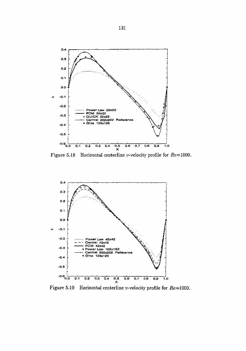
131

0.4

0.3

0.1

O.O

-O.I

-0.2 Power Law PPx??

- FCM 22x22 o QUICK 22x22 - Central 202x202 Reference • Ghia 129x129

-0.3

-0.5

-0.6 O.S 0.6 0.7 0.8 0.9 1.0 X

O.O 0.1 0.2

Figure 5.18 Horizontal centerline u-velocity profile for /2e=1000.

0.4

0.3

0.2

O.I

o.o

-O.I

-0.2 • Power Law 42x42 - Central 42x42 - FCM 42x42 o Power Law 162x162 - Central 202x202 Reference • Ghia 129x129

-0.3

-0.4

-0.5

-0.6 O.O 0.1 0.2 0.3 0.4 0.5 0.6 0.7 0.8 0.9 1.0

Figure 5.19 Horizontal centerline u-velocity profile for /2e=1000.

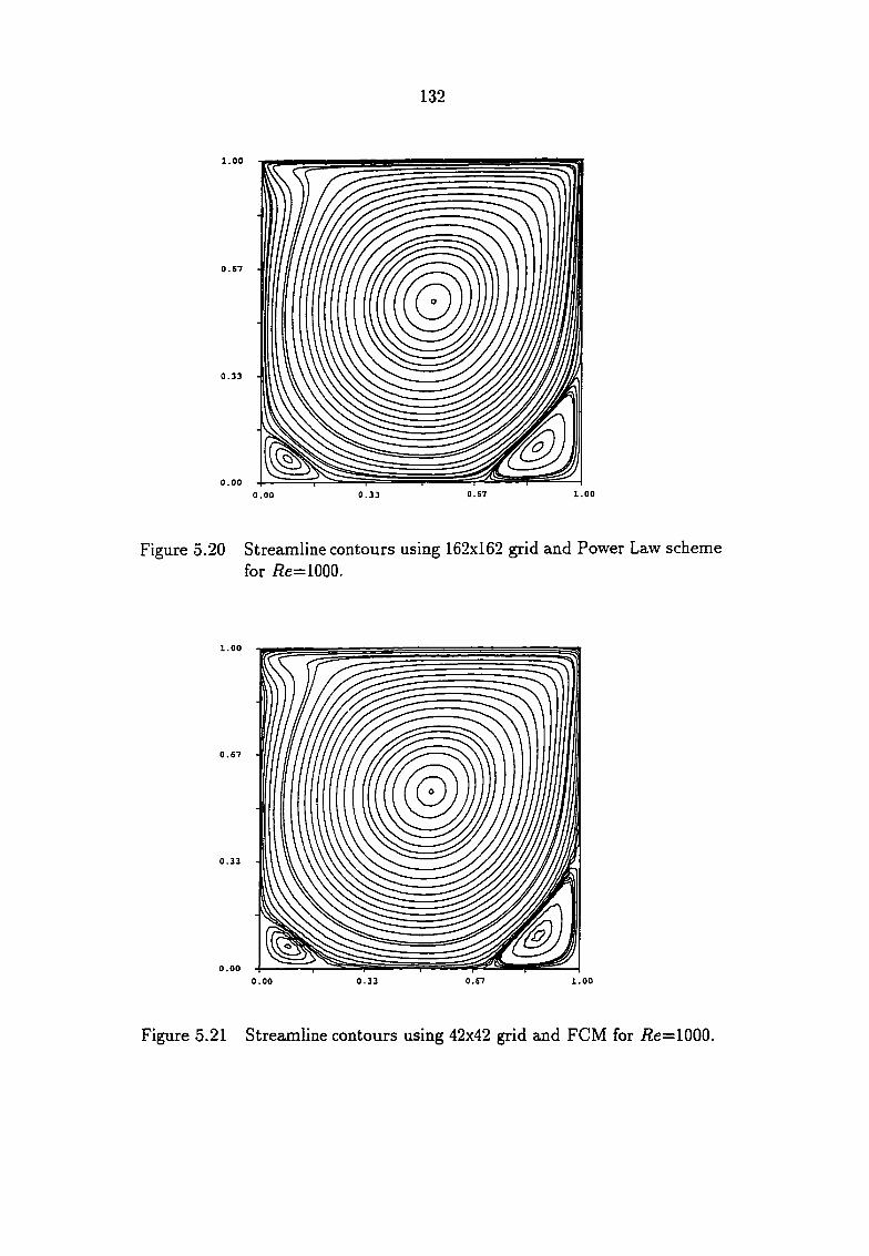
132

1.00

0.67

0 .00 0.67 1.00 0.33 0 . 0 0

Figure 5.20 Streamline contours using 162x162 grid and Power Law scheme for i?e=1000.

1 . 0 0

0.67

0.33

0 .00 0.33 0.67 1.00 0 . 0 0

Figure 5.21 Streamline contours using 42x42 grid and FCM for i?e=1000.

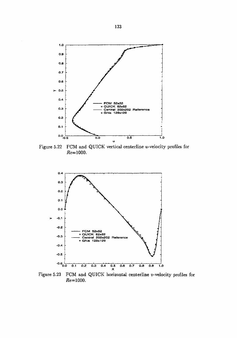
133

1.0

0.9

0.8

0.7

0.6

>- 0.S

0.4 - FCM 52x52 O QUICK 82x82 - Central 202x202 Reference • Ghia 129x129

0.3

0.2

0.1

0.0 1.0 0.5 -0.5 O.O

u

Figure 5.22 FCM and QUICK vertical centerline u-velocity profiles for i?e=1000.

0.3

0.2

0.1

0.0

-0.1

-0.2

- FCM 52x52 O QUICK 82x82 - Central 202x202 Reference • Ghia 129x129

-0.3

-0.4

-0.5

-0.6 0.0 0.1 0.2 0.3 0.4 0.5 0.6 0.7 O.a 0.9 1.0

X

Figure 5.23 FCM and QUICK horizonted centerline u-velocity profiles for /2e=1000.

134

It should be noted from Figure 5.16 that while the 22x22 grid FCM u-centerline profile

is able to follow the reference solution at the lower wall region, the QUICK solution for

the same grid resolution shows a significant deviation. However, this should not be used

as a measure for determining the better scheme. Further study is warranted before a

conclusion can be reached.

After showing that the coarse grid solution of FCM can model the reference solution

well, it is important to show the consistency of the fine grid solution of FCM. Figures 5.24

and 5.25 show that the 162x162 grid solution of the Power Law scheme is not in close

agreement with the reference solution in regions of high flow gradients. Again, this

reaffirms the conclusion of previous researchers about the limitations of the Power Law

scheme for multi-dimensional problems involving high Reynolds number flows which are

oblique or skewed with respect to the grid. Fine grid solutions of FCM and central-

difference show excellent agreement with each other and with Ghia's solution.

Figures 5.26 through 5.28 show the grid-independent study for the Power Law,

central-difference, and FCM. It can be observed visually that the grid-independent ver

tical centerline profile for the Power Law scheme barely starts at the 162x162 grid. The

central-difference scheme requires a grid slightly finer than 82x82, and FCM needs a

52x52 grid. Close observation shows that the 42x42 grid FCM solution already gives

acceptable agreement for practical purposes.

The inability of the Power Law scheme to follow the reference profile on a point-to-

point beisis even using a fine 162x162 grid (Figure 5.26) prompted the effort to employ

an even finer grid to see whether the Power Law scheme is indeed able to do so with

further grid refinement. For this purpose, a four stage V-cycle FAS multigrid using a

322x322 grid is used, and the resulting centerline u-velocity plot is given in Figure 5.29.

It is concluded from this result that while the Power Law solutions can always follow

the reference profile satisfactorily, the excessively fine grid needed renders it impractical

for many flow problems.

135

1.0

0.9

0.8

0.7

0.6

5- 0.5

•• Power Law 162x162 - Central 142x142 - FCM 142x142 • Ghia 129x129

0.3

0.2

0.1

0.0 0.5 1.0 O.O -0.5

u

Figure 5.24 Fine grid vertical centerline u-velocity profile for /2e=1000.

0.4

0.3

0.2

0.1

0.0

-0.1

-0.2

Power Law 162x162 - Central 142x142 - FCM 142x142 • Ghia 129x129

-0.3

-0.4

-0.5

-0.6 0.0 0.1 0.2 0.3 0.4 0.5 0.6 0.7 0.8 0.9 1.0

X

Figure 5.25 Fine grid horizontal centerline u-velocity profile for i?e=1000.

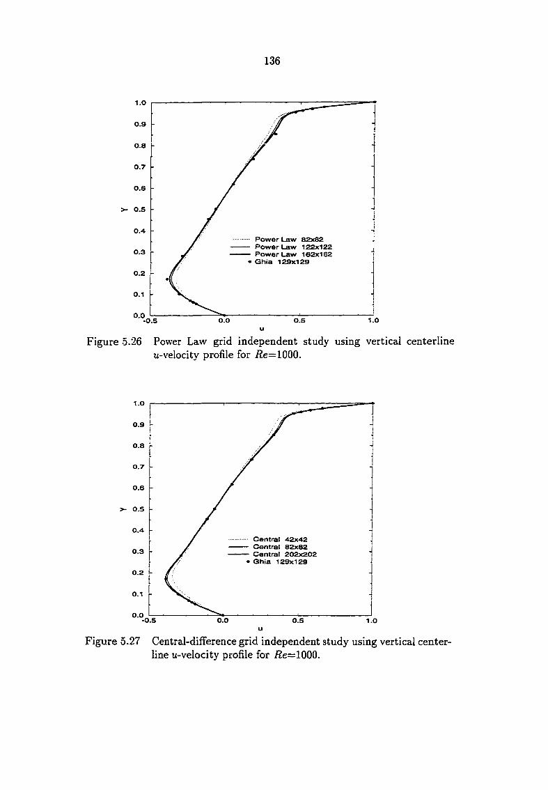
136

1.0

0.9

0.8

0.7

0.6

>- 0.5

0.4 •• Power Law 82x82 - Power Law 122x122 - Power Law 162x162 • Ghia 129x129

0.3

0.2

0.1

0.0 1.0 0.0 0.5 -0.5

u

Figure 5.26 Power Law grid independent study using vertical centerline u-velocity profile for /?e=1000.

1.0

0.9

0.8

0.7

0.6

5- 0.5

Central 42x42 Central 82x82 Central 202x202 Ghia 129x129

0.3

0.2

0.1

O.O -0.5 0.0 0.5 1.0

u

Figure 5.27 Central-difference grid independent study using vertical center-line u-velocity profile for i2e=1000.

137

1.0

0.9

0.8

0.7

0.6

>- O.S

- FCM 22x22 - FCM 42x42 - FCM 52x52 - FCM 142x142 • Ghia 129x129

0.4

0.3

0.2

O.I

0.0 0.5 1.0 0.0 -0.5

u

Figure 5.28 FCM grid independent study using vertical centerline u-velocity profile for /2e=1000.

1.0

0.9

0.8

0.7

0.6

>- 0.5

0.4

Power Law 162x162 Power Law 322x322 MG4 Central 202x202 Reference

0.3

0.2

0.1

0.0 0.0 0.5 -0.5 1.0

u

Figure 5.29 Power Law fine grid vertical centerline u-velocity profile for i?e=1000.

0.16

0.14

0.12

f

— • QUICK (3rcl) --0 QUICK (2nd) — a Central — A Hybrid — • FCM --oFCM (nb)

* Ghia

0.08

0.06

0.04 10 100

Grid

Figure 5.30 Streamfunction at cavity center for jRe=iOOO.

139

An exploration of the relative accuracy of the schemes considered is carried out for

this high /?e=1000 case. Figure 5.30 shows the value of the streamfunction, at the

center of the primaxy vortex plotted as a function of grid refinement. The value of

is commonly used as a sensitivity measure of the accuracy of the numerical schemes

being evaluated. For a given grid refinement, these results quantify the extent to which

a higher order scheme outperforms a lower order one. For example, a 20x20 grid with

QUICK or FCM is roughly equivalent to a 40x40 grid with the central-difference scheme

and an 80x80 grid with the hybrid scheme. It can edso be observed in this plot that the

effects of boundary cell correction on FCM do make a difference when the grid is coarse.

This difference quickly disappears with moderate grid refinement. Finally, it should be

understood that this rather simple form of performance evaluation should not be used

as an indicator to pick the better scheme between FCM and QUICK. A much more

extensive study using a more advanced method (i.e. the Richardson method, originally

proposed by Richardson [42. 43] and also described by Roache [44]) must be done before

any further conclusion can be justifiably drawn.

5.1.4 Calculations for ^e=10000

The flow inside a lid-driven cavity at a very high Reynolds number proves to be a

diflScult test problem to investigate. At this very high Reynolds number, very complex

flow interactions, which quite possibly are highly unsteady, are taking place. Moreover,

there have been many uncertainties and inconsistencies among the numerical findings

of various researchers in determining the limit Reynolds number at which the onset of

turbulence occurs. However, it has been the general agreement, as clearly stated by

Huser [45], that the transition to turbulence is characterized by the development of

small eddies at the vicinity of the two lower corners (and also at the upper left corner),

and the laminar mean velocity of the main vortex becomes unstable. The interaction of

these eddying motions with the mean shear eventually leads to turbulence.

140

Due to hardware limitations, early studies on the onset of turbulence for the cavity

flow were done on the basis of an analysis using the steady-state Navier-Stokes equations

and a relatively coarse grid. Bye [46] detennined a range of transition Re between 400

and 600. Kumagai [47] roughly estimated transition to occur at even lower Re. Both

authors used the formation of an inflectional velocity profile indicating reverse flow as

the criterion for the onset of an unsteady regime. However, Kumagai strongly cautioned

against the accuracy of such data obtained from steady-state calculations. More recent

work by Ghia [7] using a very fine 257x257 grid with the central-difference scheme coupled

with a multigrid technique shows that it is possible to obtain a converged steady state

solution for i?e=10000. Hayase [8] has also been able to get steady-state solutions using

QUICK with an 82x82 grid. Ghia's and Hayase's findings suggests that the flow inside

the lid-driven cavity at /?e=10000 converges to a steady-state solution. Following this

line of thought, the ability of the Power Law scheme and FCM to simulate this high

Reynolds number flow in a steady mode is investigated. Ghia's calculations are utilized

as a reference solution.

The centerline velocity profiles eu:e given in Figures 5.31 and 5.32. Again, it is evident

that the Power Law scheme is far too diffusive to accurately predict this high convection

recirculating flow. Even the 322x322 multigrid solution of the Power Law scheme is far

from adequate in following the reference solution. On the other hand, the coarse grid

solution of FCM and QUICK are able to follow Ghia's fine grid solution closely. However,

it should be understood that at this high Reynolds number, stability and convergence

of the numerical scheme become more important issues. Hayase reported that it is

necessary to retain the unsteady terms in the momentum equation in order to achieve

stable, converged solutions on grids finer than 40x40 at this Reynolds number. Although

FCM does not need this transient marching procedure, much slower convergence and

oscillations of the residuals are observed, in particular with the use of finer grids.

141

1.0

0.9

0.8

0.7

0.6

>- 0.5

- Power Law 82x82 - Power Law 142x142 - Power Law 202x202 - Power Law MG4 322x322 - FCM 82x82 • Ghia Reference O QUICK 82x82

0.4

0.3

0.2

0.1

0.0 1.0 0.0 0.5 -0.5

u

Figure 5.31 Vertical centerline u-velocity profile for /?e=10000.

- Power Law 82x82 \ - Power Law 142x142 - Power Law 202x202 - Power Law MG4 322x322 - FCM 82x82 • Ghia Reference O QUICK 82x82

Figure 5.32 Horizontal centerline u-velocity profile for i2e=10000

142

These oscillations of the residuals suggest the possibility that the lid-driven cavity flow

at i?e=10000 is indeed unsteady. In fact, it was understood that from the period of

the formation of the comer eddies which leads to transition, the flow structure is highly

unsteady and thus can no longer be simulated using steady numerical calculations. The

fact that it is possible to obtain steady-state convergence suggests that the grid resolution

used is not sufficient to resolve the transient physics of the flow, especially at the corner

regions. In this case, the use of the numerical scheme in steady mode will result in

a fortuitous steady-state solution. The steady-state fine grid Power Law and Ghia

central-difference solutions and the coaxse grid FCM solution obtained in Figures 5.31

and 5.32 are incorrect but converged solutions. It is very likely that this behavior was also

observed by Hayaise in his calculations. If the numerical scheme is used in the unsteady

mode, good converged iteration will be obtained at each timestep and a steady-state

solution will be obtained after sufficient time ha^ elapsed.

Theoretically, it is always possible to refine the grid sufficiently to reach the limit

where the numerical scheme is able to pick up the transient physics of the problem. .At

this grid resolution, the use of the numerical scheme in the steady mode will result in

very slow convergence and eventual stalling of the residuals after only a few order drop

in the magnitude of the residuals. On the other hand, in using the unsteady calculations,

satisfactory convergence will be obtained at each timestep, and the transient nature will

be captured in real time.

A higher order numerical scheme will be able to pick up the unsteady nature of

the flow using a relatively coarser grid, and this leads to residual oscillations when an

attempt is made to simulate transient behavior using steady calculations. It is therefore

clear why steady-state convergence is not obtained using a 322x322 multigrid FCM in

steady mode. A four order drop in the magnitude of the residual (Equation 5.1) is

observed before residual oscillation starts.

This finding prompted a further study of this particular test problem using FCM in

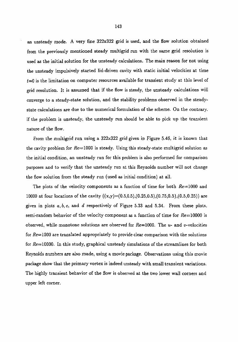
143

an unsteady mode. A very fine 322x322 grid is used, and the flow solution obtained

from the previously mentioned steady multigrid run with the same grid resolution is

used as the initial solution for the imsteady calculations. The main recison for not using

the unsteady impulsively started lid-driven cavity with static initiai velocities at time

/=0 is the limitation on computer resources available for transient study at this level of

grid resolution. It is assumed that if the flow is steady, the unsteady calculations will

converge to a steady-state solution, and the stability problems observed in the steady-

state calculations are due to the numerical formulation of the scheme. On the contrarj'.

if the problem is unsteady, the unsteady run should be able to pick up the transient

nature of the flow.

From the multigrid run using a 322x322 grid given in Figure 5.46, it is known that

the cavity problem for /2e=1000 is steady. Using this steady-state multigrid solution as

the initial condition, an unsteady run for this problem is also performed for comparison

purposes and to verify that the unsteady run at this Reynolds number will not change

the flow solution from the steady rim (used as initial condition) at all.

The plots of the velocity components as a function of time for both /2e=1000 and

10000 at four locations of the cavity ((x,y)=(0.5,0.5),(0.25,0.5),(0.75,0.5),(0.5,0.25)) are

given in plots a,6, c, and d respectively of Figure 5.33 and 5.34. From these plots,

semi-random behavior of the velocity component as a function of time for /?e=10000 is

observed, while monotone solutions are observed for i?e=1000. The u- and u-velocities

for /?e=1000 are translated appropriately to provide clear comparison with the solutions

for /?e=10000. In this study, graphical unsteady simulations of the streamlines for both

Reynolds numbers are also made, using a movie package. Observations using this movie

package show that the primary vortex is indeed unsteady with small transient variations.

The highly transient behavior of the flow is observed at the two lower wall corners and

upper left comer.

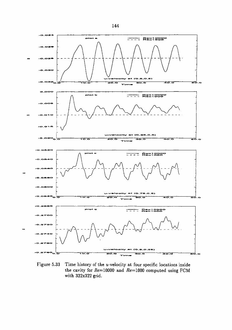
144

-1

1

lO

'O I

r u • Q

Figure 5.33 Time history of the u-velocity at four specific locations inside the cavity for i?e=10000 and i2e=1000 computed using FCM with 322x322 grid.

145

Figure 5.34 Time history of the u-velocity at four specific locations inside the cavity for i?e=10000 and i2e=I000 computed using FCM with 322x322 grid.

146

In the lower left wall corner, it is observed that three secondary vortices continuously

develop, gain and loose strength, and burst to facilitate the formation of the other

vortices. This is in clear agreement with the work of Huser mentioned previously which

is bcised on the unsteady flow calculation at Re roughly equal to 10000. This finding is

also consistent with the experimental results obtained by Koseff" et al. [48] who observed

the onset of turbulence at /?ew6000.

5.2 Grid Stretching

In solving practical flow problems, due to the limitations on the number of grid

points which can be afforded, it is always desirable to cluster grid points in regions

with high flow gradients (i.e. in the boundary layer region near the wall) and coarsen

the grid at other regions. It is well-known that mesh coarsening also degrades the

numerical solutions by introducing undershoots and/or overshoots in certain regions

of the flow. Therefore, it is very important to know the limit at which a particular

numerical scheme can tolerate local grid stretching without causing unacceptably large

error in the numerical solution. In Figures 5.35 through 5.37, three different stretchings

(moderate, high, and extreme) are tested on the lid-driven cavity flow for /?e=4Q0. It is

important to mention here that a sufficient number of grid points required to conform

point-to-point (in the unstretched mode) with the reference solution must be used to

conduct a meaningful study. From previous exercises, it is known that for this Reynolds

number, the use of a 122x122 grid ensures a grid-independent solution. For each grid, the

centerline u-velocity profile obtained using Power Law and FCM are compzired against

the unstretched fine grid reference solution obtained using the central-difference scheme.

147

i.m

iiiiiiinrri:, llliiiii::;;': 1111111:1.: . iniiiiiiii'i.; JirJiim;:. Mlliiii::'..: Iltlllil!:: " lliiiiiii:;.. mnii!:::" iiiiii!i;;:7; iiiiinii!: niiiiinr... nt!iiii:i;... Ulliiiii!!.:: itimiiii;.. nillilli:;::: ttutitiii;' Ulliiiiiir.L umiuii;:.:

Power Law 122x122 FCM 122x122 Central 142x142 Reference

Figure 5.35 Effects of moderate grid stretching u-velocity profile for Re = 400.

on vertical centerline

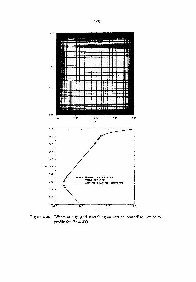
148

Figure 5.36 Effects of high grid stretching on vertical centerline u-velocity profile for Re = 400.

149

Power Law 122x122 FCM 122x122 Central 142x142 Reference

Figure 5.37 Effects of extreme u-velocity profile for

grid stretching Re = 400.

on vertical centerline

150

Observation of the moderate stretching (Figure 5.35) shows that FCM produces an

almost negligible overshoot at the high gradient (which now has a lower grid density)

region while the errors produced by the Power Law scheme have become very apparent

in more than one region. An even more importajit conclusion can be obtained by looking

at the results produced by the high and extreme stretching (Figure 5.36 and 5.37). It is

observed that while FCM solutions now display more profound overshoot error in both

the lower and upper high gradient regions, the errors produced by the Power Law scheme

are comparatively larger. It should also be noted that in the regions of the lower wall

boundary, the Power Law solution also displays slightly incorrect slope, not observed in

the FCM solution. It is therefore concluded that FCM behaves better than the Power

Law scheme when local grid stretching is used. However, regardless of which numerical

scheme is used, the use of grid stretching must always be done with caution and care.

5.3 Convergence Characteristics and CPU Requirement

Having addressed the important issues of accuracy and stretching in the previous

subsections, it is now necessary to investigate the convergence chaxacteristics of FCM

as compared with its parent method (i.e. Power Law). Recall that the main idea

behind FCM is to correct the flux computation at an interface by using the governing

conservation law itself applied to a control-volume enclosing that interface. Thus, for an

interface in a given direction, the cross transport, the unsteady term, and the original

source present in the considered conservation equation are combined into one single

source used in the one-dimensional convection-diffusion equation. Therefore, the total-

flux profile at an interface consists of a homogeneous profile and a correction profile due

to that source. Hence, an FCM iteration is bcisicaily a Power Law iteration plus iteration

on the added correction source. Consequently, FCM is expected to inherit ail the stable

convergence properties of the first-order Power Law scheme, including the 'Four Stable

151

Convergence Rules' established by Patankar [5]. The plots of the mass, x-momentum.

and u-velocity convergence for an /?e=400 lid-driven cavity problem using a 42x42 grid

are given in plots a, b, and c respectively of Figure 5.38. It is observed that FCM displays

similar convergence trends as the Power Law scheme. The fact that FCM has a lower

convergence rate can be rationalized as the extra effort needed to iterate on the extra

correction sources. It is also obvious that the FCM convergence stalls at a few orders

of magnitude higher thaji Power Law convergence and produces more noise at those

stalled levels. This behavior, while generally best avoided, should not be of any concern

here. Close observation reveals that at least a ten order drop in magnitude is achieved

for any of the convergence criteria considered, which is much more than enough for all

purposes. This stalling and subsequent oscillatory behavior are again attributed to the

presence and the iteration of the extra correction sources, which are highly non-linear. It

should be the goal of future work to investigate whether special procedures to evaluate

the correction terms will eventually reduce, if not eliminate, the stalling behavior and

noise.

Figure 5.39 gives the convergence history for i?e=1000 using a 62x62 grid and a

102x102 grid. The same convergence trend between FCM and Power Law is again

observed. For the 62x62 grid, it is observed that after a three or four order drop in

magnitude of the residuals, FCM has a noticeably lower convergence rate than the

Power Law scheme. However, it has been the common practice in CFD (as is evident

in the published literature) that under usual circumstances, it is very rarely necessary

to converge to a residual value of 10~'° or 10"^^ during the iterative process. A five or

six order drop in magnitude of the residuals is usually sufficient to consider the solution

converged.

152

plot m

^ow«r

no"

1 O'*

-lo-'®

-I o*"*"

TO'-

2000.0 ttormtiori

3000.0 <4-000.0

plot to

ROfVl

1 O""*

1 OOO.O 2000.0 Itormtion

3000.0 4000.0

plot e

1 O

•I O"*

1 O'*

10-"»

io'»

^ow«r ROM

1 OOO.O 2000.0 lt*r«tlor»

3000.0 4000.0

Figure 5.38 Convergence of the residuals for /2e=400.

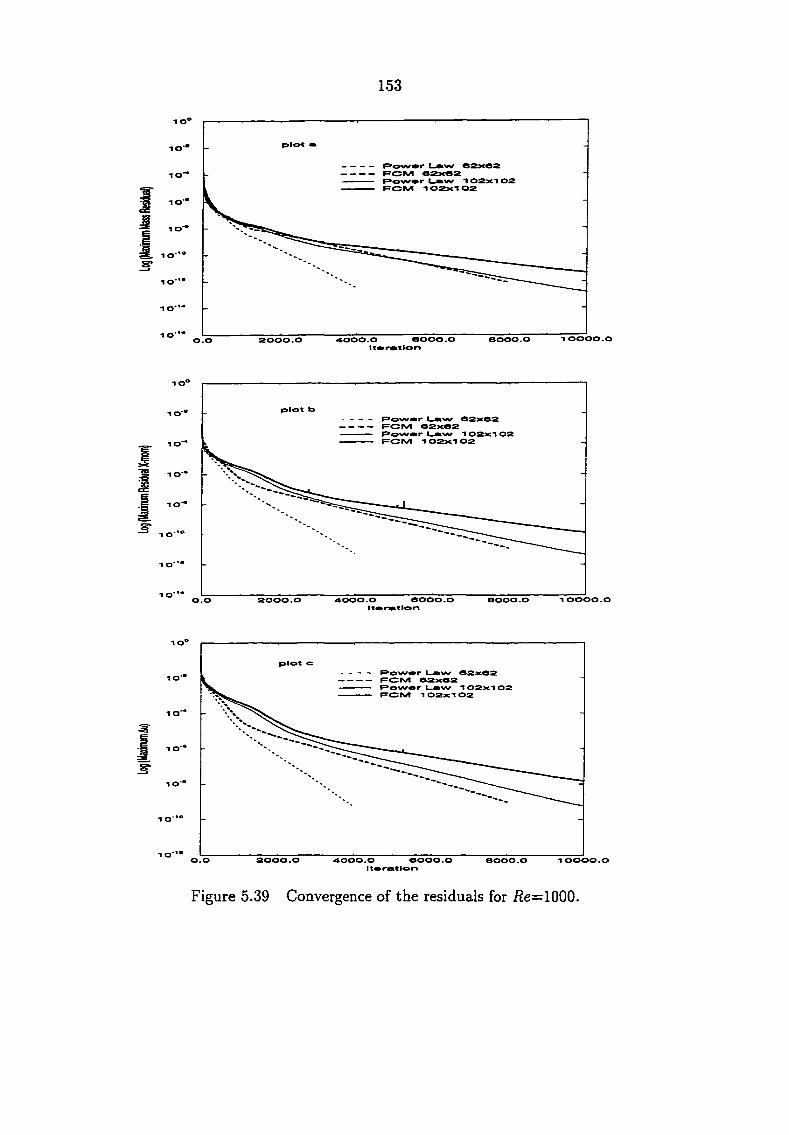
153

plot

F?OIS/l 1 02>c1 02

1 0000.0 0000.0 aooo.o 2000.0 <4000.0 it«i

0.0

plot b

>r 1 02x'l 02

-I 0000.0 eooo.o 2000.0 4000.0 8000.0 0.0 It rmtlon

10'

plot c 02>c02 lO''

^ow«r L.AW 1 02>c1 02

1 O"

1 O*'

10"

•I O'

1 O"' 2000.0 0.0 aooo.o eooo.o t 0000.0 8000.0

it*r«itlori

Figure 5.39 Convergence of the residuals for /2e=1000.

154

More importantly, from the same plots, it should be noted that as the grid is refined

to 102x102, the difference in the convergence rate between FCM and the Power Law

scheme diminishes substantially.

The fact that FCM becomes more efficient with grid refinement is also demonstrated

in Figure 5.40. In this figure, the ratio of the CPU time requirement of FCM to that

of the Power Law scheme (to converge to a given residual) for three different Reynolds

numbers is plotted as a function of the nimiber of grid points. As expected, for a given

grid size and Reynolds number, FCM requires more CPU time than the Power Law

scheme to converge to the same residual. This CPU time increase is attributed to two

factors. First, the increase is due to the extra time needed by FCM to converge. Thus,

it is inherent in the scheme's formulation. This contribution can be measured by looking

at the extra number of iterations needed, as given previously in Figures 5.38 and 5.39.

Secondly, the increase in time is also due to the time needed for the extra computation of

the source correction within each iteration. While it is not generally possible to reduce

the first contribution without introducing major changes in the scheme's formulation,

it is indeed quite possible to reduce the second contribution by using better and more

efficient coding techniques. Throughout the development pheise of FCM, clarity and

ease of debugging are given precedence over efficiency during the code development.

In fact, the expensive-to-compute total-fluxes which will be used in the FCM sources

are recalculated in order to allow testing of different schemes. These total-fluxes should

have been available from the computation of the influence coefficients. Thus, it is indeed

possible to reduce the CPU time requirement of FCM per-iteration by writing the code

used in this study more efficiently. In fact, this step must be done once sufficient maturity

is accomplished in the development of FCM. Nevertheless, the plot in Figure 5.40 still

gives a qualitative idea of the CPU time requirement of FCM.

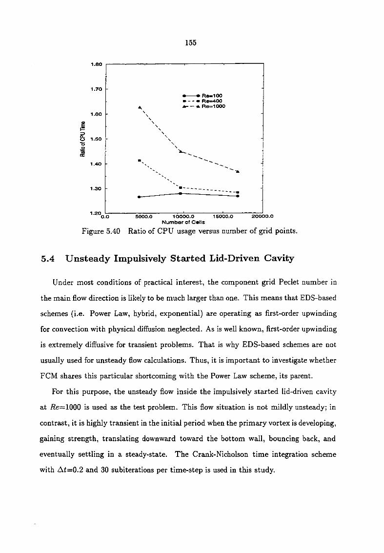
155

1.80

1.70

1.60

O 1.50 o o "S QC

1.40

1.30

1.20 O.O

• • Re=100 » - - « Re»400

—^ReslOOO

5000.0 10000.0 15000.0 Number of Cells

20000.0

Figure 5.40 Ratio of CPU usage versus number of grid points.

5.4 Unsteady Impulsively Started Lid-Driven Cavity

Under most conditions of practical interest, the component grid Peclet number in

the main flow direction is likely to be much laxger than one. This means that EDS-based

schemes (i.e. Power Law, hybrid, exponential) are operating as first-order upwinding

for convection with physical diffusion neglected. As is well known, first-order upwinding

is extremely diffusive for transient problems. That is why EDS-based schemes are not

usually used for unsteady flow calculations. Thus, it is important to investigate whether

FCM shares this particular shortcoming with the Power Law scheme, its parent.

For this purpose, the unsteady flow inside the impulsively started lid-driven cavity

at /2e=1000 is used as the test problem. This flow situation is not mildly unsteady; in

contrast, it is highly transient in the initial period when the primary vortex is developing,

gaining strength, translating downward toward the bottom wall, bouncing back, and

eventually settling in a steady-state. The Crank-Nicholson time integration scheme

with Af=0.2 and 30 subiterations per time-step is used in this study.

156

o.oo

•0.02

0.06

-O.OB

-0.10

Rower l_aw 62x62 Rower t_aw 82x82 Rower l_aw 10Zxl 02 Rower l_aw 1 62x1 62 FCM 62x62 Central 162x162 F^eference

-O.I 4

-O.I 6

-O.I 8

-0.20

-0.22 10.0 1S.O 2S.O 30.0 O.O 5.0 20.0

"Time

Figure 5.41 Time history of center u-velocity for /?e=1000.

0.20

0.18

Rower Uaw 62x62 Rower Uaw 82x82 Rower t_aw 1 02x1 02 Rower Uaw 1 62x1 62 RCM 62x62 Central 162x162 Reference

0.16

0.12

0.10

0.08

0.06

0.02

O.OO O.O 5.0 10.0 2S.O 20.0 30.0

Time

Figure 5.42 Time history of center t7-veIocity for /2e=1000.

157

The plots of the u- and u-velocities at the center of the cavity versus time are given in

Figure 5.41 and 5.42 respectively. It is observed that the Power Law scheme is indeed

very diffusive for the transient problem. The Power Law solution obtained using a

62x62 grid is far from adequate in following the reference solution. Even the 162x162

Power Law solution cannot quite follow the high transient gradient between f=5 and

i=8. On the other hand, the 62x62 FCM solution is able to closely follow the fine

grid reference solution even until steady-state is reached. It is also found during this

study that increasing the time-step to 0.4 introduces very minimal changes to the FCM

solution. This finding shows that the overall conservation idea used by FCM not only

improves steady-state accuracy, but also significantly enhances transient accuracy.

5.5 MultiGrid Technique on FCM

Over the last decade, the multigrid technique, which has been popular for accelerating

the convergence of an iterative numerical scheme for linear equations, has started to

gain wide acceptance for non-linear problems with the introduction of the FAS (Full

Approximation Storage) technique developed by Brandt [49, 50, 51]. When its potential

was realized, this technique was quickly adopted by many CFD practitioners to accelerate

the convergence of numerical schemes for Navier-Stokes equations, which are highly non

linear. The multigrid technique used in conjunction with a relaxation scheme (i.e. the

Gauss-Seidel scheme) accelerates the convergence by realizing that the relaxation sweep

on a given grid is effective only in eliminating the error components whose wavelength is

comparable to the size of the mesh. The smooth error components which posses longer

wavelengths with respect to a mesh can only be efficiently removed by using a coarser

mesh. Hence, after two or three iterations on a given fine mesh, the multigrid method

switches to a coarser mesh (usucJly constructed by combining four control-volumes in

two-dimensions) where the error components with longer wavelengths can be rapidly

158

annihilated. Thus, the multigrid method involves a procedure for transferring the flow

properties from finer to coaxser mesh (restriction) and communicates the error removal

from coarser to finer mesh (prolongation). Another aspect of the multigrid technique

is the strategy for cycling through the grid; the simplest and most common is the V-

cycle. One V-cycle iteration constitutes stepping down from the finest to the coarsest

grid by doing a few relaxation sweeps at each grid, converging the iterative scheme to

an acceptable level at the coarsest grid, and then stepping up and transferring the error

information successively by doing another few relaxation sweeps at each grid level until

the finest grid is reached. The details of the FAS technique are readily available from the

literature, as are the different types of restriction and prolongation processes. This work

closely follows the special application of the FAS technique for the segregated SIMPLER

algorithm developed by Zori [40], and a four stage V-cycle multigrid sweep is employed

in this study.

The CPU times needed by the single grid and FAS-SIMPLER multigrid using both

the Power Law scheme and FCM for the lid-driven cavity problem at ^e=1000 using a

98x98 grid are given in plot a of Figure 5.43. The residual used in this analysis is defined

by:

Rsdl = (5.1) Number of grid points

where Rx and Ry are residuals of the x- and y-momentum conservations. All compu

tations are performed using the DEC 3000 AXP workstations. It is observed that the

FAS-SIMPLER technique for Power Law and FCM has the same convergence behavior.

This is consistent with the single grid convergence characteristics of FCM relative to the

Power Law scheme. Using a 66x66 grid and the same Reynolds number, the effect of

different relaxation parameters on the multigrid convergence is given in plot 6 of Fig

ure 5.43. It is obvious that the value of the relaxation parameter used does influence

the rate of convergence of the multigrid iteration.

159

^ow«r L^w •> Singlfl Rowwr l_«w •> F^CM - SinglA

- M04.

-i o

soo.o nooo.o 1600.0 2000.0 Tlmo (sAe)

Pow®r l_«kw - n«laoCMO.' F»ow«r l_«w - R«laoCMO. PCIS/I - Fl«lmx—0..4. F^Cts/l • Ft«lAX»O.S

100.0 200.0 300.0 OPLJ "Tlmo (SVC)

•400.0 SOO.O

Figure 5.43 Multigrid convergence for /2e=400.

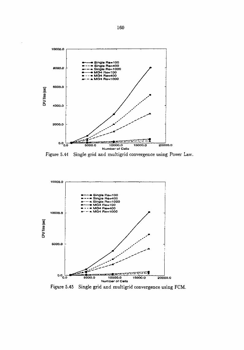
160

10000.0

m m Single Re=100 ••—Single Re=AOO * •*. Single Re=1000 • • MG4 Re=100 » — MG4- ResAOO A -A MG4- Re=1 OOO

SOOO.O

6000.0

4000.0

2000.0

O.O. 1 SOOO.O 20000.0 SOOO.O 10000.0

Number of Cells 0.0

Figure 5.44 Single grid and multigrid convergence using Power Law.

15000.0

• • Single Re=100 Single Re=400

• •*. Single Re=1000 • • MG4 Re=100 m- — m MG4 Re=s400 A MG4 Re=1000 10000.0

.P

5000.0

0.0 0.0 SOOO.O 10000.0 1 SOOO.O 20000.0

Number of Cells

Figure 5.45 Single grid and multigrid convergence using FCM.

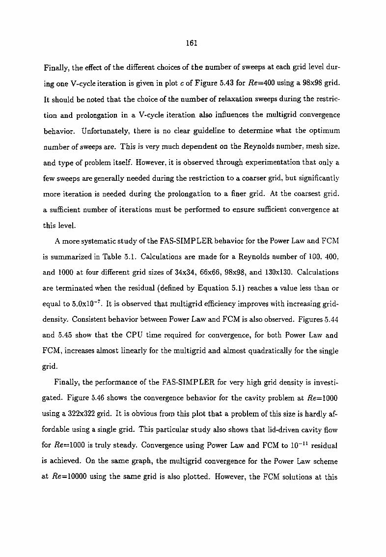
161

Finally, the effect of the different choices of the number of sweeps at each grid level dur

ing one V-cycle iteration is given in plot c of Figure 5.43 for i2e=400 using a 98x98 grid.

It should be noted that the choice of the number of relaxation sweeps during the restric

tion and prolongation in a V-cycle iteration adso influences the multigrid convergence

behavior. Unfortunately, there is no clear guideline to determine what the optimum

number of sweeps are. This is very much dependent on the Reynolds number, mesh size,

and type of problem itself. However, it is observed through experimentation that only a

few sweeps are generally needed during the restriction to a coarser grid, but significantly

more iteration is needed during the prolongation to a finer grid. At the coarsest grid,

a sufficient number of iterations must be performed to ensure sufficient convergence at

this level.

A more systematic study of the FAS-SIMPLER behavior for the Power Law aind FCM

is summarized in Table 5.1. Calculations are made for a Reynolds number of 100. 400,

and 1000 at four different grid sizes of 34x34, 66x66, 98x98, and 130x130. Calculations

are terminated when the residual (defined by Equation 5.1) reaches a value less than or

equal to 5.0x10"". It is observed that multigrid efficiency improves with increasing grid-

density. Consistent behavior between Power Law and FCM is also observed. Figures 5.44

and 5.45 show that the CPU time required for convergence, for both Power Law and

FCM, increases almost linearly for the multigrid and almost quadratically for the single

grid.

Finally, the performance of the FAS-SIMPLER for very high grid density is investi

gated. Figure 5.46 shows the convergence behavior for the cavity problem at i?e=1000

using a 322x322 grid. It is obvious from this plot that a problem of this size is hardly af

fordable using a single grid. This particular study also shows that lid-driven cavity flow

for i?e=1000 is truly steady. Convergence using Power Law and FCM to 10"^^ residual

is achieved. On the same graph, the multigrid convergence for the Power Law scheme

at /?e=10000 using the same grid is also plotted. However, the FCM solutions at this

162

Reynolds number are not obtained since the residual stalls and oscillates at about 10~®

level due to the transient characteristics of the problem. It is the stead}' converged and

non-converged solutions (for Re=lQOO and 10000 respectively) obtained using multigrid

technique in this study which are used eis the initial solutions for the FCM unsteady run

given in Figures 5.33 and 5.34.

Power Law - Single Power Law - MG4 FCM - Single FCM - MG4 Power Law - MG4 Re=1 OOOO 10"®

0.0 100000.0 200000.0 300000.0 400000.0 CPU Time (sec)

Figure 5.46 322x322 single grid and multigrid convergence for /2e=100G.

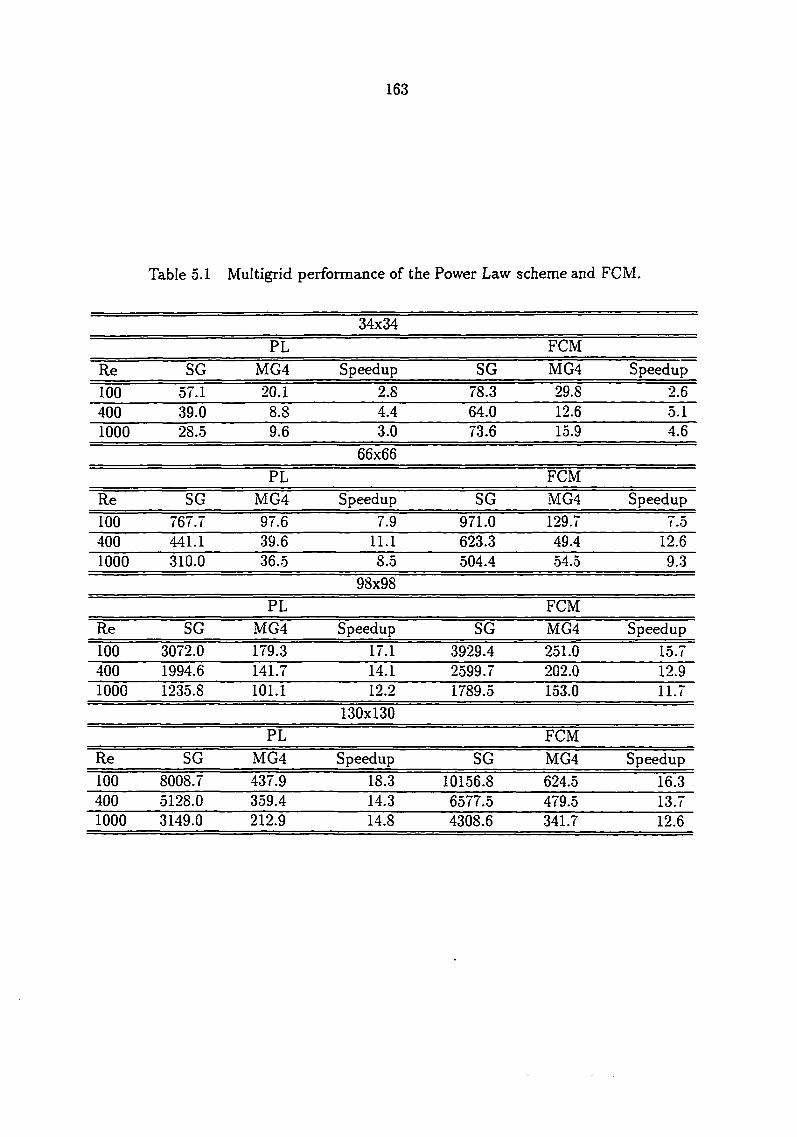
163

Table 5.1 Multigrid performance of the Power Law scheme and FCM.

34x34

PL FCM

Re SG MG4 Speedup SG MG4 Speedup

100 57.1 20.1 2.8 78.3 29.8 2.6 400 39.0 8.8 4.4 64.0 12.6 5.1 1000 28.5 9.6 3.0 73.6 15.9 4.6

66x66

PL FCM

Re SG MG4 Speedup SG MG4 Speedup

100 767.7 97.6 7.9 971.0 129.7 7.5 400 441.1 39.6 11.1 623.3 49.4 12.6 1000 310.0 36.5 8.5 504.4 54.5 9.3

98x98

PL FCM Re SG MG4 Speedup SG MG4 Speedup 100 3072.0 179.3 17.1 3929.4 251.0 15.7 400 1994.6 141.7 14.1 2599.7 202.0 12.9 1000 1235.8 101.1 12.2 1789.5 153.0 11.7

130x130

PL FCM Re SG MG4 Speedup SG MG4 Speedup 100 8008.7 437.9 18.3 10156.8 624.5 16.3 400 5128.0 359.4 14.3 6577.5 479.5 13.7 1000 3149.0 212.9 14.8 4308.6 341.7 12.6

164

5.6 Three-dimensional Lid-Driven Cavity Flow

A limited testing on the three-dimensional flow inside a cubic cavity was also con

ducted in the present study. Referring to Figure 3.1, the third-dimension is given per-

pendicvdar to the page. It is obvious from the geometry that, for the Reynolds number

case where there is a steady-state solution, the flow is symmetric about the half span

of the cavity length in the third-dimension. For this present study, the two Reynolds

number cases Re=AOO and Re=lQQO are considered, and uniform grids in all three direc

tions are used. The fine 82x82x82 grid Power Law solution will be used eis the reference

solutions.

The vertical centerline u-velocity profile at the symmetry plane for /2e=400 is given

in Figure 5.47. It is observed from this figure that the 22x22x22 grid FCM solution

fails right on top of the 42x42x42 grid Power Law solution. The reference Power Law

solution is followed very closely by using the 32x.32x32 grid FCM solution. The superior

peformance of FCM is even more obvious for the higher /?e=1000 Ccise, as shown in

Figure 5.48. In this figure, the 22x22x22 grid FCM solution follows the reference solution

closer than the 42x42x42 grid Power Law solution. Using a 32x32x32 grid, the FCM

solution is able to match the reference solution very closely.

The effectiveness of FCM for fluid flow simulations can be appreciated better when

solving three-dimensional flow problems. In solving two-dimensional problems, the in

crease in the CPU time to obtain convergence, as a result of doubling the number of

grid points in each coordinate direction, is significant but is much smaller than the CPLi

time increase resulting from doubling the grid on three-dimensional problems.

165

1.0

0.9

0.8

0.7

0.6

>- 0.5

0.4 Power Law ??xggy«?? Power Law 42x42x42 Power Law 82x82x82 - Reference FCM qgyggyg? FCM 32x32x32

0.3

0.2

0.1

O.O 1.0 0.5 0.0 -0.5

u Figure 5.47 Vertical centerline u-velocity profile at the symmetry plane for

the 3-D cavity problem for i2e=400.

1.0

0.9

0.8

0.7

0.6

>- 0.5

0.4 Power Law P2xPPxPP Power Law 42x42x42 Power Law 62x62x62 Power Law 82x82x82 - Reference FCM P?x?2x22 FCM 32x32x32

0.3

0.2

O.I

O.O 0.0 -O.S 0.5 1.0

u Figure 5.48 Vertical centerline u-velocity profile at the symmetry plane for

the 3-D cavity problem for /?e=1000.

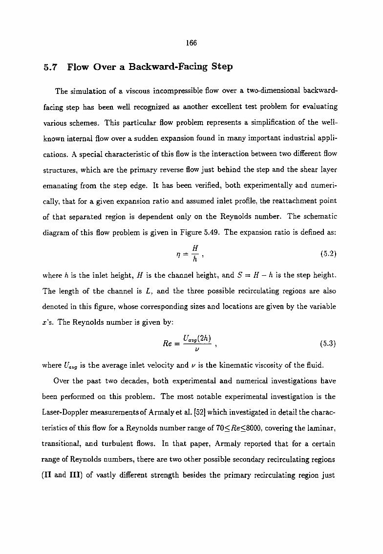
166

5.7 Flow Over a Backward-Facing Step

The simulation of a viscous incompressible flow over a two-dimensioned backward-

facing step has been well recognized as another excellent test problem for evaluating

various schemes. This particular flow problem represents a simplification of the well-

known internal flow over a sudden expansion found in many important industrial appli

cations. A special characteristic of this flow is the interaction between two different flow

structures, which are the primary reverse flow just behind the step and the shear layer

emanating from the step edge. It has been verified, both experimentally and numeri

cally, that for a given expansion ratio and assumed inlet profile, the reattachment point

of that separated region is dependent only on the Reynolds number. The schematic

diagram of this flow problem is given in Figure 5.49. The expansion ratio is defined as:

n = j , ( 0 . 2 )

where h is the inlet height, H is the channel height, and S = H — h is the step height.

The length of the channel is L, and the three possible recirculating regions are also

denoted in this figure, whose corresponding sizes and locations are given by the variable

x's. The Reynolds number is given by:

Re = , (5.3) u

where Uavg is the average inlet velocity and u is the kinematic viscosity of the fluid.

Over the pa^t two decades, both experimental and numerical investigations have

been performed on this problem. The most notable experimental investigation is the

Laser-Doppler measurements of Armaly et al. [52] which investigated in detail the charac

teristics of this flow for a Reynolds number range of 70</Ee<8000, covering the laminar,

transitional, and turbulent flows. In that paper, Armaly reported that for a certain

range of Reynolds numbers, there are two other possible secondary recirculating regions

(II and III) of vastly different strength besides the primary recirculating region just

167

H X9

L H

Figure 5.49 Two-dimensional backward-facing step.

behind the step (I). The dependence of the size and location of these separated flow

structures on the Reynolds number is summarized by Armaly in Figure 5.50. It

should be mentioned here that while Armaly's experiment is always referred to as 'two-

dimensional', the experimental apparatus itself is a three-dimensional channel with an

18:1 ratio of spanwise width to channel height. Therefore, it is important to note that

three-dimensional effects are present to some extent. Moreover, an expansion ratio of

1.94 is used instead of 2.0, giving slightly unsymmetric step and inlet heights. From the

shape of the curve fit of the reattachment length xi versus Reynolds number given in

Figure 5.50, Armaly approximated the laminar range (i2e<1200), the transitional range

(1200<i2e<6600), and the turbulent range (i2e>6600) of the flow. The laminar regime

is characterized by a reattachment length that incre«ises with the Reynolds number.

The increase, however, is not lineax, as suggested for reattachment length variations

for flows in axi ajcisymmetric sudden pipe expansion. Starting at /?e>400, a secondary

recirculating region (III) at the nonstep wail is observed. This separated region is of

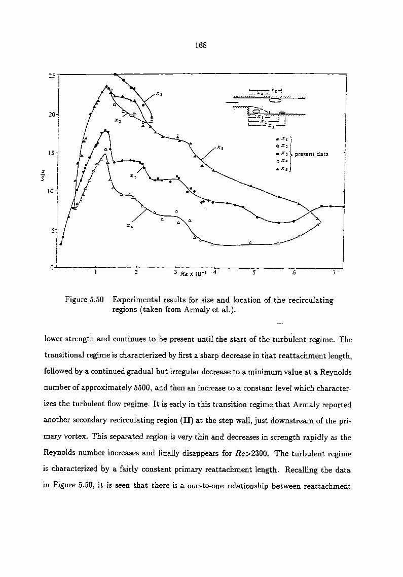
168

— J:«

20-

o X

present data

X

5

Figure 5.50 ExperimentaJ results for size and location of the recirculating regions (taken from Armaly et ai.).

lower strength and continues to be present until the start of the turbulent regime. The

transitional regime is characterized by first a sharp decrease in that reattachment length,

followed by a continued gradual but irregular decrease to a minimum value at a Reynolds

number of approximately 5500, and then an increase to a constant level which character

izes the turbulent flow regime. It is early in this transition regime that Armaly reported

another secondary recirciilating region (H) at the step wall, just downstream of the pri

mary vortex. This separated region is very thin and decreases in strength rapidly as the

Reynolds number increases and finally disappears for He>2300. The turbulent regime

is characterized by a fairly constant primary reattachment length. Recalling the data

in Figure 5.50, it is seen that there is a one-to-one relationship between reattachment

169

length Xi and the Reynolds number, with a large positive increasing slope, pointing to

the sensitivity of xi to Re. This makes the laminar backward-facing step flow an excel

lent standard problem for testing the accuracy of numerical methods. The closeness of

the predicted primary separation length to experimental values can then be used as a

measuring stick to study the methods investigated. Moreover, the large body of avail

able literature on the numerical solution of this problem provides helpful comparisons

for the particular scheme studied.

In the present study, the performance of FCM for the backward-facing step flow

for /?e=100.200.400.600. and SOO is investigated. For all the computations peformed in

this work, a step height of 0.5 is chosen, and thus for a given expansion ratio tj. the

inlet height h can be calculated. The average inlet velocity is fixed to be unity, and

subsequently the kinematic viscosity u can be calculated for a given Reynolds number.

.A. parabolic horizontal velocity is specified at the inlet and is given by:

u = c{y - yi^r)iy - yupr) , (5.4)

where the value of c is determined through the matching of the integration of the above

equation along the specified inlet to the integration of the chosen average velocity along

the same inlet. The assumption of parabolic inlet velocity is supported by both experi

mental and numerical work done by Armaly et al. [52] and Kaiktsis et al. [53] respectively.

.•\rmaly mentioned that the measurements of the profile of the inlet velocity spanwise

along the channel width is two-dimensional to within 1%. He also reported that for the

laminar range, the profile is "close' to that of a fully developed channel flow with a slight

deviation from a parabolic profile. Three-dimensional numerical simulations of Kaikt

sis, which are modeled after Armaly's e.xperiment, also show that experiments with the

parabolic profile imposed at different upstream locations result in negligible differences

in the flow-field, unless the Reynolds number is very low (i?e<200). For i2e<200, the

value of the primary separation distance is overpredicted by about 10% if the inflow

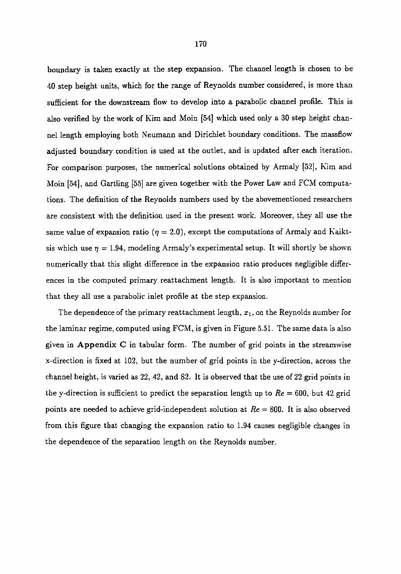
170

boundaxy is taken exactly at the step expansion. The chcinnel length is chosen to be

40 step height units, which for the range of Reynolds number considered, is more than

sufficient for the downstream flow to develop into a parabolic channel profile. This is

also verified by the work of Kim and Moin [54] which used only a 30 step height chan

nel length employing both Neumann and Dirichlet boundary conditions. The massflow

adjusted boundary condition is used at the outlet, and is updated after each iteration.

For comparison purposes, the numerical solutions obtained by Armaly [52], Kim and

Moin [54], ajid Gartling [55] are given together with the Power Law and FCM computa

tions. The definition of the Reynolds numbers used by the abovementioned researchers

are consistent with the definition used in the present work. Moreover, they all use the

same value of expansion ratio (r/ = 2.0), except the computations of Armaly and Kaikt-

sis which use 7/ = 1.94, modeling .Armaly's experimental setup. It will shortly be shown

numerically that this slight difference in the expansion ratio produces negligible differ

ences in the computed primary reattachment length. It is also important to mention

that they all use a parabolic inlet profile at the step expansion.

The dependence of the primary reattachment length, Xi, on the Reynolds number for

the laminar regime, computed using FCM, is given in Figure 5.51. The same data is also

given in Appendix C in tabular form. The number of grid points in the streamwise

x-direction is fixed at 102, but the number of grid points in the y-direction, across the

channel height, is varied as 22, 42, and 82. It is observed that the use of 22 grid points in

the y-direction is sufficient to predict the separation length up to Re = 600, but 42 grid

points are needed to achieve grid-independent solution at Re = 800. It is also observed

from this figure that changing the expansion ratio to 1.94 causes negligible changes in

the dependence of the separation length on the Reynolds number.

15.0

14.0

13.0

12.0

11.0

10.0

9.0

^ 8.0 0) Q.

U) 7.0

6.0

5.0

D) 0) x: I Q. 0)

•*—'

O)

D) C 0 1 c o

4.0 100.0

' 1 1 • 1 • 1 1 * 1 ' 1 '

-

FCM 102x22 T1=2.0 FCM 102x42 11 N)

b

- / FCM 102x82 t1=2.0

yX < FCM 102x82 TI=1.94

1 1 1 1 , 1 I . I . I .

200.0 300.0 400.0 500.0 600.0 Reynolds Number

700.0 800.0 900.0

Figure 5.51 Primary separation length versus Reynolds number. FCM grid independent study.

15.0

.O) 10.0

a. 0)

U3

"5) c © I c: o

(0 Q. a> CO

5.0

~r"

• Armaly Experimental Armaly Computational Fractional Step Method Power Law 102x42 FCM 102x42

* Gartling

to

0.0 100.0 200.0 300.0 400.0 500.0 600.0 700.0 800.0 900.0 Reynolds Number

Figure 5.52 Primary separation length versus Reynolds number. Experimental and numerical results.

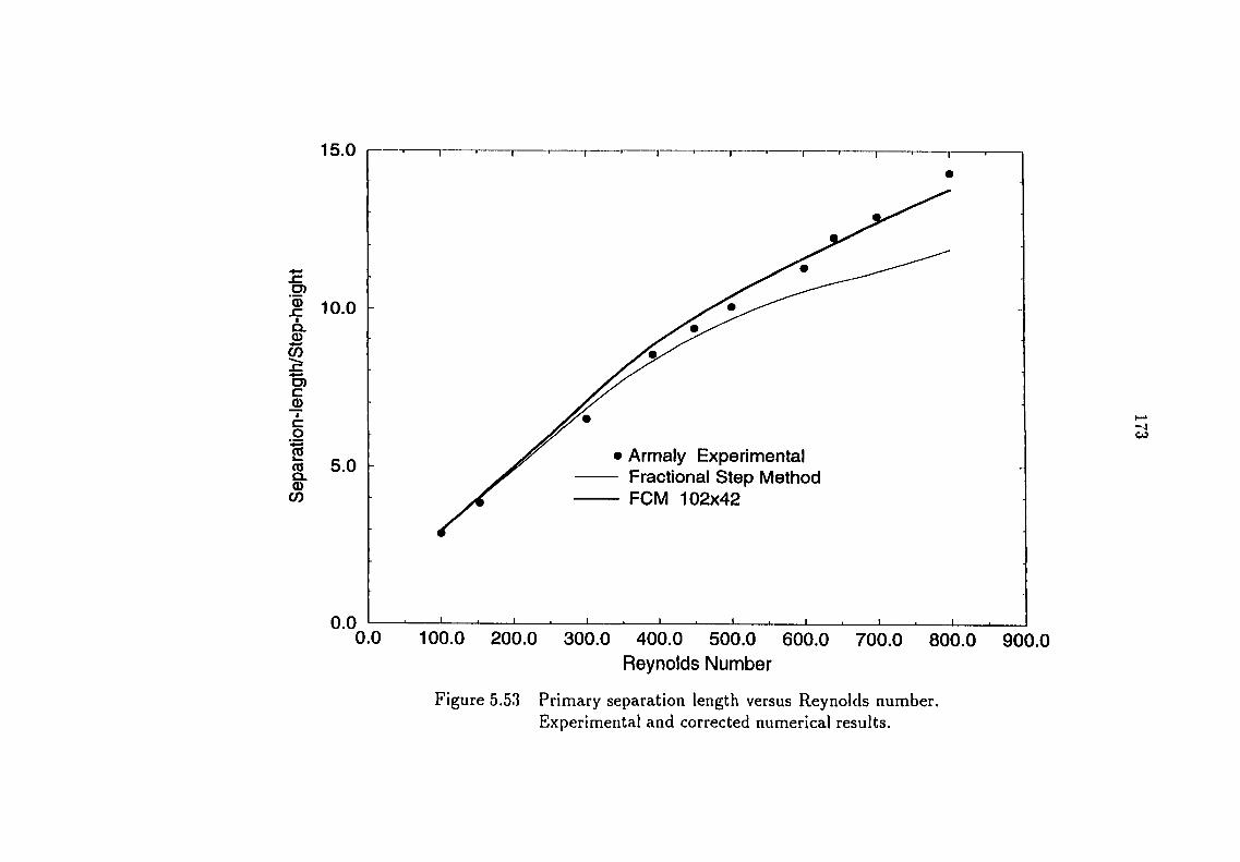
15.0

10.0

5.0

0.0

• Armaly Experimental - Fractional Step Method - FCM 102x42

0.0 100.0 200.0 300.0 400.0 500.0 600.0 Reynolds Number

700.0 800.0 900.1

Figure 5.53 Primary separation length versus Reynolds number. Experimental and corrected numerical results.

174

Figure 5.52 provides a comparison of the FCM solution to the experimental and nu

merical results obtained by the researchers mentioned previously. Armaly's numerical

results are obtained by employing the TEACH computer code, which is basically an

exponential-based scheme. Therefore, very close agreement with the Power Law com

putation is observed throughout the range of the Reynolds number investigated. It is

observed that exponential-based schemes can predict the separation length closely only

for a low Reynolds number /2e<400, but the solution quickly deteriorates at higher

Reynolds numbers. The predicted separation length is even shorter than the values pre

dicted for the lower Re case. The computation of Kim and Moin uses a second-order

accurate finite-difference fractional-step method, and good agreement with experimen

tal results is observed. The steady computation by Gartling for i?e=800 is performed

by using the code NACHOS II [56], which is based on a GaJerkin finite-element for

mulation. It is also verified by using the FIDAP [57] program, which is based on the

finite-element method as well. It is of particular importance to mention that Gartling's

result is also verified by Gresho et al. [58] using four different numerical methods to

verify both the accuracy and stability of the backward-facing step flow at Re = SOO.

These four methods, each with its brief description, are given below:

1. .A. high-order finite-element method solving the unsteady equations by time-marching

using the NACHOS II code. A quiescent initial condition is used as the initial

startup solution. This is the same code used by Gartling in his steady computation.

2. A high-order finite-element method solving the steady equations and the associated

linear-stability problem. This code is commonly known as the ENTWIFE [59]

package, a mixed finite-element approach using nine-node quadrilateral elements

with biquadratic interpolation for velocities and discontinuous piecewise-linear in

terpolation for pressures. This element type is known as one of the best two-

dimensional elements.

175

3. A second-order finite-difFerence method solving the unsteady equations in streajn-

function form by time-majching.

4. A spectral-element method solving the unsteady equations by time-marching. The

simulation package used is the NEKTON [60] code v2.8. NEKTON employs

a Uzawa spectral element method similar to that developed by Patera [61]. In

brief, the spectral element method is a high-order finite-element method where

each element has velocity nodes and {N — 2)^ pressure nodes, where iV is

the element order and D is the dimensionality. For a given number of elements,

NEKTON is capable of increasing the accuracy of the solution by using a higher

element order.

In the Ccise of the unsteady run, Gresho et al. allowed the simulations to run until

<=400 to ensure a converged steady-state solution. They also carried out significant

grid refinement studies to validate their results. It can clearly be observed from Fig

ure 5.52 that FCM gives an excellent match with the experimental solution, especially

for /2e>400. For i?e<200, FCM gives a slightly longer separation distance than the

experimental values. Recall that in the verification of FCM using the two-dimensional

lid-driven cavity problem, FCM performs very well for both the low and high Re case.

Thus, it is suspected that the slight overpredictions observed in Figure 5.52 are caused

by external means, quite possibly the inlet profile specification. The placement of the

outlet boundary a5 a possible cause is ruled out since rigorous work of other researchers

has demonstrated that even shorter channel length has been shown to be sufficient to

negate the effects of the outflow boundary condition for this particular Reynolds number.

However, the work of Kaiktsis mentioned previously, reported that if the parabolic pro

file is taken exactly at the step expansion, the value of the primary separation distance is

overpredicted by about 10% for i2e<200. This correction for the low Reynolds number

region (/2e<200) is implemented, and the resulting FCM solution is given in Figure 5.53.

176

It can now be observed that for all the laminaj rzinges considered in this backward-facing

step simulation, FCM results are in excellent agreement with the experimental results.

The underpredicted separation length at i?e=800, observed for all the numerical schemes

considered in this study, is not likely to be due to the numerical diffusion, but rather is

caused by the fact that at this Reynolds number, the three-dimensional effects are suf

ficiently strong to alter the two-dimensionality of the flow inside the 'three-dimensional

chemnel' used by Armaly et al. in their experimental study. The three-dimensionality

of the flow at i?e=800 is also shown by Armaly by plotting the spanwise velocity distri

bution.

It is importajit to mention here that the FCM solutions presented in this study are

obtained by solving the steady flow equations except for the /2e=800 case. It was noted

that during the steady run at this Reynolds number, the residuals start to oscillate after

a four or five order drop in magnitude. Prolonged running of the simulation shows that

the oscillations are stable at the original levels. The flow solution reveals that several

vortices have developed in the channel, and that these vortices change strength and

location along the channel. Recall that this residual oscillation has also been observed

before in the lid-driven cavity problem at /?e=10000, and in that ca^e, it is shown that

the physical problem investigated is not steady. However, in his paper, Gartling [55] was

able to obtain a converged solution using steady computation by successively solving

the problem at lower Re and extrapolating the converged solution using zeroth-order

continuation to higher Re. Certainly, an explanation needs to be developed.

It has been a long held view of the CFD community that the backward-facing step

flow at i?e=800 does have a steady-state solution. However, the challenges to the exis

tence of the steady-state solution at this Re are not new and have been addressed by A.

Tomboulides with M. Israeli and G. KamiadaJds as co-authors during the Second Mini

Symposium on Outflow Boundary Conditions held at Stanford University in July 1991.

The goal of this symposium was to present and discuss four benchmark problems for

177

testing various outflow boundary conditions, one of them being the backward-facing step

flow. Using the 'exponentially accurate for smooth solutions' spectral-element method.

Tomboulides showed and stated emphatically that the flow at Re=800 was, in fact, not

steady but rather time-dependent, with both eddies (top and bottom) oscillating about

their alleged steady-state. The follow-up paper [53], by basically the same group of

researchers with Kaiktsis as the primary author, pronounced again that the flow cannot

be steady at /2e=800 and that it has undergone its first bifurcation at Re %700. To

clarify understanding of this backward-facing step flow at /?e=800. at the conclusion of

the minisymposium. Gartling was charged with the teisk of investigating this problem

via the unsteady flow equations starting from rest, since it was thought that the a priori

steady assumption made by Gartling was the reason why a steady solution was obtained.

This task resulted in the paper by Gresho et al. mentioned previously which uses a finite-

element, finite-difference, and very accurate spectral-element method (almost identical

to the method used by Kaiktsis) both in steady and unsteady modes. It has been veri

fied in this paper that the backward-facing step flow at /?e=SOO does indeed asymptote

to steady-state for a sufficiently refined grid and suflSciently elapsed time. Using the

simulation with the spectral-element NEKTON code, Gresho showed that when the

resolution is increased beyond a certain point, the numerical solution develops toward an

asymptotically steady flow by a monotonous decay of the transient behavior. However,

cis the resolution is decreased, the numerical solution becomes less stable and develops

bounded chaotic behavior, as observed by Kaiktsis et al. The fact that the flow is highly

transient in its initial development and will indeed approach steady state is also veri

fied by the unsteady FCM run starting from rest. Figure 5.54 to Figure 5.56 give the

streamline plots in the transient development and its corresponding decay using FCM

at various times. It is shown in these figures that the initial development of the flow is

characterized by continuous shedding of small eddies by the developing primary vortex

just behind the step. Moreover, as the primary core flow from the inlet expands and

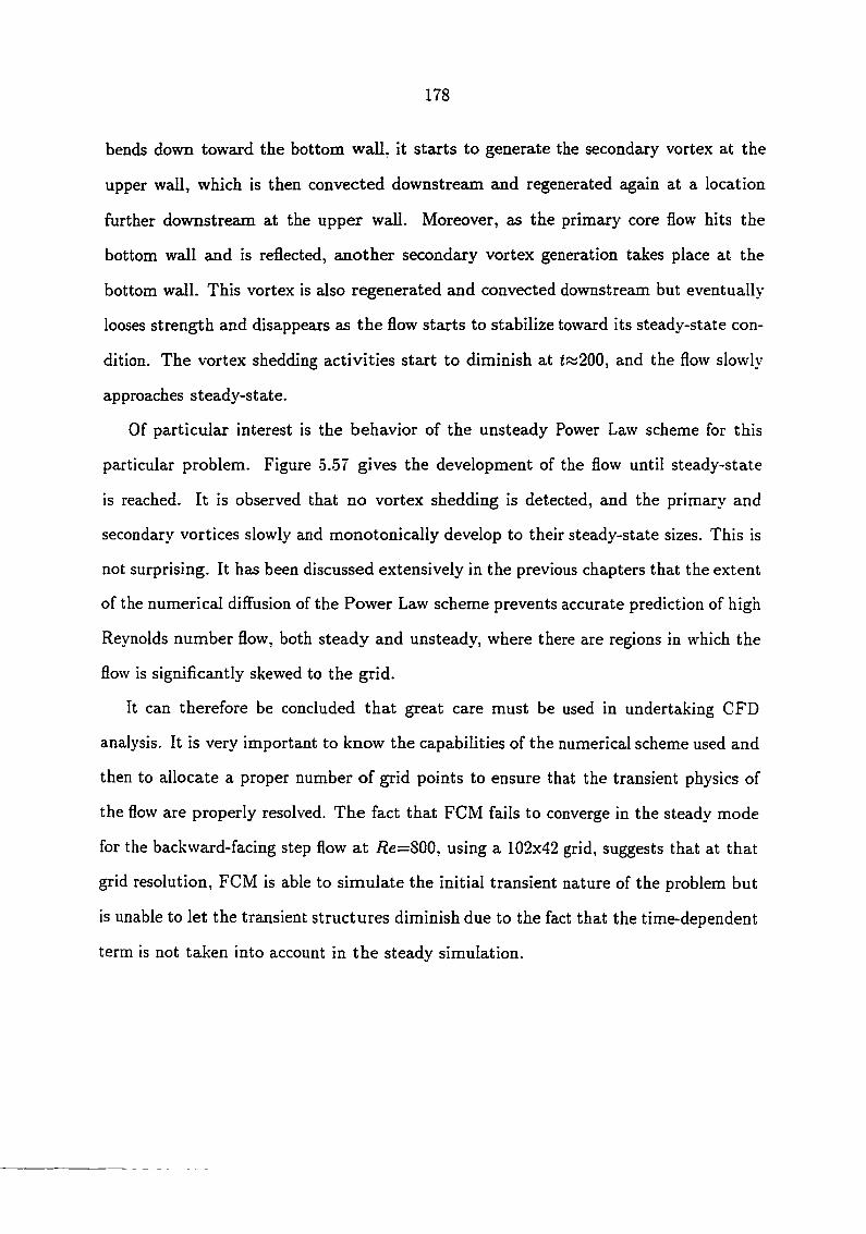
178

bends down toward the bottom wall, it staxts to generate the secondary vortex at the

upper wall, which is then convected downstream and regenerated again at a location

further downstream at the upper wall. Moreover, as the primary core flow hits the

bottom wall and is reflected, another secondary vortex generation takes place at the

bottom wail. This vortex is also regenerated and convected downstream but eventually

looses strength and disappears as the flow starts to stabilize toward its steady-state con

dition. The vortex shedding activities start to diminish at f«200, and the flow slowly

approaches steady-state.

Of peirticular interest is the behavior of the unsteady Power Law scheme for this

particular problem. Figure 5.57 gives the development of the flow until steady-state

is reached. It is observed that no vortex shedding is detected, and the primary and

secondary vortices slowly and monotonicedly develop to their steady-state sizes. This is

not surprising. It has been discussed extensively in the previous chapters that the extent

of the numerical diffusion of the Power Law scheme prevents accurate prediction of high

Reynolds number flow, both steady and unsteady, where there are regions in which the

flow is significantly skewed to the grid.

It can therefore be concluded that great care must be used in undertaking CFD

analysis. It is very important to know the capabilities of the numerical scheme used and

then to allocate a proper number of grid points to ensure that the transient physics of

the flow are properly resolved. The fact that PCM fails to converge in the steady mode

for the backward-facing step flow at i?e=SOO, using a 102x42 grid, suggests that at that

grid resolution, PCM is able to simulate the initial transient nature of the problem but

is unable to let the transient structures diminish due to the fact that the time-dependent

term is not taicen into account in the steady simulation.

179

t=l

t=2

t=3

t=4

t=5

t=6

t=7

t=8

t=9

t=10

I : I I ! I : I : I

0 1 2 3 4 5 6 J S 9 10 II 12

Figure 5.54 FCM unsteady development part 1 for i?e=800.

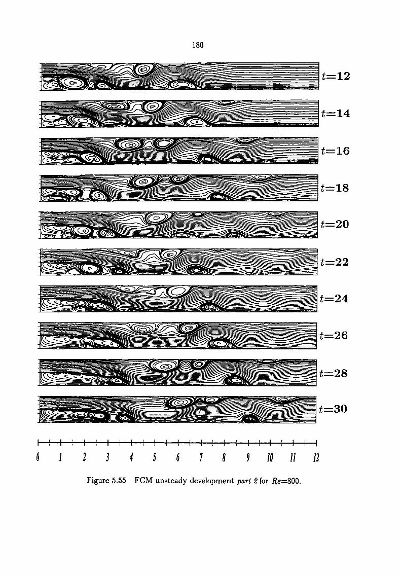
180

t=12

t=14

t=16

t=18

t=20

t=22

t=24

t=26

t=28

t=30

H—^—h _! I ' i—I—r » r •

9 I 2 3 4 S ( J S 9 ID n 12

Figure 5.55 FCM unsteady development part 2 for i2e=800.

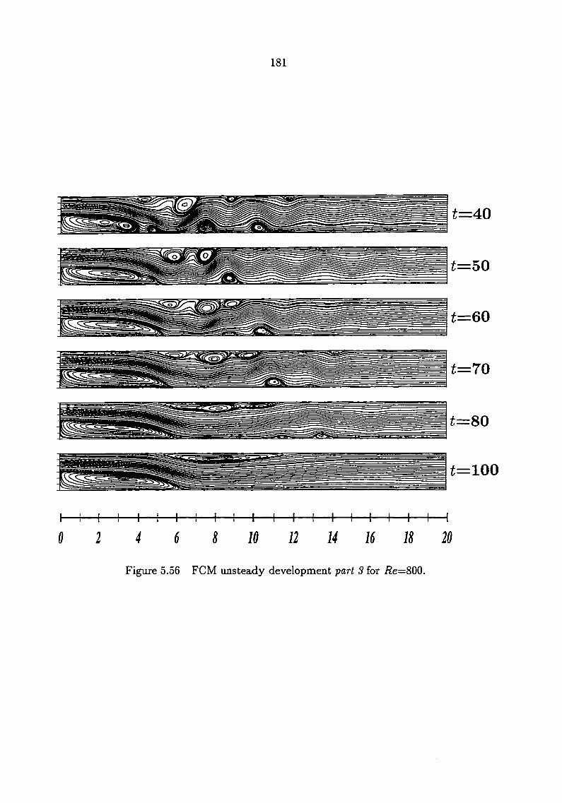
181

t=40

t=bO

t=60

t=70

t=80

t=100

H—^—f- H—i—I—^—h

0 2 4 6 S W 12 14 16 18 20

Figure 5.56 FCM unsteady development part 3 for /?e=800.

182

t=l

t=4

t=8

t=12

t=16

t=20

t=30

t=40

t=60

t=70

f 1 t 1 : 1 : I ; I I I •

S I 2 3 4 } i J S 9 ID U n

Figure 5.57 Power Law unsteady development for i2e=800.

183

Theoretically, it is always possible to refine the grid sufficiently so that the Power Law

scheme is able to adequately resolve the flow physics. But as is shown in Figure 5.29,

the cost is undoubtedly beyond what can be afforded.

Finally, the comparison of the final steady-state solution of the Power Law scheme

and FCM is given in Figure 5.58. The cross-channel profiles at locations x = 7 and

X = 15 are given in Figure 5.59 and 5.60. In these figures, the results from Gartling [55]

ajid the Power Law and FCM solutions obtained in the current study are plotted together

for comparison. It is obvious from Figure 5.59 that the cross-channel profile should not

be used as a benchmark measure for the backward-facing step problem since the profile

is very sensitive to the reattachment length and will be grossly different even if the

numerical schemes compared predict relatively small differences in the reattachment

length.

5.8 Numerical Determination of the Accuracy of the Scheme

In the previous sections, the accuracy of the FCM solution has been verified by using

the lid-driven cavity and the backward-facing step test problems. Relative performance

of FCM has been shown qucilitatively by comparing the FCM solution to other numerical

solutions obtained using the Power Law scheme, the central-difference scheme, and the

QUICK scheme. However, quantitative measures of the accuracy of FCM have not yet

been presented. In this section, a simple method of testing the accuracy of numerical

schemes which yields measurable parameters is introduced.

To reduce the number of parameters in the study, the lid-driven cavity flow is chosen

over the backward-facing step flow, since the latter requires the specification of the

outflow boundary conditions. Moreover, besides having a smaller geometry (which is

economical in the grid refinement process), the cavity flow also has more 'convenient'

Power Law t=200

FCM t=400

I—I—I—I—I—i—I—I—I—I—I—i—I—i—I—I—I—I—I—I—I

0 2 4 6 8 10 12 14 16 18 20

Figure 5.58 Power Law and FCM steady-state solutions for i?e=800.

185

1.0

0.9

0.8

0.7

0.6

Gartling Power Law 102x42 FCM 102x42

>- O.S

0.4

0.3

0.2

0.1

0.0 O.O 0.5

u 1.0 1.5 -0.5

Figure 5.59 Cross channel profile at x=7.

1.0

0.9

0.8

0.7

0.6

— Gartling — - Power Law 102x42 — FCM 102x42

>- O.S

0.4

0.3

0.2

1

O.O -0.5 0.0 0.5 1.0 1.5

u

Figiire 5.60 Cross channel profile at x=15.

186

flow profiles which can be directly compared. This order-checking method is outlined as

follows:

• Identify the computed flow quaintities or profiles (referred to as the flow variables)

which will be compaxed to the benchmark solutions. For the present study using

the chosen test flow problem (cavity flow at i2e=400), the profiles of the u- and/or

u-velocities along the vertical and horizontal lines respectively can be conveniently

chosen for this purpose. The more sensitive the chosen quantity to grid refinement,

the better it will serve the study.

• Compute the benchmark solutions of the chosen flow variables. Use the highest

number of grid points which can be practically afforded. It is observed that the

finer the grid used to obtain the benchmark solutions, the wider the applicable

range of the results of the study. In this study, a 322x322 grid is used, and

converged solutions with residuals up to 10"^'* are obtained using the multigrid

method discussed previously.

• The next step is to compute a series of solutions using progressively finer grids.

However, it is first necessary to decide whether to refine the grid in one or in all

coordinate directions simultaneously. In practice, it is usually desirable to study

how the solutions behave as one grid direction is refined and the other grid di

rections are kept constant at the resolution of the benchmark resolutions in the

corresponding grid directions. For example, in this study, if the u-velocity is cho

sen, then it is necessary to use 322 grid points in the x-direction and progressively

refine the grid in the y-direction (22, 42, 62, 82, and 102), since the u-profile is

most sensitive to Ay variations. In a similar way, the same procedure is used if

the u-velocity is chosen, only now the grid in the x-direction is refined while the

grid in the y-direction is kept at the benchmark resolution.

187

• After the coaxser grid flow vaxiables have been computed for all the grid resolutions

desired, the error of the chosen flow variable for a given grid resolution is computed.

where (j)^, is the benchmark value and <pc is the coaxser grid value. The limit

of integration can be determined easily, and ds represents either dx or dy. For

example, the error of the u-velocity for a given Ay for all the grid resolutions

considered can be computed.

• It is a common practice in CFD to address the acctiracy of a numerical scheme in

the form:

where c is the leading order constant, A is the grid spacing, and N is what is

usually referred to as the order of the scheme. Writing the above equation in

logarithmic form results in:

It is now obvious that by plotting the logarithmic of the error versus the logarithmic

of the grid spacing, and then applying a linear regression over the given data, the

value of c and N can easily be determined.

The quantitative performance of Power Law, central-difference, and FCM obtained

using this simple order-checking method is given in Figure 5.61. In this figure, the u-

velocity along the vertical centerline is used as the flow variable. Computations using

li-velocity along the other vertical lines or using u-velocity along the other horizontal

lines give similar qucJitative and quantitative results. It is observed in this figure that

tremendous improvement in the leading order term of Equation 5.7 is achieved by FCM.

It can be roughly seen from this figure that a 322x22 grid FCM has approximately the

(5.5)

error w c , (5.6)

logioierror) = logio{c) + N logio(A) . (5.7)

188

same error level as a 322x42 grid central-difference and an approximately 322x82 grid

Power Law scheme. From the slopes of the lineax fit lines, it is also obvious that modest

improvement in the value of the scheme order N is also achieved by FCM, improved

from N~l.5 of the Power Law scheme to 7Vw2.0 of the centrai-difference scheme.

It should be obvious from Equation 5.7 that both the values of c and N axe equally

important in formulating/devising a high accuracy scheme. In the present study, the

leading order term is vastly improved, but only modest improvement is observed on

the parameter N. In the finite-difference method, the improvement on the value of

iV is commonly achieved by using more grid points (larger approximating stencil) in a

coordinate direction. However, this approach often reduces the diagonal dominance of

the iteration matrix, thus resulting in a less stable numerical scheme. On the other hand,

it should be recalled that in the formulation of FCM developed in this study, no extended

cell is used to approximate the values of the dependent variable and its derivative at an

interface. Instead, the two neighboring values directly adjacent to that interface, giving

a compact stencil scheme, axe used. The corrections axe all included in the source,

preserving the desirable stability characteristics of the Power Law scheme. Although it

is theoretically possible to use a larger approximating cell in the FCM formulation, the

complexity and additional computation and CPU time needed to determine the upwind

cell may not justify the added accuracy.

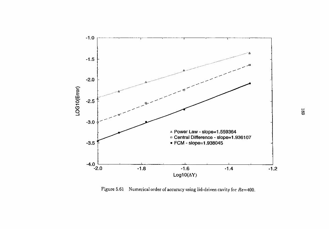
-1.0

•A

-1.5

-2.0

m o T— CD O _i er

-3.0 n

A Power Law - slope=1.559364 ° Central Difference - slope=1.936107 • FCM - slope=1.938045 -3.5

-4.0 -2.0 -1.8 -1.6 -1.4 1

LoglO(AY)

Figure 5.61 Numerical order of accuracy using lid-driven cavity for /?e=400.

190

6 CONCLUSIONS AND RECOMMENDATIONS

In this study, a new approach to the modeling of the multi-dimensional convection-

diffusion equation with a source has been developed and tested. The most important

strategy of this formulation is the realization that the profile of the dependent flow

variable at the interface of a discretized control-volume cell is governed by the governing

conservation equation itself across the cell considered. This has led to the effort to rewrite

the governing time-dependent multi-dimensional conservation equation with a source as

a one dimensional convection-diffusion problem with the other directional transports and

the original source lumped together as one constant convection-diffusion source. This

results in a non-homogeneous ODE with constant coefficients, whose analytical solution

can be directly determined. In the Ccise of zero source, whether imposed or incidental, the

resulting profile reduces to the one obtained by using the well-known Power Law scheme,

which solves the one-dimensional convection-diffusion equation without a source. For

this reason, the new scheme is referred to as the 'Flux Corrected Method' (FCM), since

it is basically the Power Law scheme plus a flux correction due to the source. It is also

important to note that the resulting formulation conserves the governing conservation

equation not only at the control-volume cells where the governing equation is integrated,

but also across the cells containing each of the sides of the former cells.

The new formulation has been applied in solving the steady/unsteady incompressible

Navier-Stokes equations in conjunction with the SIMPLER algorithm to handle the

velocity-pressure coupling in the momentum equations. It is important to note that

FCM treats the multidimensionality and the source at the equation level, rather than

191

by using an improved aigebraic profile or any other type of polynomial fit. Since the

multidimensionality and the effects of the pressiire gradients are directly accomited for.

FCM performs very well in recirculating flow regions where more than one component

of the grid Peclet ntmiber is laxge.

The test problems chosen to validate the high accuracy nature of FCM are the

well-known two-dimensional lid-driven cavity flow and the two-dimensional laminar

backward-facing step flow. These are two of the most important benchmark problems

used by the CFD commimity to test the relative accuracy of newly developed numeri

cal schemes. These test problems, though simple in geometry, consist of complex flow

structures and do not lack important interaction between the various flow structures

present. Indeed, the high Reynolds number cases of these problems are highly transient

and unsteady. Systematic study conducted in the present work results in the following

conclusions about the characteristics of FCM.

• FCM is very accurate for simulating both steady and unsteady flows, especially

when there are recirculating flow regions.

• Since the profile corrections are generated through source addition, FCM retains

the basic stable convergence characteristics of the Power Law scheme.

• FCM uses compact stencil in the discretization process. No upwind direction

checking is needed (as is required by the QUICK or the second-order upwinding

schemes).

• When local grid stretching is used, FCM solutions show less deviation to the

reference solution compared to the Power Law scheme.

• Significant additional computation required by FCM can be avoided by reusing the

already computed momentum coefficients. However, this approach is not imple

192

mented in the current work since a very general code is needed to test the various

possibilities in the development process.

• FCM conveniently provides the ability to take into account the user's applied

sources in the profile approximation. An example of this concept is the simulation

of a helicopter rotor by momentum source as developed by Rajagopalan [33].

• Since FCM corrections are only source additions to the Power Law approach, the

conversion of a Power Law based code (or exponential-based code in general) to

FCM is minimal.

• Finally, it has also been shown that no modification to the F.A.S multigrid algorithm

is necessary in order to implement FCM over the Power Law scheme. Moreover,

it is also verified that the multigrid convergence characteristics of the Power Law-

scheme are retained by FCM. The use of a high accuracy scheme in combination

with the convergence acceleration technique should open the possibility to inves

tigate difficult flow problems which were not considered affordable in the past.

Upon the completion of this study, FCM has been proven to be a highly viable

technique for accurate modeling of complex flow structures. The improvement achieved

by using FCM over the Power Law scheme is phenomenal. Upon comparing FCM results

with the published results in the literature, FCM solutions are also quite competitive

compared to the well-known, very accurate, spectral method.

During the course of this study, a procedure for the general pressure boundary con

dition has been developed and implemented. This formulation enables the specification

of either normal velocity or pressure at a given boundary. If normal velocity is specified,

then the effect of the boundary pressure is not neglected in the discretization of the

pressure and pressure correction equations of the SIMPLER algorithm, as is previously

193

suggested by Patankax [5]. An improved pressure profile is observed using this new

formulation.

Lastly, the recommendations for possible areas of future research or improvements

to the current formulation are discussed.

• It is felt that the most important follow up of the current FCM development is

the implementation of a higher order diffusion approximation for the Ccise of a wall

boundary. Recall that it has been shown that only first order diffusion is used for

the wall boundary.

• Recall that during the development phase outlined in Chapter 3, the inclusion of

the derivatives of the directional totaJ-fluxes on the non-directional sources results

in the wrong profile near the bottom wall boundary of the cavity problem. It is

felt that in-depth investigation into the cause of this problem needs to be properly

conducted to obtain a more thorough understanding of FCM.

• The extension of FCM to the compressible flow regimes is the most obvious next

step in FCM's continued development. FCM has proven to be able to accurately

predict smooth flow solutions, but its ability, and the subsequent modifications

necessary, to capture shocks sharply needs to be developed.

• Finally, the development and testing of FCM for an unstructured grid needs to be

undertaken to facilitate the ability to solve problems with complex flow geometries.

194

APPENDIX A POWER LAW APPROXIMATION OF

EXPONENTIAL SCHEME

2.5

2.0

Exponential Power Law 1.5

1 . 0

0.5

O.O 3.0 1.0 O. O 2.0 3.0 4.0 5.0 6.0 7.0 8.0

Pe

Figure A.l Power Law approximation of the exact exponential expression m ) = pfrr-

195

APPENDIX B TABULATED VELOCITY COMPONENTS

AND PRESSURE DATA FOR THE LID-DRIVEN CAVITY

PROBLEM.

Table B.l Vertical centerline data for i?e=100 using 22x22 uniform grid.

y u V P

0.00000 0.0000000 0.0000000 1.0180210 0.02500 -0.0178111 -0.0002172 1.0179880 0.07500 -0.0474099 -0.0010208 1.0179210 0.12500 -0.0737896 -0.0024016 1.0176800 0.17500 -0.0988038 -0.0039293 1.0170740 0.22500 -0.1234368 -0.0049613 1.0158510 0.27500 -0.1477521 -0.0046647 1.0136760 0.32500 -0.1707626 -0.0020876 1.0101380 0.37500 -0.1903584 0.0036873 1.0048060 0.42500 -0.2034496 0.0133019 0.9973474 0.47500 -0.2064611 0.0268254 0.9877180 0.52500 -0.1961882 0.0434871 0.9763519 0.57500 -0.1707808 0.0615647 0.9642477 0.62500 -0.1303739 0.0785336 0.9528331 0.67500 -0.0768143 0.0914681 0.9436080 0.72500 -0.0121221 0.0975285 0.9377182 0.77500 0.0645082 0.0943425 0.9356783 0.82500 0.1614371 0.0804079 0.9373727 0.87500 0.3002032 0.0562730 0.9422647 0.92500 0.5148413 0.0273274 0.9495290 0.97500 0.8253244 0.0063725 0.9599386 1.00000 1.0000000 0.0000000 0.9651434

196

Table B.2 Horizontal centerline data for /le=100 using 22x22 uniform grid.

X u V P

0.00000 0.0000000 0.0000000 1.0027080 0.02500 -0.0032818 0.0440317 1.0017690 0.07500 -0.0141496 0.1044568 0.9998927 0.12500 -0.0317645 0.1421590 0.9984159 0.17500 -0.0529650 0.1625950 0.9969093 0.22500 -0.0756702 0.1702666 0.9950841 0.27500 -0.0987018 0.1681499 0.9928250 0.32500 -0.1214953 0.1577441 0.9901760 0.37500 -0.1438095 0.1394516 0.9873290 0.42500 -0.1654714 0.1130491 0.9846179 0.47500 -0.1861514 0.0781311 0.9825082 0.52500 -0.2051478 0.0345275 0.9815617 0.57500 -0.2211635 -0.0172371 0.9823562 0.62500 -0.2320836 -0.0753552 0.9853398 0.67500 -0.2348273 -0.1359555 0.9906047 0.72500 -0.2254905 -0.1921685 0.9976107 0.77500 -0.2002279 -0.2334624 1.0049980 0.82500 -0.1574538 -0.2463454 1.0107530 0.87500 -0.1014880 -0.2183866 1.0129580 0.92500 -0.0457588 -0.1471145 1.0109220 0.97500 -0.0101336 -0.0485372 1.0052200 1.00000 0.0000000 0.0000000 1.0023690

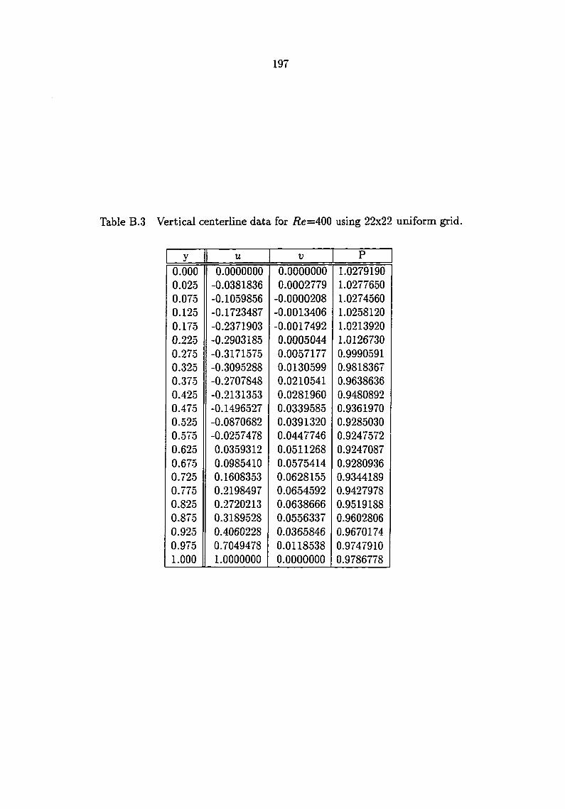
197

Table B.3 Vertical centerline data for /2e=400 using 22x22 uniform grid.

y u V P

0.000 0.0000000 0.0000000 1.0279190 0.025 -0.0381836 0.0002779 1.0277650 0.075 -0.1059856 -0.0000208 1.0274560 0.125 -0.1723487 -0.0013406 1.0258120 0.175 -0.2371903 -0.0017492 1.0213920 0.225 -0.2903185 0.0005044 1.0126730 0.275 -0.3171575 0.0057177 0.9990591 0.325 -0.3095288 0.0130599 0.9818367 0.375 -0.2707848 0.0210541 0.9638636 0.425 -0.2131353 0.0281960 0.9480892 0.475 -0.1496527 0.0339585 0.9361970 0.525 -0.0870682 0.0391320 0.9285030 0.575 -0.0257478 0.0447746 0.9247572 0.625 0.0359312 0.0511268 0.9247087 0.675 0.0985410 0.0575414 0.9280936 0.725 0.1608353 0.0628155 0.9344189 0.775 0.2198497 0.0654592 0.9427978 0.825 0.2720213 0.0638666 0.9519188 0.875 0.3189528 0.0556337 0.9602806 0.925 0.4060228 0.0365846 0.9670174 0.975 0.7049478 0.0118538 0.9747910 1.000 1.0000000 0.0000000 0.9786778

198

Table B.4 Horizontal centerline data for i?e=400 using 22x22 uniform grid.

X u V P

0.00000 0.0000000 0.0000000 1.0155550 0.02500 -0.0002003 0.0919057 1.0147480 0.07500 -0.0049376 0.1917139 1.0131340 0.12500 -0.0167932 0.2444882 1.0095820

0.17500 -0.0318632 0.2751068 1.0031770 0.22500 -0.0465665 0.2887528 0.9937059 0.27500 -0.0591347 0.2830520 0.9815885 0.32500 -0.0688676 0.2572737 0.9680101 0.37500 -0.0758213 0.2142023 0.9546536

0.42500 -0.0807782 0.1592602 0.9431825 0.47500 -0.0849830 0.0985303 0.9347702 0.52500 -0.0896744 0.0365258 0.9299298 0.57500 -0.0958184 -0.0249129 0.9286614 0.62500 -0.1043649 -0.0863245 0.9307344 0.67500 -0.1168304 -0.1503393 0.9359629 0.72500 -0.1351546 -0.2216295 0.9443925 0.77500 -0.1586383 -0.3037077 0.9563157 0.82500 -0.1778412 -0.3877972 0.9713490 0.87500 -0.1730214 -0.4385418 0.9864475 0.92500 -0.1255179 -0.3872504 0.9977758 0.97500 -0.0447104 -0.1403085 0.9949989 1.00000 0.0000000 0.0000000 0.9936104

199

Table B.5 Vertical centerline data for ile=400 using 32x32 uniform grid.

y u V P

0.00000 0.0000000 0.0000000 1.0309010

0.01670 -0.0256169 -0.0000802 1.0308500

0.05000 -0.0716648 -0.0007945 1.0307470

0.08330 -0.1158605 -0.0025272 1.0303050

0.11700 -0.1604731 -0.0047494 1.0291760

0.15000 -0.2059144 -0.0065002 1.0268960

0.18300 -0.2499028 -0.0068766 1.0229190 0.21700 -0.2877441 -0.0053483 1.0167420 0.25000 -0.3139037 -0.0018528 1.0081310

0.28300 -0.3241154 0.0032433 0.9973251 0.31700 -0.3170063 0.0092614 0.9850740

0.35000 -0.2945187 0.0154029 0.9724363 0.38300 -0.2609898 0.0209970 0.9604534 0.41700 -0.2214091 0.0257180 0.9498776

0.45000 -0.1797914 0.0296457 0.9410875 0.48300 -0.1384202 0.0331311 0.9341724 0.51700 -0.0980104 0.0365752 0.9290747 0.55000 -0.0583259 0.0402602 0.9256999 0.58300 -0.0187899 0.0442895 0.9239676 0.61700 0.0211134 0.0486027 0.9238176 0.65000 0.0616418 0.0530156 0.9251875 0.68300 0.1027314 0.0572512 0.9279831 0.71700 0.1439677 0.0609549 0.9320518 0.75000 0.1845873 0.0637073 0.9371581 0.78300 0.2235360 0.0650397 0.9429696 0.81700 0.2596831 0.0644276 0.9490634 0.85000 0.2927410 0.0611555 0.9549638 0.88300 0.3273154 0.0539346 0.9602405 0.91700 0.3856654 0.0408535 0.9646893 0.95000 0.5256302 0.0220666 0.9684694 0.98300 0.8138445 0.0057749 0.9726886 1.00000 1.0000000 0.0000000 0.9747981

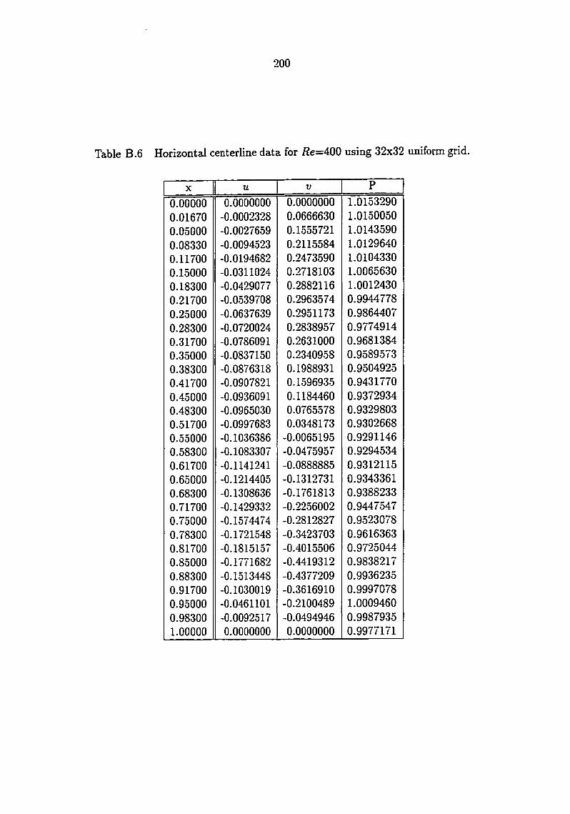
200

Table B.6 Horizontal centerline data for /2e=400 using 32x32 uniform grid.

X u V P

0.00000 0.0000000 0.0000000 1.0153290

0.01670 -0.0002328 0.0666630 1.0150050

0.05000 -0.0027659 0.1555721 1.0143590

0.08330 -0.0094523 0.2115584 1.0129640

0.11700 -0.0194682 0.2473590 1.0104330

0.15000 -0.0311024 0.2718103 1.0065630

0.18300 -0.0429077 0.2882116 1.0012430

0.21700 -0.0539708 0.2963574 0.9944778

0.25000 -0.0637639 0.2951173 0.9864407

0.28300 -0.0720024 0.2838957 0.9774914

0.31700 -0.0786091 0.2631000 0.9681384 0.35000 -0.0837150 0.2340958 0.9589573 0.38300 -0.0876318 0.1988931 0.9504925

0.41700 -0.0907821 0.1596935 0.9431770

0.45000 -0.0936091 0.1184460 0.9372934 0.48300 -0.0965030 0.0765578 0.9329803 0.51700 -0.0997683 0.0348173 0.9302668 0.55000 -0.1036386 -0.0065195 0.9291146 0.58300 -0.1083307 -0.0475957 0.9294534 0.61700 -0.1141241 -0.0888885 0.9312115 0.65000 -0.1214405 -0.1312731 0.9343361 0.68300 -0.1308636 -0.1761813 0.9388233 0.71700 -0.1429332 -0.2256002 0.9447547 0.75000 -0.1574474 -0.2812827 0.9523078 0.78300 -0.1721548 -0.3423703 0.9616363 0.81700 -0.1815157 -0.4015506 0.9725044 0.85000 -0.1771682 -0.4419312 0.9838217 0.88300 -0.1513448 -0.4377209 0.9936235 0.91700 -0.1030019 -0.3616910 0.9997078 0.95000 -0.0461101 -0.2100489 1.0009460 0.98300 -0.0092517 -0.0494946 0.9987935 1.00000 0.0000000 0.0000000 0.9977171

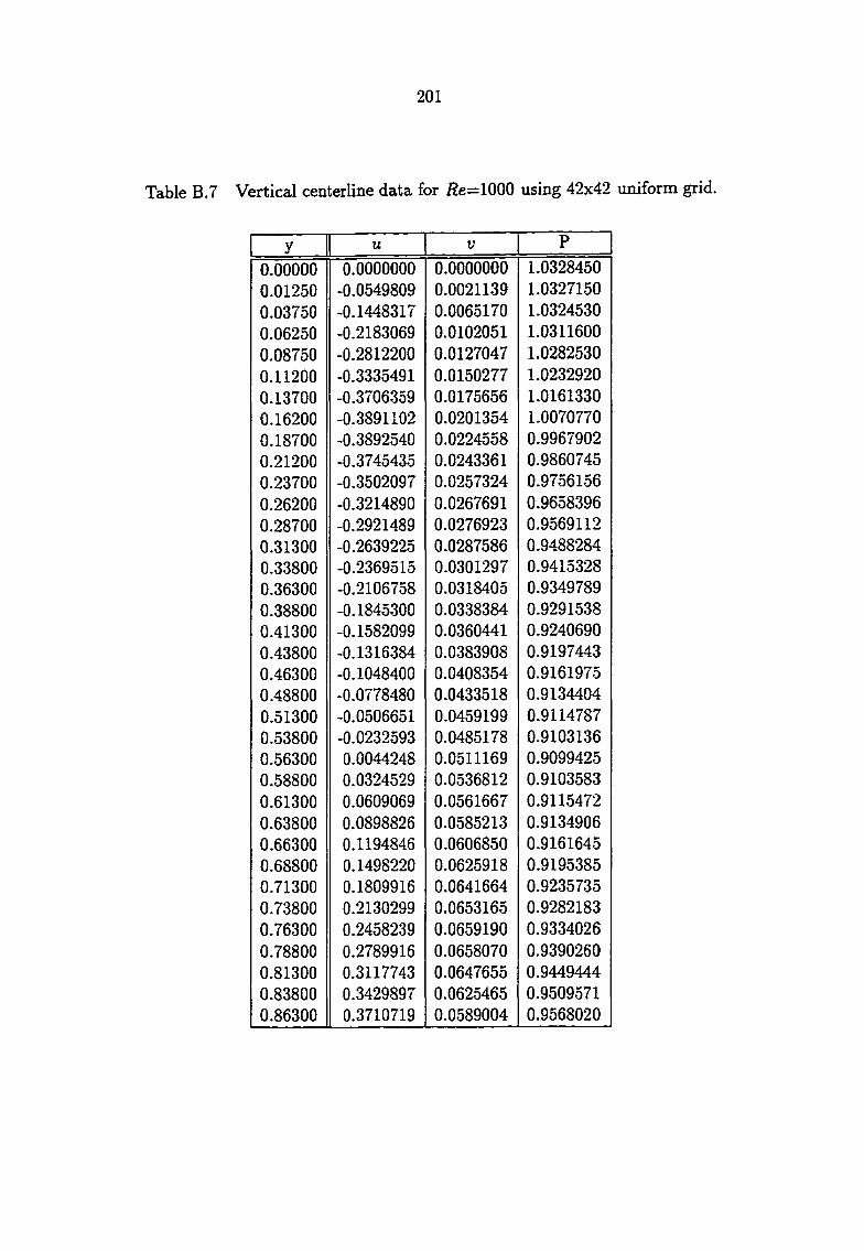
201

Table B.7 Vertical centerline data for i?e=1000 using 42x42 uniform grid.

y u V P

0.00000 0.0000000 0.0000000 1.0328450

0.01250 -0.0549809 0.0021139 1.0327150 0.03750 -0.1448317 0.0065170 1.0324530 0.06250 -0.2183069 0.0102051 1.0311600

0.08750 -0.2812200 0.0127047 1.0282530

0.11200 -0.3335491 0.0150277 1.0232920 0.13700 -0.3706359 0.0175656 1.0161330 0.16200 -0.3891102 0.0201354 1.0070770 0.18700 -0.3892540 0.0224558 0.9967902 0.21200 -0.3745435 0.0243361 0.9860745 0.23700 -0.3502097 0.0257324 0.9756156

0.26200 -0.3214890 0.0267691 0.9658396 0.28700 -0.2921489 0.0276923 0.9569112 0.31300 -0.2639225 0.0287586 0.9488284 0.33800 -0.2369515 0.0301297 0.9415328 0.36300 -0.2106758 0.0318405 0.9349789 0.38800 -0.1845300 0.0338384 0.9291538 0.41300 -0.1582099 0.0360441 0.9240690 0.43800 -0.1316384 0.0383908 0.9197443 0.46300 -0.1048400 0.0408354 0.9161975 0.48800 -0.0778480 0.0433518 0.9134404 0.51300 -0.0506651 0.0459199 0.9114787 0.53800 -0.0232593 0.0485178 0.9103136 0.56300 0.0044248 0.0511169 0.9099425 0.58800 0.0324529 0.0536812 0.9103583 0.61300 0.0609069 0.0561667 0.9115472 0.63800 0.0898826 0.0585213 0.9134906 0.66300 0.1194846 0.0606850 0.9161645 0.68800 0.1498220 0.0625918 0.9195385 0.71300 0.1809916 0.0641664 0.9235735 0.73800 0.2130299 0.0653165 0.9282183 0.76300 0.2458239 0.0659190 0.9334026 0.78800 0.2789916 0.0658070 0.9390260 0.81300 0.3117743 0.0647655 0.9449444 0.83800 0.3429897 0.0625465 0.9509571 0.86300 0.3710719 0.0589004 0.9568020

202

Table B.7 (Continued)

y u V P

0.88800 0.3942664 0.0535976 0.9621654 0.91300 0.4121196 0.0462833 0.9667186

0.93800 0.4360341 0.0358373 0.9702259 0.96300 0.5251966 0.0208158 0.9727685

0.98800 0.7935566 0.0060095 0.9752674 1.00000 1.0000000 0.0000000 0.9765169

203

Table B.8 Horizontal centerline data for i2e=1000 using 42x42 uniform grid.

X u V P

0.00000 0.0000000 0.0000000 1.0149050

0.01250 0.0011035 0.0945037 1.0146190

0.03750 0.0008077 0.2180738 1.0140450

0.06250 -0.0042845 0.2894401 1.0122200

0.08750 -0.0124349 0.3331716 1.0088580

0.11200 -0.0212252 0.3622885 1.0039240

0.13700 -0.0294433 0.3791057 0.9975091 0.16200 -0.0366464 0.3835181 0.9898854

0.18700 -0.0426841 0.3763971 0.9814653

0.21200 -0.0475789 0.3597453 0.9727093

0.23700 -0.0514954 0.3361899 0.9640356

0.26200 -0.0546870 0.3084290 0.9557613 0.28700 -0.0574219 0.2787285 0.9480842 0.31300 -0.0599179 0.2486013 0.9411019 0.33800 -0.0623105 0.2187726 0.9348484 0.36300 -0.0646632 0.1893928 0.9293301

0.38800 -0.0669987 0.1603352 0.9245488 0.41300 -0.0693307 0.1314243 0.9205106

0.43800 -0.0716810 0.1025380 0.9172254 0.46300 -0.0740826 0.0736152 0.9147031 0.48800 -0.0765745 0.0446253 0.9129503 0.51300 -0.0791947 0.0155402 0.9119688 0.53800 -0.0819751 -0.0136791 0.9117546 0.56300 -0.0849382 -0.0430843 0.9123007 0.58800 -0.0880942 -0.0727431 0.9135974 0.61300 -0.0914354 -0.1027230 0.9156304 0.63800 -0.0949299 -0.1330728 0.9183802 0.66300 -0.0985159 -0.1638001 0.9218205 0.68800 -0.1021010 -0.1948453 0.9259154 0.71300 -0.1055786 -0.2260654 0.9306155 0.73800 -0.1088885 -0.2572772 0.9358541 0.76300 -0.1121587 -0.2884821 0.9415500 0.78800 -0.1159065 -0.3204606 0.9476308 0.81300 -0.1210468 -0.3557111 0.9540891 0.83800 -0.1280727 -0.3985166 0.9610540 0.86300 -0.1350944 -0.4509825 0.9687469

204


X u V P

0.88800 -0.1363141 -0.5038100 0.9771279 0.91300 -0.1236297 -0.5288066 0.9854186 0.93800 -0.0915289 -0.4806987 0.9921272 0.96300 -0.0443061 -0.3112456 0.9955448 0.98800 -0.0091635 -0.0584320 0.9944511 1.00000 0.0000000 0.0000000 0.9939042

205

Table B.9 Vertical centerline data for i2e=1000 using 52x52 uniform grid.

y u V P

0.00000 0.0000000 0.0000000 1.0340410

0.01000 -0.0445122 0.0012285 1.0339870

0.03000 -0.1197817 0.0040121 1.0338800

0.05000 -0.1833551 0.0065628 1.0332340

0.07000 -0.2390521 0.0081538 1.0317230

0.09000 -0.2892542 0.0093628 1.0290480

0.11000 -0.3326855 0.0108000 1.0249720 0.13000 -0.3660751 0.0126209 1.0194090

0.15000 -0.3867465 0.0146689 1.0124930 0.17000 -0.3939331 0.0167030 1.0045630 0.19000 -0.3888899 0.0185147 0.9960735

0.21000 -0.3743616 0.0199774 0.9874799

0.23000 -0.3537490 0.0210707 0.9791407 0.25000 -0.3302418 0.0218779 0.9712745 0.27000 -0.3061847 0.0225501 0.9639713 0.29000 -0.2828543 0.0232502 0.9572345 0.31000 -0.2606229 0.0241025 0.9510288 0.33000 -0.2393198 0.0251701 0.9453139 0.35000 -0.2185801 0.0264595 0.9400622 0.37000 -0.1980676 0.0279425 0.9352616 0.39000 -0.1775623 0.0295781 0.9309123 0.41000 -0.1569581 0.0313276 0.9270207 0.43000 -0.1362245 0.0331612 0.9235956 0.45000 -0.1153661 0.0350582 0.9206450 0.47000 -0.0943952 0.0370049 0.9181751 0.49000 -0.0733169 0.0389908 0.9161898 0.51000 -0.0521245 0.0410064 0.9146912 0.53000 -0.0308003 0.0430412 0.9136798 0.55000 -0.0093175 0.0450821 0.9131544 0.57000 0.0123559 0.0471138 0.9131127 0.59000 0.0342567 0.0491178 0.9135499 0.61000 0.0564285 0.0510729 0.9144592 0.63000 0.0789215 0.0529548 0.9158318 0.65000 0.1017917 0.0547365 0.9176569 0.67000 0.1251019 0.0563884 0.9199212 0.69000 0.1489187 0.0578783 0.9226090

206


y u V P

0.71000 0.1733059 0.0591705 0.9257010 0.73000 0.1983091 0.0602236 0.9291735 0.75000 0.2239282 0.0609865 0.9329965 0.77000 0.2500774 0.0613937 0.9371306 0.79000 0.2765384 0.0613606 0.9415225 0.81000 0.3029149 0.0607815 0.9461001 0.83000 0.3286046 0.0595323 0.9507675 0.85000 0.3527975 0.0574797 0.9554017 0.87000 0.3745135 0.0544925 0.9598534 0.89000 0.3927595 0.0504384 0.9639533 0.91000 0.4074288 0.0450944 0.9675296 0.93000 0.4236495 0.0378552 0.9704514 0.95000 0.4647213 0.0276047 0.9727102 0.97000 0.5859711 0.0144652 0.9744555 0.99000 0.8410379 0.0036850 0.9761706 1.00000 1.0000000 0.0000000 0.9770282

207

Table B.IO Horizontal centerline data for i2e=1000 using 52x52 uniform grid.

X u V P

0.00000 0.0000000 0.0000000 1.0150740

0.01000 0.0008403 0.0764502 1.0149480

0.03000 0.0013722 0.1867891 1.0146980

0.05000 -0.0010019 0.2587516 1.0137160

0.07000 -0.0062053 0.3052269 1.0117980

0.09000 -0.0127845 0.3378219 1.0088760 0.11000 -0.0195479 0.3616321 1.0049330 0.13000 -0.0258984 0.3773649 1.0000160 0.15000 -0.0315931 0.3846575 0.9942573 0.17000 -0.0365399 0.3836203 0.9878627

0.19000 -0.0407302 0.3750768 0.9810810 0.21000 -0.0442245 0.3603787 0.9741629 0.23000 -0.0471364 0.3411417 0.9673276 0.25000 -0.0496086 0.3189800 0.9607428 0.27000 -0.0517836 0.2952805 0.9545196 0.29000 -0.0537800 0.2710586 0.9487198 0.31000 -0.0556808 0.2469245 0.9433699 0.33000 -0.0575343 0.2231441 0.9384766 0.35000 -0.0593633 0.1997524 0.9340385 0.37000 -0.0611774 0.1766696 0.9300537 0.39000 -0.0629828 0.1537857 0.9265224 0.41000 -0.0647879 0.1310067 0.9234480 0.43000 -0.0666060 0.1082688 0.9208349 0.45000 -0.0684539 0.0855343 0.9186879 0.47000 -0.0703506 0.0627810 0.9170110 0.49000 -0.0723153 0.0399924 0.9158064 0.51000 -0.0743652 0.0171507 0.9150746 0.53000 -0.0765150 -0.0057655 0.9148141 0.55000 -0.0787757 -0.0287825 0.9150218 0.57000 -0.0811541 -0.0519321 0.9156937 0.59000 -0.0836511 -0.0752494 0.9168242 0.61000 -0.0862605 -0.0987681 0.9184059 0.63000 -0.0889669 -0.1225161 0.9204298 0.65000 -0.0917430 -0.1465071 0.9228845 0.67000 -0.0945489 -0.1707321 0.9257558 0.69000 -0.0973323 -0.1951497 0.9290253

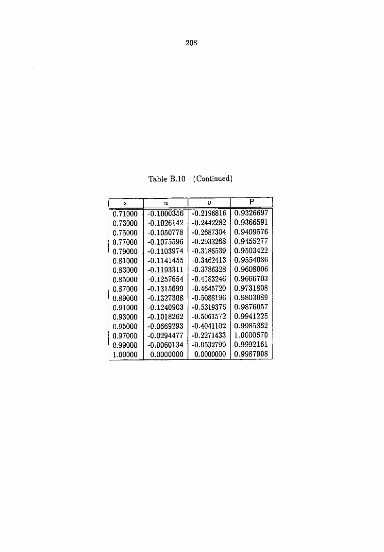
208

Table B.IO (Continued)

X u V P

0.71000 -0.1000356 -0.2196816 0.9326697

0.73000 -0.1026142 -0.2442282 0.9366591

0.75000 -0.1050778 -0.2687304 0.9409576

0.77000 -0.1075596 -0.2933268 0.9455277 0.79000 -0.1103974 -0.3186539 0.9503422 0.81000 -0.1141455 -0.3462413 0.9554086 0.83000 -0.1193311 -0.3786328 0.9608006 0.85000 -0.1257654 -0.4183246 0.9666703 0.87000 -0.1315699 -0.4645720 0.9731808 0.89000 -0.1327308 -0.5088196 0.9803089 0.91000 -0.1240903 -0.5319376 0.9876057 0.93000 -0.1018262 -0.5061572 0.9941225 0.95000 -0.0669293 -0.4041102 0.9985862 0.97000 -0.0294477 -0.2271433 1.0000670 0.99000 -0.0060134 -0.0532790 0.9992161 1.00000 0.0000000 0.0000000 0.9987908

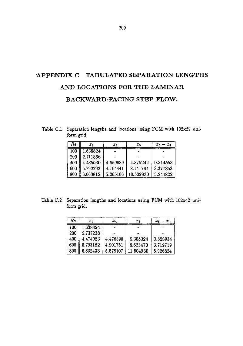
209

APPENDIX C TABULATED SEPARATION LENGTHS

AND LOCATIONS FOR THE LAMINAR

BACKWARD-FACING STEP FLOW.

Table C.l Separation lengths and locations using FCM with 102x22 uniform grid.

Re Xl X5 X5 X4

100 1.638824 - - -

200 2.711866 - - -

400 4.485030 4.560689 4.875242 0.314553 600 5.792293 4.764441 8.141794 3.377353 800 6.663812 5.265106 10.509930 5.244822

Table C.2 Separation lengths and locations using FCM with 102x42 uniform grid.

Re Xl X4 xs ^5 100 1.638824 - - -

200 2.737238 - - -

400 4.474053 4.476390 5.305324 0.828934 600 5.793182 4.901751 8.621470 3.719719 800 6.832433 5.578107 11.504930 5.926824

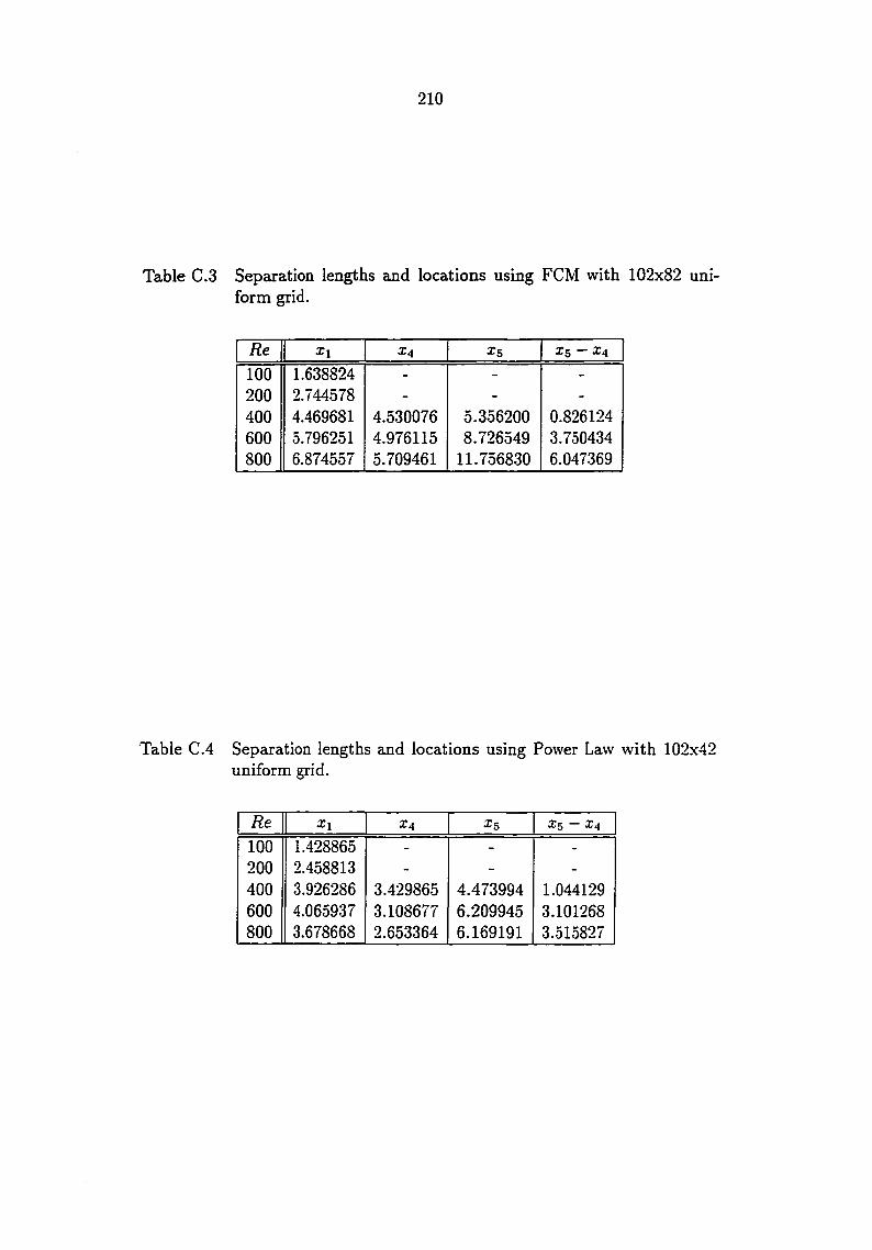
210

Table C.3 Separation lengths and locations using FCM with 102x82 uniform grid.

Re Xi X4 X5 3^5

100 1.638824 - - -

200 2.744578 - - -

400 4.469681 4.530076 5.356200 0.826124 600 5.796251 4.976115 8.726549 3.750434 800 6.874557 5.709461 11.756830 6.047369

Table C.4 Separation lengths and locations using Power Law with 102x42 uniform grid.

Re Xi X4 ^5 X5 —14 100 1.428865 - - -

200 2.458813 - - -

400 3.926286 3.429865 4.473994 1.044129 600 4.065937 3.108677 6.209945 3.101268 800 3.678668 2.653364 6.169191 3.515827

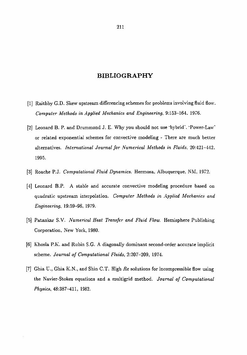
211

BIBLIOGRAPHY

[1] Raithby G.D. Skew upstream differencing schemes for problems involving fluid flow.

Computer Methods in Applied Mechanics and Engineering, 9:153-164, 1976.

[2] Leonard B. P. and Drummond J. E. Why you should not use 'hybrid'. Tower-Law"

or related exponential schemes for convective modeling - There are much better

alternatives. International Journal for Numerical Methods in Fluids, 20:421-442.

1995.

[3] Roache P.J. Computational Fluid Dynamics. Hermosa, Albuquerque, NM, 1972.

[4] Leonard B.P. A stable and accurate convective modeling procedure based on

quadratic upstream interpolation. Computer Methods in Applied Mechanics and

Engineering, 19:59-98, 1979.

[5] Patankar S.V. Numerical Heat Transfer and Fluid Flow. Hemisphere Publishing

Corporation, New York, 1980.

[6] Khosla P.K. and Rubin S.G. A diagonally dominant second-order accurate implicit

scheme. Journal of Computational Fluids, 2:207-209, 1974.

[7] Ghia U., Ghia K.N., and Shin C.T. High Re solutions for incompressible flow using

the Navier-Stokes equations and a multigrid method. Journal of Computational

Physics, 48:387-411, 1982.

212

[8] Hayase T., Humphrey J.A.C., and Greif R. A consistently formulated QUICK

scheme for fast and stable convergence using finite-volimie iterative caiculation pro

cedures. Journal of Computational Physics, 98:108-118, 1992.

[9] Harten A., Engquist B., Osher S., and Chakravarthy S.R. Uniformly high order

accurate essentially non-oscillatory schemes, III. Journal of Computational Physics,

71:231-303, 1987.

[10] Gentry R.A., Martin R.E., and Daly B.J. An Eulerian differencing method for

unsteady compressible flow problems. Journal of Computational Physics, 1:87-118,

1966.

[11] Price H.S., Varga R.S., and Warrent J.E. Applications of oscillation matrices to

diffusion-correction equations. Journal of Mathematics and Physics, 45:301-311.

1966.

[12] Atias M., Wolfshtein M., and Israeli M. Efficiency of Navier-Stokes solver. AIAA

Journal, 15:263-265, 1977.

[13] Wilkes N.S. and Thompson C.P. An evaluation of higher-order upwind differencing

for elliptic flow problems. Numerical Methods in Laminar and Turbulent Flows,

248-257, 1983.

[14] Shyy W. and Correa S.M. A systematic comparison of several numerical schemes

for complex flow calculations. AIAA 85-0440, 1985.

[15] Vanka S.P. Second-order upwind differencing in a recirculating flow. AIAA Journal,

25:1435-1441, 1987.

[16] Shyy W., Thakur S., and Wright J. Second-order upwind and central difference

schemes for recirculating flow computation. AIAA Journal, 30:923-932, 1992.

213

[17] Leschziner M.A. Practical eveJuation of three finite-difference schemes for the com

putation of steady-state recirculating flows. Computational Methods in Applied

Mechanics Engineering^ 23:293-312, 1980.

[18] Han T., Humphrey J.A.C., and Launder B.E. A comparison of hybrid and quadratic

upstream differencing in high Reynolds number elliptic flows. Computational Meth

ods in Applied Mechanics Engineering, 29:81-95, 1981.

[19] Pollard A. and Siu A.L.W. The calculation of some laminar flows using various

discretization schemes. Computational Methods in Applied Mechanics Engineering,

35:293-313, 1982.

[20] Freitas C.J., Street R.L., Findikakis A.N., and KosefF J.R. Numerical simulation of

three-dimensional flow in a cavity. International Journal of Numerical Methods in

Fluids, 5:561-575, 1985.

[21] Perng C.Y. and Street R.L. Three-dimension«il unsteady flow simulations: .Al

ternative strategies for a volume-averaged calculation. International Journal of

Numerical Methods in Fluids, 9:341-362, 1989.

[22] Leonard B.P. Proceedings of the 5th International Conference on Numerical Meth

ods in Laminar and Turbulent Flows. Edited by C. Taylor et al. Pineridge Press,

Swansea, UK, 35, 1987.

[23] Leonard B.P. and Mokhtari S. ULTRA-SHARP solution of the Smith-Hutton prob

lem. International Journal of Numerical Methods in Heat and Fluid Flow, 2:407-

427, 1992.

[24] Leonard B.P. and Mokhtari S. Beyond first-order upwinding: The ULTRA-SHARP

alternative for non-oscillatory steady state simulation of convection. International

Journal of Numerical Methods in Engineering, 30:729-766, 1990.

214

[25] Allen D.N. deG. and Southwell R.V. Relaxation methods applied to determine

the motion, in two-dimensions, of a viscous fluid past a fixed cylinder. Journal of

Mechanics and Applied Maths, 8:129-145, 1955.

[26] Spalding D.B. A novel finite-difference formulation for differential expressions in

volving both first and second derivatives. International Journal of Numerical Meth

ods in Engineering, 4:551-559, 1972.

[27] Gosman A.D. and Pun W.M. Calcidation of recirculation flows. Heat Transfer

Section Report HTS/72/2, 1974.

[28] Huajig P.G., Launder B.E., ajid Leschziner M.A. Discretization of nonlinear con

vection processes: A broad range comparison of four schemes. Computer Methods

in Applied Mechanics and Engineering, 48:1-24, 1985.

[29] Patel M.K. and Markatos N.C. An evaluation of eight discretization schemes for two-

dimensional convection-diffusion equations. International Journal for Numerical

Methods in Fluids, 6:129-154, 1986.

[30] Wong H. H. and Raithby G.D. Improved finite-difference methods bcised on a critical

evaluation of the approximating errors. Numerical Heat Transfer, 2:131, 1979.

[31] Varejao L.M.C. Flux-Spline Method for Heat, Mass, and Momentum Transfer. PhD

thesis, Department of Mechanical Engineering, University of Minnesota, 1979.

[32] Karki K., Mongia H., and Patankar S.V. Solution of three-dimensional flow prob

lems using a flux-spline method. Proceedings of the 27th Aerospace Sciences Meeting

AIAA 89-0687, Reno, Nevada, January 9-12, 1989.

[33] Rajagopalan R.G. and Fajiucci J.B. Finite-difference model for vertical axis wind

rotors. Journal of Propulsion and Power, l(6):432-436, 1985.

215

[34] Chorin A.J. A numerical method for solving incompressible viscous flow problems.

Journal of Computational Physics^ 2:12-26, 1967.

[35] Kwak D., Chang J.L.C., Shanks S.P., and Chakravarthy S.R. A three-dimensional

incompressible Navier-Stokes flow solver using primitive variables. AIAA Journal.

24:390-396, 1986.

[36] Merkle C.L. and Athavale M. Time-accurate unsteady incompressible flow algo

rithm based on artificial compressibility. AIAA 87-1137^ 1987.

[37] Harlow F.H. and Welch J.E. Numerical calculation of time-dependent viscous in

compressible flow with free surface. Physics of Fluids, 18:2182-2184, 1965.

[38] Caretto L.S., Curr R.M., and Spalding D.B. Two numerical methods for three-

dimensional boundary layers. Computer Methods in Applied Mechanics and Engi

neering, 1:39, 1972.

[39] Karamcheti K. Principles of Ideal-Fluid Aerodynamics. Huntington, New York,

NY, 1980.

[40] Zori L.A. and Rajagopalan R.G. The FAS multigrid method for the segregated so

lution of the SIMPLER algorithm. Proceedings of the 6th International Symposium

on CFD, 3:1509-1514, Lake Tahoe, Nevada, 1995.

[41] Ku H.C., Hirsh R.S., and Taylor T.D. A pseudospectral method for solution of

the three-dimensional incompressible Navier-Stokes equations. Journal of Compu

tational Physics, 70:439-462, 1987.

[42] Richardson L.F. The approximate arithmetical solution by finite-differences of phys

ical problems. Philosophical Transactions of the Royal Society of London Serial A,

210:307-357, 1911.

216

[43] Richaxdson L.F. and Gaunt J.A. The deferred approach to the limit. Philosophical

Transactions of the Royal Society of London Serial A, 226:299-361, 1927.

[44] Roache P.J. Perspective: A method for imiform reporting of uniform refinement

studies. Journal of Fluids Engineering, 116:405-413, 1994.

[45] Huser A. and Biringen S. Calculation of two-dimensional shear-driven cavity flows

at high Reynolds number. International Journal of Numerical Methods in Fluids,

14:1087-1109, 1992.

[46] Bye J.A.T. Numerical solutions of the steady state vorticity equation in rectangular

basins. Journal of Fluid Mechanics, 26:577-598, 1966.

[47] Kumagai M. A numerical study of wind-driven circulation in rectangular cavities.

Journal of Computational Physics, 47:130-145, 1982.

[48] KosefF J.R. and Street R.L. Visualization studies of a shear-driven three-dimensional

recirculating flow. Transactions of the ASME, 106:22, 1984.

[49] Brandt A. Multi-level adaptive solutions to boundary-value problems. Mathematics

of Computation, 3l(138):333-390, 1977.

[50] Brandt A. Guide to multigrid development. Lecture Notes in Mathematics, 960:220-

312, 1982.

[51] Brandt A. Multigrid techniques: 1984 guide with applications to fluid dynamics.

Computational Fluid Dynamics Lecture Notes 194-04, von-Karman Institute, 1984.

[52] Armaly B.F., Diurst F., and Pereira J.C.F. Experimental and theoretical inves

tigation of backward-facing step flow. Journal of Fluid Mechanics, 127:473-496,

1983.

217

[53] Kaiktsis L., Kaxniadaicis G.EM., ajid Orszag S.A. Onset of three-dimensionality,

equilibria, and early transition in flow over a backward-facing step. Journal of Fluid

Mechanics, 231:501-528, 1991.

[54] Kim J. and Moin P. Application of fractional-step method to incompressible Navier-

Stokes equations. Journal of Computational Physics, 59:308-323, 1985.

[55] Gartling D.K. A test problem for outflow boundary conditions - flow over a

backward-facing step. International Journal for Numerical Methods in Fluids,

11:953-967, 1990.

[56] Gartling D.K. NACHOS II - a finite-element code for incompressible flow problems.

Sandia National Laboratories Report, SAND86-1817, Albuquerque, NM, 1987.

[57] FIDAP Theoretical Manual, Version 4-o. Fluid Dynamics International. Evanston.

IL, 1988.

[58] Gresho P.M., Gartling O.K., Torczynski J.R., Garratt T.J., Spence A., and

Goodrich J.W. Is the steady viscous incompressible two-dimensional flow over

a backward-facing step at i?e=800 stable ? International Journal for Numerical

Methods in Fluids, 17:501-541, 1993.

[59] Winters K.H. ENTWIFE User Manual (Release 1), Harwell Report AERE-R 11577.

1985.

[60] NEKTON User's Guide, Version 2.7. Nektonics Inc. Cambridge, MA, 1991.

[61] Patera A.T. A spectral element method for fluid dynamics: Laminar flow in a

channel expansion. Journal of Computational Physics, 54:468-488, 1984.

Flux Corrected Method: An accurate approach to fluid flow ...

Documents

Transcript of Flux Corrected Method: An accurate approach to fluid flow ...