Finite Element Analysis

of the Human Left

Ventricle in Diastole and Systole

Thesis presented for the degree of Doctor of Philosophy

by

M.C.Beecham MSc, BSc (Hons.), GIMA

Department of Mechanical Engineering

Brunel University

February 1997

Abstract

Previously, at Brunel University, two computer programs had been developed to

facilitate the analysis of the diastolic material properties of the human left ventricle.

These two computer programs consisted of; a finite element program, "XL1", which ran

upon a Cray-1S/1000 and a post-processor and pre-processor, "HEART", which ran

upon the Multics computer system. The computer program "HEART" produced the

finite element model, which was then solved by "XL 1", and it also allowed for plotting

the results in graphical form, The patient data was supplied by the Royal Brompton

Hospital in the form of digitised cine-angiographic X-ray data plus pressure readings.

The first stage was to transfer the two separate computer programs "HEART" and

"XL 1" to the Sun Workstation system. The two programs were then combined to form a

single package which can be used for the automated analysis of the patient data.

An investigation into the effect that the elastic modulus ratio has upon the deformation

of the left ventricle during diastole was performed. It was found that the effect is quite

small and that using this parameter to match overall shape deformation would be

extremely sensitive to the accuracy of the initial data.

The main part of this work was the implementation of active cardiac contraction, by

means of a thermal stress analogy, into the finite element program. This allows the

systolic part of the cardiac cycle to be analysed. The analysis of the factors that affect

cardiac contraction, including the material properties and boundary conditions was

performed. This model was also used to investigate the effect that conditions such as

ischaemia and the formation of scar tissue have upon the systolic left ventricle.

The use of the thermal stressing analogy for cardiac contraction was demonstrated to

mirror global and local deformation when applied to a realistic ventricular geometry.

Acknowledgements

I would firstly like to extend my deepest gratitude to Prof A.L.Yettram for his

assistance and advice during this work and also for supervising it. I would also like to

thank Dr. D.Gibson for freely giving his time and advice on medical matters and also for

providing inspiration.

Lastly I would like to thank the Mechanical Engineering Department of B rune!

University for providing the equipment and the opportunity to study towards a PhD. I

would also like to thank the department for financially supporting me with a

departmental stipend for my three years of study.

II

Table of Contents

Chapter 1 ............................................................................................................. 1

Introduction...................................................................................................................................11.1 Anatomy of the Human Heart................................................................................................31.2 The Cardiac Cycle ................................................................................................................81.3 Structure and Function of the Myocardium .........................................................................101.4 Diseases of the Heart...........................................................................................................131.5 Summary ............................................................................................................................16

Chapter 2 ........................................................................................................... 17

2. Review of Cardiac Research Pertaining to the Mechanical Behaviour of the Left Ventricle..........172.1 The Development of Cardiac Models ..................................................................................17

2.1.1 Development of Thin Walled Models ........................................................................182.1.2 Development of Thick Walled Models.......................................................................192.1.3 Development of Finite Element Models.....................................................................23

2.2 Related Areas of Research...................................................................................................342.2.1 Imaging and Digitisation...........................................................................................342.2.2 Analysis and Modelling of the Myocardium..............................................................37

2.3 Sumrnaiy............................................................................................................................40

Chapter3 ........................................................................................................... 41

3. Previous Work Relevant to the Current Project ............................................................................413.1 Data Acquisition.................................................................................................................413.2 Extraction of the Finite Element Mesh................................................................................423.3 The Finite Element Model ..................................................................................................453.4 Volume Matching and the Elastic Modulus.........................................................................463.5 The Patient Data.................................................................................................................48

Chapter4 ........................................................................................................... 54

4. Programming Developments........................................................................................................544.1 The Finite Element Part......................................................................................................544.2 The Post-processor and Pre-processor ................................................................................. 55

4.2.1 Programming Alterations..........................................................................................584.2.2 Logical Alterations....................................................................................................61

4.3 Combining the Computer Programs....................................................................................644.4 Speed Improvements...........................................................................................................66

Chapter5 ........................................................................................................... 69

5. A New Volume Matching Method...............................................................................................695.1 Results and Discussion........................................................................................................70

Chapter 6 ......................................................................................................... 75

6 Matching Both Length and Volume To Derive the Elastic Modulus Ratio....................................756.1 Resolving Myocardial Stiffness into Circumferential and Longitudinal Directions ..............776.2 Initial Investigation into the Effect of Altering the Modulus Ratio.......................................876.3 Attempts at Matching the Ventflcle Length by Varying the Elastic Modulus Ratio..............906.4 Start and End Frame matching............................................................................................956.5 Effect of Digitisation Errors Upon the Modulus Ratio .........................................................976.6 Programming Enhancements ..............................................................................................996.7 Conclusions ......................................................................................................................101

Chapter 7 ......................................................................................................... 1037. Inclusion of Muscle Fibre Contraction.......................................................................................103

7.1 Revival of the FE Program "GTQSA" ...............................................................................104

III

7.2.2 Fibre Direction Calculation and Correction..............................................................110

7.2.3 Testing and Validation ............................................................................................1137.2.4 Preliminary Results Using a Cylindrical Model........................................................114

7.3 Summary...........................................................................................................................116

Chapter8 ......................................................................................................... 118

8. An Overview of the Computer Program......................................................................................1188.1 The Original Function of the Program Heart .....................................................................1208.2 An Overview of the Structure and Function of"PART4"...................................................1228.3 Automation For Diastolic Work.........................................................................................1238.4 Calculation of the Forces Generated by Muscle Contraction...............................................126

8.5 Automation For Systolic Work ..........................................................................................1288.6 Matching Routines ............................................................................................................1298.7 Summary...........................................................................................................................134

Chapter9 ......................................................................................................... 135

9. Factors Influencing General Systolic Performance......................................................................1359.1 The Analysis Procedure and Programming Enhancements ................................................136

9.2 The Analysis Procedure.....................................................................................................1389.4 Initial Results Using Standard Values................................................................................141

9.5 Material Properties............................................................................................................1449.5.1 Elastic Modulus.......................................................................................................1449.5.2 Ratio of With-Fibre and Cross-Fibre Young's Modulus............................................146

9.5.3 Modulus of Rigidity.................................................................................................1489.5.4 Poisson's Ratio ........................................................................................................150

9.6 Boundary/Fixation Conditions...........................................................................................1529.7 Endocardial and Epicardial Fibre Angle............................................................................ 155

9.8 The Effect of the Wall Volume Reducing During Systole...................................................1569.9 Assessment of the Relative Effect of the Papillary Muscles ................................................1579.10 The Effect of the Cavity Pressure.....................................................................................1589.11 Summary.........................................................................................................................159

Chapter10 ....................................................................................................... 161

10. Simulating the Left Ventricle Over End Systole .......................................................................16110.1 The Analysis procedure...................................................................................................16110.2 Matching Cavity Volume While Keeping Myocardial Volume Constant..........................16310.3 The Effect of Fibre Direction Upon Global Deformation..................................................16510.4 Length Variation During Systole.....................................................................................16910.5 The Effect of Pressure and Volume Changes....................................................................17110.8 Summary.........................................................................................................................174

Chapter11 ....................................................................................................... 175

11. Factors that can Affect the Left Ventricle .................................................................................17511.1 Local Wall ............................................................................................................ 17511.2 Local Wall Strain and Fibre Slippage..............................................................................17611.3 Greater Epicardial than Endocardial Contraction..........................................................17811.4 Ischaemia and Scar Tissue...............................................................................................17911.5 Summary.........................................................................................................................183

Chapter12 ....................................................................................................... 185

12.1 Conclusions............................................................................................................................18512.2 Further Work.........................................................................................................................189

References ....................................................................................................... 191

AppendixI ........................................................................................................ Al-I

Al. Testing and Validation............................................................................................................AMAl.! Some Test Data Files For the Inclusion of Muscle Fibre Force........................................Al-I

iv

Al. 1.1 Fibres Running at a Constant Angle of 30°. Al-IAI.1.2 A Quarter of an Aimulus .................................................................................... Al-IllAl. 1.3 For the Fibre Angle Varying Through the Depth of a Cube................................ Al-VI

Al.2 The Nodal Displacements Obtained for Various Tests ................................................. AT-DCAI.2.1 Fibres Running at a Constant Angle of 30° ........................................................ Al-DCAI.2.2 A Quarter of an Annulus ..................................................................................... AI-XAT.2.3 For the Fibre Angle Varying Through the Depth of a Cube ................................ AT-XI

AppendixII ...................................................................................................... All-I

All. Input and Output for the Computer Program ......................................................................... All-IAll. 1 A Sample Data File ")CL1-data" ................................................................................... All-IAfl.2 A Sample Output Log ............................................................................................... ATI-VI

AppendixIII .................................................................................................... AIll-I

AIII. The Computer Program Listing .......................................................................................... All-I

V

Chapter 1

1. Introduction

The current work is a continuation of that started by Vinson (1977 [1]) and expanded by

Grewal (1988 [2]), who developed the basic finite element model used in the following

work. The formation of the model is discussed later in this text and in greater detail by

Yettram eta!. [3] [4] [5].

In 1993 45 per cent of all deaths in England and Wales were as a result of cardiovascular

disease (1993 [6]). This figure is also reflected throughout the other developed nations

and is seen year on year. The largest causes of heart related death are due to coronary

artery disease, There are however also genetic, viral and bacterial causes. The figures for

heart disease in the developing countries, insofar as they are known, are probably far

lower, although as these countries turn to a more western lifestyle the incidence of heart

disease there will almost certainly rise to a rate comparable to that of the United

Kingdom. This high figure for mortality is a reduction on that of previous years. This

reduction was at first due to improvements in early detection and the long-term

treatment of cardiovascular disease, and more recently due to a reduction in the

incidence of cardiovascular disease.

With heart disease being such a major health problem, as well as a large financial strain

upon healthcare, it is no wonder that over recent years cardiology has featured

prominently as a field for medical research. It is with a hope of a better understanding of

the function of the heart and the effect diseases have that research has continued, since

greater knowledge may enable earlier detection of disease, resulting in medical

intervention at a less advanced stage. Research may also pave the way towards more

effective treatment.

1

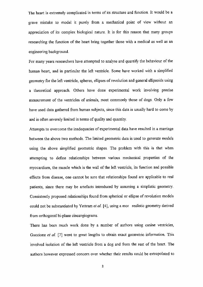
The heart is extremely complicated in terms of its structure and function. It would be a

grave mistake to model it purely from a mechanical point of view without an

appreciation of its complex biological nature. It is for this reason that many groups

researching the function of the heart bring together those with a medical as well as an

engineering background.

For many years researchers have attempted to analyse and quantify the behaviour of the

human heart, and in particular the left ventricle. Some have worked with a simplified

geometry for the left ventricle, spheres, ellipses of revolution and general ellipsoids using

a theoretical approach. Others have done experimental work involving precise

measurement of the ventricles of animals, most commonly those of dogs. Only a few

have used data gathered from human subjects, since this data is usually hard to come by

and is often severely limited in terms of quality and quantity.

Attempts to overcome the inadequacies of experimental data have resulted in a marriage

between the above two methods. The limited geometric data is used to generate models

using the above simplified geometric shapes. The problem with this is that when

attempting to define relationships between various mechanical properties of the

myocardium, the muscle which is the wall of the left ventricle, its function and possible

effects from disease, one cannot be sure that relationships found are applicable to real

patients, since there may be artefacts introduced by assuming a simplistic geometry.

Consistently proposed relationships found from spherical or ellipse of revolution models

could not be substantiated by Yettram et a!. [4], using a mor realistic geometry derived

from orthogonal bi-plane cineangiograms.

There has been much work done by a number of authors using canine ventricles,

Guccione et a!. [71 went to great lengths to obtain exact geometric information. This

involved isolation of the left ventricle from a dog and from the rest of the heart. The

authors however expressed concern over whether their results could be extrapolated to

2

an intact heart still within the subject's chest. An extensive investigation of the effect of

assuming different ventricle geometric configurations upon myocardial properties and

function was carried out by Mirsky (1969 [8]). The effect of assuming spherical, ellipse

of revolution and general ellipsoidal geometries was compared. He found that there was

a large disparity between the results obtained for each shape. It was claimed that the

human left ventricle is most closely allied to an ellipse of revolution and canine ventricles

are most closely represented by a general ellipsoid. He therefore concluded that it was

not possible to directly extrapolate results from work done with canine subjects to

humans.

1.1 Anatomy of the Human Heart

The human heart is a hollow muscular organ approximately conical in shape with large

blood vessels protruding from its base (the great vessels). It is situated approximately

mid-chest height such that one third is in the right side of the chest and the remaining

two thirds are in the \et haW ol t\ie c. Th "rit\

which protects the heart. The pericardium consists of two layers, the outer layer is the

fibrous pericardium and the inner layer is a thin membrane, the serous pericardium. The

serous pericardium is folded back on itself to form a double thickness. The outer layer,

the parietal pericardium, is attached to the fibrous pericardium, while the inner layer, the

visceral pericardium or epicardium, is attached to the heart proper and also covers the

great vessels. Between these two layers of the membrane is pericardial fluid which acts

as a lubricant to prevent excessive friction and thus damage to the membrane.

The heart is not a single pump but is in fact two pumps in one. The left half is

responsible for circulating blood around the body (systemic circulation) and the right half

around the lungs (pulmonary circulation). Each of these pumps is divided into the atrium

3

and the larger ventricle. Between the atria and the ventricles is an 8-shaped

atrioventricular (fibrous) ring.

The atria are composed of cardiac muscle fibres (the myocardium) arranged in two

layers: the inner layer belonging to the atrium proper and an outer layer common to both

atria. The ventricles have thicker walls and the left ventricle wall is the thickest. The left

and right atria (LA and RA) are separated by the atrial septum and the left and right

ventricles (LV and RV) are separated by the ventricular septum. The interior of the heart

is lined with the endocardium which is similar in form and function to the epicardium, it

also extends to cover the interior of the great vessels. The interior of the ventricles is far

from smooth as muscular structures protrude from the surface and these are known as

trabecul carn.

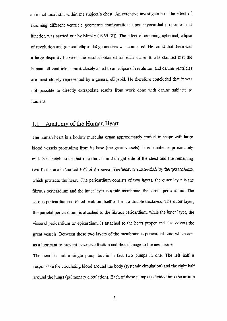
' AortaTo hmg To lung

From lung From limg

Pulmonary.. Left atrium A Aortic

lve Ive

TricUSPJgJt\\\

Mitral

atrium

ventricle

valvelve

Rcie

FromApex

Fig 1.1 This is a diagrammatic representation of the human heart. It showsthe relative location of the main structures and the direction of blood flow.(From Campen et a!. [49])

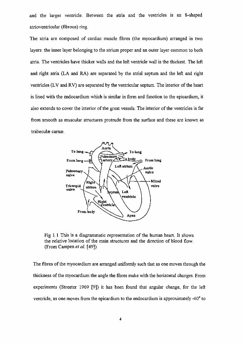
The fibres of the myocardium are arranged uniformly such that as one moves through the

thickness of the myocardium the angle the fibres make with the horizontal changes. From

experiments (Streeter 1969 [9]) it has been found that angular change, for the left

ventricle, as one moves from the epicardium to the endocardium is approximately 6O0 to

4

600 in diastole. This angular change is smooth and is often assumed to be linear and not

as had been previously believed arranged in discrete shells.

DecileEndacardium no.

?,c i1111

2.

3

.---.-1.-..-_ 4-

5Mid-wali

ii

- -9

10

Epicardiuxn

80 Fibre Angle

III

60

S

80 I0

thickness % -20

10

\ r

\i

-80

-100

Fig 1.2 This shows how the orientation of the fibres within the myocardiumvary through the thickness of the ventricular wall. On the left are slices takenat various depths through the wall. (Prom Streeter et a!. [9])

The great vessels are responsible for the transport of blood into and out of the heart.

Oxygenated blood enters the left atrium via the pulmonary vein; the pulmonary vein is

the only vein to carry oxygenated blood. This oxygenated blood leaves the left ventricle

via the aorta. Deoxygenated blood enters the right atrium through the superior vena cava

(this blood comes from the upper part of the body) and the infenor vena cava (this blood

comes from the lower part of the body).

The heart contains a number of valves which ensure that blood flows through the heart

chambers in only one direction. Surrounding each valve is a fibrous ring and this acts as

anchors for the valves to be attached to and helps maintain the shape of the valve orifice.

The four pulmonary veins that empty into the left atrium do not possess any valves. The

5

left atrioventricular or mitral valve lies between the left atrium and the left ventricle, it is

a bicuspid valve consisting of two triangular cusps. The cusps are attached by chord

tendine to papillary muscles which ensure that the valve cannot be turned in-side-out.

This valve ensures that blood only passes from the left atrium into the left ventricle. The

aortic valve consists of three semilunar cusps and is similar in structure to the pulmonary

valve only much larger and stronger. This valve prevents blood entering the left ventricle

via the aorta. The superior vena cava does not have a valve at all and the inferior vena

cava has only a rudimentary semilunar valve to restrict blood flow from the right atrium.

The right atrioventricular (tricuspid) valve consists of three triangular cusps. These cusps

are secured by chorda tendine to the papillary muscles, as in the case of the mitral

valve. This valve prevents blood from entering the right atrium from the right ventricle.

The pulmonary valve consists of three semilunar cusps and prevents blood flowing from

the pulmonary vein into the right ventricle.

Located close to the superior vena cava upon the right atrium is the sinu-atrial node or

pacemaker. The pacemaker is responsible for ensuring the timing of cardiac contraction.

An electrical signal generated in the pacemaker causes the left and right atria to contract

(atrial systole). The electrical impulse is carried through the atrial myocardium along

preferred pathways. These pathways are where the muscle fibres are thicker than those

in the rest of the atrial myocardium. When the electrical impulse reaches the

atrioventricular node, which lies in the septal fibres of the right atrium, the impulse is

conducted to the ventricular myocardium. The impulse travels long the bundle of His

which is composed of Purkinje fibres. Purkinje fibres have an approximately ten fold

greater rate of electrical conduction compared to the rest of the myocardium. The bundle

of His divides into two parts one that activates the right ventricle and the other the left

ventricle. Both these two halves subdivide many times to provide electrical activation at

many points within the myocardium of the left and right ventricles.

6

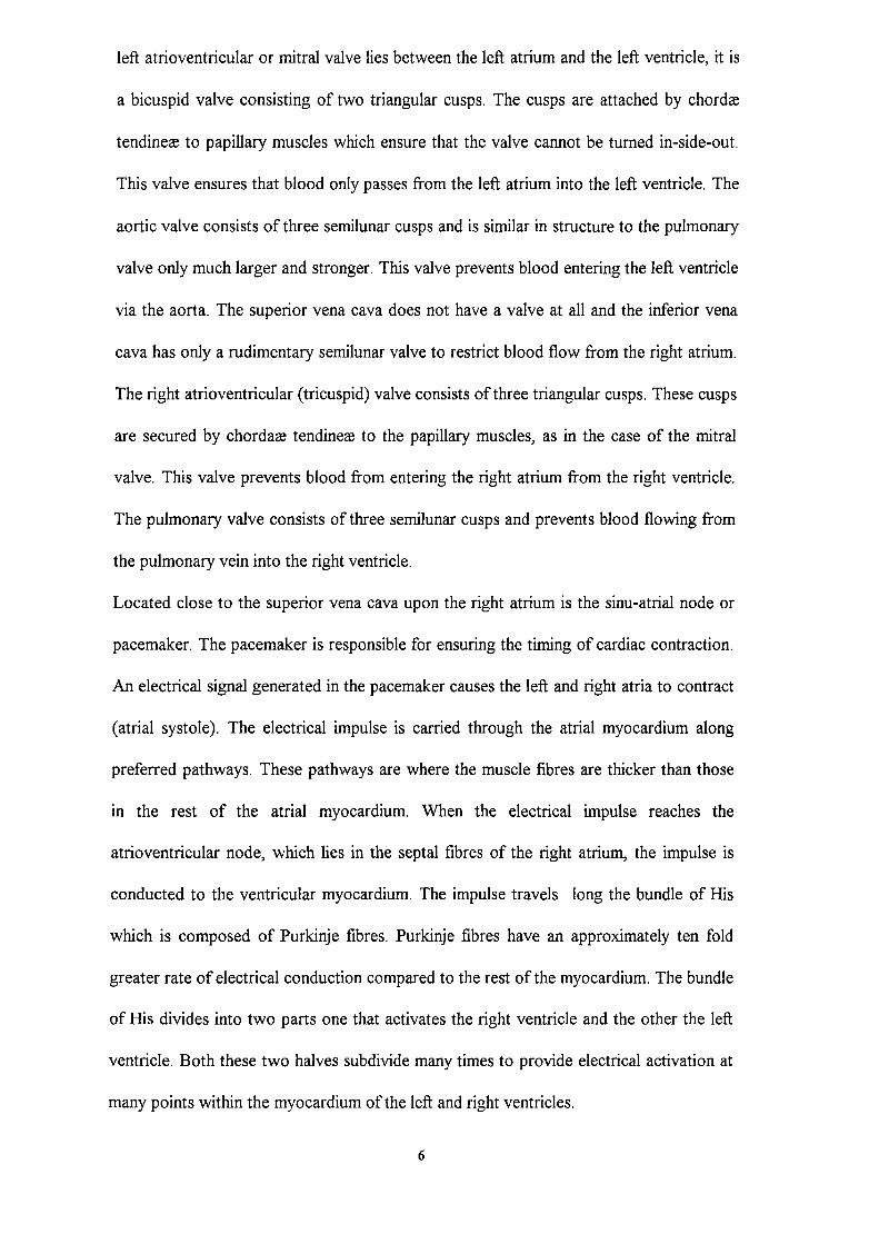
[is

branches

lentricle

iJ:ge Fibres

Superior vena ca

Sinu-atrial node

Afrioventhcularnode

Right atrium

Right ventricle

Fig 1.3 This diagram shows the location of the sinu-atrial node, theatrioventrjcular node and the bundle of His. All of these features are shownin heavy black. Arrows protruding from the sinu-atrial node represent themovement of electrical activation from that node. (From Berne and Levy[11])

To prevent the heart from moving within the chest cavity it is bound to three structures:

the parietal pericardium is attached to the root of the lungs and thus in turn to the thorax

and is also bound to the diaphragm. Lastly the heart is restrained by the super vena cava

which is attached to the structures of the neck including the surrounding fibrous material

(Keith 1907 [10]).

The above is only an outline of the major structures of the human heart. For an excellent

introduction to the human heart 'Principles of Physiology" (1996 [11]) provides a good

grounding and when combined with the canonical text "Gray's Anatomy" (1947 [12])

the information obtained should be sufficient for most needs.

7

Aoxticvalve

Mitxalvalvecloses

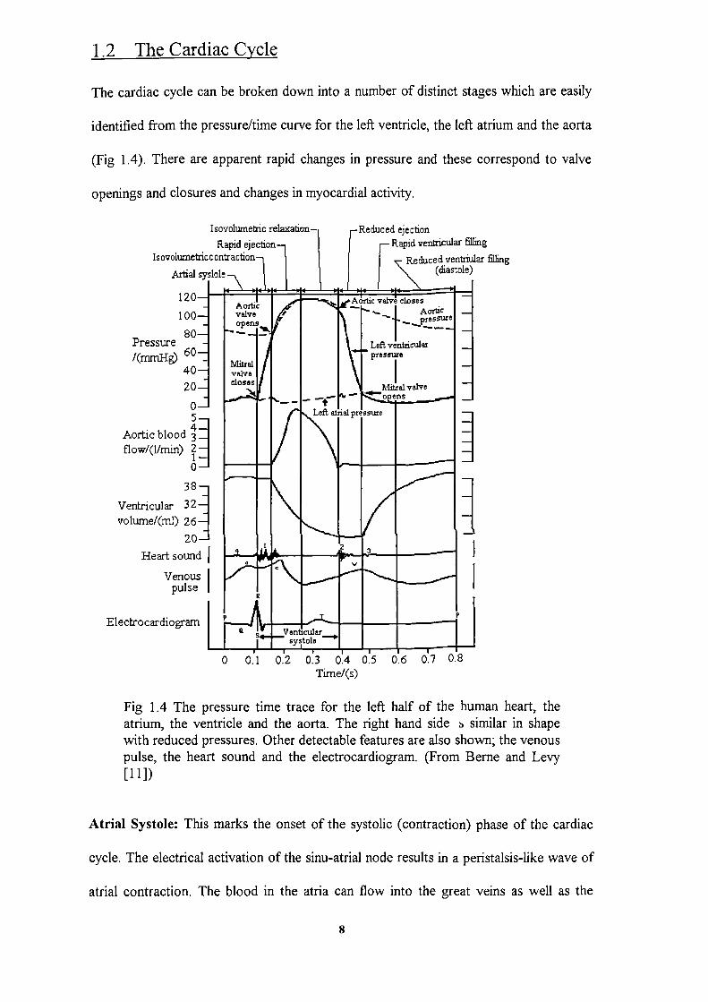
1.2 The Cardiac Cycle

The cardiac cycle can be broken down into a number of distinct stages which are easily

identified from the pressure/time curve for the left ventricle, the left atrium and the aorta

(Fig 1.4). There are apparent rapid changes in pressure and these correspond to valve

openings and closures and changes in myocardial activity.

Isovoli.unebicRapid eject

Isovolunieiccon1

Artial syslole

120

100

80Pressure

60

40

20

05

Aortic bloodflowl(llrnin)

0

38

Ventricular 32volurne/(ml) 26

20

Heart sound

Venouspulse

Electrocardiogram I

Reduced ejectionj— Rapid veritncular fi]iing

Reduced veniu1ar fifing\ (diastole)

valve closes-. I Aortj'

— .j_ ._Left ventxiculexpressuze

valveI---

r Left e.tzia1ressure

0 0.1 0.2 0.3 0.4 0.5 0.6 0.7 0.8Time/(s)

Fig 1.4 The pressure time trace for the left half of the human heart, theatrium, the ventricle and the aorta. The right hand side $ similar in shapewith reduced pressures. Other detectable features are also shown; the venouspulse, the heart sound and the electrocardiogram. (From Berne and Levy[11])

Atrial Systole: This marks the onset of the systolic (contraction) phase of the cardiac

cycle. The electrical activation of the sinu-atrial node results in a peristalsis-like wave of

atrial contraction. The blood in the atria can flow into the great veins as well as the

8

ventricles, as there are no valve structures to prevent a back flow of blood. This in

practice is minimal as the brevity and the weakness of atrial systole is not normally

sufficient to overcome the inertia of the blood entering the atria. Atrial systole

contributes about 30% to the stroke volume of the left ventricle. Despite this it is

possible with complete atrial systolic failure for sufficient blood flow to be maintained.

Electromechanical Delay: This is the earliest stage of ventricular systole and

corresponds to the time when electrical stimulation has begun and before the mitral and

tricuspid valves close due to the increased cavity pressure.

Isovolumetric Contraction: This is the time when the valves of the left and right

ventricles are closed and the myocardium is contracting. As the name suggests the

volume remains constant, as there is nowhere for the blood to flow, and the cavity

pressure increases.

Ejection: The ejection phase is marked by the opening of the aortic and pulmonary

valves. This part of the cardiac cycle may be further divided into an early, rapid ejection,

phase and the longer, reduced ejection, phase. The early phase is characterised by a

sharp rise in aortic and ventricular pressures, a sudden decrease in ventricular volume

and a large aortic blood flow.

Isovolumetric Relaxation: This part signals the beginning of diastole, the passive part

of the cardiac cycle. The pressure in the aorta is now greater than that of the left

ventricle. This pressure difference forces the aortic valve shut and results in a notch

being formed in the pressure trace for the aorta. The atrioventricular (mitral and

tricuspid) valves remain closed during this stage and the cavity volume of the ventricles

remains constant as the ventricles relax, hence isovolumetric relaxation.

Rapid Filling Phase: The atrioventricular valves now open due the reduction in

pressure within the ventricles, caused by their relaxation, and the increased pressure in

the atria, due to an inflow of blood from the great veins. This phase accounts for most of

9

the ventricular filling. During this stage the pressure continues to fall within both the

ventricles and the atria despite the increasing volume. This is due to the fact that the

ventricles and atria are relaxing and hence continue to exert less and less force upon the

blood within them.

Diastasis: This is the truly passive phase. The pressure and volume within all the heart

chambers rise under the pressure from the inflow of blood from the great veins. This part

is characterised by long slow filling of the chambers.

The above process is repeated many times a minute, approximately 60-80 times (beats)

per minute at rest. The heart rate may under loading increase to 180 beats per minute, an

increase above this value is possible for only a short period. The resting heart rate also

declines with increasing age.

1.3 Structure and Function of the Myocardium

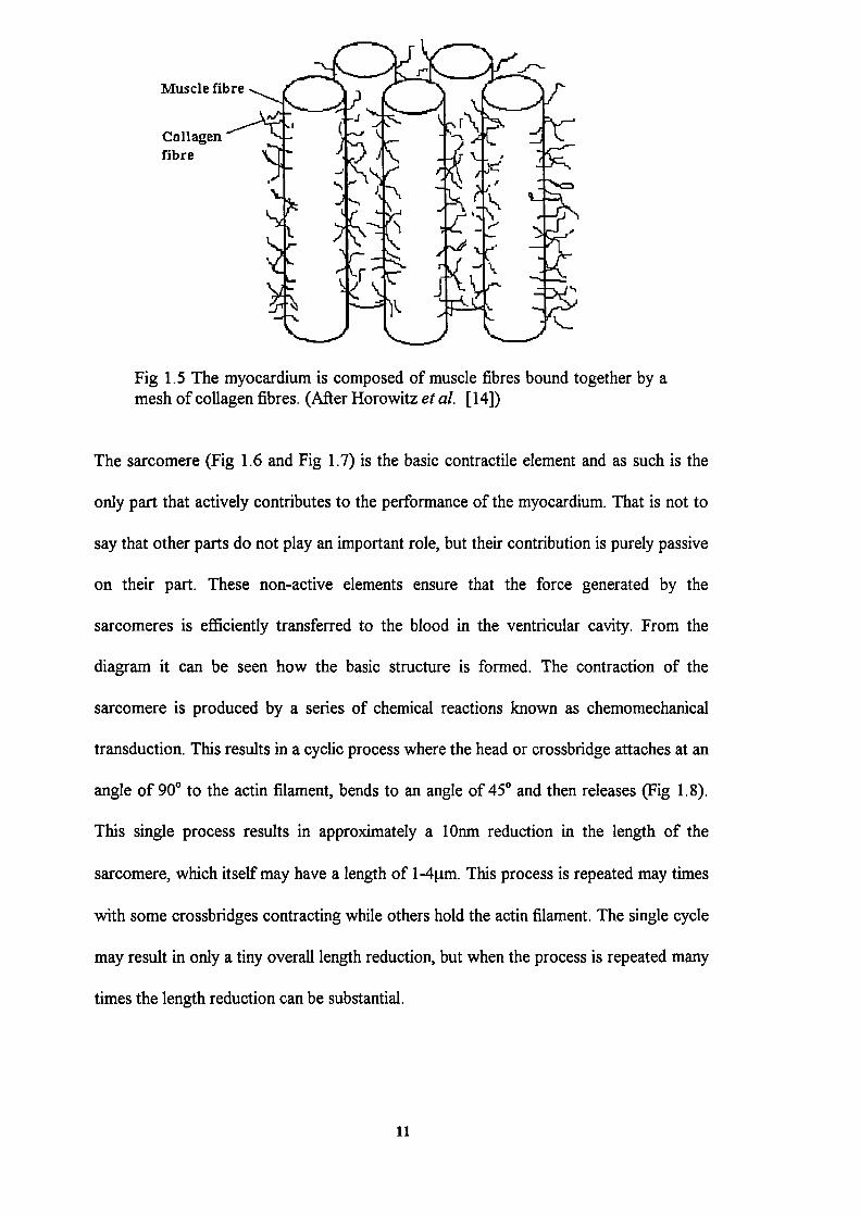
The myocardium consists of muscle fibres held together by collagen fibres (Fig 1.5). The

muscle fibres or myocytes make up approximately 70 per cent of the myocardial volume.

Only about 1.5 per cent of the myocardium is accounted for by the network of collagen

fibres. Although they are only a very small proportion of the total myocardium they can

greatly affect deformation of the myocardium (Borg Caulfield 1981 [13} and Horowitz

eta!. 1988 [141). This is due to the fact that they are several orders of magnitude stiffer

than the myocytes. The collagen mesh is sometimes referred to as the "fibrous skeleton"

and helps maintain the shape to the heart. It may also store large amounts of elastic

energy and may thus contribute to the restoring forces in diastole. The remaining

myocardium is composed of various interstitial components including a large fluid

component.

10

—Tropomyosi

Relaxed

Contracted

Z-Disk

ent

\Thck ament Sax-comere

Fig 1.6 This diagram shows how the basic units of a muscle fibre(sarcomeres) fit together. It should be noted that no part of the sarcomerereduces in length during muscle contraction. The reduction in fibre length isdue to parts sliding over each other and interleaving. (After Berne and Levy[11])

Troponin Z-Disk

Thin Iament

' Head or crosbridge

Fig 1.7 This shows the elements that form a single sarcomere. This diagramis much reduced in terms of the number of components. A real sarcomeremay be composed of approximately 3 00-400 myosin molecules. (From Berneand Levy [11])

Relaxed Attachment Cycling

Fig 1.8 This diagram illustrates the process by which the crossbridgeelements cause the length of the sarcomere to shorten. (From Berne andLevy [1 1])

12

1.4 Diseases of the Heart

The heart is a complicated organ consisting of many parts any of which may become

damaged by infection or excessive mechanical wear. A defect of a single part of the heart

may affect the performance of the organ as a whole as there is a great interdependency

between the individual parts. For instance if the left ventricle fails to fill to the correct

volume then it is obvious that this will affect the output of the ventricle during

contraction. Thus even though the initial fault was in diastole the effect may be more

obvious in systole. It is also the case that when one part of the heart malfunctions it may

put an excessive load on the other parts of the heart. It is for this reason that many heart

diseases are associated with each other and it is often the secondary condition that

causes the clinical condition of "heart failure."

Diseases that affect the heart are characterised by the type of condition and the part of

the heart affected. For example carditis is inflammation and can be associated with the

pericardium, the endocardium or the myocardium. Stenosis and insufficiency are valvular

conditions and may affect any of the four cardiac valves. There are many diseases that

can affect the performance of the heart and some of the more common are described

below:

Coronary Artery Disease (CAD): This disease is due to a narrowing of the lumen of

the coronary arteries. The main cause of this is cholesterol in the blood depositing on the

walls of the arteries. This most commonly occurs at either a bifurcation of an artery or at

a sharp bend. Over time there are fibrous reactions with the deposit and crystallisation

and calcification may occur. The arteries may become further blocked and the blood

supply to the myocardium can be severely restricted. This restriction can result in angina

pectoris (chest pain), myocardial infarction and ischaemia or sudden death, depending

upon the extent of the occlusion.

13

Myocardial infarction and Ischaemia: Coronary artery disease is the largest cause of

this and it results in more deaths in western countries than any other heart condition.

Ischaemia is when there is an impairment of myocardial function due to a loss of

coronary blood flow. Myocardial infarction is the death of the myocardium, which may

be for any reason. Myocardial infarction is not instantaneous following a complete loss

of blood flow but takes several minutes. If adequate blood supply is restored within 18

minutes then there may be no lasting damage to the myocardium (Levine and Gaasch

1985 [15]). However after 20 minutes there is a sliding scale of damage leading

ultimately to total necrosis of the affected tissue after six hours. This dead tissue is

gradually replaced with stiff non-functioning scar tissue over a period of a few weeks.

Hypertrophy (Hypertrophic Cardiomyopathy): With increased load the myocardium

naturally increases in mass to compensate for the increased cavity pressure and this

keeps the maximum systolic wall stress approximately constant. In Hypertrophy this

increase in myocardial mass is excessive and the deeper parts of the myocardium may

not get sufficient blood supply. Coupled with this the internal cavity volume may also be

reduced and hence further impede cardiac performance, particularly during diastole.

Dilated (Congestive) Cardiomyopathy: Is the commonest form of cardiomyopathy.

There is a decrease in the contractile force of the ventricles and a corresponding increase

in cavity size. Coupled with this increase in cavity size there are often associated

electrical problems such as arrhythmia.

Carditis: Is an inflammatory disease and can affect the endocard im, pericardium or the

myocardium. In endocarditis the endocardium becomes damaged and wart-like growths

can be formed. This is normally most severe around the valves, since these are subject to

the greatest amount of friction. The wart-like growths are also a site for deposition of

fibrin that will further interfere with blood flow. In pericarditis the pericardium becomes

dry and ridges of fibrin are formed due to the movement of the two surfaces over each

14

other. This condition can result in a rapid weak pulse and low blood pressure. In

myocarditis the myocardium itself becomes inflamed and may result in sinus tachycardia

and arrhythmia. In the severe cases the above conditions can result in sudden death.

Valvular Disease: This can affect any of the four cardiac valves, mitral, pulmonary,

tricuspid and aortic. In stenosis the orifice within which the valve is situated becomes

reduced in size. The result is that a greater pressure is now needed to maintain the same

rate of blood flow through the narrowed opening. In the more severe cases this pressure

increase will have already reached a maximum and sufficient blood flow will not be

possible. In regurgitation the valve leaflets may become damaged or the valvular orifice

may become enlarged. Whatever the reason the effect on blood flow is the same. The

valve is now unable to close effectively and this means that blood will be able to flow

backwards, be regurgitated. Both these conditions may lead to compensation by the

heart chambers and this in turn may lead to other conditions affecting the heart.

Electrical disorders: These include disorders affecting the rhythm of the heart and

conduction in the myocardium. The rhythm disorders can be in the form an accelerated,

decelerated or uneven rhythm (tachycardia, bradycardia and arrhythmia). It is also

possible for only some parts to be affected and for rapid uncontrollable activation to

occur. Conduction problems may, in a minor case, result in an occasional atrial or

ventricular beat being missed. It is also possible for conduction problems to result in

uncoordinated contraction of the myocardium or part of the myocardium failing to

contract.

15

1.5 Summary

It is clear the heart is an extremely complicated structure both in terms of its geometry

and the microstructure of the myocardium. It should also be obvious that it will not be

possible to model every aspect of the heart. A truly all encompassing model would

include the following: the active and passive elements of the myocardial micro structure,

all the structures of the heart, forces exerted upon the heart from outside it (the lungs,

diaphragm and the chest wall) and lastly the action of the blood within the heart

chambers.

It may be possible to devise a model that incorporated all the above features. There are

however two major problems. Firstly, to solve such a sophisticated model would be far

beyond today's computing power in terms of both storage and execution time. Secondly,

there is a lack of highly accurate data, which such a high precision model would require.

Obviously radical simplification must be made. The aim is to reduce the heart to its

computationally simplest form and yet still be able to gain useful and reasonably accurate

data.

16

Chapteri

2. Review of Cardiac Research Pertaining to the

Mechanical Behaviour of the Left Ventricle

It has long been known that the heart is an important organ, even before the days of the

early anatomists, In the beginning of man's civilisation the heart was considered by many

cultures to contain magical powers and was often used to symbolise life itself It is

therefore hardly surprising that there has been a great deal of interest in the structure and

function of the heart. Despite many years of research it is perhaps unexpected that a

complete understanding of the heart is still not available. This is not due to a lack of

quality research but is a testimony to the complexity of the heart and the mathematical

and computational intractability of highly complicated models. Simplified models can

however be useful to aid understanding of the function of the heart and may even be of

use in the clinical diagnosis of disease. It is with this hope that research in this area has

continued over the years. The advent of affordable and powerful desktop computers has

been a great boost to cardiac research. It has allowed complex finite element models of

the heart and in particular the left ventricle to be developed.

2.1 The Development of Cardiac Models

Cardiac research began properly with the early anatomists. The worked to detail the

structure of the heart and hypothesised upon the function of the individual parts. In the

1 5th century Lenardo Da Vinci wrote about the movement of the heart wall which had

been observed by the implantation of metal pins through an animal's chest wall. This

early interest could only advance understanding of the heart by a limited amount. It is

only when high precision instruments became available that the properties of the

17

myocardium, the heart muscle itself, could be directly measured. This however only

gives some of the information necessary for an understanding of the heart. Just as

important are the developments in mathematical modelling techniques, medical imaging

and pressure measuring techniques. The mathematical techniques allow more realistic

geometric and material modelling and the data acquisition techniques make it possible to

obtain in-vivo geometric data and also in-vivo pressure information.

2.1.1 Development of Thin Walled Models

The first attempts to model the left ventricle were made in 1892 and exploited Laplace's

Law. This provides a relationship for every point between pressure, tension and the

orthogonal radii of curvature in a thin shell structure. This method was not used again

until sixty years later by Burch (1952 [16]) who used a spherical model to derive the

forces, generated by the cavity pressure, within the ventricle wall. An analysis of the

importance of ventricular size and shape was also performed by Burton (1957 [17]). A

refinement of this type of analysis was produced by Sandler and Dodge (1963 [18])

where an ellipse of revolution was taken as the ventricle geometry. The shape of the

ellipse of revolution was based on single plane angiography of human patients. This

model was later used by a number of other authors to analyse human and animal patient

data. The major drawback with this type of model is in the assumption that the left

ventricle can be modelled as a thin walled vessel. It may be justified to use this approach

for a vessel whose radius is an order of magnitude greater than its wall thickness, but this

is not the case with the left ventricle where the ratio is approximately 4:1 in diastole and

up to 2:1 in systole. The membrane model does not allow for stress distribution through

the wall neither does it permit shearing of the material both of which may greatly affect

ventricular behaviour. Despite this it has been shown that not only do these models give

wall stresses to within an order of magnitude but may also be of some clinical use

18

(Mirsky 1969 [8]) provided local stress values are not required. A more thorough review

of thin walled models can be found in Vinson (1977 [1]).

It should be obvious that the next developments should include non-uniform wall

thickness, and allow for shearing and bending and uneven stress distribution through the

wall. Thick walled models were capable of these features and were developed using

thick shell theory, which is an extension of Laplace's Law. Not all of the advantages of

thick walled models were utilised from the outset and the new features were

incorporated gradually.

2.1.2 Development of Thick Walled Models

In 1968 Wong and Rautaharju [19] developed the equations which allowed the stress

distribution calculations for a thick walled ellipsoid of revolution. The model was similar

to that previously used by Sandler and Dodge (1963 [18]) except that the stresses were

allowed to vary through the thickness of the wall. Analysis of the diastolic phase showed

that the stresses were highest at the endocardium and decreased towards the epicardium

where they were lowest. This model did not include the possibility of shear within the

material which was included by Ghista and Sandler (1969 [20]). They used single plane

cineangiography to calculate the size and shape for their ellipsoid of revolution model.

They were able to show that the stress distributions in a viscoelastic and an elastic model

were similar.

Despite their inclusion in earlier models some still did not include bending and shear. A

truncated ellipsoid of revolution model was used by Streeter et. a!. [21] in 1970 which

was composed of nested tethered shells each with a unique fibre direction. The geometry

was based on that obtained from canine hearts at end diastole and systole. The stress

analysis was performed by considering fibre orientation and wall curvature.

19

It has been shown that these simple models could provide reasonable estimates to overall

stress levels in the myocardium. In 1970 Ghishta and Sandier [22] were able to use these

simple models to predict the oxygen consumption of the heart. This method only

involved catherisation of the left ventricle and cineangiocardiography. The previously

used method had required the measurement of the blood flow into and out of the heart

as well as the oxygen concentration in the blood. This new method is far less invasive

and hence much less risky to patient health.

Further sophistication was achieved in 1973 by Wong [23] who used a thick walled

truncated ellipsoid with non-uniform wall thickness. The diastolic material properties

were assumed to be isotropic, viscoelastic and homogenous. The myocardium was

modelled using a Hill's model and Huxley's sliding filament theory. This method gives

passive and active fibre tension as separate quantities within each fibre and was used to

analyse isovolumetric contraction.

In 1980 Janz [24] compared the equatorial stresses of an ellipsoid of revolution model

with those of a prolate spheroid model. It was concluded that the prolate spheroid was

the most reliable model for stress prediction. The conclusion reached from investigating

the systolic stress in a dog was "that the ratio of equatorial wall thickness to cavity semi-

minor radius appears to be the dominant geometric factor in determining this stress."

The fibre stress and fibre force during ejection were also found to decrease more rapidly

than left ventricular cavity pressure. It was noted that the models were very sensitive to

errors in measurement of the wall thickness which is also the hardest parameter to

measure.

In 1982 Janz [25] produced two equations which could predict the averaged local

circumferential wall stresses. The thick walled model was produced as a solid of

revolution from a single plane angiogram. The stress results were compared to that for a

similar finite element model and the results were found to be relatively consistent. The

20

stress values were found to differ by 5-25% depending on the area of the model being

investigated. There were however problems with each of the two formulae. For the first

equation there is a need to calculate perpendicular lines to the model's surface. In

practice this is prone to large computational errors and may make this formula unusable

in general. For the second equation in an area of simulated aneurysm the values differed

by more than a factor of two. It was however felt that "judicious use of both" equations

"yield meaningftul estimates of local averaged circumferential stress."

A cylindrical model was demonstrated by TOzeren in 1983 [26]. The myocardium was

modelled as solid fibres in an invicid fluid matrix. The cylinder was thick walled with the

fibre angle varying through the wall thickness. It was found that wall thickness and fibre

orientation do not affect the diastolic pressure volume relationship but the latter does

affect the geometric deformation. In systole the pumping efficiency was shown to

increase with increasing wall thickness and fibre contractibility. The rotation of the

cylinder was found to be small during diastole but much larger during systole. The model

did show some qualitative agreement with experimental data, but the constitutive

equations were purely theoretical and based on animal data.

The use of contractile filament stress and strain with circumferential and longitudinal

fibre strain was employed by Phillips and Petrofsky (1984 [27]). Introduced into the

model were compressive strains which were used to generate the fibre stresses. These

stresses and strains were then used to calculate the active systolic elastic modulus for the

circumferential and longitudinal axes. The values for these paran eters were determined

in an ad hoc manner for only four points in the systolic phase. The data used came from

thirty-nine human patients with various pathological conditions and was of the form of

single plane cineangiography plus pressure readings. It was found that the active systolic

moduli decreased during systole in an exponential manner. There was also some

grouping of active moduli values for patients with similar pathologic conditions.

21

A truncated thick wall ellipsoid of revolution model was used in 1985 by Kim et a!. [28]

to derive stresses from observed strains obtained from coronary cineangiography of

dogs. The bifurcation points of the coronary arteries were used as local markers and the

accuracy of using these was compared with the more invasive method of using implanted

lead beads. The new method was found to perform reasonably well, it is however

necessary for the coronary arteries to be in good condition otherwise the bifurcation

points may not be visible. The two main advantages of this method are that it can be

performed with data that would already be gathered, during assessment of the condition

of the coronary arteries, and it is far safer than implantation of lead beads.

A more extensive review of thick walled models has been done by Grewal (1988 [2])

who also provides references to other complementary reviews. Most of the thick wailed

models were used to calculate approximate stress distribution within the vessel wails.

The simplistic geometry makes the values obtained much less meaningful than this model

type might have provided had the geometric approximations been more suitable. One

example of this simplification is that the models define the internal surface of the

ventricle as being everywhere concave. In reality parts of the ventricle wall are convex

especially at the apex end of the septal region. Due to this thick wall models have

contributed relatively little to the understanding of ventricular mechanics. They do give

variation of stress though the wall, but the local values are somewhat suspect due to the

geometry and thin walled models give reasonably good global values. It is also the case

that similar thick wailed models have given stress distribution that have not been

compatible with each other (Huisman et a!. 1980 [29]). It has been the conclusion of

several reviews that the thin walled models are of far greater clinical use.

To incorporate a more realistic geometry as well as other considerations, including

inhomogeneity, anisotropy and non-linear material properties, a more advanced method

of modelling must be used. The finite element method is ideal for this sort of problem

22

and was developed in the late 1950's. The only drawback this method has is that it is

computationally expensive and that has been the reason for its lack of widespread use as

an analytical tool. The rapid increase from the mid 1980's in affordable computing

power has negated this earlier bar to its use and has seen this method become the tool of

choice for this sort of modelling.

2.1.3 Development of Finite Element Models

This part of the review will concentrate on finite element based research from 1990 with

only an overview of earlier work. More comprehensive reviews of the preceding years

can be found in Vinson (1977 [1]) and Grewal (1988 [2]).

In 1972 Janz and Grimm [30], who had previously used thick shell theory, began

working with the finite element method to analyse the mechanical behaviour of the left

ventricle. This first attempt at left ventricular finite element modelling involved ring

shaped elements to form a solid of revolution model. The geometric data used was

obtained from cross-sections of post-mortem rat hearts. The myocardium was modelled

as partly isotropic and as partly transversely isotropic. It was found that the model

deformation most closely matched the measured deformation when the inner third of the

myocardium was transversely isotropic and the rest was isotropic.

The 20-noded isparametric brick element was developed in 1971 by Zienkiewicz [31]

and is ideally suited to the finite element modelling of the left ventricle. This element

type was used in 1974 by Hamid and Ghista [32] to build a model able to predict left

ventricular chamber stresses as well as the stresses on the aortic valve. This was to

enable the design of prosthetic aortic valves and artificial heart chambers. The geometry

was produced from a single plane cine-angiographic image at mid-ejection. Their model

predicted peak stress levels in the left ventricle three times higher than had been

predicted by the previously used thick shell models. Comparisons were made between

23

the effect of normal and partially infarcted left ventricles. It was found that the tissue

surrounding the area of infarct took some of the load off the area of infarct.

Plane-strain finite element analysis was employed by Pao et a!. [33] in 1976 to analyse

the mid-plane between the base and the apex during diastole. Data had been obtained

from an isolated canine left ventricle using roentgenographic recordings and the

myocardium was modelled as an isotropic homogeneous material. It was found from the

model that for the anterior and posterior regions the maximum circumferential stresses

occurred on the endocardial surface. Contrary to this for the septal and free walls the

maximum circumferential stresses were on the epicardial surface. It was also noted that

the stress gradients were always steepest near the endocardial border. The need for

extension to three dimensions was already commented upon as was the fact that an intact

in-vivo heart would most likely behave differently to the excised isolate left ventricle.

A method for obtaining far better finite element reconstructions than offered by single or

even bi-plane cineangiography was presented by Nikravesh et a!. (1981 [34]). This

involved taking 4 to 5 short axis cross-sections and one long axis cross-section using

echocardiography. The method not only gives greater fidelity for reconstructed cross-

sections than cine-angiography but also gives wall thickness which is partially lacking

from cine-angiography. Although finite element reconstructions were shown there was

no analysis performed on the finite element meshes obtained.

In 1986 Horowitz et a!. [35] introduced a new finite element model able to model the

entire cardiac cycle for the left ventricle. The data used was fror a human source and

had been obtained by computer tomography. The model was formed from two element

types. The basic 20-noded isoparametric brick element formed the basic structure,

"Truss" elements were superimposed upon this structure to simulate the anisotropic

nature of the myocardium with the varying fibre angle. They also provided the directions

for the active contraction forces during simulated systole. The elastic modulus of the

24

myocardium is assumed to obey an exponential stress-strain relationship. The active

contraction of the model is the only thing altered to produce the required cavity volume

changes. Good agreement was found between the deformations obtained from the model

and that of the measured data. The only area of concern is that the model increased in

length during systole instead of reducing. A consequence of this was that radial

contraction was slightly greater to compensate for this. The increase in ventricle length

during systole was attributed to the exclusion of the papillary muscles which contract

tightly during systole and may thus cause the ventricle to shorten. It should also be noted

that the left ventricle "winds up" during systole and "unwinds" during diastole and this

was clearly evident from the model.

The effect of acute ischaemia was investigated by McPherson et a!. (1987 [36]) with

data obtained from canine subjects using the method of data acquisition and

reconstruction proposed by Nikravesh eta!. (1981 [34]). The myocardium was assumed

to be homogeneous, isotropic and linearly elastic. Areas of acute ischaemia were shown

to have higher elastic moduli than areas of normal diastolic myocardium.

A theoretical porous-medium finite element model was employed by Huyghe et a!. [37]

in 1991. The myocardium is assumed to consist of an incompressible liquid and solid

which is viscoelastic, with the muscle fibre angle varying linearly through the

myocardium. Since the myocardium is considered porous intracoronaiy blood is free to

enter or leave the myocardium allowing for volume strain and redistribution of mass. The

model is a truncated cofocal ellipsoid with 96 20-noded isoparal etric brick elements

with three layers through the wall. During passive filling the apex is seen to rotate in a

clockwise direction relative to the base, for an observer looking from the apex to the

base. In the pressure range O-3kPa the rotation was about 0. irad., which was considered

to reasonably approximate the rotation of a real left ventricle. This was an initial

investigation into the use of a porous-medium model of the myocardium.

25

In the same year Bovendeerd et al. [38] proposed another method to model the

myocardium using the same geometric data as Huyghe et al. [37]. Myocardial muscle

was modelled as an incompressible material consisting of muscle cells and connective

tissue embedded in fluid. The active stress generated by the sarcomeres is dependent on

time, fibre strain and fibre strain rate and is directed along the muscle fibre direction.

Muscle fibres were assumed to be twice as stiff in the fibre direction as in the cross-fibre

direction. The model considers varying fibre orientation across the left ventricle wall,

anisotropy of passive myocardial tissue, dependency of active stress on time and aortic

afterload. The global deformation pattern was found to be asymmetric with respect to an

ischaemic region. The left ventricle wall is seen to become thin and the fibres stretched

during the ejection phase. Muscle fibre shortening and active fibre stress around the

ischaemic region was seen to depend strongly upon the orientation of the border zone

with respect to the ischaemic region and the angle of the fibres within it. The ischaemic

region made up approximately 12% of the ventricle and was designed to simulate

occlusion of the left anterior descending artery. With the ischaemic region the left

ventricular pressure was found to be about 12% lower, the ejected volume was 20%

lower and aortic flow was also reduced compared to a simulation without ischaemia.

Again in the same year Han et al. [39] applied finite element analysis and optimisation to

a reconstruction of the geometry of a canine left ventricle, in order to assess myocardial

material properties during diastole. The model was subjected to an external or pericardial

pressure as well as an internal pressure and the elastic modulus changed in order to

match the left ventricle volume at the next time-step. The geometry was obtained from

eight short axis cross-section echocardiographic images taken at several intervals during

diastole. The pressures in the left and right ventricles were obtained with catheter tipped

pressure transducers inserted into both left and right ventricles. The average pericardial

pressure was calculated from the right ventricular pressure. The computed pericardial

26

pressure was found to play a significant role in the performance of the left ventricle. The

one drawback of this work is that results were only presented in respect to the effect of

pericardial pressure on left ventricular cavity pressure and myocardial elasticity, and not

to its effect upon global deformation.

Again in this year Fann et a!. [40] placed twenty two radiopaque markers into the

myocardium of canine subjects. These were located at the anterior, lateral and posterior

subepicardium and subendocardium at the midventricular level. Eight hours later bi-plane

videofluoroscopy was used for imaging of the ventricles of the closed-chested canine

subjects. It was found that circumferential shortening occurred in all layers and regions,

however longitudinal shortening did not occur in the posterior endocardium. Principal

shortening was found to be greater in the subendocardium than in the subepicardium.

Some concern was expressed as to whether such an invasive method of obtaining data

would affect the global deformation of the heart.

Still in 1991 Han et a!. [41] produced cross-sectional views of a canine left ventricle

during diastole using ultrasound. The myocardium was assumed to be a homogeneous

and isotropic elastic material. Using the finite element method the elastic modulus of the

myocardium was calculated in order to match the volume at successive time-steps. The

results suggest that during diastole the elastic modulus and pressure are linearly related,

the pressure/volume curve is exponential and this would suggest that the passive

myocardium has an exponential stress-strain relationship. Due however to the limited

number of points at which this analysis was performed the e idence is far from

conclusive. This is particularly true for the pressure/elasticity curve which could easily be

interpreted to be quadratic rather than linear. The assumed material properties for the

myocardium also give cause for concern when trying to prove relationships between

material properties and global function.

27

Two single plane X-ray angiographic images were taken by Roy et al. [42] in 1992 one

at end systole and the other at end diastole. The myocardium was then divided into

triangular finite element regions and each region then assigned an independent elastic

modulus. The boundary at end systole is then deformed under pressure so as to match

the boundary at end diastole. The elastic modulus of each of the elements was varied so

that the best least squares fit for the boundary could be obtained. Ischaemic regions

should show up as areas of significantly greater elastic modulus. The method was used

to successfully identify a patient with an ischaemic region. The major drawbacks to this

method are, that since it is 2-D an area of ischaemia may be in a position so as not to be

adequately represented by this slice and thus not be detected. The wall thickness was

also assumed to be constant and is thus far too thick at the apex.

Also in 1992 Bovendeerd et al. [43] used the model by Huyghe et a!. [37] as the basis

for their work. The muscle fibre angle distribution through the myocardium is varied in

order to make the active muscle fibre stress homogeneous throughout the myocardium

layers. The active stress is the stress that is generated in the sarcomeres and is dependent

on time. Fibre strain and fibre strain rate are directed along the muscle fibre direction.

The fibre angle is taken as the angle between the fibre and the local circumferential

direction, this is also known as the helical angle. With an endocardium angle of 600, mid-

wall angle of 0° and an epicardium angle of -60° the maximum active muscle fibre

stresses at the equatorial region were 1 lOkPa, 3OkPa and 4OkPa, in the respective

corresponding myocardium layers. However, when the mid-wall an,le is changed to 15°

these active muscle fibre stresses are all within the range 52kPa-55kPa. The change in

muscle fibre strain is also seen to be more homogeneous. The problem with this

approach is that no allowance is made for the effect that geometry may play in stress

distribution. The left ventricle is never stress free so these are stress changes and not

absolute stresses as is implied.

28

A year later in 1993 McCulloch et a!. [44] used a 128 element finite element model with

linear nodal interpolation to represent the intact left and right canine ventricles. The

original geometry had been obtained from anatomical measurement of the canine heart.

Myocardial properties were taken as homogeneous and anisotropic with the fibre angle

taken to vary through the wall from -51° (epicardium) to 590 (endocardium). The

diastolic phase of the cardiac cycle was simulated and the results compared to those

obtained from an invasive study upon a living dog. Significant regional variations in

stress and strain were observed. The strains were compared to those obtained by direct

measurement of a real canine heart. Radial, circumferential and longitudinal strains

agreed closely with experimental results. However transverse shear strains were wildly

inconsistent. It was concluded that ventricular geometry contributes greatly to the

heterogeneity in the mechanical function of the heart.

The same year saw Han et a!. [45] use echocardiographic imaging to obtain data from

canine subjects. The subject had 3-4 plexiglass markers inserted at the mid-papillary

muscle level of the myocardium. The animal was given a week to recover from this

before imaging occurred. During imaging the animal was mechanically ventilated. Eight

short axis views of the left ventricle were taken at 4-5 intervals during diastole using

echocardiography. The images were hand digitised to obtain the left ventricle epicardium

and endocardium outline. Pressure readings were obtained with a transducer-tipped

catheter inserted into the left ventricle via the femoral artery. The model used 64 8-

noded isoparametric solid elements. The myocardium was assum d homogeneous and

isotropic. An optimisation routine was employed to obtain the best least squares node

for node match for the finite element model between successive time intervals. It was

alleged from the results obtained that there was a linear relationship between the elastic

modulus of the myocardium and the pressure within the ventricle. In this study they also

calculated the value of Poisson's ratio between 0.425-0.485, thus the assumption that

29

the myocardium is incompressible would appear reasonable. As with Han et al. (1991

[411) only a few data points were obtained (three or four) so it is impossible to say with

any authority that the relation between passive elastic modulus and pressure is linear.

A study of an infarcted region of the left ventricle of a dog, due to coronary occlusion,

was made by Pao et a!. [46] in 1993. Tomographic images of cross-sectional ventricular

shapes were obtained for early and end diastole using 14 X-ray sources. Pressure

readings were taken using a catheter inserted into the left ventricle via percutaneous

arterial and venous routes. The plane-strain finite element method was used to analyse a

2-D short axis ventricular slice. It was found that the muscle in infarcted regions became

stiffer than the rest of the diastolic myocardium and this became more evident at higher

ventricular pressures. This method is similar to that used by Roy et a!. (1992 [42]) and is

also likely to suffer from the same problems. The short axis cross-section may however

give better results as areas of infarction are more likely to be longitudinal in orientation

due to the direction of coronary arteries.

The effect upon wall stress of simulated infarction was performed using an experimental

and a finite element model devised by Eberhardt et a!. (1993 [47]). Both models used a

spheroidal shape and the experimental model was constructed from 840A-urethane

which has an elastic modulus thought to be similar to that of passive myocardium, about

28OkPa. It was found that the circumferential stresses in the finite element and

experimental models differed by less than 1% at the outer wail and 4% at the inner wall,

when both models were subjected to an equivalent internal pressure Simulated infarction

was found to only affect surrounding material and had no effect upon the opposing wall.

Despite the fact that this model is isotropic and spherical it is still probably reasonable to

assume the main result, that ischaemia causes only local distortion in diastole, to be

correct.

30

Also in 1993 Guccione et a!. [7] used a finite element mesh formed from anatomical

measurements of the isolated left and right ventricles of a dog, which was subjected to

an internal pressure. The model assumed the myocardium to be homogeneous though

not isotropic and incorporated the varying fibre angle through the left ventricular wall. It

was found that sarcomeres at the anterior epicardium contribute less to left ventricle

pressure than those elsewhere. Differences were noticed in the sarcomere length between

the anterior and posterior free walls during ejection. These variations are believed to be

due to different geometries in those areas, since the myocardium is homogeneous. This

effect of geometry highlights the pitfall of using unrealistic geometry (spheres, ellipses of

revolution, etc.). In simplified geometric studies the geometric effect upon local

deformation would have been interpreted as a material difference.

In 1994 Bovendeerd et a!. [48] proposed another enhancement of the model first

described by Huyghe et a!. [41]. A further investigation was carried out into the effect of

altering the muscle fibre orientation. This time the muscle fibres are assumed to spiral

inwards from the epicardium to the endocardium. Three runs of the model were made;

the first run had the angle of spiral always zero and the helical angle 600 at the

epicardium, 00 at mid-wall and +600 at the endocardium. The second was the same

except the mid-wall angle was 150. The third was the same as the second except that the

angle of spiral varied transmurally and had a maximum at the mid-wall and was zero at

the endocardium and epicardium. It was found that a change in the helix angle had only a

slight effect on the deformation pattern, though stress and strain are very sensitive to the

spatial distribution of muscle fibre orientation. This however has very little effect upon

pressure/volume relationships. Transmural crossover of muscle fibres reduced the

transmural shear loading of passive tissue. Circumferential-radial shear strains calculated

with this model qualitatively disagreed with experimental data, This is explained by the

31

model being very sensitive to transmural crossover angle and the limited data available

on this,

In 1994 Campen et a!. [49] compared how well the two-phase axisymmetric porous

medium non-linear finite element model, Huyghe et a!. [41], and the three-dimensional

finite element model, Bovendeerd et a!. [48], predicted results obtained from canine

experiments. With the two-phase model transmural intramyocardial pressure gradients

are qualitatively consistent with experimental data. Stiffening of the myocardium due to

an increase in intracoronary blood volume was also qualitatively correctly predicted by

this model. The three-dimensional Bovendeerd model shows that regional distributions

of local ventricular wall stresses are very sensitive to the spatial distribution of muscle

fibre orientation. This however has little effect upon ventricular pressure or aortic flow.

Important aspects of the mechanics of an ischaemic left ventricle are predicted by this

model, such as a change in the pressure/volume loop, fractional decrease in stroke work

and spatial redistribution of wall stress and strain. The comparison shows that both

models have strengths and weaknesses and the recommendations for improvement are

too numerous to list here.

Again in the same year Hashima et a!. [50] attached twenty five lead markers to the

epicardium of the anterior free wall of the left ventricle in an open-chested canine. Bi-

plane cine-angiography was used to track the position of the markers before and during

induced ischaemia. The strains during the cardiac cycle were calculated using marker

triplets. Large strain gradients were observed across the infarcted reg ons.

The work done Huyghe et a!. [37] and Bovendeerd et a!. [38] [43] [48] on modelling

the myocardium is extremely impressive though the two models each has its own

strengths and weaknesses. The linear and exponential relationships between certain

myocardial properties suggested by Han et a!. [41] [45] cannot be given much weight

since these curves were only plotted though three or four points. Any data obtained from

32

invasive methods such as those used by Fann et a!. [40], Haim et a!. [44], Hashima et a!.

[50] must be treated with caution since it would be naïve to assume that the function of

the heart remained unaffected during these procedures, indeed Fann et a!. [40] expressed

these very concerns. Geometry is being seen by researchers as an important factor in the

function of the heart and great lengths have been gone by Pirolo et a!. [51] and Pao et

a!. [46] to obtain a more realistic geometry.

In the last few years heart modelling seems to have polarised into three basic areas. The

first of these is myocardial modelling, where sophisticated models of the myocardium are

used to describe cardiac muscle, such as those used by Huyghe et a!. [37] and

Bovendeerd et al. [48]. These models have the advantage that since they have active

components they can be used in systolic analysis. However, neither of the above two

models can predict complete left ventricular properties and are based around a

simplified geometry. Secondly, authors have tried to improve the geometry used to

model the left ventricle, using either dissection or modern imaging techniques. The third

group involves invasive methods to obtain strain information directly from the ventricle

wall. This is far from ideal as the myocardium is damaged due to the attachment of the

markers to it. It is not known whether this has a great effect upon the global function of

the myocardium, although local changes in myocardium function seem inevitable.

Several authors including Fann et a!. [40] have expressed concern over the damage

caused by insertion of markers into the ventricle wall. Some of the work done is

extremely impressive, the only questionable note is that the recent work has exclusively

been done with canine hearts, and it is not clear if conclusions drawn from this are

relevant to humans.

The finite element method is extremely powerful and can certainly describe many aspects

of the left ventricle and the microstructure of the myocardium. The main constraint with

this method is not as with thin and thick shell models the method itself but a lack of

33

accurate data. The models used to describe complex myocardial stmcture are not being

made full advantage of due to the use of extremely poor geometric approximations. It is

only with the use of accurate geometric information that any advantage from these

models can be properly gauged.

2.2 Related Areas of Research

The following sub-sections are not intended to be complete reviews. They are intended

as general information to aid in the understanding of the problems associated with

cardiac modelling. It is also intended to provide information that will aid in the

understanding of advancements in this and other works.

2.2.1 Imaging and Digitisation

The finite element method, as has been seen above, allows the description of complex

and unique geometry, such as that of the human heart. The restricting factor has now

become the availability of data used to define this geometry. It is thus of great

importance that research be concentrated in the area of imaging and digitisation. The

following is a short review of some of the advances in less/non-invasive imaging and

digitisation of cardiac geometry.

The problems with imaging techniques such as X-ray and ultrasound are that they tend

to produce poor quality data. Implantation of markers into the myocardium as used by

Hashima eta!. (1994 [50]) is far too invasive and dangerous to be of general clinical use.

The reconstruction method performed by Pirolo et al. (1995 [51]) which involved

dissection of the post-mortem heart can be of research use only. What is needed is a

non-invasive method that gives geometric data at least as good as implanted markers.

34

In 1988 a new method of marking the myocardium for motion tracking was proposed by

Zerhouni et a!. [52] called magnetic resonance imaging tagging (MRI tagging). This

involves using radio frequency saturation to give "hyperintense stripes" on the MRT

image. These lasted between 60-450 msec, which is long enough to image the systolic

part of the cardiac cycle. This provided the first real hope that a non-invasive method to

track local myocardial deformations would be a reality.

An enhancement to this method was reported by Axel and Dougherty [53] a year later.

A new method of tagging was described which gave a two dimensional grid as well as

sharper stripes. A method known as spatial modulation of magnetisation (SPAMM) was

responsible for the improved clarity of the stripes. The 2-D grid effect now allows the

tracking of points of the myocardium instead of stripes thus giving an extra dimension to

the tracking process.

An investigation into the use of MIRT tagging was carried out by Young and Axel [54] in

1992. One finding of this study was that the error associated with tracking tagged points

was 0.3mm, which is very close to that of implanted markers. The technique of

implanting markers has long been considered the "Gold Standard" for cardiac imaging.

This figure for the error was later confirmed by O'Dell eta!. [55] in 1994.

In 1995 McEachen et a!. [56] pointed out some drawbacks to the method of MRI

tagging. One was limited resolution due to pixel size and the other was the inability to

monitor the entire cardiac cycle. Despite these drawbacks the method still provides

greater detail than any other completely non-invasive method.

Meanwhile, the use of ultrasonography and computer tomography has been extended by

the use of data extraction methods that make better use of the available data or of some

a priori knowledge of the heart. There are two main drawbacks to the use of the above

two methods; firstly, the data tends to be somewhat blurred which necessitates the use of

a suitably qualified person to perform the digitisation process. Secondly, there can be

35

blank areas on the image. Both these problems result in digitisation being slow and

expensive and prone to observer error.

In 1994 Cho and Kim [57] demonstrated a method of edge detection for 2D

echocardiograms using a modified Hough Transform. This method allowed automatic

contour detection using a weighted function that could give greater weighting to areas of

greater clarity/certainty. Because of this it is able to cope with "dropout" and "speckle

noise" which are common problems affecting clarity of echocardiograms.

In the same year Chen et a!. [58] used a knowledge based approach with an adaptive K-

mean clustering algorithm to segment some computer tomography (CT) scan data. The

algorithm was found to create a reconstruction with a volume error of 6.7% and a

surface area error of 1.9%. The knowledge based part of the algorithm was needed to

remove and spurious data produced by the imaging technique.

The next year Chen et a!. (1995 [59) suggested the use of a priori shape knowledge as

a method to further improve the quality of reconstructions from CT scans. This method

means the shape of the final reconstruction is considered during the reconstruction

process. For this the use of 3D modelling primitives, "superquadratics", were used since

these allow deformations that simpler primitives cannot provide. To achieve this the

segmentation process considers optimisation in both image and parameter spaces as well

as the deformation progression of the reconstruction at different time intervals. This

method thus makes use of known characteristics of the left ventricle as well as the

changes in spatial configuration with time.

A similar method was proposed by Tu et a!. [60] also in 1995. This method also made

use of spatio-temporal data in order to gain maximum available information from the

data. Two sets of 4D canine data were extracted using this method and compared with

those obtained manually. The method had problems in extracting part of the ventricle

and this resulted in errors of between 5% and 32% between computed and manually

36

obtained reconstructions. When however this problem area was removed the errors were

greatly reduced to between 1% and 5%. The method does show some promise though it

is not totally automated as it requires the use of some manual editing of the raw data.

If these automated methods for data extraction can perform as they seem to promise,

then this could result in the improvement in data acquisition that the finite element

models require. Failing that MR.I data may improve and if combined with spatio-

temporal smoothing may reach the accuracy necessary for finite element models.

2.2.2 Analysis and Modellin g of the Myocardium

Another area of continued interest is the determination of the material properties of the

myocardium through the mechanical testing of excised strips of myocardium. These

strips are subjected to a variety of loads and the stresses and associated strains recorded.

From this data the stress/strain relationship can then be derived. Originally these tests

were urn-axial but more recently they have been biaxial. Biaxial tests are now the norm

as it was discovered that uni-axial tests significantly underestimated the elastic stiffness

of the myocardium.

The normal testing procedure is thoroughly documented by Lundin (1944 [61]) who

performed an extensive array of tests upon frog myocardium. The tests were performed

both on passive and contracting muscle. One property discovered was that the stifThess

of contracting muscle was approximately eight fold that of passive muscle. It was

suggested that this was due to the increased tension in the muscle and was not due to

another intrinsic property of the myocardium. This publication provides a great deal of

data as well as a good introduction to this field.

In 1983 Demer and Yin [62] performed extensive biaxial tests on human myocardial

material, They used material from a number of different sites within the left ventricular

wall. It was discovered that the ratio of long fibre to cross fibre elastic modulus can vary

37

by as much as 2: 1 to 1:2, traditionally most researchers have taken a ratio of 2:1 in their

models. It might seem plausible in the light of this to assume isotropic material

properties in models, this however was not advised as statistical analysis of the test

results suggested that the myocardium was indeed anisotropic.

Four years later in 1987 Yin et al. [63] performed further biaxial loading tests on canine

myocardium. In these tests thin sheets of myocardium were loaded such that the ratio of

strains in the fibre and cross-fibre directions remained constant. The use of a new

exponential strain energy function using non-integral powers of the strains was proposed

to model the myocardium. The new function was found to be more self consistent than

the more commonly used exponential strain energy function with quadratic powers of

the strains. The tests also gave a large spread of values of the ratio of long and cross-

fibre elastic modulus. Values of the elastic modulus ratio were found to vary from 6.5:1

to 1:4. It should be noted that there is a great deal of non-repeatability in calculating

coefficients for strain energy functions from new data. The reason for this is thought to

be due to either "numerical instability" of the algorithms used, or due to the "strain-

history" of the myocardium.

These tests are not merely limited to testing myocardial material but also involve fitting

functional descriptions to the properties observed. In 1987 Pinto [64], from work with

pig papillary muscle, suggested an equation that would give the force generated by a

contracting muscle fibre. The form of the curve produced is similar to the X 2 statistical

distribution. It has a steep rise up to the time when maximum force s achieved and is

then followed by an exponential decay.

Attempts have also been made to devise a functional descriptor of the passive properties

of myocardium. In 1990 Humphrey et a!. [65] proposed a "pseudostrain-energy

function" to describe the passive myocardial properties of canine left ventricles. Slabs of

myocardium were subjected to biaxial tests and results used to find the parameters of the

38

"pseudostrain-energy function" which was of a polynomial form. The function was

found to be useful for prediction purposes as well as being descriptive and was felt, due

to its biaxial nature and the larger range of loading conditions for which it was

applicable, that it was far more useful to the intact heart studies than previously used

functions. Great faith was placed in this function, although caution was advised in its

use, as well as further research recommended. The main area of concern was the damage

caused to the myocardium, by excising the slabs, and the effect this has upon the

properties of the material. It should also be pointed out that the function is only

applicable when passive mechanical forces are far greater than the active contraction

forces.

In 1994 Novak et a!. [66] studied the human myocardium at the equatorial region of the

left ventricle. It was discovered that the myocardium at the epicardium and endocardium

was significantly stiffer than at the mid-wall level. This has a significant impact upon

those authors who study stress distribution as even small differences in material

properties through the wall are likely to greatly affect the stress distribution.

There are two main problems that arise from this type of work over and above that of

preserving functionality of the myocardium during the testing procedure. That is that

most of these tests are carried out on non-human tissue and as a result may not be

directly applicable to humans. The requirements of the myocardium are quite likely to

vary wildly between animal species since different animals will require their heart to

function within different parameters. The second problem is that it may not be directly

applicable to finite element models of the heart. The reason for this is due to the nature

of the myocardium which is known to be quite heterogeneous as regards its material

properties. It would be quite unreasonable to expect that just because the individual

fibres follow an exponential stress strain relationship that the myocardium as a whole

would behave this way also.

39

What is really needed is a formula for the bulk properties of the myocardium. The

repeated attempts to prove that an exponential stress strain relationship exists for the

bulk myocardial properties have been less than convincing.

The real benefit that comes from this type of work is an understanding of how different

material properties may relate to each other. That is to say how along-fibre, cross-fibre

and shear elastic moduli are interrelated. Once a fuller understanding of how these

different material properties relate to each other is achieved a great deal of the

arbitrariness in the choice of these for modelling purposes can be removed.

2.3 Summary

It would appear that there are two major drawbacks with much of the current research.

There is an excessive over reliance upon simplified geometry to represent the left

ventricle. This is despite the importance of shape and change in shape being recognised

as major factors in the performance of the left ventricle (Mirsky 1969 [8]).

The other cause for concern is in the rise of more complex models for myocardial

material properties. These have largely been produced by consideration of the results of

tests on excised myocardial tissue. Due to the heterogeneity of the myocardium it does

not necessarily follow that the behaviour of the whole intact myocardium is mirrored in

these localised tests. Models performed using exponential stress/strain relationships for

the myocardium are imposing somewhat artificial constraints upon the myocardial

performance.

40

Chapter 3

3. Previous Work Relevant to the Current Project

This Chapter provides a brief summary of the work, previously carried out by Vinson [1]

and Grewal [2], upon which this work is based. The work in question is that pertaining

to the three-dimensional reconstruction and the method used to calculate the material

properties as well as some general information about the original data. In this chapter the

material properties previously found by Grewal (1988 [2]) will be presented.

3.1 Data Acquisition

The data used in the modelling process was obtained by X-ray cine-cardiography by the

Royal Brompton Hospital, London. Two orthogonal views 600 left anterior oblique

(LAO) and 30° right anterior oblique (RAO) were taken at a rate of 50/second. The two

frames are slightly out of phase by lOms due to the necessary staggering of the X-ray

exposures. The inaccuracy introduced by this is thought to be negligible compared to the

assumptions made in definition and interpretation of the images. The images were taken

at mid-inspiration with cranio-caudal tilt, this was found to give the most vivid images

with the easiest reconstruction.

In order to obtain the X-rays a contrast medium must be introduced into the ventricle.

This is achieved by the use of a catheter inserted into the left ventricle, via the pulmonary

vein. The tip of the catheter houses a micromanometer which is used to measure the

pressure within the ventricle, atmospheric pressure is taken as the zero. It should be

noted that the contrast medium only allows the endocardium to be visible, the

epicardium in most cases is only partially visible. The X-ray frames were hand digitised

using a Summagraphics digitiser connected to Brompton Hospital's Prime 300 computer

41

system. This process involves the projection onto a screen of each individual X-ray

frame which must then be hand digitised using a pen follower. To make the digitisation

process easier the screen has a grid with 0.1mm divisions. By repeating the digitisation

process several times it was found that the reconstructed volume was consistent.

There is an important point that should be made about the above digitisation process.

The process was only shown to give a reproducible volume when the reconstruction was

used. It was not however shown that any other property of the reconstruction was

adequately catered for in the digitisation process. This will be of importance later on

when consideration of overall shape will be made.

It must be also be noted that the digitisation process is extremely difficult and liable to

inaccuracy for two main of reasons. Firstly, the contrast medium is not evenly distributed

within the ventricular cavity. This leads to areas with little or no contrast medium, which

results in X-rays that have areas where the endocardium is not visible. Secondly, the

endocardium is not smooth as it is covered by the trabecul carn. This means that

instead of a distinctive change from cavity to myocardium there is in fact a blurred area

of uncertainty. It is for these reasons that digitisation requires the use of a trained

cardiologist.

3.2 Extraction of the Finite Element Mesh

A method for reconstructing the geometry of the left ventricle from bi-plane cine-

angiography was proposed by Yettram et a!. [5]. A selected right anterior oblique

(RAO) and left anterior oblique (LAO) endocardium image of the ventricle are chosen.

They are aligned at the apical point, which is defined as the lowest point on the on each

image. Definition in the RAO image was always found to be more complete than the

LAO, especially at the aorta, thus it is often necessary to extend the LAO image so that

42

LAO view

IRAO view

\

it matches the highest point on the better defined RAO image. This is done by projecting

vertically the end points of the LAO image.

Fig 3.1 This shows the typical data produced by the digitisation process fromwhich the left ventricular reconstruction is made. Typically a patient data filemay consist of between 30 - 70 such images plus the cavity pressure.

The RAO image is now sliced at fifty levels at 90° to the mid-aortic apical line. This

gives one hundred points which define the RAO image. These points are now projected

onto the LAO view and the two corresponding points, for each RAO point, are found.

This gives two hundred points which form an envelope within which the ventricular

geometry must lie. Each set of four points, corresponding to the same level on the RAO

view, form a quadrilateral.

The epicardium is treated in a similar way except that since this information is not

complete the non-digitised epicardium must first be constructed from the limited

information available from the X-ray. This is achieved by projecting parallel to the

endocardium the first and last points of the digitised epicardium. Thus the first point is

projected backwards and the last point is projected forwards. It is known that the apical

point of the myocardium is only 2mm thick. A quadratic curve is fitted around the apex

of epicardium from 5mm above the apex of the endocardium to 2mm below this point.

The four profiles defining the two three-dimensional envelopes for the endocardium and

epicardium are now rotated so that the mid-aortic apical line is vertical. The structure

can now be sliced horizontally, at fifty levels for volume calculation or twelve levels for

43

finite element mesh generation so that both envelopes are each defined by a set of

horizontally stacked quadrilateral discs. Every point of the endocardium and epicardium

must lie within their respective envelopes. How to construct the actual ventricle

geometry within these envelopes is to some extent arbitrary. The method used is to

construct a circular arc in each corner of all of the envelope discs so that the arc touches

both sides of the quadrilateral which make the corner. This arc can be subdivided to

provide the points needed to generate the finite element mesh or to calculate the volume

of the ventricle.

It would seem wise to discuss the merits and drawbacks of the above method of

reconstruction. With good data the above method has been shown to give realistic left

ventricular geometry (Vinson 1977 [1]). The problem occurs when the data is not quite

so suitable. The best possible reconstruction would be possible when the RAO and LAO

views are both aligned along the apex to mid-base line. This results in two images which

can truly be said to be longitudinal. In practice although the views are orthogonal they

will not lie along the apex to mid-base line. As the angle between the apex to mid-base

line for the two X-ray frames increases the LAO image becomes less of a longitudinal

image and more of an end on image. The result is not only a poor reconstruction but also

results in some finite elements being very much smaller than the others. The result of

having these smaller elements is that the mesh is not evenly distributed throughout the

wall volume of the model and thus full use of the elements is not made.

This problem of poor element formation could possibly be overcome by implementing a

more specialised meshing scheme. The advantages of this however would probably be

lost due to the poor reconstruction potential of these frames of data.

44

3.3 The Finite Element Model

The finite element method is widely used in many areas of engineering and in recent

years has become the main method for modelling the left ventricle. It is a numerical

method employing the use of so called shape functions to describe the solution space.

The solution space in this case is the wall of the ventricle. These shape functions provide

a functional description of the geometry of the left ventricle. The solution of problems

containing complex geometry is made possible by reducing it to a number of simpler

components, finite elements. A good description of the finite element method as used is

given by Vinson [1] and for a more advanced guide Zienkiewicz [31] is an excellent text.

The finite element model is generated from the defined geometry such that it has 72

elements with a total of 401 nodes. There are 60 isoparametric bricks with 20 nodes and

twelve wedge shaped elements with 15 nodes, which form the apex. The elements are

arranged to form two layers through the wall, with the fibre angle varying linearly

through each element. Pao et a!. [67] suggested a three layer model although Grewal [2]

found that a three layer model did not provide significantly greater accuracy to warrant

such a increase in computation time. The model assumes the myocardium to be

homogeneous, except for the apex which is particularly stifl though not isotropic. It is

assumed that the muscle fibre angle varies linearly between -60° on the outer surface to

60° on the inner surface.

45

Fig 3.2 This shows an idealised left ventricular FE. mesh and clearly shows,by means of a cut away section, how the fibre angle varies through the wallof the model. (From Grewal [2])

3.4 Volume Matching and the Elastic Modulus

The finite element model described above is used to find the elastic modulus of the

myocardium during the diastolic phase. The diastolic phase is when the left ventricle

relaxes and the pressure and the volume within it are both rising. It is assumed that in

this part of the cardiac cycle the myocardium is completely passive. Thus it is only the

pressure increasing within the left ventricle that causes the left ventricle to deform. This

is not entirely true although it is widely believed that the internal pressure is the major

driving force, especially in the latter part of diastole. The process employed to find the

material properties is to guess the solution and this guess is then iteratively refined until

the solution is found to the required tolerance. In this case the v lume calculated at one

time-step is matched to the volume calculated at the next time-step. This is achieved by

subjecting the finite element mesh, representing the left ventricle at one time-step

(frame), to the internal pressure increase that occurs between that interval and the next.

A guess is made for the value of the elastic modulus and finite element analysis is

performed upon the system. The finite element mesh is distorted by the increase in

46

internal pressure and will now have a new volume. If this new volume is larger than that

at the next time-step then the ventricle needs to be stiffer and the elastic modulus is

increased. On the other hand if the new volume is less than that required then the

ventricle is too stiff and the elastic modulus is reduced. This iterative process is then

repeated until the distorted mesh volume matches that at the next time-step. When this

process has been applied to all the diastolic data the progression of the elastic modulus

can then be analysed.

A process known as "smoothed volume matching" was developed by Grewal 2J and this

is now described. The late diastolic phase of the cardiac cycle is chosen. This is when

both the pressure and volume of the left ventricle are increasing. The volume pressure

plot for these frames is then smoothed through using cubic splines. The weighting of the

interpolating splines is two orders of magnitude greater for the first volume. This ensures

that the smoothed spline curve passes through the first point. This is important as this

volume and associated mesh are the starting point for the volume matching process.

The finite element mesh is constructed for this first frame of late diastole. The finite

element part of the program is then used to find the displacement of the mesh nodes that

would occur when subjected to the pressure increase between this and the next frame.

For this run the minor modulus is assigned an arbitrary value. The displacements are then

scaled in such a way that when added to the nodal coordinates the new mesh volume is

the smoothed volume of the next frame. The elastic modulus which was chosen is then

divided by the same scaling factor as the displacements where mu tiplied by and the finite

element part is initiated again and the matching process is repeated. At this stage, since

the displacements are small and the system is approximately linear, the modulus that

gives a volume match has been found. However some frames have larger displacements

and may require more applications of the finite element part to obtain a match. At this

stage the displacements are added to the mesh nodes and this becomes our new finite

47

14014) IE180 '120 120

ico ice

180 180

80H1CXJi/80

a. • I

r

40 4020 II , 200 0 II I 10

0 510152025Frame Number

140 CU

120

80

40200

0 7 1421 2835Frame Number

180140120ico80

40200

14012010380ED

a.40200

2c0E

>1co>

050

00 510152025

Frame Number

280 CL(A)

2c0E

150>

>050

00 612182430

Frame Number

280 CE

element mesh. The above process is repeated until the moduli for all the diastolic frames

have been calculated.

3.5 The Patient Data

There were twenty one sets of patient data available for analysis. Sadly, it had only been

possible to use the finite element method on twelve sets of data. A suitable finite element

mesh could not be formed for the remaining nine sets of patient data. Below are the

volume/pressure plots for the twenty one patients.

2c0

lEO

1aDa-

50

0

180 AN180

w1401201GJ

> 80

040200

0 6 12182430Frame Number

BA2c0 1120

80HIi 60

H II /020

I -200 8 16 24 32

Frame Number

CA180 180180 1 ,"\ ,I180

w140-l- / &-!-14)120-ji'y' tM -1-120w1OD+,\ \' -1OD

>80 +'\ / t8°\ V

040

-1-40200 I 110

0 918273645Frame Number

280 CL 1801140

180L\ 'If ico

> .J,i -1-80"I,

I'80 40

t200 I I 0

0 8 1624324048Frame Number

DA1UJ -i140

80I'\ 120

U(1°> i'k I

80

°it(

600.

°20

4

4020

01 00 7 1421 283542

Frame Number

48

140120

U

8060E

040200

18016014)

12010380 ,

40200

140120

80'5

40200

180140120ic806040200

120icx80 w6040200-20

120 DA(

ico

I:40

20

00 6 12182430

Frame Number

FO 250T

80 2c0E w

/ 150

0J\ 50

'5> I '5

'40I ico

I I I 1100 71421263542

Frame Number

140 HA

120icx806040200

0 7 14212835Frame Number

18014012010D806040200

140 JA

120wE1cX

80>60

(40200

0 9 1827364554Frame Number

Ml

140

120 80

>80140>'

60;

I 20

20 0

0 ii -200 102030405080

Frame Number

180 MI(A)

18040

120ico

>.80

040200

0 1020304050Frame Number

18014012010380

40200

180 MI(2)

180w140

120

> 80

040200

0 102030405080Frame Number

140 RE

120Elco

(40200

0 7 14 21 28Frame Number

MO 140180-i-" "

, 140 -V'(, 'I ,J 1-120

120-H\ I --1coU

ico/\_J -l-80

0 40 \ 1r 402020-1-0I I I

0 51015202530Frame Number

WET120

140 \ ,J1-io

I5

Ii>80 \ f 150 '5

'5

}40

20 20

0 I I0 102030405060

Frame Number

140 OL

120

580>60

200

0 7 1421 2835Frame Number

WE(A)2cc --14J120icc

i 1 -1-80I\J

> I a-

tf'

,J...f U

40

0 I I I I I 00 102030405060

Frame Number

Fig 3.3 These graphs show the cavity volume (cm3) and cavity pressure

(mmHg) against frame number for each of the twenty one sets of patientdata. The volume is given by the solid line and the pressure by the brokenline.

49

BAsco

4cc

fl3cTJ

Frame Number

CL

Frame Number

441

CU

I

Frame Number

FO

50

40

30

10

36 38 40 42Frame Number

The period of diastole can clearly be identified towards the right hand side of the above

graphs. The reason for the use of smoothing through the data is clearly evident from the

volume data which tends to be far from smooth. The area of diastole for each patient

was identified from each graph and the process of "smoothed volume matching" was

applied to this region. The plots of the minor elastic modulus against frame number are

given below.

AN1816

2 <E 14't12i.10

8.E 6

4

0 I I28 30 32 34

Frame Number

CL(A)9080

2 E 706050403020100 I I I26 28 30 32

Frame Number

2cc

<E lEO

-

50

HA3W

2ro

1EO

. icn50

028 30 32 34 36

Frame Number

MI180

c1

2 E 14)120icx80

.E 604020

56 58 60Frame Number

MO

01 I I I22 23 24 25 26 27

Frame Number

50

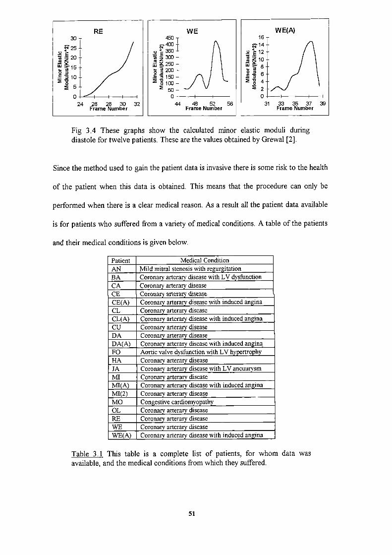
RE

2Frame Number

WE

4OJ

3co

2J. 150

1

050

44 48 52 56Frame Number

WE(A)16

14

E 12

0I

64

31 33 35 37 39Frame Number

Fig 3.4 These graphs show the calculated minor elastic moduli duringdiastole for twelve patients. These are the values obtained by Grewal [2].

Since the method used to gain the patient data is invasive there is some risk to the health

of the patient when this data is obtained. This means that the procedure can only be

performed when there is a clear medical reason. As a result all the patient data available

is for patients who suffered from a variety of medical conditions. A table of the patients

and their medical conditions is given below.

Table 3.1 This table is a complete list of patients, for whom data wasavailable, and the medical conditions from which they suffered.

51

CL

aCE

1CE(A)

ED ES

'SCL(A)

DA(A)ED ES

1%JA

ES

I

ES

I

The diagrams below show the endocardial surface of the three-dimensional

reconstruction. The end-diastolic (ED) and end-systolic (ES) frames are shown. These

represent the time when the left ventricular cavity volume is at its largest and smallest.

The diagrams are all to the same scale and clearly show the variation that occurs in size

and shape between patients and during the cardiac cycle.

BA

CA

q E a IDA

ES ED ESCU

IFO

IMI

ES

II

HA

1VU(A)ED ES

ii

52

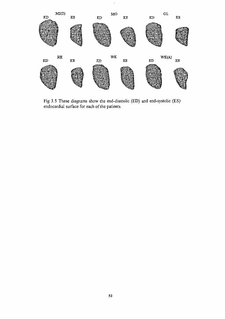
1VII(2) MO OLED ES ED ES ED ES

RE WE WE(A)ED ES ED ES ED ES

liii'

Fig 3.5 These diagrams show the end-diastolic (ED) arid end-systolic (ES)endocardial surface for each of the patients.

53

Chapter 4

4. Programming Developments

The first stage of this work was to resurrect the computer programs which had

previously been developed. There were two programs, the finite element program which

had been developed to run upon the Cray-1S/1000 at the University of London and the

pre-processor and post-processor which ran upon Brunel University's Honeywell

Multics. The idea was to combine the two programs into one which could then be run

upon a Sun Workstation; both programs were written in Fortran 77. Once they had been

combined the process of volume matching, described in detail in Chapter 3, could be

automated to speed up the analysis.

4.1 The Finite Element Part

The finite element program was fairly standard and only required a few minor changes.

The main feature that needed to be altered was to align double precision variables within

the common blocks. This had not been a problem on the Cray since the Cray uses

software double precision whereas the Sun uses hardware double precision. Double

precision is achieved by allowing two consecutive single precision words to be used to

define one double precision word. The two single precision words used for this are

important as not using the preallocated words can cause serious computational

inefficiency. This is because before computation each incorrectly aligned variable must

be aligned properly. This was very easily remedied by reordering the common blocks so

that the double precision variables appear first.

There were also several arrays that had been incorrectly defined, for example two integer

arrays had been defined as double precision and one two dimensional array was

54

inconsistent in one of its dimensions. Some alterations were also made to the way output

from the program is treated. The output was originally to standard output, (this is a file

on the Cray but to the screen on the Sun system) this was changed and output is now to

two files. One file contains the general information and the stress and strain values while

the other contains the computed displacements of the nodes of the finite element mesh.

The treatment of characters was also changed, originally they were treated as packed

integer arrays. Instead of storing a character string as a character variable, two

characters of the string are stored in each position of an integer array. However this can

cause problems when it comes to writing them to a file. They are written as the

numerical values which represent the characters instead of their character values, so they

are now treated as character variables throughout the program.

4.2 The Post-processor and Pre-processor

The first step in modifying the pre-processor and post-processor was to arrange for it

solely to use the graphical package Sivp'ePtot. Pr owAy the pe G'vo %1cj

SimplePlot had both been used to provide graphical output. However Gino was no

longer available on the computer network. The first thing that was necessary was to

discover which of the routines belonged to the Gino package. All the "calls" to routines

were then characterised as one of the following: internal subroutine, NAG library

routine, SimplePlot routine or Gino routine. Once all the internal, NAG and SimplePlot

routines were identified the ones remaining must be Gino routines.

Now that the routines to be replaced have been identified it is important to discover their

purpose so as to choose a suitable replacement. This had to be done by examining their

arguments and the context in which they were used, since a manual was not available for

the package Gino. SimplePlot however, since it was still a package supported upon the

network, had a full complement of user and reference manuals ([681 [69]). Below is a list

of Gino routines, in bold type, their function and the SimplePlot routines that were used

to replace them:

UNITS(UMILS) Sets the measurement units to UIMILS for plotting purposes. It is

removed and not replaced.

DEVPAP(XPAP,YPAP,ITYPE) Sets the paper size in the current units to width XPAP

and length YPAP and output to device ITYPE. The paper size is specified by routine

PAGE(XCMS,YCMS) and the output device is specified by routine DEVNO(ITYPE).

LINTO2(X,Y) Draws a straight line from the current position to point (X,Y). It is

replaced by BRKNT(X,Y,LTYPE), the value of LTYPE here is unimportant although it

must be in the range -6 to 6.

MOVETO2(X,Y) This moves the cursor o the point (X,Y). It is replaced by the two

routines BREAK and BRKNT(X,Y,LTYPE), the value of LTYPE specifies the type of

line and as before must be in the range -6 to 6.

LINBY2(DX,DY) Draws a straight line from the current position to a point (DX,DY)

relative to the starting point. It is replaced by the routine

BRKNT(X+DX,Y+DY,LTYPE) where the point (X,Y) is the current position and

LTYPE is as above.

DASHED(MODE,REPEAT,DASH,DOT) This routine sets the type of broken line to

be used for drawing with. In SimplePlot this is set at the time of drawing using the

parameter LTYPE.

DEVEND This routine terminates plotting in Gino. It is replaced with the SimplePlot

equivalent, ENDPLOT.

CHAHAR(NSIZE,NHV) This routine sets the character size, NSIZE, and the

orientation, NIHV=O gives horizontal and NT-IV=1 gives vertical. It is replaced with the

56

SimplePlot routine TEXTMG, although the orientation must remain horizontal. The Y-

axis however is automatically rotated vertically.

CIIASIZ(WIDTH,HEIGHT) This routine sets the width and height of the subsequent

text. As above it is replaced with TEXTMG.

CHAANG(ANGLE) This routine sets the angle to the horizontal at which all

subsequent text will be written. There is no SimplePlot equivalent.

CHAARR(ICHA,I,N) This routine writes a character string which has been stored as a

packed integer array to the specified output device. The integer array has length I and

density N. It is replaced with the SimplePlot routine CP7PT(X,Y, 1 5,CHA) where the

position on the plotting device is the point (X,Y) and the text is stored as a character

array in CHA.

SCALE2(SX,SY) This routine is used to scale X and Y-axes by amounts SX and SY

respectively. It is not directly replaced with any routine as setting up and scaling of the

output area is easily accomplished with the SimplePlot routine SCALES.

APDS4, T4014, VH7221 These three routines are used to initialise the output device to

be used for plotting purposes. The first two are for different terminal types while the

third is for a pen plotter. In SimplePlot the output device can be specified by the routine

DIEVNO(DEV) where DEV is an integer representing a logical output device.

ENCODE(IARRAY,N) 'CHA' This is a function which is used to convert the character

string "CHA" to a packed integer array IAR.RAY of length N. It is not needed under

SimplePlot since SimplePlot is able to directly output chara ter strings as character

strings and does not require conversion to a packed integer array.

As well as the changes to SimplePlot routines from Gino it was also necessary to change

one of the NAG library routines. One of the previously used routines was removed from

the NAG library of routines when the version changed from Mark 15 to Mark 16. The

function of routine "MO1AJF" was split between three new routines "MO1DAF",

57

CC 01ZJ\J and "MO1CAF" ([70]). The routine "MOIAJF" had previously been used for

the purpose of ranking a vector such that it was ascending. The role of this part of the

routine is now performed by "MO1DAF" and this routine has now been used to replace

the one previously used.

After the replacement of the above routines the program would now compile and run to

a limited extent. At this point a number of problems came to light. As with the finite

element program the common blocks required alignment and this was achieved by

rearranging the lists of variables. The other more serious problems can be split into two

basic types, programming and logical. Some of these may have been previously

corrected since there were several copies of this program and it was not known which

was the most recent version.

4.2.1 Programming Alterations

On the whole these were hardest to track down, since the effects they had on the

function of the program were not necessarily directly related to the routines in which the

errors occurred. For example a variable may take an inappropriate value but it would

only be when that variable was required that any problem could be noticed. It was often

the case that it was only the cumulative affects of an earlier error that caused a program

failure. Most of these occurred as a direct result of the way in which Multics Fortran and

SunPro Fortran handle certain situations. Thus situations that would be handled as the

programmer intended under Multics Fortran caused catastrophic failure in SunPro

Fortran. However it was also known that the program had problems processing some of

the frames of geometric data for several of the patients, but since none of these occurred

during diastole no attempt had previously been made to correct them. These problems

now require attention since we will be interested in examining systole.

58

Many Fortran compilers add extensions to the ANSI (American National Standards

Institute) standard, this is with the aim of making programming easier and programs

more robust. Relying on these extensions however is often a false economy. This is

especially so if it later becomes necessary to change to another version of Fortran. It is

thus wise to avoid compiler specific features as they will change from compiler to

compiler and sometimes between different versions of the same compiler. The problems

introduced as a result of the use of non-standard features have now been remedied and

are discussed below.

Arrays Too Small for Required Data: In some versions of Fortran, if this problem is

encountered, the program may write extraneous data to memory after the last element in

the array so that it can be assessed later. In SunPro Fortran when there is an attempt to

write data to the n+lth position of an array of length n the data may be written to

position 1. In some cases it was also seen to overwrite other variables corrupting the

data stored in them. This was remedied by increasing the size of all the arrays used to

store patient data from 101 elements to 151 elements. This type of problem is relatively

easy to find as SunPro Fortran has a compiler option, "-c", which aborts execution of the

program when there is an attempt to access an array element out of the defined array

bounds. Checks were also added so that if, in future, this value is too small a warning

message is given to the user and execution of the program will be suspended.

Inconsistent Declaration of Variables in Parameter Lists: Some versions of Fortran

ensure a complete mapping of each variable in a call list o to each element in a

subroutine's parameter list. SunPro Fortran does not do this, thus if a variable is

incorrectly defined in one parameter list then the information after and including the

mistake will be corrupted. There were several instances where there was a mismatch in

variable declaration where variables and arrays changed from real to double precision or

integer to real. To correct this problem was a considerably time consuming task, as every

59

call to every subroutine must be checked to ensure that variables in a parameter list are

declared as the same type in the subroutine and the routine from where it is called. If a

variable type mismatch occurs then the most suitable type of variable must be chosen and

all conflicting definitions changed to that.

Calculation Within a Parameter List: Under SunPro Fortran performing simple

calculations within a call list leads to variables being incorrectly overwritten when

control reverts back to the routine from which the call was made. The effect of this is

that attempting to use this variable results in a large amount of spurious text being

produced. This text is in fact the output from the "error variables". Multics and indeed

most other major versions of Fortran do not exhibit this problem. These calculations

must be carried out prior to the subroutine call, the result stored as a temporary variable

and that then placed in the call parameter list in place of the calculation.

Unassigned Variables Assumed to Take a Value of Zero: In some versions of Fortran

when entering a subroutine any unassigned variables are assigned a value of zero. Other

versions of Fortran do not even initialise unassigned variables to zero upon program

execution. For this reason the value of unassigned variables should never be relied upon

as there is no guarantee what value they may have. In SunPro Fortran these variables

retain the value they had when last exiting the routine and are only assigned a value of

zero when the routine is entered for the first time. Thus all variables that should have

value zero upon entering a subroutine are explicitly assigned the value zero.

One specific instance when the above caused a problem was in the formation of the finite

element mesh. The mesh is produced from a vertically stacked series of reconstructed

cross-sectional slices. Each slice itself being formed from four circular arcs. When the

routine which constructs these is called for the first time the mesh produced was correct.

When however another frame was reconstructed first the mesh would be different. The

problem was that the array index that selected which cross-sectional slice was being

60

produced was not set to zero upon entering the routine. The result of this was that the

first or top cross-sectional reconstruction was actually that of the first reconstruction

done during that run of the program.

4.2.2 Logical Alterations

Though there are quite a few changes within this category they only affected a small

minority of the frames within diastole. The effect upon the shape and volume of the

reconstruction was also often quite minor. Thus it is not envisaged that previous results

were greatly affected qualitatively or quantitatively.

When data was read from the patient's data file the possibility of an unequal number of

right anterior oblique (RAO) and left anterior oblique (LAO) frames was not catered for.

This would mean that about half of the patient data files could not be directly analysed

without some hand editing of the file. To add this facility only required the addition of a

few lines of code and was quickly corrected.

There existed a subroutine that aligned the RAO and LAO frames. It had been assumed

that the LAO frame always had its apex at a height zero. Another assumption was that

the apex was also at the point furthest from the midpoint between the first and last point

on the frame image. Neither of these two is universally true, the second however is

always true for the LAO image. When the apex on the RAO image is not the furthest

point from the midpoint between the first and last point on the frame image the finite

element mesh cannot be formed. The solution is to translate vertically the LAO image so

that its apex is at a height of zero and to translate the RAO image so that the lowest

point of that is also at a height of zero.

When attempting to construct the ventricle envelope it may not be possible to obtain the

two distinct values needed to form one of the sides of the envelope box. Thus two of the

points forming the corners of the box are the same. The method used to reconstruct the

61

ventricle however requires a quadrilateral and cannot cope with a triangle. The solution

to this problem is, after alignment to the RAO and LAO images, to move any RAO

points that have height zero to a height of 0. 1mm, such a small difference does not affect

the overall volume, but it is enough to ensure that a quadrilateral can always be formed.

This problem is most acute when the RAO has a number of points at zero height and is

made worse when some of these points are not close to the apex.

The subroutine "sketch" had a number of problems associated with it although few of

these had a major effect upon the diastolic frames. This routine reconstructs the

epicardium outline from the usually very limited information gained from X-ray

cineangiograms. However for one patient this information was complete but the routine

did not allow for the first point on the epicardium to be higher than the first point on the

endocardium. The result was that the entire digitised epicardium would be lost as the

reconstruction process resulted in no epicardial points being found. This meant that no

volume or geometric data could not be produced for these frames. Fortunately none of

these were in the diastolic phase. The solution was to add in a check within the

reconstruction algorithm so that if the epicardium was already complete the

reconstruction would not be performed.

The routine also could not cope effectively with concave sections of endocardium wall,

and also if the image became horizontal at the end points. Two routines had to be

written to correct these flaws in the epicardium reconstruction. Routine "TTDYUP"

ensures that the first and last points on the pericardium are o tside the first and last

points on the endocardium, since if the aorta needs to be drawn on, and the first or last

point of the pericardium are inside the first or last point of the endocardium, this area

would have a negative thickness. This is achieved by searching along the pericardium,

from the first point, until a point where the horizontal distance between this point and

the first point of the endocardium is greater than the thickness of the myocardium at this

62

point. The x value (horizontal position) of the point previous to this is given the value of

the x position of the first point of the endocardium plus the thickness of the myocardium

at this point. The position of this newly formed point in the y (vertical) plane is

calculated using linear interpolation between the two points either side of the new point

being formed. The arrays holding this coordinate data are then reordered so that the

point that has just been formed is the first point held in the arrays. The process for the

end of the epicardium is the same except that the points are traversed in the opposite

direction.

When the endocardium had a concave part a loop could then be formed when the

pericardium was reconstructed. A routine "'NOLOOP" was written which removes these

loops and also removes rogue points which were introduced when digitising occurred.

The rogue points are removed first. These are easily identified visually as a sudden spike

in the outline. The test used in the program for a rogue point is as follows. If the distance

between point n and point n+1 is more than ten times greater than the distance between

point n and point n+2 then point n+1 is removed. The removal of loops is somewhat

more complex. To aid this, the subroutine "INSECT" was constructed. This routine,

when supplied with two sets of two points, returns the value "TRUE" if the two line

sections formed from joining the two points in each set intersect. The algorithm used

constructs the line equations for each of the two lines then, providing the lines are not

parallel, the point of intersection is found. This point is then checked to see if it lies in

the domain of the two line sections and if it does then the val e "TRUE" is returned

otherwise the value "FALSE" is returned. The routine "NOLOOP" calls routine

"INSECT" for the first two points and then for each subsequent pair of points after that.

The process is repeated in turn for every pair of starting points with the exception of the

last pair, which will already have been checked with every other pair of points. Should

routine "INSECT" return with the value "TRUE" then all the points in between the two

63

pairs are removed including the second point of the first pair and the first point of the

second pair. The points are removed by reordering the arrays in which they are stored,

so that the unwanted values are overwritten by the subsequent data. Thus the length of

the array is reduced by the number of points being removed. This routine is also used on

the endocardium data to remove any rogue points found there.

There was also a subroutine "CHECKPT" which was supposed to remove duplicate

points introduced during the digitising process. The method used was to perturbate the

duplicate point. This however could cause problems since the perturbation was always in

the same direction. The result of this is that the outline can double-back upon itself and

this can cause the algorithm used to extract the finite element mesh to fail. These

duplicate points are now removed completely by reordering the arrays so that each

duplicate point is overwritten by the next non-duplicate value. The overall length of the

array is thus reduced by one for each duplicate point being removed.

4.3 Combining the Computer Proams

The rationale in combining the two programs was that the process of obtaining the

elastic moduli for the myocardium could be automated. Combining the two programs

was by no means trivial as there were in excess often thousand lines of code, only some

of which were documented and very little of which was commented. Previously the post-

processor and pre-processor program had been used to generate the data file for the

finite element program and then process the results for volume matching. The scaling

factor for the displacements which gave a volume match was then found by trial and

error. This is a very time consuming process and it requires the user to be present

throughout the operation of the program. Automating the process means that once all

the parameters that the program requires are specified by the user, the program can be

64

left to run without any further intervention. Thus the operator is now free to pursue

other work and is not restricted by having to continually provide input. The program

normally takes about eight hours to process one set of patient data, thus it is usually left

to run overnight.

To automate the volume matching process a number of changes needed to be made,

New versions of existing routines for the generating of the finite element mesh needed to

be formed. The original versions were interactive, requiring the user to select options at

each stage. Several new subroutines also had to be written to automate the volume

matching process. A subroutine 'PART4" was written to control the automated process,

it allows the selection of all the options necessary for volume matching. Routine

"NEWFIL" updates the data file, "XL1-data", for the finite element part with either new

values for the material properties or new ventricular geometric data depending upon

which is required. The process of finding the scaling factor for the displacements which

gives a volume match is carried out by subroutines "VOLMATCH" and "GOLDSEC".

Routine "VOLMATCH" checks to see if the new calculated volume (finite element mesh

plus displacements) is within the required tolerance. If it is then the mechanical

properties are written to a file, otherwise routine "GOLDSEC" is invoked. This routine

uses a linear step method to find a region in which the required scaling factor exists. The

golden section method (Fibonacci search) is then applied to the region to find the scaling

factor that gives the matched volume to the required tolerance, typically < 0.1cm 3 . The

scaling factor found is then passed to routine 'NEWFIL" to scale he elastic moduli and

the finite element data file is then updated. The finite element and volume matching parts

are repeated until a volume match is achieved (finite element mesh plus displacements

gives the required volume). The newly formed mesh coordinates for the next frame are

then substituted into the finite element data file. The newly formed coordinates being the

65

original mesh data plus the displacements. This process continues until all the diastolic

frames have been analysed.

A number of cosmetic changes were also made to aid the use of the program. Automatic

naming of input and output files was introduced so that only the patient data file to be

used need be specified and all other necessary files will be either generated, opened or

appended. Better error trapping to improve the stability of the program was developed,

e.g., if an incorrect or inconsistent input is given, the program will inform the user of the

mistake instead of crashing or producing spurious output. A more efficient user interface

was created as originally options were presented as a list of questions to be answered

one after another. This has been changed to a menu system where any option can be

chosen without having to go through several layers of unrelated options. Thus the

program was made more structured, improving efficiency, readability and ease of future

development. The program originally contained a large number of "GOTO" statements,

and many of these have now been replaced with if blocks and do loops.

Excessively long routines were split into several smaller more manageable ones. Format

statements were moved away from the executable statements to the end of the routines.

This makes the executable statements more compact, tidier and easier to follow when

examining the code.

4.4 Speed Improvements

The program took on average about twenty minutes, with low system load, to perform

one application of the finite element process. When faster machines became available

such as the Ultra Sparc"4 a significant speed increase was not achieved. On average the

speed increase was only in the order of 10% despite these machines being many times

faster than the previously use IPX Workstations"'. The reason for this was that the tasks

66

were JO (input output) bound, that is although the newer machines were

computationally faster than the older ones they were still subject to the same speed

restrictions when accessing filestore which was used to store the global stiffness matrix.

A normally slow process was further exacerbated as access to the global stiffness matrix

was made very often in small amounts as the matrix was accessed element by element.

It was obvious that the analysis was being seriously slowed by this continual reading and

writing of data to disk. There are two possible solutions to this problem; one is to lump

all the reads and all the writes together. This enables better use of the system's data

caches and reduces the time lost due to lag in requesting file data and receiving that data.

The other is to bypass the system read/writes for the global stifihess matrix altogether.

This was the method that was employed. A new subroutine was set up called

"STOREMAT" this sets up a large array in which the global stifihess matrix is stored.

All the previous reads and writes to the stiffness matrix are replaced with calls to this

subroutine.

Original

New

READ( 1 ,PBMK,REC=I) Became CALL STOREMAT(PBMK,O,I)

WRTTE( 1 ,PBMK,REC=I) Became CALL STOREMAT(PBMK, 1,1)

This resulted in a substantial increase in speed. On the Ultra Spa the execution time

for one run of the F.E. program fell from approximately 20 minutes to a little under 3

minutes. This represents a substantial saving in time and will allow for significantly faster

processing of data in the future. Even if the machine in question does not have enough

conventional memory to store the entire stiffliess matrix the operating system can use

67

virtual memory which will still be significantly more efficient than the previous storage

and retrieval method.

68

Chapter 5

5. A New Volume Matching Method

In Chapter 3 the method of "smoothed volume matching" was described. An alternative

method is now proposed, "target volume matching", which is the same as the previous

process with two exceptions. Firstly, instead of matching the smoothed volume we

match a target volume. The target volume is given by the equation below,

Ti + i = V1(S1+1—S)

Si

where T1+ 1 is the target volume for the next frame, V 1 is the volume for the present frame

and S, is the smoothed spline volume for the F.E. mesh at frame n. The smoothed spline

volumes are the same as those found for "smoothed volume matching", The finite

element mesh is constructed for the first frame of late diastole. The finite element part of

the program is then used to find the displacement of the mesh nodes, for an arbitrary

value of the elastic modulus. The displacements are then scaled so that when added to

the nodal coordinates the new mesh volume is the required target volume. The minor

elastic modulus which had been chosen is then divided by the scaling factor and the finite

element part is initiated again and the matching process is repeated. The modulus that

gives a volume match has usually been found at this stage. The results of this are now

written to file for later use. This is so far identical to "smoothed volume matching"

except for the use of the target volume instead of the smoothed volume. Even this

however takes the same value as the smoothed volume for the first volume match. The

part that is different now follows. A new finite element mesh is now reconstructed from

the RAO and LAO images for the next frame and the above process is repeated. This

process continues until moduli have been calculated for all the frames in diastole. The

advantages of this method are that errors will not be propagated from one frame to the

69

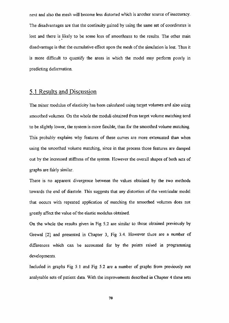
next and also the mesh will become less distorted which is another source of inaccuracy.

The disadvantages are that the continuity gained by using the same set of coordinates is

lost and there is likely to be some loss of smoothness to the results. The other main

disadvantage is that the cumulative effect upon the mesh of the simulation is lost. Thus it

is more difficult to quantify the areas in which the model may perform poorly in

predicting deformation.

5.1 Results and Discussion

The minor modulus of elasticity has been calculated using target volumes and also using

smoothed volumes. On the whole the moduli obtained from target volume matching tend

to be slightly lower, the system is more flexible, than for the smoothed volume matching.

This probably explains why features of these curves are more extenuated than when

using the smoothed volume matching, since in that process those features are damped

out by the increased stiffness of the system. However the overall shapes of both sets of

graphs are fairly similar.

There is no apparent divergence between the values obtained by the two methods

towards the end of diastole. This suggests that any distortion of the ventricular model

that occurs with repeated application of matching the smoothed volumes does not

greatly affect the value of the elastic modulus obtained.

On the whole the results given in Fig 5.2 are similar to those obtained previously by

Grewal [2] and presented in Chapter 3, Fig 3.4. However there are a number of

differences which can be accounted for by the points raised in programming

developments.

Included in graphs Fig 5.1 and Fig 5.2 are a number of graphs from previously not

analysable sets of patient data. With the improvements described in Chapter 4 these sets

70

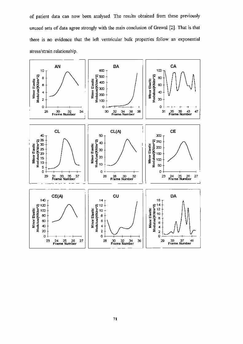
of patient data can now been analysed. The results obtained from these previously

unused sets of data agree strongly with the main conclusion of Grewal [2]. That is that

there is no evidence that the left ventricular bulk properties follow an exponential

stress/strain relationship.

BA

CA10

4

02

0 I I I28 30 32 34

Frame Number

CL4035

25

15• 10

0 I I I29 31 33 35 37

Frame Number

503

30 32 34 36 38Frame Number

CL(A)

liE:26t//f\:2

Frame Number

20

0 I I31 35 39 43 47

Frame Number

CE303

2

11: /\pico5o

0 I23 24 25 26 27

Frame Number

CE(A)140120103806040200 I Ii23 24 25 26 27

Frame Number

CU1412io

0I

4

28 30 32 34 36Frame Number

DA1614

<E 12.10

64

0 I I29 33 37 41

Frame Number

71

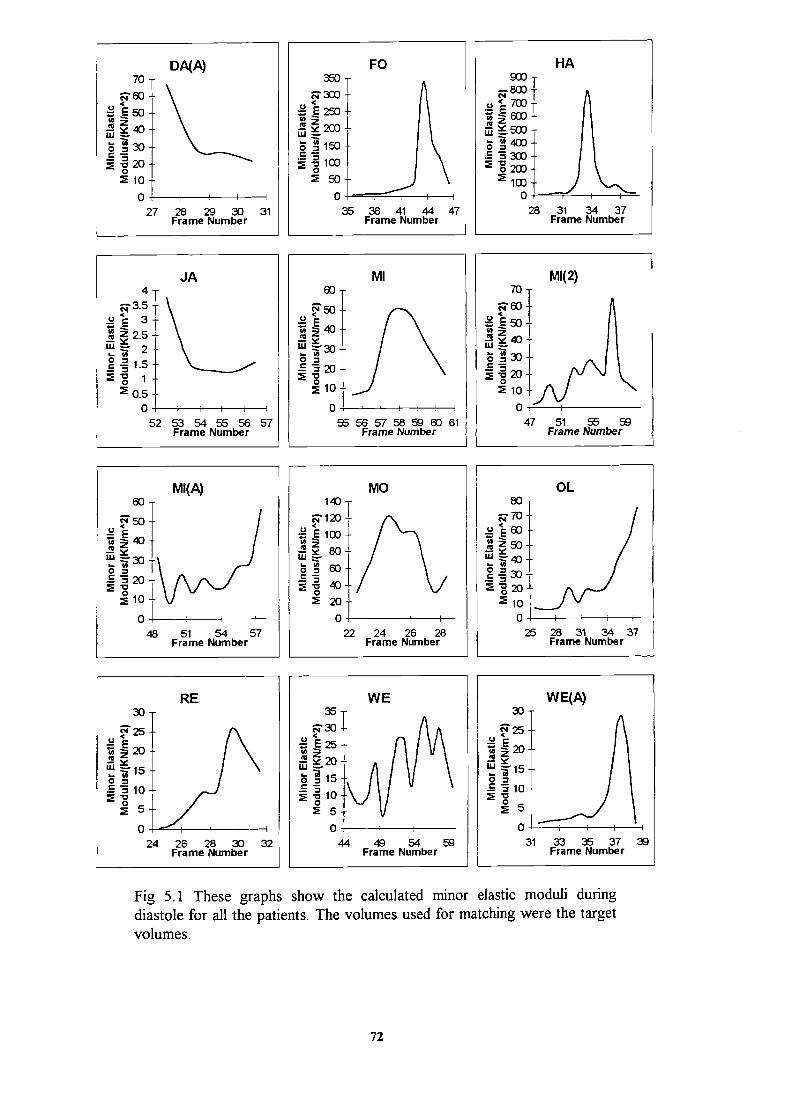
8aJ

403E 303

2 103028 31 34 37

Frame Number

DA(P4

70

Eso

1t 20

210

Oi-

47

MI(2)

51 55 59Frame Number

OL8070

E60so40

o.E5

210

025 28 31 34 37

Frame Number

70

Eso

fl4030

20

510

027 28 29 30 31

Frame Number

FO3603coI

203

160

10J

550

035 38 41 44 47

Frame Number

JA

0.50 I52 53 54 55 56 57

Frame Number

MI(A)

Frame Number

RE

MI

50

.40

30

iIlOT

55 56 57 58 59 60 61Frame Number

MO143 T

p120

. 103

U80

40

220

022 24 26 28

Frame Number

WE WE(A)30

25

20

I

.E 10

Di-

31

30

25

20-':f 15o

10

024 26 28 30 32

Frame Number

35

30

25

20

o 15

10

25

044 49 54 59

Frame Number33 35 37 35

Frame Number

Fig 5.1 These graphs show the calculated minor elastic moduli duringdiastole for all the patients. The volumes used for matching were the targetvolumes.

72

CUCE(A)

Frame Number

DA

29 32 35 38 41Frame Number

ia143

<E 120

604020023 24 25 26 27

Frame Number

FO

Frame Number

DA(P4

60

50

70

40

30

20

10

0 I I I27 28 29 30 31

Frame Number

HA7 -r

sco

4C0

o 3W

2co

1W

028 31 3.4 37

Frame Number

AN H BA 1 CA

Frame Number

CL45403530

0I

20.E 15

10

29 32 35 38Frame Number

7

<Esco

4co

3co

2c0

icx

030 32 34 36 38

Frame Number

CL(A)

Frame Number

H 40-

.2O

031 35 39 43 47

Frame Nuimber

CE260 -

2c0

50

0 I23 24 25 26 27

Frame Number

73

JA43.53

0.50 I I I52 53 54 55 56 57Frame Number

MI120ic• E 80q60. 4020

55 57 59 61Frame Number

MI(2)1GJ TN<80

o 40200 47 50 53 56 59

Frame Number

MI(A)

100 48 51 54 57Frame Number

MO140

p120

ico

ilso

0 I22 24 26 28Frame Number

OL7060*040o 30100 25 29 33 37

Frame Number

OL

;i: I15,J/\

Frame Number

WE

0E25L]\/\J\100 I I44 48 52 56 60

Frame Number

WE(A)180• E 140 +120+

.icij+80l.!5 60--4010T31 33 35 37 39

Frame Number

Fig 5.2 These graphs show the calculated minor elastic moduli duringdiastole for all the patients. The volumes used for matching were thesmoothed volumes.

74

Chapter

6. Matching Both Lenh and Volume To Derive the

Elastic Modulus Ratio

The aim of this Chapter was to gain an insight into the value of the modulus ratio, and to

discover whether there was any evidence that this value varied during the diastolic phase

To achieve this it was necessary to bring in another independent variable into the system.

Up to the present time only the volume has been matched. To allow the two elastic

moduli to vary independently, another property must also be matched, the length of the

ventricle was the property chosen for this.

Very little work has been done to determine a suitable value of the elastic modulus ratio

to be used for modelling purposes. Many authors have assumed a value of 2 for the

major to minor modulus ratio in their finite element analysis, although there appears to

be no firm evidence that this value is better than any other. A value of 2 has also been

used in the work described in Chapter 3 and Chapter 5. This value had been derived

from work done by Vinson [1] with thin shell ellipsoids and has no real connection to the

later finite element analysis, other than that the finite element analysis grew out of the

work with thin shell ellipsoids.

Work has been done by Yamada [71] on measuring the material properties of various

biological materials, including that of the myocardium of the left ventricle. In his study

small pieces of myocardium were taken from the mid-walls of the left ventricles of 61

patients. When these were tested for various material properties he concluded: "The

ultimate elongation, in the direction transverse to the course of the fibres, is about 1.3

times that in the parallel direction." This would suggest that the major and minor

modulus ratio was 1.3. However since no information on the magnitude of the stresses

75

and strains was explicitly given, or even whether the stresses in the two directions were

the same, we must therefore be cautious in assuming this ratio to be valid for this finite

element analysis, although it would seem to be the obvious conclusion. The other cause

for concern is that this muscle tissue had been removed from the myocardium and hence

results obtained may not give an adequate indication of in-vivo material properties.

Other authors have also measured the elastic modulus ratio of excised myocardial tissue.

The work of Yin et al. [62] showed that the value of this ratio could not only vary

significantly from patient to patient but could also vary from site to site within the same

heart. It was also suggested that the ratio was also history dependent. Thus the ratio

could not only vary with position within the left ventricle but could also vary with time.

This work therefore does not give any indication of what a reasonable choice for the

bulk elastic modulus ratio would be.

The effect upon the length of a ventricular model of altering the modulus ratio has been

investigated by Neckyfarow et a!. [72]. Using the averaged frame data obtained from

several cardiac cycles a thick shell solid model was produced from this composite frame.

To reconstruct the geometry from the single cine-angiography frame a circular cross-

section was assumed. The model was applied using three values for the minor to major

modulus ratio 1.0, 0.8 and 0.5. It was stated that: "with the ratio E 2fE 1 less than 0.8 the

predicted deformation agrees favourably with observed ventricle elongation." It is

important to note that the ratio referred to here is the reciprocal of that referred to

elsewhere in this text, as E 1 refers to the along-the-fibre and F 2 to the cross-the-fibre

direction. Thus the major to minor modulus ratio that was prescribed is one that is

greater than 1.3. The method used here produces in-vivo results and is thus more closely

allied to this work than that done by Yamada [71]. However there must be some concern

over the method used to average the multiple readings and align them to be at exactly

the same point in the cardiac cycle. There must also be concern that these results were

76

obtained using only single plane cine-angiography which does not give as accurate

volume information as bi-plane cine-angiography. Another concern is that the volume

obtained from the single plane reconstruction will be far more dependent upon the length

measured from the X-ray frame than is the true volume. Lastly this analysis was

performed for only one subject and it would require results from further subjects for the

result and the procedure to prove its validity.

Two independent sources using quite different methods have therefore both arrived at a

value of approximately 1.3, although the second did seem to imply that a value slightly

higher than this would give a better match with the observed ventricular behaviour The

two methods complement each other well and the value arrived at gains greater validity

because of this. However both approaches have their shortcomings when considering the

in-vivo case.

6.1 Resolving Myocardial Stiffness into Circumferential and

Longitudinal Directions

A small block of material, analogous to the myocardium in its structure was investigated

mathematically. This was to gain an understanding of the likely consequences of altering

the modulus ratio and discover how fibre angle affected the strains within the

myocardium as well as the global deformation of the myocardium. In particular this is an

attempt to investigate what effect the elastic modulus ratio has upon the stiffness of a

small element.

A small cuboid that is composed of elastic fibres was considered. Just as in the

myocardium these fibres are straight and always in a plane parallel to the two opposing

faces. The angle of the fibres to the horizontal are 600 at one face and 6O0 at the other

77

Varying fibreangle

1

A.c.k = '

E

Eqn, 6.1

face with the angle varying linearly between these two values within the cuboid (see Fig

6.1).

4

lx

Fig 6.1 This diagram shows a cuboid with a fibre angle varying linearly from60° to -60° through the depth of the block. Where, A, A, A are the areasof the three faces and l, l,, l are the lengths of the three sides.

The stiffness of a piece of material in one of the x, y, z, Cartesian coordinate directions is

given below,

Thus to find the stiffiess in the i-direction the strain in the i-direction that occurs in

response to the stress in the i-direction must be found.

The stiffness of a slice at any depth within the block in either of the x, y, Cartesian

coordinate directions will vary, provided the modulus of elasticity is not the same in the

along the fibre direction as in the across the fibre direction. A "thin" slice at an arbitrary

depth within the block was considered, the term "thin" meaning that there is no change

in fibre orientation within the slice.

78

Thin slice

Elastic fibre

Fig 6.2 This is the same block as Fig 6.1. We now consider a thin slice ofthis block at some arbitrary depth of thickness z.

This block will have the fibres running at some angle 9 to the horizontal, where 9 is in

the range -itI3, ic/3. This angle is linearly dependent upon the depth the slice is within the

block. We shall first consider the case of 9 0 and then generalise it to an arbitrary angle

by applying a transformation matrix. The slice or lamina below has the fibres running

parallel to the 2-direction and perpendicular to the 1-direction.

Fig 6.3 This shows a thin slice of material with the elastic fibres runningparallel to one of the sides. The directions 1 and 2 are the perpendicular andlongitudinal directions relative to the elastic fibres.

The material properties for a lamina such as this are given by the tensor equation.

lIE1 —v21/E2 0 a1

= —v12/E1 lIE2 0 a2

Eqn. 6.2

712 0

0 hG12 12

This equation relates the normal and shear strains in the 1 and 2-directions to the normal

stresses, the shear stresses and the material properties in the 1 and 2-directions.

79

If E2 is assumed to be related to E 1 by some ratio r then to preserve the symmetry of the

material properties matrix v21 must equal r v 12 . The above matrix equation then

simplifies to,

l/E —vIE 0 o

= —vIE 1/(Er) 0 a2 Eqn. 6.3

0 0 hG 'c12

The subscripts on the material properties can now be dropped, E 1 is replaced by E, E 2 by

Er, vu by v and v21 by rv, as there is now no need to distinguish between material

constants in the different directions.

To convert the strains from the local 1, 2-coordinate system to the global x, y-coordinate

system requires a transformation matrix. The matrix below can be deduced by resolving

forces between the two coordinate systems (Holmes and Just [73]).

cos2O

sin2 0 —sinOcosO

= s2e

cos 2 0 sinOcosO c2 Eqn. 6.4

y 2sinOcos9 —2sin0cos0 cos 2 0—sin 2 O t12

If the right hand side of tensor equation 6.3 is multiplied out and the transformation from

the local to the global coordinates is applied then the global strains can be expressed in

terms of the local stresses. The equations for the global normal strains are given below.

The global shear strain is not given, as shear deformation of the block is not being

considered in this analysis.

1sin8cos01

={(a1 - va 2 )sin 2 0+(a 2 /r- vai)cos20)+ti2sin0cos0 Eqn. 6.5

The next stage is to replace the local stresses in equations 6.5 with expressions for them

in terms of the global stresses. As with the strains there is a transformation matrix to

convert from local to global coordinates and vice versa. This matrix is similar to the one

required for the strains and is obtained in a similar manner.

80

cy 1cos20

sin2 0

2sin9Go59 cY

= sin28

cos 2 9 —2sinOCOSO a

Eqn. 6.6

712 —sinOcosO sine cosO cos2O—sin20

Equations 6.5 now become,

0— vsn 2 0)( cos2 9 + sin 2 9 +2t 1 Sin9cos9)

+ (Su12 ¶3' - vcos 2 0)(a 1 sin 2 0 + 0, cos 2 0— 2t 11 SjnO cos0)}

- ---sin 0 cos0( — sin9 cosO + sin0 cosO + 'v 1 (cos 2 0—sin 2 9))

= _-((sin 0— vcos 2 9)(c cos 2 0 + cy sin 2 0 +2'r 1 sinO cosO)

+ (CO5 2 0/ - 9)(c1 sin 2 9 + cy cos 2 0 - 2'r Sine cosO)}

+- .-sin0 cos0( — cy sinO cosO + sinO cosO + t 12,(cos 2 0—sin 2 0))

Eqn. 6.7

These two equations are unnecessarily long and can easily be simplified. If when

considering the strain in the x-direction we assume there is no stress in the y-direction

and vice versa. This will eliminate half the stress terms, almost halving the length of the

above two equations. We are also at liberty to distribute the strain over the element in

such a way that there will be no shearing in the x, y-plane. Thus the above two equations

become,

E, =54(cos4e+(1E/0_2v)sin2ocos20+sin4o/r}

= .i'{sin40+(E/0_2v)sin20cos2O+cos40/r}Eqn. 6.8

The shear modulus G is independent of the elastic modulus and the modulus ratio for all

but the isotropic case, r1, when G is given by the equation,

G= E2(1+v)

Since we are only interested at this stage with the effect of the modulus ratio and not

that of the modulus of rigidity it would seem sensible to keep its value constant while

varying the modulus ratio. Replacing the isotropic value of G into equation 6.8 yields,

81

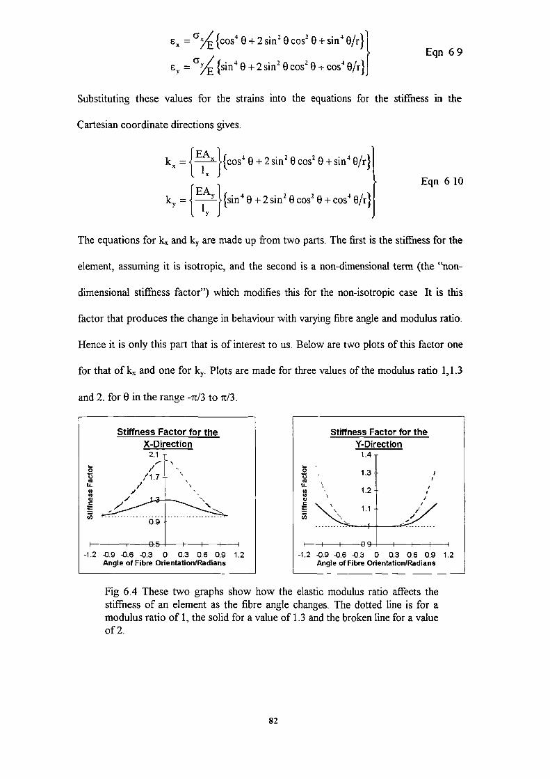
= 4{cos 9 +2sin 2 9 cos2 0 + sin 4 9/r)Eqn 69

={sin 0 + 2 sin 2 0 cos 2 9 + cos 4 Oft)

Substituting these values for the strains into the equations for the stiffness in the

Cartesian coordinate directions gives.

k = {EA }[4 0 + 2 sin 2 0 cos2 9 + sin 4 0/r}

k = { EAY }(. 49 +2 sin 2 9 cos2 9 +cos4 0/r)

Eqn 6 10

The equations for k and k are made up from two parts. The first is the stiffness for the

element, assuming it is isotropic, and the second is a non-dimensional term (the "non-

dimensional stiffness factor") which modifies this for the non-isotropic case It is this

factor that produces the change in behaviour with varying fibre angle and modulus ratio.

Hence it is only this part that is of interest to us. Below are two plots of this factor one

for that of k and one for k. Plots are made for three values of the modulus ratio 1,1.3

and 2. for 9 in the range -it/3 to it/3.

Stiffness Factor for the

Stiffness Factor for theX-Direction

Y-Direction

h-I I 00! I I

-1.2 -0.9 -06 .0.3 0 0.3 0.6 0.9 1.2 -1.2 .0.9 .0.6 .0.3 0 0.3 0.6 0.9 1.2Angle of Fibre OrientationlRadians

Angle of Fibre Onentation!Radians

Fig 6.4 These two graphs show how the elastic modulus ratio affects thestiffness of an element as the fibre angle changes. The dotted line is for amodulus ratio of 1, the solid for a value of 1.3 and the broken line for a valueof 2.

82

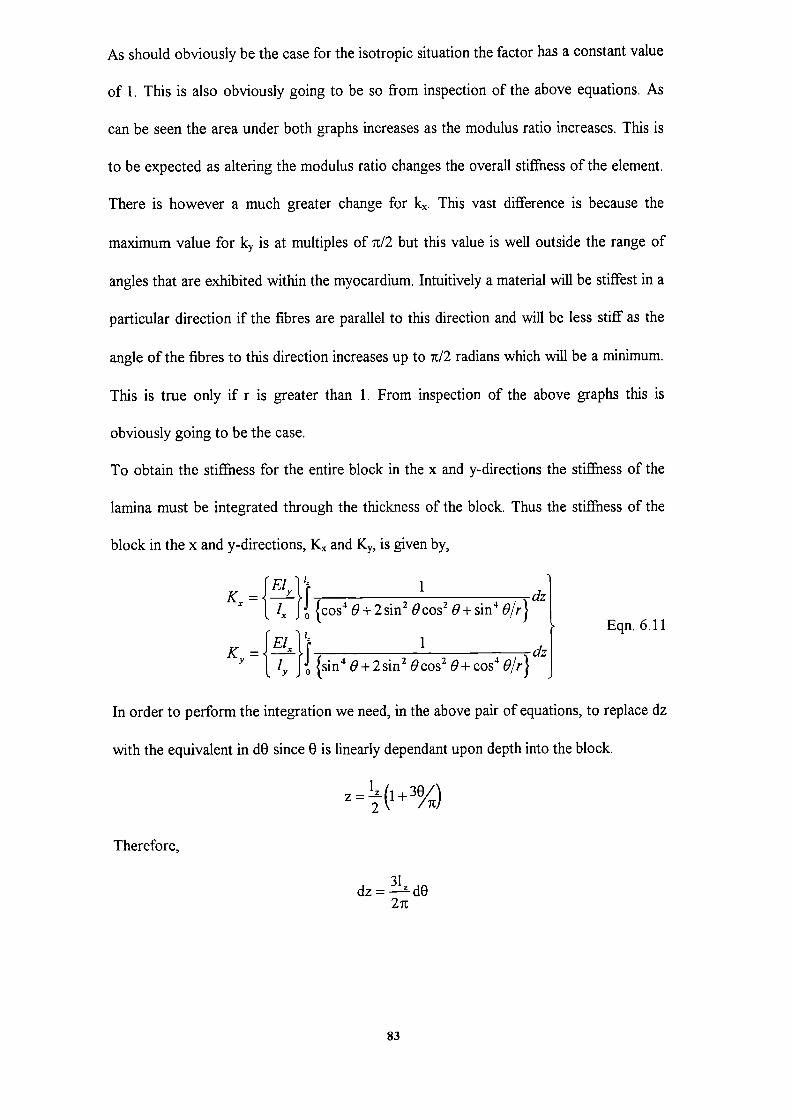
As should obviously be the case for the isotropic situation the factor has a constant value

of 1. This is also obviously going to be so from inspection of the above equations. As

can be seen the area under both graphs increases as the modulus ratio increases. This is

to be expected as altering the modulus ratio changes the overall stiffness of the element.

There is however a much greater change for k. This vast difference is because the

maximum value for k is at multiples of tI2 but this value is well outside the range of

angles that are exhibited within the myocardium. Intuitively a material will be stiffest in a

particular direction if the fibres are parallel to this direction and will be less stiff as the

angle of the fibres to this direction increases up to itI2 radians which will be a minimum.

This is true only if r is greater than 1. From inspection of the above graphs this is

obviously going to be the case.

To obtain the stiffness for the entire block in the x and y-directions the stiffness of the

lamina must be integrated through the thickness of the block. Thus the stifThess of the

block in the x and y-directions, K and K, is given by,

1El i 1dzl

= JI{cos4o+2sin29cos2e+sin4O/r} L Eqn. 6.11

x 0

1dzK

(sin49+2sin2 Ocos 2 8+cosO/r} Jy 0

In order to perform the integration we need, in the above pair of equations, to replace dz

with the equivalent in dO since 0 is linearly dependant upon depth into the block.

z=(i+3%)

Therefore,

dz = dO2ic

83

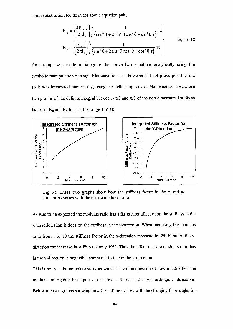
Upon substitution for dz in the above equation pair,

13E1,1 'z 1 1K= ___________________dz

2ni }{COS4e+2Sjfl2oCO52e+Sfl4eF}Eqn. 6.12

K = 1El11 I Idz I

y l2ly I{5in 4 0+2sin 2 8c0s2 8+c05 4 8 r}

An attempt was made to integrate the above two equations analytically using the

symbolic manipulation package Mathematica. This however did not prove possible and

so it was integrated numerically, using the default options of Mathematica. Below are

two graphs of the definite integral between -rc/3 and ir/3 of the non-dimensional stiffness

factor of K and K for r in the range 1 to 10.

Integrated Stiffness Factor for2.5

2A5

2.4a 2.

7ctio

u. 2.3IL. . 2.

ILl 2.2

2.15

2.t I I I

0 2 4 6 8 10Modulus ratio

Fig 6.5 These two graphs show how the stiffness factor in the x and y-directions varies with the elastic modulus ratio.

As was to be expected the modulus ratio has a far greater affect upon the stiffness in the

x-direction than it does on the stiffness in the y-direction. When increasing the modulus

ratio from 1 to 10 the stiffness factor in the x-direction increases by 250% but in the y-

direction the increase in stiffness is only 19%. Thus the effect that the modulus ratio has

in the y-direction is negligible compared to that in the x-direction.

This is not yet the complete story as we still have the question of how much effect the

modulus of rigidity has upon the relative stiffness in the two orthogonal directions.

Below are two graphs showing how the stiffness varies with the changing fibre angle, for

84

three different values of the modulus of rigidity, The value prescribed in the isotropic

case is shown by the solid line. The dotted line is for a value that is half this and the

dashed line is for a value that is twice the isotropic value. Note that Poisson's ratio is

assumed to be 0.5 and a modulus ratio of 2 is also assumed,

Stiffness Factor for the

Stiffness Factor for theX-Direction

Y-Direction

-1.2 -0.9 -0.6 -0.3 0 0.3 0.6 0.9 1.2

-1.2 -0.9 -0.6 -0.3 0 0.3 0.6 0.9 1.2Angle of Fibre OrlentationlRadians

Angle of Fibre OrientationiRadians

Fig 6.6 These two graphs show the effect that the shear modulus has uponthe stiffness of the element as the fibre angle changes. The dotted line is for ashear modulus double the normally used value, the solid line is for thenormally used value and the broken line is for a value half this.

As might be expected the effect that changing the modulus of rigidity has on the stiffness

in the x and y-directions appears to be fairly consistent, and at this stage one might be

inclined to believe that the modulus of rigidity may not be an important factor in the

relative normal strains in the x and y-directions.

Using the above three different values for the modulus of rigidity the stiffness factor for

the entire x and y faces of the block are plotted below for the modulus ratio in the range

1 - 10. It should be noted that although the plots start at a valu of 1 for the modulus

ratio, the modulus of rigidity is in reality fixed for the isotropic case. This value has been

included for comparison only.

85

Integrated Stiffness Factor for

11.4 the X-Direction10.49.4

7.4

0 2 4 6 8 10Modulus Ratio

Integrated Stiffness Factor for

4.4 the Y-DirectionU

. 3.9 - -.

1.9

1.4 I I I

0 2 4 6 8 10Modulus Ratio

Fig 6.7 These two graphs show how much effect the modulus of rigidity hasupon the stiffiess in the x and y-direction compared to the effect of themodulus ratio.

The increase in the value of the stiffness factor in the x-direction when the modulus ratio

increases from 1 to 10 varies between 209% and 298% for the three values of the

modulus of rigidity. In the y-direction for the same values the increase is in the range 8%

and 45%. Thus the modulus of rigidity has a greater relative effect upon the stiffness in

the y-direction than that in the x-direction. However this is unlikely to be of any

importance as the overall effect of the modulus ratio in the x-direction is still going to be

extremely dominant when compared to that in the y-direction.

The other thing to note is that when the value for the modulus of rigidity is changed it

has a greater effect upon the stiffness in both the x and y-directions than the same change

in the modulus ratio. This is most obvious in the y-direction where the effect the

modulus of rigidity has is far greater than that of the modulus ratio. In the x-direction the

effect of both parameters is of the same order although the effect of the modulus of

rigidity is still slightly greater.

At first glance this analysis may appear far removed from the original left ventricle

problem, since the ventricle has a complex geometry and is not composed of vertical

rectangular elements. However most of the ventricle's surface is approximately vertical.

86

At the apex, where this is patently untrue the myocardium is exceptionally stiff and any

strains here are likely to be negligible compared to those within the rest of the ventricle.

The above results suggest that there will be little or no direct effect upon the ventricle

length when changing the modulus ratio and that the greatest effect on ventricular

expansion in altering the modulus ratio will be in the circumferential direction. The

above results also suggest that the modulus of rigidity can have a significant effect upon

normal strains and that a poor choice for a value for this parameter may greatly affect

results when attempting to match ventricular volumes during diastole.

6.2 Initial Investigation into the Effect of Altering the Modulus

Ratio

An initial investigation into the effect which altering the modulus ratio has upon the

volume and length of our ventricular model was undertaken. The volume matching

process was applied to the first frame of diastole for one patient using values for the

modulus ratio in the range 0.5 - 6. Below are four graphs; Fig 6.8 shows the calculated

length against the modulus ratio for constant minor modulus, Fig 6.9 shows the

calculated volume against the modulus ratio for constant minor modulus, Fig 6.10 shows

the length of the ventricle after the volume has been matched to that of the second frame

in diastole and lastly Fig 6.11 is the same as Fig 6.10 except that the range of the

modulus ratio is much greater. The graphs were produced using ita from frames 33 and

34 of patient "BA". The initial value chosen for the modulus is 30 KN/m 2 and the

pressure increase between the two frames is 1.39 mm Hg.

87

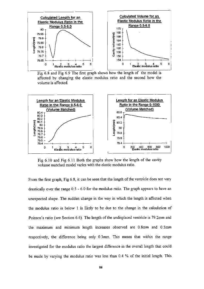
1 2 3 4 5 6Elaic modulus ratio

Calculated Length for anElastic Modulus Ratio in the

Range 0.5-6.080

79.9579.9

79.85

, 79.8

.79.7579.7

79.650

Calculated Volume for anElastic Modulus Ratio in the

Range 0.5-6.0170168

164162

158-' 156

1540

1 2 3 4 5 6EIaic modulus ratio

Fig 6.8 and Fig 6.9 The first graph shows how the length of the model isaffected by changing the elastic modulus ratio and the second how thevolume is affected.

Length for an Elastic ModulusRatio in the Range 0.5-6.0

(Volume Matched)80.480.380.2

E 80.180

79.979.879.779.679.579.4

0

1 2 3 4 5 6E1aic modulus ratio

Length for an Elastic ModulusRatio in the Range 0-1000

(Volume Matched)80.6

80.4

80.2

80C,

79.8-J

79.6

79.40 20) 40) O 80) 1 COO

Eiaic modulus ratio

Fig 6.10 and Fig 6.11 Both the graphs show how the length of the cavityvolume matched model varies with the elastic modulus ratio.

From the first graph, Fig 6.8, it can be seen that the length of the ventricle does not vary

drastically over the range 0.5 - 6.0 for the modulus ratio. The graph appears to have an

unexpected shape. The sudden change in the way in which the length is affected when

the modulus ratio is below 1 is likely to be due to the change in the calculation of

Poisson's ratio (see Section 6.6). The length of the undisplaced ventricle is 79.2mm and

the maximum and minimum length increases observed are 0.8mm and 0.5mm

respectively, the difference being only 0.3mm. This means that within the range

investigated for the modulus ratio the largest difference in the overall length that could

be made by varying the modulus ratio was less than 0.4 % of the initial length. This

88

agrees strongly with the findings of section 6.1 which suggested that altering the

modulus ratio would have little direct effect upon the calculated length of the ventricle.

The second graph, Fig 6.9, shows the volume of the ventricle calculated with a minor

elastic modulus of 30 KNIm2. The volume decreases in an exponential manner as the

modulus ratio increases. The volume decrease, in going from a modulus ratio of 0.5 to

one of 6.0, is 14.8 cm3 . This is an 8.7 % decrease in volume over this range. Thus the

effect upon the volume of altering the modulus ratio is in excess of an order of

magnitude greater than the effect it has upon the ventricle length, again supporting the

analysis of Section 6.1.

The third graph, Fig 6.10, shows the length of the ventricle after the minor modulus has

been adjusted to ensure that the volume matches that at the next frame. As the modulus

ratio increases, the curve appears to approach an asymptote at just under 80.5mm.

Therefore the length of the ventricle cannot be matched with a length greater than this by

consideration of the value of the modulus ratio alone. It is also worth noting that if a

length match is required near to the maximum achievable value, then the modulus ratio

would be extremely sensitive to the accuracy of the measured length of the ventricle.

The fourth graph, Fig 6.11, shows how the length of the volume-matched ventricle

varies as the modulus ratio becomes large. At first glance this may appear to be strange

and unexpected behaviour. The length increases to a maximum after which it reduces

slightly and then levels out to a plateau. This is entirely consistent and predictable with

the findings of Section 6.1. When the modulus ratio is small and then increased slightly

the greatest effect is in the circumferential direction and when the volume is matched the

length of the ventricle is increased. On the other hand if the modulus ratio is large then

the ventricle is almost rigid in the circumferential direction, and changes to the modulus

ratio will have little effect upon the stiffness in this direction. The longitudinal direction

however may still be far from rigid and can be affected by changes in the modulus ratio.

89

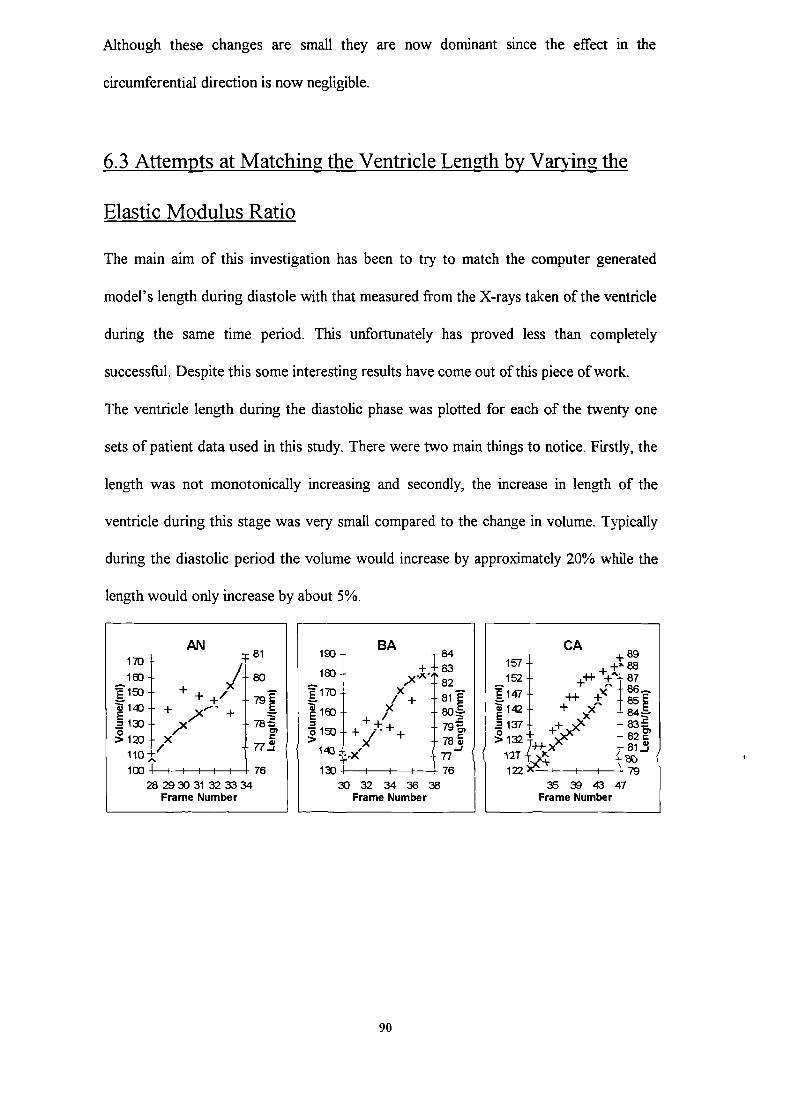
157

152E 147

142

. 137132

2T122

Although these changes are small they are now dominant since the effect in the

circumferential direction is now negligible.

6.3 Attempts at Matching the Ventricle Length by Varying the

Elastic Modulus Ratio

The main aim of this investigation has been to try to match the computer generated

model's length during diastole with that measured from the X-rays taken of the ventricle

during the same time period. This unfortunately has proved less than completely

successftil. Despite this some interesting results have come out of this piece of work.

The ventricle length during the diastolic phase was plotted for each of the twenty one

sets of patient data used in this study. There were two main things to notice. Firstly, the

length was not monotonically increasing and secondly, the increase in length of the

ventricle during this stage was very small compared to the change in volume. Typically

during the diastolic period the volume would increase by approximately 20% while the

length would only increase by about 5%.

AN

17D-L61

180 1 /180

180-1- ++/79+

2 130 + I78

>120+XI

iiof'1 I I I I 76

28293031 323334Frame Number

BA180 84180 +1183

17D X

x1+ 81

T +' -I-79,)( + I> +78w

I _i4-77

130-I- I I 7630 32 34 36 38

Frame Number

CA+89

+8867

^± 85+ 84

1 I 79

35 39 43 47Frame Number

90

939291go-898867868584

76

75

72_i

CL2cc

.,c.).+

180 ++

>170 +1 + +

I I I29 31 33 35 37

Frame Number

180CE(A)

76

1701 A,4 T75.+ x I

+1434- X 74

> 1/ U-I13J

120 I 7323 24 25 26 27

Frame Number

D/)76I

+75

7174

icox

72

90 71C,

Ux-_

Iji 70_1

60+ I I 6927 28 29 30 31

Frame Number

A

ico 2< 72

90 /X 71,

7D.

70111 6952 53 54 55 56 57

Frame Number

243 CL(A)

233220

. 2102co190

0> 180170180

26 28 30 32Frame Number

110+ +

+ 7.:

E90 X'

>

701 I I 7128 30 32 34 36

Frame Number

FO

72

180+70

'-F ++++68!

65> +i+

if 67

80xx+I

I 6634 37 40 43 46

Frame Number

MI180 T85

*87

486+

+^"'

I+vx-+ I

>130 T / +83

+)< 152

l 20 )< I 8155 57 59 61

Frame Number

CE210-

+2cc-'-

x_-x+

>185, + U/

+—j

180 7623 24 25 26 27

Frame Number

DAicx J7290

+ X71

+ +++ 70

6867

+ -f-65SOt I 1 64

2931333537304143Frame Number

HA143 82

1301[1f81

.120! +++I80

.xPo)<A

j79

Lio + + J_78^

>lcDJi77

901I j76_i

75283032343638

Frame Number

180 +88

671SoT 86

>130 Jxx+ 183:•14D

84++ ,

+ +++ + 4821201+1 +1 81

47 50 53 56 59Frame Number

919089

6887

86

8584

91

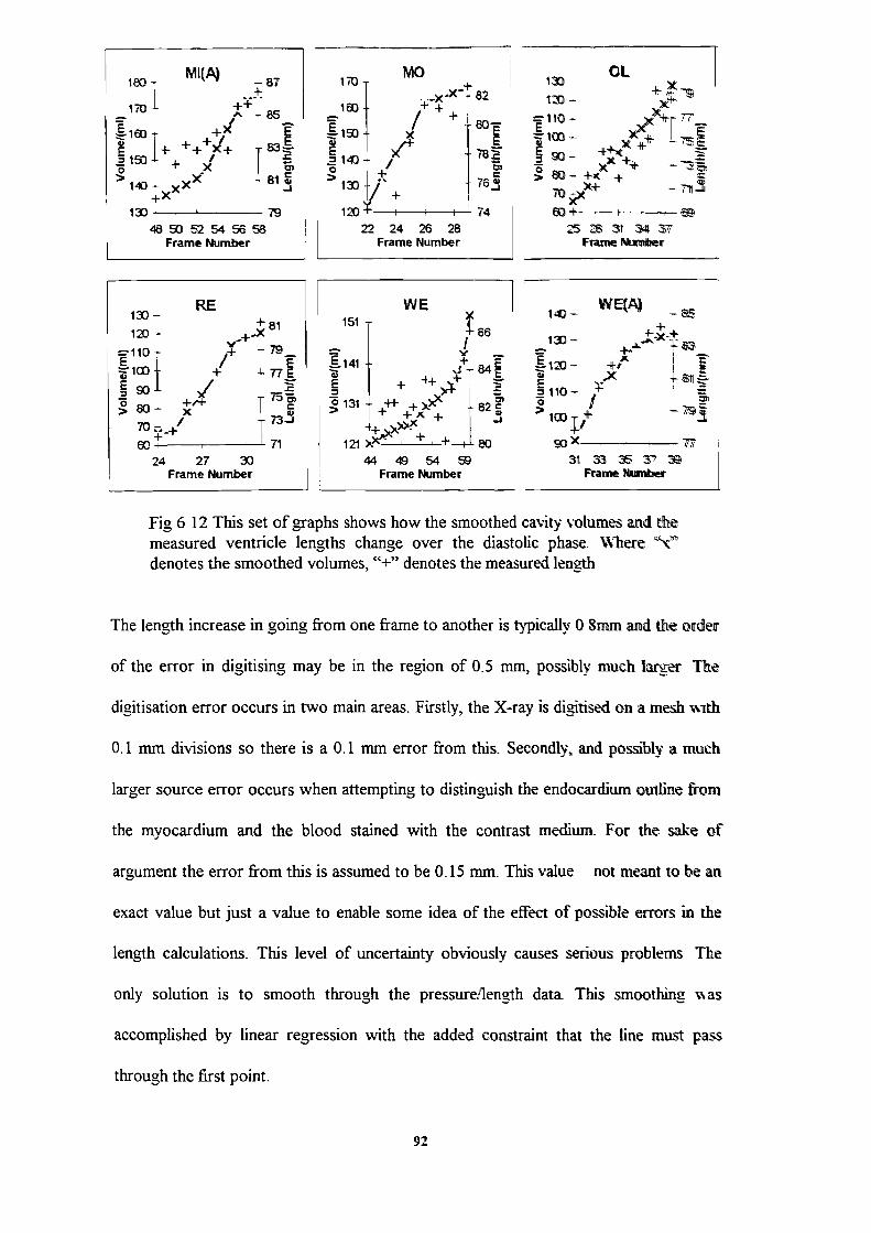
160- MI(A)

170

+

E j+.2 1w +o X

14xx

133

7952545658

Frame Number

RE+ 81

133- +_x=110- + -79

..1co /- + L77E

/80-70- / 73_I

^ TeTi_ 7124 27 3)

Frame Number

MO170

1601X+82

I14J 78

- /o +

L/ +133+ '74

22 24 26 26Frame Number

WE

151 1 s6I

V

I

+ 4+)

O 131 4+> + +>^

-62

121X I

444954Frame Number

CL133 x-

=110- 77

+ioxx+60+ F

25 26 31 3 377Frame &nther

143- WE(A)

133-

L33- +

11O-I

>1cx7

3126Frame NUther

Fig 6 12 This set of graphs shows how the smoothed cavity volumes and themeasured ventricle lengths change over the diastolic phase. Wheredenotes the smoothed volumes, "+" denotes the measured length

The length increase in going from one frame to another is typically 0 8mm and the order

of the error in digitising may be in the region of 0.5 mm, possibly much larger The

digitisation error occurs in two main areas. Firstly, the X-ray is digitised on a mesh with

0.1 mm divisions so there is a 0.1 mm error from this. Secondly, and possibly a much

larger source error occurs when attempting to distinguish the endocardium outline from

the myocardium and the blood stained with the contrast medium. For the sake of

argument the error from this is assumed to be 0.15 mm. This value not meant to be an

exact value but just a value to enable some idea of the effect of possible errors in the

length calculations. This level of uncertainty obviously causes serious problems The

only solution is to smooth through the pressure/length data This smoothing vas

accomplished by linear regression with the added constraint that the line must pass

through the first point.

92

Diastolic Lengths and Linear84 Regression83

82

81 +

80D +

79 • +I +

78 +

+

-1.6 1.4 4.4 7.4 10.4Cavity Pressure! (mm!Hg)

Fig 6.13 This graph shows how the pressure/length data for patient "BA" issmoothed through using linear regression.

Linear regression was used since, as the length increase was small and the possible

digitisation errors were relatively large, it would have been difficult to justify any other

form of smoothing for the data. It was also the easiest way to ensure that the smoothed

lengths for the matching process were always monotonically increasing.

The volume matching process was then applied to the first frame of each patient with

various modulus ratios in the range 0.25 - 2.0.

1.9

AN1.2

1

w 0.8.1wo

0.6uJ

0.4

0.2

0.9 1.4Modulus Ratio

BA0.36

0.3 ++

0.25 +WO

u. 0.15 +W

.1+U o.c

0 I

0.4 0.9 1.4 1.9Modulus Ratio

CA0.365 +

0.36

0.365 +

0.36

0.345

0.34 ++0.5 +0.3 I I I-I

0.4 0.9 1.4 1.9Modulus Ratio

CL

0.14 +

. 0.12C, +

0.1-I.-

+

0.06 +

0.04

0.02+

0 I I

0.4 0.9 1.4 1.9Modulus Ratio

CL(A)0.3

++0.1

+ +U

0.06 +0.

+0

0.4 0.9 1.4 1.9Modulus Ratio

CE0.3

0.25 ++C, +

0.2 +

+LU +

0.1

0.06

0.9 1.4 1.9Modulus Ratio

93

CuCE05 +

+ +0.4- ++

0.9 14 1.9Modulus Ratio

DA*

004- +

2W002- + +

001- +0

04 9 114 119Modu'us Ratio

D41.78 y1.76k

' 1.74- ^. j ._172-wo -

uj

1.- +

1.- +o. 1.64- +

0.4 0.9 14 1.9Modulus Ratio

JA

014- +0.12-

0.1- +

; 0cB-

006- ±0.04-- + +0.02-

0_±0.4 0.9 14 1.9

Modulus Ratio

FO0. J+ + + + + +

.i 0.07

0.060.c50.04o.a30.02

0- 0.01

00.4 0.9 1.4 1.9

Modulus Ratio

MI0. T+

0.3 ++

0.25 ++

0.15 +

0.1

0 I0.4 0.9 1.4 1.9

Modulus Ratio

HA018 -+

• 0.16-0.14-0.12- +01-

' 1 0c2-ff + +0G6-004-

0 +002- +004 09 114 119

Modulus Ratio

03 -++

025- '+a, +0 02-_l -00 +

u.I2W

01-0

09 14 19Modulus Ratio

MI(2)0.07- +

.= 0.06-

' o.-t-

0.041- +++

u.i 0.3

0.021

a 0.01.F +ol I

0.4 0.9 1.4 1.9Modulus Ratio

MO1.4 T

. 1.2.i+0,

1 +0.8 +

' i 0.6

0.4 0.9 1 +Modulus Ratio

OL0.5 --

^

': ++^

+

00.4 09 14 19

Modulus Ratio

94

RE-

02 +

+

2LU 01-C I+

0f +a. +o-04 09 114 19

Modtilus Ratio

CE O07

006- +

i +

ow- +0- +

a. OQ-

GA 09 14 19Modu'us Ratio

09

+

+

02-011- +

004 09 119

atha

Fig 6 14 These graphs show the percentage absolute error betieencalculated length of the model and the target value obtamed by hiiarinterpolation.

The results from this appeared to suggest that a modulus ratio of between 015 - 1125

would allow a length and volume match for most of the patients The length as

matched to the target length obtained from linear regression of the pres relength data

When an attempt was made to try to match subsequent frames,, using the length and

volume matched ventricle geometry, this became impossible, as the length wireases

necessary to achieve a match could not be attained. The early lo values for the modulus

ratio were artefacts generated as a result of smoothing through the pressure length data

6.4 Start and End Frame matchin_g

It is obvious that the errors that occur in the process of digitisation make It impossible to

obtain meaningful values of the modulus ratio between each frame of diastole An

attempt was made to match the volume and length of the first frame of diastole with that

of the last frame. In doing this the lack of accuracy in digitising become much less

significant since the length increase would become greater than the assumed error in the

lengths due to digitising. Table 6.1 shows the values of the major and minor elastic

moduli plus the modulus ratio for the diastolic start and end frames.

95

Patient Minor Modulus Maior Modulus Modulus RatioAN 6.90 7.30 1.06

BA 2954 9977 3.38CA________________ Not Possible _______________CL 1132 2263 200CL(M 4.21 92.70 2202CE 899.76 9.00 001CE(A 205 75 88 23 0 43CII 7.37 10.46 0.27DA 326 4.62 1 42DA(A 1018 81.43 800FO 1275 38.47 302HA 1795 97.23 5.42JA________________ Not Possible _______________MT________________ Not Possible _______________MT(A ________________ Not Possible _______________M1(2 ________________ Not Possible _______________MO________________ Not Possible _______________01. 6.09 5126 842RE________________ Not Possible _______________WE_________________ Not Possible ________________WE(M 2.91 7.28 2.50

Table 6.1 Effective elastic moduli for the complete diastolic period withventricular length matched.

As can be seen from the table there is a large spread in the results, the highest value for

the modulus ratio being 22.02 and the lowest 0.01. It was not possible to obtain results

from patient data "CA", "JA", "ivll", "IV[I(A)", "PvlT(2)", "RE", and "V.E" since the

lengths to be matched were not in the range of values that could be achieved by altering

the modulus ratio. The mean value from the above data is 4.5. This is somewhat higher

than the traditionally assumed value of 2, and the standard deviation is 5.7.

It is important to remember that results obtained are liable to be skewed towards higher

values for the modulus ratio, since errors that require the ventricle to be increased in

length more than necessary will cause the modulus ratio to increase far more than the

reverse would cause the modulus ratio to be reduced. Thus a value of 2 or even 1.3 may

not be a totally unreasonable estimate for the value of the modulus ratio. Unfortunately

without far greater accuracy in data acquisition it is not possible to gain meaningful

values for the modulus ratio.

96

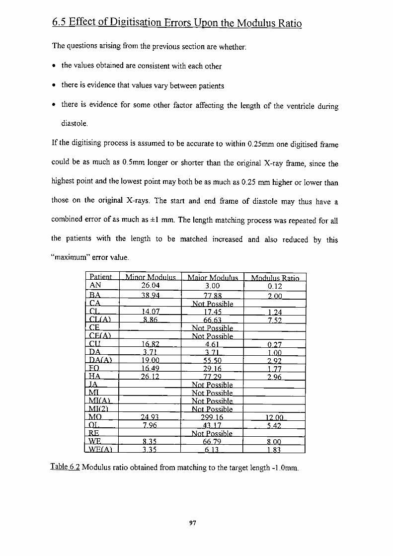
6.5 Effect of Digitisation Errors Upon the Modulus Ratio

The questions arising from the previous section are whether:

• the values obtained are consistent with each other

• there is evidence that values vary between patients

• there is evidence for some other factor affecting the length of the ventricle during

diastole.

If the digitising process is assumed to be accurate to within 0.25mm one digitised frame

could be as much as 0.5mm longer or shorter than the original X-ray frame, since the

highest point and the lowest point may both be as much as 0.25 mm higher or lower than

those on the original X-rays. The start and end frame of diastole may thus have a

combined error of as much as ±1 mm. The length matching process was repeated for all

the patients with the length to be matched increased and also reduced by this

"maximum" error value.

ThkJ6.2 Modulus ratio obtained from matching to the target length -1.0mm.

97

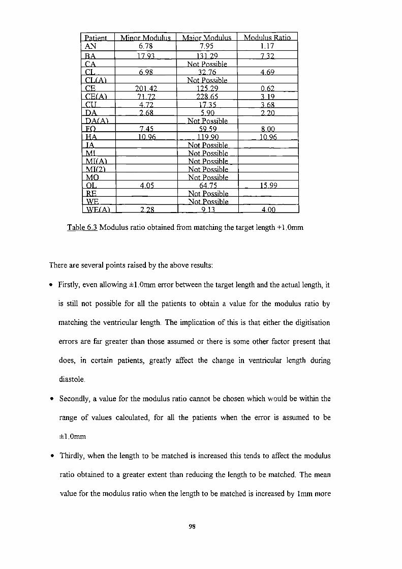
Patient Minor Modulus Major Modulus Modulus RatioAN 6.78 7.95 1.17BA 17.93 131.29 732CA_______________ Not Possible _______________CL 6.98 32.76 4.69CL(M ________________ Not Possible _______________CE 201.42 125.29 062CE(A 71.72 228.65 3 19CU 472 1735 368DA 2.68 5.90 2.20DA(M _______________ Not Possible ______________FO 7.45 59 59 8 00HA 10.96 11990 10.96TA_____________ Not Possible _____________MT_______________ Not Possible _______________________ _______________ Not Possible _______________________ _______________ Not_Possible _______________MO_______________ Not Possible _______________01. 4.05 6475 15.99RE_______________ Not Possible _______________WE_______________ Not Possible _______________WE(A 228 913 400

Table 6.3 Modulus ratio obtained from matching the target length +1.0mm

There are several points raised by the above results:

• Firstly, even allowing ±1.0mm error between the target length and the actual length, it

is still not possible for all the patients to obtain a value for the modulus ratio by

matching the ventricular length. The implication of this is that either the digitisation

errors are far greater than those assumed or there is some other factor present that

does, in certain patients, greatly affect the change in ventricular length during

diastole.

• Secondly, a value for the modulus ratio cannot be chosen which would be within the

range of values calculated, for all the patients when the error is assumed to be

±1.0mm

• Thirdly, when the length to be matched is increased this tends to affect the modulus

ratio obtained to a greater extent than reducing the length to be matched. The mean

value for the modulus ratio when the length to be matched is increased by 1mm more

98

than doubles from 3.0 to 6.5. When the length to be matched is reduced by 1mm the

mean modulus ratio becomes 1.8. Note that to calculate these mean values only those

patients for which a value for the modulus ratio could be obtained in all three cases

are used. This is a further indication, that when obtaining a mean value for the

modulus ratio, there is a tendency for the value to be an overestimate, as errors that

result in an increase in the length to be matched have a greater effect than those that

result in a decrease.

6.6 Programming Enhancements

It was necessary to make several changes and extensions to the computer program above

and beyond the obvious ones needed for the inclusion of the length matching process.

The data required for the finite element calculations are all stored in the file "XL1-data".

The major and minor elastic moduli are stored here rather than the minor modulus and

the modulus ratio. In order to represent more accurately the modulus ratio, the accuracy

to which these values are stored was increased from five to seven significant figures. The

format that the pressure values are stored in was also changed to allow for larger

pressure increases between matched frames. This was required when matching start to

end diastolic frames.

Since the material properties matrix must be symmetric it is necessary for two of the

Poisson's ratios to be equal to the other divided by the modulus ratio. Either, one can

have its value fixed and the other two set to that value divided by the modulus ratio or,

two are set to some value and the other is given this value multiplied by the modulus

ratio. Originally in the program the former of these was used. There are however

constraints upon what values Poisson's ratio can take. For instance it cannot be greater

99

than one in absolute magnitude. Another constraint is that they must also satisfy the

below inequalities,

v12vv31 <!(l - v12 v21 - vv32 - v3v3) 12 2

In order for these inequalities always to be true, it is necessary, when the modulus ratio

is below 1, for the cross-fibre Poisson's ratio (v 31) to be set and the two along-fibre

Poisson's ratios (v 12 and v) to take this value multiplied by the modulus ratio Thus the

computer program has been altered to calculate the Poisson's ratio in the appropriate

manner depending upon the value of the modulus ratio. It may seem strange that the

modulus ratio should be below 1, since this would be extremely unusual for a fibred

material, where the along-fibre elastic modulus is usually greater than the cross-fibre

modulus. However in this analysis a value below 1 is sometimes needed when attempting

to match the ventricular length. From experimentation it has also been shown that some

specimens of myocardium appear to possess a modulus ratio below 1 (Demer and Yin

62]).

Two new subroutines were necessary to perform the length matching process A

subroutine "SMOOLEN" returns an array containing the target lengths for each frame. If

start to end diastolic frame matching is being performed then only the length at end

diastole is returned in the array. The length matching process is performed by the

subroutine "LENMATCH", this routine returns the value for the next estimate of the

modulus ratio and also tests for convergence. The method used t obtain the next

estimate of the modulus ratio was a linear step method followed by quadratic

interpolation. This was found to be significantly faster than a linear step method followed

by a Fibonacci search. The quadratic interpolation is of most use when matching lengths

frame to frame throughout diastole, as this method is extremely effective at minimising

the difference between calculated and target length. Though this was not possible with

100

the data used at present, it has been kept as an option in the hope that more accurate

data may be obtained in the future allowing this process to be used.

6.7 Conclusions

The main conclusion of this Chapter is that, in order to ascertain whether the modulus

ratio is constant or varying through the diastolic cycle and what value or range of values

it takes, far greater accuracy in the digitisation is needed. The most important points for

the length and volume matching process are the base and apical points. An increase in an

order of magnitude for the accuracy of these points should be sufficient to enable length

and volume matching to a reasonable tolerance. This is not a simple task since most of

the error here is likely to be due to the fact that the ventricular outline is difficult to

distinguish from the X-ray data. However with the advances in powerful imaging

techniques such as Magnetic Resonance Imaging, this may no longer be the problem that

it was a few years ago. Magnetic Resonance Imaging has become a more frequently used

tool in recent years as it has several advantages over more traditional methods such as

ultrasound and X-rays.

There is also the possibility that the modulus ratio may not be the only or even the most

significant factor contributing to the ventricle length. It may also be the case that

pericardial pressure may significantly affect the way in which the ventricle lengthens

during diastole. In a paper written by Han et a!. [39J it was suggested that pericardial

pressure played a significant role in ventricular performance during diastole and to

completely ignore this would be detrimental to any model. The pericardium and parietal

pericardium may also restrict ventricular expansion in a non-uniform way.

From equations 6.12 it would also appear that the shear modulus may be more important

to global ventricular deformation than the value of the modulus ratio.

101

To summarise:

. Without extremely accurate length information, a tolerance of below 0.1mm should

be sufficient. It is not possible to obtain accurate values for the elastic modulus ratio

by matching both the length and volume of the left ventricle.

Also the likely significance of pericardial pressure on the length change of the

ventricle could not easily be qualitatively or quantitatively assessed without more

accurate data.

. It may also be the case that the modulus ratio is not a dominant parameter in the

global deformation of the left ventricle.

102

Chapter 7

7. Inclusion of Muscle Fibre Contraction

In this Chapter we are now looking to expand on our model. In the past, from a

structural point of view, the myocardium had almost always been treated as passive. This

is widely accepted to be a reasonable model for determining the diastolic properties of

the myocardium, as during diastole the ventricle can be assumed to be completely

passive, i.e. it deforms under an increase in internal pressure. This assumption is not

applicable when one wishes to investigate the left ventricle in systole. Here the

myocardium generates internal stresses by the contraction of the muscle fibres. The net

result of this is that the cavity volume decreases even though the cavity pressure

increases. This is a situation which cannot possibly be accounted for without the

introduction of some active contraction mechanism into the model.

To simulate left ventricular systole the finite elements must be able to simulate the

contraction of the myocardium. That is, the finite elements must shorten along the

direction of the muscle fibres and must widen in the cross fibre direction. The method to

be used here to simulate self activation of cardiac muscle is that proposed by Rosen

(1968 [74]). This involves an analogy with that of thermal stressing, where internal

strains in a structure are generated in response to a change in temperature. In order to

simulate the contraction in the fibre direction and the corresponding thickening of the

fibre it is necessary for the pseudo coefficients of thermal expansion to have opposite

sign in the fibre direction and the across fibre direction. An implementation of this

pseudo thermal method had previously been made by Kwak et a!. (1977 [75]) and it was

anticipated that, with some extension, their program known as "GTQSA" could be used

in the systolic analysis of the available patient data.

103

7.1 Revival of the FE Program "GTQSA

The program developed by Kwak et a!. [75] had several features which made its use in

this work desirable. Firstly, it included the needed thermal stressing type activation code.

Secondly, it had built in stability analysis and thirdly, it had significantly greater

documentation than did the presently used finite element code. It did however have

several drawbacks; the program was only available in the form of a listing in the

appendix of the report. This had previously been typed up from this into an electronic

form, although as is to be expected it contained many typographical errors. Secondly, it

did not include the varying fibre angle through an element or even the ability to specif,r

fibre direction in local coordinates. The fibre direction could only be described in terms

of the global coordinate system. Thirdly, the program gave only the ability to specify

elements of hexahedral topology, whereas specification of the apex of the ventricle

requires wedge shaped elements. Despite these drawbacks this program was considered

to be the best choice, as future development would be more easily accomplished due to

the availability of documentation for the program.

The problem of typographical errors would be a major task to eliminate. The situation

was made worse due to the poor quality reproduction of the program listing within the

report. The difficult task of tracking down the typographical errors was begun by

compiling the program using the "-u" and "-C" options of the SunPro Fortran compiler.

The "-u" option turns off implicit typing of variables. Implicit typing of variables is a

process whereby the type of variable, either integer or real, is decided by the first letter

of the variable's name. The use of implicit typing is a false economy as it makes it easy

for typographical errors in variable names to go unnoticed. The net result of using this

option is that error messages for non-declared variables are reported at compilation. This

makes it relatively easy to track down typographical errors in variable names, that is of

104

course provided the misprint is not itself a valid variable name. Implicit typing of

variables had been used by the author in the program so it was first necessary to

explicitly declare all variables.

The use of the "-C" option gives compilation errors or run time errors for arrays when

the subscripts of an array are not within their defined limits. It should be noted that

subscripts attached to an undefined array automatically give a compilation error.

Once all the compilation errors had been removed it was necessary to devise a simple

test element that could be used to find the more obscure typographical errors. The most

simple element that the program could accept was of an 8-noded isoparametric brick

type. After a number of further corrections, mainly to the calculation of the shape

functions, the program was able to calculate the nodal displacements for this element

subjected to thermal stress and mechanical loading. The program allowed the

specification of an even number of nodes per element within the range 8 to 20. Elements

with 12 and 14 nodes were also tested and found to give the expected values. These

elements were tested next as there were results within the report obtained using elements

of these types.

Contained within the report were some tabular results from the application of the

program to a two layer eight element orthotropic cylindrical model. The data file for this

was contained within the report, although it was not fully readable. With the aid of a

description of the model and a description for the using the program a complete data file

was produced. The program appeared to run correctly and the results were of the

correct order of magnitude. They did not however correspond to the values given within

the report. The situation was made more uncertain as the description of the cylindrical

model and the material properties used did not correspond to those in the data file given

in the report's appendix. Despite painstaking subroutine by subroutine checking and the

105

correction of several further errors the situation was not rectified. It was obvious that a

different approach would be required.

The report contained a test model used to show that the finite element program worked

correctly. This took the form of a cylinder identical to the above with the exception that

it was isotropic and was only subjected to an internal load. This model could be easily

solved using the previously used F.E. program "XL 1". The advantage of this is that the

values of the variable at each stage of calculation could be compared between "GTQSA"

and "XL 1" and the point at which these values diverged would signify where the bug lay.

Upon running this isotropic model it was immediately evident that there was a problem,

the results from "XL1" for the radial expansion agreed with those of the report however

the length reduction did not. The report gave the length reduction as 0.1mm whereas

"XL1" calculated the length reduction as 0.3mm. It was necessary to seek indepen%ent

validation as to which value was correct. Consulting Roark and Young [76] the analytic

solution was found to be 0.3 mm.

In the light of these revelations it seemed unwise to continue further with a program that

was still not fully working and there were now some doubts over its accuracy. Despite

the fact that over four months had been spent working on this program not all the 1ime

had been wasted as a greater understanding of the implementation of thermal

stressing/muscle contraction had been gained.

7.2 Adaptation of F.E. Program XL1

With the failure of the finite element program, "GTQSA", to perform as expected it left

adaptation of the originally used finite element program, "XL 1", as the next course of

action. From the work with "GTQSA" it had been realised that inclusion of thermal

stressing was relatively straight forward. It required the nodal forces that resulted from

106

the simulated muscle contraction being calculated and added to the passive mechanical

forces due to internal pressure loading. The solution of the finite element problem then

continues as before with the forces, derived from the simulation of muscle contrathon,

being treated as though they were ordinary passive nodal forces.

The only alteration to the finite element program that was necessary was to create

subroutines that would calculate the forces generated by the muscle contraction The

calculation of the force generated by muscle contraction is described below with a more

detailed description available in Chapter 8.

7.2.1 The Calculations Required For Muscle Contraction

The method used to simulate muscle contraction is computationally identical to

anisotropic thermal stressing. The reasoning behind this approach and the calculations

that are necessary for this are explored below.

In thermal stressing a piece of material is subjected to a thermal load, either a

temperature increase or a temperature decrease. The result of this is that the material will

generate internal stresses due to differential deformation. The stress/strain equation for a

one dimensional fibre is given below.

a=E(s—aT) Eqn.7.1

The working for the case of a two dimensional lamina is performed by Rosen [74. Here

however we shall content ourselves with the one dimensional case at this stage. In

muscle contraction the stresses are generated within the muscle fibres by the shortening

of the sarcomeres. We shall assume that there exists a function, F(t), that gives the strain

produced, with time, by a piece of contracting muscle. The stresses generated within the

myocardium in general will be partly due to this contraction and partly due to pressure

from the blood within the ventricular cavity. An equation representing this process is

given below.

107

a = E( - F(t)) Eqn. 7.2

In practice the function F(t) which gives the strain rate of a muscle fibre depends on

many physiological and historical factors relating to the fibre. But in this case we are

only concerned with propagation of strain with time and not the other contributing

factors.

Both equations are relatively similar and even though F(t) is an unknown function it can

be replaced by the numerical approximation C i,'. This is a numerical approximation of

F(t) at time t=i.

a=E(s_C) Eqn.7.3

The equations for thermal stressing and muscle contraction are now quite similar and the

analogy easily understood. To preserve the analogy with thermal stressing each point in

the mesh is assigned a "temperature" of minus one and the value of C is varied to

achieve the required material contraction. To preserve the wall volume of the model it is

necessary that the fibres thicken as they contract. This is achieved by applying a cross-

fibre expansion stress which is related to the along fibre contraction by some ratio, r,

which must also be determined.

E(s - rC') Eqn. 7.4

This results in equations for contraction with two unknowns and thus we have a two-

variable problem. In the three-dimensional case there will be two cross-fibre stress

equations. For the sake of simplicity the amount of active strain generated is assumed to

be the same in all cross-fibre directions. It is also likely to be the case that the fibres

expand relatively uniformly about their cross-section. It should be noted at this stage that

the shear stress component resulting from the cavity pressure loading is not directly

affected by the fibre contraction. This is as the fibre is assumed to only generate

longitudinal and cross-sectional stresses. The finite elements will however experience a

108

shear component as a result of the fibre contraction due to the course of the fibre

direction changing through the depth of the element.

To calculate the nodal forces generated by the muscle contraction required the creating

of a number of new subroutines, the function these perform will be discussed here An

in-depth description of the function of the new subroutines can be found in Chapter 8

The basic code for muscle contraction is based on that of"GTQSA". Each finite element

node has an associated "nodal temperature" or "contraction potential". This allows for

variation in the force of contraction from element to element as well as within an

element. It is not presently envisaged that the use of this variation will be required,

however once implemented it provides for future flexibility. Using the element's shape

functions the contraction potential is calculated at each integration point. The value of

this is constant throughout the element provided the contraction potential is the same at

each node.

The material also has three other properties defined for it; the contraction coefficient in

the fibre direction and the two orthogonal cross fibre expansion coefficients which as

stated above are taken to be the same as each other. The cross-fibre contraction

coefficient is related to the along-fibre contraction coefficient by the contraction

coefficient ratio. Presently this ratio is set at 1:-O.5, this means that the cross-fibre

contraction coefficient will be half the size and of opposite sign to the along-fibre one

This ratio of 1:-O.5 was suggested by Kwak et aL (1977 [75]). When these contraction

coefficients are multiplied by the contraction potential at an element's integration point a

strain tensor is formed. This tensor defines the strain generated at that point in the

material due to muscle contraction. Since we require the forces generated at this point

and not the active strains, the strains are converted into stresses by multiplication with

the compliance matrix for the material. The contraction at our integration point is now

defined in terms of the stresses necessary to generate the required contraction The

109

integration point however does not correspond to an elemental node, and thus the forces

required to produce this integration point value are calculated at each element node by

using the element's "strain shape function" matrix.

This is how the contraction forces are calculated for an element. There is however more

than this to simulating muscle contraction. Another important part is the orientation of

these forces in 3-D space since the contracting material is simulating muscle fibres of

non-uniform direction.

7.2.2 Fibre Direction Calculation and Correction

Here we shall discuss how the strains calculated for the contracting material are

orientated in three dimensional Cartesian space. The calculation of the fibre orientation is

a two fold process. Firstly, the orientation of the fibre relative to the idealised element

form, (brick or wedge) is calculated and the strains are then transformed using a

transformation matrix. This transformation matrix is formed by considering the

directional cosines associated with the specific fibre directions. The strains are now

orientated in the local element coordinates. Secondly, since the element is unlikely to be

an idealised shape a transformation into Cartesian coordinates is also necessary. The

strains in local coordinates are then multiplied by another transformation matrix to

convert them into Cartesian coordinates. This transformation has an identical form to the

previous one. This time however the matrix is produced using the inverse Jacobian of the

finite element at each integration point. Both of these transformation matrices are

applied to the compliance matrix so that the strains can be easily converted into stresses.

During the testing and validation of the wedge shaped elements it became apparent that

an oversimplification had previously been made in the calculation of the fibre direction

within the material. This was more obvious when considering the wedge shaped

elements as historically they had always been taken as isotropic. When the

110

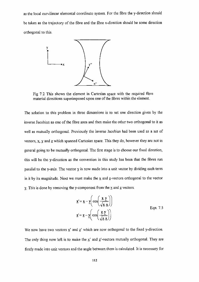
as the local curvilinear elemental coordinate system. For the fibre the y-direction should

be taken as the trajectory of the fibre and the fibre x-direction should be some direction

orthogonal to this.

Fig 7.2 This shows the element in Cartesian space with the required fibrematerial directions superimposed upon one of the fibres within the element.

The solution to this problem in three dimensions is to set one direction given by the

inverse Jacobian as one of the fibre axes and then make the other two orthogonal to it as

well as mutually orthogonal. Previously the inverse Jacobian had been used as a set of

vectors, x, y and z which spanned Cartesian space. This they do, however they are not in

general going to be mutually orthogonal. The first stage is to choose our fixed direction,

this will be the y-direction as the convention in this study has been that the fibres run

parallel to the y-axis. The vector y is now made into a unit vector by dividing each term

in it by its magnitude. Next we must make the and -vectors orthogonal to the vector

y. This is done by removing the y-component from the and vectors.

( ('i)

?'

( (.y Eqn. 7.5

We now have two vectors ' and ' which are now orthogonal to the fixed y-direction.

The only thing now left is to make the ' and '-vectors mutually orthogonal. They are

firstly made into unit vectors and the angle between them is calculated. It is necessary for

112

this angle to be 900. The angular difference between the two vectors is then halved and

each vector is then rotated by this amount plus rtI4 in opposite directions. The two

vectors are now orthogonal to each other as well as to the y vector.

x" x' zt[co{1— =---4

Eqn.7.6

z" z' x'[co(i_2J' 4

This process will always yield an orthogonal set of fibre axes provided the initial set of

vectors given by the Jacobian span Cartesian space. The only case when they will not do

so is if the element is incorrectly formed in which case a finite element solution would be

impossible.

7.2.3 Testmg and Validation

It is always wise to perform comprehensive testing of any program or program

modification. Presented here is a summary of some of those test procedures which were

carried out.

The simplest test is that of a cube with its vertices corresponding to those of the finite

element fundamental. This is particularly simple since the Jacobian will be the unit

matrix. The fibre direction for this element was taken to be in the elemental y-direction.

The element was found to deform as expected for a variety of contraction coefficients.

As a further check the finite element analysis was carried out for the element in various

orientations to the Cartesian axes. The element was also split into two small elements to

check for the correct handling of multiple elements.

The next stage was to expand upon this simple element by having the fibre direction at

some angle to the elemental y-direction. Since the results from this test are not so

intuitively obvious the test needed to be compared against another package. For this

113

purpose all the following tests were compared against the results from the finite element

package PAFEC''. The results for various angles were identical between the two

programs.

It must also be shown that the program can deal with non-cubic elements. To this end an

element which was a quarter of an annulus was created. There unfortunately is a

drawback since PAFEC cannot handle local curvilinear coordinates. For the PAFEC"

comparison model ten elements were used to simulate the changing fibre direction as one

moves around the arc of the quarter annulus. As is to be expected the results were not

exactly the same, however the overall deformation was reasonably consistent between

the two test models.

One further test also needed to be performed and that was for the varying fibre angle

through the thickness of the block. Again PAFEC does not include facilities to perform

this so a model of this element type was constructed in PAFEC' TM . This involved splitting

a cube into six slices and having each slice with a slightly different fibre angle. The

results from this were not exactly the same as from "XL1" but were reasonably close

considering the two models were not identical in their structure.

Some sample results are included in Appendix I along with sample data files for both

programs.

7.2.4 Preliminary Results Using a Cylindrical Model

A cylindrical model has been used here as a simple demonstratio that the basic

requirements of the left ventricle during systole can be modelled with the process

described above. A model of the left ventricle must be able to produce a contracting

cavity volume despite an increasing internal pressure. The cavity volume and pressure

changes are taken from patient "BA", and the values of the contraction coefficients are

114

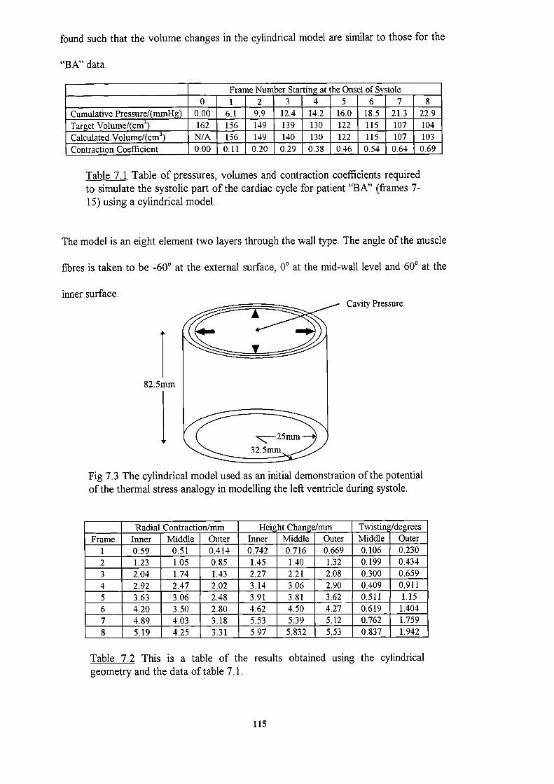
Cavity Pressure

found such that the volume changes in the cylindrical model are similar to those for the

"BA" data.

______________________ ____ Frame Number Start the Onseysto1e ________________ 0 1 2 3 4 5 6 7 8

Cumulative Pressure/(mmHg) 0.00 6.1 9.9 12.4 14.2 16.0 18.5 21.3 22.9

Target Volume/(cm3) 162 156 149 139 130 122 115 107 104

Calculated Volume/(cm3) N/A 156 149 140 130 122 115 107 103

Contraction Coefficient 0.00 0.11 0.20 0.29 0.38 0.46 0.54 0.64 0.69

Table 7.1 Table of pressures, volumes and contraction coefficients requiredto simulate the systolic part of the cardiac cycle for patient "BA" (frames 7-15) using a cylindrical model.

The model is an eight element two layers through the wall type. The angle of the muscle

fibres is taken to be -60° at the external surface, 00 at the mid-wall level and 60° at the

inner surface.

I82.5mm

IFig 7.3 The cylindrical model used as an initial demonstration of the potentialof the thermal stress analogy in modelling the left ventricle during systole.

______ Radial Contraction/mm Height_Change/mm Twisting/degrees

Frame Timer Middle Outer Inner Middle Outer Middle Outer

1 0.59 0.51 0.414 0.742 0.716 0.669 0.106 0.230

2 1.23 1.05 0.85 1.45 1.40 1.32 0.199 0.434

3 2.04 1.74 1.43 2.27 2.21 2.08 0.300 0.659

4 2.92 2.47 2.02 3.14 3.06 2.90 0.409 0.911

5 3.63 3.06 2.48 3.91 3.81 3.62 - 0.511 1.15

6 4.20 3.50 2.80 4.62 4.50 4.27 0.619 1.404

7 4.89 4.03 3.18 5.53 5.39 5.12 0.762 1.759

8 5.19 4.25 3.31 5.97 5.832 5.53 0.837 1.942

Table 7.2 This is a table of the results obtained using the cylindricalgeometry and the data of table 7.1.

115

The changes in shape of the model agree favourably with observations of ventricular

deformation. The most important feature is that cavity volume is reduced during the

application of the modelling process. It is also noticed that the wall thickens and that

radial motion of the outer surface is less than that of the inner surface. Both these

morphological changes agree with known ventricular systolic properties. It has also been

observed that the ventricle during the cardiac cycle undergoes a significant amount of

rotation. In effect the ventricle "winds up" during systole and "unwinds" during diastole.

This "winding up" process is clearly evident from Table 7.2. The values for the rotation

are however smaller than one might expect. The reason for this may be due to the

material properties and the geometry used and even to the way in which the model is

restrained.

The only real cause for concern is that the model tends to increase in length when a

reduction would be expected. This however may be due to either the poor

approximation of the ventricle by a cylinder or a poor choice for the material properties.

The true reason for this and factors contributing to global deformation will be

investigated in Chapter 9.

7.3 Summary

The process of simulating muscle contraction by a thermal stress analogy certainly does

produce an effect similar to what would be expected during myocardial contraction. The

cylindrical model used shows many of the important features of v ntricular systole.

Firstly, the cavity volume reduces and can overcome an internal pressure. Secondly, the

inner, middle and outer surfaces all show rotation relative to each other. The only

concern is that the cylinder does not reduce in length as the left ventricle is generally

116

known to do during ventricular systole. The reason for this will become apparent during

analysis of the patient data in Chapter 9.

117

Chapterl

8. An Overview of the Computer Program

This Chapter will be concerned with explaining the structure and function of the new

automated program routines. Here the extensions that were necessary for the expanded

functionality of the program will be discussed as well as the restructuring and the new

menu system of the program. The program originally consisted of three parts and little

reference to these will be made here. The full details of these can be found in Grewal [2].

Some alterations have been made in these parts of the program, however they are fairly

superficial and do not alter the overall function of these parts. The alterations made were

only to improve the clarity of the code and enable these parts to be more stable with

respect to input errors. As such the flow diagrams that can be found in Grewal [2]

Chapter 7 are still valid.

This Chapter will concentrate on the newly formed part of the program, 'PART4",

which controls the process of finding material properties. These properties can either be

the passive diastolic properties or the active systolic properties.

New Program Structure

Sefect anoption?

1

Part 1Volume and FELesh Calculation

2

Part 2Manual Elastic

ModulusCalculation

3

Part 3Material PropertyGraphs and Cross-

Sections Plotted

Quit

AutomatedMaterial Property

Calculations

118

START

Part 1?

Yes

Part 1Volume and FE

Mesh Calculation

NOjes

Part 2Manual Elastic

Modulus Calculation

jesNO

Part 3Material PropertyGraphs and Cross-

Sections Plotted

Yes / RepeatProgram

No

Stop

Fig 8.1 These two flow diagrams illustrate how the parts of the programwere originally accessed compared to how they are now accessed.

119

As can been seen each part of the program can now be directly accessed from the main

menu. Whereas before the individual parts could only be accessed sequentially one after

another.

8.1 The Original Function of the Program Heart

The program "HEART" was the post-processor and pre-processor for the finite element

program "XL 1". As stated above it was originally composed of three parts. The first

part, "PART1", was used to obtain the volume and pressure information from the X-ray

data. The pressure and volume graphs could also be plotted from within this part of the

program. As well as this the data file, "XL 1-data", which the finite element program

requires is also generated within this part of the program. The mesh generated for the

finite element analysis can also be viewed here to ensure that it is well formed and may

also be saved to a separate coordinate file.

The second part, "PART2", deals with the matching process of finding the elastic

modulus of the model required for the observed volume and pressure change. This is

done interactively and can produce an updated data file with a new value for the elastic

modulus.

The third part, 'PART3", is responsible for most of the plotting routines. It allows for

the plotting of the material property graphs and the deformed and undeformed short axis

cross-sectional views. This part has been slightly enhanced by the inclusion of multiple

graphs on a single page. A further set of plotting options has also b en included. This

new option allows a three dimensional plot to be made of the deformed and undeformed

model data. The endocardium and epicardium can be selectively plotted and up to three

sets of data may be overlaid. The endocardium is plotted with solid lines and the

120

- -

1

2

Plot material

Plot short axis cross-property graphs sectional planes

through the model

epicardium with broken lines. Each set of coordinate data is also plotted with a different

colour to make each set easily distinguishable from one and other.

Fig 8.2 This shows the shape of a typical reconstruction. The endocardium isshown by the solid lines and the epicardium in broken lines. The same frameis shown at three different orientations.

The structure of this part of the program has changed slightly from that previously

described by Grewal [2]. The changes are shown below and further information on the

unchanged parts can be gained from Grewal [21 Chapter 7.

Select anoption?

q

3

Display three I I

dimensional fim I I

element meshI

I Return to main

I I menu

Fig 8.3 This flow diagram shows the structure of the plotting routines. Theplotting options are largely unchanged from the previous version of theprogram as described in Grewal [2] Chapter 7.

121

The use of the data file generating part of 'PART 1" and the whole of 'PART2" are no

longer needed due to the inclusion of 'PART4". This part of the program has now taken

over the formation and updating of the necessary data files. The only function of the

previous two parts that is still required is the formation of the volume data file. This file

contains the original cavity volumes as well as the smoothed and target volumes.

8.2 An Overview of the Structure and Function of"PART4"

Here we shall look at the overall structure of the automation part of the program. This

shall be done by consideration of a flow diagram for this part of the program.

From the main menu

Input requiredtions and materialproperty values

Set up volume to beLatched and any othL

required factors

Generate the finiteelement data file

Select the nextframe of data Invoke the finite

element analysispart of the program

Yes

Are furtherframes to

be analysed

\ ?

NoReturn to themain menu

Yes Are parameterswithin the required

tolerance?

NoUpdate the material

properties as required

Fig 8.4 This is a flow diagram which demonstrates how the materialproperties are found for the model using an automated process.

122

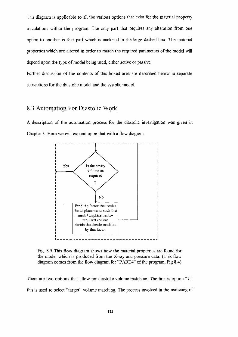
This diagram is applicable to all the various options that exist for the material property

calculations within the program. The only part that requires any alteration from one

option to another is that part which is enclosed in the large dashed box. The material

properties which are altered in order to match the required parameters of the model will

depend upon the type of model being used, either active or passive.

Further discussion of the contents of this boxed area are described below in separate

subsections for the diastolic model and the systolic model.

8.3 Automation For Diastolic Work

A description of the automation process for the diastolic investigation was given in

Chapter 3. Here we will expand upon that with a flow diagram.

Yes Is the cavityvolume as I

required

No

Find the factor that scalesthe displacements such that I

mesh+displacements=required volume I

divide the elastic modulusby this factor I

I ---------------------------------I

Fig. 8.5 This flow diagram shows how the material properties are found forthe model which is produced from the X-ray and pressure data. (This flowdiagram comes from the flow diagram for "PART4" of the program, Fig 8.4)

There are two options that allow for diastolic volume matching. The first is option "1",

this is used to select "target" volume matching. The process involved in the matching of

123

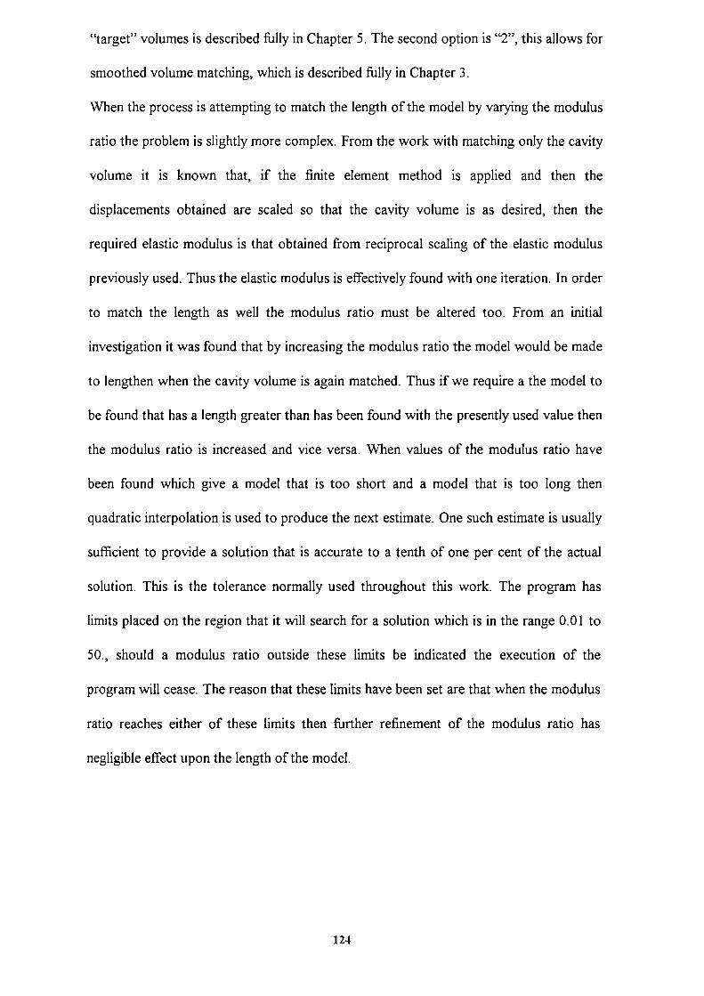
"target" volumes is described fully in Chapter 5. The second option is "2", this allows for

smoothed volume matching, which is described frilly in Chapter 3.

When the process is attempting to match the length of the model by varying the modulus

ratio the problem is slightly more complex. From the work with matching only the cavity

volume it is known that, if the finite element method is applied and then the

displacements obtained are scaled so that the cavity volume is as desired, then the

required elastic modulus is that obtained from reciprocal scaling of the elastic modulus

previously used. Thus the elastic modulus is effectively found with one iteration. In order

to match the length as well the modulus ratio must be altered too. From an initial

investigation it was found that by increasing the modulus ratio the model would be made

to lengthen when the cavity volume is again matched. Thus if we require a the model to

be found that has a length greater than has been found with the presently used value then

the modulus ratio is increased and vice versa. When values of the modulus ratio have

been found which give a model that is too short and a model that is too long then

quadratic interpolation is used to produce the next estimate. One such estimate is usually

sufficient to provide a solution that is accurate to a tenth of one per cent of the actual

solution. This is the tolerance normally used throughout this work. The program has

limits placed on the region that it will search for a solution which is in the range 0.01 to

50., should a modulus ratio outside these limits be indicated the execution of the

program will cease. The reason that these limits have been set are that when the modulus

ratio reaches either of these limits then further refinement of the modulus ratio has

negligible effect upon the length of the model.

124

No

Find the. factor that scales UT the length is not asthe displacements such that required either increase or

mesh+displacements decrease the modulus ratiorequired volume. - A linear search follod b

Di%ide the elastic modulus quadratic interpolation isby this factor. used once a bound on the

______________________ solution is found.

Fig. 8.6 This flow diagram shows how the cavity volume and the mid-base toapex length are matched. (This flow diagram comes from the flow diagramfor "PART4" of the program, Fig 8.4)

There is a choice of two volume arid length matching options available within the

program. The first is option "3", which is like option "2" of the program in that it

matches smoothed volumes, the difference here is that an attempt to also made to match

a ventricle target length. The target length was produced by linear interpolation of the

measured length values. The use of this type of process was less than successflul though

may be of ftiture use should more suitable data become available. The other length

matching option is "4", this allows the volume and length to be matched to a frame that

is not successive. It has been used to obtain a cavity volume and lenoth match between

the first and last frames of diastole.

125

8.4 Calculation of the Forces Generated by Muscle Contraction

As was previously stated in Chapter 7 the method used to simulate muscle contraction is

similar to that of thermal stressing. Ultimately within the program the active contraction

part generates the nodal forces that result from the material contraction. It is important

to note that this is not contraction in the normal sense since no volume strain occurs. It

is more a reshaping process whereby the material contracts in one direction while

expanding in another and thus it preserves its overall volume. The simplest way to

provide a measure of the material contraction is to supply the strain values for the fibre

and cross-fibre directions. This has the advantage that it is independent of the chosen

material properties and is thus far simpler to interpret and compare between patients.

Read information fromthe data file.

Generate the stiffnessmatrix.

Convert pressures intonodal forces

Is musclecontraction to be

simulated(1SW41)?

Calculate forces due toYes muscle contraction and

add them to the passivelygenerated forces

No

Invert The stiffnessmatrix to find the

displacements

Caculate the stressesand the fibre strains

Return to part 4 ofthe main program

Fig 8.7 This flow diagram shows how the simulated muscle contraction isincorporated into the original finite element program XL1.

126

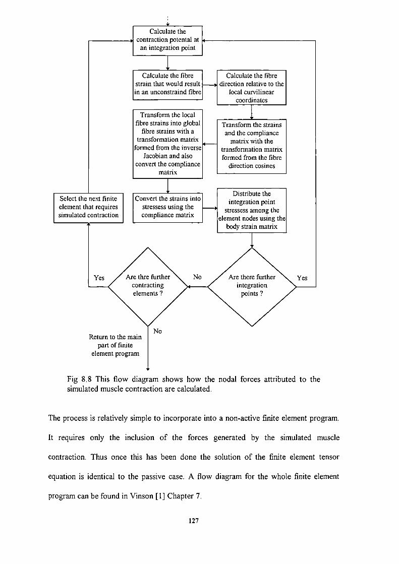
Calculate thecontraction potental at

an integration point

Calculate the fibrestrain that would resultin an unconstraind fibre

Transform the localfibre strains into global

fibre strains with atransformation matrix

[ormed from the inverseJacobian and also

convert the compliancematrix

Calculate the fibredirection relative to the

local curvilinearcoordinates

Transform the strainsand the compliance

matrix with thetransformation matrixformed from the fibre

direction cosines

Select the next finiteelement that requiressimulated contraction

Convert the strains intostressess using thecompliance matrix

Distribute theintegration point

stressess among thement nodes using tbody strain matrix

Yes Are thre furthercontractingelements?

Return toNo

the mainpart of finite

element program

Are there further 'N Yesintegration

points?

Fig 8.8 This flow diagram shows how the nodal forces attributed to thesimulated muscle contraction are calculated.

The process is relatively simple to incorporate into a non-active finite element program.

It requires only the inclusion of the forces generated by the simulated muscle

contraction. Thus once this has been done the solution of the finite element tensor

equation is identical to the passive case. A flow diagram for the whole finite element

program can be found in Vinson [1] Chapter 7.

127

8.5 Automation For Systolic Work

There are six options for systolic volume matching and their purpose is described here.

The flow diagram shows how the finite element program is used to obtain a solution for

the contraction coefficient that allows the model to mirror the observed behaviour of the

left ventricle.

It was discovered early on that the ratio of along-fibre to cross-fibre contraction

coefficient ratio was not only important to preserve wall volume but also depends upon

the size of the contraction coefficient. Thus the value of the contraction coefficient ratio

must be calculated at the same time as the contraction coefficient itself, if wall volume is

to be preserved.

Increase the contraction Increase the contractioncoefficient ratio if the coefficient if the cavity

wall volume is too small volume is too large andand vice versa, lithe vice versa. If the required

required value is bounded volume is bounded aboveabove and below use and below use quadratic

quadratic interpolation interpolation

Fig 8.9 This flow diagram gives an overview of how the wall volume andcontraction coefficient ratio are simultaneously calculated. (This flowdiagram comes from the flow diagram for "PART4" of the program, Fig 8.4)

As can be seen from the diagram this part of the program has been structured into two

distinct sets of subroutines. These can easily be combined together to provide any

128

combination of functionality. The option to match the models length by varing the

shear modulus has been retained. The fact that varying this parameter has a much

reduced effect when the fibre angle is high means this option is not of great use. The

reason that it has been retained is that is clearly shows how extensions can be easily

made to the programs functionality. It is also relatively straightforward to adapt this

option to provide a new function.

8.6 Matching Routines

The purpose of the matching routines is to produce a new estimate for the material

properties based upon the results obtained from previous estimates. The nature of these

routines is important only in that they can produce convergence to the required soution.

It is also greatly desirable that this process should seek also to minimise the number of

iterations that is necessary for suitable convergence to occur.

In order to obtain convergence in the volume matching process during the simulation of

diastole the fact that the model is linearly elastic is made use of, that is that the

displacements of the model's nodes are linearly dependent upon the material properties.

This is made use of here by scaling the displacements from an initial estimate to obtain a

volume match and then scaling the material properties by the reciprocal of this value.

129

Calculate the volumeoriginal

mesh+displacements

Yes

YesProperties found.Is there anotherframe to analyse

7

No Return to themain menu

Is the volume asrequired?

Calculate thedisplacements with the

FE program

- - -

I I

I I

Divide the elastic modulus by the Ii factor used to scale the

displacements and generate the Ii other material properties from thisI ¶. II II I

Use the golden section (Fibonacci)I method on the bounded region

until the required tolerance hasI been met.I II II I

By scaling the displacements and NoI using a linear step method to find i-4--

a bounded region in which therequired voiwne resides.

Fig 8.10 This shows the process by which the material properties are foundduring diastole. This flow diagram is valid for the description of options "1"and "2".

The golden section/Fibonacci method is a search method which incorporates trisection of

a bounded region in order to minimise a function. In this case the function is the absolute

error between the required volume and that obtained from the original F.E. mesh plus

the scaled displacements. The method is well known and most books on optimisation

should contain a good description of the method.

The area surrounded by the dashed box is the only part which requires alteration for each

of the matching options. For this reason only the part within the Gashed box will be

reproduced in the following flow diagrams.

When matching the active material properties or the ventricle length by varying the

elastic modulus ratio the model is no longer linearly dependent upon the parameters

which are varied. A more sophisticated method must be used to obtain solution values

130

for the required parameters. The fact that the system is continuous is made use of as is a

priori knowledge about the response of the system to parameter changes. The process in

each case involves finding a bounded region in which the desired solution exists and then

using quadratic interpolation to refine this boundary. In the case of matching only cavity

volumes during systole only one application of quadratic interpolation is usually

necessary to achieve a cavity volume match to within 1.0% of the required cavity

volume. In fact it is often the case that the difference between the calculated and

required volume is often an order of magnitude less than this.

Yes

/ lengti

'Divide the elastic

-I

Use quadratic interpolation with the new I

value and the boundary values to produceI

_____ a new estimate for the elastic modulus I

ratio. Replace the appropriate boundaryI

values with the newly computed values. I

_____________________________________________________________________ _____________________________________________________________________ I

No

If the model is too long setthe upper bound (store the I

elastic modulus and the

e>No

Is the required elastic modulus ratio. Andlength) and reduce the i

_________________________________ ___________________________________ Ias vice versa. (Note: if both I

bounds are now set used? length unded

provide the ne estimate. I

linear interpolation to I

lUse the linear step method and I I

tiodulus by the golden section method to find thescaung jactor wrncn givcs rnsii -r

and generate the scaledthsplacements = required

I. ---------------------------------------------------Fig 8.11 This shows the process by which the material properties and theelastic modulus ratio are found during diastole, such that the cavity volumeand length are matched. This flow diagram is valid for the description ofoptions "3" and "4". (This flow diagram comes from the flow diagram givenin Fig 8.10)

131

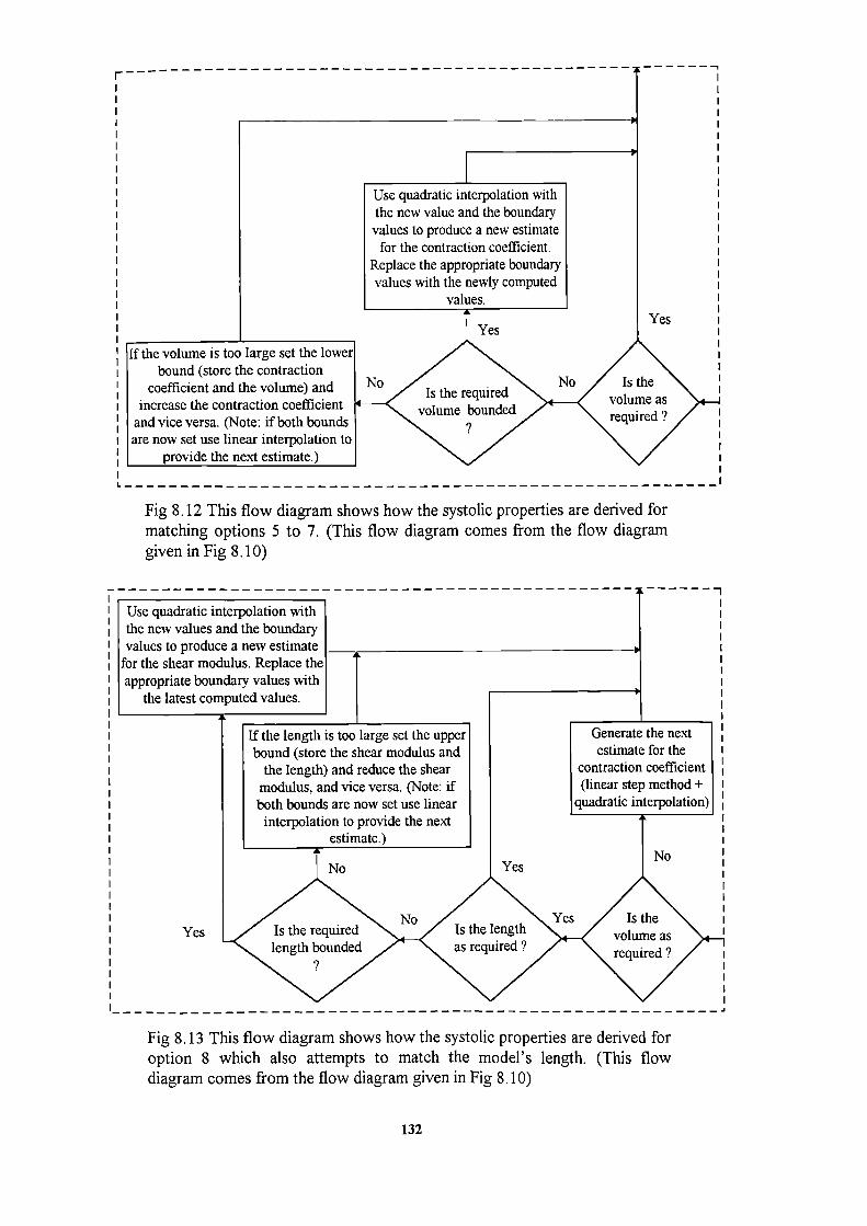
Use quadratic interpolation withI the new value and the boundaryI values to produce a new estimate II II for the contraction coefficient. II Replace the appropriate boundary II values with the newly computed

I values. II YesI Yes II__________________________________________________________________________________________________

lithe volume is too large set the lower Ibound (store the contraction I

coefficient and the volume) and NoIs the required

No Is the

increase the contraction coefficient volume asvolume bounded I

andvice versa. (Note: if both bounds ?required? I

are now set use linear interpolation to Iprovide the next estimate.)

I. -----------------------------------------------------IFig 8.12 This flow diagram shows how the systolic properties are derived formatching options 5 to 7. (This flow diagram comes from the flow diagramgiven in Fig 8.10)

--------------------------------------1Use quadratic interpolation withthe new values and the boundaryvaluesto produce a new estimate ________________________________________________

for the shear modulus. Replace theappropriate boundary values with

the latest computed values.

If the length is too large set thc upper Generate the nextbound (store the shear modulus and estimate for the

the length) and reduce the shear contraction coefficient

modulus, and vice versa. (Note: if (linear step method +

both bounds are now set use linear quadratic interpolation)

interpolation to provide the next

Yes

Fig 8.13 This flow diagram shows how the systolic properties are derived foroption 8 which also attempts to match the model's length. (This flowdiagram comes from the flow diagram given in Fig 8.10)

132

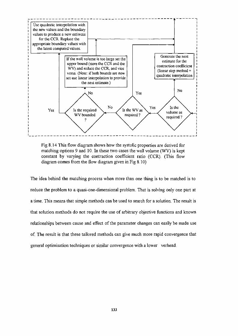
I Use quadratic interpolation withI

the new values and the boundaryI

values to produce a new estimate I

forthe CCR. Replace the ______________________________________________ I

appropriate boundary values with _________________the latest computed values. I

________________________________________________________________________________________ __________________________________________________________________________________________ __________________________________________________________ __________________________________________________________ I

If the wall volume is too large set theGenerate the next

I

upper bound (store the CCR and the estimate for the I

I

WV) and reduce the CCR, and vice contraction coefficient i

I

versa. (Note: if both bounds are now(linear step method + I

I set use linear interpolation to provide quadratic interpolation

the next estimate.)

YesNo I

No

volume asstherequiredNo

Yesr

I -I

Fig 8.14 This flow diagram shows how the systolic properties are derived formatching options 9 and 10. In these two cases the wall volume (WV) is keptconstant by varying the contraction coefficient ratio (CCR). (This flowdiagram comes from the flow diagram given in Fig 8.10)

The idea behind the matching process when more than one thing is to be matched is to

reduce the problem to a quasi-one-dimensional problem. That is solving only one part at

a time. This means that simple methods can be used to search for a solution. The result is

that solution methods do not require the use of arbitrary objective functions and known

relationships between cause and effect of the parameter changes can easily be made use

of. The result is that these tailored methods can give much more rapid convergence that

general optimisation techniques or similar convergence with a lower verhead.

133

8.7 Summary

The program as it stands provides for the automatic calculation of the active and passive

material properties. It provides a number of useful and possibly not so useful options

which can be chosen for the calculation of the material properties. It is also relatively

easy to extend the program with further procedures to enable other aspects of the model

to be more accurately simulated.

Another useful feature of the program's structure is that the finite element part can be

easily separated from the unified program so that it may easily be run upon super

computers should the need for very high performance be required. It is also equally

possible to separate the whole of "PART4" of the program including the finite element

program to allow the automated process to be run upon other computer systems which

do not support the packages Nag and SimplePlot which are used in other parts of the

program.

For further detail the program listing can be found in Appendix III and a sample data file

and a sample of the program output can be found in Appendix II.

134

Chapters

9. Factors Influencing General Systolic Performance

In this Chapter an investigation will be carried out to find some of the important

mechanical factors which are responsible for global deformation of the left ventricle.

These factors include boundary conditions, material properties and fibre orientation.

Originally it was intended that the analysis would be performed over several frames of

data. This would mean that the small changes in the geometry of the model would be

more easily quantified and might also be less susceptible to inaccuracies in the original

data. It was however not possible to perform the analysis successively over a large

number of frames, i.e. over a large time period as the mesh became badly deformed and

was thus likely to be a source of great inaccuracy. This would then compromise the

validity of any results obtained. In some cases this deformation was severe enough to

cause a total loss of integrity in some of the finite elements.

The reason that the finite element mesh became unusable was that the deformation of

myocardium has a very large shear component. This results in the finite elements

becoming badly distorted. This shearing effect has been seen in the ventricles of real

human patients by using the technique of Magnetic Resonance Myocardial Tagging

(Buchalter eta!. 1990 [77] and Buchalter 1992 [78]).

It was decided that the analysis would have to be performed over only one time period

or frame interval, as has previously been described in Chapter 5 for the method of

"target volume matching". For this process the last pair of the frames in systole were

used as they underwent the largest relative volume change. The result of this would be

that global geometric changes would thus be the greatest of any part of the systolic

phase and thus the effects of parameter changes would be more easily quantified.

135

It is important that the most significant factors influencing performance of the left

ventricle are found as this will be of benefit in the development of ventricular finite

element models. This will lead to models that are better able to quantify ventricular

performance and will hence be of greater research and clinical use.

9.1 The Analysis Procedure and Programming Enhancements

To enable us to evaluate the effect of changes to the model we must have another

descriptor for the model other than the cavity volume. What is required is some measure

of "shape". Previously there had been a shape index defined as (Grewal 1988 [21),

6 7t '2 VolumeShapelndex= 3 Eqn.9.1

Surface Area 2

which had been an expansion into three dimensions of the two dimensional shape index

(Gibson and Brown 1975 [80]),

4icCross - Sectional AreaShape Index =

Eqn. 9.2Perimeter2

The first equation relates the surface area of the three dimensional ventricle to its volume

in order to obtain an index, which is unity for a sphere. The second equation relates the

area of a cross-section to its circumference and provides an index which is unity for a

circle.

There had previously been an oversimplification in the calculation of the shape function.

The surface area was not obtained accurately and had been approximated as the curved

surface of a cylinder. This cylinder was defined as the length of the ventricle (mid-base to

apex length) and the average radius of the base. The result of this was that the change in

shape index during finite element analysis was as a result of length change only (the

endocardial base is held fully as the boundary condition so the average radius is

constant). This would then be equivalent to using length as the index of shape. Length

136

has previously proved not to be a very good parameter to use due to the nature of

digitisation errors.

It was necessary to create several new subroutines to enable the calculation of the

endocardial surface area of the model directly from the finite elements. This involves the

calculation of the area Jacobian, for that surface of a finite element, and numerical

integration of it over that surface, This is done for the "brick" as well as the "wedge"

shaped elements.

Another thing that was changed was the size of the apex region of the model. In the real

left ventricle the stiff apex is a small "button". The model however was divided equally

by height for all elements including the apex ones. This means that the size of the

"wedge" elements forming the apex was similar to that of the "brick" elements. The

meshing routine was altered so that the apex was fixed as the last 4mm of the model.

Typically the apex elements could previously have accounted for as much as 15mm of

the model's height. This was the smallest the apex could be made without compromising

the integrity of the "wedge" shaped elements. To make the "stiff apex" smaller and still

preserve the integrity of the mesh would require a significant rethink of the meshing

scheme used.

The investigation of systole is a new area in this work and it is important that global

shape change can be easily visualised. It is also important that global shape change can

be related to numerical shape change indicators such as length or "shape index". To this

end a new set of visualisation routines were created to enable a three dimensional view

of the deformed finite element mesh to be produced. Previously only two dimensional

short axis cross-sectional views had been available for the deformed data. These are

severely limited as they provide no information about longitudinal changes in the model.

137

-.-----------

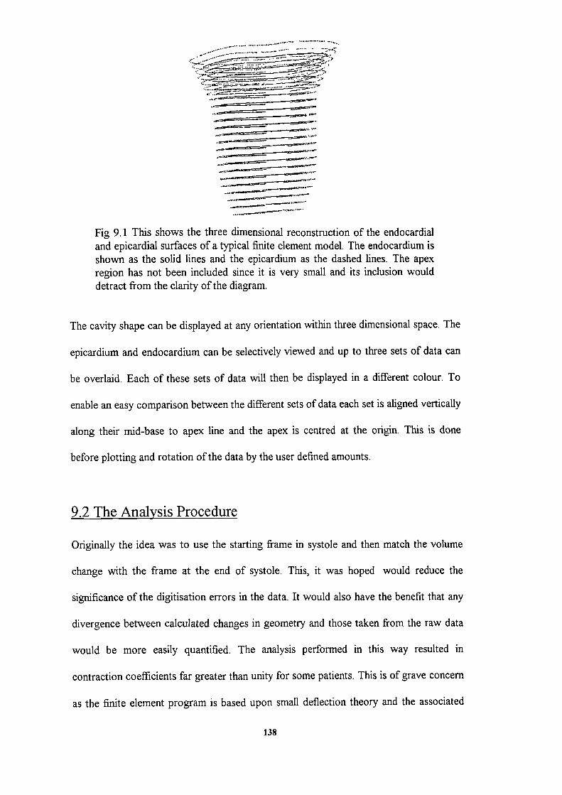
Fig 9.1 This shows the three dimensional reconstruction of the endocardialand epicardial surfaces of a typical finite element model. The endocardium isshown as the solid lines and the epicardium as the dashed lines. The apexregion has not been included since it is very small and its inclusion woulddetract from the clarity of the diagram.

The cavity shape can be displayed at any orientation within three dimensional space. The

epicardium and endocardium can be selectively viewed and up to three sets of data can

be overlaid. Each of these sets of data will then be displayed in a different colour. To

enable an easy comparison between the different sets of data each set is aligned vertically

along their mid-base to apex line and the apex is centred at the origin. This is done

before plotting and rotation of the data by the user defined amounts.

9.2 The Analysis Procedure

Originally the idea was to use the starting frame in systole and then match the volume

change with the frame at the end of systole. This, it was hoped would reduce the

significance of the digitisation errors in the data. It would also have the benefit that any

divergence between calculated changes in geometry and those taken from the raw data

would be more easily quantified. The analysis performed in this way resulted in

contraction coefficients far greater than unity for some patients. This is of grave concern

as the finite element program is based upon small deflection theory and the associated

138

strains resulting from such large values of the contraction coefficient are certain not to

be small (Note: a contraction coefficient is in effect a strain potential). For some sets of

patient data it was not even possible to obtain results as the elements would lose their

integrity and some would even be reported as having negative volume. Despite these

failings the analysis did seem to function reasonably well for some patients. It was

decided however that it would be more prudent to proceed with the analysis on a frame

by frame basis similar to the "target volume matching" process employed in the

investigation of diastole.

9.3 Wall Volume and the Contraction Coefficient Ratio

The following tests described in this section were all originally performed using an

along-fibre to cross-fibre contraction coefficient ratio of 1:-0.5, a value originally

suggested by Chen eta!. (1980 [80]). This paper, although not published until 1980, was

of work carried out prior to 1977. It was then later suggested that a value in the range of

1:-0.5 to 1:-0.3 (Chen eta!. 1978 [81]) may be more appropriate. This ratio is important

since the values are in effect potential strain values and will affect volume strain changes.

The myocardium is normally considered to be of constant volume, however there has

been some evidence that there may be as much as 10% volume strain during the cardiac

cycle (Horowitz eta!. [35] and Yin eta!. [82]). It is therefore the case that consideration

as to what is happening to the wall volume of the model is important.

It was necessary to create a number of new subroutines which were able to calculate the

wall volume of the model from the individual finite elements. This process is similar to

the calculation of the surface area except that instead of using the area Jacobian the

volume Jacobian is used and integration is over the volume and not just one surface.

139

The introduction of wall volume calculations resulted in the discovery that the

contraction coefficient ratio of 1:-O.5 resulted in the wall volume increasing. The amount

of this increase was largely dependent upon the value of the along-fibre contraction

coefficient. The larger this value the greater the volume increase was. For most tests the

increase was only a few percent but when the material properties were varied this

increase could become significant.

As stated above the following tests were originally carried out using a contraction

coefficient ratio of 1:-O.5 and this resulted in the wall volume increasing. This affected

greatly the initial results obtained is several ways. Firstly, it resulted in an elevation in the

size of contraction coefficient required to match the volume, which in itself will result in

yet a further increase in wall volume. In some cases this was so severe that the wall

volume would increase at a rate faster than the cavity volume would reduce. The effect

of this is that this reduction caused by the increase in contraction coefficient is smaller

than the increase caused by the wall volume increasing. Thus it would be impossible to

match the target volume.

Secondly, even when the volume matching process was possible the results could be self-

contradictory. That is altering a parameter may cause the system to behave in a

particular way except when the parameter reached a certain value when the effect would

be markedly different. The other part of this problem is that because of the change in

wall volume the effect that the parameters being tested had were either exaggerated or

masked by the effect of changing wall volume.

140

9.4 Initial Results Using Standard Values

In order to assess the relative importance of each of the model's parameters it is vital

that a reference set of results be obtained. The reference set of parameters was based on

those values obtarned from the analysis of diastole. The elastic modulus is taken as a

representative value of the values calculated in the diastolic investigation. The shear

moduli were obtained from the assumed relationship between elastic and shear moduli

used in Chapters 3 and 5 and Poisson's ratio was kept the same from the previous

analysis. This gives a starting point against which variations in all the relevant factors can

be compared.

In this section we use data from four patients taken at the end of systole. The reason for

this is that the relative volume change is much larger at this point which means that the

changes in deformation due to altered conditions will be more pronounced. This is

important since geometric changes are likely to be small and the even smaller variations

in these changes would otherwise be dwarfed by approximations in the calculation and

may lead to the incorrect interpretation of results.

Patient Frame Minor Elastic Pressure Volumes /(cm3) Original OriginalUsed Modulus Increase Shape Length

_______ ______ kKN/m2) I(mrnHg) Original Target Index /(mm)BA 14 50 1.62 107.19 104.08 0.852 75.71CL 14 20 3.68 122.72 114.04 0.896 82.83

MI 15 60 2.01 56.21 44.62 0.660 77.58WE(A) 15 15 2.36 58.40 54.99 0.709 73.14

Table 9.1 This table shows the original shape index and length obtainedfrom the patient data. It also shows the value of elastic modulus used foreach patient as well as the pressure and volume changes between the originaland the target frames. The other material properties can be d rived from theinformation given in Chapter 3.

141

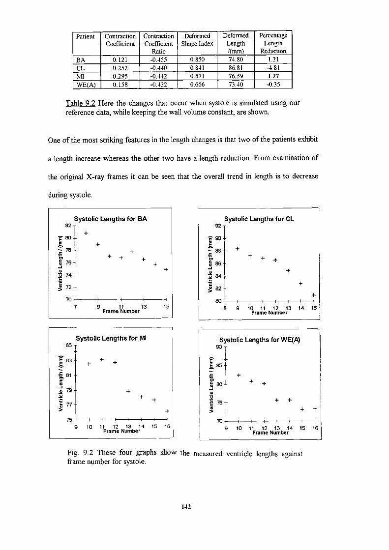
+80 I I I

8 9 10 11 12 13 14 15Frame Number

Systolic Lengths for WE(A)

E85

.C)

80 +—J

U+ +

-I-++

704— I I I

9 10 11 12 13 14 15 16Frame Number

Systolic Lengths for CL92

—88C,

86-Jwc., 84

82

Patient Contraction Contraction Deformed Deformed Percentage

Coefficient Coefficient Shape Index Length Length

________ ___________ Ratio ___________ /(mm) Reduction

BA 0.121 -0.455 0.850 74.80 1.21

CL 0.252 -0.440 0.841 86.81 4 81

Ml 0.295 -0.442 0.571 76.59 1.27

WE(A) 0.158 -0.432 0.666 73.40 -0.35

Table 9.2 Here the changes that occur when systole is simulated using ourreference data, while keeping the wall volume constant, are shown.

One of the most striking features in the length changes is that two of the patients exhibit

a length increase whereas the other two have a length reduction. From examination of

the original X-ray frames it can be seen that the overall trend in length is to decrease

during systole.

Fig. 9.2 These four graphs show the measured ventricle lengths againstframe number for systole.

142

A model that was able to simulate systole was proposed by Horowitz et aL (1986 [35])

it was based on a single set of patient data and also predicted a length increase during

systole. This was assumed to be due to the exclusion of the papillary muscles from the

model, which contract strongly during systole. It however would be unwise to agree

with this view. From patients who have undergone mitral valve replacement, and hence

have had their papillary muscles cut, it has indeed been observed that the length

reduction is affected. Despite this the ventricle is still seen to reduce in length during

systole; albeit in an abnormal manner. It is also the case that information about the force

generated by these muscles is not easily quantified.

It should also be noted that the shape index reduces in every case. The reason for this is

that the surface area is increasing relative to the volume. This may mean that the

ventricle is either becoming more elongated relative to its volume or the surface area is

increasing relative to the volume for another reason. The use of the shape index makes it

difficult to visualise ventricular geometric changes whereas length change is much easier

to visualise. The disadvantage is that length measurements taken from the data are much

less accurate than the shape index. This is because the accuracy of the length is

proportional to the digitisation errors whereas the shape index is dependent upon the

surface area and is thus proportional to the errors squared. This will make the surface

area less sensitive to the data accuracy than the length.

Another noticeable feature is that the contraction coefficient ratios are all fairly similar in

magnitude. The values are also well within the range -0.3 to -0.5 as p edicted by Chen et

a!. [80].

143

9.5 Material Properties

The importance of the various material properties upon global deformation in systole is

not well known. Here we examine the effect of each material property in turn upon the

global deformation of the left ventricle. In this way the relative importance of each upon

systolic cardiac mechanics can be quantified. This will enable a better choice for material

properties in the analysis of systole and may enable a more targeted approach to

experimental work involving direct measurement of myocardial properties.

9.5.1 Elastic Modulus

This is arguably the most important property of the myocardium during diastole since it

is almost totally responsible for governing the change in volume in response to a

pressure increase. Its importance during systole however is unknown and so the effect of

different values is investigated here. It has been suggested that the value of the elastic

modulus is almost a factor of 10 greater during systole than during diastole (Lundin

1944 [61]). To circumvent this uncertainty some authors in their systolic models have

used assumed stress/strain relationships to get over the ambiguity of the elastic modulus

during systole (Horowitz et a!. 1986 [35]). This is far from ideal as these exponential

stress/strain models have been shown not to predict diastolic properties (Grewal 1988

[2]), for which they were intended, and their use in systole must be even more suspect.

Since the volume of the ventricle is decreasing during systole it would seem reasonable

to assume that the major factor governing ventricular deformat on was sarcomere

contraction. If this is the case then the effect of the internal pressure loading and

consequently that of the elastic modulus will be small and possibly even negligible. It was

the view of Gibson (1996 [83]) that the cavity pressure of the ventricle was not an

important factor in systolic deformation of the left ventricle.

144

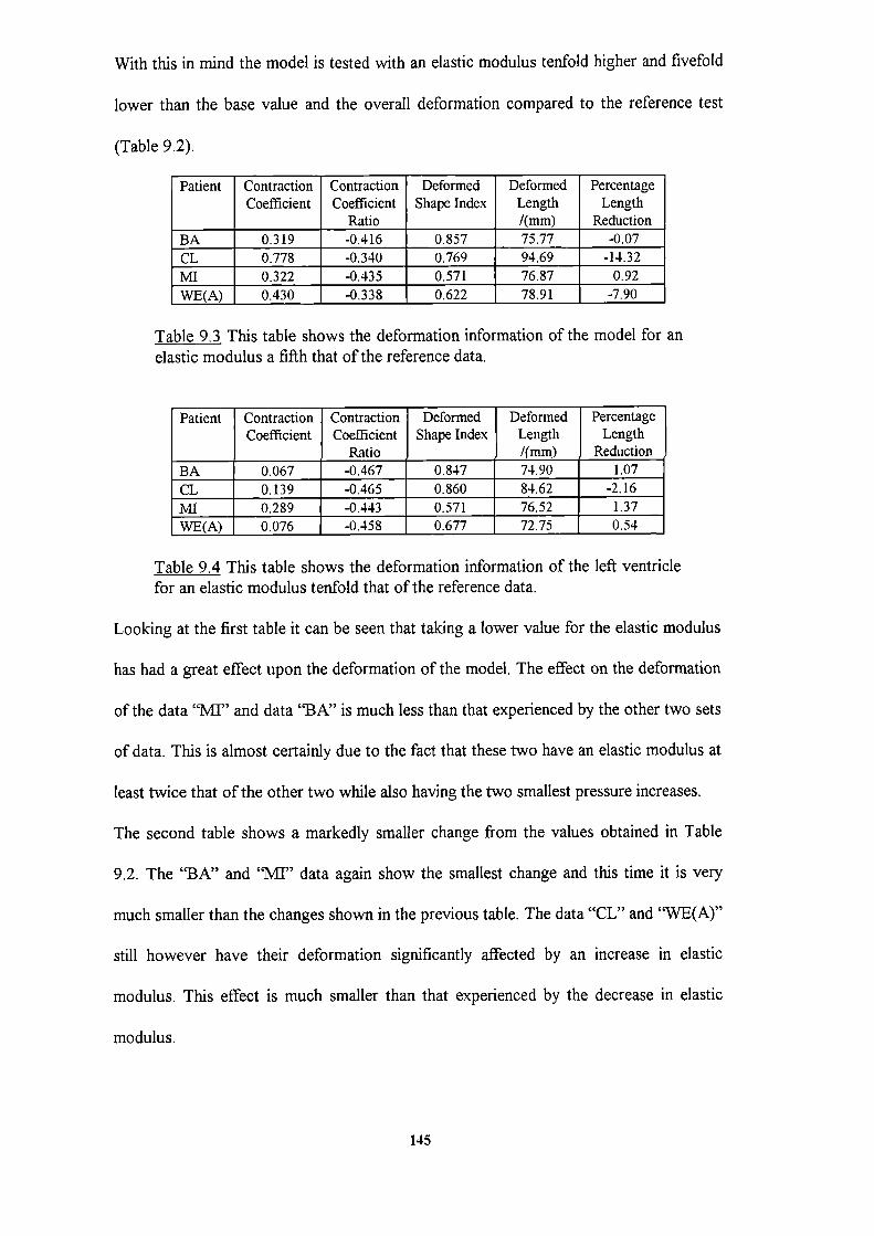
With this in mind the model is tested with an elastic modulus tenfold higher and fivefold

lower than the base value and the overall deformation compared to the reference test

(Table 9.2).

Patient Contraction Contraction Deformed Deformed PercentageCoefficient Coefficient Shape Index Length Length

_______ ___________ Ratio ___________ /(mm) ReductionBA 0.319 -0.416 0.857 75.77 -0.07CL 0.778 -0.340 0.769 94.69 -14.32Ml 0.322 -0.435 0.571 76.87 0.92WE(A) 0.430 -0.338 0.622 78.91 -7.90

Table 9.3 This table shows the deformation information of the model for anelastic modulus a fifth that of the reference data.

Patient Contraction Contraction Deformed Deformed PercentageCoefficient Coefficient Shape Index Length Length

_______ __________ Ratio ___________ /(mm) Reduction

BA 0.067 -0.467 0.847 74.90 1.07

CL 0.139 -0.465 0.860 84.62 -2.16

Ml 0.289 -0.443 0.571 76.52 1.37WE(A) 0.076 -0.458 0.677 72.75 0.54

Table 9.4 This table shows the deformation information of the left ventriclefor an elastic modulus tenfold that of the reference data.

Looking at the first table it can be seen that taking a lower value for the elastic modulus

has had a great effect upon the deformation of the model. The effect on the deformation

of the data "MI" and data "BA" is much less than that experienced by the other two sets

of data. This is almost certainly due to the fact that these two have an elastic modulus at

least twice that of the other two while also having the two smallest pressure increases.

The second table shows a markedly smaller change from the values obtained in Table

9.2. The "BA" and "Ml" data again show the smallest change and this time it is very

much smaller than the changes shown in the previous table. The data "CL" and "WE(A)"

still however have their deformation significantly affected by an increase in elastic

modulus. This effect is much smaller than that experienced by the decrease in elastic

modulus.

145

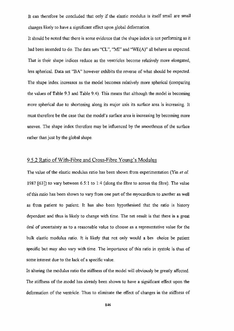
It can therefore be concluded that only if the elastic modulus is itself small are small

changes likely to have a significant effect upon global deformation.

It should be noted that there is some evidence that the shape index is not performing as it

had been intended to do. The data sets "CL", "MI" and "WE(A)" all behave as expected.

That is their shape indices reduce as the ventricles become relatively more elongated,

less spherical. Data set "BA" however exhibits the reverse of what should be expected.

The shape index increases as the model becomes relatively more spherical (comparing

the values of Table 9,3 and Table 9.4). This means that although the model is becoming

more spherical due to shortening along its major axis its surface area is increasing. It

must therefore be the case that the model's surface area is increasing by becoming more

uneven. The shape index therefore may be influenced by the smoothness of the surface

rather than just by the global shape.

9.5.2 Ratio of With-Fibre and Cross-Fibre Youn g's Modulus

The value of the elastic modulus ratio has been shown from experimentation (Yin et a!.

1987 [63]) to vary between 6.5:1 to 1:4 (along the fibre to across the fibre). The value

of this ratio has been shown to vary from one part of the myocardium to another as well

as from patient to patient. It has also been hypothesised that the ratio is history

dependent and thus is likely to change with time. The net result is that there is a great

deal of uncertainty as to a reasonable value to choose as a representative value for the

bulk elastic modulus ratio. It is likely that not only would a bes choice be patient

specific but may also vary with time. The importance of this ratio in systole is thus of

some interest due to the lack of a specific value.

In altering the modulus ratio the stiffness of the model will obviously be greatly affected.

The stiffness of the model has already been shown to have a significant effect upon the

deformation of the ventricle. Thus to eliminate the effect of changes in the stiffness of

146

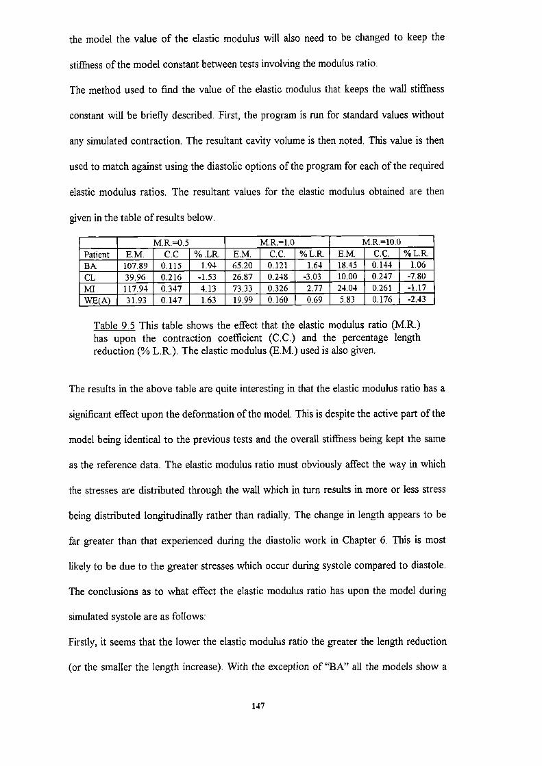
the model the value of the elastic modulus will also need to be changed to keep the

stiffness of the model constant between tests involving the modulus ratio.

The method used to find the value of the elastic modulus that keeps the wall stiffness

constant will be briefly described. First, the program is run for standard values without

any simulated contraction. The resultant cavity volume is then noted. This value is then

used to match against using the diastolic options of the program for each of the required

elastic modulus ratios. The resultant values for the elastic modulus obtained are then

given in the table of results below.

_____ _____M.R.=O.5 _____ _____M.R.=1.0 _____ M.R.=10.0

Patient E.M. C.0 %.LR. E.M. CC. %L.R E.M. CC. %L.RBA 107.89 0.115 1.94 65.20 0.121 1.64 18.45 0.144 1.06

CL 39.96 0.216 -1.53 26.87 0.248 -3.03 10.00 0.247 -7.80

MI 117.94 0.347 4.13 73.33 0.326 2.77 24.04 0.261 -1.17

WE(A) 31.93 0.147 1.63 19.99 0.160 0.69 5.83 0.176 -2.43

Table 9.5 This table shows the effect that the elastic modulus ratio (MR.)has upon the contraction coefficient (CC.) and the percentage lengthreduction (% L.R.). The elastic modulus (E.M.) used is also given.

The results in the above table are quite interesting in that the elastic modulus ratio has a

significant effect upon the deformation of the model. This is despite the active part of the

model being identical to the previous tests and the overall stiffness being kept the same

as the reference data. The elastic modulus ratio must obviously affect the way in which

the stresses are distributed through the wall which in turn results in more or less stress

being distributed longitudinally rather than radially. The change in length appears to be

far greater than that experienced during the diastolic work in Chapter 6. This is most

likely to be due to the greater stresses which occur during systole compared to diastole.

The conclusions as to what effect the elastic modulus ratio has upon the model during

simulated systole are as follows:

Firstly, it seems that the lower the elastic modulus ratio the greater the length reduction

(or the smaller the length increase). With the exception of "BA" all the models show a

147

very significant length change variation between the extreme values taken for the ebstic

modulus ratio The length change variation is less than 1° o for "BA", where as thr CL

the change is greater than 6°

Secondly, the elastic modulus ratio has a significant effect upon the contraction

coefficient. All of the patients with the exception of "Ivll" experience a reduction m

contraction coefficient when the modulus ratio is reduced. It can be concluded from this

that a low elastic modulus ratio can in some cases be beneficial to entricuhir

performance, while in others a high ratio may be beneficial. This may help to explain ihy

there is such a large disparity in the values obtained experimentally from excised cardiac

tissue. Whether a high or a low elastic modulus ratio is more desirable for greater

ventricular efficiency is likely to be dependent upon one or more of the following shape,

cavity pressure and the other material properties. Of these possible contributing factors it

is likely that shape is the most significant. This is because shape is the only thing which

differs greatly between "MI" and "BA", which exhibit markedly different responses with

respect to the elastic modulus ratio.

9.5.3 Modulus of Rigidity

The muscle fibres in the myocardium are held together by a mesh of microfibrils. It has

been hypothesised that these are fairly loose throughout the cardiac cycle, with the

exception of end diastole when they are thought to become taut (Horowitz et al. 1988

[14] and Borg and Caulfield 1981 [13]). This loose coupling of the fbres, if it were the

case, is likely to have the effect of reducing the effective shear modulus of the bulk

material in the along-the-fibre direction. It is also likely that the effective shear modulus

of the material will be reduced in the across-the-fibre direction also. The net result of

these reductions in the shear modulus is likely to allow the individual muscle fibres to

contract more freely as they would no longer be prevented from sliding over each other.

148

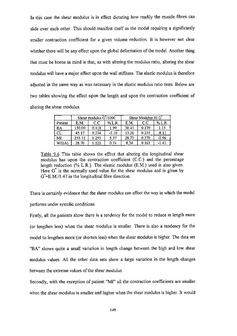
In this case the shear modulus is in effect dictating how readily the muscle fibres can

slide over each other. This should manifest itself as the model requiring a significantly

smaller contraction coefficient for a given volume reduction. It is however not clear

whether there will be any effect upon the global deformation of the model. Another thing

that must be borne in mind is that, as with altering the modulus ratio, altering the shear

modulus will have a major effect upon the wall stiffliess. The elastic modulus is therefore

adjusted in the same way as was necessary in the elastic modulus ratio tests. Below are

two tables showing the effect upon the length and upon the contraction coefficient of

altering the shear modulus.

_______ Shear modulus G/1000 Shear Modulus 10 GPatient E.M. C.0 %L.R E.M. CC. %L.RBA 150.00 0.118 1.99 30.43 0.170 1.15CL 45.17 0.234 -3.10 13.26 0.255 -8.11MI 255.31 0.293 5.37 28.73 0.270 -2.96WE(A) 38.70 0.121 0.74 8.34 0.163 -1.41

Table 9.6 This table shows the effect that altering the longitudinal shearmodulus has upon the contraction coefficient (C.C.) and the percentagelength reduction (% L.R.). The elastic modulus (EM.) used is also given.Here G is the normally used value for the shear modulus and is given byG*E.M./1 in the longitudinal fibre direction.

There is certainly evidence that the shear modulus can affect the way in which the model

performs under systolic conditions.

Firstly, all the patients show there is a tendency for the model to reduce in length more

(or lengthen less) when the shear modulus is smaller. There is also a tendency for the

model to lengthen more (or shorten less) when the shear modulus is higher. The data set

"BA" shows quite a small variation in length change between the high and low shear

modulus values. All the other data sets show a large variation in the length changes

between the extreme values of the shear modulus.

Secondly, with the exception of patient '%4J" all the contraction coefficients are smaller

when the shear modulus is smaller and higher when the shear modulus is higher. It would

149

appear that for some patients at least, a low shear modulus may be beneficial by reducing

the magnitude of the contraction coefficient required. This in turn translates into less

force being required to generate the same cavity volume reduction.

________ Shear modulus G710000 Shear Modulus 10 GPatient EM. C.0 %L.R. E.M. CC. %L.R.BA 632.42 0.13 1 2.58 25.82 0.168 0.57CL 131.60 0.155 0.59 10.93 0.335 -13.57Mu 2962.7 0.119 2.20 21.79 0.257 -0.17WE(A) 152.85 0.102 1.16 6.88 0.172 -1.17

Table 9.7 This table shows the effect that altering both the longitudinal andcross-fibre shear moduli has upon the contraction coefficient (C.C.) and thepercentage length reduction (% L.R.) Here G* is the normally used value forthe shear modulus and is given by; G'=E.M./l .47 in the longitudinal fibredirection and G=E.M./2.94 in the radial fibre direction.

On the whole the results in this table are consistent with those of the previous table and

do not require reiteration. There are however some anomalies that do require comment.

The data sets 'BA" and "CL" experience a greater effect upon their length change than

when just the longitudinal shear moduli are changed. This would seem reasonable as

greater capacity for the fibres to "slide over each other" is introduced. The data sets

"CL" and "WE(A)" both show a much greater reduction or increase in their contraction

coefficients than when only the longitudinal shear moduli are altered.

The inconsistency in the effect of the shear moduli upon the deformation of the models

would appear to be most likely due to the different shape derived from each set of

patient data. It is however likely that the contraction of the left ventricle in at least some

cases may be more easily facilitated by having low shear moduli.

9.5.4 Poisson's Ratio

It is for completeness only that the effect of Poisson's ratio is included here. It is not

expected that it will have a significant effect upon ventricular deformation. In diastolic

investigations Poisson's ratio dictates how compressible the model is in terms of its wall

150

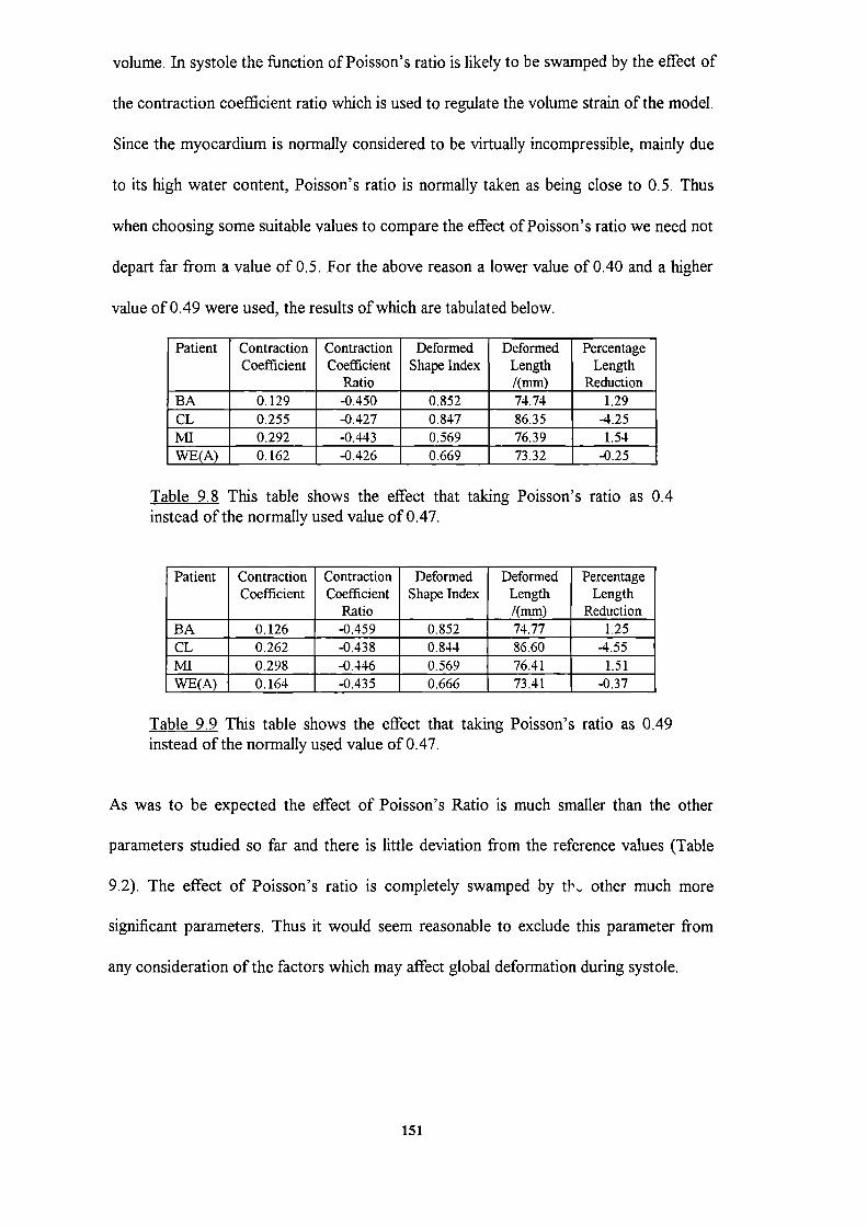
volume. In systole the function of Poisson's ratio is likely to be swamped by the effect of

the contraction coefficient ratio which is used to regulate the volume strain of the model.

Since the myocardium is normally considered to be virtually incompressible, mainly due

to its high water content, Poisson's ratio is normally taken as being close to 0.5. Thus

when choosing some suitable values to compare the effect of Poisson's ratio we need not

depart far from a value of 0.5. For the above reason a lower value of 0.40 and a higher

value of 0.49 were used, the results of which are tabulated below.

Patient Contraction Contraction Deformed Deformed PercentageCoefficient Coefficient Shape Index Length Length

________ ___________ Ratio ___________ /(mm) ReductionBA 0.129 -0.450 0.852 74.74 1.29CL 0.255 -0.427 0.847 86.35 -4.25MI 0.292 -0.443 0.569 76.39 1.54WE(A) 0.162 -0.426 0.669 73.32 -0.25

Table 9.8 This table shows the effect that taking Poisson's ratio as 0.4instead of the normally used value of 0.47.

Patient Contraction Contraction Deformed Deformed Percentage

Coefficient Coefficient Shape Index Length Length_______ ___________ Ratio ___________ I(mm) ReductionBA 0.126 -0.459 0.852 74.77 1.25CL 0.262 -0.438 0.844 86.60 -4.55

MI 0.298 -0.446 0.569 76.41 1.51WE(A) 0.164 -0.435 0.666 73.41 -0.37

[able 9.9 This table shows the effect that taking Poisson's ratio as 0.49instead of the normally used value of 0.47.

As was to be expected the effect of Poisson's Ratio is much smaller than the other

parameters studied so far and there is little deviation from the reference values (Table

9.2). The effect of Poisson's ratio is completely swamped by tl' other much more

significant parameters. Thus it would seem reasonable to exclude this parameter from

any consideration of the factors which may affect global deformation during systole.

151

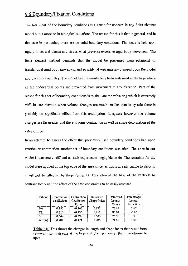
9.6 Boundary/Fixation Conditions

The treatment of the boundary conditions is a cause for concern in any finite element

model but is more so in biological situations. The reason for this is that in general, and in

this case in particular, there are no solid boundary conditions. The heart is held non-

rigidly in several places and this is what prevents excessive rigid body movement The

finite element method demands that the model be prevented from rotational or

translational rigid body movement and so artificial restraints are imposed upon the model

in order to prevent this. The model has previously only been restrained at the base where

all the endocardial points are prevented from movement in any direction. Part of the

reason for this set of boundary conditions is to simulate the valve ring which is extremely

stiff. In late diastole when volume changes are much smaller than in systole there is

probably no significant effect from this assumption. In systole however the volume

changes are far greater and there is some contraction as well as shape deformation of the

valve orifice.

In an attempt to assess the effect that previously used boundary conditions had upon

ventricular contraction another set of boundary conditions was tried. The apex in our

model is extremely stiff and as such experiences negligible strain. The restraints for the

model were applied at the top edge of the apex since, as this is already unable to deform,

it will not be affected by these restraints. This allowed the base of the ventricle to

contract freely and the effect of the base constraints to be easily assessed.

Patient Contraction Contraction Deformed Deformed PercentageCoefficient Coefficient Shape Index Length Length

_______ __________ Ratio ___________ /(mm) ReductionBA 0.155 -0.463 0.872 73.69 2.67CL 0.216 -0.436 0.861 86.02 -3.85MI 0.348 -0.399 0.606 76.50 1.71WE(A) 0.201 -0.471 0.706 71.66 2.02

Table 9.10 This shows the changes in length and shape index that result fromremoving the restraints at the base and placing them at the non-deformableapex.

152

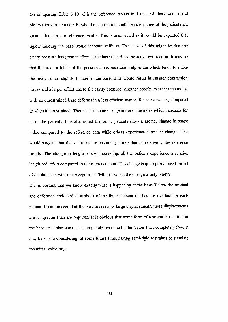
On comparing Table 9.10 with the reference results in Table 9.2 there are several

observations to be made. Firstly, the contraction coefficients for three of the patients are

greater than for the reference results. This is unexpected as it would be expected that

rigidly holding the base would increase stiffness. The cause of this might be that the

cavity pressure has greater effect at the base than does the active contraction. It may be

that this is an artefact of the pericardial reconstruction algorithm which tends to make

the myocardium slightly thinner at the base. This would result in smaller contraction

forces and a larger effect due to the cavity pressure. Another possibility is that the model

with an unrestrained base deforms in a less efficient manor, for some reason, compared

to when it is restrained. There is also some change in the shape index which increases for

all of the patients. It is also noted that some patients show a greater change in shape

index compared to the reference data while others experience a smaller change. This

would suggest that the ventricles are becoming more spherical relative to the reference

results. The change in length is also interesting, all the patients experience a relative

length reduction compared to the reference data. This change is quite pronounced for all

of the data sets with the exception of"MI" for which the change is only 0.64%.

It is important that we know exactly what is happening at the base. Below the original

and deformed endocardial surfaces of the finite element meshes are overlaid for each

patient. It can be seen that the base areas show large displacements, these displacements

are far greater than are required. It is obvious that some form of restraint is required at

the base. It is also clear that completely restrained is far better than completely free. It

may be worth considering, at some fi.iture time, having semi-rigid restraints to simulate

the mitral valve ring.

153

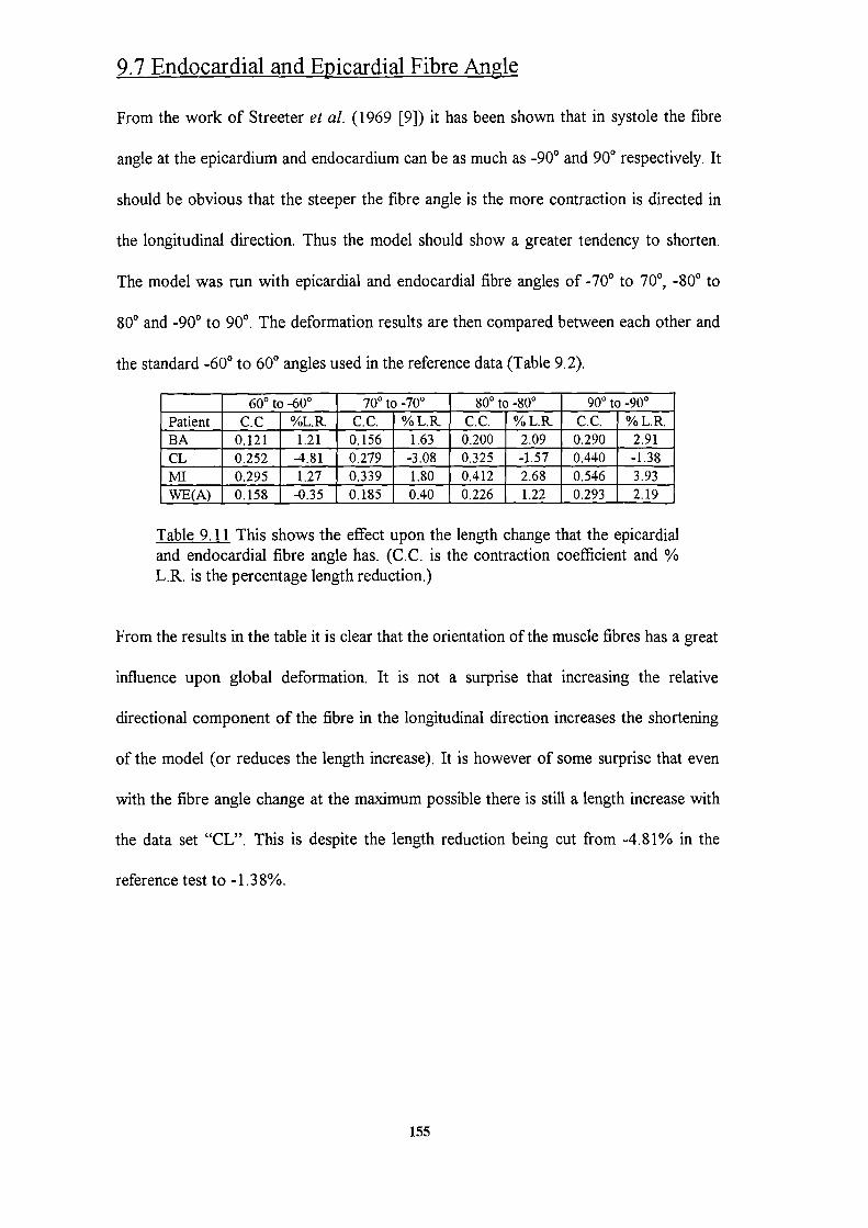
9.7 Endocardial and Epicardial Fibre Angi

From the work of Streeter et al. (1969 [9]) it has been shown that in systole the fibre

angle at the epicardium and endocardium can be as much as 900 and 900 respectively. It

should be obvious that the steeper the fibre angle is the more contraction is directed in

the longitudinal direction. Thus the model should show a greater tendency to shorten.

The model was run with epicardial and endocardial fibre angles of 700 to 70°, 800 to

80° and 900 to 90°. The deformation results are then compared between each other and

the standard -60° to 60° angles used in the reference data (Table 9.2).

________ 600 to -60° 70° to 700 80° to 800 90° to 900Patient C.0 %L.R CC. %L.R CC. %L.R CC. %L.RBA 0.121 1.21 0.156 1.63 0.200 2.09 0.290 2.91CL 0.252 -4.81 0.279 -3.08 0.325 -1.57 0.440 -1.38Ml 0.295 1.27 0.339 1.80 0.412 2.68 0.546 3.93WE(A) 0.158 -0.35 0.185 0.40 0.226 1.22 0.293 2.19

Table 9.11 This shows the effect upon the length change that the epicardialand endocardial fibre angle has. (C.C. is the contraction coefficient and %L.R. is the percentage length reduction.)

From the results in the table it is clear that the orientation of the muscle fibres has a great

influence upon global deformation. It is not a surprise that increasing the relative

directional component of the fibre in the longitudinal direction increases the shortening

of the model (or reduces the length increase). It is however of some surprise that even

with the fibre angle change at the maximum possible there is still a length increase with

the data set "CL". This is despite the length reduction being cut from -4.8 1% in the

reference test to -1.38%.

155

9.8 The Effect of the Wall Volume Reducing During Systole

We will now try to assess the importance of wall volume strain in the deformation of the

left ventricle during systole. Volume strains of approximately 10% have been seen to

occur during the cardiac cycle (Horowitz et a!. [35J and Yin et a!. [821). This wall

volume strain is due to the movement of the intracoronary blood. When the myocardium

is subjected to a load some of the blood within it will be forced out and the total volume

of the myocardium will be reduced. It would seem reasonable to assume that the

majority of this occurs during isovolumetric contraction since this is the phase when the

loading on the myocardium increases the most. If this is the case then there will be little

intracoronary blood forced out during the ejection phase, which is currently being

investigated.

Taking into consideration the above comments it would seem reasonable that between

the last two frames of systole the reduction in wall volume is likely to be far less than

1%. We will now investigate the effect of a -1% wall volume strain over the last two

frames of systole. The results of this analysis are presented in the table below.

Patient Contraction Contraction Deformed Deformed PercentageCoefficient Coefficient Shape Index Length Length

_______ __________ Ratio __________ I(mm) ReductionBA 0.107 -0.418 0.852 74.71 1.33CL 0.237 -0.421 0.845 86.34 -4.24MI 0.288 -0.428 0.574 76.35 1.59WE(A) 0.150 -0.402 0.670 73.10 0.05

Table 9.12 This table shows the effect of a -1% wall volume strain upon thedeformation of our model.

Clearly, even taking a possible unrealistically high value for the wall volume strain, the

effect upon the model is extremely small. It would thus seem reasonable to conclude that

these small reductions in wall volume between successive frames are unlikely to greatly

alter the deformation of the left ventricle. If however the 10% wall volume reduction

156

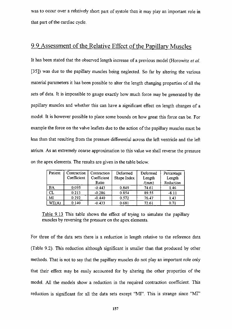
was to occur over a relatively short part of systole then it may play an important role in

that part of the cardiac cycle.

9.9 Assessment of the Relative Effect of the Papillary Muscles

It has been stated that the observed length increase of a previous model (Horowitz et a!.

[35]) was due to the papillary muscles being neglected. So far by altering the various

material parameters it has been possible to alter the length changing properties of all the

sets of data. It is impossible to gauge exactly how much force may be generated by the

papillary muscles and whether this can have a significant effect on length changes of a

model. It is however possible to place some bounds on how great this force can be. For

example the force on the valve leaflets due to the action of the papillary muscles must be

less than that resulting from the pressure differential across the left ventricle and the left

atrium. As an extremely coarse approximation to this value we shall reverse the pressure

on the apex elements. The results are given in the table below.

Patient Contraction Contraction Deformed Deformed Percentage

Coefficient Coefficient Shape Index Length Length________ ___________ Ratio ___________ /(mm) ReductionBA 0.095 -0.443 0.849 74.61 1.46CL 0.213 -0.286 0.854 89.55 -8.11Ml 0.292 -0.440 0.572 76.47 1.43WE(A) 0.140 -0.433 0.681 72.61 0.71

Table 9. 13 This table shows the effect of trying to simulate the papillarymuscles by reversing the pressure on the apex elements.

For three of the data sets there is a reduction in length relative to the reference data

(Table 9.2). This reduction although significant is smaller than that produced by other

methods. That is not to say that the papillary muscles do not play an important role only

that their effect may be easily accounted for by altering the other properties of the

model. All the models show a reduction in the required contraction coefficient. This

reduction is significant for all the data sets except "MJ". This is strange since "MT"

157

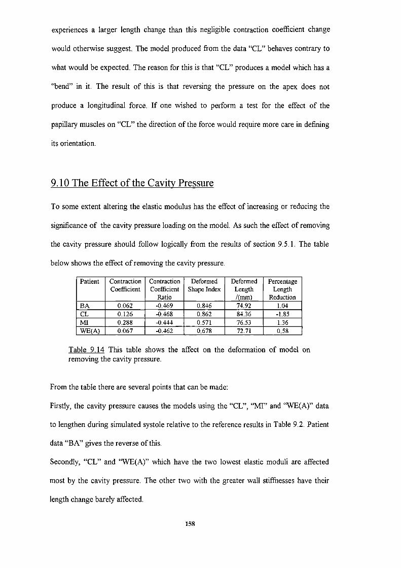
experiences a larger length change than this negligible contraction coefficient change

would otherwise suggest. The model produced from the data "CL" behaves contrary to

what would be expected. The reason for this is that "CL" produces a model which has a

"bend" in it. The result of this is that reversing the pressure on the apex does not

produce a longitudinal force. If one wished to perform a test for the effect of the

papillary muscles on "CL" the direction of the force would require more care in defining

its orientation.

9.10 The Effect of the Cavity Pressure

To some extent altering the elastic modulus has the effect of increasing or reducing the

significance of the cavity pressure loading on the model. As such the effect of removing

the cavity pressure should follow logically from the results of section 9.5.1. The table

below shows the effect of removing the cavity pressure.

Patient Contraction Contraction Deformed Deformed PercentageCoefficient Coefficient Shape Index Length Length

________ ___________ Ratio ___________ /(mm) Reduction

BA 0.062 -0.469 0.846 74.92 1.04

CL 0.126 -0.468 0.862 84.36 -1.85lviii 0.288 -0.444 0.571 76.53 1.36WE(A) 0.067 -0.462 0.678 72.71 0.58

Table 9.14 This table shows the affect on the deformation of model onremoving the cavity pressure.

From the table there are several points that can be made:

Firstly, the cavity pressure causes the models using the "CL", "MI" and "WE(A)" data

to lengthen during simulated systole relative to the reference results in Table 9.2. Patient

data "BA" gives the reverse of this.

Secondly, "CL" and "WE(A)" which have the two lowest elastic moduli are affected

most by the cavity pressure. The other two with the greater wall stiffnesses have their

length change barely affected.

158

without greatly increasing the number of elements. There was some evidence that this

was the problem when looking at the effect of the shear modulus. Even though reducing

the shear modulus should enable some "pseudo-sliding" effect it is likely to not be

remotely as great as that available in the real ventricle.

Another interesting point is that perhaps the shape index is not a good way measure

global deformation, as it can vary very little when there is a large change in length and

vice versa. Since the shape index depends upon surface area and volume it may be that it

is more sensitive to surface smoothness than the overall shape.

160

Chapter 10

10. Simulating the Left Ventricle Over End Systole

In this Chapter the information gained in the previous Chapter will be used to simulate

systole for several frames of data. The analysis procedure will be discussed as well as

attempts made to simulate the observed long dimensional changes. This will allow for

some understanding to be gained as to how the strength of myocardial contraction varies

during systole.

10.1 The Analysis procedure

The process originally to be used for analysis of systole was similar to that of "smoothed

volume matching" which is described in Chapter 3. The main difference is that the

volumes here are decreasing and not increasing as is the case in diastole. The first

attempt at systolic modelling involved starting at the onset of ejection. This however

resulted in the finite element mesh becoming badly deformed and element integrity being

severely compromised long before end systole was reached. For some patients it was not

even possible to simulate systole over the first time step. It was decided that analysis

would have to be restricted to a smaller region and end systole was chosen.

The graph of pressure verses time for patient 'BA" shows a steep rise in pressure for the

first part of systole and then an abrupt change to a less rapid rise in pressure, Fig 10.1.

The area chosen for investigation was this second part. There are two main advantages

in choosing the latter part of systole for investigation. Firstly, the ventricle is smaller and

any interaction with the pericardium is likely to be much less significant. Secondly, the

early stage of ventricular electrical activation is not considered so the effect of partial

and progressive activation will be less significant and it is thus more reasonable not to

161

element of hexahedral topology. If this is not the case then a node connection error

message is given. This was found to result from a number of different reasons Firstly, in

systole the X-ray outlines are not only smaller but also tend to have much more

convoluted outlines than in diastole. This can result in poorly formed elements

Secondly, the base of the ventricle in several of the patients was seen to noticeably tilt

during systole. This resulted in some of the elements which form the base being badly

formed. Thirdly, as has previously been discussed, the LAO image is not a longitudinal

image but in fact has a significant short axis component. In some patients the short axis

component may be dominant. If this is the case then the reconstruction algorithm

produces a shape which can be quite cylindrical. This can also result in some elements

being poorly shaped due to the way in which the mesh is formed.

The first two problems may be solved by employing a far more sophisticated

reconstruction algorithm. Unfortunately the third problem cannot be addressed by any

means other than by obtaining more suitable data. It is true that by employing a more

sophisticated meshing scheme the elements could be made more robust. This does not

however help with the fact that the shape will be a very poor representation of the

original left ventricle.

10.2 Matching Cavity Volume While Keeping Myocardial

Volume Constant

It would be preferable to be able to keep the same finite element mesh for the entire

cardiac cycle. This would mean that the effect of the simulation process could be easily

assessed by comparison of the deformed model at the end of the simulation of systole to

that produced from data for end systole. This was unfortunately not possible due to the

163

cumulative distortion of the finite element mesh which resulted in the integrity of some

of the finite elements becoming severely compromised.

The process of "target volume matching" introduced in Chapter 5 would have to be

employed. Since the finite element mesh is renewed at each time step, which is over 0.02

seconds, there is now no propagation of the distortions in the finite elements. This does,

in most situations, resolve the problem of excessive mesh distortion. On the down side it

means that there is also no cumulative change in the model's geometry, with which to

compare to the reconstructed end systolic data.

What is required is a method to sum all the geometric changes that occur between one

frame to the next frame throughout the cavity volume matching process. A simple and

straightforward method is to be preferred. The method chosen is to sum a the

percentage length changes which occur when matching one reconstzvction to the cavity

volume of the next. This overall measure can then be compared to the percentage length

change that is observed from the reconstructed X-ray data.

The table below shows how these summed length changes compare to the measured

length changes.

Patient Start End EM. M % LR C % LRBA 7 15 50 6.25 -6.03CE 8 13 150 2.26 8.39CL 8 15 20 10.10 -43.52CL(A) 7 14 30 5.52 -35.24Ml 9 16 60 9.66 6.11WE(A) 9 16 15 13.29 -12.04

Table 10.1 This table shows the summed percentage length changes (C %LR) which occur when simulating left ventricular sy ole. These arepresented with the length changes measured from the reconstructed finiteelement mesh (M % LR). Other properties of interest are also presented inthis table. The assumed value for the elastic modulus (E.M.), in KN/m 2, istaken to be a representative value for the diastolic period. (* frame 10 ofWE(A) was unusable so the M % LR was reduced accordingly from 15.51)

As can be seen there is a large spread in the measured left ventricular length changes.

The lowest change being only 2.26% and the largest being 13.29%. This is interesting

164

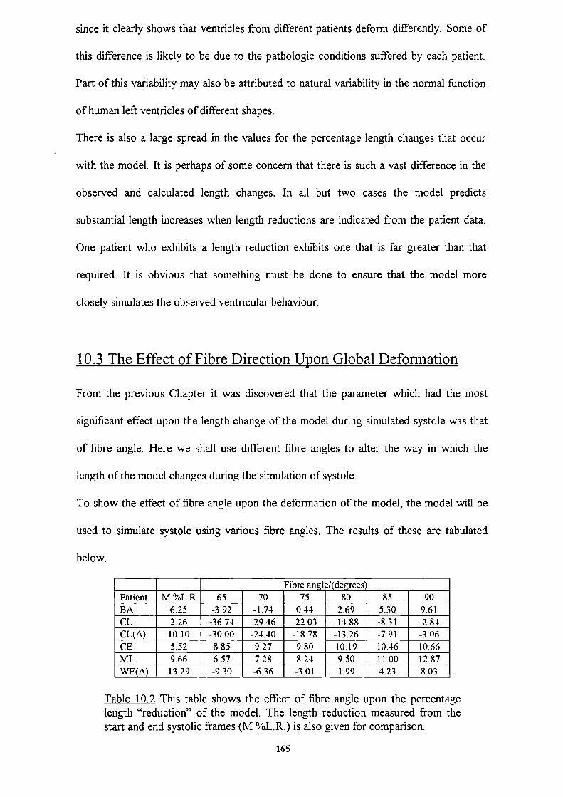
since it clearly shows that ventricles from different patients deform differently. Some of

this difference is likely to be due to the pathologic conditions suffered by each patient.

Part of this variability may also be attributed to natural variability in the normal function

of human left ventricles of different shapes.

There is also a large spread in the values for the percentage length changes that occur

with the model. It is perhaps of some concern that there is such a vast difference in the

observed and calculated length changes. In all but two cases the model predicts

substantial length increases when length reductions are indicated from the patient data.

One patient who exhibits a length reduction exhibits one that is far greater than that

required. It is obvious that something must be done to ensure that the model more

closely simulates the observed ventricular behaviour.

10.3 The Effect of Fibre Direction Upon Global Deformation

From the previous Chapter it was discovered that the parameter which had the most

significant effect upon the length change of the model during simulated systole was that

of fibre angle. Here we shall use different fibre angles to alter the way in which the

length of the model changes during the simulation of systole.

To show the effect of fibre angle upon the deformation of the model, the model will be

used to simulate systole using various fibre angles. The results of these are tabulated

below.

________ _________ ________ ________ Fibre angle/(degrees) ________ ________Patient M %L.R 65 70 75 80 85 90BA 6.25 -3.92 -1.74 0.44 2.69 5.30 9.61CL 2.26 -36.74 -29.46 -22.03 -14.88 -8.31 -2.84CL(A) 10.10 -30.00 -24.40 -18.78 -13.26 -7.91 -3.06CE 5.52 8.85 9.27 9.80 10.19 10.46 10.66MI 9.66 6.57 7.28 8.24 9.50 11.00 12.87WE(A) 13.29 -9.30 -6.36 -3.01 1.99 4.23 8.03

Table 10.2 This table shows the effect of fibre angle upon the percentagelength "reduction" of the model. The length reduction measured from thestart and end systolic frames (M %L.R.) is also given for comparison.

165

The table shows that the cumulative affect of fibre angle over the end of systole can be

quite significant. Patient data "CL" and "CL(A)" show a massive change in their length

deformation. This however is not great enough to make the length contract as is

observed from the X-ray data. An attempt was made to use the shear modulus to further

increase the length reduction of patient "WE(A)" and cause a length reduction for

patient "CL" and "CL(A)" Unfortunately the effect of this parameter had been vastly

reduced by increasing the fibre angle. It was thus not possible to use the shear modulus

and fibre angle in conjunction with each other when attempting to alter the deformation

of the model. Patient "CE" decreases in length far more than is required. In order to

obtain a more accurate length change the fibre angle was reduced. This however had

little effect and therefore these other values are not presented here.

The result of this is that one of four possibi]ities must be occurriig. Qne, the .meThoJ

used is completely unsuited to the simulation of cardiac contraction. Two, the method

used to simulate the fibre contraction results in a diminished ventricular length

contraction component. Three, there is some other external factor contributing to the

length contraction of the ventricle. Four, the muscle fibres at different depths within the

wall may contract with significantly different strengths. The result of this could be that

some of the fibres in a more longitudinal direction may be contracting with greater force

than those in a more circumferential direction. This would result in a disproportionate

amount of longitudinal contraction than would presently be predicted by the model as it

is currently employed.

Taking the above points in order. One, it would seem unlikely that the method used to

simulate cardiac contraction is completely without merit. The reasons for this are that

from the work of Chapter 9 it can be seen that at least in some cases this method can

produce results that are quite realistic in terms of global deformation.

166

Two, it is certainly possible that there may be some problem with the direction and force

calculation on the nodes of the finite element mesh. This could lead to forces in the

longitudinal direction being reduced in magnitude. One possible reason for this may be

the use of the varying fibre angle through the finite element. During systole the elemental

forces are much larger than in diastole and the coarseness of the approximation achieved

with this sort of element may give rise to an unrealistic nodal force distribution.

The possibility of some external length contracting force may exist but as to what it

could be there is little choice. Since the ventricle is becoming smaller the interaction of it

with the pericardium is likely to be small and diminishing rapidly as the ventricle

contracts. At the early stages of contraction it may be that the ventricle was constrained

in the circumferential direction and thus initial contraction would be totally longitudinal.

This however does not seem possible since there is no sign of high longitudinal

contraction in early systole. It is possible that the papillary muscles contracting to

prevent inversion of the mitral valve may provide a significant longitudinal contractile

force. It has been observed, Gibson [83], that patients who have had mitral valve

replacement and hence have had their papillary muscles cut do show some increase in

their ventricular length, though this still reduces during systole.

It is certainly true that muscle contraction is not going to be constant throughout the

myocardium, either from region to region or through the depth of the ventricular wall. It

is however difficult to quantify these differences, although it is known however that

strains at the inner surface are approximately half those at the out r surface, Gibson [83].

This unfortunately may be due to geometry rather than any indication of strength of

contraction. From analysis of excised myocardium, Novak eta!. (1994 [84]) , it has been

shown that fibres at different depths have different stifihesses. It would thus be quite

likely that the contraction force generated at different depths within the myocardium may

also be similarly non-uniform.

167

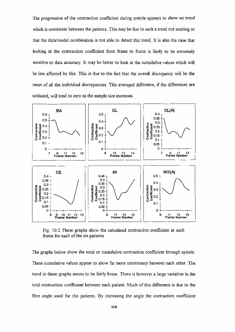
The progression of the contraction coefficient during systole appears to show no trend

which is consistent between the patients. This may be due to such a trend not existing or

that the datalmodel combination is not able to detect this trend. It is also the case that

looking at the contraction coefficient from frame to frame is likely to be extremely

sensitive to data accuracy. It may be better to look at the cumulative values which will

be less affected by this. This is due to the fact that the overall discrepancy will be the

mean of all the individual discrepancies. This averaged difference, if the differences are

unbiased, will tend to zero as the sample size increases.

BA

9 11 13 15Frame Number

CE0.4

- 0.30.250.2

0.150.1

o.c0 I I I

8 9 10 11 12 13Frame Number

CL0.5

0.4-

' 0.2

0.1

0 I I8 10 12 14

Frame Number

MI0.60.4

0.0.3

il 13 15Frame Number

CL(A)0.4

0.- 0.3

0.250.2

0.150.1

o.c0

7 9 11 13Frame Number

WE(A)0.5

0.4 Io= ' 0.3 +

0.21

0.1 +

0 I9 11 13 15

Frame Number

0.6

0.5

0.4

0.3

0.2

0.1

07

Fig. 10.2 These graphs show the calculated contraction coefficient at eachframe for each of the six patients.

The graphs below show the total or cumulative contraction coefficient through systole.

These cumulative values appear to show far more consistency between each other. The

trend in these graphs seems to be fairly linear. There is however a large variation in the

total contraction coefficient between each patient. Much of this difference is due to the

fibre angle used for the patients. By increasing the angle the contraction coefficient

168

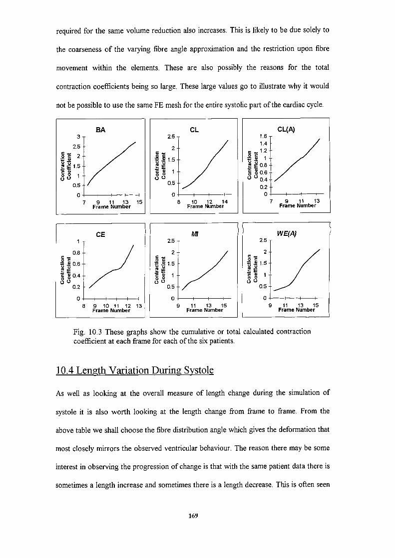
BA3

2.5

2

1.5

00 1

0.5

07 9 11 13 15

Frame Number

CE

0.8-

= W 0.6

0.400

0.2

8 9 10 11 12 13Frame Number

required for the same volume reduction also increases. This is likely to be due solely to

the coarseness of the varying fibre angle approximation and the restriction upon fibre

movement within the elements. These are also possibly the reasons for the total

contraction coefficients being so large. These large values go to illustrate why it would

not be possible to use the same FE mesh for the entire systolic part of the cardiac cycle.

CL2.5

2

. 1.5

0/

w00

0.5

8 10 12 14Frame Number

Ml

I_Frame Number

CL(A)1.61.41.2

a 1

/

0.8

0 0 0.6o 0 0.4

0.20 I

7 9 11 13Frame Number

WE(A)2.5

2-

0

0/

0°0.5

9 11 13 15Frame Number

Fig. 10.3 These graphs show the cumulative or total calculated contractioncoefficient at each frame for each of the six patients.

10.4 Length Variation During Systole

As well as looking at the overall measure of length change during the simulation of

systole it is also worth looking at the length change from frame to frame. From the

above table we shall choose the fibre distribution angle which gives the deformation that

most closely mirrors the observed ventricular behaviour. The reason there may be some

interest in observing the progression of change is that with the same patient data there is

sometimes a length increase and sometimes there is a length decrease. This is often seen

169

.c 1.9C)c

' 0.9C),

-0.1Ua.

-1.1

to happen with consecutive frames and it may be worth comparing these changes with

those measured from the patient data. It must be noted that there are likely to be large

discrepancies between the calculated values and the measured values. This is because the

measured data is dependent upon the accuracy of the digitisation process. We are

therefore only looking to see if there is any similarity in the overall trends in length

changes between the measured and the calculated lengths.

The graphs below were obtained by using the fibre angles which were identified above as

giving the most realistic length change.

BAx +

2x+

C)1 xx

C,C)

0 -

1+ I9 11 13 15

Uw -1 x

x+

-2Frame Number

CLx

xX

xx

-+1 I I

10 2 14+ +

+ +Frame Number

CL(A)4x

C)

C) (

o1 xUUU___________________

+ ++ -f: i +i

Frame Number

CE2.9t +

>c:1.9

+C,

C) i 0.9 + +

cO

10 12XX

-1.1 xFrame Number

MI5

x. 4

3+

C)

2X +x

+++1 ++x x

Ua. 0 I I

Xli 13 15-1

Frame Number

WE(A)6

x

xC)3C)

++

+UE 1

++

U

°- 0 +

11 13 15

Frame Number

Fig. 10.4 These graphs show how the change in length at each framecompares between measured and calculated. The measured length change isdenoted by an "x" and the calculated length change by a

There appears to a great deal of randomness in the length changes which occur between

successive X-ray frames. This may in part be due to the accuracy of the length

information obtained from the X-ray data. It may also be the case that the length of the

lefi ventricle does not reduce continually during systole. One thing which may support

170

this is the fact that the model predicts length increases and then reductions on successive

frames.

Despite the fact that there is a high degree of scatter in the above graphs there does

appear to be some level of correlation between the values obtained for patients "BA",

"MIT" and "WE(A)". The other patients would not be expected to show any level of

agreement since the calculated total length changes were not close to those required. It

is also of interest that the spread in the measured values in all cases is far greater than

that in the calculated. This would lend credence to the hypothesis that the ventricle

lengths are poorly reproduced by the digitisation process.

It does appear that when the total length change is adequately modelled then the changes

between individual frames will also be comparable between the observed and the

calculated.

10.5 The Effect of Pressure and Volume Changes

In this section we shall look at how the pressure increase and the volume changes

contribute to the formation of the contraction coefficient. Again we will use for

comparison purposes the fibre angles that were identified above as giving the closest fit

to the observed ventricular deformation.

It is worth mentioning that the results in this section are largely invariant to changes in

the fibre angle used in the model. This is of course not the case with length change or

even the magnitude of the contraction coefficient.

The first stage is to see if there is any relationship between pressure and the contraction

coefficient and volume change and the contraction coefficient. At this stage it would

seem reasonable to expect that there may be some dependence of the contraction

171

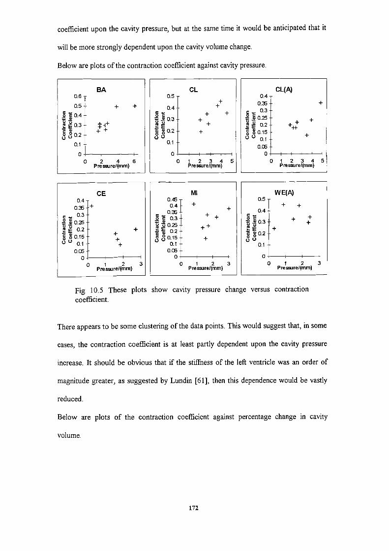
CL0.5

0.4-

o. 0.3

0.2

0.1

00 12345

Pressure!(mm)

MI

0.40.

2 0.30.250.2

1 2 3Pressure/(mm}

coefficient upon the cavity pressure, but at the same time it would be anticipated that it

will be more strongly dependent upon the cavity volume change.

Below are plots of the contraction coefficient against cavity pressure.

BA0.6

0.5

0.4

0.3

0.2

0.1

00 2 4 6

Presre/(mm)

CE0.4

+

0.3oc 0.25

0.2 ^g0.15

+o.c

0 -±----

0 1 2 3Pressurel(mm)

CL(A)0.4

o.:: +0.3

. 0.25O.2 + +

0.15000.1 +

o.c0 I 1

012345PresJreI(mm)

WE(A)0.5

0.4-. 0.3

g 0.2

0.1

00 1 2 3

Pressurel(mm)

Fig 10.5 These plots show cavity pressure change versus contraction

coefficient.

There appears to be some clustering of the data points. This would suggest that, in some

cases, the contraction coefficient is at least partly dependent upon the cavity pressure

increase. It should be obvious that if the stiffliess of the left ventricle was an order of

magnitude greater, as suggested by Lundin [61], then this dependence would be vastly

reduced.

Below are plots of the contraction coefficient against percentage change in cavity

volume.

172

BA H CL H CL(A)0.6

0.5

0.4Ut;

0.3

g 0.2

0.1

00 2 4 6

Percentage VolumeReduction

CE0.4 T

0.25+ +

o: 0.25

0.2 -4-+

o 0+

0 00.1 +o.c

0 II! II

0 2 4 6 6 1012

Percentage VolumeReduction

0.5

0.4oc

w 0.2o00 00.1

00 2 4 6

Percentage VolumeReduction

MI0.5

0.40

0.2

0 0.1

00 4 8 12 16 20

Percentage VolumeReduction

0.40.25

g . 0.3. 0.25

0.20.15

0 0 0.1o.c

00 2 4 6Percentage Volume

Reduction

WE(A0.5

+ +— 0.4

++

+0.2

0 00.1

0 I I0 4 8 12 16 20

Percentage VolumeReduction

Fig 10.6 These plots show percentage change in cavity volume versuscontraction coefficient.

It appears that, in some cases, the contraction coefficient is strongly dependent upon the

percentage volume change. The last three graphs show a quite strong dependence upon

the volume change and their dependence upon the cavity pressure is much more tenuous.

It is thus likely that the contraction coefficient in general is partly formed as a result of

the pressure increase and partly as a result of the volume change. If however the model

was taken as being significantly stiffer then the contribution from the cavity pressure

would in all cases become negligible. The contraction coefficient would then be almost

totally dependent upon the volume change.

173

10.8 Summary

The method proposed to simulate the end of systole can provide a realistic simulation of

performance.

When using an elastic modulus which is approximately the average diastolic value the

contraction coefficient appears to have a dependence on both the volume change and the

cavity pressure change. If however the stifihess of the model was increased by an order

of magnitude as suggested by Lundin [61J then the dependence on the cavity pressure

would be greatly reduced.

The fibre angle at the endocardium and epicardium can greatly affect the deformation of

the model. However, the way in which the model deforms appears to have as much to do

with the shape as any other factor.

Some patients could not have their length change sufficiently controlled, by varying the

fibre angle, to simulate the observed length change. This may in part be due to the

data/reconstruction giving rise to a model shape which will not perform in a realistic

way.

174

Chapter 11

11. Factors that can Affect the Left Ventricle

This section will mainly be concerned with the effect of simulated pathologic disorders

upon the left ventricle model. There will also be some investigation as to the effect of an

uneven distribution of contractile force. As well as this an examination will be made as to

how different model configurations affect the strain within the model and how these

values compare with those known to occur within the human left ventricle.

11.1 Local Wall Strain

It is known that the sarcomeres which make up the muscle fibres are only able to

contract by about 10 to 15% (Gibson [83]) depending upon whether they are loaded or

not. A loaded sarcomere can only contract by as much as 10%. It would thus be of great

interest to see if our model produces strains which are consistent with this. On the face

of it, it would seem unlikely as the contraction coefficient values used in the model

would indicate a value much higher than this.

The computer program, as part of its output, produces the strains in the fibre direction

for each finite element. This gives rise to a large number of values which give the fibre

strain for each corner node of each element. The number of values this generates is four

hundred and eighty. The most obvious thing to do is to find the mean value of these. For

frame fourteen of "BA" the mean strain value was found to be -4%. This is obviously

too high as it is only for about one tenth of overall systole. The combined value for the

whole of the analysed region of systole is approximately -50%. The question arises as to

why this value is not only much larger than -10% but is also very much larger than

would be expected due to simple geometrical considerations.

175

If it is correct that a sarcomere can contract by only 10%, in the loaded situation, the

question becomes is the observed volume change consistent with this value? In any

three-dimensional structure the volume and hence the volume change will be related to

the cube of the linear dimensions. Thus if there is a 10% reduction in the length of the

sarcomeres we would expect a 27% reduction in volume. In the left ventricle however

the volume reduction may be in excess of 40% which implies a greater than 15% length

reduction. The contradiction between the length reduction of the sarcomeres and the

cavity volume change seems to be paradoxical. The way in which the left ventricle

overcomes the geometrical considerations and achieves such a high output is far from

clear. Two of the important factors are likely to be the change in ventricle shape and the

twisting of the ventricle. By the ventricle changing shape the cavity volume can be

altered without changing the surface area and hence the average sarcomere length.

Likewise twisting of the ventricle may result in the contracting sarcomeres reducing the

cavity volume more than would be achieved otherwise.

It is thus obvious that the change in the shape of the ventricle and the twisting of the

epicardium relative to the endocardium are important factors to be considered.

11.2 Local Wall Strain and Fibre Slippage

The question has to be why does our model produce such high fibre strains? The logical

place to start is to consider how our model differs from the real left ventricle. The most

obvious difference is that the real left ventricle is composed f loosely bound muscle

fibres. These fibres are also continuous along the length of the ventricle. Our model does

not have this level of fibre independence. The fibres are modelled as solid blocks of

anisotropic material with the direction of anisotropicity varying through the thickness of

the block.

176

Several different arrangements for the muscle fibres were tried in order to assess '1.hich

aspect had the greatest effect upon the average fibre strain. The table below shows the

average fibre strain and the contraction coefficient for three of these different fibre

configurations.

Varying Fixed Fixed-85° to 85° -45° & 45 00 & 00

CC. 0238 0.565 0.059A.F.S. -0.043 -0.105 -0.023

Table 11.1 This table shows the contraction coefficient (C.C.) and theaverage fibre strain (A.F.S.) for various fibre configurations; a linearlyvarying fibre direction through the wall thickness and a fixed fibre directionwithin the epicardial and endocardial layers.

The above results were obtained using the data for patient "BA" at frame 14 and 15,

From the above results it can be seen that when the endocardial and epicardial fibre

direction is kept constant through the elements the fibre strain and contraction

coefficient more than double. This shows that the interface between elements may be a

significant contributor to the high values for the contraction coefficient and fibre strain.

When the fibre direction is kept fixed through all the elements at an angle of zero

degrees to the horizontal there is a quartering of the contraction coefficient and a halving

of the average fibre strain. This value is much closer to what would be considered a

reasonable value for the mean fibre strain.

The conclusion from this is that the model is inefficient at transferring the forces

generated by the fibre strains into work done in reducing the cavity volume. This appears

to be partly as a result of the simulated muscle fibres not beinb free to slide over each

other. A model based on the same principles as this one, but using a loosely tethered set

of concentric shells, previously proposed by Streeter et a!. (1970 [21]) for a diastolic

investigation is likely to give far more realistic fibre stresses. That said, if one is only

interested in global deformations the present model would seem to be adequate.

177

11.3 Greater Epicardial than Endocardial Contraction

It is known that the fibre strains in the endocardial layer are less than those in the

epicardial layer (Gibson [83]). This may just be a result of geometry. It is however

relatively straight forward to check to see whether there is any benefit to our model in

having a lower endocardial contraction coefficient. The finite element analysis was

performed for the last pair of systolic frames for each of the patients with the contraction

coefficient of the endocardial layer being half that in the epicardial layer. The effect this

had upon the model is given in the table below.

______ Uniform C.C._____ Half Inner CC.Patient CC. A.F.S. %L.R. CC. A.F.S. °0L.RBA 0.238 -0.043 2.44 0.270 -0.040 2.79CE 0.360 -0.065 0.99 0.601 -0.117 -5.05CL 0.420 -0.084 -1.02 0.428 -0.067 -0.28CL(A) 0.220 -0.026 -0.40 0.267 -0.025 -0.85Ml 0.413 -0.078 2.67 0.564 -0.078 4.62WE(A) 0.293 -0.025 2.19 0.379 -0.025 3.04

Table 11.2 This table shows how having a higher epicardial than endocardialcontraction coefficient (C.C.) affects the average fibre strain (A.F.S.) and thepercentage length reduction (% L.R.). Note: the contraction coefficientgiven in the half inner test is the epicardial value.

There is some effect upon both the percentage length reduction and on the average fibre

strain. This is relatively small in most cases and is certainly less significant than the

previously investigated model parameters. The exceptions to this are patients "CE" and

'MI" which show quite significant changes. The effect of uneven contraction in these

cases is not consistent between the patients and this as before is most likely due to

ventricular shape. It is certainly the case that partial and progressive contraction are

important factors in the performance of the left ventricle. It is, in most cases, of only

minor significance when considering global deformation using the present model.

178

11.4 Ischaemia and Scar Tissue

Ischaemia and scarring of necrotic myocardium are major conditions which affect the

performance of the left ventricle. Ischaemia is depression of function by a loss or partial

loss of blood supply to part of the myocardium. Since the muscle does not have

adequate oxygen it is unable to generate the force which the unaffected myocardium can.

If the ischaemia is prolonged then the affected myocardium will die and over a period of

several weeks will be replaced by a stiff fibrous and non-contracting scar tissue. When

blood supply is restricted the deeper (endocardial) region is affected first and this then

spreads to the higher levels of the myocardium.

In order to model the effect of the above processes upon the myocardium two areas of

the left ventricle were chosen for investigation. These two areas of the left ventricle are

taken to be the anterior free wall and the posterior free wall. To mode) the effect of

ischaemia the myocardium in the affected area is taken to be non-active and to have an

elastic modulus the same as the rest of the ventricle and also the same test is done with

an elastic modulus a tenth of this. The reason for taking two values is that, depending on

the severity of the restriction in blood flow, the myocardium will either be unable to

contract or may loose some of its stiffness.

Since scar tissue is stiff and non-contracting it is modelled as an area of increased

stifThess. In the present study it is taken as being ten times stiffer than the normal

myocardium.

Thus both conditions will be characterised by a non-functioning rea of the myocardium.

The passive stiffness in the scarred area will be stiffer than the normal myocardium. In

the ischaemic area the stiffness is likely to be reduced or of a similar value to the rest of

the myocardium.

179

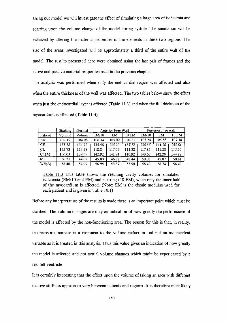
Using our model we will investigate the effect of simulating a large area of ischaemia and

scarring upon the volume change of the model during systole. The simulation will be

achieved by altering the material properties of the elements in these two regions. The

size of the areas investigated will be approximately a third of the entire wall of the

model. The results presented here were obtained using the last pair of frames and the

active and passive material properties used in the previous chapter.

The analysis was performed when only the endocardial region was affected and also

when the entire thickness of the wall was affected. The two tables below show the effect

when just the endocardial layer is affected (Table 11.3) and when the full thickness of the

myocardium is affected (Table 11.4)

________ Starting Normal Anterior Free Wall Posterior Free wallPatient Volume Volume EMJ1O EM 10 EM EMJ1O EM 10 EMBA 107.19 104.08 106.34 105.00 104.62 105.24 106.58 107.18CE 155.28 134.92 135.48 135.20 137.72 136.35 144.18 153.81

CL 122.72 114.28 118.84 117.05 111.38 117.86 115.28 115.60CL(A) 150.03 139.58 142.92 141.94 140.92 140.60 142.28 144.88MI 56.21 44.62 45.80 46.82 48.44 50.03 49.07 50.81WE(A) 58.40 54.99 56.95 59.37 55.90 58.40 56.74 56.49

Table 11.3 This table shows the resulting cavity volumes for simulatedischaemia (EM/lO and EM) and scarring (10 EM), when only the inner halfof the myocardium is affected. (Note: EM is the elastic modulus used foreach patient and is given in Table 10.1)

Before any interpretation of the results is made there is an important point which must be

clarified. The volume changes are only an indication of how greatly the performance of

the model is affected by the non-functioning area. The reason for this is that, in reality,

the pressure increase is a response to the volume reduction nd not an independent

variable as it is treated in this analysis. Thus this value gives an indication of how greatly

the model is affected and not actual volume changes which might be experienced by a

real left ventricle.

It is certainly interesting that the effect upon the volume of taking an area with different

relative stiffness appears to vary between patients and regions. It is therefore most likely

180

that it is the shape of an affected area which is likely to determine how greatly the

performance of the left ventricle is impaired by ischaemia or scarring. This is likely to be

the reason why the area of the left ventricle which is affected by coronary artery disease

will determine the prognosis for that patient, Gibson [83].

Some of the results in the above table show that performance is less impaired by a less

stiff rather than a stiffer region. This is because for those patients the volume change is

of greater significance than the pressure change. In this case the epicardial layer is still

able to overcome the cavity pressure and thus contribute to the volume reduction.

In other cases the volume change is less affected by the affected area being stiffer. In this

case the reduced contraction force in that area is unable to contribute to the volume

reduction. This area will tend to bulge out and as a result this area's contribution nay be.

a volume increase. In some of the above cases this volume increase is dwarfed by the

overall volume reduction. In other cases there is an overall increase in volume.

The simulation of scarring of the anterior free wall of patient "CL" is interesting since

this results in a greater reduction in volume than in the normal case. This would suggest

that the anterior free wall for this patient is particularly flexible and during the normal

simulation tends to bulge out. This may be due to that part of the wall being slightly

thinner in the model than in the real left ventricle or it may be due to the elastic modulus,

used for this patient, being too low. Whichever of these two reasons is correct is

immaterial since it is obviously a spurious result. That is there is no reason why a left

ventricle would perform befter when part of it was not functioning. It was found that if a

higher value of the elastic modulus was taken then this unexpected result was not

repeated.

It is difficult to say whether ischaemia and scarring have the most detrimental effect

when in the anterior or posterior region. The simulation of scarring however, appears to

be slightly more detrimental in the posterior region than in the anterior region. The effect

181

of the simulation of ischaemia appears to be far more evenly distributed between the two

regions. As a result it is harder to pinpoint which region is more greatly affected.

________ Starting Normal Anterior Free Wall Posterior Free wall

Patient Volume Volume EMJ1O EM 10 EM EM/lO EM 10 EM

BA 107.19 104.08 112.51 105.52 104.48 112.40 108.84 107.82

CE 155.28 134.92 135.13 133.62 136.48 143.28 149.66 153.33

CL 122.72 114.04 135.27 117.58 110.11 141.94 121.64 119.92

CL(A) 150.03 139.58 161,16 145.57 141.52 157.15 146.87 146.85

MI 56.21 44.62 46.73 47.17 49.05 55.91 54.05 52.64

WE(A) 58.40 54.99 67.60 57.23 54.94 69.53 60.89 57.57

Table 11.4 This table shows the resulting cavity volumes for simulatedischaemia (EMI1O and EM) and scarring (10 EM), when the ftill depth of themyocardium is affected. (Note: EM is the elastic modulus used for eachpatient and is given in Table 10.1)

The above table shows the effect of simulating ischaemia and scarring through the full

depth of the anterior and posterior wall. Unlike the previous case we do not have the

complication of half of the wall depth still being active. This has resulted in far greater

congruity between the results obtained for the different patients. All the patients, with

the exception of MI", behave consistently. That is their performance is less impaired by

a stiff region than a less stiff region. On the whole it would seem that the posterior free

wall is a more sensitive area as regards performance of the left ventricle. Again patient

"CL" shows a greater volume reduction with a stiff anterior free wall than a normal

contracting one. This adds further weight the assertion made above about the cause of

this increased volume reduction.

As with the analysis when only the endocardial half of the model wall is affected, patient

"MI" shows a smaller volume reduction with a stiff anterior ft e wall than with a less

stiff one. Since in this case the full depth of the affected part of the wall is non-

contracting the previously used explanation does not hold. The volume differences are

however very small and thus are likely to be more greatly affected by computational

approximation. This may be the reason for this unexpected phenomenon. There is

however another possible explanation. Since the volume changes are small there may be

182

another factor which could bring about this strange result. The model when systole is

simulated experiences some rotation (Chapter 7) and a very stiff region would impair this

rotation. It may be that when the rotation is impaired the volume reduction is prevented

to some extent. This could give rise to the result of a less stiff area being not as

damaging to the volume reduction as a stiff region.

11.5 Summary

There are a number of conclusions which can be made from the results of this section.

Firstly, the model as used at present does not appear to be able to accurately model the

local strains. This may in part be due to the coarse approximation which has been made

for the varying fibre angle through the wail thickness. It may also be in part due to the

lack of the ability of the simulated muscle fibres to slide over each other. A third reason

for this may even be due to the way these "fibre strains" are calculated. The "fibre

strains" in our model are calculated for each corner node of each element. In the real left

ventricle the fibres are continuous and not a series of short fibres as they are treated in

the strain calculation. It may be necessary to calculate the strain which would result in a

fibre which traverses the entire length of' the ventricle. It has been shown that the

"optimal" coarse for greatest efficiency of fibre contraction is for the fibres to lie along

geodesics (Horowitz et a!. 1993 [85]). That is they follow the shortest course possible

on some surface, at the epicardium and endocardium it will be these surfaces. It may be

that consideration of this would be necessary for the correct calculation of the fibre

strains.

Secondly, there appears, in most cases, to be little effect upon the global deformation of

the model in taking a lower contraction coefficient for the endocardial layer of elements.

That is not to say that an uneven distribution of contractile force is not important to the

183

real left ventricle. It is just that this model is not very sensitive to these differences in

contraction.

Thirdly, geometry of the left ventricle once again shows that it is important to the

function of the left ventricle. In this case it has been demonstrated that the shape and

position of an area of ischaemic or scarred left ventricle may be fundamental to how

impaired the performance of the left vertical could become.

184

Chapter 12

12.1 Conclusions

There are a number of conclusions that may be drawn from this work.

(1) The first conclusion is that the two programs "XL1" and "HEART" can be

combined into a single package which can be run upon desktop computer systems. It is

also the case that the calculation of the passive and active material properties can be

automated to provide results without constant user input. The result of this is that large

numbers of patients can be analysed and will only require user input for interpretation of

the results.

(2) The proposed method of volume matching known as "target volume rnaching"

can be used to analyse the diastolic properties of the myocardium. This method does not

have a significant effect upon the results obtained when compared with the results

obtained from "smooth volume matching". This new method does however seem to

make the model less stiff and there appears to be greater variation in the values obtained

for the elastic moduli. Another interesting aspect raised by the introduction of this

method was that, due to the lack of divergence in the results obtained by the two

methods, the method of "smooth volume matching" was reasonably accurate over the

diastolic period.

(3) The modulus ratio can have a significant effect upon the global deformation of

the left ventricle during diastole. This effect although significant is not great enough to

explain the ventricular length changes that are observed from the X-ray frames during

diastole. Whether this inability to account for the observed length changes is due to

either some other property of the myocardium or some external force is as yet unclear. It

is difficult to deduce much concerning the length and length changes of the left ventricle

since the accuracy of the length measurements must be somewhat suspect. The reason

185

for this is that when the original data was prepared it was not envisaged that the length

information would be required and thus less precision would have been required during

digitisation. It is also the case that length and displacement information is affected more

by small errors than is the volume and hence the cavity volume would always provide

greater certainty in regards to its accuracy.

(4) From the analysis of diastole it is clear that the shear modulus is likely to have a

significant effect upon the way in which the left ventricle deforms in diastole. It also

seems likely that in order to match the length of the left ventricle during diastole the

assumed relationships between the various material properties must be changed.

(5) The "thermal stressing" analogy as proposed by Rosen [641 can be used to

simulate the active contraction of the myocardium. It can also, in some cases, fully

explain the global deformation that has been observed from patient data. The relative

rotation of the endocardial and epicardial surfaces is also shown to occur in this model.

(6) The passive material properties of the myocardium do not greatly affect the

global deformation of the myocardium during systole. The exception to this is when the

overall stiffness of the model's wall is effected and when the wall stiffness is low.

Increases in the wall stifihess do not have a very significant effect. Reductions from the

"average" diastolic values do however have a more significant effect upon global

deformation, especially if the wall stiffness is low to begin with. It is an unlikely scenario

that the passive properties would be less stiff during systole than they are in diastole. The

reasoning behind this is twofold, one, if the myocardium was less stiff then the

contracting myocardium would have to work harder to over come the effect of the

cavity pressure. Two, all the research done on systolic myocardium suggest that it

behaves much stiffer than during diastole. It is thus likely that the myocardium will be

relatively stiff during systole and that consequently the effect of small changes in

myocardial stiffness are unlikely to greatly affect global deformation.

186

(7) The use of a high endocardial and epicardial fibre angle in the model reduces to

negligible the effect on the global deformation of the model of changing the ratio of

shear stiffness to elastic stiffness. It is thus likely that the passive material properties have

a much reduced effect if the particular left ventricle can be shown to have a high fibre

angle.

(8) If the myocardium can be shown to be stiffer during systole than during diastole

then the effect of the cavity pressure will be negligible. Thus systole can be modelled

using geometric data alone. This is important as pressure data is difficult to come by as it

must be obtained by invasive means. The result of this is that data suitable for the

investigation of systolic left ventricular properties could be more easily obtained.

(9) It is clear that shape is probably the single most important factor responsible for

the way in which the left ventricle deforms during systole. Other factors can affect this

deformation to some extent though the extent of this is also shape dependent.

(10) The boundary conditions for the model are also a major factor which can

contribute to the deformation. The significance of this is of a similar order to that of the

material properties.

(11) The use of the shape index as suggested by Grewal [2] has been less than

successful. An improvement to this shape index might be to consider some form of

envelope function rather than the volume and surface area.

(12) The lack of ability of the "muscle fibres" in this model to "slide over each other"

is likely to be responsible for the high values of the contraction coefficients required by

the model. The other factor to contribute to this very high value is likely to be the

coarseness of the approximation of the varying fibre angle through the wall. The first of

these problems may be overcome by the inclusion of the ability of the layers which make

up the thickness of the wall to slide freely over each other. The second of these problems

may be overcome by increasing the number of elements through the depth of the wall.

187

(13) If the total length change in the model over systole is adequately simulated by

this model then it appears that the frame to frame length changes are also velI

represented. This means that the model can provide a good simulation of what occurs to

the shape of the left ventricle during late systole.

(14) The work of Horowitz et a!. [85] has shown that the course of the muscle fibres

of the myocardium lies on geodesics. That is they run along the shortest path from one

point of the myocardium to another while remaining on some "surface" defined within

the myocardium. For the endocardium and epicardium this will be the actual surface.

Thus in order to consider the fibre strain in the myocardium the change in length of an

imaginary fibre following such a path must be considered. This is easily accomplished for

idealised ventricular shapes but is a much more complicated task when considering a

non-idealised finite element model.

(15) The uneven distribution of contraction fov 'ithin th moxm csf t

ventricle in general would not appear to greatly alter the global deformation of our

model. It is however quite likely to affect the local distribution of stress and strain within

the myocardium, especially through the depth of the ventricular wall.

(16) It is also the case that this model shows that the magnitude of the effect of

ischaemia and scarring upon the function of the myocardium is not restricted merely to

the properties of the affected area but is also dependent upon the shape of the ventricle

in the affected area. This means that the position of a damaged area of myocardium is

likely to be important as well as its size.

(17) Finally, it has been shown that the use of the thermal stressing analogy for

myocardial contraction is applicable to the simulation of a systolic left ventricle.

I 88

12.2 Further Work

There are several areas which still require investigation and improvements which can be

made and these are described below:

(1) It is vitally important that more data becomes available for the simulation of late

systole. At present only six patients have been analysed and this is a very small number

from which to draw any great conclusions.

(2) The data used in this analysis is quite old and newer imaging methods provide

greater clarity and increased accuracy. What is not generally available are the pressure

readings from within the left ventricle. If it is the case that the cavity pressure is not of

great importance during systole then geometric data alone could be used to analyse late

systole. The most suitable data for modelling purposes would be that which incorporates

not only long axis information by short axis cross-sections also.

(3) A more sophisticated method of calculating muscle fibre strains must be

introduced. This must be calculated considering the fibres to lie on geodesics.

(4) A comparison should be made between the deformation obtained with this model

compared to that of other models produced using more sophisticated constitutive

equations. This will allow this model to be rated against those with a far higher

computational overhead and see whether there is a need for other more complex models.

(5) If use was to be made of Magnetic Resonance Imaging data then a method for

limiting the distortion of the finite element mesh would be required. This is because the

temporal resolution of that method is far lower than that of X-ray angiography. The

result of this is that the simulation would have to be performed over a longer period

before a new mesh could be formed from the next set of data. The solution is to use

some form of adaptive meshing scheme similar to that in the finite difference scheme, the

"Adaptive Grid Method". This involves generating the "optimum" discretisation of the

189

solution space as the problem is solved, In our problem a similar thing could be achieed

by remeshing the FE mesh at predefined intervals. These intervals could be defined m

terms of time, maximum allowed volume reduction, as a maximum allowable contraction

coefficient or when the distortion of the finite elements reaches some tolerance This

would not only allow for the use of data with poor temporal resolution but ould also

allow the presently used geometric data to be kept throughout the analysis of sstole

190

References

[1] Analysis of Stress and Deformation in the Human Left Ventricle PhD Thesis B

C.A.Vinson. Department of Mechanical Engineering Brunel University June 1977

[2] The Mechanical Behaviour of the Left Ventricle of the Human Heart in Diastole

PhD Thesis By B.S.Grewal. Department of Mechanical Engineering Brunel University

May 1988.

[3] Analysis of Left Ventricular Behaviour in Diastole By Means of Finite Element

Method. By C.A.Vinson, D.G.Gibson and A.L Yettram. British Heart Journal Volume

XLI, No. 1, pages 60-67, January 1979.

[4] Geometric Modelling of the Human Left Ventricle. By A.L Yettram and

C.A.Vinson. Journal of Biomechanical Engineering August 1979 Vol. 101 pp22l-223

[5] Computer Modelling of the Human Left Ventricle. By A.L.Yettram, C AVinson

and D.G.Gibson. Transactions of the ASME Vol. 104, May 1982 pp 148-152.

[6] 1993 Mortality Statistics Cause England and Wales. OPCS HMSO 1993.

[7] Three-Dimensional Finite Element Analysis of Anterior-Posterior Variations in

Local Sarcomere Length and Active Fibre Stress During Left Ventricular Ejection. By

J.M.Guccione, A.D.McCulloch, W.C.Hunter. Advances in Bioengineering AS?1E 1993

BED-vol. 26 pp 571-574.

[8] Left Ventricular Stresses in the Human Heart. By I.Mirsky. Biophysical Journal

Vol. 9 pp 189-208 1969.

[9] Fiber Orientation in the Canine Left Ventricle During Diastole and Systole. By

D.D.Streeter, Jr., S.M.Henry, M.Spotnitz, D.P.Patel, J.Ross Jr. and E.H.Sonnenblick.

Circulation Research Vol. XXIV 1969.

[10] An Account of the Structures concerned in the Production of the Jugular Pulse

By AKeith MD. Journal of Anatomy and Physiology Vol. XLII pp 1-25 1907

191

[11] Principles of Physiology. Edited by R.M.Berne and M.N.Levy. Wolfe Publishing

Limited 1996.

[12] Gray's Anatomy Descriptive and Applied 29th Edition. Edited by T.B.Johnston

and J.Whillis. Longmans, Green and Co. 1947.

[13] The collagen matrix of the heart. By T.K.Borg and J.B.Caulfield. Federation

Proceedings Vol. 40 pp 2037-2041 1981.

[14] Structural Three-dimensional Constitutive Law for passive Myocardium. By

A.Horowitz, Y.Lanir, F.C.P.Yin, M.Perl, I.Sheinman and R.K.Strumpf. Transactions of

the ASM1E Journal of Biomedical Engineering Vol. 110/201 pp 200-207 August 1988.

[15] The Ventricle: Basic Clinical Aspects. Edited by H.J.Levine and W.H.Gaasch.

Martinus Nijhoff Publishing 1985.

[16] Certain Mechanical Peculiarities of the Human Cardiac Pump in Normal and

Diseased States. By G.E.Burch, C.T.Ray and J.A.Cronvich. American Heart Journal

Vol. 54 Part 6 pp 801-810 1957.

[17] Looking at Size and Shape relationship to Ventricular Performance, By

A.C.Burton. American Heart Journal Vol. 5 Part 6 pp 801-810 1957.

[18] Left Ventricular Tension and Stress in Man. By H.Sandler and H.T.Dodge.

Circulation Research Vol. 13 Part 2 pp 91-104 1963.

[19] Stress Distribution Within the Left Ventricular Wall Approximated as a Thick

Ellipsoidal Shell. By A.Y.K.Wong and P.M.Rautaharju. American Heart Journal Vol. 75

par 5 pp 649-662 1968.

[20] An Analytic Elastic-Viscoelastic Model For the Shape and Forces in the Left

Ventricle. By D.N.Ghista and H.Sandler. Journal of Biomechanics Vol. 2 pp 34-47

1969.

192

[21] Stress Distribution in the Canine Left Ventricle During Diastole and Sstok B

D.D.Streeter, J.R.Ramesh, N.Vaishnav, D.J.Patel, H.M.Spotnitz.. J Ross and

E.H.Sonnenblick. Biophysical Journal Vol. 10 Part 4pp 345-363 1970.

[22] An Indirect Determination of the Oxygen Utilisation of the Human Left

Ventricle. By D.N.Ghista and H. Sandier. Journal of Biornechanics Vol. 3 pp 161-114

1970.

[23] Myocardial Mechanics: Application of Sliding-Filament Theory to Isooiumic

Contraction of the Left Ventricle. By A.Y.K.Wong. Journal of Biomechanics Vol 6 Part

5pp565-58l 1973.

[24] Effect of Chamber Eccentricity on Equatorial Fiber Stress During Systole By

R.F.Janz. Federation Proccedings Vol. 39 Part 2 pp 183-187 1980.

[25] Estimation of Local Myocardial stress. By R.FJanz. American Journal of

Physiology Vol. 242 (Heart Circ. Physiol. 11) pp H875-H881 1982.

[26] Static Analysis of the Left Ventricle. By A.Tozeren. Journal of Biomechanical

Engineering Vol. 105 pp 39-46 1983.

[27] Myocardial Material Mechanics: Characteristic Variation of the Circumferential

and Longitudinal Systolic Moduli in Left Ventricular Dysfunction. By C.A.Phillips and

J.S.Petrofsky. Journal of Biomechanics Vol. 17 Part 8 pp 56 1-568 1984.

[28] Estimation of Local Cardiac Wall Deformation and Regional Wall Stress from

Biplane Coronary Cineangiograms. By H.C.Kim, B.G.Min, M.M.Lee, J.D.Seo, Y.W Lee

and M.C.Han. IEEE Transactions on Biomedical Engineetin Vol. BME-32 Part 7

1985.

[29] Comparison of Models Used to Calculate Left Ventricular Wall Force By

R.M.Huisman, P.Sipkema, N.Westerhof and G.Elzinga. Medical and Biological

Engineering and Computing Vol. 18 pp 133-144 1980.

193

[30] Finite Element Model for the Mechanical Behaviour of the Left Ventricle.

Prediction of Deformation in the Potassium-Arrested Rat Heart. By R.F.Janz and

A.F.Grimm. Circulation Research Vol. 30 1972.

[31] The Finite Element in Engineering Science. By O.C.Zienhiewicz. McGraw-Hill

1971.

[32] Finite Element Analysis of Human Cardiac Structures. M.S.Hamid and

D.N.Ghista. from Finite Element Methods in Engineering. Published By The University

of New South Wales pp 337-348 1974.

[33] Plane-Strain Finite-Element Analysis of Reconstructed Diastolic Left Ventricular

Cross Section. By Y.C.Pao, R.A.Robb and E.L.Ritman. Annals of Biomedical

Engineering Vol. 4 pp 232-249 1976.

[34] 3-D Finite Element Reconstruction of Left Ventricular Geometry From Cross-

Sectional Echocardiagraphic Recordings. By P.E.Nikravesh, K.B.Chandran,

D.J.Skorton, N.Pandian and R.E.Keber. ASME AIVID Vol. 3 pp 15-18 1981.

[35] Comprehensive Model for the Simulation of Left Ventricular Mechanics: Part 1

and Part 2. By A.Horowitz, M.Perl, S.Sideman and E.Ritman. Medical and Biological

Engineering and Computing Vol. 24 pp 145-156 1986.

[36] Finite Element Analysis of Myocardial Diastolic Function Using Three-

Dimensional Echocardiographic Reconstructions: Application of a New Method for

Study of Acute Ischemia in Dogs. By D.D.McPherson, D.J.Skorton, S.Kodiyalam,

L.Petree, M.P.Noel R.Kieso, R.E.Keber, S.M.Collins, and K B.Chandran. Circulation

Research Vol. 60 pp674-682 1987.

[37] A Two-Phase Finite Element Model of the Diastolic Left Ventricle. By

J.M.Huyghe, D.H.Campen, TArts, R.M.Heethaar. Journal of Biomechanics 1991 vol.

24 no. 7 pp 527-538.

194

[38] The Mechanics of the Ischemic Left Ventricle During the Cardiac Cycle. By

D.H.M.Bovendeerd, TArts, J.M.Huyghe, D.H.Campen, R.S.Reneman. Advances in

Bioengineering ASME 1991 vol. 26 pp 65 1-654.

[39] Effect of Pericardial Pressure on the Left Ventricular Expansion in Diastasis: A

Simulation Using Finite Element Analysis. By G.Han, K.B.Chandran, M.Vonesh,

N.Gotteiner, D.McPherson. American Society of Mechanical Engineers 1991 vol. 20 pp

219-222.

[40] Regional Epicardial and Endocardial Two-Dimensional Finite Deformations in

Canine Left Ventricle. By J.I.Fann, G.E.Sarris, N.B.Ingels, J.R.Marek, A.Niczyporuk,

K.L.Yun, G.T.Daughters II, G.C.Derby, D.C.Miller. American Physological Society

1991 ppHl4O2-H1410.

[41] Non-Linear Passive Elastic Properties of the Left Ventricular Myocardium:

Application of Finite Element Analysis to 3-D Geometry Obtained from Ultrasound

Images. By G.Han, K.B.Chandran, M.Vonesh, A.Joob, R.Greene, G.Lanza, F.Kasho,

D.McPherson. Mechanics Computing in 1990's & Beyond ASCE Eng. Spec. Conf.

Proc. 20-22 May 1991 pp 519-523.

[42] Inverse Problems in Biomechanics. By U.Roy, G.Ray. Engineering Mechanics.

Proc. 9th Conf. Held College Station, Texas, May 2427th 1992 pp 980-983.

[43] Dependence of Local Left Ventricular Wall Mechanics on Myocardial fiber

Orientation: A Model Study. By D.H.M.Bovendeerd, TArts, J.M.Huyghe,

D.H.Campen, R.S.Reneman. Journal of Biomechanics 1992 vol. 25 no. 10 pp 1129-

1140.

[44] Three-Dimensional Finite Element Analysis of Regional Ventricular Function. By

A.D.McCulloch J.M.Guccione. Proc. Annual Tnt. Conf. of the IEEE Enginneering in

Medicine and Biology Soc. 15th international Conference 1993 vol. 2 pp 584-585.

195

[45] Application of Finite-Element Analysis with Optimization to Assess the In-Viva

Nonlinear Myocardial Material Properties using Echocardiographic Imaging By

G.J.Han, R.BChandran, N.L.Gotteiner, M.J.Vonesh, A.WJoob, RGreene, G M Lanz&

D.D.McPherson. Medical & Biological Enginieering & Computing 1993 vol. 31 no 5 pp

459-467.

[46] Finite-Element Assessment of Change in Regional Ventricular Wall Muscle

Stiffness Due to Coronary Occlusion. By Y.C.Pao, Robert.D.Simari and Erik L.Ritman

BED-Vol. 26, 1993 Advances in Bioengineering ASME 1993.

[47] An Experimental and Finite Element Study of Ventricular \Vall Stress Models

By A.W.Eberhardt and J.A.Sanford. BED-Vol, 1993 Advances in Bioengineering

ASME 1993.

[48] Influence of Endocardial-Epicardial Crossover of Muscle Fibers on Left

Ventricular Wall Mechanics. By D.H.M.Bovendeerd, T.Arts, J.M.Huyghe,

D.H.Campen, R.S.Reneman. Journal of Biomechanics 1994 vol. 27 no. 7 pp 941-951.

[49] Biomechanics of the Heart Muscle. By D.H.Campen, J.M.Huyghe,

D.H.M.Bovendeerd, T.Arts. European Journal of Mechanics, A/Solids, Vol. 13 Pt 4

1994 pp 19-41.

[50] Nonhomogeneous Analysis of Epicardial Strain Distributions During Acute

Myocardial Ischemia in the Dog. By A.R.Hashima, A.A.Joung, A.D.McCulloch,

L.K.Waldman. Journal of Biomechanics 1994 vol. 27 no. 7 Pp 941-95 1.

[51] Mathematical Three-Dimensional Solid Modelling of Biventricular Geometry. By

J.S.Pirolo, S.J.Bresina, L.L.Creswell, R.W.Myers, B.A.Szabo, M.W.Vannier,

M.K.Pasque. Annals of Biomedical Engineering 1993 vol. 21 no. 3 Pp 199-2 19.

[52] Human Heart: Tagging with MR Imaging - A Method for Noninvasive

Assessment of Myocardial Motion. E.A.Zerhouni, D.M.Parish, W.J.Rogers, A.Yang and

E.P.Shapiro. Cardiac Radiology Vol.172 Pp 349-350 1988.

196

[53] Heart Wall Motion: Improved Method of Spatial Modulation of Magnetization

for MR Imaging. By L.Axel and L.Dougherty. Cardiac Radiology Vol.169 pp 59-63

1989.

[54] Three Dimensional Motion and Deformation of the Heart Wall: Estimation with

Spatial Modulation of Magnetisation - A Model Based Approach. By A.A.Young and

L.Axel. Radiology Vol. 185 pp 241-247 1992.

[55] Implementation of Displacement Field Fitting for Calculating 3D Myocardial

Deformations from Parallel-Tagged MR Images. By W.G.O'Dell, E.R.McVeigh,

C.C.Moore and E.A.Zerhouni. Proceedings of the 16th Annual International Conference

of the IEEE Engineering in Medicine and Biological Society pp 55 1-552 1994

[56] A Recursive Filter for Phase Velocity Assisted Shape-Based Tracking of Cardiac

Non-ridged Motion. By J.C,McEachen II, F.G.Meyer, R.T.Constable, A.Nehorai and

J.S.Duncan. Proccedings Fifth International Conference on Computer Vision Vol. 7 pp

653-658 1995.

[57] Automatic Detection of Left Ventricular Contour Using Hough Transform with

Weighted Model From 2D Echocardiograms. By J.H.Cho and M.N.Kim. Proccedings of

the SICE Annual Conference Society of Instrumentation and Control Engineers pp 997-

1002 1994.

[58] A Knowledge-Based approach to Volumetric Medical Image Segmentation. By

C.W.Chen, J.Luo. K.J.Parker and T.S.Huang. Proccedings of IEEE International

Conference on Image Proccessing Vol.3 pp 493-497 1994.

[59] CT Volumetric Data-Based Left Ventricle Motion Estimation: An Integrated

Approach. By C.W.Chen, J.Luo. K.J.Parker and T.S.Huang. Computerised Medical

Imaging and Graphics Vol. 19 Part 1 pp 85-100 1995.

197

[60] Left Ventricular Boundary Detection From Spatio-Temporal Volumetric

Computed Tomography Images. H.K.Tu, A.Matheny, D.B.Goldgof and H.Bunke.

Computerised Medical Imaging arid Graphics Vol. 19 Part 1 pp 27-46 1995.

[61] Mechanical Properties of Cardiac Muscle. By G.Lundin. ACTA Physiologica

Scandinavica Vol.7 Supplementum XX 1944.

[62] Passive Biaxial Mechanical Properties of Isolated Canine Myocardium. By

L.L.Demer and F.C.P.Yin. Journal of Physiology Vol. 339 pp 6 15-630 1983.

[63] Quantification of the Mechanical Properties of Noncontracting Canine

Myocardium Under Simultaneous Biaxial Loading. By F.C.P.Yin, R.K.Strumpf,

P.H.Chew and S.L.Zeger. Journal of Biomechanics Vol. 20 Part 6 pp 577-589 1987.

[64] A Constituative Description of Contracting Papillary Muscle and its Implications

to the Dynamics of the Intact Heart. By J.G.Pinto. Transactions of ASME Journal of

Biomechanical Engineering Vol. 109 pp 18 1-191 1987.

[65] Determination of a Constitutive Relation for Passive Myocardium: 1. A New

Functional Form. By J.D.Humphrey, R.K.Strumpf F.C.P.Yin. Transactions of ASMIE

Journal of Biomechanical Engineering Vol. 112 pp 3 33-346 1990.

[66] Regional Mechaical-Properties of Passive Myocardium. By V.P.Novak,

F.C.P.Yin and J.D.Humphrey. Journal ofBiomechanicsNo. 4 pp 403-412 1994.

[67] Finite Element in Cardiomechanics - A Selective Review. By Y.C.Pao.

Conference on Finite Elements in Biomechanics, Tucson, Arizona pp 43-68 1980.

[68] SimplePlot: A Two-Dimensional Drawing Package Mark 2, Primer. Bradford

University software services Ltd, 1991.

[69] SimplePlot: A Two-Dimensional Drawing Package Mark 2, Reference Manual.

Bradford University software services Ltd, 1991.

[70] The NAG Fortran Library Manual, Mark 16. National Algorithms Group. 13

Banbury Road, Oxford, 1993.

198

[71] Strength of Biological Materials. By H.Yamada. Williams and Wilkins 1970.

[72] Deformation of the human left ventricle Material and geometric effects. By

C.W.Neckyfarow and A.B.Perlman. Proceedings of the Fourth New England

Bioengineering Conference May 7-8, 1976.

[73] GRP in Structural Engineering. By M.Holmes and D.J.Just. Applied Science

1982.

[74] A Theoretical Model for the Analysis of Stresses and Strains in Muscle,

Including Active Contraction. By B.W.Rosen. Twenty first ACEMB, Houston Texas pp

41.3 1968.

[75] A General Three-Dimensional Quasi-Static Solid Analysis Computer Program.

By B.M.Kwak, C.J.Chen, K.Rim and H.L.Falsetti. University of Iowa, Iowa City 1977.

[76] Formulas of Stress and Strain 5rd Edition. By R.J.Roark and W.C.Young.

McGraw-Hill Kogakusha, Ltd 1975 pp 504.

[77] Non-Invasive Quantification of Left Ventricular Rotational deformation in

Normal Humans Using Magnetic Resonance Imaging Myocardial Tagging. By

M.B .Buchalter, J.L.Weiss, W.J .Rogers, E.A.Zerhouni, M.L.Weisfeldt, R.Beyar,

E.P.Shapiro. Circulation Vol. 81 pp 1236-1244 1990.

[78] The Measurement of Left Ventricular Systolic Deformations in Humans and in

the Canine Model Using Magnetic Resonance Imaging. MD Thesis By M.B.Buchalter.

The Johns Hoppkins University, Department of Cardiology 1992.

[79] A Model for an Active Left Ventricle Deformation - Formulation of a Nonlinear,

Quasi-Steady Finite Element Analysis for Orthotropic, Three Dimensional Myocardium.

By C.J.Chen, B.M.Kwak, K.Rim and H.L.Falsetti. International Conference

Proceedings: Finite Elements in Biomechanics pp 639-655 1980.

[80] Continuous assessment of left ventricular shape in man. By D.G.Gibson and

D.J.Brown. British Heart Journal Vol 37 pp 904-910 1975.

199

[81] Simulation of an Active LV by a Two Layer Orthotropic Model. By C.J.Chen,

H.L.Falsetti, C.H.Chen and K.Rim. Thirty First ACEMB pp 315 1978.

[82] Compressibility of Perfused Passive Myocardium. By F.C.P.Yin, C.C.H.Chen

and R.M.Judd. American Journal of Physiology-Heart and Circulatory Physiology Vol.

40 Part 5 pp H1864-H1 870 1996.

[83] Disscussions with Dr. D.Gibson MID. Department of Cardiology, Royal

Brompton Hospital, London, England 1996-1997.

[84] Regional Mechanical Properties of Passive Myocardium. By V.P.Novak,

F.C.P.Yin and J.D.Humphrey. Journal of Biomechanics Vol. 27 No. 4 pp 403-412 1994.

[85] Geodesics as a Mechanically Optimal Fiber Geometry for the Left-Ventricle. By

A.Horowitz, M.Perl and S.Sideman. Basic Research in Cardiology Vol. 88 No S2

pp 67-74 1993.

200

V2

7

Appendix I

AT. Testin and Validation

Al. 1 Some Test Data Files For the Inclusion of Muscle Fibre

Force

Included here are the data files for some of the test models used to check that the

inclusion of the thermal stressing was performing correctly.

AT.l.l Fibres Running at a Constant Angle of 30°

The following two data files are for a cube of side length 2 and the fibres running parallel

to one side and offset at an angle of -3 0° to the adjacent side. Due to the difference in the

way that PAIFECThI and "XL1" define the angular offset the sign of the offset is reversed

from one package to the other. The elements are subjected to a 0.1 fibre strain and a

-0.05 cross-fibre strain. The elements are not pressure loaded. The bottom face is

restrained such that it is free to expand but the centre of that face remains fixed.

6 8

1 3

Fig AlE 1 This diagram shows the test element used. The corner nodes arenumbered and the course of the fibres is represented (-30° to the horizontal).The element is a cube of side length 2 and is centred about the origin.

Al-I

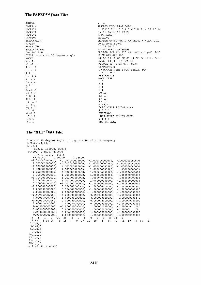
The PAFE TM Data File:

CONTROLPHASE= 1PHAS E= 2PHASE= 4PHASE= 6PHASE=7SKIP. CHECKSTRESSREACTIONSFULL. CONTROLCONTROL. ENDTITLE cube with 30 degree angleNODESXY Z-1 -1 -11 -1 -1-1 1 -11 1 -1-1 -1. 11 -1 1-1 1 1111C0 -1 -1-1 0 -11 0 -10 1 -1-1 -1 01 -1 0-1 1 01100 -1 1-1 0 1101011

ELEMNUMBER ELEM PROP T0001 1l5 1 1 2 3 4 5 6 8 12 I: 1314 15 16 17 18 19 20LAMI HATESSTORE-iNUMBER ORTHOTROPIC. MATERIAL. NJ' 55AANG2 ANG3 STORE11 12 30 0 0 1ORTHOTROPIC . MATERIALNUMBER SXX SYY S SXY SI: s:x S-Xi S-1SHZX ALX ALY AL:12 5E-03 iE-03 5E-03 -4. 5E-24 -4 .5-4 -22.5E-04 105-03 105-032.90E-03 -0.05 0.1 -0.05

TEMPERATURELOAD.CASE TEMP ST.ART FINISH ST'°1 -1 1 20 1RESTRAINTSNODE DIRE113151.7110 1213 1315 1318 12STRAINLOAD START FINISH STEP1111EXTERNALLOAD START FINISH STEP1111END.OF. DATA

The "XL!" Data File:

Constant 30 degree angle through a cube of side length 21,20,0,1,8,19,11,1,0,1

200.0, 1000.0, 200.00.4500, 0.4500, 0.0900

100.0, 100.0, 344.8-0.05000 0.10000 -0.05000-1.000000000000, -l.000000000000, -1.000000000000, -1.0000000000001.000000000000, -1.000000000000, -1.000000000000, -1.000000000000

-1.000000000000, 1.000000000000, -1.000000000000, -1.0000000000001.000000000000, 1.000000000000, -1.000000000000, -1.000000000000-1.000000000000, -1.000000000000, 1.000000000000, -1.0000000000001.000000000000, -1.000000000000, 1.000000000000, -i.000000000000

-1.000000000000, 1.000000000000, 1.000000000000, -1.0000000000001.000000000000, 1.000000000000, 1.000000000000, -1.0000000000000.000000000000, -1.000000000000, -1.000000000000, -1.000000000000

-1.000000000000, 0.000000000000, -1.000000000000, -l.0000000000001.000000000000, 0.000000000000, -1.000000000000, -1.0000000000000.000000000000, 1.000000000000, -1.000000000000, -1.000000000000-1.000000000000, -1.000000000000, 0.000000000000, -1.0000000000001.000000000000, -1.000000000000, 0.000000000000, -1.0000000000 0

-l.000D00000000, l.000000000000, 0.000000000000, -1.0000000000001.000000000000, 1.000000000000, 0.000000000000, -1.0000000000000.000000000000, -l.000000000000, 1.000000000000, -1.0000 0 000

-1.000000000000, 0.000000000000, 1.000000000000, -1.00000 001.000000000000, 0.000000000000, 1.000000000000, -1.0000000000000.000000000000, l.D000000000DO, 1.000000000000, -1.000000000000

1 1 1 1 -30-30 D 0 0 0 0 0 0 20 01 13 5 10 18 3 15 7 9 17 12 20 2 14 6 ii 19 4 16 8

1,1,0,03,1,0,05,1,0,07,1,0,010,1,1,013,1,0,115,1,0,118,1,1,0

1., 1. , 0. , 0. ,Q.00000

Al-LI

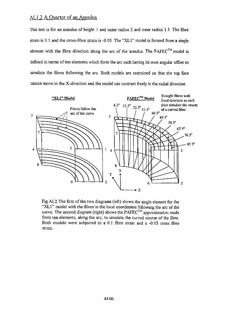
"Xli" Model

Fibres follow the

3

4

Al. 1.2 A Quarter of an Annulus

This test is for an annulus of height 1 and outer radius 2 and inner radius 1 5 The fibre

strain is 0.1 and the cross-fibre strain is -0.05. The "XLI" model is formed from a single

element with the fibre direction along the arc of the annulus. The PAFEC t model is

defined in terms often elements which form the arc each having its own angular of set to

simulate the fibres following the arc. Both models are restrained so that the top face

cannot move in the X-direction and the model can contract freely in the radial direction.

PAFECThI ModelStraight fibres withfixed direction in each

4.5° 1of a curved fibre

0.50

slice simulate the course

49.5°/ 58.50

67.50

7 76.5°

8550

14 1

8JL4

2

z

6' '2

Fig AL2 The first of the two diagrams (left) shows the single element for the"XL 1" model with the fibres in the local coordinates following the arc of thecurve. The second diagram (right) shows the PAFECThI approximation madefrom ten elements, along the arc, to simulate the curved course of the fibre.Both models were subjected to a 0.1 fibre strain and a -0.05 cross fibrestrain.

Al-rn

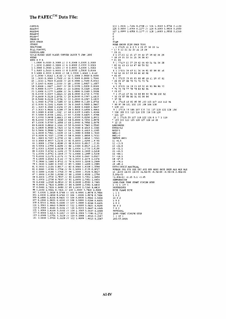
The PAFECTM Data File:

CONTROL

PHASE1

PHASE=4

PRASE6

PKASE7

PHASE9

SKIP.CHECK

STRESS

REACTIONS

FULL. CONTROL

CONTROL. END

TITLE MIKES TEST MIXES CURVED BLOCK 5 JAN 1996

NODE S

NODE K Y Z

1 1.0000 0.0000 2.0000 II 2 0.0000 0.0000 2.0000

3 1.0000 2.0000 0.0000 /1 4 0.0000 2.0000 0.0000

5 1.0000 0.0000 1.5000 II 6 0.0000 0.0000 1.5000

7 1.0000 1.5000 0.0000 II 8 0.0000 1.5000 0.0000

9 0.5000 0.0000 2.0000 II 10 1.0000 1.4102 1.4142

11 0.0000 1.4142 1.4142 II 12 0.5000 2.0000 0.0000

13 1.0000 0.0000 1.7500 II 14 0.0000 0.0000 1.7500

15 1.0000 1.7500 0.0000 II 16 0.0000 1.7500 0.0000

17 0.5000 0.0000 1.5000 II 18 1.0000 1.0607 1.0607

19 0.0000 1.0607 1.0607 II 20 0.5000 1.5000 0.0000

21 0.0000 0.1177 1.4951, /1 22 0.0000 0.1569 1.9938

23 1.0000 0.1177 1.4954 II 24 1.0000 0.1569 1.9938

25 0.0000 0.2347 1.4615 II 26 0.0000 0.2738 1.7285

27 0.0000 0.3129 1.9704 // 20 0.5000 0.2347 1.4815

29 0.5000 0.3129 1.9754 II 30 1.0000 0.2347 1.4815

31 1.0000 0.2738 1.7285 1/ 32 1.0000 0.3129 1.9754

33 0.0000 0.3502 1.4586 /1 34 0.0000 0.4669 1.9447

35 1.0000 0.3502 1.4586 II 36 1.0000 0.4669 1.9447

37 0.0000 0.4635 1.4266 II 38 0.0000 0.5408 1.6643

39 0.0000 0.6180 1.9021 1/ 40 0.5000 0.4635 1.4266

41 0.5000 0.6180 1.9021 II 42 1.0000 0.4635 1.4266

43 1.0000 0.5408 1.6643 /1 44 1.0000 0.6180 1.9021

45 0.0000 0.5740 L3858 II 46 0.0000 0.7658 1.8478

47 1.0000 0.5740 1.3858 // 48 1.0000 0.7654 1.8478

49 0.0000 0.6010 1.3365 II 50 0.0000 0.7945 1.5593

51 0.0000 0.9080 1.7820 II 52 0.5000 0.6810 1.3365

53 0.5000 0.9080 1.7820 /1 54 1.0000 0.6010 1.3365

55 1.0000 0.7945 1.5593 1/ 56 1.0000 0.9000 1.7820

57 0.0000 0.7837 1.2790 II 58 0.0000 1.0450 1.7053

59 L0000 0.7837 1.2790 II 60 1.0000 1.0450 1.7053

61 0.0000 0.8817 1.2135 /1 62 0.0000 1.0286 1.4158

63 0.0000 1.1756 1.6180 II 64 0.5000 0.8817 1.2135

65 0.5000 1.1756 1.6180 II 66 1.0000 0.8817 1.2135

67 1.0000 1.0286 1.4158 II 68 1.0000 1.1756 1.6180

69 0.0000 0.9742 1.1406 /1 70 0.0000 1.2989 1.5208

71 1.0000 0.9742 1.1406 II 72 1.0000 L2989 1.5208

73 0.0000 1.2370 1.2374 II 74 0.5000 1.0607 1.0607

75 0.5000 1.4142 1.4142 II 76 1.0000 1.2374 1.2374

77 0.0000 1.1406 0.9742 II 78 0.0000 1.5208 1.2989

79 1.0000 1.1406 0.9742 II 80 1.0000 1.5208 1.2989

81 0.0000 1.2135 0.8817 II 82 0.0000 1.4150 1.0286

83 0.0000 1.6180 1.1756 II 84 0.5000 1.2135 0.8817

85 0.1000 1.6180 1.1756 1/ 86 1.0000 1.2135 0.8817

87 1.0000 1.4158 1.0286 II 88 1.0000 16180 1.1756

89 0.0000 1.2790 0.7837 II 90 0.0000 1.7053 1.0450

91 1.0000 1.2790 0.7837 II 92 1.0000 1.7053 1.0450

93 0.0000 1.3365 0.6810 /1 94 0.0000 1.5593 0.7945

95 0.0000 L7820 0.9080 // 96 0.5000 1.3365 0.6810

97 0.5000 1.7820 0.9080 ii 98 1.0000 1.3365 0.6810

99 1.0000 1.5593 0.7945 II 100 1.0000 0.7820 0.9080

101 0.0000 1.3058 0.5740 II 102 0.0000 1.8470 0.7654

103 1.0000 1.3858 0.5740 II 104 1.0000 1.8478 0.7654

105 0.0000 1.4266 0.4635 II 106 0.0000 1.6643 0.5408

107 0.0000 1.9021 0.6180 II 108 0.5000 1.4266 0.4635

109 0.5000 1.9021 0.6180 // 110 1.0000 1.4266 0.4635

111 1.0000 1.6643 0.5408 /1 112 1.0000 1.9021 0.6180

113 0.0000 1.4586 0.3502 1/ 114 0.0000 1.9447 0.4669

115 1.0000 1.4506 0.3502 II 116 1.0000 1.9447 0.4669117 00000 1.4815 0.2347 ft 118 0.0000 1.7285 0.2738119 0.0000 1.9754 0.3129 ft 120 0.5000 1.4815 0.2347121 0.5000 1.9754 0.3129 II 122 1.0000 1.4815 0.2347

123 1.0000 1.7285 0.2738 II 124 1.0000 1.9754 0.3129

125 0.0000 1.4954 0.1177 II 126 0.0000 1.9938 0.1569

127 1.0000 1.4954 0.1177 II 128 1.0000 1.9938 0.1569

C

C

C

ELEM

NIJMB GROUP ELEM PROF TOPO

1 1 37115 11 6 2 5 1 25 27 30 32 14

17 9 13 21 22 23 24 26 28

29 31

213711512252730323739424426

28 29 31 33 34 35 36 38 40

41 43

3 137115 13 37 39 42 44 49 51 54 56 38

40 41 43 45 46 47 48 50 52

53 55

4 13711514495104566163666850

52 53 55 57 58 59 60 62 64

65 67

5 1 37115 15 61 63 66 68 1911 18 10 62

64 65 67 69 70 71 72 73 74

75 76

6137115 16 19 11 18 10 81 83 86 88 73

74 75 76 77 78 79 80 82 84

85 87

7 137115 17 8183 86 88 9395 98 100 82

• 84 85 87 89 90 91 92 94 96• 97 99

8 137115 18 93 95 98 100 105 107 110 112 94

96 97 99 101 102 103 104 106 108

• 109 111

9137115 19 105 107 110 112 117 119 122 124 106

108 109 111 113 114 115 116 118 120

121 123

10 137115 20 117 119 122 124 8473 118

* 120 121 123 125 126 127 128 16 20

12 15

LAMINATES

ORTHO12

AX IS-i

ANG2=0

AND 1= 0

NUMBER ANG3

11 -4.5

12 -13.5

13 -22.5

14 -31.5

15 -40.5

16 -49.5

17 -58.5

18 -67.5

19 -76.5

20 -85.5

0 RTNOT ROP IC . MAT ER IAL

NUMBER SXX 5?? SZZ SKY SYZ SZX SHXY SHYZ SHZX ALX AL? ALZ

12 1E-03 IE-03 1E-03 -4. SE-CA -4 5E-04 -4. 5E-04 2.908-03

2.908-03

2.90E-03 -0.05 0.1 -0.05

TEMP ERATURE

LOAD.CASE TEMP START FINISH STEP

1 -1 1 127 1

RESTRAINTS

NODE PLANE DIRE

111

102

13 0 2

502

303

15 0 3

703

EXTERNAL

LOAD START FINISH STEP

1 1 10 1

END. OF . DATA

Al-lY

The "XL!" Data File:

curved element1,20,0,1,8,19,11,1,0,1

1000.0, 1000.0, 1000.00.4500, 0.4500, 0.4500

344.8, 344.8, 344.8-0.05000 0.10000 -0.050001.000000000000, 0.000000000000,0.000000000000, 0.000000000000,1.000000000000, 2.000000000000,0.000000000000, 2.000000000000,1.000000000000, 0.000000000000,0.000000000000, 0.000000000000,1.000000000000, 1.500000000000,0.000000000000, 1.500000000000,0.500000000000, 0.000000000000,1.000000000000, 1.414213600000,0.000000000000, 1.414213600000,0.500000000000, 2.000000000000,1.000000000000, 0.000000000000,0.000000000000, 0.000000000000,1.000000000000, 1.750000000000,0.000000000000, 1.750000000000,0.500000000000, 0.000000000000,1.000000000000, 1.060660200000,0.000000000000, 1.060660200000,0.500000000000, 1.500000000000,

1 1 1 1 0 0 0 0 01 13 5 10 18 3 15 7 9

1,1,1,013,1,1,05,1,1,0

10,1, 0,018,1,0,03,1,0,1

15,1,0,17,1,0,1

0., 0., 0.00000

2.000000000000, -1.0000000000002.000000000000, -1.0000000000000.000000000000, -1.0000000000000.000000000000, -1.0000000000001.500000000000, -1.0000000000001.500000000000, -1. 0000000000000.000000000000, -1.0000000000000.000000000000, -1.0000000000002.000000000000, -1.0000000000001.414213600000, -1.0000000000001.414213600000, -1.0000000000000.000000000000, -1.0000000000001.750000000000, -1.0000000000001.750000000000, -1.0000000000000.000000000000, -1.0000000000000.000000000000, -1. 0000000000001.500000000000, -1.0000000000001.060660200000, -1.0000000000001.060660200000, -1.0000000000000.000000000000, -1.000000000000

0 0 0 0 2017 12 20 2 14

11 19 4 16 8

Al-V

2 2

735°450

550

5°

150

25°

AT. 1.3 For the Fibre Mgle Vai'ing Throu gh the Depth of a Cube

The following two data files are for a cube of side length 2 and the fibre directon

varying linearly from 600 on one side to 00 on the opposing side. The PAFEC'" model is

defined in terms of six slices through the thickness of the element. The orientation of the

fibres within each slice are such as to simulate the varying fibre angle. The cubes are

subjected to a 0.1 fibre strain and a -0.05 cross-fibre strain. The elements are not

pressure loaded.

"XL1" Model PAFECThI Model

6 8

6 8

3 1 3 --

Fibre direction varying The fixed fibre directionslinearly through the block for each PAFECTh( slice

Fig M.3 The first of these two diagrams (left) shows the "XL1" modelconsisting of one element with the fibre direction varying linearly from 600on one face to 00 on the opposing face. The second model (right) is forPAFECThI and to simulate the varying fibre angle six slices (elements) areused. Each slice has a slightly different fibre angle to the previous one.

Al-VI

The PAFECT ' Data File:

CONTROLPHASE= ISKIP. CHECKREACT IONSCONTROL. ENDTITLE CUBE 0-60 21 DEC 95NODESNODE X Y Z1 2.0000 2.0000 2.0000 // 2 2.0000 2.00001.00003 2.0000 2.0000 0.0000 // 4 2.0000 1.00002.00005 2.0000 1.0000 0.0000 II 6 2.0000 0.00002.00007 2.0000 0.0000 1.0000 /7 8 2.0000 0.00000.00009 1.0000 2.0000 2.0000 II 10 1.0000 2.00000.000011 1.0000 0.0000 2.3000 // 12 1.00000.0000 0.000013 0.0000 2.0000 2.0000 II 14 0.00002.0000 1.000015 0.0000 2.0000 0.0000 7/ 16 0.00001.0000 2.000017 0.0000 1.0000 0.0000 7/ 18 0.00000.0000 2.000019 0.0000 0.0000 1.0000 /7 20 0.00000.0000 0.000021 0.0000 0.0000 0.1667 // 22 0.00002.0000 0.166723 0.0000 0.0000 0.3333 7/ 24 0.00001.0000 0.333325 0.0000 2.0000 0.3333 7/ 26 0.00000.0000 0.500027 0.0000 2.0000 0.5000 1/ 28 0.00000.0000 0.666729 0.0000 1.0000 0.6667 /7 30 0.00002.0000 0.666731 0.0000 0.0000 0.8333 1/ 32 0.00002.0000 0.833333 0.0000 1.0000 1.0000 /7 34 0.00000.0000 1.166735 0.0000 2.0000 1.1667 /7 36 0.00000.0000 1.333337 0.0000 1.0000 1.3333 // 38 0.00002.0000 1.333339 0.0000 0.0000 1.5000 7/ 40 0.00002.0000 1.50004]. 0.0000 0.0000 1.6667 7/ 42 0.00001.0000 1.666743 0.0000 2.0000 1.6667 7/ 44 0.00000.0000 1.833345 0.0000 2.0000 1.8333 7/ 46 1.00000.0000 0.333347 1.0000 2.0000 0.3333 /7 48 1.00000.0000 0.666749 1.0000 2.0000 0.6667 7/ 50 1.00000.0000 1.000051 1.0000 2.0000 1.0000 7/ 52 1.00000.0000 1.333353 1.0000 2.0000 1.3333 7/ 54 1.00000.0000 1.666755 1.0000 2.0000 1.6667 /7 56 2.00000.0000 0.166757 2.0000 2.0000 0.1667 /7 58 2.00000.0000 0.333359 2.0000 1.0000 0.3333 /7 60 2.00002.0000 0.333361 2.0000 .0000 0.5000 /1 62 2.00002.0000 O.0OO63 2.0000 0.0000 0.6667 7/ 64 2.00001.0000 0.666765 2.0000 2.0000 0.6667 7/ 66 2.00000.0000 0.833367 2.0000 2.0000 0.8333 7/ 68 2.00001.0000 1.000069 2.0000 0.0000 1.1667 /7 70 2.00002.0000 1.166771 2.0000 0.0000 1.3333 /7 72 2.00001.0000 1.333373 2.0000 2.0000 1.3333 7/ 74 2.00000.0000 1.5000

75 2.0000 2.0000 1.5000 /I 6 2.0000.0000 1.67

77 2.0000 1.0000 1.6667 /7 8 2.000)2.0000 1,666779 2.0000 0.0000 1.8333 /7 80 2.0 002.0000 1.8333ELEMENTSELEM=37 115NUMBER PROP TOPOLOGY1 11 20 15 23 25 8 3 58 60 17*21 22 24 12 10 46 47 5 56*57 59

2 12 23 25 28 30 58 60 63 65 24*26 27 29 46 47 48 49 59 61*62 643 13 28 30 19 14 63 65 7 2 29*31 32 33 48 49 50 51 64 66*67 684 14 19 14 36 38 7 2 71 73 33*34 35 37 50 51 52 53 68 69*70 725 15 36 38 41 43 71 73 76 75 3*39 40 42 52 53 54 55 72 74*75 776 16 41 43 18 13 76 78 6 1 42*44 45 16 54 55 11 9 77 79*80 4LN1INNUMBER ORTHO PXIS.SET ANG111 11 1 -512 11 1 -1513 11 1 -2514 11 1 -3515 11 1 -4516 11 1 -55ORTHONUMBER SXX SYY SZZ SXY SYZ SZX SHXY SHYZSHZX ALK ALY ALZ11 .005 .001 .005 -.00045 -.00045 -.00225.01 .01 .0029 -0.05 0.1 -0.05RE STNODE PLANE DIRE32213 0 114 0 115 0 122 0 125 0 127 0 130 0 132 0 135 0 138 0 140 0 143 0 145 0 120314 0 3SURFACEPRESS=0LOAD NODE PLANE1 20 2TEMPLOAD TEMP START FINISH STEP2 -1 1 79 1EXTERNALLOAD START FINISH STEP11612161ST RAINLOAD START FINISH STEP11612161END. OF. DATA

AI-Vfl

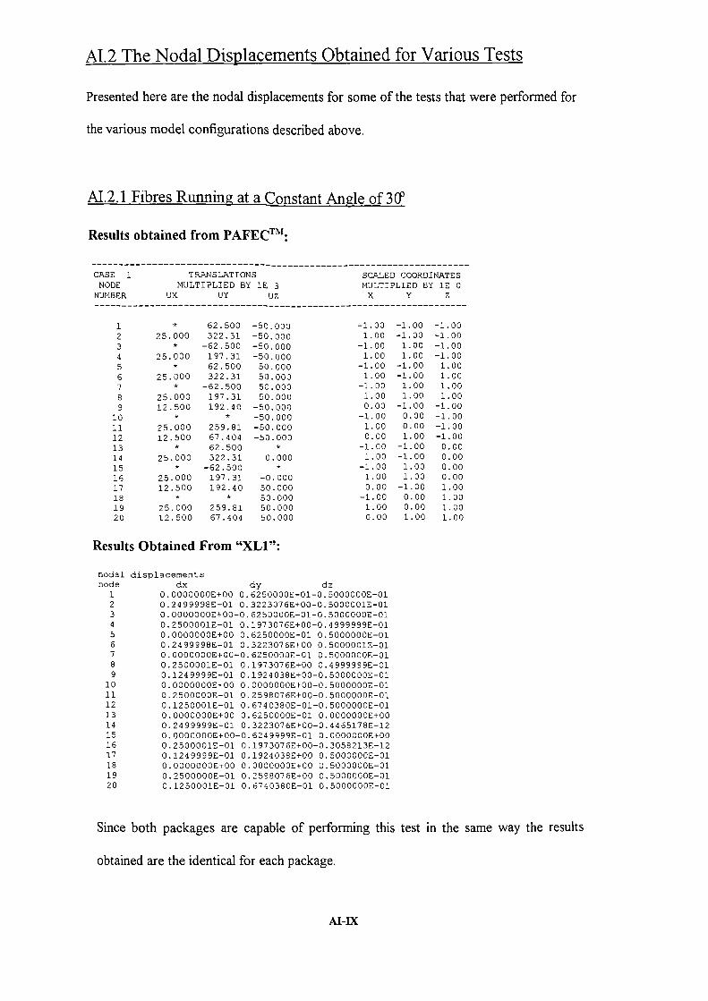
-1.001.00

-1.001.00

-1.001.00

-1.001.000.00

-1.001.000.00

-1. 001.00

-1.001.000.00

-1.001.000.00

-1.00-1.001.001.00

-1.00-1.001.001.00

-1.000.000.001.00

-1.00-1.001.001.00

-1.000.000.001.00

-1.00-1.00-1.00-1.001.001.001.001.00

-1.00-1.00-1.00-1.000.000.000.000.001.001.001.001.00

AL2 The Nodal Displacements Obtained for Various Tests

Presented here are the nodal displacements for some of the tests that were performed for

the various model configurations described above.

AI.2.1 Fibres Running at a Constant Angle of 3Cf

Results obtained from PAFECTl:

CASE 1 TRANSLATIONS

SCALED COORDINATESNODE MULTIPLIED BY 1E 3 MULTIPLIED BY 1E 0NUMBER UX UY Uz

X Y Z

123456789

1011121314151617181920

*

25.000*

25.000*

25.000*

25.00012. 500

25.00012.500

*

25.000*

25.00012.500

25.00012.500

62.500322.31

-62.500197.3162.500322.31

-62.500197.31192.40

259.8167.40462.500322.31

-62.500197.31192.40

*

259.8167.404

-50.000-50.000-50.000-50.00050.00050.00050.00050.000

-50.000-50.000-50.000-50.000

*

0.000*

-0.00050.00050.00050.00050.000

Results Obtained From "XL!":

nodal displacementsnode dx dy dz

1 0.0000000E+O0 0.6250000E-01-0.5000000E-012 0.2499998E-01 0.3223076E+00-0.5000001E-013 0.0000000E+00-0.6250000E-01-0.5000000E-014 0.2500001E-01 0.1973076E+00-0.4999999E-015 0.0000000E^00 0.6250000E-01 0.5000000E-016 0.2499998E-01 0.3223076E+00 0.5000001E-017 0.0000000E-I-00-0.6250000E-01 0.5000000E-Ol8 0.250000lE-01 0.1973076E^00 0.4999999E-0l9 0.1249999E-01 0.l924038E+00-0.5000000E-Ol

10 0.0000000E+00 0.0000000E+00-0.5000000E-0111. 0.2500000E-0l 0.2598076E+00-0.5000000E-0112 0.125000lE-01 0.6740380E-Ol-0.5000000E-0113 0.0000000E+00 0.6250000E-01 0.0000000E+0014 0. 2499999E-01 0.3223076E^00-0.4465178E-1215 O.0000000E+00-0.6249999E-0l 0.0000000E+0016 0.2500001E-01 0.1973076E+00-O.3058213E-1217 0.1249999E-01 0.1924038E+00 0.5000000E-0118 0.0000000E+00 0.0000000E+00 0.5000000E-0119 0.2500000E-01. 0.2598076E+00 0.5000000E-0120 0.].250001E-01 0.6740380E-01 0.5000000E-01

Since both packages are capable of performing this test in the same way the results

obtained are the identical for each package.

Al-IX

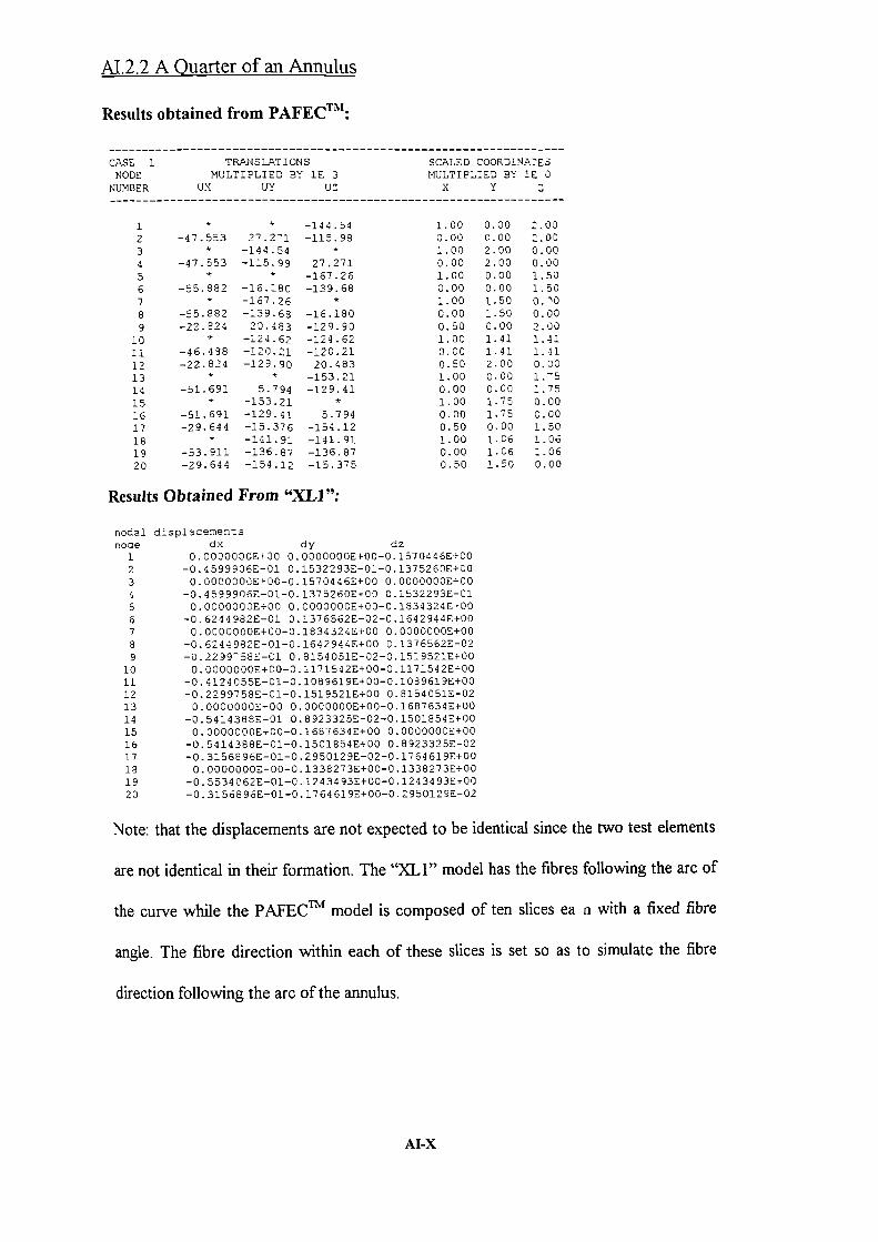
1.000.001.000.001.000.001.000.000.501.000.000.501.000.001.000.000.501.000.000.50

0.000.002 .002.000.000.001.501.500.001.411.412.000. 000.001.751.750.001.061.061.50

2.002.000.000.001.501.500.0.002.001.411.410.00

0.000.001.501 .061.060.00

AL2.2 A Ouarter of an Annulus

Results obtained from PAFECTM:

CASE 1 TRAi1STIONS SCALED COORDINATESNODE MULTIPLIED BY 1E 3

MULTIPLIED BY IE 0NUMBER UX UY U:

X Y

123456789

101112131415

17181920

-4.7.553

-47.553

-55.882

-55.882-22.824

*

-46. 4 88-22.824

-51.691

-51. 691-29.644

-53. 911-29.644

*27. 2J.

-144 .54-115.99

-16.180-167.26-139.6820.483

-124 .62-120.21-129.90

*5.7 94

-153.21-129.41-15. 376-141.91-136. 87-154.12

-144 .54-115. 98

27.271-167.26-139.68

-16.180-129.90-124.62-120.2120.483

-153.21-129.41

*5.794

-154.12-141.91-136. 87-15.375

Results Obtained From "XLI ":

nodal displacements

noce dx dy dz1 0.0000000E+00 O.0000000E+O0-0.1570446E+00

2 -0.4599906E-01 0.1532293E-01-0.1375260E+00

3 0.0000000E+OO-0.1570446E4-00 O.0000000E+00

4 -O.4599906E-01-0.1375260ErOO 0.1532293E01

5 0.0000000E+00 O.0000000E+00-0.1834324E+00

6 -0.6244982E-Ol 0.1376562E-02-0.1642944E+00

7 0.0000000E+00-O.1834324E+00 0.0000000E+00

8 -0.6244982E-0l-0.1642944E+0O 0.1376562E-02

9 -0.229958E-01 0.8154051E-02-0.151952E+00

10 0.0000000E+0O-0. 1171542E+00-0.117542E-'00

11 -0. 4124055E-01-0.1089619E+00-0.1089619E-i-00

12 -O.2299758E-0l-0.l5l9521E+00 O.8l5405lE-02

13 0.0000000E-0O 0.0000000E+00-0.l687634E-1-00

14 -0.5414388E-01 0.8923325E-02-0.1501854E+00

15 0.0000000E+00-0.1687634E+00 0.0000000E+00

16 -O.54l4388E-0l-O.l501854E+00 O.8923325E-02

17 -0. 3156896E-0l-0. 2950129E-02-0.1764619E+00

18 0. 0000000E+0O-0.1338273E+O0-0.1338273E+00

19 -0.5534062E-0l-O. 12434 93E+00-0.l243493E--00

20 -0. 3l56896E-01-O. 1764619E+00-O. 2950l29E-02

Note: that the displacements are not expected to be identical since the two test elements

are not identical in their formation. The "XL1" model has the fibres following the arc of

the curve while the PAFEC model is composed of ten slices ea a with a fixed fibre

angle. The fibre direction within each of these slices is set so as to simulate the fibre

direction following the arc of the annulus.

AI-X

2.002.002.002. 002.002.002.002.001.001.001. 001.000.000.000.000.000.000.000.000.00

2.002.002.001.001. 000.000.000.002.002. 000.000.002.002.002.001.001.000.000.000.00

2.001.000. 002.000.002.001.000.002.000.002.000.002.001.000.002.000.002.001.000.00

AT.2.3 For the Fibre Angle Varyin g Through the Depth of a Cube

Results obtained from PAFEC:

CASE 2 TRANSLATIONS SCALED COORDINATES

NODE MULTIPLIED BY 1E 3

MULTIPLIED BY 1E 0NUMBER UX UY JZ

X Y Z

123

56789

1011121314151617181920

-64.757-3. 83787. 35869.580154.13191.70222.81216.75

-18.94531.523246.53158.29

***

170.0138.568305.41207.2491.402

***

-17 . 963129.94

-34.153110.30242.72

*-1.705211.14

***

24.98788.10525.655135.17189.94

49. 174*

-33.22216. 910

-87.575-83.404-147.10-204.8530.077

-76. 789-85.207-171.27

51.066

-77.76848.983

-62. 824-15. 601-49.115-86.229

Results Obtained From "XL 1":

nodal displacements

node dx dy dz

1 -0.6331387E-01 0.0000000E+00 0.4105950E-01

2 0.2019027E-02 0.0000000E+00 0.0000000E+00

3 0.8046768E-01 0.0000000E+00-0.4057331E-01

4 0.5544898E-01-0.2206060E-01 0.4703019E-02

5 0.1499698E+00 0.1313555E+00-0.9817559E-01

6 0. 1829604E+00-0. 26993l8E-01-0. 8862164E-0l

7 0.2181579E+00 0.1008680E+00-0.1613995E+00

8 0.2051786E+00 0.2582215E+00-0.2389028E+00

9 -0.23380995-01 0.0000000E+00 0.26457025-01

10 0.2479055E-0l 0.0000000E+00-0.7848239E-01.

11 0.24610365+00-0. 8384851E-02-0. 9981860E-0l

12 0.1560327E+00 0.22590855+00-0.1912030E+00

13 0.00000005+00 0.0000000E+00 0.5171827E-01

14 0.0000000EI-00 0.0000000E+00 0.00000005+00

15 0. 00000005+00 0. 0000000E+00-0.6721945E-0l

16 0.17080815+00 0.18666035-01 0.33435975-01

17 0.3014826E-01 0.9471537E-01-0.7337212E-0l

18 0.31342405+00 0.18165975-01-0.26965585-01

19 0.1940148E+00 0. 1211384E+00-0.7167281E-0l

20 0.88251005-01 0.1976231E+00-0.1036557E--00

Note: that the displacements are not expected to be identical since ie two test elements

are not identical in their formation. The "XL 1" model has the fibre angle varying through

the depth of a cube from 60° to 00 while the PAFECTh' model is composed of six slices

each with a set fibre angle. The displacements are however extremely close considering

the differences between the two models.

A1-XI

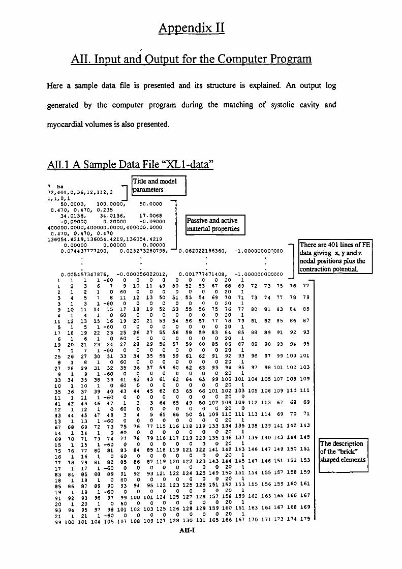
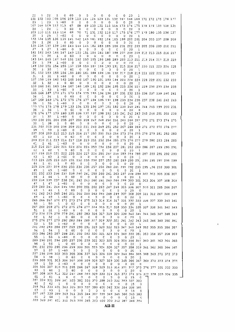
22 122 1 060 0 0 0 0 0 0 020 1101 102 103 105 106 109 110 111 128 129 131 132 167 168 169 171 172 175 176 177

23 1 23 1 -60 0 0 0 0 0 0 0 0 20 0107 108 109 112 113 67 68 69 130 131 115 116 173 174 175 178 179 133 134 135

24 124 1 060 0 0 0 0 0 0 020 0109 110 111 113 114 69 70 71 131 132 116 117 175 176 177 179 180 135 136 137

25 1 25 1 -60 0 0 0 0 0 0 0 0 20 1133 134 135 138 139 141 142 143 181 182 184 185 199 200 201 204 205 207 208 209

26 1 26 1 0 60 0 0 0 0 0 0 0 20 1135 136 137 139 140 143 144 145 182 183 185 186 201 202 203 205 206 209 210 211

27 1 27 1-60 0 0 0 0 0 0 0 0 20 1141 142 143 146 147 149 150 151 184 185 187 188 207 208 209 212 213 215 216 217

28 1 28 1 0 60 0 0 0 0 0 0 0 20 1143 144 145 147 148 151 152 153 185 186 188 189 209 210 211 213 214 217 218 219

29 1 29 1 -60 0 0 0 0 0 0 0 0 20 1149 150 151 154 155 157 158 159 187 188 190 191 215 216 217 220 221 223 224 225

30 1 30 1 0 60 0 0 0 0 0 0 0 20 1151 152 153 155 156 159 160 161 188 189 191 192 217 218 219 221 222 225 226 227

31 1 31 1 -60 0 0 0 0 0 0 0 0 20 1157 158 159 162 163 165 166 167 190 191 193 194 223 224 225 228 229 231 232 233

32 132 1 060 0 0 0 0 0 0 020 1159 160 161 163 164 167 168 169 191 192 194 195 225 226 227 229 230 233 234 235

33 1 33 1-60 0 0 0 0 0 0 0 0 20 1165 166 167 170 171 173 174 175 193 194 196 197 231 232 233 236 237 239 240 241

34 134 1 060 0 0 0 0 0 0 020 1167 168 169 171 172 175 176 177 194 195 197 198 233 234 235 237 238 241 242 243

35 1 35 1 -60 0 0 0 0 0 0 0 0 20 0173 174 175 178 179 133 134 135 196 197 181 182 239 240 241 244 245 199 200 201

36 1 36 1 0 60 0 0 0 0 0 0 0 20 0175 176 177 179 180 135 136 137 197 198 182 183 241 242 243 245 246 201 202 203

37 1 37 1-60 0 0 0 0 0 0 0 0 20 1199 200 201 204 205 207 208 209 247 248 250 251 265 266 267 270 271 273 274 275

38 138 1 060 0 0 0 0 0 0 020 1201 202 203 205 206 209 210 211 248 249 251 252 267 268 269 271 272 275 276 277

39 1 39 1 -60 0 0 0 0 0 0 0 0 20 1207 208 209 212 213 215 216 217 250 251 253 254 273 274 275 278 279 281 282 283

40 1 40 1 0 60 0 0 0 0 0 0 0 20 1209 210 211 213 214 217 218 219 251 252 254 255 275 276 277 279 280 283 284 285

41 1 41 1-60 0 0 0 0 0 0 0 0 20 1215 216 217 220 221 223 224 225 253 254 256 257 281 282 283 286 287 289 290 291

42 142 1 060 0 0 0 0 0 0 020 1217 218 219 221 222 225 226 227 254 255 257 258 283 284 285 287 288 291 292 293

43 1 43 1 -60 0 0 0 0 0 0 0 0 20 1223 224 225 228 229 231 232 233 256 257 259 260 289 290 291 294 295 297 298 299

44 1 44 1 0 60 0 0 0 0 0 0 0 20 1225 226 227 229 230 233 234 235 257 258 260 261 291 292 293 295 96 299 300 301

45 1 45 1 -60 0 0 0 0 0 0 0 0 20 1231 232 233 236 237 239 240 241 259 260 262 263 297 298 299 302 303 305 306 307

46 1 46 1 0 60 0 0 0 0 0 0 0 20 1233 234 235 237 238 241 242 243 260 261 263 264 299 300 301 303 304 307 308 309

47 1 47 1 -60 0 0 0 0 0 0 0 0 20 0239 240 241 244 245 199 200 201 262 263 247 248 305 306 307 310 311 265 266 267

48 1 48 1 0 60 0 0 0 0 0 0 0 20 0241 242 243 245 246 201 202 203 263 264 248 249 307 308 309 311 312 267 268 269

49 1 49 1-60 0 0 0 0 0 0 0 0 20 1265 266 267 270 271 273 274 275 313 314 316 317 331 332 333 336 337 339 340 341

50 1 50 1 0 60 0 0 0 0 0 0 0 20 1267 268 269 271 272 275 276 277 314 315 317 318 333 334 335 337 338 341 342 343

51 1 51 1 -60 0 0 0 0 0 0 0 0 20 1273 274 275 278 279 281 282 283 316 317 319 320 339 340 341 344 345 347 348 349

52 152 1 060 0 0 0 0 0 0 020 1275 276 277 279 280 283 264 265 317 318 320 322 341 342 343 345 346 349 350 351

53 1 53 1-60 0 0 0 0 0 0 0 020 1281 282 283 286 287 289 290 291 319 320 322 323 347 348 349 352 353 355 356 357

54 154 1 060 0 0 0 0 0 0 020 1283 284 285 287 288 291 292 293 320 321 323 324 349 350 351 353 354 357 358 359

55 1 55 1 -60 0 0 0 0 0 0 0 0 20 1289 290 291 294 295 297 298 299 322 323 325 326 355 356 357 360 361 363 364 365

56 1 56 1 0 60 0 0 0 0 0 0 0 20 1291 292 293 295 296 299 300 301 323 324 326 327 357 358 359 361 362 365 366 367

57 1 57 1 -60 0 0 0 0 0 0 0 0 20 1297 298 299 302 303 305 306 307 325 326 328 329 363 364 365 368 369 371 372 373

58 158 1 060 0 0 0 0 0 0 020 1299 300 301 303 304 307 308 309 326 327 329 330 365 366 367 369 370 373 374 375

59 1 59 1 -60 0 0 0 0 0 0 0 0 20 0305 306 307 310 311 265 266 267 328 329 313 314 371 372 373 376 377 331 332 333

60 1 60 1 0 60 0 0 0 0 0 0 0 20 0307 308 309 311 312 267 268 269 329 330 314 315 373 374 375 377 378 333 334 335

61 261 1 0 0 0 0 0 0 0 0 015 0397 339 331 399 341 333 382 336 379 398 340 332 383 337 380

62 2 62 1 0 0 0 0 0 0 0 0 0 15 0399 341 333 401 343 335 383 337 380 400 342 334 384 338 381

63 2 63 1 0 0 0 0 0 0 0 0 0 15 0397 347 339 399 349 341 385 344 382 398 348 340 386 345 383

64 264 1 0 0 0 0 0 0 0 0 015 0399 349 341 401 351 343 386 345 383 400 350 342 387 346 384

All-I!

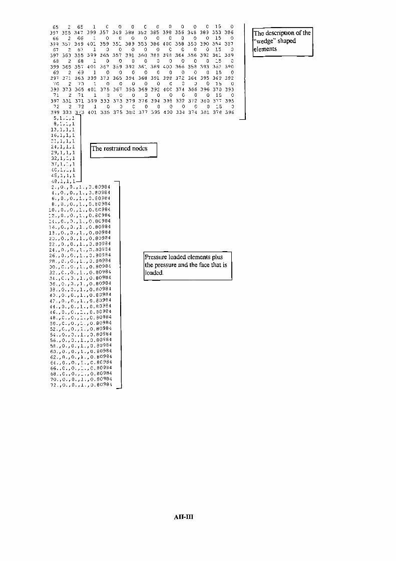
0385

0386

0388

0389

0391

0392

0394

0395

0348

0350

0356

0358

0364

0366

0372

0374

0352

0353

0360

0361

0368

0369

0376

0377

0388

0389

0391

0392

0394

0395

0379

0380

0349

0351

0357

0359

0365

0367

0373

0375

0386

0387

0389

030

0392

0393

0395

0396

0389

0390

0392

0393

0395

0396

0380

0381

0356

0358

0364

0366

0372

0374

0332

0334

0398

0400

0398

0400

0398

0400

0398

0400

15353

15354

15361

15362

15369

15370

15377

15378

65 2 65 1 0397 355 347 399 357

66 2 66 1 0399 357 349 401 359

67 2 67 1 0397 363 355 399 365

68 2 68 1 0399 365 357 401 367

69 2 69 1 0397 371 363 399 373

70 2 70 1 0399 373 365 401 375

71 2 71 1 0397 331 371 399 33372 2 72 1 0

399 333 373 401 3355,1,1,18,1,1,1

13, 1, 1,116,1,1,17 .1.1_i

iEi description of the" . ge" shaped

ients

'"' Therestrainednodes29,1,1,1St I J. S

37, 1, 1, 140, 1, 1, 145,1,1,148,1,1,12., 0., 0., 1., 0.809844. , 0. , 0. ,1. , 0. 809846., 0., 0. , 1. ,0.809848. , 0. , 0., 1., 0.80984

10.,0. ,0.,1.,0.8098412., 0., 0., 1., 0.8098414. , 0. , 0. ,1. , 0. 8098416. , 0., 0. ,1. , 0. 8098418., 0., 0., 1., 0.8098420. , 0. , 0. ,1. , 0. 8098422., 0. , 0. ,1. , 0. 8098424 . , 0. , 0. ,1. , 0. 8098426., 0. , 0. ,1. , 0. 8098428., 0., 0., 1., 0.8098430. , 0. ,0. ,1. , 0. 8098432. , 0. , 0. ,1., 0. 8098434., 0. , 0. ,1., 0. 8098436., 0., 0., 1., 0.8098438. , 0. , 0. , 1., 0.8098440.,0. ,0.,1.,0.8098442., 0. ,0. , 1., 0.8098444. ,0. , 0. ,1. ,0.8098446. , 0., 0. ,1., 0. 8098448. , 0. , 0.,1. , 0. 8098450., 0. , 0. ,1. , 0. 8098452. , 0. , 0. ,1. , 0. 8098454., 0. , 0. , 1., 0. 8098456. , 0. , 0. ,1. , 0. 8098458., 0., 0., 1., 0.8098460. , 0. , 0. ,1. , 0. 8098462., 0., 0., 1., 0.8098464., 0., 0., 1., 0.8098466. , 0. ,0. ,1., 0. 8098468., 0., 0., 1., 0.8098470. , 0. , 0. ,1. , 0. 8098472. , 0., 0. ,1. , 0. 80984

Pressure loaded elements plusthe pressure and the face that isloaded.

All-HI

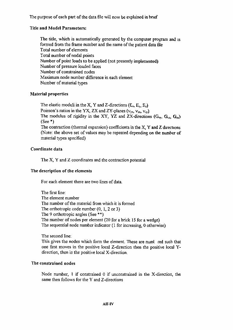
The purpose of each part of the data file will now be explained in bnef

Title and Model Parameters:

The title, which is automatically generated by the computer program and usformed from the frame number and the name of the patient data tUeTotal number of elementsTotal number of nodal pointsNumber of point loads to be applied (not presently implemented)Number of pressure loaded facesNumber of constrained nodesMaximum node number difference in each elementNumber of material types

Material properties

The elastic moduli in the X, Y and Z-directions (E, E, E1)Poisson's ratios in the YX, ZX and ZY-planes (v v v)The modulus of rigidity in the XY, YZ and ZX-directions (G. c . G G1)(See *)The contraction (thermal expansion) coefficients in the X, Y and Z directions(Note: the above set of values may be repeated depending on the number ofmaterial types specified)

Coordinate data

The X, Y and Z coordinates and the contraction potential

The description of the elements

For each element there are two lines of data.

The first line:The element numberThe number of the material from which it is formedThe orthotropic code number (0, 1, 2 or 3)The 9 orthotropic angles (See **)The number of nodes per element (20 for a brick 15 for a wedge)The sequential node number indicator (1 for increasing, 0 otherwise)

The second line:This gives the nodes which form the element. These are num red such thatone first moves in the positive local Z-direction then the positive local Y-direction, then in the positive local X-direction.

The constrained nodes

Node number, 1 if constrained 0 if unconstrained in the X-dIrection, thesame then follows for the Y and Z-directions

All-IV

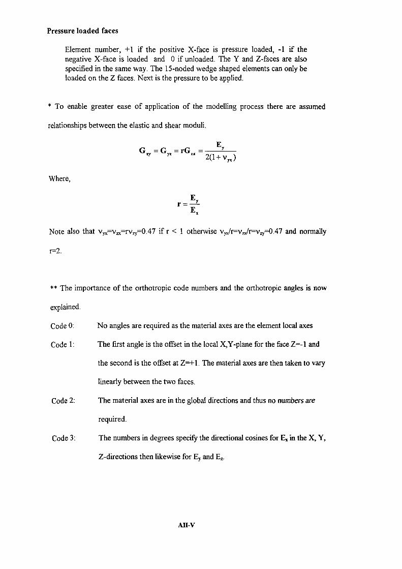
Pressure loaded faces

Element number, +1 if the positive X-face is pressure loaded, -1 if thenegative X-face is loaded and 0 if unloaded. The Y and Z-faces are alsospecified in the same way. The 15-noded wedge shaped elements can only beloaded on the Z faces. Next is the pressure to be applied.

* To enable greater ease of application of the modelling process there are assumed

relationships between the elastic and shear moduli.

G ( = = rG1 = 2(1+v)

Where,

Er =

E1

Note also that v rv0.47 if r < 1 otherwise v/r=v/r=v=0.47 and normally

r2.

** The importance of the orthotropic code numbers and the orthotropic angLes is now

explained

Code 0: No angles are required as the material axes are the element local axes

Code 1: The first angle is the offset in the local X,Y-plane for the face Z=-1 and

the second is the offset at Z=+l. The material axes are then taken to vary

linearly between the two faces.

Code 2: The material axes are in the global directions and thus no numbers are

required.

Code 3: The numbers in degrees specify the directional cosines for E in the X, Y,

Z-directions then likewise for E and E

All-V

AlI.2 A Sample Output Log

This is a sample output log from the computer program. It is for patient "BA" over end

systole. The myocardial volume is kept constant while the target volume is matched. The

contraction coefficient and contraction coefficient ratio are refined until the errors in the

required cavity and myocardial volumes are less than 0.1% of the total. The next frame

for analysis is then selected, until all frames have been analysed.

mms

mms

6mms

'rams

7 rams

Patient ba

Frame 7Iteration 1Work done 0.00008734360611Target Base to Apex Length= 79.343rnmsTarget volume is 155.780Calculated volume is 163.357Calculated Base to Apex Length= 81.494Target Shape Index 0.903Calculated Shape Index 0.932Target Myocardial Volume 113.908Calculated Myocardial Volume 114.880bounds lower 0. 0.new ratio 0.442324bounds upper 0.450000 114.880Step is 1.00000Iteration 2Work done = 0.00008700949608Target Base to Apex Length= 79.343mmsTarget volume is 155.780Calculated volume is 162.990Calculated Base to Apex Length= 81.417Target Shape Index 0.903Calculated Shape Index 0.932Target Myocardial Volume 113.908Calculated Myocardial Volume 114.533bounds lower 0. 0.new ratio 0.437470bounds upper 0.442324 114.533Step is 1.00000Iteration 3Work done 0.00008684676709Target Base to Apex Length 79.343mmsTarget volume is 155.780Calculated volume is 162.763Calculated Base to Apex Length= 8l.36Target Shape Index 0.903Calculated Shape Index 0.932Target Myocardial Volume 113.908Calculated Myocardial Volume 114.315bounds lower 0. 0.new ratio 0.434341bounds upper 0.437470 114.315Step is 1.00000Iteration 4Work done = 0.00008676208059Target Base to Apex Length= 79.343mmsTarget volume is 155.780Calculated volume is 162.613Calculated Base to Apex Length= 81.33Target Shape Index 0.903Calculated Shape Index 0.932Target Myocardial Volume 113.908Calculated Myocardial Volume 114.176bounds lower 0. 0.new ratio 0.432295bounds upper 0.434341 114.176Step is 1.00000Iteration 5Work done 0.00008671435273Target Base to Apex Length= 79.343mmsTarget volume is 155.780Calculated volume is 162.515Calculated Base to Apex Length 81.31

Target Shape Index 0.903Calculated Shape Index 0.933Target Myocardial Volume 113.908Calculated Myocardial Volume 114.085bounds lower 0. 0.new ratio 0.430956bounds upper 0.432295 114.085

Step is 1.00000Iteration 6Work done = 0.00008668651638Target Base to Apex Length= 79.343mmsTarget volume is 155.780Calculated volume is 162.450Calculated Base to Apex Length= 8l.3O3mmsTarget Shape Index 0.903Calculated Shape Index 0.933Target Myocardial Volume 113.908Calculated Myocardial Volume 114.024bounds lower 0. 0.new ratio 0.430079bounds upper 0.430956 114.024Step is 1.00000Iteration 7Work done = 0.00008667046702Target Base to Apex Length= 79.343mmsTarget volume is 155.780Calculated volume is 162.409Calculated Base to Apex Length= 81.294mmsTarget Shape Index 0.903Calculated Shape Index 0.933Target Myocardial Volume 113.908Calculated Myocardial Volume 113.986Surface Area=15081 . 40mm2Shape Index=0.932551Volume of Myocardium = 113.986Contraction Coefficient = 0.20000Contraction Coefficient Ratio = 0.43008

Frame 8Iteration 1Work done = 0.00009450791430Target Base to Apex Length= 80.324mmsTarget volume is 148.530Calculated volume is 150.198Calculated Base to Apex Length= Bl.O85mmsTarget Shape Index 0.896Calculated Shape Inde 0.908Target Myocardial Vol me 121.427Calculated Myocardial Volume 121.089bounds lower 0.430079 121.089new ratio 0.432472bounds upper 0. 0.Step is 1.00000Iteration 2Work done = 0. 0009453129230Target Base to Apex Length- 80.324mmsTarget volume is 148.530Calculated volume is 150.309Calculated Base to Apex Length= 81.1 9rrrmsTarget Shape Index 0.896Calculated Shape Index 0.908Target Myocardial Volume 121.427Calculated Myocardial Volume 121.2bounds lower 0.432472 1l.2 2new ratio 0.434 76

Afl-V1

bounds upper 0. 0.Step is 1.00000

Iteration 3Work done 0.00009455329343Target Base to Apex Length= 80.324mmsTarget volume is 148.530Calculated volume is 150.391Calculated Base to Apex Length= 81.l26minsTarget Shape Index 0.896Calculated Shape Index 0.908Target Myocardial Volume 121.427Calculated Myocardial Volume 121.281bounds lower 0.434 76 121.281new ratio .435120bounds upper 0.Step is 1.00 00

Iteration 4Work done - 0.00 9456887258Target Base to Apex Length= 80.324mmsTarget volume is 148.530Calculated volume is 150.442Calculated Base to Apex Length= 81.l36mmsTarget Shape Index 0.896Calculated Shape Index 0.9 8Target My cardial Volume 121.427Calculated Myocardial Volume 121.329Surface Area-l4586.72mm2Shape Index .9 8152V lume f My rardium = 121.329C ntracti n C efficient = 0.200 0Contraction C efficient Ratio = .43512

Frame 9Iterati n 1W rk d ne - . 96 999246Target Base t Apex Length= 78.227mmsTarget v lume is 139.2Calculated v lume is 138.284Calculated Base t Apex Length= 8 .75 mrnsTarget Shape Index .897Calculated Shape Index .868Target My cardial V lume 122.98Calculated My cardial V lume 121.952b unds 1 wer .43512 121.952new rati .44.396b unds upperStep is 1.

Iterati n 2W rk d ne - . 9674881968Target Base to Apex Length 78.227mmsTarget v lume is 139.2Calculated v lume is 138.59Calculated Base to Apex Length= 80.829mmsTarget Shape Index .897Calculated Shape Index .868Target Myocardial Volume 122.980Calculated Myocardial V lume 122.298bounds 1 wer .442396 122.298new ratio .447299bounds upper . 0.Step is 1.0 0

Iteration 3W rk d ne = 0.0 0 967643 587Target Base t Apex Length= 78.227rnmsTarget volume is 139.20Calculated volume is 138.791Calculated Base to Apex Length= 80.882mmsTarget Shape Index .897Calculated Shape Index 0.868Target My cardial V lume 122.980Calculated Myocardial V lume 122.531bounds lower 0.447299 122.531new ratio 0.45 561bounds upperStep is 1.

Iteration 4Work done = . 0 9679662705Target Base to Apex Length= 78. 27mmsTarget v lume is 139.2 0Calculated v lume is 138.925Calculated Base to Apex Length- 8 .9l8mmsTarget Shape Index .897Calculated Shape Index .868Target My caLdial V lume l.2.8QCalculated Myocardial V lume l . o86bounds lower 0.45 561 1 2.08b

new ratio 0.452712bounds upper 0. 0.Step is 1.00000

Iteration 5Work done = 0.00009682768876Target Base to Apex Length= 78.227mmsTarget volume is 139.200Calculated volume is 139.014Calculated Base to Apex Length= 80.94lmmsTarget Shape Index 0.897Calculated Shape Index 0.868Target Myocardial Volume 122.980Calculated Myocardial Volume 122.789bounds lower 0.452712 122.789new ratio 0.454119bounds upper 0. 0.Step is 1.00000

Iteration 6Work done = 0.00009685204781Target Base to Apex Length= 78.227mrnsTarget volume is 139.200Calculated volume is 139.072Calculated Base to Apex Length= 80.956mmsTarget Shape Index 0.897Calculated Shape Index 0.868Target Myocardial Volume 122.980Calculated Myocardial Volume 122.855bounds lower 0.454119 122.855new ratio 0.455037bounds upper 0. 0.Step is 1.00000

Iteration 7Work done = 0.00009687043900Target Base to Apex Length= 78.227mmsTarget volume is 139.200Calculated volume is 139.111Calculated Base to Apex Length= 80.966mrnsTarget Shape Index 0.897Calculated Shape Index 0.868Target Myocardial Volume 122.980Calculated Myocardial Volume 122.901Surface Area=l427l.04mm2Shape Index=0.867767V lume of Myocardium = 122.901C ntraction Coefficient = 0.20000Contraction Coefficient Ratio = 0.45504

Frame 10Iteration 1Work done = 0.00007966579328Target Base to Apex Length= 76.467mmsTarget volume is 130.480Calculated volume is 130.252Calculated Base to Apex Length= 78.l24mmsTarget Shape Index 0.904Calculated Shape Index 0.880Target Myocardial Volume 105.337Calculated Myocardial Volume 106.109bounds lower 0. 0.new ratio 0.448361bounds upper 0.455037 106.109Step is 1.00000

Iteration 2Work done = 0.00007953520882Target Base to Apex Length= 76.467mmsTarget volume is 130.480Calculated volume is 129.983Calculated Base to Apex Length= 78.O53mmsTarget Shape Index 0.904Calculated Shape Index 0.880Target Myocardial Volume 105.337Calculated Myocardial Volume 105.830bounds lower 0. 0.new ratio 0.444162bounds upper 0.448361 105.830Step is 1.00000

Iteration 3Work done = 0.00007948642604Target Base to Apex Length= 76.467mmsTarget volume is 130.480Calculated volume is 129.815Calculated Base to Apex Length= 78.00SmmsTarget Shape Index 0.Q04Calculated Shape Index 0.880Target Myocardial Volume 105.337Calculated Myocardial Volume 105.655

All- VII

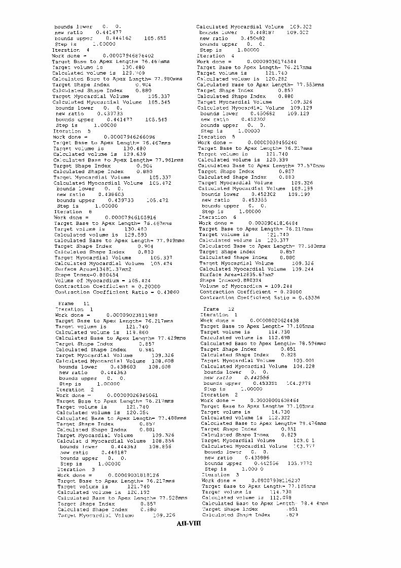
bounds lower 0. 0.new ratio 0.441477bounds upper 0.444162 105.655Step is 1.00000

Iteration 4Work done = 0.00007946876402Target Base to Apex Length= 76.467mznsTarget volume is 130.480Calculated volume is 129.709Calculated Base to Apex Length= 77.9BOmmsTarget Shape Index 0.904Calculated Shape Index 0.880Target Myocardial Volume 105.337Calculated Myocardial Volume 105.545bounds lower 0. 0.new ratio 0.439733bounds upper 0.441477 105.545Step is 1.00000

Iteration 5Work done = 0.00007946266096Target Base to Apex Length= 76.467mmsTarget volume is 130.480Calculated volume is 129.639Calculated Base to Apex Length 77.96lmmsTarget Shape Index 0.904Calculated Shape Index 0.880Target Myocardial Volume 105.337Calculated Myocsrdial Volume 105.472bounds lower 0. 0.new ratio 0.438603bounds upper 0.439733 105.472Step is 1.00000

Iteration 6Work done = 0.00007946105916Target Base to Apex Length= 76.467mmsTarget volume is 130.480Calculated volume is 129.593Calculated Base to Apex Length= 77.949mrnsTarget Shape Index 0.904Calculated Shape Index 0.880Target Myocardial Volume 105.337Calculated Myocardial Volume 105.424Surface Area=l3481.37mm2Shape Index=0.880454Volume of Myocardium = 105.424Contraction Coefficient = 0.20000Contraction Coefficient Ratio = 0.43860

Frame 11Iteration 1

Work done = 0.00009023811988Target Base to Apex Length= 76.2l7mmsTarget volume is 121.740Calculated volume is 119.860Calculated Base to Apex Lenqth= 77.429mmsTarget Shape Index 0.857Calculated Shape Index 0.881Target Myocardial Volume 109.326Calculated Myocardial Volume 108.608bounds lower 0.438603 108.608new ratio 0.444363bounds upper 0. 0.Step is 1.00000

Iteration 2Work done = 0.00009026945061Target Base to Apex Length= 76.2l7mrnsTarget volume is 121.740Calculated volume is 120.054Calculated Base to Apex Length= 77.488mmsTarget Shape Index 0.857Calculated Shape Index 0.881Target Myocardial Volume 109.326Calculat d Myocardial Volume 108.856bounds lower 0.444363 108.856new ratio 0.448187bounds upper 0. 0.Step is 1.00000

Iteration 3Work done = 0.00009031818126Target Base to Apex Length= 76.2l7mmsTarget volume is 121.740Calculated volume is 120.192Calculated Base to Apex Length= 77.528mmsTarget Shape Index 0.857Calculated Shape Index 0.880Target Myocardial Volume 109.326

Calculated Myocardial Volume 109.022bounds lower 0.448187 109.022new ratio 0.450o82bounds upper 0. 0.Step is 1.00000

Iteration 4Work done = 0.00009036174544Target Base to Apex Length= 76.2l7mrnsTarget volume is 121.740Calculated volume is 120.282Calculated Base to Apex Length= 77.553mmsTarget Shape Index 0.857Calculated Shape Index 0.880Target Myocardial Volume 109.326Calculated Myocardial Volume 109.129bounds lower 0.450682 109.129new ratio 0.452302bounds upper 0. 0.Step is 1.00000

Iteration 5Work done = 0.00009039455240Target Base to Apex Length= 76.2l7mmsTarget volume is 121.740Calculated volume is 120.339Calculated Base to Apex Length= 77.57OmmsTarget Shape Index 0.857Calculated Shape Index 0.880Target Myocardial Volume 109.326Calculated Myocardial Volume 109.199bounds lower 0.452302 109.199new ratio 0.453355bounds upper 0. 0.Step is 1.00000

Iteration 6Work done = 0.00009041816484Target Base to Apex Length= 76.2l7mmsTarget volume is 121.740Calculated volume is 120.377Calculated Base to Apex Length= 77.5BOmmsTarget Shape Index 0.857Calculated Shape Index 0.880Target Myocardial Volume 109.326Calculated Myocardial Volume 109.244Surface Area=l2835.67mm2Shape Index=0. 880324Volume of Myocardium = 109.244Contraction Coefficient = 0.20000Contraction Coefficient Ratio = 0.45336

Frame 12Iteration 1

Work done = 0.00008020624438Target Base to Apex Length= 77.lo5mmsTarget volume is 114.730Calculated volume is 112.698Calculated Base to Apex LengLh= 78.594mmsTarget Shape Index 0.851Calculated Shape Index 0.828Target Myocardial Volume 103.001Calculated Myocardisl Volume 104.228bounds lower 0. 0.new raSh, 0.442556bounds upper 0.453355 104.2279Step is 1.00000

Iteration 2Work done 0.00008001608464Target Base to Apex Length= 77.lo5mmsTarget volume is 14.730Calculated volume is 112.322Calculated Base to Apex Length= 78.476mmsTarget Shape Index 0.851Calculated Shape Index 0.829Target Myocardial Volume 103.0 1Calculated Myocardial Volume 103.777bounds lower 0. 0.new ratio 0.435886bounds upper 0.442556 103.7772Step is 1.000 0

Iteration 3Work done 0.00007998116207Target Base to Apex Length= 77.lO5mmsTarget volume is 114.730Calculated volume is 112.098Calculated Base to Apex Lngth- 78.4 4rnmsTarget Shape Index .851Calculated Shape Index .829

kLI-Vffl

Target Myocardial Volume 103.001Calculated Myocardial Volume 103.500bounds lower 0. 0.new ratio 0.431660bounds upper 0.435886 103.5004Step is 1.00000Iteration 4Work done = 0.00 07999165717Target Base to Apex Length 77.l05mrnsTarget volume is 114.730Calculated volume is 111.951Calculated Base to Apex Length= 78.358mrnsTarget Shape Index 0.851Calculated Shape Index 0.829Target Myocardial Volume 103.001Calculated Myocardial Volume 103.324bounds lower 0. 0.new ratio 0.428955bounds upper .431660 103.3238Step is 1.0 000Iterati n 5Work done = . 0 08 1160342Target Base to Apex Length= 77.lO5mmsTarget v lume is 114.730Calculated v lume is 111.857Calculated Base t Apex Length= 78.328mmsTarget Shape Index 0.851Calculated Shape Index 0.829Target My cardial V lume 1 3.001Calculated My cardial Volume 1 3.212bounds 1 wer . 0.new ratio .4272 1b unds upper .428955 1 3.2117Step is 1.Iterati n 6W rk d ne . 8 3 4673Target Base t Apex Length- 77.1 5mmsTarget v lume is 114.73Calculated v lume is 111.79Calculated Base t Apex Length 78.3 9mmsTarget Shape Index .851Calculated Shape Index .829Target My cardial V lume 1 3.0 1Calculated My cardial Volt.rne 1 3.139b unds 1 wernew rat! .42o o6b unds upper .42 2 1 1 3.1391Step is 1.Iterati n 7W rk d ne - . 8 44532 8Target Base to Apex Length= 77.1 5mmsTarget v lume is 114.730Calculated v lume is 111.757Calculated Base t Apex Length= 78.297mmsTarget Shape Index .851Calculated Shape Index 0.829Target Myocardial V lume 1 3.0 1Calculated Myocard.ial Volume 103.091Surface Area=12714 . 03mm2Shape Index=0.829 41V lume of Myocardium 103.091Contract! n Coefficient = 0.2 000Contraction C efficient Ratio = 0.42606

Frame 13Iteration 1Work done - 0. 836l80793Target Base to Apex Lengh= 76.Ol6mmsTarget volume is 107.190Calculated volume is 1 6.535Calculated Base to Apex Length= 76.253mmsTarget Shape Index 0.852Calculated Shape Index 0.838Target My cardial Volume 108.922Calculated My cardial V lume 107.818vol error .e1l273837l3682bounds 1 wer .46 56 1 7.818new ratio .4346obounds upperStep is 1. 0Iteration 2Work done . 887789°2Target Base to Apex Length- 7b.Ol6mmsTarget volume is 1 .1°Calculated v lume is 1 6.8.1Calculated Base t Apex Length 'o.33mms

All-LX

Target Shape Index 0.852Calculated Shape Index 0.838Target Myocardial Volume 108.922Calculated Myocardial Volume 108.186bounds lower 0.434696 108.186new ratio 0.440574bounds upper 0. 0.Step is 1.00000Iteration 3Work done = 0.00008230118273Target Base to Apex Length= 76.Ol6mmsTarget volume is 107.190Calculated volume is 107.009Calculated Base to Apex Length= 76.394mmsTarget Shape Index 0.852Calculated Shape Index 0.838Target Myocardial Volume 108.922Calculated Myocardial Volume 108.435bounds lower 0.440574 108.435new ratio 0.444514bounds upper 0. 0.Step is 1.00000Iteration 4Work done = 0.00008233917224Target Base to Apex Length= 76.Ol6rnrnsTarget volume is 107.190Calculated volume is 107.140Calculated Base to Apex Length= 76.432mmsTarget Shape Index 0.852Calculated Shape Index 0.838Target Myocardial Volume 108.922Calculated Myocardial Volume 108.604bounds lower 0.444514 108.604new ratio 0.447114bounds upper 0. 0.Step is 1.00000Iteration 5Work done = 0.00008237692769Target Base to Apex Length= 76.Ol6rnmsTarget volume is 107.190Calculated volume is 107.226Calculated Base to Apex Length= 76.458rnrnsTarget Shape Index 0.852Calculated Shape Index 0.838Target Myocardial Volume 108.922Calculated Myocardial Volume 108.715bounds lower 0.447114 108.715new ratio 0.448816bounds upper 0. 0.Step is 1.00000Iteration 6Work done = 0.00008240707530Target Base to Apex Length= 76.Ol6mmsTarget volume is 107.190Ca1culatd volume is 107.283Calculated Base to Apex Length= 76.474mmsTarget Shape Index 0.852Calculated Shape Index 0.838Target Myocardial Volume 108.922Calculated Myocardial Volume 108.788bounds lower 0.448816 108.788new ratio 0.449927bounds upper 0. 0.Step is 1.00000Iteration 7Work done 0.00008242991605Target Base to Apex Length= 76.Ol6mmsTarget volume is 107.190Calculated volume is 107.321Calculated Base to Apex Length= 76.4SSmmsTarget Shape Index 0.852Calculated Shape Index 0.838Target Myocardial Volume 108.922Calculated Myocardial Volume 108.837Surface Area=l2285.07mm2Shape Index=0.838l93Volume of Myocardium = 108.837Contraction Coefficient = 0.20000Contraction Coefficient Ratio = 0.44993

Frame 14Iteration 1Work done = 0Q0007504j9-7q5

Target Base to Apex Length = 75.4o2mmsTarget volurre is 1 4.08)Calcu1ate 'i-lume is 1 .903

mms

;rwns

Omms

Calculated Base to Apex Length= 74.757Target Shape Index 0.836Calculated Shape Index 0.841Target Myocardial Volume 96.421Calculated Myocardial Volume 96.880bounds lower 0. 0.new ratio 0.445648bounds upper 0.449927 96.8797Step is 1.00000Iteration 2Work done = 0.00007497528035Target Base to Apex Length= 75.46OmmsTarget volume is 104.080Calculated volume is 100.755Calculated Base to Apex Length= 74.71Target Shape Index 0.836Calculated Shape Index 0.841Target Myocardial Volume 96.421Calculated Myocardial Volume 96.716bounds lower 0. 0.new ratio 0.442922bounds upper 0.445648 96.7160Step is 1.00000Iteration 3Work done 0.00007494553878Target Base to Apex Length= 75.46OmmsTarget volume is 104.080Calculated volume is 100.665Calculated Base to Apex Length= 74.69Target Shape Index 0.836Calculated Shape Index 0.841Target Myocardial Volume 96.421Calculated Myocardial Volume 96.611

bounds lower 0. 0.new ratio 0.441174bounds upper 0.442922 96.6114Step is 1.00000Iteration 4Work done = 0.00007493185553Target Base to Apex Length= 75.460sTarget volume is 104.080Calculated volume is 100.607Calculated Base to Apex Length= 74.673sTarget Shape Index 0.836Calculated Shape Index 0.841Target Myocardial Volume 96.421Calculated Myocardial Volume 96.545bounds lower 0. 0.new ratio 0.440041bounds upper 0.441174 96.5450Step is 1.00000Iteration 5Work done = 0.00007492534502Target Base to Apex Length= 75.460!rsTarget volume is 104.080Calculated volume is 100.571Calculated Base to Apex Length= 74.663sasTarget Shape Index 0.836Calculated Shape Index 0.841Target Myocardial Volume 96.421Calculated Myocardial Volume 96.503Surface Area=11736. 46mm2Shape Index=0.841186Volume of Myocardium = 96.503Contraction Coefficient 0.20000Contraction Coefficient Ratio = 0.44004

ALI-X

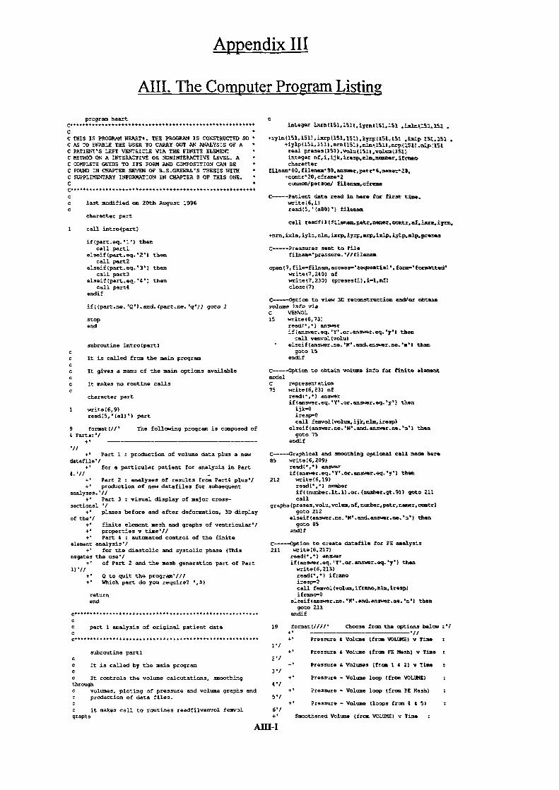
Appendix Ill

AlIl. The Computer Program Listing

program heart .................................*..

C 0C THIS IS PROSRAM NEART*. TEE PROGRAM IS C NS'TPUCTED SO *C AS TO ENASLE THE USER TO CANRY OUT AN ANALYSTS OF AC PATIEN'T 'S LEFT VENTRICLE VIA THE FINITE ELENENTC METHOD OH A INTERACTIVE OR NONINTERACTIVE LEVEL. AC COMPLETE GUIDE TO ITS FORM AND COMPOSITION CAN BE •C FOUND IN CRAPTER SEVEN OF ES.GREHAL'S THESIS WITHC SUPPLIMENTARY INFORMATION IN (APTER B OF ThIS ONE.C C

............................44******

c last modified on 20th August 1996

character part

call ntro(part)

if)part.eq. '1') thencall partl

elseif)part.eq. '2') thencall part2

elseif(part.eq. '3') thencall part3

elseit)part.eq. '6') thencall partE

endif

if((part.ne.'Q').ad.(pat.zze.'q')) gotol

stopend

subroutine intro (part)

It is called from the main program

It gives a menu of the main options available

It makes no routine calls

character part

1 write(6,9)read(5,'(al}') part

9 format (II' The following program is composed of4 Parts:'!

+' ------------------

'I,+' Part 1 : production of volume data plus a new

datafile'!^' for a particular patient for analysis in Part

4.',! -+' Part 2 : analyses of results from PartS plus'!+' production of new datafiles for subsequent

analyses.'!!+' Part 3 : visual display of major cross-

sectional 'I^' planes before and after deformation, 3D display

of the'!+' finite element mesh end graphs of ventricular'!+' properties v time'!!+' Part 4 : automated control of the finite

element analysis'!+' for the diastolic and systolic phase (This

negates the use'!+' of Part 2 and the mesh generation part of Part

1) '!/4' Q to quit the program'!! /4' Which part do you require? ',S)

returnend

C........................................................

c part 1 analysis of original patient data

integer I lS1.l51)iyrn)lS]L,153 .sin(L5L.1Sl

*iyln(lSl, 151 i*rp 51.15 ,iyrp)lSi,l5I ,imlp 1,151+iylp)l5l,l5l),nrn(1S1J(1S1I51),alp1%lreal preses)15l) ,volu4lSl).vo1um3Sl1integer of, I, ijk,iresp 1m,nimthcr, ifrmsncharacter

filnam 80, filenam 80, ancr,patr6,nm.r29,+contr02Q, cframe2common/person! filenam,cfreae

C---Patient data read in here for first time.write)6,l)read)5, '(aBO)') filenem

call teadfil (fileram.pmtr.nemer,eomtr,mf,imzm,iyrm

+nrn, ixln, iylLO, nm. ixrp, iyrp, rrp, lp, iFlp,m1.prees

C-----Pressures sent to filefilnam'pressure. '//fIlemara

open)?, filefilnam, access'sequestial ',, fors' formatted'write(7,240) ofwrite (7,230) (preses)i) • I1,nf)close)?)

C-Option to view 30 reconstruction and/or obtaunvolume info viaC VENAOL

15 write)6,73)read),) answerif)answer.eq. 'Y'.or.aoswer.eq. 'y') them

call venvol (volu)

- elseif(answerne. 'N'.and.answer.ne. 'a') themgOto 15

endif

C----Option to obtain volume info for finite clamantmodelC representation75 wrjte)6,83 nf

read(,) answerif(answer.eq. 'Y'.or.answer,eq. 'y') then

ijk0iresp=0call femvol (volum. ij k, rim, irasp)

el:eif(answer.ne. 'H' .and.answerne. 'n') thengoto 75

endif

C-----Graphical and smoothing optional call made her.85 write(6, 209)

read(, 0 ) answerif(anawer.eq, 'Y'.or.answcr.eq. 'y') them

212 write(6,19)read) 0 , '1 numberif) (nusber.lt.1).or.)number.gt.9)) goto 211cell

graphs (preses,volu,volum,nf,number,patr,namer,ccmtr)goto 212

elseif(anzwer.ne. 'M'.end.answer.e. 'n') thengoto 85

endif

C------Option to create datafile for FE analysis211 write(6,217)

read) ,) answerif(answer.eq. 'Y'.or.enswer.eq. 'y') then

write(6,213)read(, 0 ) ifrmnoiresp0call feevol (volum, ifrsmo,nlm, Iresp)ifrmno0

elseif)answer.ne. 'N'.exKLanswer.ne. 'n') thengoto 211

endif

19 format (/!!!' Choose from the options below :'/

4' -------------.---------------'//4' Pressure a Volume (from )OL1JME) v TimO

1'/subroutine parti +' Pressure & Volume (from FE Mesh) v Time

o 2'!o It is called by the main program 4' Pressure & Volumes Ifrom 1 5 2) v Tim.C 3'!C It controls the volume calcutations, smoothing +' Pressure - Volume loop (tr 'OLUME)through 4'!C volumes, ploting of pressure and volume graphs and 4' Pressure - Volume loop (from FE Mesh)

production of data files. 5'!o 4' Pressure - Volume (loops from S & 5)o it makes call to routines readfjlvenvol femyol 6'!graphs +' Smoothened Volume (from Vol.1045) v Time

Am!

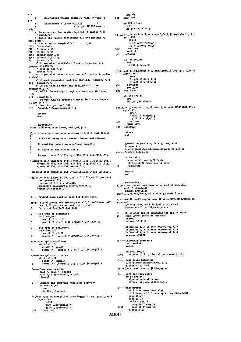
.7,,+' Smoothened Volume (from FE Mesh) v Time 184 continue

8'/+' Smoothened V I from VOLUME] '/

C Target FE Volumes0I/I

+' Enter number for graph required (0 exits) ',$)1 forinat(//II

+' Enter the filnam containing all the patiertt''sdata from 'I

the Brompton Hospital'!' ,S)1002 format(5a2)210 format(lx,i3)230 format(f7.3)

1003 format(5 (2i6,3x))1004 forsat(10(f7.2))73 format(I///

4' Do you wish to obtain volume information viaprogram VOLUME? • / /

+' (yes or no) •,S)83 format(f//I

+ Do you wish to obtain volume information from thefinite'/

+ element generated mesh for the' ,i3, • frames? ',S)209 foroiat(///I

+ Do you wish to view any results up to now

graphically? • I /^' (NOTE: Smoothing through routines are included)

''$1217 foriaat(/III

+ • Do you wish to produce a datafile for subsequentFE Puialysis'/

+ for this patient? $)

213 format(/' Frame number? ',S)

returnend

subroutinereadfil (filenam, patr, namer, comtr, nf, jam,

+jyrn,m, jaln,jyln,mm, jxrp, jyrp,mam, jxlp, jylp,mmmm, preses)

c It is called by partl venvol feavol and afemvol

c It read the data from a patient datafileCo It makes no subroutine calls

integer ixrn(151,151),iyrn(151,l51),ixln(151,151),

+iyln(151,151) ,ixrp(l51,151) ,iyrp(151,151) ,ixlp(151,151),+iylp(151,151) ,nmn(151) ,nln(151) ,nrp(151) ,nlp(151),+jxrn(151,151) ,msm(151) ,mmmm(15l)

+jyrnllSL,151) ,jxln(lSl,151) ,jyln(151,15l) ,jxrp(151,151),

1-jyrp(l5l,151) ,jxlp(151, 151) ,jylp(151, 151) ,m(lS1) ,xnm(lS1)real preses(l51)integer nf,l,j,i,k,nfr,nflcharacter filenam80,patr6,namer20,+comtr 20, cpress 10

C-----Patient data read in here for first time.

open (7, file-filenam, access-' sequential • form= formatted')zead(7,2) patr,namer,comtr,nf,nfr,nfl

2 format(a6,1x,2(a20,lx),3i6)

C-----Rao endo co-ordinatesdo 3 l-1,nfr

read(7, ) nmn(l)3 read(7,) (ixrn(l,j),iyrn(l,j),jl,nmn(l))

C----Lao endo co-ordinatesdo 4 l-1,nfl

read(7,) nln(l)4 read(7,) (ixln(l,j),iyln(l,j),jl,flln(l))

C-----Lao epi co-ordintesdo 5 l=1,nfr

read(7, ) nrp(l)5 read(7,) (ixrp(1,j),iyrp(l,j),i1,flrP(l))

C-----Rao epi co-ordinatesdo 6 l-1,nfl

read(7,) nlp(l)6 read(7,) (ixlp(l,j),iylp(l,j),j1,fllp(l))

C-----Pressures read inread(7,'(alO)') cpressread(.7,) (preses(i),i1,nf)close(7)

C-----Finding and removing duplicate readingsdo 184 i'4,nf

k-Cdo 195 j-1,nrn(i)

if(ixrn(i,j) .eq.ixrn(i,j+1) .anci.iyrn(i,j).eq.iyrn(i,j+1))+goto 185

k-k+1jxrn(i,k)-ixrn(i,j)jyrn(i, k)-iyrn(i,j)

185 continue

do 187 i-1,nfk-Cdo 188 -1,nln(i)

j f (ixln(i,i).eq5(i,i+1).amd.iYknti,))T i.+1 9+gOtO 188

k-k+1jxln(i,k)"ixlo(i,j)jyln(i,k)iyln(i,j)

188 continueam (1)-k

187 continUe

do 190 i=1,nf

do 191 j-1,nrp(i)

+gotO 191k-k^1jxrp(i,k)ixrp(i,j))yrp(i.k)iyrp(i,j)

191 continue(i)k

190 cofltiOue

do 193 11,nfk-0do 1.94 j'l,nlp(i)

if(ix.1P(i,j) .eq.i*lp(i,j+1) .and.iylp(i,j) .eq.iylpi,j4l 9+goto 194

k-k+1jxlp (1, Ic) -ixlp(i, j)ylp(i,k)-iylp(i,j)

j94 continuemmmm(i)k

193 continue

returnend

subroutine rotclk(n,rix,riy,rcos,rsifl)integer i,ndouble precision xd,rcos,rsin,ris(m) ,riy(n)

C-----Rotates clockwise

do 10 i1,nxd=rix(i( rcos-riy(i) rsinriy(i)riy(i) 'rcoa+rix(i) rsin

10 rix(i(=xd

returnend

subroutineslienv (patr,oamer, ccmtr, cmv, ax, ay, az, ijkl, ifs,tla,

+vol,nl,n2,n3,n4)double precision

env(50,l,3) ,xxx,bottx,vol,slea,aly.tenv(4,Z) ,Vy

^,vz,tmy(9),tmz(9),uy,Uz,proy(40),ProZ(40),eXea.tla(3.3).ax, ay, ac

integer ifss,ifs,i,ik,ijkl,nl,2,n3,fl4character20 patr6, namer,ccmtr

C--Calculates the co-ordinates for the 3d shapeC-----Find lowest point of top ends

if ss-1xxs-env(nl,1,l)

jf)env(n2,2,I.).lt.xxx) xxs-env(n2,2,l)if(env(n3,3,1)-lt.xxx) xxx-env(n3,3.l)if(env(nO,4,l).lt.xxx) xxx-env(M,8,l)xxxxxx- . 00001

C--Calculate constantsbotts--1234 -volO.

do 5002 1-1,45002 if(env(1,i,1) .gt.bottx) bottx.nvil,1,l)

c-----Calc slice thicknessslen-( (xxx)-(bottx+.00002) 1/49.iflifseq.1) call

title(patr,namer,00mtr.ijkl,ax,aY,aZ)

C----Loop for each slicedo 10 i-1,50

aly-(xxx)-((i-1)slen)it(i.eq.50) aly.0000l+bottx

C-----Endocardiumcall boxsiz(env,tenv,aly)call drwarc(2,l,3,tenv,vy,vz,tmy,tmz.Uy,UZ)proy(l( -vyproz(1)-vzdo 3000 ik-1,9proy(ik+1)-tmyUk)

3000 proz)ik+1)-tmz(ik)proy(l1)-uy

Am-lI

t2(2.2)c052t2(3.3)1.

C-----Find overall transformcal]. mmlt(t3.tl.t2.3.3.3

C-----Transforn envelopedo 20 i1.50

do 20 j-1.4do 20 k-1.3

loop-((i4)-4)+j -20 envt(loop,k)aAv(i.3.k

call nit (eflva,envt.t3.200.3.l)

do 30 i-1,50do 30 jt,4

do 30 t1.3loop-( (iI)-4)+j

30 env(j,j.k)=enva(locP.k

returnend

3001

3002

3003

•1777

10

proz(1I)t1zcall dxarc(l.3.tenv.vy.vz.tny,tn:,uy.uz)do 3001 ik-1.9

proy(ik+l1) t51y(ik)proz(i]c+11)t5(ik)

proy]21)uyproz(2i)uZcall dx c(3, l.tenv.vy.vz,tny,taz,uy,ux)do 3002 ik1,9

proy(ik+21)tSIY(ik)proz(ik+21}tJe(ik]

proy(31)uyprozt31)Zcall drwarc(4.2,i.tenV,vy.vz.tmy,tmz.uy.u:)do 3003 iIcl,9

proy(ik+31)tY(ik)proz(i]c+31}tnZ(ik0

call larea(40.prOy.prox, area]it]ifs.eq.0) goto 7777if]ifss.eq.1) call draws(40.proy,proz,aly,ua)continue

vo1vol+areas1encontinue

voi-vol 1000000. subroutine bossis (any, teflV.all]CFinds corner points of box for barirontal slice

return C----Last changed on 09-03-73end double precision

yl,y2,y3.y41.r2,z34.a1y.enV(SO4.3+tenv(4,20

subroutine movshp(nn, rixn.riyn) integer iinteger ianpex,nndouble precision do 1000 i-1,50

zapex,raox,raoy.x&i,rixn(15]),riyn(l51) 1000 if(aly.leenv(i.1.1 3 9010 1510

C-----Calculates position of apex as being furthest point 1510 z1=(a.ly_env(i_l.1.1F(el]i.l.1]-en'W(ifrom mid 1,1,l))](env(i,1.33-C aortic root and moves origin to apex in (x) and + env(i_1,1,3)P3+enV(i1.1.l]lowest point in yl=]((aly-env(i-l.l.l) eni.1.v(i-C (y) (lowest point not always the apex) Last changed 1,I,l)))'(env(i,l,l)-19-04-94 *- envU_1,1,2)+U-1.1.lP

zapex-0.

C-----Calc mid aortic rootraoxrisn(13+ricnon3 3/2.raoy(riyn(l(+riyn(nn}]/2.

C--Find apexdo 20 i=1.nn

dxrijai (1) -taosdr.riyn(i)-raoydddxdx+dydyif (gtzapex( then

zapex-ddzapexi

endif20 continue

C---Re-defjne coordsdxrixn (mapex)

dyriyn(1)do 30 i=2,nn

if(riyn(i) .lt.dy) dyriyn(i}30 continue

C-----Endocardiumdo 40 i-1.n0

rixn(i)=rj.sfl(j)-dx40 riyn(i)=riyn(j)-.dy

returnend

subroutine roteny (x,y, z, env}C----Last changed 30-01-78

double precisitl(3,3( , t2(3.3),enyt(200,3) ,enva(200,3),t3(3,3}

+.x.env(50,4,3),0osj,sinl,cos2,sin2,hypl.hyp2,y,Zinteger i..loop,(c

do 10 1=1,3do 10 j=1,3

tt(i,j3-O.t2U.j]=o.

10 t3(i,j)=0

C---Find angleshyp1'dsqrt (z'z+yy)Cosl=y/byp].sinl=z/hyplhyp2dsqrt Kx+hypl'hyp1)c0sZx/hyp2sin2=hyp]ihypz

C---91l1 transform matricestl(l,1(-1.tI (2.2 -cositl(3,3(..cosltl(].l)sjnlt1(2,3)-5jnj (-1. PtZ(1,JL)-c052t21,2)si02 (-1.1t2(2.1(,sjn2

do 2000 i=1,S02000 if(aly.ie.env(i,2.1 ) gOtO 2010

2010 z2((a1y_env(i1.2,1))/(enU.l.lma(i1,2.1] ))(exw(i,2,3J-

+ env(i-1,2,3ffl+eflV(i1.2.3Py2WaIy-env(i-1.2.l)) (emvU,2.13-ms'w(i-

l,2,1))) (ev(i,2,2P-+ env(i_1.2.2)])+eUV(il.2.2)

do 3000 1=1,5030Q0 it(a1y.leenV(i.3.l)) gotO 3010

3010 y3=(UaJ.Y-env(i-I,3.l )/]env(i.3.l0-'eLvU-1,3.1U]env(i,3,2)-

+ env(i-1,3.2313+eflv(i-t.3.l)z3( ( (aly-envU-1.3.]-P 1/ (enV(i,3.1)-enuU-

l,3,1)})(env(i.3.3)-+ env(i=1.3,3)))+enV(i1,3.3)

do 4000 1=1,504000 if(aly.le.eftv(i,4.l)P goto 4010

40101,4,1]])(euv(i,4,2(-

4. env(i-l.4,2)P]+eflv(i1.4.21z4( ((aly-env(i-l.4.i) 3! (env(i.4,l)-enV(i-

4. env(i=1.I,3>))+env(i1.4,3)

tenv(l, 1) '.ylteav(1,2 z1tenv 2,l)y2tenv 2,Z)z2tenv(3,l =i'teny 3,l}=z3tenvll,I)=y4tenv 4,21'.z4

returnend

subroutine

C---Fills in envelope boxes with en arc in each qaarterdouble precision

vy.vz,uy,uz.thete.teflv 4.2 • tmyf9).tnz 9],theta

+,tant, slot. rx. c,wy,wz. rn,d. ro,e.yy.s7, y.yz.zz. ::, 3wr. 1wv, cost

integer j,kk,L1.i

C----Find points a and V

y tenv(kk.13+tenV 11.1 /2.ur tenv k,20+tenV 11,2 2vy tenv kk.1 +tenV jj.1} 2.v teOv k]r.2 +tenV jj,2

C-Fid eqri u-vrm vz-uz Vy-Uy

C-ange for 90 de'.r 1_ rnk' -1.

Am-rn

oc.

egK

tot i

o i,,1J

aif t.a call

C-Fiod IJ% oatp to t- ardiif teav(jj,,l . a20tV hhJ)) ttoif tear e.tear 1i)) to 1f

w-It z,xioz( t -taea( ik))) / tear 1 -teto h 1 1) ---trto ntoitplitottca

( 1- in)) (-1..) doublealal eatU ,aati ml

1000 uratirca

Cftod 1to to 1-3 do 33if tea hk 1 ..egjtenrr U.))))) g do 23 jriLniif tv)O3 .eq.teaw) 11,,)))) ito 23i2 i,,

do 23r)t )J,3) -t 2JL / ()t Ik1 -tenv 11.1 20 eat i,,jj )i i., 4gnti i,)Id eotVr Q4JrU./ in) (-L.))

return20)0 ccatiaca

C-Otjmd pniints ofiften,) .eg a')jj,,]1 )) 33'rn-t /if tear h,2) .teavj,2 )

it(tenw kk. .-ca..teea) .1i odteae)kk,3 Y*yy d-c) / )ca-if t .,1 .tw))U.iL )) )ui-c//inif ten k,,2)) .egtc ill,.))))

if)teov k.1) etea'eJUL.))) rd..tene )k,3) .ne.tearUJLM )

+=e-c 1/ ))re-ro)

to L

C-!iod ka)Lf anq seenlezwit) )=-ea) 4 ZY!) 3Y )

(az-ea • + 7-eeJ

theta-.2 atan)teat

do 3000 i1,othettteta.j3ntSjn thetacO5ti0Z thete

C-Calc points ca arc for dotethy i).)) vy-ry c©st vs-it sint ,-tytsz vt-iticnst StAt +it

3000 ctinune

retOrend

broutine larea 0,5. y,area)C-Locp integral fr lievid to caLculate loop integralofC co-ordinate pairs x,y • each of length 'n'

double precision a rd.ya) .a.al,yl.x2.y2. areainteger i,ra

a0.xl=z ayl=y n

do 20 i1,nx2-a i)y2=y (1)a-a+ x2-x1)y2+ylzF-a2

20 yl"y2

area-. Sdabs (a)

retutOend

subroutine draws ii,yslat, caat, aly,tl)C---Subroutine for drawing 3-d ventricle shape

double precisiontl(3,3),at 40 ,ysat(40 .cor 40,3 ,cop 40,3),

+aly,axareal x,yinteger ii, in, iy, i

aiui-aly6000.

do 100 i=1.iico I, I) -axxcopU,3 = (nat(i) '6000.

100 copti,2)-(yieat(i)6000.

bintine title gatr ,,tOixttr, nuatento left heai of

tllbtrationdouble pcet.nnintegert.rartar23 pr6.,sar.,onrdtr,,onuu'3

talltoil asiacall cgO)5.,, 03.,,16jtcall cp7pt S600.iouner))call cp7gt 51,16,,iinht)call cp7Ipt 5.call 260. 100. ))6.tiun)

cod

subrctin* asia asay.at)C--?uta captonz aDd angilea in no 33

double precision as.ay,,acreal aaa.ape.an.tharacter'30 caea,caya.caca

aaa"nogl aS100. /3.11%)))ayanopl ari0o. 3.14130ara-nogl azlOO. 3.14150call kreal aaa.casacall. kreal aya.ca3a0tail kical aza.cata0

call plottl5..300L.30call plotfl00. .300..2call çtUOS..360..1LO. Ycall plot 25..330..3call plot 2S.,33.,Zcall cppt 30.,3iS.,)L0,call plot 25. ,300i. .3call plot 65. ,360.. ,a0call cp. pt 0. .340., 16. '3call plotl2S.,230..30call pintllOO..230.,21call. cpt(2S.,20)..l6.'l CI0call cplpt(O_.130_.1O. )30000'Ocall cp7pt0..10O..16. '?,000t 0033call cppt(2S. .'00.,16. 'call cpnt 1)25. ,7). •call cp?pt 25.,40.,l6,' 0caLl cppt(125.,40..16.calalcall cppt 25..10.,16. ' 'call cplptUZS.,1O..16.cazal

returnend

subroutine cbkpnt is,iy aC-Checks for coincident points

integer ix 151 ,iy 151

of f'Odo 100 i-l.a-I

nIn+lif ix it) .eq.ix n1 .and.Iy a) .eq.iy alis(nI-oft 'ix oliy ni-off) -iy 01

100 continue

a-a-off

returnend

call ealt(cor,cop,tl,10,3,3)subroutine plot x,y,ipen

C----Control of picture position on screen or paper done C----Pen plots if ipen-2 or 4; not ub*O 3 or Shere real x.y

call break integer ipendo 200 i-1,ii

Affl-IV

if(ipen.eq.2.or.ipen.eq.4) thencall brknpt)x,y,0)

else if)ipen.eq.3.or.ipen.eq.5) thencall breakcell brknpt(x,y,0)

end if

returnend

subroutine venvol (volu)C-----Constructs co-ordinates for 3D visualisation and/orvolume

integernrnr)151),nlnl(15i),nrpr(151),nrn,nln,nlpl(15l),

+ixrn)151,lSi) ,iyrn(15l,l5l) ,ixln)iSl,l51) ,iyln(151,i51),

+ixrp)i51,15i) ,iyrp(15i,151) ,ixlp(lSl,151) ,iylp)lsi,i53.),+nf,jyrn(i51) ,jxln(lSi)

+iyln)i5i).jxrn(i5l),ijkl,ifs,ifrmflo,j,j,lowye,loe,k,ij• oh n2,

+n3 ,n4double precision

rxrn(15l),ryrn(151) ,rxln(15l) ,ryln(t5].)

+tesx)200) ,temz(200) ,tla),3) ,t2a(3,3) ,t3a(3,3) ,t4a(3,3),

+env(SO,O,3),axu,any,anz,ax,ay,az,fact,xaom,yahyp+rcosr,rsinr,ht,hjgh,yelow,plowl,zelow,plo.,slic

+widthe,x,y,z,x2,axc,axs,ayc,ays,azc,azs,vol,re05lr5j0lreal volu(l5i),preses(151)character

answer,patr6,namer°2Q,comtr°2O,fjlenen8O4, cf rame*2common/person/ filenain, of rame

call readfil (filenam,patr,namer,comtr,nf, ixrn,iyrn,

+nrnr,ixln,iyln,n].nl, ixrp, iyrp,nrpr, ixlp,iylp,nlpl,preses

9 writa)6,8)8 format)////

4' Do you wish to by-pass complete viewing of theventricle at'/

4' selected frames'//+' i.e. only requiring volume info.instead? ',$)read(, ) answer

if(answer.eq. Y . .or.answer.eq. 'y') thenif s=0

elseif(answer.eq. 'N' .or.answer.eq. 'n') thenifs-i

elsegoto 9

endif

10

if(ifs.eq.0) thenanx-0.any-0.anz0.if rmno-0

elseif)ifz.eq.l) thenwrite(6,l4)

ii

format(////' Frame number for viewing2 (type 0 toexit) ',0)

read(,) ifrmnoif(ifrmno.eq.0) goto 80write(6,60)

60

format (I//f4' Input the 3 viewing angles for the X, Y and I axes

rasp'+ (in degs. from 0 to 360):')

write (6, 61)61 format)' ax- •,$)

read),) anxwrite (6,76)

76 format)' ay- ',S)read(,) anywrite (6,77)

77 format)' as- •,$)read(,) ens

call initspcall paga(20.8,29.5)call picsiz(l9.,28.)call neupiccall eqscal(0.0,900.0,0.0,900.o,0(

endjf

do 9001 ijkl-i,nfif((ijkl.eq.ifmmno( .or. )ifs.aq.0)) then

fact3.14i5926S3/180.ax-anx factay-any° factaz-anz fact

C-----Full 3d transformaxc-dcos (ax)axs-dsin)ax)ayc-dcos )ay)ays=dsin (ay)

azc-dcos (as)azs-dsin (aS)

tia(l,1).1.tla(i,2)O.tia(1,3)0.tia(2, i)0.tla(2,2(axctia)2,3)axs (-1,)tla(3,i)"O.tia(3,2)-axstia (3,3) -axc

t2a(l, 1)=ayct2a(t,2)0.t2a(i,3)-ayst2a)2,1)-0.t2a)2,2).i.t2a(2,3)0.t2a(3,i)ays (-1.)t2a)3,2(0.t2a)3,3)-ayc

t3a)l,l).azct3a(i,2)-azs (-1.)t3a(1,3).0.t3a)2,l)-azst3a(2,2)-azct3a)2,3)-0.t3a(3, 1)-a.t3a(3,2)-0.t3a(3,3)-1.

call ssnit(t4a,tla,t2a,3,3,3>call mnit)tla,t4a,t3a,3,33)

C-----Data read in sequentiallynrn-nrnr(ijkl)nln-nlnl )ijkl)do 15 i-i,nrn

jxrn(i)-ixrn(ijkl, i)15 jyrn(i)'.iyrn(ijkl,i)

do 16 il,ninjxln(i)-ixln)ijkl,i)

16 jyln)i)-iyln(ijkl,i)

call chkpnt (jxrn,jyrn,nrn)call chkpnt(jxln,jyln,nln)

C-----Float integer values to metres in double precisiondo 7000 i-t,i00

rxrn(i)-dble(jxrn(i) )(.0001)ryrn)i)-dble(jyrn(i) )°(.0001)rxln(i)-dble(jxln(i) )(.0001)

7000 ryln(i)-dble(jyln)i))(.000i)

C-----Move shapes to convenient origin at apex (definedas beingC farthest from mic(-aortic root) for x and thenlowest point onC endocardium for y

call movshp (nm, rxmn, rymn)call movshp(nln,rxln,ryln)

C-----Move Rae to ensure we can always fit a box, thiseffects thec result by less than 0.01%

do 1001 i-1,nrnif(ryrn(i) .lt.0.0001DOO) rymn(i)-0.000I000

1001 continue

C-----Moves shape up for kink removalxaom-(rxln)1)#rxla(njn))/2.yaom-)ryln(i)+ryln(nln) (/2.hypedsqrt (xaomxaom+yaom°yaom)mcosi-yacm/hyprsinl-xaoin/hypcall rotclk(nln, rxln,ryln,rcosl,rsjnl)call noloop (nm, rxln, ryin)rsinl--rsinlcall rotclk(nlri,rxln,ryln,rcosl, rsi&.)

xaan-(rxrn(1) +rxmn(nrn) (/2.yaom-(rymn(1)+ryrn(nmn (/2.hyp-dsqrt (xaomxacn+yacuyaom)rcosr'-yaom/hyprsinr-xaom/ hypcall rotclk(nrn,rxrn.ryrn,rcosr,tsinr)call noloop (nan, ram, rymn)rsinm--rsinrcall rotclk(nrn,rxrn,rymn,rcosr, rsinr)rsins—rsinr

C---Draw aorta on lao if low compared with raehtrymn(t)do 515 i-2,nrn

if(rymn(i}.gt.ht) ht-rymn(i)515 continue

If)ryln(nln) .lt.ht) thennln-nln+1ryia(nln) -htrxln(nln) -rxln (nb-i)

endif

if(ryln(1).lt.ht) then

Affl-V

do 1006 I-l.nlnjln*1-1r*ln * -rain

1006 rj*1-ryln )rain 1 -rain 1r315 1)-htnln-nin4l

endif

cafl rotolk SEn. Zr, rcosr. raint)

C-----Reverse sign * zendo 1511 i1.nrn

1511 zSx5(i -rxzn(I)(-1-)

c------find highest end point on endocardinhigh=tt(1)if hgh.it.zyrodnra)) high yrn(nrn)if lt.zyin(100 hlgh-ryln(1)if (high.itryin (nm)) high-z31n (nm)

C----Find leest point on the endocardionyelow-0 -p1.1=12345679.lye-0

do 1510 i-1.nlnif(ryln(j) .le.piowl) then

ye1ow-rin(i)pl4=zyin (1)1owyei

endif1510 continue

ze1ca0.plcw=12345678 -lcwze=0

do 1020 i-1,nrnif(zyrn(i) .le.plcie) then

ze1rxrn (iplcee-ryrn(i)lcwze-i

endif1020 continue

if (plowl .gt. plow) p1p1e1

C----SUce aodel horizontally at fifty levels to produceenvelopeC----where nothing to slice place 0.C---First endocardion

widthe . (high-plow) /50.slice-picar

do 1000 1=1,50slicesljce4widthedo 1090 j1.lcwze

if(zlicegtryrn 1)) thencoy (1,1.35 =0 -goto 1112

endifif(slica.gtryrn(j)) then

env(i,1,3)=rxrn(j)#(slice-ryrn(j)J/ (ryrn(j-1)-

iryrn(j) ) (rxrn(j-3)-rxrn(j))goto 1112

endif1090 continue

1112 env(i,2,3)-env(i,1,3)

do 1120 j=lowze,nrnk=nrn-j +lawzeif(slice.gt.ryrn(nrn)) then

env (1,3 • 35=0.goto 1132

endifif(s1icegt.ryrn(Ic)) thenenv(i,3,3)-rxrn(k) +(siice-

ryrn(k) 5/ (ryrn(k+l)-+ryrn(kS )(rxrn(k+1)-rxrn(k))

gob 1132endif

1120 continue

1132 env(i,4,3)-env(i,3,3)

do 1040 j-1,4ij-((i-1)4)+jteex(ij)-sliceteaz(ij)=env(i,j,3)env(i,j,1)=slice

1040 continue

C-----Now rotate rao points back and use 11 to slice laocall rotclk(200,temz,teinx, rcosr,tsinr)

do 1042 i=1,50do 1042 j-1,4

ij-Ui-1)4)+jif(env(i,j,3).eq.0.) temz(ij)-0.env(i,j,3)-temz(ij)

1042 env(i,j,1)-temx(ij)

do 1041 1-1,50do 1050 j1,lowye

t.2.1 -0l0 1 then

1262.nd.lf

if ea'c(i.2. 1 gtz1jt I Ieny 1.2,2 z*Zn* _ -

zy]n&j))/ (OIP1n(i15#_ry155(r*in -2 -z1.n

goto 1262

1050 continue

1062 do 1055 -1,1%i_f (en' 1..1 .gt.ryis 1 1) then

14065er.dIfifen'(i.,1.,l gt.o1s I then

eoyU.0.Z -zz1nlj* cnjeIt,41)-rylnI) 5/ (ryln(3-lI-

raIn -1 zZ1ZI0goto 105

endif

1051 contInue

1065 do 1070 -lowye,S1n

if(env(i.1.l .gt.s1n slaIl) themenv(i,l,2l.goto 14002

endifif (env(1. 1,15 .9tzy1nk) t.nv 1.1.2 -raIn k)j* ene

rylntk) )/ (ry1n(k+1)+-'i (k) S (rain (k1)-zSJi3)

goto 1092endif

1070 continue

1082 do 1031 j5ceye.sin

if .nv(i,3,l gt.q s3mI)) thenenv(i.3.2)0.goto 1041

endIfjf(env(1,3,U .gtryln(k))) then

env(i,3,2)r*1n'k)*'4eavU.3,flryin (ki /(ry1n (fell

*-ty3n(k) S (zxin(k1)-roUn(k Sgoto 101.1

endif

1071 continue

1041 continue

C----=Rotate actual ran backcall rotcik (nm. rams. mjms. ronar.raistl

C----Pind lowest ayr for end pointsdo 3060 1.1,50

j=50-i*L3060if(dabs(env(j,1.3)).gt.0..anddab3 ene 3,1,2))1.gt.0.)

+gotO 3070goto 2999

3070 nl=jdo 3080 1=1,50

j-50-i+13080&f(dab5(env5.2.3)) gt.0..and.dabs(eav0.2,2) S

+goto 3090goto 2099

3090 nZ-jdo 4000 1-1.50

j=50-i+14000if(dabs(env(j.3.3)) .gt.0..ar4.dabs(env5.3.2)) .gt.0.S

^goto 4010goto 2999

4010 ni-ido 4020 1-1,50

4020if(dabs(env(j.4.3)).gt.0..and.dabS(emtl(.4.2)).9t.O.)

+goto 4030goto 2999

4030 n4.j

C- Rotate envelope in three nensions so that nid-aoxtic lineC- is vertical

*=(ryln(1)+ryIn1nin) 5/2.y(rxln(1)+r*1n nin))IZ.r-(rzmn(1)ramo4nrn) 5/2.a2-(rymn(1)+rymstnrn0 5/2.z-z (x/a2)call motenv (*.y. Z.env)

C--Slice renaming ventricle horionateflycall

slieny patr,neaer.contr.env.a*.ay.am. ijkl. its. tle,yol,+n1,n2,n3. nO S

volu(ijkl)5gl(v0l)write 6.74 ijkl.volu(ijklS

34 foreat(' Voluse frane',i2, • t6.!. 'Cal')

C-sip1ep1ot cell to tezainat. plottmngif(ifs.eq.1) call edp1tendif

9001 continue

Aill—VI

C-Draw aorta on lao if low compared with taoht=ryrn (1)do 515 i=2,nrn

if(ryrn)i).gt.ht) ht=ryrn I515 continue

if)ryin)nln) .it.ht) thennin-ninI 1ryin (rim) =htreln)nln)=rxln)nln-l)

end if

if)ryin)1).1t.ht) thendo 1006 i=1,nln

j nin+ 1-ireln)j+1) '.rxln)j)

1006 ryln)j+1)=ryln)j)reln)1)=rxln)1)ryln)1)whtnlnnin+ 1

endif

ht=ryrp)1)do 525 i2,nrp

if)ryrp)i) .gt.ht) ht=ryrp)i)

525 continue

if)rylp nlp).lt.ht) thennlpnilp+1ryip (nip) =htrxlp nip) =rxlp (nip-i)

endif

if)rylp)1).lt.ht) thendo 2006 i=1,nlpjnlp+1-irxip)1+1) =rxip )j)

2006 rylp)j+1(rylp)j)rxlp)1)rxlp)1(rylp)1)whtnipnlp+1

endif

rsinr- (-1.) • rsinrcall rotclk)nrp,rerp,ryrp,rcosr,rsiflr)call rotclk)rirrt.rxrri,ryrn,rcoar,rsint)

C-----Reverse sign x raodo 1011 i-1,100

rem i)=rxmn)i) (-1.)1011 rerp)i)=rxmp(i)(-l.(

C-----Find highest and point on endocardiumhigh-rymn)1)if high.lt.ryrn(nrn)( high-rymn nrc)if)high.lt.ryln)1)) high=ryln(1if high.lt.ryln)nln) ) high-ryln)nln)

C-----Find lowest point on the endocardiuinyelow0.plowl=1234 5678.lowye-0do 1010 i-1,nln

if ryln(i).le.plowl) thenyelow=rxln )i)piowl=ryln)i)lowye-i

endif1010 continue

zelcw=0.piow-12345678.lowze0do 1020 i=1,nrn

if)ryrn)i).le.plOw) thenzelow-rern (i)plow-ryrn)i)lowzei

endif1020 continue

if)plowl.gt.plow( plowplowl

calltao )nlri, nlp, rim, nrp, rxrn, myrn, ramp, ryrp, reinc .ryln,rxlp,rylp)

goto 1112endif

1090 continu1112 any i,2,3 -env i,1,3

do 1120 jlcwze,nmnknrn-j+lowzeif sliCe.gt.myrn)nrn)) then

env 1,3,3 -0.goto 1132

endifif slice.gt.ryrn)k)) then

ccv i,3,3 -rxrn)k 4 slice-ryrn k^)ryrn)k+1 -rymn 0 • tern 541 -rem S

goto 1132endif

1120 continue1132 env(i,4,3 env i,3,3)

do 1040 j=l,4ij-) )i-1)4 4j

teme )ij) =slicetemz )ij )=env)i,j,3)

1040 env)i,j,1 -slice

C-----Now rotate rao points back and use a to slice laocall rotclk)200,temz,temx,rcozr,rsinr)

do 1042 i-ISOdo 1042 j-1,4ij-Hi-1 4)+jif )env i,j,3).eq.0.) tee: ij =0.env i,j,3 -temz ij

1042 env)i,j,1)temx i

do 1041 1=1,50

do 1050 j-1,iowyeif)env)i,2,1).gt.ryln)I)) thenenv)i,2,2)0.goto 1062

endi fif (cmv i,2,1).gt.rylri jo then

env (1,2, 2)=rxln)j (4 env(i, 2,1) -ryin(j+)ryln)j_l)_myln)j))*)melrt j-1)-rxln)j))

goto 1062endif

1050

continue1062

do 1051 j=1,lowyeif)env i,41).gt.ryln)1)) then

env)i,4,2 =0.goto 1065

endi fif)env i,4,1 .gt.ryln)j) then

env)i,4,2 =meln)j(+)env)i,4, 1)-rylo+)ryln)j-1)-ryln)j ) rxln)j-1)-rxln j

goto 1065endjf

1051

Continue

1065

do 1070 j-lowye,nlnk-nln-j +lowyeif)env)i,1,1 .gt.ryln)nln)) then

env)i,1,2)O.gob 1082

endifif )env)i,1,1).gt.ryln)k)) then

env)i, 1,2)-reln050+)env)i, 1, l)-ryln(k))I+)ryln)k+1(-ryln)k)))meln)k+1)-rxln 5))

gob 1082endif

1070

continue1082

do 1071 j=lowye,nlnkmeln-j 4lewyeif cmv i, 1 .gt.mylni nm then

cmv i,3,2 =0.goto 1041

endifif)env)i,3,1).gt.ryln)k)) thenenv\i,i,2.1'oct)4<emv<L,32-r?.2n/k

+)ryln)k+1)-ryln)kfl)rxlfl k*1)-rxln)kgoto 1041

endi f1071

continue

1041 continue

C-----Repeat for pericardiuni

C-----Slice model horizontally at fifty levels to produce C-----Find highest end point on pericardium

envelope . highryrp)1)

C-----where thing to slice place 0. if(high.lt.ryrp nrpo) high-ryrp)nrp)

C-----First endocardium if)high.lt.mylp 1 ) high=rylp S

c if)high.lt.rylp nlp high=cylp)nlp

widthe= high-plow) 50.ziiceplow

do 1040 i-1,50

slice-slice+widthedo 1090 j1,lowze

if )slice.gt.rymn(1)) thenenv)i,1,3(-0.goto 1112

endifif slice.gt .ry mm j ) then

nv)i,1,3) =mxmn j)4 slic-rymn j)*)rymn j-L)-rymn)j)) rem j-1)-rzmn 3

C-----Find Lowest point oil the pericardiumylow0.plowl=i2341678.lciiyO

do 8010 i=1,r.lpif)rylp 1. .lt.plOwl then

yicw-r'ip 1

plowlryipiowy=c

ndi f0010 C ntlnue

All—Vu

zlow0.plow-12345678.1owz'0do 8020 i-1,nrp

if)ryrp)i).lt.plow) thenzlow-rxrp(i)plow-ryrp(i)lowz-i

endif8020 Continue

if)plowl .gt.plow) plowplow1

width- (high-plow) / 50.slice-plow

do 2040 i-1,50slice-si jce+wjdthdo 2090 j1,lowz

if (slice.gt.ryrp)1)) thenanvp)i,1,3)-0.goto 2112

endifif (slice.gt.ryrp)j)) then

envp(i,1,3)-rxrp)j)+(slice-ryrp(j))/+(ryrp(j-1)-ryrp(j))(rxrp)j-1)-rxrp)j))

goto 2112endif

2090

Continue2112

envp)i, 2, 3)-envp(i, 1,3)do 2120 jlowz,nrp

k-nrp-j +lowzif (slice.gt.ryrp(nrp)) then

envp)i,3,3)-0.goto 2132

endifif(slica.gt.ryrp(k)) then

envp)i,3,3)-rxrp(k)+(sljce-ryrp)k) (I+(ryrp)k+1)-ryrp)k) )(rxrp)k+1>-rxrp(k)

goto 2132endif

2120 continue2132

envp(i,4,3)-envp i,3,3)

do 2040 j-1,4ij-((i-1)4)+jtemx)ij)-slicetemz)ij)-envp i,j,3)

2040

envp)i,j,1)-slice

C-----Now rotate rao points back and use x to slice laocall rotclk)200,temz,temx,rcosr,rsinr)

do 2042 i-1,50do 2042 j-1,4

ij-) )i-1)4)+jif)envp(i,j.3).eq.0.) temz ij)0envp)i,j,3 temz i)

2042 envp)i,j,1)-temx ij)

do 2041 i1,50

do 2050 j-1,lowyif )envp(i,2,1).gt.rylp 1) then

envp)i,2,2)-0.goto 2062

endifif )envp(i,2,1).gt.rylp jo then

envp)i,2,2)-rxlp)j +(envp i,2, 1)-rylp)j))/+(rylp(j-1)-rylp)j))(rxlp(j-1)-rxlp(j))

goto 2062endif

2050

continue2062

do 2051 j-1,lowyif)envp)i,4,1).gt.rylp(1)) then

anvp ) i,4 .2) -0.goto 2065

endifif)envp(i,4,1).gt.rylp)j)) then

envp)i,4,2 -rxlp)))+)envp(i,4,l)-rylp))/+(rylp(j-l)-rylp)j)) (rxlp(j-1)-rxlp)j))

goto 2065endif

2051 continue

2065 do 2070 jlowy,nlp)cnlp-j +lowyif (envp)i, 1,1) .gt.rylp)nlp)) then

envp(i, 1,2)0.goto 2082

andifif(envp)i,1,1).gt.rylp(k)) then

envp)i,1,2)-rxlp)k)+)envp)i,1,1)-rylp)k) (I+)rylp)k4. 1)-rylp)k) ) )rxlp)k+1)-rxlp)k))

goto 2082endif

2070 continue2082 do 2071 jlowy,nlp

}c-nlp-j+lowyif(envp)i,3,1).gt.rylp nip)) then

envp)i,3,2)-0.goto 2041

endifif(envp(i,3,1).gt.rylp)k)) then

envp(i,3,2)-rxlp(k)+)envp)i,3,1)-rylp(k))/+)rylp)k+1)-rylp(k)) )rxlp(k^1)-rxlp(k))

goto 2041

endif2071 continue

2041 continue

C-----Rotate actual rae backcall rotclk)nrn,rxrn, ryrn,rcosr,rsinr)call rotclk)nrp, rxrp, ryrp, rcosr,rsinr)

C-----Find lowest xyz for end pointsdo 3060 j-50,1,-1

3060if)dabs(env)j,1,3)).gt.0..and.dabs)env)j,1,2)).gt.o.)

+goto 3070goto 2999

3070 nl=jdo 3080 j-50,l,-1

3080if)dabs(env)j,2,3)).gt.0..and.dabs)env)j,2,2)).gt.o.)

+goto 3090goto 2999

3090 n2-jdo 4000 j-50,l,-1

4000if)dabs)env)j,3,3)).gt.0..and.dabs)env)j,3,2)).gt.o.)

+goto 4010goto 2999

4010 n3-jdo 4020 )-50,1,-1

4020if)dabs)env)j,4,3)).gt.0..and.dabs(env(j,4,2)).gt.o.)

+goto 4030goto 2999

4030 n4-j

epido 4060 j=50,1,-1

4060if)dabs)envp)j,1,3)).gt.0..and.dabs(envp)j,l,2)).gt.o.)

+goto 4070goto 2999

4070 nlp=jdo 4080 j=50,1,-1

4080if)dabs)envp)j,2,3)).gt.0..and.dabs)envp)j,2,2fl.gt.o.)

+goto 4090goto 2999

4090 n2p-jdo 5000 j=50,1,-1

5000if(dabs)envp)j,3,3)).gt.0..and.dabs)envp(j,3,2)).gt.0.)

+goto 5010goto 2999

5010 n3p-jdo 5020 j-50,1,-1

5020if(dabs)envp(j,4,300.gt.0..and.dabs(envp)j,4,2)).gt.0.)

+goto 5030goto 2999

5030 n4p-j

C-----Rotate envelope in three dimensions so that mid-aortic lineC-----is vertical

x-)ryln)1)+ryln)nln) (/2.y-(rxln)1)+rxln(nln) >12.z-)rxrn (1) +rxrn (nm) (/2.x2-)ryrn)1)+rymn)nmn))/2.z-z )x/x2)

c calltpenv)env,envp,nl,n2,n3,n4,nlp,n2p,n3p,n4p)

call rotatenv)x,y,z,env,envp,t3)

callarcbas)env,envp,geom,nl,n2,n3,n4,nlp,n2p,n3p,n4p)

C-----Slice remaining ventricle horizontallycall slicenv)env,envp,geom,nl,n2,n3,n4,nlp,

+n2p,n3p,n4p)call fillup)geoxn)

call 1t(geoma,t3,geom,3,3,255)

do 6000 i-1,255onod)i, l)-geoma)1, i)onod)i,2)'geoma)2,i)

6000 onod)i,3)=geoma(3,i)

goto 99992999 print, 'Run stopped-end of envelope not found'

goto 90029999 continue

if) )nlm.eq.0) .nd. (ifrmno.ne.0)) callcheckr )geoma,patr)

callsplit)onod,volum,ijkl,ifmmno,patr,namer,comtr,iresp,nlm)

9002 continue

85 returnend

subroutine noloop)np,x,y)

AHI-IX

npnp-countdo 100 j=i-count,np

x)j x j+county)j =y j+count

100 continueendif

ji-1-countif)i.ge.2) goto 00

i=ilow

10

continuecount0

dis1Hx)i)-x)i-1) "2.+)y)i)-y i-].))"2.) 100.if)i.eq.2) thendis2i000.

elsedis2 a i -x)i-2) "2.+ y i)-y i-2 "2.

endifif)dj sl.lt.dj s2) then

if y)i-1).le.y)i ) thendo 15 j=i-1,1,-1

if y)j).le.y)i)) count count4-1

15

continueendif

elsecountl

endifif)count.ne.0) then

ilow-ilow-countnpnp-countdo 20 ji-count,np

=xj+county)j)=y)j^count

20

continueendif

i=i-l-countif(i.ge.2) goto 10

C

C simulated while loop

C

i=ilow155

continuecount0if)y)i+1).le.y)i) thendo 160 ji+1,np

if)y)j).le.y)i)) count=count+1160

continueendif

if(count.ne.0) thennp=np-countdo 165 j=i+1,npx)j)x)j+county)j)=y)j+count)

165

continueendji=i+1

if)i.lt.np) goto 15i=ilow

75

continuecount-0

disl=Na)i)-xicl))"2.+)y)i)-y)i+1))"2.)/100.if)i.eq. )np-1)) then

diz2l000.elsediz2 x(i)-x(i+2))"2.+)y i -y i+2 "2.

endjfif disl.lt.dis2) then

if)y)i^1).le.y)i)) thendo 80 j=i+1,np

if)y)j).le.y)i)) count=count+180

continueendif

elsecount=1

endi fif)count.ne.0) thennp=np-countdo 85 ji+1,np

x ) j ) x ) j +count)y(j)=y(j+count)

85 continue

endifii+1

if)i.lt.np) goto 75

returnend

integer functioninsect(px1,py1,pa2py2,qxl,l qx2, qy2)

double precisionpal, pyl, px2,py2, gal, qyl, qx2, qy2,ml,

+m2, ci c2, abar,xxinteger insect

insect0

if)pxl.eq.px2) thenmilOE+34c10.

elsem1 pyi-py2) pci-palcl-pyl-ml'pxl

.'ndif

oi(qxl.eq.qX2 'hen

it is called by efemvol and femvol

this subroutine removes any loops that may havebeen

generated by the sketch routine and that theoutline

is monotonically increasing to the right of theapexo and decreasing to the left of the apex

It makes no subroutine calls

double precision x)151),y)151),low,pal,pyl,px2,py2+qxl,qyl, gx2, qy2,disl,dis2integer np,i,j,ilow,count,int,k

lowy 1)do 5 i=2np

if(y)i).lt.low) thenlowy(i)±10w-i

endifcontinue

C Remove loopscC

for 1hz )gotos used to simulate while loops)

iilow40 continue

ji+245 continue

pxl=x)i)pyly)i)pa2x)i+l)py2 =y ) i+ 1)qalC)j)rjy1y ) j)qx2x)j+l)crj2y )j +1)int.insect)pa1.py1,px2,py2,qx1,qyl,qxZ, oy2)if(int.eq.1) thennpnp-j+ido 50 ki+1,np

x)k)=x)k+j-i)y )k) =y )k-ij-i)

50 continue

endif

if)j.le.np-l) goto 45i=i+l

if)i.le.np-3) goto 40

C for rhs )gotos used to simulate while loops)

C

i=ilow55

continuej=i-2

60 continue

pxl=x i)pyly i)px2=x)i-1)py2y)i-l)qxl=x )j)qyly )j)qx2x)j-l)qy2y)j-l)±nt=insect(pal.pyl,pX2,PY2,qxl,qyl,qX2,qY2)if(int.eq.l) thennpnp+j -ido 65 k-j,np

a)k)x(k+i-j)y)k)y)k+ij)

65 continue

endifj=j-1

if(j.ge.2) goto 60i=i-1

if)i.ge.4) goto 55C

ensure that montoni.cally increasing/decreasing in yonC respective sides

C

lowy)1)do 70 i=2,np

if)y)i).lt.low) then1 w=y)i)ilow=i

endif70 Continue

simulated while loop

iilow90

Continuecount0if y i-l).le.y)i)) thendo 95 1=1-1,1,-i

if)y j).le.y)i)) count=count+195

continueendifif)count.ne.0) then

ilowjlow-count

Affl-X

endif

returnend

subroutinesketchnlpn,rixlPriYlPrixln,riYlfl,jj,'/al

e,thl. th2C-----Estimates unknown pericardial outlineC-----Bases estimated thickness at last digitized PtC-----and 2mm apex backfills on first pta thicknessC-----Last changed 06-02-77

double precisionrixip 15l),riyLp(151),rixln(151 ,riyLn 151

xLy1sav,xl,ylx2,y2hyp,thick3,Y3,t3OPP,adj,rloW,X.ra, cxl

i-factlfact2,rx2,tempxU5l) ,tempy(1Sl ,val,iow,xx,cc,aa,b

^y20,y02,x20,x02,x2Ox,xO2x,frac.thl,th2integer

jj,ij,nln,nlp,k,miss,l,kduin,knlp,mm,km,id,isavl.isav2.+ii,ilow,p(-2:2) ,nn,onp,side,jj

onp=sLpnn0

low=riyLn 1)do S j=2,nlnifriyln(i).1t.low then

low=riyin(i)xx=rixln(i)

ilowniendif

5 continue

side1if(riylp LI .lt.riyLn sin side2

iflriylp nip .lt.riyln(nln thenC-----Fond endo Pt opp last pen ptC-----and hence define thickness

xl-rixlp nipyl=riylp nipsav=L2345678.

do 10 i=1,nlsxlrixln Ii)yi=riylnli)x2=xl-xly2yl-ythyp=csqrt x2x2+y2y2if hyp.Lt.sav} sav=hyp

if hyo.eq.sav) ki+L10 continue

thick=savth2=thick

C-----Fillin pericardiuminiss0do 50 ik,nln

xi=rixl(i-1)x2'rixln iyLriyln(i-1Iy2riylni)x3x2-x1y3yt-y2if x3.ne.0).and. y3.ne.0j) thent3x3/y3t3=dabz (t3)t3=dataslt3)t3dabs t3)oppdsjn(t3) thickaddcoa t3 thickli4nlp+i-k-misaif igt.ilow+1 .or. i.ltilow-1 then

iflxl.gtx2.andyl.gt .y2) thenrixlp 1) =x2+adjriylp 11) y2-opp

elseif xl.gtx2.and.yl.lt .y21 thenrixip 1 =x2-adjriylo lJ-y2-opp

elseif xl.lt.x2and.yl.Lt.y2 thenrixip 1 =x2-adjriylp l)=y24-cpp

elseif (xi - lt.x2and.yi gt.y2 thenrixlp l(x2+adriylpL) =y2+opp

endi felse

rixlp 1 =-i000.riylp 1 -l0 0.

endifelse

print, CVEP!LOW - point missed k -> nmtissrniss+L

endie50 contiSue

nlpleridif

if riyLp 1 lt.riyln I then

C-----6aefLldo 1 _1,15i

tempx I rixip i1000 tempy i -riylp i

C-----Find endo p1 opp first pen ptC-----and hence find thickness

savl2SI 5e8.xl-'rixip(l)yiriylp 1)

do 1010 i=1,nlnxl=rixln iylriyln ix2x1-xly2yl-ylhyp=dsqrt x2x2+y2y2)if hyp.it.sav) savhypif hyp.eq.sav) k=i-1

1010 continue

if(k.ge.2) thenthick=sav

thl=thickmiss=0

do 1050 i=k,l,-ixl=nixln(i4i)x2=nixin I)yl =riyln il-i)y2=niyln(i)x3x2-xly3=yl-y2if((x3.ne.0.) .and. y3.ne.0.) ) then

t3x3 y3t3dabs(t3)t3datan(t3)oppdsin (t3) thickadj=dcoz (t3 ) thickl-i+inissif((i.gtiLow+1)or.(i.Lt.ilow-L)) then

if(xl.gt.x2.and.yl.gt .y2) thenrixlp (1) =x2-adjriyip(i)-y2+opp

elseif(xLgt.x2.and.yl.lty2 thenrixip(l)-x2+adjriyip(l)=y2*opp

elseif(xl.ltx2andyl.it .y2 tnenrixlp IL) =x24adjriyip(l)y2-opp

eLseif)xl.Lt.x2.andyl.gt .y2) thenrix1p)l)-x2-adjriylp(1)y2-oop

esdifelse

rixip)i)-1000.riylp(L)-1000.

endifelse

print, 'overf low - point missed k -> 1'iniss=miss+1

endif1050 continue

kdum=k+nlpif kdum.ge.148) k148-nlpknlp=k+nlp-iniss

if knlp.gt.148) thenprint,' ERROR array is not large noughslop

endif

C-----Move forward to accomodate missesif(miss.ne.0) then

sm=miss+ 1do 1052 iimm,k

niylp ij -riylp(ii)1052 nixLp ij =rixLp ii.

endif

knik-mjss

do 1080 ikin,knlpid=i-)an*1rixlp(iel terspxniylp i*1 =tempj

1080 continuenlpnlp+kin

endifendof

onponp+k-mizs

dd in apex points using the quadratic equationY-AAX 24kfX+cc

if side.eq.1 thennn=ldo 15 i=nlp,i,-1

if (nixlp(i eq-1000.).and. niylp i).eq.-1000.)) then

pnn)-ino-sn-i

endif15 continue

it nn.Lt.1 thenp p 1 -i

p-i pi-_no1 0

Affl-Xffl

do 80 i1,nlp80 if)riylp)i).lt..005) goto 90

90 isavi-i-1

do 81 j-i,nlp81 if)riylp)j).gt..005) goto 91

91 isav2-j

endif01. se

no--ido 25 i-1,nlp

if) (rixlp)i) .eq.-1000.) .and. (riylp(i) .eq.-

l000J) thenp)nn)1flflflfl+l

endif

25 continueif)nn.gt.-l) thenp)l)-p)-i)+2

p )O)-p) -1) + 1on-lO

endifendif

jf)nn.eq.10) then

p)-2)p(-i)-1ilow-p)-2)do 30 i-ilow,1,-i

ifCriylp(i).lt.riylp)p)-2))) p)-2)-i

30 continue

p) 2) -p (1> +1ilow-p)2)do 35 i-ilow,nlp

if)riylp(i).lt.riylp)p)2fl) p)2)-icontinue

rixlp)p(0) -xxif)side.eq.2) then

riy].p)p)O) )-low-thlelse

riylp)p)0) )10W-th2endif

y20-riylp)p(2) )-riylp(p)0))yo2riylp)p)-2) )-riylp)p)0))x2Orixlp)p(2))-rixlp p 0))xo2rixlp)p(-2))-rixlp)p 0x2Ox-rixlp)p)2))rixlp p 2

rixlp)P) 0) ) 'rixlp)p(0)xO2x-rixlp p(-2))rixlp p(-2))-

rixlp)P)0) )riXlp)P(0))

Ca- )x20y02-y2O'x02 x02xx20-x2Ox'x02)bb-(y02--aa'xO2x x02cc-riylp p 0) -aarixlp p 0 )rixlp p)0 )-

bb'rixlp p 0))

do 40 i-p 0 -1,p -2 +1,-ifrac-dble fl at i-p float p -2)-p 0))))rixlp i -tixlp p 0 • ri.xlp p -2 )-

rixlp(p 0 ))'fracriylp i)-aarixlp i rixlp i +bb'rixlp i)+cc

40 continue

do 45 i-p)0)+i,p 2 -1frac-dble )float i-p 0 float p 2 -p(0 )))rixip i)-rixlp p 0 + rixip p 2 -

rixip p)0)))'fracriylp)i)-aarixlp i)rixlp i +bbrixlp(i)+cc

45 continueendif

c calltao )nln,fllP, nb, nip, rixin, riyln, rixlp, riylp, rixln,c 4-riybn, n.xlp, riylp)

call noboop )nlp, rixlp, riylp

C-----Flatten apex to 2mm for rao and corespondigthickess for lao

rbow-12345678.

do 69 i-1,nlnif(riyln)i).lt.rlow> then

x-rixln)i)rlow-riyln)i)

endif69 continue

rlowrbow-. 002if)jj.eq.1) rlowval

if(rxl.ge.0.) riylp(i)-)rxlrxl/factl)-dabs)rlow)99 if)rxl.lt.0.) riylp)i)-(rxlrxl/fact2)-dabs)rlow)

returnend

subroutine fillup)geom)double precision geom)3,255)integer i,j,k,id,idd

c-----Fills in mid wall points as halfway between epi and

endoc-----Last changed 9-08-Ti

id-0do 10 i-1,6

do 20 j-1,3do 20 k-2,27,5

idd=id+k

20 geom)j , idd))geom)j , idd+1)+geom)j,idd-1) )/2.dO

10 id-id+42

returnand

subroutine plane)i,j,k,l,ccx,ccy,ccz,qeom)c-----Last changed 22-05-78

double precisioncx,ccY,ccz,x4,x5,y4,y5,z4,z5,c,a,b,geom)3,255)

integer j,k,l,i

x4-geom(1, i)-ccxxSgeoxn(1, l)-geom(1, i)y4-geom)2,i)-ccyy5-geom)2,l)-geom)2, i)z4'geom)3, i)-cczzsgaom(3, l)-geom)3,i)b-)x4-( )y4'xS)/yS))/)zl-) (z5y4)/yS)a-)x4- bz4))/y4c-ccx-)a'ccy)-)bccz)geom)1, j)ageom)2, j)+b*geom)3,j)+cgeom)1,k)ageom)2,k)+bgeom(3,k)+c

returnend

subroutinedrawatC)J ,kk, ll,tenv,vy,vz,by,bz,cy,cz,uy,uz)

c-----Fills in enviope boxes with an arc in each quarter

c-----Last changed 09-03-78double precision

vz, by, bz, Cr, cz, uy, uz, tenv )4 , 2) , theta, tent

+rm, ,wy,wz, rn,d, to, e,yy,xy, zy,yz,xz, zz, lwz, lwv,cost, sintinteger jj,kk,ll

c-----Find points u & vuy)tenv)kk, 1)+tenv(ll, 1) )/2.uz-(tenv)kk,2)+tenv)ll,2))/2.vy-(tenv)kk,1)+tenv)jj,1))/2.vz-(tenv(kk,2)+tenv(jj,2))/2.

c-----Find eq'n u-vrm(vz-uz)/ )vy-uy)

c-----Change for 90 degrm-(1./rm)')-l.)

c-----Find mid-chord wwy)uy4-vy) /2.wz-)uz4-vz) /2.

c-----Find eqn constantCwz-rmy

c-----Find line perp' to 1-2 8 v

2))) thenrn)tenv)jj,2)_tenv)kk,2)>/(tenV)jj,l)

tenv)kk, 1))rn-)1./rn)')-l.)d-vz-rnvy

endif

c-----Find line perp' to 1-3 6 u

if) )tenv)kk, 1) ne.tenv)ll, 1)) .and. )tenv)kk,2) .ne.tenv)ll,

2))) thenro-)tenv)kk,2)-tenv)ll,2) )/)tenv(kk,1)-

tenv)ll' 1))ro-)1./ro) )-1)e-uz-rouy

endif

rx-rixlp)isavl)-xfacti-rxrx/ )riylp)isavi +dabs)rlow))rx2-rixlp ) isav2) -xfact2-rx2rx2/ )riylp)isav2)+dabs)rlow))

do 99 i-isavl,isav2rxl-rixlp)i)-x

c-----Find points of equalityif(tenv(kk,1).eq.tenv)iil)) yy(vz-c)/rmif(tenv)kk,2).eq.tenv)jj,2)) Yr_yr

if)ten,mn0t00jj,0te2)0tf)uJfl+yy(d-c (Em-rn)if(tenv)kk,L).eq.tenv)ll,l)) xy'(U-C)/tm

Affl-XJV

character answer,title'80

dataA/ 1,3,9,ll,l7,l9,25,27,33,35,41,43,67,69,75,77 83, 85,91 9

+99, 101, 107, 109, 133, 1.35, 141, 143, 149, 151, 157, 159, 165, 167,173, 175,

+199,201,207,209,215,217,223,225,231,233,239,24 1,265,267,273, 275,

+281,283,289,291,297,299,305,307,397,399,3 97,399,397,399,397,399,

*397, 399,397,399/data

B/2,4,10,12,16,20,26,26,34,36,42,44,66,70,76,78,84,66,92,

+94,100,102,106,110,134, 136,142,144,150,152,158,160,166,168,174,

+176,200,202,208,210,216,218,224,226,232,234,240,242,266,268,274,

+194,196,197,247,248,250,2Sl,2S3,254,256,257.259,260,2b2,

263,313,

+314,316,317,319,320,322,323,325,326,328,329,379,380,38.,383, 385,

+366,388,389,391,392,394,395data

V/SO, 51, 53, 54, 56, 57, 59, 60, 62, 63, 6 5 , 66, 116, I17, 119, 120,12..

+123, 125, 126, 128, 129, 131, 132, 162, 183, 185, 186, 188, 189, 191,192, 194,

+195,197,198,248,249,251,252,254,255,257,258,260,261,263,264,314,

+315,317,318,320,321,323,324,326,327,329,330,398,400,398,400,398,

+400,398,400,398,400,398,400data

W/52,53,55,56,58,59,61,62,64,65,49,SO,118,ll9,'21,122.'24

+276,262,284,290,292,298,300,306,308,339,341,347,349,355,357,363,

+365,371, 373, 331, 333/data

C/3,S,11,13,19,21,27,28,35.37,43,45,69,71,77,79,65,67,93,

+95, 101, 103, 109, 111, 135, 137, 143, 145, 151, 153, 159, 161, 167, 169, 175,

+177,201,203,209,211,217,219,225,227,233,235,24 1,243,267,269, 275,

+277, 283, 265, 291, 293, 2 99, 301, 3 07, 309, 331, 333, 339, 341, 347,349, 355,

+357, 363, 365, 371, 3731data

D/6,7,14,15,22,23,30,31,38,39,46,47,72,73.80,61,88,89,96,

+97,104,105,112,113,136,139,146,147,154,155,162,163,170,171,178,

+179, 204 , 205, 212, 213, 220, 221, 228, 229, 236, 237, 244 , 245, 270,271, 270,

+279,286,287,294,295,302,303,310,311,399,401,399,401,399,401,399,

+401, 399,401, 399,4011data

E/7,6,1S,16,23,24,31,32,39,40,47,46,73,74,61,82,89,90,97,

+98,105,106,113, 114,139,140,147,146,155,156,163,164,171,172, 179,

+160,205,206,213,214,221,222,229,230,237,236,245,24 6,271,272,279,

+280,287,266,295,296,303,304,311,312,34 1,343,349,351,357,319,365,

+367, 373, 375, 333, 335/data

F/9, 11,17,19,25,27,33,35,41,43,1,3,75,77,83,85,91,93,99,

+101,107,109,67,69,141,143,149,151,157,159,165,167,173,171,133,

+135,207,209,215,217,223,225,231,233,239,24 1,199,201,273,275,281,

+283,289,291,297,299,305,307,265,267,333,335,341,343,349,351,357,

+359, 365, 367, 373, 375/data

G/10,12,18,20,26,28,34,36,42,44,2,4,76,78,84,86,92,94,100

+102, 108, 110, 66, 70, 142, 144, 150, 152, 118, 160, 166, 168, 174, 176, 134,

+136,208,210,216,218,224,226,232,234,240,242,200,202,274,276,262,

+284,290,292,298,300,306,308,266,268,382,383.385,386,388,389,391,

+392,394,395,379,380/data

8/11,13, 19,21 .7,29,35,37,43,45,3,5,77,79,85,87,93,95,101

+103, 109, 111, 69, 71, 143, 145, 151, 153, 159, 161, 167, 169, 175, 177,135,

+137, 209, 211, 2 17, 2 19, 225, 227, 233, 235, 241, 243, 201, 203, 275277,283,

+125,127,126,130,131,115,116,184,1.85,187,188,19 ,191,193,194, 196,

+197,181,182,250,251,253,254,256,257,259,260,262,263,247,248,316,

+317,319,320,322,323,325,326,328,329,313.314,340,342,348,350. 356,

+358, 364, 366, 372, 374,332,334data

X/53,54,56,57,59,60,62,63,65,66,50,51,119,120,122,123,125

+126,128,129,131,132,116,117,185,186,186,189,191,192,194,195, 197,

+198,182,183,251,252,254,255,257,256,260,261,263,264,24 8,249,317,

+318,320,321,323,324,326,327,329,330,314,315,332,334,340,342,348,

+350, 356, 358, 364, 366, 372, 374/

Y/67,69,75,77, 83, 85, 91, 93, 99, 101, 107, 109, 133, 135, UI,

+14 9, 151, 157, 159, 165, 167, 173, 175, 199, 201, 207, 209, 215, 2 17,223,225,

+231,233,239,24 1,265,267,273,275,261,283,289,291,297,299,305,307,

+331,333,339,34 1,347,349,355,357,363,365,371,373,383,384,386,387,

+389, 390,392, 393, 395,396, 380, 381/data

Z/68,70,76,78,84,86,92,94,100,102,108,110,134,136,142,144

+150,152,158,160,166,168,174,176,200,202,208,210,216,218,224,226,

+232,234,240,242,266,268,274,276,282,284,290,292,298,300,306,308,

+332,334,340,342,348,350,356,358,364,366,372,374,337,738,345, 346,

+353,354,361, 362,369,370,377, 378/data

O/69,71,77,79,85,87,93,95,1O1,103,109,111,135,137,143,145

+151,153,159,161,167,169,175,177,20 1,203,209,211,217,219,225,227,

+233,235,241,243,267,269,275,277,283,265,291,293,299,301,307,

+309,333,335,341,343,349,351,357,359,365,367,373,375,380,361,383,

+384,386,387,389,390,392, ,395, 396/data

p/72,73,80,81,88,89,96,97,104,105,112,113,138,139,146,147

+154, 155, 162, 163, 170, 171, 178, 179, 204, 205, 2 12, 2 13, 220, 221,228, 229,

+236,237,244,24 5,270,271,278,279,286,287,294,295,302,303,310,311,

+336,337,344,345,352,353,360,361,368,369,376,377/data

Q/73,74,81,82,89, 90,97,98,105,106,113,114,139,14 ,147, 148

+285,291,293,299,301,307,309,267,269,336,337,344,345,352, +155,156,163, 164,171,172,179,180,205,206,213,214,221,2..,

353,360, 229,230,

+361, 3 68, 3 69, 376, 377/data +237,238,245,24b,271,272,279,280,267,288,295,296, 3 3,3 4,

U/49,50,52,53,55,56,58,59,61,62,64,65,115, 116, 118,119, 121 311,312,+337,338,345,346,353,354,361,36..,369,3 7 ,3 7,378

data+122,124,125,127, 128,130,131,101,182,184,185,187,108,190, 9 75,77,83,85,91,93,99,1 1,1 7,109,67,69,141,14 149,1 -,

191, 193,

AIII-XVIII

86 read) ,') no,pressspresss-presss'9. 81'13600./1000000.presve)no)presssif)no.eq.0.and.presss.eq.0) goto 90goto 06

elsegoto 35

endif

90 continue

do 40 i=ii,nelern,2aaa)i -0bbb i)=S.ccc i)=1.

40 prelem)j)i

C-----Switches in XL1write)6,69)write 6,70)read( , ) inwiwrite)6,71)read) ,C) isw2write 6,72)read) , isw3

C-----Sending info to file for attachment to SL1open)7?, file'XLl-

deta',accoss'zequentjai', foric' formatted')write)77,41)

title,nelen,nonop,lo,nplc,co,mannd,nomatwrite)77,42) iswl,isw2,isw3write)T7,43)

)nat)i,1) ,mat(i,2) ,mat)i,3) ,mat)i,4) ,mat)i,5)+nat)i,6) ,mat)i.,?) ,mat)i,8) ,cnat(i,9) ,i=1,nomat)

write)77, 44))wnod) i 1) ,wnod( 2) ) 3) ,i=1,401)

do 45 i=1,nelemwrite(77,46

i,matno)i),elemty)i),codeno(i),anglel)j

4angie2 i) angle3 )i) ,anglel )i) ,angles )i ,angle6 i) ,angle?)i)

4-angle6(i),angle9 i),nonode(i),seqnon i)if)i.lt.ik+1) write)77,47)

A i ,B i),C)i),D i),E(i),F)i),

+G)i),}3)j),!J)j) ,V i),W)i),X)i),Y(i) ,Z)i),O)i),P)i),Q)i),R)i)

•S)i) ,T)i)if i.gt.ik write 77,46)

Ai),Bi,C)i),D(i),E)i),Fi),-'G i) ,H)i) ,U)i) ,V)i ,W i) X i) ,Y) j ) Z 1.) ,O)i)

45 continuewrite(77,52) )aa)i),bb i),cc(i),dd)i),i.'l,icount-

write 77, 53)prelem)i),aaa)i),bbb)i),ccc)i),presve)j),j=

+2,72,2)close (77)

elseif)answer.ne. 'N' .and.answer.ne. 'n thengoto 120

endif

+' Fibre angle varying through the element:1'!!

4' Fibre orientation parallel to global axes: 2'52 format)i2, ', ',il, ', '.11,', ',il)53 format(f3.0, ', ', f2.0, ', ',f2.0, ', ',f2.0, ', ',f7,554 format) I!!

+' Pteperation of the data file for the finiteelement analysis'!

+' can now be carried out. Data is entered from thekeyboard;'!

4' NOTE: this only applies to the 2 layer thro' 'wallthickness' /

+' model.' /4' Do you wish to produce this date file? ',S

68 format)!!!!4' Are the material properties of some or all or the

elements'!4' in an ordered sequential numbering order. '.5

69 format)!!!!+' There are 3 switches introduced in FE program

4' ISW1, 15512 5 15513'!!!^' 15511 = 1 FOR STRESS PLOTTING , ELSE -

0' /4' 15512 = 2 FOR STRAIN OUTPUT , ELSE

0'!^' 15W3 = 3 FOR REFLECTION OP DATA SLY, LSE

0'!!)70 format)!!/'Value for I dl? = ',S)71 format)!!!'Value for 15512? '.5)72 format)//!'Value for 15513? '.580 format /1

4' Even though the pressure is non-uniform, is therea series'!

4' of sequentially numbered elements over which thepresss is'

4' uniform? '583 format)!!!!' Pressure in ventricle in mmHg ,S87 format)!!!!

-4' Enter the 1st & last frame numbers )npaced) overwhich'!

4 pressure is uniform (TYPE ''0 0'' to exit)'85 format)!!!!

4' Enter 2 numbers for scattered elements,the 1stbeing the'!

4' element number,the 2nd the pressure in mmNg+' )''O 0'' to exrt)'/

returnend

subroutineangll)n,al,a2,a3,a4,aS,a6,a",a8,a9,jj,codeno)

integern,al 72 ,a2 72 ,a3 ?2),a4 72 , 72 ,a6 72 ,a7 72

+aB 2 ,a9 72 ,jj,codeno 2),ficst,last,alpha,beta,Jcharacter answerinteger elezmco

write)6,1) n,jjread ,' answer

if)answer.eq. 'Y' .or.answr.eq. 'y' g t 4if answer.eq. 'N' .or.answer.eq. 'n' g t 3goto 2

I wrce 6,99read)', first,lastif first.eg.0.and.last.oq.0 go 3write 6,7

7 f mat / ' Angle on ut-c ..aLl -z) f th-sselements? '.3

read ,' alpha

+' 3: ' ml4' 4 : " in S and Y directi ns on.y'+' 5: " inXandZ4-' 6: " inYandl*' 7 : " in X,Y and Z directrons

altogether//!+' Put info, for each element on seperate line4' (TYPE ''0 0'' to exit)'!+' e.g.5 '7 means element S is restrained in all 3

axes'!!36 format) /' Pressure load data entered here'

+' Is the presas uniform throughout the ventrrclel''5)38 format ' Pressure in the Ventricle 2 in nssHg',8)41format a80 12,', ',i3, ', ,il, ', ',i2, ', ',il, ', , i3, ',',iI

42 format ii,',' ,il, ', ' il)43format fli.4, ' , ', fll.4, ' , ', fll.4 f6.3, ' , ', f6.3, ', ', fa.3

+fll.4, ', ' fll.4, ', ', fll.444 format fl8.l2, ', ' ,fl7.12, ', ',fl'7.1246 format l5i447 format 20i448 format ' Fibre angle options available are

2 format)!! I' TITLE3 format) I' NUMBER OF POINT LOADS 24 format)!!! • NUMBER OF PRESSURE LOADED PACES 2 =

''5)

S format)!!!!+ NUMBER OF NODES WHERE CONSTRAINTS ARE APPLIED 2 =

''5)6 fornat(.////' NUMBER OF MATERIAL TYPES 2 = '.5)

2 format)////4' ALONGSIDE/CROSS FIBRE MODULII RATIO

)Ey Ea;Ey/Ez)3 =8 format)/!//

4' ALONGSIDE TO CROSS FIBRE POISSON RATIO )Mu-yx;Mu-zx)? ',S)9 forrsat(////

4' MODULII )Ex,Ez) FOR MINOR AXIS )MERIDIONALDIRECTION) 'I

+'inKN/m2 '.510 format)!!! /1' Material Properties for MaterialNo. ',i2,/

14 format) /!/4' Enter the 1st and last element numbers comprising

of 'I4' material no. ',i2, ' TYPE 'S I'' to exit) '/!)

17 format) I' Are any of the material propertiesscattered? ',u)20 format) /!' Enter element number of materialtype' ,i2,/

4' (TYPE IN ''0'' to exit23 format) / • No. of elements with fibre orientationcode 1? '5)24 format) / ' No. of elements with fibre orientationcode 2? ',0)25 fornt)/// ' Constraint data entered here'!

4' ----------------------------' /4' Enter 2 numbere)spaced),the first being the node

number' /' and the second being a number from to 7

depending' /4' upon the following global conditions4' 1 : restrained in S direction or.ly'4-' ..: " joY " ' ' 8

AIH-XX

do 8 j-rirs'-,last._xl alnr.emenu -

write 6,99 format ' Angle on i.nner wall cc) of these elements'?

',0)read ,' beta

do 10 j=.first,last,2a2 (j =betaa3 )ja4 )j=0aS j )=0a6 )j =0a? )j =0a? j)=0

10

a9 j)0

goto 4continuewrite(6,11) n,ijread)',') answerif )answer.eq. 'Y'.or.answer.eq. 'y') goto 13if(answereq. 'N .or.answer.eq. 'n') goto 12guts 5

13

write)6,14)read)',') elemnoif)elemno.eq.0) goto 12write 6,7)read)',' alphaal )elemno)alphacodeno (elemno) jjwrjte)6, 9)read)',') betaa2)elemno =betaa3 )elemna) =0a4 )elemno)=0aS )elemno) =0a? )elemno) =0a? )elemno) =0a? )eleeno)0a9 (elemno) =0goto 13

12 continue

99 format /+' Enter the first ar.d last element numbers'!-f' ''0 0'' toexit

11 format )////+' Are the ,i2, elements)orientation' ,i2,

scattered'? ',S)1 format I/f

•' Are the ',i2, ' elements orientation' .12,')ordered? , $14 format) • Enter element number 0 to exit)

returnend

subroutineangl2 n, al, a2, a3, a4, aS, aE,a?, a8, a9, jj ,codeno

integern,al(?2),a2 72 ,a3 ?2),a4 72),a5)?2 ,a6 72),a" 72),

+a8(72),a9 72 ,1j,codeno 72 ,elemno,first,last,icharacter answer

12 write)6,1 n,jj1 format)

+' Are the '.12,' elements fibre orientation '.11,in a'l

+' sequentially numbered order? ',$)read ',') answerif answer.eq 'Y' .or.answer.eq. 'y) goto 11if answer.eq. 'W.or.answer.eq. 'nI goto 2goto 12

11 write 6,3)3 format(// /

+' Enter 1st and last element numbers for orderedelements'

+' ''0 0'' to exit)')10 read ',') first,last

if first.eq.0.and.last.eq.0) goto 2

do 4 i=first,lastcodeno Ii) -iial 1 =0a2 i)=0a3 (i)=0al 1 =0aS i =0a6 1 0a?)i 0a? i)=0a9 i)=0

goto 10

write)6,5) jjformat)!!!!

+' Are any elenents)orientation '.11,' scattered'?$1

read ',') answerif answer.eq. 'Y'.oranswer.eq. 'y') goto 13if answer.eq. 'N'.or.answer.eq. 'fl) goto 9goto 2

7 corset 'Enter element Ounrer

8 read ',') eleslnit demo .aq.0 got 9coderis demO' =1)

goto 69 continUe

returnend

subroutinefevolLme(array,vo,sm vol,ijkl,iresp iswt-h os'..C-------arrace Area and Shape Index 'aLuLa'ad er

integerj,idiv,idivi,incr,iswt'h,kl.klm.=tnp.tJU XSW

+KX, KXE, KY,KZ, IX, Fl, 1Z,OX, JY, XXX F1'S, I:: Ill)., J.. J".3, -'ku, ii

double precisionarray)40l,3),CX)lOS ,Fl 109 ,C 1 9 vluna

4v0,smovOl,CCX 1 9),CCY 1,° .CC I thi,"i"es

+a 3 ,b)3),c)3),AA,BB,CC,D1J,d.all elI al3 aml sac sm_ Sn,

,an2,

+a03,tran)3,3),slopel,slope=,xmidl.Xmid_,Y'nldl,''Ui a_ 'Cr'

cx 12),

+xcentre,ycentre, shapeindex, surrarea, rantus, ntr

aabcd)401,3),radii 12),thick 12 ,clrcxc 'lryc a,a a'character ens

call rearrange 5,1,11,1.C3I,CY,CZ,arraycall rearrange ?,2,12,l,C2,CY.,arrSYcall rearrange 51,13,18,2,CX,Y,C2 arraycall rearrange '1,19,29,1.CX,C'f,CC,arraicall rearrange 74,20,30,1,CX,CY.CZ,arraycall rearrange ll,31,36,2,CX,CY,CZ,arraycall rearrange 137,37,47,1,CX.CY,"Z arraycall rearrange 140,38,40,1,"X,CY,",arraycall rearrange l83,49,54,2.CX,CY,,acrSYcall rearrange 203,55,65, 1,CX,CY,CI,arraycall rearrange 206, 56, 6?, l,CX, Cl, C,arraycall rearrange 249,67,72,2,CX,CV,C,arraycall rearrange 209,73,83,l,CX,CY,CC.arraycall rearrange 272,74, 84, 1,CX,CY.CZ, arraycall rearrange 315. 85, 90, 2.CX,CY.C. array)call rearrange 335,gl,1o1,1,cx,c'S.C:,arraycall rearrange 338,92,102,1,CX,CY,CI.arra.call rearrange 381,103,lOO,=,CX.CY,C,arrCX)l09 -array 401,1CY1109)array 401,_CZ)109 array)401,3call rearrange 1,l,11,l,CCX,CCY,CCZ.arraycall rearrange 6,2,l2,l,CCX,CCY,CCZ,arreycall rearrange 49,13,18,2,CCX,CCY CCZ,arraycall rearrange 67,19,29,l,CCX,CCY,CCZ,array)call rearrange 72,20,30,1,CCX,CCY,CC,arraycall rearrange)115,3l,36,2,CCX,CCY,CCZ.erraycall rearrange 133,37,47,l,CCX.CCY,CCZ,arraycall rearrange l38,38,48,1,CCX,CCY,CCZ,arraycall rearrange 181,19, 54, 2,CCX,CCY,CCZ, arraycall rearrange)199,55,65, l.CCX,CCY.C'Z. array)call rearrangc)204,56,66, i,c'rx,CCY,CCZ,arraycall rearrange)247,67,72,2,CCX,CC'f,CCl,arraycall rearrange)255,73,83,1,CCX,CCY,CCZ,arraycall rearrange)270,74,84,1,CCX,CCY,CCZ,arraycall rearrange 313,?5,90,2,CCX,CCY,CCZ,arraycall rearrange 331,91,101,1,CCX,CCY,CCZ,arraycall rearrange a6,92,102,1,CCX,CCY,CCZ,array)call rearrange 379,l03,108,2,CCX,CCY,CCZ,arrayCCX)109 =array 401,1)Ccl 109)=array 401,2)CCZ)l09)=array 401,3)

.if)lire5p.ne.1 . asd. iresp.ne .2) thenC-----Option to skip alternate nodes for layers def'ineby 12 nodesC but which are in fact n defined by 6 nodesanswer 1 forC this but with 2 if one ants every layer t bedefined by 12C points

2 write 6,3)3 format)!

+' Do you wish to skip interpolating alternatenodes? ',$

read)',' ensif)ans.eq. '1' .or.ars.eq. 'y' then

iresplelseif ans.eq. 'N' .or.ans.eq. 'n' then

iresp=2else

goto -enif

endif

C'-----Splitting =ach la3er lot ut-dc c i n

13 writ.)?,?)

AILI-XXI

C-----Taking poists 5,21,37 - 8,24,40 - 13,29,45 -t6,32,' to findc centrec-----Finding slcpe of first Line l.a.heCemaoo .5 dsd 22

xcentre=0 .00ycentre=0 .00circxc=0 . DOcircyc=0.D0IXXIXI YY=I YIzz=Iz

do 6 klm=1,4if)klrs.eq.2.or.klm.eq.4) then

TXX-0XX43IYY=IYY+3IZZ=IZZ4-3

else ifklm.eq.3) thenIXX=IXX+5

I 11=1 ZZ-5end ifslcp*l= acd IYY,_)-abcd CXX...) abcd :.'(,l -

abcd)OXX,l

C-----SloFe of perp.bi-sector rust b n='3aive r'-rpri- 1s1pel--1.D sl pal

C-----Finding nidp mts.mjdl accd I'Cf,l +abcd i:'f.,l 'ymidl=tabcd 1Y?,. •abcd IXX,

C-Set idly to 100 therefore have 1200 slices throventricle

do 1000 idiv=100,100volume0

C-----Top layeridivi=idiviinpO jdivcall

subdiv(1,13,3, 14,5,15,7,16,9,17.11,18,2,20,4,22,

+6,24,8,26, 10, 28, 12, 30,CX, CY , CZ , idivi , 0, itmp, 2,volume, ire5p,

CCCX, CCY, CCZ)

C-----Intermediate layersincr=idivitmpO'idiv+lcall

subdjv (1, 13, 3, 14, 5, 15,7, 16, 9, 17, ii, 18, 2, 20,4, 22,

+6,24,8,26,10,28, 12,30,CX,CY,CZ,idiv,S,itmp,1,voluine,ires

+CCX, CCY, CCZ)itmp=1' idiv+1call

subdiv)13,19,14,21,15,23,16,25,1 7 ,2 7 , 18,29,2,20,4,22,6,

+24,B,26,10,26,12,30,CX,CY,CZ,idiv,incr,itmp,i,volume,Lre5p,

CCCX, CCY, CCZ)itmp=2'idiv+lcall

subdlv (19, 31, 21, 32, 23, 33,25, 34 ,27,35,29, 36, 20,38,22,40,

#24,42,26,44,28,46,30,48,CX,CY,CZ,idiv,0,itmp,1,volume,iresp,

+CCX, CCY, CCZ)itmp3' idiv+1call

subdiv)31,37,32,39,33,41,34,43,35,45,36,47,20,38,22,40,

+24,42,26,44,28,46,30,48,CX,CY,CZ,idiv,incr,itmp,1,voluise

+iresp, CCX, CC?, CCZ)itmp=4idiv+1call

subdiv (37,49,39,50,41,51,43,52.45,53,47,54.36,56,40,58,

*42,6S,44,62,46,64,48,66,CX,CY,CZ,idiv,0,itmp,1,volume,irasp,

+CCX, CC?, CCZ)itmo5' idiv+i.call

subdiv 19,55,50,57,Sl,59,52,61, 53,63,54,65,38,56,40,58,

+42, 60,44, 62, 46, 64, 48, 66, CX,CY, CZ, idiv, incr, itmp, 1,voluine

C-----S.P.rea 5 S.Indeic calculationdo 1 j1,3

a j =array 5,jb(j)-array 2l,j

I c)j =array 37,j

call roots(a,b,c,AA,BB,CC,DD)C

C This method does not yield the ventricle lenth

d-dabs AA'array 401,1 •BB'array 401,2 .CC'array 401.3 +DD(Ic +dsqrt )AA'AM-BBBB+CC'CC

al(array(5,1)+array)8,1 +array 13, 1)+array 16,1) +array2

+acray(24,l)+array(29,1)^array)32,l)+array 37,1)array)4.1 +

+array 45,1 +array)48,l ) 12.dO

a2 = )array)5,2 +array)8,2 +array)13,2 Carray 16,2)carray 2

+array 24,2 Carray 29,2 +array 32.2 +array 37.2 *array 4,2)+

+array 45,2)+array(48,2 )/12.dO

a3 array 5,3)array)8,3)earray(13,3(+array 16,3 -earray 21,3)+

+array(24,3 +array)29,3)earray)32,3)+array)37,3+array 4,3 +

+array(45,3)+array(48,3) )/12.dOd= Nabs)al-array(401,l)))"3.+(abs a2-

array 40l,2)fl''3.++ abs(a3-array(45l,3 ) ''3.)" (1. 3.

C-----Base to apes. Lengthwrite)',9) dl050.

9 format)' Long Dimension (Base to ApesLength)=', f7.3, 'miss')

C-----Now outer loop for 6 layers with 12 inner nodes tofind centrec and radius and average wall thickness of each layer

IKX=1KXX=48?ZYl7KZ-33'((=5IY=21I Z=37JX=1

ire5p, CCX, CC?, Cd)itmp=6'idiv+l

do 4 kl=1,11,2call. do 5 j=l,3

subdiv 55,67,57, 68,59,69, 61,70,63,71,65,72,56,74,58,76, a(j)=array)KX,j)b j =acray KY,j)

+6S,78,62,80,64,82,66,84,CX,CY,CZ,idiv,0,itm p ,1,volume,ir 5

c)j =array)KZ,j

asp,CCCX, CCY, CCZ call rcots)a,b,c,AA,BB,CC,DD)

itmp=7idiv+lcall call dcosl)AA,BB,CC,00,al3,am3,an3)

call secos2(XX,K?,array,all,aml,anl)call dcva3)al3,asi3,an3,all,ainl,anl,a12,am2,an2)subdiv 67,73,68,75,69,77,70,79,71, 81,72,83,56,74,58,76, call

trans)a13,a3,anl,all,aml,anl,all,aml,aril,tran)+60,7B,62,BO,64,82,66,64,CX,CY,CZ,idiv,incr,itmp,1,volumecall dmciltl(KX,4Q(X,array,tran,abcd)

Ciresp , CCX, CC?, CCZ)irmp8'idiv+lcall

subdiv(73,85,75,86,77,87, 79,88,81,89,83,90,74,92,76,94,

+78, 96, 80, 96, 82, 100, 84, 102,CX, CY,CZ, idly , 0,itstp, l,volume,+iresp,CCX,CCY, CCZ)

itmpS' idiv+lcall

subdiv(85,91,86,93,87,95,68,97,89,99,90,lSl,74,92,76,94.

476,96,80,98,82,100,84,102,CX,CY,CZ,idiv,incr,itmp,1,volume,

+iresp, CCX, CC?, CCZ)itmp=lO*idiv+lcall

subdiv(9l,l03 93,104,95, L05,97,106,99,107,l01,l36,92,l09,

*94, 109,96, 09,98,109, 100, 109, l02,I09,CX,CY,CZ,idiv,0,itln

+l,voluxse, iresp,CCX, CCY,CCZ)itmpll'idiv+lcall

subdlv)103,109,104,109,105, l09,106,109,107,109,108,109,

+92,109,94,109,96,109,98, 109,100, 109, 102,109,CX,CY,CZ,idiv, incr,

+itmp, 1 ,volume, iresp, CCX, ('C?, CCZ)vovolume' 1000000.D0write 6,44) vo,idiv'12

44 rormat /' Voluase =',f7.2, 'cis3 No. r layers=',i4)

1000 continu* 5'-----Eauatisn y '!X*(' i.*. an be wr1ter. 1-'. '1 '

AllI-XXH

C-or as Y-MID1=M(X-XNIDI)C-i.e as Y=(SLOPE1X)-)SLOPEU)OIID1)-i-YNTD1C-----in force for solving using subroutine eqsolv is;C-----)SLOPEOX)-Y- SLOPEOXNID].)-YNID1C-----Finding slope of second line i.e. betwean S and 37

slope2=(abcd(IZZ,2)-abcd)IXX,2))/ (abcd(IZZ,1)-abcd(IXX,1)

slope2=-1 .D0/slope2xrnid2 .'(abcd(IZZ, 1)+abcd)IXX,l))12.ymid2 = (abcd(IZZ,2)#abcd(IXX,2) /2.

C-----Call to equation solving subroutinecall

eqsolv(slopel,slope2,ccmidl,ymidl,xcnid2,ymid2,xcentre,+ycentre, 2)

circxc,=xcerttre+circxc6 circyc=ycentre+circyc

centrx ki) =circxc/ 4.centry)kl)=circyc/4.

C-----Now taking all inner node points to find averageradius

i.e 5,8,13,16,21,24,29,32,37,40,45,48 for firstlayer

radius=O . DOIXXX=IX

do 7 ik=1,12

if)ik.eq.2.or.ik.eq.4.or.ik.eq.6.or.ik.eq.8.or.ik.eq.lQ+.or.ik.eq.12) then

IXXX=IXXX+3else

if(ik.eq.3.or.ik.eq.5.or.ik.eq.7.or.ik.eq.9.or.+ik.eq.11) then

1XXXIXXX+5end if

radius=radiuz+dsqrt( centrx(kl)-abcd(IXXX,l )2.+

+)centry(kl)_abcd)IXXX,2))*2.)7 continue

radii)kl)=radius/12,thickness=O . DOJxx=JxJyY=,2y

do 8 klll,l2ifUkll.eq.2).or.)kll.eq.4 .or.(kll.eq.6).or.

+ kOl.eq.8).or.(kll.eq.lO .or.(kll.eq.12)) thenJXX=3xx+5JYY=JYY+3

elseif(kll.eq.3.or.kll.eq.5.or.kll.eq.7.or.kll.eq.9.or.

+kll.eq.11) thenJXX=JXX*3JYY=JYY+5

end ifthickness=thickness+dsqrt((abcd JXX,1)-

abcd JYY,l) "2.++(abcd(JXX,2)-abcd(JYY,2))2.)

8 continue

thick (kl) =thickness/ 12.

C-----Put thickness into arraysIX=IX+66IY=IY+66I Z=I 2+663XJX+662Y2Y+66F(X=Fcx+66)(XX"KXX+66KY=KY+66

4 KZKZ+66

call calsa(array,surfarea)c surfarearadii)I)2.d3.l4l592654DO

write), 15) surfarealOOOOOO.15 format)' Surface Area=',f8.2, 'sim2')

shapeindex=6.dsqrt(3,l41592654DO)vol.E-6/(surfarea"l.5)

write(,16) shapeindex16 format)' Shape tndex=',f8.6)

C-----Now for the intermediate layersKX4 9KXX=66KY55KZ=611x=5110=57IZ=63JX=4 9JO-sido 10 kl=2,12,2

do 11 j-1,3a) j ) -array (KX, j)b(j)array(KY,j)

11 c)1)array)KZ,j)call roots(a,b,c,AA,BB,CC,DD)call dcosl(AA,B8,CC,DD,al3,ain3,anl)call secos2(KX,KY,array,ali,acni,anl)cell dcos3 all, am3, anl, all, arnl, ani,al2, am2,an2)call

trans(a13, aml, anl, all, aml,anl, a12,arn2, an..,tran)

call doceltl KX,KXX,array,tran,abcdcccentre=O . DOycentre-O . DOcircxcO . DOcircyc-O,DOIxx=1xby-hIzz=Izdo 12 klml,2

slopei=)abcd 100,2)-abcd)IXX,2 ) abed 110,1 -abcd)TXX, 1))

C-----Slope of perp.bi-sector must be negative recipricolslopel=-1.DO slopel

C-----Finding midpointxmidi= )abcd(IYY,l)+abcd(IXX,l) 2.ymidl = )abcd IYY,2)+abcd(IXX,2( 2.

C-----Equation is Y-MX'C i.e,can be written as Y-Yl N 0-Xl)C-----or as Y-MID1=M(X-XNID1)C-----i.e as Y= )SLOPE1X -(SLOPE1XNID1 +yN:DlC-----in form for solving using subroutine eqsolv is:C-----(SLOPE1X) -Y- (SLQPE1XNIDI) -YNID1C-----Finding slope of second line i.e. between 5 a'cd 17

slope2=(abcd IZZ,2)-abcdClXX,2 abcd 122,1 -abcd(IXX,l))

slope2=-l.DO slope2xmid2=(abcd(IZZ,l)+abcd 100,1) 2.ycnid2")abcd(IZZ,2)+abcd 100,2 2.

C-----Call to equation solving subroutinecall

eqsolv)slopel,slope2,smidl,ymidl,xmid2,ymid2,cccentre,+ycentre, 2)

circxc=xcentre+circxccircyc=ycentre+circyc1XX=IXX+3IYY-IYY+3

12 IZZ=IZZ+3

centrx)kl) =circxc/2.centry)kl) circyc/2.

C-----Now taking all inner node points to find averageradius

radius-O . DOIxXX=1Xdo 13 ik=l,6

radius=radius+dsqrt)(centrc kl)-abcd IXXX,l))"2.*

+(centry)kl)-abcd IXXX,2fl"2.)13 IXXX=IXXX+3

radii)kl) =radiuz 6.thickness=O . DOJXx-JX'300-JOdo 14 kll=l,6

thickness=thicknessdsqrt )abcd(JXX, U -abcd(JYY,1U"2.+

+)abcd JXX,2)-abcd)JYY,2 )"2.)JXX-JXX+3

14 JYY=Jyy+3thick(k1)=thjckness/6.IXIX+66IY=IY+661Z11+66JX=JX+66JY=JY+66FIXKX+66KXX=KXX*66KY=KY+66

10 KZ=KZ+66

do 17 jI=1,1217 wrlta(' ,'i%' WOQ. -,iVLC'3

18 format)' Radius ,i2, '(-',f6.3, 'mms',Sx, 'WallThickness(',i2,

+=',f6,3, mms')

47 returnend

subroutineequlan)xcord,ycord,zcord,npoint,a,b,c, I,J,)C)

double precisionxcord npoint),ycord npoint ,zcord npoint

+a)3),b)3),c Iinteger 1,2, K,nposnt

a 1 -xcord Ib(l)-xcord 2)c(l)xcord(K)a(2)ycord)1)b (2) -ye ord ) '3c)2)yccrd))'a 3(-zcorcib 3 =zccrd '3o 3 =zcord I

returnend

Affl-XXffl

subroutinemaxinin(xcord,ycord,zcord,icount,idiv,voluine,npoint)C-Finds greatest distance between two points on aplane

double precision xcord 12),ycord)12),:cord(12),

+cordyy,distce(151) ,xlenth 151) ,distx,disty,the,rolling,stones,

*5mm, axioms, amin, anax, Clean, cordxx, volumeinteger

iCount,idiv,npoint,imin,ima,ik,l,m,loop,n,j,j

axoax=1234 DOainin= 1234 .DOxlna5m-1234.DOxrsinl2ll .DOimin99imax999

do 1 loop=l,npojntCordxxexcord) loop)cordyyycord (loop)do 2 n1,npoint

di st5- ) cordxx-xcord (in) ) "2.disty=)cordyyycord(in))2.diatce (in) =dsqrt (diztx+disty

xxmax=ninaxdo 3 ik-1,npoint

j f)dintce(ik) .gt.xxmax) xxinax=distce)ik)xlenth (loop) xxmax

continue

xxlnax-xlnax

do 6 n=l,npointif(xlenth(n) .gt.xxmaz) xxinax-xlenth)n

do 9 l=1,npointcordxxxcord (1)cordyy=ycord 1do 7 j1,npoint

the=)cordxx-xcord)j))2.rolling-(cordyy-ycord)j 2.stones-dsqrt )theurolling)if)dabn(stones-xxinax) .lt.amin) then

amin-dans (stones-xxroaximinl

end ifcontinue

Continue

cordxx=xcord mm)cordyy=ycord ) imin)do 5 i-1,npoint

the= )cordxx-xcord iH"2.rolling= cordyy-ycord)iH"2.stones=dsqrt )the+rolling)if (dabs stones-5.'onax).lt.ainax) then

arnax=dabs stones-xxrnax)ilnax=i

end ifContinue

xmin=nin1 (xcord(imin ,xcord)iznax))nxoax=dmaxl )xcord)imin) ,xcord(imax

do 8 i1,npointif)xcord i).eq.xnnin) iinin=i

8 if)xcord(i).eq.xinax) i!nax=i

calltrenrot(xcord,ycord, zcord,irnin,iinax,jcount,jdjv,volume,

*npoint)

returnend

subroutinetrenrot xcord,ycord,zcord, iinin,imax,icount,idiv,

+volume, npoint)C-----Translates and transforms plane to new origin

double precisionxcord(npoint) ,ycord)npoint) ,zcord)npoint),

•txcord(151),tycord)151),rxcord(151),rycord)151),alpha,voluine

integer icount, idiv,npoint,i, ilium, iowa

do 1 i l,npointCCC rd i)-xcord)i)-xcord(iinin)

1 tycord(i)ycord)i(-ycord)jmjn)

alpha=-datan2 tycord(imax)-tycord(imin) ,txcord)imex( -

+txcord(jmjn)

do 2 i1,npointrxcord(i)=txcord)i(*dcos alpha(+tycord)i(-

doin alpha)

rycord i)=txcord)i) e dsin)alpha 4-tycord(i)dcos(alpha)

callarea rxcord,rycord,000rd,jmin,jmax,jcount,idiv,volwne,

+npoint

returnend

subroutinearea(rxcord,rycord, ocord, linin,5max, j nuot, idiv

+volume, opointdouble precision

rxcord)npoint),rycord npoint),:s rd np*int+voluuoe,avheight[1300 ,cnaroa(13 I ,volona,vcltwc+radius)13 ,angle 13 ,error,xarea,nsuid -mid heehtinteger npoint,idjv,icount,i,imin,rmas :umax,i:ai..

C-----Use NAG routine dllgaf to evaluate integral betweeupoints andC-----hence work out area using polar co-ordinatesC-----Taking minimum and naxinuuiu a co-crdnates andfinding halfwayC point given a centre for origin or axes

xmith)rxcord(ioin *rxcord inns 2.ymid-(rycord loin #rycord umax 2.

C-----Evaluating radius-the Y intesraliimaximax

do 1 i=1,npointif max.lt.1( iimax-npointradius)jI-) rxcord( j iinax -

xinid)"2.+ rycord(iiunax)-ymid)"2.

I iimax=iimax-L

C-----Last radius seine as firstradius )npoint*1 ( radius ) 1)

C----- ot um,uOen amiimaximax

do 2 i1,npointif(iimax.lt. 1) iiinax=npointif i.eq.1 angle)i -O.DOif iixnax.eq.isuin angle i =3.14l592e53if(i.eq.L) goto 2

if(rxcord)iimax) .gt.xinid.arud.rycord(jimaui .gt.yruiid)+ angle I -datan )rycord umax)-

ymid) / (rxcord(iimax) -mud))

if)rxcord)iimax).lt.x,nid.and.r ycord iiunax).gt.ymid)+ angle)i)-3.141592653-dabs(datan (ryord mimax -

ymid) /+)r5cord)iimn)-menjd)

if)rxcord(iimex).lt.xinid.and.rycord umax .lt.ymnud(+ angle(i)-3.lCll92CSJedabs datan )ryc r i maCu-

yield) /*(rxcord iimax)-xmjd

if)rxcord umax .gt.xnid.and.rycord)iimax .lt.ymid)+ angle i -6.28318530e-dabs)datan) rycord umax -

ymid) /u)rxcord)iimex)-xmidH)

2 umax-umax-I

C-------PIE for last oneangle)npointu1)=6.283185306

C-----Call to Gill and MIller's methodifail-1call

dOlgaf)angLe,radius,npoint+1,xarea,error,ifarl)

C-----Calculating average heightheight-C. DO

do 3 i1,npointheight-height+zcord) r)

height=height/ float )npoint)cxarea icount) =xareaavheight icount( -height

if)icount.eq.1 volume-O.DOif(icount.eq.1 goto 2

volone=cxarea)icount-1 avheught(icount-1 -avheight )icount))

voltwo=cnarea)icount • )evheight(icount-1 -avheight icount(

volume evolume+dabs )volone*voltwo 2.

25 returnend

subroutine rearrange(I,J,K,L,CX,Cy,CZ,array)double precision

CX(109),CY 109 ,CZ 109(,array 4 1,3)integer I,J,K,L,II,in

goto (1,.. , II 1=1

o 10 m=2,V,2CX in array 13,1Cm 0 -array OI,.J

AII1-XXLV

CZ (c) =array (II10 11=11+0

goto 12 111

do 11 mJ,KCX)ln) =array)II, 1)CY(m) =array (11,2)CZ(m) =array(II, 3)

11 11=11+3

12 continue

returnend

subroutinesubdiv(ia,ib,ic,id,ie,if, ig,ih,ii, ij, ik, ii, in, in, jo,+lp,iq,ir,is,it,iu,jv,jw,jx,CX,cy,cz,idjv,incr,icount,klm,volurne,

^iresp, CCX, CC?, CCZ)C-----Defines co-ordinates on planea after subdivision

double precisionCX)109) ,CY(109) ,CZ(109) ,xcord)12) ,a)3) ,b)3)

+c(3),ycord(12),zcord)12),vo1ume,all,ajn1,anl,al2,2,an2a13,am3,

+an3,tran(3,3),AA,00,CC,DD,CCX)109),CCy)loX),CCZ)109),epix)12)

+epiy(12) ,epiz(12),l000p,divi,fincrinteger

ia,lb,lc,id,ie,if,ig,ih,ii,ij,ik,il,npoint,loop,

im,in,i.o,ip,iq,jr,is,it,iu,iv,iw,ix,idjv,jcount,k],iresp, incr

If klm.eq.2) idiv=1fincr=dble (float )inor)divldble (float (idly)

do 1 loop-1,ldivl000p-dble (float (loop)lf(klmeq.2) l000p=0.icount=jcount+1if(icount.eq.1) goto 3if(iresp.eq.2) goto 3if(icount.eq. 2idiv+Land.iresp.eq. 1) goto 3if)icount. eq.4idiv^1 .and.iresp.eq. 1) goto 3if)icount.eq.Oidiv+1.and.iresp.eq.l) goto 3if ( icount.eq.Oidiv+1.and. jresp.eq.1) goto 3if(icount.eq.10ldiv+1.and.iresp.eq.1) goto 3ccord)1)=CX( j a)-i. ))CX(jb)_CX ia()l000p)/diviepix(1)-CCX(ia)+)(CCX(ib(_CCX(ia (*l000p)/diviycord(1(-CY(ia)+( CY)ib(-CY)ial000p)/divieply )1) =CCY) ja)+))cCy ( jb)_CCY(ia( 1000p)/divizcord(1)=CZ(ia)^))CZ(ib(_CZ)ia()1000p)/djviepiz)1) =CCZ)ia)+)(ccz(lb)CCZ)ja) l000p)/diviXcord(2( =CX(lc)+)(CX)id)_CX(ic)) . l000p /diviepix(2)=CCX)ic)+( CCX)id)-CCX)icHl000p)/diviycord 2) =CY)iC)+))Cy)id(-Cy icHl000p /diviepiy (2) =CCY(lc)+)(CCy )id)_CCY icfll000p(/diviZcord)2)=CZ lc)+)(CZ)id)-CZ(iC))l000p(/djviepiz(2(-CCZ)ic)+) )CCZ(id)-CCZ)ic) )'l000p)/diviccord)3) =CX( j e)+))Cx(jf)_c-(ç ie))l000p)/diviepic )3) =CCX(ie)+))CCX(lf)_CCX ieHl000p)/diviycord)3)=Cy(ie)+)(Cy(jf)_Cy)ie))*i000p)/dj.vjepiy(3)=CCy(ie)+))CCy)if)_CCy(je))l000p)/djvjzcord(3)=CZ)ie)^))CZ(if)_Cz(le))1000p)/divjeplz(3)=CCZ)je(+) )CCZ)if)-CCZ(ie) )'l000p)/divixcord(4)=CX)ig)+)(cx)ih)_cx)ig))l000p)/djvjepic)4)=CCX)ig)+)(CCx(ih)_cCX(ig))l000p)/diviycord)4 )=CY(ig) +) (CY(ih) -CY(ig) ) l000p( /diviepiy U-CC?(ig)+ (CCY)ih)-CCY)ig))l000p)/diviZCOrd)4)=CZ)ig)+))CZ(ih)_Cz(ig))l000p)/djvieplz)4)CCz(ig)+((CCz(ih)_ccz(ig))1000p)/diyjxcord(5)CX)ij)+))CX(ij)_C3l(jj)(i000p)/diviepiX(5)-CCX)ii(+UCCX(ij)-CCX(ii))*l000p)/diviycord(5)-C?)ii) +) )CY)ij ) -CY)ii) ) l000p) /diviepiy)5)=CCY(ii) +) (CC?(ij )-CCY(ii) ) l000p) /divizcord)5)=CZ ii)+))CZ)ij -CZ)iifll000p)/diviepiz)5(=CCZ ii)+)(CCZ(ij)-CCZ(ii))l000p)/divixcord(6)=CX(ik)+HCX)il(-CX ikH*l000p)/diviepix(6)-CCX)ik)*( CCX(il)-CCX(ik))l000p)/diviycord)6)-Cy)ik( +) )CY(il) -CY)ik( ) l000p) /diviepiy 6)CC?)ik(+UCC?(il)-CCY)ik))l000p)/dlvizcor 6(=CZ(ik)+))CZ)i1)-CZ)ik))l000p)/diviepi 6 -CCZ)ik)+NCCZ)il)-CCZ)ikfll000p)/divinpoint-6if icount.eq.11idiv+l) goto 2call elan)epix,epiy,epi:,npoint,a,b,c,1,3,5)call roots)a,b,c,AA,BB,CC,DD)call dcosl)AA,BB,CC,DD,al3,axn3,an3)call dcos2(l,4 ,epix,epiy,epiz,all,aml,anl)call dcos3(al3,an3,an3,al1,a1n1,an1,a12,2,an2)call

trans(a13,am3,an3,all,alnl,anl,a12,aJnl,a02,tran(call matmly)npoint,xcord,ycord, :cord,tran)goto 5xcord 1) =CX(ia)+UCX(ib -CX)ia))l000p)/diviepic 1)-CCX)ia)+HCCX)ib -CCX(ia l000p( divlycord 1)-CY(ia)+NCY)ib)-CY(ia )l000p(/diviepiy 1 CY(ia)+HCCY(ib -CC? ia)(l000p( dlvizcord 1(CZ)ia(+NCZ(ib -CZ(ia)(l000p(/divi

epiz(1)=CCZ is + Ccl lb -Ccl is )l000p dlvixcord(3 CX jc(+ CX(id -CX ic 'ion p dlviepic)3)-CCX Ic + CCX Id -CCX Ic l000p diviycord(3(=CY ic(c CY)id -C? ic 'l000p dlviepiy(3)-CCY ic(* CC? id)-CCY Ic l000p divj.zcord)3)-CZ ic + CZ(id -CZ Ic 'l000p dlviepiz(3(-CCZ ic(* CCZ)id(-CCZ Ic 'l000p dlviccord)5 =CX)ie + CX if(-CX ie '100 p diviepic 5)-CCX ie + (CCX if)-CCX ie 'loo p diviycord 5 =CY ie + (C? if)-CY Ic 'lonop dlviepiy(5(=CC? Ic + CCY)if)-CC? ie l000p dlvizcord 5 =CZ ie(+ CZ lf)-CZ ie i000p dlviepic 5 -Ccl Ic + CCZ(if)-CCZ ie 'l000p dlvixcord 7(-CX ig c CX lb -CX Ig 'i000p diviepic 7 =CCX ig + CCX ih(-CCX ig '1 oop dlviycord 7)-C? ig +( C?(ih -CY)lg( 'i000p dlviepiy 7 -CC? ig CC? ih)-CCY ig 'l000p djvizcord 7 -Cl ig +) CZ ih -CZ)ig) 'l000p dlvieplZ)7 =CCZ ig +CCZ)ih)-CCZ ig )'l000p divlxcord(9 -CX Ii +) CX ij -CX ii 'in op diviepic(9 =CCX ii + CCX(ij)-CCX ii))'l000p diviycord 9)=CY(ii(+ )CY)ij -CY(ii l000p) dlviepiy 9 -CCY)ii)+NCCY(ij -CCY)ii )'l000p dlvizcord)9)=CZ)ii(c))CZ ij)-CZ iiH'l000p dlviepiz(9)=CCZ(jj)+ CCZ ij)-CCZ)ii))'l000p( dlvixcord)11)=CX(ik(+) CX il(-CX(lkH'l000p) dlvieplcul)-ccX ik)+ CCX il(-CCX ikfl'l000p) diviycord(1l)=C?)ik)+ (CY li)-CY(ik()'l000p(/diviepiy)11(=CCY)ik)+) CC? il)-CCY)Ik)('l000p) divizcord)11)=CZ 15(4') CZ Ii -CZ(ik))'l oop( dlviepiz)11)-CCZ(ik(+) CCZ il)-CCZ)ik)('lnnop) dlvixcord 2)CX im(+ CX In -

CX in()')l000p.fincr (dlvi'2.)epic(2(=CCX im(+) CCX(in -

CCX)im()')loonp+fincr )/)divl'2.)ycord(2)=C? irs +))C?)in(-

CY)irn)) )iOnop+fincr) (I (divi'2.)epiy)2(-CCY)jm( +( )CCY)in)-

CC?)im))(l000p+fincr)(/(diyi'2)Zcord)2)-CZ)jjn(+) )CZ)in(-

CZ)lmH' (l000p-cfincr))/ divi'2.)epiz)2(-CC2)irs c11Ct2(1n3-

CCZ)ini) ) (l000p+fincr) (I )divi'2.)rscord)4)-CX(io(+( (CX)ip)-

CX)iofl')l000p+fincr))/ divi'2.)epic (4 ) =CCX (in) +))CCX (ip) -

CCX(in))' )l000p+flncr) (I )divl'2.)ycord)4( =CY)loH-))C?)ip(-

C?)io) )' )l000p+fincr) (I (divl'2.epiy(4)=CC? io(+HCCY)ip)-

CC?(io) ) )l000p+fincr( (I (divj'2.zcord(4)-CZ io)+NCZ)ip(-

CZ io))')l000p+fincr)) (divi'2.)epiz )4 ( -CCZ )io)c) (Ccl (ip) -

CCZ(iO(()l000p+fincrH/ divi'2.)ccord(6(=CX)ig(+( (CX(ir(-

CX(ig((' l000p+fincr()/ I'2.(epix(6(=CCX(ig)4-) CCX(ir(-

CCX ig()')l000p+fincr((/(dIvi2,(ycord)6)=C?(iq)+( (C?)ir(-

CY)ig()' (l000p+fincr( (I )divi'2.(epiy(6(=CCY)ig(+)(cCY(ir)=

CC?)ig( )' )l000p+fincrH/ (dlyi'l.(zcord)6(=CZ(iq)+( (CZ)ir)-

CZ)lq))' (loonp+fincr) (I )divi'2.)epiz)6(-CCZ(iq)+) )CCZ(ir)'

CCZ(iq)(' (l000p+fincrH/ (djyj2.(xcnrd)5)=CX(is(+( (CX(it)-

CX)is( (' )l000p+firv'r) (I (divi'2.)eplx)8(=CCX)isH-( )CCX(lt)-

CCX(is) )' )l000p+fincr) (I (divi'2.(ycord)0(=C?(is(+) (CY(it(-

CY(iz( ( (l000p+fincr( (I (divi'2.(epiy)0(-CCY(ls)+) )CC?(lt)-

CC?)ls)()l000p+fincr /(divi'2.(zcord(8)-CZ)is)4-( (CZ(lt(-

CZ(is( )' (lnoop+fincr( (I (divl'2.(epiz)B)-CCZ(is +NCCZ)it)-

CCZ)is) ) (l000p+fincr((/ (dlvi'2.)stcord(10)=CX)iu(+((CX iv)-

CX(lu)(')l000p+fincrH/ dlvi'2.epic)lO(-CCX)iu)+((CCX)iv -

CCX)iufl'(l000p*fincr )/)divi'2.)ycord 10)-C? iu + Cl v(-

C?(iu)('(l000p+fincr)) dlviepiy)10(=CC? Iu(+((C iv -

CCY)iuH'(loonp+fincr)(/ dlvi'2.(zcord(1O)-CZ)iu +( CZ iv)-

CZ)iu) (' (i000p+flncr) (I (divi'2.epiz)10)=CCZ)iu(c) CCZ(iv)-

CCZ lu))' l000p+fincr )/(divi'2.)xcord(12 -CX Iw(c CX is -

CX)iw)(')i000p+firrcrH/ dlvi'2.)epix(12(CCX jw(+NCCX ix)-

CCX(iw) )')l000p+fIncr (divi'2.)ycord)12)-CY)lw +( CY)Ix)-

C?)iwH'(i000p*fincr) divi'2.)epiy 12(-CCY)iw +))CC?)ix -

CC?)iw))')l000pcfincr( /)divi'l.(zcord)12)=Cl iv 4) CZ(lx)-

Cl Iv))' )ionnp+fincr dlvi'2.epiz 12 -CCZ(iw + CCZ lx)-

CCZ(iw) * (l000p+fincr divi'2.npolnt-12

if)icount.eq.1,'idiv+l 0 t 2call elan epix,epiy,epi',np lnt,a,bJ, 1, ,9

ALll-XXV

do 21 j1,n21 a(iC,j)=a iC,j)'p

do 24 i1,njf)i-ic) 22,24,22

22 t=a(i,ic)a)i,iC)=0.D0do 23 j=1,n

23 a)i,j )a(i,j)-a)jc,j)t24 continue

iota 1125 jc=c(ij,2)

irc(ic,1)

do 26 il,nt"a)i,ir)a(i,ir)'a)i,jc)

26 a)i,ic)"t

ij=ji-L27 if(ii) 25,28,25

28 do 29 il,nx(i)0.D0do 29 k1,n

29 x(i)"x(i)+a)i,k).b)k)

C-----x)1) =xcentre and x(2)=ycentrexcentre=x (1)ycentrex ) 2)goto 34

32 wri.te)6,33)33 format(////' ERROR)). EQUATIONS CANNOT BE SOLVED)

34 returned

subroutine moveshp)nn,rixn,riyn,np,rixp,riyp)double precision

rico 151) ,riyn)15L) ,rixp)151 ,riyp)151)+ zaax,raox,raoy,dx,dy,ddinteger nit, np,i,mapex

C-----Calculates position of apex as being furthest pointC-----from mid ao root and moves origin to apexC-----in )x) and lowest point in )y)C-----last Changed 19-04-94

zapexO.

C-----Caic mid ao rootraox rixn)1)+rixn)nn)) 2.raoy=)riyn(1)-Friyn)nn)) 2.

C-----Find apexdo 20 i1,nn

dx=rixn)i)-raoxdy=riyn(i)-raoydd=dx'dx+dydyif)dd.gt.zapex) then

zapex-ddmapexiendif

20 ContinUe

C-----Redefine coordsdx=rixn )mapex)

dy-riyn)1)do 30 i=2,nn

if)riyn)i).lt.dy) dy"riyn)i)30 cOntinue

C-----Endodo 40 i1,nn

rizn)j)=rjxn)i)-dx40 riyn)i)=riyn)i)-dy

C-----Opido 50 i=1,np

rixp)i) =rixp)i)-rL't50 riyp)i)=riyp)i)-dy

returnend

subrouine slicenv)env,envp,geom,nl,n2,n3,n4,nlp,+n2p,n3p, nip)double precision

vy,vz, by, bz,cy,cz, uy,u:,xxx,bottx, tenv)4 , 2),ienv)50,4,3),envp)50,4.3 ,gecm3,255,slen,alyinteger i,il,j ,jd,nl,n2,n3,n4,nlp,n2p,n3p,n4p

c-----Calculates the coordinates for the 3d shapeC-----Last changed 14-05-96

C-----Find lowest point of top ends

if envp n2p,2, 1 .lt.xxx xxx=envp n_p,2,lif)envp n3p,3,l .lt.xxx xxx=envpkn3p,3,lif)envp)nip,4,i .lt.xxx xxx=envp nip,4,l

C-----Calc constantsbottx=-1234.

do 5002 i=1,4if env)1,i,1 .at.bottx) bottxenv 1,i,l

5002 if(envp 1,i,1 .gt.bottx) bottx=envp 1,1,1

C-----Calc slice thicknessc slen=) xxx)- bottx+.002 11.

slen=))xxx -)bottxi.004 10.

C-----Loop for each sliceil=0do 10 i2,12

if ieq.3 il= ) i-i 2 '42if)i.eq.5) il') i-I /2 42if)i.eq.7 il( i-i 2)'42if)i.eq.9 ii-) i-i) 2)'42if)i.eq.11) il= i-i 2 '42aly=(xxx)- dble)float i-i 'slen

c if)i.eq.12) aly=001*bottx

if i.eq.11) aly=0.004+bottxif)i.eq.12) aly=0.00054bottx

C-----Endccardiuincall boxsi: env,tenv,aly

if))i.ne.2 .and.)i.ne.4).and.)i.rte.6 and.+)i.ne.8 .and. i.oe.l0).and.)t.ne.12 then

do 20 j=1,30jd=il

20 geom)1,jd)=aly

calldrawarc 2,3,3,tenv,vy,vz,by,bz,cy,cz,uy,iiz

geom)Z,it.3)=vygeos)3,il+3 vzgeom)2, il+5)=bygeom)3,il+5)=bzgeoin 2,il,8 cygeom 3,ilu8)=czgeom 2,il+10)=uygeom 3,i1410 =uzcall

drawarc 1, 3,4, tenv , Vy, VZ, by b' cy cz uy uzgeom)2,il+13 =bygeom)3,i14-13 =bzgeom)2,il+15)cygeom)3,il+l5 =ccgeom(2,iL-18 ujgecm)3,il10 =uzcall

drawarc 3,4, 2.tenv,vy,vz,by,bz,Cy,CZUYUZgeom 2,il'20 =bygeam 3,il*20 bzgeom 2,il+23 cygeom)3,il+23)=czgeom)2.i1x25)=uygeom)3,il.25 =uzcall

drawarc(4,2,1,tenv,.ly,vz,bycyczUy,genm)2,il+28)-bygeoin)3,il+28)=bzgeom)2,il+30)=cygeom)3,i14-30)=czelsedo 30 j31,42

jd= +il30 geco l,jd aly

calldraware)2,l,3,tenv,v.J,vz,by,bz,cy,cz,uy,uz

geom)2,il+32)vyaeom(3,il+32 =vzgeom(2, il+34 cygeom)3,il+34)=czcall

drawarc)1,3,4,tenv,';y,vz,ny,c- cy,cZ,uy,uZ)geom)2,il+36)bygecm)3,l.36)=nzgeom 2,il-30 =uygeCm)3,il30)uzcall

drawarc)3,4,2,tenv,vy,vz,by,bz,cy,CZ,uy,uzgeom 2,i.1,40 cygeom)O,il+4 czcall

drawarc 4,2,1,ter.;,vy,ic,by,bZ,CY,CZ.Uy,iZgeom 2,il-42 =bygeom3,il+42 =b:endif

C-----Spicardiuitcall bocci: ertvp.tenl,alY

xxxenv)nL,1,1) if ina.2 .ar.d. t.ox.i .and. .anri. .r+.

if)env n2,2,1).lt.xxx) xxxenv{n2,2,l) f.and. i.n.l .and._.cl-if)env)it3,3,l).lt.xxx) xxx-env)rtj,3,l]if any n4,4,1 .lt.x:x) xxx=envni,4,lif )envp)nlp, 1,1) .lt.xxx xxx-nvp rp,l,1) drawarc _,l,3,tn,,Iy, .by,bJ y , 5 u/,.:

AIH-XXVH

+'Too few points : graph not pctta : -neck .'data '/

'II)else

if (n.ge.7).and.(n.le.9 ( thencall

smooth)volu,volum,nf,n,patr,naiaer,ccmtr,ores.selse

anf-float nt)

call initspcall page 18. ,24.7call picsiz 16. ,22.7)

vme=-1234 5678.vvnrax=vnaxpmax=vvmax

do 7 i=1,nf7

if volu)i .gt.vmax vtnax=volu i

do 8 i1,nfif volum i).gt.vvrnaZZ) exvclum 1

volmax-inax vmax, vvmax)

do 11 11,nf11

if)preses i) .gt.pmax) prnax=preses i

icount=0do 9 i=1,nftime j)icount0.02

9

icount=icount+1

if) n.lt.4 .or.(n.gt.6)( thencall pen 1)if)n.eq.1 call

scales)0. ,anfo.02+0.1,1,0.,vmax,1)it n.eq.2 call

scales)0. ,anf0.02+0.01, 1,0.,vvmax,1if n.eq.3) call

scales 0.,anf0.02+0.1,1,0.,volmax,l

call newpiccall xaxis)0. ,anf0.02,0., T:ME

(SECONDS '.14

if(n.eq.1( call yaxis(0.,vrnam,0..+'9I-PLANE VOLUME (cm3) (celc.from VOLUME ',4

if)n.eq.2) call yaxis)0. ,vvznax,+'BI-PL?,NE VOLUME )cm3) (calc from FE Me h • .41

if n.eq.3( call yards 0. ,volmax,+'BI-PLFJ4E VOLUMES (cin3) (from VOLUME FE

Mesh)' .16)

call cvtype)2)

if n.eq.1( thencall brkncv time,volu,nf,0

else if n.eq.2( thencall pen)2(call drawcv(time,volum,nf)

else if)n.eq.3) thencall pen(1(call drawcv(time,volu,nf)call pen)2(call drawcv time,volum,nf)

end if

call pen)l)

do 10 i1,nf,2if)n.eq.1 call

numbpt(time(i) ,vclu)i) ,1l,i)if(n.eq.2) call pen)2)

10 if)n.eq.2) callnumbpt)tirne i),volurt(i),ll,i)

call pen)3)call yscale mprs,pmax,1call yards mprs,p r,anfO.02, '81-PLANE

PRESSURE )ramHg) ',21call cvtype(2call brkncv)time,presez,nf,1)

do 12 i-1,nf,212 call nutrbpt ti.'ne)i ,pre!esi),11.i

geom(2,il+3)=vygeom(3,il+3)=vzgeorn)2, il+6)bygeom)3,il+6)bzgeom 2(1+8 =cygeom)3,il+8)=czgeom)2,il+11)ygeom)3,il+11)=uzcall

drawarc)1,3,A,tenv,vy,vz,by,b,cY,cz,uY

gecm)2,il+13)"bygeom)3,il+13)=bzgeom)2,il+16 cygeom)3,il+16)-czgeom)2, (1+18) =uygeom)3,il+18)=u:call

geom 2,il+21)=bygeom(3,i1421)=bzgeocn)2,iL+23)=cygeom)3,il+23)=czgeom 2,il+26)=uygeom)3,il+26(=uzcall

geom(2,il+28(=bygeorn)3,il^28)bzgeom (2, (1+3 1) =cygeom 3,i1,31)=cZil=il+2elseil=il-1call

drawarc (2, 1, 3, tenv , vy , vz, by, bz, CY, ,Uy ut)

geom)2,il+32)=vygeom)3,il.32)VZgeom(2,il+31)=cygeom)3,il+34)cZcall

drawarc (1, 3,4 , tenv , vy, vz, by. ho, cy, Cz, uy, ut)geom 2,il+36)ubygeom 3,il+36)"bzgeom 2,i1e38 uygeom 3,il*3B)uzcall

drawarc (3,4 , 2, t any • vy, vz, by , bz. cy cZ, uy, Utgeom 2,il*40)=cygeom 3,il.10)czcall

drawarc (4, 2, 1, tenv , vy , vo, by , bz, cy, cz, uy, Ut)geoxn 2,il-'42(bygeota 3.il+42)=bz(1=11+1endif

10 continue

geom)1,255 env 1,l,1)+env)1,2,1 +env 1,3,1 +env 1,4,1/4.

geom)1,253 =geom)l,255)-002geom 1,254 = (geom)1,255 +geom)1,253) 2.

gecru)2,255 env 1,l,2)+env 1,2,2)+env 1,3,2(+env(1,4.2/4.

georn 2,253 =geoin)2,255(geom(2,254 =geom)2,255)

geom)3,255)(env 1,1,3)aenv 1.2.3 +env(1,3,3 +env 1,1,3)/4.

geom(3, 253) =geom(3, 255)gecm)3,254(=geom(3,255)

returnend

subroutinegraphs)preses,volu,volum,nf,n,patr,namer,ccratr)

realprezes(nf( ,volu(nf) ,volum(nf) ,anf,time 151) ,vuIax,

+vvmax, pmas, volmax,mprsinteger n,isum.isuoun,i.nf,

4icOu_ntcharacter patr6,nainer20,00mtr2O

mprs=0.do 5 i1,nf

if)preses)i).lt.mprs) mprs=preses)i)5 rontin a

if)mp s.lt.0.) mprs=mprs-1.

isum=0isumm0do 20 i1,nf

if)volu i).eq.0.) iswsisum+120 if)volum)i( .eq.0.) isuminisumzn+1

ifHisum. gt.0.and. )neq.1.or.n.eq.4.or.n.eq.3.or.r.eg.ó.o

call endpltendif

call pen 1

it n.eq.4) call scals 0.,Imax,i,mpr ,prnax,1if n.eq.5 call scales S.,'r,'mar,l,mprs,pmac,1if c.eg.6) 'all scalen(0.,v lmax,1,rnprs,prnax,1if n.eq.1 all axes7 'VLUME n ', 'P?r'SlU?E

)mmHg(it call are 7 'U L"ME cia fr ii FE

+n.eq.7.or.n.eq.9fl.or.)isumm.gt.0.and. n.eq._.or.n.q.S. Mesh',or. * 'PPESSUAE nlrrNg

+n.eq.3.or.n.eq.6. r.n.eq.8 ) then aeq.e u_l ax* 'V IUNDO -rn f'

write 6,,.3) VOLVUE & FE Msn'..3 f crust) / c, 'PPESSUFE r'.'nNp

Affl-XX VIII

tall cvtpe 2

it n.eq.o call pen 2if)n.eq.6 call pen 3if n.ec.4.or.n.eq.b call

drawcv volu, preses, atttn.eq.5.or.n.eq.6 call

drawcv)voluxn.preses, of

call pen 1

if n.eq.9 tall pen 2if n.eq.e7 call pen I

do 14 i=i,nf, 2if n.eg.41 call numb

ptvoiu(i ,preses i,ll,i14 it o.eqS) tall ni,mbpt)vcluct i,preses I .l1.i

call endolt

endifendif

returnend

subroutinesmooth vo1u,volu,i,patr,namer,contr,preses)C-----Snoothing through of dcgitised volumes andreccnstruction of newC-----targeted volumes using splines

double precisionax)1S1),ay 151,w l51,c 200) ,workl 151

*ak 200),ifail,ss,flrl,xxx,flnl,a,b,s 151 ,work2)4,200double precision press 151) ,opressreal

xa(151,yy 1517,pp(l5l),axxllSl).ayy 151,volu)lSl),

+volusi 151),tarvol)S0),volnex.volunetLSl ,preses151)+,apress 151 ,volmax,vollnin,voluciax,volumininteger

iflag,in, ij ivalue, i, ik, 1,11. olin, n, jj ,ii, ncap, klin, j,•ncap3,ncap,ncap2,j2,mplusl,k,irplusl,ircharacter

answer, fi1nanB4,filenam'10,patr6,numer20,*comtr2U , cfrae2ccsmorilpersonf filenam. :fraine

54 ivslue=0I rlag=0opress-123volmax=-1234 -volctinl234.voLumaxvo1inaxvoluininvolmin

do 31 i=i,mif volu)i .gcvolmax volciax-voluti)if)vclu)i .lt.volrnin vo1minvolu i)if (volum 71) - gt voLumax volumax-volum 1)

31 if)volum(i .lt.volumin voluciin=volum i)

ik=uiwrite)6,8)

callgraph volmax,volmin,volumax,volumin,m, 1, ik, ij)

do 26 i=1,m26 xx(i)tloat(i)

if ij.eq.B) thendo 27 I=l,m

27 yy(i -volu I)else

do 28 i=i,m28 yy)i -volum 1)

endif

call brkncv)xx,yy,m,-1)c do 22 i1,tn,2c22 call numb pt)xx i),yy1i),3,i)c call endplt

write 6 9)

47 writeo,23read( • ) 1write(6,32)read(, ) 11if)) 11-1 .lt.3).ancL(ll.ne.l)) thenwrite)6,53)goto 47

endit

C-----If seine numbers feinvol called onceif)1.eq.1l) then

nlm=1call fernvol)voluine,l,nLrn,0)

elseif l.lt.117 thenn=0jj =1do 25 ii-1,l1

nn* 1ax - j -dole x ti

sy j dklepress ri -do_c prssir p ress i .L. r:ncrla=1Write 0,1

-'presscress 1

37 do 9 1 ncap-.1,n

if xvalue.gt and.n-spne:.sl_e . c:a3e-g.

print, 'lI-anacap-ncan-'napl-oapf3ncap"=ncap#'if ncap. ltscapicr.a:apOtm.4 S t_ 7

C-----Positioning kots evn..) 'nkIm-Ido 30 =5ncap3ak]=press I )presa a -

press 1 Uklm, float ncsp30 klmhlm1

do 1 i=1,n1 w i7-1.DI0

w 1 =100.00

ifaillcall

eOlbaf n,ncap7,press, av,w ax workL,wcrkl - n _fa_lif ifail.ne.3 p tn 2i-iif)ivalue.eq.0 write 6,3 3 cdo 4 j-2,ncapl

22=j+2j f7ivaluee.0 Write 6 5 a). :

4 continueif1ivalue.eq.07 write 6.6 ncapl c ncanif7ivalue.eci.0 wrcte5,c 55

2 print, 'itail', ifaila=ak 4)4=ak)acap*4)mplus2=n#2flml=ri-14=0do 14 irplusl=1,nplusl

if)irplusl.eq. 1.orirplusL.eq.mplus2 g 1-44=4*1irIrplusl-1flrlir-1xxx=press 4ifail-1call e0bbf)ncap,ak,c,x.'cx,s 4if ifail.ne.)j g 15if)ivalue.eq.0 write76,16 ir.x.',5,s Sif)ivalue.gt.0.arid.ij.eq.7 write)8 I

+volu 14-k-i ,s7kif)ivalue.pt.D.ard.iJ.eq.8) write 8.4

9-.

+volum)l+k-1 .57k)polo 14

15 if)ivalue.eq.0) wrjte76,181 ir,x,'tx1.4 continue

C-----Calculating target volumesif)ivaiue.gt.0) thentarvo171)volum Ido 60 i=1,k-1

volriex( s7i)+(s)i±1 -a7i) Uvolum i 4-L-1 7/5(i)60 tarvol(i+1(-volnen

end ifif)ivalue.gtO.and.ij.eq.9) then

wrjte(8,61 )j+l-1,volum7i4-i-1) , ․ )i) ,tarvol(i),

+1=1,11+1-1)end ifif(ivalue.gt.0) write 6,44if7ivalue.gt.0) goto 70call page 29.7,21.call picsiz 29. .20.3if)ij.nq.7.or.ij.eq. call scales rolinin-

5. ,volmac^15. , 1,+preses(1)-i. ,preses1ll . .1

if)ij.eq.8 call scales)volumin-5. ,volumax415.,1,

+preses(l)-1.,preses 11 +1., 1)call axes77VOLUS1E cm3 ','PRESSURE mmcHgcall cvtype72

70 do 13 i=l,naxx(i)=sngl ac)iayy ) 1) sngl tay )i

13 apress I =sngl press Ido 19 ji,k

19 pp j)sngl)s(j7if(ivalue.gt.07 goto 71call brkncv ayy,apress,n,-1)call brkncv pp,aprss,c,0)do 20 11,n

20 call nucibpt1ayy x ,apr s r ,3,j* 1-1call endplt

55 write(6, ,5)read ,' answerit7anzw&r.4. 'Y. r.answer.e4. 'y' o I

ir(anSWer.q. '4'. r.answr-r.eq. ''

AllI-XXIX

goto 5571 if)ivalue.gt.0) goto 9672 write)6,39)

read),' answerif)answer.eq. 'Y' .or.answer.eq. 'y' goto 73if)answer.eq. 'N' or.answer.eq. 'n' goto 36goto 72

73 write)6,37)read)', ivaluefilnam='voludata. '!!filenamopen)8, file"filnam,access='sequential',

eforme' formatted')write )8 42) patr, namer, comtr, 11-1--iif)ij.eq.7) write)8,43)if)ij.eq.8) write)8,45)if)ij.eq.9) write)8,67)goto 38

36 write)6,34)read)°,') answerif)answer.eq. '1' .or.answer.eq. y' goto 997if)answer.eq. 'N' .or.answer.eq. 'n' goto 999goto 36

999 continue

goto 997998 print', 'Boundary values exceeded--going back tobeginning'

goto 54997 continue996 close)8)

49 write(6,46)read)',') answerif)answer.eq.'Y'.or.answer.eq.'y') then

ivalue-Ogoto 54

else jf)answer.rme. 'N' .and.answer.ne. 'n') thengoto 49

end if

endif48 continue

3 format)1h,i3,20,e20.5)S format lh,il,3e20.5)6 format)lh,i3,20x,e20.5)7 format ' Residual sum=' ,e20.5)8 format 3 /

*' The complete VOLUME - FRAME NO. graph is drawnfirst 'I

4' to enable choosing of range of frames foranalysis' I)9 format)!!!

4' It is advised thar whilst one attempts to findthe best'

4' smooth curve through selected cardiac frames,oneshould'

4' use the screen as a viewing device beforetrasferring'!

4' volume data for a hard copy.'!!!4' NOTE ALSO:that if one requires finite element

based' /4' volumetric and geometric data for simply one

frame '/4' anywhere in the cardiac cycle without the

necessity' /*' to smooth through a selected number of frames,

this'!4' can be done by assigning the same frame number to

the'!4' questions asked concerning the starting and end'!4' diastolic frame numbers.' !!)

10 format)!!!!4' WP,RNING )3 You must choose a different range.'4' The pressure must always be non-decreasing' !)

16 format)lh,i3,2e20.5)18 format lh,i3,e20.5, 'Argument outside range')23 format)!! !' Choose starting frame fordiastole!systoLe7 ',$)32 format)!! !' And end diastole!systole frame number?''9)34 format)!!!!

4' Do you wish to quit this plotting routine?'!4' with the option of repeating) ',$)

35 format)!!!!4' Is there here what looks like a satisfactory best

curve fit'!4' between the points? ',$)

37 format)!!!!' Value for Ncap? ',$)39 format !!

4-' Do u then wish to enter a value for Ncap whichgives'!

4' a good fit and also generate the data file? ',$)40 format)3x,i2,f23.2,f32.2)42 format)a6,lx,2)a20,lx 'NO. OF FRAMES SMOOTS{ENEDT6ROIIGH=',

+i2)43 format''FP.AME NO.',5x, 'VOLUME )cm3 fromVOLUME' ,Sx,

s'VOL7JME )cm3) from smoothoned curve')44 format)!!' VOLUME INFORMATION SENT TO FILE - FILENOW CLOSED')45 format)'FRAME NO. ',Sx, 'VOLUME )cm3 frm FEN',Sx,

'VOLUME from smoothed curve'46 format)!

1-' Do you wish to re-run thro'' this smutningsubroutine'!

4' segment again? ',$)53 format !!

4-' More data points than that are requireo frsmoothing' !)61 format)3x,t2,llx,f6.2,13x,f6.2,13x,f6.267 format)'FRAME NO. ',2x, 'VOL)cm3 --VOLUME ',lx,

+'VOL)cm3)--SMOOTH ',2x, 'VOL cm3)--TARGET'

returnend

subroutinegraph)volmax,volmin,vclumax,volumln.m,il,ik,uj)

real volmax,volmin,volumax,volumin, am bminteger m,il,ij,uk

am-float iibmf bat )ik

call initspcall picsiz)15. ,17,if)ij.eq.7.or.ij.eq.9) call

scales)ejn,bm#l. ,1,volmin-10.,4volmax4lO. , 1if(ij.eq.8 call scalen)am,bm+l.,l,volumin-

10. ,volumax+10. ,1)call axes)'FRAME N7JMBER',12, 'VOLUME cm3 '12)call cvtype 2)

returnend

o part 2 manual volume matchingc0

subroutine part2

It is called from the main program

contruls the execution of the second par'

it call subroutine pool

character fiLenams'80,cframe'2common person! fiLenam,crrazne

write (6,9)read 5,' )a20) ') filemam

call pool

9 format) / !!!' Which datafile do you wish t workon ',S)

returnend

subroutine pool

o Results frnm FE part analysed here for ongoinganalysis;C displacements are added and scaled accordingly anda datafile

built up

o This process ha been aut mated in Fart 4 so thusroutinec is nolonger used during automated analysis

double precision wnod)401,3),disp(401,3),vo,4-smovol,ewcord 401,3)real

volone)15l),voltwo)lSl ,volthr)151),preses(15l+delvol 151integer

iframe,nof,int 151 ,ncfras,i es,j,iswtch,iresp,isw,4-ireplycharacter' 80

filnems, fi:enam, title,head1,head2,patr6,namer'20+,ccmtr'20, cframe'2commcn!person/ filenam, cfraise

filnazn= 'pressure. ' filenamC-----Pressures read in here from file

cpen)7,filo=filnam,access-'sequentual',form 'f rma'ted'read(7,') nofrasread(7,' preses ,i l,n fras)close 7

C-----Inital rram- co-ordinates read in herewrite e,oread(5, ' a2 ' cframofilnam='c ords' framo '. ' filenamn

op°n 9,rilo fiThum,a:sess-' quonrial',t rm 'f rma'.'d'r.ad 9, ratr,name'-, mtr, _frar'c-read 9, ond u,1 ,wn d i,_ ,on di,? ,i 1,4

AHI-XXX

close)9)

filnam='disp Icframe//'. '//filenam

open)9,file=fi1nam,access.'sequentia1.', form"'formatted')

read)9,7) title,headl,head2read)9,8) )disp)i,l) ,disp)i,2) ,disp)i,3) ,i=1,401)clone 9)

C-----Option to add displacements if scaling factors forare unknown

44 write 6,41)read)',') noyesuf)noyes.eq.1 then

do 4 1=1,401do 4 j=1,3

4 ewcord)i,j)=wnod)j,j)*disp)i,j)iswtch=3call

fevolume)ewcord,vo,srnovol,jframe+l,iresp,iswtch,jsw)elseif)noyes.ne2) then

gob 44endif

C-----Matching volume result with targeted ones tabulatedwrite)6,18read)',') ireply

tilnam='voludata. //fjlenam

open)9, file=filnajn, access=' sequential, forui=' formatted'

read)9, 11) patr,namer,comtr,nof,title

do 12 i=1,ncfif)ireply.eq.1) then

read)9,') int(i),volone i),voltwo 1delvol tint )i) )voltwo)i

else if)ireply.eq.2 thenread)9,') int)i),volone i ,voltwo i ,volthr idelvol(int)i))=volthr)i

ed if12 continue

close ) 9)

do 13 i=1,nofif)int)i) .eq.iframe+1.and.ireply.eq.1)

smovol=voltwo i)if jot i) .eq.iframe+Land.ireply.eq.2)

smovol-volthr )i)13 continue

real preses 151 ,delvo. 151 ,stepinteger

iframe,iswtch,noyes,krep,jrep ,lrep,)k,isw ireop r'r -logical turfcommon/person filenam,cframecharacter filnais'80,answer,patr'n,namer-2,-mtr'_

+,cfrajoe'2, filenant'80,cha

if noyes.eq. 2 thenwrite)6,55) itrame-1read)',') krep

end if

if)noyes.eq.1 goto 58if)krep.eq.2) irep=2if)krep.eq.2) qoto 26

60 write)6,59)read ',') lrep

if lrep.eq.1) goto 24if)lrep.eq.2) goto 25

goto 60

58 if vo.lt.smovol goto 24if)vo.gt.smovol) goto 25

24 write)6,32)reed)',') stepprint', 'Step = ',ntep

do 2 j=1,401do 2 k=1,3

tfrco j,k) =disp j,k 'stepown d j,k)2 xtdisp j,k =disp j,k -ntepcwnod)j,k)

iow4call

fevoluine)ntdisp,vo,smovol,iframe+1,iresp,iswtch,iswwrite 6,34 vo,smovol

36 write)6,35)read)',') answer

if)answer.eq. 'Y' .or.answer.eq. 'y') goto 3if)answer.eq. 'N' .or.answer.eq. 'n' goto 24

goto 363 continue

write 6,30) vo,smovol,stepgoto 26

25 write)6,37)read)',') stepprint', 'Step 'step

if)ooyes.eq.1) write)', 14)iframe*1,vo,iframe+1,smovol

callequvol)muovol,wnod,dis p ,vo,iframe,patr,namer,ccmtr, 28

+iswtch,noyes, preses,delvol)

do 28 j=1,401do 28 k=1,3

xtfrco)j,k)=)disp ,k)/step)+wnod)j,k)xtdisp)j ,k)=)disp)j ,k) /step) +wnod)j , k)

3 forrnat)a6,ln,2)a20,lx) 28,i2)5 tormat)3f18.12)6 format) I' Which frame is to be analysed 37 format)a80/a80,'aBO)8 format)llx,3e14.7)11 format)a6,lx,2)a2O,1x)/33,i6 a8018 format)/

*' Is the present analysis considering matching thesmoothened ' /

+' VOLUME/FE volumes or the smooth FE TARGETVolumes: 'I

t' )1 =VOLUME/FE 2=TARGET) ',$)14 format)/

+' Volume from fevolume for supposed framef7.2,/

+' Volume from smoothened analysis for frame',i2, '=',f7.2/)41 format)/

+' Do you wish to obtain a new volume figure byadding the'/

f' displacements as obtained from the FE Analysis ordo you wish'/

' to bypass this stage and proceed directly Ontoadding'/

4' displacements of a known scale factor to obtain avolume' /

4' end/or directly create a new datafile for thesect frame 3'///

4' 1OBT IN VOLUME 2=PROCEED ',$)

returnend

isw=5call

fevolume xtdisp,vo,smovol,iframecl,iresp,iswtch,iswwrite 6,34 vo,smovol

38 write 6,35read)',') answerif answer.eq. 'Y' or.answer.eq. 'y' goto 29if)answereq. 'N' .oc.answer.eq. 'n' gob 25goto 38

29 continuewrite)6,30) vo,smovol,step

26 continue

if)irep.eq.2) thenwrite )6, 50)read)',') ire),write)6,40)read)',') step

end if

if)jrep.eq.l) thendo 51 j=1,401

do 51 k=1,351 xtfrco j,k)disp ,c 'step4wnod j,k)

i sw=4else if)jrep.eq.2) then

do 52 j=1,401do 52 k=1,3

52 xtfrco)j , k =(disp)j ,k) /step) +wnod)j, k)I sw=5

end if

21 write)6,17 iframe*1read)5,' answer

subroutine if)answer.eq.'Y'.or.answer.eq.'y') thenequvol)smovo,wnod,disp,vo,iframe,patr,namer,contr filnam='dcoords'//cfrain'//'. 'I filenam

+, iswtch, noyes, preses, delvol)C-----Scaling and Matching of volumes carried out here open 7, file-filnam, access=' sequential', f rm 'formattedand subsequent write)7,19 patr,namer,comtr,iframe*1C datafile for next frame in sequence built up write 7, .0

xtfrco 1,1 ,tfrco i,2 ,xtrrc i,3 ,i,i 1,4 1double precisi n smovol,wnod)401,3),disp OO1,3),vo, close 7)

+xtdisp 401,3),xtfrco)401,3) elseif answ'r.ne.'N'.and.answer.ne.'n' tnenreal 9 t ,1

Ec,Ey,Ec,Muyx,Muzx,Muzy,Gzx,Gyz,Gxy,ExEz,ratio,poirat end if

AHI-XXXI

C-Patient Material Results Pile created herewrite 6,4)read , ) ExEzwrite 6,5)read(, ) ratiowrite 6,6)read( , ) PoiratEs=ExEzEyEX' ratioEz=ExMuyoPoiratMuzxMuyxMuzy=Poirat/ ratioGzx=ExEz/ (2* )1+Poirat))Gyz=Gzx ratioGoy=Gy:

C-----Corrected values calculated hereif)isw.eq.4) then

ExEx (1. / stepEy=Ex ratioEz=ExMuy=PoiratMuzx=MuyxNu:y=Poirat/ ratioGzx=Gzs (1./step)GycGzx ratioGey=Gyz

elseif)isw.eq.S) thenE71=E0 stepEy=Ex ratioEZ=ExMuyx-PoiratMuzx=MuyxMuzy=Poirat/ratioGzx=Gzx stepGyz=Gzx ratioGxy=Gyz

end if

filnam'matprop'//'. '/ filenaminquire file=filnam,exist=torfif)torf) then

open)?, file=filnain, access = sequential', form='formatted')444 read)7, ' al) ', end=91l) cha

goto 444911 write)7,22)iframe, ifrazne+l, Es, Ey, Ez,Muyx,Muzx,Muzy, Goy, Gyx,

+Gzx, )preses)iframe.1)-preses)iframe)) 0.02, delvol)iframe+1)-

#delvol)iframe)) 0.02, )delvol)iframe^1)-delvol iframe) )/

+preses ifraine+1)-preses)iframe)close (7)

else

open)7, file=filnais, access=' sequential', form=' formattedwrite (7,14)

patr, iframe, iframe+1, Es, Ey, Ez,Muyx,Muzmc,Mu:y,Gxy,+Gyz,Gzx, )preses iframe*l)-

preses)iframeH/0.02, delvol)iframe+l)*-delvol)iframefl/0.02, delvol)iframne+1)-

delvol)ifraise) )/+)preses)jframne+1)-preses)jframe))end if

close (7)16 write(6,15)

read) , ) answerif)answer.eq.'Y'.or.answer.eq.y') thencall data)xtfrco,iframe)

else if)arjswer.ne. 'N' .andanswerne. 'n') thengoto 16

end if

4 format)////4' What was the original value for the minor

modulii'/+' i.e. Es,Ez2 ',S)

5 format)////4' And the long fibre to cross fibre modular ratiol

',0)6 format(J///' Poisson' 's ratio (for Mu-yx & Mu-ox)?',0)14 format)' MATERIAL PROPERTIES POR ',a6/' ----------

Frame)4os. ',3x, 'Es', a, 'Ey' ,5x, 'Ec' .40, 'Muyx' ,4x, 'Muza',

+4x, 'Muzy' ,45, 'Gxy' ,4x, 'Gyz' ,lx, 'Gzx' ,4x, 'Dp/Dt' ,4s, 'OvIDt' 4mm,

coy/DpI' ---------------------

'/ila, 'KM m2' ,2x,

+'KN/mnl' ,2x, 'KN/m2',25x, 'KN/m2',2x, 'KN/rs2' ,2x, 'KN/is2',2s,'sm9)g/ s',

+4x, 'cm3's',IZ, 'cml mmdg'/'

15 format+' Do you wish to complete preperst.cn of fe

frame' '5'+' entire datafole for FE smralyss ' $

17 format+' Do you wish to create part the next crame' 's

datafile'/e' which contains the new set if n-'rdirmares'+' i.e. for frame ', i2, '2

16 format ' Name of file for housrng - -ordinaL 5.',0)19 format a6,lx,2 a21,lx ' co-ORDIXATES F R FOAMS NI.',iI)20 format 3f10.12,i522 format)iS,',i2,f9.2,fB.2,f'.2,f7.3,f9.3,fB.3,f7.2,r'.2,:'.:

+f5.3, f9.3, f°.3)30 format)/

+' Volume from femesh = 'f'.l, ' Value fr msirmoothening =', f7.2,

4' Value of step ', f3.l37 format)/

4' By what factor would you now like to decrease heoriginal' /

4' displacements by (so that the volumes can bematched) 2 ',$34 format)/'Volumne from factor increase =

',f6.2, ' )cml) '/+'Smoothened Target Volume ',f6.2, ' cml)

32 format)/4' By what factor would you now like to increase -)'.e

original' /4' displacements by so that the volumes can be

matched) 7 ',$)40 format)/' Value for STEP-the scale factor 7 '.355 formnat)/

4' Do you wish to produce a volume at all or proceeddirectly'

4' onto scaling the displacements as produced by FEanalysis'

4' for the next frame i.e. frame ',i.,/+' 1=PRODUCE VOLUME 2-PROCEED '.9

59 format(/4' Are the displacements from FE part being scales

UP or DOWN'!+' 2 )1UP 2=00MM ',$)

35 format)!' Is this a satisfactory figure 7 ',S)50 format)!

4' Are you scaling the displacements up or down2 'I/I

4' )1=UP 2=00MM) ',$)

returnend

c........................................................Cc part 3 Visualisation of results from FE analysis

subroutine part3cc It is called by the main program

c It is a menu allowing a choice between materialpropery graphsc arid cross-sectional views

It calls routines planevw propgraphC

character answer

200 write)6,201)read),')al)') answerif)answer.eq. '1') then

call planevwelseif)answer.eq. '2') then

call propgraphelseif)answer.eq. '3') thencall views

endif

if)answer.ne. 'q'.and.ans- .ne. 'Q') thengoto 200

end if

201 format)!!!!4' Choose options '/4' -------------- ''II+' 1 Cross sectional planes' /+' 2 Property graphs' /4' 3 3-D F.E. Mesh Recosotructi mm' /4' 0 Return to main menu' /4'

returnend

subroutine views

+ ------------------------ c This routine allows the FE mesh t be ', icwed u ing' c a process similar to that used in Part 1 for

+/i5. ' Visualisatiun',i2,f9.,fB.2,f7 .2,f7.3,f0.3,f0.3,f7.2,f7,f.=,f8.3, c

+f9.3,f9.3) c It calls subr urines readp irmts and reerthand

AHI-XXXII

real nodesl)401,3) ,nodes2(401,3),nodes3(401,3)character80 fuel, fi1e2, file3,ansl

write (6, 9)read(5,'(al)') ens

write)6,19)read)5, ' )a80) ') fuelcall readpoints(nodesl,filel)

ifHans.eq.'2').or.(ans.eq.'3')) thenwrite)6, 19)read)5, )a80) ') file2call readpointz)nodes2, file2)

endif

if)ans.eq. '3') thenwrite (6, 19)read)5, '(aBO) 'I file?call readpoints(nodes3, file3)

endif

call screenhand(nodesl,nodes2,nodes3,ans)

9 format(//' Do you wish two overlay 1,2 or 3 sets ofdata? '.0)19 format(//' What is the name of the coordinate data

file?

returnend

subroutine plotend(tnodes)

this subroutine is called by screenhand

It plots the endocardium of the mesh

It calls only subroutine drwring

real tnodes)401,3)integer

irl)13),ir2)l3),ir3 13) ,ir4)13),ir5(13),ir6)l3)

data irl/5,8, 13,16,21,24,29,32,37,40,45,48,5/data

ir2/71,74,79, 02, 6?, 90, 95, 98, 103, 106, 111, 114 ,71/data

ir3/13?, 140, 145, 148, 153, 156, 161, 164, 169, 172, 177, 180, 137/data

trl/203,206,211,214,219,222,237,230,235,238,243,246,203/data

ir5/269, 272, 277, 280, 285,288,293,296,301,304, 309, 312, 269/data

ir6/335,338,343,346,351,354,359,362,367,370,375,379,335/

call drwring)tnodes, in, 1r2,ir3, ir4 , irS, ir6,0)

vertical linesdo 85 1=1,12,1

call brknpt)tnodes(irl(i),2),tnodes(irl(i),1),0)call brknpt(tnodes)ir2)i),2),tnodes)1r2(i),l),0)call brknpt)tnodes)ir3(i),2),tnodes)ir3)i),1),O)

c call brknpt)tnodes)irA)i),2),tnodes)ir4(i),1),0)call brknpt)tnodes(irs)i),2),tnodes)ir5)i),1),O)call brknpt(tnodes)ir6)i),2),tnodes(ir6(i),1),0)call break

85 continue

apexc do 70 i-1,12,4c call brknpt)tnodes(ir6(i),l),tnodes(ir6)i),ll,O)

call brknpt(tnodes)401,1),tnodes(40l,11,0)call break

70 continue

mark some pointscall cp7pt(tnodes(,2),tnodes),3),15,'')call cp7pt(tnodes(5,2),tnodes)5,l),15,'S')call cp7pt(tnodes)29,2),tnodes)29,1),15,'29')call cp7pt)tnodes)16,2),tnodes)16,1),15,'16')call cp7pt)tnodes)40,2),tnodes(40,1),15,'40')call cp7pt)tnodes(335,2),tnodes(335,1),15,'335')call cp7pt(tnodes(359,2),tnodes)359,1),15,'3S9')call cp7pt(tnodes(370,2),tnodes(370,1),15,'?7O')call cp7pt)tnodes(346,2),tnodes)346,1),15,'346')

returnend

subroutine plotepi (tnodes)

this subroutine is called by screenhand

dataor3/133,138, 141,146,149,154,157,162, :65, 170,173. 170, 133

dataor4 199,204,207,212,215,220,223,228,231,236,239,244, 199

dataor5 265,270,273,278,201,206,289,294,297,302,305,310,.65

datacr6 331,336,339,344,347,352,355,360,363, 368,371,376,331

call drwning tnodes,onl,or,or3,or4,or5,or6,-1

c vertical linesc do 80 i-1,12,1c call brknpt tnodes orl)i ,2),tnodes on i),1),1c call brknpt tnodes)on2 i ,2 ,tnodes)or2 1 ,l .1c call brknpt tnodes or3(i 2 ,tncdes)or3 1 .1 .1c call brknpt tnodez)or4 i).2 ,tnodes)or4 i),l ,1c call brknpt tnodes(or5 i),2),tnodes(orh i),1 .1c call brknpt tnodez)or6 i),2),trtodez)or6)i),1),1c call breakc 80 continue

c apexc do 75 i=1,12,4c call brknpt(tnodes)or6(i .1 ,tnodes or6)i),2 ,1c call brknpt(tnodes)397,1 ,tnodes 397,21,1)c call breakc 75 continue

returnend

subroutinedrwrtng)tnodes,rrl,rr2,rr3,rr4,rrs,rr6,ltyp

this subroutine is called by plotepi and plotepi

c It plots the endocardium of the meshC

c It calls only simpleplot routine brkncv

realtnodes)401,3) ,x(12) ,y)l2) ,xx)12) ,yy)12 ,sm)12) ,ym(12)

integerrnl(12 ,rr2)12),rr3(12),rr4(12),rrs(12),rr6(12),

+ i,j,ltyp

do 5 1=1,12x(i)=tnodes(rrl (11.2)y)i)=tnodes)rrlli) ,1)

5 COntinuecall brkncv)x,y,l2,ltyp)

do 10 1=1,12xx(i)=tnodes)rr2(i),2)yy(i)=tnodes(rr2 1 1)

10 continuecall brkncv)xx,yy,l2,ltyp)

do 35 1=1,7do 40 j1,12

xm)j)=)x(j)float)i)+Xx(j)'float)7-i) (/7.yra)j)=(y)j)'float(i)+yy)j)'flOat)7=i) (/7.

40 continuecall brkncv(xm,ym,l2,ltyp)

35 continue

du 15 i-1,12x)i)=tnodes(rr3(i) .2)y)i)=tnodes(rr3 (i) .1)

15 continuecall brkncv)x,y,12.0)

do 45 1=1,4do 50 j=1,12

xm(j)=)x(j)float(i)+xx)j)'flOat)41) (/4.ym)j)=)y(j)float(i)*yy)j)'float)41) (/4.

50 COntinuecall brkncv)xm,ym,12,0)

45 continue

do 20 1=1,12xx)i)=tnodes(rr4 i),2yy)i)=tnodes)rnl il .1

20 continuecall brkncv)xx,yy, 12,ltyp)

do 55 i=1,4do 60 j=1,12

xm(j)=)x)j)'float i)+xx j)'float)4-i 1/4.Yifl(j))y(j)flOat(i +yy)j)'float(4i) (/4.

60 continuecall brkncv)xm, yin, 12,ltyp)

55 continue

c do 25 i=1,12It plots the epicardiuin of the mesh x)i)tnodes(rr5 11,2

C y)i)=tnodes)rr5 ill)it calls only subroutine drwring 25 continue

call brkncv(x,y,12,ltypreal tnodes 401,3)integer do 65 i1,4

orl)13),or2)13 ,or3)13),onl(13),on5(13),or6(13) do70 i 1,12xxu)j) a j)'float i +'.x j)'fl at 4-i 4.

data orl/1,6,9,14,17,22,25,30,33,38,41,46,1/ yin(j)=y(j)'float i +yy 'fl at 4-i) 4.

data or2/67,72,75,80,83,88,91,96,99,l4,l07,ll2,O 7 / 70 Continue

Affl-XXXffl

call brkncv)xm,ym, 12,ltyp)65 continue

do 30 1=1,12xx)i)=tncdes)rr6(i) .2)yy)i)=tnodes)rr6(i) .1)

30 coOtinuecall brkncv (ax, yy, 12, ityp)

do 75 i=1,4do 90 j=1,12

xm)j =)x(j)flOat)i)4xx)j)'float)4i) (/4.ym)j)= y)j)'float(i)+yy)j)'float)4i) (/4.

80 continuecall brkncv)sm,ym, 12, ityp)

(5 continue

returnend

subroutinerotate)nodes,tnodes,anx,any,anz,anin,xmax,ymin,

+ yeas)

this subroutine is called by screenhand

o It rotates the FE mesh to a specified orientation

It calls no subroutines

real nodes)401,3),tnodes 401,3),ans,any,anz,

ammc,axs,ayc,ays,azc,azs,fact,tla 3,3 ,t2a 3,3),t3a 3,3+ tla)3,3),xmin,xmax,ymin,ysmaxinteger i

fact=3. 141592653/180.

axc=cos))anmm)'fact)axssin) anx) * fact)ayccos( (any) • fact)ays =sin) (any) 'fact)azc =cosNanz)' fact)azs=sin) ) anz) 'fact)

tla)1, 1)=1.tla)1,2)0.tla)1,3)-0.tla)2, 1)=0.tla 2,2)=axctla 2,3) = amms -1.)tla 3,1 =0.t:a 3,2 axstla)3,3 -asc

anx,any,anz,nodes2 401,3 .tnodes2 401,3 ,nodes3 4 1,3+ tnodesl 401,3character ansl,anw'l

100 continue

xmnin=0. 0msnax=0.0ymin=0.0ymax=0.0

write 6,60)60 fornat) /1/

+' Input the 3 viewing angles for the X,Y and 2 axesresp.

+ (in degs. from 0 to 360):'write)6,61

61 format)' ax= ',0read)',') answrite 6,76)

76 format)' ay= '.0)read *,) anywrite 6,7'?

77 format)' az= ',$read)',') anz

call translate )nodesl)call rotapes(nodesl)call

rotate)nodesl,tnodesl,anx,any,an:,,cin.nax,vrnn,ymaxif) ans.eq.'2').or. (ans.eq. '3' then

call translate )nodes2)call rotapemo)nodes2)call

rotate)nodes2,tnodes2,anx,any,anz,in,,ymun,ymaxendifif)ans.eq. 3') then

call translate )nodes3)call rotapex)nodes3)call

rotate)nodes3,tncdes3,anx,any,an:,simmjn,as,ymin.ymaxendif

Xmmmin=xsmin 1. 1xrLax=xmnax' 1. 1yminymims'l.lymax=ymax' 1.1

print',' X range ',osin,x.'naxprint',' I range • ,ymin,ymaax

C xsmin=-2.7E-02c xmax=6.IE-02C ymmmin=-7.1E-03c ymax=9.9E-02

t2a)1,1(=ayc call initsot2a)1,2 =0. call page)2l.0,29.'?)t2a 1,3 -ays call eqscal(yein,ynax,xmin.xnax,0t2a)2,1 =0. call newoict2a 2,2 =1.t2a 2,3 =0. call pen)1t2a 3,1 =ays')-1.)

write)6, 19)t2a 3.2 =0. read)5, al( ) anwt2a 3,3 =ayc

if )anw.eq.'y').or. anw.eq.'Y'( thencall plotepi tnodesl)

t3a 1,1(=azc

ifUans.eq.2').or.)ans.eq.l')) thent3a 1,2)=azs' (-1.)

call pen(2t3a 1,3 =0. call plotepi )tnodes2(t3a 2,t)=azs endift3a 2,2)=azc

if ans.eq. '3') thent3a 2,3 =0. call pen 2t3a 3,l)-0. call plot epl )lnnôenTit3a)3,2)0. endilt3a (3 , 3) =1. endif

write) 6,29)call rmmlt)t4a,tla,t2a,3,3,3)

read)5, ' al • anw

call rmzslt)tla,t4a,t3a,3,3,3)

if )anw.eq. 'y' .or. anw.eq. Y') thencall plor..nd tnodesl)

call reeLt)tnodes,nodes,tla,40l,3, 3)

if arms.eq.'2').or. ans.eq.'l' thencall pen 2

do 5 i=1,401 call plotend tnodes2if tnodes)i,1).lt.xisin) mmmnin=tnodes)i.1) endifif )tnodes)i, 1) .gt.xmax( xrna=tnodee)i,t)

if)ans.ea. '3') then

if)tnodes)i,2) .lt.ymnin( ymintnodes(i,2) call pen 3if)tncdes)i,2).gt.ymsax) ysmaxtnodes(i,2( call plotend tncdes3)

5 continue endifendif

returnend call endplt

"rite 6,9subroutine screenhand(noclesl,nodes2.nodes3,ans r'.ao(S, ' al ' anw

if anw.e. 'y' .or. anw.eq. 'Y' ; to 110this subroutine is called by viewm

9 fornat • dc you wish to repeat.c It handles all the ploting output

19 format /

Do you wish to plot epicardiin . '.0It calls subroutines translate, rotapex, rotate, 29 forms'

c plotepi. plotendo + Do you wj.,h to plot •rdcard m s . '.0and simpleplot routines initap , page, qscal,

cewpic, returnC pen, endplot nd

realncdesl)401,3 ,tncds1 40L,3),xmin,m.max,ymnir.,ylcax, suer rsrsla', r. 3'.

AIfl-XXXIV

this subroutine is called by screenhand

It moves the apex of the FE mesh to point zero

It calls no subroutines

real nodes(401,3),xl,yl,zlinteger i

xl=(nodes(5, l)+nodes)8, 1)+nodes)13, I *nodes(16,1)++ nodes(21,1)+nodes(24,1)+nodes 29,1 4nodes)32,1)+

nodes)37,1)4-nodes)40,1)+nodes(45,l)+nodes 48,1) (/12.yl=)nodes(5,2)-4nodes)8,2 +nodes 13,2)+nodes(16,2)+

4 nodes)21,2)+nodes)24,2)+nodes)29,2)enodes)32,2)^

nodes)37,2)rtodes)40,2)+nodes(45,2) +nodes(48,2) /12.zl=)nodes(5,3)+nodes)8,3)4nodes)13,3 -.nodes)16,3)+

+ nodes(21,3)+nodes)24, 3)+nodes(29, 3 4nodes(32,3)4-

nodes(37,3)+nodes(40,3)+nodes(45,3)+nodes(48,3fl112.

do 5 il,101nodes(i, 1)=nodes)i,l)-xlnodes)i,2)=nodes(i, 2)-ylnodes)i, 3)=nodes)i, 3)-zl

continue

returnend

subroutine rotapex (nodes)

o this subroutine is called by screenhand

o It rotates the FE mesh to be vertical

It calls only subroutine rmmlt

real nodes)401,3),nOdesa(40l,3),tl)3,3 ,t2(3,3)+ t3(3,3) ,hypl,cosl,sinl,hyp2,cos2,sio2,piinteger i

p1=3.14 1592653

do 10 i=1,3do 10 j=l,3

ti i,j)-0.t2)i,j =0.

10 t3)i,j)=0.

C-----Find angles

hypl=sqrt)nodes 399,1)'nodes)399,l)+ncdes 399,2 nodes(399,2))

cool-nodes 399,1) hyplsinl=nodes 399,2 hyplhyp2=sqrt nodes 399,3)nodes(399,3 4hyplthypl)cos2hypl/hyp2sin2nodes(399, 3) /hyp2

sinl=sin)asin sinl)=pi)cosl=cos (acos (cosl( -pi)

C-----Fill transform matricestl)1,1 =coslti (2, 2)=cosltl)3, 3) =1.tl)1,2 sinl5)-1.)tl)2,1 -sinSt2 1,1)=cos2t2)1,3)=sin2t2 (3,1) =sin2 (-1.)t2 2,2)1.t2)3,3)c052

C-----Find overall transformcall rssnit)t3.tl,t2,3.3.3)

call rmmlt)nodesa.nOdes,t3.401.3,3)

do 5 i=1,401nodes)i, 1)nodesa)i. 1nodes(i, 2)=nodesa)i, 2)nodes)i, 3)=nodesa)i, 3)

5 continue

returnend

subroutine readpoints)nodes, fileC

C this subroutine is called by viewm

It reads the coordinate point from the data fileC

C It calls no subroutines

open)7,filefile,aCceSS-'!equefltal',form."fcrrated'read)7,9 patr,namer,comtr, framearead)7, 19)

dnodes i,1) ,dnodes 1,2 ,dnodes 1,3 .1= 1,4 1close (7)

do 5 1=1,401nodes 1,1 =sngl dncdes 1,1)nodes(i,2 -sngl dnodes)i,2)nodes)i,3 sngl dnodes i,3)

S continue

9 format)a6,lx,2 a20,lx)/29x,a2)1° format 3r18.12

returnend

subroutine rmnit matp,matl,matr,nl,n2,nI)

c this subroutine is called by rotate and rotapex

It multipies two real matricies togetherC

o It calls no subroutines

real matp)nl,n3),matl)nl,n2),matr)n2,n3(integer ml,rt2,n3,i,j,k

do 20 i=1,n1do 20 j1,n3

inatp)i,j)=0.do 20 k1,n2

20 matp i,j =matp i,j)4-matl)i,k)'matr)k,jreturnend

subroutine r,lanevw

o It is called by subroutine propgraphC

C It draws the cross-sectional plan views of theventricle

o It uses routines planes dcosl roots secos2 dcos3trano dsmiltlc pointi point2

double precisionxncd(401,3),tgfrco)401,3) ,tran)3,3) ,uran)3,3)

+corxyz)401,3) ,xtfmyz)4 1,3 all,aoul,anl,al2,am2,an2,a13,am3,an3,

+bll,bml,bnl,bl2,bm2,bn2,b13,bm3,bn3,aaa,bbb,ccc,ddcj,eee,fif, ggg,

+hhh,a(3) ,b)3) ,c)3( ,d(3) ,e)3) , f)3real xinin, emax,ymin,ymax,pieinteger jl,i,ncharacter

answer, filenain'80,cframe'2, filnam'30,filel'80,patr'6,

+frnujnl2, orgpr'16,defpr'21, fraxsea'2, frameb2,namer'20,comtr' 20

corumon/person/ filenam,cfraise

n1 00pie=3.1415926

202 write)6,214)204 format(////

4' The name patient to be analysed '.0)read(',')aOO)' filenamwrite(6,205read(,')a2)'( cframe

205 format(////' The number of the original frame3 '.0)fjlnain='coords'//cfraxne//'. '//filenam

open 7,file=filnam,access'se ntial',form-'formatted'read)7,206 patr,namer tr,framea

206 format(a6,lx,2)a20,lx)/ x,a2)read 7,207) xod i,l ,xnod)i,2),Criod)i,3),i 1,401)

207 forlsat)3f18.12)close (7print 206

208 format)////4' Filename containing the 401x3 co-ordinates of the

target' /4' frame3 ',$)read ', • (a8I( ' filel

open)7, file= filel,access='sequential',f rm='formattcd'read)7,206 patr,namer,comtr,framebread(7, 207

(tgfrco)j,l),tgfrco)1,2),tgfrco i,3),i 1,401)close (7

double precision dflodes)401,3)real nodes)001,3)

froum-' FF0041 NLMBER'integer i orgpr'ORIINAL PPOFIII'character'80 rile,framea_,namer'_ ,c mtr'_0,patr, defpr='DEFlICTID PR FILE'

2-----Set 13 so gropa axes arc - nstant

AHI-XXXV

jl-0xniin=1234.xmaii-1234.min-1234.

ynrax-1234.iftl.eq.0 9010 213

238 print'print'.' DO 'lou wish to view the lot planerread ,' al)') answerif)answer.eq. '0' .or.answer.eq. 'N goto 214

C-----First layer;take nodes 1,17 and 33 to fit equationof the planec213 call places a.b.c, d, e, F, xnod, tgfrco, 1,17,33

call roots(a,b,c,aaa,bbb,ccc,ddd)call roots d,e,f,eee,fff,ggg,hhh

Finding direction cosines and new z axiscall dcosl aaa,bbb,ccc,ddd,a13,am3,ar,3

c call dcosl (ace, tff,ggg,hhh,b13,bs3,bn3caLl secos2(l, 17,xnod, all, adi,aal(call secos2)1,17,tgfrco,bll,bsl,bnlcall dcos3 al3,ain3,an3,all,ainl,anl,a12,ain2,an2call dcos3(b13,3,bn3,bil,binl,bnl,b12,bs2,b02call

trans(a13,aml,an3,all,ainl,anl.a12,ais2,an2,tran)call

tranz(b13,bfl3,bn3,bll,blnl,bnl,b12,bm2,bn2,uran)call dmcltl l,8,xnod,tran,corxyzcall ltl 1,48,tgfrco,uran,xtfxyzcall

pointi 1,5,6,8, 9,13,14,16, 1',21,22,24,25,29,30,32,33,37,3

+40,41,45,46,48,3,47,1, jl,xooin, xax,ym1n, ylsax, corxyz,xtfxyz,c +patr, frnust, frassea, ocgpr,defpr

C-----First layer;take nodes 1,17 and 33 to fit equationof the plane213 call planes a,b,c,d,e,f,xnod,tgfrco,5,21,37

call roots a,b,c,aaa,bbb,ccc,dddcall roots)d,e, f,eee, fff,ggg,hhh

C-----Finding direction cosines and new z axiscall dcosl aaa,bbb,ccc,ddd,a13,am3,an3call dccsl ace, fff,ggg,hhn,b13,bs3,bn3call secos2 5,21,xnod,all,aml,anlcall secos 5, 21,tgfrcc,bll,bsl,bnl)call dcos3 a13, am3,an3,all,aml,anl,a12,an2,an2)call dcos3 b13,bn3,bnl,bll,bml,brtl,b12,bs2,bn2call

trans al3,act3, an3,al1,ainl, ani, aL2,am2, anl,trancall

trans bl3,bin3,bn3,bll,bsl,bnl,b12,bn2,bn2,urancall lt: 1,48,xncd,tran,corxyz)call thoolti 1,46,tgfrco,uran,xtfxyz)call

pointl(1,5, 6, 8, 9, 13, 11, 16, 17, 21.22. 21, 25, 29, 30,32,33, 37,3

+40,l1,4S,46,48,],4',l,jl,xmin,xxiax,ymin,ymax,ccrxyz,xtfxyz,

+patr, frnuin, tramea, orgpr, defpr

c-----Second layer:taking nodes 6', 83 and °9 to fit eq.of plane217 call planes a,b,c,d,e,f,tcnod,tgfrco,6',93,99

call roots a,b, c, aaa,bbb,ccc,dddcall roots(d,e,f,eee,fff,ggg,hhh

C-----Finding direction cosines and new actscall dcosl aaa,bbb,ccc,dnd,a13,airtl,an3call dcosl(eee,fff,gqg,hhh,bl3,bct3,b03call secos2 67,83,xnod,all,atnl,anlcall secos2 67,83,tgfrco,bll,cml,bnlcall dcos3 a13,as3,an3,all,anl,anj,a12 aml ancall dcos3 b13,bm3,bn3,b.1,bel,bfl1,b2,b2,b02call

trans(al3,as3,an3,all,aml,anl,a12,atn2,an2,trancall

trans(b13,553,bn3,bll,bnl,bnl,bl,bool,bn2,uran)call dromiti 67,114,xnod,tran,ccrxy:call th,mltl 67,114,tgfrco,uran,xttxyzcall

pointi 67,71,72,74,75,79,80,82,63,87,68,9 91 95,°G 98,99

+103,104,106, 107,lll,1l2,114,69,l13,2,jl,smin,xicaa ysin,yflax,

ecorxyz,xtfxy:,patr,frnum,frasea,nrgpr defpr

if)jl.eq.0) goto 219218 print

print', 'Do you wish to view tne plane between ,.ndand 3rd

+layersl'read ', • al) ' answerif answer.eq. 'N' .or.answer.eq. 'it' qoto 220

C----- -Thterinediate layer between 2nd and 3rd;taktng nodes115,121 andC 127219 call planes a,b,c,d,e,f,anod,tgfrco,115,121,12'

call roots a,b,c,aaa,bbb,ccc,ddd)call roots(d,e,f,eee,fff,ggg,hhh

C-----Finding direction cosines and new z axiscall dcosltaaa,bbb,ccc,ddd,al3,am3,an3lcall dcosl eec, fff,ggg,hhh,b13,5oc3,bn3:call secos2 115,121,xnod,all,aail,anl)call secos2 115,121,tgfrco,bll,bml,bnl)call dcos3 a13,acn3,an3,all, asil, anl,al2,aro2,an2call dcos3 bl3,bs3,bn3,b11,bm1,bn1,bl2,bs.,bn24call

trans al3, an3,an3, all,aml,anl,a12,an2,an2,trancall

trans(b13,bin3,bn3,bll,bcsl,bnl,b12,bm2,bn2,urancall dnmltl 115,132,. d,tran,onrxyz)call thiniti llS,l32,tgfrcc,uran,xtfxyz)call

point2 115,117,118,120,121.123,124.126,127,129,130,132,11

+13l,2,jl,anin,anax,ymin,ymax,corxyz,xtfxyz,patr,frnam,frasea,

+orgpr, defpr

if ji eq.0) goo 215214 print' if jl,eq.0 goto 221

print'. 'Do you wish to view the plane between 1st print'and 2nd 220 print', 'Do you wish to view the 3rd plazce3'

+layersl' read)', • Cal 'C answerread ',' a?)' answer if answer.eq.'n'.or.answer.eq,'no' goto 222if,arcswer.eq. 'ri' .or.axtswer.eq. 'N' g000 216

C-----Intermediate layer between 1st and 2nd;ta(cing nodes49,55 and 61

to fit eq. of plane215 call planes)a,b,c,d,e,f,xnod,tgfrco,49,55,61

call roots a,b,c,aaa,bbb,ccc,dddcall roots d,e,f,eee,fff,ggg,hhhcall dcosl aaa,bbb,ccc,ddd,a13,am3,anlcall dcosl eee,fff,ggg,hhh,b13,btn3,bn3call secos2 49,55,xnod,all,aml,anlcall secos2 49,55,tgfrco,bll,brnl,bnlcall dcos3 a13,am3,axi3,all, aml,anl,a!2,am2,an2call dcos3 b13,bs3,bn3,bll,bml,bnl,bl2,brn2,bn2call

trans al3,an3,an3,all,ainl,an1, a12,am2,an2,trancall

trans bl3,bms,brt3,bll,bfll,bnl,b12,b52,b02,urancall thm.ltl (49, 66,xnod,tran,corxy:call dmmltl 89, 66,tgfrco,uran,xtfxy:call

point2 49,Sl,52,54,55,57,58.60.61,63.64,66,5l.65,l,jl,isni

+xflaX,ymin,yscax, corxyz, xtfxyz, patr, frnum, fractea, orgpr,defor

if jl.aq.l gob 217print'

26 print', 'Do you wish to view the 2nd plafle'read)',' al 'C answertf answer.eq. 'fl. r.answer.eq. ' ' 't_ .:e

C-----Third layer;taktng nodes 133,149 and 165221 call planes a,b,c,d,e,f.xnod.tgfrno,133,149,l65

call rcots(a,b,c,aaa,bbb,ccc,ddd)call rootsd.e,f,eee,fff,ggg,hhh(

C----Finding direction cosines and new z axiscall dcosl aaa,nbb.ccc,ddd,al3,ax3,an3call dcosl eee,fff,ggg,hhh,b13,bs3,bn3call secos2 133,149,xnod,all.asl,anlcall secos2 133,149,tgfr Dl1,bml,bnlcall dcos3 a13,an3,anl,a aml,anl,a12,as2.an2)call dcos3 bl3,bxo3,bn3,b _,binl,bnl.bl2,bxn2,tn2call

trans a13,azn3, an3, all, aml,anl,a12,am2,an2,trancall

trans b13,fn3.bn3.bll.bml.bnl,b12,bin2,bn2,urancall sssitl 133, 18O,xnod.tran,corxyzcall lt1 133,18O,tgfrco,uran,xtfcy:call

pointl 133,137,136.140,141,145,146,146,149,153,154,156,1

+161. 162,164, 165, 169, 172, 172,173, 177, 1'8, 182, 135, 179, 3, jl''coin.

+nnax,ymin,yrrtax, 'orxyz,xtfxyz, patr, fonuoc, frainra, nrgpr, decpr

C--------------------------------------------------------

if jl.eq.O goto 23222 print'

AIII-XXXVI

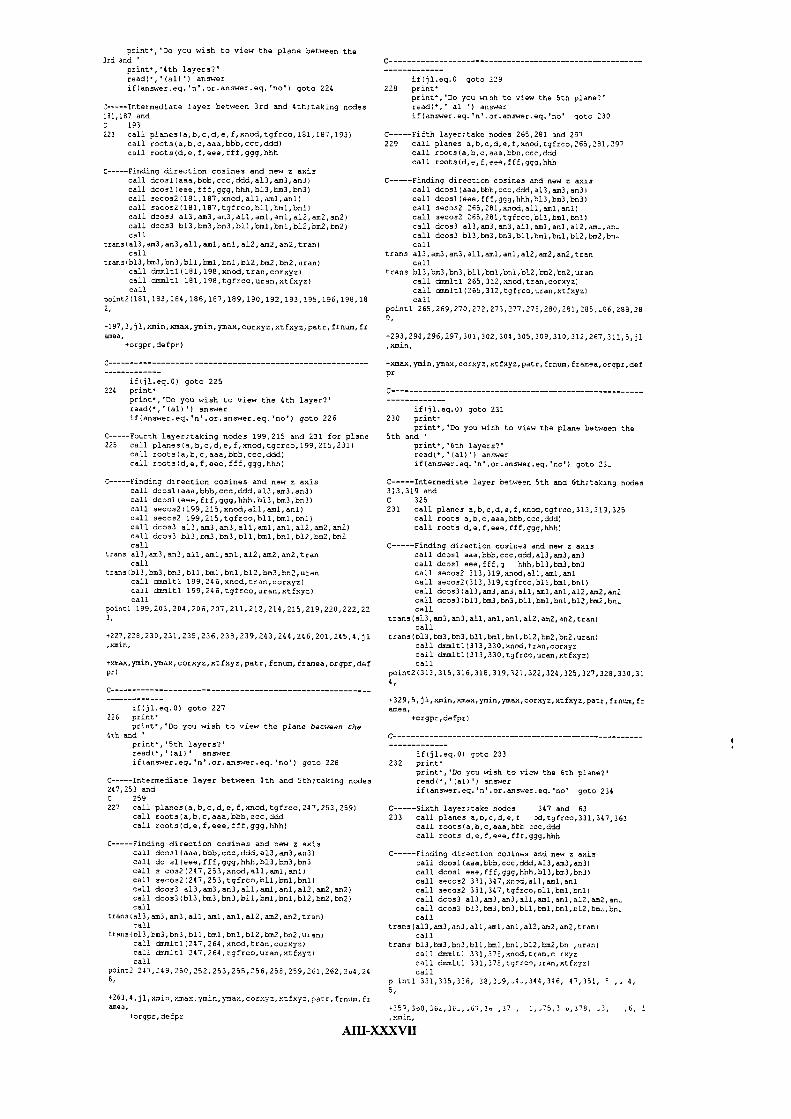
printa 'Do you wish to view the plane between the3rd and

print', '4th layers?'read)', ')al)') answerif)answer.eq. 'n'.or.answer.eq. 'no') goto 224

C-----Intermediate layer between 3rd and 4th;taking nodes181,18? andC 193223 call planes)a,b,c,d,e,f,xnod,tgfrco,181,187,193)

call roots)a,b,c,aaa,bbb,ccc,ddd)cell roots(d,e,f,eee,fff,ggg,hhh

C-----Finding direction cosines and new z axiscall dcosl)aaa,bbb,ccc,ddd,al3,am3,an3)call dcosl)eee,fff,ggg,hhh,bl3,bm3,bn3)call secos2)181,187,nnod,all,aml,anl)call secos2)181,187,tgfrco,bll,bml,bnl)call dcos3 a13, ais3,an3, all, aml,anl,a12,ain2,an2)call dcosl bl3,bm3,bn3,bll,blnl,bnl,bl2,binl,bn2)call

trans)al3,am3,an3,all,aml,anl,a12,am2,an2,trari)call

trana)bl3,bm3,bn3,bll,bml,bnl,b12,bm2,bn2,uran)call dminitl(l8l,l98,xnod,tran,corxyz)call dmmltl 181,l98,tgfrco,uran,xtfxyz)call

point2 181, 183, 184, 186, 18?, 189, 190, 192, 193, 195, 196, 198, 18

19?,3,jl,xmin,xmax,yniin,ymax,corxyz,xtfxyz,patr,frnum,fraisea,

4orgpr,defpr)

if)jl.eq.0) goto 225224 print'

print', 'Do you wish to view the 4th layer?'read)',')al)') answerif(answer.eq. 'n' .or.answer.eq. 'no') goto 226

Fourth layer;taking nodes 199,215 and 231 for plane225 call planes)a,b,c,d,e, f,xnod,tgfrco,199,215,23l)

call roots)a,b,c, aaa,bbb,ccc,ddd)call roots)d,e,f,eee,fff,ggg,hhh)

C-----Finding direction cosines and new z axiscall dcosl)aaa,bbb,ccc,ddd,al3,ajn3,an3)call dcosl)eee,frf,ggg,hhh,b13,bm3,bn3)call secos2) 199,215, xnod, all, aml , anl)call secos2 l99,215,tgfrco,bll,brnl,bnl)call dcos3 all, asn3,an3, all, aid, anl, al2, am2,an2)call dcos3 bl3,bin3,bn3, b11,bml,bnl,b12,bisl,bn2call

trans al3,am3, an3, all,aml, anl, a12, am2, an2,trancall

trans)bl3,bm3,bn3,bll,bml,bnl,b12,bm2,bri2,urarjcall ommltl 199, 246,xnod,tran,corxyz)call dm'nitl l99,246,tgfrco,uran,xtfmy:)call

pointl 199,203, 204,206,207,211,212,214,215,219,220,222,22

+227,228,230,231,235,236,238,239,243,244,246,201,245,ljlcoin'

4-xmax,ymLn,ymax,corxyz,xtfxyz,patr,frnun.frainea,orgpr,derpr)

if)jl.eq.0) goto 227226 print'

print', 'Do you wish to view the plane bacween the0th and

print','Sth layers?'read)',' )al) ' answerif)answer.eq. 'n' .or.answer.eq. 'no') gob 228

C-----Intermediate layer between 4th and lth;taking nodes247,253 andC 25922? call planes)a,b,c,d,e, f,xnod,tgfrco,247,253,259)

call roots)a,b,c,aaa,bbb,ccc,dddcall roots)d,e, f,eee, fff,ggg,hhh)

C-----Finding direction cosines and new z axiscall dcosl(aaa,bbb,ccc,ddd,a13,aml,an3)call dc sl)eee,fff,ggg,hhh,bll,bml,bn3call s cos2)247,253,xnod,all,aml,anl)call secos2)247,253,tgfrco,bll,bml,bnl)call dcos3 a13,ain3, an3, all,aml,anl,al2,ain2,an2)call dcosl)bll,bml,bn3,bll,bml,bnl,bl2,bm2,bn2)call

trans)a!3,asil,anl,all,aml,anl,a12,ain2,an2,tran)call

trans(bl3,ba3,b53,bll,bml,bnl,bll,bm2,bn2,uran)call dlmnitl)247,264,xnod,tras,corxyz)call dmmltl 24?,264,tgfrco,uran,xtfxyz)call

ooint2 247,249,250,252,253,255,256,258,259,261,262,24,24

if)jl.eq.0 goto 229228 print'

print', 'Do you wish to view the 5th plane?'read)',' al ') answerif)answer.eq. 'n' .or.answer.eq. 'no' goto 230

C-----Fifth layer;take nodes 265,281 and 297229 call planes a,b,c,d,e,f,xnod,tgfrco,265,281,297

call roots)a,b,c,aaa,bbr,ccc,dddcall roots)d,e, f,eee,fff,ggg,hhh

C-----Finding direction cosines and new r axiscall dcosl)aaa,bbb,ccc,ddd,al3,ais3,anj)call dcosl)eee,fff,ggg,hhh,bl3,bml,bn3)call secos2 265,281,xnod,all, aol, ani)call secos2 265,28l,tgfrco,bll,bsil,bnl)call dcos3 al?,am3,an3,all,aml,anl,al2,ais,an_call dcosl bl3,bn3,bn3,bll,bml,bnl,bl2,bo2,bn.call

trans a13,ainl, an?, all,ainl,anl,a12, am2,an2,trancall

trans bl3,bni3,bn3,bll,bml,bnl,b12,bsi2,bn2,urancall thidltl 265,312,xnod,tran,corxyz)call dxnmltl)265,312,tgfrco,uran,xtfxyz)call

pointl 265,269,270,272,273,277,278,280,281,285,_86,299,28

+293,294,296,29?,301,302,304,305,309,310,312,267,311,5,jl,xxnin,

+xinax,ymin,yisax, cormyc, xtfmyz,patr, frnuo, frarea, orgpr,defpr

if)l.eq.0) gcto 231230 print'

print', 'Do you wish to view the plane between the5th and

print', '6th layers?'read)',')al)') answerif)answer.eq. 'n'.or.answer.eq. 'no') goto 23,.

C-----Intermediate layer between 5th and Oth;taking nodes313,319 andC 325231 call planes a,b,c,d,e,f,xnod,tgfrco,313,319,325

call roots a,b,c,aaa,bbb,ccc,ddd)call roots d,e,f,eee,fff,ggg,hhh)

C-----Finding direction cosines and new z axiscall dcosl aaa,bbb,ccc,add,a13,ain3,en3call dcosl eee,fff,g hhh,bl3,bai3,bn3call secos2 313,319,xncd,all,ainl,anlcall secos2)313,319,tgfrco,bll,bml,bnl)call dcos3(al3,am3,anl,all,aml,anl,al2,ajnl,an2call dcos3)b13,bm3,bn3,bll,bral,bnl,bl2,bej2,bn_call

trans)al3,aJnl,an3,all,alnl,anl,a12,arZ,an2,tran)call

trans)b13,brs3,bn3,bll,brnl,bnl,bl2,bm2,bn2,uran)call dmmltl)313,330,xnod,tran,corxyzcall dzsznitl)313,330,tgfrco,uran,xtfxyz)call

poLnt2 313, 315, 316, 318, 319, 921, 322, 324, 325, 327, 328, 330,31

+329,S,jl,anmn,xinax,ymin,ymaz,corxyz,xtfxyz,patr,frnco,frarea,

+orgpr,defpr)

if(jl.eq.0) goto 233232 print'

print', 'Do you wish to view the 6th plane?'read)',')al)') answerif(answer.eq. 'n' .or.answer.eg. 'no' goto 234

C-----Sixth layer;take nodes 347 and 63233 call planes a,o,c,d,e,f id,tgfrco,331,347,363

call roots)a,b,c,aaa,bbb ccc,dddcall toots d,e,f,e'e,ffr,ggg,hhh

C-----Finding direction cosines and new z axiscall dcosl(aaa,bbb,ccc,ddd,al3,am3,an3)call dcosl eee,fff,ggg,hhh,bl3,bs3,bn3)call secos2 33l,347,xnsd,all,eml,anlcall seccs2 331,34?,tgfrco,nll,binl,bnl)call dcos3 al3,am3, anl, all,aml,anl,a12,ain2, an,.call dcos3 bl3,bm3,bn3,bl1,bn1,bn1,rl2,b,bn_call

trans)al3,a,n3,anl,all,ainl,anl,al2,am2,an2,tran)call

trans bl3,bis3,bsl,blL,bnl,bnl,bl2,bm2,bn ,uran)call iunLt1 331,378,xncd,tran,c rxyzcall dmmltl 331,378,tgrrco,iran,xtfxyz)call

p intl 331,335,336, 38,3,9,4,314,346, 47,351, , 4,

2O?,4,Jl,cm1n,icmax,ymin,ymax,corzyz,xtfxyz,patr,frnns,fr ,37 , 1,75,3 e,3?9, 3, ,6, Ianea,

coin,-forgor, drfpr

AIll-XXXVII

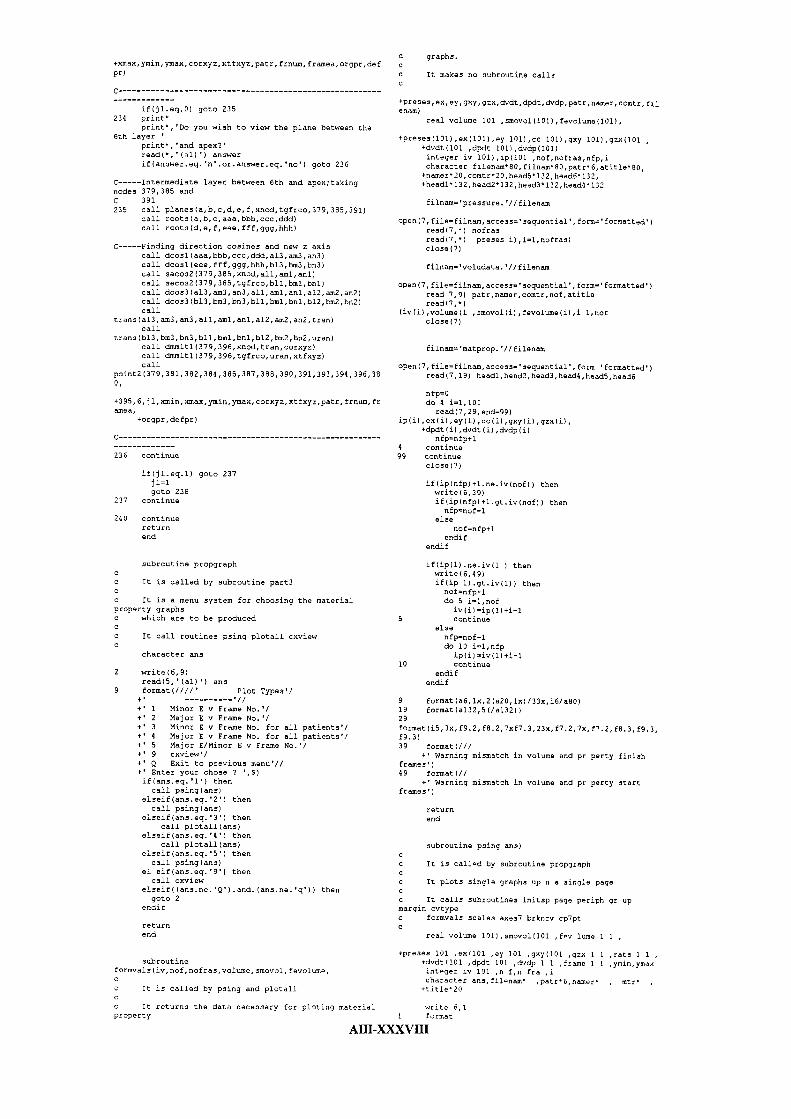
epreses 101 ,ex(101 ,ey 101 ,gxy)101 ,gzx 1 1 ,rats 1 1+dvdt(101 ,dpdt 101 ,d'idp 1 1 frame 1 1 ,ymin,ymaxintger lv 101 ,n f,n fra ,1character ans,filnam' ,patr'h,namer • , mtr'

+tjtle'20

write 6,1format

C graphs.^xnax,ymin,ymax,corxyz,xtfxyz,patr,frnum,framea,orgpr,aef cpr) C It makes no subroutine calls

C

if)jl.eq.0) goto 235234 print

print', 'Do you wish to view the plane between the6th layer

print, 'and apex?'read(','(al)') answerif(answer.eq. 'n'.or.answer.eq. 'no') goto 236

C-----Intermediate layer between 6th and apex;takingnodes 379,385 andC 391235 call planes)a,b,c,d,e, f,xnod,tgfrco,379,385,391)

call roots)a,b,c,aaa,bbb,ccc,ddd)call roots (d, e, f, eee, fff, ggg, hhh)

C-----Finding direction cosines and new z axiscall dcost)aaa,bbb,ccc,ddd,a13,ain3,an3)call dcosl(eee,fff,ggg,hhh,b13,bm3,bn3)call secos2)379,385,xnod,all,aml,anl)call secos2)379,385,tgfrco,bll,bml,bnl)call dcos3)al3,am3,an3,all,aml,anl,al2,am2,an2)call dcos3)bl3,bm3,bn3,bll,bml,bnl,bl2,bm2,bn2)call

trans(al3,am3,an3,all,axnl,anl,a12,am2,an2,tran)call

trans(bl3,bm3,bn3,bll,bml,bnl,bl2,bm2,bn2,uran)call dmmltl)379,396,xnod,tran,corxyz)call dmmltl)379,396,tgfrco,uran,xtfxyz)call

point2 379, 381, 382,384, 385, 387,388. 390, 391,393,394 ,396,38

+39S,6,jl,xmin,xmax,ymin,ymax,corxyz,xtfxyz,patr,frnum,fralnea,

+orgpr,defpr)

236 continue

if)jl.eq.1) goto 237j 1=1goto 238

237 continue

240 continuereturnend

subroutine propgraph

c It is called by subroutine part3

c It is a menu system for choosing the materialproperty graphsc which are to be produced

c It call routines psing plotall cxview

character ans

write)6, 9)read)5, ' )al) ') ansforinat)///!' Flot Types'!

4. ' --------- - 'I!+' 1 Minor E V Frame No. '/4.' 2 Major E v Frame No. 'I+' 3 Minor E V Frame No. for all patients'!4.' 4 Major E v Frame No. for all patients'!+' S Major E!Minor E v Frame No. 'I4.' 9 cxview'/4.' Q Exit to previous menu'!!+' Enter your chose 7 '.5)if)ans.eq. '1') then

call psing)ans)elseif)ans.eq. '2') then

call psing(ans)elseif)anseq. '3') then

call plotall)ans)elseif)ans.eq. '4') then

call plotall)ans)elseif(ans.eq. 5') then

call psing)ans)el eif)ans.eq. '9') thencall cxview

e1seifans.ne.'Q').and.)ans.ne.'q')) thengoto 2

endif

returnend

enam)real volume 101 ,smovol(101),fevolume(101),

+preses)101),eX)101),ey101),cc 101),gxy 101),gzx(101+dvdt(101 ,dpdt 101),dvdp)101)integer iv 101),ip(101 ,nof,nofras,nfp,icharacter filenam'80, filnam'80,patr'6,atitle'80,+namer'20, comtr'20,head5'132, head6'132,+headl' 132, head2' 132, head3' 132, head4 132

filnam='pressure. '!!filenam

open)7, file-filnam, access='sequential', form='formatted')read(7,') nofrasread)7,') preses i),i=1,nofras)close)7)

filnam-'voludata. '!!filenain

Open)7, file=filnam, access'sequential', form-formatted')read 7,9) patr,namer, ccmtr, nof, atitleread)?,')

(lv)i),volume(i ,smovol)i),fvoLume)i),i 1,nofclose)7)

filnam='inatprop. ''!filenam

open)l,file-filnam,access='sequential',form 'formatted')read(7, 19) headl,head2,head3,head4,head5,head6

nfp=0do 4 i-1,101

read)7, 29, end=99)ip)i) ,ex)i) ,ey)i) ,cc)i) ,gxy)i) ,gzx)i),

+dpdt)i) ,dvdt)i) ,dvdp)i)nfp=nfp^1

4 continue99 continue

close) 7)

if)ip)nfp)+1.ne.iv)nof)) thenwrite)6,39)if)ip)nfp)+1.gt.iv)nof)) thennfpnof-1

elsenot=nfp+1

endi fendif

if)ip)l).ne.jv(1 ) thenwrite)6,49)if)ip 1).gt.ivil)) thennof-nfp+ldo S i-1,nof

iv)i)=ip)1)+i-15 continue

elsenfpnof-1do 10 i-1,nfp

ip)i)-iv)l)+i-110 continue

endifendif

9 format)a6, lx,2)a20, 1x)!33x,i6!a80)19 format)a132,S)!al32))29format)i5,3x,f9.2, f8.2,7xf7.3,235,f7.2,7x,f7.2,f8.3,f9,3,09.3)39 format)!!!

+' Warning mismatch in volume and pr perty finishframes')49 format)!!

+' Warning mismatch in volume and pr petty startframes')

returnend

subroutine psing ans)cc It is calld by subroutine propgraph

c It plots single graphs up n a single page

c It calls subroutines initsp page periph gr upmargin cvtypec formvals scales axes7 brkncv cp7pt

real volume 101),smovol)101 ,fav lone 1 1

subroutineformvals)iv,nof,nofras,volume,smovol,fevolum,

It is called by psing and plotall

C It returns the data necessary for ploting materialproperty

Affl-XIXX VII

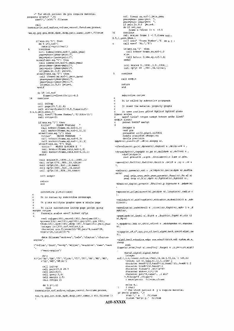
+' For which patient do you require materialproperty graphsl 9)

cead), ' )a30) ') filenam

callfor,nvals)iv,nof,nofras,voluise,sinovol,feVolume,preSes,

+ex,ey,gxy,gzx,dvdt,dpdt,dvdp,patr,naxner,coxntr,filenam

if)ans.eq. '5') thendo 5 i=1,nof-1

rats )i)ey)i) /ex)i)continuecall limexc)rats,nof-1,yinin,ymax)ymaaymax+ (ymax-ymin) /7.ymiflymifl- )ylnax-ymin) /7.

elseif)ans.eq. '1') thencall limexc)ex,nof-1,ymin,ymax)maxymax+)ymaxymin)/7.

ymin=yntin- )ymax-ylnin) /7.if)ymin.lt.0.0) ymincO.

elseif)ans.eq. '2) thencall limexc)ey,nof-1,ymin,ymax)ymax=ymax+ (ymax-ymin) /7.ymin=ymin-)ymax-yrnin)/7.if)ynin.lt.0.0) yTnin0.

endif

do 10 i=1,noffraiue)i)=float)iv(i) )+0.5

10 continue

call initspcall page)29.7,2l.0)call scales)frame)l)-0.5,frame)nof)-

0.5,1,ymin,ymax, 1)call axes7)'Frame Nuinber,E/(kN/me2))

call cvtype)2)

if)ans.eq. '1') thentitle=' MINOR MODULAScall brkncv)frame,ex,nof-1,0)call markcv(frame,ex,nof-1,1l,1)

elseif)ans.eq. '2') thentitle' MAJOR MODULAScall brkncv)fra,se,ey,nof-1,0)call markcv)frame,ey,nof-1,l1,l)

elseif)ans.eq. '5') thentitle=' MAJOR E/MINOR Ecall brkncv)trame,rats,nof-1,0)call markcv)frame,ratm,nof-1,11,1)

endif

call scalez)0. ,l000.,l,0. ,1000. .1)call cp7pt)370. 980., 16,title)call cp7pt)30. ,950. ,16,namer)call cp7pt)300. ,950., 16,patr)call cp7pt)30. ,920., l6,corstr)

call endplt

returnend

call limexc ex,nof-1,ymin,ymaxynax=ymax-i- ymax-ymin 7.ymin=ymin- ymax-ymin 7.if ymin.lt.0.0 ymcn=O.do 10 n=1,nor

frame n =float iv n +0.510 continue

call scales frame 1 -O.5,frame nof)-0.5,1,ymin,ymax, 1

call aaes7 'Frame Number', 'E kM m 2o call axes7 'No.', 'E')

if)ans.eq. '3' thencall brkncv frame,em,nof-1,0

elsecall brkncv frarne,ey,nof-1,0)

endif

call scales 0. ,1000. ,1,0. ,1000. ,1call cp7pt 40 . ,980., 16,title)j

5 continue

call endplt

returnend

subroutine cxvi3Ow

c It is called by subroutine propgraph

o It draws the material property graphs

It uses routines g02caf Ego2caf Egozcbf plotelimexc scalesc axes7 title7 cvtype numbpt brkncv setky linek7endplt limincC polout bothk7 markpt

integer nreal pieparameter n=1S1,pie3.101SO26double precision dpaoprl)n)double precision

ddpdv)n) ,result)20 ,dE)n) ,alogep n(,

^dfevolure)n),pa)n),dpress)n),dzphvol n ,dmidpress n

+dpspmidpdv(n),dspdpdv n),pb n),delldpclv n),dellvol nndpellmidpdv Inreal presss(n ,alp)n ,fevolume(n(,v lume n),pie,

*smovol)n),Eelll(n),Eell2(n),Ee113)n ,Eell4 n ,yy n ,cc n

i-delta)n),gamina)n),akk n ,elldpdv)n),pellmidpdv n),midframe In)

real xmin,xmax,ymin,ymax,ppnew)n),Faoel)n),Ps e2 n)real dvdp n),M)n),dpdv n),Ego2caf)n),Ego2cbf n)

+EPaol)n),Exp)n),press)n ,EPao2)n(,p lypresss n ,pdpdv(n(

subroutine plotall (ansI

c It is called by subroutine propgraph

c It plots multiple graphs upon a single pageCC It calls subroutines iriitsp page periph groupmargin cvtypeC formvals scales axes7 brkncv cp7pt

real voluxne)101),smovol)l0l),fevolume)101),+preses)l01(,ex)101(,ey)101),gxy)101),gzx 101),+dvdt)101),dpdt)10l),dvdp l0l),fraiue)101),ymin,yisaxinteger iv)1O1),nof,nofras,i,ncharacter ans,filenam)12)e80,patr6,namera2o,+comtr20,title)12)5

data filenasi/'andrews', 'bale', 'clayton', 'clayton-angina',

+'cullum','ford', 'hardy','miller', 'monckton', 'rees','west

+ 'west-angina'/

datatitle/ 'AN', 'BA', 'CL', 'CL)A) ', 'CU', 'FO', 'HA', 'MI', 'MO',

+' RE ' , 'WE ', 'WE IA)

call initspcall page)21.O 29.7call periph)3.call group(3,4)call margin 1.5)call cvtype 2)

+spress)n),polymidpress)n(,pmidpdv n),longdim(n),radiuz n

wallthick)n),midlongdiln)n),midrad)n),midwallthick n ,mdvolin)n),

+mdvolout(n(,radinidwall n ,cirstl)n),Esphl(n),zphv 1 n ,Esph2 In),

#pspmidpdv)n),Esph3 n),Esph4 n ,Esph5)n),Esph6 n),cir t2n( ,My)n)

+,spdpdv)n),bkk n),dd)n),ellvol n ,midshpndex n) ,shpndex

4-logep)n),r6,r7,zyx,yxz,nf,bet3,alph4,bet4,Yymid,alPhl,beti'

+alph2,bet2,edradius,edpr szs,edwallthick,edl ngdim,ak,x,r6exp

realfraine(n( ,midellvol n) ,coeffs)2 ,Faoprl n ,y,ymid,pk,alph3

4beta2,alpha2,alphal,betalinteger

nof,i,k,n,icount,nofras,ifail,lk, is,j,jj,ii, °c unt,nwinteger mt n),ideg,nl,ij,l,iran)' 2character headl'132,head2'132,head3'13_,head4'1 2character head5'l32,head6'13character filnam'3 ,atile'60character answer,til'20character p atr'6,naner.. , c mtr'

+, filenam'8 , cframe'2c nnon/person filenam,cframe

do S i=1,12 write 6,1call I f mat)

formvals)iv,nof,nofras,voluzse,smoVOl,fevOlulse,preses, +' For which patient d y u require materialpr perty graphs. ',$

+ex,ey,gxy,gzx,dvdt,dpdt,dvdp,patr,namer,c mtr,filena,n 1) read ', ' a ' fjlenamrilnam 'ma'pr p.' filenam

A1ll-XXXIX

open(7,filefilflam,access='seqUefltial', form'formatted')

C-----Read in E and dvdpread(?,3) headl,head2,head3,head4,head5,head6

3 format(a132,51/a132))

icount=0do 4 i=1,n

read(7,5,end=99) M(i),dvdp(i)icount=icount+1

4 continue5 format)8x,f9.2,76x,f9.3)

99 continueclose )7)

filnam='pressure. '//filenain

open)7, filefilnast, access'sequential', form-formatted')read(7, ) nofrasread(7,) (presss)i),i-1,nofras)clone (7)

filnam-'voludata. '//filenam

open)7, file-filnam,access'sequential' , form-formatted')read)7, 19) patr,namer,comtr,nof,atitle

19 Format )a6, lx,2 )a20, lx) /33x,i6/a80)read)?,

(ml) ,volume (i) sinovol (I), fevolume U), i=1,nof)clone (7)

C-----Converting fevolumes to double precisiondo 22 i=1,nof

C-----Giving frames a referenceframe)i)float)int)i))

22 dfevolume)i)-dble)fevolutne)i))

k=0

do 6 i=l,icountif)M)i).eq.0.) goto 6k-k+1M ) k) =M ) i)dpdv)k)1 ./dvdp)i)dE)k)"dble)M)i)ddpdv)k)=dble)1./dvdp)i))

6 continue

C-----k is the true number of values there areC---- -Call NAG routines go2caf and go2cbf for regressionrelationshipsc-----the former with a constant; the latter withoutC-----Open file to which all data is sent to

filnaxn-'results. '//filenast

open) 1, filefilnam, access' sequential', form='formatted')ifail=0call gO2caf(k,ddpdv,dE,result,ifail)write)l,7) result)6),result)?),result)S)

C-----Saving values for derivation of modulus laterr6result (6)r?=result (7)

do 9 i-1,k9 Eg02caf)i)-result)6)dpdv)i)+result)7)

format)'RegfitzE-',f126, 'D p /DV+',fl2.6, ':Cor-',f12.6)call go2cbf)k,ddpdv,dE,result,ifail)write)1,10) result)6),result)7),result)S)

do 11 i-1,k11 Ego2cbf)i)-result)6)dpdv)i)

10format)'Reg.fit:E-',f12.6, 'D p/Dv^',f12.6, ':Cor"',f12.6)

write(l, 16)16 format)'RESULTS FROM EmDP/DV+c andEmDP/DV'/lOx, 'DF/DV' , 13x,

+'E', 13x, 'Eg02caf', 13x, 'Ego2cbf')write(l, 12)

)dpdv)i) ,M)i) ,Ego2caf )i) ,Ego2cbf )i) ,i-1,k)12 format (4 (lx, f12. 6))33 write)6,30)30 format(////

+' Wish to view the individual E v Op/Dy graph? '0)al) ') answer

if)answer.eq. 'y' .or.answer.eq. '1') goto 31if)answer.eq. 'n' .or.answer.eg. 'N') goto 32goto 33

31 call plotecall limexc)dpdv,k,xmin,xmax)call limexc)M,k,yinin,ymax)call scales)0.,xmax+.1,l,ynin-5.,ymax+l.,l)call axes7) 'CHAMBER STIFFNESS OP/Dy mmHg/cml)

+'MINOR MODLLI Ex/z )KN/m2)call title7('T', 'C', 'MOD (I) V STIFF OF DV) FOR')call cv type)3)

do 13 i-1,k13 call numb Pt dpdv i),M i ,0,i

call brkncv dpdv,EgO2cbF,k,-1call setky 'B', 'R',2,20call Linek7 0, 'B DF DV • CONSTANT'call linek? -1, 'E OP DV 0'call endplt

32 continuewrite)6,2?0

270 format•' Wish to view the E v Dp Dv graphs for all the

patients? ',S)r eadV, ' al ') answerif answer.eq. 'y' .or.answer.eq. 'Y' g to 272if answer.eq. 'n' .or.answereq. 'Si' g t 253goto 32

272 call plotexmin-1234.xmax-1234.ymin=xminymaxxmax

259 write(6,254)254 format) 1/ 'Enter the patient property filnais',S)

read) , ) filnam

opan)7,filefilnain,access'sequential',form 'f risatted'read)7,3) headl,head2,head3,head4,headl,headBicount=0

do 255 i-1,nread)7,5,end256) M i),dvdp)i

255 icounticour,tfl

256 continueclose)?)lk=0

do 257 i1,icountif)M)i).eq.0.) goto 257lk-lk+1M)lk)M)i)dpdv)lk)1./dvdp)i)

257 continue

call liminc M,lk,ymin,ymax)call liminc)dpdv,lk,xmin,Sinax)

261 print 258258 format)////'Another patient property file? '8)

read),')a1)') answerif)answer.eq. 'y'.or.answer.eq. 'Y') goto 259if)answer.eq. 'n' .or.answer.eq. 'N') got 260goto 261

260 call scales xmin,xmax,1,ymin,ymax,1call aes7)'CHAMBER STIFFNESS : DP DV

)mzn}lg/cm3) ','MINOR MODULI+:Ex/z )KN/m..call title7 'T', 'C', 'DP DV V Ex z F R ALL

PATIENTS')is-a

266 isis+1zyx-l234.yxz--1234.print 273

273 format)////' Enter next patient's filnamread),' )a30) ') filnam

open)?, file=fiLnam,access'sequential', form'formettedread)7,3) headl,head2,head3,head4,headl,head6icountO

do 262 i-i,nread)7,5,end263) H i),dvdp i)

262 icounticount+1

263 continueclose)?)1k-S

do 264 il,icountif M)i).eq.0. goto 264lk-lk+ 1M)lk)-M i)dpdv)lk)l./dvdp i

264 continue

call cv type 4call brkn cv dpdv,M,Lk,

do 813 i 1,1kif dpdv i .gt.yxz) jj-iif dpdv i .gt.yxz yxz dpdv i.)

if dpdv i).lt.zys) ii 1.

613 if dpdv i .lt.zyx zyx dpdv 1.)

call polout 'oeffswrite ,z69 coeffs(i ,i 1,.

269 format / ' Constant ',fl2.6, ' ' effi ient',f12.6

268 write)6,_58read ', ' al ' answerif answ-r.eq. 'y' r.answer.eq. '/' g t 2e6if answer.eq. n. r.answer.-q. 'N' g t 26g t 2e8

267 'alL eni rJt253 pr.nt', 'P 'ting the -'.p n-n'- aL p-v grapn a 1 g IV volum-'

call hrkncv)dpdv,EgO2Caf,k,0

AIII-XL

c-Converting to logsdo 21 i=1,nof

logep(i)alog(presss)int(iH)alogep(i)=dble)alog(presss(int)i)spress)i)=presss)int)i))

21 dpress(i)dble)presss)int(i) ))

C-----Call to NAG routineifailOcall go2caf(nof,dfevolume,alogep,result,ifail)write(1,23) result(6),result(?)

C-----Storing values againr6expresult (6)

23 format(////' Slope of logeP v Vol Graph =',f12.6/i' Intercept (or logeA) = ' , f12.6(do 24 i=1,nofalp(i(=sngl)re5ult)6)'dfevolume(i)+result 7))

24 ppnew)i)expNi))

C-----Converting loge of preses35 print 3434 format)////' Wish to view the logep v vol graphl',0)

read)',')al)') answerif(answer.eq. y' .or.answer.eq. 'Y') goto 36if)answer.eq. 'n .or.answer.eg. 'U') goto 37goto 35

C-----Now plot graph36 call plots

call limexc(fevolume,nof,xmin,xmax)call limexc)alp,nof,ymin,ymax)call scalea)xmin-1.,xmax-'l.,l,ymin-.l,ymax+.l,l)call axes7)'FEVOLUME )cm3) ', 'LOGe PRESSURE')

do 25 i=1,nofcall mark pt)fevolume)i),sngl)aloqep)i)),ll(

25 call mark pt)fevolume)i),alp)i),0)

call cv type(3(call brkn cv)fevolume,alp,nof,0)call cv type(2(call brkn cv)fevolume,logep,nof,-1)call set ky)'B', 'R',2,8)call line k7)0, 'EXPECTED')call line k7)-1, ACTUAL')call title7('T', 'C', 'LOGe P V FEVOL FOR PATIENT')call end pit

37 print 250250 format)////' Wish to view p-v graph if exponentialfit? ',$)

read)',')al)') answerif)answer.eq. 'y' .or.answer.eq. 'Y') goto 251if)answer.eq. 'n'.or.answer.eq. 'U') goto 252goto 37

251 call plotsxjnin-1234.x,nax-1234.yminxmiflymax=xmaXcall liminc )volume,nof,xmin,xmax)call liminc)smovol,nof,xmin,xmax)call liminc)fevoluine,nof,xmin,xmax)call liminc)spress,nof,yinin,ymax)call liminc )ppnew, nof, ymin, ymax)call scales)xmin-1. ,xmax+l. , l,ymin-l. ,ymax+1. 1)call axes7)'VOLUME )CM3) ','PRESSURE )mmHg)call cv type)2(call brkn cv)volume,spress,nof,-6)call brkn cv)sinovol,spress,nof,-4)call brkn cv)fevolume,spress,nof,-2)call brkn cv)fevoluine,ppnew,nof,0)call set ky)'L', 'C',E,lS)call line k7(-6,'VOLUME (VOLUME)')call line k7)-4,'SMOVOL (VOLUME)')call line k7)-2, 'FEVOLUME')call line k7)0, 'FEVOLUME )PNEW)call title7)'T', 'C', 'P - V GRP.PH FOR EXPONENTIAL v

ACTUAL')call end plt

252 print', 'Comparing Modulii between fe andexponential methods...'

write 1,39) patr,namer,comtr39 format)a6,l,2)a20,lx))

write)1,l28)128 format(/'Fraines',4x'Modulus )te(',4x,'Moduluz)exp)

write)l,38()int)i), nt)i+1),M)i(,r6*(presss)int)iH+presss(

+i-t(i+l)))/2.'r6exp-r7,i-1,k)38 format)/i3,'-',i3,f12.6,2x,f12.6)

C-----Comparing values as derived for fe model,exponen-almodel andC Pao model

do 44 i1.nof-1

Exp(i)=r6')prexss)int)iH+presss(int)i+l ))/2.'r6exp-r7press(i)-)presss)int)i))+prssss)int(i+1H)/2.

44 dmidpress(i)dble)press)i

C-----Pao's linear relationship testedC-----Converting Pressures from smUg to Dynes cm2

do 45 i=l,nof-1EPaol(i)press i('1334.l6'4.9-33)0 0.

C-----Converting back to KU m2EPaol)i EPaol i 100 0.

C-----Now Pan's Quadratic Relation i.e. 8=1660.-139P+320P'2

EPao2 i =lOeO.-139'press)i u320.'press i "2.45 EPao2 i)EPaO2 i 10000.

43 print 4040 format) ' Wish to view the E-P curves. ',S

read)', '(xl ' answerif answer.eq. 'y' .or.answer.eq. 'Y' goto 41if)answer.eq. 'n' .or.answer.eq. 'N' g to 42goto 43

41 call plotecall limexc)presz,nof-1,xlnin,xmaxymin1234ymax-l2?4.call liminc(M,k,ymin,ymax)call liminc(Exp,nof-1,ymin,ymax)call liminc EPaol,nof-1,ymin,ymax)call liminc)EPao2,nof-1,ymin,ymaxcall scales xmin_.5,xmax+.5,1,ymin-. l.,ymax+l., 1call axes7)'PRESSURE mmHg)', 'MINOR MODULI

)XN/m2) ')call cv type 2)call brkn cv press,M,k,0

do 50 i=1,k50 call numb Pt press(i),M)i),0,i

call brkn cv press,Exp,k,E)

do 85 i'1,k85 call numb pt press)i),Exp)i),1,i-)

call brkn cv press,EPaol,k,0)

do 86 il,k86 call numb pt)press)i ,EPaol i),4,i)

call brkn cv press,EPao2,k,0(

do 87 i1,k87 call numb pt)press i),EPao2 i(,ll,i)

call set ky)'L', 'C',4,l2)call both k7)0,0,'E v P FE)')call both k7)0,1,'E V P (ISP)')call both k7 0,4,'E v P )PAO1)')call both k7 0,11,8 v P )PAO2)call title7)'T', 'C', '8 - P RELATI NSHIPS FE & PA

VARIOUS')call end plt

42 print 300300 format)////

+' Wish to view a 1 8-P curves vs Pao' '5relationships? ',S)

read)',')al)') answerif)answer.eq. 'y'.or.answer.eq. 'Y') goto 301if)answer.eq. 'n'.or.answer.eq. 'N') goto 302

301 call plotexmin=123456?8.xmax=-1234 5678.ymin_xminy1sax=dsax

306 print 254read)',') filnam

open)7,file=filnam,access='zequential',forsi 'f matted'read)7,3) headl,head2,heed3,head4,head5,head6icount=0

do 303 i-1,nread)7,315,end=304) int)i),M)i)

315 forinat)iS,3x,f9.2)303 icount-icount+1

304 continueclose)?)lk=0

do 305 il,ic untif)M)i .eg.O.) g 305lk=lk+lint)lk int i)M)Lk -M i.

305 continue

call liminc M,lk,ymin,ymax

C-----Now the preses307 print 1717 format ' What is the nam F the pres ft a.

read ', * fulnam

open)7,file filnam,access 'sequential',f rm 'F mattedread)7,') nofrasread 7,' przss i),i 1,n frasci se 7

d 308 i. 1,lr308 press i prsss mt i 4-pr=sss tnt 1 *1

call 1_mm -rs ,ly,xmmn,.'.maxprint 25

AIII-XLI

read)°, al) ') answerif answer.eq. 'y' .or.answer.eq. 'Y' goto 306

309 call scales)xinin-l. ,xmax+1. , i,ymin-l. ,yrnax+1. , I)call axes7)'PRESSURE mmHg) ', MINOR MYOCARDIUM

MODTJLI Rn m2 ')call title7)'T', 'C', '6 v P - PAO & RESULTS'io-0jcount 0

314 is=js+1print 254read)a , ) filnamopen 7, file=filnain,access='sequential',

+form=' formattedread)7,3) headl,head2,head3,head4,haadS,head6icount=0

do 310 ii,nread)7,315,end=311) int)j),M)i.

310 icount-icount*i

311 continueclose )7)lk=0

do 312 ii,icountif)M)i).eq.0.) goto 312ik=lk+imt lk)int)i))l)lk)-M)i)

312 continue

print 17read) a ,*) filnasa

open)7, file-fiinam, accezz= 'zequential' , form' formatted')read)7, ) nofrasread 7 ' )presse)i),i-1,nofraz)close 7)

do 316 i=l,lkjcount=jcount+1press i) = (presss)int)i))+presss iot)i +1 ) 2.

C-----Store temporarilyPaoprl jcount)=prezs)i)dPaoprl)jcount =dble)Paoprl)jcountPaoel)jcount)=)Paoprl jcount)1334.1624.9-

330000. /10000.Paoe2)jcount) = )166O.-139. p aopri)jcount +320.

+Paopri)jcount)2. /10000.316 continue

call cv type)2call brkn cv)press,M,lk,is)

do 313 i1,lk313 call mark pt)press)i),M)i),is)

print 259if answer.eq. 'y',or.answer.eq. '1') goto 314

C-----Now plot Pao points via NAGifail=0flWJ Count

print, ' routinue replacedcall molajf)dPaoprl,w,ind,indw,jcount,nw,ifaii)

call m0ldaf)dPaoprl,1,jcount, 'A',irank,ifail)

do 320 i=1,jcountPaoprl)i)-sngl)dPaoprl)i))Paoel i)=(Paopri)i)a1334.16a24.9_330500j/i0000.

320 Paoe2)i)=)i660.-139.'Paoprl)i +320.Paoprl)i)'2. /10000.

call brkn cv)Paoprl,Paoei,jcount,0call brkn cv)Paoprl,Paoe2,jcount,0)

302 continue

C-----Polynomial fitting as suggested by Mirskywrite ) 1, 06)

46 format)/'Fraxnez',4x, 'Modulus )fe) ',4x, 'Moduluscap) ',4x,

+'Modulus )Paoi)',4x,'Modulus Pao2)')write)1,127)

)int(i),int)i+1) ,M(i) ,Exp(i) ,EPao1)i) ,EPao2)i) ,i-1,+k

127 format)/i3, '-',i3, f12.6,5x,f12.6,5x,fi2.6,5x,f12.6)52 writa)6,51)51 format)!! /

4' Wish t fit 4th degree polynomial or other topresss-voluxne'

+' curve?read)',' al ') answerif answer.eq. 'y'.or.answer.eq. 'Y') goto 53if)answer.eq. 'n'.or.answer.eq 'N) goto 74goto 52

53 write)6,54)54 format) //

4' What degree of polynomial would you likegreater than'!

+' highest power) to fit7 '.0)read)',') ideg

C-----Using NAG routine e02acf and fevoluineifail-0call e _acf dfevolume,dpress,nof,pa,deg,iracl

do 55 i-i,nof

y-O.ymid=0.ni=idegdo 56 ii=i,ideg-i

y=y*zngl pa nl 'dfevolume i ni-iir)i.eq.nof) goto 73

ymid=ymid+sngl)pa ml dfevolume)i odfevolume i+i ) 2.+'' ni-i))

73 continue56 ni-ni-i

polypresss I y+srgl pa 1if)i.eq.nof goto 55polymidpress i) =ymid+ongl pa 1

55 continue

58 print 5757 format /1 ' Wish to view graphl '.0

raad)','(ai)') answerif)answer.eq. 'y',or.answer.eq. f') goto 59if)answer.eq. 'n'.or.answer,eq. 'N') goto 61goto 58

59 call plotexisin=i234.xmax--i234.call liminc volume,nof,xmin,xnaxcall liminc)smovol,nof,xmin,srrtaxcall liminc)fevolume,nof,xmin,xmax)call limexc)spress,not,ymin,ymaxcall scales cmln-1.,xmax+i. ,i,ymin-.l,ymax*.1,lcall ares7 VOLUME cm3 ''PRESSURE mm}4g)')call cv type)2)call brkn cv)volume,spress,nof,-6call brkn cv)smovoi,zpress,nof,-3call brkn cv)fevolume,spress,nof,-1call brkn cv)fevolume,polypresss,nof,0)

do 60 i=l,nofcall mark pt)volume)i),spress i),l1)call mark pt)smovol)i),spresn i),4)call mark pt fevolume)i),press 1 .1)

60 call mark Pt fevolume)i),polypreosz i),li

call set ky('L', 'C',4,i8)call both k7)-6,il, 'VOLUME )VOLUME)call both k7)-3,4,'VOIUME SMOOTH)'call both k7)-i,l,'VOLUME )FEVOL)')call both 17)0,11, 'VOLUME P01?))call title7)'T', C', 'P - V CURVE FOR PATIENT')call end plt

61 write 1,62 ideg62 format /'Results on smooth p-v ourve'/'Degree ofpal ynoieial

+i3/'Pressure',Ox, 'Polypresss',Bx, 'Volume',8x, 'SV lume',85'

+ 'Fevolume')write)i,63)

)spress)i ,polypresss)i),volume)i ,smovol)i ,fevo+lume)i) ,i=l,nof)

63 format)im,3f12.2,2fi2.3)

do 64 j=i,ideg64 print', 'pa)',j, ') ',pa j)

68 write)6,65)05 format)!!!!

+' Do you wish to continue the polynomial fittingroutine? '.0)

read)',')al)') answerif answer.eq. 'y' .or.answer.eq. ''1') goto 53if)answer.eq. 'n'.or.answer.eq. 'N') goto 67goto 68

67 continue

do 69 i-1,nofy=0.ymid=0.if)ideg.eq.2) goto 75ni=idegdo 71 ii=i,ldeg-2

y=y*sngl (nl-i)'pa n dfevolume i '')ni-2if)i,eq.nof) gotymid=ymid+sngl) ni-

i)'pa)ni '))dfevolume i)+dfevoiume+)i+ifl/2. ")nl-2))

78 continue71 ni-ni-I75 continue

pdpdv i =yesngl pa)2if)i.eq.nof) goto 69pmidpdv)i)-ymid.sngl pa 2

69 Continue

write 1,72 ideg72 format) 'DP DV for fe p-v curve'!' Degreepolynomial =', i3

+'Pressure',l x, 'Polypressu', I x, 'FEV lum', 1 c, 'dvdp', 1 m'dpdv'

1-01-0

do 7eif mcd ,2 eq. then

AIll-XLH

11+1write (1, 77)

press(l) ,polymidpress)l), (dfevolume(l)++dfevolume(1+i) (/2., 1./pmidpdv(l) ,pmidpdv(l)

77 format(ix,f8.2,2f12.2,2f12.3)else if(mod(j,2).eq.1) then

k-k+ 1write(1, 63)

spress(k) ,polypresss(k),dfevolume(k) ,1./pdpdv(k)+, pdpdv (k)

end if76 continue

74 continue

C-----Miraky's analysis tested here for sphere andellipsoid82 print 7979 format(////' Wish to derive values for E fromMirsky ct_al) • 6)

read(,'(al)') answerif(answer.eq. y .or.answer.eq. ?') goto 80if(answar.eq. 'n'.or.answer.eq. 'N') goto 81goto 82

C-----Calculating stage by stage80 print', 'If a file needs to be created enter 1 andinput for all'

print', 'frames the long dimension (base-apexlength),the inner

print', 'radius and the wall thickness (in thisorder and in mms)

print', 'for a chosen plane.However if it alreadyexists enter

+2.'read)',')al)') answerif(answer.eq.'y'.or.answer.eq.'y') thenprint 96

96 format)/'Give this file a name.........,S)read)',') filnam

open)7, file-filnam,access-'sequential', form-'formatted')print', 'Enter data on next line then......0 0 0

when finished

ij-1129 readlongdim)i),radi.us i),wallthick ij),shpndex)ij)

if)longdim ij)eq.0..or.radius(ij).eq.0..or.+wall.thick ij).aq.0.) goto 130

ij-ij+1goto 129

130 write 7,97)longdim)i),radius i ,wallthick i),shpndex i),

ti-i, ij)close (7)

elseif answer.eq. 'n'.or.answer.eq. 'N') thenprint 98

98 format / 'What is the existing filnam 7 •read)', 'C filnam

open (7, file-f ilnam, access- • sequential', form-' formatted')ij -0do 132 i1,nof

read 7,',end-131)longdim)i) ,radius(i) ,wallthick i),

+shpndex i)132 i-ij+1131 continue

close (7)end if

C-----Calculating volume for spherical configuration.do 83 i-1,ijsphvol)i)-4.'pieredius i)"3./3.dsphvol(i)-dble(4.pie'radjus i)"3./3.)

C-----Volumes for ellipsoidal geometryellvol)i)(4./3.)'pie'()longdim)i)'(7./12.)+1. -

(wallthick(j)/+2.))'radjus(i)"2.

83

dellvo1)i)-dle( )4.13.)'pie'( (longdim(i)(7./12.)+i.)-+(wallthick)i)/2.))'rad.jus i '2.)

do 84 i-1,ij-1midshpndex)i)-)shpndex i)+shpndex)i+1((/2midframe(i)-(jnt)j)+int(i+i) 2.

midlongdim)i)-)ongdj. i)+longdim i+l)) 2.)')7./i2.)+imidrad)i(-) )radius) j )+radjus(j+i) (/2.)

mictwal1thjckU)_((wallthickU)..allthick)i+1)(/2(

C-----Calculating mid-frame volumestndvolin(i)-4.'pie'midrad i)"3./3.

5dVOlOut(i ) 4• pie))midrad(i(+mid.,4allthick i))"3.-+midrad(i) ''3 (/3

midellvol(i(-(4. 3.)'pie' )midlongdim(i(-(midwallthick)i)/2) C'

+midrad(j) ''2.

rad1nirJwal1)i(jdradU + midwallthick)i) 2.)

stresacirlO

cirst1(i(prezs(ii.13l416*(mdvolin(i)/mdvolout(ifl(1.+(

+(midrad)i)+midwallthick(i))"3./(2.'radmidwa1l(j('3.))(

C-----Now working out dp/dv based on spherical models atmid points

spdpdv(i)(spress)i+1)-spress(i))/(sphvol(i+i)-sphvo]. Ci)

dspdpdv(i(-dble(spress(i+1(-spress(i))/ (sphvol(i+1(-sphvol (1))

C-----nd working out dp/dv based on ellipsoidal modelsat mid points

elldpdv(i)-(spress(i+l)-spress(i))/ (ellvol)ii-1)-ellvol(i()

delldpdv(i)-dble((spress(i+i)-spress(i))/ (ellvol(i+1)-

+ellvol Ci)))

C-----Now work out E for spherical geometry84Esphl(i)=3.'cirstl(i(')l.+)(mdvolout(i)/mdvoljn(i(('mithad(i)'

+'2.)/)midrad(i)"2.+(mjdrad(j)+midwallthick(j)(*'2))')i

+ (mdvolin(i) /press(i) )'spdpdv)i))

C-----Using NAG to calculate dp/dv for polynomial basedon sphericalC volumes

print 54readt','i idegif ail-0call e02acf(dsphvol,dpress, ij ,pa, ideg, ifail)

C-----Using NAG to calculate dp/dv for polynommial basedonC ellipsoidal volumes

ifail-0call eO2acf(dellvol,dpress,ij,pb,jdeg,jfail)

do 90 i-1,ijymid-0.yymid-0.if)ideg.eq.2) goto 91ni-idegdo 92 iil,ideg-2

if(i.eq.ij) goto 93ymid-ymid+sngl) (nl-

i)'pa(nl)'((sphvol(i)+sphvol(i+j))/2.)"+(nl-2)

yymid-yymid+sngl( )nl-1)'pb)nl)' C (ellvol)i)+ellvol(i+1))/2.)

+'')nj-Z))93 continue92 ni-ni-i91 continue

if Ci.eq.ij) goto 90pspmidpdv)i)-ymid+sngl)pa)2))pellmidpdv(i)-yymid+sngl(pb)2))dpspmidpdv Ci) dble (pspmidpdv(i))dpellmidpdv Ci) dble (pellmidpdv Ci))

90 continue

C-----Now work out Esph2 for mid poly dp/dv valuesdo 94 i-i,ij-i

94

Esph2(i)-3.'cirstl)i)'(l.+)(mdvolout(j)/mdvolin(j))'mjdrad(i)

+"2.)/(midrad(j)"2.+(mithad)j)+mi&1lt)jck(j))"2.))'(

+()mdvolin(i))/press(i)'pspmidpdv(j)))

C-----Use NAG routine g02caf to fit regressionrelationship forC exponential

relationship on spherical configuration.if ail-0call g02caf(ij-1,idpress,dspdpdv,result,ifail)write)1,103( result(6),result(7)

103 format (I 'Alpha on exponential dp/dv curve(sphere)-', f16.12/

+'Beta on exponential dp/dv curve (sphere)-', f16.J2)alphl-sngl (result (6))beti-sngl(result(7)

C-----Use NAG routine for poly nowifail-0call g02caf(ij-i,dmidpress,dpspmidpdv,result,ifail)write(i,104) result(6),result(7)

104 format(/'Alpha on poly exponential spherecurve-', fi6.i2/

+'Beta on poly exponential sphere curve', f16.l2)alph2-sngl(result (6)bet2-sngl( result (7) C

C-----Calculaing Esph3 thendo 100 i1,ij-i

100Esph3)i(-3.'cirstl)i)'(i.+)))mdvolout(i) mdvolin)i)(

C-----Now calculating stresses for spherical model i.e +mjdrad(j)''2.)/(mjdrad)j(''2.+)midrad(i(+midwallthick(i(based on ''2.)))

AHI-XLffl

+' (1.+mdvolin(i) alphl+ (mdvolin(i) betl/press(i)))

C--Now working out constants Ic and c for sphere basedon exp relat.'---Need end diastolic presss,rad us and wall.thickness.

- Read fron file where can store this info.print 101

101 fornat(/'Naae of file with end diastolicpresso, radius and wall

+thickness data 3 • ,S)read(',) fiina

open (7, file-filnan, access-' sequential' • form- • formatted'read)7,') edradius, edwaflthjck, edpreszs, edlongdiaclose)?)

e(c.'3.'(1.+alph1'(4./3.)'pie'edradjus.3.)(l-*4/3)pj

+((edradjus*edwallthjck)"3.-edradiur"3.)/U4./3.)'pieedradjusc

• edradius2. )/ (edradiun'*2 . + (edradius+edwallthjck)

x3.thett'(I./3.pieedradius'•3./edpresss

x-x'edpresss((4.13.)pieedradiu33./((4./3.).pje((ec1redius+

+edwallthick) 3 . -edradiuz'3.)))' (1.+(edradius+edwallthjck)*.3./

+(2((edradius+(edradius+edwellthick) )/2.)'3.))x=x'(1.+((4./3.)pie'((edradius+edwalltJjck)"3-

edradius'3.)/

4) (4./3.)pieedradius"3. ) edradius2. ) / )edradius'2.++ (edradjus+e.raflthicjc) "2.))

C---Now work back to find and ccpare E • a forE-k(ziglfla) +0* and for

...........E3(l.+........sigma

do 102 i1,ij-i102 Esph4 (i) =alc'cirstl. (i) +5 .133416

C---Eaph5 for polynomial fit-smiler to Esph3do 105 i-1,ij-1

105Esph5(i)3.cirstl(i)"(l.+(((nmdvo].out(i)ledvolin(i))midzad(i)

+"'2)/(inidrad(j)"2+(m,jdrad(i)+mjciwallthick(i))"2)))'(1.+

+mdvolin(i) 'alph2+ (mdvolin(i) "bet2/press(i)))

C-----Now finding k and C for poly f it

pk3.(l.+alphZ'4.pie'edradiue'3.13. ) (l.+(U(4.13.)'pi

+( (edradius+edwallthjck)"'3.-edradius"3.)/(0.'pia"edradius'3.))

+'edradiuz"'2 1/ (edradiur"2 .+ (edradiva+edwallthick) 2.)

y3.*et2(4./3.)*pie*edradju5*3./jpre3s5

yy'edpres5s'((4./3.)pie'edradius-'3./((4./3.)'pie • ((edradius+

+edwal].thjck) "3.-edradius"3.)))(l.+(edradjus+edwallthjck)'•3./

+(2.' ((edradiva+(edradius+edwallthick) )12. ("3.))y-y" (1.+((4J3.) 'pie' ( (edradius+edwallthick("3.-

edradiue'34/

+( (4/3 )pie' j ae' • 3 ) 'edradius"2. )/ (edradiva"2.++ (edradius+edwallthick) • '2.))

C----Now work back to find and comupare L's forE'kCaigma)+c• and for

...........63(1.+........sigma

do 106 i1,ij-1106 Esph6(i)-pkcirstl(i)+y.133416

C----Using NAG go2caf to fit regression relation forellipsoidc configuration

ifail-0call g02caf (iJ-1,dmidpreaz,delldpdv, result, ifail)write(1,123) result(6)..rezult(7)

123 format (I 'Alpha on ellipsoid dp/dv V p graph-',f12.6/

+'Beta on ellipsoid dp/dv v p graph -, , f12.6)alph3-sngl (result (6)bet3"sngl (result (7)

C-----Using routine for the po1y fit nowifail0call g02caf(ij-

1,dmidpress,dpellmidpdv, result, ifail)write(1,124) result(6) ,reault())

124 format(/'Alpha on poly ellipsoid dp/dv V p-',f12.6/

+'Beta on poly ellipsoid dp/dv v p -, , f12.6(alph4=angl (result (6))bet4-sngl(result (7)

C--Now working out S's based ellimsoldel g.trydo 108 3-1,2

do 107 i-l..il-1

C----Working out stress at mid points

cirst20i)-preas(i)'.133416')ramjU i mi83,ltk I

+(i.-(mjdwaflthjck(j) (2radeimjj(j)))-(radmidwall(i)"2./

+(2.midlongdin4i)•'2.)))

beta2-(maidwallthjck Ii)! (midrad(j + omi*aflthick i 2.

+(2.+( (midwallthick0i)"2) (2.' ardrad(i)+i)/2. ) (

+'2.)))+(miallthjck(j)/mjdioujm i 0

alpha2- (mnidwallthick(i) / (aldred(i) + icflthjck0I 2.

(midwallthick(j)/ (2,' (.idrad(i(+(uj*aflthjck(j 2.) ))*

+ (miàmallthick(i) "2.! (4.') (midred(i +)miflthick(jJ 2.

+) }+(miciweilthicic(j)F (2.'midlomgdim)i)))'Ol.-(micMallthick(i)/

+(2.midiongdin(i))))alpha13.-

(midwallthick (10/ (mIdrmd(i) + (eillthick(i) 2.)4-

(midwallthick(i)/ (2."aidlooqdi.(i) ))+(m1caUtbick .)'2.

+(2(midrad(j)+(mjdwallthjk)j)/2. ("2.))

betal- (mith*allthick(i) /midlongdi,s(i) ) +)2.'mi*ellthick(j3

+(rnidrad(i)+(eidwallthick(i)/2.)))

ga*ma(i)-((alphal(4./3.)pie'((midrad(i)4midealltbick I

+3.-midrad(i)"3.))-(betel' (4.13.) piemidrad(i)"3. ) (I

+((alpha2'(4./3.)'pie'((inidrad)i)+ajdsallthjck i))"3.-amidrad (i( *

+'3.))+(beta2(4./3.)pie'amidrad(i)"3.))

delta(1)=((2.+(gasma(i)amidwallthick(i))/)eidrad(i)#

4(midwalltbick(i)/2.))) (1.+(sicknallthick(j)/ (2.' (amidredti)+

+(miai1thick(i)/2.))))+(amj mailt)jck(j)"2./(4.' amidred(j)+

+(midwallthick(i)/2.))2.))))+((1.+(gaamma(j)'mj,miiJjck(i) )/

+(2.midiongdim(i)))'(l.+(ai*allthick(i)/(2.'amjdlongdji) ((0)

cc(i)'l.-((midrad(i)+)midwallthick(i)/2.))"2.)/(2.'

+midlongdim(i)"2.)yy(i)1.-

(midwallthick(i)/ (2.' (midrad(i)+(micballthjc(c(i)/+24)cc(i)))

if(.eq.1) then

Eelll(i)-delta(i)(cirst2(i)/press(i))(4./3.)'pia'+(midlongdim(i)-

(midwallthick(i)/2.) )midrad(i)"2.'elldpdv(i)++(l.+gamma(i))dirst2(i)/yy(1)

a)ck(i)-delta(i) 'a,lph3 (4 ./3.) 'pie') (edlongdim' (7.Il.2.)+1.

+-(edalithick/2.)(+((l.+gaamma(i))/yy(i))

cc(i) =bet3'delta(i)'(4./3.)piei(edlongdiam(7./12.)+1.)-

+ (edwa,llthick/2.) ) 'edpresss ((edradius+ (ec*aI,lthick/2.) 1/+edwallthick) * (1.-

(edwallthick/(2(edradius+(edwa lthick/2.flfl-

4) (edradius+(edwallthick/2.))"2./(2'(edlongdimi7./l2.)+1. ) ) ) )'

+.133416/edpresss

C-----Now go back and work out S for ellipsoidal modelusing k and cC fron above

Eell3 (i)-akk(i)cirst2(i)+cc(i)else if)j.eq.2) then

Eell2(i)-delta(i)(cirst2(i)/press(i))'(4./3.!'pie'+(mid1ongdim(i)-(mi*m1lthick(i)/2.( )'midre.d(i)'2.+pellmidpdv(i(+(1.+gamnia)i) )cirst2)i)/yy(i)

bkk(i)=delta(i)alphV)l./3.)pie((edlongdim(7./12.J+1.

+-(edwallthick/2.) )+( (1.+gaamma(ifl/yy(i))

dd(i)-bet4'delta(i)"(4./3.)pie"((edlongdiam'(7./12.)+1.)-

+(edwallthick/2.))edpresss((edradius*'(edwallthickl2.))/

Affl-XLW

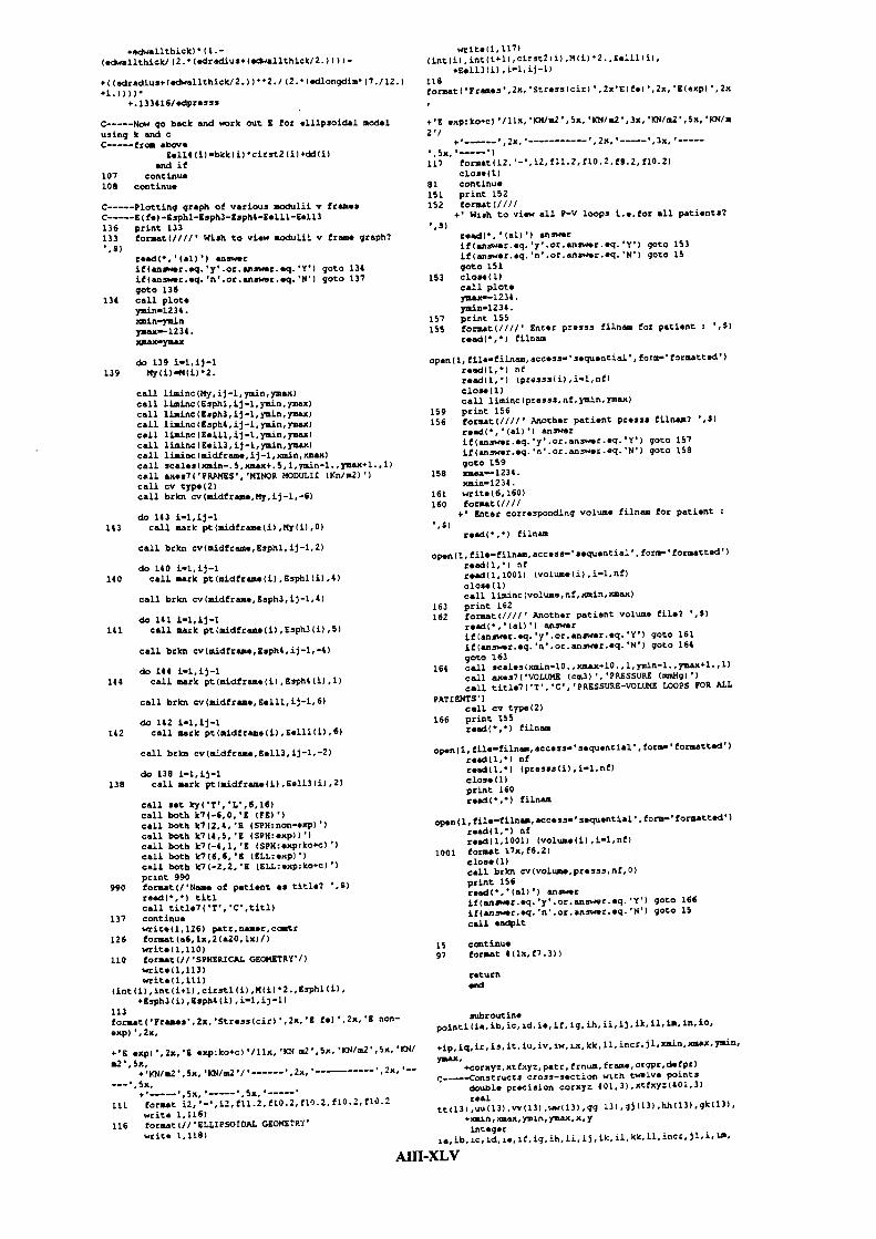
-: _c _r it -- _c _.%O .S

:re rcco_: rrpc:- - a._

1 r;l :c'7 _aI cci at: 3•c La I

c:: ..rI c:_ :':2 .r;_ rr:s: : I

- r- I

- : -cc-c

ac:r,-c r . -- I =crc_ ccc r _f 1

- rI cc-.-cc .1

4 flZ_ ac :-r __c

S 5tZ_ - ::-S -:_ .a.ccrcc :

cc •c-;_ -c r 2.La a

- fl,_ trr'-I-tc.. a.cc - __

- rc_ :::'-r .it

- a.. scc--c cc I- fl _TflZ _Z -

cc 2.S a:_ s-_cc-cc IZ I

.ZZ_ ccr't ;. -t-

P cc.rL c:: --c _z 1

-- I ;_ cc

L :-- II r:_ Zr: La. -

- L.a. :

cc : a.'c- cc a 2I .e;_1 cr;- ._::

p. ccflr3_ cc:zca2

cc 2 a..33 s'ra_

: a:-p-z _S 233 Z_ LI 2

a.-:4 1- a.t: .—c cc I

cc -;. -- =P2 a.:a- cc:ap: .. :

aT32. afa.: .j 2pp e a.tpi :rccc: t2

13 € =a.-aL cc:-- l,I

PP - cc:.c _mi

33 a.;I :ccz cc- fl_lI a.cc'r-: cc 2S ZZ:xcc

fir.;- vtf -'c cc I33 a.c;L c:r3cy:..P:

C fi:- a_:zyc a_c 233 9 ar'_ c:a.vz I

I

p 2. Sap-c c:.l:.. cr:y-c .a

:.b LI '-cc;L zccccc; L g:p.p5 1. fic; accc1z3; 2.1 fical

31 'LIIII.: rcl: :c:':

g : c_LI fl_c1 ccra';z - -:1 -i c::c: ,a

;j 1 -:c:.35 ll -'t;_ .:.t'c 2pp la -!.;. _:.t:c La 1Sc :3 sL ._cc.c 1 : Ia,...33 1 cc4l :..: _r -

c-S

-- - ;- lta.X a - -- - - -' .fl&S ma-.... -

-

a,. L -_' a_'-__ -

- ZZ I ,Z,' -a.a_'a'- -

S - - . -_caa Ca..3 r-' -tc1,ZL.' 1rcc-

-

:::c' zL::_c

LIc-ac c I, ac_c

- -r.-a_I c"-' P

a_ceca..... _c 'cc -

II-.,.:a--c arcc-, L'S .ara,a.-, L

1 -. 3taS'_ . -:ca..: -a. "1 1ca...:. aI.r _.. .3,., 1 - 4

cat:ca.2. :r;t 5,5,..pf:r'__crcall :s. :-call, a cc cc:cal.... b:eacall cral;: ::,, :,s I

—9a.k c-er. r.L

ca..:. p ccr_c: - 15,5 2::;: ::r. :s.

car. Nd

raIl ce"cal.. break:al.l c:CZ';t II'. ,S Icall r'; :: -cc.::. cp;: ::s. S.,Ia re'c:

tI 'S_aca 3cc

-all. aceca rcc-cc'.aa-. I crc_c-3S, -r.aZr-. I 'S. I

call. •'clpr' 1-a...: brca

2----Ped per. ca1le flowcall per. 2call brSc cv u,,hlc,13,-1call broc cv ww,;y....-1call breakcall )ccrc Pt cu 1 .55 1caLl 30177 Pt uw 1 ,pk Icall br-akcall join at tu 3 .5th 3call jccn p w 3 .;k 3caLl breakcall jccc ptau S Socall jcccc pt 5 ,gS. 5call breaccall. ic pt a'.. '7 .50call c.ccpa t..' ,gha1a brcaS

'al.. rir. r at P .rc 9-a.al .rc pt 'ax P .c, Pca_I br-aScell in a au 11 cc' 1.:

C-----33ccura b.a.c,c ccc cc crLe: cr,: c-c --::: :bar_ca

call par. Ica_ craw cv cc op :3ca.__ craw cv :';cal.I c:ea.cZa:.:. :rcc cc cc 1 .;; Ica_i Icco Pt yr 1 .;: 1call creakcall ::cc Pt tt 3 1call -cc cc v-; 3 ,g 3ca_i b:ea,ccall jrcc pt cc 5 .gg 5call jcan pt vv 5 ,p 5call breajccall cc pt tt '7 -call. jIm t yr '33 -call breakcall cin p1 tI PL,pg Pcall )cc.n ptvv9,p Pcall breakcall jeic pt It 11 .gg 11call jccc Pt 'r, 11 ,p 11call brea.call 20_cc at tt 13 pp 13call 70cc t yr 3 •;call break

ALH—XLVI

C-------'ada pencall pen 1call brcrpt 233. in. .0call cppt 235. • 15. 15 u:3pr

C----Red pen So .2call pen 2call creamcall orthct 210. 6.5 2call brhIi pt 133. .6.5 -1call cppt 235. ,S. 16.defpr

call ,oi.n Pt tea li • ;.0 11call brakcall jOirt Pt uu 13 'icr 13call join pt raw 31C 13call break

C-----9rintira fidel pin: with initial pen sinceinitial cc-ird.

call pen 1

do 9 i=k'z.114x-snl corxyr :,ly=nl crrxyz -

9 call riurtlapt n,y 4,

999 call endplt

19 format+' CC wish rtLt pa.t tD a File ir the Screen: F or

52 '.9

100 returnend

:1 :.eq. ;t :Pri.nt•rail t-rm

write 5read 5,' al ' artsir ase.'F' .r. acts.e:.':• tez

call devn-'a). me

call devrtc I

call pag- a•'all soa:.es - 'a 'imam-,' 5 1

035, ax=.3.s

raIl axes •• 1 • -. 1call scales 0. .4''. 1 -' 4'.call cpt 5. IS. .n cat:call rtp rt 5. iS. ,n, frrtcall cppt 49. 15. 6 framecall alayec :nc:call breamcall orrpt - ....In..

subroutir.epoint2 ia,ib,ic.id,ie.if ig,ih,i.r.,jj._k.il,lck,11,

+jncr,jl,xin,rax.yrrin,yma.'r, :o:xv:.nt:xyz, patr. frncm. frame,

+orsor,drfprC-----Constricts cross-sectoon with six points

double precision corny: .121.3 .xtfny: 4 1.3real

ttl7 ,uu ),vv 7 ,nrw ' ,gg 7 .gj 7 ,hri 7 • gk ..'ciiin.xmax, ysan, ylnax. a, yinteger

ia,ib, ic,rd.ie.if,ig. lb. iI,±j , ik,il, kk,ll,incr,jl,icharacter patr6.frn.rr12,orgpr.i6,oefpr_20,frame2

tt 1 _ngl corxyz ia,1cc 1 siagl atfay: :a,1Cv I sngl corxyz :b,1raw 1 =snq_ xtfzy: :0.1tt 2 =snal cOrny: :0.1

uu 2 -sogl stray: ic.1vv2 =sngl corny: id,ltrw - =sngl xtfxyz id.ltt 3 snglcorxyz ie,1uu 3 sngl xtfxvz i.a.1cv 3 sngl corny: if,1raw 3 =srcsl xtfxy: :f,ltt 4 sngL corny: :g,1uu 4 nngl stray: ig.lcv 4 -sngl cor.cyz ih, Itrw 4 =sngi slImy: :h.ltt 5 -sng. corny: :i.luu 5 -sngl xtfxy: :1.1VV 5 sngl corny: :j • 1raw S =nngl xtfxy: ij,itt 6 = sngl. corny: ik.1uu 6 =snl xtfny: i)c,lcv 6 -sngl corny: il.1nec 6 =sngl xtfxyz :1.1tt(7 srrgl corny: ia.1cc 7 =sngl xtfxyzia,lvv)7 sngl cormy: ib.irawfl sn gl xtfxy:lib.lgg)1 =sngl corcy:lia,2)lab 1 =sngl xtfnyz ia,2gj 1 =sngl corxyzlc.b,2gk(1 =sngl xtrnyz ib.2gg 2 =snql corny: ic,2 IhIt 2 =sngl xtfxyz ic,2gj 2 -sogl cornyz id,2gk 2 -sngl xtfxyz id,2))gg)3) =sngl corxyz)ie,2))hh)31 =sngl xtfxyzlie.2Hgj)3)=sngl corxyzlif,25k13)=sngi stfxyz if,2gg 4) = sngl corxyz ig,21lab 4)sngl xtfxyzlig,2gj 4 sngi corxyz ih,2gk(41 =sngl xtfzyz ih.2gg(5)snql corny: ii,2))hh(Slsngl xtfnyz)iI,2) Igj 5-sngl corxyz ij,2)Igk 5 "sngl(xtfxyz ij.1)gg(6)sngl cornyzlik.21)hh)61 =sn 1 xtfnyz ilc.2)gjI6lsngl corny: 11.2)gIrth sngl xtfny: 11.2qg) 7 sngl corxyz ia.2lah(7lsngl xtfny:Iia.2gj(7)5n51 corxyz(ib 2)gk(2)sngl xtfxy:ib,C1)

do 1 i'1,7jf)tt)i).gt.xxna5) Smax-tI i)jf)uu(i).gt.nsrax) xmas-cu 1)jf(ttliI.lt.Xmjn) nznlr.=tt i)jfluu i).lt.xmlrr xs,in=uu i

if ggli .gt.ymaxl yinan=gg L

if lab i .at.yma.'i) ymax-hh 11j f Iggli .l'-.ynun) ymir.7g iljfthhli .lt.yrnirr) ymin"hh 1

call scales saris-. 105,rrsra,'r*.105 I ymc.s-005.ymax+.00S. I

call cv tyme 2call break

C-----Black pen calledcall pen 1call draw cv tt,gg.'call draw cv SW, g].'call breakcall join pt tt I ,gg l)icall join pt -,', 1 ,gj 1'call breakcall join pt tt 3 ,gg 3call join pt Cv 3 ,g 1call breaccall, join pt tt S ,g 5call join pt Cv 5),gj 5call breakcall join pt tt 7),g -call join Pt SWI'),gJl'call break

C-----Red pen for displaced profilecall pen(2call brkn cv uu,hh,7,-1)call bran cv nrw,gk,7.-1call breakcall join pt cull ,hh 1call join pt)ww I .5k11)Icall breakcall join pt('cu 3),hh(3 Icall join ptlnrw(3 ,gk(3))call breakcall join Pt Uti S ,hh Scall join pt)nrw(5),gk)5 Icall breakcall join ptluu ,hh)7))call join Pt wwl7),qkl7)call breakcall penll)

do P i=kk,ll,3xengl corsyz 1., 1 I)y=sngllcorxyz)i, 2)

call crumb pt x,y.4,i.

call endplt

19 format /1+' Do you wish output to a File or the Screen: F

S 1 '.9)

100 returnend

subroutine planes a,b,c,d,=,f,xnod.tgfrco,a, ,kdouble precision

a(3) ,b)3) ,c 3) ,d 3) ,e 3 • f)3) ,nnod)40l,31+tgfrco)40l,3)integer i,j,k,l

do 1 11,3a 1 =nncd i,lb l) =xncs j,lC l) =lrrrod k,_d l) =to:rc 1,

e l) =tgfdt j,lf 1 tifr" c,l

Affl-XLVII

returnend

subroutine xlayer (incr)C

c It is called by subroutine cxview

C It writes the title for the plan views of theventricleCc It calls the simpleplot routine cp7pt

integer incr

if(incr.eq.1) thencall cp7pt)5. ,390. ,16,

+'VIEW ON MID-PLANE BETWEEN FIRST AND SECONDLAYERS')

elseifCincr.eq.2) thencall cp7pt(5. ,390. ,16,

+'VIEW ON MID-PLANE BETWEEN SECOND AND T){IRDLAYERS')

elseif(incr.eq.3) thencall. cp7pt>5.,390., 16,

+'VIEW ON MID-PLANE BETWEEN THIRD AND FOURTHLAYERS'>

elseif(incr.eq.4) thencall cp7pt(5. ,390.,16,

+'VIEW ON MID-PLANE BETWEEN FOURTH AND FIFTHLAYERS')

elseif(incr.eq.5) thencall cp7pt)5., 390. ,16,

+'VIEW ON MID-PLANE BETWEEN FIFTH AND SIXTH LAYERS')elseif(incr.eq.6) then

call cp7pt 5., 390., 16,+'VIEW ON MID-PLANE BETWEEN SIXTH LAYER AND APEX')endif

returnend

subroutine wlayer )incr)C

c It is called by subroutine cxvlewC

C It writes the title for the plan views of theventricleC

C It calls the simpleplot routine cp7ptC

integer incr

if)incr.eq.1 thencall cp7pt)5.,390.,16, 'PLAN VIEW ON FIRST PLANE)

elseif(incr.eq.2) thencall cp?pt 5., 390. .16, PLAH VIEW ON SECOND

PLANE')elseif)incr.eq.3 then

call cp7pt 5. ,390., 16, 'PLAN VIEW ON THIRD PLANE')elseif)incr.eq.4 then

call cp7pt 5..390.,16, 'PLAN VIEW ON FOURTHPLANE')

elseif(incr.eq.5) thencall cp7pt)5.,390.,16, PLAN VIEW ON FIFTH PLANE')

elseif)incr.eq.6) thencall cp7pt 5., 390. .16, 'PLAN VIEW ON SIXTH pLANE')

endif

returnend

subroutine ploteC

c It is called by subroutine cxviewC

c It initialises the plotting parameters ofsimpleplotC

c It calls the simpleplot routines initsp page picsiztextmgC

call initspcall page)29.7,21.)call picsiz>29. .20.3)call textmg).9)returnend

subroutine calyovol (coord,mvol,wvol)C

c It is called by subroutine afevolumecC It calculates the volume of the endocardium formthec FE mesh.cC It calls subroutines vol20b forma vollSw

double precisioncoord)401,3),elco(20,3),elcol5)15,3),evo].,

+volume,wvolreal mvol

integer elm,elmb)20,60),elmw)15,12)data

elmb/1,2,3,6,7,9,1O,ll,49,SO,52,53,67,EB,69,72,73,75,76,7

+3,4,5,7,8,11,12,13,50,51,53,54,69,70,71,73,74,77,78,79,9,10,11,

+14,15,17, 18,19,52,53,55,56,75,76,77,80,81,83,84,85,l1,12,13,15,

+16,19,20,21,53,54,56,57,77,78,79,81,82,85,86,87,l7,18,1g,22,23,

+25,26,27,55,56,58,59,83,84,85,88,89,91,92,g3,19,20,21,23,24 .27,

+28,29,56,57,59,60,85,86,87,89,90,93,94,95,25,26,27,30,3 1'33,34'

+35,58,59,61,62,91,92,93,96,97,99,lOO,10l,27,28,29,31,32,35,36,

+37,59,60,62,63,93,94,95,97,98,101,l02,103,33,34,35,38,39,41,42,

+43,61,62,64,65,99, 100, 101, 104, 105, 107,108,109,35,36,37,39,40,43,

+44,45,62,63,65,66,101,102,103,105,106,109,110,111,4l,42,43, 46,

+47,1,2,3,64,65,49,50,107,108,109,112,113,67,68,69,43,44,45, 47,

+48,3,4,5,65,66,50,51,109,llO,lll,113,l14,69,70,7l,67,68,69,72,

'73,75,76,77,115,116,118,119,l33,134,l35,138,139,141,142,143, 69,

+70,71,73,74,77,78,79, 116, 117,119, 120,135,136,137,139,140.143,

+144,145,75,76,77,80,81,83,84,85,l18,l19,j21,122,14l,142,143,146,

+147, 149.150,151,77,78,79,81,82,85,86,87,119,120,122,123,143,144,

+145,147,148,151,152,l53,83,84,85,88,89,91,92,93,l2l,122,124,125,

+149,150,151,154,155,157,158,l59,85,86,87,89,90,93,94,95,122, 123,

+125,126, 151, 152,153, 155,156, 159,160, 161,91,92,93,96,97,99,100,

+101,124,125,127,128,l57,l58,l59,162,163,165,l66,167,93,94,95,97,

+98,101,102,103,l25,126,128,l29,l59,160,l61,163,l64,167,i.68,169,

100,101, 104,10S,107,108,109,127,128,130,131,l65,l66,167, 170,

+171,173, 174,175,101,102, 103,105, 106,109,110,111,128, 129,131, 132,

+167,168,l69,17l,l72,175,176,177,107,108,l09,ll2,l13,67,68,69,130,

+131,1l5,116,173,174,175,178,179,133,l34,135,l09,110,lll,113,114,

+69,70,71,131, 132,116,117,l75,l76,177,179,l80,l35,136,137,133,l34,

+135,138,139,141,142,143,181,182,184,185,199,200,20l,204,205,207,

+208,209,135,l36,137,l39,140,143,144,145,l82,l83,l85,186,201,202,

+203,205,206,209,210,211,141,142,143,146,147,149,150,151,184,185,

+187, 188, 207,20B,209,212,213,215,216,217, 143, 144,145, 147,148, 151,

+152,153,l85,l86,188,189,209,210,21l,213,214,217,218,219,149,150,

+151,154,155,157,158.159,187,188,190,191.215,2l6,217,220.221,223,

+224,225,151,152, 153, 155. 156, 159,160,161,188,189.191,192,217,218,

+219,221,222,225,226,227,157,158,159,l62.163,165,166,l67,190,191,

+193, 194,223,224,225,228,229,231,232,233.159,160, 161,163,164,167,

Affl-XL VIII

+168, 169, 191, 192, 194 , 195, 225, 2.6, 227, 229, 230, 233, 234, 235,165, 166,

+167,170,171, 173,174,175.193,l94,196,197,231,232,233,236,237,239,

+240,241, 167, 1+8, 169, 171, 172, 175, 176, 117, 194 , 195, 197, 198,233,234

+235,237,238,241,242,243,173,174,175,178,179,133,134, 135,196, 197,

+081, 182, 239, 240,241,244,245,199,200,201,175,176.177,179,180, 135,

+136, 137, 197 , 198, 142, 183, 241, 242, 243, 245, 24 6, 201, 202, 203,199,200,

+201,204,2 5,207,2 8,209, 247, 248,250,251,265.266,267.270,271,273,

+274,275,201,202,203,205,206,20°, 210,211,248,249,251,252.267,268,

+269,271,272,275,276,277,207,208,209,212,213,215,216,217,250.51,

+253,254,273,274, 275,278, 279, 281, 282, 283, 209,210, 211,213,214,217,

+218,219, 251,252,254,255,275,276,27,279,280,283,284,285,215,216,

+217,220,221,223,224,225,253,254,256,257,281,282,283,286,287,289,

+290,291, 217,218, 219,221,222,225.226,227,254,255,257,258,283,264,

+285,257,288,291, .92,293,223,224,225,228,229,231,232,233,256,257,

+259,260,299,29 ,291,294,295,297,298,299,225,226,227,229,230, 233,

+234, 235, 257, 258, 260, 261, 291, 292, 293, 295, 296, 299, 300, 301.231, 232,

+233,236,237, 239, 240.241,259,260.262.263,297,298,299,302.3 3,305,

+306,307,23 .234.235,237, .36,241,242.243,26 .261.263,264.299, 302,

+301,303,304,307,3 8,309,239,210,241,244.245,199.200,201.262,263,

+247,248,305,306,307,310,311,265,266,267,241,242,243,245,246,201,

+202,203,263,264,248,249,307,308,309, 311,312,26',268,269,265, 266,

+267, 270, 271,273,274,275,313,314,316,317,331,332,333,336,337, 339,

+340, 341, 267, 268, 269. 271, 272, 275, 276, 277, 314, 3 15, 3 17, 318.333,334,

+335,337,336, 341,342,343,273,274,275,27&, 279,282, 282,293,316,317,

+319,320,339,340,341,344,345,347,348,349,275,276,27',279,280,283,

+284,285,317,318,320,321,341,342,343,345,346,349,350,351.,281,282,

+283, 286, 257, 289, 290,291,319,320.322,323,347,348,349,352,353,355,

356,357,283,284,285,287,258,291,292,293,320,321,323,324,349, 350,

+351,353,354,357,358,359,289,290,291,294,295,297,298,299,122, 323,

+325,326,355,356,3° .360, 361,363,364,365,291,292,293,295,296,299,

data elisu

397, 339,331,399, 341, 333, 382, 336,379,398,340,332,383 33 380,

399, 341, 333,401,343, 335,383,337,380,40 .342,334,384 3 8 381,

3 9,34.339.399,349,341,385,344.392,398,348,34o,38e 345 383,

399,349,341,401,351,343,386,345,383,410 35O,34,387 34384,

397, 355, 347, 399,357, 349,388,352,385,398,356,348, 389,35 386,

399,357,349,401,359,351,389,353,386,400,359,350,390,354387,

397,363,355,399,365,357,391,360,388,398,364,35e,392 391389,

399,365,357,401,367,359,392,361,369,400,3+6,358,393,362,390,

397,371,363,399,373,365,394,369,391,398,372,3e4,305,369392.

399,373,365,401,375,367,395,369,392,400,374,366,396,370393,

397,331,371,399,333,373,3'9,376,394,398,332,372,380,3-7,395.

399,333,373,401,335,375,380,377,395.400,334,374,381,3-9,396

volume=0,dOdo 5 )c=l,60

do 10 1=1,20

idue i,k00 10 j=1,3elco i,j)=ccord(idum,j

10 continuecall vol2Cb evoj,elco)if evol.le.3a0 then

print',' eem,evol ',k,evolevol=0 . dO

endifvolume-volumei-ovol

5 contitue

call forna,evol=0.dOdo 25 k=61,72

elm=Jc-60do 30 j=1,15

iduin=eln+eli,elmdo 30 :=l,3elcolS i,j =coordUduis,j

30 continuecall vollSw evol,elcolS,eL'nif evol.le.O.dO then

print',' eleis,evol ',lc,evolevol=0.dO

endifwvol=,vol+evol

25 continue

mvol=sngl (volume+wvol '1000000.0

returnend

subroutine calsa coord,saraCC It is called by subroutines arevolune and fevolume

o It caculates the surface area of the endocarthumfocin thec FE nesh

It calls suoroutines sa2ob forna selOw

double precisioncoord 401,3),e1co0,3 ,elcolS 15,3 ,esara,

+ Sarainteger elm,elrnb 20,3 ,elnw 15,6

•300,301,323,324,326,327,357,358,359,361,362,365,366,36,data

+299,302,303,305,306,307,325, 6,328,329,363,364,365,368,elmb/3,4,5,7,O,l1,12,:3,5O,u1,53,54,69,'o,-1,73,-4,7,-8,

+372,373,2°9, 300,301, 303,304,307.308,309,32+, 327,329.330 11, 12,13, 15, 16,19,2 ,21,53, 54,56,57,77,75,79, 81, 8.,85,8e,

+367,3e9,370,373,374,375,305,3O6,307,310,311,265,266,267, 27;8,,85,86,c',99,90,?3,94,95,

'313,314,371,372, 73,376, 7,3 1,332,333,307,33,3O°,.1l, ,+,63,°3,94,9',9,98,1 1,1 2,1 3,

+,8,+9, .9,330, 14,315,33,34, 35 77 ,378,33 34 335 111s:.o.. 5. se. 1 1, _,1 3,: 5,1 +: 9,11

A11I-XLLX

+43,44,45,47,48,3,4,5.65,66,50,51, 109,110,10.1, 113,114,69,70,71,69,

+70,71,73,74,T7,78,79,l16,ll7,jl9,l20,o35,136, 137,139,140,163,144,

145,77,78,79,81,02,85, 86,87,119,120,122,123.143,144,145,147,148,

+151,152,153,85,86.87.89,90,93.94.95.122,123,125,126,151.152, 153,

+155,156,159,160,161,93,94,95,97,98,101,102,l03,125,126,128,129,

+159,160,161,163,164,167,l68,169,10l,l02,103,105,106,109,l10,111,

+128,129,131,132,167,168, 169,171,172,175,176,177.109.110,111,113,

+114,69,70,71,131,132,116,117,115,l76,177,179,180,135,136,137,

+135,136,137,139,140,143, 144,145,182,183,185,186,201,202,203,205,

+200,209,210,210,143, 144,145. 147,148,151,152,153.185,186,108,189,

+209,210,211,213,214 • 217.218,219,151,152,153,155 • 156,159,160,161,

188, 189, 191. 192, 217, 218, 219. 221, 222, 225. 226, 227, 159, 160,161,163,

164,167,168,169,191,192,194. 195.225,226,227,229,230,233,234,235,

+167,168,169,171,172,175,176,177,194,195,197,198,233,234,235,237,

+238,241,242,243,175,176,177,179,180,135,136,137,197,198,182, 183,

241,242.243,245,246,201.,202,203,201,202,203,205,206,209,210,211,

+248,249,251,252,261,266,269,271,272,275,276,277,209,210,211,213,

+214,217. 218,219.251.252,254.255.275,276,277,279,280,283,280,285,

+217,218,219, 221,222.225,226.227,254,255,257,258,283,284,285,287,

+288,291,292.293,225,226,227,229,230.233,234,235,257,258,260,261,

+291,292, 293. 295, 296, 299, 300, 301, 233, 234, 235, 237,238. 241, 242.243,

+260,261,263,264,299,300,301,303,304,307,306,309,241,242,243,245,

+246,201, 202, 203 , 263, 264 • 240, 24 9, 307, 308,309, 311. 312, 261.268,269,

+267,268,269,271,272,275,276,277,314,3l5,317,318,333,334,335,337,

+334,341,312, 343,275,276,277,279,280,283,284,265,317,318,320,321,

+341, 342,343 • 345,346,349, 350,351,203,264,205,207,288,291,292,293,

+320,321,323,324,349,350,351,353,354,357,358,359,291,292,203,295,

4.

296,299,300,301,323,324,326,327,357,358,359,361,362,365,366,367,

+299,300,301,303,304,307,308,309.326,327,329,330.365,366,367,369,

370,373,374,375,307,308,309,311,312,267,268,269,329,330,314,315,

+ 373,374,375,377,376,333,334,335/data

e1./399, 341,333,401,343,335,383,337,380,400,342,334,384,+

338,380,399,349.341,401,351,343,386,345,303,400,350,342,307,346,

384,399,357,349,401,359, 351, 389,353,306,400,358,350,390,354,387,

399,365,357, 401, 367,350.392,361,309,400,366,358,393,362,390,

399,373,365,401,375,367,395,369,392,400, 374,366,396,370,393,

+399,333,373,401, 335,375,380,377,395,180,331,374,331.37L396/

sara'O.dOdo 5 k-2,60,2

e]m-k/2do 10 i.1,20

idun-elu,b(i,ein)do 10 3-1,3e1coU,j).coOrdUd*1I.j)

10 continuecall. sa2ob(esara.lcO)sara-sara+esara

5 continue

call foriaado 25 k62,72,2

e]m-1d2-30do 30 i-1.15

idui,-e1i(i,.1a3do 30 j-1,3elcolS 1i,j)-COOrdUóJ.3)

30 continuecall sal5w(esara,elcolS,ein)sara-sara+esara

25 continue

returnend

subroutine sa20b(ezara,elco)cc It 1., cafled by subroutine calsacC Calculates the aree of the internal face of C

finiteC eleaent brickCC It calls subroutines lna2Ob,C

double precision bh(14) ,xi1015) ,etalUS)double precision deter,elco(20,3)double precision jay(3,3),esaredouble precision laa(3,20) ,zi.eta.zetadouble precision dp(3,15),Va(15,15) .viuva0l5.lS)integer iCoiaaoo/lamce/ lea, xi, eta, zata,viuva,4,va

data hh/80335180055d0, 60 B06426593d0/data zil/2-0.758786911d0,2'0.758786911d0,2-

0.758786911d0,+ 20.750786911d0,0.dO,-

0.795822426d0,0.do,g.do,0.795822426d0,+ 20.dO/data etal/40.750786911d0,4-

0.758786911d0, O.795822426A0,0.dO.+ 0.dO,0.dO,0.dO,-.795822426d0,0.dOF

esare-0.dOdo S i-1,14

xi-xil(i)eta-etal (i)zeta'.l.dOcall laa20b

call ivaa(lem,3,el.co,20,jay,3)deter-sqzt( (jay(2,2)jay(1,3)-

jay(2,3)jay(1,2) )2.dO+ +(jay(2,3)jay(1,1)-jay(2,1)ay(1.3))2.dO+ +(jay(2, 1}'jay(1,2)-jay12.2)jay(l,1))2.d0)

esara-esara+deterbh(j)/2.d05 continue

returnend

subroutine sal5w(esara, elcolS,eln)cc It is called by subroutine calsacC It calculates the surface area of one fac, of a 15nodedC elenentCo It calls subroutines laa15. aC

double precision lax(3, 20), laxO (3.8) ,xi,.ta, zetadouble precision

dp(3,15) ,va(15,l5),vinva(15,15),lamlS(3,15)double precision jay(3,3)double precision h,hl,h2,deter,.saradouble precision elcol5(15,3)double precision

hhl(7),hh2(4),xil(7) ,etal(7),zetal(4)integer i,j,elm

con/leacn/laa,xi,eta. reta,vinva,ctp,vaequivalence (lax(1,1),laii8(1.1).l.am15(1,l))

data hhl/.225d0,3.13239415d0,3.12593918d0/data hh2/2'.347854845137451d0,2'.652115154862546d0/data zil/0.OdO, .41012619d0,-.41042619d0,0.OdO,-

69614 048d0,+ -69611040d0,0.OdO/

Affl-L

data etal -.333333333333333d0,2'-.0597158dO,-

08056825d0,+ 2'-.7974.699d0, . 59485397d0/

data zetal .661136311594 53d0,-.861136311594053d0,

+ .33998104358485od0,-. 33996104 S8SedO

if(elm.eq.l) call. setupvtnva

esarai.dO

do 3070 i-1,7

cl-oil Ii

eta=etal izeta=l .dO

hi hhl i

do 3070 j1,4

h2-hh2 j

h-h l'h2

call lamilu

call. stain laislS,3,elcols,15,jay,3)

deter=oqrt( jay 2,2 'jay)l,3 -

jay 23)')ay)l, 2) ''2.dO

+ + jay 2,3 'jay 1,1)-jay 2,1 'jay 1,3 "2.dO+ +)jay 2,1 'jay 1,2)-jay 2,2 'jay 1,1 "2.dO

esara=es ara+deter h

3070 contInue

return

end

subroutine vol. b evol,elco

it is called by subroutine calmyovol

Calculates the volume of a finite

element brick

It calls subroutines lais20b, mom

double precision hh 14) ,xil 15 ,etal 15 ,:etal)15)

double precision deter,elc 20.3

double precision jay 3,3 ,evol

double precision lam 3.2 ,xi,eta,zeta

double precision dp 3,15 ,va 15,15 ,vinva 15,15integer i

common lamcm lazo,xi,eta,zeta,vinva,dp,va

data hh 8'0.335180055d0,6'Q.886426593d0

data oil 2'-0.75878491ld0,2'0.7587869lld0,2-0.758786911d0,

+ 2'0.75878691ld ,0.d

0.795822426d0,0.d .dO, .7958224,.odo,+ 2' .d

data etal 4' .75878691ld0,4'-

O.75878691ld0, .795 ..2426d0, .d

o 0.d0,0.d0,0.d0,-.79582246d0,0.d0/

data octal - .7587669lld0,0.7587869l1d0,-0. 75 878 6911d

o .75878691ld0,-0.75878691ld0,O.75878691ld0,

+ -0.7587B6911d0,0.7587869l1d ,2'O.dO,-

O.795822426d0,

+. 0.795822426d0.3'O.dO

evol=0.dO

do 5 i1,14

si-nil i

eta-etal i

zta=zetel 1)

call lam2 b

call mxln lam,3,elco,20,jay,3

deter-jay 1,1 ' jay 2,2)jay 3,3 -

jay 3,2 'jay 2,3

4-jay 2,1 * jay 1,2 'jay 3,3 -jay 3,2 'jay 1,3)##jay 3,1 jay 1.2 'jay 2,3 -jay 2,2 'jay)1,3) I

evolevol*deter'hh i)

5 continue

return

end

subroutine voll5w evol,elcol5,elm

It is called by subroutine calmyovol

It calculates the volume of a finite element

It calls subroutines setupvinva, laislbw, moos

double preci ion lais)3,20),larn8 3,8),xi,eta, zeta

double pre _sion

dp)3,15),va 15,15 ,vinva)l5,l5) ,laml5 3,15)

double precision jay 3,3

double precision h,hl,h2,deter,evoldouble precision elcolS 15,3

double precision

hhi 7),hh2 4),oil 7 ,etal)7 ,zetal 4)integer i,j,elm

commos/laiscm/laos,xi,eta,zsta,vinva,dp,va

equivalence lazs)1,1) ,lam8 1.1) ,laml5 1,1)

data hhl .225d0,3',l3239415d0,3'.12593918d0

data hhl 2'.347854845l37454d0,2'.65214515464254od

data nil 0. dO, .4104619d0,-.4l042619d0,0.QdQ,-69614 46d0,

.o9a14046d , ).OdO

data atal -.3333o3333333333d0.'-. 5 Q i56Th j -

68056B25d0,

* 2'-.797 42699d0, .59485397o0

data zetal .S61l'31159405'a0,-. aslls3l:o°4 3z

4 .339991i4o56185oo ,-.33999l4358oGd

of 'lm.eq.l call setupvinva

evol=0.dO

dc 30'O i=1,7

ni-oil i)

eta-eta! i

hl=hnl i

do 3270 j-1,4

zeta-zetal

h2-hh2 j

h=hl'hl'2.d

call laisllw

call sxis)laml5,3,elcol5,15,jay,3

deter=jay)1,1 ay)2,2 'jay 3,3 -jay)3,2)'jay(2,3

4-jay 2,1 jay 1,2 'jay 3.3 -jay 3,2 'jay 1,3++jay 3,1 jay 1,2 'jay 2.3 -jay 2,_ 'jay 1 3

evol-evoj+deter'h

3070 continue

return

end

subroutine setupvinva

ft is called by subroutines vollw and sal°w

Ct sets up the element coordinates for the IS n7dad

wedge element and also constructs the derovotives

it calls subroutine fminv

double precision

lcl5w 3,15 ,deter,xo,eo,zo,va 15.15),

vinva 15,15 ,Xi,eta,zeta,lam 3,20 .dp 3,15

integer j,i,vmwork 15 ,vlwor7r 15

cooulort/lazicmllam,xi,eta,zeta,vinva,dp,va

do 100 jl,15

lcllw l,j --I.

lcllw 2,j --1.100 lciSw 3,j =-1.

lcl5w 1.1 =1.

lclSw 1,3 =0.

lcl5w 1,5 =1.

lclSw)1,6 =0.

lclSw 1,7 =0.

lci5w 1,6)=.5

lclSwIl, 9' --.5

lclSw)1.11 =1.

lcl5w)i, 12, =0.

lclSw 1,131=0.

lclSw)i,14)=.5

lclSw 1,15 --.5

lcl5w)2,3)=1.

lcl5w)2, 6)-i.

lclSw 2,8)-0.

lcl5w)2,9)=0.

lcl5w)2,12 =1.

blOw 2,l4)=0.lcl5w)2,15)=0.

lol5w 3,4 =1.

lclSw 3,5 =1.

lclSw(3,6 =1.

lclSw 3,10 -0.

lcliw 3,11 =0.

lcb5w)3,12 =0.

lcl5w)3,13 =1.

lci5w 3,14 =1.

lcl5w 3,15 =1.

do 10 i'.l,lS

oo=iclSw l,i

eo=].cl5w 2,1)

Zo"lcl5w 3,i

Va)j,1 =1.

Va)i,2 X0

Va(i,3)=eo

Va(i,4)=zo

Va) i,S) -no' so

Va) i, 6 =eo' eo

Va o, -:o'zo

va i,8 xo'eo

va 1,9 =xo'zo

Va)j,10 eo'zo

va 1,11 xo'eo'zo

Va j,12 zo'xo'xo

Vai,13 zo'eo'eo

Va)i14 x:,':o'zo10 O i,l5 =eO'zo':o

call fminv va,vinva,l5,deter,vlwork,vnwrr,15

relIc0end

Ant-LI

C,Cc part 4 the finite element control bitCC........................................................

filnam="pressure. "//filenam

open(7, file-filnam, access='sequential', form'formatted'(read(7,'( nfread)?,') (preses(i),i=l,nf)close)7)

subroutine part4Cc called from the main programCc Controls the automated application of the finiteElementc process for diastolic and systolic investigations0c It calls subroutines smoolen, afemvol, rdcoords,femvol,o knumb, newfil, fineim, matchopsc

double precision wnew(401,3(,tolreal

volum(lSl),preses(15l(,step,mat)jQ,g),modrat,stlen,+

smolens(15l(,bdx(4),bdy(4),jmod,irat,iact,tec(3,lo),sara,sidx,

+tsidx,tsidx,grat,mvol,act2, jart,myovol(151) ,sidxs(l51)

integerifrmno, start, finish, iresp, first,match,nf, typ, nlm, i,

+ nfrmno, lastcharecter' 80

filenam,cframe'2, filnam,title,answer2,cfrm'2logical tofcommon/person/ filenam, cframe

ire sp-2first0typ-1tol-0. idOimod-5.irat-2.iact'0.2iart-0.15last-0gratl .0

write(6,39)read(5,')aBO)') titlewrite(6, 9)read(','(aBO)') filenamwrite) 6, 19)read)', ) startwrite(6, 29)read)',') finish

write(6,49) typ,imod,iact,iart,grat,jrat,tolread(5,'(a2)'( answerif(answer.eq. '1') thentypl

elseif answer.eq. '2') thentyp-2

elseif(answer.eq. '3') thentyp-3

elseif)answer.eq.'4') thentyp4

elseif(answer.eq. '5') thentyp-5

elseif(answ.r.eq. '6') thentyp6

elseif)answer.eq. '7') thentyp-7

elseif(answer.eq. 8') thentyp'8

elseif(answer.eq. '9') thentyp'-9

elseif(answer.eq. '10') thentyp-lo

elseif(answer.eq. 'm') thenwrite(6, 109)

read)5,') imodelseif(answer.eq. 'r') then

write (6,119)read)5,') irat

elseif(answer.eq. 'a') thenwrite(6,139)

read(5, ) iactelseif(answer.eq. 'x') then

write(6, 169)read)5,') jart

elsaif(answer.eq. '9') thenwrite(6, 139)

read(5,') gratelseif(answer.eq. 't') thenwrite(6,69)

read(5,') tolendjfifUanswer.ne.'Q').and.)answer.ne.'q')) goto 1

write(6, 89)read(5,'(al)') answerif((answer.eq.'y').or.(answer.eq.'y'(( irespl

write(6,19)read(5, ' (al( '( answerifUanswer.eq.'y'(.or.)answer.eq.'Y'(( call

femvol (volum,+ifrinno, nlm, iresp(

ifUtyp.eq.3).or.)typ.eq.10() thencall

smoolen)filenam,s]flolens,typ,sidxs,myovol,last,start,act2(elseif()typ.eq.4).or.))typ.ge.7).and.)typ.le.9)()

thenla,t=finishfinishstart+1call

smoolen(filenam, smolens,typ,sidzs,myovol,last,start,act2)endif

Cc setup datafile or update with coordinates for thenext framec

write(6,l59( filenamdo 5 ifrmno-start,finish-1

print',' Frame ', ifrmnoif))typ.ge3).and.(typ.le.jo )) then

bdic)1(0.bdx)2)-0.bdx(3(0.bdx)4)-0.bdy)1)-O.bdy)2(O.bdy(3(0.bdy)4)=0.if((typ.eq.3( .or.)typ.eq.10)(

stlen-smolens )ifrmno+1)ifUtyp.eq.4).or.((typ.ge.7).and)typle.9))(

+ stlen=smolens (last)endiftmvol=myovol (if rmno)if(lasteq.0) then

tsidz"sidxs (ifrmno+l)elsetsidxsidxs)last)

endif

n1m'0call knumb(ifrmno, cframe)ifUtyp.eq.l).or.)typ.eq.6(.or.(typ.eq.10)) then

callafamvol )wnew,volum, if rmno,nlm, iresp, filenam, 1)

else

Check for old displacement file

if(ifrmno.eq.start) thennfrmno=ifrmno-1call knumb )nfrmno,cfrm(filnam"dcoords"//cfrmJ/". "f/filenaminquire )FILEfilnam, EXtSTtof)if)tof) then

call rdcoords )wnew, filnam)else

callafemvol (wnew,volum, ifrmno, nlm, iresp, filenam, 1)

endifendif

endif

modrat-iratcall

newf ii (2, typ, ifraino,preses, step,wnew,mat,modrat, imod,+ last,iact,tec,grat,act2,iart)

match-0stepl='Odo 10 i1,50write(6,99) iopen output files and add headersfilnam-"disp"//cframe//"//filenamopen (2, file=filnam, access=' sequential',

form-'formatted')write)2,'(all,i2,1x,a80)'( ' Iteration

',i,titlefilnam-"output"//cframe//""//filenamopen (3, file-filnam, accezs 'sequential',

+ form-'formatted')write)3,')lx,a80,/lx,a2,a80)')

title, cframe, filenamcall finelmclose)1)close)2)close (3)call

matchops (ifrmno,match, preses,typ, tol, iresp,+

step,mat,wnew,stlen,modrat,bd^c,bdy,last,tec,sara,sidx,nwo

+ tsidx,tmvol,grat,iart)

abort conditions for non-convegenceif((typ.le.9).and.(grat.gt.50.)( return

if))typ.le.8).and.)typ.ge.5).and.)tec(2,1)'ztep.gt.2.))+ return

if)(typ.le.5).and.(mat(1,1(/step.gt.100000.)(return

AIlI-Lil

if) (typ.le.5) .and. (mat(1, 1)/step.lt.0.0001)return

if(match.eq.1) thenwrite)6,15) sara'1000000,write(6,16) sidxwrite(6,17) mvolwrite(6,18) tec(2,1)write(6,219) iartgoto 5

elseif(match.eq.0) thenprint', • Step is ',step

update datafile for new modulus

callnewfil(l,typ,ifrmno,preses,step,new,mat,inodrat,)inod,

+ last, iact,tec,grat,act2,iart)elseif(match.ne,O) then

if((type.eq.1).or.)type.eq.6).or.(type.eq.1o)) thenprint',' Aborting This frame'gOto 5

elsereturn

endifendifif(i.ge.50) return

10 continue

5 continUe

9 format)!!!!4' Which patient datafile is to be analysed? ,S

19 format),'!!!+' Which is the first frame for analysis? ',$(

15 format)' Surface Area',f8.2, 'mm2')16 format)' Shape Index',f8.6(17 format)' Volume of Myocardium =',f8.3)18 format)' Contraction Coefficient =',f8.5)219 format)' Contraction Coefficient Ratio =',fB.S)29 format)!!!!

+' Which is the last frame of analysis? ',$)39 format (I//I' What title do you wish for this run?',S)49 format)!!!!' Volume Matching Options'!

+' ----------------------- 'I!Option ',12, ' Active'!!

+' 1 Match TARGET Volumes and use new'!+' frame coords for each new frame'!+' 2 Match smoothed FE volumes and use same

coords ' /+' for each frame'!^' 3 Match smoothed FE volumes and ventricle

length'!+' 4 Match first and last diastolic frame volume

and'!+' ventricle length'!+' 5 Match smoothed systolic volumes'!4-' 6 Match target systolic volumes'!+' 7 Match two systolic volumes'!+' 8 Match two systolic volumes and shape'!!+' 9 Match two systolic cavity and myocardium

volumes'!!+' 10 Match target systolic cavity and myocardium

volumes'!!+' m Alter initial guess for the modulus', f8.3!!

a Alter initial guess lot the ContractionCoefficient', f8.3//

4' x Alter initial guess for the ContractionCoefficient ratio', f8.3!!

4' g Alter initial guess for the shear modulusratio',f8.3!!

4' r Alter initial guess for the modulusratio', f8.3!!

4-' t Alter the tolerance, presently ',f7.4, '% (maxerror) '!!

4' Q Quit volume matching options'!!!+' ',S)

69 format(!!!/' What is the new value for thetolerance? ',$)109 format)!!!!' What is the new value of the modulus?',0)119 format)!!!!' What is the new value of the modulusratio? ',S)139 format)!!!!' What is the new value of theContraction Coefficient? ',S)169 format)!!!!' What is the new value of theContraction Coefficient ratio? ',$)149 fo mat)!!!!' What is the new value of the shearmoulus atm? ',$)79 format)!!!!

+' Do you wish to generate a new template file? ',$)89 format)!!!!

+' Do you wish to skip interpolating alternatenodes'!

4-' when calculating the FE volume? ',S(99 format)' Iteration',i3(159 format)!!' Patient ',alS!(

returnend

c automated routines

subroutinesmoolen(filenam, Sm lens,typ,sidxs,myovol,last,

+start, act2

C It is called by subrotine part4cc It calculates ventricle length, shapndex,myocardial volumec and also fits a straight line through the lengthpressure dataC to give a best fit.cc It makes no subroutine calls

double precision wnod)401,3 ,vo,len,uvolreal

lens(151),volum 151 ,vols(151),fra,nes l51(,sara,si.dx,

preses 151 , preas 151),smolens 151 ,ssx,sxy,grad,yint,4 mvol,myovol 151 ,sidxa 151integer i,iresp,nlm,frame,n fras,typ,last,stsrt,jcharacter filenam'80, filnam'80

filnam- 'pressure.' filenam

open(?,file-filnam,access='sequential',form 'formatted'read 7,') nofrasread)?,') preses i),i1,n frasclose)?)

fiLnam'voludata. '/!filenam

open)l, file-filna1s,acceas-'sequential',form''formatted'read(1,9) nof

do 5 i1,nofread(1,19) frame,vols)i)call

afemvol )wnod,volum, frame, nlm, iresp, filenms, 0)call

afevolume)wnod,vo, len, iresp, sara, sidx,nv l,uv 1)frames )i( =float (frame)lens(i)=lenpress )i) =preses (frame)myovol (frame) mvolsidxs (frame) -sidx

5 continueclose (1)

if typ.eg.3( then

linear regression

ssx=0.sxy-0.do 10 i-2,nof

ssx=ssx+ press(i(-press)1H°)press(i)-presa(1(sxy-sxye (press (i) -press (1)) lens (i -lens I

10 continuegrad-amy! saxyint=lens (1) -grad'press (1)do 15 i-frames(1(,frames(nof)

smolens (i) -yint+grad'preses (i(15 continue

print', ' % len inc over selected region+)lenz (nof) -lens)l)))7ena\iylt'l.

print',' grad ',gradprint',' yint ',yint

elseif )typ.eq.8).or.)typ.eq.10)) then

linear regression

sax-S.amy-S.do 40 i-2,nof

asx-ssx^ vols(i)-vols(1 )')vols(i -v ls(1)(axy-sxy+)vols i -vols)1( '(lens i)-lens 1

40 continuegrathsxy! saxyint=lens 1 -grad'vols 1)print',' Initi ngthsdo 45 i=frames(1 frames n f(

smolens i(yint+grad'vols i-frames(1(4-1)45 continue

do 35 i-frames (nof -1, frames I , -1j=i-frames 1 +1smolens i+1(=sm lens(i41 e(sngl lens

smolens i35 continue

elseif(typ.eq.4 thensinolens frames nof()-lens n

elseifNtyp.eq.7 or. (typ.eq.9 ( thendo 20 i-1,nof

if last.eq.frames i(( thensmolens last lens(i

endic20 c ntinue

endi S

9 f mat 33,i619 f rmat IS, x,f6._)

Am-Lull

tec (3,1) tec (1,1

tec 2,2)=act2tec (1, 2) =act2tec(3,2)=act2

nat (1, 1) jmodmat(1,2)-mat l,l)modratmat )l,3)mat (1,1)mat)l,5)mat(1,4)mat)l,6)mat)l,4)/modratjf(modrat.gt.1.) thenmat)l,4)0.47mat (1, 5) -mat (1, 4)mat)1, 6)mat)1,4)/modrat

elsemat)l,6)'O.47

mat)l, 4)mat(1, 6) modratmat)l, S)mat)l, 6)modrat

endifmat)1,9)mat(l,1)/)2.0)1.0+mat)1,4fl)mat)l, 7) =mat(1, 9) modrat*gratmat (1, 8) =mat (1,7)do S i1,401

wnod)i,l)wnew(j,1)wood )i, 2) =wnew ( i, 2wnod(i,3)wnew)i, 3)

5 continueif)last.eq.0) then

presve= )preses )ifrmno+1) -preses)ifrmno((0.133416

elsepresve=)preses(last)-preses)ifrmno))0. 133416

endifendif

write revised data back to file XL1-data

title-cframe//' '//filenazn

open)77,file='XLl-data' ,access='sequential', form='formatted')

write(77,41(title,nelem,nonop,lo,nplc,co,mannd,nomat

write)77,42) iswl,isw2,isw3,isw4write)77,43)

)mat)i,1) ,mat(i,2) ,mat)i,3) ,mat)i,4) ,mat)i,S)

+mat)i,6),mat)i,7),mat)i,8),mat(i,9),tec(1,i),tec)2,i),tec (3, i)

+i1 , nomat)write (77 , 44

)wnod)i,1),wood)i,2),wnod)i,3),temp)i),i=1,401)do 55 i=1,nelemwrite)77,46(

i,matno)i(,elemty)i),codeno)i),anglel(i),

+angle2)i),angle3(i),angle4(i),angleS)i),angle6)i),angle7(i)

+angle8)i),angleg)i),nonode)i),seqnon(i)if)i.le.ik( write(77,47)

A)i) ,B(i) ,C)l( ,D)i) ,E(i) ,F(i)

+G)l),H)i),U)j),V(i(,W)i),X)i),Y)i),Z)i(,O(i),P)i),Q)i),R(I)

+S)i( ,T)i)if)i.gt.ik( write(77,46)

A)i) ,B)i) ,C)i( ,D(i) ,E)i) ,F(i(+G(i) ,H)i) ,U)i( ,V)i) ,W(i( ,X)i) ,Y)i) ,Z(i) ,O)i)

55 continuewrite)77,52) (aa)i),bb)i(,cc)i),dd)i(,i=1,co)write (77,53)

)prelem(i) ,aaa(i( ,bbb)i( ,ccc)i( ,presve,i=+2, 72, 2)close)77)

41format)a80/i2, ', ',i3, ', ',il, ', ',i2, ', ',i2, ', ',i3, ,42 format)il, ', ',il, ', ',il, ', ',il)43format)fll.4,',',fll.4,',',fll.4/f6.3,',',f6.3,',',f6.3/

+fll.4,',',fll.4,',',f11.4/f12.5,',',fll.5,',',fll.5)44 format(f18.12, ' , ',f17.12, ', ', f17.12, ', ', f17.12)46 format)15i4)47 format)20i4)52 format)i3, ', ',il, ', ,il, ', ',il)53 forinat)f3.O, ' , ', f2.0, ' , ', f2.0, ' , ' , 52.0,', ',f7.5)

ret rnend

subroutineafevoluine(array,vo,len iresp,sara,sidx,mvol,wvol)

c It is called by subrotines ssioolen and neuvol

c cavity volume calculated here

c It calls subroutines rearrange,subdiv,calsa,C calmyovol

integor j,idiv, idivi,incr,itmp, irespdouble pre'ision

array 401,3),CX(109 ,CY 109),CZ 109),volume,

vo,CCX)109),CCY 109),CCZ 109 ,a 3 ,b 3),c 3 ,al,a2,a3,len

+ surfacearea,wvoireal sara,sidx,mvol

call rearrange 5,1,11,1,CX,CY,CZ,array)call rearrange 8,2,12,1,CX,CY,CZ,arraycall rearrange)51,13,l8,2,CX,CY,CZ,array)call rearrange 71,19,29,1,CX,CY,CZ,array)call rearrange 74,20,30,1,CX,CY,CZ,array)call rearrange 117, 31,36,2,CX,CY,CZ, array)call rearrange 137,37,47,1,CX,CY,CZ,array)call rearrange)140, 38,48, 1,CX,CY,CZ, array)call rearrange)l83, 49,54 ,2,CX,CY,CZ, array)call rearrange 203,55,65,1,CX,CY,CZ,array)call rearrange)206,56,66,j,CX,CY,CZ,array)call rearrange)249, 67,72,2,CX,CY,CZ, array)call rearrange)269,73,83, 1,CX,CY,CZ,array)call rearrange 272,74,84,1,CX,CY,CZ,array)call rearrange 3l5,85,90,2,CX,CY,CZ,arraycall rearrange 335,91,101,1,CX,CY,CZ,arraycall rearrange 338,92,102,1,CX,CY,CZ,arraycall rearrange)381,103, 108,2,CX,CY,CZ,arrayCX)109)array 401,1CY)109)=array 401,2)CZ)109)array 401,3)call rearrange 1,l,11,1,CCX,CCY,CCZ,arraycall rearrange)6,2,12,5,CCX,CCY,CCZ,arraycall rearraflge)49, 13,18,2,CCX,CCY,CCZ,arraycall rearrange 67, 19,29,1,CCX,CCY,CCZ,array)call rearrange)72, 20, 30, 1,CCX,CCY, CCZ, array)call rearrange(115, 31,36, 2,CCX, CCY,CCZ, arraycall rearrange 133,37,47,1,CCX,CCY,CCZ,arraycall rearrange)138,38,48, l,CCX,CCY,CCZ,arraycall rearrange)181, 49,54, 2,CCX,CCY, CCZ,array)call rearrange)199,55,65,1,CCX,CCY,CCZ,array)call rearrange 204,56,66,1, CCX, CCY, CCZ, array)call rearrange)247,67,72,2,CCX,CCY,CCZ,array(call rearrange)265,73, 83,1,CCX,CCY,CCZ,array)call rearrange)270,74,84, 1,CCX,CCY,CCZ,array(call rearrange)313, 85, 90, 2,CCX, CCY,CCZ,array(call rearrange)331,91,10l,1,CCX,CCY,CCZ,array)call rearrange)336, 92,102,1,CCX,CCY,CCZ,array)call rearrange(379,103,lOO,2,CCX,Ccy,CCZ,array)CCX(109)array)401, 1)cCY(109) =array)401, 2)CCZ )109(=array)401,3)

C-----Splitting each layer into sub-divisions

C-----Top layervolumeO

idiv100idivi=idivitmp0idivcall

subdiv (1, 13, 3, 14, 5, 15,7, le, 9, 17, 11, 18, 2,20,4 ,22,

+6,24,8,26,1O,28,12,30,CX,CY,CZ,idivj,O,itmp,2,volume,iresp,

+CCX, CCY, CCZ)

C-----Intermediate layersinc r=idivitmpoidiv+1call

subdiv)1,13,3,14,5,15,7,16,9,17,11,1B,2,20,4,22,

+6,24,8,26,lO,28,l2,3O,CX,CY,CZ,jdiv,O,itmp,1,volume,ires

+cCx,CCY,CCZ)itmpl'idiv+lcall

ubdiv)13, 19, 14,21,15,23,16,25, 17,27,18,29,2,20,4,22,6,

+24,8,26,lO,28,l2,3O,CX,CY,CZ,idiv,jncr,itmp,1,vo1jjne,iresp,

+CCX, CC?, CCZ)itmp=2idiv.1call

subdiv (19, 31,21, 32,23, 33,25, 34 , 23, 35,29, 36,20, 38, 22,40,

^24,42,26,44,28,46, 30,4 ,CX ?,CZ,idiv,0,itmp, 1,v lume,iresp,

+CCX, CC?, CCZitmp"3idiv+1call

subdiv(31, 37 , 32 , 39 , 33 , 41 , 3 4,433545,36,47,20,38, 2.,40,

02lA2 , 26 . 44 ,28,46,30,46,CX,cyczidiv,incrjtmp l,v luine

+iresp,CCX,CCY,CCZ)itmp=4idiv^1call

subdiv (37,49,39, 50,41,51,43,52 45 534754 385640,58,

+42,60,44, 62,46, 64,48,66,CX,Cy CZ,id jv, 0,itmp, 1,v l.me,iresp,

+CCX, CC?, Cclitmp_5 idii 1call

subdiv)49,55,55,5 ,Si, 5 S,S2,6l,5,b3,54,e5, 8,56,40, 8,

+42,eO,44, b , 46 , e 4,4,e+,CX- .(CZ ijiv,tnr, imp, 1,v l.mc

•iresp,mCX,O Y, - Z

AHI-LV

itznp=6idiv+1call

zubdiv(55, 67, 57, 68, 59, 69, 61, 70, 63,71, 65,72, 56,74 ,58,76,

62,80, 64, 82, 66,84,CX,CY,CZ,idiv, 0,itmp, 1,voluine,irasp,

+CCX, CCI, CCZ)itmp=7 idiv+1call

subdiv(67,73,68,75, 69,77,70,79,7181,72,83,56,7458,76,

6O, 78, 62, 80, 64 , 82, 66, 64 ,CX, CY,CZ, idiv, incr,itmp, l,voluine

+iresp, CCX, CC?, CCZ)itmp=8 idiv+ 1call

subdiv(73,85,75,86,77,87,79,88,81,89,83,90,74,92,76,94,

+78,96,80,98, 82, 100, 84, 102,CX,CY,CZ,idiv,0,itmp,1,volume,+iresp, CCX, CCI, CCZ)

itmp=9didjv+1call

subdiv(85, 91, 86, 93,87,95,88, 97,89, 99,90,101,74,92,76,94,

+78,96,BO,98,82,100,84,102,CX,CY,Cz,idiv,incr,jtmp,1,volume,

+iresp, CCX, CCY, CCZ)itmp=10 jdjv+1call

subdiv(91,103,93,104,95,l05,97,106,99,107,101,108,92,109,

+94,1O9,96,109,98,109,lOO,l09,102,109,CX,CY,CZ,idjv,0,jtmp,

+1 ,volume, iresp, CCX, CCI, CCZ)itmplldidiv+1call

subdiv(103, 109, 104, 109, 105, 109, 106,109,107,109,108, 109,

+92,109,94, 109,96,109,98,109,100,109,102,109,CX,CY,CZ,jdjv, incr,

+itmp, 1,volume, iresp,CCX,CCY,CCZ)

ye-volume' 1000000. DO

C-----S.#,rea & S.Index calculationdo 1 j=1,3

a(j)=array(5,j)b(j)=array(21,j)

1 c(j)=array(37,j)

C-----Base to apex length

al=(array(5, 1)+array(8,1)+array(13,1)+array(16,1(+array(21,1)+

+array(24,l)+array(29,j+array(321)+array(37)+array(41) +

+array(45,1)+array 48,lfl/12.dO

a2=(array(5,2)+array(8,2)+array(13,2)+array(16,2)+array(21,2)+

+array(24,2)+array(29,2)+array(322)+array)372)+array(4o,2)+

+array(45,2)+array(48,2) )/12.dO

a3=(array(5,3)+array(8,3)+array(13,3)+array(163)+array(21,3(+

+array(24,3)+array(29,3)+array(323)+array)373)+array)403) +

+array(45,3)+array)46,3))/12.dOlen= ((abs(al-array(401,1)))''3.+(abs)a2-

array(4O1,2)))"3.++(abs(a3-array(401,3) ) (1.13.)

call calsa(array,surfacearea)call calisyovol (array,mvol,wvol)sara=sngl (surfacearea)sidx=6.'daqrt(3.141592654D0)'vol.E-

6/ )surfacearea"1.5)c sidx2O.75'vo'1.E6/()(len/2.)3.0)*3.141592654D0(

returnend

subroutinematchops(icraine,match,preses,typ,tol,iresp,step

realpreses 1O1),step,mat 10,9 ,stlen,modrat,delvol 151 ,len,

+bdx(4),bdy(4 ,tec)3, 10 ,sara,sith&,tsidx,tmvol,mvol,grmt,iart

integer typ,iresp,iframe,match,i,lastchar act e r • 80

filnam,filenam,patr6,namer2O,comtr•20,cfrasie•2common/person filenain, cframe

ifNtyp.eq.1).or. typ.eq.6() then

Inital frame co-ordinates reed in here

filnam='coords' cframe '. ' filenam

open(9, file=filnam, access='zequential', form-'formatted'read(9,3 patr,namer,comtr,iframeread(9,5 wncd i,1),wnod i,2 ,wnod(i,3 ,c 1,4 1clone 9)call

volmatch iframe,match,preses,typ,tol,iresp,step,mat

,wnod,len,delvol,disp,patr,namer,comtr,last,bdy,bth,tec,+ sara,sithi,tsidx,mvol,tmvol,vo,tvol)elseif((typ.eq.2).or.(typ.eq.5 then

callvolmatch)iframe,match,preses,typ,tol,iresp,step,mat

,wnod,len,delvol,disp,patr,namer,comtr,last,bdy,bth,tec,+ sara,sidx,tsidx,mvol,tmv l,vo,tvolelseif( )typ.eq.3( .or. (typ.eq.4)) then

callvolmatch(ifraxne,match,presem,typ,tol,iresp,step,mat

,wnod,len,delvol,disp,patr,namer,comtr,last,bdy,bdi,tec,+ sara,sidx,tsidx,mvol,tmvol,vo,tvol)

write)6,19) stlenl000.call lenmatch(stleri,len,modzat,match,bdoi,bdy,t 1)

elseif)typ.eq.7( thenwrite)6,19) stlen1000.call

volmatch(iframe,match,preses, typ, tol, iresp, step,mat

nod,len,delvol,disp,patr,namer,comtr,last,by,b,tec,+ sara,sidx,tsidx,mvol,tmvol,vo,tvol)elseif(typ.eq.8( then

write(6,l9( stlenl000.call

volmatch (iframe,match, preses, typ, tel, iresp, step,mat

,wnod,len,delvol,disp,patr,namer,comtr,l,st,yjtec,+ sara, sidx,tsidx,mvol, tinvol,vo,tv 1)

if(match.eq.1( thenC callmatshape (tsidx, sidx, grat,natch, bdx, bdy, tel

call matshape tlen,len,grat,match,bthi,bdy,t 1)endif

elseif(typ.eq.9) thenwrite(6,19) ztlenl000.call

volmatch(iframe,match,presez,typ,tol,iresp, step,mat

,wnod,len,delvol,dinp,petr,namer,comtr,last,bdy,bth,tec+ sara,sidx,tsith,mvol,tmvol, y ,tvol)

callmyovol(tmvol,mvol, iart,bdy,hdx,match, tol,vo,tvol(

elseif(typ.eq.1O( thenfilnam'coords'//cframe//'. '//filenam

open(9,filee filnam,access= 'sequential,form 'f matted')read(9,3) patr,nemer,c mtr,ifmameread)9,5) (wnod)i,l),wnod(i,2),wnod)i,3),i 1,401)close (9)write(6,19( stlenl000.call

volmatch(iframe,match,presez,typ,t l,iresp,ztep,mat

,wnod,len,delvol,disp,patr,namer,comtr,last,bdy,bdx,tec,+ Sara, sidx,tsidx,mvol, tmvol,vo,tvol)

callmyovol(tmvol,mvol,iart,bdy,bdx,metch,tol,vo,tv 1

endif

if)match.eq.1) thencall

dispmat(wnod,mat,presez,delvol, iframe,typ,disp,patr,+ namer,comtr,tec,last(endi f

3 format)a6,lx,2(a20,lx /28x,i2(+,mat,wnod,stlen,modrat,bdx,bdy,lazt,tec,sara,sjdx,mvol, 5 format)3fl8.12

+ tsldis,tmvol,grat,iart) 19 format)' Target Base to Apex LenOth ',f73, 'miss'

o called from subroutine part4 returnc endo calls the subroutines volmatch, lenmatch anddispmat

subroutinecontrols the application of the different matching matshape tsith,sioii,grat,match,bdx,bdy,t 1

options C

c deffined by the variable typ and when a match is c calld by zinc utine match pnfound saves 0

o the displacements by calling dispinat. c calls n subr tine0 C

double precision c matched th- sith u ing a linear tep mci-h d andt l,wnod(401,3),disp(401,3),vo,cv 1 C linear inteop st1 n.

AIII-LVI

xxi= xl'x2'x2-x2'xi'xidouble precision tol xx3= x3'x2'x2-x2'x3'x3real tsidx,sidx,grat,bdx(4 ,bdy(4) modrat= bdx 1 'x'x2-modrat'xi'xi 'xx3-integer match + bdx)2 'z2x2-modrat'x3'x3 'xxi x2'x2-

xl'xl) 'xx3-if)))abs)tsidx-sidx)/tsidx'iOO.).gt.tol).and. + x2'x2-x3'x3 'xxi)

+) )abs)bdx)3)- if nodrat-bdx(i (bdx)2)-bdx(i .gt.0.9bdx(4)).ge.tol).or. (bdx(3)'bdx)4).eq.0.))) then then

if(sidx.gt.tsidx) then modrat=bdx 1 +0.7')bd.a 2)-bdx 1))bdx(4)grat elseif modrat-bdx 1 ) )bdx -bdy(4)=sidx bdx)1) .lt.0.1) thenif(bdx(3).eq.0.) then modrat=bdx i)4O.3')bdx 2)-bdx 1)

grat=grat' 0.5 endifelse

grat=bdx(3)+)bdx(4(-bdx(3) ) )tsidx-bdy(3) )/ print',' bounds upper len ',bdx 2 ,bdy 2 '1000.+(bdy(4)-bdy(3)) print',' modrat len ',modrat,lenlO 0.

endif print',' bounds lower len ',bdx 1 ,bdy 1 '1000.elseif(sidx.lt.tsidx) then

bdx(3)grat if len.gt.stlen thenbdy(3)=sidx bdx 2)=modratif(bdx(4).eq.0.) then bdy 2)=len

gratgrat' 1.5 elseif len.lt.stlen) thenelse bdx 1.)modrat

grat=bdx(3)+(bdx(4)-bdx)3) )'(tsidx-bdy)3) 1

bdy)i =len+(bdy(4)-bdy)3) else

endif print', ' exact value found'else match=1

print', exact value found returnretuEn endif

endif endifmat ch=0.

print',' bounds upper sidx ',bdx)4),bdy)4) endifprint',' grat sida • ,grat,sidx endifprint',' bounds lower sidx ',bdx(3),bdy(3)

returnif(grat.le.0.) then end

mat ch=3else

mat ch=0 subroutine dispmat)wnod,mat,preses,delvol,iframe,endif +typ, disp, patr, namer, comtr, tec, last

endif Cc It is called by subroutine matchops

bdx (1) =0. Cbdx (2) =0. c writes to a file the material prcperties and thebdy (1) =0. displacedbdy (2) =0. c coordinate data

creturn c It makes no subroutine callsend

double precisionwnod)401,3),wspu 401,3) ,disp 401,3)

subroutine reallenmatch)stlen, len,modrat,match,bdx,bdy,tol) preses 151),mat)iO,9),delvol lSi),tec 3,10),deltat

integer i,j,iframe,typ,tframe,lastc called by subroutine matchops character' 90

filnam, filenam, patr'G, namer'20, comtr'20,c calls no subrotjnes +cframe'2,cha

logical torfc matched the length using a linear step method and common/person/ filenam, cframec quadratic interpolation.c if) )typ.eq.4) .or. )typ.eq.7) . r. typ.eq.8) then

double precision tol tfraine-lastreal stlen,len,modrat,bdx)4),bdy)4) elseinteger match tframe=ifraine+1

endifif)(len.lt.bdy)1)).and. )bdx)2).eq.O.)) then deltat=0 . 02'float )tframe-iframe

print',print', ' GONE PAST MAXIMUMprint' Patient displaced coordinates written to filematch=3

else filnam= 'dcoords'//cfraine//'. '//filenamif(Uabs)stlen-len)/stlen'iOO.) .gt.tol) and.

+( (abs(bdx)1)- open(7, file= filnain,access= 'sequential', form-' formatted'bdx)2) ) .ge.tol) .or. (bdx)i)'bdx)2) .eq.0.) ) ) then write)7, 19) patr,nemer,comtr,tframec if)Uabs)stlen-len)/stlen'iOO.).gt.tol).or. ifUtyp.eq.i .or.)typ.eq.6).or.)typ.eq.1O ) thenC +(abs)bdx)1)- do 35 1=1,513bdx(2)).ge.tol'5.).or.(bdx)1)'bdx)2).eq.0.)) then do 30 j=i,3

ifUbdx(i).eq.0.).or. )bdx(2).eq.OJ) then wspu)i,j)-unod)i,j) +disp)i,j)if(len.gt.stlen) then 30 continue

bdx (2) =modrat 35 continuebdy)2)=len write 7,20)if(bdx(1).eq.0.) then )wspu)i,1),wspu)i,2),wspu i,3(,i,i-i,401)

modrat=modrat-0 .5 elseif)modrat.le.0.) then do 5 i-i,40i

inodrat=0.01 do 10 ji,3endif wnod)i,j -wn d i,j)+disp i,j

else 10 continuemodrat=bdx)i)+)bdx(2)-bdx(1) )' )stlen- 5 continue

bdy (1)) / write 7, 20)+ ) bdy (2) -bdy (1)) (wnod)i,i(,wnod i,2),wnod)i,3),i,i 1,401

endif endifelseif)len.lt. stien) then close 7

bdx (1) =modratbdy)i =len Patient Material Results File created hereif)bdx 2).eq.0.( then

c mod at=modrat+1. filnam='matprop' I'.' filenammodrat=modrat+2. inquire fcls=filnam,exist t rf)

else if(torf th=nmodrat=bdx(i)+)bdx(2)-bdx)i) '(stien-

bdy)i))/ open 7,file filnam,access-'sequential',f rm 'f rinatted'+(bdy)2)-bdy(i() 444 read 7,' si ',nd 911 cbs

endif got 444endif 911 write)7,22

else iframe,tframe,mat 1,1 ,mat 1, ,mat 1,xi=bdy (1) -stlen52-len-stien +tec 2,i),mat 1,4 ,mat 1,5 ,mat)1,6 ,mat 1,7 ,mat 1, ,max3=bdy)2)-stlen t 1,9),

AllI-L VII

+mat,wnod,len,delvol,disp,patr,namer,comtr,last,bdy,bdx,tcc,

C

+sara, sidm, tsidx,irwol, tmvol,vol, smovol)

+)preses(t frame)-preses)iframe))/deltat, delvol tframe)-

+delvol(iframeH/deltat, )delvol)tframe)-delvol (ifraine) ) /

+preses(tframe)-preses(iframe))close )7

else

open(7,file=filnam,access='sequential', form='formatted')write(7, 14)

patr,iframe,tfrante,rnat)1,1),mat(1,2),mat(1,3),

+tec)2,1) ,mat(1,4),mat(1,5),mat)1,6) ,mat(1,7),mat 1,8),mat 1,9),

+ (preses )tframe) -preses)iframe) )/deltat, )delvol)tframe)

+-delvol )jframe) ) /del.tat, )delvol )tframe( -del'iol)iframeH/

+)preses)tframe)-preses)iframe))close (7)

endif

14 format)+' MATERIAL PROPERTIES FOR ', a6/' -------------

+' FrameNos. ',3x, 'Em', 5x, 'Ey', lx, 'Er' ,5x, 'Ay' ,4m, 'Muyx',4x,

+'Muzx' , 4x, 'Nuzy' ,4x, 'Gxy' ,4x, 'Gyz' ,4x,+'Gzx' ,5x, 'Dp/Dt' ,4x, 'Dv/Dt',4x,+'Dv/Dp'/' -------------- -- --

-------------

+13x, 'KN/m2' ,2x, 'KN/m2',2x, 'KN/m2',32x, 'KN/m2',2x, 'K)) m2'2x,

+'KN/m2' ,3x, 'mmHg/s',4x, 'cm3/s' ,3x, 'cm3/cm})g'/+, ---------------------' ,25x,

',i2, f9. 2, f8. 2, f7.2, f7.4, f7.3, fB.3, fO.3, f7.2, f7.2, f7.2, f9

+f9.3,f9.3)19 format)a6,lx,2)a20,1x)/' CO-ORDINATES FOR FRAME NO.

12)20 format)3f18.12,i5)22 format)i5,',i2, f9.2, f8.2, f7.2,f7.4, f7.3, f8.3,fO.3, f7.2,f7.2, f7.2,

+f9.3, f9. 3, f 9. 3)

returnend

subroutinevolmatch)iframe,match,preses,typ,tol,iresp,step,

c It is called by subroutine matchops

Results from FE part analysed here for ongoinganalysis;c displacements are added and scaled accordingly anda newc guess for contration coefficient or elastic modulusformed

c It calls subroutines thrmvol and goldsec

double precision wnod)401,3),disp)401,3),vo,vol,+ smovol,tol,dlen,ddlenreal

volone)1S1) ,voltwo)151) ,volthr)151) ,preses(151) ,tsidx,

delvol)l51),step,mat)1O,9),len,bdy)4),bdx)4),tec)3,19),sara,

+ sida, mvol,tmvolinteger iframe,nof,int)151),typ,iresp,i,match,lastcharacter80

filnam, filenam,title,headl,head2,patr6,namer2o+ ,comtr2l,cframe2common/person/ filenam,cframe

stepl .0

o displacements read in

filnum='disp'//cframe//'. '//filenam

open(9, file=filnam,access='sequential' , form='formatted')read)9,7) title,headl,head2read)9,8) )disp)i,1),disp)i,2),disp 1,31,1=1,401)close (9)

C-----Matching volume result with targeted ones tabulatedfilnam='voludata. '//filenam

open)9, file=filnam,access-'sequential',form'formatted')read)9, 11) patr,namer,comtr,nof,title

elseif typ.eq.2 .Or. typ.eq.3 . r. typ.eq.5 Ithen

delvol. i.nt I )=voltwo L

elseif typ.eq.4 .or. typ.ge.7 . r. typ.le.9then

delvol. mt i )-volone Iend if

12 continueclose 9

do 13 i=1,n fif) mt I .eq.iframe+1 .and. typ.eq.1

smovol-volthr xif) mt I .eq.iframe+1 .and.)typ.eq.2 1

smovolvoltwo 1if) mt i).eq.iframe+1 .and.(typ.eq.3))

smovol=voltwo I)if) mt I .eq.last).and. typ.eq.4

smovol=volone £if (mt i .eq.iframe#1).and. typ.eq.5)

smovolvoltwo iif) mt 1 .eq.iframe+1 .and. typ.eq.6

smovolvolthr i)if mt i .eq.last .and. )typ.eq.7)

smovol-volone Iif)(int I .eq.last).and. typ.eq.8

smovol=volone I)if)(int)i .eq.last .and. typ.eq.9))

smovol=volone (i)If) mnt(i).eq.iframe+1 .and. typ.eq.10))

smovol-volone )i)13 continue

callnewvol(wnod,disp,vo,iframe,0.0,iresp,dlen,sara,sidx,

+ mvol)ddlen=dlen

c print, ' base vol ',voc print, ' base len ',dlenc print,' base sara ',SaraC print, ' base sida ',sidmC print, ' bane mvol ',mvol

callnewvol)wnod,disp,vo,iframe,1.0,iresp,dlen,sara,sidx,

+ mvol)

print,' % L.R. ', )ddlen-dlen) ddlenlOO.

vol-vowrite)6,29) smovolwrite 6,39 vuwrite 6,49 dlen1000.

if)vo/10. .gtsmovol) thenmatch=3return

endifif)typ.eq.7) thenwrite)6,59 tsidxwrite)6,69) sidxwrite)6,79) tmvolwrite)6,89) mvol.endif

print,' vol error ',dabs)vo-sm vol) am voPlOO.if)typ.eq.7) print,' shindx error ',abz(sidx-

tsidx)/tsidxlO0.if)typ.eq.9) print',' shindx error ',abs)sidx-

tsidx)/tsidx100.

if)tol.le.dabs)vosmovol)/smovol'100.) thenif))typ.ge.5).and.)typ.le.10)) then

call thmvol smovol,vo,step,bdy,bdx,tec)else

callgoldsec)smovol,wnod,disp,vo,tol, iresp, step,dlen)

endifelsematch=1

endif

1endlen

7 format)a80/a80/a80)8 format)llx,3e14.79 format)///' Warningll Occilitary behaviour'11 format)a6,lx,2)a20,lx 33x,i6/aBO)19 format(a6,lx,2)a20,lx) 'CO-ORDINATES FOP FRAMENO. ',i2)29 format)' Target volume is ', f8.3)39 format)' Calculated v lume is ',f8.3)49 format)' Calculated Base to ApexLength',f7.3, 'mms')59 format)' Target Shape Indax ', f8.3)69 format ' Calculated Shape Index ', f8.3)79 format)' Target My cardial Volums ',f8.389 format)' Calculated My cardial Volume ',fB.

returnend

do 12 i-1,nof subr utineread)9,') int)i ,volone)i),voltwo £ ,volthr I g idsec Sm V l,wn a,disp,'i , l,irasp, tsp,dlnif )typ.eq.1).or.)typ.eq.A).or. typ.eq.l then cdelvol(int i)) =volthr)i) c this subr urine 1 cal_ pd by v lma h

AllI-LVLII

c this routine uses a linear step search to find anupper and

lower bound on the correct scalling factor thenuses thec golden section method to find the correct value

c It calls only subroutine newvol

double precision smovol,wnod)401,3),disp(401,3),+vo,tol,toll,vol(4) ,dlenreal step,atepx)4), fact,aara,sidxinteger ifrazne, iresp,i

fact=(dsqrt (5 .dO) -1 .dO) /2.dOtol1tol/100.d0

if(vo.lt.srnovol) thensteps(4)=1.0vol)l)vostep=step+1.0call

newvo](wnod,disp,vo,ifraine,step,iresp,dlen,sara,+sjdx,mvol)

steps (1) ateps (4)steps (4) stepif(vo.lt.smovol) goto 1vol (4) =vo

elsestepx)4)1.0stepx)l)=0.0vol(4)=vocall

newvol)wnod,diap,vo,ifraine,0.O,jresp,dien,sara,+sjdx,mvol)

vol (1 ( voendif

do while tolerance condition not met

atepx(3)=steps)1)+)stepx)4)-stepx(1))factcall

newvol)wnod,disp,vo,iframe,steps)3),jresp,dlen,sara,+sjds,mvol)vol (3) vostepx)2)steps(4)-)stepx(4)-stepx)]j)factcall

newvol)wnod,disp,vo,iframe,steps)2) ,iresp,dlen,aara,+sidx,mvol)vol (2)=vodo 10 i=l,300

ifU)vol)2)-smovol)"2.0(.le. )vol(3)-soiovol)"2.0)) then

vol (4 )=vol(3)vol)3)vol)2)steps (4 ) steps (3)steps (3) stepx (2)stepx(2)steps(4)-)zteps)4)-stepx)1()* factcall

newvol)wnod,disp,vo,iframe,stepx)2),iresp,dlen,sara,+sids, mvol)

vol)2)-voelse

vol)l)=vol)2)vol)2)=vol)3)steps (1) steps (2)St eps (2) st eps 3steps)3)=stepx)1)+)step5)4)-stepx)1))factcall

newvol)wnod,disp,vo,iframe,stepx)3),iresp,dlen,sara,+sids,mvol)

vol (3) voendifif(toll.ge.dabs)vol)4)-vo1)1))/vol)l)loO.)

10 continue

2 vo=)vol)4)+vol(l))/2.

step=)stepx)4)+steps(1))/2.0call

newvol (wnod,disp,vo, iframe, step, ireap, dlen, sara,+ sidx,mvol)

write 6,9) vowrite(6,19) dlen'lOOO.

if)i.gt.299) thenprint',' ERROR)) no convergence on step size'if tol'lO..lt.dabs(vol 4 -vol(lfl/vol)l)'lOO.)

stopen f

9 format)' Matched volume is ',f8.3)19 format)' Matched Base to Apes Length=',f7.3, 'mms')

returnend

quadratic _nterpolation.

It calls no subroutines

d uble pr'cisi n smovol,voreal bdy 4 ,bdx 4 ,tec 3,10 ,step

if vo.gt.snovol thenbd 1 =tec 2,1bdy 1 vo

elseif vo.lt.smovol thenbdx 2 tec 2,1bdy 2 =v

endif

print',' bounds lower ',bdx)l(bdy(l)print',' bounds upper ,bdx 2),bdy)2(

ifUbdx 3 .eq.0 .and.(bdx 4).eq.O ) then

if bdm(1).eq.0. .or. bdx 2 .eq.0. thenif vo.gt.smovol thenstep= tec 2,1)+0.05) tec 2,1

ztep=2.0step= tec 2,1 +0.1) tec 2,1

elseif vo.lt.smovol thenstep0.5

endifelse

ztep)bdx l)+ bdy 1 -sngl am vol) bdy 1 -bdy 2))'

+ bdx(2 -bdm 1) tec 2,1endif

else

ifUbdx)1).eq.0.).or. bds2 .eq.0. thenif vo.gt.smovol then

step=l. 1elseif)vo.lt.smovol) then

step=0. 9end). f

else

step=(bdm)1 + bdy l)-zngl smovol bdy 1 -bdy(2(

+ (bdm 2)-bds 1) ) tec 2,1)endif

endif

print',' bounds lower ',bds)l),bdy)lprint',' new act ',tec 2,1)'stepprint',' bounds upper ,bdx 2),bdy(2

returnend

subroutinemyovol)tmvol,mvol,iart,bdy,bds,match, tol,v , tv 1

c this subroutine is called by subroutine match ps

c It calculates the neSt guess for the C otracti nCoefficient ratio to givec constant myocardial volume. It uses a geometricstep processc followed by quadratic interpolati n once b undshave beenc established

c It calls no subroutines

double precision tol,vo,tvolreal bdy(4),bds 4),iart,tmv l,mvolinteger match

if))bdx(3 .eq. or. bdx 4 .eq.0.) then

if mvol.gt.tm then

if 4.0' tmv my 1) tmv l.lt.-iart theniart-0.75'iart

elseiart-iArt' 1.0+3.0' tmvol-mv 1) tmv 1

endifelseir mvol.lt.tinvol) then

cart-ian' 1. +3.0' tmv 1-isv 1 /tm', 1endif

else

iart cdx 3 i bdy 3 -tiny 1 bdy 3 -bdy 4bd 4 -bdx 3 ) • .5endif

goto if match.eq.1) thenif)abs)tnv l-mvol tmv l'lOO. .gt.zngl to). ) then

if)mvol.gt.tmvol) thenbdx(4)'.iartbdy (4) mvol

elseif)mvoLlt.tmvoi) thenbdx)3 iartbdy 3)-mvol

endif

match

bdxl-0.bdy 1bdbdy

print',' C Lois louer ,rdY. ,bdy 3prior', • cv,, ra' ' , iart

subroutine thmvol)smovol,vo, step,bdy,bds,tec

o this subr utine is called by subroutine 'iolniatch

o It calculates the next guess for the Contracti nC efficient required for

a volume match. It uses a geometric processfollowed by

AIH-LIX

print, bounds upper ',bdx 4),bdy(4

endifelse

if)(mvol.gt.tmvoll.1).and.(vo.gt.tvoll.1 ) thenjart=iart .95bdx (1) =0. 0bdy (1) =0. 0bdx (2) =0. 0bdy(2)0.0

endifc if((mvol5l.l.lt .tmvol(.and.)vol.1.lt.tvol))thenC iart=iartl.O1C bdx)1)0. 0c bdy(1)=0.0c bdx(2)0.0c bdy)2)=O.0C endif

endif

returnend

subroutinenewvol(wnod,disp,vo,ifraaje,step,irosp,len,sara,

+ sidx,mvol(C

o This subroutine is called by subroutine volmatchand goldsec

C this subroutine adds the scaled displacements tothe originalc nodal coordinates and returns the resulting cavityvolume.C

c It makes one subroutine call to afevoluine

double precision wnod(401,3(,disp(401,3(,vo,+xtdisp)401,3( ,len,wvolreal step, sara, sidx,mvolinteger ifraise,j,k,iresp

do 2 j=l,401do 2 k=1,3

2 xtdisp(j,k(disp)j,k)dble(step(+wnod)j,k)

callafevolume)xtdisp,vo, len, iresp, sara, sidx,mvol,wvol)

returnend

subroutineafemvol(wnod,volum, ifrmno,nlm, iresp, filenam,wfil)

o this subroutine is called by subroutines part4 andsmoolencc It calculates the FE mesh for a specified patientframe

C It makes calls toreadfil,chkpnt,moveshp,rotclk,noloop, sketch,o tidyup,rotatenv,arcbas,slicenv, fillup,minit,asplit.

integerjxrn)l51(,jyrn(151),jxln)l51),jyln(151),jxrp(151),

+jyrp)151),jxlp)151),jylp)151(,ixrn(151,151),

+iyrn(lsl, 151) ,ixrp(151, 151) ,iyrp)lSl,151( ,ixln(l51, 151),+iyln)151,15l) ,ixlp)15l,15l),iylp(1Sl,l51(±nrnr(151(,nrpr(151),nlnl)l51),nlpl(151),lowy,lowz

+lowye,lowze,nl,n2,n3,n4,nlp,n2p,n3p,nop,nim,nf,jframo,jjkl, ij,

+1, nm, nrp, nln, nip, j , k, iresp, ii ,wfiidouble precision

onod(255,3),x2,plow,xaom,yaom,hyp,rsjnl,rcosl,

+rsinr,mcosr,val,te,(20O),temz(2OQ),rxmn(151),rymn(l51(

+rxrp(151) ,ryrp(151) ,rxln(151) ,ryln(151( ,rxlp)151( ,rylp(151),

+ylow,zlow,width,widthe,high,sljce,env)50,4,3),envp(50,4,3)

+geom)3, 255) ,yelow, zelow,x,y, z,geoma)3, 255) ,t3 (3,3) ,ht,+plowl,thl,th2,wnod)401, 3)real preses)151(,volum(151)character patr6,namer20,comtr20,filenmn80

call readfil(fi enam,patr,naiser,comtr,cf,ixrn,iymn,

+nrnr,ixln,iyin,nlnl,ixrp,iyrp,nrpr,ixlp,iylp,nlpl,preses

nrn=nrnr (ifrmno(nrpnrpr )ifrisno)nln=nlnl )ifrmno(nlpnipl (ifrmno(do 86 i=1,151

jxmn(i( ixrn)ifrmno, i)86 jymn)i(=iyrn(ifrmno,i)

do 87 i=1,151jxrp i =ixrp(ifrmno,i)

8 7jymp i =iyrp)ifrmno,i)do 88 i=1,151

jxln i -mm ifrmno,i)88 jyln i(-iyln(ifrmno,i)

do 89 i-1,151jxlp i)=islp(ifrmno,i)

89 jylp i =iylp ifrmno,i)

call chkpnt jxmn,jyrn,nrncall chkpnt(jxln,jyln,nln(call chkpnt(jxrp,jyrp,nrpcall chkpnt(jslp,jylp,nlp

C-----Float integer values to metresdo 7000 i=1,l5l

mm i(-dble)jxrn(i ((.0001(ryrn i(-dble)jyrn i)( .0001)rxrp(i =dble)jxrp)ifl). 001)ryrp(i)=dble)jyrp jo'). 001)rxln(i(-dble)jxln)i( ('0.0000)ryln)i(dble(jyln i))'(.00010rxlp)i( =dble(jxlp)i) ('(.0001)

7000 ryip i =dble(jylp(i '(.0001

c calltao(nln,nlp,nrn,nrp,rxrn,ryrn,rxrp,ryrp,rxln,c +ryln, rxlp, rylp)

C-----Move shapes to convenient origin at apex definedas beingC farthest from mid-aortic root) for x and thenlowest point onC endocardium for y

call moveshp)nmn,rxmn,rymn,nrp,rxrp,ryrp)call moveshp (nm, rxln, ryin, nlp, rxlp, rylp)

C-----Moves shape up for sketchxaom=)rxln(1(+rxln)nln(( 2.yaom(ryln(1(+ryln(nln( (/2.hyp=dsqrt )xaom'xaom+yacm'yaom)rcosl-yaom/hyprsinl=xeom/hypcall rotclk(nln,rxln,ryln,rcosl,rsinl)call rotclk(nip,rxlp,rylp,rcosl,rsinl)xaom=)rxrn)l)+rxmn)nrn (/2.yaom=)rymn)1(+ryrn(nmn (/2.hyp=dsqrt (Sacm'xaom+yaom'yaom)rcosr=yaom/hyprsinr=xaom/hypcall rotclk (nm, rxrn, ryrn, rcosr, rsinr)call rotclk(nrp,rxrp,ryrp,rcosr,r intOcall noloop(nln,rxln,ryln)call noloop)nrn,rxrn,rymn)

C-----Move Ram to ensure we can always fit a box, thishas ac negligable effect upon the volume

do 1001 i=1,nmnif(rymn(i).lt.0.0001dO) ryrn £0 0.000ldO

1001 continue

C-----Sketch in pericardiumij=0call

sketch(nrp,nrn,rxrp,ryrp,rxrn,ryrn,ij,0.,thl,th2)call

tidyup (rxrn, ryrn, mxmp, rymp, nm, nrp, thl, th2)rsinr= (-l. ) 'rsinrcall rotclk(nrp,rxrp,ryrp,rcosr,rsinr)call rotclk(nrn,rxrn,ryrn,rcosr,rsinr)

val-rymp 1do 1012 i2,nrp

1012 if)myrp)i( .lt.val( val rymp(i(

ii 1call

sketch(nlp,nln,rxlp,rylp,rxln,ryln,jj,val,thl,th2(rsinl 0-1.) rsinlcall rotclk)nln,rxln,myln,mcosl,rsinl)call motcik )nlp, r p, rylp, mcosl, rsinl)

calltidyup(rxln, ryln, rxlp,ryl nln,nlp,thl,th2(

c calltao)nln, nlp, nm, nrp, rxmn, ryrn, rxrp, ryrp, rxln,c +ryln, rxlp, ryip)

C-----Move Rao to ensure we can always fit a box, thishas ao negligabl.e effect upon the volumeo do 1001 i-1,nrnc rymn(i( ryrn i).0.001clOOl continue

c Reposition points on Rao Pericardium if they arebelowo or cl se t the lowest n the La

o do 1 0_ i 1,nrpc ryrp i -ryrp(i). . 01c0002 'onticue

val ryip 1do 518 1 2,nrp

AJII—LX

if)ryip(i) .lt.vai) val=rylp)i)518 continue

vaivai+0.0001D0do 519 i=1,nrpif)ryrp)i).lt.val) ryrp(i)=val

519 continue

C calltao (nm, nip, cm, nrp, marc, mymn, rarp, ryrp, rain,c +ryln,ralp,myip)

check for over fiow in the arrays

if))nrn.gt.150).or.)nin.g-t.160).or.(nrp.gt.150).or.+)nlp.gt.150)) then

print, ERROR array is not iarge enoughstop

endif

C-----Draw aorta on iao if low compared with raeht=ryrn)1)do 515 i=2,nrn

if)ryrn)i) .gt.ht) ht=ryrn)i)515 Continue

if(ryin)nln).it.ht) thenninnln+ 1ryin (nm) =htrain (nm) -rain (nm-i)

endif

if)ryln(l)1t.ht) thendo 1006 i=1,nln

j=nln+i-irxln)j+l(=raln)j)

1006 ryin(j+l)=ryln)j)raln(1)rxln)i)ryln (1) htnin-nin+ I

endif

ht=ryrp)i)do 525 i=2,nrp

if)ryrp(i).gt.ht) ht=ryrp)i)525 continue

if)ryip)nlp) .lt.ht) thennlpnip+1ryip (nip) -htraip (nip) =rxip (nip-i)

endif

if)ryip)1).it.ht) thendo 2006 i=1,nlp

j=nlp+1-irxip)j+1)=rxip)j)

2006 ryip)j+1)=ryLp)j)rxlp (1) -ralp (1)myip)1)=htnipnip+l

endif

rsinr (-1.) rsinrcall rotcik)nrp,marp,ryrp,rcosr, mint)call rotclk(nmn,rxrn,ryru,rcoar,rsinr)

C-----Reverse sign x raodo 1011 i-1,l00

rxrn)i)-rxmn)i( (-1.)1011 rxrp)i)=rxrp)i()-i.)

C-----Find highest end point on endocardiumhigh=ryrn(1)if)high.lt.ryrn)nmn)) high=ryrn)nrn)if)high.lt.ryln(1)) high-ryin)1)if)high.it.ryin)nin)) high=ryln)nin(

c-----Find lowest point on the endccardiumyeiou0.piowi=12345678.lou*yeOdo 1010 i-1,nln

if)ryin)i).ie.piowi) thenyeiow=rxln (i)plowl=ryln ) i)iowyei

endif1010 C ntinue

eiow=0.piow=i2345678.iowze=0do 1020 i=l,nmn

if)myrn(i).ie.piou) thenzolowrx n i)piowryrn)i)lowze=i

endif1020 continue

widthe= high-plow 50.siice-piow

do 1040 1-1,50

slice-sljce+widthedo 1090 -i,lowze

if slice.gt.ryrn 1 ) thenenv(i,i,3 -0.goto 1112

endifif siice.gt.ryrn jo then

env)i,i,3 rxrn j)+(siice-ryrn)j))+)rymn(j-1 -ryrn j) • ram j-i)-rxmn)J))

goto 1112endi. f

1090 continue1112 ccv i,2,3)env)i,1,3

do 1120 j=lowze,nmnk=nmn-j + lowzeif)siice.gt.ryrn nrc)) then

any 1,3,3)-S.goto 1132

end ifif siice.gt.ryrn(k ) thenenv 1,3,3 -mm k +)slice-ryrn k

+)rymn)k+l)-ryrn)k)) rarn)k+1)-ramn ko)goto 1132

endif1120 continue1132 ccv i,4,3)env i,3,3

do 1040 j1,4ilNi-1 *4 +jtemx)ij )siicetemz)ij )env)i,j, 3)

1040 env)i,j,1)-siice

C-----Now rotate rao points back and use a to slice laocall rotclk)200,temz,temx,rcosr,rsinr)

do 1042 1-1,50do 1042 j1,4

ij-) )i-1Y40+jif)env)i,j,3) .eq.0.) temz)ij)=0.env)i,j , 3)=temz)ij)

1042 env)i,j,1)-temx)ij)

do 1041 1-1,50

do 1050 ji,ios.yeif(env)i,2,1).gt.ryln)i)) then

ccvi, 2,2) =0.goto 1062

endifif)env)i,2,1 .gt.ryln)j)) then

env)i,2,2)-raln)j)+ env)i,2,1)-ryln)j) (I+)ryln)j-i)-ryln)j) ))mxln(j-].(-raln)j)

goto 1062endif

1050

cent inue1062

do 1051 j=1,iowyeif)env)i,4,1) .gt.ryln)1)) thenenv(i,4,2)0.goto 1065

endifif)env)i,4,1).gt.ryln)-fl) then

env)i,4,2)-rxin(j)+)env)i,4, ])-ryln(j+)zymn)j-i)-ryin)j) )raln)j-1)-rxin)j)

goto 1065endi f

1051

Continue

1065

do 1070 j=iowye,nlnk=nln-j +lowyeif)env)i,1,i).gt.ryln nln)) then

env)i, 1, 20-0.gore 1082

enclifif (env i,i,1).gt.ryln)k 0 thenenv)i,i,2 -raln)k)+)env)i,i,].)-rylnk 0/

+)rymn)k+i)-ryln)k) rxln)k+i(-rxln)k)goto 1082

endif1S70

continue1082

do 1071 j-lowye,nlnk nln-j+iowyeif)env)i,3,1).gt.ryln)nln() then

env)i,3,2 -0.goto 1 41

end).if)env i,3,1).gt.ryln 0') thenenv)i,3,2 -rxln)k)+)env 1,3,1 -ryin 0'

+ ryln)k41 -ryln S )maln)k+i(-mxln)kg to 1 41

endif1071

continue

1041 continueif)piowi.gt.plcw) plow-plod

C-----R.peat f r pricamdiucc-----Slice model horizontally at fitty levels to produce C-----Find highest end pint fl pri ardium

enveiope . nigh ryrp 1c-----where nothing to slice place 0. if(high.lt.ryrp nrp

hijh rymp nrp

C-----First endocardium if(high.]..ry1p 1

high ryLr)1

AIll-LXI

if)high.1t.rylp(nlp)) hiqh=rylp(nlp)

C-----Find lowest point on the pericardiuinylow0.plowl-12345678.lowy=0

do 8010 i=1,nlpif(rylp(i).lt.plowl) then

ylow=rxlp (1)plowl=rylp(i)lowy=i

endif8010

continue

zlow=0.p1ow12345678.lowz=0do 8020 i-1,nrp

if(ryrp(i).lt.plow) thenzlowrXrp)i)plowryrp(i)lowz=i

endif8020

continue

if(plowl.gt.plow) plow=plowl

width= high-plow) /50.slice=plow

do 2040 1=1,50siice=slice+widthdo 2090 j1,lowz

if (slice.gt.ryrp(1)) thenenvp(i,l,3)=0.goto 2112

endifif (slice.gt.ryrp)j)) then

envp(i,1, O)rxrp(j)+)slice-ryrp(j )/+(ryrp)j_l)_ryrp(j)) a (rxrp j-l)-rsrp(j)

goto 2112endif

2090

Continue2112

envp(i,2,3)=envp(i, 1,3)do 2120 j=lowz,nrp

k=nrp-j +lowzif (slice.gt.ryrp(nrp)) then

envp)i,3,3)=0.goto 2132

endifif slice.gt.ryrp)k)) then

envp i,3,3)rxrp(k)+(slice-ryrp(k))/+)ryrp(k+1)_ryrp)k))*(rxrp(k+l)_rxrp(k))

goto 2132end if

2120

continue2132

envp(i,4 ,3)=envp(i, 3,3)

do 2040 j1,4ij=Ni-1)4)+jteinx(ij =slicetemz(ij )=envp)i,j,3)

2040

envp(i,j,1)=slice

C-----Now rotate rao points back and use x to slice laocall rotclk)200,tenlz,tam,rcosr,rsiOr)

do 2042 1=1,50do 2042 j1,4

ij-( (i-l)4)+jif(envp(i,j,3) .eq.0.) temz)ij)-0envp)i,j , 3)=ternz)ij)

2042 envp(i,j,1)=temx)ij)

do 2041 1=1,50

do 2050 j=1,lowyif )envp(i,2,1).gt.rylp(1)) then

envp(i,2,2)=0.goto 2062

endifif (envp)i,2,1).gt.rylp)j)) then

envp(i,2,2)=rxlp)j )+(envp(i,2,1)-rylp(j) 1+(rylp(j=1)-rylp(j) ) Crxlp(j-1)-rxlp(j)

goto 2062endif

2050

Continue2062

do 2051 j1,lowyif)envp(i,4,1).gt.rylp(1)) then

envp(i,4,2)-0.goto 2065

endifif(envp(i,4,1).gt.rylp)j)) then

envp(i,4,2)-rxlp(j)+(envp(i,4,1 -rylp(j))/+)rylp(j-1)-rylp ))(rxlp)j=1)-rxlp(j )

goto 20e5endif

2051 continue

2065 do 070 j=lowy,nlpknlp-j +lowyif envp(i,1,l).gt.ryl.p nip)) then

envp)i,1,2 =0.goto 2082

endifif envp)i,1,1 .gt.ryl.p(k then

envp 1,1,2 rxlp k • envp i,1,1 -ryip k+(rylp k+1)-ryip k * rxlp k1 -rxlp k

goto 2082endif

2070 continue2082 do 2071 j=lowy,nlp

k=nlp=j +lowyif(envp i,3,1).gt.rylp nip thenenvp(i,3,2)0.goto 2041

endifif(envp(i,3,1 .gt.rylp k then

envp(i,3,2)-rxlp(k + envp i,3,1 -rylp k+(rylp(k+1(-rylp)kfl(rsip(k+1 -rxlp k

goto 2041endif

2071 COntinUe

2041 continue

C-----Rotate actual reQ backcall rotclk(nrn,rxrn,ryrn,rcosr,rsinrcall rotclk nrp,rxrp,ryrp,rc sr,rslnr)

C-----Find lowest xyz for end pointsdo 3060 j=50,1,-1

3060if(dabs)env)j,1,3) .gt.0..and.dabsenv(j,1,2 ).gt.0.

+goto 3070goto 2999

3070 nljdo 3080 j50,1,-1

3080if)dabz(env)j,2,3)) .gt.0. and.dabs env j,2,2 ).gt.0.)

+goto 3090goto 2999

3090 n2jdo 4000 j50,1,-1

4000if(dabs)env(j,3,3().gt.0..and.dabs)env(j,3,2)).gt.0.)

+goto 4010qoto 2999

4010 n3jdo 4020 j=50,l,-1

4020if(dabs(env(j,4,3( ) .gt.0. .and.dabs(env j,4,2) ) .gt.0.

+goto 4030goto 2999

4030 n4=j

epido 4060 j50,1,-1

4060if(dabs(envp(j,1,3)) .gt.0. and, dabs ( envp ( j, 1, 2) ) . gt. 0.

+goto 4070goto 2999

4070 nlp-jdo 4080 j50,1,-1

4080if (dabs (envp( j ,2, 3) ) .gt.O. .and.dabs(envp( j, 2, 2)) .gt.0.(

+goto 4090goto 2999

4090 n2p-jdo 5000 j=50,1,-1

5000if)dabs(envp(j,3,3)).gt.0..and.dabs(envp(j,3,2)) .gt.0.)

+goto 5010goto 2999

5010 n3p=jdo 5020 j=50,l,-1

5020if(dabs(envp(j,4,3) ) .gt.0..and.dabs(envp(j,4,2)).gt.0.)

+goto 5030goto 2999

5030 n4p=j

C-----Rotate envelope in three dimensi ns so that mid-aortiC lineC-----is vertical

x)ryln)l +ryln(nln))/2.y)rxln)l +rxln nln))/2.z-)rxrn)l)+rxrn)nrn))/2.x2= (ryrn(l)+ryrn nrn))/2.Z-z dm2

C calltpenv (env, envp, ml, n2, n3, mA, nip, n2p, n3p, n4p

call rotatenv(x,y,z,env,envp,t3

callarcbas(env,envp,geom,nl,n2,n3,n4,nlp,n2p,n3p,n4p

C-----Slice remaining ventricle S riz ntai.Iycall slicenv env,envp,geom,nl,n2,n ,n4,nlp,

+n2p, n3p, n4pcall fillup(gs m)

call mmit)ge ma,t3,gaom,3,3,255

do 6000 i=l,255nod i,1 ge ma l,ionod 1,2 geoma 2,

600 onod ,3 ge ma 3,i

C d 60 5 1 l,

AIfl-LXJI

c6005 onod i,1)=0.0705

goto 99992999 print, 'Run stopped-end of envelope not found

stop9999 continue

callasplit (wood, onod,volum, ijkl, ifrmno, pstr, namer,comtr,

+iresp,nlm,wfil(

65 returnend

C.......................................................c end of automated routines

C********************************************************

c Finite Element part (formaly Program XL1(

subroutine fineim

c this subroutine is called only from subroutinepart4c it was formally the main routine of program Xlic It makes numerious subrotine calls:storemat, lcoord,

forma, stf2ob,stflsw,pr2ob,prl5w,tl2ob,tllSw,dblokg,smhstr

C strain.

c This subroutine controls the setup and solutioncaculationc of the finite element problem specified by the file011-data

double precision wrmbk(3,339(,stiff(3,339,401(common/wmbk/wmbk, prmbkdouble precision wmbk(3,339(,prmbk(3,339(equivalence(umbk(1,1( ,wrobk(1,i((double precision lam(3,20(,lam0(3,8(xi,eta,zetadouble precision

dp(3,15(,va(l5,l5(,vinva(i5,15(,la*ulS(3,15(common/lamcm!lam,xi,eta,zeta,vinva,dp,vaequivalence (lam(1,1(,lain8(1,1(,lamlS(1,l()integer lwork(6(,mwork(6(,iswi,isw2,isw3,isw4integer vlwork(15(,vmwork(15(integer

nrmbk,nrb,nelem,nonop,lo,co,mannd,nomat,nplc,ncmbkinteger

ncb,ze,et,xii,prevty,p,pl,p2,courite,prevma,postinteger nonpl(72,1S(,nonp2(72,20(,rest(99,4(,enodouble precision coord(3,401(,dis(1203),f(1203)double precision work(360(,temp(401(,tec(3,10)double precision mat(l0,9(double precision

fx(401) ,fy(401( ,fz(401),dpc(401) ,dpy(401)double precision dpz(401)double precision wdx,wddx,wddy,wddzdouble precision tr(6,6(,d2(6,6(,m(6,6(,a(3,3)double precision xi2(6),eta2(6),zeta2(6)double precision

elco(20,3( ,elco8(8,3( ,k(60,60( ,jay(3,3)double precision

invjla(3,20),invjay(3,3),b(6,60(,d(6,6),dl(6,6(double precision

eldis(60( ,stn(9(,invjl8(3,8(,b8(6,24)double precision

ap(3( ,sts(6) ,lc2ib(3,20(,lcO8b(3,8) ,lclSw(3,15)double precision

n(20( ,fn(3),pforc(36,5) ,kb(24,24),detj,tmpdouble precision

k15(45,45( ,elcolS(15,3) ,invjll(3,15( ,blS(6,45(double precision vp(15),n15(15(character hedOO

common/femacm/mat,work,tr,d2,m,a,coord,xi2,eta2,zeta2,1-

elco,k,jay,invjay,invjla,b,d,dl,dis,f,eldis,stn,sts,+ ap, fn,n,vmwork,vlworjc,lc2Ob,lc06b,lcl5w,

vp,detj,nrmbk,nrb,eno,nelem,nonop,lo,co,mannd,nonat,nplc,+ ncmbk,icom,ncb,ne,loop,ioop,nonpl,nonp2,pforc,+ ze, et,xii,prevty,p,pl,p2,counte,prevma,post, restcommon! smatrix/stiffequivalence(k(l,1),kb(1,1(k15(1,l))equivalence(invjla(1,1( ,invjl8(1,l) ,invjls(1,1(equivalence(n(l(,n15(l((equivalence(elco(l,1),elcos(1,l(,elcolS(1,1((equivalence(b(i,1( ,bO(i,l( ,blS(1,1(equivalence (vlwork (1 ( , lwork (1equivalence(vmwork(i( ,mwork(1()

read(lin,1000 bed1000 format(a801001 format lx,s80

read(lin, * nelem,nonop, lo,nplc,co,mannd,ncmat

read ho, ( iswl,isw2,isw3,isw4

nrb=nonopncb=mannd+1nrmbknonop 3ncmbk=3ncbiscr='3ncmbk

do 20 i1,3do 20 j=l,ncnbk

20 wmbk(i,j =0.

do 22 i=1,nrb22 call storemat(i,1,wmbk,stiff)

write (lout, 111)nelem,nonop,lo,nplc,co,mannd,nomat,iscr111 format(lx, 'number of elements = ',i6,/,lx,

+'number of nodes ',16, ,lx, 'number of point 1. sds=

+,lx, 'number of pressure loads ',i6, ,lx,+'number of Constraints ',i6, ,lx,+'max node number difference', i6, .1w,+'number of materials+'elements on backing file ',i6(

write(lout,115( iswi,isw2,iswi,isw4115 format(lx,/' stress plotting option iswl',i2,//,lx,

+'strain output isw2 =+'data reflection only iswi+'thermal Loading required isw4+'if option 0 option inactive',/,lx,+'if option - 1 option active',//,lx,+'stress plot option relevant to 72 element model

only',/,lx,+'enzure plot option 5 off otherwise'(

101 format(10i6(

1102 format(9d9.0(

do 199 i1,nomatread(Lin,(

(mat(i,j( ,j=1,9(,tec 1, (,tec(2,i),tec(3,i(199 write(lout,112(i,mat (i, 1) ,mat(i, 2) ,mat (i, 3) ,inat (i,4(

+mat(i,5(,mat(i,6(,mat(j,7),mat(i,6(,mat(i,9(,tec(1,i),tec(2,i(

+tec(3,i(112 format(lx, 'material no ',i6, ' materialprops',/,lx, 'ex=',e14.4,

+Sx, 'ey-',e14.4,Sx, 'ez-',el4.4,/,lx, 'mu-yx-', flO.5,5x, 'mu-zx=',

+f10.5,5x, 'mu-zy=',flO.S,/,lx, 'g-xy ',el4.4,Sx, 'g-yz=',e14.4,Sx,

+'g-zx',ell.4,/' Themal Expansion Coefficients',!,+' 0 = ',E14.6, ' '0 =',E14.6, ' Z -',E14.6(

do 5189 i=1,nonop5189 read(lin,) (coord(j,i),j-1,3(,temp(i(

do 1234 i=1,nelemread(lin,) (nonp1(i,j), 1,15(jnonpl (i, 14

1234 read(lin,( (nonp2(i,jj(,jj 1,j(

105 format(36i2(read(lin,') ( (rest(i,j) ,j"1,4( ,i1,co(read(lin,') (pforc(i,j(,j1,5(,i1,nplc(

977 format(5e12.5(978 format(5d12.5(

if(isw3.eq.1( goto 9999

call lcoord

do 1989 ne=l,nelem1989 if(nonpl ne,14(.eq.15 call forms

prevty-0

do 2000 ne-1,nelemif (nonpl(ne14( .eq.20( call stf20bif (nonpl ne,14( .eq.15( call stfl5w

2000 continue

data linhi/,lout/3/,ldsp/2/

open (I, file='XLl-data',access='sequential' , form-'formatted'(

do 2010 i 1,nrmbkdis i 0.

2010 f i( 0.

9 f rmat 411

Affl-LXIII

inxrestO

do 2030 i1,cojrest )i, 1)if (j.gt.mxrest) sucrest=jjj=3 )j-1)

do 2040 iil,3tmprest)i,ii+1)if)trnp.eq.0.) goto 2040tmp0.000001iduamjj+iidin (idun) =tmpgoto 2040

2040 continUe2030 continUe

if (lo.eq.0) goto 20602060 if (nplc.eq.0) goto 3000

do 3040 icom=1,nplcj=idint )pforc (icom, 1.))if)nonpl(j,14).eq.20) call pr20bif(nonpl)j,14).eq.lS) call prllw

3040 continue

if)isw4.eq.1) thendo 3050 ne=1,nelem

if(nonpl(ne,14) .eq.20) call tl2Ob(temp,tec)if)nonpl)ne,14) .eq.15) call tll5w)temp,tec)

3050 continueendif

3000 continue

do 4010 i=1,codo 4010 j=2,4

if (rest)i,j).eq0) go to 4020idumt3rest)i, 1) +j-4if)f(idum).eq.0.dO) go to 4020f )idum) =0.

4020 continue4010 continue

write (lout, 305)305 forniat)//lx, 'final nodalforces',/,lx, 'node',13x,lhx,lOx,

+lhy, lOx, 1hz)

do 4030 i=1,nrmbk,3icount=icount+1ldum=)i+2(/3fx)icount)f)i)fy(icount)=f(i+1)fz(icount)f(i+2)

4030 write(lout,306) jdum,f)i),f)i+1),f)i+2)

306 format)1x,i3,7x,3f126)410 format)3f10.4)

do 4040 i=1,mxrestcall storernat)i 3 O,wmbk, stiff)do 4050 j1,3

idum=3 )i=l)+jif)dis)idum).eq.0.) goto 4050do 4070 ii=1,ncmbk

4070 wmbk )j ,ii( =0.

do 4080 iil,34080 wmbk)ii,j)=0.

wrnbk )j i (=1.4050

continueidum=ncb- 1do 4090 j1,iduxn

if )i+j.gt.nrb( go to 4090do 5010 ii=1,3

kdum=3 )i+j-1) +iiif )dis)kdum(.eq.0.) go to 5010do 5020 jj=l,3jdum=Uj+iiwsthk)jj,ldum)=0.

5020

continue5010

continue4090

continuecall storemat)i, 1,wmbk,stiff)

4040 continue

call dblokg)f,ncb,nrb)write )ldsp, 190)

190 format)lx, 'nodaldisplacements',/,lx, 'node',lOx, 'dx',

+llx, dy',llx, 'dz')icount0

do 6000 i=1,nrmbk,3icount=icount*1j=)i+3)/3

dpx)icount =f)i(dpy icount)=f)i^1)dpz)icount)=f )i+2(

6000 write)ldsp,400) j,f(i),f)i+1(,f)i+2)

400 format)1x,i3,7x,3e14.7)6001 format)1e20.0

wdx=0.dOdo 1 i1,401

wddx=fx i)dpx)i)

wddyfy i dpy iwddz-fz i)dpz izdx=ddddywddz+nX

continUe

wth-th/ 2. dOwrite)iout,3 wdxwrite(6,3) wdm

3 format ' Work done = ',f20,14

call. smhstr iswl,hed)

if)isw2.eq.1 call strain

9999 returnend

subroutine tl2Ob temp,tec)

c called from the main program.cc this subroutine calculates the thermal loading n anodec for a 20 noded iso parametric brick shaped element.

double precision temp)401),thta,ethr 6),ethrl(6+ sthg)6),ff 60(,tec 3,10)

integer lwork)6),mwork)6 ,nd,lninteger viwork 15),vmwork)lS)integer

nrmbk, nrb, nelem, nonop, lo, cc, mannd, nornat , nplc, ncmbkinteger

ncb,ze,et,mii,prevty,p,pl,p2,counte,prevma,postinteger nonpl)72,15 ,nonp2)72,20 rest 99,4),enodouble precision

coord)3, 401) ,dis) 1203), f)1203) ,deterdouble precision work)360(,xi,eta,zeta,lam 3,20)double precision mat)l0,9 ,dp 3,15),va)15,15)double precision tr(6,6),d2)6,6),m)6,6),a)3,3)double precision

ri2)6),eta2(6(,zeta2)6(,vinva 15,15)double precision elco)20,3(,k 60,60)Jay)3,3)double precision

invjla)3,20 ,invjay)3,3),b)6,60),d)6,6),dl 6,6double precision eldis)60(,stn)6)double precision

ap)3),sts 6),lc2Ob)3,20(,lcO8b)3,8),lcllw)3,15)double precision n 20),fn 3),pf rc)36,5),detjdouble precision vp)15)double precision hh)14),xil)15),etal 15),zetal)l5

comon/lemcm/lain,xi,eta,zeta,vinva,dp,va

coinmon/femacm/mat,work,tr,d2,m,a,coord,xi2,eta2,zeta2,

elco,k,jay, invjay, jnvjla,b,d,dl,dis, f,eldis, stn, sts,+ ap,fn,n,vmwork,vlwork,lc2Ob,lcO8b,lclSw,

vp,detj,nrmbk,nrb,eno,nelem,nonop,lo,co,mannd,nomat,nplc,+ ncmbk,icom,ncb,ne,loop,ioop,nonpl,nonp2,pf cc,+ ze,et,xii,prevty,p,pl,p2,counte,prevma,post,rest

data hh/80.335180055d0,60.886426593d0/data xil/2-0.758786911d0,20.75878691ld0,2-

0.758786911d0,+ 20.758786911d0,0.dO,-

0.795822426d0, 0.dO, 0.dO,0.795022426d0,+ 20.dO/data etal/40.758786911d0,U-

0.7587869l1d0,0.795822426d0, 0.dO,+ 0.dO,0,dO,O.dO,-.795822426d0,0.dO/data zetal/-0.758786911d0,0.758786911d0,

0.758786911d0,+ 0,758786911d0,-0.758786911d0,0.758786911d0,+ -0.75878691ld0,0.758786911d0,2'0.dO,-

0.795822426d0,+ 0.795822426d0,30.dO/

do 70 i1,60ff(i)=0.dO

70 continue

if)nonpl ne,4 .ge.2 1 transf 1, .dO)

do 1111 i=1,20do 1111 j=l,3

1111 elco i,j =coord)j,nonp2)ne,1))

do 5 i1,14xi=xil ieta=etal )izetaz,tal i)h=rth i

c calculte temp at node fr m shape fun t ncontributions

call nodeternp2ob temp,1c2 b,thta,xo,ete,Zete,+ ne,nonp2

calculate thermal 1 ads in 1 al rd nate=thr 1 t=c l,n npl n',.. 'thta'tb' 2 -tc 2,n npl ne,2 'thta=thr ,n pl n', 2) 'thtaethr 4 7.0

AIH-LX1V

+-jay(2.1) (jay(1.2)jay(3.3)-jay(3.2)ay(1.3))++jay(3.1) • Cjay(1.2)jay(2.3)-jay(2.2) jay{l.3)

if(detj.le.0.) thenc print. • node connection Error Elenent • ne

detj-0.dOC stop

endifcall fninv(jay,invjay,3deter,lwork,teor)c,6)call invjay.3lam153,inv15, 1.5)

if)nonpl (ne.4) .le.l) thencall transf(l,zeta)do 60 j1.6

ethrl (j)-0.dOdo 65 jj-1..6

ethr1Cj)ethr1(j)+tr(j.jj)ethr(jj)65 continue50 continue

elsedo 152 j-i,6

ethrl (j )ethr (j)152 continue

endif

it(ncnpltne.4).le.l) call transf(2,0d0}

do 10 j-1.6ethr (j ) -0.dOdo 15 jjal.6

ethr(j)ethr(j)+tr(j,jj)ethrl(jj)15 continue10 Continue

do 20 j-l.6sthg(j).0.dOdo 25 jj=1.6

sthgCj)sthg(j)-dl(j.jj)ethr(jj)25 continue20 continue

c calculate coefficient strain atrjxdo 1460 jj=1.6

do 1460 j-1,451460 b15(jjj)-0.

do 1470 j-1,15b15(1,3j2>invj15 (I,j)b15(43j-1)-i.nvjl5(1.j)

1470 bl5(63j)-invjl5(1.j)

do 1471. j.1,15blS(2,3j-i)-invjl5 (2.j)his (4,3j-2)'-invjl5 (2,j)

1471 b15(53j)-invjl5(2,j)

do 1472 j-1.15bl5(33j)-invjl5(3j>b15(5,3j-1).inv15(3.j)

1472 b15(6,3j-2).invjl5(3,j)

duui-detjh

calculate thernal. stresses * shape in derivativesdo 30 j-1,45

siun0.dOdo 35 jj16

sim=sue+b15(jj,j)sthg(jj)35 continue

ft(j)-ff(j)-suiuduia30 continue

55 continue

5 continue

do 85 j-1,45ln( (j-1)13+1)nd Inonp2 (ne]n) -1) 3+ (j-(]n-1) 3)ftnd)-t(nd)+ff(j)

85 continue

returnend

subroutinenodeteep2Ob(teeap. lc2Ob, thta, r, s t,ne,nonp2)Cc Called by subroutine tl2Ob0c Calculates the teaperature a a given point(integration point)o iron the contri.bution. iron the shape functions.C

double precision teep(401) ,thta,r,z,t,lc2Ob(3,20),+ n(20)integer i,ne.nonp2(72,20)

corner nodes

n(1)0.l25* (1.+rlc2Ob(1,1))(1.+s1c20b(2,1))+

(1.+tic2Ob(3,1)P(zlc2Ob(j,l)+s'lc2Ob(2,1)+tic2Ob(3,1)-2.)

n(3)-0.125(L.+rlc20b(1,3))11.+z°lc2Ob(2,3))

+(1.4tic2Ob(3.3))(rlc2Qb(1.3)*5lC20b(2.3)4t*1c20b(3,3)-2.)

n(6)-0.125(1.+rlc2Ob(1.6))t1.#31C20b(2.6))

(J..+t9.c2Ob(3 6) } (rlc2ob(1,6) +slc2Ob2. 6) +tic20b(36)-2.)

n(8) .0.125(1.+rlc2Ob(1.B)) (1.+slc2Ob)2,8))*+

(1.+tic20b)35) ) (rlc20b(1.8)+s1C20bt2.8)+t*jc2Ob(3$)-2.)

n(l3)-0.125 (1.+r1c20b(113) )(1.+slC2Ob(2.i3)).+

(1.+t1c2Ob(3 13)) • (rlc2ob(1. 13) +s'lc20b(2.13)+t.1gb(343)-2.)

n(15)-0.125 (1.+rlc20b(115) )11.+Slc2Ob(2. 15) )+

(l.+tic2Qb(3. 15) ) (rlc2Ob (i15) +slc20b(2.15)4t1c2ob(3.15) -2.)

n(1O).0.125(1.+rlC2Ob(1.l8) ) )1.+sjc2Ob2ie>).+

(1.+tic20b(3.18) ) (r*lc2Ob(l.l0)+slc2Ob(2.18)+tic2Ob(3.18) -2.)

n(20)0.125*(1.+r1C20b(1.20))(l.+31c20b(2.20))+

(1.+t*jc2Ob(3,20))*(rlc2ob(1.20)#S1C2Ob(2.20)+tdlc2ob(3•20)-2.)C

c nid podesC

n(9)_0.25*(1.rr(1.+5lC20b(2,9))*+ (1.+tic20b(3.9))n(i0)0.25*(1.r*r)(1.+31C20b(2.l0))*

* (1.*tic2Ob(3,10))n(1i).0.25*(l.-rr)'U.+51020b(2,1l))

+ (1.+tic20b(3.i1))n(1.2).0.25(1._r)*(1.+31c20b(2.12))

+ (l.*tic20b(3,12))

n(4O.25*(1..55P't1.*Elc20b(1,4))+ (1.+tic2Qb(3.4))n(5)0.25(1.-s3)(l.+r1c20bt1.S))

+ (1..+t1c20b(3.5>)n(l6)0.25*(1.-55)(1.+rlC2Ob)1.16))

+ (1.+tic2Ob(3.16))n(11)_0.25*(1.ss)*(1.+rdlC20b(1,17)

+ (1.+tic2Ob(3.17))

u)2)0.25(1.-tt)(1.+r]C20b(1.2))+ (j+1c20b(2.2))n(l)0.25 (1.-tt)(l.+rlc2Ob(1,7))

+ (l.+s1c20b(2,7))n(14)0.25(1.-tt)(1.+rlc20b(i.14))

+ (1.+slc2Ob(2.14))n(19).0.25t1._tt)(1.+r].c2Ob(1.19))

+ (1.+slc2Ob(2,19))cc calculate the thernal load (thta) at a point ironthe individualc shape function contributionsC

thte .df.do 5 il20

thta-thta+n Ci) tenp Cnonpl (n.. i))continue

returnend

subroutinenodetempl5w(teep, 1c15w,thtar, a. t,ue,ncnp2)cc Called by subroutine tl2ObCc Calculate. the tenperature a a given point(integration point)c iron the contributionj iron the shap. functions.c

double precision teuip(401) ,tbta,r,atic15w(315).+ nt15),l(6),a(3),b)3),c(3),dltinteger i,ne,nonp2 (72 20)

dlt-0.5 ClclSw(1,2)1c15w(2,3)-1c15w(2.2)*1c15w(1,3)

+ -1c15w(1,1)(lclSw(2,3)-lclSw(2,2))++ lc15w(2.1)(lc15w(l3)-lc15w(i,2)l)

a(1)-lci5w(l,2)lc15w(2,3)-1c15w(2,2)1.c1Sw(13)b(t)-1.ciSw(2,2)-lcl5w(2, 3)c(i)-tc15w(13)-1cl5w(l,2)

e(2)-lciSw(1, 3) • lclSw(2, 1)-lclSwCZ, 3) 'lci5w(1, 1)b (2)1clSw(2, 3) -lclSw(2, 1)c(2)-lclSw(l,1)-lci5w(1,3)

e(3)lclSw(1,1) lclSw(2, 2) -lclSw(2,1) lclSw(1,2)b(31 1C15w(2, 1) -lclSw(2, 2)c(3)-lclSw(1,2)-lclSw(I,1)

l(1)-1/(4.dlt)(a(1)+b(1)T+c(1)5)(1+t1.C15W(3,1))

1(2)lI(4.d1t)(a(2)+b(2)r+c(2)'s)(1+tJc1SW(3,2))

l(3)-1f(4.d1t1)a(3)+b(3)*r+c(3))(l+tic15W(3,3))

AUW(VI

1(4 1/(4.'dlt a 1)-b 1)'r+c(1 's 1+t'lclSW(3,4

15 =1/)4.'d1t)'(a)2)+b(2)'r4-c)2)s)' 1+ticlS'4(3,5)

1(6)1/(4.'dlt)'(a 3)4-b 3)'r+c)3)'s)' )14-t'lcl5w)3,6))

l)l)l/(2.'dlt)')a)j)+b(1 'r+c 1)'S)1)2 1 )2.'dlt)' a 2 +b)2)'r+c 2)'s1)3)1/)2.'dlt)')a3)4-b)3)'r+c 3)'sl4)1f)2.'d1t))a1)-b1)'r+c(])'s)1)S)1/)2.'dlt)')a 2)4-b l)'r4c 2)'s1)6)l/)2.'dlt))a 3)+b)3)'r+c 3)'s)

Cc corner nodes

n)1)0.5'1(l)' 2.'l)l)-1.)' )1.+t'lclSw)3,1(0.5'l)l(')1.-t't)

r4(2)=0.S'1(2)'(2'1 2)-i.)' )1.+t'lc15w)3,2))0.5'1)2)'(l.-t't

n)3)=0.5'l)3)' 2.'1 3)-l.)'(1.+t'1c15w)3,3))-0.5'1 (3) (1. -tt

n)4)"0.51)4 ')2.'1)4)-l.) 1.-4t'1c15w3,4))-0.5'l)4))l.-t't)

n)S) =0.5'1 5 2.'1)5)-l. • l.+t'lcllw)3,5))-0.51)5) )l.-t't)

n)6) =0.5'1 6)'(2.l)6)-l.)')l.+ticlSw)3,6) -0.S'1)6) (1.-tt)

o mid-nodes on the triangle

n(l)-2.'l 1)'l2)')l.+t'lcl5w)3,7))n)8 =2.1 2)1 3)' 1.+t'lclSw 3,9))n)9)2.1 3)'l 1)(1.+t'lclSw)3,9))n)13)2.1 i('1 2)' l.+ticlSw)3,13)n)l4) =2.1 2)l 3)')l.+ticlSw 3,14))n)15)=2.1(3)l)i))l.+ticlSw)3,15))

c mid-nodes on the rectangleC

n)10)1 1 (l-tt)n)ll) =1 2 • 1-t't)n)12 =1 3)'(l-tt)

c calculate the thermal load )thta) at a point fromthe individualc shape function contributions0

thta0.d0do 5 i=1,15

thta=thta-n i temp)nonp2 ne,i))continue

returnend

subroutine storemat)rec,rw,part,stiff)

c saves and retrives a local stiffness matrix to andfromc the global stiffness matrixc

double precision part(3,339 ,stiff)3,339,401)integer rec, r-.i, i,

if)rw.eq.0 thendo 5 i=l,3

do 5 j=l.339part(i, j)=stiff)i.j , rec

5 continueelse

do 10 i=l,3do 10 j-1,339

stiff i,j,rec =part i,j)10 continue

endif

returnend

suoroutine stf2obdoucle precision wrmhk 3,339 ,stiff)3,339,401commo/mnk/s.mbk, prebkdouble precision wmbk 3,339) ,prmbk(3.339)ecuivalence)'.mbk 1.1 ,wrmbk)1,1))double precision lam)3,20 ,lam9)3,8),ci,eta,zetadouble precision

dp)3,l5 a)15,l5(,vinva 15,15 ,LamlS 3,15o mon/ lamcm/ lam, xi, eta, zeta,vinva,dp,vaequivalence lam 1,1 .lamd 1,1 , laml5 1,1integer luork 6),mwork)6integer vlwork)15 ,vmsork 15integer

nrmbk,nrb,nelem,nono lo,co,mannd,nomat,nplc,ncmikintecer

ncb,ce.et.xii,prevty,p,pl,p2,counte,pre,ma,postinteger nonpl f 72,15),nrnp2(72,20(,rest)99,4 ,enodoole precision ccordr3,431),dis 1203),f 1203doucle precision work(36dcic.e precision mat 10,9dc_ precision tr 6,6 ,d. 6,6 ,m 6,6 ,a 3,3uc.b1e precision xi2)6 ,'ta2 6 ,z'ta2 6aole precision

1ci - ,. 60,3 ,k el,62 ,j,j 3,3

double precisioninvjla 3,20 ,10vjay 3,3 .b 6,6 ,d 6,6 .dl 6,o

double precisiondais a ,stn o),invJl8 3,9 ,bS 6,_4

double precisionap)3),sts 6),1c20b3,20 ,lcOSb)3,8 ,1r15u3,1

double precision n 23 ,fn)3(,pf rc 0,5 rb 24,_4double precision dm,h,detj,deterdouole precision

k15)45,45 ,eicolS 15,3 ,invjlS 3,15 ,b15 6,45double precision Vp is ,nlS 15

common femacra mat,work,tr,d2,m,a,coord,x12,eta,:eta_,

elco,k,jay,invjay,invjla,bddidjzfeldisstnsts4- ap, fn,n,vmwork,vlwork,jc2lb,lc Sb,lclSu,

vp,detj,nrmbk,nrb,eno,nelem,n nop,lo,c ,mannd,n mat,npl• ncmbk . icom ,ncb,ne,loop,ioop,nonpl,5o002,pr rc,+ ze.et,xii,prevty,p,pl,p2,counte,pre.,a,post,restcommon smatrix stirf

equivalence k 1,1 ,kb 1,1 ,klS 1,1equivalence inv)la 1,1 ,invjlS 1,1 ,rnvj.5 1,1equivalence n 1 ,n15)1equivalence elco)1,l),elco8 1,1 .elcoll 1.1equivalence 6 1.1 ,bB l,1i,bl5 1,1equivalence (vlwork I ,lwcrk 1equivalence vmwork 1 ,mwork 1double precision hh 14 ,xii 15 ,etal 15 ,zetai 15

data hh 80.33518 055d ,6 .966426593ddata xil/2'-0.755756911d0,2 • .75 78a9l1d

0. 75 676 6911d0+2'O.75979691ld0, 0.dO,-

0.795922426d0, 0.dO, U.dO, 0.795822425d0,

data etal/1'0.759796911d .4'-0.759786911d0,O.795622426d0,

4-0.dO,0.dO,0.dO,0.dO,-.795922426d ,data zetal -0.758786911d , .759786911d ,-

0.758786911d0,-r0.759796911d0,-O.75079691ld0, .758786911d+-0.758796911d0,Q.75975691ld0,2' .dO,- .79' _.4.6d-40.795922426d0, 30.dO/data linhI/,loutl3/,ldsp 2/

6709 format(i4)if nonpl)ne,3).eq.prevty g to 1700

do 1100 i1,60do 1100 j=1,60

1100 k)i,j)-0.

if)nonpl)ne,4).ge.2) call transf 1,

do 1600 loop-I, 4xi=xil (loop)eta-etal loopZeta-zetal looph-kb (loopif nonpl ne,4 .le.1 call transf 1,zetacall lam2 b

call msm)lam,3,elco,2 ,jay,3detj-jay)l,l '(jay l,2)'jay 3,3 -

jay)3,2 'jay(2,3+-jay)2,1)' )jay(l,2( 'jay(3,3) -lay 3,2) 'jay 1,3)e4-jay)3,l)' ]ay(1,2)'jay(2,3(-)ay 2,2)'jay 1,3

if)detj.le.0.) thenprint', ' node ccnnecti n Error Element

ne,detjdatj-0.dO

c stopendifcall fminv jay,invjay,3,deter,lw r),m-i rk,6if n npl ne,4(.le.1) call transf(2, .dOcall mxm iovjay,3,lam,3,irwjla,2

do 1460 i 1,6do 1460 j-1,6

1460 b i,j

do 147 i-i,20b l.3'i-2 -it a 1,ib 4,3'il i a l,i

1470 b(6,3'i -inv3l •,i)

do 1471 i 1,20b 2,3'i-1 -invla ,'b 4,3'i -invjla .

1471 b 5,.'i ..nvjla(2,i

do 1472 j1,2b 3,3'i rnvjla 3,b 5,3.1 inv ..a 3.

1472 b 6,3'i-2 ir4vJ_a 3,i

dum-d tj'h

do 1 20 i 16do 15 1,6

1520 d i,j dl i, 'd1fl

all btdblb,i,fr,4-,6

16 fltifl.'

AIII-LXVII

j =1do 1620 i=1,20

+ 1, j ) =6 )j + 1)k)jd-2, j ) =6 )j j+2)k)j+2,j+1 =k j+1,j+2)

1620 j=j1.3

1700 cOntinue

if)nonpl)ne,15).ne.l) goto 1800

do 1780 i=1,20ipinonp2 (ne i)call storemat ipi 3 O,wmbk, stiff)do 1770 j=i,20

ipj=nonp2)ne,j)do 1760 ii=1,3

jdum3' i-i) +iido 1760 jjl,3

idum=3' )ipj-ipi) +jjkdum=3' )j-1) +jj

1760 wsthk(ii.,idum)umbk(ii,idum +k)jduln,kduln)

1770 continue

call storemat)ipi,l,wmbk,stiff)1780 continue

goto 19001800 continue

do 1880 j=l,20ipi=nonp2 (ne, 1)call storemat)ipi 3 O,prmbk, stiff)do 1879 j=i,20

ipjnonp2(ne,j)if)ipi.gtipj) goto 1840do 1630 11=1,3

jdum=3' (i-1)+i-ido 1830 jjl,3

idum3' (ipj-ipi)+jjkdum=3' )j=1)+jj

1830 prmbk)ii, idum)=prmbk(ii, idum) +k)jdum, kdum)

go to 18791840 call storemat (ipj , 0,wmbk, stiff)

idtuu3 (ipi-ipj)jdum=3' (i-i)kdum3' )j-1)mmthk)1,iduin+1)=mmbk)1,iduin+].)+k)jdum+1,kdurn+1)mcnbk)1,idum+2)=mbk)1,idum+2) +k)jdum+2,kdum*1wmbk)1,idum+3)wmtbk)1,iduxn+3)+k)jdUm+3,kdU1n+1)wmbk(2, idum+1) = enbk)2, idum+1) +k)jduiu+1,kduxn+2)wmbk )2, idum+2) =wmbk)2, idum+2)+k)jdulnd-2, kdum+2)umbk)2,idum+3)=umbk)2,idum+3)+k)jdum+3,kdum+2)wmbk)3,iduzn+1)=wmbk)3,idum+fl+k(jdum+1,kdum4-3)umbk)3, idum*2) = csbk)3,idum+2) 4k)jdum+2,kdum+3)umhk(3,iduin+3)=wnthk)3,idum+3)+k)jdum*3,kdum+3)call storemat(ipj,1,wmbk,stiff)

1879 continuecall storemat)ipi, 1,prmbk,stiff)

1880 continue1900 continue

prevtynonp2 )ne, 3)2000 continue

returnend

subroutine stfllwdouble precision wrmbk)3,339),stiff)3,339,401)common/wmbk/wmbk, prmbkdouble precision wmbk)3,339),prinbk)3,339)equivalence )wmbk)1, 1) ,wrnbk(1, 1)double precision lam)3,20),lazn8)3,8),xi,eta,zetadouble precision

dp)3,15),va)15,15),vinva(15,15),lamlS)3,15)common! lamcm/ lain, xi, eta, zeta,vinva,dp,vaequivalence )lam)1,1),lam8)1,1),laml5)1,1))integer lwork)6) ,mwork(6)integer vlwork)15),vmwork(15)integer

nrnbk,nrb,nelem,nonop,lo,co,mannd,nomat,nplc,ncmbkinteger

ncb,ze,et,xii,prevty,p,p1,p2,coute,previsa,postinteger nonpl)72,l5),nonpl)72,20),rest)99,4),enodouble precision coord(3,401),dis)1203),f 1203double precision work)360)double precision mat)10,9)double precision tr)6,6),d2)6,6),m 6,6),a)3,3)double precision xi2 )6),eta2)6),zeta2)6double precision

elco)20,3) ,elco8)8,3) ,k)60,60) ,jay)3,3)double precision

invjla)3,20),invjay)3,3 ,b)6,60),d6,6 ,dl)6,6double precision

eldis)60),stn)6),u'vjl8 3,8 ,b8 6,24double precision

ap)3),sts)6),lc2Ob)3.20),lcOBb)3,8),lclSw 3,15)double precision n 20 ,fn 3 ,pforc)36,5 kb _4,,4double precision duin,h,hl,h2,detj,deterdouble precision

k15)45,45),elcol5 15,3 ,invjl5 3,15 ,bls)6,45double precision vp l5),nl5 15

common remacm mat,work,tr,d2,m,a,coord,xi2,eta.,z-'a_,

elco,k,jay,invjay,invjia,b,d,dl,dis, f,e1dis,stn,ss,

+ ap, fn,n,vsiwork,VlWOrk. lc2Ob,lcOOb,lcllw,

vp,detj,nrmbk,nrb,eno,nelem,nonop,1o,cO,mannd,nonat,flPlC,+ ncmbk,icom,ncb,ne,lo p,io p,n npl,n mp.,pforc,+ ze, et,xii,prevty,p,pl, p2,counte,prevma,p st, restequivalence 6 1,1),kb)1,1 ,k15 1,1equivalence invjla 1,1),invjl8 1.1 ,invjll 1,1equivalence n 1),nlS)1))equivalence elc (1,1),elco8 1,1),elcolS)1,1equivalence b 1,1),b8)1,1 ,b15 1,1equivalence vlwork(1),lwork 1equivalence vmwork(1),mwork 1double precision

hhl(7),hh2 4),xil 7 ,etal)?),zetal 4common smatrix stiff

data hhl .225d0,3' .13239415d0,3' .1259 918d0data hh2 2'.347854845137454d0,2' .e52145154862546d0data xil/0.OdO, .41042619d0,-.41042e19d0,0.OdO,=

6961404 8d0,+ .69614048d0,0.OdOdata etal -.333333333333333d0,2'-.05971587d0,

88056825d0,+ 2'=.79742699d0, . 59485397d0data zetal .861136311594053d0,=.861136311594053d0,+ .33998104'584856d0,-.3399810435856d0data tin/i ,lout/3 ,ldsp 2/

6789 format)i4)if)nonpl)ne,3 .eq.prevty) goto 1700

do 1100 1=1,45do 1100 j=1,45

1100 k15 i,j -0.

call transf 1,0.dO)

do 1111 i=1,15iduiienonp2 )ne, i)do 1111 j=1,3

1111 elcol5)i,j)=coord)j,idum)

do 1600 loop=l,lxi=sil loop)eta=etal (loop)hl =hhl loop)do 1600 ioopl,4

zeta=zetal)io p)h2=hh2 ioop)h=h1'h2'2.call lamlSw

call nuon)lamlS,3,elColS,lS,Jay,ldetj=jay)1,1.))jay 2,2 'jay 3,3 -

jay 3,2)'jay)2,3))+ -jay)2,1 ')jay i,2)'jay 3, -jay , 'jay)1,3+ +jay)3,1 • jay i,2)jay)..,3)-jay 2, jay)1,3))

if detj.1u.0.) thenprint', ' node cOnnecti n Err r Element

ne,d2t]detj =0. dO

c stopendif

call fminv jay,invjay,3,deter,iw rk,mw rk,6call mxm)invjay,3,laiulS,3,invjl5,15

do 1460 i=1,6do 1460 j=1,45

1460 blS)i,j)=0.do 1470 i=1,15

l6 cS.,1' 1=lt'r1l6 7. ,blS)4,3'i-l)invjll 1,i)

1470 b15(6,3'i) invjll)1,i)do 1471 i 1,15

b15 )2,31-i)=invjll (2,1)b15 A,3i-2)=invjlS 2,i

1471 615 S 3'i)-invjl5 2,1)do 1472 i 1,15

615 3,3i) invjl5)3,iblS)5,3'i-l)invjlS 3,1

1472 b15 6,3'i-1 invjL5)3,i)dumdetj '6do 1520 i-1,6do 1520 j1,6

1520 d i,j dl i,j dumcall bt 15,d,kll,6,45,w rk

1600 continue

j=1

do 1620 i1,iS615 )j+1,j 615 )j,j+1)k15(j+2,j k15 j,j*2)615 j.- ,j *1615 +1,j+2

1620 j ju3

1100 continueif n npl n°, 15 .me.1 g t

do 178 i 1,15ipi n np2 ne,t)call 'cr .nat ipi 3 O,wnth(', tftdo 1 i,15

up n np2 me,d 1 7 6 ui 1,3du.' i-i •id u 6 1,3

ip-ipi-1 •

AIII-LX VIII

1760 nenbk(ii, idum)wznbk)jj, idun)+kl5)jdujn,kdun)1770 continue

call storemat ipi,1,tthk,stjff)1780 continue

goto 19001800 continue

do 1880 i1,l5ipi=nonp2 (ne, i)call storeinat )ipi, 0, prmbk, stiff)do 1879 j=i,15

ipj=nonp2(ne,j)if(ipi.gt.ipj) gob 1840do 1830 iil,3

jdum=3 )i-1)+iido 1830 jjl,3

iduin=3' )ipj-ipi)+jjkdum=3' )j-1) +jj

1830prinbk)ii,iduxn)=prnthk)ii,iduin) +k15)jdw,kdwn)

go to 18791840 call storeinat )ipj, 0,umbk, stiff)

idum=3' )ipi-ipj)jduin3' )i-1)kdum=3 )j-1)

wrnbk)1, idum+1)=wznbk)1,iduin+1)+k15)jduxn+1,kdwn+1)

mbk)1,iduni+2)=eenbk)1,idu1u1-2)+k15)jdum^2,kdum+1)

w!nbk)1,iduln+3)=wmbk)1,iduln+3)+k15)jdum+3,kdum+1)

wmbk)2,idurn+1)-.o,bk)2,idum+1)+k15 )jduin+1,kdum+2)

wInbk)2,idum+2)-wmbk)2,idun+2)+k15)jdum+2,kdujfl+2)

wmbk)2,idum+3)=nmthk)2,iduin+3)+k15 )jduln+3,kduin+2)

wmbk)3,idum+1)=wmbk)3,idum+1)+k15 )jdum+1,kdum+3)

wTbk)3,idwn+2)_-nbk)3,idun+2)+k15)jdwn+2,kduo+3)

embk)3, idum+3)=sothk)3, idum+3) +k15 )jdum+3, kduln^3)call storemat(ipj,1,wmbk,stiff)

1879 continuecall storemat)ipi, 1,prmbk,stiff)

1880 continue

1900 continueprevtynonp1 )fle, 3)returnend

subroutine pr2Obdouble precision lam)3,20),lamO)3,8),xi,eta zetadouble precision

dp)3,l5) ,va)15,15) ,vinva)15,15) ,1a015)3,15)commonhlamcm/lazn,xi,eta,zeta,vjnva,dp,vaequivalence )lan)1,1),lam8 l,l),lamlS)1,i))integer iwork 6),mwork)6)integer vlwork)15),Vmwork)15)integer

nrmbk, nrb, nelem, nonop, 10, co,inannd, nomat , nplc, ncmbkinteger

ncb,ze,et,mii,prevty,p,p1,p2,counte,prea postinteger nonpl)72,lS),nonp2)72,20),rest)99,4) coodouble precision coord)3,40l),djs)l203),f)1203)double precision work)360)double precision mat)10,9)double precision tr)6,6),d2)6,6),rn)6,6),a(3,3)double precision xi2(6),eta2)6),zeta2)6)double precision

elco)20,3) ,elco8(8,3) ,k)60,60) ,jay)3,3)double precision

invjla)3,20),invjay)3,3),b)6,60) ,d)6,6) ,dl)6,6)double precision

eldis)60),stn)6) ,invjl8)3,8) ,b8)6,24)double precision

ap)3),sts)6),lc20b)3,20),1.cO8b(3,8),iul5wU,double precision n)20),fn)3 ,pforc)36,5),kb)24,24)double precision dum,xo,zo,eo,h,detjdouble precision deter,ppdouble precision

k15)45,45) ,elcolS)15,3) ,invjl5(3,15) ,blS)6,45)double precision vp)15),n15 15)

common/femacm/mat,work,tr,d2,m,a,coord,xi2,etal,zeta2,

elCO,k,jay invjay,invjla,b,d,dl,dis, f,eldis, stn,sts,+ ap fn,n,vmwork,vlwork,lc2Ob,lcO8b,lcl5w,

Vp, detj ,nrrnb)c, nrb, eno, nelem, nonop, lo, co, rnannd, nomat, nplc,+ ncmbk,icom,ncb,ne,loop,ioop,nonpl,nonp2,pforc,+ ze,et,xii,prevty,p,pl,p2,counte,prevma,post, restequivalence)k)1, ,kb)l,1) ,klS)1,1))equivalence)invjla 1, 1) ,invjl8 1, 1) invjl5)l, U)equivalence )n ) 1) , nO 5 ) 1))equivalence)elco)l, 1),elco8)1, 1) ,elcoll)1,1))equivalence)b)1,l),b8)l,1 ,b15)1,1))equivalence)vlwork 1),lwork U)equivalence)vmwork 1),mwork U)double precision hh)14),xil 15),etal 15 ,zetal 15

data hh 8'0.335180055d0,6'0.886426593d0data xii 2'-0.758786911d0,20.758786911d0,2'-

0. 75 878 6911d0,

+ 2'0.758786911d0,0.dO,-°.795822426d0,0.dO,0.dO,0.795822426do,

+ 2'O.dOdata etal 4'0.758796a11d0,4'_

0. 75878 6911d0 , 0. 7°58..24 26d0, 0 . do+ 0.dO,0.dO,0.dO,-.7958,24_6d0,0.dOdata zetal -0.'5878b911d0,0.75878e9iid0,-

0. 75 8786 911d0,+ 0.758786911d0,-0.758786911d0,0.758786911d0,+ -0.758786911d0,0.758786911d0,,.0.d

0.795822426d0,+ 0.795822426d0,30.dOdata un 1 ,lout 3 ,ldsp 2

enoidint pforc icom,1pp=pforc )icom, S

PP=-Pp

do 3111 kk2,43111 fn)kk-1 =pforc ic m,kk

do 3060 i=1,20idum=nonp2 eno, ido 3060 j1,3elco)i,j =coord j,idum)

3060 continue

do 3070 loopl,l4xi=xil loopeta=etal loop)zetazetal looph=hh looph=h' .5if )fn 1 .ne.0.dO) Xi fn)1if )fn 2 .ne.0.dO) eta fn 2if )fn 3 .ne.0.dO) zeta fn)3call Lain2Ob

call inxin)lam,3,elco,20,jay,3)detj=jay 1,iJ')jay)2,2)'jay 3,3 -

jay) 3,2) • jay) 2,3))+-jay)2,1)') j ay ) 1 , 2U jay ( 3 , 3 )- jay ) 3 , 2 'jay 1,3))++jay)3,1)Ujay 1,2)'jay(2,3)-jay)2,2 'jay 1,3)

call fininv jay,invjay,3,deter,lwork,mw rk,6)

if )fn)1 .eq.0.dO) goto 3080

do 3090 i1,33090 ap)i)-pp'invjay)i,i detj'fn)l)

3080 if fn)2).eq.0.dO) g to 3100

do 3110 i=1,33110 ap)i)-pp'invjay i,2)'detjfn 2

3100 if )fn)3).eq.0.dO) goto 3120

do 3130 i=1,33130 ap)i =pp'invjay)i,3)'detjfn 3)

3120 do 3140 i1,20Xo=lc2Ob)1,i 'Xieo1c20b)2,i 'etazolc20b 3,i 'Zetadum=0.125' 1

U XO+eO+Z-

2.)n)1) dumn)3)-duinn)6 dumn)8)=dumO ) 13) dumn) 15) "duo0)18) =dumn)20 =dumdum=0.25' )1.-xi'ai)' )i.+eo)' 1.+zo0 ) 9) -duo0)10 =dum0)11) "duo0)12)-duoduo-0.25')i.+xO)')l.-eta'eta)')l.+zo)

fl 5)"durn0)16 "duo0)17)-duoduo 0.2 1.+ 1.+eo)')l,-zeta'zetan)2)-dumn)7) -duon)14)duon ) 19) =duodo 3140 j-1,3

idum-3nonp2 )eno, i -3+j3140

f idum -f)idum)+n)i 'ap j 'h

3070 continue

6789 format i4)

returnend

suor utine prllwd uble precisi n lao .0 lao , ,X1,eta,'etad uble pr-cisi n

dp 3,15 ,va)15,1S ,'/lnva 15,15) ,lamiS ., 15o son lam m'quivalen e lam 1,1 1am 1,1 ,laml 1,Integer 1w ro F ,mw rk

Affl-LX.IX

integer vlwork(15) ,vmwork(15)integer

nrmbk,nrb,nelem,nonop,lo,co,mannd,nomat,np1c,nckinteger

ncb,ze,et,xii,prevty,p,pl,p2,counte,prevma,postinteger nonpl(72,lS),nonp2(72,20),rest(99,4),enodouble precision coord(3,401),dis(1203),f(1203(double precision work(360)double precision mat)10,9)double precision tr(6,6),d2)6,6),m(6,6),a(3,3)double precision xi2(6),eta2(6),zeta2)6)double precision

elco(20,3),elcoO(8,3),k(60,60),jay(3,3)double precision

invjla(3,20) ,invjay(3,3) ,b(6,60) ,d(6,6),dl(6,6)double precision

eldis)60) ,stn(6) ,invjl8(3,8) ,b8)6,24)double precision

ap(3) ,sts(6) ,lc20b(3,20) ,lcO8b(3,8) ,lcl5w(3,15)double precision n(20),fn(3),pforc)36,5)jcb(24,24)double precision h,hl,h2,detj,deter,ppdouble precision

k15(45,45) ,elcol5 (15,3) ,invjl5(3,15),b15(6,45)double precision vp(15),nlS)15)

colnmon/femacm/mat,work,tr,d2,m,a,coord,xi2,eta2,zeta2,+

elco, k,jay,invjay, invla,b,d,dl,dj s, f, eldis, stn, sts,+ ap, fn,n,vinWOrk,vlwork,lc2Ob,lcO8b,lcl5w,+

vp,detj,nrmbk,nrb,eno,nelem,nonop,lo,co,annd,nomat,nplc,+ ncmbk,icom,ncb,ne,loop,ioop,nonpl,nonp2,pforc,+ ze,et,xii,prevty,p,p1,p2,counte,prev,,a,post,restequivalence(Jc(l,1),kb(l,1) ,k15)1,l)equivalence(invjla)1,1),invjl8)1,1),invjlS(l,1))equivalence(n(l) ,n15 (1))equivalence(elco(1,l),elcoe)1,j),elcols(1,1))equivalence(b)1,1) ,b8(1,l) ,b15(l,1)equivalence(vlwork(1),].work(l))equivalence(vmwor)c(1) ,work)l))double precision

hhl)7),hh2(4),xil(7),etal)7) ,zetal(4)data hh1/.225d0,3'.132394l5d0,3.125939l8dO/data hh2/2'.347854845137454d0,2.652145154862546d0/data xil/0.OdO, .41042619d0,-.41042619d0,O.QdO,-

.69614048d0,+ .69614048d0,0.OdO/data etal/-.333333333333333d0,2'-.05971587d0,-

• 88056825d0,+ 2-.79742699d0, .59485397d0/data zetal/.861136311594053d0,-.961136311594053d0,+ •339981043584856d0,-.3399810435856d0/data lin/1/,lout/3 ,ldsp/2

eno-idint (pforc )ico, 16789 format)i4)

pp-pforc(icoe,5)

pp--pp

do 3111 kk-2,43111 fn(kk-l)-pforc icom,kk

if (fn)3).eq.0.) goto 9998

do 3060 i1,15idum-nonp2 (eno, i>do 3060 j-1,3

3060 elcol5)i,j)-000rd(j,idum)

do 3070 loop-i,7xi-xil (loop)eta-etal (loop)hl-hhl (loop)do 3070 ioop-1,4zeta-zetal )iooph2-hh2 (ioop)h-hlth2if )fn)1).ne.0.dO) xi-fn)1)if )fn(2).ne.0.dO) eta-fn(2)if )fn)3).ne.0.dO) zeta-fn(3)call lamlSw

call suon(lemlS,3,elcol5,15,jay,3)

detj-jay)l, 1) • )jay(2, 2) jay)3, 3)-jay)3,2) jay)2, 3))

+-j ay (2, 1) • (jay (1, 2) jay (3,3)-jay) 3,2) jay (1,3))++j ay (3, 1) • (jay) 1,2> jay (2,3)-jay) 2, 2) • jay) 1,3))

call fminv(jay,invjay,3,deter,lwork,mwork,6>if (fn)1).eq.0.dO) goto 3080

do 3090 i-1,33090 ap(i)-ppinvjay)i. 1) detjfn(1)3080 if )fn(2).eq.0.dO) goto 3100

do 3110 i1,33110 ap(i)-ppinvjay(i,2)detjfn(2)3100 if )fn(3).eq.0.dO) goto 3120

do 3130 i1,33130 ap)i)=ppinvjay(i,3)detjfn)3)

3120 vp)1)-1.vp)2)-xivp(3)etavp)4)-zetavp)5(=xixivp(6)-eta etavp(l)-zetazetavp(8)-xPeta

vp(9)-Kizetavp(10)-eta zetavp(11) xi eta zetavp(12(-zetaxixivp(13) =zeta eta etavp(14)-xi'zetazetavp (15) eta zeta' zeta

call mxin(vp,1,vinva,15,n15,15)do 3140 i1,15

do 3140 j-1,3idum-3nonp2 )eno, i) -3+j

3140 f)iduin(f(iduin) +n15(i)ap(j ) th3070 continue

3040 continuegoto 9999

9998 write(lout,7771)7771 format(lx,' loaded on wrong face')9999 continue

returnend

subroutine formadouble precision lam)3,20),lam8(3,8),xi,eta,zetadouble precision

dp)3, 15) ,va(15,l5) ,vinva(15, 15) ,lainlS (3, 15)cormnon/laincm/lam,xi, eta, zeta,vinva,dp,vaequivalence )lam(1,1),lain8(1,1),lamls(1,l))integer lwork(6),mwork(6)integer vlwork)l5) ,vmwork)i5)integer

nrmbk, nrb, nelem, nonop, lo, co,mannd, nomat, nplc, ncmbkinteger

ncb,ze,et,xii,prevty,p,pl,p2,counte,prevma,postinteger nonpl(72,l5),nonp2)72,20),rest(99,4),enodouble precision coord)3,401),dis)1203),f(1203)double precision work(360)double precision mat(10,9)double precision tr)6,6),d2(6,6),m)6,6),a(3,3)double precision xi2(6),eta2)6(,zeta2)6)double precision

elco)20,3) ,elco8(8,3) ,k(60,60) ,jay)3,3)double precision

invjla)3,20) ,invjay)3,3),b(6,60),d)6,6),dl)6,6)double precision

eldis(60) ,stn)6) ,invjl8(3,8),b8(6,24)double precision

ap)3) ,sts(6),lc2Ob(3,20) ,lco8b(3,8),lcl5w)3,l5)double precision n)20>,fn(3),pforc(36,5),kb(24,24)double precision xo, zo, eo,detj ,deterdouble precision

klS(45,45),elcolS)15,3) ,invjl5(3,15),b15(6,45)double precision vp(15),n15(1S)

coewion/femacmlmat,work,tr,d2,m,a,coord,xi2,eta2,zeta2,+

elco,k,jay,invjay,invjla,b,d,dl,dis,f,eldis,stn,sts,+ ap,fn,n,vmwork,vlwork,lc2ob,lco8b,lcl5w,

vp,detj,nrmbk,nrb,eno,nelem,nonop,lo,co,mannd,noinat,nplc,+ ncmbk, icom,ncb,ne, loop, ioop,nonpl,nonp2,pforc,+ ze,et,xii,prevty,p,pl,p2,counte,prevma,post,restequivalence(k(l,1),kb)l,1>,klS(1,1)>equivalence(invjla(1,l),invjl8(l,l),invjls(l,l))equivalence(n(1) ,n15(1))equivalence(elco(1,1),elco8(1,l),elcolS(l,l))equivalence )b(1, 1> ,b8 >1,1) ,blS (1,1))equivalence(vlwork)1> ,lwork(l))equivalence(vwork(1) ,mwork(1))

do 10 i-1,l5xo-lcl Sw (1, i)eo-lcl5w(2, i)zo=lclSw(3,i)va(i,l)=1.va)i,2)=xova)i,3)=eova(i,4)zova)i,5)xoxova)i,6)=eoeova ) i, 7) zo zova(i,8)-xoeoVa (i, 9) =X0 ZO

va)i,10>=eozova ) i, 11) xo eo rova (i, 12) =zoxoxova)i, l3>zoeoeova(i, 14)-xozozo

10 va(i,15)=eozozo

call fininv(va,vinva,lS,deter,vlwork,vmwork, 15)

returnend

subroutine icoordinteger lwork)6) ,ntwork)6)integer vlwork)15) ,vmwork)15)integer

nrmbk, nrb, nelem, nonop, lo, co,inannd, nolnat • nplc • nczbkinteger

ncb, ze, et,xii, prevty, p, p1, p2, counte,preva, postinteger nonpl(72,15),nonp2(72,20),rest(99,4(,enOdouble precision coord)3.401(.dis 1203),f(1203

AllI-LXX

do 10 i1,neleni

if (nonpl)i,14).eq.20( goto 2010 continue

goto 15

20 do 3010 j1,20

lc2Ob)1,j)=-l.

lc2Ob)2,j)=-l.3010 lc2Ob(3,j(=-1.

do 3020 j=9,12

3020 lc2Ob(l,j)=0.

do 3030 j=13,203030 lc2Ob)1,j)=1.

lc2Ob(2,4)=0.

lc2Ob(2, 51=0.lc2Ob(2,16)=0.

lc2Ob(2, 171=0.

lc2Ob(3,2(=O.

1c2 lb (3, •7 1 =0lc2Ob(3,14(=0.

lc2Ob)3, 191=0.

lc2Ob(2,6)=1.

lc2Ob (2 , 8) =1..

lc2Ob(2,7)=L

lc2Ob(2, 111=1.lc2Ob(2,l8)=i.

lc2Ob(2, 19)=1.

lc2Ob)2,20)=l.lc2Ob)3,3)1.

lc2Ob(3,5(=1.

lc2Ob(3,8)1

lc2Ob(3, 10)-i.

lc2Ob(3, 12)1.

lc2Ob(3, 15)=1.lc2Ob(3,17)=l.

lc2Ob(3,20)=l.

lc2Ob)2,12(=1.

15 do 30 i=1,nelem

if )nonp1(i,4).eq.5 goto 4030 continue

goto B

40 do 100 j=i,15

lclSw(l,j)=-.1lclSw(2,j(=..1

100 lclii-i(3,j(==1,

lclSw)1,2(1.lclSw)1,3)0

lc'Sw(l,S)l.

1 l5w(1,6(11c15w(1,7(O.lciSw(5,4)...5

lciSw)i,9).,_.5

l clSwU, 111=1.

lclsw(1,12(0lcl5w(1, 131=0.

lclSwU 14(5

lcllw 1,101=- 5lclSw(2,3)1lc15w2,611

lclS,., 2,81=0.

lclSw 2,91=0.

lci5 , 121=1.lclSw 2, 141=0.

lcliw 2,151-0

lc15, 3,41=1.

double precision work(360)

double precision rnat(l0,9)

double precision tr(6,6 ,d2(6,6),in(6,6),a(3,3)

double precision xi2(6 ,eta2(6),zeta2 6)double precision

elco(2O,3),elcoB(O,3),k(60,60),jay(3,3(

double precision

invjla(3,20) ,invjay(3,3) ,b(6,60) ,d(6,6) ,dl (6,6

double precision

eldiz(60),stn)6),invjlO(3,8),b8(6,24)

double precision

ap(3),sts(6) ,1c20b 3,20),lcOUb)3,8),jclSw)3,15)double precision

n(20), fn(3) ,pforc(36,5),kb(24,24),detj

double precision

k15 (45,45) ,elcolS(15,3) ,invjl5)3,15) ,b15(6,45)

double precision vp(15),nlS(15)

cornmonhfemacn/mat,work,tr,d2,m,a,coord,xj2,eta2,zeta2,+

elco,k,jay,invjay,invjla,b,d,dl,djs, f,eldis,stn stz

+ ap, fn, n,vmwork,vlwork, lc2Ob, lc08b, lcl5w,

vp,detj,nrmbk,nrb,eno,nelem,nonop,lo,co,mannd,nomat,nplc

+ ncnthk,icoin,ncb,ne,loop,ioop,nonpl,nonp2,pforc,

+ ze,et,xii,prevty,p,p1,p2,counte,pre,.ia,post, rest

equivalence(k(1,1( ,kb(1,1),k15)l,1) I

equivalence)invjla(1, 11 ,invj].8 (1,11 ,invjl5 (1,11equivslence(n(1( ,nlS (11)

equivalence)elco(1,1),elco8(j,l),elcols)1,1))

equivalence(b(l,1) ,b8)1,1) ,blS(1,1))equivalence(vlwork(1( ,lwork)l) I

equivalence(vwwotk(l( ,inworlc(1)(

lcllw 3,5 -1.

lcl5w 3,6 =1.

lclSw 3,10 =0.

lclSw 3,11 =0.

lcl5w 3,12 -0.

lcl5w 3,13 =1.

lcllw 3,141=1.

lclSw 3,15 =1.

8 do 50 i-1,nelem

if nonpi i,14 .eq.8) g to 6050 continue

goto 1111

60 do 1000 j=1,8

lcOBb 1,j -1.

lcOBb 2,j)=1.1000 lcOBb 3,j =1.

do 1010 j=1,4

1010 lcOBb 1,j --1.

lcOOb 2,11=-I.

lcOOb(2,2 --1.

lcOBb 2,5 --1.

lcOBb 2,61=-i.

do 1020 j=1,7,21020 lcOBb(3,i(-i.

1111 continue

return

end

subroutine lazn20b

double precision

xl,x2,x3,x4,x5,x6,x7,xB,x9,xlO,xll,xl2,x13,x14

double precision lam(3,20),la,nB)3,8),xi,eta,zeta

double precision

dp 3,15),va)i5,15),vinva(15,15 ,lainlS 3,15)

comnon/laincrn/ lani,xi, eta, Zeta,vinva, dp, Va

equivalence (lani(1,1),lainB(1,1),lainlS(1,1)

x1=1 . +ai

x2=1.-ix3i . +eta

x4 =1.-eta

x51. +Zeta

-zeta

x7=1.-Ci'Xi

8 =l . -eta eta

x91.-zeta'zetaxl0=xi+i

xl l=eta+etax12-zeta+zeta

elI. 125x14. 25

lain(l, 1)513x4x6' (xlO+eta+zeta+1.

lain (1,2) -x14x9'in4

lam(1,3)x13x4x5 (x10-eta-zeta+1. I

lais(l,4 )-x14x8x6

lain)1, S)-x14'8x5

lann(1,6 x13x3x6')xlO-eta+zeta*l.(

lam(1,7)-xl4'x9x3

lazn)l,8)13x3x5 xlO-eta-zeta+1.

las,(1, 9)-.5xix4x6

1an(1,lO)=-.5xix4x5

lain(l,ll)-.5xi'x3',n6

lain l,l2(-.S'xix3'x5

lain(1,13 x13'x4x6)xlO-eta-zeta-l.

lain(i,1O 514x9x4

larn(1,15 =x13x45)l0-eta+zeta-i.)

lazn(1,16 =x14x6x6

lann(1,l7) x14'x8x5

lain(1,16( x13x3x6')xl0+eta-Zeta-1.)

lain(1, 191 K14x9x3lain(1,20) x13x3x5)xlO+eta+zeta-1.)lam(2,1)=xl3x2x6(x11+xi+zeta*1.)

la,n(2, 21 ==x14x9*x2

lam(2,3) =x13x2x5 )xll+iii-zeta+l. I

laiu)2, 41 =-. 5etax2x6

lszn(2,5)--.S'etax2x5lainI2,6 =x13x2x6 'nll-xi-zeta-l.)

lain(2,7)=x14x9x

lam)2,8)-x13x2x 11-xi*zeta-1.

lani(2,9)-l4'x7'x6

lam(2,10 -x14'x7x5

lam 2,11) )c14x7nn6

lam(2,12 x14x7'in5

lam(2,13 -xl3'1x6(x11-xi+zeta+1.

lani(2, 14)-x14ni9x1

lam(2,15 -nnl3'x1x5),nll-xi-zeta+1.

1am 2,16 -.5etax1x6lam)2,ll(=-,5=taxl'xS

lain 2,16 -x13x1x6(zll+xi-zeta=1.)

lain(2, 19)-y.14x9x1

lain 2,20 -513x1x5(xll+xi+zeta-1.lain 3,11 x13'x2'x4 nn12+ini+eta+1.)

lam 3,2 -.Szetax2'x4

lam 3,3 513'x2x4' x12-xi-ta-1.(

lain 3,4 -inl4'xB'x2lain 3,5 x14x8'x,.

lam ,6 xl 'x..x • xi +,ni-eta*1.lam .,7 -.Szetax.x3lam(3,8 xl x2.'.3 x12-xita-1.lam 3,9 -14.'.lx4

AIII-LXXI

lain)3, lO)"x14'x7'x41an(3,1l)'X14'Xl's3lain)3, 12)i147n3lain)3, 13)=13'sl'a4' )12-Xi+eta+1.)1am(3,14)'-.5'eta'.'d'XOlann(3,15)"lil3'Xl'54' x124-ld-eta-1.)la)3,16)-Xl4'CS'Xllain)3, 17)=x14'xB'xllan)3,1B)n13'C]'53' )x12-xi-eta+l.)lain (3, 19) =-5'zeta'xl'x)lam)3,20)Xl3'lil'53' (x12+xi+eta-1.)returnend

subroutine lainllwdouble precision lam)3,2O),laciB)3,S),xj,eta,zetadouble precision

dp)3,15) ,va(15, 15) ,vinva)15, 15) ,lamlS)3,15)coinmon/laincxn/lam,xi, eta, zeta,vinva, dp,vaequivalence )lam)1,l),lainB)t,1),lamlS 1,1)

do 10 1=1,15dp)1,i)=0.dp)2,i)=0.

10 dp)3,i)=O.

dp)1,2)=1.dp(l,5)=2.'xidp)1,8)=etadp ) 1, 9) -zetadp ) 1, 11) =et a' zetadp ) 1, 12 ) =2. xi' zetadp(l, 14)=zeta'zetadp)2,3)=1.dp )2, 6) =2 . etadp)2,8)=idp)2,10)'zetadp)2,11)-si' zetadp (2, 13) "2 . eta' Zetadp(2, 15)zeta'zetadp (3,4 ) = 1.dp)3,7)=2.' zetadp ) 3, 9) =xidp)3,10)-etadp)3, 1l)=xi'etadp)3, 12(=xi'xidp(3,13)=eta'etadp (3 , 14 ) =2x zetadp)3,15)=2.'eta'zetacall asin)dp,3,vinva,15,lainlS,15)

returnend

subroutine transf)ium, zeta)integer iwork 6),sxwork)6)integer vlwork)l5(,vinwork)15)integer

nrmbk,nrb,nelem,nonop,lo,co,mannd,noniat,nplc,nccnbkinteger

ncb,ze,et,xii,prevty,o,pl,p2,counte,prevma,postinteger nonpi 72,15),nonp2)72,20),rest 99,4),enodouble precision coord 3,401) ,dis)1203 ,f)1203(double precision work 360),ffactdouble precision niat)10,9)double precision tr)6,6(,d2)6,6),rn)6,9),a)3,3)double precision 5i2(6) ,eta2(e) ,zeta2)6double precision

elco(20,3) ,elco8)8,3) ,k)60,60(,jay)3,3)double precision

invjla)3,20),invlay)3,3),b)6,60),d)6,6).d1)6,6(double precision

eldis)60) ,stn)6),invjl8)3,8) ,b8)6,24)double precision

ap(3),sts)6),lc2Ob 3,20),lcO8b(3,8),lclSw)3,l5)double precision n)20 ,fn)3(,pforc)36,5),kb)24,24)double precision duin,detjdouble precision degrad,pi,deterdouble precision

k15 (45,45) ,elcol5 (15,3) ,invjl5 3, 15) ,blS (6,45)double precision vp)15),n15)1S)

common feinacm/inat,work,tr,d2,m,a,coord,xi2,eta2,zeta2,+

elco,k,jay,invjay,invjla,b,d,dl,dis,f,eldiz,stn,sts,^ ap, fn,n,vinwork,vlwork,lc2Ob,1c08b,lclSw,+

vp,detj nrmbk,nrb,eno,nelem,nonop,Lo,co,mannd,nomat,nplc,* ncmbk,icom,ncb,ne,loop,ioop,nonpl,nonp2,pforc,• ze, et,xii,prevty,p,pl,p2,counte,prevma,post, restequivalence)k)1,1),kb 1,1),klS)1,lequivalence(invjla)1,1 ,invjl8)1,1 ,invjll)l.lequivalence n 1),n15 1)>eguivalenc co 1,1 ,elco8)1,3 ,elcolS 1,1equivalenceb 1,1),b8 1,1),b15)1,1))equivalence (viwork (1) , Lwork (1equivalence vinwor)z)l) ,rswork)1))double pr"cisicn zetainteger ium

data pi/3.14159265359d0/

degrad=pi 10 .0

if i.im.eq.. goto 1209

kkknonp1 ne,14

do 1120 i=1,kkknonnei=n op2 ne,ido 1120 j 1,3

1120 elco)i,j -coord j,nonnei

do 1140 i=1,6do 114 j=l,6

1140 in i,j)=0.

j-nonpl )ne, 2)In 1,1 =1. mat j,1a 2,2) = 1. mat)j,2In)3,3 -1. rnat(j.3)m)4,4) = 1. mat)j,7)m)5,5) = 1. mat)j,8)m)6,6)1. mat)j,9)dusi=-mat 3,4) mat)j,2)in (1,2) dumin) 2, 1) dumdum=-inat j,5 nat)j,3)in 1,3)duinin 3,1)dusiduin=-mat 1,6 mat j,3)in 2,3)dumin) 3, 2) =duincall fininv ni.dl,6,deter,1work,mw rk,6if)nonpl ne,4 .eq.0.or.nonpl ne,4 .eq.2) g 1 14 0if)nonpl ne,4).eq.1( g to 1206a)1,1) =dble float)nonpl ne,Sa)2,1)dble float n npl)ne,6a)3,l)-dble float)nonpl ne,7a)1,2)=dble float)nonpl)ne,8()a)2,2)-dble float nonpl)ne,9a)3,2(-dble)float)nonpl)ne,10)a)1,3)=dble)float)nonpl)ne,i1a)2,3)=dble(float)nonpl)ne,12)))a)3,3)=dble)float)nonpl)ne,13H)

goto 1207

1206 ffact) float)nonpl ne,6(-nonpl ne,5+ ))zeta+1.dO)/2.dOH+dbi.e)float nonpl ne,5

a) 1, 1) =ffacta)2, 1)=ffact+270.dOa)3,1)90.dOa) 1, 2) =f f act+90 . dOa)2,2)ffact

c end of edits to generalise to all

a)3,2)90.dOa 1,3 =90.dOa 2,3 =90.dOa)3,3)0.dO

1207 do 1210 i=1,3do 1210 j=1,3

1210 a)i,j)-dcos)a i,j)'degrad)

goto 1208

setup local orthogonal (to the fibre materialdirections

1209 call eleindir)a,invjay)

1208 cOntinue

tr)1, 1)=a(l,1) 'a)l, 1)t r (1,2) -a) 2, 1) • a) 2, 1)tr)1,3)-a)3,1) 'a)3,l)tr)1,4) =a 1,1 'a 2,1)tr)1,5) =a 2,1) a)3, 1)tr)1,6)-a)1, 1) 'a)3, 1)tr)2,1)=a)1,2)'a 1,2)tr)2,2)=a 2,2)'a 2,2)tr )2, 3)-a 3,2) 'a)3,2)tr 2,4) -a 1,2) 'a)2,2(tr (2,5) -a)2, 2 'a 3, 2tr)2,6)=a 1,2 'a)3,2)tr(3,l)-a)1,3 'atr)l,2)-a 2,3 'atr)3,3)-a 3,3 'a 3)tr (3,4) -a) 1,3 a 2,3)tr)3,5 -a)2,3) 'a)3,3)tr(3,6)-a)1,3('a)3,3)tr)4,l -2.dO'a 1,1 'a)l,2tr)4,2)-2.dO'a 2,1)'a)2,2tr 4, 3)-2.dO'a 3,1) 'a (3,2tr)4,4 -a 1,1 a)2,2 +a 2,1 a 1,tr)l,S -a 2,1 'a 3,2 Ia 3,1 'a 2,2tr 4.6 a 1,1 'a 3,2 ia ,,1 'a 1,tr 5,1 =Z.dOa 1,2 'a 1,'It 5,2 2.dO'a 2,2 'a ,4tr 5,.,)-2.dO'a 3,2 'a 3,3tr 5,4) a)l,2 '5 2,a •a 2,2 'a l,tr 5,5)-a ,21'a 3,3 'a)l, 'a 3tr 5,6 -a 1,2 'a 3,*a 3, 'a)l,er 6,1 .d 'a 1, 'a i,ltr 6,2 2.d 'a 2, 'a 2,1tr 6,3 2.d 'a , 'a 3,1

nO a 1,, a ,l ia ,. ,tt6,5 a,a'ai,l'a , 'atr 6,n a l, 'a ,L 'a , 'a

AIH-LXXH

subroutine munit )vec(

c This subroutine is called only by the subr utineelemdir

c This subroutine makes vector "vec" into a unitvector

C

c set new y-axis which is also the fibre directionandc also set initial aproxirsations to the localorthogonalc x and z-axesC

vi (1(invjay(l,l)vi )2(invjay)2,i(vl(3(invjay)3, 1)v2(l(invjay)i,2)v2 )2(=invjay(2,2(v2 )3)=invjay)3,2(v3 (1)=invjay)i,3(v3 )2(=invjay)2,3)v3 )3)invjay(3,3(call munit(v2)

C

c make local direction vector vi orthogonal to vectorv2c

double precision vec)3(,fact

fact=dsqrt)vec)l)vec i)+vec(2('vec(2 .vec)3)evec 3))

vec (1) -vec (1) / factvec(2)=vec(2(/factvec)3)-vec(3)/fact

returnend

subroutine fminv b,a,n,d,l,m,nn)call vecang(v2,vl,ang) double precision a n'n),b n'n),d,biga,h Idcall mortho)v2,vl,ang( integer j,n.nn,l nn ,m(nn)call mUnit(vl)

j=nnmake local direction vector v3 orthogonal to vector do 4 i=1,j

4 a(i)b Iand also make it a unit vector

d1.call vecang)v2,v3,ang( nk-ncall mortho(v2,v3,ang( do 80 )c-1,ncall munit(v3) nk=nk+n

1(k)-kmake local direction vector v3 and vi orthogonal nr(k(-kand also make it a unit vector kk=nk+k

biga a kk(call vecang)vl,v3,ang( do 20 j-k,nvO(1(-vl(i( iz,,. jvO)2)=vl(2) do 20 i k,nvO(3)-vl)3) ijIz+iangang/2.d0+3.14l59265359d0/4.d0 10 if dabs biga -dabs a)ij ) 15,2 ,2all mortho(v3,vl,ang( 5 big-a ij

call mortho(vO,v3,ang 1 k icall munit)vl( a k -jcall munit)v3) 20 continue

a)l,i(=vl)l( i l)ka)2, 1)-vl (2 1f(j-k( 35,35,25a(3, l(v1 (3a)1,2(=v2(i) 25 ki k-na)2,2(-v2(2( do 3 1 i,na)3,2)v2(3(a(l,3)v3 I) h ld-a kia)2,3(v3)2) i ki-kcja(3,3)"v3 3) a ('

30 a i h Idreturnend i-rn

if 1-,'

A1H-LXXIH

C

v2C

C

ccC

do 1220 ii,6do 1220 j=1,6

1220 d2(i,j)0.d0

call btdb(tr,dl,d2,6,6,work)

do 1230 i1,6do 1230 j=i,6

1230 dl(±,j)=d2(i,j)

dl (2, 1) =dl (1, 2)di(3, 1) =di( 1, 3)dl(4,1)=dl(1,4)dl) 5, 1) =di(i, 5)dl (6,1) =dl (1,6)dl (3,2)=dl(2,3)dl(4,2) =dl (2,4)dl(5, 2) =dl (2, 5)di )6,2)-di(2,6)dl)4,3)=dl)3,4)dl)5,3)=dl(3,5)di(6,3(=dl(3,6)di(5,4)d1(4,5(dl(6,4)=dl)4,6)dl) 6, 5) =dl(5, 6)

1400 continue

returnend

subroutine elemdir)a,invjay(C

C

This subroutine is called only by subroutine transfC

C

This subroutine makes calls to the followingC subroutines: vecang, mortho and munit

C

it also uses the function rotangC

C

this routine calculates the orthogonal coordinateaxesC

for the fibres within an ansiotropic materialC

double precision a)3,3(,vO)3),vl(3),v2)3(,v3(3),+ ang,invjay(3,3)

subroutine vecang rfv,vec,ang

c This subroutine is celled only by the subroutineelemdjrcc This subroutine calculates the angle between vectc "vec" and the unit Vector "rfv"

double precision rfv(3),vec(3 ,ang,cosang

cosang(rfv i)vec(1(+rfv 2)vec 2 .rrv 3)vec 3)+ dsqrt)vec 1('vec)i(+vec(2)vec 2(+vec 3 vec 3

if((cosang.ge.1.dO).or.)cosang.le.-i.do (( thenangO.d0

elseangdacos (cosang)

endi f

returnend

subroutine mortho(rfv,vec, ang

o This subroutine is called only by the subr utineelemdir

C This subroutine makes vector "vec" orthogonal toVectoro "rfv" if ang is the angle between the two vect rs

double precision rfv(3(,vec 3),ang,fact

fact_dsqrt(vec(1)vec(1)+vec)2)*vec 2)+vec(3('vec 3))'dc5 (ang)

vec)i(=vec)1)-rfv)i)'factvec(2(-vec)2(-rfv)2) factvec(3(=vec(3)-rfv(3(fact

returnend

38 p=n (i-i)do 40 j=l,n

j knk+jji,.jp+jhold"-a (j 6)a (j k) =a (ji)

40 a(ji)hold

45 if(dabs(biga)-1.d-20) 46,46,48

46 d0.return

48 do 55 i=1,flif(i-k) 50,55,50

50 ik=nk+ia(ik)-a(jk)/ (-biga)

55 continue

do 65 i=1,nik=nk+ihold=a uk)u-i-ndo 65 j1,n

ij=ij+nif(i-k) 60,65,60

60 if(j-k) 62,65,6262 kj=ij-ii-k

a(ij)=hold*a(kj (.4a(iJ)65 COntinue

kj k-n

do 75 j=1,nkj=kj +nif(j-k) 70, 75,70

70 a(kj)=a(kj)/biga75 continue

ddbigaa(kk)=1./biga

80 continue

100 k=(k-1)if(k) 150,150,105

105 i=l(k)if(i-k( 120,120,108

108 jq=n (k-i)jr=n (i-i)

do 110 j=1,njk=jq+jhold=a(jk)ji=jr+ja) j k) =-a (j i(

110 a(ji)hold120 j=in)k)

if(j-k( 100, 100, 125125 ki=k-n

do 130 11,nki-ki+nhold=a(ki)j i-ki-k+ja(ki)=-a)ji)

130 a)ji(-hold

go to 100150 return

end

subroutine btdb(b,d,ak,ix,iy,btd(double precision

btd(iy,ix) ,b(ix,iy) ,d(ix,ix) ,ak(iy,iy(

do 1000 j=1,ixdo 500 i=1,iy

500 btd(i,j)=0.do 3000 ll,ix

do 3000 i=l,iy3000 btd)i,j)btd)i,j( 4-b)l,i)d)1,j)1000 Continue

do 4000 im1,iyiiy+1-imdo 5000 l-1,ix

do 5000 j1,i5000 ak(j ,i)=ak(j,i(-*btd(j,1(b)1, i)4000 continue

returnend

subroutine dblok (f,ncb,nrb(double precision wrmbk(3,339),stiff(3,339,401)

common/wmbk/+mbk, prmbkdouble precision wmbk(3,339( ,prmbk(3,339(equivalence(enbk(i,1(,wrmbk(1,1double precision invsea(3,3(double precision deter,bugdouble precision

f)1203(,ffl(3(,ff2(3),a(3,3(,a2(3,3(double precision dd(113, 3,3) ,a3(3,3)integer map(113(,lwork(3(,muork 3 ,ncb,nrbcommon smatrix/stiff

ncmbk=3'ncbmand=icb-1

do 1000 i=1,nrb6789

format j4(call storemat(i3O,prmbk,stiff)do 1020 ii=1,3do 1020 jj1,3

1020

a ii,jj(=prmbk)ii,jj)call fminv(a, invsea, 3,deter, lwcrk,inwork, 3)jdurn"3iidum3i-2kdumodo 1030 iiidum,jdum

kdum-kdum+ 11030

ffl(kdum)f(ii(call nixm(invsea,3,f11,3,ff2,1

kdum=0do 1040 iiidum,jdum

kdurn"kdum+l1040

f ui)=ff2(kdum(

do 1045 imkl,ncbk-ncb-imkf 1kdum=i- (nrb-mannd( +6if kdum.gt.ncb) goto 1045bug0.jdum3kidwn3 • 6-2

do 1060 ii-1,3ldum=0do 1060 jjiduin,jdum

ldum=ldum^1a(ii,lduin)=prmbk)ii, ii)dd(k, ii, ldum( =a)ii, iduin

1060 bugbug4-prmbk(ii,jj)

if )bug.ne.0.) goto 1070map ) 6) =0goto 1045

1070 call mxm(invsea,3,a,3,a2,3(

do 1080 ii=1,3lduju-0do 1080 jj=iduin,jduinldum=ldum+ 1

1080 prmbk(ii,jj)=a2)ii,ldum(

1045 continue

do 1090 j1,manndif (i+j.gt.nrb) 9010 1090if (isap)j+1).eq.0) goto 1090do 1110 iI-X,3

do 1110 jj 1 31110

a3(jj,ii(=dd +1,ii,jj)ip=i+ jcall storemat)ip,0,wrmbk,stiff(jdum=ncb-jdo 1120 k=1,jdum

kduin3 )j+k)-2ldum3 (j+k(do 1130 ii-1,3mdum=0do 1130 jj=kduin,lduinmdum=mdum+ 1

1130 a(ii,mdum)prmbk)ii, ii)

call mxin(a3,3,a,3,a2,3)lduxn=3 Ikduinldum-2do 1140 ii=l,3

mdum=0do 114 jj-kdum,ldummdum-mdum4l

1140 wrmbk(ii,jj =wrnthk ii,jj(-a2(ii,mduin)

1120 continue

call storemat(ip,1,wrmbk, stiff)call mxci a3,3,ff2,3,ffl,1(kdum-3 )i+jjdumkdum-2ldum-0do 1150 ii-jduci,frdum

lduin Ldumci1150

f(ji(f(ii)-ffl 1 m(1090 continue

call storemat)i,1,prmbk,ztiff)1000 continue

idumnrb- 1

do 1160 iml,idumi-jdum-im*1call stormat(i3O,wrmbk,ztiff(do 1170 j_2,ncb

jdumi+j-1if jduin.gt.nrb goto 1170bug-i.ldum 3jkdumlduin-2d 1190 ii 1,3

mdum-0do 1190 jj kdum,ldum

us ndum-i 1a ii,md'.un -wrmbk ii,bug bug+ursoo ii,

All1-LXXIV

1190 continueif )bug.eq.0.( goto 1170jd3' (i+j-1)id=jd-2kd=0do 1200 iiid,jd

kd=kd+ 11200 ffl(kd)f(ii)

call mxm(a,3,ffl,3,ff2,1(jd=3'iid-jd-2kd0do 1210 ii=idjd

kdkd+ 11210 f(ii)t(ii)-ff2(kd)1170 continue1160 COfltiflUe

returnend

subroutine smhstr(iswl,hed)double precision lam(3,2O),lain8(3,8(,xi,eta,zetadouble precision

dp(3,15) ,va(15,15) ,vinva(15,1S( ,lainlS(3,1S)comrnon/lamcin/laiu,xi, eta, zeta,vinva,dp,vaequivalence (lam(l,1(,lain8(1,i),lamlS(i,1))integer iwork)6),mwork(6(integer vlwork(15( ,vmwork(15)integer

nrmbk,nrb,nelelfl,0000p,lo,co,mannd,nomat,nplc,ncmbkinteger

ncb,ze,et,xii,prevty,p,pi,p2,counte,prevma,postinteger nonpl(72,15),nonp2(72,20),rest(99,4(,enodouble precision coord(3,401) ,dis(1203( ,f(1203)double precision work(360)double precision mat(10,9)double precision tr(6,6),d2(6,6),m(6,6),a(3,3)double precision xi2(6),eta2(6),zeta2(6(double precision

elco(2O,3) ,elco8(8,3) ,k(6O,60),jay(3,3)double precision

invjla(3,20),invjay(3,3),b(6,60),d(6,6),dl(6,6)double precision

eldis(60) ,stn(6) ,invjl8(3,8) ,bO(6,24)double precision

ap(3),sts(6),lc2Ob(3,20),lcl8b(3,8),lcl5w(3,15)double precision

n(20),fn(3),pforc(36,S),kb(24,24(,detj,deterdouble precision

k15 (45, 45) , elcoiS (15, 3) ,invjl5 (3, 15) ,b15 (6,45)double precision vp(15),n15(15)double precision asig(8,8),bsts(8,6),ssts(8,6)double precision dhp,dhm,sq3,adum,bdum,cdum,ddwndouble precision

hh (14) ,xii(15) ,etai( 15) , zetai(15) ,gsts (60, 8, 6)integer id(8)character hedOO

data hh/80.335190055d0,60.886426593d0/data xi1/2'0.75878691id0,20.75879691idO,2'

0.7587869i1d0,+ 20.758786911d0,0.dO,-

0 .795822426d0, 0.dO, 0.dO, 0.795822426d0,4- 20.dO/data etai/40.758786911d0,1-

0.758786911d0, 0.795822426d0, 0.dO,+ 0.dO, 0.dO, O.dO,-.795822426d0,0.dO/data zetai/-0.758786911d0,0.758786911d0,-

0. 75 878 6911d0+ 0.758786911d0,-0.758786911d0,0.756786911d0,+ -0.758786911d0,0.758786911d0,2'O.dO,-

0.795822426d0,+ 0.7958 426d0,30.dO/data id/13, 18,6,1,15,20,8,3/data lin/i/,lout/3/,ldsp/2/

dhp. 57735026918962dhmdhp (-1.)

do 1010 i=1,8xii (i)=dhpetal (i)dhp

1010 zetal(i)=dhp

xii (3(dhmxii (4 =di-mxii (7)dhmxji(8(dhstetal (i(=dhm

etai(4(-dj-unetal 5) dhmetal (8("dkjnZetai (1) -discZetai(2(=dj-sszetal (3) dhmzetai(4)=djunsq3-dsqrt (3 .dO(adum=(5.+(3.sq3().,5bclum'(sq3^i.('(_.25(cdum=(sq3-1.).25ddum(5.-(sq33.((*25

do 1020 i1,8kii+ido 1020 j=ki,8

i020 asig(i,j(=bdu

do 1030 i1,81030 asig(i,i)=aduis

asig(1,3(=cduinasig(l,6(=cdumasig(i,8)=cduzsasig(2,4('cduxnasig(2,5(=cdumasig(2,l)=cduraasig (3,6) cdumasig(3,8(=cdumsig(4,5(=cdum

asig(4,7(=cdumasig(5,7(=cduasig(6,8('cdurcasig(1,7(-dduinasig(2,8(=ddumasig(3,5)dduznasig(4,6(dduin

do 1040 i=i,8ki=il-ido 1040 j=ki,8

1040 asig(j,i(=asig(j,j(

prevty=0

do 1050 ne=i,nelem6799 format(il(

if)nonpi(ne,14(.ne.20( goto 1050write(lout,100(

100 forinat(ix, 'element centroidal stress-lix, 'element node stress xx', 6x,4-stress yy' , 6x, 'stress zz' , 6x, 'stress

my', 6x, 'stress yz', 6,4-stress cx')

do 1060 i1,20ii=3' (i-i)jj=3')nonp2(ne,1( 1do 1060 j=i,3

iijii4jjjj=jj+j

eldis (iij ) = f (jjj

if(nonpl(ne,4).ge.2) call transf(i3O.dO(prevty=nonpi (ne, 3)

do 1070 post=1,8xi=xii (post)eta=etai (post)zeta=zeti (post)if(nospl(ne,4).le.i) call transf(i,zeta(call lam2lb

call mxm(laiu,3,elco,2O,jay,3(call fminv(jay,invjay,3,deter,lwork,mwork,6)if(nonpi(ne,4(.le.i( call transf(2,0.dO(

call mxm(invjay,3,iam,3,invjla,20(do 1080 i=i,6do 1080 j1,60

1080

b)i,j(0.

do 1090 ii,20b(i,3'i-2( =invlla(i, i(b(4,3'i-l(=invjla)i, i(

1090

b(6,3'i(=invjla(l, 1)

do 1100 i=1,20b(2,3'i-1(invjla ,i)b(4, 3'i-2(invjla (2, i)

1100

b)5, 3'i( invjla(2, I)do 1110 ii,20

b)3, 3'i(invjla(3, 1)b(5,3'i-i( invjla(3,i(

1110

b(6, 3'i-2( invjla(3, i)call mxzs(b,6,eldis,60,stn,i(do 1120 i1,6

1120

uf)stn(i 4-0.9.ge.0.( stn)i(-dl q(i.+stn(tcall mxra(di,6,stn,6,sts,i(do 1130 i=4,6

1130 stn(i(-O.S'stn i(do 1140 i-1,6

1140

bsts post,i sts(i(i070 Continue

call mmm asig,8,bsts,8,ssts,6do 1150 p ot 1,8

idnid pus'id-n spi ne,1

AH1-LXXV

common/feniacmlmat,work,tr,d2,m,a,coord,xi2,eta2,zeta2,1060

elco,k,jay,invjay,invjla,b,d,di,dis, f,eldis,stn,sts,+ ap, fn,n,vmwork,vlwork,lc2Ob,lcO8b,lclSw,

vp,detj,nrmbk,nrb,eno,nelem,nonop,lo,co,mannd,nomat,nplc,+ ncmbk,icoin,ncb,ne,loop,ioop,nonpi,nonp2,pforc,+ ze, et, xii, prevty, p,pi,p2, cOunte, prevlsa,post, restequivalence(k(i,i),kb(i,1),k15(1,l()equivalence(invjla(i,i),invjl8(1,i(,invjls(i,i((equivalence(n(i),n15(i))equivalence(elco(i,1),elco8(i,i.(,elcoli(i,i))equivalence (b(i, 1) ,b8 (1, 1) ,biS (1, 1)equivalence(vlwork(i) ,lwork(i))equivalence(vmwork(i) ,mwork(l()

write)lout,110)ide,nonp2(ide,idn),(sstz(post,j),i=1,6)110 format(lx,i3,4x,i3,lx,6e14.7)

if(iswl.eq.0) goto 1150if (ne.gt.60) goto 1150do 2001 1=1,6

2001 gzts(ne,pozt,i) = szts(post,i)1150 continue

111 format(6f10.3)1050 continue

if (iswl.eq.1) call plot72(gzts,hed)

returnend

subroutine plot72 (gstz,tit)double precision

gsts ( 60, 8, 6) , casts (8, 25) , ctsts (8, 30)double precision xcof(4),cof(4),rootr(3),rooti(3)double precision

sl,s2,s3,s4,s5,s6,rootm,sigev,shriu,hstsdouble precision a,b,c,ab,bc,ca,abss,bcs,casinteger icrcharacter titBO

calculate centre stresses

do 1000 1=1,30do 2000 j1,2

sl=0.s2=0.s3"O.s40.s50.s6=0.if)j.eq.2) ii2iif(j.eq.1) ii=(2i)-1do 3000 k1,4average mid face values1=k+)j-1)4sl =gsts)ii,1, 1)+s1s2=gsts(ii, 1, 2)+s2s3 =gsts(ii,l, 3) 4-s3s4=gsts (ii,l, 4 )+s4s5=gsts)ii,1, 5)+sSsS=gstz)ii, 1, 6)+s6

3000 cOntinuesl=s10. 25s2=s2 0.253s3 0.2554=54*0.2555=s5 0.25s6=s6 0.25xcof(3) = )sl+s2+s3) (-1.)xcof )2)=sl*52+5253+53*sl_54*54_55*55_56*56xcof)1)=)s132*53_s1.55*55_52*s6*s6_

53*54*54+2*54*55*56)*)...1)xcof(4)=l.call polrt(xcof,cof,3,rootr,rooti,jer)rootm=rootr (1)if)rootr)2) .gt.rootm) rootm=rootr)2)if)rootr)3).gt.rootm) rootm=rootr)3)ctsts)j,i)=rootma=rootr)1)b=rootr (2)c=rootr (3)ab=a-bbc=b-cca=c-aabss=ab abbcs=bcthccasca* casigev='dsqrt)O.S (abss+bcs+cas()ctsts(j-$2, i)=sigevshrm=s4if (s5. gt . shrm) shrins5if(s6.gt.zhrm) shrm=s6hsts(rootr(l(+rootr)2)+rootr)3(/3.ctsts(j+4, i)shrmctsts(j+6, i)hsts

2000 continue1000 continue

calculate corner stressesdo 4000 i=1,4

do 5000 )c=1,2if(k.eq.2) ii=1if(k.eq.1) ii=0ismo= ) (i-i) 6( *1

((i-i) 12) +1+11l(k-1) *4nO m+ 10ml 1=m+ 22m6=m+1211=1+112=1+213=1^314=1+4

sl=gsts(m,ll,1(+gsts(m5,j2,1)+gstz(m11,l3,1(^gsts(m6,14,1

s2-gsts(m,11, 2)+gsts(m5,12,2H-gsts(mll, 13,2 +gsts(in6,14,2

s3gsts (xs,ll, 3) +gsts(sS, 12,3) ^gsts isiS .13,3 •gsts(m6,14 , 3

s4=gsts(m,11,4)+gsts)mS,12,4)+gsts(mli,13,4)4gsts(se,14,4

sSgsts(m,l1,5)4-gstz m5,12,5 +gsts mll,13,5 +gsts inb,14,5

s6=gts(m,11,6 +gsts)mS,l2,6)+gsts mll,l3,6)+gsts(sib, 14,6

sl=s1 0.25s2=s2 0.25s3=s3 0.25s4 =s4 *0. 25s5=s5 0.2556=56*0.25cof(3)=(s14s2+s3) (-1.)XCOf(2)51*52+52*s3#53*5l_54*S4_55*55_56*5excof(1(=)sl*s2*s3_sl*sS*s5_s2*s6s6_

53*54*54+2*54*55*56) (-1.)

xcof 4 =1.call polrt(xcof,cof,3,rootr,rooti,ierrootin=rootr (1)if(rootr(2) .gt.rootm) rootmrootr 2if(rootr)3( .gt.rootm rootm rootr 3casts )k,mmo) =rootrna=rootr (1)b=rootr 2)c=rootr)3)ab=a-bbcb-cca=c-aabss-ab abbcs=bcbccas=ca casigev-d.sç'rt (0.5( abss+bcs+cas))casts(k+2,inino(sigevshrin=s4if(s5.gt.shrm) shrms5if(s6.gt.shrin) shrm=s6hsts=(rootr)i)+rootr(2(+rootr(3fl/3.casts (k+4 , mmo) =shrmcasts (k+6 , mOo) hstsdo 6000 n=1,5

nno=mIso+nnn=m^2+)n-l)2nnlnn-2nn5nn+10nnO=nn+12

sl=gsts(nn,11,1)+gsts(nnl,l2,1(+gsts(nnl,13,1.(+gsts)nn6,14,1)

s2gsts(nn,ll,2)+gsts(nni,12,2) 4-gsts)nnS,13,2 gsts(nn6,14,2)

s3=gsts(nn,ll,3)+gsts(nnl,12,3)+gsts(nnS,13,3)+gsts(nn6,14,3)

s4=gsts(nn,11,4(+gsts(nnl,12,4)+gsts(nnS,13,4)+gsts(nn6,l4,4)

s5=gsts(nn,ll,5)+gsts(nnl,12,5)+gsts)005,13,5)+gsts)nn6,14,5)

s6=gsts(nn,11,6)+gsts(nnl.12,6(+gsts(nns,13,6)+gsts)nn6,l4,6)

sl=s10. 25s2=s2 0.25s3s3025s4 =4 *5 25s5=s5 0.25s6s6 0.25xcof(3) = (sl+s2+s3) (-1.acof (2) -sPs2+s2s3+s3' si-s4 s4-s5 s5-s6 s6xcof(i(=(s1s2s3sls5s5s2s6s6

(-1.)xcof(4)=1.call polrt(xcof,cof,3,rootr,ro ti,ierrootmrootr (1)if)rootr)2) .gt.rootm) rootm=rootr)2)if(rootr)3).gt.rootm) rootm rootr(3(casts(k,nn Otisa=rootr (1)b=rootr(2)c=rootr (3ab=a-bbcb-ccac-aabss=ab' abbcs=bcthccas=ca casigevdsqrt(0.5 )abss+bcs+cas(casts (k^2, nno( -sigevshrm=s4if s5.gt.shrm( shrm=s5if(s6.gt.shcm) shrm s6hsts=(rootr)1( 4rootr (2) +r tr(3 (/3.casts k+4,nno( shrmcasts k+6,nno -hsts

6000 Continue5000 continue4000 continue1002 format 6f10.3

ALII-LXXVI

call prjnts(casts,ctsts,tit)

returnend

subroutine polrt(xcof,cof,m,rootr,rooti,ier)double precision xcof)4),cof)4),rootr)3),rooti)3double precision

xo,yo,x,y,xpr,ypr,ux,uy,v,yt,xt,u,xt2,yt2double precision sumsq,tmp,alpha,dx,dy, fiinteger m,ier

sumsq_x*x+y*yn-n-2goto 140

130 x=0.0nx=nx- 1flXxnxx-1

135 y-O.0sumsq=0. 0alpha-an-n-i

140 cot 2)cof 2 +alpha'cof 1

ifit=0nisier=0if)xcof)n+1)) 10,25,10

10 if)n) 15,15,32c set error code to 115 ierl20 returnc set error code to 425 ier"4

goto 20c set error code to 230 ier=2

goto 2032 if (0-36) 35,35,3035 nx=n

nx=n+1n2=1kj l-n+1do 40 11,kjl

mtkj 1-1+140 cof(mt)=xcof(l)

c set initial values45 xo=.00500101

yo= .01000 101c zero initial value counter

inO50 x=xoc increment initial values and counter

xo-10 . Oyoyo-10.0x

c set x and y to current valuex=xoyyoin in+1goto 59

55 ifit=1xpr=Xypr=y

c evaluate polynomial and derivatives59 ict060 uxO.O

uy0. 0v0 .0yt0.0xtl. 0u-coO (n+1)if(u( 65,130,65

65 do 70 i=1,n

xt2xat-yytyt2=xyt+yxtu=u+cof (1) xt2v-v+cof (1) 'yt2fi=iu=ux+fjxt°cof (1)Uyuy-fi'yt cot (1)xt=xt2

70 yt=yt2

suinsq-uxux+uyuyif(suniaq) 75,110,75

75

dx=(v*uyuux)/suissqxx+dxdy=-)uuy+vux)!sumsqy-y+dy

78

if(dabs(dy)+dabs(dx)-1.Od-05) 100,80,80c set iteration counter80

ict=ict+1if)ict-500) 60,85,85

85

if(ifit) 100,90,10090

if in-5) 50,95,95C set error code to 395

jer=3g to 20

100

do 105 11,nxxmt=kj 1-1+1tmp=xcof (mt)xcof(mt)=cof(1)

105

Cof(l)tmp

itmp=nflnxnx-itmpif(ifit) 120,55,120

110 if)ifit) 115,50,115115 Xxpr

y=ypr120 ifit=0122 if dabs(y x)-1.Od-04) 135,125,15125 alpha-e+x

145 do 150 l2,n150 cof(1+i)=cof 1+0 +alphacof 1 -sumsq'cof 1i)

155 rootj(n2)=yrootr(n2 =xn2=n2+-iif(sumsq 160,165,160

160 y--ysumaq-0 .0goto 155

165 if n) 20,20,45end

subroutine prints casta,ctsts,titdouble precision casts 8,28 ,ctsta 8,3integer i,kcharacter tit80,sti2data lin 1/,lout/3 ,ldp 2

at-

do 1000 i-1,8write)lout,iO) tit

10 format)!!' ',a80,//)if)i.eq.1.or.i.eq.2) write)lout,20 'max

principal stress'20 format)' ',a20,!!)

if)i.eq.3.or.i.eq.4) write ].out,21 'v n mtseaequivalent stress'21 format)' ',a2i,/!)

if(i.eq.5.or.i.eq.6) write)lout,22) 'max shearstress'22 format)' ',a16,!!)

if)i.eq.7.or.i.eg.8) write)lout,20)'hydrostatic stress

if)i.eq.i) write lout,40) 'epicardiumif)i.eq.3) write(lout,40) 'epicardiumif)i.eq.5) write lout,40) 'epicardjamif(i.eq.7) write(lout,40) 'epicardiumtf(i.eq.2) write lout,40) 'endocardium'if)i.eq.4) write lout,40) 'end cardiuni'if)i.eq.6 write lout,40) 'end ardium'if)i.eq.8 write lout,40) 'endocarthujo'

write(lout, 19)

919format)17x, 'POSTERIOR',!9, 'LEFT',20x, 'ANTERIOR',iOx,

+'RIG}{T' , 8x, 'BASE'!)

40 format)' ,ail,!!!)wrlte)lout,50) at, at, at, at, at, atdo 1.100 -1,4

1100 write(lout,80)write)lout,60) )ctsts)i,j),ji,6)do 1200 j=1,4

1200 write)lout,80)do 1300 j=1,4write(lout,70) )caats)i,6'(j-l)+k),k 1,6

70 format)f7.3,ix, '"'"""',lx,+ f7.3,1, '""""',ix,+ f7.3,ix, 'f '""" ',lx,+ f7.3,la, '"""',1x,+ f7.3,lx, '""""',la,+ fi.3,lx, '""

do 1301 k=1,41301 write)lout,80)

write)lout,60) )ctsta)i,6j4l),1-i,6)60format)4x,'',4x,f7,3,5y '',4x,f7.3,5x,'',4x,f7.3,

Ox, ' ',4x,f7.3,5x, ' ',4 ,f7.3,5x, '',4x,f7.3do 1302 k-1,4

1302 write)Lout,80)80format)4x, '',lGx, '' ',16x, ' ',16x, ' ',16x, ''',i6x,1300 continue

write(l ut,50) at, at, at, at, at, at50 format)Sx,a12,6x,a12,Sx,aj2,Sx,a12,Sa,a12,5x,al1000 continue

write (lout, 929)929 format(iOOa, 'APEX')

returnend

subroutine Straindouble proioion lam 3,2 ,lam8 3,8),xi,°ta,oadouble procisi. n

dp(3,15),va(i5,15 ,linva 15,15 ,laiolS 3,15common lazrr. lam, xx, -ta, zeta, viola, dp,';aequivalence isis 1,1 ,lamO 1,1 ,lamlS 1,1

A1TI-LXXVII

integer lwork(6) ,mwork(6(integer vlwork(15),vmworkUs)integer

nrmbknrb,nelem,nonop,lo,comaflfldnomatflp1Cflckinteger

integer floflpi( 7 2,15),nonp2(72,20),rest(99 4) enodouble precision coord)3,401),djs)1203),f 1203)double precision work(360)double precision mat 10,9)double precision tr(6,6),d2(6,6),m)6,6),a 3,3double precision Si2 )6),eta2(6),Zeta2(6)double precision

elco(20, 3) ,elco8(8,3) ,k)60 60) jay(3 3)double precision

invjla(3,20) ,invjay)3,3) ,b(6,60) ,d)6,6) ,dl(6,6(double precision

eldis)60) ,stn)6) ,invjl8)3,8) ,b8(6,24)double precision

ap)3) ,sts(6) ,lc2Ob(3,20) ,lcO8b(3,8) ,lcl5w)3,15)double precision n(20),fn)3),pfotc)36,5),(242g)double precision detjdouble precision deterdouble precision

kl5)45,45),elcol5)15,3),invjl5(315)blS)645)double precision Vp(l5),n15)15)

comlnon/fernacm/mat,work,trd2macoordxileta2_eta2

elco, k, jay, invjay, invjla,b,d,dl,djs, f, eldis, stn, sts,+ ap, fn,n,vmwork,vlworjc,ic2Ob,lcoOblclsw+

+ ncmbk,icom,ncb,ne,ioop,joopnoflpinonp2pforc+ ze , et ,xii,prevty,p,pl,p2 counte prevma post restequivalence)k(l,i) ,kb(1,1) ,kli(1,1))equivalence)invj1a(l,1(,jnvjl8flinvjl51()equivalence (n(1),n15(3))equivalence(elco(i,l),elcoe(11(elcol5(11((equ ivalence(b(j,i),b8(11) ,b15(1,1()equivalence)vlwork)i) ,lwork(1()equivalence(iwork)1) ,mwork(1))double precision bstn)8,6),dhp,dhndouble precision hh)14),xii)i5),etal(15),zetalUb)integer id(8)data id/13,18,6,1,15,20,8,3/data hh/80.335180Q55d0,6o.8864265g3do/data xil/2-0.758786911dO,2•O.758786911d0,2c_

0. 75 878 6911d0+ 20.758786911d0,0.dQ,-

0.795822426d0, 0.dO,O.dO,0.795822426d0,+ 20.dO/data eta1/40.7587869l1dO,4

O.75878691ld0,0.795822426d0, 0.d0,+ O.dO,0.dO,0.dO,-.795822426d0,OdO/data zetai/-0.7587869l1d0,O.75878691ld0,...

0.758786911d0,+ O.758786911d0,-O.758786911d0,O.758786911d0+ -O.7S878691ld0,o.758786g1ldo,2o.do,...

0.795822426d0,+ O.l95822426dO,3o.do/data lin/l/,lout/3/,ldsp/2/

dhp=1.dhm-1.do 1010 1=1,8xii (i)=dhpetal (i)=dhp

1010 zetal(i(=dhpxil(3)=dhinxil(4)=dhmxi1(7)dhmxii (8) =dhmetal (1) =dhisetal (4)=dhmetal (5)=dhxsetal(8)=dhmZetal(l)dhmzetal(2)=dhmzetal )3)=diunzetal )4(=dhmprevty=0

do 1050 ne=1,nelem6789 tormat(i4(

if(nonpl(ne,14).ne.20) goto 1050write(lout, 100)

100 format('element centroidal strain components'!+ 2x, 'no. no. strain xx' ,5x, 'strain

yy', 5x, 'strain zz'+,5x, 'strain xy',Sx, 'strain yz',5x, 'strain cx')

do 1060 i1,20ii=3 (i-i)jj=3 )nonp2 (ne, i) -1)do 1060 j1,3

ii =ii+jii -.jj+j

1060 eldis(iij(=f(jjj)

if(nonpl)ne,4(.ge.2( call transf)1,0.dOprevty-nonpl (me, 3

do 1070 post1,8Xixi1 (post)eta-etal (post)zeta=zetal)post)rf)nonpi(ne,4 .le.1) call traesf)1,zeta

call lam20bcall sum lasi,3,elco,20,ja'j,3

call fmxnv jay,invjay,3,deter,lwork,mw rk,eif(nonpl ne,4 .le.1 call transf 2,0.dO

call mxln invjay,3,lam,3,invjla,20do 1080 i1,6

do 1080 j=1,601080

b)i,j =0.do 1090 i1,20

b(1,3i-2)=invjla 1,ib)4,3'i-l)=invjla i,i

1090

b 6,3i)=invjla(1,ido 1100 i1,20

b(2,3i-1 =invjla 2,ib 4,3i-2)=invjla)2,i)

1100

b)5,3i)=invjla 2,ido 1110 i1,20

b)3,3i)invjla)3, ib(5,3i-1(=invjla 3,i)

1110

b(6,3i-2( invjla (3,1)call mxm)b,6,eldis,60,stn,1

do 1120 i-1,61120

if(stn)i(+0.9.ge.0.( stn i -dl g i.+stn i.do 1130 i4,6

1130

stn )j(=0.Sstn)i)do 1140 ii,6

1140

bstn(post,i(-stn i1070 Continue

do 1150 post=1,8idn=id post)ide=nonpi (ne, 1)write lout,iiO ide,nonp2 ide,idn), bstn p st,i.

+ ,i=i,6(110 format(lx, i3,45,i3, lx,6e14.7(1150 continue

112 forlsat(9f103)1050 continue

write)lout,200)200 format)lh ,'internal subroutine check F r strain')

returnend

subroutine mxm(a,nl,b,n2,c,n3)

this subroutine takes two matrices a and b andmultiplies them together to form matrix c.

integer nl,n2,n3,i,j,ldouble precision a(ni,n2(,b n2,n3(,c(nj,n3(

do 10 11,nldo 10 j1,c3

c)l,j)0.0do 10 1 i,n2

c(l,j c)l,j)+a(l,i)bi,j)10 continue

returnend

AIH-LXXVffl