Finding Interesting Associations without SupportPruningEdith Cohen� Mayur Datary Shinji Fujiwaraz Aristides Gionisx Piotr Indyk{Rajeev Motwanik Je�rey D. Ullman�� Cheng YangyyOctober 19, 1999AbstractAssociation-rule mining has heretofore relied on the condition of high support to do its worke�ciently. In particular, the well-known a-priori algorithm is only e�ective when the only rulesof interest are relationships that occur very frequently. However, there are a number of applica-tions, such as data mining, identi�cation of similar web documents, clustering, and collaborative�ltering, where the rules of interest have comparatively few instances in the data. In these cases,we must look for highly correlated items, or possibly even causal relationships between infrequentitems. We develop a family of algorithms for solving this problem, employing a combination ofrandom sampling and hashing techniques. We provide analysis of the algorithms developed, andconduct experiments on real and synthetic data to obtain a comparative performance analysis.1 IntroductionA prevalent problem in large-scale data mining is that of association-rule mining, �rst introducedby Agrawal, Imielinski, and Swami [1]. This challenge is sometimes referred to as the market-basket problem due to its origins in the study of consumer purchasing patterns in retail stores, butthe applications extend far beyond this speci�c setting. Suppose we have a relation R containingn tuples over a set of boolean attributes A1; A2; : : : ; Am. Let I = fAi1 ; Ai2 ; : : : ; Aikg and J =fAj1 ; Aj2 ; : : : ; Ajlg be two sets of attributes. We say that I ) J is an association rule if thefollowing two conditions are satis�ed: support | the set I [ J appears in at least an s-fraction ofthe tuples; and, con�dence| amongst the tuples in which I appears, at least a c-fraction also haveJ appearing in them. The goal is to identify all valid association rules for a given relation.�AT&T Shannon Lab, Florham Park, NJ.yDepartment of Computer Science, Stanford University. Supported by School of Engineering Fellowship and NSFGrant IIS-9811904.zHitachi Limited, Central Research Laboratory. This work was done while the author was on leave at the Depart-ment of Computer Science, Stanford University.xDepartment of Computer Science, Stanford University. Supported by NSF Grant IIS-9811904.{Department of Computer Science, Stanford University. Supported by Stanford Graduate Fellowship and NSFGrant IIS-9811904.kDepartment of Computer Science, Stanford University. Supported in part by NSF Grant IIS-9811904.��Department of Computer Science, Stanford University. Supported in part by NSF Grant IIS-9811904.yyDepartment of Computer Science, Stanford University. Supported by a Leonard J. Shustek Fellowship, part ofthe Stanford Graduate Fellowship program, and NSF Grant IIS-9811904.1

To some extent, the relative popularity of this problem can be attributed to its paradigmaticnature, the simplicity of the problem statement, and its wide applicability in identifying hidden pat-terns in data from more general applications than the original market-basket motivation. Arguablythough, this success has as much to do with the availability of a surprisingly e�cient algorithm,the lack of which has stymied other models of pattern-discovery in data mining. The algorithmice�ciency derives from an idea due to Agrawal et al [1, 2], called a-priori, which exploits the supportrequirement for association rules. The key observation is that if a set of attributes S appears in afraction s of the tuples, then any subset of S also appears in a fraction s of the tuples.This principle enables the following approach based on pruning: to determine a list Lk of allk-sets of attributes with high support, �rst compute a list Lk�1 of all (k � 1)-sets of attributesof high support, and consider as candidates for Lk only those k-sets that have all their (k � 1)-subsets in Lk�1. Variants and enhancements of this approach underlie essentially all known e�cientalgorithms for computing association rules or their variants. Note that in the worst case, theproblem of computing association rules requires time exponential in m, but the a-priori algorithmavoids this pathology on real data sets. Observe also that the con�dence requirement plays no rolein the algorithm, and indeed is completely ignored until the end-game, when the high-support setsare screened for high con�dence.Our work is motivated by the long-standing open question of devising an e�cient algorithmfor �nding rules that have very high con�dence, but for which there is no (or extremely weak)support. For example, in market-basket data the standard association-rule algorithms may be usefulfor commonly-purchased (i.e., high-support) items such as \beer and diapers," but are essentiallyuseless for discovering rules such as that \Beluga caviar and Ketel vodka" are almost always boughttogether, because there are few people who purchase either of the two items. We develop a bodyof techniques which rely on the con�dence requirement alone to obtain e�cient algorithms.One motivation for seeking such associations, with high-con�dence but without any supportrequirement, is that most rules with high-support are obvious and well-known, and it is the rulesof low-support that provide interesting new insights. Not only are the support-free associations anatural class of patterns for data mining in their own right, they also arise in a variety of applicationssuch as: copy detection| identifying identical or similar documents and web pages [4, 13]; clustering| identifying similar vectors in high-dimensional spaces for the purposes of clustering data [6, 9];and, collaborative �ltering | tracking user behavior and making recommendations to individualsbased on similarity of their preferences to those of other users [8, 16]. Note that each of theseapplications can be formulated in terms of a table whose columns tend to be sparse, and the goalis to identify column pairs that appear to be similar, without any support requirement. There arealso other forms of data mining, e.g., detecting causality [15], where it is important to discoverassociated columns, but there is no natural notion of support.The notion of con�dence is asymmetric or uni-directional, and it will be convenient for ourpurpose to work with a symmetric or bi-directional measure of interest. At a conceptual level, weview the data as a 0/1 matrix M with n rows and m columns. Typically, the matrix is fairly sparseand we assume that the average number of 1s per row is r and that r << m. (For the applicationswe have in mind, n could be as much as 109, m could be as large as 106, and r could be as smallas 102). De�ne Ci as the set of rows that have a 1 in column ci; also, de�ne the density of columnci as di = jCij=n. We de�ne the similarity of two columns ci and cj asS(ci; cj) = jCi \ Cj jjCi [ Cj j :That is, the similarity of ci and cj is the fraction of rows, amongst those containing a 1 in either2

ci or cj , that contain a 1 in both ci and cj . Observe that the de�nition of similarity is symmetricwith respect to ci and cj ; in contrast, the con�dence of the rule fcig ) fcjg is given byConf(ci; cj) = jCi \ Cj jjCij :To identify all pairs of columns with similarity exceeding a prespeci�ed threshold is easy when thematrix M is small and �ts in main memory, since a brute-force enumeration algorithm requiresO(m2n) time. We are more interested in the case where M is large and the data is disk-resident.In this paper, our primary focus is on the problem of identifying all pairs of columns withsimilarity exceeding a pre-speci�ed threshold s�. Restricting ourselves to this most basic versionof the problem will enable us clearly to showcase our techniques for dealing with the main issueof achieving algorithmic e�ciency in the absence of the support requirement. It is possible togeneralize our techniques to more complex settings, and we discuss this brie y before moving onto the techniques themselves. It will be easy to verify that our basic approach generalizes tothe problem of identifying high-con�dence association rules on pairs of columns, as discussed inSection 6. We omit the analysis and experimental results from this version of the paper, as theresults are all practically the same as for high-similarity pairs. It should be noted that several recentpapers [3, 14, 15] have expressed dissatisfaction with the use of con�dence as a measure of interestfor association rules and have suggested various alternate measures. Our ideas are applicable tothese new measures of interest as well. A major restriction in our work is that we only deal withpairs of columns. However, we believe that it should be possible to apply our techniques to theidenti�cation of more complex rules; this matter is discussed in more detail in Section 6.All our algorithms for identifying pairs of similar columns follow a very natural three-phaseapproach: compute signatures, generate candidates, and prune candidates. In the �rst phase, wemake a pass over the table generating a small hash-signature for each column. Our goal is to dealwith large-scale tables sitting in secondary memory, and this phase produces a \summary" of thetable that will �t into main memory. In the second phase, we operate in main memory, generatingcandidate pairs from the column signatures. Finally, in the third phase, we make another passover the original table, determining for each candidate pair whether it indeed has high similarity.The last phase is identical in all our algorithms: while scanning the table data, maintain for eachcandidate column-pair (ci; cj) the counts of the number of rows having a 1 in at least on of thetwo columns and also the number of rows having a 1 in both columns. Consequently, we limit theensuing discussion to the proper implementation of only the �rst two phases.The key ingredient, of course, is the hashing scheme for computing signatures. On the onehand, it needs to be extremely fast, produce small signatures, and be able to do so in a singlepass over the data. Competing with this goal is the requirement that there are not too manyfalse-positives, i.e., candidate pairs that are not really highly-similar, since the time required forthe third phase depends on the number of candidates to be screened. A related requirement is thatthere are extremely few (ideally, none) false-negatives, i.e., highly-similar pairs that do not make itto the list of candidates.In Section 3 we present a family of schemes based on a technique calledMin-Hashing (MH)whichis inspired by an idea used by Cohen [5] to estimate the size of transitive closure and reachabilitysets (see also Broder [4]). The idea is to implicitly de�ne a random order on the rows, selectingfor each column a signature that consists of the �rst row index (under the ordering) in which thecolumn has a 1. We will show that the probability that two columns have the same signature isproportional to their similarity. To reduce the probability of false-positives and false-negatives, wecan collect k signatures by independently repeating the basic process or by picking the �rst k rows3

in which the column has 1's. The main feature of the Min-Hashing scheme is that, for a suitablylarge choice of k, the number of false-positives is fairly small and the number of false-negatives isessentially zero. A disadvantage is that as k rises, the space and time required for the second phase(candidate generation) increases.Our second family of schemes, called Locality-Sensitive Hashing (LSH), is presented in Section 4and is inspired by the ideas used by Gionis, Indyk, and Motwani [7] for high-dimensional nearestneighbors (see also Indyk and Motwani [11]). The basic idea here is to implicitly partition the set ofrows, computing a signature based on the pattern of 1's of a column in each subtable; for example,we could just compute a bit for each column in a subtable, denoting whether the number of 1'sin the column is greater than zero or not. This family of schemes su�ers from the disadvantagethat reducing the number of false-positives increases the number of false-negatives, and vice versa,unlike in the previous scheme. While it tends to produce more false-positives or false-negatives, ithas the advantage of having much lower space and time requirements than Min-Hashing.We have conducted extensive experiments on both real and synthetic data, and the resultsare presented in Section 5. As expected, the experiments indicate that our schemes outperformthe a-priori algorithm by orders of magnitude. They also illustrate the point made above aboutthe trade-o� between accuracy and speed in our two algorithms. If it is important to avoid anyfalse-negatives, than we recommend the use of the Min-Hashing schemes which tend to be slower.However, if speed is more important than complete accuracy in generating rules, than the Locality-Sensitive Hashing schemes are to be preferred. We conclude in Section 6 by discussing the extensionsof our work alluded to earlier, and by providing some interesting directions for future work.2 MotivationOur main contribution has been to develop techniques to mine low support rules which cannot bedone e�ectively with the existing techniques namely a-priori.There are a number of applications like clustering, copy detection, and collaborative �lteringwhere the low support rules are of signi�cance.subroutine in �ltering.We have looked into one such application and we report here our �ndings. We applied ouralgorithms to mine for pairs of words that occur together in news documents to check if theyprovide any interesting information. The news articles were obtained from Reuters Press. Indeedthe similar pairs provide some very interesting information as can be seen from a few examples thatwe provide in �gure 1. Most of the pairs are names of famous international personalities, cities,terms from medicine and other �elds, phrases from foreign languages and other miscellanous itemslike author-book pairs, organisations etc. We also get clusters of words, i.e. groups of words forwhich most of the pairs in the group have high similarity. Such an example is the cluster (chess,Timman, Karpov, Soviet, Ivanchuk, Polger) that stands for a chess event. It should be noted thatthese pairs have very low support. A running time comparison between a-priori and our algorithmsis provided in section 5.3 Min-Hashing SchemesThe Min-Hashing scheme used an idea due to Cohen [5], in the context of estimating transitiveclosure and reachability sets. The basic idea in the Min-Hashing scheme is to randomly permutethe rows and for each column ci compute its hash value h(ci) as the index of the �rst row under4

Names Terminology Phrases Misc Relations(Dalai, Lama) (pneumocystis, carinii) (avant, garde) (encyclopedia, Britannica)(Meryl, Streep) (meseo, oceania) (mache, papier) (Salman, Satanic)(Bertolt, Brecht) (�brosis, cystic) (cosa, nostra) (Mardi, Gras)(Buenos, Aires) (hors, oeuvres) (emperor, Hirohito)(Darth, Vader) (presse, agence)Figure 1: Examples of di�erent types of similar pairs found in the news articlesthe permutation that has a 1 in that column. For reasons of e�ciency, we do not wish to explicitlypermute the rows, and indeed would like to compute the hash value for each column in a singlepass over the table. To this end, while scanning the rows, we will simply associate with each rowa hash value that is a number chosen independently and uniformly at random from a range R.Assuming that the number of rows is no more than 216, it will su�ce to choose the hash value as arandom 32-bit integer, avoiding the \birthday paradox" [12] of having two rows get identical hashvalue. Furthermore, while scanning the table and assigning random hash values to the rows, foreach column ci we keep track of the minimum hash value of the rows which contain a 1 in thatcolumn. Thus, we obtain the Min-Hash value h(ci) for each column ci in a single pass over thetable, using O(m) memory.Proposition 1 For any column pair (ci; cj), Prob[h(ci) = h(cj)] = S(ci; cj) = jCi \ Cj jjCi [ Cj j :This is easy to see since two columns will have the same Min-Hash value if and only if, in therandom permutation of rows de�ned by their hash values, the �rst row with a 1 in column ci isalso the �rst row with a 1 in column cj . In other words, h(ci) = h(cj) if and only if in restrictionof the permutation to the rows in Ci [ Cj , the �rst row belongs to Ci \ Cj .In order to be able to determine the degree of similarity between column-pairs, it will benecessary to determine multiple (say k) independent Min-Hash values for each column. To thisend, in a single pass over the input table we select (in parallel) k independent hash values for eachrow, de�ning k distinct permutations over the rows. Using O(mk) memory, during the single passwe can also determine the corresponding k Min-Hash values, say h1(cj); : : : ; hk(cj), for each columncj under each of k row permutations. In e�ect, we obtain a matrix cM with k rows, m columns,and cMij = hi(cj), where the k entries in a column are the Min-Hash values for it. The matrix cMcan be viewed as a compact representation of the matrix M . We will show in Theorem 1 belowthat the similarity of column-pairs in M is captured by their similarity in cM .De�nition 1 Let bS(ci; cj) be the fraction of Min-Hash values that are identical for ci and cj, i.e.,bS(ci; cj) = jfl j 1 � l � k and cMli = cMljgjk = jfl j 1 � l � k and hl(ci) = hl(cj)gjk :We have de�ned bS(ci; cj) as the fraction of rows of bS in which the Min-Hash entries for columnsci and cj are identical. We now show that bS(ci; cj) is a good estimator of S(ci; cj). Recall that weset a threshold s� such that two columns are said to be highly-similar if S(ci; cj) � s�. Assumethat s� is lower bounded by some constant c. The following theorem shows that we are unlikely toget too many false-positives and false-negatives by using bS to determine similarity of column-pairsin the original matrix M . 5

Theorem 1 Let 0 < � < 1, � > 0, and k � 2��2c�1 log ��1. Then, for all pairs of columns ci andcj, we have the following two properties.a) If S(cj; cj) � s� � c, then bS(ci; cj) � (1� �)s� with probability at least 1� �.b) If S(cj; cj) � c, then bS(ci; cj) � (1 + �)c with probability at least 1� �.We sketch the proof of the �rst part of the theorem; the proof of the second part is quite similarand is omitted. Fix any two columns ci and cj having similarity S(cj; cj) � s�. Let Xl be a randomvariable that takes on value 1 if hl(ci) = hl(cj), and value 0 otherwise; de�ne X = X1 + : : :+Xk.By Proposition 1, E[Xl] = S(ci; cj) � s�; therefore, E[X ]� ks�. Applying the Cherno� bound [12]with the random variable X , we obtain thatProb[X < (1� �)ks�] � Prob[X < (1� �)E[X ]]� e� �2E[X]2 � e� �2ks�2 � e� �2kc2 < �:To establish the �rst part of the theorem, simply notice that bS(ci; cj) = X=k.Theorem 1 establishes that for su�ciently large k, if two columns have high similarity (atleast s�) in M then they agree on a correspondingly large fraction of the Min-Hash values incM ; conversely, if their similarity is low (at most c) in M then they agree on a correspondinglysmall fraction of the Min-Hash values in cM . Since cM can be computed in a single pass overthe data using O(km) space, we obtain the desired implementation of the �rst phase (signaturecomputation). We now turn to the task of devising a suitable implementation of the second phase(candidate generation).3.1 Candidate Generation from Min-Hash ValuesHaving computed the signatures in the �rst phase as discussed in the previous section, we nowwish to generate the candidate column-pairs in the second phase. At this point, we have a k �mmatrix cM containing k Min-Hash values for each column. Since k << n, we assume the cM is muchsmaller than the original data and �ts in main memory. The goal is to identify all column-pairswhich agree in a large enough fraction (at least to (1 � �)s�) of their Min-Hash values in cM . Abrute-force enumeration will require O(k) time for each column-pair, for a total of O(km2). Wepresent two techniques that avoid the quadratic dependence on m and are considerably faster when(as is typically the case) the average similarity S =P1�i;j�m S(ci; cj)=m2 is low.Row-Sorting: For this algorithm, view the rows of cM as a list of tuples containing a Min-Hashvalue and the corresponding column number. We sort each row on the basis of the Min-Hashvalues. This groups together identical Min-Hash values into a sequence of \runs." We maintainfor each column an index into the position of its Min-Hash value in each sorted row. To estimatethe similarity of column ci with all other columns, we use the following algorithm: use m countersfor column ci where the jth counter stores the number of rows in which the Min-Hash valuesof columns ci and cj are identical; for each row 1; : : : ; k, index into the run containing the Min-Hash value for ci, and for each other column represented in this run, increment the correspondingcounter. To avoid O(m2) counter initializations, we re-use the same O(m) counters when processingdi�erent columns, and remember and re-initialize only counters that were incremented at least once.We estimate the running time of this algorithm as follows. Sorting the rows requires total timeO(km logm); thereafter, indexes on the columns can be built in time O(km). The remaining timeamounts to the total number of counter increments. When processing a row with column ci, thenumber of counter increments is in fact the length of a run. The expected length of a run equals6

the sum of similarities Pmj=1 S(ci; cj). Hence, the expected counter-increment cost when processingci is O(kPmj=1 S(ci; cj)), and the expected combined increments cost is O(kP1�i;j�m S(ci; cj)) =O(kSm2). Thus, the expected total time required for this algorithm is is O(km logm + km2S).Note that the average similarity S is typically a small fraction, and so the latter term in the runningtime is not really quadratic in m as it appears to be.Hash-Count: The next section introduces the K-Min-Hashing algorithm where the signaturesfor each column ci is a set Sigi of at most, but not exactly, k Min-Hash values. The similarityof a column-pair (ci; cj) is then estimated by computing the size of Sigi \ Sigj ; clearly, it su�cesto consider ordered pairs (cj ; ci) such that j < i. This task can be accomplished via the followinghash-count algorithm. We associate a bucket with each Min-Hash value. Buckets are indexed usinga hash function de�ned over the Min-Hash values, and store column-indexes for all columns ci withsome element of Sigi hashing into that bucket. We consider the columns c1; c2; : : : ; cm in order,and for column ci we use i� 1 counters, of which of the jth counter stores Sigj \ Sigi. For eachMin-Hash value v 2 Sigi, we access its hash-bucket and �nd the indexes of all columns cj (j < i)which have v 2 Sigj . For each column cj in the bucket, we increment the counter for (cj ; ci).Finally, we add ci itself to the bucket.Hash-Count can be easily adapted for use with the original Min-Hash scheme where we insteadwant to compute for each pair of columns the number of cM rows in which the two columns agree.To this end, we use a di�erent hash table (and set of buckets) for each row of the matrix cM , andexecute the same process as for K-Min-Hash. The argument used for the row-sorting algorithmshows that hash-count for Min-Hashing takes O(kSm2) time. The running time of Hash-Count forK-Min-Hash amounts to the number of counter increments. The number of increments made to acounter (ci; cj)) is exactly the size of jSigi\Sigj j. A simple argument (see Lemma 1) shows that theexpected size EfjSigi \Sigj jg is between minfk; jCi[Cj jgS(ci; cj) and minf2k; jCi[Cj jgS(ci; cj).Thus, the expected total running time of the hash-table scheme is O(kSm2) in both cases.3.2 The K-Min-Hashing AlgorithmOne disadvantage of the Min-Hashing scheme outlined above is that choosing k independent Min-Hash values for each column entailed choosing k independent hash values for each row. This hasa negative e�ect on the e�ciency of the signature-computation phase. On the other hand, usingk Min-Hash values per column is essential for reducing the number of false-positives and false-negatives. We now present a modi�cation called K-Min-Hashing (K-MH) in which we use only asingle hash value for each row, setting the k Min-Hash values for each column to be the hash valuesof the �rst k rows (under the induced row permutation) containing a 1 in that column. (A similarapproach was also mentioned in [5] but without an analysis.) In other words, for each column wepick the k smallest hash values for the rows containing a one in that column. If a column ci hasfewer 1s than k, we assign as Min-Hash values all hash values corresponding to rows with 1s inthat column. The resulting set of (at most) k Min-Hash values forms the signature of the columnci and is denoted by Sigi.Proposition 2 In the K-Min-Hashing scheme, for any column ci, the signature Sigi consists ofthe hash values for a uniform random sample of distinct rows from Ci.We remark that if the number of 1s in each column is signi�cantly larger than k, then the hashvalues may be considered independent and the analysis from Min-Hashing applies. The situationis slightly more complex when the columns are sparse, which is the case of interest to us.7

Let Sigi[j denote the k smallest elements of Ci[Cj ; if jCi[Cj j < k then Sigi[j = Ci[Cj . We canview Sigi[j as the signature of the \column" that would correspond to Ci[Cj . Observe that Sigi[jcan be obtained (in O(k) time) from Sigi and Sigj since it is in fact the set of the smallest k elementsfrom Sigi [ Sigj . Since Sigi[j corresponds to a set of rows selected uniformly at random from allelements of Ci[Cj , the expected number of elements of Sigi[j that belong to the subset Ci \Cj isexactly jSigi[jj�jCi\Cj j=jCi[Cj j = jSigi[j j�S(ci; cj). Also, Sigi[j\Ci\Cj = Sigi[j\Sigi\Sigj ,since the signatures are just the smallest k elements. Hence, we obtain the following theorem.Theorem 2 An unbiased estimator of the similarity S(ci; cj) is given by the expressionjSigi[j \ Sigi \ Sigj jjSigi[j j :Consider the computational cost of this algorithm. While scanning the data, we generate onehash value per row, and for each column we maintain the minimum k hash values from thosecorresponding to rows that contain 1 in that column. We maintain the k minimum hash values foreach column in a simple data structure that allows us to insert a new value (smaller than the currentmaximum) and delete the current maximum in O(logk) time. The data structure also makes themaximum element amongst the k current Min-Hash values of each column readily available. Hence,the computation for each row is constant time for each 1 entry and additional log k time for eachcolumn with 1 entry where the hash value of the row was amongst the k smallest seen so far. Asimple probabilistic argument shows that the expected number of rows on which the k-Min-Hashlist of a column ci gets updated is O(k log jCij) = O(k log n). It follows that the total computationcost is a single scan of the data and O(jM j+mk logn log k), where jM j is the number of 1s in thematrix M .that In the second phase, while generating candidates, we need to compute the sets Sigi[jfor each column-pair using merge join (O(k) operations) and while we are merging we can also�nd the elements that belong to Sigi \ Sigj . Hence, the total time for this phase is O(km2).The quadratic dependence on the number of columns is prohibitive and is caused by the need tocompute Sigi[j for each column-pair. Instead, we �rst apply a considerably more e�cient biasedapproximate estimator for the similarity. The biased estimator is computed for all pairs of columnsusing Hash-Count in O(kSm2) time. Next we perform a main-memory candidate pruning phase,where the unbiased estimator of Theorem 2 is explicitly computed for all pairs of columns wherethe approximate biased estimator exceeds a threshold.The choice of threshold for the biased estimator is guided by the following lemma.Lemma 1EfjSigi \ Sigj jg=minf2k; jCi [ Cj jg � S(ci; cj) � EfjSigi \ Sigj jg=minfk; jCi [ Cj jg :Alternatively, the biased estimator and choice of threshold can be derived from the followinganalysis. Let (ci; cj) be a column-pair with jCij � jCj j; de�ne Cij = Ci \ Cj. As before,for each column ci, we choose a set Sigi of k Min-Hash values. Let Sigij = Sigi \ Cij andSigji = Sigj \ Cij . Then, the expected sizes of Sigij and Sigji are given by kjCijj=jCij andkjCijj=jCjj. Also, jSigi \ Sigj j = min(jSigij j; jSigjij). Hence can compute the expected value asE[jSigi \ Sigj j] = kXx=0 kXy=0Prob[jSigij j = x]Prob[jSigjij = y j jSigij j = x] min(x; y):8

Since jCij > jCjj, we have E(jSigij j) � E(jSigjij). We assume that Prob[jSigij j > jSigjij] � 0 orPky=x P [jSigjij = y j jSigij j = x] � 1. Then, the above equation becomesE[jSigi \ Sigj j] = kXx=0 kXy=xProb[jSigij j = x]Prob[jSigjij = y j jSigij j = x]x= kXx=0Prob[jSigij j = x]x kXy=xProb[jSigjij = y j jSigij j = x]= E[Sigij ]:Thus, we obtain the estimator E[jSigi \ Sigj j] � kjCijj=jCij. We use this estimate to calculatejCijj and use that to estimate the similarity since we know jCij and jCjj. We compute jSigi \Sigj jusing the hash table technique that we have described earlier in Section 3.1. The time required tocompute the hash values is O(jM j+mk logn log k) as described earlier, and the time for computingjSigi \ Sigj j is O(kSm2).4 Locality-Sensitive Hashing SchemesIn this section we show how to obtain a signi�cant improvement in the running time with respectto the previous algorithms by resorting to Locality Sensitive Hashing (LSH) technique introducedby Indyk and Motwani [11] in designing main-memory algorithms for nearest neighbor search inhigh-dimensional Euclidean spaces; it has been subsequently improved and tested in [7]. We applythe LSH framework to the Min-Hash functions described in earlier section, obtaining an algorithmfor similar column-pairs. This problem di�ers from nearest neighbor search in that the data isknown in advance. We exploit this property by showing how to optimize the running time of thealgorithm given constraints on the quality of the output. Our optimization is input-sensitive, i.e.,takes into account the characteristics of the input data set.The key idea in LSH is to hash columns so as to ensure that for each hash function, theprobability of collision is much higher for similar columns than for dissimilar ones. Subsequently,the hash table is scanned and column-pairs hashed to the same bucket are reported as similar.Since the process is probabilistic, both false positives and false negatives can occur. In order toreduce the former, LSH ampli�es the di�erence in collision probabilities for similar and dissimilarpairs. In order to reduce false negatives, the process is repeated a few times, and the union of pairsfound during all iterations are reported. The fraction of false positives and false negatives can beanalytically controlled using the parameters of the algorithm.Although not the main focus of this paper, we mention that the LSH algorithm can be adaptedto the on-line framework of [10]. In particular, it follows from our analysis that each iteration of ouralgorithm reduces the number of false negatives by a �xed factor; it can also add new false positives,but they can be removed at a small additional cost. Thus, the user can monitor the progress ofthe algorithm and interrupt the process at any time if satis�ed with the results produce so far.Moreover, the higher the similarity, the earlier the pair is likely to be discovered. Therefore, theuser can terminate the process when the output produced appears to be less and less interesting.4.1 The Min-LSH SchemeWe present now the Min-LSH (M-LSH) scheme for �nding similar column-pairs from the matrix cMof Min-Hash values. The M-LSH algorithm splits the matrix cM into l sub-matrices of dimension9

r �m. Recall that cM has dimension k �m, and here we assume that k = lr. Then, for each ofthe l sub-matrices, we repeat the following. Each column, represented by the r Min-Hash valuesin the current sub-matrix, is hashed into a table using as hashing key the concatenation of all rvalues. If two columns are similar, there is a high probability that they agree in all r Min-Hashvalues and so they hash into the same bucket. At the end of the phase we scan the hash table andproduce pairs of columns that have been hashed to the same bucket. To amplify the probabilitythat similar columns will hash to the same bucket, we repeat the process l times. Let Pr;l(ci; cj) bethe probability that columns ci and cj will hash to the same bucket at least once; since the valueof P depends only upon s = S(ci; cj), we simplify notation by writing P (s).Lemma 2 Assume that columns ci and cj have similarity s, and also let s� be the similaritythreshold. For any 0 < �; � < 1, we can choose the parameters r and l such that:� For any s � (1 + �)s�, Pr;l(ci; cj) � 1� �� For any s � (1� �)s�, Pr;l(ci; cj) � �Proof: By Proposition 1, the probability that columns ci, cj agree on one Min-Hash value isexactly s and the probability that they agree in a group of r values is sr. If we repeat the hashingprocess l times, the probability that they will hash at least once to the same bucket would bePr;l(ci; cj) = 1� (1� sr)l. The lemma follows from the properties of the function P . emLemma 2 states that for large values of r and l, the function P approximates the unit stepfunction translated to the point C = s�, which can be used to �lter out all and only the pairswith similarity at most s�. On the other hand, the time/space requirements of the algorithm areproportional to k = lr, so the increase in the values of r and l is subject to a quality-e�ciencytrade-o�. In practice, if we are willing to allow a number of false negatives (n�) and false positives(n+), we can determine optimal values for r and l that achieve this quality.Speci�cally, assume that we are given (an estimate of) the similarity distribution of the data,de�ned as d(si) to be the number of pairs having similarity si. This is not an unreasonableassumption, since we can approximate this distribution by sampling a small fraction of columns andestimating all pairwise similarity. The expected number of false negatives would bePsi�s0 d(si)(1�P (si)), and the expected number of false positives would be Psi<s0 d(si)P (si). Therefore, theproblem of estimating optimal parameters turns into the following minimization problem:minimize l � rsubject to Psi�s0 d(si)(1� P (si)) � n� and Xsi<s0 d(si)P (si) � n+This is an easy problem since we have only two parameters to optimize, and their feasible valuesare small integers. Also, the histogram d(�) is typically quanti�ed in 10-20 bins. One approachis to solve the minimization problem by iterating on small values of r, �nding a lower bound onthe value of l by solving the �rst inequality, and then performing binary search until the secondinequality is satis�ed. In most experiments, the optimal value of r was between 5 and 20.4.2 The Hamming-LSH SchemeWe now propose another scheme, Hamming-LSH (H-LSH), for �nding highly-similar column-pairs.The idea is to reduce the problem to searching for column-pairs having small Hamming distance. Inorder to solve the latter problem we employ the techniques similar to those used in [7] to solve the10

nearest neighbor problem. intersection between two columns and the Hamming distance betweenthem; the proof is We start by establishing the correspondence between the similarity and Hammingdistance (the proof is easy).Lemma 3 S(Ci; Cj) = jCij+jCj j�dH(ci;cj)jCij+jCj j+dH(ci;cj) :It follows that when we consider pairs (ci; cj) such that the sum � = jCij + jCj j is �xed, thenthe high value of S(ci; cj) corresponds to small values of dH(ci; cj) and vice versa. Hence, wepartition columns into groups of similar density and for each group we �nd pairs of columns thathave small Hamming distance. First, we brie y describe how to search for pairs of columns withsmall Hamming distance. This scheme is similar to to the technique from [7] and can be analyzedusing the tools developed in there. This scheme �nds highly-similar columns assuming that thedensity of all columns is roughly the same. This is done by partitioning the rows of database into psubsets. For each partition, process as in the previous algorithm. We declare a pair of columns asa candidate if they agree on any subset. Thus this scheme is exactly similar to the earlier scheme,except that we are dealing with the actual data instead of Min-Hash values.However there are two problems with this scheme. One problem is that if the matrix is sparse,most of the subsets just contain zeros and also the columns do not have similar densities as assumed.The following algorithm (which we call H-LSH) improves on the above basic algorithm.The basic idea is as follows. We perform computation on a sequence of matrices with increasingdensities; we denote them by M0;M1;M2; : : :. The matrix Mi+1 is obtained from the matrix Miby randomly pairing all rows of Mi, and placing in Mi+1 the \OR" of each pair. 1 One can seethat for each i, Mi+1 contains half the rows of Mi (for illustration purposes we assume that theinitial number of rows is a power of 2). The algorithm is applied to all matrices in the set. A pairof columns can become a candidate only on a matrix Mi in which they are both su�ciently denseand both their densities belong to a certain range. False negatives are controlled by repeating eachsample l times, and taking the union of the candidate sets across all l runs. Hence, kr rows areextracted from each compressed matrix. Note that this operation may increase false positives.We now present the algorithm that was implemented. Experiments show that this scheme isbetter than the Min-Hashing algorithms in terms of running time, but the number of false positivesis much larger. Moreover, the number of false positives is increases rapidly if we try to reduce thenumber of false negatives. In the case of Min-Hashing algorithms, if we decreased the number offalse negatives by increasing k, the number of false positives would also decrease.The Algorithm:1. Set M0 = M and generate M1;M2; : : : as described above.2. For each i � 0, select k sets of r sample rows from Mi.3. A column pair is a candidate if there exists an i, such that (i) the column pair has den-sity in (1=t; (t � 1)=t) in Mi, and (ii) has identical hash values (essentially, identical r-bitrepresentations) in at least one of the k runs.Note that t is a parameter that indicates the range of density for candidate pairs, and we uset = 4 in our experiments.1Notice, that the \OR operation" gives similar results to hashing each columns to a set of increasingly smallerhash table; this provides an alternative view of our algorithm.11

0 20 40 60 80 1000

0.5

1

1.5

2

2.5

3

3.5

4x 10

7

Num

ber

Sim

ilar

pairs

Similarity (%)

Histogram of Sun data set

60 65 70 75 80 85 90 95 1000

1

2

3

4

5

6

7

8

9

10x 10

4

Num

ber

Sim

ilar

pairs

Similarity (%)

Histogram of Sun data set

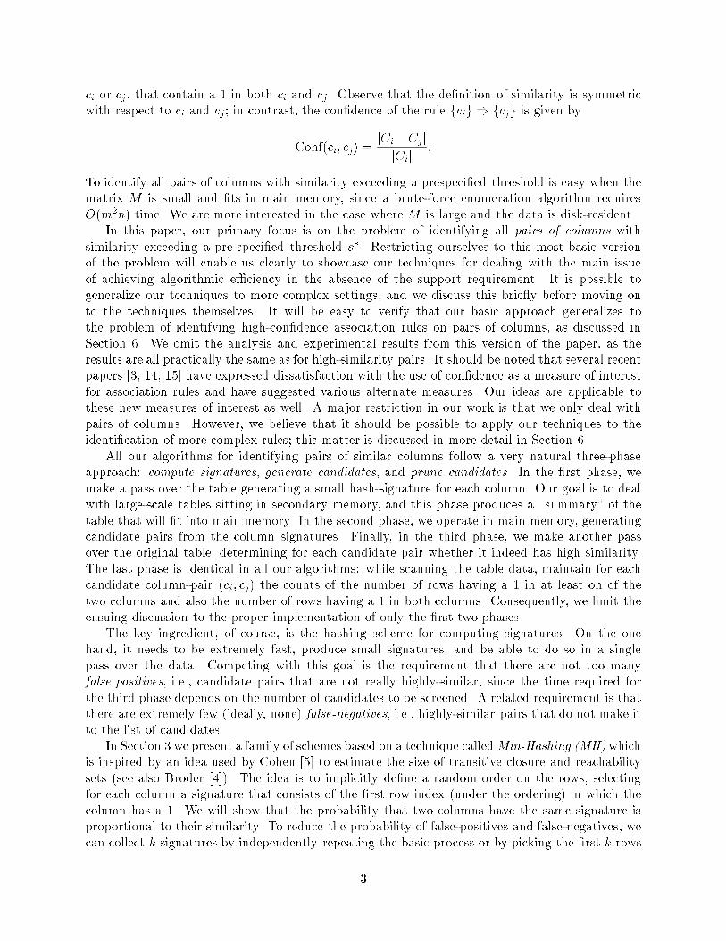
Figure 2: The �rst �gures shows the similarity distribution of the Sun data. The second showsagain the same distribution but it focuses on the region of similarities that we are interested in.5 ExperimentsWe have conducted experiments to evaluate the performance of the di�erent algorithms. In thissection we report the results for the di�erent experiments. We use two sets of data namely syntheticdata and real data.Synthetic Data: The data contains 104 columns and the number of rows vary from 104 to106. The column densities vary from 1% to 5% and for every 100 columns we have a pair of similarcolumns. We have 20 pairs similar columns whose similarity fall in the ranges (85, 95), (75, 85),(65, 75), (55, 65) and (45, 55).Real Data: The real data set consists of the log of HTTP requests made over a period of 9days to the Sun Microsystems Web server (www.sun.com). The columns in this case are the URL'sand the rows represent distinct client IP addresses that have recently accessed the server. An entryis set to 1 if there has been at least one hit for that URL from that particular client IP. The dataset has about thirteen thousand columns and more than 0.2 million rows. Most of the columns aresparse and have density less than 0.01%. The histogram in Figure 2 shows the number of columnpairs for di�erent values of similarity. Typical examples of similar columns that we extracted fromthis data were URLs corresponding to gif images or Java applets which are loaded automaticallywhen a client IP accesses a parent URL.To compare our algorithms with existing techniques, we implemented and executed the a-priorialgorithm [1, 2]. We would like to mention that although a-priori is not designed for this task it isthe only existing technique and gives us a benchmark to evaluate our algorithms. The comparisonwas done for the news articles data that we have mentioned in section 2.We conducted experiments on the news article data and our results are summarized in Figure 3.The a-priori algorithm cannot be run on the original data since it runs out of memory. Hence wedo support pruning to remove columns that have very few ones in them. Each prunned data standsfor a row of the table and the comparative results for each data are reported in the row. It shouldbe noted that for support threshold of 0:01% and less, a-priori algorithm runs out of memory onour systems and does a lot of thrashing. It should be noted that although our algorithms areprobabilistic they report the same set of pairs as that reported by a-priori.5.1 ResultsWe implemented the four algorithms described in the previous section, namely MH, K-MH, H-LSH,and M-LSH. All algorithms were compared in terms of the running time and the quality of theoutput. Due to the lack of space we report experiments and give graphs for the Sun data, which12

Support Number of columns A-priori MH K-MH H-LSH M-LSHthreshold after support pruning (sec) (sec) (sec) (sec) (sec)0:01% 15559 - 71.4 87.6 15.6 10.70:015% 11568 96.05 44.8 52.0 6.7 9.70:2% 9518 79.94 25.8 36.0 6.0 5.1Figure 3: Running times for the news articles data setin any case are more interesting, but we have also performed tests for the synthetic data, and allalgorithms behave similarly.The quality of the output is measured in terms of false positives and false negatives generatedby each algorithm. To do that, we plot a curve that shows the ratio of the number of pairs foundby the algorithm over the real number of pairs (computed once o�-line) for a given similarity range(e.g. Figure 7). The result is typically an \S"-shaped curve, that gives a good visual picture forthe false positives and negatives of the algorithm. Intuitively, the area below the curve and leftto a given similarity cuto� corresponds to the number of false positives, while the area above thecurve and right to the cuto� corresponds to the number of false negatives.We now describe the behavior of each algorithm as their parameters are varied .55 65 75 85 95

0

0.2

0.4

0.6

0.8

1

Fra

ctio

n of

pai

rs fo

und

Similarity (%)

Performance of MH on Sun data set, f=80

k = 10 k = 20 k = 50 k = 100k = 200

1020 50 100 200 500

200

400

600

800

1000

1200

1400

1600

1800

K Value

Tot

al ti

me

(sec

)

Running time of MH on Sun data set,f=80

55 65 75 85 950

0.2

0.4

0.6

0.8

1

Fra

ctio

n of

pai

rs fo

und

Similarity (%)

Performance of MH on Sun data set,k=500

f = 70f = 75f = 80f = 85f = 90

70 75 80 85 901750

1800

1850

1900

1950

F Value

Tot

al ti

me

(sec

)

Running time of MH on Sun data set,k=500(a) (b) (c) (d)Figure 4: Quality of output and total running time for MH algorithm as k and s are varied55 65 75 85 95

0

0.2

0.4

0.6

0.8

1

Fra

ctio

n of

pai

rs fo

und

Similarity (%)

Performance of K−MH on Sun data set,f=80

k = 10 k = 20 k = 50 k = 100k = 200

1020 50 100 200 500100

150

200

250

K Value

Tot

al ti

me

(sec

)

Running time of K−MH on Sun data set,f=80

55 65 75 85 950

0.2

0.4

0.6

0.8

1

Fra

ctio

n of

pai

rs fo

und

Similarity (%)

Performance of K−MH on Sun data set,k=500

f = 70f = 75f = 80f = 85f = 90

70 75 80 85 90200

210

220

230

240

250

260

270

280

290

300

F Value

Tot

al ti

me

(sec

)

Running time of K−MH on Sun data set,k=500(a) (b) (c) (d)Figure 5: Quality of output and total running time for K-MH algorithm as k and s are variedMH and K-MH algorithms have two parameters, s� the user speci�ed similarity cuto�, andk, the number of Min-Hash values extracted to represent the signature of of each column. Fig-ures 4(a) and 5(a) plots \S"-curves for di�erent values of k for the MH and K-MH algorithms. As13

the k value increases the curve gets sharper indicating better quality. In �gures 4(c) and 5(c) wekeep k �xed and change the value s� of the similarity cuto�. As expected the curves shift to theright as the cuto� value increases. Figures 4(d) and 5(d) show that for a given value of k the totalrunning time decreases marginally since we generate fewer candidates. Figure 4(b) shows that thetotal running time for MH algorithm increases linearly with k. However this is not the case forK-MH algorithm as depicted by �gure 5(b). The sub-linear increase of the running time is due tothe sparsity of the data. More speci�cally, the number of hash values extracted from each columnis upper bounded by the number of ones of that column, and therefore, the hash values extracteddo not increase linearly with k.55 65 75 85 95

0

0.2

0.4

0.6

0.8

1

Similarity (%)

Fra

ctio

n of

pai

rs fo

und

Performance of H−LSH on Sun data set, l = 8

r = 32r = 40r = 48r = 56

32 40 48 56

60

80

100

120

140

160

180

200

220

Value of parameter r

Tot

al ti

me

(sec

)

Running time of H−LSH on Sun data set, l = 8

55 65 75 85 950

0.2

0.4

0.6

0.8

1

Similarity (%)

Fra

ctio

n of

pai

rs fo

und

Performance of H−LSH on Sun data set, r = 40

l = 4 l = 8 l = 16l = 32

4 8 16 32

90

100

110

120

130

140

Value of parameter l

Tot

al ti

me

(sec

)

Running time of H−LSH on Sun data set, r = 40(a) (b) (c) (d)Figure 6: Quality of output and total running time for H-LSH algorithm as r and l are varied55 65 75 85 95

0

0.2

0.4

0.6

0.8

1

Fra

ctio

n of

pai

rs fo

und

Similarity (%)

Performance of M−LSH on Sun data set, l = 10

r = 10 r = 20 r = 50 r = 100

10 20 50 1000

50

100

150

200

250

300

350

400

450

500

Tot

al ti

me

(sec

)

Value of parameter r

Running time of M−LSH on Sun data set, l = 10

55 65 75 85 950

0.2

0.4

0.6

0.8

1

Fra

ctio

n of

pai

rs fo

und

Similarity (%)

Performance of M−LSH on Sun data set, r = 10

l = 10 l = 20 l = 50 l = 100

10 20 50 1000

50

100

150

200

250

300

350

400

450

500

550

time

(sec

)

Value of parameter l

Running time of M−LSH on Sun data set, r = 10(a) (b) (c) (d)Figure 7: Quality of output and total running time for M-LSH algorithm as r and l are variedWe do a similar exploration of the parameter space for the M-LSH and H-LSH algorithms. Theparameters of this algorithm are r, and l. Figure 7(a) and 6(a) illustrates the fact that as r increasesthe probability that columns mapped to the same bucked decreases, and therefore the number offalse positives decreases but as a trade-o� consequence the number of false negatives increases. Onthe other hand, �gure 7(c) and 6(c) shows that an increase in l, corresponds to an increase of thecollision probability, and therefore the number of false negatives decrease but the number of falsepositives increases. Figures 7(b) and 6(b) show that the total running time increases with l sincewe hash each column more times and this also results in an increase in the number of candidates. Inour implementation of M-LSH, the extraction of min hash values dominates the total computationtime, which increases linearly with the value of r. This is showed in �gure 7(c). On the other hand,in the implementation of H-LSH, checking for candidates dominates the running times, and as aresult the total running time decreases as r increases since less candidates are produced. This isshowed in �gure 6(c).We now compare the di�erent algorithms that we have implemented. When comparing the14

0.01 0.05 0.1 0.5 1 5 100

50

100

150

200

250

300

350

400

450

500

Tot

al ti

me

(sec

)

False Negative Threshold (%)

Time vs False Negatives, Similarity = 85%

MH K−MH H−LSHM−LSH

0.01 0.05 0.1 0.5 1 5 1010

4

105

False Negative Threshold (%)

False Positives vs False Negatives, Similarity = 85%

MH K−MH H−LSHM−LSH

0.01 0.05 0.1 0.5 10

20

40

60

80

100

120

140

160

180

200

Tot

al ti

me

(sec

)

False Negative Threshold (%)

Time vs False Negatives, Similarity = 95%

MH K−MH H−LSHM−LSH

0.01 0.05 0.1 0.5 1

104

105

Num

ber

of F

alse

pos

itive

s

False Negative Threshold (%)

False Positives vs False Negatives, Similarity = 95%

MH K−MH H−LSHM−LSH(a) (b) (c) (d)Figure 8: Comparison of di�erent algorithms in terms of total running time and number of falsepositives for di�erent negative thresholds.time requirements of the algorithm we compare the CPU time for each algorithm since the timespent in I/O is same for all the algorithms. It is important to note that the for all the algorithmsthe number of false negatives is very important and this is the quantity that requires to be kept incontrol. As long as the number of false positives is not too large (i.e. all of candidates can �t inmain memory) we can always eliminate them in the pruning phase. To compare the algorithms we�x the percentage of false negatives that can be tolerated. For each algorithm we pick the set ofparameters for which the number of false negatives is within this threshold and the total runningtime is minimum. We then plot the total running time and the number of false positives againstthe false negative threshold.Consider Figures 8(a) and 8(c). The �gures shows the total running time against the falsenegative threshold. We can see that the H-LSH algorithm requires a lot of time if the false negativethreshold is less while it does better if the limit is high. In general the M-LSH and H-LSH algorithmsdo better than the MH and K-MH algorithms. However it should be noted that H-LSH algorithmcannot be used if we are interested in similarity cuto�s that are low. The graph shows that thebest performance is shown by the M-LSH algorithm.Figure 8 gives the number of false positives generated by the algorithms against the tolerancelimit. The false positives are plotted on a logarithmic scale. In case of H-LSH andM-LSH algorithmsthe number of false positives decreases if we are ready to tolerate more false negatives since in thatcase we hash every column fewer times. However the false positive graph for K-MH and MH isnot monotonic. There exists a tradeo� in the time spent in the candidate generation stage andthe pruning stage. To maintain the number of false negatives less than the given threshold wecould either increase k and spend more time in the candidate generation stage or else decreasethe similarity cuto� s and spend more time in the pruning stage as we get more false positives.Hence the points on the graph correspond to di�erent values of similarity cuto� s� with which thealgorithms are run to get candidates with similarity above a certain threshold. As a result we donot observe a monotonic behavior in case of these algorithms.We would like to comment that the results provided should be analyzed with caution. Thereader should note that whenever we refer to time we refer to only the CPU time and we expectI/O time to dominate in the signature generation phase and pruning phase. If we are aware aboutthe nature of the data then we can be smart in our choice of algorithms. For instance the K-MHalgorithm should be used instead of MH for sparse data sets since it takes advantage of sparsity.15

6 Extensions and Further WorkWe brie y discuss some extensions of the results presented here as well as directions for future work.First, note that all the results presented here were for the discovery of bi-directional similaritymeasures. However, the Min-Hash technique can be extended to the discovery of column-pairs(ci; cj) which form a high-con�dence association rule of the type fcig ) fcjg but without anysupport requirements. The basic idea is to generate a set of Min-Hash values for each column, andto determine whether the fraction of these values that are identical for ci and cj is proportional tothe ratio of their densities, di=dj. The analytical and the experimental results are qualitatively thesame as for similar column-pairs.We can also use our Min-Hashing scheme to determine more complex relationships, e.g., ci ishighly-similar to cj_cj0 , since the hash values for the induced column cj_cj0 can be easily computedby taking the component-wise minimum of the hash value signature for cj and cj0 . Extending tocj ^ cj0 is more di�cult. It works as follows. First, observe that \ci implies cj ^ cj0" means that \ciimplies cj" and \ci implies cj0". The latter two implications can be generated as above. Now, we canconclude that \ci implies cj^cj0" if (and only if) the cardinality of ci is roughly that of cj^cj0 . Thispresents problems when the cardinality of ci is really small, but is not so di�cult otherwise. Thecase of small ci may not be very interesting anyway, since it is di�cult to associate any statisticalsigni�cance to the similarity in that case. It is also possible to de�ne \anti-correlation," or mutualexclusion between a pair of columns. However, for statistical validity, this would require imposinga support requirement, since extremely sparse columns are likely to be mutually exclusive by sheerchance. It is interesting to note that our hashing techniques can be extended to deal with thissituation, unlike a-priori which will not be e�ective even with support requirements. Extensionsto more than three columns and complex boolean expressions are possible but will su�er from anexponential overhead in the number of columns.References[1] R. Agrawal, T. Imielinski, and A. Swami. Mining Association Rules Between Sets of Items inLarge Databases. In Proceedings of the ACM SIGMOD Conference on Management of Data,1993, pp. 207{216.[2] R. Agrawal and R. Srikant. Fast Algorithms for Mining Association Rules. In Proceedings ofthe 20th International Conference on Very Large Databases, 1994.[3] S. Brin, R. Motwani, J.D. Ullman, and S. Tsur, Dynamic itemset counting and implicationrules for market basket data. In Proceedings of the ACM SIGMOD Conference on Managementof Data, 1997, pp. 255{264.[4] A. Broder. On the resemblance and containment of documents. In Compression and Complexityof Sequences (SEQUENCES'97), 1998, pp. 21{29.[5] E. Cohen. Size-Estimation Framework with Applications to Transitive Closure and Reacha-bility. Journal of Computer and System Sciences 55 (1997): 441{453.[6] R.O. Duda and P.E. Hart. Pattern Classi�cation and Scene Analysis. A Wiley-IntersciencePublication, New York, 1973.spatial Discovery in Databases and Data 16

[7] A. Gionis, P. Indyk, and R. Motwani. Similarity Search in High Dimensions via Hashing.Accepted to VLDB'99.[8] D. Goldberg, D. Nichols, B.M. Oki, and D. Terry. Using collaborative �ltering to weave aninformation tapestry. Communications of the ACM 55 (1991): 1{19.[9] S. Guha, R. Rastogi, and K. Shim. CURE - An E�cient Clustering Algorithm for LargeDatabases In Proceedings of the ACM-SIGMOD International Conference on Management ofData, 1998, pp. 73{84.[10] J.M. Hellerstein, P.J. Haas, and H.J. Wang. Online Aggregation. In Proceedings of the ACM-SIGMOD International Conference on Management of Data, 1997.[11] P. Indyk and R. Motwani. Approximate Nearest Neighbor: Towards Removing the Curse ofDimensionality. In Proceedings of the 30th Annual ACM Symposium on Theory of Computing,1998, pp. 604{613.[12] R. Motwani and P. Raghavan. Randomized Algorithms. Cambridge University Press, 1995.[13] N. Shivakumar and H. Garcia-Molina. Building a Scalable and Accurate Copy DetectionMechanism. In Proceedings of the 3rd International Conference on the Theory and Practice ofDigital Libraries, 1996.[14] C. Silverstein, S. Brin, and R. Motwani. Beyond Market Baskets: Generalizing AssociationRules to Dependence Rules. Preliminary version: In Proceedings of the ACM SIGMOD Confer-ence on Management of Data, 1997, pp. 265{276. Journal version: Data Mining and KnowledgeDiscovery 2 (1998): 69{96.[15] C. Silverstein, S. Brin, R. Motwani, and J.D. Ullman. Scalable Techniques for Mining CausalStructures. In Proceedings of the 24th International Conference on Very Large Data Bases,1998, pp. 594{605.[16] H.R. Varian and P. Resnick, Eds. CACM Special Issue on Recommender Systems. Communi-cations of the ACM 40 (1997).databases.17