Prediction of postpartum depression using

multilayer perceptrons and pruning

Salvador Tortajada a, Juan M. Garcıa-Gomez a, Javier Vicente a,Julio Sanjuan b, Rocıo Martın-Santos c, Isolde Gornemann d,

Alfonso Gutierrez-Zotes e, Francesca Canellas f ,Angel Carracedo g, Monica Gratacos h, Roser Guillamat i,

Enrique Baca-Garcıa j, Montserrat Robles a

aIBIME-Itaca, Universidad Politecnica de Valencia, Valencia, Spain

bFaculty of Medicine, University of Valencia, Valencia, Spain

cHospital del Mar, Barcelona, Spain

dHospital Carlos Haya, Malaga, Spain

eHospital Pere Mata, Reus, Spain

fHospital Son Dureta, Palma de Mallorca, Spain

gNational Genotyping Center, Hospital Clınico, Santiago de Compostela, Spain

hCenter for Genomic Regulation, CRG, Barcelona, Spain

iHospital Parc Tauli, Sabadell, Spain

jHospital Jimenez Dıaz, Madrid, Spain

Abstract

Objective: The main goal of this paper is to obtain a classification model basedon feed-forward multilayer perceptrons in order to predict postpartum depressionduring the 32 weeks after the childbirth with a high sensitivity and specificity. Ma-

terials and methods: Multilayer perceptrons were trained on data from 1 397 womenwho had just given birth, from 7 Spanish Hospitals. A prospective cohort study wasmade just after delivery, at 8 weeks and 32 weeks after delivery. The models wereanalyzed using hold out evaluation and comparing them with the geometric meanof the accuracies in order to obtain a balanced sensibility and specificity. Results

and conclusion: Multilayer perceptrons show a good performance -high sensibilityand specificity- as predictive models for postpartum depression. The interpretationof the models by pruning leads to a qualitative interpretation of the influence ofeach variable that may be useful for clinical protocols.

Key words: Multilayer perceptron; Neural network pruning; Postpartumdepression.

Preprint submitted to Elsevier 31 January 2008

1 Introduction1

In the first week after childbirth, around 25%-50% of women slightly suffer a2

postpartum blues episode. Pospartum Depression (PPD) seems to be a uni-3

versal condition with equivalent prevalence in different countries of around4

13% [1,2] and it implies an increase in medical care costs. Women suffering5

from postnatal depression feel a considerable deterioration of cognitive and6

emotional functions which can affect to mother-infant attachment. This may7

have an impact on child’s future development until primary school [3]. De-8

spite its serious consequences, PPD usually passes unnoticed, its detection9

takes time and it often receives inappropriate treatment.10

Although multiple studies have been carried out around PPD, its etiology is11

not well-known yet. Several psychosocial and biological risk factors have been12

suggested. For instance, it has been pointed out the importance of the social13

support, partner relantionship and stressful life events related to pregnancy14

and childbirth [4], as well as neuroticism [5]. Regarding biological factors, it15

has been shown that inducing an artificial estrogen fall can cause depressive16

symptoms in patients wih PPD antecedents. Cortisol alteration, thyroid hor-17

mones changes and low rate of prolactin are relevant factors too [6]. Treloar18

et al. in [7], through a comparative study with twin samples, they conclude19

that genetic factors would explain 40% of variance in PPD predisposition. In20

Ross et al. [8] a biopsychosocial model for anxiety and depression symptoms21

is developed by means of structural equations. However, most of the research22

involving genetic factors are separated from those involving environmental23

factors. There is a remarkable exception that explains that a functional poly-24

morphism in the promoter region of the serotonin transporter gene seems to25

moderate the influence of stressful life events on depression [9].26

An early prediction of postpartum depression may reduce the impact of the27

illness on the mother and it can help clinicians to give appropriate treatment28

to the patient in order to prevent the depression. The need of a prediction29

model rather than a description one becomes of paramount importance. In this30

way, artificial neural networks (ANN) have a remarkable ability to characterize31

discriminating patterns and derive meaning from complex and noisy data sets.32

They have been widely applied in general medicine for differential diagnosis,33

classification and prediction of disease and condition prognosis. In the field of34

psychiatric disorders, ANNs have not been widely used in spite of its predictive35

power. For instance, ANNs have been applied to he diagnosis of dementia using36

clinical data [10] or for predicting Alzheimer’s disease using mixed effects37

neural networks [11]. In [12], EEG data from patients with schizophrenia,38

obsessive-compulsive disorder and controls was used to demonstrate that a39

Email address: vesaltor@upvnet.upv.es (Salvador Tortajada).

2

trained ANN was able to classify correctly over 80% of the patients with40

obsessive-compulsive disorder and over 60% of the patients with schizophrenia.41

In Jefferson et al. [13], evolving neural networks overcome statistical methods42

in depression prediction after mania. Berdia and Metz [14] used artificial neural43

networks to provide a framework for understanding some of the pathological44

processes in schizophrenia. Finally, Franchini et al. in [15] applied these models45

to support clinical decision making for the treatment of psychopharmacological46

therapy.47

One of the main goals of this paper is to obtain a classification model based on48

feed-forward multilayer perceptrons in order to predict postpartum depression49

with a high sensitivity and specificity during the 32 weeks after the childbirth.50

A secondary goal is to find and interpret the qualitative contribution of each51

independent variable in order to obtain clinical knowledge.52

2 Materials and Methods53

Data from postpartum women were collected from 7 General Spanish Hospi-54

tals, in the period from December 2003 to October 2004 in the second to third55

day after delivery. All participants were caucasic, none of them were under56

psychiatric treatment during pregnancy and all of them were able to read and57

answer the clinical questionnaires. Women whose child died after delivery were58

excluded. This study was approved by the Local Ethic Committees, and all59

patients gave their informed written consent.60

Depressive symptoms were assessed with the total score of the Spanish version61

of Edinburgh Postnatal Depression Scale (EPDS) [16] just after delivery, at 862

and 32 weeks.63

Major depression episode were established using first the EPDS (cut-off point64

of 9 or more) at 8 or 32 weeks, and then probable cases (EPDS > 9) were65

evaluated using the Spanish version of the Diagnostic Interview for Genetics66

Studies (DIGS) [17,18] adapted to Postpartum Depression in order to deter-67

mine if the patient was suffering a depression episode (positive class) or not68

(negative class). All the interviews were conducted by clinical psychologist69

with a previous common training in the DIGS with video cases records. A70

high level of reliability (K > 0.8) was obtained among interviewers.71

From the 1 880 women initially included in the study, 76 were excluded because72

they did not fill correctly all the scales or questionnaires. With these patients,73

a prospective study was made just after delivery (initial), at 8 weeks and 3274

weeks after delivery. At 8 weeks of follow up, 1 407 (78%) women retained in75

the study. At 32 weeks of follow up 1 397 (77.4%) women were evaluated. We76

3

compared the lost of follow-up cases with the rest of the final sample. Only77

lowest social class was significantly increased in the lost of follow-up cases78

(p = 0.005). The 11.5% (160) of women at base line, 8 and 32 weeks had a79

major depressive episode during the eight months of postpartum follow-up.80

Hence, from a total number of 1 397 patients we had 160 in the positive class81

and 1 237 in the negative class.82

2.1 Independent variables83

Based on the current knowledge about PPD, several variables were taken84

into account in order to develop predictive models. In a first step, psychiatric85

and genetic information was used. These predictive models are called subjec-86

tive models. Then, social-demographic variables were included in the subject-87

environment models. For each approach, we used anxiety state (STAIE) either88

Edinburgh postnatal depression (EPDS) -just after the childbirth- as an in-89

put variable, because blues and anxiety symptoms are correlated [19]. Table 290

shows the clinical variables used in this study.91

Following recommendations from clinicians psychiatric antecedents of the pa-92

tient in postpartum depression were taken into account as well as emotional93

alterations during pregnancy with medical consultation were also considered.94

Both are binary variables (yes/no).95

Neuroticism can be defined as an enduring tendency to experience negative96

emotional states. It is measured on the Eysenck Personality Questionnaire97

short scale (EPQ) [20], which is the most used questionnaire of personality98

and consists of 12 items. For this study the validated Spanish version [21]99

was used. Individuals who score high on neuroticism are more likely than the100

average to experience such feelings as anxiety, anger, guilt and depression.101

The number of experiencies are the number of stressful life events of the patient102

just after delivery (initial) at 0-8 weeks interval and 8-32 weeks interval using103

the St. Paul Ramsey Scale [22,23]. This is an ordinal variable and depends on104

the subjective point of view of the patient.105

The anxiety state is based on the most frequently used scale of anxiety which106

is the State-Trait Anxiety Inventory (STAI) [24].107

Postpartum blues is estimated via the Edinburg Postnatal Depression Scale108

(EPDS). It is a 10-items self-report scale and it has been validated for Spanish109

population [16]. The best cut-off of the Spanish validation of the EPDS was110

9 for postpartum depression. We decided to prove its initial value, i.e. at the111

moment of birth, as an independent variable because the goal is to prevent112

and predict postpartum depression within 32 weeks.113

4

Social support is measured by means of the Spanish version of the Duke UNC114

social support scale [25], which originally consists of 11 items. This question-115

naire is rated just after delivery, at 6-8 weeks and at week 32. For this work,116

the variable used was the sum of the scores obtained immediately after the117

childbirth plus the scores obtained in week number 8. As we want to predict118

possible depression risk during the first 32 weeks after childbirth, the Duke119

score at week 32 was discarded for this experiment.120

Genomic DNA was extracted from the peripheral blood of women. Two func-121

tional polymorphisms of the serotonine transporter gene were analyzed 1 . For122

all the machine learning process we decided to use the combination genotypes123

(HAP2) proposed by Hranilovic in [26] as124

(1) no low-expressing genotype at either of the loci,125

(2) low-expressing genotype at one of the loci,126

(3) low-expressing genotypes at both loci.127

The Medical Perinatal Risk was measured as seven dichotomous variables:128

medical problems during pregnancy, use of drugs during pregnancy (including129

alcohol and tobacco), cesarea, use of anesthesia during delivery, mother med-130

ical problems during delivery, medical problems with more admission days in131

hospital and newborn medical problems. A two-step cluster analysis was done132

in order to explore this seven binary variables. From this analysis it results an133

ordinal variable with four values for every women:134

(1) no medical perinatal risk,135

(2) pregnancy problems without delivery problems,136

(3) pregnancy problems and delivery mother problems,137

(4) presence of both other and newborn problems.138

Other psychosocial and demographic variables were considered in the subject-139

environment model such as the age, the highest level of education achieved140

rated on 3-point scale (low, medium, high), labour situation during pregnancy,141

household income rated on 4-point scale (economical level), the gender of the142

baby or the number of family members whom she lives together with.143

Every input variable was normalized in the range [0, 1]. Non-categorical vari-144

ables were represented by one input unit. Missed variables were replaced by145

their mean if they were continuous or by their mode if they were discrete.146

A dummy representation was used for each categorical variable, i.e., one unit147

represents one of the possible values of the variable and this unit is activated148

only when the corresponding variable takes this value. Missed variables were149

simply represented by non activating any of the units.150

1 5-HTTLPR in the promoter region and STin2 within intron 2

5

2.2 ANNs theoretical model151

ANNs are inspired by biological systems in which large numbers of simple152

units work in parallel in order to perform tasks that conventional computers153

have not been able to tackle successfully. These networks are made of many154

simple processors (neurons or units) based on Rosenblatt’s perceptron [27]. A155

perceptron gives a linear combination, y, of the values of its D inputs, plus156

a bias value,157

y =D

∑

i=1

xiwi + w0. (1)

The output, z = f(y), is calculated by applying an activation function to158

the input. Generally, the activation function is an identity, a logistic (2) or159

a hyperbolic tangent (3). As these functions are monotonic, the form f(y)160

still determines a linear discriminant function [28]. A single unit has a limited161

computing ability, but a group of interconnected neurons has a very powerful162

adaptability and the ability to learn non-linear functions which can model163

complex relationships between inputs and outputs.164

Thus, more general functions can be constructed by considering networks hav-165

ing successive layers of processing units, with connections running from every166

unit in one layer to every unit in the next layer only. A feedforward multilayer167

perceptron consists of an input layer with one unit for every independent168

variable, one or two hidden layers of perceptrons and the output layer for169

the dependent variable -in the case of a regression problem-, or the possi-170

ble classes -if we are dealing with a classification problem-. We call a fully171

connected feed-forward multilayer perceptron when every unit of each layer172

receives an input from every unit in its precedent layer and the output of each173

unit is sent to every unit in the next layer. Networks having one hidden layer174

can generate decision boundaries which surround a single convex region of the175

input space whose boundary consists of segments of hyperplanes. Networks176

having two hidden layers can generate arbitrary decision regions which may177

be non-convex and disjoint [28].178

Since postpartum major depression is considered in this work as a binary179

dependent variable, the activation function of the output unit was the logistic180

function which is expressed as:181

f(x) =1

1 + e−x, (2)

while the activation function of the hidden units was the hyperbolic tangent182

6

which is expressed as:183

f(x) =ex − e−x

ex + e−x. (3)

As a first approach, fully connected feed-forward multilayer perceptrons were184

used with one or two hidden layers. The learning algorithm backpropagation185

with momentum was used to train the networks. The connection weights of186

the network were updated following the descent gradient rule:187

∆wij(t + 1) = ρ · δj · oi + µ · ∆wij(t), (4)

where ρ is the learning rate, µ is the momentum factor, wij is the weight188

between unit i and unit j, ∆wij(t) is the connection weight variation and oi189

is the output value of the unit i. The learning rule δj is expressed as190

δj =

{

f ′

j(∑

i wijoi)(tj − oj) if j is an output unit

f ′

j(∑

i wijoi)(∑

k δkwjk) if j is a hidden unit(5)

where tj is the desired output value, which is provided to the network in a191

supervised manner during the training of the network. The activation function192

fj(x) of unit j was a logistic or a hyperbolic tangent and f ′

j(x) is its derivative.193

Although these models, and ANNs in general, exhibit a superior predictive194

power compared to traditional approaches, they have been labeled as ”black195

box” methods because they provide little explanatory insight into the relative196

influence of the independent variables in the prediction process. This lack197

of explanatory power is a major concern to reach an interpretation of the198

influence of each independent variable on postpartum depression. In order to199

gain some qualitative knowledge of the causal relantionships about depression200

phenomena we used several pruning algorithms to obtain more simple and201

interpretable models [29,33].202

2.2.1 Pruning algorithms203

Based on the fundamental idea in Wald statistics, pruning algorithms estimate204

the importance of a parameter (or weight) in the model by how much the205

training error increases if that parameter is eliminated. Then, it removes the206

least relevant one and continues iteratively until some convergence condition207

is reached. These algorithms were initially thought as a way to achieve a208

good generalization for connectionist models, i.e., the ability to infer a correct209

7

structure from training examples and to perform well on future samples. A very210

complex model can lead to poor generalization or overfitting, which happens211

when it adjusts to specific features of the training data rather than to the212

general ones [30]. But pruning has also been used for feature selection with213

neural networks [31,32], making their operation easier to understand since214

there is less oportunity for the network to spread functions over many nodes.215

This is important in this critical application where knowing how the system216

works becomes a major concern.217

The algorithms used here are based on weight pruning. The strategy consists218

in deleting parameters with small saliency, i.e. those whose deletion will have219

the least effect on the training error. The Optimal Brain Damage (OBD)220

algorithm [29] and its descendent, Optimal Brain Surgeon (OBS) [33], use a221

second-order approximation to predict the saliency of each weight. A Taylor222

series is used to approximate the error function:223

δE =∂E(W )

∂WδW +

1

2δW T ∂2E(W )

∂W 2δW + O(||δW ||3). (6)

Here, W is the weight matrix and δE is the increment of the error function.224

In the second term of this expression we find the Hessian matrix H of E225

with respect to W . The first term can be omitted because we are at a local226

minimum after training convergence and the third term is ignored because we227

assume that the error function is nearly quadratic. So the expression finally228

reduces to:229

δE =1

2δW T HδW. (7)

In OBD high-order terms are neglected so we only need to compute the di-230

agonal elements of H. This assumption is sometimes a poor one. Hence, OBS231

method computes the full Hessian matrix leading to a more exact approxi-232

mation of the error function, but it requires more computational time and233

space.234

In order to select the best pruned topology the validation set was used to com-235

pare the networks. Then, when the best model was obtained the interpretation236

of the influence of each variable was done in the following way: if an input237

unit is directly connected to the output unit, then a positive weight means238

that it is a risk factor as it increases the probability of having depression.239

Thus, a negative weight means that the variable is a protective factor. Let a240

hidden unit be connected to the output unit with a positive weight. If an input241

unit is connected to this hidden unit with a positive value, then the variable242

represented by this unit is a risk factor. If its weight is negative then it is a243

8

protective factor. On the contrary, if the weight between the hidden unit and244

the output unit is negative then a positive value in the connection between245

the input and the hidden unit means that the variable is a protective factor.246

Thus, a negative value in the weight which connects the input to the hidden247

unit means that it is a risk factor. Table 3 summarizes these influences. This248

interpretation is justified because the hidden units have a hyperbolic tangent249

as an activation function which delimits its output activation values between250

−1 and 1.251

2.3 Evaluation criteria252

The evaluation of the models was made using a holdout validation where the253

observations were chosen randomly to form the validation and the evaluation254

sets. In order to obtain a good error estimation of the predictive model, this255

database has to be split into three different datasets: the training set with256

1 006 patients (72%), the validation set with 112 patients (8%) and the test257

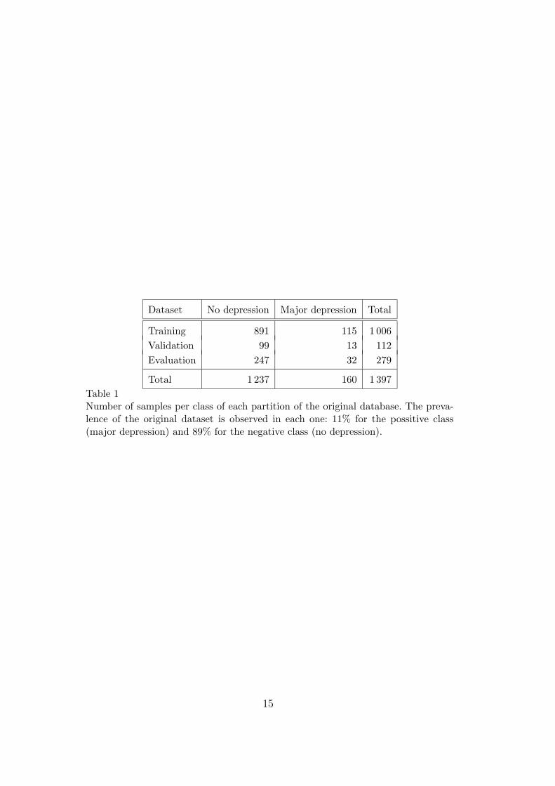
set with 279 patients (20%). Each partition follows the prevalence of the orig-258

inal database (see table 1). The best network topology and parameters were259

selected empirically using the validation set and then evaluated with the test260

set. Overfitting was avoided using the validation set to stop the learning proce-261

dure when the validation medium square error function reached its minimum.262

In the section 3 we can see that using a single hidden layer was enough to263

obtain a good predictive model.264

There is an intrinsic difficulty in the nature of the problem: the dataset is265

imbalanced [34,35], in the sense that one of the classes (the possitive examples)266

is underrepresented compared to the negative class. This means that, with this267

prevalence on the negative examples (89%), a trivial classifier consisting in268

assigning the most prevalent class to a new sample would achieve an accuracy269

of around 89%, but its sensitivity would be null.270

The main goal is to obtain a predictive model with a good sensitivity and271

specificity. Both measures depend on the accuracy on positive examples, a+,272

and the accuracy on negative examples, a−. Increasing a+ will be done at the273

cost of decreasing a−. The relation between these quantities can be captured274

by the ROC (Receiver Operating Characteristic) curve. The larger the area275

under the ROC curve (AUC), the higher the classification potential of the276

model. This relation can also be estimated by the geometric mean of the two277

accuracies, G =√

a+ · a−, reaching high values only if both values are high278

and in equilibrium. In that way, if now we use the geometric mean to evaluate279

our trivial model -which always assigns the class with the maximum a priori280

probability- we could see that G = 0, which means that the model is the worst281

we can obtain.282

9

3 Results283

The main objective of this work was to obtain feed-forward multilayer per-284

ceptron predictive models. Table 4 shows the results of the best connectionist285

models obtained from the first approach, called subjective feature models, us-286

ing multilayer perceptrons of one and two hidden layers and making use of the287

pruning algorithms as well as the results for the next subject-environment fea-288

ture model approach -which includes social and demographic features-. Each289

experiment has been done swapping initial STAIE variable and initial EPDS.290

Notice that non-pruned models have a better behaviour than pruned ones.291

In general, with the independent test set, our models are reaching more than292

80% of accuracy with a G and an area under the ROC curve of around 0.8,293

which means a sensitivity of more than 0.75 and a specificity greater than 0.8.294

We can see that non-pruned models reach a higher sensitivity when including295

EPDS as input variable than when STAIE is used. The use of pruning methods296

lead to a more understandable model at the expense of the predictive power.297

In figure 1, the subjective pruned models show that neuroticism, social support,298

life events and postpartum blues are the most outstanding features and they299

are risk factors in the prediction of postpartum depression. In the subject-300

environment models (figure 2) these variables are also main risk factors, but301

we can see that variable age and the number of people living together with the302

patient are both important protective factors. Other interesting features are303

psychiatric antecedents in relatives, which is a risk factor, and low-expressing304

genotypes, which appears to be a protective factor.305

Although the databases and used variables are not comparable, these results306

overcome the work done by Camdeviren et al. in [36] where a logistic regres-307

sion model and a classification tree were compared for predicting postpartum308

depression. With logistic regression they reached a 65.4% of accuracy with309

16% of sensibility and 95% of specificity, while with the optimal decission tree310

they had an accuracy of 71%, a sensibility of 22% and a specificity of 94%.311

4 Discussion312

The main objective of this paper was to obtain a feed-forward ANN classifica-313

tion model to predict postpartum depression during the first 32 weeks after the314

delivery with a high sensitivity and specificity. From several trained models,315

the one showing the best G-mean of the accuracies was selected thus ensuring316

a balanced sensitivity and specificity as we can see in table 4. With these mod-317

els we could achieve around 85% of accuracy. Models using socialdemographic318

10

variables (subject-enviroment models) did not significantly improve subjective319

models for prediction.320

The independent variables have different influences in the output of the clas-321

sification model. These influences depend on the connections between nodes322

as we can see in figures 1 and 2. The higher the weight of the connection,323

the bigger the final influence, which can also be positive or negative depend-324

ing on the sign of the weight. Nevertheless, this is a qualitative measure and325

we must take care interpreting the quantitative influence because some input326

variables are spreading their values over several nodes. In a future work some327

quantitative techniques will be used in order to achieve a numeric measure328

of the influence of each input feature and their interactions. In that way, the329

prevention models would give clinicians a tool to gain knowledge from the330

model.331

In this sense, the combination of the genetic features with other environmental332

features can be seen in a qualitative way. In three models out of four the333

interaction is clear.334

A classification model with this good performance, i.e. high accuracy, sen-335

sitivity and specificity, may be very useful in clinical environment. In fact,336

the ability of neural networks to tolerate missing information could be useful337

when part of the variables are missed thus giving a high reliability in a real338

environment.339

In future work, a quantitative approach will be developed in order to find out340

the real and numeric influence of each variable and their interactions, therefore341

the prevention model would give the clinicians a tool to gain knowledge from342

the model and, thus, the postpartum depression.343

11

References

[1] M. Oates, J. Cox, S. Neema, P. Asten, N. Glangeaud-Freudenthal,B. Figueiredo, L. Gorman, S. Hacking, E. Hirst, M. Kammerer, C. Klier,G. Seneviratne, M. Smith, A. Sutter-Dallay, V. Valoriani, B. Wickberg,K. Yoshida, TCS-PND Group, Postnatal depression across countries andcultures: a qualitative study, British Journal of Psychiatry Suppl. 46 (2004)s10–s16.

[2] M. O’Hara, A. Swain, Rates and risk of postnatal depression - a meta analysis,International Review of Psychiatry 8 (1996) 37–54.

[3] P. Cooper, L. Murray, Prediction, detection and treatment of postnataldepression, Archives of Disease in Childhood 77 (1997) 97–99.

[4] C. Beck, Predictors of postpartum depression: an update, Nursing Research 50(2001) 275–285.

[5] K. Kendler, J. Kuhn, C. Prescott, The interrelationship of neuroticism, sex andstressful life events in the prediction of episodes of major depression, AmericanJournal of Psychiatry 161 (2004) 631–636.

[6] M. Bloch, R. Daly, D. Rubinow, Endocrine factors in the etiology of postpartumdepression, Compr. Psychiatry 44 (2003) 234–246.

[7] S. Treloar, N. Martin, K. Bucholz, P. Madden, A. Heath, Genetic influenceson post-natal depressive symptoms: findings from an Australian twin sample,Psychological Medicine 29 (1999) 645–654.

[8] L. Ross, E. Gilbert, S. Evans, M. Romach, Mood changes during pregnancyand the postpartum period: development of a biopsychosocial model, ActaPsychiatrica Scandinavica 109 (2004) 457–466.

[9] A. Caspi, K. Sugden, T. Moffitt, A. Taylor, I. Craig, H. Harrington, J. McClay,J. Mill, J. Martin, A. Braithwaite, R. Poulton, Influence of life stress ondepression: moderation by a polimorphism in the 5-HTT gene, Science 301(2003) 386–389.

[10] B. Mulsant, E. Servan-Schreiber, A connectionist approach to the diagnosisof dementia, in: Proc. 12th Annual Symposium on Computer Applications inMedical Care, 1988, pp. 245–249.

[11] R. Tandon, S. Adak, J. Kaye, Neural networks for longitudinal studies inAlzheimers disease, Artificial Intelligence in Medicine 36 (2006) 245–255.

[12] J. Zhu, N. Hazarika, A. Chung-Tsoi, A. Sergejew, Classification of EEG signalsusing wavelet coefficients and an ANN, in: Pan Pacific Conference on BrainElectric Topography, Sydney, Australia, 1994, p. 27.

[13] M. Jefferson, N. Pendleton, C. Lucas, S. Lucas, M. Horan, Evolution of artificialneural network architecture: prediction of depression after mania, Methods ofinformation in medicine 37 (1998) 220–225.

12

[14] S. Berdia, J. Metz, An artificial neural network stimulating performance ofnormal subjects and schizophrenics on the Wisconsin card sorting test, ArtificialIntelligence in Medicine 13 (1998) 123–138.

[15] L. Franchini, C. Spagnolo, D. Rossini, E. Smeraldi, L. Bellodi, E. Politi, A neuralnetwork approach to the outcome definition on first treatment with sertraline ina psychiatric population, Artificial Intelligence in Medicine 23 (2001) 239–248.

[16] L. Garcıa-Esteve, L. Ascaso, J. Ojuel, P. Navarro, Validation of the EdinburghPostnatal Depression Scale (EPDS) in Spanish mothers, Journal of AffectiveDisorders 75 (2003) 71–76.

[17] J. Nurnberger, M. Blehar, C. Kaufmann, C. York-Cooler, S. Simpson,J. Harkavy-Friedman, J. Severe, Malaspina, Diagnostic interview for geneticstudies and training, Archives of Genetic Psychiatry 51 (1994) 849–859.

[18] M. Roca, R. Martin-Santos, J. Saiz, J. Obiols, M. Serrano, M. Torrens, S. Subir,M. Gilia, R. Navins, A. Ibaez, M. Nadal, N. Barrantes, F. Caellas, DiagnosticInterview for Genetic Studies (DIGS): Inter-rater and test-retest reliability andvalidity in a Spanish population, European Psychiatry 22 (2007) 44–48.

[19] K. Kendler, Major depression and generalised anxiety disorder. Same genes,(partly) different environments - revisited, British Journal of PsychiatrySupplement 30 (1994) 68–75.

[20] H. Eysenck, S. Eysenck, The Eysenck Personality Inventory, University ofLondon Press, London, 1964.

[21] A. Aluja, O. Garcıa, L. Garcıa, A psychometric analysis of the revised EysenckPersonality Questionnaire short scale, Personality and individual differences 35(2003) 449–460.

[22] E. Paykel, Methodological aspects of life events research, Journal ofPsychosomatic Research 27 (1983) 341–352.

[23] G. Zalsman, Y. Huang, M. Oquendo, A. Burke, X. Hu, D. Brent, S. Ellis,D. Goldman, J. Mann, Association of a triallelic serotonin transporter genepromoter region (5-HTTLPR) polymorphism with stressful life events andseverity of depression, American Journal of Psychiatry 163 (2006) 1588–93.

[24] C. Spielberger, R. Gorsuch, R. Luschene, The State-Trait Anxiety Inventory:STAI, Consulting Psychologist Press, 1970.

[25] J. Bellon, A. Delgado, J. Luna, P. Lardelli, Validity and reliability of the Duke-UNC-11 questionnaire of functional social support, Atencion Primaria 18 (1996)158–163.

[26] D. Hranilovic, J. Stefulj, S. Schwab, M. Borrmann-Hassenbach, M. Albus,B. Jernej, D. Wildenauer, Serotonin transporter promoter and intron 2polymorphisms: relationship between allelic variants and gene expression,Biological Psychiatry 55 (2004) 1090–1094.

13

[27] F. Rosenblatt, The Perceptron: a probabilistic model for information storageand organization in the brain, Psychological Review 65 (6) (1958) 386–408.

[28] C. Bishop, Neural Networks for Pattern Recognition, Clarendon Press, Oxford,UK, 1995.

[29] Y. Le Cun, J. Denker, A. Solla, Optimal brain damage, Advances in NeuralInformation Processing Systems 2 (1990) 598–605.

[30] R. Duda, P. Hart, D. Stork, Pattern Classification, Wiley-Interscience, NewYork, NY, 2001.

[31] J. Mao, A. Jain, Artificial neural networks for feature extraction andmultivariate data projection, Neural Networks, IEEE Transactions on 6 (2)(Mar 1995) 296–317.

[32] P. Leray, P. Gallinari, Feature selection with neural networks, Behaviormetrika26 (1999) 145–166.

[33] B. Hassibi, D. Stork, G. Wolf, Optimal brain surgeon and general networkpruning, in: Proceedings of the 1993 IEEE International Conference on NeuralNetworks, San Francisco, CA, 1993, pp. 293–300.

[34] M. Kubat, S. Matwin, Addressing the curse of imbalanced training sets: one-sided selection, in: Proc. 14th International Conference on Machine Learning,Morgan Kaufmann, 1997, pp. 179–186.

[35] N. Japkowicz, S. Stephen, The class imbalance problem: a systematic study,Intelligent Data Analysis Journal 6 (5) (2002) 429–449.

[36] H. Camdeviren, A. Yazici, Z. Akkus, R. Bugdayci, M. Sungur, Comparison oflogistic regression model and classification tree: an application to postpartumdepression data, Expert Systems with Applications 32 (2007) 987–994.

14

Dataset No depression Major depression Total

Training 891 115 1 006

Validation 99 13 112

Evaluation 247 32 279

Total 1 237 160 1 397

Table 1Number of samples per class of each partition of the original database. The preva-lence of the original dataset is observed in each one: 11% for the possitive class(major depression) and 89% for the negative class (no depression).

15

Input variable No miss. No PPD PPD

Psychiatric antecedents 76No 790 (90.3%) 85 (9.7%)Yes 374 (83.9%) 72 (16.1%)

Emotional alteration during pregnancyNo 73 (81.1%) 17 (18.9%)Yes 1164 (89.1%) 143 (10.9%)

Neuroticism (EPQN) 6 3.25 ± 2.73 5.68 ± 3.55

Initial number of experiencies 2 0.99 ± 1.06 1.40 ± 1.09

Number of experiencies at 8 week 176 0.88 ± 1.09 1.69 ± 1.33

Number of experiencies at 32 week 64 0.87 ± 1.07 1.95 ± 1.53

Anxiety (Initial STAIE) 5 12.20 ± 7.44 17.38 ± 9.87

Blues postpartum (Initial EPDS) - 5.64 ± 3.97 8.96 ± 4.85

Social support (DUKE) 10 88.06 ± 56.27 138.63 ± 82.45

HAP2 79No low-expressing genotype 93 (83.8%) 18 (16.2%)Low-expressing genotype at one loci 664 (87.5%) 95 (12.5%)Low-expressing genotype at both loci 408 (91.1%) 40 (8.9%)

Medical Perinatal Risk -No problems 376 (88.1%) 51 (11.9%)Pregnancy problems 426 (86.1%) 69 (13.2%)Mother problems 117 (89.3%) 14 (10.7%)Mother and child problems 318 (92.4%) 26 (7.6%)

Age - 32.16 ± 4.42 31.89 ± 4.96

Educational level 2Low 324 (85.5%) 55 (14.5%)Medium 518 (88.5%) 67 (11.5%)High 393 (91.2%) 38 (8.8%)

Labour situation during pregnancy 4Employed 879 (91.1%) 86 (8.9%)Unemployed 136 (86.1%) 22 (13.9%)Student/Housewife 103 (85.1%) 18 (14.9%)Leave 116 (77.9%) 33 (22.1%)

Economical level 17Suitable income 830 (90.9%) 83 (9.1%)Enough income 311 (85.9%) 51 (14.1%)Tight income 73 (79.3%) 19 (20.7%)Economical problems 7 (53.8%) 6 (46.2%)

Gender of the baby 18Male 599 (89.7%) 69 (10.3%)Female 623 (87.6%) 88 (12.4%)

Number of people living with 31 2.67 ± 0.96 2.66 ± 0.77

Table 2There are 160 cases with postpartum depression and 1 237 cases without it. Thesecond column shows the number of missing values for each independent variable,where ’-’ indicates no missing value. The last two columns shows the number ofpatients in each class. For categorical variables the number of patients (percentage)is shown. For non-categorical variables the mean ± standard deviation is presented16

I-H H-O Factor

+ + Risk

+ - Protective

- + Protective

- - Risk

Table 3Summary of the nature of the variables as being a risk factor or a protective factordepending on the sign of the weigths of the input-hidden conection (I-H) and thehidden-output connection (H-O).

Model Pruning Topology G Acc Sen Spe AUC

SUBJ+STAIE No 16-4-1 0.81 0.86 ± 0.04 0.750 0.870 0.832

SUBJ+EPDS No 16-14-1 0.82 0.81 ± 0.05 0.844 0.806 0.824

SUBENV+STAIE No 31-15-1 0.81 0.85 ± 0.04 0.750 0.866 0.843

SUBENV+EPDS No 31-3-1 0.81 0.84 ± 0.04 0.781 0.846 0.844

SUBJ+STAIE PR Yes 8-3-1 0.78 0.83 ± 0.04 0.718 0.846 0.794

SUBJ+EPDS PR Yes 9-1-1 0.77 0.78 ± 0.05 0.750 0.781 0.800

SUBENV+STAIE PR Yes 15-2-1 0.77 0.79 ± 0.05 0.750 0.797 0.815

SUBENV+EPDS PR Yes 13-2-1 0.80 0.84 ± 0.04 0.750 0.854 0.836

Table 4Results for the best models with the subjective feature models (SUBJ) and thesubject-environment feature models (SUBENV). We show the G-mean, the accuracyof the model with its confidence interval at 5% of significance and its sensitivity andespecificity with the AUC value. The topology shows the number of input units,hidden units and the output unit. When pruning a network we see that some inputvariables were discarded because their connections towards any hidden unit wereeliminated. Thus, these pruned models (PR) are simpler than original ones and maybe more interpretable but they loose accuracy and the area under the ROC curveis lower.

17

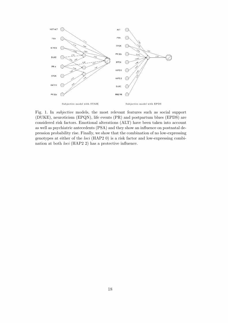
Subjective model with STAIE Subjective model with EPDS

Fig. 1. In subjective models, the most relevant features such as social support(DUKE), neuroticism (EPQN), life events (PR) and postpartum blues (EPDS) areconsidered risk factors. Emotional alterations (ALT) have been taken into accountas well as psychiatric antecedents (PSA) and they show an influence on postnatal de-pression probability rise. Finally, we show that the combination of no low-expressinggenotypes at either of the loci (HAP2 0) is a risk factor and low-expressing combi-nation at both loci (HAP2 2) has a protective influence.

18

Subjec-Environmet model with STAIE Subject-Environment model with EPDS

Fig. 2. As it was to be expected, subject-environment models show greater numberof connections. We find again the main risk factors in both models (social support(DUKE), neuroticism (EPQN) and life events (PR)). Moreover, in these models, theage (AGE) and the number of people living together with the patient (LIV TOG)appear as important protective factors. The income rate appears to be relevant:enough income rate (EC ENF) is a protective factor but a tight economy (EC TIG)can raise the probability of having depression. The anxiety state (STAIE) is a riskfactor too with a moderate influence. Finally, an unemployed (J UNM) or an activemother (J ACT) can be a risk factor but taking maternity leave (J LEA) can reducethe probability of having postnatal depression.

19