Financial Pressure and Balance Sheet Adjustment by Firms

FINANCIAL PRESSURE AND

BALANCE SHEETADJUSTMENT

Andrew Benito and Garry Young

Banco de España

Banco de España — Servicio de EstudiosDocumento de Trabajo n.º 0209

Financial Pressure and Balance Sheet Adjustmentby UK Firms∗

Andrew Benito†

Bank of England

Bank of Spain

Garry Young‡

Bank of England

∗Acknowledgements : We thank Nick Bloom and Steve Bond for providing the data used inthe paper and seminar participants at the Bank of England, Bank of Spain and Royal EconomicSociety Annual Conference (Warwick) for comments. The usual disclaimer applies. The viewsexpressed are those of the authors and should not be thought to represent those of the Bank ofEngland or Bank of Spain.

†Bank of England, Threadneedle Street, London EC2R 8AH. UK., and Bank of Spain ResearchDepartment, Calle de Alcalá 50, 28014 Madrid, Spain. E-mail: [email protected]

‡Bank of England, Threadneedle Street, London EC2R 8AH. UK. E-mail:[email protected]

Abstract

This paper examines the financial policies and balance sheet adjustment of com-panies. Using a large panel of quoted UK firms, we estimate models for dividends,new equity issuance and investment, relating them to debt adjustment. The resultssuggest that while dividends are sticky in the short run, they are an importantmeans of balance sheet adjustment in the long run. Other evidence supports theidea that companies actively target their balance sheet by variation in dividends,new equity issues and investment. There is evidence for financial pressure effects ofdebt-servicing costs on investment and dividends but not new equity issuance.

JEL Classification: G35, C23, E52.Key Words: Financial pressure; dividends; equity issues; debt; investment; com-

pany panel data.

BANCO DE ESPAÑA / DOCUMENTO DE TRABAJO Nº 02092

1 Introduction

Since Modigliani and Miller (1958), the role and importance of corporate financial

policies has been the subject of widespread controversy. This reflects the variety

of issues where corporate financial behaviour is relevant, including corporate tax

policy, the possible role of the financial system in encouraging capital investment,

the relationship between company debt and financial stability, and the impact of

monetary policy on corporate spending.

The present study examines the empirical determinants of dividends, equity

issuance and investment among UK firms. It considers how financial pressure affects

companies and how companies adjust their balance sheets in the light of this. This is

important in analysing the transmission of financial shocks throughout the economy.

In particular, we consider how outcomes at the company-level—both financial and

real—are related to the financial pressure of debt-servicing. An important focus of

our analysis is on the relative importance of balance sheet adjustment via financial

policies, notably dividend distributions and new equity issuance, compared to that

occurring through real investment decisions. This extends the analysis of Nickell and

Nicolitsas (1999) who consider how financial pressure affects a number of other firm-

level outcomes, employment, wage growth and productivity, but do not consider

financial policies nor fixed investment outcomes.

The paper is organised as follows. Section 2 describes the theoretical background

to the paper, in terms of the resolution of balance sheet pressures by various means.

Section 3 contains data description and estimation of models for the level of debt,

the level of dividend payment, the propensity to issue new equity and rates of

investment of a panel of 2,062 UK firms. Section 4 concludes.

BANCO DE ESPAÑA / DOCUMENTO DE TRABAJO Nº 0209 3

2 Economic background: The resolution of bal-ance sheet pressures

Whatever their motivation, all corporate financial decisions are bound together by

the budget constraint linking the sources and uses of funds. For the tax-paying

firm, this can be written in terms of its end-of -period net debt as:

Bt+1 = Bt + PIt It +Dt − (1− τ)(Πt − rBt Bt)−Nt (1)

where B is the stock of debt, τ is the corporate tax rate, P I is the price of

investment goods (net of tax allowances), I is the volume of gross capital investment,

D is the dividend, Π is nominal profits, rB is the interest rate paid on corporate

debt, N is the value of new shares issued. This expression states that debt increases

when outlays on investment and dividends are greater than post-tax profits and the

proceeds from new share issues.

Collecting terms in the initial level of debt and dividing through by the beginning

of period capital stock leads to the following expression for corporate gearing:

bt+1 =(1 + (1− τ)rBt )

(1 + g)bt + dt − nt + it − (1− τ)πt (2)

where lower case letters denote shares of the capital stock and g is its nomi-

nal growth rate. This difference equation is dynamically unstable when the post

corporate tax interest rate (1 − τ)rBt is greater than the growth rate, g.1 In this

case, either dividends d, new issues n, investment i, or profitability π, need to vary1The interest rate is greater than the growth rate in a dynamically efficient economy. While

tax deductibility may mean that (1− τ)rBt < g for tax-paying companies, this is unlikely to be the

case for tax exhausted companies and those who face a significant premium on their borrowing

costs.


sufficiently to prevent the debt stock and gearing b, rising or falling without limit.

How these sources or uses of funds are actually used in balance sheet adjustment is

the subject of this paper.

In principle, at least under frictionless markets, balance sheet adjustment would

occur through the financial, rather than the real, decisions of firms. Firms already

maximising profits should not be able to increase the rate of profit in response

to balance sheet pressures. Moreover, in the absence of taxes, asymmetric in-

formation or agency problems, the Modigliani-Miller theorem would hold and the

optimal investment rate would be independent of financing considerations. Under

these conditions, the debt stock would need to be stabilised by changes in dividend

payments or new share issues even though this would not affect overall company

valuations. But, in practice, Nickell and Nicolitsas (1999) find significant effects

of financial pressure on employment, wage growth and productivity and, by impli-

cation, profitability. While this paper focuses on the possible effects of financial

pressure on dividend payments, new share issues and investment, some compar-

isons are made between the size of these effects and those estimated by Nickell and

Nicolitsas (1999).

The process of balance sheet adjustment has been debated in both the finance

and tax literatures. The finance literature (Fama and French, 2000; Shyam-Sunder

and Myers, 1999) has contrasted the ‘trade-off’ with the ‘pecking-order’ models of

capital structure. According to the trade-off model, companies have an optimal

capital structure where they trade-off the tax benefits of increased indebtedness

against possible costs associated with the greater risk of insolvency. These costs

would include the direct costs of re-organisation in the event of insolvency as well


as indirect costs that arise when companies get into financial difficulty (Barclay et

al, 1995, Myers, 2001). But, according to the pecking order model of Myers and

Majluf (1984) the theoretical benefits of achieving an optimum capital structure

are second-order when compared to the effects of asymmetric information between

insiders and outsiders in valuing companies. This leads to a situation where firms

prefer internal to external finance and, when external finance is needed, prefer debt

to equity. According to this pecking order approach, “each firm’s debt ratio...

reflects its cumulative requirement for external financing” (Myers, 2001). In effect,

the pecking-order predicts that corporate gearing should show no tendency to revert

to an equilibrium level. This is in direct contrast to the trade-off model where, by

(2), any desired capital structure would need to be brought about by varying one of

the variables on the right hand side. Under either of these views, capital investment

could be affected by financial considerations. With the trade-off model, investment

could be lower than otherwise when a company is attempting to reduce debt to

its optimal level (investment need not be affected since the adjustment could be

made by raising new equity). With the pecking order model, investment is lower

than otherwise when external finance is needed to fund it, reflecting a higher cost

of capital.

The tax literature has contrasted the ‘new view’ of dividend taxation developed

by Auerbach (1979) and King (1977) and reviewed by Auerbach (2001), which

claims that dividend taxation has no effect on corporate investment decisions, with

the ‘traditional view’ that dividend taxation imposes an additional tax wedge on

corporate investment. A critical prediction of the new view, according to Auerbach

and Hassett (2000) is that firms obtain their equity funds for investment through


the retention of earnings, and distribute residual funds as dividends, rather than

using new equity as the marginal source of finance as in the traditional view. This

implies that dividends respond positively to cash flow and vary inversely with the

rate of investment. Auerbach and Hassett (2000) go on to suggest that dividends

might be sticky in the short-term, with short-term borrowing adjusting to meet

financing needs, but moving in the longer term to achieve an optimal debt-equity

ratio.

These different views of corporate finance and its relationship to capital invest-

ment have a number of different empirical implications. First, the trade-off model

predicts that corporate gearing varies over time to achieve a target level, suggesting

that gearing will be mean-reverting provided that the target itself is not changing

randomly over time. Second, in this model the target level of gearing will tend to

be higher for more profitable firms reflecting lower expected insolvency costs and

for firms with few other tax shields which may be associated with investment lev-

els (DeAngelo and Masulis, 1980). Third, both the new view and the trade-off

model predict that dividends would vary to bring about a desired capital structure,

implying a relationship between dividends and the level of indebtedness. Further-

more, the pecking order and new view tax model imply that dividends respond

positively to cash flow and negatively to rates of investment (Auerbach and Has-

sett, 2000). Fourth, under both pecking order and new view models, new equity

finance is seen as a last resort. This implies an inverse relationship between cash

flow and the propensity to issue new equity. Fifth, the models also imply a positive

relation between equity issuance and investment. The notion that companies use

equity issuance to adjust their balance sheet in response to high levels of gearing


also implies that the propensity to issue equity responds positively to high levels

of gearing. Sixth, the Modigliani-Miller model predicts that capital investment is

unaffected by financial factors, while the pecking-order model and the new view

predict that investment is lower than otherwise when external finance is used to

fund it. These various empirical predictions are considered for the UK in the next

section.

The above discussion summarises some of the theoretical influences on corporate

financial and investment decisions and how they relate to balance sheet adjustment.

Our contribution is not to test between the different models but to quantify the scale

of the various effects, focusing on the implications for balance sheet adjustment.

3 Estimation and Results

3.1 Data Description

The data employed are derived from company accounts records held on Datastream,

the on-line service covering all companies quoted on the London Stock Exchange

(LSE). The data refer to non-financial companies over the period 1973 to 1998.

We select on a minimum number of four time-series observations per company.

The resulting total number of companies for which data on all variables (with the

exception of equity issuance) are available is 2,062. The number of company-year

observations is 22,095.

Table 1 presents summary statistics on the key variables during different sub-

periods. The first eight rows refer to the dependent variables in our various models,

for dividends, investment, debt (gearing, either scaled by the replacement cost of


capital stock, B/K, or by market capitalisation, B/MV ) and new equity issuance.

The proportion of companies issuing new equity considers whether this is issued

solely for cash or also in an acquisition and for two different threshold amounts.

For the new equity issuance (binary) outcomes, as well as any positive outcome we

also consider a threshold of two per cent of market capitalisation being issued as

new equity. Companies may issue some equity for reasons other than to finance

investment (eg. as part of their remuneration policies). The two per cent threshold

was employed by Auerbach and Hassett (2000) for this reason. The remaining

rows of Table 1 describe the data for the further explanatory variables used in our

analysis. These variables refer to cash flow (CF/K), the borrowing ratio term (br)

defined as the ratio of interest payments to profits favoured by Nickell and Nicolitsas

(1999) as a measure of financial pressure, Tobin’s Q (Q) as a measure of investment

opportunities facing the firm, real sales (S/P ) and sales relative to capital stock

(S/K).

Over the period, the mean ratio of dividends to sales is 0.020, with this company-

level mean increasing during the sample period from 0.014 in 1973-78 to 0.031 in

the 1994-98 period; clearly there is also a great deal of variation across companies.2

Around 37 per cent of company-year observations involve equity issuance, having

increased from 22 per cent during 1973-78 to 48 per cent in 1989-91 and exceeded

50 per cent in the 1984-88 period. The 2 per cent issuance threshold applies to 15

per cent of observations over the period. We also report figures for equity issuance2Further data analysis of the distribution of dividend payments relative to com-

pany sales and company profits and how these distributions vary over time, is

provided in Benito and Young (2001).


for cash.3

The mean of the borrowing ratio, br, increases in the early 1980s and early 1990s

reflecting joint variation in the level of interest rates, debt and corporate profits.

Again, there is a large amount of variation across companies in this variable as

the standard deviation exceeds the mean in each period. Q averages 1.77 during

the period, increasing during the later periods; its distribution is positively skewed,

the median value being 1.04. High average values at the end of the period may

reflect an increase in the number of service sector companies whose value depends

on intangible capital. It is also worth noting that we measure Q at the end of

the calendar year in question whereas some other authors (Blundell et al, 1992)

measure it at the beginning of the accounting year.

Table 2 considers financial ‘regimes’ of companies in a particular year in the form

of whether a company pays a dividend and/or issues equity. Annual averages for the

different sub-periods are shown again separately for the any issuance and 2 per cent

threshold definitions for both all equity issued and equity issued for cash. Using

the 2 per cent issuance thresholds, the overwhelming majority of firms (around 80

per cent) are in the dividend payment, no equity issuance category. There has been

an increase in the proportion of firms issuing equity (see also Table 1) and this has

occurred amongst firms that also pay a dividend. In order to economise on the fixed

costs of issuance, companies should prefer to issue larger amounts of equity (itself

favouring larger companies) rather than repeatedly paying a dividend and issuing

equity in the same year. Table 3 considers the number of years that our 1,8473This might appear to be a cleaner measure of the raising of funds for invest-

ment purposes but since our measure of investment includes merger and acquisition

activity, the case for excluding equity issued for acquisition is not unambiguous.


companies on which we have share issuance data (or 1,751 companies in the case of

issuance for cash) both pay a dividend and issue 2 per cent equity in the same year.

The figures support the proposition that this is not a financial activity undertaken

repeatedly by the same companies. Bond and Meghir (1994) suggest the occurrence

of joint dividend payment and new share issuance may also reflect the existence of

transaction costs for trading equity and a signalling role for dividends. Around 2

per cent of firms neither pay a dividend nor issue (2 per cent) new equity. Less than

1 per cent of companies omit a dividend but issue new equity. (Table 2).

3.2 Estimation results

Our empirical strategy is to examine the behaviour of the level of dividends, in-

vestment and the use of new equity finance as functions of company financial char-

acteristics. Of key importance is the possible response of each of these to balance

sheet pressures as represented by measures of indebtedness or its servicing cost.

As such, the determinants of indebtedness are not modelled directly, instead they

can be recovered from the budget constraint, as represented by (2) and the esti-

mated behavioural relationships. The behavioural relationships that are estimated

for dividends and investment are as follows:

D

S it= αi + α1

D

S it−1+α2

CF

K it−1+ α3brit−1 + α4

I

K it−1(3)

+α5Qit−1 + α6B

K it−1+ α7 ln(S/P )it−1 + γDt + εDit


I

K it= βi + β1

I

K it−1+ β2Qit + β3Qit−1 + β4

S

K it+ β4

S

K it−1(4)

+β5CF

K it+ β6

CF

K it−1+ β7brit + β8brit−1 + γIt + εIit

where the variable definitions follow those given above. αi and βi are the

company-specific fixed effects that control for time-invariant unobservables in the

dividends and investment equations, respectively. γDt and γIt denote common time

effects in the two equations with assumed serially uncorrelated error terms εDit and

εIit.

The specification for dividends, normalised on the cash value of company sales

following Bond et al (1996), encapsulates the salient features of the models referred

to in the previous section. This specification allows dividends to respond to cash

flow and investment with a possible role for debt. We also include investment op-

portunities proxied by a Tobin’s Q variable reflecting the demand for funds and

the log of real sales as a control variable for scale of the company capturing any

agency considerations or the volatility of cash flows. All right hand side variables

are lagged to reduce possible endogeneity. Our specification for investment is based

on that of Blundell et al (1992) supplemented by the financial pressure variable, br.4

All variables are included contemporaneously and with one lag. Both dividend and

investment equations allow for persistence through the inclusion of lagged depen-4Recent investigations concerning the role of Q have highlighted the importance

of measurement error in Q and associated attenuation bias (Bond and Cummins,

2000; Erickson and Whited, 2000). To consider this point is beyond the scope of

this paper.


dent variables. In the case of dividends, the persistence estimate, α1, is of special

interest following Lintner’s (1956) suggestion that companies are averse to cutting

the dividend, attempting to maintain it at a sustainable level. This would tend to

retard balance sheet adjustment through dividends.

For both equations we estimate dynamic fixed effects models using the GMM-

System estimator proposed by Arellano and Bover (1995) and examined in detail by

Blundell and Bond (1998).5 This estimator is an extension of the GMM estimator

of Arellano and Bond (1991) and estimates equations in levels as well as in first-

differences. Where there is persistence in the data such that the lagged levels of

a variable are not highly correlated with the first difference, also estimating the

levels equations with a lagged difference term as an instrument can counter the

bias associated with weak instruments (see Blundell and Bond, 1998). The system

GMM estimator is a combination of the GMM differenced estimator and a GMM

levels estimator. Several variables display high levels of serial correlation. The

estimation method requires that there be evidence of significant negative first order

serial correlation in differenced residuals and no evidence of second order serial

correlation in the first differenced residuals. Blundell, Bond and Windmeijer (2000)

report Monte-Carlo evidence showing that when this method is used the Sargan test

of the overidentifying restrictions tends to over-reject, especially when the number

of observations per company is large.

For the new equity issuance decision, since the outcome we model is binary,

panel data probit models are estimated that incorporate a random effects term for

the company-specific unobservables (see Arulampalam, 1999 for discussion). The5Our analysis therefore relaxes the assumptions of Fama and French (2000) and

Shyam-Sunder and Myers (1999) that the regressors are strictly exogenous.


specifications use the same explanatory variables as in the dividends equation except

that all variables are included contemporaneously.

These outcomes describe the possible mechanisms by which balance sheets are

adjusted. To verify that such adjustment occurs in practice, we estimate the speed

of debt adjustment in the reduced form, estimating a debt equation as a function

of its lagged value whilst also controlling for firm fixed effects and time effects.

3.2.1 Debt adjustment

We report results for a net rather than gross debt measure, (B − C), although

this does not make much difference to the results. This is scaled by either market

capitalisation (MV ) or replacement cost capital stock (K) in the results reported

in Table 4. The time effects control for the tax changes common across companies,

whilst the existence of company-specific target debt levels would be controlled for

through the fixed effects.

In all specifications, there is no evidence of second-order serial correlation in

the first-differenced residuals, the key requirement for our estimation strategy to be

valid. Nevertheless, the results using instruments dated from t−2 in the differenced

equation and at t − 1 in the levels equation are associated with significant values

for the Sargan test statistic. We therefore move to using deeper lags starting at

t− 3 in the differenced equation and t− 2 in the levels equation in columns 2 and

4. Under these estimates, the Sargan test statistic falls short of significance at the

10 per cent level for the capital gearing measure and we focus on these results.

The results indicate that the speed of adjustment of the level of debt is around

30 to 35 per cent per year, substantially faster than the rate of 7 to17 per cent


per annum estimated in the US and described as “suspiciously slow” by Fama and

French (2000, p30). This indicates that companies actively adjust their balance

sheets to prevent levels of debt becoming excessive. The remainder of the paper

considers methods by which this adjustment may be achieved.

3.2.2 Dividends

Results for dividends are shown in Table 5. Support for the main predictions from

the previous discussion is obtained. Dividends respond positively to cash flow,

and negatively to levels of investment. These terms are highly significant, with

t-statistics (robust to heteroskedasticity) in excess of four. A further key feature of

the results is the degree of persistence in dividends. At 0.829 (0.129), the coefficient

(robust standard error) on the lagged dependent variable reveals a high level of

persistence indicating that companies are slow to adjust their balance sheets through

dividends.

The indebtedness term, B/K, is significantly negative. A high level of indebt-

edness restricts the amount companies tend to distribute to shareholders.6 This

is one of the channels by which the balance sheet is brought under control. The

dependence of dividends on the level of gearing partially offsets the effect of interest

payments in the debt accumulation process shown in (2).7

The Q term is signed positively, although not significantly, and this may reflect6 In the results reported, we employ a gross debt variable and control for cash

flow separately. Using the net debt variable, ((B-C)/K) in a specification otherwise

equivalent to that in column 1 is associated with similar results with the debt term

again being significant but the cash flow term (CF/K) loses significance.7When re-normalised on the capital stock, the coefficient on gearing is -0.03 in

the long run solution to the dividends equation.


the fact that Q will in part pick up current profitability rather than purely op-

portunities for investment. Companies with a high value for Q may also feel more

confident about paying a higher dividend.

The scale term falls short of significance. This is likely to be because, in a fixed

effects model, it is the time-series variation that is being exploited; following an

increase in sales a given company may not reduce its dividend distributions in the

same way as a comparison between a small and large firm might imply.8 In column 2

we drop instruments dated t− 2 in the differenced equation and instruments dated

t− 1 in the levels equation; the main results described above remain intact.

In column 3 we consider the financial pressure variable br, (the ratio of interest

payments to profits) added to our previous regressor set. This is Nickell and Nicolit-

sas’s (1999) preferred measure of financial pressure facing a company. The analysis

of Nickell and Nicolitsas (1999) looking at real outcomes such as employment, as

well as Fazzari et al’s (1988) analysis of investment, is predicated on the notion that

balance sheet adjustment through purely financial outcomes such as dividends or ex-

ternal finance is imperfect and some adjustment is necessary through real decisions

of the firm such as investment and employment.

In the context of dividends the results suggest that a role for the borrowing ratio

term depends upon the precise specification employed. In particular when included

alongside the cash flow and debt terms, the borrowing ratio is not significant. This

is not entirely surprising since the ‘br’ variable can be thought of as (rB/π) where

r is the effective rate of interest, B is the amount of debt and π is profits which is8 In support of this, a pooled cross-sectional model, ie omitting the fixed effects,

results in a significantly positive coefficient on the lagged sales term (coefficient

(robust standard error) of 0.000251 (0.000094)).


closely related to cash flow. Including the term alongside controls for cash flow and

debt is therefore asking rather a lot. It might seem preferable to consider a role for

the variable in place of the cash flow (CF/K) and debt (B/K) terms. This is done

in column 4 and the borrowing ratio variable is now on the margins of significance

with a ‘t-ratio’ of 1.85. This specification also omits the Q term since we believe

that in part picks up current profitability.

The impact of financial pressure can be quantified using the same experiment

as Nickell and Nicolitsas (1999) by considering the impact on individual companies

of an increase in interest rates from 5 to 8 per cent.9 Under the assumption of

no fixed rate debt, this implies an increase in br of 60 per cent. Evaluated at the

means (br = 0.21; (D/S) = 0.021), the estimates imply a reduction in dividends of

3.1 per cent in the short-run and by 18.0 per cent in the long-run, but given the

high degree of persistence this takes a long time to come through. Recall that such

effects are quantitatively smaller and statistically insignificant when we control for

cash flow. For the same increase in financial pressure, Nickell and Nicolitsas (1999)

estimate a short-run (long-run) effect of 2.9 per cent (10 per cent) on employment;

2.3 per cent (2.5 per cent) on wages and a very small positive effect on productivity

of 0.5 per cent in the long-run. Balance sheet adjustment by dividends is therefore

quantitatively important but slow-acting.

Nevertheless, the fact that the financial pressure variable, br, is insignificant

when included alongside the cash flow and debt terms tells us something about the

best way to proxy financial pressure in this context. If we think of these specifica-9Since such a change would have significant general equilibrium effects, this par-

tial experiment is best considered as a change in ‘financial pressure’ for an individual

company equivalent to a change in interest rates of this amount.


tions as asking the data to ‘fight it out’ statistically as to which factor related to

financial pressure matters most, the results favour cash flow and debt rather than

the ratio of debt-servicing payments to profits.

In sum, although we can isolate a significant effect from the borrowing ratio

term, br, depressing levels of dividends, this requires the omission of the cash flow

and indebtedness terms. Where these terms are included jointly, the borrowing ratio

term loses its significance, whilst the cash flow and debt terms remain significant.

The cash flow and underlying indebtedness variables appear to do a sufficient job

of picking up any role for financial pressure type effects.

Within this preferred specification (column 2 of Table 5), dividends can be

thought of as adjusting gearing to a target level. This target level can be derived

from the estimated equation and depends positively on cash flow and negatively

on investment.10 The negative influence of investment on target gearing comes

about because this generates an alternative tax shield to debt and so reduces the

attractiveness of higher gearing under the new view and trade-offmodels. Under the

pecking order model, there is no well-defined target level. But an inverse relation

between gearing (or its long-run solution) and investment could come about under

a more complex version of this model if firms are concerned with both current

and future financing costs and higher investment levels encourage firms to maintain

debt capacity rather than forego future investments or using costly equity to finance

them. The positive effect of cash flow on target gearing reflects the lower probability10The dividend equation can be written explicitly as a means of debt adjustment

dt = λ0dt−1+λ1(bt−1−b∗t−1) and variables other than dividends and debt interpretedas driving the target gearing level, b∗.


and expected cost of insolvency under the trade-off approach. It is not consistent

with the pecking order model, where higher profitability reduces gearing.

3.2.3 New Equity Issues

Under the pecking order model, companies are generally averse to new equity finance

because of information asymmetries, using it when investment is high relative to

cash flow. Under the new view, incentives to issue equity are dependent on taxes.

In the UK, at least until 1997, the tax system encouraged new equity issues (Benito

and Young, 2001), although this may have been offset by transactions costs, which

are likely to be larger for smaller firms. Under the trade-off model, new equity issues

would be more likely when gearing is above its target level. Taking these views into

account would suggest that new equity issues are used when investment is strong

relative to cash flow and when gearing is high, with possible effects depending on

firm size.

Carpenter and Petersen (2002) emphasise that the literature examining the fi-

nancing and investment decisions has tended to focus on debt finance with the role

of new equity finance being largely neglected. They present descriptive statistics of

a set of US (technology-based) firms. Our analysis of the propensity for firms to

issue new equity can be motivated by similar concerns but adopts a more formal ap-

proach. Table 6 presents results for the estimation of random effects probit models

for share issuance. Again, we consider the propensity to issue new equity finance as

a function of cash flow (CF/K), investment (I/K), Tobin’s Q (Q) as a proxy for

investment opportunities, and debt (B/K). We also include a control for scale (log

real sales, S/P ). A role for the financial pressure variable (br) is also considered.


Note that data on new equity issues are available for a slightly restricted period, so

our sample periods are restricted accordingly.

A key result is that the cash flow term (CF/K) is highly significant and nega-

tively signed. As predicted by the pecking order and new view models, companies

with high levels of cash flow are less likely to resort to equity issues to finance

investment since the availability of internal funds reduces their need to resort to

external equity finance. The likelihood of using new equity finance increases signif-

icantly in the level of debt (B/K) and rate of investment (I/K) of the firm. The

former is consistent with the notion that companies have a target gearing level,

with equity issuance being one response to excessive levels of debt. The positive

relation between propensity to issue equity and rate of investment is as expected,

reflecting the fact that equity finance will tend to be used more by those companies

with substantial investment programmes.

The results also suggest that larger firms are more likely to use equity finance

than smaller firms controlling for these other financial characteristics and this may

reflect fixed costs of issuance. The Q term is also highly significant and suggests

that firms with higher investment opportunities are more likely to use new equity

finance. It could also be that managers of high Q firms think that the shares are

over-valued and are issuing more to benefit the existing shareholders. Note also that

the estimate of the parameter ρ, which reflects the proportion of the total variance

accounted for by the unobserved heterogeneity term, is approximately 0.22 (in the

2 per cent issuance threshold model) and is well-determined.

In the equation that considers any equity issued as the dependent variable,

the debt term (B/K) is insignificant. Redefining the dependent variable to equity


issuance of 2 per cent of market capitalisation alters this result, with the results

indicating that in this case, a high level of debt increases the probability of equity

issuance. With the exception of this result for the debt term, the other results are

not sensitive to specifying the dependent variable using a zero versus 2 per cent

threshold for equity issues.

The addition of the financial pressure variable, br, indicates that this is not

significant. Instead, equity issuance responds as anticipated to the underlying in-

debtedness of the company (B/K) and its cash flow (CF/K), rather than a term

reflecting the flow of interest payments on debt relative to profits. This suggests

equity issues are related to more fundamental aspects of indebtedness rather than

the short-term financial pressure associated with its servicing. This is consistent

with the notion that equity issues are used for more ‘low frequency’ movements in

the target debt-equity ratio with companies perhaps using short-term borrowing to

smooth variations in its debt-equity ratio at higher frequencies.

It is clear from Table 6 that the results for equity issuance for cash are very

similar to those reported above for cash and acquisition-related issuance. Each of

the coefficients attracts the same sign and similar level of significance.

How important, quantitatively, is each variable? Table 7 presents the marginal

effects, evaluated at the means. These effects indicate the change in the probability

of observing an equity issue for a 1-unit change in the explanatory variable holding

constant the other factors, evaluated at the means. These calculations employ

the correction recommended by Arulampalam (1999) for the normalisation in the

coefficient estimates present in random effects probit models. The use of the 2 per

cent issuance threshold reduces the quantitative importance of each variable (with


the exception of the debt term, B/K). The marginal effects indicate that a 10

percentage point increase in cash flow, lowers the probability of issuing equity by

0.02 (-0.171/10). Recall that the mean company cash flow is 0.26 and the mean

proportion of companies issuing equity is 0.37 with the proportion issuing equity to

the value of 2 per cent of market capitalisation or more being 0.15. A change in the

probability of this order is by no means small. The probability of equity issuance is

more sensitive to investment. A 10 percentage point increase in investment raises

the probability of new equity issuance by 0.04 under both the zero and 2 per cent

issuance threshold results. The marginal effect for Q indicates that an increase in

Q of 0.1 (the mean value being 1.70) increases the probability of equity issuance

by 0.003. The model for a 2 per cent threshold for equity issuance indicated a

significant relation between the propensity to issue equity and the amount of debt.

Under these estimates an increase in debt of 10 percentage points is associated with

an increase in the probability of 0.004.

3.2.4 Investment

The paper thus far has concentrated on the financial policies of UK firms. We now

consider the real side of the balance sheet in the form of levels of investment. This

follows a large number of previous studies (see Hubbard, 1998, for a review). Our

contribution in presenting these results is first, to present these models in the context

of the wider financing decisions of UK corporates estimated above and second, to

consider the potential role of the financial pressure variable, br, in a UK firm-level

study of fixed investment for the first time.


We begin our results with estimates for a basic Q model without financial vari-

ables, presented in column 1 of Table 8. The results accord with our priors. Invest-

ment responds positively to the value of Q at the beginning of period (dated t− 1)

with a t-value of 5.7. As in Blundell et al (1992) there is a significantly negative

coefficient on the contemporaneous sales to capital ratio, (S/K) and positive coeffi-

cient on the lagged value. Columns 2 to 5 are again conservative in their definition

of the instruments selecting these from t− 3 in the difference equation and t− 2 in

the levels equation, though this does not materially affect our results, the standard

errors on some terms increasing slightly.11

Column 3 adds cash flow terms and we find a significantly positive effect, sup-

porting models where internally generated funds are the cheapest source of finance

to the firm.12 While this is consistent with the financial constraints literature, the11Here, the Sargan test typically returns a value in excess of the standard critical

value, although the M2 statistic indicates the key condition for the validity of this

method holds. We use conservative definitions of the instruments to help counter the

possibility of invalid instruments. As we note above, Blundell et al (2000) report

that the Sargan test over-rejects when the data are persistent and the number of

time series observations is large.12Several studies have considered whether these cash flow effects are greater for

certain types of firms which are more likely to be financially constrained (eg. Bond

and Meghir, 1994). We therefore interacted the cash flow terms with indicators

for dividend omission, omission but former dividend payment and smaller scale (in

the bottom quartile of the sales distribution). Considered alternately, these terms

(contemporaneous and lagged) were individually and jointly insignificant. Recently,

debate has focused on whether these indicators instead proxy the types of firms for

which market information and the Tobin’s Q variable is likely to be more imperfect

such that cash flow effects may proxy investment opportunities (eg. Alti, 2001).

For this reason and given the insignificance of such interaction terms, we do not


importance of cash flow could reflect other factors. For example if current cash

flow is correlated with future profitability it could simply reflect an improvement

in prospects. The inclusion of cash flow terms lowers the significance of the lagged

Q, suggesting perhaps that both serve as indicators of future prospects. In column

4 the borrowing ratio term is considered as a financial variable (omitting the cash

flow term) with the terms being significant and negatively signed. This suggests

that the financial pressure of debt servicing plays an important role in influenc-

ing investment levels of firms. This extends the results of Nickell and Nicolitsas

(1999) who consider a role for this variable in the employment, wage growth and

productivity levels of UK firms. Real outcomes at the firm-level respond to the

financial pressure effects whilst above we found that purely financial variables such

as dividends and equity issuance were not responsive to this variable, instead be-

ing affected by longer-term notions of indebtedness of the firm. Moreover, adding

the cash flow terms in column 5, the borrowing ratio variable remains significant,

the lagged variable having a ‘t-ratio’ of -3.40, with the cash flow terms also being

significant. This provides strong evidence in favour of a financial pressure effect on

investment at the company-level, at least in the short-term and is another of our

key results.

The addition of a debt term, when controlling for cash flow does not improve

on this model in column 5. The debt term, B/K, in such a specification falls short

of significance when entered in place of the borrowing ratio term, with a t-ratio on

the B/Kit term of -1.27.

discuss these results in detail.


The results for a change in investment associated with a given change in financial

pressure may again be derived and compared to those of Nickell and Nicolitsas

(1999) for other company outcomes. For a change in financial pressure equivalent

to a permanent increase in the interest rate from 5 to 8 per cent, the estimates in

column 4 imply a 5.7 per cent reduction in investment in the short-run and 13.5

per cent reduction in the long-run. Under the estimates in column 5 (controlling

for cash-flow) the results imply a 2.3 per cent short-run and 11.4 per cent long-run

effect, evaluated at the means. This compares to the short-run (long-run) impact

on dividends of 3.1 (18.0) per cent, when not controlling for cash flow (the effect

being insignificant when controlling for cash-flow). Nickell and Nicolitsas (1999)

found an impact on employment of 2.9 per cent in the short-run and 10 per cent in

the long-run, with smaller offsetting on wages and productivity.

4 Conclusions

This paper has examined methods of balance sheet adjustment of UK firms and the

forces to which such adjustments respond. A special emphasis has been placed on

adjustment in response to financial pressure. In this context, we have considered

debt adjustment, levels of dividend payment, the propensity to issue new equity

and rates of investment using company-level data.

The analysis has produced novel results in several respects. First, our analysis

of dividends identifies a number of influences. Dividends respond positively to cash

flows and negatively to rates of investment for UK firms, in a manner consistent with

the new view approach (Auerbach, 2001) and pecking order models. The new view

model of taxation and corporate finance which bases a hierarchy of funds on tax


discrimination has important implications for the design of tax policy. Dividends are

also negatively influenced by the level of indebtedness of the company. This result

highlights the use of dividends as an adjustment mechanism to maintain gearing on

a sustainable path.

Second, we find large persistence effects in levels of dividends, with coefficients

on the lagged dependent variable in our models in excess of 0.8. Companies are slow

to adjust their balance sheets through their dividend payment. Thus, in response

to some financial shock companies will use other means in the short-term to adjust

their balance sheets in addition to that through the level of dividend distributed to

shareholders.

This analysis of the role of dividend adjustment is important for wider reasons.

A large literature has developed examining how investment is affected by cash flow

in a manner consistent with financial constraints (eg. Fazzari et al (1988)). This

literature, and its macroeconomic analogue, that of the financial accelerator (eg

Bernanke et al, 1996), has neglected the potential role of dividend adjustment in

such a process. The emphasis instead has been on the notion that companies will

need to resort to external finance which, if available only at a cost premium over

internal funds, will imply that companies will forego investment opportunities fol-

lowing a shock to cash flow. Since dividend adjustment potentially offers an alter-

native means of making such funds available, our analysis has attempted to make

clear this potential role whilst also illustrating why in practice they may not be

adjusted immediately in response to such pressures. That is, the high degree of

persistence in dividend payments that we find may reflect large adjustment costs

perhaps associated with a signalling role for dividends. This then makes other


forms of adjustment, such as external finance and/or deferred real investment levels

preferable to the firms involved.

Third, we have considered external finance through the propensity for companies

to issue additional equity. We have shown that companies do not generally pay a

dividend and issue new equity in the same year, or at least not on an ongoing basis.

Further, companies with low levels of cash flow, high levels of debt and in particular,

high levels of investment are more likely to issue equity. Our analysis of each of

these outcomes, dividends, equity issuance and investment has considered the role

of the financial burden of debt-servicing. We thereby extend the analysis of Nickell

and Nicolitsas (1999) of how financial pressure affects companies. In this context,

our results for the different outcomes produced an interesting contrast. Evidence

was found to support the notion that debt-servicing costs affect the real outcome

of investment whereas we were unable to isolate a significant effect of this financial

pressure variable on the level of dividend (when controlling for cash flow) or the

propensity to issue equity. These latter outcomes instead respond more clearly to

cash flow and longer-term measures of indebtedness of the firm.


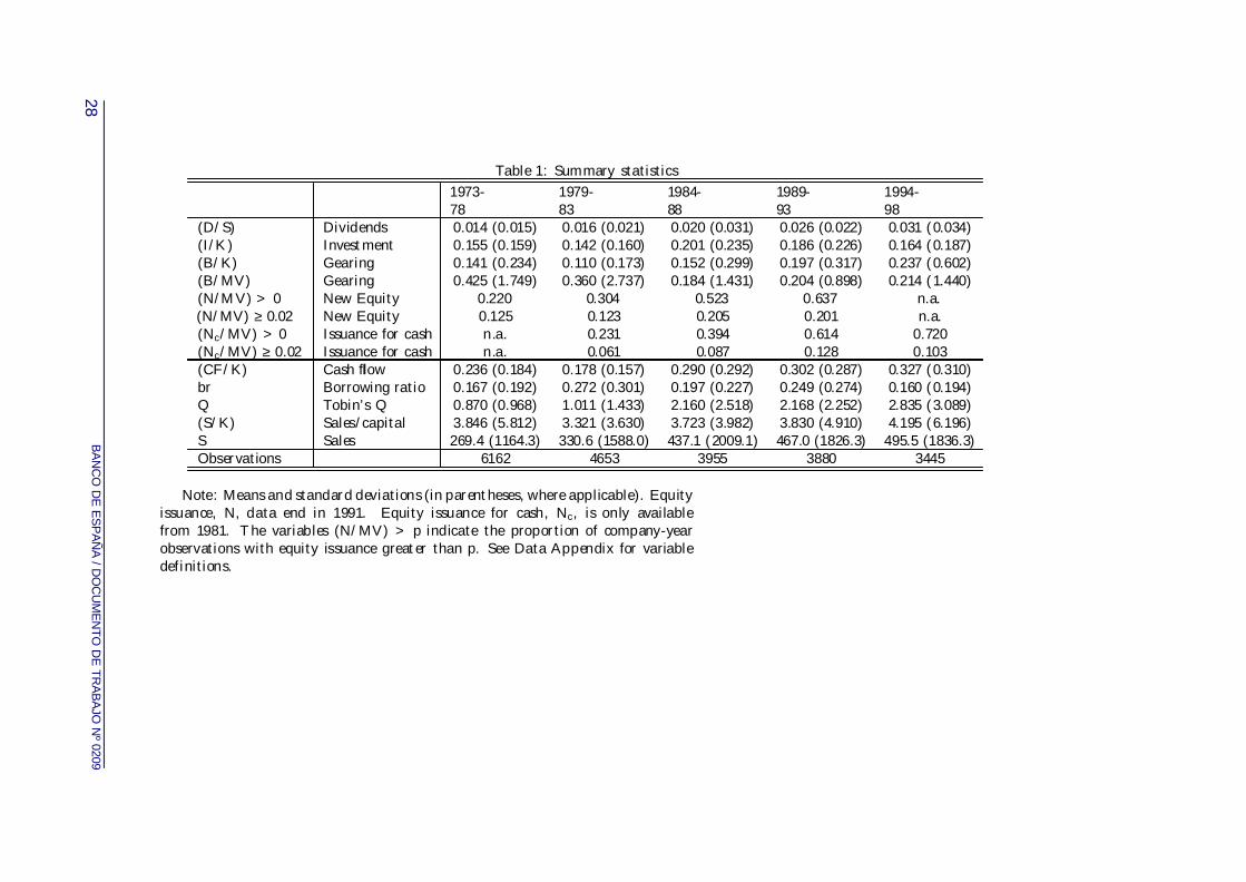
Table 1: Summary statistics1973-78

1979-83

1984-88

1989-93

1994-98

(D/S) Dividends 0.014 (0.015) 0.016 (0.021) 0.020 (0.031) 0.026 (0.022) 0.031 (0.034)(I/K) Investment 0.155 (0.159) 0.142 (0.160) 0.201 (0.235) 0.186 (0.226) 0.164 (0.187)(B/K) Gearing 0.141 (0.234) 0.110 (0.173) 0.152 (0.299) 0.197 (0.317) 0.237 (0.602)(B/MV) Gearing 0.425 (1.749) 0.360 (2.737) 0.184 (1.431) 0.204 (0.898) 0.214 (1.440)(N/MV) > 0 New Equity 0.220 0.304 0.523 0.637 n.a.(N/MV) ≥ 0.02 New Equity 0.125 0.123 0.205 0.201 n.a.(Nc/MV) > 0 Issuance for cash n.a. 0.231 0.394 0.614 0.720(Nc/MV) ≥ 0.02 Issuance for cash n.a. 0.061 0.087 0.128 0.103(CF/K) Cash fllow 0.236 (0.184) 0.178 (0.157) 0.290 (0.292) 0.302 (0.287) 0.327 (0.310)br Borrowing ratio 0.167 (0.192) 0.272 (0.301) 0.197 (0.227) 0.249 (0.274) 0.160 (0.194)Q Tobin’s Q 0.870 (0.968) 1.011 (1.433) 2.160 (2.518) 2.168 (2.252) 2.835 (3.089)(S/K) Sales/capital 3.846 (5.812) 3.321 (3.630) 3.723 (3.982) 3.830 (4.910) 4.195 (6.196)S Sales 269.4 (1164.3) 330.6 (1588.0) 437.1 (2009.1) 467.0 (1826.3) 495.5 (1836.3)Observations 6162 4653 3955 3880 3445

Note: Means and standard deviations (in parentheses, where applicable). Equityissuance, N, data end in 1991. Equity issuance for cash, Nc, is only availablefrom 1981. The variables (N/MV) > p indicate the proportion of company-yearobservations with equity issuance greater than p. See Data Appendix for variabledefinitions.

BA

NC

O D

E E

SP

AÑ

A / D

OC

UM

EN

TO D

E TR

AB

AJO

Nº 0209

28

Table 2: Dividend Payment and New Equity1973-78 1979-83 1984-88 1989-93 1994-98

For cash and acquisitionAny issuanceD=1 & N=0 0.763 0.677 0.460 0.343 n.a.D=0 & N=0 0.017 0.019 0.017 0.020 n.a.D=1 & N=1 0.217 0.301 0.516 0.628 n.a.D=0 & N=1 0.003 0.003 0.007 0.009 n.a.

2 per cent issuanceD=1 & N=0 0.857 0.856 0.776 0.776 n.a.D=0 & N=0 0.018 0.020 0.019 0.024 n.a.D=1 & N=1 0.124 0.122 0.200 0.195 n.a.D=0 & N=1 0.001 0.002 0.004 0.006 n.a.

For CashAny issuanceD=1 & N=0 n.a. 0.745 0.588 0.358 0.267D=0 & N=0 n.a. 0.024 0.019 0.027 0.013D=1 & N=1 n.a. 0.229 0.389 0.605 0.711D=0 & N=1 n.a. 0.002 0.005 0.009 0.009

2 per cent issuanceD=1 & N=0 n.a. 0.914 0.892 0.839 0.878D=0 & N=0 n.a. 0.025 0.020 0.032 0.019D=1 & N=1 n.a. 0.060 0.084 0.124 0.101D=0 & N=1 n.a. 0.002 0.003 0.004 0.003

Note: D refers to a dividend payment; N is new equity for cash or acquisition(any issuance or to the value of 2 per cent of market capitalisation); Nc is newequity for cash.


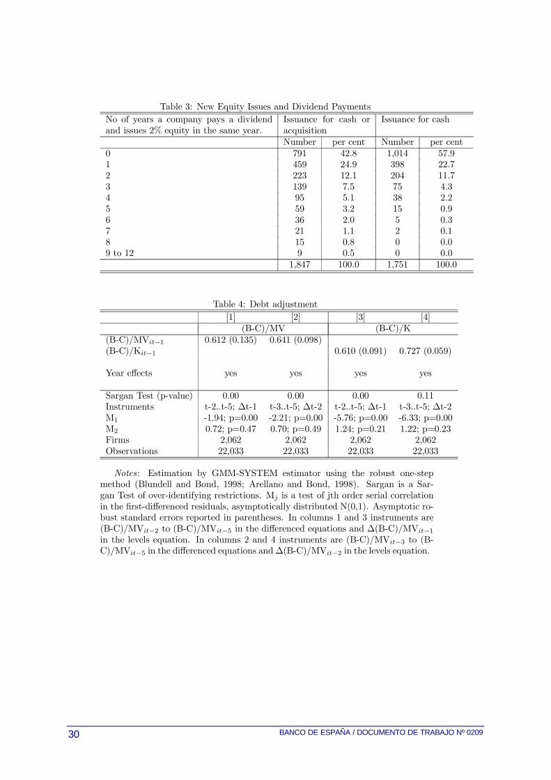
Table 3: New Equity Issues and Dividend PaymentsNo of years a company pays a dividendand issues 2% equity in the same year.

Issuance for cash oracquisition

Issuance for cash

Number per cent Number per cent0 791 42.8 1,014 57.91 459 24.9 398 22.72 223 12.1 204 11.73 139 7.5 75 4.34 95 5.1 38 2.25 59 3.2 15 0.96 36 2.0 5 0.37 21 1.1 2 0.18 15 0.8 0 0.09 to 12 9 0.5 0 0.0

1,847 100.0 1,751 100.0

Table 4: Debt adjustment[1] [2] [3] [4]

(B-C)/MV (B-C)/K(B-C)/MVit−1 0.612 (0.135) 0.641 (0.098)(B-C)/Kit−1 0.610 (0.091) 0.727 (0.059)

Year effects yes yes yes yes

Sargan Test (p-value) 0.00 0.00 0.00 0.11Instruments t-2..t-5; ∆t-1 t-3..t-5; ∆t-2 t-2..t-5; ∆t-1 t-3..t-5; ∆t-2M1 -1.94; p=0.00 -2.21; p=0.00 -5.76; p=0.00 -6.33; p=0.00M2 0.72; p=0.47 0.70; p=0.49 1.24; p=0.21 1.22; p=0.23Firms 2,062 2,062 2,062 2,062Observations 22,033 22,033 22,033 22,033

Notes: Estimation by GMM-SYSTEM estimator using the robust one-stepmethod (Blundell and Bond, 1998; Arellano and Bond, 1998). Sargan is a Sar-gan Test of over-identifying restrictions. Mj is a test of jth order serial correlationin the first-differenced residuals, asymptotically distributed N(0,1). Asymptotic ro-bust standard errors reported in parentheses. In columns 1 and 3 instruments are(B-C)/MVit−2 to (B-C)/MVit−5 in the differenced equations and ∆(B-C)/MVit−1in the levels equation. In columns 2 and 4 instruments are (B-C)/MVit−3 to (B-C)/MVit−5 in the differenced equations and∆(B-C)/MVit−2 in the levels equation.


Table 5: Dividends

(D/S)it [1] [2] [3] [4](D/S)it−1 0.829 (0.129) 0.835 (0.127) 0.826 (0.134) 0.829 (0.140)(CF/K)it−1 0.623 (0.155) 0.559 (0.242) 0.558 (0.229)brit−1 -0.229 (0.282) -0.538 (0.292)(I/K)it−1 -0.533 (0.110) -0.750 (0.367) -0.949 (0.383) -0.562 (0.327)Qit−1 0.024 (0.018) 0.055 (0.040) 0.058 (0.041)(B/K)it−1 -0.209 (0.100) -0.127 (0.068) -0.112 (0.064)ln(S)it−1 -0.082 (0.059) -0.112 (0.066) -0.106 (0.064) -0.134 (0.084)

Year effects yes yes yes yes

Sargan Test (p-value) 0.00 0.00 0.00 0.11Instruments t-2..t-5; ∆t-1 t-3..t-5; ∆t-2 t-3..t-5; ∆t-2 t-3..t-5; ∆t-2M1 -3.64; p=0.00 -3.69; p=0.00 -3.69; p=0.00 -3.67; p=0.00M2 1.43; p=0.15 1.45; p=0.15 1.46; p=0.15 1.44; p=0.15Firms 2,062 2,062 2,062 2,062Observations 22,033 22,033 22,033 22,033

Notes: Estimation by GMM-SYSTEM estimator using the robust one-stepmethod (Blundell and Bond, 1998; Arellano and Bond, 1998). Sargan is a Sar-gan Test of over-identifying restrictions. Mj is a test of jth order serial correlationin the first-differenced residuals, asymptotically distributed N(0,1). Asymptotic ro-bust standard errors reported in parentheses. Instruments as stated. Coefficientsand standard errors multiplied by 100, with the exception of those associated withthe lagged dependent variable.


Table 6: New Equity IssuanceIssuance for cash or acquisition Issuance for cash

any 2 per cent any 2 per cent(CF/K)it -0.648 (0.118) -0.816 (0.109) -0.704 (0.113) -0.736 (0.107)brit -0.010 (0.072) 0.096 (0.077)(I/K)it 1.602 (0.088) 2.238 (0.080) 2.011 (0.073) 0.842 (0.082) 1.560 (0.074) 1.379 (0.069)Qit 0.118 (0.015) 0.098 (0.013) 0.026 (0.010) 0.156 (0.013) 0.082 (0.011) 0.024 (0.008)(B/K)it -0.011 (0.069) 0.211 (0.057) 0.252 (0.059) -0.093 (0.052) 0.110 (0.036) 0.108 (0.036)ln(S)it 0.414 (0.016) 0.154 (0.012) 0.157 (0.012) 0.416 (0.016) 0.069 (0.011) 0.072 (0.012)

Year effects yes yes yes yes yes yes

log-likelihood -7635.775 -6199.427 -6228.284 -6434.336 -3953.979 -3978.161Sα 0.941 (0.028) 0.534 (0.024) 0.546 (0.024) 0.920 (0.030) 0.405 (0.030) 0.406 (0.030)ρ 0.469 (0.015) 0.222 (0.015) 0.229 (0.015) 0.458 (0.016) 0.141 (0.018) 0.141 (0.018)

Firms 1,847 1,847 1,847 1,751 1,751 1,751Observations 17,091 17,091 17,091 17,091 17,091 17,091

Notes : Maximum likelihood estimates for random effects probit model are shown. Standard errors in parentheses.ρ is the proportion of the total variance that is accounted for by the company-specific component.

BA

NC

O D

E E

SP

AÑ

A / D

OC

UM

EN

TO D

E TR

AB

AJO

Nº 0209

32

Table 7: Marginal Effects for New Equity Issuance

any 2 percentFor cash or acquisition(CF/K)it -0.171 -0.153brit 0.002(I/K)it 0.423 0.419 0.376Qit 0.031 0.018 0.005(B/K)it -0.003 0.040 0.047ln(S)it 0.109 0.029 0.029

For cash(CF/K)it -0.207 -0.105brit 0.014(I/K)it 0.247 0.222 0.198Qit 0.046 0.012 0.003(B/K)it -0.027 0.016 0.016ln(S)it 0.122 0.010 0.010

Note: The table reports marginal effects of a unit change on the probabilityof observing yit=1 evaluated at the means. The marginal effects are calculated asd[prob(y=1|x)]

dxk= φ

¡xβ√1− ρ

¢ ¡√1− ρβk

¢where φ (·) is the standard normal density

function, x is the vector of mean characteristics, β the vector of coefficient esti-mates with βk the coefficient estimate on regressor xk (see Arulampalam (1999)on the adjustment to the standard expression for marginal effects by the

p(1− ρ)

correction factor in a random effects probit model).


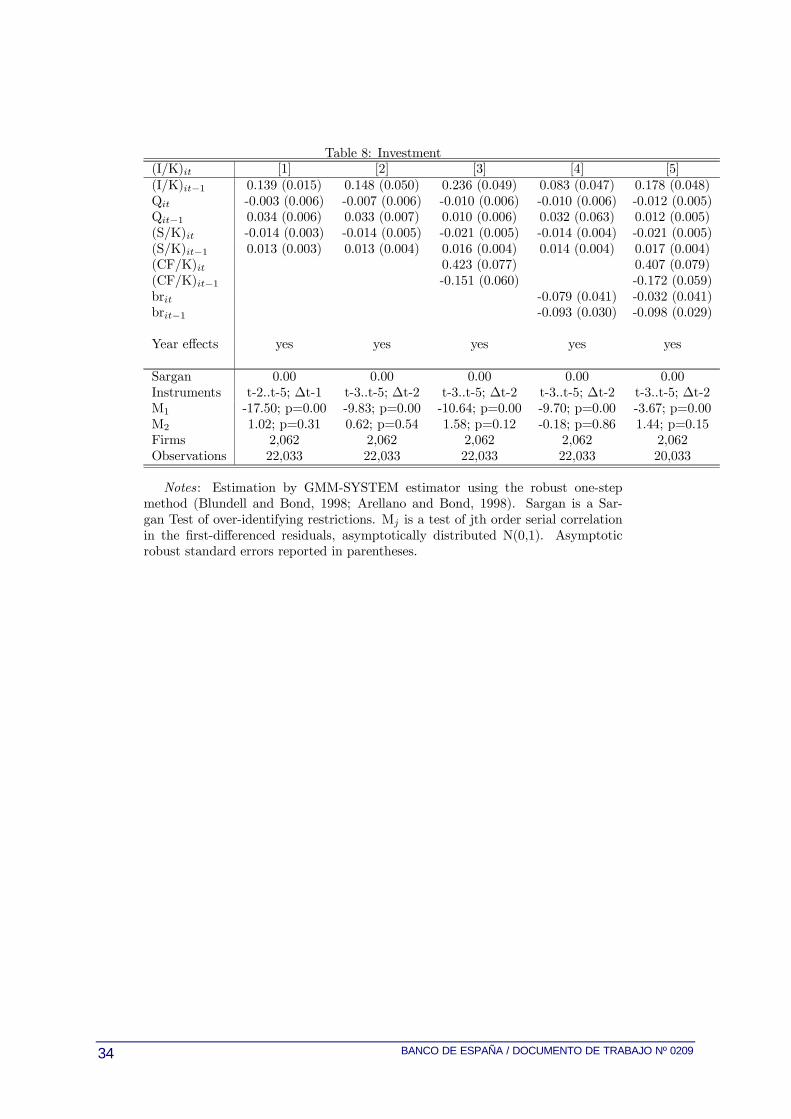
Table 8: Investment(I/K)it [1] [2] [3] [4] [5](I/K)it−1 0.139 (0.015) 0.148 (0.050) 0.236 (0.049) 0.083 (0.047) 0.178 (0.048)Qit -0.003 (0.006) -0.007 (0.006) -0.010 (0.006) -0.010 (0.006) -0.012 (0.005)Qit−1 0.034 (0.006) 0.033 (0.007) 0.010 (0.006) 0.032 (0.063) 0.012 (0.005)(S/K)it -0.014 (0.003) -0.014 (0.005) -0.021 (0.005) -0.014 (0.004) -0.021 (0.005)(S/K)it−1 0.013 (0.003) 0.013 (0.004) 0.016 (0.004) 0.014 (0.004) 0.017 (0.004)(CF/K)it 0.423 (0.077) 0.407 (0.079)(CF/K)it−1 -0.151 (0.060) -0.172 (0.059)brit -0.079 (0.041) -0.032 (0.041)brit−1 -0.093 (0.030) -0.098 (0.029)

Year effects yes yes yes yes yes

Sargan 0.00 0.00 0.00 0.00 0.00Instruments t-2..t-5; ∆t-1 t-3..t-5; ∆t-2 t-3..t-5; ∆t-2 t-3..t-5; ∆t-2 t-3..t-5; ∆t-2M1 -17.50; p=0.00 -9.83; p=0.00 -10.64; p=0.00 -9.70; p=0.00 -3.67; p=0.00M2 1.02; p=0.31 0.62; p=0.54 1.58; p=0.12 -0.18; p=0.86 1.44; p=0.15Firms 2,062 2,062 2,062 2,062 2,062Observations 22,033 22,033 22,033 22,033 20,033

Notes: Estimation by GMM-SYSTEM estimator using the robust one-stepmethod (Blundell and Bond, 1998; Arellano and Bond, 1998). Sargan is a Sar-gan Test of over-identifying restrictions. Mj is a test of jth order serial correlationin the first-differenced residuals, asymptotically distributed N(0,1). Asymptoticrobust standard errors reported in parentheses.


Data Appendix

Panel Structure

Table A.1 tabulates the number of time-series observations per company.

Table A.1: Panel structure

No of records 4 5 6 7 8 9 10 11 12 13 14 15Companies 254 187 143 185 203 154 132 102 90 94 74 59No of records 16 17 18 19 20 21 22 23 24 25 26 TotalCompanies 50 32 30 40 16 12 22 26 19 26 112 2,026

Variable Construction

Dividends (D)Ordinary dividends net of Advance Corporation Tax. (Datastream Item 187)

Debt (B/K)Total loan capital (DS321) divided by replacement cost of capital stock K (see be-

low) or market capitalisation (MV). Net debt subtracts cash and equivalent (DS375)from the numerator.

Leverage (B/MV)Total loan capital (DS321) divided by market capitalisation of the company

(Item mv).

Equity issued (N)Two definitions of equity issuance are used. Equity issued for cash (DS412) and

equity issued for cash and acquisition (DS406). The former is only available up to1991 whilst the latter is available from 1981 and both before and after the intro-duction of the cashflow standard FSR1 and FRS1(Rev) which became compulsoryin March 1992. Both figures are net of share repurchases.

Investment (I/K)Owing to changes in company accounts definitions in 1991, a different method

for calculation is used pre- and post-1991. Up to 1991, investment is calculated asTotal new fixed assets (DS435) less sales of fixed assets (DS423). From 1991, thisis calculated as total payments for fixed assets of the parent (DS1026) plus those ofany subsidiaries (DS429), net of sales of fixed assets.

Capital stock (K)Capital stock is measured on a replacement cost basis. The procedure employed

uses a perpetual inventory method as has been used in a number of company ac-counts panel data studies (eg. Blundell et al., (1992)). Kt+1 = Kit(1 − δ) + Iitwhere δ is the rate of depreciation assumed to be 0.08. I is investment. For thecompany’s first observation, the replacement cost is assumed equal to the historiccost total net fixed assets (DS339), adjusted for inflation.


Tobin’s Q (Q)Q =

¡mv+B−C

K

¢where mv is market capitalisation of the company at December 31 in year t

(Datastream Item mv); B is book value of outstanding debt (DS321); C is bookvalue of cash and equivalent (DS375). The top 1 per cent of values are recoded tothe 99th percentile.

Cash flow (CF)Profit after tax and preference dividends (DS186) plus depreciation of fixed

assets (DS136).

Borrowing ratio (br)Interest payments (DS153) divided by profit before tax (DS157) plus interest

received (DS143). Where companies have a negative value for the denominatortheir borrowing ratio is set equal to 1.

Real Sales (S/P)Total company sales S (DS104), deflated by the GDP deflator (P ).


References

Alti, A (2001), ‘How sensitive is investment to cash flow when financing is fric-tionless?’, mimeo, Carnegie Mellon University.

Arellano, M and Bond, S (1998), ‘Dynamic panel data estimation using DPD98for GAUSS: A guide for users’, mimeo, Institute for Fiscal Studies.

Arellano, M and Bond, S (1991), ‘Some tests of specification for panel data:Monte Carlo evidence and an application to employment equations’, Review ofEconomic Studies, Vol 58, pages 277-97.

Arellano, M and Bover, O (1995) ‘Another look at the instrumental-variableestimation of error-components models’, Journal of Econometrics, Vol. 69, pages29-52.

Arulampalam, W (1999), ‘A note on estimated coefficients in random effectsprobit models’, Oxford Bulletin of Economics and Statistics, Vol. 61, pages 507-602.

Auerbach, A J (2001), ‘Taxation and corporate financial policy’ NBER WorkingPaper 8203.

Auerbach, A J (1979), ‘Wealth maximization and the cost of capital’, QuarterlyJournal of Economics, Vol. 94, pages 433-436.

Auerbach, A J and Hassett K A (2000), ‘On the marginal source of investmentfunds’, NBER Working Paper No 7821.

Barclay M J, Smith, C W and Watts, R L (1995), ‘The Determinants of Corpo-rate Leverage and Dividend Policies’, Journal of Applied Corporate Finance, Vol.7, pages 4-19.

Benito, A and Young G (2001), ‘Hard Times or Great Expectations? Dividendomissions and dividend cuts by UK firms’, Bank of England Working Paper No147.

Bernanke, B, Gertler, M and Gilchrist, S (1996), ‘The financial accelerator andthe flight to quality’, Review of Economics and Statistics, Vol. 78, pages 1-15.

Blundell, R W, and Bond, S., (1998), ‘Initial conditions and moment restrictionsin dynamic panel data models’, Journal of Econometrics, Vol. 87, pages 115-143.

Blundell, R W, Bond, S R, and Windmeijer, F (2000), ‘Estimation in dynamicpanel data models: improving on the performance of the standard GMM estima-tors’, Institute for Fiscal Studies Working Paper 00/12.

Blundell, R W, Bond, S R, Devereux, M P and Schiantarelli, F (1992), ‘Invest-ment and Tobin’s Q: evidence from company panel data’, Journal of Econometrics,Vol. 51, pages 233-257.


Bond S R and Cummins J G, (2000), ‘The stock market and investment in thenew economy: some tangible facts and intangible fictions’, Brookings Papers onEconomic Activity, pages 61-108.

Bond S, Chennells, L and Devereux, M P (1996), ‘Taxes and company dividends:A microeconometric investigation exploiting cross-section variation in taxes’, Eco-nomic Journal, Vol. 106, pages 320-333.

Bond, S and Meghir, C (1994), ‘Dynamic investment models and the firm’sfinancial policy’, Review of Economic Studies, Vol. 61, pages 197-222.

Carpenter, R E and Petersen, B C (2002), ‘Capital market imperfections, high-tech investment, and new equity financing’, Economic Journal, Vol. 112, pagesF54-F72.

DeAngelo H and Masulis R (1980) ‘Optimal capital structure under corporateand personal taxation’, Journal of Financial Economics, Vol. 8, pages 3-29.

Erickson T and Whited, T M (2000), ‘Measurement error and the relationshipbetween investment and q’, Journal of Political Economy, Vol. 108, pages 1027-1057.

Fama E F and French K R (2000), ‘Testing Tradeoff and Pecking Order Predic-tions about Dividends and Debt’, CRSP Working Paper 506, University of Chicago.

Fazzari S M, Hubbard, R G and Petersen, B C (1988), ‘Financing constraintsand corporate investment’, Brookings Papers on Economic Activity, pages 141-203.

Hubbard, R G (1998), ‘Capital market imperfections and investment’, Journalof Economic Literature, Vol. 36, pages 193-225.

King, M A (1977), Public Policy and the Corporation, Cambridge UniversityPress.

Lintner, J (1956), ‘Distribution of incomes of corporations among dividends,retained earnings and taxes’, American Economic Review, Vol. 46, pages 97-113.

Modigliani, F and Miller M H (1958), ‘The cost of capital, corporation finance,and the theory of investment’, American Economic Review, Vol. 53, pages 433-443.

Myers, S C (2001), ‘Capital Structure’, Journal of Economic Perspectives, Vol.15, pages 81-102.

Myers, S C and Majluf, N S (1984), ‘Corporate financing and investment deci-sions when firms have information that investors do not have’, Journal of FinancialEconomics, Vol. 13, pages 187-221.

Nickell S and Nicolitsas, D (1999), ‘How does financial pressure affect firms?’,European Economic Review, Vol. 43, pages 1435-1456.

Shyam-Sunder, L and Myers, S C (1999), ‘Testing static tradeoff against peckingorder models of capital structure’, Journal of Financial Economics, Vol. 51, pages219-244.


Financial Pressure and Balance Sheet Adjustment by Firms

Documents

Transcript of Financial Pressure and Balance Sheet Adjustment by Firms