Financial Development and Economic Growth: Time Series Evidence from Pakistan and China

Journal of Economic Cooperation, 29, 2 (2008), 29-68

FINANCIAL DEVELOPMENT AND ECONOMIC GROWTH:

TIME SERIES EVIDENCE FROM PAKISTAN AND CHINA

Abdul Jalil & Ying Ma1

This study attempts to explore the relationship between financial

development and economic growth for China and Pakistan over the

period 1960-2005. The bound testing (ARDL) approach to cointegration

is conducted to establish the existence of a long run relationship. The

study uses deposit liability ratio (DLR) and credit to private sector

(CPS) as proxy to financial development. We find different results for

both countries, those are, DLR and CPS both have a significant impact

on the economic growth of Pakistan whereas in the case of China, CPS

has an insignificant impact while DLR has an insignificant effect on

growth. This result may be attributed to the inefficient allocation of

Pakistan

1. INTRODUCTION

The process of economic growth, a positive change in the level of

production of goods and services, is a delicate phenomenon. A countless

factors, and their interaction with each other, play their role in shaping

this process. Conventional economics suggests that factors of production

such labor, capital and land are the main determinants of growth. The

new growth theories further add that technological changes are the

sources of change in the production function. With the passage of time,

1 The authors are respectively research analyst in State Bank of Pakistan and Professor at Wuhan

University Wuhan, Hubei P.R.China. We thank anonymous referee for helpful suggestions. We

thank Muhammad Nadim Hanif and Sheharyar J. Bukhari for excellent support with the

manuscript. We also thank Abdul Haque Ali and Dr. Hrushikesh Mallick for valuable

suggestions. Any remaining errors are our own. The opinion, analysis and conclusion in this

paper are our own and do not necessarily represent those of the State Bank of Pakistan and

Wuhan University.

Journal of Economic Cooperation

30

the importance of a sound financial system is also recognized2. In one of

the earliest studies, Schumpeter (1911) discovered that a well

functioning financial system encourages technological innovation,

which then results in growth. This encourages developing countries to

introduce reforms in their financial sector, if it is not functioning well.

Most developing countries have introduced financial reforms to reap the

benefit, in terms of economic growth, of a well functioning financial

system. As a result, over the last twenty five years, a substantial volume

of research has been devoted towards analyzing the financial reforms,

verifying and understanding the existence of linkages between the real

and financial sector development of the economies3.

China and Pakistan also introduced financial reforms in 1978 and 1990

respectively. Both countries manage a fairly good rate of economic

growth. A mentionable number of theoretical and empirical studies have

explored the sources of economic growth4. Unfortunately, the role of

financial development is not well researched in both countries despite of

its importance. Importantly, even if there are some studies [cf, Khan et al

(2005) for Pakistan and Liang and Teng (2006) for China] they do not

compare the impact of reforms with other countries. The objective of the

present study is to fill this gap. It compares the reform process and

impact of financial reforms on economic growth for both countries and

takes a longer time series, from 1960 to 2005, than other studies and

additional variables as proxies for financial development.

2 See Hicks (1969), Goldsmith (1969), Mckinnon (1973), Gelb (1989), Roubini and Sala-i-

Martin (1992) King and Levine (1993) Esterly (1993) Gertler & Rose (1994), Khan and Sehadji

(2000), Khan (2000), Pagano and Volpin (2001) Leveine , Loayza and Beck (2000)

Chritodoulou and Tsinas (2004) and Khan Arshad et al (2005) 3In very broad terms Financial Sector Development means improving the whole financial sector -

everything from banks, stock exchanges and insurers to credit unions, microfinance institutions

and money lenders. There are many ways in which these improvements can be made. For

example:1) Improving efficiency and competitiveness 2) Extending the range of financial

services 3) Increasing the flow of money through the financial sector 4) Increasing private sector

capital 5) Improving regulation and stability 6)Improved access to financial products and

services 4 For example (for Pakistan see, Burney (1986), Kemal and Islam (1992), Kemal et al. (2002),

Wizarat (1981 and 1989), Pasha et al. (2002), Pasha et.al. (2002) Sabir and Ahmed (2003) and

Khan (2006), For China see Borensztein &Ostry (1996), Chen and Feng (2000), Chow (1993)

Chow and Li (2002) Wu (2000) and Yu (1998).

Financial Development and Economic Growth: Time Series Evidence from

Pakistan and China

31

The rest of the study is organized as follows. The literature review is

presented in section 2. Section 3 narrates the financial sector reform in

both countries. Section 4 defines the variables, explains their

measurement and analyzes the data using graphs, giving descriptive

statistics and correlation matrix. Section 5 discusses the econometric

specification and methodological issues to test the cointegration. The

main results of the paper are contained in Section 6. Finally, Section 7

contains our concluding comments and some policy implications

presented by the study for the developing countries.

2. LITERATURE REVIEW

The relationship between growth rate of an economy and its financial

structure is a long debated and controversial issue among the economists.

Bagehot (1873) and Hicks (1969) argue that the financial system of

England played a critical role in the Industrial Revolution. Schumpeter

(1911) points out that a well functioning financial system encourages

technological innovations by increasing funding to entrepreneurs which

ultimately leads to economic growth. Similarly, many other studies (cf

footnote 1 here) mention that the development of financial system is

positively correlated with current and future economic growth, physical

capital accumulation and economic productivity. On the contrary, the

equally prominent researchers, Robinson (1952), Kuznets (1955) and

then Friedman and Schwartz (1963) suggest that the causation goes the

other way, that is, the financial system developed as a result of economic

growth. Furthermore, Lucas (1988) thinks that “the importance of

financial matters is badly over stressed”. Similarly, Ram (1999)

mentions that there is no relationship between financial development

and economic growth. Interestingly, Stern (1989) does not even mention

finance in his survey of development economics, while Levine (1997)

provides an excellent overview of the literature on economic growth and

financial development.

Patrick (1966) clearly mentioned the “demand following” and “supply

leading” role of the financial sector development. In the „supply leading‟

role, the causality runs from financial development to economic growth

and vice versa in the „demand following role‟. He has also put forth a

hybrid view on the subject which recognizes a two-way relationship,


32

with the nature of the relationship depending on the stage of economic

development.

The „supply leading‟ hypothesis is based on the lower cost of acquiring

information and making transactions arguments that is taken from

Debreu (1959) and Arrow (1964). They claim that if there is a

framework with no information cost or transaction cost, then there is no

need for a financial system. So, finance and financial institution become

relevant in a world of positive information, transactions, and monitoring

costs (Fry 1997). Additionally, financial institutions do not only provide

the services at a lower cost but also offer higher returns (Diamond and

Dybvig, 1983). Mckinnon and Shaw (1973) think that the financial

system is important to increase savings and, consequently, investment.

The theoretical discussion that was started by Schumpeter (1911),

Debreu (1959), Arrow (1964) and Patrick (1966), was empirically tested

by Goldsmith (1969) in his pioneering study using the cross country data.

He clearly found the relationship between the growth and the financial

development. Then Mckinnon (1973) and Shaw (1973) also stated that

the development of financial intermediaries cause economic growth and

not vice versa. However, they also examined the negative effects of

government intervention on the development of the financial system and

economic growth. Their main proposition was that „government

restrictions on the banking system slow down the process of financial

development and, consequently, reduces the economic growth‟.5 It is,

for example, argued that low or negative real interest rates discourage

financial saving, thereby creating a shortage of investable funds, and

reduce the efficiency of capital.

Similar conclusions regarding the role of financial development and

government intervention are also attained by the endogenous growth

literature, in which the services provided by financial intermediaries are

explicitly modeled. These models suggest that financial intermediation

has a positive effect on steady-state growth (Greenwood and Jovanovic,

1990; Bencivenga and Smith, 1991) and that government intervention in

5 Here the government restrictions on the banking system means that , interest rate ceiling, high

reserve requirements and direct credit programmes.


Pakistan and China

33

the financial system has a negative effect on the growth rate (King and

Levine, 1993).

The validity of the hypotheses “where enterprise leads finance follows”

(Robinson, 1952, p. 86) has also been investigated and found a

considerable support for example, Friedman and Schwartz (1963),

Patrick (1966) Mckinnon (1988), Odedokun (1996), Deidda and Fattouh

(2002), and Rioja and Valev (2004). Much of these studies, which

produced the contradictory results, were based on cross-country analysis.

Moreover, despite the finding of a positive relationship, the cross-

country analyses have not yet settled the issue of causality.

These contradictory results encouraged researchers to investigate the

finance-growth relationship on country specific basis. Importantly, the

time series analyses provide an opportunity to study the causality pattern.

Gupta (1984), by using the quarterly data, and Jung (1986), by using the

annual data, discuss the causality issue. But the comprehensive study in

this regards was conducted by Demetriades and Hussein (1996). They

examined the causality issue from a time-series perspective using

recently developed econometric techniques. They utilized cointegration

tests based on both Engle and Granger (1987)‟s two-step procedure and

Johansen (1988)‟s maximum likelihood method. Moreover, their

analysis is based on 16 countries, using a comprehensive set of variables

that reflect financial development. They found evidence for both causal

directions. More recently, Rousseau and Vuthipadadorn (2005) confirm

their finding using the data of 10 Asian countries. The present study also

utilizes time series data for two Asian developing economies: China and

Pakistan.

This study covers the period from 1960 to 2005 but sometimes uses a

sub-sample from 1977 to 2005 depending on the availability of the data

to proxy financial development. To test the finance-growth nexus

hypothesis, a wide range of choices for the measurement of financial

development is suggested by the literature. They consist of monetary

aggregates such as M1, M2, M3 and financial liquid liability such as

credits, deposits and the size of financial intermediaries as a percentage

of GDP (cf Arestis and Demetriades 1997 for more detail). Notably,

Furstenberg and Fratianni (1996) neatly outline the indicators of

financial development. The present study will use two alternative


34

proxies, deposit liability ratio (DLR) and credit to private sector to GDP

ratio (CPS).

3. REFORMS IN FINANCIAL SECTOR IN CHINA AND PAKISTAN

Recently, the literature has used the development of a stock market,

along with the banking sector development, as an indicator of financial

depth. But, the net flows through stock exchanges are relatively small in

most of the developing countries (Rojas-Suarez and Weisbord, 1995 pp

6). Therefore, stock markets at best play a minor role; more often they

resemble gambling casinos and may actually slow down growth in

developing countries (Singh, 1997). Hence this study deliberately

focuses on the banking sectors of the both countries.

3.1. Reforming the Banking System of China

The objective of the economic reform, according to official documents,

was to establish a socialist market-oriented economy based primarily on

public ownership (Zhao 1987). Reform in the banking sector was

necessary to achieve this goal. The road map for financial reforms was

„to create an efficient banking system by giving more freedom of

operation and profit motives to specialized and other commercial banks‟,

while monetary policy was to be controlled by the central bank. The

restructuring of the banking system can be summarized as follows.

In 1978, the People‟s Bank of China (PBC) was formally separated from

the Ministry of Finance and was granted a ministerial rank. In January

1984, the PBC became the central bank. Its commercial banking

business was taken over by the newly established Industrial and

Commercial Bank of China (ICBC) as well as other specialized banks.

The purpose of this move was to separate the administrative functions of

the banking system from its commercial functions.

As the central bank, the PBC is a government administrative

organization directly led by the state council. Its main responsibility is to

make macro monetary policies; control the money supply, interest rates,

and exchange rate; serve as the treasury of the central government;

regulate financial markets; and formulate the overall credit and loan plan.


Pakistan and China

35

Apart from restructuring the central bank, China adopted an

evolutionary approach for the financial sector reforms (Mehran and

Quintyn. 1996). By now around 30 years will have passed, the Chinese

government is still pursuing a market oriented banking sector. However,

China‟s banking sector reforms can easily be separated into three phases

(He 2007). In the first phase, four state owned commercial banks were

established to improve the mobilization and allocation of the resources

to specific sector. These banks were China Construction Bank (CCB),

the Bank of China (BOC), the Agriculture Bank of China (ABC), and

the Industrial Commercial Bank of China (ICBC), where CCB, BOC

and ABC were also working in the pre-1978 period. They gained

operational independence in 1979.

The country‟s financial sector witnessed the second phase of reforms in

1990s. This phase was marked by the consolidation and austerity

restructuring in the banking sector (He 2007). At that time, the banks

were involved in non-banking business. This might have led to a less

secure risk management system, which in turn might have led to an

unstable and unsustainable banking system. Here, PBC became a pure

central banking agency and began performing the regularity function.

The government launched three policy banks: 1) The State Development,

2) China Import and Export Bank and 3) Agriculture Development bank.

In that way, the old banks were made to concentrate on ordinary banking

and less intervene in policy matters.

In recent times the country has entered into the third phase of financial

sector reforms. In 2006, a major American banking corporation acquired

a regional Chinese bank, together with several Chinese corporate

partners. This indicates the extent to which the Chinese government is

prepared to open the banking sector for reforms (He 2007).

Beside the banking sector, the government was also keen about the other

financial institutions. For example, the first Investment and Trust

Companies (ITC) in China, China International Trust And Investment

Company (CITIC) was launched in 1979. Over the seven hundred ITC

were established during the second half of 1980‟s. But, many of them

were required to change their securities business in late 1990s, and they

have thus experienced great difficulties to remain profitable. So there


36

was a massive decrease in the number of existing ITC‟s at the end of

2006. (He 2005)

Similarly, Rural Credit Cooperative (RCC) and Urban Credit

Cooperative (UCC) were also expanded greatly during the 1980s.

However, the RCC had been in existence before 1978. The first share

holding commercial Bank, Bank of Communication, founded in 1986 is

Shanghai. At the time of its existence, it was aimed to carry all sort of

financial service. Minsheng Bank, the first ever in post reform era that

have considerable elements of the private ownership. First Finance

Companies, with the aim to providing financial services to the enterprise

groups in concern and their constitute companies appeared in 1987.

The banking sector still dominated by the “big four” state-owned banks

despite of a considerable expansion since late 1980s. These are lending

to the state-owned firms, while the economy has increasingly shifted

towards private firms (Allen et al 2005). Importantly, these banks are

under increasing pressure to reduce the quantity of non-performing loans.

In fact, nonperforming loans (NPL) represent a significant part of the

assets of Chinese banks. According to the People‟s Bank of China

(PBC), the NPL ratio of the big four banks stood at 16 percent in 2004,

although down from 20 percent at the end of 2003

3.2.Reforming the Banking System of Pakistan

It was fully recognized, by the end of 1980s, that the prevailing

macroeconomic policies repressed the financial sector of the country.

Therefore, the GoP adopted a new stabilization policy to bail out the

country from these intricacies and, especially, to spur the economic

growth. The main objectives of these reform policies were „to establish

competitive financial institutions, competitive financial markets,

governance and supervisions based institutions and monetary, credit and

exchange management‟ (SBP 2002).

The reforms in the financial sector of Pakistan have started since 1990.

The government of Pakistan (GoP), unlike its Chinese counterpart,

established the financial infrastructure for supporting the

macroeconomic policy during the 1947 to late 1980s. Therefore, in

Pakistan, the need was to mobilize that infrastructure for the desirable

outcomes. Unlike China, the real interest rate in Pakistan remained


Pakistan and China

37

negative for most of the duration from 1961 to 1984. The possible

explanation here is that the inflation rate in Pakistan in much higher than

that in China. The major tool of monetary policy was the direct

allocation of credit. Commercial banks were lending to the specific

sectors. Additionally, the profitability of the firm was not an important

indicator for the lending decisions. In mid 1980s, the GoP put a scheme

to open the non-banking financial sector for the private sector

investment. Despite of that, the public sector institutions captured a

major chunk of funds (SBP 2002).

The State Bank of Pakistan (SBP), the central bank of Pakistan, was

responsible to implement polices for the government. The SBP designed

the reform policies for both itself and the rest of the banking sector. The

bank insisted on opening of new banks, restructuring and strengthening

the existing banks and the non-bank financial institution. The

privatization of banks was another step to enhance competition. For the

capital markets point of view, the privatization of state owned enterprise

and the creation of security exchange commission of Pakistan was a

major step6.

During this time period, SBP adopted an easy monetary policy and tried

to achieve two objectives. First, it tried to lessen the cost of domestic

loans and secondly, it wanted to expand the credit to the private sector.

The interest rate dropped down on National Saving Scheme from 13

percent to 4 percent during 1997 to 20057. The weighted average lending

rate was decreased from 14.6 percent to 8.4 percent during 1996 to

2005. Weighted average deposit rate were also decreased from 8 percent

to 4.5 percent during the same period. The decrease in lending rate is an

indicator of a little improvement in the profitability of the firms.

However, the spread between the lending rate and the deposit rate was

still high, as much as 3.9 percent in 2001 and 6.6 percent in 19998.

Additionally, the real interest rate became negative due to the high

inflation. Moreover, the high lending rate became a source of increase in

6 The lack of space does not permit us to discuss the reform in detail. It will be very fruitful for

the reader to study the SBP (2002) and Janjua (2003) history of SBP to understand the events

and process of the reforms in Pakistan. 7 There are schemes under National Saving Scheme and carry the different rates. Here we take

the rate on the savings accounts. For details see (SBP 2005) 8 This decline in the deposit rate could be a source of decrease in national savings (khan 2003).


38

cost of borrowing and decline in investment. The economy faced a low

savings rate and consumption rate due to the low deposit rate. This, in

turn, became a source of high debt to GDP ratio and ultimately lower

economic growth.

4. DATA AND VARIABLE CONSTRUCTION

Following the standard practice, (e.g.Gelb 1989; Roubini and Sala-i-

Martn 1992; King and Levine 1993, Demetriades and Hussein 1996,

Luintel and khan 1999 and Levine et al, 2000) we take natural logarithm

of per capita GDP as an indicator of Economic Growth that is denote by

Y9. More specifically, follow Demetriades and Hussein (1996) by taking

per capita GDP in domestic currency. The real per capita GDP is

measured as a ratio of real GDP to total population. The Real GDP is

measured as nominal GDP divided by GDP deflator (2000=100).

As mentioned above we deliberately dropped the stock market analysis

due to minor role of stock market in developing countries (Singh, 1997).

Gelb (1989), World Bank (1989) and King and Levine (1993) use broad

money (M2) ratio to nominal GDP for financial depth. In principal, the

increase in ratio means the increase in financial depth. But, in

developing countries, M2 contains a large portion of currency. Here the

rise of M2 will refer to monetization instead of financial depth

(Demetriades and Hussein 1996). So the amount which is out from the

banking system, that is currency, should be extracted from the broad

money. So, the ratio of deposit liabilities to nominal GDP (DLR) is more

relevant variable here. However, it is possible that credit to private

sector remain stagnant, even if the deposits are increasing. The

government can increase the private saving by the increase of the

reserve requirement. The supply of credit to private sector is important

for the quality and quantity of investment (Demetriades and Hussein

1996). So, the ratio of credit to private sector to nominal GDP (CPS) is

our second variable of financial depth. CPS is not directly available for

China, so we take the ratio of domestic credit to GDP (BSC) to proxy to

CPS. The purpose of using two variables is to check the sensitivity of

9 Real GDP per capita figure is superior to total real GDP figure, because some of the errors

inherent in the estimation pf the level of GDP and of population tend to be offsetting

(Heston,1994)


Pakistan and China

39

our analysis. As Aziz and Duenwald (2002) state that the empirical

results are sensitive to the measure of financial development. Both

financial variables are transformed into the natural logarithm for the

usual statistical reasons. So, LD and LC are the natural log of DLR and

CPS.

Besides measure of financial development and economic growth, our

study use the other information to control other factors associated with

either economic growth or financial development. In this regard, real

interest rate, capital stock and trade ratio are used. The real interest

rate R is the deposit rate minus the inflation rates, while the trade ratio TR is the total value of exports and imports as share of nominal GDP.

The capital series „ K ‟ is constructed from the investment flows. We use

the perpetual inventory method (Khan 2006). However, we use two

different rates of geometric decay for two different countries.

Researchers used 4 percent for Pakistan (Khan 2006) and 5 percent for

China (Perkins 1988 and Wang and Yao 2003). Like GDP, the capital

series is also converted into real terms that 2000=100.

For comparison purpose, we utilize international data sources. World

development Indicator is used for the real variables like GDP, Gross

Fixed Capital Formation and trade. While International Financial

Statistics 2007 (IFS) is used for the financial variables: like broad

money, deposits, and credit to private sectors.

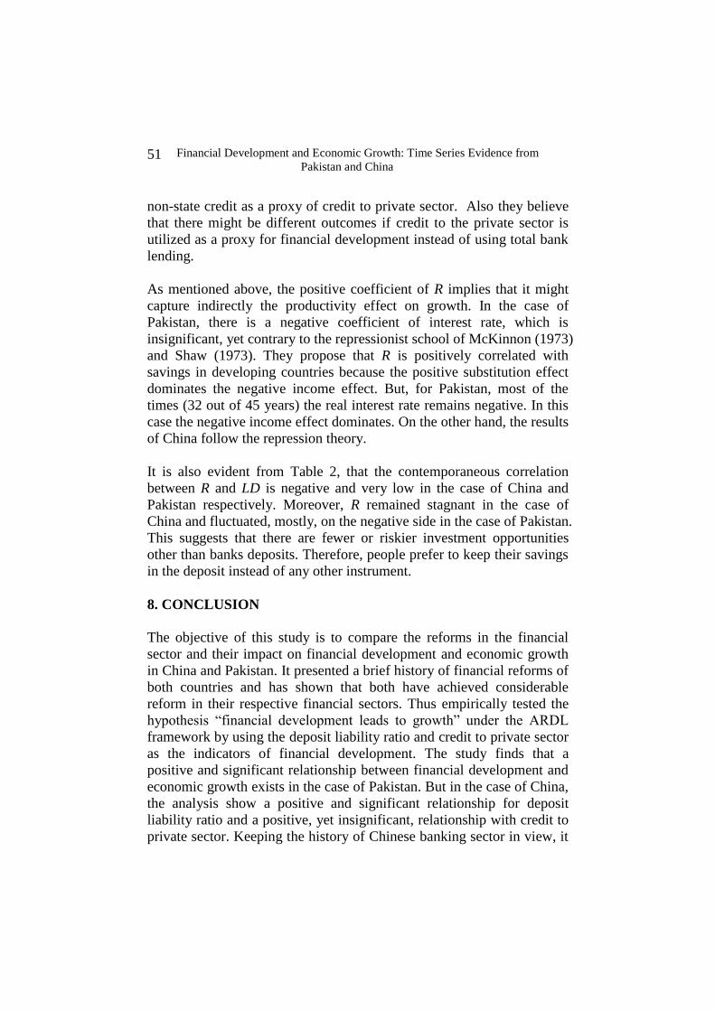
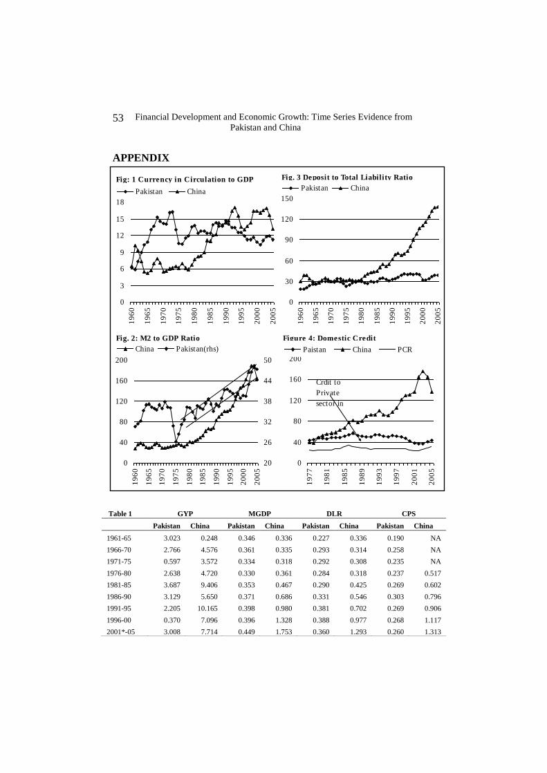
4.1. Chart Analysis

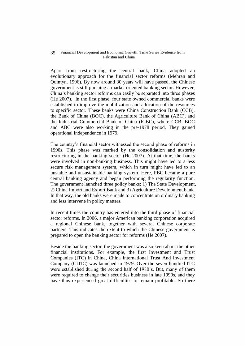
The apparent objective of this section is to show how financial sector

has developed in both countries after the reforms period. The study

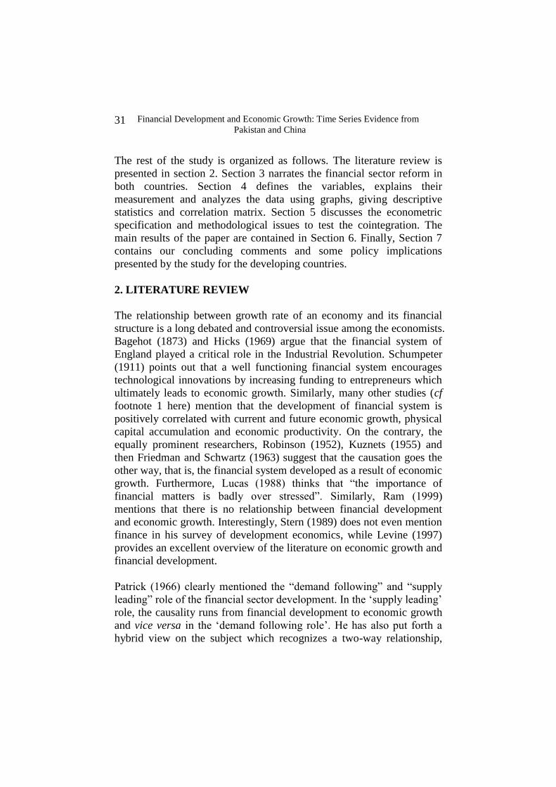
utilizes four ratios to purse the mentioned objective. These are ratio to

currency in circulation to GDP (CC), ratio to M2 to GDP (MGDP), ratio

to deposit liabilities to GDP (DLR) and domestic credit by the banking

sector to GDP (BSC).

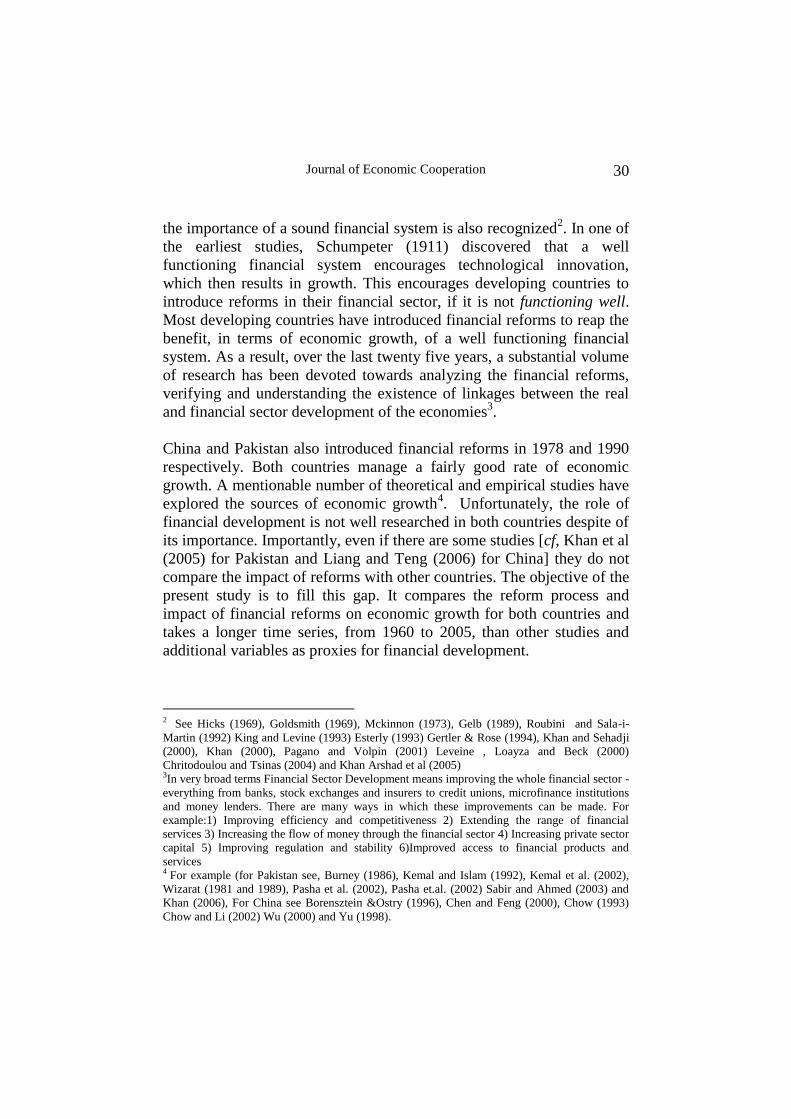
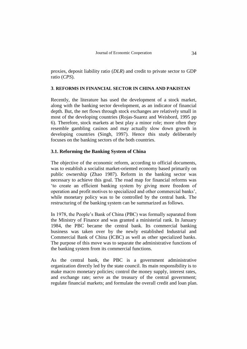
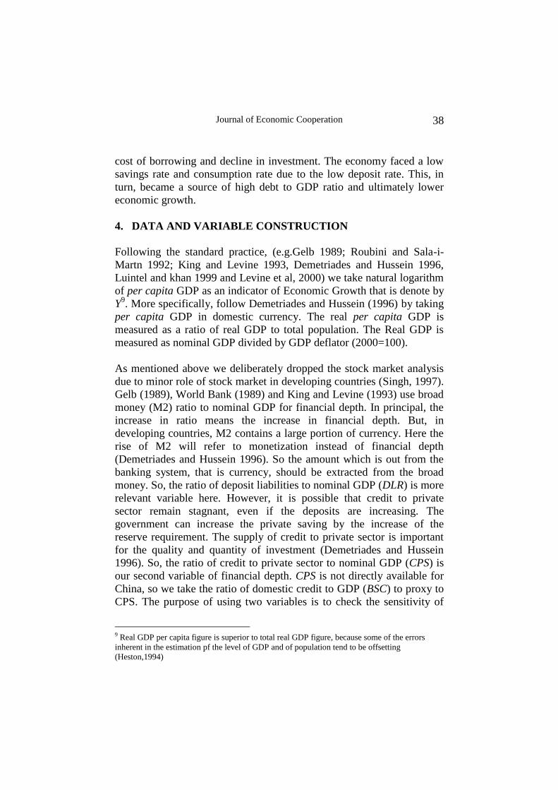
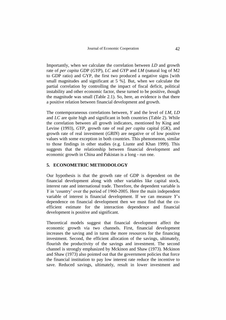
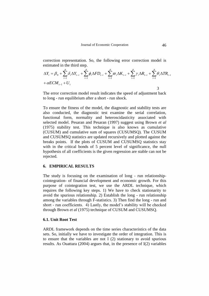
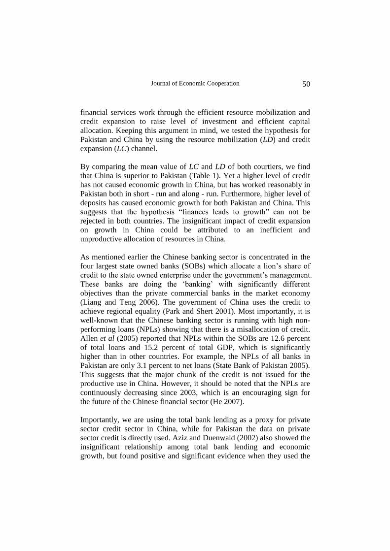
M2 to GDP ratio (MGDP) is one of the measures that are used for the

financial deepening. As evident from Figure: 2 the MGDP was, on

average, 30 percent from 1960 to 1977 in China. Importantly, it was

stagnant if we ignore the cyclical fluctuations. It was 32 percent in the

start of financial sector reforms and reached to 164 percent till the end of


40

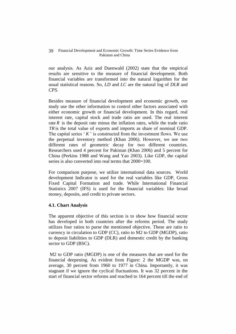
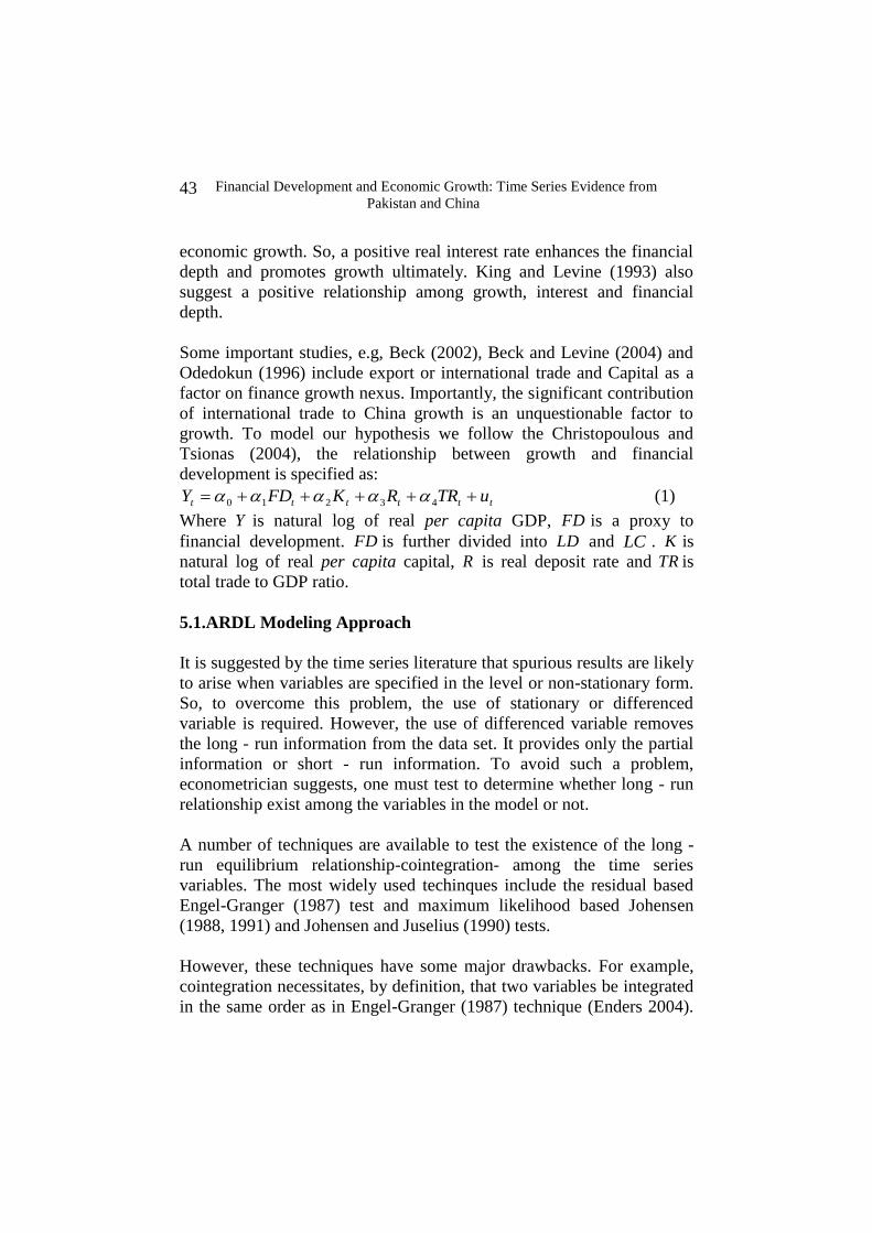
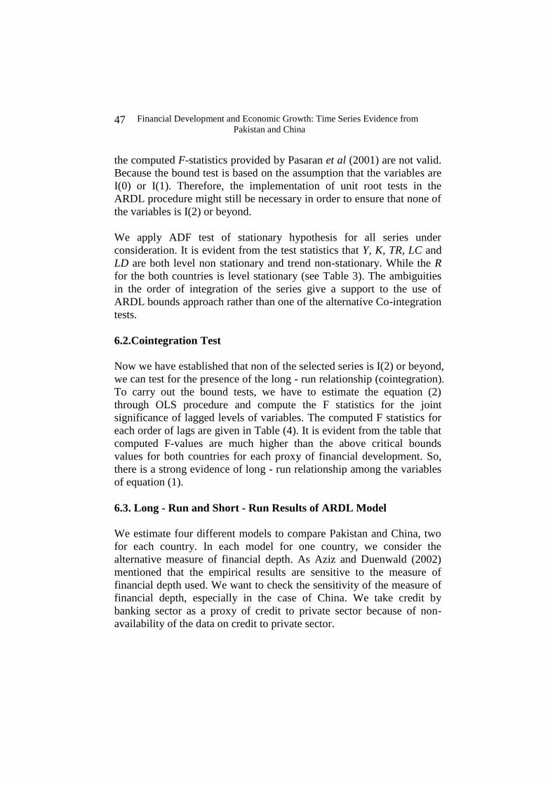
2005. That means, there is five and a half times bigger than 1978. While

CC ratio was about 6 percent, on average, in the pre reform era and

reached to 13 percent at the end of 2005 in China (Figure 1). That is the

highest one amongst the world. However, in Pakistan, CC ratio dropped

significantly. MGDP ratio remained volatile within an increasing band

in the post reform era that is from 1990 (Figure 1 and Figure 2). But CC

ratio is still more than 10 percent of the GDP.

What does that imply? The higher CC shows that the people of China

and Pakistan are tend to using cash in their payment and there are not

many financial services and instruments available, specially for the

payment. While the trend of MGDP is same the implication is different.

M2 consists of CC and other services like deposit, travelers cheques etc.

The increase in MGDP implies that the financial sector is getting

stronger and stronger.

Here again the level and growth rate of MGDP China is much higher

than Pakistan. Importantly, the speed of MGDP is much higher than CC

ratio in China. And, in the case of Pakistan, it is much fluctuating in an

increasing band. Thus, so far, it can be safely concluded that the

financial sector reform has done a good job in both countries.

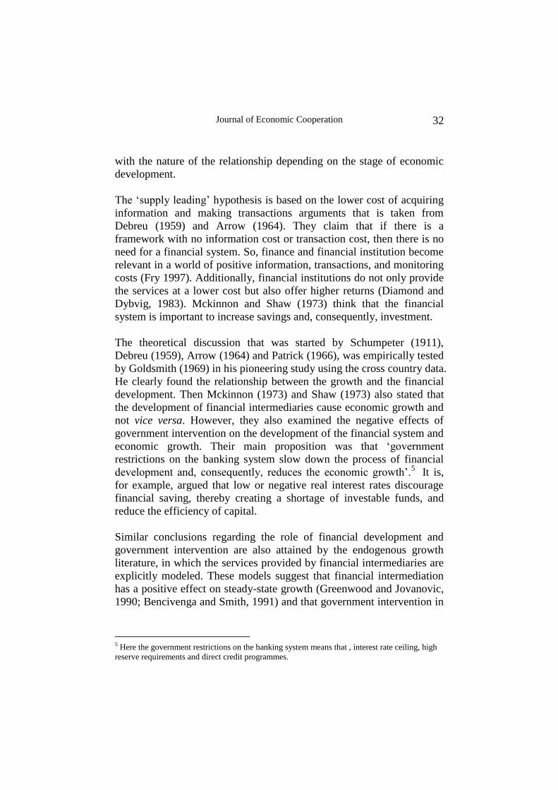
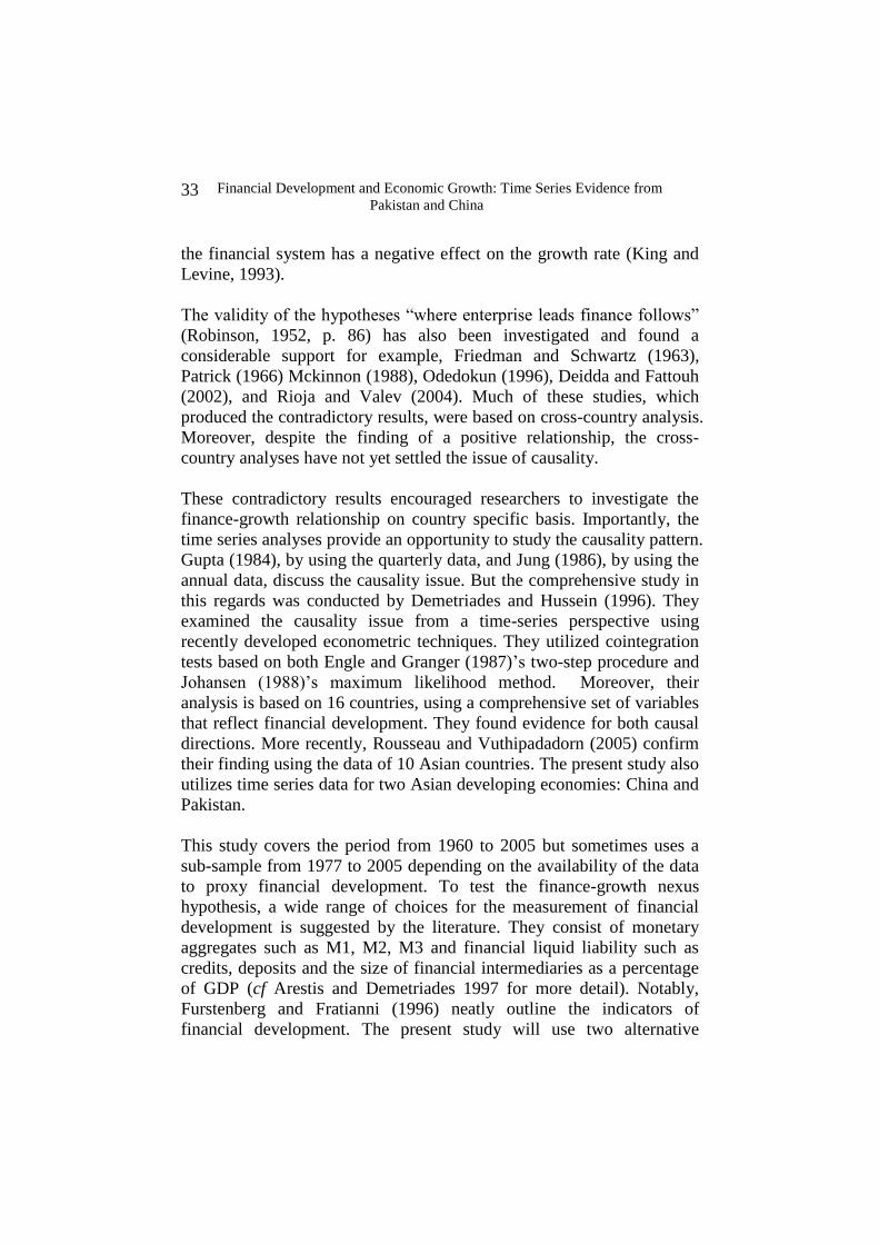
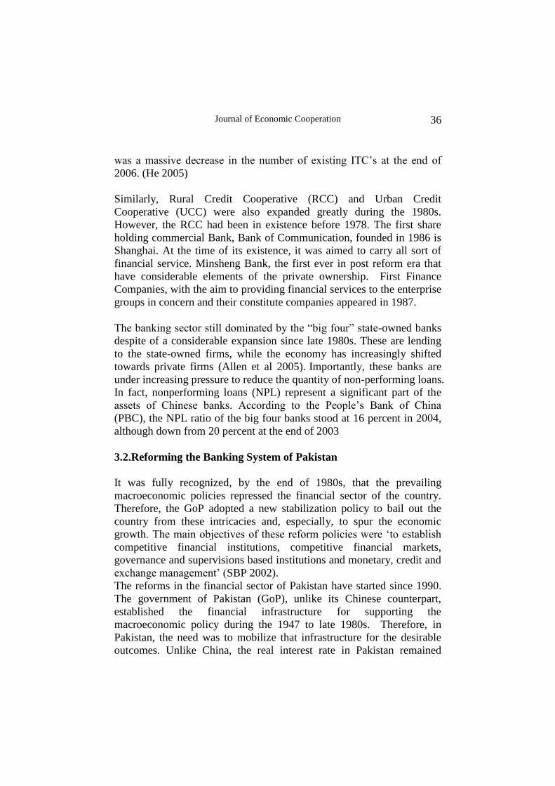
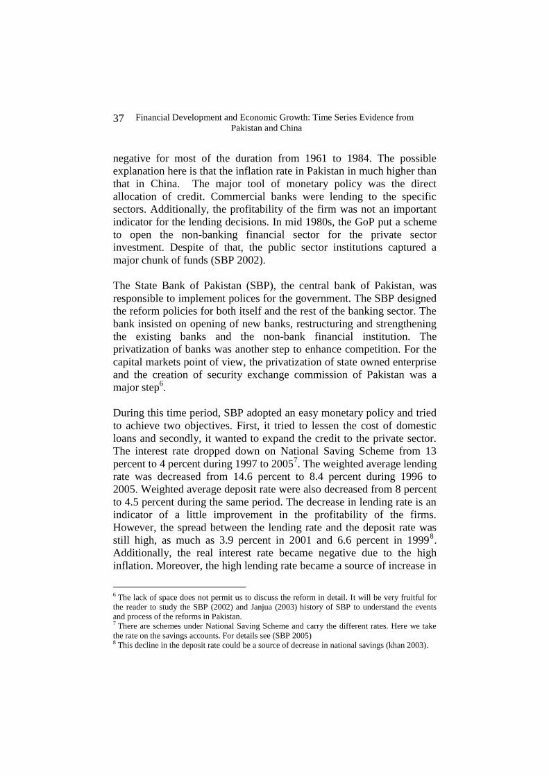
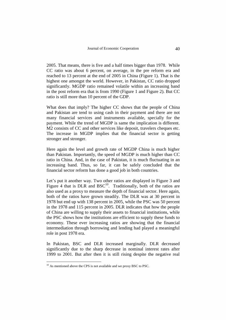
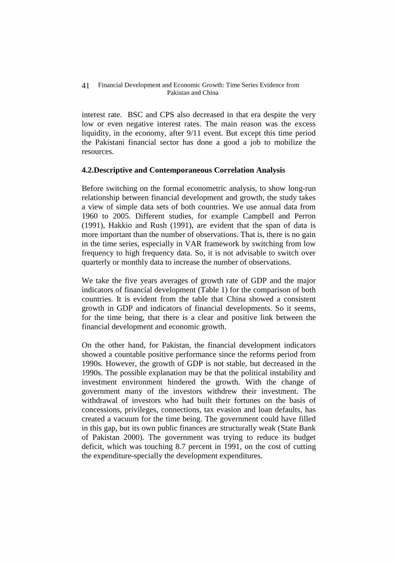
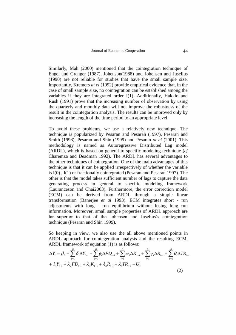
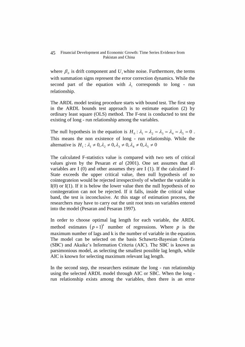
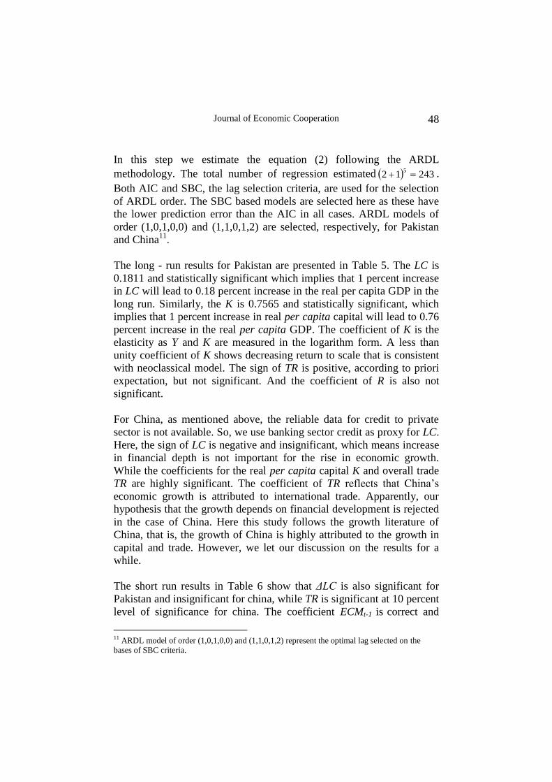
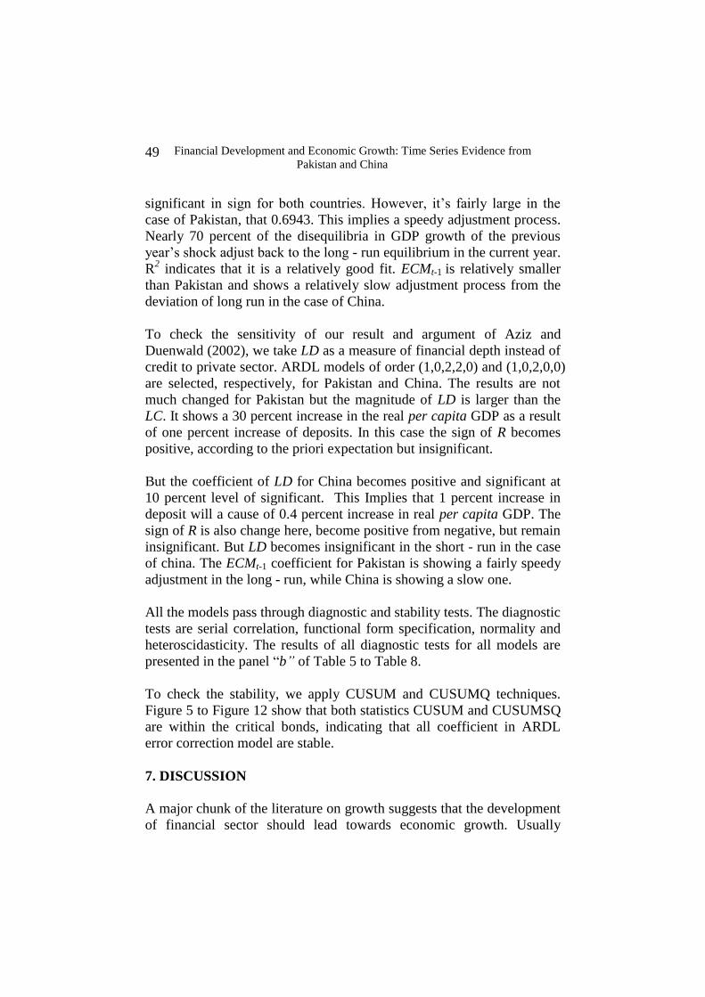
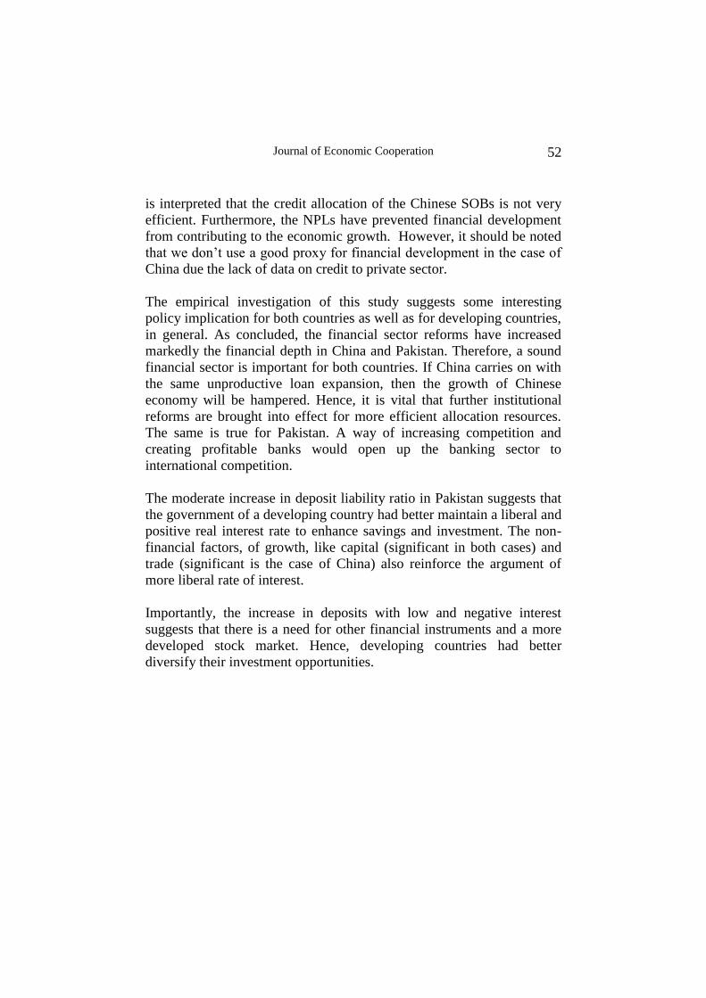
Let‟s put it another way. Two other ratios are displayed in Figure 3 and

Figure 4 that is DLR and BSC10

. Traditionally, both of the ratios are

also used as a proxy to measure the depth of financial sector. Here again,

both of the ratios have grown steadily. The DLR was at 30 percent in

1978 but end up with 138 percent in 2005, while the PSC was 50 percent

in the 1978 and 115 percent in 2005. DLR indicates that how the people

of China are willing to supply their assets to financial institutions, while

the PSC shows how the institutions are efficient to supply these funds to

economy. These ever increasing ratios are showing that the financial

intermediation through borrowing and lending had played a meaningful

role in post 1978 era.

In Pakistan, BSC and DLR increased marginally. DLR decreased

significantly due to the sharp decrease in nominal interest rates after

1999 to 2001. But after then it is still rising despite the negative real

10 As mentioned above the CPS is not available and we proxy BSC to PSC.


Pakistan and China

41

interest rate. BSC and CPS also decreased in that era despite the very

low or even negative interest rates. The main reason was the excess

liquidity, in the economy, after 9/11 event. But except this time period

the Pakistani financial sector has done a good a job to mobilize the

resources.

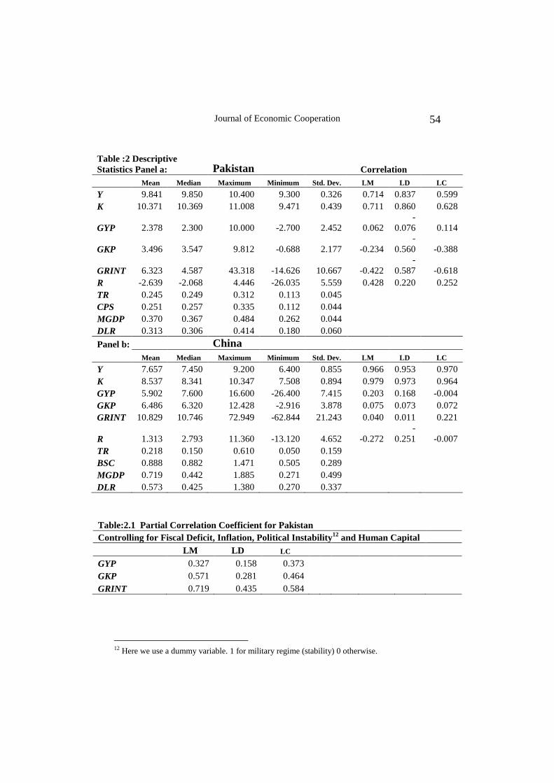
4.2.Descriptive and Contemporaneous Correlation Analysis

Before switching on the formal econometric analysis, to show long-run

relationship between financial development and growth, the study takes

a view of simple data sets of both countries. We use annual data from

1960 to 2005. Different studies, for example Campbell and Perron

(1991), Hakkio and Rush (1991), are evident that the span of data is

more important than the number of observations. That is, there is no gain

in the time series, especially in VAR framework by switching from low

frequency to high frequency data. So, it is not advisable to switch over

quarterly or monthly data to increase the number of observations.

We take the five years averages of growth rate of GDP and the major

indicators of financial development (Table 1) for the comparison of both

countries. It is evident from the table that China showed a consistent

growth in GDP and indicators of financial developments. So it seems,

for the time being, that there is a clear and positive link between the

financial development and economic growth.

On the other hand, for Pakistan, the financial development indicators

showed a countable positive performance since the reforms period from

1990s. However, the growth of GDP is not stable, but decreased in the

1990s. The possible explanation may be that the political instability and

investment environment hindered the growth. With the change of

government many of the investors withdrew their investment. The

withdrawal of investors who had built their fortunes on the basis of

concessions, privileges, connections, tax evasion and loan defaults, has

created a vacuum for the time being. The government could have filled

in this gap, but its own public finances are structurally weak (State Bank

of Pakistan 2000). The government was trying to reduce its budget

deficit, which was touching 8.7 percent in 1991, on the cost of cutting

the expenditure-specially the development expenditures.


42

Importantly, when we calculate the correlation between LD and growth

rate of per capita GDP (GYP), LC and GYP and LM (natural log of M2

to GDP ratio) and GYP, the first two produced a negative signs [with

small magnitudes and significant at 5 %]. But, when we calculate the

partial correlation by controlling the impact of fiscal deficit, political

instability and other economic factor, these turned to be positive, though

the magnitude was small (Table 2.1). So, here, an evidence is that there

a positive relation between financial development and growth.

The contemporaneous correlations between, Y and the level of LM, LD

and LC are quite high and significant in both countries (Table 2). While

the correlation between all growth indicators, mentioned by King and

Levine (1993), GYP, growth rate of real per capita capital (GK), and

growth rate of real investment (GRIN) are negative or of low positive

values with some exception in both countries. This phenomenon, similar

to those findings in other studies (e.g. Liunte and Khan 1999). This

suggests that the relationship between financial development and

economic growth in China and Pakistan is a long - run one.

5. ECONOMETRIC METHODOLOGY

Our hypothesis is that the growth rate of GDP is dependent on the

financial development along with other variables like capital stock,

interest rate and international trade. Therefore, the dependent variable is

Y in „country‟ over the period of 1960-2005. Here the main independent

variable of interest is financial development. If we can measure Y‟s

dependence on financial development then we must find that the co-

efficient estimate for the interaction dependence and financial

development is positive and significant.

Theoretical models suggest that financial development affect the

economic growth via two channels. First, financial development

increases the saving and in turns the more resources for the financing

investment. Second, the efficient allocation of the savings, ultimately,

flourish the productivity of the savings and investment. The second

channel is strongly emphasized by Mckinon and Shaw (1973). Mckinon

and Shaw (1973) also pointed out that the government policies that force

the financial institution to pay low interest rate reduce the incentive to

save. Reduced savings, ultimately, result in lower investment and


Pakistan and China

43

economic growth. So, a positive real interest rate enhances the financial

depth and promotes growth ultimately. King and Levine (1993) also

suggest a positive relationship among growth, interest and financial

depth.

Some important studies, e.g, Beck (2002), Beck and Levine (2004) and

Odedokun (1996) include export or international trade and Capital as a

factor on finance growth nexus. Importantly, the significant contribution

of international trade to China growth is an unquestionable factor to

growth. To model our hypothesis we follow the Christopoulous and

Tsionas (2004), the relationship between growth and financial

development is specified as:

tttttt uTRRKFDY 43210 (1)

Where Y is natural log of real per capita GDP, FD is a proxy to

financial development. FD is further divided into LD and LC . K is

natural log of real per capita capital, R is real deposit rate and TR is

total trade to GDP ratio.

5.1.ARDL Modeling Approach

It is suggested by the time series literature that spurious results are likely

to arise when variables are specified in the level or non-stationary form.

So, to overcome this problem, the use of stationary or differenced

variable is required. However, the use of differenced variable removes

the long - run information from the data set. It provides only the partial

information or short - run information. To avoid such a problem,

econometrician suggests, one must test to determine whether long - run

relationship exist among the variables in the model or not.

A number of techniques are available to test the existence of the long -

run equilibrium relationship-cointegration- among the time series

variables. The most widely used techinques include the residual based

Engel-Granger (1987) test and maximum likelihood based Johensen

(1988, 1991) and Johensen and Juselius (1990) tests.

However, these techniques have some major drawbacks. For example,

cointegration necessitates, by definition, that two variables be integrated

in the same order as in Engel-Granger (1987) technique (Enders 2004).


44

Similarly, Mah (2000) mentioned that the cointegration technique of

Engel and Granger (1987), Johenson(1988) and Johensen and Juselius

(1990) are not reliable for studies that have the small sample size.

Importantly, Kremers at el (1992) provide empirical evidence that, in the

case of small sample size, no cointegration can be established among the

variables if they are integrated order I(1). Additionally, Hakkio and

Rush (1991) prove that the increasing number of observation by using

the quarterly and monthly data will not improve the robustness of the

result in the cointegartion analysis. The results can be improved only by

increasing the length of the time period to an appropriate level.

To avoid these problems, we use a relatively new technique. The

technique is popularized by Pesaran and Pesaran (1997), Pesaran and

Smith (1998), Pesaran and Shin (1999) and Pesaran at el (2001). This

methodology is named as Autoregressive Distributed Lag model

(ARDL), which is based on general to specific modeling technique (cf

Charemza and Deadman 1992). The ARDL has several advantages to

the other techniques of cointegration. One of the main advantages of this

technique is that it can be applied irrespectively of whether the variable

is I(0) , I(1) or fractionally cointegrated (Pesaran and Pesaran 1997). The

other is that the model takes sufficient number of lags to capture the data

generating process in general to specific modeling framework

(Lauranceson and Chai2003). Furthermore, the error correction model

(ECM) can be derived from ARDL through a simple linear

transformation (Banerjee et al 1993). ECM integrates short - run

adjustments with long - run equilibrium without losing long run

information. Moreover, small sample properties of ARDL approach are

far superior to that of the Johensen and Juselius‟s cointegration

technique (Pesaran and Shin 1999).

So keeping in view, we also use the all above mentioned points in

ARDL approach for cointegeration analysis and the resulting ECM.

ARDL framework of equation (1) is as follows:

tttttt

p

i

iti

p

i

iti

p

i

iti

p

i

iti

p

i

itii

UTRRKFDY

TRRKFDYY

1514131211

11111

0

(2)


Pakistan and China

45

where 0 is drift component and tU white noise. Furthermore, the terms

with summation signs represent the error correction dynamics. While the

second part of the equation with i corresponds to long - run

relationship.

The ARDL model testing procedure starts with bound test. The first step

in the ARDL bounds test approach is to estimate equation (2) by

ordinary least square (OLS) method. The F-test is conducted to test the

existing of long - run relationship among the variables.

The null hypothesis in the equation is :0H 054321 .

This means the non existence of long - run relationship. While the

alternative is :1H 0,0,0,0,0 54321

The calculated F-statistics value is compared with two sets of critical

values given by the Pesaran et al (2001). One set assumes that all

variables are I (0) and other assumes they are I (1). If the calculated F-

State exceeds the upper critical value, then null hypothesis of no

cointegrateion would be rejected irrespectively of whether the variable is

I(0) or I(1). If it is below the lower value then the null hypothesis of no

conitegeration can not be rejected. If it falls, inside the critical value

band, the test is inconclusive. At this stage of estimation process, the

researchers may have to carry out the unit root tests on variables entered

into the model (Pesaran and Pesaran 1997).

In order to choose optimal lag length for each variable, the ARDL

method estimates kp 1 number of regressions. Where p is the

maximum number of lags and k is the number of variable in the equation.

The model can be selected on the basis Schawrtz-Bayesian Criteria

(SBC) and Akaike‟s Information Criteria (AIC). The SBC is known as

parsimonious model, as selecting the smallest possible lag length, while

AIC is known for selecting maximum relevant lag length.

In the second step, the researchers estimate the long - run relationship

using the selected ARDL model through AIC or SBC. When the long -

run relationship exists among the variables, then there is an error


46

correction representation. So, the following error correction model is

estimated in the third step.

tt

p

i

iti

p

i

iti

p

i

iti

p

i

iti

p

i

itii

UECM

TRRKFDYY

1

11111

0

3

The error correction model result indicates the speed of adjustment back

to long - run equilibrium after a short - run shock.

To ensure the fitness of the model, the diagnostic and stability tests are

also conducted, the diagnostic test examine the serial correlation,

functional form, normality and heteroscidasticity associated with

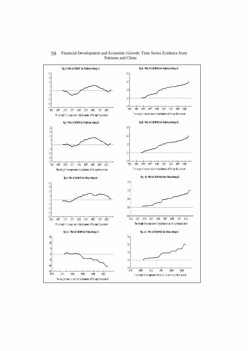
selected model. Pesaran and Pesaran (1997) suggest using Brown et al

(1975) stability test. This technique is also knows as cumulative

(CUSUM) and cumulative sum of squares (CUSUMSQ). The CUSUM

and CUSUMSQ statistics are updated recursively and plotted against the

breaks points. If the plots of CUSUM and CUSUMSQ statistics stay

with in the critical bonds of 5 percent level of significance, the null

hypothesis of all coefficients is the given regression are stable can not be

rejected.

6. EMPIRICAL RESULTS

The study is focusing on the examination of long - run relationship-

cointegration- of financial development and economic growth. For this

purpose of cointegration test, we use the ARDL technique, which

requires the following key steps. 1) We have to check stationarity to

avoid the spurious relationship. 2) Establish the long - run relationship

among the variables through F-statistics. 3) Then find the long - run and

short - run coefficients. 4) Lastly, the model‟s stability will be checked

through Brown et al (1975) technique of CUSUM and CUSUMSQ.

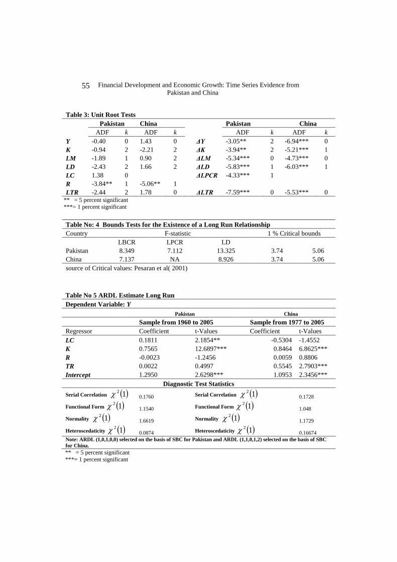
6.1. Unit Root Test

ARDL framework depends on the time series characteristics of the data

sets. So, initially we have to investigate the order of integration. This is

to ensure that the variables are not I (2) stationary to avoid spurious

results. As Ouattara (2004) argues that, in the presence of I(2) variables


Pakistan and China

47

the computed F-statistics provided by Pasaran et al (2001) are not valid.

Because the bound test is based on the assumption that the variables are

I(0) or I(1). Therefore, the implementation of unit root tests in the

ARDL procedure might still be necessary in order to ensure that none of

the variables is I(2) or beyond.

We apply ADF test of stationary hypothesis for all series under

consideration. It is evident from the test statistics that Y, K, TR, LC and

LD are both level non stationary and trend non-stationary. While the R

for the both countries is level stationary (see Table 3). The ambiguities

in the order of integration of the series give a support to the use of

ARDL bounds approach rather than one of the alternative Co-integration

tests.

6.2.Cointegration Test

Now we have established that non of the selected series is I(2) or beyond,

we can test for the presence of the long - run relationship (cointegration).

To carry out the bound tests, we have to estimate the equation (2)

through OLS procedure and compute the F statistics for the joint

significance of lagged levels of variables. The computed F statistics for

each order of lags are given in Table (4). It is evident from the table that

computed F-values are much higher than the above critical bounds

values for both countries for each proxy of financial development. So,

there is a strong evidence of long - run relationship among the variables

of equation (1).

6.3. Long - Run and Short - Run Results of ARDL Model

We estimate four different models to compare Pakistan and China, two

for each country. In each model for one country, we consider the

alternative measure of financial depth. As Aziz and Duenwald (2002)

mentioned that the empirical results are sensitive to the measure of

financial depth used. We want to check the sensitivity of the measure of

financial depth, especially in the case of China. We take credit by

banking sector as a proxy of credit to private sector because of non-

availability of the data on credit to private sector.


48

In this step we estimate the equation (2) following the ARDL

methodology. The total number of regression estimated 243125 .

Both AIC and SBC, the lag selection criteria, are used for the selection

of ARDL order. The SBC based models are selected here as these have

the lower prediction error than the AIC in all cases. ARDL models of

order (1,0,1,0,0) and (1,1,0,1,2) are selected, respectively, for Pakistan

and China11

.

The long - run results for Pakistan are presented in Table 5. The LC is

0.1811 and statistically significant which implies that 1 percent increase

in LC will lead to 0.18 percent increase in the real per capita GDP in the

long run. Similarly, the K is 0.7565 and statistically significant, which

implies that 1 percent increase in real per capita capital will lead to 0.76

percent increase in the real per capita GDP. The coefficient of K is the

elasticity as Y and K are measured in the logarithm form. A less than

unity coefficient of K shows decreasing return to scale that is consistent

with neoclassical model. The sign of TR is positive, according to priori

expectation, but not significant. And the coefficient of R is also not

significant.

For China, as mentioned above, the reliable data for credit to private

sector is not available. So, we use banking sector credit as proxy for LC.

Here, the sign of LC is negative and insignificant, which means increase

in financial depth is not important for the rise in economic growth.

While the coefficients for the real per capita capital K and overall trade

TR are highly significant. The coefficient of TR reflects that China‟s

economic growth is attributed to international trade. Apparently, our

hypothesis that the growth depends on financial development is rejected

in the case of China. Here this study follows the growth literature of

China, that is, the growth of China is highly attributed to the growth in

capital and trade. However, we let our discussion on the results for a

while.

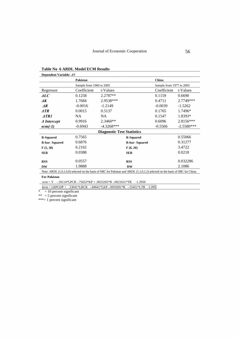
The short run results in Table 6 show that ΔLC is also significant for

Pakistan and insignificant for china, while TR is significant at 10 percent

level of significance for china. The coefficient ECMt-1 is correct and

11 ARDL model of order (1,0,1,0,0) and (1,1,0,1,2) represent the optimal lag selected on the

bases of SBC criteria.


Pakistan and China

49

significant in sign for both countries. However, it‟s fairly large in the

case of Pakistan, that 0.6943. This implies a speedy adjustment process.

Nearly 70 percent of the disequilibria in GDP growth of the previous

year‟s shock adjust back to the long - run equilibrium in the current year.

R2 indicates that it is a relatively good fit. ECMt-1 is relatively smaller

than Pakistan and shows a relatively slow adjustment process from the

deviation of long run in the case of China.

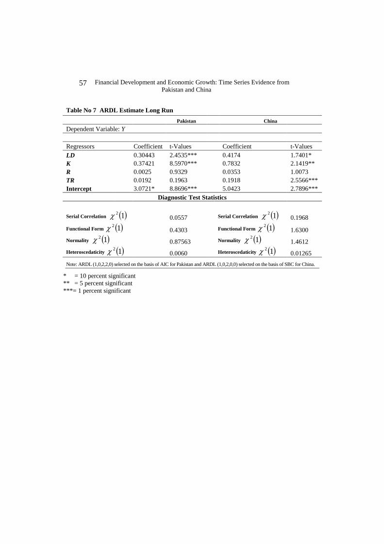
To check the sensitivity of our result and argument of Aziz and

Duenwald (2002), we take LD as a measure of financial depth instead of

credit to private sector. ARDL models of order (1,0,2,2,0) and (1,0,2,0,0)

are selected, respectively, for Pakistan and China. The results are not

much changed for Pakistan but the magnitude of LD is larger than the

LC. It shows a 30 percent increase in the real per capita GDP as a result

of one percent increase of deposits. In this case the sign of R becomes

positive, according to the priori expectation but insignificant.

But the coefficient of LD for China becomes positive and significant at

10 percent level of significant. This Implies that 1 percent increase in

deposit will a cause of 0.4 percent increase in real per capita GDP. The

sign of R is also change here, become positive from negative, but remain

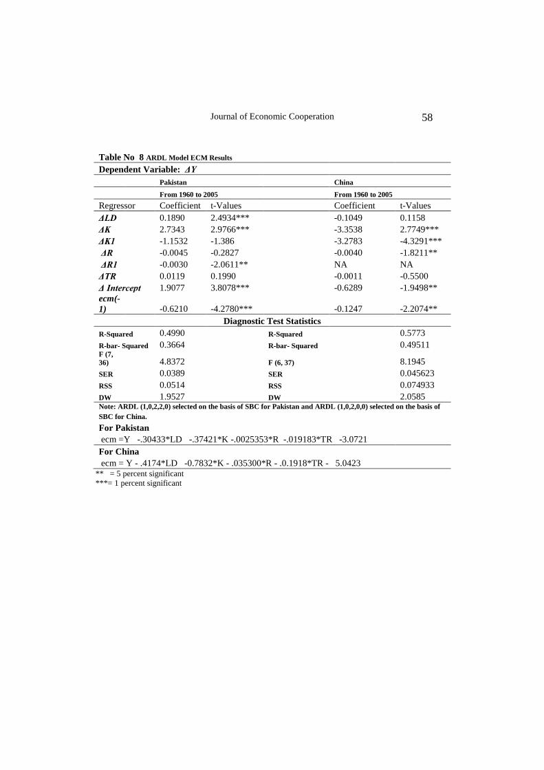
insignificant. But LD becomes insignificant in the short - run in the case

of china. The ECMt-1 coefficient for Pakistan is showing a fairly speedy

adjustment in the long - run, while China is showing a slow one.

All the models pass through diagnostic and stability tests. The diagnostic

tests are serial correlation, functional form specification, normality and

heteroscidasticity. The results of all diagnostic tests for all models are

presented in the panel “b” of Table 5 to Table 8.

To check the stability, we apply CUSUM and CUSUMQ techniques.

Figure 5 to Figure 12 show that both statistics CUSUM and CUSUMSQ

are within the critical bonds, indicating that all coefficient in ARDL

error correction model are stable.

7. DISCUSSION

A major chunk of the literature on growth suggests that the development

of financial sector should lead towards economic growth. Usually


50

financial services work through the efficient resource mobilization and

credit expansion to raise level of investment and efficient capital

allocation. Keeping this argument in mind, we tested the hypothesis for

Pakistan and China by using the resource mobilization (LD) and credit

expansion (LC) channel.

By comparing the mean value of LC and LD of both courtiers, we find

that China is superior to Pakistan (Table 1). Yet a higher level of credit

has not caused economic growth in China, but has worked reasonably in

Pakistan both in short - run and along - run. Furthermore, higher level of

deposits has caused economic growth for both Pakistan and China. This

suggests that the hypothesis “finances leads to growth” can not be

rejected in both countries. The insignificant impact of credit expansion

on growth in China could be attributed to an inefficient and

unproductive allocation of resources in China.

As mentioned earlier the Chinese banking sector is concentrated in the

four largest state owned banks (SOBs) which allocate a lion‟s share of

credit to the state owned enterprise under the government‟s management.

These banks are doing the „banking‟ with significantly different

objectives than the private commercial banks in the market economy

(Liang and Teng 2006). The government of China uses the credit to

achieve regional equality (Park and Shert 2001). Most importantly, it is

well-known that the Chinese banking sector is running with high non-

performing loans (NPLs) showing that there is a misallocation of credit.

Allen et al (2005) reported that NPLs within the SOBs are 12.6 percent

of total loans and 15.2 percent of total GDP, which is significantly

higher than in other countries. For example, the NPLs of all banks in

Pakistan are only 3.1 percent to net loans (State Bank of Pakistan 2005).

This suggests that the major chunk of the credit is not issued for the

productive use in China. However, it should be noted that the NPLs are

continuously decreasing since 2003, which is an encouraging sign for

the future of the Chinese financial sector (He 2007).

Importantly, we are using the total bank lending as a proxy for private

sector credit sector in China, while for Pakistan the data on private

sector credit is directly used. Aziz and Duenwald (2002) also showed the

insignificant relationship among total bank lending and economic

growth, but found positive and significant evidence when they used the


Pakistan and China

51

non-state credit as a proxy of credit to private sector. Also they believe

that there might be different outcomes if credit to the private sector is

utilized as a proxy for financial development instead of using total bank

lending.

As mentioned above, the positive coefficient of R implies that it might

capture indirectly the productivity effect on growth. In the case of

Pakistan, there is a negative coefficient of interest rate, which is

insignificant, yet contrary to the repressionist school of McKinnon (1973)

and Shaw (1973). They propose that R is positively correlated with

savings in developing countries because the positive substitution effect

dominates the negative income effect. But, for Pakistan, most of the

times (32 out of 45 years) the real interest rate remains negative. In this

case the negative income effect dominates. On the other hand, the results

of China follow the repression theory.

It is also evident from Table 2, that the contemporaneous correlation

between R and LD is negative and very low in the case of China and

Pakistan respectively. Moreover, R remained stagnant in the case of

China and fluctuated, mostly, on the negative side in the case of Pakistan.

This suggests that there are fewer or riskier investment opportunities

other than banks deposits. Therefore, people prefer to keep their savings

in the deposit instead of any other instrument.

8. CONCLUSION

The objective of this study is to compare the reforms in the financial

sector and their impact on financial development and economic growth

in China and Pakistan. It presented a brief history of financial reforms of

both countries and has shown that both have achieved considerable

reform in their respective financial sectors. Thus empirically tested the

hypothesis “financial development leads to growth” under the ARDL

framework by using the deposit liability ratio and credit to private sector

as the indicators of financial development. The study finds that a

positive and significant relationship between financial development and

economic growth exists in the case of Pakistan. But in the case of China,

the analysis show a positive and significant relationship for deposit

liability ratio and a positive, yet insignificant, relationship with credit to

private sector. Keeping the history of Chinese banking sector in view, it


52

is interpreted that the credit allocation of the Chinese SOBs is not very

efficient. Furthermore, the NPLs have prevented financial development

from contributing to the economic growth. However, it should be noted

that we don‟t use a good proxy for financial development in the case of

China due the lack of data on credit to private sector.

The empirical investigation of this study suggests some interesting

policy implication for both countries as well as for developing countries,

in general. As concluded, the financial sector reforms have increased

markedly the financial depth in China and Pakistan. Therefore, a sound

financial sector is important for both countries. If China carries on with

the same unproductive loan expansion, then the growth of Chinese

economy will be hampered. Hence, it is vital that further institutional

reforms are brought into effect for more efficient allocation resources.

The same is true for Pakistan. A way of increasing competition and

creating profitable banks would open up the banking sector to

international competition.

The moderate increase in deposit liability ratio in Pakistan suggests that

the government of a developing country had better maintain a liberal and

positive real interest rate to enhance savings and investment. The non-

financial factors, of growth, like capital (significant in both cases) and

trade (significant is the case of China) also reinforce the argument of

more liberal rate of interest.

Importantly, the increase in deposits with low and negative interest

suggests that there is a need for other financial instruments and a more

developed stock market. Hence, developing countries had better

diversify their investment opportunities.


Pakistan and China

53

0

30

60

90

120

150

19

60

19

65

19

70

19

75

19

80

19

85

19

90

19

95

20

00

20

05

Pakistan China

Fig. 3 Deposit to Total Liability Ratio

0

40

80

120

160

200

19

60

19

65

19

70

19

75

19

80

19

85

19

90

19

95

20

00

20

05

20

26

32

38

44

50

China Pakistan(rhs)

Fig. 2: M2 to GDP Ratio

0

3

6

9

12

15

18

19

60

19

65

19

70

19

75

19

80

19

85

19

90

19

95

20

00

20

05

Pakistan China

Fig: 1 Currency in Circulation to GDP

0

40

80

120

160

200

19

77

19

81

19

85

19

89

19

93

19

97

20

01

20

05

Paistan China PCR

Figure 4: Domestic Credit

Crdit to

Private

sector in

APPENDIX

Table 1 GYP MGDP DLR CPS

Pakistan China Pakistan China Pakistan China Pakistan China

1961-65 3.023 0.248 0.346 0.336 0.227 0.336 0.190 NA

1966-70 2.766 4.576 0.361 0.335 0.293 0.314 0.258 NA

1971-75 0.597 3.572 0.334 0.318 0.292 0.308 0.235 NA

1976-80 2.638 4.720 0.330 0.361 0.284 0.318 0.237 0.517

1981-85 3.687 9.406 0.353 0.467 0.290 0.425 0.269 0.602

1986-90 3.129 5.650 0.371 0.686 0.331 0.546 0.303 0.796

1991-95 2.205 10.165 0.398 0.980 0.381 0.702 0.269 0.906

1996-00 0.370 7.096 0.396 1.328 0.388 0.977 0.268 1.117

2001*-05 3.008 7.714 0.449 1.753 0.360 1.293 0.260 1.313


54

Table :2 Descriptive

Statistics Panel a: Pakistan Correlation

Mean Median Maximum Minimum Std. Dev. LM LD LC

Y 9.841 9.850 10.400 9.300 0.326 0.714 0.837 0.599

K 10.371 10.369 11.008 9.471 0.439 0.711 0.860 0.628

GYP 2.378 2.300 10.000 -2.700 2.452 0.062

-

0.076 0.114

GKP 3.496 3.547 9.812 -0.688 2.177 -0.234

-

0.560 -0.388

GRINT 6.323 4.587 43.318 -14.626 10.667 -0.422

-

0.587 -0.618

R -2.639 -2.068 4.446 -26.035 5.559 0.428 0.220 0.252

TR 0.245 0.249 0.312 0.113 0.045

CPS 0.251 0.257 0.335 0.112 0.044

MGDP 0.370 0.367 0.484 0.262 0.044

DLR 0.313 0.306 0.414 0.180 0.060

Panel b: China

Mean Median Maximum Minimum Std. Dev. LM LD LC

Y 7.657 7.450 9.200 6.400 0.855 0.966 0.953 0.970

K 8.537 8.341 10.347 7.508 0.894 0.979 0.973 0.964

GYP 5.902 7.600 16.600 -26.400 7.415 0.203 0.168 -0.004

GKP 6.486 6.320 12.428 -2.916 3.878 0.075 0.073 0.072

GRINT 10.829 10.746 72.949 -62.844 21.243 0.040 0.011 0.221

R 1.313 2.793 11.360 -13.120 4.652 -0.272

-

0.251 -0.007

TR 0.218 0.150 0.610 0.050 0.159

BSC 0.888 0.882 1.471 0.505 0.289

MGDP 0.719 0.442 1.885 0.271 0.499

DLR 0.573 0.425 1.380 0.270 0.337

Table:2.1 Partial Correlation Coefficient for Pakistan

Controlling for Fiscal Deficit, Inflation, Political Instability12

and Human Capital

LM LD LC

GYP 0.327 0.158 0.373

GKP 0.571 0.281 0.464

GRINT 0.719 0.435 0.584

12 Here we use a dummy variable. 1 for military regime (stability) 0 otherwise.


Pakistan and China

55

Table 3: Unit Root Tests

Pakistan China Pakistan China

ADF k ADF k ADF k ADF k

Y -0.40 0 1.43 0 ΔY -3.05** 2 -6.94*** 0

K -0.94 2 -2.21 2 ΔK -3.94** 2 -5.21*** 1

LM -1.89 1 0.90 2 ΔLM -5.34*** 0 -4.73*** 0

LD -2.43 2 1.66 2 ΔLD -5.83*** 1 -6.03*** 1

LC 1.38 0 ΔLPCR -4.33*** 1

R -3.84** 1 -5.06** 1

LTR -2.44 2 1.78 0 ΔLTR -7.59*** 0 -5.53*** 0 ** = 5 percent significant

***= 1 percent significant

Table No: 4 Bounds Tests for the Existence of a Long Run Relationship

Country F-statistic 1 % Critical bounds

LBCR LPCR LD

Pakistan 8.349 7.112 13.325 3.74 5.06

China 7.137 NA 8.926 3.74 5.06

source of Critical values: Pesaran et al( 2001)

Table No 5 ARDL Estimate Long Run

Dependent Variable: Y

Pakistan China

Sample from 1960 to 2005 Sample from 1977 to 2005

Regressor Coefficient t-Values Coefficient t-Values

LC 0.1811 2.1854** -0.5304 -1.4552

K 0.7565 12.6897*** 0.8464 6.8625***

R -0.0023 -1.2456 0.0059 0.8806

TR 0.0022 0.4997 0.5545 2.7903***

Intercept 1.2950 2.6298*** 1.0953 2.3456***

Diagnostic Test Statistics

Serial Correlation 12 0.1760 Serial Correlation 12 0.1728

Functional Form 12 1.1540 Functional Form 12 1.048

Normality 12 1.6619 Normality 12 1.1729

Heteroscedaticity 12 0.0874 Heteroscedaticity 12 0.16674

Note: ARDL (1,0,1,0,0) selected on the basis of SBC for Pakistan and ARDL (1,1,0,1,2) selected on the basis of SBC

for China.

** = 5 percent significant



56

Table No 6 ARDL Model ECM Results

Dependent Variable: ΔY

Pakistan China

Sample from 1960 to 2005 Sample from 1977 to 2005


ΔLC 0.1258 2.2787** 0.1159 0.6690

ΔK 1.7684 2.9538*** 0.4711 2.7749***

ΔR -0.0016 -1.2149 -0.0039 -1.5262

ΔTR 0.0015 0.5137 0.1765 1.7496*

ΔTR1 NA NA 0.1547 1.8393*

Δ Intercept 0.9916 2.3460** 0.6096 2.8156***

ecm(-1) -0.6943 -4.3268*** -0.5566 -2.5580***


R-Squared 0.7565 R-Squared 0.55066

R-bar- Squared 0.6876 R-bar- Squared 0.31277

F (5, 38) 6.2162 F (6, 20) 3.4722

SER 0.0388 SER 0.0218

RSS 0.0557 RSS 0.032286

DW 1.9888 DW 2.1086

Note: ARDL (1,0,1,0,0) selected on the basis of SBC for Pakistan and ARDL (1,1,0,1,2) selected on the basis of SBC for China.

For Pakistan

ecm = Y -.18114*LPCR -.75653*KP + .0023265*R -.0021631*TR -1.2950

ecm = LRPGDP + .53041*LBCR -.84641*LKP -.0059281*R -.55451*LTR -1.095

* = 10 percent significant




Pakistan and China

57

Table No 7 ARDL Estimate Long Run

Pakistan China

Dependent Variable: Y

Regressors Coefficient t-Values Coefficient t-Values

LD 0.30443 2.4535*** 0.4174 1.7401*

K 0.37421 8.5970*** 0.7832 2.1419**

R 0.0025 0.9329 0.0353 1.0073

TR 0.0192 0.1963 0.1918 2.5566***

Intercept 3.0721* 8.8696*** 5.0423 2.7896***


Serial Correlation 12 0.0557 Serial Correlation 12 0.1968

Functional Form 12 0.4303 Functional Form 12 1.6300

Normality 12 0.87563 Normality 12 1.4612

Heteroscedaticity 12 0.0060 Heteroscedaticity 12 0.01265

Note: ARDL (1,0,2,2,0) selected on the basis of AIC for Pakistan and ARDL (1,0,2,0,0) selected on the basis of SBC for China.

* = 10 percent significant




58

Table No 8 ARDL Model ECM Results

Dependent Variable: ΔY

Pakistan China

From 1960 to 2005 From 1960 to 2005


ΔLD 0.1890 2.4934*** -0.1049 0.1158

ΔK 2.7343 2.9766*** -3.3538 2.7749***

ΔK1 -1.1532 -1.386 -3.2783 -4.3291***

ΔR -0.0045 -0.2827 -0.0040 -1.8211**

ΔR1 -0.0030 -2.0611** NA NA

ΔTR 0.0119 0.1990 -0.0011 -0.5500

Δ Intercept 1.9077 3.8078*** -0.6289 -1.9498**

ecm(-

1) -0.6210 -4.2780*** -0.1247 -2.2074**


R-Squared 0.4990 R-Squared 0.5773

R-bar- Squared 0.3664 R-bar- Squared 0.49511 F (7,

36) 4.8372 F (6, 37) 8.1945

SER 0.0389 SER 0.045623

RSS 0.0514 RSS 0.074933

DW 1.9527 DW 2.0585 Note: ARDL (1,0,2,2,0) selected on the basis of SBC for Pakistan and ARDL (1,0,2,0,0) selected on the basis of

SBC for China.

For Pakistan

ecm =Y -.30433*LD -.37421*K -.0025353*R -.019183*TR -3.0721

For China

ecm = Y - .4174*LD -0.7832*K - .035300*R - .0.1918*TR - 5.0423 ** = 5 percent significant



Pakistan and China

59


60

REFERENCE

Allen, F., J. Qian, and M. Qian (2005) Law, Finance, and Economic

Growth in China. Journal of Financial Economics 77, 57–116. Arestis, P. and H.T. Demetriades (1997) Financial Development and

Economic Growth: Assessing the Evidence. Economic Journal 107,

109-121. Arrow, K.J (1964) The Role of Securities in the Optimal Allocation of

Risk Bearing. Review of Economic Studies 2, 91-96 Aziz, J. and C. Duenwald (2002) Growth-Financial Intermiation Nexus

in China,” IMF working Paper 02/194 (Washington: IMF) Bell, C. and P. L Rousseau (2001) Post-independence India: A case of

Finance-led Industrialization Journal of Development Economics 65,

153–175. Bagehot, W. (1873, 1962 edition) Lombard Street. Homewood IL:

Richard D. Irwin. Banerjee, A., J. Dolado, J.W. Galbraith and D.F. Hendry (1993) Co-

integration, Error-correction, and the Econometric Analysis of Non-

stationary Data Oxford University Press, Oxford. Bencivenga, V.R. and B. D. Smith (1991) Financial Intermediation and

Endogenous Growth. Review of Economic Studies 58, 195-209. Borensztein, E. and D. J. Ostry (1996) Accounting for China‟s Growth

Performance. American Economic Review 86, 224–228. Brown, R.L., J. Durbin, J. and J.M. Evans (1975) Techniques for Testing

the Constancy of Regression Relations Over Time. Journal of the Royal

Statistical Society 37, 149-163. Burney, N.A. (1986). „Sources of Pakistan‟s Economic Growth‟,

Pakistan Development Review 25, 573-589. Caldero´n, C. and L. Liu (2003) The Direction of Causality Between

Financial Development and Economic Growth. Journal of Development

Economics 72, 321–334.


Pakistan and China

61

Campbell, J. Y., and P. Perron (1991) Pitfalls and Opportunities: What

Macroeconomists Should Know about Unit roots. In O. J. Blanchard,

and S. Fisher (Eds.), NBER Macroeconomics Annual (pp. 141–201).

Cambridge, MA7 MIT Press. Charemza, W. W. and D. F. Deadman (1992) New Directions in

Econometric Practice: General to Specific Modelling, Cointegration

and Vector Autoregression. Aldershot, Edward Elgar. Chen, B. Z. and Y. Feng (2000) Determinants of Economic Growth in

China: Private Enterprise, Education, and Openness. China Economic

Review 11, 1– 15. Chow, G. C. (1993). Capital Formation and Economic Growth in China.

Quarterly Journal of Economics 108, 809–842. Chow, G. C. and K. W. Li (2002) China‟s Economic Growth: 1952–

2010. Economic Development and Cultural Change51, 247–256. Christopoulos, D. K. and E. G. Tsionas (2004) Financial Development

and Economic Growth: Evidence from Panel Unit Root and

Cointegration Tests. Journal of Development Economics 73, 55–74. Debreu G. (1959) Theory of Value, New York :Wiley Deidda, L., and B. Fattouh (2002) Non-linearity Between Finance and

Growth. Economics Letters 74, 339–345. Demetriades, P.O. and K.A. Hussein (1996) Does Financial

Development Cause Economic Growth? Time Series Evidence from 16

Countries Journal of development Economics 51, 387-411. Diamond, D. and P. Dybvig (1983) Bank Runs, Deposit Insurance and

Liquidity. Journal of Political Economy 91, 401–419. Easterly, W.(1993) How Much Do Distortions Affect Growth? Journal

of Monetary Economics.32, 187-212 Enders, W. (2004) Applied Econometric Time Series Second Edition

John Wiley & sons Inc. Engle, R. and C. Granger (1987) Cointegration and Error Correction

Representation: Estimation and Testing. Econometrica 55, 251-276.


62

Fase, M. and R. Abma (2003) Financial Environment and Economic

Growth in Selected Asian Countries. Journal of Asian Economic 14, 11

–21. Friedman, M. and A.J. Schwartz (1963) A Monetary History of the

United States, Princeton University Press, Princeton. Fry, M. J. (1997) In Favour of Financial Liberalisation. Economic

Journal 107, 754–770. Furstenbeg, G.V. and M. Fratranni (1996) Indicators of Financial

Development,, North American Journal of Economics and Finance 7,

19-29 Gelb, A.H. (1989) Financial Policies, Growth, and Efficiency, Policy

Planning, and Research Working Papers, No. 202 (World Bank). Goldsmith, R.W. (1969) Financial Structure and Development, Yale

University Press, New Haven. Greenwood, J., and B. Jovanovic (1990) Financial Development,

Growth, and the Distribution of Income. Journal of Political Economy

98, 1076– 1107. Gupta, K.L.(1984) Finance and Economic Growth in Developing

Countries Croom Helm, London. Hakkio, C.S. and M. Rush (1991) Cointegration: How Short is the Long-

run? Journal of International Money and Finance December, 571-581. He, L. (2005) Evolution of Financial Institutions in Post -1978 China:

Interaction between the State and Market China and World Economy 13,

10-26 He, L. (2007)"China's Banking Sector reform: A Critical Survey”, as

Chapter 8 in China’s Surging Economy: Adjusting for More Balanced

Development, edited by John Wong and Lin Shuanglin. New York,

London and Singapore: World Scientific Publishing Co. 2007 Heston, A. (1994). A Brief Review of Some Problems in Using National

Accounts Data in Level of Output Comparisons and Growth Studies.

Journal of Development Economics 44, 29–52. Hicks, J. (1969) A Theory of Economic History, Oxford, Claredon Press


Pakistan and China

63

Janjua, M. A. (2003). History of State Bank of Pakistan 1977-1988.

Karachi: State Bank of Pakistan. Johansen, S. (1988) Statistical Analysis of Cointegrating Vectors.

Journal of Economic Dynamics and Control .12, 231-254. Johansen, S. (1991). Estimation and Hypothesis Testing of

Cointegration Vectors in Gaussian Vector Autoregressive Models.

Econometrica 59, 1551–1580. Johansen, S. (1991) Estimation and Hypothesis Testing of Cointegration

Vectors in Gaussian Vector Autoregressive Models. Econometrica 59,

1551-1580 Johansen, S. and K. Juselius (1990) Maximum Likelihood Estimation

and Inference on Cointegration–with Application to the Demand for

Money, Oxford Bulletin of Economics and Statistics 52, 169-210. Jung, W.S. (1986) Financial Development and Economic Growth:

International Evidence. Economic Development and Cultural Change 34,

336-346. Kemal, A. R. and M. Islam (1992). “Report of the Sub-Committee on

Sources of Growth inPakistan”. The Report. Islamabad: Pakistan

Institute of Development Economics. Kemal, Muslehuddin and Usman Qadir(2002), Global Research Project:

Pakistan Country Report,Global Research Project Workshop, Dhaka Khan S. (2006) Macro Determninant of Total Factor productivity in

Pakistan. State Bank of Pakistan, Working paper No. 10. Khan, A., A. Qayyum and S. Sheikh (2005) Financcial Development

and Economics Growth: The Case of Pakistan. The Pakistan

Development Review 44, 819-837. Khan, S. M., and A. S. Senhadji (2000) Financial Development and

Economic Growth: An Overview. International Monetary Fund,

Washington, D. C. (IMF Working Paper 00/209.) King, R.G., and R. Levine (1993) Finance and Growth: Schumpeter

Might be Right. Quarterly Journal of Economics 108, 717-737.


64

Kremers, J.J.M., N.L. Ericsson and J. Dolado (1992) The Power of

Cointegration Tests, The Journal of Econometrics 52, 389-402. Kuznets, S. (1955) Economic Growth and Income Inequality. American

Economic Review 45, 1–28. Laurenceson, J, and C.H.. J Chai (2003) Financial Reform and

Economic Development in China. Cheltenham, UK, Edward Elgar. Liang,Qi, and J.Z Teng (2006) Financial Development an Economic

Growth: Evidence from China. China Economic Review 17, 395-411 Levine, R. (1997) Financial Development and Economic Growth: Views

and Agenda. Journal of Economic Literature 35, 688–726. Levine, R., N. Loayza and T. Beck (2000) Financial Intermediation and

Growth: Causality and Causes. Journal of Monetary Economics 46, 31–

77. Lucas Jr., R. E. (1988) On the Mechanics of Economic Development.

Journal of Monetary Economics 22, 3–42. Luintel, K. B. and M. Khan (1999) A Quantitative Reassessment of the

Finance–Growth Nexus: Evidence from a Multivariate VAR. Journal of

Development Economics 60, 381–405. Mah, J.J. (2000) An Empirical Examination of the Disaggregated Import

Demand of Korea-the Case of Information Technology Products.

Journal of Asian Studies 11, 233-244 Mehran, H. and M. Quintyn (1996) Financial Sector Reforms in China.

Finance and Development . International Monetary Fund, Washington, D.

C. https://www.imf.org/external/pubs/ft/fandd/1996/03/pdf/mehran.pdf McKinnon, R.I. (1973) Money and Capital in Economic Development,

Brookings Institution, Washington D.C. McKinnon, R.I., 1988, Financial Liberalisation in Retrospect: Interest

Rate Policies in LDC's, in: G. Ranis and T.P. Shultz, eds., The State of

Development Economics: Progress and Perspectives (Basil Blackwell,

New York).


Pakistan and China

65

Odedokun, M. O. (1996). Alternative Econometric Approaches for

Analyzing the Role of the Financial Sector in Economic Growth: Time-

series Evidence from LDCs. Journal of Development Economics 50,

119–146. Ouattara, B. (2004) Foreign Aid and Fiscal Policy in Senegal. Mimeo

University of Manchester. Pagano, M, and P Volpin, (2001) The Political Economy of Finance

Oxford Review of Economic Policy. 17, 502-519 Park, A., and K. Sehrt (2001). Tests of Financial Intermediation and

Banking Reform in China. Journal of Comparative Economics 29, 608–

644. Pasha, H. A., Pasha A.G. and Hyder. K. (2002). “The Slowing Down of

the Growth of Total Factor Productivity in Pakistan”. Karachi: Social

Policy and Development Center. Patrick, H.T. (1966) Financial and Economic Growth in

Underdeveloped Countries. Economic Development and Cultural

Change 14, 174-187. Perkins, D. H. (1988). Reforming China‟s Economic System. Journal of

Economic Literature 26, 601–645. Pesaran, M. H., and B. Pesaran (1997). Working with Microfit 4.0:

Interactive Econometric Analysis. Oxford University Press, Oxford. Pesaran, M. H. and Y. Shin (1999) An Autoregressive Distributed Lag

Modelling Approach to Cointegration Analysis, In Strom, S. (Ed.):

Econometrics and Economic Theory in 20th Century: The Ragnar Frisch

Centennial Symposium, Chapter 11, Cambridge University Press,

Cambridge. Pesaran, M. H. and R. P. Smith (1998) Structural Analysis of

Cointegrating VARs. Journal of Economic Survey 12: 471-505. Pesaran, M.H., Y. Shin and R.J. Smith (2001) Bounds Testing

Approaches to the Analysis of Level Relationships. Journal of Applied

Econometrics 16, 289-326.


66

Quah, D.(1993) Empirical Cross Section Dynamics in Economic Growth.

European Economic Review 37, 426-434. Ram, R. (1999). Fianncial Development and Economic Growth :

Additional Evidence The Journal of development studies 35, 164-174 Rioja, F. and N. Valev (2004) Does One Size Fit All? A Reexamination

of the Finance and Growth Relationship. Journal of Development

Economics 74, 429–447. Robinson, J. (1952) The Rate of Interest and Other Essays, Macmillan,

London. Rojas-Suarez, L. and S.R. Weisbrod (1996) Building Stability in Latin

American Financial Markets. Inter American Development Bank, Office

of the Chief Economist, Working Paper No. 320. Roubini, N. and X. Sala-i-Martin, 1992, Financial repression and

economic growth, Journal of Development Economics 39, 5-30. Rousseau, P.L. and D. Vuthipadadorn (2005) Finance, Investment, and

Growth: Time Series Evidence from 10 Asian Economies. Journal of

Macroeconomics 27, 87-106 Sabir, M. and Q.M. Ahmed (2003), “Macroeconomic Reforms and Total

Factor Productivity Growth in Pakistan: An Empirical Analysis”, 56th

International Atlantic Economic Conference, Quebec, Canada. Schumpeter, J. A. (1911). The Theory of Economic Development.

Cambridge, MA7 Harvard Univ. Press. Shan, J. (2005) Does Financial Development Lead Economic Growth?

A Vector Auto-regression Appraisal. Applied Economics 37, 1353-1367. Shaw, E.S. (1973) Financial Deepening in Economic Development,

Oxford University Press, New York. Singh, A. (1997) Financial Liberalization, Stock Markets and Economic

Development. Economic Journal 107, 771–782. State Bank of Pakistan (2000) Annual Report 2000 Karachi: State Bank

of Pakistan.


Pakistan and China

67

State Bank of Pakistan (2002) Financial Sector Assessment. Karachi:

State Bank of Pakistan. State Bank of Pakistan (2005) Hand Book of Statistics. Karachi: State

Bank of Pakistan. Stern, N. (1989) The Economics of Development: A Survey The

Economic Journal 99, 597-685. Wang, Y., and Y. Yao (2003) Sources of China‟s Economic Growth

1952–1999: Incorporating Human Capital Accumulation. China

Economic Review 14, 32– 52. Wizarat, S. (1981). “Technological Change in Pakistan‟s Agriculture:

1953-54 to 1978-79,”Pakistan Development Review, Vol. 20: 427-445. Wizarat, S. (1989). Sources of Growth in Pakistan‟s Large Scale

Manufacturing Sector: 1955-56 to 1980-81. Pakistan Economic and

Social Review 27:2 139-159.

World Bank (1989) World Development Report 1989. New York:

Oxford University Press. Wu, Y. R. (2000). Is China‟s Economic Growth Sustainable? A

Productivity Analysis. China Economic Review, 11, 278–296. Yi, G. (1994) Money, Banking and financial Markets in China West

view press USA. Yu, Q. (1998). Capital Investment, International Trade and Economic

Growth in China: Evidence in the 1980–90s. China Economic Review, 9,

73– 84. Zhao, Z. (1987).”Marching Along the Socialist Road with Chinese

Characteristics,” People‟s Daily, October 25,1987.

Financial Development and Economic Growth: Time Series Evidence from Pakistan and China

Documents

Transcript of Financial Development and Economic Growth: Time Series Evidence from Pakistan and China