
Final Report - Maharashtra Pollution Control Board
415
Final Report [February-2010] Air Quality Monitoring and Emission Source Apportionment Study for Pune [ ARAI/IOCL-AQM/R-12/2009-10] Submitted to Central Pollution Control Board (CPCB), MoEF By The Automotive Research Association of India, Pune
-
Upload
khangminh22 -
Category
Documents
-
view
1 -
download
0
Transcript of Final Report - Maharashtra Pollution Control Board

Final Report
[February-2010]
Air Quality Monitoring and Emission Source Apportionment Study for Pune
[ ARAI/IOCL-AQM/R-12/2009-10] Submitted to
Central Pollution Control Board (CPCB), MoEF
By The Automotive Research Association of India, Pune

Executive Summary
on
“Air Quality Monitoring and Emission Source Apportionment study for city of Pune”
Submitted to
Central Pollution Control Board (CPCB), MoEF
The Automotive Research Association of India, Pune

SA Study‐Pune: Executive Summary
1
ARAI and other leading research institutes, along with the oil companies in India have signed Memorandum of Collaboration and undertaken joint ventures to find feasible solutions in order to ensure better quality of the environment in selected Indian cities. One such joint venture is the “Air Quality monitoring and emission source apportionment studies”. The study was carried out over a period of 12 months to get representative data incorporating seasonal variations that have bearing on air quality of Pune city. A total of seven Air monitoring stations were installed at various locations. As per the finalized protocol, air quality monitoring for the city of Pune was carried out in two sets of 4 sites each with background site common in each set in three seasons.
Pune, the cultural and educational capital of the state of Maharashtra is located approximately 160 kilometers south-east of Mumbai. Pune is also known as a twin city with two municipal corporations of Pune and Pimpri-Chinchwad. The major economic activities in Pune are service industries, government, construction, and more recently, information technology and biotechnology.
Geography: Pune is situated at the elevation of approximately 560m above sea level, in the Sahyadri Hills near west coast of India. PMC has jurisdiction over an area of about 243 sq. km.
Climate: Pune experiences three distinct seasons: summer, monsoon & winter. Typical summer months are March to May, with max temperatures ranging from 35 to 39 deg C, with high diurnal variations in temperatures. The wind directions of Pune city are westerly from February to September & easterly during October to January months of year. The prominent wind directions of Pune city are westerly & north-westerly.
Demographics: As estimated from 2001 census, the urban agglomeration around Pune is expected to have population of 3.4 millions in 2007. This figure includes the population of Pimpri-Chinchwad, which is the industrial twin of Pune.
Road Transport: Public transport in Pune is bus system under PMT & PCMT. PMT operates 960 buses on 184 routes. The total register vehicles in March 07 are around 14.5 lakh with 2W prominent population of more than 11 lakh. The estimated area consumed by road network is hardly 10 sq. km, mainly due to narrow road widths.
Background of the Study
About Pune City
SA Study‐Pune: Executive Summary
2
• Pune is blessed with good weather conditions of good sunlight and very cool breeze in evenings. Situated in western ghats of Sahyadri
• Just 160 km away from Mumbai, well connected by road, rail network.
• Pune is facing the problem of exponential population growth, with wide job opportunities starting from automotive, IT & bio‐technology. Pune has a twin city i.e. Pimpri‐Chinchwad. The growth of Pune is not limited to only PMC or PCMC, but all the circumferential area with industries, universities, institutes coming up in that area.
• Pune has narrow roads in core parts of the city and poor public transport system. Due to this fact, personal mobility medium is using a bike. The same is reflected in exponential vehicle growth and high two wheeler numbers.
• Road Connectivity of Mumbai to southern India is via Pune, with lack of circumferential roads, majority traffic passing though the city area.
• Perception of common Puneite about worsening air quality is due to vehicles and bad road conditions. Common saying about roads of Pune is “Pune Gele Khaddyat”.
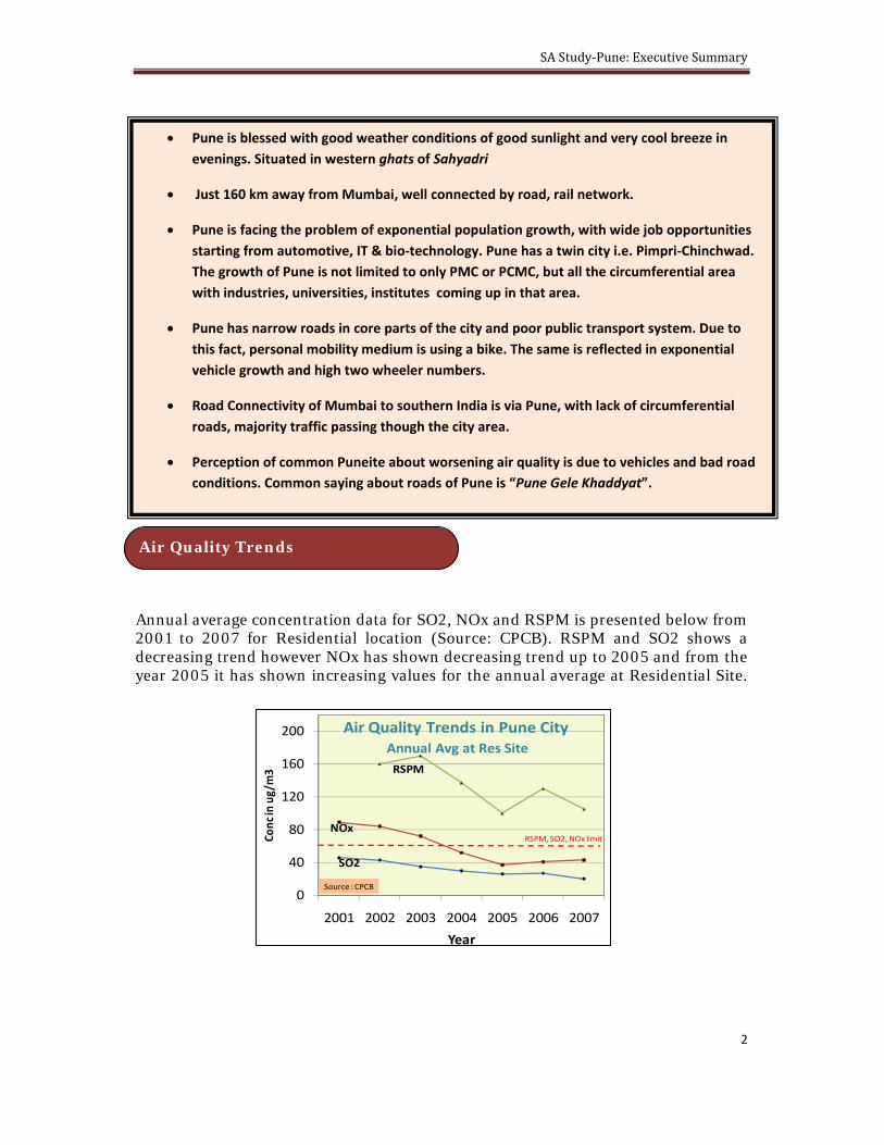
Annual average concentration data for SO2, NOx and RSPM is presented below from 2001 to 2007 for Residential location (Source: CPCB). RSPM and SO2 shows a decreasing trend however NOx has shown decreasing trend up to 2005 and from the year 2005 it has shown increasing values for the annual average at Residential Site.
Air Quality Trends
0
40
80
120
160
200
2001 2002 2003 2004 2005 2006 2007
Conc in ug/m3
Year
SO2
NOx
RSPM
Air Quality Trends in Pune City Annual Avg at Res Site
Source : CPCB
RSPM, SO2, NOx limit
SA Study‐Pune: Executive Summary
3
The recent Auto Fuel Policy report submitted to the Government of India by the Mashelkar Committee, clearly points to the existence of a knowledge gap in the areas of emission factor determination for Indian vehicles, air quality monitoring and source apportionment studies.
An integrated approach towards air quality management was felt necessary in this regard. A database collected using all the relevant scientific tools for design of modular air quality management plan was required for decision support.
With the above background, source apportionment studies have been undertaken in six cities viz. Delhi, Bangalore, Pune, Kanpur, Mumbai and Chennai. With a focus on apportionment of respirable particulate matter [PM10 and PM2.5 (limited)], being most critical.
The main objective of Ambient Air Quality Monitoring is to generate baseline data of ambient concentration of critical air pollutants and source apportionment study for PM10 in different parts of the city of Pune. A comprehensive air quality monitoring exercise was carried out for a period of one year at seven representative locations including two residential sites, two kerbside sites, one industrial site, one institutional site, and one background site, having different land use pattern and sources of activity. Air Quality Monitoring was carried out in 2 sets of 4 sites each in a season. Background site was common to both the sets. One residential and one kerbside site were included in each set.
Monitoring was carried out, continuously for 20 days in a season at each site during summer, post-monsoon and winter seasons, for suspended particulate matter (SPM) using high volume sampler, PM10 using 4 channel speciation samplers, SO2, NOx by wet chemical method. PM2.5 monitoring was carried out at sites for seven days in a season for all three seasons using FRM sampler. Monitoring of meteorological data was carried out for wind direction, wind velocity, ambient temperature, relative humidity, solar radiation and rainfall. Aldehydes, Benzene, 1,3-butadiene were monitored at all sites once in a season.
PM10 was collected on three types of filters depending upon the analytical requirement of the source apportionment studies viz. PTFE, Nylon and Quartz filter papers. PM2.5 was collected on PTFE filters and Quartz filters. Chemical speciation of PM10 samples was carried out for source apportionment for various marker
Air Quality Monitoring
Need for the Study

SA Study‐Pune: Executive Summary
4
species such as Anions & Cations using Ion Chromatograph, Elements using Energy Dispersive- X-Ray Fluorescence (ED-XRF), Organic & Elemental carbon using Thermal Optical Carbon Analyzer and Molecular Markers using Gas Chromatograph-Mass Spectrometer (GC-MS), High Resolution Gas Chromatograph-Flame Ionization Detector (HRGC-FID) and High Performance Liquid Chromatography (HPLC).
Air quality of Pune with respect to NAAQS:
Study design and air quality monitoring network was designed with a specific objective of source apportionment of the PM10 and not for regulatory purpose. However, to get an idea of air quality with respect to standard limits, exceedence of daily average value with respect to CPCB standards for criteria pollutant are observed. Air quality in critical winter season is presented below-
o SPM was found to exceed the standards (200 ug/m3 daily average for residential
area) for almost all days at all sites in winter season. At background site also, 75% of times exceedence was observed. At residential site, 85% of times exceedence was observed, out of which 30%
times it was exceeding 400 ug/m3. At kerbside site, 80% times daily avg. values were exceeding 400 ug/m3 and
55% times it was exceeding 650 ug/m3. At industrial site, 10% times the average values were exceeding 500 ug/m3
(SPM limit for industrial site) out of 80% values, which was exceeding 400 ug/m3.
o PM10 data in winter season is re-presented below.
At background site 35% of times the PM10 concentration exceeded daily average limit value for residential area. While at residential site, exceedence
Note: Limit shown is 24 hrly average limit for residential area.

SA Study‐Pune: Executive Summary
5
observed was more than 55% of values out of these, 25% of daily average values exceeded 200 ug/m3.
At Kerbside site, 80% times daily avg. values were exceeding 200 ug/m3 out of which 35% times they were exceeding 250 ug/m3.
At industrial site, 90% times the daily average values were exceeding 150 ug/m3 (24 hrly limit for industrial site). For 20% times PM10 concentration was exceeding 300 ug/m3.
Note: Limit shown is 24 hrly average limit for residential area.

SA Study‐Pune: Executive Summary
6
o
o NOx was not found to exceed except at kerbside sites in winter season, which is restricted to 50% time which were found to be below 100 ug/m3
o SO2 was found to be very well below the limits (80 ug/m3 -24 hrly daily average for residential) at all sites including Industrial location (120 ug/m3 -24 hrly daily average for industrial). At industrial site, however, 20% values were between 80 and 105 ug/m3
o 8hrly average concentration of CO was found to exceed the limit (2000 ug/m3-8hrly average) at kerbside site during summer and winter. 1 hrly average CO conc. were found to exceed standards (4000 ug/m3) during morning peak (9 am to 1 pm) and evening peak(7 pm to 10 pm)
PM Fraction Data & Chemical Speciation
Re-suspended road dust was found to be a major source of PM. From the fraction data, it is observed that, fraction of particle greater than PM10 (PM10/SPM ratio) is found to be more than 40% at all the sites during all the seasons of monitoring period. This high proportion of SPM is attributed to the re-suspended dust.
Following observations can be made from fraction of various chemical species inPM10 from chemical speciation of the PM10-
• The contribution of earth-crust metals like Silicon, Sodium, Aluminum and Iron is about 40 % in PM10 during all seasons indicates re-suspension of soil dust as a major source.
• Sulphate, Nitrate and Chloride ions were found to contribute major portion among anions. Ammonium and Calcium with Sodium and Potassium were the major contributors to the cations. Presences of higher amount of sulphate and nitrate ions with ammonium ions indicate formation of secondary particles.
Note: Limit shown is 24 hrly average limit for residential area.

SA Study‐Pune: Executive Summary
7
Comparative representation of the distribution of group of chemical species in PM10 and PM2.5 is presented below.
• PM2.5 mass was found to contribute about 35% of the PM10, at all the sites during all the season. Crustal elements are found to comparatively higher in PM10 than in PM2.5 which indicates major portion of the PM10 is coming from resuspended dust.
• The average EC/OC ratio at all the sites was observed to be more than 0.35 during all the seasons of monitoring. At both the Kerbside sites COEP and Hadapsar, average EC/OC ratio was 0.5. Higher EC/OC may be attributed to the predominant vehicle exhaust
• PM. Higher TC is observed at Kerbside and Residential site. EC/OC ratio is higher at Kerbside and Industrial site.
• Although, the total carbon concentration in PM2.5 is lower ratio of EC/OC was observed to be higher than PM10 at respective site suggesting higher contribution of combustion sources to PM2.5.
Though, controlling the coarser PM and SPM is comparatively easier and control options result into better impact on overall PM concentration reduction, considering

SA Study‐Pune: Executive Summary
8
health impacts of finer particles, controlling fine particulates (PM2.5 ) would be important.

SA Study-Pune: Executive Summary
9
Comparison of various pollutants observed in first set of monitoring during summer, post-monsoon and
winter season
Site Season
EC/OC Concentration (ug/m3) Concentration in PM10 (ug/m3)
(PM10)
Ratio PM2.5/PM10
Ratio PM10/SPM SO2 NOx SPM PM10 PM2.5 EC OC SO4-- NO3-- NH4+ Na+ Ca+ Si
CWPRS-Background
Winter 0.40 0.32 0.44 14 17 225 100 32 9 21 8 3 5 2 2 23
Post- Monsoon
0.37 0.45 0.67 9 10 76 51 23 2 6 6 0 1 1 2 10
Summer 0.30 0.28 0.55 6 10 142 78 22 3 9 10 7 5 2 4 18
Shantiban- Residential-1
Winter 0.39 0.45 0.39 14 27 328 130 58 11 28 9 5 4 3 7 24
Post- Monsoon
0.43 0.40 0.60 9 10 107 64 26 3 6 8 2 1 2 3 19
Summer 0.34 0.27 0.50 7 15 210 106 28 3 9 12 12 5 3 5 24
CoEP - Kerbside-1
Winter 0.36 0.47 0.57 21 74 466 266 124 16 46 8 6 4 1 6 46
Post- Monsoon
0.68 0.32 0.50 13 33 282 140 45 14 21 8 3 1 2 4 36
Summer 0.50 0.32 0.28 7 65 517 143 46 13 25 11 11 4 3 5 29
SAJ-Industrial
Winter 0.46 0.27 0.57 47 57 412 237 64 24 53 12 6 5 3 10 27
Post- Monsoon
0.47 0.30 0.46 18 18 188 87 26 6 12 9 3 2 2 4 16
Summer 0.39 0.30 0.45 25 23 272 124 37 7 18 14 10 3 3 4 32

SA Study-Pune: Executive Summary
10
Comparison of various pollutants observed in second set of monitoring during summer, post-monsoon and winter season
Site Season
EC/OC Concentration (ug/m3) Concentration in PM10 (ug/m3)
(PM10)
Ratio PM2.5/PM10
Ratio PM10/SPM SO2 NOx SPM PM10 PM2.5 EC OC SO4-- NO3-- NH4+ Na+ Ca+ Si
CWPRS-Background
Winter 0.4 0.36 0.44 16 20 214 93 33 10 24 9 3 4 1 2 14
Post- Monsoon
0.36 0.44 0.36 10 14 176 64 28 6 18 3 1 7 2 3 14
Summer 0.34 0.37 0.60 5 9 68 41 15 2 6 4 1 2 1 1 12
Sahakarnagar-Residential-2
Winter 0.34 0.27 0.35 19 45 511 178 48 27 79 13 8 5 3 8 22
Post- Monsoon
0.35 0.26 0.36 12 45 384 137 35 16 45 10 3 8 2 6 32
Summer 0.37 0.33 0.39 5 10 173 67 22 4 11 3 1 2 2 2 14
Hadapsar - Kerbside- 2
Winter 0.40 0.51 0.36 41 68 663 237 120 28 69 15 9 5 3 10 26
Post-Monsoon
0.37 0.29 0.35 13 44 600 212 62 17 46 10 4 9 1 9 34
Summer 0.63 0.29 0.32 6 26 321 103 30 10 16 6 2 5 2 4 21
UoP- Winter 0.48 0.34 0.52 24 38 259 134 45 21 42 15 9 7 2 7 26
Institute (other)
Post-Monsoon
0.47 0.45 0.34 10 35 212 72 32 10 21 7 2 6 1 4 17
Summer 0.35 0.24 0.49 6 10 121 59 15 3 8 6 2 5 2 3 20

SA Study‐Pune: Executive Summary
11
Emission inventory study was carried out for city of Pune by converting Pune city map into 2X 2 km grids for area, point and line sources. Primary surveys were carried out for identification and spatial distribution of sources around the monitoring sites in an area of 2 km X 2 km. To study the emissions loading from line sources, various factors such as number of vehicles of different categories, age distribution, utilization pattern, quality of fuels and technology, fuel efficiency, and emission factors were considered. Primary data of vehicle counts is collected by carrying out vehicle counting on various roads for various categories of roads. Various multiplex, institutes, colleges , on road and designated parking lots are surveyedfor types of vehicle, vehicle model, registration number and odometer reading. Totally more than 12000 vehicles were surveyed. Following graphs present overall emission inventory for PM10, NOx, CO and SO2 for Pune city.
Following are the observations based on city level Emission Inventory
• From total PM10 emission load (32 T/day)Highest pollution loads of PM10, NOx and CO are observed at the central part of the city with major commercial activities and high population and road densities.
• Road dust emerges as the highest contributor towards PM10 in the city (61%). Line sources (Mobile) contribute to 18% of PM10 with more than 40% contribution is from 2, 3 wheelers and cars. Most of these vehicles are gasoline or LPG fuelled vehicles. The high contribution from these vehicles is due to high number of vehicles. (65%-2Wheelers, 13% -auto rickshaws and 15% cars).
• Industrial contribution to PM10 in the city is limited to 1.25 % due to confined industrial areas within the city and very low numbers of air polluting industries.
• Prominent area sources other than road dust are construction and brick klins (4.5%), domestic and slum fuel usage (including solid fuel burnig) (7.5%) and hotels and bakeries (3%).
• For NOx emissions (41.4 T/day), major contribution is from vehicles (95%). The contribution from industries is limited (2%) due to confined industrial area with in the city limits. Domestic and commercial fuel burning for cooking contribute to balnce 3%.
Emission Inventory

SA Study‐Pune: Executive Summary
12
0.8, 14.2%
0.6, 9.6%
0.9, 15.4%0.3, 5.8% 0.7, 12.3% 0.2, 2.9%
1.1, 19.1%
1.2, 20.6%
City level PM 10 (Line Sources) Emission Inventory (TPD) - 2007
Bikes Scooters Autorick 3WGC4WGC Cars Buses Trucks
Total5.91
T/day5.9, 18.2%
19.7, 60.7%
6.5, 19.8%
0.4, 1.2%
City level PM 10 (All Sources) Emission Inventory (TPD) - 2007
Mobile Paved & Unpaved Roads
Other Area Sources Industries
Total32.27T/day
39.19, 94.6%
1.33, 3.2%0.89, 2.2%
City level NOx (All Sources) Emission Inventory (TPD) - 2007
Mobile Paved & Unpaved Roads
Other Area Sources Industries
Total41.42T/day
7.8, 19.8%
1.9, 4.7%
2.4, 6.0%0.8, 2.1%
2.7, 7.0% 3.2, 8.2%
11.7, 29.9%
8.7, 22.2%
City level NOx (Line Sources) Emission Inventory (TPD) - 2007
Bikes Scooters Autorick 3WGC4WGC Cars Buses Trucks
Total39.19T/day
0.9, 13%
5.2, 73%
1.0, 14%
City level SO2 (All Sources) Emission Inventory (TPD) - 2007
Mobile Industry Other
Total7.15T/day
111.6, 84%
21.5, 16%
City level CO (All Sources) Emission Inventory (TPD) - 2007
Mobile Other
Total133.18T/day

SA Study‐Pune: Executive Summary
13
• SO2 baseline (year 2007) emission inventory of 7.15 T/day has the major source as Industry (73.53%) followed by mobile (12.70%) and brick kilns (6%). Contribution from solid fuel burning in slums is 4.55%. This is due to very high fuel consumption in industrial area wherein largest forging industry in Asia is located. Similarly sulfur content of these industrial fuels is very high (FO 4%, LDO 1.8%).
• Vehicles are major source for CO emissions contributing to about 85 % emission load followed by fuel burning in slum (11%).
5.9 7.0 8.2
39.2
59.5
98.0
19.7534.07
60.096.5
6.9
8.6
1.3
10.2
12.5
0.4
0.5
0.6
0.9
1.1
1.4
0
20
40
60
80
100
120
2007 2012 BaU 2017 BaU 2007 2012 BaU 2017 BaU
PM NOx
T/da
y
City Level Emission Inventory (T/day): BaU
Mobile Paved & Unpaved RoadsOther Area Sources Industries

SA Study‐Pune: Executive Summary
14
Factor analysis and Chemical Mass Balance (CMB8.2) model was used for receptor modeling.
The Varimax rotated factor analysis technique based on the principal components has been used in the determination of the contribution of respirable particulate matter pollution sources.
Results of the factor analysis, with the probable sources indicated by group of constituents, carried out for different sites show that the first component (factor) extracted was always of earth crust metals indicating re-suspended dust as source and is grouped with the markers like Ca, Mg for construction source. Other sources indicated are combustion/vehicles, wood/ vegetative burning and coal combustion. Secondary particulates formation was indicated by presence of NH4, SO2 and NO3 in one group.
Site Factor 1 Factor 2 Factor 3 Factor 4 Factor 5
Residential Resuspended dust and Construction
Combustion/ Vehicles
Coal/Wood Combustion
Vegetative Burning
Secondary Particulates
Kerbside
Resuspended dust and Construction
Combustion/ Vehicles
Secondary Particulates
Wood Combustion
-
Industrial Resuspended dust and Construction
Combustion/ Vehicles
Secondary Particulates
Industrial Fuel Oil Combustion
-
BackgroundResuspended dust and Construction
Combustion/ Vehicles
Secondary Particulates
Coal/Wood Combustion
-
Receptor Modeling & Source Apportionment

SA Study‐Pune: Executive Summary
15
Results of receptor modeling (CMB8.2 ) of PM10 at all sites in three seasons viz., summer (s), post-monsoon (p) and winter (w) are presented below.
Seasonal variation in the contribution by different sources was observed. However, the source which dominates in all the seasons is re-suspended road dust. Contribution from vegetative burning, solid-fuels burning was found to be higher during winter season, which may be attributed to the increased use of wood, coal for water heating, specifically in slum areas.
Factor analysis and Chemical Mass Balance (CMB8.2) model was used for receptor modeling. Receptor modeling by factor analysis and CMB8.2 confirmed re-suspended road dust as major source of PM10. Sources identified through receptor modeling at different sites in Pune are as follows-
o Re-suspended road dust o Vehicles/ Combustion, o Construction/ Brick Kilns, o Solid fuels burning, o Vegetative burning (agricultural waste, garden waste).

SA Study‐Pune: Executive Summary
16
Industrial Source Complex Short Term-3 (ISCST3) model was used for dispersion modeling exercise with urban dispersion coefficients and flat terrain condition. Pune city map (22km X 20km) was divided into 2km X 2km. Number of grids with substantial activity level was 87. Emission information of all sources including point, area and line is included from the baseline gridded emission inventory (2km X 2km) prepared for year 2007. Meteorological data, used in the model, was collected at the monitoring sites. Meteorological station was installed at monitoring sites to capture data on wind direction, wind velocity, ambient temperature and % relative humidity. Predominant meteorological data was used for modeling for Pune city. Winter season was found to be critical with respect to ambient concentration levels. Re-suspended dust was found to be the major source with a contribution of around 58%. Mobile source and other area sources contribute around 22% and 19% respectively. Average contribution of all the grids in Pune of Industrial sources was found to be very less (0.1%). Site-specific dispersion modeling results show higher contribution of about 30-40% from mobile sources at all sites, especially kerbside. However, re-suspended dust was found to be the highest contributor at all sites with contribution ranging from 40 to 60%. Other area sources contributed in the range from 8 to 19%. Contribution from industries were found to be very less (below 1%), however, higher contribution
Dispersion Modeling: Existing scenario
0 2000 4000 6000 8000 10000 12000 14000 16000 18000 20000 22000
X Co-ord
0
2000
4000
6000
8000
10000
12000
14000
16000
18000
20000
X C
o-or
d
10ug/m3
20ug/m3
30ug/m3
40ug/m3
50ug/m3
60ug/m3
70ug/m3
80ug/m3
90ug/m3
100ug/m3
110ug/m3
120ug/m3
130ug/m3
140ug/m3
0
2000
4000
6000
8000
1000
0
1200
0
1400
0
1600
0
1800
0
2000
0
2200
0
X Co-ord
0
2000
4000
6000
8000
10000
12000
14000
16000
18000
20000
Y C
o-or
d
10ug/m320ug/m330ug/m340ug/m350ug/m360ug/m370ug/m380ug/m390ug/m3100ug/m3110ug/m3120ug/m3130ug/m3140ug/m3150ug/m3160ug/m3170ug/m3180ug/m3190ug/m3200ug/m3
0
2000
4000
6000
8000
1000
0
1200
0
1400
0
1600
0
1800
0
2000
0
2200
0
X Co-ord
0
2000
4000
6000
8000
10000
12000
14000
16000
18000
20000
Y C
o-or
d
0.00
6.00
12.00
18.00
24.00
30.00
36.00
42.00
48.00
54.00
60.00
66.00
72.00
(a) (b)
(c) (d)
Dispersion Modeling -2007 Winter for (a) PM10, (b) NOx, (c) SO2, and (d) Windrose

SA Study‐Pune: Executive Summary
17
(3%) was observed at industrial site.
Mobile source was found to be largest contributor towards the NOx concentration with average contribution more than 95% from dispersion modeling for Pune city and at various sites. Area sources, including hotels, bakeries, residential fuels, contributed for about 3% of the NOx concentrations. Contribution from industry was about 1%. SO2 concentrations were found to higher around the grids having industrial source.
Hot-spots are found to be present at the central part of Pune with higher population as well as road densities.
49 B07
49 B12
49 B17
50 B07
50 B12
50 B17
48 B07
48 B12
48 B17
37 B07
37 B12
37 B17
38 B07
38 B12
38 B17
36 B07
36 B12
36 B17
47 B07
47 B12
47 B17
35 B07
35 B12
35 B17
39 B07
39 B12
39 B17
59 B07
59 B12
59 B17
0
200
400
600
800
1,000
1,200
1,400
B07
B12
B17
B07
B12
B17
B07
B12
B17
B07
B12
B17
B07
B12
B17
B07
B12
B17
B07
B12
B17
B07
B12
B17
B07
B12
B17
B07
B12
B17
49 50 48 37 38 36 47 35 39 59
PM10
Conc. (ug
/m3)
Top 10 grids
Predicted concentrations of PM10 at Top 10 grids for year 2007, 2012 & 2017
Industrial
Mobile
Other Area
Road Dust
38 B07
38 B12
38 B17
37 B07
37 B12
37 B17
48 B07
48 B12
48 B17
39 B07
39 B12
39 B17
36 B07
36 B12
36 B17
50 B07
50 B12
50 B17
62 B07
62 B12
62 B17
35 B07
35 B12
35 B17
40 B07
40 B12
40 B17
51 B07
51 B12
51 B17
0
50
100
150
200
250
300
350
400
450
500
B07
B12
B17
B07
B12
B17
B07
B12
B17
B07
B12
B17
B07
B12
B17
B07
B12
B17
B07
B12
B17
B07
B12
B17
B07
B12
B17
B07
B12
B17
38 37 48 39 36 50 62 35 40 51
NOx C
onc. (ug/m3)
Top 10 grids
Predicted concentrations of NOx at Top 10 grids for year 2007, 2012 & 2017
Non‐Ind. Gen.
Industrial
Other Area
Mobile

SA Study‐Pune: Executive Summary
18
With Business as Usual (BaU) assumptions, city level emission inventory for PM and NOx is projected for year 2012 and 2017 based on year 2007 baseline emission inventory. The projected emission load is with percentage increase is given below.
High growth rate of urbanization in Pune, poses challenges in terms of increasing infrastructure demands. This in turn is responsible for increasing population including slums and increase in fuel usage, construction activities, traffic density etc.
For PM emissions, area sources particularly road dust emerges to be the largest contributor (77%) which will have very high growth rate which directly depends on the VKT. Effective control options for road dust on the regional basis need to be considered for controlling PM emission growth.
Sr no.
Sources
Baseline 2007
(T/day)
BAU 2012 (T/day)
BAU 2017 (T/day)
% increase over base in
2012
% increase over base in
2017
PM NOx PM NOx PM NOx PM NOx PM NOx
1 Area 25.95 1.33 40.99 10.2 68.74 12.53 57.95 664.31 164.89 838.90
2 Line 5.91 39.19 6.99 59.49 8.17 98 18.27 51.80 38.24 150.06
3 Point 0.4 0.89 0.5 1.13 0.64 1.44 25.00 26.97 60.00 61.80
Total 32.26 41.41 48.49 70.82 77.55 111.98 50.31 71.00 140.39 170.39
Future Projections
The key issues regarding planning transportation in Pune • Mixing of transit travelers from city with the local traffic due to absence of by‐passes
and circumferential road network
• Lack of adequate public transport system
• Congestion problem in central city due to restricted capacity of narrow roads
• Poor road surface quality, absence of wall to wall road pavement
• Absence of signage, markings, street name boards and other street furniture resulting in poor accessibility
• Only 40% of the roads with footpaths and most of the existing ones encroached upon by informal activities and street hawkers
• No control or inadequate control systems like one‐ways, heavy vehicles restrictions, no‐vehicles zone and other traffic management systems for the arterial
• Highly inadequate parking facilities; lack of planned on‐street parking facilities
• Lack of civic sense towards traffic and poor travel behavior
• Lack of coordination among agencies involved in planning and providing for traffic and transportation

SA Study‐Pune: Executive Summary
19
With planned enforcement of new vehicular emission regulations since 2010, the growth in PM load due to vehicles is restricted to around 18% though number of vehicles increase cumulatively by 66% in next 5 years.
The highest growth rate of vehicles is of bus category with annual growth over 23%. Increase in buses include city buses, company and school buses steep increase in last five years particularly reflecting growth in industry outskirts of the city. By implementation of BSIV in 2010, the emission factor of diesel buses/ trucks is reduced by 83% in case of PM and 30% in case of NOx. The same is also a reason for restricted growth of PM due to line sources.
The percentage growth of vehicular NOx over base year is 52% & 150% for 2012 and 2017 respectively in vehicle category which, contributes to about 85% of total NOx emissions. The major contributors in vehicle categories are LCVs and HCVs including buses and bikes due to large numbers. This scenario also alerts to have strong NOx control measures for the future.
The contribution of point sources is limited to around 1% due to confined industrial areas in small pockets within city limits.
Pune was having a special ‘Pune Model’ implemented for the supply of electricity in the Pune & Pimpri-Chinchwad area, wherein 100% electricity was ensured to whole of the city. This was possible with understanding with Confederation of Indian Industries (CII), wherein deficit in electricity demand was fulfilled by industry sector through CII. This has ensured zero usage of non-industrial generators. Therefore, while generating baseline year 2007 emission inventory, non-industrial generator source was not considered. However, the ‘Pune Model’ for supply of electricity is discontinued and at present, Pune is experiencing daily 6 hours power-cuts since May 2008. Considering this to continue, BAU 2012 & 2017 scenario is generated with non-industrial generators as emission source.

SA Study‐Pune: Executive Summary
20
Various control options available were selected for evaluation and subsequent scenario generation. Control options selected for evaluation for line, area and point sources are presented below. The line source control options are divided in two types, technology based and management based control options.
Control Option Considered Scenario 2012 Scenario 2017
Technology Based Control Options for Line Sources
Implementation of BS – V norms
BS-III for 2-3 W, BS-IV for rest all from 2010 onward
BS-III for 2-3 W, BS-IV for rest all from 2010-2015
BS-IV for 2-3 W, BS-V for rest all from 2015 onwards
Implementation of BS – VI norms
BS-III for 2-3 W, BS-IV for rest all from 2010 onwards
BS-III for 2-3 W, BS-IV for rest all from 2010-2015
BS-IV for 2-3 W, BS-VI for rest all from 2015 onwards
Electric Vehicles Share of Electric vehicles in total city fleet – Two wheeler: 1%,Auto Rickshaw and Taxi: 5%,Public buses: 5%
Share of Electric vehicles in total city fleet – Two wheeler: 2%,Auto Rickshaw and Taxi:10%,Public buses: 10%
Hybrid vehicles Share of Hybrid vehicles in total city fleet of Gasoline powered four-wheelers 1%
Share of Hybrid vehicles in total city fleet of Gasoline powered four-wheelers 2%
CNG/LPG to commercial (all 3 and 4-wheelers)
25% conversion 100% conversion
Ethanol blending (E10 – 10% blend)
E-10 all petrol vehicles E-10 all petrol vehicles
Bio-diesel (B5/B10: 5 – 10% blend)
B-5 all diesel vehicles B-10 all diesel vehicles
Hydrogen – CNG blend (H10/H20: 10 – 20% blend)
-- H-10 all CNG vehicles
Retrofitment of Diesel Oxidation Catalyst (DOC) in 4-wheeler public transport (BS – II)
BS-II buses retro- 50% BS-II buses retro- 100%
Retrofitment of Diesel Particulate Filter in 4-wheeler public transport(BS – III city buses)
BS-III buses retro- 50% BS-III buses retro- 100%
Management based Control Options for Line Sources
Inspection/ maintenance to all BSII & BSIII personal & public transport vehicles
50% compliance 100% compliance
Evaluation of Control Options

SA Study‐Pune: Executive Summary
21
Banning of 10 year old commercial vehicles
100% compliance –pre 2002 3W, GC, buses and trucks
100% compliance –pre 2007 3W, GC, buses and trucks
Control Option Considered Scenario 2012 Scenario 2017
Banning of 15 year old private vehicle
100% compliance 100% compliance
Synchronization of traffic signals
All highways, 10% of major roads
All major & minor roads excluding feeder roads
Improvement of public transport: % share
10% shift of VKT 20% shift of VKT
Control Options for Area Sources
Shift to LPG from solid fuel &kerosene for domestic applications
50% compliance 100% compliance
Shift to LPG from solid fuel &kerosene for commercial applications (bakeries, open eat outs etc)
100% compliance 100% compliance
Better construction practices with PM reduction of 50%
50% compliance 50% compliance
Strict compliance of ban on open burning, including open eat outs
50% compliance 100% compliance
Reduction in non-industrial generators
50% 100%
Converting unpaved roads to paved roads
50% compliance 100% compliance
Wall to wall paving (brick) All major roads All major & minor roads excluding feeder roads
Mechanised sweeping & watering
All major roads All major & minor roads excluding feeder roads
Industrial Sources
Shifting of air polluting industries
50% compliance 100% compliance
Banning of new industries in existing city limit
100% compliance 100% compliance
• In Pune, Road dust is a major contributor to PM10 (more than 60%) Major portion of the re-suspended road dust is attributed to the paved road dust (about 78% of total road dust) with the share of unpaved road dust as 22% of total road dust. Improving the quality of road to reduce the re-suspended road dust is essential. Present silt loading of paved road in Pune is about 0.9 g/m2, whereas the international (EPA, AP-42) default silt-loading value is around 0.2 or less. It is, therefore, evident that, road conditions need to be improved. With the reduction in silt loading factor by 50% of the existing value, total PM10 reduction benefit of about 35% can be achieved. Though Mechanized sweeping

SA Study‐Pune: Executive Summary
22
and watering shows higher benefits, the implementation is difficult. Wall to wall pavement can yield around 10% and 16 % benefits if implemented on all major roads and all major and minor roads respectively. Therefore, road infrastructure needs to be set up and maintained as per national/inter-national standards. Guidelines should be made available for the quality of the roads based on traffic patterns.
• In Pune, mass transportation system is inadequate and not in pace with the transportation requirement. This also increases the use of personalized vehicles which intern contributes to road dust as well as vehicle tail pipe emissions. Effective Mass transport system must be established to reduce the rising tendency of owning personal vehicles. In Pune, the average occupancy of 2 Wheelers is 1 and for cars around 1.3. The 10% & 20% shift of 2W & cars to public transport in 2012 & 2017 respectively, gives benefit of 1-3 % for PM10 & NOx. However, the reduction in VKT also reduces the road dust of 3.5 % and 12% respectively for year 2012 &2017.
• Progressive tightening of emission norms must be implemented and Vehicle emission regulation road map should be ready for 10 years, which need to be updated on continuous basis. Progressive tightening of emission regulations since 1991 to BS-III regulations for 2& 3 wheelers and BS-IV regulations for all other categories of vehicles (in line EURO-IV) scheduled to be implemented in 2010; have given an edge over the multifold growth of cities and Mega cities of India and in turn the number of vehicles. The cities like Pune have been showing the growth of vehicles around 10% continuously for more than last 10 years.
• Ensuring nationwide same quality of fuel is strongly recommended for ensuring the benefits expected from new technology options. BS-III regulations except for 2&3 wheelers are implemented in 11 cities of India including Pune since 2005. However, there will be vehicles plying in the city which are not registered in Pune (Such numbers are also high due to local tax structures). Similarly, BS-III fuel is available only in the city and not even 20-30km away from city boundary. As the city growth is circumferential particularly the industrial growth, the number of city vehicles traveling out of the city boundary are much higher and tend to refuel the vehicles outside the city because of the lesser cost of the fuel. Thus not using the required fuel (particularly low sulfur content fuel), which deteriorates the emission performance of these vehicles and in turn increase the in-use vehicle emissions.
• Continuous power supply must be ensured to avoid use of non-industrial generators, as it has remarkable benefits in terms of emission reduction. Reduction in use of non-industrial by ensuring continuous power supply can give benefits as reduction in PM and NOx emissions by 5.86% and 83.14% respectively in year 2012 and by 5.76% and 82.92% respectively in year 2012.

SA Study‐Pune: Executive Summary
23
• Infrastructure and availability for supply of cleaner gaseous fuels like LPG/CNG for domestic combustion fuels especially in slum areas and for transport sector. As in Pune, around 40% of population lives in slums representing a typical urban slum scenario with slum population using kerosene and wood is around 45% and 21% respectively. This will curb the use of solid fuels like coal and wood for domestic cooking in slums.
• Banning of 10 years old commercial vehicles yield highest benefits in terms of emission reduction. However, the socio economic impacts of banning of older vehicles need to be evaluated. Entry of these vehicles in the city area must be restricted as an immediate measure to curb major portion of vehicle pollution. Higher NOx reduction benefits, 45% and 56% for year 2012 and 2017 respectively, are observed mainly due to banning of old vehicles.
• An effective I&M implementation regime is to be implemented with periodic pollution and safety checks for commercial vehicles. In the phase-I, commercial vehicles must be considered due to longer trip lengths and higher VKT travelled. While evaluating the control option of inspection and maintenance, reductions on BS-II & BS-III personal and public transport vehicles have been considered. It is very difficult to evaluate benefits possible for BS-IV and beyond vehicles due to the different advanced technologies, which still have to come in market. If the benefits on the commercial vehicles like trucks and LCVs are assumed same as public transport vehicles (buses) and for all technology vehicles then the additional benefit of 1.1 -1.3 % on PM10 and 0.6-1.1% on NOx is achievable. Additionally, no data is available for effect of Inspection & Maintenance on PM reductions from gasoline vehicles which contribute to more than 40% of the vehicle PM.
• Management control options are more effective and may not require huge infrastructure and national policy level decisions. Following traffic and transportation management control options, which are relatively easy to implement are recommended-
o Adequate number of pedestrian crossing means like conveyor of sub-ways to be provided based on traffic flow on the roads.
o Sufficient traffic signage, road markings to be provided on the roads for easy access.
o Adequate number of parking lots to be provided across the city. Also, on-road parking space to be provided on major roads.
o Restricting entry of polluting trucks and heavy duty goods vehicles in the cities by providing circumferential roads/by-passes.
o Staggered working hours, Increase occupancy of personal vehicles by options like car-pooling.

SA Study‐Pune: Executive Summary
24
o Certain highly polluting areas can be identified as low emission zone and restricted for certain air polluting activities like no vehicle zone, only electric vehicles zone.
o Encroachment of foot-paths by street hawkers to be strictly banned. o Construction of fly-overs for vehicles to avoid congestion of traffic in certain
areas. o Earmarking one-ways in congested area of cities and restricting entry to heavy
vehicles during peak hours. o Dissemination of information on traffic congestion update. o Application of IT in traffic management solutions
• Technology based Control options
o Biodiesel blending with diesel fuel (B-10) is recommended for benefits vehicular PM emissions.
o Retro fitment of public transport vehicles is not so good option when it comes for implementation. Instead, financial incentives for replacement of older vehicles with the newer generation vehicles are recommended.
o Use of CNG as auto fuel particularly for public transport as well as for the cleaner industry fuel is recommended.
o Similarly, financial incentives on non-polluting vehicles like electric- hybrid will also increase the penetration of these vehicles in public as well as in personal vehicles category.
• Pune, Pimpri-Chinchwad and circumferential area earmarked for development and industrialization should be grouped under a Metropolitan Development Authority for better planning and administration.
• Guidelines to be prepared for better construction practices and strict compliance of the same is to be ensured. Brick kilns operation, which is observed near the major construction activity in the city, must be totally restricted inside the city area. Better construction practices give 50% benefit in PM from construction. With 50% compliance the benefit is 4.18% and 7.15% in PM in 2012 & 2017
• Solid fuel burning is identified as one of the major sources of PM, through receptor modeling. This is more prominent in winter season due to use of wood and other solid fuels for water heating, burning of dry leaves and heat generation. Open /trash burning must be strictly restricted. Street-vendors, open eat-outs using kerosene to be switched to cleaner fuels like LPG. Ban on open-burning contributes to benefits up to 3.2% in PM & 4.4 % in NOx in year 2017 6% in PM & 18 % in NOx in year 2017.

SA Study‐Pune: Executive Summary
25
• Switch over of fuel from wood to LPG be implemented for combustion operations in bakeries. Shift from solid fuel and kerosene to LPG particularly in domestic areas and commercial activities like bakeries show the improvement of total 30% for PM when compared to area sources contribution excluding dust and around 39% benefit for NOx similarly.
• Although, pollution load from industries is less in Pune, industries should be encouraged for use of air pollution control devices like Bag filter. ESP, etc.
Air quality monitoring in the major cities shall be carried out on continuous/on-line basis, which will create awareness and also sensitize the policy makers through the actual monitored data. This will also help to organize transport planning and on-line traffic giving information about the congestion and avoiding blockage jamming of traffic. It is recommended that a proper allocation of resources shall be made available on continuous basis to carry out this activity

SA Study‐Pune: Executive Summary
26
Based on the evaluation of the impact of various individual control options and their feasibility in implementation for both management and technology based options, a list of control options considered is prepared for generating controlled scenario-1. Alternate control scenario-2 was also generated for PM10. For generating controlled scenario-2, all control options as listed in Scenario-I have been considered except for road dust control option. For road dust, reduction of silt loading by 50 % has been considered on highways and major-minor roads. However, No reduction of silt loading is assumed on feeder roads.
Comparison of BaU and Controlled scenario based on emission
inventory for PM10 and NOx Pollutants
Emission Load (T/day) % reduction w.r.t. BaU
Baseline-2007
BaU-2012
BaU-2017
Cont. 2012
Cont. 2012-
2
Cont. 2017
Cont. 2017-
2
Cont. 2012
Cont. 2012-
2
Cont. 2017
Cont. 2017-
2 PM10 32.27 48.49 77.55 38.37 24.63 58.15 39.01 21% 49% 25% 50%
NOx 41.42 70.82 111.98 38.96 ----- 49.39 ---- 45% ---- 56% ----
Pollutants % increase over Baseline 2007
BaU-2012
BaU-2017
2012 Contrld
Contrld 2012-2
2017 Contrld
Contrld 2017-2
PM10 50% 140% 19% -24% 80% 21%
NOx 71% 170% -6% ---- 19% ----
5.9 7.0 2.8 2.88.2
2.5 2.5
39.2
59.5
33.1
98.0
47.719.7
34.131.3
17.5
60.152.9
33.86.5
6.94.0
4.0
8.6
2.3
2.3 1.3
10.2
4.9
12.5
0.8
0.4
0.50.4
0.4
0.6
0.4
0.4 0.9
1.1
0.9
1.4
0.9
0
20
40
60
80
100
120
20
07
20
12
BaU
20
12
Con
trol
Sce
nari
o 1
20
12
Con
trol
Sce
nari
o 2
20
17
BaU
20
17
Con
trol
Sce
nari
o 1
20
17
Con
trol
Sce
nari
o 2
20
07
20
12
BaU
20
12
Con
trol
Sce
nari
o 1
20
17
BaU
20
17
Con
trol
Sce
nari
o 1
PM10 NOx
T/d
ay
City Level Emission Inventory (T/day) BaU & Controlled Scenarios
Mobile Paved & Unpaved RoadsOther Area Sources Industries
Controlled Scenario

SA Study‐Pune: Executive Summary
27
Percent reduction in PM10 and NOx concentration levels with respect to BaU scenario, observed using ISCST3 dispersion modeling, at top 10 grids is presented below. These top10 grids were found to be present at the central part of Pune where population and road densities are higher.
In case of PM10 controlled scenario-2 (i.e. all control options in scenario-1 and reduction in silt loading factor by 50% on all major roads) was found to reduce the ambient concentrations by about 50% in the year 2012 and 2017 with respect to BaU scenario in that year. Similarly with controlled scenario-1 NOX concentration was found to be reduced by 40-50% in top 10 grids with respect to BaU scenario.
0%
10%
20%
30%
40%
50%
60%
49 50 48 37 38 36 47 35 39 59
% Re
ducti
on in
PM10
conc
.
Grid No.
Percentage Reduction in PM10 concentrations in top 10 grids with control options for year 2012 and 2017
Reduction with control options (1)- Year 2012Reduction with control options (2)- Year 2012Reduction with control options (1)- Year 2017Reduction with control options (2)- Year 2017

SA Study‐Pune: Executive Summary
28
• In Pune city, suspended particulate matter (SPM & PM10) is presently a major
pollutant of concern. NOx is found to be higher than the limit values at the vehicular junctions but overall still within the national limit. However, with Business As Usual scenario, NOx will become a concern, in near future, if not controlled. Similarly, SOx is very low throughout the city except in small pockets of industrial areas.
• The major sources of PM10 in Pune city are re-suspended road dust followed by vehicle tailpipe emissions, construction and solid fuel usage. The air quality monitoring data, chemical speciation of PM10, source apportionment of PM10 & PM2.5 as well as emission inventory and dispersion modeling corroborate these sources of PM.
o To curb pollution from road dust (more than 60% of total PM10), it is necessary to improve the road quality to national international standards, reduce un-paved portion of roads, use plantation or lawns to cover grounds and open areas as well as control the use of personalized vehicles. This is possible by strengthening public transport system and discouraging the use of personalized vehicles. Improving road quality by reducing silt loading by 50% of present value itself will yield total PM10 reduction benefit of about 35%.
o Though, contribution from vehicles to PM10 is limited around 20%, this will be a major contributor to PM2.5. Similarly, Vehicle is a major source of NOx in Pune city (More than 85%). To control increasing tailpipe emissions, other than national level decisions, it is necessary to implement management based control options. Most effective amongst the listed options is the banning of old commercial vehicles (more than 15 year old). Incentives for replacing old vehicles with eco-friendly new commercial/ personal vehicles, synchronization of traffic, earmarked parking places, online congestion information, avoiding traffic hindrances, restricting entry to heavy commercial vehicles passing through city by constructing circumferential roads, by-pass roads, effective I&M implementation for commercial vehicles are few of the evaluated effective management based control options for vehicular sources and traffic management.
o To limit pollution from construction activities, guidelines should be prepared for better construction practices and strict compliance of the same is to be ensured along with banning brick kiln operations in the city boundaries.
Conclusions

SA Study‐Pune: Executive Summary
29
o Though emission inventory does not show solid fuel burning as major source for PM, source apportionment studies using receptor modeling show higher contributions of solid fuel particularly in PM2.5 in winter season. Usage of solid fuel shall be restricted by encouraging use of clean fuels like CNG & LPG for personal as well as for commercial use. Similarly, banning of open burning (trash/ wood) has to be strictly implemented.
• To curb NOx emissions which show up alarming increase in Business As Usual Scenario, two major sources of NOx emissions namely vehicles and generators need well laid control strategies.
o To control pollution from vehicular sources, national level policy decisions like progressive tightening of norms as well as “One country, One fuel” should be implemented. Apart from these national level decisions, vehicular control options discussed above in controlling PM are equally effective to control NOx
o The second most important source of NOx is generators. Pune was having a special ‘Pune Model’ implemented for the supply of electricity in the Pune & Pimpri-Chinchwad area, wherein 100% electricity was ensured to whole of the city. This was possible with understanding with Confederation of Indian Industries (CII), wherein deficit in electricity demand was fulfilled by industry sector through CII. This has ensured zero usage of non-industrial generators and has yielded more than 11% benefit in NOx emission inventory in base year of 2007. However, since 2008 this model is discontinued and Pune is experiencing daily power cuts up to 6 hrs. The same is contributing to the tune of 8.48 tons/day (11.97%) & 10.39 tons/day (9.28%) in BAU scenario for year 2012 & 2017 respectively. Continuous power supply must be ensured to avoid use of generators and control emissions from this source.
• For SOx emissions, industrial sources are the only major contributors. Though immediate control strategies within the city area may not be required, long term approach, considering growth of industry around periphery of Pune city, need to be laid down. Secondly, source apportionment studies also indicate presence of high secondary pollutants in the city which may be contributed by SOx / NOx emissions outside the city area. To address these issues following is recommended.
o Pune, Pimpri-Chinchwad and circumferential area earmarked for development and industrialization should be grouped under a Metropolitan development authority for better planning and administration. The fuel (vehicular and industry) of corresponding quality in this area should be ensured.

SA Study‐Pune: Executive Summary
30
o Similarly, national level decision of controlling sulfur content of these industrial fuels will yield good results (present sulfur content: FO 4%, LDO 1.8%).
Policy Level Recommendations
o Road infrastructure needs to be set up and maintained as per national/inter-national standards. Guidelines should be made available for the quality of the roads based on traffic patterns
o Progressive tightening: Progressive tightening of emission norms must be implemented and Vehicle emission regulation road map should be ready for 10 years, which need to be updated on continuous basis.
o Uniform fuel quality: Ensuring nationwide same quality of fuel is strongly recommended for ensuring the benefits expected from new technology options.
o No retro-fitment of CNG-LPG on 2-stroke vehicles is recommended as conversion of 2stroke auto rickshaws to LPG/ CNG is not an effective control option due to oil leakages observed in the field. The emission factor for PM is almost three times as compared to conventional petrol vehicle or OE 2 stroke CNG/LPG vehicles.
o An effective I&M implementation regime is to be implemented with periodic pollution and safety checks for commercial vehicles. In the phase-I, commercial vehicles must be considered due to longer trip lengths and higher VKT travelled.
o Pune, Pimpri-Chinchwad and circumferential area earmarked for development and industrialization should be grouped under a Metropolitan development authority for better planning and administration.
o Continuous monitoring of PM10, PM2.5, SOx, NOx, CO, CO2, VOCs and O3 using online analyzers.
Most importantly, for effective air quality management, the sustainable air quality
management framework based on this study experience to be built up to ensure the continuous update of database to achieve an ultimate goal of
better air quality.

This page is intentionally left blank

2-1
Index
Sr. No. Description Page Chapter 1 Introduction 1-1-1-10 1.1 Background of the Study 1-1 1.2 General Description of City 1-1 1.3 Need for the Study 1-6 1.4 Objectives and Scope of Work 1-7 1.5 Approach to the Study: 1-9 1.6 Report Structure 1-10 Chapter 2 Air Quality Status 2.1 Introduction 2-1
2.2 Methodology (sampling sites, area maps-GIS, parameters, instruments, frequency)
2-2 - 2-24
2.2.1 Sampling Sites 2-2 2.2.1.1 Background location (CWPRS Guest House) 2-4 2.2.1.2 Residential location (R1) 2-5 2.2.1.3 Residential location (R2) 2-6 2.2.1.4 Kerbside location (K1) 2-7 2.2.1.5 Kerbside location (K2) 2-8 2.2.1.6 Industrial location (I) 2-9 2.2.1.7 Institute location (O) 2-10
2.2.1.8 Geographical Locations of source Apportionment sites with NAMP sites
2-11
2.2.2 Air Quality Monitoring 2-11 2.3 Quality Assurance/Quality Control 2-17 2.4 Ambient Air Monitoring Results 2-26 2.4.1 Summer Season Data 2-26 2.4.2 Post Monsoon Season Data 2-43 2.4.3 Winter Season Data 2-58 2.5 Distribution of Chemical species in PM10 2-75 2.5.1 Summer Season data 2-75 2.5.2 Post-monsoon Season data 2-79 2.5.3 Winter Season data 2-83 2.6 Distribution of Chemical Species in PM 2.5 2-87 2.7 Summary of results 2-91
2.8 Comparison of Observations in Different Seasons for different monitoring sites
2-95
2.8.1 Background location (CWPRS Guest House) PM Fractions (SPM, PM 10 and PM2.5)
2-95
2.8.2 Residential location PM Fractions (SPM, PM 10 and PM2.5)
2-97
2.8.3 Kerbside location PM Fractions (SPM, PM 10 and PM2.5)
2-99
2.8.4 Industrial location (I) 2-101

2-2
PM Fraction (SPM, PM 10 and PM2.5)
2.8.5 Other Institutional location(O)-University of Pune PM Fraction (SPM, PM 10 and PM2.5)
2-102
Chapter 3 Emission Inventory 3.1 Introduction 3-1 3.2 General Methodology 3-1 3.2.1 Area Source 3-6 3.2.2 Point Sources 3-13 3.3 Line Source 3-15 3.3.1 Primary Data Collection Elements and Methodology 3-15 3.3.1.1 Road network Road network is divided into categories 3-15 3.3.1.2 Road length measurement 3-16 3.3.1.3 Vehicle Counts 3-19 3.3.1.4 Parking lot survey for technology distribution 3-23 3.4 Sitewise Emission Inventory 3-25 3.5 City level emission inventory 3-39 3.6 Conclusions 3-43 Chapter 4 Receptor modeling & Source Apportionment
4.1 Receptor Modeling 4-1 4.1.1 Analysis: Methodology & results 4-1 4.1.2 CMB Model 8.2: Methodology & results 4-10 4.2 Conclusions 4-16
Chapter 5 Dispersion Modeling: Existing Scenario
5.1 Methodology 5-1 5.2 Emission Loads 5-4 5.3 Meteorological data 5-7 5.3.1 Summer 5-7 5.3.2 Post-Monsoon 5-7 5.3.3 Winter 5-7 5.4 Concentration Profiles 5-10 5.5 Conclusions 5-19
Chapter 6 Emission Control options and Analysis
6.1 Summary of prominent Sources 6-1 6.2 Future Growth Scenario 6-1 6.2.1 Future Projections of Emission Inventory- Methodology 6-1 6.2.2 Results of Emission Inventory Projections (BaU) Estimation 6-4 6.2.3 Summary of Emission Inventory Projections 6-8 6.3 Line Source Control Options & Analysis 6-12 6.3.1 Technology based line source control options 6-12 6.3.1.1 Implementation of BS-V or BS-VI norms 6-14 6.3.1.2 Electric & Hybrid Vehicles 6-14

2-3
6.3.1.3 CNG-LPG and Hydrogen-CNG blend for commercial vehicles 6-15 6.3.1.4 Ethanol Blending (E-10) and Biodiesel Blending (B-10) 6-15
6.3.1.5 Retro fitment of DOCs and DPFs for 4wheeler public transport vehicle
6-16
6.3.2 Management based line source control options 6-16 6.3.2.1 Effective I&M 6-18 6.3.2.2 Synchronization of Traffic signals 6-18
6.3.2.3 Banning of 10 year old commercial vehicles 6-18
6.3.2.4 Banning of 15 year old personal vehicles 6-18
6.3.2.5 Shift to Public transport 6-19
6.4 Area Source Control Options & Analysis 6-20
6.5 Point Source Control Options & Analysis 6-22
Chapter 7 Prioritization of management/Control Options
7.1 Prioritization of control options 7-1
7.2 Benefits anticipated from prioritized control options 7-4
7.3 Discussions on the Control Options & prioritization 7-13
7.3.1 Area Sources 7-13 7.3.2 Line Sources 7-14 7.3.2.1 Management control options 7-14 7.3.2.2 Technology based control options 7-16 7.3.3 Point Sources 7-18 7.4 Action plan 7-19
Chapter 8 Highlights and Recommendations
8.1 Highlights 8-1 8.1.1 Air Quality Results 8-1 8.1.2 PM Speciation & Receptor Modeling 8-2 8.1.3 Emission Inventory and Dispersion Modeling 8-2 8.1.4 Control Options Evaluations 8-3 8.2 Recommendations 8-9 8.3 Way Forward 8-12 References 1-3

2-4
List of Figures
Fig No. Title Page
Figure 2.1 Monitoring Sites Locations 2-3
Figure 2.2 Daily (24 hrly) average values of PM Fractions (SPM, PM10, PM2.5) at various sites during set 1 of Summer Season
2-26
Figure 2.3 Daily (24 hrly) average values of PM Fractions (SPM, PM10, PM2.5) at various sites during set 2 of Summer Season
2-27
Figure 2.4 Daily (24 hrly) average values of Gaseous Pollutants (SO2, NOx and CO) at various sites during set 1 of Summer Season
2-28
Figure 2.5 Daily (24 hrly) average values of Gaseous Pollutants (SO2, NOx and CO) at various sites during set 2 of Summer Season
2-29
Figure 2.6 Average, range and standard deviation of PM Fractions and Gaseous Pollutants during set-1 of summer season
2-31
Figure 2.7 Average, range and standard deviation of PM Fractions and Gaseous Pollutants during set-2 of summer season
2-32
Figure 2.8 Hrly average values of CO (ppm) at various sites during set-1 of summer season
2-34
Figure 2.9 Hrly average values of CO (ppm) at various sites during set-2 of summer season.
2-35
Figure 2.10 Hrly average values of O3 (ppm) at various sites during set-1 of summer season.
2-36
Figure 2.11 Hrly average values of O3 (ppm) at various sites during set-2 of summer season.
2-37
Figure 2.12 Correlation between PM10 and PM2.5 with all sites data during summer
2-40
Figure 2.13 Correlation between EC and OC with all sites data during summer
2-40
Figure 2.14 Correlation between NOx and EC with all sites data during summer
2-41
Figure 2.15 Correlation between PM10 and EC with all sites data during summer
2-41
Figure 2.16 Correlation between SO2 and SO4with all sites data during summer
2-42
Figure 2.17 Correlation between NOx and NO3 with all sites data during summer
2-42
Figure 2.18 Daily (24 hrly) average values of PM Fractions (SPM, PM10, PM2.5) at various sites during set 3 of Post-monsoon Season
2-44
Figure 2.19 Daily (24 hrly) average values of PM Fractions (SPM, PM10, PM2.5) at various sites during set 4 of Post-monsoon Season
2-45
Figure 2.20 Daily (24 hrly) average values of Gaseous Pollutants (SO2, NOx and CO) at various sites during set 3 of Post-monsoon Season
2-46
Figure 2.21 Daily (24 hrly) average values of Gaseous Pollutants (SO2, NOx and CO) at various sites during set 4 of Post-monsoon Season
2-47

2-5
Figure 2.22 Average, range and standard deviation of PM Fractions and Gaseous Pollutants during set-3 of Post-monsoon season
2-48
Figure 2.23 Average, range and standard deviation of PM Fractions and Gaseous Pollutants during set-4 of Post-monsoon season
2-49
Figure 2.24 Hrly average values of CO (ppm) at various sites during set-3 of post-monsoon season
2-51
Figure 2.25 Hrly average values of O3 (ppm) at various sites during set-3 of post-monsoon season.
2-52
Figure 2.26 Correlation between PM10 and PM2.5 with all sites data during post-monsoon
2-55
Figure 2.27 Correlation between EC and OC with all sites data during post-monsoon
2-55
Figure 2.28 Correlation between NOx and EC with all sites data during post-monsoon
2-56
Figure 2.29 Correlation between PM10 and EC with all sites data during post-monsoon
2-56
Figure 2.30 Correlation between SO2 and SO4with all sites data during post-monsoon
2-57
Figure 2.31 Correlation between NOx and NO3 with all sites data during post-monsoon
2-57
Figure 2.32 Daily (24 hrly) average values of PM Fractions (SPM, PM10, PM2.5) at various sites during set 5 of Winter Season
2-59
Figure 2.33 Daily (24 hrly) average values of PM Fractions (SPM, PM10, PM2.5) at various sites during set 6 of Winter Season
2-60
Figure 2.34 Daily (24 hrly) average values of Gaseous Pollutants (SO2, NOx and CO) at various sites during set 5 of Winter Season
2-61
Figure 2.35 Daily (24 hrly) average values of Gaseous Pollutants (SO2, NO2 and CO) at various sites during set 6 of Winter Season
2-62
Figure 2.36 Average, range and standard deviation of PM Fractions and Gaseous Pollutants during set-I of winter season
2-63
Figure 2.37 Average, range and standard deviation of PM Fractions and Gaseous Pollutants during set-I of summer season
2-64
Figure 2.38 Hrly average values of CO (ppm) at various sites during set-5 of winter season.
2-66
Figure 2.39 Hrly average values of CO (ppm) at various sites during set-6 of winter season.
2-67
Figure 2.40 Hrly average values of O3 (ppm) at various sites during set-5 of winter season.
2-68
Figure 2.41 Hrly average values of O3 (ppm) at various sites during set-6 of winter season.
2-69
Figure 2.42 Correlation between PM10 and PM2.5 with all sites data during Winter
2-72
Figure 2.43 Correlation between EC and OC with all sites data during Winter
2-72
Figure 2.44 Correlation between NO22 and EC with all sites data during Winter
2-73

2-6
Figure 2.45 Correlation between PM10 and EC with all sites data during Winter
2-73
Figure 2.46 Correlation between SO2 and SO4with all sites data during Winter
2-74
Figure 2.47 Correlation between NO2 and NO3 with all sites data during Winter
2-74
Figure 2.48 PM 10 mass distribution at sites during set-1 monitoring of summer season
2-77
Figure 2.49 PM 10 mass distribution at sites during set-2 monitoring of summer season
2-78
Figure 2.50 PM 10 mass distribution at sites during set-3 monitoring of post-monsoon season
2-80
Figure 2.51 PM 10 mass distribution at sites during set-4 monitoring of post-monsoon season
2-82
Figure 2.52 PM 10 mass distribution at sites during set-5 monitoring of winter season
2-85
Figure 2.53 PM 10 mass distribution at sites during set-6 monitoring of winter season
2-86
Figure 2.54 PM 2.5 mass distribution at all the sites during monitoring seasons
2-87
Figure 2.55 Site and Season wise distribution of molecular markers present in PM10 using GC-FID
2-89
Figure 3.1 Gridded (2 X 2 km) Pune city base map 3-2
Figure 3.2 Road length measurement 3-16
Figure 3.3 Peak Hour Vehicle Count for all Categories of road 3-19
Figure 3.4 Vehicle Category wise distribution in Pune City 3-22
Figure 3.5 On-road technology distribution of diffferent category of vehicles
3-24
Figure 3.6 Emission inventory for PM10, NOx, CO and SO2 from all sources around Background site (CWPRS)
3-25
Figure 3.7 Emission inventory for PM10, NOx and CO from line sources around Background site (CWPRS)
3-26
Figure 3.8 Emission inventory for PM10, NOx, CO and SO2 from all sources around Residential-1 site (Shantiban)
3-27
Figure 3.9 Emission inventory for PM10, NOx and CO from line sources around Residential-1 site (Shantiban)
3-28
Figure 3.10 Emission inventory for PM10, NOx, CO and SO2 from all sources around Residential-2 site (Sahakarnagar)
3-29
Figure 3.11 Emission inventory for PM10, NOx and CO from line sources around Residential-2 site (Sahakarnagar)
3-30
Figure 3.12 Emission inventory for PM10, NOx, CO and SO2 from all sources around Kerbside-1 site (CoEP)
3-31
Figure 3.13 Emission inventory for PM10, NOx and CO from line sources around Kerbside-1 site (CoEP)
3-32
Figure 3.14 Emission inventory for PM10, NOx, CO and SO2 from all sources around Kerbside-2 site (Hadapsar)
3-33

2-7
Figure 3.15 Emission inventory for PM10, NOx and CO from line sources around Kerbside-2 site (Hadapsar)
3-34
Figure 3.16 Emission inventory for PM10, NOx, CO and SO2 from all sources around Industrial site (SAJ)
3-35
Figure 3.17 Emission inventory for PM10, NOx and CO from line sources around Industrial site (SAJ)
3-36
Figure 3.18 Emission inventory for PM10, NOx, CO and SO2 from all sources around Other-Institute site (UoP)
3-37
Figure 3.19 Emission inventory for PM10, NOx and CO from line sources around Other-Institute site (UoP)
3-38
Figure 3.20 City level emission inventory for PM10 for year 2007 for all sources together and line sources separately
3-40
Figure 3.21 City level emission inventory for NOx for year 2007 for all sources together and line sources separately
3-41
Figure 3.22 City level emission inventory for SO2 for year 2007 for all sources together and line sources separately
3-42
Figure 4.1 Source contribution to PM10 samples at various sites through CMB8.2 in summer season
4-14
Figure 4.2 Source contribution to PM10 samples at various sites through CMB8.2 in post-monsoon season
4-15
Figure 4.3 Source contribution to PM10 samples at various sites through CMB8.2 in winter season
4-16
Figure 5.1 Pune city map (a) Gridded base map (b) gridded map for air quality modeling
5-3
Figure 5.2 Distribution of PM10 Emission Load (Kg/day) for all sources in year 2007
5-5
Figure 5.3 Distribution of PM10 Emission Load (Kg/day) for all sources without re-suspended road dust in year 2007
5-5
Figure 5.4 Distribution of NOx Emission Load (Kg/day) for all sources in year 2007
5-6
Figure 5.5 Distribution of SO2 Emission Load (Kg/day) for all sources in year 2007
5-6
Figure 5.6 Seasonal variation in minimum, maximum and mean temperatures at different site
5-9
Figure 5.7 PM-2007-All sources-Summer 5-11
Figure 5.8 PM-2007-All Sources-Post-monsoon 5-11
Figure 5.9 PM- 2007-All sources-Winter 5-11
Figure 5.10 NOx- 2007- All sources- Summer 5-12
Figure 5.11 NOx- 2007-All sources- Post Monsoon 5-12
Figure 5.12 NOx-2007-All sources-Winter 5-12
Figure 5.13 SO2- 2007- All sources- Summer 5-13
Figure 5.14 SO2- 2007- All sources- Post-monsoon 5-13
Figure 5.15 SO2- 2007- All sources- Winter 5-13

2-8
Figure 5.16
Distribution of concentration of PM10 from various source categories from dispersion modeling (winter-2007) for (a) Pune city, (b) Residential-1 site and (c) Residential-2 site(d) Kerbside-1, (e) Kerbside-2, (f) Industrial site and (g) Other-Institute site
5-15 - 5-16
Figure 5.17
Distribution of concentration of NOx from various source categories from dispersion modeling (winter-2007) for (a) Pune city, (b) Residential-1 site and (c) Residential-2 site(d) Kerbside-1, (e) Kerbside-2, (f) Industrial site and (g) Other-Institute site
5-17 - 5-18
Figure 5.18 Hot spots (Top 10 grids) based on predicted PM10 and NOx concentrations
5-19
Figure 5.19 Source wise contribution to PM10 and NOx at top 10 grids 5-20
Figure 6.1 Emission Inventory BaU Scenario for Year-2012 for PM10 6-4
Figure 6.2 Emission Inventory BaU Scenario for Year-2012 for NOx 6-5
Figure 6.3 Emission Inventory BaU Scenario for Year-2017 for PM10 6-6
Figure 6.4 Emission Inventory BaU Scenario for Year-2017 for NOx 6-7
Figure 6.5 Contribution from different sources of PM10 and NOx to city level emission inventory (T/day) for base year 2007, 2012 and 2017
6-7
Figure 6.6 Site specific baseline and projected emission inventory (T/day) for (a) PM10 and (b) NOX
6-10
Figure 6.7 Ground level concentration plots for (a) PM10-2007, (b) NOx-2007, (c) PM10-BaU2012, (d) NOx- BaU2012, (e) PM10-BaU2017 & (f) NOx-BaU2017
6-11
Figure 6.8 Reduction in PM10 and NOx with technology based line source control options
6-13
Figure 6.9 Reduction in PM and NOx with management based line source control options
6-17
Figure 7.1 Source wise contribution to PM10 and NOx for baseline, projected BaU and controlled scenario
7-6
Figure 7.2 Concentrations of PM10 in top 10 grids for baseline 2007 and projected BaU year 2012 and 2017 scenario
7-7
Figure 7.3 Concentrations of NOx in top 10 grids for baseline 2007 and projected BaU year 2012 and 2017 scenario
7-7
Figure 7.4 Percent reduction w.r.t. BaU in concentrations of PM10 in top 10 grids with controlled scenario for year 2012 and 2017
7-8
Figure 7.5 Percent reduction w.r.t. BaU in concentrations of NOx in top 10 grids with controlled scenario for year 2012 and 2017
7-8
Figure 7.6 Projected concentration (BaU) of PM10 for year 2012 7-9
Figure 7.7 Projected concentration (Controlled) of PM10 for year 2012 7-9

2-9
Figure 7.8 Projected concentration (BaU) of NOx for year 2012 7-10
Figure 7.9 Projected concentration (Controlled) of NOx for year 2012 7-10
Figure 7.10 Projected concentration (BaU) of PM10 for year 2017 7-11
Figure 7.11 Projected concentration (Controlled) of PM10 for year 2017 7-11
Figure 7.12 Projected concentration (BaU) of NOx for year 2017 7-12
Figure 7.13 Projected concentration (Controlled) of NOx for year 2017 7-12

2-10
List of Tables
Table No. Title Page
Table 2.1 Details of locations of air quality monitoring sites 2-2
Table 2.2 Details of Air Monitoring Network 2-13
Table 2.3(A) Sampling and Analytical Protocol for Source Apportionment Study conducted for Pune City
2-14
Table 2.3(B) Target Physical and Chemical components (groups) for Characterization of Particulate Matter for Source Apportionment studies at Pune
2-15
Table 2.3(C) Pollutants and their Methods of analysis 2-16
Table 2.4 Outlines of field & laboratory performance audits are summarized in following table
2-20
Table 2.5 % exceedence of observed values of PM fractions and gaseous pollutants at all sites during summer season
2-33
Table 2.6 Concentration of air toxins during at various sites during summer season
2-38
Table 2.7 (a) & (b)
(a) Correlation matrix for NH4, SO4 and NO3; (b) Correlation matrix for EC, OC and TC for summer
2-39
Table 2.8 % exceedence of observed values of PM fractions and gaseous pollutants at all sites during Post-monsoon season
2-50
Table 2.9 Concentration of air toxins during at various sites during post-monsoon season
2-53
Table 2.10 (a) & (b)
(a) Correlation matrix for NH4, SO4 and NO3; (b) Correlation matrix for EC, OC and TC for post-monsoon
2-54
Table 2.11 % exceedence of observed values of PM fractions and gaseous pollutants at all sites during winter season
2-65
Table 2.12 Concentration of air toxins during at various sites during winter season
2-70
Table 2.13 (a) & (b)
(a) Correlation matrix for NH4, SO4 and NO3; (b) Correlation matrix for EC, OC and TC for winter
2-71
Table 2.14 Qualitative results of molecular markers analysis of PM10 samples using GC-MS
2-88
Table 2.15 (A) Comparison of various pollutants observed in first set of monitoring during summer, post-monsoon and winter season
2-93
Table 2.15 (B) Comparison of various pollutants observed in second set of monitoring during summer, post-monsoon and winter season
2-94
Table 3.1 Methodology for emission inventory 3-4
Table 3.2 Data collected (primary/secondary) for emission inventory preparation
3-5

2-11
Table 3.3 Area source data collected around monitoring sites 3-6
Table 3.4 Methodology for area source emission inventory preparation 3-9
Table 3.5 Details of industries in zone of influence of air quality monitoring stations
3-14
Table 3.6 List of roads for vehicle counting 3-20
Table 4.1 Factor Analysis results for Background Site 4-3
Table 4.2 Factor Analysis results for Residential Site- 1 4-4
Table 4.3 Factor Analysis results for Residential Site-2 4-5
Table 4.4 Factor Analysis results for Kerbside Site- 1 4-6
Table 4.5 Factor Analysis results for Kerbside Site- 2 4-7
Table 4.6 Factor Analysis results for Industrial Site 4-8
Table 4.7 Factor Analysis results for Other(Institutional)Site 4-9
Table 5.1 Seasonal variations in wind speeds at different sites 5-8
Table 6.1(a) Growth rate for Area Sources 6-3
Table 6.1(b) Growth rate for Line Sources 6-3
Table 6.2 Baseline and future BaU projections of emission inventory for PM10 and NOx
6-8
Table 6.3 Technology based control options for line sources 6-12
Table 6.4 Management based control options for line sources 6-16
Table 6.5 Area source control options 6-20
Table 6.6 Control options for road dust 6-21
Table 6.7 Point source control options 6-22
Table 7.1 Control options selected for controlled scenario for year 2012 and 2017
7-2
Table 7.2 Comparison of BaU and Controlled scenario based on emission inventory for PM10 and NOx
7-6

2-12
Annexure
Annexure I A1-Geometric mean and percent exceedence of SPM observed at all sites during three seasons. AI-1
A2-Geometric mean and percent exceedence of PM10 observed at all sites during three seasons. AI-2
A3-Geometric mean and percent exceedence of PM2.5 observed at all sites during three seasons. AI-3
A4-Geometric mean and percent exceedence of NO2 observed at all sites during three seasons. AI-4
A5-Geometric mean and percent exceedence of SO2 observed at all sites during three seasons. AI-5
B1&B2-Variability of concentration of different parameters at various locations with respect to background location based on geometric mean
AI-6-7
Annexure II Emission Factors for Area Source AII-1 – AII-42
Annexure III Grid wise Emission Load from Area, Point and Line AIII-1 – AIII-13
Annexure IV In- house working Instruction Manual & QA & QC
1 Standard Operating Procedure for FRM Sampler Model 2000
AIV-1.1 – 1.9
2 Work Instructions for Speciation Samplers Partisol 2300 AIV 2.1 – 2.8
3 Chemical Analysis of Molecular Markers AIV-3.1 – 3.2
4 Application of CMB8.2 AIV 4.1 – 4.10
5 DRI Standard Operating procedure for EC/OC analysis AIV-5.1 – 5.5
6 Standard operating procedure for HVS & RDS sampler AIV- 6.1 – 6.7
7 SOP for Calibration and Maintenance of CO Analyzer AIV-7.1 – 7.7.
8 SOP for Calibration and Maintenance of HC AIV- 8.1 – 8.6
9 Methodology for VOC Analysis AIV- 9.1 – 9.4
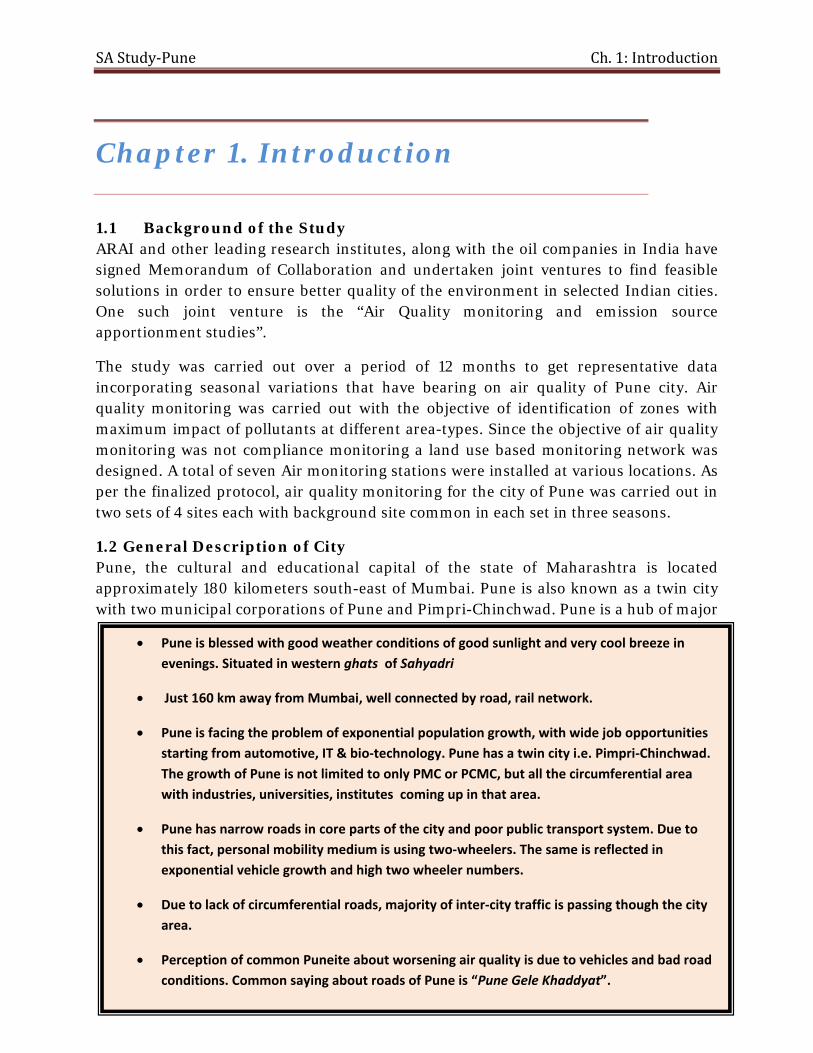
SA Study‐Pune Ch. 1: Introduction
1-1
• Pune is blessed with good weather conditions of good sunlight and very cool breeze in evenings. Situated in western ghats of Sahyadri
• Just 160 km away from Mumbai, well connected by road, rail network.
• Pune is facing the problem of exponential population growth, with wide job opportunities starting from automotive, IT & bio‐technology. Pune has a twin city i.e. Pimpri‐Chinchwad. The growth of Pune is not limited to only PMC or PCMC, but all the circumferential area with industries, universities, institutes coming up in that area.
• Pune has narrow roads in core parts of the city and poor public transport system. Due to this fact, personal mobility medium is using two‐wheelers. The same is reflected in exponential vehicle growth and high two wheeler numbers.
• Due to lack of circumferential roads, majority of inter‐city traffic is passing though the city area.
• Perception of common Puneite about worsening air quality is due to vehicles and bad road conditions. Common saying about roads of Pune is “Pune Gele Khaddyat”.
Chapter 1. Introduction
1.1 Background of the Study ARAI and other leading research institutes, along with the oil companies in India have signed Memorandum of Collaboration and undertaken joint ventures to find feasible solutions in order to ensure better quality of the environment in selected Indian cities. One such joint venture is the “Air Quality monitoring and emission source apportionment studies”.
The study was carried out over a period of 12 months to get representative data incorporating seasonal variations that have bearing on air quality of Pune city. Air quality monitoring was carried out with the objective of identification of zones with maximum impact of pollutants at different area-types. Since the objective of air quality monitoring was not compliance monitoring a land use based monitoring network was designed. A total of seven Air monitoring stations were installed at various locations. As per the finalized protocol, air quality monitoring for the city of Pune was carried out in two sets of 4 sites each with background site common in each set in three seasons.
1.2 General Description of City Pune, the cultural and educational capital of the state of Maharashtra is located approximately 180 kilometers south-east of Mumbai. Pune is also known as a twin city with two municipal corporations of Pune and Pimpri-Chinchwad. Pune is a hub of major

SA Study‐Pune Ch. 1: Introduction
1-2
automotive companies with presence of Bajaj Auto, Bajaj Tempo, Kinetic Motors and Tata Motors along with associated support industry. Pune is part of an important agricultural and manufacturing region. The major economic activities in Pune are service industries, government, construction, and more recently, information technology and biotechnology.
Geography: Pune is situated at the elevation of approximately 560m above sea level, in the Sahyadri Hills near west coast of India. PMC has jurisdiction over an area of about 243 sq. km.
Climate: Pune experiences three distinct seasons: summer, monsoon & winter. Typical Summer months are March to May, with max temperatures ranging from 35 to 39 deg C, with high diurnal variations in temperatures. City experiences winter from November to February. The day temperature hovers around 29°C, while the night temperature dips below 10°C for mostly in December and January. The prominent wind directions of Pune city are westerly & north-westerly. The city receives an annual rainfall of 722 mm, mainly between June and September Details of the climate of Pune City are as follows- (Source: Environmental Status Report, Pune Municipal Corporation) Location: 18° 31’N & 73 ° 51’E Altitude: 560 m above MSL Wind Direction: Feb to Sep – Westerly; Oct to Jan - Easterly
Residential Area
Cantonment Area
Forest/Hill Area
Industrial Area
Map of Pune city with Land-use Pattern

SA Study‐Pune Ch. 1: Introduction
1-3
Historical Meteorological Data
Attribute Units Minimum Maximum Mean Value
Month Mean Value
Month
Temperature- Summer
0C 23 May 40 May
Temperature- Winter
12 December 30 December
Humidity % 36 March 81 August
Rainfall mm 00 Jan, Feb, Mar, Apr, Dec
330.3 August
Wind Speed km/h 1.9 December 7.5 June
Representative Wind Roses
Demographics: As estimated from 2001 census, the urban agglomeration around Pune is expected to have population of 3.4 millions in 2007. This figure includes the population of Pimpri-Chinchwad, which is the industrial twin of Pune.

SA Study‐Pune Ch. 1: Introduction
1-4
Road Transport: Public transport in Pune is bus system under PMT & PCMT. PMT operates 960 buses on 184 routes. The total register vehicles in March 07 are around 14.5 lakh with 2W prominent population of more than 11 lakh. The likely age distribution of vehicle shows that more than 65 % personal vehicles have age less than 5 years. The total area connected by road network is around 139 sq. km with road length per sq. km around 2km. About 88 km are within congested part of city. The estimated area consumed by road network is hardly 10 sq. km, mainly due to narrow road widths.(City Development Plan for Pune 2006-2012,JNNURM Volume-I & II, April-2006)
Pune was selected as a demonstration city for the Urban Air Quality Management Project taken up by the US-AEP, MoEF and GoI agreement since 2002.
Ambient Air Quality Monitoring Program of NAQM
There are many agencies which carryout air quality monitoring on individual basis in the city like the University (earlier to handing over to MPCB), MPCB (Maharashtra Pollution Control Board) itself, Pune Municipal Corporation (PMC) by contracting its own Air Quality Management Cell and some colleges for their academic purposes and research organizations like IITM and others. However, most of these except MPCB under the National Ambient Monitoring Program (NAMP) carryout intermittent and project based monitoring. The present network of AQM of Pune City under MPCB has five monitoring locations. Out of these - Pimpri-Chinchwad under SAMP (Residential), Nalstop (Rural & other Areas), Bhosari (Industrial), Swargate (Residential) are monitored by University Of Pune under NAMP whereas Karve Road (Residential) location is monitored by M/s Honeywell Automation Ltd under supervision of MPCB. These stations monitor basic criteria pollutants like SPM, RSPM, SO2 and NO2 as per CPCB protocol in the city and data is available on MPCB site.
It was observed from the monthly variation in air quality parameters across the city that gaseous pollutants are never over the standard safe limits in the city since last decade or so hence the all the concerns are now based on Particulate Matter pollution in the city.

SA Study‐Pune Ch. 1: Introduction
1-5
The monthly statistics for the period April 2007 to January 2008 monitored under NAMP by MPCB at residential area locations is as follows:-
Nal-stop, Karve Road (Residential Site)
Month SO2(ug/m3) NO2 (ug/m3) RSPM (ug/m3)
Min Max Avg Min Max Avg Min Max Avg
April 17 27 23 36 57 48 80 227 128
May 13 28 22 37 56 46 47 150 108
June 11 26 18 29 53 40 37 99 65
September 13 24 19 39 55 49 40 126 74
October 16 29 21 42 58 51 58 146 102
December 16 26 22 44 57 51 85 180 135
January 14 25 19 34 50 43 109 211 155
Air Quality Trend in Pune City (2001-2007) Annual average concentration data for SO2, NOx and RSPM is presented below from 2001 to 2007 for Residential location (Source: CPCB). RSPM and SO2 shows a decreasing trend however NO2 has shown decreasing trend up to 2005 and from the year 2005 it has shown increasing values for the annual average at Residential Site. The variation in annual average concentrations during different years is may be due to
0
40
80
120
160
200
2001 2002 2003 2004 2005 2006 2007
Conc in ug/m3
Year
SO2
NOx
RSPM
Air Quality Trends in Pune City Annual Avg at Res Site
Source : CPCB
RSPM, SO2, NOx limit

SA Study‐Pune Ch. 1: Introduction
1-6
multiple factors including meteorology, neighborhood activity pattern or levels during monitoring period, etc.
1.3 Need for the Study The recent Auto Fuel Policy report submitted to the Government of India by the Mashelkar Committee, clearly points to the existence of a knowledge gap in the areas of emission factor determination for Indian vehicles, air quality monitoring and source apportionment studies. An integrated approach towards air quality management was felt necessary in this regard. A database collected using all the relevant scientific tools for design of modular air quality management plan was required for decision support With the above background, source apportionment studies have been undertaken in six cities viz. Delhi, Bangalore, Pune, Kanpur, Mumbai and Chennai. With a focus on apportionment of respirable particulate matter [PM10 and PM2.5 (limited)], being most critical.

SA Study‐Pune Ch. 1: Introduction
1-7
1.4 Objectives and Scope of Work
Critical air pollutants that impact human health and environment will be monitored and inventoried during this project with the overall objectives of the study as under-
• Air Quality Monitoring: To measure baseline critical air pollutants and air toxic levels at different parts of Pune for identification of “Hot Spots” representing maximum impact zone of different land use categories
• Source Apportionment: To conduct source apportionment study of particulate matter (PM10) using receptor model CMB-8.2.
• Emission Inventory Generation: To prepare emission inventory of various pollutants in the city of Pune. To project emission inventories for different future scenario with and without control options
• Dispersion Modeling using ISCST-3 for prediction of spatial variation of pollutant concentration.
• Action Plan: To assess the impact of sources on ambient air quality under different management/interventions/control options and draw a roadmap of short term and long term measures as considered appropriate and cost effective for air quality management
Scope of work
• The overall project scope includes city-specific air quality monitoring complete characterization of ambient dust (PM10 and PM2.5), emission inventory, source apportionment using chemical mass balance model and dispersion modeling using ISCST3.
• To address all the expected anthropogenic emission sources in urban areas, major air pollutants covered in this project include PM10, PM 2.5, SO2, NO2, CO, Benzene, Aldehydes, Alkenes, NMHC, THC and PAH
• The ambient air monitoring to be carried out over a period covering all three seasons in year to get representative data on seasonal variations in meteorology as well as activities that have bearing on air quality. Air quality monitoring to be carried out continuously for 20 days in each season for three seasons covering the whole year at seven monitoring locations including kerbside, residential, industrial and background (away from all the sources and in upwind direction).
• In order to catch the diurnal variations of sources as well as the typical meteorological changes, to conduct 8-hourly monitoring in a day.
• To carry out monitoring of meteorological parameters simultaneously at each station at same height of ambient air monitoring to ensure proper representation of the activities of the surrounding area for a given monitoring location

SA Study‐Pune Ch. 1: Introduction
1-8
• To carry out primary surveys for identification & spatial distribution of sources and preparation of detailed emission inventory for zone of influence (2km x 2km area) around each ambient air quality monitoring location.
• To carry out detailed emission inventory for line, point and area sources emission through Information/data from secondary sources.
• To carry out systematic survey of vehicle population in the city in order to get a wider cross section of vehicles in-use or on-road and the actual distance traveled by each sample vehicle, inspection & maintenance practices being adopted etc.,
• To prepare emission inventory of industrial and other sources through secondary sources.
• To carry out source apportionment analysis for PM10 and PM2.5 using receptor model like CMB model using detailed analysis of PM10 and PM2.5.
• To carry out dispersion modeling and intervention analysis using refined city level emission inventory.
• On completion of data collection, validation and interpretation of the assimilated information, a detailed road map to be drawn considering all possible measures for air quality improvement. These measures will be classified into short and long term with due priority to low cost measures that give maximum benefits.

SA Study‐Pune Ch. 1: Introduction
1-9
1.5 Approach to the Study:
The overall approach for the study is shown in following figure
Monitored ambient
concentrations
Onsite meteorological conditions
Emission inventorisation (present and future)
Air dispersion modeling
Source profiles
Receptor modeling
Source Apportionment
of PM10
Interpretation of model outputs (dispersion/ receptor models)
Air quality management
plan
Chemical characterization of PM10 samples

SA Study‐Pune Ch. 1: Introduction
1-10
1.6 Report Structure
This report contains the details of the activities like air quality monitoring, emission inventory preparation source apportionment, dispersion modeling and air quality management plan under the project air quality monitoring and emission source apportionment for city of Pune. The report is divided into eight chapters. Chapter One contains background of the study, need, objectives, approach and scope of work of the study. Details of air quality monitoring including sampling, analysis, QA/QC, results and interpretations are presented in Chapter Two. Chapter Three contains details of methodology followed and results of emission inventory for various sources like line, area and point sources. Source apportionment exercise using factor analysis and CMB-8.2 modeling are presented in Chapter Four. Chapter Five contains methodology followed and source category-wise dispersion modeling results for city. Future projections of emission scenario with and without control options and its effect on ambient concentrations for various sources is described in Chapter Six. Chapter Seven contains analysis of prioritized management/control options and action plan for management of air quality. Highlights and recommendations of the study are given in Chapter Eight.

SA Study‐Pune Ch. 2: Air Quality Status
2‐1
Chapter 2. Air Quality Status
2.1 Introduction The main objective of Ambient Air Quality Monitoring is to generate baseline data of ambient concentration of critical air pollutants and source apportionment study for PM10 in different parts of the city of Pune. A comprehensive air quality monitoring were carried out for a period of one year at seven representative locations including kerbside, industrial, commercial, residential and reference sites, which has different land use pattern and sources of activity. Levels of pollutants such as SPM, RSPM (PM10), PM2.5, SO2, NO2, CO, O3 and other toxic pollutants were monitored throughout the year. Characterization of PM10 was done using 2300 Partisol Multichannel Speciation Sampler.PM10 samples for various marker species such as Anions, Cations, Elements, Organic carbon, Elemental carbon and Molecular Markers etc.
Monitoring locations representing different land use namely kerbside, residential, industrial, etc. were selected so as to capture air quality levels under different activity profiles. In addition, one background location (away from all the sources and in upwind direction) was also included. The seven monitoring sites were distributed as 1 background, 2 residential, 2 kerbside, 1 industrial, 1 other (institutional) based on land use type and prominent wind direction. The Institutional site with not major activities in the near vicinity was selected to observe the impact of air pollution due to the Pimpri-Chinchwad area which is located at the north west of the Pune city (12 km) and called as twin city of Pune as north-west wind direction is a dominant wind direction. The selected stations are different from the existing NAMP stations monitored by MPCB as described in 2.2.1.8 as Pune Air Quality monitoring Location Map.
List of Monitoring Stations:
1. Background Site (CWPRS Guest House, Khadakwasla)
2. Residential site-1 (Shantiban, Kothrud)
3. Residential site-2 (Sahakarnagar Colony, Sahakarnagar)
4. Kerbside site-1 (College of Engineering Ground, Shivajinagar)
5. Kerbside site-2 (Hadapsar square, Hadapsar)

SA Study‐Pune Ch. 2: Air Quality Status
2‐2
6. Industrial Site (SAJ Test Plant Pvt. Ltd., Mundhwa)
7. Other (Institute) site (Geography Dept., University of Pune)
2.2 Methodology (sampling sites, area maps-GIS, parameters, instruments, frequency)
2.2.1 Sampling Sites
As per the finalized protocol a total of seven monitoring stations were selected with the
local stakeholders and CPCB experts. The seven monitoring sites were distributed as 1
background, 2 residential, 2 kerb-side, 1 industrial, 1 other (institutional) based on the
area type. Details of geographical locations of the monitoring sites are given in Table 2.1
and Fig. 2.1.
Table2-1: Details of locations of air quality monitoring sites
Location Type Location
Latitute # (Dir Deg Min Sec)
Longitude # (Dir Deg Min Sec)
Altitude (Feet)
Back GroundCWPRS Guest House, Khadakwasla N 18 26 44 (N 18 26 52) E 73 47 32 (E 73 47 28.86) 1789
Other (InstituteGeography Dept., University of Pune N 18 32 50 (N 18 32 49.35) E 73 49 40 (E 73 49 36.35) 1722
Residential 1Shantiban Hsg. Society, Kothrud N 18 29 40 (N 18 29 47.3) E 73 48 05 (E 73 48 01) 1760
Residential 2 Sahakarnagar Colony N 18 28 32 (N 18 28 35.8) E 73 51 13 (E 73 51 9.60) 1792
KerbsideCollege of Engg Pune- Hostel, Shivajinagar N 18 31 40 (N 18 31 42 ) E 73 51 9 (E 73 51 6.22) 1630
Kerbside 2 Hadapsar Square N 18 29 59 (N 18 30 02) E 73 56 24 (E 73 56 21) 1660
IndustrialSaj Test Plant, Mundhwa N 18 31 08 (N 18 31 12.65) E 73 55 02 (E 73 55 01.38) 1637
1

SA Study‐Pune Ch. 2: Air Quality Status
2‐3
Fig. 2.1: Air quality monitoring locations
Pune‐Air Quality Monitoring Locations
1
2
3
4
5
6
7
Background Site Residential Sites Kerbside Sites Industrial Site Institutional Site
CWPRS Guest House, Khadakwasla
Shantiban Society, Kothrud
Sahakarnagar Colony, Sahakarnagar
College of Engg. Pune, Shivajinagar
Pune-Solapur Highway, Hadapsar
SAJ Test Plant, Mundhwa
Univ. of Pune, Shivajinagar
Monitoring Locations

SA Study‐Pune Ch. 2: Air Quality Status
2‐4
2.2.1.1 Background location (CWPRS Guest House)
Map 2X 2 km, LAND-USE AND SOURCES (IDENTIFIED THROUGH PRIMARY SURVEYS)
This site is situated at the South-West part of the Pune city, which is the most predominant wind direction. It is away from the main city area. Also, land-use pattern around the monitoring sites in 2 X 2 km grid suggests very low vehicle traffic activity levels with 40% of the land is agricultural land, about 20% bare land, 16 % forest and hilly area and about 11% residential area. The residential area is at the east of the monitoring site.
40%
19%
15%
1%2%
11%
4%3%
4%1% 0%
Site: CWPRS Guest House, Khadakwasla (Background)
Agricultural Land
Non-agriculture Bare Land
Forest
Hilly Area
Water Body
Residential
Slum
Commercial
Contruction
Industry
Brick Kilns
Background
(CWPRS Guest House), Khadakwasla
Latitude (N 180 26’ 44’’), Longitude (E 730 47’ 32’’), Altitude (1789 ft)

SA Study‐Pune Ch. 2: Air Quality Status
2‐5
2.2.1.2 Residential location (R1) Map 2X 2 km, LAND-USE AND SOURCES (IDENTIFIED THROUGH PRIMARY SURVEYS)
This is a purely residential site with the residential bungalows around the monitoring sites. 40% of the area around the 2X2 km grid is residential area, 20% of bare land and 15% of hilly area. Considerable vehicular traffic activity is observed around the site due to commuting of dwellers around the site.
Residential 1
(Shantiban Hsg. Society), Kothrud
Latitude (N 180 29’ 40’’), Longitude (E 730 48’ 05”) Altitude (1760 ft)
1%
21%
1%
15%
0%39%
5%
7%
8%3%
0%0%
Site: Shantiban (Residential 1)
Agricultural Land
Non-agriculture Bare Land
Forest
Hilly Area
Water Body
Residential
Slum
Commercial
Contruction
Industry
Brick Kilns
Others (School/Road)

SA Study‐Pune Ch. 2: Air Quality Status
2‐6
2.2.1.3 Residential location (R2) Map2X2, LAND-USE & SOURCES (IDENTIFIED THROUGH PRIMARY SURVEYS)
Sahakarnagar colony represents a mixed residential and commercial site with many small stalls near the site. The residential area also includes slum area in vicinity of the monitoring site. The land use distribution is residential area 40%, Slum 8%, bare land 25% and Hilly area 11%.
Residential 2
(Sahakarnagar Colony)
Latitude (N 180 28’ 32’’). Longitude (E 730 51’ 13’’) Altitude (1792 ft)
2%
25%
4%
11%
2%
40%
8%
3%5%
0%
0% 0%
Site: Sahakarnagar Colony (Residential 2)
Agricultural Land
Non-agriculture Bare Land
Forest
Hilly Area
Water Body
Residential
Slum
Commercial
Contruction
Industry
Brick Kilns
Others (School/Road)

SA Study‐Pune Ch. 2: Air Quality Status
2‐7
2.2.1.4 Kerbside location (K1) MAP (2 x 2 Km), LANDUSE AND SOURCES (IDENTIFIED THROUGH PRIMARY SURVEYS)
This site is along a major road with continuous traffic flow from the old Mumbai highway. 2 X 2 km grid landuse is residential area (31%) with commercial activities (17%), slum (12%) and 16% agricultural land.
Kerbside 1
(College of Engineering, Pune Hostel), Shivajinagar
Latitude (N 180 31’ 40’’).Longitude (E 730 51’ 9’’)
Altitude (1630 ft)
16%
6% 0%0%
11%
31%
12%
17%
3% 0% 0%
4%
Site: CoEP Hostel (Kerbside 1)Agricultural Land
Non-agriculture Bare LandForest
Hilly Area
Water Body
Residential
Slum
Commercial
Contruction
Industry
Brick Kilns
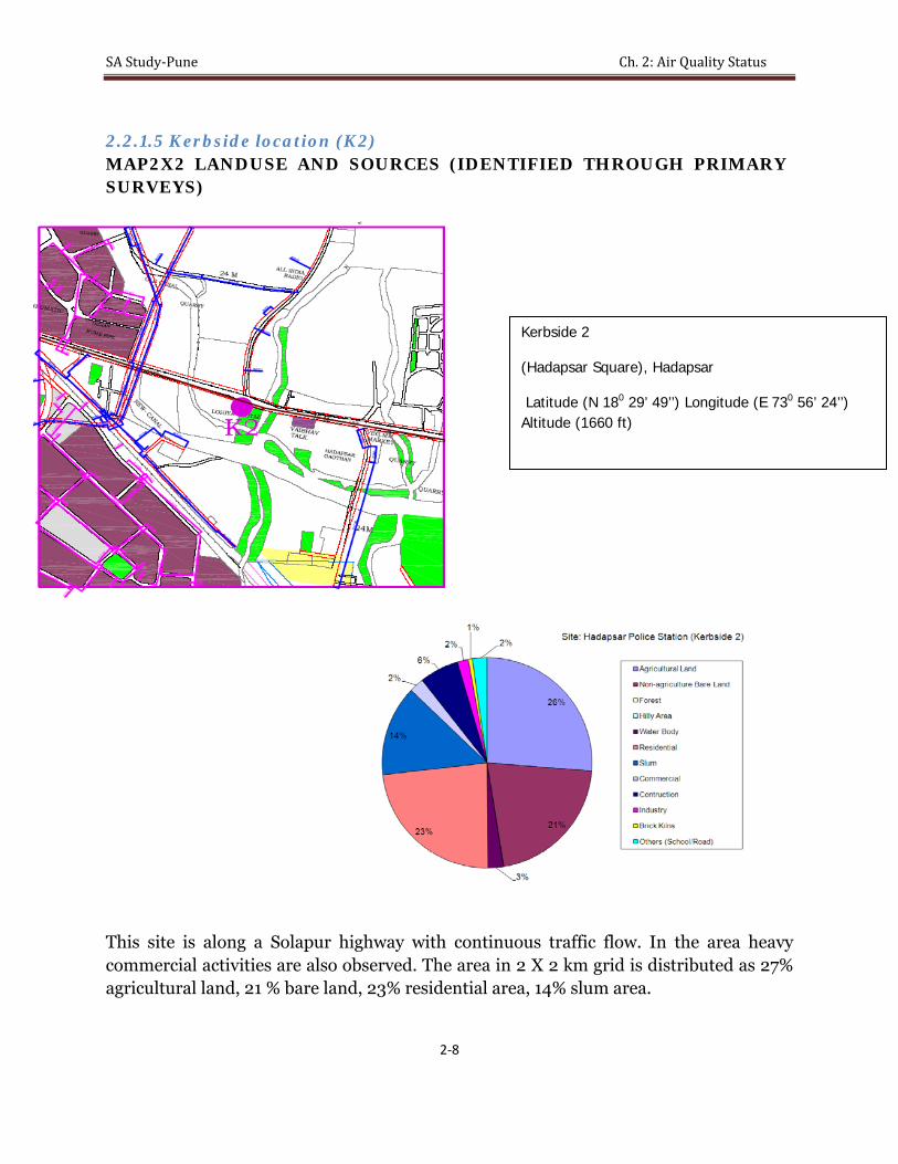
SA Study‐Pune Ch. 2: Air Quality Status
2‐8
2.2.1.5 Kerbside location (K2) MAP2X2 LANDUSE AND SOURCES (IDENTIFIED THROUGH PRIMARY SURVEYS)
This site is along a Solapur highway with continuous traffic flow. In the area heavy commercial activities are also observed. The area in 2 X 2 km grid is distributed as 27% agricultural land, 21 % bare land, 23% residential area, 14% slum area.
Kerbside 2
(Hadapsar Square), Hadapsar
Latitude (N 180 29’ 49’’) Longitude (E 730 56’ 24’’) Altitude (1660 ft)

SA Study‐Pune Ch. 2: Air Quality Status
2‐9
2.2.1.6 Industrial location (I) MAP 2X2 LANDUSE AND SOURCES (IDENTIFIED THROUGH PRIMARY SURVEYS)
It is located in the Mundhwa industrial area with major industries in 2 X 2 km area including metal industries like Bharat Forge Ltd., Kalyani Carpenter and Speciality Steels Ltd., ceramic and clay products industries like Siporex India Ltd., B G Shirke Construction Tech Ltd. 2 X 2 km grid includes 37% agricultural land, 13% bare land and 10% residential area.
Industrial
(SAJ Test Plant), Mundhwa
Latitude (N 180 31’ 08’’). Longitude (E 730 55’ 02’’) Altitude (1637 feet)

SA Study‐Pune Ch. 2: Air Quality Status
2‐10
2.2.1.7 Institute location (O) MAP2X2 LAND-USE AND SOURCES (IDENTIFIED THROUGH PRIMARY SURVEYS)
This site is at the north-west part of the Pune. Site (2 X 2 km) is surrounded by Forest plantation (59%), bare land (16%), Residential area (10%) and commercial (9%). As such there are no major air pollution sources in the impact zone other than the vehicular activity for commuting. The site was selected to observe the impact of air pollution due to the industries located in Pimpri-Chinchwad industrial area which is located at the north west of the Pune city (12 km) as north-west wind direction is the second predominant wind direction.
Other Institutional
(Geography Dept.), University of Pune
Latitude (N 180 32’ 50’’). Longitude (E 730 49’ 50’’) Altitude (1637 feet)
0%
16%
59%
2%0%
10%
1% 9%
2% 0%0% 1%
Agricultural Land
Non-agriculture Bare LandForest
Hilly Area
Water Body
Residential
Slum
Commercial
Contruction
Industry
Brick Kilns

SA Study‐Pune Ch. 2: Air Quality Status
2‐11
2.2.1.8 Geographical Locations of source Apportionment sites with NAMP sites
2.2.2 Air Quality Monitoring
Ambient air quality data has been collected for 20 days at each monitoring site. Table
2-2 gives the details of air monitoring network. Features of air quality monitoring
protocol followed are as follows-
• Monitoring in 2 sets of 4 sites each in a season. Background site common to both
the sets. One residential and one kerbside site included in each set.
• Monitoring continuously for 20 days in a season at a site.
1
1
1
1
1
1
NAMP Monitoring Sites
Karve Road, Residential
Bhosari, Industrial Area
Swargate, Residential
Nal Stop, Rural and Other Area
Background Site Residential Sites Kerbside Sites Industrial Site Institutional Site
CWPRS Guest House, Khadakwasla
Shantiban Society, Kothrud
Sahakarnagar Colony, Sahakarnagar
College of Engg. Pune, Shivajinagar
Pune-Solapur Highway, Hadapsar
SAJ Test Plant, Mundhwa
Univ. of Pune, Shivajinagar
SA Studies Monitoring Sites
1
2
3
4
5
6
7
Pune‐Air Quality Monitoring Locations

SA Study‐Pune Ch. 2: Air Quality Status
2‐12
• Monitoring of PM10 with speciation sampler Partisol 2300 at 4 sites
simultaneously for 20 days. During this period, 24 hrly sampling for first 7 and last
7 days and 8 hrly sampling in between for 6 days for last 7 days were carried out.
• Monitoring of PM2.5 with FRM Partisol 2000 at 2 sites simultaneously for one
week and shifting of these samplers to other two sites for one week monitoring at
those sites.
• Online monitoring of CO & Ozone at sites with short-term averaging period of 3
min, and long-term averaging period of 30 min.
• Monitoring of meteorological data for wind direction, wind velocity, ambient
temperature, relative humidity, solar radiation and rainfall.
• Monitoring of Aldehydes, Benzene, 1,3-butadiene once in a season
Ambient air quality data (24 hrly.) on the above sites has been collected for 20 days at each monitoring site. Detailed sampling and analytical protocol followed for the study is given in Table2-3 (a), (b) and (c).

SA Study‐Pune Ch. 2: Air Quality Status
2‐13
Table 2-2: Details of Air Monitoring Network Set-I
Set-II
Site Name Site Type Monit. Height Samplers Installed Land-use in 2 X 2 grid
Partisol 2300 Speciation Agricultural land- 40%Partisol 2000 FRM Bare land (non-agri)- 19%Respirable Dust Sampler Forest & Hilly area- 16%CO, O3 Online AnalyserMet-sensorsPartisol 2300 Speciation Residential- 40%Partisol 2000 FRM Bare land (non-agri)- 20%
Hilly area- 15%Construction- 8%
Partisol 2300 Speciation Agricultural land- 37%Partisol 2000 FRM Industry- 19%Respirable Dust Sampler Bare land (non-agri)- 13%High Volume sampler Residential- 10%Partisol 2300 Speciation Residential- 31%Partisol 2000 FRM Commercial- 17%Respirable Dust Sampler Agricultural land- 16%CO Online AnalyserMet-sensors
Slum- 12%
3 m
College of Engineering Pune, Shivajinagar
Kerbside 3 m
Respirable Dust Sampler
Residential- 11%
SAJ Test Plant Pvt. Ltd., Mundhwa
Industrial 6 m
CWPRS Guest House, Khadakwasla
Background 6 m
Shantiban Society, Kothrud
Residential
Site Name Site Type Monit. Height Samplers Installed Land-use in 2 X 2 grid
Partisol 2300 Speciation Agricultural land- 40%Partisol 2000 FRM Bare land (non-agri)- 19%Respirable Dust Sampler Forest & Hilly area- 16%CO, O3 Online AnalyserMet-sensorsPartisol 2300 Speciation Residential- 40%Partisol 2000 FRM Bare land (non-agri)- 25%Respirable Dust Sampler Hilly area- 11%High Volume sampler Slum- 8%Partisol 2300 Speciation Forest, Plantation- 59%Partisol 2000 FRM Bare land (non-agri)- 16%Respirable Dust Sampler Residential- 10%High Volume sampler Commercial- 9%Partisol 2300 Speciation Agricultural land- 27%Partisol 2000 FRM Bare land (non-agri)- 21%Respirable Dust Sampler Residential- 23%CO Online AnalyserMet-sensors
Slum- 14%
3 m
Hadapsar Kerbside 3 m
Residential- 11%
Geography Dept., Univ. of Pune
Other (Institute)
6 m
CWPRS Guest House, Khadakwasla
Background 6 m
Sahakarnagar Colony, Sahakarnagar
Residential

Table 2-3 (A): Sampling and Analytical Protocol for Source Apportionment Study conducted for Pune City
Particulars
Parameters
SPM
PM10 PM 2.5 NO2 SO2 CO
OC/EC
Ions
VOC (Benzene
and 1,3 Butadiene,)
O3
Aldehydes
NMHC
HC
Sampling Instrument
Respirable Dust sampler (RDS)
Multichannel (4 channel) Speciation Sampler
FRM Partisol (PM2.5) sampler
Impingers attached to RDS
Impingers attached to RDS
Continuous Online Analyzer / Tedlar bags
PM10 Sampler Particulate collected on Quartz filter
PM10 Sampler Particulate collected on Nylon filter
Adsorbent tube attached to VOC sampler
Continuous Online Analyzer
Impinger attached to VOC sampler
Low volume sampling pump connected to Tedlar bags
Low volume sampling pump connected to Tedlar bags
Sampling Principle
Filtration of aerodynamic sizes
Filtration of aerodynamic sizes with a size cut by impaction
Filtration of aerodynamic sizes with a size cut by impaction followed by cyclone separation
Chemical absorption in suitable media
Chemical absorption in suitable media
Suction by Pump As per instrument specification
Filtration of aerodynamic sizes with a size cut by impaction
Filtration of aerodynamic sizes with a size cut by impaction
Active pressurised sampling / Adsorption
Suction by Pump
Chemical Absorption (DNPH–Acetonitrile)
Suction by Pump
Suction by pump
Flow rate 0.8-1.2 m3/min
16.7 LPM
16.7 LPM 1.0 LPM 1.0 LPM As per instrument specification
16.7 LPM
16.7 LPM 50-100 mlpm As per instrument specification
0.5 LPM As per instrument specification
As per instrument specification
Sampling Period
8 change of filter, 24 Hourly Reporting
14 days 24 hourly and 6 days 8 Hourly filter change
24 hourly
4 Hourly change of absorbing media, 24 Hourly Reporting
4 Hourly change of absorbing media, 24 Hourly Reporting
8 Hourly sampling and 24 Hourly Reporting / 20 days continuous
24 hourly Or 8 / 24 Hourly
24 hourly Or 8 / 24 Hourly
4 Hourly sampling and 24 Hourly Reporting
One week continuous
4 Hourly sampling and 24 Hourly Reporting
8 Hourly sampling and 24 Hourly Reporting
8 Hourly sampling and 24 Hourly Reporting
Sampling frequency
20 Days continuous in each season, for three seasons
20 Days continuous in each season, for three seasons
1 Week continuous in each season, for three seasons
20 Days continuous in each season, for three seasons
20 Days continuous in each season, for three seasons
One week continuous during 20 days of monitoring in each season
20 Days continuous in each season, for three seasons
20 Days continuous in each season, for three seasons
Once during 20 days of monitoring in each season
One week continuous during 20 days of monitoring in each season
Once in 20 days of monitoring in each season
One week continuous during 20 days of monitoring in each season
One week continuous during 20 days of monitoring in each season
Analytical instrument
Electronic Balance
Electronic Micro Balance
Electronic Micro Balance
UV/VIS Spectrophoto-meter
UV/VIS Spectrophoto-meter
Online-NDIR
OC/EC Analyser
Ion Chromatograph
GC-ATD-FID
Automatic analyser
HPLC-UV
Online analyzer with FID/ GC - FID
Online analyzer with FID/ GC - FID
Analytical method
Gravimetric Gravimetric Gravimetric
sodium Arsenite) Improved West & Gaeke Method
Pararosaniline Jacobs & Hochheiser Modified method
NDIR
TOR/TOT Method CARB/ MLD No. 065
Ion Chromatography CARB/ MLD No. 064
EPA 625/ TO-17/ CARB/MLD-051
UV-Absorption
EPA TO-5 CARB/ No. 104
FID Analysis
FID Analysis
Minimum Reportable value
5 µg/m3 5 µg/m3 5 µg/m3 9 µg/m3 4 µg/m3 0.05 ppm
TOC 1 µg/ cm2, TEC 0.5 µg/ cm2, TC 1.5 µg/ cm2
0.020ppm 0.5 ppb 0.6 ppb
1ppm 0.05 ppm 0.05 ppm

SA Study‐Pune Ch. 2: Air Quality Status
2‐15
Table 2-3 (B): Target Physical and Chemical components (groups) for Characterization of Particulate Matter for Source Apportionment studies at Pune
Components Required filter matrix Analytical methods
PM10 / PM2.5 G/F (PM10) / Teflon (PM2.5) filter paper. Pre and post exposure conditioning of filter paper is mandatory
Gravimetric
Elements (Al, Pb, Cu, Zn, As, Se, Br, Ni, Fe, Mn, Mg, Cr, Ti, Ca, Cd, S, Si, Na, Ba, Sb, Cd, Sr.)
Teflon filter paper ED-XRF
Ions (Ammonium, Nitrate -, Sulfate, Soluble Potassium, Chloride +)
Nylon filter paper Ion chromatography with conductivity detector
Carbon Analysis (OC and EC) Quartz filter. Prebaking of quartz filter paper at 600 ºC is essential
TOR/TOT method using DRI Carbon Analyzer
Molecular markers
Alkanes
n- Hentriacontane
n-Tritriacontane
n- Pentatriacontane
The left over quartz filter paper after OC/EC analysis were taken as composite sample (for one week) to represent a location and specified duration of exposure. One composite of 20 days were then used for analysis in each season.
Extraction, followed by GC-MS analysis with and without derivatization
Qualitative Analysis carried out on GC-MS whereas, quantification done on HRGC with FID as a detector.
Hopanes 22, 29, 30 – Trisnorneohopane
17α(H), 21β(H)-29 Norhopane
17α(H), 21β(H) Norhopane
Alkanoic acid
Hexadecanamide
Octadecanamide
Others Stigmasterol
Levoglucosan
PAHs Anthracene Fluoranthene Benzo(k)fluoranthene Benzo(a)pyrene Pyrene Benzo(g,h,i) perylene Indeno(1,2,3-c,d)pyrene Benz (b) Fluoranthene Benz (a) Anthracene
Teflon filter paper Acetone : Methylene Chloride Soxhlet extraction and analysis using HPLC-UV

SA Study‐Pune Ch. 2: Air Quality Status
2‐16
Table 2-3(C): Pollutants and their Methods of analysis
Pollutants Methods
SO2 Spectrophotometric measurement, Improved West & Gaeke Method
NO2 Spectrophotometric measurement, Jacobs & Hochheiser Method
CO Automatic Analyser Online- NDIR
O3 Automatic Analyser, UV Photometric Method
Aldehydes HPLC- UV
Benzene Active sampling on adsorbent and GC-FID determination
1,3 Butadiene Active sampling on adsorbent and GC-FID determination
HC Online analyzer/ GC-FID
NMHC Online analyzer/ GC-FID
SA Study‐Pune Ch. 2: Air Quality Status
2‐17
2.3 Quality Assurance/Quality Control Sampling
Quality assurance and Quality control (QA/QC) is an essential part of any monitoring system, it is a program of activities that ensures that measurements meet defined and appropriate standards of quality, with a stated level of confidence. Each sample to be sent to the field for monitoring was prepared carefully by following QA/QC system (Table 2-3). Unique sample ID was given to each sample collected for future reference and database generation.
Standard Operating procedures, Work Instruction Manuals and Maintenance Procedures were prepared for all the instruments and equipments used for conducting Ambient Air Quality Monitoring and Source Apportionment Study (Model Operating Procedures for Source Apportionment Stydy, CPCB, 2006).Specimen of some Work Instruction and SOPs can be viewed at Annexures. Field staff whosoever handling the sample kit were trained for the specific tasks like handling of filters and Chemcomb cartridges. Operating instructions were described in local languages for indigenous samplers and imported PM samplers. Proper training in association with equipment manufacturers and suppliers of samplers were arranged for field staff at working level and supervisors for conducting intermediate performance checks.
Analysis
The details of Analytical Techniques/ Instrumentation, Calibration standard, SOPs used, for conducting above mentioned analysis is given in Table 2-4. Partisol Model 2300, FRM Model 2000, APM 460DXm Respirable Dust Sampler (Envirotech Instruments Pvt.Ltd.) and set of continuous online analyzers for CO and Ozone were used at each of the seven sites for three seasons over a period of one year.
Suspended Particulate Matter (SPM) monitoring was carried out using High Volume Sampler. It was not possible to operate HVS to monitor SPM at residential sites due to the high noise levels of the sampler. Hence SPM monitoring at residential sites was not carried out. Monitoring of RSPM (PM10) was carried out using Respirable Dust Sampler (RDS) with cyclone attached for PM10 separation. Particles more than 10 microns were collected at the bottom of cyclone. The Total Suspended Particulates (TSP) is reported as sum of PM10 collected on glass-fibre filter paper and dust collected at bottom of cyclone. Thermoelectrically cooled gaseous sampling attachment was used for SO2 and NO2 sampling, wherein the temperature of absorbing solution was always kept below 18OC for better absorption efficiency. Speciation sampling was carried out with Partisol

SA Study‐Pune Ch. 2: Air Quality Status
2‐18
2300 samplers with PM10 head and at a flow rate of 16.7 lpm. Teflon, Nylon and Quartz filter papers were used in ChemComb cartridges for sample collection. Partisol 2000 sampler with PM2.5 head and 16.7 lpm flow rate was used for PM2.5 monitoring
PM10 was collected on three types of filters depending upon the analytical requirement of the source apportionment studies viz., PTFE filters Teflo (P. No. R2PJ047) of diameter size 47mm, 2.0 um pore size, Nylon paper Nylasorb (P. No. 64509) and Quartz paper Tissuquartz (P No. 2500QAT UP7202).PM2.5 was collected on PTFE filters Teflo and Quartz paper Tissuquartz as per the CPCB designed sampling protocol. Particulate matter was collected on pre-baked quartz fiber filter and pre-washed Nylon Filters. PTFE filters were also conditioned before and after sample collection as per the SOPs mentioned. The air flow rate through each filter was measured before and after each 24-hour sampling period with a calibrated rotameter.
The primary chemical species of interest are selected elements, sulphates, nitrates and elemental & organic carbon. Chemical speciation analysis can be broken into the three most common categories: elements, ions and carbons. This would be helpful in identifying the sources of major activities in the study area of Pune city. An outline of field & laboratory performance audits is summarized in Table 2-4.Typical analytical technique/methodology applicable for each of speciation categories is described below:
Elements
For quantification of elements present in PM10/PM2.5 collected at seven locations in city of Pune, Energy Dispersive X-ray fluorescence (ED-XRF) technique was used. It is a non-destructive technique of inorganic speciation analysis, XRF does not require sample preparation or long operator time after it is loaded into the analyzer (James P.Lodge, Lewis Publishers). Even filters remain intact after analysis and can be used for many additional analyses by other methods. About 33 elements were analyzed using this technique.
Ions
Ionic species are those that are soluble in water. Anions and Cations were analyzed using Ion Chromatograph with conductivity detector. In PM10 and PM2.5 dust samples ions that are analyzed on Ion Chromatograph are under group Anions as Fluoride, Chloride, Bromide, Nitrite, Nitrate, Phosphate and Sulphate and amongst Cations such as Sodium, Ammonium, Potassium, Calcium and Magnesium. But polyatomic ions, such as sulphate, nitrate, ammonium, and phosphate are typically quantified by ion chromatography (IC). Sample preparation was done by using Ultrasonication method.

SA Study‐Pune Ch. 2: Air Quality Status
2‐19
Milli-Q grade water freshly produced from Gradient A10 Millipore system, having resistivity of 18 M-Ohm was used for sample preparation and analysis. Each lab blank, field blank and sample was always filtered through 0.2 micron Nylon membrane filters to avoid background matrix interference.
Elemental/Organic Carbon
For our studies three classes of carbon are commonly measured in aerosol samples collected on quartz fiber filters: 1) organic, volatilized or non-light absorbing carbon; 2) elemental or light absorbing carbon; and 3) carbonate carbon.
Many methods have been applied to the separation of organic and elemental carbon in ambient and source particulate samples. “Organic Carbon” and “Elemental carbon” generally refers to particles that appear black and are also called: Soot”, “graphitic carbon” or “black carbon”. The various methods include thermal/optical reflectance (TOR), thermal/optical transmission (TOT), and thermal manganese oxidation (TMO) methods for organic and elemental carbon. TOR/TOT method of analysis was used for analysis of carbon fractions. DRI 2001 Model Carbon analyzer were used for the carbon measurement study. Pre-baked filters were used for carrying out blank analysis.
Organic Molecular Markers
The most common method used is the extraction of a filter with a suitable organic solvent (or combination of solvents), followed by the analysis of the extract by gas chromatography (GC) combined with mass spectrometry (MS) or with other specific detectors. We have extracted PM10 and Pm2.5 samples using Soxhlet extraction method with Acetone and Methylene Dichloride as organic solvents in 1:1 proportion. We have used GC-MS for qualitative analysis of organic species and quantification was done by using High resolution Gas Chromatograph (HR-GC) with Flame Ionization Detector (FID) as detector and High performance liquid chromatography (HPLC) with Uv detector. Analysis of Alkanes, Hopanes and Alkanoic Acids were done on HRGC-FID whereas , HPLC-Uv detector were used for analysis of PAHs compounds. The detailed list of organic species is given in analytical protocol for the city of Pune . (Refer Table 2-3 B).
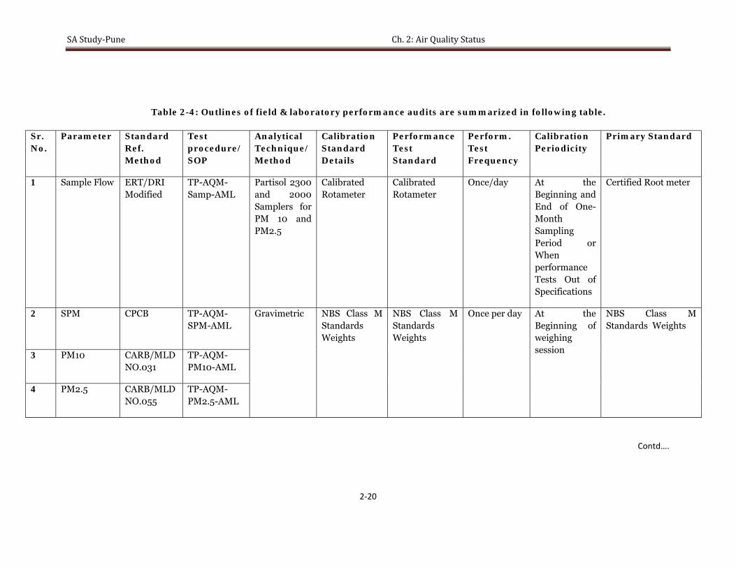
SA Study‐Pune Ch. 2: Air Quality Status
2‐20
Table 2-4: Outlines of field & laboratory performance audits are summarized in following table.
Sr. No.
Parameter Standard Ref. Method
Test procedure/ SOP
Analytical Technique/ Method
Calibration Standard Details
Performance Test Standard
Perform. Test Frequency
Calibration Periodicity
Primary Standard
1 Sample Flow ERT/DRI Modified
TP-AQM-Samp-AML
Partisol 2300 and 2000 Samplers for PM 10 and PM2.5
Calibrated Rotameter
Calibrated Rotameter
Once/day At the Beginning and End of One-Month Sampling Period or When performance Tests Out of Specifications
Certified Root meter
2 SPM CPCB TP-AQM-SPM-AML
Gravimetric NBS Class M Standards Weights
NBS Class M Standards Weights
Once per day At the Beginning of weighing session
NBS Class M Standards Weights
3 PM10 CARB/MLD NO.031
TP-AQM-PM10-AML
4 PM2.5 CARB/MLD NO.055
TP-AQM-PM2.5-AML
Contd….

SA Study‐Pune Ch. 2: Air Quality Status
2‐21
Sr. No.
Parameter Standard Ref. Method
Test procedure/ SOP
Analytical Technique/ Method
Calibration Standard Details
Performance Test Standard
Perform. Test Frequency
Calibration Periodicity
Primary Standard
5 SO2 CPCB/EPA Appendix A Part 50
TP-AQM-SOx-AML
Wet Chemical Method Pararosaniline, West & Gaeke method using Uv-Vis Spectrometer
Calibration using MERCK ,Germany make Pararoseaniline HCl dye and Sodium Metabisulphite
Solution Standard
1/10 th sample
At Beginning of analysis
MERCK ,Germany make Pararoseaniline HCl dye nd Sodium Metabisulphite
6 NO2 CPCB TP-AQM-NO2-AML
Wet Chemical Method (Sodium Arsenite), Modified Jacob & Hochheiser using Uv-Vis Spectrometer
Calibration using AR grade NaNO2 salt
Solution Standard
1/10 th sample
At Beginning of analysis
AR grade NaNO2 salt
7 Elements Method IO –3.3 for XRF CARB
TP-AQM-Elements-AML
Energy Dispersive -X-Ray Fluorescence (ED-XRF)
Micromatter Thin Film Standards
Replicate Thin Film Standard
1/10 th sample
Once/2-months When Performance test Not Met
Micromatter Thin Film Standards

SA Study‐Pune Ch. 2: Air Quality Status
2‐22
Sr. No.
Parameter Standard Ref. Method
Test procedure/ SOP
Analytical Technique/ Method
Calibration Standard Details
Performance Test Standard
Perform. Test Frequency
Calibration Periodicity
Primary Standard
8 Ions CARB/MLD NO.064
TP-155-AML Ion Chromatograph with Conductivity Detector
NIST Traceable MERCK make Certipur Standards
Solution Standard
1/10 th sample
At Beginning of Each Run
Certified NIST traceable standards
9 EC/OC CARB/MLD NO.065
TP-156-AML Thermal Optical Reflectance/Transmission Carbon Analyzer
Methane, CO2 Gas and ACS Certified KHP
Replicate Methane Gas Run
1/10 th sample
Once/2-months or When Performance test not met
ACS Certified chemicals
10 Molecular Markers
CPCB provided SOP for SA Studies.
TP-AQM-MM-AML
Gas Chromatograph -Mass Spectrometer(GC-MS)
Available Sigma Aldrich and Fluka Make authentic standards
Solution Standard
Intermediate checks with authentic standard before analysis of set of samples.
ACS Certified chemicals
11 Poly-Aromatic Hydrocarbons (PAH)
As per NIST SRM 1647d
TP-148-AML High Performance Liquid Chromatography (HPLC) with UV Detector
NIST SRM-1647d 16 component PAH-Mix. Acceptance criterion of +/- 5 % of the NIST Standards
Solution Standard
Intermediate checks with NIST standard before analysis of set of samples.
Certified NIST traceable standards

SA Study‐Pune Ch. 2: Air Quality Status
2‐23
Sr. No.
Parameter Standard Ref. Method
Test procedure/ SOP
Analytical Technique/ Method
Calibration Standard Details
Performance Test Standard
Perform. Test Frequency
Calibration Periodicity
Primary Standard
12 VOC (Benzene and 1,3-butadiene)
EPA Method TO-17
TP-146-AML Automated Thermal Desorber-Gas Chromatography Method (ATD-GC-FID)
Benzene 1.2 ppm and 1,3 Butadiene 1.9 ppm mixture in nitrogen. Alchemie Gases and Chemicals
Intermediate checks with certified standard before analysis of set of samples.
Authentic gas cylinder with certificate of analysis
13 Carbonyls (Aldehydes & Ketones)
EPA Method 1004
TP-140-AML High Performance Liquid Chromatography (HPLC) with UV Detector
Accustandard (NIST Traceable) for Carbonyl Compounds at DNPH Derivatives- 13 component. Acceptance criterion of +/- 5 % of the NIST Standards
Replicate mix standard Run
Intermediate checks with NIST traceable standard before analysis of set of samples.
Accustandard (NIST Traceable) for Carbonyl Compounds
NOTE:- Audit frequency was kept once per set of monitoring for Aldehydes, PAHs, Molecular Markers, SO2 and NO2. Whereas, it was kept once per 2 months for other parameters in above mentioned table.

SA Study‐Pune Ch. 2: Air Quality Status
2‐24
Flow Chart for Sample identification, pre-treatment, post sampling-treatment and analysis
Preconditioning of filter papers (Teflon, Nylon, Quartz and Glass-fiber) around 7 days stock at a time
Teflon & Nylon Filter: Temp. = 27oC +/- 3oC and RH= 40% +/- 5% (In Humidity Chamber of CHL) for 24 hrs.
Quartz Filter: Pre-baking of filters at 600oC for 24 Hrs and storage in petridish wrapped in aluminium foil.
Glass Fibre Filter: Temp. = 27oC +/- 3oC and RH= 40% +/- 5% (In Humidity Chamber of CHL) for 24 hrs
Filter paper numbering:
Teflon, Nylon and Quartz Filter: Numbers on petridishes
Label format: Season code-Set code/Site code/Parameter
Paper type & running no.
Generation of running no: Set no, wk no, serial no.
Serial no = 1 for B, 2 for R, 3 for I, 4 for k; 5 for B and so on…
FOR EXAMPLE: to refer the Nylon filter paper sampled in summer season at the site CWPRS in set 1 on day 4 in first wk with frequency of 24 hourly would have label as
S-I/B/ PM10/N1113
Glass Fibre Filter: On filter paper with numbering machine and on envelope in a predefined format printed on envelope.
Label format: Season code-Set code/Site code/Parameter

SA Study‐Pune Ch. 2: Air Quality Status
2‐25
Initial Weighing:
Teflon Filter: Mettler MT5 (AML/Inst/50) (Resolution 1 microgram)
Nylon and Quartz Filter: Afcoset (AML/Inst/117) (Resolution 10 microgram)
Glass Fibre Filter and Dust Bottles: Afcoset (AML/Inst/118) (Resolution 10 microgram)
Storage before sampling:
Teflon, Nylon and Quartz Filter: In Respective labeled Petridishes in Humidity Chamber
Glass Fibre Filter: In respective envelops stored in desiccators in CHL
Preparation of Sampling Kit:
Contents- Each Cold storage Box must contain items listed in Chart pasted on Cold Storage Box (Things to Carry). It is a responsibility of the Lab. Operator to keep the Cold storage Box ready with the material for the next day sampling.
Sample verification, post conditioning and storage:
Sample received from sites are first checked for validity and then post conditioning is carried out before further analysis.
Teflon, Nylon, Quartz and G/F Filter: Temp. = 27oC +/- 3oC and RH= 40% +/- 5% (In Humidity Chamber of CHL) for 24 hrs.
Analysis: Final Weighing of filters:
Teflon Filter: Mettler MT5 (AML/Inst/50) (Resolution 1 microgram)
Nylon and Quartz Filter: Afcoset (AML/Inst/117) (Resolution 10 microgram)
Glass Fibre Filter and Dust Bottles: Afcoset (AML/Inst/118) (Resolution 10 microgram)

SA Study‐Pune Ch. 2: Air Quality Status
2‐26
2.4 Ambient Air Monitoring Results:
Data for PM fractions (SPM, PM10, and PM2.5) and gaseous pollutants (SO2 and NO2) plotted in above section under Air Quality Status is an arithmetic average values for 24 hrs period. PM10 and SO2 and NO2 were monitored for 20 days in each season whereas PM 2.5 was monitored for a period of 1 week (out of 7 days , monitoring was done on Teflon Filter for 3 days and on Quartz filter for 4 days ) continuously in each season.
2.4.1 Summer Season Data Monitoring for set-1 was carried out at background, residential-1, kerbside-1 and industrial site during April 18, 2007 to May 07, 2007 whereas monitoring for set-2 was carried out at background (repeated for comparison), residential-2, kerbside-2 and other (institute) during May 21, 2007 to June 10, 2007. However, drop in ambient temperature during the second set of monitoring was observed. Ambient daily peak temperatures during first set of monitoring were found to vary from 38 o C to 40 o C, whereas during the set-II of monitoring the daily peak ambient temperature was found in the range from 31oC to 34oC. Average relative humidity during the set-I was varied from 30-50%, whereas during set-II, it was observed to be in the range of 60 to 75%. Due to the change in climatic conditions in summer to pre-monsoon, the concentrations of criteria pollutants were found to be remarkably lower.
Thus monitoring at background site was carried out for more than 40 days in both the sets. Unique sample ID was given to each sample collected for future reference and database generation.

SA Study‐Pune Ch. 2: Air Quality Status
2‐27
Set-1: PM Fractions:
Daily average (24 hrly) values of PM fractions like SPM, PM10, and PM2.5 at various sites during summer season are presented in Fig. 2-2 & Fig. 2.3.
During Summer Season 24hrly Average value of 20 days in 2 sets of SPM ranges from 68 ug/m3 (Background) to 517 ug/m3 (Kerbside-1).whereas PM10 value ranges from 41 ug/m3 (Background)to 143 ug/m3 (Kerbside-1). PM2.5 concentration was in the range from 15 ug/m3 (Background) to 46 ug/m3 (Kerbside-1)
Fig. 2.2: Daily (24 hrly) average values of PM Fractions (SPM, PM10, PM2.5) at various sites during set 1 of Summer Season

SA Study‐Pune Ch. 2: Air Quality Status
2‐28
Set-II: PM Fraction
Fig. 2.3: Daily (24 hrly) average values of PM Fractions (SPM, PM10, PM2.5) at various sites during set 2 of Summer Season

SA Study‐Pune Ch. 2: Air Quality Status
2‐29
Set-I: Gaseous Pollutants
Daily average (24 hrly) values of Gaseous Pollutants (SO2, NO2 & CO) at various sites during summer season are presented in Fig. 2.4 & Fig. 2.5
SO2 24hrly Average value of 20 days during summer season (Set-I and & Set-II) were in the range from 5 ug/m3 (Background)to 25 ug/m3 (Industrial) in summer season and NO2 concentration were found to be in the range from 9 ug/m3 (Background) to 65 ug/m3 (Kerbside-1).
Fig. 2.4: Daily (24 hrly) average values of Gaseous Pollutants (SO2, NO2 and CO) at various sites during set 1 of Summer Season
SO2 NO2
CPCB limits- SO2 and NO2
CO CPCB limits- 8 Hrly CO
SO2 NO2
CPCB limits- SO2 and NO2
CO CPCB limits- 8 Hrly CO
SO2 NO2
CPCB limits- SO2 and NO2
CO CPCB limits- 8 Hrly CO
CPCB limits- SO2 and NO2 CPCB limits- SO2 and NO2
CPCB limits- SO2 and NO2
CPCB limits- SO2 and NO2
NO2
NO2

SA Study‐Pune Ch. 2: Air Quality Status
2‐30
Set-II: Gaseous Pollutants
Fig. 2.5: Daily (24 hrly) average values of Gaseous Pollutants (SO2, NO2 and CO) at various sites during set 2 of Summer Season
NO2 NO2
NO2
NO2
SO2 NO2 CPCB limits- SO2 and NO2 CO CPCB limits- 8 Hrly CO
CPCB limits- SO2 and NO2 CPCB limits- SO2 and NO2
CPCB limits- SO2 and NO2 CPCB limits- SO2 and NO2
SO2NO2 CPCB limits- SO2 and NO2 CO CPCB limits- 8 Hrly CO
SO2 NO2 CPCB limits- SO2 and NO2 CO CPCB limits- 8 Hrly CO

SA Study‐Pune Ch. 2: Air Quality Status
2‐31
Summary of Criteria Pollutants
Average, Minimum, Maximum and standard deviation of PM fraction and Gaseous pollutant data collected at various sites in both the sets during summer season is presented below (Fig. 2.6 and Fig. 2.7).
Fig. 2.6: Average, range and standard deviation of PM Fractions and Gaseous Pollutants during set-1 of summer season
NO2

2‐32
Fig. 2.7: Average, range and standard deviation of PM Fractions and Gaseous Pollutants during set-2 of summer season
NO2
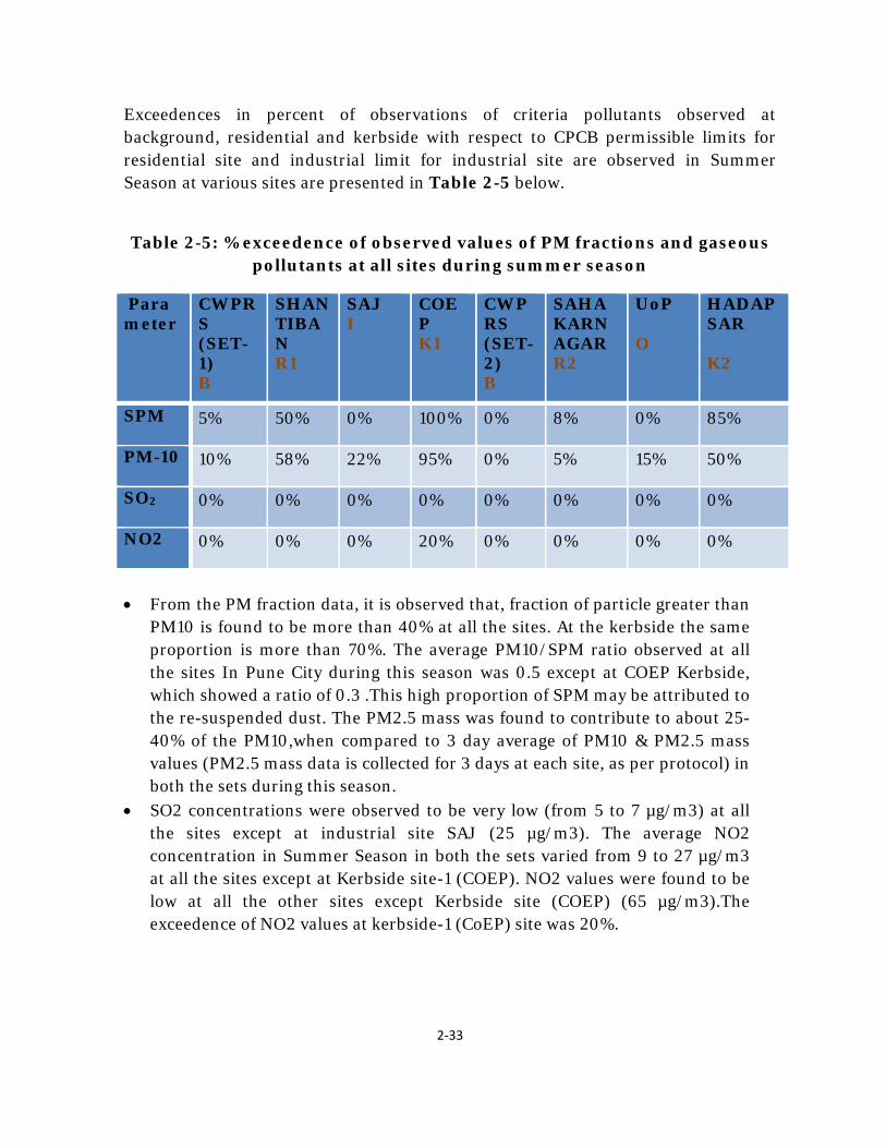
2‐33
Exceedences in percent of observations of criteria pollutants observed at background, residential and kerbside with respect to CPCB permissible limits for residential site and industrial limit for industrial site are observed in Summer Season at various sites are presented in Table 2-5 below.
Table 2-5: % exceedence of observed values of PM fractions and gaseous
pollutants at all sites during summer season
Parameter
CWPRS (SET-1) B
SHANTIBAN R1
SAJ I
COEP K1
CWPRS (SET-2) B
SAHAKARNAGAR R2
UoP O
HADAPSAR K2
SPM
5% 50% 0% 100% 0% 8% 0% 85%
PM-10
10% 58% 22% 95% 0% 5% 15% 50%
SO2
0% 0% 0% 0% 0% 0% 0% 0%
NO2
0% 0% 0% 20% 0% 0% 0% 0%
• From the PM fraction data, it is observed that, fraction of particle greater than
PM10 is found to be more than 40% at all the sites. At the kerbside the same proportion is more than 70%. The average PM10/SPM ratio observed at all the sites In Pune City during this season was 0.5 except at COEP Kerbside, which showed a ratio of 0.3 .This high proportion of SPM may be attributed to the re-suspended dust. The PM2.5 mass was found to contribute to about 25- 40% of the PM10,when compared to 3 day average of PM10 & PM2.5 mass values (PM2.5 mass data is collected for 3 days at each site, as per protocol) in both the sets during this season.
• SO2 concentrations were observed to be very low (from 5 to 7 µg/m3) at all the sites except at industrial site SAJ (25 µg/m3). The average NO2 concentration in Summer Season in both the sets varied from 9 to 27 µg/m3 at all the sites except at Kerbside site-1 (COEP). NO2 values were found to be low at all the other sites except Kerbside site (COEP) (65 µg/m3).The exceedence of NO2 values at kerbside-1 (CoEP) site was 20%.

2‐34
Continuous Monitoring Data of CO and Ozone:
Continuous monitoring data of carbon monoxide (CO) in ppm for seven days at each site is presented as hrly average value for set-I and set-II in Fig. 2.8 and Fig. 2.9 respectively.
Fig. 2.8: Hrly average values of CO (ppm) at various sites during set-1 of summer season.

2‐35
Fig. 2.9: Hrly average values of CO (ppm) at various sites during set-2 of summer season.

2‐36
Continuous monitoring data of Ozone (O3) in ppm for seven days at each site is presented as hrly average value for set-I and set-II in Fig. 2.10 and Fig. 2.11 respectively.
Fig. 2.10: Hrly average values of O3 (ppm) at various sites during set-1 of summer season.

2‐37
Set-II: Ozone
Fig. 2.11: Hrly average values of O3 (ppm) at various sites during set-2 of summer season.
0.000
0.010
0.020
0.030
0.040
0.050
0.060
0.070
0.080
8:00
AM
9:00
AM
10:00 AM
11:00 AM
12:00 PM
1:00
PM
2:00
PM
3:00
PM
4:00
PM
5:00
PM
6:00
PM
7:00
PM
8:00
PM
9:00
PM
10:00 PM
11:00 PM
12:00 AM
1:00
AM
2:00
AM
3:00
AM
4:00
AM
5:00
AM
6:00
AM
7:00
AM
Conc. in pp
m
Time
1hrly avg data: Ozone (ppm)Summer Season: Residential‐2 Site(Sahakarnagar)
Monday, May 21, 2007
Tuesday, May 22, 2007
Wednesday, May 23, 2007
Thursday, May 24, 2007
Friday, May 25, 2007
Saturday, May 26, 2007
Sunday, May 27, 2007

2‐38
Data of Air Toxins (Summer Season)
Concentration of Air Toxins observed at each site are presented in Table 2-6. One representative sample was collected at each site in a season.
Table 2-6: Concentration of air toxins during at various sites during summer season
Conc. In ug/m3 CWPRS Shantiban
SAJ CoEP Sahakarnagar
UoP Hadapsar
THC 957.49 2768.64
1268.96 1886.14 2595.60 1003.63 1793.85
NMHC 807.49 2582.93
740.39 1500.42 2374.17 732.21 1529.56
CH4 150.00 185.71 528.57 385.71 221.43 271.43 264.28 Benzo(a)Pyrene 0.000 0.000 0.002 0.000 0.002 0.000 0.000 Total PAHs * 0.32 0.26 1.34 0.44 0.12 0.24 0.26 VOCs Benzene 23.19 45.85 32.46 24.50 65.94 28.28 38.57
1,3 Butadiene
0.58 1.56 1.13 0.45 1.31 1.99 1.07
Formaldehyde 3.41 6.82 5.47 8.39 20.56 2.67 24.17 *Total PAHs :-Napthalene,Acenapthalene,Fluorene + Acenapthene, Phenanthrene, Anthracene, Fluoroanthene, Pyrene, Benzo(a)Anthracene, Chrysene, Benzo(b)Fluoroanthene, Benzo(k)Fluoroanthene, Benzo(a)Pyrene, Dibenz(a,h)anthracene, Benzo(ghi)Perylene, Indeno(1,2,3 cd)Pyrene

2‐39
Correlation Plots:
Correlation plots are analysed to observe the variability of certain pollutants with respect to each other which are expected to be emitted from a single source.
Correlation Plots for Summer Season considering all sites’ observations are presented below. Fig. 2.12 depicts correlation between PM10 and PM2.5 with reasonable factor of 0.61. Similarly, correlation curve was plotted between EC & OC (Fig. 2.13), NO2 & EC (Fig. 2.14), PM10 & EC (Fig. 2.15), SO2 & SO4 (Fig. 2.16) and NO2 & NO4 (Fig. 2.17).
EC and OC were found to correlate very well with a factor of 0.81. Correlation factor of 0.43 and 0.44 was observed for NO2 and EC and PM10 and EC respectively. Poor correlation was observed between SO2 & SO4 and NO2 and NO4. This may be due the fact that the NO4 and SO4 associated with secondary particulates are formed at distance and not at the point of release of SO2 and NO2.
Correlation matrix for EC, OC and TC showed a good correlation for summer. Similarly, correlation matrix for NH4, SO4 and NO3 was also observed. NH4 and SO4 were found to have better correlation factor than NH4 and NO3. Correlation matrix for EC, OC & TC and NH4, SO4 & NO3 are presented in Table 2-7 (a) and 2.7 (b) respectively.
Table 2.7: (a) Correlation matrix for NH4, So4 and NO3 for summer; (b) Correlation matrix for EC, OC and TC for summer
(a) (b)
1.000 .681** .856**.681** 1.000 .764**.856** .764** 1.000
. .000 .000.000 . .000.000 .000 .
48 48 4848 48 4848 48 48
NH4NO3SO4NH4NO3SO4NH4NO3SO4
PearsonCorrelation
Sig.(2-tailed)
N
NH4 NO3 SO4
Correlations
Correlation is significant at the 0.01 level (2-tailed).**.
1.000 .900** .957**.900** 1.000 .987**.957** .987** 1.000
. .000 .000.000 . .000.000 .000 .153 153 153153 153 153153 153 153
ECOCTCECOCTCECOCTC
PearsonCorrelation
Sig.(2-tailed)
N
EC OC TC
Correlations
Correlation is significant at the 0.01 level (2-tailed).**.

2‐40
Fig. 2.12: Correlation between PM10 and PM2.5 with all sites data during summer
Fig. 2.13: Correlation between EC and OC with all sites data during summer

2‐41
Fig. 2.14: Correlation between NO2 and EC with all sites data during summer
Fig. 2.15: Correlation between PM10 and EC with all sites data during summer
NO2
NO2
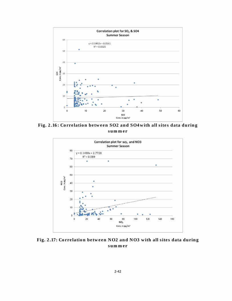
2‐42
Fig. 2.16: Correlation between SO2 and SO4with all sites data during
summer
Fig. 2.17: Correlation between NO2 and NO3 with all sites data during summer
NO2
NO2

SA Study‐Pune Ch. 2: Air Quality Status
2‐43
2.4.2 Post Monsoon Season Data Monitoring for set-3 was carried out at background, residential-1, kerbside-1 and industrial site during September 14, 2007 to October 04, 2007 whereas monitoring for set-4 was carried out at background (repeated for comparison), residential-2, kerbside-2 and other (institute) during October 12, 2007 to October 31, 2007. Ambient daily average temperatures during set-3 of monitoring were found to vary from 21oC to 31oC, whereas during the set-4 of monitoring the daily average ambient temperature was found in the range from 18oC to 32oC. Daily average relative humidity during the set-3 was varied from 36-98%, whereas during set-4, it was observed to be in the range of 26 to 79%.
Daily average (24 hrly) values of PM fractions like SPM, PM10, PM2.5 at various sites during post-monsoon season are presented in Fig. 2.18 & Fig. 2.19.
During post-monsoon season 24hrly Average value of 20 days in 2 sets of SPM ranges from 76 ug/m3 (Background) to 600 ug/m3 (Kerbside-2).whereas PM10 value ranges from 51 ug/m3 (Background)to 212 ug/m3 (Kerbside-2). PM2.5 concentration was in the range from 23 ug/m3 (Background) to 62 ug/m3 (Kerbside-2)

SA Study‐Pune Ch. 2: Air Quality Status
2‐44
Fig. 2.18: Daily (24 hrly) average values of PM Fractions (SPM, PM10, PM2.5) at various sites during set 3 of Post-monsoon Season
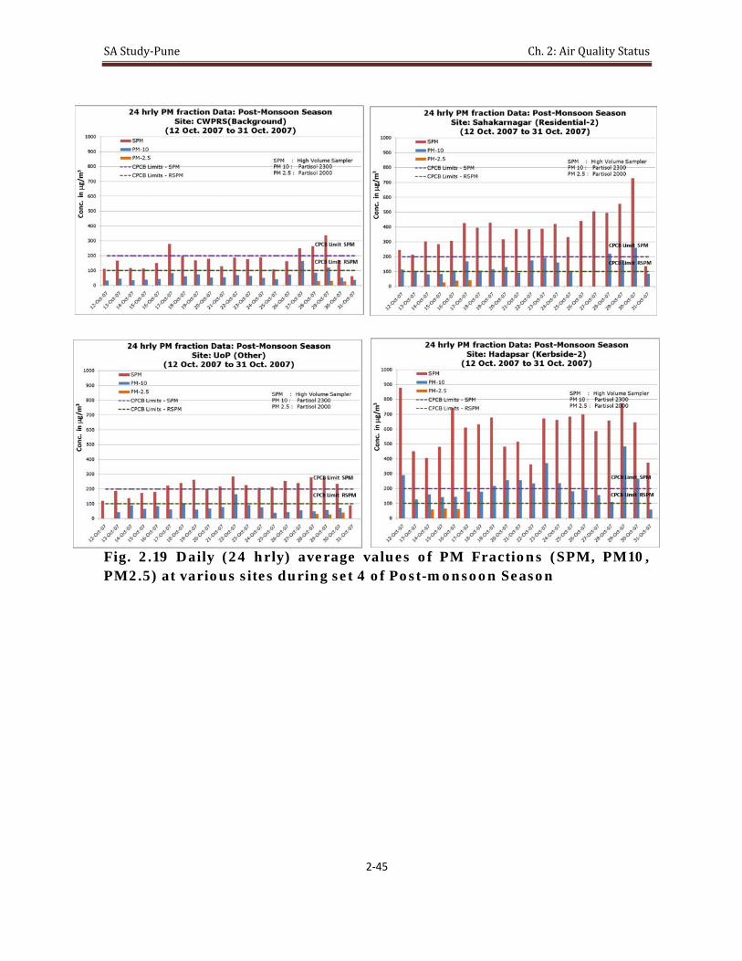
SA Study‐Pune Ch. 2: Air Quality Status
2‐45
Fig. 2.19 Daily (24 hrly) average values of PM Fractions (SPM, PM10, PM2.5) at various sites during set 4 of Post-monsoon Season

SA Study‐Pune Ch. 2: Air Quality Status
2‐46
Set-III: Gaseous Pollutants Daily average (24 hrly) values of Gaseous Pollutants (SO2, NO2 & CO) at various sites during post-monsoon season are presented in Fig. 2.20 & Fig. 2.21.
SO2 24hrly Average value of 20 days during summer season (Set-I and & Set-II) were in the range from 9 ug/m3 (Background)to 18 ug/m3 (Industrial) in post-monsoon season and NO2 concentration were found to be in the range from 10 ug/m3 (Background) to 45 ug/m3 (Residential-2/ Kerbside-2).
Fig. 2.20: Daily (24 hrly) average values of Gaseous Pollutants (SO2, NO2 and CO) at various sites during set 3 of Post-monsoon Season
CPCB limits- SO2 and NO2 CPCB limits- SO2 and NO2
CPCB limits- SO2 and NO2
CPCB limits- SO2 and NO2
CPCB limits- SO2 and NO2 CPCB limits- SO2 and NO2
CPCB limits- SO2 and NO2
CPCB limits- SO2 and NO2
SO2 NO2
CPCB limits- SO2 and NO2
CO CPCB limits- 8 Hrly CO
SO2 NO2
CPCB limits- SO2 and NO2
CO CPCB limits- 8 Hrly CO
SO2 NO2
CPCB limits- SO2 and NO2
CO CPCB limits- 8 Hrly CO
SO2 NO2
CPCB limits- SO2 and NO2
CO CPCB limits- 8 Hrly CO

SA Study‐Pune Ch. 2: Air Quality Status
2‐47
Set-IV: Gaseous Pollutants
Fig.2.21: Daily (24 hrly) average values of Gaseous Pollutants (SO2, NO2 and CO) at various sites during set 4 of Post-monsoon Season
CPCB limits- SO2 and NO2 CPCB limits- SO2 and NO2
CPCB limits- SO2 and NO2 CPCB limits- SO2 and NO2
SO2 NO2
CPCB limits- SO2 and NO2
CO CPCB limits- 8 Hrly CO
SO2 NO2
CPCB limits- SO2 and NO2
CO CPCB limits- 8 Hrly CO
SO2 NO2
CPCB limits- SO2 and NO2
CO CPCB limits- 8 Hrly CO
SO2 NO2
CPCB limits- SO2 and NO2
CO CPCB limits- 8 Hrly CO
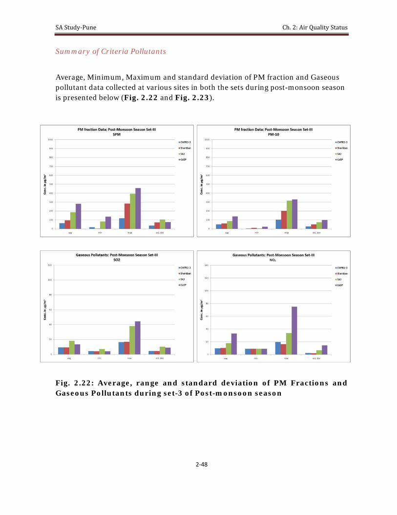
SA Study‐Pune Ch. 2: Air Quality Status
2‐48
Summary of Criteria Pollutants
Average, Minimum, Maximum and standard deviation of PM fraction and Gaseous pollutant data collected at various sites in both the sets during post-monsoon season is presented below (Fig. 2.22 and Fig. 2.23).
Fig. 2.22: Average, range and standard deviation of PM Fractions and Gaseous Pollutants during set-3 of Post-monsoon season
NO2

SA Study‐Pune Ch. 2: Air Quality Status
2‐49
Fig. 2.23: Average, range and standard deviation of PM Fractions and Gaseous Pollutants during set-4 of Post-monsoon season
NO2
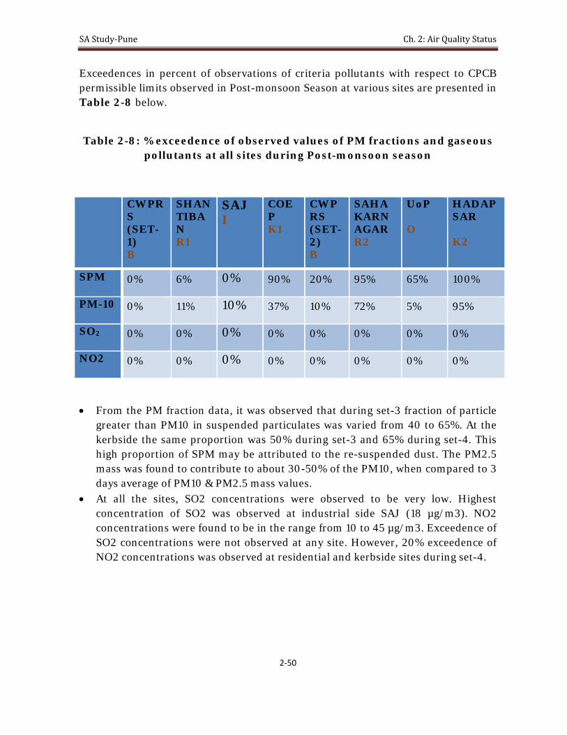
SA Study‐Pune Ch. 2: Air Quality Status
2‐50
Exceedences in percent of observations of criteria pollutants with respect to CPCB permissible limits observed in Post-monsoon Season at various sites are presented in Table 2-8 below.
Table 2-8: % exceedence of observed values of PM fractions and gaseous
pollutants at all sites during Post-monsoon season
CWPRS (SET-1) B
SHANTIBAN R1
SAJ I
COEP K1
CWPRS (SET-2) B
SAHAKARNAGAR R2
UoP O
HADAPSAR K2
SPM
0% 6% 0% 90% 20% 95% 65% 100%
PM-10
0% 11% 10% 37% 10% 72% 5% 95%
SO2
0% 0% 0% 0% 0% 0% 0% 0%
NO2
0% 0% 0% 0% 0% 0% 0% 0%
• From the PM fraction data, it was observed that during set-3 fraction of particle greater than PM10 in suspended particulates was varied from 40 to 65%. At the kerbside the same proportion was 50% during set-3 and 65% during set-4. This high proportion of SPM may be attributed to the re-suspended dust. The PM2.5 mass was found to contribute to about 30-50% of the PM10, when compared to 3 days average of PM10 & PM2.5 mass values.
• At all the sites, SO2 concentrations were observed to be very low. Highest concentration of SO2 was observed at industrial side SAJ (18 µg/m3). NO2 concentrations were found to be in the range from 10 to 45 µg/m3. Exceedence of SO2 concentrations were not observed at any site. However, 20% exceedence of NO2 concentrations was observed at residential and kerbside sites during set-4.

SA Study‐Pune Ch. 2: Air Quality Status
2‐51
Continuous Monitoring Data of CO and Ozone:
Continuous monitoring data of carbon monoxide (CO) in ppm for seven days is presented as hrly average value for set-I in Fig. 2-24
Fig. 2.24: Hrly average values of CO (ppm) at Kerbside site during set-3 of post-monsoon season.

SA Study‐Pune Ch. 2: Air Quality Status
2‐52
Continuous monitoring data of Ozone (O3) in ppm for seven days is presented as hrly average value in Fig. 2.25.
Fig. 2.25: Hrly average values of O3 (ppm) at background site during set-3 of post-monsoon season.

SA Study‐Pune Ch. 2: Air Quality Status
2‐53
Data of Air Toxins (Post-monsoon Season)
Concentration of Air Toxins observed at each sites are presented in Table 2-8. One representative sample was collected at each site in a season.
Table 2-9: Concentration of air toxins during at various sites during post-monsoon season
Conc. ug/m3 CWP
RS Shantiban
SAJ CoEP Sahakarnagar
UoP Hadapsar
THC NA 1799.62 934.42 2393.72 2243.75 876.74 2128.39
NMHC NA 1499.62 577.28 2108.01 1879.47 755.31 1742.68
CH4 NA 300.00 357.14 285.71 364.28 121.43 385.71
Benzo(a)Pyrene 0.001 0.000 0.000 0.001 0.002 0.001 0.001
Total PAHs * 0.176 0.320 0.013 0.309 0.145 0.166 0.291
VOCs Benzene NA 5.53 31.05 9.71 41.21 15.28 23.66
1,3 Butadiene NA 0.65 1.23 7.67 6.50 1.45 4.67
Formaldehyde 2.3 9.8 6.4 15.9 76.8 27 89.5
*Total PAHs :-Napthalene,Acenapthalene,Fluorene + Acenapthene, Phenanthrene, Anthracene, Fluoroanthene, Pyrene, Benzo(a)Anthracene, Chrysene, Benzo(b)Fluoroanthene, Benzo(k)Fluoroanthene, Benzo(a)Pyrene, Dibenz(a,h)anthracene, Benzo(ghi)Perylene, Indeno(1,2,3 cd)Pyrene
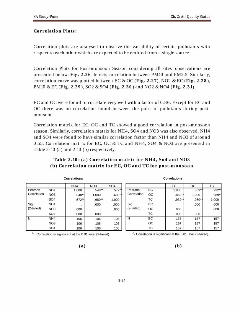
SA Study‐Pune Ch. 2: Air Quality Status
2‐54
Correlation Plots:
Correlation plots are analysed to observe the variability of certain pollutants with respect to each other which are expected to be emitted from a single source.
Correlation Plots for Post-monsoon Season considering all sites’ observations are presented below. Fig. 2.26 depicts correlation between PM10 and PM2.5. Similarly, correlation curve was plotted between EC & OC (Fig. 2.27), NO2 & EC (Fig. 2.28), PM10 & EC (Fig. 2.29), SO2 & SO4 (Fig. 2.30) and NO2 & NO4 (Fig. 2.31).
EC and OC were found to correlate very well with a factor of 0.86. Except for EC and OC there was no correlation found between the pairs of pollutants during post-monsoon.
Correlation matrix for EC, OC and TC showed a good correlation in post-monsoon season. Similarly, correlation matrix for NH4, SO4 and NO3 was also observed. NH4 and SO4 were found to have similar correlation factor than NH4 and NO3 of around 0.55. Correlation matrix for EC, OC & TC and NH4, SO4 & NO3 are presented in Table 2-10 (a) and 2.10 (b) respectively.
Table 2.10: (a) Correlation matrix for NH4, So4 and NO3 (b) Correlation matrix for EC, OC and TC for post-monsoon
(a) (b)
1.000 .548** .572**.548** 1.000 .680**.572** .680** 1.000
. .000 .000.000 . .000.000 .000 .106 106 106106 106 106106 106 106
NH4NO3SO4NH4NO3SO4NH4NO3SO4
PearsonCorrelation
Sig.(2-tailed)
N
NH4 NO3 SO4
Correlations
Correlation is significant at the 0.01 level (2-tailed).**.
1.000 .869** .932**.869** 1.000 .989**.932** .989** 1.000
. .000 .000.000 . .000.000 .000 .157 157 157157 157 157157 157 157
ECOCTCECOCTCECOCTC
PearsonCorrelation
Sig.(2-tailed)
N
EC OC TC
Correlations
Correlation is significant at the 0.01 level (2-tailed).**.

SA Study‐Pune Ch. 2: Air Quality Status
2‐55
Fig. 2.26: Correlation between PM10 and PM2.5 with all sites data during post-monsoon
Fig. 2.27: Correlation between EC and OC with all sites data during post-
monsoon

SA Study‐Pune Ch. 2: Air Quality Status
2‐56
Fig. 2.28: Correlation between NO2 and EC with all sites data during post-monsoon
Fig. 2.29: Correlation between PM10 and EC with all sites data during post-monsoon
NO2
NO2

SA Study‐Pune Ch. 2: Air Quality Status
2‐57
Fig. 2.30: Correlation between SO2 and SO4with all sites data during post-monsoon
Fig. 2.31: Correlation between NO2 and NO3 with all sites data during post-monsoon
NO2
NO2

SA Study‐Pune Ch. 2: Air Quality Status
2‐58
2.4.3 Winter Season Data
Monitoring for set-5 was carried out at background, residential-2, kerbside-2 and University Of Pune site during December12, 2007 to December31, 2007 whereas monitoring for set-6 was carried out at background (repeated for comparison), residential-1, kerbside-1 and industrial site during January13, 2008 to February 02, 2008. However, drop in ambient temperature during the set of monitoring was observed. Ambient daily peak temperatures during set-5 of monitoring were found to vary from 15 o C to 28 o C, whereas during the set-6 of monitoring the daily peak ambient temperature was found in the range from 16oC to 31oC. Average relative humidity during the set-5 was varied from 14-71%, whereas during set-6, it was observed to be in the range of 27 to 83%.
Daily average (24 hrly) values of PM fractions like SPM, PM10, PM2.5 at various sites during winter season are presented in Fig. 2.32 & Fig. 2.33.During winter Season 24hrly Average value of 20 days in 2 sets of SPM ranges from 214 ug/m3 (Background) to 663 ug/m3 (Kerbside-2).whereas PM10 value ranges from 93 ug/m3 (Background)to 226 ug/m3 (Kerbside-1). PM2.5 concentration was in the range from 32 ug/m3 (Background) to 124 ug/m3 (Kerbside-1).

SA Study‐Pune Ch. 2: Air Quality Status
2‐59
Fig. 2.32: Daily (24 hrly) average values of PM Fractions (SPM, PM10, PM2.5) at various sites during set 5 of Winter Season
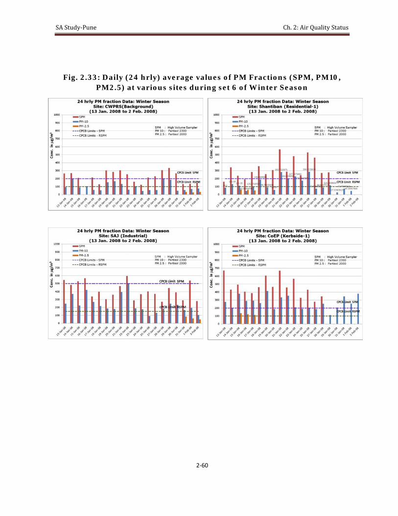
SA Study‐Pune Ch. 2: Air Quality Status
2‐60
Fig. 2.33: Daily (24 hrly) average values of PM Fractions (SPM, PM10,
PM2.5) at various sites during set 6 of Winter Season

SA Study‐Pune Ch. 2: Air Quality Status
2‐61
Set-5: Gaseous Pollutants Daily average (24 hrly) values of Gaseous Pollutants (SO2, NO2 & CO) at various sites during winter season are presented in Fig. 2.34 & Fig. 2.35.
SO2 24hrly Average value of 20 days during winter season (Set-5 and & Set-6) were in the range from 14 ug/m3 (Background)to 47 ug/m3 (Industrial) in all the three seasons and NO2 concentration were found to be in the range from 17 ug/m3 (Background) to 74 ug/m3 (Kerbside-1).
Fig. 2.34: Daily (24 hrly) average values of Gaseous Pollutants (SO2, NO2 and CO) at various sites during set 5 of Winter Season
CPCB limits- SO2 and NO2 CPCB limits- SO2 and NO2
CPCB limits- SO2 and NO2
SO2 NO2
CPCB limits- SO2 and NO2
CO CPCB limits- 8 Hrly CO
SO2 NO2
CPCB limits- SO2 and NO2
CO CPCB limits- 8 Hrly CO
SO2 NO2
CPCB limits- SO2 and NO2
CO CPCB limits- 8 Hrly CO
NO2
CPCB limits- SO2 and NO2

SA Study‐Pune Ch. 2: Air Quality Status
2‐62
Set-6: Gaseous Pollutants
Fig. 2.35: Daily (24 hrly) average values of Gaseous Pollutants (SO2, NO2 and CO) at various sites during set 6 of Winter Season
CPCB limits- SO2 and NO2 CPCB limits- SO2 and NO2
CPCB limits- SO2 and NO2 CPCB limits- SO2 and NO2
SO2 NO2
CPCB limits- SO2 and NO2
CO CPCB limits- 8 Hrly CO
SO2 NO2
CPCB limits- SO2 and NO2
CO CPCB limits- 8 Hrly CO
SO2 NO2
CPCB limits- SO2 and NO2
CO CPCB limits- 8 Hrly CO
SO2 NO2
CPCB limits- SO2 and NO2
CO CPCB limits- 8 Hrly CO
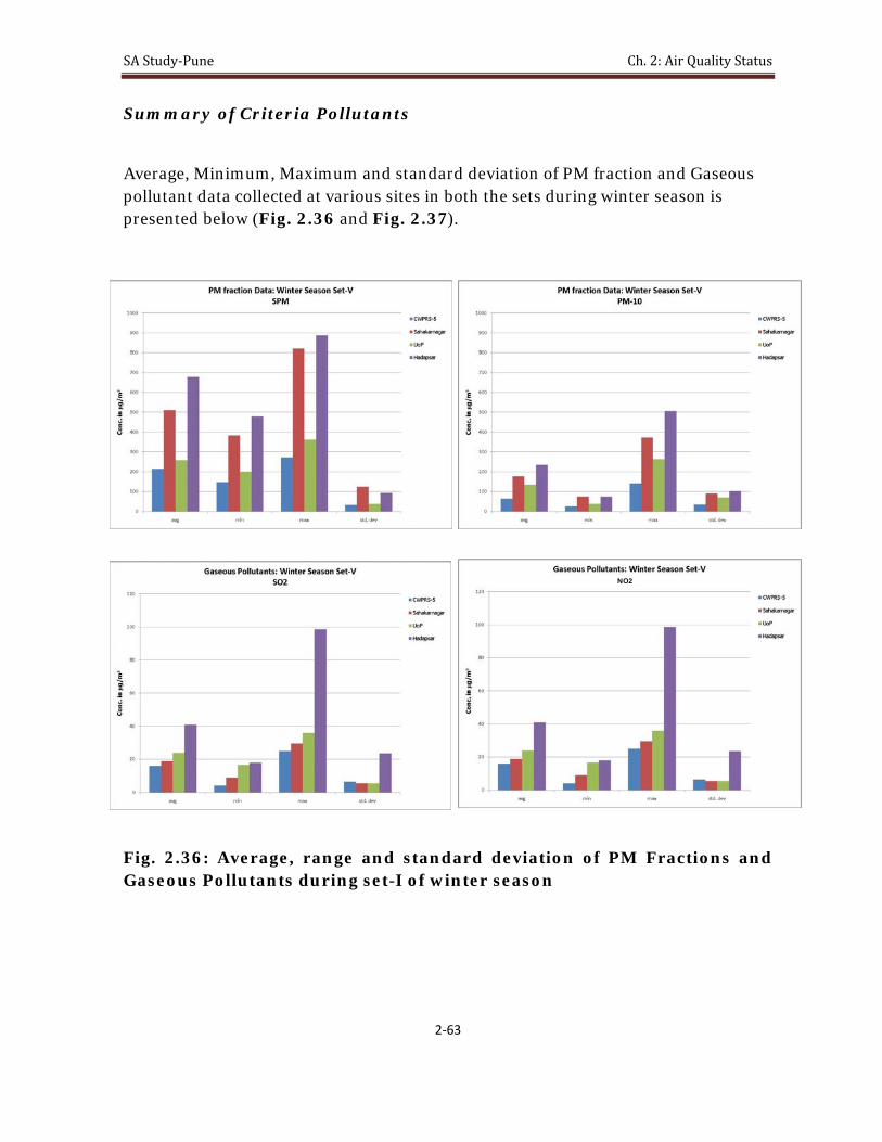
SA Study‐Pune Ch. 2: Air Quality Status
2‐63
Summary of Criteria Pollutants
Average, Minimum, Maximum and standard deviation of PM fraction and Gaseous pollutant data collected at various sites in both the sets during winter season is presented below (Fig. 2.36 and Fig. 2.37).
Fig. 2.36: Average, range and standard deviation of PM Fractions and Gaseous Pollutants during set-I of winter season
NO2

SA Study‐Pune Ch. 2: Air Quality Status
2‐64
Fig. 2.37: Average, range and standard deviation of PM Fractions and Gaseous Pollutants during set-VI of Winter season
NO2

SA Study‐Pune Ch. 2: Air Quality Status
2‐65
Exceedences in percent of observations of criteria pollutants with respect to CPCB permissible limits observed in Winter Season at various sites are presented in Table 2-11 below.
Table 2-11: % exceedence of observed values of PM fractions and gaseous pollutants at all sites during winter season
CWPRS (SET-1) B
SHANTIBAN R1
SAJ I
COEP K1
CWPRS (SET-2) B
SAHAKARNAGAR R2
UoP O
HADAPSAR K2
SPM
80% 88% 25% 100% 80% 100% 95% 100%
PM-10
32% 53% 85% 100% 32% 95% 60% 100%
SO2
0% 0% 0% 6% 0% 0% 15% 0%
NO2
0% 6% 0% 40% 0% 0% 10% 56%
• From the PM fraction data, it was observed that, fraction of particle greater than
PM10 was found to be more than 40% at all the sites. At the kerbside the same proportion was around 70%. The average PM10/SPM ratio observed at all the sites in Pune City during this season was 0.46 except at COEP-Kerbside, which showed a ratio of 0.57 .This high proportion of SPM may be attributed to the re-suspended dust. The PM2.5 mass was found to contribute to about 30- 50% of the PM10,when compared to 3 day average of PM10 & PM2.5 mass values in both the sets during this season.
• The average SO2 concentration in Winter Season in both sets varies from 14 to 41 µg/m3 at all the sites except industrial site-SAJ.SO2 concentrations were observed to be low and no exceedence found at any of the location. At industrial site-SAJ highest average SO2 concentration in Winter Season was found as 47 ug/m3. The average NO2 concentration in Winter Season in both sets varied from 17 to 74 µg/m3 at all the sites .The exceedence of NO2 values at kerbside-1 (CoEP) site is 40% and at Hadapsar site was found to be 56 % during Winter Season. hantiban-Residential-1 location had shown 6% exceedence and University Of Pune also observed 10 % exceedence during this season.

SA Study‐Pune Ch. 2: Air Quality Status
2‐66
Data of Continuous Monitoring Stations Continuous Monitoring Data of CO and Ozone:
Continuous monitoring data of carbon monoxide (CO) in ppm for seven days at each site during winter season is presented as hrly average value for set-I and set-II in Fig. 2.38 and Fig. 2.39 respectively.
Fig. 2.38: Hrly average values of CO (ppm) at various sites during set-5 of winter season.

SA Study‐Pune Ch. 2: Air Quality Status
2‐67
Fig. 2.39: Hrly average values of CO (ppm) at various sites during set-6 of winter season.

SA Study‐Pune Ch. 2: Air Quality Status
2‐68
Continuous monitoring data of Ozone (O3) in ppm for seven days at each site is presented as hrly average value for set-I and set-II in Fig. 2.40 and Fig. 2.41 respectively.
Fig. 2.40: Hrly average values of O3 (ppm) at various sites during set-5 of winter season.
0.000
0.010
0.020
0.030
0.040
0.050
0.060
0.070
0.080
0.090
0.100
8:00
AM
9:00
AM
10:00 AM
11:00 AM
12:00 PM
1:00
PM
2:00
PM
3:00
PM
4:00
PM
5:00
PM
6:00
PM
7:00
PM
8:00
PM
9:00
PM
10:00 PM
11:00 PM
12:00 AM
1:00
AM
2:00
AM
3:00
AM
4:00
AM
5:00
AM
6:00
AM
7:00
AM
Conc. in pp
m
Time
1hrly avg data:Ozone (ppm)Winter Season: Background Site(CWPRS)
Wednesday, December 12, 2007 Thursday, December 13, 2007Friday, December 14, 2007 Saturday, December 15, 2007Sunday, December 16, 2007 Monday, December 17, 2007Tuesday, December 18, 2007
0.000
0.010
0.020
0.030
0.040
0.050
0.060
0.070
0.080
0.090
0.100
8:00
AM
9:00
AM
10:00 AM
11:00 AM
12:00 PM
1:00
PM
2:00
PM
3:00
PM
4:00
PM
5:00
PM
6:00
PM
7:00
PM
8:00
PM
9:00
PM
10:00 PM
11:00 PM
12:00 AM
Conc. in pp
mTime
1hrly avg data:Ozone (ppm)Winter Season: Residential‐2 Site (Sahakarnagar)
Wednesday, December 12, 2007
0.000
0.010
0.020
0.030
0.040
0.050
0.060
0.070
0.080
0.090
8:00
AM
9:00
AM
10:00 AM
11:00 AM
12:00 PM
1:00
PM
2:00
PM
3:00
PM
4:00
PM
5:00
PM
6:00
PM
7:00
PM
8:00
PM
9:00
PM
10:00 PM
11:00 PM
12:00 AM
1:00
AM
2:00
AM
3:00
AM
4:00
AM
5:00
AM
6:00
AM
7:00
AM
Conc. in pp
m
Time
1hrly avg data:Ozone(ppm)Winter Season: Industrial Site(SAJ)
Sunday, January 13, 2008 Monday, January 14, 2008
Tuesday, January 15, 2008

SA Study‐Pune Ch. 2: Air Quality Status
2‐69
Fig. 2.41: Hrly average values of O3 (ppm) at various sites during set-6 of winter season.
0.000
0.020
0.040
0.060
0.080
0.100
0.120
0.140
8:00
AM
9:00
AM
10:00 AM
11:00 AM
12:00 PM
1:00
PM
2:00
PM
3:00
PM
4:00
PM
5:00
PM
6:00
PM
7:00
PM
8:00
PM
9:00
PM
10:00 PM
11:00 PM
12:00 AM
1:00
AM
2:00
AM
3:00
AM
4:00
AM
5:00
AM
6:00
AM
7:00
AM
Conc. in pp
m
Time
1hrly avg data:Ozone(ppm)Winter Season: Background Site(CWPRS)
Sunday, January 13, 2008 Monday, January 14, 2008Tuesday, January 15, 2008 Wednesday, January 16, 2008Thursday, January 17, 2008 Friday, January 18, 2008Saturday, January 19, 2008
0.000
0.010
0.020
0.030
0.040
0.050
0.060
0.070
0.080
0.090
8:00
AM
9:00
AM
10:00 AM
11:00 AM
12:00 PM
1:00
PM
2:00
PM
3:00
PM
4:00
PM
5:00
PM
6:00
PM
7:00
PM
8:00
PM
9:00
PM
10:00 PM
11:00 PM
12:00 AM
1:00
AM
2:00
AM
3:00
AM
4:00
AM
5:00
AM
6:00
AM
7:00
AM
Conc. in pp
m
Time
1hrly avg data:Ozone(ppm)Winter Season: Residential‐1 Site(Shantiban)
Sunday, January 13, 2008 Monday, January 14, 2008Tuesday, January 15, 2008 Wednesday, January 16, 2008Thursday, January 17, 2008 Friday, January 18, 2008Saturday, January 19, 2008
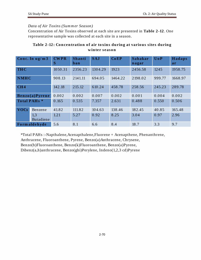
SA Study‐Pune Ch. 2: Air Quality Status
2‐70
Data of Air Toxins (Summer Season) Concentration of Air Toxins observed at each site are presented in Table 2-12. One representative sample was collected at each site in a season.
Table 2-12: Concentration of air toxins during at various sites during winter season
Conc. In ug/m3 CWPRS
Shantiban
SAJ CoEP Sahakarnagar
UoP Hadapsar
THC 1050.31 2356.23 1304.29 1923 2456.58 1245 1958.75
NMHC 908.13 2141.11 694.05 1464.22 2198.02 999.77 1668.97
CH4 142.18 215.12 610.24 458.78 258.56 245.23 289.78
Benzo(a)Pyrene 0.002 0.002 0.007 0.002 0.001 0.004 0.002 Total PAHs * 0.165 0.535 7.357 2.631 0.488 0.550 0.506
VOCs Benzene 41.82 111.82 104.63 138.46 182.45 40.85 165.48 1,3 Butadiene
1.21 5.27 0.92 8.25 3.04 0.97 2.96
Formaldehyde 5.6 8.1 6.6 8.4 18.7 3.3 9.7
*Total PAHs :-Napthalene,Acenapthalene,Fluorene + Acenapthene, Phenanthrene, Anthracene, Fluoroanthene, Pyrene, Benzo(a)Anthracene, Chrysene, Benzo(b)Fluoroanthene, Benzo(k)Fluoroanthene, Benzo(a)Pyrene, Dibenz(a,h)anthracene, Benzo(ghi)Perylene, Indeno(1,2,3 cd)Pyrene

SA Study‐Pune Ch. 2: Air Quality Status
2‐71
Correlation Plots:
Correlation Plots for Winter Season considering all sites’ observations are presented below. Fig. 2.42 depicts correlation between PM10 and PM2.5 with reasonable factor of 0.79. Similarly, correlation curve was plotted between EC & OC (Fig. 2.43), NO2 & EC (Fig. 2.44), PM10 & EC (Fig. 2.45), SO2 & SO4 (Fig. 2.46) and NO2 & NO4 (Fig. 2.47).
EC and OC were found to correlate very well with a factor of 0.76. No correlation was observed in other pairs of pollutants.
Correlation matrix for EC, OC and TC showed a good correlation in winter season. Similarly, correlation matrix for NH4, SO4 and NO3 was also observed. NH4 and SO4 were found to have better correlation factor (0.758) than NH4 and NO3 (0.57). Correlation matrix for EC, OC & TC and NH4, SO4 & NO3 are presented in Table 2-13 (a) and 2.13 (b) respectively.
Table 2.13: (a) Correlation matrix for NH4, So4 and NO3 (b) Correlation matrix for EC, OC and TC for winter
(a) (b)
1.000 .571** .758**.571** 1.000 .743**.758** .743** 1.000
. .000 .000.000 . .000.000 .000 .114 114 114114 114 114114 114 114
NH4NO3SO4NH4NO3SO4NH4NO3SO4
PearsonCorrelation
Sig.(2-tailed)
N
NH4 NO3 SO4
Correlations
Correlation is significant at the 0.01 level (2-tailed).**.
1.000 .927** .960**.927** 1.000 .995**.960** .995** 1.000
. .000 .000.000 . .000.000 .000 .160 160 160160 160 160160 160 160
ECOCTCECOCTCECOCTC
PearsonCorrelation
Sig.(2-tailed)
N
EC OC TC
Correlations
Correlation is significant at the 0.01 level (2-tailed).**.

SA Study‐Pune Ch. 2: Air Quality Status
2‐72
Fig. 2.42: Correlation between PM10 and PM2.5 with all sites data during Winter
Fig. 2.43: Correlation between EC and OC with all sites data during Winter

SA Study‐Pune Ch. 2: Air Quality Status
2‐73
Fig. 2.44: Correlation between NO2 and EC with all sites data during Winter
Fig. 2.45: Correlation between PM10 and EC with all sites data during Winter
NO2
NO2

SA Study‐Pune Ch. 2: Air Quality Status
2‐74
Fig. 2.46: Correlation between SO2 and SO4with all sites data during Winter
Fig. 2.47: Correlation between NO2 and NO3 with all sites data during Winter
NO2
NO2

SA Study‐Pune Ch. 2: Air Quality Status
2‐75
2.5 Distribution of Chemical species in PM10: Detailed chemical analysis of PM10 and PM2.5 (limited) samples collected on different filter papers like Teflon,, Nylon and Quartz was carried out for Ions, Carbon Fractions, elements, Molecular markers. Details of the season-wise results obtained are given below.
2.5.1 Summer Season data
Results of chemical speciation of PM10 samples are presented in Fig. 2.48 and Fig. 2.49 for set 1 and set2 monitoring.
• The average EC/OC ratio at all the sites was observed to be 0.3 except at Kerbside. At both Kerbside sites EC/OC ratio was 0.5 to 0.6.The ratio of OC to EC indicates higher proportion of EC at kerbside in the total carbon. Higher EC/OC can be attributed to the predominant vehicle exhaust PM.
• Sulphate, Nitrate and Chloride ions were found to contribute to more than 90% among anions. Ammonium, calcium, sodium and potassium were the major contributors to the cations. Presences of higher amount of sulphate and nitrate ions with ammonium ions indicate formation of secondary particles (John H Seinfied, S.N.Pandis, Atmo. Chem. & Physics from Air Pollution to Climate Change,1998) Calcium and sodium may be attributed to the soil dust. Potassium may be present due to use of fertilizers in the agricultural fields nearby by area. Presence of NH3 can be attributed to vegetation/forests cover, use of fertilizers, bare land, biomass burning and other biogenic sources etc.
• The percent contribution of Silicon measured in PM10 dust for the city of Pune varies from 20 to 34 % at all the sites. Sodium and Aluminum percentage varies from 3 to 7 % and 6 to 11 % respectively and Iron 4-5 % in PM10 dust during Summer Season. Iron % varies from 2 to 5 % at all the sites. Amongst all the elements measured for PM 10 speciation Silicon, Sodium, Aluminium and Iron showed major contribution which indicates re-suspension of soil dust as a major contributing source. (Pune Regional Emission Inventory Report,, Dr.Ajay Ojha , 2003-2004).
• Total 16 PAHs are monitored in PM10 and PM2.5 samples during monitoring period. Naphthalene, Acenaphthalene, Fluorene+Acenaphthalene, Phenanathrene, Anthracene, Fluoranthene, Dibenz(a,h)anthracene and Benzo(ghi)Perylene are found to be commonly prominent at Shantiban-Residential-1 Site, SAJ-Industrial Site and COEP-Kerbside-1 Site in Summer Season.
• Naphthalene, Acenaphthalene, Fluorene+Acenaphthalene, Phenanathrene, Anthracene, Fluoranthene and Benzo(ghi)Perylene found to be commonly

SA Study‐Pune Ch. 2: Air Quality Status
2‐76
predominant at Sahakarnagar-Residential-2 ,University Of Pune and Hadapsar-Kerbside-2 site in Summer Season.
• Highest total PAHs concentrations were observed at Industrial location followed by COEP Kerbside site. Amongst total PAHs concentration Naphthalene, Acenaphthalene, Fluorene+Acenaphthalene and Pyrene contributed about 90 %. It shows that mass concentration of lighter PAHs (2,3 and 4 ring) compounds is higher than 5 ring heavier compounds in ambient PM10 dust.
• A concentration of Octadecanamide is observed in the range of 7-64 ng/m3 at all the sites. Alkanes as n-Hentriacontane, n-tritriacontane and n-Pentatricontane are observed in the range of 1-9 ng /m3. Whereas, Hopane which is a marker of Industrial fuels/fuel oil/vehicles and lube oil is found in the range of 2-28 ng/m3.
• EC/OC ratio at Background site was found to be 0.33 and 0.37 during Summer season in PM2.5 samples. At residential -1 it was 0.46 and residential-2 it was found as 0.45. Kerbside-1 and Kerbside-2 showed very high ratio values of about 0.82 and 0.87 respectively during this season of monitoring. Whereas, 0.52 ratio was observed at Industrial site and 0.37 was observed at University Of Pune site which represents Other-institutional location. High EC/OC ratio at Kerbside in PM2.5 clearly indicates dominated mobile source. The average EC/OC ratio at all the sites in PM10 was observed to be 0.3 except at Kerbside.
• Amongst Anions Chloride and Sulphate were found to have significant contribution, in which Chloride % varied from 2 to 7 % and Sulphate varies from 11 to 21 % at all the sites. Cations constitute mostly Sodium, Potassium, Ammonium and Calcium. Calcium varied from 2 to 4 %, Ammonium varied from 2 to 3 % , Sodium varied from 2 to 7 % at all the sites during this season.
• Elements contribution in PM2.5 dust has dominance of Silicon, Sodium and Magnesium at all the sites. It is observed that Sodium and Magnesium % increased in PM 2.5 dust as compared to PM10 which indicate finer wood combustion source particles.

SA Study‐Pune Ch. 2: Air Quality Status
2‐77
Fig. 2.48: PM 10 mass distribution at sites during set-1 monitoring of summer season

SA Study‐Pune Ch. 2: Air Quality Status
2‐78
Fig. 2.49: PM 10 mass distribution at sites during set-2 monitoring of summer season

SA Study‐Pune Ch. 2: Air Quality Status
2‐79
2.5.2 Post-monsoon Season data
Results of chemical speciation of PM10 samples are presented in Fig. 2.50 and Fig. 2.51 for set 3 and set4 monitoring.
• At kerbside location the ratio of EC to OC was found to be 0.68 and 0.37 during set-3 and set-4 respectively. This indicates higher proportion of EC at kerbside in the total carbon. Higher EC/OC can be attributed to the predominant vehicle exhaust PM. Similarly at residential sites ratio of EC to OC was found to be around 0.43 and 0.35 as compared to the background EC/OC of 0.37. At industrial site the EC/OC ratio was 0.47, which may be due to predominant combustion of industrial fuels in the vicinity of monitoring location.
• Sulphate, nitrate and chloride ions were found to contribute to more than 90% among anions. Ammonium, calcium, sodium and potassium were the major contributors to the cations. Presences of higher amount of sulphate and nitrate ions with ammonium ions indicate formation of secondary particles. Calcium and sodium may be attributed to the soil dust. Potassium may be present due to use of fertilizers in the agricultural fields nearby by area. Presence of NH3 can be attributed to vegetation/forests.
• Molecular Markers-Total 16 PAHs are monitored in PM10 and PM2.5 samples during monitoring period. Naphthalene, Acenaphthalene, Fluorene + Acenaphthalene and Pyrene are found to be commonly prominent at all the Sites in Post Monsoon Season. Other PAHs like Dibenz(a,h)anthracene, Benzo(ghi)Perylene and Indeno(1,2,3 cd)Pyrene were also observed but found in low concentrations.
• High total-PAHs concentrations were observed at COEP-Kerbside-1 and Hadapsar-Kerbside-2 sites followed by Industrial location. Amongst total PAHs concentration Naphthalene, Acenaphthalene, Fluorene+Acenaphthalene and Pyrene contributed about 90 %. It shows that mass concentration of lighter PAHs (2,3 and 4 ring) compounds is higher than 5 ring heavier compounds in ambient PM10 dust.
• A concentration of Octadecanamide is observed in the range of 2-25 ng/m3 at all the sites during this season. Alkanes as n-Hentriacontane, n-tritriacontane and n-Pentatricontane are observed in the range of 0.5-3 ng /m3. Whereas, Hopane which is a marker of Industrial fuels/fuel oil/vehicles and lube oil is found in the range of 1-8 ng/m3.Lower concentrations as compared to other season may be attributed to wash out of organic species and subsequent reduction in Organic carbon of Particulates.
• EC/OC ratio at Background site was found to be 0.3 and 0.5 during Post Monsoon season in PM2.5 samples. At residential-1 it was 0.58 and residential-2 it was found as 0.53. Kerbside-1 and Kerbside-2 showed very high ratio values of

SA Study‐Pune Ch. 2: Air Quality Status
2‐80
about 1 and 0.67 respectively during this season of monitoring. Whereas, 0.52 ratio was observed at Industrial site and 0.31 was observed at University Of Pune site which represents Other-institutional location. High EC/OC ratio at Kerbside in PM2.5 attributed to dominated mobile source.
• Amongst Anions Chloride and Sulphate were found to have significant contribution, in which Chloride % varies from 1 to 4 % and Sulphate varies from 8 to 17 % at all the sites. Cations constitute mostly Sodium, Potassium, Ammonium and Calcium. Out of which Calcium varies from 1 to 4 %, Ammonium varies from 3 to 10%, Potassium varies from 2 to 3% at all the sites during this season. Sodium fall in the range of 1 to 3 % at all the sites monitored during this season.
• Elements contribution in PM2.5 dust has dominance of Silicon, Sodium, Aluminium and Magnesium. It is observed that Sodium and Magnesium % increased in PM 2.5 dust as compared to PM10 which indicate finer wood combustion source particles in of Pune City

SA Study‐Pune Ch. 2: Air Quality Status
2‐81
Fig. 2.50: PM 10 mass distribution at sites during set-3 monitoring of post-monsoon season

SA Study‐Pune Ch. 2: Air Quality Status
2‐82
Fig. 2.51: PM 10 mass distribution at sites during set-4 monitoring of post-monsoon season

SA Study‐Pune Ch. 2: Air Quality Status
2‐83
2.5.3 Winter Season data
Results of chemical speciation of PM10 samples are presented in Fig. 2.52 and Fig. 2.53 for set 5 and set6 monitoring.
• The average EC/OC ratio at all the sites was observed to be 0.4 at all the sites. At both Kerbside sites COEP and Hadapsar, EC/OC ratio was 0.36 and 0.40 respectively .The ratio of EC to OC indicates higher proportion of EC at University of Pune (0.48) and SAJ (0.46) in the total carbon. Higher EC/OC can be attributed to the predominant vehicle exhaust PM and industrial fuel used at SAJ industrial area.
• Sulphate, Nitrate and Chloride ions were found to contribute major portion among anions. Ammonium and Calcium with Sodium and Potassium were the major contributors to the cations. Presences of higher amount of sulphate and nitrate ions with ammonium ions indicate formation of secondary particles. Calcium and sodium may be attributed to the soil dust.
• The percent contribution of Silicon in PM10 dust for the city of Pune varied from 11 to 19 % at all the sites. Sodium and Aluminum percentage varied from 2 to 6 % and 3 to 9 % respectively in PM 10 dust during Winter Season. Amongst all the elements measured for PM 10 speciation Silicon, Sodium and Aluminium showed major contribution which indicates re-suspension of soil dust as a major source.
• Molecular Markers- Total 16 PAHs were monitored in PM10 and PM2.5 samples during monitoring period. Naphthalene, Acenaphthalene, Fluorene+Acenaphthalene and Pyrene were found to be commonly prominent at all the sites in Winter Season. Highest total PAHs concentrations were observed at Industrial location followed by COEP Kerbside site.
• Amongst total PAHs concentration Naphthalene, Acenaphthalene, Fluorene+Acenaphthalene and Pyrene contributed about 95 %. It shows that mass concentration of lighter PAHs (2,3 and 4 ring) compounds is higher than 5 ring heavier compounds in ambient PM10 dust.
• It is observed that heavier PAH compounds like Benzo(b)Fluoranthene, Benzo(k)Fluoranthene, Chrysene, Benzo(a)Pyrene, Dibenz(a,h)anthracene , Benzo(ghi)Perylene and Indeno(1,2,3 cd)Pyrene concentrations were also increased as compared to Summer and Post Monsoon Season. But their contribution to total PAHs is about 5 %.
• Higher conc. of Octadecanamide (Biomass/Cow-dung) is observed at Sahakarnagar, Res-2 (81 ng/m3) and industrial sites (75 ng/m3) which has more population of slum dwellers. Picene (Coal combustion) is found higher at Sahakarnagar, Res-2 (6 ng/m3) and Industrial sites. Hopane (Industrial fuels/fuel oil/vehicles/lube oil) is found higher at Industrial site (42

SA Study‐Pune Ch. 2: Air Quality Status
2‐84
ng/m3).Benzo[e]pyrene was observed at all sites in the range 3 – 18 ng/m3 indicating presence of combustion sources.
• EC/OC ratio at Background site was found to be 0.5 during Winter season in PM2.5 samples. At residential -1 it was 0.6 and residential-2 it was found as 0.5. Kerbside-1 and Kerbside-2 showed a high ratio of about 0.63 and 0.43 respectively during this season of monitoring. Whereas, 0.63 ratio was observed at Industrial site and 0.58 was observed at University Of Pune site which represents Other institutional location. Higher EC/OC ratio at Kerbside and Industrial site in PM2.5 clearly indicates dominated mobile source and other combustion sources.
• The average EC/OC ratio at all the sites was observed to be 0.4 at all the sites in PM10 fraction. At both Kerbside sites COEP and Hadapsar, EC/OC ratio was 0.36 and 0.40 .The ratio of EC to OC indicates higher proportion of EC at University of Pune (0.48) and SAJ (0.46) in the total carbon. Lower value of EC/OC at Kerbside sites during Winter season as compared to Summer and Post Monsoon indicates increase in other combustion activities during Winter season. Both the Kerbside sitess i.e COEP and Hadapsar has 12 to 14 % Slum area, where wood combustion and trash burning activities are predominant.
• Amongst Anions, Sulphate and Chloride were found to have significant contribution, in which Chloride % varies from 1 to 4 % and Sulphate varies from 7 to 22 % at all the sites. Cation constitutes mostly Sodium, Potassium, Ammonium and Calcium. Out of which Calcium varies from 1to 2 %, Ammonium varies from 4 to 8 % , Sodium found to be present around 1 % at all the sites during this season. Sulphate and Ammonium concentrations increased in Winter season as compared to other season.
• Elements contribution in PM2.5 dust has dominance of Silicon, Sodium, Magnesium Aluminium, Potassium and Chlorine. Out of which percentage of Silicon, Sodium and Magnesium is higher as compared to Aluminium, Potassium and Chlorine elements..

SA Study‐Pune Ch. 2: Air Quality Status
2‐85
Fig. 2.52: PM 10 mass distribution at sites during set-5 monitoring of winter season

SA Study‐Pune Ch. 2: Air Quality Status
2‐86
Fig. 2.53: PM 10 mass distribution at sites during set-6 monitoring of winter season

SA Study‐Pune Ch. 2: Air Quality Status
2‐87
2.6 Distribution of Chemical species in PM 2.5: The chemical analysis of PM2.5 samples collected on two different filter papers like Teflon and Quartz was carried out for Ions, Carbon Fractions, elements, Molecular markers. Monitoring frequency were once in a week per season. Out of seven days 4 days sampling were done on Quartz filters for carbon and organic fraction analysis and 3 days sampling were done on Teflon for carrying out Mass as well as Ions, Element analysis. Thus, average data per site per season compiled for following comparison. Details of the season-wise and site wise comparison of results obtained are given below.
Fig. 2.54 : PM 2.5 mass distribution at all the sites during monitoring seasons
From the above graph it is observed that as compared to PM 10 fraction crustal element concentration has been decreased in PM 2.5 mass. Organic Carbon fraction percentage is significant at Res-2 and Kerb-2 sites. 15 to 30 % contribution of Ions is observed amongst the all sites during three seasons. OC is presented as organic carbon and not organic matter. As such, other elements like hydrogen, oxygen and nitrogen present in the organic matter are not accounted for, and reflected in the unaccounted mass. Oxygen in Oxides of elements are also not get measured. In general unidentified portion of PM mass was found to be higher at Kerbside site and lower at Background, higher unidentified portion may be attributed to the presence of multiple sources at Kerbside location . It is also pertinent to mention that sampling was done using Quartz, Teflon filters on different

SA Study‐Pune Ch. 2: Air Quality Status
2‐88
days for analysis of OC/EC, ions and elements. Samples using teflon filters provided mass of PM10/PM2.5, which were used for mass closure. However, total mass of PM10/PM2.5 was not available on the days, when sampling was done using quartz filters for OC/EC analysis. Besides, in case of PM2.5, limited sampling was carried out for seven days with data on mass available for three days. This, probably, has resulted in negative mass closure in some cases.
Analysis of Molecular Markers Particulate Matter (PM10) collected on Quartz filter for EC/OC analysis was then used for Organic Molecular Marker Analysis. The detailed extraction and analysis procedure is enclosed as an Annexure III, AIII-5. Initially Soxhlet extracted samples were analyzed on GC-MS for qualitative analysis and then finally quantified by using HR-GC with FID detector.
Quantitative analysis of molecular markers during different season and at all the selected locations in PM10 samples is carried out using GC-FID which is presented in Figure 2.54. The listed compounds in Table 2.14 are qualitatively observed in the samples on GC-MS, however due to unavailability of standards these could not be quantified.
Table 2.14: Qualitative results of molecular markers analysis of PM10 samples using GC-MS
Sr.No.
Summer Post Monsoon Winter
A Alkanes and alkenes(Qualitative)
Pentacosane Tetradecane, 1-iodo- 2-Methyldocosane Dotriacontane 2-Methyldocosane 1-Nonane Eicosane 1-Tetradecene 1-Dodecane
Heptadecane 1-Hexadecene 1-Tetradecene Tridecane 1-Hexadecene Tricosane 1-Docosene
Octadecane Dodecene Nonadecane Tetradecene Heneicosane
B Alkanoic Acid (Qualitative)
1. n-Hexadecanoic acid ND Decanoic acid 2. Oleic acid Oleic Acid 3. Eicosanoic acid

SA Study‐Pune Ch. 2: Air Quality Status
2‐89
C Acid Ester (Methyl)(Qualitative)
Hexanedioic acid, dioctyl ester
Tetradecanoic acid, 12-methyl-, methyl ester
Tridecanoic acid, methyl ester
Tetradecanoic acid, 12-methyl-, methyl ester
Eicosenoic acid, methyl ester 9-Hexadecenoic acid, methyl ester
Cyclopentanetridecanoic acid, methyl ester
Hexadecanoic acid, 4-nitrophenyl ester
Hexadecanoic acid, methyl ester
Phenanthrene-1-carboxylic acid, methyl ester
1,2-Benzenedicarboxylic acid, ditridecyl ester
11-Octadecenoic acid, methyl ester
Heptadecanoic acid, 10-methyl-, methyl ester
Cyclopentaundecanoic acid, methyl ester
Trifluoroacetic acid, n-tetradecyl ester
Phenanthrene-1-carboxalic acid, ,methyl ester
Formic acid, 2,4,6-tri-t-butyl-phenyl ester
Phenanthrene-1-carboxalic
acid, methyl ester
Fig. 2.55: Site and Season wise distribution of molecular markers present in PM10 using GC-FID
0.00
10.00
20.00
30.00
40.00
50.00
60.00
70.00
R1
R2 K1
K2 I O
ng
/m3
Site wise distribution of molecular markers-Summer season
n-Tritriacontane n- Hentriacontane n-Pentatriacontane
Benzo[e]pyrene Indeno[1,2,3-cd]fluoranthene Picene
Hexadecanamide Octadecanamide 17 alpha(H),21beta(H)-Hopane

SA Study‐Pune Ch. 2: Air Quality Status
2‐90
SA Study‐Pune Ch. 2: Air Quality Status
2‐91
2.7 Summary of results:
Summer Season
• Monitoring for set-1 was carried out at background, residential-1, kerbside-1 and industrial site during April 18, 2007 to May 07, 2007 whereas monitoring for set-2 was carried out at background (repeated for comparison), residential-2, kerbside-2 and other (institute) during May 21, 2007 to June 10, 2007. However, drop in ambient temperature during the second set of monitoring was observed. Ambient daily peak temperatures during first set of monitoring were found to vary from 38 o C to 40 o C, whereas during the set-II of monitoring the daily peak ambient temperature was found in the range from 31oC to 34oC. Average relative humidity during the set-I was varied from 30-50%, whereas during set-II, it was observed to be in the range of 60 to 75%. Due to the change in climatic conditions in summer to pre-monsoon, the concentrations of criteria pollutants were found to be remarkably lower.
• From the PM fraction data, it is observed that, fraction of particle greater than PM10 is found to be more than 40% at all the sites. At the kerbside the same proportion is more than 70%. The average PM10/SPM ratio observed at all the sites In Pune City during this season was 0.5 except at COEP Kerbside, which showed a ratio of 0.3 .This high proportion of SPM may be attributed to the re-suspended dust. This statement is substantiated by the elemental analysis of the PM10 samples. The PM2.5 mass was found to contribute to about 25- 40% of the PM10,when compared to 3 day average of PM10 & PM2.5 mass values (Only 3 day PM2.5 mass data is collected at each site, as per protocol) in both the sets during this season.
• The average SO2 concentration in Summer Season in both sets varies from 5 to 7 µg/m3 at all the sites except industrial site SAJ.SO2 concentrations were observed to be very low at all the sites except at industrial site SAJ (25 µg/m3). The average NO2 concentration in Summer Season in both sets varies from 9 to 27 µg/m3 at all the sites except at Kerbside site COEP. NO2 values were found to be low at all the other sites except Kerbside site COEP (65 µg/m3). The exceedence of NO2 values at kerbside-1 (CoEP) site is 20%. Post-monsoon Season
• Monitoring for set-3 was carried out at background, residential-1, kerbside-1 and industrial site during September 14, 2007 to October 04, 2007 whereas monitoring for set-4 was carried out at background (repeated for comparison), residential-2, kerbside-2 and other (institute) during October 12, 2007 to October 31, 2007. Ambient daily average temperatures during set-3 of monitoring were

SA Study‐Pune Ch. 2: Air Quality Status
2‐92
found to vary from 21oC to 31oC, whereas during the set-4 of monitoring the daily average ambient temperature was found in the range from 18oC to 32oC. Daily average relative humidity during the set-3 was varied from 36-98%, whereas during set-4, it was observed to be in the range of 26 to 79%.
Winter Season
• Monitoring for set-5 was carried out at background, residential-2, kerbside-2 and University Of Pune site during December12, 2007 to December31, 2007 whereas monitoring for set-6 was carried out at background (repeated for comparison), residential-1, kerbside-1 and industrial site during January13, 2008 to February 02, 2008. However, drop in ambient temperature during the set of monitoring was observed. Ambient daily peak temperatures during set-5 of monitoring were found to vary from 15 o C to 28 o C, whereas during the set-6 of monitoring the daily peak ambient temperature was found in the range from 16oC to 31oC. Average relative humidity during the set-5 was varied from 14-71%, whereas during set-6, it was observed to be in the range of 27 to 83%.
• From the PM fraction data, it is observed that, fraction of particle greater than PM10 is found to be more than 40% at all the sites. At the kerbside the same proportion is around 70%. The average PM10/SPM ratio observed at all the sites in Pune City during this season was 0.46 except at COEP Kerbside, which showed a ratio of 0.57 .This high proportion of SPM may be attributed to the re-suspended dust. The PM2.5 mass was found to contribute to about 30- 50% of the PM10,when compared to 3 day average of PM10 & PM2.5 mass values in both the sets during this season.
• The average SO2 concentration in Winter Season in both sets varies from 14 to 41 µg/m3 at all the sites except industrial site SAJ.SO2 concentrations were observed to be low and no exceedence found at any of the location. At industrial site SAJ highest average SO2 concentration in Winter Season was found as 47µg/m3 amongst all the sites. . The average NO2 concentration in Winter Season in both sets varies from 17 to 74 µg/m3 at all the sites .The exceedence of NO2 values at kerbside-1 (CoEP) site is 40% and at Hadapsar site is found as 56 % during Winter Season. Residential location -1 had shown 6% exceedence and University Of Pune also observed 10 % exceedence during this season.
Site wise comparisons of results in different seasons for first and second sets are presented in Table 2.15 (A) and (B) respectively. Geometric mean concentrations of SPM, PM10, PM2.5, SO2 and NO2 for all sites and three seasons are presented at Annexure-I

SA Study‐Pune Ch. 2: Air Quality Status
2‐93
Table 2.15 (A): Comparison of various pollutants observed in first set of monitoring during summer, post-monsoon and winter season
Site Season
EC/OC Concentration (ug/m3)
(PM10)
Ratio PM2.5/PM10
Ratio PM10/SPM SO2
NO2 SPM PM10 PM2.5 EC OC SO4-- NO3-- NH4+ Na+ Ca+ Si
CWPRS-Background
Winter 0.40 0.32 0.44 14 17 225 100 32 9 21 8 3 5 2 2 23
Post- Monsoon
0.37 0.45 0.67 9 10 76 51 23 2 6 6 0 1 1 2 10
Summer 0.30 0.28 0.55 6 10 142 78 22 3 9 10 7 5 2 4 18
Shantiban- Residential-1
Winter 0.39 0.45 0.39 14 27 328 130 58 11 28 9 5 4 3 7 24
Post- Monsoon
0.43 0.40 0.60 9 10 107 64 26 3 6 8 2 1 2 3 19
Summer 0.34 0.27 0.50 7 15 210 106 28 3 9 12 12 5 3 5 23
CoEP - Kerbside-1
Winter 0.36 0.47 0.57 21 74 466 266 124 16 46 8 6 4 1 6 46
Post- Monsoon
0.68 0.32 0.50 13 33 282 140 45 14 21 8 3 1 2 4 36
Summer 0.50 0.32 0.28 7 65 517 143 46 13 25 11 11 4 3 5 29
SAJ-Industrial
Winter 0.46 0.27 0.57 47 57 412 237 64 24 53 12 6 5 3 10 27
Post- Monsoon
0.47 0.30 0.46 18 18 188 87 26 6 12 9 3 2 2 4 16
Summer 0.39 0.30 0.45 25 23 272 124 37 7 18 14 10 3 3 4 32

SA Study‐Pune Ch. 2: Air Quality Status
2‐94
Table 2.12 (B): Comparison of various pollutants observed in second set of monitoring during summer, post-monsoon and winter season
Site Season
EC/OC Concentration (ug/m3)
(PM10)
Ratio PM2.5/PM10
Ratio PM10/SPM SO2 NO2 SPM PM10 PM2.5 EC OC SO4-- NO3-- NH4+ Na+ Ca+ Si
CWPRS-Background
Winter 0.4 0.36 0.44 16 20 214 93 33 10 24 9 3 4 1 2 14
Post- Monsoon
0.36 0.44 0.36 10 14 176 64 28 6 18 3 1 7 2 3 14
Summer 0.34 0.37 0.60 5 9 68 41 15 2 6 4 1 2 1 1 12
Sahakarnagar-Residential-2
Winter 0.34 0.27 0.35 19 45 511 178 48 27 79 13 8 5 3 8 22
Post- Monsoon
0.35 0.26 0.36 12 45 384 137 35 16 45 10 3 8 2 6 32
Summer 0.37 0.33 0.39 5 10 173 67 22 4 11 3 1 2 2 2 14
Hadapsar - Kerbside- 2
Winter 0.40 0.51 0.36 41 68 663 237 120 28 69 15 9 5 3 10 26
Post-Monsoon
0.37 0.29 0.35 13 44 600 212 62 17 46 10 4 9 1 9 34
Summer 0.63 0.29 0.32 6 26 321 103 30 10 16 6 2 5 2 4 21
UoP- Winter 0.48 0.34 0.52 24 38 259 134 45 21 42 15 9 7 2 7 26
Institute (other)
Post-Monsoon
0.47 0.45 0.34 10 35 212 72 32 10 21 7 2 6 1 4 17
Summer 0.35 0.24 0.49 6 10 121 59 15 3 8 6 2 5 2 3 20

SA Study‐Pune Ch. 2: Air Quality Status
2‐95
2.8 Comparison of Observations in Different Seasons for different monitoring sites:
Data for PM fractions (SPM, PM10, and PM2.5) and gaseous pollutants (SO2 and NO2) plotted in above section under Air Quality Status is an arithmetic average values for 24 hrs period. PM10 and SO2 and NO2 were monitored for 20 days in each season whereas PM 2.5 was monitored for a period of 1 week (out of 7 days, monitoring was done on Teflon Filter for 3 days and on Quartz filter for 4 days ) continuously in each season. Season-wise comparison of pollutants at different sites is presented below.
2.8.1Background location (CWPRS Guest House)
PM Fractions (SPM, PM 10 and PM2.5)
• During 20 days monitoring period it is observed that, SPM and PM10 values exceeded the CPCB limit for 5 % and 10 % times during set-1 of Summer Season .No Exceedences were observed in set-2 of Summer Season monitoring program me for PM fraction at background site.
• During Post Monsoon Season of set-3 no Exceedences observed for SPM and PM10, while set-4 showed 20 % exceedence for SPM values and 10 % for PM10.
• PM fractions showed 80 % exceedence for SPM in set-5 and 65 % in set-6 in winter. Whereas, PM 10 values were exceeded the CPCB limit for 11% times in set-5 and 30 % times in set-6.
• During Summer Season 24hrly Average value of 20 days in 2 sets of SPM ranges from 68 to 142 ug/m3.whereas PM 10 value ranges from 51 to 76 ug/m3.
• During Post Monsoon Season 24hrly Average value of 20 days in 2 sets of SPM ranges from 76 to 176 ug/m3.whereas PM 10 value ranges from 51 to 64 ug/m3
• During Winter Season 24hrly Average value of 20 days in 2 sets of SPM ranges from 214 to 225 ug/m3.whereas PM 10 value ranges from 93 to 100 ug/m3
Gaseous Pollutants (SO2, NO2 and CO)
• SO2, NO2 and 8hrly average of CO values showed no exceedence against the CPCB standard limit for Summer, Post Monsoon and Winter Season.

SA Study‐Pune Ch. 2: Air Quality Status
2‐96
• SO2 24hrly Average value of 20 days in 2 sets were in the range from 5 to 16 ug/m3 in all the three seasons and NO2 concentration varied from 9 to 20 ug/m3.
• 8hrly CO values during Summer season ranges from 179 to 378 ug/m3 whereas during Post Monsoon Season average value were found to be around 90 ug/m3.

SA Study‐Pune Ch. 2: Air Quality Status
2‐97
2.8.2 Residential location
PM Fractions (SPM, PM 10 and PM2.5)
• During 20 days monitoring period it was observed that, SPM and PM10 values exceeded the CPCB limit for 50 % and 55 % times during Summer Season at Shantiban (R1) Residential location.
• At Sahakarnagar (R2) Residential location, it was observed that SPM and PM10 values exceeded the CPCB limit for 8 % and 5 % times during Summer Season.
• During Post Monsoon Season SPM and PM10 values exceeded the CPCB limit for 6 % and 11 % times of 20 days period respectively at Shantiban (R1) Residential location.
• At Sahakarnagar (R2) Residential location, it was observed that SPM and PM10 values exceeded the CPCB limit for 95 % and 65 % times during Post Monsoon Season.
• In PM fractions, SPM showed 100 % exceedence and 95 % times for PM10 values observed during the period. at Shantiban (R1)Residential location, while exceedence was 88 % and 42 % for SPM and PM10 respectively at Sahakarnagar (R2) Residential location in winter season.
• During Summer Season, 24hrly Average concentration of SPM at Shantiban (R1) Residential location and at Sahakarnagar (R2) Residential location was found to be 210 and 173 ug/m3 respectively. Whereas, average concentration of PM 10 value was observed as 106 and 66 ug/m3 respectively at Shantiban (R1) and Sahakarnagar (R2)Residential location
• During Post Monsoon Season, 24hrly Average concentration of SPM at Shantiban (R1) Residential location and at Sahakarnagar (R2)Residential location was found to be 107 and 384 ug/m3 whereas average concentration of PM 10 value was observed as 64 and 137 ug/m3 respectively at Shantiban (R1) and Sahakarnagar (R2) Residential location
• During Winter Season, 24hrly Average concentration of SPM at Shantiban (R1)Residential location and at Sahakarnagar (R2)Residential location is found to be 328 and 511 ug/m3 whereas average concentration of PM 10 value is observed as 130 and 178 ug/m3 respectively at Shantiban (R1) and Sahakarnagar (R2) Residential location

SA Study‐Pune Ch. 2: Air Quality Status
2‐98
Gaseous Pollutants (SO2, NO2 and CO)
• SO2, NO2 and 8hrly average of CO conc. showed no exceedence against the CPCB standard limit in Summer, Post Monsoon Season at both the Residential sites. Whereas, no exceedence were observed for SO2 during Winter season at both the Residential sites but 24hrly average NO2 values exceeded the CPCB limit for 6 % times at Shantiban (R1) Residential location and with no exceedence at Sahakarnagar (R2) site.
• 24hrly Average concentration of SO2 during 20 days at Shantiban (R1) site was in the range from 6 to 14 ug/m3 and at Sahakarnagar (R2) Residential location conc. of SO2 were in the range from 5 to 20 ug/m3 in all the three seasons.
• NO2 concentration varied from 10 to 27 ug/m3 at Shantiban (R1) site and 9 to 45 ug/m3 at Sahakarnagar (R2) Residential location.
• 8hrly CO values during Summer season were found to be around 547 ug/m3 at Shantiban (R1) site and 208 ug/m3 at Sahakarnagar (R2) Residential location.

SA Study‐Pune Ch. 2: Air Quality Status
2‐99
2.8.3 Kerbside location
PM Fractions (SPM, PM 10 and PM2.5)
• During 20 days monitoring period it is observed that, SPM and PM10 values exceeded the CPCB limit for 100 % and 95 % times respectively in Summer Season at COEP (K1) Kerbside location.
• At Hadapsar (K2) Kerbside location, it was observed that SPM and PM10 values exceeded the CPCB limit for 85 % and 50 % times during Summer Season
• During Post Monsoon Season, SPM and PM10 values exceeded the CPCB limit for 90 % and 80 % times of 20 days period respectively at COEP (K1) Kerbside location.
• At Hadapsar (K2) Kerbside location, it was observed that SPM and PM10 values exceeded the CPCB limit for 100 % and 95 % times during Post Monsoon Season.
• Winter season for PM fractions showed 100 % exceedence for SPM as well as PM10 at both the Kerbside location.
• During Summer Season, 24hrly Average concentration of SPM during 20 days at COEP (K1) Kerbside location and at Hadapsar (K2) Kerbside location was found to be 517 and 321 ug/m3 whereas, average concentration of PM 10 value was observed as 143 and 103 ug/m3 respectively at COEP (K1) Kerbside location and at Hadapsar (K2) Kerbside location.
• During Post Monsoon Season, 24hrly Average concentration of SPM at COEP (K1) Kerbside location and at Hadapsar (K2) Kerbside location was found to be 282 and 599 ug/m3 whereas average concentration of PM 10 value was observed as 140 and 212 ug/m3 respectively at COEP (K1) Kerbside location and at Hadapsar (K2) Kerbside location.
• During Winter Season 24hrly Average concentration of SPM during 20 days at COEP (K1)Kerbside location and at Hadapsar (K2) Kerbside location was found to be 466 and 663 ug/m3 whereas average concentration of PM 10 value was observed as 266 and 237 ug/m3 respectively at COEP (K1) Kerbside location and at Hadapsar (K2) Kerbside location
Gaseous Pollutant (SO2, NO2 and CO)
• No exceedence against the CPCB standard limit for SO2 was observed for summer and Post Monsoon Season at both the Kerbside locations. Whereas, 6 %

SA Study‐Pune Ch. 2: Air Quality Status
2‐100
times SO2 was exceeded the CPCB limit at COEP (K1) location during winter season and no exceedence observed at Hadapsar site (K2).
• At Hadapsar site (K2) 50 % times exceedence was observed for NO2 values during Winter Season. Whereas, no exceedence observed during Post Monsoon at both the Kerbside sites.
• 8hrly average of CO values showed exceedence against the CPCB standard limit for Post Monsoon and Winter Season at both the Kerbside sites.
• 24hrly Average concentration of SO2 during 20 days at COEP (K1) Kerbside location was in the range from 7 to 21 ug/m3 and 6 to 41 ug/m3 at Hadapsar site (K2) in all the three seasons.
• NO2 concentration varied from 33 to 74 ug/m3 at COEP (K1) Kerbside site and 26 to 68 ug/m3 at Hadapsar site (K2).
• 8hrly CO values during Summer season were found to be in the range from 1379 to 3297 ug/m3 at COEP (K1) Kerbside site and 6064 to 7599 ug/m3 at Hadapsar (K2) location.

SA Study‐Pune Ch. 2: Air Quality Status
2‐101
2.8.4 Industrial location (I)
PM Fraction (SPM, PM 10 and PM2.5)
• During 20 days monitoring period it is observed that, PM10 values exceeded the CPCB limit for 22 % times whereas no exceedences observed for SPM during Summer Season.
• Similarly, during Post Monsoon Season it is observed that CPCB values exceeded for PM10for 10 % of times and no exceedences observed for SPM .
• Winter being a critical season for PM fractions showed 25 % exceedence for SPM and 85 % for PM 10 values.
• 24hrly Average value of 20 days for SPM is found to be in the range from 188 to272 ug/m3 and PM 10 conc. is found in the range from 87 to 133 ug/m3 in all the three seasons.
Gaseous Pollutant (SO2, NO2 and CO)
• SO2, NO2 and 8hrly average of CO values showed no exceedence against the CPCB standard limit for summer, Post Monsoon Season .and winter season.
• SO2 24hrly Average values of 20 days were in the range from 18 to 25 ug/m3 in all the three seasons and NO2 concentration varied from 18 to 38 ug/m3.
• 8hrly CO values during Summer season were found to be around 295 ug/m3.

SA Study‐Pune Ch. 2: Air Quality Status
2‐102
2.8.5 Other Institutional location (O)-University of Pune
PM Fraction (SPM, PM 10 and PM2.5)
• During 20 days monitoring period it was observed that, PM10 values exceeded the CPCB limit for 15 % times during Summer Season. No Exceedences were observed for SPM during Summer Season.
• During Post Monsoon Season it was observed that CPCB values exceeded for SPM and PM10, for 65 and 5 % times respectively.
• Winter being a critical season for PM fractions showed 100 % exceedence for SPM and 95 % for PM 10 values.
• 24hrly Average values of 20 days for SPM were found to be in the range from 121 to 412 ug/m3 and PM 10 value were 59 to 236 ug/m3 in all the three seasons.
Gaseous Pollutant (SO2, NO2 and CO)
• SO2, NO2 and 8hrly average of CO values showed no exceedence against the CPCB standard limit for Summer and Post Monsoon Season.
• SO2 24hrly Average values of 20 days were in the range from 6 to 47 ug/m3 in all the three seasons and NO2 concentration varied from 10 to 57 ug/m3.
• 8hrly CO values during Summer season were found to be around 133 ug/m3.

SA Study‐Pune Ch. 3: Emission Inventory
3‐1
Chapter 3. Emission Inventory
3.1 Introduction
Emission Inventory (EI) is a scientific tool for quantification of pollutant emission load from various sources. Impact of pollution from activities in various sectors depends on many factors, viz. vicinity of emission sources, the concentration of pollutants, temporal/spatial variations in emission patterns, receptor types etc.
Emission inventory data generation is required for assessment of major polluting sources and effect of control options on pollution load.
3.2 General Methodology
Emission inventory study is carried out with the following objectives under this project.
Converting Pune city map into 2X 2 km grids (Fig. 3.1) Identification of various air pollution sources in Pune under Broad Categories of
point, area and line sources Primary surveys for identification and spatial distribution of sources around the
monitoring sites in an area of 2 km X 2 km Point sources: Identification of all significant sources. Line sources: Vehicle count surveys at various locations (maximum 25 Nos.)
covering different type of roads with focus on zone of influence Area sources: Total area under each emission source category/typeSpatial
variation of source emissions through inventory surveys. Temporal variation for certain sources around monitoring sites (other than
traffic) Analysis of data to estimate emission loads for-
Contributions of emission load from different categories of vehicles Contributions from domestic, commercial, power and industrial sources Impact of alternative strategies in the transport sector on emission loading
for a five-year horizon

SA Study‐Pune Ch. 3: Emission Inventory
3‐2
Fig. 3.1: Gridded (2 X2 km) Pune city base map

SA Study‐Pune Ch. 3: Emission Inventory
3‐3
Mapping of area (Around monitoring sites)
For carrying out primary surveys around the monitoring sites, area of 2 X 2 km around the monitoring sites was marked using Google Earth Software. The area around monitoring sites was then divided into 4 parts as 4 quadrants of 1 km X 1 km. Each quadrant was then sub-divided into 4 parts of 0.5 km X 0.5 km. Images of all the subparts of 0.5 km X 0.5 km area obtained from Google Earth were used as guidelines for conducting surveys.
Table 3.1 describes the methodology used for the emission inventory data collection. Primary and secondary data for point area sources was collected for emission sources around monitoring sites. Primary data on domestic fuel usage pattern and citizen perspective about air pollution is collected at slums and residential areas. Data collection for line source emission inventory through video shooting and manual counting. Primary data on vehicle usage patterns and vehicle technology mix is completed through surveys at parking lots, theaters, petrol pumps, institutes etc. Activity data collected for various sources is presented in Table 3.2.

SA Study‐Pune Ch. 3: Emission Inventory
3‐4
Table 3.1: Methodology for emission inventory
Sr. No.
Task Methodology
1 Source identification
Mapping of area of 2 X 2 km around sites usingGoogleEarth
Division of the area into smaller grids of 0.5 X 0.5 km (16nos.). Primary survey for identification of sources
2 Point sources
Secondary data from MPCB
Primary survey for additional data
3 Area Sources Primary Survey around monitoring sites
Secondary data from PMC
4 Line sources Video recording at 25 representative location aroundmonitoring sites
Counting of vehicles based on recordings
Parking-lots surveys for traffic mix
Surveys at petrol pumps for vehicle usage pattern
5 Emission Inventory (EI) Generation of 4 km2 each for 7 monitoring sites
Compilation of Emission Factors for various vehicletypes/ categories
Generation of EI from emission factors and activity data
6 Emission Inventory generation for base year 2007: city level
2X2 km grid formation, use of secondary data for pointsources (Data source MPCB), area sources (Data sourcePMC). Use of counted road lengths and vehicle countdata for different category of roads, with socio-economicconsiderations.

SA Study‐Pune Ch. 3: Emission Inventory
3‐5
Table 3.2: Data collected (primary/secondary) for emission inventory preparation
Sr. No.
Data type Details
1 Air pollutionsource identification
Identification of major air-pollution sources in the zone ofinfluence around monitoring sites (area of 2 km X 2 km)
–Division of area (2km X 2km) in smaller 16 grids (0.5km X 0.5km)
–Sources of air pollution and Land-use pattern in each smaller grid
2 Point sources •Collection of data on point sources (industries andhotels) of air pollution from MPCB, Pune
–Name and Address of Industry/Hotel
–Stack details including no. of stacks and
–Type of fuel and consumption
–Stack monitoring results
•Biomedical-Waste Incinerator details
3 Area sources •Details of area sources at 7 locations. Area of 2km X 2kmaround each monitoring site was divided into 16 smallergrids of 0.5km X 0.5km. Information on presence andactivity for area sources was collected for all smaller gridsat each location
- Agricultural
- Construction
- Cooking
- Paved & unpaved road dust
- Trash burning, etc
- Domestic Fuel (LPG) Supply cells

SA Study‐Pune Ch. 3: Emission Inventory
3‐6
3.2.1 Area Source
The sources, which are not covered under the point and line sources, are considered as area sources. Primary data collected for area source in 4 sq. km grid (0.5 X 0.5km) around monitoring sites for each grid is presented below (Table 3.3).
Table 3.3: Area source data collected around monitoring sites
Site/ Type Mobile Residential Population
Slum Population Hotels Bakeries
Street Vendors
Units VKT/day No. No. nos nos. nos CWPRS/ Background 40791 4409 4852 13 0 50Shantiban/ Residential-1 117037 13680 6340 34 2 406Sahakarnagar/ Residential-2 125062 31257 9100 18 2 460CoEP/ Kerbside-1 161030 25411 16520 42 6 510Hadapsar/ Kerbside-2 189064 21514 16780 28 7 266SAJ/ Industrial 203851 21514 5360 6 4 268Pune University/ Other-Institute 120200 25411 3360 13 0 178
Site/ Type Agri. Land
Bare Land (Non-Agri.) Construction
Brick Kilns
Non-Industrial
Generators
Units acre acre sq. m Tons of
bricks/year nos CWPRS/ Background 198 93 8500 24090 0 Shantiban/ Residential-1 5 101 16240 56210 20 Sahakarnagar/ Residential-2 7 125 10500 0 39 CoEP/ Kerbside-1 79 27 6000 0 76 Hadapsar/ Kerbside-2 128 105 12120 16060 30 SAJ/ Industrial 183 66 23120 0 29 Pune University/ Other-Institute 5 77 3620 0 35

SA Study‐Pune Ch. 3: Emission Inventory
3‐7
City level projections: Use of secondary data
Demography
The area under Pune Municipal Corporation (PMC) limit is 243.84 sq. km with 14 numbers of administrative wards. Population of Pune as per census-2001 was around 25.4 lakhs. Estimated 2007 population was around 34 lakhs. Thus Pune observed around 47% of decadal growth in population. Estimated 2005-population in the slum is around 13.0 lakhs, which amounts to about 40% of the total population. Population density (estimated 2005) of Pune is 12328/sq. km.
Housing
• Total Number of household (2001 census) 555771 household
• Total Number of household (2005) 679018 (Estimated)
• Building permissions last year (floor area) 250450 sq.mts.
Slum
• Number of slums 503
• Number of declared slum 353
• Number of undeclared slum 150
• The slum under process of declaration 129
• Slum population 2001 1025000
• Slum population 2005 (Estimated) 1297000
• Total population in declared slum 720220
• Area under declared slum 9.6163 Sq. Km.
• Number of slums on government land 61
• Number of slums on private land 292

SA Study‐Pune Ch. 3: Emission Inventory
3‐8
Shop & Manufacturing Units
There are in all more than 30,000 shops and around 93,000 trading establishments in the Pune city. Number of theaters amounts to 36 and the total number of hotels are 2,895 (Environmental Status Report, PMC-2006-07)
Solid Waste
• Solid waste generated 1000 to 1200 Metric tons per day
• Per capita waste generation 450 gm/capita/day
• Waste segregated and separated 300 to 350 MT
• Waste collected and disposed by PMC 750 to 800 MT
• Total waste segregation 45%
• % of dry-wet waste generation 50%-50%
• Disposal by landfill Devachi Uruli 17.2 Ha New site for waste disposal Extension to Uruli Devachi Pimpri Sandus & Yevalewadi
Bio-medical Waste Management
Pune Municipal Corporation has provided site for central incineration facility for the disposal of Bio-medical waste and installation of three incinerator in the campus of Kailash Crematorium. In Pune city, 510 Private Hospitals, 9 Blood Banks and 53 Pathological Laboratories, 25 Dispensaries have enrolled for the Central incinerator facility provided by Pune Municipal Corporation. Two hospital are having their own incinerator facility (viz. Ruby Hall Clinic and Bharati Vidyapeeth). Hospital waste from Pune Municipal Corporation hospitals is also disposed off in this facility. The Incinerator ash is properly disposed off in Municipal Land field. It is disposing off around 550 kgs of Bio medical waste per day on an average.
Details of methodology followed for emission inventory preparation for different area sources is provided in Table 3.4.

SA Study‐Pune Ch. 3: Emission Inventory
3‐9
Table 3.4: Methodology for area source emission inventory preparation
1 Source Name Food Stalls/ open eat-outs/Street hawkers 2 Description Emissions caused by cooking (food stalls by the hawkers taking into
consideration the various types of fuels used) 3 Assumptions • The fuel consumption was calculated from the per capita consumption
data gathered from actual survey carried out in 2 X 2 grids of monitoring sites
• Estimates for two types of fuel i.e. kerosene and LPG are calculated from the respective EF’s for individual fuel type. It was known from the survey that only two types of fuel is used by the street vendors.
4 Emission Estimations: Emission Factors
Emission Factors for each type of fuel is taken as follows
Fuel PM TSP SO2 NOx CO CO2 CH4 VOC TNMOC Kerosene (gm/lit)
1.95 0.61 4.0 2.5 62 - 1 19
LPG (gm/kg)
2.1 - 0.4 1.8 0.252 1716 0.024 88 .091
5 Data Constraints
The fuel consumption data is based on survey of only a few areas. Spatial distribution of the hawkers has to be actually considered.
6 Primary/ secondary data collection
Per stall consumption for each type of fuel is taken as For Kerosene-3 lit/ day For LPG- 3 cylinders of 14.2 kg/month For wood/Coal- 8.33 kg/day Source: Primary Survey carried out. The distribution of street vendors using various fuel types was found to be in the ratio of 30:41:29 for Kerosene: LPG: wood. Data collection on spatial distribution of the population based on the total number of the hawkers in PMC area Source :Department of Health, PMC
7 Estimated Emissions
Total emissions from the hawkers in entire Pune region are estimated to be 0.76 Tons/day. The contribution of various fuel types to the total emissions is as follows 0.04 tons/day from Kerosene 0.03 tons/day from LPG. 0.69 tons/day from wood/coal.
Contnd…

SA Study‐Pune Ch. 3: Emission Inventory
3‐10
1 Source Name Crematorium 2 Description In Pune dead bodies are cremated by burning either electrically
using fuel wood & dung-cake. 3 Assumptions 40 % of bodies are cremated non-electrically using fuel wood &
dung-cake. This causes more emission. 60 % of bodies are cremated electrically using diesel. This cause very less emission.
4 Emission Estimations Emission Factors
For Fire Wood-15.3 gm/kg For dungcake-5.04 gm/kg For diesel-7lb/1000gal i.e.0.838 g/litre
5 Data Constraints
The proportion of fuelwood & dungcake needed for each body may not be exact. Burning of bodies per day is variable
6 Primary/ secondary data collection
Primary data collected for following- Bodies burned per day-50 Burning by nonelectrical method – 40 % i.e.20 Fuelwood needed per body – 200 kg Dungcake needed per body – 60 kg Burning by electrical method – 60 % i.e.30 Diesel needed per day – 25 liter i.e. 6.065 gal (Source :- PMC Health Department)
7 Estimated Emissions Total emission by fuel-wood – 6.0 kg/day Total emission by dung-cake – 6.048 kg/day Total emission by non electrical method – 12.048 kg/day Total emission by electrical method- 0.019 kg/day
Contnd…

SA Study‐Pune Ch. 3: Emission Inventory
3‐11
1 Source Name Large Scale Engg. Industries 2 Description Large Scale Engg. Industries 3 Assumptions Fuel sulfur content was assumed from the standard value. 4 Emission Estimations
Emission Factors
EF=[9.19*S+3.22]*0.12 kg/T EF for PM 10 from Fuel Oil (4 % S) = 4.79 kg/T EF for PM 10 from LDO (2 % S) = 2.59 kg/T EF for PM 10 from LPG = 2.1 kg/T Total Emission = Fuel Consumption *EF for PM10
5 Data Constraints
Average daily fuel consumption was considered. Daily fuel consumption may vary. Sulfur content in fuel may vary from lot to lot.
6 Primary/ secondary data collection
Primary data on Location, type of industry, no. of stacks, type and quantity of fuel used is collected. GPS locations of the industries were also recorded in 2X2km grid.
7 Estimated Emissions Total Emission = 0.4 tonnes/day
1 Source Name Brick Kilns 2 Description Small Scale Brick Kilns. Emissions due to fuel usage 3 Assumptions Coal used as fuel for brick production ,considering 2.2 kg weight per
brick
4 Emission Estimations Emission Factors
EF for PM 10 = 1.4 lb/T of Brick Production = 0.7 kg/ T of Brick Production Total Emission = EF* Total Brick Production
5 Data Constraints
No. of bricks produced per lot may vary.
6 Primary/ secondary data collection
Brick produced by each unit = 10000 bricks/day Weight of each brick = 2.2 kg [Source : Primary survey]
7 Estimated Emissions Total Emission = 0.5 tonnes/day
Contnd…

SA Study‐Pune Ch. 3: Emission Inventory
3‐12
1 Source Name Slums
2 Description Particulate matter emissions caused by domestic cooking in the slum areas taking into consideration the various types of fuels used
3 Assumptions The fuel consumption was calculated from the per capita consumption data gathered from primary surveys
4 Emission Estimations
Emission Factors for each type of fuel is taken as follows
Emission Factors Fuel PM TSP SO2 NOx CO CO2 Kerosene 1.95 0.61 4 2.5 62 -
(gm/lit) LPG 2.1 - 0.4 1.8 0.252 1716 (gm/kg)
Wood 15.3 - 0.2 1.4 115.4 - (gm/kg)
5 Data Constraints Actual consumption of the fuel has not been considered.
Distribution of fuel type is just an assumption based on the talks with PMC officials. The fuel type use distribution has to be actually surveyed.
Per capita consumption in the slum area has to be actually determined through BSES.
6 Primary/ secondary data collection
Per capita consumption for each type of fuel is taken as For Kerosene-60 kg/capita.yr (34.5% of population) For LPG- 33 kg/capita.yr (44% of population) For Wood/Coal- 175 kg/capita.yr (21.5% of population) Data collection on spatial distribution of the population based on the total population of the slum area
7 Estimated Emissions
Emissions load Fuel wood/Coal : 1.65 T/day Kerosene : 0.14 T/day LPG : 0.07 T/day

SA Study‐Pune Ch. 3: Emission Inventory
3‐13
3.2.2 Point Sources
List of industries in 2X2 , types of industries and fuel consumption data is given in Table 3.5.
The Pune city is surrounded by 7 Nos. of Talukas including Pimpri-Chinchwad Municipal Corporation (PCMC) area. The industrial scenario and the pollution load is given below (Revised Action Plan for Control of Air Pollution in Pune-Part I & II, MPCB)
Area Industry-type No. of Industries
Pune Large 12
Medium
Small 876
Pimpri-Chinchwad
Large 41
Medium 35
Small 629
The small-scale industries mainly belong to service category. The large and medium scale industries are very few. These industries are not having high air pollution potential. Air quality in these industrial areas generally meets the standards as prescribed by MPCB except on one or two occasions. There are total 56 no. of air polluting industries in Pune corporation area. The total fuel consumption of LDO, Furnace oil, HSD and Diesel is 58428, 62152, 2841 and 1980 lit/day respectively. The total estimated SOx emission is 7793.5 kg/day.
There are no thermal power plants within Pune city limits and therefore the pollution load contribution from this source is nil. However, the industries in Pune and Pimpri-Chinchwad have set up D.G. sets to meet the power requirements of the respective industries particularly during the load shedding and weekly power holidays. The total number of D.G.sets established by the industries in Pune and PCMC area is about 120.
There are total 67 air polluting industries in Pimpri-Chinchwad corporation area. Total fuel consumption (FO/LDO/HSD) from these units is 3,51,361 lit/day. In Pimpri Chinchwad there are two stone crushers & there are about 23 stone crushers in Mulshi & Chowiasawadi area, which falls under Pimpri Chinchwad Corporation. All these stone crushers are in operation.

SA Study‐Pune Ch. 3: Emission Inventory
3‐14
Table 3.5: Details of industries in zone of influence of air quality monitoring stations (Source: MPCB)
Sr. No. Name & Address of Industryattached to No. Height in Mtr. Type of Fuel Consumption SPM SO2
1 Incab Industries Ltd., Hadapsar, Pune
Boiler D.G.Set
1 1
26 10
LDO 650 Lit/Day
2 Sudarshan Chemical Industries Ltd., Wellesley Road, Pune-1
Boiler D.G.Set Scrubber Chlorinator
1 3 1 1
39 H=2.5 15 15
LDO F.O.
5500 Kg/Day
3 Kalyani Carpenter & Speciality Steels Ltd., Mundhwa, Pune-36
Furnace 3 13.5 F.O. 1100 Lit/Day 111.13 97.69
4 Rajastan Rolling Mill, Kondhwa, Pune
Furnace 2 10 F.O.
5 Western Metal Industries, Hadapsar, Pune
Furnace 1 30 F.O. 800 Lit/Day
6 Siporex India Ltd., Industrial Estate, Mundhwa, Pune
Boiler D.G.Set
1 1
45 H+5
F.O. Diesel
5500 Lit/Day 50 Lit/Day
124.66 79.54
89.54 115.18
7 Vanaz Engineering Ltd., Paud Road, Kothrud, Pune
Furnace D.G.Set
4 2
11 H+3.5
LDO HSD LPG
216 Lit/Day 250 Lit/Day 113 Kg./Day
29.69 14.93
8 Bharat Forge Ltd., Mundhwa, Pune Furnaces Funaces D.G.Set
6 26 2
30 12 H+3.5
LOD FO LSHS
45 KL/Day 26 KL/Day 6 KL/Day
222.37 136.87
107.24 99.18
9 Ajay Metachem Ltd., Mundhwa, Pune
Boiler 2 13 LDO 500 Lit/Day 156.66 44.8
10 Pravin Masalewale, Hadapsar, Pune Boiler 1 11 LDO 200 Lit/Day 189.04 72.55
11 B.G. Shirke Construction Tech Ltd., Mundhwa, Pune
D.G.Set Scrubber
1 2
3 2
HSD 100 Lit/Day
12 Kwality Bakers & Confectioners, 20/3, Hadapsar, Pune
Furnaces 5 4 F.O. 150 Lit/Day 194.29 95.98
Details of stack Fuel Consumption Stack Monitoring

SA Study‐Pune Ch. 3: Emission Inventory
3‐15
3.3 Line Source:
To study the emissions loading from line sources, understanding of the traffic composition in real life situation is very critical along with other factors such as number of vehicles of different categories, age distribution, utilization pattern, quality of fuels and technology, fuel efficiency, and emission factors.
Following secondary data is collected for number of vehicles registered, average fuel usage and estimated daily emission load of PM10, sulfur dioxide and carbon monoxide from RTO and PMC.
• Daily fossil fuel consumption (Estimated) Petrol 11,24,111 Liters Diesel 15,77,701 Liters LPG 2,09,595 Liters
• Pune RTO total registration vehicles 14,45,364 (March 2007)
• Yearly vehicles or number increase 72,538
• Vehicles passing through the Pune city-span Heavy vehicles (daily) Appx. 18,000 Other vehicles (daily) Appx. 80,000
3.3.1 Primary Data Collection Elements and Methodology
Primary surveys were conducted, using a questionnaire, which was administered at places such as parking lots, fuel stations, major institutes, theaters and workshops to capture information on vehicle utilization pattern, fuel efficiency, vehicle occupancy, weekly fuel expenditure, etc.
Primary Data Collection was carried out in area of 4km2 around 7 monitoring sites.
3.3.1.1 Road network: Road network is divided into categories:
• A category roads: National/state highways • B category roads: Major Roads ( road width > 15m and peak hourvehicle counts >
1500 per hour) • C category roads: Minor roads (road width <15m& >10m and peak hourvehicle
counts between 750& 1500 per hour) • D category roads: Feeder roads/ lanes

SA Study‐Pune Ch. 3: Emission Inventory
3‐16
3.3.1.2 Road length measurement:
AutoCad map of Pune city (digital map) has been used as reference. A separate road layer is identified and road lengths are measured in 4 km2 area for different categories of road. Following is the data summerised for all sites (Fig. 3.2):

SA Study‐Pune Ch. 3: Emission Inventory
3‐17

SA Study‐Pune Ch. 3: Emission Inventory
3‐18

SA Study‐Pune Ch. 3: Emission Inventory
3‐19
3.3.1.3 Vehicle Counts:
Primary data of vehicle counts is collected by carrying out vehicle counting on various roads for various categories of roads. The data is collected on more than 25 roads of A, B & C categoty with in 28km2 (zone of influence around 7 monitoring sites. The data collected covers temporal variations, peak hors and nonpeak hours data, week days and non weekdays variations on selected sites. This counting is carried out using video recording method.
For locations where manual counting is engaged ( A, B, C category roads), 2hr morning peak data, 2 hr evening peak dat and 1 hour offpeak hr data is collected. For feeder roads, 1 hr (morning peak) data has been collected. Additional manual count data on A, B, C category roads out of 28km2 for peak hours is also collected for city level emission inventory preparation.
Fig 3.3 shows the peak hour vehicle count data of all category roads,. List of the roads where vehicle counting is performed is also given in Table 3.6.

SA Study‐Pune Ch. 3: Emission Inventory
3‐20
Table 3.6: List of roads for vehicle counting
Sr. No. Site Road Name Road Type 1 CoEP Corporation - Mangla D 2 CoEP Kamgar Putla - Shivaji Putla D 3 SAHAKAR NGR Sahakarnagar Road D 4 SAHAKAR NGR Vivekanand Putla - Sangamner So. C 5 UoP Rangehill Road C 6 SHANTIBAN Dhanukar colony D 7 UoP Pune University Road D 8 SHANTIBAN Mahatma Road C 9 SAJ Mundhawa Near Railway Crossing D 10 HADAPSAR Hadapsar- Mundhawa D 11 HADAPSAR Ramtekadi - S.R.P. Road C 12 SAJ Bharat Forge Gate C 13 CWPRS Nanded Phata (Sinhagad Road) B 14 SHANTIBAN Chandani Chowk A
15 CoEP Wakadewadi to Sancheti A 16 Hadapsar Lohiya garden A 17 Hadapsar Ghorpadi Gaon C
18 CWPRS CWPRS C 19 SHANTIBAN Karve Putala to Kothrud Stand B 20 Shantiban New DP Road D
21 Hadapsar Magarpatta City (Hadapsar to Mundhwa) B
22 UoP Yashada to University C
23 UoP Bremen chowk-Khadki C
24 UoP Bremen chowk-Aundh Jakat Naka B
25 UoP Parihar Chowk - Bremen Chowk C
26 UoP Parihar Chowk - University B
27 CoEP Bal Gandharva - PMC Road C 28 CoEP Bal Gandharva-Shivajinagar Road B
29 CoEP Ghole Road B
30 CoEP J.M.Road B 31 SAHAKAR NGR K.K.Market to Bibvewadi C 32 SAHAKAR NGR City Pride to Bibvewadi B
33 SAHAKAR NGR Sahakar nagar (Shinde High school) C

SA Study‐Pune Ch. 3: Emission Inventory
3‐21
34 SAJ Bharat Forge Gate D
35 CoEP Mangla - Corporation c
Sr. No. Site Road Name Road Type
36 CWPRS Nanded Phata c
37 SAHAKAR NGR Padmavati D 38 SAJ Rail Way crossing C
39 Shantiban Woodland D
40 Shankarshet Road - I (Swarget - Hadapsar) A
41 Shankarshet Road - II (Hadapsar - Swarget) A 42 Satara Road A
43 Shivaji Road B
44 Sinhagad Road B
45 CoEP Road (Sancheti Hospital To J.M. Road) B
46 CoEP Road (J.M.Road To Sancheti Hospital) D
47 Laxmi narayan A 48 ABC B 49 Lal Mahal B 50 Engg college Chowk A 51 Kumbhar Ves Chowk C 52 Khandojibaba chowk B 53 Belbaug Chowk B 54 Savarkar Chowk B 55 Wadia Collage Chowk A 56 Puram Chowk B 57 Aundh (Parihar Chowk) B 58 Sant Kabir Chowk B 59 Gultekdi Post Office B 60 Chandan Nagar B 61 Vadgaon Bk. B 62 Warje Malwadi B 63 Chandani Chowk A 64 Baner B 65 Dandekar Chowk B 66 Dehu Road B 67 Aundh Road C

SA Study‐Pune Ch. 3: Emission Inventory
3‐22
Typical vehicle categorywise distribution on A,B, C category roads is given below (Fig. 3.4)

SA Study‐Pune Ch. 3: Emission Inventory
3‐23
3.3.1.4 Parking lot survey for technology distribution:
Various multiplex, institutes, colleges , on road and designated parking lots are surveyedfor types of vehicle, vehicle model, registration number and odometer reading. These are basically targetted for personal vehicles like 2wheelers and cars. Similarly, commercial vehicle survey for 3W goods carrier, 4W goods carrier, and trucks is carried out at octroi check posts and market yard. 3wheeler auto rickshaws are surveyed at rickshaw stands. Totally more than 12000 vehicles are surveyed. For personal vehicles and autorickshaws, regisration number is used for deciding age of vehicle/ registration year depending upon the RTO data. (Fig. 3.5)

SA Study‐Pune Ch. 3: Emission Inventory
3‐24
Fig. 3.5: On-road technology distribution of diffferent category of vehicles

SA Study‐Pune Ch. 3: Emission Inventory
3‐25
3.4 Sitewise Emission Inventory
Based on the above data and emission factors reported at Annexure-II, site wise emission inventory is calculated for all the sources (line, point and area source) in 4km2 area. Vehicle categorywise emission inventory is also presented sitewise (Fig. 3.6 to 3.19)..
Fig. 3.6: Emission inventory for PM10, NOx, CO and SO2 from all sources around Background site (CWPRS)

SA Study‐Pune Ch. 3: Emission Inventory
3‐26
Fig. 3.7: Emission inventory for PM10, NOx and CO from line sources around Background site (CWPRS)
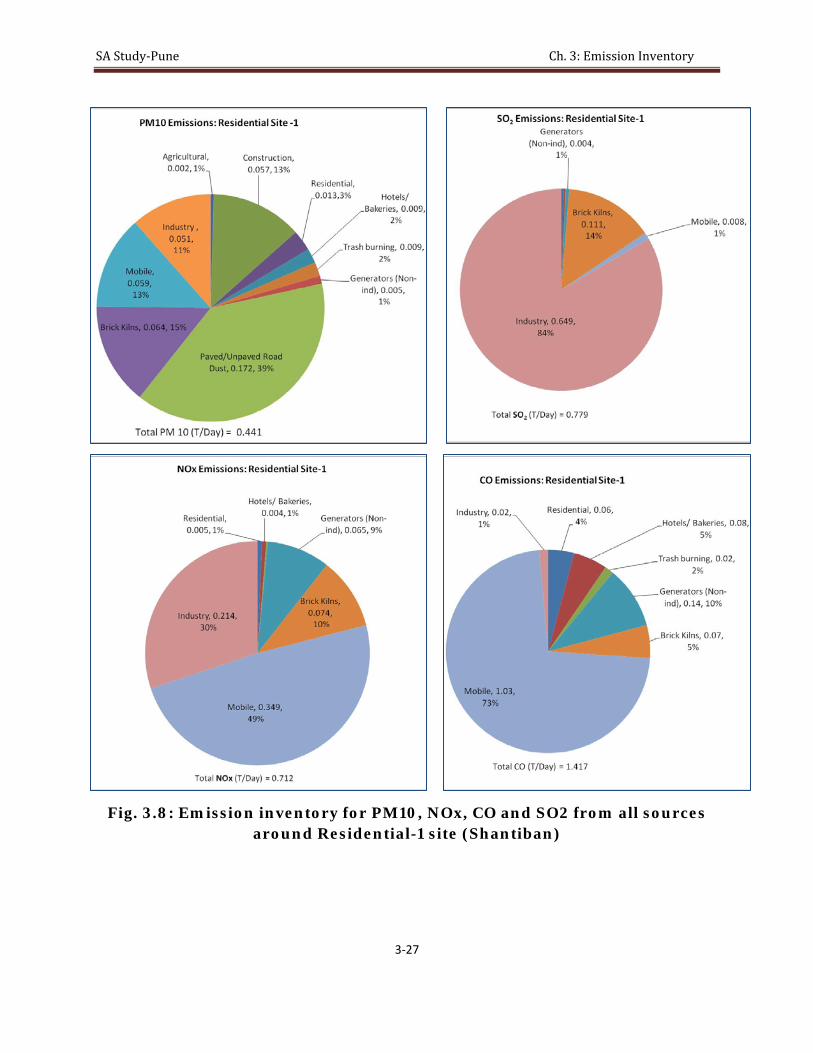
SA Study‐Pune Ch. 3: Emission Inventory
3‐27
Fig. 3.8: Emission inventory for PM10, NOx, CO and SO2 from all sources around Residential-1 site (Shantiban)

SA Study‐Pune Ch. 3: Emission Inventory
3‐28
Fig. 3.9: Emission inventory for PM10, NOx and CO from line sources around Residential-1 site (Shantiban)

SA Study‐Pune Ch. 3: Emission Inventory
3‐29
Fig. 3.10: Emission inventory for PM10, NOx, CO and SO2 from all sources around Residential-2 site (Sahakarnagar)

SA Study‐Pune Ch. 3: Emission Inventory
3‐30
Fig. 3.11: Emission inventory for PM10, NOx and CO from line sources around Residential-2 site (Sahakarnagar)

SA Study‐Pune Ch. 3: Emission Inventory
3‐31
Fig. 3.12: Emission inventory for PM10, NOx, CO and SO2 from all sources around Kerbside-1 site (CoEP)

SA Study‐Pune Ch. 3: Emission Inventory
3‐32
Fig. 3.13: Emission inventory for PM10, NOx and CO from line sources around Kerbside-1 site (CoEP)

SA Study‐Pune Ch. 3: Emission Inventory
3‐33
Fig. 3.14: Emission inventory for PM10, NOx, CO and SO2 from all sources around Kerbside-2 site (Hadapsar)

SA Study‐Pune Ch. 3: Emission Inventory
3‐34
Fig. 3.15: Emission inventory for PM10, NOx and CO from line sources around Kerbside-2 site (Hadapsar)

SA Study‐Pune Ch. 3: Emission Inventory
3‐35
Fig. 3.16: Emission inventory for PM10, NOx, CO and SO2 from all sources around Industrial site (SAJ)

SA Study‐Pune Ch. 3: Emission Inventory
3‐36
Fig. 3.17: Emission inventory for PM10, NOx and CO from line sources around Industrial site (SAJ)

SA Study‐Pune Ch. 3: Emission Inventory
3‐37
Fig. 3.18: Emission inventory for PM10, NOx, CO and SO2 from all sources around Other-Institute site (UoP)

SA Study‐Pune Ch. 3: Emission Inventory
3‐38
Fig. 3.19: Emission inventory for PM10, NOx and CO from line sources around Other-Institute site (UoP)

SA Study‐Pune Ch. 3: Emission Inventory
3‐39
3.5 City level emission inventory:
Gridded emission inventory is prepared for the base year 2007. Following methodology was followed-
• Pune city is divided into 2km X 2km grid.
• Primary data collected for 28km2, secondary data for all area and point sources from MPCB and PMC has been used for calculating emission inventory at city level.
• For line sources, actual road lengths are calculated for all the grids for A, B, C and D category roads.
• The suitable data from the primary vehicle count at different road types was used for the individual grids.
• While using secondary data, socio-economic distribution was taken into consideration.
• Gridded emission inventory was prepapred for PM10 and NOx for following categories separately to assess the distribution and impact of these source categories
o all sources together,
o Mobile sources,
o industrial sources,
o other area sources and
o road dust (in case of PM10 only).
The gridwise emission inventory is presented in Annexure-III. City level emission inventory, with the activity data collected as above and emission factors (ARAI Report,2007 and USEPA 1995 AP-42) reported at Annexure-II, was prepared for all sources together and line sources separately, for year 2007 for PM10, NOx,and SO2 is shown in Fig. 3.20 to 3.22.

SA Study‐Pune Ch. 3: Emission Inventory
3‐40
Fig. 3.20: City level emission inventory for PM10 for year 2007 for all sources together and line sources separately
Bikes0.84
14.22%
Scooters0.569.55%
Autorick0.91
15.43%
3WGC0.345.83%
4WGC0.73
12.27%Cars0.172.94%
Buses1.13
19.13%
Trucks1.22
20.62%
City level PM 10 (Line Sources) Emission Inventory (TPD) ‐ 2007
Total PM10 5.91 TPD
Paved Rd. Dust15.447747.88%
Unpaved Rd. Dust
4.302113.33%
Mobile5.913318.33%
Construction 1.43134.44%
Slums1.86425.78%
Agricultural0.59841.85%
Hotels/ Bakeries/street
vendors1.01153.14%
Industry0.40191.25%
Others0.83272.58%
Residential0.46261.43%
City level PM 10 Emission Inventory (TPD) ‐ 2007
Total PM10 32.27 TPD

SA Study‐Pune Ch. 3: Emission Inventory
3‐41
Fig. 3.21: City level emission inventory for NOx for year 2007 for all sources together and line sources separately
Bikes7.76
19.80%Scooters1.864.75%
Autorick2.366.03%
3WGC0.812.07%
4WGC2.757.01%
Cars3.218.19%
Buses11.7429.94%
Trucks8.70
22.21%
City level NOx (Line Sources) Emission Inventory (TPD) ‐ 2007
Total NOx39.19 TPD
Mobile39.191094.62%
Slums0.39130.94%
Hotels/ Bakeries/street
vendors0.24230.58%
Industry0.89322.16%
Others0.30450.74%
Residential0.39650.96%
City level NOx Emission Inventory (TPD) ‐ 2007
Total NOx TPD 51.54
Total NOX TPD
41.42

SA Study‐Pune Ch. 3: Emission Inventory
3‐42
Fig. 3.22: City level emission inventory for SO2 for year 2007 for all sources together and line sources separately
Mobile111.617983.81%
Slums14.647811.00%
Hotels/ Bakeries/street
vendors4.77583.59%
Industry0.08370.06%
Others1.99641.50%
Residential0.05550.04%
City level CO Emission Inventory (TPD) ‐ 2007
Total CO TPD
133.18
Mobile0.903412.70%
Slums0.32364.55%
Hotels/ Bakeries/street
vendors0.11831.66%
Industry5.231373.53%
Others0.44946.32%
Residential0.08811.24%
City level SO2 Emission Inventory (TPD) ‐ 2007
Total SO2TPD 7.11

SA Study‐Pune Ch. 3: Emission Inventory
3‐43
3.6 Conclusions:
• Highest pollution loads of PM10, NOx and CO are observed at the central part of the city with major commercial activities and high population and road densities.
• Road dust emerges as the highest contributor towards PM10 in the city (61%) • Line sources (Mobile) contribute to 18% of PM10 with more than 40%
contribution is from 2, 3 wheelers and cars. Most of these vehicles are gasoline or LPG fuelled vehicles. The high contribution from these vehicles is due to high number of vehicles. (65%-2Wheelers, 13% -auto rickshaws and 15% cars).
• Industrial contribution to PM10 in the city is limited to 1.25 % due to confined industrial areas within the city and very low numbers of air polluting industries.
• Prominent area sources other than road dust are constructionand brick klins (4.5%), domestic and slum fuel usage (including solid fuel burnig) (7.5%) and hotels and bakeries (3%).
• For NOx emissions, major contribution is from vehicles (95%). The contribution from industries is limited (2%) due to confined industrial area with in the city limits. Domestic and commercial fuel burning for cooking contribute to balnce 3%.
• Pune was having a special ‘Pune Model’ implemented for the supply of electricity in the Pune & Pimpri-Chinchwad area, wherein 100% electricity was ensured to whole of the city. This was possible with understanding with Confederation of Indian Industries (CII), wherein deficit in electricity demand was fulfilled by industry sector through CII. This has ensured zero usage of non-industrial generators. Therefore, while generating baseline year 2007 emission inventory, non-industrial generator source was not considered.
• SO2 inventory for industrial area shows very high SO2 emission loads (4 ton/day) due to very high fuel consumption in industrial area wherein largest forging industry in Asia is located. Similarly sulfur content of these industrial fuels is very high (FO 4%, LDO 1.8%).
• Vehicles are major source for CO emissions contributing to about 85 % emission load followed by fuel burning in slum (11%).

This page is intentionally left blank

SA Study‐Pune Ch. 4: Receptor Modeling & Source Apportionment
4-1
Chapter4. Receptor Modeling &
Source Apportionment
4.1 Receptor Modeling
The fundamental principle of receptor models is that mass conservation can be assumed and a mass balance analysis can be used to identify and apportion sources of airborne particulate matter in the atmosphere. The approach to obtaining a data set for receptor modeling is to determine a large number of chemical constituents such as elemental concentrations in a number of samples. Receptor models use monitored pollutant concentration and some information about the chemical composition of local air pollution sources (profiles) to estimate the relative influence of these sources on pollutant concentrations at any single monitoring location. Receptor models are retrospective i.e. they can only assess the impacts of air pollution source categories on pollutant concentrations that have already been monitored.
In this study Factor Analysis and Chemical Mass Balance (CMB8.2) model was used for receptor modeling (CMB 8.2,USEPA 2004).
4.1.1 Factor Analysis: Methodology & results
Factor analysis is a form of exploratory multivariate analysis that is used to either reduce the number of variables in a model or to detect relationships among variables. It replaces a large set of inter-correlated variables with a smaller number of independent variables. Thus, the new variables (Factors) are the linear combinations of original variables used in the analysis. The factor analysis assumes that the total concentration of each constituent is made up of the sum of elemental contributions from each of different pollution source components. All variables involved in the factor analysis need to be interval and are assumed to be normally distributed. The goal of the analysis is to try to identify factors which underlie the variables. There may be fewer factors than variables, but there may not be more factors than variables.
The factor analysis method is quick and requires characterization of PM10 collected at receptors only. Factor analysis is often used in data analysis to:
• Study the correlations of a large number of variables by grouping the variables into “factors”, The variables within each factor are more highly correlated with variables in their factor than with variables in other factors

SA Study‐Pune Ch. 4: Receptor Modeling & Source Apportionment
4-2
• Interpret each factor according to the meaning of the variables • Summarize many variables by a few factors. The scores from the factors can be
used as data for tests, regression etc.
In order to reduce the dimensionality in the data set, the new variables i.e. factors must have simple interpretations. But un-rotated principal components are often not readily interpretable since they each attempt to explain all remaining variance in the data set. For this reason, a limited number of components are usually subjected to rotation that constitutes a maximization of the variance of the communality normalized loadings (correlations). Such rotations tend to drive variable loadings toward either zero or one on a given factor.
Based on the above considerations, the Varimax rotated factor analysis technique based on the principal components has been used in the determination of the contribution of respirable particulate matter pollution sources. The components or factors rotated had Eigen values greater than one after rotation. It is widely used technique, because it is a simple, non-parametric method of extracting relevant information from confusing data sets. With minimal additional effort PCA provides a roadmap for how to reduce a complex data set to a lower dimension to reveal the sometimes hidden, simplified structure that often underlie it.
Chemical analysis data of PM10 samples collected at each of the sites representing different activity zones used as input to the factor analysis. The past studies carried out in India for particulate matter source apportionment are restricted to one or few activity zones (Vinodkumar et al. 2001; Tripathi et al. 2004; Gupta et al. 2007).
Principal Component analysis was applied to the chemical speciation data of selected species of all the samples collected at a site in all the seasons.
Factor Analysis Results:
Results of the factor analysis, with the probable sources indicated by group of constituents, carried out for different sites are presented in Table 4.1 to 4.7. From the analysis of data for different sites in Pune it was observed that the first component (factor) extracted was always of earth crust metals indicating re-suspended dust as source and is grouped with the markers like Ca, Mg for construction source. Other sources indicated are combustion/vehicles, wood/ vegetative burning and coal combustion. Secondary particulates formation was indicated by presence of NH4, SO2 and NO3 in one group.

SA Study‐Pune Ch. 4: Receptor Modeling & Source Apportionment
4-3
Table: 4.1 – Factor Analysis results for Background Site
Rotated Component Matrix
Species Component
1 2 3 4 AL 0.9678 0.1221 0.1002 0.0886 AS 0.1042 0.0615 0.1406 0.7914 BR 0.1607 0.0978 0.0168 0.6946 CA 0.9481 0.1169 0.1276 0.1060 CU 0.4849 -0.0332 -0.1353 0.2352 EC 0.2307 0.8430 0.2047 0.2364 FE 0.8939 0.2046 0.0463 0.1286 K 0.7757 0.3988 0.0910 0.1344 MASS -0.0099 0.1217 0.5498 0.0515 MG 0.9079 -0.0405 0.0820 0.0497 NA 0.5858 0.0199 -0.0162 0.0173 NH4 0.0672 0.2599 0.6683 -0.1195 NO3 0.0982 -0.0886 0.7562 0.1236 NOX 0.0159 0.8491 0.1556 -0.0238 OC 0.3365 0.8063 0.2199 0.2519 S 0.4771 0.5983 0.0706 0.1143 SI 0.9651 0.1146 0.0787 0.0874 SO2 -0.0118 0.7449 -0.0649 -0.0852 SO4 0.1573 0.1238 0.7543 0.1977 Extraction Method: Principal Component Analysis. Rotation Method: Varimax with Kaiser Normalization.
Based on the observed factors contributing to the components following sources can be identified-
• Component 1 (Al, Si, Fe and Ca, Mg): Soil Dust/Road dust and Construction • Component 2 (EC, OC & NOx): Combustion/ Vehicles • Component 3 (NH4, NO3, SO4): Secondary Particulates • Component 4 (As, Br): Coal/Wood Combustion

SA Study‐Pune Ch. 4: Receptor Modeling & Source Apportionment
4-4
Table: 4.2 – Factor Analysis results for Residential Site- 1
Rotated Component Matrix
Species Component
1 2 3 4 5 AL 0.9767 -0.0605 0.1177 -0.0223 0.0656 AS 0.2960 -0.0683 0.7773 0.0790 -0.0626 BR 0.2507 0.2591 -0.0118 0.7884 -0.1050 CA 0.9703 0.0504 0.0212 0.0148 -0.0894 CU 0.4317 0.5048 -0.2198 0.5105 -0.2283 EC -0.1421 0.7984 0.0557 0.2137 -0.0245 FE 0.9289 0.1444 0.1534 0.0405 -0.0932 K 0.8781 -0.0238 0.3324 0.2076 0.0281 MASS -0.0398 0.7135 0.0663 -0.0501 0.1246 MG 0.9149 -0.2386 0.0680 -0.0384 0.1281 NA 0.5641 -0.1869 0.3517 0.3508 0.3194 NH4 0.0910 0.2900 0.2612 -0.1509 0.6292 NO3 0.1930 0.0315 -0.0976 -0.1386 0.7290 NOX 0.0848 0.2388 0.7801 0.0026 -0.0924 OC -0.0168 0.9162 0.0849 0.2170 0.0157 S 0.5689 0.1062 0.5207 0.4107 0.2220 SI 0.9791 -0.0563 0.0918 -0.0004 0.0294 SO2 -0.1190 0.0648 0.1132 0.6124 -0.0154 SO4 -0.2160 -0.1048 -0.1874 0.1362 0.6708 Extraction Method: Principal Component Analysis. Rotation Method: Varimax with Kaiser Normalization.
Based on the observed factors contributing to the components following sources can be identified-
• Component 1 (Al, Si, Fe, K and Ca, Mg): Soil Dust/Road dust and Construction • Component 2 (EC, OC): Combustion/ Vehicles • Component 3 (As, NOx): Coal/Wood Combustion • Component 4 (Br, SO2): Vegetative Burning • Component 5 (NH4, NO3, SO4): Secondary Particulates

SA Study‐Pune Ch. 4: Receptor Modeling & Source Apportionment
4-5
Table: 4.3 – Factor Analysis results for Residential Site- 2
Rotated Component Matrix
Species Component
1 2 3 4 5 AL 0.9328 0.1591 0.1940 -0.0498 0.2080 AS 0.2778 0.7113 0.0841 -0.1394 -0.3057 BR 0.1307 0.1069 -0.0112 0.8819 -0.0423 CA 0.7836 0.4264 0.1997 0.1264 0.0607 CU 0.0740 0.0275 0.1521 0.8909 0.0164 EC 0.1119 0.2037 0.9444 0.0938 -0.0701 FE 0.8725 0.1221 0.1826 0.0164 0.3227 K 0.7845 0.4912 0.2204 0.1533 -0.0210 MASS 0.3203 0.4454 0.4280 0.0289 0.2736 MG 0.9294 0.2618 0.1058 0.0584 -0.0592 NA 0.7879 0.2961 -0.1764 0.2259 -0.1737 NH4 0.0428 0.0156 -0.0964 -0.0381 0.8592 NO3 0.3686 0.7844 0.2997 0.1060 0.1984 NOX 0.3385 0.2150 0.6092 -0.0387 0.5014 OC 0.0847 0.1925 0.9376 0.0895 -0.1036 S 0.7786 0.1995 0.0509 0.2021 -0.0726 SI 0.9228 0.1659 0.1976 -0.0482 0.2240 SO2 0.2220 0.6964 0.1886 0.1450 0.0722 SO4 0.4184 0.5798 0.2247 0.2316 0.3698 Extraction Method: Principal Component Analysis. Rotation Method: Varimax with Kaiser Normalization.
Based on the observed factors contributing to the components following sources can be identified-
• Component 1 (Al, Si, Fe, K, Na and Ca, Mg): Soil Dust/Road dust and Construction • Component 2 (As, NOx): Coal/Wood Combustion • Component 3 (EC, OC, NOx): Combustion/ Vehicles • Component 4 (Br, Cu): Vegetative Burning • Component 5 (NH4, SO4): Secondary Particulates

SA Study‐Pune Ch. 4: Receptor Modeling & Source Apportionment
4-6
Table: 4.4 – Factor Analysis results for Kerbside Site- 1
Rotated Component Matrix
Species Component
1 2 3 4 AL 0.0767 -0.0122 0.1143 0.9285 AS 0.3720 0.4028 0.2062 0.3077 BR 0.7456 -0.3457 -0.0591 0.4126 CA 0.9003 0.0239 0.1233 -0.2365 CU 0.7353 -0.3086 -0.0029 0.3193 EC 0.0664 0.6783 0.7900 -0.1741 FE 0.8778 0.0504 0.1974 0.1693 K 0.8945 0.2413 0.0867 -0.1867 MASS 0.1387 -0.0690 -0.1472 0.0086 MG 0.9097 0.1751 0.0038 0.1753 NA 0.8413 0.1600 -0.2602 0.0773 NH4 0.1387 0.6759 0.0596 -0.0123 NO3 -0.0797 0.2867 0.5914 0.0175 NOX 0.1124 -0.1772 0.8658 0.0929 OC 0.4651 0.3409 0.4321 0.1385 S 0.8500 0.1882 -0.0379 0.3814 SI 0.8977 0.1907 0.1263 -0.2622 SO2 0.0774 -0.3064 -0.2542 0.1164 SO4 0.0642 0.7975 -0.1057 0.0392 Extraction Method: Principal Component Analysis. Rotation Method: Varimax with Kaiser Normalization.
Based on the observed factors contributing to the components following sources can be identified-
• Component 1 (Si, Fe, K, Na and Ca, Mg): Soil Dust/Road dust and Construction • Component 2 (NH4, SO4): Secondary Particulates • Component 3 (EC, OC, NOx): Combustion/ Vehicles

SA Study‐Pune Ch. 4: Receptor Modeling & Source Apportionment
4-7
Table: 4.5 – Factor Analysis results for Kerbside Site- 2
Rotated Component Matrix
Species Component
1 2 3 AL 0.9862 0.0799 0.1098 AS 0.9702 0.0821 0.1019 BR 0.9724 0.0631 0.0047 CA 0.9850 0.0676 0.1147 CU 0.9718 0.0722 0.1445 EC 0.4604 0.6540 0.2954 FE 0.9847 0.0657 0.1291 K 0.9865 0.0826 0.1116 MASS -0.0057 0.3522 0.6388 MG 0.9866 0.0834 0.1104 NA 0.9833 0.0749 0.1055 NH4 -0.1115 0.7770 -0.1326 NO3 0.0593 0.8153 0.2901 NOX 0.2467 0.4415 0.7122 OC 0.3588 0.6854 0.4482 S 0.9465 0.1241 0.1858 SI 0.9862 0.0790 0.1099 SO2 0.1475 -0.1426 0.8063 SO4 0.0417 0.9316 0.0283 Extraction Method: Principal Component Analysis. Rotation Method: Varimax with Kaiser Normalization.
Based on the observed factors contributing to the components following sources can be identified-
• Component 1 (Al, Si, Fe, K, Na/ Br, Cu, S/ and Ca, Mg): Soil Dust-Road dust/ Wood Combustion/ and Construction
• Component 2 (EC, OC/ NH4, SO4, NO3): Combustion/ Vehicles/ Secondary Particulates
• Component 3 (SO2, NOx): Industrial Fuel Oil Combustion

SA Study‐Pune Ch. 4: Receptor Modeling & Source Apportionment
4-8
Table: 4.6 – Factor Analysis results for Industrial Site
Rotated Component Matrix
Species Component
1 2 3 4 AL 0.9604 0.0550 0.1135 0.0720 AS 0.4176 0.3517 0.0280 -0.3995 BR 0.3423 0.2986 -0.1976 0.4384 CA 0.9471 0.1342 0.0788 0.0676 CU 0.1492 -0.0156 -0.0543 0.8249 EC -0.0312 0.8050 0.4519 0.1792 FE 0.9328 0.0339 0.0166 0.0510 K 0.8619 0.3369 -0.1513 0.1963 MASS 0.2789 0.6683 -0.3842 -0.1060 MG 0.9781 0.0445 0.0560 0.0556 NA 0.8151 0.0690 0.0855 -0.0003 NH4 0.0316 0.3516 0.6265 0.2343 NO3 0.1477 -0.0165 0.6937 -0.1278 NOX 0.3680 0.8323 -0.0394 0.2314 OC 0.0421 0.8619 0.3871 0.0841 S 0.8502 0.2442 0.1104 0.0125 SI 0.9478 0.0956 0.1017 0.0858 SO2 0.0293 0.2536 0.2047 0.7002 SO4 0.1022 0.0531 0.8268 0.0110 Extraction Method: Principal Component Analysis. Rotation Method: Varimax with Kaiser Normalization.
Based on the observed factors contributing to the components following sources can be identified-
• Component 1 (Al, Si, Fe, K, Na and Ca, Mg): Soil Dust/Road dust and Construction • Component 2 (EC, OC, NOx): Combustion/ Vehicles • Component 3 (NH4, SO4, NO3): Secondary Particulates • Component 4 (Cu, SO2): Industrial Fuel Oil Combustion

SA Study‐Pune Ch. 4: Receptor Modeling & Source Apportionment
4-9
Table: 4.7 – Factor Analysis results for Other (Institute) Site
Rotated Component Matrix
Species Component
1 2 3 4 AL 0.9483 0.2748 0.0011 -0.0144 AS 0.1411 0.2002 0.7830 0.1638 BR -0.0477 0.0489 0.0834 0.9210 CA 0.9077 0.3285 -0.0967 -0.0259 CU 0.3219 0.2348 -0.4883 0.3346 EC 0.2362 0.9013 0.1033 -0.0029 FE 0.8976 0.3601 -0.0901 -0.0078 K 0.8015 0.3863 0.1793 0.0560 MASS 0.1426 0.7141 -0.3808 0.0066 MG 0.9298 0.1673 -0.0446 -0.0557 NA 0.8161 0.0464 0.0259 0.0987 NH4 0.0582 0.8795 0.0407 -0.1143 NO3 0.2560 0.8468 0.0402 0.0800 NOX 0.4643 0.5771 0.2896 -0.0263 OC 0.3334 0.8936 0.1851 0.0031 S 0.7719 0.2390 0.3124 0.1490 SI 0.9408 0.2911 -0.0535 -0.0158 SO2 0.3973 0.6987 -0.1161 0.2782 SO4 0.2718 0.7673 0.1552 0.0419 Extraction Method: Principal Component Analysis. Rotation Method: Varimax with Kaiser Normalization.
Based on the observed factors contributing to the components following sources can be identified-
• Component 1 (Al, Si, Fe, K, Na and Ca, Mg): Soil Dust/Road dust and Construction • Component 2 (EC, OC and NH4, SO4, NO3): Combustion/ Vehicles and Secondary
Particulates • Component 3 (As): Coal/Wood Combustion • Component 4 (Br): Vegetative Burning

SA Study‐Pune Ch. 4: Receptor Modeling & Source Apportionment
4-10
4.1.2 CMB Model 8.2: Methodology & results
A mass balance equation can be written to account for all m chemical species in the n samples as contributions from p independent sources: Where, Ci is the concentration of species i measured at a receptor site, xij is the ith elemental concentration measured in the jth sample, and mj is the airborne mass
concentration of material from the jth source contributing to the jth sample. The term aij
is included as an adjustment for any gain or loss of species i between the source and receptor. The term is assumed to be unity for most of the chemical species.
CMB model assumptions are: • Compositions of source emissions are constant over the period of ambient and
source sampling; • Chemical species do not react with each other (i.e., they add linearly); • All sources with a potential for contributing to the receptor have been identified
and have had their emissions characterized; • The number of sources or source categories is less than or equal to the number of
species; • The source profiles are linearly independent of each other; and • Measurement uncertainties are random, uncorrelated, and normally distributed.
Following approach was used for CMB modeling: Identification of the contributing source types based on primary emission
inventory data collected around the monitoring sites in the area of 4 sq. km; Selection of chemical species to be included in the calculation. Following species
were analysed from the daily PM10 samples collected at respective sites for 20 days in three seasons. • Carbon fractions based on temperature (Organic Carbon & Elemental
Carbon) using Thermal Optical Reflectance (TOR) Carbon Analyzer, • Ions (Anions- fluoride, chloride, bromide, sulphate, nitrate & phosphate and
Cations sodium, ammonium, potassium, magnesium & calcium) using Ion Chromatography
• Elements (Na, Mg, Al, Si, P, S, Cl, Ca, Br, V, Mn, Fe, Co, Ni, Cu, Zn, As, Ti, Ga, Rb, Y, Zr, Pd, Ag, In, Sn, La Se, Sr, Mo, Cr, Cd, Sb, Ba, and Pb) using Energy Dispersive X-Ray Fluorescence Spectrometer (ED-XRF)
• Molecular Markers (Alkanes, Hopane, Alkanoic acids qualitative analysis using GC-MS & quantitative analysis using GC-FID; PAHs analysis using High
Ci=∑ mj xij aij j

SA Study‐Pune Ch. 4: Receptor Modeling & Source Apportionment
4-11
Performance Liquid Chromatography (HPLC)). Analysis of organic molecular markers was performed on 20 days composite sample and the species analysed were distributed in proportion to the organic carbon content in the respective samples.
Selection of representative source profiles with the fraction of each of the chemical species and uncertainty. Source profiles developed for non-vehicular sources (IITB Report,2008) and vehicular sources (ARAI Report,2008 ) were used.
Estimation of the both ambient concentrations and uncertainty of selected chemical species from the particulate matter collected at respective sites; and
Solution of the chemical mass balance equations through CMB-8.2 model run. Source contribution estimates (SCE) are the main output of the CMB model. The sum of these concentrations approximates the total mass concentrations. When the SCE is less than its standard error, the source contribution is undetectable. Two or three times the standard error may be taken as the upper limit of the SCE in this case. Assuming that the errors are normally distributed, there is about a 66% probability that the true source contribution is within one standard error and about a 95% probability that the true concentration is within two standard errors of the SCE. The reduced chi square (χ2 ), R2, and percent mass are goodness of fit measures for the least-squares calculation. The χ2 is the weighted sum of squares of the differences between calculated and measured fitting species concentrations divided by the effective variance and the degrees of freedom. The weighting is inversely proportional to the squares of the precision in the source profiles and ambient data for each species. Ideally, there would be no difference between calculated and measured species concentrations and χ2 would be zero. A value of less than one indicates a very good fit to the data. Values greater than 4 indicate that one or more of the fitting species concentrations are not well-explained by the source contribution estimates. R2 is determined by the linear regression of the measured versus model-calculated values for the fitting species. R2 ranges from 0 to 1. The closer the value is to 1.0, the better the SCEs explain the measured concentrations. When R2 is less than 0.8, the SCEs do not explain the observations very well with the given source profiles. Percent mass is the percent ratio of the sum of model-calculated SCEs to the measured mass concentration. This ratio should equal 100%, though values ranging from 80 to 120% were considered acceptable.
Results of CMB8.2 modeling for PM10:
Daily average concentrations of different species for 20 days each at site were used as input to the receptor model. Results obtained in terms of source contribution estimates for individual daily samples for a site in a season were averaged to calculate source contribution to that site for that season. Results of the PM10 source apportionment by CMB-8.2 modeling for various sites are presented in Figure 4.1 for summer, post-monsoon and winter season.

SA Study‐Pune Ch. 4: Receptor Modeling & Source Apportionment
4-12
Residential locations
Shantiban represents a purely residential site (Residential-1) with the residential bungalows around the monitoring sites.40% of the area around the 2X2 km grid is residential area, 20% of bare land and 15% of hilly area. Considerable vehicular traffic activity is observed around the site due to commuting of dwellers around the site.
At Shantiban Society (residential site-1), source contribution estimates show re-suspended dust as a major source of PM10 in the range from 47% to 74% contribution. Contribution from vehicles varied from 5% to 21%.During post-monsoon season contribution from construction was found to be very high (47%). Solid fuel combustion was found to contribute about 14% during winter. This may be attributed to increased use of wood, coal during winter for water heating, etc in the nearby slum area.
Sahakarnagar colony represents (Residential-2) a mixed residential and commercial site with many small stalls near the site. The residential area also includes slum area in vicinity of the monitoring site. The land use distribution is residential area 40%, Slum 8%, bare land 25% and Hilly area 11%.
At residential site-2, contribution from re-suspended dust was varied from 50 to 66%. Contribution from solid fuels burning was found to be higher at residential site-2 due to higher percentage of slum area around the site. (Seung S. Park, Young J. Kim, Chemosphere 59 (2005) Construction sources contribution was varied from 7 to 20%. Contribution from vehicles was 24% during post-monsoon. In winter season, vegetative/trash burning was observed to contribute to around 18%.
Kerbside locations
College of Engineering Pune (CoEP) represents a Kerbside location in the city of Pune. This site is along a major road with continuous traffic flow from the old Mumbai highway. 2 X 2 km grid land-use is residential area (31%) with commercial activities (17%), slum (12%) and 16% agricultural land.
At krbside-1, less seasonal variation in road dust contribution was observed (58-61%). Contribution from vehicles was varied from 4% in post-monsoon to 12% in summer season. Contribution from diesel generators was around 3-5%. Agricultural waste/vegetative burning was found to contribute around 18% during winter season.
Hadapsar represents a kerbside location in the city of Pune. This site is along a Solapur highway with a continuous traffic flow. In the area heavy commercial activities are also observed. The area in 2 X 2 km grid is distributed as 27% agricultural land, 21 % bare land, 23% residential area, 14% slum area.

SA Study‐Pune Ch. 4: Receptor Modeling & Source Apportionment
4-13
At kerbside-2, re-suspended road dust contribution was found to vary from 60% to 78%. Contribution from vehicles was found to vary between 4% and 15%. Solid fuel burning contribution was from 10% to 22% (winter). Agricultural waste/vegetative burning contribution of 6% was found in winter samples.
Industrial location
SAJ Test Plant Pvt. Ltd. represents an industrial location in the city of Pune .It is located in the Mundhwa industrial area with major industries in 2 X 2 km area including forging industries, metallurgical industries, ceramic and clay products industries. 2 X 2 km grid includes 37% agricultural land, 13% bare land and 10% residential area.
At industrial site, diesel generator sets were found to contribute to about 11-26%. Contribution of re-suspended road/soil dust varied from 48-71%. Contribution from vehicle source was from 3-14%. Construction source was found to vary as 4-8%. Contribution of construction source may be attributed to the nearby clay and ceramic industry.
Other (Institute) location
Geography Dept., University of Pune represents an Institutional location in the city of Pune. This site is at the north-west part of the Pune. Site (2 X 2 km) is surrounded by Forest plantation (59%), bare-land (16%), Residential area (10%) and commercial (9%).
At, institute site, re-suspended road dust contribution was varied from 44% to 56%. Although, unpaved roads in city of Pune are very less, paved roads are not paved from wall to wall. This fine dust entrains from the corner of the road to the paved portion of road. (Alan Gertler, Judy Chow et al.(2006),and (J. J. Cao, et. Al., July 2002.)
Construction was found to be major source with contribution varied from 24-31%. This can be attributed to the fly-over construction activity being carried out during monitoring period. Garden waste/vegetative burning was found to be around 12 and14% in post-monsoon and winter seasons respectively.

SA Study‐Pune Ch. 4: Receptor Modeling & Source Apportionment
4-14
CMB8.2 modeling for PM2.5
Chemical speciation data for PM2.5 was available for limited samples (7 days per site). Sampling was carried out for 7 days at each site in a season with Teflon filter paper for 3 days and quartz paper for 4 days. Therefore, daily average concentrations of ions and elements were available for 3 days while carbon fraction concentrations were available for 4 days. As daily average concentrations for all the species were not available for a single day sample, average of all species of 7 days samples were used as an ambient air input data for apportionment of PM2.5 through receptor modeling using CMB-8.2 to get an idea of the distribution of sources in PM2.5.
Results for PM2.5 source apportionment based on single sample, with average data are presented in Fig. 4.2. Secondary particulates, vehicles and solid fuel combustion were found to dominate the PM2.5 sources with little contribution from resuspended road dust and other area sources. Seasonal variation contributing sources was observed with contribution from solid fuel combustion was found to be low during summer.

SA Study‐Pune Ch. 4: Receptor Modeling & Source Apportionment
4-15
Fig. 4.1: Source contribution to PM10 samples at various sites using CMB8.2
receptor model in all seasons
Fig. 4.2: Source contribution to PM2.5 samples at various sites using
CMB8.2 receptor model in all seasons

SA Study‐Pune Ch. 4: Receptor Modeling & Source Apportionment
4-16
4.3: Conclusions:
• Receptor modeling by factor analysis and CMB8.2 confirms re-suspended road dust as major source of PM10.
• Sources contributing to PM10, identified through receptor modeling, at different sites in Pune are as follows-
o Re-suspended road dust o Vehicles/ Combustion, o Construction/ Brick Kilns, o Solid fuels burning, o Vegetative burning (agricultural waste, garden waste).
• Seasonal variation in the contribution by different sources of PM10 was observed. However, the source which dominates is re-suspended road dust. Although, unpaved roads in city of Pune are very less, paved roads are not paved from wall to wall. This fine dust entrains from the corner of the road to the paved portion of road. (Alan Gertler, Judy Chow et al.(2006),and (J. J. Cao, et. Al., July 2002.)
• Contribution to PM10 from vegetative burning, solid-fuels burning was found to be higher during winter season, which may be attributed to the increased use of wood, coal for water heating, specifically in slum areas.
• Sources contributing to PM2.5 include mainly secondary particulates, vehicles and solid fuels combustion

SA Study‐Pune Ch. 5: Dispersion Modeling‐Existing Scenario
5-1
Chapter 5. Dispersion Modeling:
Existing scenario
One of the major roles for modeling inventories is development of control strategy and preparation of city specific Action Plan. Modeling inventories can be based on either allowable or actual emissions, depending on the purpose of the modeling. For control measure evaluation and the impact demonstration, the modeling of emission inventory consists of the emissions for the projected year with business-as-usual (BaU) scenario without any control and with controlled scenario.
5.1 Methodology
Industrial Source Complex Short Term-3 (ISCST3) model (USEPA, 1995, User’s guide for Industrial Source Complex (ISC3), Volume I & II (EPA-454/ B-95-003 a & b) was used for dispersion modeling exercise with urban dispersion coefficients and flat terrain condition. It is used for air quality simulation modeling for short term ground level concentrations (GLCs) at multiple receptors resulting from multiple point/area. It is a Gaussian plume model used to calculate the concentration of pollutants due to the emission from source. Various options available with this model were utilized to simulate the actual physical conditions at the sources. The parameter regulating the transport and dispersion of air pollution emissions is the hourly micrometeorological data recorded at the site, which was essentially the input to the model.
In order to predict the impact on air environment, the inputs to model include data on emissions, source details, and meteorology of the region and receptor locations. This model has flexibility in specifying receptor locations. Receptors were selected in Cartesian co-ordinate system wherein multiple receptor networks in single run were defined. Collected meteorological data on wind speed (m/s), wind vector (degree), temperature (K), Stability class and mixing height (m) was converted into daily mean hourly parameters and used for prediction.
Following methodology was used for preparing source input files-
• Pune city map (22km X 20km) was divided into 2km X 2km grids (Fig. 5.1-a). Number of grids with substantial activity level was 87. Emission information of

SA Study‐Pune Ch. 5: Dispersion Modeling‐Existing Scenario
5-2
all sources including point, area and line is included from the baseline gridded emission inventory (2km X 2km) prepared for year 2007.
• Information available through detailed primary surveys (4 sq. km) around the monitoring sites in 0.5km X0.5km grids was also included in the grid for dispersion modeling.
• Line sources emissions on major roads are converted to elongated area sources with an aspect ratio of 1:10 and included in the city specific grids.
• Discrete receptor locations (Cartesian) were selected at the centre of each 2km X 2km grid.
Overall distribution of grids, including city level 2km X 2km grids and site specific 0.5km X 0.5km grids for Pune is shown in Fig. 5.2-b.
Pollutant wise input files were prepared for point and area sources. Line sources were converted to area sources. Source emission rates were considered constant throughout the modeling period. Details of the information required for different source types are as follows.
Point Sources:
Name (ID) of the Source: Location: X(m) & Y(m) Pollutant Emission Rate [g/s] Following detail information of stack was included: Stack Height [m], Diameter [m], Stack Exit Temperature [K], Stack Exit Velocity [m/s]
Area Sources: Source Name: Location (Southwest Vertex): X(m) & Y(m): Pollutant Modeled Emission Rate [g/(s-m2)], Source Height [m], Easterly Dimension [m], Northerly Dimension [m], Initial Vertical Dimension [m], Angle from North [degrees],

SA Study‐Pune Ch. 5: Dispersion Modeling‐Existing Scenario
5-3
Fig. 5.1: Pune city map (a) Gridded base map (b) gridded map for air quality modeling
(a)
(b)

SA Study‐Pune Ch. 5: Dispersion Modeling‐Existing Scenario
5-4
5.2 Emission Loads
Grid-wise distribution of emission loads (kg/day) of various source categories viz., all sources together, mobile sources, industrial sources, road dust and other area sources for PM10 were evaluated. Grid-wise distribution of PM10 emission load for all sources together and all sources without road dust is presented in Figure 5.2 and Fig. 5.3 respectively. Similarly, Figure 5.4 and 5.5 represent grid-wise distribution of NOx and SO2 emission load respectively for all sources together. As can be seen from emission loads, grids covering central part of the city show highest emission loads for PM10 and NOx. PM10 load distribution without road dust also shows similar trends as in case of PM10 loads with all sources together with lower overall PM10 load. This can be attributed to the activity of vehicles (VKT). Thus, load without road dust can be mainly attributed to the PM from mobile source and load with all sources together, which include contribution from vehicles and road dust of around 78%. SO2 emission loads are higher in the grids which include industries.

SA Study‐Pune Ch. 5: Dispersion Modeling‐Existing Scenario
5-5
0 0 0 0 0 0 10 355 7 0 0
186 79 1 37 174 118 184 353 89 157 48
239 374 232 25 255 194 409 341 117 76 4
229 210 419 482 378 226 492 464 569 527 78
52 153 248 599 599 505 659 344 355 276 49
198 285 476 665 1294 1763 584 716 515 55 0
198 419 612 826 973 881 538 707 686 351 0
16 191 272 342 700 726 618 436 469 156 0
0 0 220 164 409 432 480 315 147 33 0
0 59 210 1 360 401 395 0 0 0 0
Fig. 5.2: Distribution of PM10 Emission Load (Kg/day) for all sources in year 2007
0 0 0 0 0 0 10 107 7 0 0
39 18 1 10 45 34 73 121 55 70 11
89 104 85 25 68 82 144 109 49 76 4
84 60 159 186 83 68 152 145 191 133 33
52 51 79 193 221 304 271 128 113 86 23
85 91 230 251 463 657 183 486 256 35 0
76 171 260 302 365 355 182 222 317 205 0
7 110 148 139 250 239 209 172 233 103 0
0 0 81 76 144 187 195 111 73 26 0
0 22 77 1 118 176 178 0 0 0 0
Fig. 5.3: Distribution of PM10 Emission Load (Kg/day) for all sources without resuspended road dust in year 2007
Less than 100
100 to 200
200 to 300
300 to 400
Above 400
Less than 100
100 to 200
200 to 300
300 to 400
Above 400
Numbers in blocks are emission load in kg/day
Numbers in blocks are emission load in kg/day

SA Study‐Pune Ch. 5: Dispersion Modeling‐Existing Scenario
5-6
0 0 0 0 0 0 1 399 4 0 0
250 97 1 78 319 134 184 381 76 140 59
277 428 380 3 414 192 431 422 119 14 2
253 238 616 549 529 258 600 560 694 742 76
9 170 285 950 738 449 1053 460 571 449 70
206 351 483 903 1797 2148 792 1435 841 65 0
254 472 648 957 1121 1078 976 1314 1327 476 0
21 197 220 347 781 762 635 687 888 178 0
0 0 310 194 458 356 477 328 300 32 0
0 85 294 1 446 357 295 0 0 0 0
Fig. 5.4: Distribution of NOx Emission Load (Kg/day) for all sources in year 2007
Fig. 5.5: Distribution of SO2 Emission Load (Kg/day) for all sources in year 2007
Less than 100
100 to 200
200 to 300
300 to 400
Above 400
0 0 0 0 0 0 0 15 1 0 0
6 3 0 2 7 5 11 32 19 4 2
8 11 11 1 106 13 19 14 6 18 1
7 7 19 19 14 7 23 21 325 21 3
18 5 11 30 32 472 43 16 16 12 2
22 12 99 33 70 93 23 4252 44 1 0
23 50 32 37 53 51 25 47 123 38 0
0 39 17 17 35 31 25 17 52 37 0
0 0 9 8 19 24 49 11 6 1 0
0 2 10 0 32 47 58 0 0 0 0
Less than 25
25 to 50
50 to 75
75 to 100
Above 100
Numbers in blocks are emission load in kg/day
Numbers in blocks are emission load in kg/day

SA Study‐Pune Ch. 5: Dispersion Modeling‐Existing Scenario
5-7
5.3 Meteorological data
Meteorological data, used in the model, was collected at the monitoring sites. Meteorological station was installed at monitoring sites to capture data on wind direction, wind velocity, ambient temperature and % relative humidity. Relevant data for the monitoring period was converted into daily mean hourly parameters and used for prediction at respective sites. Predominant meteorological data was used for modeling for Pune city. Hourly surface data and upper air meteorological data was used for preparing meteorological files with diurnal and seasonal variations.
5.3.1 Summer
Monitoring for summer season was carried out during April 18, 2007 to June 10, 2007 at all the sites in two sets. Daily maximum temperature was found to vary between 34.8 and 37.2oC Drop in ambient temperature during the second set of monitoring was observed. Average relative humidity during the set-I was varied from 30-50%, whereas during set-II, it was observed to be in the range of 60 to 75%.
5.3.2 Post-monsoon
Monitoring for post-monsoon season was carried out at during September 14, 2007 to October 31, 2007 in two sets. Daily maximum temperature was found to vary between 29.5 and 34.8oC. Daily average relative humidity during the set-3 was varied from 36-98%, whereas during set-4, it was observed to be in the range of 26 to 79%.
5.3.3 Winter
Monitoring for winter season was carried out during December12, 2007 to February 02, 2008 in two sets. Daily maximum temperature was found to vary between 30.7 and 33.8oC. Daily minimum temperature varied in the range from 12.3 to 16.7oC Average relative humidity during the set-5 was varied from 14-71%, whereas, during set-6, it was observed to be in the range of 27 to 83%.
Seasonal variation in wind speeds at various sites is given in Table 5.1. Higher wind speeds were observed during summer season and during winter season the average velocities were typically low and most of the times wind speed were found to be below 2.0 m/s during winter. Fig. 5.6shows seasonal variation in minimum, maximum, and average ambient temperatures at different sites.

SA Study‐Pune Ch. 5: Dispersion Modeling‐Existing Scenario
5-8
Table 5.1: Seasonal variations in wind speeds at different sites
Site
Wind Speed (m/s) Occurrences (%) Site
Wind Speed (m/s) Occurrences (%)
Res
iden
tial
- 1
From To Summer Post-monsoon Winter
Ker
bsid
e- 1
From To Summer Post-monsoon Winter
0.5 1 2 0 0 0.5 1 2 9 40 1 2 40 7 33 1 2 64 80 43 2 3 19 37 47 2 3 34 11 0 3 4 16 26 13 3 4 0 0 0 4 5 16 21 6 4 5 0 0 0
Above 5 7 10 1 Above 5 0 0 0
Res
iden
tial
- 2
From To Summer Post-monsoon Winter
Ker
bsid
e -
2
From To Summer Post-monsoon Winter
0.5 1 1 0 0 0.5 1 80 0 71 1 2 17 47 24 1 2 15 94 21 2 3 21 40 54 2 3 0 6 5 3 4 26 13 11 3 4 0 0 0 4 5 26 0 5 4 5 0 0 0
Above 5 8 0 7 Above 5 0 0 0
Indu
stri
al
From To Summer Post-monsoon Winter
Oth
er (i
nst
itu
te) From To Summer
Post-monsoon Winter
0.5 1 47 5 69 0.5 1 19 19 54 1 2 51 95 29 1 2 70 74 43 2 3 0 0 0 2 3 7 0 1 3 4 0 0 0 3 4 3 0 0 4 5 0 0 0 4 5 0 0 0
Above 5 0 0 0 Above 5 0 0 0

SA Study‐Pune Ch. 5: Dispersion Modeling‐Existing Scenario
5-9
Fig. 5.6: Seasonal variation in minimum, maximum and mean temperatures at different site (a) residential-R1, (b) residential-R2, (c) kerbside-K1, (d) kerbside-K2, (e) industrial-I and (f) Other-institute -O
(a) (b)
(c) (d)
(e) (f)

SA Study‐Pune Ch. 5: Dispersion Modeling‐Existing Scenario
5-10
5.4 Concentration Profiles
Ground level concentration isopleths of PM10 for base year 2007 for summer, post-monsoon and winter season are presented in Fig. 5.7 to 5.9 respectively. Comparison of season wise plots shows highest ground level concentrations at during winter season. Highest concentrations were observed in the grids covering central part of Pune city where the population densities and road densities are higher. During summer and post-monsoon seasons, winds are mostly westerly. However, during winter season reversal in wind direction was observed. Also, the wind speeds were also observed to be very low i.e. always below 2 m/s.
Fig. 5.10 to 5.12 represents ground level concentration isopleths of NOx for base year 2007 for summer, post-monsoon and winter seasons. Higher NOx concentrations were also observed in the grids covering central part of Pune city with comparatively higher concentrations during winter season.
Baseline ground level concentration isopleths for SO2 are presented in Fig. 5.13 to 5.15 for summer, post-monsoon and winter seasons. High levels of SO2 are confined to the industrial area, which is towards the eastern part of the city. It was observed that due to westerly predominant winds during summer and post-monsoon seasons, dispersion of SO2 is towards the east of the source i.e. out of city area. However during winter the SO2 was observed to be dispersed into the city area.
Model evaluation:
Ground level concentrations of PM10 and NOX predicted by model are compared with the observed concentrations at respective sites for evaluation of the model. The model was found to under predict the PM10 concentration to some extent. Ratio of observed concentrations and predicted concentrations for PM10 at different sites varied in the range of 1.1 to 2.3. Average ratio of observed and predicted ground level concentrations was found to be 1.7.
In case of NOx, Variation in ratio of observed to predicted ground level concentrations at different sites was found in the range 0.3 to 0.8 with overall average ratio of observed to predicted concentrations of 0.6. Thus the model was found to over predict the concentrations to some extent, which may be attributed to the fact that the observed concentrations are representative of NO2 while the emission inventory data used for predictions include all oxides of nitrogen.

SA Study‐Pune Ch. 5: Dispersion Modeling‐Existing Scenario
5-11
Fig. 5.7: PM10- 2007- All sources- Summer
0
2000
4000
6000
8000
1000
0
1200
0
1400
0
1600
0
1800
0
2000
0
2200
0
X co-ord
0
2000
4000
6000
8000
10000
12000
14000
16000
18000
20000
Y co
-ord
25ug/m3
50ug/m3
75ug/m3
100ug/m3
125ug/m3
150ug/m3
Fig. 5.8: PM10- 2007- All sources- Post-monsoon
0
2000
4000
6000
8000
1000
0
1200
0
1400
0
1600
0
1800
0
2000
0
2200
0
X Co-ord
0
2000
4000
6000
8000
10000
12000
14000
16000
18000
20000
Y C
o-or
d
25ug/m3
50ug/m3
75ug/m3
100ug/m3
125ug/m3
150ug/m3
Fig. 5.9: PM10- 2007- All sources- Winter
0 2000 4000 6000 8000 10000 12000 14000 16000 18000 20000 22000
X Co-ord
0
2000
4000
6000
8000
10000
12000
14000
16000
18000
20000
X C
o-or
d
25ug/m3
50ug/m3
75ug/m3
100ug/m3
125ug/m3
150ug/m3

SA Study‐Pune Ch. 5: Dispersion Modeling‐Existing Scenario
5-12
Fig. 5.11: NOx-2007-All sources-Post-monsoon
0
2000
4000
6000
8000
1000
0
1200
0
1400
0
1600
0
1800
0
2000
0
2200
0
X-Co-ord
0
2000
4000
6000
8000
10000
12000
14000
16000
18000
20000
Y C
o-or
d
0ug/m3
40ug/m3
80ug/m3
120ug/m3
160ug/m3
200ug/m3
Fig. 5.10: NOx-2007-All sources-Summer
0
2000
4000
6000
8000
1000
0
1200
0
1400
0
1600
0
1800
0
2000
0
2200
0
X-Co-ord
0
2000
4000
6000
8000
10000
12000
14000
16000
18000
20000
Y C
o-or
d
0ug/m3
40ug/m3
80ug/m3
120ug/m3
160ug/m3
200ug/m3
Fig. 5.12: NOx-2007-All sources-Winter
0
2000
4000
6000
8000
1000
0
1200
0
1400
0
1600
0
1800
0
2000
0
2200
0
X Co-ord
0
2000
4000
6000
8000
10000
12000
14000
16000
18000
20000
Y C
o-or
d
0ug/m3
40ug/m3
80ug/m3
120ug/m3
160ug/m3
200ug/m3

SA Study‐Pune Ch. 5: Dispersion Modeling‐Existing Scenario
5-13
0
2000
4000
6000
8000
1000
0
1200
0
1400
0
1600
0
1800
0
2000
0
2200
0
X Co-ord
0
2000
4000
6000
8000
10000
12000
14000
16000
18000
20000
Y C
o-or
d
0.00
6.00
12.00
18.00
24.00
30.00
36.00
42.00
48.00
54.00
60.00
66.00
72.00
Fig. 5.13: SO2- 2007- All sources- Summer
0 2000 4000 6000 8000 10000 12000 14000 16000 18000 20000 22000
X Co-ord
0
2000
4000
6000
8000
10000
12000
14000
16000
18000
20000
Y C
o-or
d
0.00
6.00
12.00
18.00
24.00
30.00
36.00
42.00
48.00
54.00
60.00
66.00
72.00
Fig. 5.14: So2- 2007- All sources- Post-monsoon
0
2000
4000
6000
8000
1000
0
1200
0
1400
0
1600
0
1800
0
2000
0
2200
0
X Co-ord
0
2000
4000
6000
8000
10000
12000
14000
16000
18000
20000
Y C
o-or
d
0.00
6.00
12.00
18.00
24.00
30.00
36.00
42.00
48.00
54.00
60.00
66.00
72.00
Fig. 5.15: SO2- 2007- All sources- Winter

SA Study‐Pune Ch. 5: Dispersion Modeling‐Existing Scenario
5-14
Site- specific distribution of pollutant concentrations:
Dispersion modeling exercise was carried out, for city of Pune and all the site specific grids, separately with the PM10 emission load data from different source categories like mobile, re-suspended road dust, industry and other area sources together to find out contribution of these sources towards the ambient concentrations. Emission loads from the primary data collected in the area of 4 sq. km with grid resolution of 0.5 km X 0.5 km (16 grids) around the monitoring sites and Pune city emission load data in 2km X 2km grids was used as input.
Contribution of different source categories, based on dispersion modeling, to PM10 concentrations for Pune city and various sites is presented in Fig. 5.16(a-g) for critical season winter. Re-suspended dust was found to be the major source with a contribution of around 58%. Mobile source and other area sources contribute around 22% and 19% respectively. Average contribution of all the grids in Pune of Industrial sources was found to be very less (0.1%). Site-specific dispersion modeling results show higher contribution of about 30-40% from mobile sources at all sites, especially kerbside. However, re-suspended dust was found to be the highest contributor at all sites with contribution ranging from 40 to 60%. Other area sources contributed in the range from 8 to 19%. Contribution from industries were found to be very less (below 1%), however, higher contribution (3%) was observed at industrial site.
Contribution of different source categories to NOx concentrations for Pune city and various sites is presented in Fig. 5.17(a-g) for critical season winter. Mobile source was found to be largest contributor towards the NOx concentration with average contribution more than 95% from dispersion modeling for Pune city and at various sites. Area sources, including hotels, bakeries, residential fuels, contributed for about 3% of the NOx concentrations. Contribution from industry was about 1%.

SA Study‐Pune Ch. 5: Dispersion Modeling‐Existing Scenario
5-15
Fig. 5.16: Distribution of concentration of PM10 from various source categories from dispersion modeling (winter-2007) for (a) Pune city, (b)
Residential-1 site and (c) Residential-2 site (contd..)
Mobile22.02%
Industrial0.10%
Road Dust58.50%
Other19.38%
Contibution of various source categories to PM10 concentration in year 2007 from disperion modeling for Pune City
Mobile31.11%
Road Dust49.76%
Industrial0.50%
Other Area18.64%
Contibution of various source categories to PM10 concentration in year 2007 from disperion modeling for Shantiban (Residential‐1)
Mobile31.94%
Road Dust52.68%
Industrial0.56%
Other Area14.82%
Contibution of various source categories to PM10 concentration in year 2007 from disperion modeling for Sahakarnagar (Residential‐2)
(b) (c)
(a)

SA Study‐Pune Ch. 5: Dispersion Modeling‐Existing Scenario
5-16
Fig. 5.16: Distribution of concentration of PM10 from various source categories from dispersion modeling (winter-2007) for (d) Kerbside-1,
(e) Kerbside-2, (f) Industrial site and (g) Other-Institute site
Mobile31.85%
Road Dust52.78%
Industrial1.43%
Other Area13.94%
Contibution of various source categories to PM10 concentration in year 2007 from disperion modeling for CoEP (Kerbside‐1)
Mobile42.56%
Road Dust38.49%
Industrial0.06%
Other Area18.89%
Contibution of various source categories to PM10 concentration in year 2007 from disperion modeling for Hadapsar (Kerbside‐2)
Mobile36.16%
Road Dust44.90%
Industrial3.15%
Other Area15.78%
Contibution of various source categories to PM10 concentration in year 2007 from disperion modeling for SAJ (Industrial)
Mobile33.12%
Road Dust57.67%
Industrial0.64%
Other Area8.58%
Contibution of various source categories to PM10 concentration in year 2007 from disperion modeling for UoP (Other)
(d) (e)
(f) (g)

SA Study‐Pune Ch. 5: Dispersion Modeling‐Existing Scenario
5-17
Fig. 5.17: Distribution of concentration of NOx from various source categories from dispersion modeling (winter-2007) for (a) Pune city,
(b) Residential-1 site and (c) Residential-2 site (contd..)
Mobile95.86%
Industrial1.25%
Other Area2.89%
Contibution of various source categories to NOx concentration in year 2007 from disperion modeling for Pune City
Mobile95.32%
Industrial1.10%
Other Area3.59%
Contibution of various source categories to NOx concentration in year 2007 from disperion modeling for Shantiban (Residential‐1)
Mobile96.75%
Industrial0.95%
Other Area2.30%
Contibution of various source categories to NOx concentration in year 2007 from disperion modeling for Sahakarnagar (Residential‐2)
(a)
(b) (c)

SA Study‐Pune Ch. 5: Dispersion Modeling‐Existing Scenario
5-18
Fig. 5.17: Distribution of concentration of NOx from various source categories from dispersion modeling (winter-2007) for (d) Kerbside-1,
(e) Kerbside-2, (f) Industrial site and (g) Other-Institute site
Mobile95.55%
Industrial2.18%
Other Area2.26%
Contibution of various source categories to NOx concentration in year 2007 from disperion modeling for CoEP (Kerbside‐1)
Mobile97.12%
Industrial0.16%
Other Area2.72%
Contibution of various source categories to NOx concentration in year 2007 from disperion modeling for Hadapsar (Kerbside‐2)
Mobile94.16%
Industrial4.03%
Other Area1.81%
Contibution of various source categories to NOx concentration in year 2007 from disperion modeling for SAJ (Industrial)
Mobile98.22%
Industrial0.83%
Other Area0.95%
Contibution of various source categories to NOx concentration in year 2007 from disperion modeling for UoP (Other)
(d) (e)
(f) (g)

SA Study‐Pune Ch. 5: Dispersion Modeling‐Existing Scenario
5-19
Conclusions
Dispersion modeling exercise was carried out for PM10, NOx and SO2, for summer, post-monsoon, and winter seasons. Winter season was found to be critical with respect to ambient concentration levels.
Based on the maximum 100 concentrations obtained through dispersion modeling grid number 35, 36, 37, 38, 39, 47, 48, 49, 50 and 59 were identified as hot-spots with respect to PM10. For NOx, grid number 35, 36, 37, 38, 39, 48, 50, 51, 59 and 62 were identified as hot-spots. Hot-spots are found to be present at the central part of Pune (Fig. 5.18) with higher population as well as road densities.
Fig. 5.18: Hot spots (Top 10 grids) based on predicted PM10 and NOx concentrations
Source wise contribution to PM10 and NOx is at top 10 grids is shown in Fig. 5.19. Re-suspended road dust was found to be major contributor towards ambient PM10 concentrations followed by mobile and other area sources. Major contributor for ambient NOx concentrations was found to be mobile source with a share of more than 95%.
SO2 concentrations were found to higher around the grids having industrial source.

SA Study‐Pune Ch. 5: Dispersion Modeling‐Existing Scenario
5-20
Fig. 5.19: Source wise contribution to PM10 and NOx at top 10 grids

SA Study‐Pune Ch. 6: Emission Control Options and Analysis
6‐1
Chapter 6. Emission Control
Options and Analysis
6.1 Summary of prominent Sources PM: Major sources of PM10 are identified based on emission inventory and dispersion model as well as source apportionment outcome of receptor modeling using CMB and factor analysis.
• Paved and unpaved road dust • Vehicle exhaust of different categories and vintages of vehicles • Construction Activities including brick kilns • Solid fuels combustion
NOx: Major sources of NOx are derived from city level emission inventory estimates and dispersion modeling as.
• Vehicle exhaust • Industrial sources, in limited areas where industry is dominating. However,
within city area polluting industries are limited and dominated by forging and automotive engines industry.
• Other source of NOx pollution is domestic or commercial cooking/ bakeries.
6.2 Future Growth Scenario 6.2.1 Future Projections of Emission Inventory- Methodology
Emission inventory has been prepared for the base year 2007 and corresponding concentrations and hotspots are identified for PM10 & NOx using ISCST3 dispersion modeling exercise.
Various sources divided in categories of line, area and point have been compiled with emission rates, activity data based on primary survey and secondary data. For predictive estimates for next five years i.e. year 2012 and for next 10 years i.e. year 2017, business as usual scenario has been prepared. The cumulative growth rates for each of the activities involved for various categories of sources i.e. point, line & area have been considered based on the historic growth rate data. The emission rates are considered to the same as that of year 2007. However, the roadmap already planned is considered as the business as usual scenario e.g. BS-III regulations for 2&3 wheeler vehicles and BS-

SA Study‐Pune Ch. 6: Emission Control Options and Analysis
6‐2
IV regulations for all other categories of vehicles from the year 2010. Hence, it is considered that all registered vehicles since 2010 will be complying with these regulations and corresponding emission factors have been used for emission estimations. The details of the emission factors used are summarized in Annexure-I for all categories of sources. The Table 6-1 (a) and (b) below gives details of the growth rates used and source of information for area and line sources respectively.

SA Study‐Pune Ch. 6: Emission Control Options and Analysis
6‐3
Table 6-1 (a): Growth rate for Area Sources
Sr. No.
Area Sources
Unit Annual
Growth rate (%)
Growth rate (5 years
cumulative) Remarks
1 Agriculture Land Acre -2.00 -10%
Based on Jawaharlal
Nehru National
Urban Renewal Mission -
City Development plan 2006 -
2017
2 Slums Population 6.06 34% 3 Hotels Nos. 4.14 22% 4 Bakeries Nos. 4.14 22% 5 Crematoria Mortality 5.10 28% 6 VKT - 15.00 101% 7 Street Vendors Nos. 4.14 22% 8 Trash Burning Population 4.14 22% 9 Residential Population 4.14 22% 10 Construction Acre 5.00 28% 11 Brick Kilns no. of units 5.00 28% 12 Non- industrial
Generators Nos.
4.14 22%
Table 6-1 (b): Growth rate for Line Sources
Sr No.
Vehicle category Annual Growth
Rate %
Growth (5 years
cumulative) Remarks
1 Bikes 12.87 83% Based on
RTO registration
data , average
growth of last 5 years
2 Scooters 5.55 31% 3 Auto rickshaw 1.41 7% 4 3WGC 8.91 53% 5 4WGC 6.47 37% 6 Cars 15.58 106% 7 Buses 23.20 184% 8 Trucks 4.67 26%
The highest growth rates are from vehicle sector, particularly buses reflecting highest growth rates in VKT and hence in vehicle exhaust emissions and road dust.

SA Study‐Pune Ch. 6: Emission Control Options and Analysis
6‐4
6.2.2 Results of Emission Inventory Projections (BaU) Estimation:
City level emission inventory for PM and NOx for future projection (BaU) for year 2012 and 2017 is presented in Fig. 6.1 to Fig. 6.4
Fig. 6.1: Emission Inventory BaU Scenario for Year-2012 for PM10
Paved Rd. Dust25.9853.58%
Unpaved Rd. Dust8.09
16.68%
Mobile6.99
14.42%
Construction 1.833.77%
Slums1.833.77%
Agricultural0.541.12%
Hotels/ Bakeries/street
vendors1.242.55%
Industry0.501.04%
Others1.042.14%
Residential0.050.10%
Non Ind Generator0.40610.84%
City level PM 10 Emission Inventory (TPD) ‐ 2012
Total PM10 48.49 TPD
Bikes1.191717.04%
Scooters0.638.96%
Autorick0.94
13.45%
3WGC0.395.62%
4WGC0.85
12.14%Cars0.233.34%
Buses1.49
21.33%
Trucks1.27
18.12%
City level PM 10 (Line Sources) Emission Inventory (TPD) ‐ 2012
Total PM10 6.99 TPD

SA Study‐Pune Ch. 6: Emission Control Options and Analysis
6‐5
Fig. 6.2: Emission Inventory BaU Scenario for Year-2012 for NOx
Mobile59.4984.00%
Slums0.550.77%
Hotels/ Bakeries/street
vendors0.300.42%
Industry1.131.60% Others
0.380.54%
Residential0.490.69%
Non Ind Generator8.483811.98%
City level NOx Emission Inventory (TPD) ‐ 2012
Total NOx TPD 70.82
Bikes11.5419.39%
Scooters2.694.51%
Autorick2.554.28%
3WGC1.131.90%
4WGC3.505.88%
Cars4.587.70%
Buses23.4639.44%
Trucks10.0516.89%
City level NOx (Line Sources) Emission Inventory (TPD) ‐ 2012
Total NOx 59.49TPD

SA Study‐Pune Ch. 6: Emission Control Options and Analysis
6‐6
Fig. 6.3: Emission Inventory BaU Scenario for Year-2017 for PM10
Paved Rd. Dust45.830259.09%
Unpaved Rd. Dust14.264218.39%
Mobile8.171210.54%
Construction 2.33143.01%
Slums2.45103.16%
Agricultural0.48900.63%
Hotels/ Bakeries/street
vendors1.51761.96%
Industry0.63970.82% Others
1.30411.68%
Residential0.05780.07%
Non Ind Generator0.49750.64%
PM10 emission Load: Projected 2017
Total PM10 77.55 TPD
Bikes1.77
21.69%
Scooters0.708.53%
Autorick0.96
11.74%
3WGC0.445.40%
4WGC0.90
10.97%Cars0.334.00%
Buses1.79
21.95%
Trucks1.28
15.72%
City level PM 10 (Line Sources) Emission Inventory (TPD) ‐ 2017
Total PM10 8.17 TPD

SA Study‐Pune Ch. 6: Emission Control Options and Analysis
6‐7
Fig. 6.4: Emission Inventory BaU Scenario for Year-2017 for NOx
Bikes17.1517.50%
Scooters3.613.69%
Autorick2.772.83%
3WGC1.591.62%
4WGC4.374.46%
Cars6.506.63%
Buses50.5251.55%
Trucks11.4911.72%
City level NOx (Line Sources) Emission Inventory (TPD) ‐ 2017
Total NOx 98TPD
Mobile98.000687.52%
Slums0.70460.63%
Hotels/ Bakeries/street
vendors0.36340.32%
Industry1.44061.29%
Others0.48030.43%
Residential0.59490.53%
Non Ind Generator10.39159.28%
NOx emission Load: Projected 2017
Total NOx 111.98 TPD

SA Study‐Pune Ch. 6: Emission Control Options and Analysis
6‐8
6.2.3 Summary of Emission Inventory Projections:
Summary of emission inventory for PM10 and NOx for baseline year 2007 and future BAU projections for 2012 and 2017 is presented in Table 6-2 and Fig. 6.5.
Table 6-2: Baseline and future BaU projections of emission inventory for PM and NOx
Fig. 6.5: Contribution from different sources of PM10 and NOx to city level emission inventory (T/day) for base year 2007, 2012 and 2017
Sr no.
Sources 2007 (T/day)
BAU 2012 (T/day)
BAU 2017 (T/day)
% increase over base in
2012
% increase over base in
2017
PM NOx PM NOx PM NOx PM NOx PM NOx
1 Area 25.95 1.33 40.99 10.2 68.74 12.53 57.95 664.31 164.89 838.90 2 Line
5.91 39.19 6.99 59.49 8.17 98 18.27 51.80 38.24 150.06 3 Point
0.4 0.89 0.5 1.13 0.64 1.44 25.00 26.97 60.00 61.80 Total
32.26 41.41 48.49 70.82 77.55 111.98 50.31 71.00 140.39 170.39
5.9 7.0 8.2
39.259.5
98.0
19.734.1
60.16.2
6.9
8.6
1.3
10.2
12.5
0.4
0.5
0.6
0.9
1.1
1.4
0
20
40
60
80
100
120
2007 2012 BaU
2017 BaU
2007 2012 BaU
2017 BaU
PM NOx
Emission
Load (T/day)
Contribution of sources to City Level Emission Inventory (T/day)
Industries
Other Area Sources
Paved & Unpaved Roads
Mobile

SA Study‐Pune Ch. 6: Emission Control Options and Analysis
6‐9
Area Sources:
For PM emissions, area sources particularly road dust emerges to be the largest contributor (77%) which will have very high growth rate which directly depends on the VKT. Effective control options for road dust on the regional basis need to be considered for controlling PM emission growth. Pune was having a special ‘Pune Model’ implemented for the supply of electricity in the Pune & Pimpri-Chinchwad area, wherein 100% electricity was ensured to whole of the city. This was possible with understanding with Confederation of Indian Industries (CII), wherein deficit in electricity demand was fulfilled by industry sector through CII. This has ensured zero usage of non-industrial generators. Therefore, while generating baseline year 2007 emission inventory, non-industrial generator source was not considered. However, the ‘Pune Model’ for supply of electricity is discontinued and at present, Pune is experiencing daily 6 hours power-cuts since May 2008. Considering this to continue, BAU 2012 & 2017 scenario is generated with non-industrial generators as emission source.
Due to high growth rates of slums (annual 6%), the use of solid fuel will be increasing in the same proportion in BaU scenario. Similarly the construction growth rates (annual 5%) will have increase in percentage share of PM in BaU scenario. Other sources indicated in the pie charts include soil dust, trash burning and brick kilns.
Line Sources:
The average growth rate per year of vehicles is around 10% making cumulative growth of 66% over five years. However, due to planned enforcement of new emission regulations since 2010, the growth in PM load is restricted to around 18%. The highest growth rate of vehicles is of bus category with annual growth over 23%. Increase in buses include city buses, company and school buses steep increase in last five years particularly reflecting growth in industry outskirts of the city. By implementation of BSIV in 2010, the emission factor of diesel buses/ trucks is reduced by 83% in case of PM and 30% in case of NOx. The same is also a reason for restricted growth of PM due to line sources.
The percentage growth of vehicular NOx over base year is 52% & 150% for 2012 and 2017 respectively in vehicle category which, contributes to about 85% of total NOx emissions. The major contributors in vehicle categories are LCVs and HCVs including buses and bikes due to large numbers. This scenario also alerts to have strong NOx control measures for the future.
Point Sources: The contribution of point sources is limited to around 1% due to confined industrial areas.
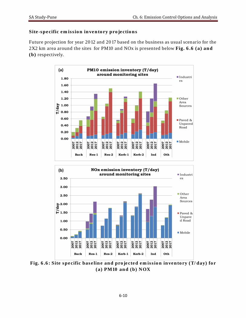
SA Study‐Pune Ch. 6: Emission Control Options and Analysis
6‐10
Site-specific emission inventory projections
Future projection for year 2012 and 2017 based on the business as usual scenario for the 2X2 km area around the sites for PM10 and NOx is presented below Fig. 6.6 (a) and (b) respectively.
Fig. 6.6: Site specific baseline and projected emission inventory (T/day) for (a) PM10 and (b) NOX
0.00
0.20
0.40
0.60
0.80
1.00
1.20
1.40
1.60
1.80
2007
2012
2017
2007
2012
2017
2007
2012
2017
2007
2012
2017
2007
2012
2017
2007
2012
2017
2007
2012
2017
Back Res-1 Res-2 Kerb-1 Kerb-2 Ind Oth
T/da
y
PM10 emission inventory (T/day) around monitoring sites
Industries
Other Area Sources
Paved & Unpaved Road
Mobile
(a)
0.00
0.50
1.00
1.50
2.00
2.50
3.00
3.50
2007
2012
2017
2007
2012
2017
2007
2012
2017
2007
2012
2017
2007
2012
2017
2007
2012
2017
2007
2012
2017
Back Res-1 Res-2 Kerb-1 Kerb-2 Ind Oth
T/da
y
NOx emission inventory (T/day) around monitoring sites Industri
es
Other Area Sources
Paved & Unpaved Road
Mobile
(b)

SA Study‐Pune Ch. 6: Emission Control Options and Analysis
6‐11
Ground level concentration plots for PM10 and NOx based on emission inventory for baseline year 2007 and BaU projections for year 2012 and 2017 are presented in Fig. 6.7 below.
Fig. 6.7: Ground level concentration plots for (a) PM10-2007, (b) NOx-2007, (c) PM10-BaU2012, (d) NOx- BaU2012, (e) PM10-BaU2017 & (f) NOx-
BaU2017
(a) (b)
(c)
(e) (f)
(d) 0
2000
4000
6000
8000
1000
0
1200
0
1400
0
1600
0
1800
0
2000
0
2200
00
2000
4000
6000
8000
10000
12000
14000
16000
18000
20000
0ug/m3
90ug/m3
180ug/m3
270ug/m3
360ug/m3
450ug/m3
0 2000 4000 6000 8000 10000 12000 14000 16000 18000 20000 22000
X Co-ord
0
2000
4000
6000
8000
10000
12000
14000
16000
18000
20000
X C
o-or
d
25ug/m3
50ug/m3
75ug/m3
100ug/m3
125ug/m3
150ug/m3
0
2000
4000
6000
8000
1000
0
1200
0
1400
0
1600
0
1800
0
2000
0
2200
0
X Co-ord
0
2000
4000
6000
8000
10000
12000
14000
16000
18000
20000
Y C
o-or
d
0ug/m3
70ug/m3
140ug/m3
210ug/m3
280ug/m3
350ug/m3
0
2000
4000
6000
8000
1000
0
1200
0
1400
0
1600
0
1800
0
2000
0
2200
00
2000
4000
6000
8000
10000
12000
14000
16000
18000
20000
0ug/m3
100ug/m3
200ug/m3
300ug/m3
400ug/m3
500ug/m3
0
2000
4000
6000
8000
1000
0
1200
0
1400
0
1600
0
1800
0
2000
0
2200
0
X Co-ord
0
2000
4000
6000
8000
10000
12000
14000
16000
18000
20000
Y C
o-or
d
0ug/m3
40ug/m3
80ug/m3
120ug/m3
160ug/m3
200ug/m3
0
2000
4000
6000
8000
1000
0
1200
0
1400
0
1600
0
1800
0
2000
0
2200
00
2000
4000
6000
8000
10000
12000
14000
16000
18000
20000
0ug/m3
160ug/m3
320ug/m3
480ug/m3
640ug/m3
800ug/m3

SA Study‐Pune Ch. 6: Emission Control Options and Analysis
6‐12
6.3 Line Source Control Options & Analysis
6.3.1 Technology based line source control options
The line source control options are divided in two types, technology based and management based control options. CPCB has centrally compiled the list of various technology based and management based control options along with reductions expected. Table 6-3 gives details of technology based control options considered.
Table 6-3: Technology based control options for line sources
Control Option Considered Scenario 2012 Scenario 2017
Implementation of BS – V norms
BS-III for 2-3 W, BS-IV for rest all from 2010 onwards
BS-III for 2-3 W, BS-IV for rest all from 2010-2015
BS-IV for 2-3 W, BS-V for rest all from 2015 onwards
Implementation of BS – VI norms
BS-III for 2-3 W, BS-IV for rest all from 2010 onwards
BS-III for 2-3 W, BS-IV for rest all from 2010-2015
BS-IV for 2-3 W, BS-VI for rest all from 2015 onwards
Electric Vehicles Share of Electric vehicles in total city fleet – Two wheeler: 1%,Auto Rickshaw and Taxi: 5%,Public buses: 5%
Share of Electric vehicles in total city fleet – Two wheeler: 2%,Auto Rickshaw and Taxi:10%,Public buses: 10%
Hybrid vehicles Share of Hybrid vehicles in total city fleet of Gasoline powered four-wheelers 1%
Share of Hybrid vehicles in total city fleet of Gasoline powered four-wheelers 2%
CNG/LPG to commercial (all 3 and 4-wheelers)
25% conversion 100% conversion
Ethanol blending (E10 – 10% blend)
E-10 all petrol vehicles E-10 all petrol vehicles
Bio-diesel (B5/B10: 5 – 10% blend)
B-5 all diesel vehicles B-10 all diesel vehicles
Hydrogen – CNG blend (H10/H20: 10 – 20% blend)
-- H-10 all CNG vehicles
Retrofitment of Diesel Oxidation Catalyst (DOC) in 4-wheeler public transport (BS – II)
BS-II buses retro- 50% BS-II buses retro- 100%
Retrofitment of Diesel Particulate Filter in 4-wheeler public transport(BS – III city buses)
BS-III buses retro- 50% BS-III buses retro- 100%

SA Study‐Pune Ch. 6: Emission Control Options and Analysis
6‐13
Analysis of reduction with line source control options Reductions possible with the above control options scenario in PM10 & NOx as compared to BAU scenario of 2012 & 2017 is presented in Fig. 6.5.
Fig. 6.8: Reduction in PM10 and NOx with technology based line source control options

SA Study‐Pune Ch. 6: Emission Control Options and Analysis
6‐14
6.3.1.1 Implementation of BS-V or BS-VI norms:
Total emission load in 2012 is a total of 2007 load , 2007-2010 load( as no new regulations only growth rates applicable), 2010-2012 load ( with new emission regulations and hence new emission factors with reductions applied. Similarly, total emission load in 2017 is a sum of 2012 emission load, 2012-2017 emission load with suitable control option applied.
In case of new emission regulations, the scenario is generated by considering the next stage of emission regulations BS-V or BSVI (from 2015) in line with EURO-V & EURO-VI for all categories of vehicles except 2 & 3 wheelers. In absence of road map for 2& 3 wheeler vehicles after BSIII (2010) regulations nominal improvements of 20% are considered in PM10& NOx. No separate improvements for equivalent BSV & BSVI have been considered for 2 &3Wheeler vehicles.
With the implementation of BSV or BSVI from 2015 onwards, all new vehicles from 2015 onwards will be compliant to corresponding norms. The benefits of BSV and BSVI in PM are 1% and 2.5 % of total PM respectively. Similarly the NOx benefits with BSV & BSVI are 7.5 & 14.6 % respectively. The improvement will increase as the population of newer generation vehicles increase over the years. Very small effect is visible with this control options due to very small contribution of emission load from year 2015 to 2017 vehicles (7% and 20 % of total vehicle emission load for PM & NOx respectively in BaU itself).
6.3.1.2 Electric & Hybrid Vehicles:
Electric vehicle fleet considered is: Two-wheeler: 1%, Auto Rickshaw and Taxi: 5%, Public buses: 5%in 2the year 2012 and double penetration in the year 2017. With such a small penetration, PM benefit is 2-4 % and benefit in NOx is 2-3 %.
The benefit received due to electric vehicle options is equivalent to a no vehicle (zero emissions vehicle) option. This seems to be very effective, particularly in congested city areas and hot spots. However, the availability of electricity and well-to-wheel ratio needs to be evaluated over larger context.
Hybrid option is considered for only passenger cars wherein 50% NOx reduction is possible. However; very small penetration does not show any visible effect. This option of using hybrid vehicles will also have much better CO2 emissions.
With context of above, electric public transport particularly three wheelers / buses within city area and engine options for long distance trips could be an effective control option for avoiding city level hotspot emissions. It means using electric/hybrid vehicles

SA Study‐Pune Ch. 6: Emission Control Options and Analysis
6‐15
for public transport with availability of options to run only on electric mode may be effective to curb city level hotspots. Other aspects of electrification of vehicles need to be addressed separately.
6.3.1.3 CNG-LPG and Hydrogen-CNG blend for commercial vehicles:
Delhi has set an example for use of CNG in public transport. New CNG/ LPG vehicles give very effective vehicle PM control option. Similarly, conversions of diesel buses to CNG fuel also give benefit of PM.
However, to curb NOx, this option is not very useful. As these vehicles will have high mileage, deterioration of catalytic converters particularly in retro vehicles over the time needs to be addressed by periodic effective inspection & maintenance or by replacement of catalytic convertors over specified time period.
The conversion of 2stroke auto rickshaws to LPG/ CNG is not an effective control option due to oil leakages observed in the field. The emission factor for PM is almost three times as compared to conventional petrol vehicle or OE 2 stroke CNG/LPG vehicles. This conversion of old auto rickshaws have not been considered as it shows the negative effect on PM emissions. For two stroke vehicles, NOx will be minimal due to scavenging effect.
For implementation of considering CNG /LPG option, the proper infrastructure availability needs to be evaluated. Similarly, if CNG infrastructure is available, restricting use of LPG as a domestic fuel only may be evaluated to avoid misuse of domestic cylinders and enhance safety.
Hydrogen-CNG blend (H-10/20): this option is evaluated in addition to CNG option. The NOx benefit of 10% can be gained for all CNG vehicles with the use of Hydrogen-CNG blend (H-10). However, infrastructure availability, hydrogen availability and dispensing need to be addressed while considering this option.
6.3.1.4 Ethanol Blending (E-10) and Biodiesel Blending (B-10)
If all the gasoline fuel is used with ethanol blending (E-10), improvement in NOx from 1.5 to 2% is observed.
Biodiesel blending with diesel fuel (B-10) gives improvement of 6-6.5 % in PM but has negative effect of around 2%.
The percentage benefit will vary depending upon the availability of ethanol and biodiesel for dispensing of fuel to complete fleet of vehicles.

SA Study‐Pune Ch. 6: Emission Control Options and Analysis
6‐16
6.3.1.5 Retro fitment of DOCs and DPFs for 4wheeler public transport vehicles:
Retro-fitment of DOCs option is evaluated for BS-II buses and retro-fitment of DPFs is evaluated for BS-III. The PM benefit for DOC option is around 0.8-1.5 %, while DPF option gives benefit of 2-3%.
However feasibility options of retro-fitment needs to be evaluated. Functionality of DPF and online regeneration due very low city speeds and durability of DOC & DPF may be limited.
6.3.2 Management based line source control options:
Management base control options considered for line sources are presented in Table 6-4.
Table 6-4: Management based control options for line sources
Control Option Considered Scenario 2012 Scenario 2017
Inspection/ maintenance to all BSII & BSIII personal & public transport vehicles
50% compliance 100% compliance
Banning of 10 year old commercial vehicles
100% compliance –pre 2002 3W, GC, buses and trucks
100% compliance –pre 2007 3W, GC, buses and trucks
Banning of 15 year old private vehicle
100% compliance 100% compliance
Synchronization of traffic signals
All highways, 10% of major roads
All major & minor roads excluding feeder roads
Improvement of public transport: % share
10% shift of VKT 20% shift of VKT

SA Study‐Pune Ch. 6: Emission Control Options and Analysis
6‐17
Analysis of reduction with management based line source control options
Reductions possible with the above control options scenario in PM10 & NOx as compared to BAU scenario of 2012 & 2017 is presented in Fig. 6.6 below
Fig. 6.9: Reduction in PM and NOx with management based line source control options

SA Study‐Pune Ch. 6: Emission Control Options and Analysis
6‐18
The management options can easily be separated in quantifiable control options and non-quantifiable control options. The quantifiable control options are evaluated as per different scenarios foe year 2012 & 2017.
6.3.2.1 Effective I&M: The effective inspection maintenance regime for older vehicles or badly maintained vehicles can have a very good improvement in vehicle emissions contribution. Many of the international studies state that 80% vehicle pollution is due to 20% of highly polluting vehicles. The effective I&M regime identifies such high polluters and control their emissions by proper maintenance.
While evaluating the control option of inspection and maintenance, reductions on BS-II & BS-III personal and public transport vehicles have been considered. It is very difficult to evaluate benefits possible for BS-IV and beyond vehicles due to the different advanced technologies, which still have to come in market. If the benefits on the commercial vehicles like trucks and LCVs are assumed same as public transport vehicles (buses) and for all technology vehicles then the additional benefit of 1.1 -1.3 % on PM10 and 0.6-1.1% on NOx is achievable.
Additionally, no data is available for effect of Inspection & Maintenance on PM reductions from gasoline vehicles which contribute to more than 40% of the vehicle PM.
6.3.2.2 Synchronization of Traffic signals: Though this option seems to be very simple for implementation, benefits up to 5% in PM & 10%in NOx are possible if all the major & minor roads are synchronized.
6.3.2.3 Banning of 10 year old commercial vehicles: 60-70% of vehicle PM10 & NOx is contributed from commercial and public transport vehicles. With application of newer emission norms from 91 to BSIII in 2005, the emission factors of these vehicles have improved with the technology used. Hence, banning of 10 year old commercial vehicles including the public transport vehicles has a very huge effect on the PM and NOx reductions. In 2012, the reductions possible are 38% for PM & 30% for NOx while in 2017; the benefits will be 52 & 27 % for PM10 & NOx respectively. The separate replacement of these vehicles has not been considered as the same will be covered in the annual growth rates.
However, the socio economic impacts of banning of older vehicles need to be evaluated. The entry of these vehicles in the city area may be restricted.
6.3.2.4 Banning of 15 year old personal vehicles: The benefits possible are 2-4 % in NOx 2-6% in PM in 2012 and 2017 respectively. The limited benefits are due to the higher percentage of gasoline vehicles for personal mobility. The on-road two-wheeler population is more than 65% in the city, all being gasoline.

SA Study‐Pune Ch. 6: Emission Control Options and Analysis
6‐19
6.3.2.5 Shift to Public transport: The calculations are done based on the VKT shift to public transport. In Pune, the average occupancy of 2 Wheelers is 1 and for cars around 1.3. The 10% & 20% shift of 2W & cars to public transport in 2012 & 2017 respectively, gives benefit of 1-3 % for PM10 & NOx. However, the reduction in VKT also reduces the road dust of 3.5 % and 12% respectively for year 2012 &2017.No addition of equivalent buses is considered as the occupancy of present buses and other public transport such as Metro is possible.

SA Study‐Pune Ch. 6: Emission Control Options and Analysis
6‐20
6.4 Area Source Control Options & Analysis Control option for area sources are given in Table 6-5. As the road dust contribution in total PM is very high, the control options for road dust are considered separately (Table 6-6) in area source control options.
Table 6-5: Area source control options
Control Option Considered
Scenario 2012
% reduction wrt BAU- area sources excluding road dust
Scenario 2017
% reduction w.r.t. BAU- area sources excluding road dust
PM NOx PM NOx
Shift to LPG from solid fuel &kerosene for domestic applications
50% compliance
6.97%
31.53%
100% compliance
17.17%
32.50%
Shift to LPG from solid fuel &kerosene for commercial applications (bakeries, open eat outs etc)
100% compliance
16.15%
6.47%
100% compliance
15.36%
6.33%
Better construction practices with PM reduction of 50%
50% compliance
4.18%
-- 50% compliance
7.15%
--
Strict compliance of ban on open burning, including open eat outs
50% compliance
3.15%
4.37%
100% compliance
6.00%
18.20%
Reduction in non-industrial generators
50% 5.86% 83.14%
100% 5.76% 82.92%
Shift from solid fuel and kerosene to LPG particularly in domestic areas and commercial activities like bakeries show the improvement of total 30% for PM when compared to area sources contribution excluding dust and around 39% benefit for NOx similarly. However, the contribution of NOx in total PM due to area sources is very small.
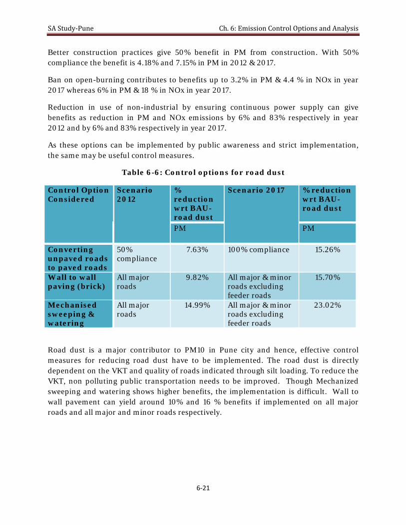
SA Study‐Pune Ch. 6: Emission Control Options and Analysis
6‐21
Better construction practices give 50% benefit in PM from construction. With 50% compliance the benefit is 4.18% and 7.15% in PM in 2012 & 2017.
Ban on open-burning contributes to benefits up to 3.2% in PM & 4.4 % in NOx in year 2017 whereas 6% in PM & 18 % in NOx in year 2017.
Reduction in use of non-industrial by ensuring continuous power supply can give benefits as reduction in PM and NOx emissions by 6% and 83% respectively in year 2012 and by 6% and 83% respectively in year 2017.
As these options can be implemented by public awareness and strict implementation, the same may be useful control measures.
Table 6-6: Control options for road dust
Control Option Considered
Scenario 2012
% reduction wrt BAU- road dust
Scenario 2017 % reduction wrt BAU- road dust
PM PM
Converting unpaved roads to paved roads
50% compliance
7.63%
100% compliance 15.26%
Wall to wall paving (brick)
All major roads
9.82%
All major & minor roads excluding feeder roads
15.70%
Mechanised sweeping & watering
All major roads
14.99%
All major & minor roads excluding feeder roads
23.02%
Road dust is a major contributor to PM10 in Pune city and hence, effective control measures for reducing road dust have to be implemented. The road dust is directly dependent on the VKT and quality of roads indicated through silt loading. To reduce the VKT, non polluting public transportation needs to be improved. Though Mechanized sweeping and watering shows higher benefits, the implementation is difficult. Wall to wall pavement can yield around 10% and 16 % benefits if implemented on all major roads and all major and minor roads respectively.

SA Study‐Pune Ch. 6: Emission Control Options and Analysis
6‐22
6.5 Point Source Control Options & Analysis In Pune city, air polluting industries are limited and are located in restricted industrial areas. Major of the industries are located in Pimpri-Chinchwad, twin city of Pune and other peripheral areas.
Thus the total contribution of industries in the city pollution is restricted to 1%. Reduction in percentage obtained w.r.t. BaU with the control options is presented in Table 6-7 below.
Table 6-7: Point source control options
Control Option Considered
Scenario 2012
% reduction w.r.t. BAU- Point Sources
Scenario 2017
% reduction wrt BAU- Point Sources
PM NOx PM NOx
Shifting of air polluting industries
50% compliance
61%
83%
100% compliance
100%
100%
Banning of new industries in existing city limit
100% compliance
21%
21%
100% compliance
38%
38%

SA Study‐Pune Ch. 7: Prioritization of Management/Control Options
7‐1
Chapter 7. Prioritization of
Management/Control Options
7.1 Prioritization of control options:
Based on the evaluation of the impact of various individual control options and their feasibility in implementation for both management and technology based options, a list of control options considered is prepared for generating controlled scenario-1. Alternate control scenario-2 was also generated for PM10. Table 7-1 gives the details of options selected for control of pollution for generating controlled scenario-1 for 2012 and 2017.
As the major source of PM10 was found to be re-suspended road dust from paved roads (48%), benefits for PM10 control options could be higher if only the silt-loading of the road is reduced i. e. if the road quality itself is improved. Present silt loading of paved road in Pune if about 0.9 g/m2, whereas the international (EPA, AP-42) default silt-loading value is around 0.2 or less. It is, therefore, evident that, road conditions need to be improved. With the reduction in silt loading factor by 50% of the existing value, total PM10 reduction benefit of about 35% can be achieved. However, silt loading improvements will depend upon the methods used for road quality improvement and subsequent reduction in silt loading.
For generating controlled scenario-2, all control options as listed in Scenario-I have been considered except for road dust control option. For road dust, reduction of silt loading by 50 % has been considered on highways and major-minor roads. However, No reduction of silt loading is assumed on feeder roads.

SA Study‐Pune Ch. 7: Prioritization of Management/Control Options
7‐2
Table 7-1: Control Options selected for controlled scenario for year 2012 and 2017-
Technology based control options for line sources Control Option Considered
Scenario 2012 Scenario 2017 Remarks
Implementation of BS – V norms
Same as BAU.
BS-III for 2-3 W, BS-IV for rest all from 2010 onwards.
BS-III for 2-3 W, BS-IV for rest all from 2010 to 2015
Progressive tightening of emission regulations for new vehicles
-- BS-IV for 2-3 W, BS-V for rest all from 2015
Electric / Hybrid Vehicles
Share of Electric vehicles in total city fleet – Two wheeler: 1%, Auto-Rickshaw and Taxi: 5%, Public buses: 5%
Share of Electric vehicles in total city fleet – Two wheeler: 2%, Auto-Rickshaw and Taxi:10%, Public buses: 10%
Though electric / hybrid vehicles are very effective in city pollution curbing, the infrastructure and initial cost may limit the penetration.
OE-CNG for new Public transport buses
47.5% fleet 90% of fleet Retro fitment has may issues like effectiveness and durability along with safety related problems
Ethanol blending (E10 – 10% blend)
E-10 all petrol vehicles
E-10 all petrol vehicles
Considering proposed implementation in near future
Bio-diesel (B5/B10: 5 – 10% blend)
-- B-10 all diesel vehicles
Effective in vehicle PM reduction, but availability by 2012 is questionable.
Retro-fitment of Diesel Oxidation Catalyst (DOC) in 4-wheeler public transport (BS–II and BS-III)
BS-II & III buses retro-fitment - 20%
BS-II & III buses retro-fitment 50%
Feasibility and effectiveness along with durability issues, will limit the penetration.
Retro-fitment of Diesel Particulate Filter in 4-wheeler public transport(BS – III city buses)
BS-III buses retro- 10%
BS-III buses retro- 20%
Feasibility, effectiveness, regeneration and durability issues will limit the penetration.
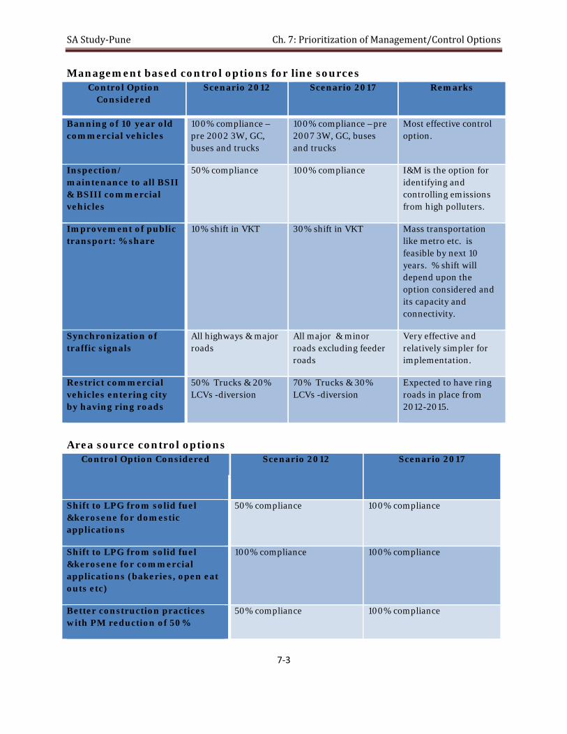
SA Study‐Pune Ch. 7: Prioritization of Management/Control Options
7‐3
Management based control options for line sources Control Option
Considered Scenario 2012 Scenario 2017 Remarks
Banning of 10 year old commercial vehicles
100% compliance –pre 2002 3W, GC, buses and trucks
100% compliance –pre 2007 3W, GC, buses and trucks
Most effective control option.
Inspection/ maintenance to all BSII & BSIII commercial vehicles
50% compliance 100% compliance I&M is the option for identifying and controlling emissions from high polluters.
Improvement of public transport: % share
10% shift in VKT 30% shift in VKT Mass transportation like metro etc. is feasible by next 10 years. % shift will depend upon the option considered and its capacity and connectivity.
Synchronization of traffic signals
All highways & major roads
All major & minor roads excluding feeder roads
Very effective and relatively simpler for implementation.
Restrict commercial vehicles entering city by having ring roads
50% Trucks & 20% LCVs -diversion
70% Trucks & 30% LCVs -diversion
Expected to have ring roads in place from 2012-2015.
Area source control options
Control Option Considered Scenario 2012 Scenario 2017
Shift to LPG from solid fuel &kerosene for domestic applications
50% compliance 100% compliance
Shift to LPG from solid fuel &kerosene for commercial applications (bakeries, open eat outs etc)
100% compliance 100% compliance
Better construction practices with PM reduction of 50%
50% compliance 100% compliance

SA Study‐Pune Ch. 7: Prioritization of Management/Control Options
7‐4
Banning of operation of brick kilns in city area
100% compliance 100% compliance
Strict compliance of ban on open burning, including open eat outs
50% compliance 100% compliance
Reduction in DG set operation/ Un-interrupted power supply
50% reduction in power cut 100% reduction in power cut
Control options for road dust
Point source control options
Control Option Considered Scenario 2012 Scenario 2017
Banning of new industries in existing city limit
100% compliance 100% compliance
7.2 Benefits anticipated from prioritized control options
Projected emission inventory for PM10 and NOx for year for year 2012 based on BaU scenario and controlled scenario is given in Table 7.2. Source wise contribution to PM10 and NOx for baseline, projected BaU and controlled scenario are presented in Fig. 7.1.Reduction in PM10 emission load with respect to BaU for controlled scenario in year 2012 and 2017 was 21% and 25% respectively. While, with controlled scenario-2 i.e. improvement in silt loading factor by 50% for road dust and all other control options together, reduction in PM10 by 49% and 50% was observed in year 2012 and 2017 respectively.
Banning of 10 year old commercial vehicles proves to be most effective control option for curbing emissions from in-use vehicles. Higher NOx reduction benefits, 45% and 56% for year 2012 and 2017 respectively, are observed mainly due to banning of old vehicles. This has resulted into reduction in NOx emission loads below the baseline-2007 (-6%) in the controlled Year 2012 scenario.
Concentrations obtained, after dispersion modeling in top-10 grids, for baseline year 2007 and projected BaU year 2012 and 2017 for PM10 and NOx are presented in Fig. 7.2 and Fig. 7.3 respectively. Percent reduction in PM10 and NOx concentration levels with respect to BaU scenario, observed using ISCST3 dispersion modeling, at top 10
Control Option Considered Scenario 2012 Scenario 2017
Wall to wall paving (brick) All major roads All major & minor roads excluding feeder roads

SA Study‐Pune Ch. 7: Prioritization of Management/Control Options
7‐5
grids is presented in Fig. 7.4 and Fig. 7.5. These top10 grids were found to be present at the central part of Pune where population and road densities are higher.
Ground level concentration isopleths for projected BaU and controlled scenario for year 2012 and 2017 for PM and NOx are presented in Fig. 7.6 to Fig. 7.13.
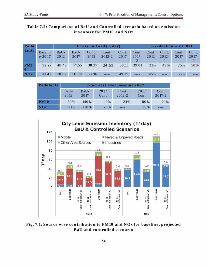
SA Study‐Pune Ch. 7: Prioritization of Management/Control Options
7‐6
Table 7.2: Comparison of BaU and Controlled scenario based on emission inventory for PM10 and NOx
Pollutants
Emission Load (T/day) % reduction w.r.t. BaU
Baseline-2007
BaU-2012
BaU-2017
Cont. 2012
Cont. 2012-2
Cont. 2017
Cont. 2017-
2
Cont. 2012
Cont. 2012-
2
Cont. 2017
Cont. 2017-
2 PM10
32.27 48.49 77.55 38.37 24.63 58.15 39.01 21% 49% 25% 50%
NOx 41.42 70.82 111.98 38.96 ----- 49.39 ---- 45% ---- 56% ----
Pollutants % increase over Baseline 2007
BaU-2012
BaU-2017
2012 Cont
Cont 2012-2
2017 Cont
Cont 2017-2
PM10 50% 140% 19% -24% 80% 21%
NOx 71% 170% -6% ---- 19% ----
Fig. 7.1: Source wise contribution to PM10 and NOx for baseline, projected
BaU and controlled scenario
5.9 7.0 2.8 2.88.2
2.5 2.5
39.2
59.5
33.1
98.0
47.719.7
34.131.3
17.5
60.152.9
33.86.5
6.94.0
4.0
8.6
2.3
2.3 1.3
10.2
4.9
12.5
0.8
0.4
0.50.4
0.4
0.6
0.4
0.4 0.9
1.1
0.9
1.4
0.9
0
20
40
60
80
100
120
20
07
20
12
BaU
20
12
Con
trol
Sce
nari
o 1
20
12
Con
trol
Sce
nari
o 2
20
17
BaU
20
17
Con
trol
Sce
nari
o 1
20
17
Con
trol
Sce
nari
o 2
20
07
20
12
BaU
20
12
Con
trol
Sce
nari
o 1
20
17
BaU
20
17
Con
trol
Sce
nari
o 1
PM10 NOx
T/da
y
City Level Emission Inventory (T/day) BaU & Controlled Scenarios
Mobile Paved & Unpaved RoadsOther Area Sources Industries

SA Study‐Pune Ch. 7: Prioritization of Management/Control Options
7‐7
Fig. 7.2: Concentrations of PM10 in top 10 grids for baseline 2007 and projected BaU year 2012 and 2017 scenario
Fig. 7.3: Concentrations of NOx in top 10 grids for baseline 2007 and
projected BaU year 2012 and 2017 scenario
49 B07
49 B12
49 B17
50 B07
50 B12
50 B17
48 B07
48 B12
48 B17
37 B07
37 B12
37 B17
38 B07
38 B12
38 B17
36 B07
36 B12
36 B17
47 B07
47 B12
47 B17
35 B07
35 B12
35 B17
39 B07
39 B12
39 B17
59 B07
59 B12
59 B17
0
200
400
600
800
1,000
1,200
1,400
B07
B12
B17
B07
B12
B17
B07
B12
B17
B07
B12
B17
B07
B12
B17
B07
B12
B17
B07
B12
B17
B07
B12
B17
B07
B12
B17
B07
B12
B17
49 50 48 37 38 36 47 35 39 59
PM10
Con
c. (u
g/m3)
Top 10 grids
Predicted concentrations of PM10 at Top 10 grids for year 2007, 2012 & 2017
Industrial
Mobile
Other Area
Road Dust
38 B07
38 B12
38 B17
37 B07
37 B12
37 B17
48 B07
48 B12
48 B17
39 B07
39 B12
39 B17
36 B07
36 B12
36 B17
50 B07
50 B12
50 B17
62 B07
62 B12
62 B17
35 B07
35 B12
35 B17
40 B07
40 B12
40 B17
51 B07
51 B12
51 B17
0
50
100
150
200
250
300
350
400
450
500
B07
B12
B17
B07
B12
B17
B07
B12
B17
B07
B12
B17
B07
B12
B17
B07
B12
B17
B07
B12
B17
B07
B12
B17
B07
B12
B17
B07
B12
B17
38 37 48 39 36 50 62 35 40 51
NOx Co
nc. (ug
/m3)
Top 10 grids
Predicted concentrations of NOx at Top 10 grids for year 2007, 2012 & 2017
Non‐Ind. Gen.
Industrial
Other Area
Mobile

SA Study‐Pune Ch. 7: Prioritization of Management/Control Options
7‐8
Fig. 7.4: Percent reduction w.r.t. BaU in concentrations of PM10 in top 10 grids with controlled scenario for year 2012 and 2017
Fig. 7.5: Percent reduction w.r.t. BaU in concentrations of NOx in top 10 grids with controlled scenario for year 2012 and 2017
0%
10%
20%
30%
40%
50%
60%
49 50 48 37 38 36 47 35 39 59
% R
educ
tion
in P
M10
con
c.
Grid No.
Percentage Reduction in PM10 concentrations in top 10 grids with control options for year 2012 and 2017
Reduction with control options (1)- Year 2012Reduction with control options (2)- Year 2012Reduction with control options (1)- Year 2017Reduction with control options (2)- Year 2017

SA Study‐Pune Ch. 7: Prioritization of Management/Control Options
7‐9
Fig. 7.6: Projected concentration (BaU) of PM10 for year 2012
Fig. 7.7: Projected concentration (controlled) of PM10 for year 2012
0
2000
4000
6000
8000
1000
0
1200
0
1400
0
1600
0
1800
0
2000
0
2200
0
X Co-ord
0
2000
4000
6000
8000
10000
12000
14000
16000
18000
20000
Y C
o-or
d
0ug/m3
70ug/m3
140ug/m3
210ug/m3
280ug/m3
350ug/m3
Controlled-2
0
2000
4000
6000
8000
1000
0
1200
0
1400
0
1600
0
1800
0
2000
0
2200
00
2000
4000
6000
8000
10000
12000
14000
16000
18000
20000
0ug/m3
70ug/m3
140ug/m3
210ug/m3
280ug/m3
350ug/m3
0
2000
4000
6000
8000
1000
0
1200
0
1400
0
1600
0
1800
0
2000
0
2200
00
2000
4000
6000
8000
10000
12000
14000
16000
18000
20000
0ug/m3
70ug/m3
140ug/m3
210ug/m3
280ug/m3
350ug/m3
Controlled-1

SA Study‐Pune Ch. 7: Prioritization of Management/Control Options
7‐10
Fig. 7.8: Projected concentration (BaU) of NOx for year 2012
Fig. 7.9: Projected concentration (Controlled) of NOx for year 2012
0
2000
4000
6000
8000
1000
0
1200
0
1400
0
1600
0
1800
0
2000
0
2200
0
X Co-ord
0
2000
4000
6000
8000
10000
12000
14000
16000
18000
20000
0ug/m3
90ug/m3
180ug/m3
270ug/m3
360ug/m3
450ug/m3
(b)
(b)
0
2000
4000
6000
8000
1000
0
1200
0
1400
0
1600
0
1800
0
2000
0
2200
00
2000
4000
6000
8000
10000
12000
14000
16000
18000
20000
0ug/m3
90ug/m3
180ug/m3
270ug/m3
360ug/m3
450ug/m3

SA Study‐Pune Ch. 7: Prioritization of Management/Control Options
7‐11
Fig. 7.10: Projected concentration (BaU) of PM10 for year 2017
Fig. 7.11: Projected concentration (Controlled-1) of PM10 for year 2017
Controlled-2
0
2000
4000
6000
8000
1000
0
1200
0
1400
0
1600
0
1800
0
2000
0
2200
00
2000
4000
6000
8000
10000
12000
14000
16000
18000
20000
0ug/m3
100ug/m3
200ug/m3
300ug/m3
400ug/m3
500ug/m3
(c) 0
2000
4000
6000
8000
1000
0
1200
0
1400
0
1600
0
1800
0
2000
0
2200
00
2000
4000
6000
8000
10000
12000
14000
16000
18000
20000
0ug/m3
100ug/m3
200ug/m3
300ug/m3
400ug/m3
500ug/m3
Controlled-1
0
2000
4000
6000
8000
1000
0
1200
0
1400
0
1600
0
1800
0
2000
0
2200
00
2000
4000
6000
8000
10000
12000
14000
16000
18000
20000
0ug/m3
100ug/m3
200ug/m3
300ug/m3
400ug/m3
500ug/m3
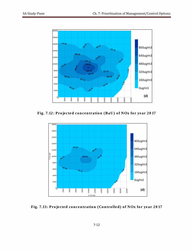
SA Study‐Pune Ch. 7: Prioritization of Management/Control Options
7‐12
Fig. 7.12: Projected concentration (BaU) of NOx for year 2017
Fig. 7.13: Projected concentration (Controlled) of NOx for year 2017
0
2000
4000
6000
8000
1000
0
1200
0
1400
0
1600
0
1800
0
2000
0
2200
0
X Co-ord
0
2000
4000
6000
8000
10000
12000
14000
16000
18000
20000
Y C
o-or
d
0ug/m3
160ug/m3
320ug/m3
480ug/m3
640ug/m3
800ug/m3
(d)
0
2000
4000
6000
8000
1000
0
1200
0
1400
0
1600
0
1800
0
2000
0
2200
00
2000
4000
6000
8000
10000
12000
14000
16000
18000
20000
0ug/m3
160ug/m3
320ug/m3
480ug/m3
640ug/m3
800ug/m3
(d)

SA Study‐Pune Ch. 7: Prioritization of Management/Control Options
7‐13
7.3 Discussions on the Control Options & prioritization 7.3.1 Area Sources Re-suspension of road dust
Re-suspension of road dust is a major contributor to the PM10 pollution from area sources in Pune city. Therefore, effective control measures need to be taken to curb the emission from the dust. Although, unpaved roads in city of Pune are very less, paved roads are not paved from wall to wall. Almost all roads have some collar left unpaved at the corner on each side of road with a very high silt loading. This fine dust entrains from the corner of the road to the paved portion of road.
Re-suspension of dust can be reduced by improving the quality of roads like wall to wall pavement to avoid the dust from unpaved portion of the road to entrain to the paved road, which gets re-suspended due to vehicle movement. Watering, mechanized sweeping can also be used as control measures with higher benefits; however, practical implementation is difficult.
Wall to wall pavement option have been considered, which gives benefit in terms of PM10 reduction as 10% and 16% with respect to road dust emissions in BaU scenario in year 2012 and 2017. Due to wall to wall pavement, silt loading of paved road is also expected to be reduced.
Road condition improvement/ Silt loading reduction
Major portion of the re-suspended road dust is attributed to the paved road dust (about 78%) with the share of unpaved road dust as 22%. Improving the quality of road to reduce the re-suspended road dust is essential. With the reduction in silt loading factor by 50% of the existing value, total PM10 reduction benefit of about 35% can be achieved.
Other area sources
Use of solid fuels and kerosene for combustion is common in slums and by street vendors. Bakeries also use wood as fuel for combustion. Considering, around 40% of population of Pune lives in urban slums with slum population using kerosene and wood is around 45% and 21% respectively, the usage of these fuels is also very high. Considering the pace of urban growth, construction activities are present is every part of the city except the central part where the construction activity is limited due to saturation. Brick kilns are observed to be operated near almost all major construction activities particularly at the outskirts of the city.

SA Study‐Pune Ch. 7: Prioritization of Management/Control Options
7‐14
Pune is experiencing power-cuts since May-2008 due to discontinuation of Pune Model for un-interrupted power supply. This has resulted into use of non-industrial generators as a back-up arrangement for, shopping malls, commercial complexes, elevators in big residential complexes, etc. Due to this usage of non-industrial generators, this source share about 12% and 10% of emission load of NOx in year 2012 and 2017 respectively. By improving the power scenario as reduction in power-cuts to 50% and 100% by year 2012 and year 2017, benefits in terms of NOx reduction can be achieved as around 83% reduction w.r.t. area sources in 2012 and 2017. 7.3.2 Line Sources
The contribution of line sources in PM10 is restricted to around 18%, 15% & 10% in baseline 2007, BaU 2012 and BaU 2017 respectively. Various management and technology based control options are discussed below, which will be effective, feasible & prioritized.
7.3.2.1 Management control options
• Transportation
The road networks in the core areas of city of Pune are largely congested. Also, to compound the problem city is situated at the confluence of the National Highways. National and state highways measure about 50 km in a city with a total road length of 1800 km. Due to this major share of the traffic entering the city through the highways is neither the point of origin nor the destination. The intra-city traffic moving between from one end of city to other has to invariably pass through the congested central core due to absence of circumferential roads. Density of population is high at the central part along with the commercial/hawkers and institutional activities on both sides of roads leaving vary little or no scope for widening of roads to escape congestion. Comprehensive Traffic and Transportation Plan (CTTP) indicated that less than 40% of the road length has footpaths against 28% of the trips generated in the city being pedestrian. Consequently, most of the roads in the city witness a continuous struggle for space between the vehicles and pedestrians. The key issues regarding planning transportation in Pune are:
• Mixing of transit travelers from city with the local traffic due to absence of by-passes and circumferential road network
• Lack of adequate public transport system • Congestion problem in central city due to restricted capacity of narrow roads • Poor road surface quality, absence of wall to wall road pavement
SA Study‐Pune Ch. 7: Prioritization of Management/Control Options
7‐15
• Absence of signage, markings, street name boards and other street furniture resulting in poor accessibility
• Only 40% of the roads with footpaths and most of the existing ones encroached upon by informal activities and street hawkers
• No control or inadequate control systems like one-ways, heavy vehicles restrictions, no-vehicles zone and other traffic management systems for the arterial
• Highly inadequate parking facilities; lack of planned on-street parking facilities • Lack of civic sense towards traffic and poor travel behavior • Lack of coordination among agencies involved in planning and providing for
traffic and transportation To address these issues, following Simple management options can be implemented:
• Synchronization of traffic • Controlling traffic hindrance: Proper footpaths, crossing using subways, no
encroachment on the roads, Planned and paid parking areas, providing information using signage, markings, street name boards
• Increased civic sense for traffic rules and regulations along with the strict implementation
• Restricting heavy vehicles on selected roads and / or selected timings.
• Improving public transport: Public transport system needs to be improved by providing adequate number of additional vehicles during peak hours, using smaller vehicles in the congested city areas and following the time schedules on different routes. The existing public transportation system falls short while catering to the rising demand. In the absence of reliable and extensive public transportation systems, the local population has been increasingly resorting to personal ownership of vehicles to meet their mobility requirements. Only 15% of the vehicle kilometers travelled (VKT) in the city is accounted for by public transportation. • Non polluting Mass Transportation System: Mass transportation system such as Metro, Tram, Monorail, etc. need to be considered for non –polluting Mass transportation connecting growing city and circumferential developing areas. • Circumferential Roads: To by-pass the heavy intra-city traffic crossing the city to move from one end to other and the intercity traffic which connected by 50km national/state highway traffic crossing the city which is neither the point of origin nor the destination.

SA Study‐Pune Ch. 7: Prioritization of Management/Control Options
7‐16
• Banning of 10 year old commercial vehicles: With progressive tightening of emission regulations, the newer generation vehicles are much cleaner. However, the older generation commercial vehicles still ply on roads in large numbers and contribute to very high PM10 & NOx emissions. Hence, banning of 10 years old commercial vehicles including the public transport vehicles is a very effective control option and can yield the highest benefits. However, the socio economic impacts of banning of older vehicles need to be evaluated. Entry of these vehicles in the city area must be restricted to curb major portion of vehicle pollution.
• Effective Inspection & Maintenance Regime: After banning the older generation commercial vehicles, an effective I&M implementation regime will still improve the scenario. I&M including periodic pollution and safety checks for commercial vehicles will enhance safety as well as reduce the pollution. In the phase-I, commercial vehicles must be considered due to longer trip lengths and higher VKT travelled. The control options discussed above for transportation sector have a direct impact on controlling vehicle pollution in the city and avoiding the hot spots. 7.3.2.2 Technology based control options: Technology based control options, for curbing pollution from vehicles, are normally implemented as national level decisions. They are also linked with the huge infrastructure costs and availability. However management based options can be implemented at regional level and are relatively simpler and may be cost-effective. • Emission Regulations Road Map Progressive tightening of emission regulations since 1991 to BS-III regulations for 2& 3 wheelers and BS-IV regulations for all other categories of vehicles (in line EURO-IV) scheduled to be implemented in 2010; have given an edge over the multifold growth of cities and Mega cities of India and in turn the number of vehicles. The cities like Pune have been showing the growth of vehicles around 10% continuously for more than last 10 years. The vehicle registered are doubled in last 7 years and tripled in last 12 years.
The implementation roadmap for emission regulations for all categories of vehicles for next 10 years need to be prepared and has to be updated on the continuous basis. The leap frog strategies must be implemented for advancements in the vehicle technologies and emission regulations.
Every five years, progressive tightening of emission regulations must be implemented. As a next stage BS-V regulations in line with EURO-V regulations may be implemented from 2015 for all categories of vehicles except 2&3 wheelers. Technology wise leap frog

SA Study‐Pune Ch. 7: Prioritization of Management/Control Options
7‐17
strategy for 2015 for BS-VI in line with EURO-VI seems to be difficult in absence of consolidated road map.
Also, the discussion of implementation of new generation technology options for vehicles cannot be completed without discussing the availability of fuel required for the technology. • One Country.. One fuel quality.. One regulation Since last 8 years, the new emission regulations are implemented in the country in patches of areas, due to non availability of advanced fuel for whole country.
BS-III regulations except for 2&3 wheelers are implemented in 11 cities of India including Pune since 2005. However, there will be vehicles plying in the city which are not registered in Pune (Such numbers are also high due to local tax structures). Similarly, BS-III fuel is available only in the city and not even 20-30km away from city boundary. As the city growth is circumferential particularly the industrial growth, the number of city vehicles travelling out of the city boundary are much higher and tend to refuel the vehicles outside the city because of the lesser cost of the fuel. Thus not using the required fuel (particularly low sulfur content fuel), which deteriorates the emission performance of these vehicles and in turn increase the in-use vehicle emissions. To address this issue, measures are required to be taken at regional and national level:
Local level: Pune, Pimpri-Chinchwad and circumferential area earmarked for development and industrialization should be grouped under a Metropolitan development authority for better planning and administration. The fuel of corresponding quality in this area should be ensured. National level: Ensuring nationwide same quality of fuel will definitely improve the conditions of in-use vehicle pollution noticeably due to the fact that the after-treatment devices and other newer technologies are very susceptible to the quality of fuel used. Very short distance exposure to low grade fuel quality may damage these devices permanently and thus making newer generation of in-use vehicles not effective or even worse than those of earlier generation vehicles due to the failures of emission control devices. With this background, it is must to have the policy of One country.. One fuel quality and One regulation. • Electric-hybrid vehicles: Though electric vehicles are zero emission vehicles; charging infrastructure, availability of electricity, range (distance per battery charge) of pure electric vehicles as traveling distances will increase with circumferential growth of city, are the key issues along with battery pack energy density and disposal. With this

SA Study‐Pune Ch. 7: Prioritization of Management/Control Options
7‐18
background, hybrid vehicles of different category are very attractive options. Particularly, if hybrid public transport (bus/ auto rickshaws) can be an effective option. Even the mild hybrids can have the option of starting with motor and battery power thus making zero idling and starting emissions. The hybrids can also have an option of running on ZEV mode in the congested city areas. The initial cost of these vehicles is high due o higher motor, battery back and dual power packs. Some financial incentives on these non-polluting vehicles will also enhance personal/ commercial vehicles sales. • Alternate Fuel Vehicles: Use of alternate fuels like CNG-LPG reduces the running cost and gives direct benefit of PM reduction. However, conversion of existing fleet is not very successful option for public transport either buses or auto rickshaws. The two stroke auto rickshaws have very high PM emission rate after retro-fitment due to oil leakage issues and it is cannot be considered as a control option for PM reduction. In case of buses, though conversion of older diesel fleet to CNG gives benefit in terms of PM, feasibility of retro-fitment, risks involved in safety and performance, no benefits over NOx, possibility of failures of after treatment devices and in turn increasing gaseous pollutants are the issues. The GHG potential of CNG fueled vehicles also need to be evaluated while considering enforcement of these alternate fuels. New CNG vehicle fleet may be considered, if the infra structure is available (expected beyond 2010) in Pune. 50% and 100% of original equipment (OE) public transport vehicles have been considered in 2012 and 1017 respectively. This will give PM reduction benefits from vehicle sector.
Biodiesel blending with diesel fuel (B-10) can give good improvement of in PM but availability will be the issue. Ethanol blending will give very marginal benefits. The percentage benefit will vary depending upon the availability of ethanol and biodiesel for complete dispensing of fuel.
• Retro fitment of DOCs & DPFs: The feasibility options of retro-fitment needs to be evaluated. Functionality of DPF and online regeneration due very low city speeds may be limited. DOCs to BS-II &III public transport vehicles may be considered, however, implementation and verifying functionality will limit effectiveness of these options. Hence only limited penetration has been considered.
7.3.3 Point Sources Though industrial sector growth in city is limited, the growth of industry in peripheral areas is very high (Growth in SSI &MSI from Pune district registration data is more than 100%).But these industries are mostly non-polluting. However, pollution control measures, use of cleaner industrial fuels for combustions needs to be encouraged.

SA Study‐Pune Ch. 7: Prioritization of Management/Control Options
7‐19
The city level SO2 emission loads are less and confined to the localized industrial zones. The higher sulfur content in industrial fuel like Furnace Oil, LDO needs to be reduced to curb SO2 emission loads in these areas.
7.4 Action plan
Short Term (2-5 years) • Wall to wall pavement of all major roads and proper maintenance of roads • Improvement in mass transport system • Banning / restricting the entry of 10 year old commercial vehicles in the city. • Implementation of various management control options for transport planning
like ring roads, synchronization of traffic, avoiding traffic hindrances by constructing flyovers, subways etc.
• Continuous power supply • Infrastructure for supply of cleaner fuel to slums, bakeries, etc. • Strict compliance of better construction practices and banning brick kilns in the
city • Strict compliance of banning of open burning • Use of CNG as auto fuel for public transport vehicles and as a clean industrial
fuel. • Promoting electric/ hybrid public transport by financial incentives. • Establishment of Metropolitan Development Authority for better planning and
administration of developing area in and around the city.
At national level- • Implementation of an effective I & M regime for commercial vehicles. • Availability of same quality auto-fuel throughout the country. • Preparation of road map for progressive tightening of vehicular emission
regulations for next 10 years.
Long Term (5-10 years) • Improvement in quality of roads as per national/international standards and
strengthening of road network. • High capacity Non-polluting mass transport like metro, mono-rail, etc • Increasing penetration of cleaner vehicle technologies/ fuels like use of Bio-diesel
(B10), CNG and electric-hybrid vehicles.
At national level- • Progressive tightening of vehicular emission regulations for next 10 years. • Continuous update of vehicle emission regulation road map.

This page is intentionally left blank

SA Study‐Pune Ch. 8: Highlights and Recommendations
8-1
Chapter 8. Highlights and
Recommendations
8.1 Highlights
8.1.1 Air Quality Results:
• Study covered evaluation of ambient concentration of various PM fractions including SPM, PM10 and PM2.5 with more focus on PM10. Continuous monitoring for 20 days was carried out at all the seven sites, including residential, kerbside, industrial, institute and background location, in summer, post-monsoon and winter seasons.
• Resuspended road dust was found to a major source of PM10. From the PM fraction data, it is observed that, fraction of particle greater than PM10 (PM10/SPM ratio) is more than 40% at all the sites during all the seasons of monitoring period. This high proportion of SPM is attributed to the re-suspended dust.
• PM2.5 mass was found to contribute about 35% of the PM10, at all the sites during all the season. Though, controlling the coarser PM and SPM is comparatively easier and control options result into better impact on overall PM concentration reduction, considering health impacts of finer particles, controlling fine particulates (PM2.5 ) would be important.
• Air quality of Pune with respect to NAAQS: Study design and air quality monitoring network was designed with a specific objective of source apportionment of the PM10 and not for regulatory purpose. However, to get an idea of air quality with respect to standard limits, exceedence of daily average value with respect to CPCB standards for criteria pollutant are observed. Overall general observations are as follows-
o SPM was found to exceed the standards for almost all days. o PM10 was found to exceed at kerbside sites for more than 90% times
and for more than 50% of the time at residential sites. o NO2 was not found to exceed except at kerbside sites, which is
restricted to 20% time.

SA Study‐Pune Ch. 8: Highlights and Recommendations
8-2
o SO2 was found to be very well below the limits at all sites including Industrial locations.
o 8hrly average concentration of CO was found to exceed the limit at kerbside site during summer and winter.
8.1.2 PM Speciation & Receptor Modeling
• The contribution of earth-crust metals like Silicon, Sodium, Aluminum and Iron is about 40 % in PM10 during all seasons indicates re-suspension of soil dust as a major source.
• Sulphate, Nitrate and Chloride ions were found to contribute major portion among anions. Ammonium and Calcium with Sodium and Potassium were the major contributors to the cations. Presences of higher amount of sulphate and nitrate ions with ammonium ions indicate formation of secondary particles.
• The average EC/OC ratio at all the sites was observed to be more than 0.35 during all the seasons of monitoring. At both the kerbside sites COEP and Hadapsar, average EC/OC ratio was 0.5. Higher EC/OC may be attributed to the predominant vehicle exhaust PM.
• From receptor modeling using CMB8.2, the major sources for PM10 are o Re-suspended road dust o Vehicles/ Combustion, o Construction/ Brick Kilns, o Solid fuels burning, o Vegetative burning (agricultural waste, garden waste).
8.1.3 Emission Inventory and Dispersion Modeling • From baseline year 2007 emission inventory for PM10 (32.26 T/day), re-
suspended road dust appears to be the major source (61.5%) followed by mobile source (18.4%). Other area sources including residential burning, slums, hotels, bakeries, construction, etc. contributes to about 18.8%. Industrial PM10 emissions are very less (1.3%) due to very few air polluting industries in the study area.
• NOx baseline year 2007 emission inventory (41.41 T/day) reflects mobile as a single most major source (94.6%) followed by Industry (2.2%) and other area sources (3.2%). As during 2007 ‘Pune-Model’ was being implemented in collaboration with CII, for continuous supply of electricity, minimal use of non-industrial generators was considered. However, from May 2008, Pune is experiencing daily power cuts of 6 hrs, hence while generating BaU year 2012

SA Study‐Pune Ch. 8: Highlights and Recommendations
8-3
and 2017 scenario use in non-industrial generators was considered accordingly.
• Vehicles were found to have major share (83.81%) in CO baseline emission inventory for year 2007 of 133.18 T/day. Second major source was found to be solid fuels combustion in slums (11.0%) followed by hotels, bakeries and street vendors (3.59%).
• SO2 baseline (year 2007) emission inventory of 7.15 T/day has the major source as Industry (73.53%) followed by mobile (12.70%) and brick kilns (6%). Contribution from solid fuel burning in slums is 4.55%. This is due to very high fuel consumption in industrial area wherein largest forging industry in Asia is located. Similarly sulfur content of these industrial fuels is very high (FO 4%, LDO 1.8%).
• Projected PM10 emission inventory, based on business as usual (BaU) scenario without application of control measures, for year 2012 and year 2017 show increase of around 50.31% (48.49 T/day) and 140.39 % (77.55 T/day) respectively over base year 2007. Similarly, NOx emission inventory projected for year 2012 and year 2017 show increase of around 71% (70.82 T/day) and 170.39% (111.98T/day) respectively over base year 2007.
• From concentrations at various receptors calculated through dispersion modeling using ISCST3, winter season was found to be critical season due to adverse meteorological conditions like low wind velocities and lower mixing heights affecting dispersion of pollutants.
• Grids showing higher concentrations (Hotspots) were identified from the concentrations obtained from ISCST3 modeling. These grids (Hotspots) mainly include the grids covering the central part of Pune where the road density as well as population density is significantly higher.
8.1.4 Control Options Evaluation
Various control options available were selected for evaluation and subsequent scenario generation. Control options selected for evaluation for line, area and point sources are presented below. The line source control options are divided in two types, technology based and management based control options.
• Following management control options were considered-
o Banning of 10 year old commercial vehicles

SA Study‐Pune Ch. 8: Highlights and Recommendations
8-4
o Inspection/ maintenance to all BSII & BSII personal & public transport vehicles
o Improvement of public transport: % share o Synchronization of traffic signals o Restrict commercial vehicles by having ring roads o Shift to LPG from solid fuel &kerosene for domestic applications o Shift to LPG from solid fuel &kerosene for commercial applications
(bakeries, open eat outs etc) o Better construction practices with PM reduction of 50% o Banning of operation of brick kilns in city area o Strict compliance of ban on open burning, including open eat outs o Reduction in DG set operation/ Un-interrupted power supply o Wall to wall paving (brick) o Banning of new industries in existing city limit
• Following technology based control options were evaluated-
o Implementation of BS-V norms o Electric / Hybrid Vehicles o OE-CNG for new Public transport buses o Ethanol blending (E10-10% blend) o Bio-diesel (B5/B10: 5-10% blend) o Retro-fitment of Diesel Oxidation Catalyst (DOC) in 4-wheeler public
transport (BS–II and BS-III) o Retro-fitment of Diesel Particulate Filter in 4-wheeler public transport(BS
– III city buses)
• In Pune, Road dust is a major contributor to PM10 (more than 60%) Major portion of the re-suspended road dust is attributed to the paved road dust (about 78% of total road dust) with the share of unpaved road dust as 22% of total road dust. Improving the quality of road to reduce the re-suspended road dust is essential. Present silt loading of paved road in Pune is about 0.9 g/m2, whereas the international (EPA, AP-42) default silt-loading value is around 0.2 or less. It is, therefore, evident that, road conditions need to be improved. With the reduction in silt loading factor by 50% of the existing value, total PM10 reduction benefit of about 35% can be achieved. Though Mechanized sweeping and watering shows higher benefits, the implementation is difficult. Wall to wall pavement can yield around 10% and 16 % benefits if implemented on all major roads and all major and minor roads respectively.

SA Study‐Pune Ch. 8: Highlights and Recommendations
8-5
Therefore, road infrastructure needs to be set up and maintained as per national/inter-national standards. Guidelines should be made available for the quality of the roads based on traffic patterns.
• In Pune, mass transportation system is inadequate and not in pace with the transportation requirement. This also increases the use of personalized vehicles which intern contributes to road dust as well as vehicle tail pipe emissions. Effective Mass transport system must be established to reduce the rising tendency of owning personal vehicles. In Pune, the average occupancy of 2 Wheelers is 1 and for cars around 1.3. The 10% & 20% shift of 2W & cars to public transport in 2012 & 2017 respectively, gives benefit of 1-3 % for PM10 & NOx. However, the reduction in VKT also reduces the road dust by 3.5 % and 12% respectively for year 2012 &2017.
• Progressive tightening of emission norms must be implemented and Vehicle emission regulation road map should be ready for 10 years, which need to be updated on continuous basis. Progressive tightening of emission regulations since 1991 to BS-III regulations for 2& 3 wheelers and BS-IV regulations for all other categories of vehicles (in line EURO-IV) scheduled to be implemented in 2010; have given an edge over the multifold growth of cities and Mega cities of India and in turn the number of vehicles. The cities like Pune have been showing the growth of vehicles around 10% continuously for more than last 10 years.
• Ensuring nationwide same quality of fuel is strongly recommended for ensuring the benefits expected from new technology options. BS-III regulations except for 2&3 wheelers are implemented in 11 cities of India including Pune since 2005. However, there will be vehicles plying in the city which are not registered in Pune (Such numbers are also high due to local tax structures). Similarly, BS-III fuel is available only in the city and not even 20-30km away from city boundary. As the city growth is circumferential particularly the industrial growth, the number of city vehicles traveling out of the city boundary are much higher and tend to refuel the vehicles outside the city because of the lesser cost of the fuel. Thus not using the required fuel (particularly low sulfur content fuel), which deteriorates the emission performance of these vehicles and in turn increase the in-use vehicle emissions.
• Continuous power supply must be ensured to avoid use of non-industrial generators, as it has remarkable benefits in terms of emission reduction. Reduction in use of non-industrial generators by ensuring continuous power supply can give benefits as reduction in PM and NOx emissions by 5.86% and 83.14% respectively in year 2012 and by 5.76% and 82.92% respectively in year 2017.

SA Study‐Pune Ch. 8: Highlights and Recommendations
8-6
• Infrastructure and availability for supply of cleaner gaseous fuels like LPG/CNG for domestic combustion fuels especially in slum areas and for transport sector. As in Pune, around 40% of population lives in slums representing a typical urban slum scenario with slum population using kerosene and wood is around 45% and 21% respectively. This will curb the use of solid fuels like coal and wood for domestic cooking in slums.
• Banning of 10 years old commercial vehicles yield highest benefits in terms of emission reduction. However, the socio economic impacts of banning of older vehicles need to be evaluated. Entry of these vehicles in the city area must be restricted as an immediate measure to curb major portion of vehicle pollution. Higher NOx reduction benefits, 45% and 56% for year 2012 and 2017 respectively, are observed mainly due to banning of old vehicles.
• An effective I&M implementation regime is to be implemented with periodic pollution and safety checks for commercial vehicles. In the phase-I, commercial vehicles must be considered due to longer trip lengths and higher VKT travelled. While evaluating the control option of inspection and maintenance, reductions on BS-II & BS-III personal and public transport vehicles have been considered. It is very difficult to evaluate benefits possible for BS-IV and beyond vehicles due to the different advanced technologies, which still have to come in market. If the benefits on the commercial vehicles like trucks and LCVs are assumed same as public transport vehicles (buses) and for all technology vehicles then the additional benefit of 1.1 -1.3 % on PM10 and 0.6-1.1% on NOx is achievable. Additionally, no data is available for effect of Inspection & Maintenance on PM reductions from gasoline vehicles which contribute to more than 40% of the vehicle PM.
• Management control options are more effective and may not require huge infrastructure and national policy level decisions. Following traffic and transportation management control options, which are relatively easy to implement are recommended-
o Adequate number of pedestrian crossing means like conveyor of sub-ways to be provided based on traffic flow on the roads.
o Sufficient traffic signage, road markings to be provided on the roads for easy access.
o Adequate number of parking lots to be provided across the city. Also, on-road parking space to be provided on major roads.
o Restricting entry of polluting trucks and heavy duty goods vehicles in the cities by providing circumferential roads/by-passes.

SA Study‐Pune Ch. 8: Highlights and Recommendations
8-7
o Staggered working hours, Increase occupancy of personal vehicles by options like car-pooling.
o Certain highly polluting areas can be identified as low emission zone and restricted for certain air polluting activities like no vehicle zone, only electric vehicles zone.
o Encroachment of foot-paths by street hawkers to be strictly banned. o Construction of fly-overs for vehicles to avoid congestion of traffic in certain
areas. o Earmarking one-ways in congested area of cities and restricting entry to heavy
vehicles during peak hours. o Dissemination of information on traffic congestion update. o Application of IT in traffic management solutions
• Technology based Control options
o Biodiesel blending with diesel fuel (B-10) is recommended for benefits vehicular PM emissions.
o Retro fitment of public transport vehicles is not so good option when it comes for implementation. Instead, financial incentives for replacement of older vehicles with the newer generation vehicles are recommended.
o Use of CNG as auto fuel particularly for public transport as well as for the cleaner industry fuel is recommended.
o Similarly, financial incentives on non-polluting vehicles like electric- hybrid will also increase the penetration of these vehicles in public as well as in personal vehicles category.
• Pune, Pimpri-Chinchwad and circumferential area earmarked for development and industrialization should be grouped under a Metropolitan Development Authority for better planning and administration.
• Guidelines to be prepared for better construction practices and strict compliance of the same is to be ensured. Brick kilns operation, which is observed near the major construction activity in the city, must be totally restricted inside the city area. Better construction practices give 50% benefit in PM from construction. With 50% compliance the benefit is 4.18% and 7.15% in PM in 2012 & 2017
• Solid fuel burning is identified as one of the major sources of PM, through receptor modeling. This is more prominent in winter season due to use of wood and other solid fuels for water heating, burning of dry leaves and heat generation. Open /trash burning must be strictly restricted. Street-vendors, open eat-outs using kerosene to be switched to cleaner fuels like LPG. Ban on

SA Study‐Pune Ch. 8: Highlights and Recommendations
8-8
open-burning contributes to benefits up to 3.2% in PM & 4.4 % in NOx in year 2012 and 6% in PM & 18 % in NOx in year 2017.
• Switch over of fuel from wood to LPG be implemented for combustion operations in bakeries. Shift from solid fuel and kerosene to LPG particularly in domestic areas and commercial activities like bakeries show the improvement of total 30% for PM when compared to area sources contribution excluding dust and around 39% benefit for NOx similarly.
• Although, pollution load from industries is less in Pune, industries should be encouraged for use of air pollution control devices like Bag filter. ESP, etc.

SA Study‐Pune Ch. 8: Highlights and Recommendations
8-9
8.2 Recommendations • In Pune city, suspended particulate matter (SPM & PM10) is presently a major
pollutant of concern. NOx is found to be higher than the limit values at the vehicular junctions but overall still within the national limit. However, with Business As Usual scenario, NOx will become a concern, in near future, if not controlled. Similarly, SOx is very low throughout the city except in small pockets of industrial areas.
• The major sources of PM10 in Pune city are re-suspended road dust followed by vehicle tailpipe emissions, construction and solid fuel usage. The air quality monitoring data, chemical speciation of PM10, source apportionment of PM10 & PM2.5 as well as emission inventory and dispersion modeling corroborate these sources of PM.
o To curb pollution from road dust (more than 60% of total PM10), it is necessary to improve the road quality to national international standards, reduce un-paved portion of roads, use plantation or lawns to cover grounds and open areas as well as control the use of personalized vehicles. This is possible by strengthening public transport system and discouraging the use of personalized vehicles. Improving road quality by reducing silt loading by 50% of present value itself will yield total PM10 reduction benefit of about 35%.
o Though, contribution from vehicles to PM10 is limited around 20%, this will be a major contributor to PM2.5. Similarly, Vehicle is a major source of NOx in Pune city (More than 85%). To control increasing tailpipe emissions, other than national level decisions, it is necessary to implement management based control options. Most effective amongst the listed options is the banning of old commercial vehicles (more than 10 year old). A benefit of around 40% for year 2012 and 50% for year 2017 for PM10 can be observed. Similarly a benefit of 25% for year 2012 and 30% for year 2017 in case of NOx can be observed banning of old commercial vehicles.
o Incentives for replacing old vehicles with eco-friendly new commercial/ personal vehicles, synchronization of traffic, earmarked parking places, online congestion information, avoiding traffic hindrances, restricting entry to heavy commercial vehicles passing through city by constructing circumferential roads, by-pass roads, effective I&M implementation for commercial vehicles are few of the evaluated effective management based control options for vehicular sources and traffic management.

SA Study‐Pune Ch. 8: Highlights and Recommendations
8-10
o To limit pollution from construction activities, guidelines should be prepared for better construction practices and strict compliance of the same is to be ensured along with banning brick kiln operations in the city boundaries.
o Though emission inventory does not show solid fuel burning as major source for PM, source apportionment studies using receptor modeling show higher contributions of solid fuel particularly in PM2.5 in winter season. Usage of solid fuel shall be restricted by encouraging use of clean fuels like CNG & LPG for personal as well as for commercial use. Similarly, banning of open burning (trash/ wood) has to be strictly implemented.
• To curb NOx emissions which show up alarming increase in Business As Usual Scenario, two major sources of NOx emissions namely vehicles and generators need well-laid control strategies.
o To control pollution from vehicular sources, national level policy decisions like progressive tightening of norms as well as “One country, One fuel” should be implemented. Apart from these national level decisions, vehicular control options discussed above in controlling PM10 are equally effective to control NOx
o The second most important source of NOx is generators. Pune was having a special ‘Pune Model’ implemented for the supply of electricity in the Pune & Pimpri-Chinchwad area, wherein 100% electricity was ensured to whole of the city. This was possible with understanding with Confederation of Indian Industries (CII), wherein deficit in electricity demand was fulfilled by industry sector through CII. This has ensured zero usage of non-industrial generators and has yielded more than 11% benefit in NOx emission inventory in base year of 2007. However, since 2008 this model is discontinued and Pune is experiencing daily power cuts up to 6 hrs. The same is contributing to the tune of 8.48 tons/day (11.97%) & 10.39 tons/day (9.28%) in BAU scenario for year 2012 & 2017 respectively. Continuous power supply must be ensured to avoid use of generators and control emissions from this source.
• For SOx emissions, industrial sources are the only major contributors. Though immediate control strategies within the city area may not be required, long term approach, considering growth of industry around periphery of Pune city, need to be laid down. Secondly, source apportionment studies also indicate presence of high secondary pollutants in the city which may be contributed by SOx / NOx emissions outside the city area. To address these issues following is recommended.

SA Study‐Pune Ch. 8: Highlights and Recommendations
8-11
o Pune, Pimpri-Chinchwad and circumferential area earmarked for development and industrialization should be grouped under a Metropolitan Development Authority for better planning and administration. The fuel (vehicular and industry) of corresponding quality in this area should be ensured.
o Similarly, national level decision of controlling sulfur content of these industrial fuels will yield good results (present sulfur content: FO 4%, LDO 1.8%).
Policy Level Recommendations
o Road infrastructure needs to be set up and maintained as per national/inter-national standards. Guidelines should be made available for the quality of the roads based on traffic patterns
o Progressive tightening: Progressive tightening of emission norms must be implemented and Vehicle emission regulation road map should be ready for 10 years, which need to be updated on continuous basis.
o Uniform fuel quality: Ensuring nationwide same quality of fuel is strongly recommended for ensuring the benefits expected from new technology options.
o No retro-fitment of CNG-LPG on 2-stroke vehicles is recommended as conversion of 2-stroke auto rickshaws to LPG/ CNG is not an effective control option due to oil leakages observed in the field. The emission factor for PM is almost three times as compared to conventional petrol vehicle or OE 2-stroke CNG/LPG vehicles.
o An effective I&M implementation regime is to be implemented with periodic pollution and safety checks for commercial vehicles. In the phase-I, commercial vehicles must be considered due to longer trip lengths and higher VKT travelled.
o Pune, Pimpri-Chinchwad and circumferential area earmarked for development and industrialization should be grouped under a Metropolitan Development Authority for better planning and administration.
o Continuous monitoring of PM10, PM2.5, SO2, NO2, CO, CO2, VOCs and O3 using online analyzers.
Most importantly, for effective air quality management, the sustainable air quality management framework based on this study experience to be
built up to ensure the continuous update of database to achieve an ultimate goal of better air quality.

SA Study‐Pune Ch. 8: Highlights and Recommendations
8-12
8.3 Way forward
• Ozone and its pre-cursors study to be initiated including continuous monitoring of ozone and inventorisation of precursors and modeling.
• More focused study on PM 2.5 & secondary particles, aerosols.
• Health effects and exposure studies linked with air toxins and PM2.5.
• Very limited studies are conducted on analysis of Molecular Markers, may be due to limited availability of specialized analytical equipments (like GC-MS) and skilled/trained manpower, in India. The same can be undertaken for future PM2.5 speciation studies, giving more attention on organic markers.
• Continuous updation of emission inventory considering not only PMC but complete area of Pune, Pimpri-Chinchwad and circumferential area earmarked for development and industrialization to be grouped under a Metropolitan Development Authority.
• Trans-boundary emissions study through modeling exercise for identifying the possible sources outside the city.
• Continuous update of vehicle emission factors for new-generation in-use vehicles and assessment of their performance over the mileage.
• Integrated traffic management system shall be established based on online air quality and traffic congestion data.

SA Study‐Pune References
1
References
• An article on “Sources Of PM2.5 And PM10 In Hyderabad, India”, Alan Gertler1, Judy Chow1, Johann Engelbrecht1, Collin Green2, Sarath Guttikunda3 and et.al
• Atmospheric Chemistry and Physics-From Air Pollution to Climate Change, John H Seinfield, S. N. Pandis, Wiley Interscience Publications, 1998
• Characterization of Roadside Fine Particulate Carbon and its 8 fractions in Hong Kong, J. J. Cao, et. Al., The Science of the Total Environment, July 2002.
• City Development Plan for Pune- 2006-2012, Jawaharlal Nehru National Urban Renewal Mission (JNNURM)- Volume-I, April-2006
• City Development Plan for Pune- 2006-2012, Jawaharlal Nehru National Urban Renewal Mission (JNNURM)- Volume-II, April-2006
• EPA Quality Assurance Handbook for Air Pollution Measurement Systems Volume II: Part 1, Ambient Air Quality Monitoring Program Quality System Development, Environmental Protection Agency, EPA-454/R-98-004, August 1998
• Emission Factor Development for Indian Vehicles, The Automotive Research Association of India (ARAI) Report 2007
• Environmental Status Report 2004-2005, Pune Municipal Corporation
• Environmental Status Report 2006-2007, Pune Municipal Corporation
• Environmental Status Report 2007-2008, Pune Municipal Corporation
• Model Standard Operating Procedures (SOPs) For Sampling And Analysis, prepared for Air Quality Monitoring, Emission Inventory & Source Apportionment Studies For Indian Cities by Dr. A.L. Aggrawal, Consultant, ASEM – GTZ, Dr. Prashant Gargava, Environmental Engineer, and Abhijeet Pathak, SSA, Central Pollution Control Board (CPCB), Delhi, India (2005)
• Multi-element Analysis of Environmental Samples by X-ray Fluorescence Spectrometry Using a Simple Thin-layer Sample Preparation Technique, Tomohiro Kyotani and Masaaki Iwatsuki, Analyst, 1998, 123, 1813–1816
• Non-vehicular Emission Source Profiles, Indian Institute of Technology, Bombay (IITB) Report 2008
• Pune, India Regional Emissions Inventory Study (PREIS), Dr.Ajay Ojha, May 2004

SA Study‐Pune References
2
• Revised Action Plan for Control of Air Pollution in Pune- Part-I, Maharashtra Pollution Control Board (MPCB)
• Revised Action Plan for Control of Air Pollution in Pune- Part-II, Maharashtra Pollution Control Board (MPCB)
• Source Contributions to Fine Particulate Matter in an Urban Atmosphere, Seung S. Park, Young J. Kim, Chemosphere 59 (2005), 217-226.
• Source Profiling for Vehicular Emissions, The Automotive Research Association of India (ARAI) Report 2008
• USEPA, 1995, Compilation of Air pollutant Emission Factors AP-42, United States Environment Protection Agency, NC
• USEPA, 1995, User’s guide for Industrial Source Complex (ISC3) Dispersion Model, Volume I & II (EPA-454/ B-95-003 a & b), United States Environment Protection Agency, NC
• USEPA, 2004, Chemical Mass Balance- CMB 8.2, Air Quality Modeling Group, United States Environment Protection Agency, NC
• Urban Particulate Pollution Source, Part 1. Definition, Methodology, and Resources ,Dr. Sarath Guttikunda, January, 2009, SIM-air Working Paper Series: 16-2009
• Vertical distribution of atmospheric trace metals and their sources at Mumbai, India. Atmos Environ 38:135–146. doi:10.1016/j.atmosenv.2003. 09.006, Tripathi RM, Vinod Kumar A, Manikandan ST, Bhalke S, Mahadevan TN, Puranik VD (2004)
• X-ray Fluorescence Spectrometry for Mulitelemental Analysis of Airborne Particulate and Biological material in Methods of Air Sampling and Analysis, James P. Lodge, Lewis Publishers.
---------------

Annexure

This page is intentionally left blank

SA Study‐Pune Annexure
AI-1
Annexure-I
A1-Geometric mean and percent exceedence of SPM observed at all sites during three seasons.
# Geometric mean (Geo. Mean) is in ug/m3
## % Exceedence (% Excd.) is calculated based on number of daily average concentration from the total number of observations (N)
SPM (ug/m3) Location /
( CPCB limit in ug/m3)
Monitoring Period /Avrg
Temp & Avrg.RH
Winter Monitoring Period /Avrg
Temp & Avrg.RH
Post-Monsoon Monitoring Period /Avrg Temp &
Avrg.RH
Summer
Geo. Mean#
% Excd
## N Geo.
Mean %
Excd N Geo. Mean
% Excd N
Background (200 )
JAN 13,2008 to FEB 02,2008 Avrg Temp 16 ‐ 31 0C Avrg RH 14‐71 %
214 80 20 SEPT 14,2007 to OCT 04,2007 Avrg Temp 20 ‐ 31 0C Avrg RH 36‐98 %
71 0 20 APRIL 18,2007 to MAY 07,2007 Avrg Temp 38 ‐ 40 0C Avrg RH 30‐50 %
139 5 20
Industrial (500 )
400 25 20 164 0 20 270 0 20
ResIdential-1 (200)
309 88 16 97 6 18 206 50 20
Kerbside-1 (200)
453 100 15 271 90 20 507 100 20
Background (200)
DEC 12,2007 to DEC 31,2007 Avrg Temp 15 ‐ 28 0C Avrg RH 30‐50 %
211 80 20 OCT 12,2007 to OCT 31,2007 Avrg Temp 18 ‐ 32 0C Avrg RH 26‐79 %
164 20 20 MAY 21,2007 to JUNE 10,2007 Avrg Temp 31 ‐ 34 0C Avrg RH 60‐75 %
61 0 19
Residential-2 (200)
499 100 20 362 95 20 172 8 13
Kerbside-2 (200)
655 100 20 583 100 20 307 85 20
Institute (200)
257 95 20 204 65 20 112 0 20

SA Study‐Pune Annexure
AI-2
A2-Geometric mean and percent exceedence of PM10 observed at all sites during three seasons.
# Geometric mean (Geo. Mean) is in ug/m3
## % Exceedence (% Excd.) is calculated based on number of daily average concentration from the total number of observations (N)
PM10 (ug/m3) Location /
( CPCB limit in ug/m3)
Monitoring Period /Avrg
Temp & Avrg.RH
Winter Monitoring Period /Avrg
Temp & Avrg.RH
Post-Monsoon Monitoring Period /Avrg Temp &
Avrg.RH
Summer
Geo. Mean
% Excd N Geo.
Mean %
Excd N Geo. Mean
% Excd N
Background (100)
JAN 13,2008 to FEB 02,2008 Avrg Temp 16 ‐ 31 0C Avrg RH 14‐71 %
88 32 19 SEPT 14,2007 to OCT 04,2007 Avrg Temp 20 ‐ 31 0C Avrg RH 36‐98 %
47 0 20 APRIL 18,2007 to MAY 07,2007 Avrg Temp 38 ‐ 40 0C Avrg RH 30‐50 %
76 10 20
Industrial (150)
216 85 20 71 10 20 121 22 18
ResIdential-1 (100)
106 53 19 52 11 18 103 58 19
Kerbside-1 (100 )
254 100 20 133 37 19 138 95 20
Background (100)
DEC 12,2007 to DEC 31,2007 Avrg Temp 15 ‐ 28 0C Avrg RH 30‐50 %
91 32 19 OCT 12,2007 to OCT 31,2007 Avrg Temp 18 ‐ 32 0C Avrg RH 26‐79 %
58 10 20 MAY 21,2007 to JUNE 10,2007 Avrg Temp 31 ‐ 34 0C Avrg RH 60‐75 %
35 0 20
Residential-2 (100 )
164 95 20 128 72 18 64 8 13
Kerbside-2 (100)
222 100 20 193 95 20 96 50 20
Institute (100 )
123 60 20 63 5 19 49 15 20
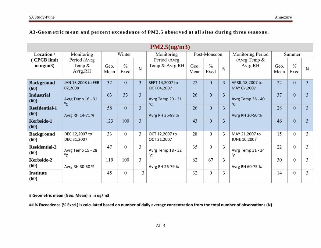
SA Study‐Pune Annexure
AI-3
A3-Geometric mean and percent exceedence of PM2.5 observed at all sites during three seasons.
# Geometric mean (Geo. Mean) is in ug/m3
## % Exceedence (% Excd.) is calculated based on number of daily average concentration from the total number of observations (N)
PM2.5(ug/m3) Location /
( CPCB limit in ug/m3)
Monitoring Period /Avrg
Temp & Avrg.RH
Winter Monitoring Period /Avrg
Temp & Avrg.RH
Post-Monsoon Monitoring Period /Avrg Temp &
Avrg.RH
Summer
Geo. Mean
% Excd N Geo.
Mean %
Excd N Geo. Mean
% Excd N
Background (60)
JAN 13,2008 to FEB 02,2008 Avrg Temp 16 ‐ 31 0C Avrg RH 14‐71 %
32 0 3 SEPT 14,2007 to OCT 04,2007 Avrg Temp 20 ‐ 31 0C Avrg RH 36‐98 %
22 0 3 APRIL 18,2007 to MAY 07,2007 Avrg Temp 38 ‐ 40 0C Avrg RH 30‐50 %
22 0 3
Industrial (60)
63 33 3 26 0 3 37 0 3
ResIdential-1 (60)
58 0 3 26 0 3 28 0 3
Kerbside-1 (60)
123 100 3 43 0 3 46 0 3
Background (60)
DEC 12,2007 to DEC 31,2007 Avrg Temp 15 ‐ 28 0C Avrg RH 30‐50 %
33 0 3 OCT 12,2007 to OCT 31,2007 Avrg Temp 18 ‐ 32 0C Avrg RH 26‐79 %
28 0 3 MAY 21,2007 to JUNE 10,2007 Avrg Temp 31 ‐ 34 0C Avrg RH 60‐75 %
15 0 3
Residential-2 (60)
47 0 3 35 0 3 22 0 3
Kerbside-2 (60)
119 100 3 62 67 3 30 0 3
Institute (60)
45 0 3 32 0 3 14 0 3

SA Study‐Pune Annexure
AI-4
A4-Geometric mean and percent exceedence of NO2 observed at all sites during three seasons.
NO2 (ug/m3) Location /
( CPCB limit in ug/m3)
Monitoring Period /Avrg
Temp & Avrg.RH
Winter Monitoring Period /Avrg
Temp & Avrg.RH
Post-Monsoon Monitoring Period /Avrg Temp &
Avrg.RH
Summer
Geo. Mean
% Excd N Geo.
Mean %
Excd N Geo. Mean
% Excd N
Background (80)
JAN 13,2008 to FEB 02,2008 Avrg Temp 16 ‐ 31 0C Avrg RH 14‐71 %
16 0 15 SEPT 14,2007 to OCT 04,2007 Avrg Temp 20 ‐ 31 0C Avrg RH 36‐98 %
9 0 18 APRIL 18,2007 to MAY 07,2007 Avrg Temp 38 ‐ 40 0C Avrg RH 30‐50 %
9 0 20
Industrial (120)
55 0 20 17 0 20 22 0 19
ResIdential-1 (80 )
25 0 20 10 0 20 14 0 20
Kerbside-1 (80)
71 50 18 30 0 19 59 20 20
Background (80)
DEC 12,2007 to DEC 31,2007 Avrg Temp 15 ‐ 28 0C Avrg RH 30‐50 %
18 0 15 OCT 12,2007 to OCT 31,2007 Avrg Temp 18 ‐ 32 0C Avrg RH 26‐79 %
13 0 19 MAY 21,2007 to JUNE 10,2007 Avrg Temp 31 ‐ 34 0C Avrg RH 60‐75 %
9 0 20
Residential-2 (80)
41 6 18 43 0 20 9 0 13
Kerbside-2 (80)
65 40 15 43 0 20 24 0 19
Institute (80)
36 0 20 34 0 20 9 0 20
# Geometric mean (Geo. Mean) is in ug/m3
## % Exceedence (% Excd.) is calculated based on number of daily average concentration from the total number of observations (N)

SA Study‐Pune Annexure
AI-5
A5-Geometric mean and percent exceedence of SO2 observed at all sites during three seasons.
SO2 (ug/m3) Location /
( CPCB limit in ug/m3)
Monitoring Period /Avrg
Temp & Avrg.RH
Winter Monitoring Period /Avrg
Temp & Avrg.RH
Post-Monsoon Monitoring Period /Avrg Temp &
Avrg.RH
Summer
Geo. Mean
% Excd N Geo.
Mean %
Excd N Geo. Mean
% Excd N
Background (80)
JAN 13,2008 to FEB 02,2008 Avrg Temp 16 ‐ 31 0C Avrg RH 14‐71 %
12 0 19 SEPT 14,2007 to OCT 04,2007 Avrg Temp 20 ‐ 31 0C Avrg RH 36‐98 %
8 0 17 APRIL 18,2007 to MAY 07,2007 Avrg Temp 38 ‐ 40 0C Avrg RH 30‐50 %
5 0 20
Industrial (120)
40 0 20 16 0 20 22 0 19
ResIdential-1 (80 )
11 0 20 8 0 20 6 0 20
Kerbside-1 (80)
18 0 18 11 0 18 7 0 18
Background (80)
DEC 12,2007 to DEC 31,2007 Avrg Temp 15 ‐ 28 0C Avrg RH 30‐50 %
14 0 15 OCT 12,2007 to OCT 31,2007 Avrg Temp 18 ‐ 32 0C Avrg RH 26‐79 %
9 0 18 MAY 21,2007 to JUNE 10,2007 Avrg Temp 31 ‐ 34 0C Avrg RH 60‐75 %
5 0 20
Residential-2 (80)
18 0 18 11 0 20 5 0 13
Kerbside-2 (80)
35 7 15 12 0 20 6 0 20
Institute (80)
23 0 20 10 0 20 5 0 20
# Geometric mean (Geo. Mean) is in ug/m3
## % Exceedence (% Excd.) is calculated based on number of daily average concentration from the total number of observations (N)

SA Study‐Pune Annexure
AI-6
B1-Variability of concentration of different parameters at various locations with respect to background location based on geometric mean
Location SPM
Winter Post-Monsoon Summer Variability % Excd N Variability % Excd N Variability % Excd N
Background-1 1.00 80 20 1.00 0 20 1.00 5 20Industrial 1.87 25 20 2.31 0 20 1.94 0 20Resdential-1 1.45 88 16 1.36 6 18 1.48 50 20Kerbside-1 2.12 100 15 3.82 90 20 3.65 100 20Background-2 1.00 80 20 1.00 20 20 1.00 0 19Residential-2 2.36 100 20 2.21 95 20 2.80 8 13Kerbside-2 3.10 100 20 3.55 100 20 5.01 85 20Institute 1.21 95 20 1.25 65 20 1.84 0 20
Location PM10
Winter Post-Monsoon Summer Variability % Excd N Variability % Excd N Variability % Excd N
Background-1 1.00 32 19 1.00 0 20 1.00 10 20Industrial 2.45 85 20 1.52 10 20 1.61 22 18Resdential-1 1.20 53 19 1.11 11 18 1.36 58 19Kerbside-1 2.87 100 20 2.84 37 19 1.83 95 20Background-2 1.00 32 19 1.00 10 20 1.00 0 20Residential-2 1.80 95 20 2.22 72 18 1.81 8 13Kerbside-2 2.43 100 20 3.33 95 20 2.72 50 20Institute 1.35 60 20 1.08 5 19 1.39 15 20
Location PM2.5
Winter Post-Monsoon Summer Variability % Excd N Variability % Excd N Variability % Excd N
Background-1 1.00 0 3 1.00 0 3 1.00 0 3 Industrial 1.96 33 3 1.15 0 3 1.67 0 3 Resdential-1 1.82 0 3 1.14 0 3 1.27 0 3 Kerbside-1 3.87 100 3 1.93 0 3 2.08 0 3 Background-2 1.00 0 3 1.00 0 3 1.00 0 3 Residential-2 1.42 0 3 1.24 0 3 1.42 0 3 Kerbside-2 3.58 100 3 2.21 67 3 1.98 0 3 Institute 1.37 0 3 1.14 0 3 0.94 0 3

SA Study‐Pune Annexure
AI-7
B2-Variability of concentration of different parameters at various locations with respect to background location based on geometric mean
Location
NO2 Winter Post-Monsoon Summer
Variability % Excd N Variability % Excd N Variability % Excd N
Background-1 1.00 0 15 1.00 0 18 1.00 0 20Industrial 3.35 0 20 1.80 0 20 2.30 0 19Resdential-1 1.59 0 20 1.00 0 20 1.50 0 20Kerbside-1 4.35 50 18 3.30 0 19 6.50 20 20Background-2 1.00 0 15 1.00 0 19 1.00 0 20Residential-2 2.25 6 18 3.21 0 20 1.11 0 13Kerbside-2 3.40 40 15 3.14 0 20 2.89 0 19Institute 1.90 0 20 2.50 0 20 1.11 0 20
Location
SO2 Winter Post-Monsoon Summer
Variability % Excd N Variability % Excd N Variability % Excd N
Background-1 1.00 0 19 1.00 0 17 1.00 0 20Industrial 3.29 0 20 1.85 0 20 4.08 0 19Resdential-1 0.94 0 20 1.01 0 20 1.04 0 20Kerbside-1 1.50 0 18 1.36 0 18 1.23 0 18Background-2 1.00 0 15 1.00 0 18 1.00 0 20Residential-2 1.25 0 18 1.23 0 20 1.05 0 13Kerbside-2 2.46 7 15 1.34 0 20 1.28 0 20Institute 1.62 0 20 1.09 0 20 1.18 0 20

This page is intentionally left blank

SA Study‐Pune Annexure
AII-1
Annexure II: - Emission Factors for Area/Line Source (Chapter – 3) A: Line (Emission Factor Developemnt for Indian Vehicles, ARAI Report 2007) Vehicle Type Model PM CO HC NOx
Year g/km g/km g/km g/km Scooters-2s 1991-1995 0.073 6 3.68 0.02 Scooters-2s 1996-2000 0.073 5.1 2.46 0.01 Scooters-2s 2001-2005 0.049 2.37 2.05 0.03 Scooters-4s 2001-2005 0.015 0.93 0.65 0.35 Scooters-4s 2006-2010 0.015 0.4 0.15 0.25 (4 Stroke) Motorcycles 1991-1995 0.01 3.12 0.78 0.23 (4 Stroke) Motorcycles 1996-2000 0.015 1.58 0.74 0.3 (4 Stroke) Motorcycles 2001-2005 0.035 1.65 0.61 0.27 (4 Stroke) Motorcycles 2006-2010 0.013 0.72 0.52 0.15 3-Wheeler - CNG- 4S Oe 2006-2010 0.015 1 0.26 0.5 3-Wheeler - Auto rick-Petrol 2S Post 2000 0.045 1.37 2.53 0.2 3-Wheeler - Auto rick-LPG 2S Ret-pre 2000 0.721 4.39 3.6 0.08 Ret-post-2000 0.13 1.7 1.03 0.04 3-Wheeler - Auto rick-D Post 2000 0.347 2.09 0.16 0.69 Post 2005 0.091 0.41 0.14 0.51 4 Wheeler - Petrol 1991-1995 0.008 4.75 0.84 0.95 4 Wheeler - Petrol 1996-2000 0.008 4.53 0.66 0.75 4 Wheeler - Petrol 2001-2005 0.004 1.3 0.24 0.2 4 Wheeler - Petrol 2006-2010 0.002 0.84 0.12 0.09 4 Wheeler - Diesel 1996-2000 0.145 0.87 0.22 0.45 4 Wheeler - Diesel 2001-2003 0.19 0.72 0.14 0.84 4 Wheeler - Diesel 2003-05 0.06 0.3 0.26 0.49 4 Wheeler - Diesel 2006-2010 0.015 0.06 0.08 0.28 4 Wheeler - LPG 1996-2000 0.001 6.46 1.78 0.44 2001-2005 0.002 2.72 0.23 0.2 2006-2010 0.002 2.72 0.23 0.2 4 Wheeler - CNG 2006-2010 0.006 0.06 0.46 0.74 LCVs 1991-1995 0.998 3.07 2.28 3.03 (Light Commercial Vehicles) 4 Wheeler GC
1996-2000 0.655 3 1.28 2.48 2001-2005 0.475 3.66 1.35 2.12
2006-2010 0.475 3.66 1.35 2.12

SA Study‐Pune Annexure
AII-2
Contd…
Vehicle Type Model PM CO HC NOx Year g/km g/km g/km g/km
Large Trucks + MAV 1991-1995 1.965 19.3 2.63 13.84 1996-2000 1.965 19.3 2.63 13.84 2001-2005 1.24 6 0.37 9.3 2006-2010 0.42 4.13 0.28 8.63 Buses-Diesel 1991-1995 2.013 13.06 2.4 11.24 1996-2000 1.213 4.48 1.46 15.25 2001-2005 1.075 3.97 0.26 6.77 2006-2010 0.3 3.92 0.16 6.53 Buses - CNG 2001-2005 N A 3.72 3.75 6.21 2006-2010 0 3.72 3.75 6.21
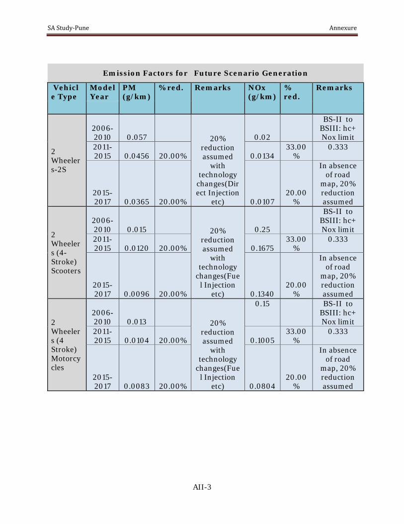
SA Study‐Pune Annexure
AII-3
Emission Factors for Future Scenario Generation
Vehicle Type
Model Year
PM (g/km)
% red. Remarks NOx (g/km)
% red.
Remarks
2 Wheelers-2S
2006-2010 0.057 20%
reduction assumed
with technology
changes(Direct Injection
etc)
0.02
BS-II to BSIII: hc+ Nox limit
2011-2015 0.0456 20.00% 0.0134
33.00%
0.333
2015-2017 0.0365 20.00% 0.0107
20.00%
In absence of road
map, 20% reduction assumed
2 Wheelers (4-Stroke) Scooters
2006-2010 0.015 20%
reduction assumed
with technology
changes(Fuel Injection
etc)
0.25
BS-II to BSIII: hc+ Nox limit
2011-2015 0.0120 20.00% 0.1675
33.00%
0.333
2015-2017 0.0096 20.00% 0.1340
20.00%
In absence of road
map, 20% reduction assumed
2 Wheelers (4 Stroke) Motorcycles
2006-2010 0.013 20%
reduction assumed
with technology
changes(Fuel Injection
etc)
0.15 BS-II to BSIII: hc+ Nox limit
2011-2015 0.0104 20.00% 0.1005
33.00%
0.333
2015-2017 0.0083 20.00% 0.0804
20.00%
In absence of road
map, 20% reduction assumed

SA Study‐Pune Annexure
AII-4
Emission Factors for Future Scenario Generation
Vehicle Type
Model Year
PM (g/km)
% red. Remarks NOx (g/km)
% red.
Remarks
3-Wheeler- OE - 4S CNG/ LPG/ Petrol
2006-2010 0.015 20%
reduction assumed
with technology changes( Injection
etc)
0.5 BS-II to BSIII: hc+ Nox limit
2011-2015 0.0120 20.00% 0.3125
37.50%
0.375
2015-2017 0.0096 20.00% 0.2500
20.00%
In absence of road
map, 20% reduction assumed
3-Wheeler - Diesel
2006-2010 0.091
BS-II to BSIII
0.51 BS-II to BSIII: hc+ Nox limit
2011-2015 0.0455 50.00% 0.5 0.4202
17.60%
0.176
2015-2017 0.0364 20.00%
In absence of road map,
20% reduction assumed 0.3362
20.00%
In absence of road
map, 20% reduction assumed
3-Wheeler- OE - 2S CNG/ LPG/ Petrol
2006-2010 0.045 20%
reduction assumed
with technology changes( Injection
etc)
0.2 BS-II to BSIII: hc+ Nox limit
2011-2015 0.0360 20.00% 0.1250
37.50%
0.375
2015-2017 0.0288 20.00% 0.1000
20.00%
In absence of road
map, 20% reduction assumed
3-Wheeler - LPG 2S- retro
2006-2010 0.13
20% reduction assumed
with technology changes( Injection
etc)
0.04
BS-II to BSIII: hc+ Nox limit
2011-2015 0.1040 20.00% 0.0250
37.50%
0.375
2015-2017 0.0832 20.00% 0.0200
20.00%
In absence of road
map, 20%

SA Study‐Pune Annexure
AII-5
reduction assumed
Emission Factors for Future Scenario Generation
Vehicle Type
Model Year
PM (g/km)
% red. Remarks NOx (g/km)
% red.
Remarks
3-Wheeler - CNG 2S- retro
2006-2010 0.118 20%
reduction assumed
with technology changes( Injection
etc)
0.19
BS-II to BSIII: hc+ Nox limit
2011-2015 0.0944 20.00% 0.1188
37.50%
0.375
2015-2017 0.0755 20.00% 0.0950
20.00%
In absence of road
map, 20% reduction assumed

SA Study‐Pune Annexure
AII-6
Emission Factors for Future Scenario Generation
Vehicle Type
Model Year
PM (g/km)
% red. Remarks NOx (g/km)
% red.
Remarks
4 Wheeler - Petrol
2006-2010 0.0020
0.0900
2011-2015 0.0016 20.00% 0.0477
47.00%
2015-2017 0.0013 20.00%
EURO-V, PM norm
instruction in line with
diesel values 0.0358 25.00
% EURO-V
2015-2017 0.0013 0.00%
EURO-VI, no change in norms from EURO-V to
VI 0.0358 0.00%
EURO-VI, no change in norms
from EURO-V to
VI
4 Wheeler - Diesel
2006-2010 0.0150
0.2800
2011-2015 0.0083 45.00% 0.1400
50.00%
2015-2017 0.0008 90.00% EURO-V 0.1008
28.00% EURO-V
2015-2017 0.0008 0.00% EURO-VI 0.0454
55.00% EURO-VI
4 Wheeler - CNG
2006-2010 0.006
0.74
2011-2015 0.0048 20.00%
0.3922
47.00%
In line with petrol
2015-2017 0.0038 20.00% 0.2942
25.00%
2015-2017 0.0038 0.00% 0.2942 0.00%
4 Wheeler - LPG
2006-2010 0.002
0.2
2011-2015 0.0016 20.00%
0.1060
47.00%
In line with petrol
2015-2017 0.0013 20.00% 0.0795
25.00%
2015-2017 0.0013 0.00% 0.0795 0.00%

SA Study‐Pune Annexure
AII-7
Emission Factors for Future Scenario Generation
Vehicle Type
Model Year
PM (g/km)
% red. Remarks NOx (g/km)
% red.
Remarks
LCVs (Light Commercial Vehicles)-diesel
2006-2010 0.475
2.12
2011-2015 0.0808 83.00% 1.4840
30.00%
2015-2017 0.0808 0.00% EURO-V 0.8459
43.00% EURO-V
2015-2017 0.0339 58.00% EURO-VI 0.1692
80.00% EURO-VI
LCVs (Light Commercial Vehicles) - CNG
2006-2010 0.058
data taken from vehicle
emissions source profile
5.7 data taken from vehicle
emissions source profile
2011-2015 0.0464 20.00% 3.9900
30.00%
In line with diesel
2015-2017 0.0371 20.00% 2.2743
43.00%
2015-2017 0.0297 20.00% 0.4549
80.00%
Large Trucks + MAV
2006-2010 0.42
data taken from vehicle
emissions source profile 8.63
2011-2015 0.0714 83.00% 6.0410
30.00%
2015-2017 0.0714 0.00% EURO-V 3.4434
43.00% EURO-V
2015-2017 0.0300 58.00% EURO-VI 0.6887
80.00% EURO-VI
Large Trucks + MAV CNG
2006-2010 0.032
data taken from vehicle
emissions source profile 3.92
2011-2015 0.0256 20.00% 2.7440
30.00%
In line with diesel
2015-2017 0.0205 20.00% 1.5641
43.00%
2015-2017 0.0164 20.00% 0.3128
80.00%

SA Study‐Pune Annexure
AII-8
Emission Factors for Future Scenario Generation
Vehicle Type
Model Year
PM (g/km)
% red. Remarks NOx (g/km)
% red.
Remarks
Buses-Diesel
2006-2010 0.3 6.53
2011-2015 0.0510 83.00% 4.5710
30.00%
2015-2017 0.0510 0.00% EURO-V 2.6055
43.00% EURO-V
2015-2017 0.0214 58.00% EURO-VI 0.5211
80.00% EURO-VI
Buses - CNG-OE
2006-2010 0.044
taken from TERI-ARAI
report
6.21
2011-2015 0.0352 20.00% 4.3470
30.00%
In line with diesel
2015-2017 0.0282 20.00% 2.4778
43.00%
2015-2017 0.0225 20.00% 0.4956
80.00%
Buses - CNG-Retro
2006-2010 0.032
data taken from vehicle
emissions source profile
3.92
2011-2015 0.0256 20.00% 2.7440
30.00%
In line with diesel
2015-2017 0.0205 20.00% 1.5641
43.00%

SA Study‐Pune Annexure
AII-9
Annexure-II B: Other sources – Area
S. No. Source/Activity Common Emission Factor Reference/Remarks
1 Fuel Oil Combustion TSP = {9.19(S) + 3.22} * 0.120
SO2 = 18.84S
NOx = 6.6
CO = 0.6
CH4 = 0.0336
TOC = 0.1248
NMTOC = 0.091
(Unit: Kg/103 L)
TSP May Be Considered As PM10.
TOC Is Total Organic Compound Including VOC.
EPA-42: Table 1.3 – 1 And Table 1.3 – 3; S – Sulphur Content In Fuel (For 1% Sulphur S=1); Gm/Lit Oil, Fuel Oil Combustion, Normal Firing.
2 Natural Gas Combustion TSP = 121.6
SO2 = 9.6
NOx = 1600
CO = 1344
CO2 =1,920,000
CH4 = 36.8
VOC =88
TSP May Be Considered As PM10.
http://www.epa.gov/ttn/chief/ap42/ch01/Final/C01s04.Pdf

SA Study‐Pune Annexure
AII-10
S. No. Source/Activity Common Emission Factor Reference/Remarks
TOC = 176
NMTOC = 0.091
(Unit: Kg/103 L)
3 Liquified Petroleum Gas Combustion
PM= 2.1
SO2 = 0.4
(Unit: Gm/Kg)
NOx = 1.8
CO = 0.252
CO2 =1716
CH4 = 0.024
VOC =88
TOC = 0.072
NMTOC = 0.091
(Unit: Kg/106 M3)
Reddy And Venkatraman
Http://Www.Epa.Gov/Ttn/Chief/Ap42/Ch01/Final/C01s05.Pdf
(Commercial Boilers)
4 Bagasse Combustion PM = 7.8]
NOx = 0.6
CO2 = 780
EPA-AP42: Table 1.8-1,
Uncontrolled Emission Factors

SA Study‐Pune Annexure
AII-11
S. No. Source/Activity Common Emission Factor Reference/Remarks
(Unit: Kg/Ton)
5 Residential Wood Stoves / Restaurants
PM10=15.3
CO=115.4
NOx=1.4
Sox= 0.2
TOC=41.5
CH4=15
TNMOC=26.5
(Unit: Kg/Mg)
Table 1.10-1 Conventional AP-42
6 Kerosene Combustion Domestic
PM=1.95
SO2=4
(Unit: G/Lit)
TSP=0.61
CO=62
NOx=2.5
CH4=1
TNMOC=19
PM & SO2 – Reddy And Venkatraman
TSP May Be Considered As PM10.
USEPA 2000

SA Study‐Pune Annexure
AII-12
S. No. Source/Activity Common Emission Factor Reference/Remarks
(Unit: G/Kg)
7 Coal Combustion - Tandoor / Domestic
TSP=20
CO=24.92
Nox=3.99
SO2= 13.3
(Unit: Kg/Mg)
TERI Report
Uncontrolled wherever controlled use efficiency.
8 Coal Combustion Boilers Stoker Fired Boilers CO=0.3
CO2=2840
Sox=19.5S
Nox=4.5
PM=
FBC Boilers CO=0.3
CO2=ND
Sox=1.45
Nox=0.9
S= Weight Percent Sulphur.
AP-42 1.2-1,2,3
Use suitable EF pertinent to the city & 2x2 grid
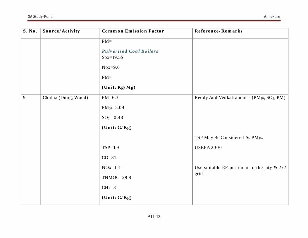
SA Study‐Pune Annexure
AII-13
S. No. Source/Activity Common Emission Factor Reference/Remarks
PM=
Pulverized Coal Boilers Sox=19.5S
Nox=9.0
PM=
(Unit: Kg/Mg)
9 Chulha (Dung, Wood) PM=6.3
PM10=5.04
SO2= 0.48
(Unit: G/Kg)
TSP=1.9
CO=31
NOx=1.4
TNMOC=29.8
CH4=3
(Unit: G/Kg)
Reddy And Venkatraman - (PM10, SO2, PM)
TSP May Be Considered As PM10.
USEPA 2000
Use suitable EF pertinent to the city & 2x2 grid

SA Study‐Pune Annexure
AII-14
S. No. Source/Activity Common Emission Factor Reference/Remarks
10 Agricultural Waste (From Pune And Kanpur)
PM=11
PM10=11
CO=58
CO2=207
SO2=0.12
NOX=0.49
(Unit: Kg/Ton)
EPA-AP42: Table 2.5-5 Emission Factors For Open Burning Of Agricultural Materials, Kg/Ton; Unspecified Field Crop Burning Emission Factor Is Considered. Particulate Matter From Most Agricultural Refuse Burning Has Been Found To Be In The Sub micrometer Size Range.
For SO2 And NO2: M. S. Reddy And C. Venkatraman (2002), Inventory Of Aerosol And Sulphur Dioxide Emissions From India. Part II - Biomass Combustion, Atm. Envt., Vol 36, Issue 4, Pp 699-712
Manish Shrivastava, Gazala Habib, Venkatraman C, Jeffery W.Sterh, Russell R.Dickerson(Sept.8 2003) Emissions From Biomass Burning In India : II - Sulfur Dioxide And Nitrogen Dioxide, Global Biogeochemical Cycles, Pp15
11 Garden Waste Combustion
(Same as under 10)
12 Medical Waste Incineration
PM=2.33
SO2=1.09
CO=2.95
EPA-AP42: Table 2.3.2;
Apply Emission Factors for uncontrolled Emission

SA Study‐Pune Annexure
AII-15
S. No. Source/Activity Common Emission Factor Reference/Remarks
Nox=1.78
(Unit: Kg/Ton)
13 Solid Waste Burning (Landfill Sites)
PM10 = 8
PM2.5 =5.44
CO=42
Sox=0.5000
Nox=3
VOC= 21.5
(Unit: Kg/MT)
A Guide To Rapid Source Inventory Techniques And Their Use In Formulating Environmental Control Strategies – Part One – Rapid Inventory Techniques In Environmental Pollution By A.P. Economopolous, WHO, Geneva, 1993
14 Kerosene Generators Domestic
Apply same EF as for item no. 6: domestic Kerosene combustions
15 Diesel Industrial Generators Large Stationary Diesel And All Stationary Dual - Fuel Engines(Film Shooting)
PM10 = 1.33 E-03
CO2= 0.69
CO=4.06 E-03
Sox= 1.24 E-03
NOx=0.0188
Aldehydes= 2.81 E-04
AP-42 (Table 3.3-1) EF For Uncontrolled Gasoline & Diesel Industrial Engines.

SA Study‐Pune Annexure
AII-16
S. No. Source/Activity Common Emission Factor Reference/Remarks
TOC
Exhaust = 1.50 E-03
Evaporative =0
Crankcase = 2.68 E-03
Refueling =0
(Unit: Kg/Kw-Hr)
16 Petroleum Refining Boilers & Process Heaters Fuel Oil – EF Used For Fuel Oil Combustion (Sec 1.3 AP-42)
Natural Gas - EF Used For Natural Gas Combustion (Sec 1.4 AP-42)
Fluid Catalytic Cracking Units Uncontrolled PM=0.695
SO2=1.413
CO=39.2
Total Hydrocarbons=0.630
NO2=0.204
Aldehydes=0.054
AP-42 (Table 5.1-1 To 5.1-3).
Calculate EF inclusive for all the processes for each ton of product.

SA Study‐Pune Annexure
AII-17
S. No. Source/Activity Common Emission Factor Reference/Remarks
Ammonia=0.155
Electrostatic Precipitator and CO Boiler
PM=0.128
SO2=1.413
CO=Neg
Total Hydrocarbons=Neg
NO2=0.204
Aldehydes=Neg
Ammonia=Neg
Moving Bed Catalytic Cracking Units PM=0.049
SO2=0.171
CO=10.8
Total Hydrocarbons=0.250
NO2=0.014
Aldehydes=0.034

SA Study‐Pune Annexure
AII-18
S. No. Source/Activity Common Emission Factor Reference/Remarks
Ammonia=0.017
Fluid Coking Units Uncontrolled PM=1.50
SO2=ND
CO= ND
Total Hydrocarbons= ND
NO2= ND
Aldehydes= ND
Ammonia= ND
Electrostatic Precipitator and CO Boiler PM=0.0196
SO2=ND
CO=Neg
Total Hydrocarbons=Neg
NO2=ND
Aldehydes=Neg

SA Study‐Pune Annexure
AII-19
S. No. Source/Activity Common Emission Factor Reference/Remarks
Ammonia=Neg
(Unit: Kg/103 L Fresh Feed)
Vapor Recovery System and Flaring PM=Neg
SO2=0.077
CO=0.012
Total Hydrocarbons=0.002
NO2=0.054
Aldehydes=Neg
Ammonia=Neg
(Unit: Kg/103 L Refinery Feed)
Vacuum Distillation Column Condensers Uncontrolled PM=Neg
SO2=Neg
CO=Neg
Total Hydrocarbons=0.14

SA Study‐Pune Annexure
AII-20
S. No. Source/Activity Common Emission Factor Reference/Remarks
NO2=Neg
Aldehydes=Neg
Ammonia=Neg
Controlled (Vented To Heater Or
Incinerator)
PM=Neg
SO2=Neg
CO=Neg
Total Hydrocarbons=Neg
NO2=Neg
Aldehydes=Neg
Ammonia=Neg
(Unit: Kg/103 L Refinery Feed)
Claus Plant And Tail Gas Treatment (See Sec 8.13-“Sulphur Recovery” AP-42)
Cooling Towers (Uncontrolled Emissions)

SA Study‐Pune Annexure
AII-21
S. No. Source/Activity Common Emission Factor Reference/Remarks
PM=0.7
(Unit: Kg/106 L Cooling Water)
Oil Water Separators (Uncontrolled Emissions)
PM=0.6
(Unit: Kg/103 L Waste Water)
Storage (Uncontrolled Emissions)
(See Chapter 7-Liquid Storage Tanks AP-42)
Loading (Uncontrolled Emissions)
(See Section 5.2 – Transportation And Marketing Of Petroleum Liquids AP-42)
Fugitive VOC Emissions (Uncontrolled Oil Refinery Of 52,500 M3/Day)
Total =20,500
(Unit: Kg/Day)
17 Electric Arc Welding TSP=6.3
SO2=NA
WHO 1993, Rapid Techniques In Environmental Pollution Part 1 By Alexander P. Economopoulos

SA Study‐Pune Annexure
AII-22
S. No. Source/Activity Common Emission Factor Reference/Remarks
NOx=0.16
CO=9.75
VOC=0.09
(Unit: Kg/Ton)
EF Are Cited Without Control Equipments
18 Secondary Metal Smelting (Lead) And Other Operations (Foundries)
Lead
Sweating
PM=16-35
Pb=4-8
SO2=ND
Reverberatory Smelting PM=162
Pb=32
SO2=40
Blast Smelting Cupola PM=153
Pb=52
SO2=27
Kettle Refining
AP-42 12.11 For Lead; 12.13 For Steel Foundries; 12.4 For Zinc

SA Study‐Pune Annexure
AII-23
S. No. Source/Activity Common Emission Factor Reference/Remarks
PM=0.02
Pb=0.006
SO2=ND
Kettle Oxidation PM=< 20
Pb=ND
SO2=ND
Casting
PM=0.02
Pb=0.007
SO2=ND
(Unit: Kg/Mg)
Steel Foundries
Melting
Electric Arc TSP=6.5 (2 To 20)
NOx=0.1
PM10=ND

SA Study‐Pune Annexure
AII-24
S. No. Source/Activity Common Emission Factor Reference/Remarks
Open Hearth TSP =5.5 (1 To 10)
NOx=0.005
PM10=ND
Open Hearth Oxygen Lanced TSP =5.5 (1 To 10)
NOx=0.005
PM10=ND
Electric Induction TSP =0.05
NOx=ND
PM10=0.045
Sand Grinding/Handling In Mold And
Core Making
TSP =ND
Nox=NA
PM10=0.27 3.0
Core Ovens

SA Study‐Pune Annexure
AII-25
S. No. Source/Activity Common Emission Factor Reference/Remarks
TSP =ND
NOx=ND
PM10=1.11 0.45
Pouring and Casting TSP =ND
NOx=NA
PM10=1.4
Casting Cleaning TSP =ND
NOx=NA
PM10=0.85
Charge Handling TSP =ND
NOx=NA
PM10=0.18
Casting Cooling TSP =ND
NOx=NA

SA Study‐Pune Annexure
AII-26
S. No. Source/Activity Common Emission Factor Reference/Remarks
PM10=0.7
(Unit: Kg/Mg)
Zinc Reverberatory Sweating
Clean Metallic Scrap
PM= Negligible
General Metallic Scrap PM=6.5
Residual Scrap PM=16
(Unit: Mg/Mg Of Feed)
Rotary Sweating PM=5.5-12.5
Muffle Seating PM=5.4-16
Kettle Sweating Clean Metallic Scrap PM= Negligible
General Metallic Scrap PM=5.5
Residual Scrap

SA Study‐Pune Annexure
AII-27
S. No. Source/Activity Common Emission Factor Reference/Remarks
PM=12.5
Electric Resistance Sweating PM=<5
Sodium Carbonate Leaching Calcining PM=44.5
(Unit: Kg/Mg Of Zinc Used)
Kettle Pot PM=0.05
(Unit: Mg/Mg)
Crucible Melting PM=ND
Reverberatory Melting PM=ND
Electric Induction Melting
PM=ND
Alloying PM=ND
Retort and Muffle Distillation Pouring PM=0.2 – 0.4

SA Study‐Pune Annexure
AII-28
S. No. Source/Activity Common Emission Factor Reference/Remarks
Casting PM=0.1-0.2
Muffle Distillation PM=22.5
(Unit: Kg/Mg Of Product)
Graphite Rod Distillation PM-Neg
Retort Distillation/Oxidation PM=10-20
Muffle Distillation/Oxidation PM=10-20
Retort Reduction PM=23.5
Galvanizing PM=2.5
(Unit: Kg/Mg Of Zinc Used)
19 Cast Iron Furnace Cupola
Uncontrolled
PM=6.9
Electric Arc Furnace
AP-42 (Table 12.10-2)
Use suitable EF pertinent to the city & 2x2 grid
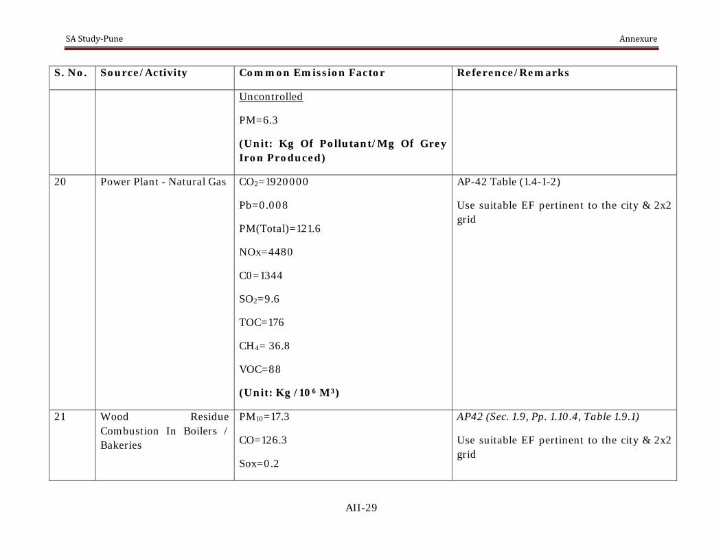
SA Study‐Pune Annexure
AII-29
S. No. Source/Activity Common Emission Factor Reference/Remarks
Uncontrolled
PM=6.3
(Unit: Kg Of Pollutant/Mg Of Grey Iron Produced)
20 Power Plant - Natural Gas CO2=1920000
Pb=0.008
PM(Total)=121.6
NOx=4480
C0=1344
SO2=9.6
TOC=176
CH4= 36.8
VOC=88
(Unit: Kg /106 M3)
AP-42 Table (1.4-1-2)
Use suitable EF pertinent to the city & 2x2 grid
21 Wood Residue Combustion In Boilers / Bakeries
PM10=17.3
CO=126.3
Sox=0.2
AP42 (Sec. 1.9, Pp. 1.10.4, Table 1.9.1)
Use suitable EF pertinent to the city & 2x2 grid

SA Study‐Pune Annexure
AII-30
S. No. Source/Activity Common Emission Factor Reference/Remarks
NOx=1.3
CO2=1700
Total VOC=114.5
(Unit: Kg /Mg)
22 Coal Combustion - Power Plant
PC, Dry Bottom, Wall-Fired, Sub-Bituminous Pre-NSPS
Sox=19S
NOx=11 (5.5 With Low NOx Burners)
CO=0.25
Filterable PM=5A
Filterable PM10=1.15
(Unit: Kg /Mg)
AP-42 (Table 1.1-3-4)
Use suitable EF pertinent to the city & 2x2 grid
Particulate Is Expressed In Terms Of Coal Ash Content, A, Factor Is Determined By Multiplying Weight % Ash Content Of Coal (As Fired) By The Numerical Value Preceding The A.
23 Plastic And Leather Waste Burning
SO2=0.5
NOx=3
CO=42
CH4=6.5
AP 42/(Table 2.4-7)

SA Study‐Pune Annexure
AII-31
S. No. Source/Activity Common Emission Factor Reference/Remarks
TSP=8
(Unit: Kg /Mg Of Waste)
24 Bricks And Related Clay Products (Earthen Pot Kiln)
PM=0.9
PM10=0.7
SO2=0.6
NOx=0.255
CO=0.4
CO2=150
(Unit: Kg /Tons Of Bricks)
EPA-AP42 (Table: 11.3-2)
Apply for uncontrolled Emissions for Coal Fired Kiln unless a different fuel is used.
25 Cupola Cast Iron TSP=6.9
SO2=0.6S
NOx=NA
CO=73
VOC=NA
Pb=0.32
(Unit: Kg /Tons)
WHO 1993, Rapid Techniques In Environmental Pollution Part 1 By Alexander P. Economopoulos
26 Municipal Solid Waste PM10 = 8 A Guide To Rapid Source Inventory

SA Study‐Pune Annexure
AII-32
S. No. Source/Activity Common Emission Factor Reference/Remarks
Landfills PM2.5 =5.44
CO=42
Sox=0.5000
NOx=3
VOC= 21.5
(Unit: Kg/MT)
Techniques And Their Use In Formulating Environmental Control Strategies – Part One – Rapid Inventory Techniques In Environmental Pollution By A.P. Economopoulos, WHO, Geneva, 1993
Divide under different types of emissions such as vehicular movement on unpaved roads, combustion of organic content, loading and unloading etc. Determine the activity levels for each category and apply suitable factors given.
27 Manufacture Of Rubber Products / Plastics Small Scale
PM=17.5
Gases=8.5
(Unit: Kg /Mg)
AP-42 (Table 6.6.1-1)
Use suitable EF pertinent to the city & 2x2 grid
28 Fertilizer And Inorganic Chemical Industry
Solution Formation And Concentration PM=0.0105
NH4=9.23
Non Fluidized Bed Prilling
AP-42 8.2-1 – Chapter – 8
Use suitable EF pertinent to the city & 2x2 grid

SA Study‐Pune Annexure
AII-33
S. No. Source/Activity Common Emission Factor Reference/Remarks
Agricultural Grade
PM=1.9
NH4=0.43
Feed Grade PM=1.8
NH4=ND
Fluidized Bed Prilling
Agricultural Grade PM=3.1
NH4=1.46
Feed Grade PM=1.8
NH4=2.07
Drum Granulation PM=120
NH4=1.07
Rotary Drum Cooler PM=3.89
NH4=0.0256

SA Study‐Pune Annexure
AII-34
S. No. Source/Activity Common Emission Factor Reference/Remarks
Bagging PM=0.095
NH4=NA
(Unit: Kg /Mg Of Product)
29 Hot Mix Asphalt Plants Batch HMP PM=16
PM10=2.25
CO=0.2(Natural Gas-Fired Dryer, Hot Screens and Mixer)
0.2 (Fuel Oil-Fired Dryer, Hot Screens and Mixer)
0.2 (Waste Oil-Fired Dryer, Hot Screens and Mixer)
CO2=18.5(For All Type O Process)
NOx=0.0125(Natural Gas-Fired Dryer, Hot Screens And Mixer)
0.06 (Fuel Oil-Fired Dryer And Waste Oil-Fired Dryer, Hot Screens And Mixer)
SO2=0.0023(Natural Gas-Fired Dryer
AP-42 11.1-1, 5 & 6
Use suitable EF pertinent to the city & 2x2 grid

SA Study‐Pune Annexure
AII-35
S. No. Source/Activity Common Emission Factor Reference/Remarks
,Hot Screens And Mixer)
0.044(Fuel Oil-Fired Dryer, And
Waste Oil-Fired Dryer Hot Screens And
Mixer)
0.0215 (Coal-Fired Dryer, Hot Screens And Mixer)
TOC =0.0075 (Natural Gas-Fired Dryer, Hot Screens And Mixer)
0.0075 (No.2 Fuel Oil-Fired Dryer, Hot Screens And Mixer)
0.0215(No.6 Fuel Oil-Fired Dryer, Hot Screens And Mixer)
CH4= 0.0037(For All Type O Process)
VOC=0.0041(Natural Gas-Fired Dryer, Hot Screens And Mixer)
0.0041(No.2 Fuel Oil-Fired Dryer, Hot Screens And Mixer)
0.018(No.6 Fuel Oil-Fired Dryer, Hot Screens And Mixer)
(Unit: Kg /Mg)

SA Study‐Pune Annexure
AII-36
S. No. Source/Activity Common Emission Factor Reference/Remarks
Drum Mix HMP PM=14
PM10=3.25
CO=0.065 (For All Process Type)
CO2= 16.5(For All Process Type)
NOx=0.013 (Natural Gas Fired Dryer)
0.0275(No.2 Fuel Oil And Waste
Oil Fired Boiler)
TOC=0.022 (For All Process Type)
CH4=0.006(For All Process Type)
VOC=0.016(For All Process Type)
(Unit: Kg /Mg)
30 Glass Manufacturing TSP=0.7
SO2=1.7
NOX=3.1
CO=0.1
VOC=0.1
WHO 1993, Rapid Techniques In Environmental Pollution Part 1 By Alexander P. Economopoulos

SA Study‐Pune Annexure
AII-37
S. No. Source/Activity Common Emission Factor Reference/Remarks
(Unit: Kg /Ton)
31 Lead Oxide And Pigment Production
TSP=7
SO2=NA
NOX= NA
CO= NA
VOC= NA
Pb=7
(Unit: Kg /Ton)
WHO 1993, Rapid Techniques In Environmental Pollution Part 1 By Alexander P. Economopoulos
32 Construction (Building) TSP=1.2
(Unit: Tons/Acre/ Month Of Activity)
For Details Refer AP-42 Section 13.2.3.3
Use suitable EF pertinent to the city & 2x2 grid depending upon construction activity
33 Construction Roads (A) Aggregate Laying And (B) Asphalt
TSP=1.2
(Unit: Tons/Acre/ Month Of Activity)
For Details Refer AP-42 Section 13.2.3.3
Use suitable EF pertinent to the city & 2x2 grid depending upon construction activity
34 Construction Of Flyovers TSP=1.2
(Unit: Tons/Acre/ Month Of Activity)
For Details Refer AP-42 Section 13.2.3.3
Use suitable EF pertinent to the city & 2x2 grid depending upon construction activity
35 Carbon Black Oil Furnace Process Main Process Vent
AP 42 Table 6.1-3

SA Study‐Pune Annexure
AII-38
S. No. Source/Activity Common Emission Factor Reference/Remarks
PM=3.27
CO=1400
NO=0.28
SO=0
CH4=25
Non CH4 VOC=50
Flare PM=1.35
CO=122
NO=ND
SO=25
Non CH4 VOC=1.85
CO Boiler and Incinerator PM=1.04
CO=0.88
NO=4.65
SO=17.5
Use suitable EF pertinent to the city & 2x2 grid

SA Study‐Pune Annexure
AII-39
S. No. Source/Activity Common Emission Factor Reference/Remarks
Non CH4 VOC=0.99
Oil Storage Tank Vent Non CH4 VOC=0.72
Fugitive Emissions PM=0.10
(Unit: Weight Of Emissions /Weight Of Carbon Black Produced)
36 Paint Applications (Auto) Prime Coat (Solvent borne Spray)
6.61
Guide Coat (Solvent borne Spray)
1.89
Top Coat (Enamel)
7.08
(Unit: Automobile Kg Of VOC/Vehicle)
AP 42 Table 4.2.2.8-1
Based on the number of vehicles being painted in each location
37 Paved Roads Refer Section 13.2.1.3 Of AP-42 AP 42 (13.2.1.3)
Given equation has to be used and respective parameters shall vary for each city and/or grid
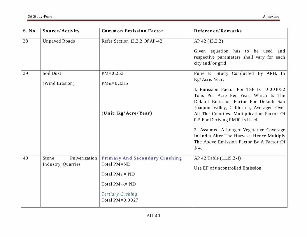
SA Study‐Pune Annexure
AII-40
S. No. Source/Activity Common Emission Factor Reference/Remarks
38 Unpaved Roads Refer Section 13.2.2 Of AP-42 AP 42 (13.2.2)
Given equation has to be used and respective parameters shall vary for each city and/or grid
39 Soil Dust
(Wind Erosion)
PM=0.263
PM10=0.1315
(Unit: Kg/Acre/Year)
Pune EI Study Conducted By ARB, In Kg/Acre/Year,
1. Emission Factor For TSP Is 0.001052 Tons Per Acre Per Year, Which Is The Default Emission Factor For Default San Joaquin Valley, California, Averaged Over All The Counties. Multiplication Factor Of 0.5 For Deriving PM10 Is Used.
2. Assumed A Longer Vegetative Coverage In India After The Harvest, Hence Multiply The Above Emission Factor By A Factor Of 1/4.
40 Stone Pulverization Industry, Quarries
Primary And Secondary Crushing Total PM=ND
Total PM10= ND
Total PM2.5= ND
Tertiary Cushing Total PM=0.0027
AP 42 Table (11.19.2-1)
Use EF of uncontrolled Emission

SA Study‐Pune Annexure
AII-41
S. No. Source/Activity Common Emission Factor Reference/Remarks
Total PM10= 0.0012
Total PM2.5= ND
Fines Crushing Total PM=0.0195
Total PM10= 0.0075
Total PM2.5= ND
Screening Total PM=0.0125
Total PM10= 0.0043
Total PM2.5= ND
Fines Screening Total PM=0.15
Total PM10= 0.036
Total PM2.5= ND
Conveyor Or Transfer Point Total PM=0.0015
Total PM10= 0.00055
Total PM2.5= ND
Wet Drilling Unfragmanted Stone

SA Study‐Pune Annexure
AII-42
S. No. Source/Activity Common Emission Factor Reference/Remarks
Total PM=ND
Total PM10= 4.0 X 10⁻⁵
Total PM2.5= ND
Truck Unloading –Fragmented Stone Total PM=ND
Total PM10= 8.0 X 10⁻⁶
Total PM2.5= ND
Truck Unloading –Conveyor Crushed Stone Total PM=ND
Total PM10= 5.0 X 10⁻⁵
Total PM2.5= ND
(Unit: Kg/Mg)

SA Study‐Pune Annexure
AIII-1
Annexure III: - Grid wise Emission Load from Area, Point and Line Sources (Chapter – 3)
0 0 0 0 0 0 10 355 7 0 0
186 79 1 37 174 118 184 353 89 157 48
239 374 232 25 255 194 409 341 117 76 4
229 210 419 482 378 226 492 464 569 527 78
52 153 248 599 599 505 659 344 355 276 49
198 285 476 665 1294 1763 584 716 515 55 0
198 419 612 826 973 881 538 707 686 351 0
16 191 272 342 700 726 618 436 469 156 0
0 0 220 164 409 432 480 315 147 33 0
0 59 210 1 360 401 395 0 0 0 0
PM10 Emission Load (Kg/day)- All Sources 2007
less than 100
100 to 200
200 to 400
400 to 500
Above 500

SA Study‐Pune Annexure
AIII-2
0 0 0 0 0 0 0 62 0 0 0
38 15 0 10 45 20 27 56 10 22 9
40 67 53 0 53 27 65 63 17 0 0
37 37 88 80 75 38 91 82 100 113 11
0 26 42 129 106 53 129 59 71 55 8
29 51 68 124 269 323 120 101 122 9 0
34 66 95 145 167 154 147 192 191 62 0
3 24 31 52 121 121 101 101 130 24 0
0 0 52 28 70 55 72 51 47 5 0
0 15 45 0 68 55 46 0 0 0 0
PM10 Emission Load (Kg/day)- Mobile Sources 2007
less than 50
50 to 75
75 to 100
100 to 125
Above 125

SA Study‐Pune Annexure
AIII-3
0.0 0.0 0.0 0.0 0.0 0.0 0.0 0.0 0.0 0.0 0.0
0.0 0.0 0.0 0.0 0.0 0.0 0.0 0.0 0.0 0.0 0.0
0.0 0.0 0.0 0.0 7.6 0.0 0.0 0.0 0.0 0.0 0.0
0.0 0.0 0.0 0.0 0.0 0.0 0.0 0.0 19.2 0.2 0.0
0.0 0.0 0.0 0.0 0.0 27.9 0.3 0.0 0.0 5.3 0.0
0.0 0.0 5.6 0.0 0.5 0.4 0.0 329.8 0.0 0.0 0.0
0.0 0.0 0.0 0.0 0.0 0.0 0.0 1.2 3.8 0.0 0.0
0.0 0.0 0.0 0.0 0.0 0.0 0.0 0.0 0.0 0.0 0.0
0.0 0.0 0.0 0.0 0.0 0.0 0.0 0.0 0.0 0.0 0.0
0.0 0.0 0.0 0.0 0.2 0.0 0.0 0.0 0.0 0.0 0.0
PM10 Emission Load (Kg/day)- Industrial Sources 2007
less than 0.1
0.1 to 5
5 to 20
20 to 50
Above 50

SA Study‐Pune Annexure
AIII-4
0 0 0 0 0 0 0 248 0 0 0
147 61 0 27 129 84 111 232 34 87 36
150 270 147 0 187 112 265 232 68 0 0
144 150 260 296 296 158 341 319 378 393 45
0 102 169 406 378 201 387 216 242 189 27
113 195 246 413 831 1106 401 230 259 20 0
122 248 351 524 608 527 356 485 368 147 0
9 81 124 203 450 487 409 264 235 53 0
0 0 139 88 265 245 285 204 74 7 0
0 37 133 0 243 225 217 0 0 0 0
PM10 Emission Load (Kg/day)- Road Dust 2007
less than 50
50 to 100
100 to 200
200 to 300
Above 300

SA Study‐Pune Annexure
AIII-5
0 0 0 0 0 0 10 45 7 0 0
1 3 1 0 0 15 46 66 46 48 2
50 36 32 25 8 55 79 45 32 76 4
48 23 72 106 8 30 61 63 71 20 22
52 25 37 64 115 223 142 69 42 26 14
56 40 156 127 193 333 63 55 134 26 0
42 105 165 157 198 200 35 29 122 142 0
4 86 117 87 129 119 108 71 103 78 0
0 0 29 49 74 132 123 60 26 21 0
0 8 32 1 50 121 132 0 0 0 0
PM10 Emission Load (Kg/day)- Other Area Sources 2007
less than 50
50 to 75
75 to 100
100 to 125
Above 125

SA Study‐Pune Annexure
AIII-6
NOx
0 0 0 0 0 0 1 399 4 0 0
250 97 1 78 319 134 184 381 76 140 59
277 428 380 3 414 192 431 422 119 14 2
253 238 616 549 529 258 600 560 694 742 76
9 170 285 950 738 449 1053 460 571 449 70
206 351 483 903 1797 2148 792 1435 841 65 0
254 472 648 957 1121 1078 976 1314 1327 476 0
21 197 220 347 781 762 635 687 888 178 0
0 0 310 194 458 356 477 328 300 32 0
0 85 294 1 446 357 295 0 0 0 0
NOx Emission Load (Kg/day)- All Sources 2007
less than 100
100 to 200
200 to 500
500 to 750
Above 750

SA Study‐Pune Annexure
AIII-7
0 0 0 0 0 0 0 391 0 0 0
250 96 0 78 319 133 174 361 62 138 57
275 426 375 0 380 182 419 410 108 0 0
252 234 607 539 525 255 589 546 652 736 71
0 167 277 936 710 359 1019 446 562 442 68
195 341 444 876 1741 2059 782 667 815 64 0
243 443 618 928 1065 1016 970 1305 1285 448 0
21 176 196 327 753 736 616 678 866 161 0
0 0 300 175 434 328 450 322 296 31 0
0 84 277 0 427 334 270 0 0 0 0
NOx Emission Load (Kg/day)- Mobile Sources 2007
less than 100
100 to 200
200 to 500
500 to 750
Above 750

SA Study‐Pune Annexure
AIII-8
0.0 0.0 0.0 0.0 0.0 0.0 0.0 0.0 0.0 0.0 0.0
0.0 0.0 0.0 0.0 0.0 0.0 0.0 0.0 0.0 0.0 0.0
0.0 0.0 0.0 0.0 33.0 0.0 0.0 0.0 0.0 0.0 0.0
0.0 0.0 0.0 0.0 0.0 0.0 0.0 0.0 26.4 0.7 0.0
0.0 0.0 0.6 0.0 0.0 40.6 4.0 0.0 0.0 0.0 0.0
0.0 0.0 16.4 0.0 1.3 1.0 0.0 755.0 0.0 0.0 0.0
0.0 0.0 0.0 0.0 0.0 0.0 0.0 2.3 11.3 0.0 0.0
0.0 0.0 0.0 0.0 0.0 0.0 0.0 0.0 0.0 0.0 0.0
0.0 0.0 0.0 0.0 0.0 0.0 0.0 0.0 0.0 0.0 0.0
0.0 0.0 0.0 0.0 0.6 0.0 0.0 0.0 0.0 0.0 0.0
NOx Emission Load (Kg/day)- Industrial Sources 2007
less than 0.1
0.1 to 5
5 to 10
10 to 20
Above 20

SA Study‐Pune Annexure
AIII-9
0 0 0 0 0 0 1 8 4 0 0
0 1 1 0 0 1 10 19 14 2 1
2 2 5 3 1 11 12 13 11 14 2
1 3 9 10 4 3 11 14 15 6 5
9 4 7 13 28 50 30 14 9 7 2
11 10 23 27 55 87 10 13 26 1 0
11 29 30 29 56 62 6 7 31 28 0
0 20 23 20 28 26 19 9 22 17 0
0 0 10 19 25 28 28 6 4 0 0
0 1 17 1 19 23 24 0 0 0 0
NOx Emission Load (Kg/day)- Other Area Sources 2007
less than 10
10 to 20
20 to 30
30 to 40
Above 40

SA Study‐Pune Annexure
AIV-1.1
Annexure IV- In- house working Instruction Manual & QA & QC
(Chapter – 2)
1. Standard Operating Procedure for FRM Sampler Model 2000
TURNING ON THE PARTISOL-FRM SAMPLER
Follow these steps to TURN ON the sampler:
1) Press the power switch on the main panel to its “on” (1) position to activate the sampler.
2) If necessary, turn the adjustment knob on the lower left-hand corner of the keypad to adjust the contrast of the liquid crystal display (LCD).
3) Press <F1: FiltSet> when in the Main screen to enter the Filter Setup screen. Ensure that the sampler is in the Stop Operating Mode before making any changes to the parameters contained in this screen.
The Filter Setup screen contains the following fields to define the sampling program of the Partisol-FRM unit:
Start Time: The Start Time parameter defines the time of day (hh.mm) at which sampling is to begin. When editing this parameter, treat each part of the time as a separate field. Start Date: The Start Date parameter sets forth the date (yy/mm/dd) on which sampling is to begin. When editing this parameter, treat each part of the date as a separate field. End Time: The End Time parameter defines the time of day (hh.mm) at which sampling is to end. When editing this parameter, treat each part of the time as a separate field.- End Date: The End Date parameter sets forth the date (yy/mm/dd) on which sampling is to end. When editing this parameter, treat each part of the date as a separate field.
For example, to sample during the entire day of 15 April 2007 starting from 10:00 AM, enter 07/04/15 as the Start Date and 07/04/16 as for the End Date. Both the Start Time and End Time settings would be 10.00 in this case.
NOTE: A convenient way to define the sampling program is to press <F3: Next Day> to define a base sampling period according to the Def Start and Def Dur parameters in the Setup Screen. Then press <F4: +Day> to increment the Start Date and End Date and arrive at the desired date.
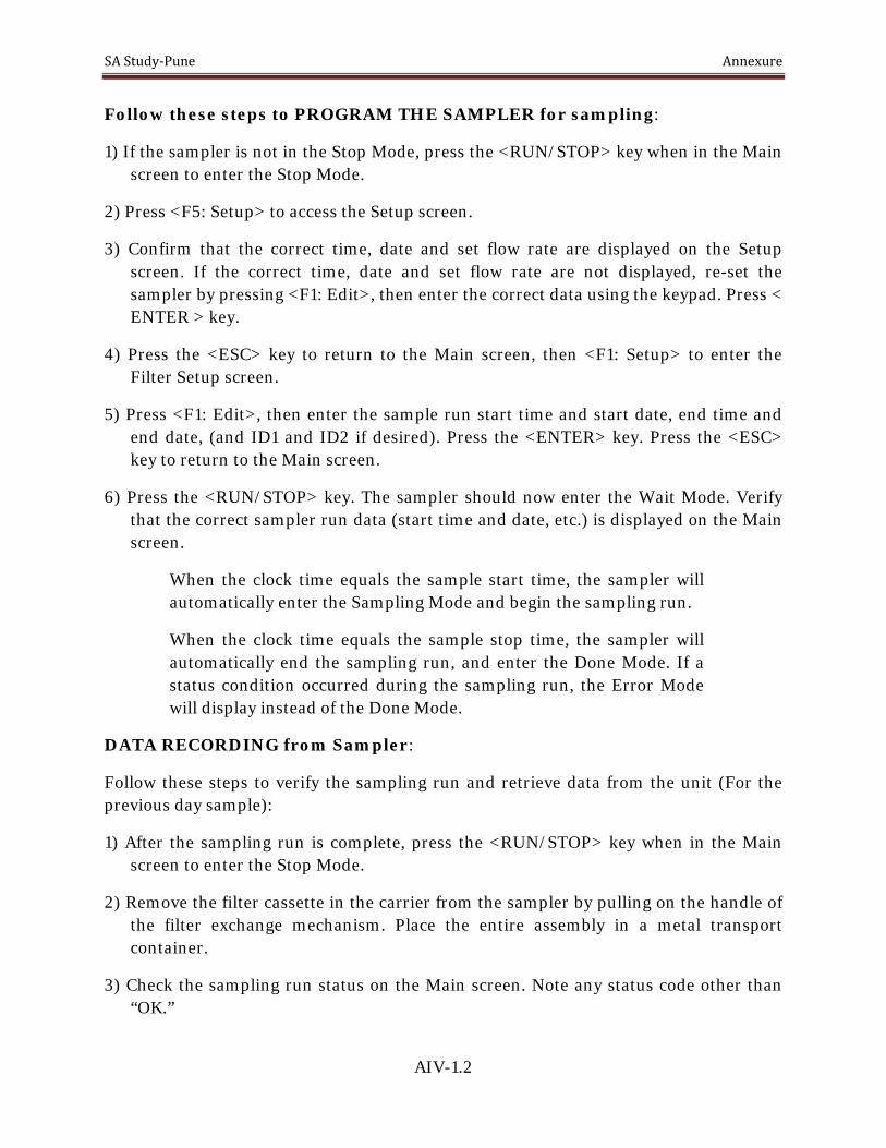
SA Study‐Pune Annexure
AIV-1.2
Follow these steps to PROGRAM THE SAMPLER for sampling:
1) If the sampler is not in the Stop Mode, press the <RUN/STOP> key when in the Main screen to enter the Stop Mode.
2) Press <F5: Setup> to access the Setup screen.
3) Confirm that the correct time, date and set flow rate are displayed on the Setup screen. If the correct time, date and set flow rate are not displayed, re-set the sampler by pressing <F1: Edit>, then enter the correct data using the keypad. Press < ENTER > key.
4) Press the <ESC> key to return to the Main screen, then <F1: Setup> to enter the Filter Setup screen.
5) Press <F1: Edit>, then enter the sample run start time and start date, end time and end date, (and ID1 and ID2 if desired). Press the <ENTER> key. Press the <ESC> key to return to the Main screen.
6) Press the <RUN/STOP> key. The sampler should now enter the Wait Mode. Verify that the correct sampler run data (start time and date, etc.) is displayed on the Main screen.
When the clock time equals the sample start time, the sampler will automatically enter the Sampling Mode and begin the sampling run.
When the clock time equals the sample stop time, the sampler will automatically end the sampling run, and enter the Done Mode. If a status condition occurred during the sampling run, the Error Mode will display instead of the Done Mode.
DATA RECORDING from Sampler:
Follow these steps to verify the sampling run and retrieve data from the unit (For the previous day sample):
1) After the sampling run is complete, press the <RUN/STOP> key when in the Main screen to enter the Stop Mode.
2) Remove the filter cassette in the carrier from the sampler by pulling on the handle of the filter exchange mechanism. Place the entire assembly in a metal transport container.
3) Check the sampling run status on the Main screen. Note any status code other than “OK.”

SA Study‐Pune Annexure
AIV-1.3
4) Press <F3: Data> to view the filter data from the sampling run. Record data from the Filter Data screen onto a sampling run log sheet.
5) If there were any status codes other than “OK,” verify the validity of the sampling run from the output of the Filter Data screen. Press <F4: PwrDat> to view the Power Outage Data screen. Press the <ESC> key to return to the Filter Data screen.
6) Insert a new filter cassette assembly with a 47 mm filter into the filter exchange mechanism. Push the handle to raise the platform, and enclose the filter cassette in the sampling position.
STATUS CODES
The sampler displays operational status codes in the upper left-hand corner of the Main screen next to “Stat,” as well as on several other screens. The hardware resets the status to “Ok” (no current conditions) after the user presses <F4:Run/Stp> from the Main screen to return the unit to the Stop Operating Mode.
7) Write down the status code in the Log-sheet (Ok, F, X, S, P, T, I, V, E, C)
TURNING OFF THE PARTISOL-FRM SAMPLER
1) Display the Main screen by pressing <ESC> repeatedly, if necessary.
2) If the device is not in the Stop Operating Mode, press <F4: Run/Stp> to enter the Stop Operating Mode.
3) Press the power switch on the main panel of the Partisol-FRM Sampler into its “OFF” (“0”) position.
CCaalliibbrraattiioonn ooff PPaarrttiissooll 22000000 FFRRMM SSaammpplleerr
FLOW AUDIT
Perform the ambient temperature audit; filter temperature audit, pressure audit and external leak check before executing the flow audit procedure.
Follow these steps to perform a flow audit:
1) When in the Setup screen, press <F5: Audit> to display the Audit screen.
2) Install a filter cassette containing a 47 mm filter into the hardware. This filter will be thrown away at the end of this flow audit.

SA Study‐Pune Annexure
AIV-1.4
3) Remove the PM-10 inlet from the end of the sample tube.
4) If you are using the Streamline Flow Transfer Standard (FTS) to audit the flow of the Partisol-FRM Sampler, go to step 5. If you are not using the Streamline FTS to audit the flow of the Partisol- FRM Sampler, go to step 13.
5) Press the <ESC> key to display the Setup screen.
6) When in the Setup screen, press <F1: EDIT>.
7) Press the down (<↓>) arrow to display the “FTS CONST m” field.
8) Locate the “m” constant on the FTS Calibration sheet, and enter it into the “FTS CONST m” field.
9) Press the down (<↓>) arrow to display the “FTS CONST b” field.
10) Locate the “b” constant on the FTS Calibration sheet, and enter it into the “FTS CONST b” field.
11) Press the <ENTER> key.
12) Press <F5: Audit> to display the Audit screen. Go to step 13.
13) If you are using the Streamline FTS to audit the flow of the Partisol-FRM Sampler, install the Streamline FTS onto the end of the sample tube. If you are not using the Streamline FTS to audit the flow of the Partisol-FRM Sampler, you may need to install the flow audit adapter (57-000618) onto the end of the sample tube. If you will be using the flow audit adapter, ensure that you install it onto the end of the sample tube with its valve in the open position.
14) Press <F3: Pump>.
15) Press <F2: Valve>.
16) If you are using the Streamline FTS, go to step 17. If you are not using the Streamline FTS, go to step 19.
17) Press <F1: Edit>.
18) Enter the pressure drop (inches H2O) in the “FTS Pres” field, and then press the <ENTER> key. The unit will automatically calculate the flow (l/min) and display it in the “FTS Flow” field. Go to step 21.
19) Determine the flow in units of actual (volumetric) l/min using the external flow meter.

SA Study‐Pune Annexure
AIV-1.5
20) Verify that this flow matches the value displayed in the “Flow Rate” field to within ±4%. If the flow rate measured on the flow meter matches the value displayed in the “Flow Rate” field to within ±4%, go to step 21. If the flow rate measured on the flow meter does not match the value displayed in the “Flow Rate” field to within ±4%, perform the flow calibration procedure.
21) Verify that the flow rate measured on the flow meter matches the sampler’s original flow design value (16.7 l/min) to within ±5%. If the flow rate measured on the flow meter matches the sampler’s original flow design value (16.7 l/min) to within ±5%, go to step 22. If the flow rate measured on the flow meter does not match the sampler’s original flow design value (16.7 l/min) to within ±5%, calibrate the external flow meter.
22) return to the Main screen by pressing the <ESC> key twice.
23) Remove the flow metering hardware.
24) Install the PM-10 inlet onto the end of the sample tube.
25) Remove the filter cassette from the sampler and discard the 47 mm filter.
FLOW CALIBRATION-P2000
The temperature and pressure calibrations described above must be performed before performing the flow calibration. In addition, the leak check discussed in Section 9.2.4 must also be undertaken before executing the following instructions.
The Partisol-FRM Sampler supports both a single-point and five-point flow calibration routine (refer to the U.S. EPA 2.12 Quality Assurance Handbook, Section 6). R&P recommends that the user perform the flow calibration whenever the sampler has been transported, any electromechanical maintenance has been done, or the sampler flow deviates from the set flow by ±5%. The sampler should be calibrated at least once per calendar year.
SINGLE-POINT FLOW CALIBRATION-P2000
Follow these steps to perform the single-point flow calibration:
1) Return the sampler to the Main screen.
2) The device must be in the Stop Operating Mode to perform a single-point flow calibration.
3) Remove the PM-10 inlet from the sampler.

SA Study‐Pune Annexure
AIV-1.6
4) Install a filter cassette containing a 47 mm filter into the filter holding mechanism. This filter will be thrown away at the end of this flow calibration.
5) When in the Main screen, press <F5: Setup> and then <F2: Calib> to display the Calibration screen.
6) If you are using the Streamline Flow Transfer Standard (FTS) to calibrate the flow of the Partisol-FRM Sampler, go to step 7. If you are not using the Streamline Flow Transfer Standard (FTS) to calibrate the flow of the Partisol-FRM Sampler, go to step 14.
7) Press the <ESC> key to display the Setup screen.
8) Press <F1: Edit>.
9) Press the arrow keys to scroll down to the “FTS CONST” field.
10) Enter the “m” constant from the FTS Calibration sheet.
11) Enter the “b” constant from the FTS Calibration sheet.
12) Press the <ENTER> key.
13) Press <F2: Calib> to return to the Calibration screen.
14) Attach the Streamline FTS or other flow metering device to the sample tube. Other flow meters may require the use of the flow audit adapter, which should be installed with its valve open.
15) Leave the pump turned off. If it is currently on, press <F7: Flow> to turn it off.
16) Press <F1: Edit> to enter the Edit Mode, and move the cursor to the row labeled “Flow” under the “Act” (actual) column.
17) Enter “0” in this position and press the <ENTER> key. This causes the microprocessor to compute the “Offset” value, which is the zero offset value for the mass flow controller. Record this value for future reference.
18) Turn on the pump by pressing <F7: Flow>.
19) Press <F8: DecrFlow> to continuously decrease the flow, <F9: HoldFlow> to maintain the current flow rate, and <F10: IncrFlow> to continuously increase the flow, until the flow rate displayed in the “Calc” column of the Calibration screen is approximately 16.7 l/min.

SA Study‐Pune Annexure
AIV-1.7
20) Determine the flow in actual l/min using the external flow meter. If you are using the Streamline FTS, go to step 21. If you are not using the Streamline FTS, go to step 23.
21) Enter the pressure (inches H2O) in the “FTS Pres” field by pressing <F1: Edit>, entering the value using the keypad, then pressing the <ENTER> key. The sampler will calculate the volumetric flow in l/min.
22) If you are using the Streamline FTS, the sampler will automatically display the calculated flow in the “ACT” field and compute the “Span” value. The “Span” value is the span offset value for the mass flow controller. Record this value for future reference. Go to step 25.
NOTE: If the instrument has been reset and you have recorded the “Offset” and “Span” values for the flow, you may enter these values directly when in the Edit Mode.
23) Press <F1: Edit> to enter the Edit Mode and moving the cursor to the row labeled “Flow” under the “Act” (actual) column.
24) Enter the volumetric flow rate measured by the external flow meter and press the <ENTER> key. The unit will now compute the “Span” value, which is the span offset value for the mass flow controller. Record this value for future reference. Go to step 25.
NOTE: If the instrument has been reset and you have recorded the “Offset” and “Span” values for the flow, you may enter these values directly when in the Edit Mode.
25) return to the Main screen by pressing the <ESC> key twice.
26) Restore the sampling hardware to its original state by removing the flow metering hardware and reinstalling the PM-10 inlet on the sample tube. Remove the filter cassette from the sampler, and discard the installed filter.
FIVE-POINT FLOW CALIBRATION-P2000
Follow these steps to perform the five-point flow calibration:
1) Return the sampler to the Main screen.
2) The device must be in the Stop Operating Mode to perform a five-point flow calibration.
3) Carefully remove the PM-10 inlet from the sampler.
4) Install a filter cassette containing a 47 mm filter into the filter holding mechanism. This filter will be thrown away at the end of this flow calibration.

SA Study‐Pune Annexure
AIV-1.8
5) When in the Main screen, press <F5: Setup>, <F2: Calib> and then <F2: Flow Cal> to display the Flow Calibration screen.
6) If you are using the Streamline Flow Transfer Standard (FTS) to calibrate the flow of the Partisol-FRM Sampler, go to step 7. If you are not using the Streamline FTS to calibrate the flow of the Partisol-FRM Sampler, go to step 14.
7) Press the <ESC> key to display the Setup screen.
8) Press <F1: Edit>.
9) Press the arrow keys to scroll down to the “FTS CONST” field.
10) Enter the “m” constant from the FTS Calibration sheet.
11) Enter the “b” constant from the FTS Calibration sheet.
12) Press the <ENTER> key.
13) Press <F2: Calib> to return to the Calibration screen.
14) Attach the Streamline FTS or other flow metering device to the sample tube. Other flow meters may require the use of the flow audit adapter, which should be installed with its valve open.
15) Press <F2: Start> to begin the five-point flow calibration routine.
16) With the pump turned off, the sampler first computes the flow offset value before automatically starting the span calibration using five flow rates around the default sample flow rate of 16.7 l/min.
NOTE: Follow the instructions displayed by the sampler at the bottom of the Flow Calibration screen.
17) Determine the flow in actual l/min using the external flow meter. If you are using the Streamline FTS, go to step 18. If you are not using the Streamline FTS, go to step 20.
18) Press <F1: Edit>.
19) Enter the pressure (inches H2O) in the “FTS Pres” field, then press the <ENTER> key. The sampler will now calculate the volumetric flow in l/min.
20) The unit will now operate at flow rates of 16.7, 17.5, 15.8, 18.3 and 15.0 l/min in succession. If you are using the Streamline FTS, go to step 21. If you are not using the Streamline FTS, go to step 22.

SA Study‐Pune Annexure
AIV-1.9
21) The sampler will automatically enter the calculated flow into the “ACT” field and compute “Span” value, which is the span offset for the mass flow controller. Go to step 23.
NOTE: If the instrument has been reset and you have recorded the “Offset” and “Span” values for the flow, you may enter these numbers directly when in the Edit Mode.
22) When in the Flow Calibration screen, wait for the “Current Flow” value to stabilize at each of these levels (16.7, 17.5, 15.8, 18.3 and 15.0 l/min). When “Current Flow” value stabilizes at each of these levels, press <F1: Edit>, move the cursor to the “Actual Flow” field, and enter the flow rate displayed by the external flow meter. Then press the <ENTER> key. The sampler uses this information to compute the proper flow span value. Go to step 23.
NOTE: If the instrument has been reset and you have recorded the “Offset” and “Span” values for the flow, you may enter these numbers directly when in the Edit Mode.
23) Return to the Main screen by pressing the <ESC> key three times.
24) Restore the sampling hardware to its original state by removing the flow metering hardware and reinstalling the PM-10 inlet on the sample tube. Remove the filter cassette from the sampler, and discard the installed filter.

SA Study‐Pune Annexure
A IV-2.1
2. Work Instructions for Speciation Samplers Partisol 2300
Sampler Start-up:
1) Install the Chem Comb cartridges in the shelter.
2) Press the power switch on the main panel (lower left) to its “on” (1) position to activate the sampler.
3) If necessary, turn the adjustment knob, located to the right of the keypad / display, to adjust the contrast of the liquid crystal display (LCD).
Steps to program the sampler for a sampling run:
1) Install the desired number of Chem Comb cartridges in the Chem Comb shelter.
2) Ensure that your sampler is in the Stop Mode.
3) While in the Main screen, press <F1: St Codes> to display the Status Codes screen.
The following list details the system’s status codes and definitions:
OK No current status conditions.
Z Power Failure. A power outage occurred during sampling on the current filter. Power outage events of less than 60 seconds are not logged by the sampler.
U User Pressed Stop. The user pressed the <RUN/STOP> button during sampling.
4) While in the Status Codes screen, ensure that there are no status codes reported and the present status of the unit is “OK.” Then press <ESC> to return to the Main screen.
5) While in the Main screen, press <F4: Sample> to enter the Sample Setup screen. Press <EDIT>, choose your sampling program and enter the start time, sampling duration and sample repeat time for your sampling run(s). Press <ENTER> to save these changes.
SAMPLE SETUP SCREEN
NOTE: When in the Edit Mode, use the arrow keys (<↑>, <↓>, <←> and <→>) to select the field that you want to edit. After you have finished
editing the fields, press <ENTER> to save your changes

SA Study‐Pune Annexure
A IV-2.2
Press <F4: Sample> when in the Main screen to enter the Sample Setup screen. All of the fields in the Sample Setup screen can be edited when the sampler is in the Stop Operating Mode.
The following fields make up the Sample Setup screen:
5a-Sample Definition Type: This parameter allows the user to select the type of sampling program: BASIC, TIME, TIME2, ADV (Advanced), EPISOD (Episodic) and RS232. Basic 24-hour continuous sampling (BASIC) is the unit’s default setting. Press <+List> or <-List> in the Edit Mode to access the sampling program selections. Select BASIC
5b-Default Sample Start Time: When editing this parameter, treat each part of the time as a separate field.
5c-Default Sample Duration: The default for this parameter is “024:00.” When editing this parameter, treat each part of the time as a separate field.
5d-Default Sample Repeat Time: For the unit to sample for 24 hours, switch to the next cartridge or group of cartridges and then sample for another 24 hours, set the Default Sample Repeat Time and the Default Sample Duration to 024:00.
5e-Default Filter Type: The default for this parameter is “P” (EPA filter).
6) While in the Sample Setup screen, press <F4: Samp Set> to enter the specific sampling setup screen that matches the sampling program you selected in the Sample Setup screen (step 5). Check the values you have set for your sampling run(s). If these values are correct, press <ESC> to return to the Sample Setup screen. If the values are incorrect, check the System Setup screen and the Sample Setup screen to correct these values.
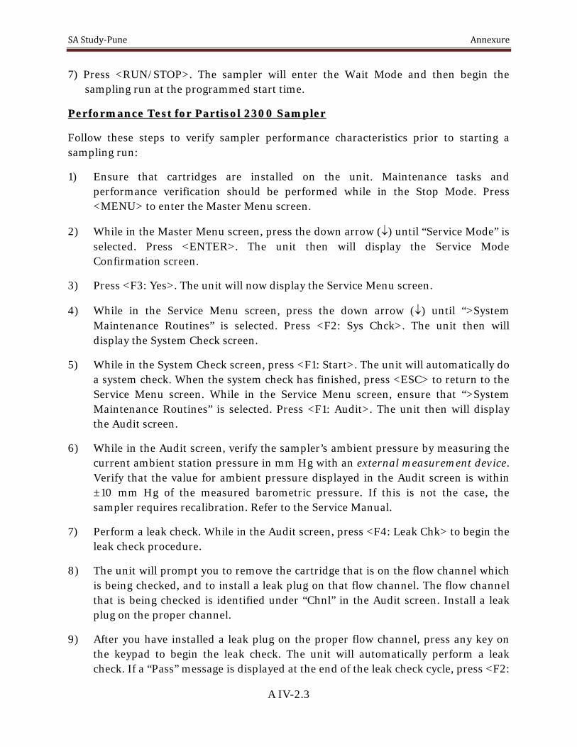
SA Study‐Pune Annexure
A IV-2.3
7) Press <RUN/STOP>. The sampler will enter the Wait Mode and then begin the sampling run at the programmed start time.
PPeerrffoorrmmaannccee TTeesstt ffoorr PPaarrttiissooll 22330000 SSaammpplleerr
Follow these steps to verify sampler performance characteristics prior to starting a sampling run:
1) Ensure that cartridges are installed on the unit. Maintenance tasks and performance verification should be performed while in the Stop Mode. Press <MENU> to enter the Master Menu screen.
2) While in the Master Menu screen, press the down arrow (↓) until “Service Mode” is selected. Press <ENTER>. The unit then will display the Service Mode Confirmation screen.
3) Press <F3: Yes>. The unit will now display the Service Menu screen.
4) While in the Service Menu screen, press the down arrow (↓) until “>System Maintenance Routines” is selected. Press <F2: Sys Chck>. The unit then will display the System Check screen.
5) While in the System Check screen, press <F1: Start>. The unit will automatically do a system check. When the system check has finished, press <ESC> to return to the Service Menu screen. While in the Service Menu screen, ensure that “>System Maintenance Routines” is selected. Press <F1: Audit>. The unit then will display the Audit screen.
6) While in the Audit screen, verify the sampler’s ambient pressure by measuring the current ambient station pressure in mm Hg with an external measurement device. Verify that the value for ambient pressure displayed in the Audit screen is within ±10 mm Hg of the measured barometric pressure. If this is not the case, the sampler requires recalibration. Refer to the Service Manual.
7) Perform a leak check. While in the Audit screen, press <F4: Leak Chk> to begin the leak check procedure.
8) The unit will prompt you to remove the cartridge that is on the flow channel which is being checked, and to install a leak plug on that flow channel. The flow channel that is being checked is identified under “Chnl” in the Audit screen. Install a leak plug on the proper channel.
9) After you have installed a leak plug on the proper flow channel, press any key on the keypad to begin the leak check. The unit will automatically perform a leak check. If a “Pass” message is displayed at the end of the leak check cycle, press <F2:

SA Study‐Pune Annexure
A IV-2.4
+ Chan> to switch the unit to the next flow channel. If a “Fail” message is displayed, refer to the Service Manual.
10) Re-install a cartridge on the flow channel that passed the leak check. Press <F4: Leak Chk> to begin the leak check procedure on the next flow channel, and follow the instructions on the unit’s screen. Repeat the leak check procedure for all of the flow channels.
11) Verify the sampler’s flow. Ensure that the unit is set on the flow channel that you want to verify. Press <F5: Audit> and follow the instructions displayed on the unit’s screen. The unit will automatically verify the flow rate.
12) A “Pass” or “Fail” message will display at the end of the flow verification procedure. If a “Fail” message is displayed, refer to the Service Manual. If a “Pass” message is displayed at the end of the flow verification procedure, proceed to step 13.
13) Press <F2: + Chan> to switch the unit to the next flow channel. Press <F5: Audit> and follow the instructions displayed on the unit’s screen. Repeat the flow verification procedure for all of the flow channels.
RReettrriieevvaall ooff DDaattaa ffrroomm PPaarrttiissooll 22330000
Follow these steps to verify the sampling run status and retrieve the sampling run data:
The Partisol Speciation Sampler stores three types of data in its internal data logger: filter data, interval data and input data. This information is stored in three separate circular buffers whose contents can be viewed on the screen of the sampler and/or downloaded through the RS232 port. Once these buffers are filled, the oldest data points are replaced with the most recent information (“first in, first out”). The following describes the three types of data stored internally in the hardware:
Filter Data Each record in this buffer contains information for a different collection filter exposed to the sample stream. The sampler displays records from this buffer in the Filter Data Statistics screen and its sub-screens. These screens contain information about the operation and status of the sampler while it sampled through each cartridge, calculated averages of cartridge data recorded by the sampler and a list of the unit’s recorded power failures during sampling. The Partisol Speciation Sampler has a capacity of 240 records of filter data.
Interval Data The sampler writes a new record of interval data every 5 minutes. Each record contains the latest 5- minute average of the ambient temperature, ambient pressure and average flow rate(s). The unit displays

SA Study‐Pune Annexure
A IV-2.5
records from this buffer in the Interval Data screen. The Partisol Speciation Sampler has a capacity of 16 days of interval data.
Input Data The sampler stores calculated averages of meteorological data and other information received through its analog input channels at the rate specified by the user in the Average Time field of the System Setup screen. The unit displays these stored values in the Input Data screen. The sampler has a data storage interval of 30 minutes and a 32-day capacity of input data.
1) If the sampler has not been previously set up for data transfer to a PC, check the RS232 setup in the RS232 Setup screen. Press <F3: System> from the Main screen to display the System Setup screen. Press <F1: I/O>, then <F1: RS232> to enter the RS232 Setup screen. Make sure that the parameter in the Protocol field is set correctly for the file transfer software installed in the PC (refer to Section 10.2.1 for setting RS232 parameters). Press <ESC> twice to return to the Main screen.
2) Connect the PC to the sampler with the 9-to-9 pin RS232 cable. Use any data transfer program such as Pro Comm. Plus to transfer data from the sampler to the PC.
3) Check the sampling run status on the Main screen, and note any status code other than “OK.” Press <F5: Data> to enter the Filter Data Statistics screen and view the filter data from the sampling run. Record data from the Filter Data Statistics screen onto a sampling run log sheet if desired. If there were any status codes other than “OK,” check the Cartridge Data Status Codes screen to verify the validity of the sampling run.
4) While in the Filter Data Statistics screen, press <F1: More Dat> twice to reach the Cartridge Data Status Codes screen. After checking the validity of the sampling run from this screen, press <ESC> until you return to the Main screen.
5) Press <F3: System> from the Main screen to display the System Setup screen. Press <F1: I/O>, then <F1: RS232> to enter the RS232 Setup screen. Press <EDIT> and set the Protocol field to “Storage.” To save this change, press <ENTER>. Press <ESC> until you return to the Main screen.
6) Press <F5: Data> to display the Filter Data Statistics screen. The record from the last sampling run is displayed in the upper right hand corner of the Filter Data Statistics screen. Press <F5: Download> to display the Download Data screen. Scroll to the Last Record field, and use the <F4: Last> key to select the last data record. Scroll to the First Record field, and use the <F1: First> to select the first data record. Press the <F2: - Ptr> or <F3: +Ptr> key to select the first data record you want to download.
7) Once the PC communications software is ready to receive the records, press <F5: Download> while in the Download Data screen. The sampler will download all data

SA Study‐Pune Annexure
A IV-2.6
from the currently displayed record to the last record in the data file. If you need to download output for interval data, status codes or any of the other screens accessed from the Filter Data screen, display the screen and repeat the download process.
8) If any status code conditions occurred, press <ESC> to return to the Main screen. From the Main screen, press <F1: St Code> to reach the Status Codes screen. Press <F1: Reset> to reset the unit’s status condition for the next run to “OK.”
33 SSOOPP ffoorr mmiiccrroobbaallaannccee Internal calibration External calibration EQUIPMENTS USED FOR CALIBRATION:
Select the appropriate Master Equipment. Master Equipment to be selected by using following criteria-
a. Uncertainty of Master should be better than the Accuracy requirement of balance or at least equal to Accuracy requirement of balance, where it is not possible to maintain Test Uncertainty Ratio.
b. It should have valid calibration. c. The traceability to National / International Standards directly or
through accredited laboratory. The appropriate Standard Weights may be selected from following for Balance Calibration:
PREPARATION:
• Enter the necessary information regarding the Master equipment and the balance in Calibration Result Sheet.
• Select the operating manual for the Master equipment • Check the availability of the specified power supply for selected balance • Check the leveling of the balance. For leveling refer the procedure given in the manual
of balance (if required) • Ensure that the balance is clean and dry. • Ensure the identification of the balance. • Switch on the balance and allow it to warm up for 15-20 minutes or as specified in its
manual.
ENVIRONMENTAL CONDITIONS :
Temperature: 18°C to 35°C
Humidity : < 80%

SA Study‐Pune Annexure
A IV-2.7
METHOD OF CALIBRATION:
Before starting the calibration, Balance should be exercised near to its full range at least for 3 times. After completion of this exercise following procedure to be followed.
Balance Calibration
For the proper operation of BALANCE, refer its operating manual
For Digital Balance Tests for the following parameters to be performed
i. Repeatability (Using minimum ten repeated measurements when calibrating a range up to 50 kg, and a minimum of five repeated measurements when calibrating a range exceeding 50 kg) : This test can be performed at or near the nominal maximum capacity of BALANCE or at the largest load generally weighed, returning to zero after each reading.
For BALANCE having more than one range, this test should be carried out for each range.
Note down the above readings and take these for repeatability “Type -A” component in Uncertainty Calculations.
ii. Departure of Indication from nominal value : This test can be performed on equidistant points in the selected range. Preferably, the number of test points should not be less than 5.
Note down the above readings and take these for Calculations of deviation.
iii. Eccentric or off-center loading : Using a load between 1/4 and 1/3 of the maximum capacity of BALANCE typically placed between 1/2to 2/3 of the distance from the center of the load receptor to the edge, in a sequence of center, front left, back right, center or equivalent.
Note down the above readings and report these in calibration report.
Weighing on balance (Sample preparation)
• Filter Identification (Labeling) o Teflon, Nylon, Quartz 47 mm papers in petridishes o Number-label to petridishes o Glass fibre paper ID using automatic numbering machine
• Filter conditioning

SA Study‐Pune Annexure
A IV-2.8
o Conditioning of filter for 24 hrs at 20-30 deg. C and around 50% RH as follows-
Teflon (Des/T-01) Nylon (Des/N-01) Quartz (Des/Q-01)
• Filter weighing (Initial weight) o Weighing of Teflon, Nylon, Quartz 47 mm papers in triplicates using
Balance (Make Afcotech- AML/INST/117, accuracy 0.01 mg) and noting down average of three.
o Weighing of Glass fibre filter papers in triplicates using Balance (Make Afcotech- AML/INST/118, accuracy 0.1 mg) and noting down average of three.
Sample ready for loading at site to be stored in Petridishes in respective Cold Storage Box

SA Study‐Pune Annexure
A IV-3.1
3. Chemical Analysis of Molecular Markers
(Chapter – 2)
1.0 SCOPE This method describes a procedure for separating saturate and aromatic hydrocarbon compounds from particulate matter samples. This method describes a gas chromatography/mass spectroscopy (GC/MS) technique for determination of hydrocarbon compounds including C8 through C41 normal alkenes, target polycyclic aromatic hydrocarbons (PAHs), alkylated PAHs, Hopanes and other biomarkers listed in following Table 1.
2.0 REFERENCE DOCUMENT 1. “Conceptual Guidelines and Common Methodology for Air Quality Monitoring,
Emission Inventory And Source Apportionment Studies For Indian Cities” (November 06) prepared by
Dr. A.L.Aggrawal, Consultant, ASEM – GTZ Dr. Prashant Gargava, Environmental Engineer, CPCB Abhijeet Pathak, SSA, CPCB 2. Model Standard Operating Procedure for Organic Speciation (Molecular Markers) (Chapter X)-February 07 3. MSDS of Chemicals & Reagents specified in this method.
3.0 SUMMARY OF TEST PROCEDURE PRINCIPLE
Organic molecular markers attached or adhered to the particles are extracted in suitable solvents. Then cleaned and pre-treated according to requirement and finally analysed using GC-MS in SIM mode.
4.0 APPARATUS: 4.1 GC/MS System: (Schimadzu make Model QP5050) The mass spectrometer is
operated in both scan and SIM mode utilizing 70-volt electron energy in the electron impact ionization mode and producing a qualified mass spectrum. A computer system, interfaced to the mass spectrometer, is used for system control as well as data acquisition, storage and data processing.
4.2 GC Columns: 30 m long x 0.25 mm ID, 0.25 µm film thickness capillary DB-5 MS or equivalent column will be used in GC/MS system for analyses of PAHs, alkylated PAH, Hopanes and Other Biomarkers listed in Table.
4.3 Apparatus for Sample Extraction and Concentration
• Glassware: All glassware are washed and rinsed manually with deionised water. It is then rinsed with three portions each of acetone and Dichloromethane. Glassware is air-dried in an oven and then stored in a contaminant free area.

SA Study‐Pune Annexure
A IV-3.2
• Ultrasonic bath and Vacuum filtration system. • Soxhlet Extractor Soxhlet Extraction Assembly: 250 ml Capacity of round bottom Flask • Analytical balance capable of accurately weighing 0.0001 g. • Erlenmeyer flasks, 250 mL. • Beakers: 100, 250 and 500 mL. • Glass funnel • Glass wool and glass fibre filters (9.0 cm). • Graduated cylinder: 100 ml • Vials: 5 mL and 15 mL, with Teflon-lined screw cap septa. • Pipettes: Pipettes with capacities from 10 to 1000 µL capacity and appropriate
condensers. • Syringe: 5ml capacity • Macro Kuderna Danish Concentrator with ground glass joints (Supelco ,Sigma
Aldrich Make) – Note: The Soxhlet extraction assembly should be vented into a hood to prevent unnecessary exposure of the analyst to the organic vapor.
5.0 REAGENTS
5.1 All solvents should be of ultra pure HPLC grade or equivalent.
5.2 Dichloromethane (Extra Pure): For Soxhlet Extraction 5.3 Acetone (Extra Pure): For Soxhlet Extraction 5.4 Reagents For Sample Methylation: 5.4.1 Diethyl ether 5.4.2 N-nitroso-N-methyl Urea (Sigma Aldrich make) 5.4.3 Potassium hydroxide (5 N) 5.4.4 Methanol 5.5 Reagents For Sample Silylation:
300 ul BSTFA [N, O-Bis (trimethyl silyl) trifluoroacetamide] (99%) + 1% TMCS (trimethylchlorosilane)

SA Study‐Pune Annexure
A IV-4.1
4. Application of CMB8.2
1. CMB8.2 Model Launch
A screen that first appears when EPA-CMB8.2 is launched prompts to select start-up options 1. Use control files, 2. Select Individual Input Files. Control Files are commonly used in air quality models to specify input files that will be invoked during runtime.
If Use Control File was selected, a browse dialog appears. This dialog allows the user to find a particular Control File. Once a Control File is chosen, the Select Input Files window appears where Control file can be selected.
2. Options
Several options are available in EPA-CMB8.2 that are selected from the Options tab where various values and selections may be changed from their default values.
2.1 Iteration Delta. This parameter sets the maximum number of iterations EPA-CMB8.2 will attempt to arrive at a solution. If no convergence can be achieved, there is probably excessive collinearity for this sample and combination of fitting sources. Its value is adjusted via the spinners. (Must be >0; no theoretical upper limit; default = 20)
2.2 Maximum Source Uncertainty / Minimum Source Projection. These parameters allow the eligible space collinearity evaluation method of Henry to be implemented with each CMB calculation. The eligible space method uses: 1) maximum source uncertainty; and 2) minimum source projection on the eligible space. The maximum source uncertainty is a threshold expressed as a percentage of the total measured mass and is adjustable via the spinners (default = 20%; acceptable range 0 - 100). The minimum source projection is set to a default value of 0.95 (acceptable range 0.0 - 1.0), but can be changed in the display field.
2.3 Decimal Places Displayed. This parameter sets the number of decimal places displayed in the output window and output files. This depends on the units used in the input data files. For example, data reported in ng/m3 require fewer decimal places than values expressed in µg/m3. Reducing this value from 5 to 4 accommodates most PM2.5 mass and chemical concentrations expressed in µg/m3. This setting affects the display columns for source contributions estimates, measured species concentrations (ambient samples and source profiles), calculated contributions by species, as well as for inverse singular values. This parameter may be adjusted by using the spinners. The default value is 5 and the maximum value is 6.
2.4 Units. The units used for reporting results may be changed via a pull-down menu. Other typical units are available, or one may be created (the number of characters is limited to 5 or less).

SA Study‐Pune Annexure
A IV-4.2
2.5 Output File Format. The file format for spreadsheet-type output is selected in the pull-down box. As discussed in Section 4.5, the default is ASCII (txt); comma-separated value (CSV) is also available (which ports nicely to Microsoft Excel®). This selection is echoed on the status bar at the top of the screen.
2.6 Britt and Luecke. Checking this box applies the Britt and Luecke linear least squares solution. This option allows the source profiles used in the fit calculation to vary, and enables a general solution to the least squares estimation that includes uncertainty in all the variables (i.e., the source compositions as well as the ambient concentrations). The Britt-Luecke algorithm, as implemented in EPA-CMB8.2, has not undergone comprehensive testing, and is not recommended for inexperienced users
2.7 Source Elimination. Checking this box eliminates negative source contributions from the calculation, one at a time. After each fit attempt, if any sources have negative contributions, the source with the largest negative contribution is eliminated and another fit is attempted. This process is repeated until EPA-CMB8.2 finds no sources with negative contributions. Invocation of this option affects the fit obtained by effectively removing collinear sources
2.8 Best Fit. Checking this box causes the program to cycle through the corresponding pairs (same array index) of fitting species and source profile arrays specified in the source and species selection input windows until the best composite Fit Measure has been achieved. When Best Fit is invoked, EPA-CMB8.2 ignores any arrays of species and sources that may have been selected. The first fitting species array is paired with the first fitting sources array, and so on. EPA-CMB8.2 only attempts a search for a best fit among available corresponding pairs. Any arrays without a corresponding array to make a pair are ignored. The fit with the largest Fit Measure is then displayed and becomes the current fit. After a Best Fit has been made, the fitting species and fitting sources arrays will be tagged (highlighted) in their respective windows.
2.9 Fit Measure Weight. These are the weights (coefficients) applied to each of the performance measures chi square, r-square, percent mass, and fraction of eligible sources (number in eligible space divided by number of fitting sources). Adjustment of these weights is not enabled in EPACMB8.2 unless Best Fit is invoked. Positive values between 0 and 1 may be entered by typing into the appropriate display fields. Defaults are 1.0 for each performance measure weight.
3. Sample selection:
Individual samples are “tagged” by clicking in the respective fields under “SELECTED”. Clicking again deselects the sample. Use of Select /Clear All Samples may also be used to help establish the desired list of samples.

SA Study‐Pune Annexure
A IV-4.3
Toggling between View Selected/View All determines whether data will be displayed for selected (tagged) samples only, or for all samples in the list. Clicking View Graph will provide a bar chart for any sample (selected or not) for which any field is filled with blue. This graph is useful to verify that input data files have been properly read.
3.1 Select Fitting Species:
Fitting species should be selected that are major or unique components of the source types influencing the receptor concentrations.
Species contained in the selection file are listed down the left hand side and a field of up to 10 arrays is provided. At startup, the first array (in a series) will always be initially selected as a default. Other arrays may be selected by clicking on the array index (1 - 10). Within a given array that is first activated by clicking its index number, species may be added or removed by clicking in the appropriate field. Select/Clear All Array X may also help in configuring a selection array.
3.2 Select Fitting Sources
Fitting source profiles are included in the CMB calculation. The user should select profiles that represent the emissions most likely to influence receptor concentrations. Several profiles may be available that represent the same source type, but only one of these is usually used as a fitting source. Profiles of similar chemical composition are often found to be collinear when two or more are selected as fitting sources.
As with fitting species, arrays are selected by clicking on the array index (1 - 10). Within a given array, source profiles may be added or removed by clicking in the appropriate field. Select/Clear All Array X may also help in configuring a selection array. As for ambient samples, clicking View Graph will provide a bar chart for any source profile (selected or not) for which any field is filled with blue This graph is useful for visual inspection; it helps to verify that input data files have been properly read and to identify abundant components in each profile. View Grid returns to the array screen.
3.3 Running model
When Run is invoked, EPA-CMB8.2 performs the least-squares estimation of source contribution estimates and performance measures on the selected sample data using the designated fitting species and source profiles. Note also that if more fitting sources than fitting species have been selected, a warning appears and the user is forced to reconfigure.

SA Study‐Pune Annexure
A IV-4.4
4. Input files preparation
Six data files are normally used for input to EPA-CMB8.2, the first of which is a control file that directs EPA-CMB8.2 to five specific files. Three of the files are optional selection files, which provide substantial user convenience by establishing commonly used arrays and sample subsets that would otherwise need to be initialized each time the model is run. The remaining two - the ambient and source profile data files - are required by EPA-CMB8.2.
4.1 Control File: IN*.in8
This fixed format file contains a list of the names of EPA-CMB8.2 input data files, all of which must reside in the same directory that stores the Control File itself. This filename consists of five lines as shown below. These lines, in succession, contain the names of the files which are described in the following subsections. If a selection file is absent, the corresponding line in the Control File should be labeled with one or more characters, e.g., a series of asterisks (‘******’) - or any name that doesn’t reside in the Control File directory. Here’s an example:
PRpune.sel
SPpune.sel
*******
ADpune.csv
PRpune.csv
File name entries should be left justified and in the sequence shown. In EPACMB8.2, the only restriction on file names is that they are acceptable to the operating system. The utility of the Control File is to save the effort of keying in the input filenames individually. If a Control File is not used at startup, EPACMB8.2 will accept the names of individual data input files on the fly, provided they are compatible with each other.
4.2 Ambient Data Input File:
Ambient data files may be formatted as comma-separated values in ASCII text (*.csv), xBASE (*.dbf), blank-delimited ASCII text (*.txt), or Lotus Worksheet (*.wks). The csv and dbf formats are preferred, as they are easier to prepare in spreadsheet The appropriate file extension must be associated with each format, as EPACMB8.2 recognizes the file type by this extension.
Following is an example file:
ID,DATE,DUR,STHOUR,SIZE,TMAC,TMAU,N3IC,N3IU,.....,PBXC,PBXU

SA Study‐Pune Annexure
A IV-4.5
BAKERS,06/20/88,24,0,FINE,17.2788,0.9920,0.2816,0.1715,.....,0.0236,0.0052
Of the first 5 field names in the header, note that as currently configured, EPA-CMB8.2 limits the first 2 field names to 4 characters; the last 3 fields must be named identically as indicated above. The “total” pair (e.g., TMAC & TMAU) preceding the species list differentiates the AD*.* header from that for PR*.*; there is no practical limitation for the pair names. All subsequent species names in the header are restricted to 6 characters.
The 1st line contains the field identifiers, followed by (beginning in field 6) the species codes, which occur in pairs (concentration, followed by uncertainty). Note that the name (code) for the concentration component of each pair must correspond identically (including case) with its counterpart in both the species selection files (SP*.sel) and the source profile data input file (PR*.*). Note that it is on this line where EPACMB8.2 gets the labels that appear in the species selection window (not from the species selection file, SP*.sel). Regardless of how the AD*.sel file is organized in terms of the sequence of ambient samples listed, in the sample selection screen they will appear according to the sequence dictated by the ambient data file (e.g., AD*.txt). Note also this line is the source of all species labels appearing in the Main Report. Beginning with the 2nd line are the actual data, one line per ambient sample, starting with the Site ID in Field 1. Note also that it is this ambient data input file that controls the sequence of ambient samples displayed in the samples selection window (not the samples selection file, AD*.sel). The records for each sample are formatted as follows:
Field 1: Site ID (up to 12 characters)
Field 2: Sampling date (up to 8 characters)
Field 3: Sample duration (up to 2 characters)
Field 4: Sample start hour (up to 2 characters)
Field 5: Particle size fraction (up to 6 characters)
Field 6: Total Mass concentration (any number of characters in integer, floating point, or exponential format)
Field 7: Uncertainty of total mass concentration (same format as Field 6)
Field 8+2n: Concentrations of chemical species (same format as Field 6), where n = 0, 1, 2, ...
Field 9+2n: Uncertainty of species concentrations (same format as Field 6), where n = 0, 1, 2,

SA Study‐Pune Annexure
A IV-4.6
...
EPA-CMB8.2 always assumes that Field 6 is the total mass concentration, and it does not use this as a fitting species. Uncertainty values in fields 7 and 9+2n are in the same units as the measured concentration values.
Positive uncertainty values (> 0) must be assigned to all (non-missing) chemical concentrations used as fitting species. EPA-CMB8.2 will return an error message when it detects (in the input data file for ambient samples) a value for uncertainty that is less than or equal to zero for any species concentration value not flagged as missing. A species for which the concentration value is missing (i.e., invalid) cannot be used as a fitting species for that sample. Missing values for either concentrations or associated uncertainty must be designated by placing -99. in the appropriate field in the data file.
4.3 Source Profile Input File
Source profile data files may be formatted as comma-separated values in ASCII text (csv), xBase (dbf), blank-delimited ASCII text (txt), or Lotus Worksheets (wks). The csv and dbf formats are the most portable and easily prepared.
The appropriate file extension must be associated with each format, as EPA-CMB8.2 recognizes the file type by this extension. Examples of all supported file types are provided with EPA-CMB8.2's test case. Following is an example file:
PNO,SID,SIZE,N3IC,N3IU,.....,PBXC,PBXU
SJV001,SOIL01,FINE,0.002700,0.004700,.......,0.000000,0.000000
As mentioned for the AD*.* file *, all species names in the header are restricted to 6 characters.
The 1st line contains the field identifiers followed by the species codes (fields > 3), which can be up to 6 alphameric characters in length. As with the ambient data input file, these codes appear in abundance / uncertainty pairs, and that the name (code) for the concentration component of each pair must correspond identically (including case) with its counterpart in both the species selection files (SP*.sel) and the ambient data input file (PR*.*). Beginning with the 2nd line are the actual data, one line per source profile. The first two fields are the source code and mnemonic, respectively. The source code must correspond identically with that used in the source profile selection file (PR*.sel) The limitations on each field are:
Field 1: Profile number or source code (up to 6 characters)

SA Study‐Pune Annexure
A IV-4.7
Field 2: Source mnemonic (up to 8 characters)
Field 3: Particle size fraction (up to 6 characters)
Field 4+2n: Fraction of species in primary mass of source emissions (floating point or exponential format), where n = 0, 1, 2, ...
Field 5+2n: Uncertainty of fraction of species in primary mass of source emissions (same format as Field 4), where n = 0, 1, 2, ....
If the name (code) used in field 1 does not match identically (including case) its counterpart in the source profile selection file, the source will not appear on the Sources selection screen when EPA-CMB8.2 is run, and thus not be available for use in a calculation. Source profile abundances are expressed in fractions of total mass, not in percent.
Unlike the ambient data file, the source profile input file does not contain a mass concentration field because all species abundances have been divided by this mass.
Missing values for chemical species in source profile files can be replaced by a best estimate with a large uncertainty if they are to be used as fitting species. Missing values must be flagged with –99. if the species is not intended for use as fitting species.
In certain cases in which an uncertainty value >0 is applied to a species whose abundance=0, the uncertainty represents the lower quantifiable limit of the measurement. A zero value for abundance means that the true value is something between zero and the detection limit. Zeros are important in some source profiles when they occur in other source profiles. This makes that species a marker for the source in which it occurs. The uncertainty for the zero adds to the effective variance weighting. If this uncertainty is high and the source contribution estimate is high, the influence of that species is reduced by the weighting.
4.4 Source (PR*.sel), Species (SP*.sel), and Sample Selection (AD*.sel) Input Files
The optional source, species and sample selection files provide initial selection arrays that do not have to be entered from the program each time a EPA-CMB8.2 session is begun. These files limit the profiles, species, and ambient data records to those listed in the selection file The selection files also dictate the sequence in which species and sources appear in the output. The total species list is that common to the species selection file, the ambient data file, and the source profiles file. The total sources list is that common to the sources selection file and the source profiles file. The total ambient samples list is that common to the ambient sample selection file and the ambient data file.

SA Study‐Pune Annexure
A IV-4.8
As with the source profile input file, the first fields are the source profile code and mnemonic, respectively. A source code with up to six characters is located in Columns 1 to 6. Columns 9 to 16 are available for an eight-character profile name (mnemonic). The names used in both fields must correspond identically with those used in the source profile input file For each source listed in the selection file, some information must appear in either (1) the mnemonic field, (2) the selection array field (at least one column must be tagged with ‘*’), or (3) the comment field in order for the source to appear on the selection screen in EPA-CMB8.2.
If the name used in field 1 does not match identically (including case) its counterpart in the source profile input file, or if any of the aforementioned conditions is not met, the source will not appear on the Sources selection screen when EPA-CMB8.2 is run, and thus not be available for use in a calculation.
A species code with up to six characters is located in Columns 1 to 6, and must correspond identically with that used in both the ambient data input file and source profile input data file. Columns 9 to 16 are available for an eight character species name, which is optional.
The maximum number of species is essentially unlimited. Comments can be added to this file beginning in column 39 to document the meaning and units of the chemical components Note that if the species code in field 1 doesn’t match exactly (including case) its counterpart in both the ambient data input file and the source profile input file, or is missing, the species will not appear in the selection screen when the model is run regardless of any other condition. If the species does not appear on the selection screen when EPA-CMB8.2 is run, it will not be available for use in a calculation.
For the ambient data records (sample) selection file, columns 1 through 12 are for the Site ID, columns 14 through 21 are for the date, columns 23 and 24 for the sample duration, columns 26 and 27 for the sample start hour, and columns 29-33 for the particle size fraction, if appropriate. Intermediate columns should be blank. An asterisk in column 36 initializes (selects) a record for processing.
5. Output Files
5.1 Report Output File
The report output file is generated from the Main Report screen and presents the source contribution estimates, standard errors, model performance measures, and measured and calculated chemical concentrations for each sample. The report written to the output file is identical to that which appears in the Output window during an interactive modeling session. It is in ASCII text format and can be imported into word processing programs to document the source contributions calculated for each sample. All

SA Study‐Pune Annexure
A IV-4.9
information needed to independently repeat the source apportionment is contained in this report, including an echo of the *.in8 input file that was used in its generation.
5.2 Data Base Output File
The data base (spreadsheet-type) output file records the contribution of each source-type to a particular species in a single data record, one record per species. Sample identifiers and model performance measures are also included in each record.
The file structure is:
Field 1: Species Code
Field 2: Species Name
Field 3: Fitting flag; a '*' indicates a fitting species, while a '_' indicates a floating species
Field 4: Sampling site identifier
Field 5: Sampling date
Field 6: Sample start hour
Field 7: Sample duration
Field 8: Particle size fraction
Field 9: Measured species concentration
Field 10: Uncertainty of measured species concentration
Field 11: Calculated species concentration
Field 12 Uncertainty of calculated species concentration
Field 13: R-square value
Field 14: Chi-square value
Field 15: Percent of measured mass
Field 16+2n: Source contribution estimate, n = 0, 1, 2, ....
Field 17+2n: Standard error of source contribution estimate, n = 0, 1, 2, ....
Fields 1, 2, and 4 through 8 record the sample information. Fields 3 and 11 through 15 provide information about the EPA-CMB8.2 calculation. The remaining fields correspond to each source profile in the PR*.* data file and contain the source contribution estimates and standard errors for these sources. A value of -99. is recorded

SA Study‐Pune Annexure
A IV-4.10
when a profile was not used in the calculation. The first record in this output file contains the field identifiers. All subsequent records contain data. Fields 16+2n and 17+2n are labeled with source codes and source names, respectively.
5.3 Reading Output Files
Main Report (ASCII) text files can be read directly into a word processing application where the detailed output for each sample can usually be displayed on a single page with columns aligned using a non-proportional font, e.g., a New Courier or Letter Gothic 8-point to 10-point.
The output file will be stored in the directory in which the Control File resides, which can be changed in the browse dialog). These output files can be opened directly by data base or spreadsheet applications, e.g., Microsoft’s Excel®, and from there exported into any of several different formats, e.g., xls.
The contents of the EPA-CMB8.2 output screen can also be selected and copied to the clipboard for pasting into other Windows® applications. Graphs made with EPA-CMB8.2 (Section 3.3 & 3.5) can be printed directly from the screen or copied to the Windows® clipboard via copy command, then pasted into a text box or frame in a word processing application.

SA Study‐Pune Annexure
A IV-5.1
5. DRI Standard Operating procedure for EC/OC analysis
(Chapter – 2)
1.0 REFERENCE DOCUMENT 1. Standard Operating Procedure (SOP) MLD 065 Standard Operating Procedure
for the analysis of Organic and Elemental Carbon in Particulate matter (PM) samples by using DRI Model 2001 TOR/TOT Carbon Analyzer.
2. Operation manual of DRI make Thermal/Optical Carbon Analyzer. 3. NABL 141 estimation & expression of uncertainty in measurement
2.0 SUMMARY OF TEST PROCEDURE PRINCIPLE
The operation of the DRI Model 2001 Thermal/Optical Carbon Analyzer is based on the Preferential oxidation of organic carbon (OC) compounds and elemental carbon (EC) at different temperatures. The principal function of the optical (laser reflectance and transmittance) component of the analyzer is to correct for pyrolysis charring of OC compounds into EC. Without this correction, the OC fraction of the sample might be underestimated and the EC fraction might include some pyrolyzed OC.
3.0 INSTRUMENT: Desert Research Institute (DRI) Model 2001A Thermal Optical Carbon Analyzer (AML/ INST/ 149) System with computer (ARAI/120/02/0562).
3.1 The programmable combustion oven is the heart of the carbon analyzer and includes loading, combustion, and oxidation zones in a single quartz "oven". In addition to the DRI Model 2001 thermal/optical analyzer, the following items are needed for routine carbon analysis: • Stainless steel punching tool: 5/16-inch diameter, 0.5 cm2 nominal area. • Syringes: Hamilton Gas-Tight 1000 µl syringe for calibration injections; 25 µl syringe for carbonate analysis and for analyzer calibration. • Flat-tip tweezers. • Flat glass plate. • Tissue paper • Lighter • Glassware
3.2 Gases: All gases are required of high purity grade

SA Study‐Pune Annexure
A IV-5.2
Sr. No.
Name of the gas Regulated pressure (psi)
Purpose
1 Helium 15-40 As a carrier gas
2 10 % O2 in helium 15 As a carrier gas
3 Hydrogen 15 As a fuel for FID
4 Zero air 15 As an Oxidiser for FID
5 Zero air ~25 For pneumatic activation
6 5% methane in He 10 Internal Calibration
7 5% CO2 in He 10 Calibration
4.0 REAGENTS • Potassium Hydrogen Phthalate (KHP) • Sucrose • Hydrochloric Acid (HCL) • Nanopure ASTM type 1 deionized water (>16 Mega Ohm-cm)
5.0 PROCEDURE: 6.1 Analyzer start-up (When the analyzer is started up for the first time, or after
an extended period of non-operation): • Check the gases for their pressures/settings. • Start all the gases except Air to FID on front panel • Start PC only. • Put on Analyzer (Switch is on the rear side of the analyzer.) • Set FID temperature to 125oC and Line Heater temperature to 105oC. • Heat Both Oxygenator to 912oC and Methanator to 425oC with an increment of
100oC with hold time 30 minutes at each increment. • It will take a period of three days for conditioning to reach a stable system
background. • When system stabilization is achieved then perform the leak check test. For daily
routine operation, start the operation with leak check test onwards. 6.2 Leak Check test
Close sample oven outlet toggle valve on right side of control panel. Wait for sample oven pressure display to reach approximately 5 units from 2.6
units. Then close sample oven inlet valve on the front panel.
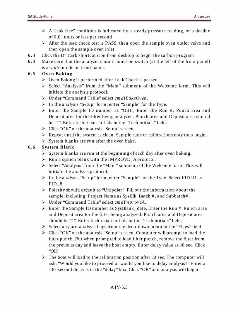
SA Study‐Pune Annexure
A IV-5.3
A “leak free” condition is indicated by a steady pressure reading, or a decline of 0.01 units or less per second
After the leak check test is PASS, then open the sample oven outlet valve and then open the sample oven inlet.
6.3 Click the DriCarb shortcut icon from desktop to begin the carbon program 6.4 Make sure that the analyzer’s multi-function switch (at the left of the front panel)
is at auto mode on front panel. 6.5 Oven Baking
Oven Baking is performed after Leak Check is passed Select “Analysis” from the “Main” submenu of the Welcome form. This will
initiate the analysis protocol. Under “Command Table” select cmdIBakeOven. In the analysis “Setup” form, enter “Sample” for the Type. Enter the Sample ID number as “OB1”, Enter the Run #, Punch area and
Deposit area for the filter being analyzed. Punch area and Deposit area should be “1”. Enter technician initials in the “Tech initials” field.
Click “OK” on the analysis “Setup” screen. Repeat until the system is clean. Sample runs or calibrations may then begin. System blanks are run after the oven bake.
6.6 System Blank System blanks are run at the beginning of each day after oven baking. Run a system blank with the IMPROVE_A protocol. Select “Analysis” from the “Main” submenu of the Welcome form. This will
initiate the analysis protocol. In the analysis “Setup” form, enter “Sample” for the Type. Select FID ID as
FID_8 Polarity should default to “Unipolar”. Fill out the information about the
sample, including: Project Name as SysBlk, Batch #, and Subbatch#. Under “Command Table” select cmdImproveA. Enter the Sample ID number as SysBlank_date, Enter the Run #, Punch area
and Deposit area for the filter being analyzed. Punch area and Deposit area should be “1”. Enter technician initials in the “Tech initials” field.
Select any pre-analysis flags from the drop-down menu in the “Flags” field. Click “OK” on the analysis “Setup” screen. Computer will prompt to load the
filter punch. But when prompted to load filter punch, remove the filter from the previous day and leave the boat empty. Enter delay value as 10 sec. Click “OK”
The boat will load to the calibration position after 10 sec. The computer will ask, “Would you like to proceed or would you like to delay analysis?” Enter a 130-second delay is in the “delay” box. Click “OK” and analysis will begin.

SA Study‐Pune Annexure
A IV-5.4
Calculated carbon concentrations should not be more than 0.2 µg carbon. Values greater than this warrant additional system blanks. Samples may not be analyzed until the system blank is <0.2 µg carbon. After this carry out filter-blank analysis
6.7 Auto-calibration Auto-calibration is performed after system blank Select “Analysis” from the “Main” submenu of the Welcome form. This will
initiate the analysis protocol. Under “Command Table” select cmdIAutoCalibcheck. In the analysis “Setup” form, enter “Sample” for the Type. Enter the Sample ID number as “AutoCalib_Date”, Enter the Run #, Punch
area and Deposit area for the filter being analyzed. Punch area and Deposit area should be “1”. Enter technician initials in the “Tech initials” field.
Click “OK” on the analysis “Setup” screen. After the run time is over, computer will prompt the calibration check result. Do not proceed to sample analysis unless calibration is established or
confirmed. There should not be more than 10% difference in three peak areas of calibration.
6.8 Sample analysis- Note down the sample details. Examine the filter visually and note any non-uniformity or unusual deposit.
Place the filter on the flat glass plate and remove a sample punch using punching tool.
Select “Analysis” from the “Main” submenu of the Welcome form. This will initiate the analysis protocol.
In the analysis “Setup” form, enter “Sample” for the Type. Select FID ID as FID_8
Polarity should default to “Unipolar”. Fill out the information about the sample, including: Project Name as SysBlk, Batch #, and Subbatch#.
Under “Command Table” select cmdImprove. Enter the Sample ID number, enter the Run #, Punch area and Deposit area
for the filter being analyzed. Enter technician initials in the “Tech initials” field.
Select any pre-analysis flags from the drop-down menu in the “Flags” field. Click “OK” on the analysis “Setup” screen. Computer will prompt to load the
filter punch. But when prompted to load filter punch, remove the filter from the previous day and leave the boat empty. Enter delay value as 10 sec. Click “OK”
The boat will load to the calibration position after 10 sec. The computer will ask, “Would you like to proceed or would you like to delay analysis?” Enter a

SA Study‐Pune Annexure
A IV-5.5
130-second delay is in the “delay” box. Click “OK” and analysis will begin. Report of analysis will be generated automatically.
6.9 Filter blank – Filter blank analysis, one for every 10 samples analyzed, is performed similar
to sample analysis with pre-baked blank filter paper punch loaded instead of sample punch.
Pre-baking of blank filter paper is carried out by heating the blank filter paper in furnace at 900oC for 4 hrs using porcelain dishes and preserved in dessicator. 6.10 Calibration –
The instrument is calibrated every six months or the internal calibration gas cylinder is changed, whichever is earlier. 5% CO2 in He, 5% CH4 in He and KHP are used for calibration. 5% CH4 in He is also used for end of run calibration automatically injected by the instrument.
5% CO2 in He is injected in the volume 100 �l, 200 �l, 500 �l, 700 �l and 1000 �l.
5% CH4 in He is injected in the volume 100 �l, 200 �l, 500 �l, 700 �l and 1000 �l.
KHP solution of 1800 ppm concentration is used for calibration. Following volumes were injected- 5 �l, 10 �l, 15 �l and 20 �l, which corresponds to 9 �g, 18 �g, 27 �g and 36 �g Carbon.
The gas standard concentrations are corrected for temperature and pressure at laboratory conditions using ideal gas law and certified percent of gas in cylinder.
The injection peak counts divided by calibration peak counts is calculated and slope is determined by plotting calculated carbon in �g vs. injection peak area/calibration peak area. The line is forced through zero.
The slope value determined from three calibration standards is entered into carbon.par table
CALCULATIONS: The conversion of integrated peak counts to µg of carbon for each peak in the thermo gram is performed by the computer at the end of the analysis program based on analysis result, punch area, deposit area, internal calibration peak area.
REPORT Report the concentration of Organic carbon fractions (OC1, OC2, OC3 and OC4) and Elemental Carbon Fractions (EC1, EC2 and EC3) in the PM.

This page is intentionally left blank

SA Study‐Pune Annexure
A IV-6.1
6. Standard operating procedure for HVS & RDS sampler
(Chapter – 2)
a) High Volume Sampler (HVS)
Collection of previous sample:
Record the flow rate indicated by the orifice meter In case the system was operating under control of the timer and the blower has
already been shut off, restart the blower using the ON/OFF switch and allow the flow rate to stabilize for a minute before recording the flow rates mentioned above.
Switch off the sampler using MCB switch. Record the final sampling time indicated by Time Totalizer. Open the filter-holder and carefully remove the filter paper. Fold the filter paper along its length so that the soiled sides are in contact and are
facing inwards. Store the filter paper in a clean envelope
New sample loading:
Filter Inspection-
Prior to use, expose each filter to a light source and inspect for Pinholes, particles and other imperfections. Filters with visible defects should not be used
Always handle the filter papers from their edges and do not crease or fold the filter medium prior to use
Verify that the filter identification no. is given to the filter Note down the identification number and date of sampling in the log-sheet
Filter Loading-
Always install or remove a filter paper only when the sampler is OFF. Open the Gable Roof of the shelter, loosen the wing nuts and remove the face
plate from the filter holder. Place a numbered, pre-weighed filter in position with its rough side up. Replace the face plate without disturbing the filter and fasten securely. Under-
tightening will allow air leakage; over-tightening will damage the rubber face plate gasket.
Close the roof of the shelter Ensure that the fluid in the orifice-meter is at “Zero” level

SA Study‐Pune Annexure
A IV-6.2
Timer setting:
For Manual operation-
Pull out all the pins on the timing dial outwards Use the main On-OFF switch on the instrument panel/manometer plate to
manually switch the blower ON or OFF.
Automatic Operation-
Pull outwards all the pins located on the timing wheel. Rotate the wheel clockwise until it is synchronized with the real time of the day.
For example, if the actual time is 10 AM the pointer should be aligned to number 10. Similarly, if the actual time is 3 PM, the pointer should be aligned to number 15. At this position, the timer is ON as in the manual position.
Decide the OFF time and push all the pins on the dial from selected OFF time to the start time inwards. This will switch off the blower at the desired time. Each pins of the tuning dial corresponds to approximately 15 minutes. It enables to select many ON time and OFF time intervals as per requirements
Operation of Orifice meter:
Open the brass screw mounted on the meter plate. Fill the distilled water using syringe provided upto the zero mark on the meter
scale. Close the filling plug Drain the excessive water using drain plug provided at left side of cover.
b) Respirable Dust Sampler (RDS) for RSPM
Installing the filter on the 460Dx The filter is mounted on the backing screen at the top of the filter adapter assembly. The filter is clamped down by the top cover (14) held in the place by four wing nuts.
To mount the filter follow the steps given below
• Loosen the 4 wing nuts (15) & remove the top cover. • Check that the filter clamping gasket and backing screen are clean
Caution: The timing wheel provides an endless loop, and so the timer will repeat the operation after 24 hours, unless the sampler is externally switched
off.

SA Study‐Pune Annexure
A IV-6.3
• Place the filter sheet on the backing screen taking care to ensure that it is centralized.
• The top cover is polarized, align the mounting slots to the eye –bolts and gently place it on the filter adapter pressing down the filter paper. While placing the top cover ensure that the side with Envirotech printed remains towards the front side of the equipment. Avoid repositioning the cover since it is likely to shift the filter away from its position on the backing screen.
• Uniformly tighten the wing nuts maintaining almost equal pressure on all sides of the cover. It is advisable to tighten nuts placed diagonally together so that one side of the gasket does not get pressed too much.
Pre-use checks for the cyclone assembly • Remove the dust collection bottle (12) at the bottom of the cyclone. • Use a small paint brush to clean bottom hole of the cyclone body. If the seal rings
are dry apply tittle silicon grease. • Replace a clean pre-weighed dust collection bottle and push it upwards until it
rests firmly against the bottom seal ring Function Button
(A) AUTO- This switch provides manual over- ride function. 1. In the left position machine will remain continuously ON. 2. In the middle position (AUTO) the machine will operate according to
the programme set in the timer. 3. In the right position (0) the machine will remain OFF.
(B) RUN- mode switch allows you to programme clock & timer. 1. In the left position, clock can be set by pressing buttons 1…7. (DAY), h
(Hours) and m (Minutes) 2. In the middle position (RUN), the machine will operate as per the
programme fed in the timer. 3. In the right position, the timer can be set to be feed 16 programmes i.e.
8 programmes for ON and 8 programmes for OFF. (C) (P)- This button is used to select a programme cycle. Active only when mode
switch is in programme (P) position. (D) 1…7 For setting days, 1 being Monday & 7 being Sunday. (E) H- for setting Hours. (F) M- for setting Minutes (G) X for temporarily putting machine OFF. It is active only when ON cycle is active. (H) R- For resetting all the programmes & the clock (I) * Lamp symbol, which indicates the programme set, is on function (J) ▲ it indicates the day.
Operating instructions for setting the programmes

SA Study‐Pune Annexure
A IV-6.4
Set the (AUTO) switch in the middle position.
Set the (RUN) switch in the right.
For programming the timer press button D, E& F to select appropriate programme.
For example- Suppose the time by clock is 12:30 & day is Monday. The timer is required to be ON on Tuesday at 13:30 & OFF on Wednesday at 11:15.
To set the programme
Put the RUN button to right position. The display will indicate the previous setting for programme. After reset button is operated display shows 0:00, 1 * where * will flash, 1 indicate the programme NO. 1 & * indicates programme in ON position. Press button 1..7 (Day) two times, the day indicator ▲ will move to day 2 I e. Tuesday. Press button h (Hour) & m (Minutes) to set 13:30.
• The time is set for 1st programme i.e. ON position • Press P button to move to OFF time. • Again press button D, E& F to set the Day Wednesday & time 11:15. • It will complete one set of programme i.e. the timer will put your sampler ON at
13:30 on Tuesday and OFF on Wednesday at 11:15. • Switch the button (RUN) in middle position.
c) Work Instruction –SOx and NOx sampling
• Check the alignment of APM 411 TE gaseous attachment to the RDS. • Connect the mains chord of the unit to female IEC socket of RDS and male IEC
socket of 411TE. • Switch on the RED colored switch for power supply provided on the front panel
inside the main cabinet of APM 411TE. • Connect the silicone tubes of manifold to the suction nozzle provided on the main
RDS instrument. • Ensure that filter paper (Glass Fibre 8x10 inch size) is mounted on the filter
holder of RDS.Do not operate the instrument without filter paper. • Check the Distilled water level in the manometer of RDS.Ensure that it is zero
prior to sampling • Assemble the properly marked impingers filled with absorbing reagent inside the
stand of APM 411TE. • Connect the regenerated drying tube (filled with dry silica gel) to the nozzle of
manifold. • Connect the lower narrow end of drying tube to the lower side out let of impinger
with silicone tube.

SA Study‐Pune Annexure
A IV-6.5
• Adjust the flow rate using needle valve of manifold by screwdriver and with the help of rotameter. Flow shall be visible in Rota meter when RDS is ON and Rota meter tube is connected at the inlet of impinger (central tube of impinger)
• Close the door and leave the sampler after checking that green LED is ON and cooling in cold box is taking place.
• Note down the time totalizer reading before starting the sampler. • Always keep APM 411TE away from the wall so that fan of instrument can suck
ambient air without any obstruction.
d) Work Instruction For Sox Analysis Reagent Blank
Take 10ml Unexposed Absorbing Reagent (0.04MTCM Solution) Add to it 1ml 0.6% Sulphamic acid & wait for 10 min.
Add 2ml Formaldehyde solution (0.2%) & 2ml working PRA solution Dilute to 30ml with Absorbing solution. Wait for 30 min. Record the absorbance at 560nm.
Control Solution
Take 2ml Standard Sulphite solution. Add to it 8ml Absorbing Reagent. Add 1ml Sulphamic acid (0.6%) & wait for 10 min. Add to it 2ml formaldehyde solution & 2ml working PRA solution. Dilute it to 30ml with Ultra pure water & wait for 30 min. Record the Absorbance at 560nm.
Sample Analysis
Take 10ml Sample &1ml 0.6% Sulphamic acid. Wait for 10 min. Add 2ml 0.2% formaldehyde solution & 2ml working PRA solution. Dilute it to 30ml with Ultra pure water & wait for 30 min. Record the Absorbance at 560nm.
e) Work Instruction for NOx Analysis 1.1 Reagent Blank:-
Take 10ml unexposed Absorbing solution & add 0.5ml H2O2 Solution. Add 5ml sulpharilamide. Add 1ml NEDA solution. Dilute it to 30ml with Absorbing Reagent.

SA Study‐Pune Annexure
A IV-6.6
After 10 min Record the absorbance at 540nm.
1.2 Control Solution:- Take 0.5ml, 4ml, & 10ml standard Nitrite solution & make the final
volume to 10ml with Absorbing Reagent. Add 0.5ml Hydrogen Peroxide solution. Add 5ml sulphanilamid solution. Add 1ml NEDA solution. Dilute it with Ultra pure water to 30ml. After 10 min Record the absorbance at 540nm.
Sample Analysis:-
Take 10ml sample & add 0.5ml Hydrogen Peroxide solution. Add 5ml sulphanilamid solution. Add 1ml NEDA solution. Dilute it with 30ml Ultra pure water. After 10 min Record the absorbance at 540nm.
Work Instruction for Spectrophotometer 1) Switch on the main button. 2) Check the connection between computer & Spectrophotometer. 3) Switch on computer & Spectrophotometer. 4) Click on uvpc 10go. 5) For Sox Analysis – open the file – click on standard Sox file – open. Go to a quire
mode & check quantitative. Open configuration & sheet parameter. Check = Method = Multipoint Working curve Wavelength = 560nm.
Range = 0 to 1. Click concentration & please check units micro ml, Range & then click OK.
6) For Nox analysis = open the file – click on Nox standard file – open. Go to a quire mode & check quantitative. Open configuration & select parameter. Check = Method = Multipoint Working curve Wavelength = 540nm. Range = 0 to 1. Click concentration & please check units micro ml, Range & then click OK.
7) Select standard for calibration curve & unknown for sample analysis. 8) Use distilled water as reference solution & make the reading zero with Auto zero. 9) Record the absorbance of blank solution. 10) Record the absorbance of controlled solution C1, C2, C3.

SA Study‐Pune Annexure
A IV-6.7
11) Record the absorbance of sample solution. 12) Closed the file & turn off computer. 13) Switch off the Spectro photometer and then main Switch

This page is intentionally left blank

SA Study‐Pune Annexure
A IV-7.1
7. SOP for Calibration and Maintenance of CO Analyzer
(Chapter – 2)

SA Study‐Pune Annexure
A IV-7.2
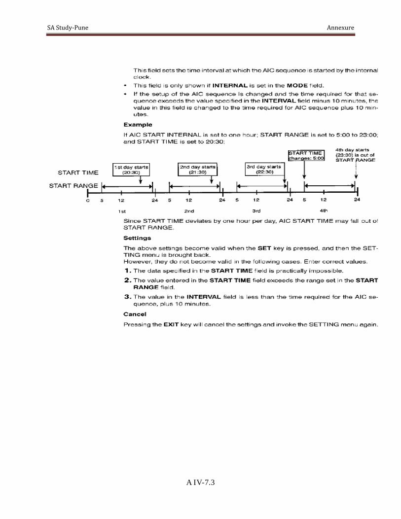
SA Study‐Pune Annexure
A IV-7.3

SA Study‐Pune Annexure
A IV-7.4

SA Study‐Pune Annexure
A IV-7.5

SA Study‐Pune Annexure
A IV-7.6

SA Study‐Pune Annexure
A IV-7.7

This page is intentionally left blank
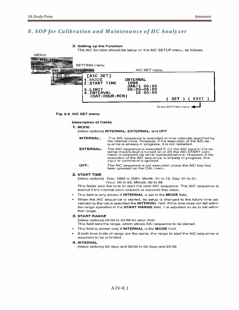
SA Study‐Pune Annexure
A IV-8.1
8. SOP for Calibration and Maintenance of HC Analyzer
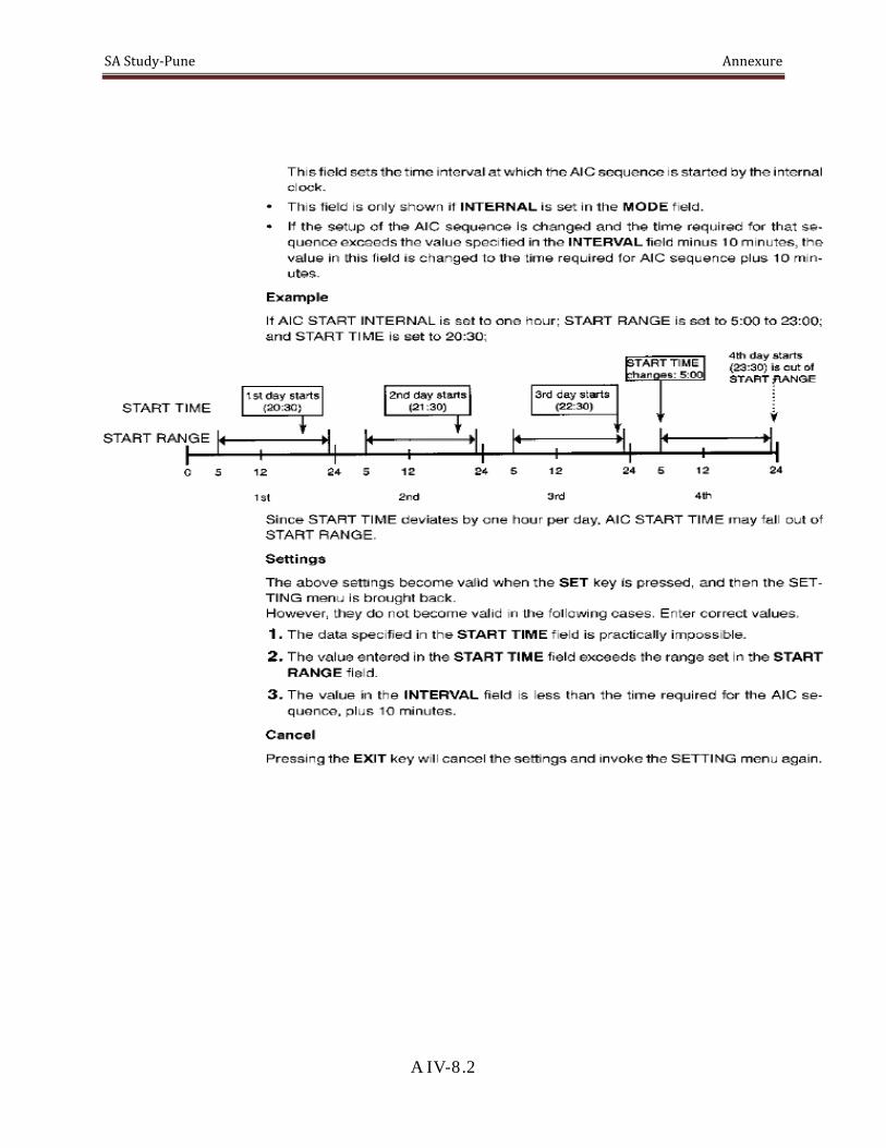
SA Study‐Pune Annexure
A IV-8.2

SA Study‐Pune Annexure
A IV-8.3

SA Study‐Pune Annexure
A IV-8.4

SA Study‐Pune Annexure
A IV-8.5

SA Study‐Pune Annexure
A IV-8.6

SA Study‐Pune Annexure
A IV-9.1
9. Methodology for VOC Analysis
(Chapter – 2)
1.0 SCOPE This test procedure is applicable for the determination of Volatile Organic Compounds like Benzene and 1,3 butadiene present in in ambient air.
2.0 REFERENCE DOCUMENT 2.1 As per guidelines of EPA TO-17 2.2 Operating Manual of Turbo matrix ATD and Auto system XL HRGC. 2.3 Refer file No. CHL/MSDS/74 for applicable MSDS for proper handing,
storage, use and disposal of chemicals for Benzene and 1,3 butadiene Helium, Air and Hydrogen
3.0 CALIBRATION 3.1 Standard: Following standard gas cylinders were used
• Benzene 1.2 ppm and 1,3 Butadiene 1.9 ppm mixture in nitrogen from Alchemie Gases and Chemicals. Capacity 3.0 Ltr. Certification Accuracy +/- 5%
• Benzene 4.5 ppm and 1,3 Butadiene 6.5 ppm mixture in nitrogen from Chemtron Science Laboratory. Capacity 0.5 Ltr. Certification Accuracy +/- 5%
• Benzene 1.67 ppm and 1,3 Butadiene 1.44 ppm mixture in nitrogen from Chemtron Science Laboratory. Capacity 0.5 Ltr. Certification Accuracy +/- 5%
3.2 Frequency: One yearly 3.3 Calibration Record: In a Calibration Test Report format attached
4.0 APPARATUS
The general instruments are as follows
4.1 Perkin Elmer Auto system XL High Resolution Gas Chromatograph with Flame Ionization Detector
4.2 Perkin Elmer make Turbo matrix Automated Thermal Desorber 4.3 Low-flow Sampler Gilian LFS-1130 with flow measuring device. 4.4 Stainless Steel Adsorbent sampling tubes-CarbotrapTM300.

SA Study‐Pune Annexure
A IV-9.2
5.0 REAGENTS 5.1 Gas Cylinders -- Hydrogen, Air and Helium 99.99% pure. 5.2 Calibration Gas Mixtures of Benzene and 1,3 butadiene
6.0 SUMMARY OF TEST PROCEDURE
The method involves drawing of a known volume of ambient air through a Stainless Steel tube to collect VOC’s like Benzene & 1,3 butadiene followed by a Thermal Desorption – Capillary GC- FID analytical procedure. Adsorbent material of the tube used to concentrate desired analytes are selected on the basis of their affinity towards the analytes as recommended in EPA TO-1, TO-2, TO-3 & TO-14 test methods. Extraction of Benzene, 1,3 butadiene by Thermal Desorption involves use of heat & a flow of inert (Carrier) gas to extract volatiles from a solid matrix directly into the carrier gas & transfer them to downstream system of High resolution Capillary GC column.
DETAILED PROCEDURE 6.1 Sampling Procedure:
Adsorbent tubes for sampling are prepared by conditioning as mentioned below
For Automated Thermal Desorption Unit: -
(a)Temperature. (b) Time (c ) Carrier Gas Helium
Tube 345 0C Purge 1 min Desorbs Flow
30 ml/min
Valve 100 0C Desorbs
60 min Pressure 22 psi
Transfer line
100 0C
• Ambient air is drawn through labeled adsorbent tube at a constant flow rate of 50 ml/min using pump and flow meter assembly.
• Field blank should always be taken along with sample following the same sample collection procedure.
• Laboratory blanks, must be taken before sampling.

SA Study‐Pune Annexure
A IV-9.3
• After collection of sample, tubes should be sealed properly and should be refrigerated & analyzed within 30 days of sample collection.
6.2 GC- ATD Analysis:
After collection of sample tubes are placed on ATD unit under standard conditions for analysis of sample for Benzene & 1,3 butadiene as follow-
For Automated Thermal Desorption Unit: -
(a) Temperature. (b) Time ( c ) Carrier Gas Helium)
Tube 325 0C Purge 1 min Outlet Split 60 ml/min
Valve 175 0C Desorbs 10 min Desorbs Flow
30 ml/min
Transfer line
200 0C Trap hold 7 min Pressure 22 psi
Trap -30 to 325 0C
For Gas Chromatograph: -
(a) Oven Program. (b) Detector Program
(c) Carrier Gas
Rate (0C/min) Temperature (0C)
Hold Time (min)
Temperature (0C)
250 1.2.1.1.1.1 22 psi
50 2.00 Range 1
10 200 10.00 Attenuation
8 & 64
30 250 1.00
6.3 Calibration using external standard method:

SA Study‐Pune Annexure
A IV-9.4
Concentrated pressurized gas phase standard with (+/- 5%) accuracy is used for calibration by passing it through conditioned blank adsorbent tube for 5 min. at constant flow rate of 50 ml/min. Then the tube is subjected for analysis under the same conditions as used for sample tubes. This procedure should be repeated at least three times for repeatability. If the results (peak area) show variation beyond +/- 5% check for leakage, condition of trap, column till the result of target compound is within +/- 5%. Record the result of calibration in the form of enclosed format.
7.0 CALCULATIONS
Measure the areas of peaks of 1,3 butadiene & Benzene for unknown sample & arithmetically correlate with standard peak areas of known calibration mix. Subtract the field blanks & laboratory blanks from the sample tube areas before arriving at final areas. Accordingly the concentration of sample in PPM or Micrograms can be calculated.
Concentration of Benzene or 1,3 Butadiene (microgram) = A * B / C
Where,
A= Peak area of Sample
B= Concentration of Standard (microgram of Benzene or 1,3 Butadiene)
C= Peak area of Standard.
6.0 REPORT
Report the concentration of Benzene and 1, 3 butadiene in microgram (µg/m3 air).