Final Report for All Island Grid Study Work-stream 2(b): Wind Variability

Management Studies

Peter Meibom, Risoe National Laboratory

Rüdiger Barth, Heike Brand, Bernhard Hasche, Derk Swider, IER, University of Stuttgart

Hans Ravn, RAM-løse EDB

Christoph Weber, University of Duisburg-Essen

Risø National LaboratoryRoskildeDenmarkJuly 2007

3

Contents

List of figures 5

List of tables 9

List of abbreviations 12

Summary 14

1 Introduction 18

2 Overview of approach 19

3 Verification 25

4 Results for the year 2020 28 4.1 Renewable power production 29 4.2 Net load 30 4.3 Operation costs 33 4.4 CO2 emissions 35 4.5 Fuel consumption 36 4.6 Reserve management 36 4.6.1 Demand for spinning reserves 37 4.6.2 Provision of spinning reserves 39 4.6.3 Demand for replacement reserves 42 4.6.4 Provision of replacement reserves 44 4.7 Reliability of the All Island power system 46 4.7.1 Loss of load expectation 47 4.7.2 Reliability in model runs 47 4.8 Dispatch of conventional power plants 49 4.9 Power exchange with Great Britain 59 4.10 Impact of unit constraints on variability management 62 4.11 Impact of different plant mix 66 4.12 Impact of improved forecasting 67 4.13 Effect of fuel price and CO2 emission permit price 68

5 Conclusions 73

www.risoe.dk 4

A Appendix 77 A.1 Methodology of the Scenario Tree Tool and of the Scheduling Model 77 A.1.1 Overview of methodology 78 A.1.2 Scenario Tree Tool – Renewable generation time-series 79 A.1.2.1 Simulation of forecast errors 80 A.1.2.2 Scenario Reduction 86 A.1.2.3 Simulation of forced outages 87 A.1.2.4 Determination of demand for replacement reserves 90 A.1.2.5 Implementation 93 A.1.3 Data input into Scenario Tree Tool 95 A.1.4 Model of system operation – Scheduling model 101 A.1.4.1 Rolling Planning 101 A.1.4.2 Unit commitment using integer variables 104 A.1.4.3 Fuel consumption curves 104 A.1.4.4 Balancing of demand and supply 105 A.1.4.5 Reserve requirements 105 A.1.4.6 Wind power providing reserves 109 A.1.4.7 Minimum system inertia 109 A.1.4.8 System stability and security limits 109 A.1.4.9 Generation limits 109 A.1.4.10 Ramp up/down rates 109 A.1.4.11 Start-up and Shut-down ramp rates 110 A.1.4.12 Minimum up/down times 110 A.1.4.13 Start-up time 110 A.1.4.14 Pumped storage constraints 110 A.1.4.15 Gas constraints 111 A.1.4.16 Emission characteristics 111 A.1.4.17 Forced outages 111 A.1.4.18 Interconnectors 113 A.1.4.19 Must run units 114 A.1.5 Data input to Scheduling model 114 A.1.5.1 Data for the All Island power system 114 A.1.5.2 Data for the power system of Great Britain 125 A.2 Power Plant portfolios used in the study 128

References 134

5

List of figures

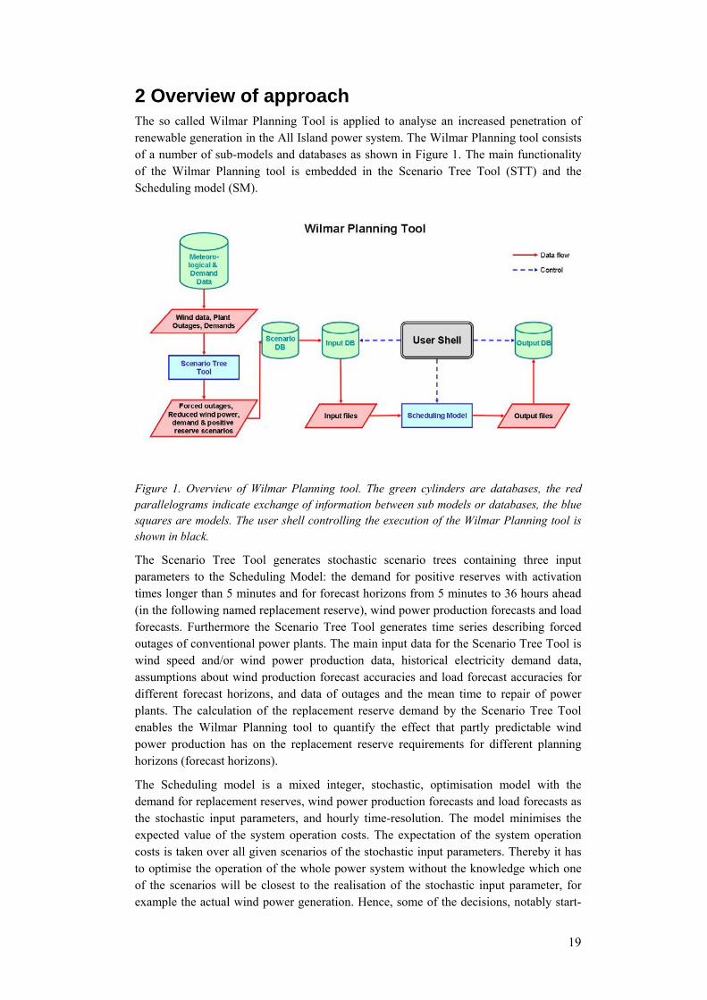
Figure 1. Overview of Wilmar Planning tool. The green cylinders are databases, the red parallelograms indicate exchange of information between sub models or databases, the blue squares are models. The user shell controlling the execution of the Wilmar Planning tool is shown in black. 19

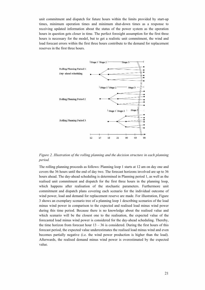
Figure 2. Illustration of the rolling planning and the decision structure in each planning period. 21

Figure 3. Exemplary scenario tree of a planning loop 1 containing forecasts of the load minus wind power compared with the expected and realised load minus wind power. 22

Figure 4. Exemplary scheduling of unit Dublin Bay Power (DBP) for day two due to the day-ahead forecast as depicted in Figure 3 and the following rescheduling. 23

Figure 5. Exemplary rescheduling of unit Dublin Bay Power (DBP) during the forecast hours of day two for each scenario in planning loop 2. 23

Figure 6. Resulting total electricity production distributed on fuels for model runs with the Scheduling Model (SM) and Plexos using the same input data. 25

Figure 7. Total electricity production of each unit during the year for model runs with the Scheduling Model (SM) and Plexos using the same input data. 26

Figure 8. Online hours of individual power plants for model runs with the Scheduling Model (SM) and Plexos using the same input data. 27

Figure 9. Duration curves of the net load (load minus wind power production) in the All Island power system for all portfolios for the whole year considered. Because the installed wind power capacity is the same in power plant portfolio P2, P3 and P4, the net load is equal as well. 31

Figure 10. Duration curves of the net load (load minus wind power production) in the All Island power system for all portfolios for those 1000 hours with the lowest net load. Because the installed wind power capacity is the same in power plant portfolio P2, P3 and P4, the net load is equal as well. 31

Figure 11. Duration curves of delta net load (the change in net load from one hour to the next) for all portfolios in the All Island power system. As the installed wind power capacity is the same in P2, P3 and P4, the delta net load is equal as well. Only values between 2500 MW and -2500 MW are shown to allow a better resolution of the curves for most hours. 32

Figure 12. Yearly fuel consumption for all portfolios in the All Island power system. 36

Figure 13. Average demand for spinning reserve during the year distributed on hours during the day in MW. 38

Figure 14. Average demand for spinning reserve during the year distributed on weeks in MW. 39

Figure 15 Provision of spinning reserve from each unit averaged over the year in MW. Turlough Hill (TH1-TH4) only shows the provision of spinning reserves in the generation mode. Each pump in Turlough Hill also delivers 70 MW of spinning reserve when pumping. 41

www.risoe.dk 6

Figure 16. Average demand for replacement reserves due to load forecast errors and forced outages dependant on the forecast horizon for different percentiles given in MW. 43

Figure 17. Average demand for replacement reserves dependant on the forecast horizon for portfolios P1 – P6 given in MW. 43

Figure 18. Demand for replacement reserves during a year for portfolio P1 – P6 given in MW. 44

Figure 19. Hourly supply of replacement reserves distributed on units and averaged over the year. 46

Figure 20. Yearly electricity production distributed on fuel type for all portfolios in the All Island power system. 49

Figure 21. Yearly electricity production distributed on units for all portfolios in GWh. 51

Figure 22. Capacity factors for units in all portfolios. 52

Figure 23. Number of start-ups during a year of each unit. 53

Figure 24. Number of online hours during a year of each unit. 54

Figure 25. Utilisation factors for units in all portfolios (the yearly production divided by the product of the installed capacity and the number of hours online). 55

Figure 26. The yearly electricity production and electricity consumption of Turlough Hill distributed on the hours during a day in MWh. 56

Figure 27. The number of pumping hours for each pump in Turlough Hill during the year for all portfolios. 57

Figure 28. The electricity production distributed on fuel type in portfolio P5 in the period 2020-01-09 to 2020-01-13. 59

Figure 29. The electricity consumption, realised wind power production, power exchange with Great Britain with negative values indicating import, and production exclusive wind power production in portfolio P5 in the period 2020-01-09 to 2020-01-13. 59

Figure 30. Duration curves of the hourly power exchange between the All Island power system and Great Britain. Positive values mean export to Great Britain and negative values mean import into the All Island power system. The maximum import capability is reduced to 900 MW because a capacity of 100 MW is reserved for providing spinning reserves. 60

Figure 31. Transmission between the All Island power system and Great Britain during a year for the portfolio P1 – P6. Positive values mean export to Great Britain and negative values mean import into the All Island power system. The maximum import capability is reduced to 900 MW because a capacity of 100 MW is reserved for providing spinning reserves. 61

Figure 32. Duration curves of the hourly variation of the transmission from one hour to the next between the All Island power system and Great Britain. A positive value means a reduced import, a negative value an inreased import to the All Island power system. 62

Figure 33. Standard deviation of the hourly variation of the power production of the power plants in MW taken over the hours during the year where the plants are online. 64

7

Figure 34.Duration curves of the number of units online in the 1000 hours with the lowest number of units online for each portfolio. 65

Figure 35. Duration curves of the change in the number of units online from one hour to the next for all hours during a year for each portfolio. 65

Figure 36. Sum of total operation costs of the All Island power system and payments related to import and export between the All Island power system and Great Britain of portfolio P1 – P6 with consideration of fuel price scenario ”Central” and ”High” and CO2 emission permit prices of 30 (80 in P6) Euro/ton CO2 and 60 Euro/ton CO2. 68

Figure 37. Yearly electricity production in the All Island power system distributed on the fuel type of portfolio P1 – P6 with consideration of fuel price scenario ”Central” and ”High” and CO2 emission permit prices of 30 (80 in P6) Euro/ton CO2 and 60 Euro/ton CO2 and net import from Great Britain. A negative value of the net import means net export to Great Britain. 69

Figure 38. Sum of total operation costs of the All Island power system and payments related to import and export between the All Island power system and Great Britain of portfolio P1 with consideration of all fuel price scenarios. 71

Figure 39. Yearly electricity production in the All Island power system distributed on fuel type for portfolio P1 and import from Great Britain with consideration of all fuel price scenarios. A negative value of the import means export to Great Britain. 71

Figure 40. Overview of Wilmar Planning tool. The green cylinders are databases, the red parallelograms indicate exchange of information between sub models or databases, the blue squares are models. The user shell controlling the execution of the Wilmar Planning tool is shown in black. 78

Figure 41. Example of the probability function for the block-averaged wind speeds for the individual wind turbines in an area at a given time. An offset adjustment of –0.15 m/s results in an unchanged accumulated production for the aggregated multi-turbine power curve and the given wind speed distribution. 82

Figure 42. Example for normalised wind power curves corresponding to single and aggregated multi turbines. 82

Figure 43. Four examples of ARMA(1,1)-outcomes of wind speed forecast errors with assumed ARMA-parameters α=0.95, β=0.02 and σZ=0.5. 83

Figure 44. Correlation between forecast errors for different pairs of stations (Söder 2004). The distances between the stations are Maglarp-Bösarp (15 km), Maglarp-Sturup (26 km), Näsudden-Ringhals (370 km). 85

Figure 45. Principle setup of the scenario tree used in the Scheduling Model. 87

Figure 46. Generating unit states. 87

Figure 47. Repairable unit cycle. 88

Figure 48. Sequence of actions within the Scenario Tree Tool. 94

Figure 49. Wind farm zones in the All Island power system. 95

Figure 50. Wind duration curves for zone ROI_H and the All Island power system before and after smoothing. 96

Figure 51. Standard deviations of given wind speed forecast errors. 97

Figure 52. Standard deviation of wind speed forecast error. 97

www.risoe.dk 8

Figure 53. Wind power forecast scenarios and their standard deviation. 98

Figure 54. Correlation of wind speed forecast errors. 98

Figure 55. Standard deviation of load forecast errors. 99

Figure 56. Resulting availability of Ballylumford CCGT 31 (FOR 3.01 %; MTTR 72 h) and Moneypoint Unit 1 (FOR 5 %; MTTR 50 h) of power plant portfolio P1. 100

Figure 57. Duration curve of unavailable capacity due to forced and scheduled outages for portfolio P1 to P6. 101

Figure 58. Illustration of the rolling planning and the decision structure in each planning period. 103

Figure 59. POR, SOR and TR1 requirements in the All Island power system as a function of installed wind power capacity. Data delivered from the All Island Grid Study working group. 107

Figure 60. Fuel price scenarios for BASELOADGAS and MIDMERITGAS for Republic of Ireland in Euro/GJ. Notice that the price differences between BASELOADGAS and MIDMERITGAS are small. 118

Figure 61. Development of Generation portfolio for Great Britain from 2006 to 2012 (National Grid 2006, aggregation of information in Table 3.14 and 3.15). The categories CHP and CHP steam have been included in the CCGT category. The categories Biomass, Tidal and Waste with capacities below 50 MW have been ignored. 126

Figure 62. Annual electricity demand forecasts for Great Britain made by National Grid (National Grid 2006, Table 2.4 and 2.5). The historical data is weather adjusted annual electricity requirements. 127

9

List of tables

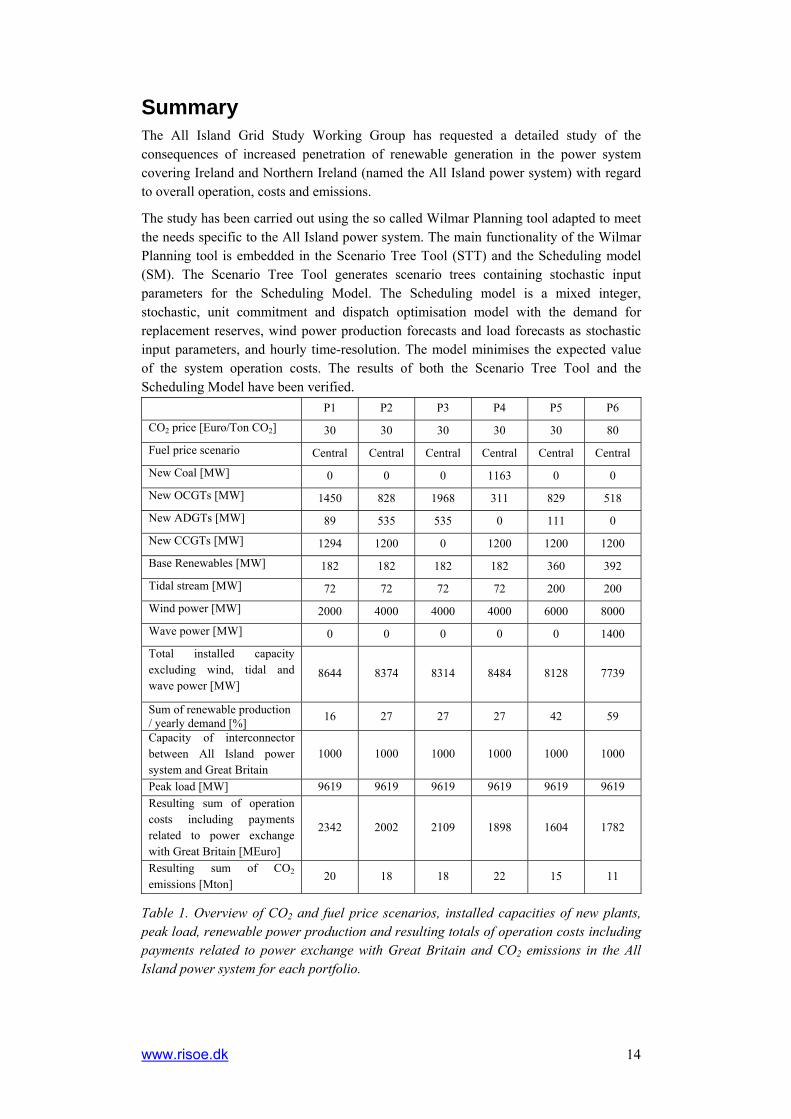
Table 1. Overview of CO2 and fuel price scenarios, installed capacities of new plants, peak load, renewable power production and resulting totals of operation costs including payments related to power exchange with Great Britain and CO2 emissions in the All Island power system for each portfolio. 14

Table 2. Yearly renewable power production in each portfolio. The production from biomass, biogas, sewage and landfill gas, run-of-river, tidal and wave power production is aggregated to “other renewables”. Wind power curtailment is not considered with the given values. 29

Table 3. Yearly curtailment of wind power production for provision of spinning reserves and activated due to other reasons than provision of spinning reserve in the All Island power system. 30

Table 4. Statistical properties of the yearly net load in the All Island power system in MW. 32

Table 5. Statistical numbers describing the properties of the delta net load in MW. All numbers are calculated over the hours in the year. Positive mean indicates the average of the values where load increases from one hour to the next. Negative mean indicates the average of the values with decreasing load from one hour to the next. 33

Table 6. Operation costs of power production in the All Island power system and payments related to import and export of power between the All Island power system and Great Britain for portfolio P1 – P5 in MEuro. 33

Table 7. Operation costs in the All Island power system divided into start-up costs, fuel costs and CO2 costs for portfolio P1 – P5 in MEuro. 34

Table 8. Operation costs of power production in the All Island power system and payments related to import and export of power between the All Island power system and Great Britain for portfolio P6 in MEuro. 35

Table 9. Yearly sum of CO2 emissions in portfolios P1 – P5 in MTon. 35

Table 10. Number of online hours of PBC in each portfolio. 38

Table 11 Provision of spinning reserve from wind power. Duration indicates the number of hours where wind power is curtailed to provide spinning reserve. Average gives the average capacity provided during these hours. Maximum gives the maximum capacity provided during these hours. The average and maximum contribution relative to the installed wind power capacity are also presented. 42

Table 12. Hourly supply of replacement reserves from offline units and online units, hourly demand for replacement reserves averaged over the year in GW. 45

Table 13 The installed capacity of dispatchable power plants in the All Island power system (excluding wind, wave, hydropower, tidal and base renewables) distributed on start-up times. Start-up times corresponding to the unit being in the hot state are used in the model runs. 45

Table 14. Comparison of the total installed capacity excluding wind, tidal and wave power with the peak load in MW. 47

Table 15. Realised LOLE of each power plant portfolio. 47

www.risoe.dk 10

Table 16 Number of hours where load, demand for spinning reserve and replacement reserves is not met. The logic in the model ensures that load is met before the demand for spinning reserves, and the demand for spinning reserve is met before the demand for replacement reserves. 48

Table 17. Average and maximum amount of load, spinning reserve and replacement reserve not met. 48

Table 18. Unit dispatch in the hour with lowest net load for all portfolios. 58

Table 19. Yearly import, export and sum of the power exchange between the All Island power system and Great Britain in TWh. Positive values mean export to Great Britain and negative values mean import into the All Island power system. 61

Table 20. Maximum number of units brought online or taken offline from one hour to the next during a year in all portfolios. Number of instances where the change in the units online from one hour to the next is above 5. 66

Table 21. Sequence of power plant portfolios in dependence of operation costs and CO2 emissions. 67

Table 22. Absolute and relative reduction of total system operation costs caused by using a perfect forecast of wind power production and load compared to forecasts reflecting the precision of present forecast tools. The relative cost reduction refers to the system operation costs of the All Island power system with consideration of payments related to imports and exports. 67

Table 23. Yearly sum of CO2 emissions of each portfolio with consideration of fuel price scenario ”Central” and ”High” and CO2 emission permit prices of 30 (80 in P6) Euro/ton CO2 and 60 Euro/ton CO2. All values are given in Mton. 70

Table 24. Yearly sum of CO2 emissions of portfolio P1 with consideration of all fuel price scenarios. All values are given in Mton. 72

Table 25. Wind power zones and corresponding sources of wind power series. 96

Table 26. Maximal number of simultaneous forced outages of each power plant portfolio. 100

Table 27. Additional demands for spinning reserves as a function of installed wind power capacity. All values in MW. 108

Table 28. The fuel price scenarios for Great Britain (GB), Northern Ireland (IR_NI) and Republic of Ireland (IR_ROI) in Euro/GJ excluding baseload gas and mid-merit gas. 115

Table 29. The price scenarios for baseload gas for Great Britain (GB), Northern Ireland (IR_NI) and Republic of Ireland (IR_ROI) in Euro/GJ. 116

Table 30. The price scenarios for mid-merit gas for Great Britain (GB), Northern Ireland (IR_NI) and Republic of Ireland (IR_ROI) in Euro/GJ. 117

Table 31. Power plant parameter for thermal power plants already existing today. 119

Table 32. Power plant parameter for thermal power plants already existing today (cont.). 120

Table 33. Power plant parameter for new technologies. 121

Table 34. Incremental heat rate slope parameter for existing and new power plants. 122

Table 35. Power plant parameter for the pumped hydro storage plant Turlough Hill. 123

11

Table 36. Overview of data demands and data sources. 124

Table 37. Generation capacities distributed on type for Great Britain (National Grid 2006, Table 3.14 and 3.15). 125

Table 38. Considered generation capacities and efficiencies of power plants in Great Britain. 127

www.risoe.dk 12

List of abbreviations Power plants

Code Power plant Code Power plant

AA1 Ardnacrusha Unit 1 NAT4 New ADGT AA2 Ardnacrusha Unit 2 NAT5 New ADGT AA3 Ardnacrusha Unit 3 NCG1 New Moneypoint Coal Unit AA4 Ardnacrusha Unit 4 NCG2 New Moneypoint Coal Unit AD1 Aghada Unit 1 NCG3 New Moneypoint Coal Unit B10 Ballylumford Unit 10 NCT1 New CCGT B31 Ballylumford CCGT 31 NCT2 New CCGT B32 Ballylumford Unit 32 NCT3 New CCGT BG Total Biogas NOT1 New OCGT BGT1 Ballylumford GT1 NOT2 New OCGT BGT2 Ballylumford GT2 NOT3 New OCGT BM Total Biomass NOT4 New OCGT CGT8 Coolkeeragh GT8 NOT5 New OCGT CPS CCGT Coolkeeragh CCGT NOT6 New OCGT DBP Dublin Bay Power NOT7 New OCGT ED1 Edenderry NOT8 New OCGT ER1 Erne Unit 1 NOT9 New OCGT ER2 Erne Unit 2 NOT10 New OCGT ER3 Erne Unit 3 NOT11 New OCGT ER4 Erne Unit 4 NOT12 New OCGT HNC Huntstown NOT13 New OCGT Inter 1 Interconnector NOT14 New OCGT Inter 2 Interconnector NOT15 New OCGT K1 Kilroot Unit 1 NOT16 New OCGT K2 Kilroot Unit 2 NOT17 New OCGT KGT1 Kilroot GT1 NOT18 New OCGT KGT2 Kilroot GT2 NOT19 New OCGT LE1 Lee Unit 1 PBC Poolbeg Combined Cycle LE2 Lee Unit 2 RH1 Rhode Unit 1 LE3 Lee Unit 3 RH2 Rhode Unit 2 LFG Total Landfill Gas SG Total Sewage Gas LI1 Liffey Unit 1 SK1 Aughinish (Sealrock) LI2 Liffey Unit 2 TE Tynagh LI4 Liffey Unit 4 TH1 Turlough Hill Unit 1 LI5 Liffey Unit 5 TH2 Turlough Hill Unit 2 LR4 Lough Ree TH3 Turlough Hill Unit 3 MP1 Moneypoint Unit 1 TH4 Turlough Hill Unit 4 MP2 Moneypoint Unit 2 TP1 Asahi Peaking Unit MP3 Moneypoint Unit 3 TS Total Tidal Stream MRT Marina CC WD Wind Generation NAT1 New ADGT WE Wave Energy NAT2 New ADGT WO4 West Offaly Power NAT3 New ADGT

13

Further abbreviations

Abbreviation Explanation Abbreviation Explanation

ACS Average cold spell OCGT Open cycle gas turbine ADGT Aeroderivative gas turbine OS Off-shore AGR Advanced gas-cooled POR Primary operating reactor margin AGT Advanced gas turbine PWR Pressurized water ARMA Auto Regressive Moving reactor Average ROI Republic of Ireland CCGT Combined cycle gas turbine SEI Sustainable Energy CHP Combined heat and power Island conv conventional SM Scheduling Model FOP Full outage probability SOR Secondary operating FOR Forced outage rate margin GB Great Britain STT Scenario Tree Tool HVDC High voltage direct current TR1 Tertiary operating LOLE Loss of load expectation reserve band 1 MTTF Mean time to failure TTF Time to failure MTTR Mean time to repair TTR Time to repair NI Northern Ireland

www.risoe.dk 14

Summary The All Island Grid Study Working Group has requested a detailed study of the consequences of increased penetration of renewable generation in the power system covering Ireland and Northern Ireland (named the All Island power system) with regard to overall operation, costs and emissions.

The study has been carried out using the so called Wilmar Planning tool adapted to meet the needs specific to the All Island power system. The main functionality of the Wilmar Planning tool is embedded in the Scenario Tree Tool (STT) and the Scheduling model (SM). The Scenario Tree Tool generates scenario trees containing stochastic input parameters for the Scheduling Model. The Scheduling model is a mixed integer, stochastic, unit commitment and dispatch optimisation model with the demand for replacement reserves, wind power production forecasts and load forecasts as stochastic input parameters, and hourly time-resolution. The model minimises the expected value of the system operation costs. The results of both the Scenario Tree Tool and the Scheduling Model have been verified.

P1 P2 P3 P4 P5 P6

CO2 price [Euro/Ton CO2] 30 30 30 30 30 80 Fuel price scenario Central Central Central Central Central Central

New Coal [MW] 0 0 0 1163 0 0 New OCGTs [MW] 1450 828 1968 311 829 518 New ADGTs [MW] 89 535 535 0 111 0

New CCGTs [MW] 1294 1200 0 1200 1200 1200 Base Renewables [MW] 182 182 182 182 360 392 Tidal stream [MW] 72 72 72 72 200 200

Wind power [MW] 2000 4000 4000 4000 6000 8000 Wave power [MW] 0 0 0 0 0 1400 Total installed capacity excluding wind, tidal and wave power [MW]

8644 8374 8314 8484 8128 7739

Sum of renewable production / yearly demand [%] 16 27 27 27 42 59

Capacity of interconnector between All Island power system and Great Britain

1000 1000 1000 1000 1000 1000

Peak load [MW] 9619 9619 9619 9619 9619 9619 Resulting sum of operation costs including payments related to power exchange with Great Britain [MEuro]

2342 2002 2109 1898 1604 1782

Resulting sum of CO2 emissions [Mton]

20 18 18 22 15 11

Table 1. Overview of CO2 and fuel price scenarios, installed capacities of new plants, peak load, renewable power production and resulting totals of operation costs including payments related to power exchange with Great Britain and CO2 emissions in the All Island power system for each portfolio.

15

Four different levels of renewable power production are represented in six power plant portfolios enabling analysis of the economic and technical impacts of increasing the share of renewable energy in the All Island power system. These power plant portfolios consist of modified results from the final report of work-stream 2A of the All Island Grid Study (Doherty 2006). The derivation of these least-cost generation power plant portfolios was based on a number of scenarios of uncertain future parameters, e.g. CO2 emission permit price, natural gas price and capital costs of wind turbines. CO2 and fuel price assumptions, the structure of the resulting portfolios and resulting totals of operation costs and CO2 emissions are summarised in Table 1.

Power plant portfolios P2, P3 and P4 with the same capacity of renewable power plants installed have different shares of base load plants (coal fired thermal plants and natural gas fired CCGTs) relatively to more flexible plants (OCGTs and ADGTs). Thus, comparing portfolios P2, P3 and P4 allows evaluation of the impact of the structure of conventional power plant portfolio when renewable energy is integrated. To consider the power exchange with Great Britain, the power system in Great Britain is also represented.

The main conclusions from the yearly model runs for each portfolio are the following:

• Integration of renewable power production: The assumed amount of renewable power production of the individual portfolios can be integrated into the All Island power system. Especially with power plant portfolios P1 – P5, no significant wind power curtailment and reliability problems occur.

• Renewable power production: The share of the renewable power production of the yearly electricity demand in the All Island power system raises from 16 % in portfolio P1 to 59 % in portfolio P6. The amount of curtailed wind power production increases with wind power capacity installed. Wind power is curtailed for provision of spinning reserves and mainly to keep the balance between supply and demand. The amount of wind power curtailed is negligible in P1-P4 and amounts to 0.5 % in P5 and 2.3 % in P6 in terms of percentages of yearly wind power production.

• Yearly operation costs: With increasing wind power capacity installed, yearly operation costs of the All Island power system are reduced for portfolio P1 – P5. Due to the assumption of higher CO2 emission permit prices in portfolio P6, the total operation costs increase in this portfolio. Comparing those portfolios with an equal wind power capacity installed (portfolio P2 – P4), portfolio P4 shows the lowest and portfolio P3 the highest total operation costs. Concerning operation costs, it is preferable to have a high share of base load units with low variable costs in the portfolio.

• Yearly CO2 emissions: The CO2 emissions in the All Island power system tends to decrease with increasing wind power installed. However, portfolio P4 shows the highest sum of CO2 emissions caused by the net import into the All Island power system being significantly smaller in P4 relatively to P1, i.e. the effect of decreasing CO2 emissions due to increased wind power production in P4 relatively to P1 is offset by the increased share of domestic power production in P4 relatively to P1. The significant decrease of CO2 emissions in portfolio P6 is due to the higher CO2 emission permit price assumed for this portfolio. Comparing only those portfolios with an equal wind power capacity installed (portfolio P2 – P4), portfolio P2 shows the lowest sum of CO2 emissions.

www.risoe.dk 16

Concerning CO2 emissions, it is preferable to have a high share of gas fired and simultaneously base load units in the portfolio.

• Fuel consumption: The fuel consumption is strongly correlated to the structure of the power plants in each portfolio. Generally, baseload gas and coal constitute the main fuels. With increasing wind power capacity installed, the fuel consumption in the All Island power system tends to be reduced. The consumption of mid-merit gas is increased in portfolio P3 in comparison to the other portfolios. The consumption of coal is significantly higher in portfolio P4. The high CO2 price assumed in portfolio P6 leads to an increase of the consumption of baseload and midmerit gas and to a strong decrease of coal consumption.

• Provision of reserves: Pumped hydro storage facility Turlough Hill, coal fired unit Moneypoint and new CCGTs are main sources of positive spinning reserves. Comparing those portfolios with an equal wind power capacity installed (portfolio P2 – P4), portfolio P3 shows the highest and portfolio P4 the lowest provision of spinning reserves from wind power. Because curtailment of wind power is a relatively expensive way of providing spinning reserve, this indicates that providing spinning reserves is most costly in portfolio P3 with no new large units and many OCGTs compared to portfolio P2 with new CCGTs and portfolio P4 with both new CCGTs and new coal power plants.

Nearly the whole demand for replacement reserves is provided by offline OCGTs in all portfolios.

• Reliability of the All Island power system: All portfolios rely on the production from non-dispatchable generation and on the import from Great Britain to cover the load in peak load hours. Generally, portfolio P3 shows the highest overall reliability, portfolio P6 the lowest.

• Dispatch of conventional power plants: The distribution of the dispatch of the units is strongly correlated to the structure of the power plants in each portfolio. Generally, the bigger part of the electricity production in the All Island power system from conventional power plants is borne by coal fired plants and newer CCGTs. With increasing wind power capacity installed, the production of these units tends to be decreased. The assumption of a higher CO2 emission permit price in portfolio P6 leads to a strong decrease in the use of coal fired units. OCGTs and ADGTs generally show a small contribution to the electricity production.

No restriction on the minimum number of conventional power plants online was used in the study, which in portfolio P5 and P6 give operation hours with the number of conventional units online being from 2 to 5 units. Using a restriction that defines the minimum number of units online would increase the wind curtailment, because the minimum stable operation limit of the units would displace some wind power production.

The resulting dispatch does not consider load flow restrictions of the electricity network because it has been decided to model the All Island power system without consideration of the electricity network.

For the pumped hydro storage facility Turlough Hill, no general trend depending on the wind power capacity installed can be observed. However, Turlough Hill shows an increased use in the case of portfolio P6.

17

• Power exchange with Great Britain: With increasing wind power capacity installed in the All Island power system and constant wind power capacity installed in Great Britain, the predominant transmission pattern of import into the All Island power system changes into more power exports to Great Britain. With portfolio P6, the All Island power system becomes a net exporter. With increasing wind power capacity installed, the hourly variation of the transmission generally increases.

• Impact on unit constraints on variability management: With the chosen hourly time resolution of the model, only one unit has restricting ramp up and ramp down rates. Considering the variation of the resulting power production from one to the next hour for all portfolios, almost the whole operating range is utilized by all units independent of the wind power capacity installed. Generally, the overall variation of the electricity production increases with increasing wind power capacity installed.

• Impact of improved forecasting: Cost reductions due to perfect forecasts of the load and the wind power production are relatively small in comparison to the total system operation costs of the All Island power system. However, the absolute sum of the cost reductions is not negligible. Generally, the value of perfect forecast increases with increasing wind power capacity installed.

• Effect of fuel price and CO2 emission permit price: With the assumption of the ”High” fuel price scenario and a CO2 emission permit price of 60 Euro/ton CO2 for all portfolios, the system operation costs increases for all portfolios. Portfolio P6 becomes the portfolio with the lowest operation costs. The yearly sum of CO2 emissions increases for all portfolios and in both regions. The modification of fuel prices and of the CO2 emission permit price leads to a decrease in the use of gas fired power plants and an increase in the use of coal and peat fired units.

www.risoe.dk 18

1 Introduction The All Island Grid Study Working Group has requested a detailed study of the consequences of increased penetration of renewable generation in the power system covering Ireland and Northern Ireland (named the All Island power system in the following text) with regard to overall operation, costs and emissions.

The study has been carried out using the so called Wilmar Planning tool adapted to meet the needs specific to the All Island power system. The methodology of the Wilmar Planning Tool and its main parts, namely the Scenario Tree Tool and the Scheduling Model, are documented in the appendix.

Briefly the study consisted of the following parts:

• Extension of the Scenario Tree Tool to include demand uncertainties and forced plant outages in the generation of scenario trees. The inclusion of these factors secures that the scenario trees generated provide a realistic estimate for the positive reserve required in the next 36 hours in the power system.

• Collection of wind power production data, wind speed data and data for the historical accuracy of the wind forecasting tools currently used in the All Island power system. The data are used by the Scenario Tree Tool to create wind power production forecasts.

• Modification of the Scheduling model in order to meet the requirements for the study. The modifications are described in the Methodology report. In short they encompass extending the model to include load uncertainty and forced outages in the scheduling process, and introducing integers in the modelling of unit commitment.

• Collection of demand and generation data for the All Island power system and Great Britain and inclusion of this data in the data structures of the Scheduling model.

• First round of model runs in order to test and calibrate the model.

• Yearly model runs of 2020 power system scenarios defined in a dialogue with Work-stream 2(a).

• Derivation of conclusions from model runs

• Input to work-stream 1, 3 and 4.

Section 2 in this report gives an overview of the approach applied. Section 3 gives a verification of the approach. Section 4 presents results and section 5 concludes. The methodology, the data input for the model runs and the power plant portfolios considered are presented in the appendix.

19

2 Overview of approach The so called Wilmar Planning Tool is applied to analyse an increased penetration of renewable generation in the All Island power system. The Wilmar Planning tool consists of a number of sub-models and databases as shown in Figure 1. The main functionality of the Wilmar Planning tool is embedded in the Scenario Tree Tool (STT) and the Scheduling model (SM).

Figure 1. Overview of Wilmar Planning tool. The green cylinders are databases, the red parallelograms indicate exchange of information between sub models or databases, the blue squares are models. The user shell controlling the execution of the Wilmar Planning tool is shown in black.

The Scenario Tree Tool generates stochastic scenario trees containing three input parameters to the Scheduling Model: the demand for positive reserves with activation times longer than 5 minutes and for forecast horizons from 5 minutes to 36 hours ahead (in the following named replacement reserve), wind power production forecasts and load forecasts. Furthermore the Scenario Tree Tool generates time series describing forced outages of conventional power plants. The main input data for the Scenario Tree Tool is wind speed and/or wind power production data, historical electricity demand data, assumptions about wind production forecast accuracies and load forecast accuracies for different forecast horizons, and data of outages and the mean time to repair of power plants. The calculation of the replacement reserve demand by the Scenario Tree Tool enables the Wilmar Planning tool to quantify the effect that partly predictable wind power production has on the replacement reserve requirements for different planning horizons (forecast horizons).

The Scheduling model is a mixed integer, stochastic, optimisation model with the demand for replacement reserves, wind power production forecasts and load forecasts as the stochastic input parameters, and hourly time-resolution. The model minimises the expected value of the system operation costs. The expectation of the system operation costs is taken over all given scenarios of the stochastic input parameters. Thereby it has to optimise the operation of the whole power system without the knowledge which one of the scenarios will be closest to the realisation of the stochastic input parameter, for example the actual wind power generation. Hence, some of the decisions, notably start-

www.risoe.dk 20

ups of power plants, have to be made before the wind power production and load (and the associated demand for replacement reserve) is known with certainty. The methodology ensures that these unit commitment and dispatch decisions are robust towards different wind power prediction errors and load prediction errors as represented by the scenario tree for wind power production and load forecasts.

The demand for positive reserves (both spinning reserves with activation times below 5 minutes and replacement reserves) determines together with the expected values of load forecasts and wind power forecasts and the technical restrictions of power plants, the day-ahead unit commitment planned for the next 36 hours. The realised load and wind power production together with the technical restrictions of power plants determine the actual dispatch of the power plants in the operating hour in question.

The uncertainty due to the wind power production, load and demand for replacement reserve in the optimisation model is considered by using a scenario tree. The scenario tree represents forecasts of load, wind power production and replacement reserve demand with different forecast horizons corresponding to each hour in the optimisation period. Load and wind power production forecasts are independent of each other, whereas the demand for replacement reserve is influenced by the wind power production and load forecasts. Therefore for a given forecast horizon one scenario consists of a forecast of wind power production, load and replacement reserve with an associated probability expressing the weight that the forecast has when calculating the expected costs, i.e. how likely the forecast is judged to be.

As it is not possible to cover the whole simulated time period with only one single scenario tree, the model is formulated by introducing a multi-stage recursion using rolling planning. Therewith, the unit commitment and dispatch decisions are reoptimised taking into account that more precise wind power production and load forecasts become available as the actual operation hour gets closer in time, and taking into account the technical restrictions (e.g. start-up times, minimum up and down times) of different types of power plants. Furthermore, it is taken into account that forced outages may occur between the day-ahead dispatch and the actual operating hour. The resulting production of each power plant and the changes in the production (up and down regulation) relative to the day-ahead production plan are calculated for each hour.

In general, new information arrives on a continuous basis and provides updated information about wind power production and forecasts, the operational status of other production and storage units and about the load. Thus, an hourly basis for updating information would be most adequate. However, stochastic optimisation models quickly become intractable, thus it is necessary to simplify the information arrival and decision structure in the Scheduling Model. In the current version of the model a three stage model is implemented. The model steps forward in time using rolling planning with a three hour step, so a one-day cycle consists of eight planning loops. For each time step new forecasts (i.e. a new scenario tree) that consider the change in forecast horizons are applied. This decision structure is illustrated in Figure 2 showing the scenario tree for three planning periods. For each planning period a three-stage, stochastic optimisation problem is solved having a deterministic first stage covering 3 hours, a stochastic second stage with three scenarios covering 3 hours, and a stochastic third stage with six scenarios covering a variable number of hours according to the rolling planning period in question. Hence, the scenario tree represents a decision structure where the system operator performs unit commitment and dispatch assuming perfect knowledge about the realised wind and load in the first three hours, and uncertain knowledge about wind and load in subsequent hours. Every three hour, there is the possibility to change the planned

21

unit commitment and dispatch for future hours within the limits provided by start-up times, minimum operation times and minimum shut-down times as a response to receiving updated information about the status of the power system as the operation hours in question gets closer in time. The perfect foresight assumption for the first three hours is necessary for the model, but to get a realistic unit commitment, the wind and load forecast errors within the first three hours contribute to the demand for replacement reserves in the first three hours.

Figure 2. Illustration of the rolling planning and the decision structure in each planning period.

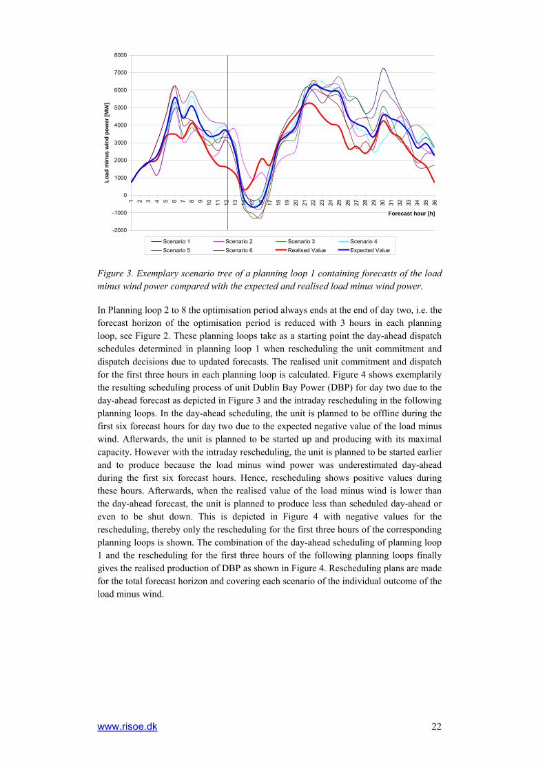
The rolling planning proceeds as follows: Planning loop 1 starts at 12 am on day one and covers the 36 hours until the end of day two. The forecast horizons involved are up to 36 hours ahead. The day-ahead scheduling is determined in Planning period 1, as well as the realised unit commitment and dispatch for the first three hours in the planning loop, which happens after realisation of the stochastic parameters. Furthermore unit commitment and dispatch plans covering each scenario for the individual outcome of wind power, load and demand for replacement reserve are made. For illustration, Figure 3 shows an exemplary scenario tree of a planning loop 1 describing scenarios of the load minus wind power in comparison to the expected and realised load minus wind power during this time period. Because there is no knowledge about the realised value and which scenario will be the closest one to the realisation, the expected value of the forecasted load minus wind power is considered for the day-ahead scheduling. Thereby, the time horizon from forecast hour 13 – 36 is considered. During the first hours of this forecast period, the expected value underestimates the realised load minus wind and even becomes partially negative (i.e. the wind power production is higher than the load). Afterwards, the realised demand minus wind power is overestimated by the expected value.

www.risoe.dk 22

-2000

-1000

0

1000

2000

3000

4000

5000

6000

7000

8000

1 2 3 4 5 6 7 8 9 10 11 12 13 14 15 16 17 18 19 20 21 22 23 24 25 26 27 28 29 30 31 32 33 34 35 36

Forecast hour [h]

Load

min

us w

ind

pow

er [M

W]

Scenario 1 Scenario 2 Scenario 3 Scenario 4Scenario 5 Scenario 6 Realised Value Expected Value

Figure 3. Exemplary scenario tree of a planning loop 1 containing forecasts of the load minus wind power compared with the expected and realised load minus wind power.

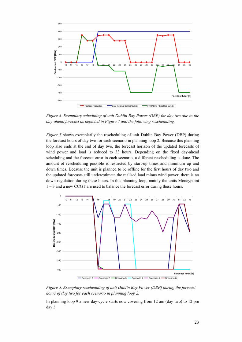
In Planning loop 2 to 8 the optimisation period always ends at the end of day two, i.e. the forecast horizon of the optimisation period is reduced with 3 hours in each planning loop, see Figure 2. These planning loops take as a starting point the day-ahead dispatch schedules determined in planning loop 1 when rescheduling the unit commitment and dispatch decisions due to updated forecasts. The realised unit commitment and dispatch for the first three hours in each planning loop is calculated. Figure 4 shows exemplarily the resulting scheduling process of unit Dublin Bay Power (DBP) for day two due to the day-ahead forecast as depicted in Figure 3 and the intraday rescheduling in the following planning loops. In the day-ahead scheduling, the unit is planned to be offline during the first six forecast hours for day two due to the expected negative value of the load minus wind. Afterwards, the unit is planned to be started up and producing with its maximal capacity. However with the intraday rescheduling, the unit is planned to be started earlier and to produce because the load minus wind power was underestimated day-ahead during the first six forecast hours. Hence, rescheduling shows positive values during these hours. Afterwards, when the realised value of the load minus wind is lower than the day-ahead forecast, the unit is planned to produce less than scheduled day-ahead or even to be shut down. This is depicted in Figure 4 with negative values for the rescheduling, thereby only the rescheduling for the first three hours of the corresponding planning loops is shown. The combination of the day-ahead scheduling of planning loop 1 and the rescheduling for the first three hours of the following planning loops finally gives the realised production of DBP as shown in Figure 4. Rescheduling plans are made for the total forecast horizon and covering each scenario of the individual outcome of the load minus wind.

23

-500

-400

-300

-200

-100

0

100

200

300

400

500

13 14 15 16 17 18 19 20 21 22 23 24 25 26 27 28 29 30 31 32 33 34 35 36

Forecast hour [h]

Prod

uctio

n D

BP

[MW

]

Realised Production DAY_AHEAD SCHEDULING INTRADAY RESCHEDULING

Figure 4. Exemplary scheduling of unit Dublin Bay Power (DBP) for day two due to the day-ahead forecast as depicted in Figure 3 and the following rescheduling.

Figure 5 shows exemplarily the rescheduling of unit Dublin Bay Power (DBP) during the forecast hours of day two for each scenario in planning loop 2. Because this planning loop also ends at the end of day two, the forecast horizon of the updated forecasts of wind power and load is reduced to 33 hours. Depending on the fixed day-ahead scheduling and the forecast error in each scenario, a different rescheduling is done. The amount of rescheduling possible is restricted by start-up times and minimum up and down times. Because the unit is planned to be offline for the first hours of day two and the updated forecasts still underestimate the realised load minus wind power, there is no down-regulation during these hours. In this planning loop, mainly the units Moneypoint 1 – 3 and a new CCGT are used to balance the forecast error during these hours.

-400

-350

-300

-250

-200

-150

-100

-50

010 11 12 13 14 15 16 17 18 19 20 21 22 23 24 25 26 27 28 29 30 31 32 33

Forecast hour [h]

Res

ched

ulin

g D

BP

[MW

]

Scenario 1 Scenario 2 Scenario 3 Scenario 4 Scenario 5 Scenario 6

Figure 5. Exemplary rescheduling of unit Dublin Bay Power (DBP) during the forecast hours of day two for each scenario in planning loop 2.

In planning loop 9 a new day-cycle starts now covering from 12 am (day two) to 12 pm day 3.

www.risoe.dk 24

Work-stream 2A has derived generation portfolios for the All Island power system in 2020 dependent on a number of uncertain future parameters, e.g. CO2 emission permit price, natural gas price and capital costs of wind turbines. The final report of work-stream 2A outlines five generation portfolios in 2020, which can be used in analyses taking place in other work-streams (Doherty 2006). After consultation with the All Island Grid Study working group it has been decided to use modified versions of these five generation portfolios. The modifications are done in order to take some recently decided investments in CCGTs into account and to obtain a LOLE (Loss of load expectation) of at least 8 hours per year. To get portfolios with different ratios of peak load plants relatively to base load plants, all in all six portfolios have been generated. The resulting portfolios are shown in the appendix and summarised in Table 1.

Four levels of renewable power production are represented in the portfolios enabling analysis of the economic and technical impacts of increasing the share of renewable energy in the All Island power system. Portfolios P2, P3 and P4 with the same capacity of renewable power plants installed have different shares of base load plants (coal fired thermal plants and natural gas fired CCGTs) relatively to more flexible plants (OCGTs and ADGTs). Thus, comparing portfolios P2, P3 and P4 enables analysis of the impact of the structure of conventional power plant portfolio on the emissions and costs of the power system when renewable energy is integrated. This analysis contributes to determine the most suitable plant mix in the future All Island power system for an installed wind power production of 4000 MW.

25

3 Verification The results of the Planning tool were verified by comparison with a Plexos model run (www.plexossolutions.com) of the year 2007 carried out in the All Island Modelling Study. The verification run had the following properties:

• Treatment of interconnector to Great Britain (GB): imports/exports as a power series as produced by Plexos.

• Usage of Plexos wind power series.

• Usage of fuel prices including a monthly profile for gas prices as taken into account by Plexos.

• Usage of load times series as taken into account by Plexos.

• Usage of same generator data as taken into account by Plexos.

• Run with and without demand for reserve power.

• Usage of carbon price of 30 Euros/tons CO2.

• Usage hydropower time series as taken into account by Plexos.

• Beside power plant SK1, must-run power plants are not considered.

• No differentiation between forced outages and scheduled outages and usage of same scheduled and forced outages times series as taken into account by Plexos.

The basis of the verification is the unit commitment and dispatch derived with both models. In general, both results of the Scheduling Model and Plexos show a high consistency. The resulting aggregated production distributed on fuels during the year is shown in Figure 6.

0

4000

8000

12000

16000

20000

BASELOADGAS

MIDMERITGAS

COAL

GASOIL

LIGHTOIL

PEAT

STORAGE

WATER

WIN

D

Prod

uctio

n [G

Wh]

Scheduling Model Plexos

Figure 6. Resulting total electricity production distributed on fuels for model runs with the Scheduling Model (SM) and Plexos using the same input data.

More detailed, the total production of each unit during the year is shown in Figure 7.

www.risoe.dk 26

0

500

1000

1500

2000

2500

3000

3500

K1 K2MP1

MP2MP3 B4 B6

B31B32

CPS_CCGT

DBPHN2

HNCPBC

SK1 TEAD1

AT4B10

MRTNW4

AP5AT1

AT2BGT1

BGT2

Prod

uctio

n [G

Wh]

0

500

1000

1500

2000

2500

3000

3500

CGT8KGT1

KGT2NW5

RH1RH2

TP1GI1 GI2 GI3

PB1PB2

PB3TB1

TB2TB3

TB4ED1

LR4WO4

TH1TH2

TH3TH4

RUNOFRIVER

WIND

Prod

uctio

n [G

Wh]

Scheduling Model Plexos

Figure 7. Total electricity production of each unit during the year for model runs with the Scheduling Model (SM) and Plexos using the same input data.

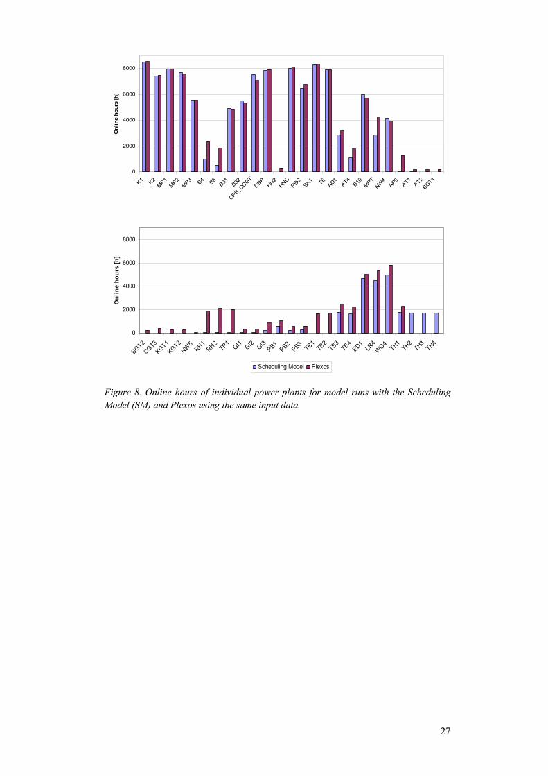
In comparison to Plexos, the results of the Scheduling Model show an increased utilisation of base load units whereas the use of peak load units burning gas oil and light oil is decreased. This leads to lower utilization factors and more start-ups of the units in the Plexos model. Generally, this indicates that the solution derived with Plexos is less optimal. This was expected because the Scheduling Model uses the full mixed integer approach when determining unit commitment whereas Plexos optimises the unit commitment with an approximated algorithm. For further comparison, Figure 8 shows the online hours of the individual power plants for both model runs.

27

0

2000

4000

6000

8000

K1 K2MP1

MP2MP3 B4 B6

B31 B32

CPS_CCGT

DBPHN2

HNCPBC SK1 TE AD1

AT4 B10MRT

NW4

AP5 AT1 AT2BGT1

Onl

ine

hour

s [h

]

0

2000

4000

6000

8000

BGT2CGT8

KGT1KGT2

NW5

RH1RH2

TP1GI1 GI2 GI3

PB1PB2

PB3TB1

TB2TB3

TB4ED1

LR4

WO4TH1

TH2TH3

TH4

Onl

ine

hour

s [h

]

Scheduling Model Plexos

Figure 8. Online hours of individual power plants for model runs with the Scheduling Model (SM) and Plexos using the same input data.

www.risoe.dk 28

4 Results for the year 2020 The following sections present the results of yearly model runs for each power system portfolio in 2020. For these model runs, the following assumptions on the necessary data input are made (see appendix for further information):

• Structure of power plant portfolios and installed capacities of individual power plants in 2020.

• Power plant parameters and maintenance schedules for existing and new power plants.

• Spatial distribution of wind power capacites installed in the All Island power system.

• Time-series for production from wind power, run-of-river, tidal and wave power in 2020.

• Time-series for electricity demand in 2020.

• Requirements for spinning reserve category TR1.

• Fuel price scenarios “Low”, “Central” and “High”, see appendix. For the results presented in the sections 4.3 - 4.12, fuel price scenario “Central” is applied for all portfolios. A sensitivity analysis is presented in section 4.13.

• CO2 emission permit price scenario of 30 Euro/Ton CO2 for portfolios P1 – P5 and of 60 Euro/Ton CO2 for portfolio P6. A sensitivity analysis is presented in section 4.13.

• Gas fired unit SK1 is treated as a must run unit.

• Forecast accuray of wind speed and electricity demand.

• Installed capacity of interconnector between the All Island power system and Great Britain.

• Reduced representation of the power system in Great Britain. The power system in Great Britain is not modified for the individual power plant portfolios of the All Island power system.

• No consideration of the grid structure and load flow issues.

Due to calculation time restrictions the model runs have been carried out with less complexity than implemented, see appendix. The following simplifications have been considered for the model runs:

• Three spinning reserve categories have been implemented in the model namely POR, SOR and TR1 (see list of abbrevations) as defined in the ROI grid code (ESB National Grid 2005). In this study only one spinning reserve category (TR1) is taken into account, i.e. power plant restrictions concerning POR and SOR are not taken into account. This simplification leads to a minor underestimation of the required online capacities reserved for providing spinning reserves.

• No consideration of outtime dependent start-up fuel consumption and start-up times, i.e. start-up fuel consumption and start-up times are constant and correspond to the power plants being in the hot state when started up. Thus, a

29

more flexible unit commitment and dispatch is allowed especially of those units with a short cooling time from hot to warm state and start-up costs are underestimated. However, most of the units with cooling times from the hot to warm state of one hour show the same start-up fuel consumption and start-up times for the hot and warm state, see Table 32 and Table 33. Other units have cooling times from the hot to warm state that reach into the third stage of scenario trees describing forecast errors. Thus, the state of these unit remains the same within the first stage of the scenario trees. Only this stage is considered for the subsequent evaluation of the system operation after the optimal unit commitment and dispatch has been determined. Hence, the consideration of start-up fuel consumption and start-up times according only to the hot state has a limited influence on the results.

• Without the possibility to use the state “Spinning in water” for the pumped hydro storage facility Turlough Hill. This state was not used in the previous model runs, thus removing this state does not influence the results considerably.

Test runs showed that the reduced version of the model offers a good compromise between calculation time and accuracy of model results.

4.1 Renewable power production P1 P2 P3 P4 P5 P6

All Island power system Wind power [TWh] 6.2 12.3 12.3 12.3 18.4 25.4 Other renewables [TWh] 2.3 2.3 2.3 2.3 4.1 6.3

Sum of wind power and other renewables [TWh]

8.5 14.6 14.6 14.6 22.6 31.7

Sum of renewable production / yearly demand [%]

16 27 27 27 42 59

Great Britain Wind power [TWh] 44.6 44.6 44.6 44.6 44.6 44.6 Other renewables [TWh] 4.2 4.2 4.2 4.2 4.2 4.2

Sum of wind power and other renewables [TWh]

48.8 48.8 48.8 48.8 48.8 48.8

Sum of renewable production / yearly demand [%]

13 13 13 13 13 13

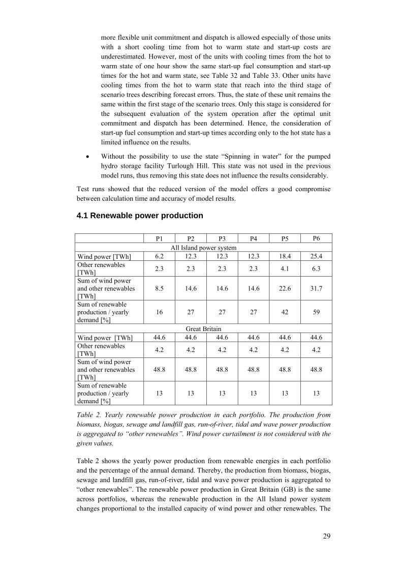
Table 2. Yearly renewable power production in each portfolio. The production from biomass, biogas, sewage and landfill gas, run-of-river, tidal and wave power production is aggregated to “other renewables”. Wind power curtailment is not considered with the given values.

Table 2 shows the yearly power production from renewable energies in each portfolio and the percentage of the annual demand. Thereby, the production from biomass, biogas, sewage and landfill gas, run-of-river, tidal and wave power production is aggregated to “other renewables”. The renewable power production in Great Britain (GB) is the same across portfolios, whereas the renewable production in the All Island power system changes proportional to the installed capacity of wind power and other renewables. The

www.risoe.dk 30

share of the renewable power production of the yearly electricity demand in the All Island power system raises from 16 % in portfolio P1 to 59 % in portfolio P6. With respect to wind power production, the capacity factor of wind power in the All Island power system is approximately 35 % in all portfolios. It is calculated as the ratio between the annual wind power production divided by the product of the installed wind power capacity multiplied with the number of hours per year.

The methodology allows to curtail available wind power production in the All Island power system due to the following, mainly economic, reasons:

• Superfluous wind power production has to be curtailed to maintain the power balance.

• It is more cost optimal to keep conventional power plants running instead of shutting them down thereby avoiding start-up costs.

• It is more cost optimal to provide spinning reserves with wind power.

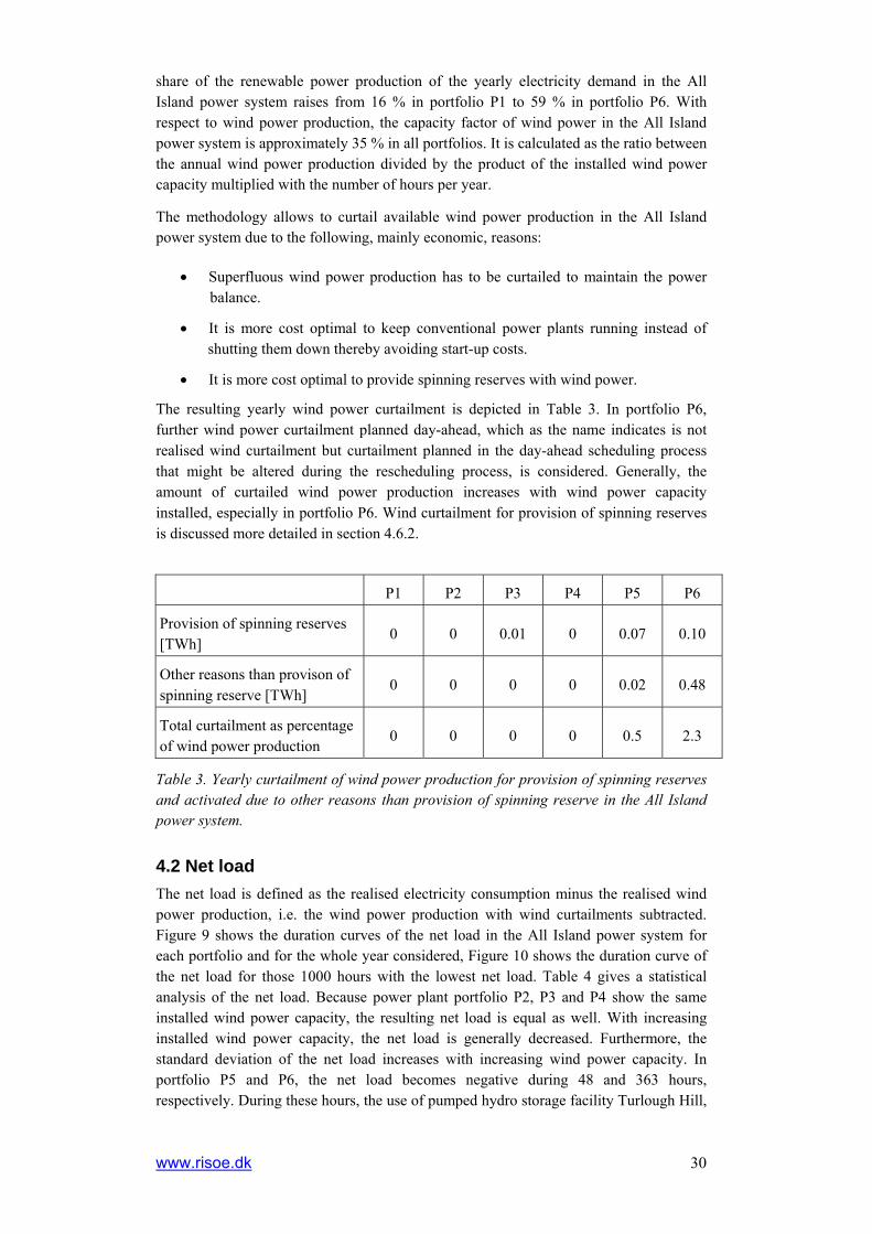
The resulting yearly wind power curtailment is depicted in Table 3. In portfolio P6, further wind power curtailment planned day-ahead, which as the name indicates is not realised wind curtailment but curtailment planned in the day-ahead scheduling process that might be altered during the rescheduling process, is considered. Generally, the amount of curtailed wind power production increases with wind power capacity installed, especially in portfolio P6. Wind curtailment for provision of spinning reserves is discussed more detailed in section 4.6.2.

P1 P2 P3 P4 P5 P6

Provision of spinning reserves [TWh]

0 0 0.01 0 0.07 0.10

Other reasons than provison of spinning reserve [TWh]

0 0 0 0 0.02 0.48

Total curtailment as percentage of wind power production

0 0 0 0 0.5 2.3

Table 3. Yearly curtailment of wind power production for provision of spinning reserves and activated due to other reasons than provision of spinning reserve in the All Island power system.

4.2 Net load The net load is defined as the realised electricity consumption minus the realised wind power production, i.e. the wind power production with wind curtailments subtracted. Figure 9 shows the duration curves of the net load in the All Island power system for each portfolio and for the whole year considered, Figure 10 shows the duration curve of the net load for those 1000 hours with the lowest net load. Table 4 gives a statistical analysis of the net load. Because power plant portfolio P2, P3 and P4 show the same installed wind power capacity, the resulting net load is equal as well. With increasing installed wind power capacity, the net load is generally decreased. Furthermore, the standard deviation of the net load increases with increasing wind power capacity. In portfolio P5 and P6, the net load becomes negative during 48 and 363 hours, respectively. During these hours, the use of pumped hydro storage facility Turlough Hill,

31

export power to Great Britain and wind power curtailment are possible measures to ensure a stable power system operation.

-2000

0

2000

4000

6000

8000

10000

1 673 1345 2017 2689 3361 4033 4705 5377 6049 6721 7393 8065 8737

Net

load

[MW

]

P1 P2, P3, P4 P5 P6

Figure 9. Duration curves of the net load (load minus wind power production) in the All Island power system for all portfolios for the whole year considered. Because the installed wind power capacity is the same in power plant portfolio P2, P3 and P4, the net load is equal as well.

-2000

0

2000

4000

6000

8000

10000

0 200 400 600 800 1000

Net

load

[MW

]

P1 P2, P3, P4 P5 P6

Figure 10. Duration curves of the net load (load minus wind power production) in the All Island power system for all portfolios for those 1000 hours with the lowest net load. Because the installed wind power capacity is the same in power plant portfolio P2, P3 and P4, the net load is equal as well.

www.risoe.dk 32

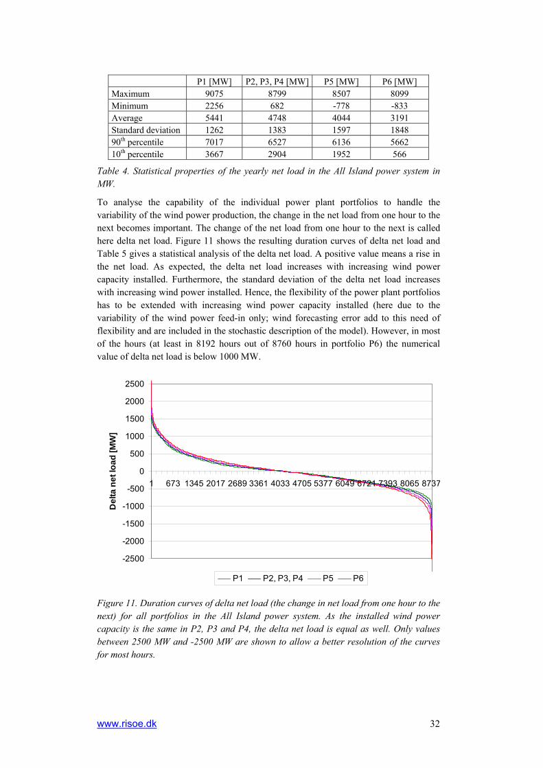
P1 [MW] P2, P3, P4 [MW] P5 [MW] P6 [MW] Maximum 9075 8799 8507 8099 Minimum 2256 682 -778 -833 Average 5441 4748 4044 3191 Standard deviation 1262 1383 1597 1848 90th percentile 7017 6527 6136 5662 10th percentile 3667 2904 1952 566

Table 4. Statistical properties of the yearly net load in the All Island power system in MW.

To analyse the capability of the individual power plant portfolios to handle the variability of the wind power production, the change in the net load from one hour to the next becomes important. The change of the net load from one hour to the next is called here delta net load. Figure 11 shows the resulting duration curves of delta net load and Table 5 gives a statistical analysis of the delta net load. A positive value means a rise in the net load. As expected, the delta net load increases with increasing wind power capacity installed. Furthermore, the standard deviation of the delta net load increases with increasing wind power installed. Hence, the flexibility of the power plant portfolios has to be extended with increasing wind power capacity installed (here due to the variability of the wind power feed-in only; wind forecasting error add to this need of flexibility and are included in the stochastic description of the model). However, in most of the hours (at least in 8192 hours out of 8760 hours in portfolio P6) the numerical value of delta net load is below 1000 MW.

-2500

-2000

-1500

-1000

-500

0

500

1000

1500

2000

2500

1 673 1345 2017 2689 3361 4033 4705 5377 6049 6721 7393 8065 8737

Del

ta n

et lo

ad [M

W]

P1 P2, P3, P4 P5 P6

Figure 11. Duration curves of delta net load (the change in net load from one hour to the next) for all portfolios in the All Island power system. As the installed wind power capacity is the same in P2, P3 and P4, the delta net load is equal as well. Only values between 2500 MW and -2500 MW are shown to allow a better resolution of the curves for most hours.

33

P1 [MW] P2, P3, P4 [MW] P5 [MW] P6 [MW] Maximum 1600 1822 2572 3732 Minimum -1619 -2383 -3366 -4473 Positive Mean 338 361 392 412 Negative Mean -289 -315 -346 -373 Standard deviation 417 447 489 529 90% percentile 538 572 610 647 10% percentile -486 -518 -561 -602

Table 5. Statistical numbers describing the properties of the delta net load in MW. All numbers are calculated over the hours in the year. Positive mean indicates the average of the values where load increases from one hour to the next. Negative mean indicates the average of the values with decreasing load from one hour to the next.

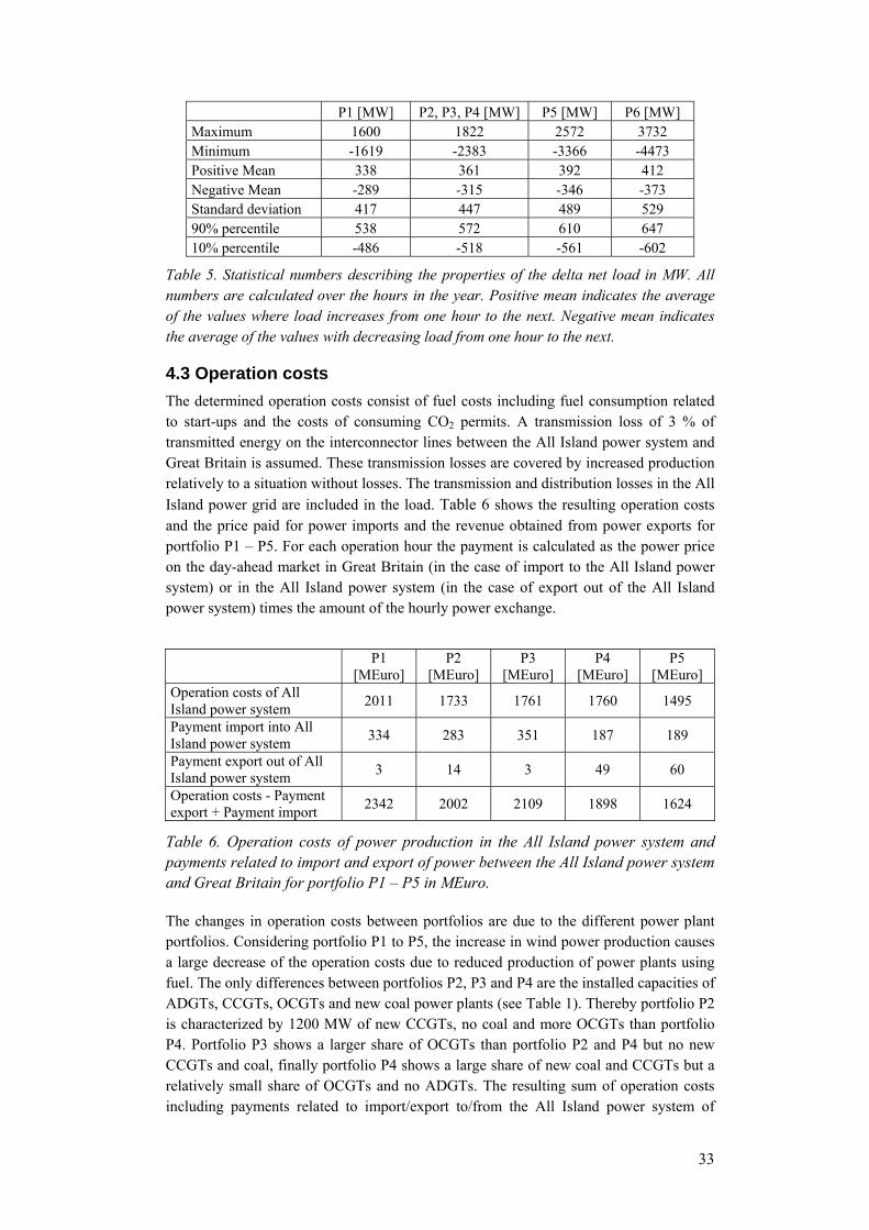
4.3 Operation costs The determined operation costs consist of fuel costs including fuel consumption related to start-ups and the costs of consuming CO2 permits. A transmission loss of 3 % of transmitted energy on the interconnector lines between the All Island power system and Great Britain is assumed. These transmission losses are covered by increased production relatively to a situation without losses. The transmission and distribution losses in the All Island power grid are included in the load. Table 6 shows the resulting operation costs and the price paid for power imports and the revenue obtained from power exports for portfolio P1 – P5. For each operation hour the payment is calculated as the power price on the day-ahead market in Great Britain (in the case of import to the All Island power system) or in the All Island power system (in the case of export out of the All Island power system) times the amount of the hourly power exchange.

P1

[MEuro] P2

[MEuro] P3

[MEuro] P4

[MEuro] P5

[MEuro] Operation costs of All Island power system 2011 1733 1761 1760 1495

Payment import into All Island power system 334 283 351 187 189

Payment export out of All Island power system 3 14 3 49 60

Operation costs - Payment export + Payment import 2342 2002 2109 1898 1624

Table 6. Operation costs of power production in the All Island power system and payments related to import and export of power between the All Island power system and Great Britain for portfolio P1 – P5 in MEuro.

The changes in operation costs between portfolios are due to the different power plant portfolios. Considering portfolio P1 to P5, the increase in wind power production causes a large decrease of the operation costs due to reduced production of power plants using fuel. The only differences between portfolios P2, P3 and P4 are the installed capacities of ADGTs, CCGTs, OCGTs and new coal power plants (see Table 1). Thereby portfolio P2 is characterized by 1200 MW of new CCGTs, no coal and more OCGTs than portfolio P4. Portfolio P3 shows a larger share of OCGTs than portfolio P2 and P4 but no new CCGTs and coal, finally portfolio P4 shows a large share of new coal and CCGTs but a relatively small share of OCGTs and no ADGTs. The resulting sum of operation costs including payments related to import/export to/from the All Island power system of

www.risoe.dk 34

portfolio P4 are 104 MEuro lower than of portfolio P2 and 211 MEuro lower than of portfolio P3. These results show that with regard to total costs it is most optimal to have a large share of power plants with low variable costs, even when integrating fluctuating wind power. With the fuel prices and CO2 emission permit price assumed, new coal power plants show smaller marginal costs than CCGTs. Although OCGTs show comparable small start-up costs, the low efficiencies of these plants and the higher price of their fuel (mid-merit gas) result in higher costs like for example in portfolio P3. Thus, the higher flexibility of OCGTs does not compensate for their higher fuel costs.

With these portfolios, the main transmission flow is import into the All Island power system, see section 4.9. With increased amounts of wind power production in the All Island power system the export to Great Britain increases. The lower total costs in portfolio P4 relatively to portfolio P2 and P3 are also reflected in a lower cost of the marginal power plant in the hour i.e. a lower power price on the day-ahead market in the All Island power system. Because the power plant portfolio in Great Britain is constant for all portfolios a lower power price in the All Island power system will decrease import into the All Island power system and increase export. Therefore the import to the All Island power system decreases and the export to Great Britain increases in portfolio P4 relatively to portfolio P2 and P3.

Table 7 shows the operation costs in the All Island power system distributed on start-up costs, fuel costs excluding start-up fuel consumption and costs of consuming CO2 emission permits for portfolios P1 – P5. Generally, start-up costs constitute a small part of the total operation costs. These costs tend to increase with higher installed wind power capacity. However, the structure of the portfolio has an important influence on the start-up costs as well. Comparing portfolio P2, P3 and P4, the latter portfolio with less units that are more inflexible shows high start-up costs. Fuel costs in the All Island power system decrease with increasing wind power installed.

P1 [MEuro] P2 [MEuro] P3 [MEuro] P4 [MEuro] P5 [MEuro] Start-up costs 5 6 5 24 11 Fuel costs 1404 1200 1204 1080 1024 CO2 costs 603 527 552 655 460

Table 7. Operation costs in the All Island power system divided into start-up costs, fuel costs and CO2 costs for portfolio P1 – P5 in MEuro.

Due to the high CO2 emission permit price in portfolio P6, the resulting total costs of portfolio P6 are comparably high, see Table 8. However, fuel costs are the lowest compared to portfolio P1 – P5.

35

P6 [MEuro] Operation costs of All Island power system 1861

thereof start-up costs 20 thereof fuel costs 977 thereof CO2 costs 864

Payment import into All Island power system 141

Payment export out of All Island power system 220

Operation costs – Payment export + Payment import 1782

Table 8. Operation costs of power production in the All Island power system and payments related to import and export of power between the All Island power system and Great Britain for portfolio P6 in MEuro.

PBC (Poolbeg combined cycle) was modelled as one unit in this study. A consideration of PBC as two units would reduce the operation costs in the All Island power system including payments related to imports and export for example in portfolio P4 and P5 with 0.5%. The costs reductions are mainly caused by a decrease in the average demand for spinning reserve with approximately 50 MW, see section 4.6.1.

4.4 CO2 emissions Table 9 shows the yearly sum of CO2 emissions of portfolio P1 – P5 in the All Island power system and in Great Britain.

Region P1 [Mton] P2 [Mton] P3 [Mton] P4 [Mton] P5 [Mton] GB 199.8 197.6 198.6 195.7 195.4 All Island 20.1 17.6 18.4 21.8 15.3 Total 219.9 215.2 217.0 217.5 210.8

Table 9. Yearly sum of CO2 emissions in portfolios P1 – P5 in MTon.

Generally, with increasing wind power capacity installed, the sum of CO2 emission decreases for the All Island power system and Great Britain. The change of the transmission pattern between the All Island power system and Great Britain significantly influences the CO2 emission in the All Island power system. This can be observed most clearly by comparison of the portfolios P3 and P4. Portfolio P4 shows a sum of CO2 emissions in the All Island power system being 18% higher than in P3 but with the total CO2 emissions in both power systems being almost the same in both portfolios. Among those portfolios with an equal wind power capacity installed (portfolio P2 – P4) and when only the All Island power system is considered, portfolio P2 shows the lowest CO2 emissions.

The assumption of a higher CO2 emission permit price of 80 Euro/ton CO2 in portfolio P6, see Table 1, causes a shift from the use of coal fired power plants to base load gas fired power plants, especially in Great Britain. This effect leads to a significant decrease of CO2 emissions of 10.8 Mton CO2 in the All Island power system and of 107.2 Mton CO2 in Great Britain in portfolio P6. A comparison of the resulting CO2 emissions with equal CO2 emission permit prices assumed for all portfolios is given in section 4.13.

www.risoe.dk 36

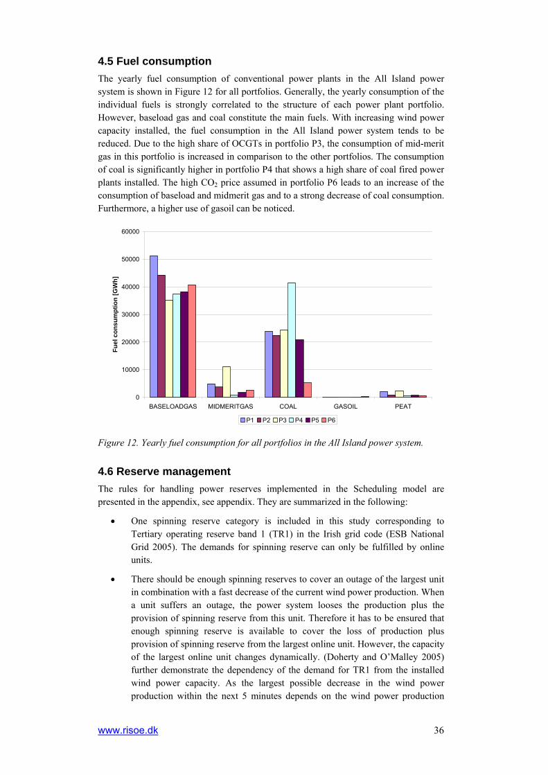
4.5 Fuel consumption The yearly fuel consumption of conventional power plants in the All Island power system is shown in Figure 12 for all portfolios. Generally, the yearly consumption of the individual fuels is strongly correlated to the structure of each power plant portfolio. However, baseload gas and coal constitute the main fuels. With increasing wind power capacity installed, the fuel consumption in the All Island power system tends to be reduced. Due to the high share of OCGTs in portfolio P3, the consumption of mid-merit gas in this portfolio is increased in comparison to the other portfolios. The consumption of coal is significantly higher in portfolio P4 that shows a high share of coal fired power plants installed. The high CO2 price assumed in portfolio P6 leads to an increase of the consumption of baseload and midmerit gas and to a strong decrease of coal consumption. Furthermore, a higher use of gasoil can be noticed.

0

10000

20000

30000

40000

50000

60000

BASELOADGAS MIDMERITGAS COAL GASOIL PEAT

Fuel

con

sum

ptio

n [G

Wh]

P1 P2 P3 P4 P5 P6

Figure 12. Yearly fuel consumption for all portfolios in the All Island power system.

4.6 Reserve management The rules for handling power reserves implemented in the Scheduling model are presented in the appendix, see appendix. They are summarized in the following:

• One spinning reserve category is included in this study corresponding to Tertiary operating reserve band 1 (TR1) in the Irish grid code (ESB National Grid 2005). The demands for spinning reserve can only be fulfilled by online units.

• There should be enough spinning reserves to cover an outage of the largest unit in combination with a fast decrease of the current wind power production. When a unit suffers an outage, the power system looses the production plus the provision of spinning reserve from this unit. Therefore it has to be ensured that enough spinning reserve is available to cover the loss of production plus provision of spinning reserve from the largest online unit. However, the capacity of the largest online unit changes dynamically. (Doherty and O’Malley 2005) further demonstrate the dependency of the demand for TR1 from the installed wind power capacity. As the largest possible decrease in the wind power production within the next 5 minutes depends on the wind power production

37

right now, the latest wind power forecasts are used instead of the installed wind power. The demands for spinning reserves are therefore updated in each planning loop according to the planned unit commitment and the latest wind power forecast.

• The capability of a unit to provide spinning reserves is restricted by:

o The maximum reserve capability of this unit.

o The online capacity minus the generation.

• The demand for positive reserves with activation times longer than 5 minutes (forecast horizons from 5 minutes to 36 hours ahead) is determined by the Scenario Tree Tool, see appendix. These reserves are labelled replacement reserves.

• A unit planned to be online in a given time step and scenario can deliver both spinning and replacement reserves. The amount of online capacity reserved for providing these types of reserves will be the sum of the obligation undertaken to provide TR1 and the obligation to provide replacement reserve.

• A unit planned to be offline in a given time step and scenario can only provide replacement reserves and only in hours further ahead in time than the start-up time of the unit.

• Wind turbines can provide positive spinning reserves by reducing their production.

• At least 50% of the demand for spinning reserves must be provided by regulating units i.e. excluding wind power and pumped hydro storage (Turlough Hill) when it is pumping.

4.6.1 Demand for spinning reserves The demand for spinning reserves depends on the largest online unit and the wind power forecasts. Figure 13 and Figure 14 show the demand for spinning reserve averaged on the hours during the day and the weeks of the year, respectively. 100 MW of spinning reserve is assumed to be delivered from Great Britain and 50 MW is delivered from interruptible load.

www.risoe.dk 38

300

350

400

450

500

550

600

650

700

00 01 02 03 04 05 06 07 08 09 10 11 12 13 14 15 16 17 18 19 20 21 22 23

Dem

and

spin

ning

rese

rves

[MW

]

P1 P2 P3 P4 P5 P6

Figure 13. Average demand for spinning reserve during the year distributed on hours during the day in MW.

The main determinant for the demand for spinning reserve constitutes the power production plus the provision of spinning reserve of the largest unit. Portfolio P1 has two units with a largest capacity of 480 MW (Poolbeg Combined Cycle (PBC) and New CCGT 1) and the third largest unit with a capacity of 414 MW (New CCGT 2). The largest unit in portfolio P2, P3, P4, P5 and P6 is PBC and the second largest unit with a capacity of 404 MW (Tynagh (TE) and Coolkeeragh CCGT (CPS_CCGT)). Table 10 shows the number of online hours of PBC for each portfolio. Portfolio P1 and P3 have a relatively large number of OCGTs, hence PBC is in operation during many hours. PBC has also long operation times in portfolio P6 due to the high CO2 emission permit price assumed. This explains why the demand for spinning reserves is more constant during the 24 hours of the day for portfolio P1, P3 and P6. For the other portfolios, the average demand during the night is about 5-10 % lower than the demand for spinning reserves during the peak load hour (hour 17). Further on, P6 has on average a higher demand for spinning reserves due to the large wind and wave power capacity installed.

P1 [h] P2 [h] P3 [h] P4 [h] P5 [h] P6 [h]PBC 5535 4637 6335 2900 3739 6348

Table 10. Number of online hours of PBC in each portfolio.

During the year, the demand for spinning reserves is rather constant for portfolio P1 - P5, see Figure 14. However, due to a scheduled outage of PBC in the weeks 31, 32 and 33, the demand for spinning reserves is obviously reduced during these weeks for portfolios P2, P3, P4, P5 and P6. The reason that this reduction cannot be observed for portfolio P1 is that there is one unit of the same size as PBC in P1, namely New CCGT 1. In portfolio P6, the seasonal pattern in the wind power production with smaller production in the summer months is also reflected in the demand for spinning reserves.

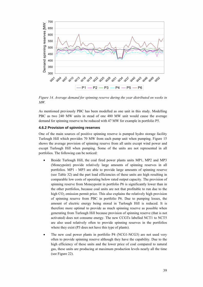
39

300

350

400

450

500

550

600

650

700

W01W04 W07 W10

W13W16

W19 W22W25 W28

W31 W34 W37 W40 W43 W46 W49W52

Dem

and

spin

ning

rese

rves

[MW

]

P1 P2 P3 P4 P5 P6

Figure 14. Average demand for spinning reserve during the year distributed on weeks in MW.

As mentioned previously PBC has been modelled as one unit in this study. Modelling PBC as two 240 MW units in stead of one 480 MW unit would cause the average demand for spinning reserve to be reduced with 47 MW for example in portfolio P5.

4.6.2 Provision of spinning reserves One of the main sources of positive spinning reserve is pumped hydro storage facility Turlough Hill which provides 70 MW from each pump unit when pumping. Figure 15 shows the average provision of spinning reserve from all units except wind power and except Turlough Hill when pumping. Some of the units are not represented in all portfolios. The following can be noticed:

• Beside Turlough Hill, the coal fired power plants units MP1, MP2 and MP3 (Moneypoint) provide relatively large amounts of spinning reserves in all portfolios. MP1 - MP3 are able to provide large amounts of spinning reserve (see Table 32) and the part load efficiencies of these units are high resulting in comparable low costs of operating below rated output capacity. The provision of spinning reserve from Moneypoint in portfolio P6 is significantly lower than in the other portfolios, because coal units are not that profitable to run due to the high CO2 emission permit price. This also explains the relatively high provision of spinning reserve from PBC in portfolio P6. Due to pumping losses, the amount of electric energy being stored in Turlough Hill is reduced. It is therefore more optimal to provide as much spinning reserve as possible when generating from Turlough Hill because provision of spinning reserve (that is not activated) does not consume energy. The new CCGTs labelled NCT1 to NCT5 are also used relatively often to provide spinning reserves in the portfolios where they exist (P3 does not have this type of plants).

• The new coal power plants in portfolio P4 (NCG1-NCG3) are not used very often to provide spinning reserve although they have the capability. Due to the high efficiency of these units and the lower price of coal compared to natural gas, these units are producing at maximum production levels nearly all the time (see Figure 22).

www.risoe.dk 40

• Portfolio P3 does not have new CCGTs or new coal power plants, hence it is optimal to run the existing large coal power plant and CCGTs units closer to maximum production levels and distribute the spinning reserve requirements on ADGTs (NAT1-NAT7) and OCGTs (NOT1-NOT19).

• ADGTs form good sources for spinning reserves because of their high part-load efficiencies. Portfolio P2 has relatively large amounts of these units (see Table 1), thus in portfolio P2 the large coal power plants and CCGTs are used less to provide spinning reserve compared to the other portfolios.

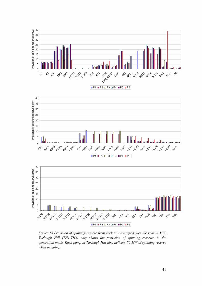
41

0

5

10

15

20

25

30

35

40

K1 K2MP1

MP2MP3

NCG1NCG2

NCG3B10 B31 B32

CPS_CCGT

DBPHNC

NCT1NCT2

NCT3NCT4

NCT5PBC

SK1 TE

Pro

visi

on o

f spi

nnin

g re

serv

es [M

W]

P1 P2 P3 P4 P5 P6

0

5

10

15

20

25

30

35

40

AD1BGT1

BGT2CGT8

KGT1KGT2

MRTNAT1

NAT2NAT3

NAT4NAT5

NAT6NAT7

NOT1NOT2

NOT3NOT4

NOT5NOT6

NOT7NOT8

Pro

visi

on o

f spi

nnin

g re

serv

es [M

W]

P1 P2 P3 P4 P5 P6

0

5

10

15

20

25

30

35

40

NOT9

NOT10

NOT11

NOT12

NOT13

NOT14

NOT15

NOT16

NOT17

NOT18

NOT19RH1

RH2TP1

ED1LR

4WO4

TH1TH2

TH3TH4

Pro

visi

on o

f spi

nnin

g re

serv

es [M

W]

P1 P2 P3 P4 P5 P6

Figure 15 Provision of spinning reserve from each unit averaged over the year in MW. Turlough Hill (TH1-TH4) only shows the provision of spinning reserves in the generation mode. Each pump in Turlough Hill also delivers 70 MW of spinning reserve when pumping.

www.risoe.dk 42

Table 11 shows the provision of spinning reserve from wind power (the approach how wind power is able to contribute to spinning reserves is depicted in the appendix). With increasing wind power capacity installed, wind power is used more frequently to provide spinning reserves. Comparing portfolios P2, P3 and P4, wind power is used for spinning reserves most often in portfolio P3 followed by portfolio P2 and P4. Because curtailment of wind power is a relatively expensive way of providing spinning reserve, this indicates that providing spinning reserves is most costly in portfolio P3 with no new large units and many OCGTs compared to portfolio P2 with new CCGTs and portfolio P4 with both new CCGTs and new coal power plants. It is more expensive to provide spinning reserve from an OCGT with low efficiency and usage of expensive fuel compared to a new CCGT or coal power plant unit with high efficiencies and usage of cheap fuel, because provision of spinning reserve enforces the unit to be online with a certain amount of power production due to the requirement of a minimum stable operation limit.

P1 P2 P3 P4 P5 P6 Duration [h] 1 29 64 2 228 1322 Average [MW] 2 17 23 5 31 78 Average/installed capacity [%] 0.1 0.4 0.6 0.1 0.5 0.9 Maximum [MW] 2 102 142 9 210 278 Max/installed capacity [%] 0.1 2.6 3.6 0.2 3.5 3.5

Table 11 Provision of spinning reserve from wind power. Duration indicates the number of hours where wind power is curtailed to provide spinning reserve. Average gives the average capacity provided during these hours. Maximum gives the maximum capacity provided during these hours. The average and maximum contribution relative to the installed wind power capacity are also presented.

4.6.3 Demand for replacement reserves The demand for replacement reserves is determined with the Scenario Tree Tool, i.e by a different approach than the determination of the demand for spinning reserves. The demand for replacement reserves corresponds to the total forecast error of the power system considered which is defined according to the hourly distribution of wind power and load forecast errors and according to forced outages of conventional power plants. Thereby it is assumed that the nth percentile of the total forecast error has to be covered by replacement reserves. The applied methodology is further described in the appendix.

Before determination of the demand for replacement reserves for power plant portfolios P1 - P6, the applied percentile had to be determined with respect to the present power system. Therefore, it has been agreed with the All Island Grid Study Working Group that only load forecast errors and forced outages had to be considered. The resulting average demand for replacement reserves over the forecast horizon depending on the 80th, 85th, 90th, 95th, 97th and 99th is shown in Figure 16. The illustration does not consider the structure of the scenario tree. It has been decided by the All Island Grid Study Working Group as a working assumption that the 90th percentile of the total forecast error has to be used for the determination of the demand for replacement reserves.

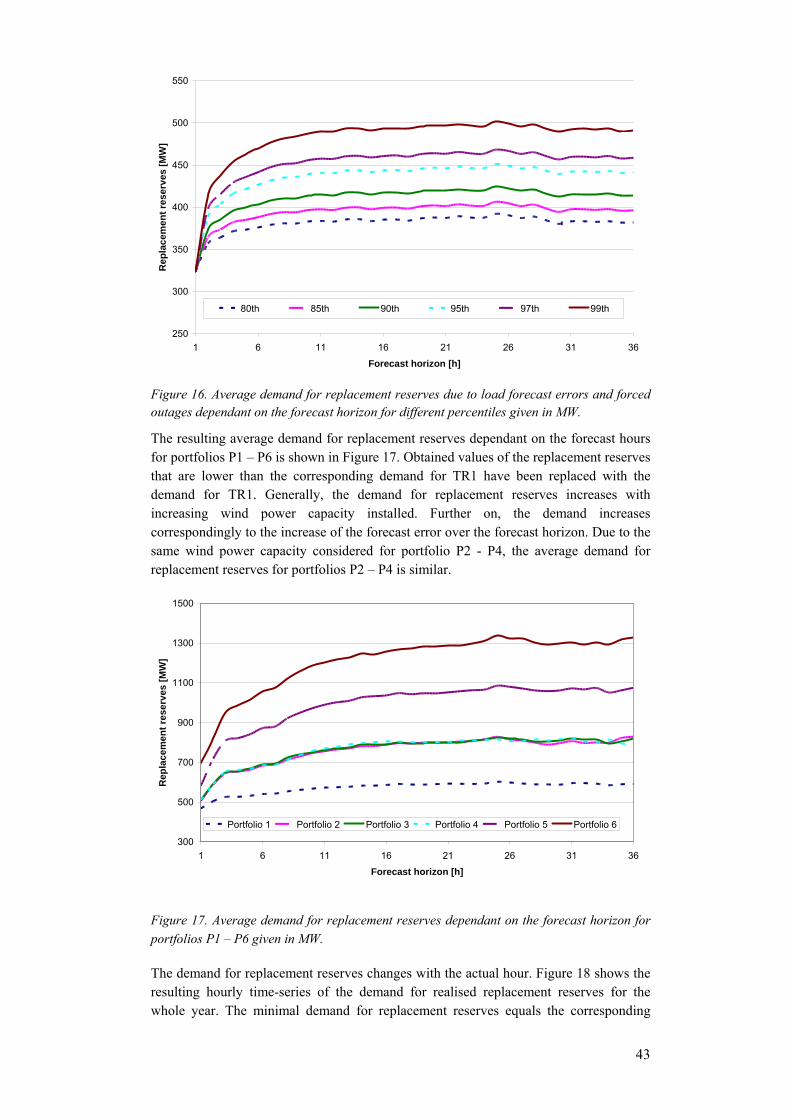
43

250

300

350

400

450

500

550

1 6 11 16 21 26 31 36

Forecast horizon [h]

Rep

lace

men

t res

erve

s [M

W]

80th 85th 90th 95th 97th 99th

Figure 16. Average demand for replacement reserves due to load forecast errors and forced outages dependant on the forecast horizon for different percentiles given in MW.

The resulting average demand for replacement reserves dependant on the forecast hours for portfolios P1 – P6 is shown in Figure 17. Obtained values of the replacement reserves that are lower than the corresponding demand for TR1 have been replaced with the demand for TR1. Generally, the demand for replacement reserves increases with increasing wind power capacity installed. Further on, the demand increases correspondingly to the increase of the forecast error over the forecast horizon. Due to the same wind power capacity considered for portfolio P2 - P4, the average demand for replacement reserves for portfolios P2 – P4 is similar.

300

500

700

900

1100

1300

1500

1 6 11 16 21 26 31 36

Forecast horizon [h]

Rep

lace

men

t res

erve

s [M

W]

Portfolio 1 Portfolio 2 Portfolio 3 Portfolio 4 Portfolio 5 Portfolio 6

Figure 17. Average demand for replacement reserves dependant on the forecast horizon for portfolios P1 – P6 given in MW.

The demand for replacement reserves changes with the actual hour. Figure 18 shows the resulting hourly time-series of the demand for realised replacement reserves for the whole year. The minimal demand for replacement reserves equals the corresponding

www.risoe.dk 44

demand for TR1, see above. The occurence of high demands for replacement reserves is mainly driven by a high number of simultaneous forced outages that happens simultaneously to relatively high wind power or load forecast errors. The value of these peaks tends to increase with increasing wind power capacity installed.

Portfolio 1

0

500

1000

1500

2000

2500

3000

3500

4000

1 673 1345 2017 2689 3361 4033 4705 5377 6049 6721 7393 8065 8737Time [h]

Rep

lace

men

t res

erve

s [M

W]

Portfolio 2

0

500

1000

1500

2000

2500

3000

3500

4000

1 673 1345 2017 2689 3361 4033 4705 5377 6049 6721 7393 8065 8737Time [h]

Rep

lace

men

t res

erve

s [M

W]

Portfolio 3

0

500

1000

1500

2000

2500

3000

3500

4000

1 673 1345 2017 2689 3361 4033 4705 5377 6049 6721 7393 8065 8737Time [h]

Rep

lace

men

t res

erve

s [M

W]

Portfolio 4

0

500

1000

1500

2000

2500

3000

3500

4000

1 673 1345 2017 2689 3361 4033 4705 5377 6049 6721 7393 8065 8737Time [h]

Rep

lace

men

t res

erve

s [M

W]

Portfolio 5

0

500

1000

1500

2000

2500

3000

3500

4000

1 673 1345 2017 2689 3361 4033 4705 5377 6049 6721 7393 8065 8737Time [h]

Rep

lace

men

t res

erve

s [M

W]

Portfolio 6

0

500

1000

1500

2000

2500

3000

3500

4000

1 673 1345 2017 2689 3361 4033 4705 5377 6049 6721 7393 8065 8737Time [h]

Rep

lace

men

t res

erve

s [M

W]

Figure 18. Demand for replacement reserves during a year for portfolio P1 – P6 given in MW.

4.6.4 Provision of replacement reserves Table 12 shows the average supply and demand of replacement reserves during the year. Nearly the whole demand for replacement reserves is provided with offline units in all portfolios. Furthermore in most hours the provision of replacement reserves is significantly higher than the demand for replacement reserves. This indicates that the costs of providing replacement reserves are equal to zero in most hours. The explanation is that the portfolios show large power plant capacities with start-up times below one or two hours (see Table 13) compared to the demand for replacement reserves. Some of the power plants with start-up times below one hour are OCGTs with relatively low efficiencies and usage of expensive fuel. In those hours with a available power plant capacity higher than the actual load, these OCGTs would be offline irrespective of the demand for replacement reserves because they are the most expensive units to be operated. Hence, the costs of providing replacement reserves from OCGTs in these hours are zero. In the hours with a strict capacity balance where the demad for replacement reserves can not be entirely fulfilled, the costs of providing replacement reserves are positive,

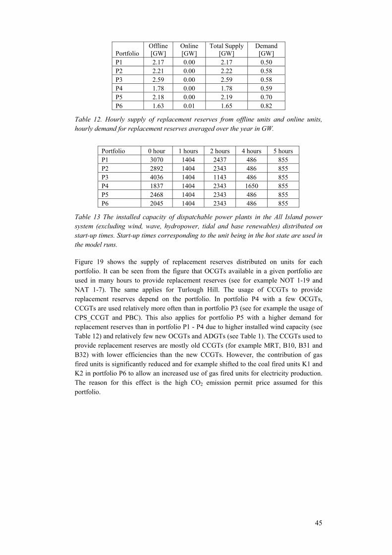
45

Portfolio Offline [GW]

Online [GW]

Total Supply [GW]

Demand [GW]

P1 2.17 0.00 2.17 0.50 P2 2.21 0.00 2.22 0.58 P3 2.59 0.00 2.59 0.58 P4 1.78 0.00 1.78 0.59 P5 2.18 0.00 2.19 0.70 P6 1.63 0.01 1.65 0.82

Table 12. Hourly supply of replacement reserves from offline units and online units, hourly demand for replacement reserves averaged over the year in GW.

Portfolio 0 hour 1 hours 2 hours 4 hours 5 hours P1 3070 1404 2437 486 855 P2 2892 1404 2343 486 855 P3 4036 1404 1143 486 855 P4 1837 1404 2343 1650 855 P5 2468 1404 2343 486 855 P6 2045 1404 2343 486 855

Table 13 The installed capacity of dispatchable power plants in the All Island power system (excluding wind, wave, hydropower, tidal and base renewables) distributed on start-up times. Start-up times corresponding to the unit being in the hot state are used in the model runs.

Figure 19 shows the supply of replacement reserves distributed on units for each portfolio. It can be seen from the figure that OCGTs available in a given portfolio are used in many hours to provide replacement reserves (see for example NOT 1-19 and NAT 1-7). The same applies for Turlough Hill. The usage of CCGTs to provide replacement reserves depend on the portfolio. In portfolio P4 with a few OCGTs, CCGTs are used relatively more often than in portfolio P3 (see for example the usage of CPS_CCGT and PBC). This also applies for portfolio P5 with a higher demand for replacement reserves than in portfolio P1 - P4 due to higher installed wind capacity (see Table 12) and relatively few new OCGTs and ADGTs (see Table 1). The CCGTs used to provide replacement reserves are mostly old CCGTs (for example MRT, B10, B31 and B32) with lower efficiencies than the new CCGTs. However, the contribution of gas fired units is significantly reduced and for example shifted to the coal fired units K1 and K2 in portfolio P6 to allow an increased use of gas fired units for electricity production. The reason for this effect is the high CO2 emission permit price assumed for this portfolio.

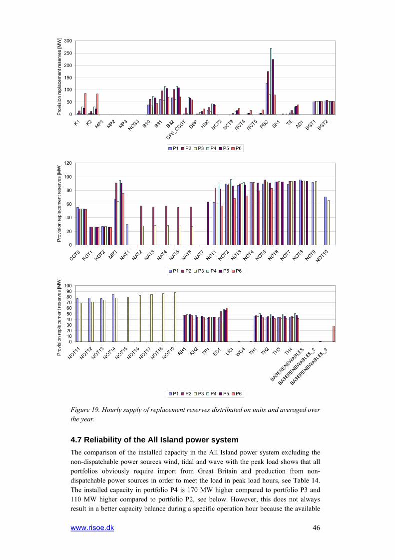
www.risoe.dk 46

0

50

100

150

200

250

300

K1 K2MP1

MP2MP3

NCG3B10 B31 B32

CPS_CCGT

DBPHNC

NCT2NCT3

NCT4NCT5

PBCSK1 TE

AD1BGT1

BGT2

Pro

visi

on re

plac

emen

t res

erve

s [M

W]

P1 P2 P3 P4 P5 P6

0

20

40

60

80

100

120

CGT8KGT1

KGT2MRT

NAT1NAT2

NAT3NAT4

NAT5NAT6

NAT7NOT1

NOT2NOT3

NOT4NOT5

NOT6NOT7

NOT8NOT9

NOT10

Pro

visi

on re

plac

emen

t res

erve

s [M

W]

P1 P2 P3 P4 P5 P6

0102030405060708090

100

NOT11

NOT12

NOT13

NOT14

NOT15

NOT16

NOT17

NOT18

NOT19RH1

RH2TP1

ED1LR

4WO4

TH1TH2

TH3TH4

BASERENEWABLES

BASERENEWABLES_2

BASERENEWABLES_3P

rovi

sion

repl

acem

ent r

eser

ves

[MW

]

P1 P2 P3 P4 P5 P6

Figure 19. Hourly supply of replacement reserves distributed on units and averaged over the year.

4.7 Reliability of the All Island power system The comparison of the installed capacity in the All Island power system excluding the non-dispatchable power sources wind, tidal and wave with the peak load shows that all portfolios obviously require import from Great Britain and production from non-dispatchable power sources in order to meet the load in peak load hours, see Table 14. The installed capacity in portfolio P4 is 170 MW higher compared to portfolio P3 and 110 MW higher compared to portfolio P2, see below. However, this does not always result in a better capacity balance during a specific operation hour because the available

47

capacity is equal to the installed capacity modified by scheduled and forced outages of power plants and because the variability of unit commitment and dispatch can be further restricted for example by start-up times.

P1 [MW] P2 [MW] P3 [MW] P4 [MW] P5 [MW] P6 [MW]

Total installed capacity excluding wind, tidal and wave power

8644 8374 8314 8484 8128 7739

Peak load 9619 9619 9619 9619 9619 9619

Table 14. Comparison of the total installed capacity excluding wind, tidal and wave power with the peak load in MW.

4.7.1 Loss of load expectation The capacity balances of the portfolios were calibrated to a given LOLE (Loss of load expectation) of 8 hours per year. Adding the available capacities of the power plant portfolios including the effects of scheduled and forced outages with 500 MW of the capacity of the interconnector to Great Britain with the realised time-series of wind power production, tidal stream production and wave power production and subtracting the load, the number of hours during the year with negative capacity balances were determined. Thereby the usage of capacity for provision of spinning or replacement reserves was not considered. The results for portfolios P1, P2 and P4 showed higher values of LOLE than 8 hours. Therefore, the All Island Grid Study Working Group decided to add one OCGT power plant with a capacity of 103.6 MW to the original portfolios P1, P2 and P4 as derived in work-stream 2A, respectively (Doherty 2006). The resulting LOLE in hours is shown for each power plant portfolio in Table 15. However, portfolio 1 still shows a LOLE higher than 8 hours.

Portfolio 1 Portfolio 2 Portfolio 3 Portfolio 4 Portfolio 5 Portfolio 6

LOLE 11 6 0 7 2 4

Table 15. Realised LOLE of each power plant portfolio.

4.7.2 Reliability in model runs Table 16 shows the number of hours where respectively load, demand for spinning reserves and demand for replacement reserves is not met in the model runs. The differences compared to the values given in Table 15 are mainly due to the consideration of the entire capacity of the interconnector to Great Britain in the model runs.

The logic in the model ensures that load is met before the demand for spinning reserves, and the demand for spinning reserve is met before the demand for replacement reserves. Portfolio P1 – P5 show a high reliability, i.e. the number of hours where the load is not met remains below the considered LOLE. The load is met in portfolio P1, P3 and P5 in every hour. The number of hours where load cannot be met raises to 23 in portfolio P6. However, the occurrences of these hours is not always related to a strict capacity balance. The load cannot be met in three hours due to lack of capacity in portfolio P6. In these hours, the maximal missing capacity is 166 MW and 111 MW on average. In the remaining hours, the load cannot be covered because the power exchange with Great Britain is not modified during the rescheduling with the applied method, see appendix.

www.risoe.dk 48

With a reduction of the export to or an increased import from Great Britain, the load could have been covered during these hours. Table 16 further shows that in portfolio P1 - P5 the demand for replacement reserves is not fulfilled in approximately 100 hours per year due to lack of capacity. This value raises in portfolio P6 to 544 hours. Hence, the power system would not be able to cover the 90th percentile of the total forecast errors that can occur during these hours. The coverage of the 90th percentile of the total forecast errors was chosen as a suitable reliability level by the All Island Grid Study working group (see section 4.6.3).

Portfolio Hours where load

is not met Hours where demand spinning reserve is not met

Hours where demand for replacement reserve is not met due to lack of capacity

P1 0 4 96 P2 3 6 101 P3 0 1 98 P4 1 5 115 P5 0 3 88 P6 23 77 544

Table 16 Number of hours where load, demand for spinning reserve and replacement reserves is not met. The logic in the model ensures that load is met before the demand for spinning reserves, and the demand for spinning reserve is met before the demand for replacement reserves.

Table 17 shows the average and maximum values of load, demand for spinning reserves and replacement reserves not covered during those hours where a shortage occurs. Portfolio P3 has the overall best reliability of the portfolios caused by many small units in portfolio P3 reducing the impact of forced outages. Portfolio P6 shows the worst overall reliability, however portfolio P2 shows the highest value of demand for replacement reserves not covered.

Portfolio Average (max)

load not met [MW]

Average (max) demand for spinning

reserve not met [MW]

Average (max) demand for replacement reserve not met

due to lack of capacity [MW] P1 0 170 (259) 336 (1255) P2 26 (44) 155 (258) 442 (1908) P3 0 8 (8) 325 (958) P4 85 (85) 148 (321) 449 (1302) P5 0 62 (128) 362 (973) P6 186 (551) 132 (353) 249 (1480)

Table 17. Average and maximum amount of load, spinning reserve and replacement reserve not met.

49

4.8 Dispatch of conventional power plants Figure 20 shows the yearly electricity production distributed on fuel of the All Island power system. Generally, the distribution of the electricity production on the individual fuels is strongly correlated to the structure of each power plant portfolio. However, with increasing wind power capacity installed, the electricity production using baseload gas in the All Island power system tends to be reduced. Due to the high share of OCGTs in portfolio P1 and P3, the consumption of mid-merit gas in these portfolios is increased in comparison to the other portfolios. The high CO2 price assumed in portfolio P6 leads to a strong decrease in the production of coal consuming power plants.

0

5000

10000

15000

20000

25000

30000

BASELOADGAS

MIDMERITGAS

COAL

GASOIL

BIOGAS

PEAT

STORAGE

WATER

WIND

Prod

uctio

n [G

Wh]

P1 P2 P3 P4 P5 P6

Figure 20. Yearly electricity production distributed on fuel type for all portfolios in the All Island power system.

Figure 21 to Figure 25 show the yearly production, capacity factors, online hours, number of start-ups and utilisation factors of the units in the All Island power system for all portfolios. The bigger part of the electricity production in the All Island power system is borne by coal plants and newer CCGTs, see Figure 21. This is also reflected in comparable high capacity factors of these units. With increasing wind power capacity, the production and capacity factors of these power plants tends to be decreased. Due to the high CO2 emission permit price in portfolio P6, the contribution of coal fired power plants is further reduced in this portfolio. In portfolio P3, new ADGTs have a higher share than in portfolio P2 due to lacking new CCGTs. OCGTs generally show very little power production. This leads also to low capacity factors of OCGTs (see Figure 22). SK1 has a high capacity factor because it has been assumed that it is a must run unit. The capacity factors of Turlough Hill only include the generation state i.e. the pumping state is not considered.

Coal fired units and newer CCGTs have relative low number of start-ups and high number of online hours during the year for portfolio P1 to P5 (see Figure 23 and Figure 24). However, the number of start-ups of newer CCGTs and coal fired units increases with increasing wind power capacity installed due to a higher need of flexible operation. The resulting significant increase of start-ups and decrease of online hours of coal fired

www.risoe.dk 50

units in portfolio P6 may be explained with the high CO2 emission permit price. Among the portfolios with the same wind power capacity installed (portfolio P2 – P4), the number of start-ups of the units with a relatively high capacity (i.e. CPS_CCGT, DPB, HNC, PBC and TE) is significantly decreased in portfolio P3 with a high share of OCGTs. Whereas these units show a comparable high number of online hours in portfolio P3. In portfolio P5 with less OCGTs as well, the low production and online hours but high number of start-ups of PBC show its use as flexible unit to follow the high variability of the net load in this portfolio.

The general high numbers of start-ups of flexible OCGTs (especially in portfolio P6) and ADGTs indicate their use to cope with the variability of the net load. Further on, OCGTs show low number of online hours due to their lower efficiency. Notice that NOT1 to NOT19 are 19 power plants of the same type. When the model needs to use a new OCGT it chooses NOT1 first followed by NOT2 and so forth depending on the OCGTs available in each portfolio. This results in NOT1 having a higher number of start-ups and online hours relatively to the other OCGTs. In reality the number of start-ups and online hours of new OCGTs could be distributed evenly on the new OCGTs available in each portfolio without changing results. Figure 25 shows the resulting utilisation factors of the individual power plants. The utilisation factor has been derived by division of the yearly production with the product of the installed capacity and the number of hours online. Beside the units BGT1 and BGT2, the utilisation factor tends to decrease with increasing wind power capacity installed. Coal fired units and new CCGTs generally show higher utilisation factors than the other units.

51

0

500

1000

1500

2000

2500

3000

3500

4000

K1 K2MP1

MP2MP3

NCG1NCG2

NCG3B10 B31 B32

CPS_CCGT

DBPHNC

NCT1NCT2

NCT3NCT4

NCT5PBC

SK1 TEAD1

BGT1

Prod

uctio

n [G

Wh]

P1 P2 P3 P4 P5 P6

0

500

1000

1500

2000

2500

3000

3500

4000

BGT2CGT8

KGT1KGT2

MRTNAT1

NAT2NAT3

NAT4NAT5

NAT6NAT7

NOT1NOT2

NOT3NOT4

NOT5NOT6

NOT7NOT8

NOT9

NOT10

NOT11

NOT12

Prod

uctio

n [G

Wh]

P1 P2 P3 P4 P5 P6

0

500

1000

1500

2000

2500

3000

3500

4000

NOT13

NOT14

NOT15

NOT16

NOT17

NOT18

NOT19 RH1RH2

TP1ED1

LR4

WO4

TH1TH2

TH3TH4

BASERENEWABLE

S

BASERENEWABLE

S_2

BASERENEWABLE

S_3

RUNOFRIVER

TIDALS

TREAM

TIDALS

TREAM_2

Prod

uctio

n [G

Wh]

P1 P2 P3 P4 P5 P6

Figure 21. Yearly electricity production distributed on units for all portfolios in GWh.

www.risoe.dk 52

0.00.10.20.30.40.50.60.70.80.91.0

K1 K2MP1

MP2MP3

NCG1NCG2

NCG3B10 B31 B32

CPS_CCGT

DBPHNC

NCT1NCT2

NCT3NCT4

NCT5PBC

SK1 TEAD1

Cap

acity

fact

or

P1 P2 P3 P4 P5 P6

0.0

0.1

0.1

0.2

0.2

0.3

0.3

0.4

0.4

0.5

0.5

BGT1BGT2

CGT8KGT1

KGT2MRT

NAT1NAT2

NAT3NAT4

NAT5NAT6

NAT7NOT1

NOT2NOT3

NOT4NOT5

NOT6NOT7

NOT8NOT9

NOT10

Cap

acity

fact

or

P1 P2 P3 P4 P5 P6

0.0

0.2

0.4

0.6

0.8

1.0

1.2

NOT11

NOT12

NOT13

NOT14

NOT15

NOT16

NOT17

NOT18

NOT19 RH1RH2

TP1ED1

LR4

WO4TH1

TH2TH3

TH4

BASERENEWABLES

BASERENEWABLES_2

BASERENEWABLES_3

WIND

Cap

acity

fact

or

P1 P2 P3 P4 P5 P6

Figure 22. Capacity factors for units in all portfolios.

53

0100200300400500600700800900

1000

K1 K2MP1

MP2MP3

NCG1NCG2

NCG3B10

B31B32

CPS_CCGTDBP

HNCNCT1

NCT2NCT3

NCT4NCT5

PBC

Star

t-ups

P1 P2 P3 P4 P5 P6

0

100

200

300

400

500

600

700

800

900

1000

SK1 TEAD1

BGT1BGT2

CGT8KGT1

KGT2MRT

NAT1NAT2

NAT3NAT4

NAT5NAT6

NAT7NOT1

NOT2NOT3

NOT4

Star

t-ups

P1 P2 P3 P4 P5 P6

0

100

200

300

400

500

600

700

800

900

1000

NOT5NOT6

NOT7NOT8

NOT9

NOT10

NOT11

NOT12

NOT13

NOT14

NOT15

NOT16

NOT17

NOT18

NOT19

RH1RH2

TP1

ED1LR

4W

O4

Star

t-ups

P1 P2 P3 P4 P5 P6

Figure 23. Number of start-ups during a year of each unit.

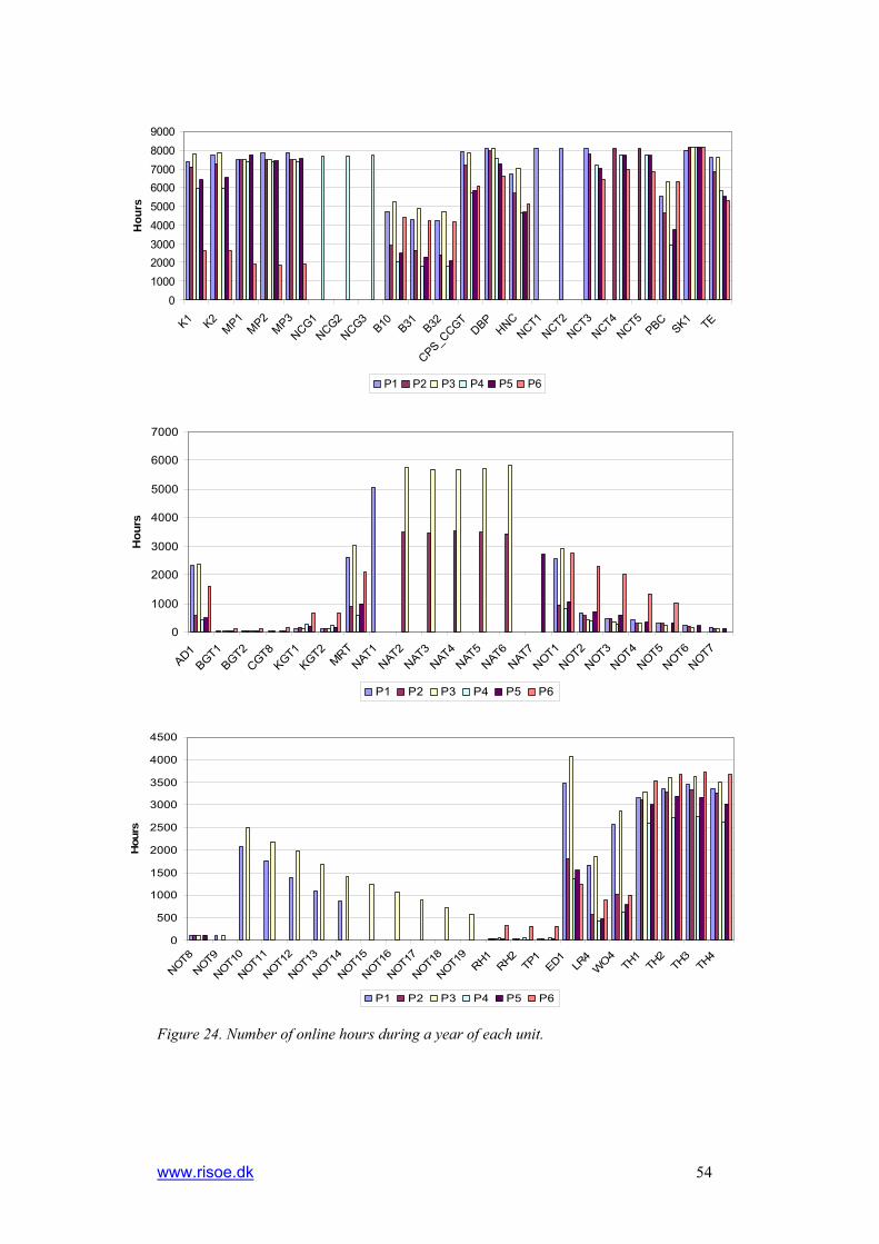
www.risoe.dk 54

0

1000

20003000

4000

5000

60007000

8000

9000

K1 K2MP1

MP2MP3

NCG1NCG2

NCG3B10 B31 B32

CPS_CCGT

DBPHNC

NCT1NCT2

NCT3NCT4

NCT5PBC

SK1 TE

Hou

rs

P1 P2 P3 P4 P5 P6

0

1000

2000

3000

4000

5000

6000

7000

AD1BGT1

BGT2CGT8

KGT1KGT2

MRTNAT1

NAT2NAT3

NAT4NAT5

NAT6NAT7

NOT1NOT2

NOT3NOT4

NOT5NOT6

NOT7

Hou

rs

P1 P2 P3 P4 P5 P6

0

500

1000

1500

2000

2500

3000

3500

4000

4500

NOT8NOT9

NOT10

NOT11

NOT12

NOT13

NOT14

NOT15

NOT16

NOT17

NOT18

NOT19

RH1RH2

TP1

ED1LR

4W

O4TH

1TH

2TH

3TH

4

Hou

rs

P1 P2 P3 P4 P5 P6

Figure 24. Number of online hours during a year of each unit.

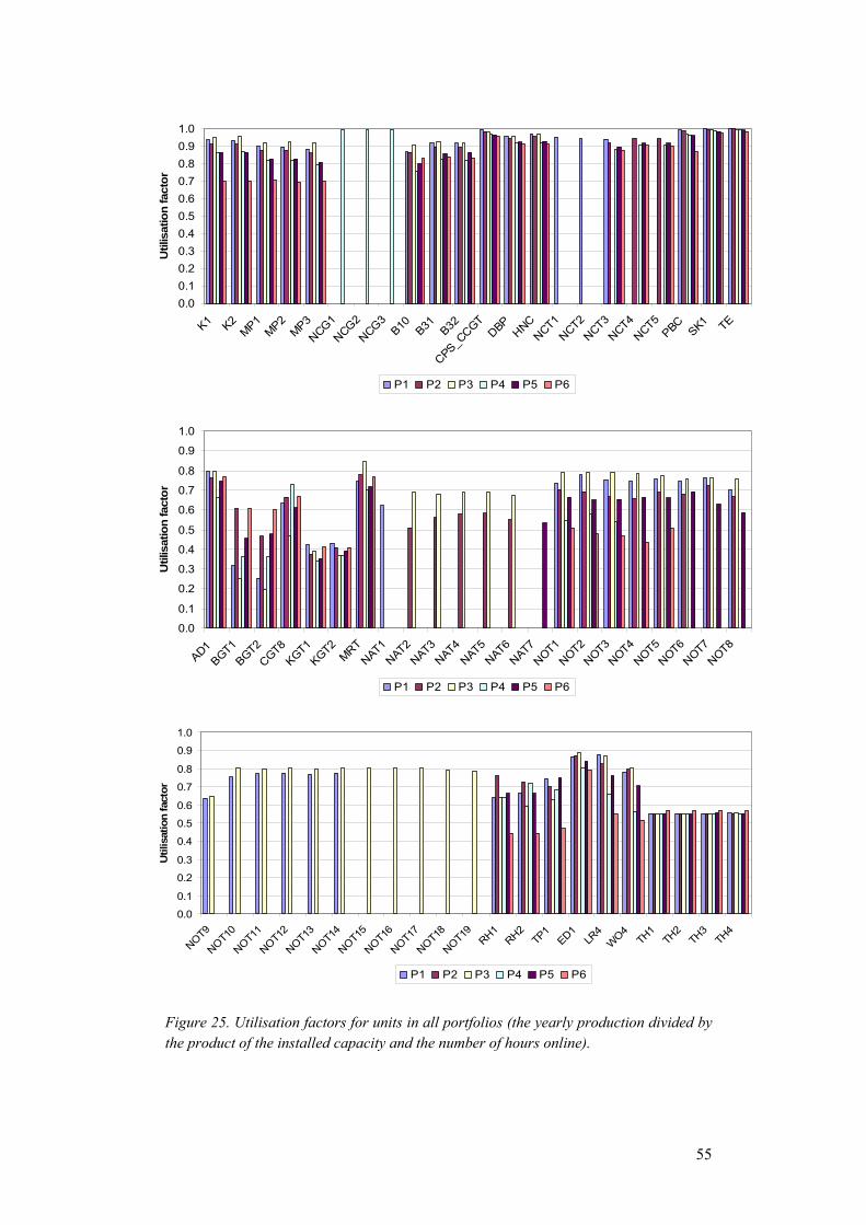
55

0.00.10.20.30.40.50.60.70.80.91.0

K1 K2MP1

MP2MP3

NCG1NCG2

NCG3B10 B31 B32

CPS_CCGT

DBPHNC

NCT1NCT2

NCT3NCT4

NCT5PBC

SK1 TE

Util

isat

ion

fact

or

P1 P2 P3 P4 P5 P6

0.0

0.1

0.2

0.3

0.4

0.5

0.6

0.7

0.8

0.9

1.0

AD1BGT1

BGT2CGT8

KGT1KGT2

MRTNAT1

NAT2NAT3

NAT4NAT5

NAT6NAT7

NOT1NOT2

NOT3NOT4

NOT5NOT6

NOT7NOT8

Util

isat

ion

fact

or

P1 P2 P3 P4 P5 P6

0.0

0.1

0.2

0.3

0.4

0.5

0.6

0.7

0.8

0.9

1.0

NOT9

NOT10

NOT11

NOT12

NOT13

NOT14

NOT15

NOT16

NOT17

NOT18

NOT19

RH1RH2

TP1

ED1LR

4W

O4TH

1TH

2TH

3TH

4

Util

isat

ion

fact

or

P1 P2 P3 P4 P5 P6

Figure 25. Utilisation factors for units in all portfolios (the yearly production divided by the product of the installed capacity and the number of hours online).

www.risoe.dk 56

Figure 26 shows the yearly electricity production and consumption of the pump storage facility Turlough Hill distributed on the hours during the day. Generally, pumping takes place during night and generation takes place during the peak load hours in the morning (hour 08 - 12) and in the afternoon (hour 16 - 19). During the day, there can be observed no general trend of the amount of electricity production and consumption dependent on the wind power installed. In those portfolios with a large share of new OCGTs (portfolios P1 and P3), the expensive OCGTs are often the marginal plant during peak load hours. Whereas in those portfolios with a lower number of new OCGTs (portfolio P4 – P6) and a higher wind power capacity installed (portfolio P5 and P6), the OCGTs are less producing. This result in Turlough Hill being used significantly less in portfolio P4 and P5 than in portfolio P1 and P3, because the price differences between hours with a low load (during the night) and with peak load hours (in the morning and in the afternoon) are smaller in portfolio P4 and P5 relatively to portfolio P1 and P3. However, with the highest wind power capacity installed in portfolio P6, the production during peak hours is increased in comparison to portfolio P4 and P5. Furthermore, portfolio P6 shows the highest consumption during the day.

0

10000

20000

30000

40000

50000

60000

70000

80000

00 01 02 03 04 05 06 07 08 09 10 11 12 13 14 15 16 17 18 19 20 21 22 23

Prod

uctio

n / C

onsu

mpt

ion

[MW

h]

P1 ElecProd P1 ElecCons P2 ElecProd P2 ElecConsP3 ElecProd P3 ElecCons P4 ElecProd P4 ElecConsP5 ElecProd P5 ElecCons P6 ElecProd P6 ElecCons

Figure 26. The yearly electricity production and electricity consumption of Turlough Hill distributed on the hours during a day in MWh.

The reduced usage of Turlough Hill in P4 and P5 can also be observed from the number of pumping hours during the year shown in Figure 27. There is not a trend of the development of pumping hours dependant on the wind power capacity installed. However, Turlough Hill shows the highest number of pumping hours in portfolio P6 with the highest wind power capacity installed.

The consideration of PBC as two units with a capacity of respectively 240 MW in portfolio P4 and P5 instead of one unit with a capacity of 480 MW has neglible influences on the dispatch of power plants.

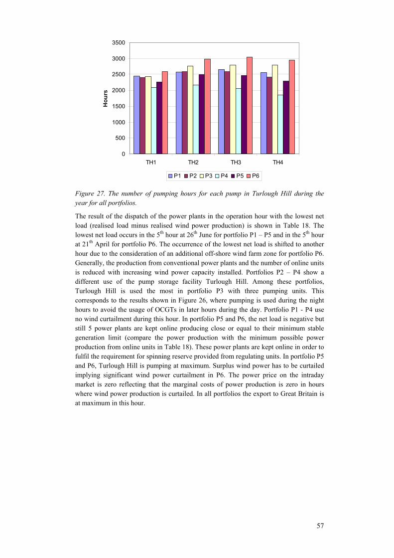
57

0

500

1000

1500

2000

2500

3000

3500

TH1 TH2 TH3 TH4

Hou

rs

P1 P2 P3 P4 P5 P6

Figure 27. The number of pumping hours for each pump in Turlough Hill during the year for all portfolios.

The result of the dispatch of the power plants in the operation hour with the lowest net load (realised load minus realised wind power production) is shown in Table 18. The lowest net load occurs in the 5th hour at 26th June for portfolio P1 – P5 and in the 5th hour at 21th April for portfolio P6. The occurrence of the lowest net load is shifted to another hour due to the consideration of an additional off-shore wind farm zone for portfolio P6. Generally, the production from conventional power plants and the number of online units is reduced with increasing wind power capacity installed. Portfolios P2 – P4 show a different use of the pump storage facility Turlough Hill. Among these portfolios, Turlough Hill is used the most in portfolio P3 with three pumping units. This corresponds to the results shown in Figure 26, where pumping is used during the night hours to avoid the usage of OCGTs in later hours during the day. Portfolio P1 - P4 use no wind curtailment during this hour. In portfolio P5 and P6, the net load is negative but still 5 power plants are kept online producing close or equal to their minimum stable generation limit (compare the power production with the minimum possible power production from online units in Table 18). These power plants are kept online in order to fulfil the requirement for spinning reserve provided from regulating units. In portfolio P5 and P6, Turlough Hill is pumping at maximum. Surplus wind power has to be curtailed implying significant wind power curtailment in P6. The power price on the intraday market is zero reflecting that the marginal costs of power production is zero in hours where wind power production is curtailed. In all portfolios the export to Great Britain is at maximum in this hour.

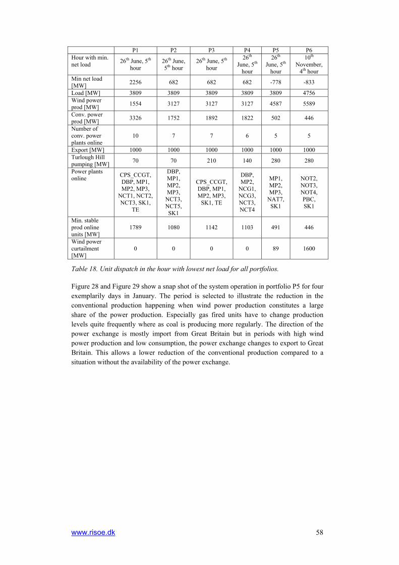
www.risoe.dk 58

P1 P2 P3 P4 P5 P6 Hour with min. net load 26th June, 5th

hour 26th June, 5th hour

26th June, 5th hour

26th June, 5th

hour

26th June, 5th

hour

10th November,

4th hour Min net load [MW] 2256 682 682 682 -778 -833

Load [MW] 3809 3809 3809 3809 3809 4756 Wind power prod [MW] 1554 3127 3127 3127 4587 5589

Conv. power prod [MW] 3326 1752 1892 1822 502 446

Number of conv. power plants online

10 7 7 6 5 5

Export [MW] 1000 1000 1000 1000 1000 1000 Turlough Hill pumping [MW] 70 70 210 140 280 280

Power plants online CPS_CCGT,

DBP, MP1, MP2, MP3,

NCT1, NCT2, NCT3, SK1,

TE

DBP, MP1, MP2, MP3,

NCT3, NCT5, SK1

CPS_CCGT, DBP, MP1, MP2, MP3,

SK1, TE

DBP, MP2,

NCG1, NCG3, NCT3, NCT4

MP1, MP2, MP3,

NAT7, SK1

NOT2, NOT3, NOT4, PBC, SK1

Min. stable prod online units [MW]

1789 1080 1142 1103 491 446

Wind power curtailment [MW]

0 0 0 0 89 1600

Table 18. Unit dispatch in the hour with lowest net load for all portfolios.

Figure 28 and Figure 29 show a snap shot of the system operation in portfolio P5 for four exemplarily days in January. The period is selected to illustrate the reduction in the conventional production happening when wind power production constitutes a large share of the power production. Especially gas fired units have to change production levels quite frequently where as coal is producing more regularly. The direction of the power exchange is mostly import from Great Britain but in periods with high wind power production and low consumption, the power exchange changes to export to Great Britain. This allows a lower reduction of the conventional production compared to a situation without the availability of the power exchange.

59

0100020003000400050006000700080009000

10000

2020

-01-

09-0

0

2020

-01-

09-0

6

2020

-01-

09-1

2

2020

-01-

09-1

8

2020

-01-

10-0

0

2020

-01-

10-0

6

2020

-01-

10-1

2

2020

-01-

10-1

8

2020

-01-

11-0

0

2020

-01-

11-0

6

2020

-01-

11-1

2

2020

-01-

11-1

8

2020

-01-

12-0

0

2020

-01-

12-0

6

2020

-01-

12-1

2

2020

-01-

12-1

8

2020

-01-

13-0

0

2020

-01-

13-0

6

2020

-01-

13-1

2

2020

-01-

13-1

8

Pro

duct

ion

[MW

h]

02 Peat 03 Coal 04 BaseLoad_gas05 MidMerit_gas 07 Gas oil 16 Water18 Storage 20 Wind 21 Biogas

Figure 28. The electricity production distributed on fuel type in portfolio P5 in the period 2020-01-09 to 2020-01-13.

-2000

0

2000

4000

6000

8000

10000

2020

-01-09

-00

2020

-01-09

-06

2020

-01-09

-12

2020

-01-09

-18

2020

-01-10

-00

2020

-01-10

-06

2020

-01-10

-12

2020

-01-10

-18

2020

-01-11

-00

2020

-01-11

-06

2020

-01-11

-12

2020

-01-11

-18

2020

-01-12

-00

2020

-01-12

-06

2020

-01-12

-12

2020

-01-12

-18

2020

-01-13

-00

2020

-01-13

-06

2020

-01-13

-12

2020

-01-13

-18

MW

h

Consumption Realised Wind Power exchange Production exclusive wind

Figure 29. The electricity consumption, realised wind power production, power exchange with Great Britain with negative values indicating import, and production exclusive wind power production in portfolio P5 in the period 2020-01-09 to 2020-01-13.

4.9 Power exchange with Great Britain The available transmission capacity between the All Island power system and Great Britain consists of the existing Moyle interconnector with 500 MW and an assumed new interconnector with 500 MW resulting in a sum of total 1000 MW transmission capacity. The power exchange between the All Island power system and Great Britain is determined in the day-ahead scheduling process for the hours of the next day. This planned power exchange cannot be modified in the rescheduling process taking place

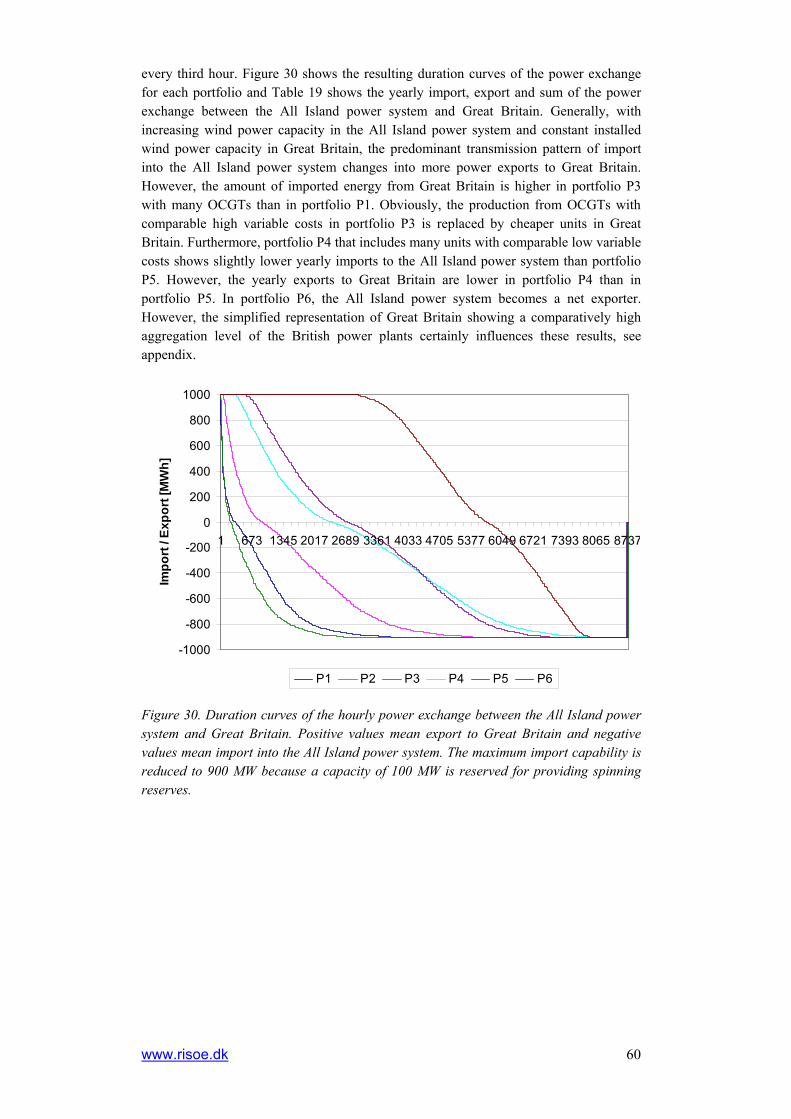
www.risoe.dk 60

every third hour. Figure 30 shows the resulting duration curves of the power exchange for each portfolio and Table 19 shows the yearly import, export and sum of the power exchange between the All Island power system and Great Britain. Generally, with increasing wind power capacity in the All Island power system and constant installed wind power capacity in Great Britain, the predominant transmission pattern of import into the All Island power system changes into more power exports to Great Britain. However, the amount of imported energy from Great Britain is higher in portfolio P3 with many OCGTs than in portfolio P1. Obviously, the production from OCGTs with comparable high variable costs in portfolio P3 is replaced by cheaper units in Great Britain. Furthermore, portfolio P4 that includes many units with comparable low variable costs shows slightly lower yearly imports to the All Island power system than portfolio P5. However, the yearly exports to Great Britain are lower in portfolio P4 than in portfolio P5. In portfolio P6, the All Island power system becomes a net exporter. However, the simplified representation of Great Britain showing a comparatively high aggregation level of the British power plants certainly influences these results, see appendix.

-1000

-800

-600

-400

-200

0

200

400

600

800

1000

1 673 1345 2017 2689 3361 4033 4705 5377 6049 6721 7393 8065 8737

Impo

rt / E

xpor

t [M

Wh]

P1 P2 P3 P4 P5 P6

Figure 30. Duration curves of the hourly power exchange between the All Island power system and Great Britain. Positive values mean export to Great Britain and negative values mean import into the All Island power system. The maximum import capability is reduced to 900 MW because a capacity of 100 MW is reserved for providing spinning reserves.

61

P1 [TWh]

P2 [TWh]

P3 [TWh]

P4 [TWh]

P5 [TWh]

P6 [TWh]

Yearly import to All Island power system

-6.81 -5.74 -7.13 -3.75 -3.80 -1.70

Yearly export from All Island power system

0.07 0.33 0.07 1.12 1.49 4.49

Sum of yearly power exchange

-6.74 -5.41 -7.07 -2.63 -2.30 2.79

Table 19. Yearly import, export and sum of the power exchange between the All Island power system and Great Britain in TWh. Positive values mean export to Great Britain and negative values mean import into the All Island power system.

Portfolio 1

-1000

-800

-600

-400

-200

0

200

400

600

800

1000

1 673 1345 2017 2689 3361 4033 4705 5377 6049 6721 7393 8065 8737

Time [h]

Tran

smis

sion

[MW

]

Portfolio 2

-1000

-800

-600

-400

-200

0

200

400

600

800

1000

1 673 1345 2017 2689 3361 4033 4705 5377 6049 6721 7393 8065 8737

Time [h]

Tran

smis

sion

[MW

]

Portfolio 3

-1000

-800

-600

-400

-200

0

200

400

600

800

1000

1 673 1345 2017 2689 3361 4033 4705 5377 6049 6721 7393 8065 8737

Time [h]

Tran

smis

sion

[MW

]

Portfolio 4

-1000

-800

-600

-400

-200

0

200

400

600

800

1000

1 673 1345 2017 2689 3361 4033 4705 5377 6049 6721 7393 8065 8737

Time [h]

Tran

smis

sion

[MW

]

Portfolio 5

-1000

-800

-600

-400

-200

0

200

400

600

800

1000

1 673 1345 2017 2689 3361 4033 4705 5377 6049 6721 7393 8065 8737

Time [h]

Tran

smis

sion

[MW

]

Portfolio 6

-1000

-800

-600

-400

-200

0

200

400

600

800

1000

1 673 1345 2017 2689 3361 4033 4705 5377 6049 6721 7393 8065 8737

Time [h]

Tran

smis

sion

[MW

]

Figure 31. Transmission between the All Island power system and Great Britain during a year for the portfolio P1 – P6. Positive values mean export to Great Britain and negative values mean import into the All Island power system. The maximum import capability is reduced to 900 MW because a capacity of 100 MW is reserved for providing spinning reserves.

www.risoe.dk 62

Figure 31 shows the transmission time-series between the All Island power system and Great Britain of the considered year for portfolio P1 – P6. The predominant import into the All Island power system in portfolio P1 and P3 is obvious. Furthermore, the available export capacity to Great Britain of 1000 MW is completely used only in a few hours. Generally, the possibility to import or export energy is used with a high flexibility to balance wind power production in all portfolios. To further show the flexibility of the usage of the transmission possibility, the hourly variation of the transmission between the All Island power system and Great Britain from one hour to the next is depicted in Figure 32. With increasing wind power capacity installed in the All Island power system, the hourly variation of the transmission generally increases. However, the hourly variation in portfolio P3 is lower than in portfolio P2. In portfolio P5 and P6, the transmission changes from maximal import to maximal export in 1 and 11 hours, respectively.

-2000

-1500

-1000

-500

0

500

1000

1500

2000

1 673 1345 2017 2689 3361 4033 4705 5377 6049 6721 7393 8065 8737

Hou

rly v

aria

tion

impo

rt/ex

port

[MW

h]

P1 P2 P3 P4 P5 P6

Figure 32. Duration curves of the hourly variation of the transmission from one hour to the next between the All Island power system and Great Britain. A positive value means a reduced import, a negative value an inreased import to the All Island power system.

4.10 Impact of unit constraints on variability management The model runs are performed with hourly time resolution. With hourly resolution, only one peat fired plant plant, ED1 (Edenderry), has restricting ramp up rate and ramp down rates. All other plants can vary the production from minimum stable generation limit to maximum power output within one hour or alternatively from maximum power output to minimum stable generation limit. Hence, there are no further problems to follow the variation of the net load (load minus the realised wind power production) in the model runs. If a half-hourly time resolution had been chosen, 6 power plants (ED1, AD1, MP1, MP2, MP3 and WO4) would have ramp rates that would restrict the changes in power output within a half-hour. However, the variability of the net load would be lower with a half-houry than with an hourly time resolution.

Start-up times, minimum up and down times restrict the ability of the power system to follow the variation of the net load by starting up or shutting down power plants. This may be depicted with the portfolios P2, P3 and P4 that show the same wind power

63

capacity installed but that show a different share of power plants with different unit constraints, efficiencies and fuel types. Thereby, portfolio P4 has the highest share of relatively inflexible power plants and portfolio P3 has the lowest share of these plants, see appendix. All of these portfolios can handle the variability in the net load and have a high reliability to meet the load, see section 4.7. However, the number of hours where the demand for spinning reserves or replacement reserves is not met is lower in portfolio P3 compared to portfolio P2 and P4, i.e. the reliability is higher in portfolio P3 compared to portfolio P2 and P4.

For each power plant of the different portfolios, the variation of the resulting power production from hour to hour has been analysed. Taking the average over the year, the variation of the hourly production is equal to zero for all power plants. Generally, almost the whole operating range is utilized by all units independent of the wind power capacity installed. Figure 33 shows the standard deviation of the hourly variation of the power production of each power plant. Except the power plants AD1, B10, B31, B32 and the OCGTs, the standard deviation of the hourly variation increases with increasing wind power capacity installed for portfolio P1 – P5. Hence, the power plants are operated with a higher variability. However, the standard variation is reduced for the units HNC, PBC and TE in portfolio P6 in comparison to portfolio P5. The relative high variation of PBC reflects its high flexibility. In portfolio P3 with a high share of flexible OCGTs, the standard deviation of the hourly variation of the power plants with a relative high capacity (i.e. CPS_CCGT, DPB, HNC, MP1-MP3, PBC and TE) is significantly reduced. It is apparent that OCGTs are used to follow the variability of the net load, see also section 4.8.

Apart from unit constraints such as start-up times, minimum stable generation limit and minimum number of up or down times, restrictions on the minimum number of units online can also have an influence on the ability of the portfolios to handle situations with a low net load. The reasoning behind such a restriction is that a certain number of online units in a certain number of places in the grid are necessary due to system stability reasons (e.g. inertia). The problem with enforcing such a restriction is that it is not obvious what the minimum number of online units should be. A corresponding restriction on the minimum number of units online has not been used in this study. The requirement on a certain amount of spinning reserve coming from conventional units does enforce some conventional units to be online. However as the demand for spinning reserve depends on the largest unit online, the model can achieve a low demand for spinning reserve by only having small units online. Figure 34 shows the 1000 hours with the lowest number of units online during a year for each portfolio. It is clear that the number of units online is decreased as the installed wind power capacity is increased. Portfolio P6 has approximately 500 hours with 5 units online or less. If for example a minimum limit of 6 units online was required, wind curtailment would be used more in portfolio P5 and P6 as a certain amount of minimum production from online units would replace wind power production

Figure 35 and Table 20 show another interesting aspect concerning the management of the variability in the net load namely the change in the number of units online from one hour to the next. No firm restriction on the number of units that can be brought online or taken offline from one hour to the next was used in the model runs. However if such restrictions apply the management of the variability in the net load would become more difficult and hence more expensive.

www.risoe.dk 64

0

20

40

60

80

100

120

140

160

180

200

K1 K2MP1

MP2MP3

NCG1

NCG2

NCG3B10 B31 B32

CPS_CCGT

DBPHNC

NCT1NCT2

NCT3NCT4

NCT5PBC

SK1 TE

Varia

tion

Prod

uctio

n St

dDev

[MW

]

P1 P2 P3 P4 P5 P6

0

20

40

60

80

100

120

140

160

180

200

AD1

BGT1

BGT2CGT8

KGT1KGT2

MRTNAT1

NAT2NAT3

NAT4NAT5

NAT6NAT7

NOT1NOT2

NOT3NOT4

NOT5NOT6

NOT7NOT8

Varia

tion

Prod

uctio

n St

dDev

[MW

]

P1 P2 P3 P4 P5 P6

0

20

40

60

80

100

120

140

160

180

200

NOT9

NOT10

NOT11

NOT12

NOT13

NOT14

NOT15

NOT16

NOT17

NOT18

NOT19

RH1RH2

TP1

ED1LR

4W

O4TH

1TH

2TH

3TH

4

BASERENEW

ABLE

S

Varia

tion

Prod

uctio

n St

dDev

[MW

]

P1 P2 P3 P4 P5 P6

Figure 33. Standard deviation of the hourly variation of the power production of the power plants in MW taken over the hours during the year where the plants are online.

65

0

2

4

6

8

10

12

1 72 143 214 285 356 427 498 569 640 711 782 853 924 995

Num

ber o

f uni

ts o

nlin

e

P1 P2 P3 P4 P5 P6

Figure 34. Duration curves of the number of units online in the 1000 hours with the lowest number of units online for each portfolio.

-20

-15

-10

-5

0

5

10

15

20

1 717 1433 2149 2865 3581 4297 5013 5729 6445 7161 7877 8593

Del

ta u

nits

onl

ine

P1 P2 P3 P4 P5 P6

Figure 35. Duration curves of the change in the number of units online from one hour to the next for all hours during a year for each portfolio.

www.risoe.dk 66

P1 P2 P3 P4 P5 P6

Max number of units brought online 15 17 19 12 14 17

Max. number of units taken offline 12 15 17 11 14 16

Number of instances with more than 5 units brought online

414 418 585 152 339 527

Number of instances with more than 5 units taken offline

237 338 463 134 295 483

Table 20. Maximum number of units brought online or taken offline from one hour to the next during a year in all portfolios. Number of instances where the change in the units online from one hour to the next is above 5.

4.11 Impact of different plant mix The comparison of different power plant portfolios should take both the costs connected to operating the power system (maintenance costs, fuel costs, CO2 emission costs, start-up costs) and investment costs related to new power plants and grid extensions into account. Furthermore the environmental impact of operating the power system (mainly CO2 emission but also emissions of SO2 and NOX) and the quality of the output from the power system (reliability) should be compared. The analysis in this report only includes operation costs, CO2 emissions and reliability, so a comparison between portfolios will be limited in scope.

As stated in section 4.7, the reliability is high in all portfolios except portfolio P6. Comparing the operation costs in the All Island power system (see Table 7) that also consider the costs of consuming CO2 emission permits, P5 is the best portfolio followed by P2, P4, P3, P6 and P1. If the payments related to import and export of power between the All Island power system and Great Britain are further considered, P5 is the best portfolio followed by P6, P4, P2, P3 and P1. Concerning CO2 emissions only in the All Island power system, P6 is best followed by P5, P2, P3, P1 and P4. Table 21 summarizes the resulting sequences of the power plant portfolios. Generally, portfolio P5 and P6 show the best results. However, because of the high assumption for the CO2 emission permit price in portfolio P6, this portfolio shows the second highest operation costs when payments related to the power exchange with Great Britain are neglected. Concerning only fuel costs, portfolio P6 is the best one, see Table 7. Among the portfolios with the same wind power capacity installed (portfolio P2 – P4), portfolio P4 with a high share of base load plant is the best concerning operation costs and the worst concerning CO2 emissions.

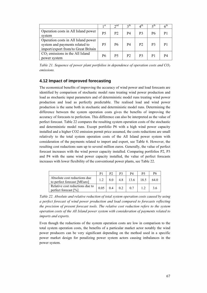
67

1st 2nd 3th 4th 5th 6th Operation costs in All Island power system P5 P2 P4 P3 P6 P1

Operation costs in All Island power system and payments related to import/export from/to Great Britain

P5 P6 P4 P2 P3 P1

CO2 emissions in the All Island power system P6 P5 P2 P3 P1 P4

Table 21. Sequence of power plant portfolios in dependence of operation costs and CO2 emissions.

4.12 Impact of improved forecasting The economical benefits of improving the accuracy of wind power and load forecasts are identified by comparison of stochastic model runs treating wind power production and load as stochastic input parameters and of deterministic model runs treating wind power production and load as perfectly predictable. The realised load and wind power production is the same both in stochastic and deterministic model runs. Determining the difference between the system operation costs gives the benefits of improving the accuracy of forecasts to perfection. This difference can also be interpreted as the value of perfect forecast. Table 22 compares the resulting system operation costs of the stochastic and deterministic model runs. Except portfolio P6 with a high wind power capacity installed and a higher CO2 emission permit price assumed, the costs reductions are small relatively to the total system operation costs of the All Island power system with consideration of the payments related to import and export, see Table 6. However, the resulting cost reductions sum up to several million euros. Generally, the value of perfect forecast increases with the wind power capacity installed. Comparing portfolios P2, P3 and P4 with the same wind power capacity installed, the value of perfect forecasts increases with lower flexibility of the conventional power plants, see Table 22.

P1 P2 P3 P4 P5 P6 Absolute cost reductions due to perfect forecast [MEuro] 1.2 8.0 4.8 13.6 18.5 64.0

Relative cost reductions due to perfect forecast [%] 0.05 0.4 0.2 0.7 1.2 3.6

Table 22. Absolute and relative reduction of total system operation costs caused by using a perfect forecast of wind power production and load compared to forecasts reflecting the precision of present forecast tools. The relative cost reduction refers to the system operation costs of the All Island power system with consideration of payments related to imports and exports.

Even though the reductions of the system operation costs are low in comparison to the total system operation costs, the benefits of a particular market actor notably the wind power producers can be very significant depending on the method used in a specific power market design for penalizing power system actors causing imbalances in the power system.

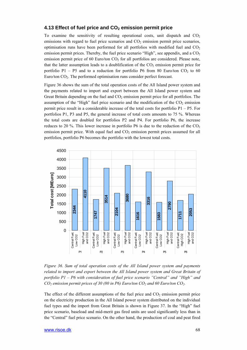
www.risoe.dk 68

4.13 Effect of fuel price and CO2 emission permit price To examine the sensitivity of resulting operational costs, unit dispatch and CO2 emissions with regard to fuel price scenarios and CO2 emission permit price scenarios, optimisation runs have been performed for all portfolios with modified fuel and CO2 emission permit prices. Thereby, the fuel price scenario “High”, see appendix, and a CO2 emission permit price of 60 Euro/ton CO2 for all portfolios are considered. Please note, that the latter assumption leads to a doublification of the CO2 emission permit price for portfolio P1 – P5 and to a reduction for portfolio P6 from 80 Euro/ton CO2 to 60 Euro/ton CO2. The performed optimisation runs consider perfect forecast.

Figure 36 shows the sum of the total operation costs of the All Island power system and the payments related to import and export between the All Island power system and Great Britain depending on the fuel and CO2 emission permit price for all portfolios. The assumption of the “High” fuel price scenario and the modification of the CO2 emission permit price result in a considerable increase of the total costs for portfolio P1 – P5. For portfolios P1, P3 and P5, the general increase of total costs amounts to 75 %. Whereas the total costs are doubled for portfolios P2 and P4. For portfolio P6, the increase reduces to 20 %. This lower increase in portfolio P6 is due to the reduction of the CO2 emission permit price. With equal fuel and CO2 emission permit prices assumed for all portfolios, portfolio P6 becomes the portfolio with the lowest total costs.

2344

4110

1747

3514

2104

3680

1616

3316

1583

2790

1711 20

53

0

500

1000

1500

2000

2500

3000

3500

4000

4500

Cen

tral F

uel;

Low

CO

2

Hig

h Fu

elan

d C

O2

Cen

tral F

uel;

Low

CO

2

Hig

h Fu

elan

d C

O2

Cen

tral F

uel;

Low

CO

2

Hig

h Fu

elan

d C

O2

Cen

tral F

uel;

Low

CO

2

Hig

h Fu

elan

d C

O2

Cen

tral F

uel;

Low

CO

2

Hig

h Fu

elan

d C

O2

Cen

tral F

uel;

Hig

h C

O2

Hig

h Fu

elan

d C

O2

P1 P2 P3 P4 P5 P6

Tota

l cos

t [M

Euro

]

Figure 36. Sum of total operation costs of the All Island power system and payments related to import and export between the All Island power system and Great Britain of portfolio P1 – P6 with consideration of fuel price scenario ”Central” and ”High” and CO2 emission permit prices of 30 (80 in P6) Euro/ton CO2 and 60 Euro/ton CO2.

The effect of the different assumptions of the fuel price and CO2 emission permit price on the electricity production in the All Island power system distributed on the individual fuel types and the import from Great Britain is shown in Figure 37. In the “High” fuel price scenario, baseload and mid-merit gas fired units are used significantly less than in the “Central” fuel price scenario. On the other hand, the production of coal and peat fired

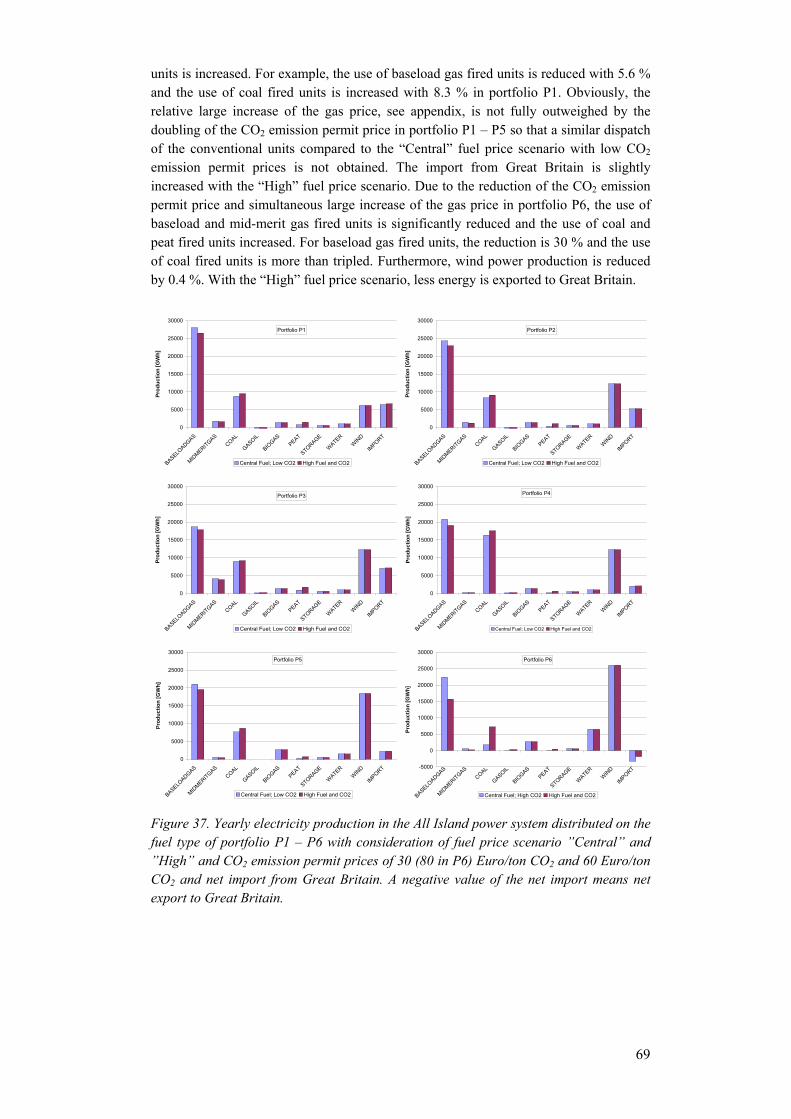
69

units is increased. For example, the use of baseload gas fired units is reduced with 5.6 % and the use of coal fired units is increased with 8.3 % in portfolio P1. Obviously, the relative large increase of the gas price, see appendix, is not fully outweighed by the doubling of the CO2 emission permit price in portfolio P1 – P5 so that a similar dispatch of the conventional units compared to the “Central” fuel price scenario with low CO2 emission permit prices is not obtained. The import from Great Britain is slightly increased with the “High” fuel price scenario. Due to the reduction of the CO2 emission permit price and simultaneous large increase of the gas price in portfolio P6, the use of baseload and mid-merit gas fired units is significantly reduced and the use of coal and peat fired units increased. For baseload gas fired units, the reduction is 30 % and the use of coal fired units is more than tripled. Furthermore, wind power production is reduced by 0.4 %. With the “High” fuel price scenario, less energy is exported to Great Britain.

Portfolio P1

0

5000

10000

15000

20000

25000

30000

BASELOADGAS

MIDMERITGAS

COAL

GASOIL

BIOGAS

PEAT

STORAGE

WATER

WIN

D

IMPORT

Prod

uctio

n [G

Wh]

Central Fuel; Low CO2 High Fuel and CO2

Portfolio P2

0

5000

10000

15000

20000

25000

30000

BASELOADGAS

MIDMERITGAS

COAL

GASOIL

BIOGAS

PEAT

STORAGE

WATER

WIN

D

IMPORT

Prod

uctio

n [G

Wh]

Central Fuel; Low CO2 High Fuel and CO2

Portfolio P3

0

5000

10000

15000

20000

25000

30000

BASELOADGAS

MIDMERITGAS

COAL

GASOIL

BIOGAS

PEAT

STORAGE

WATER

WIN

D

IMPORT

Prod

uctio

n [G

Wh]

Central Fuel; Low CO2 High Fuel and CO2

Portfolio P4

0

5000

10000

15000

20000

25000

30000

BASELOADGAS

MIDMERITGAS

COAL

GASOIL

BIOGAS

PEAT

STORAGE

WATER

WIN

D

IMPORT

Prod

uctio

n [G

Wh]

Central Fuel; Low CO2 High Fuel and CO2

Portfolio P5

0

5000

10000

15000

20000

25000

30000

BASELOADGAS

MIDMERITGAS

COAL

GASOIL

BIOGAS

PEAT

STORAGE

WATER

WIN

D

IMPORT

Prod

uctio

n [G

Wh]

Central Fuel; Low CO2 High Fuel and CO2

Portfolio P6

-5000

0

5000

10000

15000

20000

25000

30000

BASELOADGAS

MIDMERITGAS

COAL

GASOIL

BIOGAS

PEAT

STORAGE

WATER

WIN

D

IMPORT

Prod

uctio

n [G

Wh]

Central Fuel; High CO2 High Fuel and CO2

Figure 37. Yearly electricity production in the All Island power system distributed on the fuel type of portfolio P1 – P6 with consideration of fuel price scenario ”Central” and ”High” and CO2 emission permit prices of 30 (80 in P6) Euro/ton CO2 and 60 Euro/ton CO2 and net import from Great Britain. A negative value of the net import means net export to Great Britain.

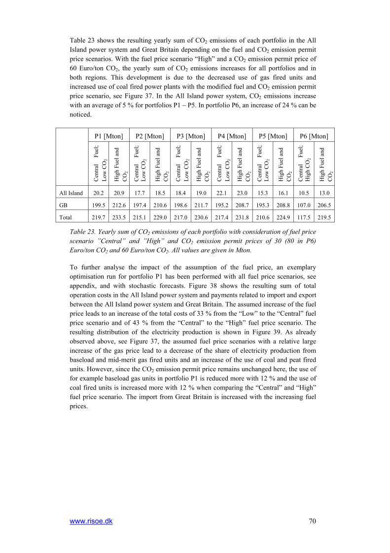
www.risoe.dk 70

Table 23 shows the resulting yearly sum of CO2 emissions of each portfolio in the All Island power system and Great Britain depending on the fuel and CO2 emission permit price scenarios. With the fuel price scenario “High” and a CO2 emission permit price of 60 Euro/ton CO2, the yearly sum of CO2 emissions increases for all portfolios and in both regions. This development is due to the decreased use of gas fired units and increased use of coal fired power plants with the modified fuel and CO2 emission permit price scenario, see Figure 37. In the All Island power system, CO2 emissions increase with an average of 5 % for portfolios P1 – P5. In portfolio P6, an increase of 24 % can be noticed.

P1 [Mton] P2 [Mton] P3 [Mton] P4 [Mton] P5 [Mton] P6 [Mton]

Cen

tral

Fuel

; Lo

w C

O2

Hig

h Fu

el a

nd

CO

2

Cen

tral

Fuel

; Lo

w C

O2

Hig

h Fu

el a

nd

CO

2

Cen

tral

Fuel

; Lo

w C

O2

Hig

h Fu

el a

nd

CO

2

Cen

tral

Fuel

; Lo

w C

O2

Hig

h Fu

el a

nd

CO

2

Cen

tral

Fuel

; Lo

w C

O2

Hig

h Fu

el a

nd

CO

2

Cen

tral

Fuel

; H

igh

CO

2

Hig

h Fu

el a

nd

CO

2

All Island 20.2 20.9 17.7 18.5 18.4 19.0 22.1 23.0 15.3 16.1 10.5 13.0

GB 199.5 212.6 197.4 210.6 198.6 211.7 195.2 208.7 195.3 208.8 107.0 206.5

Total 219.7 233.5 215.1 229.0 217.0 230.6 217.4 231.8 210.6 224.9 117.5 219.5

Table 23. Yearly sum of CO2 emissions of each portfolio with consideration of fuel price scenario ”Central” and ”High” and CO2 emission permit prices of 30 (80 in P6) Euro/ton CO2 and 60 Euro/ton CO2. All values are given in Mton.

To further analyse the impact of the assumption of the fuel price, an exemplary optimisation run for portfolio P1 has been performed with all fuel price scenarios, see appendix, and with stochastic forecasts. Figure 38 shows the resulting sum of total operation costs in the All Island power system and payments related to import and export between the All Island power system and Great Britain. The assumed increase of the fuel price leads to an increase of the total costs of 33 % from the “Low” to the “Central” fuel price scenario and of 43 % from the “Central” to the “High” fuel price scenario. The resulting distribution of the electricity production is shown in Figure 39. As already observed above, see Figure 37, the assumed fuel price scenarios with a relative large increase of the gas price lead to a decrease of the share of electricity production from baseload and mid-merit gas fired units and an increase of the use of coal and peat fired units. However, since the CO2 emission permit price remains unchanged here, the use of for example baseload gas units in portfolio P1 is reduced more with 12 % and the use of coal fired units is increased more with 12 % when comparing the “Central” and “High” fuel price scenario. The import from Great Britain is increased with the increasing fuel prices.

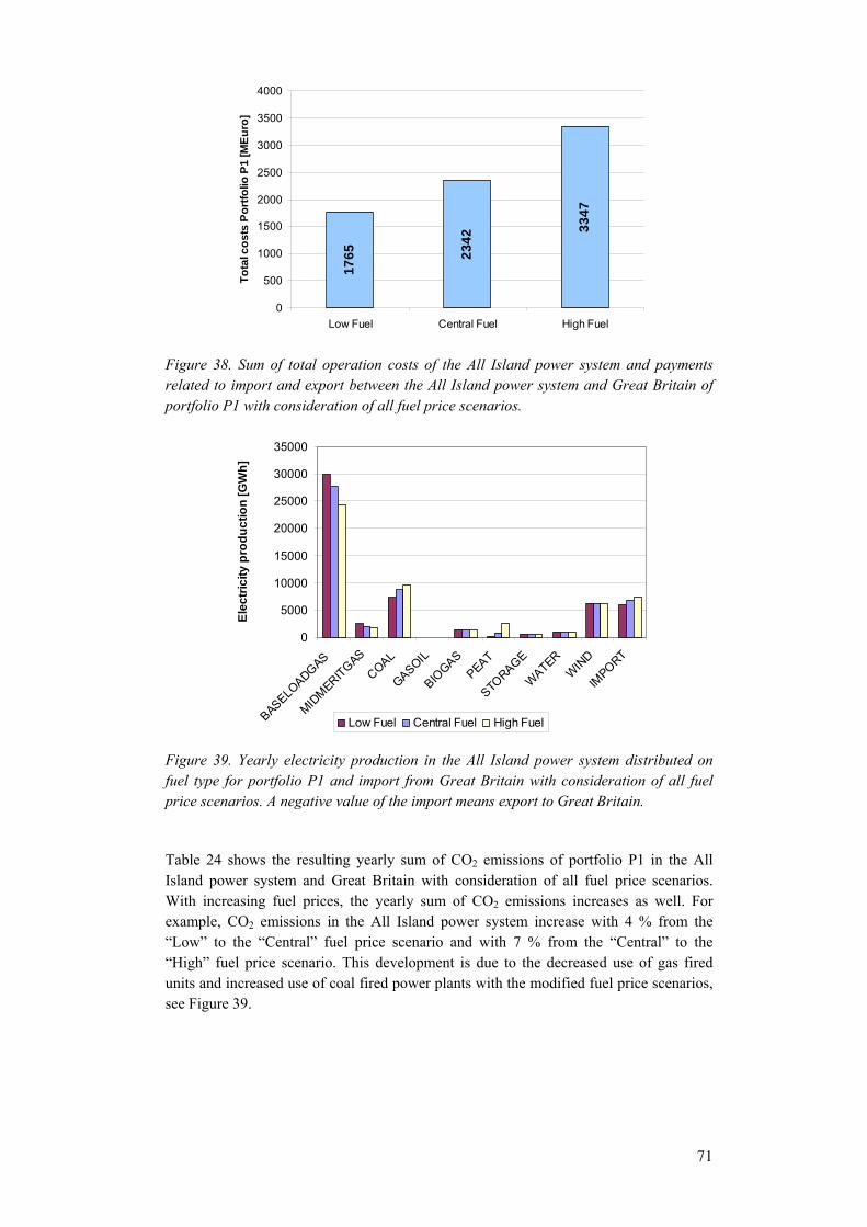
71

1765 23

42

3347

0

500

1000

1500

2000

2500

3000

3500

4000

Low Fuel Central Fuel High Fuel

Tota

l cos

ts P

ortfo

lio P

1 [M

Euro

]

Figure 38. Sum of total operation costs of the All Island power system and payments related to import and export between the All Island power system and Great Britain of portfolio P1 with consideration of all fuel price scenarios.

0

5000

10000

15000

20000

25000

30000

35000

BASELOADGAS

MIDMERITGAS

COAL

GASOIL

BIOGAS

PEAT

STORAGE

WATERWIN

D

IMPORT

Elec

trici

ty p

rodu

ctio

n [G

Wh]

Low Fuel Central Fuel High Fuel

Figure 39. Yearly electricity production in the All Island power system distributed on fuel type for portfolio P1 and import from Great Britain with consideration of all fuel price scenarios. A negative value of the import means export to Great Britain.

Table 24 shows the resulting yearly sum of CO2 emissions of portfolio P1 in the All Island power system and Great Britain with consideration of all fuel price scenarios. With increasing fuel prices, the yearly sum of CO2 emissions increases as well. For example, CO2 emissions in the All Island power system increase with 4 % from the “Low” to the “Central” fuel price scenario and with 7 % from the “Central” to the “High” fuel price scenario. This development is due to the decreased use of gas fired units and increased use of coal fired power plants with the modified fuel price scenarios, see Figure 39.

www.risoe.dk 72

Low fuel [Mton] Central fuel [Mton] High fuel [Mton]

All Island 19.4 20.1 21.4

Great Britain 149.6 199.8 213.4

Total 168.9 219.9 234.8

Table 24. Yearly sum of CO2 emissions of portfolio P1 with consideration of all fuel price scenarios. All values are given in Mton.

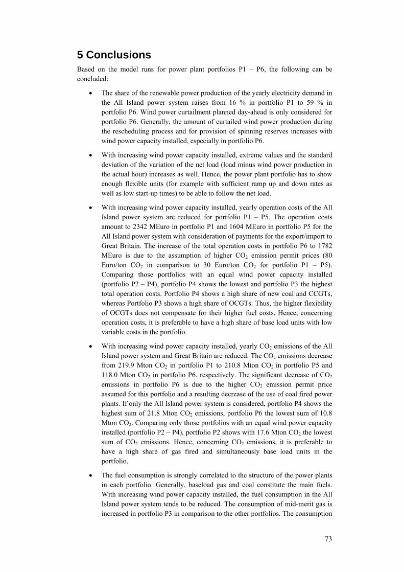
73

5 Conclusions Based on the model runs for power plant portfolios P1 – P6, the following can be concluded:

• The share of the renewable power production of the yearly electricity demand in the All Island power system raises from 16 % in portfolio P1 to 59 % in portfolio P6. Wind power curtailment planned day-ahead is only considered for portfolio P6. Generally, the amount of curtailed wind power production during the rescheduling process and for provision of spinning reserves increases with wind power capacity installed, especially in portfolio P6.

• With increasing wind power capacity installed, extreme values and the standard deviation of the variation of the net load (load minus wind power production in the actual hour) increases as well. Hence, the power plant portfolio has to show enough flexible units (for example with sufficient ramp up and down rates as well as low start-up times) to be able to follow the net load.

• With increasing wind power capacity installed, yearly operation costs of the All Island power system are reduced for portfolio P1 – P5. The operation costs amount to 2342 MEuro in portfolio P1 and 1604 MEuro in portfolio P5 for the All Island power system with consideration of payments for the export/import to Great Britain. The increase of the total operation costs in portfolio P6 to 1782 MEuro is due to the assumption of higher CO2 emission permit prices (80 Euro/ton CO2 in comparison to 30 Euro/ton CO2 for portfolio P1 – P5). Comparing those portfolios with an equal wind power capacity installed (portfolio P2 – P4), portfolio P4 shows the lowest and portfolio P3 the highest total operation costs. Portfolio P4 shows a high share of new coal and CCGTs, whereas Portfolio P3 shows a high share of OCGTs. Thus, the higher flexibility of OCGTs does not compensate for their higher fuel costs. Hence, concerning operation costs, it is preferable to have a high share of base load units with low variable costs in the portfolio.

• With increasing wind power capacity installed, yearly CO2 emissions of the All Island power system and Great Britain are reduced. The CO2 emissions decrease from 219.9 Mton CO2 in portfolio P1 to 210.8 Mton CO2 in portfolio P5 and 118.0 Mton CO2 in portfolio P6, respectively. The significant decrease of CO2 emissions in portfolio P6 is due to the higher CO2 emission permit price assumed for this portfolio and a resulting decrease of the use of coal fired power plants. If only the All Island power system is considered, portfolio P4 shows the highest sum of 21.8 Mton CO2 emissions, portfolio P6 the lowest sum of 10.8 Mton CO2. Comparing only those portfolios with an equal wind power capacity installed (portfolio P2 – P4), portfolio P2 shows with 17.6 Mton CO2 the lowest sum of CO2 emissions. Hence, concerning CO2 emissions, it is preferable to have a high share of gas fired and simultaneously base load units in the portfolio.

• The fuel consumption is strongly correlated to the structure of the power plants in each portfolio. Generally, baseload gas and coal constitute the main fuels. With increasing wind power capacity installed, the fuel consumption in the All Island power system tends to be reduced. The consumption of mid-merit gas is increased in portfolio P3 in comparison to the other portfolios. The consumption

www.risoe.dk 74

of coal is significantly higher in portfolio P4. The high CO2 price assumed in portfolio P6 leads to an increase of the consumption of baseload and midmerit gas and to a strong decrease of coal consumption.

• The main determinant for the demand for positive spinning reserves constitutes the power production plus the provision of spinning reserve of the largest unit. However, the demand for spinning reserves is observable increased for portfolio P6 due to the large wind and wave power capacity installed.

• Pumped hydro storage facility Turlough Hill, Moneypoint and new CCGTs are main sources of positive spinning reserves. However, in portfolios with ADGTs (portfolio P2 and P3), the share of coal fired units and CCGTs in provision of spinning reserves is reduced. With increasing wind power capacity installed, wind power is used more frequently to provide spinning reserves. Comparing those portfolios with an equal wind power capacity installed (portfolio P2 – P4), portfolio P3 with a high share of OCGTs shows the highest and portfolio P4 with a high share of both new coal power plants and CCGTs shows the lowest provision of spinning reserves from wind power. This indicates that providing spinning reserves is most costly in portfolio P3.

• The demand for replacement reserves is set equal to the 90th percentile of the total forecast error (wind power and load forecast error and occurrence of forced outages) of the All Island power system. With increasing wind power capacity installed, the demand for replacement reserves increases as well. Because the total forecast error increases with the forecast horizon, the demand for replacement reserves increases with the forecast horizon as well. High peaks of the demand for replacement reserves can be observed in the case of simultaneous forced outages and relatively high wind and load forecast errors.

• Nearly the whole demand for replacement reserves is provided by offline units in all portfolios. Since the portfolios show many power plants with start-up times below one or two hours, the provision of replacement reserves exceeds the demand during most hours. Within the portfolios, the demand for replacement reserves is mainly provided by OCGTs.

• All portfolios rely on the production from non-dispatchable generation and on the import from Great Britain to cover the load. Generally, portfolio P3 shows the highest overall reliability, portfolio P6 the lowest. In portfolio P1 – P5, the number of hours where the load cannot be met is lower than the considered LOLE of 8 hours per year and increases up to 3 hours in portfolio P2. In portfolio P1, P3 and P5, the load is met in every hour. The maximal load not covered in these portfolios amounts to 85 MW in portfolio P4. In portfolio P6, the load cannot be covered in 23 hours and the maximal load not met is 551 MW. However, the load cannot be covered in portfolio P6 in 20 hours because the export to Great Britain cannot be reduced during the rescheduling.

For portfolio P1 – P5, the number of hours where the demand for spinning reserves cannot be met amounts to maximal 6 hours in portfolio P2. The maximal demand for spinning reserves that cannot be met is 321 MW in portfolio P4. In portfolio P6, the demand for spinning reserves is not covered in 77 hours. The maximal demand of spinning reserves not met is 353 MW.

The demand for replacement reserves cannot be covered in 100 hours at an average due to lack of capacity in portfolio P1 – P5. Thus, the power system would not be able to cover the 90th percentile of the total forecast errors that can

75

occur during these hours. Thereby the maximal missing capacity amounts from 958 MW in portfolio P3 to 1908 MW in portfolio P2. In portfolio P6, the demand for replacement reserves is not covered during 544 hours and the maximal demand for replacement reserves not covered amounts to 1480 MW.

• The distribution of the dispatch of the units is strongly correlated to the structure of the power plant mix in each portfolio. Generally, the bigger part of the electricity production in the All Island power system from conventional power plants is borne by coal fired plants and newer CCGTs. With increasing wind power capacity installed, the production and capacity factors of these units tends to be decreased. However, the assumption of a higher CO2 emission permit price in portfolio P6 leads to a strong decrease in the use of coal fired units. Coal fired units and newer CCGTs have a relative low number of start-ups and high number of online hours. The number of start-ups of these units tends to be increased with increasing wind power capacity installed. OCGTs and ADGTs generally show a small contribution to the electricity production, this is also reflected in low capacity factors of these units. Furthermore, these units show a high number of start-ups, OCGTs additionally low number of online hours.

• For the pumped hydro storage facility Turlough Hill, no general trend depending on the wind power capacity installed can be observed. Portfolio P1 and P3 with a higher share of OCGTs and therefore larger price differences between peak and low load periods show an increased use of Turlough Hill. However, an increased use of Turlough Hill can also be observed in portfolio P6.

• With increasing wind power capacity installed, the predominant transmission pattern of import into the All Island power system changes into more power exports to Great Britain. However, the amount of imported energy from Great Britain is higher in portfolio P3 with many OCGTs than in portfolio P1. With portfolio P6, the All Island power system becomes a net exporter. With increasing wind power capacity installed in the All Island power system, the hourly variation of the transmission generally increases. In portfolio P5 and P6, the transmission changes from maximal import to maximal export in 1 and 11 hours, respectively.

• With the chosen hourly time resolution of the model, only the unit Edenderry (ED1) has restricting ramp up and ramp down rates. The impact of unit constraints on the variability management may be depicted for example with portfolio P2 – P4 that show the same wind power capacity installed. All of these portfolios can handle the variability in the net load and have a high reliability to cover the load. However, the number of hours where the demand for spinning or replacement reserves is not met is the lowest in portfolio P3. Considering the variation of the resulting power production from one to the next hour for all portfolios, almost the whole operating range is utilized by all units independent of the wind power capacity installed. Generally, the overall variation of the electricity production increases with increasing wind power capacity installed. However, the variation of the production from power plants with a relative high capacity is significantly reduced in portfolio P3 with a high share of OCGTs.

• Cost reductions due to perfect forecasts of the load and the wind power production are relatively small in comparison to the total system operation costs of the All Island power system with consideration of the payments related to import and export. However, the absolute sum of the cost reductions is not

www.risoe.dk 76

negligible. Generally, the value of perfect forecast increases with increasing wind power capacity installed from 1.2 MEuro for portfolio P1 to 64 MEuro for portfolio P6. Furthermore, the value of perfect forecast increases with lower flexibility of the conventional power plants.

• With the assumption of the ”High” fuel price scenario and a CO2 emission permit price of 60 Euro/ton CO2 for all portfolios, the total costs increase with 75 % for portfolio P1, P3 and P5. Whereas the total costs are doubled for portfolios P2 and P4. Due to the resulting decrease of the CO2 emission permit price in portfolio P6, the increase of the total costs is reduced to 20 % in the All Island power system. With equal fuel and CO2 emission permit prices assumed for all portfolios, portfolio P6 becomes the portfolio with the lowest total costs. The modification of fuel prices and of the CO2 emission permit price leads to a decrease in the use of gas fired power plants and an increase in the use of coal and peat fired units. This is due to the relatively large increase of the gas price compared to other fuels. The yearly sum of CO2 emissions increases for all portfolios and in both regions. In the All Island power system, CO2 emissions increase with an average of 5 % for portfolios P1 – P5. In portfolio P6, an increase of 24 % can be noticed.

With an equal CO2 emission permit price taken into account but simultaneously modifying the fuel prices, the increase of the system operation costs due to different assumptions of the fuel prices becomes lower in portfolio 1. Furthermore, the fuel shift from gas to coal and peat fired units is more significant. With increasing fuel prices, the yearly sum of CO2 emissions increases as well. CO2 emissions in the All Island power system increase with 4 % from the “Low” to the “Central” fuel price scenario and with 7 % from the “Central” to the “High” fuel price scenario.

77

A Appendix A.1 Methodology of the Scenario Tree Tool and of the Scheduling

Model The All Island Grid Study Working Group has requested a detailed study of the impact of increased penetration of renewable generation in the power system covering Ireland and Northern Ireland (named the All Island power system) with regard to overall operation, costs and emissions.

The study will be carried out using the Wilmar Planning tool (see section A.1.1) adapted to meet the needs specific to the All Island power system. The Scheduling model before adaptations is documented in (Meibom et al. 2006a)1. The Scenario Tree Tool before modifications is documented in (Barth et al. 2006a). These two reports supplement the description of the methodology in this report in that they provide further details about the models used. Furthermore an article by (Carrión and Arroyo 2006) describes a linear, mixed integer formulation of unit commitment. The equations in the article reformulated to cover a stochastic setup have been implemented in the Scheduling model, and the reader should consult the article for documentation of the equations.

Briefly the extension of the methodology consists of the following parts:

• Extension of the Scenario Tree Tool to include demand uncertainties and forced plant outages in the generation of scenario trees. The inclusion of these factors will ensure that the scenario trees generated provide a realistic estimate for the positive replacement reserves required in the next 36 hours in the power system. The approach is described in section A.1.2.

• Collection of wind power production data, wind speed data, data for the historical accuracy of the wind forecasting tools currently used in the All Island power system and data describing the reliability of the conventional power plants. The data are used by the Scenario Tree Tool to create wind power production forecasts (see section A.1.3).

• Modification of the Scheduling model in order to meet the requirements for the study. The modifications are described in section A.1.4. The main extension of the model is the usage of integer variables in the modelling of unit commitment.

• Collection of demand and generation data for the All Island power system and inclusion of these data in the data structures of the Scheduling model (see section A.1.5).

1 The Scheduling model was named the Joint Market model in (Meibom et al. 2006), because it was

originally conceived as a model of a power market consisting of a day-ahead market for the day-ahead scheduling followed by a series of intra-day markets taking care of the balancing of supply and demand in the actual operation hours. As the Joint Market model assumes perfect market operation, this is equivalent to minimisation of operational costs in a power system with day-ahead scheduling followed by redispatching of power plants to secure the real-time power balances in the actual operation hours, which is the situation modelled in this study. To avoid reference to a specific market structure the Joint Market model was renamed the Scheduling model.

www.risoe.dk 78

A.1.1 Overview of methodology The study uses the Wilmar Planning tool. The Wilmar Planning tool consists of a number of sub-models and databases as shown in Figure 40. The main functionality of the Wilmar Planning tool is embedded in the Scenario Tree Tool (STT) and the Scheduling model (SM).

Figure 40. Overview of Wilmar Planning tool. The green cylinders are databases, the red parallelograms indicate exchange of information between sub models or databases, the blue squares are models. The user shell controlling the execution of the Wilmar Planning tool is shown in black.

The Scenario Tree Tool generates scenario trees containing three inputs to the Scheduling Model: the demand for positive reserves with activation times longer than 5 minutes and for forecast horizons from 5 minutes to 36 hours ahead (in the following named replacement reserve, see section A.1.4.5), wind power production forecasts and load forecasts. Furthermore the Scenario Tree Tool generates time series for forced outages of power plants. The input data for the Scenario Tree Tool is wind speed and/or wind power production data, historical electricity demand data, assumptions about wind production forecast accuracies and load forecast accuracies for different forecast horizons, and data on the reliability of conventional power plants. The calculation of the replacement reserve demand by the Scenario Tree Tool enables the Wilmar Planning Tool to quantify the effect wind power forecast errors have on the replacement reserve requirements for different planning horizons (forecast horizons).

The Scheduling Model is a linear, mixed integer, stochastic, unit commitment and dispatch optimisation model with the demand for replacement reserves, wind power production forecasts and load forecasts as the stochastic inputs. It has an hourly time-resolution. The model minimises the expected value of the operation costs where the expectation is taken over the stochastic inputs. Thereby it has to optimise the operation of the whole power system taking into account that it does not know which one of the scenarios will be closest to the actual wind power production. Some decisions, notably connected to day-ahead scheduling, have to be made before the wind power production and load (and the demand associated for replacement reserve) is known with certainty. The methodology ensures that these unit commitment and dispatch decisions are robust

79

towards different wind power prediction errors and load prediction errors as represented by the scenario tree for wind power production and load forecasts.

The demand for positive reserves (both spinning reserves with activation times below 5 minutes and replacement reserves) determines together with the expected values of load forecasts and wind power forecasts and the technical restrictions of power plants, the unit commitment planned for the next 36 hours. The realised load and wind power production together with the technical restrictions of power plants determine the actual dispatch of the power plants in the operating hour in question. In the actual operation hour the realised wind power production forecast error and load forecast error is equal to the expected wind power production and load for this hour minus the realised wind power production and load. The expectation is calculated at the hour where day-ahead scheduling was made (i.e. the expectation taken over the wind power production forecasts and the load forecasts made at the day-ahead scheduling hour for this hour).

The SM uses rolling planning enabling the unit commitment and dispatch decisions to be reoptimised taking into account more precise wind power production and load forecasts becoming available as the actual operation hour gets closer in time, and taking into account the technical restrictions (e.g. start-up times, minimum up and down times) of different types of power plants, and taking into account that forced outages may occur between the clearing of the day-ahead market and the actual operating hour. The resulting production of each power plant and the changes in the production (up and down regulation) relative to the day-ahead production plan are calculated for each hour.

As work-stream 3 in the All Island Grid Study analyses grid issues, it has been agreed to disregard grid issues in work-stream 2B and to treat the All Island power system as one model region in this study.

The user shell allows selection of which case to run with the Planning tool in terms of simulation year, time period analysed, scenarios for fuel prices and CO2 emission permit prices. The databases store input or output data used in the Wilmar Planning tool.

A.1.2 Scenario Tree Tool – Renewable generation time-series Within the Wilmar Planning Tool, the Scenario Tree Tool is responsible for the generation of realistic forecast scenarios of wind power and load, the determination of the demand for replacement reserves (see section A.1.4.5) as well as for time-series describing forced outages. This information is required by the Scheduling Model. Developed over several years in the context of the Wilmar project, the main advantage of the Scenario Tree Tool is its high flexibility and direct applicability to model large regions or whole countries. Varying wind power capacities and regional distributions of wind stations as well as varying forecast parameters can be taken into account. The generated data of forecast errors is presented in the form of scenario trees and therefore applicable in big system models, where, due to the extended computing time in stochastic optimization, the number of different scenarios should be kept small. Until now the Scenario Tree Tool served to simulate wind power generation in Germany and the Scandinavian countries for different future energy scenarios.

For this study, the existing Scenario Tree Tool is extended to generate scenarios of load forecasts, to determine the demand for replacement reserves and to describe forced outages of conventional power plants. The individual functions that are implemented in MatLab are grouped into different modules executed by a main function.

In the following sections, the methodologies of the individual modules of the Scenario Tree Tool are briefly described. Section A.1.2.1 explains the simulation of wind power and load forecast scenarios. Since a significant number of scenarios is generated by

www.risoe.dk 80

Monte-Carlo-simulations that cannot be handled by the Scheduling Model, a scenario reduction algorithm as described in section A.1.2.2 is applied. In section A.1.2.3, the generation of Semi-Markov processes to consider forced power plant outages is described. Finally, the methodology to determine the need for replacement reserves due to forecast errors and forced outages is presented in section A.1.2.4. The data input requirements of the Scenario Tree Tool ist listed in section A.1.3.

A.1.2.1 Simulation of forecast errors

The following section describes the simulation of wind and load forecast errors. For the load forecast only the first (“wind and load forecast scenarios”) and the third (“simulate isolated forecast errors”) sections are relevant.

Wind and load forecast scenarios

The approach to simulate forecast errors is quite similar for wind and load forecast errors. This section explains the difference between the two methods. For this a brief outline of the wind forecast simulation module is presented.

The module simulates for each hour a set of wind prediction scenarios on hourly basis up to 36 hours days ahead. The development of this method is based on (Söder 2004). The simulated wind prediction scenarios include:

a) The wind forecast errors over the forecast length for a specific wind measurement station (standard deviations of forecast errors).

b) The correlations of the wind forecast errors between individual wind measurement stations for the individual forecast hours (spatial correlation of forecast errors).

The approach to handle point a) is described in the section “Simulate isolated forecast errors”. It applies also to the simulation of load forecast errors. In the subsequent section “Simulate correlated forecast errors”, the method to simulate spatial correlations of different regional wind forecasts is presented. This section does not apply to the simulation of load forecasting as only one load forecast for the whole All Island power system is given.

The forecast error is always simulated by Auto Regressive Moving Average (ARMA) series that are established by tuning their statistical characteristics to those of real forecasts. Many sample paths of the ARMA series, that are drawn randomly, represent many different possible outcomes of forecasting. So, for example, i sample paths (or scenarios) of wind forecasts and j scenarios of load forecasts are derived. The scenarios of wind forecasts are aggregated with the load scenarios. It is not necessary to combine every wind scenario with every load scenario and to apply the scenario reduction module, see section A.1.2.2, to j⋅i scenarios in this example. It is sufficient to allocate one load scenario for each wind scenario in a random way and to apply the scenario reduction module to a large number of scenarios (for example i = 1000). Statistically this leads to the same result.

The following section describes how the necessary statistical wind characteristics can be derived from the data provided to adapt the proposed method to our case.

Adapting wind data

Within the approach it is assumed that data concerning the accuracy of wind speed forecasts in different regions and the correlations of the wind speed prediction errors are known. This data can be derived from the wind series and wind forecast series provided. Both typical empiric standard deviations for every forecast hour and typical empiric

81

spatial correlations for every forecast hour have to be calculated by averaging the corresponding values for single wind stations and pairs of wind stations respectively.

The simulation of wind power forecast errors and future wind power series is based on wind speed series. If only wind power series are available as metered data, these power series have to be transformed to speed series by the use of an appropriate power curve. The speed series derived in this manner are added to the simulated wind speed forecast error scenarios (see next section). The resulting speed forecast scenarios are transformed to power forecast scenarios following (Norgard, Holtinnen 2004). The power output from a single wind power turbine is depending on the short-term variation of wind speed at the location of the wind power turbine. Due to the spatial distribution of the individual wind turbines within a region in combination with the stochastic behaviour of wind speeds, the power outputs at a given time from different wind power turbines vary. The simultaneous power outputs from the individual wind turbines are assumed to be distributed around an average value and the deviation of the spatial distribution depends on the extent of the considered region. Thus the aggregated power generation from more wind power units in a certain area will smooth out the short-term fluctuations of wind speed, as the power generation from the individual units are not fully correlated.

Typically the information of the instantaneous wind resource for an area is available in terms of only one time-series of the wind speed, valid only for the specific site, but representative for the entire area. A time-series of the aggregated power generation from a cluster of wind turbines in a region on the basis of the time-series of the wind speed in a single point or alternatively on the basis of the time-series of power generation from a single wind power turbine or a smaller wind farm is derived. Thereby a standard wind power curve representative for all wind turbine units in question (it is assumed that all wind power turbines within the regarded area are similar in size and control principle) and the smoothing effects both in time and space is considered.

The methodology is described in the following step by step:

1. Specification of a representative dimension of the regarded region describing the extent of the region in the North-South and West-East direction. This parameter is called “AreaSize”.

2. Specification of the wind speed distribution representative for the regarded regions by defining the two Weibull distribution parameters (scale factor A and form factor k).

3. The various wind speeds at the individual wind turbine units are assumed to be distributed around the block-average wind speed according to a normal distribution, compare Figure 41. Thereby the appropriate normalised standard deviation of the spatial wind speed distribution has to be identified in dependence of the spatial dimension “AreaSize”.

www.risoe.dk 82

0%

10%

20%

30%

-6 -4 -2 0 2 4 6

Wind speed offset (m/s)

Prob

abili

ty (%

)

Figure 41. Example of the probability function for the block-averaged wind speeds for the individual wind turbines in an area at a given time. An offset adjustment of –0.15 m/s results in an unchanged accumulated production for the aggregated multi-turbine power curve and the given wind speed distribution.

4. Generation of the normalised aggregated multi-turbine curve by applying the normal distribution of the spatial wind speed distribution on the standard single-turbine power curve. The smoothed normalised multi-turbine power curve is representative for the aggregated power curve of the wind turbines within the regarded region. The aggregated power curve will result at lower wind speed levels in a higher average power generation per unit than for the single unit and at higher wind speed levels in a lower average power generation, compare Figure 42.

0.0

0.1

0.2

0.3

0.4

0.5

0.6

0 5 10 15 20 25 30

Wind speed (m/s)

Pow

er (p

er u

nit)

(kW

/m2)

Single Multiple

Figure 42. Example for normalised wind power curves corresponding to single and aggregated multi turbines.

5. The estimated normalised annual energy productions for a given wind speed distribution in time (Weibull distribution) should be equal for the single- and multi-turbine power curve. This is obtained by comparing the normalised annual

83

energy production and adjusting the offset of the spatial wind speed distribution found in step 4 until the energy productions of both power curves are equal.

6. Generation of the aggregated power curve for the considered region by up scaling the normalised aggregated power curve appropriately to the corresponding installed wind power capacity.

7. Generation of wind power time-series for the considered region by applying the aggregated wind power curve to the block-averaged wind speed time-series.

With the described approach the wind speed series can be transformed to wind power series to get typical wind series that can also be applied in the future.

Simulate isolated forecast errors

The transformation of wind data as described above results in the generation of wind power time-series for the regions considered. In order to simulate forecast errors a simulation method has to generate realistic possible forecast error outcomes considering the historic statistical behavior of wind power. This is done using an ARMA approach, i.e. Auto Regressive Moving Average series, following (Söder 2004). For example by using an ARMA(1,1) approach, this series is defined as

(1)

Where

X(k) = forecast error in forecast hour k ∈ N

Z(k) = random Gaussian variable with standard deviation σZ in forecast hour k ∈ N

α, β = parameter of the ARMA-series.

Here the wind speed forecast errors are simulated with this approach, compare Figure 43. The assumed wind speed forecasts for each hour can then be calculated as the sum of the measured wind speed time-series and the wind speed forecast error scenarios.

0 5 10 15 20 25 30-4

-3

-2

-1

0

1

2

3

4

Fore

cast

err

or [m

/s]

Forecast length [h] Figure 43. Four examples of ARMA(1,1)-outcomes of wind speed forecast errors with assumed ARMA-parameters α=0.95, β=0.02 and σZ=0.5.

The variance of the exemplarily ARMA(1,1) model, i.e. the variance of X(k), can be calculated in the following way:

)1()()1()(0)0(0)0(

−++−===

kZkZkXkXZX

βα

www.risoe.dk 84

(2)

For 2≥k , this equation can be rewritten as

(3)

The standard deviation of the forecast error is then calculated as

(4)

To estimate the parameters of the ARMA series, the standard deviations of the ARMA series (that can be calculated theoretically) are compared to empiric standard deviations for every forecast hour that can be estimated analyzing the historic forecasts. By comparing the empiric and ARMA standard deviations and trying to have a minimal deviation between the two values one get a typical optimization problem that allows the estimation of the parameters of the ARMA time series, cf. Figure 7 and its discussion in section 3.1.

Simulate correlated forecast errors

The preceding approach enables the simulation of wind forecast errors and generation of representative scenarios for single wind stations. If the system considered is a region with several wind stations or wind areas spatial correlations between these single stations have to be taken into account.

When wind speeds are forecasted for the same time period but for different locations, the forecast errors will be correlated because unpredicted wind conditions will affect both sites. The short time forecast errors of two measurement stations that are far from each other are assumed to be less correlated, since the unpredictable wind situations are not the same for the two sites. For longer forecasts the unpredictable wind conditions are, however, similar for the two stations, so the forecast errors become more correlated.

In Figure 44 three examples of correlations between wind speed forecast errors are shown. As no real wind speed forecasts have been available for these measurement stations, it has been assumed that persistence forecasts have been used.

222

2

)21()1()()1(

0)0(

Z

Z

kVkVVV

σαββασ

+++−=

=

=

⎟⎠

⎞⎜⎝

⎛+++= ∑

=

−−k

i

ikZkV

1

)1(2)1(22 )21()( ααββασ

( ) )()( kVkX =σ

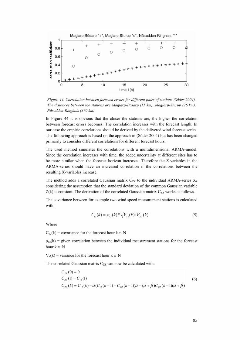
85

Figure 44. Correlation between forecast errors for different pairs of stations (Söder 2004). The distances between the stations are Maglarp-Bösarp (15 km), Maglarp-Sturup (26 km), Näsudden-Ringhals (370 km).

In Figure 44 it is obvious that the closer the stations are, the higher the correlation between forecast errors becomes. The correlation increases with the forecast length. In our case the empiric correlations should be derived by the delivered wind forecast series. The following approach is based on the approach in (Söder 2004) but has been changed primarily to consider different correlations for different forecast hours.

The used method simulates the correlations with a multidimensional ARMA-model. Since the correlation increases with time, the added uncertainty at different sites has to be more similar when the forecast horizon increases. Therefore the Z-variables in the ARMA-series should have an increased correlation if the correlations between the resulting X-variables increase.

The method adds a correlated Gaussian matrix CZZ to the individual ARMA-series Xk considering the assumption that the standard deviation of the common Gaussian variable Z(k) is constant. The derivation of the correlated Gaussian matrix CZZ works as follows.

The covariance between for example two wind speed measurement stations is calculated with:

)()(*)()( 211212 kVkVkkC XX ⋅= ρ (5)

Where

C12(k) = covariance for the forecast hour k ∈ N

ρ12(k) = given correlation between the individual measurement stations for the forecast hour k ∈ N

Vx(k) = variance for the forecast hour k ∈ N

The correlated Gaussian matrix CZZ can now be calculated with:

)ˆˆ)(1()ˆˆ(ˆ))1()1((ˆ)()(

)1()1(0)0(

1212

12

βαβααα +−+−−−−−=

==

kCkCkCkCkC

CCC

ZZZZZZ

ZZ

ZZ (6)

[h]

www.risoe.dk 86

Where

CZZ = correlated Gaussian matrix

C12(k) = covariance for the forecast hour k ∈ N

βα ˆ,ˆ = diagonal matrix containing the elements of α and β

The correlation between the individual ARMA-series X(k) is constant, equal to the correlation between the Gaussian variables Z and independent of the regarded hour when the forecast is made. The standard deviations of the Gaussian variables do not have to be the same, thus the variances of the individual ARMA-series X(k) do not have to be the same.

For the generation of the wind speed forecast error scenarios, the eigenvalues (D) and eigenvectors (V) of the correlated Gaussian matrix CZZ are determined. In the style of the Cholesky decomposition the matrix M is derived with:

DVM= (7)

Historical wind power forecast data shows that the expected wind power forecast errors corresponding to different forecast horizons are not zero. As our wind speed error scenarios are linear combinations of normally distributed random values, the expected wind power forecast errors calculated from these wind speed error scenarios would in fact be close to zero. Hence, when generating the scenarios for each individual forecast hour there is the option to draw firstly one scenario of the Gaussian variable by multiplying the matrix M with a normally distributed random value. This scenario is then treated as a simulation of the expected forecast error. Secondly a defined number of scenarios are generated by multiplying the M-matrix with the defined number of drawings of the normally distributed random values. This Monte-Carlo-simulation represents the uncertainty in the forecast. Finally the single drawing is added to these drawings.

A.1.2.2 Scenario Reduction

The generation of forecasts for wind power and load is based on a Monte-Carlo-simulation of a significant number of scenarios, see section A.1.2.1. For very large numbers of scenarios it is impractical to obtain numerically a solution for the multi-stage optimisation problem. Moreover, the scenario tree consisting of these scenarios is only a one-stage tree. Thus, strategies for reducing the number of scenarios have to be studied to find a numerical solution of the problem as well as algorithms for constructing a multi-stage scenario tree out of a given set of scenarios. Simply generating a very small number of scenarios by Monte Carlo simulations is not desirable since less scenarios give less information. Indeed, the aim is to lose only a minimum of information by the reduction process applied to the whole set of scenarios.

Actually, two steps are necessary: first, the pure number of scenarios is reduced. Afterwards, based on the remaining scenarios that still form a one-stage tree, a multi-stage scenario tree is constructed by deleting inner forecasts and creating branching within the scenario tree. The principle chosen for the setup of the scenario tree used in the Scheduling Model is shown in Figure 45. It consists of a three stage tree with 6 leaves.

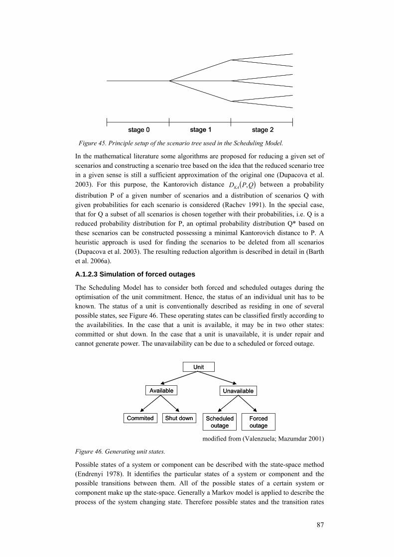
87

stage 0 stage 2stage 1stage 0 stage 2stage 1

Unit

UnavailableAvailable

Shut downCommited Forcedoutage

Scheduledoutage

Unit

UnavailableAvailable

Shut downCommited Forcedoutage

Scheduledoutage

Figure 45. Principle setup of the scenario tree used in the Scheduling Model.

In the mathematical literature some algorithms are proposed for reducing a given set of scenarios and constructing a scenario tree based on the idea that the reduced scenario tree in a given sense is still a sufficient approximation of the original one (Dupacova et al. 2003). For this purpose, the Kantorovich distance ( )QPDKA , between a probability distribution P of a given number of scenarios and a distribution of scenarios Q with given probabilities for each scenario is considered (Rachev 1991). In the special case, that for Q a subset of all scenarios is chosen together with their probabilities, i.e. Q is a reduced probability distribution for P, an optimal probability distribution Q* based on these scenarios can be constructed possessing a minimal Kantorovich distance to P. A heuristic approach is used for finding the scenarios to be deleted from all scenarios (Dupacova et al. 2003). The resulting reduction algorithm is described in detail in (Barth et al. 2006a).

A.1.2.3 Simulation of forced outages

The Scheduling Model has to consider both forced and scheduled outages during the optimisation of the unit commitment. Hence, the status of an individual unit has to be known. The status of a unit is conventionally described as residing in one of several possible states, see Figure 46. These operating states can be classified firstly according to the availabilities. In the case that a unit is available, it may be in two other states: committed or shut down. In the case that a unit is unavailable, it is under repair and cannot generate power. The unavailability can be due to a scheduled or forced outage.

modified from (Valenzuela; Mazumdar 2001)

Figure 46. Generating unit states.

Possible states of a system or component can be described with the state-space method (Endrenyi 1978). It identifies the particular states of a system or component and the possible transitions between them. All of the possible states of a certain system or component make up the state-space. Generally a Markov model is applied to describe the process of the system changing state. Therefore possible states and the transition rates

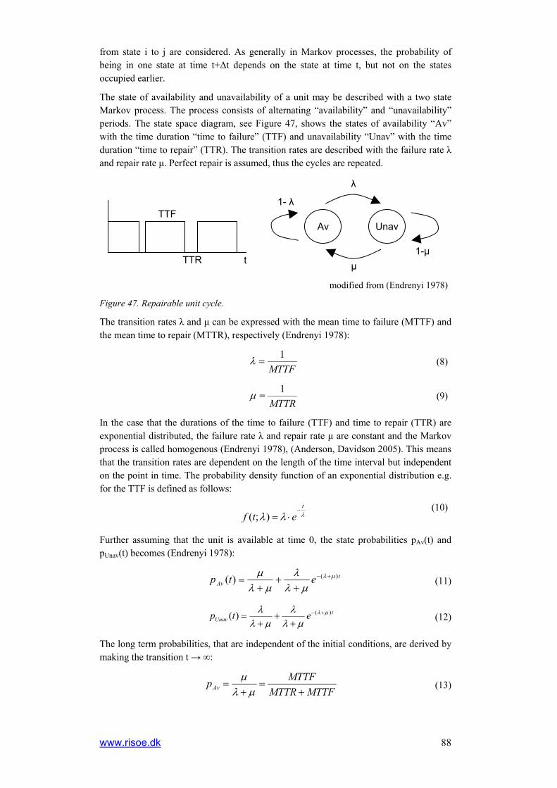
www.risoe.dk 88

t

TTF

TTR

Av Unav

λ

μ

1- λ

1-μ

from state i to j are considered. As generally in Markov processes, the probability of being in one state at time t+Δt depends on the state at time t, but not on the states occupied earlier.

The state of availability and unavailability of a unit may be described with a two state Markov process. The process consists of alternating “availability” and “unavailability” periods. The state space diagram, see Figure 47, shows the states of availability “Av” with the time duration “time to failure” (TTF) and unavailability “Unav” with the time duration “time to repair” (TTR). The transition rates are described with the failure rate λ and repair rate μ. Perfect repair is assumed, thus the cycles are repeated.

modified from (Endrenyi 1978)

Figure 47. Repairable unit cycle.

The transition rates λ and μ can be expressed with the mean time to failure (MTTF) and the mean time to repair (MTTR), respectively (Endrenyi 1978):

MTTF

1=λ (8)

MTTR

1=μ (9)

In the case that the durations of the time to failure (TTF) and time to repair (TTR) are exponential distributed, the failure rate λ and repair rate μ are constant and the Markov process is called homogenous (Endrenyi 1978), (Anderson, Davidson 2005). This means that the transition rates are dependent on the length of the time interval but independent on the point in time. The probability density function of an exponential distribution e.g. for the TTF is defined as follows:

λλλt

etf−

⋅=);( (10)

Further assuming that the unit is available at time 0, the state probabilities pAv(t) and pUnav(t) becomes (Endrenyi 1978):

tAv etp )()( μλ

μλλ

μλμ +−

++

+= (11)

tUnav etp )()( μλ

μλλ

μλλ +−

++

+= (12)

The long term probabilities, that are independent of the initial conditions, are derived by making the transition t → ∞:

MTTFMTTRMTTFpAv +

=+

=μλ

μ (13)

89

MTTFMTTRMTTRpUnav +

=+

=μλ

λ (14)

pUnav, compare equation (14), corresponds to the so called “forced outage rate” (FOR), which is in fact not a rate. The FOR is further commonly described by:

hoursavailablehoursoutageforced

hoursoutageforcedpFOR Unav +== (15)

Although it is often realistic to model times to failure by an exponential distribution, repair and maintenance durations are better represented with bell-shaped distributions, compare e.g. (Endrenyi 1978). E.g. the fraction longer than the expected MTTR is smaller for the bell-shaped distribution than for the exponential distribution due to the longer tail of the exponential distribution. Thus, the generation of homogenous Markov processes describing the unavailability of a unit with exponential distributed TTR may lead to unrealistic results. As alternative to the exponential distribution, the two-parameter Weibull distribution is proposed, compare (Van Casteren et al. 2000), (Anderson, Davidson 2005). The probability density function of a Weibull distribution e.g. for the TTR is defined as follows:

ktk etkktf

)(1)(),,( μ

μμμ

−− ⋅= (16)

The Weibull distribution with the shape factor k = 1 corresponds to an exponential distribution. Using shape factors k > 1, the Weibull distribution becomes bell-shaped.

To consider the description of non-exponential distributions, the approach of Semi-Markov models is applied, compare e.g. (Anderson, Davidson 2005), (Perman et al. 1997), (Pievatolo et al. 2004) and (Van Casteren et al. 2000). Characteristic feature of Semi-Markov models is the use of a random value describing the sojourn of a unit in a given state. Thereby the distribution of this random value can be chosen to meet the characteristics. I.e. if X(t) is the state of the unit at time t and Sn represents the time of the nth transition, the duration Un = Sn - Sn-1 is a random draw of the considered duration for the present state X(t). Hence, Un depends only on the present state X(t) and not on the states X(t) with t < Sn-1 (Anderson, Davidson 2005).

The generation of Semi-Markov processes for consideration of forced outages for each unit in the Scheduling Model are based on given data of FOR and MTTR. Based on this data, the MTTF can be calculated after some rearrangement of equation (14) and (15):

FOR

FORMTTRMTTF −⋅=1 (17)

The algorithm to generate Semi-Markov processes describing the availability or unavailability of a unit proceeds as follows. For each individual unit, a Semi-Markov process covering a whole year is generated. Thereby it is assumed that forced outages of individual units are uncorrelated.

1. To start a Semi-Markov process, the state of a unit at the beginning of the process has to be determined. This is done by drawing a random number y on the unit interval and by comparing it to the “full outage probability” (FOP) of a unit as defined by (Doherty; O’Malley 2005):

MTTRFORFOP = (18)

www.risoe.dk 90

In the case that the drawn random number y is smaller than FOP of a unit, i.e. y ≤ FOP, the unit is considered to be unavailable. Otherwise if y > FOP, the unit is considered to be available.

2. In the case that a unit is unavailable, a random value of the TTR is drawn from a Weibull distribution with scale factor equal to the given MTTR and shape factor k. When the drawn sample of TTR has elapsed, the state of the unit changes to available.

In the case that a unit is available, a random value of the TTF is drawn from an exponential distribution. The MTTF is used as distribution parameter. When the drawn sample of TTF has elapsed, the state of the unit changes to unavailable.

3. Generate successive TTR and TTF until a whole year is covered.

4. The Semi-Markov processes of the individual units only cover forced outages. Thus, scheduled outages have to be included into the Semi-Markov processes describing the availability or unavailability of an individual unit. The data of scheduled outages are provided by the All Island Grid Study Working Group. To include these time-series of scheduled outages, the following rules are applied:

a. In the case that the drawn sample of the TTF extends into the time period of a scheduled outage, the state of the unit is changed to be unavailable at the time when the scheduled outage begins.

b. In the case that the drawn sample of the TTR after a forced outage extends into the time period of a scheduled outage, the duration of the scheduled outage is not altered. Since there is no knowledge whether the cause for the forced outage is related to the coverage of the maintenance work, no assumption of a possible reduction or extension of the time duration of the scheduled outage can be made.

c. After the termination of a scheduled outage, the unit is considered to be available for a random value of TTF until the next forced outage.

5. The resulting FOR of the yearly Semi-Markov processes due to forced outages is compared to the given FOR of each unit. The algorithm is restarted until the resulting FOR is equal to the given FOR with a tolerance of 0.0005.

A.1.2.4 Determination of demand for replacement reserves

Reserve capacity has to be provided to cope with forecast errors of load and wind power and with unexpected events happening in a power system like forced outages. In the Scheduling Model one reserve category named replacement reserve is used to cope with these uncertainties in an activation time of 5 minutes or more, and three reserve categories are representing the demand for spinning reserves with activation times lower than 5 minutes, see section A.1.4.5. The demand for replacement reserves is determined corresponding to the total forecast error of the power system considered which is defined according to the hourly distribution of wind power and load forecast errors and the possibilities of forced outages. Since the forecast errors and the probability of outages vary during the time, the demand for replacement reserves varies as well. Furthermore, since the Scheduling Model considers individual scenarios of the forecast error within the scenario tree, the demand for replacement reserves varies within the scenario tree, too. Thereby it is assumed that a certain percentile of the total forecast error has to be covered by the replacement reserves. Before the methodology of the determination of the

91

demand for replacement reserves is illustrated, considered indices and parameters are defined:

Indices:

r: model region

g: generating unit

G(r): generating units in region r

n: node in the scenario tree

t: hour t

t0: the first hour of the scenario tree, i.e. the hour when the wind power forecasts are made

f: the horizon for the wind power production forecasts, i.e. f = (1,2,3, …, 36)

i: number of generated scenarios

s: Scenario

sF(n,f): the part of unreduced scenarios that belong to node n, i.e. the unreduced scenarios s covering the hours f belonging to node n that are bundled into n by the scenario reduction algorithm

Parameters:

WR(r,t): realised wind power production in time t and region r

WE(r,t0,f,s): expected wind power production in region r, in time t0 at forecast horizon f, scenario s

LR(r,t): realised load in time t at region r

LE(r,t0,f,s): expected load in region r, time t0 at forecast horizon f, scenario s

C(r,g): installed capacity of generating unit g in region r

Y(r,g,t): state (available or unavailable) of installed capacity of generating unit g in region r in time step t in scenario s

PRef(r,t): reference of the power balance in region r in time t

P(r,t0,f,s): power balance in region r in time t0 at forecast horizon f in scenario s

ΔP(r,t,n): total forecast error in region r at time t in node n

ΔPnth(r,t,n): nth percentile of the total forecast error in region r at time t in node n

www.risoe.dk 92

The methodology proceeds as follows:

1. Generate i scenarios of wind power forecasts WE(r,t0,f,s) in region r in time t0 at forecast horizon f based on Monte-Carlo-simulations, compare section A.1.2.1.

2. Generate i scenarios of load forecasts LE(r,t0,f,s) in region r in time t0 at forecast horizon f based on Monte-Carlo-simulations, compare section A.1.2.1.

3. Generate scenario of Y(r,g,t) describing availability / unavailability capacity of each generating unit g at forecast horizon f in time step t based on Monte-Carlo-simulations of Semi-Markov processes, compare section A.1.2.3.

4. Determine the reference of the power balance PRef in model region r at time step t considering the realised wind power feed-in and load as well as the installed capacity minus scheduled outages but ignoring forced outages:

),(),(),(),()(

Ref trLtrWgrCtrP RRrGg

−+= ∑∈

(19)

5. Determine the power balance of scenario s. Thereby the hours of the forecast horizon f are allocated to the corresponding hours of the Markov chains describing the availability of the generating unit g. The individual scenarios of wind power forecasts, load forecasts and forced outages are randomly allocated to each other.

)s,f,t,r(L)s,f,t,r(W)t,g,r(Y)g,r(C)s,f,t,r(P EE)r(Gg

000 −+= ∑∈

(20)

6. Determine the difference between the reference power balance and the power balance of scenario s. This is equal to scenarios of the total forecast error within the considered region r due to errors of wind power forecasts and of load forecasts as well as of forced outages (t is equal to t0 + f):

),,,(),(),,,( 0Ref0 sftrPtrPsftrP −=Δ (21)

7. The number of scenarios s of wind power and load forecasts is reduced according to the scenario tree, compare section A.1.2.2. Thereby it is recorded which scenarios are represented by a reduced scenario belonging to node n, i.e. which scenarios represent the set of scenarios sF(n,f) belonging to node n. Based on this allocation, the distribution of the total forecast error ΔP(r,t,n) in the considered region r of node n in time t is determined.

8. Determine the e.g. nth percentile of ΔP(r,t,n), labelled ΔPnth(r,t,n). This percentile of the total forecast error is considered to be the demand of non-spinning positive reserves. The choice of the percentile is discussed in section 4.6.3.

It may be interesting to compare the suggested approach to quantify the reserve demand with the approach proposed in (Doherty; O’Malley 2005). The latter takes load and wind power forecast errors as well as forced total and partial outages into account. The main differences to the methodology proposed above are different representations of the distributions and probabilities of the individual deviations:

• Distribution of forecast errors: In (Doherty; O’Malley 2005), a Gaussian distribution of the aggregated load and wind power forecast error is considered. Since the stochastic representation of load and wind power forecasts in the Scheduling Model uses discrete scenarios derived by the

93

scenario reduction process, compare section A.1.2.2, the demand for replacement reserves has to be determined according to these discrete scenarios. Hence, the distribution of forecast errors of that part of unreduced scenarios which belong to a certain scenario has to be considered when determining the reserve requirements.

• Treatment of forced outages of units: In (Doherty; O’Malley 2005), outages are represented by probabilities of the occurrence of total and partial outages of each individual unit. Thereby it is assumed that only one forced outage may happen in a short time after another unit has suffered an outage already. In the approach proposed above, a distribution of the available capacity in the power system at a certain hour is derived using Monte-Carlo-simulations of Semi-Markov processes describing the available generation capacities. Hence, it is assumed that forced outages of individual units are statistical independent. Thus, it is possible to consider that more than two outages may occur during an hour or during short time duration. Further on, the chronology process of repair due to forced and scheduled outages is considered by determining the available capacity in the power system.

A.1.2.5 Implementation

The individual modules are implemented in Matlab and their individual functions are arranged into several directories according to the individual modules. A main Matlab function organizes the data input and the distribution of the data matrices between the executed modules and is located in the main directory of the Scenario Tree Tool. The input data files in ASCII format are stored in a separate directory. The required input data files are generated by a MS Access Scenario Tree Tool input database holding the input data. The process of reading out data into the individual ASCII is controlled using a form. Therewith it is possible to select flexible time periods that have to be covered by the resulting scenario trees, the consideration of different forecast accuracies and wind power capacities.

By running the main programme, the required data is read into the Scenario Tree Tool and the individual modules are executed. The sequence of actions is organized as showed in Figure 48. The resulting ASCII files for the Scheduling Model are written out to a separate directory.

www.risoe.dk 94

Scenario Tree Tool Input Database

1. Read-in of input data

Time-series of wind power

2. Transformation of wind power time-series into wind speed time-series

Time-series of wind speed

3. Generation of n wind speed forecast error scenarios

Scenarios of wind speed forecast error

4. Combination of wind speed forecast error scenarios with wind speed time-

series

Wind power forecast scenarios

5. Transformation of wind speed forecast scenarios into wind power forecast

scenarios

6. Generation of n load forecast error scenarios

Scenarios of load forecast errors

7. Combination of load forecast error scenarios with load time-series

Load forecast scenarios

Wind speed forecast scenarios

8. Generation of n Semi-Markov processes of outages

of individual units

Scenarios of Semi-Markov processes of

unit outages

9. Random allocation of scenarios of wind power and load forecasts and of

Semi-Markov processes of unit outages

Allocated scenarios of wind power and load forecasts

Allocated scenarios of wind power and load forecasts

and Semi-Markov processes of unit outages

11. Determination of non-spinning positive reserves

10. Scenario reduction and generation of scenario trees

Input files for the Scheduling Model

Reliability data of units

12. Read-out of resulting data

Time-series of load

Scenario Tree Tool Input Database

1. Read-in of input data

Time-series of wind power

2. Transformation of wind power time-series into wind speed time-series

Time-series of wind speed

3. Generation of n wind speed forecast error scenarios

Scenarios of wind speed forecast error

4. Combination of wind speed forecast error scenarios with wind speed time-

series

Wind power forecast scenarios

5. Transformation of wind speed forecast scenarios into wind power forecast

scenarios

6. Generation of n load forecast error scenarios

Scenarios of load forecast errors

7. Combination of load forecast error scenarios with load time-series

Load forecast scenarios

Wind speed forecast scenarios

8. Generation of n Semi-Markov processes of outages

of individual units

Scenarios of Semi-Markov processes of

unit outages

9. Random allocation of scenarios of wind power and load forecasts and of

Semi-Markov processes of unit outages

Allocated scenarios of wind power and load forecasts

Allocated scenarios of wind power and load forecasts

and Semi-Markov processes of unit outages

11. Determination of non-spinning positive reserves

10. Scenario reduction and generation of scenario trees

Input files for the Scheduling Model

Reliability data of units

12. Read-out of resulting data

Time-series of load

Figure 48. Sequence of actions within the Scenario Tree Tool.

In the following the sequence of actions within the Scenario Tree Tool is described:

1. Read in the required data from the individual ASCII input data files into relevant Matlab matrices from the Scenario Tree Tool input database.

2. In the case where a region or zone is represented by measured wind power time-series, these time-series are converted into wind speed time-series. Otherwise the measured wind speed time-series are used directly.

3. Monte-Carlo-simulation of n scenarios of wind speed forecast errors for a forecast horizon up to 36 hours based on ARMA-processes describing the wind speed forecast error. The correlations of the wind speed forecast errors between individual zones are considered, see section A.1.2.1.

4. Combination of the generated wind speed forecast errors with the corresponding values of the wind speed time-series to simulate the wind speed forecast scenarios.

5. Transformation of wind speed forecast scenarios into wind power forecast scenarios. For this purpose an aggregated power curve considering the spatial distribution of wind farms within a zone is used, see section A.1.2.1. Subsequently, the individual wind power scenarios of the individual zones are aggregated on a regional level.

6. Monte-Carlo-simulation of n scenarios of load forecast errors for a forecast horizon up to 36 hours based on ARMA-processes describing the load forecast error, see section A.1.2.1.

95

7. Combination of the generated load forecast errors with the corresponding values of the load time-series to simulate the load forecast scenarios.

8. Monte-Carlo-simulation of n scenarios of Semi-Markov processes describing the availability or unavailability of the generation units considered over a whole year, see section A.1.2.3.

9. Random allocation of individual scenarios of forecasts of wind power and load and of Semi-Markov processes describing availability or unavailability of units considered.

10. Reduction of combined scenarios of wind power and load forecasts and generation of scenario trees, see section A.1.2.2.

11. Determination of the requirements for replacement reserves due to wind power and load forecast errors and unit availabilities, see A.1.2.4.

12. The resulting ASCII files holding the scenarios of wind power and load forecasts, Semi-Markov processes describing the availability or unavailability of the units considered and the requirements for replacement reserves are saved into the result directory of the Scenario Tree Tool. These resulting ASCII files are read-in by scenario tree database directly, see Figure 40.

A.1.3 Data input into Scenario Tree Tool Wind power generation in the All Island Power System is simulated under consideration of the spatial distribution of installed wind power capacity. Therefore, the island is divided into different zones. For each portfolio and each zone, wind power capacity was delivered by work stream 1. Figure 49 shows all zones. There are eleven onshore zones (two for Northern Ireland and nine for Ireland) and ten offshore zones.

Figure 49. Wind farm zones in the All Island power system.

Besides installed wind power capacity measured wind power series are taken into account to simulate wind power generation. Measured wind power series of several wind farms were provided by EirGrid/SONI. Table 25 shows the wind farms and corresponding zones for those wind power series were available.

www.risoe.dk 96

Zone Wind Farm Zone Wind Farm ROI A Cark, Cranaloght, Cuillagh, Meenadreen OS A Arklow Banks ROI B Bellacorrick, Inverin, Kingsmountain OS B ROI C Corneen, Largan Hill OS C ROI D Corneen OS D ROI E Beale II OS E Burtonport ROI F Beenageeha, Tursillagh OS F ROI G Carnsore, Corneen OS G ROI H Curabwee, Milane Hill OS H ROI I Carnsore OS I NI A NI_A1, NI_A2 OS J

NI B NI_B1 - NI_B4, Altnahullion, Snugborough, Lendrums Bridge GB NI A, NI B, ROI A

Table 25. Wind power zones and corresponding sources of wind power series.

Wind correlation effects within one zone are taken into account by smoothing out the wind series. The corresponding approach is explained in the section “Adapting Wind Data” in section A.1.2.1. Wind power generation in a region is more smoothed than power generation at a single wind farm. The level of smoothing depends on the zone size and the number of considered wind series in the zone. Wind power generation of all zones is summed up to get the aggregated generation of the All Island power system. Figure 50 shows for example wind power duration curves for the zone ROI_H and the All Island power system before (solid line) and after smoothing (dashed line). The dotted and dash-dotted lines (called frequency) indicate power fluctuations within two hour periods. This representation of fluctuations follows the statistical analysis of the All Island Grid Study working group. In about 85% of the time the unsmoothed wind power generation in ROI_H does not vary more than +/- 20% of the capacity installed. After smoothing, variation of up to 20% of the capacity installed can be expected 95% of the time. Hence relative power fluctuations are not so extreme for one region than for one single wind farm. The duration curve of smoothed wind power generation throughout the island indicates that at least 5% of the installed capacity is always producing.

Figure 50. Wind duration curves for zone ROI_H and the All Island power system before and after smoothing.

Correlation effects between different zones are reproduced in a natural way as measured power series were taken. For some offshore zones representative wind power series are not needed because wind power capacity is assumed as zero in these zones for all portfolios. Wind generation in Great Britain was simulated by means of the aggregated wind power series of the zones NI_A, NI_B and ROI_A. Therefore, these series have been shifted one hour in time.

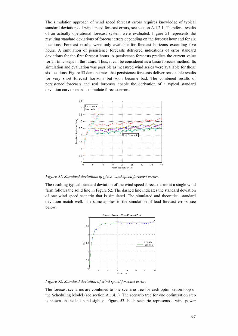
97

The simulation approach of wind speed forecast errors requires knowledge of typical standard deviations of wind speed forecast errors, see section A.1.2.1. Therefore, results of an actually operational forecast system were evaluated. Figure 51 represents the resulting standard deviations of forecast errors depending on the forecast hour and for six locations. Forecast results were only available for forecast horizons exceeding five hours. A simulation of persistence forecasts delivered indications of error standard deviations for the first forecast hours. A persistence forecasts predicts the current value for all time steps in the future. Thus, it can be considered as a basic forecast method. Its simulation and evaluation was possible as measured wind series were available for those six locations. Figure 53 demonstrates that persistence forecasts deliver reasonable results for very short forecast horizons but soon become bad. The combined results of persistence forecasts and real forecasts enable the derivation of a typical standard deviation curve needed to simulate forecast errors.

Figure 51. Standard deviations of given wind speed forecast errors.

The resulting typical standard deviation of the wind speed forecast error at a single wind farm follows the solid line in Figure 52. The dashed line indicates the standard deviation of one wind speed scenario that is simulated. The simulated and theoretical standard deviation match well. The same applies to the simulation of load forecast errors, see below.

Figure 52. Standard deviation of wind speed forecast error.

The forecast scenarios are combined to one scenario tree for each optimization loop of the Scheduling Model (see section A.1.4.1). The scenario tree for one optimization step is shown on the left hand sight of Figure 53. Each scenario represents a wind power

www.risoe.dk 98

forecast scenario for the All Island Power System. The legend specifies the probabilities of the different scenarios at this optimization step. The figure on the right hand sight indicates the average standard deviation of resulting forecast scenarios depending on the forecast horizon. In the illustration, they are normalized to the wind power capacity installed (here for example of portfolio P1). A relative standard deviation of about 7% for a day-ahead forecast corresponds to indications in literature, compare (Dena 2005) for example.

Figure 53. Wind power forecast scenarios and their standard deviation.

However, the applied simulation method of forecast errors not only requires knowledge of standard deviations but also of correlations between forecast errors at different locations. Forecast errors at different locations are not perfectly correlated and can partially compensate each others. Figure 54 shows forecast error correlations between two locations depending on their distance and the forecast horizon. The correlations were calculated by means of real and persistence forecasts (the latter for the first forecast hours). The resulting mesh was fitted to get indications about correlations for other distances and to balance outliers.

Figure 54. Correlation of wind speed forecast errors.

The transformation of speed forecast errors to power forecast errors is based on the appropriate power curves of the concerned wind farms, see section A.1.2.1.

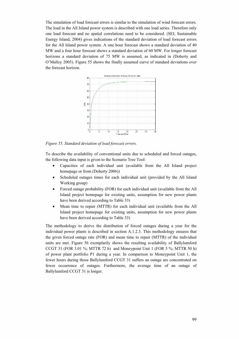
99

The simulation of load forecast errors is similar to the simulation of wind forecast errors. The load in the All Island power system is described with one load series. Therefore only one load forecast and no spatial correlations need to be considered. (SEI, Sustainable Energy Island, 2004) gives indications of the standard deviation of load forecast errors for the All Island power system. A one hour forecast shows a standard deviation of 40 MW and a four hour forecast shows a standard deviation of 60 MW. For longer forecast horizons a standard deviation of 75 MW is assumed, as indicated in (Doherty and O’Malley 2005). Figure 55 shows the finally assumed curve of standard deviations over the forecast horizon.

Figure 55. Standard deviation of load forecast errors.

To describe the availability of conventional units due to scheduled and forced outages, the following data input is given to the Scenario Tree Tool:

• Capacities of each individual unit (available from the All Island project homepage or from (Doherty 2006))

• Scheduled outages times for each individual unit (provided by the All Island Working group)

• Forced outage probability (FOR) for each individual unit (available from the All Island project homepage for existing units, assumption for new power plants have been derived according to Table 33)

• Mean time to repair (MTTR) for each individual unit (available from the All Island project homepage for existing units, assumption for new power plants have been derived according to Table 33)

The methodology to derive the distribution of forced outages during a year for the individual power plants is described in section A.1.2.3. This methodology ensures that the given forced outage rate (FOR) and mean time to repair (MTTR) of the individual units are met. Figure 56 exemplarily shows the resulting availability of Ballylumford CCGT 31 (FOR 3.01 %; MTTR 72 h) and Moneypoint Unit 1 (FOR 5 %; MTTR 50 h) of power plant portfolio P1 during a year. In comparison to Moneypoint Unit 1, the fewer hours during those Ballylumford CCGT 31 suffers an outage are concentrated on fewer occurrence of outages. Furthermore, the average time of an outage of Ballylumford CCGT 31 is longer.

www.risoe.dk 100

0

1

1 673 1345 2017 2689 3361 4033 4705 5377 6049 6721 7393 8065 8737

Time [h]

Ava

ilabi

lity

Ballylumford CCGT 31Moneypoint Unit 1

Available

Unavailable

Figure 56. Resulting availability of Ballylumford CCGT 31 (FOR 3.01 %; MTTR 72 h) and Moneypoint Unit 1 (FOR 5 %; MTTR 50 h) of power plant portfolio P1.

For each power plant portfolio, a set of time-series describing the availability due to forced and scheduled outages with a minimum number of simultaneous outages has been determined. The resulting maximal number of simultaneous outages of each power plant portfolio is shown in Table 10. Generally, portfolios with a higher number of conventional power plants considered tend to have a higher number of simultaneous forced outages. For example, portfolio 3 with 56 conventional thermal power plants in the All Island power system considered shows a maximal number of 6 simultaneous forced outages, whereas portfolio 6 with 40 conventional thermal power plants considered shows a maximal number of 4 simultaneous forced outages. Further on, the value of the FOR and MTTR of the individual power plants influences the maximal number of simultaneous forced outages. For example, portfolio 1 with 50 conventional thermal power plants considered and an average FOR of 3.15 % and an average MTTR of 53.57 h shows the same maximal number of simultaneous forced outages than portfolio 5 with 44 conventional thermal power plants considered and an average FOR of 3.18 % and an average MTTR of 54.07 h.

Portfolio 1

Portfolio 2

Portfolio 3

Portfolio 4

Portfolio 5

Portfolio 6

Maximal number of simultaneous forced outages

5 5 6 4 5 4

Table 26. Maximal number of simultaneous forced outages of each power plant portfolio.

The resulting duration curves of the unavailable capacity due to forced and scheduled outages for the individual power plant portfolios are shown in Figure 57. Generally, portfolios with a higher number of conventional power plants considered tend to show higher maximal values of unavailable capacity due to forced and scheduled outages.

101

Further on, these portfolios also tend to show fewer hours with no forced or scheduled outage.

Portfolio 1

0

200

400

600

800

1000

1200

1400

1600

1800

2000

1 673 1345 2017 2689 3361 4033 4705 5377 6049 6721 7393 8065 8737Time [h]

Una

vaila

ble

capa

city

[M

W]

Portfolio 2

0

200

400

600

800

1000

1200

1400

1600

1800

2000

1 673 1345 2017 2689 3361 4033 4705 5377 6049 6721 7393 8065 8737Time [h]

Una

vaila

ble

capa

city

[M

W]

Portfolio 3

0

200

400

600

800

1000

1200

1400

1600

1800

2000

1 673 1345 2017 2689 3361 4033 4705 5377 6049 6721 7393 8065 8737Time [h]

Una

vaila

ble

capa

city

[M

W]

Portfolio 4

0

200

400

600

800

1000

1200

1400

1600

1800

2000

1 673 1345 2017 2689 3361 4033 4705 5377 6049 6721 7393 8065 8737Time [h]

Una

vaila

ble

capa

city

[M

W]

Portfolio 5

0

200

400

600

800

1000

1200

1400

1600

1800

2000

1 673 1345 2017 2689 3361 4033 4705 5377 6049 6721 7393 8065 8737Time [h]

Una

vaila

ble

capa

city

[M

W]

Portfolio 6

0

200

400

600

800

1000

1200

1400

1600

1800

2000

1 673 1345 2017 2689 3361 4033 4705 5377 6049 6721 7393 8065 8737Time [h]

Una

vaila

ble

capa

city

[M

W]

Figure 57. Duration curve of unavailable capacity due to forced and scheduled outages for portfolio P1 to P6.

A.1.4 Model of system operation – Scheduling model The representation in the Scheduling model of the system and generating unit constraints mentioned in the tender document and discussed with the All Island Grid Study working is explained in section A.1.4.1 to A.1.4.19.

It has been decided to use an hourly time resolution in the Scheduling model. The electricity demand data used will be those measured at 30 minutes past the hour as the island peak occurs ½ hour past the hour.

A.1.4.1 Rolling Planning

The inclusion of uncertainty about the wind power production, electricity demand and demand for replacement reserve in the optimisation model is considered by using a scenario tree. The scenario tree represents forecasts of electricity demand, wind power production and replacement reserve demand with different forecast horizons corresponding to each hour in the optimisation period. The electricity demand and wind power production forecasts are independent of each other, whereas the demand for replacement reserve is influenced by the wind power production and electricity demand forecasts. Therefore for a given forecast horizon one scenario consists of a forecast of wind power production, electricity demand and replacement reserve with an associated probability expressing the weight that the forecast has when calculating the expected costs, i.e. how likely the forecast is judged to be.

www.risoe.dk 102

As it is not possible to cover the whole simulated time period with only one single scenario tree, the model is formulated by introducing a multi-stage recursion using rolling planning. In stochastic multi-stage linear recourse models, there exist two types of decisions: “root” decisions that have to be taken before the outcome of uncertain events (stochastic parameters) is known and hence must be robust towards the different possible outcomes of the uncertain events, and “recourse decisions” that can be taken after the outcome of uncertain events is resolved. With these “recourse decisions” actions can be started which might possibly revise the first decisions. In the case of a power system with wind power, the power generators have to decide on the day-ahead scheduling before the precise wind power production is known (root decision). And as the wind power prediction is uncertain, recourse actions in the form of up or down regulations of power production is necessary in most cases.

In general, new information arrives on a continuous basis and provides updated information about wind power production and forecasts, the operational status of other production and storage units, the operational status of the transmission and distribution grid, and electricity demand. Thus, an hourly basis for updating information would be most adequate. However, stochastic optimisation models quickly become intractable so it is necessary to simplify the information arrival and decision structure in the stochastic model.

In the current version of the model a three stage model is implemented. The model steps forward in time using rolling planning with a three hour step, so a one-day cycle consists of eight planning loops. For each time step new forecasts (i.e. a new scenario tree) that consider the change in forecast horizons are used. This decision structure is illustrated in Figure 58 showing the scenario tree for three planning periods. For each planning period a three-stage, stochastic optimisation problem is solved having a deterministic first stage covering 3 hours, a stochastic second stage with three scenarios covering 3 hours, and a stochastic third stage with six scenarios covering a variable number of hours according to the rolling planning period in question. The scenario tree represents a decision structure where the system operator performs unit commitment and dispatch assuming perfect knowledge about the realised wind and load in the first three hours, and uncertain knowledge about wind and load in subsequent hours, and having the possibility of every three hours to change the planned unit commitment and dispatch for future hours as a response to receiving updated information about the status of the power system as the operation hours in question gets closer in time. The perfect foresight assumption for the first three hours are necessary for the model, but to get a realistic unit commitment, the wind and load forecast errors within the first three hours contribute to the demand for replacement reserves in the first three hours.

Planning loop 1 starts at 12 am on day one and covers the 36 hours until the end of day two. The forecast horizons involved are 3 to 36 hours ahead. The day-ahead scheduling is determined in Planning period 1, as well as the realised unit commitment and dispatch for the first three hours in the planning loop, which happens after realisation of the stochastic parameters. Furthermore unit commitment and dispatch plans covering each scenario for the outcome of wind power, load and demand for replacement reserve are made.

In Planning loop 2 to 8 the optimisation period always ends at 12 pm day 2, i.e. the optimisation period is reduced with 3 hours in each planning loop. These planning loops take the day-ahead dispatch schedules into account when rescheduling the unit commitment and dispatch decisions due to updated forecasts. The realised unit commitment and dispatch for the first three hours in each planning loop is calculated.

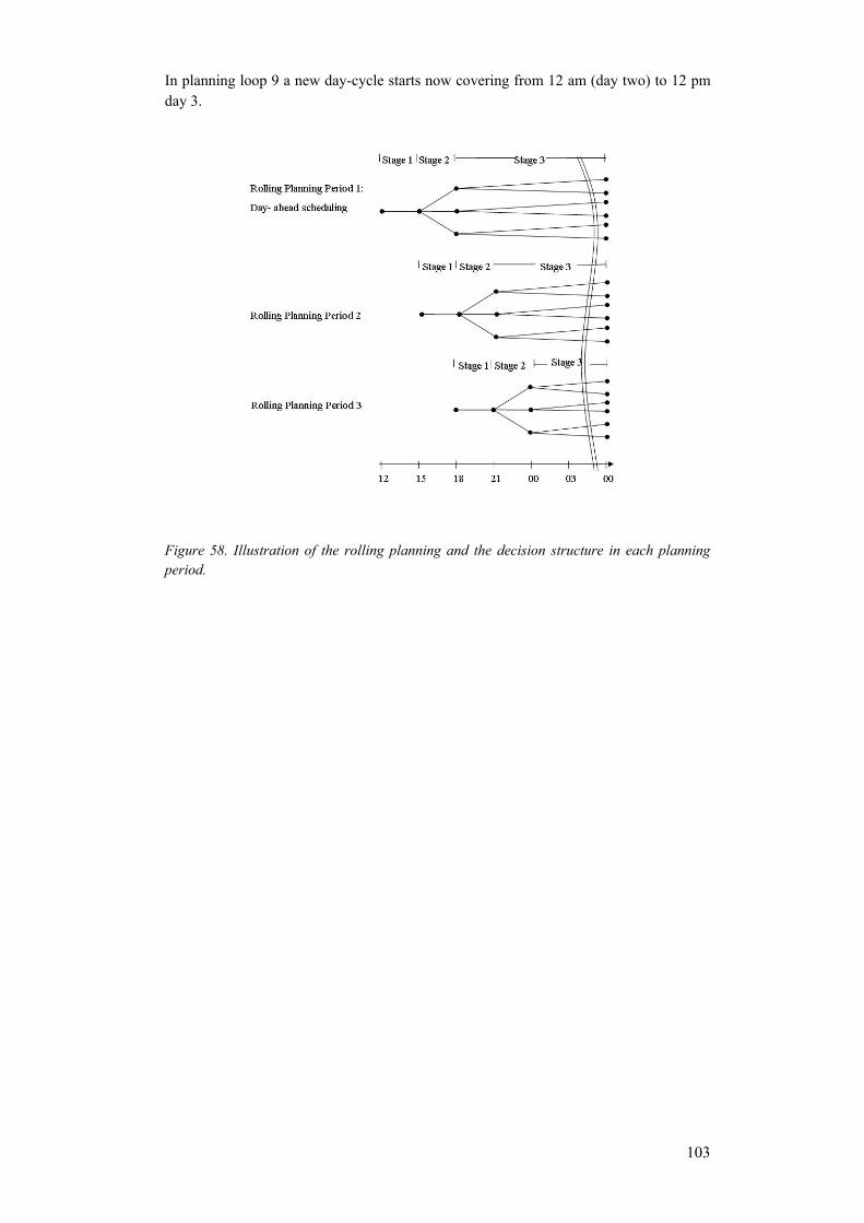
103

In planning loop 9 a new day-cycle starts now covering from 12 am (day two) to 12 pm day 3.

Figure 58. Illustration of the rolling planning and the decision structure in each planning period.

www.risoe.dk 104

A.1.4.2 Unit commitment using integer variables

The stochastic optimisation induces quite long calculation times to solve the problem. Therefore for the previous Wilmar studies that analysed a model area covering Denmark, Finland, Germany, Norway and Sweden, it was considered necessary to introduce a linear approximation of the unit commitment in the Wilmar Planning tool to avoid the usage of integer variables.

In the linear approximation the capacity online is implemented as a continuous variable. Compared to using integer variables the main difference with the linear approximation is that any amount of additional capacity can be brought online, as long as the amount is smaller than the available capacity. This is not as problematic as it sounds in a model where individual power plants are aggregated into unit groups, such as for the large model area analysed in previous studies performed with the precedent version of the Wilmar Planning Tool, see (Barth et al. 2006b); (Meibom et al. 2006b).

In this study unit commitment using integer variables has been implemented. The approach is based on an article by (Carrión and Arroyo 2006). The method is a linear, mixed integer formulation of minimum up time, minimum down time, ramp-up, ramp-down, start-up ramp, shut-down ramp, and an out time dependant, stepwise start-up cost function. The formulation assumes that a start-up process is irreversible, i.e. when the start-up process is initiated it will continue until the minimum stable generation limit is reached. Not until then a shut-down process can be initiated.

The unit commitment implemented in the SM has the following restrictions:

1. Minimum up and minimum down times.

2. Ramp-up and ramp-down rates.

3. Start-up ramp rate.

4. Out-time dependant start-up fuel consumption.

5. Piecewise linear fuel consumption.

The following issues have been omitted from the SM, either because they are not important for the All Island power system, or due to a consideration about their importance relatively to the increase in model complexity and calculation time, if they where to be implemented:

1. Shut-down costs.

2. Shut-down ramp rates.

3. Start-up and shut-down power trajectories.

4. Non-convex production costs.

A.1.4.3 Fuel consumption curves

Piecewise linear fuel consumption curves have been implemented in the SM. The fuel consumption of each thermal unit is described by a constant heat rate independent of load (no load heat rate) and a set of incremental heat rate slopes when producing in specific generation intervals as specified by capacity points. It is assumed for all units that the slope from 0MW to Capacity Point 1 (minimum stable generation limit) is the same as the slope from Capacity Point 1 to Capacity Point 2.

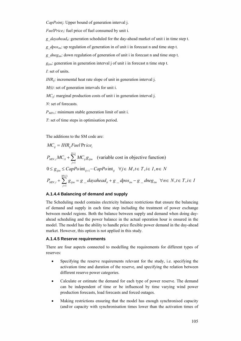
105

CapPointj: Upper bound of generation interval j.

FuelPricei: fuel price of fuel consumed by unit i.

g_dayaheadit: generation scheduled for the day-ahead market of unit i in time step t.

g_dpositn: up regulation of generation in of unit i in forecast n and time step t.

g_dnegitn: down regulation of generation of unit i in forecast n and time step t.

gijtn: generation in generation interval j of unit i in forecast n time step t.

I: set of units.

IHRij: incremental heat rate slope of unit in generation interval j.

M(i): set of generation intervals for unit i.

MCij: marginal production costs of unit i in generation interval j.

N: set of forecasts.

PMIN.i: minimum stable generation limit of unit i.

T: set of time steps in optimisation period.

The additions to the SM code are:

( )

, 11

1

( )

,1

Pr

(variable cost in objective function)

0 int int , , ,

_ _ _ ,

M i

ij ij i

MIN i i ij ijtnj

ijtn ij ij

M i

MIN i ijtn it itn itnj

MC IHR Fuel ice

P MC MC g

g CapPo CapPo j M t T i I n N

P g g dayahead g dpos g dneg n N t T

=

+

=

=

+

≤ ≤ − ∀ ∈ ∈ ∈ ∈

+ = + − ∀ ∈ ∈

∑

∑ , i I∈

A.1.4.4 Balancing of demand and supply

The Scheduling model contains electricity balance restrictions that ensure the balancing of demand and supply in each time step including the treatment of power exchange between model regions. Both the balance between supply and demand when doing day-ahead scheduling and the power balance in the actual operation hour is ensured in the model. The model has the ability to handle price flexible power demand in the day-ahead market. However, this option is not applied in this study.

A.1.4.5 Reserve requirements

There are four aspects connected to modelling the requirements for different types of reserves:

• Specifying the reserve requirements relevant for the study, i.e. specifying the activation time and duration of the reserve, and specifying the relation between different reserve power categories.

• Calculate or estimate the demand for each type of power reserve. The demand can be independent of time or be influenced by time varying wind power production forecasts, load forecasts and forced outages.

• Making restrictions ensuring that the model has enough synchronised capacity (and/or capacity with synchronisation times lower than the activation times of

www.risoe.dk 106

the reserve requirements) to cover the reserve requirements. This also includes modelling of the ability of each power plant to deliver a specific type of reserve, which in some cases depends on the production level of each power plant.

• Model the actual activation of reserves due to the sum of load and wind power production forecasts having an error compared to realised load and wind power production or due to a forced outage of a power plant. As the SM has hourly time resolution, activation of reserves can only happen with hourly time resolution.

The main division between categories of positive reserves is between spinning reserves that can only be provided by synchronised units due to the low activation times of these types of reserves, and reserves which can be provided by both synchronised and desynchronised units with low start-up times. Gas turbines using light oil (distillate) have start-up times from cold of around 5 minutes (All Island Modelling generator data, 2005), so the split between spinning and other reserves can be set at reserve categories with 5 minutes activation times after an event. For the grid code for the Republic of Ireland (ESB National Grid 2005), reserves therefore corresponds to the following reserve categories: Primary operating margin (5 s – 15 s), Secondary operating margin (15 s – 90 s), Tertiary operating reserve band 1 (90 s – 5 min), and the other reserve categories are: Tertiary operating reserve band 2 (5 min – 20 min), Replacement reserve (20 min – 4 hours).

In this study the following spinning reserve categories are represented:

• Primary operating margin (POR).

• Secondary operating margin (SOR).

• Tertiary operating reserve band 1 (TR1).

POR is replaced by SOR being replaced by TR1. The Irish power system is first ready to handle another outage approximately one hour after the first outage. This implies that the demands for each type of spinning reserve do not add up. A unit reserving capacity for providing POR can use the same capacity to provide SOR and TR1. The demand for replacement reserve does add up on the demands for spinning reserves, because the replacement reserves are activated in order to restore power plants providing spinning reserves to a state where they again are able to deliver spinning reserves.

For each spinning reserve category the reserve capability of a unit is restricted by:

• A maximum reserve capability.

• The online capacity minus the generation.

The provision of POR, SOR and TR1 are optimised in each planning loop (see section A.1.4.1).

The demand for replacement reserves with activation times longer than 5 minutes (forecast horizons from 5 minutes to 36 hours ahead) are determined by the Scenario Tree Tool (see section A.1.2). It is represented as one category in the SM.

A unit planned to be online in a given time step and scenario can deliver all four types of positive reserves. The spinning capacity reserved for providing these types of reserve will be the maximum of the obligations undertaken to provide respectively POR, SOR and TR1, plus the obligation to provide replacement reserve. A unit planned to be offline in a given time step and scenario can only deliver replacement reserve and only in hours further ahead in time than the start-up time of the unit.

107

The unit commitment is dependant on the wind power and load forecast. This implies that the variables used to model the provision of different types of spinning reserves also must be forecast dependant, because delivering spinning reserve enforces a unit to be online.

There should be enough spinning reserves to cover an outage of the largest unit in combination with fast decreases in the wind power production. The size of the largest online unit changes dynamically. The largest possible decrease in the wind power production within the next 5 minutes is dependant on the wind power production right now. If the actual wind power production is zero, the largest decrease is zero. The demands for spinning reserves should therefore be updated dynamically according to the actual unit commitment and wind power production.

The demand for POR in a given operation hour (t) and forecast (n) due to an outage can be calculated as:

( )),,(),,(),( ntuPORntuGenerationMaxntutageDemandPORO Unitsu += ∈

Where Generation(u,t,n) is the generation of unit u, and POR(u,t,n) is the primary reserve delivered by the unit. Likewise with the demand for SOR and TR1.

(Doherty and O’Malley 2005) finds that the demand for POR, SOR and TR1 is dependant on the installed wind power capacity. Figure 10 shows the dependence calculated using the methodology from (Doherty and O’Malley 2005).

0100200300400500600700800

010

0020

0030

0040

0050

0060

0070

0080

0090

00

Wind power capacity [MW]

Res

erve

dem

and

[MW

]

PORSORTR1

Figure 59. POR, SOR and TR1 requirements in the All Island power system as a function of installed wind power capacity. Data delivered from the All Island Grid Study working group.

Subtracting the POR, SOR and TR1 demand at zero wind power capacity (corresponding to the requirement due to an outage), gives the additional spinning reserves due to wind power fluctuations.

www.risoe.dk 108

Installed Wind POR [MW] SOR [MW] TR1 [MW]0 0 0 0 1000 1 2 5 2000 3 6 18 3000 4 12 37 4000 6 18 63 5000 8 27 94 6000 10 36 131 7000 13 48 174 8000 16 61 225 9000 18 75 279

Table 27. Additional demands for spinning reserves as a function of installed wind power capacity. All values in MW.

We want to take into account that the actual wind power production provides a higher bound on the spinning reserve demand due to wind power fluctuations. Therefore the additional demand for spinning reserves due to wind power fluctuations (DemandPORWind) is found by look-up in Table 27 using the actual wind power production as the wind power capacity installed.

To save calculation time it has been decided not to include the optimisation of the spinning reserve requirements in the unit commitment decisions in the SM. Therefore the following approach has been implemented:

1. Planning loop 1:

a. For hour 1-12 covered by the previous planning loop: Calculate DemandPOROutage using primary reserve and generation of units found in the previous planning loop.

b. For hour 13-36 not covered by the previous planning loop: Use fixed values of DemandPOROutage corresponding to 80% of installed capacity of largest unit2.

c. For all hours: Calculate DemandPORWind from Table 1 using the wind power forecasts belonging to Planning loop 1.

d. Demand for POR equal to DemandPOROutage + DemandPORWind.

2. Planning loop 2-8:

a. For all hours; Calculate DemandPOROutage using primary reserve and generation of units found in the previous planning loop.

b. For all hours: Calculate DemandPORWind from Table 1 using the wind power forecasts belonging to this planning loop.

Similar approaches are used for SOR and TR1.

The day-ahead scheduling takes the expected wind power production and electricity demand during the next day (average of the six wind power production and load forecasts) into account. Provision of negative reserve is represented by some of the forecasts in the scenario tree having a higher wind power forecast (and sometimes lower load) than the expected wind power production (and expected load), such that relatively

2 DemandSOROutage 80% of capacity of largest unit. DemandTR1Outage 100% of capacity of largest

unit.

109

to the day-ahead scheduling down regulation of production needs to be planned in the unit commitment and dispatch covering plans covering these scenarios.

A.1.4.6 Wind power providing reserves

Wind power turbines can provide down regulation in the SM by reducing production in the actual operation hour. This possibility is used in high wind scenarios in time periods where production is close to become bigger than demand.

Wind turbines providing positive spinning reserve will be modelled by the following:

1. One decision variable determine the percentage of the wind power production forecast with the lowest wind power production that will be provided as POR, SOR and TR1, i.e. how much of the lowest forecasted wind power production which is planned to be lost in exchange of getting positive spinning reserve power from the wind turbines. Choosing the lowest wind power production forecast reflects that the TSO wants to be as certain as possible that the wind turbines will be able to provide the forecasted amount of reserve, and that is most likely when the starting point is the forecast being most negative with regard to the future wind power production.

2. The planned POR, SOR and TR1 provision of the wind turbines is included in the balance equations for these reserves categories.

3. The wind power production forecasts are all reduced with the amounts of wind power production reserved.

The optimisation of the amounts of POR, SOR and TR1s to be delivered from wind power is done in each planning loop.

A.1.4.7 Minimum system inertia

Assumed covered by the approach explained in the next section.

A.1.4.8 System stability and security limits

Restrictions enforcing a certain number of units to be online will be implemented according to input from the All Island Grid Study working group, see section A.1.4.19.

A.1.4.9 Generation limits

The maximum output from a power plant in the Scheduling model is restricted by the online variable multiplied with the capacity of the power plant multiplied with the binary parameters for scheduled and forced outages. The minimum output from a power plant is restricted by the minimum stable generation limit multiplied with the online variable multiplied with the binary parameters for respectively scheduled and forced outages.

A.1.4.10 Ramp up/down rates

Ramp rates have been implemented in the Scheduling model. Ramp rate unit data taken from (All Island Modelling generator data, 2005) shows that with hourly time resolution ramp rate restrictions (both up and down) are binding for only one unit.

www.risoe.dk 110

A.1.4.11 Start-up and Shut-down ramp rates

A start-up ramp rate restriction is implemented such that when started up a unit will go online with a maximum production within the first hour corresponding to the start-up ramp rate restriction. In the next hour the production will reach the minimum stable generation level or higher.

A.1.4.12 Minimum up/down times

Restrictions representing minimum up/down times are present in the Scheduling model. As these restrictions increase calculation time, care should be taken to restrict the number of units having respectively minimum up time and minimum down time restrictions to the lowest number possible.

A.1.4.13 Start-up time

Start-up time describes the needed time from deciding to put capacity online and to the capacity actually becoming online. The start-up time of a unit is dependant on the number of hours the unit has been offline. The start-up time of a unit is represented in two ways:

1. A restriction QLEADTIME (Meibom et al. 2006a) ensures that the capacity online status of a unit is the same across all load and wind power production scenarios for all hours within the start-up time of the unit. Thereby it is only possible to change unit commitment as a result of realisation of a certain load and wind power production scenario after the start-up time of the unit has passed.

2. The start-up times of units imply that when optimizing a planning loop, it should not be allowed to put a unit online in the first start-up time hours of the planning loop. Therefore before solving a planning loop, the capacity online status of a unit in the first start-up time hours of the planning loop cannot be bigger than the capacity online found in the previous planning loop for the same hours.

Implementing out-time dependant start-up times in the model is complicated, because the start-up times act as a higher bound in the restriction QLEADTIME, and is expected to significantly slow down the model. We therefore implemented the following:

1. The start-up time of each unit at the beginning of each planning loop is updated according to the heating status of the unit (hot or warm).

2. The updated start-up time is used in the planning loop as an out-time independent start-up time, i.e. no change of the start-up time during the optimization period happens.

A.1.4.14 Pumped storage constraints

Restrictions related to pumped hydro storage are implemented in the SM. They are the following:

1. The pumped hydro storage can switch between three states: generating, pumping, spinning in water (Min Gen).

2. Energy consumption of each pump when pumping is 71 MW. Efficiency of each pump in pumping state is 75%. Provision of POR, SOR and TR1 equal to pumping load.

111

3. Minimum power production of each pump when generating is 40 MW and maximum power production of each pump when generating is 73 MW. Maximum POR capability is 10 MW per pump. Provision of POR, SOR and TR1 restricted by 73 MW minus actual generation.

4. Power production of each pump in state “Min Gen” (spinning in water) is 5 MW. Generation efficiency in this state is 50%. Maximum POR capability is 15 MW per pump. Provision of SOR and TR1 restricted by 73 MW minus actual generation (5 MW).

5. The energy capacity of the upper reservoir is 1.59 GWh.

6. The minimum filling of the upper reservoir is 0.3 GWh.

A.1.4.15 Gas constraints

In agreement with the All Island Grid Study working group, such constraints are not included in the model.

A.1.4.16 Emission characteristics

The Scheduling model calculates CO2 emissions based on fuel properties and power plant efficiencies. The costs related to CO2 emissions are included in the objective function. SO2 emissions are calculated based on fuel properties, power plant efficiencies and efficiencies of SO2 reduction equipment installed in power plants. It has been agreed with the All Island Grid Study working group that the costs of SO2 emissions are not in the objective function. NOX emissions are calculated on basis of power plant data and efficiencies of NOX reduction equipment. NOX-emission data has been provided. These data shows that NOX-emissions are a non-convex function of electricity production. It is therefore not practical to include costs associated with the NOX-emissions in the objective function.

A.1.4.17 Forced outages

Forced outages of individual power plants have to be considered during the optimisation of the unit commitment in the Scheduling Model. This consideration is done in two ways:

• Forced outages (besides scheduled outages) are considered when the requirements for the forecast and time dependent replacement reserve due to the total forecast error in the power system are determined by the Scenario Tree Tool (see section A.1.2.3). Hence, the model is obliged to reserve power plant capacity to provide positive replacement reserves according to these requirements.

• One Semi-Markov process for each individual unit is forwarded to the Scheduling model describing the availability or unavailability of the unit due to forced outages during a whole year. Units that are unavailable at a certain time cannot be committed at the day-ahead and intraday scheduling process during this time, i.e. their capacity is expected to be 0 during this time. This Semi-Markov process, generated by the Scenario Tree Tool (see section A.1.2.3), is dependent on time and independent on forecast.

Since there is only one independent Semi-Markov process describing the availability or unavailability of an individual unit, forced outages are treated as deterministic exogenous parameter to the Scheduling model. In the case that this information is accessible at the day-ahead scheduling process or at the second and third stages of the planning loops describing the intraday rescheduling, the unit commitment would take into account

www.risoe.dk 112

forced outages that are unknown at these time steps in reality. To avoid this unrealistic consideration of forced outages, the following approach is implemented:

In the hour when the day-ahead scheduling is optimised, i.e. at 12 o’clock, any future forced outages as determined following the Semi-Markov process are not considered. This means that all units are expected to be available during the optimisation horizon up to 36 hours, expect those that (a) are planned to have a scheduled outage during the optimisation period, (b) suffer a forced outage at 12 o’clock or (c) have suffered a forced outage before and are still under repair during the optimisation period.

This means that the parameters describing forced outages for the forecast time steps T13 - T36 are set to “available” except for those units where:

• A scheduled outage is planned during the forecast time steps T13 - T36, i.e. a further parameter is needed describing scheduled outages depending on unit and time.

• The considered unit is unavailable due to a forced or scheduled outage at forecast time step T01, i.e. at 12 o’clock, and the repair time extends into the forecast time steps T13 - T36.

During the optimisation of the subsequent planning loops describing the intraday rescheduling, the Scheduling model considers the information of forced outages that occur within the first stage of the scenario tree. The knowledge of future outages in the stages 2 and 3 of the scenario tree has to be neglected since also this would correspond to an unrealistic knowledge of future forced outages.

This means that the parameters describing forced outages for the time steps of the second and third stage are set to “available” except for those units where:

• A scheduled outage is planned during the time steps of the second and third stage.

• The considered unit is unavailable due to a forced or scheduled outage at forecast time steps T01 - T03 and the repair time extends into the time steps of the second or third stage.

In the case that an individual unit suffers a forced outage during the first stage of the intraday rescheduling, i.e. at forecast time steps T00 – T03, its committed power at the day-ahead scheduling is not available any more. Hence, the production planned for the day-ahead scheduling (value of the variable vgelec_t) of this unit has to be subtracted also in the electricity balance equation for the intraday rescheduling (QEEQINT) for the time duration of the outage.

The forced outage of a unit is considered by the reservation of capacity to provide positive replacement reserves. The amount of reserved capacity is forecast and time dependent. This capacity may have to be disposable for committing at the intraday rescheduling to balance the forced outage. This can be achieved by reducing the size of the capacity that has to be reserved to cover the remaining forecast error (e.g. due to wind power and load forecast error) by:

• In case of a spinning unit suffering a forced outage: the online capacity of the unit planned in the previous planning loop.

• In case of a non-spinning unit suffering an outage: the replacement reserve obligation undertaken by the unit in the previous planning loop.

113

In the second and third stage of the planning loop the reserved capacity for replacement reserves has to be recovered to the original required capacity to be able to consider a further forced outage. I.e. there is no subtraction of the committed power in the second and third stages.

A.1.4.18 Interconnectors

The HVDC connection between Northern Ireland and Scotland has a transmission capacity of 500 MW. An additional 500 MW interconnector between the Republic of Ireland and Wales will be analysed in the study. 1000 MW of transmission capacity corresponds to approximately 15% of peak load in the All Island power system, and 70% of installed wind power capacity in the All Island power system in 2010 (1300 MW expected according to Tender document). The representation of the interconnectors in the SM therefore has a significant impact on model results. The interconnectors link the power systems in Great Britain and the All Island, such that the price levels of electrical energy and reserve power in the two power systems will become more similar. The modelling challenge can be split into two:

1. Impact on the day-ahead scheduling of power plants (production of energy).

2. Impact on the different categories of reserve power i.e. the costs associated with securing reserve power and the distribution of reserve power on the All Island power plants.

In work stream 2A import through the interconnector was modelled using an import power price being 4% greater than the costs of energy from a new CCGT on the All Island power system (Doherty 2006). The possibility of exporting through the interconnector was disregarded.

In this study, the influence of the interconnectors on the day-ahead scheduling is modelled by an additional model region containing a simplified representation of the power system in Great Britain and connected to the All Island power system with a 1000 MW transmission capacity limit. This model region contains:

1. An hourly time series for the electricity demand in Great Britain.

2. 14 GW installed wind power in 2020. The wind power production is deterministic and follows a fixed hourly time series taken from historical data for the Irish wind power production shifted one hour in time.

3. A conventional power generation portfolio for year 2012 taken from the National Grid latest Seven Year Statement (National Grid 2006), see section A.1.5.2.

4. The conventional plants are not subject to any technical restrictions and are modelled with a constant production efficiency thereby giving production costs only dependant on the fuel prices.

The merits of this approach are that it encompasses some of the impacts from Great Britain. By using correlated time series for wind power production in the All Island power system and Great Britain, it to some extent takes into account that export possibilities in high wind situations in the All Island power system probably will be limited by also having high wind situations in Scotland at the same time.

It is assumed that the interconnectors provide 100 MW POR, SOR and TR1 in every hour during the year. Consequently the import capability into the All Island power system is reduced to 900 MW.

www.risoe.dk 114

A.1.4.19 Must run units

The production from tidal stream, hydro and wave power and is determined by production time series. Gas fired unit SK1 is treated as a must run unit because it is an industrial combined heat and power plant operating independently of the power market prices.

A.1.5 Data input to Scheduling model The data input to the Scheduling model is stored in a Microsoft Access database named the Scheduling Model input database, except for electricity demand and wind data, which is stored in a Microsoft Access database named the Scenario Tree Tool input database.

During discussions between Risoe/IER and EirGrid/SONI it was agreed that the Wilmar Planning tool should treat the All Island power system as one model region, i.e. disregard grid issues within Ireland and Northern Ireland. This implies that apart from the input to the Scenario Tree Tool (wind speed data, wind power production data, wind forecast data, see section A.1.3), the geographical resolution of the data is on the country level (All Island level). The time resolution of the model runs is hourly, so the required time resolution of the input time series are hourly.

A.1.5.1 Data for the All Island power system

There are three main data sources for SM data for the All Island power system (apart from wind data):

• The data available for the All Island Modelling project website http://www.allislandproject.org/allislandmodellingproject.html).

• The data (and assumptions) used in work-stream 2A (Doherty 2006).

• Data delivered by EirGrid/SONI.

The capacity of the units in the power production portfolios are specified in section A.2. The yearly electricity consumption in 2020 in the All Island power system has been assumed to be 54 TWh. Table 28, Table 29 and Table 30 contain the fuel price scenarios. Figure 60 shows the yearly variation in natural gas prices. Obviously the price differences between baseload gas and mid-merit gas are small.

115

Fuel Scenario GB [Euro/GJ] IR_NI [Euro/GJ] IR_ROI [Euro/GJ] COAL Central 1.75 2.11 1.75 High 2.34 2.71 2.34 Low 1.12 1.49 1.12 GASOIL Central 9.64 8.33 9.64 High 15.44 14.14 15.44 Low 6.83 5.52 6.83 LIGHTOIL Central 5.22 4.83 5.22 High 7.74 7.35 7.74 Low 3.65 3.25 3.65 NUCLEAR Central 0.4 0.4 0.4 High 0.4 0.4 0.4 Low 0.4 0.4 0.4 PEAT Central - 3.71 3.71 High - 3.71 3.71 Low - 3.71 3.71

Table 28. The fuel price scenarios for Great Britain (GB), Northern Ireland (IR_NI) and Republic of Ireland (IR_ROI) in Euro/GJ excluding baseload gas and mid-merit gas.

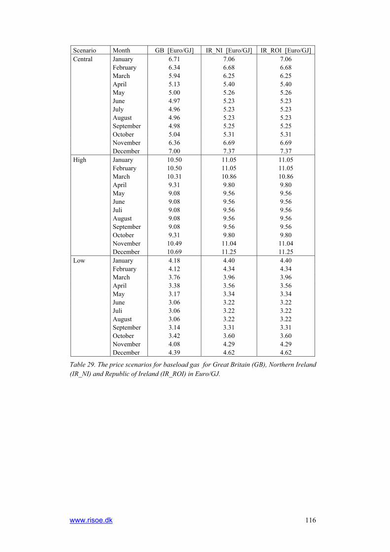
www.risoe.dk 116

Scenario Month GB [Euro/GJ] IR_NI [Euro/GJ] IR_ROI [Euro/GJ] Central January 6.71 7.06 7.06 February 6.34 6.68 6.68 March 5.94 6.25 6.25 April 5.13 5.40 5.40 May 5.00 5.26 5.26 June 4.97 5.23 5.23 July 4.96 5.23 5.23 August 4.96 5.23 5.23 September 4.98 5.25 5.25 October 5.04 5.31 5.31 November 6.36 6.69 6.69 December 7.00 7.37 7.37 High January 10.50 11.05 11.05 February 10.50 11.05 11.05 March 10.31 10.86 10.86 April 9.31 9.80 9.80 May 9.08 9.56 9.56 June 9.08 9.56 9.56 Juli 9.08 9.56 9.56 August 9.08 9.56 9.56 September 9.08 9.56 9.56 October 9.31 9.80 9.80 November 10.49 11.04 11.04 December 10.69 11.25 11.25 Low January 4.18 4.40 4.40 February 4.12 4.34 4.34 March 3.76 3.96 3.96 April 3.38 3.56 3.56 May 3.17 3.34 3.34 June 3.06 3.22 3.22 Juli 3.06 3.22 3.22 August 3.06 3.22 3.22 September 3.14 3.31 3.31 October 3.42 3.60 3.60 November 4.08 4.29 4.29 December 4.39 4.62 4.62

Table 29. The price scenarios for baseload gas for Great Britain (GB), Northern Ireland (IR_NI) and Republic of Ireland (IR_ROI) in Euro/GJ.

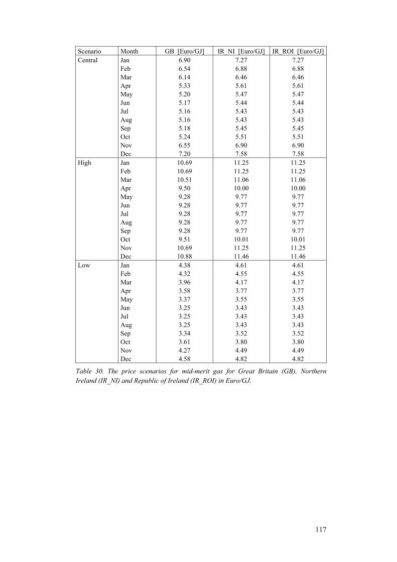
117

Scenario Month GB [Euro/GJ] IR_NI [Euro/GJ] IR_ROI [Euro/GJ] Central Jan 6.90 7.27 7.27 Feb 6.54 6.88 6.88 Mar 6.14 6.46 6.46 Apr 5.33 5.61 5.61 May 5.20 5.47 5.47 Jun 5.17 5.44 5.44 Jul 5.16 5.43 5.43 Aug 5.16 5.43 5.43 Sep 5.18 5.45 5.45 Oct 5.24 5.51 5.51 Nov 6.55 6.90 6.90 Dec 7.20 7.58 7.58 High Jan 10.69 11.25 11.25 Feb 10.69 11.25 11.25 Mar 10.51 11.06 11.06 Apr 9.50 10.00 10.00 May 9.28 9.77 9.77 Jun 9.28 9.77 9.77 Jul 9.28 9.77 9.77 Aug 9.28 9.77 9.77 Sep 9.28 9.77 9.77 Oct 9.51 10.01 10.01 Nov 10.69 11.25 11.25 Dec 10.88 11.46 11.46 Low Jan 4.38 4.61 4.61 Feb 4.32 4.55 4.55 Mar 3.96 4.17 4.17 Apr 3.58 3.77 3.77 May 3.37 3.55 3.55 Jun 3.25 3.43 3.43 Jul 3.25 3.43 3.43 Aug 3.25 3.43 3.43 Sep 3.34 3.52 3.52 Oct 3.61 3.80 3.80 Nov 4.27 4.49 4.49 Dec 4.58 4.82 4.82

Table 30. The price scenarios for mid-merit gas for Great Britain (GB), Northern Ireland (IR_NI) and Republic of Ireland (IR_ROI) in Euro/GJ.

www.risoe.dk 118

0

2

4

6

8

10

12

14

Jan Feb Mar Apr May Jun Jul Aug Sep Oct Nov Dec

Eur

o/G

J

Central - BASELOADGAS Central - MIDMERITGASHigh - BASELOADGAS High - MIDMERITGASLow - BASELOADGAS Low - MIDMERITGAS

Figure 60. Fuel price scenarios for BASELOADGAS and MIDMERITGAS for Republic of Ireland in Euro/GJ. Notice that the price differences between BASELOADGAS and MIDMERITGAS are small.

The applied parameter data (except incremental heat slope parameter) for the thermal power plants that already exist today is shown in Table 31 and Table 32, for new power plant technologies in Table 33. Incremental heat rate slope parameter are summarised in Table 34 for existing and new power plants. Table 35 lists the applied parameter for the pumped hydro storage plant Turlough Hill.

Work-stream 2A provides data input for five least-cost generation portfolios in 2020 covering installed capacities of power plants, fuel prices and CO2 emission permit prices along with 2020 electricity demand. The data used for new power plants in work-stream 2A (Table 3-2 p. 13 in Doherty 2006) does not cover unit commitment and fuel consumption parameters such as minimum up and down times, start-up times, incremental fuel consumption curves and forced outage data required in this study. Additional assumptions regarding the properties of the power plants outlined in Table 3-2 in (Doherty 2006) have therefore been made (see Table 33).

119

Unit ID Fuel Max Production capacity [MW]

Min Production capacity [MW]

Efficiency (100% load)4

Heat rate min load [GJ/Hour]

Forced outage rate [%]

Mean time to repair [h]

Run up rate [MW/min]

Ramp rate up [MW/min]

Ramp rate down [MW/min]

Minimum up time [h]

Minimum down time [h]

K1 Coal 201 64 0.37 213 3 72 1 6 6 1 8

K2 Coal 201 64 0.37 213 3 72 1 6 6 1 8

MP1 Coal 285 115 0.37 148 5 50 4 4 4 8 5

MP2 Coal 285 115 0.37 148 5 50 4 4 4 8 5

MP3 Coal 285 115 0.37 148 5 50 4 4 4 8 5

AD1 Natural gas 258 35 0.40 187 5 50 4 4 4 5 4

B10 Natural gas 103 63 0.47 98 3 72 1 4 4 10 8

B31 Natural gas 240 116 0.46 496 3 72 2 11 11 10 8

B32 Natural gas 240 116 0.46 496 3 72 2 11 11 10 8

CPS_CCGT Natural gas 404 260 0.54 496 3 72 4 22 12 1 8

DBP Natural gas 396 200 0.57 533 2 31 11 11 11 4 1

HNC Natural gas 342.7 222.8 0.54 324 3 24 5 5 10 8 4

MRT Natural gas 112.3 77 0.39 251 5 50 2 2 2 2 1

PBC Natural gas 480 280 0.51 716 5 50 10 10 10 1 1

SK1 Natural gas 150 135 0.47 506 3 33 6 6 6 0 0

TE Natural gas 404 202 0.56 467 4 40 19 19 19 4 4

BGT1 Gasoil 58 8 0.23 180 1 72 6 10 10 1 1

BGT2 Gasoil 58 8 0.23 180 1 72 6 10 10 1 1

CGT8 Gasoil 58 8 0.24 177 1 72 10 10 10 1 1

KGT1 Gasoil 29 5 0.25 101 1 72 5 10 10 1 1

KGT2 Gasoil 29 5 0.25 101 1 72 5 10 10 1 1

RH1 Gasoil 52 5 0.34 85 7 50 5 5 5 1 1

RH2 Gasoil 52 5 0.34 85 7 50 5 5 5 1 1

TP1 Gasoil 52 5 0.34 85 7 50 5 5 5 1 1

ED1 Peat 117.6 40 0.38 498 5 72 2 1 1 4 0

LR4 Peat 91 40 0.36 90 5 50 2 2 2 12 2

WO4 Peat 137 46 0.37 124 5 50 2 2 2 12 2

Table 31. Power plant parameter for thermal power plants already existing today.

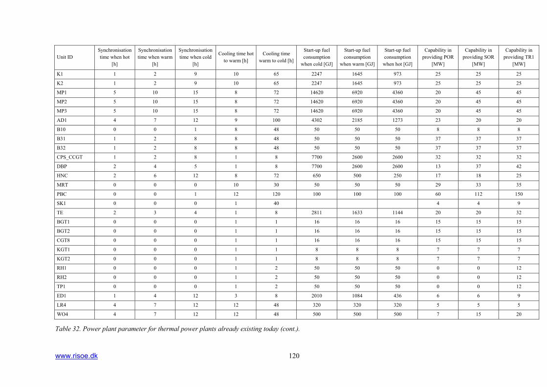
www.risoe.dk 120

Unit ID Synchronisation time when hot

[h]

Synchronisation time when warm

[h]

Synchronisation time when cold

[h]

Cooling time hot to warm [h]

Cooling time warm to cold [h]

Start-up fuel consumption

when cold [GJ]

Start-up fuel consumption

when warm [GJ]

Start-up fuel consumption

when hot [GJ]

Capability in providing POR

[MW]

Capability in providing SOR

[MW]

Capability in providing TR1

[MW]

K1 1 2 9 10 65 2247 1645 973 25 25 25

K2 1 2 9 10 65 2247 1645 973 25 25 25

MP1 5 10 15 8 72 14620 6920 4360 20 45 45

MP2 5 10 15 8 72 14620 6920 4360 20 45 45

MP3 5 10 15 8 72 14620 6920 4360 20 45 45

AD1 4 7 12 9 100 4302 2185 1273 23 20 20

B10 0 0 1 8 48 50 50 50 8 8 8

B31 1 2 8 8 48 50 50 50 37 37 37

B32 1 2 8 8 48 50 50 50 37 37 37

CPS_CCGT 1 2 8 1 8 7700 2600 2600 32 32 32

DBP 2 4 5 1 8 7700 2600 2600 13 37 42

HNC 2 6 12 8 72 650 500 250 17 18 25

MRT 0 0 0 10 30 50 50 50 29 33 35

PBC 0 0 1 12 120 100 100 100 60 112 150

SK1 0 0 0 1 40 4 4 9

TE 2 3 4 1 8 2811 1633 1144 20 20 32

BGT1 0 0 0 1 1 16 16 16 15 15 15

BGT2 0 0 0 1 1 16 16 16 15 15 15

CGT8 0 0 0 1 1 16 16 16 15 15 15

KGT1 0 0 0 1 1 8 8 8 7 7 7

KGT2 0 0 0 1 1 8 8 8 7 7 7

RH1 0 0 0 1 2 50 50 50 0 0 12

RH2 0 0 0 1 2 50 50 50 0 0 12

TP1 0 0 0 1 2 50 50 50 0 0 12

ED1 1 4 12 3 8 2010 1084 436 6 6 9

LR4 4 7 12 12 48 320 320 320 5 5 5

WO4 4 7 12 12 48 500 500 500 7 15 20

Table 32. Power plant parameter for thermal power plants already existing today (cont.).

121

Generation option Coal CCGT3 OCGT ADGT Production capacity (MW) 390 400-480 100 100 Fuel Coal Natural gas Natural gas Natural gas Minimum load factor 0.5 0.5 0.1 0.1 Efficiency (100% load)4 0.41 0.57 0.36 0.465 Efficiency (min. load) 0.39 0.49 0.15 0.352 Forced outage rate (%) 3 2 3 3 Mean time to repair (h) 50 31 50 50 Run up rate (MW/min) 86 11 10 10 Ramp rate up (MW/min) 8 11 10 10 Ramp rate down (MW/min) 8 11 10 10 Minimum up time (h) 6 4 0 0 Minimum down time (h) 4 1 0 0 Synchronisation time when hot (h) 4 2 0 0 Synchronisation time when warm (h) 8 4 0 0

Synchronisation time when cold (h) 12 5 0 0 Cooling time hot to warm (h) 8 1 1 1 Cooling time warm to cold (h) 72 8 2 2 Start-up fuel consumption when hot (GJ) 16000 2600 8 8

Start-up fuel consumption when warm (GJ) 8000 2600 8 8

Start-up fuel consumption when cold (GJ) 5000 7700 20 20

Capability in providing POR (MW) 25 13 10 10 Capability in providing SOR (MW) 50 37 20 20 Capability in providing TR1 (MW) 50 42 20 20

Table 33. Power plant parameter for new technologies.

3 Used data for Dublin Bay CCGT power plant.

4 Stating the efficiencies at maximum and minimum load are sufficient information to be able to calculate the no load heat rate and the marginal heat rate curve, assuming that the technology is modelled with only one marginal heat rate curve.

5 Efficiency of GE´s LMS100: 0.46 at 100% load, 0.40 at 50% load (GE Energy 2004).

6 Regulation speed assumed to be 2% of maximum capacity.

www.risoe.dk 122

Incremental heat rate slope [GJ/MWh] Capacity point (right border) [MW] Unit ID To point 1 Point 1 to point 2 Point 2 to point 3 Point 1 Point 2 Point 2

K1 8.63 - - 201 - - K2 8.63 - - 201 - - MP1 9.28 9.37 - 200 285 - MP2 9.28 9.37 - 200 285 - MP3 9.28 9.37 - 200 285 - NCG1 8.33 - - 387.5 - - NCG2 8.33 - - 387.5 - - NCG3 8.33 - - 387.5 - - B10 6.67 - - 103 - - B31 5.76 - - 240 - - B32 5.76 - - 240 - - CPS_CCGT 5.454 - - 260 - - DBP 4.665 5.525 5.954 279.2 370.9 396 HNC 5.706 - - 342.7 - - NCT1 4.655 5.515 5.944 279.2 370.9 480 NCT2 4.665 5.525 5.954 279.2 370.9 414 NCT3 4.675 5.535 5.964 279.2 370.9 400 NCT4 4.665 5.525 5.954 279.2 370.9 400 NCT5 4.665 5.525 5.954 279.2 370.9 400 PBC 5.5 - - 480 - - SK1 4.06 5.35 - 135 150 - TE 5.262 - - 404 - - AD1 7.86 8.64 8.72 100 180 258 BGT1 11.05 - - 58 - - BGT2 11.05 - - 58 - - CGT8 10.86 - - 58 - - KGT1 10.86 - - 29 - - KGT2 10.86 - - 29 - - MRT 7.03 8.93 - 108 112.3 - NAT1 7.56 - - 89 - - NAT2 7.56 - - 106.97 - - NAT3 7.56 - - 106.97 - - NAT4 7.56 - - 106.97 - - NAT5 7.56 - - 106.97 - - NAT6 7.56 - - 106.97 - - NAT7 7.56 - - 111 - - NOT1 8.35 - - 103.58 - - NOT2 8.46 - - 103.58 - - NOT3 8.47 - - 103.58 - - NOT4 8.48 - - 103.58 - - NOT5 8.49 - - 103.58 - - NOT6 8.5 - - 103.58 - - NOT7 8.51 - - 103.58 - - NOT8 8.52 - - 103.58 - - NOT9 8.53 - - 103.58 - - NOT10 8.36 - - 103.58 - - NOT11 8.37 - - 103.58 - - NOT12 8.38 - - 103.58 - - NOT13 8.39 - - 103.58 - - NOT14 8.4 - - 103.56 - - NOT15 8.41 - - 103.56 - - NOT16 8.42 - - 103.56 - - NOT17 8.43 - - 103.56 - - NOT18 8.44 - - 103.56 - - NOT19 8.45 - - 103.56 - - RH1 9 - - 52 - - RH2 9 - - 52 - - TP1 9 - - 52 - - ED1 3.933 8.95 8.839 88.2 98.3 117.6 LR4 9.09 - - 91 - - WO4 8.95 - - 137 - -

Table 34. Incremental heat rate slope parameter for existing and new power plants.

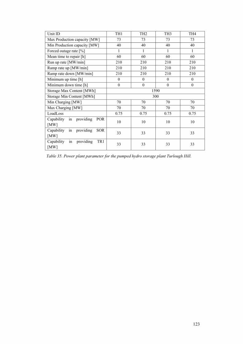
123

Unit ID TH1 TH2 TH3 TH4 Max Production capacity [MW] 73 73 73 73 Min Production capacity [MW] 40 40 40 40 Forced outage rate [%] 1 1 1 1 Mean time to repair [h] 60 60 60 60 Run up rate [MW/min] 210 210 210 210 Ramp rate up [MW/min] 210 210 210 210 Ramp rate down [MW/min] 210 210 210 210 Minimum up time [h] 0 0 0 0 Minimum down time [h] 0 0 0 0 Storage Max Content [MWh] 1590 Storage Min Content [MWh] 300 Min Charging [MW] 70 70 70 70 Max Charging [MW] 70 70 70 70 LoadLoss 0.75 0.75 0.75 0.75 Capability in providing POR [MW]

10 10 10 10

Capability in providing SOR [MW]

33 33 33 33

Capability in providing TR1 [MW]

33 33 33 33

Table 35. Power plant parameter for the pumped hydro storage plant Turlough Hill.

www.risoe.dk 124

The table below gives an summary of the data and data sources for the All Island power system:

Data Object Scope Fuel data - Carbon and Sulphur content, heating values - Fuel prices (Euro/GJ) (data delivered by EirGrid)

Not time dependant 2020

Electricity consumption - Hourly electricity demand (MWh/h) (2004 data delivered from EirGrid and SONI, 2007 data obtained from All Island Modelling project website) - Yearly electricity demand (Data delivered from EirGrid and SONI). - Data expressing the accuracy of electricity demand forecasts depending on forecast horizon (from 0 to 36 hours ahead)

2004, 2007 2020 2020

Need for reserve power - The demand for reserve power distributed on 3 categories of reserves (MW) (demand for spinning reserve of wind obtained from (Doherty and O’Malley 2005), demand for replacement reserves calculated in Scenario Tree Tool)

2020

Thermal units (all data exclude the power consumption of the plant itself): - Fuel type - Generation type (dispatch or must-run) - Maintenance schedule - Probability for unscheduled outages - Maximum capacity (MW) - Minimum stable running level (MW) - Minimum down time (h) - Minimum up time (h) - Ramp rates when starting up and shutting down - Start-up times (divided into cold, warm hot) (h) - Start-up energy - Boundary times (time to go from hot to warm, warm to cold) - Data describing the fuel consumption (heat rate characteristics) - Reserve characteristics (ability to provide reserves for 3 categories of reserves)

Data for units present in year 2007 and 2020 Data taken from All Island Modelling project website supplemented with information from SONI and EirGrid

Hydro power (modelled as must-run) - Time series describing the distribution of hydropower production during the year (data delivered from SONI and EirGrid)

Pumped hydro storage (Turlough Hill) (data obtained from All Island Modelling project website) - Maximum and minimum content of reservoir - Efficiencies of pumps - Restrictions on the operation of the pumps

Taxes and tariffs: - CO2 emission permit price

2020

Table 36. Overview of data demands and data sources.

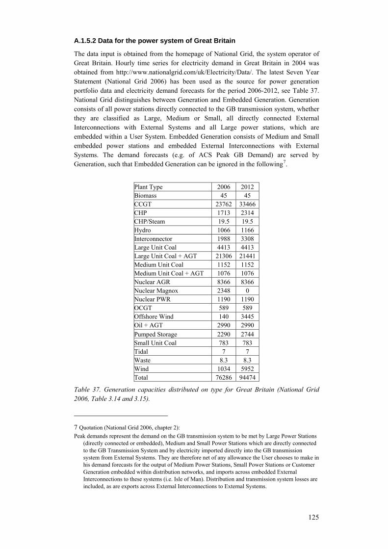
125

A.1.5.2 Data for the power system of Great Britain

The data input is obtained from the homepage of National Grid, the system operator of Great Britain. Hourly time series for electricity demand in Great Britain in 2004 was obtained from http://www.nationalgrid.com/uk/Electricity/Data/. The latest Seven Year Statement (National Grid 2006) has been used as the source for power generation portfolio data and electricity demand forecasts for the period 2006-2012, see Table 37. National Grid distinguishes between Generation and Embedded Generation. Generation consists of all power stations directly connected to the GB transmission system, whether they are classified as Large, Medium or Small, all directly connected External Interconnections with External Systems and all Large power stations, which are embedded within a User System. Embedded Generation consists of Medium and Small embedded power stations and embedded External Interconnections with External Systems. The demand forecasts (e.g. of ACS Peak GB Demand) are served by Generation, such that Embedded Generation can be ignored in the following7.

Plant Type 2006 2012 Biomass 45 45 CCGT 23762 33466 CHP 1713 2314 CHP/Steam 19.5 19.5 Hydro 1066 1166 Interconnector 1988 3308 Large Unit Coal 4413 4413 Large Unit Coal + AGT 21306 21441 Medium Unit Coal 1152 1152 Medium Unit Coal + AGT 1076 1076 Nuclear AGR 8366 8366 Nuclear Magnox 2348 0 Nuclear PWR 1190 1190 OCGT 589 589 Offshore Wind 140 3445 Oil + AGT 2990 2990 Pumped Storage 2290 2744 Small Unit Coal 783 783 Tidal 7 7 Waste 8.3 8.3 Wind 1034 5952 Total 76286 94474

Table 37. Generation capacities distributed on type for Great Britain (National Grid 2006, Table 3.14 and 3.15).

7 Quotation (National Grid 2006, chapter 2): Peak demands represent the demand on the GB transmission system to be met by Large Power Stations

(directly connected or embedded), Medium and Small Power Stations which are directly connected to the GB Transmission System and by electricity imported directly into the GB transmission system from External Systems. They are therefore net of any allowance the User chooses to make in his demand forecasts for the output of Medium Power Stations, Small Power Stations or Customer Generation embedded within distribution networks, and imports across embedded External Interconnections to these systems (i.e. Isle of Man). Distribution and transmission system losses are included, as are exports across External Interconnections to External Systems.

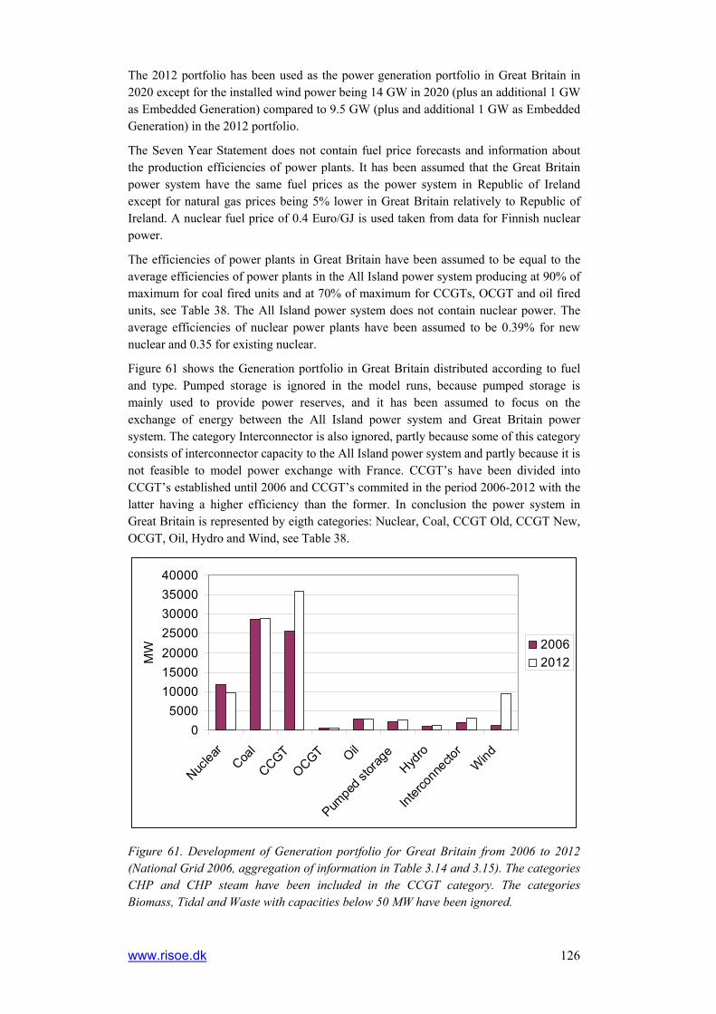
www.risoe.dk 126

The 2012 portfolio has been used as the power generation portfolio in Great Britain in 2020 except for the installed wind power being 14 GW in 2020 (plus an additional 1 GW as Embedded Generation) compared to 9.5 GW (plus and additional 1 GW as Embedded Generation) in the 2012 portfolio.

The Seven Year Statement does not contain fuel price forecasts and information about the production efficiencies of power plants. It has been assumed that the Great Britain power system have the same fuel prices as the power system in Republic of Ireland except for natural gas prices being 5% lower in Great Britain relatively to Republic of Ireland. A nuclear fuel price of 0.4 Euro/GJ is used taken from data for Finnish nuclear power.

The efficiencies of power plants in Great Britain have been assumed to be equal to the average efficiencies of power plants in the All Island power system producing at 90% of maximum for coal fired units and at 70% of maximum for CCGTs, OCGT and oil fired units, see Table 38. The All Island power system does not contain nuclear power. The average efficiencies of nuclear power plants have been assumed to be 0.39% for new nuclear and 0.35 for existing nuclear.

Figure 61 shows the Generation portfolio in Great Britain distributed according to fuel and type. Pumped storage is ignored in the model runs, because pumped storage is mainly used to provide power reserves, and it has been assumed to focus on the exchange of energy between the All Island power system and Great Britain power system. The category Interconnector is also ignored, partly because some of this category consists of interconnector capacity to the All Island power system and partly because it is not feasible to model power exchange with France. CCGT’s have been divided into CCGT’s established until 2006 and CCGT’s commited in the period 2006-2012 with the latter having a higher efficiency than the former. In conclusion the power system in Great Britain is represented by eigth categories: Nuclear, Coal, CCGT Old, CCGT New, OCGT, Oil, Hydro and Wind, see Table 38.

05000

10000150002000025000300003500040000

Nuclea

rCoa

l

CCGTOCGT Oil

Pumpe

d stor

age

Hydro

Interc

onne

ctor

Wind

MW 2006

2012

Figure 61. Development of Generation portfolio for Great Britain from 2006 to 2012 (National Grid 2006, aggregation of information in Table 3.14 and 3.15). The categories CHP and CHP steam have been included in the CCGT category. The categories Biomass, Tidal and Waste with capacities below 50 MW have been ignored.

127

The average annual hydropower production in United Kingdom is 4.3 TWh during the period 2000-2003 (United Nations 2005). The hydropower production is modelled with an hourly production profile during the year taken from the Irish hydropower production scaled to an annual production of 4.3 TWh.

Plant type Nuclear Coal CCGT Old

CCGT New OCGT Oil Hydro Wind

Capacity [MW] 9556 28865 25495 10305 589 2990 1166 14000

Efficiency [-] 0.35 0.37 0.49 0.55 0.26 0.34 1.00 1.00

Table 38. Considered generation capacities and efficiencies of power plants in Great Britain.

Figure 62 shows three demand forecasts for Great Britain. The Base Scenario is used in the model runs.

050

100150200250300350400450

2001

/02

2002

/03

2003

/04

2004

/05

2005

/06

2006

/07

2007

/08

2008

/09

2009

/10

2010

/11

2011

/12

2012

/13

TWh Low

BaseHigh

Figure 62. Annual electricity demand forecasts for Great Britain made by National Grid (National Grid 2006, Table 2.4 and 2.5). The historical data is weather adjusted annual electricity requirements.

www.risoe.dk 128

A.2 Power Plant portfolios used in the study Input data used in WS2A for portfolio 1: Natural gas price: 5.5 €/GJ (33 p/therm), Carbon price: 30 €/Tonne CO2, WACC: 6%, High wind turbine costs. PORTFOLIO 1

Code Power plant Capacity (MW) Code Power plant Capacity (MW)

AD1 Aghada Unit 1 258 B32 Ballylumford Unit 32 240

AA1 Ardnacrusha Unit 1 21 B10 Ballylumford Unit 10 103 AA2 Ardnacrusha Unit 2 22 BGT1 Ballylumford GT1 53 AA3 Ardnacrusha Unit 3 19 BGT2 Ballylumford GT2 53 AA4 Ardnacrusha Unit 4 24 CPS CCGT Coolkeeragh CCGT 404 DBP Dublin Bay Power 396 CGT8 Coolkeeragh GT8 53 ED1 Edenderry 117.6 K1 Kilroot Unit 1 201 ER1 Erne Unit 1 10 K2 Kilroot Unit 2 201 ER2 Erne Unit 2 10 KGT1 Kilroot GT1 29 ER3 Erne Unit 3 22.5 KGT2 Kilroot GT2 29 ER4 Erne Unit 4 22.5 Inter 1 Interconnector 500 LE1 Lee Unit 1 15 Inter 2 Interconnector 500 LE2 Lee Unit 2 4 NCT1 New CCGT (2+1) 480 LE3 Lee Unit 3 8 NCT2 New CCGT 414 LI1 Liffey Unit 1 15 NOT1 New OCGT 103.6 LI2 Liffey Unit 2 15 NOT2 New OCGT 103.6 LI4 Liffey Unit 4 4 NOT3 New OCGT 103.6 LI5 Liffey Unit 5 4 NOT4 New OCGT 103.6 LR4 Lough Ree 91 NOT5 New OCGT 103.6 HNC Huntstown 342.7 NOT6 New OCGT 103.6 MRT Marina CC 112.3 NOT7 New OCGT 103.6 MP1 Moneypoint Unit 1 285 NOT8 New OCGT 103.6 MP2 Moneypoint Unit 2 285 NOT9 New OCGT 103.6 MP3 Moneypoint Unit 3 285 NOT10 New OCGT 103.6 PBC Poolbeg Combined Cycle 480 NOT11 New OCGT 103.6 RH1 Rhode Unit 1 52 NOT12 New OCGT 103.6 RH2 Rhode Unit 2 52 NOT13 New OCGT 103.6 TP1 Asahi Peaking Unit 52 NOT14 New OCGT 103.6 SK1 Aughinish (Sealrock) 150 NCT3 New CCGT 400 TE Tynagh 404 NAT1 New ADGT 89 TH1 Turlough Hill Unit 1 73 LFG Total Landfill Gas 42.5 TH2 Turlough Hill Unit 2 73 BG Total Biogas 47 TH3 Turlough Hill Unit 3 73 BM Total Biomass 89 TH4 Turlough Hill Unit 4 73 SG Total Sewage Gas 4 WO4 West Offaly Power 137 TS Total Tidal Stream 71.5

B31 Ballylumford CCGT 31 240 WD Wind Generation 2000

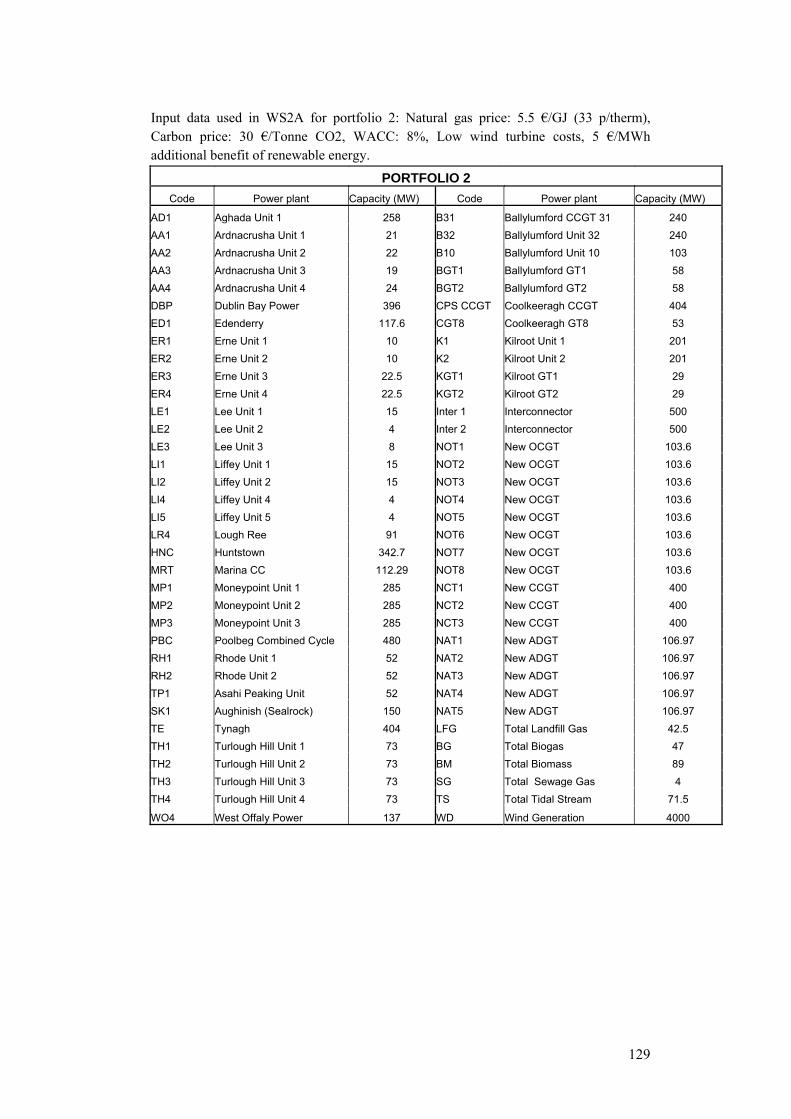
129

Input data used in WS2A for portfolio 2: Natural gas price: 5.5 €/GJ (33 p/therm), Carbon price: 30 €/Tonne CO2, WACC: 8%, Low wind turbine costs, 5 €/MWh additional benefit of renewable energy. PORTFOLIO 2

Code Power plant Capacity (MW) Code Power plant Capacity (MW)

AD1 Aghada Unit 1 258 B31 Ballylumford CCGT 31 240 AA1 Ardnacrusha Unit 1 21 B32 Ballylumford Unit 32 240 AA2 Ardnacrusha Unit 2 22 B10 Ballylumford Unit 10 103 AA3 Ardnacrusha Unit 3 19 BGT1 Ballylumford GT1 58 AA4 Ardnacrusha Unit 4 24 BGT2 Ballylumford GT2 58 DBP Dublin Bay Power 396 CPS CCGT Coolkeeragh CCGT 404 ED1 Edenderry 117.6 CGT8 Coolkeeragh GT8 53 ER1 Erne Unit 1 10 K1 Kilroot Unit 1 201 ER2 Erne Unit 2 10 K2 Kilroot Unit 2 201 ER3 Erne Unit 3 22.5 KGT1 Kilroot GT1 29 ER4 Erne Unit 4 22.5 KGT2 Kilroot GT2 29 LE1 Lee Unit 1 15 Inter 1 Interconnector 500 LE2 Lee Unit 2 4 Inter 2 Interconnector 500 LE3 Lee Unit 3 8 NOT1 New OCGT 103.6 LI1 Liffey Unit 1 15 NOT2 New OCGT 103.6 LI2 Liffey Unit 2 15 NOT3 New OCGT 103.6 LI4 Liffey Unit 4 4 NOT4 New OCGT 103.6 LI5 Liffey Unit 5 4 NOT5 New OCGT 103.6 LR4 Lough Ree 91 NOT6 New OCGT 103.6 HNC Huntstown 342.7 NOT7 New OCGT 103.6 MRT Marina CC 112.29 NOT8 New OCGT 103.6 MP1 Moneypoint Unit 1 285 NCT1 New CCGT 400 MP2 Moneypoint Unit 2 285 NCT2 New CCGT 400 MP3 Moneypoint Unit 3 285 NCT3 New CCGT 400 PBC Poolbeg Combined Cycle 480 NAT1 New ADGT 106.97 RH1 Rhode Unit 1 52 NAT2 New ADGT 106.97 RH2 Rhode Unit 2 52 NAT3 New ADGT 106.97 TP1 Asahi Peaking Unit 52 NAT4 New ADGT 106.97 SK1 Aughinish (Sealrock) 150 NAT5 New ADGT 106.97 TE Tynagh 404 LFG Total Landfill Gas 42.5 TH1 Turlough Hill Unit 1 73 BG Total Biogas 47 TH2 Turlough Hill Unit 2 73 BM Total Biomass 89 TH3 Turlough Hill Unit 3 73 SG Total Sewage Gas 4 TH4 Turlough Hill Unit 4 73 TS Total Tidal Stream 71.5

WO4 West Offaly Power 137 WD Wind Generation 4000

www.risoe.dk 130

Input data used in WS2A for portfolio 3: Natural gas price: 5.5 €/GJ (33 p/therm), Carbon price: 30 €/Tonne CO2, WACC: 8%, Low wind turbine costs, 5 €/MWh additional benefit of renewable energy. PORTFOLIO 3

Code Power plant Capacity (MW) Code Power plant Capacity (MW)

AD1 Aghada Unit 1 258 BGT2 Ballylumford GT2 58 AA1 Ardnacrusha Unit 1 21 CPS CCGT Coolkeeragh CCGT 404 AA2 Ardnacrusha Unit 2 22 CGT8 Coolkeeragh GT8 53 AA3 Ardnacrusha Unit 3 19 K1 Kilroot Unit 1 201 AA4 Ardnacrusha Unit 4 24 K2 Kilroot Unit 2 201 DBP Dublin Bay Power 396 KGT1 Kilroot GT1 29 ED1 Edenderry 117.6 KGT2 Kilroot GT2 29 ER1 Erne Unit 1 10 Inter 1 Interconnector 500 ER2 Erne Unit 2 10 Inter 2 Interconnector 500 ER3 Erne Unit 3 22.5 NOT1 New OCGT 103.6 ER4 Erne Unit 4 22.5 NOT2 New OCGT 103.6 LE1 Lee Unit 1 15 NOT3 New OCGT 103.6 LE2 Lee Unit 2 4 NOT4 New OCGT 103.6 LE3 Lee Unit 3 8 NOT5 New OCGT 103.6 LI1 Liffey Unit 1 15 NOT6 New OCGT 103.6 LI2 Liffey Unit 2 15 NOT7 New OCGT 103.6 LI4 Liffey Unit 4 4 NOT8 New OCGT 103.6 LI5 Liffey Unit 5 4 NOT9 New OCGT 103.6 LR4 Lough Ree 91 NOT10 New OCGT 103.6 HNC Huntstown 342.7 NOT11 New OCGT 103.6 MRT Marina CC 112.29 NOT12 New OCGT 103.6 MP1 Moneypoint Unit 1 285 NOT13 New OCGT 103.6 MP2 Moneypoint Unit 2 285 NOT14 New OCGT 103.6 MP3 Moneypoint Unit 3 285 NOT15 New OCGT 103.6 PBC Poolbeg Combined Cycle 480 NOT16 New OCGT 103.6 RH1 Rhode Unit 1 52 NOT17 New OCGT 103.6 RH2 Rhode Unit 2 52 NOT18 New OCGT 103.6 TP1 Asahi Peaking Unit 52 NOT19 New OCGT 103.6 SK1 Aughinish (Sealrock) 150 NAT1 New ADGT 107 TE Tynagh 404 NAT2 New ADGT 107 TH1 Turlough Hill Unit 1 73 NAT3 New ADGT 107 TH2 Turlough Hill Unit 2 73 NAT4 New ADGT 107 TH3 Turlough Hill Unit 3 73 NAT5 New ADGT 107 TH4 Turlough Hill Unit 4 73 LFG Total Landfill Gas 42.5 WO4 West Offaly Power 137 BG Total Biogas 47 B31 Ballylumford CCGT 31 240 BM Total Biomass 89 B32 Ballylumford Unit 32 240 SG Total Sewage Gas 4 B10 Ballylumford Unit 10 103 TS Total Tidal Stream 71.5

BGT1 Ballylumford GT1 58 WD Wind Generation 4000

131

Input data used in WS2A for portfolio 4: Natural gas price: 6.5 €/GJ (40 p/therm), Carbon price: 30 €/Tonne CO2, WACC: 6%, High wind turbine costs, 5 €/MWh additional benefit of renewable energy. PORTFOLIO 4

Code Power plant Capacity (MW) Code Power plant Capacity (MW)

AD1 Aghada Unit 1 258 TH3 Turlough Hill Unit 3 73 AA1 Ardnacrusha Unit 1 21 TH4 Turlough Hill Unit 4 73 AA2 Ardnacrusha Unit 2 22 WO4 West Offaly Power 137 AA3 Ardnacrusha Unit 3 19 B31 Ballylumford CCGT 31 240 AA4 Ardnacrusha Unit 4 24 B32 Ballylumford Unit 32 240 DBP Dublin Bay Power 396 B10 Ballylumford Unit 10 103 ED1 Edenderry 117.6 BGT1 Ballylumford GT1 58 ER1 Erne Unit 1 10 BGT2 Ballylumford GT2 58 ER2 Erne Unit 2 10 CPS CCGT Coolkeeragh CCGT 404 ER3 Erne Unit 3 22.5 CGT8 Coolkeeragh GT8 53 ER4 Erne Unit 4 22.5 K1 Kilroot Unit 1 201 LE1 Lee Unit 1 15 K2 Kilroot Unit 2 201 LE2 Lee Unit 2 4 KGT1 Kilroot GT1 29 LE3 Lee Unit 3 8 KGT2 Kilroot GT2 29 LI1 Liffey Unit 1 15 Inter 1 Interconnector 500 LI2 Liffey Unit 2 15 Inter 2 Interconnector 500 LI4 Liffey Unit 4 4 NOT1 New OCGT 103.6 LI5 Liffey Unit 5 4 NOT2 New OCGT 103.6 LR4 Lough Ree 91 NOT3 New OCGT 103.6 HNC Huntstown 342.7 NCG1 New Moneypoint Coal Unit 387.5 MRT Marina CC 112.29 NCG2 New Moneypoint Coal Unit 387.5 MP1 Moneypoint Unit 1 285 NCG3 New Moneypoint Coal Unit 387.5 MP2 Moneypoint Unit 2 285 NCT1 New CCGT 400 MP3 Moneypoint Unit 3 285 NCT2 New CCGT 400 PBC Poolbeg Combined Cycle 480 NCT3 New CCGT 400 RH1 Rhode Unit 1 52 LFG Total Landfill Gas 42.5 RH2 Rhode Unit 2 52 BG Total Biogas 47 TP1 Asahi Peaking Unit 52 BM Total Biomass 89 SK1 Aughinish (Sealrock) 150 SG Total Sewage Gas 4 TE Tynagh 404 TS Total Tidal Stream 71.5

TH1 Turlough Hill Unit 1 73 WD Wind Generation 4000

TH2 Turlough Hill Unit 2 73

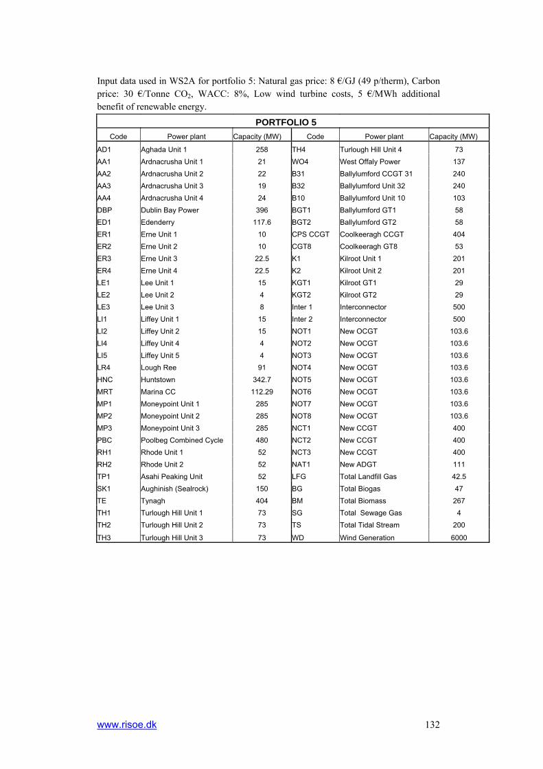
www.risoe.dk 132

Input data used in WS2A for portfolio 5: Natural gas price: 8 €/GJ (49 p/therm), Carbon price: 30 €/Tonne CO2, WACC: 8%, Low wind turbine costs, 5 €/MWh additional benefit of renewable energy. PORTFOLIO 5

Code Power plant Capacity (MW) Code Power plant Capacity (MW)

AD1 Aghada Unit 1 258 TH4 Turlough Hill Unit 4 73 AA1 Ardnacrusha Unit 1 21 WO4 West Offaly Power 137 AA2 Ardnacrusha Unit 2 22 B31 Ballylumford CCGT 31 240 AA3 Ardnacrusha Unit 3 19 B32 Ballylumford Unit 32 240 AA4 Ardnacrusha Unit 4 24 B10 Ballylumford Unit 10 103 DBP Dublin Bay Power 396 BGT1 Ballylumford GT1 58 ED1 Edenderry 117.6 BGT2 Ballylumford GT2 58 ER1 Erne Unit 1 10 CPS CCGT Coolkeeragh CCGT 404 ER2 Erne Unit 2 10 CGT8 Coolkeeragh GT8 53 ER3 Erne Unit 3 22.5 K1 Kilroot Unit 1 201 ER4 Erne Unit 4 22.5 K2 Kilroot Unit 2 201 LE1 Lee Unit 1 15 KGT1 Kilroot GT1 29 LE2 Lee Unit 2 4 KGT2 Kilroot GT2 29 LE3 Lee Unit 3 8 Inter 1 Interconnector 500 LI1 Liffey Unit 1 15 Inter 2 Interconnector 500 LI2 Liffey Unit 2 15 NOT1 New OCGT 103.6 LI4 Liffey Unit 4 4 NOT2 New OCGT 103.6 LI5 Liffey Unit 5 4 NOT3 New OCGT 103.6 LR4 Lough Ree 91 NOT4 New OCGT 103.6 HNC Huntstown 342.7 NOT5 New OCGT 103.6 MRT Marina CC 112.29 NOT6 New OCGT 103.6 MP1 Moneypoint Unit 1 285 NOT7 New OCGT 103.6 MP2 Moneypoint Unit 2 285 NOT8 New OCGT 103.6 MP3 Moneypoint Unit 3 285 NCT1 New CCGT 400 PBC Poolbeg Combined Cycle 480 NCT2 New CCGT 400 RH1 Rhode Unit 1 52 NCT3 New CCGT 400 RH2 Rhode Unit 2 52 NAT1 New ADGT 111 TP1 Asahi Peaking Unit 52 LFG Total Landfill Gas 42.5 SK1 Aughinish (Sealrock) 150 BG Total Biogas 47 TE Tynagh 404 BM Total Biomass 267 TH1 Turlough Hill Unit 1 73 SG Total Sewage Gas 4 TH2 Turlough Hill Unit 2 73 TS Total Tidal Stream 200

TH3 Turlough Hill Unit 3 73 WD Wind Generation 6000

133

Input data used in WS2A for portfolio 6: Natural gas price: 9 €/GJ (55 p/therm), Carbon price: 80 €/Tonne CO2, WACC: 6%, Low wind turbine costs, 10 €/MWh additional benefit of renewable energy. PORTFOLIO 6

Code Power plant Capacity (MW) Code Power plant Capacity (MW)

AD1 Aghada Unit 1 258 TH2 Turlough Hill Unit 2 73 AA1 Ardnacrusha Unit 1 21 TH3 Turlough Hill Unit 3 73 AA2 Ardnacrusha Unit 2 22 TH4 Turlough Hill Unit 4 73 AA3 Ardnacrusha Unit 3 19 WO4 West Offaly Power 137 AA4 Ardnacrusha Unit 4 24 B31 Ballylumford CCGT 31 240 DBP Dublin Bay Power 396 B32 Ballylumford Unit 32 240 ED1 Edenderry 117.6 B10 Ballylumford Unit 10 103 ER1 Erne Unit 1 10 BGT1 Ballylumford GT1 58 ER2 Erne Unit 2 10 BGT2 Ballylumford GT2 58 ER3 Erne Unit 3 22.5 CPS CCGT Coolkeeragh CCGT 404 ER4 Erne Unit 4 22.5 CGT8 Coolkeeragh GT8 53 LE1 Lee Unit 1 15 K1 Kilroot Unit 1 201 LE2 Lee Unit 2 4 K2 Kilroot Unit 2 201 LE3 Lee Unit 3 8 KGT1 Kilroot GT1 29 LI1 Liffey Unit 1 15 KGT2 Kilroot GT2 29 LI2 Liffey Unit 2 15 Inter 1 Interconnector 500 LI4 Liffey Unit 4 4 Inter 2 Interconnector 500 LI5 Liffey Unit 5 4 NOT1 New OCGT 103.6 LR4 Lough Ree 91 NOT2 New OCGT 103.6 HNC Huntstown 342.7 NOT3 New OCGT 103.6 MRT Marina CC 112.29 NOT4 New OCGT 103.6 MP1 Moneypoint Unit 1 285 NOT5 New OCGT 103.6 MP2 Moneypoint Unit 2 285 NCT1 New CCGT 400 MP3 Moneypoint Unit 3 285 NCT2 New CCGT 400 PBC Poolbeg Combined Cycle 480 NCT3 New CCGT 400 RH1 Rhode Unit 1 52 LFG Total Landfill Gas 42.5 RH2 Rhode Unit 2 52 BG Total Biogas 47 TP1 Asahi Peaking Unit 52 BM Total Biomass 299 SK1 Aughinish (Sealrock) 150 SG Total Sewage Gas 4 TE Tynagh 404 TS Total Tidal Stream 200

TH1 Turlough Hill Unit 1 73 WE Wave Energy 1400

WD Wind Generation 8000

www.risoe.dk 134

References (All Island Modelling generator data, 2005)

All Island Modelling generator data, 2005, AIP-SEM-124-05.xls, downloadable from http://www.allislandproject.org/allislandgeneratorparameters.html.

(Anderson, Davidson 2005)

Anderson, C.L.; Davidson, M.: An aggregate Weibull approach for modelling short-term system generating capacity. IEEE Transactions on power systems, Vol. 20 (2005), No. 4, pages 1783 - 1789

(Barth et al. 2006a)

Barth, R., Söder, L., Weber, C., Brand, H., Swider, D., 2006, Deliverable D6.2 (b) – Documentation Methodology of the Scenario Tree Tool, Institute of Energy Economics and the Rational Use of Energy (IER), University of Stuttgart, available from www.wilmar.risoe.dk.

(Barth et al., 2006b)

Barth, R., Brand, H., Swider, D.J., Weber, C., Meibom, P., 2006b, Regional electricity price differences due to intermittent wind power in Germany – Impact of extended transmission and storage capacities. International Journal of Global Energy Issues, vol. 25 (2006), issue 3/4, pp. 276 – 297.

(Carrión and Arroyo 2006)

Carrión, M., Arroyo, J.M., A Computationally Efficient Mixed-Integer Linear Formulation for the Thermal Commitment Problem, IEEE Transactions on Power System, Vol 21, NO 3, pp. 1371-1378, August 2006.

(Dena 2005)

Deutsche Energie-Agentur, 2005, Energiewirtschaftliche Planung für die Netzintegration von Windenergie in Deutschland an Land und Offshore bis zum Jahr 2020, Berlin.

(Doherty 2006)

Doherty, R., 2006, All Island grid study work-stream 2A – High level assessment of suitable generation portfolios for the All Island system in 2020, Electricity Research Centre, University College Dublin.

(Doherty and O’Malley 2005)

Doherty, R.; O’Malley, M.: A new approach to quantify reserve demand in systems with significant installed wind capacity. IEEE Transactions on power systems, Vol. 20, No 2, 2005

(Dupacova et al. 2003)

Dupacova, J.; Gröwe-Kuska, N.; Römisch, W.: Scenario reduction in stochastic programming: An approach using probability metrics. Mathematical programming. Volume 95, number 3, 2003. Pages 493 - 511

135

(Endrenyi 1978)

Endrenyi, J.: Reliability modelling in electric power systems. John Wiley & Sons. Chichester, New York, Brisbane, Toronto, 1978

(ESB National Grid 2005)

ESB National Grid, Grid Code, Version 1.2 May 2005, downloadable from www.eirgrid.com.

(GE Energy 2004)

Reale, M.J.: New high efficiency simple cycle gas turbine – GE’s LMS100. GER-4222A, GE-Energy, 2004, downloadable from http://www.gepower.com/prod_serv/products/tech_docs/en/downloads/ger4222a.pdf

(Meibom et al. 2006a)

Meibom, P., Barth, R., Brand, H., Larsen, H., Voll, O. Weber, C., 2006, Wilmar Scheduling model documentation, Deliverable 6.2 (b), available from www.wilmar.risoe.dk.

(Meibom et al., 2006b)

Meibom, P., Kiviluoma, J., Barth, R., Brand, H., Weber, C., v. Larsen, H, 2006b, Value of electrical heat boilers and heat pumps for wind power integration. In: Proceedings (online). 2006 European Wind Energy Conference and Exhibition, Athens (GR), 27 Feb - 2 Mar 2006. (Brussels, European Wind Energy Association)

(National Grid 2006)

National Grid: GB Seven Year Statement, May 2006, downloadable from http://www.nationalgrid.com/uk/sys%5F06/default.asp?sNode=SYS&action=&Exp=Y.

(Norgard; Holtinnen 2004)

Norgaard, P.; Holtinnen, H.: A multi-turbine power curve approach. Contribution to the Nordic Wind Power Conference 2004. Göteborg, 2004

(Perman et al. 1997)

Perman, M.; Senegacnik, A.; Tuma, M.: Semi-Markov models with an application to power-plant reliability analysis. IEEE Transactions on reliability, Vol. 46 (1997), No. 4, pages 526 - 532

(Pievatolo et al. 2004)

Pievatolo, A.; Tironi, E.; Valade, I.: Semi-Markov processes for power system reliability assessment with application to uninterruptible power supply. IEEE Transactions on power systems, Vol. 19 (2004), No. 3, pages 1326 - 1333

(Rachev 1991)

Rachev, S. T.: Probability metrics and the stability of stochastic models, J. Wiley and Sons, New York, 1991

www.risoe.dk 136

(Söder 2004)

Söder, L.: Simulation of Wind Speed Forecast Errors for Operation Planning of Multi-Area Power Systems. Contribution to the 8th International Conference on Probabilistic Methods Applied to Power Systems. Ames (Iowa), 2004

(SEI, Sustainable Energy Island, 2004)

Operating Reserve Requirements as Wind Power Penetration Increases in the Irish Electricity System. August 2004.

(Valenzuela; Mazumdar 2001)

Valenzuela, J.; Mazumdar, M.: Monte-Carlo computation of power generation production costs under operating constraints. IEEE Transactions on power systems, Vol. 16 (2001), No. 4, pages 671 - 677

(Van Casteren et al. 2000)

Van Casteren, J.F.L.; Bollen, M.H.J.; Schmieg, E.: Reliability assessment in electrical power systems: The Weibull-Markov stochastic model. IEEE Transactions on power systems. Vol. 36, No. 3, 2000