Field Studies of Seed Biology - Ministry of Forests
81
40 1997 L A N D M A N A G E M E N T H A N D B O O K Field Studies of Seed Biology Ministry of Forests Research Program
-
Upload
khangminh22 -
Category
Documents
-
view
3 -
download
0
Transcript of Field Studies of Seed Biology - Ministry of Forests

4 0
1 9 9 7
L A N D M A N A G E M E N T H A N D B O O K
Field Studies of Seed Biology
Ministry of ForestsResearch Program

Carole L. Leadem, Sharon L. Gillies, H. Karen Yearsley,
Vera Sit, David L. Spittlehouse, and Philip J. Burton
Field Studies of Seed Biology
Ministry of ForestsResearch Program

ii
Canadian Cataloguing in Publication DataMain entry under title:Field studies of seed biology
(Land management handbook ; )
“Tree seed biology.”--Cover. ---
. Trees – British Columbia – Seeds – Experiments.. Trees – Seeds – Experiments. . Reforestation –British Columbia – Experiments. . Reforestation –British Columbia – Experiments. I. Leadem, CaroleLouise Scheuplein, – II. British Columbia.Ministry of Forests. Research Branch. III. Series
.. .’’ --
Copies of this and other Ministry of Forests
titles are available from
Crown Publications Inc.
Fort Street
Victoria, BC
© Province of British Columbia
Published by the
Research Branch
B.C. Ministry of Forests
Bastion Square
Victoria, BC
Please address any comments or suggestions to the
senior author:
Carole L. Leadem
Glyn Road Research Station
B.C. Ministry of Forests
PO Box Stn Prov Govt
Victoria, BC

iii
CREDITS
Carole L. Leadem B.C. Ministry of Forests, Research Branch, GlynRoad Research Station, PO Box Stn Prov Govt,Victoria, BC
Sharon L. Gillies University College Fraser Valley, King Road,Abbotsford, BC
H. Karen Yearsley B.C. Ministry of Forests, Research Branch,PO Box Stn Prov Govt, Victoria, BC
Vera Sit B.C. Ministry of Forests, Research Branch,PO Box Stn Prov Govt, Victoria, BC vw c
David L. Spittlehouse B.C. Ministry of Forests, Research Branch,PO Box Stn Prov Govt, Victoria, BC vw c
Philip J. Burton Symbios Research and Restoration,PO Box , Smithers, BC
Editor, indexer: Fran AitkensTypesetting: Dynamic TypesettingGraphic production: Lyle OttenbreitProofreading: Rosalind C. Penty
Steve SmithPublication design: Anna Gamble
Original photos and illustrations:Figures ., ., . Dr. David SpittlehouseFigure . Dr. John Owens, Dep. Biol., Univ., Victoria, B.C.Figures . and . Paul Nystedt, B.C. Min. For.Figures ., ., . H. Karen YearsleyFigures . and . Dr. D.G.W. Edwards, Can. For. Serv., (retired)
Pac. For. Cent., Victoria, B.C.

v
INTRODUCTION
I like trees because they seem more resigned to the way they have to live than other things do.(Willa Cather “O Pioneers!”)
Except in limited areas where there is enoughadvance regeneration, establishment of forest coveron harvested lands continues to depend on seedlingplanting programs or on natural regeneration byseeds. Whereas successful plantation programsdepend primarily on plant competition and sitevariables at the time of planting, successful naturalregeneration depends not only on the availabilityof seeds, but on favourable environmental condi-tions throughout the processes of seed production,dispersal, germination, and seedling establishment.
Site preparation and other silvicultural treat-ments can improve the suitability of the seedbedand its micro-environment, but there is still muchwe do not understand about how various factorscontribute to successful forest establishment. Wehave gained some insights, under controlled condi-tions, about the influence of major factors such aslight and temperature, but we have limited experi-ence with biological responses under actualconditions in the field.
Anyone who has conducted research in the fieldquickly comes to realize the complexity of the sys-tems chosen for study. An immense number ofexternal and internal factors that affect livingorganisms must be taken into account—with lim-ited possibilities to control these factors. A majorconstraint, particularly in a forest environment, isthe difficulty inherent in conducting field studiesinvolving seeds. Infrequent seed production, preda-tion by animals, difficulty locating small seeds,estimating the numbers of buried seeds, measuringgermination, and monitoring survival pose myriadchallenges for the field researcher. Added to thesedifficulties is the lack of information about effective
methods for conducting field studies of tree seeds. Arecent assessment of ecosystem management needsstressed the importance of standardized samplingand monitoring techniques, and the lack of consist-ent methods for archiving, accessing, and updatingdatabases (U.S. Dep. Agric. For. Serv. a). Tech-niques gleaned from agriculture literature are generallynot applicable, and traditional ecological studies(e.g., of seed banks) tend to be primarily descriptivewith little emphasis on experimental approaches.
The primary objective of this manual is to detailmethods that have been gleaned from the literatureand from personal experience of the authors. It is amanual of methods with some general guidelinesand interpretation. Relevant background papers arecited where appropriate, but it is not a literaturereview. The manual is intended for use by researchersin public and private forest resource managementagencies, universities, and colleges. Although specifi-cally directed to tree seed research in forestedecosystems, many of the methods described canbe used to study seeds of graminoid, herb, andshrub species in both forest and non-forest plantcommunities. The extensive background informa-tion included in the text also provides valuablereference material for many who have an interestin tree seeds, but who are not directly involved inresearch activities. The detailed examples fromprevious studies are included, not to prescribe howsuch studies should be done, but to assist in plan-ning by providing reference values on which tobase measurements, sample sizes, and otherexperimental details.
Since the manual is directed primarily to re-searchers working in the province of British

vi
Columbia (B.C.), Canada, many examples (foresttypes, species, research topics), procedures (thebiogeoclimatic ecosystem classification system), andregulatory policies are specific to this geographicand political jurisdiction. Nevertheless, it is hopedthat the underlying principles are self-evident andwill be generally applicable to the conduct of fieldresearch elsewhere.

vii
Following a discussion of planning and organizing afield study (Section ) and setting up an environ-mental monitoring program for the experimentalsite (Section ), the manual is arranged by subjectareas most often associated with field studies of treeseeds: natural seed production (Section ), seed dis-persal (Section ), seed predation (Section ), seedbanks (Section ), assessing seed quality and viabil-ity (Section ), and effects of silvicultural practiceson emergence (Section ). Each section was writtenby one or more experts as follows:
Carole Leadem, Ph.D., R.P.Bio., earned herdegree in plant physiology from the Botany Depart-ment, University of British Columbia, and is amember of the Association of Professional Biolo-gists of British Columbia. She has been in charge ofthe tree seed biology research program with the B.C.Ministry of Forests in Victoria since . CaroleLeadem wrote the sections on planning andorganizing field studies (Section ), natural seedproduction (Section ), seed responses to the envi-ronment (Section .), seed testing in the laboratory(Section .), seedbed preferences (Section ..),and contributed to the sections on seed dispersaland silvicultural practices.
Sharon Gillies, Ph.D., earned her degree in plantphysiology from the Department of Biological Sci-ences, Simon Fraser University. She has been abiology instructor at the University College FraserValley since . Sharon Gillies coordinated compi-lation of the original manuscript, was responsiblefor creating the handbook structure and adheringto Ministry of Forests style manual, edited authorsubmissions for the first complete draft, wrote thesection on seed dispersal (Section ), and providedenvironmental monitoring material for Section ,and Table . on seedbed suitability.
H. Karen Yearsley, M.Sc., R.P.Bio., earned hergraduate degree from the Faculty of Forestry, Uni-versity of British Columbia, and is a member of theAssociation of Professional Biologists of BritishColumbia. Her years of research experience inB.C. include work on ecosystem classification,forest succession, and forest soil seed banks. KarenYearsley wrote the sections on seed predation(Section ) and soil seed banks (Section ), andcontributed to the sections on planning fieldstudies (Table .) and seed dispersal (Section ).
Vera Sit, M.Sc., earned her graduate degree fromthe Statistics Department, Dalhousie University, andis a member of the Statistical Society of Canada. Shehas been with Biometrics Section, Research Branch,B.C. Ministry of Forests, since . Vera Sit wrotethe sections on experimental design and data analy-sis (Sections ., ., ., ., ., ., .) and thecase studies (Section .), and reviewed and contrib-uted to all the statistical sections.
David Spittlehouse, Ph.D., P.Ag., earned hisgraduate degree in forest climatology from the De-partment of Soil Science, University of BritishColumbia. His research includes modifying sitemicroclimate to improve seedling regeneration, anddetermining how forest harvesting and regrowth ofthe forest affects forest hydrology. He has workedfor the B.C. Ministry of Forests in Victoria since. Dave Spittlehouse wrote most of the sectionon designing an environmental monitoring program(Section ).
Philip Burton, Ph.D., R.P.Bio., earned his degreein plant biology from the University of Illinois atUrbana-Champaign. An independent researcher andconsultant, he has been investigating seed biology,forest regeneration, and vegetation dynamics since. Phil Burton contributed material for the
ORGANIZATION OF THE HANDBOOK

viii
sections on seed dispersal (Section ), field germina-tion studies (Section .), and effects of silviculturalpractices (Section ).
Each section contains background material onthe subject and descriptions of some of the methodsand approaches that have been used. There is alsoadvice on experimental design and analysis of thedata. Some laboratory procedures have been in-cluded to serve as controls for experimentsconducted in the field. Laboratory experiments canprovide valuable data to supplement field measure-ments because the results are generally reproducibleand environmental variables can be controlled.Many terms are discussed in a comprehensive glos-sary, and the main subject areas have been indexed.
The logistics of field research are difficult enoughin their own right. We hope the information con-tained in this handbook will help those
contemplating new research projects to avoid someof the pitfalls associated with studies in the field. Weanticipate other benefits: that this handbook will helpstandardize field methods and enable comparisonsbetween studies, will increase cooperation betweeninvestigators, and will promote more efficient use ofresources (equipment, finances, personnel). All ofthese efforts will help broaden the forest resourcedatabase and increase our understanding of themultiplicity of factors involved in forestregeneration.
We anticipate that methods documented in thishandbook will be improved once they undergomore extensive field testing, and we invite com-ments about the information and methodssuggested here, and about your own field experi-ences. Please direct your suggestions to the seniorauthor at the address inside the front cover.

ix
ACKNOWLEDGEMENTS
Very special thanks are due to Dr. John Zasada,USDA Forest Service, North Central ExperimentStation, Rhinelander, Wisconsin, who reviewed theentire handbook twice. From the time John reviewedthe first draft, his interest, enthusiasm, and encour-agement have helped immeasurably to sustain ourown commitment to the project. His deep under-standing of the subject matter emanating from hisyears of experience in the field has substantiallybroadened the context and increased the value ofthe field manual. We thank him, too, for insistingthat we include more coverage on hardwood species,forcing us to go beyond the traditional tendency toregard conifers as the only trees in the forest.
Next, we want to thank Fran Aitkens, who hasgiven us an understanding of the importance of aneditor. It’s not an easy task to try to meld all thestyles and approaches of a group of authors withvery different backgrounds. Fran’s thoroughness andattention to detail, understanding of the technicalaspects of the text, and ability to craft disparate textinto a cohesive manual have vastly improved thematerial she was given by the authors. Readers willalso appreciate the clarity and organizational struc-ture she has introduced into the manual.
Performing a technical review is not an especiallyrewarding task, but it is essential to the reviewprocess and to gain the benefits of a range ofperspectives. Thus, we extend our sincere apprecia-tion to the reviewers of the various drafts of themanuscript:
William Archibold, Ph.D., Department of Geog-raphy, University of Saskatchewan, Saskatoon, Sask.(Section : Seed Banks).
Wendy Bergerud, M.Sc., B.C. Ministry of Forests,Research Branch, Victoria, B.C. (Biometrics in allsections).
Edith Camm, Ph.D., University College FraserValley, Abbotsford, B.C. (Glossary terms).
Andrea Eastham, M.Sc., Industrial Forest Service,Regeneration and Research Specialist, IndustrialForestry Service Ltd., Fifth Ave., Prince George,B.C. (Section : Silvicultural Practices and Tree SeedBiology).
D. George W. Edwards, Ph.D., Canadian ForestService, Pacific Forestry Centre, Victoria, B.C.(Section : Seed Quality and Viability).
David F. Greene, Ph.D., Departments of Geogra-phy and Biology, Concordia University, Montreal,Quebec (Section : Seed Dispersal).
Robert (Bob) Karrfalt, Ph.D., USDA Forest Serv-ice, National Tree Seed Laboratory, Dry Branch,Georgia (Section : Natural Seed Production andSection : Seed Quality and Viability).
Gina Mohammed, Ph.D., Ontario Ministry ofNatural Resources, Ontario Forest Research Insti-tute, Sault Ste. Marie, Ontario (Section : SeedQuality and Viability).
Peter Ott, M.Sc., B.C. Ministry of Forests,Research Branch, Victoria, B.C. (Biometrics in allsections).
George Powell, M.Sc., Agriculture CanadaResearch Station (Range), Kamloops, B.C.(Section : Seed Banks).
Michael Stoehr, Ph.D., B.C. Ministry of Forests,Glyn Road Research Station, Victoria, B.C.(Section : Natural Seed Production and Section :Silvicultural Practices and Tree Seed Biology).
Tom Sullivan, Ph.D., Applied Mammal Research,Summerland, B.C. (Section : Seed Predation).
The following, all of the B.C. Ministry of Forests,reviewed and commented on administrative detailsassociated with Section Planning Tree Seed Researchin the Field: Brian Barber, Seed Policy Officer, Forest

x
Practices Branch, Victoria; Ken Bowen, Special Pro-jects and Boundaries Supervisor, Resource Tenuresand Engineering Branch, Victoria; Dave Cooper-smith, Research Silviculturist, Prince George ForestRegion, Prince George; Ann Cummings, RecordsManagement Analyst, Technical and AdministrationBranch, Victoria; Brian D’Anjou, Research Silvi-culturist, Vancouver Forest Region, Nanaimo;Dr. Suzanne Simard, Research Silviculturist,Kamloops Forest Region, Kamloops; and Alan Vyse,Research Group Leader, Kamloops Forest Region,Kamloops.
In addition, we thank Dave Kolotelo, Tree SeedCentre, Surrey, for the germination value data(Table .); Gordon Nigh, Research Branch, for
information on site index; Dr. John Owens, Univer-sity of Victoria, for the pollen micrographs (Figure.); and Heather Rooke, Tree Seed Centre, Surrey,for valuable information on cone and seed charac-teristics of B.C. conifers.
Carole L. LeademSharon L. GilliesH. Karen YearsleyVera SitDavid L. SpittlehousePhilip J. Burton
Victoria, B.C.September

xi
CONTENTS
credits . . . . . . . . . . . . . . . . . . . . . . . . . . . . . . . . . . . . . . . . . . . . . . . . . . . . . . . . . . . . . . . . . . . . . . . . . . . . . . . . . . . . . . . . . . . . . . . . . . . . . . . . . . . . . . . . . . . . . . . . . . . . iii
introduction . . . . . . . . . . . . . . . . . . . . . . . . . . . . . . . . . . . . . . . . . . . . . . . . . . . . . . . . . . . . . . . . . . . . . . . . . . . . . . . . . . . . . . . . . . . . . . . . . . . . . . . . . . . . . . . . . . v
organization of the handbook . . . . . . . . . . . . . . . . . . . . . . . . . . . . . . . . . . . . . . . . . . . . . . . . . . . . . . . . . . . . . . . . . . . . . . . . . . . . . . . . . . . . . . . vii
acknowledgements . . . . . . . . . . . . . . . . . . . . . . . . . . . . . . . . . . . . . . . . . . . . . . . . . . . . . . . . . . . . . . . . . . . . . . . . . . . . . . . . . . . . . . . . . . . . . . . . . . . . . . . . . ix
section 1 planning tree seed research in the field . . . . . . . . . . . . . . . . . . . . . . . . . . . . . . . . . . . . . . . . . . . . . . . . . . . . . .
. Overview . . . . . . . . . . . . . . . . . . . . . . . . . . . . . . . . . . . . . . . . . . . . . . . . . . . . . . . . . . . . . . . . . . . . . . . . . . . . . . . . . . . . . . . . . . . . . . . . . . . . . . . . . . . . . . . . .
. General Structure of Successful Field Studies . . . . . . . . . . . . . . . . . . . . . . . . . . . . . . . . . . . . . . . . . . . . . . . . . . . . . . . . . . . . . .
. Designing a Field Study . . . . . . . . . . . . . . . . . . . . . . . . . . . . . . . . . . . . . . . . . . . . . . . . . . . . . . . . . . . . . . . . . . . . . . . . . . . . . . . . . . . . . . . . . . . .
.. Formulating the hypothesis . . . . . . . . . . . . . . . . . . . . . . . . . . . . . . . . . . . . . . . . . . . . . . . . . . . . . . . . . . . . . . . . . . . . . . . . . . . . . . .
.. Stating the objectives . . . . . . . . . . . . . . . . . . . . . . . . . . . . . . . . . . . . . . . . . . . . . . . . . . . . . . . . . . . . . . . . . . . . . . . . . . . . . . . . . . . . . . . .
.. Selecting the factors to study . . . . . . . . . . . . . . . . . . . . . . . . . . . . . . . . . . . . . . . . . . . . . . . . . . . . . . . . . . . . . . . . . . . . . . . . . . . . . .
.. Selecting the methods . . . . . . . . . . . . . . . . . . . . . . . . . . . . . . . . . . . . . . . . . . . . . . . . . . . . . . . . . . . . . . . . . . . . . . . . . . . . . . . . . . . . . . .
.. Setting the time frame and determining a schedule . . . . . . . . . . . . . . . . . . . . . . . . . . . . . . . . . . . . . . . . . . . . . . .
.. Choosing the test conditions . . . . . . . . . . . . . . . . . . . . . . . . . . . . . . . . . . . . . . . . . . . . . . . . . . . . . . . . . . . . . . . . . . . . . . . . . . . . . .
. Experimental Design . . . . . . . . . . . . . . . . . . . . . . . . . . . . . . . . . . . . . . . . . . . . . . . . . . . . . . . . . . . . . . . . . . . . . . . . . . . . . . . . . . . . . . . . . . . . . . . .
.. Basic concepts . . . . . . . . . . . . . . . . . . . . . . . . . . . . . . . . . . . . . . . . . . . . . . . . . . . . . . . . . . . . . . . . . . . . . . . . . . . . . . . . . . . . . . . . . . . . . . . . . .
.. Determining the sample size . . . . . . . . . . . . . . . . . . . . . . . . . . . . . . . . . . . . . . . . . . . . . . . . . . . . . . . . . . . . . . . . . . . . . . . . . . . . . .
. Data Management . . . . . . . . . . . . . . . . . . . . . . . . . . . . . . . . . . . . . . . . . . . . . . . . . . . . . . . . . . . . . . . . . . . . . . . . . . . . . . . . . . . . . . . . . . . . . . . . . . . .
.. Establishing a coding scheme . . . . . . . . . . . . . . . . . . . . . . . . . . . . . . . . . . . . . . . . . . . . . . . . . . . . . . . . . . . . . . . . . . . . . . . . . . . . .
.. Creating a permanent file . . . . . . . . . . . . . . . . . . . . . . . . . . . . . . . . . . . . . . . . . . . . . . . . . . . . . . . . . . . . . . . . . . . . . . . . . . . . . . . . . .
.. Preparing to collect data and samples . . . . . . . . . . . . . . . . . . . . . . . . . . . . . . . . . . . . . . . . . . . . . . . . . . . . . . . . . . . . . . . . .
.. Collecting the samples and recording the data . . . . . . . . . . . . . . . . . . . . . . . . . . . . . . . . . . . . . . . . . . . . . . . . . . . . .
.. Reporting . . . . . . . . . . . . . . . . . . . . . . . . . . . . . . . . . . . . . . . . . . . . . . . . . . . . . . . . . . . . . . . . . . . . . . . . . . . . . . . . . . . . . . . . . . . . . . . . . . . . . . . .
. Selecting and Describing the Study Site . . . . . . . . . . . . . . . . . . . . . . . . . . . . . . . . . . . . . . . . . . . . . . . . . . . . . . . . . . . . . . . . . . . . . .
.. Selecting the study site . . . . . . . . . . . . . . . . . . . . . . . . . . . . . . . . . . . . . . . . . . . . . . . . . . . . . . . . . . . . . . . . . . . . . . . . . . . . . . . . . . . . . .
.. Deciding on temporary or permanent plots . . . . . . . . . . . . . . . . . . . . . . . . . . . . . . . . . . . . . . . . . . . . . . . . . . . . . . . . .
.. Determining size and shape of the plots . . . . . . . . . . . . . . . . . . . . . . . . . . . . . . . . . . . . . . . . . . . . . . . . . . . . . . . . . . . . . .
.. Installing, marking, and relocating the plots . . . . . . . . . . . . . . . . . . . . . . . . . . . . . . . . . . . . . . . . . . . . . . . . . . . . . . . .
.. Describing the site . . . . . . . . . . . . . . . . . . . . . . . . . . . . . . . . . . . . . . . . . . . . . . . . . . . . . . . . . . . . . . . . . . . . . . . . . . . . . . . . . . . . . . . . . . . .
.. Site index . . . . . . . . . . . . . . . . . . . . . . . . . . . . . . . . . . . . . . . . . . . . . . . . . . . . . . . . . . . . . . . . . . . . . . . . . . . . . . . . . . . . . . . . . . . . . . . . . . . . . . . .
. Analyzing and Interpreting the Data . . . . . . . . . . . . . . . . . . . . . . . . . . . . . . . . . . . . . . . . . . . . . . . . . . . . . . . . . . . . . . . . . . . . . . . . . .
. Administration of the Research Site . . . . . . . . . . . . . . . . . . . . . . . . . . . . . . . . . . . . . . . . . . . . . . . . . . . . . . . . . . . . . . . . . . . . . . . . . . .
.. Obtaining site approvals . . . . . . . . . . . . . . . . . . . . . . . . . . . . . . . . . . . . . . . . . . . . . . . . . . . . . . . . . . . . . . . . . . . . . . . . . . . . . . . . . . . .
.. Registering field installations . . . . . . . . . . . . . . . . . . . . . . . . . . . . . . . . . . . . . . . . . . . . . . . . . . . . . . . . . . . . . . . . . . . . . . . . . . . . .
.. Security . . . . . . . . . . . . . . . . . . . . . . . . . . . . . . . . . . . . . . . . . . . . . . . . . . . . . . . . . . . . . . . . . . . . . . . . . . . . . . . . . . . . . . . . . . . . . . . . . . . . . . . . . .
.. Safety . . . . . . . . . . . . . . . . . . . . . . . . . . . . . . . . . . . . . . . . . . . . . . . . . . . . . . . . . . . . . . . . . . . . . . . . . . . . . . . . . . . . . . . . . . . . . . . . . . . . . . . . . . . . . .
.. Using registered seeds . . . . . . . . . . . . . . . . . . . . . . . . . . . . . . . . . . . . . . . . . . . . . . . . . . . . . . . . . . . . . . . . . . . . . . . . . . . . . . . . . . . . . . .
.. Making seed collections . . . . . . . . . . . . . . . . . . . . . . . . . . . . . . . . . . . . . . . . . . . . . . . . . . . . . . . . . . . . . . . . . . . . . . . . . . . . . . . . . . . .

xii
. Ecosystem Management . . . . . . . . . . . . . . . . . . . . . . . . . . . . . . . . . . . . . . . . . . . . . . . . . . . . . . . . . . . . . . . . . . . . . . . . . . . . . . . . . . . . . . . . . . . .
. Summary . . . . . . . . . . . . . . . . . . . . . . . . . . . . . . . . . . . . . . . . . . . . . . . . . . . . . . . . . . . . . . . . . . . . . . . . . . . . . . . . . . . . . . . . . . . . . . . . . . . . . . . . . . . . . . . .
section 2 designing an environmental monitoring program . . . . . . . . . . . . . . . . . . . . . . . . . . . . . . . . . . . . . . .
. Background . . . . . . . . . . . . . . . . . . . . . . . . . . . . . . . . . . . . . . . . . . . . . . . . . . . . . . . . . . . . . . . . . . . . . . . . . . . . . . . . . . . . . . . . . . . . . . . . . . . . . . . . . . . . .
. Designing an Environmental Monitoring Program . . . . . . . . . . . . . . . . . . . . . . . . . . . . . . . . . . . . . . . . . . . . . . . . . . . . . .
. Methods for Measuring Environmental Factors . . . . . . . . . . . . . . . . . . . . . . . . . . . . . . . . . . . . . . . . . . . . . . . . . . . . . . . . . . .
.. Soil temperature . . . . . . . . . . . . . . . . . . . . . . . . . . . . . . . . . . . . . . . . . . . . . . . . . . . . . . . . . . . . . . . . . . . . . . . . . . . . . . . . . . . . . . . . . . . . . .
.. Soil moisture . . . . . . . . . . . . . . . . . . . . . . . . . . . . . . . . . . . . . . . . . . . . . . . . . . . . . . . . . . . . . . . . . . . . . . . . . . . . . . . . . . . . . . . . . . . . . . . . . . .
.. Solar radiation (light) . . . . . . . . . . . . . . . . . . . . . . . . . . . . . . . . . . . . . . . . . . . . . . . . . . . . . . . . . . . . . . . . . . . . . . . . . . . . . . . . . . . . . . .
.. Wind speed and wind direction . . . . . . . . . . . . . . . . . . . . . . . . . . . . . . . . . . . . . . . . . . . . . . . . . . . . . . . . . . . . . . . . . . . . . . . . .
.. Precipitation . . . . . . . . . . . . . . . . . . . . . . . . . . . . . . . . . . . . . . . . . . . . . . . . . . . . . . . . . . . . . . . . . . . . . . . . . . . . . . . . . . . . . . . . . . . . . . . . . . . .
.. Air temperature and humidity . . . . . . . . . . . . . . . . . . . . . . . . . . . . . . . . . . . . . . . . . . . . . . . . . . . . . . . . . . . . . . . . . . . . . . . . . . .
.. Plant temperature . . . . . . . . . . . . . . . . . . . . . . . . . . . . . . . . . . . . . . . . . . . . . . . . . . . . . . . . . . . . . . . . . . . . . . . . . . . . . . . . . . . . . . . . . . . .
.. Canopy cover . . . . . . . . . . . . . . . . . . . . . . . . . . . . . . . . . . . . . . . . . . . . . . . . . . . . . . . . . . . . . . . . . . . . . . . . . . . . . . . . . . . . . . . . . . . . . . . . . . .
.. Soil variables . . . . . . . . . . . . . . . . . . . . . . . . . . . . . . . . . . . . . . . . . . . . . . . . . . . . . . . . . . . . . . . . . . . . . . . . . . . . . . . . . . . . . . . . . . . . . . . . . . .
section 3 natural seed production . . . . . . . . . . . . . . . . . . . . . . . . . . . . . . . . . . . . . . . . . . . . . . . . . . . . . . . . . . . . . . . . . . . . . . . . . . . . . . .
. Background . . . . . . . . . . . . . . . . . . . . . . . . . . . . . . . . . . . . . . . . . . . . . . . . . . . . . . . . . . . . . . . . . . . . . . . . . . . . . . . . . . . . . . . . . . . . . . . . . . . . . . . . . . . . .
.. Collecting stand and study plot information . . . . . . . . . . . . . . . . . . . . . . . . . . . . . . . . . . . . . . . . . . . . . . . . . . . . . . . .
.. Determining sample size . . . . . . . . . . . . . . . . . . . . . . . . . . . . . . . . . . . . . . . . . . . . . . . . . . . . . . . . . . . . . . . . . . . . . . . . . . . . . . . . . . .
. Predicting Natural Seed Yields . . . . . . . . . . . . . . . . . . . . . . . . . . . . . . . . . . . . . . . . . . . . . . . . . . . . . . . . . . . . . . . . . . . . . . . . . . . . . . . . . . .
.. Correlation with weather variables . . . . . . . . . . . . . . . . . . . . . . . . . . . . . . . . . . . . . . . . . . . . . . . . . . . . . . . . . . . . . . . . . . . . .
.. Correlation with aspect and slope . . . . . . . . . . . . . . . . . . . . . . . . . . . . . . . . . . . . . . . . . . . . . . . . . . . . . . . . . . . . . . . . . . . . . .
.. Correlation with crown size and crown class . . . . . . . . . . . . . . . . . . . . . . . . . . . . . . . . . . . . . . . . . . . . . . . . . . . . . . . .
.. Sampling methods using bud counts . . . . . . . . . . . . . . . . . . . . . . . . . . . . . . . . . . . . . . . . . . . . . . . . . . . . . . . . . . . . . . . . . .
.. Scales for rating cone crops . . . . . . . . . . . . . . . . . . . . . . . . . . . . . . . . . . . . . . . . . . . . . . . . . . . . . . . . . . . . . . . . . . . . . . . . . . . . . . .
.. Monitoring the seed crop . . . . . . . . . . . . . . . . . . . . . . . . . . . . . . . . . . . . . . . . . . . . . . . . . . . . . . . . . . . . . . . . . . . . . . . . . . . . . . . . . .
. Determining Fruit and Seed Maturity and Quality . . . . . . . . . . . . . . . . . . . . . . . . . . . . . . . . . . . . . . . . . . . . . . . . . . . . . . .
.. Description of conifer and hardwood fruits . . . . . . . . . . . . . . . . . . . . . . . . . . . . . . . . . . . . . . . . . . . . . . . . . . . . . . . . .
.. Assessing embryo development . . . . . . . . . . . . . . . . . . . . . . . . . . . . . . . . . . . . . . . . . . . . . . . . . . . . . . . . . . . . . . . . . . . . . . . . . .
.. Assessing seed colour . . . . . . . . . . . . . . . . . . . . . . . . . . . . . . . . . . . . . . . . . . . . . . . . . . . . . . . . . . . . . . . . . . . . . . . . . . . . . . . . . . . . . . . .
.. Measuring cone and seed dimensions . . . . . . . . . . . . . . . . . . . . . . . . . . . . . . . . . . . . . . . . . . . . . . . . . . . . . . . . . . . . . . . . .
.. Estimating seed weight and volume . . . . . . . . . . . . . . . . . . . . . . . . . . . . . . . . . . . . . . . . . . . . . . . . . . . . . . . . . . . . . . . . . . . .
. Collecting and Processing Seeds . . . . . . . . . . . . . . . . . . . . . . . . . . . . . . . . . . . . . . . . . . . . . . . . . . . . . . . . . . . . . . . . . . . . . . . . . . . . . . . . .
.. Conifer seeds . . . . . . . . . . . . . . . . . . . . . . . . . . . . . . . . . . . . . . . . . . . . . . . . . . . . . . . . . . . . . . . . . . . . . . . . . . . . . . . . . . . . . . . . . . . . . . . . . . .
.. Hardwood seeds . . . . . . . . . . . . . . . . . . . . . . . . . . . . . . . . . . . . . . . . . . . . . . . . . . . . . . . . . . . . . . . . . . . . . . . . . . . . . . . . . . . . . . . . . . . . . . .
. Assessing Factors that Reduce Seed Yields . . . . . . . . . . . . . . . . . . . . . . . . . . . . . . . . . . . . . . . . . . . . . . . . . . . . . . . . . . . . . . . . . . .
.. Assessing serotiny . . . . . . . . . . . . . . . . . . . . . . . . . . . . . . . . . . . . . . . . . . . . . . . . . . . . . . . . . . . . . . . . . . . . . . . . . . . . . . . . . . . . . . . . . . . . .
.. Assessing predation . . . . . . . . . . . . . . . . . . . . . . . . . . . . . . . . . . . . . . . . . . . . . . . . . . . . . . . . . . . . . . . . . . . . . . . . . . . . . . . . . . . . . . . . . .
.. Using X-ray analysis to determine causes of loss . . . . . . . . . . . . . . . . . . . . . . . . . . . . . . . . . . . . . . . . . . . . . . . . . . .
. Experimental Design . . . . . . . . . . . . . . . . . . . . . . . . . . . . . . . . . . . . . . . . . . . . . . . . . . . . . . . . . . . . . . . . . . . . . . . . . . . . . . . . . . . . . . . . . . . . . . . .
.. Estimation studies . . . . . . . . . . . . . . . . . . . . . . . . . . . . . . . . . . . . . . . . . . . . . . . . . . . . . . . . . . . . . . . . . . . . . . . . . . . . . . . . . . . . . . . . . . . .
.. Modelling studies . . . . . . . . . . . . . . . . . . . . . . . . . . . . . . . . . . . . . . . . . . . . . . . . . . . . . . . . . . . . . . . . . . . . . . . . . . . . . . . . . . . . . . . . . . . . .
.. Comparative studies . . . . . . . . . . . . . . . . . . . . . . . . . . . . . . . . . . . . . . . . . . . . . . . . . . . . . . . . . . . . . . . . . . . . . . . . . . . . . . . . . . . . . . . . .
. Data Analysis . . . . . . . . . . . . . . . . . . . . . . . . . . . . . . . . . . . . . . . . . . . . . . . . . . . . . . . . . . . . . . . . . . . . . . . . . . . . . . . . . . . . . . . . . . . . . . . . . . . . . . . . . . .
.. Estimation studies . . . . . . . . . . . . . . . . . . . . . . . . . . . . . . . . . . . . . . . . . . . . . . . . . . . . . . . . . . . . . . . . . . . . . . . . . . . . . . . . . . . . . . . . . . . .
.. Modelling studies . . . . . . . . . . . . . . . . . . . . . . . . . . . . . . . . . . . . . . . . . . . . . . . . . . . . . . . . . . . . . . . . . . . . . . . . . . . . . . . . . . . . . . . . . . . . .
.. Comparative studies . . . . . . . . . . . . . . . . . . . . . . . . . . . . . . . . . . . . . . . . . . . . . . . . . . . . . . . . . . . . . . . . . . . . . . . . . . . . . . . . . . . . . . . . .
. Seed Production Case Studies . . . . . . . . . . . . . . . . . . . . . . . . . . . . . . . . . . . . . . . . . . . . . . . . . . . . . . . . . . . . . . . . . . . . . . . . . . . . . . . . . . . .

xiii
section 4 seed dispersal . . . . . . . . . . . . . . . . . . . . . . . . . . . . . . . . . . . . . . . . . . . . . . . . . . . . . . . . . . . . . . . . . . . . . . . . . . . . . . . . . . . . . . . . . . . . . . . .
. Background . . . . . . . . . . . . . . . . . . . . . . . . . . . . . . . . . . . . . . . . . . . . . . . . . . . . . . . . . . . . . . . . . . . . . . . . . . . . . . . . . . . . . . . . . . . . . . . . . . . . . . . . . . . . .
.. Why study seed dispersal? . . . . . . . . . . . . . . . . . . . . . . . . . . . . . . . . . . . . . . . . . . . . . . . . . . . . . . . . . . . . . . . . . . . . . . . . . . . . . . . . .
.. Mechanisms of seed dispersal . . . . . . . . . . . . . . . . . . . . . . . . . . . . . . . . . . . . . . . . . . . . . . . . . . . . . . . . . . . . . . . . . . . . . . . . . . . .
.. Timing of seed release . . . . . . . . . . . . . . . . . . . . . . . . . . . . . . . . . . . . . . . . . . . . . . . . . . . . . . . . . . . . . . . . . . . . . . . . . . . . . . . . . . . . . . .
.. Dispersal distance . . . . . . . . . . . . . . . . . . . . . . . . . . . . . . . . . . . . . . . . . . . . . . . . . . . . . . . . . . . . . . . . . . . . . . . . . . . . . . . . . . . . . . . . . . . . .
.. Quantity and quality of dispersed seeds . . . . . . . . . . . . . . . . . . . . . . . . . . . . . . . . . . . . . . . . . . . . . . . . . . . . . . . . . . . . . .
.. Climatic conditions . . . . . . . . . . . . . . . . . . . . . . . . . . . . . . . . . . . . . . . . . . . . . . . . . . . . . . . . . . . . . . . . . . . . . . . . . . . . . . . . . . . . . . . . . .
.. Dispersal patterns . . . . . . . . . . . . . . . . . . . . . . . . . . . . . . . . . . . . . . . . . . . . . . . . . . . . . . . . . . . . . . . . . . . . . . . . . . . . . . . . . . . . . . . . . . . . .
.. Dynamics of seedfall . . . . . . . . . . . . . . . . . . . . . . . . . . . . . . . . . . . . . . . . . . . . . . . . . . . . . . . . . . . . . . . . . . . . . . . . . . . . . . . . . . . . . . . . .
.. Approaches to Studying Seed Dispersal . . . . . . . . . . . . . . . . . . . . . . . . . . . . . . . . . . . . . . . . . . . . . . . . . . . . . . . . . . . . . . . . . . . . . .
. Measurements and Methods . . . . . . . . . . . . . . . . . . . . . . . . . . . . . . . . . . . . . . . . . . . . . . . . . . . . . . . . . . . . . . . . . . . . . . . . . . . . . . . . . . . . . .
.. Basic considerations . . . . . . . . . . . . . . . . . . . . . . . . . . . . . . . . . . . . . . . . . . . . . . . . . . . . . . . . . . . . . . . . . . . . . . . . . . . . . . . . . . . . . . . . .
.. Seed trap design . . . . . . . . . . . . . . . . . . . . . . . . . . . . . . . . . . . . . . . . . . . . . . . . . . . . . . . . . . . . . . . . . . . . . . . . . . . . . . . . . . . . . . . . . . . . . . .
. Experimental and Sampling Design . . . . . . . . . . . . . . . . . . . . . . . . . . . . . . . . . . . . . . . . . . . . . . . . . . . . . . . . . . . . . . . . . . . . . . . . . . . .
.. Estimating seed rain density . . . . . . . . . . . . . . . . . . . . . . . . . . . . . . . . . . . . . . . . . . . . . . . . . . . . . . . . . . . . . . . . . . . . . . . . . . . . . .
. Data Analysis . . . . . . . . . . . . . . . . . . . . . . . . . . . . . . . . . . . . . . . . . . . . . . . . . . . . . . . . . . . . . . . . . . . . . . . . . . . . . . . . . . . . . . . . . . . . . . . . . . . . . . . . . . .
.. Descriptive analysis . . . . . . . . . . . . . . . . . . . . . . . . . . . . . . . . . . . . . . . . . . . . . . . . . . . . . . . . . . . . . . . . . . . . . . . . . . . . . . . . . . . . . . . . . .
.. Comparative analysis . . . . . . . . . . . . . . . . . . . . . . . . . . . . . . . . . . . . . . . . . . . . . . . . . . . . . . . . . . . . . . . . . . . . . . . . . . . . . . . . . . . . . . . .
.. Regression analysis . . . . . . . . . . . . . . . . . . . . . . . . . . . . . . . . . . . . . . . . . . . . . . . . . . . . . . . . . . . . . . . . . . . . . . . . . . . . . . . . . . . . . . . . . . .
.. Spatial analysis . . . . . . . . . . . . . . . . . . . . . . . . . . . . . . . . . . . . . . . . . . . . . . . . . . . . . . . . . . . . . . . . . . . . . . . . . . . . . . . . . . . . . . . . . . . . . . . . .
.. Mechanistic modelling . . . . . . . . . . . . . . . . . . . . . . . . . . . . . . . . . . . . . . . . . . . . . . . . . . . . . . . . . . . . . . . . . . . . . . . . . . . . . . . . . . . . . .
section 5 seed predation . . . . . . . . . . . . . . . . . . . . . . . . . . . . . . . . . . . . . . . . . . . . . . . . . . . . . . . . . . . . . . . . . . . . . . . . . . . . . . . . . . . . . . . . . . . . . . .
. Background . . . . . . . . . . . . . . . . . . . . . . . . . . . . . . . . . . . . . . . . . . . . . . . . . . . . . . . . . . . . . . . . . . . . . . . . . . . . . . . . . . . . . . . . . . . . . . . . . . . . . . . . . . . . .
. Seed Predators . . . . . . . . . . . . . . . . . . . . . . . . . . . . . . . . . . . . . . . . . . . . . . . . . . . . . . . . . . . . . . . . . . . . . . . . . . . . . . . . . . . . . . . . . . . . . . . . . . . . . . . . .
. Approaches to Studying Seed Predation . . . . . . . . . . . . . . . . . . . . . . . . . . . . . . . . . . . . . . . . . . . . . . . . . . . . . . . . . . . . . . . . . . . . . .
.. Natural seed crops versus artificially introduced seeds . . . . . . . . . . . . . . . . . . . . . . . . . . . . . . . . . . . . . . . . . .
.. Predation on natural seed crops . . . . . . . . . . . . . . . . . . . . . . . . . . . . . . . . . . . . . . . . . . . . . . . . . . . . . . . . . . . . . . . . . . . . . . . . .
.. Predation on artificially introduced seeds . . . . . . . . . . . . . . . . . . . . . . . . . . . . . . . . . . . . . . . . . . . . . . . . . . . . . . . . . . . .
.. Quantifying seed predation . . . . . . . . . . . . . . . . . . . . . . . . . . . . . . . . . . . . . . . . . . . . . . . . . . . . . . . . . . . . . . . . . . . . . . . . . . . . . . .
. Methods, Techniques, and Equipment . . . . . . . . . . . . . . . . . . . . . . . . . . . . . . . . . . . . . . . . . . . . . . . . . . . . . . . . . . . . . . . . . . . . . . . .
.. Distributing seeds . . . . . . . . . . . . . . . . . . . . . . . . . . . . . . . . . . . . . . . . . . . . . . . . . . . . . . . . . . . . . . . . . . . . . . . . . . . . . . . . . . . . . . . . . . . .
.. Excluding seed predators . . . . . . . . . . . . . . . . . . . . . . . . . . . . . . . . . . . . . . . . . . . . . . . . . . . . . . . . . . . . . . . . . . . . . . . . . . . . . . . . . . .
.. Marking and recovering seeds . . . . . . . . . . . . . . . . . . . . . . . . . . . . . . . . . . . . . . . . . . . . . . . . . . . . . . . . . . . . . . . . . . . . . . . . . . . .
. Data Analysis . . . . . . . . . . . . . . . . . . . . . . . . . . . . . . . . . . . . . . . . . . . . . . . . . . . . . . . . . . . . . . . . . . . . . . . . . . . . . . . . . . . . . . . . . . . . . . . . . . . . . . . . . . .
section 6 seed banks . . . . . . . . . . . . . . . . . . . . . . . . . . . . . . . . . . . . . . . . . . . . . . . . . . . . . . . . . . . . . . . . . . . . . . . . . . . . . . . . . . . . . . . . . . . . . . . . . . . . . .
. Background . . . . . . . . . . . . . . . . . . . . . . . . . . . . . . . . . . . . . . . . . . . . . . . . . . . . . . . . . . . . . . . . . . . . . . . . . . . . . . . . . . . . . . . . . . . . . . . . . . . . . . . . . . . . .
. Approaches to Studying Soil Seed Banks . . . . . . . . . . . . . . . . . . . . . . . . . . . . . . . . . . . . . . . . . . . . . . . . . . . . . . . . . . . . . . . . . . . . .
.. Seed separation versus direct counts . . . . . . . . . . . . . . . . . . . . . . . . . . . . . . . . . . . . . . . . . . . . . . . . . . . . . . . . . . . . . . . . . . .
.. Assessing vertical distribution . . . . . . . . . . . . . . . . . . . . . . . . . . . . . . . . . . . . . . . . . . . . . . . . . . . . . . . . . . . . . . . . . . . . . . . . . . . .
.. Monitoring germination in the field . . . . . . . . . . . . . . . . . . . . . . . . . . . . . . . . . . . . . . . . . . . . . . . . . . . . . . . . . . . . . . . . . . .
.. Seed burial experiments . . . . . . . . . . . . . . . . . . . . . . . . . . . . . . . . . . . . . . . . . . . . . . . . . . . . . . . . . . . . . . . . . . . . . . . . . . . . . . . . . . . .
. Methods, Techniques, and Equipment . . . . . . . . . . . . . . . . . . . . . . . . . . . . . . . . . . . . . . . . . . . . . . . . . . . . . . . . . . . . . . . . . . . . . . . .
.. Collecting and preparing soil samples . . . . . . . . . . . . . . . . . . . . . . . . . . . . . . . . . . . . . . . . . . . . . . . . . . . . . . . . . . . . . . . . .
.. Seed separation and direct counts . . . . . . . . . . . . . . . . . . . . . . . . . . . . . . . . . . . . . . . . . . . . . . . . . . . . . . . . . . . . . . . . . . . . . .
.. Germinating sseds in samples . . . . . . . . . . . . . . . . . . . . . . . . . . . . . . . . . . . . . . . . . . . . . . . . . . . . . . . . . . . . . . . . . . . . . . . . . . . .
.. Monitoring germination in the field . . . . . . . . . . . . . . . . . . . . . . . . . . . . . . . . . . . . . . . . . . . . . . . . . . . . . . . . . . . . . . . . . . .
.. Seed burial experiments . . . . . . . . . . . . . . . . . . . . . . . . . . . . . . . . . . . . . . . . . . . . . . . . . . . . . . . . . . . . . . . . . . . . . . . . . . . . . . . . . . . .

xiv
. Experimental and Sampling Designs . . . . . . . . . . . . . . . . . . . . . . . . . . . . . . . . . . . . . . . . . . . . . . . . . . . . . . . . . . . . . . . . . . . . . . . . . .
.. Seed bank inventory studies . . . . . . . . . . . . . . . . . . . . . . . . . . . . . . . . . . . . . . . . . . . . . . . . . . . . . . . . . . . . . . . . . . . . . . . . . . . . . . .
.. Comparison studies . . . . . . . . . . . . . . . . . . . . . . . . . . . . . . . . . . . . . . . . . . . . . . . . . . . . . . . . . . . . . . . . . . . . . . . . . . . . . . . . . . . . . . . . . .
. Data Analysis . . . . . . . . . . . . . . . . . . . . . . . . . . . . . . . . . . . . . . . . . . . . . . . . . . . . . . . . . . . . . . . . . . . . . . . . . . . . . . . . . . . . . . . . . . . . . . . . . . . . . . . . . . .
section 7 seed quality and viability . . . . . . . . . . . . . . . . . . . . . . . . . . . . . . . . . . . . . . . . . . . . . . . . . . . . . . . . . . . . . . . . . . . . . . . . . . . . .
.. Factors Affecting Seed Biology . . . . . . . . . . . . . . . . . . . . . . . . . . . . . . . . . . . . . . . . . . . . . . . . . . . . . . . . . . . . . . . . . . . . . . . . . . . . . . . . . . .
.. Factors affecting dormancy and emergence . . . . . . . . . . . . . . . . . . . . . . . . . . . . . . . . . . . . . . . . . . . . . . . . . . . . . . . . .
.. Factors affecting germination . . . . . . . . . . . . . . . . . . . . . . . . . . . . . . . . . . . . . . . . . . . . . . . . . . . . . . . . . . . . . . . . . . . . . . . . . . . .
. Seed Testing in the Laboratory . . . . . . . . . . . . . . . . . . . . . . . . . . . . . . . . . . . . . . . . . . . . . . . . . . . . . . . . . . . . . . . . . . . . . . . . . . . . . . . . . . .
.. Sampling methods . . . . . . . . . . . . . . . . . . . . . . . . . . . . . . . . . . . . . . . . . . . . . . . . . . . . . . . . . . . . . . . . . . . . . . . . . . . . . . . . . . . . . . . . . . .
.. Seed purity, seed weight, and moisture content . . . . . . . . . . . . . . . . . . . . . . . . . . . . . . . . . . . . . . . . . . . . . . . . . . . .
.. Preparing seeds for testing . . . . . . . . . . . . . . . . . . . . . . . . . . . . . . . . . . . . . . . . . . . . . . . . . . . . . . . . . . . . . . . . . . . . . . . . . . . . . . . . .
.. Dormancy-breaking procedures . . . . . . . . . . . . . . . . . . . . . . . . . . . . . . . . . . . . . . . . . . . . . . . . . . . . . . . . . . . . . . . . . . . . . . . . .
.. Laboratory germination tests . . . . . . . . . . . . . . . . . . . . . . . . . . . . . . . . . . . . . . . . . . . . . . . . . . . . . . . . . . . . . . . . . . . . . . . . . . . . .
... Quick tests and other viability tests . . . . . . . . . . . . . . . . . . . . . . . . . . . . . . . . . . . . . . . . . . . . . . . . . . . . . . . . . . . . . . . . . . . . .
. Field Tests of Tree Seed Germination . . . . . . . . . . . . . . . . . . . . . . . . . . . . . . . . . . . . . . . . . . . . . . . . . . . . . . . . . . . . . . . . . . . . . . . . . .
.. Experimental design and analysis . . . . . . . . . . . . . . . . . . . . . . . . . . . . . . . . . . . . . . . . . . . . . . . . . . . . . . . . . . . . . . . . . . . . . . .
.. Delimiting the site . . . . . . . . . . . . . . . . . . . . . . . . . . . . . . . . . . . . . . . . . . . . . . . . . . . . . . . . . . . . . . . . . . . . . . . . . . . . . . . . . . . . . . . . . . . .
.. Excluding other seeds . . . . . . . . . . . . . . . . . . . . . . . . . . . . . . . . . . . . . . . . . . . . . . . . . . . . . . . . . . . . . . . . . . . . . . . . . . . . . . . . . . . . . . .
.. Preparing the seeds . . . . . . . . . . . . . . . . . . . . . . . . . . . . . . . . . . . . . . . . . . . . . . . . . . . . . . . . . . . . . . . . . . . . . . . . . . . . . . . . . . . . . . . . . . .
.. Excluding predators . . . . . . . . . . . . . . . . . . . . . . . . . . . . . . . . . . . . . . . . . . . . . . . . . . . . . . . . . . . . . . . . . . . . . . . . . . . . . . . . . . . . . . . . . .
.. Monitoring germinants . . . . . . . . . . . . . . . . . . . . . . . . . . . . . . . . . . . . . . . . . . . . . . . . . . . . . . . . . . . . . . . . . . . . . . . . . . . . . . . . . . . . .
. Experimental Design for Germination Studies . . . . . . . . . . . . . . . . . . . . . . . . . . . . . . . . . . . . . . . . . . . . . . . . . . . . . . . . . . . .
.. Experimental factors . . . . . . . . . . . . . . . . . . . . . . . . . . . . . . . . . . . . . . . . . . . . . . . . . . . . . . . . . . . . . . . . . . . . . . . . . . . . . . . . . . . . . . . . .
.. Experimental designs . . . . . . . . . . . . . . . . . . . . . . . . . . . . . . . . . . . . . . . . . . . . . . . . . . . . . . . . . . . . . . . . . . . . . . . . . . . . . . . . . . . . . . . .
.. Replication and randomization . . . . . . . . . . . . . . . . . . . . . . . . . . . . . . . . . . . . . . . . . . . . . . . . . . . . . . . . . . . . . . . . . . . . . . . . . .
. Data Analysis in Germination Studies . . . . . . . . . . . . . . . . . . . . . . . . . . . . . . . . . . . . . . . . . . . . . . . . . . . . . . . . . . . . . . . . . . . . . . . .
.. anova . . . . . . . . . . . . . . . . . . . . . . . . . . . . . . . . . . . . . . . . . . . . . . . . . . . . . . . . . . . . . . . . . . . . . . . . . . . . . . . . . . . . . . . . . . . . . . . . . . . . . . . . . . . . .
.. Categorical data analysis . . . . . . . . . . . . . . . . . . . . . . . . . . . . . . . . . . . . . . . . . . . . . . . . . . . . . . . . . . . . . . . . . . . . . . . . . . . . . . . . . . .
.. Regression . . . . . . . . . . . . . . . . . . . . . . . . . . . . . . . . . . . . . . . . . . . . . . . . . . . . . . . . . . . . . . . . . . . . . . . . . . . . . . . . . . . . . . . . . . . . . . . . . . . . . . .
section 8 silvicultural practices and tree seed biology . . . . . . . . . . . . . . . . . . . . . . . . . . . . . . . . . . . . . . . . . . . . .
. Background . . . . . . . . . . . . . . . . . . . . . . . . . . . . . . . . . . . . . . . . . . . . . . . . . . . . . . . . . . . . . . . . . . . . . . . . . . . . . . . . . . . . . . . . . . . . . . . . . . . . . . . . . . . . .
.. Principles of forest stand manipulation . . . . . . . . . . . . . . . . . . . . . . . . . . . . . . . . . . . . . . . . . . . . . . . . . . . . . . . . . . . . . . .
.. Standard silvicultural practices . . . . . . . . . . . . . . . . . . . . . . . . . . . . . . . . . . . . . . . . . . . . . . . . . . . . . . . . . . . . . . . . . . . . . . . . . .
. Effects of Canopy Manipulation . . . . . . . . . . . . . . . . . . . . . . . . . . . . . . . . . . . . . . . . . . . . . . . . . . . . . . . . . . . . . . . . . . . . . . . . . . . . . . . . .
.. Light . . . . . . . . . . . . . . . . . . . . . . . . . . . . . . . . . . . . . . . . . . . . . . . . . . . . . . . . . . . . . . . . . . . . . . . . . . . . . . . . . . . . . . . . . . . . . . . . . . . . . . . . . . . . . . .
.. Temperature . . . . . . . . . . . . . . . . . . . . . . . . . . . . . . . . . . . . . . . . . . . . . . . . . . . . . . . . . . . . . . . . . . . . . . . . . . . . . . . . . . . . . . . . . . . . . . . . . . . .
.. Moisture . . . . . . . . . . . . . . . . . . . . . . . . . . . . . . . . . . . . . . . . . . . . . . . . . . . . . . . . . . . . . . . . . . . . . . . . . . . . . . . . . . . . . . . . . . . . . . . . . . . . . . . . .
.. Suggested questions and approaches . . . . . . . . . . . . . . . . . . . . . . . . . . . . . . . . . . . . . . . . . . . . . . . . . . . . . . . . . . . . . . . . . . .
. Effects of Seedbed Manipulation . . . . . . . . . . . . . . . . . . . . . . . . . . . . . . . . . . . . . . . . . . . . . . . . . . . . . . . . . . . . . . . . . . . . . . . . . . . . . . . .
.. Seedbed preferences . . . . . . . . . . . . . . . . . . . . . . . . . . . . . . . . . . . . . . . . . . . . . . . . . . . . . . . . . . . . . . . . . . . . . . . . . . . . . . . . . . . . . . . . . .
.. Site preparation . . . . . . . . . . . . . . . . . . . . . . . . . . . . . . . . . . . . . . . . . . . . . . . . . . . . . . . . . . . . . . . . . . . . . . . . . . . . . . . . . . . . . . . . . . . . . . .
.. Suggested questions for seedbed studies . . . . . . . . . . . . . . . . . . . . . . . . . . . . . . . . . . . . . . . . . . . . . . . . . . . . . . . . . . . . . .
.. Methods for seedbed research . . . . . . . . . . . . . . . . . . . . . . . . . . . . . . . . . . . . . . . . . . . . . . . . . . . . . . . . . . . . . . . . . . . . . . . . . . . .
. Combined Studies . . . . . . . . . . . . . . . . . . . . . . . . . . . . . . . . . . . . . . . . . . . . . . . . . . . . . . . . . . . . . . . . . . . . . . . . . . . . . . . . . . . . . . . . . . . . . . . . . . . .
. Summary . . . . . . . . . . . . . . . . . . . . . . . . . . . . . . . . . . . . . . . . . . . . . . . . . . . . . . . . . . . . . . . . . . . . . . . . . . . . . . . . . . . . . . . . . . . . . . . . . . . . . . . . . . . . . . . .
index . . . . . . . . . . . . . . . . . . . . . . . . . . . . . . . . . . . . . . . . . . . . . . . . . . . . . . . . . . . . . . . . . . . . . . . . . . . . . . . . . . . . . . . . . . . . . . . . . . . . . . . . . . . . . . . . . . . . . . . . . . . . . . .

xv
figures
. Framework for evaluating the seed reproduction process in boreal forest trees . . . . . . . . . . . . . . .
. Maps giving details of the research site should be included in the permanent file . . . . . . . . . . . .
. Sustainability can only be achieved when the needs of society and the potentialcapacity of the earth we live in overlap . . . . . . . . . . . . . . . . . . . . . . . . . . . . . . . . . . . . . . . . . . . . . . . . . . . . . . . . . . . . . . . . . . . . . .
. Climate station with wind direction and wind speed sensor, a rain gauge, and towerwith solar radiation, air temperature, and humidity sensors . . . . . . . . . . . . . . . . . . . . . . . . . . . . . . . . . . . . . . . . .
. Electronic datalogger used to monitor and capture data from a series of environmentalsensors . . . . . . . . . . . . . . . . . . . . . . . . . . . . . . . . . . . . . . . . . . . . . . . . . . . . . . . . . . . . . . . . . . . . . . . . . . . . . . . . . . . . . . . . . . . . . . . . . . . . . . . . . . . . . . . . . .
. Automatic tram system that moves back and forth over a m span to determinethe variation in short- and longwave radiation, and surface and air temperatureunder a forest canopy . . . . . . . . . . . . . . . . . . . . . . . . . . . . . . . . . . . . . . . . . . . . . . . . . . . . . . . . . . . . . . . . . . . . . . . . . . . . . . . . . . . . . . . . . . . . . .
. Influence of forest canopy on the intensity and spectral distribution of solar radiationreaching the forest floor . . . . . . . . . . . . . . . . . . . . . . . . . . . . . . . . . . . . . . . . . . . . . . . . . . . . . . . . . . . . . . . . . . . . . . . . . . . . . . . . . . . . . . . . . . .
. A fine wire thermocouple is used to measure the temperature inside the leader ofa young spruce tree . . . . . . . . . . . . . . . . . . . . . . . . . . . . . . . . . . . . . . . . . . . . . . . . . . . . . . . . . . . . . . . . . . . . . . . . . . . . . . . . . . . . . . . . . . . . . . . . .
. Different spatial arrangements comprising % canopy cover . . . . . . . . . . . . . . . . . . . . . . . . . . . . . . . . . . . . . .
. Typical development and maturation cycles of British Columbia conifer seeds . . . . . . . . . . . . . . .
. Climatic conditions required for cone crop production in Douglas-fir . . . . . . . . . . . . . . . . . . . . . . . . . .
. Percentages of black spruce trees (concentric circles) – years old from seed,growing on slight (–%) slopes and on various aspects . . . . . . . . . . . . . . . . . . . . . . . . . . . . . . . . . . . . . . . . . . . . .
. Position of measurement for trunk diameters, the diameter of the base of a branch,and main axes for estimating of the number of cones . . . . . . . . . . . . . . . . . . . . . . . . . . . . . . . . . . . . . . . . . . . . . . . . . .
. Scanning electron micrographs showing whole pollen and details of the exine . . . . . . . . . . . . . . .
. The oval, raised cone scars of Pinus albicaulis can be counted and aged by thenearby annual bud scars on twigs . . . . . . . . . . . . . . . . . . . . . . . . . . . . . . . . . . . . . . . . . . . . . . . . . . . . . . . . . . . . . . . . . . . . . . . . . . . . .
. Longitudinal and transverse sectioning of cones . . . . . . . . . . . . . . . . . . . . . . . . . . . . . . . . . . . . . . . . . . . . . . . . . . . . . . . . .
. Anatomy of a mature Douglas-fir seed . . . . . . . . . . . . . . . . . . . . . . . . . . . . . . . . . . . . . . . . . . . . . . . . . . . . . . . . . . . . . . . . . . . . . .
. Tree seed anatomy (longitudinal sections) . . . . . . . . . . . . . . . . . . . . . . . . . . . . . . . . . . . . . . . . . . . . . . . . . . . . . . . . . . . . . . . . .
. Outline drawing of a typical seed of Thuja occidentalis . . . . . . . . . . . . . . . . . . . . . . . . . . . . . . . . . . . . . . . . . . . . . . . .
. Salix capsules at various stages of opening and the dispersal unit at various stages . . . . . . . . . .
. Partial life table for jack pine conelet crop, Oneida County, Wisconsin . . . . . . . . . . . . . . . . . . . .
appendices
a Tree Species Occurring in British Columbia . . . . . . . . . . . . . . . . . . . . . . . . . . . . . . . . . . . . . . . . . . . . . . . . . . . . . . . . . . . . . . . . . . .
b Conversion Factors . . . . . . . . . . . . . . . . . . . . . . . . . . . . . . . . . . . . . . . . . . . . . . . . . . . . . . . . . . . . . . . . . . . . . . . . . . . . . . . . . . . . . . . . . . . . . . . . . . . . .
c Resources for Tree Seed Studies . . . . . . . . . . . . . . . . . . . . . . . . . . . . . . . . . . . . . . . . . . . . . . . . . . . . . . . . . . . . . . . . . . . . . . . . . . . . . . . . . . . .
glossary . . . . . . . . . . . . . . . . . . . . . . . . . . . . . . . . . . . . . . . . . . . . . . . . . . . . . . . . . . . . . . . . . . . . . . . . . . . . . . . . . . . . . . . . . . . . . . . . . . . . . . . . . . . . . . . . . . . . . . . . . .
references cited . . . . . . . . . . . . . . . . . . . . . . . . . . . . . . . . . . . . . . . . . . . . . . . . . . . . . . . . . . . . . . . . . . . . . . . . . . . . . . . . . . . . . . . . . . . . . . . . . . . . . . . . . . . . . .

xvi
. X-rays of tree seeds . . . . . . . . . . . . . . . . . . . . . . . . . . . . . . . . . . . . . . . . . . . . . . . . . . . . . . . . . . . . . . . . . . . . . . . . . . . . . . . . . . . . . . . . . . . . . . . . .
. Correlation coefficients for hypothetical relationships . . . . . . . . . . . . . . . . . . . . . . . . . . . . . . . . . . . . . . . . . . . . . . . . .
. A descriptive model of eastern redcedar (Juniperus virginiana L.) cone-crop dispersalfrom June through May of the following year . . . . . . . . . . . . . . . . . . . . . . . . . . . . . . . . . . . . . . . . . . . . . . . . . . . . . . . . . . . . .
. Seed dispersal curves for nine conifers of the Inland Mountain West . . . . . . . . . . . . . . . . . . . . . . . . . . . . .
. Examples of dispersal mechanisms of winged seeds . . . . . . . . . . . . . . . . . . . . . . . . . . . . . . . . . . . . . . . . . . . . . . . . . . . .
. Seed trap designs . . . . . . . . . . . . . . . . . . . . . . . . . . . . . . . . . . . . . . . . . . . . . . . . . . . . . . . . . . . . . . . . . . . . . . . . . . . . . . . . . . . . . . . . . . . . . . . . . . . .
. Schematic of the distribution of seed-traps placed around a point-source . . . . . . . . . . . . . . . . . . . . .
. Recommended seed-trap layouts at a forest edge for an area source . . . . . . . . . . . . . . . . . . . . . . . . . . . . . .
. Small mammal exclosures . . . . . . . . . . . . . . . . . . . . . . . . . . . . . . . . . . . . . . . . . . . . . . . . . . . . . . . . . . . . . . . . . . . . . . . . . . . . . . . . . . . . . . . .
. Using a soil auger to remove a soil core for seed bank studies . . . . . . . . . . . . . . . . . . . . . . . . . . . . . . . . . . . . . . .
. Method for cutting a square forest floor sample . . . . . . . . . . . . . . . . . . . . . . . . . . . . . . . . . . . . . . . . . . . . . . . . . . . . . . . . . .
. Preparing square soil samples for greenhouse germination . . . . . . . . . . . . . . . . . . . . . . . . . . . . . . . . . . . . . . . . . .
. Dividing a soil core into layers . . . . . . . . . . . . . . . . . . . . . . . . . . . . . . . . . . . . . . . . . . . . . . . . . . . . . . . . . . . . . . . . . . . . . . . . . . . . . . . . . .
. Soil samples in the greenhouse . . . . . . . . . . . . . . . . . . . . . . . . . . . . . . . . . . . . . . . . . . . . . . . . . . . . . . . . . . . . . . . . . . . . . . . . . . . . . . . . .
. Absorption of far-red light converts the pigment phytochromefar-red (usually theactive form) back to phytochromered (the inactive form) . . . . . . . . . . . . . . . . . . . . . . . . . . . . . . . . . . . . . . . . . . . . .
. Sampling seeds by hand (a) and with a grid (b) . . . . . . . . . . . . . . . . . . . . . . . . . . . . . . . . . . . . . . . . . . . . . . . . . . . . . . . . . .
. Germination of (a) lodgepole pine, (b) Sitka spruce, and (c) Douglas-fir at differenttemperatures and after stratification for , , , and weeks . . . . . . . . . . . . . . . . . . . . . . . . . . . . . . . . . . . . . . . .
. Stages of germinant development in hypogeal and epigeal germination . . . . . . . . . . . . . . . . . . . . . . . . .
. Stages of germination for Populus seeds, showing time period in which each stageusually occurs . . . . . . . . . . . . . . . . . . . . . . . . . . . . . . . . . . . . . . . . . . . . . . . . . . . . . . . . . . . . . . . . . . . . . . . . . . . . . . . . . . . . . . . . . . . . . . . . . . . . . . . .
. Cutting diagram for the tetrazolium test . . . . . . . . . . . . . . . . . . . . . . . . . . . . . . . . . . . . . . . . . . . . . . . . . . . . . . . . . . . . . . . . . . . .
. A recommended frame design for delimiting field germination plots . . . . . . . . . . . . . . . . . . . . . . . . . . . .
. Layouts for one factor with two levels . . . . . . . . . . . . . . . . . . . . . . . . . . . . . . . . . . . . . . . . . . . . . . . . . . . . . . . . . . . . . . . . . . . . . . . .
. The two stages of a split-plot design . . . . . . . . . . . . . . . . . . . . . . . . . . . . . . . . . . . . . . . . . . . . . . . . . . . . . . . . . . . . . . . . . . . . . . . . . .
. Effective natural regeneration depends on an adequate seed supply, a suitable seedbed,and an appropriate environment . . . . . . . . . . . . . . . . . . . . . . . . . . . . . . . . . . . . . . . . . . . . . . . . . . . . . . . . . . . . . . . . . . . . . . . . . . . . . .
. Illustration of stand structure resulting from five different silvicultural systems usedin the Lucille Mountain Project in the Engelmann Spruce–Subalpine Fir ()biogeoclimatic zone, Prince George Forest Region, British Columbia . . . . . . . . . . . . . . . . . . . . . . . . . . . .
. Measured levels of photosynthetic active radiation (par) available to seedlings aboveand below the shrub layer in various partial cut systems at the Lucille Mountain Project,Prince George Forest Region, British Columbia . . . . . . . . . . . . . . . . . . . . . . . . . . . . . . . . . . . . . . . . . . . . . . . . . . . . . . . . . .

xvii
. Growing-season soil temperatures (at cm depth, -year means on a north-facingslope) in clearcut, small patch cut, and group selection treatments . . . . . . . . . . . . . . . . . . . . . . . . . . . . . . . .
. Number of subalpine fir and Engelmann spruce germinants per hectare within threesilvicultural treatments at the Lucille Mountain Project, Prince George Forest Region,British Columbia . . . . . . . . . . . . . . . . . . . . . . . . . . . . . . . . . . . . . . . . . . . . . . . . . . . . . . . . . . . . . . . . . . . . . . . . . . . . . . . . . . . . . . . . . . . . . . . . . . . .
tables
. Installing and marking the research plots . . . . . . . . . . . . . . . . . . . . . . . . . . . . . . . . . . . . . . . . . . . . . . . . . . . . . . . . . . . . . . . . . . .
. Seed production characteristics of hardwoods native to British Columbia . . . . . . . . . . . . . . . . . . . . .
. Seed production characteristics of conifers native to British Columbia . . . . . . . . . . . . . . . . . . . . . . . . . .
. Cone crop rating based on the relative number of cones on the trees . . . . . . . . . . . . . . . . . . . . . . . . . . . . .
. Rating of seed crops by number of filled seeds per hectare . . . . . . . . . . . . . . . . . . . . . . . . . . . . . . . . . . . . . . . . . . .
. Seed-bearing structures of trees occurring in British Columbia . . . . . . . . . . . . . . . . . . . . . . . . . . . . . . . . . . . .
. Seed sizes of tree species occurring in British Columbia . . . . . . . . . . . . . . . . . . . . . . . . . . . . . . . . . . . . . . . . . . . . . .
. Seed dispersal mechanisms of winged seeds . . . . . . . . . . . . . . . . . . . . . . . . . . . . . . . . . . . . . . . . . . . . . . . . . . . . . . . . . . . . . . .
. Mean terminal velocities reported for seeds (with seed wings attached) of someBritish Columbia tree species . . . . . . . . . . . . . . . . . . . . . . . . . . . . . . . . . . . . . . . . . . . . . . . . . . . . . . . . . . . . . . . . . . . . . . . . . . . . . . . . . . .
. Split-plot-in-time analysis of variance (anova) table for a hierarchicalsampling design . . . . . . . . . . . . . . . . . . . . . . . . . . . . . . . . . . . . . . . . . . . . . . . . . . . . . . . . . . . . . . . . . . . . . . . . . . . . . . . . . . . . . . . . . . . . . . . . . . . . .
. Summary of exclosure choices for seed predators . . . . . . . . . . . . . . . . . . . . . . . . . . . . . . . . . . . . . . . . . . . . . . . . . . . . . . .
. Two-dimensional contingency table for analyzing seed losses to two predators . . . . . . . . . . . . . . .
. Comparison of methods for calculating proportion of seeds lost to predationover time . . . . . . . . . . . . . . . . . . . . . . . . . . . . . . . . . . . . . . . . . . . . . . . . . . . . . . . . . . . . . . . . . . . . . . . . . . . . . . . . . . . . . . . . . . . . . . . . . . . . . . . . . . . . . . .
. Moisture content guidelines for orthodox tree seeds . . . . . . . . . . . . . . . . . . . . . . . . . . . . . . . . . . . . . . . . . . . . . . . . . . .
. Classification of mould infestation in seeds . . . . . . . . . . . . . . . . . . . . . . . . . . . . . . . . . . . . . . . . . . . . . . . . . . . . . . . . . . . . . . . .
. Stratification and incubation conditions for British Columbia conifer seeds . . . . . . . . . . . . . . . . . .
. Stratification and incubation conditions for British Columbia hardwood seeds . . . . . . . . . . . . . .
. Summary of stratification methods . . . . . . . . . . . . . . . . . . . . . . . . . . . . . . . . . . . . . . . . . . . . . . . . . . . . . . . . . . . . . . . . . . . . . . . . . . .
. Dormancy release treatments for tree seeds . . . . . . . . . . . . . . . . . . . . . . . . . . . . . . . . . . . . . . . . . . . . . . . . . . . . . . . . . . . . . . . .
. Germination values for British Columbia conifers . . . . . . . . . . . . . . . . . . . . . . . . . . . . . . . . . . . . . . . . . . . . . . . . . . . . . .
. Comparative seedbed suitability of some northwestern tree species . . . . . . . . . . . . . . . . . . . . . . . . . . . . . .
. (a) The relative abundance of seedbed substrates in an interior Douglas-fir stand(b) Expected and observed seedling association with four forest floor substrates inan interior Douglas-fir stand . . . . . . . . . . . . . . . . . . . . . . . . . . . . . . . . . . . . . . . . . . . . . . . . . . . . . . . . . . . . . . . . . . . . . . . . . . . . . . . . . . . .

section 1 planning tree seed research in the field 1
SECTION 1 PLANNING TREE SEED RESEARCH IN THE FIELD
The road to chaos is paved with good assumptions.(Anon.)
It is much less expensive to learn from other people’s mistakes than your own.(McRae and Ryan )
. Overview
Forests cover only about % of the earth’s surface,yet they account for nearly half of its net primaryproductivity, and about % of the net productivityoccurring on land (Whittaker and Likens ). For-est ecosystems are complex and diverse, and developrelatively slowly. Thus, forest ecosystem researchprojects may require years to produce meaningfulfindings that can be widely applied.
The duration of a study depends entirely on whatyou want to find out. Many of the biological, physical,and chemical phenomena associated with forest eco-systems can be studied over relatively brief periodson temporary field plots or in the laboratory. Todocument and compare natural processes, short-termdescriptive and baseline studies are essential. Short-term studies also are important to establish theimmediate impact of processes on a system, eventhough they are prone to being confounded byenvironmental fluctuations such as climate.
On the other hand, many biological phenomena,such as plant succession, occur on time scales ofdecades or centuries. Long-term studies allow usto evaluate interactions among the various factorscontrolling ecosystem function that, on a short timescale, might seem inconsequential. Forest ecosystemsusually require many years for the effects of per-turbations to subside and for long-term trends toappear. This is especially true for communities notin equilibrium, such as those recovering from fireor harvesting.
. General Structure of Successful Field Studies
A survey of long-term forest research programs con-ducted at many locations throughout the world byPowers and Van Cleve () stressed the importanceof planning, commitment, and focus. They con-cluded that successful long-term experiments sharedeight essential components. Not all field studies areconducted over long periods, nonetheless, consid-eration of the following principles is instructive toanyone contemplating field research, regardless ofduration.
. Sustained commitmentFluctuations in philosophy, politics, and funding arethe surest way to dampen scientific spirit and inspira-tion. Field studies, once established, must have a faircertainty of continued support, at least to the levelrequired to maintain research sites and to collectcore data. This support should be free from politicalinterference. To enlist this level of commitment,researchers should present their arguments basedprimarily on the benefits that can be derived frominvestigating socially relevant issues (e.g., sustainingwood production, providing clean water, protectingsoils). Proposals that are couched in terms of “under-standing how forest ecosystems work” are far lesslikely to be granted support by funding administrators.
. Long-term dedication of a sitePlots maintained after the original questions havebeen answered can continue to have demonstration

2 field studies of seed biology
value for professionals and the public, and can paysubstantial dividends well beyond the life of theoriginal study. Again, the chances of having landdedicated for the site will be enhanced if the researchhas a central, timeless theme. Support is more likelyto continue if research results are disseminated rap-idly to administrators and land managers.
. A guiding paradigmA central focus is necessary to provide structure andmaintain research objectives. As long-term objectivesmay grow hazy with time and personnel changes,periodic reference to the guiding paradigm will helpto refocus the research.
. A central hypothesisA clear statement of the principal scientific questionthat the research is designed to answer helps to clarifythe research direction and stimulate development ofthe experimental approaches. The central hypothesisis tested through a number of individual studies withdefinite life spans that terminate once a particularquestion has been addressed.
. Large plots and replicationPlots should be large enough to simulate natural eco-system conditions as closely as possible. Large plotsnot only minimize edge effects, but also increase theflexibility of future studies on research sites. Optionsmight include retaining extra control plots that couldlater be converted to secondary treatments, or creat-ing split-plots for treatments supplemental to theoriginal design. Large plots facilitate replication oftreatments, which is essential for statistical analysisand setting confidence intervals.
. Interdisciplinary approach to researchField installations should be made available to allresearch collaborators, regardless of affiliation orspecialty. This will attract excellent scientists andpromote openness and synergy. Studies that attracta broad array of scientific interests result in muchgreater understanding than can be achieved throughisolated, independent efforts. In addition, programscientists benefit from exchanging ideas, cooperatingon experimental work, and collaborating on profes-sional papers. Because collaborators have an interest
in continuity and maintaining the research site,interdisciplinary field studies inherently promote thestability of long-term projects. However, interdiscipli-nary studies only work if there is strong centralplanning and coordination.
. Extension of resultsResearch must be designed to make data as portableas possible so that results can be generalized to avariety of species, soils, and forest types. Research willhave the highest value if results can be incorporatedinto a network of coordinated, but geographicallyseparated, studies. Experiments should be sufficientlycomparable so that databases can be shared, and eachresearch site should be instrumented so that abaseline of climatological data can be established.
. Low red tapeMaintain the least amount of bureaucratic structureneeded to prevent chaos. Initially, a board of seniorscientists from a variety of disciplines should reviewall research proposals. Later, a research coordinatorcan review projects to ensure that one study does notinterfere with another, and that all collaborators arekept abreast of the overall research program. Depen-ding on the size of the research site, a site managermay be needed to facilitate day-to-day (or seasonal)scheduling.
. Designing a Field Study
Careful initial planning and organization are criticalto the success of any field study. Considering the com-plexity, the expense, and the duration of many fieldstudies, the consequences of poor planning can be great.
Most studies consist of three stages—planning(Stage I), data gathering (Stage II), and data analysisand interpretation (Stage III). However, the frame-work for all three stages is constructed during theplanning stage. The planning process can be articu-lated as a series of steps that provide answers to thequestions: why, what, how, when, where, how much,and so what.
.. Formulating the hypothesisThe first step before undertaking any field study is toformulate a clear statement of the principal scientific

section 1 planning tree seed research in the field 3
question or central hypothesis that the research isdesigned to answer—the why of the experiment. Aresearch plan with a clear statement of the problemhelps to identify the research direction and providevaluable guidance if the project should run intodifficulty (such as loss of support, changes in per-sonnel, or environmental disaster).
.. Stating the objectivesOnce the principal scientific problem has beenelucidated, research objectives provide the necessarystructure for planning and executing the project. Ob-jectives are succinct summary statements of what theresearch is trying to achieve. Keeping research objec-tives in focus during all stages of planning will stimu-late development of experimental approaches, guidecomplete and efficient collection of data, and keepthe research on track.
.. Selecting the factors to studyThe factors to be studied—another aspect of what—are usually specifically identified in the statementof objectives. The factors chosen will depend uponwhether the study is primarily descriptive or experi-mental in nature. In experimental studies, factors arethe vehicles through which the objectives areachieved, and they are generally identified as treat-ments. Factors may consist of one or several levels.For example, suppose your objective is to determineif light affects the survival of lodgepole pinegerminants on open harvested sites. To investigatethis objective experimentally, you would identify lightas the factor to be tested. You might also want tomore specifically compare how different light levelsaffect seedling survival; then you would expand thelight treatment to include several levels, such as fullsun, partial shade, and full shade.
Constructing a schematic diagram of the bio-logical cycle (or other process) is an effective wayto identify what variables affect the process beinginvestigated. Diagrams help to clarify relationshipsand suggest the most appropriate factors to study(Figure .). For example, if you want to study initia-tion of reproductive buds, you will want to includeclimate, plant condition, and resource availability asmajor factors in the experiment. On the other hand,if you want to examine the factors affecting field
germination, the most suitable variables to studywould be (micro)climate, substrate, and species.
Treatments should be chosen to reflect majorchanges in ecosystem function. Viewing ecosystemsunder extreme conditions is most likely to revealhow various ecosystem components function andto demonstrate the capacity of these components torecover from change. Studies will have greater valueif the treatments have a generally continuous pattern(i.e., increasing or decreasing in size). Data obtainedfrom such treatments lend themselves to predictiveregression analysis. Changes in responses can then becorrelated with changes in the magnitude of specificfactors, and results can be more readily extrapolatedto similar sites. Choosing treatments that span andextend slightly beyond the full range of expected re-sponses helps to define the end points and establishthe limits of the system under study.
Particularly in long-term studies, it is advisableto retain some flexibility in the original design byincorporating ways the experiment can be changedif future circumstances should require it (Leigh et al.). To ensure the longevity of the field site, it isbest if only minimum changes are made to the treat-ments. Changing the experiment to obtain moreinformation in the short term generally results insacrificing the longevity of the treatments. It is some-times advantageous to incorporate innovations inforest management practices into the study, but thisshould be done only if the major objectives can beretained. Another possibility is to modify the originalobjectives and continue the experiment in a differentform, but again longevity will be lost. A final, butgenerally less desirable option, is to set aside the siteindefinitely or reserve it for future use.
.. Selecting the methodsMethods can be considered the how of experimentalstudies. The techniques chosen for the study willbe governed by the study objectives, and the mosteffective means of achieving those goals. Usually,more than one method will achieve a particularpurpose, and for this reason a variety of methods forfield studies of tree seeds has been included in thishandbook. Ultimately, the choice of the most suitabletechnique will depend on the available resources.In most cases, the final decision will be based on

4 field studies of seed biology
balancing the trade-offs between the detail desiredand the constraints of time and money.
Most research projects will employ a variety ofmethods. Often the distinction between differentmethods is determined more by the purpose than bythe type and intensity of the monitoring. Note thatdifferent objectives do not necessarily require distinctand independent data collection efforts. There maybe some overlap in the data needs. As long as the re-search objectives are kept clearly in mind, takingadvantage of this overlap can result in substantialcost savings.
Answers to the following questions will help inchoosing appropriate methods: What is the primarypurpose of the measurement? How well does the chosenmethod quantify the factor or characterize the inten-sity of the response? How precise or accurate is themethod? How many measurements are required? Ifmany or frequent measurements are required, can the
process be automated? The choice may also be affec-ted by the logistics of the experimental site—certaintechniques may not be suitable for field use. For ex-ample, precise and automated methods may be idealfor making a particular measurement, but the instru-ments may not be robust enough for field conditionsor may require an external source of reliable power.
After choosing the methods, it should be deter-mined whether the research data are continuous orcategorical. The term continuous implies that themeasurements, in theory, belong to a numerical scaleconsisting of an infinite number of possible values.However, sometimes you need to measure a qualityor condition that cannot be expressed on a continu-ous scale. This discrete, noncontinuous type of datais called categorical because it generally consists ofthe number of observations falling into prespecifiedclassifications, groups, or categories (e.g., number ofseeds that have or have not germinated).
. Framework for evaluating the seed reproduction process in boreal forest trees (adapted from Zasada et al.1992). A schematic diagram can help to clarify processes and suggest factors for the study.

section 1 planning tree seed research in the field 5
Continuous data can usually be analyzed usingparametric methods such as anova, regression, andmanova (Sections ., ..). However, nonparametricanalysis is sometimes required for continuous data ifthe assumptions of anova, for example, cannot bemet. Categorical data, on the other hand, are usuallyanalyzed using methods such as contingency tablesand log linear models (Sections ., ..) althoughalternative nonparametric techniques are available,if necessary.
Data can also be categorized by the type of meas-urement used for collection. Determining the typeof measurement needed helps to identify the typeof information required, the frequency of datacollection, and the most suitable means of analysis.Types of measurement include assessment, inventory,monitoring, and visual data.
An assessment is an estimation or evaluation ofthe significance, importance, or value of a quality orcharacter. It generally implies a subjective judgement(e.g., maturity) to determine placement in a class.The classification scheme may be based on some ar-bitrary characteristic or a ranked order. Assessmentdata are usually nonparametric.
An inventory is an itemized list or catalog that may or may not be organized into groups. Usuallythe number of items in a group are simply counted,with no additional judgement or interpretation.For example, for an inventory of seeds in a seedbank, a count is made of the number of seeds byspecies present in the soil. An inventory is usuallya one-time measurement, but it can be repeatedperiodically (e.g., annually). Greater use often canbe made of inventory data if the samples are strati-fied in some way, for example, by making separateseed counts at various depths of a soil core, ratherthan performing a single count of the total core. De-pending on the manner in which samples are taken,inventory data can be parametric or nonparametric.
The term monitoring is used to describe a series ofobservations made over time. The repetition of meas-urements to detect change over time is the qualitythat distinguishes monitoring from the related proc-esses of inventory and assessment. The data obtainedcan be parametric or nonparametric. MacDonald et al.(), in compiling guidelines for monitoring waterquality, recognized seven types of monitoring: base-line monitoring, trend monitoring, implementation
monitoring, effectiveness monitoring, project moni-toring, validation monitoring, and compliancemonitoring.
Visual data are another significant source of primaryscientific information, although they are not gener-ally considered as data. Visual representations maybe the most effective way to present information thatotherwise would be too unwieldy or difficult tounderstand (e.g., site maps or structural diagrams).Some information can only be captured visually (e.g.,seed X-rays or photomicrographs of plant structure).Although not quantitative, visual data represent animportant source of research information, and avaluable means of portraying certain characteristics.Unfortunately, visual data are underutilized in mostresearch studies.
.. Setting the time frame and determininga scheduleBefore starting the study, a schedule should be pre-pared to outline the temporal distribution of themajor components of the study. This is the when ofexperimental studies. Many field studies are short induration, but some studies can be very lengthy, suchas the ecological studies of the Carnation Creek wa-tershed on Vancouver Island, which have been underway for over years.
The experimental design and type of data analysiswill direct how often to collect the data (e.g., daily,weekly, monthly), but the timing of treatments mustalso be taken into consideration when designing fieldstudies. Treatments may be applied only once, repeatedat fixed periods (e.g., annually), or even rotated. Thetiming will also depend on what type of informationis required—whether you are interested in the directeffects in the year the treatment is applied, the re-sidual (or carry-over) effects in subsequent years, orthe cumulative effects of repeated treatments.
The length of the study periods should be clearlydefined, especially when planning a long-term study.The most suitable period length is defined by howlong plot management can be kept constant. Periodlength might also be governed by the time when thefirst full assessment can be made (e.g., at the end ofthe first growing season), or when treatment differ-ences might first be discernible.
In some instances, period length may be used toapportion temporal variation (McRae and Ryan ).

6 field studies of seed biology
In the same way that blocks are used to controlspatial variation among plots within a site, changesover time can be partitioned into periods. Althoughperiod lengths may sometimes differ because ofoperational constraints, analysis is simpler whenall plots have study periods of the same length.
.. Choosing the test conditionsThe next step is to determine where the factors will betested. Depending on the research objectives, the testconditions are sometimes considered to be a factorof the experiment. If this is the case, you shouldchoose test sites or conditions that follow some sortof progression or gradient (e.g., small to large open-ings, low to high elevation). This will allow the resultsto be more readily generalized to other sites (if therequisite experimental design criteria have been met).
Most details relating to test conditions will bespecific to the study and what you are trying to ascer-tain. For further details refer to the section of interest:seed production (Section ), dispersal (Section ),predation (Section ), germination of seed banks(Section ), laboratory and field germination tests(Section ), and silvicultural practices (Section ).
. Experimental Design
If you don’t deal with each of these levels of variation,your sampled population may not be representativeof your target population, and in that casea statistician or a sharp lawyer can make youand your data look pretty lame.(MacDonald and Stednick )
Once the objectives are identified and the factors, meth-ods, and test conditions are established, attentionshould be turned to experimental design. The experi-mental design will prescribe how essential elements ofdata collection (Stage II) and data analysis and inter-pretation (Stage III) are executed. Field studies requiresubstantial commitments of time, labour, money,materials, and maintenance; inadequate attentionto details such as experimental design and data man-agement can pose considerable risks to the resourcesinvested in the project. Losses due to errors inexperimental design may severely damage a scientist’sreputation and will reflect badly on collaborators.
.. Basic conceptsIt is assumed that readers of this handbook havesome knowledge of statistics, and will know where toobtain assistance for particular statistical problems.The statistical discussions included in various chap-ters are intended only to provide general backgroundon important aspects of experimental design anddata analysis, and to raise awareness of some poten-tial pitfalls or problems that may be encountered inspecific topic areas. Discussions relating to somecommon statistical methods can be found in the fol-lowing sections: summary statistics (Sections ..,.); anova (Sections ., .., ., .); regression(Sections .., ., .); correlation (Section .);and chi-square (Sections ., ..).
Careful study of the proposed designs can be in-valuable during the planning stage (McRae and Ryan). Trial analyses will demonstrate whether thecontrasts of interest can be estimated, and will pointout deficiencies in the design and analysis methods.A postmortem of similar experiments often providesdata sets and estimates of experimental errors thatcan be used to evaluate the proposed design. As inthe actual experiment, there should be sufficient rep-lication to achieve the degree of precision requiredto detect the treatment differences. If trial analysesreveal it is unlikely that differences will be found,the study may not warrant the investment. This isespecially critical for long-term studies.
The distribution of replicates in space and timeis the most critical element of experimental design.Randomization provides for estimates of the experi-mental errors, which should always be reported,either as the standard error of the mean or thedifference between means (McRae and Ryan ).Replication is generally accomplished by applyingtreatments to two or more plots within the site(often divided into blocks) and/or by repetitionsof the experiments at other locations or times.
The allocation of replicates will be largely a func-tion of the objectives and the expected variability(MacDonald and Stednick ). The more sourcesof variability you address, the more reliable your re-sults will be. In general, it is not efficient to test for allsources of variability everywhere. However, if you donot repeat any of your measurements, you have anunknown source of error that will weaken all yoursubsequent conclusions. Repeated measurements

section 1 planning tree seed research in the field 7
can give a better estimate of a variable such as seedproduction or field germination, but when you arereplicating your measurements, you have to be clearabout the level of variability with which you are deal-ing. Measurement variability is very different fromthe variability between experimental units (e.g., fieldgermination plots).
Each time you design a project, you need to identifyall these potential sources of variation, and deter-mine how you want to deal with them. If you don’tdeal with each source of variation, your sampledpopulation may not be representative of your targetpopulation. Hurlburt () uses the term pseudo-replication to refer to the testing of treatment effectswith an inappropriate error term for the hypothesesbeing tested. You can think of it as a source of vari-ability which is inherent in the data but cannot bedefined because of the sampling strategy. In otherwords, if you have some sources of error in the datathat cannot be tested, then typically you are dealingwith pseudoreplication.
One of the examples Hurlburt () uses is astudy to determine the effect of water depth on therate at which leaves rot in a lake. Although this is nota seed-related example, it is worthwhile using herebecause it is so clear and succinct. Four bags of leaveswere placed together at one location at a depth of m, and another four bags were placed together atanother location at a depth of m. After some timethe bags were retrieved, dried, and weighed. If therewas a significant difference between the two setsof bags, all that can be said is that there was somedifference between the two locations. To make aninference about the effect of a particular water depthon leaf rotting in this lake, the bags would have to bedistributed at the same depth around the lake. Tomake a more general statement, replicated sampleswould have to be distributed at different depths inseveral lakes. The design depends on the questionyou want to answer, but placing all the bags in oneplace is pseudoreplication. From Hurlburt’s point ofview, you must have replication on at least one level.If you don’t have the ability to test for differences, itis not an experiment.
Often you need to make statistical compromises,and if so, you should be explicit about the statisticaltrade-offs that you have made, rather than lettingthem be set by neglect or default (MacDonald and
Stednick ). For example, in natural resourcemanagement, the significance level is typically set atα = ., meaning that there is a in chance that anobserved difference will be due to chance. A stronglevel of significance combined with high variabilitymeans that usually you will not detect a statisticallysignificant change until damage to the resource hasoccurred. However, given the high natural variabilityin natural systems, it may be better to use a less strin-gent significance level in exchange for a higher levelof resource protection. Another example is power,which is usually designated as -β. When comparingtwo sample means, the quantity β is known as aType II error, which is the probability of incorrectlyconcluding that two populations are the same whenin fact they are different. Again, if a resource is slowto recover or is of high value, you probably want toincrease the value of α. In natural resources manage-ment α should probably be set at . (MacDonaldand Stednick ).
Excellent discussions of pseudoreplication can befound in Stewart-Oaten et al. (), Bergerud (),and MacDonald and Stednick (). Additionaldiscussion of randomization and replication inrelation to field studies of tree seeds can be foundin Section ...
Blocking of the plots reduces experimental errorby removing any gradient effects in site variation.Choosing blocks that are arranged contrary to thefield gradient will increase the experimental error,but this is difficult to avoid because the field gradientis often unknown. Appropriate variables on the site(temperature, soil, moisture) can be measured andthe results used as a basis for blocking. If elevationsof the site vary considerably, blocking would mostlikely be parallel to contour lines, and not perpen-dicular. The effectiveness of a block arrangementcan be assessed only after the experiment has beenrun. A good strategy is to have a robust blockingstructure that allows for an environmental gradientin either or both directions in a rectangular sitelayout (McRae and Ryan ). See also Section ..
In forestry research the same unit or process isusually measured on more than one occasion. Forexample, in trials to compare several treatments,data are typically collected before and after treat-ments are applied. Such data tend to be seriallycorrelated, or autocorrelated, which means that the

8 field studies of seed biology
most recent measurements are dependent on, or tosome extent predictable from, earlier observations.Because this violates the independence assumptionon which many standard statistical methods arebased, alternative methods are required for theiranalysis. Two broad classes of methods have beendeveloped for this purpose: repeated-measuresanalysis and time-series analysis. For additionalbackground and discussion of this topic, refer toNemec ().
Carry-over effects from previous treatments area hazard of long-term studies in which multipletreatments are applied. When analyzing by anovaor multiple linear regression, estimates of the directeffects of later treatments must be adjusted for anyresidual effects remaining from previous treatments(McRae and Ryan ).
.. Determining the sample sizeTo ensure that enough samples are collected for astudy—the how much of the experiment—it is advis-able to determine the appropriate sample size specificto the parameter being studied.
Sample sizes for each measurement must be deter-mined independently, because variability may bedifferent for different characteristics. For example,the sample size required for measuring cone charac-teristics may not be the same as that needed for seedcharacteristics, even for the same species, becauseof differences in the variability of the data (Carlsonand Theroux ). Environmental changes may alsoresult in year-to-year variations, but these differencescan sometimes be minimized by adjusting all valuesto be relative to those observed in a particular year(Ager and Stettler ).
Sample size is usually determined by applyingstatistical efficiency calculations to a preliminaryset of measurements (Sokal and Rohlf ; Agerand Stettler ). See also Stauffer (, ) forsample-size tables oriented to forestry applications.In the absence of any other information, a samplesize of is often a good place to start (MacDonaldet al. ; MacDonald and Stednick ).
The topic of sampling, both how to sample andhow many samples to collect, is a critical aspect ofall field studies of tree seeds. For more detaileddiscussions relating to particular subject areas, seeSection for seed production, Section for seed
dispersal, Section for seed banks, and Section forseed germination tests. A more general discussion ofvarious types of sampling can be found in Cochran() or Thompson ().
. Data Management
Data management protocols should be establishedwhen the study is initiated. The type of data, experi-mental design, and method of analysis will guide howthe records and data are organized and managed.This section provides a brief overview of the majorpoints of data management, as well as some specialconsiderations required for long-term studies.
.. Establishing a coding schemeA consistent coding scheme should be established tocorrelate all data records with the research plots andtreatments. The coding scheme is best defined in atable assigning unique label codes to identify fieldplots, factor levels, treatments, and replications. Thetable should indicate the exact units in which thedata will be recorded (e.g., millimetres, kilograms,or watts per square metre). For categorical data(Section ..), a brief description should be givenof the significance of each classification code (e.g., inSection .., for cones, = scales fully open; = scalespartly open; = scales completely closed).
Allow for some flexibility in the coding schemeso that labels can be added if new treatments areincorporated, or if treatments change over time.If treatments are changed, ensure that the codingscheme is annotated to relate the new treatments tothe original treatments.
The same format should be established for fieldand computer records so that data can be easilyaccessed for future examination or analysis. Wherefeasible, coordinate with other agencies or researchersto use standard codes or data-entry protocols. Thiswill facilitate exchange of data between programs. Forexample, the standard coding formats used for thebiogeoclimatic ecosystem classification data shouldbe used for all site and vegetation data. Standard spe-cies names and codes for British Columbia can befound in both access . and excel . files at theB.C. Ministry of Forests Research Branch ftp site(see Appendix C) in the directory/pub/provspp. Thefiles are regularly revised and updated. If you want

section 1 planning tree seed research in the field 9
. Maps giving details of the research site shouldbe included in the permanent file. (a) Loca-tions where western larch and subalpine larchare sympatric (Carlson and Theroux 1993).(b) Sketch of investigated stands of Pinussylvestris (Bergsten 1985).
b)
a)to collect vegetation data, then you should followDescribing Terrestrial and Aquatic Ecosystems in theField (in preparation ) which will update Lutt-merding et al. (). This is also a useful referencefor making site descriptions (see Section ..). Avariety of computer data entry and reporting tools(e.g., venus) are also available (see Appendix C formore complete information).
.. Creating a permanent fileThe permanent file should include the initial plansand objectives and all parameters of the experiment.A statistical guide should be included in the perma-nent file giving full details of the experimentaldesign(s), the proposed method of analysis, and allassociated computer programs. Include the type andnumber of annual data sets, and a list of the differentannual records. Special notes about the trial shouldbe recorded and arranged by date or other logical se-quence. Include maps giving details of the researchsites, the location of the plots, and the arrangement ofthe treatment blocks and replications (see Figure .).
Provide room in the structure of the permanentfile so that you can add data and field notes for thecurrent year and update the parameters, if necessary.It is useful to link computer data files to a spreadsheetor graphics program to produce a series of graphsdepicting the different responses over time for eachtreatment. Create a summary table of the cumulativeeffects for each variate, giving the relevant summarystatistics.
Plan the permanent file so that computer formatsand files will remain compatible over changes incomputers and software. To ensure efficient dataentry, carefully design data sheets and formatcomputer files. The spreadsheet software into whichyou plan to import your data should guide the datafile format. For most data, a row/column format isbest. If you are uncertain about the type of softwarethat will be used, a simple ascii (text) file format isrecommended.
The permanent file should also contain detaileddirections for finding the plots again after installation.The importance of this step cannot be emphasizedenough, especially if different people are resamplingthe plots. Several scales of maps are needed to relo-cate plots. Section .. includes a more detaileddiscussion of recording site parameters for relocation.

10 field studies of seed biology
.. Preparing to collect data and samplesComputer-generated administrative aids (labels, datasheets, random order lists) will simplify data andsample collection. Organic tissue and soil samplescollected during the study must be properly codedand archived for analysis or future reference. Pre-printed labels simplify collection of samples in thefield and act as an additional check that codingsequences are complete. Colours and symbols(e.g., stars, circles, triangles) used in addition to,or instead of, numerical codes will help to reduceerrors, which may result from performing repetitioustasks under arduous field conditions.
The sequence prescribed by the randomizationscheme can be used to arrange labels, sample con-tainers, and data sheets. If you have a large numberof items, it may be convenient to subdivide theminto smaller groups (e.g., by plot number).
Permanent markers (stamped metal or plasticare best) should be generated for all treatments, andsecurely attached to durable, highly visible posts orother stationary devices in the field plots. For furtherdetails, see Section .., Table ..
.. Collecting the samples and recording the dataData can be recorded in the field using manualrecords or hand-held dataloggers or other automaticrecording apparatus. Pre-labelled sheets can be usedfor manual data entry, or datalogger files can be pre-programmed with plot, treatment, and sample codes.Refer to Spittlehouse () and Section . for addi-tional information on using dataloggers in the field.
Transfer of data is now relatively easy using com-puters and computer interface devices, but all filesmust be regularly backed up to avoid loss of data.You should have spare power sources, in case primaryequipment fails.
.. ReportingA complete analysis of the research and a summaryreport should be prepared annually or at the end ofeach field season. This can be considered the so whatof the experiment—what do the results mean in thegreater scheme of things. Strive to disseminate asquickly as possible the interim results or updates attechnical meetings, in short articles, or in newsletters.Prompt reporting will help maintain support whilethe research is in progress.
. Selecting and Describing the Study Site
.. Selecting the study siteAn essential part of planning is selecting a suitablesite—the where of the experiment. Site selectionshould take into consideration practical aspects suchas accessibility, the frequency of site visits, and howseasonal changes may affect access and any perma-nently installed instrumentation.
As early as possible in the planning process,contact the local forest district or the forest manage-ment office responsible for the proposed study area.Establishing a good relationship with those ulti-mately responsible for the site can have unexpectedbenefits and will also serve to promote your researchamongst the forestry community. Local staff may beable to suggest potential sites that meet your criteriaand provide more detailed information if they knowthe objectives and the key factors you wish to study.From them you can gain considerable informationand knowledge about local forestry practices thatwill directly and indirectly influence your work orresearch, now and in the future. Because they arelocated near the site, they may be able to maintainsecurity or assist with site maintenance. In addition,if local forestry staff know about your study, thechances of the trial being damaged by concurrentindustrial or silvicultural activities is greatly reduced.
The scientific criteria for selecting a site depend onthe goal of the study, but all critical site-related factorsmust be identified. For example, if the objective ofthe study is to determine the difference in seed pro-duction between north- and south-facing slopes,then site selection will be dictated by the aspectand grade of the slope. In other studies, slope andaspect would not be primary factors. If the goal is todescribe seed production in mixed stands as opposedto uniform stands, then the primary selection criteriawould be the species composition of the stands. Forlong-term research on seed production in a naturalstand, it would be important to locate each site awayfrom openings or roads. In this case, a fixed area oneach site might be delineated in the centre of thestand, with the trees surrounding the plot acting as abuffer zone to reduce edge effects.
Site illustrations are useful in documenting thekey elements of the field site (Figure .), and shouldform part of the permanent file (Section ..). They

section 1 planning tree seed research in the field 11
may also be used to find the plots again for repeatedmeasurements (Section ..).
.. Deciding on temporary or permanent plotsA decision must be made whether to use temporarysites (entirely new units are randomly selected forobservation each time), or permanent sites (thesame units are observed repeatedly over time). Thechoice of temporary or permanent plots dependson the degree of correlation you expect between theinitial and final plot values. If a high positive correla-tion is desired, permanent plots will generally givebetter precision. If large-scale changes are expectedin the nature of the site, temporary plots should beused (Freese ). Sometimes a combination oftemporary and permanent sites can be used—perma-nent (intensive) sites for detailed aspects of the studyand temporary (extensive) sites for broadening thenumber of samples and site types.
.. Determining size and shape of the plotsThe size and shape of the plot depend on a numberof factors, including the goal of the research, the costor time required for sampling, the required precision,and the uniformity or heterogeneity of the area(Freese ). There are obvious trade-offs betweenplot size and homogeneity of samples. You want aslarge a sample size as possible, with good treatedbuffers, but the larger the plot size, the more likelyyou are to introduce heterogeneity (in soils, nutrientregime, moisture regime, slope, etc.) into your plotselection, thereby increasing the within-plot errorsources. To assess homogeneity, a full site descriptionof each plot is recommended. Plots should only beaccepted for inclusion in the study if the variation insite type would not compromise the long-term re-sults. In general, moving more than one full site series(or other environmental gradient) within a plot isprobably sufficient reason to abandon it. Larger plots(more than × m) should have multiple soil pitsto ensure homogeneity.
The duration of the study will also govern plotsize. If there is any possibility of continuing the studyfor years or more, consider the plot size carefully. Forexample, if your original objective was to study germ-ination and initial development, but later you decideto extend the length of the study, you may be unableto do so if the plot size initially chosen was too small.
The choice of plot size often depends on standdensity and heterogeneity. To compensate for differ-ing stand densities or species mixes in a study, theplot size could vary to maintain a constant numberof trees or species types within each plot. See Smithet al. () for an example of this approach.
Another approach for studying tree density effectsis to use rectangles of fixed dimensions (width andlength) for all sample areas. Tree density can be esti-mated by dividing the number of healthy trees withina sample rectangle by the area of the rectangle. Thisapproach is preferable because the fixed dimensionsprovide consistent estimates of site variation acrossall study areas, and ensure the validity of tests for treedensity effects.
.. Installing, marking, and relocating the plotsOnce the experimental site has been selected, theplots must be identified and the boundaries clearlymarked. Markings must be highly visible and dura-ble. The choice of marking method will depend on anumber of site factors such as the distance from theroad, steep terrain, annual snowpack, rocky ground,or height of vegetation. The durability required ofmarkers will depend on the amount of exposure tothe elements, the possibility of crushing or topplingby large animals (bears, moose, cows, humans), andthe total length of time the plot will be sampled. Asummary of important points for installing andmarking plots is given in Table ..
After installation, the site location should be re-corded in detail in the permanent file. This is animportant step, and will prove particularly valuableif the plots are resampled by different people or overmany years.
• To locate the general vicinity of the site: Mark sitelocations on topographic maps, forest cover maps,airphotos, orthophotos, etc. Write out directions in-cluding distances (km) to each turning point androad names, etc., from likely starting points (towns).Use GPS locations if you can afford and have accessto this technology.
• To locate the site from the point of access (e.g., road):Draw a site map of the plot(s) and surrounding areawith local landmarks (e.g., roads, water, rocks, slopes,directions, etc.). If there is more than one plot, ensure

12 field studies of seed biology
they are mapped in relation to each other as accu-rately as possible, using compass bearings and dis-tance measurements.
• To locate the plot(s): Flagging tape and paintedstakes will help you spot the plots once you are at thesite (See Table .). Plots marked with metal stakes,pins, or tags can be relocated with a metal detector.
• Take photographs of the plot to have a visual recordof changes that occur and assist in relocating theplots. Mark the photo points on your site map.
.. Describing the siteGeneral site characteristics should be described fora field site even though they may not be identifiedas the primary factors under investigation. A sitedescription should include the slope, aspect, eleva-tion, longitude and latitude, soil classification
(Agriculture Canada Expert Committee on Soil Sur-vey ), humus classification (Green et al. ),and for sites in British Columbia and some otherareas, the appropriate biogeoclimatic ecosystemclassification (refer to the B.C. Ministry of Forestsregional field guides listed in Appendix C). Topo-graphic grid references are also useful to locate thegeneral area of the site.
Keeping the objectives of the study clearly in focuswill help identify other factors that should be docu-mented in the site description because they mightaffect the outcome of the study. For example, thepercent cover of major non-tree species that com-monly invade to sites following disturbance shouldbe listed if their presence could influence the resultsof your experiment. Soil profile details could beincluded if the experiment would benefit from thisinformation. If the site has been harvested, the de-gree of soil disturbance should be quantified and
. Installing and marking the research plots
Stakes
Weight: This factor is critical (unless few stakes are needed) if the site is inaccessible and materials have tobe carried a long way. In rocky ground, thinner stakes are easier to install. On steep slopes, stakesusually get pushed over in the winter, especially where there is a lot of snow and/or vegetation.Use strong, slim stakes and pound them far into the ground to reduce this problem.
Visibility: Stakes should be taller than the tallest understorey vegetation, but short enough that you canreach the top to pound it in. Allow enough length to compensate for the amount that is poundedinto the ground. Ensure the stakes are clearly visible by painting the tops bright, contrastingcolours (white, fluorescent pink, orange, or blue; not yellow, green, or dull or dark colours).
Wood: Pros: relatively lightweight; broader surface more visible when painted; easy to attach labels;moderate cost.Cons: bulky; eventually rot; can split and break; may be harder to pound into the ground; greatersurface area, more easily pushed over by snow.
Steel Bend the ends of rebar stakes to prevent injury to people and animals. Pros: compact, long-lastingreinforcing (but rust); relatively cheap; easy to pound into even rocky ground; can be relocated with a metalbar (rebar): detector. Cons: heavy; not very visible even when painted, difficult when rusty; harder to attach
labels; <1 cm diameter can bend fairly easily; larger diameters (>1 cm) are too heavy (except forshort stakes).
Aluminum: Use either conduit or Y-beam. Pros: lightweight; visible when unpainted; strong (doesn’t bendeasily), won’t corrode, can engrave plot information directly on so don’t have to attach separatelabels; can be relocated with a metal detector. Cons: expensive (3–4 times cost of rebar).

section 1 planning tree seed research in the field 13
. Continued
Installation
Pound stakes until they are as steady as possible. Carpenters’ hammers (unless they have metal handles) break tooeasily. A short-handled 2 lb. (0.9 kg) sledge hammer is ideal because the handle is stronger and the head has abroader surface area. If topofil (hipchain) is used to measure distances, remove the thread after measurementbecause it can entrap birds and other small animals and kill them.
To form Use one rope to measure the length of two sides of the plot (marking the middle), and a secondsquare plots: rope for the diagonal length. A tape measure can be used instead if it is long enough. Install the
first stake. Measure the distance to the diagonally opposite stake and install. Measure the length ofa side towards a third corner from each of the first two stakes. Where these meet, install a thirdstake. Repeat the last two steps to locate the fourth stake. Ropes with loops on the ends (one thediagonal length and the other the length of two sides with the middle marked) or two flexiblefibreglass tapes can be used to make the measurements.
For circular Install a single stake in the middle of the plot. Use a rope the length of the plot radius to measureplots: from the centre stake to the plot boundaries and mark with flagging tape.
Labelling
Labels are essential if there is more than one plot in the installation. Identify the plot with a number code and otherpertinent information. (See also Section 1.5.1.)
Washers: Stamp large washers (3.5 cm diameter with 1.5 cm hole) with plot numbers using a die set, thenslip them over the rebar stakes. Pros: easy to use. Cons: eventually rust so much you cannot readthe numbers; work their way into the ground and must be excavated; can slip off and be lost if thestake is pushed over in the winter.
Aluminum Can be wired, nailed, or stapled onto wooden stakes, or folded around rebar stakes and stapled.sheets: Pros: easy to engrave; won’t corrode; easy to see; can attach them to the tops of stakes (no exca-
vating); easy to mold to stake. Cons: easily ripped by animals or vegetation rubbing in winter, etc.;sharp edges unless each edge is bent.
Plastic or Can be purchased from engineering or survey equipment suppliers either pre-numbered or blank.metal tags: Some suppliers will engrave custom numbers on blanks. Pre-numbered plastic livestock ear tags
are also available from agricultural suppliers. Plastic tags come in different colours but may breakor fade over time. Metal tags are more durable but less visible. Use coated wire to attach tags toplot stakes, trees, etc.
Flagging tape: If resampling frequently (e.g., every 1 or 2 years or less), use plastic flagging tape on stakes. Usethe most durable winter-weight flagging; although more expensive, it lasts much longer. Usefluorescent pink, orange, etc. (same as for paint) for the best visibility. A long tail of tape moving inthe wind will catch the eye better than many short pieces and wrap-arounds. Biodegradable tape isnot recommended as it is almost impossible to see. If sampling is infrequent, don’t bother withflagging; it is not very durable, and animals chew on it. Rely on painted stakes, photos, and goodsite maps instead. Felt pen on flagging tape is OK for temporary labelling purposes (about oneyear), but not for long term.

14 field studies of seed biology
documented using the methods prescribed in theForest Practices Code Soil Conservation Surveys Guide-book () (Appendix C).
When a stand is present on the site, then the de-scription should include an estimate of tree speciescomposition based on basal area. This can be doneusing variable-radius sample plots. The basal areafactor of the prism or relaskop and species of “in”trees are used to estimate species-specific basal area(British Columbia Ministry of Forests ). Rela-skops are used most commonly, but a set of prismsworks as well and is less expensive (about $ insteadof $ for a relaskop).
Environmental conditions, such as relative humid-ity, rainfall, hourly temperature averages, and dailymaximum and minimum temperatures, can bemonitored using on-site dataloggers. Note thatclimatic data collected from standard weather sta-tions may not be sufficient to accurately documentfactors that affect flowering, pollen dispersal, coneopening, and seed maturity at the stand level.Weather variables monitored several metres abovethe ground may not reflect the conditions within thecrown, or on the north and south sides of a tree. Insome cases it may be useful to establish correlationsto capture these relationships. For further discussionon these and related topics, refer to Section ., Datamanagement, and Section ., Designing an environ-mental monitoring program.
.. Site indexThe site index is commonly used in forestry to meas-ure site productivity. The site index is the averageheight of top height trees (unsuppressed dominantor codominant trees) measured at breast height age. The more productive the site, the higher the siteindex. Site index can be obtained in at least two ways:from tree measurements or from the site series. Toobtain accurate tree-based estimates of site index,good top height trees should be present in the plot.A description of what constitutes good top heighttrees can be found in Forest Productivity Councilsof British Columbia () and Soderberg and Nigh(). These publications also detail the samplingprotocol. The total height of the tree and its breastheight age are required to estimate site index. Thisinformation and the name of the tree species can be
entered into the SiteTools software (available fromResearch Branch, B.C. Ministry of Forests) to obtainan estimate of site index.
When good top height trees are not present on thesite, the site index can be approximated through a siteseries–site index correlation, by which a site index isestimated from the site series present. This method isgenerally less accurate than the tree-based estimates,and should not be used if good top height trees canbe found. Site series–site index correlations are notyet widely available, but may be found in the Minis-try of Forests field guides for Nelson (Braumandl andCurran ), Prince Rupert (Banner et al. ), andVancouver (Green and Klinka ), and in the scien-tific literature (Green et al. ; Klinka and Carter; Carter and Klinka ; Wang et al. ;Kayahara et al. ; Wang et al. ). First approxi-mation provincial correlations are available in draftform (Meidinger and Martin []).
. Analyzing and Interpreting the Data
The great tragedy of Science:the slaying of a beautiful hypothesis by an ugly fact.(T.H. Huxley)
For many researchers, the most enjoyable (and chal-lenging) part of a study occurs after the data havebeen acquired and entered into the database. At thedata analysis and interpretation stage (Stage III) therelevance of research results must be recognized andarticulated. If the project has been well planned(including site selection, experimental design, andanalyses), this stage is usually straightforward. How-ever, unexpected things happen, and you may need tomanipulate and analyze the data in ways not initiallyplanned. For example, look for confounding factorsthat may be influencing your results, or try groupingyour data differently and reanalyzing.
The value of reanalysis is best demonstrated usingan example (D. Coopersmith, pers. comm., ). Italso demonstrates how a detailed site description canlater be used for other purposes.
Recently, an analysis was performed on perma-nent sample plots at the Aleza Lake Research Forestin north-central British Columbia (lat °'N, long

section 1 planning tree seed research in the field 15
°'W). The stand had been logged in the susing diameter-limit selection (all trees larger than cm were taken, and smaller trees were left). Thesite was a very productive moisture-receiving site atthe base of a long slope. It was also micromounded,probably from previous windfall events in the stand.Some of the spruce were as old as years, so itwas probably or more years since this site hadbeen burned. An initial examination of the treedata showed that basal area and volumes had notincreased since the last evaluation in . Thiswas surprising because some very large spruce andsubalpine fir appeared to be growing very vigorouslyon the site.
A second analysis was performed. This time thetrees were separated into two classes: those growingin the wetter hollows of the micromounds (charac-terized by Equisetum); and those growing on thedrier mounds of the site. The results of this reanalysiswere dramatic: all trees in the hollows showed littleor no growth (in fact, large numbers had died sincethe last evaluation), showing that trees on thesemicrosites had not contributed anything to basal areaand volume in the stand, while those on the highermicrosites were still growing vigorously and addingsignificant additional growth. By not differentiatingbetween these two microsite types, much of the storyof these plots was lost in the “noise.”
Researchers should consult a statistician beforeembarking on any of the more elaborate statisticalanalysis methods to ensure the proper application ofthe techniques.
. Administration of the Research Site
Field research must always be undertaken with theknowledge and approval of the land owner and thelocal land manager. In British Columbia, researcherswishing to locate research sites on provincial Crownland must follow the regulations and guidelines set bythe B.C. Ministry of Forests and other agencies. Thesteps outlined in this section are specific for researchsites in British Columbia, but are similar to require-ments in other areas. Ensure that you contact theagencies with jurisdiction over the area you havechosen and that you know and follow the appro-priate regulations.
.. Obtaining site approvalsFor sites in British Columbia, researchers are respon-sible for obtaining the B.C. Ministry of Forestsdistrict manager’s agreement for the location andpurpose of the research. The district manager willwant to ensure that the project can be accommodatedwithin the objectives of the management plan for thesite. Researchers must adhere to the Forest PracticesCode of British Columbia; for silvicultural systemand natural regeneration trials, this may requireamendment of silviculture plans and cutting permits.Plans normally must be filed at least year in advancewith the district office. For trials not affecting silvi-culture prescriptions, the district manager must benotified a minimum of months before the proposedresearch work.
Before beginning any study on developed lands,check with the local offices of major utilities to ensurethat site activities will not disrupt water, electrical, orgas services in the area. Field personnel should knowthe name and telephone number of the appropriateutility companies to contact in case of emergency.
.. Registering field installationsSome regional offices maintain a list of the objectivesand locations of all known research plots within theregion. Researchers establishing research plots orinstallations on provincial Crown land must conveythe site location and other pertinent informationto the regional research manager, as well as to therelevant district managers.
A protocol for plot registration and map notationhas now been established for all permanent sampleplots (psp) by the B.C. Ministry of Forests for theforest inventory mapping system (famap). Mapnotations are made on all mylars furnished to theforest districts. When a district is proposing a standtreatment, such as thinning or fertilization, all districtmylars are checked for the area of the proposed treat-ment. This is how the forest district avoids treatingwell sites, archaeological sites, and research plots.
There is a standard procedure for getting informa-tion entered on the map mylars, such as a harvestingtenure or an experimental project (ep), usually byproviding a sketch map and documentation. Note,however, that the researcher is responsible for keep-ing track of sub-eps in the permanent research file.

16 field studies of seed biology
.. SecurityFor security purposes, the location of research sitesmust be on file with the applicable district, regional,and licensee offices. Installations that will be repeat-edly visited (i.e., more than once) should be registeredon forest cover maps as either a map notation (codedon the forest cover map to notify users that an activ-ity is occurring there) or a map reserve (to reservethe site from harvest within a specified time period).Map notations or reserves can be critical in saving asite from disturbance or inadvertent damage.
Experimental plots benefit greatly from havingsigns posted on the site. This will keep out most ofthe public. At the minimum, the sign should state“Research Site, Do Not Disturb. If you would likemore information, please contact the nearest districtoffice.” Locate valuable equipment such as meteoro-logical stations so they are not visible from the road;this will lessen the possibility of equipment beingvandalized or used for target practice.
.. SafetyEnsure that you know the radio and check-in proto-cols for the district you are working in (see B.C.Ministry of Forests Research Branch OperatingPolicies and Procedures).
Use radio or cellphone communication whenpossible. Radios are essential on active logging roads.The forest district office or logging company cansupply you with radio frequencies, but they are alsousually posted at the beginning of the road. Theappropriate frequencies can be programmed intoradios by staff of the B.C. Ministry of Forests Techni-cal and Administrative Services Branch (for ministryemployees) or at most radio shops. In the field, callyour location frequently and monitor the location oflogging trucks so you can pull over well before youmeet them. Logging trucks always have the right-of-way. Always drive with your headlights on when onlogging roads.
Report your destination and return time before anyfield trip, and check in during the day so that someoneknows where you are and your next stop. B.C. Minis-try of Forests policy advises against working alone inthe field and strongly discourages the practice. Thispolicy relates specifically to situations in which anemployee is working in a remote area off paved roads,and may be unable to call for help if injured, or is
unlikely to be discovered by passers-by. If workingalone is necessary, you should know and closely ad-here to policy guidelines of the forest managementagency, your employer, and your local authority.
In British Columbia, the safety of crews workingin the field is governed by Workers’ CompensationBoard (wcb) regulations and Industrial Health andSafety and Occupational First Aid Regulations. Ensurethat you are aware of and comply with all the require-ments—only a few are highlighted here. Regulationsstipulate that a Level I first aid kit and someone withappropriate first aid training must be on-site. Specificwritten procedures for transporting injured workersmust be developed and be present at the field sitebefore operations begin.
.. Using registered seedsIn British Columbia, only registered seeds maybe used for reforestation on Crown land (ForestPractices Code, Silviculture Practices Regulation,Sec. ()(a)). This regulation also applies to forestryresearch trials if the seeds will be planted on Crownland. Refer to the Forest Practices Code Guidebook:Seed and Vegetative Material or consult with districtstaff for current seed use guidelines. The SeedlingPlanning and Registry (spar) system can identifyavailable registered seed sources. Contact the districtoffice for assistance with spar and other Code-relatedmatters. (See Appendix C for resources.)
.. Making seed collectionsIf the seedlings resulting from individual seed collec-tions will not be planted on Crown land, the use ofregistered seeds is not required. However, if you planto collect your own seeds, you must obtain a conecollection permit from the district office in whichthe collections will be made. B.C. Ministry of Forestsresearchers are not required to have a permit, butthey are still encouraged to inform district staff oftheir intention to collect cones.
Anyone making seed collections is responsible forrigorously adhering to all precautions restricting theuse of climbing gear and collection equipment. InBritish Columbia, aerial operations are subject towcb regulations, the helicopter company must becertified, and the pilots appropriately qualified formaking aerial collections. Refer to wcb regulations,Eremko et al. (), and Camenzind () for
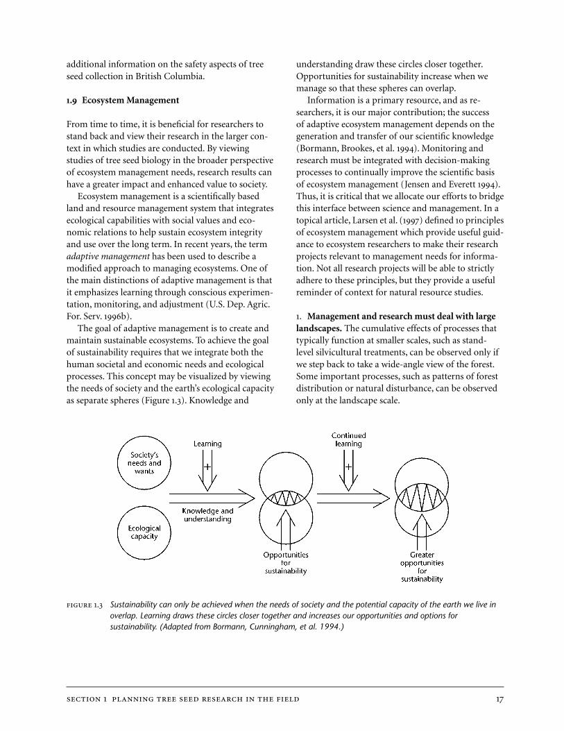
section 1 planning tree seed research in the field 17
additional information on the safety aspects of treeseed collection in British Columbia.
. Ecosystem Management
From time to time, it is beneficial for researchers tostand back and view their research in the larger con-text in which studies are conducted. By viewingstudies of tree seed biology in the broader perspectiveof ecosystem management needs, research results canhave a greater impact and enhanced value to society.
Ecosystem management is a scientifically basedland and resource management system that integratesecological capabilities with social values and eco-nomic relations to help sustain ecosystem integrityand use over the long term. In recent years, the termadaptive management has been used to describe amodified approach to managing ecosystems. One ofthe main distinctions of adaptive management is thatit emphasizes learning through conscious experimen-tation, monitoring, and adjustment (U.S. Dep. Agric.For. Serv. b).
The goal of adaptive management is to create andmaintain sustainable ecosystems. To achieve the goalof sustainability requires that we integrate both thehuman societal and economic needs and ecologicalprocesses. This concept may be visualized by viewingthe needs of society and the earth’s ecological capacityas separate spheres (Figure .). Knowledge and
understanding draw these circles closer together.Opportunities for sustainability increase when wemanage so that these spheres can overlap.
Information is a primary resource, and as re-searchers, it is our major contribution; the successof adaptive ecosystem management depends on thegeneration and transfer of our scientific knowledge(Bormann, Brookes, et al. ). Monitoring andresearch must be integrated with decision-makingprocesses to continually improve the scientific basisof ecosystem management (Jensen and Everett ).Thus, it is critical that we allocate our efforts to bridgethis interface between science and management. In atopical article, Larsen et al. () defined principlesof ecosystem management which provide useful guid-ance to ecosystem researchers to make their researchprojects relevant to management needs for informa-tion. Not all research projects will be able to strictlyadhere to these principles, but they provide a usefulreminder of context for natural resource studies.
. Management and research must deal with largelandscapes. The cumulative effects of processes thattypically function at smaller scales, such as stand-level silvicultural treatments, can be observed only ifwe step back to take a wide-angle view of the forest.Some important processes, such as patterns of forestdistribution or natural disturbance, can be observedonly at the landscape scale.
. Sustainability can only be achieved when the needs of society and the potential capacity of the earth we live inoverlap. Learning draws these circles closer together and increases our opportunities and options forsustainability. (Adapted from Bormann, Cunningham, et al. 1994.)

18 field studies of seed biology
. We must be concerned with long time frames.Just as the extent, structure, and condition of today’sforests have been determined by harvesting practicesthat took place a century ago, so the impact of thecurrent management activities will persist at least acentury into the future.
. We must consider both where and when we createa disturbance. Important spatial and temporal com-ponents are associated with any forest managementactivity or any natural disturbance. If, for example,our management activities will disturb large areas ina given landscape over the next century, it makes adifference whether the affected areas are contiguousor dispersed, and whether the disturbance occurs in asingle year or is spread over the full century.
. We have enough scientific knowledge to startmanaging ecosystems, but we will never fully under-stand all aspects of forest ecosystems. We know agreat deal about some parts of forest ecosystems andat least a little about most parts; a prudent approachis to begin by using the best science we have availablenow, while we continue with our research.
. We must synthesize the results of research thataddress many different ecosystem attributes andprocesses. We must combine what we know aboutecosystem components and ecosystem processes toarrive at a more complete understanding of how eco-systems work and how they respond to disturbance.Synthesis also serves to identify the major gaps inour knowledge.
. The complexity associated with ecosystemmanagement is so great that we must employmathematical models. Tracking details, measuringinteractions and trade-offs, dealing with long timeframes, dealing simultaneously with many species,and mapping the results—all require the use ofcomputer models.
. We must facilitate cooperation and collabora-tion. The complexity of forest ecosystems requiresthe attention of teams of scientists and managersrepresenting a wide range of expertise.
. Researchers must share sites so that they canintegrate their findings and investigate change ineach ecosystem component over many differentspatial and temporal scales. Agencies must makelong-term commitments to maintain research sitesas well as to fund basic site measurements. The mar-ginal cost of additional projects is quite low as longas a base level of measurements exists.
. We must simultaneously focus our collabor-ative research efforts on real landscapes. We willincrease our understanding of the interactions andtrade-offs only when experts from many fields applytheir collective wisdom to the same piece of landover the same time frame. Purely theoretical ap-proaches to ecosystem management research havegreat merit, but ultimately the evaluation must bein the field.
. We must remember that people are part of theecosystem. Human activity has left an indelible markon our forest resources, and ultimately, it is peoplewho decide which forest practices are acceptable.Our role as scientists and practitioners must be to:(a) identify and discourage those activities that willlikely cause short-term or long-term ecosystemdegradation, (b) clarify the trade-offs among manyacceptable management alternatives, and (c) identifyand encourage the alternatives that will most likelyproduce the desired outcomes.
. Summary
A long-term experiment whose sole sponsor has left,died, or lost interest is a sad orphan,and adoption is seldom quite successful.(Dyke )
Planning constitutes the major activity associatedwith field studies, and may even take longer than thestudy itself. Care is needed in defining the experi-mental protocol, data management, and reportingroutine. Good plans are especially critical when themain investigators are not readily available at alltimes during plot establishment and site selection.

section 1 planning tree seed research in the field 19
Flexibility is also required, and possible modificationsshould be considered even while the study is beingconceptualized. The plan must try to anticipate somelevel of uncertainty and be flexible enough to coverunexpected conditions in the field. Change is inevita-ble, and consideration of alternative approaches duringthe design stage will help to focus the planning effortand secure long-term success of the project.
Field experiments require sustained commitmentby the scientific staff so that the study will reach itsfull potential. Sustained commitment by fundingorganizations is also essential to maintain stability.Finally, the information needs urgently requiredby natural resource managers necessitates that theresults of field studies reach the end user as quicklyand as accurately as possible.
The role of a scientist in the ecosystem manage-ment model is to provide information for thedecision-making process. Such information helpsto identify the current status of an ecosystem aswell as potential options for addressing the social,physical, economic, and biological issues (Haynes etal. [technical editors] ). This information helpsclarify feasible limits, options within the limits,consequences of those options, and trade-offsbetween options. It is the role of the decision-makerto choose among options; it is not the role of science.The challenge for resource managers is to balancebiological science with social science and with thephilosophical views of how society values renewableand nonrenewable natural resources (Haynes et al.[technical editors] ).

section 2 designing an environmental monitoring program 21
. Background
Environmental and site factors influence the produc-tion, dispersal, survival, longevity, and germinationof tree seeds. Researchers must have a general under-standing of the effects of various environmentalfactors to select the most suitable location, timeframe, experimental techniques, and types of sensorsfor field studies. The nature of these factors and theoverall objectives of the study will also determinewhich environmental variables should be measured,and how frequently.
Environmental variables such as temperature andprecipitation may be considered in the context oflong-term average conditions, as ranges and extremes(climate), or as day-to-day conditions (weather). Fur-thermore, environmental variables can be viewed atthree scales: macro (or regional) weather, site weather,and tree weather. The complexity involved in obtain-ing data increases as we go from macroclimate to treeweather.
Macroclimate and synoptic weather conditions canbe obtained from the nearest Environment Canada orother government-operated weather stations, andmay be adjusted for the elevation of the site of inter-est. Usually, climate data are summarized as monthlyor annual values and include average, maximum,minimum, and extreme values for temperature, totalprecipitation, and derived data, such as degree-days
and frost-free period. Wind speed and direction areavailable for a few locations. For some parts of BritishColumbia, annual temperature and precipitationsummaries by subzone can be obtained from thebiogeoclimatic ecosystem classification database(see Appendix C).
Site climate and site weather conditions involveon-site measurements of air and soil temperature,precipitation, humidity, wind speed and direction,solar radiation, and soil moisture. Monitoring usuallyrequires an electronic datalogging system. Weatherdata may only be needed for a short time during anevent of interest (e.g., pollen release); in this case,you may need hourly rather than daily summaries.However, to characterize the climate (averages andvariation), – years of data collection are required.These data should be referenced to the nearestlong-term weather stations to determine howdifferent the period being measured may be fromthe “normal.”
Tree weather describes conditions in cones orflowers, or beside germinating seeds. Small, delicatesensors, such as thermocouples, are usually requiredto make these measurements. Variables of interest inregard to tree weather are temperature, radiationbalance, and soil moisture (for germination). Thedata can be used to develop physically based modelsor regression models of tree conditions as a functionof site conditions.
SECTION 2 DESIGNING AN ENVIRONMENTAL MONITORING PROGRAM
Every raincloud, however fleeting, leaves its mark,not only on trees and flowers whose pulses are quickened,and on the replenished streams and lakes,but also on the rocks are its marks engraved …(John Muir “Gentle Wilderness, the Sierra Nevada”)

22 field studies of seed biology
. Climate station with wind direction and windspeed sensor, a rain gauge (lower right), andtower with solar radiation, air temperature, andhumidity sensors. A robust tower is required atthis site to support the large precipitationgauge used for winter snowfall measurements.
. Designing an Environmental MonitoringProgram
In designing an environmental monitoring programfor a research site, you must first decide which vari-ables you need to measure. For field germinationstudies, near-surface (– cm depth) soil temperatureand soil moisture are the important variables. How-ever, soil temperature and moisture will be affectedby a variety of other environmental variables. Soiltemperature, for example, depends on soil moisture,solar radiation, wind speed, air temperature, soil tex-ture, and surface colour. On the other hand, surfacesoil moisture depends on rainfall, solar radiation,evaporation, vegetation cover (transpiration), soiltexture, and soil temperature. The humidity of theair and solar radiation can critically affect the initialestablishment of germinants through its effects onsoil evaporation and plant transpiration. Humidityalso affects seed production through its effects onpollination. Slope and aspect affect temperature andmoisture because they influence the solar radiationand rainfall reaching the surface. Wind is of interestprimarily for studies of seed dispersal (see Section ).
The frequency of environmental measurementswill vary depending on the type of measurement.Light and temperature can vary rapidly and thusrequire frequent monitoring. Relatively stable sitefactors, such as soil type, soil pH, presence and typeof duff layer, biogeoclimatic zone, elevation, slope,and aspect, may need only to be measured once.
Researchers sometimes rely on environmentaldata from the nearest weather station to provide datasuch as rainfall and daily minimum and maximumtemperatures, but if the microclimate of the siteis significantly different from that of the weatherstation it is advantageous to set up a small weatherstation at the site (Figure .). Dataloggers can beused to continuously record a variety of environmen-tal variables (Figure .). Spittlehouse () providesguidance on using dataloggers in the field and theaccuracy that can be expected from such measure-ments. While it is tempting to collect large amountsof weather data on the assumption that somehowthey will be useful, a few days of manual measure-ments under a range of weather conditions may bejust as effective as installing electronic dataloggerson the site. The disadvantage of manual sampling,
however, is that you may be able to demonstrate dif-ferences between treatments only when they are large.
Whatever the means of recording data, the com-plexity of environmental factors and their interactionsnecessitates careful planning of all field measurements.Four steps to developing an environmental monitor-ing program are illustrated here using an example ofa study to determine conditions that initiate flowering.
. Why do you need environmental data?To determine weather conditions that initiateflowering, and their variation from year to year.
. What data are needed?Air and bud temperatures and solar radiation, frombud initiation through flowering (over months ormore). The year-to-year variation could be obtainedby monitoring for many years, or by calculatingregression equations that are based on weather data.Site weather conditions could be related to the near-est long-term weather station to provide the datathat would be needed to drive the model. Ideally, aphysically based model of bud/flower temperatureas a function of site weather conditions and budcharacteristics should be developed to allow porta-bility to other sites with a minimum of calibration.Both methods require – years of on-site data fordevelopment and validation.

section 2 designing an environmental monitoring program 23
. What needs to be done to get the data?Is continual monitoring necessary, or is a short-termmanual measuring program adequate? Fine wirethermocouples are needed in the buds to measuretemperature; they are sensitive and inflict minimaldamage. The site may need frequent visits to ensurethat bud temperature sensors have not beendisturbed.
. Can the work be done physically and whatdoes it cost?Is the site readily accessible, and are equipment andpersonnel available? A datalogger-based monitoringsystem would cost $ to $. Installation requires– days depending on the number and location ofsensors, and monthly site visits are required to checkequipment and collect data. At least day per monthshould be allowed per site for data processing andanalysis—an important consideration that isoften overlooked.
. Methods for Measuring Environmental Factors
.. Soil temperatureNear-surface soil temperature (– cm depth) can beeasily measured, but measurements must be adequatelyreplicated. Soil temperature varies substantially, notonly horizontally and vertically, but temporally aswell. Individual locations can be averaged by using aseries of thermocouples connected in parallel. Data-loggers are a convenient way to monitor the numberof sensors required to assess the spatial and temporalvariability. The diurnal trend of the near-surfacetemperature parallels the diurnal course of solarradiation; thus a reasonable approximation of thedaily maximum temperature can be obtained bymaking the measurement about an hour after solarnoon. An estimate of solar noon in your area is avail-able on the Internet at http:/www.crhnwscr.noaa.gov/grr/sunlat.htm. The average near-surface soil temper-ature (during the summer) can be approximated bymeasuring at about a.m. solar time ( hours beforesolar noon). A comparison of treatments with thisapproach requires that measurements be made underthe same weather conditions. This manual samplingmethod will only be useful for showing differenceslarger than °C and should only be used to give anidea of trends.
Shade can significantly reduce solar radiation,resulting in a corresponding decrease in the near-surface temperature. On the other hand, shade alsoreduces night-time cooling. When solar radiationis reduced by over %, the surface temperaturecan be approximated by the air temperature at. m above the ground. For more informationon forest soil temperature, see Stathers andSpittlehouse ().
.. Soil moistureThere is no easy way to obtain good soil moisturemeasurements, and the difficulty increases as onegets closer to the surface. Gravimetric sampling andtime-domain reflectometry (tdr) measure soil watercontent (Hook et al. ), but further work is re-quired to develop tdr probes and techniques. tdrrequires substantial replication, and although it isusually done manually, it can be automated. Watercontent can be converted to soil water potential (ortension) using a soil water retention curve obtained
. Electronic datalogger used to monitor andcapture data from a series of environmentalsensors. The datalogger is housed in awaterproof box (shown open) and data areroutinely retrieved using a portable computer.This datalogger can monitor many sensors atonce; less expensive dataloggers are availablethat will monitor only one sensor.

24 field studies of seed biology
from undisturbed soil samples analyzed by a com-mercial soil physics laboratory.
Gravimetric sampling is labour intensive anddestructive. Some – replicates at each depth ofinterest are required. It is best to use a sharpenedmetal tube to take a soil core of known volume,rather than a grab sample. The sample is sealed inplastic bags, and returned to the laboratory forweighing and drying. Gravimetric samples are pre-sented on either a weight of dry soil or a volumetricbasis. The latter is the common approach and can beconverted to soil water potential (or tension) using asoil water retention curve.
Gypsum or fibreglass soil moisture blocks can beused to measure soil moisture potential (or tension)in the to -. MPa ( bars) range; they can be readmanually or with a datalogger. Moisture blocks pro-vide relatively coarse resolution, and require testingover several drying cycles before installation. Theymay have poor contact with substrates such ascoarse sandy soil or partially decomposed organicmaterial and cannot be used at soil depths shallowerthan cm.
Tensiometers measure soil water potential in the to -. MPa (. bars) range. They are usually readmanually but can be automated. As with moistureblocks, they cannot be used at depths shallower than cm. Soil water potential can also be obtained byequilibrating soil samples with the air or filter paperin a sealed container, then measuring the humidityof the air or filter paper. In situ measurements of soilwater potential using soil psychrometers or hygrom-eters is extremely difficult, particularly in the top cm of the soil. Further information on measuringsoil moisture can be found in Schmugge et al. ().
.. Solar radiation (light)Three ranges of the radiation spectrum are usuallyconsidered when assessing the light regime at theearth’s surface: ultraviolet radiation from to nm, photosynthetically active radiation (par)from to nm, and solar radiation from to nm. Radiation above nm is called longwaveor thermal radiation. Different sensors are requiredto measure each of these bands of energy. There is agood correlation between the energy in each bandboth above and below the canopy (Yang et al. ;Alados et al. ).
Radiant flux density is the energy in the light emit-ted, transmitted, or received per unit area (W/m2).Irradiance is the radiant flux density incident on asurface; emittance is the radiant flux density emittedby a surface.
The units and the instruments used for lightmeasurement will depend upon the intent of thestudy. Some radiometers (for example the li-cormodel li- radiometer) can be fitted with a varietyof sensors to measure irradiance. A quantum sensoris used to measure photosynthetic photon flux den-sity (ppfd) or par. A pyranometer (or radiometricsensor) is used to measure solar radiation. Photomet-ric measurements using illumination units (lux orfootcandles) should not be used in plant studies.Plants do not respond to the light spectrum in thesame way as the human eye, so such measurementshave no value unless the characteristics of the lightsource are precisely known (Salisbury and Ross ).par is usually the radiation measurement made whenassessing physiological responses such as plant produc-tivity (although other wavelengths may have specificphotomorphogenic effects such as the induction offlowering or cold hardiness). par is commonly meas-ured in units of µmol • m-2 • s-1. Special sensors arerequired to measure ultraviolet radiation, and variousfilters are available that modify sensor output tomatch the biological response of tissue. Longwaveradiation sensors are not easy to use, so longwaveestimates are usually obtained by subtraction of solarradiation from total radiation measurements (seeBlack et al. ).
The controlling influence of vegetation on thelight regime will render a shaded surface more moistand cool than a bare surface. The amount of directcover over the study area, the distance from the edgeof openings, and the aspect of the edge will influencethe light regime in openings. These influences can beestimated from measurements of above-canopy lightand the amount of cover. When measuring irradianceunder a plant canopy with uneven light levels, rea-sonable averages can be obtained by moving a smallsensor repeatedly along a track (Figure .), by usinga long linear sensor, or by using many spot sensors.It is generally best to spend some time generatingradiation interception curves with an intensive meas-urement program over a short period. These curvesare used with continuously monitored above-canopy

section 2 designing an environmental monitoring program 25
radiation to give below-canopy data through theyear. The variability or patchiness of the canopy mayindicate that there is a range of light environmentsthat must be quantified separately. Radiation rapidlydecreases as canopy cover increases. The interceptioncurve is of the form
I = Ioe(-KC),
where:I = the radiation at the forest floor,Io = the radiation above the canopy,C = percent canopy cover (range –), andK = an extinction coefficient (range .–.).
Shaded and sunny areas of small openings and clear-cut edges can be determined using the formulae forlength and direction of tree shadows at differenttimes of the day and year (Sit a).
Forest canopies change the quality as well as theintensity of light reaching the forest floor (Vezina andBoulter ; Atzet and Waring ; Ross et al. ;Messier et al. ). Figure . illustrates how thespectral distribution is changed due to plant foliagedifferentially absorbing and reflecting the variouswavelengths. The relatively thick needles of coniferoustrees transmit very little radiation and most radiation
reaching the forest floor passes between needles andother gaps in the canopy. Consequently, the changein the shape of the spectrum is not as great as inhardwoods where more radiation passes throughthe thinner leaves. The biggest change is in the in-crease in the ratio of red (– nm) to far-red(– nm). It changes from .–. under clearskies above the canopy to .–. under hardwoodforest canopies, and to .–. under coniferouscanopies.
Light quality—the incident light spectrum—af-fects the germination of many conifer seeds (Section..) and the production of female cones (Durzan etal. ). For measurement of irradiances under for-est canopies, see Black et al. () and Yang et al.(). The measurement of the total light spectrum
. Automatic tram system that moves back andforth over a 50 m span to determine thevariation in short- and longwave radiation,and surface and air temperature under a forestcanopy. The system is controlled by thedatalogger in the tube hanging on the end.(System designed by R. Adams, B.C. Ministryof Forests.)
. Influence of forest canopy on the intensity andspectral distribution of solar radiation reachingthe forest floor. The upper panel shows theincident radiation from a clear sky during themiddle of the day. The lower panel (note thedifference in scale) indicates that pine andmaple canopies have greater absorption in themiddle range (400–700 nm) than in the nearinfrared range (700–750 nm). (Based on datain Federer and Tanner 1966 and Vezina andBoulter 1966.)

26 field studies of seed biology
at a site requires a portable spectroradiometer. BothAtzet and Waring () and Floyd et al. () con-ducted spectroradiometric analyses to determine thelight-filtering capacity of coniferous forests. However,the changes in light quality can simply be measuredwith a portable red:far-red meter, since most of thecanopy effects are due to the canopy cover shiftingthe ratio of red to far-red light.
.. Wind speed and wind directionWind, acting either directly or by wind-inducedvibration, plays a major role in the distribution ofpollen and seeds. Seeds of some species are veryresponsive to updrafts or vertical air movements (seeSection ..). Wind speed is a vector quantity withattributes of direction and magnitude, although onlythe horizontal component is usually measured. Cup orpropeller anemometers are generally used to monitorwind speed. They can be connected to a datalogger orhave their own display. Many ane-mometers comewith a wind direction indicator. Topography and veg-etation cover affect wind speed and direction andcare must be taken in locating the anemometer andwind vane. The sensors should be located – mabove vegetation canopy and away from clearcutedges. Robust anemometers usually have stall speedsof . m s–1 or greater. Low stall speed anemometersare required if you are interested in conditions at theedge of a clearing, in a small opening, or below thecanopy. Hot-wire anemometers (commercial orhome-made) can be used to measure wind flowaround cones and flowers, but they are delicate andeasily damaged. They can be monitored manually orwith a datalogger. A discussion of wind dynamics andinstrumentation can be found in Pearcy et al. ().
.. PrecipitationRainfall can be reliably measured with tipping-bucketor storage gauge. The gauge should be located in anopening where a line projected from the top of thegauge to the top of the surrounding vegetation has anangle of no more than ° to minimize any shadingeffects. Snowfall cannot be measured with a standardtipping-bucket gauge. Although gauges that melt thesnow and can be monitored with a datalogger areavailable, they are expensive. A low-power, reliablesensor that measures the depth of snow on theground can be used in conjunction with a datalogger.
.. Air temperature and humidityA hygrothermograph in an instrument shelter(Stevenson Screen) located on the study site canrecord air temperature and relative humidity for upto a month before the chart requires changing. Elec-tronic temperature and humidity sensors can beplaced inside the Stevenson Screen. Smaller shieldscan be built or are available commercially, but somecommercial varieties overheat under low windspeeds. Spot measurements can be made usingaspirated or sling psychrometers.
.. Plant temperatureObtaining temperature measurement in cones andbuds requires extremely small sensors. Thermocouples(Figure .) are the best option, being more robust andeasier to make than thermistor or platinum resistancesensors. They are best monitored with a datalogger.Surface temperature can be measured using an infra-red thermometer with a narrow field of view.
.. Canopy coverCanopy cover is the environmental factor most im-mediately affected by forest harvesting activities andby silvicultural practices (see Section ). It signifi-cantly affects the microclimate of a site, influencingthe solar radiation, air and soil temperatures, windspeed, humidity and rainfall experienced at theground (Hanley ). Canopy cover is also impor-tant because the position of vegetation within thecanopy is used as a criterion for the relative domi-nance of individuals within a plant community(Section ..).
. A fine wire thermocouple is used to measurethe temperature inside the leader of a youngspruce tree. The thermocouple is monitoredwith a datalogger, as are the accompanyingenvironmental sensors. The same techniquecan be used to measure cone temperature.

section 2 designing an environmental monitoring program 27
Canopy cover is often expressed as a percentagevalue, usually by species, growth form, or canopystratum; in a dense or multilayered community, totalvegetative cover may exceed %. The methodchosen to measure canopy cover depends on theavailable technology and the type of site; somemethods are suitable for low herbaceous vegetationor clearcut areas, while others are designed forforested areas. Bunnell and Vales () present acomparison of different methods of measuring forestcanopy cover.
Many researchers obtain percentage cover ofdifferent species and canopy layers with the visual-estimation technique (Mueller-Dombois andEllenberg ). Cover can be estimated to the nearestpercentage point or to the nearest th or th percen-tile. Cover estimates may be restricted to the plotsbeing studied for germination or other responses, ormay be used for more general descriptive purposes(such as describing the study site, Section .). Thevisual-estimation method is especially suitable forgrasslands or clearcuts, because of the low profile ofthe vegetation. Plot size for cover estimation averagesabout . m2 (either circular or square), but may besmaller when working in exclusively herbaceous veg-etation, or larger when working with tall shrubs andtrees. A good guideline for plot size is that plot diam-eter should be approximately equal to the height ofthe vegetation being described.
Visual estimates are subject to personal bias, thushuman error will introduce variability into the data(Bunnell and Vales ). This can be checked andcorrected (calibrated) by other people working on thesame project. It is also useful to have examples ofhow different spatial arrangements affect one’s per-ception of canopy cover. Figure ., for example,compares different spatial arrangements of %canopy cover. These kinds of comparisons are espe-cially useful when observers are not experienced incanopy estimation methods.
Canopy cover can be measured more objectivelyusing a line-intercept method, which is suitable forwoody plants, shrubs, and trees (Chambers andBrown ; Habitat Monitoring Committee ).A line or tape measure is stretched tightly across thevegetation between two stakes. The best samplingprocedure is the stratified-random sample using abaseline and perpendicular transects (see Chambers
and Brown for a sample layout). The length ofthe canopy intercept of each species along the line ismeasured from the tape or with a ruler. If the cano-pies overlap in layered vegetation, it may be desirableto measure each height layer separately. Transect linesshould be – m in length. Many short lines aregenerally preferred to a few long lines; – transectsare usually required for an adequate sample. Severalcover values can be calculated:
percent cover for each transect by species =
length intercepted by a speciestransect length
× ;
percent cover of a species by sampling unit =
sum of all transect lengths interceptedtotal transect length sampled
× .
While this method is generally precise and accurate(Cook and Stubbendieck ), it can also be timeconsuming.
. Different spatial arrangements comprising50% canopy cover. Some experience maybe needed to estimate different proportionsof cover.

28 field studies of seed biology
Objective measurements of canopy cover canalso be obtained with a point-intercept method(Owensby ; Levy and Madden ) or point-quadrat method (Chambers and Brown ). Thesemethods use a point- or pin-frame, often consistingof pins spaced or cm apart, with pins posi-tioned vertically or at an inclined angle. The frame ispositioned randomly within the sampling units oralong a transect and a single pin lowered towards theground. The first strike of any part of the vegetationcanopy becomes a “hit.” Each “hit” is recorded byspecies or growth-form (Chambers and Brown ).The sample size required for statistical adequacy isusually – pins. Several cover values can bederived from this information: percentage canopycover for each species or life-form (Chambers andBrown ); percent total canopy cover; and percen-tage vegetation cover by species. The user should beaware that the line is the sample unit, so it is betterto have fewer points per line and more lines, ratherthan vice versa (Bonham ). The frame shouldbe held vertically; if the frame is at an angle, thenumber of intercepts may increase and overestimatethe cover.
In woodland areas, other instruments such as themoosehorn and the spherical densiometer are fre-quently used to measure tree canopy cover (Lemmon; Bunnell and Vales ). The moosehorn is apoint-intercept method where the canopy is viewedthrough a screen and coincidences between vegeta-tion and dots on the screen are tallied. The sphericaldensiometer has a curved mirror with a grid thatreflects the overstorey at a particular point, thenprovides an estimate of the relative amount of thegrid covered by vegetation. At each location, fourreadings (facing north, east, south, and west) arerecorded and averaged.
A canopy analyzer uses measurements from afisheye optical sensor placed above and below theplant canopy; in this way canopy transmittance datacan be used to calculate the leaf area index and themean leaf inclination angle (Chen et al. ; Wellesand Norman ). The canopy analyzer functions ina variety of sky conditions, with overcast being thebest; the instrument can be used in canopies rangingin size from short grasses to forests.
The area of leaf per unit area of ground (leaf areaindex - lai) is another measure used to quantify
canopy cover. It is measured by sampling the foliageor by using light penetration techniques (Gholz et al.; Smith et al. ; Fassnacht et al. ; Chen ).In the former method, all the foliage in the shrub andherb layers is removed from – samples of knownarea (usually m2). The area of the leaves is thenmeasured using an image analyzer. All the leaves froma tree (or from a representative branch in each whorl)are sampled and leaf area measured with an imageanalyzer. Trees of different diameter at breast height(dbh) are sampled to produce a dbh/leaf area rela-tionship (or sapwood cross-sectional area/leaf area)which is then used with stand dbh distribution tocalculate tree lai. Leaf area can be determined usinglight sensors such as the ceptometer and the lai-.Both measure the “effective” leaf area and must becorrected for leaf clumping to get the true leaf areaindex (Smith et al. ; Fassnacht et al. ; Chen). These sampling techniques can be used todetermine how leaf area changes with height andto calculate foliage area density.
The canopy can be photographed from groundlevel using a camera fitted with a hemispherical orfisheye lens with a ° field of view. Film exposuremust be standardized (Chen et al. ).The resultingphotographic negatives, prints, or slides can be digi-tized, and then analyzed by a computer program toaccurately measure canopy cover above the point ofmeasurement. Available computer programs includesolarcalc (Chazdon and Field ), gli (Canham), sunshine (Smith and Somers ), andhemiphot (ter Steege ). This photographicmethod is suitable in herbaceous, scrub, forested, ormixed cover, but has the drawback that considerableoffice time is required to obtain cover estimates.These same programs also model solar radiationinput for the point at which the photograph wastaken (see Section ..), but the cover estimatesrequire fewer assumptions.
.. Soil variablesSoil nutrient levels are important because they affectseed production, germination, and seedling growth.Three principal methods are used to diagnose nutri-ent deficiencies: deficiency symptoms, soil chemicalanalysis, and foliar analysis. (For other methods seeMorrison .) Soil chemical analysis has some valuefor diagnosing site nutrient status on sites where

section 2 designing an environmental monitoring program 29
foliage sampling is impractical. There are majorproblems with conducting soil chemical analysis inforest soils. Typically, the root zone is not homogene-ous, often containing dissimilar horizons that mayyield different analytical values. Nutrient standardsfor forestry soils are not available, and criteria cannotbe extrapolated from one kind of soil to another. Itcan be problematic to integrate these disparate resultsto determine the nutrient status of the compositesoil profile.
The high variability of some soils may require alarge number of samples. The most useful routinesoil chemical analyses for forest soil fertility inB.C. are likely to be: pH, organic carbon concentra-tion, and total nitrogen concentration (Watts[editor] ).
Oxygen is usually a limiting factor only in water-logged soils, where water may fill pore spaces. Oxygenis difficult to measure in the field, but under suitableconditions, an oxygen electrode may be used. Thistechnique uses glass electrodes that are delicate andeasily broken, and is not generally suitable for fieldstudies. It is primarily designed for laboratorystudies, but can be set up and operated adjacent to astudy site. A key requirement is constant-temperaturewater, obtained from a thermoregulated circulatoror a large-reservoir flow-through system. Someinstruments can be configured to determine oxygenindirectly by heating the sample in a stream of inertgas and converting all oxygen-containing gases tocarbon monoxide or carbon dioxide. Refer to Pearcyet al. () for further information on such methods.

section 3 natural seed production 31
SECTION 3 NATURAL SEED PRODUCTION
O sweet spontaneousearth how often havethedoting
fingers ofprurient philosophers pinchedandpoked
thee, has the naughty thumbof science proddedthy
beauty .(e.e. cummings)
. Background
The path to the production of a viable seed beginswith the growth and development of reproductivebuds, continues with pollination and fertilization,and ends with embryo development and seed matu-ration. Throughout all these developmental stageslosses occur for a variety of reasons; losses may bedue to environmental factors, or may result fromvarious diseases and animal predators that attackcones and seeds. Researchers investigating tree seedproduction must be able to assess which and to whatextent these factors limit natural seed supplies.
Angiosperms characteristically produce seeds an-nually, but production can vary considerably fromyear to year (Table .). Most conifers do not producecollectable crops every year (Table .), a phenomenoncalled periodicity. Mature cones are produced at in-tervals ranging from to years, and sometimes asinfrequently as every years. Crop yields vary indifferent years, and in poor crop years, the quality
of seeds also tends to be poor (Edwards ; Caronand Powell a, b). Depending upon thespecies, conifer seed production varies in length andcomplexity of the production cycle (Figure .), repro-ductive success (due to different sexual mechanisms),and the timing of natural seedfall (Zobel ).
The reproductive structures of trees are derivedfrom reproductive buds. The time of initiation ofmale and female reproductive buds can vary fromyear to year due to factors such as the relative abun-dance of seed trees (trees/ha) (Smith et al. ) andtree age (Caron and Powell b). Natural seed pro-duction is rare in trees younger than years.Generally, the volume of seeds produced increases asthe tree ages. Bergsten (), however, found no bio-logical differences between mature Scots pine seedsobtained from young stands and those collected fromold stands. Environmental conditions, such as tem-perature, drought (Eis a, ), and nutrientavailability (Heidmann ), affect reproductive budproduction. Environmental stresses can reduce the

32 field studies of seed biology
Ace
r m
acro
phyl
lum
bigl
eaf
map
le
Aln
us
rubr
are
d a
lder
Arb
utu
s m
enzi
esii
arbu
tus
Bet
ula
pap
yrif
era
pap
er b
irch
Cor
nus
nutt
alli
iP
acif
ic d
ogw
ood
Frax
inu
s la
tifo
lia
Ore
gon
ash
Mal
us
fusc
aP
acif
ic c
rab
app
le
Popu
lus
bals
amif
era
ssp.
bals
amif
era
bals
am p
opla
r
Popu
lus
bals
amif
era
ssp.
tric
hoca
rpa
blac
k co
tton
woo
d
Mon
oeci
ous;
imp
erfe
ctfl
ower
s
Mon
oeci
ous
Mon
oeci
ous;
per
fect
flo
wer
s
Mon
oeci
ous
Mon
oeci
ous;
per
fect
flo
wer
s
Dio
ecio
us
Mon
oeci
ous;
per
fect
flo
wer
s
Dio
ecio
us
Dio
ecio
us
Gre
enis
h y
ello
w (
3m
mac
ross
); n
um
erou
s in
han
gin
g cy
lin
dri
cal c
lust
er;
mal
e an
d f
emal
e in
dif
fere
nt
par
ts o
f cr
own
Dro
opin
g re
dd
ish
mal
eca
tkin
s (5
–12
cm);
fem
ale
catk
ins
are
wo
ody
con
es(2
cm)
Wh
ite,
urn
-sh
aped
(7
mm
),in
larg
e d
roop
ing
clu
ster
s
Mal
e st
amin
ate
flow
er a
nd
fem
ale
stro
bile
(2–
4cm
);br
eak
up
at
mat
uri
ty
Smal
l (3
mm
) w
hit
e in
tigh
t cl
ust
ers
surr
oun
ded
by 4
–6 w
hit
e sh
owy
brac
ts(2
–7cm
)
Smal
l (3
mm
) m
ale
(yel
low
ish
) an
d fe
mal
e(g
reen
ish
) fl
ower
s in
bun
ched
clu
ster
s on
tw
igs
Wh
ite
to p
ink
frag
ran
tbl
osso
ms
(2cm
); 5
–12
infl
at-t
opp
ed c
lust
ers
Mal
e an
d f
emal
e ca
tkin
s
Mal
e ca
tkin
s (2
–3cm
)w
ith
40–
60 s
tam
ens/
flow
er, f
emal
e ca
tkin
s(8
–20
cm)
wit
h 3
sti
gmas
/fl
ower
s
Ap
pea
r w
ith
or
bef
ore
leav
es(A
pr–
May
)
Mal
e, p
revi
ous
fall;
fem
ale,
Feb–
May
Ap
r–M
ay
Mal
e, p
revi
ous
fall;
fem
ale,
Ap
r–Ju
ne
Alw
ays
insp
rin
g; o
ften
infa
ll
Ap
pea
r be
fore
leav
es
Ap
r–Ju
ne
Ap
r
Ap
pea
r be
fore
leav
es (
Ap
r–Ju
ne)
Rip
en S
ept–
Oct
;d
isp
erse
Oct
–Jan
Rip
en A
ug–
Sep
t;d
isp
erse
Au
g–sp
rin
g
Fall
Rip
en A
ug–
Sep
t;d
isp
erse
Au
g–sp
rin
g
Rip
en la
tesu
mm
er/f
all
Lat
e su
mm
er/f
all
Lat
e fa
ll
Jun
e–Ju
ly
May
–Ju
ly
Pai
red
win
ged
see
ds
(sam
aras
); 3
–6cm
lon
g
Bro
wn
con
es (
2cm
)re
mai
n o
ver
win
ter;
con
tain
ova
l, w
inge
dn
utl
ets
Ora
nge
-red
ber
ry-l
ike
(1cm
), s
urf
ace
fin
ely
gran
ula
r
Nu
tlet
s w
ith
win
gsbr
oad
er t
han
bo
dy
Clu
ster
s of
bri
ght
red
“ber
ries
” (1
cm);
glob
ula
r or
ovo
idd
rup
es
Pad
dle
-sh
aped
, sam
ara
(3–5
cm)
in la
rge
clu
ster
s on
fem
ale
tree
s
Yello
w t
o re
dd
ish
sm
all
(10–
15m
m)
fles
hyp
omes
2-va
lved
cap
sule
s; n
oth
airy
Rou
nd
, gre
en h
airy
cap
sule
s th
at s
pli
t in
to3
par
ts; s
eed
s co
vere
dw
ith
wh
ite
flu
ffy
hai
rs
2 (1
/ s
amar
a);
no
end
osp
erm
50–1
00se
eds
/ co
ne
no
end
osp
erm
20 h
ard
, an
gled
seed
s+
en
dos
per
m
Nu
mer
ous
no
end
osp
erm
1–2
/ st
one;
+ e
nd
osp
erm
1 /
sam
ara
+ e
nd
osp
erm
3–5
carp
els
1–2
seed
s /
carp
el+
en
dos
per
m
Nu
mer
ous;
no
end
osp
erm
Nu
mer
ous;
no
end
osp
erm
1 ye
ar
4 ye
ars
1 ye
ar
2 ye
ars
2–4
year
s
1 ye
ar
1 ye
ar
.Se
ed p
rodu
ctio
n ch
arac
teris
tics
of h
ardw
oods
nat
ive
to B
ritis
h C
olum
bia.
Sou
rces
: Sc
hopm
eyer
(19
74);
Poj
ar a
nd M
acKi
nnon
(19
94);
Wyc
koff
and
Zasa
da[1
998]
; Zas
ada
et a
l. [1
998]
Seed
sIn
terv
alSp
ecie
sFl
ower
sFl
ower
sm
atu
reFr
uit
Ave
rage
#b
etw
een
Com
mon
nam
eTr
ee t
ype
(des
crip
tion
)(m
onth
)(m
onth
)(d
escr
ipti
on)
seed
s/fr
uit
crop
s

section 3 natural seed production 33
.(C
ontin
ued)
Seed
sIn
terv
alSp
ecie
sFl
ower
sFl
ower
sm
atu
reFr
uit
Ave
rage
#b
etw
een
Com
mon
nam
eTr
ee t
ype
(des
crip
tion
)(m
onth
)(m
onth
)(d
escr
ipti
on)
seed
s/fr
uit
crop
s
Popu
lus
trem
ulo
ides
quak
ing
asp
en
Pru
nus
emar
gina
tabi
tter
ch
erry
Qu
ercu
s ga
rrya
naG
arry
oak
Rha
mnu
s pu
rshi
ana
casc
ara
Sali
x am
ygda
loid
esp
each
-lea
f w
illo
w
Sali
x be
bbia
na
Beb
b’s
wil
low
Sali
x di
scol
orp
uss
y w
illo
w
Sali
x ex
igu
asa
nd
bar
wil
low
Sali
x lu
cida
ssp
.la
sian
dra
Pac
ific
wil
low
Sali
x sc
oule
rian
aSc
oule
r’s
wil
low
Dio
ecio
us
Mon
oeci
ous;
per
fect
flo
wer
s
Mon
oeci
ous
Mon
oeci
ous
Dio
ecio
us
Dio
ecio
us
Dio
ecio
us
Dio
ecio
us
Dio
ecio
us
Dio
ecio
us
Mal
e ca
tkin
s (2
–3cm
);fe
mal
e ca
tkin
s (4
–10
cm)
5–10
wh
ite
to p
inki
shfl
ower
s (1
0–15
cm)
in f
lat-
top
ped
clu
ster
Tin
y in
con
spic
uou
sfl
ower
s; m
ale,
in h
angi
ng
catk
ins;
fem
ale,
sin
gle
orin
sm
all c
lust
ers
Lo
ose
clu
ster
s of
5–1
2 ti
ny,
yello
wis
h-g
reen
flo
wer
s
Stam
inat
e ca
tkin
s so
ft,
silk
y
Ap
r–M
ay
Ap
r–Ju
ne
Feb–
May
Ap
r–Ju
ly
May
–Ju
ne
Ap
r–Ju
ne
May
May
–Ju
ly
Ap
r–M
ay
Ap
r–Ju
ne
May
–Ju
ne
July
–Sep
t
Au
g–D
ec
July
–Sep
t
July
May
–Ju
ne
May
–Ju
ne
Jun
e–A
ug
May
–Ju
ly
Cat
kin
s of
tin
y, g
reen
ish
cap
sule
s co
vere
d w
ith
cott
ony
dow
n
Dar
k re
d d
rup
es (
1cm
)
Aco
rns
(2–3
cm)
insh
allo
w, s
caly
cu
ps
Pu
rpli
sh-b
lack
, rou
nd
ber
ryli
ke d
rup
e
Smal
l, 2-
valv
ed c
apsu
leco
nta
ins
hai
ry s
eed
s
2-va
lved
cap
sule
; 24–
48ca
psu
les/
catk
in
2-va
lved
cap
sule
2-va
lved
cap
sule
2-va
lved
cap
sule
2-va
lved
cap
sule
2–7
/ ca
psu
le; 7
7–50
0 se
eds
/ ca
tkin
no
end
osp
erm
1 /
dru
pe
1 /
acor
n;
coty
led
ons
only
,n
o en
dos
per
m
2–3
nu
tlik
e se
eds
/d
rup
e+
en
dos
per
m
14–1
8 se
eds
/ca
psu
le
5–7
seed
s /
cap
sule
;14
4–31
1 se
eds
per
catk
in
8–12
/ c
apsu
le
15–3
6 /
cap
sule
12–2
0 /
cap
sule
4–5
year
s
2–3
year
s
Goo
d c
rop
sal
tern
ate
wit
hp
oor

34 field studies of seed biology
. Seed production characteristics of conifers native to British Columbia (Eremko et al. 1989). (Cones refer to femalecones only.)
Cone Cone- Years Viable seeds Position of Ease ofSpecies length bearing age between per hectolitre cones in coneCommon name (cm) (years) crops of cones crown detachment
Difficult
Difficult
Difficult
Easy
Moderate
Moderate
Moderate
Difficult
Moderate
Difficult
Difficult unlessfrozen
Moderate
Moderate
Difficult
Easy
Easy
Easy
Easy
Top ¼
Top ¼
Top ¼
Throughout
Non-shadedpart of crown
Non-shadedpart of crown
Top ⅓
Top ¼
Top ⅓
Throughout
Throughout
Throughout
Top ¼
Throughout
Top ½
Throughout
Throughout
Top ⅓
30 389
50 776
40 582
93 965
32 000
119 312
347 163
108 000
194 270
515
coast: 176 660interior: 70 546
6 454
7 687
31 522
coast: 39 577interior: 70 343
897 837
366 698
356 428
2–3
2–3
2–4
4 or more
3–6
1–10
6
4 or more
3–4
3–5
2–4
2–4
3–7
4–6
2–10
2–4
3–4
3–6
20
50
20
Unknown
40
25
40
10
25–40
20–30
15–20
20–30
20
12–16
20–25
20–30
25–30
30
9–13
5–12
6–12
0.5–1.5
1.5
2–3
3–6
2.5
5–10
3–8
3–6
7–20
10–25
7–9
5–10
1–2
2–3
2–8
Abies amabilisamabilis fir
Abies grandisgrand fir
Abies lasiocarpasubalpine fir
Chamaecyparisnootkatensis
yellow-cedar
Larix laricinatamarack
Larix occidentaliswestern larch
Picea glaucawhite spruce
Picea marianablack spruce
Picea sitchensisSitka spruce
Pinus albicauliswhitebark pine
Pinus contortashore pine
Pinus flexilislimber pine
Pinus monticolawestern white pine
Pinus ponderosaponderosa pine
Pseudotsuga menziesiiDouglas-fir
Thuja plicatawestern redcedar
Tsuga heterophyllawestern hemlock
Tsuga mertensianamountain hemlock

section 3 natural seed production 35
number of reproductive buds or, in other cases, canstimulate prodigious production of cones. Plantgrowth regulators (pgr) such as gibberellins havebeen used to increase cone production in conifer seedorchards (Ross and Bower ; Ross ), but pgrlevels are difficult to alter, for logistical reasons, innatural stands.
Pollen, produced in male cones or anthers, istransported to female cones or flowers in the processof pollination. Successful pollination results in thefertilization of ovules; ovules then develop into seeds.Reduced pollination efficiency may be due to lowpollen-cloud densities (few pollen-cone buds initi-ated), climatic conditions (e.g., rain, frost), or thepresence or absence of pollen vectors. In conifers,which are wind pollinated, the absence of wind, orbarriers to wind may inhibit pollination. Thus, thepositioning of cones relative to tree height or relativeto the windward and leeward sides of a tree can in-fluence the frequency of filled seeds (Smith et al. ).In angiosperms, animals (insects, birds, and mammals)usually are the primary vectors of pollination. Pollen
. Typical development and maturation cycles of British Columbia conifer seeds (Leadem 1996, adapted fromEremko et al. 1989). Most angiosperms exhibit a reproductive cycle similar to that shown for Douglas-fir,redcedar, true firs, and hemlocks.
is sometimes dispersed by wind, but generally angio-sperm pollination is less affected by climatic variables,although extreme conditions (cold temperatures,heavy rain) may still affect pollination success.
Fertilization efficiency may be reduced due to poorfemale cone production, self-pollination (which oftenresults in embryo abortion), lack of pollen tube growth,or freezing temperatures (Shearer and Carlson ).Some conifers (e.g., Douglas-fir) can produce seeds(megagametophyte, but no embryo) without fertili-zation, but other conifers (e.g., pines) require thepresence of pollen to form seeds (Owens and Molderb). Additional background on the sexual repro-duction of conifers may be found in Owens andMolder (a, b, c, d, ).
Once fertilized, seeds may fail to mature due toabortion (which may be caused by self-incompatibility,insects, or disease), or because of climatic conditionsduring embryo development, particularly cool,cloudy weather during the summer (Eis ; Zasadaet al. ). Some conifers do not shed their seedswhen they mature in the fall, and instead may retain
Mature seeds

36 field studies of seed biology
their seeds in the cones several years, a phenomenonreferred to as serotiny (see Section ..).
Further information on tree seed biology may befound in Leadem ().
Seed production studies are usually undertaken todetermine:• the quantity and quality of seeds that may be
produced relative to some variable, or• the reasons for seed loss.
Other, more specific objectives may include:• to predict the frequency of good seed crops
(e.g., relative to climatic variables);• to relate seed production to stand, tree, or crown
characteristics;• to examine the relationship between pollen abun-
dance and filled seeds per cone;• to relate the number of seeds per cone to cone age
or cone size;• to determine the relationship between the number
of seeds in the cone half-face and the total numberof filled seeds per cone;
• to determine the date of cone and seed maturation;or
• to establish the relation between seed quality andcollection date, or cone handling methods.
Several examples of seed production studies aredescribed as case studies in Section ..
.. Collecting stand and study plot informationBefore conducting seed production studies in naturalstands, data should be collected on the tree and standcharacteristics known to influence natural seed pro-duction. Examples are:• density (number of seed trees per hectare);• spatial arrangement of seed trees;• age of seed trees;• evidence of past production;• evidence of animal use (e.g., squirrel caches, cones
that have been broken or split);• height and diameter at breast height (dbh);• assessments of the general health and vigour of the
crowns; and• basal area values (in square metres per hectare).
Specific selection criteria may be included, forexample the basal area of all Engelmann sprucetrees with dbh of . cm and larger, because trees
of this size probably would be sufficiently matureto produce seeds (McCaughey and Schmidt ).
Once a site has been selected, data on individualtrees may be collected. Examples of the data thatcould be included are (Alexander et al. ):• dbh to the nearest . cm (trees . cm dbh
and larger);• total height, to the nearest . m;• crown class;• species;• average length of live crown to the nearest . m
(average of four sides); and• average width of live crown to nearest . cm
(average of two measurements).
.. Determining sample sizeThe choice of sample size, such as the number of seedsto sample per tree, can be made by applying statisticalefficiency calculations to a preliminary set of meas-urements (Sokal and Rohlf ; Ager and Stettler). See also Stauffer (, ) for sample sizetables prepared specifically for forestry applications.
Sample sizes for measuring cone characteristicswill depend on the species and the sites from whichthe cones were collected. Carlson and Theroux ()randomly selected cones each from some sub-alpine larch, hybrid larch, and western larch collections.Only five cones were selected from six other westernlarch collections because initial sampling error esti-mates indicated that five cones would be adequate.Sample sizes for seed measurements should also bedetermined before the study. For a study of westernlarch and subalpine larch, length, width, and thick-ness were measured on only seeds randomlyselected from each lot; initial sampling estimates in-dicated this would enable standard errors to within% of the mean (% confidence)(Carlson and Theroux ).
Environmental changes may result in year-to-year variations in cone and seed measurements.Ponderosa pine seeds collected in , , and
showed negligible differences in seed weight, length,and width when comparisons were made within thesame year. However, differences were found in allthree measures when year-to-year variations wereremoved by adjusting values to be relative to thoseobserved in (Ager and Stettler ).

section 3 natural seed production 37
. Climatic conditions required for cone crop production in Douglas-fir (Eremko et al. 1989).
. Predicting Natural Seed Yields
It is often desirable to be able to predict the occur-rence of natural seed production, to betterunderstand what factors promote seed crops, todetermine whether seed production will be greatenough to merit collection of the crop, or to provideadvance notification for organizing pre-collectionactivities. In the sense used in this section, a distinc-tion is made between prediction and correlation.Prediction is the objective of these studies (we aretrying to predict natural seed production) and corre-lation is the means to do so (correlations with variousvariables are used to predict the size of the crop).
.. Correlation with weather variablesMany models for predicting the size of natural seedcrops have been developed, and those based on cli-matic variables indicate that the influence of weatherconditions may be cumulative. In Douglas-fir andgrand fir, a cool, cloudy summer – monthsbefore crop maturation appears to be a prerequisitefor abundant lateral bud initiation. These conditionsmust be followed by cold, sunny weather through thewinter (– months before maturation); a wetApril ( months in advance) to promote lateral buddifferentiation; and a warm, dry, sunny June beforepollination ( months before maturation) (Eis a,b). (See Figure . for a summary.) The impor-tance of dry summers to floral initiation has alsobeen demonstrated in other species, such as spruce,larch, and ponderosa pine (Eis and Craigdallie ).
For estimates of Douglas-fir, grand fir, and westernwhite pine cone crops, Eis (a, ) countedcones on one side of mature trees in July. Countingwas done using -power binoculars mounted on atripod at a permanent station that offered a goodview of the crown. Cone counts were multiplied byconversion factors (obtained by comparing binocularobservations with physical cone counts on felledtrees). Weather variables were derived from variousexpressions of temperature, precipitation, sunshine,and wind velocity. Starting months ( months forwestern white pine) before the cones matured, coneestimates were correlated with all monthly meteoro-logical parameters. Where several meteorologicalvariables were important in the same month, the datawere combined and analyzed by stepwise, forward,multiple regressions.
Caron and Powell (b) correlated annual pro-duction of black spruce seed cones with warm weatherin early May and early July and with low June rainfall,all in the year preceding maturation. Cone produc-tion data were recorded branch-by-branch duringlater spring. Seed-cone estimates of previous cropswere obtained from a combination of () cones per-sisting on the trees, () stubs and basal cone scales lefton the bearing shoots where squirrels had removedcones, and () cones or stubs on nearby shoots ofcomparable size and position within the crown whenshoots of bearing type had been removed.
Mosseler () used accumulated growingdegree-days (gdd) to predict when cones of blackspruce and white spruce could be collected without
Aug Sept
Seedfall
0

38 field studies of seed biology
. Percentages of black spruce trees (concentric circles) 8–12 years old from seed, growing on slight (2–12%) slopesand on various aspects (Simpson and Powell 1981), which in 1980 bore: (a) more than five, (b) morethan 15, and (c) more than 25 pollen cones.
adversely affecting seed quality. Accumulated gdd isa cumulative sum of the degrees of temperature above°C counted on each day that the daily mean tem-perature exceeds the °C threshold. In this study,Mosseler based the gdd on the simple mean of themaximum and minimum daily temperatures recordedat the Atmospheric Environment Service (Environ-ment Canada) weather station nearest to each site.Cones were harvested at intervals of gdd begin-ning at about gdd. Mosseler found that naturalseed release in white spruce occurred between
and gdd. Cones from black spruce can be col-lected as early as gdd and white spruce as earlyas gdd without significant losses in seed yieldor quality. Similar results were found for white sprucein Alaska (J. Zasada, pers. comm., ).
Note that when attempting to correlate environ-mental factors to seed production, it is important toplace sensors as near as possible to where pollen andseed cones are produced to ensure you are monitor-ing the conditions actually present in the canopy.Also, because comparable events in the reproductivecycle are not always synchronous, male and femaleflowers, for example, may not experience the sameclimatic conditions, so the environmental effects maybe different. In paper birch, male flowers are inducedin May before bud burst and thus must depend onresources stored in overwintering materials. Femaleflowers develop in late June to early July, so they areable to draw on current metabolites for their growth(Macdonald and Mothersill ).
.. Correlation with aspect and slopeAspect and slope can significantly affect cone produc-tion, especially in northern regions. For example,black spruce trees growing on southerly aspects bore. and times more seed cones and pollen cones,respectively, than trees growing on northerly aspects(Simpson and Powell ). Variations in slope andaspect can be difficult to depict, yet Simpson andPowell effectively conveyed their results by usingconcentric circles to show the percentage of conesproduced in all compass directions (see Figure .).
.. Correlation with crown size and crown classIn a closed canopy, the crowns of the trees formingthe canopy are touching and intermingled so thatlight cannot directly reach the forest floor. However,dominant trees have crowns extending above thegeneral level of the canopy and thus receive full lightfrom above and partly from the side. The crowns ofcodominant trees, which form the general level of thecanopy, receive full light from above, but compara-tively little light from the sides. The relatively morefavourable light environment for tree crowns in theupper canopy appears to enhance the cone produc-tion of dominant and codominant trees.
For example, dominant and codominant crownclasses of Engelmann spruce produced three-quartersor more of the total seedfall in an experimental forestin the Colorado Rocky Mountains (Alexander et al.) (see Case Study , Section .). Also in blackspruce, dominant trees produced almost three times
a) b) c)

section 3 natural seed production 39
. Position of measurement for trunk diameters, the diameter of the base of a branch, and main axes for estimatingof the number of cones (Seki 1994). Allometric relationships between various parts of a tree can be used forrelating cone production to tree dimensions.
as many cones as codominant or the intermediatetrees. Intermediate trees, on the other hand, producedabout twice as many seeds per cone as dominant trees(Payandeh and Haavisto ) (see Case Study , Sec-tion .). Note, however, in exceptionally good coneyears, trees in all crown classes produce cones, notjust the dominant and codominant trees (J. Zasada,pers. comm., ).
One possible reason for the periodicity observedin conifers is the substantial drain that cone produc-tion evidently places on the tree’s resources. InDouglas-fir, decreased needle, shoot, and xylem ringgrowth was noted in good seed years in the trees thatregularly produced cones (Tappeiner ). No suchreductions were seen in trees that did not producecones. Similar effects have been seen in grand fir,western white pine (Eis et al. ), subalpine fir,and mountain hemlock (Woodward et al. ).
Seki () wanted to know the specific location ofresources used to produce seeds in Abies mariesii, sohe studied the allometric relationship between coneproduction and the productivity of the entire crown
and of cone-producing branches. He concluded thattotal cone production was related to the square of thetrunk diameter just below the lowest living branch(DB
2 in Figure .). He concluded that cone produc-tion was not related to the total amount of dry matterin the tree, but rather to the amount of dry matteraccumulated in the neighbouring trunk and branchesadjacent to cone production sites. Thus, cone pro-duction per branch depends on the resource status ofa branch, to which at least part of the resources maybe imported from other branches or the trunk forlocal cone production. In this way, the investment inseed production in individual branches may not nec-essarily cost the whole plant its vegetative growth orfuture survival.
.. Sampling methods using bud countsEis (b, ) developed a sequential sampling meth-od to estimate white spruce and western white pinecone crop potential in the fall preceding the seed year.The method is based on the cumulative total count offemale buds from one branch per tree collected from

40 field studies of seed biology
the third whorl from the top. Bud counts from threeterminal nodes on a branch of the fourth or fifthstem node may also be used, but with slightly loweraccuracy. Trees should be – years old, – mhigh, of dominant class, with well-developedcrowns. The observer must be able to distinguish repro-ductive buds (both male and female) from vegetativebuds (identification based on general morphology,location in the crown and along the branch, and col-our). When the cumulative bud count falls betweengiven limits, cone crop potential can be classified with% probability, and no further samples are required.
Male pollen buds can be used in birch and alder toindicate the next year’s seed production. Male budsare easily identifiable any time after September, andcan be counted from the ground to provide reason-able estimates of female catkin production thefollowing spring (J. Zasada, pers. comm., ).
A multistage variable probability sampling method,originally developed to estimate seed orchard effi-ciencies, could be applied to assess seed productionin natural stands. Bartram and Miller () firstimplemented a standard multistage approach inmany seed orchards over several years. The effective-ness of this approach was evaluated against severalalternative methods using the efficiency data initiallycollected for the study. Refer to the original paperfor an example using this methodology in coastalDouglas-fir seed orchards in British Columbia.Mattson () also suggested a multistage approachto evaluate red pine cone and seed production. In thisscheme, the first stage is based on weather factors andthe second stage on insect predators.
.. Scales for rating cone cropsCrop rating is an operational assessment procedureused by the B.C. Ministry of Forests to determinewhether developing cone crops are collectable(Eremko et al. ). Suitable stands are located, andthe relative size of developing cone crops is assessedin late June or early July. A visual assess-ment is madeof the relative number of cones in the cone-bearingportion of dominant and co-dominant tree crowns.The number of cones on each cone-bearing tree andpercentage of trees bearing cones in the stand are alsoassessed. Observations are grouped into classesdepending on the relative number of cones observedon the tree (Table .).
. Cone crop rating based on the relative numberof cones on the trees (Eremko et al. 1989)based on dominant and codominant trees only
Class Rating Definition
1 none No cones
2 very light Few cones on less than 25%of the trees
3 light Few cones on more than 25%of the trees
4 light Many cones on less than 25%of the trees
5 medium a Many cones on 25–50% ofthe trees
6 heavy a Many cones on more than 50%of the trees
7 very heavy a Many cones on almost all ofthe trees
a Crops rated as class 5 or higher are generally consideredcollectable.
The rating of potential cone crops is highly subjec-tive and dependent on the surveyor’s experience. Thenumber of cones produced—and their distributionthrough the crown—varies considerably with treespecies. Thousands of cones can constitute “many”on a spruce tree; the same number could be classed as“few” on a mature cedar.
A method based on seedfall data has been used inOregon and California for rating cone crops of Abies,Pseudotsuga, Tsuga, and Chamaecyparis (Zobel ).Seeds were collected from traps approximately once amonth over a -year period. The monthly trap sam-ples from a site were usually combined, except whereseed production was high enough to separately countindividual traps. Basal area of each tree species over cm dbh in each stand was measured using a wedgeprism, with each trap as a sample point. Seed produc-tion effectiveness of a site was expressed as the annualseedfall per square metre of basal area of each species.
In another study, seed production of Engelmannspruce was based on seeds captured in traps andgrouped into categories (Table .).
Note that there may be some discrepancy betweenthe cone crop rating and the number of seeds col-lected in seed traps. Such discrepancies can occur

section 3 natural seed production 41
in areas where there is heavy predation of cones bysquirrels. Thus, generally it is best to count whencones have attained maximum physical dimensions,and before squirrels begin to harvest.
Cone crop estimates also can be obtained bydirect sampling of cone-bearing regions or fertilizedflowers. For example, cone crops of eastern redcedar(Juniperus virginiana) were estimated by multiplyingthe average number of cones per sample branch(–) in October by the cone-bearing canopyfoliage (Holthuijzen et al. ).
.. Monitoring the seed cropThe sequence and length of different componentsof the reproductive cycle must be understood whenplanning and executing seed production studies be-cause different components are not the same in eachspecies. For example, you need to know the length ofthe entire reproductive cycle of each species involvedin the study, since this will determine when monitor-ing should begin. You must also know the timing ofother critical events, such as pollination, fertilization,and periods of bud dormancy, to ensure you are atthe right place at the right time.
For Douglas-fir, redcedar, spruces, true firs, andhemlocks, the development and maturation cycletakes about months (Figure .). For these species,male and female strobili appear in the spring, andseeds mature in the fall of the same year. In maple,alder, birch, Garry oak, and willows, seeds are alsoproduced in the same year as the female flowers.However, in pines, complete development takes months because fertilization is delayed for yearafter pollination. In yellow-cedar, pollination and
fertilization take place in the same growing season,but the total cycle usually lasts about months.Under natural conditions, seed maturation is delayedby a period of dormancy until the following year(Figure .); however, under favourable conditionsin seed orchards, pollination, fertilization, andseed maturation can occur within the same year(El-Kassaby et al. ).
In conifers, male and female strobili appear on thesame tree (with the exception of yew). However, thedistribution of cones within the crown varies withthe species (Table .), and even within the samespecies, male and female cones may occur in differentparts of the crown. In hardwoods, it may be necessaryto identify male and female clones before monitoring,since dioecious hardwoods, such as Salix, Populus,and Fraxinus, bear male and female flowers ondifferent trees.
Monitoring pollenPollen abundance in the air during female receptivityis believed to be closely related to seed production.Estimates of pollen abundance can be used to formu-late a relationship to () total seed production for thestand, and () total filled seeds per cone. In lodgepolepine, the number of male meristems produced onindividual trees was correlated to the frequency offilled seeds on those trees (Smith et al. ). Weatherdata for previous and current year also can beincorporated to develop predictive models for seedyield. Possible relationships that can be studied arethe amount of rain during flower initiation andtemperature minima during critical stages of conematuration (Stoehr and Painter ).
Many different kinds of pollen samplers have beenused to assess pollen abundance. Each has its advan-tages and disadvantages, but often the choice dependson the financial resources available. The least expen-sive approach is a microscope slide placed on a flatsurface or on the ground. The results from such amethod may have little relationship to the actualdensities experienced at the female cone level, butit may be possible to correlate the data with crownmeasurements.
Another inexpensive method used in Sweden andFinland is to trap old pollen strobili that fall to theground to obtain estimates of pollen cone production(Leikola et al. ). At the other end of the spectrum
. Rating of seed crops by number of filled seedsper hectare (Alexander et al. 1982)
Filled seeds per hectare Seed crop rating
< 25 000 Failure
25 000–125 000 Poor
125 000–250 000 Fair
250 000–625 000 Good
625 000–1 250 000 Heavy
> 1 250 000 Bumper

42 field studies of seed biology
are automated air samplers that pull a known volumeof air through the sampler so that air movement isdynamic. This differs from strip chart recorders,which are “passive” and depend on natural wind andair movement to adhere pollen to the “sticky” surface.
The abundance of pollen in conifer stands canbe estimated using a -day pollen monitor (Webberand Painter ). Several monitors (three is good,depending upon the size of the plot) should be placedin the experimental sites week before expected pol-len shed and left in the field until the pollinationperiod is completed. The monitor is mounted on apole m above the ground and always turns into thewind. The monitor consists of a permanent chartwrapped around a drum, which is rotated with aclock mechanism. The chart is made of mylar coatedwith petroleum jelly so that pollen will adhere; heat-ing the petroleum jelly slightly creates a smooth, evencoat. Since the drum completes one turn each week,pollen charts must be changed weekly. Pollen chartsare assessed in the laboratory, where pollen densities,timing of dispersal, and pollen identification can bedetermined on a daily basis. Proper evaluation ofpollen charts depends on the experience and exper-tise of an analyst familiar with pollen density patterns.
Sarvas (, ) used different types of pollensamplers to estimate pollen density in Scots pine(Pinus sylvestris) and Norway spruce (Picea abies),and was able to closely relate flowering to heat-sumcalculations. He placed all his pollen samplers ontowers at the height of the female flowers. Zasada etal. () used this method for white spruce. Sarvasalso used a small globe sampler to measure pollenrain density. The globe shape was chosen because itmore closely resembled the shape of a female cone,and thus better approximated the pollen density pat-terns expected on a “cone-shaped” surface.
Another pollen trap described by Caron andPowell (a) consists of a glass rod ( mm diameter× cm long); one end is coated with a thin layer ofwhite petroleum jelly to serve as the catching surface,the other end is tightly fitted through a rubber stop-per into a hole on a wooden base. The square woodenbase is grooved to slide into a holder, which can beset so that the edges are aligned to the four cardinaldirections. Each trap holder is protected from rain bypolyethylene film installed on a wire frame – cmabove the base. A vial ( mm diameter × mm
long) with a fitted rubber stopper is used to protectthe catching surface from contamination before in-stallation and after collection. The traps are collectedand replaced daily.
Smith et al. () sampled airborne pollen for den-sity estimates of lodgepole pine at canopy level nearthe centres of two squares that made up a centralrectangle surrounded by a m bank. Air sampleswere taken at -minute intervals over or dayswith Kramer-Collins air samplers (Kramer et al. ).Pollen counts averaged over the peak days were usedto calculate relative pollen densities in the standschosen for study. Pollen cone production was estimatedby counting the number of terminal meristems pro-ducing male strobili. Using binoculars, terminalmeristems were counted for either the entire tree,or or meristems were counted on a portionof larger trees, and that portion was estimated as apercentage of the total surface area to provide ameristem total for the tree. Estimates ranged from to male meristems per tree. To check theconsistency of the technique, trees were countedon consecutive days. Of the counts that differedon the days, the second day had the smaller count times. The smaller count averaged % of thelarger count for the trees that had male meri-stems. Using a similar sight estimation of femalecones on trees that were later cut down so that conescould be counted, Elliott () and Smith ()found that their under- or overestimation deviatedfrom the actual count by an average of %.
Pollen from different species can usually be identi-fied microscopically (Figure .). In a study of blackspruce, the pollen catch was systematically examined(-power magnification) on the four directionalfaces of each trap (Caron and Powell a). Pollenidentification to the species level (or at least genus)was accomplished by comparing pollen samplescollected directly from trees with micrographs andspecies descriptions (Richard ; Adams andMorton ). In mixed stands comprised of specieswith similar-looking pollen, it is advisable to installadditional pollen monitors in pure stands of thespecies located near to the study site. Pollen densityrecords from mixed stands can then be comparedto those from pure stands to determine the relativepollen abundance and time of pollination of differentspecies (Stoehr and Painter ).

section 3 natural seed production 43
Monitoring seed conesThis section focuses on monitoring female conifercones, although the same procedures could also be usedfor the flowers, fruits, and seeds of hardwood species.
To sample for cone production (either male orfemale cones) it is necessary to determine wherethe cones are produced. In western larch, most seedcones are produced on ascending branches or onrecent terminal leaders within the upper third of thecrown; most pollen cones are found on horizontal or
. Scanning electron micrographs showing whole pollen and details of the exine. (a), Chamaecyparis nootkatensis(×1100); (b), Betula (×860); (c), Abies amabilis (×400); (d), Pinus contorta (×720); (e), Pseudotsugamenziesii (×360); (f), Tsuga heterophylla (×540). (Owens and Simpson 1986).
a) b)
c) d)
e) f)
descending branches within the lower two-thirds ofthe crown (Shearer and Schmidt ). In British Co-lumbia considerable overlap of the seed and pollencones occurs within the lower half of the crown(Owens and Molder a, b) (Table .).
In species such as whitebark pine, cone scars canbe monitored to estimate past cone crops (Morganand Bunting ) (Figure .). Morgan and Buntingchose a m transect that contained mature,cone-producing whitebark pine trees with crowns

44 field studies of seed biology
Similarly, in Douglas-fir, it is possible to tracepedicle remains to estimate previous cone production(Tappeiner ). In Abies, cone spindles remain onbranches for several years after the cones have disin-tegrated; these also might be used to estimate previousproduction (J.C. Tappeiner, pers. comm., ).
In a study of ponderosa pine, four branches in theupper half of the crown were randomly selected andpermanently marked for the presence of male andfemale flowers (strobili), conelets, and mature cones(Heidmann ). Flowers were counted in July ofeach year for years. Because of the great number ofmale flowers on some branches (as many as clus-ters per branch), an average was determined for asample of clusters, then multiplied by the numberof clusters to obtain the total flower count for thatbranch. All female flowers were counted.
Fourteen western larch stands ranging in age from to years were monitored by Shearer andCarlson () in Idaho, Montana, Oregon, andWashington. Using binoculars, they estimated thenumber of new seed cones in spring. Five trees withthe greatest seed cone counts were climbed and thenumber of developing cones was estimated by count-ing the number of branches with seed cones, and newseed cones (living and dead) on six random branches(two from each third of the crown). The number ofpotential seed cones was estimated by multiplying theaverage number of cones per sample branch by thenumber of cone-bearing branches. Seed cone survivalwas estimated in August by counting the number ofcones that matured on the six branches selected inthe spring. Seed cone mortality was determined bysubtracting surviving cones from the total conescounted at the first visit of the year. During the firstvisit, researchers marked cones on the two treesbearing the most cones at each site. During subse-quent visits they documented cone development, aswell as the time and cause of cone damage. Deadcones were removed and the probable cause of deathwas identified.
Cone and seed analysisInitially developed for southern pines, cone and seedanalysis is an excellent procedure for identifyingactual and potential seed production and the causesof seed loss in conifers. Bramlett et al. () providecomplete background and procedures.
readily visible from the ground from at least two angles.The data were obtained by visiting each transect in lateJuly or early August (before appreciable harvesting byred squirrels and Clark’s nutcrackers); binocularswere used to count the mature cones visible fromthe ground. Each tree was climbed to access cone-bearing branches normally found in the uppermostportion of the canopy; cone-bearing branches arevisibly shorter and stouter than other branches. Fivebranches were sampled that bore either cones or re-cent cone scars. The mean number of cones or conescars was calculated for each sampled stand. Thetransformed values of the nonzero data were stand-ardized by calculating z (the difference betweenthe individual observation and the means of allobservations, divided by the standard deviation of allobservations). The z-scores were calculated separatelyfor scar and cone counts, then combined for classi-fication into poor, average, or excellent cone crops.Morgan and Bunting recommend counting imma-ture cones as an index of cone production in thefollowing year. Another method involves countingimmature cones on high-resolution aerial photo-graphs. The immature cones are readily visible fromabove; they occur at the ends of upswept branchesnear the top of crowns and their deep purple colourcontrasts with the foliage.
. The oval, raised cone scars of Pinus albicauliscan be counted and aged by the nearbyannual bud scars on twigs (Morgan andBunting 1992).

section 3 natural seed production 45
Cone and seed analysis is based on calculatingfour critical ratios (efficiencies), which are usedto identify the sources (stages) in which majorlosses occur:
cone efficiency = number of cones harvested
number of conelets initiated,
seed efficiency = number of filled seeds
number of fertile sites,
extraction efficiency = extracted seeds per cone
total filled seeds per cone, and
germination efficiency = number of germinated seeds
total filled seeds.
The analysis requires the determination of:• the potential number of seeds per cone;• the total number of seeds per cone;• the number of extracted seeds per cone;• the number of filled seeds per cone; and• the number of empty and insect-damaged seeds
per cone.
Note that the number of filled seeds must bedetermined in addition to the total number of seeds.This is essential to reflect the actual seed productionpotential of the species.
Commercial services are available if you do notwish to perform your own cone and seed analyses(refer to Portlock [compiler] ).
Cone and seed analysis has been applied in BritishColumbia to analyze seed production of lodgepolepine and Douglas-fir (McAuley a, b). Forthe analysis, samples were randomly selected fromfive sacks among those filled that day. Random sub-samples consisting of one cone per sack were placedin separate bags for subsequent analysis. Based onprevious experience, a sample size of Douglas-fircones per orchard ( cones for lodgepole pine) wasconsidered to yield a reasonably precise estimate ofsingle, orchard-level means. Samples for cone andseed analysis of western larch consisted of conescollected from each of individual trees per hectare(Stoehr and Painter ).
Hardwood trees could also be assessed usingconeand seed analysis methods. Determining the
cone and seed efficiencies would require somemodifications since, in species such as Salix andPopulus, catkins are comprised of capsules, each ofwhich has several to many seeds. In Alnus and Betula,catkins are more like conifer strobili. In Acer andFraxinus, fruits are paired or single samaras, respec-tively, each containing one seed per samara. Refer toTable . and to Section .. for further informationon hardwood fruit characteristics.
Whether the method is used for conifers orhardwoods, two cautions should be considered inconducting cone and seed analysis and extending theresults to the species:. If at all possible, the cone analysis should berepeated during another good seed crop year.. If an unharvested stand can be found near thestudy plot, cones should also be collected from theunharvested stand for comparison.
Filled seeds per coneMeasurements of the number of filled seeds per coneare obtained primarily for predictive purposes.Numbers are used to plan the size of cone collectionsin a particular area, or to estimate the potential of asite for natural regeneration. Large samples aregenerally not needed. For example, in ponderosa pineonly closed cones from each lot were required toobtain good corre-lations between filled seeds percone and kilograms of seeds per hectolitre of cones(Ready ).
Determining the total number of filled seeds percone is time consuming, as it requires complete dis-section of the cone. Special tools are needed as mostcones are hard and woody. For these reasons manystudies have attempted to relate the number of filled,sound seeds seen in the cone half-face to the totalnumber of seeds in the cone (see Figure .). Schmidet al. () tested several sampling designs to deter-mine the accuracy and precision of each design inestimating the mean numbers of filled seeds. Theyfound that half-face counts on cones (two conesfrom each of trees) from a ponderosa pine standestimated the filled-seed percentage for whole coneswithin ± units of the mean. Olsen and Silen ()multiplied the number of filled Douglas-fir seedsseen in the cone half-face by . for an estimate of thetotal seeds per cone. From each . L of undriedcones, they cut cones in half longitudinally,

46 field studies of seed biology
counted the number of full seeds on one cut surface,then dried and extracted the cones to determine thetotal number of filled seeds.
Half-cone counts have been used extensively inBritish Columbia to determine whether developingcone crops are collectable. Recommended collectionstandards based on filled seeds in the cone half-faceare given in Eremko et al. () for Abies amabilis,Abies grandis, Abies lasiocarpa, Chamaecyparisnootkatensis, Larix occidentalis, Picea glauca, Piceamariana, Picea sitchensis, Pinus contorta, Pinusmonticola, Pinus ponderosa, Pseudotsuga menziesii,Thuja plicata, and Tsuga heterophylla.
. Determining Fruit and Seed Maturity andQuality
Understanding fruit and seed morphology is vital indesigning and implementing a seed production study.A brief description of the seed-bearing structures of
British Columbia tree species follows (summarizedin Table .). In addition, various cone and seed at-tributes (such as colour, weight, and length) can beused to indicate seed maturity. Assessment of seedmaturity may be the objective of the study or may beimportant for obtaining the best-quality seeds foranother study.
Because conifer and hardwood seeds can vary sogreatly, the procedures for collecting, processing, andstoring seeds of various species are discussed sepa-rately in Section . according to the characteristicsof their fruits.
.. Description of conifer and hardwood fruitsThe dry multiple fruit of a conifer is called a cone orstrobilus (plural strobili). A female cone consists of acentral axis supporting overlapping bracts, each ofwhich subtends a scale bearing naked seeds. Gymno-sperm, another term for conifer, means “naked fruit,”referring to the fact that conifer seeds are borne
. Longitudinal and transverse sectioning of cones: (a) longitudinal sectioning of an interior spruce cone;(b) sectioned Douglas-fir cone; (c) transverse sectioning of a lodgepole pine cone; (d) sectioned lodgepole pinecone (Eremko et al. 1989). The number of filled, sound seeds seen in the cone half-face can be used to estimatethe total number of seeds in the cone.

section 3 natural seed production 47
. Seed-bearing structures of trees occurring in British Columbia
Fruit type Definition Example
achene Dry, indehiscent one-seeded fruit. Betula
acorn One-seeded fruit of oaks; consists of a cup-like base and the nut. Quercus garryana
aril Exterior covering or appendage that develops after fertilization as an Taxus brevifoliaoutgrowth from the point of attachment of the ovule.
berry Pulpy fruit developed from a single pistil and containing one or more immersed Arbutus menziesiiseeds, but no true stone.
capsule Dry, many-seeded fruit composed of two or more fused carpels that split at Populus, Salixmaturity to release their seeds.
catkin Spike-like inflorescence, usually pendulous, of unisexual flowers (either staminate Alnus, Betula, Populus, Salixor pistillate). Also used to describe the fruit. Compare strobile.
cone Dry multiple fruit of conifers. A female cone consists of a central axis supporting all B.C. conifers, except Taxusoverlapping bracts, each of which subtends a scale bearing naked seeds. A malecone consists of a central axis supporting spirally arranged microsporophyllsbearing pollen sacs that contain the pollen grains. Syn. strobilus.
drupe Fleshy indehiscent fruit, usually one-seeded, containing a seed enclosed in a hard, Cornus, Prunusbony endocarp (pericarp). Syn. stone fruit.
nut Dry, indehiscent, one-seeded fruit with a hard wall. Quercus garryana
pome Many-seeded fruit of the apple family consisting of an enlarged fleshy receptacle Malus fuscasurrounding the papery, fleshy pericarp.
samara Dry, indehiscent winged fruit; may be one- or two-seeded. Acer (two-seeded),Fraxinus (one-seeded)
strobile Spiky pistillate inflorescence or the resulting fruit; not a true strobilus. Alnus, Betula, Populus, Salix(pl. strobiles) Syn. female catkin.
strobilus Male or female fruiting body of the gymnosperms. all conifers, except Taxus(pl. strobili)
Notes:
carpel: simple pistil or single member of a compound pistil.
imperfect flower: flower which contains either, but not both, functional male or female parts.
indehiscent: refers to dry fruits that normally do not split open at maturity.
nutlet: nut-like fruit or seed, as in Alnus or Betula.
perfect flower: flower that contains both pistil and stamens.
pericarp: wall of a ripened ovary that is homogeneous in some genera and in others is comprised of three distinct layers: exocarp,mesocarp, and endocarp. Syn. fruit wall.
pistil (or pistillate): the female part of angiosperm flowers, containing the ovary, from which seeds develop.
staminate: referring to male angiosperm flowers, containing the stamens, from which pollen is produced.
stone: part of a drupe consisting of a seed enclosed in a hard, bony endocarp as in Prunus and Cornus.
naked on the ovuliferous scales of their cones. A malecone consists of a central axis supporting spirallyarranged microsporophylls bearing pollen sacs thatcontain the pollen grains. Conifers in British Colum-bia produce several to numerous seeds in a singlecone. An exception is Pacific yew, whose fruit is a red,berry-like aril that contains a single “naked” seed.
The seeds of hardwoods are enclosed in protectivefruits that vary considerably in size, colour, andstructure. The seeds of bigleaf maple and Oregon ashare contained in dry winged fruits called samaras. Inmaple, two winged seeds are joined to form a V, butin ash, each fruit contains only a single winged seed.The fruits of red alder, birch, poplar, and willow are

48 field studies of seed biology
catkins (or strobiles), which develop from the spike-like female flowers. The drooping catkins of poplarand willow comprise many capsules that split openat maturity to release many seeds per capsule. Thecatkins of birch break up at maturity to release thesmall winged nutlets. The female catkins of alder arewoody cones; the cones contain oval nutlets that donot break up at maturity. The fruit of Garry oak isan acorn, consisting of a hard-coated nut in cup-like base.
Several hardwoods have fleshy fruits surroundingtheir seeds. The fleshy fruit of Pacific dogwood, bittercherry, and cascara is a drupe, sometimes called astone fruit. A drupe usually contains a single seedenclosed in a hard, bony ovary wall (the stone). Thearbutus fruit is a berry, a pulpy fruit developed froma single pistil (female part of a flower) and containingone or more immersed seeds, but no true stone. ThePacific crab apple is a pome, a many-seeded fruit con-sisting of an enlarged fleshy receptacle surrounding apapery ovary wall.
.. Assessing embryo developmentThe most commonly used indicators of maturity inconifer seeds are cone and seed colour, degree of coneopening, condition of the megagametophyte, andlength of the embryo (Edwards ; Shearer ;Eremko et al. ). Cones lose moisture as theymature, and cone colour usually changes from greento brown. In the field, specific gravity of the coneshas been used to monitor maturation of Douglas-fircones (Shearer ). The rate of maturation is in-fluenced by the number of degree-days (Mosseler), elevation (Shearer ), and latitude.
Conifer seeds should not be collected until embryosfill at least % of the embryo cavity (Figure .).Although collection can begin when embryos fill %of the cavity, collecting seeds when embryos are moremature will result in better-quality seeds (Edwards; Zasada ; Eremko et al. ).
Embryo development and size may be determineddestructively or non-destructively. Non-destructivemethods depend on an external visual assessmentof the seeds. For example, with paper birch it ispossible to distinguish viable well-filled seeds fromnon-germinable seeds by viewing the seeds with adissecting microscope equipped with substage illumi-nation (Bevington ). The small size of eastern
white cedar (Thuja occidentalis) seeds makes it diffi-cult to determine if the seeds are filled. Briand et al.() therefore used swelling of the embryo area asa means of classifying developed from undevelopedseeds. Seed colour can also be used as a key to viabil-ity, and is discussed in more detail in Section ...
Destructive methods of seed assessment includecutting seeds open to expose the embryo. This proce-dure allows for a greater variety of measurements,such as embryo length, embryo cavity length, andcotyledon length. Alternatively, you can germinatethe seeds and determine the anatomical characteris-tics of the embryos. Cotyledon numbers of ponderosapine were determined by germinating seeds, andselecting germinants for scoring (Ager andStettler ).
See Sections .. and .. for quick tests andother viability tests.
.. Assessing seed colourColour is frequently used as an indicator of both coneand seed maturity. In some instances, the purpose ofthe study may be to assess seed colour as an indicatorof seed maturity. In other instances, determining ma-turity (using colour) may be simply a tool to ensurethat the best quality seeds are collected.
Seed colour is one of the more difficult indicatorsto quantify, as it relies on the subjective judgementof the observer, and cone and fruit colour can varyamong different individuals of the population. Sev-eral instruments, such as Tristimulus colorimetersand video imaging systems (McGuire ), can be
. Anatomy of a mature Douglas-fir seed. Ninetypercent elongation of the embryo is therecommended standard for collection(Leadem 1984).

section 3 natural seed production 49
used to quantify seed colour and reduce the subjec-tivity of colour readings.
Seed colour variation in ponderosa pine wasquantified by constructing a -seed gradient withseeds from the entire collection (one seed from eachof trees) (Ager and Stettler ). Trees were thenscored by comparing the adaxial (exposed) surfaceof five typical seeds from a given tree with the gradi-ent. Mottled seeds were evaluated on overall shade.Although there were large colour variations amongthe populations studied, the seeds of a single treewere remarkably uniform when compared to seedsfrom different trees. This uniformity is probably aresult of the high heritability and maternal controlof seed morphology in pines (Kraus ).
Seed colour can be used as a key to the viability ofwillow and poplar. In willow the presence or absenceof the embryo can be determined by the dark greenof the cotyledons showing through the transparentseed coat.
.. Measuring cone and seed dimensions
Cone dimensionsCone length can be measured using vernier calipers(. mm precision) (Caron and Powell a).Depending on the type of data presentation or dataanalysis, it may be convenient to group measurementsof cone length into classes. Bergsten () initiallygrouped cone length measurements of Scots pine in-to classes (. mm each) from . to . mm, butsubsequently combined them into six length classes.
Temperature and humidity may affect some conemeasurements. In western larch and subalpine larch,Carlson and Theroux () measured cone lengthand diameter on both wet and dry cones, becausemoisture differentially influences their shape. Theyhydrated dry cones by placing them in a chamber at% humidity for hours, then measured conediameter at the midpoint along the longitudinal axisof the cone.
Cone measurements are sometimes used as stabletaxonomic markers to distinguish between speciesof the same genera, and their hybrids. Carlson andTheroux () measured the length and width of fivescales and five bracts of western larch and subalpinelarch, randomly selected from the middle one-third ofeach cone (measured when dry) to the nearest . mm.
Bract length was measured from the base to the tip ofthe pointed apex; width was measured at the widestpoint of the bract.
Large differences in cone morphology may benoted between stands and between years. Abnormalcone morphology may also be observed, for example,“forked” cones, proliferated cones (with needlesformed at the apex), and combinations of male andfemale in the same cone. (See Zasada et al. forexamples in white spruce.)
Seed dimensionsMeasurements of seed size (length, width, andthickness) will depend on the anatomical charac-teristics of the seed (Figure .). In ponderosa pine,Ager and Stettler () defined seed length as thedistance between the micropylar and basal ends, andwidth as the maximum distance across the seedperpendicular to the long axis. Length and width datawere based on five seeds per tree.
. Tree seed anatomy (longitudinal sections): (a)red alder, an angiosperm; and (b) Douglas-fir,a gymnosperm (Leadem 1996).
a)
b)

50 field studies of seed biology
In western larch and subalpine larch, Carlson andTheroux () measured seed length, width, andthickness to the nearest . mm. Width and thick-ness were measured at the widest part of the seed,then each seed was sliced longitudinally. The thick-ness of the seed coat was measured to the nearest. mm midway between the base and apex ofthe seed. Sampling was done on seeds randomlyselected from each lot, as initial sampling estimatesindicated that this sample size would enable standarderrors within % of the mean with % confidence.
Briand et al. () used a dissecting microscopeequipped with an ocular micrometer to measure thesmall seeds of eastern white cedar (Thuja occidentalis).Seeds were positioned such that the micropylar endwas facing up and the concave face of the seed wastowards the viewer. The following measurementswere determined to the nearest . mm: length andwidth of the seed and the embryo area, length of theright wing, and right wing width measured at themidpoint (Figure .).
Extremely small seeds of Salix and Populus, whichcan be especially difficult (and tedious) to measure,can be graded by sifting them through a set of soilscreens. Although this method is not as precise asusing a micrometer, it is effective and less expensive(J. Zasada, pers. comm., ).
If X-ray equipment is available, seeds can beplaced on celluloid film and exposed to X-rays (seeSection ..). Once developed, the films can beplaced on a microfiche viewer (of the type commonlyused in libraries). Precise seed dimensions can beobtained by direct measurement of the projectedimages. Actual and projected dimensions can becompared to calculate an appropriate conversionfactor. If the size and shape of seeds are suitable, anoverhead light projector and mm camera film canbe used in a similar manner.
Anatomical measurements were made on whitespruce seeds by cutting the seeds longitudinally andmeasuring the embryo length, embryo cavity length,and cotyledon length with a micrometer mounted inthe eyepiece of a binocular microscope (Zasada ).When multiple embryos were present, embryo meas-urements were made on the dominant embryo.Samples consisted of white spruce seeds taken fromthe central portion of four cones from each tree. Inmany conifers, seeds at the apical and basal portionsof the cone are poorly developed (Bramlett et al. ).
.. Estimating seed weight and volumeSeed weight can be expressed as the fresh weight (fw)or dry weight (dw) of seeds. The expression used forseed weight will depend on the context in which it isused. International seed testing rules prefer the use offresh seed weight (before drying in an oven), whereasecologists more often use the dry weight of seeds. SeeSection .. where fresh weight and dry weight aremore thoroughly discussed.
Seed weights should be determined to at leasttwo significant figures. The sample size required toestimate seed weight varies with the species and thevariability of the crop. For example, two -seed rep-licates per tree were used by Ager and Stettler ()to determine the weight of ponderosa pine seeds.International standards for sample sizes for weightmeasurements may be found in International SeedTesting Association () or the Association of Offi-cial Seed Analysts (). Seed weights of tree speciesoccurring in British Columbia are listed in Table ..
For serotinous cones of species such as jack pine andlodgepole pine, the volume of cones can be determinedby immersing individual cones in a graduated cylin-der containing water and a wetting agent (Rudolph et
. Outline drawing of a typical seed of Thujaoccidentalis (Briand et al. 1992) showingsignificant seed dimensions. LEA = length ofembryo axis; W = width of entire seed; LRW =length right wing; WRW = width right wing;WEA = width embryo axis.

section 3 natural seed production 51
. Seed sizes of tree species occurring in British Columbia
Seeds per gram Seeds per gramScientific name Average Range Scientific name Average Range
Abies amabilis 25 18–36
Abies grandis 50 26–63
Abies lasiocarpa 85 52–108
Chamaecyparis nootkatensis 240 145–396
Juniperus scopulorum 60 39–93
Larix laricina 701 463–926
Larix lyallii 313 231–359
Larix occidentalis 302 216–434
Picea engelmannii 300 152–709
Picea glauca 405 298–884
Picea mariana 890 738–1124
Picea sitchensis 465 341–881
Pinus albicaulis 6 5–7
Pinus banksiana 290 156–551
Pinus contorta var. contorta 263 225–300
Pinus contorta var. latifolia 263 225–300
Pinus flexilis 10 7–14
Pinus monticola 60 31–70
Pinus ponderosa 25 15–51
Pseudotsuga menziesii 85 63–117var. glauca
Pseudotsuga menziesii 95 65–100var. menziesii
Taxus brevifolia 34 32–36
Thuja plicata 915 447–1307
Tsuga heterophylla 655 416–1119
Tsuga mertensiana 251 132–458
Acer macrophyllum 7 6–8
Alnus rubra 1468 844–2396
Arbutus menziesii 570 434–705
Betula papyrifera 3040 1344–9083
Cornus nuttallii 10 9–13
Fraxinus latifolia 18 13–21
Malus fusca 119
Populus balsamifera 3766 3583–3949ssp. balsamifera
Populus balsamifera 1652 1233–2070ssp. trichocarpa
Populus tremuloides 8353 5984–10 707
Prunus emarginata 15 9–19
Quercus garryana 0.19 0.17–0.22
Rhamnus purshiana 27 11–42
Salix amygdaloides 5720
Salix bebbiana 5500
Salix discolor no data available
Salix exigua 22 000
Salix lucida ssp. lasiandra 25 000
Salix scouleriana 14 300
Sources: Stein et al. 1986; Wyckoff and Zasada [1998]; Zasada and Strong [1998]; Zasada et al. [1998].
al. ). A similar procedure has been used effec-tively for white spruce cones (Zasada et al. ).
. Collecting and Processing Seeds
In many studies, seeds are an end product by whichsuccessful reproduction is assessed. Thus, efficientmethods of collecting, extracting, and storing seedsmust be known. The method selected for collectingand extracting seeds depends on the species being
studied. Conifers generally require some effort toextract the seeds from the cone, and hardwood seedsare enclosed in a hard or fleshy fruit which must beremoved to obtain the seeds.
Another factor affecting seed collection is thecapacity of seeds for long-term storage. All coniferseeds and many hardwood seeds can retain viabilityfor long periods if seed moisture content (mc) isreduced to low levels (–%) and the seeds arestored at subzero temperatures. Such seeds are called

52 field studies of seed biology
orthodox in their storage behaviour. Some hardwoodseeds do not store well, remaining viable only forseveral weeks up to – years. These seeds are calledrecalcitrant. They must be stored at relatively highmoisture content (–%) and above zero tempera-tures, and may require other special handling.
.. Conifer seeds
Collecting conifer seedsConifer cones may be collected by climbing (Yeatmanand Nieman ) or felling trees. Many aerial conecollecting techniques are also available (Camenzind). Aerial methods are much more efficient,especially for species that produce cones in the uppercrown, but collection costs are much higher since theuse of a helicopter is required. Advantages and disad-vantages of various cone collection methods may befound in Camenzind (). The choice of methodfor specific cone collection projects depends both onthe crop and the techniques available. Factors toconsider include species, crop size, quantity of conesto be collected, site characteristics, the capabilities ofeach harvesting technique, safety, efficiency, and cost.
For relatively small trees, and where conditionspermit, cones and fruits can be collected using a fruitpicker with a hydraulic lift. If cone-bearing regionsare clearly visible, branches can be shot down witha rifle. Occasionally, cones may be collected fromsquirrel caches, but it is not recommended becausethe seeds may be infected with moulds and otherpathogens (Sutherland et al. ).
Collecting Pacific yew and Rocky Mountain juniperseeds requires strategies different from most otherBritish Columbia conifers. Both Pacific yew andRocky Mountain juniper are dioecious and beartheir fleshy fruits only on female trees.
The fruit of Pacific yew, which ripens in late sum-mer or autumn, consists of a red, fleshy, cup-like arilbearing a single hard seed. To prevent losses to birds,yew fruits should be picked from the branches byhand as soon as they are ripe (Rudolf ).
The scales of the female flowers of Rocky Moun-tain juniper become fleshy and fuse to form small,indehiscent strobili commonly called “berries.”Immature berries are green; ripe berries are blue andcovered with a white, waxy bloom. The fruit coat ofRocky Mountain juniper is thin and resinous. Juniper
berries are usually collected in the fall by strippingor picking by hand directly into bags or baskets, orby shaking or flailing the fruits from the plant ontoa canvas spread on the ground (Johnsen andAlexander ).
With all collection methods, safety precautionsmust be rigorously maintained. Safety belts andstraps must be checked at least twice each day. Toolssuch as pruning poles and cone rakes should not becarried while the tree is being climbed. For aerialcollections, the helicopter company must be certified,and the pilots appropriately qualified. Aerial collec-tion operations in British Columbia are subject toWorkers’ Compensation Board regulations; makesure that you have access to current regulationsappropriate for the area, and confer with personsexperienced in cone collection operations.
Extracting conifer seedsSerotinous cones such as black spruce may requirea period of high temperature to open the conescales, and sometimes may need multiple extrac-tion cycles, as for example, the procedure used byHaavisto et al. ():. soak cones in lukewarm water for hours,. oven-dry cones at °C for – hours, and. tumble cones in a revolving screened drum for
minutes.
Using this procedure, an average of eight seeds percone still remained after the th cycle (average seeds/cone = ).
Note that the application of this procedure and theones that follow will depend on the degree of serotinyof black spruce cones (see Section ..).
Mosseler () used only two seed-extractioncycles (sec) to remove most of the seeds from blackspruce cones. The first sec consisted of oven dryingat °C for hours. A second sec was conductedafter a -hour water soaking treatment, which wasfollowed by drying at °C for hours. Few seedsremained in the cones following this extraction pro-cedure, and no further attempt was made to retrievethe remaining seeds. Seeds were counted with anelectronic counter and were judged to be filled if theysank in % ethanol. Verification of ethanol separationwas made by cutting sample seeds from the filled seedfraction, and crushing seeds from the empty fraction.

section 3 natural seed production 53
Although multiple extraction cycles were alsoused, the method used by Caron and Powell (a)differs significantly from the previous two, in that theblack spruce seeds are not heated during extraction.Instead, after the cones were shaken individually in acovered jar to dislodge seeds, the remaining seedswere extracted with forceps. This shaking and seed-extraction step was repeated two or three times untilall seeds were extracted. Cone scales were separatedinto three general categories (basal, central, andapical) before being counted. Central scales, whichspread apart considerably on cone drying to permiteasy release of seeds, were considered potentially seedbearing (fertile). The extracted seeds were separatedinto filled and empty seeds by alcohol flotation(% ethanol) after dewinging. X-ray analysis (seeSection ..) indicated that .% of the seeds thatsank contained well-developed megagametophytetissue and a fully developed embryo, whereas .%of those that floated were empty or had a rudimen-tary embryo. Empty and filled seeds were countedand weighed to the nearest . mg. Cones (with seedwings) were dried in a forced-draft oven at °C for hours and weighed to the nearest . mg.
In jack pine, which is a predominantly serotinousspecies, individual cones were dipped in boiling waterfor up to seconds to break the resinous bondsbetween cone scales (Rudolph et al. ). The coneswere dried in a circulating oven at °C until theywere fully open, after which the cone scales wereremoved and the seeds were extracted by hand.
Seeds of most conifers (Douglas-fir, larch, westernredcedar, western hemlock, etc.) are obtained bydrying cones to open them, shaking out the seeds,separating the seeds from cone scales and debris, thenloosening the seed wings, and finally separating cleanfull seeds from wings, dust, empty seeds, and othersmall particles. It may be advantageous to run closedcones over sorting tables or screens to remove foliageand debris before the cones open. On freshly pickedcones of many species (e.g., Abies), pitch is soft andsticky. Chunks of pitch that become attached toextracted seeds may be extremely difficult to remove.Therefore, true firs should not be heated, but leftunder cool, dry conditions on trays to disintegratenaturally. Most other conifer species require onlygood ventilation and slight heating for several days toopen the cones. Small lots of cones can be dried by
improvised means in a well-vented laboratory ovenwith a circulating fan, over a hot-air register or radia-tor, or similar location.
Cones should be shaken or slowly tumbled toextract the seeds from the opened cones. Small-lotcollections of seeds can be efficiently extracted usinga multiple compartment tumbler-drier (Leadem andEdwards ). Although some wings are loosenedduring tumbling and preliminary cleaning, manyconifer seeds must be dewinged. Wings of most pinesand spruces separate readily from their seeds; thewings are hygroscopic, so slight misting can facilitatetheir removal. For Douglas-fir, larch, and true firs,wings can be gently broken. Wings cannot beremoved from western redcedar or yellow-cedarwithout damaging the seeds.
Wings can be removed from small quantities ofseeds by rubbing the seeds between the hands oragainst a screen or roughened surface. The sameprinciple is employed for larger quantities by gentlytumbling dry or wetted seeds in a rotating containersuch as a cement mixer. Loosened wings, small parti-cles, and dust are removed from good seed in finalcleaning. Small lots may be effectively cleaned usinga laboratory aspirator (Edwards ) or by flotationin water.
The seeds of Pacific yew may be extracted by mac-erating the fleshy “berries” in water and floating offthe pulp and empty seed (Rudolf ). Alternatively,the fruits can be soaked for – days in warm water,then rubbed over screens and washed thoroughly tofloat off light seeds. The viability of yew seeds can bemaintained for – years if, just after extraction, theyare dried at room temperatures for – weeks, andthen stored in sealed containers at –°C.
After twigs, leaves, and other debris have been re-moved with a fanning mill (air separation combinedwith screens), Rocky Mountain juniper seeds can beextracted by running the fruit through a maceratorwith water and floating away the pulp and empty seeds(Johnsen and Alexander ). Dried fruits should besoaked in water for several hours before macerating.Seeds should then be dried to less than % moisturecontent (mc) and stored between – and +°C.
For additional information on conifer seed collec-tion, processing, testing, and storage, refer to Stein etal. (), Edwards (), Eremko et al. (), andLeadem et al. ().

54 field studies of seed biology
.. Hardwood seedsHardwoods are more variable than conifers in thetime of flowering, seed maturation and dispersal,the type of seed-bearing structures (fruits), and thenumber of seeds per fruit (Tables ., ., .). Manyhardwoods are dioecious; in species such as ash,aspen, willow, and cottonwood, seeds are only pro-duced on female trees. Since the fruits of species suchas maple or ash contain only one seed, collection ofhardwood seeds may be more labour intensive. Forconvenience of discussion, the maturation, collection,and processing of hardwood seeds is discussed byfruit type.
Samaras (Acer, Fraxinus)Bigleaf maple seeds are double samaras, which turnfrom green to reddish brown when ripe. The pericarphas a dry, wrinkled appearance when fully mature,and the surface is covered with dense, reddish-brownpubescence. Within the pericarp is an embryo withassociated seed coats, but there is no endosperm.Seed collection may begin when the Acer samaras arefully ripened and the wing and pericarp have turnedtan or brown (Zasada and Strong []). Acer seedsmay be picked from standing trees or collected byshaking or whipping the trees and collecting thesamaras on sheets of canvas or plastic spread on theground. Samaras may also be collected from treesrecently felled in logging operations, and sometimesgathered from the surface of water in pools or streams.
Bigleaf maple seeds should be collected beforethe fall rains. Once the fall rains start, seed moisturecontent () may increase from to % (dry weightbasis) to as high as %. If bigleaf maple seeds re-main attached to the tree, they may germinate(Zasada ). Moisture also affects the longevity ofbigleaf maple seeds, which apparently can exhibiteither orthodox or recalcitrant seed properties(Zasada et al. ; J. Zasada, unpublished data). Thesignificance of collecting before or after the start offall rains is that bigleaf maple seeds with low be-have more like orthodox seeds, while seeds collectedat high mc have characteristics similar to recalcitrantseeds. The pubescent pericarp may play an importantrole in the moisture content of the samaras.
Ash fruits occur in clusters of one-seeded samaras,and are collected in fall when their colour has fadedfrom green to yellow or brown (Bonner ).
Another good index of maturity is the presence ofa firm, crisp, white, fully elongated seed within thesamara. The clusters can be picked by hand or withpruners and seed hooks. Fully dried samaras may beshaken or whipped from branches of standing treesonto sheets spread on the ground.
After collection, leaves and other debris can beremoved by hand-stripping, screening, or using afanning mill. Since the pubescence on the pericarpcan be very irritating to the nose and skin, a facemask and rubber gloves should be used when work-ing for extended periods with bigleaf maple seeds.Maple seeds generally are not extracted from thesamaras following collection. However, dewingingreduces weight and bulk for storage, since wings ac-count for about –% of samara weight (Zasadaand Strong []). Empty samaras can be removedreadily on a gravity table.
Fraxinus samaras should be spread in shallow lay-ers for complete drying, especially when collectedearly (Bonner ). Dried clusters may be brokenapart by hand, by flailing sacks of clusters, or byrunning fruits through a macerator dry. Stems andother debris can then be removed by fanning or withair-screen cleaners.
Catkins (Alnus, Betula, Populus, Salix)Birch catkins should be collected while strobiles arestill green enough to hold together, or immediatelyafter a rain to keep them from shattering (Brinkmana). In Populus and Salix, catkins should becollected as close to the time of seed dispersal aspossible (Wyckoff and Zasada []; Zasada et al.[]). Timing of collection can be based on catkincolour (which changes from green to yellow oryellow-brown) and the condition of the capsule. Itis often best to wait until a few capsules start to split(Figure ., stage b) and then collect catkins fromthe plant, since this usually results in the most rapidopening and efficient seed extraction. Note thatinsect-damaged capsules may appear to be dispersingseeds, but are often still immature. Once capsulesbegin to open, the rate of seed dispersal is deter-mined by weather conditions; under warm, dry,windy conditions all seeds may be dispersed withina few days.
If only limited numbers of seeds are needed,branches with attached, immature catkins of Populus

section 3 natural seed production 55
and Salix can be collected and ripened in a green-house or controlled environment (Wyckoff andZasada []; Zasada et al. []). Catkins must behandled carefully after they have been removed fromthe tree. During transport catkins should be looselypacked in paper bags to allow for drying. Catkinsplaced in a warm dry spot will open in a few days,and seeds can be collected as the capsules open.
Since alder catkins do not disintegrate at maturity,they may be collected from standing or recently felledtrees as soon as the bracts (scales) start to separate onthe earliest-ripening strobiles.
After collection, catkins from Betula papyriferacan be air dried on newspapers at room temperature(–°C), and the achenes separated from catkinbracts using a series of standard sieves, or with an air-driven seed blower (Bevington ). Seed samplescan then be stored dry in sealed containers at -°Cuntil used.
Populus catkins should be spread out in thin layersin pans or on screens at room temperature (Wyckoffand Zasada []). Seeds will be shed in – days,depending on the ripeness of the catkin. Seeds can beextracted from the catkins with a shop-type vacuumcleaner with a clean cloth bag substituted for the dustbag. Populus seeds can be freed from their cotton bytumbling the seeds in a rotating drum or a stream ofrelatively high-pressure air. For small quantities ofseeds, the uncleaned seeds can be placed between twosoil sieves and a high velocity air stream applied totumble the seeds in the container. Seeds should beextracted and placed in subfreezing storage (- to-°C) as soon as possible, since seeds stored at –°Close viability quickly. Storage with a desiccant appearsto provide long-term benefit for Populus seeds(Wyckoff and Zasada []).
Salix catkins should not be left at ambient tem-peratures, and seeds should be extracted and stored
. Salix capsules at various stages of opening (a-e) and the dispersal unit at various stages (f,g) (Zasada et al.[1998]). (f) shows hairs while still in the capsule; (g) shows hairs fully deployed and separating from the seed.Seeds should be collected when capsules start to split (b).
a)
b)
c)
d)
g)
e)
f)

56 field studies of seed biology
at low temperatures as soon as possible (Simak ).The seeds should be separated from the cotton toreduce bulk, and because storage with the cottonmay reduce viability (Simak ). To clean small- tomedium-sized lots, place catkins in a single layer inscreen-covered boxes in a relatively warm, dry area(–°C, –% relative humidity), with good aircirculation (Zasada et al. []). If capsules are be-ginning to open when collected, opening will becompleted in ‒ days. The seeds separate easily fromthe cotton if the catkins and the cotton containingthe seeds are placed in a container, so the materialcan be blown in an air stream or tumbled in a cementmixer. Seeds can be separated from coarser and finerresidue by passing them through a screen or sieve. Atthis time seed mc should be close to the –% rec-ommended for storage (Simak ). To maintainmaximum viability, seeds should be placed in sealedcontainers and stored between - and -°C.
Note that the seed quality of both Salix andPopulus can be graded to a certain degree by passingseeds through a nest of soil sieves. In general, thelargest and best seeds will be found on larger sieveopenings (J. Zasada, pers. comm., ).
Alder strobiles will open after being exposed indrying racks in a well-ventilated room for severalweeks at ambient air temperature (Schopmeyer ).They can be opened in a shorter time by drying themin a kiln at –°C. Most seeds will fall out of thestrobiles during the drying process; however, theremaining seeds may be extracted by shaking ortumbling if necessary.
Nuts (Quercus garryana)Garry oak acorns are brown when they ripen in latesummer and early fall; they may be collected fromthe ground, or flailed or shaken from branches ontocanvas or plastic sheets (Olson ). Garry oakbelongs to the white oak group, which is character-ized by seeds with little or no dormancy, so acornsshould be collected soon after they have fallen toretard early germination.
The only processing required before storing or sow-ing Garry oak acorns is removal of loose cups, twigs,and other debris (Olson ). However, the propor-tion of sound seeds can be increased by removingdefective, hollow, and partially consumed acorns,either by flotation or by hand. To retain viability,
acorns should be kept under moist, cold conditions.As a member of the white oak group, Garry oak ex-hibits recalcitrant storage behaviour (Section .), sothe mc must not drop below –%.
Drupes (Cornus, Prunus, Rhamnus)Dogwood fruits are ovoid drupes which ripen in fall.To reduce losses to birds, fruit should be collected assoon as ripe by stripping or shaking from the branches.Ladders may be useful for collecting fruit from tallertrees (Brinkman a, b).
Bitter cherry fruits should be collected in latesummer or early fall when fully mature and dark red.Fruits are collected by hand-stripping, or by spread-ing sheets of suitable material under trees to catch thenatural fall or fruits shaken off the trees (Grisez ).Fruit may be carried in bags, but boxes or basketsprovide better protection against bruising and spoilage.
Cascara fruits should be picked in late summer orfall. The fruits are relished by birds so they should beharvested about weeks before they are fully ripe(Hubbard ).
To extract seeds of fleshy fruits, most species canbe macerated in a blender. Maceration can be facili-tated by softening fruits for – days in running water(or with daily water changes). The mixture is thenplaced in water to separate the pulp and emptyseeds from the good seeds by flotation. Seeds arethoroughly air dried and placed in sealed containersfor storage at –°C.
Dogwood stones can be sown without extractingthem from the fruit, but seeds to be stored usually arecleaned to reduce bulk (Brinkman b). If fruitscannot be cleaned soon after collection, they shouldbe spread in shallow layers to prevent excessive heat-ing, although slight fermentation may facilitateremoval of the pulp. The stones can be extracted bymacerating the fruit in water and allowing the pulpand empty stones to float away. Clean, air-driedstones may be stored in sealed containers at –°C.
For bitter cherry it is usually desirable to cleanseeds of all pulp and juice (Grisez ). Cleaning isdone by macerators with water to float off or screenout the pulp. Small quantities may be cleaned bysoaking and rubbing over a screen. Fermentationhas been used to soften fruit, but germination maybe severely reduced if seeds are allowed to becometoo warm or to ferment too long.

section 3 natural seed production 57
Cascara fruits can be allowed to decay for a fewdays to soften the pericarp, but usually fruits are runthrough a macerator with water soon after collecting,then the pulp is skimmed off (Hubbard ).
Berries (Arbutus menziesii)The fruit of arbutus is a berry with a thin, rough,granular skin, which is bright red or orange red whenripe. Berries can be collected from standing treesfrom October to December (Roy ).
Arbutus berries can be dried at room temperatureor seeds can be separated from the pulp immediatelyafter being collected. Fresh or dried fruit can besoaked in water in a warm place to soften the pulp.Fruits then can be macerated and the seeds separatedfrom the pulp by flotation. Seeds or uncleaned ber-ries should be thoroughly dried, then stored inairtight containers at –°C (Roy ).
Pomes (Malus fusca)The pomes of Pacific crab apple are yellowish to reddishwhen they ripen in late fall. Ripe crab apples may be
collected either by picking the fruit from the tree or bygathering fallen fruit from the ground (Crossley ).
Pacific crab apple seeds may be extracted byputting the fruits through a macerator with water,floating off the pulp, and screening out the seeds.Seeds should be dried to less than % mc and storedat –°C (Crossley ).
. Assessing Factors that Reduce Seed Yields
Seed yields are sometimes lower than expected orpredicted and we must identify when or why theselosses occur, either to verify the value of predictiveequations or to prevent future losses. In this section,we examine the effects of serotiny and predation onseed yields. Seed crop losses may occur due to envi-ronmental factors, disease, or animal predation, andcan be analyzed using life tables (Figure .). Lifetables quantify the magnitude and sources of lossand are helpful in interpreting seed crop failure.Life tables might also be applied to hardwoodflower production and seed development.
Age interval Number Mortality Number Percent(months) cones alive factors dying mortality
0–1 1182 C. pinus pinus 37 3.13Abortion 27 2.28Missing 1 0.08Breakage 2 0.17Unknown 9 0.76
insects
76 6.42
1–2 1106 Abortion 13 1.10Shoot borer 23 1.95Missing 1 0.08
37 3.13
2–5 1069 Abortion 122 10.32Missing 5 0.42Squirrel 4 0.43
131 11.08
Conelets remaining 938 Total mortality 244 20.54
. Partial life table for 1981 jack pine conelet crop, Oneida County, Wisconsin (adapted from Rauf et al. 1985).Life tables quantify the magnitude and sources of loss and are helpful in interpreting seed crop failure.
58 field studies of seed biology
.. Assessing serotinySome conifers do not shed their seeds when theymature in the fall, and instead may retain their seedsin the cones for several years. This is termed serotiny,but is sometimes called canopy banking (as opposedto seed banking in the soil). Serotinous species retaintheir seeds in tightly closed cones until high tempera-tures (such as those achieved in a forest fire) open thecones. The degree of serotiny appears to depend onsuch factors as the frequency of fire, the local climate,and hybridization between interior populations thatare predominantly serotinous and coastal popula-tions that are not. Serotiny has great silviculturalsignificance because large quantities of seeds arepotentially available for release after fires orharvesting.
In British Columbia, coastal lodgepole pine isprimarily non-serotinous, whereas interior lodgepolepine usually bears serotinous cones (Eremko et al. ).In both varieties, cones remain on the trees for manyyears, but freshly ripened cones have the highestnumber of viable seeds. Jack pine are serotinous overmost of their range, although southern sources tendto be non-serotinous. Black spruce cones are semi-serotinous; the cones remain on the tree and theseeds are viable for several years (Safford ),and sometimes as long as years (J. Zasada, pers.comm., ).
To estimate the quantity and quality of seedsavailable for regeneration, it may be necessary toassess the age of serotinous cones. Eremko et al.() provide photographic examples of lodgepolepine cones in different age classes, and recommendthat, for lodgepole pine, only cones in classes I and II(i.e., less than years old) be collected. The conesshould be only partially weathered and completelyclosed.
Viability of seeds in serotinous cones of harvestedtrees can decline rapidly, and older cones presentin the slash may have to be discounted as a sourcefor natural regeneration of a site. Ackerman ()found that years after logging there was a sub-stantial decrease in the germination percentage ofseeds. To conduct his study Ackerman devisedscales to classify the degree of serotiny and degreeof weathering of lodgepole pine cones present inlogging slash:
Classes of resin-bond rupture
. fully open cone scales free over –% of cone surface
. partly open scales free over –% of cone surface
. closed scales free over –% of cone surface
Classes of weathering as index of age
– yr no evidence of weathering
– yr weathered over –% of surface
– yr weathered over –% of surface
– yr weathered over –% of surface
+ yr weathered over entire surface
.. Assessing predationSeeds represent an excellent food source becauseof their stored reserves, thus mature seed crops areattractive to insects, birds, squirrels, or other animals.This section primarily describes predation of imma-ture seeds (pre-dispersal); for a detailed discussion ofthe predation of mature seeds, see Section .
During excellent seed years there are usually morethan enough seeds to support both animal predationand natural regeneration. In moderate years, how-ever, predation can present a problem. Since predatorpopulations usually lag a year or so behind abundantseed crops, a mast year is often followed by a pooryear with higher predator populations. Insect anddisease damage to seeds and cones may range frommoderate to severe, and sometimes can result inthe loss of an entire seed crop (Miller et al. ;Schmid et al. ). Depending on the type of insector disease, the attack may occur any time from budinitiation to final seed development. Damage mayresult in cone or seed abortion or in partial or com-plete destruction of cones or seeds (Mattson ).Effects are sometimes indirect, for example, insects ordisease may cause the premature opening of cones sothat seeds are shed before they are fully developed.
Insect predation can alter cone crop phenology(Rauf et al. ) and seed dispersal, and may causeconelet and cone mortality. Seed losses due to insectpredation can be determined by dissecting the conesand examining cone length, width, and the numberof sound, hollow, and insect-damaged seeds (Schmidet al. ). The percentage of seeds damaged in eachcone may vary, depending upon the insect species.
In areas where squirrel predation can have a majorimpact on natural seed production, it is advisable to

section 3 natural seed production 59
collect cones early, but only if seeds can be ripened suf-ficiently under artificial conditions. Hurly et al. ()found that intensive harvesting by red squirrels beganin early September, and most caching occurred in lateSeptember and October. Early in this period most conescut were eaten rather than cached. Caches are easilyfound; cones can be recovered from the caches within weeks following the peak of caching behaviour.
More information on cone and seed insects isavailable in Hedlin (), Hedlin et al. (), Ruth(), and Ruth et al. ().
Microbial diseases may also be considered seedpredation, and substantial cone and seed losses dueto disease occur each year. For further informationon cone and seed diseases of North Americanconifers, refer to Sutherland et al. () andRuth et al. ().
.. Using X-ray analysis to determine causesof lossSeed X-rays are a quick and effective way to analyzeseed production, but they depend upon the use ofexpensive X-ray equipment. If such equipment isavailable, X-radiography can provide non-destructivemeasurements of the number of filled, immature,and empty seeds, as well as the numbers of seedswhich have been damaged or attacked by insects (Fig-ure .). In research studies, comparison of seeds totheir X-ray images facilitates the efficient removal ofempty seeds. For detailed procedures, see Section.. and Leadem ().
. Experimental Design
“Cheshire Puss,” she began, “would you tell me, please,which way I ought to go from here?”“That depends a good deal on where you want to go to,”said the cat.(Lewis Carroll “Alice in Wonderland”)
A study design is a plan for obtaining the maximumamount of information from available resources (Sit). A good design should begin with clear, well-defined objectives. Three general objectives of naturalseed production studies are:• estimation (e.g., how many seeds per cone?)• modelling (e.g., what is the relationship between
seed production and stand, tree, and crowncharacteristics?)
• comparison (e.g., is seed morphology the samein cliff and swamp areas?)
.. Estimation studiesTo estimate a parameter such as the average numberof seeds per cone or the total number of seeds in aplot, proper sampling design must be considered toensure that the estimates are unbiased. Many sam-pling designs can be used, such as simple randomsampling, cluster sampling, stratified sampling, andmultistage sampling. For detailed discussions onthese and other sampling schemes, refer to Cochran(), Thompson (), and Buckland et al. ().
. X-rays of tree seeds (Leadem 1996). X-rays are used to determine whether seeds are fully developed, damaged,or have been attacked by insects. (a) mature seed: c = cotyledon, m = megagametophyte, r = radicle, s = seedcoat; (b) immature seed; (c) insect larva; (d) damaged seed.
a) b) c) d)

60 field studies of seed biology
Regardless of which sampling design is chosen,sampling should be done through a random mecha-nism. This will ensure that no systematic bias will beintroduced to the data. Sometimes, due to convenienceor convention, an investigator may subjectively selectsamples that are considered typical for the popula-tion of interest. These samples, called representativeand judgement samples, are discouraged becausethey are subject to personal bias and their statisticalproperties are unknown. Systematic samples are oftentaken because of their ease of execution. However,they can be unreliable, especially when the samplingscheme coincides with an underlying pattern in thesampling population. It is best not to consider sys-tematic samples for estimation.
To capture the variability in the population ofinterest, the sampling design must provide an ad-equate sample size. The sample size depends on thevariability in the population, the accuracy desired,and the cost. You may want to consider stratifying thecollection of samples (e.g., collecting from differentlevels of the crown of a tree) to reduce variation andbetter understand effects of position (vertical andhorizontal). For estimation type studies, the samplesize can be determined using confidence intervalmethods. See Section .. for a discussion and anexample of sample size determination methodsusing confidence intervals.
.. Modelling studiesTo sample for modelling, the sampling guidelinesdiscussed above should be followed. All variablesinvolved in the model must be sampled from thesame sampling points. For example, if you want torelate the number of seeds per cone with the numberof exposed seeds in the cone half-face, then the totalseeds per cone and the seeds in the half-face must bedetermined from the same cone.
To model a relationship, there must be enoughdata to capture the relationship between the vari-ables. A general rule is to have at least data pointsper parameter involved in the model. For example, astraight line model,
Y = a + bX,
has two parameters, Y-intercept (a) and slope (b),and requires at least data points. A logistic model,
Y = ,
has three parameters (a, b, and c) and requires at least data points.
The data collected should also cover the full rangeof interest. For example, suppose you want to modelthe relationship between cone production and accu-mulated growing degree-days (gdd). If you wantto use the model to predict cone production for– gdd, then the data you use in developingthe model must span the range – gdd. Theresulting model would only be suitable for predic-tions within this range; extrapolations beyond therange would be unreliable.
In general, more data points are needed for com-plex relationships than for simple relationships.
.. Comparative studiesIn contrast to sampling for estimation and modelling,comparative studies require an experimental design.In a comparative experiment, treatments are randomlyassigned to a number of experimental units (thesmallest collection of the experimental material towhich a treatment is applied). If you wish to compareseed morphology in two different habitats (e.g., cliffand swamp), five sites each can be selected randomlyfrom all cliffs and swamps within the population ofinterest. Within each site, trees can be selected forcone measurement. In this example, a site is the ex-perimental unit; a tree or a cone is a subsample.
Comparisons based on a single application of thetreatments are unreliable because variations are ex-pected between experimental materials. Differencesbetween a cliff site and a swamp site could be due todifferences in the habitat, or to natural variation fromsite to site, or both. The only way to distinguishthe possible causes of variation is to replicate thetreatments.
Replication of a treatment is an independentobservation of the treatment. The number of replica-tions is the number of experimental units to which atreatment is assigned. Replication should not beconfused with subsamples, which are multiple meas-urements of a single treatment. In the cliff/swampexample, each treatment is replicated five times. The trees within each site are subsamples. Pseudo-replication occurs when replication is claimed whenin fact there is none. Pseudoreplication usually leads
a + e b-cX

section 3 natural seed production 61
to underestimation of the variability in the data. SeeBergerud () for additional discussion of pseudo-replication.
The number of replications necessary for a studydepends on the variability in the data, the size ofdifference you wish to detect, the significance leveldesired, and the desired statistical power. Poweranalysis is the computation of statistical power foran experimental design, and should be carried outbefore the experiment to determine the amount ofreplication required. For more discussion on the useof power analysis for sample size determination, seeCohen () and Nemec ().
Random assignment of the treatments to theexperimental material is also essential to soundexperimentation. Randomization assures that nosystematic bias is introduced to the experiment,and the natural variation is approximately the samewithin each treatment group. Sometimes randomassignment of the treatments to the experimentalmaterial is not possible. In the cliff/swamp example,it is not possible for the experimenter to assign a cliffor a swamp to a particular location; an area is a cliffor a swamp before the experiment is even conceived.In this case, to satisfy the randomization criteria, cliffand swamp sites must be randomly selected fromall cliff and swamp sites within the population ofinterest. Subsamples for measurements must also berandomly chosen within each experimental unit.
The design of a comparative experiment dependslargely on the treatments to be compared, the experi-mental material available, and the type of data to becollected. Common experimental designs employedin seed production studies include completelyrandomized design, factorial designs, and random-ized block design. For discussions on these and otherexperimental designs, see Sit ().
It is vital that the sampling design and experimen-tal design optimize all essential factors of the study.Researchers should discuss their designs and analysisplans with a statistician before implement-ing a studyto ensure that all relevant factors have been considered.
. Data Analysis
The success of an experiment requires both a well-designed plan and an appropriate analysis method,because the two are closely related. The method of
analysis depends on the design plan, while the designplan is strongly influenced by the analysis methoddeemed to be the most suitable for the data. Theanalysis method should conform with the designof the study, the nature of the data, and the studyobjectives.
.. Estimation studiesIf the objective of a study is sampling for estimation,then care must be taken to ensure that the formulaefor computing mean, total, and standard error areappropriate for the chosen sampling scheme. A com-mon mistake is to use formulae for simple randomsampling design in more complex designs, whichresults in underestimation of the standard error ofthe estimate. That is, the estimate would appear morereliable than it really is. Nemec () provides anexample that illustrates the consequences of usingsimple random sampling formulae for data collectedfrom cluster sampling.
.. Modelling studiesWhen the objective is to sample for modelling, thenregression and correlation are typical analysis meth-ods. Depending on the relationship between thevariables of interest, linear or nonlinear regressionmay be required. If the goal is to determine the bestset of variables for predicting a relationship, thenstepwise regression can be used to systematicallyeliminate any unnecessary variables.
Regression assumes that the residuals (the differ-ence between the observed data and the predictedvalues) are normally distributed, with a mean equalto zero and a constant standard deviation. The nor-mal distribution of the residuals can be checkedusing a normal probability plot on the residuals. Anapparently straight line indicates that the residualsare approximately normally distributed. Regressionalso assumes that the residuals are: a) independent ofthe values in the explanatory variables (x-variables),and b) have equal variance for all values of the ex-planatory variables. The independent and equalvariance assumptions can be checked by plotting theresiduals against the predicted values derived fromthe regression model. A random scatter of the pointsimplies that both assumptions are satisfied.
Violation of the normality and equal varianceassumptions sometimes can be corrected by

62 field studies of seed biology
transforming the data using square root, natural log,or exponential functions. Transformation should notbe done routinely without first checking the resi-duals. Keep in mind that the regression assumptionsare for the residuals, not for the data. It is possibleto have non-normal data, but normal residuals. Acommon mistake is to examine the data and applytransformation when the data are not normal orhave unequal variance.
Regression is a robust procedure against slightdepartures from normality and equal variance whenthe data set is large. That is, with a large data set, youcan still use regression on the data (without transfor-mation) for slightly non-normal residuals. However,like most statistical procedures, regression is not ro-bust against independence. That is, regression resultsare invalid if the residuals are dependent (e.g., whenlarge residuals tend to associate with large x-values.)Provision for randomization during data collectionwill ensure that the data, and thus the residuals, areindependent.
To assess the goodness of fit of a model to thedata, the coefficient of determination, r2 value, can becalculated. The coefficient of determination representsthe proportion of variation in the data explained bythe model. The higher the r2 value, the more varia-tion is accounted for by the model. The r2 value isdirectly related to the number of explanatory vari-ables in the model: the more explanatory variablesthere are, the higher the r2 value. When comparingseveral regression models, it is more suitable to usethe adjusted coefficient of determination (r2
adj) whichis r2 modified by the number of explanatory variablesin the model. A model with large r2
adj is favourable,
that is, it explains most of the variation in the datawith the minimum number of variables. Rawlings() may be consulted for further information onregression analysis. See also Sit and Poulin-Costello() for additional discussions on nonlinearregression.
If the objective is to assess the strength of therelationship between two variables, then correlationanalysis can be used. There are two types of correlation:Pearson product-moment correlation coefficient,r(p), and Spearman’s rank order correlation coeffi-cient, r(sp). The Pearson correlation assesses thelinear relationship between two variables (seeFigures .a and b), and is based on the observeddata. Spearman’s correlation assesses the monotonerelationship between two variables, that is, whetherthe two variables have a strictly increasing (linearlyor nonlinearly) or strictly decreasing relationship(see Figures .c and d). Spearman’s correlation isbased on the rank order of the data, with tied scoresassigned the average of the scores that would havebeen assigned had no ties occurred.
A correlation coefficient must have a value between+ and -. A positive value implies that the two vari-ables increase together; a negative value implies thatone variable increases as the other variable decreases.A Pearson correlation coefficient near zero impliesthere is no linear relationship between the twovariables, but the two variables may be related in anonlinear way (see Figures .c, d, and e). A Spear-man’s correlation coefficient near zero impliesthat the two variables do not increase or decreasetogether, but they may be related in a curvilinearmanner (Figure .e).
. Correlation coefficients for hypothetical relationships. r(p): Pearson product-moment correlation coefficient;r(sp): Spearman’s rank order correlation coefficient.
a) b) c) d) e)

section 3 natural seed production 63
CASE STUDY 1: Estimating potential Engelmann spruce seed production on the Fraser Experimental Forest,Colorado (Alexander et al. 1986)
Objectives• To predict the frequency of good seed crops.• To relate seed production to stand, tree, and or
crown characters (sampling for modelling).
Study Design. The sampling was carried out over a long period
of time (annually for years).. Thirteen permanent sample plots with seed
traps were randomly located in each plot.. Seed trap contents were collected each fall and
again the following spring.. Only filled seeds were counted; the response
variable was the number of filled seeds per trap.
Data Analysis. The sample mean (by plot) was the best estimate of
average number of filled seeds per trap.. anova was used to test for location and year
effects.. Seed counts were transformed ( ) to
stabilize variance.
. Regression was used to relate the number of filledseeds per trap and the total seedfall per trap.
. Stepwise regression was used to select the best setof stand, tree, and/or crown measures forpredicting seed production.
. Transformation of the data may be considered tocorrect for heterogeneity of variance beforeregression; possible transformations are squareroot and natural log.
Cautions• Sampling units should be randomly selected from
all possible units.• Seed traps should be randomly located within
each sampling unit (sample plot).• Seeds from several traps should not be bulked.• If data are collected over a long period of time,
check whether the model residuals areindependent; and consider using time-seriesmodels or repeated measures (incorporating lagvariables in the regression).
x + ⅜
.. Comparative studiesIf the objective is to compare the effects of severaltreatments on seed production, then analytical meth-ods should be used. The method chosen depends onthe nature of the data and the design of the study.For continuous data such as seed weight, seed length,or seed width, methods such as the t-test and analysisof variance (anova) F-test could be used for anal-ysis. Both the t-test and the anova F-test assumenormally distributed residuals. This assumption canbe checked by plotting the residuals in a normalprobability plot (see Section ..). If the residualsare far from normal, then nonparametric proceduressuch as the Wilcoxon tests could be used. Refer toSections ., .., ., and .. for discussions ofanova analysis. See Sit () for a detailed discus-sion of anova.
For discrete data such as seed crop rating or thenumber of full and empty seeds on a tree, contin-gency table tests (chi-square test, Sections . and..) or log-linear models could be used. If data arecollected on the same units over time and the objec-tive is to assess trend, then repeated measures analysismethods should be considered. See Nemec () fordetailed discussions of repeated measures analysis.
. Seed Production Case Studies
Six seed production case studies, taken from theliterature, are summarized below. To highlight thedesign and analysis aspects, the studies are presentedin point form. The cautions given at the end of eachcase emphasize the items that require special atten-tion to ensure that study objectives are met.

64 field studies of seed biology
CASE STUDY 3: Cone size and seed yield in young Picea mariana trees (Caron and Powell 1989a)
Objectives• To investigate the variation in cone size, seed yield
per cone, and seed weight from cones collected in plantations in three consecutive years.
• To determine the correlation between cone size,seed yield per cone, and seed weight.
• To examine the relationship between pollenabundance and filled seeds per cone.
Study Design. Five plantations (, , , , and years from
seed in ), located in northwestern NewBrunswick, were used in the study.
. Two study areas were selected within each planta-tion; trees were randomly selected for measurement.
. Responses included cone length, cone weight, totalscales per cone, potential filled seeds per cone,total seeds per cone, total filled seeds per cone,seed efficiency, weight of filled seeds, andweight of empty seeds.
Data Analysis. Correlation was used to assess the relationships of
the nine response measures.. Regression was used to relate the number of filled
seeds per cone to the number of pollen conesper tree; logarithmic transformation was used onthe response variables to correct for unequalvariance.
Cautions• Correlation can be used to assess the relationship
between two variables, but Pearson correlation canassess only linear relationships. It is possible thattwo variables are nonlinearly related and thecorrelation coefficient is near zero.
• A variable that shows a high correlation to seedyield per cone may not be the best predictorfor seed yield; another variable that is nonlinearlyrelated with seed yield may be a better predictor.
• Always plot the data in a scatter plot.
CASE STUDY 2: Comparative seed morphology of Thuja occidentalis (eastern white cedar) from upland andlowland sites (Briand et al. 1992)
Objectives• To test whether a relationship exists between seed
morphology and the habitat where seeds areproduced (cliff and swamp).
• To explain the greater root plasticity amongupland seedlings.
Study Design. This is a one-factor completely randomized design
with subsamples.. Three cliff sites and three swamps were randomly
selected.. Ten trees were sampled at each site; five cones were
collected from each tree for measurements.. Responses included total number of seeds,
number of fully developed seeds per cone, seedfresh weight, seed length and width, embryo arealength and width, and right wing length andwidth.
Data Analysis. anova was used to compare the responses of the
two habitats (at significance level .).. Sequential Bonferroni technique was used to
adjust the α-probability level for simultaneouscomparisons to reduce the risk of Type I error.
. Satterthwaite’s approximation (Zar ) was usedto compute % confidence intervals based on thet-distribution.
. Pearson product-moment correlation coefficientswere computed between all characters.
Cautions• Since cliff and swamp could not be assigned to an
area, sites were randomly selected from all cliffsand swamps within the population of interest.
• Be careful when identifying the experimental unit.In this example, an individual site is the experi-mental unit, not tree, or cone.
• The trees in the two habitats should be as similar aspossible to avoid confounding the habitat and treecharacteristic factors (e.g., cliff sites had older trees).
• If the two habitats had trees of different ages, agecould be used as a covariate in the analysis of co-variance, provided that the covariate (age) is notaffected by the factor of interest (in this case,habitat).

section 3 natural seed production 65
CASE STUDY 4: Prediction equations for black spruce seed production and dispersal in northern Ontario(Payandeh and Haavisto 1982)
Objective• To use nonlinear regression to relate the number
of black spruce seeds per cone with cone age andcrown class.
Study Design. Data on seed production (number of seeds per
cone and cone age in years) were collected fromblack spruce in three crown classes: dominant,codominant, and intermediate.
. Two sets of data on seed dispersal across thestripcuts were also available for modelling.
Data Analysis. A simple exponential decay function, Y = Be-B2X,
was fitted to the data to relate the total number ofseeds per cone (Y) with cone age (X) for eachcrown class.
. An inverse sigmoidal function,
Y = B - B(1 - e-B2X)B3,
was fitted to the data to relate seed viability (Y)with seed cone age (X).
. An exponential decay-exponential model,
Y = B XB2e-B3X2 + B X
B5e-B6/X2,
was developed to relate estimated seedfall perhectare (Y) with strip width (X) and distancefrom stand edge (X).
Cautions• Enough points are needed to cover the entire
X-range.• Know the form of the equation, and the deriv-
atives with respect to the unknown parameters,and an estimate of the parameters (starting pointfor iteration).
• Models should be compared based on adjusted r2.• Do not extrapolate results from the fitted models
beyond the range of the original data.
CASE STUDY 5: Estimating sound seeds per cone in white spruce (Fogal and Alemdag 1989)
Objectives• To determine whether the number of filled seeds
per cone half-face is a valid indicator of the totalnumber of seeds per cone.
• To determine the relationship between the num-ber of filled seeds per cone and cone length anddiameter.
• To determine whether the relationship is the sameacross time and location.
Study Design. Cone data were collected from three white spruce
plantations in and .. Seed counts were made on cones from each of
trees at each location.. Measurements included cone length and maxi-
mum diameter, number of sound seeds per sectionon one cone half-face, and number of sound seedsper cone.
Data Analysis. The mean and coefficient of variation were cal-
culated for each of the four variables for eachlocation and crop year.
. anova was use to compare locations and yearsbased on the number of seeds per cone.
. Scattergrams were prepared for each location andyear to visually assess possible relationshipsbetween number of sound seeds per cone andnumber of sound seeds per section, cone length,and diameter.
. Multiple regression was used to relate the numberof sound seeds per cone with the followingindependent variables: number of sound seeds persection, cone length, and cone diameter. Eightmodels were fitted to the data.
Cautions• Use adjusted r2 to compare models, not r2.

66 field studies of seed biology
CASE STUDY 6: Consistency of cone production in individual red pine (Pinus resinosa) (Stiell 1988)
Objectives• To compare production by stand and by
individual trees at two dates ( and ).• To relate cone production to stem diameter and
subsequent diameter growth.
Study Design. Data were collected from an -year-old red pine
plantation that was established as a spacing trial.. Permanent sample plots were established for each
of six spacings.. Cone counts were made on mechanically selected,
numbered trees in and .
Data Analysis. Linear regression with square root transformation
was used to relate crop size to tree size at bothdates, and to relate crop size to crop size.
. Potential cone production was approximatedusing the sum of both mature and aborted cones.
. Relationship between crop size to –
basal area growth was also analyzed.
Caution• Use adjusted r2 to compare models.