HAL Id: tel-01745467https://tel.archives-ouvertes.fr/tel-01745467

Submitted on 28 Mar 2018

HAL is a multi-disciplinary open accessarchive for the deposit and dissemination of sci-entific research documents, whether they are pub-lished or not. The documents may come fromteaching and research institutions in France orabroad, or from public or private research centers.

L’archive ouverte pluridisciplinaire HAL, estdestinée au dépôt et à la diffusion de documentsscientifiques de niveau recherche, publiés ou non,émanant des établissements d’enseignement et derecherche français ou étrangers, des laboratoirespublics ou privés.

Field monitoring and trophic modelling as managementtools to assess ecosystem functioning and the status ofhigh trophic level predators in Mediterranean marine

protected areasGiulia Prato

To cite this version:Giulia Prato. Field monitoring and trophic modelling as management tools to assess ecosystemfunctioning and the status of high trophic level predators in Mediterranean marine protected ar-eas. Agricultural sciences. Université Nice Sophia Antipolis, 2016. English. �NNT : 2016NICE4000�.�tel-01745467�

UNIVERSITE NICE-SOPHIA ANTIPOLIS - UFR Sciences Ecole Doctorale de Sciences Fondamentales et Appliqués

T H E S E

pour obtenir le titre de

Docteur en Sciences de l'UNIVERSITE Nice-Sophia Antipolis

Discipline : Sciences de l'Environnement

présentée et soutenue par Giulia Prato

Stratégie d'échantillonnage et modélisation trophique : des outils de

gestion pour évaluer le fonctionnement des écosystèmes et le statut des prédateurs de haut niveau trophique dans les aires marines protégées

méditerranéennes.

Field monitoring and trophic modelling as management tools to assess ecosystem functioning and the status of high trophic level predators in Mediterranean Marine Protected Areas

Thèse dirigée par et codirigée par

Patrice FRANCOUR Didier GASCUEL

soutenue le 29 janvier 2016

Mme. Marta COLL Docteur Rapporteur M. Giuseppe DI CARLO Docteur Examinateur M. Patrice FRANCOUR Professeur Directeur de thèse M. José GARCIA CHARTON Professeur Rapporteur M. Didier GASCUEL Professeur Directeur de thèse M. Paolo GUIDETTI Professeur Président du jury  

Abstract

The overexploitation of high trophic level predators (HTLP) may trigger trophic cascades,

often leading to a simplification of marine food-webs and reducing their resilience to

human impacts. Marine protected areas (MPAs) can foster increases of HTLP

abundance and biomass, but long time frames are needed to observe a recovery, when

possible, of lost trophic interactions.

This PhD aimed to propose integrated management-tools to monitor HTLP recovery and

the restoration of trophic interactions in Mediterranean MPAs, and to evaluate the

effectiveness of these tools at assessing fishing impacts upon HTLP and the associated

food-web. Two often distant approaches were combined: field monitoring and food-web

modelling. First, to survey the fish assemblage, we proposed to improve the traditional

underwater visual census technique of one size-transects with variable size transects

adapted to fish mobility. This improvement increased the accuracy of density and

biomass estimates of HTLP at three Mediterranean MPAs. We then evaluated the

potential of food-web modelling with the Ecopath with Ecosim and Ecotroph approach as

a tool to inform ecosystem-based management in Mediterranean MPAs. We proposed a

standard model structure as the best compromise between model complexity, feasibility

of model construction in terms of data collection, and reliability of model outputs. Key

functional groups for which local accurate biomass data should be collected in priority in

order to get reliable model outputs were identified. Applying this approach to an old data-

rich MPA allowed to highlight the keystone functional role of HTLPs and cephalopods,

and to assess the cumulated impact of artisanal and recreational fishing on the food-web.

Model outputs highlighted that reducing recreational fishing effort would benefit both the

ecosystem and the naturally declining artisanal fishery, through increased availability of

higher quality catches. Finally, we estimated the costs of model development for a data-

poor reserve and suggested how to cost-efficiently increase model quality.

Overall this PhD work emphasised the potential of combining field monitoring and food-

web modelling tools, which can mutually enhance each other to achieve an effective

ecosystem based management in MPAs.

Abstract FranÇais

La surexploitation des prédateurs de haut niveau trophique (HTLP) peut déclencher des

cascades trophiques qui souvent conduisent à une simplification des réseaux trophiques

marins en réduisant leur résistance aux impacts humains. Les aires marines protégées

(AMP) peuvent favoriser des augmentations d’abondance et biomasse des HTLP, mais

la complète restauration des interactions trophiques, lorsque cela est possible, nécessite

des délais importants.

Cette thèse vise à proposer des outils intégrés de gestion pour évaluer le retour des

HTLP et la restauration des interactions trophiques dans les AMP méditerranéennes, et à

évaluer l’efficacité de ces outils pour estimer les impacts de la pêche sur les HTLP et le

réseau trophique associé. Deux approches souvent éloignés ont été combinées : les

suivis de terrain et la modélisation des réseaux trophiques. Pour échantillonner la

communauté de poissons, nous avons proposé d'améliorer la technique traditionnelle de

recensement visuel sous-marin en recourant à des transects de taille variable, adaptée à

la mobilité des poissons. Cette méthode a lors permis d'augmenter la précision des

estimations de densité et de biomasse des HTLP dans les trois AMP méditerranéennes

suivies. Ensuite, nous avons évalué l'apport de la modélisation trophique avec les

approches EwE et EcoTroph comme outil de gestion écosystémique pour les AMP

méditerranéennes. Une structure standard de modèle a été proposée comme étant le

meilleur compromis entre la complexité du modèle, la faisabilité de sa construction et la

fiabilité de ses sorties. Les groupes fonctionnels clés pour lesquels des données de

biomasse locales exactes devraient être recueillis en priorité afin d'obtenir des sorties de

modèles fiables ont été identifiés. L'application de cette approche à une AMP ancienne,

riche en données, a permis de mettre en évidence le rôle fonctionnel clé des HTLP et

des céphalopodes, et d'évaluer l'impact cumulé de la pêche artisanale et de loisir sur

l'ensemble du réseau trophique. Les résultats du modèle ont montré qu’une réduction de

l'effort de la pêche de loisir profitait à la fois l'écosystème et améliorait la rentabilité de la

pêche artisanale, grâce à une disponibilité accrue des captures de niveau trophique

supérieur. Enfin, les coûts de développement d'un tel modèle pour une AMP ne

disposant que de peu de données ont été estimés, tout en suggérant des pistes pour

améliorer la qualité du modèle.

Globalement, ce travail de thèse a souligné le potentiel d'une approche conjuguant des

suivis de terrain et de la modélisation trophique, des outils se renforçant mutuellement,

pour parvenir à une gestion écosystémique efficace dans les AMP.

 

TABLE OF CONTENTS

1. Chapter 1. General introduction ...................................................................................... 1

1.1 The ecological importance of high trophic level predators. .................................. 1

1.2 High trophic level predators recovery in Mediterranean Marine Protected Areas

and related management challenges ............................................................................. 3

1.3 Thesis objectives and approaches ....................................................................... 4

1.4 Structure of the manuscript .................................................................................. 6

2 Chapter 2. The importance of high-level predators in marine protected area

management: Consequences of their decline and their potential recovery in the

Mediterranean context. Prato G, Guidetti P, Bartolini F, Mangialajo L, Francour P

(2013). Advances in oceanography and Limnology 4:176–193 ....................................... 15

Section 1. Field monitoring .................................................................................................... 34

3 Chapter 3. Reviewing fish underwater visual census methods in the

Mediterranean Sea: setting a baseline for standardisation. .......................................... 35

3.1 Abstract .............................................................................................................. 35

3.2 Introduction ......................................................................................................... 36

3.3 Methods .............................................................................................................. 38

3.3.1 Bibliographic review ..................................................................................... 38

3.3.2 Field methods comparison ........................................................................... 39

3.3.3 Integration of bibliographic and field work .................................................... 40

3.4 Results ............................................................................................................... 42

3.4.1 Bibliographic review ..................................................................................... 42

3.4.2 Field methods comparison ........................................................................... 48

3.4.3 Integration of bibliographic and field work .................................................... 51

3.4.4 Transects standardisation across the Mediterranean .................................. 55

3.5 Discussion .......................................................................................................... 55

3.6 References ......................................................................................................... 60

3.7 Annex ................................................................................................................. 66

4 Chapter 4. Combining multiple underwater visual census transect sizes to

survey the whole fish assemblage in Mediterranean marine protected areas: an

application in 3 case studies ................................................................................................. 82

4.1 Abstract .............................................................................................................. 82

4.2 Introduction ......................................................................................................... 84

4.3 Methods .............................................................................................................. 87

4.3.1 Study area ................................................................................................... 87

4.3.2 Sampling design and data collection ............................................................ 88

4.3.3 Data analysis ............................................................................................... 89

4.4 Results ............................................................................................................... 93

4.4.1 Effectiveness of two transect sizes to survey large mobile fish .................... 93

4.4.2 Fish assemblage analysis .......................................................................... 100

4.5 Discussion ........................................................................................................ 105

4.5.1 Effectiveness of two transect sizes to survey large mobile fish .................. 105

4.5.2 Fish assemblage analysis .......................................................................... 107

4.6 Conclusion ........................................................................................................ 109

4.7 References ....................................................................................................... 109

Section 2. Food web modelling ........................................................................................... 114

Ecopath and EcoTroph core principles and equations ............................................... 114

5 Chapter 5. Balancing complexity and feasibility in Mediterranean coastal food-

web models: uncertainty and constraints. Prato G, Gascuel D , Valls A, Francour P

(2014) Marine Ecology Progress Series 512:71–88 ............................................................ 119

6 Chapter 6. A trophic modelling approach to assess artisanal and recreational

fisheries impacts and conflicts in MPAs .......................................................................... 138

6.1 Abstract ............................................................................................................ 138

6.2 Introduction ....................................................................................................... 140

6.3 Methods ............................................................................................................ 143

6.3.1 Study area ................................................................................................. 143

6.3.2 Ecopath model structure ............................................................................ 144

6.3.3 Species interactions, keystonness scores and fisheries impact ................. 147

6.3.4 Data quality and MTI sensitivity analysis ................................................... 148

6.3.5 Ecotroph model .......................................................................................... 148

6.3.6 Scenarios of fisheries closures and analysis of interacting impacts ........... 149

6.4 Results ............................................................................................................. 151

6.4.1 Food web structure .................................................................................... 151

6.4.2 Species interactions and keystonness scores............................................ 153

6.4.3 Current catch and fishing loss rates by fishery .......................................... 156

6.4.4 Simulation of fisheries closures .................................................................. 158

6.5 Discussion ........................................................................................................ 161

6.5.1 Building a trophic model in the context of Mediterranean MPAs ................ 161

6.5.2 Interacting fishing impacts on the food-web ............................................... 162

6.5.3 Management applications of trophic modelling .......................................... 163

6.6 Conclusions ...................................................................................................... 165

6.7 References ....................................................................................................... 166

6.8 Annex ............................................................................................................... 171

6.8.1 Model balancing ......................................................................................... 177

6.8.2 Sensitivity analysis ..................................................................................... 178

6.8.3 References input parameters ..................................................................... 180

7 Building a standard trophic model for a data-poor marine reserve: cost-benefit

analysis. .................................................................................................................................... 183

7.1 Abstract ............................................................................................................ 183

7.2 Introduction ....................................................................................................... 184

7.3 Methods ............................................................................................................ 185

7.3.1 Study area ................................................................................................. 185

7.3.2 Field sampling ............................................................................................ 187

7.3.3 Ecopath model structure ............................................................................ 190

7.3.4 Keystone groups analysis .......................................................................... 192

7.3.5 Data quality and MTI sensitivity analysis ................................................... 192

7.3.6 Cost analysis .............................................................................................. 193

7.4 Results ............................................................................................................. 194

7.4.1 Model balancing ......................................................................................... 196

7.4.2 Ecopath model ........................................................................................... 197

7.4.3 Keystone groups and mixed trophic impact ............................................... 199

7.4.4 Effort and cost analysis .............................................................................. 200

7.5 Discussion ........................................................................................................ 202

7.6 References ....................................................................................................... 206

7.7 Annex ............................................................................................................... 210

8 General discussion ......................................................................................................... 219

8.1 The initial questions .......................................................................................... 219

8.2 Main results ...................................................................................................... 219

8.3 Further discussion and perspectives ................................................................ 224

9 References ........................................................................................................................ 240

10 Communication & Outreach ......................................................................................... 245

 

 

Aknowledgments

First and foremost I would like to thank Pr. Patrice Francour and Pr. Didier Gascuel for accepting to supervise my PhD. I have had the privilege of working with two extremely experienced scientists, who taught me to carry on scientific research independently, keeping my motivation high throughout the PhD through their constant encouragement. Thank you Patrice for your immense help underwater, and for teaching me to think to the wider context of my research whenever I was getting lost in the details. Thank you Didier for your patience in guiding me through the world of modelling, I have learned so much from each of our discussions. You have both constantly encouraged me to have faith in my abilities and thanks to your support, advice and experience, I gained confidence in diving into ecology from different perspectives, through field work and through modelling. I’m sure this flexibility will help me throughout my carreer.

Thanks to the Université de Nice, the EU, all the MMMPA project partners and especially to the coordinator Carlo Cerrano, to Patrice Francour and Luisa Mangialajo for giving me the opportunity to pursue my PhD, providing me with the financial possibility and the encouragement to participate to conferences, training events, secondments and courses which have enriched me with knowledge, skills, contacts and friends for life. And for sure thank to all those who made this experience possible: Carlo Cerrano, Massimo Ponti, Martina Milanese, Antonio Sarà, Claudia Ciotti, Silvia Tazioli, Luisa Mangialajo, Patrice Francour, Marco Palma, Ubaldo Pantaleo, José G. Charton, Pedro and Maria Noguera.

I would like to thank all the colleagues and friends of the Ecomers lab who have helped, supported and had fun with me throughout these years.

A special thanks goes to Paolo Guidetti, who taught me by example the importance of rigorous research, provided me with precious suggestions any time I needed, accepting to thoroughly discuss with me despite his busy schedule, and for giving me a hard but more than welcome time with his critical insight. I’m deeply grateful for that, and still have a hard time believing at my luck, ”finding” him in this lab when I first arrived. Last but not least.. thank you Paolo for prompting me to learn more about my home town, Milan, in order to counterattack your “genovese” strikes. I love Milan much more than I did before meeting you, “Despicable-you”!

Deep thanks to my friends and colleagues Antonio Di Franco and Pierre Thiriet. Thank you both for your patience during our infinite discussions on methodology, sampling design and statistics. I have often felt admired by your confidence in discussing these issues, and I admit I have sometimes got lost in the labyrinth.. (but I guess you perfectly know that). Without Antonio’s wise insight and Pierre’s magic R skills, I would have probably needed longer time and more drinks to end this PhD! And for sure, thanks for the barbecues, the sicilian delicacies, the sea and mountain weekends, the tips, and for that sparkling amused eye you both often looked at me.. I had a lot of fun teasing your sceptic expressions.

Thousands thanks to my little penguin, Claudia. Thank you for being my desk-mate (I bet anyone to have better decorated desks!) and friend, for the most exhilarating skype discussions despite we were sitting next to each other, for adjusting my presentations’ aesthetics and helping to better clarify my thoughts, for your “sicialinty“ which gave you endless patience and empathy, for always being there ready to support me and cheer me up in my most stressful moments, for your chocolate reserves (I’m complaining), and finally, for your effort and motivation to follow our “Milanese” life-teachings. Thank you to both the sweet and killer-penguin who co-exist within you and made me laugh so much, making every-day life at work and after so pleasant. I hope our opposed northerness and southerness will keep influencing each other for life!

Thanks Fabrizio for being my reference point for deliverables and deadlines, for your artistic and creative help. Together we have finally created THE video, and I still almost can’t believe we made it. It was great to work with you and I hope it will happen again.

Thanks to Jean Michel Cottalorda, Catherine Seytre and Heike Molenaar for your invaluable help underwater and on the boat, for your always positive attitude and for the huge amounts of food shared together on board!

Thanks to my tireless helper, Celine, it was my “first time” and I hope I didn’t drive you too much crazy! And surely thank you so much for the amazing drawings, the success of the video is also yours! I’m sure you will find your way with Art and Science in your backpack.

Thank you so much Emna for all the help underwater and the fun moments, I probably wouldn’t have survived without you in Scandola, and I’m so glad you’re now part of the “Nice crew”.

Sylvaine, you brought a breadth of good vibes and energy to the lab and I will always remember when I was told: “you know, the new girl is asking if there is any African dancing in Nice…”. Talking with you about research, travels, and life in front of a (or several) glass of wine has been of inspiration and motivation, and I hope I will have the same strength as you to follow my path with a smile.

Thanks Patricia for sharing thoughts with me on PhDs and life after, and also thanks because…if I survived to your Portoguese humour these years, I’ll survive to anything! Daniela, I’m sure you will do great with your project, keep going! Thanks Simona for your support and your constant smile, and Natasha for your patience, Alexis for the help at the Science festival and your innate humour, and thanks to all the other Ecomers lab members, past and present, for the nice atmosphere I’ve always felt since my first arrival here. Deep thanks to all the helpful people who greatly facilitated my field and computer work at some stage of my research, Marc Bouchacha, Valentina Cappanera, Riccardo Cattaneo, José G. Charton, Vessa Markantonatou, Pier Panzalis, Jeremy Pastor and Corinne Pelaprat.

Thanks to Augusto Navone and the whole Tavolara MPA team for hosting me for a whole month, introducing me to the secrets of a successful MPA management, and raising high my interest for this world. Thanks to Jean Marie Dominici for the amazing dives in Scandola, to Giuseppe di Carlo for helping out our field work in Ustica and for organising some amazing trainings with NOAA, and to Dario Fanciulli, Valentina Cappanera and the Portofino team for their enthusiastic help to “feed” my model of their beautiful MPA.

Thanks to all the people who helped me out in Rennes, and especially to Mathieu Colléter and Audrey Valls, it has been great working with you and I hope we’ll meet again.

The dream team, Antonio, Dani, Katie, Sarah, Eli, David, Paty, Vessa and Paula: many of the best moments of this PhD were with you, during our trainings together. I will never be able to explain how much I have loved to carry on this adventure with you, to work, to party, to run, to dance, to grow with you these years. I deeply hope, with my usual optimism, that we will keep seeing each other.. and who knows, maybe one day we will really run our MPA!

I think also of all the researchers, professors, PhD students, divers I’ve worked with since my bachelor thesis, from Milan, to Pisa, Galapagos, Germany, Ireland and Portugal. Every single experience allowed me to step into this PhD, and I often think how much all of you, consciously or not, have helped me to achieve this point.

Friends from Nice, Milan, Europe and beyond, I can’t name you all, it would be another thesis chapter: THANK YOU! Each of you has helped me to keep going while enjoying life.. it has been

a pleasure to be “your friend who counts fish” and I hope I will keep living up to your expectations. But I do have to name you, Marta. I still can’t believe you actually ended up here with me in the Côte d’Azur, after 27 years of friendship and many dreams of Californication. Another “lucky strike”! It would have all been much harder without you, helping me to make decisions and to be brave when it was needed. Hope we will keep living in the same city, possibly in Villa Inferno with the Penguin.

Ai miei genitori, mio fratello e la mia famiglia: grazie, per avermi appoggiato sempre, in tutti i miei vagabondaggi, qualunque fosse la distanza a cui andavo. Per avermi spinto a essere più sicura di me, ad apprezzare i miei risultati, per aver pazientemente sopportato e zittito le mie lamentele quando avevate ben altro a cui pensare, e soprattutto, per avermi insegnato a comunicare. E persino (e qui bisogna ringraziare anche la rete di supporto amici-dei-genitori) per avermi aiutato concretamente in varie fasi della mia ricerca, persino nella costruzione dei miei aggeggi scava-sabbia-conta-pesci sottomarini!

E infine, grazie a te, Fabri. Per essere stato sempre al mio fianco, come amico e compagno, per aver creduto in me incessantemente, per avermi non solo aiutato nel lavoro sott’acqua, in casa, in ufficio, in “vacanza” anche quando non era vacanza, ma soprattutto per avermi insegnato a conoscere meglio me stessa. E per avermi capito, nonostante le differenze. Chissà, forse un giorno il nostro continuare a completarci e ad imparare l’uno dall’altra ci porterà ad essere entrambi ottimi ballerini, chef di prima categoria, infaticabili viaggiatori, ed appassionati esploratori della natura umana ed animale.

1  

1. Chapter 1. General introduction

1.1 The ecological importance of high trophic level predators.

At a global scale, the overexploitation of fisheries resources has affected in the first place

fish species at the higher trophic levels of the food-web (high trophic level predators,

hereafter HTLP), which have been disproportionately targeted for centuries (Jackson et

al. 2001, Myers & Worm 2005). Generally characterised by slow growth rates and late

sexual maturity, HTLP are highly vulnerable to fishing (Duffy 2002, Gascuel et al. 2014)

as shown by their rapid decline in many areas of the world (Pauly et al. 1998). The

decline in the abundance of HTLP populations has often triggered trophic cascades (Box

1), eventually leading to large-scale ecosystem shifts (Estes et al. 2011). These dramatic

consequences have drawn attention to the key ecological role that HTLP play in shaping

marine communities. High trophic levels indeed represent functional ‘information’ which

reveals the energetic efficiency of ecosystems and improves their stability (Jørgensen et

al. 2000, Odum 1969). In their absence, the functional diversity and redundancy of many

ecosystems are reduced, leading to less complex food-webs, reduced community

stability and lower resilience to anthropogenic impacts (Bascompte et al. 2005, Coll et al.

2008, Estes et al. 2011, Britten et al. 2014). The significance of HTLP role has become

even more clear observing the few pristine ecosystems left in the world, where

unprecedented levels of fish biomass at the higher levels of the food-web have been

reported, setting new baselines for evaluating present and historical human impacts and

providing new targets for conservation efforts (Stevenson et al. 2007, Sandin et al. 2008).

If the depletion of HTLP may lead to trophic cascades, an important build up in their

biomass can promote indirect effects and help to re-establish lost trophic interactions and

ecosystem functions (Ray et al. 2005). However, indirect effects of HTLP recovery are

highly variable depending on several factors and can show conspicuous time lags with

respect to direct effects (Micheli et al. 2004, Lester et al. 2009).

 

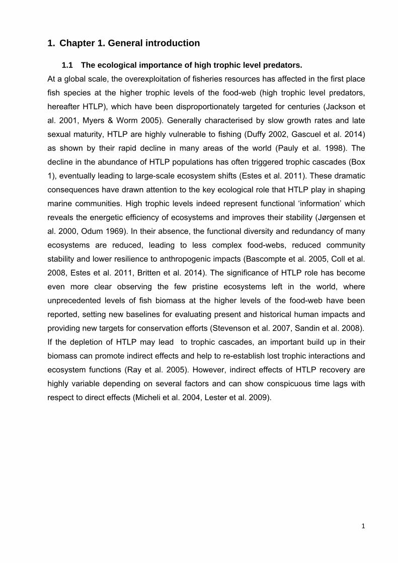
Trophic cinteractiotriggers Mediterrurchin provergrazovergraz(Sala et Prato & G

 

cascades arons, involvinthe release o

ranean rockyredators in thzed erect mzing inducedal.1998, GuGianni 2015

re indirect effng three or mof herbivoresy sublittoral, his basin, ca

macroalgal ad the shift fruidetti 2007).”, MMMPA p

 

BOX

fects of fishemore trophics and conseq

the overfishaused an incrassemblagesrom complex

Drawings frproject (see O

@ Celin

X 1. Trophic

ery removals c levels, whequently a dehing of sea rease in sea

s. In areas x macroalgarom the outreOutreach & C

ne Barrier

cascades

on the food-ere the remo

ecrease in prbreams (Di

a urchins abuwhere sea

al assemblageach video “Communicati

-web. They aoval of impoimary produciplodus spp.undance (Par

urchins couges to speci“The Book ofion) 

are describedortant carnivcers (Menge.), the most racentrotus luld reach hies-poor cor

of Marine Pro

d as predatovore predatoe 1995). In th

effective selividus), whicigh densitie

ralline barrenotected Area

2 

ry rs he ea ch es, ns as,

3  

1.2 High trophic level predators recovery in Mediterranean Marine Protected

Areas and related management challenges

In the last century, the Mediterranean was subject to an exponential increase in both

commercial fishing and coastal development, causing the overexploitation of most of its

fish stocks and the collapse of many of them (Colloca et al. 2013). Overfishing strongly

impacted Mediterranean food-webs, which are nowadays deprived of high trophic level

predators, with medium-sized fish like sea breams (Diplodus spp.) controlling ecosystem

shape (Box 1) (Sala 2004). Observation of the dramatic ecosystem shifts caused by

changes in the abundance of small and medium-sized predators, in some areas of the

Mediterranean, prompted reflections on the changes that food–webs must have

experienced over historical time frames after depletion of HTLP, and if recovery to a

former level is possible (Sala 2004).

Overfishing and the depletion of HTLP also affected traditional small-scale artisanal

fishing, a millenary activity depicted in ancient art catching fish almost the size of a man

at the water surface (Guidetti & Micheli 2011).

To face such situation, Marine Protected Areas (MPAs) have spread across the

Mediterranean, gaining wide acceptance as efficient tools contributing to an effective

ecosystem-based management strategy (Lubchenco et al. 2003). MPAs were indeed

established not only as a tool to conserve and restore biodiversity, but also to “achieve

the long term conservation of associated ecosystem services and cultural values”

(Dudley et al. 2008), thus seeking a balance between biodiversity protection and

continued human use (Abdulla et al. 2008). Several large-scale studies and global

synthetises have shown that MPAs allowed to increase the density and biomass of the

most commonly exploited species and reveal initial trajectories of ecosystem recovery

(Halpern & Warner 2002, Lester et al. 2009). When properly managed, Mediterranean

MPAs have also allowed to achieve remarkably large fish biomass compared to exploited

areas, highlighting the high potential of recovery of Mediterranean ecosystems (Sala et

al. 2012, Guidetti et al. 2014).

However, long-term observations from some of the oldest MPAs have shown that

abundances of HTLP are still increasing, denoting that long time frames are needed

before carrying capacity is reached (Micheli et al. 2004, Babcock et al. 2010, Garcia

Rubies et al. 2013).Long time frames are required also to observe indirect changes

triggered by HTLP recovery (Micheli et al. 2005), while most Mediterranean reserves are

young (established a few decades ago, at most). Long-term management strategies are

4  

thus needed to assess the evolution of MPAs along the observed trajectory of recovery,

but are often lacking in the Mediterranean (Garcia Rubies et al. 2013).

Furthermore, management of MPAs should go beyond the monitoring of a subset of

species of recognised ecological importance and should account for the complexity of the

food-webs they host. Unravelling trophic interactions is essential on one hand to assess

the recovery of ecosystem structure and functions (Libralato et al. 2010) and on the other

hand to understand and mitigate the influences that multiple human uses might have on

food-webs, allowing thus to anticipate or deal with ecosystem shifts (Sala 2004, Plagany

et al. 2014, Fulton et al. 2015).

1.3 Thesis objectives and approaches

The above considerations were further developed in the first publication arouse from this

PhD work and presented in the second chapter of the manuscript (Prato G, Guidetti P,

Bartolini F, Mangialajo L, Francour P (2013) The importance of high-level predators in marine protected

area management: Consequences of their decline and their potential recovery in the Mediterranean

context. Advances in Oceanography and Limnology 4:176–193). The paper was based upon a

literature review aimed at answering the following questions:

Are high-trophic level predators currently recovering in marine protected areas?

What are the indirect consequences of such recovery on the food-webs?

Are increasing levels of these predators a signal of increasing ecosystem health?

Addressing these issues was necessary to introduce the main questions which drove this

PhD thesis: if the fundamental role of high trophic level predators in shaping marine

communities and food-webs is finally acknowledged, as well as their leading position in

ecosystem recovery, how can we, in the context of an efficient MPA management:

Q1. effectively monitor high trophic level predators’ recovery?

Q2. unravel and monitor trophic interactions?

Q3. quantify fishing impacts upon HTLP and associated food-webs?

5  

Effective management of Mediterranean ecosystems needs to merge the two often

distant disciplines of field ecology and modelling (Pellétier et al. 2008). We thus coupled

both approaches in order to answer the above questions and ultimately provide useful

and cost-efficient tools for MPAs management.

Underwater visual census (UVC) surveys are to date the only possible non-destructive

approach to monitor the fish assemblage in Marine Protected Areas. A challenging

objective for both research and management is the development and implementation of

consistent UVC methods across the Mediterranean to assess the abundance of the

entire fish assemblage, accounting for the different mobility and behaviour of fish, from

the smallest crypto-benthic species to the large highly motile predatory fish. This is

essential to measure reliable relative values of high-trophic level predators increase and

assess variations in fish assemblage composition over time.

But field studies alone cannot aim at unravelling the complexity of food-web interactions,

an essential step to evaluate the indirect effects of several and often interacting human

impacts (Plaganyi et al. 2014, Fulton et al. 2015). Ecosystem models can help to shed

light on these issues. They are increasingly recognised as necessary tools to apply the

ecosystem approach to fisheries management (Espinoza-Tenorio et al. 2012), and are

more and more used for conservation purposes, i.e to design and holistically evaluate the

performance of Marine Protected Areas (Fulton et al. 2015). Food-web modelling in

particular is a useful tool to unravel trophic interactions and identify keystone species,

describe ecosystem structural traits, derive indexes of ecosystem maturity and

complexity and evaluate the consequences of several human impacts on the food-web

(Christensen & Walters 2004, Libralato et al. 2010, Heymans et al. 2014, Valls et al.

2015). The tropho-dynamic modelling approach Ecopath with Ecosim (Christensen &

Pauly 1992, Christensen & Walters 2004) and its more recent implementation EcoTroph

(Gascuel et al. 2009, 2011) fostered more than 400 applications across the world

(Colléter et al. 2015), addressing a multitude of issues related to both fisheries

management and conservation. However, EwE has not yet gained full attention as a

possible tool for the management of small coastal areas, and model applications in MPAs

are still few, especially in the Mediterranean (Coll & Libralato 2012). This scarcity is

largely due to the large amount of data needed to get reliable models and the associated

uncertainties on data precision. Issues of data availability and quality are particularly

accentuated in this naturally and geopolitically heterogeneous basin (Katsanevakis et al.

6  

2015), however, if reliable ecosystem models could be built in a cost-effective way, they

could provide useful information for the research and management of MPAs.

1.4 Structure of the manuscript In order to address the above mentioned challenges we adopted an integrative approach,

combining literature synthesis, field studies (Section 1) and theoretical and applied

modelling exercises (Section 2), which were alternatively applied in the following

chapters to face specific issues:

A literature review: to assess the state of the art on the importance of high trophic

level predators for MPAs management. (Chapter 2)

A semi-quantitative literature synthesis, integrated with a field survey: to identify

the most appropriate and cost-effective UVC method to survey the whole fish

assemblage. (Question 1, Chapter 3)

A field study: to i) evaluate the effectiveness of two UVC transect sizes to survey

large mobile predators (Question 1) and ii) combine three transect sizes to

assess the whole fish assemblage (Question 2 and 3, Chapter 4)

A theoretical modelling exercise: to identify an optimal Ecopath model structure

that considers trade-offs between feasibility of data gathering, complexity, and

uncertainty. (Question 2, Chapter 5)

An applied modelling exercise, based upon the integration of available local data:

to assess artisanal and recreational fishing impacts and conflicts on the food-web

associated with a NW Mediterranean MPA. (Question 2 and 3, Chapter 6)

An applied modelling exercise, based upon collection of new data in the field: to i)

unravel trophic interactions and identify keystone species to be monitored in a

data poor MPA and ii) evaluate the costs of building a standard trophic model in a

data poor MPA, following the guidelines for model structure and data collection

developed in chapter 5. (Question 2, Chapter 7)

7  

Overall results of this PhD work are synthetized and discussed in Chapter 8, and some

perspectives on the possible applications for MPAs management and on potential

avenues of research are presented

8  

1. Chapitre 1. Introduction générale français

1.1 L’importance écologique des prédateurs de haut niveau trophique

À l'échelle mondiale, la surexploitation des ressources halieutiques a surtout touché les

espèces de poissons des niveaux trophiques supérieurs dans les chaînes trophiques

(prédateurs de niveau trophique supérieur, ci-après HTLP), qui ont été ciblées de

manière disproportionnée pendant des siècles (Jackson et al. 2001 Myers et Worm

2005). Généralement caractérisés par des taux de croissance lents et une maturité

sexuelle tardive, les HTLP sont très vulnérables à la pêche (Duffy 2002, Gascuel et al.

2014), comme en témoigne leur rapide déclin dans de nombreuses régions du monde

(Pauly et al., 1998). Ce déclin d'abondance des populations de HTLP a souvent entraîné

des cascades trophiques (encadré 1), se traduisant souvent par des changements à

grande échelle des écosystèmes (Estes et al., 2011). Ces conséquences dramatiques

ont attiré l'attention sur le rôle écologique clé que les HTLP jouent dans la structuration

des communautés marines. Les hauts niveaux trophiques représentent en effet

l'information fonctionnelle qui témoigne de l'efficacité énergétique des écosystèmes et

améliore leur stabilité (Jørgensen et al. 2000, Odum 1969). En leur absence, la diversité

fonctionnelle et la redondance de nombreux écosystèmes sont réduits, se qui se traduit

par des réseaux trophiques moins complexes, une stabilité réduite de la communauté et

une plus faible résilience aux impacts anthropiques (Bascompte et al., 2005, Coll et al.

2008, Estes et al., 2011 , Britten et al. 2014).

La signification du rôle des HTLP est devenue encore plus claire en observant les rares

écosystèmes vierges encore existant dans le monde. Des niveaux sans précédent de

biomasse de poissons en haut du réseau trophique ont été rapportés, établissant de

nouveaux niveaux de référence pour l'évaluation actuelle et historique des impacts

humains et fournissant de nouveaux seuils à atteindre pour les efforts de conservation

(Stevenson et al. 2007, Sandin et al., 2008).

Si l'effondrement des HTLP peut conduire à des cascades trophiques, une accumulation

importante de leur biomasse peut promouvoir des effets indirects et aider à rétablir les

interactions trophiques perdues et les fonctions des écosystèmes (Ray et al., 2005).

Cependant, les effets indirects de la récupération des HTLP varient fortement en fonction

de différents facteurs et peuvent nécessiter plus de temps que les effets directs (Micheli

et al. 2004, Lester et al., 2009).

 

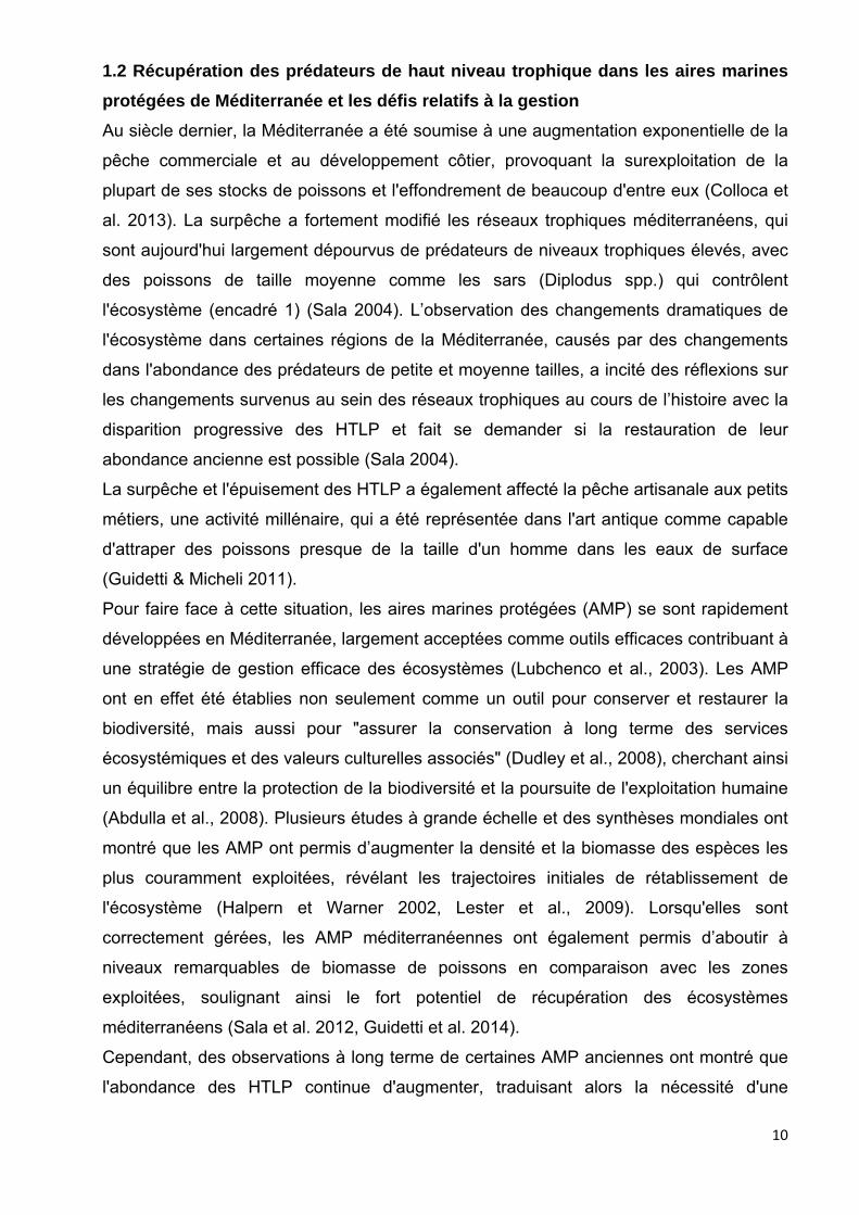
Les cascsont décsuppressconséqu, la suraugmentsurpâturatteignenlaissent Dessins 2015», p

cades trophiqcrits comme sion des p

uent, une dimpêche de station de l'a

rage des fornt des densplace à des extraits de

projet MMMP

ques sont lesdes interac

rédateurs cminution des sars (Diploduabondance rmations de sités élevéepeuplementsla vidéo de

PA (voir chap

Encadré

s effets indirctions de préarnivores improducteurs us spp.), ledes oursinsmacroalgue

s, les assems simplifiés, pe sensibilisatpitre Sensibil

@ Celin

é 1. Cascade

rects des préédation, impmportants e primaires (Ms prédateur

s de mer (es érigées. mblages initpauvres en etion "Le Livrisation et Co

ne Barrier

es trophique

élèvements dliquant trois ntraîne une

Menge, 1995rs d'oursins ParacentrotuDans ces ztiaux de maespèces (Sare des airesommunication

es

de la pêche sou plusieur

e augmentat5). En Médite

les plus effus lividus), zones de suacroalgues, la et al.1998

s marines prn)

sur le réseaurs niveaux trtion d'herbiverranée, en mfficaces, a pqui a alors

urpâturage ocomplexes

8, Guidetti 20rotégées, Pr

u trophique. Irophiques :vores et, pamilieu rocheuprovoqué uns entraîné uoù les oursinet diversifié

007). rato et Gian

9 

Ils la ar ux ne un ns és,

ni

10  

1.2 Récupération des prédateurs de haut niveau trophique dans les aires marines

protégées de Méditerranée et les défis relatifs à la gestion

Au siècle dernier, la Méditerranée a été soumise à une augmentation exponentielle de la

pêche commerciale et au développement côtier, provoquant la surexploitation de la

plupart de ses stocks de poissons et l'effondrement de beaucoup d'entre eux (Colloca et

al. 2013). La surpêche a fortement modifié les réseaux trophiques méditerranéens, qui

sont aujourd'hui largement dépourvus de prédateurs de niveaux trophiques élevés, avec

des poissons de taille moyenne comme les sars (Diplodus spp.) qui contrôlent

l'écosystème (encadré 1) (Sala 2004). L’observation des changements dramatiques de

l'écosystème dans certaines régions de la Méditerranée, causés par des changements

dans l'abondance des prédateurs de petite et moyenne tailles, a incité des réflexions sur

les changements survenus au sein des réseaux trophiques au cours de l’histoire avec la

disparition progressive des HTLP et fait se demander si la restauration de leur

abondance ancienne est possible (Sala 2004).

La surpêche et l'épuisement des HTLP a également affecté la pêche artisanale aux petits

métiers, une activité millénaire, qui a été représentée dans l'art antique comme capable

d'attraper des poissons presque de la taille d'un homme dans les eaux de surface

(Guidetti & Micheli 2011).  

Pour faire face à cette situation, les aires marines protégées (AMP) se sont rapidement

développées en Méditerranée, largement acceptées comme outils efficaces contribuant à

une stratégie de gestion efficace des écosystèmes (Lubchenco et al., 2003). Les AMP

ont en effet été établies non seulement comme un outil pour conserver et restaurer la

biodiversité, mais aussi pour "assurer la conservation à long terme des services

écosystémiques et des valeurs culturelles associés" (Dudley et al., 2008), cherchant ainsi

un équilibre entre la protection de la biodiversité et la poursuite de l'exploitation humaine

(Abdulla et al., 2008). Plusieurs études à grande échelle et des synthèses mondiales ont

montré que les AMP ont permis d’augmenter la densité et la biomasse des espèces les

plus couramment exploitées, révélant les trajectoires initiales de rétablissement de

l'écosystème (Halpern et Warner 2002, Lester et al., 2009). Lorsqu'elles sont

correctement gérées, les AMP méditerranéennes ont également permis d’aboutir à

niveaux remarquables de biomasse de poissons en comparaison avec les zones

exploitées, soulignant ainsi le fort potentiel de récupération des écosystèmes

méditerranéens (Sala et al. 2012, Guidetti et al. 2014).

Cependant, des observations à long terme de certaines AMP anciennes ont montré que

l'abondance des HTLP continue d'augmenter, traduisant alors la nécessité d'une

11  

protection à long terme avant que la capacité de charge de l’écosystème ne soit atteinte

(Micheli et al. 2004, Babcock et al. 2010, Garcia Rubies et al., 2013). Des délais

importants sont aussi nécessaires avant d'observer les changements indirects provoqués

par la récupération des HTLP (Micheli et al., 2005), alors que la plupart des réserves de

Méditerranée sont jeunes (créées il y a quelques décennies, tout au plus). Des stratégies

de gestion à long terme sont donc nécessaires pour apprécier le degré d'évolution des

AMP, mais elles font souvent défaut en Méditerranée (Garcia Rubis et al. 2013).

En outre, la gestion des AMP ne devrait pas se contenter de la surveillance d'un sous-

ensemble d'espèces même d'importance écologique reconnue mais doit tenir compte de

la complexité des réseaux trophiques qu'elles hébergent. Comprendre les interactions

trophiques est essentiel, d'une part pour évaluer la récupération de la structure et des

fonctions des écosystèmes (Libralato et al., 2010) et, d'autre part, pour comprendre et

atténuer les influences que les usages multiples pourraient avoir sur les réseaux

trophiques, permettant ainsi d'anticiper ou de traiter les changements de l'écosystème

(Sala 2004, Plagany et al. 2014, Fulton et al. 2015).

1.3 Objectifs et approches de la thèse

Les considérations ci-dessus ont été développées dans la première publication issue de

ce travail de thèse et sont présentées dans le deuxième chapitre du manuscrit (Prato G,

Guidetti P, Bartolini F, Mangialajo L, Francour P (2013) The importance of high-level

predators in marine protected area management: Consequences of their decline and

their potential recovery in the Mediterranean context. Advances in Oceanography and

Limnology 4:176–193). Le travail s'appuie sur une revue de la littérature et cherche à

répondre aux questions suivantes :

Est-ce qu’il y a actuellement une récupération des prédateurs de haut niveau

trophique dans les aires marines protégées ?

Quelles sont les conséquences indirectes de cette reprise sur les réseaux

trophiques ?

Est-ce que les niveaux croissants de ces prédateurs sont un signal de

l’amélioration de la santé des écosystèmes ?

12  

Aborder ces questions était nécessaire afin d'introduire les questions principales qui ont

motivé cette thèse : si le rôle fondamental des prédateurs de haut niveau trophique dans

la structuration des communautés marines et des réseaux trophiques est finalement

reconnu, ainsi que leur importance clé dans la récupération de l'écosystème, il faut alors

se demander, dans un contexte de gestion efficace des AMP, comment il est possible de

:

Q1. quantifier efficacement la récupération des prédateurs de haut niveau

trophique ?

Q2. comprendre et suivre les interactions trophiques ?

Q3. quantifier les impacts de la pêche sur les HTLP et les réseaux trophiques

associés ?

Une gestion efficace des écosystèmes méditerranéens nécessite de combiner deux

disciplines souvent éloignées : l'écologie de terrain et la modélisation (Pelletier et al.,

2008). Nous avons ainsi couplé ces deux approches afin de répondre aux questions ci-

dessus et, finalement, fournir des outils efficaces et utiles pour la gestion des aires

marines protégées.

Les comptages visuels en plongée sous-marine (UVC) sont à ce jour la seule approche

non destructive possible de suivi des peuplements de poissons dans les aires marines

protégées. Un objectif difficile à la fois pour la recherche et la gestion est le

développement et la mise en œuvre de méthodes cohérentes à l'échelle de la

Méditerranée, pour évaluer l'abondance de l'ensemble du peuplement de poissons. Ces

méthodes doivent prendre en considération les différences de mobilité et de

comportement des poissons, allant des petites espèces crypto-benthiques aux grandes

espèces de poissons prédateurs très mobiles. Cela est essentiel pour mesurer des

valeurs relatives fiables de l’augmentation de prédateurs de haut niveau trophique et

pour évaluer les modifications de la composition des peuplements de poissons au fil du

temps.

Mais les seules études de terrain ne peuvent pas suffire à démêler la complexité des

interactions des réseaux trophiques, une étape essentielle pour évaluer les effets

indirects de plusieurs impacts humains, qui souvent interagissent (Plagányi et al. 2014,

13  

Fulton et al. 2015). Les modèles écosystémiques peuvent contribuer à éclairer ces

questions. Ils sont de plus en plus reconnus comme des outils nécessaires pour

appliquer l'approche écosystémique aàa gestion de la pêche (Espinoza-Tenorio et al.

2012) et ils sont de plus en plus utilisés à des fins de conservation pour concevoir et

évaluer de manière holistique la performance d’aires marines protégées (Fulton et al.,

2015). La modélisation du réseau trophique en particulier est un outil utile pour

comprendre les interactions trophiques, identifier les espèces clés, décrire les

caractéristiques structurelles de l'écosystème, en tirer des indices de maturité et de

complexité de l'écosystème et pour évaluer les conséquences de plusieurs impacts

humains sur le réseau trophique (Christensen et Walters 2004, Libralato et al. 2010,

Heymans et al. 2014, Valls et al. 2015). L'approche de modélisation tropho-dynamique

Ecopath avec Ecosim (Christensen et Pauly 1992, Christensen et Walters 2004), et plus

récemment EcoTroph (Gascuel et al. 2009, 2011) a été utilisée plus de 400 fois à travers

le monde (Colléter et al. 2015), en abordant une multitude de questions liées à la fois à la

gestion des pêches et à la conservation. Cependant, Ecopath n'est pas encore reconnu

comme un outil possible de gestion des petites zones côtières et les applications de tels

modèles dans les AMP sont encore peu nombreuses, notamment en Méditerranée (Coll

& Libralato 2012). Cette rareté est en grande partie due à la grande quantité de données

nécessaires pour obtenir des modèles fiables et aux incertitudes associées à la précision

des données. Les questions de la disponibilité et de la qualité des données sont

particulièrement accentuéers dans ce bassin naturellement et géopolitiquement très

hétérogène (Katsanevakis et al. 2015). Cependant, si des modèles écosystémiques

fiables pouvaient être construits d'une manière efficace, ils pourraient fournir des

informations utiles pour la recherche et la gestion des AMP.

1.4 Structure du manuscrit

Afin de relever les défis mentionnés ci-dessus et répondre aux questions posées, nous

avons adopté une approche intégrative, combinant des synthèses de la littérature, des

études de terrain (Section 1) et des exercices de modélisation théoriques et appliqués

(Section 2) à travers les chapitres suivants :

Une revue de la littérature : pour évaluer l'état de l'art sur l'importance des

prédateurs de haut niveau trophique pour la gestion des aires marines protégées.

(Chapitre 2)

14  

Une synthèse de la littérature semi-quantitative, intégrée à un travail de terrain :

pour identifier la méthode UVC la plus appropriée et rentable de quantification de

l'ensemble du peuplement de poissons. (Question 1, chapitre 3)

Une étude de terrain : pour i) comparer l'efficacité de deux largeurs de transects

UVC dans l'étude des grands prédateurs mobiles (question 1) et ii) combiner trois

largeurs de transects pour évaluer l'ensemble du peuplement de poissons

(Question 2 et 3, chapitre 4)

Un exercice de modélisation théorique : pour identifier une structure de modèle

Ecopath optimal permettant un compromis entre la faisabilité de la collecte de

données, la complexité du modèle et l'incertitude des résultats. (Question 2,

chapitre 5)

Un exercice de modélisation appliquée fondé sur l'intégration des données locales

disponibles : pour évaluer les impacts et les conflits de la pêche artisanale et de

loisir sur le réseau trophique d'une AMP en Méditerranée nord-occidentale.

(Question 2 et 3, chapitre 6)

Un exercice de modélisation appliquée, sur la base de la collecte de nouvelles

données sur le terrain : pour i) décrire les interactions trophiques et identifier les

espèces clés à surveiller dans une AMP pauvre en données ii) évaluer les coûts

de construction d'un modèle trophique standard dans une AMP pauvre en

données, en suivant les lignes directrices développées dans le chapitre 5 pour la

structure du modèle et la collecte de données. (Question 2, chapitre 7)

Les résultats de cette thèse sont synthétisés et discutés dans le chapitre 8 et quelques

perspectives sur les applications possibles en terme de gestion des aires marines

protégées et sur les développements à venir possibles en recherche sont présentées.

15  

2 Chapter 2. The importance of high-level predators in marine protected area management: Consequences of their decline and their potential recovery in the Mediterranean context.

 

Prato G1, Guidetti P1, Bartolini F1, Mangialajo L1, Francour P1 (2013)

1 Université de Nice-Sophia Antipolis, EA 4228 ECOMERS, Parc Valrose, 06108 Nice Cedex 2, France

Published in Advances in Oceanography and Limnology 4:176–193

   

The importance of high-level predators in marine protected area

management: Consequences of their decline and their potential

recovery in the Mediterranean context

Giulia Prato*, Paolo Guidetti, Fabrizio Bartolini, Luisa Mangialajo and Patrice Francour

Universit�e de Nice Sophia-Antipolis; Facult�e de Sciences, EA 4228 ECOMERS,06108 Nice cedex 2, France

(Received 27 March 2013; accepted 3 September 2013)

High-level predators have been depleted in the oceans worldwide following centuriesof selective fishing. There is widespread evidence that high-level predators’ extirpa-tion may trigger trophic cascades leading to the degradation of marine ecosystems.Restoration of large carnivores to former levels of abundance might lead to ecosystemrecovery, but very few pristine ecosystems are left as baselines for comparison.

Marine protected areas (MPAs) can trigger initial rapid increases of high-levelpredator abundance and biomass. Nevertheless, long term protection is needed beforethe ecosystem’s carrying capacity for large carnivores is approached and indirecteffects on lower trophic levels are observed.

The Mediterranean is probably very far from its pristine condition, due to a longhistory of fishing. Today small to medium-sized consumers (e.g. sea breams) are themost abundant predators shaping coastal benthic communities, while historical recon-structions depict abundant populations of large piscivores and sharks inhabitingcoastal areas. Mediterranean MPAs are following a promising trajectory of ecosystemrecovery, as suggested by a strong gradient of fish biomass increase. Consistent moni-toring methods to assess relative variations of high-level predators, together withfood-web models aimed at disentangling the indirect effects of their recovery, couldbe useful tools to help set up appropriate management strategies of MPAs.

Keywords: high-level predator; top predator; trophic cascades; MPAs; ecosystemshift; overfishing; baseline; ecosystem recovery

1. Introduction

High-level predators, a category including top predators, are generally large-sized long-

living animals like marine mammals, sharks and large teleosts that occupy the higher tro-

phic levels in the food web. They are commonly characterized by late sexual maturity

and their abundance, at adult stage, is usually not subject to predator control. Together

these characteristics result in low resilience to demographic perturbation and high risk of

extinction, conditions making them highly vulnerable to fishing [1]. In a number of

regions worldwide, their almost complete extirpation from marine ecosystems is a direct

consequence of fishing that has disproportionately targeted them for centuries [2,3].

Today we face a situation where almost no pristine marine ecosystems are left and where

historical information on pre-exploitation abundance of high-level predators is very rare.

In many places, high-level predators have been absent or rare for so long that scientists

and managers have never realized how important they were in the ecosystem. In this con-

*Corresponding author. Email: giulia.prato@unice.fr

� 2013 Taylor & Francis

Advances in Oceanography and Limnology, 2013

Vol. 4, No. 2, 176–193, http://dx.doi.org/10.1080/19475721.2013.841754

Dow

nloa

ded

by [

Giu

lia P

rato

] at

08:

19 2

1 N

ovem

ber

2013

text a clear understanding of their ecological role is limited by the fact that our observa-

tions are restricted to already altered ecosystems, affected by the decline and, in some

cases, disappearance of top predators. Historical data from coastal ecosystems are more

abundant and suggest that losses of large predatory fish and mammals were especially

pronounced here and led to marked changes in coastal ecosystems structure and function

[2]. In fact, the fauna of predators we have today in many coastal ecosystems is a ‘ghost’

[4] of what it was before human impacts. Such ecosystems nowadays are often controlled

by medium-sized predators, although larger carnivores originally preying upon them

likely controlled the trophic web in the past [5]. In terrestrial ecosystems, medium-sized

predators have sometimes replaced top predators: i.e. coyotes are mesopredators where

wolves have been reintroduced, while they have ascended to the role of apex predators

where larger predators have been extirpated [6–8]. Due to this possible shift between mes-

opredators and apex predators, we will here use the term ‘top predator’ to qualify the

highest level trophic category of predators.

Management of marine ecosystems should consider how they looked in the presence

of top predators to be able to set meaningful conservation targets. The Mediterranean is

an especially interesting area in this context. This sea has a history of thousands of years

of exploitation. In fact, the first evidence of fishing in the shallow Mediterranean comes

from prehistory, with the Mediterranean dusky grouper being among the target fishes

fished for more than 10,000 years and the blue fin tuna, being an important part of Medi-

terranean culture for 12,000 years, for millennia exploited by many coastal artisanal fish-

eries [9]. Apparently first local fish depletions started during Roman times [10], due to

rising human population and food demand. During medieval times, strong human popula-

tion growth resulted in the depletion of fisheries in coastal waters [11]. In the late nine-

teenth century fishing capacity grew exponentially and in the twentieth century it

expanded offshore and to deeper waters. Today most, if not all, of Mediterranean impor-

tant stocks are overexploited and this sea is very far from the pristine condition depicted

in antiquity.

Here we will analyse the reasons that stand for the largely accepted hypothesis

that high-level predators have an important ecological role in shaping marine communi-

ties, as shown by empirical observations on the far reaching impacts caused by

their depletion, which is especially heavy in coastal ecosystems. Subsequently, we will

review the effects of Marine protected areas (MPAs) implementation, in terms of high-

level predator recovery and their impact on food webs. We will specifically focus on

the Mediterranean region, signed by the previous extinction of many top predators and

by a general lack of historical data. As a conclusion we will try to answer the following

questions: are high-level predators currently recovering in marine protected areas?

What are the indirect consequences of such a recovery? Are increasing levels of

these predators a good signal of increasing ecosystem health? We will finally suggest

possible ways to overcome the general lack of data and knowledge on high-level

predators.

2. The importance of high-level predators

2.1 Trophic cascades and pristine ecosystems

In a seminal paper published in 1960, Hairston, Smith and Slobodkin proposed that preda-

tors have the potential to maintain global plant biomass by limiting the densities of herbi-

vores (‘The world is green’ hypothesis) [12]. For the first time, it was stated that

Advances in Oceanography and Limnology 177

Dow

nloa

ded

by [

Giu

lia P

rato

] at

08:

19 2

1 N

ovem

ber

2013

predators at the upper trophic levels might control the abundance of consumers and pri-

mary producers at lower trophic levels.

Following the ‘The world is green’ revolution, the idea that ecosystems might be

shaped by apex predators stimulated several avenues of research.

In 1966 Paine stated the hypothesis that ‘local species diversity is directly related to

the efficiency with which predators prevent the monopolization of the major environmen-

tal requisites of one species’. Paine experimentally demonstrated that the removal of the

apex sea star predator Pisaster ochraceus from the rocky intertidal (Pacific Coast of North

America) resulted in a pronounced decrease in diversity, with local extinctions of certain

benthic invertebrates and algae due to outcompetition from more efficient space occupiers

(mussels) [13]. This was one of the first experimental evidences about the role of a key-

stone predator and showed that in communities controlled by the natural predation of a

top predator, the sea star, prey abundances were controlled and local diversity was higher.

The strength of carnivore effects generally depends on the strength of the link

between the predator and its prey [14] and often relates to the predator’s body size [15].

In a system of strongly interacting links, large top predators frequently initiate the top-

down control leading to indirect effects on food webs (i.e. trophic cascades) [16].

Clearly, experimental demonstration is logistically impractical for large animals.

What we observe today in marine systems is a situation of generalized absence of large

top predators, which have long been reduced or extirpated from much of the world

[2,17,18] and whose depletion has triggered trophic cascades that sometimes led to dra-

matic ecosystem shifts. Trophic cascades are generally a signature of the vast and grow-

ing human impact on natural systems and since the 1960s they have been demonstrated in

a wide variety of systems, as witnessed by the number of reviews written on the subject

[18–22].

A review from the end of the 1990s [19] provided evidence that trophic cascades were

no longer limited to sole simple systems like lakes, streams and intertidal zones, as previ-

ously reported [23]. Discoveries of trophic cascades were reported from previously unex-

pected systems, such as the open ocean, tropical forests, fields, and soils. The amplitude

of such phenomenon was assessed in several benthic marine ecosystems [20], showing

that trophic cascades range from Mediterranean rocky sublittoral, kelp forests and rocky

subtidal to coral reefs, rocky intertidal and soft bottoms. A comparison of six different

ecosystems, demonstrated that trophic cascades were strongest in lentic and marine ben-

thos and weakest in marine plankton and terrestrial food webs [21]. Evidence of oceanic

top-down control from large high trophic level piscivores was also found [22]. Substantial

marine mammal, sharks and large piscivorous fish depletions led to mesopredator and

invertebrate predator increases and in some cases to trophic cascades negatively impact-

ing commercial species. A more recent empirical study on top predators [18] revealed the

unanticipated impacts of trophic cascades on processes as diverse as the dynamics of dis-

ease, wildfire, carbon sequestration, invasive species, and biogeochemical cycles defining

the loss of these animals as humankind’s most pervasive influence on nature.

When fishery data or ecologists’ observations are available from a time when top

predators were still present, the far reaching impacts of high-level marine carnivore

depletion on the ecosystem appear clear.

One of the most well studied examples of such phenomena comes from the Aleutian

Islands, where variations in sea otter abundances due to overfishing and subsequent pro-

tection have been responsible for dramatic variations of sea urchin population density.

These changes have determined the alternation between the natural kelp forest systems

and the impoverished condition of overgrazed rocky reefs. Moreover, diet switching of

178 G. Prato et al.

Dow

nloa

ded

by [

Giu

lia P

rato

] at

08:

19 2

1 N

ovem

ber

2013

killer whales in this area and subsequent increased predation on sea otters has demised sea

urchins from otter predation ultimately causing the destruction of kelp forests [24,25].

The depletion of cod (Gadus morhua) followed by the shifting of the fishery to lower

trophic levels (fishing down the food web [26]) caused a transition towards a kelp forests

ecosystem that superficially looked like its initial state, but de facto was very different

[5]. The ecological extinction of cod in Canadian coastal zones led to dramatic increases

in sea urchin populations, which overgrazed kelp forests leaving widespread barrens [27].

The subsequent shift of the fisheries towards sea urchins allowed kelp forests to recover

[28]. The combination of abundant kelp without high-level predators was ideal for a pop-

ulation increase of the predatory crab Cancer borealis [29]. Today this mesopredator

crab is the dominant species of the ecosystem and is only limited by the availability of

nursery habitats (bottom-up control), as opposed to predation on adults (top-down

control) [5].

Sharks are one of the largest predators in the oceans, generally foraging on large

areas. Today they are still subject to catch and mortality rates that are far exceeding

the estimated rebound rates for many populations, causing their worldwide decline and

the consequently relevant ecological consequences [30,31]. In some cases (New England,

South Africa) the dramatic depletion of large sharks has resulted in the proliferation of

smaller elasmobranchs, of which large sharks were the sole predators, and the decline of

bony fish at lower levels in the food web [22].

The diversity of species within each trophic level is a type of insurance against the

disruption of the ecological functions that species assemblages perform [32]. A long his-

tory of fishing down the food web has left Caribbean coral reefs with low species diver-

sity and few functional players at each trophic level (low functional redundancy) [21].

Predators such as sharks, large groupers and snappers have been extirpated from many

reefs and many herbivorous fish have been removed by selective fishing. Thanks to the

reduction in population density and the size of its predators and competitors, the sea

urchin Diadema antillarum was left as the primary herbivore in this system. The very

high abundance of Diadema favoured the explosion of a disease that induced mass mor-

tality of urchins in the 1980s, with resulting uncontrolled macroalgal growth and over-

competition on hard corals. This was one of the world’s most rapid and widespread shifts

in community state ever documented [5,33]. This shift was probably possible because of

the historical overfishing and consequently reduced low functional redundancy of

Caribbean reef communities, a condition that negatively affected the resilience of this

ecosystem to catastrophic and unpredictable events [34,35].

In many areas only medium–upper trophic level predators are left to control the eco-

system, since their original predators have long been depleted. These are today the main

fishing target and are subject to strong fishing pressures. In Kenyan coral reefs, the main

keystone species we can identify today is the triggerfish (Balistapus undulates), the single

most important predator of sea urchins. Where this fish is overfished, sea urchin densities

largely increase and turf filamentous algae overgrow corals bioeroded by the sea urchins’

grazing activity. Sea urchins can outcompete important grazer fish such as parrotfishes

and hard corals cover decreases sharply [36–39].

Deleterious effects of sea urchin predator depletion have been observed also in the

Canary Islands, where it has been demonstrated that losses in the diversity of predatory

fish species lead to a loss of functional roles and cascading effects that constrain ecosys-

tem processes, leading to the spread of barren grounds [40].

Although the last mentioned species are not top predators, examples of their effects on

the ecosystem need to be mentioned in order to imagine the role that previously abundant

Advances in Oceanography and Limnology 179

Dow

nloa

ded

by [

Giu

lia P

rato

] at

08:

19 2

1 N

ovem

ber

2013

and larger top predators probably had. In fact, if removing a few species of small scale

fishes can change the underwater landscape so dramatically, it is unavoidable to ask one-

self what were the consequences of removing large predators from such ecosystems [41]

and how these looked in their presence.

There are very few examples left in the world of pristine ecosystems but their obser-

vation has provided fundamental information on the shape of an ecosystem in the pres-

ence of top predators.

The observation of Shark Bay, Australia, a remote subtropical location characterized

by healthy sea grass communities and large population sizes of many large-bodied taxa

[42], released important information on the role of tiger sharks as top predators. It was

demonstrated that tiger sharks have widespread risk effects on both large-bodied herbi-

vores and mesopredators (sea turtles, dolphins, dugongs, pied cormorants). Behaviour-

mediated cascades leading to effects on the micro-habitats of the area have been sup-

posed. In fact risk-induced heavy grazing by large herbivores led to reduced seagrass

quality in habitats of lower incidence of tiger sharks, and increased quality in areas of

higher shark abundance.

Recent studies revealed the structure of two pristine ecosystems, the Palmyra and

Kingman atolls in the Line Islands (central Pacific) and the North Western Hawaiian

Islands [43–46]. At both locations large high-level predators (specifically large piscivo-

rous snappers, groupers, carangids and sharks) account for 55% to 85% of total fish bio-

mass, with sharks accounting for 57% and 74% of total piscivore biomass in the Line

Islands. Despite enhanced predation, high biomass of herbivores is also supported by the

coral reefs, together with higher coral cover when compared to nearby fished islands of

the same archipelago [46].

The Palmyra and Kingman atolls and the North Western Hawaiian Islands ecosystems

have been described as characterized by an inverted trophic pyramid with most fish bio-

mass at top levels, a structure that, due to historical overfishing of our oceans, had never

been observed before by ecologists. Even if the existence of inverted pyramids has

recently been questioned due to size-based constraints [47], it is undeniable that these

pristine ecosystems set new baselines for evaluating present and historical human impacts

and provide new targets for MPA conservation efforts.

2.2 High-level predators in the Mediterranean: historical

reconstruction and degradation

The actual state of the Mediterranean is characterized by a paucity of high-level preda-

tor species both in richness and abundance and with medium-sized fish like sea breams

left alone to control ecosystem shape. In fact the Mediterranean harbours a classical

example of a trophic cascade controlled by a medium-sized fish [48]. Here the rocky

sublittoral is characterized by the shift between a developed community with high fish

and macroalgal biomass (e.g. Cystoseira forests, the Mediterranean ‘kelp’) and an over-

grazed community with high abundance of sea urchins and low algal biomass (e.g.

encrusting coralline algae and barren grounds). It has been largely demonstrated that

overfishing of sea breams (Diplodus spp.), the most effective sea urchin predators in

the Mediterranean, led in many areas to large increases in sea urchin population densi-

ties with consequent algal overgrazing and shift to low diversity coralline barrens

[49,50].

Our understanding of Mediterranean food webs is actually based on a mix of unnatu-

ral, simplified communities, dominated by small species, where megafauna has been

180 G. Prato et al.

Dow

nloa

ded

by [

Giu

lia P

rato

] at

08:

19 2

1 N

ovem

ber

2013

virtually eliminated by overfishing. [2,17,41]. This impoverished state is supposedly very

far from the pristine conditions.

In fact, the Mediterranean has not been pristine since long before the onset of indus-

trial fishing, but it is signed by a millenary history of exploitation, thus it is very difficult

to evaluate the current state of this sea. Historical reconstructions have proved to be a use-

ful strategy to fill this gap for many ecosystems, as already reviewed by several authors

[51,52], but they are still scarce in the Mediterranean.

Archaeozoological reconstructions based on the study of fish bone remains (i.e. oste-

ometry) allowed investigation of the history of fishing in times preceding the advent of

writing. The data have revealed how Mediterranean shallow waters were once dominated

by large sized piscivores which attained much bigger sizes than nowadays [53]. Desse

and Desse-Berset proposed that these observations allow us to chronologically set the

beginning of overexploitation [53].

The analysis of a large amount of fish bones recovered from a Neolithic coastal site of

Cap Andr�eas Kastros, Cyprus, revealed evidences of early exploitation of pristine popula-tions. Here selective fishing conducted from the coast was directed to large specimens of

tunas and groupers [54]. Similarly, other Neolithic coastal Mediterranean sites revealed

large specimens, attaining sizes that are not comparable with the mediocre dimensions of

fish captured by fishermen today [53]. Fish remains from a Spanish cave revealed how

fish fauna diversity and size decreased over the last 12,000 years [55]. Osteometry studies

also revealed the presence of almost locally extinct species, such as the sturgeon (Aci-

penser sturio), and some elasmobranch species that appear to have been very abundant in

coastal waters, contrary to the current situation.

Until the end of the Mesolithic and during Neolithic eras the groupers were very

abundant in the coastal systems between the 35th and 40th parallel, accounting for 30–

80% of the examined bony remains. Sites in Spain, Tunisia, Corse, Cyprus, Sicily and

other Italian sites revealed the presence of healthy populations of Epinephelus spp., with

all size ranges represented [56].

Anecdotal research has also led to very interesting discoveries on this topic. A survey

of ancient Greek, Etruscan and Roman mosaics and paintings depicted large groupers

often reaching the size of a man, being caught at the water surface by fishermen using

poles or harpoons from boats, a technique that would yield no grouper catch today [57].

As illustrated in ancient frescoes many Mediterranean top predators (e.g. dolphinfish

Coryphaena hippurus) may have been all actively fished in antiquity [51].

An especially striking implication of these studies is that not only in ancient times

much larger individuals were commonly fished, but that their abundance in coastal waters

was high, allowing humans to fish them directly from land [57] or from little boats [57].

Current groupers’ bathymetric distribution shows well how populations actively respond

to human exploitations. Largest individuals of this species indeed find refuge at depths

that exceed the diving limit of most of the recreational spearfishermen [53,58,59].

A recent study coupling historical reconstruction and modelling delivered a detailed

account of successive waves of fish depletions in the Adriatic sea and shows well the tra-

jectory of degradation undergone by the Mediterranean ecosystem [10]. Marine mammals

at the top of the food web were largely common in antiquity and have been depleted or

are very rare today. The common dolphin (Delphinus delphis), bottlenose dolphins and

the monk seal were hunted in classical Greek, Roman and medieval times and are today

ecologically extinct in almost all the Mediterranean Sea.

Predilection for tuna, sharks, rays, sturgeons, common bass, sea bream and hake on

Roman and Greek tables led to a large increase in their exploitation. Bluefin tuna fishery

Advances in Oceanography and Limnology 181

Dow

nloa

ded

by [

Giu

lia P

rato

] at

08:

19 2

1 N

ovem

ber

2013

was coastal, subsistence and small scale for millennia. Industrial overexploitation proba-

bly started around 1950 with open water purse seining substituting coastal trap fisheries.

Today the Atlantic-Mediterranean bluefin tuna stock is considered overfished. Similar

fate touched the swordfish and the demersal high-level predator Merluccius merluccius.

Common dentex (Dentex dentex) and common Pandora (Pagellus erythrinus) are today

considered depleted and the dusky grouper (Epinephelus marginatus) may be locally

extinct [10]. Lotze’s results show that large predators and consumers >1 m in length

were reduced to 11% of former abundance, a far more drastic reduction than smaller mac-

rofauna (47%), especially in the last century.

As a result, a process of trophic downgrading [18] was observed in the Adriatic [10],

with diversity shifting towards smaller, lower trophic level species. Increased exploitation

and functional extinctions have altered and largely simplified food webs by changing the

proportions of top predators, intermediate consumers and basal species.

Sharks, rays and chimaeras, are by far the most endangered group of marine fish in the

Mediterranean Sea, with 31 species (40% of all) critically endangered, endangered or vul-

nerable [60]. Another detailed historical reconstruction concerned large predatory sharks

in the Northwestern Mediterranean Sea, using a diverse set of historical records dating

back to the early nineteenth and twentieth centuries [61]. Records from the 1920s–1930s

showed that the Mediterranean Sea sustained abundant populations of large sharks, regu-

larly targeted by many coastal fisheries. The analysed species, mackerel sharks (I. oxyrin-

chus and Lamna nasus), requiem shark (Prionace glauca), hammerhead shark (Sphyrna

zygaena), and thresher shark (Alopias vulpinus), showed rates of decline up to 99.99%,

levels at which they can be considered functionally extinct in coastal and pelagic waters

of the Northwestern Mediterranean Sea. Trends of biomass data also showed a significant

reduction in mean size over time, which is the lowest in the world [62].

In addition to large predatory sharks and bony fishes, other top predators like ceta-

ceans and the monk seal underwent extreme declines due to a variety of human impacts

[63,64].

A concluding remark could be that wherever high-level predators have been extir-

pated, ecosystems have consequently become degraded and simplified [65]. It is then

plausible to assume that a return of high-level carnivores to a system will allow degraded

systems to recover [16]. A tempting question is whether conservation of these predators

could restore biodiversity and ecological functioning [16]. The science of marine reserves

can give insights on this potential.

3. Recovery of high-level predators and biodiversity within

marine protected areas

3.1 Data from the world

Several studies have demonstrated that marine reserves are an effective tool for the recov-

ery of large piscivorous fish and upper trophic levels (direct effects), but have also shown a

large variability of effects in terms of triggered trophic cascades (indirect effects). In fact,

while in some temperate ecosystems it was possible to demonstrate that recovery of high-

level predators (sea otters, snappers, spiny lobster, sea bream) can lead to the re-establish-

ment of lost trophic interactions (e.g. sea urchins and macroalgae) [66,67], in more diverse

ecosystems like coral reefs a more variable response is observed, depending on conditions

such as duration of protection, taxonomic resolution of the study (species or functional

group) and possible compensation effects due to functional redundancy [67–76].

182 G. Prato et al.

Dow

nloa

ded

by [

Giu

lia P

rato

] at

08:

19 2

1 N

ovem

ber

2013

Recent meta-analytical studies give a useful global overview of marine reserve pro-

tection effects in terms of recovery of upper trophic levels and trophic changes.

A global meta-analysis based on data from 124 reserves demonstrated that protection

yielded significant average increases of density, biomass, average organism size and spe-

cies richness of the communities within reserves [77]. Differential responses were

observed among taxonomic groups, with large fish and invertebrates targeted by fishing

showing significant increases in density and biomass overall, while algal cover increased

in temperate reserves and decreased in tropical reefs, due to the recovery of exploited

large herbivores.

Through the analysis of long term time series of ecological data in and out of marine

reserves from several regions, it was demonstrated that positive effects on target preda-

tory fish and lobsters occurred rapidly after reserve establishment but continued to

increase, in some cases up to 25–40 years after protection (respectively Serranide and

Lutjaniae in the Apo islands and triggerfish in Kenyan reserves) [78]. This analysis

showed that the ecosystems were still generally far away from their carrying capacity in

terms of high-level predators. Large herbivorous fish showed decadal increases in abun-

dance too. Indirect effects through trophic cascades were common especially in terms of

sea urchin reductions, but showed conspicuous time lags (average 13 years after protec-

tion) with respect to direct effects, probably due to behavioural mechanisms of predation

risk reduction [78].

Similar conclusions on the magnitude and timing of protection effects were drawn

from a meta-analysis of data from several temperate and tropical locations [79]. The

authors observed clear trophic changes in protected ecosystems due to a time lasting

build-up of biomass and abundance of upper trophic levels. Indirect negative effects were

also evident for low mobility, small sized, and non-target fish species.

Other meta-analytical studies revealed that commercial species including many top

predatory fish were observed to increase in density in many southern Europe MPAs

[80,81]. Response of commercial exploited fishes to protection depended on species max-

imum body size, with large species showing the strongest increase in MPAs. Moreover

the response of large species increased with time of protection. Commercial exploited

fish with a benthic habitat responded positively to protection, while exploited fish with a

bentho-pelagic habitat did not show a demonstrable response to protection. For non-

commercial unexploited fish with a benthic habitat, densities were higher inside the

reserve, probably because positive effects in habitat changes were more important than

possible negative trophic cascade effects [80,81]. On the other hand, densities were higher

outside the reserve for bentho-pelagic non-exploited species, suggesting possible trophic

cascade effects due to predator increases.

A crucial question is whether MPAs are able to protect and restore species performing

key ecological functions, but remarkably few studies have evaluated functional recovery

after habitat degradation [82]. An interesting study in this regard reported that recovery

of species richness and diversity in marine reserves coincided with increases in functional

richness and diversity of fish assemblages [83]. Species recovery in reserves resulted in

increased representation across different functional categories, particularly key groups

like large carnivores and herbivores.

Thus reserves reveal initial trajectories towards recovery, but if compared with the

few studied pristine ecosystems, it appears clear that the levels of piscivore biomass

observed in recent marine reserves across the world are well below what the ecosystems

could sustain. Moreover, for indirect changes to occur in marine reserves an absolute

increase in abundance, mean size or biomass of target species, i.e. a restoration or build

Advances in Oceanography and Limnology 183

Dow

nloa

ded

by [

Giu

lia P

rato

] at

08:

19 2

1 N

ovem

ber

2013

up to some (unknown) former level, is necessary [78,84]. Management of marine reserves

should thus acknowledge that the potential for recovery of ecosystem functioning through

protection is high, but will likely require long time frames [76,78,84]. In this context

long-term monitoring is necessary and needs to be carried out for long enough lapses of

time to have the chance to detect indirect effects. Special attention should be paid to var-

iations in high-level predator biomass, a variable that can yield useful information on the

state of recovery of a system following protection.

3.2 Mediterranean marine protected areas

Mediterranean MPAs, when well enforced [85], have shown to be very effective in lead-

ing to increases in the biomass and diversity of large piscivorous and invertebrate feeding

fish, especially for serranids, sciaenids, sparids, and the larger labrids [50,58,84, 86–96],

as also reviewed in [97].

Due to Mediterranean food web complexity the indirect effects of predator recovery

are often masked by many factors, such as local conditions of oceanography, habitat

topography and complexity (presence of refuges for prey species) and intensity of fishing

outside the reserve. As in the rest of world, moreover, indirect effects can occur with con-

siderable time lags with respect to direct effects [98].

Variable results have been drawn from the observation of indirect protection effects.

In the Scandola Marine Reserve lower abundance and species richness of macrozooben-

thos were observed [99] where predators attained higher abundance compared to nearby

unprotected sites [88]. At the Ustica Marine Reserve, increases in piscivores (groupers)

coincided with a decrease of small size microcarnivorous fish [58,100] and a seasonal

increase of abundance and species richness of polychaetes and gasteropods [101,102].

Even with regard to the strong trophic interaction sea breams – sea urchin – algae [82],

somewhat contradictory results have resulted on the potential for recovery of algal beds

in MPAs through sea bream protection [49,92,98]. In fact, densities of fish need to reach

a critical threshold in order to reduce sea urchins and drive the transition [50]. It has been

demonstrated that when a protected area has the proper physical and biological character-

istics (appropriate habitat for sea breams, as well as dimension and duration of protection

encompassing their mobility and life cycle) to trigger changes at population and/or com-

munity levels, it allows the recovery of the predatory sea bream population, and the re-

establishment of predatory control upon sea urchins, as happened in the Torre Guaceto

MPA [92]. In the protected zone of Torre Guaceto, moreover, coralline barrens were less

extended whereas turf forming and erect-branched algae showed an opposite pattern.

Due to the absence of pristine sites left in the Mediterranean and the few quantitative

historical data to set a baseline against which to compare the health of current ecosystems

and set precise conservation targets, comparisons among marine protected areas of differ-

ent age, or between MPAs and fished sites (space for time substitutions) have shown to

be useful in setting some reference points.

A recent large-scale study covering several MPAs and fished sites across the Mediter-

ranean revealed a trajectory of degradation and recovery, with high-level predator bio-

mass being significantly larger at protected than at non protected sites [96]. A gradient of

31-fold range increase in fish biomass was observed, reaching a maximum of 115-fold.

This is the largest fish biomass gradient ever reported for reef fish assemblages and is

probably indicative of the large impact of historical and current fishing pressure in the

Mediterranean [96]. Continuous increase of high-level predators (particularly groupers)

at the Medes islands, where they reached 49% of fish biomass after 27 years of

184 G. Prato et al.

Dow

nloa

ded

by [

Giu

lia P

rato

] at

08:

19 2

1 N

ovem

ber

2013

protection, show that the potential for recovery in Mediterranean MPAs is comparable to

other parts of the world and that aiming at achieving fish biomass values similar to those

observed in the pristine tropical systems is possible. The authors finally suggest how the

marine reserves with highest fish biomass are a useful current baseline against which

managers can compare recovery trends for fish assemblages in rocky habitats across the

Mediterranean. No clear pattern in the structure of benthic community was associated

with the gradient on fish biomass, but three alternative community states were revealed in

the trajectory of recovery: large fish biomass and reef dominated by non-canopy algae,

lower fish biomass but abundant algal canopies and suspension feeders, and low fish bio-

mass and extensive barrens.

The functional approach is still rare in the Mediterranean. Spanish marine pro-

tected areas were shown to support higher functional diversity than adjacent

unprotected sites, due to a difference in the trophic structure rather than in species

diversity [103]. High-level predators contributed the most to the dissimilarity between

protected and unprotected sites. Coupling a functional approach with food web model-

ling it was also found that protected areas support higher trophic levels and are char-

acterized by more complex food webs than exploited areas [104]. Finally it was

demonstrated that the Lavezzi Islands Reserve significantly protects functional origi-

nality (‘original’ species are species that support unique and essential processes) and

diversity, with the most original species being the large predator Seriola dumerili

[105]. Protection of these species is an insurance against functional diversity erosion

and a prerequisite to sustain coastal goods and services derived from ecosystem

functioning [81,105].

4. Food web modelling in the Mediterranean

The complexity of species interactions in Mediterranean ecosystems together with the

long history of exploitation and the variety and intensity of anthropogenic stressors (fish-

ing, pollution, aquaculture, etc.) that differentially impact them, has prompted the need

for a holistic approach to the comprehension of this ecosystem and the management of its

marine resources. Thus, in the context of an ecosystem-based management of marine

resources [106,107], food web modelling, already largely applied across the world espe-

cially through the software Ecopath with Ecosym [108–110], has gained growing recogni-

tion also in the Mediterranean. As already recently reviewed [110], food web modelling

in the Mediterranean has allowed the unification of a large amount of sparse ecological

information in order to identify keystone species and disentangle species interactions in

different ecosystems, as well as quantify structural and functional ecosystem traits, assess

the impacts of human activities and analyse management options for marine resources.

While the majority of models in the Mediterranean have described fished ecosystems to

assess fishing impact, models applied to marine protected areas are scarce, yet they deliv-

ered interesting results. The management of the Port Cros MPA in France was shown to

be succeeding in protecting top trophic level groups, and the model released interesting

information on dusky grouper export from the MPA [111]. A model built on the Bonifa-

cio Strait natural reserve of Corsica, analysed high-level predator sensitivity to increased

artisanal and recreational fishing effort and examined management options for recrea-

tional fisheries [112]. Ecosystem effects of protection were analysed by comparing the

Miramare Reserve in the Adriatic with an industrially exploited area, revealing higher

mean trophic level of the community, higher food web complexity, and higher fish/inver-

tebrates and pelagic/demersal ratios in the MPA [104].

Advances in Oceanography and Limnology 185

Dow

nloa

ded

by [

Giu

lia P

rato

] at

08:

19 2

1 N

ovem

ber

2013

A meta-analysis conducted on results from 39 Ecopath models from the Mediterra-

nean allowed the determination of the main keystone species or functional group from

different Mediterranean ecosystems. High-level predators such as marine mammals, sea-

birds and large fishes ranked high in several models and a higher proportion of keystone

groups appeared in non-fished or slightly fished ecosystems with respect to exploited

ecosystems [110].

Trophic modelling coupled with historical data allowed assessment of the structural

degradation of two food webs in the Mediterranean (the North-Central Adriatic and the

South Catalan Sea) from the 1970s to the 1990s, largely consequent to top predator deple-

tion. Clear reductions in the mean and maximum trophic level of the community, decreas-

ing fraction and percentage biomass of top predators, together with reductions in indexes

of food web complexity were a clear sign of the degradation due to the overexploitation

of higher trophic levels and to food web simplification. The Mediterranean resulted more

degraded and less robust to species loss than other non-Mediterranean systems [113].

A previously mentioned study that interestingly analysed palaeontological, archaeo-

logical, fisheries and ecological data through food web modelling, delivered dramatic

results on the historical degradation of the Adriatic ecosystem [10] and through simula-

tions of species losses showed that today’s ecosystems are probably less robust to species

extinctions than in the past.

5. Conclusions

Similarly to what happened in terrestrial ecosystems [16,18], we are nowadays witnessing

the far reaching impacts of high-level predator depletion in marine ecosystems, impacts

that are far more striking when ecological observations are available from a time previous

to predator depletion. In these cases we have seen how extirpation of predators may cause

prominent ecosystem shifts. Kelp forests were replaced by barren grounds in the Aleutian

Islands, and corals were outcompeted by macroalgae on coral reefs, with consequent

reductions in species and functional diversity. Moreover, on long time scales, superfi-

cially less evident but not less dramatic changes occurred in some ecosystems, like the

shift towards the poorly diverse and macroinvertebrate-dominated kelp forests of Canada

coastal zones.

The few pristine ecosystems existing in the world show an ecosystem shape with sur-

prisingly high biomass levels at the top of the trophic pyramid, setting new baselines and

targets for MPA management.

Nevertheless, for many ecosystems, information on their state prior to the beginning

of exploitation does not exist. Most of our knowledge on the state of Mediterranean eco-

systems originates from field studies in the last 30 years [96]. At this time, when the first

marine protected areas were created (Port Cros, 1963; Scandola, 1975; Medes Islands,

1983) the ecosystem structure of the Mediterranean had already been largely affected by

many centuries of exploitation, in some cases dating back to prehistory [56]. Large preda-

tors such as sharks, monk seal and large piscivores that were once very common had

already been actively fished or hunted. As has been shown for other ecosystems in the

world, the communities we observe today in the Mediterranean, with sea breams being

the key benthic predators causing habitat shift, are probably not representative of the past

and of the natural conditions of this ecosystem. In fact, it was suggested that if recent

changes in the abundance of medium-sized predators have caused trophic cascades in

coastal communities leading to ecosystem shifts, it is plausible to hypothesize that the

dramatic changes in the size and abundance of once common large fish must have caused

186 G. Prato et al.

Dow

nloa

ded

by [

Giu

lia P

rato

] at

08:

19 2

1 N

ovem

ber

2013

significant changes in food web structure over historical periods, as this has been shown

for marine food webs worldwide [2,17].

With this background, a crucial question is unavoidable: how would Mediterranean

marine ecosystems look in the presence of large predators?

We have seen how historical reconstruction of the abundances and sizes of large ani-

mals in the last century is scant in the Mediterranean [61], but may help setting up appro-

priate conservation and fisheries management goals and targets for assessing the recovery

of endangered species, food webs and whole communities [50].

To answer our questions, we have highlighted that marine protected areas across the

world and in the Mediterranean are significantly leading to a slow recovery of high-level

predators, but even the oldest MPAs have not yet reached their carrying capacity. We

have reviewed how these predators can have a major role in strongly shaping communi-

ties and modifying ecosystem functions and that they can be a good indicator of the state

of recovery of an MPA.

We have seen that for highly complex food webs like the Mediterranean ones, it is dif-

ficult to ascertain information on the food web consequences of high-level predator recov-

ery from empirical ecological studies [41]. Food web modelling is largely considered a

very useful tool to unravel trophic interactions, describe ecosystem structural traits, derive

maturity indexes for comparisons [104,109,114] and also assess the potential for recovery

of high-level predators [115], but model applications in marine protected areas are still

few, especially in the Mediterranean. This scarcity is largely due to the large amount of

data needed to get reliable models and the associated uncertainties on data precision. Nev-

ertheless, if reliable ecosystem models could be built in a cost effective way, they could

provide useful information for the research and management of marine protected areas.

If the fundamental role of high-level predators in marine ecosystems is finally

acknowledged [18], as well as their leading position in MPA recovery, their monitoring

should then be a fundamental point in the design and management plan of MPAs.

Nevertheless the pre-existing disturbance of millennia of exploitation undergone by

the Mediterranean Sea, which led to the ecological extinction of large top predators such

as many species of sharks and marine mammals, must be acknowledged by MPA man-

agement, which should define realistic targets of recovery and conservation thereafter.

For some of these wide ranging large animals, recovery is a challenging task, but can be

enhanced by comprehensive MPA networks that in order to be effective, should be built

on sound scientific data and with the help of advanced scientific tools like predictive habi-

tat modelling and spatial mapping, integrated with life history and behavioural data

[116,117]. We have seen that the recovery of high-level predators like large predatory

fish in MPAs is an important and realistic target, but their monitoring is not an easy task.

A challenging objective for both research and management could be the development and

implementation of consistent field monitoring methods to assess the abundance of the

entire fish assemblage, from the smallest cryptobenthic species to the large highly motile

predatory fish. In this way reliable relative values of high-level predator increase could be

obtained. Complementing historical reconstruction, ecosystem modelling and effective

long term monitoring of high-level predators in the field could help us to effectively

assess the recovery of marine coastal ecosystems.

Acknowledgements

Many thanks are expressed to the anonymous reviewers for critically reviewing an early draft of themanuscript.

Advances in Oceanography and Limnology 187

Dow

nloa

ded

by [

Giu

lia P

rato

] at

08:

19 2

1 N

ovem

ber

2013

Funding

The MMMPA - Training Network for Monitoring Mediterranean Marine Protected Areas hasreceived funding from the European Community’s Seventh Framework Programme (FP7/2007-2013) [grant number 290056].

References

[1] J.E. Duffy, Biodiversity and ecosystem function: The consumer connection, Oikos 99 (2002),pp. 201–219.

[2] J.B.C. Jackson, M.X. Kirby, W.H. Berger, K.A. Bjorndal, L.W. Botsford, B.J. Bourque, R.H.Bradbury, R. Cooke, J. Erlandson, and J.A. Estes, Historical overfishing and the recent col-lapse of coastal ecosystems, Science 293 (2001), pp. 629–637.

[3] R.A. Myers and B. Worm, Extinction, survival or recovery of large predatory fishes, Philo-sophical Transactions of the Royal Society B: Biological Sciences 360 (2005), pp. 13–20.

[4] P.K. Dayton, M.J. Tegner, P.B. Edwards, and K.L. Riser, Sliding baselines, ghosts, andreduced expectations in kelp forest communities, Ecological Applications 8 (1998), pp. 309–322.

[5] R. Steneck and E. Sala, Large marine carnivores: Trophic cascades and top-down controlsin coastal ecosystems past and present, University of Maine Sea Grant College Program,2005.

[6] K.M. Berger, E.M. Gese, and J. Berger, Indirect effects and traditional trophic cascades: Atest involving wolves, coyotes, and pronghorn, Ecology 89 (2008), pp. 818–828.

[7] G.W. Roemer, M.E. Gompper, and B.V. Valkengurgh, The ecological role of the mammalianmesocarnivore, BioScience 59 (2009), pp. 165–173.

[8] L.R. Prugh, C.J. Stoner, C.W. Epps, W.T. Bean, W.J. Ripple, A.S. Laliberte, and J.S.Brashares, The rise of the mesopredator, BioScience 59 (2009), pp. 779–791.

[9] B.A. Block, Of tuna and tonnaroti, Science 289 (2000), pp. 876–877.[10] H.K. Lotze, M. Coll, and J.A. Dunne, Historical changes in marine resources, food-web

structure and ecosystem functioning in the Adriatic Sea, Mediterranean, Ecosystems 14(2011), pp. 198–222.

[11] D.T. Neil, A thousand years of human-coastal interactions in Venice: Lessons from theserene republic. Coast to Coast 2002-Source to Sea, National Coast.

[12] N.G. Hairston, F.E. Smith, and L.B. Slobodkin, Community structure, population control,and competition, American Naturalist (1960), pp. 421–425.

[13] R.T. Paine, Food web complexity and species diversity, American Naturalist (1966), pp. 65–75.

[14] —, Food webs: Linkage, interaction strength and community infrastructure, Journal of Ani-mal Ecology 49 (1980), pp. 667–685.

[15] A.R.E. Sinclair, S. Mduma, and J.S. Brashares, Patterns of predation in a diverse predator–prey system, Nature 425 (2003), pp. 288–290.

[16] J. Ray, K.H. Redford, R. Steneck, and J. Berger, Large Carnivores and the Conservation ofBiodiversity, Island Press, 2005.

[17] J.B.C. Jackson and E. Sala, Unnatural oceans, Scientia Marina 65 (2001), pp. 273–281.[18] J.A. Estes, J. Terborgh, J.S. Brashares, M.E. Power, J. Berger, W.J. Bond, S.R. Carpenter,

T.E. Essington, R.D. Holt, J.B.C. Jackson, R.J. Marquis, L. Oksanen, T. Oksanen, R.T.Paine, E.K. Pikitch, W.J. Ripple, S.A. Sandin, M. Scheffer, T.W. Schoener, J.B. Shurin,A.R.E. Sinclair, M.E. Soule, R. Virtanen, and D.A. Wardle, Trophic downgrading of planetEarth, Science 333 (2011), pp. 301–306.

[19] M.L. Pace, J.J. Cole, S.R. Carpenter, and J.F. Kitchell, Trophic cascades revealed in diverseecosystems, Trends in Ecology & Evolution 14 (1999), pp. 483–488.

[20] J.K. Pinnegar, N.V.C. Polunin, P. Francour, F. Badalamenti, R. Chemello, M.L. Harmelin-Vivien, B. Hereu, M. Milazzo, M. Zabala, and G. d’Anna, Trophic cascades in benthicmarine ecosystems: Lessons for fisheries and protected-area management, EnvironmentalConservation 27 (2000), pp. 179–200.

[21] J.B. Shurin, E.T. Borer, E.W. Seabloom, K. Anderson, C.A. Blanchette, B. Broitman, S.D.Cooper, and B.S. Halpern, A cross-ecosystem comparison of the strength of trophic cascades,Ecology Letters 5 (2002), pp. 785–791.

188 G. Prato et al.

Dow

nloa

ded

by [

Giu

lia P

rato

] at

08:

19 2

1 N

ovem

ber

2013

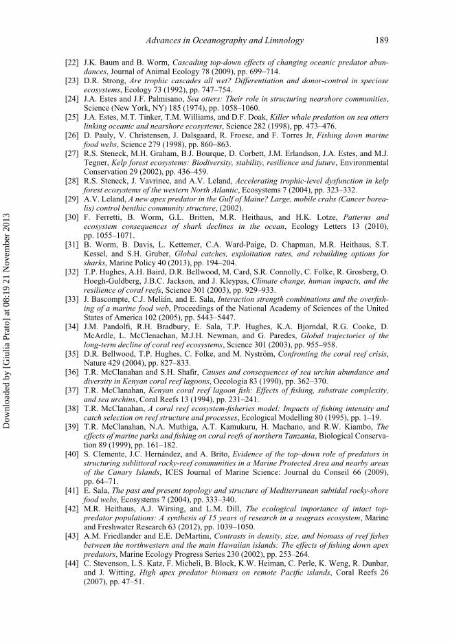
[22] J.K. Baum and B. Worm, Cascading top-down effects of changing oceanic predator abun-dances, Journal of Animal Ecology 78 (2009), pp. 699–714.

[23] D.R. Strong, Are trophic cascades all wet? Differentiation and donor-control in specioseecosystems, Ecology 73 (1992), pp. 747–754.

[24] J.A. Estes and J.F. Palmisano, Sea otters: Their role in structuring nearshore communities,Science (New York, NY) 185 (1974), pp. 1058–1060.

[25] J.A. Estes, M.T. Tinker, T.M. Williams, and D.F. Doak, Killer whale predation on sea otterslinking oceanic and nearshore ecosystems, Science 282 (1998), pp. 473–476.

[26] D. Pauly, V. Christensen, J. Dalsgaard, R. Froese, and F. Torres Jr, Fishing down marinefood webs, Science 279 (1998), pp. 860–863.

[27] R.S. Steneck, M.H. Graham, B.J. Bourque, D. Corbett, J.M. Erlandson, J.A. Estes, and M.J.Tegner, Kelp forest ecosystems: Biodiversity, stability, resilience and future, EnvironmentalConservation 29 (2002), pp. 436–459.

[28] R.S. Steneck, J. Vavrinec, and A.V. Leland, Accelerating trophic-level dysfunction in kelpforest ecosystems of the western North Atlantic, Ecosystems 7 (2004), pp. 323–332.

[29] A.V. Leland, A new apex predator in the Gulf of Maine? Large, mobile crabs (Cancer borea-lis) control benthic community structure, (2002).

[30] F. Ferretti, B. Worm, G.L. Britten, M.R. Heithaus, and H.K. Lotze, Patterns andecosystem consequences of shark declines in the ocean, Ecology Letters 13 (2010),pp. 1055–1071.

[31] B. Worm, B. Davis, L. Kettemer, C.A. Ward-Paige, D. Chapman, M.R. Heithaus, S.T.Kessel, and S.H. Gruber, Global catches, exploitation rates, and rebuilding options forsharks, Marine Policy 40 (2013), pp. 194–204.

[32] T.P. Hughes, A.H. Baird, D.R. Bellwood, M. Card, S.R. Connolly, C. Folke, R. Grosberg, O.Hoegh-Guldberg, J.B.C. Jackson, and J. Kleypas, Climate change, human impacts, and theresilience of coral reefs, Science 301 (2003), pp. 929–933.

[33] J. Bascompte, C.J. Meli�an, and E. Sala, Interaction strength combinations and the overfish-ing of a marine food web, Proceedings of the National Academy of Sciences of the UnitedStates of America 102 (2005), pp. 5443–5447.

[34] J.M. Pandolfi, R.H. Bradbury, E. Sala, T.P. Hughes, K.A. Bjorndal, R.G. Cooke, D.McArdle, L. McClenachan, M.J.H. Newman, and G. Paredes, Global trajectories of thelong-term decline of coral reef ecosystems, Science 301 (2003), pp. 955–958.

[35] D.R. Bellwood, T.P. Hughes, C. Folke, and M. Nystr€om, Confronting the coral reef crisis,Nature 429 (2004), pp. 827–833.

[36] T.R. McClanahan and S.H. Shafir, Causes and consequences of sea urchin abundance anddiversity in Kenyan coral reef lagoons, Oecologia 83 (1990), pp. 362–370.

[37] T.R. McClanahan, Kenyan coral reef lagoon fish: Effects of fishing, substrate complexity,and sea urchins, Coral Reefs 13 (1994), pp. 231–241.

[38] T.R. McClanahan, A coral reef ecosystem-fisheries model: Impacts of fishing intensity andcatch selection on reef structure and processes, Ecological Modelling 80 (1995), pp. 1–19.

[39] T.R. McClanahan, N.A. Muthiga, A.T. Kamukuru, H. Machano, and R.W. Kiambo, Theeffects of marine parks and fishing on coral reefs of northern Tanzania, Biological Conserva-tion 89 (1999), pp. 161–182.

[40] S. Clemente, J.C. Hern�andez, and A. Brito, Evidence of the top–down role of predators instructuring sublittoral rocky-reef communities in a Marine Protected Area and nearby areasof the Canary Islands, ICES Journal of Marine Science: Journal du Conseil 66 (2009),pp. 64–71.

[41] E. Sala, The past and present topology and structure of Mediterranean subtidal rocky-shorefood webs, Ecosystems 7 (2004), pp. 333–340.

[42] M.R. Heithaus, A.J. Wirsing, and L.M. Dill, The ecological importance of intact top-predator populations: A synthesis of 15 years of research in a seagrass ecosystem, Marineand Freshwater Research 63 (2012), pp. 1039–1050.

[43] A.M. Friedlander and E.E. DeMartini, Contrasts in density, size, and biomass of reef fishesbetween the northwestern and the main Hawaiian islands: The effects of fishing down apexpredators, Marine Ecology Progress Series 230 (2002), pp. 253–264.

[44] C. Stevenson, L.S. Katz, F. Micheli, B. Block, K.W. Heiman, C. Perle, K. Weng, R. Dunbar,and J. Witting, High apex predator biomass on remote Pacific islands, Coral Reefs 26(2007), pp. 47–51.

Advances in Oceanography and Limnology 189

Dow

nloa

ded

by [

Giu

lia P

rato

] at

08:

19 2

1 N

ovem

ber

2013

[45] E.E. DeMartini, A.M. Friedlander, S.A. Sandin, and E. Sala, Differences in fish-assemblagestructure between fished and unfished atolls in the northern Line Islands, central Pacific,Marine Ecology Progress Series 365 (2008), pp. 199–215.

[46] S.A. Sandin, J.E. Smith, E.E. DeMartini, E.A. Dinsdale, S.D. Donner, A.M. Friedlander, T.Konotchick, M. Malay, J.E. Maragos, and D. Obura, Baselines and degradation of coralreefs in the northern Line Islands, PLoS One 3 (2008).

[47] R. Trebilco, J.K. Baum, A.K. Salomon, and N.K. Dulvy, Ecosystem ecology: Size-based con-straints on the pyramids of life, Trends in Ecology & Evolution 28 (2013), 423–431.

[48] E. Sala and M. Zabala, Fish predation and the structure of the sea urchin Paracentrotus liv-idus populations in the NW Mediterranean, Marine Ecology Progress Series 140 (1996),pp. 71–81.

[49] E. Sala, C.F. Boudouresque, and M. Harmelin-Vivien, Fishing, trophic cascades, and thestructure of algal assemblages: Evaluation of an old but untested paradigm, Oikos 82(1998), pp. 425–439.

[50] P. Guidetti, Predator diversity and density affect levels of predation upon strongly interac-tive species in temperate rocky reefs, Oecologia 154 (2007), pp. 513–520.

[51] J.K. Pinnegar and G.H. Engelhard, The ‘shifting baseline’ phenomenon: A global perspec-tive, Reviews in Fish Biology and Fisheries 18 (2008), pp. 1–16.

[52] H.K. Lotze and B. Worm, Historical baselines for large marine animals, Trends in Ecology& Evolution 24 (2009), pp. 254–262.

[53] J. Desse and N. Desse-Berset, Peche et surpeche en M�editerran�ee: le t�emoignage des os,Exploitation des Animaux Sauvages a Travers le Temps 13 (1993), pp. 332–333.

[54] J. Desse, and N. Desse-Berset, Osteometry and fishing strategies at Cape Andreas Kastros(Cyprus, 8th millennium BP), Annalen-Koninklijk Museum voor Midden-Afrika-Zoologische Wetenschappen 274 (1994).

[55] Cueva de Nerja (prov. Malaga): a close look at a twelve thousand year ichthyofaunalsequence from southern Spain [Paleolithic, Neolithic, Chalcolithic], Annales Musee Royalde l’Afrique Centrale Sciences Zoologiques Vol. 274.

[56] —, Pr�ehistoire du m�erou, Marine Life 9 (1999), pp. 19–30.[57] P. Guidetti and F. Micheli, Ancient art serving marine conservation, Frontiers in Ecology

and the Environment 9 (2011), pp. 374–375.[58] G. La Mesa and M. Vacchi, An analysis of the coastal fish assemblage of the Ustica Island

marine reserve (Mediterranean Sea), Marine Ecology 20 (2002), pp. 147–165.[59] A. Di Franco, S. Bussotti, A. Navone, P. Panzalis, and P. Guidetti, Evaluating effects of total

and partial restrictions to fishing on Mediterranean rocky-reef fish assemblages, MarineEcology Progress Series 387 (2009), pp. 275–285.

[60] M.N. Bradai, B. Saidi, and S. Enajjar, Elasmobranchs of the mediterranean and black sea:Status, ecology and biology bibliographic analysis, Food and agriculture organization of theUnited nations (FAO), 2011.

[61] F. Ferretti, R.A. Myers, F. Serena, and H.K. Lotze, Loss of large predatory sharks from theMediterranean Sea, Conservation Biology 22 (2008), pp. 952–964.

[62] P. Megalofonou, Incidental catch and estimated discards of pelagic sharks from the sword-fish and tuna fisheries in the Mediterranean Sea, Fishery Bulletin 103 (2005), pp. 620–634.

[63] W.M. Johnson and D.M. Lavigne, The Mediterranean monk seal, Conservation Guidelines.Multilingual Edition. IMMA Inc. Ghelph, Canada. 152p. Internet edition: http://www.monachus.org/library.htm (1998).

[64] R.R. Reeves, The status and distribution of cetaceans in the Black Sea and MediterraneanSea.

[65] M.E. Soul�e and J. Terborgh, Continental conservation: Scientific foundations of regionalreserve networks, Island Press, 1999.

[66] J.A. Estes, Growth and equilibrium in sea otter populations, The Journal of Animal Ecology(1990), pp. 385–401.

[67] N.T. Shears and R.C. Babcock,Marine reserves demonstrate top-down control of communitystructure on temperate reefs, Oecologia 132 (2002), pp. 131–142.

[68] G.R. Russ and A.C. Alcala, Marine reserves: Rates and patterns of recovery and decline oflarge predatory fish, Ecological applications (1996), pp. 947–961.

[69] S. Jennings and N.V.C. Polunin, Impacts of predator depletion by fishing on the biomass anddiversity of non-target reef fish communities, Coral Reefs 16 (1997), pp. 71–82.

190 G. Prato et al.

Dow

nloa

ded

by [

Giu

lia P

rato

] at

08:

19 2

1 N

ovem

ber

2013

[70] T.R. McClanahan, Recovery of a coral reef keystone predator,”Balistapus undulatus”, inEast African marine parks, Biological Conservation 94 (2000), pp. 191–198.

[71] N.T. Shears and R.C. Babcock, Continuing trophic cascade effects after 25 years of no-takemarine reserve protection, Marine Ecology Progress Series 246 (2003), pp. 1–16.

[72] G.R. Russ and A.C. Alcala, Marine reserves: Rates and patterns of recovery and decline ofpredatory fish, 1983-2000, Ecological Applications 13 (2003), pp. 1553–1565.

[73] N.A.J. Graham, R.D. Evans, and G.R. Russ, The effects of marine reserve protection on thetrophic relationships of reef fishes on the Great Barrier Reef, Environmental Conservation30 (2003), pp. 200–208.

[74] T.R. McClanahan, N.A.J. Graham, J.M. Calnan, and M.A. MacNeil, Toward pristinebiomass: Reef fish recovery in coral reef marine protected areas in Kenya, EcologicalApplications 17 (2007), pp. 1055–1067.

[75] K. Kramer and K.L. Heck, Top-down trophic shifts in Florida Keys patch reef marineprotected areas, Marine Ecology Progress Series 349 (2007), pp. 111–123.

[76] G.R. Russ and A.C. Alcala, Decadal-scale rebuilding of predator biomass in Philippinemarine reserves, Oecologia 163 (2010), pp. 1103–1106.

[77] S.E. Lester, B.S. Halpern, K. Grorud-Colvert, J. Lubchenco, B.I. Ruttenberg, S.D. Gaines, S.Airam�e, and R.R. Warner, Biological effects within no-take marine reserves: A global syn-thesis, Marine Ecology Progress Series 384 (2009), pp. 33–46.

[78] R.C. Babcock, N.T. Shears, A.C. Alcala, N.S. Barrett, G.J. Edgar, K.D. Lafferty, T.R.McClanahan, and G.R. Russ, Decadal trends in marine reserves reveal differential rates ofchange in direct and indirect effects, Proceedings of the National Academy of Sciences 107(2010), pp. 18256–18261.

[79] F. Micheli, P. Amarasekare, J. Bascompte, and L.R. Gerber, Including species interactions inthe design and evaluation of marine reserves: Some insights from a predator-prey model,2004.

[80] J. Claudet, C.W. Osenberg, L. Benedetti-Cecchi, P. Domenici, J.-A. Garc�ıa-Charton, �A.P�erez-Ruzafa, F. Badalamenti, J. Bayle-Sempere, A. Brito, and F. Bulleri, Marine reserves:Size and age do matter, Ecology Letters 11 (2008), pp. 481–489.

[81] J. Claudet, C.W. Osenberg, P. Domenici, F. Badalamenti, M. Milazzo, J.M. Falc�on, I.Bertocci, L. Benedetti-Cecchi, J.A. Garc�ıa-Charton, and R. Go~ni, Marine reserves: Fish lifehistory and ecological traits matter, Ecological applications 20 (2010), pp. 830–839.

[82] J. Claudet, P. Guidetti, D. Mouillot, N.T. Shears, and F. Micheli, Ecological effects of marineprotected areas: Conservation, restoration, and functioning, Marine Protected Areas: AMultidisciplinary Approach (2011).

[83] F. Micheli and B.S. Halpern, Low functional redundancy in coastal marine assemblages,Ecology Letters 8 (2005), pp. 391–400.

[84] F. Micheli, B.S. Halpern, L.W. Botsford, and R.R. Warner, Trajectories and correlates ofcommunity change in no-take marine reserves, Ecological Applications 14 (2004),pp. 1709–1723.

[85] P. Guidetti, M. Milazzo, S. Bussotti, A. Molinari, M. Murenu, A. Pais, N. Spano, R. Balzano,T. Agardy, and F. Boero, Italian marine reserve effectiveness: Does enforcement matter?Biological Conservation 141 (2008), pp. 699–709.

[86] J.G. Harmelin, and J. Marinopoulos, Recensement de la population de corbs (Sciaena umbra,Linnaeus, 1758: Pisces) du Parc National de Port-Cros (M�editerran�ee, France) par inven-taires visuels, Scientific Report of Port-Cros National Park 15 (1993), pp. 265–276.

[87] J.G. Harmelin, F. Bachet, and F. Garcia, Mediterranean marine reserves: Fish indices astests of protection efficiency, Marine Ecology 16 (1995), pp. 233–250.

[88] P. Francour, Pluriannual analysis of the reserve effect on ichthyofauna in the Scandola natu-ral reserve (Corsica, Northwestern Mediterranean), Oceanologica Acta 17 (1994), pp. 309–317.

[89] J. Claudet, D. Pelletier, J.Y. Jouvenel, F. Bachet, and R. Galzin, Assessing the effects ofmarine protected area (MPA) on a reef fish assemblage in a northwestern Mediterraneanmarine reserve: Identifying community-based indicators, Biological Conservation 130(2006), pp. 349–369.

[90] J. Garcia-Charton and S. Planes, Etude de l’impact de la R�eserve Naturelle Marine deCerb�ere-Banyuls comme source d’exportation de poissons littoraux adultes vers les zonesavoisinantes, Rapport EPHE–Conseil G�en�eral des Pyr�en�ees-Orientales, 6 (2002) 43p.

Advances in Oceanography and Limnology 191

Dow

nloa

ded

by [

Giu

lia P

rato

] at

08:

19 2

1 N

ovem

ber

2013

[91] J.A. Garc�ıa-Charton, A. P�erez-Ruzafa, P. S�anchez-Jerez, J.T. Bayle-Sempere, O. Re~nones,and D. Moreno, Multi-scale spatial heterogeneity, habitat structure, and the effect of marinereserves on Western Mediterranean rocky reef fish assemblages, Marine Biology 144(2004), pp. 161–182.

[92] P. Guidetti, Marine reserves reestablish lost predatory interactions and cause communitychanges in rocky reefs, Ecological Applications 16 (2006), pp. 963–976.

[93] M. Harmelin-Vivien, L. Le Dir�each, J. Bayle-Sempere, E. Charbonnel, J.A. Garc�ıa-Charton,D. Ody, A. P�erez-Ruzafa, O. Re~nones, P. S�anchez-Jerez, and C. Valle, Gradients of abun-dance and biomass across reserve boundaries in six Mediterranean marine protected areas:Evidence of fish spillover? Biological conservation 141 (2008), pp. 1829–1839.

[94] E. Macpherson, A. Garc�ıa-Rubies, and A. Gordoa, Direct estimation of natural mortalityrates for littoral marine fishes using populational data from a marine reserve, MarineBiology 137 (2000), pp. 1067–1076.

[95] E. Macpherson, A. Gordoa, and A. Garcıa-Rubies, Biomass size spectra in littoral fishes inprotected and unprotected areas in the NW Mediterranean, Estuarine, Coastal and ShelfScience 55 (2002), pp. 777–788.

[96] E. Sala, E. Ballesteros, P. Dendrinos, A. Di Franco, F. Ferretti, D. Foley, S. Fraschetti, A.Friedlander, J. Garrabou, H. G€ucl€usoy, P. Guidetti, B.S. Halpern, B. Hereu, A.A. Karamanli-dis, Z. Kizilkaya, E. Macpherson, L. Mangialajo, S. Mariani, F. Micheli, A. Pais, K. Riser,A.A. Rosenberg, M. Sales, K.A. Selkoe, R. Starr, F. Tomas, and M. Zabala, The structure ofMediterranean rocky reef ecosystems across environmental and human gradients, and con-servation implications, Plos One 7 (2012).

[97] J.A. Garc�ıa-Charton, A. P�erez-Ruzafa, C. Marcos, J. Claudet, F. Badalamenti, L. Benedetti-Cecchi, J.M. Falc�on, M. Milazzo, P.J. Schembri, B. Stobart, F. Vandeperre, A. Brito, R.Chemello, M. Dimech, P. Domenici, I. Guala, L. Le Dir�each, E. Maggi, and S. Planes, Effec-tiveness of European Atlanto-Mediterranean MPAs: Do they accomplish the expected effectson populations, communities and ecosystems? Journal for Nature Conservation 16 (2008),pp. 193–221.

[98] F. Micheli, L. Benedetti-Cecchi, S. Gambaccini, I. Bertocci, C. Borsini, G.C. Osio, and F.Romano, Cascading human impacts, marine protected areas, and the structure of Mediterra-nean reef assemblages, Ecological Monographs 75 (2005), pp. 81–102.

[99] C.F. Boudouresque, A. Caltagirone, J.R. Lefevre, V. Rico, and R. Semroud, Macrozooben-thos de la reserve naturelle de Scandola (Corse, Medit�erran�ee nord-occidentale). Analysepluriannuelle de l’effet reserve, 1992, pp. 15–20.

[100] M. Vacchi, S. Bussotti, P. Guidetti, and G. La Mesa, Study of the coastal fish assemblage inthe marine reserve of the Ustica Island (southern Tyrrhenian Sea), Italian Journal of Zoology65 (1998), pp. 281–286.

[101] R. Chemello, Studio della malacofauna costiera dell’isola di Ustica (Gastropoda), LavoriSIM 1 (1986), pp. 51–76.

[102] F. Badalamenti, G. Cantone, R. Domina, N. Di Pietro, D. Catalano, E. Mollica, and G.D’Anna, Primi dati sulla fauna a policheti di substrato duro dell’infralitorale fotofilo superi-ore dell’Isola di Ustica, Biologia Marina Mediterranea 6 (1999), pp. 230–236.

[103] A. Villamor and M.A. Becerro, Species, trophic, and functional diversity in Marine Pro-tected and non-Protected Areas, Journal of Sea Research 73 (2012), pp. 109–116.

[104] S. Libralato, M. Coll, M. Tempesta, A. Santojanni, M. Spoto, I. Palomera, E. Arneri, and C.Solidoro, Food-web traits of protected and exploited areas of the Adriatic Sea, BiologicalConservation 143 (2010), pp. 2182–2194.

[105] D. Mouillot, J.M. Culioli, D. Pelletier, and J.A. Tomasini, Do we protect biological original-ity in protected areas? A new index and an application to the Bonifacio Strait NaturalReserve, Biological Conservation 141 (2008), pp. 1569–1580.

[106] A.M. Duda and K. Sherman, A new imperative for improving management of large marineecosystems, Ocean & Coastal Management 45 (2002), pp. 797–833.

[107] P. Cury, L. Shannon, and Y.-J. Shin, The functioning of marine ecosystems: A fisheries per-spective, Responsible Fisheries in the Marine Ecosystem (2003), pp. 103–123.

[108] D. Pauly, V. Christensen, and C. Walters, Ecopath, Ecosim, and Ecospace as tools for evalu-ating ecosystem impact of fisheries, ICES Journal of Marine Science: Journal du Conseil 57(2000), pp. 697–706.

192 G. Prato et al.

Dow

nloa

ded

by [

Giu

lia P

rato

] at

08:

19 2

1 N

ovem

ber

2013

[109] V. Christensen and C.J. Walters, Ecopath with Ecosim: Methods, capabilities and limita-tions, Ecological Modelling 172 (2004), pp. 109–139.

[110] M. Coll and S. Libralato, Contributions of food web modelling to the ecosystem approach tomarine resource management in the Mediterranean Sea, Fish and Fisheries 13 (2012),pp. 60–88.

[111] A. Valls, D. Gascuel, S. Gu�enette, and P. Francour, Modeling trophic interactions to assessthe effects of a marine protected area: Case study in the NW Mediterranean Sea, MarineEcology Progress Series 456 (2012), pp. 201–214.

[112] C. Albouy, D. Mouillot, D. Rocklin, J. Culioli, and F. Le Loc’h, Simulation of the combinedeffects of artisanal and recreational fisheries on a Mediterranean MPA ecosystem using atrophic model, Marine Ecology Progress Series 412 (2010), pp. 207–221.

[113] M. Coll, H.K. Lotze, and T.N. Romanuk, Structural degradation in Mediterranean Sea foodwebs: Testing ecological hypotheses using stochastic and mass-balance modelling, Ecosys-tems 11 (2008), pp. 939–960.

[114] V. Christensen, Ecosystem maturity—towards quantification, Ecological Modelling 77(1995), pp. 3–32.

[115] V. Christensen, and D. Pauly, Changes in models of aquatic ecosystems approaching carry-ing capacity, Ecological Applications 8 (1998), pp. 104–109.

[116] S.K. Hooker and L.R. Gerber, Marine reserves as a tool for ecosystem-based management:The potential importance of megafauna, BioScience 54 (2004), pp. 27–39.

[117] S.K. Hooker, A. Ca~nadas, K.D. Hyrenbach, C. Corrigan, J.J. Polovina, and R.R. Reeves,Making protected area networks effective for marine top predators, Endanger SpeciesResearch 13 (2011), pp. 203–218.

Advances in Oceanography and Limnology 193

Dow

nloa

ded

by [

Giu

lia P

rato

] at

08:

19 2

1 N

ovem

ber

2013

 

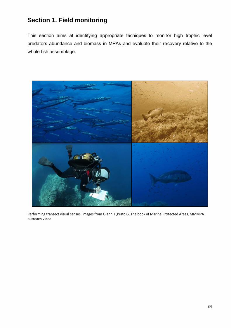
Secti

This se

predato

whole f

 

 

Performinoutreach 

ion 1. F

ection aim

ors abunda

fish assem

ng transect vi video 

ield mo

ms at iden

ance and

mblage.

sual census. I

onitoring

ntifying ap

biomass in

mages from G

g

ppropriate

n MPAs a

Gianni F,Prato

tecniques

and evalua

o G, The book 

to monito

te their re

of Marine Pro

tor high tr

ecovery rel

otected Areas

3

rophic leve

ative to th

, MMMPA 

34 

el

he

35  

3 Chapter 3. Reviewing fish underwater visual census methods in the Mediterranean Sea: setting a baseline for standardisation.

Prato G1, Bouchacha M2, Di Franco A1, Thiriet P1-4, Guidetti P1, Pastor J3, Lenfant P3, Mangialajo L1, Francour P1

1 Université de Nice-Sophia Antipolis, EA 4228 ECOMERS, Parc Valrose, 06108 Nice Cedex 2, France 2 Ifremer, Laboratoire Environnement Ressources Provence Azur Corse, France 3Université de Perpignan Via Domitia, Centre de Formation et de Recherche sur les Environnements Méditerranéens, UMR 5110, F-66860, Perpignan, France This chapter will be submitted to the international journal Plos One. 

3.1 Abstract Underwater visual census (UVC) is the only non-destructive technique to survey fish

assemblages. Several UVC techniques exist and are used across the world in order to

pursue different objectives. Choosing the most appropriate technique for a given

research and management objective can thus be hampered by the wide range of

choices, and inherent advantages and disadvantages of each method should be

considered. Moreover, the large availability of methods, which often allow to measure

different variables, arouses the need for standardisation in method application, especially

if data are to be compared.

Here, we focused on the Mediterranean infralittoral (0-40 m) and aimed at setting a

baseline for a standardisation of UVC method selection and application to pursue

different research and coastal resource management objectives. We combined a semi-

quantitative review of the papers adopting UVC techniques in Mediterranean coastal

areas, with a field method comparison of different UVC techniques. Based on the

variable needed to pursue a specific objective, we evaluated the suitability of each

method to measure such variable, as well as its costs and benefits. Finally, we assessed

the level of standardisation in the Mediterranean for the most common UVC method

adopted to date. Results show that strip transects are the most commonly adopted

technique to survey fish communities in the Mediterranean, providing the most complete

quantitative description of the fish assemblage at the lower economic and time costs.

Standardization in transect surface has not yet been achieved across the Mediterranean,

since more than 50% of the studies targeting similar species use different transect

dimensions. Other methods, such as video-UVC can be complementary to transects (i.e

to survey fish at depths exceeding diving limits or to study fish behaviour). A synthetic

table is provided to guide choice of the most appropriate method depending on the

needed variable.

36  

3.2 Introduction  

It is a widely accepted notion that monitoring marine ecosystems is a general

requirement, preparatory to design sound measures aimed at ensuring conservation and

management of biodiversity. Fish communities, as an intrinsic component of marine

biodiversity, have been severely impacted worldwide via overfishing and habitat

destruction, often leading not only to negative commercial consequences (i.e.

overexploited fish stocks) (Pauly et al. 1998, Watson & Pauly 2001), but also to

ecosystem-wide degradation through the disruption of trophic interactions (Pace et al.

1999, Pinnegar et al. 2000, Jackson et al. 2001) and loss of ecosystem services fishes

may ensure (Holmund & Hammer 1999, Worm et al. 2006).

Preserving fish communities is thus crucial in order to conserve biodiversity, ecosystem

functions and ecosystem services (Holmund & Hammer 1999; Jackson et al. 2001). In

this perspective, field observations can provide a solid scientific knowledge through

which the sustainable use of marine resources can be devised (Carstensen 2014).

Underwater visual census performed by divers (hereinafter UVC) was introduced in 1954

(Brock et al 1954) to quantitatively assess fish communities in coral reefs. UVC was

proposed as a non-destructive alternative to extractive monitoring techniques. Since its

first introduction, a variety of in situ UVC techniques have been used to study tropical and

temperate fish assemblages, including the first video methods already in 1965 (Steinberg

et al 1965). The variety in census techniques (Thresher & Gunn, 1986) triggered the

development of studies dealing with methods’ cost-effectiveness and biases (Bannerot &

Bohnsack 1986, Sale & Sharp 1983). In more recent years two global reviews described

existing UVC methods, the first one providing a broad picture of existing destructive and

visual census methods to monitor fish and associated habitats (Murphy et al. 2010) and

the second documenting in detail existing video techniques and their possible

applications (Mallet et al. 2014). The large availability of methods, each one with its

inherent advantages and disadvantages, arouses the need for standardisation in method

application, especially if data are to be compared. Such need was already highlighted in

1986 (Thresher & Gunn, 1986), and the development of standardised monitoring

protocols for marine biodiversity in response to specific research and coastal resource

management objectives, has been achieved in some areas of the world, such as for

some Large Marine Ecosystem (LME) (Sherman & Duda 2002, PISCO 2010). Being

areas characterized by distinct bathymetry, hydrography, productivity, and trophically

37  

dependent populations (Sherman & Hempel 2009), LMEs represent units from a

management perspective, and shall thus benefit from standardised monitoring programs.

In this perspective, coastal resource management in the Mediterranean LME (Sherman &

Hempel. 2009), does not yet benefit from standardised monitoring protocols for

biodiversity, which would allow for data comparisons on a regional scale. Visual census

was introduced in this basin twenty one years after its first appearance. Mediterranean

marine communities had been facing centuries of over-exploitation (Guidetti & Micheli

2011), and coastal development along with habitat loss were rapidly intensifying (Airoldi

& Beck 2007) arousing the urgency for monitoring. Harmelin-Vivien & Harmelin (1975)

first proposed a UVC protocol aimed at inventorying the fish assemblage at an MPA (Port

Cros National Park), in an easy, objective and non-destructive way. Since this first

publication (Harmelin-Vivien & Harmelin, 1975) and after the review on available UVC

practices (among which transects, stationary point counts, random paths, etc.) provided

by Harmelin Vivien et al. (1985) UVC techniques have been regularly used across the

Mediterranean (Sala & Ballesteros, 1997, Garcia-Charton et al. 2004, Guidetti et al.

2008, Harmelin Vivien et al. 2008, Sala et al. 2012, La Mesa et al. 2013; Guidetti et al.,

2014) and have been adapted to pursue different research and management objectives,

in different habitats. Like in other temperate and tropical regions, the advent of several

underwater video technologies especially in the last 15 years, with Remotely Operated

Videos (Andaloro et al. 2013), Baited Underwater Videos (Condal et al. 2012) and Diver

Operated Video (Tessier et al. 2013) (see Appendix for definitions), further diversified

UVC methods. But different UVC techniques, employing or not videos, often allow for

different variables to be measured, and such diversification was not accompanied by a

standardization in method selection and application across the Mediterranean LME.

In this scenario, our paper focuses on the Mediterranean infralittoral (0-40 m) and aims at

setting the baseline for a standardisation in UVC method selection and application to

pursue different research and coastal resource management objectives (e.g. within

MPAs).

To achieve such goal, we reviewed semi-quantitatively papers adopting UVC techniques

in Mediterranean coastal areas since its first advent, following some key steps:

1) identifying the variables needed to pursue specific objectives

2) analysing the pertinence and the cost-benefits of the methods available to measure

such variables

38  

3) assessing the level of standardisation in the Mediterranean for the most common UVC

method adopted to date

We further integrated our review by comparing data collected in the field through

traditional UVC (transects performed by diving operators) with more recent video

techniques (Diver Operated Video and a Remote Rotating Video System), that have

already been used in coral reefs (Pelletier et al. 2011, 2012) but are still little applied in

the Mediterranean. In particular, to our knowledge this is the first paper in the

Mediterranean testing a Remote Rotating Video System to survey the fish community.

3.3 Methods  

3.3.1 Bibliographic review We carried out a bibliographic search in ISI Web of Knowledge on all databases, using

the key words “(visual census OR recensement visuel* OR censiment* visiv* OR censo*

visual*) AND Mediterran*)”, considering the years from 1975 to august 2014. Since ISI

Web of knowledge did not find papers older than 1990, we completed the search going

through the bibliography of the available papers and pursuing them with google scholar.

Overall 256 references resulted from our search. Among these we excluded studies that

used only extractive methods (experimental fishing), studies from non-Mediterranean

zones and studies not focusing on fish. Finally 179 papers were retained.

The papers were classified according to publication journal, year of publication (using five

years categories), country where the study was performed, research topic, considered

species or group of species, methods applied, measured variables and habitat. Surface

units and time measures of the applied method, when provided, were also noted for

further analyses on standardisation across the Mediterranean.

Research topics were divided in the following categories: artificial structures (whenever a

paper included artificial reefs, gas platforms, breakwaters, fish farms or FADs), behaviour

(only papers including quantitative or semi-quantitative data), human impacts (pollution,

tourism impact, fishing impact), methodological studies (methods comparisons or

methods evaluations), population dynamics, recruitment and settlement, reserve effect

(including papers assessing changes in the living components within a marine protected

area when one or several human impacts are excluded, as well as papers dealing with

the assessment of the spillover effect to adjacent areas), fish assemblage

characterization/spatio-temporal distribution and species occurrence.

39  

Concerning the methods used, the considered categories were: transects, transects

coupled with other methods (transect +), circular point counts, video + (all papers dealing

with a video method involved comparison with at least one other technique, thus the

category was video techniques coupled to other methods), total counts, random counts,

spatial census, rapid visual census, and others. A short description for each method is

provided in the Annex.

Results of published papers dealing with methods comparisons were also briefly

summarised.

3.3.2 Field methods comparison For comparison in the field we selected the most common UVC method adopted in the

Mediterranean according to our previous analysis (strip transects performed by divers)

and two video methodologies: diver operated video transects (Tessier et al. 2013) and

Staviro (Pelletier et al 2012, Bouchoucha et al. 2013a, 2013b), a remote high-definition

un-baited rotating video system (see Appendix for system description).

The three census methods were tested in Bay of Villefranche (SE France) in May 2013.

All methods were applied in the same area, between 5 and 15 meters depth, on a

predominantly rocky substrate interspersed with Posidonia oceanica patches (rocky

coverage ≥ 70 %). Multiple operators performed UVC within the same temporal window.

When multiple census have been done, a minimum distance (> 25 m) was kept among

operators in order to reasonably reduce the risk of reciprocal disturbance and spatial

dependence of data.

Among 3 close days of similar good weather and visibility conditions we carried out 18

strip transects (Harmelin-Vivien & Harmelin 1975) of 25 meter length and 5 meter width,

21 video transects 25 meter long, and 27 Staviro deployments at randomly selected sites

over the study area. Strip transects were carried out by two expert operators swimming at

constant speed (approx. 8-10 min/25 m) and close distance from the sea floor.

Concerning video transects, the same operator swam at a constant speed (approx. 3

min/25 m) at 1.5 m from the bottom, keeping the video camera steady, horizontal and

toward the end of the transect, thus recording in front of himself (Tessier et al. 2013).

The Staviro system was set on the sea floor and programmed so that the camera

housing rotated from 60° every 30 seconds, at a fixed angle. Hence, six observation

sectors were recorded per 360° rotation, each rotation lasting approximately 3 minutes.

The system was left in place for 12 minutes, in order to complete three whole rotations

(making one replicate) and account for one minute before and after each triplet, in order

40  

to minimise disturbances due to boat presence, engine noise and setting and retrieval of

the system. Further technical details on the Staviro system can be found in (Pelletier et

al. 2012, Bouchoucha et al. 2013).

For the three methods, fish were recognized to the lowest taxonomic level possible. For

isolated fish and small groups (<10 individuals) the actual number of fish was counted,

while schools of fish (> 10 individuals) were recorded as follow: in strip transects

Harmelin-Vivien (1985) categories of abundance were used (i.e. 11–30,31–50, 51–200,

201–500, >500 ind.) and the mid point of each category was retained, while in both video

methods freeze frames were used and the maximum number of individuals among freeze

frames for the same school was retained. During Staviro video analysis, individuals were

counted per sector, and then summed up for each 360 rotation. For each species and

each sampling unit, the maximum abundance observed over the three rotations was

retained.

Since we could not measure surface area in video methods, direct comparison of density

data was not possible. Multivariate analyses were thus performed on the fish assemblage

with presence-absence data. Methods could not equally identify all fish seen to the

species level, thus analysis were carried out at different levels of taxonomical scale-up

(species, genus and functional group), in order not to lose possibly relevant information.

For each level of aggregation, data were analysed for differences among methods

through a multivariate PERMANOVA (Anderson 2001) with one fixed factor “method“

(fixed factor, 3 levels) and based on Jaccard distance measure. We used Montecarlo

permutations whenever number of possible permutations was low, <500. A Permdisp

analysis was carried out to assess differences in data dispersion among methods.

Results were graphically represented with an unconstrained principal coordinate analysis

(PCO) and vectors of presence-absence variables were superposed to the ordination

through Spearman correlation to identify the taxonomic groups principally responsible for

differences between methods. Species accumulation plots allowed discriminating which

method captured the most complete image of the fish assemblage with the least time

cost (where time cost = field time + analysis time). The PRIMER 6 and PERMANOVA +

package (Plymouth Marine Laboratory) was used to perform the analyses.

3.3.3 Integration of bibliographic and field work

Bibliographic and field work were integrated in a final table in order to provide a synthesis

of indications to guide the choice of the most suitable method for each variable that was

analysed in the reviewed papers. A compendium of factors was integrated in the table: as

41  

a proxy for method appropriateness we referred to the number of published papers using

the specific method to assess the variable in question, plus field and lab time

requirements, training and costs. We coded semi-quantitative variables to highlight the

level of appropriateness of each method according to the previous factors. Thus, in order

to code the factor “number of papers using the specific method to assess a given

variable”, we assigned the following 3 categories: maximum number of papers, minimum

number of papers, number of papers within the two extremes. Additionally, to treat the

“zero” case (when zero papers used a method to measure a given variables), we further

defined three categories based on expert judgement: “0” was assigned when no paper in

the literature had applied the method for the given variable, although it would have been

feasible. “Feasible”(F) was assigned when the given variable could be assessed by the

method, but with some limitations (i.e. density could be estimated by fixed video methods

by setting two fixed land marks at a known distance and angle from the camera, and

calculating the arrival time of each fish species) (Stobart et al. 2005). “NA” was

assigned when the method does not allow for the computation of the variable. The

factors time, training and equipment costs were classified each in three categories based

respectively on expert knowledge and a survey. Time included field and lab work per

sample: < 15 minutes (1), between 15 and 30 minutes (2) and between 30 minutes and 2

hours (3). Training was classified by listing all the skills needed to carry out a fish visual

census with each method, i.e.: diving, underwater fish identification, fish counting, fish

size estimation, sampling surface estimation, video-equipment handling and video

analysis. For each method we summed the number of skills needed, and coded three

categories with the following criteria: maximum number of skills (3), minimum number of

skills (1), number of skills within the two extremes (2). To quantify equipment costs we

provided rough price estimates for each method, including selling price and material

amortization, and classified them from 1 (lowest costs) to 3 (highest costs). We did not

include an estimate of costs for boat rental, assuming each method would need a boat to

reach the sampling spot. We then filled the table cells with colours grading from bright

green (max number of papers, least sampling time, least training and least equipment

costs) to light grey (0 papers) and to dark grey (NA).

42  

3.4 Results

3.4.1 Bibliographic review

Most studies were carried out in Italy (84 papers), followed by Spain (37 papers) and

France (30 papers). Fewer studies came from the eastern Mediterranean, with Greece (4

papers), Turkey (3 papers), and scattered papers from Croatia, Slovenia, Israel and

Lebanon. Only 8 studies interested more than one country.

Published studies adopting UVC methods dramatically increased after 1994. Maximum

number of published papers was reached in the last 5 years. From 1995, research

objectives and applied visual census methods became more diversified (Fig. 1).

Fig. 1 Evolution in time in the number of papers, research topics and methods applied, resulting from the literature research in Isi Web of Knowledge “(visual census OR recensement visuel* OR censiment* visiv* OR censo* visual*) AND Mediterranean”, plus authors archives. 

According to our review the most common research objective addressed through UVC

(26% of published papers) was the spatial and/or temporal characterization of the fish

assemblage (either the whole assemblage or a subset of species), followed by reserve

effect (22%) and artificial structures (20%). Less addressed issues were methodological

assessments (10%) and the study of fish recruitment and settlement (8%) (Tab. 1). 

   

0

5

10

15

20

25

30

35

40

45

50

Papers

Topics

Methods

N

43  

Tab. 1 Total number of papers measuring each variables (rows) within each  research objective (columns). Numbers in  parenthesis  indicate  the  percentage  of  papers  addressing  each  research  topic  (head  line)  or measuring  each variable (head column). Scores along  columns are assigned a  gradation of colours from bright green (best score) to grey (worst score).  

 

 

Table 1 summarizes the main variables measured by the reviewed papers according to

the research objective. For each objective, density was the most commonly measured

variable (77% of the papers), followed by size (50 % of the papers), retained in particular

by reserve effect studies, and species richness/community metrics (49% of the papers).

This last variable was the most used (11 papers) in methodological evaluation studies.

Most of the reviewed papers used transects (64%), either alone (87 papers), either

complemented by other methods (e.g. experimental fishing - 10 papers, random or total

counts - 6 papers, and others (see Appendix for method description) (27 papers) (Fig.2).

Stationary point counts were the second most used method, but were large behind

transects in terms of papers adopting them (11), followed by total counts and video

methods (10 papers) (Fig.2).

  

Spatio‐temporal distribution, 

characterization 

Reserve effect 

Artificial structure

Method Recruitment settlement 

Human impact 

Population dynamics 

Species occurrence 

Behaviour 

    (26 %)  (22 %)  (20 %)  (9 %)  (8 %)  (4 %)  (3 %)  (2 %)  (3 %) 

Density  (77 %)  42  33  23  11  13  5  2  1  4 

Size / Biomass  (50 %)  16  30  16  9  9  1  4  0  3 

Sp. richness,   Community metrics 

(49 %)  

33 19  17  11  1  3  0  1  0 

Abundance, pres/abs 

(19 %)  4  6  13  4  3  1  1  1  1 

Functional categories 

(15 %)  8  5  6  6  0  1  0  0  0 

Frequency of occurrence 

(11 %)  3  3  9  1  1  1  0  0  1 

Semi‐quant. behaviour obs. 

(8 %)  2  2  2  3  2  1  1  0  1 

N, Max N,  Spp/ minute 

(2 %)  0  0  0  1  0  3  0  0  0 

 

Fig.2 Nuand  viderandom mobile p

Method

Method

commo

of impr

The 19

quantita

introdu

classes

propos

Vivien

until th

quadra

than tra

estimat

around

conside

assemb

species

such as

mber of papeo  +  stand  fpaths, FAST,point counts.

dological c

dological c

on (8 pape

roved video

975 study

ative UVC

ced strip

s and 4 s

ed. Ten y

et al., 198

en, and a

ats and fixe

ansects an

te fish abu

isolated s

ered more

blage, kee

s, to visibi

s depth, tim

pers adoptingfor  transect , etc.). “Othe.  

omparison

comparison

ers), but sh

o technique

by Harm

C techniq

transects

size classe

years later

85), presen

analysing t

ed points).

nd fixed p

undance no

structures o

e appropri

eping in mi

lity conditi

me and no

g each methand  videos

er” includes 

ns in the lite

ns among

howed an

es.

melin-Vivien

ques in t

of 5 met

es. Codifie

r, the sam

nting the m

he criticali

. According

oints to de

or biomass

or in heter

ate for ho

nd that tra

ons and to

ise influen

hod. See thes  coupled  wmethods use

erature

g UVC tec

increasing

n & Harm

the Medit

ter width a

ed procedu

me authors

methods a

ities and b

g to this r

escribe sp

s. Fixed po

rogeneous/

omogenou

ansect widt

o the habi

ce on fish,

Annex for dewith  other  teed only by o

chniques i

trend in t

elin set th

terranean.

and fish c

ures for b

published

adopted in

biases of e

review, ran

pecies rich

oints were

/patchy ha

s habitats

th should b

itat type. U

, were also

escription ofechniques  (ene or two pa

n the Med

he latest y

he basis f

Harmelin

counting th

ehaviour a

d a review

temperate

each (rand

ndom path

ness, but

suggested

abitats. Tra

s and to s

be adapted

UVC limits

o discussed

f each methoe.g.  experimapers, such a

diterranea

years, with

for the ex

n-Vivien &

hrough 5

annotation

w on UVC

e and trop

dom walks

s were mo

they did n

d mainly t

ansects, ins

study the

d to the mo

due to sc

d.

4

od. Transect mental  fishinas quadrats o

n were no

h the adven

xpansion o

& Harmeli

abundanc

n were als

(Harmelin

ical region

s, transects

ore efficien

not allow t

o study fis

stead, wer

whole fis

obility of th

cuba diving

44 

 + g, or 

ot

nt

of

in

ce

so

n-

ns

s,

nt

to

sh

re

sh

he

g,

45  

In 1997, Francour compared transects, stationary point counts and total counts (meaning

counts of all the individuals inhabiting a given area, see Appendix) to assess the density

of a subset of species in a Posidonia oceanica meadow at the Port Cros national park.

Density estimates obtained with the different methods were compared for selected

species, differing for mobility and behaviour. For each species, small size class fishes

(total length < 1/3 maximum total length) were recorded mostly by transects and circular

points, and medium and large size class fishes by circular points or total count.

Differences among methods were dependent on the season of sampling and from

species behaviour: schooling fish were better detected by fixed points, and very mobile

species were mainly recorded through transects.

The paper by D’Anna et al. (1999) showed the logic applied to select the most

appropriate UVC technique to assess fish biomass and assemblage structure in both

natural and artificial habitats: substrates were first classified and then appropriate

techniques were chosen accordingly. Horizontal transects were applied to P. oceanica

meadows and homogenous sandy bottoms, while vertical transects were used for vertical

cliffs. Point counts were preferred to survey scattered P. oceanica patches on the sandy

bottom and for mixed substrates of sand and stones. Finally, spatial census (a mixed

technique including point counts and circular transects) was chosen to assess the fish

assemblage around artificial structures (artificial reef and FAD). The study stressed the

importance of choosing coherent units of measures for comparative studies, concluding

that density related to volumes (m3) resulted more appropriate than density related to

surfaces (m2) for assessments of fish assemblages around artificial structures.

The paper by De Girolamo & Mazzoldi (2001) was the first one to attempt a

methodological assessment of some biases in UVC transect on rocky habitats. Main

results from the study were that i) separate survey methods adapted to different fish

behaviour (a higher speed transect for epi-benthic species followed by a lower speed

survey for benthic fish) although more time consuming, provided more realistic fish

counts by better detecting cryptic fish. And ii) continuous size estimates were more

advantageous than size classes estimates, yielding the best biomass assessments.

The only statistical comparison conducted in the Mediterranean between strip transects

(25x5 m, 8 min/transect) and stationary point counts (radius = 5m, 8 min/point count)

came by Guidetti et al. 2005. Results showed that, once results from both methods were

adjusted for surface area, strip transects yielded higher number of fish taxa and fish

densities, both with and without including gregarious species. The authors thus confirmed

46  

what suggested by Harmelin-Vivien et al. (1985) that strip transects should be preferred

when working on homogenous habitats.

The following methodological assessments were mainly comparisons between video

techniques and underwater visual census.

Baited Underwater Video (BUV) was adopted only once in the Mediterranean shallow

habitats by Stobart et al. 2007 in order to assess its performance in estimating fish

abundance and diversity on rocky reefs. The studied variables were species richness,

maximum number of species at the bait and maximum % presence of species at different

sampling sites. BUV resulted to be an effective tool when estimation of species richness

is the prime objective, while UVC using 25x5 m transects was more suitable to estimate

fish abundance and size at sites not constrained by diving limits, especially given the

higher time costs of BUV.

In Tessier et al. 2013 the effectiveness of Diver operated underwater video (DOV) along

transects was compared to transects UVC to assess reserve effect. Results showed that

DOV was able to detect significant but weaker effects of protection than UVC on

abundance and species richness of the fish assemblage. According to the authors, when

reserve effect is weaker, DOV might fail to detect it due to some limitations of videos

such lower camera field of view compared to human eye and lower species identification

chance linked both to image quality and to the avoidance behaviour of shy species. In

fact, when fleeing away or keeping a large distance from the operator, shy species are

more difficult, if not impossible, to identify through image analysis. On the other hand

DOV allowed to archive and thus further analyse data without spending extra time

underwater, for example quantifying fish aggregations, a potentially useful parameter to

assess reserve effect, or classifying substrate types and quantifying their percentage

cover.

The study by Andaloro et al. (2013a) compared ROV with mobile point counts UVC (see

Appendix for description) to describe the fish assemblage around gas platforms.

Estimates of abundance, species richness and frequency of occurrence were compared,

and fish were categorized in ecological categories on the basis of their spatial

organisation in the water column. ROV overall failed to give a truthful representation of

the fish assemblage being more limited in the detection of crypto-benthic and necto-

benthic fish, thus providing lower species richness and abundances estimates than UVC.

ROV proved nevertheless to be useful in detecting low mobile and abundant

planktonivorous species and was thus suggested to be used in complementarity to UVC,

especially at depths and sampling times not affordable to the latter.

47  

An interesting contribution by Bulleri & Benedetti-Cecchi (2014) investigated the potential

of spearfishermen videos to assess the structure of fish assemblages. Videos from the

sit-and-wait fishing technique were compared with transect UVC. The measured

parameter was the maximum number of species seen at any one time over the whole

duration of one video. Density estimates were derived by accounting for maximum

visibility. Although fish assemblage composition differed, spearfishing videos and

transects provided comparable estimates of species richness. Videos in particular were

able to detect relatively uncommon and shy species like Dentex dentex and Sparus

aurata, but they underestimated sedentary species. The authors stressed how the large

availability of fishing videos all over the Mediterranean would make them an invaluable

source of information on fish assemblages on shallow rocky reefs.

48  

3.4.2 Field methods comparison

Overall 39 fish taxa were identified by the three methods, most of which were detected by

strip transects (32 detected in total, 7 uniquely detected by transect), followed by Staviro

(26 total, 3 unique) and video transects (10 total, 1 unique) (Tab.2)

Tab.  2  Species  unique  to  each  method  and  combination  of methods. T= transects, S= Staviro, V= video transects 

  Taxa    Method   

  Boops boops    S     Mugilidae    S     Sciaena umbra    S     Blenniidae    T     Epinephelus marginatus    T     Labrus viridis    T     Scorpaena porcus    T     Scorpaena scrofa    T     Spondyliosoma canthaurus    T     Thalassoma pavo    T     Oblada melanura    V     Labrus merula     S,T     Mullus surmuletus    S,T     Muraena helena    S,T     Serranus cabrilla    S,T     Serranus scriba    S,T     Sparus aurata    S,T     Symphodus cinereus    S,T     Symphodus doderleinii    S,T     Symphodus mediterraneus    S,T     Symphodus melanocercus    S,T     Symphodus ocellatus    S,T     Symphodus roissali    S,T     Tripterygiidae    S,T     Chromis chromis    S,T,V     Coris julis    S,T,V     Diplodus annularis    S,T,V     Diplodus puntazzo    S,T,V     Diplodus sargus    S,T,V     Diplodus vulgaris    S,T,V     Sarpa salpa    S,T,V     Serranus spp.    S,T,V     Spicara spp.    S,T,V     Symphodus rostratus    S,T,V     Symphodus spp.    S,T,V     Symphodus tinca    S,T,V            

 

Perman

possibl

species

pair of

method

percen

display

transec

showin

transec

correla

Staviro

capturi

slight c

 

nova anal

e (Blennid

s level), sh

f methods

ds was be

tage of v

yed the lea

ct data, as

g significa

cts, but no

tions > 0.5

o were pos

ng most o

correlation

Fig.3

lysis on p

dae, Trypte

howed sign

s (P<0.001

est describ

variability r

ast dispers

s confirmed

ant differe

ot betwee

5 as well as

sitively cor

of the fish

trend with

3 PCO at the s

presence/a

erigidae, S

nificant diff

1) (post-h

bed by th

remained

ion among

d from the

ences betw

n staviro

s vectors fo

rrelated to

species (F

video met

species (a), ge

absence o

Spicara sp

ferences am

oc pair-w

he first ax

unexplain

g samples,

e Permdisp

ween tran

v video t

for gregario

o the first

Fig. 3a). S

thods.

enus (b), and f

of each ta

p. and Mu

mong the t

ise tests)

is of the

ed (Fig.

, as oppos

p analysis

nsects v S

ransect).

ous specie

axis of the

chooling fi

functional gro

axon ident

ugilidae we

three meth

. Differenc

PCO (30%

3a). Here

sed to the

(P < 0.01

Staviro an

Only vecto

es were vis

e PCO an

sh like Bo

up aggregatio

tified to lo

ere never

hods and a

ce among

%), althou

e, strip tra

more scat

7, with pa

nd transec

ors of var

sualised. T

nd were th

oops boops

on level (c) 

4

owest leve

identified a

among eac

g the thre

ugh a larg

ansect dat

ttered vide

airwise test

cts v vide

riables wit

ransect an

he method

s showed

49 

el

at

ch

ee

ge

ta

eo

ts

eo

th

nd

ds

a

 

When

signific

represe

transec

transec

When

signific

differen

video

differen

discrim

differen

better v

were m

method

Specie

three m

method

detecte

increas

terms o

Staviro

transec

detecte

F

aggregatin

ant (PER

entation, w

cts. Here,

cts, Boops

aggregatin

ant differe

nces betw

transects

nces were

minated by

nces amon

visible alo

more relate

ds (Fig. 3c)

s accumul

methods a

ds and that

ed a much

sing sampl

of number

o could de

cts recorde

ed schoolin

Fig. 4 Species 

ng presenc

MANOVA,

where Stav

Sarpa, Se

was again

ng presen

ences amo

een strip

(Pmc <

detected

the PCO

ng method

ng the ver

ed to transe

).

lation plots

alone could

t at an equ

h higher pr

ling and a

of species

etect most

ed higher

ng detritivo

accumulation

ce-absence

, P<0.001

iro was slig

erranus, A

n slightly m

nce-absenc

ong method

transects

0.005 and

between

at this lev

ds, in part

rtical axis.

ects, while

s showed t

d record a

ual effort in

roportion o

nalysis tim

s recorded

of them

trophic le

ors (mugilid

n plots. Cumu

e by genu

) although

ghtly overl

Apogon, M

more related

ce by func

ds (P<0.00

and Stavi

d Pmc <0

Staviro an

vel of func

rticular am

Carnivoro

e planktoni

that at the

all the spe

n terms of s

of species

me, the two

(Fig. 4). In

(5/6), con

evel preda

dae) (Tab 2

lated time inc

us, differen

h they we

apping bo

ullus and

d to video

ctional gro

05) and pa

iro, as we

0.007 resp

nd video t

ctional agg

mong trans

ous crypto

vorous sch

e achieved

ecies dete

sampling a

than the v

o video me

n terms of f

trary to vi

ators (E. m

2).

cludes field an

nces amon

ere less

th with vid

Diplodus w

methods (

oup, PERM

airwise tes

ell between

pectively),

transects.

gregation

ects and

-benthic a

hooling fis

level of re

ected by t

and analysi

video meth

ethods wo

functional

deo trans

marginatus

nd analysis tim

ng method

evident in

eo transec

were more

(Fig. 3b).

MANOVA

sts showed

n strip tra

while no

Samples

of the var

video tran

and necto-

h characte

eplication

the sum o

is time, str

hods. More

on’t reach t

groups, tra

ects (3/6)

s), while o

me for each m

5

ds were st

n the PCO

cts and stri

e related t

highlighte

d significan

ansects an

o significan

where les

riables, an

nsect, wer

benthic fis

erised vide

none of th

of the thre

rip transect

eover, eve

transects i

ansects an

. Only stri

only Stavir

ethod. 

50 

till

O

ip

to

ed

nt

nd

nt

ss

nd

re

sh

eo

he

ee

ts

en

in

nd

ip

ro

51  

3.4.3 Integration of bibliographic and field work

Tab. 3 displays the classification of each method according to time needed per each

replicate, training and equipment costs. UVC methods such as transects, point counts,

rapid visual census and spatial census require the highest number of skills underwater

(higher training), but are less time consuming and less expensive than video methods.

UVC through random counts, total counts and fast are slightly more time consuming but

require less skills underwater than the previous methods, not needing estimates of

surface area or, in the case of random counts, size estimates (Tab. 3). Video methods

require video equipment handling skills and video analysis skills (such as species

identification a posteriori, which can be guided through books), but are more time

consuming especially in terms of video-analysis time and, in average, more expensive

(Tab.3)

 

Tab.3 Classification of methods according to training (based on the number of skills required), time (including field and digitisation time), and equipment costs. For each attribute, three categories were defined (see Methods section) 

  TRAINING  TIME  

EQUIPMENT 

Diving 

Underw

ater species identification  

Underw

ater individual counts 

Underw

ater fish size estim

ation 

Underw

ater area estim

ation 

Video equipment handling 

Video analysis 

Total 

Training index 

  Time  cost (min) 

Tim

e cost index 

  Equipment cost (€) 

Equipment cost index 

Transect  1  1  1  1  1  0  0  5  3  < 15  1  

1000‐2000  1 

Stationary point counts 

1  1  1  1  1  0  0  5  3  < 15  1  

1000‐2000  1 

Rapid Visual Census 

1  1  1  1  1  0  0  5  3  < 15  1  

1000‐2000  1 

Spatial census  1  1  1  1  1  0  0  5  3  < 15  1  

1000‐2000  1 

Total counts   1  1  1  1  0  0  0  4  2  15‐30  2  

1000‐2000  1 

Random counts  1  1  0  0  0  0  0  2  2  15‐30  2  

1000‐2000  1 

Fast  1  1  0  1  0  0  0  3  2  15‐30  2  

1000‐2000  1 

Video transect  1  0  0  0  0  1  1  3  2  30‐120  3  

3000‐4000  2 

BUV  0  0  0  0  0  1  1  2  1  30‐120  3  

3000‐4000  2 

Staviro  0  0  0  0  0  1  1  2  1  30‐120  3  

3000‐4000  2 

52  

Results of the bibliographic review, field survey and costs analysis were integrated in

Table 4. For each analysed variable (as density, biomass, species richness, etc),

transects showed the highest score (highlighted in bright green) for most of the factors

considered: largest number of papers adopting them, reduced time and costs of

application. In particular, transects were adopted with large majority respect to other

methods to measure density (96), biomass (59) and species richness and/or community

metrics (54), given the relative ease of surface estimates. Concerning this last variable,

our field comparison confirmed the higher efficiency of transects respect to remote high-

definition rotating video systems and DOV. In fact, the same variables were measured

with other methods in less than 10 papers for each method. On the other hand, to

perform UVC by transects highly skilled and trained specialists working underwater are

needed (Harmelin-Vivien et al., 1985). Stationary point counts (Harmelin-Vivien et al.,

1985) followed transects, sharing similar time, training and equipment costs, but showing

lower success in the literature (Fig. 2).

Rapid Visual Census (RVC) (Dempster et al. 2002) and spatial census (D’Anna et al.

1999b) are adaptations of fixed points and transects specifically designed for fish farms

and artificial structures, sharing thus similar field time, costs and training needs of the two

previous methods.

Total counts (Macpherson et al. 1997, Biagi et al. 1998) did allow for a range of variables

to be measured, and require less strict training than previous methods, given that

underwater surface area estimation is not generally required. However, they were less

adopted in the literature, likely because these are not properly sampling techniques.

Sampling implies the random selection of a subset of individuals from a statistical

population, from which estimates can be derived. A relevant portion of statistical

techniques (e.g. ANOVA, MANOVA, t-tests, etc) are based on sampling data.

Standardization and comparison of data collected with this kind of approach is thus

difficult.

Random paths (Harmelin-Vivien et al. 1985, La Mesa et al. 2010), have always been

applied in concomitance to other methods, given the possibility to reach a wider spectrum

of species. Assuming that the same detail of species identification is required in transects

and point counts, random paths required less skills underwater (lower training), not

needing any surface estimate, but consequently not allowing to derive variables related

to surface.

Most video techniques adopted in the Mediterranean (video transects, Remote Operated

Vehicles, Baited Underwater Video, Staviro, cabled observatories) did not allow to derive

53  

surface related variables (density and biomass respectively derived from abundance and

size measured in the field) and were mainly used to derive estimates of species richness

and of total or relative abundance. This, together with the longer time required for video

analysis and the generally higher costs, resulted in few papers adopting such techniques

in visual census studies. Nevertheless, density and biomass estimates would be feasible

if field of view is known and if stereo-videos are used, allowing to measure size of fish

and observation distance. Training with fish silhouettes of known size at different

distances prior to video analysis would also be a solution (Cheal & Thompson 1997,

Francour 1999, Mallet et al. 2014). Other variables that have been measured or can be

easily measured through video methods are species/minute, frequency of occurrence

and behavioural observations. These are particularly suited to video methods due to the

possibility of leaving instruments in the field for prolonged times (Mallet et al. 2014) (Tab.

4). Among video methods, a remote high-definition rotating video system like Staviro is

more successful than diver operated videos in detecting the species composition of the

fish assemblage, as shown from our field observation. This, together with the need for a

diver in DOV, reduces the advantage of such method respect both to traditional transects

or point counts (higher time and equipment costs, less variables to be possibly derived),

and to remotely operated video methods. For remotely operated videos, training

requirements are lower than traditional UVC (Tab. 3) and scuba diving time and depth

limits can be overcome. Data archiving moreover allows for further data analysis and

double-checks from different observers.

Two citizen science methods are also proposed in the table: fish census through

spearfishermen videos has been used to assess density, species richness and

species/minute, and has the advantage of having extremely low costs (no diving

involved, large availability of videos on youtube) and allowing large-scale geographical

assessments. The Fish Assemblage Sampling Technique (FAST) is a random walk used

to quantify few variables (presence/absence, frequency of occurrence and size) for a

reduced set of easy-to recognize target species (Seytre & Francour 2008, 2009). This

method allows for computation of several indices useful to monitor the healthiness of fish

assemblages, and its relatively low cost and training needed make it a good candidate

method for citizen science.

54  

Table 4 Total number of papers using a given method to measuring a given variable. Numbers in parenthesis are the total number of papers found in the literature for each method. 

BUV  =  baited  underwater  video,  ROV  =  remote  operated  vehicle.  Scores  are  assigned  a gradation  of  colours  from  bright  green  (best  score)  to  dark  grey  (worst  score).  0  = feasible/appropriate but not applied in the available literature (light grey). F= feasible with conditions (medium grey) NA not feasible (dark grey) 

VARIABLES  COSTS     

   Density 

Size 

Biomass 

Abundance 

pres/ab

s 

S/Comm.  

metrics 

N,Spp/m

in 

Freq. o

f occurrence 

Semi‐

quan

t. 

Behav.  

TIME   TRAINING  EQUIPMENT  COMMENTS 

Transect (112) 100 

62  13  57  1  7  9  1  3  1 Best in homogeneous habitats (Harmelin Vivien 1985) 

Stationary  point count (12) 

11  4  1  8  0  2  1  1  3  1 Best in heterogeneous habitats (Harmelin Vivien 1985) 

Rapid  Visual Census (5) 

5  5  4  3  NA  0  NA  1  3  1 Specific for fish farms (Dempster et al. 2002) 

Spatial census (8)  4  3  6  3  0  6  1  1  3  1 Specific for artificial reefs (D’Anna et al. 1999) 

Total counts (10)  4  6  3  2  0  1  1  2  2  1 

Random counts (5) NA 

0  3  3  0  1  0  2  2  1 Always combined with other method 

Video transect (2) NA 

F  2  1  0  0  0  3  2  2 Data archiving, allows to quantify  fish aggregations (Tessier et al. 2013) 

FAST (2) NA 

2  NA  NA  0  2  NA  2  2  1   

BUV (1)  F  1  0  1  1  0  0  3  1  3 Data archiving, no depth limit (Stobart et al. 2007) 

ROV (1) NA 

F  1  1  0  1  0  3  1  3 Data archiving, no depth limit  (Andaloro et al. 2013) 

Cabled  observatory (2) 

F  F  2  1  0  1  0  3  1  3 Data archiving ,Continuous deployment, no depth limit (Condal et al. 2012) 

Spearfishing  video (1) 

1  NA  0  1  1  0  NA  1  1  1 Citizen science, free and  large samples availability (Bulleri et al. 2014) 

Staviro (this paper)  F  F  0  1  1  1  0  3  1  3 Data archiving, no depth limit (Pelletier et al. 2012) 

55  

3.4.4 Transects standardisation across the Mediterranean

Since strip transects are the most commonly adopted method according to our review,

we assessed if standard measures were adopted across the Mediterranean, and if not,

which measures had been mostly applied. Moreover we assessed how often and in

which way transect counts had been modified to account for the different mobility and

behaviour of fish. Eighty-six out of the 116 papers focusing on the whole fish assemblage

used transects, and 22% of these used transects of 25x5 meters, 19% of 50x5 m and 6%

of 20x2 m. The remaining 53% used a variety of measures, ranging mostly from 2 to 6

meters width and from 10 to 200 meters length. Similarly, 33% of the studies focusing on

just one or few necto-benthic species used 25x5 meter transects. Among the 9 papers

focusing on recruits and juveniles through transects, different measures were used (25x2

m, 10x2 m, 20x1 m, 2x1 m and 1x1m). Similarly also 66% of the studies focusing on high

trophic level predators used transects of different widths such as 50 x 15 m, 50 x 5 m,

100 x 10 m. Finally transects to assess crypto-benthic fish (6 studies over 7) measured

30x1, 50x1,50x2.5 and 25x 5 m.

Among the 86 studies adopting transects to assess the whole fish assemblage, only 13

modified the method to assess different parts of the fish assemblage. Nine papers used

separate swims on the same transect, either swimming at different speeds, through a

second observer, or on the swim back to record more sedentary and cryptic fish. Only 2

papers modified transect widths, using narrower transects to assess crypto-benthic fish.

3.5 Discussion

Focusing on the Mediterranean our study has highlighted some main conclusions

concerning the use of fish UVC methods in this basin up to date: 1) density is the most

commonly measured variable, allowing to address several research objectives, followed

by biomass and species richness; 2) diver – UVC through transects is up to date the

most regularly used method, allowing to effectively measure the widest range of possible

quantitative and qualitative variables; 3) standardization of transect dimensions in the

Mediterranean has not yet been achieved, since more than 50% of the studies targeting

the whole fish assemblage use different and varying transect dimensions.

Standardization seems however to be an ongoing process, with 5 meters being the

preferred width measure (47% of the studies).

Density is a key variable that allows for comparisons in time and space. If coupled with

species richness, size distribution and biomass (which can be derived from size), a

56  

comprehensive picture of the fish assemblage can be provided and its evolution

consequent to management actions (i.e. fishery or protection) can be assessed. Size

and, consequently, biomass, is necessary if the protection effect of conservation areas

needs to be assessed (Lester & Halpern 2008, Di Franco et al. 2009, Sala et al. 2012,

Guidetti et al. 2014) and if energy flows in food-webs is to be quantitatively described

(MSFD, Christensen & Pauly 1993,2004, Prato et al 2014). Information on size for key

species in protected areas can also be coupled to economic studies to evaluate the

income resulting from the diving attraction caused by abundant and large-sized

individuals (Bassu et al. 2007).

Comparisons of UVC techniques with experimental fishing (Harmelin-Vivien & Francour

1992, Andaloro et al. 2011) often led to the common result that both methods differ in

their ability to detect species with different mobility or behaviour and thus if used alone

lead to a different and incomplete description of the fish community. Similar conclusions

derived from comparisons of traditional UVC methods and video methods, as highlighted

both from the literature review and from our field observations. To date, transects are the

census method that allow for the more accurate and complete estimates of density,

biomass and species richness, with least costs, and thus gained the most success in

Mediterranean research.

Stationary circular points also allow for computation of such variables, but comparisons

among the these and transects showed that, once adjusted for surface, stationary points

reach lower density estimates (Guidetti et al. 2005). Moreover, when this method is used

(for example in specific cases like isolated artificial structures), care should be given to

perform instantaneous counts. Observations through fixed points sometimes lasted up to

several minutes in the literature, and such practice was generally not accompanied by an

adequate calculation of density, since during such lapse of time the diver is in fact

observing a flux of fish entering and exiting the survey area, instead than a snapshot of

the fish assemblage (Francour, 1999). Such risk is less evident during transects where

the observer swims forward, instantaneously scanning the area immediately in front of

himself.

Diver - UVC practices have been more successful than video methods, in Mediterranean

even more than elsewhere (Cappo et al. 2003, Mallet et al. 2014). This tendency,

although partially due to the more recent advent of video methods, has still not being

inverted, for several reasons. A proper estimate of surface area (and thus density) and

size of fish (and thus biomass) is more complicated and often not possible using video

techniques. Video systems alone generally detect lower fish abundances and do not

57  

allow to assess the whole fish community, failing to properly record crypto-benthic and

necto-benthic fish, due to their inherent limitations (lower field of view, image quality,

harder identification of shy species). Their technological costs and the long time needed

to perform video analysis are an additional important limitation to their application. Their

higher success in many areas of the world (Mallet et al. 2014), other than their more

ancient introduction, is probably linked to the need of surveying fish communities in

limiting oceanic conditions, like strong currents and/or presence of sharks, that might

affect divers safety much more than in Mediterranean conditions.

Despite their limits nonetheless, video methods can be a useful complement to traditional

UVC methods also in the Mediterranean. Fixed video methods for instance, if the

surveyed area is known, they could allow to quantify highly abundant planktonivorous

fish, characterized by lower mobility and tendency to aggregation (Andaloro et al. 2013b).

Moreover they allow to monitor fish assemblages at depths exceeding diving limits, are

well suited to study fish behaviours over long time intervals and to monitor the ecosystem

on a long temporal scale through fixed observatories (Condal et al. 2012, Azzurro et al.

2013). In particular, as we observed in the field, remote rotating video systems like

Staviro are promising complementary methods to UVC, since they provide a good

description of the fish assemblage in terms of functional groups, while not requiring

specialised staff on the field. Lastly, they give the possibility to collect several replicates

thanks to the short time needed for each one (12 minutes).

Our analysis clearly showed that transects had the highest success in the Mediterranean,

being the most effective technique to address a variety of objectives and variables with

the least cost, but it also pointed out that their application for monitoring fish

assemblages still needs improvement.

Firstly, more than 50% of the analysed studies that aimed at surveying the whole fish

assemblage, differed among them for the adopted transect sizes. Different transect size

can affect the efficiency of the method in detecting a given species, according to the

species’ behaviour and mobility (Cheal & Thompson 1997, Kulbicki 1998, Bozec at al.

2011). When different studies target the same species or group of species,

standardisation in transect size is necessary, or else comparisons of density and

biomass values could be biased. Secondly, if a study targets the whole fish assemblage,

thus species with very different mobility (i. e large mobile fish, necto-benthic fish or

crypto-benthic fish) different transect widths should be adopted for each mobility group.

To date this has seldom been done in the Mediterranean, while it is a more common

practice in coral (Sandin et al 2008). Overall, standardization of transect size should be

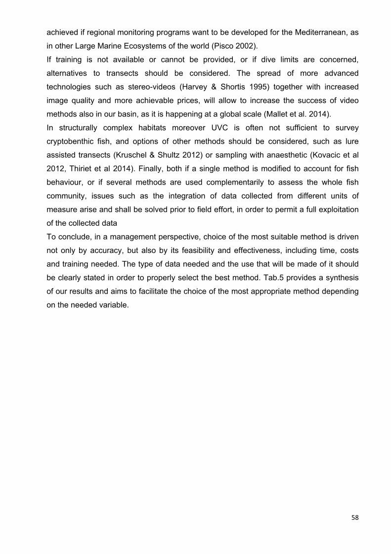
58  

achieved if regional monitoring programs want to be developed for the Mediterranean, as

in other Large Marine Ecosystems of the world (Pisco 2002).

If training is not available or cannot be provided, or if dive limits are concerned,

alternatives to transects should be considered. The spread of more advanced

technologies such as stereo-videos (Harvey & Shortis 1995) together with increased

image quality and more achievable prices, will allow to increase the success of video

methods also in our basin, as it is happening at a global scale (Mallet et al. 2014).

In structurally complex habitats moreover UVC is often not sufficient to survey

cryptobenthic fish, and options of other methods should be considered, such as lure

assisted transects (Kruschel & Shultz 2012) or sampling with anaesthetic (Kovacic et al

2012, Thiriet et al 2014). Finally, both if a single method is modified to account for fish

behaviour, or if several methods are used complementarily to assess the whole fish

community, issues such as the integration of data collected from different units of

measure arise and shall be solved prior to field effort, in order to permit a full exploitation

of the collected data

To conclude, in a management perspective, choice of the most suitable method is driven

not only by accuracy, but also by its feasibility and effectiveness, including time, costs

and training needed. The type of data needed and the use that will be made of it should

be clearly stated in order to properly select the best method. Tab.5 provides a synthesis

of our results and aims to facilitate the choice of the most appropriate method depending

on the needed variable.

59  

Tab. 5 Synthetic scores for each method according to the variables to be measured and to their cost‐efficiency. Scores are assigned a   gradation of colours from bright green (best score) to dark grey (worst score). Asterisks :method aptness to measure the given variable, based on the number of papers adopting the method in the literature.  *low aptness, *** high aptness,  F= feasible with conditions. NA= not feasible. 

‐ Time : T= < 15 min, TT= >15,<30 min, TTT=  30 – 120 min ‐ Training : S = skills in video analysis and video equipment handling, SS = skills in in diving and species identification, SSS=  skills in diving, species identification, enumeration of 

fish, estimation of fish size,  estimation of sampling surface area) .  ‐ Costs: € = 1000‐2000 € , €€= 3000‐4000 €, €€€ = 4000‐10000 € 

  

  

Tran

sect 

Circular 

fixed point 

Total counts 

Ran

dom 

counts 

FAST 

Video 

tran

sect 

Staviro 

BUV 

ROV 

Cab

led 

observatory 

Spearfishing 

video 

Variables/surface Density, Size/Biomass  ***  **  **  NA  NA  NA  NA  F  NA  F  * 

Total variables Abundance, pres/abs, Sp. richness and community  metrics, Freq. of occurrence, Behaviour  

***  **  **  **  NA  *  *  *  *  *  * 

Variables/time  Tot N, Max N, Spp/min  *  *  *  *  *  *  *  *  *  *  * 

 

Time       T  T  TT  TT  T  TTT  TTT  TTT  TTT  TTT  TT 

Training  SSS  SSS  SS  SS  SS  SS  S  S  S  S  S 

Costs  €  €  €  €  €  €€  €€  €€  €€€  €€€  € 

60  

3.6 References Addis P, Cau A, Massuti E, Merella P, Sinopoli M, Andaloro F (2006) Spatial and temporal

changes in the assemblage structure of fishes associated to fish aggregation devices in the Western Mediterranean. Aquat Living Resour 19:149–160

Airoldi L, M W Beck (2007). Loss, status and trends for coastal marine habitats of Europe. Oceanography and Marine Biology 45:345–405.

Andaloro F, Castriota L, Ferraro M, Romeo T, Sarà G, Consoli P (2011) Evaluating fish assemblages associated with gas platforms: evidence from a visual census technique and experimental fishing surveys. Cienc Mar 37:1–9

Andaloro F, Ferraro M, Mostarda E, Romeo T, Consoli P (2013a) Assessing the suitability of a remotely operated vehicle (ROV) to study the fish community associated with offshore gas platforms in the Ionian Sea: a comparative analysis with underwater visual censuses (UVCs). Helgol Mar Res 67:241–250

Andaloro F, Ferraro M, Mostarda E, Romeo T, Consoli P (2013b) Assessing the suitability of a remotely operated vehicle (ROV) to study the fish community associated with offshore gas platforms in the Ionian Sea: a comparative analysis with underwater visual censuses (UVCs). Helgol Mar Res 67:241–250

Anderson MJ (2001) Permutation tests for univariate or multivariate analysis of variance and regression. Can J Fish Aquat Sci 58:626–639

Azzurro E, Aguzzi J, Maynou F, Chiesa JJ, Savini D (2013) Diel rhythms in shallow Mediterranean rocky-reef fishes: a chronobiological approach with the help of trained volunteers. J Mar Biol Assoc U K 93:461–470

Bannerot SP, Bohnsack JA (1986) A stationary visual census technique for quantitatively assessing community structure of coral reef fishes. NOAA Technical Report NMFS 41:1–15

Bassu V, Porcu C, Niccolini F (2007) Studio sul valore economico delle popolazioni di cernie nell' Area Marina Protetta di Tavolara Punta Coda Cavallo. Rapporto finale 2008, Intervento E1.

Biagi F, Gambaccini S, Zazzetta M (1998) Settlement and recruitment in fishes: the role of coastal areas. Ital J Zool 65:269–274

Boland GS, Lewbel GS (1986) Estimation of demersal fishdensities in biological surveys using underwater television systems. Oceans 2: 9−13

Bombace G, Fabi G, Fiorentini L, Spagnolo A (1995) Assessment of the ichthyofauna of an artificial reefe through visual census and trammel net: comparison between the two sampling techiques

Bouchoucha B, Pelletier D, Herves, G. H, Roman W, Mallet D (2013) Guide méthodologique simplifié pour la mise en oeuvre des STAVIRO et l’analyse des images.

Bouchoucha M, Witkowski F, Mallet D, Roman W, Hervé G, Pelletier D (2013) Remote rotating video for fast spatial survey of coastal Mediterranean macrofauna and habitats.

61  

Bozec Y-M, Kulbicki M, Laloë F, Mou-Tham G, Gascuel D (2011) Factors affecting the detection distances of reef fish: implications for visual counts. Marine Biology 158:969–981

Brock VE (1954). A preliminary report on a method of estimating reef fish popula-tion. J. Wildlife Manag. 18: 297–308.

Bulleri F, Benedetti-Cecchi L (2014) Chasing fish and catching data: recreational spearfishing videos as a tool for assessing the structure of fish assemblages on shallow rocky reefs. Mar Ecol Prog Ser 506:255–265

Cappo M, Harvey E, Malcolm H, Speare P, others (2003) Potential of video techniques to monitor diversity, abundance and size of fish in studies of marine protected areas. Aquat Prot Areas-What Works Best We Know:455–464

Cardona L, Lopez D, Sales M, Caralt S De, Diez I (2007) Effects of recreational fishing on three fish species from the Posidonia oceanica meadows off Minorca (Balearic archipelago, western Mediterranean). Sci Mar 71:811–820

Carstensen J (2014) Need for monitoring and maintaining sustainable marine ecosystem services. Frontiers in Marine Science 1:33

Cheal AJ, Thompson AA (1997) Comparing visual counts of coral reef fish: implications of transect width and species selection. Mar Ecol Prog Ser 158:241–248

Christensen V, Pauly D (1993) Trophic Models of Aquatic Ecosystems. The World Fish Center

Christensen V, Walters CJ (2004) Ecopath with Ecosim: methods, capabilities and limitations. Ecological modelling 172:109–139

Clarke KR, Green RH (1988) Statistical design and analysis for a“ biological effects” study. Mar Ecol Prog Ser 46:213–226

Coll M, Piroddi C, Albouy C, Rais Lasram F Ben, Cheung WWL, Christensen V, Karpouzi VS, Guilhaumon F, Mouillot D, Paleczny M, others (2011) The Mediterranean Sea under siege: spatial overlap between marine biodiversity, cumulative threats and marine reserves. Glob Ecol Biogeogr 24:12

Condal F, Aguzzi J, Sarda F, Nogueras M, Cadena J, Costa C, Rio J Del, Manuel A (2012) Seasonal rhythm in a Mediterranean coastal fish community as monitored by a cabled observatory. Mar Biol 159:2809–2817

D’Anna G, Lipari Ro, Badalamenti F, Cuttitta A (1999a) Questions arising from the use of visual census in natural and artificial habitats. Fish Vis Census Mar Prot Areas Il Nat Sicil 23:187–204

D’Anna G, Lipari Ro, Badalamenti F, Cuttitta A (1999b) Questions arising from the use of visual census in natural and artificial habitats. Fish Vis Census Mar Prot Areas Il Nat Sicil 23:187–204

Dempster T, Sanchez-Jerez P, Bayle-Sempere JT, Giménez-Casalduero F, Valle C (2002) Attraction of wild fish to sea-cage fish farms in the south-western Mediterranean Sea: spatial and short-term temporal variability. Mar Ecol Prog Ser 242:237–252

Di Franco A, Bussotti S, Navone A, Panzalis P, Guidetti P (2009) Evaluating effects of total and partial restrictions to fishing on Mediterranean rocky-reef fish assemblages. Mar Ecol Prog Ser 387:275–285

62  

Fedra K, Machan R (1979) A Self-Contained Underwater Time-Lapse Camera for in situ Long-Term Observations. Marine Biology 55: 239-246

Francour P (1997) Fish assemblages of Posidonia oceanica beds at Port-Cros (France, NW Mediterranean): Assessment of composition and long-term fluctuations by visual census. Mar Ecol 18:157–173

Francour P (1999a) A critical review of adult and juvenile fish sampling techniques in Posidonia oceanica seagrass beds. Nat Sicil 23:33–57

Francour P (1999b) A critical review of adult and juvenile fish sampling techniques in Posidonia oceanica seagrass beds. Nat Sicil 23:33–57

Giakoumi S, Kokkoris GD (2013) Effects of habitat and substrate complexity on shallow sublittoral fish assemblages in the Cyclades Archipelago, North-eastern Mediterranean sea. Mediterranean Marine Science 14:58–68

De Girolamo M, Mazzoldi C (2001) The application of visual census on Mediterranean rocky habitats. Mar Environ Res 51:1–16

Guidetti P, Baiata P, Ballesteros E, Di Franco A, Hereu B, Macpherson E, Micheli F, Pais A, Panzalis P, Rosenberg AA, Zabala M, Sala E (2014) Large-Scale Assessment of Mediterranean Marine Protected Areas Effects on Fish Assemblages. PLoS ONE 9:e91841

Guidetti P, Micheli F (2011) Ancient art serving marine conservation. Frontiers in Ecology and the Environment 9:374–375

Guidetti P, Verginella L, Viva C, Odorico R, Boero F (2005) Protection effects on fish assemblages, and comparison of two visual-census techniques in shallow artificial rocky habitats in the northern Adriatic Sea. J Mar Biol Assoc U K 85:247–255

Harmelin-Vivien ML, Francour P (1992) Trawling or visual censuses? Methodological bias in the assessment of fish populations in seagrass beds. Mar Ecol 13:41–51

Harmelin-Vivien M, Harmelin J (1975) Présentation d’une méthode d’évaluation in situ de la faune ichtyologique. Trav Sci Parc Nation Port-Cros 1:47–52

Harmelin-Vivien M, Harmelin J, Chauvet C, Duval C, Galzin R, Lejeune P, Barnabé G, Blanc F, Chevalier R, Duclerc J (1985) Evaluation visuelle des peuplements et populations de poissons: méthodes et problèmes. Rev Décologie 40:467–539

Harvey E, Shortis M (1995) A system for stereo-video measurement of sub-tidal organisms. Mar Technol Soc J 29:10–22

Holmlund CM, Hammer M (1999) Ecosystem services generated by fish populations. Ecological Economics, 29: 253–268

Jackson JBC, Kirby MX, Berger WH, Bjorndal KA, Botsford LW, Bourque BJ, Bradbury RH, Cooke R, Erlandson J, Estes JA (2001) Historical overfishing and the recent collapse of coastal ecosystems. science 293:629–637

Kingsford MJ, CN Battershil. (1998): Procedures for establishing a study. Studying temperate marine environments-A handbook for ecologists. Canterbury University Press, Christchurch 29-48.

Kovačić M, Patzner RA, Schliewen U (2012) A first quantitative assessment of the ecology of cryptobenthic fishes in the Mediterranean Sea. Mar Biol 159:2731–2742

63  

Kruschel C, Schultz ST (2012) Use of a lure in visual census significantly improves probability of detecting wait-ambushing and fast cruising predatory fish. Fisheries Research 123–124:70–77

Kulbicki M (1998) How the acquired behaviour of commercial reef fishes may influence the results obtained from visual censuses. Journal of Experimental Marine Biology and Ecology 222:11–30

La Mesa G, Molinari A, Tunesi L (2010) Coastal fish assemblage characterisation to support the zoning of a new Marine Protected Area in north-western Mediterranean. Ital J Zool 77:197–210

La Mesa G, Guidetti P, Bussotti S, Cattaneo-Vietti R, Manganaro A, Molinari A, Russo GF, Spano N, Vetrano G, Tunesi L (2013) Rocky reef fish assemblages at six Mediterranean marine protected areas: broad-scale patterns in assemblage structure, species richness and composition. Italian Journal of Zoology 80:90–103

Lester SE, Halpern BS (2008) Biological responses in marine no-take reserves versus partially protected areas. Marine Ecology Progress Series 367:49–56

Macpherson E, Biagi F, Francour P, García-Rubies A, Harmelin J, Harmelin-Vivien J, Jouvenel J, Planes S, Vigliola L, Tunesi L (1997) Mortality of juvenile fishes of the genus Diplodus in protected and unprotected areas in the western Mediterranean Sea. Mar Ecol Prog Ser 160:135–147

Mallet D, Pelletier D (2014) Underwater video techniques for observing coastal marine biodiversity: A review of sixty years of publications (1952–2012). Fish Res 154:44–62

Mallet D, Wantiez L, Lemouellic S, Vigliola L, Pelletier D (2014) Complementarity of Rotating Video and Underwater Visual Census for Assessing Species Richness, Frequency and Density of Reef Fish on Coral Reef Slopes. PLoS ONE 9:e84344

Moreno I (2006) Artificial reefs as a tool for coastal management in Balearic Islands (Western Mediterranean). J Coast Res:1843–1846

Murphy HM, Jenkins GP (2010) Observational methods used in marine spatial monitoring of fishes and associated habitats: a review. Mar Freshw Res 61:236

Myers RA, Worm B (2003) Rapid worldwide depletion of predatory fish communities. Nature 423:280–283

Pace ML, Cole JJ, Carpenter SR, Kitchell JF (1999) Trophic cascades revealed in diverse ecosystems. Trends Ecol Evol 14:483–488

Pauly D, Christensen V, Dalsgaard J, Froese R, Torres Jr F (1998) Fishing down marine food webs. Science 279:860–863

Pelletier D, Leleu K, Mou-Tham G, Guillemot N, Chabanet P (2011) Comparison of visual census and high definition video transects for monitoring coral reef fish assemblages. Fisheries Research 107:84–93

Pelletier D, Leleu K, Mallet D, Mou-Tham G, Hervé G, Boureau M, Guilpart N (2012) Remote High-Definition Rotating Video Enables Fast Spatial Survey of Marine Underwater Macrofauna and Habitats (SJ Goldstien, Ed.). PLoS ONE 7:e30536

Pinnegar JK, Polunin NVC, Francour P, Badalamenti F, Chemello R, Harmelin-Vivien ML, Hereu B, Milazzo M, Zabala M, Anna G d’ (2000) Trophic cascades in benthic

64  

marine ecosystems: lessons for fisheries and protected-area management. Environ Conserv 27:179–200

Pisco (2010) Monitoring MPAs by SCUBA in waters off Central California. Partnership for Interdisciplinary Studies of Coastal Oceans. www.piscoweb.org.

Prato G, Gascuel D, Valls A, Francour P (2014) Balancing complexity and feasibility in Mediterranean coastal food-web models: uncertainty and constraints. Mar Ecol Prog Ser 512:71–88

Relini M, Torchia G, Relini G (1994) Seasonal variation of fish assemblages in the Loano artificial reef (Ligurian Sea Northwestern-Mediterranean). Bull Mar Sci 55:2–3

Rilov G, Benayahu Y (2000) Fish assemblage on natural versus vertical artificial reefs: the rehabilitation perspective. Mar Biol 136:931–942

Sala E, Ballesteros E, Dendrinos P, Di Franco A, Ferretti F, Foley D, Fraschetti S, Friedlander A, Garrabou J, Güçlüsoy H, Guidetti P, Halpern BS, Hereu B, Karamanlidis AA, Kizilkaya Z, Macpherson E, Mangialajo L, Mariani S, Micheli F, Pais A, Riser K, Rosenberg AA, Sales M, Selkoe KA, Starr R, Tomas F, Zabala M (2012) The Structure of Mediterranean Rocky Reef Ecosystems across Environmental and Human Gradients, and Conservation Implications. PLoS ONE 7:e32742

Sale PF, Sharp BJ (1983) Correction for bias in visual transect censuses of coral reef fishes. Coral Reefs 2:37–42

Sandin SA, Smith JE, DeMartini EE, Dinsdale EA, Donner SD, Friedlander AM, Konotchick T, Malay M, Maragos JE, Obura D (2008) Baselines and degradation of coral reefs in the northern Line Islands. PLoS One 3: e1458

Seytre C, Francour P (2008) Is the Cape Roux marine protected area (Saint-Raphael, Mediterranean Sea) an efficient tool to sustain artisanal fisheries? First indications from visual censuses and trammel net sampling. Aquat Living Resour 21:297–305

Seytre C, Francour P (2009) The Cap Roux MPA (Saint-Raphael, French Mediterranean): changes in fish assemblages within four years of protection. ICES J Mar Sci 66:180–187

Sherman K, Duda A (2002). Large marine ecosystem monitoring, assessment, and management across the global north-south divide. ICES Council Meeting Papers CM 2002/W:2

Sherman K, Hempel G (Editors) 2009. The UNEP Large Marine Ecosystem Report: A perspective on changing conditions in LMEs of the world Regional Seas. UNEP Regional Seas Report and Studies No. 182. United Nations Environment Programme. Nairobi, Kenya.

Steele JH, Schumacher M (2000) Ecosystem structure before fishing. Fish Res 44:201–205

Steinberg JC, Koczy FF, (1964). An acoustic-video system for marine biologicalresearch: objectives and requirements. In: Tavolga WN (Ed.), Marine Bio-Acoustics. Pergamon Press, New York, pp. 1–9

Stobart B, García-Charton JA, Espejo C, Rochel E, Goñi R, Reñones O, Herrero A, Crec’hriou R, Polti S, Marcos C, Planes S, Pérez-Ruzafa A (2007) A baited

65  

underwater video technique to assess shallow-water Mediterranean fish assemblages: Methodological evaluation. J Exp Mar Biol Ecol 345:158–174

Tessier A, Pastor J, Francour P, Saragoni G, Crec’hriou R, Lenfant P (2013) Video transect as a complement to underwater visual census to study reserve effect on fish assemblages. Aquat Biol

Thiriet P (2014) Comparison of fish assemblage structure and underlying ecological processes, between Cystoseira forests and less structurally complex habitats of North-Western Mediterranean rocky subtidal. PhD diss., Université Nice Sophia Antipolis

Thresher RE, Gunn JS (1986) Comparative analysis of visual census techniques for highly mobile, reef-associated piscivores (Carangidae). Environ Biol Fish 17:93–116

UNEP-MAP-RAC/SPA: Strategic Action Programme For The Conservation Of Biological Diversity (SAP BIO) InThe Mediterranean Region, Tunis, 2003

Vacchi M, La Mesa G, Boyer M, Bearzi P (1999) fish visual census in marine protected areas. Il Naturalista Sicilano 23,Proceedings of the International workshop, Ustica

Vacchi M, Tunesi L (1993) Stationary visual census: A technique for the assessment of fish assemblages in Mediterranean protected coastal areas. Boll Oceanol Teor Appl 11:225–229

Watson R, Pauly D (2001) Systematic distortions in world fisheries catch trends. Nature 414:534–536

Worm B, Barbier EB, Beaumont N, Duffy JE, Folke C, Halpern BS, Jackson JBC, Lotze HK, Micheli F, Palumbi SR, Sala E, Selkoe KA, Stachowicz JJ, Watson R (2006) Impacts of Biodiversity Loss on Ocean Ecosystem Services. Science 314:787–790

66  

3.7 Annex  

Transects (Harmelin Vivien 1975): visual census along transects involves a trained diver

swimming at constant speed along a straight path of known length and recording all fish

visible within a pre-determined distance at each side of the path. Transect width can be

adapted according to fish mobility (generally 1 m width for cryptic fish, 5 meter width for

nectobenthic fish).

Stationary point counts (Bohnsack & Bannerot 1986; Vacchi & Tunesi 1993): this

technique involves a diver who sets on the seafloor and records all fish visible within an

imaginary cylinder of pre-determined radius length, extending from the bottom to the

surface. When all species within his field of view are recorded, the diver rotates to scan

another sector, until the full circle is completed. A whole circle count lasts 5 minutes.

Possible adaptations are different radius lengths or different total sampling time due to

separation of functional groups counts (i.e at the first rotation necto-benthic fish are

counted, then cryptic fish in a second rotation) (La Mesa et al. 2013)

Mobile point counts (Rilov & Benayahu 2000): this technique was specifically developed

to census the fish community at gas platforms and consisted in swimming along an

imaginary circle of 3 meters radius with the pillar as centre and counting all fish within the

circle.

Rapid Visual Census (RVC) (Kingsford & Battershill 1998, Dempster et al 2002): Method

designed to census fish around fish farm cages. Swimming through the water mass

adjoining fish farm cages, the diver counts all fish present within a strip 15 m wide, 50

length and 15 m deep, covering a volume of approximatively 11 250 m3. Each count lasts

5 minutes.

Spatial counts (Charbonnel et al 1997, D’Anna et al 1999): mixed technique designed to

census fish around artificial reefs, including line transects, circular transects and point

counts. First phase: a diver sets on top of the artificial pyramid and counts all fish present

around the complete perimeter of the pyramid during 5-8 minutes. Second phase: the diver

swims around the perimeter of the pyramid (circular transect) and then through one of its

internal passages (line transect), to record more sedentary and cryptic fish (10 minutes).

67  

Last phase: the diver swims through a transect 25 m x 6 m to reach the second pyramid,

where the census operations are repeated in the same way. Length of the transects and

duration of the census are adapted according to artificial reefs structure.

Total counts (Harmelin Vivien 1985, Planes et al 1998): the principle of this method is to

count all target fish within a given area, generally defined by a trait of coastline of known

length and a given isobath.

Random paths (Harmelin Vivien 1985, Francour 1999): technique involving counts of

fixed or varying duration made on random paths across the selected area. Data collected

in this way provide information on species diversity and spatial distribution. This method is

generally used in concomitance to other census techniques were the sampled surface is

known (allowing estimates of density).

Fish assemblage survey technique (FAST) (Seytre & Francour 2009): this technique is

a modification of random counts consisting in six 15 min random visual censuses covering

all kind of substrata (sand, seagrass, rock). Census are performed on a presence-absence

basis and on a two size class basis (large fish >2/3 of fish total length, and small to

medium fish <2/3 total length). Only a predetermined set of species are recorded, which

are those targeted by professional and/or recreational fishing. The so collected data are

treated in a standard way in order to compute a set of indices describing the health of the

fish assemblage. Being very easy to apply this technique is well adapt for citizen science.

Diver Operated Video transects (DOV) (Boland and Leubel 1986, Tessier et al 2013):

the method involves a diver holding a camera and swimming 1.5 m above the bottom at

constant speed, along a transect of fixed length. The operator keeps the video camera

steady and perpendicular to the bottom, recording in front of himself. A reference bar

attached to the camera housing is sometimes used to control the camera elevation.

Remotely Operated Video (ROV) (Fedra & Machan 1979, Stokesbury et al 2004): ROV

systems are equipped with HD camera and can be stationary and linked to a vessel or

platform, autonomous and thus set on the seafloor, or finally towed by a vessel. Towed

systems are towed by the vessel at low speed in order to film along a predefined

trajectory of known length. Systems can be deployed in the water column at a constant

68  

elevation from the seafloor or above the seabed using a sledge, depending on the targeted

fish assemblage. The cameras can be set vertically in order to face the sea floor or with a

fixed downward angle. ROV systems can also be adapted to record fish around gas

platform pillars, simulating the trajectory of a mobile point count (Andaloro et al 2013)

Remote rotating video system (Staviro, STAtion Video ROtative in French) (Pelletier

et al 2012, Bouchacha et al 2013): The Staviro is a remote high definition rotating video

system fixed on a tripod, dropped from the boat onto the seabed, and retrieved using

buoys and rigging. The rotation affords a 360◦ providing panoramic images and a much

larger surveyed area than fixed ROV systems, while avoiding the image distortion

characteristic of fisheye lenses (Pelletier et al 2012). Potential double counting is

minimized by paying particular attention to the direction of fish movement with respect to

rotation, and by calculating the mean abundance over rotations, to average out the

variability between rotations. More details on image analysis are given in the methods

section.

Baited Underwater Video (BUV) (Cappo et al 2004, Stobart et al 2007): a BUV ystem

consists in one or two HD video cameras sheltered by a video housing firmly mounted

within a protective cage. The cameras film the sea surrounding the bait, which is placed

close to the camera, at a distance that can range from 0.5 to 1.5 m. The choice of the bait

depends on the species that want to be attracted. The orientation of the system can be

either horizontal or vertical to the bottom, resulting in different abundances and species

compositions of the observed fish assemblage (Langlois et al., 2006; Wraith, 2007).

Cabled observatory (Condal et al 2012): these structures are permanent video platforms

using cables for energy supply, data transfer and instrument control. They are equipped

with cameras that can continuously acquire digital images of the surrounding environment

at 360, for long periods (months-years). For image analysis the field of view of interest can

be selected. This system has been used to document seasonal rhythms of fish

communities over long time windows.

Spearfishing video: while spearfishing, videos are generally recorded using Go-pro HD

micro cameras mounted on a spear gun, recording footage with a given angle. Bulleri et al

69  

2014 proposed to use widely available spearfishing videos to monitor fish assemblage at

large spatial and temporal scales with low costs.

References of reviewed papers

Addis P, Cau A, Massuti E, Merella P, Sinopoli M, Andaloro F (2006) Spatial and temporal changes in the assemblage structure of fishes associated to fish aggregation devices in the Western Mediterranean. Aquatic Living Resources 19:149–160

Addis P, Secci M, Cau A (2013) The effect of Mistral (a strong NW wind) episodes on the occurrence and abundance of Atlantic bluefin tuna (Thunnus thynnus) in the trap fishery of Sardinia (W Mediterranean). Scientia Marina 77:419–427

Andaloro F, Castriota L, Ferraro M, Romeo T, Sara G, Consoli P (2011) Evaluating fish assemblages associated with gas platforms: Evidence from a visual census technique and experimental fishing surveys. Ciencias Marinas 37:1–9

Andaloro F, Ferraro M, Mostarda E, Romeo T, Consoli P (2013) Assessing the suitability of a remotely operated vehicle (ROV) to study the fish community associated with offshore gas platforms in the Ionian Sea: a comparative analysis with underwater visual censuses (UVCs). Helgoland Marine Research 67:241–250

Arechavala-Lopez P, Uglem I, Sanchez-Jerez P, Fernandez-Jover D, Bayle-Sempere JT, Nilsen R (2010) Movements of grey mullet Liza aurata and Chelon labrosus associated with coastal fish farms in the western Mediterranean Sea. Aquaculture Environment Interactions 1:127–136

Arigoni S, Francour P, Harmelin-Vivien M, Zaninetti L (2002) Adaptive colouration of Mediterranean labrid fishes to the new habitat provided by the introduced tropical alga Caulerpa taxifolia. Journal of Fish Biology 60:1486–1497

Azzurro E, Aguzzi J, Maynou F, Chiesa JJ, Savini D (2013) Diel rhythms in shallow Mediterranean rocky-reef fishes: a chronobiological approach with the help of trained volunteers. Journal of the Marine Biological Association of the United Kingdom 93:461–470

Azzurro E, Matiddi M, Fanelli E, Guidetti P, Mesa G La, Scarpato A, Axiak V (2010) Sewage pollution impact on Mediterranean rocky-reef fish assemblages. Marine environmental research 69:390–397

Azzurro E, Pais A, Consoli P, Andaloro F (2007) Evaluating day-night changes in shallow Mediterranean rocky reef fish assemblages by visual census. Marine Biology 151:2245–2253

Bayle-Sempere JT, Ramos-Espla AA, Garcia Charton JA (1994) Intra-annual variability of an artificial reef fish assemblage in the marine reserve of Tabarca (Alicante, Spain, SW Mediterranean). Bulletin of Marine Science 55:2–3

Bell JD (1983) Effects of depth and marine reserve fishing restrictions on the structure of a rocky reef fish assemblage in the north-western Mediterranean Sea. Journal of Applied Ecology:357–369

Bellier E, Neubauer P, Monestiez P, Letourneur Y, Ledireach L, Bonhomme P, Bachet F (2013) Marine reserve spillover: Modelling from multiple data sources. Ecological Informatics 18:188–193

70  

Biagi F, Gambaccini S, Zazzetta M (1998) Settlement and recruitment in fishes: the role of coastal areas. Italian Journal of Zoology 65:269–274

Bodilis P, Louisy P, Draman M, Arceo HO, Francour P (2014) Can Citizen Science Survey Non-indigenous Fish Species in the Eastern Mediterranean Sea? Environmental Management 53:172–180

Bodilis P, Seytre, C. C, Charbonnel E, Francour, P. F (2011) Monitoring of the artificial reef fish assemblages of the Gulf Juan marine protected area (France, North Western Mediterranean). Brazilian Journal of Oceanography 59:167–176

Bombace G, Fabi G, Fiorentini L, Spagnolo A (1995) Assessment of the ichthyofauna of an artificial reefe through visual census and trammel net: comparison between the two sampling techiques

Bonaca MO, Lipej L (2005) Factors affecting habitat occupancy of fish assemblage in the Gulf of Trieste (Northern Adriatic Sea). Marine Ecology-an Evolutionary Perspective 26:42–53

Bonaviri C, Fernández TV, Badalamenti F, Gianguzza P, Lorenzo M Di, Riggio S (2009) Fish versus starfish predation in controlling sea urchin populations in Mediterranean rocky shores. Marine Ecology Progress Series 382:129–138

Bubic TS, Grubisic L, Ticina V, Katavic I (2011) Temporal and spatial variability of pelagic wild fish assemblages around Atlantic bluefin tuna Thunnus thynnus farms in the eastern Adriatic Sea. Journal of Fish Biology 78:78–97

Bulleri F, Benedetti-Cecchi L (2014) Chasing fish and catching data: recreational spearfishing videos as a tool for assessing the structure of fish assemblages on shallow rocky reefs. Marine Ecology Progress Series 506:255–U569

Bussotti S, Denitto F, Guidetti P, Belmonte G (2002) Fish Assemblages in Shallow Marine Caves of the Salento Peninsula (Southern Apulia, SE Italy). Marine Ecology-Pubblicazioni Della Stazione Zoologica Di Napoli I 23:11–20

Bussotti S, Guidetti P (1999) Fish communities associated with different seagrass systems in the Mediterranean Sea. Naturalista siciliano 23:245–259

Bussotti S, Guidetti P (2005) Distribution patterns of the golden goby, Gobius auratus, in Mediterranean sublittoral rocky cliffs. Italian Journal of Zoology 72:305–309

Bussotti S, Guidetti P (2009) Do Mediterranean fish assemblages associated with marine caves and rocky cliffs differ? Estuarine Coastal and Shelf Science 81:65–73

Bussotti S, Guidetti P (2011) Timing and habitat preferences for settlement of juvenile fishes in the Marine Protected Area of Torre Guaceto (south-eastern Italy, Adriatic Sea). Italian Journal of Zoology 78:243–254

Bussotti S, Guidetti P, Belmonte G (2003) Distribution patterns of the cardinal fish, Apogon imberbis, in shallow marine caves in southern Apulia (SE Italy). Italian Journal of Zoology 70:153–157

Cardona L, Lopez D, Sales M, Caralt S De, Diez I (2007) Effects of recreational fishing on three fish species from the Posidonia oceanica meadows off Minorca (Balearic archipelago, western Mediterranean). Scientia Marina 71:811–820

Cecchi E, Piazzi L, Balata D (2007) Interaction between depth and protection in determining the structure of Mediterranean coastal fish assemblages. Aquatic Living Resources 20:123–129

71  

Cenci E, Pizzolon M, Chimento N, Mazzoldi C (2011) The influence of a new artificial structure on fish assemblages of adjacent hard substrata. Estuarine Coastal and Shelf Science 91:133–149

Charbonnel E, Francour P, Harmelin J (1996) Finfish population assessment techniques on artificial reefs: a review in the European Union. In: p 261–278

Charbonnel E, Francour P, Harmelin J, Ody D (1995) Les problèmes d’échantillonnage et de recensement du peuplement ichtyologique dans les récifs artificiels. Biol Mar Med 2:85–90

Charbonnel E, Serre C, Ruitton S, Harmelin JG, Jensen A (2002) Effects of increased habitat complexity on fish assemblages associated with large artificial reef units (French Mediterranean coast). ICES Journal of Marine Science 59:S208–S213

Charton JG, Williams I, Ruzafa AP, Milazzo M, Chemello R, Marcos C, Kitsos M-S, Koukouras A, Riggio S (2000) Evaluating the ecological effects of Mediterranean marine protected areas: habitat, scale and the natural variability of ecosystems. Environmental Conservation 27:159–178

Cheminee A, Sala E, Pastor J, Bodilis P, Thiriet P, Mangialajo L, Cottalorda JM, Francour P (2013) Nursery value of Cystoseira forests for Mediterranean rocky reef fishes. J Exp Mar Biol Ecol 442:70–79

Ciriaco S, Costantini M, Italiano C, Odorico R, Picciulin M, Verginella L, Spoto M (1998) Monitoring the Miramare Marine Reserve: assessment of protection efficiency. Italian Journal of Zoology 65:383–386

Claudet J, Pelletier D, Jouvenel JY, Bachet F, Galzin R (2006) Assessing the effects of marine protected area (MPA) on a reef fish assemblage in a northwestern Mediterranean marine reserve: Identifying community-based indicators. Biological Conservation 130:349–369

Coll J, Abad R, Alvarez E, Deudero S, Mas R, Riera F, Moreno I (2009) Dtate of fish populations and influence on the trammel net fishery at three balearic island (Western Mediterranean) artificial reefs a decade after their deployment. Bulletin of Marine Science 85:77–100

Coll J, Garcia-Rubies A, Morey G, Reñones O, Álvarez-Berastegui D, Navarro O, Grau AM (2013) Using no-take marine reserves as a tool for evaluating rocky-reef fish resources in the western Mediterranean. ICES Journal of Marine Science: fst025

Coll J, Moranta J, Renones O, Garcia-Rubies A, Moreno I (1998) Influence of substrate and deployment time on fish assemblages on an artificial reef at Formentera Island (Balearic Islands, western Mediterranean). Hydrobiologia 385:139–152

Condal F, Aguzzi J, Sarda F, Nogueras M, Cadena J, Costa C, Rio J Del, Manuel A (2012) Seasonal rhythm in a Mediterranean coastal fish community as monitored by a cabled observatory. Marine Biology 159:2809–2817

Consoli P, Romeo T, Ferraro M, Sara G, Andaloro F (2013) Factors affecting fish assemblages associated with gas platforms in the Mediterranean Sea. Journal of Sea Research 77:45–52

Consoli P, Romeo T, Giongrandi U, Andaloro F (2008) Differences among fish assemblages associated with a nearshore vermetid reef and two other rocky habitats along the shores of Cape Milazzo (northern Sicily, central Mediterranean

72  

Sea). Journal of the Marine Biological Association of the United Kingdom 88:401–410

Claudet J, Garcia - Charton JA, Lenfant P (2011) Combined effects of levels of protection and environmental variables at different spatial resolutions on fish assemblages in a marine protected area. Conservation Biology 25:105–114

Consoli P, Sara G, Mazza, G. M, Battaglia, P. B, Romeo, T. R, Incontro, V. I, Andaloro, F A (2013) The effects of protection measures on fish assemblage in the Plemmirio marine reserve (Central Mediterranean Sea, Italy): A first assessment 5 years after its establishment. Journal of Sea Research 79:20–26

D’Anna G, Badalamenti F, Lipari R, Cuttitta A, Pipitone C (1995) Fish assemblage analysis by means of a visual census survey on an artificial reef and on natural areas in the Gulf of Castellammare (NW Sicily). In: p 27–31

D’Anna G, Giacalone VM, Badalamenti F, Pipitone C (2004) Releasing of hatchery-reared juveniles of the white seabream Diplodus sargus (L., 1758) in the Gulf of Castellammare artificial reef area (NW Sicily). Aquaculture 233:251–268

D’Anna G, Lipari Ro, Badalamenti F, Cuttitta A (1999) Questions arising from the use of visual census in natural and artificial habitats. Fish Visual Census in Marine Protected Areas Il Naturalista Siciliano 23:187–204

Dempster T, Sanchez-Jerez P, Bayle-Sempere JT, Giménez-Casalduero F, Valle C (2002) Attraction of wild fish to sea-cage fish farms in the south-western Mediterranean Sea: spatial and short-term temporal variability. Marine Ecology Progress Series 242:237–252

Di Franco A, Bussotti S, Navone A, Panzalis P, Guidetti P (2009) Evaluating effects of total and partial restrictions to fishing on Mediterranean rocky-reef fish assemblages. Marine Ecology Progress Series 387:275–285

Di Franco A, Coppini G, Pujolar JM, Leo GA De, Gatto M, Lyubartsev V, Melia P, Zane L, Guidetti P (2012) Assessing Dispersal Patterns of Fish Propagules from an Effective Mediterranean Marine Protected Area. PLoS ONE 7

Di Franco A, Di Lorenzo M, Guidetti P (2013) Spatial patterns of density at multiple life stages in protected and fished conditions: an example from a Mediterranean coastal fish. Journal of Sea Research 76:73–81

Di Franco A, Graziano M, Franzitta G, Felline S, Chemello R, Milazzo M (2011) Do small marinas drive habitat specific impacts? A case study from Mediterranean Sea. Marine Pollution Bulletin 62:926–933

Di Martino V, Stancanelli B, Molinari A (2007) Fish community associated with Halophila stipulacea meadow in the Mediterranean Sea. Cybium 31:451–458

Dufour V, Jouvenel JY, Galzin R (1995) Study of a Mediterranean rocky reef fish assemblage - comparisons of population-distributions between depths in protected and unprotected areas over one decade. Aquatic Living Resources 8:17–25

Fasola M, Canova L, Foschi F, Novelli O, Bressan M (1997) Resource use by a Mediterranean rocky slope fish assemblage. Marine Ecology 18:51–66

Felix-Hackradt FC, Hackradt CW, Trevino-Oton J, Perez-Ruzafa A, Garcia-Charton JA (2013) Temporal patterns of settlement, recruitment and post-settlement losses in

73  

a rocky reef fish assemblage in the South-Western Mediterranean Sea. Marine Biology 160:2337–2352

Fernández TV, D’Anna G, Badalamenti F, Perez-Ruzafa A (2008) Habitat connectivity as a factor affecting fish assemblages in temperate reefs. Aquatic Biology 1:239–248

Fernandez-Jover D, Sanchez-Jerez P, Bayle-Sempere JT, Valle C, Dempster T (2008) Seasonal patterns and diets of wild fish assemblages associated with Mediterranean coastal fish farms. ICES Journal of Marine Science 65:1153–1160

Forcada A, Bayle-Sempere JT, Valle C, Sanchez-Jerez P (2008) Habitat continuity effects on gradients of fish biomass across marine protected area boundaries. Marine environmental research 66:536–547

Franco A, Perez-Ruzafa A, Drouineau H, Franzoi P, Koutrakis ET, Lepage M, Verdiell-Cubedo D, Bouchoucha M, Lopez-Capel A, Riccato F, Sapounidis A, Marcos C, Oliva-Paterna FJ, Torralva-Forero M, Torricelli P (2012) Assessment of fish assemblages in coastal lagoon habitats: Effect of sampling method. Estuarine Coastal and Shelf Science 112:115–125

Francour P (1997) Fish assemblages of Posidonia oceanica beds at Port Cros (France, NW Mediterranean): Assessment of composition and long-term fluctuations by visual census. Marine Ecology-Pubblicazioni Della Stazione Zoologica Di Napoli I 18:157–173

Francour P (1999) A critical review of adult and juvenile fish sampling techniques in Posidonia oceanica seagrass beds. Naturalista sicil 23:33–57

Francour P (2000) Long term monitoring of Posidonia oceanica fish assemblages of the Scandola Marine Reserve (Corsica, northwestern Mediterranean). Cybium 24:85–95

Garcia-Charton JA, Perez-Ruzafa A (1998) Correlation between habitat structure and a rocky reef fish assemblage in the southwest Mediterranean. Marine Ecology-Pubblicazioni Della Stazione Zoologica Di Napoli I 19:111–128

García-Charton J, Pérez-Ruzafa A, Sánchez-Jerez P, Bayle-Sempere J, Reñones O, Moreno D (2004) Multi-scale spatial heterogeneity, habitat structure, and the effect of marine reserves on Western Mediterranean rocky reef fish assemblages. Marine Biology 144:161–182

Garcia-Rubies A (1999) Effects of fishing on community structure and on selected populations of Mediterranean coastal reef fish. Naturalista siciliano 23:59–81

Garcia-Rubies A, Hereu B, Zabala M (2013) Long-Term Recovery Patterns and Limited Spillover of Large Predatory Fish in a Mediterranean MPA. PLoS ONE 8

García-Rubies A, Macpherson E (1995) Substrate use and temporal pattern of recruitment in juvenile fishes of the Mediterranean littoral. Marine Biology 124:35–42

García-Rubies A, Zabala i Limousin M (1990) Effects of total fishing prohibition on the rocky fish assemblages of Medes Islands marine reserve (NW Mediterranean). Scientia Marina, 1990, vol 54, num 4, p 317-328

Georgiadis M, Mavraki N, Koutsikopoulos C, Tzanatos E (2014) Spatio-temporal dynamics and management implications of the nightly appearance of Boops boops (Acanthopterygii, Perciformes) juvenile shoals in the anthropogenically modified Mediterranean littoral zone. Hydrobiologia 734:81–96

74  

Giakoumi S, Grantham HS, Kokkoris GD, Possingham HP (2011) Designing a network of marine reserves in the Mediterranean Sea with limited socio-economic data. Biological Conservation 144:753–763

Giakoumi S, Kokkoris GD (2013) Effects of habitat and substrate complexity on shallow sublittoral fish assemblages in the Cyclades Archipelago, North-eastern Mediterranean sea. Mediterranean Marine Science 14:58–68

Girolamo M De, Mazzoldi C (2001) The application of visual census on Mediterranean rocky habitats. Marine environmental research 51:1–16

Girolamo M De, Scaggiante M, Rasotto M (1999) Social organization and sexual pattern in the Mediterranean parrotfish Sparisoma cretense (Teleostei: Scaridae). Marine Biology 135:353–360

Guidetti P (2000) Differences among fish assemblages associated with nearshore Posidonia oceanica seagrass beds, rocky-algal reefs and unvegetated sand habitats in the Adriatic Sea. Estuarine Coastal and Shelf Science 50:515–529

Guidetti P (2001) Population dynamics and post-settlement mortality of the ornate wrasse, Thalassoma pavo, in the Tyrrhenian Sea (western Mediterranean). Italian Journal of Zoology 68:75–78

Guidetti P (2002) Temporal changes in density and recruitment of the Mediterranean ornate wrasse Thalassoma pavo (Pisces, Labridae). Archive of Fishery and Marine Research 49:259–267

Guidetti P (2004) Fish assemblages associated with coastal defence structures in south-western Italy (Mediterranean Sea). Journal of the Marine Biological Association of the United Kingdom 84:669–670

Guidetti P, Bianchi CN, Chiantore M, Schiaparelli S, Morri C, Cattaneo-Vietti R (2004) Living on the rocks: substrate mineralogy and the structure of subtidal rocky substrate communities in the Mediterranean Sea. Marine Ecology Progress Series 274:57–68

Guidetti P, Bianchi CN, Mesa G La, Modena M, Morri C, Sara G, Vacchi M (2002) Abundance and size structure of Thalassoma pavo (Pisces : Labridae) in the western Mediterranean Sea: variability at different spatial scales. Journal of the Marine Biological Association of the United Kingdom 82:495–500

Guidetti P, Boero F (2001) Occurrence of the Mediterranean parrotfish Sparisoma cretense (Perciformes : Scaridae) in south-eastern Apulia (south-east Italy). Journal of the Marine Biological Association of the United Kingdom 81:717–718

Guidetti P, Boero F (2002) Spatio-temporal variability in abundance of the parrotfish, Sparisoma cretense, in SE Apulia (SE Italy, Mediterranean Sea). Italian Journal of Zoology 69:229–232

Guidetti P, Bussotti S (1997) Recruitment of Diplodus annularis and Spondyliosoma cantharus (Sparidae) in shallow seagrass beds along the Italian coasts (Mediterranean Sea). Marine Life 7:47–52

Guidetti P, Bussotti S (2000) Fish fauna of a mixed meadow composed by the seagrasses Cymodocea nodosa and Zostera noltii in the Western Mediterranean. Oceanologica Acta 23:759–770

75  

Guidetti P, Bussotti S (2002) Effects of seagrass canopy removal on fish in shallow Mediterranean seagrass (Cymodocea nodosa and Zostera noltii) meadows: a local-scale approach. Marine Biology 140:445–453

Guidetti P, Bussotti S, Boero F (2005) Evaluating the effects of protection on fish predators and sea urchins in shallow artificial rocky habitats: a case study in the northern Adriatic Sea. Marine environmental research 59:333–348

Guidetti P, Cattaneo-Vietti R (2002) Can mineralogical features influence distribution patterns of fish? A case study in shallow Mediterranean rocky reefs. Journal of the Marine Biological Association of the United Kingdom 82:1043–1044

Guidetti P, Fanelli G, Fraschetti S, Terlizzi A, Boero F (2002) Coastal fish indicate human-induced changes in the Mediterranean littoral. Marine environmental research 53:77–94

Guidetti P, Milazzo M, Bussotti S, Molinari A, Murenu M, Pais A, Spano N, Balzano R, Agardy T, Boero F, Carrada G, Cattaneo-Vietti R, Cau A, Chemello R, Greco S, Manganaro A, Sciara GN di, Russo GF, Tunesi L (2008) Italian marine reserve effectiveness: Does enforcement matter? Biological Conservation 141:699–709

Guidetti P, Terlizzi A, Fraschetti S, Boero F (2002) Spatio-temporal variability in fish assemblages associated with coralligenous formations in south eastern Apulia (SE Italy). Italian Journal of Zoology 69:325–331

Guidetti P, Terlizzi A, Fraschetti S, Boero F (2003) Changes in Mediterranean rocky-reef fish assemblages exposed to sewage pollution. Marine Ecology Progress Series 253:269–278

Guidetti P, Verginella L, Viva C, Odorico R, Boero F (2005) Protection effects on fish assemblages, and comparison of two visual-census techniques in shallow artificial rocky habitats in the northern Adriatic Sea. Journal of the Marine Biological Association of the United Kingdom 85:247–255

Gul B, Lok A, Ozgul A, Ulas A, Duzbastilar FO, Metrin C (2011) Comparison of fish community structure on artificial reefs deployed at different deothe on turkish aegean coast. Brazilian Journal of Oceanography 59:27–32

Harmelin J (1987) Structure et variabilité de I’ichtyofaune d’une zone rocheuse protégée en Méditerranée (Pare national de Port‐Cros, France). Marine Ecology 8:263–284

Harmelin J (1990) Ichthyofauna of the Mediterranean rocky bottoms: Structure of the coralligenous ground assemblage of Port-Cros Island(National Park, France). MARSEILLE 50:23–30

Harmelin J-G (1999) Visual assessment of indicator fish species in Mediterranean marine protected areas. Il Naturalista siciliano 23:83–104

Harmelin JG, Bachet F, Garcia F (1995) Mediterranean marine reserves: Fish indices as tests of protection efficiency. Marine Ecology-Pubblicazioni Della Stazione Zoologica Di Napoli I 16:233–250

Harmelin-Vivien ML, Bitar G, Harmelin JG, Monestiez P (2005) The littoral fish community of the Lebanese rocky coast (eastern Mediterranean Sea) with emphasis on Red Sea immigrants. Biological Invasions 7:625–637

Harmelin-Vivien M, Direach L Le, Bayle-Sempere J, Charbonnel E, Garcia-Charton JA, Ody D, Perez-Ruzafa A, Renones O, Sanchez-Jerez P, Valle C (2008) Gradients

76  

of abundance and biomass across reserve boundaries in six Mediterranean marine protected areas: Evidence of fish spillover? Biological Conservation 141:1829–1839

Harmelinvivien ML, Francour P (1992) Trawling or visual census - methodological bias in the assessment of fish populations in seagrass beds. Marine Ecology-Pubblicazioni Della Stazione Zoologica Di Napoli I 13:41–51

Harmelin-Vivien M, Harmelin J (1975) Présentation d’une méthode d’évaluation in situ de la faune ichtyologique. Trav Sci Parc Nation Port-Cros 1:47–52

Harmelin-Vivien M, Harmelin J, Chauvet C, Duval C, Galzin R, Lejeune P, Barnabé G, Blanc F, Chevalier R, Duclerc J (1985) Evaluation visuelle des peuplements et populations de poissons: méthodes et problèmes. Revue d’écologie 40:467–539

Harmelin-Vivien M, Harmelin J, Leboulleux V (1995) Microhabitat requirements for settlement of juvenile sparid fishes on Mediterranean rocky shores. In: Space Partition within Aquatic Ecosystems. Springer, p 309–320

Illich IP, Kotrschal K (1990) Depth distribution and abundance of North Adriatic littoral roky reef bellioid fishes (Blennidae and Trypterigion). Marine Ecology-Pubblicazioni Della Stazione Zoologica Di Napoli I 11:277–289

Jouvenel JY (1997) Inventory of Cerbere/Banyuls-sur-Mer marine reserve ichtyofauna (N.-W. Mediterranean, France). Vie Et Milieu-Life and Environment 47:77–84

Jouvenel J-Y, Pollard DA (2001) Some effects of marine reserve protection on the population structure of two spearfishing target-fish species, Dicentrarchus labrax (Moronidae) and Sparus aurata (Sparidae), in shallow inshore waters, along a rocky coast in the northwestern Mediterranean Sea. Aquatic Conservation: Marine and Freshwater Ecosystems 11:1–9

Koeck B, Tessier A, Brind’Amour A, Pastor J, Bijaoui B, Dalias N, Astruch P, Saragoni G, Lenfant P (2014) Functional differences between fish communities on artificial and natural reefs: a case study along the French Catalan coast. Aquatic Biology 20:219–234

Kruschel C, Schultz ST (2012) Use of a lure in visual census significantly improves probability of detecting wait-ambushing and fast cruising predatory fish. Fisheries Research 123:70–77

La Mesa G, Guidetti P, Bussotti S, Cattaneo-Vietti R, Manganaro A, Molinari A, Russo GF, Spano N, Vetrano G, Tunesi L (2013) Rocky reef fish assemblages at six Mediterranean marine protected areas: broad-scale patterns in assemblage structure, species richness and composition. Italian Journal of Zoology 80:90–103

La Mesa G, Longobardi A, Sacco F, Marino G (2008) First release of hatchery juveniles of the dusky grouper Epinephelus marginatus (Lowe, 1834) (Serranidae: Teleostei) at artificial reefs in the Mediterranean: results from a pilot study. Scientia Marina 72:743–756

La Mesa G, Micalizzi M, Giaccone G, Vacchi M (2004) Cryptobenthic fishes of the “Ciclopi Islands” marine reserve (central Mediterranean Sea): assemblage composition, structure and relations with habitat features. Marine Biology 145:233–242

77  

La Mesa G, Molinari A, Bava S, Finoia MG, Cattaneo-Vietti R, Tunesi L (2011) Gradients of abundance of sea breams across the boundaries of a Mediterranean marine protected area. Fisheries Research 111:24–30

La Mesa G, Molinari A, Gambaccini S, Tunesi L (2011) Spatial pattern of coastal fish assemblages in different habitats in North-western Mediterranean. Marine Ecology-an Evolutionary Perspective 32:104–114

La Mesa G, Molinari A, Tunesi L (2010) Coastal fish assemblage characterisation to support the zoning of a new Marine Protected Area in north-western Mediterranean. Italian Journal of Zoology 77:197–210

La Mesa G, Vacchi M (1999) An analysis of the coastal fish assemblage of the Ustica Island marine reserve (Mediterranean Sea). Marine Ecology-Pubblicazioni Della Stazione Zoologica Di Napoli I 20:147–165

Lenfant P, Louisy P, Licari ML (2003) Inventory of dusky groupers (Epinephelus marginatus) in the marine reserve of Cerbere-Banyuls (France, North-Western Mediterranean Sea) after 17 years of protection. Cybium 27:27–36

Letourneur Y, Ruitton S, Sartoretto S (2003) Environmental and benthic habitat factors structuring the spatial distribution of a summer infralittoral fish assemblage in the north-western Mediterranean Sea. Journal of the Marine Biological Association of the UK 83:193–204

Lipej L, Bonaca MO, Šiško M (2003) Coastal fish diversity in three marine protected areas and one unprotected area in the Gulf of Trieste (Northern Adriatic). Marine Ecology 24:259–273

Macpherson E (1998) Ontogenetic shifts in habitat use and aggregation in juvenile sparid fishes. Journal of Experimental Marine Biology and Ecology 220:127–150

Macpherson E, Biagi F, Francour P, García-Rubies A, Harmelin J, Harmelin-Vivien J, Jouvenel J, Planes S, Vigliola L, Tunesi L (1997) Mortality of juvenile fishes of the genus Diplodus in protected and unprotected areas in the western Mediterranean Sea. Marine Ecology Progress Series 160:135–147

Macpherson E, Garcia-Rubies A, Gordoa A (2000) Direct estimation of natural mortality rates for littoral marine fishes using populational data from a marine reserve. Marine Biology 137:1067–1076

Macpherson E, Gordoa A, Garcıa-Rubies A (2002) Biomass size spectra in littoral fishes in protected and unprotected areas in the NW Mediterranean. Estuarine, Coastal and Shelf Science 55:777–788

Macpherson E, Raventos N (2005) Settlement patterns and post-settlement survival in two Mediterranean littoral fishes: influences of early-life traits and environmental variables. Marine Biology 148:167–177

Macpherson E, Zike U (1999) Temporal and spatial variability of settlement success and recruitment level in three blennoid fishes in the northwestern Mediterranean. Marine Ecology Progress Series 182:269–282

Mazzoldi C, Girolamo M De (1998) Littoral fish community of the Island Lampedusa (Italy): a visual census approach. Italian Journal of Zoology 65:275–280

78  

Milazzo M, Anastasi I, Willis TJ (2006) Recreational fish feeding affects coastal fish behavior and increases frequency of predation on damselfish Chromis chromis nests. Marine Ecology Progress Series 310:165–172

Milazzo M, Badalamenti F, Fernandez TV, Chemello R (2005) Effects of fish feeding by snorkellers on the density and size distribution of fishes in a Mediterranean marine protected area. Marine Biology 146:1213–1222

Milazzo M, Palmeri A, Falcon JM, Badalamenti F, Garcia-Charton JA, Sinopoli M, Chemello R, Brito A (2011) Vertical distribution of two sympatric labrid fishes in the Western Mediterranean and Eastern Atlantic rocky subtidal: local shore topography does matter. Marine Ecology-an Evolutionary Perspective 32:521–531

Moreno I (2002) Effects of substrate on the artificial reef fish assemblage in Santa Eulalia Bay (Ibiza, western Mediterranean). ICES Journal of Marine Science 59:S144–S149

Moreno I (2006) Artificial reefs as a tool for coastal management in Balearic Islands (Western Mediterranean). Journal of Coastal Research:1843–1846

Mouillot D, Culioli JM, Lepretre A, Tomasini JA (1999) Dispersion statistics and sample size estimates for three fish species (Symphodus ocellatus, Serranus scriba and Diplodus annularis) in the Lavezzi Islands Marine Reserve (South Corsica, Mediterranean Sea). Marine Ecology-Pubblicazioni Della Stazione Zoologica Di Napoli I 20:19–34

Nieder J, Mesa G La, Vacchi M (2000) Blenniidae along the Italian coasts of the Ligurian and the Tyrrhenian Sea: Community structure and new records of Scartella cristata for northern Italy. Cybium 24:359–369

Ordines F, Moranta J, Palmer M, Lerycke A, Suau A, Morales-Nin B, Grau AM (2005) Variations in a shallow rocky reef fish community at different spatial scales in the western Mediterranean Sea. Marine Ecology Progress Series 304:221–233

Pais A, Azzurro E, Chessa LA (2004) Distribution patterns of coastal fish assemblages associated with different rocky substrates in Asinara Island National Park (Sardinia, Italy). Italian Journal of Zoology 71:309–316

Pais A, Azzurro E, Guidetti P (2007) Spatial variability of fish fauna in sheltered and exposed shallow rocky reefs from a recently established Mediterranean Marine Protected Area. Italian Journal of Zoology 74:277–287

Pastor J, Francour P (2010) Occurrence and distribution range of Parablennius pilicornis (Actynopterigii: perciformes: blennidae) along the french Mediterranean. Acta Ichthyologica Et Piscatoria 40:179–185

Pastor J, Koeck B, Astruch P, Lenfant P (2013a) Coastal man-made habitats: Potential nurseries for an exploited fish species, Diplodus sargus (Linnaeus, 1758). Fisheries Research 148:74–80

Pelaprat C (1999) Influence of protection measures on the seasonal and annual variations of densities and biomasses within the no invigilated fishing reserve of Calvi. Nat Sic 23:223–242

Piazzi L, Cecchi E, Serena F (2012) Spatial and temporal patterns of diversity in Mediterranean rocky reef fish assemblages. Vie Et Milieu-Life and Environment 62:129–136

79  

Pizzolon M, Cenci E, Mazzoldi C (2008) The onset of fish colonization in a coastal defence structure (Chioggia, Northern Adriatic Sea). Estuarine Coastal and Shelf Science 78:166–178

Planes S, Jouvenel J-Y, Lenfant P (1998) Density dependence in post-recruitment processes of juvenile sparids in the littoral of the Mediterranean Sea. Oikos:293–300

Planes S, Macpherson E, Biagi F, Garcia-Rubies A, Harmelin J, Harmelin-Vivien M, Jouvenel JY, Tunesi L, Vigliola L, Galzin R (1999) Spatio-temporal variability in growth of juvenile sparid fishes from the Mediterranean littoral zone. Journal of the Marine Biological Association of the United Kingdom 79:137–143

Raedemaecker F De, Miliou A, Perkins R (2010a) Fish community structure on littoral rocky shores in the Eastern Aegean Sea: Effects of exposure and substratum. Estuarine Coastal and Shelf Science 90:35–44

Raedemaecker F De, Miliou A, Perkins R (2010b) Fish community structure on littoral rocky shores in the Eastern Aegean Sea: Effects of exposure and substratum. Estuarine Coastal and Shelf Science 90:35–44

Relini G, Relini M, Montanari M (2000) An offshore buoy as a small artificial island and a fish-aggregating device (FAD) in the Mediterranean. Hydrobiologia 440:65–80

Relini G, Relini M, Palandri G, Merello S, Beccornia E (2007) History, ecology and trends for artificial reefs of the Ligurian sea, Italy. Hydrobiologia 580:193–217

Relini G, Relini M, Torchia G (1998) Fish biodiversity in a Caulerpa taxifolia meadow in the Ligurian Sea. Italian Journal of Zoology 65:465–470

Relini G, Relini M, Torchia G (2000) Fish population changes following the invasion of the allochthonous alga Caulerpa taxifolia in the Ligurian Sea (NW Mediterranean). ICES Documents, CM:1–17

Relini G, Relini M, Torchia G, Palandri G (2002) Ten years of censuses of fish fauna on the Loano artificial reef. ICES Journal of Marine Science: Journal du Conseil 59:S132–S137

Relini M, Torchia G, Relini G (1994) Seasonal variation of fish assemblages in the Loano artificial reef (Ligurian Sea Northwestern-Mediterranean). Bulletin of Marine Science 55:2–3

Relini M, Torchia G, Relini G (1995) Fish population patterns in a coastal artificial habitat in the north-western Mediterranean. Biology and ecology of shallow coastal waters, Olsen & Olsen, Denmark, Fredensborg:359–368

Reñones O, Goñi R, Pozo M, Deudero S, Moranta J (1999) Effects of protection on the demographic structure and abundance of Epinephelus marginatus (Lowe, 1834). Evidence from Cabrera Archipelago National Park (West-central Mediterranean). Marine Life 9

Renones O, Moranta J, Coll J, Morales-Nin B (1997) Rocky bottom fish communities of Cabrera Archipelago National Park (Mallorca, western Mediterranean). Scientia Marina 61:495–506

Rius M (2007) The effect of protection on fish populations in the Ses Negres Marine Reserve (NW Mediterranean, Spain). Scientia Marina 71:499–504

80  

Sala E, Ballesteros E (1997) Partitioning of space and food resources by three fish of the genus Diplodus (Sparidae) in a Mediterranean rocky infralittoral ecosystem. Oceanographic Literature Review 44

Sanchez-Jerez P, Gillanders BM, Rodriguez-Ruiz S, Ramos-Espla AA (2002) Effect of an artificial reef in Posidonia meadows on fish assemblage and diet of Diplodus annularis. ICES Journal of Marine Science 59:S59–S68

Sanchez-Jerez P, Ramos-Espla A (2000) Changes in fish assemblages associated with the deployment of an antitrawling reef in seagrass meadows. Transactions of the American Fisheries Society 129:1150–1159

Seytre C, Francour P (2008) Is the Cape Roux marine protected area (Saint-Raphael, Mediterranean Sea) an efficient tool to sustain artisanal fisheries? First indications from visual censuses and trammel net sampling. Aquatic Living Resources 21:297–305

Seytre C, Francour P (2009) The Cap Roux MPA (Saint-Raphael, French Mediterranean): changes in fish assemblages within four years of protection. ICES Journal of Marine Science 66:180–187

Seytre C, Francour P (2013) A long-term survey of Posidonia oceanica fish assemblages in a Mediterranean Marine Protected Area: emphasis on stability and no-take area effectiveness. Marine and freshwater research

Seytre C, Vanderklift MA, Bodilis P, Cottalorda JM, Gratiot J, Francour P (2013) Assessment of commercial and recreational fishing effects on trophic interactions in the Cap Roux area (north-western Mediterranean). Aquatic Conservation-Marine and Freshwater Ecosystems 23:189–201

Spanier E (2000) Changes in the ichthyofauna of an artificial reef in the southeastern Mediterranean in one decade. Scientia Marina 64:279–284

Stobart B, Garcia-Charton JA, Espejo C, Rochel E, Goni R, Renones O, Herrero A, Crec’hriou R, Polti S, Marcos C, Planes S, Perez-Ruzafa A (2007) A baited underwater video technique to assess shallow-water Mediterranean fish assemblages: Methodological evaluation. Journal of Experimental Marine Biology and Ecology 345:158–174

Tessier A, Pastor J, Francour P, Saragoni G, Crec’hriou R, Lenfant P (2013) Video transects as a complement to underwater visual census to study reserve effect on fish assemblages. Aquatic Biology 18:229–241

Tunesi L, Molinari A, Salvati E (2006) Fish assemblage of the marine protected area of Cinque Terre (NW Mediterranean Sea): First characterization and assessment by visual census. Chemistry and Ecology 22:245–253

Ulas A, Duzbastilar FO, Aydin C, Lok A, Metin C (2011) Determining Density of Caulerpa racemosa (Forsskal) J. Agardh and its Effects on Catch Compositions of Fishing Gears. Turkish Journal of Fisheries and Aquatic Sciences 11:385–391

Vacchi M, Boyer M, Bussotti S, Guidetti P, Mesa G La (1999a) Some interesting species in the coastal fish fauna of Ustica Island (Mediterranean Sea). Cybium 23:323–331

Vacchi M, Boyer M, Bussotti S, Guidetti P, Mesa G La (1999b) Some interesting species in the coastal fish fauna of Ustica Island (Mediterranean Sea). Cybium 23:323–331

81  

Vacchi M, Bussotti S, Guidetti P, Mesa G La (1998) Study of the coastal fish assemblage in the marine reserve of the Ustica Island (southern Tyrrhenian Sea). Italian Journal of Zoology 65:281–286

Vacchi M, Tunesi L (1993) Stationary visual census: A technique for the assessment of fish assemblages in Mediterranean protected coastal areas. Boll Oceanol Teor Appl 11:225–229

Valle C, Bayle-Sempere JT (2009) Effects of a marine protected area on fish assemblage associated with Posidonia oceanica seagrass beds: temporal and depth variations. Journal of Applied Ichthyology 25:537–544

Valle C, Bayle-Sempere JT, Dempster T, Sanchez-Jerez P, Gimenez-Casalduero F (2007) Temporal variability of wild fish assemblages associated with a sea-cage fish farm in the south-western Mediterranean Sea. Estuarine Coastal and Shelf Science 72:299–307

Vigliola L, Harmelin-Vivien M, Biagi F, Galzin R, García-Rubies A, Harmelin J, Jouvenel J, Direach-Boursier L, Macpherson E, Tunesi L (1988) Spatial and temporal patterns of settlement among sparid fishes of the genus Diplodus in the north-western Mediterranean. Marine Ecology Progress Series 168:45–56

Villamor A, Becerro MA (2012) Species, trophic, and functional diversity in Marine Protected and non-Protected Areas. Journal of Sea Research 73:109-116

Zabala M, Louisy P, GarciaRubies A, Garcia V (1997) Socio-behavioural context of reproduction in the Mediterranean dusky grouper Epinephelus marginatus (Lowe, 1834) (Pisces, Serranidae) in the Medes Islands Marine Reserve (NW Mediterranean, Spain). Scientia Marina 61:79–98

82  

4 Chapter 4. Combining multiple underwater visual census transect sizes to survey the whole fish assemblage in Mediterranean marine protected areas: an application in 3 case studies

Prato G1, Thiriet P1-2, Di Franco1, Francour P1

1Université de Nice-Sophia Antipolis, EA 4228 ECOMERS, Parc Valrose, 06108 Nice Cedex 2, France 2Muséum National d'Histoire Naturelle, Service des Stations Marines, Station Marine de Dinard, 38 rue de Port-Blanc 35801 DINARD, France

This chapter will be submitted to the international journal Marine Ecology Progress Series

4.1 Abstract

Monitoring fish communities in Marine Protected Areas (MPAs) is necessary to assess if

MPAs are meeting the goals for which they have been designed, allowing to detect

changes in the abundance and size of exploited species and recovery of associated

communities. High trophic level predators (HTLP) in particular play an important functional

role in marine ecosystems and monitoring them within MPAs is essential to assess if the

ecosystem is recovering. Monitoring techniques based on underwater visual census (UVC)

should be adapted to fish mobility and behaviour, which can largely affect fish detectability

to the survey technique. In the Mediterranean however, UVC transects of one dimension

(often 25 x 5 m) are commonly used to survey the whole fish assemblage, from large

mobile predators to crypto-benthic fish. Large mobile predators and shy species (often

corresponding to HTLP) seldom approach the diver at such short distances, thus their

abundances are likely under-estimated. Here we propose a simple improvement to

traditional transect surveys to better account for the different mobility of species. First we

compared the effectiveness of two transects surfaces (35 x 20 m and 25 x 5 m) both in i)

quantifying large mobile predators and shy species within and outside Mediterranean

MPAs, and ii) assessing the effect of protection on these species. Both transect sizes

detected a significant protection effect on large mobile predators and more accurate

density and biomass estimates were obtained with larger transects in MPAs. We thus

combined three transect surfaces (10 x 1, 25 x 5, 35 x 25 m) in order to assess the

recovery of HTLP relative to the full fish assemblage. We evidenced a significant effect of

protection on HTLP, whose response was always higher in magnitude than that of other

functional groups. Relative contribution of each functional group to total fish biomass

differed within and outside MPAs and HTLP displayed the largest biomass ratios,

83  

dominating trophic pyramids in MPAs. This was especially marked at older and highly

enforced MPAs. Surveys with multiple transect sizes would allow for a more realistic

assessment of HTLP and associated fish assemblage recovery within MPAs.

84  

4.2 Introduction

The spread of marine protected areas (MPAs) across the world as conservation and

fisheries management tools encouraged the development of non-destructive methods to

monitor biodiversity and assess MPAs performance (Harmelin-Vivien et al. 1985, Murphy

& Jenkins 2010, Mallet & Pelletier 2014). One of the most largely documented effects of

protection within MPAs is the recovery (in terms of increased density, size and biomass) of

species usually targeted by fishing. Monitoring programs based on underwater visual

census (UVC) surveys have spread to assess such recovery (Harmelin et al. 1995,

Samoilys & Carlos 2000, Colvocoresses & Acosta 2007, Murphy & Jenkins 2010, Mallet &

Pelletier 2014). Fish at the higher trophic levels of the food web (hereafter high trophic

level predators, HTLP) are typically the most targeted and the most sensible to exploitation

(Myers & Worm 2003, Garcia-Rubies et al. 2013, Britten et al. 2014). HTLP play keystone

roles in marine ecosystems, and their recovery within MPAs can trigger indirect effects

encompassing all levels of the food web, through the re-establishment of lost trophic

interactions (Pace et al. 1999, Pinnegar et al. 2000, Shears & Babcock 2002, Guidetti

2006a, Prato et al. 2013). To track such changes in the food web monitoring programs are

needed to survey not only a selection of commercial fish species, but the whole fish

community, from high trophic level predators and target fish, to non-commercial species,

like small crypto-benthic fish.

Several visual census techniques have been developed across the world to survey fish

assemblages in coastal areas, ranging from UVC by transects or fixed points (Brock 1954,

Harmelin-Vivien & Harmelin 1975, Harmelin-Vivien et al. 1985, Bannerot & Bohnsack

1986) to video techniques operated by SCUBA divers or remote operated vehicles (ROV)

(Murphy & Jenkins 2010, Mallet & Pelletier 2014). For shallow areas, UVC with transects

and fixed points are often more convenient than video methods. Despite their known

biases (i.e. observer effects, errors in size and width estimation) (Willis 2001, Edgar et al.

2004, Williams et al. 2006) and SCUBA-diving-related constraints (depth and time dive-

limits), these techniques usually combine lower economic and time costs, allowing to

detect and identify a higher number of species, and to quantitatively describe the fish

assemblage composition by assessing density and biomass variables, which is

complicated if not impossible with video methods (Tessier et al. 2013, Mallet & Pelletier

2014, Prato et al. in prep). Nonetheless, it is often agreed that methods aiming at

quantifying fish abundance through observation within a fixed surface area (i.e. until a

85  

fixed distance from the observer, as strip transects or fixed points) provide under-

estimates of density, due to problems in detecting subjects within the sample surface

(Thresher & Gunn 1986). More recently, it was also pointed out that if UVC counts are not

instantaneous, the density of fast swimming fish can be over-estimated (Ward-Paige et al.

2010). Overall, the magnitude of the error varies widely depending on the species’

moniltiy, behaviour (Mintevera et al. 2008) and morpho-anatomy.

Some studies have compared the effectiveness of different transect widths and/or, radius

length of fixed points to survey fish species, generally concluding that dimensions of

sampling surfaces should be adapted to the different fish mobility, accounting for the

minimum distance of species approach and for species detectability based on size, body

shape (e.g. flat fish), colors (e.g. sandy gobids) and behaviours (Cheal & Thompson 1997,

Kulbicki 1998, Samoilys & Carlos 2000, MinteVera et al. 2008). According to fish mobility

and size for instance, most fish species can be broadly grouped in three categories, and

the surface of a visual census sampling unit should be adapted differently to each

(Harmelin et al. 1995, Kulbicki 1998, Bozec et al. 2011): (1) crypto-benthic fish spending

most of their life cycle hidden within macrophytes stands, holes and crevasses, or resting

motionless but camouflaged upon the substrate, thanks to coloration and/or suitable body-

shape. The detectability of these species is low and reduces sharply as a function of

distance from the observer, thus they should generally be surveyed within small surfaces

(0.5 - 1 meter from the observer) (Kovačić et al. 2012). (2) small-medium necto-benthic

fish (< 40 cm total length) that are generally easy to detect, are not strongly affected by

diver presence (Kulbicki 1998) and whose abundance is large enough to be surveyed at a

medium distance from the observer. (3) large mobile necto-benthic fish (> 40 cm total

length), that are easy to detect but are shy and/or generally occur at low abundances, thus

they need to be surveyed within a larger surface than the previous group (Kulbicky 1998,

Bozec et al. 2011). Distances from the observer adopted in the literature for these fish

range from 5 to 15 meters (Harmelin et al. 1985, Tresher & Gunn 1986, Kulbicky 1998,

Colvocoresses & Acosta 2007).

While in monitoring programs for coral reefs, transects of different widths have been

adopted to survey fish of different size and behaviour (Halford & Thompson 1994,

Mapstone et al. 1998, Sandin et al. 2008), this is not a common practice in the

Mediterranean sea. To our knowledge no study in the Mediterraenan has compared the

effect of different surface units for the same method in quantifying fish density and

biomass, nor have different surfaces been combined to survey the whole fish assemblage.

86  

UVC by strip transects, the most widely adopted method in this basin (Prato et al. in prep),

has been seldom adapted to different fish mobility. Variable transect widths were used in

studies specifically targeting both cryptic (1-2 meters) and necto-benthic fish (4-5 meters)

(De Girolamo & Mazzoldi 2001, Di Franco et al. 2013), but a single transect width was

always used to target both small-medium necto-benthic fish (< 40 cm total length) and

larger and more mobile fish. The most common transect widths adopted here ,moreover,

do not exceed 5 meters, meaning a distance of 2.5 meters from the observer (Prato et al in

prep), thus possibly underestimating the abundance of large mobile and shy fish that

seldom approach the observer at such short distance. These fish generally correspond to

the high trophic level predators, most sensible to fishing.

Monitoring programs adopting variable transect widths to survey crypto-benthic, necto-

benthic and large mobile fish are thus particularly needed to more realistically assess the

abundance of high trophic level predators and their relative contribution to total fish

biomass, an important indicator of ecosystem health and recovery (Russ & Alcala 2003,

Garcia-Rubies et al. 2013, Prato et al. 2013), as well as to investigate the indirect effects

of protection on the whole fish assemblage. Based on these premises, this study has two

main objectives: first to compare the effectiveness of two transects surfaces (35 x 20 m

and 25x 5 m) both in i) quantifying the density and biomass of large mobile predators and

species highly sensible to fishing within and outside Mediterranean MPAs, and ii)

assessing the effect of protection on these species. Secondly, to integrate three transect

surfaces (small, medium and large) in order to survey the whole fish assemblage, in

particular to i) evaluate the response of HTLP to protection in comparison to the other

functional groups, ii) quantify the relative contribution of each functional group to total fish

biomass.

 

4.3  

4.3.1 Stu

This stud

Tavolara-

Sardinia

became e

divided in

integral re

two zone

Spearfish

The Cabo

southeast

its establi

Methods

udy area

dy was pe

Punta Cod

(Italy, 40°

effective ar

nto three s

eserve (no

es of par

ing is not a

o de Palo

tern Spain

ishment (H

erformed a

da Cavallo

35’ N, 0

round 2003

ubareas c

o-take zone

rtial prote

allowed wit

s-Islas Ho

, and was

Hackradt e

at three M

o MPA (h

9° 49’ E)

3-04. It inc

characterise

e, 529 ha)

ction diffe

thin the MP

ormigas M

establishe

et al. 2014

MPAs in th

hereafter T

and was

cludes 76 k

ed by diffe

) only rese

erent acti

PA borders

MPA (heraf

ed in 1995

4). The MP

he Wester

Tavolara M

establish

km of coas

erent level

earch activ

vities are

s.

fter Cabo

5. Enforcem

PA extend

n Mediterr

MPA) is lo

ed in 199

stline, cove

s of protec

vities are a

allowed

de Palos

ment is hig

ds from the

Fig.1  Locat

sampling site

take zone  (fil

outside  each

arrows).  Bla

delimit  the 

while dotted 

buffer zones. 

ranean (F

ocated in

97, but en

ers 15,357

ction. In th

allowed, w

under re

MPA) is

gh in the M

e coast to

tion  of  t

es within the 

lled arrows) a

h  MPA  (em

ck  filled  are

no‐take  zon

borders deli

87

Fig.1). The

north-east

nforcement

ha, and is

he zone of

while in the

egulations.

located in

MPA since

o the Islas

the 

no‐

and 

pty 

eas  

nes, 

mit 

7 

e

t

t

s

f

e

.

n

e

s

88  

Hormigas archipelago (37º 38’ N, 0º 42’ W), for a total surface of 1,898 ha divided into two

zones: a no-take zone of 270 ha, surrounding the Hormigas islands archipelago, where

only scientific research activities are allowed, and a zone of partial reserve where small

scale fishing, recreational diving and boating are allowed with some limitations.

Recreational fishing, including spearfishing, is not allowed within the MPA borders.

The Scandola MPA is located in north-west Corsica (France) and was established in 1975,

with regular enforcement (Francour et al. 2001). It extends over 25 km of coastline, for a

total area of 1,000 ha. It is divided into a no-take zone of 122 ha and a buffer zone where

professional fishing is allowed under authorizations. In the no-take zone only scientific

research activities are allowed and boating respecting speed limits (anchoring is

forbidden). Recreational fishing, including spearfishing, is not allowed within the MPA

borders. In the zones outside the three MPAs all activities are allowed.

 

4.3.2 Sampling design and data collection Fish assemblage surveys were conducted at each MPA during 3-4 consecutive days in the

warm season under optimal visibility conditions, respectively in summer 2013 for the

Tavolara and Cabo de Palos MPAs and in summer 2014 for the Scandola MPA. At each

MPA, on rocky habitats, four sites inside the no-take zone and four sites outside the MPA

were randomly selected at a distance of about 500 m between each other. Visual census

transects of three different surfaces were used in order to account for different fish mobility

and to allow assessments on the whole fish community, as required by our second

objective. Firstly, large transects 35 x 20 m² transects were used to record only large

mobile necto-benthic fish and species very sensible to fishing (i.e. Sciaena umbra,

Epinephelus marginatus). A transect width of 20 meters (i.e. 10 meters on each side of the

diver) was chosen to encompass a large enough sample area for these shy species.

Similar distances were selected in UVC studies including large mobile fish, although in

some of those cases fixed points were used (Thresher & Gunn 1986, Samoilys & Carlos

2000).

Secondly, medium transects 25 x 5 m², which is the most common transect in

Mediterranean (Prato et al, in prep.) were adopted to record all necto-benthic fish (>5 cm

total length). The species previously recorded in larger transect were also counted in

medium transects to allow transect sizes comparison, as required by our first objective.

Thirdly, small transects 10x1 m² were adopted to survey crypto-benthic fish (e.g.

Blenniidae, Gobiidae, Scorpaenidae) and juveniles of necto-benthic fish (<5 cm total

89  

length). Chromis chromis, Boops boops and Spicara spp juveniles were counted in small

transects starting from < 4 cm total length, since it is the size at which these are more

commonly seen near refuges (Pinnegar & Polunin 2000), while at greater sizes they are

more commonly observed in the water column, and thus better surveyed with the 25 x 5 m

transects.

Actual number of fish encountered was recorded up to 10 individuals, whereas larger

groups were recorded using categories of abundance (i.e. 11–30, 31–50, 51–200, 201–

500,500-1000 ind.; see Harmelin-Vivien et al.1985). Fish size (total length) was recorded

within 5 cm size classes for large sized fish (maximum size >50 cm), 2 cm size classes for

necto-benthic fish and 1 cm for small crypto-benthic fish. Fish wet weight was estimated

from size data by means of length–weight relationships from the available literature,

selecting coefficients referring to Mediterranean samples whenever possible

(www.fishbase.org).

At each site, four replicates of each transect size were completed between 5 and 15

meters depth, obtaining 4 replicate “triplets” per site. Each “triplet” of transects was

completed in the following order: one large transect, one medium transect at 4-5 meters

distance from the former and one small transect on the swim back of the medium transect,

while rewinding the reel thread. Distance among adjacent triplets was approximatively 30-

40 meters.

4.3.3 Data analysis Each species was assigned to one of five functional groups following (Guidetti et al. 2008).

Groups were: high trophic level predators, small piscivores, invertebrate feeders group 1

(major predators of sea urchins), invertebrate feeders group 2 (whose diet seldom includes

sea urchins), small carnivorous crypto-benthic fish (including also juveniles of all species <

5 cm total length), planktonivores and herbivores (Tab.1). We split invertebrate feeders

into two groups similarly to Guidetti et al. 2008 because of the major role the few fish

species of group 1 can have in regulating sea urchin populations and hence potentially

controlling ecosystem states (Sala et al. 1998, Guidetti 2006b). The same species (Sparus

aurata, Diplodus sargus, Diplodus vulgaris) are also important fishery targets.

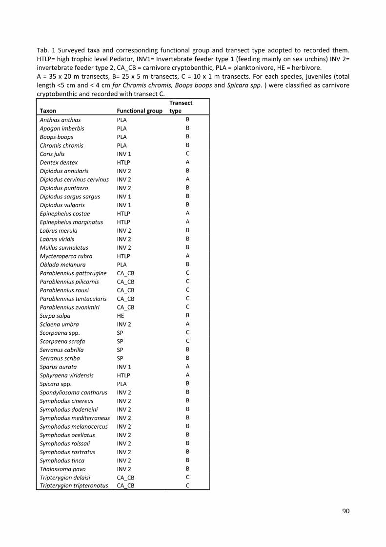
90  

Tab. 1  Surveyed  taxa and  corresponding  functional group and  transect  type  adopted  to  recorded  them. HTLP= high trophic level Pedator, INV1= Invertebrate feeder type 1 (feeding mainly on sea urchins) INV 2= invertebrate feeder type 2, CA_CB = carnivore cryptobenthic, PLA = planktonivore, HE = herbivore.  A = 35 x 20 m transects, B= 25 x 5 m transects, C = 10 x 1 m transects. For each species,  juveniles  (total length <5 cm and < 4 cm for Chromis chromis, Boops boops and Spicara spp. ) were classified as carnivore cryptobenthic and recorded with transect C. 

Taxon  Functional group Transect type 

Anthias anthias  PLA  B

Apogon imberbis  PLA  B

Boops boops  PLA  B

Chromis chromis  PLA  B

Coris julis  INV 1  C

Dentex dentex  HTLP  A

Diplodus annularis  INV 2  B

Diplodus cervinus cervinus  INV 2  A

Diplodus puntazzo  INV 2  B

Diplodus sargus sargus  INV 1  B

Diplodus vulgaris  INV 1  B

Epinephelus costae  HTLP  A

Epinephelus marginatus  HTLP  A

Labrus merula  INV 2  B

Labrus viridis  INV 2  B

Mullus surmuletus  INV 2  B

Mycteroperca rubra  HTLP  A

Oblada melanura  PLA  B

Parablennius gattorugine  CA_CB  C

Parablennius pilicornis  CA_CB  C

Parablennius rouxi  CA_CB  C

Parablennius tentacularis  CA_CB  C

Parablennius zvonimiri  CA_CB  C

Sarpa salpa  HE  B

Sciaena umbra  INV 2  A

Scorpaena spp.  SP  C

Scorpaena scrofa  SP  C

Serranus cabrilla  SP  B

Serranus scriba  SP  B

Sparus aurata  INV 1  A

Sphyraena viridensis  HTLP  A

Spicara spp.  PLA  B

Spondyliosoma cantharus  INV 2  B

Symphodus cinereus  INV 2  B

Symphodus doderleini  INV 2  B

Symphodus mediterraneus  INV 2  B

Symphodus melanocercus  INV 2  B

Symphodus ocellatus  INV 2  B

Symphodus roissali  INV 2  B

Symphodus rostratus  INV 2  B

Symphodus tinca  INV 2  B

Thalassoma pavo  INV 2  B

Tripterygion delaisi  CA_CB  C

Tripterygion tripteronotus  CA_CB  C

91  

Effectiveness of two transect sizes to survey large mobile fish

First we analysed the effectiveness of using large (35 x 20 m2) or medium size (25 x 5 m2)

transects to survey 8 large mobile fish species and species sensible to fishing (Tab. 1). To

compare the effectiveness of the two transect sizes at surveying large mobile fish we

analysed two null hypothesis: i) the two transect sizes detected similar density, biomass

and species richness at each level of protection and ii) the two transect sizes were equally

effective in detecting an effect of protection. Accuracy and precision were the metrics used

to select the most appropriate transect size. We used higher density and biomass

estimates as a proxy for accuracy (Sale & Sharp 1983, Colvocoresses & Acosta 2007,

Mintevera et al. 2008). We quantified precision using the 95% confidence interval of the

mean estimates.

We analysed the data (8 species, 188 samples, 94 samples per each transect size) as

density (n/m2) and biomass (g/m2) using 4-way permutational multivariate analysis of

variance (PERMANOVA) (Anderson 2001) based on Bray-Curtis dissimilarity matrix.

“Region” (R) was treated as a random factor with three levels (Corse, Sardinia and Spain),

“Protection” (P) and “Transect size” (T) were treated as fixed orthogonal factors both with

two levels, respectively IN and OUT for P, and A (large transects) and B (medium

transects) for M. Site was treated as random factor with 4 levels nested in Region and

Protection. The interaction between the two fixed factors P and T was tested first, and, if

interactions were significant, post-hoc pairwise tests with Montecarlo test were performed

to compare among transect sizes (T) for each protection level (P), and among protection

levels for each transect size.

Non metric multidimensional scaling (nMDS) was used to visualise multivariate patterns.

Species relevant for contributing to the significant differences among levels of the

interaction factor were identified using similarity percentage (SIMPER) (Clarke & Warwick

2001).

Univariate metrics describing large mobile/shy fish (tab.1) assemblage structure - species

richness, density and biomass for all fish pooled, and for each species - were individually

compared between transect sizes by using univariate permutational analysis of variance

based on Euclidean distance to avoid any assumption on the distribution of the data. Since

our objective was to select the transect size allowing to identify most species of a fish

assemblage in a given area, we considered raw estimates of species richness per

transect, instead of standardizing it per transect surface.

92  

Finally, in order to assess if Permanova results were due to differences among means

and/or to differences among variances, we performed a PERMDISP analysis over the

hierarchy of scales (following Di Franco et al 2014). We first calculated in PERMDISP the

individual deviation values for each transect from centroids of the combined factor

Transect size-Site-Protection-Region (i.e. the distances, in the normalized Euclidean

space, of the individual replicates from the centroids of the 4 replicates in each site and

transect). The individual deviation values obtained were then analysed using

PERMANOVA under the same sampling design used above. The analysis was performed

both on univariate and multivariate abundance and biomass data.

High trophic level predators contribution to total fish assemblage

Once the difference among transect sizes was tested, we analysed protection effect

considering the whole fish assemblage, with univariate and multivariate analyses. For

these analyses, the 8 large mobile/shy species sampled by using both large and medium

transects, were removed from medium transects data matrix, in order to avoid overlap

among large and medium transect data matrix. Thus, 3 matrix were obtained, containing

data related to, respectively, (1) the 8 large mobile species sampled within large transects,

(2) all necto-benthic fish (> 5 cm TL) sampled within medium transects, excluding the 8

large mobile species that were sampled also within large transect, (3) crypto-benthic fish

and juveniles (<5 cm for necto-benthic fish and < 4 cm for the planktonivores C. chromis,

S. spicara and B. boops) sampled only in small transects. The three matrices were then

bind into one matrix accounting for the whole fish assemblage, and since species were

surveyed on different surface units and thus had different variance scales, we performed

the analysis on total counts and total biomass after down-weighting the dispersion

measure of each species, in order to obtain data with comparable variance scales (Clarke

et al 2006). This procedure consisted in dividing the counts/biomasses for each species by

their dispersion index D, i.e. the variance to mean ratio calculated from replicates within a

group (in our case the group was defined by the finest spatial scale, i.e. factor Site nested

in Protection x Region). The resulting dispersion-weighted data matrix had a common

(Poisson-like) variance structure across species, but unchanged relative responses of a

species in different groups (Clarke et al. 2006). Permutational multivariate analysis of

variance based on Bray Curtis dissimilarity were performed on down-weighted and then

square root transformed abundance and biomass data, Permutational univariate analysis

of variance based on Euclidean distance measure were performance on total abundance

93  

and biomass data. As before, to assess if Permanova results were due to real differences

among means or to differences in the variance, we assessed dispersion variability across

the hierarchy of levels of our sampling design ( Di Franco et al 2014). We calculated in

PERMDISP the individual deviation values for each down-weighted transect from centroids

of the combined factor Site-Protection-Region (i.e. the distances, in the normalized

Euclidean space, of the individual replicates from the centroids of the 4 replicates in each

site). The individual deviation values obtained were then analysed using PERMANOVA

under the same sampling design used above. The analysis was performed both on

univariate and multivariate dispersion-downweighted abundance and biomass data.

In order to evaluate the magnitude of the reserve effect for each functional group, we

analysed average effect sizes (ES) for each species based on Cohen’s index (Cohen

1988) calculated as the difference between the mean biomass inside the MPAs and the

mean biomass outside the MPAs, divided by the cumulated standard deviations of the two

means. To test for significance of effect sizes we computed 95% confidence intervals and

assessed if they overlapped or not with 0 (no overlap = significant ES). Finally, the

contribution of each functional group to total fish density and biomass was analysed at the

three MPAs, and relative contributions were compared between protected and non-

protected zones in each MPA.

Analyses were performed using the R 3.1.0 software (R Development Core Team 2014)

and the Primer 6 and PERMANOVA multivariate statistics package (Clarke & Gorley

2006).

4.4 Results

4.4.1 Effectiveness of two transect sizes to survey large mobile fish

Multivariate analysis on density and biomass data showed a significant interaction among

Region, Protection and Transect size (p=0.001 and p=0.002 respectively) (Tab. 2).

Pairwise tests on the interaction were performed between levels of Transect size and

between levels of Protection. Transect sizes A and B significantly differed for biomass data

inside the reserve both in Corsica (p=0.02) and Spain (p=0.002), while no significant

differences among transect size resulted in Sardinia nor outside the 3 MPAs (Tab. 3, Fig.

2). When density data was considered p values were close to significance for the same

regions (p=0.05 in Corsica and p=0.06 in Spain). Concerning the Protection factor, a

significant reserve effect on density data was detected by both transect sizes in the

94  

Tavolara MPA (Sardinia), and only by large transects in Cabo de Palos (Spain) (Tab. 3).

When biomass data was analysed, both transect sizes detected a significant protection

effect in all regions. Permdisp at the multiple scale showed that variances were

homogenous for the interaction factor Region x Protection x Transect size for both density

and biomass data (respectively p = 0.074 and p = 0.267).

Tab. 2 Multivariate Permanova on square root transformed density (n/m2) and biomass data (g/m2). Only  high trophic level  predators  and  shy/mobile  species  are  included  in  the  analysis.  Significant  results    are  highlighted  in bold.R= region, P = protection, T ) transect size, S= site

        D (n/m2)  B (g/m2) 

Source  df    MS  Pseudo‐F  P(perm)    MS  Pseudo‐F  P(perm)

R  2    96.58  2.1763  0.019  4551.5  2.2742  0.019

P  1    435.48  8.1415  0.087  45653  28.302  0.115

T  1    78.976  0.84384  0.554  4480.8  1.413  0.403

RxP  2    53.492  1.2054  0.322  1613.1  0.80601  0.624

RxT  2    93.597  6.2932  0.001  3171.4  6.7217  0.001

PxT  1    68.065  1.0383  0.404  3388  1.8305  0.279

S(RxP)  18    44.431  2.1757  0.001  2003.1  2.1827  0.001

RxPxT  2    65.56  4.408  0.001  1851  3.9231  0.002

TxS(RxP)  18    14.86  0.7277  0.889  471.1  0.51334  1

Rs  143    20.421                     917.72                    

Total  190                     

Tab. 3 Pairwise tests with Monte‐carlo permutations for the combined  factor Region x Potection x Method  (multivariate Permanova)  on  square  root  transformed  density  (D,  n/m2) and biomass data  (B, g/m2)  . Tests were performed among levels of the factor Protection and among levels of the factor Method. Significant results are highlighted in bold. 

   Levels    D  B

Inside MPA   

vs  

Outside MPA  Corsica, Transect A   0.087  0.035

Corsica, Transect B   0.1471  0.046Sardinia, Transect A    0.036  0.009Sardinia, Transect B    0.013  0.001Spain, Transect A   0.029  0.001Spain, Transect B   0.077  0.022

Tran

sect A  

vs  

Tran

sect B 

Corsica, IN    0.0512  0.019Corsica, OUT    0.1448  0.215Sardinia, IN    0.2515  0.739Sardinia, OUT    0.728  0.342Spain, IN    0.0603  0.002Spain, OUT    0.204  0.124

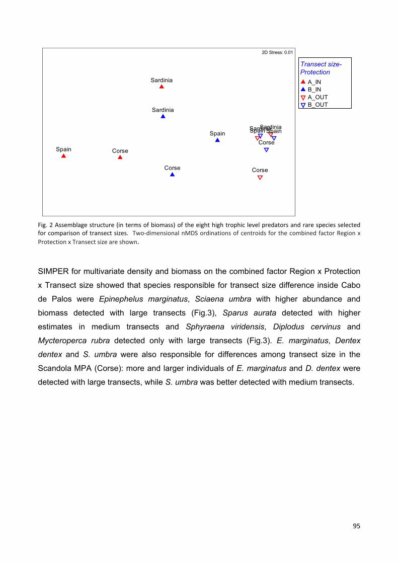
95  

Fig. 2 Assemblage structure (in terms of biomass) of the eight high trophic  level predators and rare species selected for comparison of transect sizes.   Two‐dimensional nMDS ordinations of centroids for the combined factor Region x 

Protection x Transect size are shown. 

SIMPER for multivariate density and biomass on the combined factor Region x Protection

x Transect size showed that species responsible for transect size difference inside Cabo

de Palos were Epinephelus marginatus, Sciaena umbra with higher abundance and

biomass detected with large transects (Fig.3), Sparus aurata detected with higher

estimates in medium transects and Sphyraena viridensis, Diplodus cervinus and

Mycteroperca rubra detected only with large transects (Fig.3). E. marginatus, Dentex

dentex and S. umbra were also responsible for differences among transect size in the

Scandola MPA (Corse): more and larger individuals of E. marginatus and D. dentex were

detected with large transects, while S. umbra was better detected with medium transects.

Corse

Corse Corse

Corse

Sardinia

Sardinia

SardiniaSardinia

Spain

Spain Spain Spain

2D Stress: 0.01

Transect size-Protection

A_INB_INA_OUTB_OUT

 

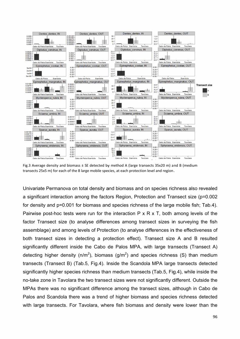
Fig.3 Average

transects 25x

Univariate

a significa

for density

Pairwise p

factor Tra

assembla

both tran

significant

detecting

transects

significant

no-take zo

MPAs the

Palos and

with large

e density and

x5 m) for each

e Permano

ant interac

y and p=0

post-hoc te

ansect size

age) and am

sect sizes

tly differen

higher de

(Transect

tly higher s

one in Tav

ere was no

d Scandola

e transects

d biomass ± S

h of the 8 larg

ova on tota

tion amon

.001 for bi

ests were

e (to analy

mong leve

s in detec

nt inside th

ensity (n/m

B) (Tab.5

species ric

volara the t

o significan

a there wa

s. For Tav

E detected by

ge mobile spec

l density a

g the facto

omass and

run for th

yse differe

ls of Prote

cting a pro

he Cabo d

m2), biomas

5, Fig.4). In

chness tha

two transec

nt differenc

as a trend

olara, whe

y method A (l

cies, at each p

and biomas

ors Region

d species

e interacti

ences amo

ction (to a

otection ef

de Palos

ss (g/m2)

nside the

n medium

ct sizes we

ce among

of higher

ere fish bio

large transect

protection lev

ss and on s

n, Protectio

richness o

on P x R

ong transe

nalyse diff

ffect). Tra

MPA, with

and speci

Scandola

transects

ere not sig

the transe

biomass a

omass and

ts 35x20 m) a

el and region.

species ric

on and Tra

of the large

x T, both

ect sizes in

erences in

nsect size

h large tra

es richnes

MPA large

(Tab.5, Fig

nificantly d

ect sizes, a

and specie

d density w

and B (medium

. 

chness also

ansect size

e mobile fis

among lev

n surveyin

n the effect

e A and B

nsects (Tr

ss (S) tha

e transects

g.4), while

different. O

although in

es richness

were lowe

96

m 

o revealed

e (p=0.002

sh; Tab.4).

vels of the

ng the fish

tiveness of

B resulted

ransect A)

n medium

s detected

inside the

Outside the

n Cabo de

s detected

er than the

6 

d

2

.

e

h

f

d

)

m

d

e

e

e

d

e

 

other cas

higher bio

the multip

the intera

were foun

tests am

homogeno

 Fig.4 Mean transects 35xdifferences a 

se studies,

omass, de

ple scale o

action facto

nd for biom

ong levels

ous among

total  density x20 m) and B among metho

the trend

nsity and

n univariat

or RxPxT

mass data

s of the

g the two t

(n.m‐2),  biom(medium trands.  

 

d was opp

species ric

te density

(p = 0.23

for the sa

factor Tr

ransect siz

mass  (g.m‐2)  ansects 25x5 m

posite, with

chness tha

data show

34), while s

me interac

ransect si

zes inside

 

and  species  rm) at each pro

h medium

an large tr

wed that va

significant

ction factor

ze reveal

Cabo de P

ichness  (S)  ± tection level a

transects

ransects (F

ariances w

difference

r (p=0.001

ed that v

Palos MPA

SE  detected and region. As

showing

Fig. 4). Pe

were homog

es among

). Pairwise

variances

A (p=0.03).

by  Transect sterisks indica

 

97

a trend of

ermdisp at

genous for

variances

e post-hoc

were not

size  A  (largeate significant

7 

f

t

r

s

c

t

e t 

98  

 Tab. 4 Univariate Permanova on square root transformed density  (D; n/m2) and biomass data  (B; g/m2) and on raw species richness data  (S; number of species per replicate). Only high trophic  level predators and shy/mobile species are included in the analysis. Re = Region, T= transect size, P= protection, S = site. Significant results are highlighted in bold.

Tab.  5    Pairwise  tests  with  Montecarlo  permutations  for  the combined  factor Region  x  Potection  x  Transect  size  (univariate Permanova)  on  square  root  transformed  density  (D;  n/m2)  and biomass  data  (B;  g/m2)  and  on  raw    species  richness  (S)  of  the large mobile  fish.  Tests  were  performed  among  levels  of  the factor  Potection  and  among  levels  of  the  factor  transect  size Significant results are highlighted in bold. 

  Levels    D  B  S 

Inside MPA   

vs 

 Outside M

PA 

Corsica, Transect A    0.113  0.154  0.028

Corsica, Transect B    0.092  0.118  0.086 

Sardinia, Transect A    0.002  0.01  0.008

Sardinia, Transect B    0.005  0.013  0.002

Spain, Transect A    0.008  0.002  0.001

Spain, Transect B    0.219  0.061  0.128 

Tran

sect A  

vs 

Tran

sect B 

Corsica,IN    0.636  0.934  0.03 

Corsica,OUT    0.684  0.56  0.399 

Sardinia,IN    0.429  0.865  0.615 

Sardinia,OUT    0.104  0.162  0.204 

Spain,IN    0.016  0.002  0.003

Spain,OUT    0.824  0.097  0.083 

Concerning levels of the factor Protection, when univariate density and biomass data were

analysed, both transect sizes detected a significant effect of protection in Tavolara, while

in Cabo de Palos only transect A detected a significant effect of protection (Tab. 5). In

Scandola protection effect was never significant. When Permdisp pairwise post-hoc tests

were performed among levels of the factor Protection, variances were never homogenous

      D   B   S  

Source  df         MS  Pseudo‐F  P(perm)         MS   Pseudo‐F  P(perm)         MS  Pseudo‐F  P(perm) 

R  2  0.009  0.75  0.526    28.41  0.74  0.565    3.79  5.36  0.013

P  1  0.231  41.14  0.074  567.69  27.51  0.073  35.52  14.79  0.167

T  1  0.006  0.24  0.583    35.85  0.96  0.582    14.32  1.98  0.280

RxP  2  0.006  0.46  0.693    20.65  0.53  0.696    2.40  3.40  0.050

RxT  2  0.023  11.92  0.002  37.18  40.02  0.001  7.23  36.64  0.001

PxT  1  0.013  0.83  0.435    31.59  1.00  0.412    10.65  2.64  0.277

S(RxP)  18  0.012  2.55  0.001  38.78  4.15  0.001  0.71  1.20  0.264

RxPxT  2  0.016  8.33  0.002    31.54  33.95  0.001    4.04  20.49  0.001

TxS(RxP)  18  0.002  0.40  0.987  0.88  0.09  1.000  0.19  0.33  0.997

Rs  140  0.005            9.35             0.59                    

Total     188.00                             

 

among ins

consistent

effect (p=

When eva

confidenc

variable d

transects

transects,

Outside th

precise th

Tavolara,

precise.

Fig. 5. 95 % cprotected ar

side and o

t for Cabo

0.03) was

aluating th

ce intervals

depending

showed a

, with the e

he three M

han mediu

while out

confidence inteas 

outside eac

o de Palos

detected w

he precisio

s (Fig. 5),

on the r

trend of la

exception o

MPAs, whe

m ones. C

tside Scan

tervals on the

ch MPA. W

s and Tav

with transe

on of diffe

difference

region and

arger confid

of Tavolara

n density d

Considering

ndola and

 mean density

When spec

volara, wh

ect A (Tab.

erent trans

es among

d protectio

dence inte

a for biom

data was c

g biomass

Cabo de

y and biomass

cies richne

ile for Sca

5).

sect sizes

the two tr

on level. I

rvals (thus

ass data, w

considered

s data this

e Palos la

s estimates w

ess was an

andola a s

through t

ransect siz

nside the

s lower pre

where the

d larger tra

trend was

rger trans

ithin and outs

nalysed re

significant

he analys

zes appea

three MP

ecision) tha

trend was

ansect resu

s confirme

sects appe

side the three

99

sults were

protection

is of 95%

ared highly

PAs larger

an medium

s opposite.

ulted more

ed only for

eared less

e marine 

9 

e

n

%

y

r

m

.

e

r

s

100  

4.4.2 Fish assemblage analysis

Multivariate analysis revealed a significant interaction among the factors Region and

Protection for both abundance and biomass data (p = 0.001, Tab. 6). Pairwise tests

showed a significant effect of protection in Sardinia and Spain, while no significant

protection effect was highlighted in Corsica.(Tab. 7, Fig. 6).

Permdisp at the multiple scale showed that after dispersion weighting, variances were

homogenous for all interaction factors and for the protection factor, while significant

differences among variances were found only for the factor Region.

 

Tab. 6 Multivariate Permanova on square  root  transformed abundance  (n) and biomass  (g  ) data  for  the 

whole fish assemblage. Significant results are highlighted in bold.

        N  B 

Source   df        MS  Pseudo‐F  P(perm)      MS  Pseudo‐F  P(perm) 

R  2    9472.7  4.6514  0.001  9735.3  4.2272  0.001

P  1    12392  3.0522  0.146  14166  3.1114  0.154

RxP  2    4082.3  2.0046  0.003  4577.1  1.9875  0.003

S(RxP)  18    2059.6  1.6959  0.001  2326  1.5638  0.001

Rs  67    1214.5                     1487.4                    

Total  90                     

Tab.  7  Pairwise  tests  with  Montecarlo permutations  for  the  combined  factor  Region  x Potection    on  dispersion  weighted  and  square root  transforTd  abundance  (n)  and  biomass  (g) data  . Tests were performed among  levels of  the factor  Potection.  Significant  results    are highlighted in bold. 

       N    B 

Inside M

PA  

 Vs 

 Outside M

PA 

Corsica 

 

0.272 

 

0.232 

Sardinia 

 

0.002 

 

0.001 

Spain 

 

0.001 

 

0.001 

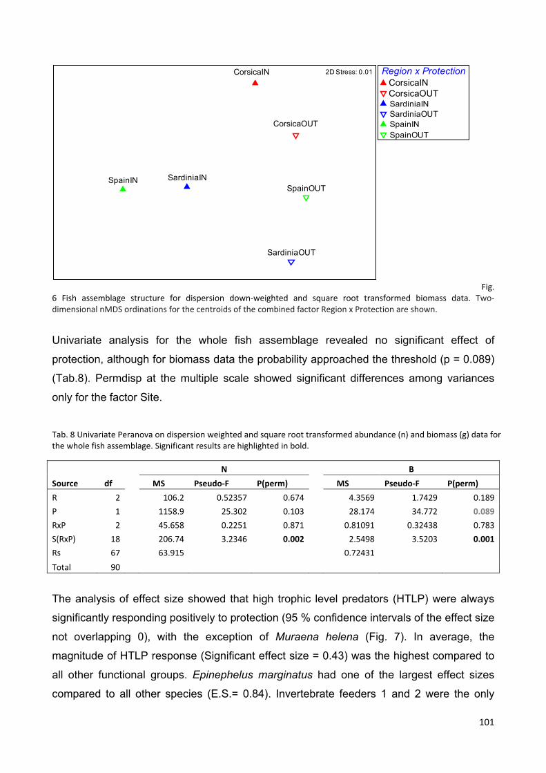
101  

Fig. 6  Fish  assemblage  structure  for  dispersion  down‐weighted  and  square  root  transformed  biomass  data.  Two‐dimensional nMDS ordinations for the centroids of the combined factor Region x Protection are shown.

Univariate analysis for the whole fish assemblage revealed no significant effect of

protection, although for biomass data the probability approached the threshold (p = 0.089)

(Tab.8). Permdisp at the multiple scale showed significant differences among variances

only for the factor Site.

Tab. 8 Univariate Peranova on dispersion weighted and square root transformed abundance (n) and biomass (g) data for the whole fish assemblage. Significant results are highlighted in bold. 

        N  B 

Source   df        MS  Pseudo‐F  P(perm)      MS  Pseudo‐F  P(perm) 

R  2    106.2  0.52357  0.674  4.3569  1.7429  0.189 

P  1    1158.9  25.302  0.103  28.174  34.772  0.089 

RxP  2    45.658  0.2251  0.871  0.81091  0.32438  0.783 

S(RxP)  18    206.74  3.2346  0.002  2.5498  3.5203  0.001 

Rs  67    63.915                     0.72431                    

Total  90                     

The analysis of effect size showed that high trophic level predators (HTLP) were always

significantly responding positively to protection (95 % confidence intervals of the effect size

not overlapping 0), with the exception of Muraena helena (Fig. 7). In average, the

magnitude of HTLP response (Significant effect size = 0.43) was the highest compared to

all other functional groups. Epinephelus marginatus had one of the largest effect sizes

compared to all other species (E.S.= 0.84). Invertebrate feeders 1 and 2 were the only

Region x ProtectionCorseINCorseOUTSardiniaINSardiniaOUTSpainINSpainOUT

CorseIN

CorseOUT

SardiniaIN

SardiniaOUT

SpainINSpainOUT

2D Stress: 0.01CorsicaIN

CorsicaOUT

CorsicaINCorsicaOUT

102  

other groups showing a significantly positive response to protection. While all species of

group 1 had positive effect sizes, the magnitude and direction of the response in group 2

was highly species-specific. The response of small piscivores, crypto-benthic fish and

planktonivores was also highly variable, with most species not showing significant

increases within the no-take zones. Some species showed higher biomasses outside the

MPAs (negative E.S.) (Scorpaena scrofa, Diplodus annularis, Parablennius gattorugine

and the two planktonivores Anthias anthias and Boops boops), although significance could

not be assessed for most of them since these species were not recorded at all three MPAs

in this study and therefore was not possible to calculate confidence intervals. The largest

positive response to protection was shown by the crypto-benthic fish Tripterygion delaisi

with an effect size of 0.87 (Fig. 7).

 

Fig.7 AveragIndex.  Black positive effesize,    or  jussignificantly 

Analysis o

relative co

within and

and juven

e effect size ±points  standct sizes (whenst    negative  opositive effec

of function

ontribution

d outside

nile fish alw

± IC 95% calcd  for  significan  confidenceor  null  effectct size for trop

al groups

n of functio

the three

ways dom

ulated for eacntly  positive e intervals cout  sizes  when phic class, opa

percentage

onal group

MPAs, wit

minating, fo

ch species (poeffect  size, m

uld not be comerror  bars  c

aque red mean

e composi

ps to total

th plankton

ollowed by

oints) and tromeaning  erromputed). Grecould  not  be ns  non‐ signif

ition showe

fish assem

nivorous a

invertebra

ophic group (sr  bars  not  ovy points standcomputed.   ficant effect si

ed that in t

mblage did

and carnivo

ate feeders

squares) baseverlapping  0,d for non‐signBright  red  size.  

terms of d

d not vary

orous cryp

rs of type

103

ed on Cohen’s  or markedlynificant effectquares mean

ensity, the

y markedly

pto-benthic

1 (Fig. 8).

3 

s y t n  

e

y

c

.

 

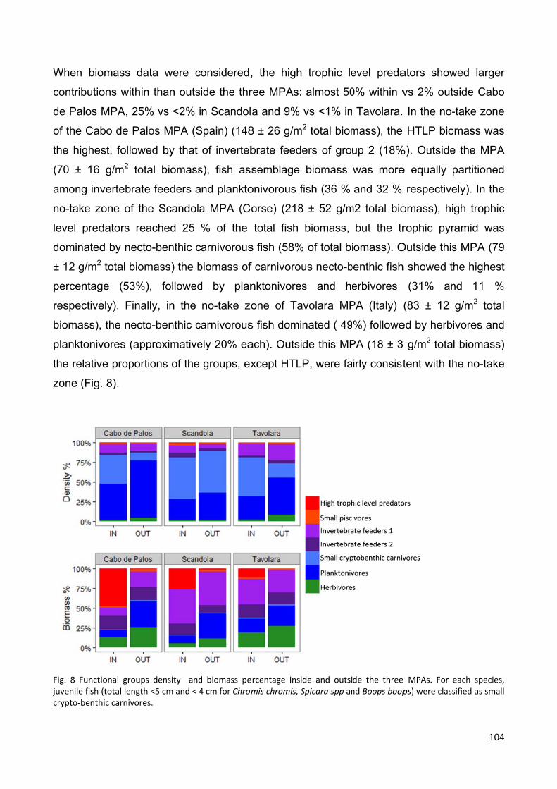
When bio

contributio

de Palos

of the Cab

the highe

(70 ± 16

among inv

no-take z

level pred

dominated

± 12 g/m2

percentag

respective

biomass),

planktoniv

the relativ

zone (Fig

Fig.  8  Functjuvenile fish crypto‐benth

omass dat

ons within

MPA, 25%

bo de Palo

st, followe

g/m2 tota

vertebrate

one of the

dators rea

d by necto2 total biom

ge (53%),

ely). Finall

, the necto

vores (app

ve proportio

. 8).

ional  groups (total length <hic carnivores

ta were co

than outsi

% vs <2% i

os MPA (S

ed by that

al biomass

feeders a

e Scandola

ached 25

o-benthic c

mass) the b

, followed

y, in the

o-benthic ca

proximative

ons of the

density    and<5 cm and < 4.  

onsidered,

ide the thr

n Scandol

Spain) (148

of inverteb

s), fish ass

nd plankto

a MPA (Co

% of the

arnivorous

biomass of

d by plan

no-take zo

arnivorous

ely 20% ea

groups, ex

d  biomass  pe4 cm for Chrom

, the high

ree MPAs:

a and 9%

8 ± 26 g/m

brate feed

semblage

onivorous f

orse) (218

total fish

s fish (58%

f carnivorou

nktonivores

one of Ta

s fish domi

ach). Outsi

xcept HTL

rcentage  insimis chromis, S

 

trophic le

almost 50

vs <1% in2 total biom

ers of gro

biomass

fish (36 %

8 ± 52 g/m

biomass,

% of total bi

us necto-b

s and he

avolara MP

nated ( 49

de this MP

P, were fa

de  and  outsiSpicara spp an

evel preda

0% within v

Tavolara.

mass), the

up 2 (18%

was more

and 32 %

m2 total bio

but the tr

iomass). O

benthic fish

erbivores

PA (Italy)

%) followe

PA (18 ± 3

irly consist

de  the  threend Boops boop

ators show

vs 2% out

. In the no-

e HTLP bio

%). Outside

e equally p

respective

omass), hi

rophic pyr

Outside this

h showed t

(31% an

(83 ± 12

ed by herb

3 g/m2 tota

tent with th

e MPAs.  For ps) were class

104

wed larger

side Cabo

-take zone

omass was

e the MPA

partitioned

ely). In the

gh trophic

ramid was

s MPA (79

he highest

nd 11 %

g/m2 total

ivores and

l biomass)

he no-take

each  species,sified as small

4 

r

o

e

s

A

d

e

c

s

9

t

%

l

d

)

e

, l 

105  

4.5 Discussion

Here, we highlight how adopting large size transects (20 x 35 m) instead of standard 5 x

25 m transects to survey large mobile and shy fish within MPAs increases the accuracy of

density and biomass estimates, allowing to reduce the bias of under-estimation due to the

common avoidance behaviour of these fish. Next, through the adoption of three transect

sizes to survey the whole fish assemblage at three Mediterranean MPAs, we highlighted a

significant effect of protection on high trophic level predators, whose response was always

higher in magnitude than that of other functional groups. Trophic pyramids differed within

and outside MPAs due to the larger contribution of HTLP to total fish biomass at protected

sites. This, coupled with the highest contribution of HTLP to total fish biomass at older

MPAs, suggests this metric as an effective indicator of MPA performance.

4.5.1 Effectiveness of two transect sizes to survey large mobile fish

Achieving a realistic estimate of fish assemblage density and biomass through visual

census is an arduous task. On one hand, many authors agree that UVC underestimates

the true abundance of fish, since a human observer will likely always miss a small

percentage of fish that are really on the census area (e.g. Sale & Douglas 1981, Sale &

Sharp 1983, Short & Bayliss 1985). Thus, when several visual census methods are

compared, greater accuracy is generally assumed to be represented by the highest

density of fish recorded (Samoylis & Carlos 2000, Mintevera et al. 2008). On the other

hand, other authors suggest that underwater visual census may overestimate the

abundance of fish because of non-instantaneous counts being performed (Ward-Paige et

al. 2010, Trebilco et al. 2013). This bias can occur especially in presence of predator

fishes displaying high swimming speed and attractive behaviour towards divers (Ward-

Page et al. 2010). The mobility of fish relative to the census area is likely to have the

greatest effect on the accuracy of the visual census method (Myers 1989): simultaneously

counting a range of species with different mobility leads to lesser accuracy in estimates

than if species groups are counted separately using the most adapted method to their

mobility ((Smith 1989, De Girolamo & Mazzoldi 2001). In this perspective, we analysed the

effectiveness of large sized transects and medium sized transects at recording large

mobile and shy fish, that in the Mediterranean are generally surveyed using the same

transect dimensions adopted for all necto-benthic fish (Prato et al. in prep). Strip transects

of larger size resulted more accurate than medium ones in no-take zones of older MPAs

106  

(Cabo de Palos and Scandola), detecting higher abundance and biomass of large mobile

fish. In particular, Dentex dentex, Sphyraena viridensis and Mycteroperca rubra were

always more accurately surveyed with larger transects (i.e. higher abundances and

biomass in large transects). Large transects also reached higher density and biomass

estimates for Epinephelus marginatus in Scandola and Cabo de Palos MPAs. By

comparing dispersion of the data across the full hierarchy of scales we could moreover

confirm that identified differences among transects sizes for the single species were

actually due to real differences in the estimated means and not to differences in their

dispersion. These results well agree with what observed by Kulbicky (1998), i.e that larger

numbers of shy fish would be observed further away from the observer than directly on the

transect path. Even where these species are abundant, such as in our above-mentioned

case studies, they will still keep at a “safety distance” from the observer, thus the

probability of detection (sensu Kulbicky, 1989) within a distance of 10 m is higher than that

of detecting them within 2.5 from each side of the observer. Larger transect size could thus

help reducing the bias of under-estimation due to fish behaviour. Additionally, the possible

overestimation bias of non-instantaneous visual counts due to the higher speed of the

large mobile fish with respect to the speed of the observer (Ward-Page et al. 2010), is

unlikely to insist here. As stated also in Guidetti et al. 2014 in fact, the large mobile fish in

the analysed ecosystem are not particularly fast-swimming species that can be attracted

by divers. Moreover, larger transects were surveyed at an average speed (700m² / 5min)

approximatively 8 times higher than the speed of survey on medium transects (125m² /

8min), thus overestimation bias due to fish flux across the sampling surface is likely

reduced. Nonetheless, further testing would be needed to formally assess this issue.

In unprotected areas and in the Tavolara MPA, finally the two transect sizes did not

significantly provide different estimates , although a trend of higher density estimates was

observed with smaller transects. This trend could be due to the smaller individuals

observed in the external sites and in Tavolara MPA. Indeed, smaller dusky grouper

individuals tend to be more hidden in crevices and thus be less visible, which might explain

why an observer having to survey a larger surface would miss them (Cheal & Thompson

1997, Bozec et al. 2011). In medium transects a smaller area can be more easily searched

and thus it is more probable to detect more sedentary and hidden species (Mintevera et al.

2008), such as, in our case, smaller individuals of the dusky grouper. Although large

mobile fish were not considered in their study, Mintevera et al 2008 compared nested

cylinders of varying radius length to survey fish of different size classes, showing that best

107  

density estimates for small sized individuals were obtained on smaller surfaces, while

larger individuals were recorded with higher accuracy and precision in larger surface units.

The same is likely happening in our case, and although we did not directly test it, the

approach would possibly benefit from a separation among size classes for the large mobile

fish.

Both transect sizes were effective in detecting a protection effect at the three MPAs,

although the lower abundance estimates provided by small transects did not allow to reach

significance when total density estimates were analysed. Finally, differences in precision

among the two transect sizes did not show clear univocal trends within and outside the

MPAs. The trend of lower precision shown by large transects within MPAs is likely due to

the detection of more rare and shy species (i.e M. rubra, E. costae, S. viridensis,) that are

always missed by medium transects, and generally absent outside the MPAs due to their

avoidance behaviour. The choice of the transect size to be adopted should thus balance

the trade-offs of detecting higher number of species, while achieving lower precision.

4.5.2 Fish assemblage analysis

Overall, the higher accuracy (i.e. biomass) and species richness on large transects in two

of the three MPAs, coupled to the non-significance in transect differences in Tavolara led

us to select the combination of large, medium and small transect sizes, as the best option

to analyse the full fish assemblage and assess the relative contribution of high trophic level

predators to fish biomass within the three MPAs.

A significant effect of protection was detected both for large mobile fish analysed alone

and for the whole fish assemblage at both the Cabo de Palos and Tavolara MPAs, in

agreement with previous studies (García-Charton et al. 2004, Di Franco et al. 2009). For

the Scandola MPA instead, a protection effect was detected only for large mobile fish, and

not when the whole fish assemblage was analysed. This result was probably a

consequence of the high among-site variability in this MPAs, as confirmed by a significant

difference among dispersions at the site scale. Within the no-take zone in fact remarkably

high biomass estimates were concentrated in one particular site (Palazzu). On one hand,

the exposure and structural complexity of this site make it a refuge zone for the dusky

grouper in particular (Francour 1994). Striking differences in fish biomass have indeed

been observed since few years after the MPA establishment, when this site was compared

with the same external sites we surveyed (Francour 1989). Since 1995 moreover, an

almost exponential increase in the abundance of dusky groupers has been observed at the

108  

same site, highlighting the occurrence of a strong refuge effect after fishing was banned

(Seytre et al. in prep). On the other hand, one site within the no-take zone showed

biomass values in the same range of those observed outside the MPA, which were

relatively high for a non-protected area. The protection effect in this MPA is thus likely

masked by a combination of factors: a high inter site variability within the no take zone,

probably linked to differences in the geomorphological complexity of the habitat, and a

relatively high abundance and biomass of fish outside the MPA (79 g/m2 outside

Scandola, a higher value than what observed in a multitude of non-protected areas across

the Mediterranean (Sala et al. 2012, Guidetti et al. 2014).

Overall, the average response of HTLP to protection was always positive at the three

MPAs, and was higher in magnitude than the response of other functional groups.

Invertebrate feeders of group 1 were also always favoured by protection since they

included species usually targeted by fishing. Lower trophic level species (many of which

are also non - commercial species) showed high variability in response, including

reduction of some species in the MPAs, which highlighted the occurrence of possible

indirect effects of protection through predation or competition for resources. These results

were similar to meta-analytical studies encompassing several Mediterranean MPAs

(Micheli et al. 2004, Guidetti 2007), and well corresponded to the response observed by

the same trophic groups in well enforced MPAs (Guidetti et al. 2008). Nonetheless,

although cascading trophic interactions are likely occurring at the species level, at the

trophic group level there was no significant evidence of biomass reduction within the MPAs

compared to the exploited sites. Exploitation at the non-protected sites is thus likely to

have larger impact across the food-web than the top-down control exerted by high trophic

level predators at protected sites (Soler et al. 2015).

Finally, analysis of trophic pyramids showed that biomass contribution of high trophic level

predators is larger within each MPA than outside compared to other functional groups,

markedly contributing to total fish biomass in the total protection zones. As also suggested

by Soler et al 2015, such disparity in biomass ratios between MPAs and open access sites

for the different trophic groups implies a trophic re-organisation that is likely to have

substantial consequences for ecological functions. This is likely to be more evident at older

and highly enforced MPAs like Scandola (1975) and Cabo de Palos (1995), where HTLP

contribution to total fish biomass eventually led to top heavy trophic pyramids and was

higher than in the more recently established and enforced Tavolara MPA (1997, but

enforced in 2003). Similar trends were observed in a study covering 13 MPAs and 17

109  

unprotected sites across the Mediterranean (Guidetti et al 2014), suggesting that this

metric is a useful indicator of MPA performance.

4.6 Conclusion

It has been demonstrated that high trophic level predators keep increasing in MPAs up to

several years after protection (Garcia Rubies et al. 2013), and long term monitoring

programs are thus essential to establish whether carrying capacity has been reached or

not for these species (Garcia Rubies et al. 2013). On the basis of our results, we

additionally suggest that such monitoring programs should adopt transects of variable

surface adapted to fish mobility and behaviour, as it is has long been suggested (Harmelin

Vivien et al. 1985). Although the use of the 20 m transect width we proposed might be

limited by lower visibility conditions in the cold season and increase the chance of errors in

surface estimations, we suggest that the necto-benthic fish and large mobile fish should be

counted separately, especially in MPAs with high fish abundance, and that the size of the

transects should be larger for large mobile fish than for necto-benthic fish. We did not test

if separating the counts for large mobile fish and necto-benthic fish would also increase the

accuracy of counts for the latter, but this is very likely to be the case especially in MPAs

with high abundances of both groups. Counting a small number of fish is in fact generally

more accurate than counting a large number (Cheal & Thompson 1997, De Girolamo &

Mazzoldi 2001).

Adoption of transects of variable surface respectively for large mobile fish, necto-benthic

fish and cryptic fish, in monitoring programs would be a simple improvement to traditional

one-size transect surveys, and would allow to increase the accuracy of total fish

assemblage estimates within MPAs, especially when the abundance of high trophic level

predators within them is significantly recovering.

4.7 References

Bannerot SP, Bohnsack JA (1986) A stationary visual census technique for quantitatively assessing community structure of coral reef fishes. NOAA Tech Rep NMFS 41:1–15

Britten GL, Dowd M, Minto C, Ferretti F, Boero F, Lotze HK (2014) Predator decline leads to decreased stability in a coastal fish community. Ecol Lett 17:1518–1525

Brock VE (1954) A preliminary report on a method of estimating reef fish populations. J Wildl Manag:297–308

110  

Cheal AJ, Thompson AA (1997) Comparing visual counts of coral reef fish: implications of transect width and species selection. Mar Ecol Prog Ser 158:241–248

Clarke KR, Chapman MG, Somerfield PJ, Needham HR (2006) Dispersion-based weighting of species counts in assemblage analyses. Mar Ecol Prog Ser 320:11–27

Clarke KR, Gorley RN (2006) User manual/tutorial. Primer-E Ltd Plymouth:93 Cohen J (1988) The effect size index: d. Stat Power Anal Behav Sci 2nd Ed N J Lawrence

Erl-Baum Assoc:20–26 Colvocoresses J, Acosta A (2007) A large-scale field comparison of strip transect and

stationary point count methods for conducting length-based underwater visual surveys of reef fish populations. Fish Res 85:130–141

Bozec Y-M, Kulbicki M, Laloë F, Mou-Tham G, Gascuel D (2011) Factors affecting the detection distances of reef fish: implications for visual counts. Marine Biology 158:969–981

De Girolamo M, Mazzoldi C (2001) The application of visual census on Mediterranean rocky habitats. Mar Environ Res 51:1–16

Di Franco A, Bulleri F, Pennetta A, De Benedetto G, Clarke KR, Guidetti P (2014) Within-Otolith Variability in Chemical Fingerprints: Implications for Sampling Designs and Possible Environmental Interpretation (S Thrush, Ed.). PLoS ONE 9:e101701

Di Franco A, Bussotti S, Navone A, Panzalis P, Guidetti P (2009) Evaluating effects of total and partial restrictions to fishing on Mediterranean rocky-reef fish assemblages. Mar Ecol Prog Ser 387:275–285

Di Franco A, Di Lorenzo M, Guidetti P (2013) Spatial patterns of density at multiple life stages in protected and fished conditions: an example from a Mediterranean coastal fish. J Sea Res 76:73–81

Edgar GJ, Barrett NS, Morton AJ (2004) Biases associated with the use of underwater visual census techniques to quantify the density and size-structure of fish populations. J Exp Mar Biol Ecol 308:269–290

Francour P (1989) Les peuplements ichtyologiques de la réserve de Scandola: influence de la réserve intégrale. Trav Sci Nat Régional Réserves Nat Corse:33–93

Francour P (1994) Pluriannual analysis of the reserve effect on ichthyofauna in the Scandola natural reserve (Corsica, Northwestern Mediterranean). Oceanol Acta 17:309–317

Francour P, Harmelin JG, Pollard D, Sartoretto S (2001) A review of marine protected areas in the northwestern Mediterranean region: siting, usage, zonation and management. Aquat Conserv Mar Freshw Ecosyst 11:155–188

García-Charton JA, Pérez-Ruzafa A, Sánchez-Jerez P, Bayle-Sempere JT, Reñones O, Moreno D (2004) Multi-scale spatial heterogeneity, habitat structure, and the effect of marine reserves on Western Mediterranean rocky reef fish assemblages. Mar Biol 144:161–182

Garcia-Rubies A, Hereu B, Zabala M (2013) Long-Term Recovery Patterns and Limited Spillover of Large Predatory Fish in a Mediterranean MPA. PLoS ONE 8

Guidetti P (2006a) Marine reserves reestablish lost predatory interactions and cause community changes in rocky reefs. Ecol Appl 16:963–976

111  

Guidetti P (2006b) Marine reserves reestablish lost predatory interactions and cause community changes in rocky reefs. Ecol Appl 16:963–976

Guidetti P (2007) Potential of Marine Reserves to Cause Community-Wide Changes beyond Their Boundaries. Conserv Biol 21:540–545

Guidetti P, Baiata P, Ballesteros E, Di Franco A, Hereu B, Macpherson E, Micheli F, Pais A, Panzalis P, Rosenberg AA, Zabala M, Sala E (2014) Large-Scale Assessment of Mediterranean Marine Protected Areas Effects on Fish Assemblages. PLoS ONE 9:e91841

Guidetti P, Milazzo M, Bussotti S, Molinari A, Murenu M, Pais A, Spano N, Balzano R, Agardy T, Boero F, Carrada G, Cattaneo-Vietti R, Cau A, Chemello R, Greco S, Manganaro A, Sciara GN di, Russo GF, Tunesi L (2008) Italian marine reserve effectiveness: Does enforcement matter? Biol Conserv 141:699–709

Hackradt CW, García-Charton JA, Harmelin-Vivien M, Pérez-Ruzafa Á, Le Diréach L, Bayle-Sempere J, Charbonnel E, Ody D, Reñones O, Sanchez-Jerez P, others (2014) Response of rocky reef top predators (Serranidae: Epinephelinae) in and around marine protected areas in the Western Mediterranean Sea.

Halford AR, Thompson AA (1994) Visual census surveys of reef fish. Australian Institute of Marine Science

Harmelin J-G, Bachet F, Garcia F (1995) Mediterranean Marine Reserves: Fish Indices as Tests of Protection Efficiency. Mar Ecol 16:233–250

Harmelin-Vivien M, Harmelin J (1975) Présentation d’une méthode d’évaluation in situ de la faune ichtyologique. Trav Sci Parc Nation Port-Cros 1:47–52

Harmelin-Vivien M, Harmelin J, Chauvet C, Duval C, Galzin R, Lejeune P, Barnabé G, Blanc F, Chevalier R, Duclerc J (1985) Evaluation visuelle des peuplements et populations de poissons: méthodes et problèmes. Rev Décologie 40:467–539

Kovačić M, Patzner RA, Schliewen U (2012) A first quantitative assessment of the ecology of cryptobenthic fishes in the Mediterranean Sea. Mar Biol 159:2731–2742

Kulbicki M (1998) How the acquired behaviour of commercial reef fishes may influence the results obtained from visual censuses. J Exp Mar Biol Ecol 222:11–30

Mallet D, Pelletier D (2014) Underwater video techniques for observing coastal marine biodiversity: A review of sixty years of publications (1952–2012). Fish Res 154:44–62

Mapstone BD, Ayling T, Great Barrier Reef Marine Park Authority (1998) An investigation of optimum methods and unit sizes for the visual estimation of abundances of some coral reef organisms. Great Barrier Reef Marine Park Authority, Townsville, Qld.

Micheli F, Halpern BS, Botsford LW, Warner RR (2004) Trajectories and correlates of community change in no-take marine reserves. Ecol Appl 14:1709–1723

Mintevera CV, Moura RL de, Francini-Filho RB (2008) Nested sampling: an improved visual-census technique for studying reef fish assemblages. Mar Ecol Prog Ser 367:283–293

Myers (1989) Micronesian reef fishes. A practical guide to the identification of coral reef fishes of the tropical Central and Western Pacific. Coral Graphics. Guam. 298 pp

112  

Murphy HM, Jenkins GP (2010) Observational methods used in marine spatial monitoring of fishes and associated habitats: a review. Mar Freshw Res 61:236

Myers RA, Worm B (2003) Rapid worldwide depletion of predatory fish communities. Nature 423:280–283

Pace ML, Cole JJ, Carpenter SR, Kitchell JF (1999) Trophic cascades revealed in diverse ecosystems. Trends Ecol Evol 14:483–488

Pinnegar JK, Polunin NVC, Francour P, Badalamenti F, Chemello R, Harmelin-Vivien ML, Hereu B, Milazzo M, Zabala M, Anna G d’ (2000) Trophic cascades in benthic marine ecosystems: lessons for fisheries and protected-area management. Environ Conserv 27:179–200

Prato G, Guidetti P, Bartolini F, Mangialajo L, Francour P (2013) The importance of high-level predators in marine protected area management: Consequences of their decline and their potential recovery in the Mediterranean context. Adv Oceanogr Limnol 4:176–193

Russ GR, Alcala AC (2003) Marine reserves: rates and patterns of recovery and decline of predatory fish, 1983-2000. Ecol Appl 13:1553–1565

Sala E, Ballesteros E, Dendrinos P, Di Franco A, Ferretti F, Foley D, Fraschetti S, Friedlander A, Garrabou J, Guclusoy H, Guidetti P, Halpern BS, Hereu B, Karamanlidis AA, Kizilkaya Z, Macpherson E, Mangialajo L, Mariani S, Micheli F, Pais A, Riser K, Rosenberg AA, Sales M, Selkoe KA, Starr R, Tomas F, Zabala M (2012) The Structure of Mediterranean Rocky Reef Ecosystems across Environmental and Human Gradients, and Conservation Implications. Plos One 7:e32742

Sala E, Boudouresque CF, Harmelin-Vivien M (1998) Fishing, trophic cascades, and the structure of algal assemblages: evaluation of an old but untested paradigm. Oikos:425–439

Sale PF, Douglas WA (1981) Precision and accuracy of visual census technique for fish assemblages on coral patch reefs. Environ Biol Fishes 6:333–339

Sale PF, Sharp BJ (1983) Correction for bias in visual transect censuses of coral reef fishes. Coral Reefs 2:37–42

Samoilys MA, Carlos G (2000) Determining Methods of Underwater Visual Census for Estimating the Abundance of Coral Reef Fishes. Environ Biol Fishes 57:289–304

Sandin SA, Smith JE, DeMartini EE, Dinsdale EA, Donner SD, Friedlander AM, Konotchick T, Malay M, Maragos JE, Obura D (2008) Baselines and degradation of coral reefs in the northern Line Islands. PLoS One 3:e1548

Shears NT, Babcock RC (2002) Marine reserves demonstrate top-down control of community structure on temperate reefs. Oecologia 132:131–142

Short J, Bayliss P (1985) Bias in aerial survey estimates of kangaroo density. J Appl Ecol:415–422

Smith MPL (1989) Improving multispecies rocky reef fish censuses by counting different groups of species using different procedures. Environ Biol Fishes 26:29–37

Soler GA, Edgar GJ, Thomson RJ, Kininmonth S, Campbell SJ, Dawson TP, Barrett NS, Bernard ATF, Galván DE, Willis TJ, Alexander TJ, Stuart-Smith RD (2015) Reef

113  

Fishes at All Trophic Levels Respond Positively to Effective Marine Protected Areas. PLOS ONE 10:e0140270

Tessier A, Pastor J, Francour P, Saragoni G, Crec’hriou R, Lenfant P (2013) Video transect as a complement to underwater visual census to study reserve effect on fish assemblages. Aquat Biol

Thresher RE, Gunn JS (1986) Comparative analysis of visual census techniques for highly mobile, reef-associated piscivores (Carangidae). Environ Biol Fishes 17:93–116

Trebilco R, Baum JK, Salomon AK, Dulvy NK (2013) Ecosystem ecology: size-based constraints on the pyramids of life. Trends Ecol Evol

Ward-Paige C, Flemming JM, Lotze HK (2010) Overestimating fish counts by non-instantaneous visual censuses: consequences for population and community descriptions. Plos One 5:e11722

Williams ID, Walsh WJ, Tissot BN, Hallacher LE (2006) Impact of observers’ experience level on counts of fishes in underwater visual surveys. Mar Ecol Prog Ser 310:185–191

Willis TJ (2001) Visual census methods underestimate density and diversity of cryptic reef fishes. J Fish Biol 59:1408–1411

 

Section 

The troph

trophic lev

functions

allows to

protection

In this se

EcoTroph

and stand

the mana

data and

and guide

Location of the chapter

Ecopath

Ecopath

The EwE

founded o

ecosystem

n 2. Foo

hic re-orga

vel predato

and their

o unrave

n/exploitatio

ection we

h as a man

dardised w

gement of

build upon

e for efficie

the MPAs frs of this sect

and EcoT

modelling

on the Eco

m in terms

od web

anization o

ors biomas

reponse t

l trophic

on on ecos

aim to te

agement t

while kept r

f MPAs., b

n it accord

nt monitor

or which motion. 

roph core

approach

path mode

of trophic

modelli

observed w

ss, as high

to human

interactio

system fun

est the po

ool within

reliable (Ch

oth as an

ding to ma

ing (Chapt

odels where 

e principle

(Christens

el, which p

flows and

ing

within MPA

hlighted in

impacts (

ons and

nctions (Lib

otential of

MPAs. If th

hapter 5),

integrative

anagement

ter 7)

developed 

es and equ

sen & Pau

rovides a q

biomasse

As linked

Chapter 4

(Soler et a

to dig

bralato et

food web

he process

EwE mode

e approach

t needs (C

(Portofino, C

uations

uly 1992, C

quantitative

s for a def

to the lar

4, is likely

al 2015). F

deeper o

al. 2010, P

modelling

s of model

elling could

h to make

Chapter 6),

Cap Roux) or

Christensen

e represen

ined time p

rge increas

to affect e

Food-web

on the e

Plagany et

g with Eco

building is

d be incor

the most

, as well a

r analysed (P

n & Walter

ntation of t

period (a s

114

se in high

ecosystem

modelling

effects of

t al. 2014).

opath and

s simplified

rporated to

of existing

as a driver

Port Cros)  in

rs 2004) is

he studied

snap-shot).

4 

h

m

g

f

.

d

d

o

g

r

n 

s

d

.

115  

The ecosystem is represented by trophically linked functional groups, which can be

composed of species, groups of species with ecological similarities, or ontogenetic

fractions of a species.

The key principle of Ecopath is mass balance: for each group represented in the model,

the energy removed from that group, for example by predation or fishing, must be

balanced by the energy consumed, i.e. consumption. Two linear equations represent the

the energy balance among groups (Eq.1) and the energy balance within a group (Eq.2) :

P/Bi × Bi = Bi × P/Bi × (1 − EEi) + ΣNj (Q/B)ji × Bi × DCji + Yi + NMi + Bai (1)

Qi=Pi + Ri + UAi (2)

N is the number of functional groups in the model, B is the biomass, P/B is the production

rate, Q/B is the consumption rate, DCji, the diet composition, is the fraction of prey i

included in the diet of predator j, NMi is the net migration of prey I, BAi is the biomass

accumulation of prey i, Yi is the catch of prey i and EEi is the ecotrophic efficiency of prey i,

i.e. the fraction of production which is used in the system, R the respiration, P the

production, Q the consumption, and UA the unassimilated consumption because of

egestion and excretion. The quantity (1 − EE) × P/B is the ‘other mortality’ rate

unexplained by the model.

Ecopath parameterizes the model by describing a system of linear equations for all the

functional groups in the model. For each functional group, three of the basic parameters:

Bi, (P/B)i, (Q/B)i or EEi have to be known in addition to the fisheries yield (Yi) and the diet

composition. The energy balance within each group is ensured when consumption by

group (i) equals production by (i), respiration by (i) and food that is unassimilated by (i)

(see Eq. 2). The units of the model are expressed in terms of nutrient or energy related

currency by unit of surface (frequently expressed as tons x km–2 x yr-1).

One of the main outputs that Ecopath provides is the trophic level of each group, which

characterizes their position within ecosystem’s food web (Lindeman, 1942; Odum & Heald,

1975). By convention, primary producers and detritus have TL = 1, while values for

consumer groups are calculated from the weighted average TL of their prey.

The TL is computed as follows:

j = 1 + Σ( DCji x i) (3)

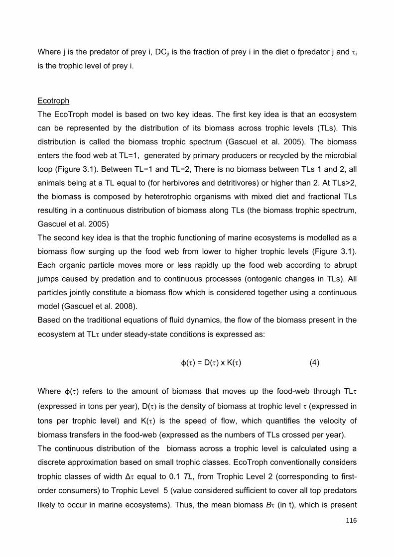
116  

Where j is the predator of prey i, DCji is the fraction of prey i in the diet o fpredator j and i

is the trophic level of prey i.

 

Ecotroph

The EcoTroph model is based on two key ideas. The first key idea is that an ecosystem

can be represented by the distribution of its biomass across trophic levels (TLs). This

distribution is called the biomass trophic spectrum (Gascuel et al. 2005). The biomass

enters the food web at TL=1, generated by primary producers or recycled by the microbial

loop (Figure 3.1). Between TL=1 and TL=2, There is no biomass between TLs 1 and 2, all

animals being at a TL equal to (for herbivores and detritivores) or higher than 2. At TLs>2,

the biomass is composed by heterotrophic organisms with mixed diet and fractional TLs

resulting in a continuous distribution of biomass along TLs (the biomass trophic spectrum,

Gascuel et al. 2005)

The second key idea is that the trophic functioning of marine ecosystems is modelled as a

biomass flow surging up the food web from lower to higher trophic levels (Figure 3.1).

Each organic particle moves more or less rapidly up the food web according to abrupt

jumps caused by predation and to continuous processes (ontogenic changes in TLs). All

particles jointly constitute a biomass flow which is considered together using a continuous

model (Gascuel et al. 2008).

Based on the traditional equations of fluid dynamics, the flow of the biomass present in the

ecosystem at TL under steady-state conditions is expressed as:

φ() = D() x K() (4)

Where φ() refers to the amount of biomass that moves up the food-web through TL

(expressed in tons per year), D( is the density of biomass at trophic level (expressed in

tons per trophic level) and K() is the speed of flow, which quantifies the velocity of

biomass transfers in the food-web (expressed as the numbers of TLs crossed per year).

The continuous distribution of the biomass across a trophic level is calculated using a

discrete approximation based on small trophic classes. EcoTroph conventionally considers

trophic classes of width ∆ equal to 0.1 TL, from Trophic Level 2 (corresponding to first-

order consumers) to Trophic Level 5 (value considered sufficient to cover all top predators

likely to occur in marine ecosystems). Thus, the mean biomass B (in t), which is present

117  

in the [∆] trophic class under steady-state conditions, can be estimated as ∫D () × d

or D() × ∆ for a small interval ∆ Therefore:

B = φ × ∆ / K (5)

where φ and K are the mean biomass flow and mean speed of flow within the [∆]

trophic class, respectively.

As natural losses occur during trophic transfers (through non-predation mortality,

respiration, and excretion), the biomass flow Φ is a decreasing function of TL. Exploitation

by fisheries can be considered a diversion of one part of the trophic flow, which adds to

this negative natural trend. Therefore, from one trophic class to the next, the biomass flow

is calculated as

φ = φ × exp[-(+) ×] (6)

where is the natural loss rate (related to excretion and respiration) and is the fishing

loss rate (with = F / K, where F is the fishing mortality). Eq. (6) implies that the biomass

flow at a given TL depends on the flow from lower TLs. Thus, it implicitly introduces a

bottom–up control of prey on predators in the model. Eq. (6) also defines the net transfer

efficiency (NTE) between continuous TLs as exp(‐μτ).  

The speed of the biomass flow Kτ  (flow kinetic) depends on the turnover of the biomass,

and must be estimated for each trophic class. It is expressed as

K= (P/B)

K is first estimated for a reference state (usually the current state). Then, starting with

values defined for the reference state, the speed of flow for a given simulated state is

calculated using the top-down equation:

, , 1 ∝ ,

, (8)

118  

This equation takes into account the effect of fishing on flow kinetics K and the effect of

predators on prey. Fishing reduces the life expectancy of individuals; animals spend less

time in their trophic class and hence the speed of flow is increased, according to the term

of fishing mortality F. The speed of flow at TL depends partly also on the abundance of

predators (Bpred), since the more predators there are, the faster prey are likely to be eaten.

The coefficient ∝ defines the intensity of this control and may vary between 0 (no top-

down control) and 1 (all natural mortality M depends on predator abundance). The

coefficient γ is a shape parameter varying between 0 and 1, defining the functional

relationship between prey and predators.

Equations (5), (6), and (8) are used to calculate the biomass trophic spectrum Bt for any

simulated fishing pattern

Finally, catches per time unit (in tons x year–1) are derived from earlier equations, as

follows:

Y =  φ or Y = FB (9)

where F is the usual fishing mortality (year-1), defined as the ratio Y/B and equal to  

(from Equations (5) and (9)). Since only a fraction of ecosystem biomass is usually

accessible to fisheries, a selectivity coefficient Sestimated from field observations or from

a theoretical selectivity function (see Gascuel et al. 2011 for details) is added to the model.

Hence, Band F are replaced by the accessible biomass Band the accessible biomass

flow F* in Equation (9). Two distinct kinetics of trophic transfer are used to characterize

the speed of flow in the reference state, one for the entire biomass (Kref,), and the other

for the accessible biomass only (K∗ref,) ,accounting for the fact that exploited species

usually do not have the same characteristics as the unexploited ones.

Equations presented here constitute the core of the ET-Transpose and ET-Diagnosis

routines accessible through an R package which was used in this PhD work.

   

119  

5 Chapter 5. Balancing complexity and feasibility in Mediterranean coastal food-web models: uncertainty and constraints.

Prato G1, Gascuel D2 , Valls A3, Francour P1

1Université de Nice Sophia‐Antipolis; Faculté de Sciences, EA 4228 ECOMERS, 06108 Nice cedex 2, France

2Université Européenne de Bretagne, UMR Agrocampus ouest / INRA Ecologie et Santé des Ecosystèmes, 65 rue de Saint Brieuc, CS 84215, 35042 Rennes cedex, France

3University of British Columbia, AERL, Fisheries Centre, Vancouver, British Columbia V6T1Z4, Canada

Published in Marine Ecology Progress Series 512:71–88

MARINE ECOLOGY PROGRESS SERIESMar Ecol Prog Ser

Vol. 512: 71–88, 2014doi: 10.3354/meps10988

Published October 9

INTRODUCTION

With the oceans facing increasing impacts byhumans, unravelling the complexity of marine eco-system functioning and species interactions hasgradually become a pressing necessity. Single spe-cies approaches are not sufficient to ensure a sustain-able exploitation of marine resources (Botsford et al.

1997, Hofmann & Powell 1998). Instead, ecosystem-based approaches enable a deeper understanding ofthe consequences of human exploitation by consider-ing the whole ecosystem, and assist managers in im -plementing the sustainable use of natural resources(Coll et al. 2013a).

The development of the ecosystem approach tofisheries has triggered an exponential growth of

© Inter-Research 2014 · www.int-res.com*Corresponding author: gprato@unice.fr

Balancing complexity and feasibility in Mediterranean coastal food-web models:

uncertainty and constraints

Giulia Prato1,*, Didier Gascuel2, Audrey Valls3, Patrice Francour1

1Université de Nice Sophia Antipolis, Faculté de Sciences, EA 4228 ECOMERS, 06108 Nice cedex 2, France2Université Européenne de Bretagne, UMR Agrocampus ouest/INRA Ecologie et Santé des Ecosystèmes,

65 rue de Saint Brieuc, CS 84215, 35042 Rennes cedex, France3University of British Columbia, Fisheries Centre, Vancouver, British Columbia V6T1Z4, Canada

ABSTRACT: Mass-balance trophic models (Ecopath and EcoTroph) are valuable tools that can beused to describe ecosystem structure and functioning, identify target species to be monitored, andallow comparisons of ecosystem states under different management options. Nevertheless, theEcopath modelling approach is constrained by 2 major sources of uncertainty: model complexityand input data quality. We developed an approach for identifying the optimum model structurethat considers trade-offs between feasibility, complexity, and uncertainty, using a Mediterraneancoastal ecosystem as a case study. We began with an existing well-documented and good-qualityfood-web model comprising 41 functional groups at Port-Cros National Park, France. Based onthis model, we assessed the effects of different aggregation choices, driven by a simplification ofsampling effort, on the Ecopath and EcoTroph model outputs. We identified the functional groupsin which imprecise biomass input significantly influenced the food-web model, and measured therelative effects on the ecosystem trophic structure and ecosystem maturity and complexity indices.A simplified model comprising 32 functional groups was identified as the best compromisebetween model complexity and reliability. High trophic level predators, abundant primary pro-ducers, and groups with a high biomass and/or diversified diet significantly influenced the modelstructure. We concluded that the collection of local and accurate biomass data, especially for themost influential functional groups we identified, should be a priority when developing food-webmodels for similar ecosystems. Our method enables simplified and standardized models, whileconsidering both the feasibility and reliability of the Ecopath and EcoTroph applications for Mediterranean coastal ecosystems.

KEY WORDS: Aggregation · Uncertainty · Complexity · Trophic spectrum · Ecosystem indices ·Biomass · Ecopath · EcoTroph · Mediterranean Sea

Resale or republication not permitted without written consent of the publisher

Contribution to the Theme Section ‘Trophodynamics in marine ecology’ FREEREE ACCESSCCESS

Mar Ecol Prog Ser 512: 71–88, 2014

modelling tools worldwide (Plagányi 2007, Espinoza-Tenorio et al. 2012). Originally developed by Polov-ina (1984), Ecopath with Ecosim (EwE) (Christensen& Pauly 1992, Walters et al. 1997, Christensen & Wal-ters 2004) is the most widely used approach to repre-sent marine food webs. About 400 EwE models withdifferent objectives and representing a wide varietyof ecosystems worldwide have been published (Colléter et al. 2013), ranging from exploring food-web interactions to computing ecosystem indicatorsuseful for cross-system comparisons, as well as forassessing the impact of fishing or marine protectedareas (MPAs) on the ecosystem (Pauly et al. 2000,Christensen & Walters 2005, Guénette et al. 2014).Ecopath is a mass-balanced and species-basedmodel in which species with similar life cycles anddiets are aggregated into functional groups. Thedescriptive Ecopath model is the key initializationstep in the EwE modelling process, from which fur-ther dynamic and spatial predictions can be simu-lated with Ecosim and Ecospace for policy scenariotesting (Walters et al. 1997, 1999). EcoTroph, a tropho -dynamic model recently integrated as a plug-in in theEwE software (Gascuel 2005, Gascuel & Pauly 2009,Gascuel et al. 2009, 2011), is based on the idea thatan ecosystem can be represented by the distributionof its biomass across trophic levels (TLs), called thebiomass trophic spectrum. The simplified picture ofecosystem functioning provided by EcoTroph hasproven to be very useful for exploring theoreticalaspects of ecosystems, as well as for analysing theimpacts of fishing or protection (Colléter et al. 2012,Gasche & Gascuel 2013).

The use of ecosystem models such as the EwEmodel is generally constrained by 2 major sources ofuncertainty: (1) structural complexity (Abarca-Arenas& Ulanowicz 2002, Fulton et al. 2003, Pinnegar et al.2005, Johnson et al. 2009), and (2) the amount andquality of the input data (Essington 2007, Link 2010,Fulton 2010, Kearney et al. 2013, Lassalle et al. 2014).Structural complexity in Ecopath models is measuredas the number of compartments in the model, theway species are aggregated in these compartments,and the inclusion of stanzas, i.e. groups representingdifferent life history stages for species that have acomplex trophic ontogeny. In fact, it is unrealistic toinclude all interactions at the species level in a foodweb model. Moreover, adding complexity does notnecessarily improve a model’s performance, but gen-erally increases uncertainty (Fulton et al. 2003). Spe-cies aggregation is thus necessary, but can stronglyinfluence the model outputs. The over-aggregationof certain components of the food web, at either the

upper or lower trophic levels, produces models withvery different behaviours (Pinnegar et al. 2005) andhas sometimes led to dissimilar and conflicting rec-ommendations for management action (Punt & But-terworth 1995, Yodzis 2001). In addition, Ecopathmodels require a large amount of input data, thequality of which can vary significantly. An in-depthevaluation of the sensitivity of Ecopath models toimprecise input data showed that the Ecopath model-ling process is most sensitive to biomass and produc-tion rate parameters, and only occasionally sensitiveto consumption rate and diet (Essington 2007). In ouranalysis, we decided to focus on the biomass inputparameter. Biomass is of direct relevance to marineresource management, yet it is not easy to estimateaccurately for the totality of the food web compo-nents due to the costs and constraints of sampling inthe marine environment.

In the Mediterranean Sea, several Ecopath modelshave been built with various levels of detail, depend-ing on the research questions and data availabil -ity (Table 1). For some exploited ecosystems (e.g. Northern Adriatic Sea, South Catalan Sea, NorthernAegean Sea, and Greek Ionian Sea), rather compre-hensive models have been developed that includemore than 30 functional groups based on the highavailability of biomass data from industrial fishingmonitoring (experimental trawling) (Table 1). In con-trast, few models (e.g. Libralato et al. 2006, Albouy etal. 2010, Valls et al. 2012) representing coastal zonesin the Mediterranean Sea have been developed andused to analyse MPAs (Table 1). The scarcity of food-web models for the Mediterranean coastal MPAs islikely due to the high diversity and complexity oftheir food webs (Sala 2004), and the many challengesin terms of data collection. A protected area is a zonein which fishing and other human impacts arerestricted to achieve conservation objectives. Thus,destructive sampling methods such as experimentalfishing (i.e. trawl surveys), which could provideextensive data on the studied ecosystem, are gener-ally prohibited or limited. However, less destructivemethods also have limitations. Underwater monitor-ing techniques, such as visual censusing to assessfish and mega-invertebrate biomass or suctionpumps to sample macrofauna, are time consumingand require a considerable workload for collectingthe samples in the field and analysing them at thelaboratory. Thus, field-based estimates of biomassare generally available only for a subset of species ofrecognized ecological importance in coastal zonesand/or of particular management relevance in pro-tected areas. For instance, in the Mediterranean,

72

Prato et al.: Mediterranean coastal ecosystem food-web models

there is extensive knowledge onthe trophic interactions between seabream, sea urchins, and macroalgaeand their role in controlling coastalecosystem states (Sala et al. 1998,Guidetti 2007). These groups arethus common monitoring targets inMediterranean MPAs, while we facea lack of data and knowledge formany other functional groups (Sala2004). Consequently, the applicationof food-web modelling has remainedrelatively limited in coastal Medi -terranean ecosystems.

The objective of this work was todetermine an optimum and stan-dardized model structure to repre-sent a northwestern Mediterraneancoastal food web that accounts forthe trade-offs between feasibility,complexity, and uncertainty. To doso, we selected the Ecopath modelrepresenting the MPA of Port-Cros,a French marine national park inthe northwestern Mediterranean Sea(Valls et al. 2012). This model wasoriginally built to synthesize all avail-able data and identify knowledgegaps regarding the described ecosys-tem. Thus, the study presents de -tailed information on species aggre-gation into the 41 defined functionalgroups (Table 2), which makes it themost detailed model available repre-senting a Mediterranean coastal foodweb (Table 1). Such a comprehensivesynthesis was made possible by themany years of research and moni -toring that produced a significantamount of data for this old MPA, created in 1963 (e.g. Khoury 1987,Francour 1990). Hence, the biomassparameters were estimated fromlocal field-based studies for 57.5% ofthe functional groups, which is a rel-atively high score compared to simi-lar modelled ecosystems (Table 1).We used the original Port-Crosmodel as our control state, and wesimplified its trophic structure byapplying different levels of speciesaggregation, the choice of which wasdriven by sampling feasibility con-

73

IDL

ocat

ion

Fis

hin

gF

un

ctio

nal

Sam

pli

ng

Exp

erim

enta

l L

ocal

Ind

irec

t N

on-l

ocal

M

odel

S

ourc

eg

rou

ps

fish

ing

/fi

eld

m

eth

odli

tera

ture

/es

tim

ate

(n)

mon

itor

ing

stu

die

sot

her

mod

el

1M

iram

are

Nat

ura

l M

arin

e R

eser

ve

Non

e/A

rt.

2378

.365

.213

.021

.70

0L

ibra

lato

et

al. (

2006

, 20

00−

2003

2010

)2

Bon

ifac

io S

trai

ts N

atu

ral

Res

erve

, N

one/

Art

.31

48.4

48.4

00

9.7

32.3

Alb

ouy

et a

l. (

2010

)C

orsi

ca 2

000−

2001

3P

ort-

Cro

s N

atio

nal

Par

k 1

998−

2008

Non

e/A

rt.

4057

.50

57.5

15.0

027

.5V

alls

et

al. (

2012

)4

Bay

of

Cal

vi, C

orsi

ca 1

998

Non

e/A

rt.

2661

.50

61.5

7.7

30.8

0P

inn

egar

(20

00)

5A

ran

cy B

ay, S

ard

inia

200

6In

d.

1225

.025

.00

25.0

050

.0D

iaz

Lop

ez e

t al

. (20

08)

6S

anta

Pol

a B

ay, S

pai

n 2

001−

2007

Ind

.39

100

010

00

00

Bay

le-S

emp

ere

(201

3)7

Sou

ther

n C

atal

an S

ea 1

994

Ind

.36

86.1

66.7

19.4

2.8

011

.1C

oll

et a

l. (

2006

)8

N A

dri

atic

Sea

199

7−20

00In

d.

1710

00

100

00

0Z

ucc

het

ta e

t al

. (20

03)

9N

C A

dri

atic

Sea

197

5−19

80In

d.

3710

081

.118

.90

00

Col

l et

al.

(20

08)

10N

Ad

riat

ic S

ea 1

990

Ind

.32

84.4

53.1

31.3

6.3

09.

4B

arau

sse

et a

l. (

2009

)11

N A

dri

atic

Sea

199

7−20

00In

d.

1710

00

100

00

0P

ran

ovi

& L

ink

(20

09)

12N

E I

onia

n S

ea 1

964

Ind

.17

23.5

5.9

17.6

76.5

00

Pir

odd

i et

al.

(20

10)

13N

Aeg

ean

Sea

200

3−20

06In

d.

3876

.368

.47.

918

.42.

62.

6T

sag

arak

is e

t al

. (20

10)

14G

reek

Ion

ian

Sea

199

8−20

06In

d.

3770

.370

.30

10.8

13.5

5.4

Mou

top

olou

s (2

013)

15B

lack

Sea

196

0In

d.

1310

00

100

00

0D

ask

alov

(20

02)

16B

lack

Sea

196

0In

d.

666

.70

66.7

00

33.3

Gu

cu (

2002

)17

Bla

ck S

ea 1

980,

199

0In

d.

650

.00

50.0

00

50.0

Gu

cu (

2002

)18

Eta

ng

de

Th

au L

agoo

n 1

980s

Ind

.10

30.0

030

.00

070

.0P

alom

ares

et

al. (

1993

)19

Ven

ice

Lag

oon

− P

alu

de

del

la R

osa

Non

e/A

rt.

1573

.366

.76.

726

.70

0C

arre

r &

Op

itz

(199

9)19

90s

20V

enic

e L

agoo

n 1

990s

Ind

.19

26.3

026

.30

73.7

0L

ibra

lato

et

al. (

2002

)21

Ven

ice

Lag

oon

199

8In

d.

2572

.036

.036

.020

.08.

00

Pra

nov

i et

al.

(20

03)

22O

rbet

ello

Lag

oon

199

5, 1

996

Ind

.11

00

018

.20

81.8

Bra

nd

o et

al.

(20

04)

Tab

le 1

. Ori

gin

of b

iom

ass

inp

ut d

ata

for

22 m

odel

s of

the

Med

iter

ran

ean

. Th

e 4t

h c

olu

mn

list

s th

e n

um

ber

of g

rou

ps

incl

ud

ed in

the

rela

ted

mod

el (e

xclu

din

g n

on-l

ivin

gg

rou

ps,

i.e

. d

etri

tus,

byc

atch

/dis

card

s an

d d

isso

lved

org

anic

mat

ter)

. T

he

nex

t co

lum

ns

exp

ress

th

e p

erce

nta

ges

of

fun

ctio

nal

gro

up

s fo

r w

hic

h b

iom

ass

dat

a w

ere

der

ived

fro

m t

he

met

hod

sp

ecif

ied

in

col

um

n h

ead

er.

Sam

pli

ng

-bas

ed d

ata

are

der

ived

fro

m e

ith

er e

xper

imen

tal

fish

ing

, m

onit

orin

g o

r fi

eld

-bas

ed l

ocal

stu

die

s. E

sti-

mat

es f

rom

th

e in

dir

ect

met

hod

in

clu

de

dat

a ob

tain

ed f

rom

em

pir

ical

mod

els,

per

son

al c

omm

un

icat

ion

s, a

nd

ext

rap

olat

ion

fro

m v

isu

al s

urv

eys

for

mar

ine

mam

mal

s,

sea

turt

les

and

bir

ds.

Th

e li

st o

f m

odel

s w

as d

eriv

ed f

rom

Col

l &

Lib

rala

to (

2012

) an

d C

olle

ter

et a

l. (

2013

). A

rt.:

arti

san

al; I

nd

.: in

du

stri

al

Mar Ecol Prog Ser 512: 71–88, 2014

siderations. We then identified the functional groupsfor which local and accurate biomass data should becollected as a priority, as they have the most signifi-cant influence on the model outputs. Specifically, wefocused on 3 main questions: (1) how do sampling-driven aggregation choices alter the model descrip-tion of ecosystem functioning; (2) to what level ofaggregation can the model be simplified without sig-

nificantly altering its accuracy; and (3) what are thefunctional groups in the simplified model for whichimprecise biomass input significantly influences thebiomass calculations of other groups, and thus theoverall description of the ecosystem functioning.

By addressing these issues, we intended to proposesome priority guidelines, in terms of model structureand data collection, that could enable the develop-ment of standardized models of complex Mediterran-ean coastal ecosystems.

METHODS

Two food-web modelling approaches were used inour analysis: the species-based Ecopath model andthe TL-based EcoTroph model. Ecopath was used tobuild several versions based on the control model,with different levels of aggregation and differentinput biomass values, while EcoTroph was used tocompute the trophic spectra for each new model.Sensitivity analyses were performed on selected eco-system maturity and complexity indices computed byEcopath, and on the trophic description of the ecosys-tem provided by EcoTroph.

Ecopath

Ecopath uses a mass-balanced food-web model,assuming that the production of one functional groupis equal to the sum of all predation, non-predatorylosses, exports, biomass accumulations, and catches,as expressed by the following equation:

P/Bi × Bi = P/Bi × Bi × (1 − EEi) + Σj (Q/B)ji × Bi × DCji + Yi + NMi + BAi (1)

where B is the biomass, P/Bi is the production rate,Q/B is the consumption rate, DCji is the diet composi-tion representing the fraction of prey i in the diet ofpredator j, NMi is the net migration of prey i, BAi isthe biomass accumulation of prey i, Yi is the catch ofprey i, and EEi is the ecotrophic efficiency of prey i(the proportion of production that is used in the sys-tem, e.g. through predation and harvest). Assumingthere is no export and no biomass accumulation, andthe catches are known, only 3 of the 4 remainingpara meters (B, P/Bi, Q/B, and EEi) have to be set ini-tially for each group. The parameterization routinesolves the equations for each missing parameter iter-atively (Christensen et al. 2008).

A comprehensive Ecopath model was built by Vallset al. (2012) for the Port-Cros MPA (Table 2), which

74

Sampling method Functional group

VS SeabirdsVC Amberjack+VC Dusky grouper − mediumVC Dusky grouper − largeVC Dusky grouper − smallVC, NF RaysVC, NF Large-scaled scorpionfish+VC, NF Scorpionfishes+VC, NF Striped red mullet+VC, NF PagellusVC, Ac, NF Horse mackerels+VC, NF Diplodus+VC, NF WrassesVC, NF MulletsVC, C CephalopodsVC, SS BlenniesVC, SS Pipefishes+VC, SS GobiesSS, SC GastropodsSS Small crustaceansSS AmphipodsSS Brittle stars+SS, SC SuspensivoresSS, VC CrabsSS, VC DecapodsSS, Co, SC PolychaetesSS, VC, SC BivalvesVC Sea starsVC Sea cucumbersVC Sea urchinsPNB Large zooplanktonPNB Small zooplanktonVC GorgoniansVC, NF Salema − adultsVC Salema − juvenilesCo, SC ForaminiferaA, SC PosidoniaSC Shallow seaweedsSC Deep seaweedsPNB, CRS PhytoplanktonCo, SS Detritus

Table 2. The 41 functional groups of the Port-Cros controlmodel. Details in Valls et al. (2012). Only the least destruc-tive methods were considered: visual survey (VS), visualcensus (VC), acoustics (Ac), suction sampler (SS), scraping(SC), plankton nets/bottles (PNB), chlorophyll remote sens-ing (CRS), corer (Co), and net fishing (NF). The groups in

bold are those considered for aggregation

Prato et al.: Mediterranean coastal ecosystem food-web models

covers a surface area of 13 km2 and reaches a maxi-mum depth of 50 m. Biotopes are typical of the north-western Mediterranean, with nearshore rocky reefs,large Posidonia oceanica meadows, and a corallige-nous habitat, hosting a high biodiversity of commer-cially important fish and decapod crustaceans; only5% of the reserve is a no-take area, outside of whichfishing is permitted with severe restrictions (Francouret al. 2001). The Ecopath model represents an aver-age situation for the period from 1998 to 2008, de -fined by the data used in the model. Large amountsof data were available for this old and well-studiedMPA, which allowed for the development of a rela-tively detailed model, including 40 living functionalgroups (plus one detrital group). More precisely, themodel comprises 18 groups of fish, 17 groups ofinvertebrates, 4 groups of primary producers, and1 group of seabirds. In addition, the model is welldocumented in terms of both species aggregationchoices and species-level information for each func-tional group. Moreover, all fish biomass data are ofgood quality as they were derived from visual cen-susing and scientific trawling in the area. Local field-based biomass data were also available for someinvertebrate and primary producer groups. Detailson the species composition of each functional groupin the control Port-Cros model, as well as the inputparameters for each group, can be found in Valls etal. (2012). Finally, the model respected Link’s recom-mendations of data quality (Link 2010), and its repre-sentation of the Port-Cros ecosystem was in accor-dance with the current available knowledge (Vallset al. 2012).

EcoTroph

The trophic level-based EcoTroph model assumesthat biomass has a continuous distribution in anecosystem as a function of continuous TLs. Thebiomass is represented as entering the system atTL = 1, generated by the photosynthetic activity ofprimary producers or recycled from the detritus bythe microbial loop. Then, at TLs >2, the biomass isdistributed along a continuum of TL values and allfractional TLs are filled due to the diet variabilityof the various consumers. The resulting biomassdistribution constitutes the biomass trophic spec-trum (Gascuel et al. 2005). The functioning of theecosystem is then modelled as a continuous flowof biomass, surging up the food web from lower tohigher TLs, through predation and ontogenic pro-cesses.

Based on the usual equations of fluid dynamics, theflow of the biomass present in the ecosystem at TL τunder steady-state conditions is expressed as:

ϕ(τ) = D(τ) × K(τ) (2)

where ϕ(τ) refers to the amount of biomass thatmoves up the food web through TL τ (metric t peryear), D(τ) is the density of biomass at TL τ (metric tper trophic level), and K(τ) is the speed of flow, whichquantifies the velocity of biomass transfers in thefood web (number of TLs crossed per year).

The continuous distribution of the biomass across aTL is calculated using a discrete approximationbased on small trophic classes. EcoTroph convention-ally considers trophic classes of width Δτ equal to0.1 TL, from TL 2 (corresponding to first-order con-sumers) to TL 5 (a value considered sufficient tocover all top predators likely to occur in marine eco-systems). Thus, the mean biomass Bτ (in metric t),which is present in the [τ, τ + Δτ] trophic class understeady-state conditions, can be estimated as ∫D(τ) ×dτ or D(τ) × Δτ for a small interval Δτ. Therefore,

Bτ = ϕτ × Δτ / Kτ (3)

where ϕτ and Kτ are the mean biomass flow and meanspeed of flow within the [τ, τ + Δτ] trophic class,respectively; see the supplementary material in Vallset al. (2012) for further explanation.

In this study, we used the ET-Transpose routinedescribed in Gascuel et al. (2009) to translate the out-puts of the original Ecopath model into an EcoTrophmodel and to build the biomass trophic spectrum.The biomass of each functional Ecopath group wasdistributed over a range of trophic classes aroundthe mean TL of the group (estimated by Ecopath),assuming a log-normal distribution. The trophicspectrum is the curve obtained by summing the bio-mass parameter over all functional groups and pro-vides a synthetic view of the trophic structure of theecosystem.

We then used the ET-Diagnosis routine to conductsensitivity testing. We simulated how the baselineecosystem would be impacted by increasing ordecreasing the fishing effort. Fishing effort can bemodified per fleet by applying various effort multi -pliers, and the structure of the trophic spectrumwill vary under different efforts (Gascuel et al. 2011,Gasche & Gascuel 2013).

Aggregated models and comparisons

The original version of the Ecopath model for thePort-Cros National Park’s MPA, described by Valls et

75

Mar Ecol Prog Ser 512: 71–88, 2014

al. (2012), was selected as the control model in oursimplification procedure, and 6 models were derivedfrom this, using successive aggregation steps. Purelytaxonomical aggregations were avoided. Aggregationchoices were driven by sampling efficiency consider-ations; for each functional group, the most adequateand least destructive sampling methods were as -signed, and groups that shared at least one commonsampling method were considered for aggregation.Thus, aggregation choices were also consistent withthe habitat use among groups, so that species in thesame group occupied the same habitat. Aggregationchoices were also constrained by diet compositionoverlap and similarities in production and consump-tion (P/B and Q/B rates), which should differ by lessthan 3-fold between groups (Fulton et al. 2003).Small cryptobenthic fish (blennies, pipefishes, andgobies) were grouped based on the difficulty in sam-pling them and because they share similar life- history parameters. The other fish functional groupswere not further aggregated relative to the originalmodel, in which they were grouped according totheir TL, maximum length, and feeding type (Vallset al. 2012).

Starting from the first aggregated model (the onewith the broadest aggregation of the invertebrategroups), a biomass trophic spectrum was computed,and the trophic spectra ratios between this firstmodel and the control were compared. The TLs cor-responding to the widest changes in the trophic spec-trum were identified, and the corresponding func-tional groups were isolated in the subsequent model,in which different levels of aggregation were tested.For each new model, static ecosystem indices werecomputed and the percentage difference betweeneach aggregated model and the control were com-pared. This procedure was repeated stepwise untilthe aggregation with the fewest differences from thecontrol in the trophic spectra and ecosystem indiceswas identified. P/B and Q/B ratios were computed forthe newly aggregated groups; they were weightedwith the biomass and summed over all of the groupsto be aggregated. Similarly, the new diet composi-tions were obtained by weighting the food intake ofeach group with the consumption of the group, andthen summing the food intakes over all of the groupsto be aggregated.

To evaluate the successive species aggregations,we compared the ecosystem indices that are mostwidely accepted as indicators of ecosystem maturityand complexity in the literature: Finn’s cycling index(FCI), system omnivory index (SOI), relative ascen-dency (%A), and TL of the community (TLco) (Chris-

tensen 1995, Libralato et al. 2010). Because the totalamount of matter flowing in each model was main-tained constant and equal to the original, the matu-rity indices related to the flows and biomasses werenot considered. FCI measures the fraction of the eco-system’s throughput that is recycled. The degree ofenergy and nutrient recycling in an ecosystem is as -sumed to increase as ecosystems mature and developroutes for nutrient conservation (Odum 1969). SOI isdefined as the average omnivory index of all con-sumers, weighted by the logarithm of the foodintakes (Christensen & Pauly 1992). It expresses thevariance in the TLs of the consumers’ prey groups(Pauly et al. 1993) and is considered a measure offood-web complexity. Ascendency is a measure ofthe average mutual information in a system, scaledby system throughput, and is derived from informa-tion theory (Ulanowicz & Norden 1990). If one knowsthe location of a unit of energy, the uncertainty aboutwhere it will flow to next is reduced by an amountknown as the ‘average mutual information’. Theamount of the average mutual information multipliedby the total system throughput (TST) gives the as -cendancy (A). There is an upper limit for the devel-opment of the ascendancy, which is called the ‘devel -opment capacity’. Here, we are considering %A,defined as the ratio between A and the developmentcapacity that was demonstrated to be clearly corre-lated with maturity sensu Odum (Christensen 1994).The average TLco is estimated as the biomass-weighted average TL for all functional groups of theweb, excluding those at TL = 1. Libralato et al. (2010)showed that TLco was consistently lower in a fishedfood web compared to an adjacent unexploited one.Given the similarity of fishing patterns in coastalMediterranean waters, we retained TLco as a goodindicator of the fishing effects.

The model that showed the smallest differencesfrom the control in the trophic spectra and ecosystemindices was considered to offer the best speciesaggregation scheme, and was therefore selected forfurther analysis. The ET-Diagnosis function wasapplied to test whether the selected model wouldbehave differently from the control in terms ofassessing the fishing impact on the ecosystem. Forboth the control and the selected model, we built 2different fishing scenarios by applying 2 effort multi-pliers (mF) to the current fishing mortality of eachtrophic class. Specifically, we applied an mF = 0 tosimulate a closure of the fishery and an mF = 12 tosimulate an increase in fishing effort. The latter valueof mF was shown to be of the same order of magni-tude as those observed in surrounding and similar

76

Prato et al.: Mediterranean coastal ecosystem food-web models

unprotected areas (Valls et al. 2012). We then com-pared the simulation outputs to the unexploited stateand identified the differences between the patternsof the 2 models.

Sensitivity to error in input biomass and identification of the most influential species

The model selected after aggregation was set asthe new reference (ref. model) to test the effects ofvariation in each group’s input biomass on the bio-mass estimates of the other groups, and to evaluatethe impact of these errors on the overall model out-puts; 31 new models were built by increasing the bio-mass of each group by 10% and obtaining the bio-mass of the other groups (except primary producers)from the Ecopath equation solutions (with ecotrophicefficiencies fixed). During this process, the biomassof the primary producers was not obtained from theEcopath equation solutions, but instead was kept atits original value, because it was input data in theoriginal model and therefore avoided a potentialmodelling artefact: i.e. strong increases in primaryproducer biomass to sustain increased consumerabundance due to the Ecopath routine estimation ofthe primary production re quired to sustain consump-tion. Thus, we were conservative by evaluating theminimum impact that imprecise input biomass forconsumers would have on the model outputs. Subse-quently, the biomass of each primary producer wasalso varied by 10%, and the biomasses of all othergroups were obtained from the Ecopath equationsolutions to test the influence of an error in the pri-mary producer input biomass.

A variation of 10% was assumed to be small enoughto keep the models mass-balanced and large enoughto create differences between the models. To test themodel sensitivity to the biomass increments, the bio-mass trophic spectra and maturity indices were com-pared between each new model and the ref. model.The trophic spectra of the ratios between the newmodel and the ref. model were plotted, and 3 indiceswere derived: the number of trophic levels affectedby a variation in the biomass of >1% (i.e. the width ofthe trophic spectra, Width_TS); the maximum level ofbiomass increase (i.e. the peak of the trophic spectra,Peak_TS), and the total biomass increase (i.e. thearea of the trophic spectra, B_TS); the latter wasexpressed as the percentage difference from the ref.model biomass and was increased for several func-tional groups simultaneously to test for any amplify-ing effect on the trophic spectra. The percentage

differences from the ref. model were compared for%A, SOI, FCI, TLco, and 2 additional flow indices: theratio of total primary production to total respiration(TPP/R) and the ratio of total biomass to total systemthroughput (B/TST). The latter 2 flow-related matu-rity indices were included at this step of the analysisbecause variations in the functional groups’ biomassinputs induced variations in the amount of matterflowing in the model.

A principal component analysis (PCA) was con-ducted to visualize the impact of each functionalgroup on the ecosystem attributes. The previouslymentioned indices of maturity, complexity, and trophicstructure were the explicative variables of the PCA,while the different models obtained by 10% in -creases in the biomass of each functional group werethe samples. All variables were standardized to azero mean and unit variance to compensate for dif-ferences in the value ranges. TL and biomass wereincluded in the PCA as supplementary continuousvariables and trophic class was included as a supple-mentary categorical variable, so that they would notbe considered in the computation of the principalcomponents. The groups were then ranked accord-ing to their contribution to each of the first 3 principalcomponents, and their mean ranking was computed.Thus, summarized information was obtained for thefunctional groups with the most impact on the vari-ables overall. The functional groups were then plot-ted in decreasing order of their mean rank (a rank of1 was attributed to the group having the greatestimpact). The groups with the highest rankings wereidentified and selected as those having the mostimpact on the model’s output, and thus requiringlocal and accurate biomass input data.

RESULTS

Model aggregations and comparisons

Model A included 33 living groups (Table 3) andwas characterized by the largest aggregation ofinvertebrate groups that can be sampled with suctiondevices (gastropods, small crustaceans, amphipods,brittle stars, suspensivores, crabs, decapods, andpoly chaetes comprised a new Epifauna+ group). Seastars and sea cucumbers were not included, becausetheir constant production and consumption rates differ significantly from the other invertebrates, andestimates of their biomass are more commonly ob -tained from a visual census. Model B (34 livinggroups) differed from Model A by the separation of a

77

Mar Ecol Prog Ser 512: 71–88, 201478

pooled crab and decapod group (Decapods+) fromthe Epifauna+ group. In Model C, suspensivoreswere excluded from the Epifauna+ group as well,and aggregated with bivalves (Suspensivores+).Moreover, sea stars were grouped with sea cu -cumbers (Echinoderms+), blennies with pipefishes(Blennies+), and shallow seaweeds with deep sea-weeds (Seaweeds+), resulting in an overall aggrega-tion into 31 living groups. Model D (32 living groups)was equal to Model C, except for the polychaetes,which were excluded from the Epifauna+ group anddefined as a separate group. In Model E (31 livinggroups), the suspensivores and bivalves were addedto the Epifauna+ group, while the polychaetes werekept separated. Finally, Model F (31 living groups)was characterized by an Epifauna+ group that in -cluded gastro pods, small crustaceans, amphipods,

and brittle stars. The previously defined groupsof Decapods+, Sus pen sivores+, Echinoderms+, and Seaweeds+ remained as separate groups, while aGobies+ group was created to aggregate gobies,blennies, and pipefishes.

For every aggregated model, FCI and %A werehigher than in the control model, while the SOI wassystematically lower. The differences in TLco wereeither negative or null. The aggregation thatcaused the largest variations in ecosystem indices(Fig. 1) and trophic spectra (Fig. 2) was that ofcrabs and decapods with Epifauna+ (Model A),causing a 30% increase in FCI (Fig. 1) andnegative biomass differences for TL > 3.5 (Fig. 2a).Suspensivores+ and polychaetes also significantlyaffected ecosystem indices and trophic spectrawhen aggregated with the Epifauna+ group; Mod-

Table 3. Aggregation schemes. The groups that were not modified from the control model are not listed. Number of functionalgroups (excluding detritus) given at bottom. Grey boxes indicate functional groups that have been mapped to an aggregate group

listed higher in the table. Co: corer; SC: scraping; SS: suction sampler; VC: visual census

Sampling Control Model A Model B Model C Model D Model E Model F

VC, SS Blennies Blennies Blennies Blennies+ (blennies, pipefishes)

Blennies+ (blennies, pipefishes)

Blennies+ (blennies, pipefishes)

Gobies+ (blennies, pipefishes, gobies)

VC, SS Pipefishes+ Pipefishes+ Pipefishes+

VC, SS Gobies Gobies Gobies Gobies Gobies Gobies

SS, SC Gastropods Epifauna (gastropods, small crustaceans, amphipods, brittle stars, suspensivore, crabs, decapods, polychaetes)

Epifauna (gastropods, small crustaceans, amphipods, brittle stars, suspensivore, polychaetes)

Epifauna (gastropods, small crustaceans, amphipods, brittle stars, polychaetes)

Epifauna (gastropods, small crustaceans, amphipods, brittle stars)

Epifauna (gastropods, small crustaceans, amphipods, brittle stars, suspensivore, bivalves)

Epifauna (gastropods, small crustaceans, amphipods, brittle stars)

SS Small crustaceans

SS Amphipods

SS Brittle stars+

SS, SC Suspensivores Suspensivores+ (bivalves, suspensivores)

Suspensivores+ (bivalves, suspensivores)

Suspensivores+ (bivalves, suspensivores)

SS, VC Crabs Decapods+ (crabs, decapods)

Decapods+ (crabs, decapods)

Decapods+ (crabs, decapods)

Decapods+ (crabs, decapods)

Decapods+ (crabs, decapods) SS, VC Decapods

SS, Co, SC Polychaetes Polychaetes Polychaetes Polychaetes

SS,VC, SC Bivalves Bivalves Bivalves

VC Sea stars Sea stars Sea stars Echinoderms+ (sea stars, sea cucumbers)

Echinoderms+ (sea stars, sea cucumbers)

Echinoderm+ (sea stars, sea cucumbers)

Echinoderms+ (sea stars, sea cucumbers) VC Sea cucumbers Sea cucumbers Sea cucumbers

SC Shallow seaweeds

Shallow seaweeds

Shallow seaweeds

Seaweeds+ (shallow seaweeds, deep seaweeds)

Seaweeds+ (shallow seaweeds, deep seaweeds)

Seaweeds+ (shallow seaweeds, deep seaweeds)

Seaweeds+ (shallow seaweeds, deep seaweeds)

SC Deep seaweeds

Deep seaweeds

Deep seaweeds

No. of groups 40 33 34 31 32 31 31

Prato et al.: Mediterranean coastal ecosystem food-web models

els D and F showed the least differences from thecontrol (Figs. 1 & 2b). The aggregations of Echino-derms, Seaweeds+ and Gobies+ caused no majormodifications in model properties. Model F, with 31living functional groups, had the most simplifiedspecies aggrega tion scheme, i.e. the smallest varia-tions in the ecosystem indices and trophic structurerelative to the control for the highest level of spe-cies aggregation possible.

The simulation test confirmed that the behaviour ofModel F was similar to that of the control, when bothclosure (mF = 0) and increased fishing effort (mF =12) were simulated. The exploitation effect was sig-nificant only at TL > 3.5, and in neither the originalnor the aggregated model did the exploitation causemajor biomass variations at the lower TLs (Fig. 3).Model F was thus selected for successive analysis.

Sensitivity to error in the input biomass

A sensitivity analysis was applied toModel F. The analyses of the trophicspectra (Fig. 4) and the differences inthe ecosystem indices due to biomassvariations (see Appendix 1) showedthat the high TL predator groups,Amberjack+ and Dusky grouper −large, had the largest impacts on thebiomass of the other groups, and thusmost influenced the trophic spectra andecosystem indices. Increments of 10%in the biomass of these 2 large fish

groups affected the biomass of all other trophicgroups by more than 1%, with most TLs affected bymore than 5% (Fig. 4A). The trophic spectra sensitiv-ity to Dusky grouper − large increased when TL ≥ 4,since this was the only group occupying the highestTLs. The trophic spectra for both Amberjack+ andDusky grouper − large reached peaks with anapproximately 9% increase in biomass, and overallbiomass increased (B_TS) by 0.25 and 0.28%, respec-tively, relative to Model F. With regard to the otherfish groups, the highest impact in terms of number ofTLs affected and shifts in biomass was caused by

79

Fig. 1. Percentage differences in the system indices between the aggregated models and the control model

Fig. 2. Trophic spectra of the ratios of the biomass between thecontrol model and (A) aggregated Models A, B, and C or

(B) aggregated Models D, E, and F, in relative values

Fig. 3. Simulation scenarios for Model F and the control model. Relative bio-mass values were obtained from the trophic spectra ratios, with effort multi-

pliers mF = 12 (Sim12) and mF = 0 (Sim0) applied to both models

Mar Ecol Prog Ser 512: 71–88, 201480

Horse mackerels+ (Width_TS = 21, Peak_TS= 7.5%, B_TS = 0.09%), followed by Scorpi-onfishes+ and Wrasses (Fig. 4B).

Among the invertebrates (Fig. 4C), Ce -phalopods+ affected the largest number oftrophic levels (Width_TS = 19), followed byDecapods (Width_TS = 9). Decapods wasthe group with the most impact on thePeak_TS index; under their influence, thetrophic spectrum reached the maximumpeak resulting from a 10% increment in thebiomass. An increase of 10% in the biomassof Sea worms and Echinoderms+ led to highbiomass peaks in the trophic spectra(Peak_TS = 8.8, Peak_TS = 8.4%, respec-tively), but their impacts were limited to avery narrow range of TLs corresponding totheir own range (Width_TS = 4, Width_TS= 2, respectively). A simultaneous biomassincrease of several functional groups re -sulted in a simple additive effect on thetrophic spectra and thus was not consideredfurther.

Similar to the trophic spectra analysis, a10% increment in the biomass of the Duskygrouper − large and Amberjack+ groupscaused the largest variations in absoluteterms in all ecosystem indices, especiallyimpacting FCI (7.2 and 8.1%, respectively),TPP/R (6.4 and 7.2%, respectively), and %A(2.1% for both). As for the Epifauna+,Decapods+, Cepha lo pods, and Horse mack-erels+ groups, the biomass incrementscaused large variations in FCI (max. value =7.0% for Epifauna+) and SOI (max. value =1.6% for Horse mackerels+). Increments inthe biomass of Foraminifera and Small zoo-plankton had a strong influence on FCI (6.3and 6.6%, respectively). Posidonia oceanicahad a high overall impact and principallycaused large variations in the flow indicesTPP/R (4.7%) and B/TST (6.1%), and in %A(2.1%).

Principal component analysis

A PCA on all indices was performed(Fig. 5). The first PC accounted for almost50% of the variability of the data, and thesecond PC accounted for 25% (Fig. 5A).The first PC summarized the variabilityexplained by 2 sets of variables: recycling

Fig. 4. Biomass ratios between the trophic spectra of each model ob-tained after an increase of 10% to the biomass of one functional groupand the trophic spectra of the reference model (represented by the solidline at relative biomass = 1). The dotted line corresponds to the thresh-old value of a 1% variation in biomass. (A) Higher trophic level preda-

tors; (B) other fish groups; (C) invertebrates

Prato et al.: Mediterranean coastal ecosystem food-web models 81

Fig. 5. Principal component analysis (PCA) plots. (A) Variables and (B) individual factors for the first 2 principal components.(C) Individual factors for principal components 1 and 3. In the variables plot (A), B and TL are the supplementary variables(blue). In the individual factor plots (B,C), only the non-overlapping points were labelled to improve visualization. B: biomass;B_TS: biomass of the trophic spectra; B/TST: biomass/total system throughput; FCI: Finn’s cycling index; Peak_TS: peak of thetrophic spectra; SOI: system omnivory index; TC: trophic class; TLco: mean trophic level of the community; TL: trophic level;

TPP/R: total primary production/total respiration; TS: trophic spectra; Width_TS: width of the trophic spectra

Mar Ecol Prog Ser 512: 71–88, 2014

(FCI), %A, and trophic spectra structure (Width_TSand Peak_TS) on the one hand, and the energy fluxindices (TPP/R and B/TST) and trophic spectra-derived biomass index (B_TS) on the other. Withineach set, the variables appeared to be highly corre-lated to one another. The influence of the functionalgroups on the variables (i.e. their effect on theindices) was related to their biomass. Several spe-cies which cover the whole range of trophic levels,but with low biomass, influenced the variables lessthan average (Fig. 5b). In contrast, the top predatorsDusky grouper − large and Amberjack+ (TL >4),having higher biomasses, strongly affected manyecosystem indices, particularly the trophic spectraindices (Width_TS, Peak_TS), ecosystem maturity(FCI, %A), and flow indices (TPP/R, B/TST) summa-rized by PC1. Groups feeding on a wide range oftrophic levels and with consistent biomass (Decapods,Epifauna+, Horse mackerels+ and Cephalo pods)affected the ecosystem complexity indices (SOI andTLco), while the Posidonia group affected the flowand biomass related indices (TPP/R,B/TST, andB_TS).

When the third PC was visualized (Fig. 5C), thefunctional groups were ordered by TL. Following thehigh TL predator groups, the Scorpionfishes+,Cephalopods, and Horse mackerels+ were arrangedin decreasing order of TL and contributed equallyto PC1. On the positive side of PC3, the TL of thegroups decreased, and biomass became the domi-nant supplementary variable. Thus, Decapods+ andEpifauna+ contributed equally to both PC1 and PC3in terms of the ecosystem complexity indices (SOI

and TLco), while Posidonia, having the highest bio-mass, showed the highest contribution to PC1 andPC3 in terms of overall biomass increase (B_TS), andto PC1 for %A.

The first 3 PCs summarized approximately 80% ofthe variability explained by the indices, so the func-tional groups were ranked according to their contri-butions to these axes. By plotting the species indecreasing order of their mean rank (rank of 1 for thespecies having the highest impact) (Fig. 6), we high-lighted 2 major gaps among the ranking scores. Thefirst and most evident gap separated Posidonia,Amberjack+, Epifauna+, Decapods+ and Duskygrouper − large, which had the highest ranking on all3 PCs, from Cephalopods. The second gap separatedthe Cephalopods and Horse mackerels+ from theother groups. The rankings gradually de creased afterthese groups, so no further groups were selected.

DISCUSSION

We have addressed 2 issues in this paper related tomodel uncertainty: functional group aggregation andsensitivity to biomass data input. Our intent was toimprove the feasibility of Ecopath applications forcomplex Mediterranean coastal ecosystems by ac -counting for the constraints that field sampling andmonitoring impose on the collection of reliable data.We evaluated how these constraints might lead to analtered description of ecosystem functioning and pro-posed a model structure that allows for a compromisebetween reliability and feasibility.

82

Fig. 6. Ranking of thefunctional groups basedon their contributions tothe first 3 principal com-ponents. Red boxes sepa-rate the first and secondgroups with the highest

rankings

Prato et al.: Mediterranean coastal ecosystem food-web models 83

Aggregating trophic groups

Initially, we dealt with the effects of aggregation onfood-web properties. The issue of the ecosystem in-dices’ dependence upon the model structure hasbeen largely discussed in the literature. Many studieshave concluded that food-web properties are affectednot only by the reduction in the number of compart-ments, but also and primarily by the way the func-tional groups are aggregated in such compartments(Christensen 1995, Abarca-Arenas & Ulanowicz 2002,Fulton et al. 2003, Pinnegar et al. 2005). Until furtherknowledge is obtained, models built in a standardizedway, at least for similar ecosystems, could increasethe reliability of model comparisons over time and/orspace (Dame & Christian 2006, Fulton 2010).

Focusing on a northwestern Mediterranean coastalecosystem, we identified which species aggregationchoices, defined on the basis of sampling efficiencyconsiderations, caused major modifications in themodel description of the ecosystem state and shouldtherefore be avoided. We mainly focused on lower TLgroups that are often less studied and overly aggre-gated in ecosystem models.

From our analysis, it appeared that some indices(SOI and %A) vary significantly less than others(FCI) among the different model configurations(Fig. 1). These configurations primarily differed forthe invertebrate functional groups. Pinnegar et al.(2005) tested aggregation schemes emphasizing dif-ferent parts of the food web (fish, marine mammals,and invertebrates) and reported greater variation forthe same 2 indices compared to our results. Never-theless, in a recent meta-analysis on 105 food-webmodels from different areas of the world, %A provedto be robust to the model construction in terms of thenumber of functional groups (Heymans et al. 2014).FCI showed the strongest variations among all ourmodel configurations.

Decapods, crabs, suspensivores, and polychaeteswere responsible for the main differences betweenthe ecosystem structures described by the models.These groups show different degrees of connectionwithin the food web in comparison to the othermacrofaunal invertebrates (amphipods, small crus-taceans, gastropods, and brittle stars) and have dif-ferent predators (low predator overlap index). Con-sequently, aggregating them together increased theconnections between the primary producers and theupper levels of the food web, and it introduced canni-balism within the group. By altering the feedbackcycles in the model, it is likely that this poolingaffects the overall stability of the system (Dambacher

et al. 2003). This aggregation thus led to an erro-neous and increased quantification of FCI, whichmight affect interpretation of the ecosystem’s resili-ence and maturity. This result agrees with the analy-sis in Pinnegar et al. (2005), in which the fish-centredmodel, including a compartment equivalent to ourepifaunal group, showed the greatest increase inFCI. In addition, SOI largely decreased, because thevariety of the TLs upon which the upper consumersfeed is reduced. Species interactions in the food webmight thus appear less complex than they are in real-ity. More particularly, given the important biomass ofdecapods and their con nections with higher TLs,their inclusion in the Epifauna group significantlyaltered the biomass trophic spectrum, impacting thedistribution of biomass up to higher TLs and causinga general decrease in the mean TL of the community.Trophic spectra are now recognized as a useful toolwith which to analyse the impacts of fisheries and/orprotection on the whole trophic network (Gascuel etal. 2009, Libralato et al. 2010, Colléter et al. 2012,Lassalle et al. 2012), but if they are initially altered bya biased model structure, in accurate conclusionscould be derived from their observation. The inclu-sion of polychaetes and suspensivores in the Epi-fauna group should be avoided, although it wouldsimplify sampling. This confirms the existing knowl-edge that groups accessing primarily different foodsources within the system should not be over-aggregated (Fulton et al. 2003, Pinnegar et al. 2005).

The groupings that did not significantly affect themodel behaviour were the amphipods with smallcrustaceans, gastropods, and brittle stars; decapodswith crabs; suspensivores with bivalves; sea stars withsea cucumbers; and grouping all small cryptobenthicfishes together (i.e. gobies, blennies, and pipefishes).Some of these results may be explained by the similarfunctional role of the groups (amphi pods, smallcrusta ceans, and gastropods), while others are possi-bly due to the very low biomass of one of the 2 groupsin the control model (i.e. bivalves and sea stars). Itwould be interesting to compare such results withother aggregation approaches used in ecosystemmodelling. The regular coloration algorithms appliedin Johnson et al. (2001), for example, formalize the ag-gregation procedure by collapsing groups that haveties to equivalent prey and predators, with equivalentgroups being those that pertain to the same TL.

The simplified trophic structure implied a substan-tial reduction in complexity and a simplification ofthe data collection process due to greater aggrega-tion than in the control model (31 living groupsinstead of 40). Nevertheless, even after applying a

Mar Ecol Prog Ser 512: 71–88, 201484

simulated increase in the fishing effort, the level ofaggregation did not noticeably affect the distributionof biomass across the TLs. The simplified model isstill rather detailed in comparison to other models ofthe Mediterranean, such as the Miramare NaturalMarine Re serve model (Libralato et al. 2006), whichhas 23 functional groups, or the Bonifacio Strait Natural Reserve model (Albouy et al. 2010), whichhas 31 groups.

Prioritizing groups for biomass estimates

Next, we assessed the model uncertainty related tothe quality of the biomass input data. Based on Essington’s conclusions on biomass input data beingthe parameter that most affects the model outputestimations, we wanted to identify which groups ourmodel was most sensitive to after a variation in theirbiomass. The most influential species we identifiedwere all characterized by a high biomass, a high TLand a diversified diet, or a combination of the two.Abundant high TL predators, such as the large duskygrouper Epinephelus marginatus and species inthe Amberjack group (including Seriola dumerili,Sphyraena viridensis, Dicentrarchus labrax, Congerconger, and Muraena helena; see Appendix 1), com-prised the groups with the most impact on the trophicspectra and ecosystem maturity indices (%A, FCI,TPP/R, and TB/TST). Thus, inaccurate input biomassdata for these groups would alter the biomass esti-mates of all other groups. As demonstrated by thebio mass trophic spectra, higher prey biomass wouldbe required to sustain a higher biomass for thesepredators, consequently affecting the trophic struc-ture of the ecosystem. Our results were similar toChristensen & Pauly’s (1998) simulations, where thetop predators’ biomass was increased to assess thecarrying capacity of an ecosystem. A 10-fold increasein the top predators’ biomass, given a fixed primaryproduction, increased FCI and TPP/R approached 1,meaning less sedimentation, better utilization of thedetritus, and nutrient recycling within the food web,which corresponds to an image of a more mature sys-tem sensu Odum (1969). Our results on the influenceof high TL predators on food-web properties are inaccordance with the general knowledge that thesepredators are good indicators of ecosystem healthand maturity (Ray et al. 2005, Prato et al. 2013), andtheir recovery in a protected zone is the first sign ofimproved ecosystem health (Sandin & Sala 2012). Aswe demonstrated, models built with inaccurate bio-mass data for high TL predators and fixed primary

producer values would depict a significantly alteredfood web.

Epifauna, Decapods+, Horse mackerels+, and Ce -pha lopods were the groups that most influenced theecosystem complexity by modifying the SOI and themean TL of the community. Epifauna and decapodsare abundant in the ecosystem and are the main preyitems of many other groups (high ecotrophic effi -ciencies), and therefore act as connectors betweenthe primary producers and the upper TLs. The plank -tivorous fish group (including horse mackerels,Chromis chromis, Spicara spp., Boops boops, andOblada melanura) and cephalopods significantly af -fected the biomass trophic spectra, causing biasedbiomass estimates for a wide range of functionalgroups. Indeed, planktivorous fish represent up to32% of fish biomass and are responsible for up to40% of all fish throughput in some Mediterra neanecosystems (Pinnegar & Polunin 2004). These fishesare important prey for coastal predators, as well asimportant detritus producers (Pinnegar 2000, Pin-negar & Polunin 2004). They may also be in volved inwasp-waist control mechanisms, similar to those inthe South Catalan Sea (Coll et al. 2006). Cephalopodshave high consumption rates (the highest among allupper TLs), a widely diversified diet, and are a pre-ferred prey for many predatory fish. Thus, this groupis very likely playing a significant role in the energyand material flow of marine ecosystems (Coll et al.2013b). However, it is often difficult to assess theirabundance and role in marine ecosystems, primarilydue to logistical problems (Piatkowski et al. 2001).

The strong influence of Posidonia oceanica on thematurity indices related to flow measures was proba-bly due to its high biomass, which was an order ofmagnitude greater than any other functional group.Moreover, given the low consumption rate of P.oceanica by other functional groups (low ecotrophicefficiency), an increase in its biomass might cause anincreased flow to detritus, thereby affecting FCI.

Our study was based on the single example of thePort-Cros ecosystem, for which a large amount ofinformation was available. Nonetheless, useful in -sights can be derived from an in-depth analysis of awell-known complex food web and applied to com-parable ecosystems (i.e. northwestern Mediterran-ean) (Sala 2004).

The identification of high TL predators and P.oceanica as the most influential groups in our study isin agreement with Mediterranean monitoring pro-grams (Moreno et al. 2001, Levin & Grimes 2002, Collet al. 2008, Montefalcone 2009, Di Franco et al. 2009,Prato et al. 2013). Nevertheless, ac curate methods to

Prato et al.: Mediterranean coastal ecosystem food-web models

assess their biomass are still a challenging issue,especially for high TL predators. In addition to thesegroups, our results highlighted the important role inthe food web of groups that are usually poorlydetailed, such as epifauna, deca pods, planktivorousfish, and cephalo pods. Al though the importance ofthese groups has been demonstrated in Mediterran-ean coastal ecosystems (Sala 1997, Pinnegar 2000,Piat kowski et al. 2001, Goñi et al. 2006), they arerarely included in monitoring programs for manyreasons, e.g. the challenges in obtaining good qualitydata, the absence of commercial value or of a protec-tion status, and the lack of public awareness for non-charismatic species.

CONCLUSIONS

Food-web modelling enables setting reference lev-els for indicators of ecosystem structure and function-ing (Dame & Christian 2006, Heymans et al. 2014),which is very useful in the context of the ecosystemapproach to marine resource management. In thisstudy, we showed that ecosystem indicators largelydepend on model structure and that the reliability ofthe reference levels for the ecosystem indicators maybe improved by developing standardized models thataccount for input data quality.

We identified a level of trophic aggregation thatsimplifies the model structure and data collection,without significantly altering the model results. Thepriority functional groups requiring accurate biomassestimates were also identified (Dusky grouper −large, Amberjack+, Posidonia oceanica, Decapods+,Epifauna+, Horse mackerels+, and Cephalopods).Link et al. (2012) stated that if the component ofmodel uncertainty linked to observation error needsto be overcome, sampling designs should be im -proved in a cost-effective way; priority should begiven to increasing the data accuracy for poorlyknown components of the food web, rather thanadding further precision to already well-knowngroups. However, we should acknowledge that ob -taining accurate biomass data for all functionalgroups is not always feasible in complex and highlydiverse Mediterranean coastal ecosystems. Thus, wesuggest focusing on better documenting the biomassof the poorly known but important groups (such asthose we identified), which could help to increase thereliability of the Ecopath-standardized applicationsin such complex ecosystems.

The methodological approach proposed here toaddress the issue of model simplification is of interest

for 2 reasons: (1) it increases the feasibility of modelbuilding in terms of data collection; and (2) it adds toour knowledge of the modelled system by analysingthe effects of simplification and imprecise biomassdata on the ecosystem indices, trophic structure, andthe capacity of the model to assess fishery impacts.This approach is easily applicable, and it could helpfoster the development of standardized Ecopath mo -dels to represent complex Mediterranean food webs.

Acknowledgements. The present study was supported bythe MMMPA − Training Network for Monitoring Mediter-ranean Marine Protected Areas, which has received fundingfrom the European Community’s Seventh Framework Pro-gramme (FP7/2007-2013) under Grant Agreement no.290056. A.V. acknowledges support from the Nereus − Pre-dicting the Future Ocean Program, a scientific cooperationbetween the Nippon Foundation and UBC with four addi-tional partners. Many thanks are expressed to the anony-mous reviewers for helpful comments on an early draft ofthis manuscript.

LITERATURE CITED

Abarca-Arenas LG, Ulanowicz RE (2002) The effects of tax-onomic aggregation on network analysis. Ecol Model149: 285−296

Albouy C, Mouillot D, Rocklin D, Culioli J, Le Loc’h F (2010)Simulation of the combined effects of artisanal and recre-ational fisheries on a Mediterranean MPA eco system using a trophic model. Mar Ecol Prog Ser 412: 207−221

Barausse A, Duci A, Mazzoldi C, Artioli Y, Palmeri L (2009)Trophic network model of the Northern Adriatic Sea:analysis of an exploited and eutrophic ecosystem. EstuarCoast Shelf Sci 83:577–590

Bayle-Sempere JT, Arreguín-Sánchez F, Sanchez-Jerez P,Salcido-Guevara LA, Fernandez-Jover D, Zetina-RejónMJ (2013) Trophic structure and energy fluxes around aMediterranean fish farm. Ecol Model 248:135–147

Botsford LW, Castilla JC, Peterson CH (1997) The manage-ment of fisheries and marine ecosystems. Science 277: 509−515

Brando VE, Ceccarelli R, Libralato S, Ravagnan G (2004)Assessment of environmental management effects in ashallow water basin using mass-balance models. EcolModel 172:213–232

Carrer S, Opitz S (1999) Trophic network model of a shallowwater area in the northern part of the Lagoon of Venice.Ecol Model 124:193–219

Christensen V (1994) On the behavior of some proposedgoal functions for ecosystem development. Ecol Model75−76: 37−49

Christensen V (1995) Ecosystem maturity—towards quan-tification. Ecol Model 77: 3−32

Christensen V, Pauly D (1992) Ecopath II—a software forbalancing steady-state ecosystem models and calculat-ing network characteristics. Ecol Model 61: 169−185

Christensen V, Pauly D (1998) Changes in models of aquaticecosystems approaching carrying capacity. Ecol Appl 8: S104−S109

Christensen V, Walters CJ (2004) Ecopath with Ecosim: methods, capabilities and limitations. Ecol Model 172: 109−139

85

Mar Ecol Prog Ser 512: 71–88, 2014

Christensen V, Walters CJ (2005) Using ecosystem modelingfor fisheries management: where are we. ICES CM / M:19

Christensen V, Walters CJ, Pauly D, Forrest R (2008). Eco-path with Ecosim version 6 user guide. Lenfest OceanFutures Project, University of British Columbia, Van -couver

Coll M, Libralato S (2012) Contributions of food web model-ling to the ecosystem approach to marine resource man-agement in the Mediterranean Sea. Fish Fish 13: 60−88

Coll M, Palomera I, Tudela S, Sardà F (2006) Trophic flows,ecosystem structure and fishing impacts in the SouthCatalan Sea, northwestern Mediterranean. J Mar Syst59: 63−96

Coll M, Lotze HK, Romanuk TN (2008) Structural degrada-tion in Mediterranean Sea food webs: testing ecologicalhypotheses using stochastic and mass-balance model-ling. Ecosystems 11: 939−960

Coll M, Cury P, Azzurro E, Bariche M and others (2013a)The scientific strategy needed to promote a regional eco-system-based approach to fisheries in the Mediterraneanand Black Seas. Rev Fish Biol Fish 23: 415−434

Coll M, Navarro J, Olson RJ, Christensen V (2013b) Assess-ing the trophic position and ecological role of squidsin marine ecosystems by means of food-web models.Deep-Sea Res II 95: 21−36

Colléter M, Gascuel D, Ecoutin JM, Tito de Morais L (2012)Modelling trophic flows in ecosystems to assess the effi-ciency of marine protected area (MPA), a case study onthe coast of Senegal. Ecol Model 232: 1−13

Colléter M, Guitton J, Gascuel D (2013) An introduction tothe EcoTroph R package: analyzing aquatic ecosystemtrophic networks. R Journal 5: 98−107

Dambacher JM, Luh H, Li HW, Rossignol PA (2003) Qualita-tive stability and ambiguity in model ecosystems. AmNat 161: 876−888

Dame JK, Christian RR (2006) Uncertainty and the use ofnetwork analysis for ecosystem-based fishery manage-ment. Fisheries 31: 331−341

Daskalov GM (2002) Overfishing drives a trophic cascade inthe Black Sea. Mar Ecol Prog Ser 225:53–63

Di Franco A, Bussotti S, Navone A, Panzalis P, Guidetti P(2009) Evaluating effects of total and partial restrictionsto fishing on Mediterranean rocky-reef fish assemblages.Mar Ecol Prog Ser 387: 275−285

Díaz López B, Bunke M, Bernal Shirai JA (2008) Marineaquaculture off Sardinia Island (Italy): ecosystem effectsevaluated through a trophic mass-balance model. EcolModel 212:292–303

Espinoza-Tenorio A, Wolff M, Taylor MH, Espejel I (2012)What model suits ecosystem-based fisheries manage-ment? A plea for a structured modeling process. Rev FishBiol Fish 22: 81−94

Essington TE (2007) Evaluating the sensitivity of a trophicmass-balance model (Ecopath) to imprecise data inputs.Can J Fish Aquat Sci 64: 628−637

Francour P (1990) Dynamique de l’écosystème à Posidoniaoceanica dans le Parc National de Port-Cros. Analyse descompartiments matte, litière, faune vagile, échinodermeset poissons. PhD thesis, Université Pierre et Marie Curie,Paris

Francour P, Harmelin JG, Pollard D, Sartoretto S (2001) Areview of marine protected areas in the northwesternMediterranean region: siting, usage, zonation and management. Aquat Conserv Mar Freshw Ecosyst 11: 155−188

Fulton EA (2010) Approaches to end-to-end ecosystem models. J Mar Syst 81: 171−183

Fulton EA, Smith ADM, Johnson CR (2003) Effect of com-plexity on marine ecosystem models. Mar Ecol Prog Ser253: 1−16

Gasche L, Gascuel D (2013) EcoTroph: a simple model toassess fishery interactions and their impacts on ecosys-tems. ICES J Mar Sci 70: 498−510

Gascuel D (2005) The trophic-level based model: a theoreti-cal approach of fishing effects on marine ecosystems.Ecol Model 189: 315−332

Gascuel D, Bozec YM, Chassot E, Colomb A, Laurans M(2005) The trophic spectrum: theory and application asan ecosystem indicator. ICES J Mar Sci 62: 443−452

Gascuel D, Pauly D (2009) EcoTroph: modelling marine eco-system functioning and impact of fishing. Ecol Model220: 2885−2898

Gascuel D, Tremblay-Boyer L, Pauly D (2009) EcoTroph(ET): a trophic level based software for assessing theimpacts of fishing on aquatic ecosystems. Res Rep 17,Fisheries Centre, University of British Columbia, Canada

Gascuel D, Guénette S, Pauly D (2011) The trophic-level-based ecosystem modelling approach: theoretical over -view and practical uses. ICES J Mar Sci 68: 1403−1416

Goñi R, Quetglas A, Reñones O (2006) Spillover of spiny lobsters Palinurus elephas from a marine reserve to anadjoining fishery. Mar Ecol Prog Ser 308: 207−219

Gucu AC (2002) Can overfishing be responsible for the suc-cessful establishment of Mnemiopsis leidyi in the BlackSea? Estuar Coast Shelf Sci 54:439–451

Guénette S, Meissa B, Gascuel D (2014) Assessing the con-tribution of marine protected areas to the trophic func-tioning of ecosystems: a model for the Banc d’Arguin andthe Mauritanian Shelf. PLoS ONE 9: e94742

Guidetti P (2007) Predator diversity and density affect levelsof predation upon strongly interactive species in temper-ate rocky reefs. Oecologia 154: 513−520

Heymans JJ, Coll M, Libralato S, Morissette L, ChristensenV (2014) Global patterns in ecological indicators of marine food webs: a modelling approach. PLoS ONE 9: e95845

Hofmann EE, Powell TM (1998) Environmental variabilityeffects on marine fisheries: four case histories. Ecol Appl8: S23−S32

Johnson JC, Borgatti SP, Luczkovich JJ, Everett MG (2001)Network role analysis in the study of food webs: anapplication of regular role coloration. J Social Struct 2: 1−15

Johnson GA, Niquil N, Asmus H, Bacher C, Asmus R, BairdD (2009) The effects of aggregation on the performanceof the inverse method and indicators of network analysis.Ecol Model 220: 3448−3464

Kearney KA, Stock C, Sarmiento JL (2013) Amplificationand attenuation of increased primary production in amarine food web. Mar Ecol Prog Ser 491: 1−14

Khoury C (1987) Ichtyofaune des herbiers de posidoniesdu Parc National de Port-Cros: composition, éthologie alimentaire et rôle dans le réseau trophique. PhD thesis,Université Aix-Marseille II, France

Lassalle G, Gascuel D, Le Loc’h F, Lobry J and others (2012)Assessing the effects of fisheries on marine top preda-tors: the Bay of Biscay case study. ICES J Mar Sci 69: 925−938

Levin PS, Grimes CB (2002) Reef fish ecology and grouperconservation and management. In: Sale PF (ed) Coral

86

Prato et al.: Mediterranean coastal ecosystem food-web models

reef fishes: dynamics and diversity in a complex ecosys-tem. Academic Press, San Diego, CA, p 377−390

Libralato S, Pastres R, Pranovi F, Raicevich S, Granzotto A,Giovanardi O, Torricelli P (2002) Comparison betweenthe energy flow networks of two habitats in the VeniceLagoon. Mar Ecol 23:228–236

Libralato S, Tempesta M, Solidoro C, Spoto M (2006) Anecosystem model applied to Miramare natural marinereserve: limits, advantages and perspectives. Biol MarMediterr 13: 386−395

Libralato S, Coll M, Tempesta M, Santojanni A and others(2010) Food-web traits of protected and exploited areasof the Adriatic Sea. Biol Conserv 143: 2182−2194

Link JS (2010) Adding rigor to ecological network models byevaluating a set of pre-balance diagnostics: a plea forPREBAL. Ecol Model 221: 1580−1591

Link JS, Ihde TF, Harvey CJ, Gaichas SK and others (2012)Dealing with uncertainty in ecosystem models: the para-dox of use for living marine resource management. ProgOceanogr 102: 102−114

Montefalcone M (2009) Ecosystem health assessment usingthe Mediterranean seagrass Posidonia oceanica: areview. Ecol Indic 9: 595−604

Moreno D, Aguilera PA, Castro H (2001) Assessment of theconservation status of seagrass (Posidonia oceanica)meadows: implications for monitoring strategy and thedecision-making process. Biol Conserv 102: 325−332

Moutopoulos DK, Libralato S, Solidoro C, Stergiou KI (2013)Toward an ecosystem approach to fisheries in the Medi-terranean Sea: multi-gear/multi-species implicationsfrom an ecosystem model of the Greek Ionian Sea. J MarSyst 113-114:13–28

Odum EP (1969) The strategy of ecosystem development.Science 164: 262−270

Palomares MLD, Reyes-Marchant P, Zainure L, Barnabe G,Lasserre G (1993) A trophic model of a Mediterraneanlagoon, Etang de Thau, France. In: Christensen V, PaulyD (eds), Trophic models of aquatic ecosystems. ICLARMConf Proc 26:153–158

Pauly D, Bartz MS, Palomares MLD (1993) Improved con-struction, parametrization and interpretation of steady-state ecosystem models. In: ICLARM Conf Proc 26: 224−229

Pauly D, Christensen V, Walters C (2000) Ecopath, Ecosim,and Ecospace as tools for evaluating ecosystem impact offisheries. ICES J Mar Sci 57: 697−706

Piatkowski U, Pierce GJ, Morais da Cunha M (2001) Impactof cephalopods in the food chain and their interactionwith the environment and fisheries: an overview. FishRes 52: 5−10

Pinnegar JK (2000) Planktivorous fishes: links between theMediterranean littoral and pelagic. PhD thesis, Univer-sity of Newcastle, UK

Pinnegar JK, Polunin NVC (2004) Predicting indirect effectsof fishing in Mediterranean rocky littoral communitiesusing a dynamic simulation model. Ecol Model 172: 249−267

Pinnegar JK, Blanchard JL, Mackinson S, Scott RD, DupliseaDE (2005) Aggregation and removal of weak-links infood-web models: system stability and recovery from disturbance. Ecol Model 184: 229−248

Plagányi ÉE (2007) Models for an ecosystem approach tofisheries. Fish Tech Pap 477, FAO, Rome

Polovina JJ (1984) Model of a coral reef ecosystem. CoralReefs 3: 1−11

Piroddi C, Giovanni B, Christensen V (2010) Effects of localfisheries and ocean productivity on the northeastern Ion-ian Sea ecosystem. Ecol Model 221:1526–1544

Pranovi F, Link JS (2009) Ecosystem exploitation andtropho dynamic indicators: a comparison between thenorthern Adriatic Sea and southern New England. ProgOceanogr 81:149–164

Pranovi F, Libralato S, Raicevich S, Granzotto A, Pastres R,Giovanardi O (2003) Mechanical clam dredging inVenice Lagoon: ecosystem effects evaluated with atrophic mass-balance model. Mar Biol 143:393–403

Prato G, Guidetti P, Bartolini F, Mangialajo L, Francour P(2013) The importance of high-level predators in marineprotected area management: consequences of theirdecline and their potential recovery in the Mediterran-ean context. Adv Oceanogr Limnol 4: 176−193

Punt AE, Butterworth DS (1995) The effects of future con-sumption by the Cape fur seal on catches and catch ratesof the Cape hakes. 4. Modelling the biological interac-tion between Cape fur seals Arctocephalus pusilluspusillus and the Cape hakes Merluccius capensis and M.paradoxus. S Afr J Mar Sci 16: 255−285

Ray J, Redford KH, Steneck R, Berger J (2005) Large carni-vores and the conservation of biodiversity. Island Press,Washington, DC

Sala E (1997) The role of fishes in the organization of aMediterranean sublittoral community. II. Epifaunal com-munities. J Exp Mar Biol Ecol 212: 45−60

Sala E (2004) The past and present topology and structure ofMediterranean subtidal rocky-shore food webs. Ecosys-tems 7: 333−340

Sala E, Boudouresque CF, Harmelin-Vivien M (1998) Fish-ing, trophic cascades, and the structure of algal assem-blages: evaluation of an old but untested paradigm.Oikos 82: 425−439

Sandin SA, Sala E (2012) Using successional theory to measure marine ecosystem health. Evol Ecol 26: 435−448

Tsagarakis K, Coll M, Giannoulaki M, Somarakis S, Papa-constantinou C, Machias A (2010) Food-web traits of theNorth Aegean Sea ecosystem (eastern Mediterranean)and comparison with other Mediterranean ecosystems.Estuar Coast Shelf Sci 88:233–248

Ulanowicz RE, Norden JS (1990) Symmetrical overhead inflow networks. Int J Syst Sci 21: 429−437

Valls A, Gascuel D, Guénette S, Francour P (2012) Modelingtrophic interactions to assess the effects of a marine pro-tected area: case study in the NW Mediterranean Sea.Mar Ecol Prog Ser 456: 201−214

Vasconcellos M, Mackinson S, Sloman K, Pauly D (1997) Thestability of trophic mass-balance models of marine eco-systems: a comparative analysis. Ecol Model 100: 125−134

Walters C, Christensen V, Pauly D (1997) Structuringdynamic models of exploited ecosystems from trophicmass-balance assessments. Rev Fish Biol Fish 7: 139−172

Walters C, Pauly D, Christensen V (1999) Ecospace: predic-tion of mesoscale spatial patterns in trophic relationshipsof exploited ecosystems, with emphasis on the impacts ofmarine protected areas. Ecosystems 2: 539−554

Yodzis P (2001) Must top predators be culled for the sake offisheries? Trends Ecol Evol 16: 78−84

Zucchetta M, Libralato S, Granzotto A, Pranovi F, RaicevichS (2003) Modelling approach for the evaluation of theefficacy of MPA in the northern Adriatic Sea. In: Özhan E(ed) Proc 6th Int Conf Mediterranean Coast Environ,MEDCOAST, Ravenna, Vol 3, p 433–444

87

Mar Ecol Prog Ser 512: 71–88, 201488

AP

PE

ND

IX

Tab

le A

1. T

he

sen

siti

vity

of

the

mod

el in

dic

es t

o 10

% in

crem

ents

in f

un

ctio

nal

gro

up

bio

mas

s. T

he

valu

es o

f th

e sy

stem

ind

ices

are

giv

en a

s th

e p

erce

nta

ge

dif

fere

nce

fr

om t

he

con

trol

mod

el. T

L: t

rop

hic

lev

el; T

S: t

rop

hic

sp

ectr

a

Fu

nct

ion

al g

rou

ps

Tro

ph

ic

Bio

mas

sW

idth

_TS

Pea

k_T

SB

iom

ass_

TS

Rel

ativ

e F

inn

’s

Sys

tem

T

L

Bio

mas

s/T

otal

pri

mar

y le

vel

asce

nd

ancy

cycl

ing

om

niv

ory

com

mu

nit

yto

tal

syst

em

pro

du

ctio

n/

ind

exin

dex

thro

ug

hp

ut

resp

irat

ion

Ray

s4.

370.

030

0.07

30.

002

0.41

20.

154

0.09

40.

000

0.01

50.

050

Gro

up

er l

arg

e4.

374.

3231

9.33

30.

256

2.05

87.

220

0.00

30.

052

1.95

36.

379

Gro

up

er m

ediu

m4.

250.

4326

2.20

10.

076

0.82

32.

304

0.02

60.

003

0.61

02.

043

Lar

ge-

scal

e sc

orp

ion

fish

+4.

200.

494

1.12

60.

018

0.41

20.

768

0.02

40.

024

0.19

00.

589

Sea

bir

ds

4.09

0.29

00.

230

0.00

20.

000

0.15

40.

050

0.00

60.

059

0.13

6A

mb

erja

ck+

4.08

5.55

318.

796

0.28

32.

058

8.14

10.

071

0.00

22.

212

7.16

2G

rou

per

sm

all

3.99

0.25

21.

061

0.03

30.

412

1.07

50.

020

0.01

10.

266

0.90

5S

corp

ion

fish

es+

3.78

4.29

204.

140

0.10

11.

235

3.53

30.

008

0.01

40.

980

3.18

6P

agel

lus

3.66

0.65

00.

596

0.01

40.

412

0.46

10.

000

0.00

50.

116

0.39

7S

trip

ed m

ull

et+

3.62

0.24

00.

211

0.00

70.

412

0.30

70.

049

0.00

40.

056

0.19

0C

eph

alop

ods

3.59

3.00

192.

434

0.07

90.

823

6.67

01.

565

0.05

80.

227

0.55

0H

orse

mac

ker

els+

3.52

20.0

021

7.53

80.

089

0.82

36.

750

1.55

00.

137

0.22

80.

548

Gob

ies+

3.34

0.58

00.

445

0.01

00.

412

0.30

70.

015

0.01

00.

087

0.30

4D

iplo

du

s+3.

103.

6310

3.87

90.

053

0.41

20.

768

0.03

30.

081

0.18

30.

727

Lar

ge

zoop

lan

kto

n3.

042.

193

2.31

10.

009

0.41

23.

072

0.07

00.

005

0.81

01.

693

Wra

sses

+2.

955.

0412

6.15

80.

066

0.82

31.

690

0.03

10.

069

0.43

01.

558

Dec

apod

s+2.

6617

.21

99.

907

0.16

81.

646

6.88

01.

518

0.28

00.

227

0.54

5S

ea w

orm

s2.

3327

.83

48.

822

0.05

80.

823

2.45

80.

011

0.07

20.

633

1.98

2M

ull

ets+

2.27

4.50

00.

537

0.00

50.

412

0.15

40.

002

0.00

60.

021

0.06

6S

usp

ensi

vore

s2.

2627

.89

23.

330

0.03

20.

412

1.69

00.

021

0.04

20.

445

1.34

7G

org

onia

ns

2.23

40.5

62

4.83

40.

044

0.41

20.

154

0.01

40.

064

0.00

30.

092

Ep

ifau

na+

2.18

72.4

55

6.17

70.

150

2.05

86.

950

1.51

30.

305

0.22

70.

545

Sea

urc

hin

s2.

1538

.27

13.

087

0.04

50.

412

0.30

70.

017

0.09

90.

029

0.27

4S

mal

l zo

opla

nk

ton

2.10

9.70

13.

850

0.05

80.

000

6.60

50.

061

0.13

61.

350

2.23

0E

chin

oder

ms+

2.06

77.7

92

8.43

60.

129

0.41

20.

461

0.04

50.

364

0.04

00.

294

For

amin

ifer

a2.

004.

841

3.08

80.

050

0.82

36.

298

0.05

70.

118

0.99

01.

823

Sal

ema

larg

e2.

000.

000

0.58

30.

006

0.41

20.

000

0.05

70.

022

0.00

30.

028

Sal

ema

smal

l2.

000.

000

0.44

20.

004

0.00

00.

154

0.05

70.

017

0.00

00.

040

Pos

idon

ia1.

0086

66.8

5

19.

677

9.28

12.

058

4.45

50.

000

0.00

06.

068

4.67

3P

hyt

opla

nk

ton

1.00

20.1

60

0.02

30.

022

0.41

23.

994

0.00

00.

000

2.62

54.

082

Sea

wee

ds+

1.00

182.

98

00.

204

0.19

60.

000

1.22

90.

000

0.00

00.

626

1.24

5

Submitted: February 3, 2014; Accepted: August 4, 2014 Proofs received from author(s): September 18, 2014

138  

6 Chapter 6. A trophic modelling approach to assess artisanal and

recreational fisheries impacts and conflicts in MPAs

Prato G1, Barrier C1, Francour P1, Cappanera V3 ,Markantonatou V4, Guidetti P1,

Cattaneo-Vietti R4, Mangialajo L1, Gascuel D2

1 Université de Nice Sophia‐Antipolis; Faculté de Sciences, EA 4228 ECOMERS, 06108 Nice cedex 2, France 2 Université Européenne de Bretagne, UMR Agrocampus ouest / INRA Ecologie et Santé des Ecosystèmes, 65 rue de Saint Brieuc, CS 84215, 35042 Rennes cedex, France 3 Portofino Marine Protected Area, Santa Margherita Ligure, Genova, Italy 4 Università Politecnica delle Marche, Via Brecce Bianche, Ancona, Italy This chapeter will be submitted to the international journal Biological Conservation

Abstract

Marine Protected Areas (MPAs) have spread across the Mediterranean to protect its rich

biodiversity and manage human activities for a more sustainable coastal development.

Within MPAs, traditional artisanal fishing is competing for space and resources with

increasing recreational fishing, likely leading to interacting ecological effects. Such effects

are difficult to unravel given the multispecies character of both fisheries and the complexity

of the food-webs upon which they both impact. In order to address these issues, we

developed an Ecopath and Ecotroph trophic model for the Portofino MPA case study (NW

Mediterranean), in particular to i) identify keystone species and assess fishing impact on

them, ii) analyse the interacting impact of artisanal and recreational fishing on ecosystem

biomass and trophic structure, iii) assess the potential for biomass recovery in the MPA

under different scenarios of fisheries management iv) assess the impact of recreational

fishing on artisanal fishing catches. Two high trophic level predators (HTLP) groups

coupled important keystone roles with strong fishing pressure, and should thus be

prioritised for the definition of management actions. Recreational fishing had the widest

impact on the food-web, strongly impacting HTLP. Simulation of different mortality

scenarios for each fishery highlighted that the ecosystem is far from its carrying capacity

for HTLP. Forbidding recreational fishing allowed a 24% increase in HTLP biomass, and

benefited artisanal fishing by increased HTLP catches availability. Artisanal fishing alone

could be maintained with a moderate impact on the food-web. Overall Ecopath and

Ecotroph modelling is a valuable tool to advise MPAs management, but it is essential to

139  

increase data availability and quality by developing long-term monitoring programs on key

species and on artisanal and recreational fishing.

Keywords: Marine Protected Area, food-web, artisanal fishing, recreational fishing,

Ecopath, EcoTroph

Highlights:

MPAs lack tools to unravel artisanal and recreational fishing interacting impacts

We modelled the Portofino MPA food-web (NW Mediterranean) to assess such

impacts

High trophic level predators (HTLP) couple keystone roles and high fishing losses

Limiting recreational fishing increases HTLP biomass, benefiting artisanal fishing

We prove that Ecopath and EcoTroph are useful tools to advise management of

MPAs

140  

6.1 Introduction

In the last decade the ecosystem-based management approach has become the major

call of action in the marine research context. Ignoring the nature, strength and complexity

of species interactions, single species approaches have generally failed to cope with the

increasing human impacts on the world’s oceans that often cause dramatic changes in

marine ecosystems (Roux et al. 2013, Travis et al. 2014). The Mediterranean, hosting an

estimated 7% of the world’s marine biodiversity (Coll et al. 2010, 2011), exemplifies the

scarce success of these approaches, since most of its fish stocks are currently overfished

(Colloca et al. 2013, Vasilakopoulos et al. 2014) and irreversible ecosystem changes have

occurred in some areas open to fishing (Sala et al. 1998, 2012). The overexploitation of

fish stocks also affected traditional activities like small-scale artisanal fishing by reducing

the availability of catches. Artisanal fishing is usually operated by relatively small vessels

(less than 12 meters total length, with low-power engine) typically fishing within the first

three nautical miles from the coast (Coppola 2006, Guyader et al. 2013). Usually, artisanal

fisheries are highly multi-specific (Farrugio et al. 1993) and multi-métier, using a broad

range of gears and techniques selected according to seasonal availability of target species

(the concept of “métier” denotes a combination of fishing gear, target species, area and

season; Mesnil & Shepherd 1990, Biseau 1998). Such activity has long played a

fundamental role in both the economy and society (Farrugio et al. 1993) of the

Mediterranean, with considerable cultural and historical significance, but is now declining

in many areas with a downward trend in the number of vessels and licenses, catches and

net revenues (Gómez et al. 2006, Guyader et al. 2013, Lloret & Font 2013, Di Franco et al.

2014).

In addition to commercial fishing, Mediterranean coastal ecosystems are facing a boom in

leisure activities, particularly recreational fishing. An increasing number of studies

supported the idea that the increasing recreational fishing effort can have similar or even

higher effects on fish populations as commercial fishing (Cooke & Cowx 2004, 2006,

Lewin et al. 2006). Nonetheless, recreational fishing is not as controlled nor as well

investigated as commercial fishing, especially in the Mediterranean, where it would

represent more than 10% of the total fishing catches (Coll et al. 2004, Morales-Nin et al.

2005, Font et al. 2012).

To face this situation and in the perspective of an ecosystem-based approach to coastal

management (Lubchenco et al. 2003), Marine Protected Areas have spread across the

141  

coastal zones of the Mediterranean as a tool to protect the ecosystem and manage human

activities for a more sustainable coastal development (Abdulla et al. 2008, Forcada et al.

2008). Where they are well managed and enforced, MPAs have proved to be effective in

protecting exploited fish and invertebrate stocks (Goñi et al. 2006, Guidetti et al. 2008,

Sala et al. 2012), and have in some successful cases helped to enhance artisanal fisheries

(Guidetti & Claudet 2010, Fenberg et al. 2012). Nonetheless, Mediterranean MPAs are

often small and competition for space and resources is increasingly causing conflicts

among artisanal and recreational fishermen, the activity of these latter within MPAs being

often less regulated and controlled (Edgar GJ, 2011). Artisanal and recreational fishing

pressure are indeed likely to have interacting ecological effects, which are difficult to

unravel given the multispecies character of both fisheries and the complexity of the

protected food webs upon which they both impact (Baskett et al. 2007).

Ecosystem models could help to shed light on such issues by accounting for the direct and

indirect trophic interactions among multiple species (Colléter et al. 2012, Travis et al.

2014) The use of EwE (Ecopath with Ecosim) modelling software (Christensen & Pauly

1992, Christensen & Walters 2004) has grown significantly in the last 15 years (Fulton

2010, Colléter et al. 2015) and is by now gaining widespread acceptance as a tool to apply

the EAM (Ecosystem Approach to Management) (Coll et al. 2015). Ecopath was largely

demonstrated to be useful in unravelling trophic relationships and providing a picture of

ecosystem functioning, that can be updated in time. The more recent plug-in EcoTroph

(Gascuel et al. 2005, 2011) provides a simplified representation of ecosystem functioning

and allows to evaluate fisheries impacts and analyse the conflicts among interacting

fishing fleets (Gasche & Gascuel 2013, Colléter et al. 2014).

Thus, the objective of this study was to show how Ecopath and EcoTroph trophic models

can be used to assess impacts of artisanal and recreational fisheries on the marine food

web within a coastal MPA, and to analyse interactions and potential conflicts between

fisheries. As a case study, we focussed on the Portofino MPA (Ligurian Sea). This MPA

was established with the objective of conserving marine biodiversity around the Portofino

promontory, and in the last years has also become the promoter of a sustainable socio-

economic development of the area. Traditionally, the area hosted a well-developed

artisanal fishing fleet, which, although declining naturally because of the old age of local

fishermen, is increasingly competing for space with recreational fishing (Salmona &

Verardi 2001, Catteneo-Vietti et al. 2010, Markantonatou et al., 2015).

142  

We thus approached these issues by building an Ecopath and Ecotroph model for the

Portofino MPA on the basis of the standard model structure proposed in Prato et al (2014).

In particular we aimed at:

1 unravelling trophic relationships in the model area, identifying keystone groups and

assessing how these are affected by artisanal and recreational fishing;

2 analysing the interacting impact of artisanal and recreational fishing on ecosystem

biomass and fish assemblage, and assess the potential for biomass recovery in the MPA

under different scenarios of fisheries management;

3 analysing the impact of recreational fishing on artisanal fishing, both quantitatively and

qualitatively.

 

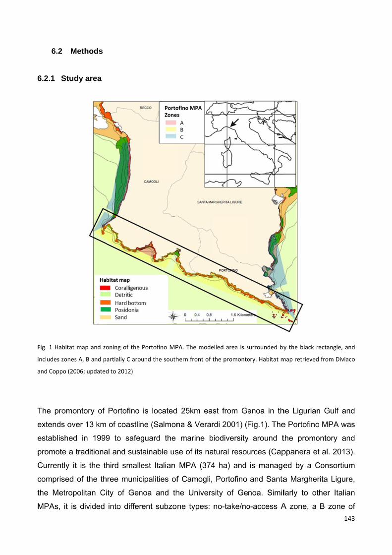
6.2  

6.2.1 Stu 

Fig. 1 Habita

includes zon

and Coppo (2

The prom

extends o

establishe

promote a

Currently

comprised

the Metro

MPAs, it

Methods

udy area

at map and zo

es A, B and p

2006; updated

montory of

over 13 km

ed in 1999

a traditiona

it is the th

d of the th

opolitan Ci

is divided

oning of  the 

artially C arou

d to 2012) 

Portofino

of coastlin

9 to safeg

al and sust

hird smalle

hree munic

ity of Gen

into differ

Portofino MP

und the south

is located

ne (Salmon

guard the

tainable us

est Italian

cipalities of

noa and th

ent subzo

PA. The mode

hern front of 

25km ea

na & Verar

marine b

se of its na

MPA (374

f Camogli,

he Univers

ne types:

elled area  is s

the promonto

st from Ge

rdi 2001) (F

biodiversity

atural resou

4 ha) and

Portofino

sity of Ge

no-take/no

surrounded by

ory. Habitat m

enoa in th

Fig.1). The

y around t

urces (Cap

is manage

and Santa

noa. Simil

o-access A

 

y  the black  re

map retrieved

he Ligurian

e Portofino

the promo

ppanera et

ed by a C

a Margher

larly to ot

A zone, a

143

ectangle, and

 from Diviaco

n Gulf and

o MPA was

ontory and

t al. 2013).

Consortium

rita Ligure,

her Italian

B zone of

3 

d 

o 

d

s

d

.

m

,

n

f

144  

general reserve and a C zone of partial protection, where different restrictions regulate

human uses. Artisanal fishing involves 35 operating vessels <10 meters in length (MARTE

+ project, 2011) and is allowed in zones B and C only for the residents of the three

municipalities. This fishery is multi-métier and multi-specific, and fixed nets including gill

nets, trammel nets and combined nets are the mostly used gears (70% of total used

gears), followed by longlines and surrounding net, locally named “lampara” and hereafter

referred to as “small purse seine” (both around 20% of total used gears). Other traditional

fishing gears (e.g. tonnarella targeting small pelagic, and mugginara, specifically targeting

mugilids) are allowed during specific periods and are restricted to a single site within zone

C of the MPA (Cattaneo-Vietti et al., 2014). Recreational fishing is permitted for residents

of the three municipalities under authorization in Zones B and C and for non-residents only

in Zone C. For both recreational and artisanal fishing other restrictions such as the fishing

of some species, spatial closures, prohibitions or modifications of fishing techniques,

regulations in fishing effort and minimum landing sizes are also implemented in the MPA in

order to control the activities, according to the MPA Regulation (2008), (Markantonatou et

al. 2014). The modeled surface (57 ha) thus includes the southern front of the MPA,

encompassing zones A and B and two sectors of zone C (Fig.1) and is characterized

mainly by hard bottoms (51% rocky habitat, 31% coralligenous habitat ), with some

Posidonia oceanica meadows and shallow sands (overall 18% of the area). This area

supports most of the artisanal and recreational fishing pressure in the MPA, with highest

overlap between coralligenous habitat and fishing footprint around 30-40 meters depth

(Markantonatou et al. 2014). The southern submerged steep cliffs of the promontory and

the particular hydrodynamic conditions of the area (Doglioli et al. 2004) create in fact a

unique system where rocky reefs, caves, and massive blocks support a very diversified

benthic community, including extended coralligenous habitat cover (Cattaneo-Vietti et al.

2010). This in turn, provides food and shelter for a rich coastal fish community. The

hydrodynamic conditions also attract large pelagic fish that are frequently fished in this

small area (Cattaneo-Vietti et al. 2014). In the model area main fishing activities are fixed

nets and surrounding net fishing (“Lampara”), in addition to recreational fishing.

6.2.2 Ecopath model structure

The species-based Ecopath model and the trophic levels (TLs)-based EcoTroph model

were used in this study. The Data-rely toolbox developed by (Lassalle et al. 2014) was

applied to evaluate data reliability and robustness of the Ecopath model predictions.

145  

Ecopath is a mass-balanced model based on the assumption that the production of one

functional group is equal to the sum of all predation, non-predatory losses, exports,

biomass accumulations and catches, as expressed by the following equation:

P/Bi × Bi = P/Bi × Bi × (1 − EEi) + Σj (Q/B)ji × Bi × DCji + Yi + NMi + Bai (1)

B is the biomass, P/Bi is the production rate, Q/B is the consumption rate, DCji is the

fraction of prey i included in the diet of predator j, NMi is the net migration of prey i, BAi is

the biomass accumulation of prey i, Yi is the catch of prey i and EEi is the ecotrophic

efficiency of prey i, that is the proportion of production used in the system. The model

represents an average situation of the southern front of the Portofino MPA for the period

2007-2014, to ensure that protection effects were already in place. A simplified model

structure developed by (Prato et al. 2014) for the Port Cros MPA with the intent of

standardizing Ecopath modelling for Mediterranean MPAs was used in our study. Three

new functional groups specific of the Portofino area were added to the standard model

structure: small tuna-like fishes (hereafter small tunas), dolphins and horse mackerels.

Small tuna-like fishes include species such as Sarda sarda, Auxis rochei and Euthynnus

alletteratus, which, although pelagic, are often caught within the MPA boundaries and are

thus important fishery resources. A group of dolphins of the species Tursiops truncatus

permanently lives in the waters just in front of the MPA (Alessi et al. 2011), and are very

likely interacting with the modeled food-web. The “horse mackerels and sand smelts+”

group (the notation “+” following the name of each functional group signifies that several

species are included in the group) (Valls et al. 2012, Prato et al. 2014) was split in two to

account for some additional pelagic species frequently reported in the catches within the

MPA (Scomber spp., Sardinella aurita), that have different diets from the “sand smelts +”

group. An import component was added to the diet of migratory and pelagic species that

are not present during the whole year in the study area. Similarly, due to the small size of

the study area and the mixing of currents characteristic of this zone, we had to integrate

zooplankton and phytoplankton advection in the model, which are likely continually

imported and exported from the zone (Pinnegar et al. 2000). We thus added a component

of import both in the diet of zooplankton and of benthic invertebrates which feed on

zooplankton and phytoplankton. Finally, due to the absence of biomass data, together with

their likely weak interaction with the shallow food web, some fish caught in the modelled

area but known to live at depths >50 m were excluded from the model (Lophius

piscatorius, Scyliorhinus canicula and Merluccius merluccius).

146  

Details on the origins of all input parameters are given in Annex 1.

Catches estimates

The MPA partially monitors artisanal fishing effort and catches. Only available fishing

catches within the model area were thus considered, including catches from fixed nets

(trammel nets, gill nets and combined nets), small purse seine and recreational fishing.

In order to obtain an annual picture of catches in the model area we had to attain from two

main sources of data:

‐ A dataset of fishermen interviews (MARTE+ project, 2011) from which effort in the

model area in one year was estimated, computed as total number of boats and

days of fishing for fishing metier.

‐ The available logbooks from three boats (two boats monitored in 2012, one in 2013-

2014), from which catches in kg/day for each fishing métier were estimated.

Thus, data from the logbooks (kg/day of fishing for each species and fishing métier) were

multiplied for the total number of fishing days/year for the same métier.

Recreational fishermen must fill logbooks concerning catches within the MPA boundaries.

From the logbooks we computed average catches expressed as kg /hour within our model

area and multiplied for the total number of hours of recreational fishing in the MPA in one

year (Cappanera et al. 2013).

From these estimates, we derived alternative data sets, using 2 multiplier coefficients for

professional fishing (0.5 and 2) and 7 coefficients (0.5 and from 2 to 7) for recreational

fishing, in order to account for larger uncertainty. Resulting values were then proposed to

the evaluation of the MPA staff fishing experts, responsible for the monitoring of

professional and recreational fishing. For each species, the most realistic estimate

according to the expert’s knowledge was retained. These expert-modified values were

used to build our reference model. Two other models were then built with expert’s

estimates both multiplied and divided by the coefficient 1.5 to account for uncertainty in the

data, and a fourth model was also built with the original logbook’s estimates, to identify

differences and data gaps. Accounting for uncertainty, we aimed at highlighting the

potential of Ecopath and Ecotroph as a tool for advising MPAs management, and thus

147  

stress on the urgent need to improve monitoring strategies and increase ecological and

fisheries data quality and availability.

6.2.3 Species interactions, keystonness scores and fisheries impact The mixed trophic impact routine (MTI) of Ecopath assesses the relative impact of a slight

increase in abundance of any group on the biomass of other groups on the food-web

(Christensen & Pauly 1992).

Keystone species are defined as the species having the highest and widest impact on the

food web despite a low biomass. They were identified by applying the new keystonness

index developed by (Valls et al. 2015). The index is characterized by an impact component

(IC, defining the trophic impact of a group on the other groups) and a biomass component

(BC), according to the following equation:

KS= Ln (IC x BC) (2)

Where IC is defined from (Libralato et al. 2006) as:

ICi =√ Σ j≠i mij2 (3)

Parameter ICi represents the overall effect of group i on all the other groups in the food

web (and is expressed as the sum of the squared values of mij (the MTI score) of group i,

paired with each of the other living group j in the food web. The mixed-trophic impact of

group i on itself (mii) is excluded, as well as the mixed-trophic impact on non-living groups

such as detritus (Libralato et al. 2006).

The biomass component is defined as the rank of the group’s biomass in descending

order:

BC = drank(Bi) (4)

Fishing loss (Floss) is an indicator of fishing impact given by the ratio between catches

and the production of each functional group (Y/P). After obtaining production (P) from P/B

x B we computed Floss for each functional group, in order to analyze the impact of fishing

on keystone groups. Fishing fleets are treated as predators in the MTI routine, thus we

148  

analysed direct and indirect fisheries impacts within the ecosystem by computing and

cumulatively plotting the MTI index of each fleet.

6.2.4 Data quality and MTI sensitivity analysis

Since data availability and quality is the main limitation to EwE, like for any ecosystem

model (Prato et al. 2014, Lassalle et al. 2014), data quality was assessed applying the

food web diagnostics proposed by Link 2010 and the Data-Reli toolbox developed by

Lassalle et al 2014. The Pedigree index (Morissette 2007) of the model was computed to

summarise the uncertainty related to each input value and was used to assess if model

quality was sufficient (Pedigree >0.4) to pursue with the analysis (Lassalle et al. 2014).

Respiration / consumption ratio was not ecologically correct for sea urchins and

cephalopods, thus their Q/B ratio was slightly increased.

Robustness of MTI results was tested through a sensitivity analysis (Lassalle et al 2014).  

We rebuilt the original net impact matrix where qij is the net impact of i on j and is given by

the difference between positive effects (quantified by the fraction of prey i in the diet of

predator j j), and negative effects fij (evaluated as the fraction of total consumption of j

used by predator i). Then, in the analysis routine, 5000 Q matrices are created by drawing

qij values from independent uniform distributions defined by original qij ± 20% (Richardson

et al. 2006). The mij values for each pairwise intersection of the Q matrices are then

calculated, their signs recorded and the percentage of mij values with the same sign as in

the original MTI matrix (SMTI) is estimated. Results were summarized into one matrix

recording the sign of the original mij values and the SMTI percentages that are categorized

into four classes:[0; 50], ]50; 75], ]75; 95] and ]95; 100].

6.2.5 Ecotroph model

The EcoTroph model summarizes the ecosystem functioning as a flow of biomass surging

up the food web from lower to higher Trophic Levels (TL), through predation and ontogenic

processes. The biomass enters the system at TL = 1, generated by primary producers or

recycled from the detritus. For TLs > 2, the biomass is distributed along a continuum of TL

due to the diet variability of the various consumers. The resulting biomass distribution is

called trophic spectrum (Gascuel et al. 2005). EcoTroph thus allows to simulate various

fishing scenarios and their impact on the biomass trophic spectrum.

149  

On the basis of usual equations of fluid dynamics, the flow of the biomass present in the

ecosystem at TL under steady-state conditions is expressed as:

                                             φ() = D() x K() (5) 

Where φ() refers to the amount of biomass that moves up the food-web through TL

(expressed in tons per year), D( is the density of biomass at trophic level (expressed in

tons per trophic level) and K() is the speed of flow, which quantifies the velocity of

biomass transfers in the food-web (expressed as the numbers of TLs crossed per year).

The continuous distribution of the biomass across a trophic level is calculated using a

discrete approximation based on small trophic classes. EcoTroph conventionally considers

trophic classes of width ∆ equal to 0.1 TL, from Trophic Level 2 (corresponding to first-

order consumers) to Trophic Level 5 (value considered sufficient to cover all top predators

likely to occur in marine ecosystems). Thus, the mean biomass B (in t), which is present

in the [∆] trophic class under steady-state conditions, can be estimated as ∫D () × d

or D() × ∆ for a small interval ∆ Therefore:

B = φ × ∆ / K (5) 

where φ and K are the mean biomass flow and mean speed of flow within the [∆]

trophic class, respectively.

The flow of biomass from one trophic class to the next is non conservative and is thus

expressed as:

φ = φ × exp[-(+) ×] (7) 

where is the natural loss rate (related to excretion and respiration) and is the fishing

loss rate (with = F / K, where F is the fishing mortality). We refer to the Appendix in

Gascuel et al. 2011 for further explanation of EcoTroph dynamics.

6.2.6 Scenarios of fisheries closures and analysis of interacting impacts

For each functional group, accessibility to fishing was defined according to the number of

targeted species within the functional group (if none of the species within the group is

fished, then the accessibility value is zero). Afterwards, we used the ET-transpose routine

described in Gascuel et al. (2009) to translate the outputs of the original Ecopath model

150  

into an ET model and to build the trophic spectra of the cumulated catches and the trophic

spectra of the fishing loss for each fishing fleet.

We simulated the unexploited state of the ecosystem by setting fishing loss () to 0 for all

fleets in the ET-diagnosis routine. The current condition and two alternative fishing

scenarios were compared to the unexploited state: no recreational fishing (=Ycom/P,

where Ycom is the catch of commercial fisheries only, at trophic level ) to test the effect of

an interdiction of this activity, and double artisanal and recreational fishing (=2·Y/P,

where Y is the total catch at trophic level ) to assess the impact that an increase in the

fishing effort could have in the ecosystem.

Finally, we plotted artisanal and recreational fisheries’ mixed impact on accessible

biomass, TL of the accessible biomass, catches of the artisanal fishery and mean TL of

the artisanal fishery’s catch.

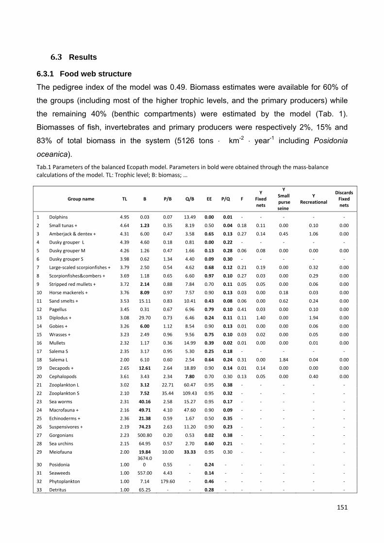
151  

6.3 Results

6.3.1 Food web structure

The pedigree index of the model was 0.49. Biomass estimates were available for 60% of

the groups (including most of the higher trophic levels, and the primary producers) while

the remaining 40% (benthic compartments) were estimated by the model (Tab. 1).

Biomasses of fish, invertebrates and primary producers were respectively 2%, 15% and

83% of total biomass in the system (5126 tons ∙  km-2 ∙ year-1 including Posidonia

oceanica).

Tab.1 Parameters of the balanced Ecopath model. Parameters in bold were obtained through the mass‐balance calculations of the model. TL: Trophic level; B: biomass; … 

 Group name  TL  B  P/B  Q/B  EE  P/Q  F 

Y Fixed  nets 

Y Small  purse seine 

Y Recreational 

Discards Fixed  nets 

1  Dolphins  4.95  0.03  0.07  13.49  0.00  0.01 ‐  ‐  ‐  ‐  ‐ 

2  Small tunas +  4.64  1.23  0.35  8.19  0.50  0.04 0.18  0.11  0.00  0.10  0.00 

3  Amberjack & dentex +  4.31  6.00  0.47  3.58  0.65  0.13 0.27  0.14  0.45  1.06  0.00 

4  Dusky grouper  L  4.39  4.60  0.18  0.81  0.00  0.22 ‐  ‐  ‐  ‐  ‐ 

5  Dusky grouper M  4.26  1.26  0.47  1.66  0.13  0.28 0.06  0.08  0.00  0.00  0.00 

6  Dusky grouper S  3.98  0.62  1.34  4.40  0.09  0.30 ‐  ‐  ‐  ‐  ‐ 

7  Large‐scaled scorpionfishes +  3.79  2.50  0.54  4.62  0.68  0.12 0.21  0.19  0.00  0.32  0.00 

8  Scorpionfishes&combers +  3.69  1.18  0.65  6.60  0.97  0.10 0.27  0.03  0.00  0.29  0.00 

9  Stripped red mullets +  3.72  2.14  0.88  7.84  0.70  0.11 0.05  0.05  0.00  0.06  0.00 

10  Horse mackerels +  3.76  8.09  0.97  7.57  0.90  0.13 0.03  0.00  0.18  0.03  0.00 

11  Sand smelts +  3.53  15.11  0.83  10.41  0.43  0.08 0.06  0.00  0.62  0.24  0.00 

12  Pagellus  3.45  0.31  0.67  6.96  0.79  0.10 0.41  0.03  0.00  0.10  0.00 

13  Diplodus +  3.08  29.70  0.73  6.46  0.24  0.11 0.11  1.40  0.00  1.94  0.00 

14  Gobies +  3.26  6.00  1.12  8.54  0.90  0.13 0.01  0.00  0.00  0.06  0.00 

15  Wrasses +  3.23  2.49  0.96  9.56  0.75  0.10 0.03  0.02  0.00  0.05  0.00 

16  Mullets  2.32  1.17  0.36  14.99  0.39  0.02 0.01  0.00  0.00  0.01  0.00 

17  Salema S  2.35  3.17  0.95  5.30  0.25  0.18 ‐  ‐  ‐  ‐  ‐ 

18  Salema L  2.00  6.10  0.60  2.54  0.64  0.24 0.31  0.00  1.84  0.04  0.00 

19  Decapods +  2.65  12.61  2.64  18.89  0.90  0.14 0.01  0.14  0.00  0.00  0.00 

20  Cephalopods  3.61  3.43  2.34  7.80  0.70  0.30 0.13  0.05  0.00  0.40  0.00 

21  Zooplankton L  3.02  3.12  22.71  60.47  0.95  0.38 ‐  ‐  ‐  ‐  ‐ 

22  Zooplankton S  2.10  7.52  35.44  109.43  0.95  0.32 ‐  ‐  ‐  ‐  ‐ 

23  Sea worms  2.31  40.16  2.58  15.27  0.95  0.17 ‐  ‐  ‐  ‐  ‐ 

24  Macrofauna +  2.16  49.71  4.10  47.60  0.90  0.09 ‐  ‐  ‐  ‐  ‐ 

25  Echinoderms +  2.36  21.38  0.59  1.67  0.50  0.35 ‐  ‐  ‐  ‐  ‐ 

26  Suspensivores +  2.19  74.23  2.63  11.20  0.90  0.23 ‐  ‐  ‐  ‐  ‐ 

27  Gorgonians  2.23  500.80  0.20  0.53  0.02  0.38 ‐  ‐  ‐  ‐  ‐ 

28  Sea urchins  2.15  64.95  0.57  2.70  0.60  0.21 ‐  ‐  ‐  ‐  ‐ 

29  Meiofauna  2.00  19.84  10.00  33.33  0.95  0.30 ‐  ‐  ‐  ‐  ‐ 

30  Posidonia  1.00 3674.0

0  0.55  ‐  0.24  ‐  ‐  ‐  ‐  ‐  ‐ 

31  Seaweeds  1.00  557.00  4.43  ‐  0.14  ‐  ‐  ‐  ‐  ‐  ‐ 

32  Phytoplankton  1.00  7.14  179.60  ‐  0.46  ‐  ‐  ‐  ‐  ‐  ‐ 

33  Detritus  1.00  65.25  ‐  ‐  0.28  ‐  ‐  ‐  ‐  ‐  ‐ 

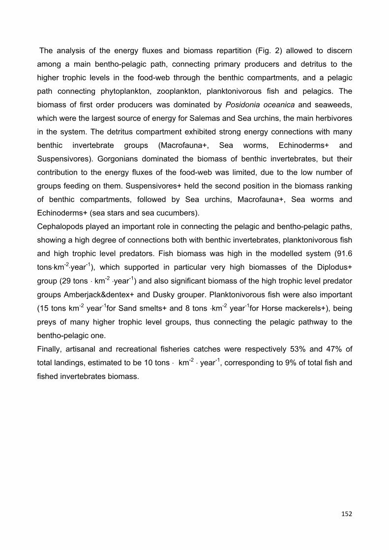
152  

The analysis of the energy fluxes and biomass repartition (Fig. 2) allowed to discern

among a main bentho-pelagic path, connecting primary producers and detritus to the

higher trophic levels in the food-web through the benthic compartments, and a pelagic

path connecting phytoplankton, zooplankton, planktonivorous fish and pelagics. The

biomass of first order producers was dominated by Posidonia oceanica and seaweeds,

which were the largest source of energy for Salemas and Sea urchins, the main herbivores

in the system. The detritus compartment exhibited strong energy connections with many

benthic invertebrate groups (Macrofauna+, Sea worms, Echinoderms+ and

Suspensivores). Gorgonians dominated the biomass of benthic invertebrates, but their

contribution to the energy fluxes of the food-web was limited, due to the low number of

groups feeding on them. Suspensivores+ held the second position in the biomass ranking

of benthic compartments, followed by Sea urchins, Macrofauna+, Sea worms and

Echinoderms+ (sea stars and sea cucumbers).

Cephalopods played an important role in connecting the pelagic and bentho-pelagic paths,

showing a high degree of connections both with benthic invertebrates, planktonivorous fish

and high trophic level predators. Fish biomass was high in the modelled system (91.6

tons∙km-2∙year-1), which supported in particular very high biomasses of the Diplodus+

group (29 tons  ∙ km-2 ∙year-1) and also significant biomass of the high trophic level predator

groups Amberjack&dentex+ and Dusky grouper. Planktonivorous fish were also important

(15 tons km-2 year-1for Sand smelts+ and 8 tons ∙km-2 year-1for Horse mackerels+), being

preys of many higher trophic level groups, thus connecting the pelagic pathway to the

bentho-pelagic one.

Finally, artisanal and recreational fisheries catches were respectively 53% and 47% of

total landings, estimated to be 10 tons ∙  km-2 ∙ year-1, corresponding to 9% of total fish and

fished invertebrates biomass.

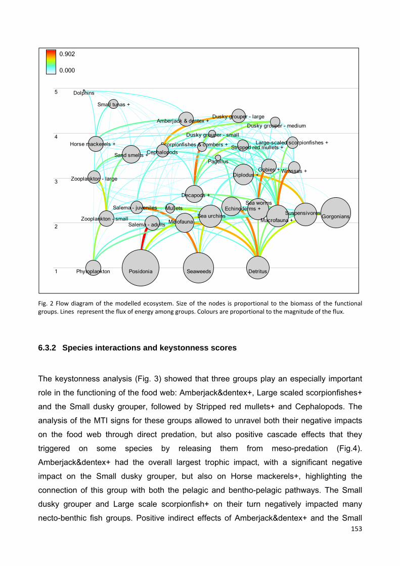
153  

Fig. 2 Flow diagram of  the modelled ecosystem. Size of  the nodes  is proportional  to  the biomass of  the  functional groups. Lines  represent the flux of energy among groups. Colours are proportional to the magnitude of the flux. 

6.3.2 Species interactions and keystonness scores

 

The keystonness analysis (Fig. 3) showed that three groups play an especially important

role in the functioning of the food web: Amberjack&dentex+, Large scaled scorpionfishes+

and the Small dusky grouper, followed by Stripped red mullets+ and Cephalopods. The

analysis of the MTI signs for these groups allowed to unravel both their negative impacts

on the food web through direct predation, but also positive cascade effects that they

triggered on some species by releasing them from meso-predation (Fig.4).

Amberjack&dentex+ had the overall largest trophic impact, with a significant negative

impact on the Small dusky grouper, but also on Horse mackerels+, highlighting the

connection of this group with both the pelagic and bentho-pelagic pathways. The Small

dusky grouper and Large scale scorpionfish+ on their turn negatively impacted many

necto-benthic fish groups. Positive indirect effects of Amberjack&dentex+ and the Small

5

4

3

2

1

0.902

0.000

Dolphins

Small tunas +

Amberjack & dentex +Dusky grouper - large

Dusky grouper - medium

Dusky grouper - small

Large-scaled scorpionfishes +Scorpionfishes & combers + Stripped red mullets +Horse mackerels +

Sand smelts +Pagellus

Diplodus +Gobies + Wrasses +

MulletsSalema - juveniles

Salema - adults

Decapods +

Cephalopods

Zooplankton - large

Zooplankton - small

Sea worms

Macrofauna +

Echinoderms +Suspensivores +

GorgoniansSea urchins Meiofauna

Posidonia SeaweedsPhytoplankton Detritus

 

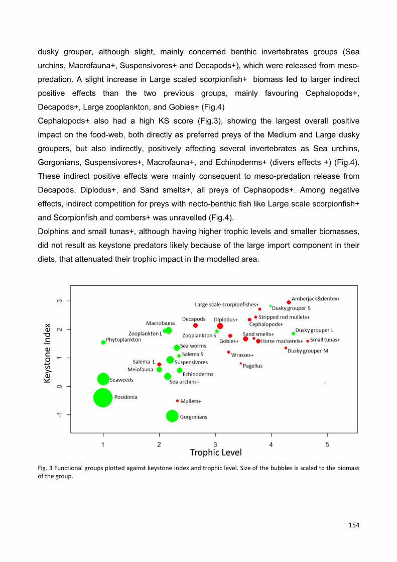
dusky gro

urchins, M

predation

positive

Decapods

Cephalop

impact on

groupers,

Gorgonian

These ind

Decapods

effects, in

and Scorp

Dolphins

did not re

diets, that

Fig. 3 Functioof the group  

ouper, alt

Macrofauna

. A slight i

effects th

s+, Large z

pods+ also

n the food-

but also

ns, Suspe

direct posi

s, Diplodus

ndirect com

pionfish an

and small

esult as key

t attenuate

onal groups p.  

hough slig

a+, Suspen

increase in

han the

zooplankto

o had a h

-web, both

indirectly,

nsivores+,

tive effect

s+, and S

mpetition fo

nd combers

tunas+, a

ystone pre

ed their trop

plotted agains

ght, mainl

nsivores+

n Large sc

two prev

on, and Go

igh KS sc

directly a

positively

Macrofau

s were ma

Sand smel

or preys wit

s+ was unr

lthough ha

edators like

phic impac

t keystone ind

y concern

and Decap

caled scor

ious grou

obies+ (Fig

core (Fig.3

s preferred

y affecting

una+, and

ainly cons

ts+, all pr

th necto-b

ravelled (F

aving highe

ely becaus

ct in the mo

dex and troph

ned benth

pods+), wh

pionfish+

ups, main

.4)

3), showin

d preys of

several i

Echinoder

sequent to

reys of Ce

enthic fish

Fig.4).

er trophic

se of the la

odelled are

hic level. Size 

ic inverteb

hich were r

biomass l

nly favour

ng the larg

the Mediu

nvertebrat

rms+ (dive

meso-pre

ephaopods

like Large

levels and

arge impor

ea.

of the bubble

brates gro

released fr

led to larg

ring Ceph

gest overa

um and La

tes as Se

ers effects

edation rel

s+. Among

e scale sco

d smaller b

rt compone

es is scaled to

154

oups (Sea

rom meso-

er indirect

halopods+,

all positive

arge dusky

a urchins,

+) (Fig.4).

ease from

g negative

orpionfish+

biomasses,

ent in their

o the biomass

4 

a

-

t

e

y

,

.

m

e

+

,

r

s 

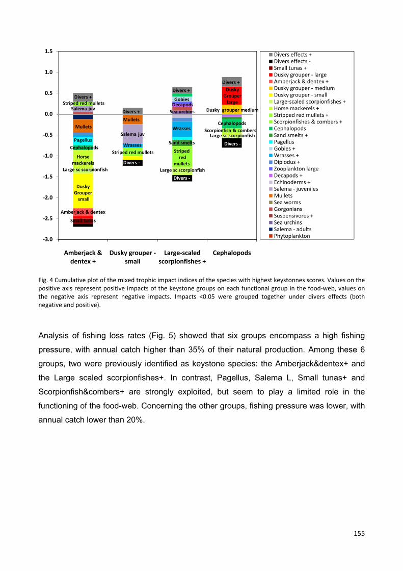
155  

 

Fig. 4 Cumulative plot of the mixed trophic impact indices of the species with highest keystonnes scores. Values on the positive axis represent positive  impacts of the keystone groups on each functional group  in the food‐web, values on the  negative  axis  represent  negative  impacts.  Impacts  <0.05  were  grouped  together  under  divers  effects  (both negative and positive). 

 

Analysis of fishing loss rates (Fig. 5) showed that six groups encompass a high fishing

pressure, with annual catch higher than 35% of their natural production. Among these 6

groups, two were previously identified as keystone species: the Amberjack&dentex+ and

the Large scaled scorpionfishes+. In contrast, Pagellus, Salema L, Small tunas+ and

Scorpionfish&combers+ are strongly exploited, but seem to play a limited role in the

functioning of the food-web. Concerning the other groups, fishing pressure was lower, with

annual catch lower than 20%.

‐3.0

‐2.5

‐2.0

‐1.5

‐1.0

‐0.5

0.0

0.5

1.0

1.5

Amberjack &dentex +

Dusky grouper ‐small

Large‐scaledscorpionfishes +

Cephalopods

Divers effects +Divers effects ‐Small tunas +Dusky grouper ‐ largeAmberjack & dentex +Dusky grouper ‐ mediumDusky grouper ‐ smallLarge‐scaled scorpionfishes +Horse mackerels +Stripped red mullets +Scorpionfishes & combers +CephalopodsSand smelts +PagellusGobies +Wrasses +Diplodus +Zooplankton largeDecapods +Echinoderms +Salema ‐ juvenilesMulletsSea wormsGorgoniansSuspensivores +Sea urchinsSalema ‐ adultsPhytoplankton

Divers +

Salema juv

Mullets

Pagellus

Cephalopods

Horse mackerels

Large sc scorpionfish

Dusky Groupersmall

Amberjack & dentex

Small tunas

Mullets

Salema juv

Wrasses

Striped red mullets

Divers +

Divers ‐

Gobies

Divers +

Wrasses

Sand smelts

Stripedred 

mullets

Divers ‐

Dusky Grouperlarge

Dusky  grouper medium

Divers +

Cephalopods

Divers ‐

Large sc scorpionfish

Decapods

Sea urchins

Scorpionfish & combersLarge sc scorpionfish

Striped red mullets

156  

Fig. 5 Fishing loss rate for each functional group. Fishing loss= Y/P 

The sensitivity analysis performed on the MTI matrix revealed that MTI signs were robust

to a variation of +/-20% in the original net impact value: 85 % of the pairwise intersections

in the original MTI matrix had a sign equal to that of the original matrix with a confidence

percentage > 95% (70% of the pairwise intersections reached 100% confidence) (Tab. 1,

Annex).

6.3.3 Current catch and fishing loss rates by fishery

Trophic spectra of the cumulated fisheries catches showed overlap among the three

fisheries, in particular for trophic levels > 3.5 (Fig.6a). Recreational fishing catches

targeted trophic levels > 3 (mean TL catch = 3.56), while artisanal fixed nets catches

concentrated mainly around TL 3 (mean TL catch = 3.35). Purse seine fishing caught high

biomasses at TL 2 (Salemas), and also at TL > 3.5 (mean TL catch= 2.75). The overlap of

the three fisheries on high trophic levels resulted in the strongest fishing losses for trophic

levels higher than 4, due to the lower turnover rates of these predators (Fig. 6b). On the

contrary, high catches at TL 2 and 3 did not translate into strong fishing impact. When

confidence intervals were added according to the two alternative estimates provided by the

0

0.1

0.2

0.3

0.4

0.5

0.6

0.7

Fishihng loss

 

MPA fishe

based on

consistent

However,

levels was

Fig. 6

When fish

direct neg

reducing t

due to rel

total impa

level grou

ery expert

n non-corre

tly lower,

the gener

s maintaine

6 Trophic spe

heries wer

gative impa

the prey a

ease from

act on the f

ups Small

ts, results

ected logb

due to an

ral trend of

ed.

ctra of the cu

re conside

acts on the

availability

predation

food web. S

tunas+, Am

kept cons

book fishin

n underest

f major imp

mulated fishe

red as pre

e species t

for some s

. In particu

Species di

mberjack&

sistent. Wh

ng data, f

timation of

pact from th

ery’s catches (

edators in

they target

species (co

ular, the re

irectly targ

&dentex+ a

hen the an

fishing loss

f total fish

he three fis

(a) and trophi

the MTI a

ted, but als

ompetition

ecreational

eted by th

and Large

nalysis wa

s by recre

ing catche

sheries ove

c spectra of fi

analysis (F

so indirect

) and indir

fishing fle

is fishery w

scaled sco

as run on

eational fis

es (Fig. A1

erlap on h

ishing loss (Y/

Fig.7), they

negative i

rect positiv

eet had the

were the h

orpionfish+

157

the model

shing was

1 Annex.).

igh trophic

P) (b)

y had both

mpacts by

ve impacts

e strongest

igh trophic

+. Release

7 

l

s

.

c

h

y

s

t

c

e

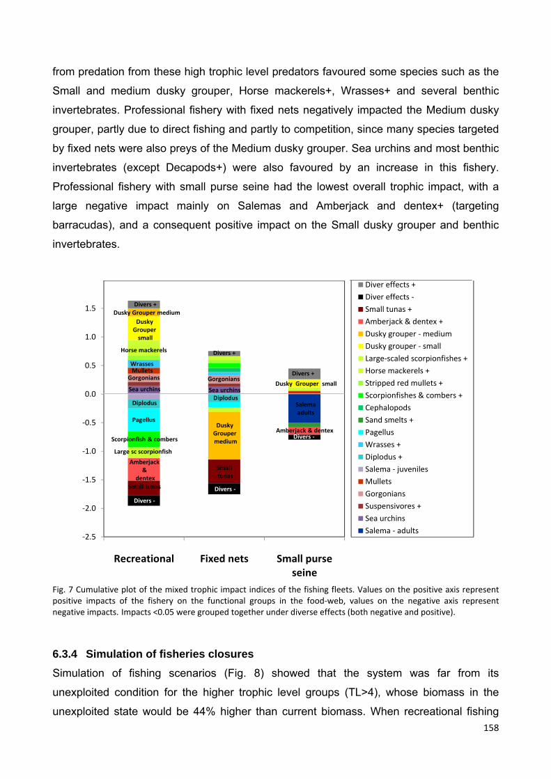
158  

from predation from these high trophic level predators favoured some species such as the

Small and medium dusky grouper, Horse mackerels+, Wrasses+ and several benthic

invertebrates. Professional fishery with fixed nets negatively impacted the Medium dusky

grouper, partly due to direct fishing and partly to competition, since many species targeted

by fixed nets were also preys of the Medium dusky grouper. Sea urchins and most benthic

invertebrates (except Decapods+) were also favoured by an increase in this fishery.

Professional fishery with small purse seine had the lowest overall trophic impact, with a

large negative impact mainly on Salemas and Amberjack and dentex+ (targeting

barracudas), and a consequent positive impact on the Small dusky grouper and benthic

invertebrates.

Fig. 7 Cumulative plot of the mixed trophic  impact  indices of the fishing fleets. Values on the positive axis represent positive  impacts  of  the  fishery  on  the  functional  groups  in  the  food‐web,  values  on  the  negative  axis  represent negative impacts. Impacts <0.05 were grouped together under diverse effects (both negative and positive). 

 

6.3.4 Simulation of fisheries closures

Simulation of fishing scenarios (Fig. 8) showed that the system was far from its

unexploited condition for the higher trophic level groups (TL>4), whose biomass in the

unexploited state would be 44% higher than current biomass. When recreational fishing

‐2.5

‐2.0

‐1.5

‐1.0

‐0.5

0.0

0.5

1.0

1.5

2.0

Recreational Fixed nets Small purseseine

Diver effects +

Diver effects ‐

Small tunas +

Amberjack & dentex +

Dusky grouper ‐ medium

Dusky grouper ‐ small

Large‐scaled scorpionfishes +

Horse mackerels +

Stripped red mullets +

Scorpionfishes & combers +

Cephalopods

Sand smelts +

Pagellus

Wrasses +

Diplodus +

Salema ‐ juveniles

Mullets

Gorgonians

Suspensivores +

Sea urchins

Salema ‐ adults

Dusky Groupersmall

Pagellus

Scorpionfish & combers

Large sc scorpionfish

Amberjack & 

dentex

Small tunas

Divers ‐

Horse mackerels

Dusky Grouper medium

MulletsGorgonians

Sea urchins

Diplodus

Wrasses

Dusky Groupermedium

Smalltunas

Divers ‐

Diplodus

Divers +

Divers +

Divers +

Dusky  Grouper  small

Salemaadults

Amberjack & dentex

Gorgonians

Sea urchins

Divers ‐

 

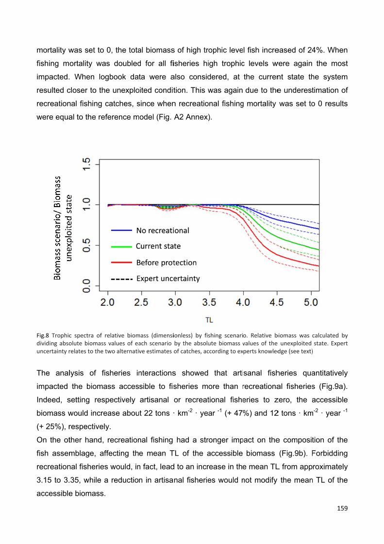
mortality w

fishing m

impacted.

resulted c

recreation

were equa

Fig.8  Trophicdividing absouncertainty r

The anal

impacted

Indeed, s

biomass w

(+ 25%), r

On the ot

fish assem

recreation

3.15 to 3.

accessible

was set to

ortality wa

. When lo

closer to th

nal fishing

al to the re

c  spectra  of olute biomassrelates to the 

lysis of f

the bioma

setting res

would incre

respectivel

ther hand,

mblage, af

nal fisherie

.35, while

e biomass

0, the tota

as doubled

ogbook da

he unexplo

catches, s

eference m

relative  bioms values of eatwo alternati

fisheries in

ass acces

spectively

ease abou

ly.

recreation

ffecting th

s would, in

a reductio

.

al biomass

d for all fi

ta were a

oited condit

since when

model (Fig.

mass  (dimensiach  scenario ve estimates 

nteractions

sible to fis

artisanal

ut 22 tons ·

nal fishing

e mean T

n fact, lead

n in artisa

s of high tr

isheries hi

also consid

tion. This w

n recreatio

A2 Annex)

ionless)  by  fisby  the absoluof catches, ac

s showed

sheries m

or recreat

· km-2 · ye

had a str

TL of the a

d to an incr

nal fisherie

rophic leve

igh trophic

dered, at

was again

onal fishing

).

shing  scenariute biomass vccording to ex

that arti

ore than r

tional fishe

ar -1 (+ 47

ronger imp

accessible

rease in the

es would n

l fish incre

c levels w

the curren

due to the

g mortality

o.  Relative  bvalues of  the perts knowled

sanal fish

recreationa

eries to z

%) and 12

pact on the

biomass

e mean TL

not modify

eased of 24

were again

nt state th

e underest

was set to

biomass was e unexploited dge (see text)

heries qua

al fisheries

zero, the a

2 tons · km

e composit

(Fig.9b). F

L from app

y the mean

159

4%. When

the most

he system

timation of

o 0 results

calculated  bystate. Expert) 

antitatively

s (Fig.9a).

accessible

m-2 · year -1

tion of the

Forbidding

roximately

n TL of the

9 

n

t

m

f

s

y t 

y

.

e

e

g

y

e

 

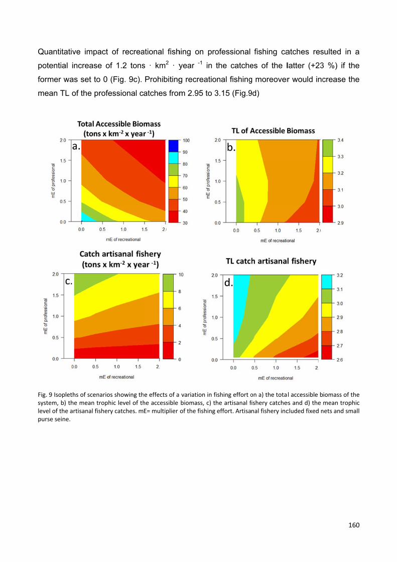
Quantitati

potential

former wa

mean TL

Fig. 9 Isopletsystem, b) thlevel of the apurse seine. 

ve impact

increase o

as set to 0

of the prof

ths of scenariohe mean tropartisanal fishe

t of recrea

of 1.2 tons

(Fig. 9c).

fessional c

os showing thphic level of thry catches. m

ational fish

s · km2 · y

Prohibiting

atches from

he effects of a he accessible E= multiplier 

hing on pro

year -1 in

g recreatio

m 2.95 to 3

 variation in fbiomass, c) tof the fishing

ofessional

the catche

onal fishing

3.15 (Fig.9

fishing effort ohe artisanal feffort. Artisa

fishing ca

es of the l

g moreover

9d)

on a) the totaishery catchenal fishery inc

atches res

latter (+23

r would inc

al accessible bes and d) the cluded fixed n

160

sulted in a

3 %) if the

crease the

iomass of themean trophicnets and small

0 

a

e

e

e c l 

161  

6.4 Discussion

6.4.1 Building a trophic model in the context of Mediterranean MPAs

Scientific ecological knowledge on Mediterranean MPAs, when available, is often

dispersed among several sources of information, ranging from local or foreign universities

or environmental agencies, to local/traditional ecological knowledge, historical archives,

and expert opinions. Integration of this wealth of information is essential for a holistic

understanding of protection effects on ecosystem functioning and thus a fully informed

management of MPAs. The trophic modelling approach adopted here is a useful tool to

accomplish such integration, allowing us to fit largely scattered data into a coherent picture

of ecosystem functioning for the Portofino MPA. In particular, a snapshot of the highly

productive area surrounding the southern promontory of the MPA was provided,

representing an average year between 2007 and 2014. This model provides a baseline

that can be easily updated in the years to come, when more geo-referenced data

regarding fishing effort and catch become available, together with updated monitoring data

on key species biomass.

Similarly to most ecosystem models, it was not possible to obtain local data for all

functional groups (Pedigree index = 0.46), but model-derived estimates were in

accordance with ecological knowledge of the area. Biomass ranking of benthic

invertebrates was confirmed by expert opinion (C. Cerrano pers comm.) with highest

biomasses of gorgonians, followed by suspensivores+, macrofauna+, sea worms and

echinoderms+ (sea stars and sea cucumbers). Trophic levels computed by the model fell

also within the range of results for the Mediterranean (Stergiou & Karpouzi 2001).

The analysis of the energy fluxes allowed to unravel a complex food-web despite the

relatively small area, with a main bentho-pelagic energy path exchanging energy with a

more pelagic path through some key groups like cephalopods, planktonivorous fish and

high trophic level predators. Comparison of relative biomass partitioning among primary

producers, benthic invertebrates and fish with another modelled Mediterranean MPA (Port

Cros, Valls et al 2012) allowed highlighting the peculiarities of Portofino. This area

supports high benthic community biomass (15% of total biomass) when compared to the

Port Cros MPA (3.5%), sustaining high biomass of fish at all trophic levels (2% of total

biomass, against 0.65% in Port Cros). The fish biomass observed was particularly high

especially for high trophic level predators (10 tons · km-2 · year-1) and sea breams (29

tons · km-2 · year-1) in comparison to the Port Cros MPA (9 and 3 tons · km-2 · year-1

162  

respectively, Valls et al 2012). Sea breams biomass in the MPA was in fact shown to be

higher than the accepted threshold of 12 individuals per 125 m2 necessary to maintain sea

urchins abundance low and avoid rocky reef ecosystem shifts towards barrens (Guidetti &

Sala 2007, Guidetti et al 2008). Indeed, extended sea-urchin barrens are absent in the

Portofino MPA (Sala et al. 2012). The identification of high trophic level predators

(Amberjack&dentex+ group and Dusky grouper) as keystone groups supports current

conservation strategies aiming at protecting these target fish within Mediterranean MPAs.

It is noteworthy that cephalopods have also shown a high keystonness index in the

Portofino MPA, similarly to the Port Cros model (Valls et al. 2012) and to a subsequent

sensitivity analysis performed on it, which highlighted the impact that uncertain input

biomass data for cephalopods can have on biomass estimates of other groups (Prato et al.

2014). Being both a preferred prey for many high trophic level predators, but also

predators acting on a wide range of trophic levels, cephalopods occupy an important

functional role in both coastal and pelagic ecosystems (Piatkowski et al. 2001, Coll et al.

2013). Large variations in cephalopods biomass can indeed lead to strong effects on the

marine food-webs, both through bottom up and top down impacts. In the Portofino MPA

they are subject to some artisanal and recreational fishing pressure, which is likely

underestimated due to the presence of illegal fishing in the MPA. This is a common issue

in most Mediterranean coastal areas, but is generally difficult to address. If the exploitation

state of cephalopods is not controlled, their biomass could become a limiting food item for

their predators, especially for the protected Dusky grouper. Cephalopods should thus be

regarded as an important monitoring target in the context of Mediterranean MPAs.

6.4.2 Interacting fishing impacts on the food-web

This study was the first attempt to assess the impact of recreational fisheries on a

Mediterranean MPA food-web, and its interaction with the artisanal fishery, starting from

available although limited local logbook data. Estimates of artisanal fishing catches within

the MPA zones surrounding the southern promontory front (3.35 tons · km-2 · year-1) were

much higher than catches in the Port Cros MPA (0.3 tons · km-2 · year-1) and Bonifacio

Straits Natural Reserve (0.09 tons · km-2 · year-1) for which similar Ecopath models had

been built (Valls et al 2012, Albouy et al 2010). Estimates of recreational fishing (3.56 tons

· km-2 · year-1) were also markedly higher when compared to Bonifacio (0.1 tons · km-2 ·

year-1), although in Bonifacio these were indirectly derived by applying a percentage to

professional fishing catches (Albouy et al 2010). Total estimates were instead similar to

163  

those from the Cote Bleu Marine Park (SW France), comparable to Portofino in terms of

number of fishing boats and metiers, with 4.6 tons · km-2 · year-1 landed by coastal

artisanal fisheries operating with fixed nets, and approximately 3.6 tons · km-2 · year-1of

recreational fishing catches (from boat and shore) (Leleu et al. 2014, Cote bleu Scientific

Report 2013-2014). The catches overlap among artisanal and recreational fisheries in the

Portofino MPA led to strong fishing losses on high trophic level predators, due to the lower

turnover rates of these groups. Although the Portofino MPA was demonstrated to be

effective in sustaining a recovery of fish biomass within its borders (Guidetti et al. 2008),

as also shown by the high biomass levels within it, fishing losses on high trophic level

predators are still high within the MPA. Recreational fishing, in particular, contributed for

approximately half of these fishing losses, leading to the largest impact on the whole food

web, as shown by the mixed trophic impact analysis. Fisheries primarily targeting high

trophic level predators often lead to such wide impacts on the ecosystem, as it has been

shown to happen in the whole Ligurian sea (Britten et al. 2014). An analysis of 25 years of

landings (1950-1974) from the tuna trap (“tonnarella”) situated in the zone C of the

Portofino MPA, just outside our modelled area, revealed the occurrence of a strong

depletion of top predators, including sharks, tunas and other large piscivores associated

with this coastal area, which were gradually replaced by lower trophic levels (Britten et al.

2014). Such trophic downgrading was parallel to an intensification of fishing effort and

ultimately led to a decrease in the stability of the fish community due to a release from top-

down control. The community became dominated by intermediate trophic levels with

variable life history (mainly herbivores, cephalopods and planktonivores), subject to wide

oscillations in time (Britten et al. 2014). Here, the analysis of the mixed trophic impact of

the recreational fishery showed that the similar intermediate trophic level groups also

benefited from a slight increase in its effort.

6.4.3 Management applications of trophic modelling

The presented modelling approach can provide some useful outcomes for the

management of MPAs. First, it allows identifying species that play important keystone

roles in the food-web, but are at the same time subject to strong fishing impact. These

species (included in the Amberjack&dentex+ and Large Scaled Scorpionfishes+ groups for

the Portofino case study) can be considered as “sentinels” of the condition of the food-web

and their monitoring should therefore be regarded as a priority within MPAs. Monitoring

should take place both by assessing their biomass state in the ecosystem, but also

164  

evaluating their exploitation status through the survey of artisanal and recreational fishing

catches. These species could also be a reference for the definition of management actions

(for instance, calculating the reduction of fishing mortality needed to attain predefined

conservation objectives) and for the assessment of their efficiency.

The model also revealed that regarding high trophic level predators, the ecosystem is

likely far away from its carrying capacity, assumed to be equal to our simulated condition

of no fishing. An eventual interdiction of recreational fishing would lead to a significant

increase in the biomass of this group (TL>4), up to 24%. A similar analysis performed on

the Port Cros MPA showed that the ecosystem was very near to its simulated unexploited

state (Valls et al. 2012). The habitat and ecological differences among the two areas, but

also the older age of the Port Cros MPA (more than 50 years), and the lower fishing

pressure within this area are probably influencing this difference. MPA carrying capacity

for high trophic level predators for instance generally needs between 13 and 30 years

depending on the species (Garcia-Rubies et al. 2013). According to our results, the

potential carrying capacity for high trophic level predators in the Portofino MPA is likely to

be high, but the current level of fishing within the MPA borders should be reduced in order

to pursue the MPAs conservation objectives.

Finally, the model allowed to inform about the impact of recreational fishing on artisanal

fisheries catches. The competition for target fish among recreational and artisanal fishing

is a growing issue in many Mediterranean coastal areas, but few MPAs assess such

impact. In the Cote Bleu Marine Park for example the long term assessment of both

fisheries highlighted a strong competition of resources, where over 36 species highly

targeted by artisanal fishermen, 25 were also a spearfishing target and 17 were targeted

by recreational fishing from boat. Moreover, recreational fishing was less selective,

targeting both the prey of species normally targeted by artisanal fishermen and also the

large carnivores (Leleu et al 2014, Charbonnel et al. 2014). Such trend was also

highlighted in our study, and is likely to be more intense given the probable

underestimation of recreational fishing catches. Illegal spearfishing is in fact likely

occurring in the MPA, and monitoring recreational fishermen is further complicated by the

common custom of providing lower catches estimates to the MPA board, as revealed by

the mismatch among logbooks and local expert’s estimates in our study.

Artisanal fishery is a conservation target for many Mediterranean MPAs, which often

promote a sustainable socio-economic development and the conservation of traditional

activities, when carried on in a sustainable way, and of local identities/cultures (Di Franco

165  

et al. 2014). Our results suggested that the artisanal fishery alone would have moderate

impact on the food web, reducing by less than 15% the biomass of top predators (TL>4.0),

with almost no effect on the total biomass of lower trophic levels. Limiting recreational

fishing effort could therefore allow the MPA to pursue both its conservation and socio-

economic development targets, by i) reducing the impact on high trophic level predators

and thus benefiting the whole ecosystem and ii) increasing the availability of catches at

higher trophic levels for artisanal fishing. This type of catch is generally more valuable on

the market, thus providing economic benefits to the naturally-declining artisanal fishing

activity.

Lastly, integrating these results to other impact assessments on the Portofino MPA

(Markantonatou et al. 2014), which highlighted the high spatial overlap among artisanal

and recreational fishing activities on the coralligenous habitat, allows to provide a holistic

set of information that could help driving management actions within the MPA.

6.5 Conclusions  

The trophic modelling approach with Ecopath and Ecotroph provided useful insights on the

food-web structure associated with the Portofino MPA. Amberjack&dentex+ and Large-

scaled scorpionfishes+ were identified as sentinel groups, cumulating high keystonness

and a currently high fishing impact. The interacting impacts of artisanal and recreational

fishing on the food-web were also unravelled. Despite some limits in input data availability,

application of pre-balancing rules (Link 2010), coupled with the novel sensitivity analysis

on the mixed trophic impact matrix (Lassalle et al. 2014) and the comparisons of 4

different models based on alternative catch estimates, provided consistent trends in the

results. The potential of the approach is thus high, not only to assess large scale

ecosystem impacts such as those of industrial fisheries and climate change (Fouzai et al.

2012, Albouy et al. 2014, Coll et al. 2015) but also at a more local scale to address crucial

issues such as those of users conflicts, common to most coastal ecosystems and MPAs.

Nonetheless, it is essential that coastal Mediterranean MPAs develop long term monitoring

programs on key species and on extractive professional and recreational activities. Only

by increasing data availability and integration it will be possible to develop more robust

food-web models and enhance their potential as management tools, by integrating

dynamic simulations and bridging them with spatial modelling approaches (Steenbeek et

al. 2013, Levin et al. 2014).

166  

6.6 References  

Abdulla A, Gomei M, Maison E, Piante C (2008) Status of marine protected areas in the Mediterranean Sea. IUCN Malaga WWF Fr

Albouy C, Velez L, Coll M, Colloca F, Loc’h F, Mouillot D, Gravel D (2014) From projected species distribution to food-web structure under climate change. Glob Change Biol 20:730–741

Baskett ML, Micheli F, Levin SA (2007) Designing marine reserves for interacting species: Insights from theory. Biol Conserv 137:163–179

Biseau A (1998) Definition of a directed fishing effort in a mixed-species trawl fishery, and its impact on stock assessments. Aquat Living Resour 11:119–136

Britten GL, Dowd M, Minto C, Ferretti F, Boero F, Lotze HK (2014) Predator decline leads to decreased stability in a coastal fish community (G De Leo, Ed.). Ecol Lett 17:1518–1525

Cappanera V, Venturini S, Campodonico P (2013) Valutazione dell’impatto antropico legato alle attività svolte nell’area Marina Protetta Portofiino. Le attività di fruizione 2012-2013

Cattaneo-Vietti R, Albertelli G, Aliani S, Bava S, Bavestrello G, Cecchi LB, Bianchi CN, Bozzo E, Capello M, Castellano M, others (2010) The Ligurian Sea: present status, problems and perspectives. Chem Ecol 26:319–340

Cattaneo-Vietti R, Cappanera V Castellano M, Povero P. (2014) Yield and catch changes in a Mediterranean Small Tuna Trap: a climate change effect? Marine Ecology 35: 1-12

Charbonnel E, Bachet F, Monin M, Bellan-Santini D (2014). Rapport sur les travaux scientifiques du Parc Marin de la Côte Bleue. Années 2012-2014. Rapport Parc Marin de la Côte Bleue - Agence de l’Eau RMC, Fr.: 1-180.

Christensen V, Pauly D (1992) Ecopath II—a software for balancing steady-state ecosystem models and calculating network characteristics. Ecol Model 61:169–185

Christensen V, Walters CJ (2004) Ecopath with Ecosim: methods, capabilities and limitations. Ecol Model 172:109–139

Coll M, Akoglu E, Arreguín-Sánchez F, Fulton EA, Gascuel D, Heymans JJ, Libralato S, Mackinson S, Palomera I, Piroddi C, others (2015) Modelling dynamic ecosystems: venturing beyond boundaries with the Ecopath approach. Rev Fish Biol Fish 25:413–424

Colléter M, Gascuel D, Albouy C, Francour P, Tito de Morais L, Valls A, Le Loc’h F (2014) Fishing inside or outside? A case studies analysis of potential spillover effect from marine protected areas, using food web models. J Mar Syst 139:383–395

Colléter M, Gascuel D, Ecoutin JM, Tito de Morais L (2012) Modelling trophic flows in ecosystems to assess the efficiency of marine protected area (MPA), a case study on the coast of Senegal. Ecol Model 232:1–13

Colléter M, Walters CJ, Gatti P, Gascuel D (2015) Including foraging arena and top-down controls improves the modeling of trophic flows and fishing impacts in aquatic food webs. Mar Ecol Prog Ser 534:17–37

167  

Coll J, Linde M, García-Rubies A, Riera F, Grau AM (2004) Spear fishing in the Balearic Islands (west central Mediterranean): species affected and catch evolution during the period 1975–2001. Fish Res 70:97–111

Coll M, Navarro J, Olson RJ, Christensen V (2013) Assessing the trophic position and ecological role of squids in marine ecosystems by means of food-web models. Deep Sea Res Part II Top Stud Oceanogr 95:21–36

Colloca F, Cardinale M, Maynou F, Giannoulaki M, Scarcella G, Jenko K, Bellido JM, Fiorentino F (2013) Rebuilding Mediterranean fisheries: a new paradigm for ecological sustainability. Fish Fish 14:89–109

Coll M, Piroddi C, Albouy C, Ben Rais Lasram F, Cheung WWL, Christensen V, Karpouzi VS, Guilhaumon F, Mouillot D, Paleczny M, others (2011) The Mediterranean Sea under siege: spatial overlap between marine biodiversity, cumulative threats and marine reserves. Glob Ecol Biogeogr

Coll M, Piroddi C, Steenbeek J, Kaschner K, Ben Rais Lasram F, Aguzzi J, Ballesteros E, Bianchi CN, Corbera J, Dailianis T, Danovaro R, Estrada M, Froglia C, Galil BS, Gasol JM, Gertwagen R, Gil J, Guilhaumon F, Kesner-Reyes K, Kitsos M-S, Koukouras A, Lampadariou N, Laxamana E, López-Fé de la Cuadra CM, Lotze HK, Martin D, Mouillot D, Oro D, Raicevich S, Rius-Barile J, Saiz-Salinas JI, San Vicente C, Somot S, Templado J, Turon X, Vafidis D, Villanueva R, Voultsiadou E (2010) The Biodiversity of the Mediterranean Sea: Estimates, Patterns, and Threats. PLoS ONE 5:e11842

Cooke SJ, Cowx IG (2004) The role of recreational fishing in global fish crises. BioScience 54:857–859

Cooke SJ, Cowx IG (2006) Contrasting recreational and commercial fishing: searching for common issues to promote unified conservation of fisheries resources and aquatic environments. Biol Conserv 128:93–108

Coppola SR (2006) Inventory of Artisanal Fishery Communities in the Western and Central Mediterranean. Food & Agriculture Org.

Di Franco A, Bodilis P, Piante C, Thiriet P, Francour P, Guidetti P. (2014) Fishermen engagement, a key element to the success of artisanal fisheries management in Mediterranean marine protected areas. MedPAN North Project. WWF-France.

Diviacco G, Coppo S (2006). Atlante degli habitat marini della Liguria. Region Liguria, Genova, Italy, pp. 205

Doglioli AM, Griffa A, Magaldi MG (2004) Numerical study of a coastal current on a steep slope in presence of a cape: The case of the Promontorio di Portofino. J Geophys Res Oceans 1978–2012 109

Edgar GJ (2011). Does the global network of marine protected areas provide an adequate safety net for marine biodiversity? Aquatic Conserv: Mar. Freshw. Ecosyst. 21: 313–316. doi:10.1002/aqc.1187

Farrugio H, Oliver P, Biagi F (1993) An overview of the history, knowledge, recent and future research trends in Mediterranean fisheries. Sci Mar 57:105–119

Fenberg PB, Caselle JE, Claudet J, Clemence M, Gaines SD, García-Charton JA, Gonçalves EJ, Grorud-Colvert K, Guidetti P, Jenkins SR, others (2012) The

168  

science of European marine reserves: Status, efficacy, and future needs. Mar Policy 36:1012–1021

Font T, Lloret J, Piante C (2012) Recreational fishing within Marine Protected Areas in the Mediterranean. MedPAN North Proj WWF Fr

Forcada A, Bayle-Sempere JT, Valle C, Sanchez-Jerez P (2008) Habitat continuity effects on gradients of fish biomass across marine protected area boundaries. Mar Environ Res 66:536–547

Fouzai N, Coll M, Palomera I, Santojanni A, Arneri E, Christensen V (2012) Fishing management scenarios to rebuild exploited resources and ecosystems of the Northern-Central Adriatic (Mediterranean Sea). J Mar Syst 102-104:39–51

Fulton EA (2010) Approaches to end-to-end ecosystem models. J Mar Syst 81:171–183 Garcia-Rubies A, Hereu B, Zabala M (2013) Long-Term Recovery Patterns and Limited

Spillover of Large Predatory Fish in a Mediterranean MPA. PLoS ONE 8 Gasche L, Gascuel D (2013) EcoTroph: a simple model to assess fishery interactions and

their impacts on ecosystems. ICES J Mar Sci J Cons Gascuel D, Bozec Y-M, Chassot E, Colomb A, Laurans M (2005) The trophic spectrum:

theory and application as an ecosystem indicator. ICES J Mar Sci J Cons 62:443–452

Gascuel D, Guénette S, Pauly D (2011) The trophic-level-based ecosystem modelling approach: theoretical overview and practical uses. ICES J Mar Sci J Cons 68:1403–1416

Gascuel D, Tremblay-Boyer L, Pauly D (2009) EcoTroph (ET): a trophic level based software for assessing the impacts of fishing on aquatic ecosystems. Fisheries Centre Research Reports 17:83 p

Gómez S, Lloret J, Demestre M, Riera V (2006) The decline of the artisanal fisheries in Mediterranean coastal areas: the case of Cap de Creus (Cape Creus). Coast Manag 34:217–232

Goñi R, Quetglas A, Renones O (2006) Spillover of spiny lobsters Palinurus elephas from a marine reserve to an adjoining fishery. Mar Ecol Prog Ser 308:207–219

Guidetti P, Claudet J (2010) Comanagement practices enhance fisheries in marine protected areas. Conserv Biol 24:312–318

Guidetti P., M. Milazzo, S. Bussotti, A. Molinari, M. Murenu, A. Pais, N. Spano, R. Balzano, T. Agardy, F. Boero, G. Carrada, R. Cattaneo-Vietti, A. Cau, R. Chemello, S. Greco, A. Manganaro, G. Notarbartolo di Sciara, G. Russo, L. Tunesi, 2008. Italian marine reserve effectiveness: does enforcement matter? Biol Conserv, 41: 699-709.

Guyader O, Berthou P, Koutsikopoulos C, Alban F, Demaneche S, Gaspar MB, Eschbaum R, Fahy E, Tully O, Reynal L, others (2013) Small scale fisheries in Europe: A comparative analysis based on a selection of case studies. Fish Res 140:1–13

Lassalle G, Bourdaud P, Saint-Béat B, Rochette S, Niquil N (2014) A toolbox to evaluate data reliability for whole-ecosystem models: Application on the Bay of Biscay continental shelf food-web model. Ecol Model 285:13–21

169  

Leleu K, Pelletier D, Charbonnel E, Letourneur Y, Alban F, Bachet F, Boudouresque CF (2014) Métiers, effort and catches of a Mediterranean small-scale coastal fishery: The case of the Côte Bleue Marine Park. Fish Res 154:93–101

Levin N, Coll M, Fraschetti S, Gal G, Giakoumi S, Göke C, Heymans JJ, Katsanevakis10 S, Mazor T, Öztürk11 B, others (2014) Biodiversity data requirements for systematic conservation planning in the Mediterranean Sea. Mar Ecol Prog Ser 508:261–281

Lewin W-C, Arlinghaus R, Mehner T (2006) Documented and potential biological impacts of recreational fishing: insights for management and conservation. Rev Fish Sci 14:305–367

Libralato S, Tempesta M, Solidoro C, Spoto M (2006) An ecosystem model applied to Miramare natural Marine Reserve: limits, advantages and perspectives. Biol Mar Mediterr 13: 386-395

Link JS (2010) Adding rigor to ecological network models by evaluating a set of pre-balance diagnostics: A plea for PREBAL. Ecol Model 221:1580–1591

Lloret J, Font T (2013) A comparative analysis between recreational and artisanal fisheries in a Mediterranean coastal area. Fish Manag Ecol 20:148–160

Lubchenco J, Palumbi SR, Gaines SD, Andelman S (2003) Plugging a hole in the ocean: the emerging science of marine reserves 1. Ecol Appl 13:3–7

Marte + Progetto Strategico (2011) La pesca artigianale nel territorio trans-frontaliero: capacita', sforzo di pesca e caratterizzazione dei principali metiers. In: Modelli di governance e Monitoraggio per la salvaguardia e valorizzazione delle risorse ittiche; Componente 4:monitoraggio delle risorse ittiche e acquacoltura sostenibile

Markantonatou V, Noguera P, Semitiel-Garcia M, Hogg K, Sano M, 2015. Social networks and information flow: building the ground for collaborative marine conservation planning in Portofino Marine Protected Area (MPA). Journal of Ocean and Coastal Management. In press.

Mesnil B, Shepherd JG (1990) A hybrid age-and length-structured model for assessing regulatory measures in multiple-species, multiple-fleet fisheries. J Cons ICES J Mar Sci 47:115–132

Morales-Nin B, Moranta J, García C, Tugores MP, Grau AM, Riera F, Cerdà M (2005) The recreational fishery off Majorca Island (western Mediterranean): some implications for coastal resource management. ICES J Mar Sci J Cons 62:727–739

Morissette L (2007) Complexity, cost and quality of ecosystem models and their impact on resilience. PhD thesis, University of British Columbia

Piatkowski U, Pierce GJ, Morais da Cunha M (2001) Impact of cephalopods in the food chain and their interaction with the environment and fisheries: an overview. Fish Res 52:5–10

Pinnegar JK, Polunin NVC, Francour P, Badalamenti F, Chemello R, Harmelin-Vivien ML, Hereu B, Milazzo M, Zabala M, Anna G d’ (2000) Trophic cascades in benthic marine ecosystems: lessons for fisheries and protected-area management. Environ Conserv 27:179–200

170  

Prato G, Gascuel D, Valls A, Francour P (2014) Balancing complexity and feasibility in Mediterranean coastal food-web models: uncertainty and constraints. Mar Ecol Prog Ser 512:71–88

Richardson TL, Jackson GA, Ducklow HW, Roman MR (2006) Spatial and seasonal patterns of carbon cycling through planktonic food webs of the Arabian Sea determined by inverse analysis. Deep Sea Res Part II Top Stud Oceanogr 53:555–575

Roux J-P, Van Der Lingen CD, Gibbons MJ, Moroff NE, Shannon LJ, Smith AD, Cury PM (2013) Jellyfication of marine ecosystems as a likely consequence of overfishing small pelagic fishes: lessons from the Benguela. Bull Mar Sci 89:249–284

Sala E, Ballesteros E, Dendrinos P, Di Franco A, Ferretti F, Foley D, Fraschetti S, Friedlander A, Garrabou J, Güçlüsoy H, Guidetti P, Halpern BS, Hereu B, Karamanlidis AA, Kizilkaya Z, Macpherson E, Mangialajo L, Mariani S, Micheli F, Pais A, Riser K, Rosenberg AA, Sales M, Selkoe KA, Starr R, Tomas F, Zabala M (2012) The Structure of Mediterranean Rocky Reef Ecosystems across Environmental and Human Gradients, and Conservation Implications (TN Romanuk, Ed.). PLoS ONE 7:e32742

Sala E, Boudouresque CF, Harmelin-Vivien M (1998) Fishing, trophic cascades, and the structure of algal assemblages: evaluation of an old but untested paradigm. Oikos:425–439

Salmona P, Verardi D (2001) The marine protected area of Portofino, Italy: a difficult balance. Ocean Coast Manag 44:39–60

Steenbeek J, Coll M, Gurney L, Mélin F, Hoepffner N, Buszowski J, Christensen V (2013) Bridging the gap between ecosystem modeling tools and geographic information systems: Driving a food web model with external spatial–temporal data. Ecol Model 263:139–151

Stergiou KI, Karpouzi VS (2001) Feeding habits and trophic levels of Mediterranean fish. Rev Fish Biol Fish 11:217–254

Travis J, Coleman FC, Auster PJ, Cury PM, Estes JA, Orensanz J, Peterson CH, Power ME, Steneck RS, Wootton JT (2014) Integrating the invisible fabric of nature into fisheries management. Proc Natl Acad Sci 111:581–584

Valls A, Coll M, Christensen V (2015) Keystone species: toward an operational concept for marine biodiversity conservation. Ecol Monogr 85:29–47

Valls A, Gascuel D, Guénette S, Francour P (2012) Modeling trophic interactions to assess the effects of a marine protected area: case study in the NW Mediterranean Sea. Mar Ecol Prog Ser 456:201–214

Vasilakopoulos P, Maravelias CD, Tserpes G (2014) The alarming decline of Mediterranean fish stocks. Curr Biol 24:1643–1648

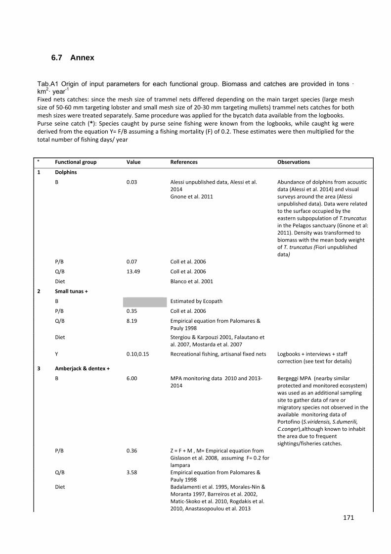
171  

6.7 Annex  

Tab.A1 Origin of input parameters for each functional group. Biomass and catches are provided in tons · km2· year-1

Fixed nets catches: since the mesh size of trammel nets differed depending on the main target species  (large mesh size of 50‐60 mm targeting lobster and small mesh size of 20‐30 mm targeting mullets) trammel nets catches for both mesh sizes were treated separately. Same procedure was applied for the bycatch data available from the logbooks. Purse  seine  catch  (*): Species  caught by purse  seine  fishing were known  from  the  logbooks, while  caught kg were derived from the equation Y= F/B assuming a fishing mortality (F) of 0.2. These estimates were then multiplied for the total number of fishing days/ year 

°  Functional group  Value  References  Observations 

1  Dolphins        

   B  0.03  Alessi unpublished data, Alessi et al. 2014  Gnone et al. 2011 

Abundance of dolphins from acoustic data (Alessi et al. 2014) and visual surveys around the area (Alessi  unpublished data). Data were related to the surface occupied by the eastern subpopulation of T.truncatus in the Pelagos sanctuary (Gnone et al: 2011). Density was transformed to biomass with the mean body weight of T. truncatus (Fiori unpublished data) 

   P/B  0.07  Coll et al. 2006    

   Q/B  13.49  Coll et al. 2006    

   Diet    Blanco et al. 2001    

2  Small tunas +        

   B     Estimated by Ecopath    

   P/B  0.35  Coll et al. 2006    

   Q/B  8.19  Empirical equation from Palomares & Pauly 1998 

  

   Diet    Stergiou & Karpouzi 2001, Falautano et al. 2007, Mostarda et al. 2007 

  

   Y   0.10,0.15  Recreational fishing, artisanal fixed nets  Logbooks + interviews + staff correction (see text for details) 

3  Amberjack & dentex +        

   B  6.00  MPA monitoring data  2010 and 2013‐2014 

Bergeggi MPA  (nearby similar protected and monitored ecosystem) was used as an additional sampling site to gather data of rare or migratory species not observed in the available  monitoring data of Portofino (S.viridensis, S.dumerili, C.conger),although known to inhabit the area due to frequent sightings/fisheries catches. 

   P/B  0.36  Z = F + M , M= Empirical equation from Gislason et al. 2008,  assuming  F= 0.2 for lampara 

  

   Q/B  3.58  Empirical equation from Palomares & Pauly 1998 

  

   Diet    Badalamenti et al. 1995, Morales‐Nin & Moranta 1997, Barreiros et al. 2002, Matic‐Skoko et al. 2010, Rogdakis et al. 2010, Anastasopoulou et al. 2013  

  

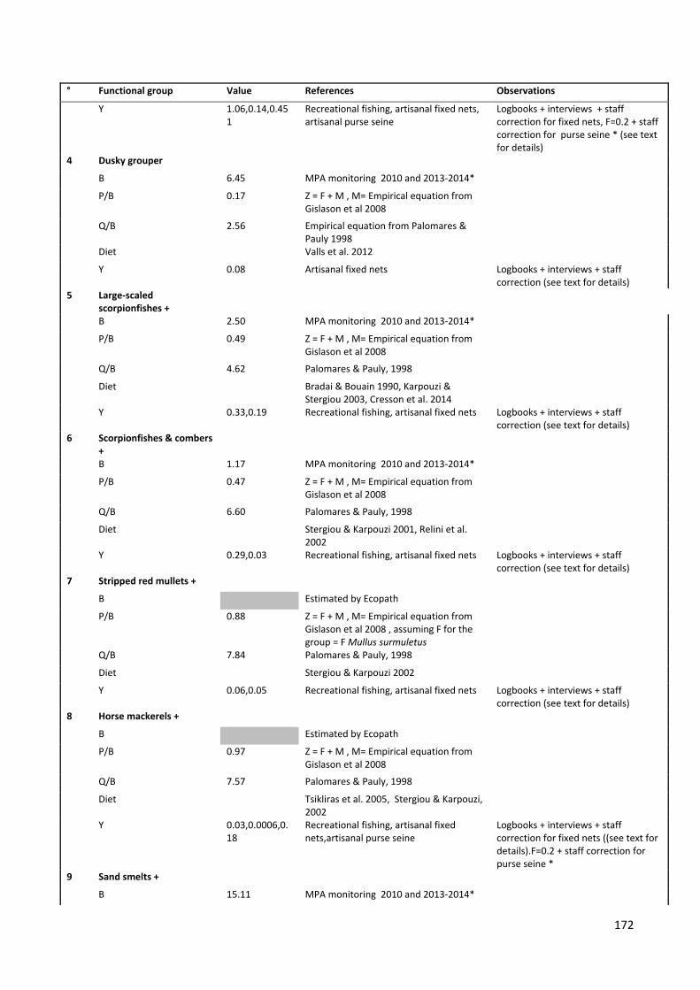
172  

°  Functional group  Value  References  Observations 

   Y   1.06,0.14,0.451 

Recreational fishing, artisanal fixed nets, artisanal purse seine 

Logbooks + interviews  + staff correction for fixed nets, F=0.2 + staff correction for  purse seine * (see text for details) 

4  Dusky grouper        

   B  6.45  MPA monitoring  2010 and 2013‐2014*    

   P/B  0.17  Z = F + M , M= Empirical equation from Gislason et al 2008  

  

   Q/B  2.56  Empirical equation from Palomares & Pauly 1998 

  

   Diet    Valls et al. 2012    

   Y   0.08  Artisanal fixed nets  Logbooks + interviews + staff correction (see text for details) 

5  Large‐scaled scorpionfishes + 

     

   B  2.50  MPA monitoring  2010 and 2013‐2014*    

   P/B  0.49  Z = F + M , M= Empirical equation from Gislason et al 2008  

  

   Q/B  4.62  Palomares & Pauly, 1998    

   Diet    Bradai & Bouain 1990, Karpouzi & Stergiou 2003, Cresson et al. 2014 

  

   Y   0.33,0.19  Recreational fishing, artisanal fixed nets  Logbooks + interviews + staff correction (see text for details) 

6  Scorpionfishes & combers + 

      

   B  1.17  MPA monitoring  2010 and 2013‐2014*    

   P/B  0.47  Z = F + M , M= Empirical equation from Gislason et al 2008  

  

   Q/B  6.60  Palomares & Pauly, 1998    

   Diet    Stergiou & Karpouzi 2001, Relini et al. 2002 

  

   Y   0.29,0.03  Recreational fishing, artisanal fixed nets  Logbooks + interviews + staff correction (see text for details) 

7  Stripped red mullets +        

   B     Estimated by Ecopath    

   P/B  0.88  Z = F + M , M= Empirical equation from Gislason et al 2008 , assuming F for the group = F Mullus surmuletus 

  

   Q/B  7.84  Palomares & Pauly, 1998    

   Diet    Stergiou & Karpouzi 2002    

   Y   0.06,0.05  Recreational fishing, artisanal fixed nets  Logbooks + interviews + staff correction (see text for details) 

8  Horse mackerels +        

   B     Estimated by Ecopath    

   P/B  0.97  Z = F + M , M= Empirical equation from Gislason et al 2008  

  

   Q/B  7.57  Palomares & Pauly, 1998    

   Diet    Tsikliras et al. 2005,  Stergiou & Karpouzi, 2002 

  

   Y   0.03,0.0006,0.18 

Recreational fishing, artisanal fixed nets,artisanal purse seine 

Logbooks + interviews + staff correction for fixed nets ((see text for details).F=0.2 + staff correction for purse seine * 

9  Sand smelts +        

   B  15.11  MPA monitoring  2010 and 2013‐2014*    

173  

°  Functional group  Value  References  Observations 

   P/B  0.79  Z = F + M , M= Empirical equation from Gislason et al. 2008 , assuming  F= 0.2 for purse seine 

  

   Q/B  10.41  Palomares & Pauly, 1998    

   Diet    Pinnegar & Polunin 2000, Stergiou & Karpouzi 2001, Cresson et al. 2014 

  

   Y   0.24,0.002,0.62 

Recreational fishing, artisanal fixed nets, artisanal purse seine 

Logbooks + interviews + staff correction for fixed nets (see text for details). F=0.2 + staff correction for purse seine* 

10  Pagellus        

   B  0.28  MPA monitoring  2010 and 2013‐2014*  Biomass of the group was obtained  multiplying the biomass of  Pagellus erythrinus x 3  to account for Pagellus bogaraveo and Pagellus acarne, which are fished in the area, but were not detected during visual census 

   P/B  0.88  Z = F + M , M= Empirical equation from Gislason et al 2008  

  

   Q/B  6.96  Palomares & Pauly, 1998    

   Diet    Stergiou & Karpouzi, 2002    

   Y   0.1,0.03  Recreational fishing, artisanal fixed nets  Logbooks + interviews + staff correction (see text for details) 

11  Diplodus +        

   B  29.70  MPA monitoring  2010 and 2013‐2014*    

   P/B  0.70  Z = F + M , M= Empirical equation from Gislason et al 2008  

  

   Q/B  6.46  Palomares & Pauly, 1998    

   Diet    Sala 1997, Pita et al. 2002    

   Y   1.94,1.4  Recreational fishing, artisanal fixed nets  Logbooks + interviews + staff correction (see text for details) 

12  Gobies +        

   B  0.14  Estimated by Ecopath  Understimated by visual census 

   P/B  1.19  Z = F + M , M= Empirical equation from Gislason et al 2008  

  

   Q/B  8.54  Palomares & Pauly, 1998    

   Diet    Pita et al. 2002, Karpouzi & Stergiou 2003, Velasco et al. 2010 

  

   Y   0.06  Recreational fishing  Logbooks + interviews + staff correction (see text for details) 

13  Wrasses +        

   B  2.49  MPA monitoring  2010 and 2013‐2014*    

   P/B  0.94  Z = F + M , M= Empirical equation from Gislason et al 2008  

  

   Q/B  9.56  Palomares & Pauly, 1998    

   Diet    Cresson et al. 2014, Stergiou & Karpouzi 2002, Velasco et al. 2010 

  

   Y   0.06,0.02  Recreational fishing, artisanal fixed nets  Logbooks + interviews + staff correction (see text for details) 

14  Mullets        

   B  1.06  MPA monitoring  2010 and 2013‐2014*    

   P/B  0.45  Z = F + M , M= Empirical equation from Gislason et al 2008  

  

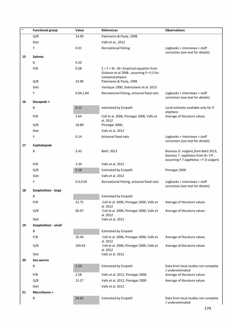
174  

°  Functional group  Value  References  Observations 

   Q/B  14.99  Palomares & Pauly, 1998    

   Diet    Valls et al., 2012    

   Y   0.01  Recreational fishing  Logbooks + interviews + staff correction (see text for details) 

15  Salema         

   B  9.20      

   P/B  0.58  Z = F + M , M= Empirical equation from Gislason et al 2008 , assuming F= 0.2 for LamparaLampara 

  

   Q/B  23.90  Palomares & Pauly, 1998    

   Diet    Verlaque 1990, Dobroslavić et al. 2013    

   Y   0.04,1.84  Recreational fishing, artisanal fixed nets  Logbooks + interviews + staff correction (see text for details) 

16  Decapods +        

   B  0.12  estimated by Ecopath  Local estimate available only for P. elephans  

   P/B  2.64  Coll et al. 2006, Pinnegar 2000, Valls et al. 2012 

Average of literature values 

   Q/B  18.89  Pinnegar 2000,     

   Diet    Valls et al. 2012     

   Y   0.14  Artisanal fixed nets  Logbooks + interviews + staff correction (see text for details) 

17  Cephalopods        

   B  3.43  Betti  2013   Biomass O. vulgaris from Betti 2013, biomass T. sagittatus from B= Y/F , assuming F T.sagittatus = F O.vulgaris 

   P/B  2.34  Valls et al. 2012    

   Q/B  5.18  Estimated by Ecopath   Pinnegar 2000 

   Diet    Valls et al. 2012     

   Y   0.4,0.05  Recreational fishing, artisanal fixed nets  Logbooks + interviews + staff correction (see text for details) 

18  Zooplankton ‐ large        

   B     Estimated by Ecopath    

   P/B  22.71   Coll et al. 2006, Pinnegar 2000, Valls et al. 2012 

Average of literature values 

   Q/B  60.47   Coll et al. 2006, Pinnegar 2000, Valls et al. 2012 

Average of literature values 

   Diet    Valls et al. 2012     

19  Zooplankton ‐ small        

   B     Estimated by Ecopath    

   P/B  35.44   Coll et al. 2006, Pinnegar 2000, Valls et al. 2012 

Average of literature values 

   Q/B  109.43   Coll et al. 2006, Pinnegar 2000, Valls et al. 2012 

Average of literature values 

   Diet    Valls et al. 2012     

20  Sea worms        

   B  3.50  Estimated by Ecopath  Data from local studies not complete / underestimated 

   P/B  2.58  Valls et al. 2012, Pinnegar 2000  Average of literature values 

   Q/B  15.27  Valls et al. 2012, Pinnegar 2000  Average of literature values 

   Diet    Valls et al. 2012     

21  Macrofauna +        

   B  24.62  Estimated by Ecopath  Data from local studies not complete / underestimated 

175  

°  Functional group  Value  References  Observations 

   P/B  4.10  Coll et al. 2006, Pinnegar 2000, Valls et al. 2012  

Average of data 

   Q/B  47.60  Coll et al. 2006, Pinnegar 2000, Valls et al. 2012 

  

   Diet    Valls et al. 2012     

22  Echinoderms +        

   B     Estimated by Ecopath    

   P/B  0.59  Coll et al. 2006, Pinnegar 2000, Valls et al. 2012  

Average of literature values 

   Q/B  2.70  Pinnegar 2000    

   Diet    Valls et al. 2012     

23  Suspensivores +        

   B  4.45  Estimated by Ecopath  Data from local studies not complete / underestimated 

   P/B  2.63  Coll et al. 2006, Pinnegar 2000, Valls et al. 2012  

Average of literature values 

   Q/B  11.20  Pinnegar 2000, Valls et al. 2012   Estimated by the model for  a P/Q = 0,3  

   Diet    Valls et al. 2012    

24  Gorgonians        

   B  500.80  Cerrano et al. 2005, Bavestrello et al. 2014 

 

   P/B  0.20  Mistri & Ceccherelli 1994, Weinbauer & Velimirov 1995 

  

   Q/B  0.53  Valls et al. 2012    

   Diet    Valls et al. 2012     

25  Sea urchins         

   B  64.95  Chiantore et al. 2008    

   P/B  0.57  Coll et al. 2006, Pinnegar 2000, Valls et al. 2012  

Average of literature values 

   Q/B  2.77  Pinnegar 2000    

   Diet    Valls et al. 2012     

26  Meiofauna        

   B     Estimated by Ecopath    

   P/B  10.00  Danovaro et al. 2002    

   Q/B     Estimated by Ecopath for a P/Q of 0.3    

   Diet    Valls et al. 2012    

27  Posidonia        

   B  3674.00  Montefalcone et al. 2015  Leaf,frond,rhyzome,roots. Conversion factors AFDW = 80% DW from (Westlake 1964), WW = 5.7 x DW from Valls et al. 2012 

   P/B  0.55  Francour 1990    

28  Seaweeds        

   B  557.00  Mangialajo et al. 2008, Montefalcone et al. 2015 

Biomass of macrophytes + biomass of  algal epiphytes on P.oceanica leafs  

   P/B  4.43  Valls et al. 2012     

29  Phytoplankton        

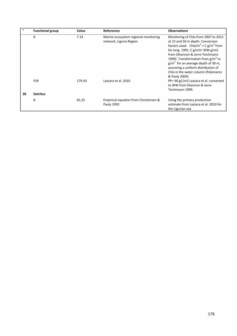
176  

°  Functional group  Value  References  Observations 

   B  7.14  Marine ecosystem regional monitoring network, Liguria Region  

Monitoring of Chla from 2007 to 2012 at 15 and 50 m depth. Conversion  factors used:   Chla/m3 > C g/m3 from De Jong  1991, C g/m3> WW g/m3 from (Shannon & Jarre‐Teichmann 1999)  Transformation from g/m3 to g/m2  for an average depth of 30 m, assuming a uniform distribution of Chla in the water column (Palomares & Pauly 2004) 

   P/B  179.50  Lazzara et al. 2010  PP= 90 gC/m2 Lazzara et al. converted to WW from Shannon & Jarre‐Teichmann 1999. 

30  Detritus        

   B  65.25  Empirical equation from Christensen & Pauly 1993 

Using the primary production estimate from Lazzara et al. 2010 for the Ligurian sea 

177  

6.7.1 Model balancing The model was balanced by acting mainly on diets, since these derived from studies in

other Mediterranean areas, and were often not sufficiently detailed. Biomass values were

modified only for the most uncertain cases.

Initial ecotrophic Efficiencies of fish groups were > 1 for Scorpionfish and combers+,

Pagellus, Gobids+ and Mullets. Predation on these groups was reduced by shifting small

percentages of the diet of Amberjack + and Large-scale scorpionfishes+ to Wrasses+,

Sand smelts+, Gobids+ and cephalopods.

Biomass of Gobids+ was too low to sustain predation, probably because underwater visual

census underestimates these cryptic fish (Kovacic et al. 2012), and was thus let to model

estimate by setting EE=0.9.

Similar reasoning was applied to Mullets and Pagellus, who are likely underestimated by

visual census, thus their biomass was increased of 10% (within the pedigree range).

Initial biomass estimates for invertebrates (Decapods+, Sea worms and Macrofauna+)

were too low to sustain predation. The field biomass available for Decapods+ related only

to P. elephans, while a wider range of species are included in this group, upon which many

predators feed. Sea worms and Macrofauna+ estimates derived from local field studies

(Thrush et al 2011, Misic et al. 2011) that had assessed the abundance of invertebrates

only in some specific spots of the MPA for specific study purposes. These estimates were

probably not representative of the abundance in the whole model area, thus we preferred

to estimate the biomass of these groups by setting the value of Ecotrophic efficiency.

Sea urchins did not cope with predation from the highly abundant Diplodus + group,

although biomass estimates for both were considered reliable. We thus increased the P/B

ratio of sea urchins which was very low when compared to other literature values and

adopted an average of these.

 

 

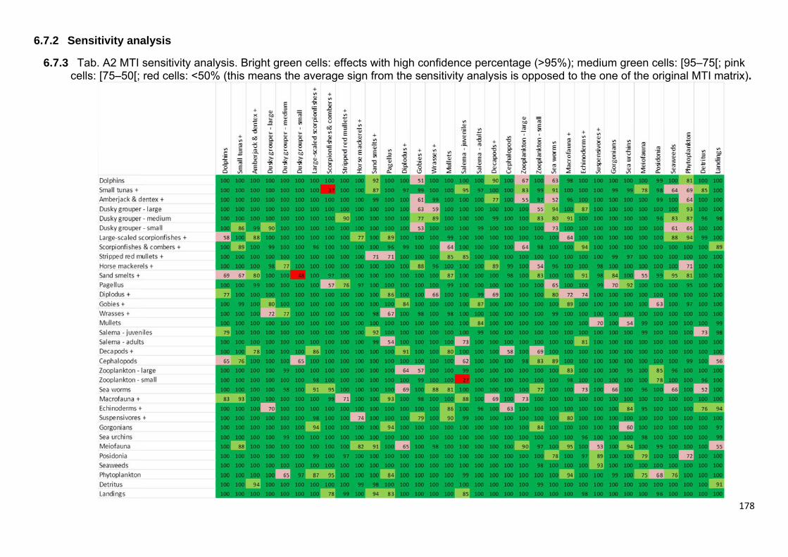
6.7.2 S

6.7.3 c

Sensitivity ana

Tab. A2 MTI scells: [75–50[;

alysis

sensitivity analred cells: <50%

lysis. Bright gre% (this means t

een cells: effecthe average sig

cts with high cogn from the se

onfidence percensitivity analys

entage (>95%)is is opposed t

); medium greeto the one of th

en cells: [95–75he original MTI

178 

5[; pink matrix).

 

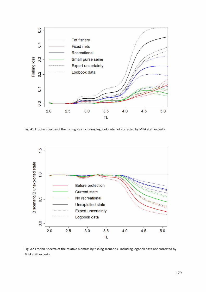
Fig. A1 Tr

Fig. A2 Tr

MPA staf

rophic spectra

rophic spectra

ff experts. 

a of the fishing

a of the relativ

g loss includin

ve biomass by

ng logbook da

y fishing scena

ta not correct

arios,  includin

ted by MPA st

ng logbook da

taff experts. 

ata not correct

179 

 

 

ted by 

180  

6.7.4 References input parameters Alessi J, Bianchi CN, Bozzini G, Brunoldi M, Cappanera V, Casale A, Corvisiero P,

Fanciulli G, Grosso D, Magnoli N, Melchiorre C, Morri C, Povero P, Stasi N, Taiuti M, Viano G, Wurtz M (2014) ARION: a tool for real time bottlenose dolphin monitoring in the Portofino MPA, 28th Annual Conference of the European Cetacean Society, Liége

Anastasopoulou A, Mytilineou C, Lefkaditou E, Kavadas S, Bekas P, Smith CJ, Papadopoulou KN, Christides G (2013) The diet and feeding ecology of Conger conger (L. 1758) in the deep waters of the Eastern Ionian Sea. Mediterr Mar Sci 14

Badalamenti F, D’Anna G, Lopiano L, Scilipoti D, Mazzola A (1995) Feeding habits of young-of-the-year greater amberjack Seriola dumerili (Risso, 1810) along the N/W Sicilian Coast. Sci Mar 59:317–323

Barreiros JP, Santos RS, Borba AES (2002) Food habits, schooling and predatory behaviour of the Yellowmouth Barracuda, Sphyraena viridensis Cuvier, 1829 (Perciformes: Sphyraenidae) in the Azores. Cybium 26(8):83-88

Bavestrello G, Bo M, Bertolino M, Betti F, Cattaneo-Vietti R (2014) Long-term comparison of structure and dynamics of the red coral metapopulation of the Portofino Promontory (Ligurian Sea): a case-study for a Marine Protected Area in the Mediterranean Sea. Mar Ecol

Blanco C, Salomón O, Raga JA (2001) Diet of the bottlenose dolphin (Tursiops truncatus) in the western Mediterranean Sea. J Mar Biol Assoc UK 81:1053–1058

Bradai MN, Bouain A (1990) Régime alimentaire de Scorpaena porcus et de S. scrofa (Teleostei, Scorpaenidae) du Golfe de Gabès, Tunisie. Cybium 14:207–216

Cappanera V, Venturini S, Campodonico P (2013) Valutazione dell’impatto antropico legato alle attività svolte nell’area Marina Protetta Portofiino. Le attiiviità dii fruizione 2012-2013

Cerrano C, Arillo A, Azzini F, Calcinai B, Castellano L, Muti C, Valisano L, Zega G, Bavestrello G (2005) Gorgonian population recovery after a mass mortality event. Aquat Conserv Mar Freshw Ecosyst 15:147–157

Chiantore M, Vielmini I, Privitera D, Mangialajo L, Cattaneo-Vietti R (2008) Habitat effects on the population structure of Paracentrotus lividus and Arbacia lixula. Chem Ecol 24:145–157

Christensen V, Pauly D (1993) Trophic Models of Aquatic Ecosystems. The WorldFish Center

Coll M, Palomera I, Tudela S, Sardà F (2006) Trophic flows, ecosystem structure and fishing impacts in the South Catalan Sea, Northwestern Mediterranean. J Mar Syst 59:63–96

Cresson P, Ruitton S, Ourgaud M, Harmelin-Vivien M (2014) Contrasting perception of fish trophic level from stomach content and stable isotope analyses: A Mediterranean artificial reef experience. J Exp Mar Biol Ecol 452:54–62

Danovaro R, Gambi C, Mirto S, others (2002) Meiofaunal production and energy transfer efficiency in a seagrass Posidonia oceanica bed in the western Mediterranean. Mar Ecol Prog Ser 234

De Jong, S.A, Haufman, PAG., Sandee AJJ. and Nienhuis PH, 1991. Community oxygen budgets on seagrass beds and microbial mats on the Banc d’Arguin, Mauritania, p. 67-68. In: PMJ. Herman and CHR. Heip (eds.) Report on the workshop, ‘Modeling the benthos’, Yerseke, The Netherlands, 20-22 March 1991. Delta Institute for Hydrobiological Research, Yerseke

Dobroslavić T, Zlatović A, Bartulović V, Lučić D, Glamuzina B (2013) Diet overlap of juvenile salema ( Sarpa salpa ), bogue ( Boops boops ) and common two-

181  

banded sea bream ( Diplodus vulgaris ) in the south-eastern Adriatic. J Appl Ichthyol 29:181–185

Falautano M, Castriota L, Finoia MG, Andaloro F (2007) Feeding ecology of little tunny Euthynnus alletteratus in the central Mediterranean Sea. J Mar Biol Assoc UK 87:999

Francour P (1990) Dynamique de l'écosystème à Posidonia oceanica dans le Parc National de Port-Cros.Analyse des compartiments matte, litière, faune vagile, échinodermes et poissons. Doctorat, Université Pierre et Marie Curie, Paris

Gislason H, Daan N, Rice J, Pope J (2008) Does natural mortality depend on individual size. ICES CM

Gnone G, Bellingeri M, Dhermain F, Dupraz F, Nuti S, Bedocchi D, Moulins A, Rosso M, Alessi J, McCrea RS, Azzellino A, Airoldi S, Portunato N, Laran S, David L, Di Meglio N, Bonelli P, Montesi G, Trucchi R, Fossa F, Wurtz M (2011) Distribution, abundance, and movements of the bottlenose dolphin (Tursiops truncatus) in the Pelagos Sanctuary MPA (north-west Mediterranean Sea): The bottlenose dolphin in the pelagos sanctuary MPA. Aquat Conserv Mar Freshw Ecosyst 21:372–388

Karpouzi VS, Stergiou KI (2003) The relationships between mouth size and shape and body length for 18 species of marine fishes and their trophic implications. J Fish Biol 62:1353–1365

Mangialajo L, Chiantore M, Cattaneo-Vietti R (2008) Loss of fucoid algae along a gradient of urbanisation, and structure of benthic assemblages. Mar Ecol Prog Ser 358:63–74

Matic-Skoko S, Tutman P, Marcejla E, Skaramuca D, \DJikic D, Lisicic D, Skaramuca B (2010) Feeding habits and trophic status of Mediterranean moray eel, Muraena helena L., 1758 in the Adriatic Sea—preliminary approach. Rapp Comm Int Pour Mer Méditerranée 39:583

Misic C, Castellano M, Harriague AC (2011) Organic matter features, degradation and remineralisation at two coastal sites in the Ligurian Sea (NW Mediterranean) differently influenced by anthropogenic forcing. Marine environmental research. 72(1):67-74.

Mistri M, Ceccherelli VU (1994) Growth and secondary production of the Mediterranean gorgonian Paramuricea clavata. Mar Ecol-Prog Ser 103:291–291

Montefalcone M, Vassallo P, Gatti G, Parravicini V, Paoli C, Morri C, Bianchi CN (2015) The exergy of a phase shift: Ecosystem functioning loss in seagrass meadows of the Mediterranean Sea. Estuar Coast Shelf Sci 156:186–194

Morales-Nin B, Moranta J (1997) Life history and fishery of the common dentex (Dentex dentex) in Mallorca (Balearic Islands, western Mediterranean). Fish Res 30:67–76

Mostarda E, Campo D, Castriota L, Esposito V, Scarabello MP, Andaloro F (2007) Feeding habits of the bullet tuna Auxis rochei in the southern Tyrrhenian Sea. J Mar Biol Assoc UK 87:1007

Palomares MLD, Pauly D (1998) Predicting food consumption of fish populations as functions of mortality, food type, morphometrics, temperature and salinity. Mar Freshw Res 49:447–453

Palomares Ld, Pauly D (2004) West African Ecosystems. Fish Cent Res Rep 12:4 Pinnegar JK, Polunin NVC (2000) Contributions of stable-isotope data to elucidating

food webs of Mediterranean rocky littoral fishes. Oecologia 122:399–409 Pita C, Gamito S, Erzini K (2002) Feeding habits of the gilthead seabream (Sparus

aurata) from the Ria Formosa (southern Portugal) as compared to the black seabream (Spondyliosoma cantharus) and the annular seabream (Diplodus annularis). J Appl Ichthyol 18:81–86

182  

Relini G, Relini M, Torchia G, De Angelis G (2002) Trophic relationships between fishes and an artificial reef. ICES J Mar Sci J Cons 59:S36–S42

Rogdakis Y, Ramfos A, Koukou K, Dimitriou E, Katselis G (2010) Feeding habits and trophic level of sea bass (Dicentrarchus labrax) in the Messolonghi-Etoliko lagoons complex (Western Greece). J Biol Res 13:13–26

Sala E (1997) Fish predators and scavengers of the sea urchin Paracentrotus lividus in protected areas of the north-west Mediterranean Sea. Mar Biol 129:531–539

Shannon LJ, Jarre-Teichmann A (1999) A model of trophic flows in the northern Benguela upwelling system during the 1980s. South Afr J Mar Sci 21:349–366

Stergiou KI, Karpouzi VS (2001) Feeding habits and trophic levels of Mediterranean fish. Rev Fish Biol Fish 11:217–254

Thrush S, Chiantore M, Asnagi V, Hewitt J, Fiorentino D, Cattaneo-Vietti R (2011) Habitat–diversity relationships in rocky shore algal turf infaunal communities. Marine Ecology Progress Series 424:119–132

Tsikliras AC, Torre M, Stergiou KI (2005) Feeding habits and trophic level of round sardinella (Sardinella aurita) in the northeastern Mediterranean (Aegean Sea, Greece). J Biol Res 3:67–75

Valls A, Gascuel D, Guénette S, Francour P (2012) Modeling trophic interactions to assess the effects of a marine protected area: case study in the NW Mediterranean Sea. Mar Ecol Prog Ser 456:201–214

Velasco EM, Gómez-Cama MC, Hernando JA, Soriguer MC (2010) Trophic relationships in an intertidal rockpool fish assemblage in the gulf of Cádiz (NE Atlantic). J Mar Syst 80:248–252

Verlaque M (1990) Relations entre Sarpa salpa (Linnaeus, 1758)(Téléostéen, Sparidae), les autres poissons brouteurs et le phytobenthos algal méditerranéen. Oceanol Acta 13:373–388

Weinbauer M, Velimirov B (1995) Biomass and secondary production of the temperate gorgonian coral Eunicella cavolini (Coelenterata:Octocorallia). Mar Ecol Prog Ser 121:211–216

Westlake DF (1964) Light extinction, standing crop and photosynthesis within weed beds.

 

183  

7 Building a standard trophic model for a data-poor marine reserve: cost-benefit analysis.

 

7.1 Abstract

Mediterranean coastal ecosystems support a great diversity of habitats, species and

communities, being a major challenge for an ecosystem management approach. In

particular, effective management of Marine Protected Areas should account for the

complexity of the food-webs they host to properly evaluate priority actions. The

application of food-web modelling through the Ecopath with Ecosim software (EwE)

may allow to unravel such a complexity and could thus help to better pursue the

conservation and management objectives of Mediterranean MPAs. Unfortunately,

whilst widely applied at larger ecosystem scales where the presence of industrial

fisheries allows for large data availability covered by global databases, EwE has not

yet gained full attention as a possible tool for the management of smaller and highly

diverse coastal areas. At this small scale fine resolution local data is needed in order

to develop useful models for management, but is costly to obtain for all functional

groups. Here we evaluate costs associated with the development of a standard

Ecopath model for a recently established coastal fishery reserve, where no

quantitative biological data is available (Cap Roux, NW Mediterranean sea). Field

campaigns were designed to obtain local data in priority for a selection of groups for

which imprecise biomass input can widely affect model outputs (Prato et al. 2014).

Trophic interactions were unravelled and keystone functional groups such as high

trophic level predators and cephalopods were identified, highlighting the need for

monitoring these groups. Costs associated with all steps of model building, from data

collection to model balancing, were provided and evaluated in relation to the

achieved model quality. The least cost-efficient surveys were identified and the

benefits of integrating regular monitoring programs with food-web models

development were discussed.

184  

7.2 Introduction  

Marine protected areas (MPAs) have spread worldwide in response to the increasing

calls for an ecosystem based fisheries management (EBFM), as an alternative or

additional measure to policies focused on single species (Browman et al 2005,

Gaines et al 2010). Up to date the performance of MPAs in achieving their

conservation and fisheries management objectives has been generally assessed

through empirical studies analysing the direct effects of protection, such as the

response of single species or groups of species (Lester et al 2009, Guidetti & Sala

2007) or the spillover effect for adjacent fisheries (Murawski et al al 2005, Goni et al

2008, Colléter et al. 2014). The complex linkages and interactions among species

instead, can hardly be unravelled through observational studies, but are a key

component of the EBFM and essential to fully comprehend the mechanisms driving

species response to protection (Kellner et al. 2010).

The limits of empirical studies concerning these issues can be overcome with

ecosystem modelling, a tool that has the high potential to assess both the

conservation performance of MPAs at the ecosystem scale, but also their outcomes

in fisheries management (Pelletier et al. 2005). In this context, the “Ecopath with

Ecosim” (EwE, Christensen & Walters 2004) modelling approach is increasingly

gaining interest as a management-advice tool, in both areas of fisheries management

and conservation, and has been widely applied worldwide thanks to its capability of

integrating ecological, economic and social aspects and analysing trade-offs, both

temporally and spatially (Christensen et al. 2009). Yet, the development of EwE

models, like all ecosystem models, is burdened by the amount of data needed and

the uncertainty associated with it (Dame and Christian 2005, Morisette 2007).

Sensitivity analysis on model outputs are thus increasingly becoming part of the

model building routine (Link et al. 2010, Lassalle et al. 2014, Steenbeek 2015).

Efforts have also been implemented to provide standard model structures facilitating

the construction of EwE models (Christensen et al 2009). Standard model structures

have for instance been used to model Large Marine Ecosystems (Piroddi et al 2015),

based on data available in global databases (Christensen et al. 2009, Piroddi et al.

2015). Nonetheless, to be considered as tools to advise management in MPAs,

models must achieve a trade-off between parsimony and complexity, and,

essentially, must be grounded on local fine-resolution data (Pelletier et al. 2005,

Prato et al. 2014). If more realistic models are developed, the long-lasting gap

185  

between empirical studies and modelling could be overcome and the two approaches

would more often be integrated, allowing more representative and thorough

assessments of MPA effects (Pelletier et al. 2005).

The few existing Ecopath models built for Mediterranean MPAs largely differ in model

complexity. In Prato et al. 2014 we proposed a simplified and standardised model

structure to be applied to Mediterranean coastal MPAs and we identified the

functional groups for which accurate local biomass data are needed in priority to

develop a reliable model (high trophic level predators, planktonivorous fish,

decapods, cephalopods, macrofauna and abundant primary producers). Here we

take a step forward, and analyse the feasibility and costs of building a trophic model

grounded on newly collected local data, based on the simplified and standardised

structure proposed in Prato et al. 2014. We selected the case study of the Cap Roux

fishery reserve (NW Mediterranean, France) representative of recently established

Mediterranean MPAs where few if none quantitative biological data are available, and

designed a monitoring program targeted specifically to collect biomass data for the

above mentioned groups. We then evaluated the costs associated with all steps of

model building, from data collection to model balancing, and discussed model costs

in relation to the achieved model quality. Providing this effort and cost analysis, we

aim to assess if EwE can be realistically considered as a management tool for

Mediterranean MPAs.

7.3 Methods  

7.3.1 Study area

The Cap Roux fishery reserve (Fig. 1) comprises 450 ha and extends from the shore

out to the 80 m isobath. The area has been protected from all kinds of extractive

activities (both commercial and recreational) since December 2003, but daily

enforcement surveys were implemented in 2008 in summer time. As part of of the

Natura 2000 site of the Esterel, the Cap Roux reserve includes priority habitats for

conservation such as extensive Posidonia oceanica meadows and coralligenous

formations (Bonhomme et al. 2010). The modelled area (145 ha, Fig.1) represents

the subtidal portion of the reserve including the following habitats: soft bottoms (7%),

Posidonia oceanica (75%), corallogenous bioconcretions (10%), rocky infralittoral (6

%) and coralligenous (2 %). Coastal detritic habitat, extending from approximatively

 

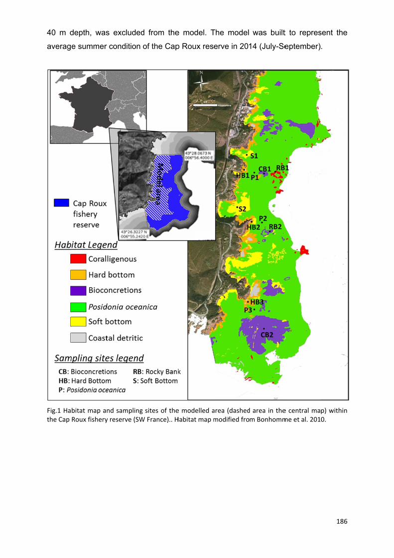
40 m d

averag

Fig.1 Hathe Cap 

depth, was

e summer

bitat map aRoux fishery

s excluded

condition

nd samplingy reserve (SW

d from the

of the Cap

g sites of theW France).. H

e model. T

p Roux res

e modelled aHabitat map m

The model

erve in 20

area (dashedmodified fro

was built

14 (July-Se

d area  in them Bonhomm

t to repres

eptember)

e central mame et al. 201

186 

sent the

.

p) within 0.  

 

7.3.2

Tab.1 Sam

replicates

  

  

Transect 2  

  

Transect 2 

   

Circles r=5 

  

Quadrats  

   

Air lift dev 

  

Field sam

mpling sites f

s 

25 x 5 m 

 

25 x 1 m 

 

5 m 

  

1x1 m 

 

vice r=40cm 

 

mpling

or each habit

CoastalHard botto

(5 m) 

Sites  N 

HB1  4 

HB2  4 

HB3  4 

HB1  4 

HB2  4 

HB3  4 

HB1  6 

HB2  6 

HB3  6 

HB1  20 

HB2  20 

HB3  20 

HB1  3 

HB2  3 

tat and metho

l om 

Roba

(5‐1

Sites

RB1

RB2

 

RB1

RB2

 

RB1

RB2

 

RB1

RB2

 

RB1

  

od. Refer to F

ocky  ank 15 m) 

Bioco(

N  Site

8  CB1

8  CB2

   

8  CB1

8  CB2

   

6  CB1

6  CB2

   

20   

20   

   

6  

     

Fig.1 for  locat

oncretions (12 m) 

P

es  N  S

1  4 

2  4 

 

1  4 

2  4 

 

1  3 

2  3 

 

 

 

 

 

  

ion of sampli

Posidonia oceanica (12 m) 

Sites  N  S

P1  4  

P2  4  

P3  4  

   

   

   

   

   

   

P1  10  

P2  10  

P3  10  

P1  3  S

P2  3  S

ng sites.N = n

Soft bottom (5m) 

Sites  N   

 

Fis   

 

 

 CeDeSe    

 

 

  CeDeSe    

 

 

 SeHoOp    

 

 

S1  3 

M  

S2  3 

187 

number of 

Target taxa 

sh  

ephalopodsecapods ea stars 

ephalopodsecapods ea stars 

ea urchins olothurians phiuroids 

Macrofauna 

188  

Location of sampling sites was determined using a stratified random sampling

approach where sites were assigned randomly to each of 3 major habitat types

(Coastal hard bottoms, Posidonia oceanica, coralligenous bioconcretions) plus two

rocky banks (characterised by rocky and coralligenous habitat). Habitats were

distributed along a depth gradient from the coast to 30 meters depth. Three sites

were randomly selected within coastal hard bottoms at 5 meters depth (HB 1-3),

three sites within P. oceanica beds at 15 meter depth (P 1-3), and two sites within the

coralligenous bioconcretions at 15 m depth (CB 1-2). Finally, two sites were selected

at each rocky bank, respectively between 5 and 10 meters and between 15 and 30

meters depth (RB 1-2) (Fig.1, Tab.1).

Field data were collected for fish, echinoderms (including sea urchins, holothurians

sea stars and ophiuroids), decapods, octopus and macrofauna. Tab. 1 synthetises

the sampling scheme for each functional group.

Fish were surveyed monthly (July, August and September 2014), while invertebrate

surveys were conducted only in July and September. Fish and echinoderms

(excluding sea stars) surveys were carried out at all habitats and sites. Surveys for

sea stars, decapods and cephalopods were not carried out in P; oceanica habitat,

given the low abundances of such organisms in this habitat (pers. obs. P. Francour)

and accounting for the too long time needed to search through dense P. oceanica

meadows. Macrofauna was sampled in two sites for each habitat, excluding

coralligenous bioconcretions to avoid damage of this fragile habitat. Two sites at soft

bottoms (S 1-2, Fig.1) were also sampled, since macrofauna was expected to be

abundant in such habitat.

Fish abundance, species composition and size (recorded using 2 cm size classes)

were recorded along 4 replicate transects 25 x 5 meters long.

Sea urchins, holothurians and ophiuroids were identified, counted and measured

within 1 m2 quadrats. Twenty replicates were performed at coastal hard bottom sites

to account for the heterogeneity of the substrate (rocks and pebbles), while 10

replicates were sampled in P. oceanica and rocky banks sites. Sea urchins and

holothurians were recognised to the species level and measured with a calliper to

nearest mm. Recorded measures were respectively the largest radius of the disk and

the contracted body length. Ophiuroids disk was estimated to the nearest cm due to

the difficulty at catching the organism.

189  

Two methods were used to record mobile mega-invertebrates (sea stars, octopus

and decapods) (Tab.1). The first method consisted in 25x1 meter transect (4

replicates/site), which were coupled with the fish transects, where a diver searched

the substrate behind the fish counts operator. Since we could not detect any

decapods or octopuses with transects, we then designed a method characterised by

replicate circles of 5 m radius, allowing to easily survey a wider surface for each

replicate and thus better accounting for the mobility and distribution of these

organisms. The method was characterised by replicate circles of 5 m radius, where

two operators searched the substrate while swimming around an iron pole. Each

operator held respectively the extremity and the mid-point of a 5 m rope, which was

fixed to the iron pole with a rotating ring. In such way the operators could define the

surface to be sampled while holding tight the rope and swimming around the pole

(Tab.1). Three replicate circles were completed at each depth in rocky bank (6 in

total per each rocky bank) and at each coralligenous bioconcretion site, while 6

replicates were carried out on coastal hard bottoms to account for the heterogeneity

of the substrate (3 on rock and 3 on pebbles). Sea stars were measured for the

maximum arm length from the tip of the longest arm to the centre of the disk; for

decapods we recorded carapace length and for cephalopods we visually estimated

cephalothorax length.

To survey macrofauna (> 1mm), three replicates of 40 cm diameter were sampled at

each site with an air lift pump fixed at one extremity to interchangeable nylon nets of

1 mm mesh size (Tab.1). We did not select smaller mesh sizes since these would

significantly increase sorting time (Jameson 1995, Ferraro et al 2011) while not

significantly affecting biomass estimates (Bachelet 1990, Covazzi-Harriague 2006).

Samples were then sieved through 0.50 mm sieves and preserved under 6% formalin

and seawater solution. At sand and P. oceanica sites we used an inox steel cylinder

to define our sampling area. The cylinder (40 m diameter) was equipped with handles

on the upper side and a sharp cut edge on the bottom side, specifically realised to

facilitate insertion in the substrate. Two divers were needed at each operation : one

diver pressed the cylinder in the sediment up to ca 30 cm depth and the other diver

activated the air lift pump during 2 minutes (Vassapollo et al 2009, Michel et al 2010),

moving the tube in circles within the walls of the cylinder for sand samples, and

vertically for P. oceanica samples. To sample in rocky habitat, a hard plastic cylinder

(40 cm diameter) with handles was used. An extra tissue strip was fixed all around

190  

the base of the cylinder (like a skirt) with galvanized chain at its perimeter, so that the

base could be moulded to the substrate, thus preventing organisms to escape from

underneath. While one diver moved the air lift tube, the other one held the cylinder on

the bottom while scraping algae from the substrate, which were thus directly aspired

by the air lift pump. This technique was preferred to previous scraping and collection

of algae since many vagile macroinvertebrates could fly away during the scraping

process.

7.3.3 Ecopath model structure

The species-based Ecopath model was used in this study.

Ecopath is a mass-balanced model based on the assumption that the production of

one functional group is equal to the sum of all predation, non-predatory losses,

exports, biomass accumulations and catches, as expressed by the following

equation:

P/Bi × Bi = Bi × P/Bi × (1 − EEi) + ΣNj (Q/B)ji × Bi × DCji + Yi + NMi + Bai (1)

Qi=Pi + Ri + UAi (2)

Where N the number of functional groups in the model, B is the biomass, P/Bi is the

production rate, Q/B is the consumption rate, DCji is the fraction of prey i included in

the diet of predator j, NMi is the net migration of prey I, BAi is the biomass

accumulation of prey I, Yi is the catch of prey i and EEi is the ecotrophic efficiency of

prey i, that is the proportion of production used in the system. The model represents

the average summer condition of the Cap roux fishery reserve ecosystem in 2014.

The simplified model structure developed by Prato et al. (2014) for the Port Cros

MPA was used in our study. Seabirds and rays were not included in the model, since

their biomasses are likely to be very low in the model area. We thus preferred to

exclude them instead of estimating their biomasses through the mass-balance

calculations.

Input parameters

Fish wet weight was estimated from size data by means of length–weight

relationships from the available literature, selecting coefficients referring to

Mediterranean samples whenever possible (from www.fishbase.org). Echinoderms

wet weight was also estimated using available length-weight relationships from the

191  

literature and, where needed, dry weight-wet weight conversion factors from Brey et

al 2010 were used (Annex, Tab. 1). Macrofauna samples were sorted and identified

to the genus level when possible. Ash free dry weight was obtained by drying

organisms at 60°C and incinerating them at 450°C. Ash free dry weight was

converted to wet weight using conversion factors from Brey et al.2 010. Algae wet

weight was measured after blotting for water in excess. Per each species, the

calculation of biomass in the model area accounted for the surface of its habitat types

inside the model area.

Biomass of Posidonia oceanica (leaves, frond, rhizome and root) was calculated

using the average biomass (g/m2) of a Mediterranean Posidonia oceanica meadow

(Montefalcone et al. 2015) extrapolated for habitat surface at Cap Roux (Bonhomme

et al. 2010). Biomass of phytoplankton was estimated from the value of primary

productivity in the Ligurian sea (Lazzara et al 2010) divided by the P/B rate of

phytoplankton used in Valls et al. 2012 for the Port Cros ecopath model. Biomass of

detritus was estimated through an empirical relationship (Christensen & Pauly 1993).

For consumers that were not quantified on the field (since we prioritised data

collection for sensible groups for which imprecise input biomass values can affect

model outputs) (Prato et al. 2014), biomass was estimated through the mass-balance

calculations of the model.

Production to biomass ratio (P/B) of fish corresponds to the total mortality rate Z

(Allen 1971), the sum of natural (M) and fishing (F) mortality rates. F was assumed to

be null, while M was calculated with an empirical equation (Gislason et al. 2008).

Fish consumption per unit biomass Q/B was calculated with the empirical equation

from Palomares & Pauly 1998, while for invertebrates’ production and consumption

rates we used the average of the best literature values available for similar coastal

Mediterranean ecosystems (Pinnegar et al. 2000, Albouy et al. 2010, Valls et al.

2012).

Diet composition of fish and invertebrates were based on available Mediterranean

literature and, for aggregation into functional groups, were weighted for the local

biomass and consumption rates of each species. All input parameters and empirical

equations used are listed in Tab.2 in the Annex.

192  

7.3.4 Keystone groups analysis The mixed trophic impact routine (MTI) of Ecopath assesses the relative impact of a

slight increase in abundance of any group on the biomass of other groups on the

food-web (Christensen et al 2005). Keystone species are defined as the species

having the highest and widest impact on the food web despite a low biomass. They

were identified by applying the new keystonness index developed by Valls et al 2015.

The index is characterized by an impact component (IC, defining the trophic impact

of a group on the other groups) and a biomass component (BC) , according to the

following equation:

KS= Ln(IC x BC) (2)

Where IC is defined from Libralato et al 2006 as:

Ɛi =√ Σ j≠i mij2 (3)

Parameter Ɛi represents the overall effect of group i on all the other groups in the

food web (without including the effect of the group on itself) and is expressed as the

sum of the squared values of mij (the MTI score) of group i, paired with each of the

other living group j in the food web. The mixed-trophic impact of group I on itself (mii)

is excluded, as well as the mixed-trophic impact on dead groups such as detritus

(Libralato et al.2006).

The biomass component is defined as the rank of the group’s biomass in descending

order:

BC = drank(Bi) (4)

We calculated the KS index for each group in the model (excluding fisheries) and

plotted the groups according to their KS index and biomass, scaled by trophic level.

7.3.5 Data quality and MTI sensitivity analysis Data quality was assessed applying the food web diagnostics proposed by Link 2010

and Lassalle et al 2014. The Pedigree routine to summarise the uncertainty around

the input data, based on a set of qualitative choices relative to the origin of biomass,

193  

P/B, Q/B, catch and diet input for each functional group. The range of uncertainty of

biomass data, for example, varies from ± 10% (locally sampled high precision data,

low uncertainty,) to ± 80% (model estimate, high uncertainty) (Morissette 2007). An

overall pedigree of the model is then calculated as the average of the individual

pedigree values (Pauly et al. 2000). According to Lassalle et al. 2014, a Pedigree

index > 0.4 testifies sufficient quality to pursue with model analysis.

Robustness of MTI results was tested through a sensitivity analysis (Lassalle et al

2014). We rebuilt the original net impact matrix where qij is the net impact of i on j

and is given by the difference between positive effects (quantified by the fraction of

prey i in the diet of predator j), and negative effects fij (evaluated as the fraction of

total consumption of j used by predator i). Then, in the analysis routine, 5000 Q

matrices are created by drawing qij values from independent uniform distributions

defined by original qij± 20% (Richardson et al. 2006). The mij values for each

pairwise intersection of the Q matrices are then calculated, their signs recorded and

the percentage of mij values with the same sign as in the original MTI matrix (SMTI)

is estimated. Results were summarized into one matrix recording the sign of the

original mij values and the SMTI percentages that are categorized into four

classes:[0; 50], ]50; 75], ]75; 95] and ]95; 100].

7.3.6 Cost analysis

Effort devoted to the construction of the model was quantified as total hours of field

work, total hours of lab. work for macrofaunal sample treatment (sorting and

identification) and total hours of computer work for data analysis and model building.

Costs for field work were quantified assuming a flat rate of 500 € per dive for a

scientific underwater operator (including fees, field trip, and diving material

amortization). Analysis of macrofaunal samples was carried out by a specialised

laboratory, thus we reported the total cost invested for such service, selected after a

market analysis. Cost of computer work was quantified on the basis of 35 € / hour,

calculated from the average 2014 annual salary of a researcher enrolled at the

French national centre for scientific research (

CNRS, www.cnrs.fr).

Field and lab costs were also analysed separately for each ecological group,

reporting number of campaigns to survey each group within the warm season, total

number of samples (replicates) performed, total hours of field and lab work and total

cost.

194  

Finally, the minimum unit of effort was provided in terms of hours/replicate in the field

for each ecological group sampled. Cost for equipment amortization was also

considered, including amortization for boat maintainance and diving equipment and

data recording equipment (including reels 25m long, pvc quadrats, plastic callipers,

underwater writing slates and papers, pencils, and macrofauna and algae sampling

equipment: inox steel cylinder, plastic cylinder with embedded chain, airlift sampler

device, nylon collecting bags, scalpel).

7.4 Results  

A total of 35 fish species were recorded and grouped in 11 functional groups

following the standard model structure proposed in Prato et a. 2014 (Tab.2a). Two

sea urchin species, three holothurian species and two sea star species were also

identified. Ophiuroids were not identified to the species level. Holothurians, stars and

ophiuroids were aggregated into one functional group (echinoderms+), while sea

urchins in another (sea urchins+), again following Prato et al. 2014. Sampling with

the air lift device allowed to identify 12 invertebrate taxa aggregated in two separate

functional groups (polychaetes and macrofauna + , Tab. 2b), 11 dominant seaweed

taxa (aggregated in 1 functional group). Overall, the model was made of 18 functional

groups, for 78 % of which we could use biomass estimates collected in the field (10

groups of fish, echinoderms, sea urchins, macrofauna and algae). Tab.2b shows the

list of the recorded taxa and their aggregation into the 18 functional groups for model

building. We were not able to obtain estimates of biomass for decapods and

cephalopods, since field surveys allowed to record only very few individuals of

Palinurus elephas and Octopus vulgaris.

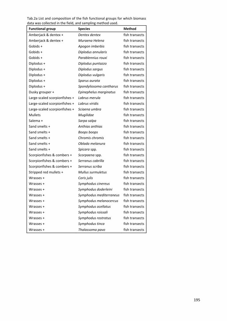
195  

Tab.2a List and composition of the fish functional groups for which biomass data was collected in the field, and sampling method used.

Functional group  Species  Method 

Amberjack & dentex +  Dentex dentex  fish transects

Amberjack & dentex +  Muraena Helena  fish transects

Gobids +  Apogon imberbis   fish transects

Gobids +  Diplodus annularis  fish transects

Gobids +  Parablennius rouxi  fish transects

Diplodus +   Diplodus puntazzo  fish transects

Diplodus +   Diplodus sargus  fish transects

Diplodus +   Diplodus vulgaris  fish transects

Diplodus +   Sparus aurata  fish transects

Diplodus +   Spondyliosoma cantharus  fish transects

Dusky grouper +  Epinephelus marginatus  fish transects

Large‐scaled scorpionfishes +  Labrus merula  fish transects

Large‐scaled scorpionfishes +  Labrus viridis  fish transects

Large‐scaled scorpionfishes +  Sciaena umbra  fish transects

Mullets  Mugilidae  fish transects

Salema +  Sarpa salpa  fish transects

Sand smelts +  Anthias anthias  fish transects

Sand smelts +  Boops boops  fish transects

Sand smelts +  Chromis chromis  fish transects

Sand smelts +  Oblada melanura  fish transects

Sand smelts +  Spicara spp.  fish transects

Scorpionfishes & combers +  Scorpaena spp.  fish transects

Scorpionfishes & combers +  Serranus cabrilla  fish transects

Scorpionfishes & combers +  Serranus scriba  fish transects

Stripped red mullets +  Mullus surmuletus  fish transects

Wrasses +  Coris julis  fish transects

Wrasses +  Symphodus cinereus  fish transects

Wrasses +  Symphodus doderleini  fish transects

Wrasses +  Symphodus mediterraneus  fish transects

Wrasses +  Symphodus melanocercus  fish transects

Wrasses +  Symphodus ocellatus  fish transects

Wrasses +  Symphodus roissali  fish transects

Wrasses +  Symphodus rostratus  fish transects

Wrasses +  Symphodus tinca  fish transects

Wrasses +  Thalassoma pavo  fish transects

 

   

196  

Tab.2b List  and  composition  of  the  invertebrate    and  primary  producers functional  groups  for which  biomass  data was  collected  in  the  field,  and sampling method used.

Functional group  Species  Method 

Decapods +  Palinurus elephas  invertebrate transects and circles 

Cephalopods  Octopus vulgaris  invertebrate transects and circles 

Echinoderms +  Echinaster sepositus  invertebrate transects and circles 

Echinoderms +  Marthasterias glacialis  invertebrate transects and circles 

Echinoderms +  Holothuria forskali  quadrats 

Echinoderms +  Holothuria poli  quadrats 

Echinoderms +  Holothuria tubulosa  quadrats 

Sea urchins  Arbacia lixula  quadrats 

Sea urchins  Paracentrotus lividus  quadrats 

Macrofauna+  Ophiura  quadrats 

Macrofauna+  Arthropoda  air lift pump 

Macrofauna+  Briozoa  air lift pump 

Macrofauna+  Chordata  air lift pump 

Macrofauna+  Cnidaria  air lift pump 

Macrofauna+  Echinodermata  air lift pump 

Macrofauna+  Mollusca  air lift pump 

Macrofauna+  Porifera  air lift pump 

Polychaetes  Anellida  air lift pump 

Polychaetes  Nermertea  air lift pump 

Polychaetes  Plathyelminthe  air lift pump 

Polychaetes  Sipuncula  air lift pump 

Sea weeds  Cladostephus spongiosus  air lift pump 

Sea weeds  Corallinacea  air lift pump 

Sea weeds  Cystoisera compressa  air lift pump 

Sea weeds  Cystoseira brachycarpa  air lift pump 

Sea weeds  Dictyota spp.  air lift pump 

Sea weeds  Halopteris filicina  air lift pump 

Sea weeds  Jania spp.  air lift pump 

Sea weeds  Padina pavonica  air lift pump 

Sea weeds  Peyssonnelia sp.  air lift pump 

Sea weeds  Stypocaulon scoparia  air lift pump 

Sea weeds  Lithothamnion sp  air lift pump 

     

7.4.1 Model balancing

Ecotrophic efficiency was >1 for six fish groups ( Amberjack&dentex +, Scorpionfish

and combers +, Striped red mullets +, Gobies and Mullets) and two invertebrate

groups (Polychaetes and Macrofauna+).

Predation mortality on Amberjack and dentex + from Dusky grouper medium was

reduced shifting 4% of grouper’s diet from the mentioned group to other preys

through proportional rescaling. Cannibalism on Scorpionfish and combers+ was

reduced by shifting their diet to Wrasses +, a known prey of this group (Thiriet et al

197  

2014). The proportion of diet of Dusky grouper small on Striped red mullets+ was

reduced of 3% and diet was rescaled proportionally. Transect visual census is not

appropriate to detect small cryptic species, and in fact gobies biomass was too low to

sustain predation. It was thus calculated through the model’s mass-balance

equations. Mullets were subject to a strong predation mortality from cephalopods,

which was reduced by rescaling a 5% of cephalopod’s diet to their other preys.

Sea worms input biomass estimated on the field (1.6 tons/km2) was far too low to

sustain predation. Biomass was very low compared to other similar ecosystem

models (Albouy et al 2010, Valls et al 2012, Prato et al. in prep) and likely strongly

underestimated, since our field sampling did not occur on coralligenous concretions.

This habitat is likely hosting high abundance of sea worms, but is also very fragile,

thus it would have been damaged by the air lift pump sampling. We thus estimated

sea worms biomass through the mass balance calculations of the model.

Macrofauna input biomass was low to sustain predation from Decapods+. Our input

biomass value was probably underestimated since we did not sample in

coralligenous concretions, thus we increased input biomass by 40% according to the

standard pedigree range provided for low precision-local sampling data (Morisette

2007). Then, by reducing Decapods diet on macrofauna by 20%, we reached a

reasonable biomass estimate that satisfied the mass-balance requisite.

7.4.2 Ecopath model

The balanced model had a pedigree of 4.1 and respected all pre-balancing rules

(Link et al 2010, Lassalle et al. 2014). Final model parameters are provided in Tab.3.

Biomasses of fish, invertebrates and primary producers were respectively 0.07%,

0.64% and 99% of total biomass in the system ( tons ∙  km-2 ∙ year-1 including

Posidonia oceanica). Analysis of fluxes showed that the food-web was mainly

organised around a bentho-pelagic pathway, with limited exchanges with the pelagic

domain (Fig. 2). Biomass of first order producers was dominated by Posidonia

oceanica and seaweeds, which were the largest source of energy for Salemas and

Sea urchins, the main herbivores in the system (Fig. 2). Strong energy fluxes

connected the detritus compartment with many benthic invertebrate groups

(Meiofauna, Suspensivores+ and Echinoderms+) and Mullets. Main fluxes

connecting the benthic and fish groups were those between Macrofauna+ and

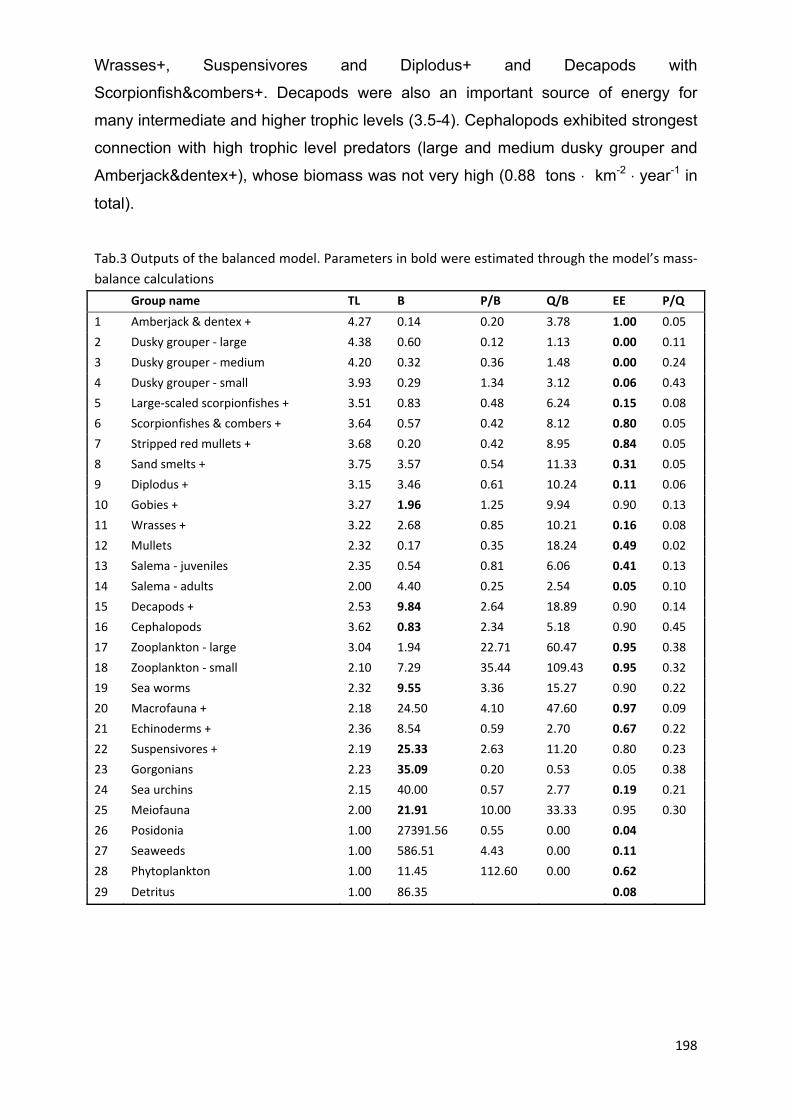
198  

Wrasses+, Suspensivores and Diplodus+ and Decapods with

Scorpionfish&combers+. Decapods were also an important source of energy for

many intermediate and higher trophic levels (3.5-4). Cephalopods exhibited strongest

connection with high trophic level predators (large and medium dusky grouper and

Amberjack&dentex+), whose biomass was not very high (0.88 tons ∙  km-2 ∙ year-1 in

total).

Tab.3 Outputs of the balanced model. Parameters in bold were estimated through the model’s mass‐

balance calculations 

Group name  TL  B  P/B  Q/B  EE  P/Q 

1  Amberjack & dentex +  4.27  0.14  0.20  3.78  1.00  0.05 

2  Dusky grouper ‐ large  4.38  0.60  0.12  1.13  0.00  0.11 

3  Dusky grouper ‐ medium  4.20  0.32  0.36  1.48  0.00  0.24 

4  Dusky grouper ‐ small  3.93  0.29  1.34  3.12  0.06  0.43 

5  Large‐scaled scorpionfishes +  3.51  0.83  0.48  6.24  0.15  0.08 

6  Scorpionfishes & combers +  3.64  0.57  0.42  8.12  0.80  0.05 

7  Stripped red mullets +  3.68  0.20  0.42  8.95  0.84  0.05 

8  Sand smelts +  3.75  3.57  0.54  11.33  0.31  0.05 

9  Diplodus +  3.15  3.46  0.61  10.24  0.11  0.06 

10  Gobies +  3.27  1.96  1.25  9.94  0.90  0.13 

11  Wrasses +  3.22  2.68  0.85  10.21  0.16  0.08 

12  Mullets  2.32  0.17  0.35  18.24  0.49  0.02 

13  Salema ‐ juveniles  2.35  0.54  0.81  6.06  0.41  0.13 

14  Salema ‐ adults  2.00  4.40  0.25  2.54  0.05  0.10 

15  Decapods +  2.53  9.84  2.64  18.89  0.90  0.14 

16  Cephalopods  3.62  0.83  2.34  5.18  0.90  0.45 

17  Zooplankton ‐ large  3.04  1.94  22.71  60.47  0.95  0.38 

18  Zooplankton ‐ small  2.10  7.29  35.44  109.43  0.95  0.32 

19  Sea worms  2.32  9.55  3.36  15.27  0.90  0.22 

20  Macrofauna +  2.18  24.50  4.10  47.60  0.97  0.09 

21  Echinoderms +  2.36  8.54  0.59  2.70  0.67  0.22 

22  Suspensivores +  2.19  25.33  2.63  11.20  0.80  0.23 

23  Gorgonians  2.23  35.09  0.20  0.53  0.05  0.38 

24  Sea urchins  2.15  40.00  0.57  2.77  0.19  0.21 

25  Meiofauna  2.00  21.91  10.00  33.33  0.95  0.30 

26  Posidonia  1.00  27391.56  0.55  0.00  0.04 

27  Seaweeds  1.00  586.51  4.43  0.00  0.11 

28  Phytoplankton  1.00  11.45  112.60  0.00  0.62 

29  Detritus  1.00  86.35  0.08 

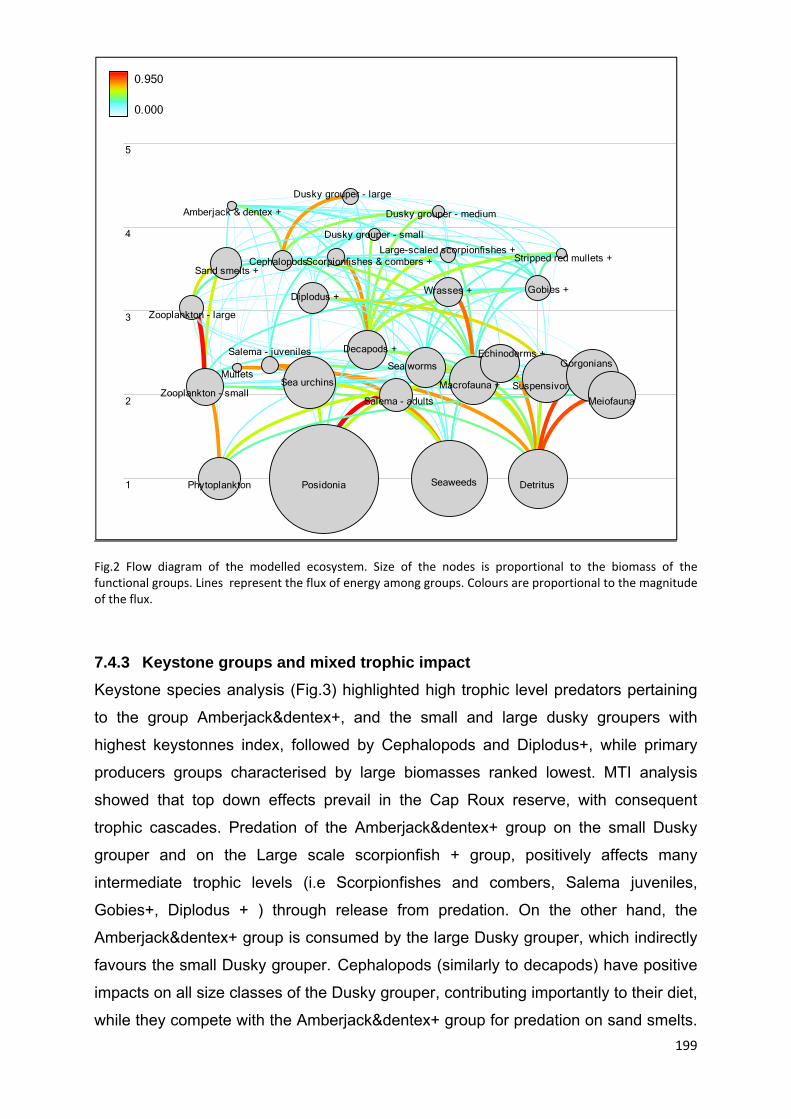
199  

Fig.2  Flow  diagram  of  the modelled  ecosystem.  Size  of  the  nodes  is  proportional  to  the  biomass  of  the functional groups. Lines  represent the flux of energy among groups. Colours are proportional to the magnitude of the flux. 

7.4.3 Keystone groups and mixed trophic impact

Keystone species analysis (Fig.3) highlighted high trophic level predators pertaining

to the group Amberjack&dentex+, and the small and large dusky groupers with

highest keystonnes index, followed by Cephalopods and Diplodus+, while primary

producers groups characterised by large biomasses ranked lowest. MTI analysis

showed that top down effects prevail in the Cap Roux reserve, with consequent

trophic cascades. Predation of the Amberjack&dentex+ group on the small Dusky

grouper and on the Large scale scorpionfish + group, positively affects many

intermediate trophic levels (i.e Scorpionfishes and combers, Salema juveniles,

Gobies+, Diplodus + ) through release from predation. On the other hand, the

Amberjack&dentex+ group is consumed by the large Dusky grouper, which indirectly

favours the small Dusky grouper. Cephalopods (similarly to decapods) have positive

impacts on all size classes of the Dusky grouper, contributing importantly to their diet,

while they compete with the Amberjack&dentex+ group for predation on sand smelts.

5

4

3

2

1

0.950

0.000

Amberjack & dentex +

Dusky grouper - large

Dusky grouper - medium

Dusky grouper - small

Large-scaled scorpionfishes +Scorpionfishes & combers + Stripped red mullets +

Sand smelts +

Diplodus +Gobies +Wrasses +

Mullets

Salema - juveniles

Salema - adults

Decapods +

Cephalopods

Zooplankton - large

Zooplankton - small

Sea worms

Macrofauna +

Echinoderms +

Suspensivores +

Gorgonians

Sea urchins

Meiofauna

Posidonia SeaweedsPhytoplankton Detritus

 

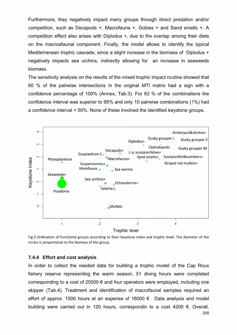
Further

compet

compet

on the

Medite

negativ

biomas

The se

60 %

confide

confide

a confid

Fig.3 Ord

circles is 

7.4.4

In orde

fishery

corresp

skipper

effort o

building

rmore, the

tition, such

tition effec

macroafa

rranean tro

vely impac

ss.

nsitivity an

of the pa

ence perce

ence interv

dence inte

dination of fun

proportional t

Effort and

er to collec

reserve r

ponding to

r (Tab.4).

of approx.

g were ca

ey negative

h as Deca

ct also aris

aunal com

ophic casc

cts sea ur

nalysis on t

irwise inte

entage of

val was sup

rval < 50%

nctional group

to the biomas

d cost ana

ct the nee

representin

a cost of 2

Treatmen

1500 hou

arried out

ely impact

apods +, M

ses with D

ponent. F

cade, since

rchins, ind

the results

ersections

100% (Ann

perior to 95

%. None of

ps according t

ss of the group

lysis

eded data

ng the wa

25500 € a

t and iden

rs at an e

in 120 ho

t many gro

Macrofauna

iplodus +,

inally, the

e a slight in

irectly allo

s of the mix

in the ori

nex, Tab.3

5% and on

these invo

to their keyst

p. 

for buildin

arm seaso

nd four op

ntification

expense of

ours, corre

oups throu

a +, Gobie

due to the

model al

ncrease in

owing for

xed trophic

iginal MTI

3). For 83

nly 10 pairw

olved the id

tone index an

ng a troph

on, 51 div

perators we

of macrofa

f 16000 €

espondin t

ugh direct

es + and S

e overlap

lows to id

the bioma

an increa

c impact ro

matrix ha

% of the

wise comb

dentified ke

d trophic leve

hic model

ing hours

ere employ

aunal sam

. Data an

to a cost

predation

Sand sme

among the

dentify the

ass of Dip

ase in sea

outine show

ad a sign

combinati

binations (1

eystone gr

el. The diame

of the Ca

were com

yed, includ

mples requ

nalysis and

4200 €. 200 

n and/or

lts +. A

eir diets

typical

plodus +

aweeds

wed that

with a

ons the

1%) had

roups.

 

eter of the 

p Roux

mpleted

ding one

uired an

d model

Overall,

201  

including 2000 € for equipment amortization and if scientific underwater operators

must be contracted for field data collection, on the basis of our salary assumption

45700 € would need to be invested to build a model for the Cap Roux reserve.

 Tab.4  Total  effort  and  cost  covering  the  whole  process  of model  building.  Effort  was quantified as hours/process, and  staff employed. Prices were  calculated assuming a  flat rate  of  500  €  per  dive  for  a  scientific  underwater  operator  (approx.  60 min/dive  and  including material  amortization) and 35 € per hour of  computer work    for  a  researcher (based on 2014 annual salary for a CNRS researcher) 

 Hours  Cost (€)    Staff 

Field work  51  25500    2‐3 scientific divers, 1 skipper 

Macrofauna + algae sorting,identification  1500  16000    2 biologists 

Data analysis + model building  120  4200    1 biologist 

Equipment amortization    2000     

Total cost    47700     

 

The least cost-efficient field surveys in terms of cost per total replicates were surveys

for mega-invertebrates and macrofauna (respectively 6500 € / 78 replicates and 5000

€ / 50 replicates, against 8000 €/ 150 fish transects and 6000 € / 260 echinoderm

quadrats) (Tab. 5). When the cost for lab. work was added, the most expensive

process was data collection for macrofauna and algae, reaching an overall

investment of 21000 € for data collection, sample sorting and taxa identification (Tab.

5).

Tab.5 Total data collection cost for each ecological group. Lab cost for fish and invertebrates inlcudes data digitalisation and standardisation. 

Total cost / group  Campaigns  Replicates  Field hours  Field cost (€)  Lab cost (€)  Total cost (€) 

Fish  3  150  16  8000  560  8560 

Mega‐invertebrates  2  78  13  6500  560  7060 

Echinoderms  2  260  12  6000  280  6280 

Macrofauna + algae  2  50  10  5000  16000  21000 

Efficiency of fish and echinoderms surveys was related to the short time needed to

survey one replicate (6 min / transect, 3 min / quadrat) (Tab. 6). Both could be

performed by one operator. Sampling with circles for sea stars, decapods and

cephalopods required longer time per replicate, since it allowed to sample a larger

surface (78.5 m2/replicate circle against 25 m2/replicate transect). One operator was

needed per transect replicate, while two operators were needed for each circle

replicate (Tab. 6).To sample macrofauna and algae four operators were needed: two

underwater operators collected the sample, and two operators on-board (other than

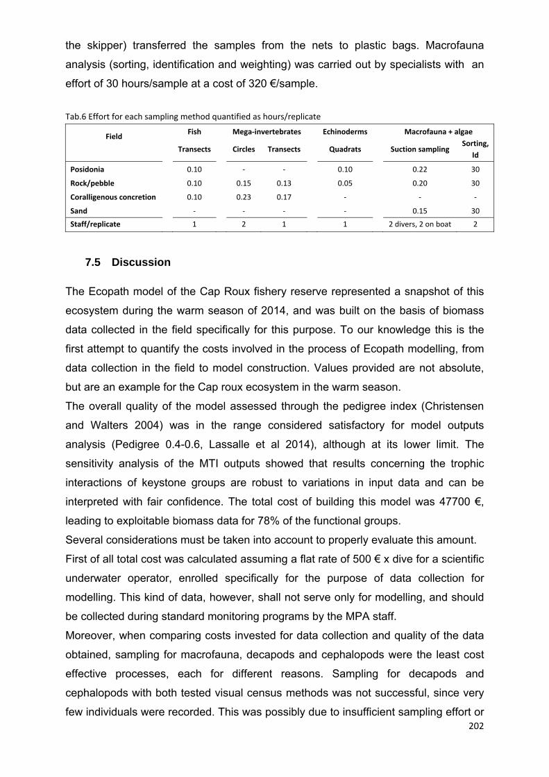
202  

the skipper) transferred the samples from the nets to plastic bags. Macrofauna

analysis (sorting, identification and weighting) was carried out by specialists with an

effort of 30 hours/sample at a cost of 320 €/sample.

Tab.6 Effort for each sampling method quantified as hours/replicate 

 

7.5 Discussion The Ecopath model of the Cap Roux fishery reserve represented a snapshot of this

ecosystem during the warm season of 2014, and was built on the basis of biomass

data collected in the field specifically for this purpose. To our knowledge this is the

first attempt to quantify the costs involved in the process of Ecopath modelling, from

data collection in the field to model construction. Values provided are not absolute,

but are an example for the Cap roux ecosystem in the warm season.

The overall quality of the model assessed through the pedigree index (Christensen

and Walters 2004) was in the range considered satisfactory for model outputs

analysis (Pedigree 0.4-0.6, Lassalle et al 2014), although at its lower limit. The

sensitivity analysis of the MTI outputs showed that results concerning the trophic

interactions of keystone groups are robust to variations in input data and can be

interpreted with fair confidence. The total cost of building this model was 47700 €,

leading to exploitable biomass data for 78% of the functional groups.

Several considerations must be taken into account to properly evaluate this amount.

First of all total cost was calculated assuming a flat rate of 500 € x dive for a scientific

underwater operator, enrolled specifically for the purpose of data collection for

modelling. This kind of data, however, shall not serve only for modelling, and should

be collected during standard monitoring programs by the MPA staff.

Moreover, when comparing costs invested for data collection and quality of the data

obtained, sampling for macrofauna, decapods and cephalopods were the least cost

effective processes, each for different reasons. Sampling for decapods and

cephalopods with both tested visual census methods was not successful, since very

few individuals were recorded. This was possibly due to insufficient sampling effort or

Field 

 

  Fish    Mega‐invertebrates    Echinoderms    Macrofauna + algae 

 Transects 

 Circles  Transects 

 Quadrats 

 Suction sampling 

Sorting,

Id 

Posidonia    0.10    ‐  ‐    0.10    0.22  30 

Rock/pebble    0.10    0.15  0.13    0.05    0.20  30 

Coralligenous concretion    0.10    0.23  0.17    ‐    ‐  ‐ 

Sand    ‐    ‐  ‐    ‐    0.15  30 

Staff/replicate    1    2  1    1    2 divers, 2 on boat  2 

203  

for the paucity of these species in the studied area, in agreement with declarations of

fishermen from the surrounding area (Lepetit 2014). Non-destructive surveys for

decapods and cephalopods biomass are rare in the literature. In most modelling

studies for Mediterranean coastal areas indeed, the biomass for these groups is

generally estimated through model mass-balance calculations or is derived from

other areas of the Mediterraenan (Valls et al 2012, Albouy et al. 2010, Pinnegar et al

2000, Diaz et al. 2008).

Sampling for macrofaunal and polychaetes biomass data required a total expense of

21 000 €, 16 000 € of which were needed only for sample sorting and identification.

The biomass value obtained with this sampling effort was too low to balance the

model without some modifications. While for the macrofauna group model balance

could be reached increasing input biomass within the pedigree range, biomass of

polychaetes (1.60 tons·km2·year-1) was far too low and had to be estimated by the

mass-balance calculations of the model. In other models from coastal Mediterranean

(Valls et al 2012, Albouy et al 2010, Pinnegar et al 2000), macrofauna and

polychaetes biomass are much higher than our input values (respectively 60-100

tons · km2 · year -1 for macrofauna and 30-60 tons · km2 · year -1 for polychaetes in

other models, compared to our 18 and 1.6 tons · km2 · year -1) but similarly to

decapods and cephalopods these values were either obtained through model

estimation or derived from studies in other Mediterranean areas. Local values for

these groups were never available in any model we considered.

The question thus arises whether uncertainty resides in the input biomass value for

macrofauna and polychaetes, or in the structure of the model itself, such as the

number and composition of functional groups or the input parameters (i.e diet

composition) of other groups preying upon macrofauna and polychaetes. For

instance, biomass of macrofauna and polychaetes was possibly underestimated in

our study for reasons such as insufficient sampling effort, lack of sampling on the

probably rich coralligenous bioconcretions and lack of sampling for infaunal

polychaetes on rocky reefs. Another bias could be related to the spatial extension of

our model, which did not include deeper areas dominated by coastal detritic habitat,

also part of the Cap Roux reserve (30-40 m until 80 m isobath). Fish from the

shallower zone might rely on macrofauna from the deeper coastal detritic habitat for

a non-negligible portion of their diet. Although it would be interesting to investigate

the trophic functioning of such deeper zone and its exchanges with the shallower

habitats, its study is hampered by the complexity and costs of sampling at depths

204  

exceeding diving limits. Experimental trawling would be useful in this view, but is not

advisable in a protected area. For all these reasons we decided to exclude coastal

detritic from the model.

However, the cost implied in increasing sampling effort for macrofauna, both at

shallower and deeper areas, would be substantial, and it would thus be more

advantageous to invest for increased quality of input data for higher trophic levels

feeding on it, including decapods and cephalopods, that are of more direct relevance

for MPA management. Moreover, the development of models with standard structure,

thus same number and similar composition of functional groups and similar input diet

values (Christensen et al 2009) (that are anyway often obtained from the

Mediterranean literature) might allow to isolate this potential source of error when

model comparisons are performed, either among different seasons or years for the

same area or among different coastal Mediterranean areas.

If these cost-benefit issues are considered and macrofauna is not sampled, total

costs for model building lower to approximatively 26 700 €. 8000 € of these would be

devolved to fish monitoring, but generally this activity is already part of standard

monitoring programs in Mediterranean MPAs. An additional 6500 € (24% of total

cost) should then be invested in monitoring decapods and cephalopods. Considering

the ecological importance of both decapods and cephalopods, as well as their

commercial interest for both artisanal and recreational fishing, it would be worth to

establish appropriate monitoring surveys which would allow more comprehensive

assessment of the effects of protection, while providing valuable data for modelling.

Finally 6000 € should be invested into echinoderms monitoring, which, too, is often

already carried on in Mediterranean MPAs, in particular to assess the biomass of sea

urchins (key actors in the trophic cascade sea breams – sea urchins – seaweeds

characteristic of the Mediterranean) (Sala et al 1998, Guidetti & Sala 2007).

Overall, if collection of biomass data of some key groups like fish (especially high

trophic level predators), cephalopods and decapods is integrated to regular

monitoring activities implemented by qualified MPA staff, model building costs can be

reduced to only computer work (4200 €).Once a first model is built moreover, much

less effort is needed to update it in time, providing outputs useful for informing

management decisions (Christensen and Pauly 1993, Dame & Christian 2005, Coll et

al 2010). In our case study for example, the investment in model building allowed to

identify the keystone groups of the studied area, such as high trophic level predators

(including the dusky grouper, Epinephelus marginatus) and cephalopods (i.e. mainly

205  

Octopus vulgaris) and to unravel the trophic interactions among these, with

interesting possible management applications.

The dusky grouper for instance is a species protected by moratorium in France and

also a flag species in Mediterranean MPAs, being a strong attraction for diving

tourism (Bassu et al 2007). The Ecopath model showed that its biomass is positively

affected by that of cephalopods, which on the other hand are an important target of

both artisanal and recreational fishing within Mediterranean MPAs. In the Cap roux

reserve they are likely subject to a considerable amount of illegal fishing, due to the

absence of regular surveillance in the area (estimates for these illegal catches were

ot available), as it is often the case in the Mediterranean. Implementing management

measures such as intensified surveillance or reduction of artisanal and/or

recreational fishing catches for cephalopods would have the double effect of

protecting a functional group of recognised ecological importance (Piatkowski et al

2001,Coll et al 2013), with additional beneficial effects for the groupers population.

Building an EwE model thus offers a standardised framework both to define

monitoring programs as well as to organise the so-collected ecological information

into a coherent picture of ecosystem functioning. As we have seen moreover,

highlighting the uncertainties of a model is important to correctly interpret model

results, but should not discourage their construction (Dame & Christian 2011).

Investing in the construction of a first model would provide an MPA with an

ecosystem-based management tool which can be easily updated in time, and which

can deliver useful information, such as the identification of priority species to be

targeted by management actions, or the evaluation of fisheries impact on the

ecosystem and on key species (Prato et al. in prep), and the quantification of spill

over from the MPA (Colléter et al 2014). The more the availability of data in

Mediterranean MPAs increases, the more applications can be envisaged, up to

spatial and temporal simulations of the effects of management actions on the food-

web (Dame & Christian 2011, Coll et al 2015).

206  

7.6 References  

Albouy C, Mouillot D, Rocklin D, Culioli J, Le Loc’h F (2010) Simulation of the combined effects of artisanal and recreational fisheries on a Mediterranean MPA ecosystem using a trophic model. Mar Ecol Prog Ser 412:207–221

Bassu V, Porcu C, Niccolini F (2007) Studio sul valore economico delle popolazioni di cernie nell' Area Marina Pr otetta di Tavolara Punta Coda Cavallo. Rapporto finale 2008, Intervento E1

Bonhomme D, Astruch P, Antonioli PA, Bonhomme P, Perez T, Ruitton S, Ivanisevic J, 2010. Inventaire et Cartographie des Habitats Naturels, des espèces végétales et animales du Site Natura 2000 « l’Estérel et des abords de Fréjus (FR9301628) » – Lot 2 : Milieux marins. Contrat GIS Posidonie – Ville de Saint Raphaël,267 p.

Brey T, Müller-Wiegmann C, Zittier ZMC, Hagen W (2010) Body composition in aquatic organisms — A global data bank of relationships between mass, elemental composition and energy content. Journal of Sea Research 64:334–340

Christensen V, Ferdaña Z, Steenbeek J (2009) Spatial optimization of protected area placement incorporating ecological, social and economical criteria. Ecol Model 220:2583–2593

Christensen V, Pauly D (1992) Ecopath II—a software for balancing steady-state ecosystem models and calculating network characteristics. Ecological modelling 61:169–185

Christensen V, Pauly D (1993) Trophic Models of Aquatic Ecosystems. The WorldFish Center

Christensen V, Walters CJ (2004) Ecopath with Ecosim: methods, capabilities and limitations. Ecological modelling 172:109–139

Christensen V, Walters CJ, Ahrens R, Alder J, Buszowski J, Christensen LB, Cheung WWL, Dunne J, Froese R, Karpouzi V, Kaschner K, Kearney K, Lai S, Lam V, Palomares MLD, Peters-Mason A, Piroddi C, Sarmiento JL, Steenbeek J, Sumaila R, Watson R, Zeller D, Pauly D (2009) Database-driven models of the world’s Large Marine Ecosystems. Ecol Model 220:1984–1996

Christensen V, Walters CJ, Pauly D. Ecopath with Ecosim: a user’s guide (2005).. Fisheries Centre, University of British Columbia, Vancouver 154

Coll M, Akoglu E, Arreguín-Sánchez F, Fulton EA, Gascuel D, Heymans JJ, Libralato S, Mackinson S, Palomera I, Piroddi C, others (2015) Modelling dynamic ecosystems: venturing beyond boundaries with the Ecopath approach. Rev Fish Biol Fish 25:413–424

Colléter M, Gascuel D, Albouy C, Francour P, Tito de Morais L, Valls A, Le Loc’h F (2014) Fishing inside or outside? A case studies analysis of potential spillover effect from marine protected areas, using food web models. J Mar Syst 139:383–395

Coll M, Libralato S (2012) Contributions of food web modelling to the ecosystem approach to marine resource management in the Mediterranean Sea. Fish Fish 13:60–88

207  

Coll M, Navarro J, Olson RJ, Christensen V (2013) Assessing the trophic position and ecological role of squids in marine ecosystems by means of food-web models. Deep Sea Res Part II Top Stud Oceanogr 95:21–36

Dame JK (2005). Evaluation of ecological network analysis for ecosystem-based management. PhD diss. East Carolina University

Dame JK, Christian RR (2006) Uncertainty and the Use of Network Analysis for Ecosystem-Based Fishery Management. Fisheries 31:331–341

Dame JK, Christian RR (2011) Uncertainty and the Use of Network Analysis for Ecosystem-Based Fishery Management. Fisheries 31:331–341

Díaz López B, Bunke M, Bernal Shirai JA (2008) Marine aquaculture off Sardinia Island (Italy): ecosystem effects evaluated through a trophic mass-balance model. Ecol Model 212:292–303

Gascuel D, Bozec Y-M, Chassot E, Colomb A, Laurans M (2005) The trophic spectrum: theory and application as an ecosystem indicator. ICES J Mar Sci 62:443–452

Gascuel D, Morissette L, Palomares MLD, Christensen V (2008) Trophic flow kinetics in marine ecosystems: toward a theoretical approach to ecosystem functioning. ecological modelling 217:33–47

Gascuel D, Guénette S, Pauly D (2011) The trophic-level-based ecosystem modelling approach: theoretical overview and practical uses. ICES J Mar Sci 68:1403–1416

Gislason H, Daan N, Rice J, Pope J (2008) Does natural mortality depend on individual size. ICES CM

Goñi R, Adlerstein S, Alvarez-Berastegui D, Forcada A, Reñones O, Criquet G, Polti S, Cadiou G, Valle C, Lenfant P, others (2008) Spillover from six western Mediterranean marine protected areas: evidence from artisanal fisheries. Mar Ecol Prog Ser 366:159–174

Guidetti P, Sala E (2007) Community-wide effects of marine reserves in the Mediterranean Sea. Mar Ecol Prog Ser 335:43–56

Kellner JB, Litvin SY, Hastings A, Micheli F, Mumby PJ (2010) Disentangling trophic interactions inside a Caribbean marine reserve. Ecol Appl 20:1979–1992

Lassalle G, Bourdaud P, Saint-Béat B, Rochette S, Niquil N (2014) A toolbox to evaluate data reliability for whole-ecosystem models: Application on the Bay of Biscay continental shelf food-web model. Ecol Model 285:13–21

Lazzara L, Marchese C, Massi L, Nuccio C, Maselli F, Santini C, Pieri M, Sorani V (2010) Sub-regional patterns of primary production annual cycle in the Ligurian and North Tyrrhenian seas, from satellite data. Italian Journal of Remote Sensing 42:87–102

Lepetit A, 2014. Quel avenir pour le cantonnement du Cap Roux ? Etude du contexte et des différents scenarii possibles d’évolution du cantonnement pour assurer son efficacité et sa pérennité. Master diss., Agrocampus Ouest Rennes

Lester SE, Halpern BS, Grorud-Colvert K, Lubchenco J, Ruttenberg BI, Gaines SD, Airamé S, Warner RR (2009) Biological effects within no-take marine reserves: a global synthesis. Mar Ecol Prog Ser 384:33–46

Lindeman RL (1942) The trophic-dynamic aspect of ecology. Ecology 23:399–417

208  

Link JS (2010) Adding rigor to ecological network models by evaluating a set of pre-balance diagnostics: A plea for PREBAL. Ecol Model 221:1580–1591

Michel L, Lepoint G, Dauby P, Sturaro N (2010) Sampling methods for amphipods of Posidonia oceanica meadows: a comparative study. Crustaceana 83:39–47

Montefalcone M, Vassallo P, Gatti G, Parravicini V, Paoli C, Morri C, Bianchi CN (2015) The exergy of a phase shift: Ecosystem functioning loss in seagrass meadows of the Mediterranean Sea. Estuarine, Coastal and Shelf Science 156:186–194

Morissette L (2007) Complexity, cost and quality of ecosystem models and their impact on resilience. PhD diss., University of British Columbia

Murawski SA, Wigley SE, Fogarty MJ, Rago PJ, Mountain DG (2005) Effort distribution and catch patterns adjacent to temperate MPAs. ICES Journal of Marine Science: Journal du Conseil 62:1150–1167

Odum WE, Heald EJ, (1975). The detritus-based food web of an estuarine community, in: Cronin LE (Ed.), Estuarine Research. Academic Press, New York, pp. 265–286

Palomares MLD, Pauly D (1998) Predicting food consumption of fish populations as functions of mortality, food type, morphometrics, temperature and salinity. Mar Freshw Res 49:447–453

Pelletier D, Claudet J, Ferraris J, Benedetti-Cecchi L, Garcìa-Charton JA (2008) Models and indicators for assessing conservation and fisheries-related effects of marine protected areas. Can J Fish Aquat Sci 65:765–779

Piatkowski U, Pierce GJ, Morais da Cunha M (2001) Impact of cephalopods in the food chain and their interaction with the environment and fisheries: an overview. Fish Res 52:5–10

Pinnegar, J.K., 2000. Planktivorous Fishes: Links Between the Mediterranean Littoral and Pelagic. Ph.D. diss. University of Newcastle, 213 pp.

Pinnegar JK, Polunin NVC (2004) Predicting indirect effects of fishing in Mediterranean rocky littoral communities using a dynamic simulation model. Ecol Model 172:249–267

Piroddi C, Coll M, Steenbeek J, Macias Moy D, Christensen V (2015) Modelling the Mediterranean marine ecosystem as a whole: addressing the challenge of complexity. Mar Ecol Prog Ser 533:47–65

Prato G, Gascuel D, Valls A, Francour P (2014) Balancing complexity and feasibility in Mediterranean coastal food-web models: uncertainty and constraints. Mar Ecol Prog Ser 512:71–88

Sala E, Boudouresque CF, Harmelin-Vivien M (1998) Fishing, trophic cascades, and the structure of algal assemblages: evaluation of an old but untested paradigm. Oikos:425–439

Steenbeek J, Buszowski J, Christensen V, Akoglu E, Aydin K, Ellis N, Felinto D, Guitton J, Lucey S, Kearney K, others (2015) Ecopath with Ecosim as a model-building toolbox: Source code capabilities, extensions, and variations. Ecol Model

Thiriet P (2014)Comparisons of fish assemblage structure and underlying ecological processes, between Cystoseira forests and less structurally complex habitats

209  

of North-Western Mediterranean subtidal rocky reefs. PhD diss. Université Nice Sophia Antipolis, Nice.

Valls A, Coll M, Christensen V (2015) Keystone species: toward an operational concept for marine biodiversity conservation. Ecological Monographs 85:29–47

Valls A, Gascuel D, Guénette S, Francour P (2012) Modeling trophic interactions to assess the effects of a marine protected area: case study in the NW Mediterranean Sea. Mar Ecol Prog Ser 456:201–214

Vasapollo C (2009) Spatio-temporal variability of plant features and motile invertebrates in Posidonia oceanica seagrass meadows. PhD diss. Open University.Milton Keynes (UK)

210  

7.7 Annex Tab.1 Parameters used  for  the  length‐weight  conversions of  echinoderms,  according  to  the power  function WW =a L^b, where WW is the wet weight expressed in grams or mg depending on the size unit of  measure. For Echinaster sepositus dry weight (DW) was converted to WW with a  conversion factor = 0.283 (Brey et al. 2010)  

Power function 

parameters 

Species 

Size 

unit  Size measure  a  b 

Biomass 

unit  References 

Holothuria polii  Cm  contracted length  0.48  1.66  g WW Francour 1990 

Holothuria tubulosa 

Cm  contracted length  0.05  2.53  g WW Francour 1990 

Arbacia lixula  Mm  maximum diameter without spines  0.00  2.53  g WW Pais et al. 2007 

Paracentrotus lividus 

Mm  maximum diameter without spines  0.00  2.48  g WW Pais et al. 2007 

Spharechinus granularis 

Mm  maximum diameter without spines  0.00  2.75  g WW  Dance 1987 

Marthasterias glacialis 

Cm length of the longest arm from the 

centre of the disk 0.31  2.74  mg WW 

O' Gormann 2009 

Echinaster sepositus 

Cm length of the longest arm from the 

centre of the disk 0.05  2.29  g DW 

Schiebling 1981 

Ophiouroids  Cm  disk diameter  0.00  2.41  g WW Robinson 2010 

211  

Tab. 2 Origin of input parameters for each functional group 

N°  Funtional group  Value  References  Observations 

1  Amberjack & dentex +    

   B  0.14  Underwater visual census in the study area    

   P/B  0.20 

Z = M when fishing mortality is null. M= 

Empirical equation from Gislason et al 

2008 

  

   Q/B  3.78 Empirical equation from Palomares & 

Pauly 1998   

   Diet  

Badalamenti et al. 1995,Morales‐Nin & 

Moranta, 1997, Barreiros et al. 2002, 

Anastasopoulou et al. 2013,  Matic‐Skoko 

et al., 2010, Rogdakis et al 2010  

  

2  Dusky grouper    

   B  1.21  Underwater visual census in the study area    

   P/B  0.16 

Z = M when fishing mortality is null. M= 

Empirical equation from Gislason et al 

2008  

  

   Q/B  3.12 Empirical equation from Palomares & 

Pauly 1998   

   Diet  Valls et al., 2012    

3  Large‐scaled scorpionfishes + 

   B  0.83  Underwater visual census in the study area    

   P/B  0.48 

Z = M when fishing mortality is null. M= 

Empirical equation from Gislason et al 

2008  

  

   Q/B  6.24  Palomares & Pauly, 1998    

   Diet  

Stergiou & Karpouzi 2002, Cresson et al. 

2014   

4  Scorpionfishes & combers +    

   B  0.57  Underwater visual census in the study area    

   P/B  0.42 

Z = M when fishing mortality is null. M= 

Empirical equation from Gislason et al 

2008  

  

   Q/B  8.12  Palomares & Pauly, 1998    

   Diet  Relini et al 2002, Stergiou & Karpouzy 2002    

5  Stripped red mullets +    

   B  0.20  Underwater visual census in the study area    

   P/B  0.42 

Z = M when fishing mortality is null. M= 

Empirical equation from Gislason et al 

2008  

  

   Q/B  8.95  Palomares & Pauly, 1998    

   Diet  Stergiou & Karpouzi 2002    

6  Sand smelts +    

   B  3.57  Underwater visual census in the study area    

   P/B  0.54 

Z = M when fishing mortality is null. M= 

Empirical equation from Gislason et al 

2008  

  

   Q/B  11.33  Palomares & Pauly, 1998    

   Diet  

Pinnegar 2000, Stergiou & Karpouzi 2002, 

Cresson et al. 2014,    

7  Diplodus +    

   B  3.46  Underwater visual census in the study area    

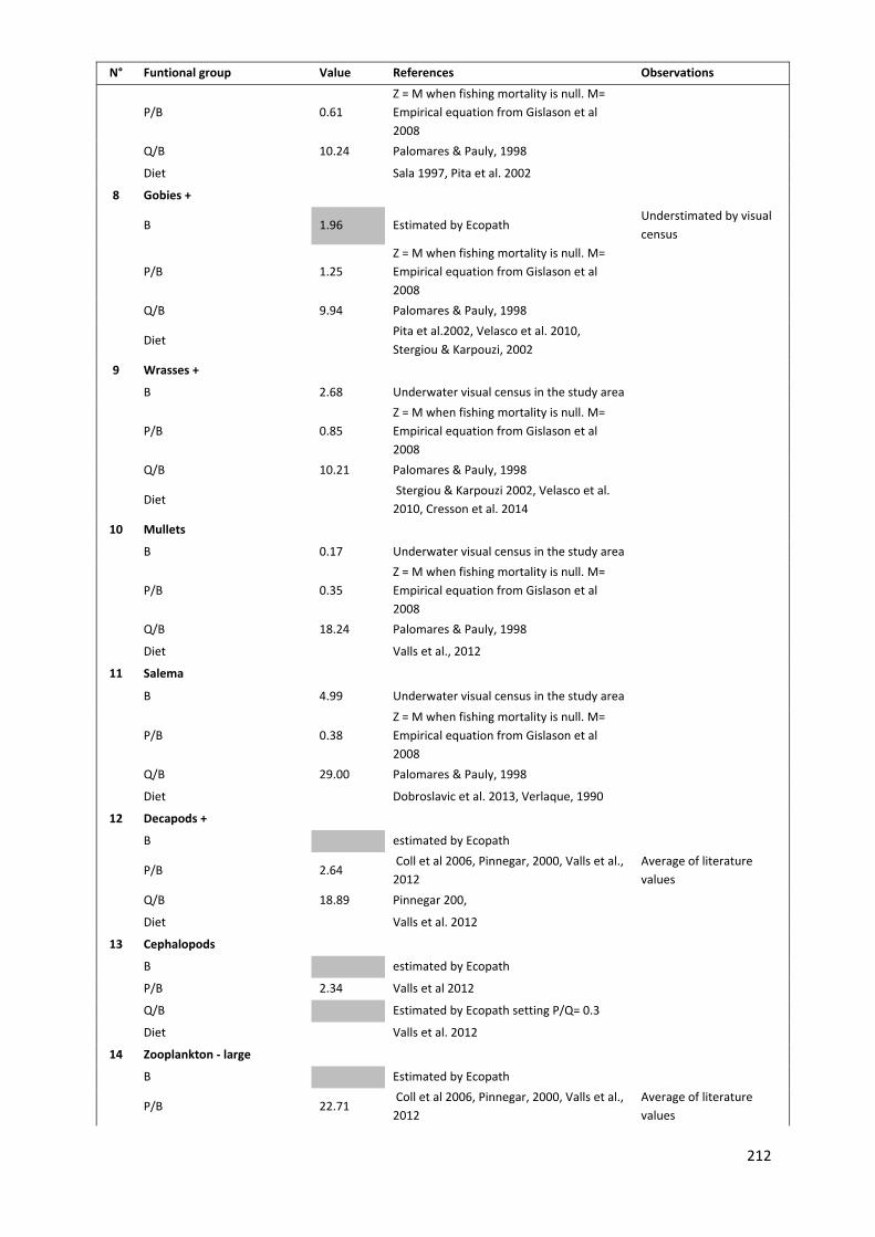
212  

N°  Funtional group  Value  References  Observations 

   P/B  0.61 

Z = M when fishing mortality is null. M= 

Empirical equation from Gislason et al 

2008  

  

   Q/B  10.24  Palomares & Pauly, 1998    

   Diet  Sala 1997, Pita et al. 2002     

8  Gobies +    

   B  1.96  Estimated by Ecopath Understimated by visual 

census 

   P/B  1.25 

Z = M when fishing mortality is null. M= 

Empirical equation from Gislason et al 

2008  

  

   Q/B  9.94  Palomares & Pauly, 1998    

   Diet  

Pita et al.2002, Velasco et al. 2010, 

Stergiou & Karpouzi, 2002   

9  Wrasses +    

   B  2.68  Underwater visual census in the study area    

   P/B  0.85 

Z = M when fishing mortality is null. M= 

Empirical equation from Gislason et al 

2008  

  

   Q/B  10.21  Palomares & Pauly, 1998    

   Diet  

 Stergiou & Karpouzi 2002, Velasco et al. 

2010, Cresson et al. 2014   

10  Mullets    

   B  0.17  Underwater visual census in the study area    

   P/B  0.35 

Z = M when fishing mortality is null. M= 

Empirical equation from Gislason et al 

2008  

  

   Q/B  18.24  Palomares & Pauly, 1998    

   Diet  Valls et al., 2012    

11  Salema     

   B  4.99  Underwater visual census in the study area    

   P/B  0.38 

Z = M when fishing mortality is null. M= 

Empirical equation from Gislason et al 

2008  

  

   Q/B  29.00  Palomares & Pauly, 1998    

   Diet  Dobroslavic et al. 2013, Verlaque, 1990    

12  Decapods +    

   B     estimated by Ecopath    

   P/B  2.64  Coll et al 2006, Pinnegar, 2000, Valls et al., 

2012 

Average of literature 

values 

   Q/B  18.89  Pinnegar 200,     

   Diet  Valls et al. 2012     

13  Cephalopods    

   B     estimated by Ecopath    

   P/B  2.34  Valls et al 2012    

   Q/B     Estimated by Ecopath setting P/Q= 0.3   

   Diet  Valls et al. 2012     

14  Zooplankton ‐ large    

   B     Estimated by Ecopath    

   P/B  22.71  Coll et al 2006, Pinnegar, 2000, Valls et al., 

2012 

Average of literature 

values 

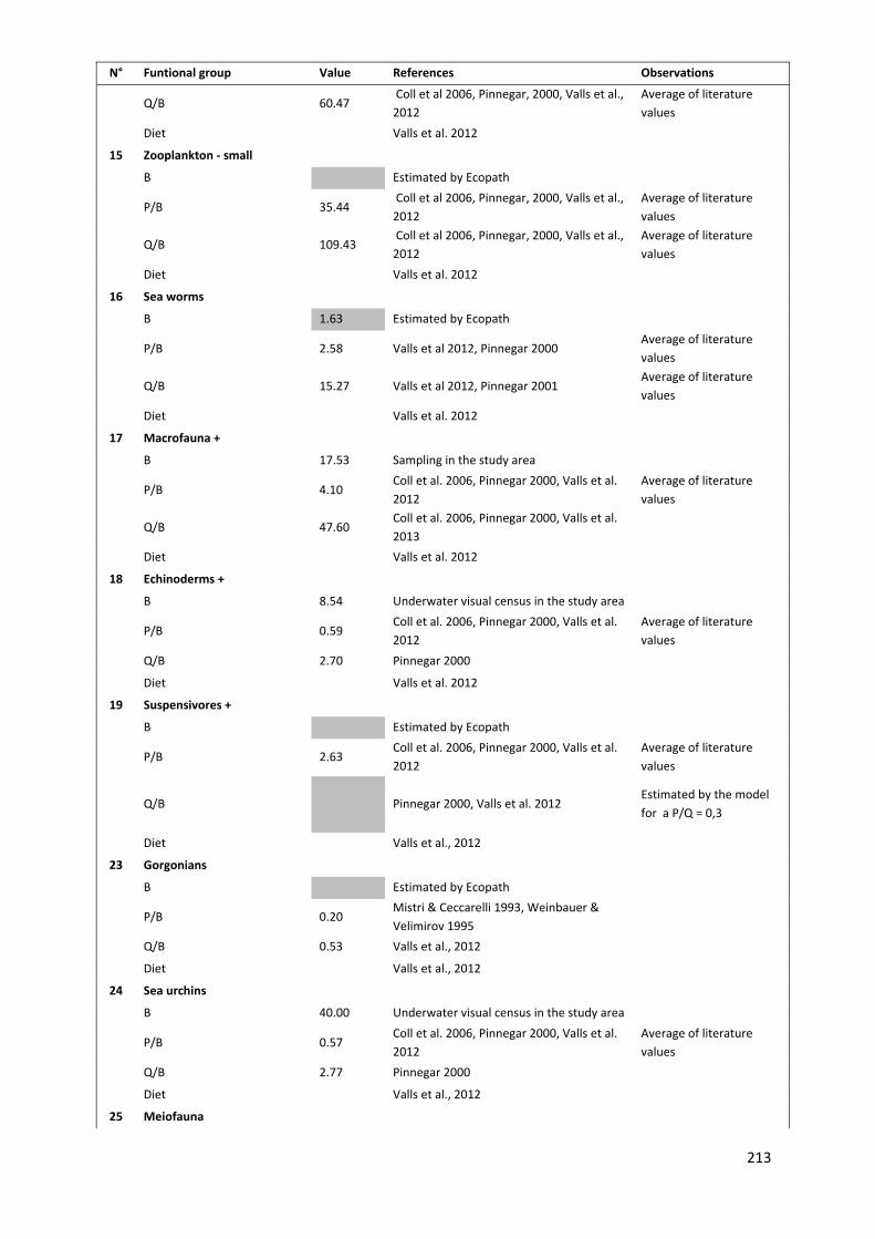
213  

N°  Funtional group  Value  References  Observations 

   Q/B  60.47  Coll et al 2006, Pinnegar, 2000, Valls et al., 

2012 

Average of literature 

values 

   Diet  Valls et al. 2012     

15  Zooplankton ‐ small    

   B     Estimated by Ecopath    

   P/B  35.44  Coll et al 2006, Pinnegar, 2000, Valls et al., 

2012 

Average of literature 

values 

   Q/B  109.43  Coll et al 2006, Pinnegar, 2000, Valls et al., 

2012 

Average of literature 

values 

   Diet  Valls et al. 2012     

16  Sea worms    

   B  1.63  Estimated by Ecopath    

   P/B  2.58  Valls et al 2012, Pinnegar 2000 Average of literature 

values 

   Q/B  15.27  Valls et al 2012, Pinnegar 2001 Average of literature 

values 

   Diet  Valls et al. 2012     

17  Macrofauna +    

   B  17.53  Sampling in the study area    

   P/B  4.10 Coll et al. 2006, Pinnegar 2000, Valls et al. 

2012  

Average of literature 

values 

   Q/B  47.60 Coll et al. 2006, Pinnegar 2000, Valls et al. 

2013   

   Diet  Valls et al. 2012     

18  Echinoderms +    

   B  8.54  Underwater visual census in the study area    

   P/B  0.59 Coll et al. 2006, Pinnegar 2000, Valls et al. 

2012  

Average of literature 

values 

   Q/B  2.70  Pinnegar 2000    

   Diet  Valls et al. 2012     

19  Suspensivores +    

   B     Estimated by Ecopath    

   P/B  2.63 Coll et al. 2006, Pinnegar 2000, Valls et al. 

2012  

Average of literature 

values 

   Q/B     Pinnegar 2000, Valls et al. 2012  Estimated by the model 

for  a P/Q = 0,3  

   Diet  Valls et al., 2012    

23  Gorgonians    

   B     Estimated by Ecopath    

   P/B  0.20 Mistri & Ceccarelli 1993, Weinbauer & 

Velimirov 1995   

   Q/B  0.53  Valls et al., 2012    

   Diet  Valls et al., 2012     

24  Sea urchins     

   B  40.00  Underwater visual census in the study area    

   P/B  0.57 Coll et al. 2006, Pinnegar 2000, Valls et al. 

2012  

Average of literature 

values 

   Q/B  2.77  Pinnegar 2000    

   Diet  Valls et al., 2012     

25  Meiofauna    

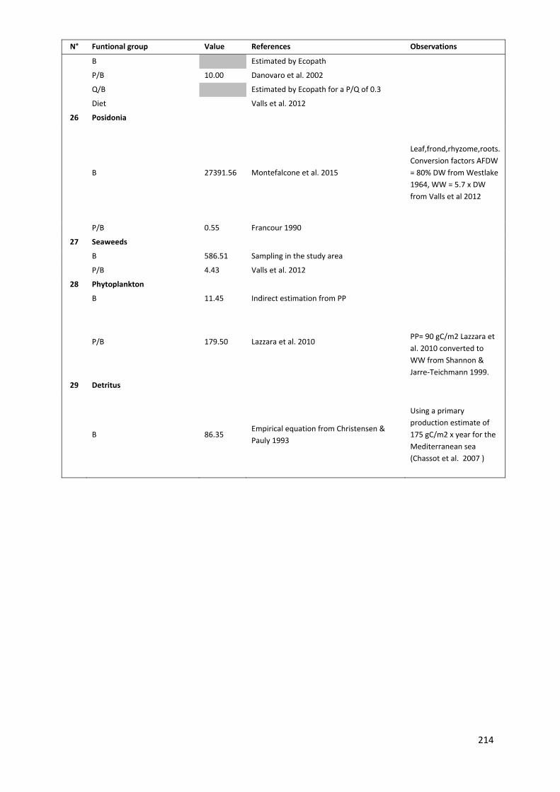
214  

N°  Funtional group  Value  References  Observations 

   B     Estimated by Ecopath    

   P/B  10.00  Danovaro et al. 2002    

   Q/B     Estimated by Ecopath for a P/Q of 0.3    

   Diet  Valls et al. 2012    

26  Posidonia    

   B  27391.56  Montefalcone et al. 2015 

Leaf,frond,rhyzome,roots. 

Conversion factors AFDW 

= 80% DW from Westlake 

1964, WW = 5.7 x DW 

from Valls et al 2012 

   P/B  0.55  Francour 1990    

27  Seaweeds    

   B  586.51  Sampling in the study area    

   P/B  4.43  Valls et al. 2012     

28  Phytoplankton    

   B  11.45  Indirect estimation from PP    

   P/B  179.50  Lazzara et al. 2010 PP= 90 gC/m2 Lazzara et 

al. 2010 converted to 

WW from Shannon & 

Jarre‐Teichmann 1999. 

29  Detritus    

   B  86.35 Empirical equation from Christensen & 

Pauly 1993 

Using a primary 

production estimate of 

175 gC/m2 x year for the 

Mediterranean sea 

(Chassot et al.  2007 ) 

215  

Tab. 3 MTI sensitivity analysis. Bright green cells: effects with high confidence percentage (>95%); medium green cells: [95–75[; pink cells: [75–50[; red cells: <50% 

(this means the average sign from the sensitivity analysis is opposed to the one of the original MTI matrix). 

Amberjack & dentex +

Dusky grouper ‐ large

Dusky grouper ‐ 

medium

Dusky grouper ‐ sm

all

Large‐scaled 

scorpionfishes +

Scorpionfishes & 

combers +

Stripped red m

ullets +

Sand smelts +

Diplodus +

Gobies +

Wrasses +

Mullets

Salema ‐ juveniles

Salema ‐ adults

Decapods +

Cephalopods

Zooplankton ‐ large

Zooplankton ‐ small

Sea worm

s

Macrofauna +

Echinoderm

s +

Suspensivores +

Gorgonians

Sea urchins 

Meiofauna

Posidonia

Seaw

eeds

Phytoplankton

Detritus

Amberjack & dentex + 100 100 98.4 100 100 100 92.9 100 100 98.6 90.2 99 100 100 83.3 100 100 100 100 91.3 100 100 100 100 95.1 99.8 100 99 100

Dusky grouper ‐ large 100 100 100 100 56.6 100 100 99.5 99.8 91.7 100 83 100 100 100 100 99.9 97.6 60.7 98.7 99.9 99.8 99.9 99.9 39.3 99.7 66.7 100 96.4

Dusky grouper ‐ medium 100 98.9 100 100 99.1 100 100 82.8 99.6 99.8 100 96.3 100 100 52.5 45.8 82.2 58.7 50.1 99.9 100 99.8 99.7 99.7 63.1 45.8 51.4 83.9 46.7

Dusky grouper ‐ small 100 100 96.8 100 52.1 100 100 100 100 100 74.7 100 100 100 91.3 100 100 100 98.1 92.3 100 100 100 100 100 100 100 100 100

Large‐scaled scorpionfishes + 100 100 100 99.5 100 100 100 100 100 99.1 100 86.7 64.8 100 90.4 100 100 100 100 99.6 63.4 100 100 100 100 100 100 100 100

Scorpionfishes & combers + 88.4 100 99.8 72.4 85.9 100 100 100 95.6 100 100 99.3 75.2 99.4 97.9 100 100 100 93.2 100 100 100 100 100 100 100 100 100 100

Stripped red mullets  + 100 100 80.7 97 100 44.7 100 100 100 100 70.9 99.6 97 99.2 100 100 100 100 57.4 99.8 100 95.6 100 77.1 98.5 99.9 100 100 100

Sand smelts  + 100 99.4 100 99.4 60.4 100 100 100 100 91.1 100 100 100 100 100 75.9 100 100 100 100 99.7 99.9 86.7 100 100 99.8 72.5 100 99.9

Diplodus + 100 100 100 71.1 100 73.9 100 100 100 87.4 100 100 100 100 100 100 100 100 100 64.6 100 100 100 100 100 100 100 93 100

Gobies  + 100 100 95.2 85.7 92.2 100 99.9 94.3 95.1 100 99.8 99.9 74.7 100 100 100 84.7 85.2 100 100 100 99.8 61.5 100 100 100 97.1 100 100

Wrasses + 100 100 87.2 100 100 49.9 100 100 100 100 100 100 100 100 99 100 85.9 100 50.1 100 100 99.5 100 100 100 100 100 100 100

Mullets 100 100 100 28.2 100 80.8 100 100 76.6 100 99.4 100 97.9 100 100 94 100 100 100 86.6 99.4 65.7 92.7 62 99.9 88.3 100 100 100

Salema  ‐ juveniles 100 100 100 100 100 100 100 100 100 100 98.9 100 100 100 99.7 99.2 100 69.7 100 100 100 100 100 100 100 100 100 100 100

Salema  ‐ adults 98.3 100 100 99.3 100 70.6 99.8 100 100 100 88.7 39.4 78.7 100 100 100 100 99.9 99.7 100 100 99 100 100 100 100 100 81.5 100

Decapods  + 100 100 100 100 100 100 100 100 100 100 100 100 100 95.7 100 100 74.6 66.5 90.4 100 100 100 100 100 100 100 100 100 100

Cephalopods 100 100 100 99.1 100 98.1 85.5 100 100 87.7 100 100 100 100 100 100 100 100 99.8 77.7 100 100 100 100 47.1 99.9 100 100 100

Zooplankton ‐ large 94.7 100 100 99.6 100 100 100 100 66.6 94.8 99.3 100 100 100 100 100 100 100 100 100 100 100 100 99.2 100 100 98.6 100 74.1

Zooplankton ‐ small 93.4 100 100 100 74 99.4 99.9 100 100 100 99.7 100 100 100 100 100 100 100 57.8 74.9 76.8 100 100 100 100 98.1 100 100 80.5

Sea  worms 97.1 74.7 99.9 99.2 92.6 97.8 100 98.5 100 100 96.4 99.9 99.9 100 88 64.2 100 100 100 100 100 100 65.4 78.1 99.9 100 99.4 100 100

Macrofauna  + 74.6 99.6 89 100 97.5 53.8 98.4 100 100 100 100 100 53.2 100 100 100 87.1 100 100 100 100 100 100 100 100 100 100 100 100

Echinoderms + 100 100 100 100 100 100 100 88.3 99.2 60.3 100 100 99 100 100 79.1 100 100 98.6 100 100 100 100 100 100 100 100 72.6 100

Suspensivores + 100 100 100 50.8 100 98 66 84.6 100 100 89.6 87.4 100 100 96.7 100 100 100 99 96.3 53.5 100 100 100 100 100 100 100 99.1

Gorgonians 99.9 100 100 100 85.1 95.7 100 100 100 100 100 100 100 100 100 100 100 100 100 99.5 100 100 100 100 100 100 100 89.9 100

Sea  urchins   90.5 98.9 100 100 100 100 100 100 96.4 82.6 100 100 100 100 100 54.7 100 100 100 100 99.8 100 45.1 100 99.1 100 100 100 100

Meiofauna 94 100 100 100 100 100 100 94.7 90.5 100 95.6 100 100 60.7 100 99.3 98.7 100 100 97.5 100 99.9 100 99.6 100 94.4 72.6 100 100

Posidonia 74.4 100 100 100 100 100 100 100 76.2 98.7 100 100 100 100 100 100 62.6 79.5 97.5 100 100 96 100 100 100 100 100 99.7 100

Seaweeds 95 100 100 100 100 98.9 56.7 100 94.9 100 99.6 99.8 100 100 100 99.4 63.5 91.5 100 100 53.8 100 74.7 100 97.3 100 100 99.9 99

Phytoplankton 98.3 100 100 100 97.8 54.9 100 100 100 100 59 100 100 99.3 98 95.7 100 100 100 96.4 97 100 100 100 99.1 99.9 100 100 98.8

Detritus 77.3 100 100 100 100 100 100 90 100 100 97.5 100 100 100 100 98.4 86.9 100 100 99.8 100 100 100 100 100 99.9 100 100 100

216  

Annex references Anastasopoulou A, Mytilineou C, Lefkaditou E, Kavadas S, Bekas P, Smith CJ,

Papadopoulou KN, Christides G (2013) The diet and feeding ecology of Conger conger (L. 1758) in the deep waters of the Eastern Ionian Sea. Mediterr Mar Sci 14

Badalamenti F, D’Anna G, Lopiano L, Scilipoti D, Mazzola A (1995) Feeding habits of young-of-the-year greater amberjack Seriola dumerili (Risso, 1810) along the N/W Sicilian Coast. Sci Mar 59:317–323

Barreiros JP, Santos RS, Borba AES (2002) Food habits, schooling and predatory behaviour of the Yellowmouth Barracuda, Sphyraena viridensis Cuvier, 1829 (Perciformes: Sphyraenidae) in the Azores. Cybium 26(8):83-88

Bavestrello G, Bo M, Bertolino M, Betti F, Cattaneo-Vietti R (2014) Long-term comparison of structure and dynamics of the red coral metapopulation of the Portofino Promontory (Ligurian Sea): a case-study for a Marine Protected Area in the Mediterranean Sea. Mar Ecol

Blanco C, Salomón O, Raga JA (2001) Diet of the bottlenose dolphin (Tursiops truncatus) in the western Mediterranean Sea. J Mar Biol Assoc UK 81:1053–1058

Chassot E, Mélin F, Le Pape O, Gascuel D (2007) Bottom-up control regulates fisheries production at the scale of eco-regions in European seas. Marine Ecology Progress Series 343:45–55

Christensen V, Pauly D (1993) Trophic Models of Aquatic Ecosystems. The WorldFish Center

Coll M, Palomera I, Tudela S, Sardà F (2006) Trophic flows, ecosystem structure and fishing impacts in the South Catalan Sea, Northwestern Mediterranean. J Mar Syst 59:63–96

Cresson P, Ruitton S, Ourgaud M, Harmelin-Vivien M (2014) Contrasting perception of fish trophic level from stomach content and stable isotope analyses: A Mediterranean artificial reef experience. J Exp Mar Biol Ecol 452:54–62

Dance C, Kuiper N (1987) Size weight relations in the sea urchin Sphaerechinus granularis in Port-Cros island (Var, French Mediterranean). Colloque international sur Paracentrotus lividus et les oursins comestibles. Gis Posidonie. Faculté des Sciencies de Luminy. Marseille.

Danovaro R, Gambi C, Mirto S, others (2002) Meiofaunal production and energy transfer efficiency in a seagrass Posidonia oceanica bed in the western Mediterranean. Mar Ecol Prog Ser 234

De Jong, S.A, Haufman, PAG., Sandee AJJ. and Nienhuis PH, 1991. Community oxygen budgets on seagrass beds and microbial mats on the Banc d’Arguin, Mauritania, p. 67-68. In: PMJ. Herman and CHR. Heip (eds.) Report on the workshop, ‘Modeling the benthos’, Yerseke, The Netherlands, 20-22 March 1991. Delta Institute for Hydrobiological Research, Yerseke

Dobroslavić T, Zlatović A, Bartulović V, Lučić D, Glamuzina B (2013) Diet overlap of juvenile salema ( Sarpa salpa ), bogue ( Boops boops ) and common two-banded sea bream ( Diplodus vulgaris ) in the south-eastern Adriatic. J Appl Ichthyol 29:181–185

Francour P (1990) Dynamique de l'écosystème à Posidonia oceanica dans le Parc National de Port-Cros.Analyse des compartiments matte, litière, faune vagile, échinodermes et poissons. Doctorat, Université Pierre et Marie Curie, Paris

Gislason H, Daan N, Rice J, Pope J (2008) Does natural mortality depend on individual size. ICES CM

217  

Karpouzi VS, Stergiou KI (2003) The relationships between mouth size and shape and body length for 18 species of marine fishes and their trophic implications. J Fish Biol 62:1353–1365

Matic-Skoko S, Tutman P, Marcejla E, Skaramuca D, \DJikic D, Lisicic D, Skaramuca B (2010) Feeding habits and trophic status of Mediterranean moray eel, Muraena helena L., 1758 in the Adriatic Sea—preliminary approach. Rapp Comm Int Pour Mer Méditerranée 39:583

Mistri M, Ceccherelli VU (1994) Growth and secondary production of the Mediterranean gorgonian Paramuricea clavata. Mar Ecol-Prog Ser 103:291–291

Montefalcone M, Vassallo P, Gatti G, Parravicini V, Paoli C, Morri C, Bianchi CN (2015) The exergy of a phase shift: Ecosystem functioning loss in seagrass meadows of the Mediterranean Sea. Estuar Coast Shelf Sci 156:186–194

Morales-Nin B, Moranta J (1997) Life history and fishery of the common dentex (Dentex dentex) in Mallorca (Balearic Islands, western Mediterranean). Fish Res 30:67–76

Mostarda E, Campo D, Castriota L, Esposito V, Scarabello MP, Andaloro F (2007) Feeding habits of the bullet tuna Auxis rochei in the southern Tyrrhenian Sea. J Mar Biol Assoc UK 87:1007

O’Gorman EJ, Emmerson MC (2009) Perturbations to trophic interactions and the stability of complex food webs. Proceedings of the National Academy of Sciences 106:13393–13398

Pais A, Chessa LA, Serra S, Ruiu A, Meloni G, Donno Y (2007) The impact of commercial and recreational harvesting for Paracentrotus lividus on shallow rocky reef sea urchin communities in North-western Sardinia, Italy. Estuarine, Coastal and Shelf Science 73:589–597

Palomares MLD, Pauly D (1998) Predicting food consumption of fish populations as functions of mortality, food type, morphometrics, temperature and salinity. Mar Freshw Res 49:447–453

Palomares Ld, Pauly D (2004) West African Ecosystems. Fish Cent Res Rep 12:4 Pinnegar JK, Polunin NVC (2000) Contributions of stable-isotope data to elucidating

food webs of Mediterranean rocky littoral fishes. Oecologia 122:399–409 Pita C, Gamito S, Erzini K (2002) Feeding habits of the gilthead seabream (Sparus

aurata) from the Ria Formosa (southern Portugal) as compared to the black seabream (Spondyliosoma cantharus) and the annular seabream (Diplodus annularis). J Appl Ichthyol 18:81–86

Relini G, Relini M, Torchia G, De Angelis G (2002) Trophic relationships between fishes and an artificial reef. ICES J Mar Sci J Cons 59:S36–S42

Robinson LA, Greenstreet SPR, Reiss H, Callaway R, Craeymeersch J, Boois I de, Degraer S, Ehrich S, Fraser HM, Goffin A, Kröncke I, Jorgenson LL, Robertson MR, Lancaster J (2010) Length–weight relationships of 216 North Sea benthic invertebrates and fish. Journal of the Marine Biological Association of the United Kingdom 90:95

Rogdakis Y, Ramfos A, Koukou K, Dimitriou E, Katselis G (2010) Feeding habits and trophic level of sea bass (Dicentrarchus labrax) in the Messolonghi-Etoliko lagoons complex (Western Greece). J Biol Res 13:13–26

Sala E (1997) Fish predators and scavengers of the sea urchin Paracentrotus lividus in protected areas of the north-west Mediterranean Sea. Mar Biol 129:531–539

Scheibling RE, Lawrence JM (1982) Differences in reproductive strategies of morphs of the genus Echinaster (Echinodermata: Asteroidea) from the Eastern Gulf of Mexico. Marine Biology 70:51–62

218  

Shannon LJ, Jarre-Teichmann A (1999) A model of trophic flows in the northern Benguela upwelling system during the 1980s. South Afr J Mar Sci 21:349–366

Stergiou KI, Karpouzi VS (2001) Feeding habits and trophic levels of Mediterranean fish. Rev Fish Biol Fish 11:217–254

Valls A, Gascuel D, Guénette S, Francour P (2012) Modeling trophic interactions to assess the effects of a marine protected area: case study in the NW Mediterranean Sea. Mar Ecol Prog Ser 456:201–214

Velasco EM, Gómez-Cama MC, Hernando JA, Soriguer MC (2010) Trophic relationships in an intertidal rockpool fish assemblage in the gulf of Cádiz (NE Atlantic). J Mar Syst 80:248–252

Verlaque M (1990) Relations entre Sarpa salpa (Linnaeus, 1758)(Téléostéen, Sparidae), les autres poissons brouteurs et le phytobenthos algal méditerranéen. Oceanol Acta 13:373–388

Weinbauer M, Velimirov B (1995) Biomass and secondary production of the temperate gorgonian coral Eunicella cavolini (Coelenterata:Octocorallia). Mar Ecol Prog Ser 121:211–216

Westlake DF (1964) Light extinction, standing crop and photosynthesis within weed beds.

219  

8 General discussion  

8.1 The initial questions

Centuries of selective fishing on high trophic level predators (HTLP) caused a

gradual simplification of Mediterranean food-webs, which are nowadays mostly

controlled by smaller and lower trophic level species (Sala et al. 2004). The depletion

of HTLP affected the overall stability of Mediterranean ecosystem and reduced its

resilience to human impacts (Coll et al. 2008, Britten et al. 2014). The protection from

fishing within MPAs allowed to trigger a recovery in HTLP abundance and biomass,

but long time frames are needed in order to re-establish lost trophic interactions and

ecosystem functions (Sala et al. 2012, Guidetti et al. 2014). Long-term monitoring of

both HTLP and trophic interactions is thus essential to assess if MPAs are effectively

promoting an overall ecosystem recovery and to adapt management consequently.

This PhD aimed at evaluating and proposing effective and operational management-

tools to: Q1) effectively monitor high trophic level predators recovery, Q2) unravel

and monitor trophic interactions and Q3) quantify fishing impacts upon HTLP and

associated food-webs within Mediterranean MPAs.

 

8.2 Main results

The chapters of this thesis developed interconnected steps necessary to pursue the

final management-oriented objectives, and provided at the same time results that

further elucidate the important functional role of HTLP in marine ecosystems and the

state of their recovery in MPAs. We will summarise here the main outcomes of each

section of the thesis: field monitoring and food web modelling.

Underwater visual census (UVC) to survey high trophic level predators

Results from our literature analysis (Chapter 3) highlighted that UVC transects are by

far the most commonly adopted technique to survey fish communities in the

Mediterranean. Compared with other methods, such as video – UVC, transects

provide the most complete quantitative description of the fish assemblage, detecting

the highest number of species and allowing to measure several variables (i.e.

density, size), at the lower economic and time costs. They are thus better suited for

the regular monitoring activities of coastal Mediterranean MPAs, where the

220  

quantification of fish density and biomass is necessary to assess the efficiency of

protection. Despite the success of transect UVC across the Mediterranean however,

standardization in transect surface is not yet achieved, with more than 50% of the

analysed studies that aimed at surveying the whole fish assemblage, differing for the

adopted transect sizes. Different transect size can affect the efficiency of the method

in detecting a given species, according to its behaviour and mobility (Cheal &

Thompson 1997, Kulbicki 1998, Bozec et al. 2011). On one hand thus,

standardisation is needed, since comparisons of density or biomass values obtained

with different transect width for the same species could be biased. On the other

hand, different transect widths should be applied to survey fish species differing for

mobility and behaviour (Harmelin-Vivien et al. 1985, Bozec et al. 2011). This is

seldom done in the Mediterranean, where the same transect width has been always

used to survey both large mobile fish and less mobile necto-benthic fish (Chapter 3).

This evidence encouraged us to evaluate if transects of larger dimensions than those

most commonly adopted across the Mediterranean (25 x 5 m), would better account

for the behaviour of large mobile and shy predators (often corresponding to HTLP),

that seldom allow the observer to approach at such short distance. Results from our

field comparison (Chapter 4) showed that within MPAs large size transects (20 x 35

m) provided more accurate density and biomass estimates for large mobile and shy

fish than medium transects (5 x 25 m), allowing to reduce under-estimation bias due

to the common avoidance behaviour of these fish. Precision of density and biomass

estimates tended to be lower when large transects were used within MPAs, because

more rare and shy species or species with shoaling behaviour (i.e, Mycteroperca

rubra, Epinephelus costae, Sphyraena viridensis) were detected. The choice of the

transect size to be adopted should thus balance the trade-offs of detecting higher

number of species, while achieving lower precision.

Following these results we opted for the combination of three transect sizes (20 x 35

m, 5 x 25 m and 1 x 10 m), adapted respectively to large mobile predators, necto-

benthic fish and small crypto-benthic fish, to survey the whole fish assemblage at

three Mediterranean MPAs. We evidenced a significant effect of protection on HTLP,

whose response in terms of increased biomass within the MPA was always higher in

magnitude than that of other functional groups. Trophic pyramids differed within and

outside MPAs in terms of relative contribution of each functional group to total fish

biomass, with HTLP displaying the largest inside vs outside biomass ratios. This was

221  

especially marked at older and highly enforced MPAs (Cabo de Palos, Spain, and

Scandola, Corsica-France), suggesting this metric as an effective indicator of HTLP

recovery.

In the context of monitoring the recovery of HTLP within MPAs, detecting higher

density, biomass and species number for this group should be the priority in the

selection of a UVC method. In light of our results we suggested that the combination

of large, medium and small transect sizes (respectively for large mobile fish, necto-

benthic fish and cryptic fish) in monitoring programs is a simple improvement to

traditional one-size transect surveys, allowing to increase the accuracy of total fish

assemblage estimates within MPAs, and should thus be considered to assess

recovery of HTLP in relation to total fish biomass.

The trophic re-organization we observed caused by the large increase of HTLP within

MPAs, is likely to affect the ecosystem functions (Soler et al. 2015). Food-web

modelling allows to unravel trophic interactions and to dig deeper on the effects of

protection/exploitation on ecosystem functions (Libralato et al. 2010, Plagányi et al.

2014). If the process of model building is simplified and standardised while kept

reliable, food-web models can be effective tools for an ecosystem based

management in MPAs.

Food web modelling

The second section of this PhD was introduced by a theoretical modelling exercise

(Chapter 5) where, starting from the most detailed model available for a

Mediterranean MPA (Port Cros, Valls et al. 2012), we identified an optimal level of

functional groups aggregations which was the best compromise between model

complexity, feasibility of model construction in terms of data collection, and reliability

of model outputs. In particular the aggregation of several benthic taxa sharing similar

predators into one unique macrofaunal group, allows for a substantial simplification in

the data collection process, without significantly affecting model outputs. We also

identified the key functional groups for which small variations in input biomass data

mostly influenced model outputs. These include high trophic level predators, species

with a high level of connections in the trophic network such as macrofauna and

decapods and primary producers generally present in high biomasses in the

Mediterranean, such as Posidonia oceanica. We concluded that local and accurate

222  

biomass data should be collected in priority for these groups when developing food-

web models for similar Mediterranean ecosystems.

This model structure was then applied to two case studies representative of

Mediterranean data-availability: the older and relatively data rich Portofino MPA

(Chapter 6) and the more recently established and data-poor Cap Roux fishery

reserve (Chapter 7). Model structure was kept standard in terms of species

aggregation into functional groups, but necessarily had to be adapted to the local

conditions of each case study, by adding or deleting functional groups depending on

their presence or absence at each MPA.

The Portofino MPA food-web model allowed to identify the HTLP groups

Epinephelus marginatus, Amberjack&dentex+ (including Dentex dentex, Seriola

dumerili, Sphyraena viridensis, Dicentrarchus labrax, Muraena helena, Conger

conger) and Large scaled scorpionfish+ (Scorpaena scrofa, Sciaena umbra, Labrus

merula, Labrus viridis, Pagrus pagrus and Phycis phycis) as keystone species in the

food-web, followed by Cephalopods. At the same time, a strong fishing pressure was

highlighted on Amberjack&dentex+ and Large scaled scorpionfish+, which were thus

considered “sentinel species”, i.e species combining high ecological importance and

highly fishing pressure in the ecosystem under study, that should thus be prioritised

for monitoring and could be “anchor points’ for the definition of management actions

that deserve to be taken (ex. to calculate the reduction of fishing mortality needed to

attain predefined conservation objectives) and for the assessment of their efficiency.

The interacting impacts of artisanal and recreational fishing were unravelled showing

that HTLP were mostly threatened by the recreational fishing, which also had the

widest effect on the food-web. The ecosystem was far from reaching carrying

capacity for HTLP, whose biomass could still increase of 44 %, confirming the high

sensitivity of this group to fishing and thus also to protection measures. According to

model results, additionally, measures aiming at forbidding recreational fishing would

not only benefit the ecosystem by increasing HTLP biomass (24%), but would also

increase the mean trophic level (and thus the quality) of the catch of the artisanal

fishery. Artisanal fishing alone reduced the biomass of HTLP by less than 15% and

could instead be maintained with a moderate impact on the ecosystem.

Overall, some useful insights for MPA management were derived from this study:

limiting recreational fishing effort for example would allow the MPA to pursue both its

223  

conservation and socio-economic development targets, by i) reducing the impact on

HTLP and thus encouraging their further recovery within the MPA, whose carrying

capacity is far to be reached ii) increasing the availability of catches at higher trophic

levels for artisanal fishing, thus providing economic benefits to this naturally-declining

traditional fishing activity.

Despite the uncertainties associated with some input biomass and fishing data,

extensive sensitivity analysis through recently developed routines (Data-reli toolbox,

Lassalle et al 2014 and pre-balancing rules, Link 2010) and the comparison of

alternative models with varying input data, allowed to increase the confidence in

model results.

Modelling the food-web associated with the Cap roux fishery reserve (Chapter

7) also allowed to identify HTLP (Amberjack&dentex+ group and E. marginatus) as

well as cephalopods as keystones groups in the ecosystem, further stressing the

need for monitoring these species. No biological data was available on the area, thus

input biomass data was collected on the field, prioritising the functional groups

identified in Chapter 5, for which imprecise biomass data can widely affect model

outputs. Cost and effort analysis on the full process of model construction pointed out

where it would be advisable to invest, in order to increase model quality cost-

efficiently: rather than concentrating effort and resources onto macrofauna sampling,

for instance, at least in the first place it would be more advisable to invest in sampling

effort for HTLP, as well as decapods and cephalopods. The two latter groups are

very seldom included in MPAs monitoring programs, despite their ecological and

economical importance, being targets of both artisanal and recreational fishing.

(Piatkowski et al. 2001, Goñi et al. 2006, Wagner 2008). It would be thus worth to

establish appropriate monitoring surveys for these groups, which would allow more

comprehensive assessments of the effects of protection, while providing valuable

data for modelling. Excluding sampling for macrofauna, the average estimate for

model development costs for an area of 145 ha totalled 26 700 €, including field data

collection for fish and mobile mega-invertebrates (decapods, cephalopods and

echinoderms), data analysis and model building. If monitoring programs are already

in place in an MPA and thus data is already available, model building (data

integration and analysis) would require an investment of ca 4 200 €, i.e. less than 1/6

of the previous amount.

224  

8.3 Further discussion and perspectives  

Making food-web models operational in MPAs

By providing a standard model structure and identifying the most sensitive groups for

which local biomass data should be collected in priority (Chapter 5), we aimed at

simplifying the process of model development and encouraging its application within

MPAs. However, other sources of uncertainty were not addressed in this manuscript.

While reviewing the literature of Mediterranean models for our analysis (Chapter 5)

we noted that not only biomass is often not locally estimated, but also other required

input parameters are often derived from the literature, such as diet compositions, or

P/B and Q/B ratios for invertebrate groups. Local studies providing estimates for

these parameters are indeed very rare and this often causes circular referencing

among models, eventually leading to a literature source which often pertains to

another time period and a far-away and different ecosystem. These uncertain input

data could bias the biomass estimates of groups for which local data is not available

or cannot be measured in the field, and that are thus obtained from the model mass-

balance equations (Morissette 2007, Lassalle et al. 2014). For instance, in Chapter 7

we evidenced how data collected in the field for some groups (macrofauna,

cephalopods and decapods) did not provide realistic values to feed the model, and

more sampling effort would have been needed to increase quality of these data, at

very high costs for some groups. When comparing our values, we evidenced that in

other studies from coastal Mediterranean macrofaunal biomass was always

estimated by the model. In each study, moreover, P/B, Q/B and diet compositions of

many groups feeding on macrofauna were often derived from other models, often

relative to other areas of the Mediterranean or even further away.

On one hand, it is paramount that models are grounded on local data. They have the

important function of highlighting eventual inconsistencies in such data, and can

serve to encourage the upgrading of estimates. Investing on data collection and

monitoring is thus needed (Carstensen 2014). However, it shall also be

acknowledged that obtaining local estimates for all parameters and groups is often

not feasible and that costs to increase data quality for some groups can be very high

in a management perspective. Alternative solutions can be those of 1) simplifying

and standardising model structure and use models to identify groups for which local

biomass should be collected in priority, as we did (Chapter 5) 2) developing a

225  

Mediterranean data-base with the most updated and reliable estimates for diets, P/B

and Q/B (the latter two especially for invertebrates, since empirical equations can be

used to derive these parameters for fish) to which modellers could refer as a start.

Christensen et al. (2009) provided guidelines to develop database-driven models of

large marine ecosystems starting from common default values of input parameters.

While they suggested to use the approach as a draft model for improvement, that

would make it easier to get started with the modelling process, they also cautioned

from the use of these models for management advice, stressing that, for such use,

models should be enriched with as much as finer scale data is available. For small-

scale models of Mediterranean MPAs high resolution data is essential, however, a

Mediterranean data-base to be used as a common reference for critical parameters

(very unlikely to be available locally) could help to further standardise the process of

model development, and would allow to isolate some of the sources of uncertainty

related with input data, eventually increasing models comparability. If, for instance, in

every MPA model developed with a standard structure, P/B, Q/B and diet were

derived from a common source, when models are compared the eventual differences

in the biomass of estimated groups would be more probably due to each MPA’s

particular environmental or management characteristics, than to a bias in model

structure and parameters. A Mediterranean database for these parameters would

also largely simplify the process of model construction, where a large amount of time

is spent in integrating and transforming data from different sources, allowing a large

gain in time and thus efficiency in a management perspective.

The complementarity of monitoring and modelling

Monitoring is an essential management tool per-se, allowing to assess if MPAs are

meeting the goals for which they have been designed, by detecting change in the

abundance and growth rate of species and communities of concern and evaluating

how well a reserve fulfils the goal of enhancing a local fishery. But data derived from

monitoring can also bridge the gap between field ecology and modelling. On one

hand, monitoring data can feed food-web models, needed to investigate issues that

cannot be addressed by field studies alone. On the other hand, food-web models can

help to identify priority targets for monitoring and to bring to light data gaps or

inconsistencies in local data, thus they can re-direct monitoring, in a feed-back loop

that shall be accordingly translated into adaptive management . Models developed in

226  

this study for instance, either built with newly collected data (Chapter 7) or with data

from past monitoring (Chapter 5 and 6), highlighted the keystone role of high trophic

level predators in the protected ecosystems (Valls et al. 2015). This further

emphasised the importance of monitoring HTLP and to obtain more accurate

estimates of their abundance and biomass in MPAs through appropriate non-

destructive techniques (Chapter 4). Additionally, in all the presented case studies,

food-web models agreed in assigning a keystone role to cephalopods, which are

often (or totally) overlooked when designing monitoring plans in the Mediterranean.

Cephalopods play an important functional role in both coastal and pelagic

ecosystems (Piatkowski et al. 2001, Coll et al. 2013), being a preferred prey for many

high trophic level predators, but also predators acting on a wide range of trophic

levels. Moreover, they are economically important artisanal and recreational fishing

targets. Studies are needed to assess their abundance and biomass in coastal areas,

appropriate non-destructive techniques should be identified and monitoring should be

implemented. Fishing pressure on this group should also be regularly monitored.

Finally, modelling can build upon monitoring data to develop ecosystem based

indicators, such as food-web indicators, as also required by the Marine Strategy

Framework Directive, in order to achieve the Good Environmental Status (Heymans

et al. 2014, Guesnet et al. 2015). In this view, MPAs and corresponding models could

be very useful to define targets for indicators and to provide reference values

corresponding to different conservation states. Indicators based on trophic levels, for

example, are increasingly being used to assess fisheries impact on the whole

ecosystem (Shannon et al. 2014) and modelling can serve to generate reference

values for indicators through dynamic simulations, which would need very long time

series if only monitoring data were used (Pelletier et al. 2008). In this perspective, a

further development of our study could be the application of the recently proposed

Apex Predator Indicator (API) and High Trophic Indicator (HTI) (Bourdaud et al.

2015). Both are trophic level based indicators centred on the proportion of apex

and/or high trophic level predators in the ecosystem, as a proxy for the good

functioning of the whole food web, and ecosystem-specific targets could be proposed

for each indicator through simulation (Bourdaud et al. 2015).

227  

Perspectives on food web models as operative ecosystem based management tools

in MPAs,

On the basis of the data we had strengthened by extensive sensitivity analysis, we

proved the potential of food-web models for MPAs management in i) identifying

keystone and sentinel species in the ecosystem ii) highlighting the MPA’s possible

carrying capacity for HTLP iii) unravelling the food-web consequences of variations in

HTLP biomass iv) advising for a reduction of recreational fishing effort on HTLP and

evaluating the impact of recreational fishing on artisanal fishing. 

If 1) exhaustive monitoring programs are implemented in MPAs, targeting both

biological resources but also, importantly, human impacts (local fisheries catches and

effort), and 2) food web modelling becomes a regular step to integrate data from

monitoring, the range of the possible management applications of food web models

developed with the EwE – EcoTroph - Ecospace package is extremely wide, and is in

continuous expansion (Coll et al. 2015). Here we provide some examples of possible

perspectives.

The spread of invasive species in the Mediterranean is widely recognised as a critical

threat to its biodiversity and ecosystem functioning and to the provision of ecosystem

services in this basin (Katsanevakis et al. 2014). Food web models could help to

address this issue, allowing to understand the role and impact of invasive species on

the food web and to analyse management scenarios (Arias-González et al. 2011)

Although the interest for this approach is growing (Coll et al. 2015), in the

Mediterranean applications are still scant.

EwE-Ecotroph models have been used in a couple of studies to assess biomass

spillover from MPAs (Valls et al. 2012, Colléter et al. 2014) and, in one study, to

quantify the contribution of an MPA to the trophic functioning and productivity of the

larger surrounding ecosystem (Guénette et al. 2014). MPAs are often very small in

the Mediterranean, it could be thus interesting to assess if extending their borders

could increase their contribution in terms of spillover to adjacent systems and also to

the total production and catches of the surrounding ecosystem. Through the dynamic

modules Ecosim and Ecospace, moreover, it is possible to explore the potential

effects on ecosystem structure and on fisheries production of alternative fisheries

management (and also climate change) scenarios, to model energy exchanges from

MPAs to external areas and to quantify MPAs impact on larger ecosystems. Finally, if

several MPA food-web models are developed, large-scale analysis could be carried

228  

out in Ecospace to assess the effects of different spatial configurations of MPAs

networks and/or different fisheries management scenarios on ecosystem structure,

functioning and fisheries production.

In order to fully exploit this high potential, MPAs should start integrating food-web

modelling as a regular tool in their management plan, using it in the first place to

direct monitoring and integrate data into a coherent picture of ecosystem functioning,

and then, once a reliable basis is set, to build upon this picture according to

management needs.

229  

8 Discussion Generale

8.1 Les questions initiales

Des siècles de pêche ciblant les prédateurs de haut niveau trophique (HTLP) ont

provoqué une simplification progressive de réseaux trophiques de Méditerranée,

avec un contrôle exercé aujourd'hui principalement par de petites espèces de plus

bas niveau trophique (Sala et al., 2004). L'épuisement des HTLP a affecté la stabilité

globale des écosystème méditerranéens et réduit sa capacité de résistance aux

impacts humains (Coll et al. 2008, Britten et al. 2014). L'interdiction de pêche dans

les AMP a favorisé une augmentation de l'abondance et de la biomasse des HTLP.

Toutefois, les délais nécessaires afin de rétablir les interactions trophiques perdues

et les fonctions des écosystèmes sont assez importants (Sala et al. 2012, Guidetti et

al. 2014). La surveillance à long terme des HTLP et des interactions trophiques est

donc essentielle pour apprécier si les AMP peuvent efficacement favoriser une

restauration globale de l'écosystème et adapter en conséquence leur gestion.

Cette thèse visait à évaluer et proposer des outils de gestion efficaces et

opérationnels pour : Q1) quantifier efficacement la récupération des prédateurs de

haut niveau trophique, Q2) comprendre et suivre les interactions trophiques et Q3)

quantifier les impacts de la pêche sur les HTLP et les réseaux trophiques associés.

8.2 Principaux résultats

Les différents chapitres de cette thèse ont permis d'apporter des résultats

complémentaires nécessaires pour répondre aux objectifs affichés de gestion des

AMP en élucidant en particulier l’importance du rôle fonctionnel des HTLP dans le

fonctionnement des écosystèmes marins et en appréciant leur degré de restauration

dans les AMP. Nous allons résumer ici les principaux résultats des deux sections de

la thèse : suivis de terrain et modélisation du réseau trophique.

Suivi des prédateurs de haut niveau trophique avec comptage visuel en plongée

(UVC)

Les résultats de notre analyse de la littérature (chapitre 3) ont confirmé que les

transects UVC sont de loin la technique la plus couramment adoptée pour étudier les

communautés de poissons en Méditerranée. Comparés à d'autres méthodes, telles

que la vidéo en plongée sous-marine, les transects fournissent la description

quantitative la plus complète des peuplements de poissons, détectant le plus grand

nombre d'espèces et permettant de mesurer plusieurs variables (i.e. densité, taille),

230  

avec des coûts économiques faibles et des temps d'acquisition réduits. Ils sont donc

mieux adaptés aux activités régulières de surveillance des AMP côtières

méditerranéennes, où la quantification de la densité et de la biomasse des poissons

est nécessaire pour évaluer l'efficacité de la protection. Malgré le succès des

comptages visuels sur transects, aucune normalisation de leur surface n'a encore été

réalisée en Méditerranée : plus de 50% des études analysées prenant en compte

l'ensemble du peuplement de poissons, adoptent des tailles de transects variables.

Selon le comportement et la mobilité des espèces, des largeurs de transect non

adaptées peuvent affecter l'efficacité de la méthode dans leur prise en compte

(Cheal & Thompson 1997, Kulbicki 1998, Bozec et al., 2011). D'un côté donc, la

normalisation est nécessaire, car les comparaisons de densité ou de biomasse,

obtenues pour le même jeu d'espèces pourraient varier selon la largeur de transect

retenue,. D'autre part, il est nécessaire de retenir des transects de différentes

largeurs pour étudier des espèces de poissons dont la mobilité et le comportement

diffèrent (Harmelin-Vivien et al., 1985, Bozec et al., 2011). Ceci est rarement le cas

en Méditerranée, où une largeur unique de transect a toujours été utilisée pour

échantillonner à la fois les espèces mobiles de grande taille mais aussi les poissons

necto-benthiques moins mobiles (chapitre 3). Ce constat nous a encouragé à évaluer

si des transects de dimensions supérieures à celles plus communément adoptées en

Méditerranée, à savoir 25 x 5 m, permettraient de mieux prendre en compte le

comportement des prédateurs de grande taille, mobiles (généralement des HTLP) et

craintifs (se laissant rarement approcher par un plongeur sous-marin à courte

distance). Les résultats de notre comparaison sur le terrain (Chapitre 4) ont montré

que, dans les AMP, les transects de grande taille (35 x 20 m) fournissent des

estimations de densité et de biomasse plus réalistes pour les poissons de grande

taille, mobiles et craintifs que les transects classiques (25 x 5 m). Ceci permet de

réduire le biais de sous-estimation dû au comportement d'évitement communément

observé avec ces espèces. Cependant, la précision des estimations de densité et de

biomasse tend à être plus faible (plus forte variance) lorsque des transects de

grande taille sont utilisés au sein des AMP, car plus d'espèces rares et craintives ou

espèces au comportement grégaire (i.e. Mycteroperca rubra, Epinephelus costae,

Sphyraena viridensis) sont détectées. Le choix de la taille de transect à adopter est

donc un compromis entre la détection d'un plus grand nombre d'espèces et la

diminution de la précision des estimations.  Suite à ces résultats, nous avons opté

pour la combinaison de trois tailles de transects (L x l : 35 x 20 m, 25 x 5 m et 10 x 1

231  

m), adaptées respectivement aux grands prédateurs mobiles, aux espèces necto-

benthiques et aux petites espèces crypto-benthiques, pour échantillonner le plus

complètement possible la totalité du peuplement de poissons. Dans les trois AMP

méditerranéennes suivies, nous avons montré un effet significatif de la protection sur

les HTLP : leur réponse en termes d'augmentation de biomasse dans la zone

protégée est toujours meilleure que pour les autres groupes fonctionnels. Les

pyramides trophiques diffèrent au sein et en dehors des AMP en termes de

contribution relative de chaque groupe fonctionnel à la biomasse totale de poissons.

Les HTLP en particulier présentent les plus forts ratios intérieur/extérieur en

biomasse. Cela est particulièrement marqué dans les AMP les plus âgées et les

mieux surveillées (Cabo de Palos, Espagne et Scandola, en Corse-France), et

suggère que ce ratio est un indicateur pertinent du degré de récupération des HTLP.

Dans le contexte du suivi de la récupération des HTLP au sein des AMP, être

capable de mesurer efficacement une densité, une biomasse ou une richesse

spécifique d'HTLP doit être une priorité dans la sélection de la méthode de comptage

à retenir. Compte tenu de nos résultats, nous avons suggéré que l'adoption d'une

combinaison de transects de taille variable (respectivement pour les espèces

mobiles de grande taille, les espèces necto-benthiques et les espèces cryptiques)

dans les programmes de surveillance représente une amélioration des suivis

traditionnels effectués avec des transects de largeur unique. Cette amélioration de la

méthode permet d'augmenter la précision globale des estimations des peuplements

de poissons au sein des AMP et devrait donc être retenue pour apprécier le taux de

récupération de HTLP en utilisant le rapport biomasse des HTLP/biomasse totale de

poissons.

Les modifications trophiques que nous avons observées, dues à l'augmentation

importante des HTLP au sein des AMP, sont susceptibles d'affecter les fonctions des

écosystèmes (Soler et al. 2015). La modélisation du réseau trophique permet de

comprendre les interactions trophiques et d'analyser plus en détail les effets de la

protection et/ou de l'exploitation sur les fonctions de l'écosystème (Libralato et al.

2010, Plagányi et al. 2014). Si les étapes de construction des modèles sont

simplifiées et standardisées, tout en respectant la fiabilité des modèles, ces derniers

peuvent être alors des outils efficaces d'une gestion écosystémique des AMP.

232  

La modélisation du réseau trophique

La deuxième partie de cette thèse a débuté par un exercice de modélisation

théorique (Chapitre 5). A partir du modèle disponible le plus détaillé pour une AMP

méditerranéenne (Port-Cros, Valls et al. 2012), nous avons identifié le niveau optimal

d’agrégation en groupes fonctionnels, respectant le compromis entre la complexité

du modèle, la faisabilité de la construction du modèle en termes de collecte de

données et la fiabilité des sorties du modèle. En particulier, l'agrégation de plusieurs

taxons benthiques qui partagent des prédateurs similaires en un seul groupe de

macrofaune permet une simplification importante dans le processus de collecte de

données, sans affecter significativement les résultats du modèle. Nous avons

également identifié les groupes fonctionnels clés pour lesquels de petites variations

dans les données de biomasse d'entrée influencent fortement les résultats issus du

modèle. Ces groupes comprennent les prédateurs de niveau trophique supérieur, les

espèces ayant un niveau élevé de connexion dans le réseau trophique, telles que la

macrofaune et décapodes, et les producteurs primaires généralement présents avec

de fortes biomasses en Méditerranée comme Posidonia oceanica. Nous avons

conclu que des données locales et précises de biomasse devraient être collectées

en priorité pour ces groupes lors de l'élaboration des modèles trophiques dans des

écosystèmes méditerranéens similaires.

Cette structure de modèle a ensuite été appliquée en Méditerranée à deux cas

d’étude représentatifs de la disponibilité préalable des données : l’AMP de Portofino,

assez ancienne et pour laquelle de nombreuses données sont disponibles (chapitre

6) et le cantonnement de pêche du Cap Roux, établi plus récemment et ne disposant

que de peu de données (chapitre 7). La structure du modèle a été conservée en

termes d'agrégation d'espèces en groupes fonctionnels, mais a nécessairement dû

être adaptée aux conditions locales de chaque cas d’étude, en ajoutant ou

supprimant des groupes fonctionnels en fonction de leur présence ou de leur

absence dans chaque AMP.

Le modèle trophique de l’AMP de Portofino a permis d'identifier les groupes de

HTLP Epinephelus marginatus, Amberjack & dentex + (comprenant Dentex dentex,

Seriola dumerili, Sphyraena viridensis, Dicentrarchus labrax, Muraena helena,

Conger conger) et Large scale scorpionfish + (Scorpaena scrofa, Sciaena umbra,

Labrus merula, Labrus viridis, Pagrus pagrus et Phycis Phycis) comme des groupes-

clés dans le réseau trophique, suivis par les céphalopodes. Dans le même temps,

233  

une forte pression de pêche a été mise en évidence sur Amberjack & dentex + et

Large scale scorpionfish +, qui ont donc été considérés comme des «espèces

sentinelles», c’est-à-dire des espèces alliant une grande importance écologique et

une forte sensibilité aux pressions de pêche dans l'écosystème à l'étude. Ces

espèces devraient donc être prioritaires pour la surveillance et pourraient servir de

pierres angulaires à la définition des mesures de gestion à prendre (ex. pour calculer

la réduction de la mortalité par pêche nécessaire pour atteindre les objectifs de

conservation prédéfinis) et pour l'évaluation de leur efficacité.

Les effets croisés de la pêche artisanale et de loisir ont été étudiés et ont montré que

les HTLP étaient pour la plupart menacés par la pêche récréative. Cette dernière a

également l'effet le plus important sur le réseau trophique. L'écosystème n'a pas

encore atteint sa capacité de charge pour les HTLP : leur biomasse pourrait encore

augmenter de 44%, confirmant la forte sensibilité de ce groupe à la pêche et donc

aussi aux mesures de protection. En outre, selon les résultats du modèle, des

mesures visant à interdire la pêche récréative bénéficieraient l'écosystème non

seulement en augmentant la biomasse de HTLP (24%), mais également en

augmentant le niveau trophique moyen (et donc la qualité) des captures de la pêche

artisanale. La pêche artisanale à elle seule réduit la biomasse de HTLP de moins de

15% et pourrait donc être maintenue avec un impact modéré sur l'écosystème.

Dans l'ensemble, des indications utiles pour la gestion de l'AMP découlent de cette

étude : une limitation de l'effort de pêche récréative, par exemple, permettrait à l'AMP

de poursuivre ses objectifs à la fois de conservation et de développement socio-

économique par i) la réduction de l'impact sur les HTLP, favorisant ainsi leur

restauration au sein de l'AMP dont la capacité de charge est loin d'être atteinte, ii)

l’accroissement de la disponibilité de captures à des niveaux trophiques supérieurs

pour la pêche artisanale, équivalant alors à des avantages économiques pour cette

activité de pêche traditionnelle naturellement en déclin.

Malgré les incertitudes associées à certaines données initiales en termes de

biomasse ou de pêche, l’analyse de sensibilité réalisée à l'aide des routines

développées récemment (la boîte à outils Data-Reli, Lassalle et al. 2014 et les règles

de pré-équilibrage, Link 2010) et la comparaison de modèles alternatifs avec des

données d'entrée variables, a permis d’accroître la confiance dans les résultats du

modèle.

234  

La modélisation du réseau trophique associé à la réserve de pêche du Cap

Roux (chapitre 7) a également permis d'identifier les HTLP (les groupes Amberjack

& dentex + et Epinephelus marginatus) ainsi que les céphalopodes comme groupes

clés dans l'écosystème, soulignant en outre la nécessité d'un suivi de ces espèces.

Aucune donnée biologique n'était disponible sur la zone, donc les données de

biomasse ont été recueillies sur le terrain, focalisant en priorité sur les groupes

fonctionnels identifiés dans le chapitre 5 et pour lesquels des données de biomasse

imprécises peuvent largement influer les sorties du modèle. L’analyse des coûts

associés et des efforts d'échantillonnage nécessaires au processus de construction

du modèle a permis d'identifier comment il serait souhaitable d'investir pour

augmenter la qualité du modèle de façon économiquement efficace. Au lieu de

concentrer les efforts et les ressources sur l’échantillonnage de la macrofaune, par

exemple, au moins dans un premier temps, il serait plus judicieux d'investir dans

l'échantillonnage des HTLP, mais aussi des décapodes et des céphalopodes. Les

deux derniers groupes sont très rarement inclus dans les programmes de

surveillance des AMP, en dépit de leur importance écologique et économique en tant

qu'espèces cibles de la pêche artisanale et récréative (Piatkowski et al., 2001, Goñi

et al. 2006, Wagner 2008). Il serait donc intéressant de mettre en place des

programmes de suivis appropriés pour ces groupes, ce qui permettrait des

évaluations plus complètes des effets de la protection, tout en fournissant des

données précieuses pour la modélisation. Sans compter l'échantillonnage de la

macrofaune, l'estimation moyenne des coûts de développement du modèle pour une

superficie de 145 ha s'élève à 26 700 €, comprenant la collecte de données sur le

terrain pour les poissons et les méga-invertébrés mobiles (décapodes, céphalopodes

et échinodermes), l'analyse des données et la construction du modèle. Si des

programmes de suivis sont déjà en place dans une AMP et que des données sont

déjà disponibles, la construction d’un modèle (incluant l'intégration et l'analyse des

données) ne représenterait alors qu'un investissement de 4 200 € ca, soit moins de

1/6ème du montant précédent.

8.3 Synthèse et perspectives

Rendre les modèles de réseau trophique opérationnels au sein des AMP

En proposant une structure standard de modèle et en identifiant les groupes les plus

sensibles pour lesquels des données locales de biomasse doivent être recueillies en

235  

priorité (chapitre 5), nous avons cherché à simplifier le processus de développement

des modèles et à favoriser leur utilisation au sein des AMP. Cependant, d'autres

sources d'incertitude n’ont pas été abordées dans ce manuscrit. Lors de l'analyse

critique de la littérature sur les modèles méditerranéens (chapitre 5), nous avons

constaté que non seulement la biomasse est rarement estimée localement, mais

aussi que d'autres paramètres d'entrée requis proviennent souvent de la littérature,

en particulier le régime alimentaire, ou le rapport P/B et Q/B pour les groupes

d'invertébrés. Les études locales fournissant des estimations pour ces paramètres

sont en effet très rares, ce qui se traduit souvent par un référencement circulaire

entre modèles, entraînant finalement le recours à une référence qui se rapporte

initialement à une période de temps et/ou un écosystème complètement différent.

Ces données d'entrée incertaines pourraient biaiser les estimations de biomasse des

groupes pour lesquels des données locales ne sont pas disponibles ou ne peuvent

pas être mesurées sur le terrain, et qui ont ainsi été obtenues à partir des équations

de bilan de masse du modèle (Morissette 2007, Lassalle et al. 2014). Par exemple,

dans le chapitre 7, nous avons souligné que les données recueillies sur le terrain

pour certains groupes (macrofaune, céphalopodes et décapodes) n'étaient pas

réalistes pour alimenter le modèle. Un effort d'échantillonnage supplémentaire aurait

donc été nécessaire pour améliorer la qualité de ces données, mais cela avec des

coûts très élevés pour certains groupes. La comparaison de nos données avec celles

de la littérature a montré que dans certaines études les biomasses de macrofaune

ont toujours été estimées par les modèles. De plus, dans ces études, les données de

P/B, Q/B et de régime alimentaire de nombreux groupes se nourrissant de la

macrofaune ont souvent été dérivées d'autres modèles, le plus souvent issus

d’autres régions de la Méditerranée ou d'encore plus loin.

Il est donc primordial que les modèles soient développés avec des données locales.

Ces modèles sont importants car ils permettent de mettre en évidence les

incohérences éventuelles parmi ces données et peuvent servir à encourager

l'amélioration des estimations. Investir sur la collecte des données et le suivi est donc

nécessaire (Carstensen 2014). Cependant, il est également reconnu que l'obtention

d'estimations locales pour tous les paramètres et les groupes est souvent impossible

et que dans une perspective de gestion les coûts nécessaires pour améliorer la

qualité des données de certains groupes peuvent être très élevés. Des solutions

alternatives peuvent être : 1) simplifier et standardiser la structure des modèles et

236  

utiliser ces modèles pour identifier les groupes pour lesquels les données de

biomasse doivent être obtenues de façon prioritaire en local, comme nous l'avons fait

(chapitre 5); 2) élaborer une base de données pour l'ensemble de la Méditerranée

avec une estimation des régimes alimentaires et des rapports P/B et Q/B la plus

fiable et actualisée possible (en particulier les deux dernières variables pour les

invertébrés, puisque des équations empiriques sont disponibles pour les calculer

pour les poissons). Les modélisateurs pourraient donc se rapporter à cette base de

données pour une version initiale de leur modèle. Christensen et al. (2009) ont fourni

des lignes directrices pour développer des modèles de grands écosystèmes marins

en utilisant pour les paramètres d'entrée des valeurs par défaut tirées de bases de

données. Ils ont d’un côté suggéré d'utiliser cette approche pour développer une

version initiale du modèle avant de l'améliorer en raison d'une facilitation des

différents processus de modélisation; ils ont toutefois mis en garde contre l'utilisation

de tels modèles dans le cas d'une politique de gestion. Dans ce dernier cas, ils ont

souligné que les modèles devraient alors être enrichis avec autant des données

locales que possible. Dans le cas des modèles développés pour des AMP de petite

taille en Méditerranée, des données à haute résolution sont donc essentielles.

Cependant, une base de données méditerranéenne qui serait utilisée comme

référence commune pour les paramètres critiques (probablement très peu

disponibles localement) pourrait aider à normaliser davantage le processus de

développement d'un modèle et permettrait aussi d'isoler certaines des sources

d'incertitude liées aux données d'entrée, tout en augmentant éventuellement la

comparabilité entre modèles. Si, par exemple, dans chaque modèle d’AMP

développé avec une structure standard, les données de P/B, Q/B et de régime

alimentaire sont obtenues à partir d'une source commune, lorsque les modèles

seront comparés les éventuelles différences de biomasse des groupes estimés

seraient plus probablement dues à des caractéristiques environnementales ou de

gestion, spécifiques à chaque AMP, plutôt qu'à un biais dans la structure et les

paramètres du modèle. Une base de données méditerranéenne pour ces paramètres

pourrait aussi largement simplifier le processus de construction du modèle, en évitant

une perte certaine de temps passé à intégrer et transformer des données provenant

de différentes sources. Ceci permettrait un gain de temps certain, et donc d'efficacité,

dans une perspective de gestion.

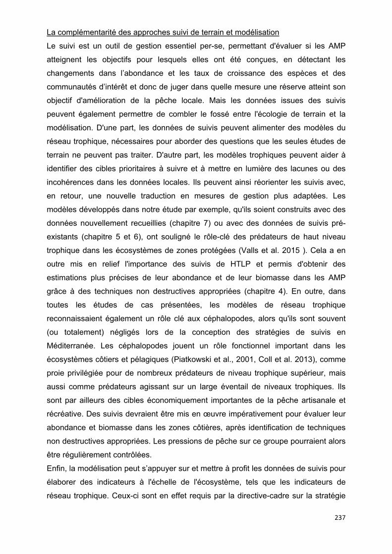
237  

La complémentarité des approches suivi de terrain et modélisation

Le suivi est un outil de gestion essentiel per-se, permettant d'évaluer si les AMP

atteignent les objectifs pour lesquels elles ont été conçues, en détectant les

changements dans l’abondance et les taux de croissance des espèces et des

communautés d’intérêt et donc de juger dans quelle mesure une réserve atteint son

objectif d'amélioration de la pêche locale. Mais les données issues des suivis

peuvent également permettre de combler le fossé entre l'écologie de terrain et la

modélisation. D'une part, les données de suivis peuvent alimenter des modèles du

réseau trophique, nécessaires pour aborder des questions que les seules études de

terrain ne peuvent pas traiter. D'autre part, les modèles trophiques peuvent aider à

identifier des cibles prioritaires à suivre et à mettre en lumière des lacunes ou des

incohérences dans les données locales. Ils peuvent ainsi réorienter les suivis avec,

en retour, une nouvelle traduction en mesures de gestion plus adaptées. Les

modèles développés dans notre étude par exemple, qu'ils soient construits avec des

données nouvellement recueillies (chapitre 7) ou avec des données de suivis pré-

existants (chapitre 5 et 6), ont souligné le rôle-clé des prédateurs de haut niveau

trophique dans les écosystèmes de zones protégées (Valls et al. 2015 ). Cela a en

outre mis en relief l'importance des suivis de HTLP et permis d'obtenir des

estimations plus précises de leur abondance et de leur biomasse dans les AMP

grâce à des techniques non destructives appropriées (chapitre 4). En outre, dans

toutes les études de cas présentées, les modèles de réseau trophique

reconnaissaient également un rôle clé aux céphalopodes, alors qu'ils sont souvent

(ou totalement) négligés lors de la conception des stratégies de suivis en

Méditerranée. Les céphalopodes jouent un rôle fonctionnel important dans les

écosystèmes côtiers et pélagiques (Piatkowski et al., 2001, Coll et al. 2013), comme

proie privilégiée pour de nombreux prédateurs de niveau trophique supérieur, mais

aussi comme prédateurs agissant sur un large éventail de niveaux trophiques. Ils

sont par ailleurs des cibles économiquement importantes de la pêche artisanale et

récréative. Des suivis devraient être mis en œuvre impérativement pour évaluer leur

abondance et biomasse dans les zones côtières, après identification de techniques

non destructives appropriées. Les pressions de pêche sur ce groupe pourraient alors

être régulièrement contrôlées.

Enfin, la modélisation peut s’appuyer sur et mettre à profit les données de suivis pour

élaborer des indicateurs à l'échelle de l'écosystème, tels que les indicateurs de

réseau trophique. Ceux-ci sont en effet requis par la directive-cadre sur la stratégie

238  

du milieu marin, afin de parvenir à un bon état écologique (Good Ecological Status)

(Heymans et al. 2014, Guesnet et al. 2015). Dans cette perspective, les AMP et les

modèles correspondants pourraient être très utiles pour définir des seuils pour les

indicateurs et pour proposer des valeurs de référence correspondant à différents

états de conservation. Les indicateurs fondés sur les niveaux trophiques, par

exemple, sont de plus en plus utilisés pour évaluer l'impact de la pêche sur

l'ensemble de l'écosystème (Shannon et al. 2014). La modélisation peut servir à

générer des valeurs de référence pour les indicateurs à travers des simulations

dynamiques. Cela nécessiterait des très longues séries temporelles si seules les

données de suivis sont utilisées (Pelletier et al., 2008). Dans cette perspective, un

nouveau développement à notre étude pourrait être l'application des indicateurs

proposés récemment comme l'Apex Predator Indicateur (API) et le High Trophic

Indicator (HTI) (Bourdaud et al. 2015). Ces deux indicateurs sont fondés sur les

niveaux trophiques, et en particulier sur la proportion des prédateurs apicaux et/ou

de niveaux trophiques supérieurs dans l'écosystème, utilisés comme proxy du bon

fonctionnement de l'ensemble du réseau trophique. Des objectifs spécifiques à

l'écosystème pourraient donc être proposés pour chaque indicateur par simulation

(Bourdaud et al. 2015).

Perspectives sur les modèles du réseau trophique comme outils de gestion

écosystémiques opérationnels dans les AMP

Sur la base des données collectées, complétées par des analyses de sensibilité

approfondies, nous avons démontré le potentiel des modèles de réseau trophique en

termes d'outils de gestion des AMP pour i) identifier les espèces clés et sentinelles

de l'écosystème ii) mettre en évidence la capacité de charge possible de l'AMP pour

les HTLP, iii) analyser les conséquences des variations de biomasse des HTLP dans

le réseau trophique iv) recommander une réduction de l'effort de pêche récréative sur

les HTLP et évaluer l'impact de la pêche récréative sur la pêche artisanale.

Si 1) des programmes de suivi exhaustifs sont mis en œuvre dans les AMP, ciblant à

la fois les ressources biologiques, mais aussi et surtout, les impacts humains

(captures et effort des pêcheries locales) et si 2) la modélisation du réseau trophique

devient une étape régulière pour intégrer les données des suivis, la gamme des

applications de gestion possibles des modèles trophiques développés avec

l'ensemble EwE-EcoTroph-Ecospace est extrêmement large, et en expansion

239  

continue (Coll et al 2015). Quelques applications possibles sont données ici à titre de

perspectives.

La propagation des espèces envahissantes en Méditerranée est largement reconnue

comme une grave menace pour la biodiversité et le fonctionnement de l'écosystème

et pour la fourniture de services écosystémiques (Katsanevakis et al. 2014). Les

modèles trophiques pourraient aider à aborder ce problème pour mieux comprendre

le rôle des espèces envahissantes et leur impact sur le réseau trophique et analyser

des scénarios de gestion (Arias-González et al., 2011). Bien que l'intérêt de cette

approche soit en pleine croissance (Coll et al . 2015), les applications en

Méditerranée sont encore rares.

Les modèles EwE-EcoTroph ont été utilisés dans quelques études pour évaluer

l’export de biomasse à partir des AMP (Valls et al. 2012, Colleter et al. 2014) et, dans

une étude, pour quantifier la contribution d'une AMP au fonctionnement et à la

productivité trophique de l'écosystème environnant (Guénette et al. 2014). Les AMP

sont souvent très petites en Méditerranée, il pourrait donc être intéressant d'évaluer

si l'extension de leurs frontières permettrait d'accroître leur contribution en termes

d’export aux systèmes adjacents et à la production totale ou en termes de captures

dans les écosystèmes environnants. D'ailleurs, à travers les modules dynamiques

Ecosim et Ecospace, il est possible d'explorer les effets potentiels des scénarios de

gestion alternative de la pêche (et aussi du changement climatique) sur la structure

de l'écosystème et sur la production de la pêche, de modéliser les échanges

d'énergie à partir des AMP vers les zones externes et de quantifier l’impact des AMP

sur les écosystèmes plus vastes. Enfin, si plusieurs modèles de réseau trophique

sont développés dans plusieurs AMP, une analyse à grande échelle pourrait être

effectuée avec Ecospace pour évaluer les effets des différentes configurations

spatiales de réseaux d'AMP et / ou de différents scénarios de gestion des pêches sur

la structure et le fonctionnement de l'écosystème et sur la production par pêche.

Afin d'exploiter pleinement ce potentiel élevé, les AMP devraient commencer à

intégrer la modélisation du réseau trophique comme un outil régulier dans leur plan

de gestion, en l'utilisant en premier lieu pour mieux orienter les suivis et intégrer les

données en une image cohérente du fonctionnement de l’écosystème pour ensuite,

une fois cette base fiable disponible, optimiser et améliorer cette image en fonction

des besoins de gestion.

 

240  

9 References  

Abdulla A, Gomei M, Maison E, Piante C (2008) Status of marine protected areas in the Mediterranean Sea. IUCN, Malaga and WWF, FranceBabcock RC, Shears NT, Alcala AC, Barrett NS, Edgar GJ, Lafferty KD, McClanahan TR, Russ GR (2010) Decadal trends in marine reserves reveal differential rates of change in direct and indirect effects. PNAS 107:18256–18261

Arias-González JE, González-Gándara C, Cabrera JL, Christensen V (2011) Predicted impact of the invasive lionfish Pterois volitans on the food web of a Caribbean coral reef. Environ Res 111:917–925

Bascompte J, Melián CJ, Sala E (2005) Interaction strength combinations and the overfishing of a marine food web. PNAS 102:5443–5447

Bourdaud P, Gascuel D, Bentorcha A, Brind’Amour A (2015) New trophic indicators and target values for an ecosystem-based management of fisheries. Ecol Indic

Bozec Y-M, Kulbicki M, Laloë F, Mou-Tham G, Gascuel D (2011) Factors affecting the detection distances of reef fish: implications for visual counts. Mar Biol 158:969–981

Britten GL, Dowd M, Minto C, Ferretti F, Boero F, Lotze HK (2014) Predator decline leads to decreased stability in a coastal fish community. Ecology Letters 17:1518–1525

Carstensen J (2014) Need for monitoring and maintaining sustainable marine ecosystem services. Front Mar Sci 1:33

Cheal AJ, Thompson AA (1997) Comparing visual counts of coral reef fish: implications of transect width and species selection. Mar Ecol Prog Ser 158:241–248

Christensen V, Pauly D (1992) Ecopath II—a software for balancing steady-state ecosystem models and calculating network characteristics. Ecological modelling 61:169–185

Christensen V, Walters CJ (2004) Ecopath with Ecosim: methods, capabilities and limitations. Ecological modelling 172:109–139

Christensen V, Walters CJ, Ahrens R, Alder J, Buszowski J, Christensen LB, Cheung WWL, Dunne J, Froese R, Karpouzi V (2009) Database-driven models of the world’s Large Marine Ecosystems. Ecol Model 220:1984–1996

Coll M, Akoglu E, Arreguín-Sánchez F, Fulton EA, Gascuel D, Heymans JJ, Libralato S, Mackinson S, Palomera I, Piroddi C, others (2015) Modelling dynamic ecosystems: venturing beyond boundaries with the Ecopath approach. Rev Fish Biol Fish 25:413–424

Coll M, Libralato S (2012) Contributions of food web modelling to the ecosystem approach to marine resource management in the Mediterranean Sea. Fish and Fisheries 13:60–88

241  

Coll M, Lotze HK, Romanuk TN (2008) Structural degradation in Mediterranean Sea food webs: testing ecological hypotheses using stochastic and mass-balance modelling. Ecosystems 11:939–960

Coll M, Navarro J, Olson RJ, Christensen V (2013) Assessing the trophic position and ecological role of squids in marine ecosystems by means of food-web models. Deep Sea Res Part II Top Stud Oceanogr 95:21–36

Colléter M, Valls A, Guitton J, Gascuel D, Pauly D, Christensen V (2015) Global overview of the applications of the Ecopath with Ecosim modeling approach using the EcoBase models repository. Ecological Modelling 302:42–53

Colloca F, Cardinale M, Maynou F, Giannoulaki M, Scarcella G, Jenko K, Bellido JM, Fiorentino F (2013) Rebuilding Mediterranean fisheries: a new paradigm for ecological sustainability. Fish and Fisheries 14:89–109

Dudley N, Stolton S (2008). Defining protected areas: an international conference in Almeria, Spain. Gland, Switzerland: IUCN. 220pp.

Duffy JE (2002) Biodiversity and ecosystem function: the consumer connection. Oikos 99:201–219

Espinoza-Tenorio A, Wolff M, Taylor MH, Espejel I (2012) What model suits ecosystem-based fisheries management? A plea for a structured modeling process. Reviews in Fish Biology and Fisheries 22:81–94

Estes JA, Terborgh J, Brashares JS, Power ME, Berger J, Bond WJ, Carpenter SR, Essington TE, Holt RD, Jackson JBC, Marquis RJ, Oksanen L, Oksanen T, Paine RT, Pikitch EK, Ripple WJ, Sandin SA, Scheffer M, Schoener TW, Shurin JB, Sinclair ARE, Soule ME, Virtanen R, Wardle DA (2011) Trophic Downgrading of Planet Earth. Science 333:301–306

Fulton EA, Bax NJ, Bustamante RH, Dambacher JM, Dichmont C, Dunstan PK, Hayes KR, Hobday AJ, Pitcher R, Plagányi ÉE, Punt AE, Savina-Rolland M, Smith ADM, Smith DC (2015) Modelling marine protected areas: insights and hurdles. Philosophical Transactions of the Royal Society B: Biological Sciences 370:20140278

Garcia-Rubies A, Hereu B, Zabala M (2013) Long-Term Recovery Patterns and Limited Spillover of Large Predatory Fish in a Mediterranean MPA. PLoS ONE 8

Gascuel D, Coll M, Fox C, Guénette S, Guitton J, Kenny A, Knittweis L, Nielsen JR, Piet G, Raid T, Travers-Trolet M, Shephard S (2014) Fishing impact and environmental status in European seas: a diagnosis from stock assessments and ecosystem indicators. Fish and Fisheries

Gascuel D, Guénette S, Pauly D (2011) The trophic-level-based ecosystem modelling approach: theoretical overview and practical uses. ICES J Mar Sci 68:1403–1416

Gascuel D, Pauly D (2009) EcoTroph: modelling marine ecosystem functioning and impact of fishing. Ecological Modelling 220:2885–2898

Goñi R, Quetglas A, Renones O (2006) Spillover of spiny lobsters Palinurus elephas from a marine reserve to an adjoining fishery. Mar Ecol Prog Ser 308:207–219

242  

Guénette S, Meissa B, Gascuel D (2014) Assessing the Contribution of Marine Protected Areas to the Trophic Functioning of Ecosystems: A Model for the Banc d’Arguin and the Mauritanian Shelf. PloS One 9:e94742

Guesnet V, Lassalle G, Chaalali A, Kearney K, Saint-Béat B, Karimi B, Grami B, Tecchio S, Niquil N, Lobry J (2015) Incorporating food-web parameter uncertainty into Ecopath-derived ecological network indicators. Ecol Model 313:29–40

Guidetti P (2007) Predator diversity and density affect levels of predation upon strongly interactive species in temperate rocky reefs. Oecologia 154:513–520

Guidetti P, Baiata P, Ballesteros E, Di Franco A, Hereu B, Macpherson E, Micheli F, Pais A, Panzalis P, Rosenberg AA, Zabala M, Sala E (2014) Large-Scale Assessment of Mediterranean Marine Protected Areas Effects on Fish Assemblages. PLoS ONE 9:e91841

Guidetti P, Micheli F (2011) Ancient art serving marine conservation. Frontiers in Ecology and the Environment 9:374–375

Halpern BS, Warner RR (2002) Marine reserves have rapid and lasting effects. Ecology letters 5:361–366

Harmelin-Vivien M, Harmelin J, Chauvet C, Duval C, Galzin R, Lejeune P, Barnabé G, Blanc F, Chevalier R, Duclerc J (1985) Evaluation visuelle des peuplements et populations de poissons: méthodes et problèmes. Rev Décologie 40:467–539

Heymans JJ, Coll M, Libralato S, Morissette L, Christensen V (2014) Global Patterns in Ecological Indicators of Marine Food Webs: A Modelling Approach. PLoS ONE 9:e95845

Jackson JBC, Kirby MX, Berger WH, Bjorndal KA, Botsford LW, Bourque BJ, Bradbury RH, Cooke R, Erlandson J, Estes JA (2001) Historical overfishing and the recent collapse of coastal ecosystems. science 293:629–637

Jørgensen SE, Patten BC, Straškraba M (2000) Ecosystems emerging:4. Growth. Ecological Modelling 126:249–284

Katsanevakis S, Coll M, Piroddi C, Steenbeek J, Ben Rais Lasram F, Zenetos A, Cardoso AC (2014) Invading the Mediterranean Sea: biodiversity patterns shaped by human activities. Marine Ecosystem Ecology 1:32

Kulbicki M (1998) How the acquired behaviour of commercial reef fishes may influence the results obtained from visual censuses. J Exp Mar Biol Ecol 222:11–30

Lassalle G, Bourdaud P, Saint-Béat B, Rochette S, Niquil N (2014) A toolbox to evaluate data reliability for whole-ecosystem models: Application on the Bay of Biscay continental shelf food-web model. Ecol Model 285:13–21

Lester SE, Halpern BS, Grorud-Colvert K, Lubchenco J, Ruttenberg BI, Gaines SD, Airamé S, Warner RR (2009) Biological effects within no-take marine reserves: a global synthesis. Marine Ecology Progress Series 384:33–46

Libralato S, Coll M, Tempesta M, Santojanni A, Spoto M, Palomera I, Arneri E, Solidoro C (2010) Food-web traits of protected and exploited areas of the Adriatic Sea. Biological Conservation 143:2182–2194

243  

Link JS (2010) Adding rigor to ecological network models by evaluating a set of pre-balance diagnostics: A plea for PREBAL. Ecol Model 221:1580–1591

Lubchenco J, Palumbi SR, Gaines SD, Andelman S (2003) Plugging a hole in the ocean: the emerging science of marine reserves. Ecological applications 13:3–7Menge BA (1995) Indirect effects in marine rocky intertidal interaction webs: patterns and importance. Ecological monographs 65:21–74

Morissette L (2007) Complexity, cost and quality of ecosystem models and their impact on resilience. PhD diss. University of British Columbia

Micheli F, Benedetti-Cecchi L, Gambaccini S, Bertocci I, Borsini C, Osio GC, Romano F (2005) Cascading human impacts, marine protected areas, and the structure of Mediterranean reef assemblages. Ecological Monographs 75:81–102

Micheli F, Halpern BS, Botsford LW, Warner RR (2004) Trajectories and correlates of community change in no-take marine reserves. Ecological Applications 14:1709–1723Myers RA, Worm B (2005) Extinction, survival or recovery of large predatory fishes. Philosophical Transactions of the Royal Society B: Biological Sciences 360:13–20

Pauly D, Christensen V, Dalsgaard J, Froese R, Torres Jr F (1998) Fishing down marine food webs. Science 279:860–863

Pelletier D, Claudet J, Ferraris J, Benedetti-Cecchi L, Garcìa-Charton JA (2008) Models and indicators for assessing conservation and fisheries-related effects of marine protected areas. Canadian Journal of Fisheries and Aquatic Sciences 65:765–779

Plagányi E, Ellis N, Blamey L, Morello E, Norman-Lopez A, Robinson W, Sporcic M, Sweatman H (2014) Ecosystem modelling provides clues to understanding ecological tipping points. Marine Ecology Progress Series 512:99–113

Piatkowski U, Pierce GJ, Morais da Cunha M (2001) Impact of cephalopods in the food chain and their interaction with the environment and fisheries: an overview. Fish Res 52:5–10

Prato G, Guidetti P, Bartolini F, Mangialajo L, Francour P (2013) The importance of high-level predators in marine protected area management: Consequences of their decline and their potential recovery in the Mediterranean context. Advances in Oceanography and Limnology 4:176–193

Odum EP (1969) The strategy of ecosystem development. Science 164:262–270 Ray J, Redford KH, Steneck R, Berger J (2005) Large Carnivores and the

Conservation of Biodiversity. Island Press, Washington Sala E (2004) The past and present topology and structure of Mediterranean

subtidal rocky-shore food webs. Ecosystems 7:333–340 Sala E, Ballesteros E, Dendrinos P, Di Franco A, Ferretti F, Foley D, Fraschetti S,

Friedlander A, Garrabou J, Guclusoy H, Guidetti P, Halpern BS, Hereu B, Karamanlidis AA, Kizilkaya Z, Macpherson E, Mangialajo L, Mariani S, Micheli F, Pais A, Riser K, Rosenberg AA, Sales M, Selkoe KA, Starr R, Tomas F, Zabala M (2012) The Structure of Mediterranean Rocky Reef

244  

Ecosystems across Environmental and Human Gradients, and Conservation Implications. Plos One 7:e32742

Sala E, Boudouresque CF, Harmelin-Vivien M (1998) Fishing, trophic cascades, and the structure of algal assemblages: evaluation of an old but untested paradigm. Oikos:425–439

Sandin SA, Smith JE, DeMartini EE, Dinsdale EA, Donner SD, Friedlander AM, Konotchick T, Malay M, Maragos JE, Obura D (2008) Baselines and degradation of coral reefs in the northern Line Islands. PLoS One 3:e1548

Shannon L, Coll M, Shin Y, others (2014) Trophic level-based indicators to track fishing impacts across marine ecosystems. Mar Ecol Prog Ser 512:115–140

Soler GA, Edgar GJ, Thomson RJ, Kininmonth S, Campbell SJ, Dawson TP, Barrett NS, Bernard ATF, Galván DE, Willis TJ, Alexander TJ, Stuart-Smith RD (2015) Reef Fishes at All Trophic Levels Respond Positively to Effective Marine Protected Areas. PLOS ONE 10:e0140270

Stevenson C, Katz LS, Micheli F, Block B, Heiman KW, Perle C, Weng K, Dunbar R, Witting J (2007) High apex predator biomass on remote Pacific islands. Coral Reefs 26:47–51

Valls A, Coll M, Christensen V (2015) Keystone species: toward an operational concept for marine biodiversity conservation. Ecological Monographs 85:29–47

Valls A, Gascuel D, Guénette S, Francour P (2012) Modeling trophic interactions to assess the effects of a marine protected area: case study in the NW Mediterranean Sea. Mar Ecol Prog Ser 456:201–214

Wagner HP (2008) Lobsters: biology, management, aquaculture and fisheries. Crustaceana 81:381–381

 

10 Co

This sincreaand thimportA sucwhereachievnegati

ommunica

Th

short movie ase of humahe fishing dtant macroa

ccession of e the coved represive trend an

tion & Ou

he BooAut

F

wants to tean populati

down the fooalgal habitadrawings t

ollaborationsent one ond restore o

treach

k of Mathors: Giuli

ilming & E

Drawin

ell the story ion and fishod web cauts were repthat come t among f the best

our sea.

arine Pia Prato &

diting: Kev

ngs: Celine

y of depletioh demand. used ecosysplaced by mto life in vi

managersolutions

ProtectFabrizio G

vin Peyrou

e Barrier

on of the MeThe overe

stem shifts marine deserideos showrs, stakehto prevent

ted AreGianni

sse

editerraneanxploitation in many corts overgraz

w how marinholders an

and some

eas.

n Sea folloof larger p

oastal areaszed by sea ne protectend scient

etimes reve

245 

wing the predators s, where urchins.

ed areas tists is erse this