Few-shot Image Classification: Just Use a Library of Pre ...

Few-shot Image Classification: Just Use a Library of Pre-trained FeatureExtractors and a Simple Classifier

Arkabandhu Chowdhury 1 Mingchao Jiang 1 Swarat Chaudhuri 2 Chris Jermaine 1

AbstractRecent papers have suggested that transfer learn-ing can outperform sophisticated meta-learningmethods for few-shot image classification. Wetake this hypothesis to its logical conclusion, andsuggest the use of an ensemble of high-quality,pre-trained feature extractors for few-shot imageclassification. We show experimentally that a li-brary of pre-trained feature extractors combinedwith a simple feed-forward network learned withan L2-regularizer can be an excellent option forsolving cross-domain few-shot image classifica-tion. Our experimental results suggest that thissimple approach far outperforms several well-established meta-learning algorithms.

1. IntroductionThere has been a lot of recent interest in few-shot imageclassification (Fei-Fei et al., 2006; Lee et al., 2019; Li et al.,2019; Finn et al., 2017, 2018; Kim et al., 2018; Nichol &Schulman, 2018; Lee & Choi, 2018). Various papers haveexplored different formulations of the problem, but in onegeneral formulation, we are given a data setDtrn of (image,label) pairs sampled from a distribution Ptrn . The goal isto devise a method that uses Dtrn to learn a function fthat is itself a few-shot learner. The few-shot learner ftakes as input a new labeled data set Dfew consisting of aset of samples from a new distribution Pfew 6= Ptrn . fthen returns a classification function g, which is targeted atclassifying samples from the distribution Pfew .

The process of learning f is often referred to as meta-learning in the literature. Learning to classify samples fromPfew is a “few shot” problem when Dfew is small, perhapshaving only one example for each class produced by Pfew .In the most difficult and generally applicable variant of thefew-shot problem—which we consider in this paper—Pfew

has no known relationship to Ptrn (this is “cross-domain”

1Rice University 2University of Texas, Austin.

Accepted at ICCV 2021

few-shot learning) and Dfew is not available while learn-ing f . Thus, the meta-learning process has no access toinformation about the eventual application. The only in-formation we have about Pfew is the set Dfew , and this isavailable only when constructing g. We cannot, for exam-ple, choose any hyperparameters controlling the learning ofg using information not extracted from Dfew .

Our goal is to devise a learner f that works well, out-of-the-box, on virtually any new distribution Pfew . We argue thatin such a scenario, developing novel meta-learning meth-ods to learn f from scratch on given Dtrn may not be themost productive direction of inquiry. Because no informa-tion about Pfew is available during meta-learning, it makessense to choose a Dtrn that has many different types of im-ages, so it is likely to contain some images with featuressimilar to those produced by Pfew , whatever form this dis-tribution takes. Fortunately, in computer image classifica-tion, the standard benchmark data set is now ILSVRC2012,a 1000-class version of the full ImageNet (Russakovskyet al., 2015). ILSVRC2012 consists of a wide variety ofimages, and it has become quite standard for researcherswho design and train new image classifiers to publish clas-sifiers trained on ILSVRC2012. Such published artifactsrepresent thousands of hours of work by researchers whoare well-versed in the “black art” of wringing every lastpercent of accuracy out of a deep CNN. Instead of develop-ing new meta-learning methods, it may be more productiveto simply fix Dtrn = ILSVRC2012, and attempt to lever-age all of the effort that has gone into learning deep CNNsover ILSVRC2012, by using those CNNs as the basis forthe few-shot learner f . As other, even more wide-rangingand difficult benchmark data sets become prevalent (suchas the full, 20,000+ class ImageNet), high-quality classi-fiers trained using that data set may be preferred.

We first show that it is possible to use any of a num-ber of published, high-quality, deep CNNs, learned overILSVRC2012, as the basis for a few-shot learner that sig-nificantly outperforms state-of-the art methods. The way todo this is embarrassingly simple: remove the classifier fromthe top of the deep CNN, fix the weights of the remainingdeep feature extractor, and replace the classifier with a sim-ple MLP that is trained using L2 regularization to prevent

arX

iv:2

101.

0056

2v3

[cs

.CV

] 2

0 A

ug 2

021

Few-shot Image Classification: Just Use a Library of Pre-trained Feature Extractors and a Simple Classifier

over-fitting. We call these “library-based” learners becausethey are based on standard, published feature extractors.

Next, we ask: if a published deep CNN can be used to pro-duce a state-of-the-art, few-shot learner, can we produce aneven higher-quality few-shot learner by combining togethermany high-quality, deep CNNs? We call such a learner a“full library” learner.

Then, we note that other researchers have suggested theutility of re-using high-quality, pre-trained feature extrac-tors for few-shot image classification. In particular, the au-thors of the “Big Transfer” paper (Kolesnikov et al., 2019)argue that a very large network trained on a huge data set(the JFT-300M data set (Sun et al., 2017), with 300 mil-lion images) can power an exceptionally accurate transfer-learning-based few-shot learning. Unfortunately, the au-thors have not made their largest JFT-300M-trained net-work public, and so we cannot experiment with it directly.However, they have made public several versions of their“Big Transfer” network, trained on the full, 20,000+ classImageNet benchmark public. Interestingly, we find that“big” may not be as important as “diverse”: a single, few-shot classifier comprised of many different high-qualityILSVRC2012-trained deep CNNs seems to be a better op-tion than a single few-shot classifier built on top of any ofthe Google-trained CNNs. Finally, we investigate why afull library learner works so well. We postulate two rea-sons for this. First, having a very large number of features(> 10,000) does not seem to be a problem for few-shotlearning. Second, there seems to be strength in diversity,in the sense that different CNNs appear useful for differenttasks.

2. High Accuracy of Library-Based Learners2.1. Designing a Library-Based Learner

We begin by asking: what if we eschew advanced meta-learning methods, and instead simply use a very high-quality deep CNN pulled from a library, trained on theILSVRC2012 data set, as the basis for a few-shot classi-fier?

Specifically, we are given a high-quality, pre-trained deepCNN, from a library of pre-trained networks; we take theCNN as-is, but remove the topmost layers used for clas-sification. This results in a function that takes an image,and returns an embedding. We then use that embeddingto build a classifier in an elementary fashion: we feed theembedding into a multi-layer perceptron with a single hid-den layer; a softmax is used to produce the final classifica-tion. Given a few-shot classification problem, two weightmatrices W1 and W2 are learned; the first connecting theembedding to the hidden layer, the second connecting thehidden layer to the softmax. To prevent over-fitting dur-

ing training, simple L2 regularization is used on the weightmatrices.

2.2. Evaluation

To evaluate this very simple few-shot learner, we first iden-tify nine, high-quality deep CNNs with published models,trained on ILSVRC2012: ResNet18, ResNet34, ResNet50,ResNet101, ResNet152 (all of the ResNet implementa-tions are the ones from the original ResNet designers (Heet al., 2016)), DenseNet121, DenseNet161, DenseNet169,and DenseNet201 (all of the DenseNet implementations arealso from the original designers (Huang et al., 2017)).

Our goal is to produce an “out-of-the-box” few-shot learnerthat can be used on any (very small) training setDfew with-out additional data or knowledge of the underlying distribu-tion. We are very careful not to allow validation or param-eter tuning on testing data domains, so all parameters andsettings need to be chosen apriori. If it is possible to buildsuch a few-shot learner, it would be the most widely appli-cable: simply produce a few training images for each class,apply the learner. Thus, we perform an extensive hyper-parameter search, solely using the Caltech-UCSD Birds200 set (Welinder et al., 2010) as a validation data set, andthen use the best hyperparameters from that data set in all ofour experiments. Hyperparameters considered were learn-ing rate, number of training epochs, regularization penaltyweight, the number of neurons in the MLP hidden layer,and whether to drop the hidden layer altogether. A separatehyper-parameter search was used for 5-way, 20-way, and40-way classification.

We then test the resulting few-shot learner—one learner perdeep CNN—on eight different data sets, FGVC-Aircraft(Maji et al., 2013), FC100 (Oreshkin et al., 2018), Om-niglot (Lake et al., 2015), Traffic Sign (Houben et al.,2013), FGCVx Fungi (Schroeder & Cui, 2018), QuickDraw (Jongejan et al., 2016), and VGG Flower (Nilsback& Zisserman, 2008). To evaluate a few-shot learner on adata set, for an “m-way n-shot” classification problem, werandomly select m different classes, and then randomly se-lect n images from each class for training; the remainderare used for testing. As this is “out-of-the-box” learning,no validation is allowed.

We performed this evaluation for m in {5, 20, 40} and nin {1, 5}. Due to space constraints, the full results are pre-sented as supplementary material, and we give only a syn-opsis here (Table 2 and Table 3). In Table 1, we show thebest and worst accuracy achieved across the 9 learners, foreach of the 8 data sets, for m in {5, 20, 40} and n = 1.

To give the reader an idea of how this accuracy comparesto the state-of-the-art, we compare these results with anumber of few-shot learners from the literature. We com-


Aircraft FC100 Omniglot Texture Traffic Fungi Quick Draw VGG Flower

5-way, 1-shot

Worst 40.9 ± 0.9 50.8 ± 0.9 77.2±0.9 59.1 ± 0.9 55.5 ± 0.8 53.0 ± 0.9 57.3 ± 0.9 79.7 ± 0.8RN18 DN121 RN152 DN169 RN152 DN201 RN101 RN18

Best 46.2 ± 1.0 61.2±0.9 86.5 ± 0.7 65.1 ± 0.9 66.6 ± 0.9 56.6 ± 0.9 62.8 ± 0.9 83.5 ± 0.8DN161 RN152 DN121 RN101 DN201 DN121 RN18 DN161

20-way, 1-shot

Worst 20.1 ± 0.3 27.8 ± 0.4 56.2 ± 0.5 38.0 ± 0.4 29.7 ± 0.3 31.7 ± 0.4 33.2 ± 0.5 62.4 ± 0.5RN101 DN121 RN101 RN18 RN101 RN101 RN101 RN101

Best 24.3 ± 0.3 36.4 ± 0.4 69.1 ± 0.5 42.5 ± 0.4 38.5 ± 0.4 33.9 ± 0.5 39.5± 0.5 70.0 ± 0.5DN161 RN152 DN121 RN152 DN201 DN161 DN201 DN161

40-way, 1-shot

Worst 14.2 ± 0.2 19.6 ± 0.2 47.3 ± 0.3 28.9 ± 0.2 22.2 ± 0.2 23.7 ± 0.3 26.4 ± 0.3 53.1 ± 0.3RN34 RN18 RN152 RN18 RN152 RN34 RN152 RN34

Best 17.4 ± 0.2 27.2 ± 0.3 61.6 ± 0.3 33.2 ± 0.3 29.5 ± 0.2 26.8 ± 0.3 31.2 ± 0.3 62.8 ± 0.3DN161 RN152 DN201 DN152 DN201 DN161 DN201 DN161

Table 1. Accuracy obtained using library deep CNNs for few-shot learning.


Baseline 47.6 ± 0.7 66.9 ± 0.7 96.5 ± 0.2 62.5 ± 0.7 82.1 ± 0.7 57.6 ± 1.7 75.6 ± 0.7 90.9 ± 0.5Baseline++ 40.9 ± 0.7 59.8 ± 0.8 90.6 ± 0.4 59.9 ± 0.7 79.6 ± 0.8 54.1 ± 1.7 68.4 ± 0.7 83.1 ± 0.7MAML 33.1 ± 0.6 62.0 ± 0.8 82.6 ± 0.7 56.9 ± 0.8 67.4 ± 0.9 48.3 ± 1.8 77.5 ± 0.8 78.0 ± 0.7MatchingNet 33.5 ± 0.6 59.4 ± 0.8 89.7 ± 0.5 54.7 ± 0.7 73.7 ± 0.8 55.7 ± 1.7 70.4 ± 0.8 74.2 ± 0.8ProtoNet 41.5 ± 0.7 64.7 ± 0.8 95.5 ± 0.3 62.9 ± 0.7 75.0 ± 0.8 53.1 ± 1.8 74.9 ± 0.7 86.7 ± 0.6RelationNet 37.5 ± 0.7 64.8 ± 0.8 91.2 ± 0.4 60.0 ± 0.7 68.6 ± 0.8 58.7 ± 1.8 71.9 ± 0.7 80.6 ± 0.7Meta-transfer 46.2 ± 0.7 75.7 ± 0.8 93.5 ± 0.4 70.5 ± 0.7 80.0 ± 0.8 66.1 ± 0.8 77.7 ± 0.7 90.5 ± 0.6FEAT 46.2 ± 0.9 60.5 ± 0.8 85.3 ± 0.7 70.7 ± 0.7 70.5 ± 0.8 67.3 ± 1.7 69.9 ± 0.7 92.1 ± 0.4SUR 45.2 ± 0.8 67.2 ± 1.0 98.7 ± 0.1 59.6 ± 0.7 70.6 ± 0.8 60.0 ± 1.8 73.5 ± 0.7 90.8 ± 0.5

Worst library- 61.0 ± 0.9 71.9 ± 0.8 94.0 ± 0.4 79.3 ± 0.6 78.8 ± 0.7 77.1 ± 0.8 77.8 ± 0.7 95.3 ± 0.4based RN34 DN121 RN152 RN18 RN152 RN34 RN152 RN34Best library- 66.0 ± 0.9 80.0 ± 0.6 96.7 ± 0.2 83.4 ± 0.6 85.3 ± 0.7 79.1 ± 0.7 81.8 ± 0.6 96.8 ± 0.3based DN161 RN152 DN201 DN161 DN201 DN121 DN201 DN161

Table 2. Comparing competitive methods with the simple library-based learners, on the 5-way, 5-shot problem.

pare against Baseline and Baseline++ (Chen et al., 2019),MAML (Finn et al., 2017), MatchingNet (Vinyals et al.,2016), ProtoNet (Snell et al., 2017), RelationNet (Sunget al., 2018), Meta-transfer (Sun et al., 2019), FEAT (Yeet al., 2020), and SUR (Dvornik et al., 2020). When adeep CNN classifier must be chosen for any of these meth-ods, we use a ResNet18. For methods that require a pre-trained CNN (FEAT, Meta-transfer, and SUR), we use theResNet18 trained by the ResNet designers (He et al., 2016).Lest the reader be concerned that we chose the worst op-tion (ResNet18), we point out that of the library-basedfew-shot learners, on the 5-way, 5-shot problem ResNet18gave the best accuracy out of all of the ResNet-based learn-ers for two of the data sets (see Table 4). Further, thesecompetitive methods tend to be quite expensive to train—MAML, for example, requires running gradient descentover a gradient descent—and for such a method, the shal-lower ResNet18 is a much more reasonable choice than the

deeper models (even using a ResNet18, we could not suc-cessfully train first-order MAML for 5-shot, 40-way clas-sification, due to memory constraints).

For the competitive methods (other than SUR) we followthe same procedure as was used for the library-based few-shot classifiers: any training that is necessary is performedon the ILSVRC2012 data set, and hyperparameter valida-tion is performed using the Caltech-UCSD Birds 200 dataset. Each method is then used without further tuning onthe remaining eight data sets. To evaluate SUR on dataset X , we use feature extractors trained on the data setsin {Omniglot, Aircraft, Birds, Texture, Quickdraw, Flow-ers, Fungi,and ILSVRC} − X . Traffic Sign and FC100datasets are reserved for testing only.

A comparison of each of these competitive methods withthe the best and worst-performing library-based learners onthe 5-way, 5-shot learning problem is shown in Table 2; a




Worst library- 37.5 ± 0.4 47.1 ± 0.4 84.3 ± 0.3 58.7 ± 0.4 55.9 ± 0.4 56.1 ± 0.5 57.2 ± 0.4 86.8 ± 0.3based RN18 RN18 RN101 RN18 RN152 RN34 RN101 RN101Best library- 44.6 ± 0.4 58.8 ± 0.4 92.0 ± 0.2 65.1 ± 0.4 66.0 ± 0.4 60.8 ± 0.5 63.9 ± 0.4 91.6 ± 0.2based DN161 RN152 DN201 DN161 DN201 DN161 DN161 DN161

Table 3. Comparing competitive methods with the simple library-based learners, on the 20-way, 5-shot problem.

comparison on 20-way, 5-shot learning in Table 3. A morecomplete set of results is in the supplementary material.

2.3. Discussion

There are a few key takeaways from these results. The bestlibrary-based learner always beat every one of the othermethods tested, with the only exception of SUR when test-ing on Omniglot data set. For the other data sets, the gaponly grows as the number of ways increases. In fact, forthe 20-way problem, the worst library-based learner al-ways beat all of the other methods tested (except SUR onOmniglot). The gap can be quite dramatic, especially onthe 20-way problem. The best non-transfer based few-shotlearner (MAML, Proto Nets, Relation Nets, and Match-ing Nets fall in this category) was far worse than even theworst library-based learner: 39% accuracy for Proto Netsvs. 59% accuracy for a classifier based on RestNet18 onTexture, 48% accuracy for Relation Nets vs. 57% accuracyfor classifier based on ResNet101 on Quick Draw. Therehave been a large number of non-transfer-based methodsproposed in the literature (with a lot of focus on improvingMAML in particular (Finn et al., 2017, 2018; Kim et al.,2018; Nichol & Schulman, 2018; Lee & Choi, 2018)) butthe gap between MAML and the library-based classifiers isvery large.

We also note that of the rest non-library methods, Meta-transfer, Baseline, and FEAT were generally the best. Wenote that Meta-transfer, Baseline, and FEAT use the pre-trained ResNet18 without modification. This tends to sup-port the hypothesis at the heart of this paper: starting witha state-of-the-art feature extractor, trained by experts, maybe the most important decision in few-shot learning.

3. A Simple Full Library Classifier3.1. Extreme Variation in Few-Shot Quality

There is not a clear pattern to which of the library-basedclassifiers tends to perform best, and which tends to per-form worst. Consider the complete set of results, over allof the library-based few-shot learners, for the 5-way, 5-shot problem, shown in Table 4. For “out-of-the-box” use,where no validation data are available, it is very difficultto see any sort of pattern that might help with picking aparticular library-based classifier. The DenseNet variationssometimes do better than ResNet (on the Aircraft data set,for example), but sometimes they do worse than the ResNetvariations (on the FC100 data set, for example). And withina family, it is unclear which library-based CNN to use.As mentioned before, ResNet18 provides the best ResNet-based few-shot learner for two of the data sets, but it formsthe basis of the worst ResNet-based learner on another two.

3.2. Combining Library-Based Learners

Given the relatively high variance in accuracies obtainedusing the library deep CNNs across various data sets, it isnatural to ask: Is it perhaps possible to use all of these li-brary feature extractors in concert with one another, to de-velop a few-shot learner which consistently does as well as(or even better then) the best library CNN?

Given the lack of training data in few-shot learning, thefirst idea that one might consider is some simple variantof ensembling: given a few-shot learning problem, simplytrain a separate neural network on top of each of the deepCNNs, and then use a majority vote at classification time(hard ensembling) or we can average the class weights atclassification time (soft ensembling).

Another option is to take all of the library deep CNNs to-gether, and view them as a single feature extractor. Using



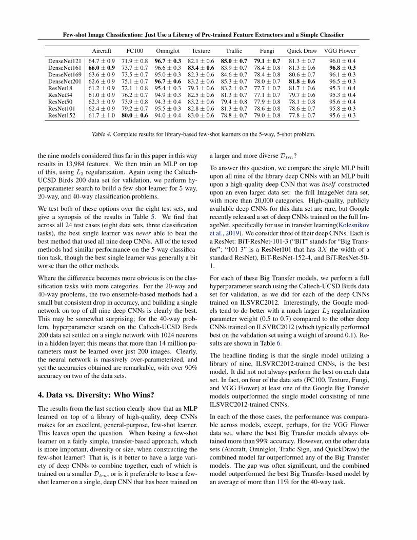
DenseNet121 64.7 ± 0.9 71.9 ± 0.8 96.7 ± 0.3 82.1 ± 0.6 85.0 ± 0.7 79.1 ± 0.7 81.3 ± 0.7 96.0 ± 0.4DenseNet161 66.0 ± 0.9 73.7 ± 0.7 96.6 ± 0.3 83.4 ± 0.6 83.9 ± 0.7 78.4 ± 0.8 81.3 ± 0.6 96.8 ± 0.3DenseNet169 63.6 ± 0.9 73.5 ± 0.7 95.0 ± 0.3 82.3 ± 0.6 84.6 ± 0.7 78.4 ± 0.8 80.6 ± 0.7 96.1 ± 0.3DenseNet201 62.6 ± 0.9 75.1 ± 0.7 96.7 ± 0.6 83.2 ± 0.6 85.3 ± 0.7 78.0 ± 0.7 81.8 ± 0.6 96.5 ± 0.3ResNet18 61.2 ± 0.9 72.1 ± 0.8 95.4 ± 0.3 79.3 ± 0.6 83.2 ± 0.7 77.7 ± 0.7 81.7 ± 0.6 95.3 ± 0.4ResNet34 61.0 ± 0.9 76.2 ± 0.7 94.9 ± 0.3 82.5 ± 0.6 81.3 ± 0.7 77.1 ± 0.7 79.7 ± 0.6 95.3 ± 0.4ResNet50 62.3 ± 0.9 73.9 ± 0.8 94.3 ± 0.4 83.2 ± 0.6 79.4 ± 0.8 77.9 ± 0.8 78.1 ± 0.8 95.6 ± 0.4ResNet101 62.4 ± 0.9 79.2 ± 0.7 95.5 ± 0.3 82.8 ± 0.6 81.3 ± 0.7 78.6 ± 0.8 78.6 ± 0.7 95.8 ± 0.3ResNet152 61.7 ± 1.0 80.0 ± 0.6 94.0 ± 0.4 83.0 ± 0.6 78.8 ± 0.7 79.0 ± 0.8 77.8 ± 0.7 95.6 ± 0.3

Table 4. Complete results for library-based few-shot learners on the 5-way, 5-shot problem.

the nine models considered thus far in this paper in this wayresults in 13,984 features. We then train an MLP on topof this, using L2 regularization. Again using the Caltech-UCSD Birds 200 data set for validation, we perform hy-perparameter search to build a few-shot learner for 5-way,20-way, and 40-way classification problems.

We test both of these options over the eight test sets, andgive a synopsis of the results in Table 5. We find thatacross all 24 test cases (eight data sets, three classificationtasks), the best single learner was never able to beat thebest method that used all nine deep CNNs. All of the testedmethods had similar performance on the 5-way classifica-tion task, though the best single learner was generally a bitworse than the other methods.

Where the difference becomes more obvious is on the clas-sification tasks with more categories. For the 20-way and40-way problems, the two ensemble-based methods had asmall but consistent drop in accuracy, and building a singlenetwork on top of all nine deep CNNs is clearly the best.This may be somewhat surprising; for the 40-way prob-lem, hyperparameter search on the Caltech-UCSD Birds200 data set settled on a single network with 1024 neuronsin a hidden layer; this means that more than 14 million pa-rameters must be learned over just 200 images. Clearly,the neural network is massively over-parameterized, andyet the accuracies obtained are remarkable, with over 90%accuracy on two of the data sets.

4. Data vs. Diversity: Who Wins?The results from the last section clearly show that an MLPlearned on top of a library of high-quality, deep CNNsmakes for an excellent, general-purpose, few-shot learner.This leaves open the question. When basing a few-shotlearner on a fairly simple, transfer-based approach, whichis more important, diversity or size, when constructing thefew-shot learner? That is, is it better to have a large vari-ety of deep CNNs to combine together, each of which istrained on a smaller Dtrn , or is it preferable to base a few-shot learner on a single, deep CNN that has been trained on

a larger and more diverse Dtrn?

To answer this question, we compare the single MLP builtupon all nine of the library deep CNNs with an MLP builtupon a high-quality deep CNN that was itself constructedupon an even larger data set: the full ImageNet data set,with more than 20,000 categories. High-quality, publiclyavailable deep CNNs for this data set are rare, but Googlerecently released a set of deep CNNs trained on the full Im-ageNet, specifically for use in transfer learning(Kolesnikovet al., 2019). We consider three of their deep CNNs. Each isa ResNet: BiT-ResNet-101-3 (“BiT” stands for “Big Trans-fer”; “101-3” is a ResNet101 that has 3X the width of astandard ResNet), BiT-ResNet-152-4, and BiT-ResNet-50-1.

For each of these Big Transfer models, we perform a fullhyperparameter search using the Caltech-UCSD Birds dataset for validation, as we did for each of the deep CNNstrained on ILSVRC2012. Interestingly, the Google mod-els tend to do better with a much larger L2 regularizationparameter weight (0.5 to 0.7) compared to the other deepCNNs trained on ILSVRC2012 (which typically performedbest on the validation set using a weight of around 0.1). Re-sults are shown in Table 6.

The headline finding is that the single model utilizing alibrary of nine, ILSVRC2012-trained CNNs, is the bestmodel. It did not not always perform the best on each dataset. In fact, on four of the data sets (FC100, Texture, Fungi,and VGG Flower) at least one of the Google Big Transfermodels outperformed the single model consisting of nineILSVRC2012-trained CNNs.

In each of the those cases, the performance was compara-ble across models, except, perhaps, for the VGG Flowerdata set, where the best Big Transfer models always ob-tained more than 99% accuracy. However, on the other datasets (Aircraft, Omniglot, Trafic Sign, and QuickDraw) thecombined model far outperformed any of the Big Transfermodels. The gap was often significant, and the combinedmodel outperformed the best Big Transfer-based model byan average of more than 11% for the 40-way task.



5-way, 5-shot

Full Library 68.9 ± 0.9 79.1 ± 0.8 97.5 ± 0.3 85.3 ± 0.6 85.8 ± 0.7 81.2 ± 0.8 84.2 ± 0.6 97.4 ± 0.3Hard Ensemble 67.8 ± 0.9 79.9 ± 0.7 97.8 ± 0.2 85.4 ± 0.5 85.2 ± 0.7 82.1 ± 0.7 83.5 ± 0.6 97.7 ± 0.2Soft Ensemble 68.4 ± 0.9 80.5 ± 0.6 98.0 ± 0.2 85.7 ± 0.6 85.2 ± 0.7 82.0 ± 0.7 84.1 ± 0.5 97.9 ± 0.2Best Single 66.0 ± 0.9 80.0 ± 0.6 96.7 ± 0.2 83.4 ± 0.6 85.2 ± 0.7 79.1 ± 0.7 81.8 ± 0.6 96.8 ± 0.3

20-way, 5-shot


40-way, 5-shot


Table 5. Accuracy obtained using all nine library CNNs as the basis for a few-shot learner.

It was also interesting that while the Big Transfer modelswere generally better than the ILSVRC2012-trained libraryCNNs, this varied across data sets. On the Aircraft andOmniglot data sets, for example, even the best individualILSVRC2012-trained library CNNs outperformed the BigTransfer models.

All of this taken together seems to suggest that, when build-ing a transfer-based few-shot learner, having a large libraryof deep CNNs is at least as important—and likely moreimportant—than having access to a CNN that was trainedon a very large Dtrn .

5. Why Does This Work?5.1. Few-Shot Fine-Tuning Is Surprisingly Easy

We turn our attention to asking: why does using a fulllibrary of pre-trained feature extractors seem to work sowell? One reason is that fine-tuning appears to be veryeasy with a library of pre-trained features. Consider thefollowing simple experiment, designed to test whether thenumber of training points has much effect on the learnedmodel.

We choose a large number of 40-way, problems, over alleight of our benchmark data sets, and train two classifiersfor each. Both classifiers use all of the 13,984 features pro-vided by the nine library feature extractors. However, thefirst classifier is trained as a one-shot classifier, and the sec-ond classifier is trained using all of the available data in thedata set. Our goal is to see whether the sets of learnedweights have a strong correspondence across the two learn-ers; if they do, it is evidence that the number of trainingpoints has a relatively small effect. Note that in a neu-

ral network with a hidden layer consisting of hundreds orthousands of neurons, there are likely to be a large num-ber of learned weights that are of equal quality; in fact,simply permuting the neurons in the hidden layer resultsin a model that is functionally identical, but that has verydifferent weight matrices. Thus, we do not use a hiddenlayer in either classifier, and instead use a softmax directlyon top of an output layer that linearly combines the inputfeatures. Both the one-shot and full-data classifiers werelearned without regularization.

Over each of the eight benchmark data sets, for each fea-ture, we take the L1 norm of all of the 40 weights asso-ciated with the feature; this serves as an indication of theimportance of the feature. We compute the Pearson cor-relation coefficient for each of the 13,984 norms obtainedusing the models learned for the 1-shot and full data classi-fiers. These correlations are shown in Table 7.

What we see is a remarkably high correlation between thetwo sets of learned weights; above 80% correlation in everycase, except for the Traffic Sign data set. However, evenin the case of the Traffic Sign data set, there was a weakcorrelation (the Traffic Sign data is a bit of an outlier inother ways as well, as we will see subsequently).

This would seem to indicate that there is a strong signalwith only one data point per class, as the learned weightsdo not differ much when they are learned using the wholedata set. This may be one explanation for the surprisingaccuracy of the full library few-shot learner. Of course, thestrong correlation may gloss over significant differences,and more data does make a significant difference (considerthe difference between the one-shot accuracies in Table 1and the five-shot accuracies in Table 2.). But even one im-


Aircraft FC100 Omniglot Texture Traffic Fungi QDraw Flower

5-way, 5-shot

Full Library 68.9 ± 0.9 79.1 ± 0.8 97.5 ± 0.3 85.3 ± 0.6 85.8 ± 0.7 81.2 ± 0.8 84.2 ± 0.6 97.4 ± 0.3BiT-ResNet-101-3 54.0 ± 1.1 78.6 ± 0.8 82.5 ± 1.2 82.0 ± 0.9 69.2 ± 0.9 81.2 ± 1.2 63.7 ± 1.1 99.6 ± 0.1BiT-ResNet-152-4 59.5 ± 1.0 80.9 ± 0.7 94.2 ± 0.5 85.4 ± 0.6 73.3 ± 0.8 82.5 ± 0.9 74.8 ± 0.8 99.7 ± 0.1BiT-ResNet-50-1 61.9 ± 1.2 79.0 ± 0.8 87.2 ± 1.1 84.2 ± 0.6 75.6 ± 1.0 82.5 ± 0.8 71.5 ± 0.8 99.3 ± 0.2

20-way, 5-shot


40-way, 5-shot


Table 6. Comparing a few-shot learner utilizing the full library of nine ILSVRC2012-trained deep CNNs with the larger CNNs trainedon the full ImageNet.

age per class seems to give a lot of information.

5.2. Different Problems Utilize Different Features

Another reason for the accuracy obtained by the full librarymethod may be that different problem domains seem to uti-lize different sets of features, and different feature extrac-tors. Having a large library ensures that some features rel-evant to any task are always present.

To investigate this, we construct a large number of 40-waytraining tasks over each of the various data sets, and foreach, we learn a network without a hidden layer on topof all 13,984 features obtained using the library of deepCNNs. Again, we compute the L1 norm of the set ofweights associated with each of the features. This time,however, for each problem we then consider the featureswhose norms are in the top 20%; these could be consid-ered the features most important to solving the classifica-tion task.

For each of the (data set, data set) pairs, we compute theaverage Jaccard similarity of these top-feature sets. Sinceeach set consists of 20% of the features, if each set of fea-tures chosen was completely random, for n features in all,we would expect a Jaccard similarity of 0.04n

.2n+.2n−0.04n =0.04

.4−0.04 = 0.111. Anything greater indicates the sets offeatures selected are positively correlated; lower indicatesa negative correlation. Results are in Figure 1. For eachof the nine CNNs, we also compute the fraction of eachCNN’s features that are in the top 20% when a full libraryclassifier is constructed. These percentages are in Figure 2.

The data in these two plots, along with the previous results,tells a consistent story: there appears to be little correspon-

dence between data sets in terms of the set of features thatare chosen as important across data sets. The largest Jac-card value in Figure 1 is less than 0.5 (observed betweenFC100 and Texture). This shows, in our opinion, a rela-tively weak correspondence. The Traffic Sign data set, hadan average Jaccard of 0.108 across the other eight data sets,which is even lower than the 0.111 that would be expectedunder a purely random feature selection regime. One mightspeculate that the lack of correspondence across data setsis evidence for the hypothesis that different tasks tend touse different features, which would explain why it is so ef-fective to use an entire library of deep CNNs for few-shotlearning.

Also note that in Figure 2, we tend to see that differentdeep CNNs contribute “important” features at very differ-ent rates, depending on the particular few-shot classifica-tion task. This also seems to be evidence that diversityis important. In general, the DenseNets’ features are pre-ferred over the ResNets’ features, but this is not universal,and there is a lot of variation. It may not be an accidentthat the three data sets where the selection of features fromlibrary CNNs shows the most diversity in Figure 2 (TrafficSign, Quick Draw, and Omniglot) are the three data setswhere the classifier built on top of all nine library CNNshas the largest advantage compared to the few-shot classi-fiers built on top of the single, “Big Transfer”-based deepCNN.

6. Related WorkWhile most research on few-shot learning (Wang et al.,2018; Oreshkin et al., 2018; Rusu et al., 2018) has focused


Aircraft Birds FC100 Fungi Omniglot Quick Draw Texture Traffic VGG Flower

Correlation 0.95 0.88 0.89 0.86 0.93 0.92 0.80 0.18 0.87

Table 7. Correlation between weight learned using one example per class, and the full data.

Aircraft BirdsFC100

Fungi

Omniglot

Quick DrawTexture

Traffic Sign

VGG Flower

Aircraft

Birds

FC100

Fungi

Omniglot

Quick Draw

Texture

Traffic Sign

VGG Flower

Similarity In Top Features

0.39

0.399

0.372

0.314

0.277

0.431

0.107

0.369

0.39

0.382

0.417

0.291

0.268

0.413

0.101

0.387

0.399

0.382

0.373

0.335

0.331

0.485

0.108

0.342

0.372

0.417

0.373

0.287

0.264

0.46

0.101

0.416

0.314

0.291

0.335

0.287

0.331

0.332

0.124

0.281

0.277

0.268

0.331

0.264

0.331

0.326

0.109

0.244

0.431

0.413

0.485

0.46

0.332

0.326

0.125

0.399

0.107

0.101

0.108

0.101

0.124

0.109

0.125

0.093

0.369

0.387

0.342

0.416

0.281

0.244

0.399

0.093

1

1

1

1

1

1

1

1

10.1

0.2

0.3

0.4

0.5

0.6

0.7

0.8

0.9

1

Figure 1. Jaccard similarity of sets of most important features forthe various (data set, data set) pairs.

on developing new and sophisticated methods for learn-ing a few-shot learner, there have recently been a few pa-pers that, like this work, have suggested that transfer-basedmethods may be the most accurate.

In Section 1, we mentioned Google’s “Big Transfer” paper(Kolesnikov et al., 2019). There, the authors argued thatthe best approach to few-shot learning is to concentrate onusing a high-quality feature extractor rather than a sophis-ticated meta-learning approach. We agree with this, butalso give evidence that training a huge model and a mas-sive data set may not be the only key to few-shot imageclassification. We found that a library with a wide diversityof high-quality deep CNNs can lead to substantially betteraccuracy than a single massive CNN, even when that deepCNN is trained on a much larger data set. Tian et al. (Tianet al., 2020) make a similar argument to the Big Transferauthors, observing that a simple transfer-based approachcan outperform a sophisticated meta-learner.

Chen et al. (Chen et al., 2019) were among the first re-searchers to point out that simple, transfer-based methodsmay outperform sophisticated few-shot learners. They pro-posed Baseline which uses a simple linear classifier on topof a pre-trained deep CNN, and Baseline++ which uses adistance-based classifier. Dhillon et al. (Dhillon et al.,2019) also point out the utility of transfer-based meth-ods, and propose a transductive fine-tuner; however, sucha method relies on having an appropriately large number

densenet121

densenet161

densenet169

densenet201

resnet101

resnet152resnet18

resnet34resnet50

Aircraft

Birds

FC100

Fungi

Omniglot

Quick Draw

Texture

Traffic Sign

VGG Flower

Percent of Features Selected

43.85

47.17

37.4

43.36

41.11

29.69

40.43

20.61

48.05

25.95

42.46

25.58

26.13

22.42

18.93

30.43

11.05

23.73

46.03

43.75

42.79

48.02

37.62

31.55

46.51

12.5

46.75

47.5

50.83

39.01

36.56

48.54

11.72

52.19

0

0

1.37

0

5.81

11.25

0

20.95

0

0.05

0

1.86

0

7.9

15.09

0

19.92

0

0.39

0

12.3

0

19.53

25.98

0.39

0

0.2

0

6.05

0

8.4

14.06

0.2

0

0

0

0.98

0

3.96

6.01

0.05

18.02

0

54.43

54.43

65.23 71.88

0

10

20

30

40

50

60

70

Figure 2. Percent of each deep CNN’s features that appear in thetop 20% of features, on each data set.

of relevant, unlabeled images to perform the transductivelearning. Sun et al. (Sun et al., 2019) consider transferlearning, but where transfer is realized via shifting and scal-ing of the classification parameters.

Dvornik et al. (Dvornik et al., 2020) propose SUR, andargue that diversity in features is best obtained through di-versity in data sets. Their method trains many feature ex-tractors, one per data set. We argue that instead, a singlehigh-quality data set is all that is needed. Adding additionalfeature extractors trained on that data set is the best way tohigher accuracy. This may be counter-intuitive, but thereis an obvious argument for this: training on less diversedata sets such as Aircraft or VGG Flowers is apt to resultin feature extractors that are highly specialized, do not gen-eralize well, and are not particularly useful. The proposedlibrary-based classifier generally outperformed SUR in ourexperiments.

Dvornik et al. (Dvornik et al., 2019) also consider the ideaof ensembling for few-shot learning, although their ideais to simultaneously train a number of diverse deep CNNsas feature extractors during meta-learning; adding penaltyterms that encourage both diversity and conformity duringlearning. We propose the simple idea of simply using aset of existing deep CNNs, trained by different groups ofengineers.


7. ConclusionsWe have examined the idea of using a library of deep CNNsas a basis for a high-quality few-shot learner. We haveshown that a learner built on top of a high-quality deepCNN can have remarkable accuracy, and that a learner builtupon an entire library of CNNs can significantly outper-form a few-shot learner built upon any one deep CNN.

While we conjecture that it will be hard to do better thanusing a library of high-quality deep CNNs as the basis for afew-shot learner, there are key unanswered questions. First,

future work should study if the accuracy continues to im-prove as the library is made even larger. Also, it may beexpensive to feed a test image through a series of nine (ormore) deep CNNs. It would be good to know if the compu-tational cost of the library-based approach can be reduced.Finally, it would be good to know if there are better meth-ods to facilitate transfer than learning a simple MLP.

Acknowledgments. The work in this paper was funded byNSF grant #1918651; by NIH award # UL1TR003167, andby ARO award #78372-CS.


ReferencesChen, W.-Y., Liu, Y.-C., Kira, Z., Wang, Y.-C. F., and

Huang, J.-B. A closer look at few-shot classification.arXiv preprint arXiv:1904.04232, 2019.

Cimpoi, M., Maji, S., Kokkinos, I., Mohamed, S., , andVedaldi, A. Describing textures in the wild. In Proceed-ings of the IEEE Conf. on Computer Vision and PatternRecognition (CVPR), 2014.

Dhillon, G. S., Chaudhari, P., Ravichandran, A., andSoatto, S. A baseline for few-shot image classification.arXiv preprint arXiv:1909.02729, 2019.

Dvornik, N., Schmid, C., and Mairal, J. Diversity withcooperation: Ensemble methods for few-shot classifica-tion. In Proceedings of the IEEE International Confer-ence on Computer Vision, pp. 3723–3731, 2019.

Dvornik, N., Schmid, C., and Mairal, J. SelectingRelevant Features from a Multi-domain Representa-tion for Few-shot Classification. arXiv e-prints, art.arXiv:2003.09338, March 2020.

Fei-Fei, L., Fergus, R., and Perona, P. One-shot learning ofobject categories. IEEE transactions on pattern analysisand machine intelligence, 28(4):594–611, 2006.

Finn, C., Abbeel, P., and Levine, S. Model-agnostic meta-learning for fast adaptation of deep networks. In Pro-ceedings of the 34th International Conference on Ma-chine Learning-Volume 70, pp. 1126–1135. JMLR. org,2017.

Finn, C., Xu, K., and Levine, S. Probabilistic model-agnostic meta-learning. In Advances in Neural Informa-tion Processing Systems, pp. 9516–9527, 2018.

He, K., Zhang, X., Ren, S., and Sun, J. Deep residual learn-ing for image recognition. In Proceedings of the IEEEconference on computer vision and pattern recognition,pp. 770–778, 2016.

Houben, S., Stallkamp, J., Salmen, J., Schlipsing, M., andIgel, C. Detection of traffic signs in real-world images:The german traffic sign detection benchmark. In The2013 international joint conference on neural networks(IJCNN), pp. 1–8. IEEE, 2013.

Huang, G., Liu, Z., Van Der Maaten, L., and Weinberger,K. Q. Densely connected convolutional networks. InProceedings of the IEEE conference on computer visionand pattern recognition, pp. 4700–4708, 2017.

Jongejan, J., Rowley, H., Kawashima, T., Kim, J., and Fox-Gieg, N. The quick, draw!-ai experiment. Mount View,CA, accessed Feb, 17(2018):4, 2016.

Kim, T., Yoon, J., Dia, O., Kim, S., Bengio, Y., and Ahn, S.Bayesian model-agnostic meta-learning. arXiv preprintarXiv:1806.03836, 2018.

Kolesnikov, A., Beyer, L., Zhai, X., Puigcerver, J., Yung,J., Gelly, S., and Houlsby, N. Big transfer (bit):General visual representation learning. arXiv preprintarXiv:1912.11370, 6, 2019.

Krizhevsky, A., Hinton, G., et al. Learning multiple layersof features from tiny images. 2009.

Lake, B. M., Salakhutdinov, R., and Tenenbaum, J. B.Human-level concept learning through probabilistic pro-gram induction. Science, 350(6266):1332–1338, 2015.

Lee, K., Maji, S., Ravichandran, A., and Soatto, S. Meta-learning with differentiable convex optimization. In Pro-ceedings of the IEEE Conference on Computer Visionand Pattern Recognition, pp. 10657–10665, 2019.

Lee, Y. and Choi, S. Gradient-based meta-learning withlearned layerwise metric and subspace. arXiv preprintarXiv:1801.05558, 2018.

Li, H., Eigen, D., Dodge, S., Zeiler, M., and Wang, X.Finding task-relevant features for few-shot learning bycategory traversal. In Proceedings of the IEEE Confer-ence on Computer Vision and Pattern Recognition, pp.1–10, 2019.

Maji, S., Rahtu, E., Kannala, J., Blaschko, M. B., andVedaldi, A. Fine-grained visual classification of aircraft.CoRR, abs/1306.5151, 2013. URL http://arxiv.org/abs/1306.5151.

Nichol, A. and Schulman, J. Reptile: a scalable metalearn-ing algorithm. arXiv preprint arXiv:1803.02999, 2:2,2018.

Nilsback, M.-E. and Zisserman, A. Automated flower clas-sification over a large number of classes. In 2008 SixthIndian Conference on Computer Vision, Graphics & Im-age Processing, pp. 722–729. IEEE, 2008.

Oreshkin, B., Rodrıguez Lopez, P., and Lacoste, A. Tadam:Task dependent adaptive metric for improved few-shotlearning. Advances in Neural Information ProcessingSystems, 31:721–731, 2018.

Ravi, S. and Larochelle, H. Optimization as a model forfew-shot learning. 2016.

Russakovsky, O., Deng, J., Su, H., Krause, J., Satheesh, S.,Ma, S., Huang, Z., Karpathy, A., Khosla, A., Bernstein,M., Berg, A. C., and Fei-Fei, L. ImageNet Large ScaleVisual Recognition Challenge. International Journal ofComputer Vision (IJCV), 115(3):211–252, 2015. doi: 10.1007/s11263-015-0816-y.

http://arxiv.org/abs/1306.5151

http://arxiv.org/abs/1306.5151


Rusu, A. A., Rao, D., Sygnowski, J., Vinyals, O., Pas-canu, R., Osindero, S., and Hadsell, R. Meta-learningwith latent embedding optimization. arXiv preprintarXiv:1807.05960, 2018.

Schroeder, B. and Cui, Y. Fgvcx fungi classification chal-lenge 2018. https://github.com/visipedia/fgvcx_fungi_comp, 2018.

Snell, J., Swersky, K., and Zemel, R. Prototypical networksfor few-shot learning. In Advances in Neural Informa-tion Processing Systems, pp. 4077–4087, 2017.

Sun, C., Shrivastava, A., Singh, S., and Gupta, A. Revis-iting unreasonable effectiveness of data in deep learningera. In Proceedings of the IEEE international conferenceon computer vision, pp. 843–852, 2017.

Sun, Q., Liu, Y., Chua, T.-S., and Schiele, B. Meta-transferlearning for few-shot learning. In Proceedings of theIEEE conference on computer vision and pattern recog-nition, pp. 403–412, 2019.

Sung, F., Yang, Y., Zhang, L., Xiang, T., Torr, P. H., andHospedales, T. M. Learning to compare: Relation net-work for few-shot learning. In Proceedings of the IEEEConference on Computer Vision and Pattern Recogni-tion, pp. 1199–1208, 2018.

Tian, Y., Wang, Y., Krishnan, D., Tenenbaum, J. B., andIsola, P. Rethinking few-shot image classification: a

good embedding is all you need? arXiv preprintarXiv:2003.11539, 2020.

Triantafillou, E., Zhu, T., Dumoulin, V., Lamblin, P., Evci,U., Xu, K., Goroshin, R., Gelada, C., Swersky, K.,Manzagol, P.-A., and Larochelle, H. Meta-Dataset: ADataset of Datasets for Learning to Learn from Few Ex-amples. arXiv e-prints, art. arXiv:1903.03096, March2019.

Vinyals, O., Blundell, C., Lillicrap, T., Wierstra, D., et al.Matching networks for one shot learning. In Advances inneural information processing systems, pp. 3630–3638,2016.

Wang, Y.-X., Girshick, R., Hebert, M., and Hariharan, B.Low-shot learning from imaginary data. In Proceedingsof the IEEE conference on computer vision and patternrecognition, pp. 7278–7286, 2018.

Welinder, P., Branson, S., Mita, T., Catherine, W., Schroff,F., Belongie, S., and Perona, P. Caltech-UCSD Birds200. Technical Report CNS-TR-2010-001, CaliforniaInstitute of Technology, 2010.

Ye, H.-J., Hu, H., Zhan, D.-C., and Sha, F. Few-shot learn-ing via embedding adaptation with set-to-set functions.In Proceedings of the IEEE/CVF Conference on Com-puter Vision and Pattern Recognition, pp. 8808–8817,2020.

https://github.com/visipedia/fgvcx_fungi_comp

https://github.com/visipedia/fgvcx_fungi_comp


Appendix

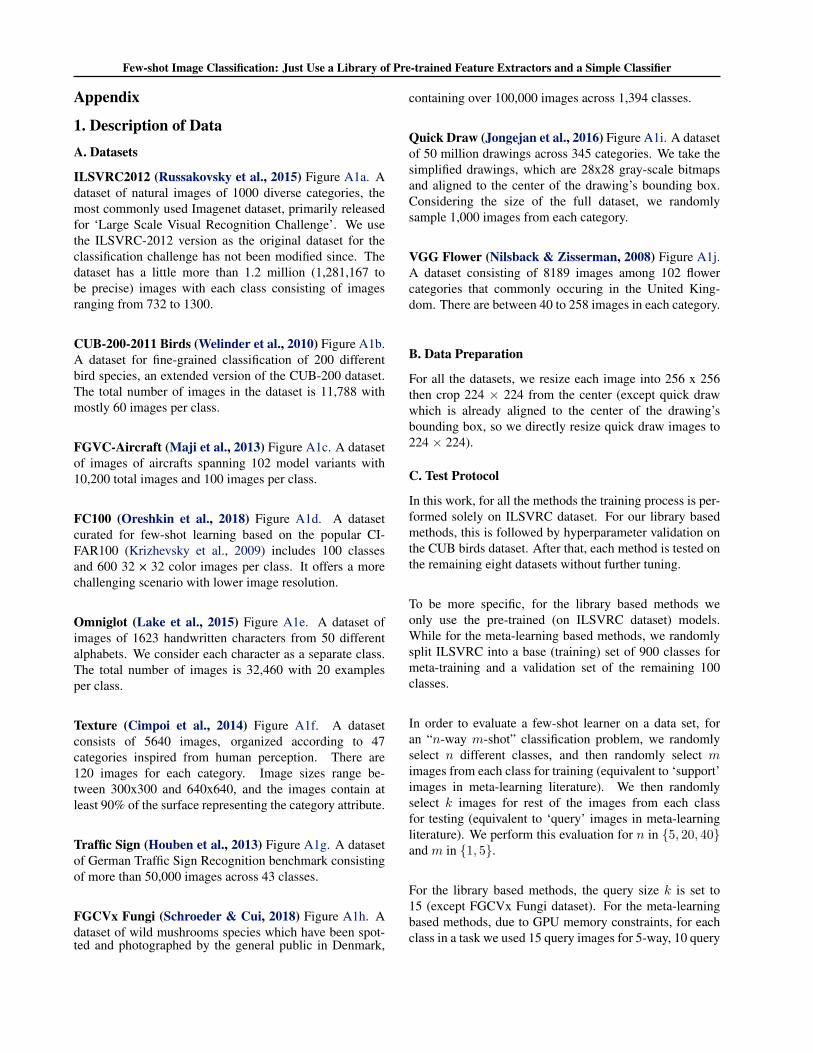
1. Description of DataA. Datasets

ILSVRC2012 (Russakovsky et al., 2015) Figure A1a. Adataset of natural images of 1000 diverse categories, themost commonly used Imagenet dataset, primarily releasedfor ‘Large Scale Visual Recognition Challenge’. We usethe ILSVRC-2012 version as the original dataset for theclassification challenge has not been modified since. Thedataset has a little more than 1.2 million (1,281,167 tobe precise) images with each class consisting of imagesranging from 732 to 1300.

CUB-200-2011 Birds (Welinder et al., 2010) Figure A1b.A dataset for fine-grained classification of 200 differentbird species, an extended version of the CUB-200 dataset.The total number of images in the dataset is 11,788 withmostly 60 images per class.

FGVC-Aircraft (Maji et al., 2013) Figure A1c. A datasetof images of aircrafts spanning 102 model variants with10,200 total images and 100 images per class.

FC100 (Oreshkin et al., 2018) Figure A1d. A datasetcurated for few-shot learning based on the popular CI-FAR100 (Krizhevsky et al., 2009) includes 100 classesand 600 32 × 32 color images per class. It offers a morechallenging scenario with lower image resolution.

Omniglot (Lake et al., 2015) Figure A1e. A dataset ofimages of 1623 handwritten characters from 50 differentalphabets. We consider each character as a separate class.The total number of images is 32,460 with 20 examplesper class.

Texture (Cimpoi et al., 2014) Figure A1f. A datasetconsists of 5640 images, organized according to 47categories inspired from human perception. There are120 images for each category. Image sizes range be-tween 300x300 and 640x640, and the images contain atleast 90% of the surface representing the category attribute.

Traffic Sign (Houben et al., 2013) Figure A1g. A datasetof German Traffic Sign Recognition benchmark consistingof more than 50,000 images across 43 classes.

FGCVx Fungi (Schroeder & Cui, 2018) Figure A1h. Adataset of wild mushrooms species which have been spot-ted and photographed by the general public in Denmark,

containing over 100,000 images across 1,394 classes.

Quick Draw (Jongejan et al., 2016) Figure A1i. A datasetof 50 million drawings across 345 categories. We take thesimplified drawings, which are 28x28 gray-scale bitmapsand aligned to the center of the drawing’s bounding box.Considering the size of the full dataset, we randomlysample 1,000 images from each category.

VGG Flower (Nilsback & Zisserman, 2008) Figure A1j.A dataset consisting of 8189 images among 102 flowercategories that commonly occuring in the United King-dom. There are between 40 to 258 images in each category.

B. Data Preparation

For all the datasets, we resize each image into 256 x 256then crop 224 × 224 from the center (except quick drawwhich is already aligned to the center of the drawing’sbounding box, so we directly resize quick draw images to224 × 224).

C. Test Protocol

In this work, for all the methods the training process is per-formed solely on ILSVRC dataset. For our library basedmethods, this is followed by hyperparameter validation onthe CUB birds dataset. After that, each method is tested onthe remaining eight datasets without further tuning.

To be more specific, for the library based methods weonly use the pre-trained (on ILSVRC dataset) models.While for the meta-learning based methods, we randomlysplit ILSVRC into a base (training) set of 900 classes formeta-training and a validation set of the remaining 100classes.

In order to evaluate a few-shot learner on a data set, foran “n-way m-shot” classification problem, we randomlyselect n different classes, and then randomly select mimages from each class for training (equivalent to ‘support’images in meta-learning literature). We then randomlyselect k images for rest of the images from each classfor testing (equivalent to ‘query’ images in meta-learningliterature). We perform this evaluation for n in {5, 20, 40}and m in {1, 5}.

For the library based methods, the query size k is set to15 (except FGCVx Fungi dataset). For the meta-learningbased methods, due to GPU memory constraints, for eachclass in a task we used 15 query images for 5-way, 10 query


(a) ILSVRC-2012 (b) CUB-200-2011 Birds (c) Aircraft

(d) FC100 (e) Omniglot (f) Texture

(g) Traffic Sign(h) Fungi (i) Quick Draw

(j) VGG Flower

Figure A1. Images sampled from the data sets used in our experiments.


images for 10-way, and 5 query images for 40-way prob-lems, with only exception being the Fungi dataset. Fungidataset has several classes with a very small number of im-ages (6 being the minimum). Hence for Fungi dataset, weuse 5 query images per class for 1-shot and 1 query imageper class for 5-shot problems. Finally, for every problem,we report the mean of 600 randomly generated test tasksalong with the 95% confidence intervals.

For the FC100 data set, there is a small portion overlapswith ILSVRC2012 data set but we still think that the FC100as a testing set is interesting, as (1) all of the few-shotlearners benefitted from the overlapping classes, and (2)this shows how the methods work in the case that the testclasses are close to something that the few-shot learner hasseen before.

2. Hyper-parameters for Library-BasedLearnersIn order to achieve an “out-of-the-box” few-shot learnerthat can be used on any (very small) training set Dfew with-out additional data or knowledge of the underlying distribu-tion, an extensive hyper-parameter search is performed onthe validation dataset (CUB birds). The hyper-parametersthat are found to be the best are then applied in the few-shot training and testing phase for each of our library basedmethods. The hyper-parameters we are considering includelearning rate, number of training epochs, L2-regularizationpenalty constant, the number of neurons in the MLP hiddenlayer, and whether to drop the hidden layer altogether. Aseparate hyper-parameter search is used for 5-way, 20-way,and 40-way 1-shot classification. 5-shot problems are us-ing the same hyper-parameters as 1-shot ones. Experimentssuggest that dropping the hidden layer did not significantlyhelp performance, but did occasionally hurt performancesignificantly on the validation set; as a result, we alwaysuse a hidden layer. We train all our methods using Adamoptimizer. The hyper-parameters details can be found inTable A8.

3. Competitive MethodsFor methods that require a pre-trained CNN (FEAT,Meta-transfer, and SUR), we use the pre-trained ResNet18pytorch library as the backbone. We follow the hyper-parameter setting from (Sun et al., 2019), (Ye et al.,2020), and (Dvornik et al., 2020). For the FEAT andMeta-transfer methods, we perform meta-training onILSVRC dataset(Russakovsky et al., 2015) before testingon eight different datasets. For the SUR method, wefollow (Dvornik et al., 2020) and build a multi-domainrepresentation by pre-training multiple ResNet18 onMeta-Dataset (Triantafillou et al., 2019) (one per data set).

To evaluate SUR on data set X , we use feature extractorstrained on the rest of the data sets in {Omniglot, Aircraft,Birds, Texture, Quickdraw, Flowers, Fungi,and ILSVRC}.Traffic Sign and FC100 data sets are reserved for testingonly. To be more specific, the meta-training setting are asfollows:

Meta-transfer LearningThe base-learner is optimized by batch gradient descentwith the learning rate of 10−2 and gets updated every 50steps. The meta learner is optimized by Adam optimizerwith an initial learning rate of 10−3, and decaying 50%every 1,000 iterations until 10−4.

FEATThe vanilla stochastic gradient descent with Nesterovacceleration is applied. The initial rate is set to 2 × 10−4

and decreases every 40 steps with a decay rate of 5× 10−4

and momentum of 0.9. The learning rate for the scheduleris set to 0.5.

SURWe follow (Dvornik et al., 2020) and apply SGD with mo-mentum during optimization. The learning rate is adjustedwith cosine annealing. The initial learning rate, the max-imum number of training iterations (“Max Iter.”) and an-nealing frequency (“Annealing Freq.”) are adjusted individ-ually according to each data set (Table A1). Data augmen-tation is also deployed to regularize the training process,which includes random crops and random color augmenta-tions with a constant weight decay of 7× 10−4.

BaselinesWe train the two pre-training based methods, Baselineand Baseline++ (Chen et al., 2019) following the hyper-parameters suggested by the original authors. However,since we train them on ILSVRC data as opposed tomini-imagenet (Ravi & Larochelle, 2016). During thetraining stage, we train 50 epochs with a batch size of16. In the paper, the authors have trained 400 epochs onthe base set of mini-imagenet consisting of 64 classes.Mini-imagenet has 600 images per class, whereas ILSVRChas an average of around 1,200 images per class. So,the total number of batches trained in our baselines is50 × (1000 × 1, 200)/16 = 3, 750, 000, as opposed to400× (64× 600)/16 = 960, 000 in the original paper.

Metric-Learning Methods and MAMLFor the three most popular metric-learning methods,MatchingNet (Vinyals et al., 2016), ProtoNet (Snell et al.,2017) and RelationNet (Sung et al., 2018), again we fol-lowed the implementation and hyper-parameters provided


Learning Weight Max Annealing BatchRate Decay Iter. Freq. Size

ILSVRC 3× 10−2 7× 10−4 480,000 48,000 64Omniglot 3× 10−2 7× 10−4 50,000 3,000 16Aircraft 3× 10−2 7× 10−4 50,000 3,000 8Birds 3× 10−2 7× 10−4 50,000 3,000 16Textures 3× 10−2 7× 10−4 50,000 1,500 32Quick Draw 1× 10−2 7× 10−4 480,000 48,000 64Fungi 3× 10−2 7× 10−4 480,000 15,000 32VGG Flower 3× 10−2 7× 10−4 50,000 1,500 8

Table A1. Hyper-parameter settings for SUR individual feature networks on MetaDataset.



Worst library- 40.9 ± 0.9 50.8 ± 0.9 77.2 ± 0.8 59.0 ± 0.9 55.5 ± 0.8 53.0 ± 0.9 57.3 ± 0.9 79.7 ± 0.8based RN18 DN121 RN152 DN169 RN152 DN201 RN101 RN18Best library- 46.1 ± 1.0 61.2 ± 0.9 86.5 ± 0.6 65.1 ± 0.9 66.6 ± 0.9 56.6 ± 0.9 62.8 ± 0.9 83.2 ± 0.8based DN161 RN152 DN121 RN101 DN201 DN121 RN18 DN201

Table A2. Comparing competitive methods with the simple library-based learners, on the 5-way, 1-shot problem.

by (Chen et al., 2019).

All the metric-learning methods and MAML (Finn et al.,2017) are trained using the Adam optimizer with initiallearning rate of 10−3. For MAML, the inner learning rateis kept at 10−2 as suggested by the original authors. Andfollowing (Chen et al., 2019), we do the following modi-fications: For MatchingNet, we use an FCE classificationlayer without fine-tuning and also multiply the cosine sim-ilarity by a constant scalar. For RelationNet, we replacethe L2 norm with a softmax layer to expedite training. ForMAML, we use a first-order approximation in the gradi-ent for memory efficiency. Even then, we could not trainMAML for 40-way in a single GPU due to memory short-age. Hence, we drop MAML for 40-way experiments.

During the meta-training stage of all these methods, wetrain 150,000 episodes for 5-way 1-shot, 5-way 5-shot, and20-way 1-shot problems, and 50,000 episodes for all otherproblems on the base split of ILSVRC. Here an episoderefers to one meta-learning task that includes training onthe ‘support’ images and testing on the ‘query’ images.The stopping episode number is chosen based on no signif-icant increase in validation accuracy. In the original paper,the authors trained 60,000 episodes for 1-shot and 40,000episodes for 5-shot tasks. We meticulously observe that

those numbers are too low for certain problems in termsof validation accuracy. Hence, we allow more episodes.We select the best accuracy model on the validation set ofILSVRC for meta-testing on other datasets.

4. Complete ResultsHere we conduct additional experiments which are notreported in our main paper.

Single Library Learners VS. Competitive MethodsTable A2, A3, A4, A5 show the performance comparisonof single library learners and the competitive methodsincluding Baseline, Baseline++, MAML, MatchingNet,ProtoNet, RelationNet, Meta-transfer Learning, and FEAT.The comparison is conducted on problems of 1-shot under5-way, 20-way, and 40-way and 5-shot under 40-way.

Full Library VS. Google BiT MethodsTable A6 shows the performance comparison of thefull library method and the Google BiT methods. Theproblems addressed here are 1-shot under 5-way, 20-way,and 40-way. The full library method utilizes a library




Worst library- 20.1 ± 0.3 27.8 ± 0.4 56.2 ± 0.5 38.0 ± 0.4 29.7 ± 0.3 31.7 ± 0.4 33.3 ± 0.5 62.4 ± 0.5based RN101 DN121 RN101 RN18 RN101 RN101 RN101 RN101Best library- 24.3 ± 0.3 36.4 ± 0.4 69.1 ± 0.4 42.5 ± 0.4 38.5 ± 0.4 33.9 ± 0.5 39.5 ± 0.5 70.0 ± 0.5based DN161 RN152 DN121 DN152 DN201 DN161 DN201 DN161



Baseline 6.9 ± 0.2 9.7 ± 0.1 27.1 ± 0.4 11.2 ± 0.1 20.0 ± 0.3 8.2 ± 0.2 14.8 ± 0.3 28.7 ± 0.3Baseline++ 6.1 ± 0.1 10.1 ± 0.1 29.9 ± 0.3 12.1 ± 0.2 23.2 ± 0.2 8.7 ± 0.2 15.9 ± 0.2 24.2 ± 0.3MatchingNet 5.1 ± 0.1 11.6 ± 0.2 32.5 ± 0.4 15.0 ± 0.2 19.3 ± 0.2 11.0 ± 0.2 19.0 ± 0.3 26.9 ± 0.3ProtoNet 7.2 ± 0.2 13.8 ± 0.2 47.2 ± 0.4 14.4 ± 0.2 21.6 ± 0.3 11.3 ± 0.2 22.9 ± 0.3 31.0 ± 0.3RelationNet 6.2 ± 0.2 13.8 ± 0.2 45.2 ± 0.4 11.4 ± 0.2 18.2 ± 0.2 10.7 ± 0.2 21.1 ± 0.3 28.1 ± 0.3Meta-transfer 7.6 ± 0.2 20.6 ± 0.2 37.5 ± 0.3 19.2 ± 0.2 24.4 ± 0.2 10.2 ± 0.2 22.2 ± 0.2 40.4 ± 0.3FEAT 10.1 ± 0.2 12.9 ± 0.3 35.7 ± 0.4 21.8 ± 0.3 24.9 ± 0.3 18.0 ± 0.3 19.4 ± 0.3 47.6 ± 0.4SUR 9.9 ± 0.1 13.3 ± 0.2 78.1 ± 0.3 15.0 ± 0.2 19.7 ± 0.2 15.6 ± 0.3 26.7 ± 0.3 48.8 ± 0.3




Baseline 17.0 ± 0.2 29.4 ± 0.3 80.0 ± 0.3 27.1 ± 0.2 49.1 ± 0.3 24.0 ± 0.5 41.5 ± 0.3 68.3 ± 0.3Baseline++ 12.3 ± 0.2 24.4 ± 0.3 67.0 ± 0.3 25.1 ± 0.3 44.1 ± 0.3 19.7 ± 0.5 35.2 ± 0.3 53.9 ± 0.3MatchingNet 8.6 ± 0.2 22.1 ± 0.3 59.1 ± 0.4 23.3 ± 0.3 37.1 ± 0.3 19.0 ± 0.5 31.5 ± 0.3 46.7 ± 0.4ProtoNet 13.8 ± 0.2 28.0 ± 0.3 80.0 ± 0.3 29.6 ± 0.3 39.7 ± 0.3 23.6 ± 0.5 42.6 ± 0.4 61.6 ± 0.3RelationNet 10.7 ± 0.2 26.1 ± 0.3 77.0 ± 0.3 18.7 ± 0.2 29.6 ± 0.3 18.3 ± 0.5 40.6 ± 0.3 47.0 ± 0.3Meta-transfer 9.7 ± 0.2 29.9 ± 0.2 48.1 ± 0.3 29.8 ± 0.2 33.3 ± 0.2 12.2 ± 0.3 31.6 ± 0.2 55.4 ± 0.3FEAT 16.2 ± 0.3 27.1 ± 0.4 58.5 ± 0.4 36.8 ± 0.3 37.3 ± 0.3 32.9 ± 0.6 35.6 ± 0.4 74.0 ± 0.4SUR 15.5 ± 0.2 32.6 ± 0.3 94.2 ± 0.1 25.8 ± 0.1 37.0 ± 0.2 26.3 ± 0.6 45.0 ± 0.3 69.8 ± 0.3



of nine, ILSVRC-trained CNNs, while the Google BiTmethods individually use three deep CNNs trained on thefull ImageNet.

Full Library VS. Hard and Soft Ensemble MethodsTable A7 compares the performances of the full librarymethod and the hard and soft ensemble methods (bagging)for 1-shot problems under 5-way, 20-way, and 40-way.


Aircraft FC100 Omniglot Texture Traffic Fungi QDraw Flower

5-way, 1-shot


20-way, 1-shot


40-way, 1-shot


Table A6. Comparing a few-shot learner utilizing the full library of nine ILSVRC2012-trained deep CNNs with the larger CNNs trainedon the full ImageNet.


5-way, 1-shot


20-way, 1-shot


40-way, 1-shot


Table A7. Accuracy obtained using all nine library CNNs as the basis for a few-shot learner.


Number of Hidden Learning RegularizationEpochs Size Rate Constant

5-way, 1-shot and 5-shot

DenseNet121 200 1024 1× 10−3 0.2DenseNet161 100 1024 5× 10−4 0.2DenseNet169 300 1024 5× 10−4 0.5DenseNet201 100 512 5× 10−4 0.5ResNet18 200 512 1× 10−3 0.2ResNet34 100 1024 5× 10−4 0.2ResNet50 300 2048 5× 10−4 0.1ResNet101 100 512 1× 10−3 0.1ResNet152 300 512 5× 10−4 0.1Full Library 300 1024 5× 10−4 0.1BiT-ResNet-101-3 300 4096 1× 10−3 0.7BiT-ResNet-152-4 300 2048 5× 10−4 0.7BiT-ResNet-50-1 200 2048 5× 10−4 0.5





Table A8. Hyper-parameter settings for different backbones in 5, 20, and 40 ways.

Few-shot Image Classification: Just Use a Library of Pre ...

Documents

Transcript of Few-shot Image Classification: Just Use a Library of Pre ...