AN ANALYTICAL THEORY OF MOIST CONVECTION

by

CHRISTOPHER STEPHEN BRETHERTON

B.S., California Institute of Technology(1980)

SUBMITTED TO THE DEPARTMENT OF MATHEMATICSIN PARTIAL FULFILLMENT OF THE REQUIREMENTS

FOR THE DEGREE OF

DOCTOR OF PHILOSOPHY

at the

MASSACHUSETTS INSTITUTE OF TECHNOLOGYDecember, 1984

( Christopher Stephen Bretherton, 1984

The author hereby grants to M.I.T. permission to reproduce and to

distribute copies of this thesis document in whole or in part.

Signature of AuthQr

Certified by

Certified by

Accepted by

ARCHIVEt

]epartment of MathematicsSeptember 13, 1984

Kerry A. Emanuel

\ Thesis Supervisor

David J. Benney,Chajrma Ajplied Mathematics Committee

Arthur P. MattuckChairman, Department of Mathematics

M A SS9A CHUSE f ITS iN'S fTEOF TFCHNLOGY

FEB 2 0 1985

AN ANALYTICAL THEORY OF MOIST CONVECTION

by

CHRISTOPHER STEPHEN BRETHERTON

Submitted to the Department of Mathematics on September 12, 1984

in partial fulfillment of the requirements for the Degree of

Doctor of Philosophy

ABSTRACT

I formulate a thermodynamically accurate model of two-dimensional non-

precipitating moist convection in a shallow conditionally unstable layer

of air between two conducting plates which exactly saturate the air

between them. In this model, the buoyancy is a piecewise linear functionof a single thermodynamic variable, the liquid buoyancy, which combines

linearly when air parcels are mixed and is proportional in saturated air

to the amount of suspended liquid water.

I first examine the stability of infinitesimal perturbations from static

equilibrium. Isolated updrafts with vertical cloud boundaries growfastest; the subsidence around them decays exponentially in a horizontal

radius which is the minimum of three length scales determined by eddy

mixing, rotation, and gravity wave propagation. Multiple updraft clouds

can also grow but are unstable. Variational methods show that no growing

oscillatory or travelling wave solutions are possible. In three dimen-

sions, cylindrical updrafts grow even faster, but the rest of the theory

is analogous.

I then do an asymptotic nonlinear analysis of a field of widely spaced

clouds when the latent heating is barely sufficient to allow a cloud to

grow. The effects of a weak mean vertical motion induced by horizontal

temperature variations is included. A complex amplitude expansion

leads to equations for the slowly varying strength and position of eachcloud. If uniformly spaced clouds of equal amplitude are closer than a

critical distance they are subject to a subharmonic instability. Every

second cloud is suppressed. A strict upper bound on the spacing exists

only in a mean upward motion, but for clouds more than twice the criti-

cal distance apart, a sufficiently large finite amplitude perturbationproduces a stable new cloud. Gradual spatial modulations of the cloud

spacing diffuse away and cannot lead to mesoscale organization. The

observed inhomogeneity of cloud fields is due to strongly supercritical,

time dependent convection. My theory suggests that two scales, the

Rossby and wave-propagation radii, characterize mesoscale and cloud-scale

organization respectively.

Thesis Supervisor: Dr. Kerry A. EmanuelTitle: Assistant Professor of Meteorology

ACKNOWLEDGEMENT

I would like to thank Dr. Kerry Emanuel for his unfailing good

cheer and for the physical insights that he lent to this work, Dr.

William V. R. Malkus for leading me into the excitements of nonlinear

stability theory as a language of inquiry, and Marge Zabierek for

putting it all in print.

Pertinax - Robert Frost

Let chaos storm!

Let cloud shapes swarm!

I wait for form.

TABLE OF CONTENTS

CHAPTER 1.

CHAPTER 2.

CHAPTER 3.

CHAPTER 4.

CHAPTER 5.

APPENDICES

Introduction . . . . . . . . . . . . . . . . . . . . . -

A Mathematical Model of Moist Convection . . .2.1 Introduction. . . . . . . . . . . . . . .2.2 The Buoyancy in Shallow Nonprecipitating

Convection . . . . . . . a. .. . . .. 2.3 The Equations of Motion . . . . . . . . .

The "Linear Dynamics of Moist Convection in an ExactlySaturated Atmosphere . . . . . . . . . . . . . . . . .3.1 Introduction. . . . . . . . . . . . . . . . . . .3.2 The Simplest Case . . . . . . . . . . . . . . . .3.3 Cylindrically Symmetric Moist Convection. . . . .3.4 Multiple Updraft Solutions. . . . ........3.5 The Effects of Variable Viscosity . . . . . . . .3.6 Moist Convection with Rotation. . . . . . . . . .3.7 The Stability of Separable Eigenmodes . . . . . .3.8 A Variational Principle and the Nonexistence of

Oscillatory Modes . . . . . . . . . . . . . . . .3.9 A Summary of "Linear" Moist Convection. . . . . .

The Interaction of Weakly Nonlinear Clouds in MeanVertical Motion. . . . . . . . . . . . . . . . . . . .4.1 Introduction. . ... *....... . . . .. .. .. .4.2 An Overview of the Asymptotic Expansion . . . . .4.3 Derivation of the Amplitude Equations . . . . . .4.4 The Amplitude Equations and Cloud Spacing . . . .4.5 Collective Disturbances of a Cloud Field. . . . .4.6 Summary . . . . . . . . . . . . . . . . . . . . .

Conclusion . . . . . . . . . . . . . . . . . . . . . .5.1 A Synopsis. . . . . . . . . . . . . . . . . . . .5.2 Limitations . . . . . . . . . . . . . . . . . . .5.3 Some Extensions . . . . . . . . . . . . . . . . .5.4 Some Mesoscale Convective Phenomena . . . . . . .

I.II.

III.IV.

V.VI.

VII.

Some Thermodynamics . . . . . . . . . . . . . . .The Mean Fields in the Absence of Convection.Product Formulas . . . . .... .. .... .. ..Inverting the "Linear" Operator . . . . . . . . .

The O(p3/2 ) Inhomogeneous Solutions . . . . . .Numerical Values of the Coefficients. . . ....The Buoyancy Flux from a Uniform Field of Clouds.

BIBLIOGRAPHY . . . . . . . . . . . .. . . .. . - - - - -. - - -

. 95

. 102

. 103

. 103

. 104

. 114

. 133

. 149. 153

. 155. 155. 160. 162. 164

* 169. 175. 179. 181

. 191

. 205

. 206

- 208

.. .

CHAPTER 1

Introduction

Among the most ubiquitous sights of the sky the world over are

cumulus clouds, a manifestation of atmospheric convection. An under-

standing of the dynamics of moist convective circulations has proved

elusive, however. They range enormously in scale and organization

from scattered fair-weather cumuli to squall lines to "supercell"

thunderstorms to hurricanes. What unites them is that their principal

source of energy is latent heating due to the condensation of water

vapor from humid air rising from near the ground.

There are four principal complications not present in Rayleigh-

Bdnard convection. Firstly, the interplay of latent heating and com-

pressibility is fundamental to moist convention and is the reason a good

laboratory analogue to the process has not been found. To release

latent heat, an air parcel must cool by adiabatic expansion. This

heating must more than counteract the usually stable entropy strati-

fication to allow convection to continue--the mechanism explored in

this work. In fact, much of the energy of a hurricane may be derived

from the heating of air by warm ocean water as it spirals into the

low-pressure core and tries to cool by adiabatic expansion. Since

deep convection may extend over two pressure scale heights, it cannot

accurately even be assumed to be almost incompressible. Secondly,

rain can fall out of a cloud, either evaporating below cloudbase or

reaching the ground. Air parcels in the cloud can thus increase their

buoyancy while cooling the drier air below, resulting in tilted up-

drafts and wavelike propagation of clouds. Thirdly, vertical wind

shear tends to organize linear dry convection in rolls along the mean

shear vector [Asai, 1971]. However, precipitating clouds can organize

so as to tilt into the shear so that the right amount of cross-roll

shear can substantially strengthen the convection [Seitter and Kuo,

1983]. Fourthly, convection in the atmosphere is not bounded between

flat conducting plates. It is penetrative and heat and moisture

transfer from the lower boundary may be quite complex. These four

effects combine to produce the wealth of phenomena that is seen.

Analytical Studies

I will concentrate on obtaining an understanding of the effects

of latent heating alone and ignore the dynamical effects of precipi-

tation and shear. Despite twenty-five years of numerical and

analytic studies there has been no clear understanding of how a field

of convective clouds evolves, of what determines the spacing and

clustering ofclouds and thus the average upward heat flux, and whether

collective instabilities of the cloud field could lead to wave-CISK,

a self-exciting, nearly vertically propagating gravity wave. I will

now review some of what has been learned theoretically.

The peculiar nature of moist convection was explored in an

elegant paper by Bjerknes (1938). When the atmosphere is stable to

dry overturning, but enough latent heat is released in the ascent of

a moist parcel to keep it buoyant relative to undistrubed dry air

at the same level, it is called "conditionally unstable." However,

to compensate for the upward movement of cloudy air there must be

subsidence of dry air. Bjerknes pointed out that part of the latent

heating is matched by the adiabatic warming of air outside the cloud,

so it cannot be converted into kinetic energy and stifles the con-

vection unless the subsidence rate is small. By considering a hori-

zontal slice through the atmosphere, assuming the motion in the

clouds is uniform and upward while the clear air outside is uniformly

descending, he derived a critical ratio of cloud area m' to clear

area m which could not be exceeded for convection to occur and

expressed the belief that "...it is likely that a system with rela-

tively small m'/m will dominate, that is a system with appreciable

upward motion in narrow cloud towers and slow downward motion in the

wide cloudless spaces."

The next step was made by Haque (1952), who was interested in the

development of hurricanes. He imagined that a hurricane arises from

the convection of a localized area of unstable air embedded in stably

stratified air and asked how broad a wavelength of convection could

be sustained. Using an inviscid hydrostatic linear stability theory

for convection between two plates he found that the maximum wavelength

was about 150 km (about a Rossby deformation radius), in broad

agreement with hurricane radii; however,he did not explain why such

an instability should not prefer the much faster growing short

wavelengths.

In a seminal paper, Lilly (1960) realized that if the unstable

air in Haque's model is identified with rising cloudy air and the

stable air with descending dry air, one obtains a simple model of

moist convection in which the stability of the atmosphere depends on

the sign of the vertical motion, an ad-hoc but broadly correct para-

metrization. He extended the model to a uniformly spaced field of

clouds and showed that in accordance with Bjerknes' prediction,

infinitely spaced but infinitely narrow clouds grow the fastest. He

also compared cylindrical clouds to slab-symmetric (two-dimensional)

clouds and showed that if the dry air was sufficiently stable,

cylindrical clouds grew substantially faster. Lastly, he computed

the first nonlinear corrections to all the fields. The vertical

velocity and thus the cloud boundary remain unchanged. The average

temperature in the upper half of the cloud increases, presumably

stabilizing the convection, but if the growth rate is so msall as to

be comparable to the Coriolis parameter f, the pressure minimum at

the center of the cloud is deepened. He did not address the nonlinear

equilibration of the cloud, and his use of the hydrostatic approxi-

mation even in narrow intense updrafts was somewhat inaccurate.

Kuo (1961, 1965) extended Lilly's model to include the effects of

mixing by adding an eddy diffusivity and dropping the hydrostatic

assumption, and calculated the marginally stable mode. However, he

did not realize there is a matching condition on the horizontal

temperature gradient and was left with an underdetermined system.

Using a variational method to resolve the ambiguity, he was led to

the conclusion that clouds grow faster the further they are apart.

Unsatisfied with this result he used coarser trial functions for which

the marginal latent heating was minimized at a finite wavelength, a

conclusion corroborated by a flawed finite amplitude stability

criterion. The new feature of his results was a scale selection for

the marginal cloudwidth--clouds have a width comparable to the domain

height. Just as important, his model served as a guide for later work.

Yamasaki (1972, 1974) corrected and elaborated Kuo's work,

making the peculiar assumption that the eddy diffusivity works only

in the horizontal direction. Numerically solving the linear stability

problem, he found that Lilly's conclusions hold for the viscous model

as well--i.e. that cylindrical clouds appear to grow faster and that

isolated clouds grow fastest. He considered a nonlinear finite

difference numerical model of the equations and found steady nonlinear

solutions with a similar character to the linear modes. He studied

the interaction between clouds and concluded that clouds suppress

each other even faster nonlinearly than linearly, but the width of

his computation domain, only two cloud heights, was inadequate.

Kitade (1972) treated the effects of a mean vertical motion

(created by large scale weather systems and the average global cir-

culation, for instance). Unfortunately, he did not realize the

limitations of Kuo's work. Further, he considered a wide region

between two plates in which vertical motion is induced by pumping

fluid in through the lower halves of the lateral boundaries and re-

moving it in their top halves and looked for a marginally stable

cloud assumed to form in the center of the domain. In the absence

of convection this forcing does not produce a uniform vertical motion;

instead the vertical motion is localized to regions within a domain

height of the lateral boundaries, so clouds will first form near the

domain edges. He used an improper variational formulation to pick

out a solution to the inhomogeneous problem which minimizes the amount

of latent heating necessary to trigger convection, even though such a

forced solution exists even in the absence of latent heating. Many of

his solutions had more than one region of upward motion, yet only one

region in which latent heating was accounted for. Kitade's results

indicated upward motion enhanced convection, but were not definitive.

Asai and Nagasuji (1977,1982) continued Yamasaki's numerical

investigations, using a wider domain and in their second paper a

correct formulation of the thermodynamics of nonprecipitating convec-

tion. They found steady state cloud fields in which all clouds were

of approximately equal strength and spacing but did not explore the

dependence of the spacing on such parameters as the eddy viscosity and

the amount of latent heating; all their numerical experiments used a

fairly high value of the eddy viscosity (100 m2/s) which leads to a

Rayleigh number based on the latent heating of only about seven times

the marginal value. They found with their choice of parameters that

the spacing is not unique but is most likely to coincide with the

spacing which minimizes the total gravitational potential energy and

is less than that which would maximize the total heat flux. Since

latent heating, which raises the potential energy, plays such an

important role it is difficult to understand why this should be true

in general, and the issue has remained clouded.

In contrast stands the "mutual protection hypothesis" of Randall

and Huffman (1980), who claim that even nonprecipitating clouds will

not tend to be evenly spaced, because each cloud creates in its

neighborhood relatively favorable conditions for the development of

succeeding clouds. Their argument depends crucially on the time-

dependence of each cloud. After a cloud begins to decay it leaves

behind a moist region surrounded by a dry region of air adiabatically

warmed by subsidence. The temperature anomalies rapidly propagate

away as gravity waves but the moistening remains, creating favorable

conditions for the growth of more clouds in the neighborhood of the

old cloud. They showed that a very idealized model of a cloud field in

which this hypothesis is implicit leads to clumping of clouds into

ever larger groups surrounded by large regions of clear subsiding air.

This idea has received some support from a recent numerical simulation

of Delden and Gerlemans (1982) described below.

Lastly, Shirer and Dutton (1979) looked at a Lorenz-type model

of moist convection, with mixed success. They assumed condensation

occurred wherever the motion was upward. They allowed only a single

sinusoidal mode in the horizontal, which cannot adquately describe

the different physics inside and outside a cloud. Their equations

were identical to a truncated model of dry convection with an effective

stability equal to the average of the dry and cloudy values, because

in this model latent heating is positive in the updrafts and zero in

the downdrafts, so it has a nonzero average at all heights where

clouds can occur. Shirer (1982) generalized the model by allowing

condensation only above a certain critical height, biasing the hori-

zontally uniform component of latent heating toward the upper half of

the domain. This vertical asymmetry causes the bifurcation of convec-

tion from the rest state to become transcritical, and Shirer claimed

it leads to subcritical finite amplitude steady convection. However,

he did not properly account for the fact that the uniform heating is

always positive, regardless of the sign of the amplitude of the sinu-

soidal mode. This should change the bifurcation structure so as to make

finite amplitude convection always supercritical. Physically, the

latent heating of the upper half of the domain stabilizes the stratifi-

cation. Regardless, Shirer's model seems more appropriate to boundary

layer convection in which clouds are restricted to the very top of the

domain and latent heat release is not the fundamental driving force. His

investigations (Shirer, 1980) of convection in shear are quite valuable

if thought of in such terms.

In summary, linear moist convection theories in which condensation

is assumed to occur simultaneously with upward motion predict that

clouds should be infinitely spaced and have a width roughly equal to the

depth of convection. Further, unlike for dry convection, a three-

dimensional planform is linearly preferred. Numerical investigations

into the nonlinear regime show that steady clouds can coexist in a wide

enough domain, and that their spacing tends to become uniform but is

not uniquely determined and tends to decrease in the presence of mean

vertical motion. Nobody has tried to rationalize this spacing or under-

stood these results in a more thermodynamically appropriate model. It

is also not clear how to fit the clumping hypothesis together into the

same framework, or whether wavelike modes might also be possible to

excite in a horizontally infinite domain. A physical understanding of

these points can perhaps be pivoted on a mathematical understanding of

the bifurcation structure of simple models of moist convection.

Numerical Modelling

Cumulus convection has been the subject of frequent numerical

modelling efforts. Although most of them have been slanted toward

comparison with real observations rather than a systematic under-

standing of the factors governing cloud evolution, I will concentrate

on those studies which lend some insight into these factors.

Ogura (1963) first incorporated the effects of latent heating

into a numerical model which I will describe in some detail as it

formed the basis of the more sophisticated models which followed.

He considered nonprecipitating convection in a 3 km by 3 km computa-

tional domain between two perfectly conducting stress-free boundaries

which maintained constant levels of relative humidity, and parameterized

turbulent mixing processes with a constant but small (40 m2 Is) eddy

viscosity. As in the atmosphere, the degree of conditional instability

decreased strongly with height. The stratification of dry air was

independent of height, but because the cooler air at higher altitudes

can hold much less water vapor, cloudy air parcels release less latent

heat as they rise higher in the atmosphere. Thus conditional insta-

bility usually gives rise to penetrative convection. He looked at

the growth of a bubble of warm air which initiated a cloud in a condi-

tionally unstable atmosphere. The bubble grew into a buoyant vortex

ring which rose as a cloud to the top of the domain and then decayed

due to cool, dry inflow. The integration was stopped when the circu-

lation collapsed into a gravity wave-like oscillation; no steady

convective circulation could be maintained, probably because of the

low eddy viscosity. The time it took for the plume to rise through

the layer was much shorter than the time in which diffusion could

replace the moisture which it took with it. He compared slab-symmetric

(two-dimensional) clouds to cylindrically symmetric clouds and noted

that the slab-symmetric clouds had significantly larger compensating

downdrafts around their updraft cores. Unlike in Lilly's model there

were regions of downward motion within the cloud and the downdraft

maxima were close to the cloud edge. His clouds were quite narrow

compared to their height due to the lack of an effective mixing

mechanism, and subsidence outside the cloud appeared to be restricted

to within a cloud height of its edge.

Murray (1970) and Soong and Ogura (1973) did further numerical

experiments aimed primarily at understanding the differences between

slab-symmetric and cylindrical clouds. Murray found that for a basic

state corresponding to a summer Florida sounding, a cylindrical cloud

grew much larger than its two-dimensional counterpart before collapsing

and growing again in the same place. He did not look at other basic

states, however, and used a larger grid spacing of 200 m which could

only poorly resolve cloud features often one or two gridpoints wide.

Soong and Ogura used a Smagorinsky-type turbulent diffusivity propor-

tional to the mean shear and added simple precipitation physics.

With a different mean profile they again found that cylindrical

clouds grew faster and achieved larger amplitudes before decaying,

although the differences were not nearly as spectacular as in Murray's

study, probably because Murray's basic state was only barely condi-

tionally unstable. They attributed these differences to the fact that

the buoyant acceleration of air at the cloud center was opposed by a

pressure gradient which was larger in two dimensions. More funda-

mentally, there is more room for subsidence to take place around the

perimeter of a cylindrical cloud. Air need not be forced to descend

and warm as rapidly, so the vertical pressure gradient which forces

this return flow (but which retards the updraft) can be smaller.

Hill (1974) first numerically examined the evolution of a field

of clouds in a two-dimensional domain 5km by 16km wide as the ground

was randomly heated, again starting with a realistic morning sounding.

Until the convective boundary layer grew deep enough so that its top

saturated, rolls of aspect ratio one dominated, but once clouds began

to form and grow vertically in the conditionally unstable stratifi-

cation, the larger circulations grew at the expense of those less

vigorous, and the aspect ratio widened until only two cells were left

in the domain, at which point rain began to fall out of the larger

cell, evaporating in the air beneath. The cooled air induced the

formation of other clouds as it spread outward along the ground.

Hill's primary objective was simulation, and indeed his model quite

accurately portrayed the cloudtop heights and the rise of cloudbase as

dry air was mixed into the boundary layer observed by Plank (1969).

It left open what determined the cloud spacing and whether, if the

heating had been less intense, a statistically steady cloud field

would have developed and whether clumping of clouds could have begun

before rain started.

Yau and Michaud (1982) extended Hill's work to three dimensions.

They studied convection in a strongly sheared environment, so long

two-dimensional rolls (cloud streets) tended to dominate. Within the

streets cloud towers formed; the preference of nonprecipitating

moist convection for three-dimensional circulations seemed again to

manifest itself. Again they were mainly interested in modelling,

so they did not consider the effect of varying the shear on the planform.

Delden and Qerlemans (1982), however, were more interested in

cloud clumping. They used a 4 km by 60 km domain and went back to a

constant, rather small eddy diffusivity of 25 m2 Is (except for water

vapor, which they only allowed to diffuse horizontally). Maintaining

the top of their domain at a fixed temperature and imposing a constant

heat flux through the bottom boundary, they found that after two

hours, clouds began to clump even though no precipitation was allowed.

Initially, circulations became broader and broader until only a few

long-lasting clouds were left in the domain. After about two hours

a transition to a pulsating form of convection began in which each

cloud lasted briefly, but spawned two neighbors a fixed distance away

before decaying. Clusters of such clouds dominated the remaining

three hours of simulation, lending support to the Randall-Huffman

clumping mechanism. The simulation leaves room for criticism. The

grid spacing of 200m was rather large to deal with such a slowly

damped model. The eddy diffusion was applied to inappropriate thermo-

dynamic variables such as the temperature and water vapor instead of

quantities which are not created or destroyed in the process of

mixing, such as the total water mixing ratio. It remains unclear

from their work whether clumping was induced by evaporatively cooled

downdrafts or moistening. However, it raises the possibility of an

interesting new mechanism for mesoscale organization of convection.

Observations of Nonprecipitating Cumuli

Although there have been many observational studies of cumulus

convection, few of them have addressed the interaction between clouds

in an unsheared environment, and because of the lack of specific

theoretical predictions, the data available are not easily compared

with theory.

Riehl and Malkus (1964) were among the first to look at cumulus

organization over the oceans. They found that cloud rows predominate;

the spacing of clouds within each row was much less than the row

spacing. A pure roll-like structure was almost never observed; each

row was made of discrete units. Two modes of organization occurred.

When convection did not penetrate the inversion which typically

capped the moist boundary layer, the rows aligned along the mean wind

in this layer ("parallel organization"), typically spaced proportional

to and little more than a boundary layer depth apart. If the inversion

weakened and the depth of cloud increased, so did the aspect ratio.

I quote a remarkable example of a "subharmonic" instability of these

cloud rows observed while approaching a region of large scale upward

motion in the trough of an easterly wave:

"...at the halfway point [of the flight] evenly sized rowsat 4-km normal intervals were found. One hour (370 km)later, it appeared that every fourth cloud was being builtup at the expense of the intervening three. Rows of cumuli4 km apart were still measured, but every 16 km a much moredeveloped row was found, in which the larger clouds wereclose to congestus. By the time the aircraft had reached alocation about 300 km east of the trough, the major lineshad become 24-26 km apart and the minor ones intervening hadbeen suppressed almost to the vanishing point."

In situations permitting deeper convection in which there was signi-

ficant wind shear above the boundary layer a "crosswind mode" of

rows of tall cumululonimbus clouds occurred lined up with this shear

(but across the low-level winds) and spaced much more widely (30-80 km);

often the two patterns were superposed. The aspect ratio of this

mode, in which cloud towers extended through most of the depth of

convection was large (between two and six). In regions of light

winds little organization of the cloud field was present; wind shear

was the dominant patterning force. Cloudiness and cloud field

structure depended substantially on the large scale upper-level flow,

but did not change gradually; instead, many mesoscale regions with

abrupt transitions were observed.

Using aerial photography, Plank (1969) looked at boundary layer

convection over Florida when there was little mean shear, mainly

to determine the statistical distribution of cloud sizes at various

times in the day. Cloud spacing grew in the morning, and as convec-

tion deepened and coagulated into larger cells, rain began. To this

point no organization was observed. Groups of larger clouds surrounded

by tremendous numbers of tiny clouds often characterized the afternoon

cloud field, in which the size and spacing of the larger clouds often

increased a factor of ten from their early morning values. Since the

boundary layer thickness increased steadily through the day and was not

measured, it is difficult to calculate the aspect ratio of convection

except to say that it clearly increased by a factor of two to four. Any

clumping of nonprecipitating clouds did not occur fast enough to be

noticeable before rain came into play. The fractional cloud cover was

almost always small (10-30%) except just after noon, when it rose to

near one half.

Lopez (1976) used airborne radar to study cloud populations

east of the Caribbean Sea. Small radar echos (< 100 km 2) corresponding

to nonprecipitating clouds almost all grew and dissipated independently,

lasting less than ten minutes. Although they often were clustered

they rarely merged or arose from a splitting of a preexisting echo.

A statistical analysis by Cho (1978) showed that in regions of homo-

geneous weak convection the cloud distribution was consistent with

the notion that each cloud does not feel the effects of any other.

The fractional cloud clover was quite small (3-10%) except in regions

of intense precipitation; correspondingly, the distance between a

cloud and its nearest neighbor had a distribution very skewed toward

small spacings, but was on the average quite large (13.6 km) compared

to the boundary layer depth. There was typically little low-level

wind, and linear organization was only seen in large (precipitating)

echoes, but the degree of mesoscale variation was again remarkable.

There has also been much interest in a process which has been

thought to be primarily convective--"mesoscale cellular convection"

(MCC). Satellite pictures show that large areas of ocean are often

covered by either polygonal lattices of cloud separated by clear air

(open MCC) or wide blobs of cloud surrounded by clear air (closed

MCC). These patterns occur at the top of convecting boundary layers

over the ocean topped by strong inversions produced by synoptic

scale subsidence (Agee and Dowell, 1973). Although the striking

resemblance to Bdnard cells has led many investigators to the con-

clusion that this is a quintessential example of mesoscale organization

in moist convection, I will discuss in chapter five why there is

probably more to it.

The primary conclusions that one can draw from these observa-

tions are as follows. If the cloud depth is a large fraction of the

layer depth, the spacing between clouds or cloud clusters is large

(30-80 km), so that the aspect ratio is large. Clouds organize into

evenly spaced rows in a vertical wind shear, but seem more-or-less

randomly spaced in light winds until precipitation begins, when

clumping, merging and splitting of clouds occur. Even in light winds

strong mesoscale (100-300 km) variations in the cloud field occur.

Mesoscale cellular convection is another regular form of organization.

To understand any of these processes it is important to explore com-

pletely the more basic problem of unsheared nonprecipitating convec-

tion, despite the apparent randomness of the cloud field that appears

to result from it, because it forms a conceptual template of moist

convection onto which physical effects can be added.

The Aims of this Work

In chapter two I formulate a model of moist convection based on

accurate thermodynamics while retaining the conceptual simplicity of

an eddy viscosity. The temperature and relative humidity are speci-

fied at two plates. If the basic state is exactly saturated with

water vapor, "linear" equations identical to those of Kuo's model

obtain, but in a different variable.

In chapter three I reproduce (except now with vertical diffusion)

analytically the results of Yamasaki (1972) for those "linear"

equations. I find exponentially growing separable solutions with

stationary vertical cloud boundaries. The subsidence around each

cloud decays on a characteristic length which I calculate and physi-

cally interpret as the minimum of a three length scales based on the

eddy viscosity, the earth's rotation, and the growth rate. I consider

a crude model of the effect of reduced turbulent mixing in the stable

air outside the cloud. I also show that these separable solutions to

the equations are stable and that no growing wavelike or oscillatory

modes exist.

In chapter four I derive a set of nonlinear equations for the

updraft strengths and positions of a field of clouds when isolated

clouds are barely unstable. The equations capture all the dynamics

of Asai and Nagasuji's simulations and predict a minimum stable cloud

spacing for weakly nonlinear convection. Their general form is quite

robust to changes in the boundary conditions or mean state, and their

only stable equilibria seem to be uniformly spaced steady clouds of

equal strength.

In chapter five I point to the future. Simplified amplitude

equations may be able to help in the understanding of time-dependent

convection, precipitating convection, wave-CISK, and clumping. In

the end, it is our analytical understanding of idealized models of

convection and their bifurcation structure that allows us to properly

interpret more realistic simulations and understand the effects of

moist convection on larger scale weather systems and climate.

CHAPTER 2

A Mathematical Model of Moist Convection

2.1 Introduction

Moist convection in the atmosphere is thermodynamically and

dynamically complicated. All three phases of water participate in

turbulent motions,often extending through the entire troposphere in

which water droplets, snowflakes, or hail may all move at various

rates relative to the air around them. In this chapter I will con-

struct the equations for an idealized model which allows one to

understand the simplest of these effects.

The first thermodynamic assumption is a shallow layer approxi-

mation. Boundary layer convection typically has a depth of 1-2 km,

much smaller than the pressure and potential temperature scale

heights. Deep full-troposphere convection can penetrate up to two

scale heights; nevertheless, numerical models of such convection such

as those of Seitter and Kuo (1983) show there is little qualitative

change in the character of convection due to the density falloff.

The second thermodynamic assumption, that any water which con-

denses forms into liquid water droplets whose fall speeds are small

compared to typical advective velocities, restricts this model to

clouds out of which no rain is falling, such as often occur in the

marine boundary layer. In more violent convective systems rain can

play an important role and lead to wavelike disturbances such as

tropical squall lines which do not form in this model.

The dynamical assumptions are more unrealistic, although they

could be realized in a laboratory experiment. The convecting air is

confined between two rigid plates which act as stress-free boundaries

at which the temperature and water content of the air are prescribed.

Turbulence is modelled in the simplest possible way using a large

eddy diffusivity.

In the atmosphere the constraints are often quite different.

Moist convection is usually confined by a cap of very stably

stratified dry air, so it is penetrative and may entrain air from

above. The convection usually extends to the surface, which if it

is ocean, may act as a source of air of the almost-constant sea-

surface temperature which is nearly saturated with water vapor (so

that the water content is fixed). However, if the surface is land,

its temperature can rapidly change (due to shadow or rain) in

response to the convection, and it transfers water to the air much

less efficiently. Finally, I have deliberately ignored the generation

and organization of turbulence by the convection by treating it as

isotropic diffusion. Turbulence within a convective cloud is much

stronger than outside it (an effect modelled primitively in section

3.5) and may lead to evaporatively cooled downdrafts driven by

downward mixing of air from above the cloud which can much modify the

fluxes of heat and water that this simple model predicts. However,

an eddy viscosity gives us a benchmark model which is easily compre-

hensible, yet allows mixing to occur.

In this chapter I'll derive the equations for the model. Using

the thermodynamic assumptions. I derive in section 2.2 a simple new

representation of the buoyancy of an air parcel in terms of two

quantities that are conserved following it in the absence of mixing.

In section 2.3 I will write down the equations which incorporate the

dynamical assumptions as well.

2.2 The Buoyancy in Shallow Nonprecipitating Convection

If motions in a fluid are slow compared to its sound speed, as are

convective motions in the atmosphere, and occur in a layer shallow to

the density and entropy scale heights, then the Boussinesq approximation

holds [Spiegel and Veronis, 1962]. The variations in the

density of the fluid which lead to its convection enter only into the

vertical momentum equation as a vertical acceleration called the buoyancy,

(2.2.1) B = - -i- (p -p (z))poPO0

which is proportional to the deviation of the density p(x,y,z) from

an arbitrary reference density pa(z) normalized by a mean density p0

which I take to be p evaluated at a mean height z0 An atmospheric

air parcel contains both air and water in any of its phases. I will

identify properties of this mixture which do not change as it responds

adiabatically to pressure changes and express B as a function of

these "invariants."

One such invariant is the mass ratio "r" of water in all phases

to dry air. The total mass of water carried along by a mass of air

remains unchanged if, as I assume, no rain falls out or in. I parti-

tion this mass ratio into the mass mixing ratios of water vapor qv

and liquid water q.. I assume no frozen water is present, so

(2.2.2) r = qv + q.

Notice r is "linearly mixing"; if a mass of air m1 with r = r

is mixed with a mass m2 of air with r = r2, it follows from the

conservation of mass for water that

mir + mr2(2.2.) r=1 1 2 2

(2.2.3) rmixture - m1 + m2

In adiabatic motions, the entropy S per unit mass of dry air

is also invariant. In appendix (I) I derive from S an approximately

invariant, approximately linearly mixing quantity evt, the liquid water

virtual potential temperature. It is the virtual temperature a parcel

would have if lowered reversibly to a reference pressure pref'

usually taken as 1000mb, at which it is unsaturated. In terms of

the more familiar potential temperature 0, the virtual temperature

e isv

(2.2.4a) ev = e + eqv6, ,

R(2.2.4b) c = .608 = -_ - I

Rd

and

(2.2.5a) v = 0v y = + eqve0 - yqz,

LOvo vo(2.2.5b) Y = C T

pdo o

in a shallow layer around a reference level z at which typical

valves of thermodynamic quantities are denoted by a subscript "o".

Define a reference state which is completely dry and lies along

an adiabat

(2.2.6a) a(z) =6 0

(2.2.6b) qva z)= 0

Relative to this state, the buoyancy of an air parcel is (see

appendix I again)

e -e(2.2.7) B = g v 0 - q -

Neither q nor ev is an invariant, so I will next express the

buoyancy in terms of the two invariants ev and r.

In a cloud, small liquid water droplets evaporate in milliseconds

if the ambient air is not saturated and form equally fast on existing

condensation nuclei if it supersaturates. Therefore, if the saturation

mixing ratio is q*(p,T)

0 , r < q*(p,T)(2.2.8) q= (r -q*(p,T), r > q*(pT)

In the unsaturated air it is now easy to relate the buoyancy to

the invariants, since when q = 0, 0v =e67

(2.2.9). B = Bu E g{} , r < q*(p,T)

If the air is saturated matters are more complicated, since q

must be calculated from knowledge of q*(p,T), so q must be written

in terms of 0vZ and r alone. In the shallow-layer approximation

q* can be linearized about the reference pressure and temperature:

(2.2.10) q* (p,T) = q + (p -p ) + (T -TO)3Top0 0

In the Boussinesq approximation,

p -O (z) <T -T a(z) 0 -0a(z)

(2.2.11) T 0 'oo 0

so

p - p PPa(z) - p ~(z -Z z 0

T -T = T -T a(z) + T a(z) -T0

T 3T=(6 -a(z)) + (z -z )-,

0 9z0 0

(2.2.12a) q* (pT) = q* + (z-z0 ) +P1 9q *1]0 0 T

T *+ IT

0 a 0

=q - - Udz-z ) + e - '

where, noting the coefficient of (z -z ) is the total derivative

*of q

(2.2.12b)

(2.2.12c)

along an adiabat,

a =-dq~dz

a

T *

o 0

*I now have q in terms of 6. Since (2.2.5a) can be solved

*for 6 in terms of 6vt, r and q , (2.2.5a) and (2.2.12a) can be

simultaneously solved for q

(2.2.13a) q* - q* -a(z -Z0

and 6 in terms of 6v9 and r:

*.

0) + S(6v -6vo + By(r -q )1 + cy (y + 6,

at(Y + e69)(z - z) + (8v -6vo + y(r -q *)(2.2.13b) 6 - 60 = 1 - v(y+ o 0

y t1 + i(Y + 7et )

Finally, these may be substituted into (2.2.7) to obtain the

saturated buoyancy

(Ov ~ evo)

(2.2.14) B = B e V + -9 O - (r -

s -

= g vi 0 o 1)(r-q*) eo eo

-B + B

where the liquid buoyancy is

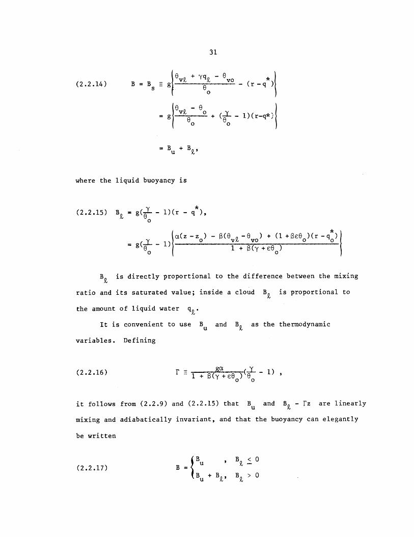
(2.2.15) B = g( - 1)(r - q ),0

I *g( - Oa(z -z 0 ) - ( -6 ) + (1 + 3e 0 )(r -q 0)

o 1 (y 0+e6)

B is directly proportional to the difference between the mixing

ratio and its saturated value; inside a cloud B is proportional to

the amount of liquid water q t.

It is convenient to use Bu and B as the thermodynamic

variables. Defining

(2.2.16) r (go- - 1)1 + (y +66 ) 00 0

it follows from (2.2.9) and (2.2.15) that Bu and B - 1z are linearly

mixing and adiabatically invariant, and that the buoyancy can elegantly

be written

B , B < 0

(2.2.17) B B u -B + B, B > 0u 9, 9,

In shallow, nonprecipitating convection, the effect of moisture is to

increase the buoyancy inside a cloud in proportion to the amount of

liquid water present, due to the latent heat release from the conden-

sation of that water.

2.3 The Equations of Motion

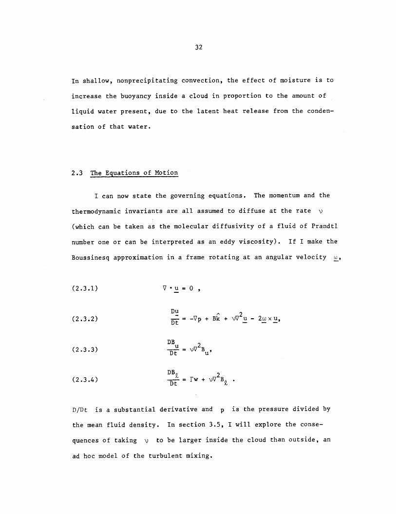
I can now state the governing equations. The momentum and the

thermodynamic invariants are all assumed to diffuse at the rate v

(which can be taken as the molecular diffusivity of a fluid of Prandtl

number one or can be interpreted as an eddy viscosity). If I make the

Boussinesq approximation in a frame rotating at an angular velocity w,

(2.3.1) V -u = 0

(2..2)Du 2

(2.3.2) --- = -Vp + Bk + v u - 2w x u,

DB(2.3.3) DBu = 2 B

DB2, 2(2.3.4) -B = F w + vV B

D/Dt is a substantial derivative and p is the pressure divided by

the mean fluid density. In section 3.5, I will explore the conse-

quences of taking v to be larger inside the cloud than outside, an

ad hoc model of the turbulent mixing.

The boundary conditions are applied at two rigid, stress-free

plates at which the temperature and water mixing ratio are specified

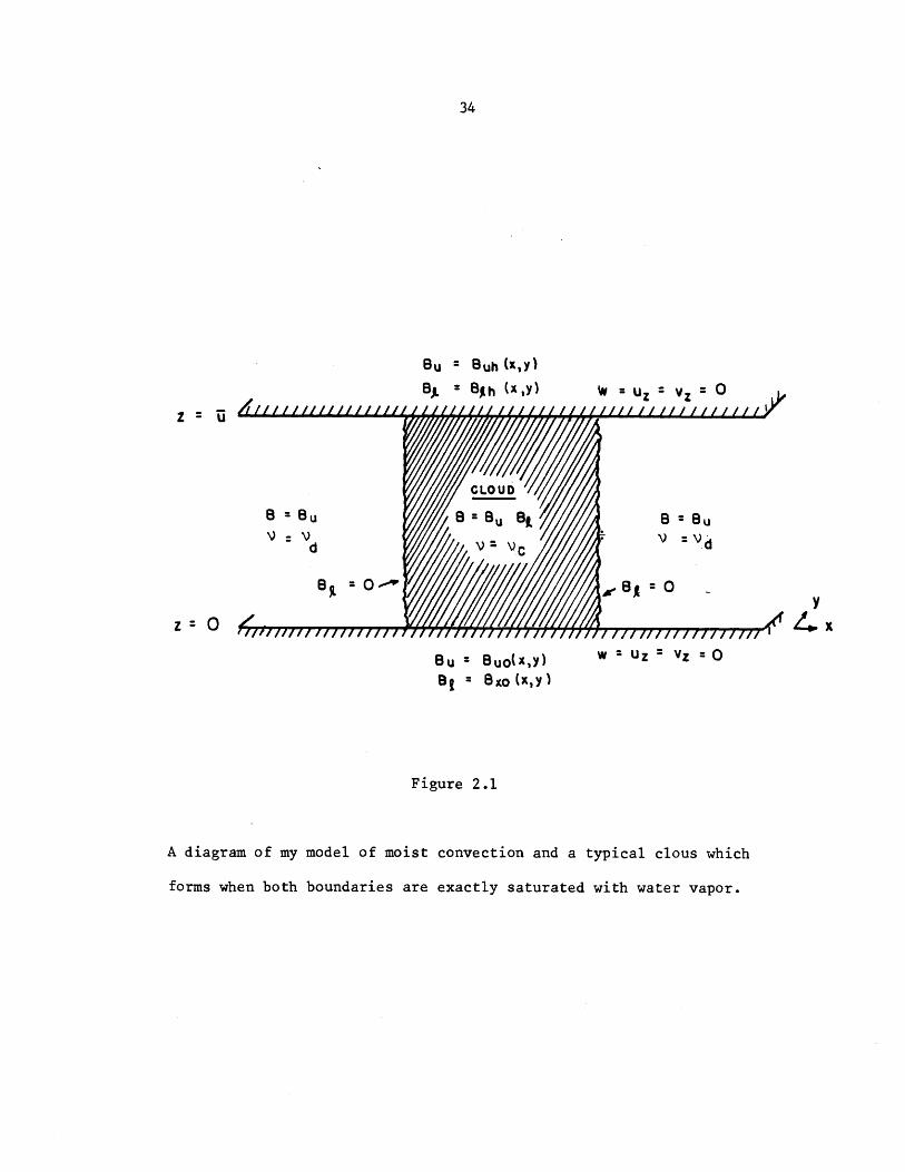
(figure 2.1):

w=u = v = 0 ,z z

B u,(x,y,0) = B uooy),

Bu,(x,y,h) = Buhth(XY) at z = 0,h .

It is convenient to non-dimensionalize the equation using h/7

as a length scale and h2 7 2v as a timescale. The nondimensional

versions of (2.3.1)-(2.3.7) are identical to their original counter-

parts with (from here on, dimensional quantities are starred)

(2.3.8)*

V + 1,

* h 42 4V IT

wh2

V T

(for nondimensionalization)

These equations cover all situations treated in this work.

However, for two-dimensional flow between two nonrotating plates,

each exactly saturated at a fixed temperature, the nondimensional

equations simplify somewhat. Define a streamfunction $ such that

(2.3.5)

(2.3.6)

(2.3.7)

(2.3.9)

(2.3.10)

Bu = Buh (x,y)

Bg = Bjh (xy)

Bu Buo(x,y)t= BXo (x,y)

W =luz = vz =0

B = BuV :V'

W = uz = vz = 0

Figure 2.1

A diagram of my model of moist convection and a typical clous which

forms when both boundaries are exactly saturated with water vapor.

z = U

d

B = 0 r

z:=0

Be S = 0

CLOUD

B=z BU

V - VC

4f x

(2.3.11) u = , = -z '

Let B and B be the unsaturated buoyancy of the fluid in contactuo uh

with the bottom and top plates. Then the nondimensional buoyancy

frequency Nd of the fluid in its state of rest is

2(2.3.12) Nd = (Bh - B )

Let B be the deviation of the unsaturated buoyancy from its valueu

B in the state of no motion,u

(2.3.13) B (z) = B + N 2u uo dz

and similarly for B Since both plates are exactly saturated,

B t = Buo 0, so

(2.3.14) 91(z) = 0

The boundary conditions (2.3.6) - (2.3.8) imply

(2.3.15) ) = =0zz = '

( =B =0 au

at z = 0,7 .(2.3.16)

For a growing disturbance, Bu and B are related because

they are advected and diffused identically. From the nondimensional

versions of (2.3.2) and (2.3.3), if I define

B B(2.3.17) = + u

then d

(2.3.18) $ = 0 at 0,T,

(2.3.19) D = v 2-

Since decays through diffusion it cannot grow on the average.

Let an average < > of a function f be defined as

(2.3.20) <f> = lim --- 27T dz ILdx Jdy f(x,y,z)L-o 4TL 0 -L -L

Then

2q- D 9 2 12 = - 22

so

d 1-2 -2 -2 -2(2.3.21) d7 > = -<V(V) > < -V<$z > < -v< >

The second inequality follows from an expansion of $ in a Fourier

C~2sine series = sin nz. < 2> decays exponentially fast to

n- n

zero no matter how much convection occurs, so it is consistent to

set 4 to its t -+ o limit, when perturbations B and Bu are

in phase:

N2

(2.3.22) 0 , - 91

Having done this, I can write the buoyancy perturbation in terms of

B alone. From (2.2.17) and (2.3.22),

2

(2.3.23) = B9,

where

2~

(2.3.24) N 2 2 2 ~<-N c E-N d, BZ > 0.

depends on whether the parcel is saturated. If the dry buoyancy

stratification N, is small enough so that r > N N2 < 0 insidedd

the cloud and parcels there can extract energy from the mean state by

buoyant overturning.

The remaining equations (2.3.2) and (2.3.4) can be written in

terms of $ and B :

D 2 2~ -(2.3.25) Dt B X

(2.3.26) (D - 2 ) =--Dt V)B, =x

These equations possess both the advective nonlinearity and a

new nonlinearity resulting from the different form of B inside and

outside clouds. The latter has the peculiar feature that B is

linear in B if all one does is to multiply 5 by a positive

scalar, and introduces a free boundary (the cloud edge) which must be

calculated as part of the solution, across which the fields must be

matched.

From (2.3.23), B has a discontinuity at the cloud boundary

which must be matched by a discontinuity in the highest derivative of

$ normal to the cloud boundary in (2.3.25). All lower derivatives of

$, however, can be continuous, so $ and its first three x deri-

vatives are continuous. Expanding (2.3.26),

(2.3.27) (- -)Bz = (r -B )$ - B $ ;

the right hand side can be differentiated twice in x and still

have no discontinuous ib derivatives, so the highest derivative of

B9, V2 is continuously twice differentiable. Thus

(2.3.28) are continuous across B = 0BB ,B B B,' 9,x 9xx' Qxxx' xxxx

The free boundary significantly alters the mathematical structure

of the equations. This reflects itself in quite different physics

from those of dry convection, as I show in the next two chapters.

CHAPTER 3

The "Linear" Dynamics of Moist Convection in an

Exactly Saturated Atmosphere

3.1 Introduction

The Boussinesq equations (2.3.12-14) are nonlinear even for small

amplitude disturbances because the buoyancy is a different function of

the "liquid water buoyancy" B depending on whether an air parcel is

inside or outside a cloud. In this limit, solutions with different

cloud boundaries still cannot be superposed to obtain another solution.

However, there are some important solutions which can be found

analytically. These solutions are exponentially growing clouds with

boundaries which are stationary and vertical; because of this geometry

they are separable, and mathematically can be found by matching at

the unknown cloud boundary the solutions of sixth-order ordinary differ-

ential equations for the horizontal structure inside and outside the

cloud. This entails solving two nonlinear equations for two parameters,

the cloud width and growth rate, given a cloud spacing. The most

unstable modes in a conditionally unstable atmosphere are single cloudy

updrafts surrounded by an infinite expanse of dry, descending air. The

subsidence decays exponentially away from the cloud in a "frictional

deformation radius"

* **3 3*R = Nh /T v ,fr d

*unless the eddy viscosity away Vd away from the cloud is so small that

either the Rossby deformation radius due to the vertical component

*f /2 of the earth's rotation,

* * * *R = N h /flT,rot -

* *or the "transient deformation radius" due to the finite speed N h

of which information about changes in the convection propagates away

from the cloud,

* * * *Rt = N h/Q,

where Q is the growthrate of the convective mode, is smaller.

One might expect that since there is an asymmetry between up

and downgoing motions, concentrated updrafts surrounded by broad

hexagonal regions of descent would be favored. In fact the limit of

such a planform as clouds become widely spaced, a circular updraft

surrounded by an infinite region of descent, is substantially more

unstable than the two-dimensional circulations so far considered.

Lastly, what is not seen? First, I find that clouds with several

updrafts and saturated downdrafts can grow; however they are unstable

to modification of their cloud boundaries which lead to development

of single-updraft clouds. Simulations seem to show that convective

clusters of clouds interspersed with unsaturated downdrafts also are

not seen. Second, I will show, using a variational approach, that

growing wavelike convection is impossible in the model, as is any form

of periodic oscillation in the geometry of the convection. Lastly,

I apply the variational principle to show that the modes with vertical

cloud boundaries are stable to "nonseparable" perturbations which

wrinkle the cloud-edge. Thus, there are no modes with almost, but not

quite vertical cloud boundaries which grow faster than the separable

modes.

In conclusion, it seems highly probable that any small initial

perturbation will evolve into a set of widely spaced stationary cloudy

updrafts with vertical cloud boundaries. In three dimensions these

updrafts will be nearly cylindrical. In chapter four, I'll look at

how these updrafts interact with each other, and the effect of non-

linearity and a mean forced vertical motion on the resulting field of

convection.

3.2 The Simplest Case

In this section I do the simplest problem, in which rotation is

neglected, the motion is two-dimensional, and the eddy viscosity is

the same inside and outside the cloud, in the "linear" limit in which

fluid velocities are infinitesimal.

The picture which emerges is that updrafts prefer to be widely

spaced but have a width approximately equal to the domain height

surrounded by a region of subsidence concentrated within a "frictional

deformation radius" of the cloud. This subsidence extends into the

edges of the cloud, where it is driven by evaporative cooling.

42

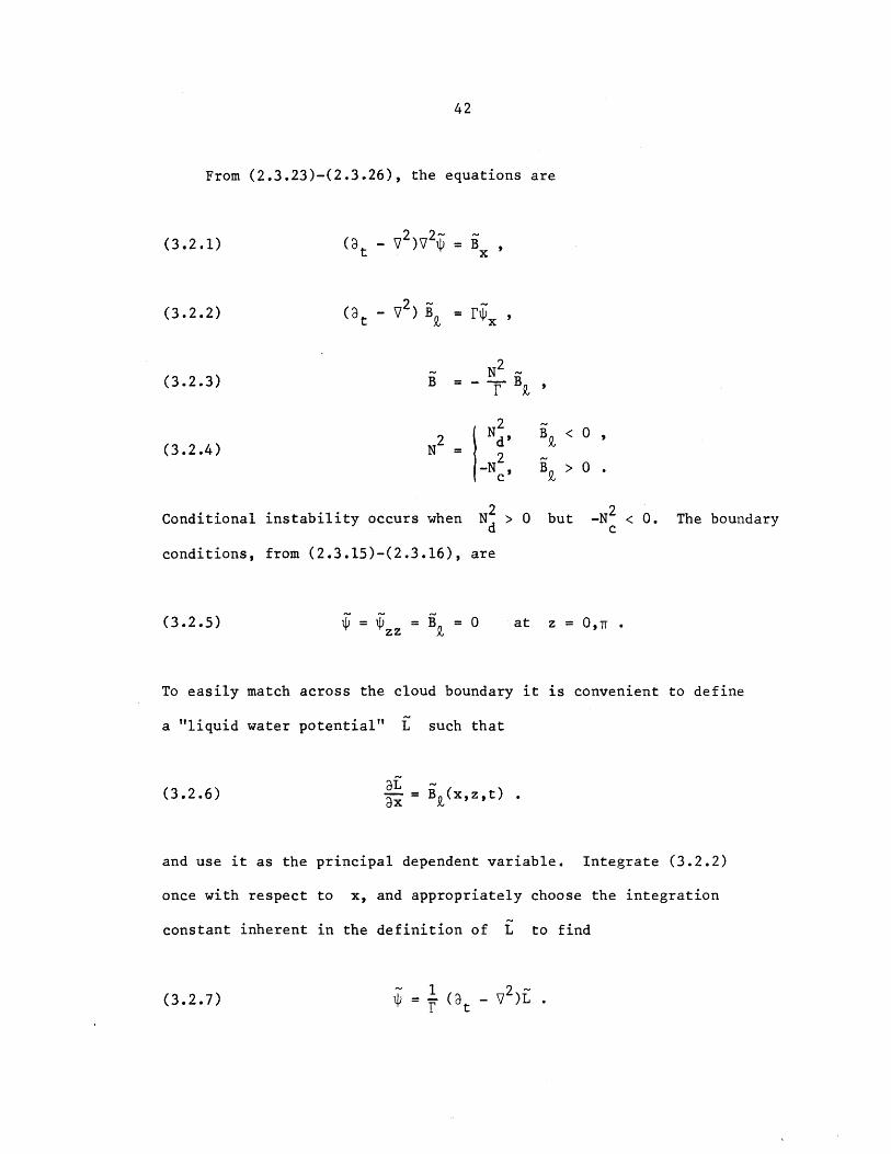
From (2.3.23)-(2.3.26), the equations are

1) 2 2~ ~1)- ) $ = B

2)t 2x2) (3 -v?) B = $

N23) 5 = - BP ,

2

N = 2 2-N ,2

c

4)B 91< 0,

B > 0.9,

Conditional instability occurs when N2 > 0d

conditions, from (2.3.15)-(2.3.16), are

(3.2.5) = zz 0

2but -Nc < 0. The boundary

at z = 0,-r .

To easily match across the cloud boundary it is convenient to define

a "liquid water potential" L such that

3L(3.2.6) a= B9 (x,z,t)

and use it as the principal dependent variable. Integrate (3.2.2)

once with respect to x, and appropriately choose the integration

constant inherent in the definition of L to find

1 2 ~(3.2.7) $ =2t( )L

(3.2.

(3.2.

(3.2.

(3.2.

Use this to eliminate $ from (3.2.1) and obtain an equation for

L alone,

22 2~ 2~(3.2.8) ( - V ) VL = -N L .

e bxx

The boundary conditions can be derived from (3.2.5) and (3.2.7),

(3.2.9) L =L =L = 0zz zzzzon z = 0,1 .

A special class of separable solutions with sinusoidal vertical

structure exist in which the cloud boundaries are vertical. The most

unstable of these have the structure

(3.2.10) L = L(x,t) sinz

and obey a horizontal structure equation

(3.2.11)2 2(32 _1^ 2^(0 +1-3)(3-1)L = -N L

t x x xx

22At the cloud boundary, B cc -N L xxchanges discontinuously in

response to the discontinuous change in N there. The matching

conditions (2.3.28) imply the first five derivatives of L are

continuous. Since $ is continuous, (3.2.7) shows L itself is also

continuous:

(3.2.12) L, L , L , L , L , L continuous at L = 0x x xx xxx xxxxx x

In fact, an even more special class of solutions (which I call

eigenmodes) have stationary, vertical cloud boundaries and grow

exponentially with time:

(3.2.13) L = L(x) sin z -e .

They obey the sixth order ODE

2 22

(3.2.14) d 2 d2 1)L = -N Ldx dx xx

I seek solutions with clouds of width "a" spaced periodically

with wavelength X. If the x-origin is taken to be at the center of

the cloud then we may assume B is symmetrical about x = 0, so

L(x) is antisymmetrical about x = 0. Let g(x,p) satisfy

2(3.2.15) - = 02

dx2

Then g will satisfy (3.2.14) in the cloudy air if p satisfies the

characteristic polynomial.

(3.2.16) p (p) = (Q +1 - p 2 (p2 1) - N2p2 0c c

and in the clear air if

~22 2 2 2(3.2.17) pd(p) = (+1 - p) (p -1) + NdP 0.

Physically, the first root corresponds to a vertical shearing of the

fluid which decays exponentially with x on a viscous lengthscale.

If conditional convection occurs with growth rate Q, then purely

moist convection must be even more unstable for some range of wave-

numbers. The edges of this band are the two pairs of "convective"

modes of (3.2.16) which are sinusoidal,

pel = recl , (viscous)

(3.2.18) p = ±p~c = ir , (vsosc2 = c2 (convective)

pc3 = ir c3'

In the clear air the modes are a pair of viscously damped modes with

complex p and a gravity wave response in which an exponentionally

decaying temperature perturbation drives horizontal motions as far as

viscosity will allow:

p = rdl, (gravity wave)

(3.2.19) p = ± = rd2 + ird 3 ' (viscous)

p = rd2 - ird 3 '

I construct a solution L in the cloudy air which obeys the

condition of antisymmetry at x = 0, and a solution in the dry air

obeying antisymmetry at x = X/2. The fundamental solutions g which

do this can be written

1 1g (x,p) = i- sin i = - sinh px,c p px p

(3.2.20) g(x,p) = 1 sinh p(x -2), X < o

- e(xP) - 2

so the most general real L is

bclc(xpcl) + bc2gc(xpc2 ) + bc3gc(xpc3 )(3.2.21) L =

bdld (x'Pdl) + bd2gc(xpd2) + bd3g (x,d 3

where the b ci and b di are real constants (except bd2

0 < x <2'

a X

and b d3 9

which are complex conjugates) to be determined by the matching condi-

tions (3.2.12), which give a matrix equation

(3.2.22a) M[bdl bd2 bd3 -bcl -bc2 -bc3] = 0

(3.2.22b) M =

fdl

2Pdlgdl

fd2 fd3

2 2 2 2 2Pd2gd2 Pd3gd3 Pclgcl Pc2gc2 Pc3gc3

2 2 2 2 2 2Odl dl Od2 d2 Od3 d3 Ocl cl Oc2 c2 Pc3 c3

4 4 4 4 4 4Pdlgdl Pd2gd2 d3d3 Pclgcl Pc2gc2 Pc3c3

4-di dl

4 4 4 4 4Od2 d2 Od3 d3 Ocl cl Oc2 c2 c3 c3

in which

fc(x,P)

(3.2.23) f(x,o) = (x,p)

fc

= cos iPx = cosh px

cosh p(x - )

exp{-p(x - )}

(3.2.24)

(3.2.25)

f,gdci d di

fcgi c '2c ci

X < o,

For a solution to exist and for the resulting cloud boundary to be at a/2,

(3.2.26) det M = 0 ,

(3.2.27) L (a/2) = b f + b 2 f + b 3 f 3 = 0x cl e 2c 3c

The two constraints (3.2.26) and (3.3.27) are nonlinear equations

for the growth rate 2 and cloudwidth a. To simultaneously solve

these equations, I first did a coarse search. For any Q and a, det M

is computed, and setting bc3 = 1 the first five rows of (3.2.22a)

are solved for the remaining b's, allowing L (a/2) to be computedx

from (3.2.27). Let

1 ... det M < 0, L (a/2) < 0

(3.2.28) (a)=2 ... det M < 0, L (a/2) > 0

3 ... det M > 0 L x(a/2) < 0

4 ... det M > 0, L (a/2) > 0

A computer-generated map of a over a reasonable range of 2 and

a can be made to arbitrary resolution. A solution is demarcated by

the intersection of regions with a = 1,2,3,4. After coarsely locating

solutions in this way, the values of det M and L (a/2) at three

points close to the root give a better guess at the solutiong using a

two-dimensional extension of the "secant method" [Ralston and Rabinowitz,

p. 338] which assumes det M and L (a/2) are locally linear functions

of Q and a. The method converges at a faster-than-linear rate to a

root pair.

Once a root pair (Q,a) and the associated constants {b } are

found, B and w can easily be found using (3.2.6) and (3.2.7),

b f (x'p )+b bf (xp c2+ cf 3' 0<x <cl c cl c2c * +b f c3 c c3

(3.2.29a) Bf) =

bdl d dl) +bd 2 d d2) +bd 3 d d3 < x <

Yclbcl fc (xPcl)

(3.2.29b) w =

ydlbdlf d(x'pdl)

+Yc 2bc2 fc (Xpc2) +yc 3bc3 f (xpc3

a

0 < x <

+yd2bd2fd 'OPd2) +yd3bd3fd ',Pd3)

where

(3.2.30)2

yc,d = (Q+ 1 - pc)/T'

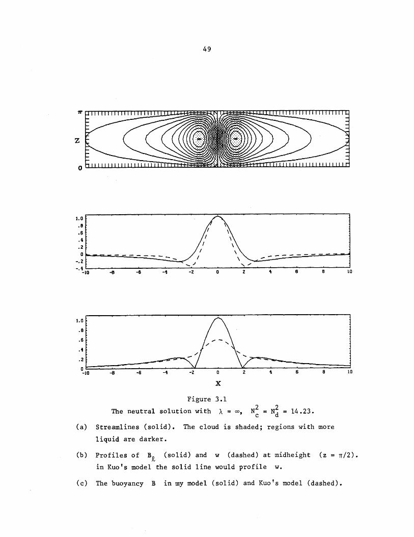
Shown in figure 3.1 is a typical solution with infinite intercloud

spacing and N = N just large enough to make Q = 0. The cloud

width "a" is about equal to the domain height, and the cloud is

surrounded by a broad expanse of air which is dry and warm due to its

descent through a stable mean stratification. The descent rate drops

off exponentially as exp(-rdlx); for fairly large Nd, rdl is approx-

imately (from 3.2.17)

(3.2.31) rdl ~ 2+Nd

1.0

.4

.20

-. 2

-1

1.0

.8

.6

.4

.2

0- I

-8 -6 -4 -z o z 1 6 a to0

0

Figure 3.12 2

The neutral solution with X = co, Nc = Nd = 14.23.

(a) Streamlines (solid). The cloud is shaded; regions with more

liquid are darker.

(b) Profiles of B (solid) and w (dashed) at midheight (z = r/2).

in Kuo's model the solid line would profile w.

(c) The buoyancy B in my model (solid) and Kuo's model (dashed).

so that the dimensional width of the region of descent is proportional

*to the "frictional deformation radius" R f, which is the horizontal

fric'

distance over which a buoyancy perturbation can induce motion while

working against friction.

** h 1 *

(3.2.32) Rd t = ---- + .ricdescent rld +1fi

*2* *h* h h*

(3.2.33) R fric N -- N - .

vd

Since N must be at least 3-4 and typically N 2 N in the atmo-c d c

sphere, the region of descent is wider than the region of ascent.

Near the edge of the cloud a strong downdraft develops since the

air is coldest there. This cold air forms from diffusive mixing of

moist air from inside the cloud with dry air outside the cloud. The

mixture cools by evaporation of the liquid water in the cloudy air

until it is no longer saturated, forming cold air around the cloud

boundary.

It is interesting to compare this eigenfunction to the model pro-

posed by Kuo (1961), a variant of which was correctly solved by

Yamasaki (1972) (he curiously assumed the vertical eddy viscosity to

be zero, probably by analogy with large-scale flows in which eddies

have a much larger characteristic lengthscale horizontally than

vertically because differential vertical motion is inhibited by the

earth's rotation, leading to a much larger effective diffusivity in

the horizontal). In Kuo's model, air contained between two plates

feels an effective stratification N2 which depends on the sign of

the vertical motion. In my notation, he would take the stratification

as

(3.2.34)

N2

N2 ) dB dN(w) = -- =

-N 2c

w < 0,

w > 0

and propose the equations analogous to (3.2.1-2) of my model

(3.2.35) 3t V =x + V4 $

~ 2 2~(3.2.36) 3 B =-N $ + VB,

zzat z = 0,7 .

Solving these for $

(3t _z 2 2 = -

$ zz " *zzzz 0.

2(3.2.38) indicates that the discontinuity of N where X = 0 is

matched by a jump in V *, but all lower derivatives of $ are con-

tinuous across the cloud boundary,

(3.2.40) $,$4, ,...,$x continuous at the cloud boundary $ = 0.

This problem is identical to the one I considered, except the stream-

function replaces the liquid water potential L. However, the solution

(3.2.37)

(3.2.38)

(3.2.39)

is clearly different, as is seen from figure 3.1. Now the region of

upward motion by definition extends to the cloud edge; the evaporative

downdraft at the cloud edge is missed. Further, the buoyancy distri-

bution is very different. From (3.2.35) the buoyancy can be expressed

in terms of $, choosing an integration constant B = 0 at the cloud

edge.

(3.2.41a) B(x) = B(x) sin z eQt

(3.2.41b) 2 2bcl~l Oc2b (-.-)[f (x'p )-f I +b c2 - [f (xQ )-f I +

clcl 2 c cl cl c2yc2 2 c c2 c2Ocl 2 -l c2

Oc3a+ by(-)[ f (x'p)-f]1 0< x <-a

c3yc3 2 c c3 c3 2

B(x) = 2c3

Pdl~ )bdlydl 2 d 'dl dl+

dl 2Od2~I( a X

+ ReL (-_)(b +ib Xf 2(xdP <- 2[Yd2 2 d2 d3 d d2 d2 x 2

d2

B(x) is the curve of long dashes in figure 3.1, and is drastically

N2different than the buoyancy - B of my theory. Instead, the entire

region around the cloud is buoyant; there is no cold air at the cloud

edge. This is because positive buoyancy is being generated everywhere

since N (w)-w > 0 always, and diffusion smears out the local minimum

of generation where w = 0 (the cloud edge). This wide peak in

buoyancy naturally leads to a wider updraft (the solid line in the

figure) than in my model (the dashed line).

One might think that the Kuo model is a good physical representation

of a cloud from which all liquid water falls as rain. In an exactly

saturated atmosphere with no mixing this is initially indeed so. But

a parcel rising through the cloud sheds all of its liquid water so

that it becomes distinctly sub-saturated as it descends in the return

circulation. When it once again begins to rise, it clearly will not

saturate at all unless it picks up moisture in the course of its

circulation, and no latent heating, ergo no change in N , will occur

as the parcel rises. Thus the Kuo hypothesis is not consistent with

any form of cloud physics, but merely reflects the reasonable intuition

that rising air is cloudy.

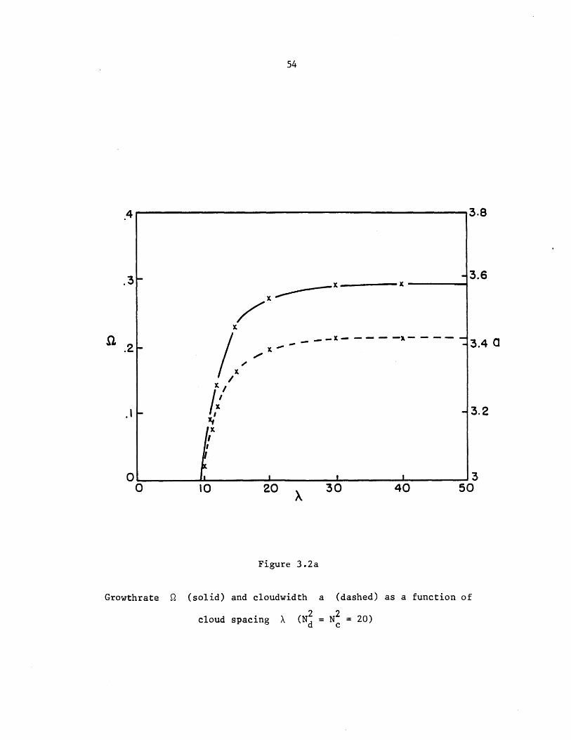
In either model, if the growthrate Q and cloud width "a" are

plotted as functions of the intercloud spacing A (figure 3.2a), one

sees that the infinite wavelength mode grows the fastest, but all

modes with A :t 2N = 2R have very similar structure. As thec fr

intercloud spacing increases, the cloud width expands slightly to a

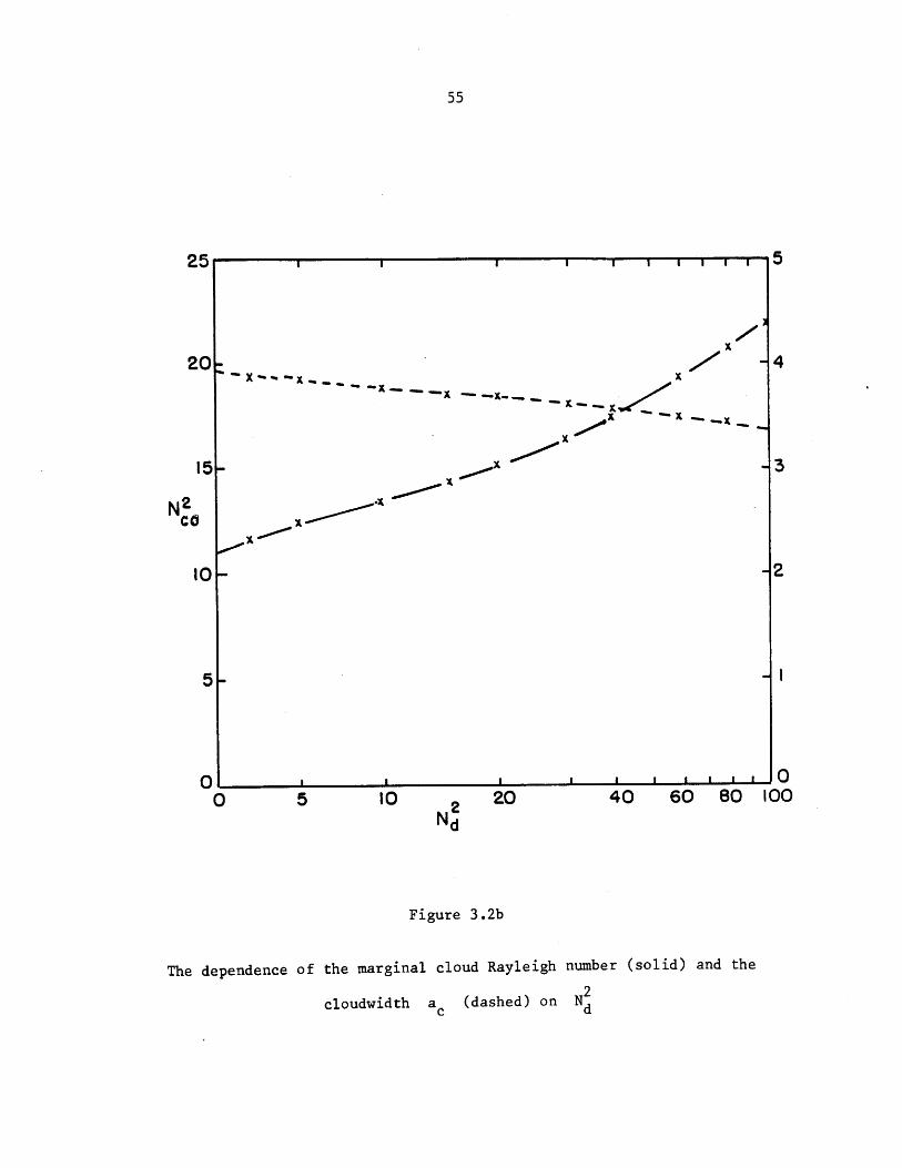
2 onywakyolimiting value. The critical value of N depends only weakly on Nd

c 2

(figure 3.2b), and when N2 = N , the critical value N2 14.23 isc d co

about twice that needed to induce moist convection in a cloudy

22atmosphere of stratification -N (which is 27/4). At larger N2

C c

(figure 3.3) the clouds narrow down, reflecting the narrower preferred

scale of pure moist convection, and secondary modes corresponding to

clouds with several updrafts appear, albeit with lower growthrates.

These I will discuss in section 3.4.

-~---~-

4 3.8

.3K -3.6

xKX

-K3.2,

01 113.

0 to 20 30 40 50

Figure 3.2a

Growthrate Q (solid) and cloudwidth a (dashed) as a function of

2 2cloud spacing X (Nd = Nc = 20)

I I I I I I I I

x

' x -. x

A pi i I I I I I

40 60O0

80 100

Figure 3.2b

The dependence of the marginal cloud Rayleigh number (solid) and the

2cloudwidth a (dashed) on Nd

Cd

20

15~

N2CO

10

5

N-

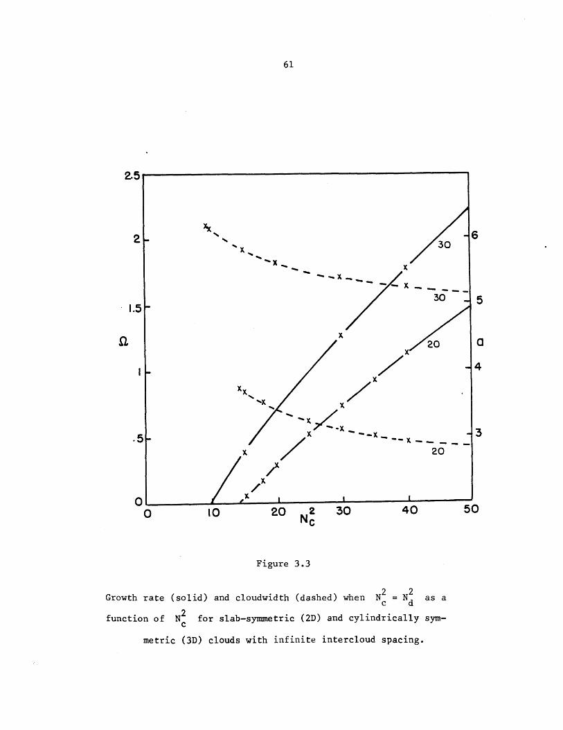
3.3 Cylindrically Symmetric Moist Convection

Since there is a strong asymmetry between up and downward motions

in moist convection, one might expect a cylindrical cloud, which has

more room for downwelling around its perimeter, to have different

stability properties from a "line" cloud such as discussed in section

3.2. In fact, I will show that a cylindrical cloud surrounded by an

infinite expanse of clear air is distinctly more unstable than its

two-dimensional analogue due to the slower downward velocities re-

quired in the stable dry air. This conclusion was reached also by

Lilly (1960), Yamasaki (1972) in his modification of Kuo's model,

as well as by numerous numerical studies such as those of Murray

(1970) and Soong and Ogura (1973).

For three dimensional moist convection the "linearized" equations

of motion in a nonrotating reference frame are (from 2.3.1-4, 2.3.24),

2 ~(3.3.la) t - )u = -p

2 ~ ~(3.3.lb) (t - V )v = -p y

(3.3.lc) (3t - V 2 = -pz + B

(3.3.ld) ( t - V )B ,= rw

u + v + w = 0x y z(3.3.le)

Using (3.3.la) + - (3.3.lb) and continuity, u and v can beax 9yeliminated:

(3.3.1f) (3 - Z2~) - - + p ).t z xx yy

T 2 a2To eliminatep, take + ](3.3.lc) - (3.3.lf),

3x 3y 2Z

(3.3.lg) (3t - V2 2~2 - + g .ytxx yy

N2-Using (3.3.ld) to eliminate w and remembering = -

(3.3.lh) ( - V2 )2 V B -N 2( + a2t Ex y

For cylindrically symmetrical convection the liquid water potential

L defined such that

(3.3.2) 1 = aL(r) - sin z - er 3r

is introduced. Define

(3.3.3) A = r

Since

2 1 3F a2 1 3 9 1dF 1 d(3.3.4) V g 37= + 3r drsin z =-- [A -1]F,ra.r caz l r r d r oa

(3.3.1h) can be multiplied by r and integrated to obtain

(3.3.5) ( + I-A)2 (A - 1)L = -N AL .

To solve (3.3.5) we first find eigenfunctions of A. The related

problem

1 d df 2(3.3.6) 1 - rd p f(r,p)

has solutions

J(ipr)f(r,p) = 0iKpr)

K0(pr)

regular as r + 0,

regular as r + o.

Let g(r,p) be defined by

f(r,p) = .dgr dr

Clearly, g solves

1d dg 1 d 2rdr dr dr ~ r r

Multiplying by r and integrating it is clear g(r,p) is the desired

eigenfunction:

(3.3.10) Ag = P 2g

Using the recursion relations (derived from [9.1.27] and [9.6.26] of

Abramowitz and Stegun (1964))

(3.3.7)

(3.3.8)

(3.3.9)

1 d(3.3.lla) J = zd [zJ],

(3.3.11b) K= - d zK]

dJ(3.3.llc) = -J ,

dK(3.3.lld) = -K ,

one sees that (7) and (8) imply

gc (r,p) r JI(ipr) regular as r + 0,

(3.3.12) g(r,p) =

gd(r,p) -r K1 (pr) regular as r + co.

From this point on the analysis parallels section (3.2). The

most general solution regular at r = 0 and as r -+ o for a cloud

of diameter "a" is, as before

blcgc(rplc) +b 2cc(r,p2 c) +b 3 g(rc ' 3c r < ,

(3.3.13) L =

b ldgd (r,pld) +b 2dgd 'p2d ) +b 3dgd '3d r > .

The solution must be matched across the cloud boundary r = , where

2 2 dB , 2N AL = N r~E has a discontinuity due to the jump in N , which must

be compensated by a discontinuity only in the highest derivative

on the left side of (3.3.5). Thusdr

1ldL 1ld 2 1ld 2(3.3.14) L, 1 -, -L, AL, A L d A L are continuous

aacross r -

These conditions lead to equations identical to (3.2.22)-(3.2.27)

except for the new definitions of f and g. The vertical velocity

and liquid buoyancy can be found, using (3.3.6) and (3.3.8), to satisfy

the same equations as (3.2.29)-(3.2.30) with x replaced by r. But

the new functional forms have a sizeable influence on the growth rate

of the solutions (figure 3.3); the three dimensional modes become

2 2 2unstable at 30% lower values of N for N = N .

c c d

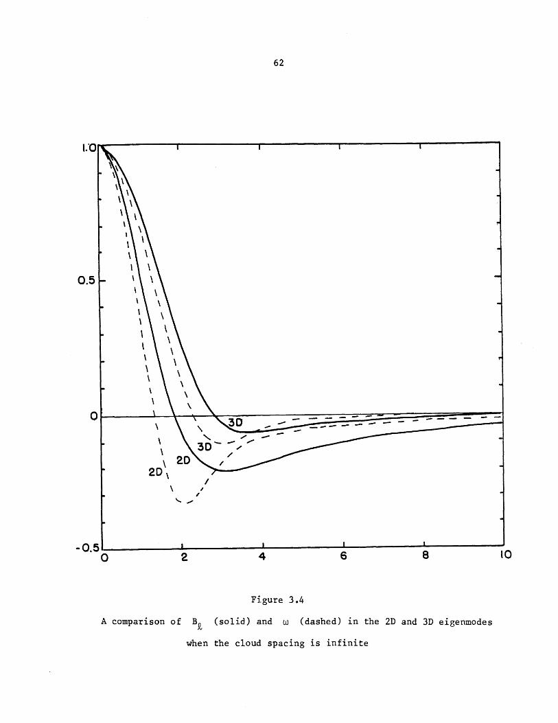
A look at the eigenfunction (figure 3.4) shows why this is so.

For a given peak updraft speed, the downdraft speeds are uniformly

smaller in the circular cloud since the whole annular region around

the cloud can absorb the return flow. The fluid moves slower and

warms less due to adiabatic compression, so the rate of work -wB

(excluding pressure work, which averages to zero along any closed

steady parcel trajectory) which must be done on the stably stratified

fluid to force it back down into- the updraft is less in the circular

case, allowing the buoyancy from latent heating to more efficiently

cause kinetic energy growth.

Although it would be complex to prove, it is plausible to assume

that a cylindrical updraft surrounded by an infinite expanse of drier

downwelling air is the most unstable three-dimensional eigenmode.

However, for simplicity I will continue to work in two dimensions.

The features and equations of the theory I will develop could be

carried over naturally (but with tedious algebra) to such three-

dimensional modes without qualitative change.

2.5

2-310 -630 6

1.5 -

20 ax

4

xx -%

K

.5- K 3

x 20

x

01O 10 20 2 30 40 50

Nc

Figure 3.3

2 2Growth rate (solid) and cloudwidth (dashed) when N = N as ac d

function of N for slab-symmetric (2D) and cylindrically sym-

metric (3D) clouds with infinite intercloud spacing.

0.5-

2D3D2D

02

-0.510 2 4 6 B 10

Figure 3.4

A comparison of B (solid) and w> (dashed) in the 2D and 3D eigenmodes

when the cloud spacing is infinite

3.4 Multiple Updraft Solutions

Cumulus clouds are often observed to have a more complex pattern

of updrafts and downdrafts than the solutions so far presented. One

reason for this, cloudtop entrainment instability, was first proposed

by Squires (1958). Unsaturated air above a cloud is mixed into cloudy

air, evaporating some of its liquid water and cooling the mixture. If

the air above the cloud is not too warm, the mixed parcel is denser

than the cloudtop air and sinks. The densest mixture occurs when

enough unsaturated air has been mixed in to just evaporate all the

liquid water, so one might expect just saturated plumes to descend

from cloudtop. If they entrain enough moist air to compensate for the

evaporation of liquid water by adiabatic warming, they can remain

dense and sink deep into the cloud. A model of this process based on

self-similar plumes was proposed by Emanuel (1981).

In my theory, the physics of condensation, a crude version of

turbulent mixing, and a source of cold, just-saturated air at "cloudtop"

(z = iT) are present, so one might ask whether the equations of

section (3.2) admit solutions with analogous downdrafts. Indeed they

can; there are growing eigensolutions with an arbitrary number of

updrafts separated by such plumes. However, these solutions grow

slower than single updraft eigenmodes, and even within the "linear"

theory they are unstable to perturbations which alter the cloud

boundaries and lead to the growth of single-updraft modes. Therefore,

they are not selected while the "linear" dynamics predominate.

An identical procedure to that used to find the single updraft

solution recovers these modes. A three-updraft example is shown in

figure 3.5. Each downdraft remains slightly saturated, fed by

diffusion of water from the adjacent updrafts. The average motion on

the cloud remains upward, condensing the liquid water necessary to

sustain cloud, and outside the cloud the motions are little different

from the single updraft mode. I could find no eigenmodes in which a

cloud was split by unsaturated downdrafts.

The greater the number of updrafts, the more sluggishly the

mode grows (figure 3.6). Since the equation (3.2.8) is nonlinear,

it is also sensible to ask about the stability of its eigenmodes.

It is remarkably simple to determine when an eigenmode is unstable

to perturbations of the same vertical structure as it, for such

perturbations leave the solution separable in z and obey an

equation closely related to the equation for the eigenmode itself.

Consider a separable eigensolution L of (3.2.14) with cloud

width a0 and growthrate Q0 with an infinitesimal perturbation

EL1 of the same vertical structure

(3.4.la) L(x,z,t) = A{L 0 te + L I(x,t)} sinz

where A is chosen so there is no mean Ll, i.e.

00'

(3.4.1b) fC L1(x,t)dx = 0

Let N0 be the effective buoyancy frequency associated with this mode,

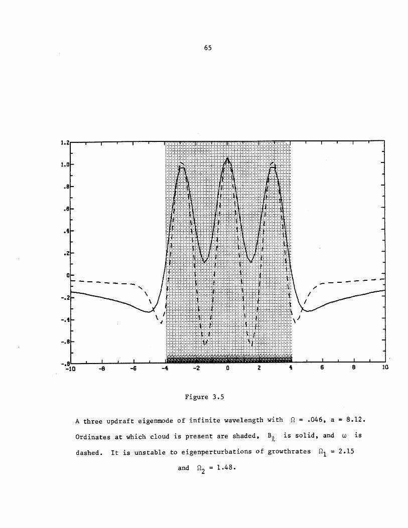
65

...2.. - - -. .... ... ... ...

1.0 -P

.8 -

8 -1.2A

.. ........

r -

.2 \

a Ne 1 d1

... ...... .... .. ... .. . .. ..

. .

'I iii

-10 -8 -6 -4 -2 0 2 4 6 8 10

Figure 3.5

A three updraft eigenmode of infinite wavelength with G2 =046, a = 8.12.

Ordinates at which cloud is present are shaded, B~ is solid, and w is

dashed. It is unstable to eigenperturbationls of growthrates 01 = 2.15

and 22= 1.48.

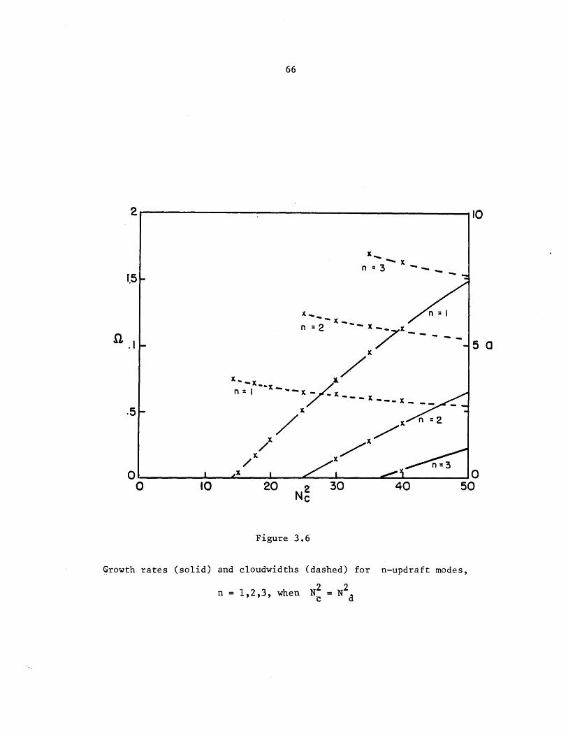
n 2x

x

X, .

x-

I

.51-

/x I

2NC

30

Figure 3.6

Growth rates (solid) and cloudwidths (dashed) for n-updraft modes,

2 2n = 1,2,3, when N = Nc a

2

1.51-n =3

10

5 a

00

n 3

20 40 5ff

(3.4.2a)

-N ,2 x[ < a /2

2N , Jx > a0/ '

where for simplicity I consider the case of infinite cloud separation,

although this is not important to the argument. In section 3.7 I will

show (see (3.7.8) and (3.7.12)) that

2 22 ^ 2^(0 +1 -3 ) 2(32 -1) LS -NO2L ,(3.4.2b)

(3.4.2c) Li, L , L , L , L

(3.4.2d)

are continuous across x = a0 -2,

L L (± a0/2 t)c

(fd denotes the jump in f from the "cloudy" side of aO/2 to the

"dry" side.)

If I define a first integral 9 of L,

(3.4.3) d91/dx = L1 (x,t) ,

and integrate (3.4.2b), I obtain (using (3.4.1b))

2 2 2 - - N2 ,t -x x 1 0 lxx z( CO) -+ 0

The matching conditions (3.4.2c) and (3.4.2d) become:

(3.4.4a)

(3.4.4b) Z , Z , Z , Z , Z , Z are continuous

across x = ±a 0/2

This is identical to the original equation (3.2.11) for LO

except the cloud boundaries are fixed at ±a 0/2 and can be solved

in exactly the same way for "eigenperturbations"

(3.4.5) Z1 (xt) = Zjx)e t

by just solving (3.2.27) for 21,

(3.4.6) det M = 0 ,

with "a" fixed equal to a0. Since L lx = B %(a 0 /2 , t) need not

be zero, the cloud boundary begins to move.

For an n-updraft eigenmode, numerically one finds there are n-l

eigenperturbations with growthrates Q > Q0 to which the eigenmode

is unstable, and numerical simulations of "separable" clouds evolving

according to (3.2.11) show all such perturbations lead in the end to

the formation of a single-updraft cloud. Although multiple-updraft

modes can exist in this "linear" model, they will not be observed until

it breaks down.

The single updraft still has perturbations with Q2 = Q0 its own

growthrate, with

(3.4.7) Z1 (x,t) = c L (x)e

69

dL 2t(3.4.8) L(x,z,t) = (LO(x) + c 0)e sin z

LO(x + ec)e sinz

but these clearly represent translations of the eigenmode, not

instabilities of it, and it is stable (for single-updraft modes of

finite cloud spacing, stable to perturbations of the same wavelength)

to perturbations with the same vertical structure as the eigenmode.

3.5 The Effects of Variable Viscosity

Cumulus convection in the atmosphere is turbulent. I have chosen

for simplicity to model it as a laminar process in which the effective

Rayleigh number is lowered by an increased eddy mixing.

Because kinetic energy can be created only within clouds, motions

there (as I showed already) are more intense and turbulent. If an

eddy diffusivity is associated with the unsteady part of the flow,

then it should be much larger within the clouds.

In this section, I sidestep the problem of how this turbulence

is generated and concentrate on the effects of its spatial inhomogeneity.

A simple ad hoc model is to replace the constant eddy diffusivity v by

(Vd T, B~ < 0,v , or after nondimensionalizing,

1, B > 0,c

d

c

Convection is destabilized at small T due to the increased

frictional deformation radius R * V , which allows subsidencefr d

to spread out over a wider area and reduces the downward motion against

the stable stratification. However, an interesting feature of the

solution is a sharp viscous boundary layer which forms just outside the

cloud edge.

From (2.3.24)-(2.3.28) the "linearized" vorticity and buoyancy

equations are

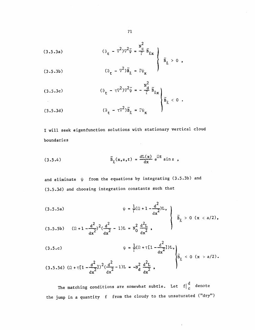
N2

t 2 2-

(9 t 2

2 2~-(3t

( t r 2 )

B > 0,

N2_Nd ~

B z,

B 9 <0 .

I will seek eigenfunction solutions with stationary vertical cloud

boundaries

dL(x) Qt.(x, z, t) = dx e sin z ,

and eliminate $ from the equations by integrating (3.5.3b) and

(3.5.3d) and choosing integration constants such that

(3.5.5a) $

d22 d2(3.5.5b) (2+1- ) (- 1)L

2 d2dx dx

(3.5.c)

1 d= (2+1 -- )L,

dx 2

2 d2L= N ~~ *dx

$= g-(Q +T[1 -

2 2

dx dx

d 2

dxB < 0 (x > a/2).

2 d2L= -Nd 2

dx

dThe matching conditions are somewhat subtle. Let f c

denote

the jump in a quantity f from the cloudy to the unsaturated ("dry")

(3.5.3a)

(3.5.3b)

(3.5.3c)

(3.5.3d)

(3.5.4)

B > 0 (x < a/2),

air. The viscous stresses instantly remove any discontinuity in u

or B9,

d d d(3.5.6) u [ =w = | = 0.

c c c

Consider a pillbox of unit depth in y, infinitesimal thickness and

height Az centered on the vertical cloud boundary. Since there can

be no net force on the pillbox,

d d(3.5.7a) F = Az *a = 0

c c

d d(3.5.7b) F z = Az a xz = 0

c c

where [. .] is the stress tensor, in nondimensional form13

av. 3v.(3.5.7c) a.. = -p6.. + v(-- +

13 = 3p~x. 3x.J 1

Consequently

d(3.5.8a) CT = [-p + 2vyw] = 0

xx x cc

d~ ~ d

(3.5.8b) a = vd + w ] = 0xz z x cc

The first condition involves the pressure change across the interface.

To relate this to velocity changes, differentiate (3.5.8a) with respect

to z and use mass conservation,

d d d(3.5.9) pz I = 2vy I = -2v zz I

c c c

Substitute this into the vertical momentum equation on both sides,

remembering B = 0 on both sides of the interface,

d d d d

t-VV )5z 1 + I 2 zz Ic c c c

2 2 ~ 0(3.5.10) (3 -v[ +33]) | = 0 .

tx zc

The last condition is that B not accumulate in the pillbox.

Its viscous flux must balance:

d(3.5.11) = 0.

c

The equations (3.5.6), (3.5.8b), (3.5.10), (3.5.11) generate six

matching conditions on L(x):

(3.5.12a) 1 12+j -d d =0,1 d2 d

(3.5.12a) 1[2 +v\(1 - )] L d= 0,

dx c

1 d2 d(3.5.12b) [E +v(1 -3. )]LI = 0,

dx c

d(3.5.12c) L j= 0

c

(3.5.12d)

(3.5.12e)

1 d2 d 2 dN(d2+1)[Q + v(1- -7)]L = 0

dx dx c

2 d2 d[Q + dv(3 -2)][Q +(l 2)]L = 0

dx dx c

d(3.5.12f) vL I= 0.

c

When T = 1 these conditions reduce to those used in section (3.2)

and the solution proceeds similarly. The characteristic polynomial in

the dry air is now

(3.5.8) (7) = [Q+ T(l-p 2)]2 p 1] + N 2 '

so its roots ±pdl' ±Pd2' 4 d3 are altered. In particular, the

root p1 associated with the thermally driven eigenmode of (3.5.8)

is much decreased to

(3.5.9) p NT1 N d

because with less diffusion a heat source can induce convergence from

a much wider region. L still has the form (3.2.21) but the matrix

matching L between the dry and cloudy regions is altered to

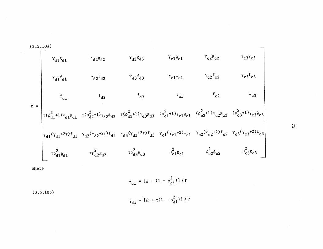
6 4

(3.5.10a)

c3gc3

ydl d 1

d

-1p2Tdp+1)ydlgdl

ydl(ydl+ 2T) fdl

p

'd2 d2

fd2

-1p2d2+1)yd2gd2

Yd2(Yd2+2T) fd2

2TPd~d

'd3 fd3

d3 +1)yd3gd3

Yd3(yd3+2T) fd3

2TP d3 gd3

cl fcl

(p +1)yci lc

2

(p2 2+1)y 29~c2+ c2 c2

-c2 (yc2 +2)f c2

Pc2gc2

(p +1)y gc3 c3c3

2Pc3g c3

where

[ci = + (1 - p )]/

)di = [Q + 1(12

- d /1'

(3.5.10b)

One may now solve (3.5.26) and (3.2.27) exactly as before with

this new matching matrix. In figure 3.7 the growthrate and cloudwidth

2 2are plotted as functions of T for N = N = 15. As T is lowered

the growthrate increases and the cloud spreads out somewhat. A glance

at how the eigenfunction w(x) changes with T (figure 3.8) shows

the more even descent at low T. However, a viscous boundary layer of

thickness O(T 1/2) forms just outside the cloud. Just inside this

boundary layer at the cloud edge descent still occurs due to evaporative

cooling. Inside the cloud, the eigenfunction is changed almost

imperceptibly.

Clearly, then, the most important effect of lowering the turbulent

diffusivity of the dry air is to give each cloud a much wider region

of influence, * *3 2 ** d * d

fric 3 * 2

R 2*descent * * T2

*h dRt 2 *

(from (3.5.9)), while leaving its internal structure nearly unaltered.

*It is quite possible, if Vd is small, that the region of downwelling

around a growing cloud is not limited by its frictional deformation

*radius, but by the distance Rt, which is the distance internal

2 *gravity waves, which have speed N h /7, can propagate in an e-folding

d

time for the convection. In the next section, I'll show that rotation

can also influence the radius of downwelling.

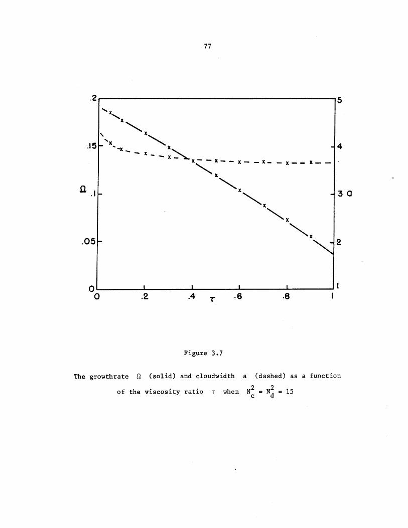
77

.2 5

x

xx.15- x -

xx

.05- -

0 .2 .4 r .6 .8 I

Figure 3.7

The growthrate 2 (solid) and cloudwidth a (dashed) as a function

2 2of the viscosity ratio T when Nc = Nd = 15

c d

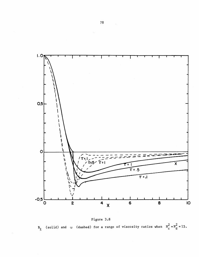
1.0

0.5 -

T=5-' T=1 -I

IT

\ T = .5 I

0.50 4 X6 10I

Figure 3.8

B (solid) and w (dashed) for a range of viscosity ratios when N2 =Nd2 =15.

91 : d

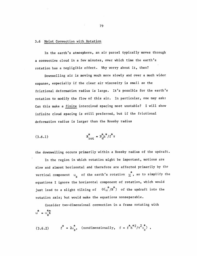
3.6 Moist Convection with Rotation

In the earth's atmosphere, an air parcel typically moves through

a convective cloud in a few minutes, over which time the earth's

rotation has a negligible effect. Why worry about it, then?

Downwelling air is moving much more slowly and over a much wider

expanse, especially if the clear air viscosity is small so the

frictional deformation radius is large. It's possible for the earth's

rotation to modify the flow of this air. In particular, one may ask:

Can this make a finite intercloud spacing most unstable? I will show

infinite cloud spacing is still preferred, but if the frictional

deformation radius is larger than the Rossby radius

* * * *(3.6.1) Rro = N h /f T

rot d

the downwelling occurs primarily within a Rossby radius of the updraft.

In the region in which rotation might be important, motions are

slow and almost horizontal and therefore are affected primarily by the

*vertical component wz of the earth's rotation w , so to simplify the

equations I ignore the horizontal component of rotation, which would

just lead to a slight tilting of O(o /N ) of the updraft into the

rotation axis; but would make the equations nonseparable.

Consider two-dimensional convection in a frame rotating with

*A

z

(3.6.2)* * * *2 2 *f = 2w , (nondimensionally, f = f h /r v )

Z c

and assume vc = v * Even though a large clear air viscosity decreases

the lengthscale of convection and thus the effectiveness of rotation,

by considering artifically large values of "f" we may qualitatively

deduce its effects.

Absorbing the centrifugal acceleration into the gravitational

acceleration and thus redefining the "vertical" axis slightly, one

obtains nondimensionalized "linear" (i.e., no advective terms)

equations (3.2.1)-(3.2.2) with Coriolis accelerations added for per-

turbations from an exactly saturated atmosphere, with the addition of

an equation for the velocity along a roll v(x,z):

2 2- ~(3.6.3a) (3-V7)V = B - fv ,(3.6.3a) x z

(3.6.3b) (t - 2 )B = $

2 ~(3.6.3c) (0 -V )v = f$ ,

(3.6.3d) u = v = w = B = 0 at z = Ot.

There are separable solutions with

(3.6.4) F(xz,t) = F(x) *e sin z

B (x) = dL/dx

Integrating (3.6.3b) and noting $z = -$ in (3.6.3a),

81

2dx

d2

(3.6.5b) (A+ 1 -x )vz=dx

2v L

(3.6.5c) (2 + 1 2 ~L + T) = 0dx-

For a growing solution, as discussed in section 2.3, equations

(2.3.19)-(2.3.25), I must take

(3.6.6) v = - fL/r

which, when used with (3.6.5a) in (3.6.3a) produces a sixth order

equation for L(x) alone:

d22 d2 2 2(3.6.7) (+ - ) ( 2 1)L = -N L + f L

dx dx

that is almost identical to the equation (3.2.14) derived in the

absence of rotation. Since L(x) is continuous across cloud edges,

so is v . Consequently, the matching conditions remainz

the same as (3.2.12),

(3.6.8) LL ,L , . .. are continuous across L = 0,

and one proceeds exactly as in section (3.2) except that the charac-

teristic polynomials are altered to

2 2 2 2 2 2(3.6.9a) pc(p) = (Q + 1- p ) (p -1) - Ncp + f = 0

(3.6.9b) p p) = (2 +1 -p )2 (p2 1) + N2p2 + f = 0

Solving (3.2.26) and (3.2.27) with these new characteristic poly-

nomials for N = N2 I found the critical N needed to triggerd c c

convection as a function of the nondimensionalized rotation f

(figure 3.9); the small f (s 1/10) typical of the atmosphere raise

the critical N only O(f 2). Plotting the growthrate as a functionC

of the intercloud spacing A, (figure 3.10), I found the maximum

growthrate occurred at infinite X and the growthrate decreased

,R*Isubstantially when A e 4 min [Ri rot

To understand this, examine the root pdl of d p) which

determines the decay scale in the clear air of the thermal perturbations

due to the cloud. Assuming

(3.6.10) Nd 1, ft

(3.6.9b) can be solved assuming pdl << 1 to obtain

(3.6.11) pdl = ,/(2 +1)2 +f / Nd '

which implies a dimensional decay scale

2 ** * * rd 2 *21/

(3.6.12) Rd = h/pldi =Ndh / {(Q + + f 1/2 .h

83

751

x

50-

x

NCx

25-

x

0 I 2 3 4 5f

Figure 3.9

2The critical N needed to trigger convection in the presence of

nondimensional rotation f about the vertical when N = Nd'

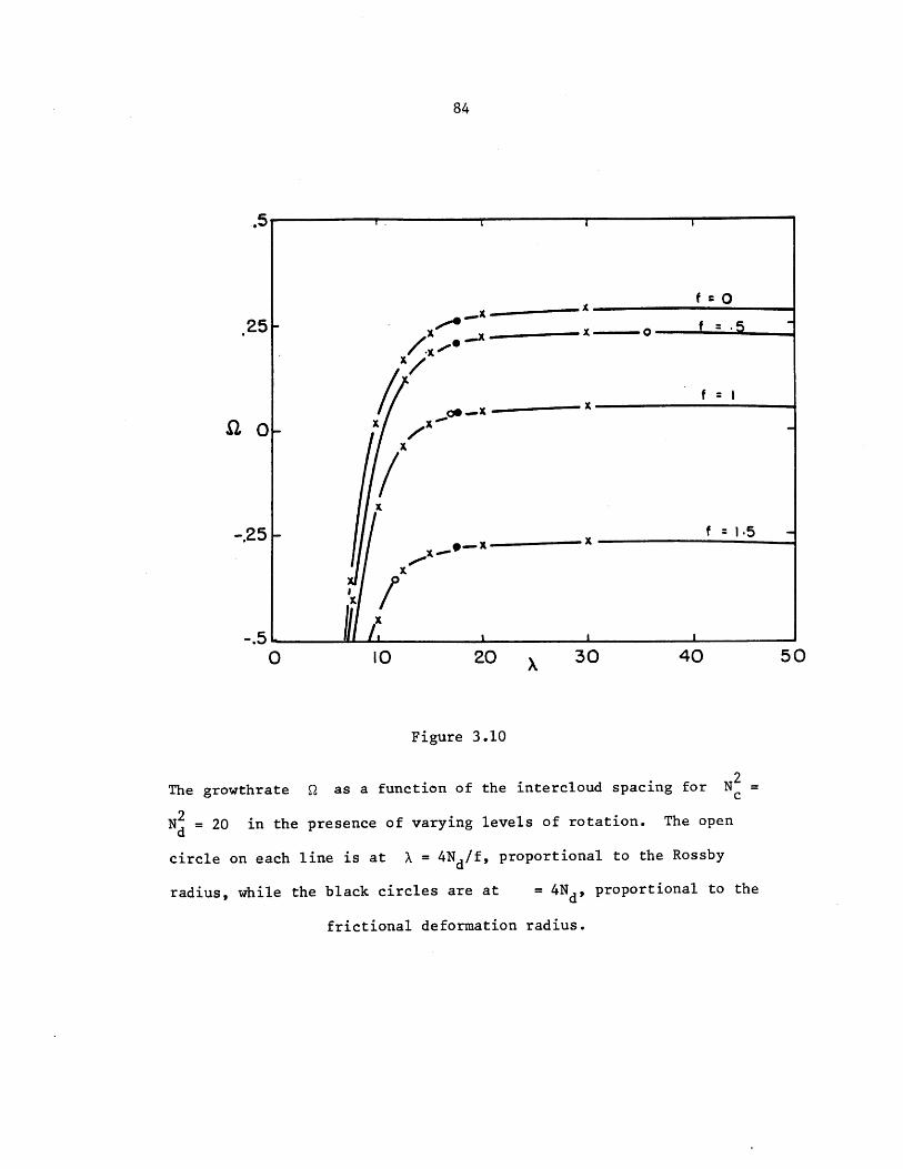
.25

-.25 - f = .5-

-.5 L/0 10 20 x 30 40 50

Figure 3.10

2The growthrate 2 as a function of the intercloud spacing for N ~

N = 20 in the presence of varying levels of rotation. The open

circle on each line is at X = 4Nd/f, proportional to the Rossby

radius, while the black circles are at = 4Nd, proportional to the

frictional deformation radius.

The three effects which compete to set the width of downwelling are

nicely exhibited; one sees

** *(3.6.13) R d ~ min [Rfric, Rrot , Rt*

*clouds damp each other significantly when X >; 4Rd and they start to

enter the regions of downwelling induced by their neighbors. In the

model just considered, I took v to be uniform, so the frictional

deformation radius was smallest except for rotation rates much higher

* *than that of the earth. However, in the real atmosphere, d c

because turbulence is suppressed in the stably stratified dry air.

* -2 -1 * 2Taking typical values Nd = 10 s , Vd = 10 - 100 m /s, h = 2 km,

f = 10~1s , 10-3 s1 for boundary layer convection,

*(3.6.14a) R fi = 25 - 250 km,

fric

(3.6.14b) Rrot 60 km,

(3.6.14c) Rt 2 6 kmn,

so rotation and especially rapid growth limit the extent of downwelling

as much or more than turbulent mixing.

3.7 The Stability of Separable Eigenmodes

So far I've restricted attention to convection with separable

vertical structure sin(z) and showed that the fastest growing mode

consists of a cloud with a single updraft surrounded by an infinite

region of downwelling. Integration of (3.2.11) forward in time from

many initial conditions suggests (as the analysis of section (4.2)

will show for widely spaced updrafts) that at large time this mode is

always the asymptotic solution to the separated problem.

However, I haven't considered the possibility of exponentially

growing modes with curved cloud edges which could grow faster than

this separable mode. I do not believe such solutions to (3.2.1)-(3.2.4)

exist, but this is extremely difficult to prove, requiring the solution

of a two-dimensional free-boundary problem with an unknown eigenvalue,

the growth rate. A first step is to show no such solutions exist

adjacent to the separable mode.

I employ an interesting variational technique. I derive a linear

equation for the evolution of small perturbations to the separable

eigenmode and its variational formulation. This can be used to bound

the growth rate of all perturbations whose vertical structure is not

sin(z) below that of the separable mode; at large time they become

negligible to it. Therefore, the single updraft separable mode is

stable to all small perturbations on it and no faster growing modes

with slightly curved boundaries can exist.

I look for solutions of (3.2.1)-(3.2.4) which are a normal mode

0 plus a small perturbation ef'L,

2(3.7.la) L(x,z,t) = L0 (xz,t) + cL1 (x,z,t) + O(82

(3.7.1b) L0(x,z,t) - LOx sin z-e

The boundaries of the resulting cloud are at

(3.7.2) Ca (z,t) = ±(a0 /2 ) + ca 1±(zt) .

Since

0 = B (ax ,z,t) = L (a +,z,t) + cL x(cx±,z,t)

~ ~ 2= cal L (±(a /2),z,t) + cLl (±(a 0 /2),zt) + O()

L (t( a/2),z,t)

(3.7.3) a (z,t) = -

L Oxx(±(a 0/2),z,t)

In (3.7.3) one sees how movement of the cloud boundary is related to

the perturbation. How does this movement influence the boundary

conditions? As in the case in which the cloud had vertical boundaries,

L and its first five normal and tangential derivatives are continuous

across the cloud edge, so in particular

are continuous across a+.

Rather than working with a free boundary, I translate these conditions

into effective jumps of L and its derivatives between the solutions

(3..4) x $ -xx xxxxx

inside and outside (continuously extended if necessary) at ±a /2.

Let this jump be denoted

d a a

(3.7.5) f = fd ,z,t) - fc (,zgt) .

Taylor expand (3.7.4):

~n n+1~9n(+L) ad 9n L a d o~

(3.7.6) 0n 2 ,zt) +al n+1 'zt) =0(2 0 < n < 5.ax c 9x c

Now, from (3.2.14),

6-2 2-

f0 d 2 2 0 a 3L0 a(3.7.7a) 6 =-(Nc + N )y(2 ,z,t) = -I 2 TqzFt) ,

3x c dx 2x

3'0Ld(3.7.7b) =0, 0 < n < 5,

3x c

so, substituting (3.7.3) into (3.7.6)

35E d a a

(3.7.8a) - (+ xx z zt) = -FL (-,z,t) ,35 C +Ox2 ' lx 2

3x c

(3.7.8b) n =0, 0 < n < 4.9x c

Having established the matching conditions, I round out the problem

by noting that, since LO + L L1 and L both obey (3.2.8), and except

2within 0(e) of ±a /2, both have the same N , which for the infinite

wavelength separable eigenmode is

(3.7.9a)-N 2

2 2 e NN 2= NO 2

N N d

|x < a /2,

lx| > a /2,

I can subtract to find

(3.7.9b)22 2~ 2~

(9 - V ) 2L 1 = -N L1t 0 lxx

Unlike (3.2.8), (3.7.8) and (3.7.9) are linear equations for Ll so I

can break into its separable components.

(3.7.10a) L1 =(x,t) sinnz,n=l n

(3.7.10b) L = - L1 (x,z,t) sinnz dzIn =T 0

Integrating (3.7.9) with sin nz and using the boundary conditions

(3.7.11) L = lzz = Llzzzz = 0'

one obtains

(3.7.12)2 2 2 2 2"- 2^

( + n - 2 ) (9 - n )L =N Lt x x In 0 lxx'

together with the matching conditions (3.7.8) with L1 replaced by LIn'

There is a discrete spectrum of exponentially growing solutions and a

continuous spectrum of viscously damped modes. The fastest growing dis-

crete mode will dominate the large-time behavior, so let

- -- . ... .....

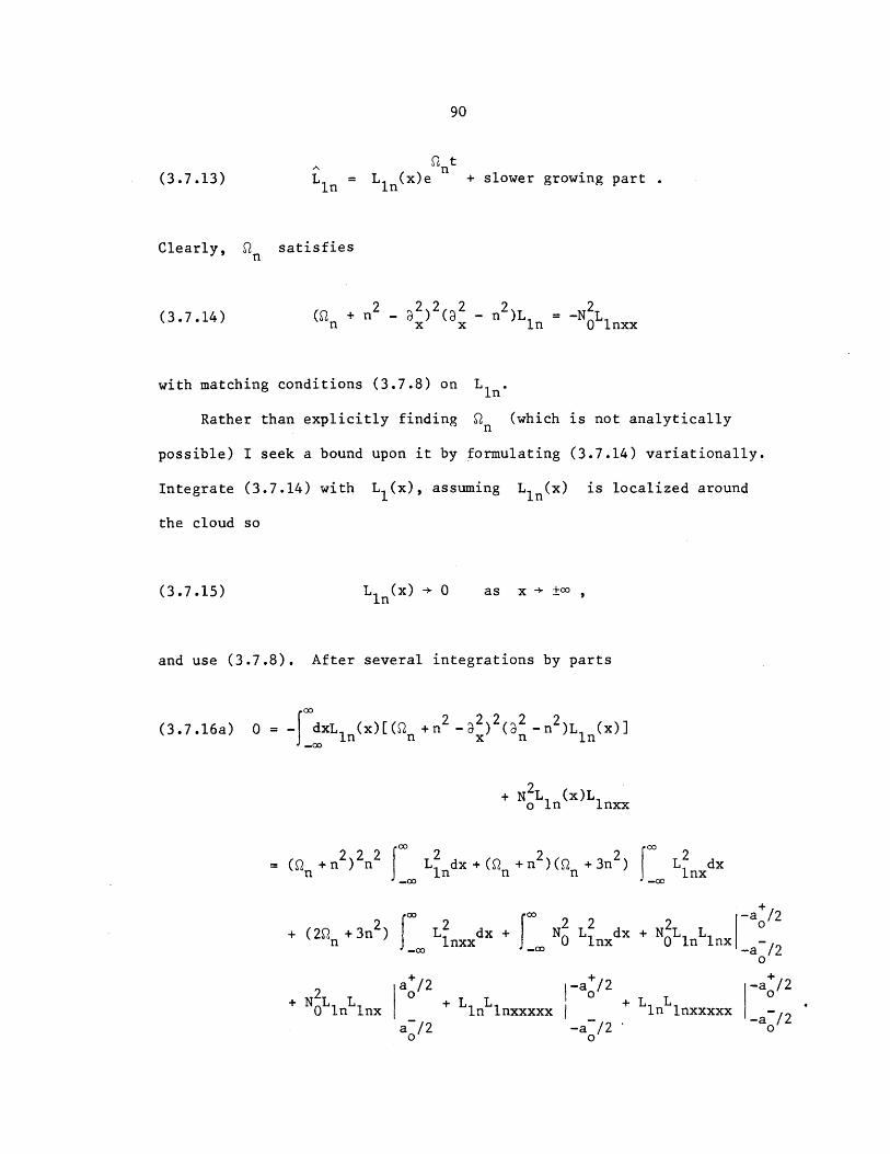
Q nL = L (nxWen+ slower growing part

Clearly, Qn satisfies

+ n2 - )2(92 - n2)L = -N2 Ln x x In 0 1Inxx

with matching conditions (3.7.8) on Lin'

Rather than explicitly finding Qn (which is not analytically

possible) I seek a bound upon it by formulating (3.7.14) variationally.

Integrate (3.7.14) with L 1 (x), assuming LIn(x) is localized around

the cloud so

L n(x) - 0 as x +co ,

and use (3.7.8). After several integrations by parts

(3.7.16a) 0 = -0 dxln Q +n2 -2 2 -n2 )Ll ]

+ N2 L (x)Lo in lnxx

2 222 2 2 2= ( +2n ) n 2 Ldx + (n +n )(2n + 3n )n J-CO i n nn2

f 2Llnxdx

+ (2n + 3n)

+ N2 L L a0 in Inx

L nxxdx + 0 N 2 L d

+/2 -a+/2+ L L l

in lnxxxxx |-_a /2 -a0/2

-+/

-a /2.x+ NL L 0

0 Ininxi-a /20

-a+/2+ L Lln lnxxxxx -a~/2

0

(3.7.13)

(3.7.14)

(3.7.15)

Although Lin and L are continuous across ±a /2, N2 has ainIx 0 0

jump of ±, while Llnxxxxx has a jump of + FLnx. Therefore, the

boundary terms cancel to yield

(3..16) 0 I(L )=I (L )+ 21 (L )2 +1 (L )2

(3.7.16b) 0= in 0 in 1 in n 2 In n

where I(L I) is the integral in (3.7.16a) and

(3.7.16c) IO(L) = n6 L2ndx + 3n4 {' Llndx + 2n2 L 2nxxdx

f 2 r 2+1 L dx -I N L dx

Inxxx - 0 1nx

4 2 2 2 V 2S Ld + 2n Ldx L nxdx > 0(3.7.16d) Iln (L n 4 jc LnX x + 2n2lO i nxx

(3.7.16e) 12(Ln) = n2 f Lindx + 2L 2ndx > 0lnx

The variation of I(L n) over functions which satisfy the matching

conditions (3.7.8) and decay as x -+ ±cO is easily calculated to be

zero, iff LIn satisfies (3.7.14),

SI(L 1n) = 0 for a solution of (3.7.14).

Together, (3.7.16) and (3.7.17) allow me to recast (3.7.14) to write

the true growthrate as the minimum of a functional Q (L n). For any

admissible trial function, solve (3.7.16a) for Q0, discarding the

negative root.

(3.7.17)

2 1 )1/2* -IS + (It -1012)/

1nn 1 2

Now when Lin

*is a solution of (3.7.14), Gn = n Lin). Thus at that

point (3.7.17) implies

* *2

0 n 2 n 0.(3.7.19)

However, since 2 is defined so that for any Lin

(3.7.20) 10 + 2In (Lin) + 1=2 (L 0

when Lln

(3.7.21)

Since 2I

is varied,

* *2 ~*r2 I*]61 + 26I Qn + I Q + ni[21 + 22n] 0

i 1n 2 n n2n

* *+ 21 Q > 0 when G2 = Q > 0, (3.7.19) can be subtracted

2 n n n

from (3.7.21) to get

(3.7.22)*

= 0n

for any solution of (3.7.14); the true growth rate is an extremum

(in fact a maximum) of Qn over all functions L (x) which satisfyng In

the boundary and matching conditions.

I would now like to show Qn is a decreasing function of n, so

that modes of increasing oscillatory vertical structure sin(nz) grow

(3.7.18)

I I-' - -11MW -- 1--- - - -

increasingly slowly. To do this, pick any admissible trial function,

and for the moment, regard n as a continuous variable, calculating

how Q varies with n. Glancing back at (3.7.16c) - (3.7.16e),

310 91 312(3.7.23) 0> 0

so

0 * 31l *2 2 *(3.7.24) - + 2 -- + 2 -- > 0, Q > 0.

We are finding the larger root of an upward-bending parabola which is

*rising higher as n increases, so 2 decreases with n. To show

this formally, differentiate (3.7.20) with respect to n,

0 * 1 *2 2 93 *(3.7.25) + 22 + + 2 2 0n n n (12-( + 2 0

* 2 1/2Since II + I2* = (1 - 1012) > 0, (3.7.23b) shows

*

(3.7.26) g-< 0,

so for an trial function L (x)

(3.7.27) 21 (L ) > Q2 (L ) > 3(L1) ...

so the maximum value of must be larger than the maximum of

* *

V21'0 ,. . But these maxima, from our variational principle (3.7.22)

are just the true growth rates, so

94

(3.7.28) 20 =1 > 2>Q3 '

Thus the fastest growing perturbations are those with vertical structure

sin(z) which leave the cloud boundary vertical and the solution

separable, and are governed by (3.2.11). As shown in section 3.5, these

modes have Q2 = 0 for a single updraft mode only for perturbations

which represent translations in x of the original eigenmode. Non-

trivial perturbations all grow less fast than the eigenmode.

3.8 A Variational Principle and the Nonexistence of Oscillatory Modes

Even though even small perturbations from an exactly saturated static

state of the atmosphere are governed by a nonlinear equation, variational

principles for several kinds of potential eigenmodes can be found. In

this section, I show by such means that there are no growing travelling

wave solutions, nor any growing oscillatory solutions. Since squall

lines and thunderstorms in the atmosphere are often observed not to

travel with the mean wind, this strongly indicates rain is very important

in their dynamics. It also shows there is no linear "wave-CISK" possible,

i.e. no self-exciting gravity wave of wavelength many times the inter-

cloud spacing which relies on the fact that convection can generate

kinetic energy (and perhaps feed it into the wave) even though the hori-

zontally averaged stratification is stable.

Firstly, I derive a variational principle for steadily growing

eigenmodes, not necessarily separable in x and z,

(3.8.1) E = L(x,z)e .

Multiplying (3.2.8) by -L (with t replaced by the real growth rate

Q), averaging over all space using the operator < > defined by

(2.3.20), and integrating by parts using (3.2.9),

2 2 2~ 2~-(3.8.2) I(f) = -<{(Q -V ) V L + N L }> = 0 ,xx

2 ~-2 2~-2 2~ 2 2-20 = Q <(VL) > + 2Q<(V L) > + <[V(V L)] > + <N LE>,x

where N2 is

2 ~~02 N L < 0,

(3.8.3) N = d2 ~-N L > 0.

c x

Taking the variation of I with respect to all functions L satisfying

the boundary conditions (3.2.9) at z = 0 and 7 which are continuously

five times differentiable across L = 0 recovers the original equation

(3.2.8) since, integrating by parts and using the continuity of

2 2 ~2-~(3.8.4) SI = I(L +6L) -I(L) = Q <2V(6L)*VL> + 2Q<2V (6L)V (L)> +

+ <2V(V L)V(V26)> + <2N 2L 6 >x x

2 -2~ ~- 4~- 6~= -2Q <L6V L> + 4Q<6LV L> - 2<6LV L> +

+ lim -2N2L 6L + 2N L L -- +L oc x x J d x x 2 7L

L >0 L <0x x

+ O([6L] )

The last term must be treated with care since N2 is not a continuous

function of L , so cannot directly be integrated by parts. However

lim -2N L 6LL -*oj - c x x

L >0X

= lim

L >0x

+ JJ 2Nx x 21TLL <0x

2N L 6L +

L <0x

2N L 6 -1

cloud'L =0[2N L

xedges

2~ -=-<2N L SL> ,

since the boundary terms vanish because L = 0 there xC

is the normal

vector in the x direction pointing out of the cloud).

(3.8.5) 61 = -2<6E -{(Q -V2)2 V2 + N2 }>

will vanish for all infinitesimal variations

It follows that

+ O((6) 2)

iff (3.2.8) is satisfied.

If it is assumed

(3.8.6) s =N /Nc d

is fixed (although if2or N were fixed, analogous procedures wouldd

follow) then from (3.8.2), for the true solution,

2 22 -2> + 22<(V2E2> +(3.8.7) N2 =

c <-(N2/N2 2>c x

However, since for this true solution,

(3.8.8a) 6I(E) = 61 - N2 2 = 0,1 2 2

(3.8.8b)

dm2' 2

2 11 1 2 1 26Nc 1- 2 1 c 2

2 2 2

+ 2N ] x c

I2(L)

I2(L)

So N2 is extremized (in fact, minimized) at the true eigenmode:C

2 .m 2 > +2 2> + 2 2(3.8.9) N = min 2'-

c L <-(N2/N2 2c x

2This allows a variational determination of the lowest N at which

c

growing modes of any growth rate 2 are possible and nicely shows how

the solution is a compromise between smoothness, which reduces the

2 2. .numerator, and amplitude mainly in the unstable region N = -N inside

c

the cloud, which increases the denominator.

A similar idea shows there are no growing, steadily translating

wavelike solutions to (3.2.8),

(3.8.10) L = e tL(x -ct,z)

where Q is again real. Such solutions obey

(3.8.11) ( -c3 -V22 V L = -N2 Lx xx

which when multiplied by L and integrated implies

(3.8.12) 0 = <L (n-c3 -V22 V L +N2 LL>

= Q 2{<L L > +<L L >} -2Qc{<L L +L L >1xx x zz x xxx x xzz

- 2Q<L (2 +9 2)2L> +c2 2 + 2)L -L > +2c<(92 + 32 2L -L >x x z x z xx x x z xx

+ <(92 + 2)L.L > [ (N2 +N 2)L2dxx z x 2TL cloud IL =0 ( d x

edges X

All the terms with an odd number of derivatives inside an average can

be integrated by parts into averages of perfect differentials which

vanish, while the rest can be written

(3.8.13)2 2 2 2 2

2Qc<L + L > + 2c [(9 +3 )L ] > = 0xx xz x z x

If Q > 0 so that the wave grows, either c = 0 or L = 0 so there

are no growing travelling wave solutions.

A similar technique rules out growing periodic oscillations of

some period T:

(3.8.14a) L(x,z,t) = e tL(x,z,t) ,

(3.8.14b)

This time,

(3.8.15)

L(x,z,t+T) = L(x,z,t) .

L obeys

( - 22 2L + N2 L = 0 .

Multiply by Lt and integrate over x,z, and a period in time, denoted

by an over bar:

(3.8.16)T

f =n <f(x,z,t)>dt.

Then, integrating by parts in space (again the boundary term due to the

discontinuity in N vanishes)

100

(3.8.17) 0 = Lt t + 2 - 2 2 2 L + N2 Lt xx

= t V2Ltt + 2Lt 2 Lt + Lt 2_V 2 L + N2Lt xx

= - VLt tt - 2[Q(VLt 2 +(V 2L t 2] _[( _ )VL]-[( -V )VL t

N t xt *

The first and third terms are averages over a period of the perfect

derivatives of periodic functions, so they vanish. Interchanging the

order of integration in the last term,

(3.8.18) N 2 L Lt = j <N2 L L t>dt0

= < N2 L L tdt>0

The time integral can be divided into segments for which L > 0 and

L < 0. The function L is periodic so either there is one segment,

N2 is constant, so the integral is the perfect time derivative of

1 N L averaged over a period, or there are several segments, and

L (x,z,tO) = 0 for some t 0 . Then

rT 2 T+t

(3.8.19) N 2L L dt = 0 N2L L dt0 xxt t xxt

= legment xx

segments segment segmentend beginning

=0,

101

since L = 0 at the ends of a segment by definition. In either case,

from (3.8.18),

(3.8.20) N2 LL = 0,x xt

so from (3.8.17),

(3.8.21) 2 Q(VLt)2 + (V2Lt2 = 0,

which requires Lt be constant. Since L is periodic, the constant is

zero, and

(3.8.22) L =0 ,

so there are no growing periodic oscillations. The same argument with T

taken infinite establishes there are no exponentially growing aperiodic

oscillations either.

This severely restricts the possible asymptotic states of the

"linear" system at t-+o. Section 3.7 suggests that all of the eigen-

modes have vertical cloud boundaries and are "separable." This section

indicates that if clouds grow at all, their boundaries asymptote to fixed

positions. Numerical experiments and the upcoming results of chapter

four show that separable clouds do not c6exist for infinite time.

symptotically, the only plausible state is a single isolated cloud such

as described in section 3.2, surrounded by subsiding dry air.

102

3.9 A Summary of "Linear" Moist Convection

The study of small amplitude perturbations of an exactly saturated

static atmosphere has led to several interesting results. The fastest

growing solutions are isolated cylindrical clouds whose radius is almost

equal to the depth of convection, surrounded by a broad area of subsidence

exponentially decaying away from the cloud in a radius which is the

minimum of the frictional, Rossby, and transient deformation radii. For

a growing cloud, the transient deformation radius is smallest under

conditions typical of boundary layer convection, but is still upward

of 6 km.

Each cloud is centered on an updraft with evaporatively driven

downdrafts near its edges. Clouds with several updrafts can grow, but

are unstable to the growth of perturbations which in the end collect

all the upward motion into a single updraft.

Arguments based on variational techniques show single-updraft clouds

are stable to the growth of perturbations, and that convection cannot

take the form of travelling waves or oscillations. This strongly

suggests that almost any initial conditions will result in one isolated,

single updraft cloud growing in place with vertical cloud boundaries.

However, moist convective updrafts are not infinitely far apart in

deep moist convection even when little precipation is falling. In the

next chapter I will explore within this model the reasons why this can

be so by extending this study to include a nonlinear equilibration of a

field of growing cumuli, possibly in a region of large-scale vertical

motion.

103

CHAPTER 4

The Interaction of Weakly Nonlinear Clouds

in Mean Vertical Motion

4.1 Introduction

The "linear" theory of moist convection explored in chapter 3 left

some important questions unanswered. No mechanism for producing a finite

intercloud spacing was found, so what is it that sets the horizontal

distance between clouds? Often, large scale processes such as baroclinic

instability, frontal uplifting, or nonuniform surface heating can induce

a mean slow vertical motion. How does this influence the convection?

As convection intensifies, the nonlinear advections of heat and water

can be expected to stabilize the convection. How does this occur and

what are the consequences for a field of clouds? Does this cause clouds

to cluster as is often observed?

In this chapter I will derive equations for the amplitudes of weakly

nonlinear, sparsely distributed clouds in the presence of a mean vertical

motion induced by a slowly varying temperature perturbation of the lower

boundary. To do this N is reduced until the fastest growing linearc

1/2.mode grows at a very small rate V << 1, and i is used as the

basis of an asymptotic solution of the equations. In section 4.2 I

sketch the method of the expansion, and in section 4.3 carry it out in

detail to obtain evolution equations for the strength and position of

each cloud. In section 4.4 I discuss the equilibrium solutions of these

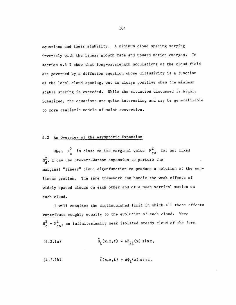
104

equations and their stability. A minimum cloud spacing varying

inversely with the linear growth rate and upward motion emerges. In

section 4.5 I show that long-wavelength modulations of the cloud field

are governed by a diffusion equation whose diffusivity is a function

of the local cloud spacing, but is always positive when the minimum

stable spacing is exceeded. While the situation discussed is highly

idealized, the equations are quite interesting and may be generalizable

to more realistic models of moist convection.

4.2 An Overview of the Asymptotic Expansion

When N is close to its marginal value N2 for any fixedC cO

N 2 , I can use Stewart-Watson expansion to perturb thed

marginal "linear" cloud eigenfunction to produce a solution of the non-

linear problem. The same framework can handle the weak effects of

widely spaced clouds on each other and of a mean vertical motion on

each cloud.

I will consider the distinguished limit in which all these effects

contribute roughly equally to the evolution of each cloud. Were

N = N2 , an infinitesimally weak isolated steady cloud of the formc co

(4.2.la) B (x,z,t) = AB U (x) sinz,

$4(x,z,t) = A$(x) sinz,(4.2.1b)

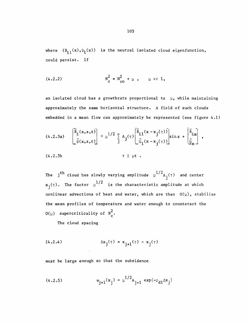
105

where (B 1(x), 1(x)) is the neutral isolated cloud eigenfunction,

could persist. If

(4.2.2) N2 = N2 + y , p << 1,c co

an isolated cloud has a growthrate proportional to p, while maintaining

approximately the same horizontal structure. A field of such clouds

embedded in a mean flow can approximately be represented (see figure 4.1)

B Z(x,z,t) 1/2B 9, ( - x.(19,(4.2.3a) L (plt) /2 A .(T)xT sinz + M

(4.2.3b T = pt

th 1/2The j cloud has slowly varying amplitude p A.(T) and center

x.(T). The factor p1 2 is the characteristic amplitude at which

nonlinear advections of heat and water, which are then O(pi), stabilize

the mean profiles of temperature and water enough to counteract the

20(p) supercriticality of NC

The cloud spacing

(4.2.4) Ax.(T) = x (T) - x.(T)j+1

must be large enough so that the subsidence

(4.2.5) wj+1 (x ) p e/2A{j+ dl

Bu=P (x)+N 2I

B, = 0

Bu =LE O)

Bj 0

Figure 4.1

Part of a representative field of clouds considered in chapter four.

Stremlines are dashed and the wavy solid lines are cloud boundaries.

Z x

107

induced by the j+l'st cloud near the j'th cloud does not overwhelm

the growth 3/2A. of the j'th cloud. ThereforeJT

(4.2.6a) C = exP{-pdl Ax} 0(y)

(4.2.6b) Ax. > ---{log(1/y) + 0(1)}3 Edl

Notice that the effect of the j+2'nd cloud on the j'th cloud is

O(I 2); only adjacent clouds affect each other significantly.

The mean vertical motion wn , which I induce by slow horizontal

variations of the temperature on the boundaries, must also not overwhelm

p3/2 A , so

(4.2.7) W 0(yI) .

I will now outline a consistant asymptotic theory which predicts

the evolution of such a cloud field. The equations which are to be

solved are (2.3.25-26):

2 2~ ~ ~(4.2.8a) (3 - 2 )V 1 + J(4,V $) = Bt x

(4.2.8b) (0t - V 2 + J($,B ) = $

(4.2.8c) J(F,G) = F Gz - G Fz

First, I generate a mean flow consistent with (4.2.7) by choosing

108

1/2ur = 6(X)um

B9 = 0

X = 1/2

at z = 0,

At the boundaries, small gradual variations of the temperature force

upward motion near temperature maxima. Since the boundaries saturate

the air with water, there will be more liquid water available to fuel

convection in such regions. There are mean fields in the absence of

convection:

(4.2.10a)

(4.2.10b)

(4.2.10c)

where

(4.2.lla)

(4.2.11b)

(4.2.lc)

B (x,z,t) = p/ 2 Zm3 (Xz) ...

1/2 3/2B (x,zt) = y 6(X) + B 3 (Xz) +

$m(xZt) = pIm 2 (X~z) + O(p2

$m2 (X,z) = e X 1S(z),5m (X,z) -

BE9m3 =Z e (XS2 (z)- ,

LBu (X,z) XX 2 N2um3 - -d

S=2 + N20 d co

and S 1(z) and S2(z) are fixed polynomials in z derived in

appendix II. To a good approximation,

(4.2.9a)

(4.2.9b)

(4.2.9c)

109

4.S (z) ~~ S2 (z) ~ - sin z

Each variable is broken up into its mean value and a perturbation

due to convection, denoted by a prime. The induced mean flow alters

the formula (2.3.23) for B to

um(4.2.12) B=

um

+ B z + (N c/r)B'm c 9

- (N2d/r)9'

B' + Bz zm

> 0

,' + M <

In the neighborhood of the

(4.2.13a)

(4.2.13b)

~ 1/2~,-

1/2~-= y BB1

+ y$

j'th cloud, expand

+ 3/2~1+y 3

~,2 3/2 ,+ yIB2 +Py B3'

'1 = A (T)$' (X - x (T)) sin z,

(4.2.14b) B ,= A (T)B 1(x - x (T)) sin z.

The presence of the j+l'st and j-l'st clouds enforces boundary

conditions

(4.2.15a)

j+1 1

y1/2A. (T)$ (X -x

.l(T)) sinz as x + "w"

(really 1 << x -x. << Ax.)

J J

. (T)) sin z as x +~ "-o"

(1 << x -x << Ax ),

(4.2.lld)

where

(4.2.14a)

3-1

110

and similarly for B;.

Since 41(x. -x ) = O(p) these boundary conditions imply13 j+1

(4.2.15b) 1, t + 0 as x + "oo" ,

and similarly for B 1 ,2' but affect and 3

Lastly, at every cloud boundary, the six independent matching

conditions derivable from (2.3.28) are

B, B , $, $9 , *) , $mare continuous across B = 0.

The cloud boundaries are no longer at x ± a /2; instead their positions

must be expanded as

S%(xzt) = 0 at x = (z,t) ,

1/2~~± t 0 + y a + pat 2

0 j(T) ± a /2

The equations (4.2.10a-b) must now be solved accurate to successively

higher powers of i/2 until solvability conditions determining the

evolution of A.(T) and x.(T) emerge. I will outline the calculatione lJ

here, leaving the calculation of specific terms for the next section.

(4 .2.15c)

(4.2.16a)

(4.2.16b)

(4.2.16c)

111

0(11/2

V - (N2 /r = 0 ,

V25' + ' = 0 ,11ol

-N 2

N2 coN =o N 2

Nd

B > 0

B < 0

These equations, by the construction of Nco, indeed do have solu-

tions of the form (4.2.14a,b), where from section 3.2 the neutral eigen-

mode can be written

Ycibci 'tci

Ydi bdig 'Odi) 11

bcif(xp ci)

1

fxj

1xj

< a /2,

- ao/2,

< a 0/2,

> a /2.

are defined as in (3.5.10b),

yc,di = c,di) o

V4 - (N /r 2 +9z4m2 + X 2

2i2 + r i2x JW19i'Z2 0 2x £1

(4.2.17a)

(4.2.17b)

(4.2.17c)

Ycil'di

(4.2. 18b)

where the

(4.2.18c)

(4.2.19a)

(4.2.19b)

(4.2.18a) $1(x)

112

The mean fields, which persist in the absence of convection, obey

(4.2.20) 4zm2 + = 0

The remainder of the equation is solved in section 4.3 to obtain

(4.2.21) rB A sin 2z5' 3 B (x)

and the cloud boundary perturbations

(4.2.22) ± = A a Cos zj.

0(3/2

74 - (N /tS3 2 + J( ,V2$ )V ; -(N 2/1 )B' = J(lP{,V 2+

N2 N2+

+ 3 V

N2

0B2 0 9Lx0r

+ J($ ,2mzz) + 2m 1

V2'3+ r OiX = J(p1 ,2 + J (ip2 ,BQ,) + Tl

2~+ JB + o- -lx z Em3 +o0m2X

is determined from

2'2z = m2z, m3 0rn2X

(4.2.23a)

(4.2.23b)

(4.2.24)

113

The mean fields enter to this order not only through their contribution

to vorticity advection, but also implicitly by perturbing the cloud

boundary, which is at

(4.2.25) B+ =0B+B =0.

At this order solvability conditions arise when the parts of $ and3

B1, proportional to sin(z) are matched across the cloud boundary,

and these will be the goal of section 4.3. Their derivation is

tremendously complicated, and the reader is urged to skip to section 4.4,

where the resulting evolution equations for the cloud field are stated.

Given their underlying assumptions, these equations contain all of

the physical effects modifying the growthrates at least 0(y1). The

shearing of the mean flow on each cloud at a rate du m/dz = O(P) reduces

the growth rate by O(p 2),a negligible effect, as do the non-

linear interactions of neighboring clouds. The three physical effects

which are important are

(1) The stabilization of a cloud by its own nonlinear buoyancy

fluxes;

(2) The moistening of the basic atmosphere by upward motion;

(3) The two-fold competition of clouds with each other due to

their linear interaction, first by competing for inflow air

and second, suppressing each other by drying the environment

through forced subsidence.

114

4.3 Derivation of the Amplitude Equations

In this section I will carry through the method outlined in

section 4.2 to obtain equations for the slowly varying amplitude and

position of each cloud and to examine the nonlinear modification of the

structure of each cloud.

O(p)-

To find the leading nonlinear corrections to the cloud structure,

I must solve (4.2.19a,b). The solution can consistently be assumed to

have the form (4.2.20). I first compute the Jacobians

2~ 2(4.3.la) =A sin 2z J(x -x.(T))

(4.3.1b) J(A, ) =A sin 2z J (x-x.([))

From (4.2.14a,b), in the cloudy air,

(4.3.2) J (x) = Y .(P 2. -1)[f (x'p )g (x'p .Ic 2. ci cj cj c ci c cj

i j

- fc cj c 'tci)]bcibcj

Noting that p2 .-1 can be rewritten as -y .l' and using multipli-c3 c3 0

cation formulas from appendix II to write the products as sums of

characteristic functions,

(4.3.3a) J1c(x) = {a c 'Oci cj) +a ge ' (xP j -Plc J 1 ic 2 ic

115

where

(i,j)(4.3.3b) alle = (F /2)y j2 ci p. ~0 ci

/4y(F /240 ci cj

(4.3.3c) j) /2( y 2a 1 2c O/2)CiCj

c +p )(

ci +pcjbb

2p . bcibcjci

~ci

p .p .ci c3

... L b .bci cc

Pci ~, Pcj Pci ~ Pc i2p . 2p .cjc - ~cic b cbcci ci

-(i~j)= -a

In the dry air,

(i,j)(4.3.4a) alid

(4.3.4b) a 2d

(4.3.3a) holds with subscript "c" replaced by "d" and

2 d +pdj Pdi djOdi dj

bdi bdj

= 0 .

Similarly,

(4.3.5a) J 2 (x) = I ci c 'ci c (x' f 'c

i j- y c (x,cj c )g

ii 21c c ci cj

'Pci )bcibcj

) + ai fI (x f 'ci -PCj22c c ci cI

(ij) 1 ci~ cj

a 2 1 c 4 ci p.4 ~ci

where

(4.3.5b)

116

(4.3.5c) (ij) 122c 4 ci

Pci + Pcj

pc.Ci

and in the dry air

(4.3.6a)

(3.3.6b)

(ij) 121d 2 ' di

a (ij)a2 2 d

4di

Pdi

= 0

Consulting appendix IV, I can find particular inhomogeneous solu-

tions in the cloudy and the dry air by substituting the a1 's and a2 's

for the R1 and R2 of the appendix.

(4.3.7a) $ ( xl) i c I ')c+pic

+ (i~j)g(x+ 2c Sc 'ci~Pcj

2c Sc 'ci~c21c c ci +pcj

(4.3.7b) $2d(X) =1 ld (x Pd +Pdi j

=y ~ii

(ij) )$21d d di + pd)

Since p. ±p. is never a characteristic root of p2 (p), I have usedi j

(IV.3e) to eliminate the operator Q1 in favor of new coefficients

(4.3.7c) $2 =c llc c2

(likewise for the other coefficients).

117

The most general solution is of the form

(4.3.8a) $2c (x) = 2hc(x) + 2c (x)

(4.3.8b) (x)=) (2) b(2) 9 (2)2h ci ci C ci

1

and similarly in the dry air. To find the unknown coefficients b .C1

and b I derive matching conditions at x = . The right clouddi 2-o'

boundary x = 5+(z,T) is where

(4.3.9) 0 = B (X,Z,T) = /y A jAB 1(x) sin z + pA B2(x) sin 2z + 0(p 3/2

Recalling = Bx (a ) and Taylor-expanding about x = ao/2,

(4.3.10a) &+ (z,T) = (a0/2) + y1 /2a1(zT) + 0(y)

(4.3.10b) $A S sin z = -A B2(a /2) sin 2z

From (2.3.28), the appropriate nonlinear matching conditions are the

same as for the "linear" problem, namely continuity of B and its

first x-derivative and of j and its first three x-derivatives.

Using the jump notation (3.7.5), for any function continuous across

the cloud boundary

(4.3.11) F(x,z,T) = 11/2F1 (x,z,T) + pF2(x,z,T) ...

118

the effective jump condition at x = a0/2 is found by Taylor expansion

to be

d 3F ~d(4.3.12) F2 = I .

c c

Now by construction

d d d N 2 N2

(4.3.13) V = - - (a /2,z,T)

c c r r 9' o

= B9 (a 0/2,zT),

so

d d d d

(4.3.14) 2 2x 2xx 2xxx -B 2(a /2)

C c c c

d 1d= B2 =d B dx| 0'

c c

By splitting $2 and B into their homogeneous and inhomogeneous

parts, matching conditions for the homogeneous solution are obtained

which can be written in the manner of (IV.16) with

(4.3.15a) A A~p + n-- L- (x) (x}+ B a0)ns 2h n 4 2h d n-1 2d 2c 1 n4 Z 2 2

dx x= a9

(4.3.15b) A na[2h] =

and similarly for B2h. The unknown coefficients bi and b(2) cannow ci di

now be found from (IV.20) of the appendix.

119

0(113/2)

The leading nonlinear correction term could be found without

imposing any conditions on the solution. To find such solvability

conditions, I go one order further in the expansion and solve (4.2.23a,b)

for the sin(z) components 3(x,T) and B (x,T) of and B .

Components of the right hand sides of (4.2.23a) proportional to higher

harmonics do not lead to further conditions on the solution. Let

(4.3.16) f(x,t) = - f (x,z,T) sinz dz0

denote the

(4 .3.17a)

(4.3.17b)

sin(z) component of any function f. Then

N2

- B 9

0= R1 + R12 + R1 3 + R 1 4,

V + ' x = R2 1 + R2 2 + R 2 3 '

where

(4.3.18a)

(4.3.18b)

R + , 9V ,q

R = J( ,B2) + J($,B ),21 - ;'92) 29

are nonlinear self-interaction terms,

(4.3.19a) R12 ~ T 1

120

(4.3.19b) R22 $9,1

depend on the slow variation of the clouds,

(4.3.20a)

(4.3.20b)

N2 2 2 N2N N 0 1 dAN

R =-(rr B =- B13 P 2 0 Rlx = - Bx,

0 0

R23 0 1x 0

x

depend on the supercriticality, and

14 ^ ~ ~ ~9 2~(4.3.21)

depends on the mean field (but will turn out to be zero).

There are two complications. Firstly, the boundary conditions at

this order must finally take into account the presence of other clouds.

From (4.2.14a),

y A. (+T)$ (x -x.j~ (-U) )

$3-1 j+1 1 ( +1y~' ACiT y&- T))

x >> x.(T)

x << x. (T)

and similarly for B 9. The intercloud spacing has been chosen in

(4.2.6a) to make y~ 4i1(x - x j+1(T)) an 0(1) quantity near the jth

cloud. Secondly, the cloud boundaries at

(4.3.23) 0 = B = yA B 1(xc) sin z + UA B2 c) sin 2z

+ P3/2[BI3 cxz,)+ B ].Z 3 \XcZ 93m .

(4.3.22)

121

are affected by the mean circulation.

In Appendix V I calculate the inhomogeneous terms and find parti-

cular inhomogeneous solutions in the neighborhood of the jth cloud:

"(n) 3 %-(t) Xx)(4.3.24) $ (x,T) = (x -x 3)A +A. +3 ( $ (x -x.)A.x.3 3 JxxA J 3 xxJ)AJT 3 i .J JT

+ $' (x -x.)A. + e(x- +G A. }3Jj 3 J jJ+1 j-1 3-1}

+ 4) (x-x.){C.A. -3 J j+l j-1 3-1

in the cloudy and dry air which satisfy the boundary conditions at

x = xc. Next I add to them homogeneous solutions $ 3h(x,T) to satisfy

the matching conditions at the two cloud boundaries. The singular

matrix equations which result are solvable only given two constraints

which lead to evolution equations for the amplitude and position of

each cloud.

The Matching Conditions

B93, its first x-derivative, $3, and its first three x-derivatives

are continuous across the cloud boundaries a (z,T). +(z,T) can be

expanded

(4.3.25) += x + 1a 0 + pj 1 + ya2

(in this and what follows, all functions are evaluated at x = ba 0 unless

explicitly stated and arguments 'z' and 'T' are omitted.) By definition,

122

(4.3.26a) 0 = B (& +)

1 1 12

1 + p -2 + 2 a lx + 2}lxx

+ p{ ,2 + x + p3/26 + 9,m3} + O(p2

Equating the 0(p3/2) terms to zero,

(4.3.26b) B' +-& ' (&2/2)i' -.E,3 2 Elx 1 2x 1 Elxx Em3

Let F be any function continuous across the cloud boundary with

a functional form F inside the cloud and Fd outside it. Like B

Fc -Fd is zero at the cloud boundary. The same procedure shows that

(4.3.27)d d - I d _ F d

F + a2F = - F2 lx .c 21 c 1 xc 1 c

and its first three derivatives, $2 and its first two derivatives,

B and its first four derivatives, and B92 and its first three

derivatives are continuous across x = Ca. onsequently, (4.3.27)

implies

(4.3.28a)

(4.3.28b)

d d d d

$3 ~ 3x 3 9 3 x 0,c c c c

d d d

$x = -$2x - acy1ic e c

(4.3.28c) + 21xxxx c 1 2xxxx ~ 21xxxxx *c c c c

123

The matching condition (4.3.28b) can be simplified using (4.3.13,14):

d(4.3.29a) lxxxx B ,

c

(4.3.29b)d

42xxxI

Only the components of the matching conditions proportional to

sin(z) contribute to the solvability conditions. Let

sin(z) component of

(4.3.30a)

(4.3.30b)

denote the

and recall (4.3.10b),

S = -2A i B92 cos z,

= B .

Then

3 -1 2=-2A i B 2 cos z sin 2z +

1 3 -1 2- 4A B 2 cos z sin z

=-1 A 3 B B22 3 2

With (4.3.29a) and (4.3.26b) I can eliminate from (4.3.28c),

(4.3.32) 3xxxId

-3 l'2xxxx

1~2 - d

+ 7al {lxxxxxic

d(4.3.31)

$3xx cI

-B2x

+ B m3- BL }

124

From appendix II,

(4.3.33a) B =F 0Wm

where wm is the approximate maximum vertical velocity

4(4.3.33b) Wm = - - e ,

The rest of (4.3.32) has sin(z) component

d - -d

(4.3.34) $ - B 3 2A {$ 2xxxx - B I cos z sin z3xxx 23 j 2xxx 2xc c

3 -2 1dB- 2A xxxxx - B }cos z sinz - B

3 ld c= A { [ 1 -B ] -412[$L --B ]}

j 2xxxxc 92x lxxxxx d 1xxc d

+ r w.o m

The Solvability Conditions

Knowing the matching conditions, I attempt to satisfy them at both

cloud boundaries by adding "symmetric" and "antisymmetric" homogeneous

solutions to $3 (x,T) and B (x,T). The "symmetric" homogeneous solu-

tion takes care of jumps in the parts of the inhomogeneous solution which

are symmetric about the cloud center. The "antisymmetric" homogeneous

solution takes care of the unbalanced effects of the two neighboring

clouds. Write

125

(s)(3 3 ,

(s)(x,) 1 3h (,T)

^(a)

3h (x,T(a)3 xT)

^(a)+ $3' (xT)

'J(s)+ $3 (xT)

+ (a)+ $ 3 XT

where from (4.3.24)

Q(n) 3x -x.)A13 3 3

+ t) (x-x .)A. + (x x .) .)3 3 3 3 3 3

+ 1) (x -x ){C A + c A. },33 .3 j+1 - .-

(a) =-(o)(4.3.36b) 1)3 = 3 ji A jAj -1} (x)3 j j R

while the symmetric and antisymmetric homogeneous solutions which decay

as x -+ ±co are given in appendix IV, equations (IV.14-15):

Y bdibdsigd 'lodi *

ci b csic (x'ci

+-(

x > a0x < -2a0-

cib cai c 'Pci1

and similarly for B3h'

(4.3.35a)

(4.3.35b) ^(s)$3

(4.3.35c)

(4.3.36a) -(s) (

3

(4.3.37a)

(4.3.37b)

(4.3.37c)

^(s)$3hd

-(s)1 3hc

A (a)1 3hd

-(a)$3hc(4.3.37d)

Ydi bdaigdxpd di

126

^(s)The jumps in the matching conditions are symmetric, so (xT)

obeys the same conditions as $3 (x,T), while there are no jumps in the

antisymmetric solution. Therefore, the homogeneous solutions obey

dn-l (S) d3h (S) (S)

n-l n43h 0 n 3hdx c

dn- B(s) d (S)3h An[B3hn-1 c

and similarly for the asymmetric solution; from (4.3.28a, 31, 34)

dn-l (r) d(4.3.39a) An[ ] = - 3 + B) +

n 3h n-1 n4 3dx c

0 n = 1,2, r = s; n = 1,2,3,4, r

+ - 1 1B A , n = 3, r

d d1

A 2xxxx 2x lxxxxx -Blxx]c c

+0 w M n= 4, r

-a

-2

= s,

dn-1 (r) d(4.3.39b) An B r n-1

dx cn = 1,2, r = s,a .

Consulting (IV.19), two matrix equations for the coefficients

bd,csi of the symmetric homogeneous solution and the coefficients

b dcai of the antisymmetric homogeneous solution are obtained. Using

the notation of the appendix:

(4 .3.38a)

(4.3.38b)

127

(4.3.40a) M b = R R(n) A + R(t) A. + R gA.s -s -s -s j -s JT -s j

+ R (e)+-R {c.A. 1 +c A. },-s j3+1 - -

(1) (x) (o)(4.3.40b) M b = R = R A.x. + R {c.A. -c A. } .

a -a -a -a J JT -a j j+1 j-1 3-1

The matrices are both singular, with left null vectors u and u-s -a

respectively. For a solution to exist the solvability conditions

(4.3.41a) u - R = 0-s -s

u -*R = 0.-a -a(4.3.41b)

must hold.

(4.3.42a)

They can be solved for the slow evolution of A. and x.:J J

3A. =aA. - T.A -n A. -kA. + ww,JT j j j+1 j-1 5-1 m

A.X. = -d.A. + d A3 jT j j+1 3-1 5-1

where

(4 .3.42c)-l

a ,d. =nd c = rn, d'y exp {-p (x. -x.)}.j j j1 dl 5+1 3

Numerical values of the coefficients except for k for various N aredo

tabulated in Appendix VI. As a check of a and TI, I can use these equa-

tions to predict the "linear" growth rate Q of a periodic array of clouds

128

spaced a distance X apart. From (4.3.42a),

(4.3.43) Q = (Nc - No)c - 2Hnexp {-pdl X.

In figure (4.2a) this prediction is compared with the true growth rates

of the "linear" eigenmodes found in section 3.2; it. is quite accurate for

clouds more than a frictional deformation radius apart whose linear

growth rate is only a few percent of Nc'

The coefficients d and o can be checked by solving the linear

initial value problem (3.2.1-4) assuming a vertical structure sin(z)

and replacing the effective stratification N2 of (3.2.4) by that felt

in the presence of mean vertical motion

2~(4.3.44) N 2 N d B 9,< -r w msin z

(4.3.44) N2 = 2 ~ :~m:I-N c B z> -r w msin z

c o m

By first taking wm = 0 and then considering two clouds of equal ampli-

tude a distance x apart, (4.3.42b) predicts

(4.3.45a) dx = 2d exp {-PdlX,

d(4.3.45b) - [exp(pdlx)] = 2dp.

If w # 0 but only one isolated cloud is present, (4.3.42a) predicts

2 2that if N2 = N ,

c CO

(4.3.46) d =ow

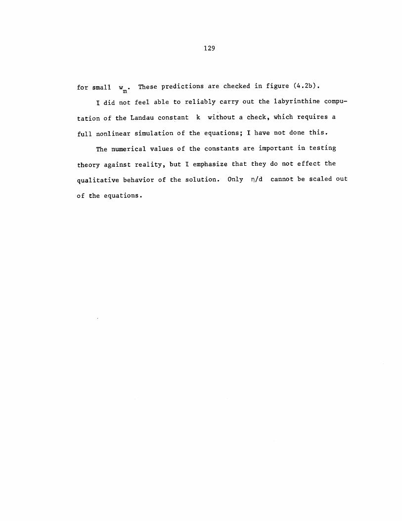
129

for small w . These predictions are checked in figure (4.2b).

I did not feel able to reliably carry out the labyrinthine compu-

tation of the Landau constant k without a check, which requires a

full nonlinear simulation of the equations; I have not done this.

The numerical values of the constants are important in testing

theory against reality, but I emphasize that they do not effect the

qualitative behavior of the solution. Only r)/d cannot be scaled out

of the equations.

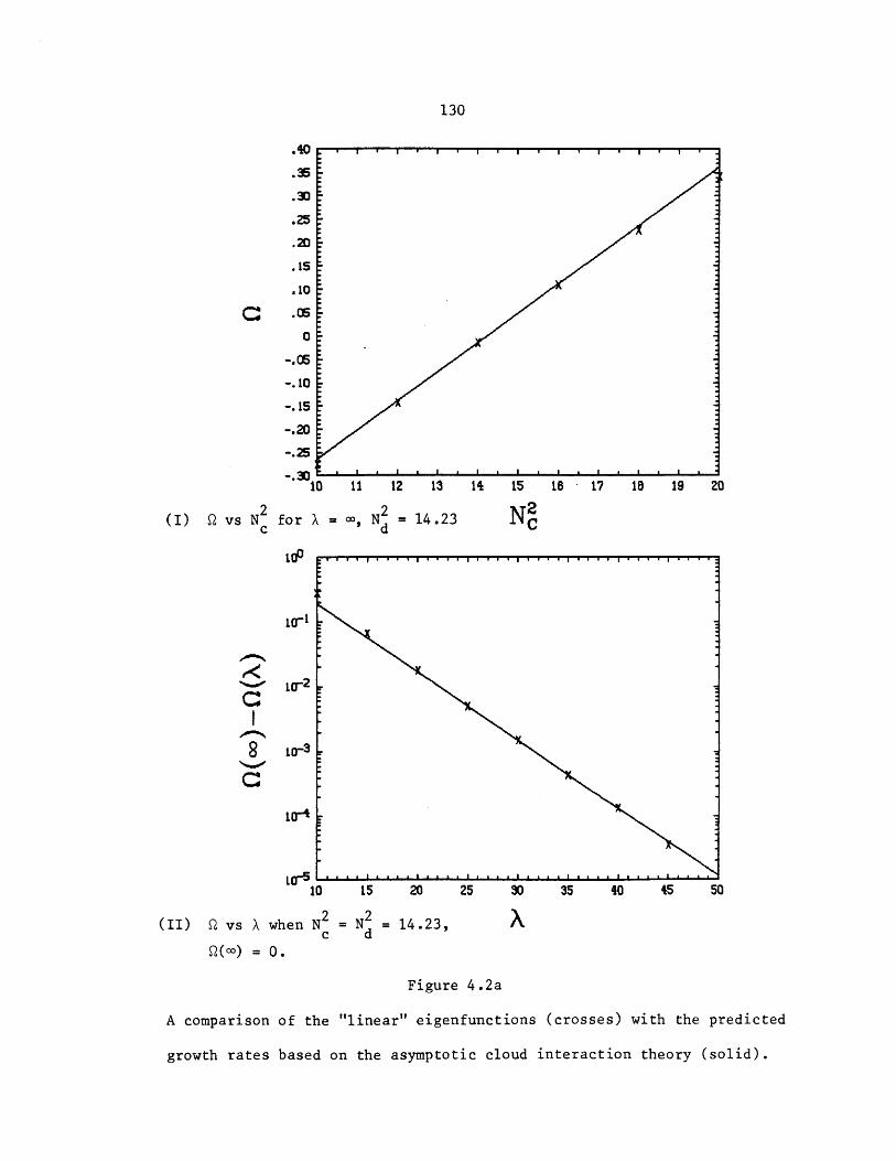
130

.40 .

.35

.30

.25

.20

.15

.10

C.050

-. 05

-. 10

-. 15

-. 20

-. 25

-. 30 *

10 11 12 13

2 2(I) Qvs N for X= o, N = 14.23

c d

I0 G ...............

C

7

10-1

10-2

t0-4

10 15 20

(II) vs X when N = N2 = 14.23,c d

2(0o) = 0.

14 15 18 - 17 18 19 20

N2C

25 30

x35 40 45 50

Figure 4.2a

A comparison of the "linear" eigenfunctions (crosses) with the predicted

growth rates based on the asymptotic cloud interaction theory (solid).

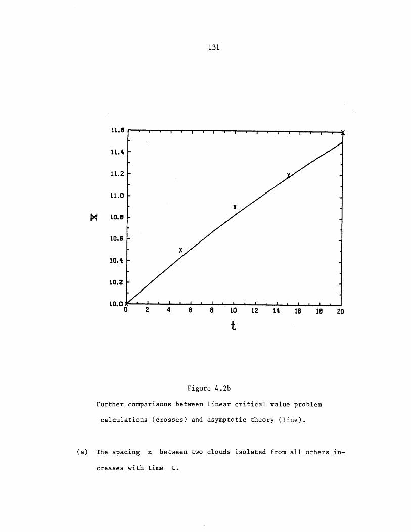
131

11.2

11.0

X 10.8

10.6

10.4-

10.2

10.00 2 4 8 8 10 12 14 16 18 20

t

Figure 4.2b

Further comparisons between linear critical value problem

calculations (crosses) and asymptotic theory (line).

(a) The spacing x between two clouds isolated from all others in-

creases with time t.

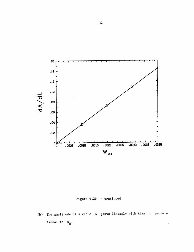
132

.16

.14

.12

.10

.02

.0005 .0010 .0015 .0020 .0025 .0030 .0035 .0040

Wm

Figure 4.2b -- continued

(b) The amplitude of a cloud A grows linearly with time t propor-

tional to Wm

133

4.4 The Amplitude Equations and Cloud Spacing

In the previous section I derived equations for the amplitudes and

positions of a field of widely spaced clouds. The essential fact that

allows each cloud to be determined by its amplitude and position was

that its horizontal structure is always approximately that of a "linear"

isolated eigenmode; motions inside and outside the cloud are completely

coupled. The idealized model considered was very special; if the

boundaries are not saturated, or the nonlinear behavior of q (p,T), the

saturation mixing ratio, is-considered, or if a more realistic upper

boundary (such as a region of strongly stratified air) were used, the

equations would change.

However, the qualitative character of their solutions would be

2little altered, as I will show. As long as N is near the critical

c

value N for the onset of convection, there is a stable steadyco

solution in which clouds are equally spaced at least a critical distance

Xc apart. If clouds are closer than this distance, they strongly

suppress each other. A subharmonic instability which amplifies every

second cloud leads to a field of clouds with twice the spacing which

can achieve much larger amplitude and thus increase the buoyancy flux.

A second type of equilibrium in which clouds of two amplitudes inter-

mingle in any combination is probably always unstable.

Having established that clouds are (at least locally) equally strong

and equally spaced, I will turn to "large-scale" variations of the cloud

field in which cloud amplitude and spacing change slowly compared to the

intercloud distance. I will obtain a diffusion equation for the cloud

134

spacing in which the diffusivity is positive precisely if the cloud

spacing exceeds X c; all such variations decay by a slow adjustment in

the position of the clouds.

The Equations

The equations (4.3.42) of the previous section can be written

(4.4.la) dA./dT = -n.A. - 1 A. + p(A.), A. > 0,

(4.4.lb) A.(dx./dT) = -d.A. + dj.A. ,

where

(4.4.lc) T = Pt,

(4.4.ld) .,dj = T 9d -1 exp{-pldx },

2 2

(4.4.le) = N 2 N 2c co

The restriction that A. > 0 is necessary to ensure each cloud really

is saturated. Notice that this allows the number of clouds in the field

to change. A cloud which is suppressed until A = 0 is thereafter

deleted from the equations. Conversely, new clouds can grow at any new

position x at which mean upward motion more than compensates for the

subsidence induced by the two nearest clouds.

135

For my model,

3(4.4.2) p(A.) = aA. - kA. + ww

where a, k, w, q, and d are constants depending only on N andco

2 3/2Ndo, and j w is the mean vertical velocity at midheight. Different

do m

boundary conditions or non-Boussinesq thermodynamics lead to the same

equations with different forms of p(A ), different q and d, and

-1perhaps a different subsidence radius Pdl. If convection is not too

pentrative, it will stabilize the environment by its upward buoyancy

flux so

(4.4.3a) d2p(a)/da2 > 0, a > 0.

This does not mean that moist convection is supercritical, however.

If wm < 0 any cloud requires a finite amplitude kick to grow.

I will also assume the linear growth rate a of an isolated cloud

is positive. Physically, this is reasonable because it is viscosity

which allows convection to be damped in a conditionally unstable

environment, yet an eddy viscosity is generated only as the cloud grows.

Thus p(a) has a maximum,

(4.4.3b) dp/da = 0, a = a .max

If p(a) has these properties then the equilibria and their stability

behave identically to the case (4.4.2). In this sense the equations

136

(4.4.1) and the solutions I will discuss are generic. I now seek

their equilibria.

The Equilibria of an Adjacent Pair of Clouds

Steady solutions of (4.4.2 a,b) obey (since d. c n.)Ji J

0 = p(A ) - 5 Aj+1 ~ Tj-Ajl

0 = - ? Aj+1 + A .

a specific pair of adjacent clouds i and i+l. Equation

can be used to eliminate Ai+2 and A from the equation

for each cloud to yield a pair of simultaneous equations for

A. = p(A. )/2A i+1 i

A. = p(A.)/2T. .

If these equations hold for every cloud pair, then direct substitution

into (4.4.4) shows the cloud field is steady.

The number of solutions depends on p(O) and 11. In my model

p(O) is proportional to the mean vertical velocity wm and the solu-

tions are shown in figure 4.3. However, more generally p(O) measures

.the moisture in the basic state and would be reduced if, for instance,

the air at the plates were less than completely saturated.

(4.4.4a)

(4.4.4b)

Consider

(4.4.4b)

(4.4.4a)

A. and

(4.4.5a)

(4.4.5b)

137

If p(O) > 0 there is always one equilibrium in which both clouds

have equal strength:

(4.4.6a) A. = Ai+ 1 = a1 (fl) ,

(4.4.6b) ai = p(al)/2TI,

Since p(a)/2n - a is a decreasing function of a near a,, dal/di < 0;

when the damping of a cloud on its neighbor increases, its neighbor does

not grow as strong.

If dp/da were not a monotone decreasing function of a, as might

occur were the convection penetrative, there could be a pair of much

smaller equilibria of this type for some range of ni, corresponding to

a subcritical instability. 'A finite amplitude "kick" would then be

necessary to realize the strongly convecting equilibrium; otherwise only

the barely convecting weaker equilibrium of the pair would be attained.

If the clouds are close together (case I) the equal strength equi-

librium is the only possible solution to (4.4.5). But if the clouds are

far enough apart (case II) so that

(4.4.7a) ni < C = r(x c)

where

(1 )/2nc) (dp/da)(a 1 (c)) = -1 > (1/2rn )(dp/da)(a1(n.)) ,(4 .4.7b)

138

there is a pair of solutions in which adjacent clouds are unequal,

(4.4.8a) (A ,A i+1 (a2 (ia 3 01i)) or (a3 i),a2(Ei))

(4.4.8b) a 2 p(a 3 )/2n ) < a(3 p(c2)/2) ,

which bifurcate from the equal strength solution at i = ric'

When p(0) < 0, there are no equilibria at all when clouds are very

closely spaced (case III). This occurs if ni > damp i =

(2n p(aL) - a < 0 for all a. At -ldamp' q(a) reaches its maximum

of 0 at a = damp

(4.4.9) q(adamp damp) = dq/da)(adamp damp) = 0

For my form (4.4.2) of p(a), ridamp is given by

3 1/2 2/3(4.4.10) a - 2 n p= [.(3k) (-ow )] = ad ;

damp 2m damp

,damp decreases proportional to the two-thirds power of the subsidence.

In sufficiently strong subsidence (case IV) a < adamp and the convection

is entirely suppressed.

If a > a and .f< )damp there are two equilibria in which

both clouds have equal strength (case V). If ni < nerit there also

are two unequal equilibria as in case II (case VI).

139

(A

7- - I

, - /7

I.7 -

9-II

II

~%%.4 ~

* II *

8Bz P(A)1 ~ 29

Case r: wm-O (one unstable equilibrium) Case1: Wm.O (one stable equilibrium A=8)m two unstable equilibria A*B

I 8 f 0 J J/.v I~ -

7 -7 - I

--

.W -,- I ~

- . - I= - d ~/ -

II - - ~ - /

- , *1 7 /- - / -

- , / pI, / /I /

- I I /- I / /

-d ~ * I,

- I I _____

Win'0 no equilibria

CoOS N. 'tao much damping 77B

- - --- /

a - ~-- -

- - - /- -

/ /

- - -- I /

- I I- I I *

// I p I

-9. / \ 'I II

D ~ ~_____ - ' ~I , IA -

I I- -

- - I- -

- -- I'

, - -- ~

- I -1 -

- I

- - -/ ,

/ I

I/ /I /

I *I

Case I subsidence)

-4-

one stable equilibrium A =8Case :: Wm. O (two unstable equilibria) Case M I.' w O one unstable " A=8

large 77 (two unstable " A i8

Figure 4.3

The equilibria of adjacent clouds and their stability. The solid lines

are the curves B = p(A)/2I and A = p(B)/20. Their intersections

give the equilibria and are shown as solid circles if they are stable

and are shown as solid circles if they are stable and unfilled circles

if they are unstable. The dotted lines are the trajectories of (4.4.5).

140

Equilibria of a Field of Clouds

So far I have just constructed solutions in which a particular pair

of clouds can be in equilibrium. That such relations hold between every

adjacent pair of clouds is a necessary condition for an equilibrium of

an infinite field of clouds.

If all the clouds are of equal strength, (4.4.5a) shows that they

must be equally spaced. If wm > 0 their spacing uniquely determines

their amplitude; if w < 0 there will either be no solutions or two

possible cloud amplitudes if the spacing is large enough.

If all the clouds are not of equal strength, I can show they all

have one of two different amplitudes. There must be a pair (A ,A i+

of adjacent clouds with different strengths; assume without loss of

generality that Ai = a3 (i) is stronger than A i 1 = a2 i) and

consider A . It is either equal to A or unequal to it. In the

latter case, I will show it must also be spaced a distance Ax _ = Ax

away from A and have amplitude at2 ni). To prove this, I will show

first that

dt2 da 3(4.4.11) 2- > __>--_

dT1 dTa

Differentiate (4.4.8b) with respect to n,

(4.4.12a) -- 2 = - - - p(a3n T 53 @T - 2-n2

a3 2 1(4.4.12b) @-= 3 2 a~ ~ ~~2 2'

2n

141

s3=1. 3S3 2TIdot c3 --LP(, (1TI)) >

(4.4.12d) s2 27I2Ti sl 2

These equations can be simultaneously solved,

3a2= I(4.4.13a)

3a3(4.4.13b)

- 22ri (1 +ss

~ ~ )(1 + s2 s3)

1

=-n(1l+s s2s3

{p ( a3)

{a2 - s3 a3}

- s3 P( 2 )I

> 0

{s2a 2 + a3 <

where I used (4.4.8b) and (4.4.12cd).

Since qi < rcrit and from the definition of

(4.4.14)

rIcrit'

2 %crit = a3 (crit = a crit

this shows that for any choices of nu_ and ai ,

(4.4.15)

Consequently, A. cannot be the smaller of the pair (A 1 ,A). if

it is larger,

(3..i = Y3i-1*

(4.4.12c)

a 2 ( Ii-1) <Y crit) < a3n i

(4.4.16)

142

so from (4.4.11) A. 1 is equally far from A as is Ai+1'

(4 .4.17a) Ili = n _l,

and so is equally big,

A _1 = a2 i-1) = Ai+1 =2 i '

It is also possible

specifies ni_1 to be

(4.4.18)

that A i 1 = A = a 3(ni). This uniquely

p(a3) a2( i)

n_1 = 2a = a ( . i '3 3 i

By extending this reasoning in both directions along the line of clouds,

I can show that every pair of unequal adjacent clouds must have ampli-

tudes a2 (ni) and a3(0i). The only equilibria of (4.4.1) are fields

of clouds, each of which has amplitude a2 (n) or a3 (-i) for some T1.

The distance between the clouds is such that

(4.4.19) 1 i =

1

a2n3

a3- 1a2

A = a2 , Ai+ 1 = a3 or vice versa

Ai = i+l 3

A = Ai+l 2

It is easily verified by direct substitution that all such solutions

are indeed equilibria, as they satisfy (4.4.la,b).

(4.4.17b)

143

Physically, what are these equilibria? One can easily understand

the equilibria in which all clouds are equal. If the intercloud spacing

is large, clouds damp their neighbors little and achieve almost the

amplitude of an isolated cloud. The stability of such a cloud field

depends on the stability of the equilibrated isolated cloud; physically,

the nonlinearity is what keeps the linearly unstable convection down to

a finite amplitude, so the isolated cloud which is the result of this

process is always stable. If wm < 0 there are two equilibria p(o) = 0

for an isolated cloud, but the smaller one represents the amplitude

above which a cloud is established enough to grow against the mean

subsidence and below which it is squelched by mean subsidence. This

solution is clearly an unstable equilibrium. Thus, there will always

be one stable equilibrium in which clouds are widely, but equally spaced.

If the intercloud spacing is small, clouds damp each other much

more, and do not come close to the amplitude of an isolated, steady cloud.

Then an array of equally spaced clouds is unstable, because if a cloud

is bigger than its neighbors, it induces greater subsidence around it-

self, damping them more. As they decay, it is no longer held down by

the subsidence they induced and grows further. Consequently, a cloud

can force its neighbors to disappear entirely if they are too close;

this sets a minimum intercloud spacing.

Next I turn to the equilibria in which clouds of two amplitudes

coexist. These are always unstable. To see why, I consider the extreme

case in which clouds alternate in strength between amplitudes c2(n)

and a3 (r), so are all equidistant. The larger clouds are little

affected by the smaller ones, and have grown almost to the amplitude of

144

an isolated cloud. The smaller clouds, however, are balanced on a

razor edge. Were they any smaller, they would be wiped out entirely by

the subsidence around the larger clouds. Were they larger, they could

damp the larger clouds more and decrease the subsidence they induce,

allowing further growth of the smaller clouds.

On physical grounds, I have concluded the only stable steady cloud

fields have uniformly strong clouds spaced a sufficiently large uniform

distance apart. Now I turn to the mathematical justification of this

statement.

The Stability of Equilibrium Solutions

Unfortunately, a complete stability analysis of this infinite

set of coupled equations appears intractable to me. I will content my-

self with the stability analysis of two important special cases to a

particular kind of perturbation. The first case is that of alternating

larger and smaller clouds, the second case is that of uniformly strong

equidistant clouds, and I do a stability analysis with respect to

perturbations which are equal for every second cloud. It will show the

alternating equilibrium is unstable, and give a minimum critical cloud

spacing for the uniform equilibrium to be unstable. It is reasonable

to suppose that if the uniform equilibrium is unstable by means of the

mechanism discussed above, the most unstable perturbation should alter-

nately damp and enhance cloud amplitudes and so should have the form I

now consider.

Let me assume, then, that

... A_l = A I

... n- = I 1

The equations (4.4.91a,b) reduce to (since

(4.4.21a)

(4.4.21b)

(4.4.21c)

(4.4.21d)

dA

dBdt

dx0

dt

dx1B d t

for some c)

p(A) - (010 + n1)B,

p(B) - (no + Ty)A,

-I0 + 1}B-c,

{-n0 - 1 }A-c.

The last pair of equations imply (since

d(x 1-x0)dt

d(x2-x1dt

x2 and x0 change synchronously)

= c{ifA + B= ~ 0 ~ l BI A*

Since 11 c exp(-pdl (x1 i '

1 d0 1 alA

(4.4.21f) = - =d1 -cpdl j 0 ~1 ( + A)'T1O dt 111 dt dl=-Ti

145

(4.4.20a) = A,

(4.4.20b)

(4.4.20c)

(4.4.20d)

= B'

= 110,t

= I 0

= A3 '''

= 121 ''

- a3''

di = c-qi

(4.4.21e)

146

so O- il must decay exponentially,

d A{C ) B }T(4.4.22) 0 } = dl 0 BA 0 1

It is therefore consistent, and asymptotically necessary for large

times, to take

(4.4.23) = =

all clouds become equidistant since their neighbors have the same strength

on both sides. Then

(4.4.24a) dA = p(A) - 2DB,

dB

(4.4.24b) dB = p(B) - 2rnA

These equations encompass and allow an examination of the stability of

all pairwise equilibria (4.4.8), giving the phase portraits (dotted

lines) of each case in figure 4.3. When clouds are close together,

there are no stable equilibria; either A or B is forced down to zero

and half the clouds disappear. When clouds are further apart, both

the uniform and alternating equilibria are possible, but only the uniform

equilibrium A = B is stable (cases II and VI). The uniform equilibrium

becomes stable when n decreases below n c and the alternating equi-

libria bifurcate from it. To calculate fc, I simultaneously solve

(4.4.6b) and (4.4.7b) using the p(a) of my model from (4.4.2),

147

leading to an implicit equation for Icp

(4.4.22a)a2-4n c a +2n 1/2

3 3k

in terms of a, k, and w

+ ww = 0 ,m

whose solution

-1/2-= N k m

a 3/2j(4.4.22b)

is graphed in figure 4.4. For

Wm < wdamp2 a3/2

- ~ 1/2k w

convection cannot occur. -c increases, and the minimum stable cloud

spacing decreases, as wm grows, until for large positive wm,

SL(4)1/2() 2/3 W > .c 3 k .m m(4.4.24)

Lastly, as the supercriticality y decreases, the cloud spacing

(4.4.25) c lo{ dli-r I 'IC dl

corresponding to ac increases -- in the "linear" limit y + 0 no

finite cloud spacing is stable, confirming a conjecture of chapter three.

(4.4.23)

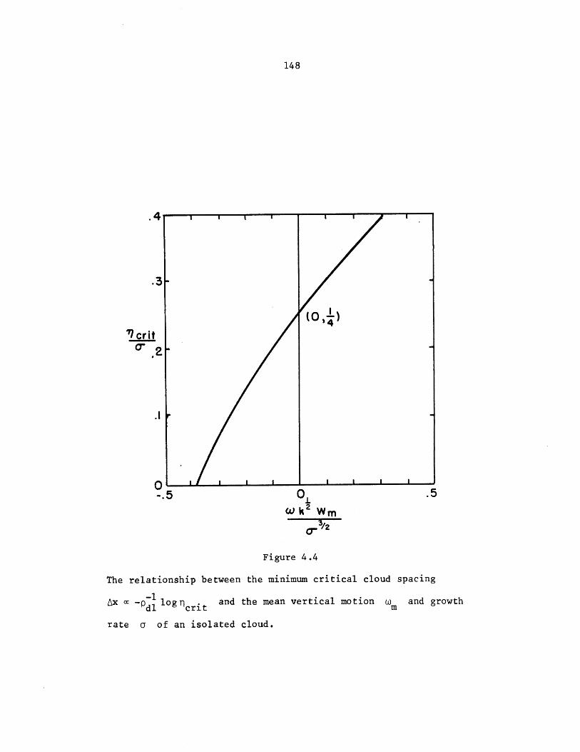
148

.4

(0,A)'9crit

0 1 I

-. 5 0.CO k 2 Wm

a /2

Figure 4.4

The relationship between the minimum critical cloud spacing

Ax a -p-1 log -n . and the mean vertical motion w and growthdl cri m

rate a of an isolated cloud.

149

4.5 Collective Disturbances of a Cloud Field

The stability theory just presented was restricted to the shortest

wavelength disturbances possible on a cloud field. It is also inter-

esting that disturbances of long wavelength compared to the cloud

spacing obey a diffusion equation whose diffusivity is positive, so long

wavelength disturbances are smoothed away, precisely when X > Ac'

In a long wavelength disturbance, the spacing X = Ax and

amplitude A = A. are slowly varying functions of x,T. From

equations (4.4.la), A(x,T) equilibrates to

(4.5.1) 2p(X)A(x,T) = p(A(x,T))

in time T = 0(1), but X itself changes on a much slower timescale

as a result of the small imbalance of the effects of its neighbors. On

this scale, (4.5.1) implicitly determines A as a function of X,

(4.5.2) A = a(X) .

Now, from (4.4.lb), omitting the argument "T" of A and X,

(4.5.3a) A(x )x. = -d(X(x.))A(x. +X(x.)) +d(X(x. -X(x.))A(x. -. (x.))

= -d(X(x ))[A(x.) +X(x.)A (x.)].3 .3 3 x.

+ [d(X(x.)) -X(x )d (x(x ))][A(x.) -X(x )A (X(x )]

+ O(X )

150

= F(X(x.)) *x (x )

where

d(x) = y11d exP{-pldX}

F(X) = -X{2da + ad }

A(x. +X(x.))xj+1 = F(X(x. +X(x ))) - (x. +x(x )) ,

T (x ) = xj+l,T~ x.J ,T

F(X)j X(xI){ x (x )}J a(X) x j x

which is a nonlinear diffusion equation 'for X = log X,

(4.5.4b) A = (k(A)x ) ,

(4.5.4c) k(k) = XF(X)

The diffusion coefficient is positive as long as F(X) > 0. From the

definition (4.5.3c) I may rewrite F using the notation o(n) for the

equilibrium value a(X) when Tn = T(M,

(4.5.5) F(X) = Xd(X){a[-d /d] - 2a }

= Xr(X)pdl{a + 2na I ,

(4.5.3b)

(4.5.3c)

Similarly

(4.5.3d)

(4.5.4a)

151

since d(X), n(X) c exp{-pdl '

F(X) > 0, I assert, is precisely equivalent to stability criterion

1 dp(ax)(4.5.6) -- < -1 at at = a(n)2 n da

for alternating disturbances. Differentiating condition (4.5.1) with

respect to TI,

(4.5.7) .aR = 2na + 2a,

so (4.5.6) implies

(4.5.8a) L- + 2-n < 0da

or since ax < 0

(4.5.8b) a (d + 2TI) = 2(2Tca + 0) > 0TI da TI

as claimed.

This is a somewhat remarkable result, since the type of instability

which would result when k(X) < 0 is an instability of cloud spacing,

while the alternating instability changes only the cloud amplitudes.

When k(X) > 0, i.e. when X > Xc across the whole cloud field, there

are no collective instabilities of the system and no propagation of con-

vective disturbances, i.e. no wave-CISK. This is physically reasonable,

since buoyancy is generated in phase with vertical motion within each

152

cloud, and there is no means of decoupling motions in the stably

stratified air outside the clouds to allow a gravity wave to grow.

153

4.6 Summary

In conclusion, it appears the only stable steady solutions of the

amplitude equations are uniformly spaced clouds of uniform amplitude

a(A) a distance X apart. If the clouds are packed more closely,

subharmonic instability causes every second cloud to grow and annihilate

its neighbors. Slow variations of convection simply diffuse away; no

wave-CISK can occur.

One may ask whether there is also an upper bound on cloud spacing.

Infinitesimal clouds can grow wherever p(O) (or wm in my model)

exceeds the damping due to the two closest clouds, which is smallest

halfway between them,

(4.6.1) -2n(X/2)a(X) + p(O) > 0 (infinitesimal).

However, finite amplitude clouds can be inserted into the cloud field

when it is more closely spaced. Clearly, if X < 2Xc such clouds will

be damped out by the subharmonic instability mechanism. But if clouds

of amplitude a(X) are introduced when X > 2Xc, a new stable equi-

librium with twice the cloud density is possible. It is quite reasonable

to consider such finite amplitude disturbances, for in the real atmo-

sphere dry convection of a heated boundary layer below cloudbase can

maintain quite strong circulations when it is not interfered with by a

nearby cloud. In the band

(finite amplitude)X < X < 2Xe c(41.6.2)

154

the cloud field is stable both to disturbances of the existing clouds

and to the introduction of new clouds. As shown in Appendix VII, the

volume average buoyancy flux <wB> is maximized for a cloud spacing

in this band slightly larger than Xc. It is nonlinearity, therefore,

which permits many clouds to coexist by limiting the strength of each

cloud and consequently the damping effect of the subsidence-induced

drying near its neighbors.

155

CHAPTER 5

Conclusion

5.1 A Synopsis

I have formulated a thermodynamically accurate but analytically

tractable model of conditional instability, obtaining solutions in the

"linear" limit of infinitesimal motions and equations for the develop-

ment of a widely spaced, weakly nonlinear field of clouds. These

which all clouds are of equal amplitude and spacing unless they are

too densely packed, in which case every second cloud is suppressed.

In chapter two I showed that if the Boussinesq approximation is

made and the saturation mixing ratio can be regarded as a linear

function of temperature and pressure over the convecting region, the

buoyancy of an air parcel can be simply written

[B B < 0

(5.1.1) B Bu = -B +B B > 0u 9, 9

The unsaturated buoyancy Bu is a scaled virtual liquid water potential

temperature, and is invariant in adiabatic motions. The liquid buoy-

ancy B91 is proportional to the amount of liquid water in the air (or

the deficit of water vapor from that required to saturate the air when

it is negative), and increases linearly with height as water condenses

156

in the adiabatic ascent of a parcel. Both B and B combine linearly

when air parcels are mixed.

If the temperature and water content of the air are specified at an

upper and lower plate, then perturbations of the two buoyancies from a

hydrostatic, purely diffusive basic state are proportional to one another

and the perturbation buoyancy is simply proportional to B ; since the

constant of proportionality depends on the sign of B9, the dependence

is nonlinear.

Lastly, a constant isotropic eddy viscosity is assumed.

In chapter three I considered the stability of infinitesimalmotions.

Remarkably, the equations are identical to those posed by Kuo (1961)

but the dependent variable is no longer the vertical velocity but the

liquid buoyancy. Thus the stability problem is identical, but the

solutions are different. Strong evaporatively driven downdrafts near

the cloud edge surround an updraft core. Away from the clouds subsi-

dence of dry air slowly decays on a lengthscale which is the minimum of

three "deformation radii"--the frictional deformation radius Rfr

Nh(h2 /

radius Rtr where 2 is the growthrate. In the atmosphere,

typically R tr = 5 -20km is the smallest; the influence of a growing

cloud is limited primarily by the finite maximum horizontal group

velocity

section 3.5, the eddy viscosity was taken to be large even in the stably

stratified air and the frictional deformation radius artifically became

the smallest.

The downwelling around each cloud dries out the air and suppresses

157

the growth of clouds, so a periodic array of clouds grows fastest when

the spacing substantially exceeds the subsidence radius. A circularly

symmetric cloud is more unstable than a slab-symmetric cloud. These

findings are well known from numerical models and accord with the

results of Lilly (1960) and Yamasaki (1972). If the eddy viscosity is

decreased to a much smaller constant value outside the cloud, the growth

rate increases and less subsidence occurs outside the cloud, but is

spread over a much wider region due to the much increased frictional

deformation radius. The abrupt change in the diffusion of horizontal

momentum causes a pressure jump across the cloud boundary.

One might ask if other solutions of the "linear" equations grow

as fast or render the clouds with vertical edges unstable (the nonlinear

expression for the buoyancy makes the question of stability meaningful).

I proved there are no growing periodically oscillating solutions or

growing travelling waves, and that the separable solutions just consi-

dered are stable to any nontrivial perturbation of their cloud boundaries.

But there are other separable solutions corresponding to clouds with

multiple updrafts separated by barely saturated downdrafts; these are a

crude response to cloudtop entrainment instability. These solutions are

unstable to perturbations which in the end transform them into the

faster growing single updraft clouds. Any initial condition evolves

toward an ever smaller number of ever stronger stationary single updraft

clouds.

The cloud spacing is nonlinearly determined. In chapter four I

explored the dynamics of a field of clouds when an individual isolated

cloud is slightly linearly unstable and a very weak mean vertical motion

158

is includedby slight horizontal variations of the temperature on the

boundaries. Any clouds which persist must not be too close to one

another, so each cloud has a structure close to that of the isolated

"linear" cloud with a slowly varying amplitude and position found from

solvability conditions determined from a very involved amplitude

expansion. The procedure is much complicated by having to match two

solutions across a moving cloud boundary whose deformation depends on

the solutions themselves. Clouds interact linearly to both damp their

neighbors and to force them to move away by cutting off their inflow

and outflow, but the nonlinear advections due to a cloud affect only

itself. A small mean upward motion causes every cloud to grow linearly

in time. A cloud is annihilated when its amplitude drops to zero. It

can be created in a region in which mean upward motion is strong enough

to allow an infinitesimal cloud to grow despite the suppressing effects

of its neighbors; the number of clouds is not fixed.

These equations have two types of equilibria--either all clouds

are of equal strength or clouds of two distinct amplitudes coexist in

an arbitrary ordering. Although a general stability analysis is

intractable, a revealing special case can be solved. If every second

cloud has equal amplitude the infinite set of equations reduces to two.

When the cloud spacing is too small, alternate clouds grow by suppressing

their neighbors. But nonlinearity limits the amplitude which clouds

can attain. When the spacing exceeds a critical distance proportional

to the subsidence radius and inversely related to the supercriticality,

clouds cannot wield a great enough influence on each other to stop the

growth of their neighbors, and a uniformly strong field of clouds is

159

stable. In this situation, there is another equilibrium, characteristic

of the second class, in which every second cloud is just strong enough

to survive against the subsidence induced by its stronger neighbors.

All non-uniform equilibria have clouds which balance on this razor edge;

I believe they are all unstable.

In general the equations nicely reproduce the features of the

nonlinear numerical simulations of Asai and Nakasuji (1982). The

minimum cloud spacing increases as the mean vertical velocity decreases,

until in sufficiently strong large-scale subsidence no convection is

possible. Unless there is mean upward motion there is no maximum

possible cloud spacing unless new clouds of finite size are introduced,

in which case they can grow if they exceed a threshold amplitude (the

razor edge mentioned in the previous paragraph) which decreases expo-

nentially with cloud spacing. The band between one and two times the

minimum spacing is stable even to these perturbations. The buoyancy

flux is maximized at a spacing in the band just above the minimum.

Lastly, I considered modulations of the cloud amplitude and spacing

on a lengthscale much larger than the spacing itself. In this case, a

nonlinear diffusion equation for the spacing can be obtained from the

evolution equations. The diffusivity is positive, and variations tend

to smooth out with time, unless the clouds are closer than the minimum

stable spacing. No wavelike modulations can propagate.

160

5.2 Limitations

The set of coupled amplitude equations I have derived provide an

interesting new view of a cloud field. They predict cloud dynamics

consistent with the much more nonlinear model of Asai and Nagasuji

(1982), while giving greater insight into the processes involved, in

particular the nonlinearly determined minimum distance between clouds

and the subharmonic instability of a more closely spaced cloud field.

Their versatility compensates for their restrictive scope. But, most

important, they provide a framework for further questions, to which I

now turn.

As a model of nonprecipitating, nonsheared convection, my equations

have two serious related deficiencies. Firstly, they do not lead to time

dependent convection, and secondly, the assumption of a uniform eddy

viscosity is rather poor.

An important drawback of replacing turbulent mixing by an eddy

viscosity is to reduce the time-dependence of the flow. In a steady

circulation the moisture and temperature fields are coupled, but

Randall and Huffman (1982) speculated that a decaying cloud may leave

behind primarily a relatively moist region which provides a favorable

environment for further clouds to grow, leading to cloud clustering.

Their argument must be applied carefully. In the model I have discussed,

the unsaturated buoyancy B and the total moisture r are linearly

proportional in the basic state and remain so regardless of the motion

or mixing of air parcels. Perturbations of Bu cannot radiate away

without precisely the same thing happening to perturbations in r.

161

But for deep, moist convection in the atmosphere this is often far

from the case. Near the surface, r drops strongly with height, but

in the cold air of the upper troposphere, r is nearly zero and cannot

further decrease. Over the whole depth, Bu increases at a nearly

constant rate with height. Mixing equal quantities of air from the

top and bottom of the troposphere produces air much moister than

undisturbed air with the same B . This may allow convection to leaveu

behind the moisture anomalies required for Randall and Huffman's

clustering mechanism to work.

There may be another effect of time-dependence, which can numeri-

cally be studied by gradually lowering the viscosity from the value at

which steady isolated clouds are marginally stable until a bifurcation

to oscillatory behavior occurs. As the viscosity is further lowered

the amplitude of the cloud updraft will oscillate increasingly violently

until, one may speculate, the cloud splits. It is possible that at

this stage isolated convection is no longer possible; bunches of

oscillating cells begin to spread outward from the formerly steady up-

draft, the width of the cell packet determined by a modulational

instability. This would provide an intriguing interpretation of the

simulation of Delden and Oerlemans (1982). In any case, the bifurcation

of the steady isolated updraft into unsteady convection seems a pro-

mising area of investigation. A vertical truncation of the equations

to sin(z) and sin(2z) modes might recreate some of the same dynamics

in a simpler model.

The assumption of a large and constant eddy viscosity casuses subsi-

dence to occur within a frictional deformation radius of the cloud. As

162

I discussed earlier, there is in reality very little turbulent mixing

except in the vicinity of clouds in a more turbulent subcloud boundary

layer generated by thermals and shear instability near the lower

boundary. The effect of this is difficult to estimate, but since it

covers a small fraction of the domain near the lower boundary, the

influence of the subcloud layer on the convective circulation is probably

small. It is the finite group velocity of gravity waves which really

limits the subsidence radius of a growing cloud. But what happens when

the cloud stops growing? The gravity wave response is quite complicated,

and becomes even more so when the upper boundary is removed. It is only

rotation that can finally corral the thermal perturbations, so the

long term effects of a region of intense convection will be felt over

a Rossby radius.

5.3 Some Extensions

The base of a convective cloud is always some distance from the

ground, and in boundary layer convection in which clouds are not very

deep, the aspect ratio is observed to be similar to that of dry con-

vection. How does the aspect ratio vary with the fraction of the depth

over which air can be saturated? Some numerical results of Asai and

Nagasuji (1982) in which they maintained the boundaries of their domain

at various relative humidities indicate that as long as conditional

instability is possible the aspect ratio of steady nonlinear convective

clouds remains approximately the same. They considered a domain which

163

was stably stratified to dry convection through its entire depth.

Typically, however, convection is induced by surface heating and a dry

convective boundary layer forms and deepens to the point where con-

densation can occur and soon thereafter the clouds rapidly deepen in

the conditionally unstable layer above. One might model this in the

spirit of Lilly as a domain in which the stability is a function of

the sign of the upward motion above a condensation level and search for

a most unstable aspect ratio.

Two physical effects that must also be understood are precipi-

tation and shear. Shear is observed to be a powerful organizing force

in the atmosphere. The prominence of cloud rows in the study of Malkus

and Riehl (1964), however, begs the following question. Is a purely

roll-like nonprecipitating moist circulation aligned along the shear

unstable to the growth of three-dimensional perturbations which grow

into cloud towers, no matter how strong the shear? Such basic states

are separable, so this stability problem is analytically tractable.

Rain is perhaps the most interesting dynamical element missing

from my model. If the stability of a purely saturated basic state in

which all liquid water falls at a constant terminal velocity is examined,

convective cells tilt and begin to propagate under certain conditions

(Emanuel, personal communication) because this allows the updrafts to

shed their load of liquid water and further weigh down the colder

return flow. This theory could be extended to a conditionally unstable

basic state, albeit only numerically, because clouds with sloping

boundaries do not correspond to separable solutions of the equations of

my model. Now the downdraft can be further cooled by evaporation if it

164

is unsaturated. Is there a preference for two-dimensional flow if rain

falls fast enough? When can cloud complexes form?

The joint effects of shear and rain can be very powerful, because

the updraft can tilt into the shear and release kinetic energy. To

summarize the interesting dynamical issues that have been brought up in

this area would require many pages.

5.2 Some Mesoscale Convective Phenomena

I will lastly comment on wave-CISK and mesoscale cellular convec-

tion, neither of which is yet on a firm theoretical footing.

A very interesting application of simplified equations describing

a cloud field is to the concept of wave-CISK, the excitation of a long-

wavelength gravity wave whose energy is derived from conditional in-

stability. Usually the mean latent heating due to the convection is

parameterized by relating it to the mean vertical motion due to the

gravity wave. For instance, Lindzen (1974) assumed that all the upward

mass flux through the top of the boundary layer occurs in cumulus

towers, so the latent heating is proportional to some vertical structure

function multiplied by the low level convergence due to the wave. A

very serious problem with simple theories of wave-CISK in an unsheared

environment is that there is no reasonable short-wave cutoff unless lag

effects which violate the scale separation are also present; waves are

predicted to grow at a rate proportional to their horizontal wavenumber.

165

tackle the problem by trying to find an analogous instability of a

field of clouds, all of which are resolved. In the model I have dis-

cussed, no "linear" instability of this type exists. This primarily

reflects several special restrictions of the model. The rigid upper

boundary does not allow the lines of constant phase of a gravity wave

to tilt away from the vertical. The large eddy viscosity artifically

damps such a wave. The latent heating of a saturated parcel is pro-

portional to its vertical velocity with the same proportionality

constant at all heights, rather than being weighted toward the warmer air

at the bottom of the domain. However, the model suggests that the para-

metrization must be carefully thought through, since the dominant effect

of a mean upward motion in the model is to moisten the environmental

air at the mid-levels of the cloud. This effect depends not on the

downward convective fluxes of air. This effect depends not on the

boundary layer convergence, but the convergence throughout the whole

lower half of the convecting region, and brings the mean vertical

velocity and the latent heat release into phase where both are strongest,

which is not conducive to the growth of a wave. One of the most exciting

applications of my approach is to understand when and if wave-CISK can

really occur.

Mesoscale cellular convection, described in the introduction, is

a pervasive feature of convection over the oceans. Satellite pictures

show the broad cells forming within outbreaks of cold arctic air over

the much warmer Gulf Stream waters of the Atlantic or the Kuroshio

current off Japan. A shallow boundary layer of convecting air, usually

1-2 km thick, forms and becomes capped by cloud as it moistens. The

166

large scale descent which typically occurs above such an outbreak and

the radiative cooling near the cloudtop encourages the growth of a

strong inversion.

Because of the superficial resemblance of open MCC to Be'nard cells,

it has usually been attributed primarily to convection, despite its

broad aspect ratio. A recent paper of Fiedler (1984) summarized the

shortcomings of these theories (none of which explicitly takes into

account the effects of moisture) in accounting for the aspect ratio.

I have shown that latent heating can broaden the aspect ratio sub-

stantially. Could this resolve the dilemma? Probably not. Open 14CC

has characteristics of moist convection--a 15-30:laspect ratio and a

fractional cloud cover which is fairly low (typically 40%, but often

less), and is associated with a convecting boundary layer, but the

cloudiness is at the edge of the polygonal cells. In dry convection

with a hexagonal planform, the vertical motion in the center of a cell

is twice as intense as the maximum along the edges (Chandrasekhar,

1961); the preference of moist convection for stronger updrafts than

downdrafts favors upward motion at the center of each hexagon. When the

cell width is much larger than the subsidence radius, this is parti-

cularly clear. A hexagonal array of nearly isolated cylindrical clouds

produces ascent in the center of each cell. A honeycomb of long roll

clouds, which have a smaller growth rate, lead to rising motion at the

edges. The circulation in cells of open MCC is thus the reverse of

that preferred by nonprecipitating moist convection. The cloud is

restricted to the upper few hundred meters of the layer, so it is

unlikely to drastically increase the most unstable aspect ratio.

167

Further, the cell width seems to be almost independent of the boundary

layer depth (Agee and Dowell, 1973), while the subsidence radius (which

determines the distance between convecting clouds) is proportional to

it. Lastly, Agee and Lomax (1978) constructed a thermodynamic profile

of an open 14CC cell from two soundings, one through a cloudy region and

one through the clear air in another cell six hours later. To the extent

this technique can be trusted, they observed that the virtual potential

temperature in the convective layer was well mixed without noticeable

mesoscale variations, suggesting that convection was working on a much

shorter lengthscale. Large horizontal buoyancy gradients were observed

in the inversion above the cell only.

Closed MCC, in which cloudy areas are surrounded by connected

regions of clear air has a planform similar to that predicted simply

by convection. However, all the other arguments against the convective

origin of open MCC apply. In addition, Agee and Rothermel (1982)

analyzed data from two flights through two adjacent closed cells, and

obtained power spectra of the fluctuations of temperature, moisture and

wind. The virtual potential temperature fluctuations were dominated by

horizontal scales of a few kilometers, as were the velocity components.

A fairly strong mesoscale fluctuation in the mixing ratio was observed

well separated from the variations in shorter length scales, suggesting

differential entrainment of the very dry air above the mixed layer. In

fact, Fiedler (1984) has shown that such entrainment could lead to an

instability with the horizontal scale of MCC, at least in a totally

cloud-capped mixed layer. Above the entrainment interface there is a

strong stable temperature stratification. Clouds which penetrate higher

168

into this stratification encounter potentially warmer air. Since the

entrainment interface consequently is more stable, they entrain less

air, and thus dry out less fast than the dips in between. Yet since the

air they entrain is warmer, they entrain more buoyancy. Differential

entrainment slowly amplifies the perturbation. A rather strong

inversion is needed to produce the instability, and it is unclear what

the effects of the partial breakup of the cloud cover would be. The

hexagonal planform and the difference between open and closed cells

remains a mystery, and a picture in Agee and Rothermel taken from

Gemini 10 of beautiful hexagons of almost entirely clear air with lines

of small cumuli around their edges suggest that a primarily cloud-

capped layer may not be necessary. But the large aspect ratio, its

relative insensitivity to the boundary layer depth, and the formative

conditions of MCC are nicely explained by this theory. It appears that

MCC cannot simply be thought of as moist convection, but involves the

more subtle interplay of convection, radiation, and entrainment which

characterize the oceanic boundary layer.

Perhaps it is now clear why one must always return to a simplistic

theoretical model. Such a model allows a clear understanding of the

effects of a single physical mechanism such as condensation. Equally

important in a complicated system are the features it does not predict.

By precisely mapping the frontiers of our knowledge, we, like Columbus,

learn where to search next, and perhaps may also stumble upon the New

World.

169

APPENDIX I

Some Thermodynamics

(A) The Buoyancy of Moist Air

My aim is to express the buoyancy

(I.1) B = -(g/p 0 )(P - Pa z))

in terms of quantities invariant in adiabatic motions of an air parcel.

In this section I write B in terms of a quantity ev, the virtual

potential temperature, which is invariant until condensation occurs,

correcting for liquid water loading.

The density of a moist air parcel can be partitioned

(1.2) p = Pd( 1 + qv + qj)

The pressure is the sum of the partial pressures of dry air and water

vapor

(1.3) P Pd + pv

= (pdRd + pvRv )T

170

In order to simplify the gas law for a mixture of water vapor and air,

the "virtual" temperature Tv is introduced,

(I.4a) p = (Pd + Pv)RdTv '

(I.4b) T = T V dV= T{l + eq , q << 1,v 1+ q v v

(I.4c) E = (Rv/R ) = 1 = (Wd/w 1 = .608 ,

where wd 29 and w v 18 are the molecular weights of dry air and

water vapor. Tv is the temperature dry air must have at the pressure

p of the mixture to have the same density as the mixture. As water

vapor is less dense than air at a given temperature and pressure,

Tv > T, but the difference is rarely more than 2*K in the atmosphere.

The virtual temperature is not an invariant, however. For an

unsaturated air parcel, the potential temperature

R /c

(1.5) 6 = T(pref/pd R (p ref = 1000 mb)

and q are invariants, so the virtual potential temperature

(1.6) 6v = e{l + eqV

is also invariant.

I can express the part of the buoyancy not due to liquid water

loading in terms of 6. In a shallow layer around the reference level

171

Z 0 , pd q ~ x0 q so from (I.1) and (1.2) B can be written

(I.7a) B = Bu - gqk *

(I.7b) Bu = o)d + pv - Pa(z)) .

From (I.4b), (1.5) and (I.6),

p( +) vP Pa (z) p - p a(z) T -T a(z) R d p -pa (z) 6 -0(I.8) d v a _ ay a = 1 +- -

Po PO T0 e po l

The reference state is absolutely dry, so T va(z) = T a(z), and adiabatic,

So eva(z) = 0a(z) = 00.

For the Boussinesq approximation to hold, motions must be slow

compared to the speed of sound in air. The relative pressure perturba-

tions from a hydrostatic state due to such motions are much smaller

than their density perturbations, so

p - p a(Z) p - p a(z) T v ~ a(z) e67 - 60(1.9) Po Po To )

and from (1.7) and (1.8)

(I.10) B =g-q .

Outside a cloud this expresses B in terms of an invariant, but inside

6v and q are not invariant and must be expressed in terms of

invariants.

172

(B) An Invariant 69 for Moist Air

I will

v outside

capacities

The entropy

partitioned

(1.11)

now develop a linearly mixing invariant which reduces to

a cloud. Neglect the very weak dependence of the heat

Cpd of dry air and C of liquid water on temperature.

S of a parcel (per unit mass of dry air therein) can be

S = Sd + Svqv + S Zq2

The entropy Sd of dry air is

(1.12) Sd = Cpd in T - Rd ln pd '

where Pd is the partial pressure of dry air in the mixture. The

entropy S of the liquid water is

(I.13) S = C ln T .

From the Clausius-Clapeyron equation, if Lv is the latent heat of

vaporization,

S - S = L /T .v 9, v

substituting into (I.11),

(I1.14)

173

(I.15a) S = C MnT - R Inp + (q L /T)pm dlnd vv

(I.15b) Cpm = Cpm + rC

Except for neglect of the slight temperature variation of Cpd and C.,

this is exact and allows the construct of an exact invariant temperature

e = exp{S/C }.

However, I will instead use an approximate, but more convenient

invariant. Since C depends on the water content of a fluid parcel,pm

it is desirable to elininate it in favor of a fixed constant. Since r

is small (r < .02 typically), C z Cpd to a fair approximation.

However, the systematic error this produces can be partially balanced by

replacing ln T by ln Tv'

(1.16) S ~ C lnT - R lnp + (q L /T)pd v d d v v

z C lne + (q L /T) .pd v v v

Since qv << 1, in a shallow layer around z it is a good approxima-

tion to take q L /T ~ q L /T . I eliminate q in favor of q andv v v vo o v

define the liquid water virtual potential temperature

(1.17) evt = exp{(S/Cpd) - (L o/CpdT)r}

= v exp{-(L o/Cpd oql ,

ev :: 8v & *(I. 18a)

174

(I.18b) y = OL / Cf T 0

Within the shallow layer approximation, 6% is a function of the

invariants S and r, so is itself invariant. Outside a cloud vi

equals the virtual potential temperature 6v, but inside it is reduced

because of the energy required to evaporate the liquid water. 6vz is

also nearly linearly mixing. To understand this take any two parcels

of air at some pressure p1 . Instead of mixing them at that pressure,

reversibly lower them to a pressure p2 at which neither parcel is

saturated. Since the enthalpy H = C T (z C pdTv by our earlier

approximation) is linearly mixing, Tv, and thus 6vi = av, is approxi-

mately linearly mixing in the unsaturated air. Now move the mixed parcel

back to its original pressure adiabatically, leaving 6vt invariant.

The result is the same as if the parcels had been mixed at pressure p2'

so 6vz is linearly mixing even if either one or both parcels are

saturated.

175

APPENDIX II

The Mean Fields in the Absence of Convection

If mean vertical motions are forced by slow small variations of

the temperature at the boundaries

(II.la)

(II.lb)

Bum(X,z) = 1l/2e(x)

Bk(Xz) = 0 , (saturated boundaries)

(II.lc) X = y x

then the equations of motion (4.2.10) reduce to

2 2 2~ ~(z + a $)m + yB

2 2-~~(@z + IX)B + y$ mX

2 2 ~ 2-z+ X)B - Ndimx

J($m'V 2m

= J($m' & '

mJ(imB ) .J m 9Burn

These have the solution

(II.3a) Bum(X,z) = Pl/M + P 3/2B um3(X,z) + 0(p2 )

(II.2a)

(II.2b)

(II.2c)

(II.3b) Bm(Xz) =

$m(Xz) =(II.3c)

where, since F = N2 + N =c d

(II.4a)

(II.4b)

(II.4c)

176

3/2B9m3 (X,z) + O(p2 )

ym2 (X,z) + 0(y2 )

p + F,

4,-z m2

2-zB m

+ x = 0 ,

+ rom2X = 0 ,

B - 2 -3 m N d~m2X =-

Using the boundary conditions

$m(Xtz) = $mzz (X,z) = BZu (X,z) = 0 at z = 0,T ,

I find from (II.4a) that

$m2 = -6X Sl(z)

S (z) = (c2 _ 22 - 5p2)

C =z - (/2) ,

p = 'r/2 .

(II.5)

(II.6a)

(II.6b)

(II.6c)

(II.6d)

177

From (II.4bc)

=I OgS2(z),B 93 N 0um3 Nd

where

b) S2(z) = - C6 - 15C4p2 + 75C2p -

I will require the Fourier expansions of S 1 (z)

61p 6

and S2(z)

(II.8a) S1 (z) = $1n sinnzn=l

(II.8b) S2 (z) = I 2n sinnzn=1

Rather than computing the Fourier coefficients directly from the

expressions (II.6b) and (II.

(II.9a) d4 S/dz4 = 1

(II.9b) d6S 2 /dz6 = -

7b), I note that by construction,

S1 = d2S1/dz2 = 0 at z = 0,,

2 = d2 S2 /dz2 = d4 S2 /dz

4 = 0 at z = 0,T.

Integrating by parts,

S n i 1 S (z) sin nz dz

2

- 4 S lzzzzTrn 0

sin nz dz ,

(II.7a)

(11.7

178

0 n even(II.10a) Sln = 14/n5 n odd

Similarly

0 n even

(II.10b) S2n =4/Tmn n odd

Thus, to a very good approximation (1% for S (z) and .1% for S 2(z)),

1 2 T(II.ll) Si z S2 (z) ~ sin z

The mean velocity, from (II.6a),

4(II.12a) X = e (dS /dz) ~ --cos z

(I.12b) = P3/2 Z P3/2m XX XX iT

is an inflow at low levels and an outflow at high levels from a region

of boundary heating, where there is a weak upward motion which produces

a liquid water maximum,

3/2 3/2 04.~(II.12c) Bm = ~O eXX S2 ~ r OP e - sinz z owm

This source of liquid water is the most important effect of the mean

flow on the convection. The relationship is exact for the

sin(z) component of (II.12c), which I denote by carats:

B2 m3(XT) = o m3(XT)(II.12d)

179

APPENDIX III

Product Formulas

I derive in this appendix identities which allow products of

characteristic functions to be simplified. In the cloudy air, if

and q are nonzero,

fc(x,p)

gc(xP)

f c(xp)f c(x,q)

= cosh px ,

= sinh px/p

= cosh px cosh qx

1'{f (x,p+qI) + f (x,p-q)}2 2c

= 1 cosh px sinh qxq

= p c pq - p c*-q=-g (x,p+q) -231g (x,p-q)2q c 2q c

=- sinh px sinh qxpq

- {f (x,p+q) - f (x,p-q)}2pq c c

p or q is zero, one simply takes the limits of the formulas

(III.la)

(III.lb)

(III.2a)

(III.2b)

(III.2c)

If either

above:

f C(x,p)fc (x,q)

180

(III.3a)

(III.3b)

(1II.4a)

(III.4b)

(III.4c)

(III.4d)

In the dry

(111.5)

(III.6a)

(III.6b)

(III.6c)

f c(x,0) = 1{g

S(xO) = x (p

c (XP)fc (x,O) = f c(xp)

f (XP)g~ (x,O) = a{g(x,p)},

9C (xP)f~ (x~p) = g (xop)

(xP)gc XO = p 3(xp)

air

fd(x'p) = dPgd(xtp) = exp{-p(jx - /2)}

f d(X,P)f d(x~q) f d (x~p+q)

f (X,P)g (x~q) q 9d~ g(x~p+q)fd d(d

fd ~ q dl fd xp

gd XP~ d qd

The case that p or q is zero never appears in the calculation and

will not be considered.

181

APPENDIX IV

Inverting the "Linear" Operator

I will repeatedly be forced to find particular solutions of inhomo-

geneous equations

4 2$- (N2/F)Bj = RI(x)

m o0 E

7 B + r 4 = R 2m 1 0 2'

72 = (d2/dx2 - m2

m

and N can be either -N2 or N 2, depending on whether |xj > a /2,o co Nd, deedn0li a

the cloud boundary for the neutral isolated linear mode. In general,

the inhomogeneities will be sums of terms

R 1(x) = R g(xp)

R2(W = 2f(xp)

For this choice of R and R2, there is an inhomogeneous solution

(IV .la)

(IV. lb)

where

(IV.lc)

(IV. 2a)

(IV.2b)

182

$ = Q 8[m1g(xp)]

B = QEm 2f(x3p)]

2 2 2 2ml R1 (p -m ) + R2 -Np /

=-1' +R 2 2M2 ~ 1 0 + R 2( - m ) ,

and the operator Q, is defined

F(p)

Q F(p) = I dF/dp(IV.3e)

(IV.3f)

if pm(p) # 0

2n 2)3 + N 2

p m(p) = (p - m 2) 3 + N p ..P

This can easily be verified by direct substitution for pm(p) A 0,

after recalling

(IV.4a)

(INT.4b)

(xp) = P2 f(x

3x2

(xf )= P2 g(xP)x

f(x,P) = T~g(x,p).(IV.4c)

(IV.3a)

(IV.3b)

where

(IV.3c)

(IV.3d)

183

Suppose pn(o) = 0. Then

g(x,p0 )(IV.5a) h = M (p ) ,

(IV.5b) B = m2 (ph 2o p m (P

solves the homogeneous equation (IV.1) for any p in the neighborhood

of p0 and may be subtracted from the inhomogeneous solution already

found. Taking the limit p -+ po, I find an inhomogeneous solution by

l'Hopital's rule:

m 1g(xP) -m 1(PO)g(x,p0 )(IV.6a) =lim = Q m g(x, po)

m m2 f(xp) -m 2 (p )f(xp 0 )(IV.6b) B = lim = Qm 2 f(x' 0 )

which is exactly as claimed in (IV.3e).

In fact, I will also need to evaluate derivatives of $ and B

with respect to x, so I will have to calculate

(IV.7) Qn+l x,p) = (gn/an)Q 1F(x~P).

when F(x,p) = f(x,p) or g(x,p). This can be done quite neatly by

noting that since Q1 depends on p alone, it commutes with 9/3x.

This allows one to conclude

(IV.8a) n n(x) ~ Q m g(xp)

9x n n+ll

184

nB k(x,p)

3Xn ~ Qn 1m 2

(IV.9a) Qn+1 (xp)

(IV.9b) Q n+1 '~gp

n g (x, p)

PM_P gf(x,p)

[npn-1 n ]g(x,p)

pm dp (n-1)p n-2 n-l ]f(x,p)

pnf(x,P)

M(I n+g(x,p)

[npn-l n ]f xp):n p +

m [(n+1)pn+p n+19 ]gx,p)

To explicitly compute these derivatives I recollect from (3.2.20) and

(3.2.23) that in the cloudy air

(IV.10a) f c(x,p) = cosh px,

(IV.l0b) g (xP) = sinh pxc 'p

3 = x sinh px

3gc x cosh px sinh px30 p 2

or if p = 0,

(IV.8b)

where

n even

n odd

n even

n odd

n even

n odd

n even

n odd

p (p) #0

p (p) =0

p (p)#0

p (p) =0m

185

(IV.10c) f (x,0) = 1 ,

(IV.10d) c (x,O) = x

while in the "dry", i.e. unsaturated, air

a 3f a a(IV.lla) fd(x p) exp{-p(x- -)} f- = _(x--f) exp{-p(x--2)}

aa 1g xa-0

(IV.llb) gd p2exp-P(x - 01- -, } -

It is also convenient to define the simpler operator

n n(IV.12) Dn+1 F(x) (d /dx )F(x)

The effect of applying Dn+l to g(x,p) and f(x,p) is

png(x,p) n even

(IV.13a) D n+lg(xp) = n-l

p f(x,p) n odd

p nf(x,p) n even

(IV.13b) D n+1f(xp) = 1n~l n+lp g(x,p) n odd

Lastly, it is necessary to add homogeneous solutions to the

inhomogeneous solutions (IV.3a,b) to satisfy appropriate matching

conditions at x = ± a /2. The most general homogeneous solution of

(IV.la,b) which decays as x - ±co and for which B (x) is symmetric

about x = 0 is

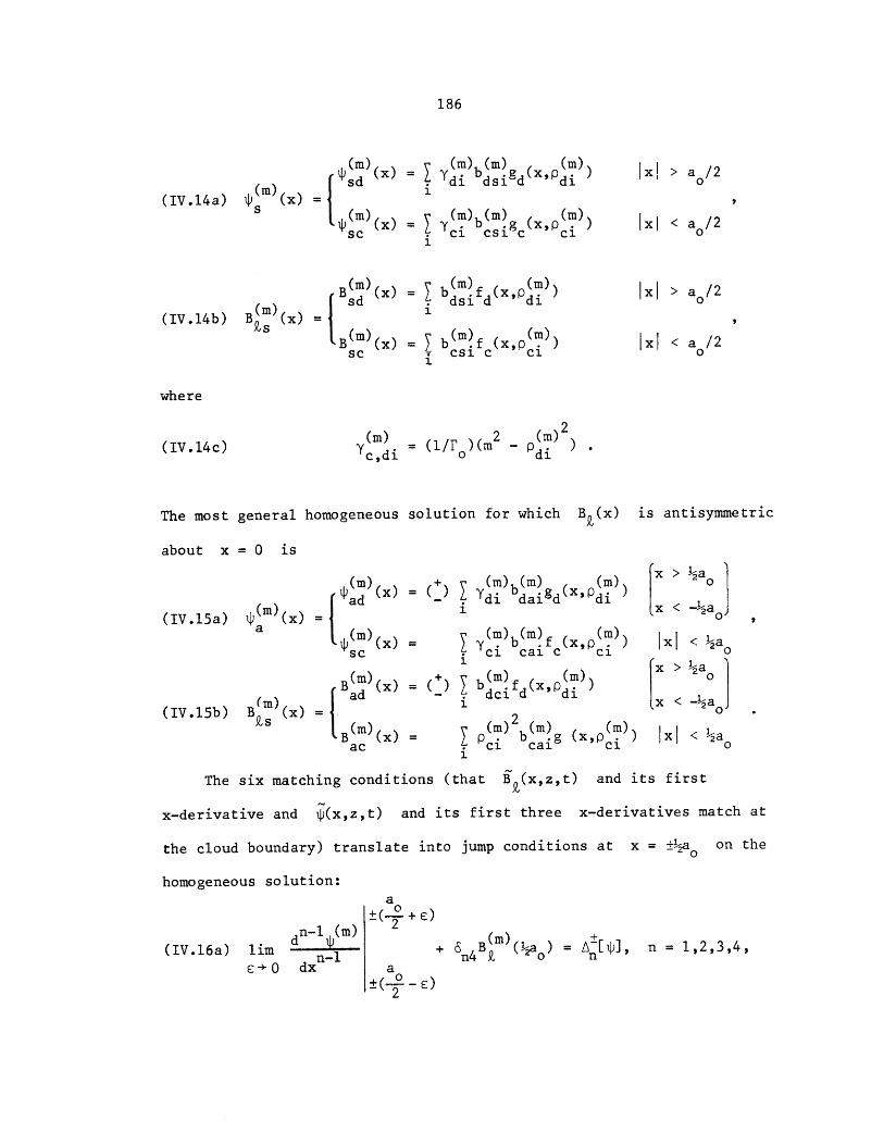
186

(W)

(IV.14a) $ (x)

(B (x)sc

(IV.14b) B~ (x) =

s BW(se

(m y)b~gxp)

y W b W g (x,p ()

= b d (x,p )

di di ddi

= b f (x,p ()csi C ci

fx1 > a /2

Ix! < a 0 /2

lxi > a0 /2

lx! < a /2

where

= (1/l~')(m2 _ )2

homogeneous solution for which B (x) is antisymmetric

(m) + (m) W (m) (m) x > 12a0$ad -di bdaigd di

(IV.15a) B (x) = 2 0

a 2 g)() = (x,p ) x < -a

sc Cl cai c Ci0

(in)W + bmf (in)) W o

(IV.15b) B (in) t ad =c d di {x < -.1 a 0

Zs(X (BWin)W b(in) g(xp~)P W lxi < 1 aac ci ci ci0

The six matching conditions (that I P(x,z,t) and its first

x-derivative and $(x,z,t) and its first three x-derivatives match at

the cloud boundary) translate into jump conditions at x = ±,a on the

homogeneous solution:a

( +)n-1 (in) 2

(IV.16a) lim d n-1C+0 dx a

+ n4B W(-,a) = A [$], n = 1,2,3,4,

(IV.14c) Ycdi

The most

about x

general

= 0 is

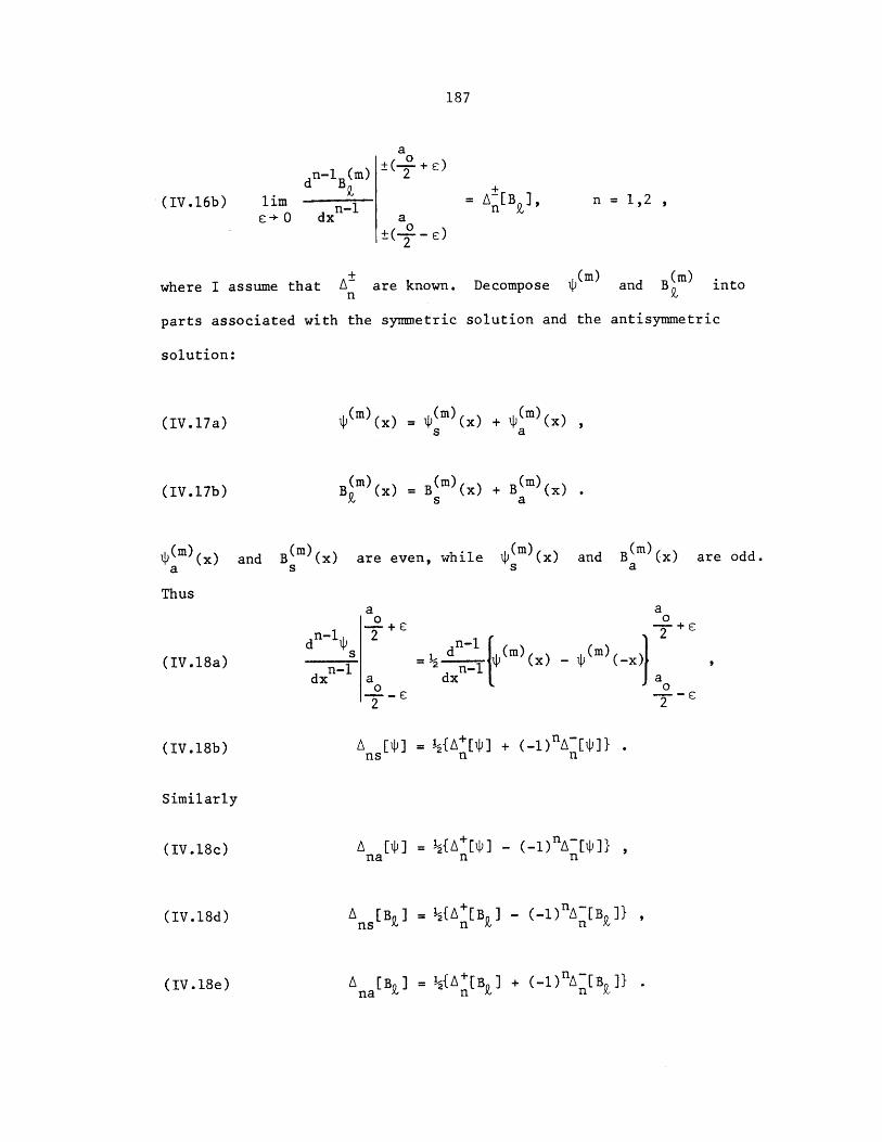
187

dn-iB

(IV.16b) limC+ 0

a( +

a

= A~[B ], n = 1,2 ,

+ (in) (in) .where I assume that A are known. Decompose $' and B into

nz

parts associated with the symmetric solution and the antisymmetric

solution:

(in) (in) (in)(IV.17a) M (x) = 4s (x) + $a ()

(IV.17b) B ( (x) = B (x) + B (x) .z a

$) (x) and B (x)a T

Thus

(IV.18a)

(IV.18b)

Similarly

(IV.18c)

(IV.18d)

are even, while M (x) and B (x)s a

n-1id $s

a0

a0

dn-l () -

=2 n-ldxa

A [$] = fAA[9] + (-1)nA~[4 .ns n n

A [$] = A+n - [*]na n n

A [B] = {A [B ] - (-1)nA [B ]}

Ana[B,] = {A+[B9,] + (-1)nA[B ]}.(IV.18e)

are odd.

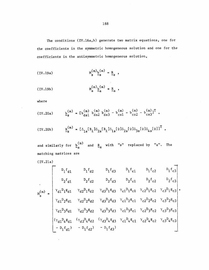
188

The conditions (IV.16a,b) generate two matrix equations, one for

the coefficients in the symmetric homogeneous solution and one for the

coefficients in the antisymmetric homogeneous solution,

M(m)b (M)= R

M b - Ra -a -a

b(m) - [b m) b(M) b(m) - b(m) - b(m) - b(m) ]T-s dsl ds2 ds3 csi cs2 cs3

R ( ) = [A [B ]A [B ]A 2s 3N T

-s is Z~ 2s Z. is 2s 3s 4s

and similarly for

matching matrices

(IV.21a)

M(m)s

DifdD1 dl

D2 ldl

dl D2dl

d1D32dl

Ydl D43dl

- D If dl)

b (i)-a and R with "s" replaced by "a". The

are

D fd2

D2 d2

d2D gd 2

'd2 D29d2

Yd2 D39d2

(dZ 4 d2

- D 1f d2)

D1 fd3

D2 d3

Yd3 D ld3

Yd3D22d3

-d3D3d 3

Yd3 D4gd3

- D 1f d3)

D fcl

D2 cl

YclD2 cl

YclD 3cl

Ycl D49cl

D1 fc2

D2 c2

Yc2 D gc2

Yc2 D2gc2

Yc2D3c2

Yc2D49c2

D1 c3

D2 c3

Yc3 1 lc3

yc3D2 gc3

Yc3 D 3gc3

Yc3 D49c3

(IV.19a)

(IV. 19b)

where

(IV. 20a)

(IV. 20b)

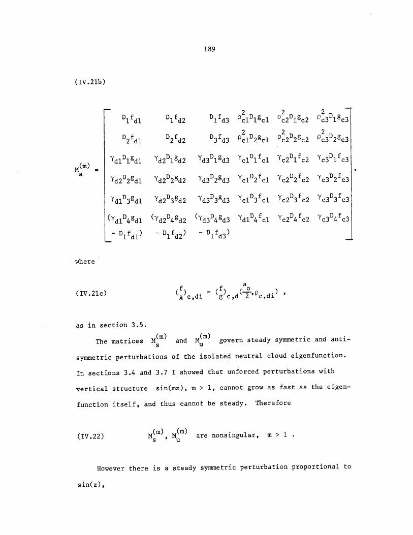
189

(IV.21b)

D1 fdl

2 dl

Ydl D gdl

Yd2 D2gdl

Ydl D39dl

(Yd 1D4 gdl

- D fdl)

D1 fd2

D2 d2

Yd2 D gd2

Yd2 D2gd2

'd2 D39d2

(Yd 2D4 d2

- DIfd2 )

D1 d3

D3 d3

'd 3 D1gd 3

Yd3D22d3

Yd3 D3gd3

(Yd3D4 gd3

-1 fd3

2OClicl

2OclD2cl

ycl Dfcl

YclD 2 fcl

YclD3f cl

dl D4 fcl

2c2Dlgc2

2Pc2 2gc2

Yc2Di fc2

c2D2 fc2

Yc2D3 fc2

c2D4 c2

2

c3D gc3

2Sc3D29c3

c3 Dfc3

Yc3D2f c3

c3 D3f c3

Yc3D4 f c3

f f a0g c,di g c,d '9c,di(IV.21c)

as in section 3.5.

The matrices M and M govern steady symmetric and anti-s U

symmetric perturbations of the isolated neutral cloud eigenfunction.

In sections 3.4 and 3.7 I showed that unforced perturbations with

vertical structure sin(mz), m > 1, cannot grow as fast as the eigen-

function itself, and thus cannot be steady. Therefore

(IV.22) M , M are nonsingular, m > 1s u

However there is a steady symmetric perturbation proportional to

sin(z),

M(m)a

where

190

(IV.23a) b) = [b b b - b - b -b ]T-so dl d2 d3 cl c2 c3

which represents a slight change in amplitude of the eigenmode, so

(1) (1)(IV.23b) M1 b = 0

s so

A slight translation of the eigenmode produces a steady antisymmetric

perturbation

(IV.24a) i)-ao

= [Pdlbdl ~ Pd2bd2 d3 bd3 - bel - bc 2 - bc3 '

corresponding to the representation of dL/dx in the basis of charac-

teristic functions, for which

(IV.24b) M b1) = 0a so

The right hand sides R-Sand R must be orthogonal to the null

-a

vectors of the adjoint matrices, which are computed in appendix VI:

(1)T(IV.25a) u -R = 0, M u = 0.-s -s s -s

u - R = 0,-a -a

( 1 )TM ua -a(IV. 25b) = 0 .

191

APPENDIX V

The 0(y3/2) Inhomogeneous Solutions

I calculate the four sets of inhomogeneous terms (4.3.18-21) due

to nonlinearity, time dependence, supercriticality, and the mean fields,

and for each set I find a particular solution to the equations (4.3.17)

in the cloudy and the dry air. To the sum of these solutions I add a

homogeneous solution in the dry air which accounts .for the growing

exponential behavior at large x due to neighboring clouds.

Nonlinear Self Interaction Terms

From (4.3.18),

(V.la) ll = J(A $ (x) sinz,A jV22(x) sin 2z)

+ ^T(A ? 2(x) sin 2z,A V 1 (x) sin z)

3= A [J31 9+ 32 j

2 2(V.lb) J3 1 xx = 1xl2 2 sin z 2 cos 2z -l 7 2 2x cos z sin 2z

x 2 1 2

( )lxv2 2 sinl 2 $s

2 2(V.lc) j3 2(x-xj) =i 2 1 'sn2 2z cos z -2 cos 2z sin z

2 1 2-'22x~l 1 + xP2V 1 l

192

while

R = J(A $ (x) sin z,A B2 (x) sin 2x)

+ J(A $ 2 (x) sin 2z,A B1 (x) sin z)

= A.[J (x) + J (x)]J33 34

J 3 (x-x.)4-lx B 2--W1B2

(V.2c) J3 4 (x-x ) = 2x B 1 + $2Blx '

Using the explicit formulas (4.2.18) and (4.3.7-8) to expand the

and B's,

(V.3) J31(x) =k

b f(xq -y(2) b(2)(- (2) )gxp(2)ckbck c ck ci ci o ci ci

+ 1$ (ci +cj i c +cj

+ $ j (p c-i ~ )2g (xQ -Q j22 i cj c ci C]

- yckbckc ck C b i Ci c Ci

+ (i~j) (P)2f l ++t (pcci+P cj 2c 'ci pcj1,3Ji C i C

+ pi(i~)( c j ) 2 ( xp -c .)]22c c cj c ci c3

= 7 (2) b b (2 )[f C(XP k)g( (2)

+=I 'oyckyc bckb [fc ek Scik

+ ,, (X, )f XP(2)+gc ck c ci

(V. 2a)

(V.2b)

Is

193

+

i,j,k

+

i,j,k

ck ci cj 21c ck c ck c ci ej

-g (x'Pck )f '(xpci pcj

ck ci cj 22 ck c ck c ci cj

c 'Ock c 'Oci cj

Simplifying the products using appendix III, in the cloudy air

(V.4a) J3 1 (x) =1c i,k

+

,vjk

+

,i ,k

(1) (2) (1) ((2))1{cik+ 'ck c )+ ik-c ck ci

g (1) (xp (1)ijk+ c ck ci cj +dijk-gc 'Ock~ ci~ cj

{e (1) )+e{ijk+gc 'opck+pciPcj) +eijk- gc 'Ock~0ci ej 't

where

(V.4b)(1) - c (2)ik± 2 ck ci

1 1 (2)2 b (2)(2) + 2pck ckyci obckbcici

(V.4c) d+ ci 1 l 1(.c diik- ck ci+ cj p .+p .2p

Ici Ocj cki

(v.4d) e = (pck[ci cj di dj

12p dkJ

Yck(~i+P 2 )(i~j)bci cj 21c ck

ck ci~ cj 2 j bck

(= 0 if i = j)

In the dry air, analogous manipulations show

(1l) (P+P(2) )(V.5a) J3ld(x) . kdd dk di)i~j

(1)dijkd d dk di dj

i,3,k

194

c(1) (2p p ) 1 1 (22 b2ikd dk di (2) + 2pdk odkdi dkbdi

di

(V-5c) d (1) =( +p+(V.5c) d dk di dj1

pdi +p dj

1 2 (idj)~2padk Idk di dj 21d bk

Next,

(V.6a) J3 2(X) = h 'ckYck(- y )g (x,Qk " (2 ) yb(f (x,p.(2(.a J32c k ckbck 0 ek Ac ck)] yi b fc

+ I ij (x,p +p)+ 9 {$ c fc ci cj

1i,]

+ *(ii fp'1 (x p .+P .

+ 2 c ci cj

+ [ y (- y f~xp y(2) b(2) 9 Xp(2)

+ [ cb oe c(i~Q bci c) ci

+ ge ' ci cj+ 2 $ c 'ci~cj

= (2) g(x p (2))

ik ik+ c ck ci(2) (2)

+ik- c 'ck ci

(2)ijk+ c ck ci cj

(2) P + -P *)+ k{eijk+ c 'ck ci

i,3,k

d2)+ ijk- c 'ck~c ~ j

(2)+eijk-c 'ck~ci cj

(2) (2) 1 2 (2) (2)cik± ck cij(2) 2pcko ck ci ck ci

(V.5b)

where

(V. 6b)

195

(V.6c) d (2)dijk+ = (pck±[P ci +P1

p .+p .ci cj

1 r2 4( i 9j)b2p ko ck 21cbck

(V.6d) e (2) Pck±[Pc 1)4(2)- -(V.6d) eikk ci cj +1 1

ci cj~ CI ckJ2 (ij) ko ck 22c bck'

(= 0, i = j)

The last term vanishes when i = j since 'D22c - 0. In the dry air

(V.7a) J 32d(x) =

(V.7b)

(2) ( 1) +cikdgd 'dk di +

i,k

I I )d i

i,j,kijkdgd dk di dj

1 2 (2) b b (2)+ 2pdk o dk di dk di

(V.7c) (2)dijkd = (pdk+pdi+pdj I

1 1 F 2 (ij)b

pdi pdj 2p dkJ o dk 21d dk

The advection term reduces in the cloudy air to

(V.8a) J b b(2) f XP(2)(V.8a) J3 3c(x) Yckbckfc(x'Pck)][ bei c 'ci

k 1

+ f B(i~J)f (xlp .p .t.J 21c c ci+ cj

+ B ( i~)f (X *-Q M)22c c ci cj

Y(2) (2)

Y ckbckc 'ck)] bci ci

+ {B

J 21c(pci+cj 2 c 'ci cj

+ B i (pi -P )2g (xP -p .)}]22c ci cj c ci cj

c(2) ( +p(2)cikd dk di

9 xp(2)Sc c i

196

Y Y ,bb(2)[-f(X f (2)

ik ck ck ci c ck c ci

(2)2 (2):- 4ci gc ock gc ci

+ ck ck 21c [fc 'ck c 'Pci+cji,j ,k

- (Pci+ cj)2 c 'ck c 'ci+cj

+ 22 b ii[f (xo )fk (xqp .p .+ yckbckB [c ck 'ci

i, ),k

ci j2c 'c c 'c~c

(3) (2) (3)

ik ik+ c ck ci ik-

+ {d (3) f (x,Pck+Q p~ *+ qq {dk fc 'ck ci+Pcj)ij,k ci

+ {ejkf c ',Pck+pci~cj)

((2)c ck~ ci

+d Mf (x,p -P .-P )ijk c ck ci cj

+ e _3)_f ' c 0le.kf xPkP .i+Qc

(V.8b)(3)C ik±

(3)(V.8c) di jk

(V.8d) e (k±

In the dry air,

(2)ci(2 (2)

= -4(1 Yckbcb ,~ck

-i yc B(i"j)2p ck ckbck 21c

= - (1 ± 2c cj cbck(even if i = j).

where

197

(V.9a) J33d =i,k

( 3) f(2)ikd d 'dk di )

( p3)f+pijkd d ',dk di dj

(V.9b) (3)c ikd

(V.9c) d jid

di y (2)2p dk dk didk

=di p d dj b (ij)= ~ 2 -1+ 2dk )dkbdkB21d

Lastly,

(V.10a) J (x) = [ b (XP ck ( b fXp (2)34c kc k c ic ci

+ I{ JtUi DfC(xvpdp *) + $ (x,p M .}+ .2lc c ci+pcj + 2c c ci~ cj

i,j

+ [ Ik

12

bck ckgS * ck)](2) (2)Pcb ig(xtpci

+ l { isl' g (X~p~+~

+ { $ c ',ci3c j

(4) (2) (4) (2){cik+c 'ck+Pci ) +cik- fc ckPci)I

i,k

f(4) f xpc~{diik+ c 'ck ci+pcj)

(4)+dik f (x'ijk-c ck~ ci~cj)

(4) (4){eijk+ c 'ck ci~c) +eijk- f (x'pijk+C c c pi-CJ ijk- c ck-c oj

(V.10b) c

(V.10c) d..k

S( ±ck (2) (2) b(2) ci bci ck

Pci

_ ck )14iU jb

p A-p .)$ bckci C

+

1, ,k

+1,3 ,k

where

+ 2 c c 'ci~0cj

198

(4) Pck (it')(V.10d) eijk + .cipcj 22c bck O i = j)

The last term vanishes when i = j since $ = 0. In the dry air,~22c

(V.lla) i c(4) (2) + d (4)34d cikdfd(Pdk+pdi + ijkd d dkpdipdj

3 ,k i,j,k

(4) (1 + dk (2) (2)ikd (2) di di dk

Odi

(V.llc) d =( + dk (ij)bijkd p di2j +p 22d dk

Using appendix IV I can find inhomogeneous solutions to (4.3.17)

which produce the inhomogeneous terms R and R2, now that they are

written as sums of characteristic functions:

Li(n) (n) 3(V.12) I (x,T) =($ (x - x.)A.

3 3 1 J

For each term in the double sums in the Jacobian, I replace

(1) (2)(V.13a) R + c + cik

1 ik± ik±

(V.13b) R c ik±+ c ik

to find the inhomogeneous solution generated by that term in the cloudy

air, and similarly for the triple sums. The result is

199

(n)(V.14) 3c W

-(1) (2)+ cik-Q18c 'pck~0ciI ( ) (2)

ikcik+ l9c ('P ckPci )

+ A~(1) c

+ ik kijk+ c ck ci+ cj

iIJk ijk+c (xpck +pci-pcj)

^(1)" d. C' g(xQ-P. )

ijk- c ck~ci~4cj

Se(1)+ e gc 'ck~0ci+Pcj

B (x) can be written in the same form if superscripts (1) are replaced3c

by (1) and "g" is repleced by f. Q is an operator defined in (IV.3e)

and c 2) are the m and m2 defined in (IV.3c,d) for the choice

of R's above, and likewise for the other coefficients. These remarks

(n)apply in the dry air also, where 'P3 (x) has the simpler form

(n)(V.5) 3d

^(1) (2)c ikdQlgd 'Opdk +Pdi

^ (1)Q 1 dijkdgd '0pdk +Pdi dj 'j

i,k

Terms due to Slow Variations

From (4.3.19),

2 R12 x. 2R12 A. V 14 1 JJTVlplx

R 2=2 A jFB H(x) -A ix .TB 91l

In the cloudy air,

V 2 = Eck gc ' ckk

(V.16a)

(V.16b)

(V.17a)

200

(V.17b) Bl= 1 bk cf'(xock)k

2(V.17c) eck o ckbck

Replacing "c" by "d", the same holds in the dry air.

Inhomogeneous solutions are found precisely as described in the

previous section by replacing R1 + ck and R2 + bck for each k.

Using the carat notation again,

(t) ~(t) ~x(V.18a) $ (x,T) = A. $ (x) - A.x. $W (x)3 jT 3 3 jT 3

-(t) -(1(V.18b) $3c (x) ck 1c'ck )

k

(V.18c) B(t) (x) = 2 ( Q fc 'Ock '3ck ck1c

x (t)-(x) (t)(V.18d) $ x) d$i /dx ; B = (d/dx)B ,

3c 3c 3c 3c

and similarly in the dry air (the superscripts are "t" for time-

dependent, "x" for x-translation).

Terms due to Supercriticality

From (4.3.20), since

(V.19a) N -N2 _c co

201

2 2d do'

rF N + N 2= r + y,I'= +d 0 11

-' 2R =-(Ndo /0)A B (x)

R2 3 =-A $i.(x)

In the cloudy air

-(Ndo/ro)B (x-x.) = ck g(xPk

S(-x ) = Yckbck f ck'k

Jck =-(Ndo ock k

and likewise in the dry air with "c" and "d" interchanged except in

Ndo. With R 1 ack and R2 Yckbck for each k, a solution is found

from appendix IV again:

(V.22a) U (x, ) = A (3)3J 3

(g) ^(1)(V.22b) $3c ( = Q l1Fck fc (XPck

k

(V.19b)

(V.19c)

(V. 19d)

(V.20b)

(V.21a)

(V.21b)

(V.21c)

202

(V.22c)(g) ^ (2)B3c (1) ack f c(X9Pck *

k

and similarly in the dry air (superscript "g" is for growth-inducing).

Terms due to Mean Field Interactions

From appendix II,

(V.23) m2 =-e [ sin sin nz].n odd

From (4.3.21), since $m2 is not a function of the short horizontal

scale x

2(V.24) R 4 = '-A JX lx sin z $m2zzz 1 lx sin z $m3z

3 2= .-A jx [-n $lx - n $I ]in sin z cos nz

n odd

=0,

so this inhomogeneity is illusory.

The Boundary Conditions at Large x

To take care of the exponential growth mandated by the boundary

conditions (4.3.22), I recall that the asymptotic form of $ 1(x) for

large jxj is dominated by its slowest decaying characteristic function,

203

$1(x) Ydlbdlgd dl

= ydlbdl exp d(x - a /2)]

exp(p dl [x j+1

~ IC Aj+ld j dl x. << x < Xj1J +

and similarly,

x < x j-13 ej-1A g1d j dl

j = bdl xp dl a )

(V.26d) C = 1J l exP[-dl(x j+lxj)]

These boundary conditions can be satisfied by a homogeneous solution

(V.27a) (x-x ){Aj+1 j + c_} + (0) (x-x ){A j

(V.27b) 3(x=)t '~g(x-Qdl) both right and left of the cloud

0 inside the cloud

(V.25)

Thus

(V.26a) + a9])

(V.26b)

where

(V.26c)

~ A j+1 dl bdl '

204

-I, g d d

(V.27c) $3) (x'd dl)

L 0

right of the cloud

left of the cloud

inside the cloud

A complete inhomogeneous solution is the sum of all of these

solutions

(V.28) $ (x,T)= ) (x-x.)A3 + $(t) (x-x.)A. T+ $ (x-x.)A.x.'3 33 3 3 JT 3 j j JT

u(g) +u {e)+ $)3) (x-x)A + $3 {Aj1

V(o) A C A C-

+ $3 {Aj 1 j - A. C } ;

however, this solution does not satisfy the matching condition across

the cloud boundaries. This solution is symmetric about the cloud

center x = x. except for the terms proportional to A.x. and3 3 3T

A +1C - Aj_,%j_ which are antisymmetric in their effects.

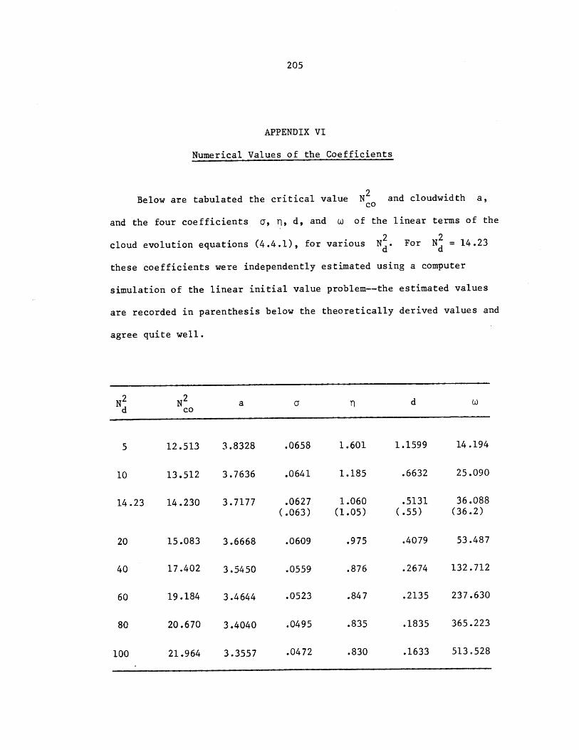
205

APPENDIX VI

Numerical Values of the Coefficients

2Below are tabulated the critical value N and cloudwidth a,

co

and the four coefficients a, q, d, and w of the linear terms of the

2 2cloud evolution equations (4.4.1), for various N. For Nd = 14.23

these coefficients were independently estimated using a computer

simulation of the linear initial value problem--the estimated values

are recorded in parenthesis below the theoretically derived values and

agree quite well.

N2 N2 a a 1 d Wd co

5 12.513 3.8328 .0658 1.601 1.1599 14.194

10 13.512 3.7636 .0641 1.185 .6632 25.090

14.23 14.230 3.7177 .0627 1.060 .5131 36.088(.063) (1.05) (.55) (36.2)

20 15.083 3.6668 .0609 .975 .4079 53.487

40 17.402 3.5450 .0559 .876 .2674 132.712

60 19.184 3.4644 .0523 .847 .2135 237.630

80 20.670 3.4040 .0495 .835 .1835 365.223

100 21.964 3.3557 .0472 .830 .1633 513.528

206

APPENDIX VII

The Buoyancy Flux from a Uniform Field of Clouds

Since all clouds have the same spatial structure, each cloud

produces a vertically averaged buoyancy flux Hr, where H is the flux

from a neutral isolated "linear" cloud of unit amplitude

(VII. la) H = I J dx sin 2z { w(x)B(x)dxTr 0 -CO

-3

Ycibcif(xp ci) x < a /2

(VII.lb) wy 1x)=3

Yd ibdif 'odi) |xI > ao/2

-2 3

1 co bci fx ci 1X

(VII.lc) B (x) = 11 r0 2 3

-N d b di fx di) |x|-i=1

< a0 /2

> a /2

Thus the average buoyancy flux H from a field of clouds spaced a

distance X apart is

(VII.2) H =aX H 1

where a(X) = A(n(X)), the equilibrium cloud amplitude, is the solution of

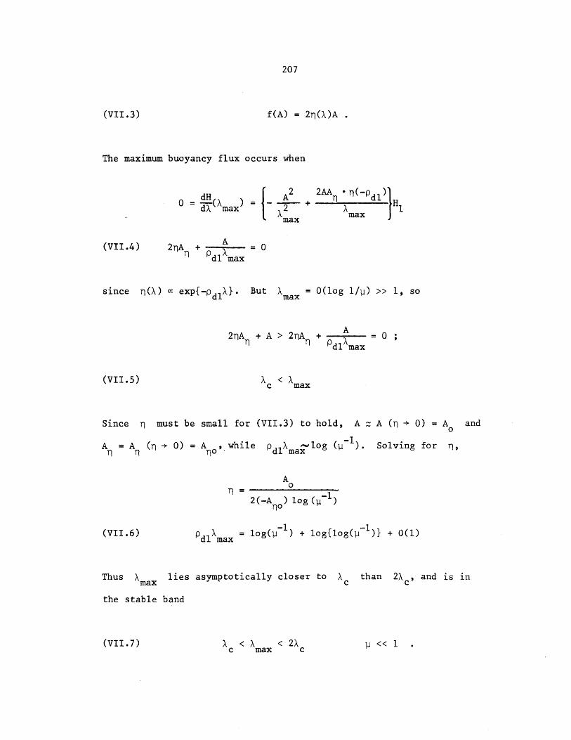
207

f(A) = 2n(X)A .

The maximum buoyancy flux occurs when

0 = (maxA 22

max

2AA *n( PdlHH1max

2nA + A = 0f dl max

since r(X) o exp{-pdlX}. But Xmax

= 0(log l/y) >> 1, so

2TA + A > 2nA + A = 0Tj P d1 max

< Xc max

Since ra must be small for (VII.3) to hold, A z A (n + 0) = A and

A = A ( - 0) = A , while pdl X ma~log (yI ). Solving for q,dlmx

-n 0

2 (-A ) log(y)

Pdl Xmax = log(y~ ) + log{log(y~ )} + 0(1)(VII.6)

Thus Xmax lies asymptotically closer to A than 2Xc, and is in

the stable band

< 2Amax c

(VII.3)

(VII.4)

(VII.5)

~

I

(VII. 7) X < Ac yI << 1 .

208

REFERENCES

Abramowitz, M. and I. A. Stegun, 1964: Handbook of MathematicalFunctions. National Bureau of Standards, New York, 1046pp.

Agee, E. M. and K. E. Dowell, 1974: Observational Studies of MesoscaleCellular Convection. J. Appl. Met., 13, 46-53.

Agee, E. M. and F. E. Lomax, 1978: Structure of the Mixed Layer andInversion Layer Associated with Patterns of Mesoscale CellularConvection During AMTEX 1975. J.A.S., 35, 2281-2301.

Asai, T. and I. Nakasuji, 1977: On the Preferred Mode of CumulusConvection in a Conditionally Unstable Atmosphere. J. Met. Soc.Japan, 55, 151-167.

Asai, T. and I. Nakasuji, 1982: A Further Study of the PreferredMode of Cumulus Convection in a Conditionally Unstable Atmosphere.J. Met. Soc. Japan, 60, 425-431.

Bjerknes, J., 1938: Saturated-Adiabatic Ascent of Air Through Dry-Adiabatically Descending Environment. Q.J.R.M.S., 64, 325-330.

Chandrasekhar, S., 1961: Hydrodynamic and Hydromagnetic Stability.Oxford Univ. Press, Lond, 652pp.

Cho, H. R., 1978: Some Statistical Properties of a Shallow HomogeneousCloud Field. J.A.S., 35, 125-138.

van Delden, A. and J. Oerlemans, 1982: Grouping of Clouds in a NumericalConvection Model. Beitr. Phys. Atmosph., 55, 239-252.

Emanuel, K. A., 1981: A Similarity Theory for Unsaturated Downdraftswithin Clouds. J.A.S., 38, 1541-1557.

Fiedler, B., 1984: The Mesoscale Stability of Entrainment into Cloud-Topped Mixed Layers. J.A.S., 41, 92-101.

Fiedler, B., 1984: Is Mesoscale Cellular Convection Really Convection?Submitted to Tellus.

Haque, S. M. A., 1952: The Initiation of Cyclonic Circulation in aVertically Unstable Airmass. Q.J.R.M.S., 78, 394-406.

209

Hill, G. E., 1974: Factors Controlling the Size and Spacing of CumulusClouds as Revealed by Numerical Experiments. J.A.S., 31, 646-673.

Kitade, T., 1972: On the Convection in a Conditionally UnstableAtmosphere with Mean Vertical Motion. J. Met. Soc. Japan, 50,243-258.

Kuo, H. L., 1961: Convection in a Conditionally Unstable Atmosphere.Tellus, 13, 441-459.

Kuo, H. L., 1963: Perturbations of Plane Couette Flow in StratifiedFluid and the Origin of Cloud Streets. Phys. Fluids, 6, 195-211.

Kuo, H. L., 1965: Further Studies of the Properties of CellularConvection in a Conditionally Unstable Atmosphere. Tellus, 17,413-433.

Lilly, D. K., 1960: On the Theory of Disturbances in a ConditionallyUnstable Atmosphere. Mon. Weath. Rev., 88, 1-17.

Lindzen, R. S., 1974: Wave-CISK in the Tropics. J.A.S., 31, 156-179.

Lopez, R. E., 1976: Radar Characteristics of the Cloud Populationsof Tropical Disturbances in the Northwest Atlantic. Mon. Weath.Rev., 104, 268-283.

Malkus, J. S. and H. Riehl, 1964: Cloud Structuring and Distributionover the Tropical Pacific Ocean. Univ. of Calif. Press, Berkeley,229pp.

Murray, F. W., 1970: Numerical Models of a Tropical Cumulus Cloudwith Bilateral and Axial Symmetry. Mon. Weath. Rev., 98, 14-28.

Ogura, Y., 1963: The Evolution of a Moist Convective Element in aShallow, Conditionally Unstable Atmosphere: A Numerical Calcu-lation. J.A.S., 20, 407-424.

Plank, V. G., 1969: The Size Distribution of Cumulus Clouds in Repre-sentative Florida Populations. J. Appl. Met., 8, 46-67.

Ralston, A. and P. Rabinowitz, 1978: A First Course in NumericalAnalysis. McGraw-Hill, New York, 556pp.

Randall, D. A. and G. J. Huffman, 1980: A Stochastic Model of CumulusClumping. J.A.S., 37, 2068-2078.

Rothermel, J. and E. M. Agee, 1980: Aircraft Investigation of Meso-scale Cellular Convection during AMTEX 75. J.A.S., 37, 1027-1040.

Soong, S. T. and Y. Ogura, 1973: A Comparison Between Axisymmetric andSlab-Symmetric Cumulus Convection. J.A.S., 30, 879-893.

210

Shirer, H. N., 1980: Bifurcation and Stability in a Model of MoistConvection in a Shearing Environment. J.A.S., 37, 1586-1602.

Shirer, H. N., 1982: Toward a Unified Theory of Atmospheric ConvectiveInstability. In Cloud Dynamics, E. M. Agee and T. Asai, eds.D. Reidel, Dordrecht, 163-177.

Shirer, H. N. and Dutton, J., 1979: The Branching Hierarchy of MultipleSolutions in a Model of Moist Convection. J.A.S., 36, 1705-1721.

Spiegel, E. A. and G. Veronis, 1960: On the Boussinesq Approximationfor a Compressible Fluid. Astrophys. J., 131, 442-447.

Squires, P., 1958: Penetrative Downdraughts in Cumuli. Tellus, 10,381-389.

Yamasaki, M., 1972: Small Amplitude Convection in a ConditionallyUnstable Stratification. J. Met. Soc. Japan, 50, 465-481.

Yamasaki, M., 1974: Finite Amplitude Convection in a ConditionallyUnstable Stratification. J. Met. Soc. Japan, 52, 365-379.

Yau, M. K. and R. Michaud, 1982: Numerical Simulations of a CumulusEnsemble in Three Dimensions. J.A.S., 39, 1062-1079.