Feasibility Study of a Heat-powered Liquid Piston Stirling Cooler

Feasibility Study of a Heat-powered Liquid

Piston Stirling Cooler

Samuel Blair Langdon-Arms

PhD

2017

Feasibility Study of a Heat-powered Liquid

Piston Stirling Cooler

Samuel Langdon-Arms

Design and Creative Technologies

Department of Mechanical Engineering

2017

A thesis submitted to

Auckland University of Technology

in fulfilment of the requirements for the degree of

Doctor of Philosophy

i

Abstract

This thesis presents a feasibility study of the proposed liquid piston Stirling cooler or

LPSC, which is a 4-cylinder double-acting alpha-type Stirling machine capable of

utilising a heat input to produce a cooling effect. The novel aspects of the work include:

(a) the first known experimental results of the two heater-LPSC configuration, and the

associated performance predictions from a validated third order computer model; (b)

development of two independent methods for obtaining the system’s operational

frequency; (c) evidence and quantification of the Rayleigh-Taylor instability in

reciprocating liquid pistons, and the mitigation of this instability via the use of piston

floats; and finally (d) the development of design constraints and recommendations

specific to the LPSC.

The LPSC is a tri-thermal, thermo-mechanical, free-piston system based on the Siemens-

Stirling configuration first proposed in the late 1970s. A test-rig was constructed and used

as part of an experimental investigation into understanding the complex multi-degree of

freedom system and identifying its feasibility for heat-powered cooling applications. In

its current, un-optimised state, it has proven to be functional over a wide range of mean

gas pressures (1 bar–6 bar) and relatively low heat source temperatures (80°C–150°C). A

third order model of the LPSC was constructed in the computer modelling software, Sage.

The model encompasses the complex system dynamics and heat transfer characteristics

and is validated against experimental results. The model was used to predict a more

optimised piston geometry which led to the first tangible cooling effect in subsequent

experiments, in the range of 5°C below ambient.

Evidence of a liquid piston acceleration limit, likely resulting from the Rayleigh-Taylor

(RT) instability phenomenon, is consistently observed during the experiments. The use

of submerged polyethylene piston floats is found to increase surface stability and enable

ii

maximum accelerations of 25 ms-2 to 30 ms-2. The two heater configuration, with two

adjacent heated spaces connected in series with two adjacent absorber spaces, is shown

to be the optimal configuration for cooling performance, with relative phase angles close

to 90° and a conversion ratio of heater gas pressure amplitude to absorber gas pressure

amplitude of 1.02 to 1. When considering test-rig performance at 150°C heater

temperature and a maximum charge pressure of 6 bar, the Sage model predicts a thermal

COP of 0.53 for the current set-up (19.3 mm diameter, 94 cm long liquid water pistons).

This rises to 0.59 with the installation of 23 mm diameter, 3 m long liquid pistons. When

the working gas in the model is replaced with hydrogen, the performance of the LPSC

increases significantly: the COP increases by 2.7%, to 0.6, the cooling capacity increases

by 59.1%, the cold-side temperature in the primary absorber is decreased from 13.1°C to

7°C, and the second law efficiency increases from 5.3% to 9.9%.

A number of design considerations for the LPSC are explored. The existence of a potential

piston acceleration limit imposed by the RT instability imposes a constraint on the

minimum piston length. A crude capacity evaluation is also conducted, which indicates

that a LPSC capable of generating a cooling effect of approximately 5 kW is feasible

using 15 L liquid water pistons. Based on the research findings, it is deduced that such an

LPSC system is feasible both technically and commercially, although to what extent in

either regard is still unknown.

iii

Table of Contents

Abstract ............................................................................................................................. i

Attestation of Authorship ............................................................................................. vii

List of Figures ............................................................................................................... viii

List of Tables ................................................................................................................ xvi

List of Abbreviations ................................................................................................. xviii

Acknowledgements ........................................................................................................ xx

Intellectual Property Rights ....................................................................................... xxii

Confidential Material................................................................................................. xxiii

Nomenclature.............................................................................................................. xxiv

1 Introduction ............................................................................................................. 1

1.1 Energy from the Sun ...................................................................................... 1

1.2 Solar Heating and Cooling Rationale ............................................................. 3

1.3 Solar Cooling Background ............................................................................. 4

1.4 Research Objectives ....................................................................................... 7

1.5 Methodology ................................................................................................ 10

1.6 Novel Aspects of the Work .......................................................................... 12

2 Literature ............................................................................................................... 14

2.1 Solar Cooling Technologies ......................................................................... 14

2.1.1 Solar Electric .................................................................................... 15

2.1.2 Solar Thermal ................................................................................... 17

2.1.3 Summary of Solar Cooling Technology Prospects .......................... 26

2.2 Stirling Engine Technology ......................................................................... 28

2.2.1 History .............................................................................................. 29

2.2.2 Stirling for Cooling ........................................................................... 31

2.2.3 The Ideal Stirling Cycle .................................................................... 33

2.2.4 Practical Limitations ......................................................................... 35

2.2.5 Stirling System Configurations ........................................................ 37

2.2.6 Free-Piston Stirling Engines ............................................................. 40

2.2.7 Liquid Piston Stirling Machines ....................................................... 42

2.3 Theoretical Background Analysis ................................................................ 46

2.3.1 Introduction ...................................................................................... 46

2.3.2 FPSEs as Vibrating Systems ............................................................ 46

2.3.3 Power Estimation .............................................................................. 50

2.3.4 Frequency Estimation ....................................................................... 51

2.3.5 First Order Analysis ......................................................................... 52

iv

2.3.6 Second Order Analysis ..................................................................... 54

2.3.7 Third Order Analysis ........................................................................ 55

3 Heat-powered Liquid Piston Stirling Cooler Test-rig ........................................ 57

3.1 Preliminary Design ....................................................................................... 57

3.1.1 Heat Exchangers ............................................................................... 60

3.1.2 Housing and Regenerator ................................................................. 61

3.1.3 Liquid Pistons ................................................................................... 63

3.1.4 PID Controller .................................................................................. 64

3.1.5 Temperature and Pressure Sensors ................................................... 66

3.1.6 Piston Displacement Sensors ............................................................ 68

3.2 Commissioning and Modifications .............................................................. 70

3.2.1 Piston Floats ..................................................................................... 70

3.2.2 Pressure Manifold ............................................................................. 74

3.2.3 Displacement Sensors ....................................................................... 75

3.2.4 Minor Alterations ............................................................................. 82

3.2.5 Experimental Accuracy .................................................................... 82

3.2.6 Commissioned Test-rig Setup .......................................................... 83

3.3 Operating Configurations ............................................................................. 84

3.3.1 4HEAT Configuration ...................................................................... 85



3.4 Experimental Parameters.............................................................................. 88

3.5 Experimental Procedure ............................................................................... 89

4 System Modelling ................................................................................................... 92

4.1 Analytical Modelling.................................................................................... 92

4.1.1 Natural Frequency ............................................................................ 92

4.1.2 Schmidt Analysis of Frequency ........................................................ 94

4.1.3 Frequency Dependence on Heater Temperature .............................. 99

4.2 Sage Modelling .......................................................................................... 102

4.2.1 Description of Sage Modelling Software ....................................... 102

4.2.2 Sage Model Overview .................................................................... 108

4.2.3 Compression and Expansion Spaces .............................................. 110

4.2.4 Cold and Hot Spaces ...................................................................... 112

4.2.5 Heat Exchangers ............................................................................. 113

4.2.6 Regenerators ................................................................................... 115

4.2.7 Liquid Pistons ................................................................................. 119

4.2.8 Sage Model Input Requirements .................................................... 122

4.2.9 Frequency Deduction ...................................................................... 123

v

4.2.10 Solving 3HEAT and 2HEAT models ........................................... 126

4.2.11 Grid Independent Solutions .......................................................... 128

4.2.12 Complete Model Diagram ............................................................ 130

5 Results for 15 mm OD Piston Tubes .................................................................. 132

5.1 Experimental Results.................................................................................. 132

5.1.1 4HEAT Configuration .................................................................... 132



5.1.4 Configuration Comparisons ............................................................ 183

5.1.5 Rayleigh-Taylor Instability Assessment ......................................... 187

5.2 Sage Modelling Results .............................................................................. 192

5.2.1 Initial Validation and Sensitivity Analysis ..................................... 192

5.2.2 4HEAT Model ................................................................................ 198

5.2.3 3HEAT Model ................................................................................ 202

5.2.4 2HEAT Model ................................................................................ 210

5.2.5 Validation Summary ....................................................................... 216

5.3 Preliminary Piston Investigation ................................................................ 217

6 Results for 22 mm OD Piston Tube ................................................................... 221

6.1 Test-rig Modifications and Commissioning ............................................... 221

6.2 Experiment Results .................................................................................... 225




6.2.4 Summary ......................................................................................... 245

6.3 Sage Modelling Results .............................................................................. 247




6.3.4 Summary ......................................................................................... 268

6.4 Results Summary Table ............................................................................. 270

7 Liquid Piston Optimisation ................................................................................ 271

7.1 Mapping Piston Dimensions ...................................................................... 271

7.2 Selection of Piston Length and Diameter ................................................... 275

7.3 Comparison Between 23 mm and 30 mm Diameter 3 m Pistons............... 277

7.3.1 Simulation Results Overview ......................................................... 277

7.3.2 Cooling Potential ............................................................................ 282

8 Discussion ............................................................................................................. 287

8.1 LPSC Configurations ................................................................................. 287

vi


8.1.2 3HEAT and 2HEAT Configurations .............................................. 287

8.1.3 Alternative Configurations ............................................................. 288

8.2 Limitations of Research Presented ............................................................. 289

8.2.1 Frequency Considerations .............................................................. 289

8.2.2 Test-rig Asymmetries ..................................................................... 290

8.2.3 Fluid Friction .................................................................................. 291

8.2.4 Liquid Evaporation ......................................................................... 292

8.2.5 Multi-modal Behaviour .................................................................. 293

8.3 Rayleigh-Taylor Instability and Piston Floats ............................................ 294

8.4 Design Considerations................................................................................ 297

8.4.1 Working Fluids ............................................................................... 297

8.4.2 Piston Sizing ................................................................................... 298

8.5 Overall Feasibility ...................................................................................... 301

8.5.1 Cooling Potential ............................................................................ 301

8.5.2 Capacity limitations ........................................................................ 302

8.6 Future Research .......................................................................................... 305

8.6.1 Piston Floats ................................................................................... 305

8.6.2 Liquid Pistons ................................................................................. 305

8.6.3 Thermal Energy Storage ................................................................. 306

8.6.4 Solid Pistons ................................................................................... 306

9 Conclusions and Recommendations .................................................................. 307

9.1 Design, Construction and Testing of the LPSC Machine .......................... 307

9.2 System Modelling and Performance Evaluation ........................................ 307

9.3 Liquid Piston Acceleration Limit and Design Implications ....................... 308

9.4 Recommendations ...................................................................................... 309

References .................................................................................................................... 310

Appendix I – Displacement Sensor Circuit Diagram .............................................. 317

Appendix II – Rayleigh-Taylor Instability ............................................................... 318

vii

Attestation of Authorship

I hereby declare that this submission is my own work and that, to the best of my

knowledge and belief, it contains no material previously published or written by another

person (except where explicitly defined in the acknowledgements), nor material which to

a substantial extent has been submitted for the award of any other degree or diploma of a

university or other institution of higher learning.

Signed:

Samuel Langdon-Arms

viii

List of Figures

Figure 1.1 – Total energy resources. ................................................................................. 2 Figure 1.2 – Heating and cooling demand profiles compared with solar collector supply

for Central Europe. ............................................................................................................ 4 Figure 1.3 – Renewable Heating and Cooling Technology Development........................ 6

Figure 1.4 – Traditional thermo-mechanical cooling procedure using separate Stirling

machines ............................................................................................................................ 7 Figure 1.5 – Proposed thermo-mechanical cooling procedure using a single Stirling

machine ............................................................................................................................. 7 Figure 1.6 – Liquid piston Stirling cooler (LPSC) concept .............................................. 8

Figure 2.1 – Solar electric cooling with vapour compression system............................. 16 Figure 2.2 – Thermo-mechanical Cooling System. ........................................................ 18 Figure 2.3 – Closed Sorption Cooling System. ............................................................... 23

Figure 2.4 – COP of Sorption systems reviewed in SACE project. ................................ 26 Figure 2.5 – The ideal Stirling Cycle. ............................................................................. 33 Figure 2.6 – Single acting Stirling machine configurations. ........................................... 38 Figure 2.7 – Four-cylinder double-acting Siemens-Stirling configuration. .................... 39

Figure 2.8 – Sunpower M100 FPSE ............................................................................... 41 Figure 2.9 – Basic ‘Fluidyne’ operation. ........................................................................ 42

Figure 2.10 – Simple spring-mass-damper system ......................................................... 47 Figure 2.11 – Vector representation of the generic solutions for piston or displacer

motion. ............................................................................................................................ 49

Figure 3.1 – First liquid piston Stirling cooler (LPSC) set-up with U-tubes. ................. 57 Figure 3.2 – Liquid piston Stirling cooler Schematic. .................................................... 58

Figure 3.3 – Subsystem composition. The LPSC machine is comprised of four of these

units connected in series.................................................................................................. 59

Figure 3.4 – Brass heat exchanger showing side view of the annular fins and protrusion

for heating cartridge access (RHS). ................................................................................ 60 Figure 3.5 – Brass heat exchanger end showing a view of the annular fins ................... 60

Figure 3.6 – Stainless Steel housing component. ............................................................ 62 Figure 3.7 – Stainless Steel housing component assembled with brass heat exchanger

and vacuum clamp........................................................................................................... 62 Figure 3.8 – Steel shot material used in the regenerators ............................................... 63 Figure 3.9 – Liquid piston housing U-tubes with expansion flange fittings. .................. 64 Figure 3.10 – Controller Circuit for regulating the power supply to the heaters. ........... 65

Figure 3.11 – PID controller and SSR housing images. ................................................. 66 Figure 3.12 – Pressure transducer and temperature sensor ports. ................................... 67 Figure 3.13 – Capacitive sensor setup for measuring piston displacement. ................... 68 Figure 3.14 – First generation capacitive sensors used for measuring liquid piston

displacements. ................................................................................................................. 69 Figure 3.15 – Cylindrical polyethylene liquid piston float for improved surface stability.

......................................................................................................................................... 72

Figure 3.16 – Gas temperature stability comparison for different float diameters.

Experiments were conducted with the 3HEAT configuration with 150 °C heaters and 4

bar charge pressure. ......................................................................................................... 73 Figure 3.17 – The impact of piston float diameter on the development of pressure

amplitudes within the gas spaces. ................................................................................... 74 Figure 3.18 – Pressure manifold with individual control valves for each subsystem. .... 75 Figure 3.19 – Capacitive sensor circuit with reference capacitors.................................. 76

ix

Figure 3.20 – Piston displacement profiles over one second interval during a typical

experiment. ...................................................................................................................... 77

Figure 3.21 – Example of phasor representation and optimisation for Piston A

displacement profile using least mean squares approximation. ...................................... 78 Figure 3.22 – Scales for calibrating displacement sensors with slow motion video

recordings. ....................................................................................................................... 79

Figure 3.23 – Displacement sensor 4 calibration curve comparing sample experiment

readings with slow motion video displacements. ............................................................ 79 Figure 3.24 – Comparison of surface profiles between moving and stationary liquid

pistons. ............................................................................................................................ 80 Figure 3.25 – Fully commissioned 15 mm OD piston tube test-rig. ............................... 84

Figure 3.26 – 4HEAT configuration (4 Heaters, 0 Absorbers). ...................................... 86 Figure 3.27 – 3HEAT configuration (3 Heaters, 1 Absorber). ....................................... 86 Figure 3.28 – 2HEAT configuration (a) with alternating heaters and absorbers (2

Heaters, 2 Absorbers). ..................................................................................................... 87

Figure 3.29 – 2HEAT configuration (b) with adjacent heaters (2 Heaters, 2 Absorbers).

......................................................................................................................................... 87 Figure 4.1 – Spring and mass representation of the LPSC. ............................................ 93 Figure 4.2 – Graph showing how little the heater temperature affects the operational

frequency of the LPSC system. ..................................................................................... 101 Figure 4.3 – Example showing the graphical interface of Sage. ................................... 103 Figure 4.4 – Sage model component visualisation infographic with test-rig parts. ...... 108

Figure 4.5 – Sage model of a liquid piston Stirling cooler subsystem. ......................... 109 Figure 4.6 – Structure of the compression space model-component within Sage. ....... 110 Figure 4.7 – Structure of the hot and cold space component within Sage. ................... 112

Figure 4.8 – Structure of the heat exchanger model-component within Sage. ............. 114 Figure 4.9 – Structure of the central regenerator model-component within Sage. ....... 116

Figure 4.10 – Structure of the side regenerator model-component within Sage. .......... 117

Figure 4.11 – Piston A work output mapped against piston displacement. Simulation

was conducted for 3HEAT configuration at 4 bar and 150ºC heaters with 100 ml

pistons. .......................................................................................................................... 127

Figure 4.12 – Objective function 1 mapped against Piston A amplitude. Simulation was

conducted for 4HEAT configuration at 4 bar and 100ºC heaters with 100 ml pistons. 128 Figure 4.13 – Complete Sage model diagram ............................................................... 131 Figure 5.1 – Gas pressure amplitude variations during a typical 4HEAT experiment. 133

Figure 5.2 – Heater gas temperature variations during a typical 4HEAT experiment. . 134 Figure 5.3 – Gas pressure profiles over one second interval during a typical 4HEAT

experiment. .................................................................................................................... 134 Figure 5.4 – Piston displacement profiles over one second interval during a typical

4HEAT experiment. ...................................................................................................... 135

Figure 5.5 – Phasor plot of example 4HEAT experiment pressure and displacement

profiles........................................................................................................................... 137

Figure 5.6 – Phasor plot of example 4HEAT experiment pressure and displacement

profiles........................................................................................................................... 138 Figure 5.7 – Pressure and displacement phase angles for 4HEAT example experiment.

....................................................................................................................................... 139 Figure 5.8 – Frequency variation with mean operating pressure for all 4HEAT

configuration experiments using 100 ml liquid pistons ................................................ 140 Figure 5.9 – Pressure amplitude variations of all gas spaces with increasing charge

pressure for 4HEAT experiments conducted with 105°C heater temperatures and 100 ml

pistons. .......................................................................................................................... 141

x

Figure 5.10 – Pressure amplitude variation of Gas Space 1 with changing charge

pressure for all 4HEAT experiments using 100 ml liquid pistons. ............................... 141

Figure 5.11 – Gas space temperature differentials and their variation with charge

pressure for the 4HEAT experiments with 105°C heater temperatures. ....................... 143 Figure 5.12 – Piston amplitude variation with charge pressure for the 105ºC, 4HEAT

configuration experiments using 100 ml liquid pistons. ............................................... 144

Figure 5.13 – Average piston amplitude variation with mean operating pressure for all

4HEAT configuration experiments using 100 ml liquid pistons. ................................. 144 Figure 5.14 – Pressure phasor relative phase angles' variation with gas charge pressure

for the 105ºC 4HEAT experiments with 100 ml liquid pistons. ................................... 146 Figure 5.15 – Relative phase angles' variation with gas charge pressure for the piston

displacement phasors in the 105ºC 4HEAT experiments conducted with 100 ml liquid

pistons. .......................................................................................................................... 147 Figure 5.16 – Pressure amplitude variation with charge pressure for the 105ºC 4HEAT

experiments using 115 ml liquid pistons. ...................................................................... 148

Figure 5.17 – Temperature differentials between the expansion and compression spaces

for each gas space and their variation with charge pressure for the 105ºC 4HEAT

experiments with 115 ml liquid pistons. ....................................................................... 148 Figure 5.18 – Pressure phasor phase angles' variation with gas charge pressure for the

105ºC 4HEAT experiments with 115 ml liquid pistons. ............................................... 149 Figure 5.19 – Gas pressure amplitude variations during a typical 3HEAT experiment.

....................................................................................................................................... 151

Figure 5.20 – Heater gas temperature variations during a typical 4HEAT experiment.

....................................................................................................................................... 151 Figure 5.21 – Gas pressure profiles over one second interval during a typical 3HEAT

experiment. .................................................................................................................... 153 Figure 5.22 – Piston displacement profiles over one second interval during a typical

3HEAT experiment. ...................................................................................................... 153

Figure 5.23 – Phasor plot of the pressure and displacement profiles for the example

3HEAT experiment. ...................................................................................................... 155 Figure 5.24 – Pressure and displacement phase angles for 3HEAT example experiment.

....................................................................................................................................... 156 Figure 5.25 – Frequency variation with mean operating pressure for all 3HEAT

configuration experiments using 100 ml liquid pistons. ............................................... 157 Figure 5.26 – Pressure amplitude variations of all gas spaces with increasing charge


pistons. .......................................................................................................................... 157 Figure 5.27 – Pressure amplitude variation of Gas Space 1 with changing charge

pressure for all 3HEAT experiments using 100 ml liquid pistons. ............................... 159 Figure 5.28 – Temperature difference between expansion and compression spaces in

Gas Space 1 for the 3HEAT configuration experiments using 100 ml liquid pistons. . 160

Figure 5.29 – Heater gas space temperature differentials and their variation with charge

pressure for the 3HEAT experiments with 150°C heater temperatures and 100 ml liquid

pistons. .......................................................................................................................... 161 Figure 5.30 – Piston amplitude variation with charge pressure for the 150ºC, 3HEAT

configuration experiments using 100 ml liquid pistons. ............................................... 161 Figure 5.31 – Average piston amplitude variation with charge pressure for all of the

3HEAT experiments conducted using 100 ml liquid pistons........................................ 162 Figure 5.32 – Relative phase angle variations with gas charge pressure for the pressure

phasors in the 150ºC 3HEAT experiments using 100 ml liquid pistons. ...................... 163

Figure 5.33 – Relative phase angle variations with gas charge pressure for the piston

displacement phasors in the 150ºC 3HEAT experiments using 100 ml liquid pistons. 164

xi

Figure 5.34 – Gas pressure amplitude variations for Gas Space 1 in the 3HEAT

experiments conducted using 115 ml liquid pistons. .................................................... 165

Figure 5.35 – Temperature difference between expansion and compression spaces in

Gas Space 1 for the 3HEAT configuration experiments using 115 ml liquid pistons. . 166 Figure 5.36 – Relative phase angle variations with gas charge pressure for the pressure

phasors in the 150ºC 3HEAT experiments using 115 ml liquid pistons. ...................... 166

Figure 5.37 – Relative phase angle variations with gas charge pressure for the piston

displacement phasors in the 150ºC 3HEAT experiments using 115 ml liquid pistons. 167 Figure 5.38 – Gas pressure amplitude variations during a typical 2HEAT experiment.

....................................................................................................................................... 170 Figure 5.39 – Heater space gas temperature variations during a typical 2HEAT

experiment. .................................................................................................................... 171 Figure 5.40 – Absorber space gas temperature variations during a typical 2HEAT

experiment. .................................................................................................................... 171 Figure 5.41 – Gas pressure profiles over a one second interval during a typical 2HEAT

experiment. .................................................................................................................... 172 Figure 5.42 – Piston displacement profiles over a one second interval during a typical

2HEAT experiment. ...................................................................................................... 173 Figure 5.43 – Phasor plot of example 2HEAT experiment pressure amplitude and

displacement profiles. ................................................................................................... 174 Figure 5.44 – Pressure and piston displacement phasor phase angles for 2HEAT

example experiment. ..................................................................................................... 175

Figure 5.45 – Shows the frequency variation with mean operating pressure for all

2HEAT configuration experiments using 115 ml liquid pistons. ................................. 176 Figure 5.46 – Pressure amplitude variations of all gas spaces with increasing charge


pistons. .......................................................................................................................... 177

Figure 5.47 – Heater gas space temperature differentials and their variation with charge

pressure for the 2HEAT experiments with 190°C heater temperatures and 115 ml liquid

pistons. .......................................................................................................................... 178 Figure 5.48 – Temperature difference between expansion and compression spaces in gas

spaces 1 and 4 for the 2HEAT configuration experiments using 115 ml liquid pistons.

....................................................................................................................................... 178 Figure 5.49 – Piston amplitude variation with charge pressure for the 190ºC, 2HEAT


Figure 5.50 – Relative phase angle variations with gas charge pressure for the pressure

phasors in the 190°C 2HEAT experiments using 115 ml liquid pistons. ..................... 180 Figure 5.51 – Relative phase angle variations with gas charge pressure for the piston

displacement phasors in the 190°C 2HEAT experiments using 115 ml liquid pistons. 181 Figure 5.52 – Operational frequency variation with mean operating pressure for all

experiments using 100 ml liquid pistons. ...................................................................... 183

Figure 5.53 – Operational frequency variation with mean operating pressure for all

experiments using 115 ml liquid pistons. ...................................................................... 184 Figure 5.54 – Operational frequency differences between 100 ml and 115 ml liquid

pistons. .......................................................................................................................... 184 Figure 5.55 – Differences in pressure amplitudes between 100 ml and 115 ml liquid

pistons for the 4HEAT, 105ºC experiments. ................................................................. 185

Figure 5.56 – Differences in pressure amplitudes between 100 ml and 115 ml liquid

pistons for the 3HEAT 150ºC experiments. .................................................................. 186 Figure 5.57 – Pressure amplitude stability for different charge pressures. ................... 188

Figure 5.58 – Piston displacement profiles over a one second interval at 3.25 bar charge

pressure. ........................................................................................................................ 189

xii

Figure 5.59 – Piston displacement profiles over a one second interval at 5 bar charge

pressure. ........................................................................................................................ 189

Figure 5.60 – Average maximum piston acceleration for experiments with 115 ml

pistons and 15 mm piston tubes. ................................................................................... 191 Figure 5.61 – Sage model predictions for operating frequency. 4HEAT configuration

with 100°C heaters and 100 ml pistons. ........................................................................ 192

Figure 5.62 – Sage model predictions for piston amplitude. 4HEAT configuration with

100ºC heaters and 100 ml pistons. ................................................................................ 193 Figure 5.63 – Sage model predictions of piston amplitude for different water viscosities.

....................................................................................................................................... 194 Figure 5.64 – Sage model predictions for piston amplitude with different values for the

sum of the minor pipe flow loss coefficients. ............................................................... 195 Figure 5.65 – Sage model predictions for piston amplitude with different heater

temperatures. ................................................................................................................. 196 Figure 5.66 – Sage model sensitivity to heat rejection temperature. ............................ 197

Figure 5.67 – Phasor plot of example 4HEAT Sage simulation pressure and

displacement profiles. ................................................................................................... 199 Figure 5.68 – Pressure and displacement phase angles for 4HEAT Sage simulation... 200 Figure 5.69 – Sage model pressure amplitude variations compared with experimental

results for 4HEAT experiments conducted with 100°C heater temperatures and 100 ml

pistons. .......................................................................................................................... 201 Figure 5.70 – Sage model predictions for the relative phase angles between pressure

amplitude phasors.......................................................................................................... 201 Figure 5.71 – Sage model predictions for the relative phase angles between piston

amplitude phasors.......................................................................................................... 202

Figure 5.72 – Phasor plot of example 3HEAT Sage simulation pressure and

displacement profiles. ................................................................................................... 203

Figure 5.73 – Sage model predictions for the relative phase angles between pressure and

displacement phasors in the example 3HEAT simulation. ........................................... 204

Figure 5.74 – Sage predictions for pressure amplitudes developed in all four gas spaces

with increasing charge pressure for 3HEAT configuration. ......................................... 205

Figure 5.75 – Sage model predictions for pressure amplitude in Gas Space 1 compared

with experimental results for 3HEAT configuration. ................................................... 206 Figure 5.76 – Sage predictions for piston amplitudes with increasing charge pressure for

3HEAT configuration.................................................................................................... 207

Figure 5.77 – Sage model predictions for Piston A amplitude compared with

experimental results for 3HEAT configuration............................................................. 208 Figure 5.78 – Sage model predictions for the relative phase angles between pressure

amplitude phasors.......................................................................................................... 208 Figure 5.79 – Sage model predictions for the relative phase angles between piston

amplitude phasors.......................................................................................................... 209

Figure 5.80 – Sage model coefficient of performance predictions for the 3HEAT

configuration. ................................................................................................................ 210 Figure 5.81 – Phasor plot of example 2HEAT Sage simulation pressure and

displacement profiles. ................................................................................................... 211 Figure 5.82 – Sage model predictions for the relative phase angles between pressure and

displacement phasors in the example 2HEAT simulation. ........................................... 212

Figure 5.83 – Sage predictions for pressure amplitudes with increasing charge pressure

for 2HEAT configuration. ............................................................................................. 213 Figure 5.84 – Sage predictions for piston amplitudes with increasing charge pressure for

2HEAT configuration.................................................................................................... 213

xiii

Figure 5.85 – Sage model predictions for the relative phase angles between pressure

amplitude phasors for 2HEAT configuration. ............................................................... 214

Figure 5.86 – Sage model predictions for the relative phase angles between piston

phasors for 2HEAT configuration. ................................................................................ 215 Figure 5.87 – Sage model predictions for the coefficient of performance for the 2HEAT

configuration. ................................................................................................................ 216

Figure 5.88 – Piston diameter influence on the heater temperatures needed for self-

sustained operation. ....................................................................................................... 219 Figure 5.89 – Identification of the optimal piston diameter based on Sage model

predictions with constant piston length. ........................................................................ 220 Figure 6.1 – New support structure created for larger pistons. ..................................... 222

Figure 6.2 – Fully commissioned 22 mm piston test-rig. ............................................. 224 Figure 6.3 – Frequency variation of the 22 mm piston experiments with 275 ml pistons

for all configurations. .................................................................................................... 226 Figure 6.4 – Experimental frequencies of both piston sizes compared with predictions

from natural frequency derivation. ................................................................................ 226 Figure 6.5 – Scaled phasor plot of pressure and displacement profiles for the example

4HEAT experiment with 22 mm piston tubes............................................................... 228 Figure 6.6 – Relative phase angles for the example 4HEAT experiment with 22 mm

piston tubes. .................................................................................................................. 229 Figure 6.7 – Pressure amplitude variation of Gas Space 1 with changing charge pressure

for all 4HEAT experiments using 275 ml liquid pistons. ............................................. 230

Figure 6.8 – Pressure amplitude progressions of experiments conducted at or near the

transition pressure of 4 bar for the 4HEAT configuration. ........................................... 230 Figure 6.9 – Pressure amplitude progressions for 75ºC heater experiments. ................ 231

Figure 6.10 – Piston amplitude variation with charge pressure for the 4HEAT


Figure 6.11 – Performance of LPSC 4HEAT system with and without piston surface

floats. ............................................................................................................................. 233

Figure 6.12 – Scaled phasor plot of pressure and displacement profiles for the example

3HEAT experiment with 22 mm piston tubes............................................................... 235

Figure 6.13 – Relative phase angles for the example 3HEAT experiment with 22 mm

piston tubes. .................................................................................................................. 235 Figure 6.14 – Pressure amplitude variation of Gas Space 1 with changing charge


Figure 6.15 – Pressure amplitude variations of all gas spaces with increasing charge


pistons. .......................................................................................................................... 237 Figure 6.16 – Piston amplitude variation with charge pressure for the 3HEAT

configuration experiments with 105ºC and 110ºC heaters and using 275 ml liquid

pistons. .......................................................................................................................... 238

Figure 6.17 – Temperature difference between expansion and compression spaces in

Gas Space 1 for the 3HEAT configuration experiments using 275 ml liquid pistons with

different heater temperatures......................................................................................... 238 Figure 6.18 – Scaled phasor plot of pressure and displacement profiles for the example

2HEAT experiment with 22 mm piston tubes............................................................... 240 Figure 6.19 – Relative phase angles for the example 2HEAT experiment with 22 mm

piston tubes. .................................................................................................................. 240 Figure 6.20 – Pressure amplitude variation of Gas Space 1 with changing charge


xiv

Figure 6.21 – Pressure amplitude variations of all gas spaces with increasing charge


pistons. .......................................................................................................................... 242 Figure 6.22 – Piston amplitude variation with charge pressure for the 2HEAT

configuration experiments with 160ºC heaters and using 275 ml liquid pistons. ......... 243 Figure 6.23 – Shows the temperature difference between expansion and compression

spaces in the two absorber spaces for the 2HEAT configuration experiments using 275

ml liquid pistons with different heater temperatures..................................................... 244 Figure 6.24 – Frequency comparison between Sage predictions, experiment and natural

estimates. ....................................................................................................................... 248 Figure 6.25 – Gas pressure amplitudes predicted by Sage compared with the

experimental results for the 22 mm 275 ml pistons. ..................................................... 250 Figure 6.26 – Average maximum piston acceleration for 22 mm experiments with 275

ml pistons when compared with Sage model. ............................................................... 251 Figure 6.27 – Scaled phasor plot of example 3HEAT Sage simulation pressure and

displacement profiles compared with experiment results. ............................................ 252 Figure 6.28 – Sage model predictions for the relative phase angles between pressure and

displacement phasors in the example 3HEAT simulation. ........................................... 253 Figure 6.29 – Sage predictions for pressure amplitudes developed in all four gas spaces

with increasing charge pressure for 3HEAT configuration. ......................................... 254 Figure 6.30 – Gas Space 1 pressure amplitudes predicted by Sage compared with the

experimental results in the 22 mm 275 ml pistons for the 3HEAT configuration. ....... 255

Figure 6.31 – Piston amplitudes predicted by Sage compared with the experimental

results in the 22 mm 275 ml pistons for the 3HEAT configuration with 110ºC heaters.

....................................................................................................................................... 256


results in the 22 mm 275 ml pistons for the 3HEAT configuration with 105°C heaters.

....................................................................................................................................... 256

Figure 6.33 – Average maximum piston acceleration for 22 mm experiments with 275

ml pistons when compared with Sage model for 3HEAT configuration. ..................... 258 Figure 6.34 – Temperature difference between expansion and compression spaces in

Gas Space 1 for the 3HEAT Sage simulations compared with experiments. ............... 258 Figure 6.35 – Sage model coefficient of performance predictions for the 3HEAT

configuration. ................................................................................................................ 259 Figure 6.36 – Scaled phasor plot of example 2HEAT Sage simulation pressure and

displacement profiles compared with experiment results. ............................................ 260 Figure 6.37 – Sage model predictions for the relative phase angles between pressure and

displacement phasors in the example 2HEAT simulation. ........................................... 261 Figure 6.38 – Sage predictions for pressure amplitudes developed in all four gas spaces

with increasing charge pressure for 2HEAT configuration. ......................................... 262

Figure 6.39 – Gas Space 1 pressure amplitudes predicted by Sage compared with the

experimental results in the 22 mm 275 ml pistons for the 2HEAT configuration. ....... 263



....................................................................................................................................... 264 Figure 6.41 – Piston amplitudes predicted by Sage compared with the experimental


....................................................................................................................................... 265 Figure 6.42 – Average maximum piston acceleration for 22 mm experiments with 275

ml pistons when compared with Sage model for 2HEAT configuration. ..................... 265

xv

Figure 6.43 – Shows the temperature difference between expansion and compression

spaces in the absorber spaces for the 165°C 2HEAT Sage simulations compared with

experiments. .................................................................................................................. 266 Figure 6.44 – Sage model coefficient of performance predictions for the 2HEAT

configuration. ................................................................................................................ 267 Figure 7.1 – Pressure amplitude predictions for pistons of different diameter and length.

Simulations are conducted with 4HEAT configuration with 90ºC heaters and 6 bar

charge pressure. ............................................................................................................. 272 Figure 7.2 – Variation of the product of frequency and pressure amplitude (objective

function 3) with increasing piston length for different piston diameters. ..................... 274 Figure 7.3 – Maximum piston accelerations sustained for variations in piston length and

diameter. ........................................................................................................................ 274 Figure 7.4 – Predicted pressure amplitudes developed for 3 m pistons with varying

piston diameters. ........................................................................................................... 276 Figure 7.5 – Product of pressure amplitude and frequency (objective function 3) for 3 m

pistons with varying piston diameters. .......................................................................... 276 Figure 7.6 – Heater temperature influence on the pressure amplitudes developed with 3

m long pistons of diameter 23 mm and 30 mm. ............................................................ 278 Figure 7.7 – Gas Space 1 pressure amplitude comparison for 2HEAT simulations with

different heater temperatures......................................................................................... 279 Figure 7.8 – Average piston amplitude comparison for 2HEAT simulations with

different heater temperatures......................................................................................... 280

Figure 7.9 – Average maximum piston acceleration comparison for 2HEAT simulations

with different heater temperatures. ............................................................................... 281 Figure 7.10 – Coefficient of performance comparison for 2HEAT simulations with

different heater temperatures......................................................................................... 282 Figure 7.11 – Average absorber heat exchanger fin temperatures achieved for 23 mm

and 30 mm diameter pistons in 2HEAT configuration at 6 bar charge pressure. ......... 283

Figure 7.12 – Heat flow through absorber heat exchanger fins achieved for 23 mm and

30 mm diameter pistons in 2HEAT configuration at 6 bar charge pressure. ................ 284 Figure 7.13 – Predicted COP values depending on the absorber temperature achieved.

....................................................................................................................................... 286 Figure 7.14 – Predicted heat flows into the system through the heaters and absorbers for

different pre-set absorber temperatures. ........................................................................ 286 Figure 8.1 – Optimal configuration for cooling (2HEAT with adjacent heaters) ......... 301

xvi

List of Tables

Table 2.1 – Overview of sorption cooling options .......................................................... 25 Table 3.1 – Displacement Sensor Calibration Coefficients. ........................................... 81 Table 3.2 – Set of parameters for first experimental investigation. ................................ 88 Table 4.1 – Compression and expansion space model-component input parameters ... 111

Table 4.2 – Hot and cold space model-component input parameters. .......................... 113 Table 4.3 – Heat exchanger model-component input parameters. ................................ 115 Table 4.4 – Input parameter values for the central regenerator model-components. .... 117 Table 4.5 – Input parameters for regenerator side model-components. ........................ 118 Table 4.6 – Piston input parameters used in the Sage model for 100 ml pistons.......... 122

Table 4.7 – General input parameters for LPSC Sage model. ...................................... 122 Table 4.8 – Sage model sensitivity to NTnode parameter. (Example 3HEAT simulations

at 4 bar with 150ºC heaters and 100 ml pistons) ........................................................... 129

Table 4.9 – Sage model sensitivity to Ncells parameter. (Example simulations at 4 bar

with 100ºC heaters and 100 ml pistons). ....................................................................... 130 Table 5.1 – Set of parameters for first experimental investigation (reproduced from

Section 3.4). .................................................................................................................. 132

Table 5.2 – Phasor representations of gas pressure and piston displacement amplitudes

for example 4HEAT experiment. .................................................................................. 137


for example 3HEAT experiment. .................................................................................. 154 Table 5.4 – Phasor representations of gas pressure and piston displacement amplitudes

for example 2HEAT experiment. .................................................................................. 173 Table 5.5 – Experimental results summary for 15 mm OD piston experiments. .......... 187

Table 5.6 – Sage model phasors predictions for 4HEAT experiment at 4 bar with 100ºC

heaters and 100 ml pistons. ........................................................................................... 199

Table 5.7 – Sage model phasors predictions for 3HEAT experiment at 4 bar with 150°C

heaters and 100 ml pistons. ........................................................................................... 203 Table 5.8 – Sage model phasors predictions for 2HEAT experiment at 4 bar with 100°C

heaters and 100 ml pistons. ........................................................................................... 211 Table 5.9 – Operating frequencies and starting temperatures for 94 cm pistons of

varying diameter............................................................................................................ 218 Table 6.1 – Set of parameters for second experimental investigation. ......................... 221 Table 6.2 – Phasor representations of gas pressure and piston displacement amplitudes



for example 3HEAT experiment. .................................................................................. 234 Table 6.4 – Phasor representations of gas pressure and piston displacement amplitudes


Table 6.5 – Sage parameter adjustments for 22 mm, 275 ml liquid piston test-rig. ..... 247 Table 6.6 – Sage model phasors predictions for 4HEAT experiment at 4 bar with 80°C

heaters and 275 ml pistons. ........................................................................................... 249

Table 6.7 – Sage model phasors predictions for 3HEAT experiment at 4 bar with 110°C

heaters and 275 ml pistons. ........................................................................................... 252 Table 6.8 – Sage model phasors predictions for 2HEAT experiment at 4 bar with 165°C

heaters and 275 ml pistons. ........................................................................................... 261 Table 6.9 – 22 mm piston tube results summary for 275 ml pistons. ........................... 270 Table 7.1 – Piston dimension variations and resulting volumes ................................... 272 Table 7.2 – Prototypes considered for performance assessment................................... 277

xvii

Table 7.3 – LPSC performance summary for 2HEAT simulations at 6 bar and various

heater temperatures. ...................................................................................................... 279

Table 7.4 – LPSC performance summary for simulations with 150ºC heaters at 6 bar

and various pre-set absorber temperatures. ................................................................... 285 Table 8.1 – Sage model predictions for air and hydrogen with the 23 mm diameter, 3 m

long liquid piston test-rig. ............................................................................................. 297

xviii

List of Abbreviations

0HEAT LPSC configuration with zero heaters

2HEAT LPSC configuration with two heaters

3HEAT LPSC configuration with three heaters

4HEAT LPSC configuration with four heaters

BDC Bottom Dead Centre

CFCs Chlorofluorocarbons

CFD Computational Fluid Dynamics

CHP Combined Heat and Power

COP Coefficient of Performance

DAQ Data Acquisition

EOM Equation of Motion

FPSE Free-Piston Stirling Engine

GS Gas Space

HCFCs Hydrochlorofluorocarbons

HX Heat Exchanger

ID Inner Diameter

IEA International Energy Agency

IECEC International Energy Conversion Engineering Conference

ISEC International Stirling Engine Conference

LH Left Hand

LPSC Liquid Piston Stirling Cooler

MDOF Multiple Degrees of Freedom

OD Outer Diameter

ODE Ordinary Differential Equation

OECD Organisation for Economic Co-operation and Development

ORC Organic Rankine Cycle

PID Proportional-Integral-Derivative

PV Photovoltaic

xix

PV-T Photovoltaic-Thermal

PVC Polyvinyl Chloride

REHC Renewable Energy Heating and Cooling

RH Right Hand

RT Rayleigh-Taylor

SACE Solar Air Conditioning in Europe

SHC Solar Heating and Cooling

SSR Solid State Relay

TDC Top Dead Centre

TES Thermal Energy Storage

VC Vapour Compression

xx

Acknowledgements

Firstly, I would like to thank my two main supervisors. To Dr Martin Neumaier, who

hosted/tolerated me during my (extended) stay in Germany, you were an absolute pleasure

to work with and I will miss our mid-afternoon coffee-infused discussions almost as much

as I will the German beer. To Dr Michael Gschwendtner, during the course of this project

your council and support, both academically and personally, has been absolutely

immense, and far in excess of what is mandatory (from a job requirement standpoint). I

can’t imagine having guidance from a better mentor or friend, and I am extremely grateful

your extensive list of virtues included patience.

I would like to acknowledge the financial support of AUT university for facilitating this

research opportunity, Fachhochschule Rosenheim for hosting me during my time in

Germany, and the Todd Foundation, who supported this research since it began in 2013.

A Special mention should also be made for TS-dot Engineering Limited for initiating this

project.

I would also like to express my gratitude to my friends and family who have stubbornly

supported me from the outset. Specifically: my mother Michelle Arms; my father Blair

Langdon; my sister Kate Langdon-Arms; and lastly, my fiancé Nicolette Bobsien, for her

tireless love, encouragement and friendship during this journey.

xxi

For Nelva Arms and Kay Langdon

xxii

Intellectual Property Rights

The work described in this thesis is a continuation of a joint project between Samuel

Langdon-Arms, the New Zealand sponsor company TS-dot Engineering Limited, and the

University of Applied Sciences Rosenheim in Germany.

xxiii

Confidential Material

This thesis contains confidential and commercially sensitive material. It is under

restricted access until 1 December 2019.

xxiv

Nomenclature

A Liquid piston surface area

AS Solar collector surface area

Ax Flow area in x-direction

C Damping constant

Cp Capacitance of a parallel-plate capacitor

COP Coefficient of performance

dp Separation distance between plates

e Mass-specific total gas energy

Ėvis Rate of viscous energy loss

Ėkin Rate of kinetic energy loss

f Frequency

F Experience factor

g Gravitational constant

Ip Solar irradiance

k Spring constant

kp Liquid piston spring constant

K Kinetic flow loss coefficient

L Liquid piston length

m Liquid piston mass

n Unit outward normal vector of surface, s

p Pressure

p0 Charge pressure

P Power

q Axial heat flux

q Heat-flux vector

Qw Empirical film heat transfer per unit length

QA Heat rejected to ambient

QC Heat rejected to ambient

xxv

QE Heat absorber as the cooling effect

QG Heat supplied by solar thermal collector

QS Heat energy deposited to the solar collector

R Gas constant

RF Viscous flow resistance term

Rt Liquid piston U-tube radius

s Surface of volume, v

t Time

TC Cold-side temperature

TH Hot-side temperature

TL Low temperature

TM Medium temperature

Tmax Maximum temperature

Tmin Minimum temperature

v Control volume

V0 Mean gas volume

VS Swept volume

Vlp Liquid piston volume

V Newtonian-frame flow velocity vector

Vr Boundary-relative flow velocity vector

W Work

x Displacement

X Displacement amplitude

αMax Maximum acceleration limit

γ Ratio of specific heats

ε Mass-specific internal energy

εr Dielectric material constant

ε0 Electric constant

η Thermal efficiency

xxvi

ρ Density

σ Stress tensor

φ Phase angle

ω Angular frequency

1

1 Introduction

1.1 Energy from the Sun

It is almost trivial to observe—but nonetheless very true—that all life on Earth is

dependent on the sun’s incoming radiation (along with a small amount of geothermal

energy). Indeed, from an evolutionary perspective, it is unlikely that complex life would

have been possible without the sun providing a near-constant source of energy into

Earth’s ‘closed’ thermodynamic system.

Humankind’s dependence on the sun has changed dramatically throughout our history as

a species. Prior to the Neolithic Revolution (approximately 12,000 years ago) humans

relied on the sun only for light and warmth (Bocquet-Appel, 2011). It was not until the

development and adoption of agriculture that humans began to actively control and wield

the sun’s power. Cultivated crops and domesticated animals allowed large centralised

populations to exist, which eventually led to non-farming specialists who drove rapid

technological advancement.

Humans began to replace themselves as prime movers in energy-intensive processes,

firstly with animals, and then with mechanical systems such as waterwheels and

windmills. Although stored solar energy in the form of biomass had long been used for

heating and basic manufacturing, it was discovered that even greater benefits were offered

by stored solar energy in the form of fossil fuels—the high energy density and relative

abundance allowed large amounts of energy to be rapidly procured, easily transported,

and efficiently released when desired.

Over the last hundred years humankind has consumed fossil fuels at a rate never before

seen or even contemplated; the sheer quantity of atmospheric emissions has begun to

transform the Earth’s climate and ecosystems. Along with the limited availability of

2

fossil fuel resources, this fact has led to a conscientious push for the development of new

sustainable technologies capable of reducing our consumption and dependence on fossil

fuels. Advancements made in the understanding of the physical world (including

mathematics, thermodynamics, material science, and electromagnetism) mean that we

can convert the sun’s solar energy directly into a number of usable forms for a large range

of end-use objectives—including transportation, power generation, and water treatment,

as well as process heating, cooling, and air-conditioning.

Figure 1.1 – Total energy resources. © OECD/IEA 2011 “Solar Energy Perspectives” IEA Publishing. Licence: www.iea.org/t&c.

It is now possible to quantify the available potential of the solar resource that would be

required to replace fossil fuels. The solar radiation which reaches Earth’s biosphere (after

subtracting about 30% of the incoming radiation which is reflected away) totals

approximately 3.8 YJ per annum (Smil, 2010). This figure is four orders of magnitude

greater than the world’s total final energy consumption reported by the International

Energy Agency (IEA) for 2010, of 8677 million tonnes of oil equivalent or 363 EJ (IEA,

2012). This means that one hour’s worth of incident solar radiation is more than the total

3

energy that human civilisation currently uses in a year. Figure 1.1 shows the relative

scales of energy sources available. The main omission is geothermal energy, which has a

very high theoretical potential, but is likely to be much harder to exploit than solar energy.

1.2 Solar Heating and Cooling Rationale

Research into Solar Heating and Cooling (SHC) has attracted a great deal of interest over

the last few decades. SHC utilises the distributed nature of the solar resource to provide

tailored direct heating and cooling services where needed. In 1977 the International

Energy Agency established the SHC Programme as one of its first initiatives. The IEA is

an autonomous body which was founded in 1974, within the framework of the

Organisation for Economic Co-operation and Development (OECD), to implement an

international energy programme. New Zealand is one of 29 member countries of the IEA

(IEA, 2016).

One of the agency’s main aims is to improve the world’s energy supply and demand

structure by developing alternative energy sources, and increasing the efficiency of

energy use. In 2007 the IEA released a publication entitled ‘Renewables for Heating and

Cooling – Untapped Potential’. This publication reviewed the technologies, market

conditions and relative costs for heat and cold production using biomass, geothermal and

solar-assisted systems (IEA, 2007). Within this report, Renewable Energy Heating and

Cooling (REHC) was described as the “sleeping giant” of renewable energy potential

from a global perspective. The report stated that: “In recent years, and in many regions,

policies developed to encourage the wider deployment of renewable electricity

generation, transport bio-fuels and energy efficiency have over-shadowed policies aimed

at REHC technology deployment.” (p. 15).

In 2012 the IEA released another report entitled “Technology Roadmap – Solar Heating

and Cooling” (IEA, 2012). In this document the IEA identifies the present day rationale

4

for SHC, including increased resilience against the volatility of oil, gas and electricity

prices, reduced transmission costs, and the creation of regional and local jobs. According

to this report, “… by 2050, solar energy could annually produce 16.5 EJ of solar heating,

more than 16% of total final energy use for low temperature heat, and 1.5 EJ solar cooling,

nearly 17% of total energy use for cooling. For solar heating and cooling to play its full

role in the coming energy revolution, concerted action is required by scientists, industry,

governments, financing institutions and the public.” (p. 1).

1.3 Solar Cooling Background

In many ways solar energy is more suited to cooling applications than it is to heating.

Solar cooling technologies benefit from the strong correlation between the intensity of

the solar resource and the energy demand for cooling, especially for air-conditioning

applications. Figure 1.2 compares the annual heating and cooling demand profiles with

the solar collector supply potential in Central Europe.

Figure 1.2 – Heating and cooling demand profiles compared with solar collector supply for Central Europe. © OECD/IEA 2011 “Solar Energy Perspectives” IEA Publishing. Licence: www.iea.org/t&c.

The International Institute for Refrigeration (IIR) estimated that 15% of total electricity

production is used for refrigeration and air-conditioning—with these processes

5

accounting for 45% of the total energy demand in domestic and commercial buildings.

Cooling demand is rapidly increasing in many parts of the world, particularly in moderate

climates. The potential for solar air-conditioning systems in Europe was highlighted by

Balaras et al. (2007). The authors referred to the rapid growth of the air-conditioning

industry as a leading cause in the dramatic increase in electricity demand. This is creating

peak loads for electric utilities during hot summer days, which frequently leads to ‘brown

out’ conditions when the grid is barely capable of meeting demand. The spread of solar

cooling technologies would contribute to the reduction of this peak loading scenario and

the unnecessary use of fossil and nuclear energy currently being relied upon.

Solar cooling technology can be traced back to the 1878 Universal Exposition in Paris,

when Augustin Mouchot and his assistant, Abel Pifre, showcased their ‘sun Engine’ and

produced the first block of ice using concentrated solar energy1 (Perlin, 1999). But, even

so, solar cooling technology is still in its relative infancy compared to solar heating

technology. Solar heating technology first saw large-scale deployment with solar water

heaters in countries such as Japan, Australia, and Israel during the 1960s (IEA, 2011).

Since then, new technologies for other applications have been developed and adopted for

a range of other uses. Solar refrigeration, on the other hand, received great interest during

the 1970s oil crisis. While this interest continued into the 1980s, improvements in the

competing vapour compression technology as well as higher generation efficiencies in

electrical power plants have hindered its commercial viability (Lamp & Ziegler, 1998).

In 2010 the global solar thermal collector capacity equalled 195.8 GW (thermal),

corresponding to 279.7 million square metres of collector surface area. By the end of 2011

this figure was estimated to have grown by 25% to 245 GW (Weiss and Mauthner, 2012,

1 The method used was an early form of absorption cooling, with the concentrated solar heat engine

producing steam, which provided the heat input to drive an absorption cycle based on an ammonia solution.

6

as cited in IEA, 2012). At this same point in time, it was estimated that only 750 solar

cooling technology systems had been installed worldwide (Mugnier and Jakob 2012, as

cited in IEA, 2012), accounting for a tiny fraction of total installed solar collector capacity

(< 0.1%).

Figure 1.3 – Renewable Heating and Cooling Technology Development. © OECD/IEA 2007 “Renewables for Heating and Cooling” IEA Publishing. Licence: www.iea.org/t&c.

Figure 1.3 depicts the current market deployment positions of renewable heating and

cooling technologies. Solar-assisted cooling technologies are designated as being in the

development stage. This stage is characterised by a much higher cost than conventional

refrigeration technology. While the economics of large systems have been more

favourable (due to economies of scale and equipment limitations in smaller capacities),

the installation of small (<20 kW) solar cooling “kit” systems did increase considerably

leading up until the economic crisis in 2008. At this point, new installations almost

completely stopped (IEA, 2012): “Significant market growth is expected once the costs

are further reduced as a result of continued research, development & demonstration

investment.” (IEA, 2007).

7

1.4 Research Objectives

This research project conducts a feasibility study into an integrated heat-powered Stirling

refrigerator that employs liquid pistons. This machine is termed the liquid piston Stirling

cooler (LPSC) and the underlying principle of the proposed concept is to use heat as the

primary form of energy input so as to directly produce cold temperatures—as opposed to

the sequence of generating electricity first, and then using the electricity to drive a

traditional refrigeration system. The primary end-use target is for solar cooling

applications; however, the machine can also be powered by waste heat or other low-

temperature heat sources.

Figure 1.4 – Traditional thermo-mechanical cooling procedure using separate Stirling machines

Figure 1.5 – Proposed thermo-mechanical cooling procedure using a single Stirling machine

8

Figure 1.4 shows how a traditional thermo-mechanical Stirling system would function,

and Figure 1.5 shows how the proposed system simplifies the process. The proposed

system aims to combine the forward and reverse heat engine units into a single sealed

system that transforms the work internally. The focus is on the development of an

environmentally-friendly refrigeration unit that will not only operate in an efficient and

reliable way, but which can also be manufactured in a cost-effective way. The long term

objective of the proposed research project is to develop a solar-powered refrigerator in

the lower capacity range of up to 5 kW of cooling power. A schematic of the proposed

system is shown in Figure 1.6. The system comprises four liquid piston Stirling engines,

or ‘Fluidynes’ (West, 1971), connected in series.

Figure 1.6 – Liquid piston Stirling cooler (LPSC) concept

This concept is very similar to the double-acting Siemens-Stirling configuration

explained in the later Section 2.2.5 and depicted in Figure 2.7. A major difference is that

liquid free-pistons are employed—in comparison to solid pistons that are connected to an

external work coupling mechanism. The use of liquid pistons makes piston seals and

lubrication redundant, which reduces cost and makes the system almost maintenance-

free. The system can also be hermetically sealed as no work transfer takes place across

the system boundary. However, the use of liquid pistons does add another degree of

9

difficulty to the analysis of the system, as the interaction between liquid columns and

adjacent gas spaces of varying gas pressures has not been extensively researched in this

context.

The other main difference is that two of the hot heat exchangers have been converted into

absorbers. Gas expansion occurs in both types of components and heat still flows into the

system through the absorbers—but the difference is that gas expansion in the heaters is

induced by the high temperature heat input, which results in work being done on the liquid

pistons; whereas in the absorber, the gas is forced to expand due to the relative motion of

adjacent pistons as they move away from each other. In this forced expansion, the gas

cools and absorbs heat through the absorber heat exchanger fins and walls, thus creating

the cooling effect. Essentially, the work produced as a result of the heat input from the

hot heat exchangers is used to force heat absorption by the working gas in the absorbers,

resulting a reduction in temperature below ambient conditions.

In totality, the system behaves as a set of heat engines coupled with a set of reversed heat

engines—all combined into a single, hermetically-sealed system with the work being

transferred internally. The heat energy flowing into the system through the heaters and

absorbers is then rejected at ambient temperature through the rejectors (when the gas

undergoes compression). The rejectors are kept close to ambient temperature via a water

coolant system, which is explained in more detail in Chapter 4. The arrangement of heated

spaces (or engines) to absorber spaces (reverse engines) can be manipulated so as to

structure the system into a number of different operating configurations—each

individually assessed in order to identify the most promising configuration. The concept

was first proposed by the father of Fluidyne machines, C. D. West, and tested in the late

1970s and early 1980s by a few research groups with limited success. Gerstmann and

Friedman patented a four U-tube machine which was designed to use low-quality solar

10

heat to produce heat or coolth (Gerstmann & Friedman, 1979), while a similar idea was

presented at the 1982 International Energy Conversion Engineering Conference (IECEC),

except that the liquid pistons were replaced with solid pistons and bellow seals (Cook-

Yarborough, 1982). There was a debate amongst experts as to whether or not this type of

machine would function at all (Martini, 1983). W.R. Martini from Martini Engineering

reported that neither group had been able to successfully achieve a functioning test-rig

and decided to conduct some experiments to test the concept himself. He conducted

experiments using lamp oil as the fluid for the liquid pistons and tested air, helium and

hydrogen as working gases1. Heater temperatures in the range of 170°C–200°C were

tested with an undefined charge pressure, assumed to be atmospheric. Using air as the

working gas, the system would only operate with all four expansion spaces being heated,

while with helium and hydrogen, the system achieved self-sustained operation using three

heated spaces. The fourth space, an absorber, was measured as achieving temperatures

6°C below ambient. No attempt at explaining how the machine functioned in detail was

attempted, and there was no mention made of achieving results with only two of the four

heaters operating. Since this time, there has not been much interest in this machine as a

potential heat-powered cooling system. It would appear that the inability to produce

successful tests with any two heater configurations has dissuaded continued research

efforts.

1.5 Methodology

In the words of C. D. West: “The best way to learn something about Fluidyne engines is

to build one and operate it” (West, 1983, p. 53). As with Martini’s proof of concept, this

is the approach taken in this research project. Preliminary experiments based on this

concept were carried out in 2011 at the University of Applied Sciences in Rosenheim (FH

1 For the details of the experiments the reader is directed to the aforementioned paper (Martini, 1983).

11

Rosenheim) in collaboration with the New Zealand company TS-dot Engineering

Limited. The results were promising, with the achievement of a self-starting 4-cylinder

system. Although the amplitude of oscillation of the pistons was minimal, pressure

readings showed that, as hoped, the system achieved steady-state motion with adjacent

pistons having a phase difference of 90°. These preliminary experiments incorporated

concentric tubes for housing the liquid pistons, whereas all subsequent experiments

employed U-tube shaped housings. The U-tube shaped housings conferred several

advantages, allowing for the manipulation of the diameter of the liquid pistons and other

parameters, as well as reducing the complexity of the physical modelling of the liquid

piston motion. The preliminary findings of the initial experiments were then expanded

upon and used to develop an experimentally validated, numerical model of a heat-

powered liquid-piston Stirling Cooler in order to understand how to tune and optimise the

system.

The numerical modelling was initially based on a combination of two software tools: the

commercial Stirling simulation software Sage, and the standard programming language

MATLAB. The MATLAB model was intended to be used, along with some simplifying

assumptions, to model the physical mechanics of the liquid pistons and gas spaces in order

to determine an approximate frequency of the system. Next, using this frequency, a Sage

model would be employed to assess the performance characteristics of the system1. The

need for the MATLAB model was to satisfy Sage’s requirement for the frequency as an

input, which was unknown and variable for an unconstrained system like the one

proposed. During the course of the research, this step was circumvented by utilising a

symmetrical property of the system, which will be discussed in further detail in Section

4.2.9. The end result was that the MATLAB model was no longer a prerequisite for the

1 In other words, the MATLAB model would take care of the dynamics of the machine, while Sage would

deal with the thermodynamics.

12

Sage model, allowing the Sage model to be used in isolation as an independent tool for

comparison with the experiments.

Alongside the development of the computer models, the experimental test-rig was

designed, modified and commissioned. The test-rig was used to generate behavioural data

for a range of operating conditions and configurations which could then be compared with

a Sage model. Once the system was more fully understood and the models experimentally

validated, they could be used to identify design and configuration improvements that

would enhance cooling performance.

The intention was to develop an understanding of the dynamics, fluid-mechanics and

thermodynamics associated with the interaction of oscillating free pistons and adjacent

gas spaces in this 4-cylinder arrangement—and thus to evaluate the potential performance

of such a machine in a “real-world” context. If found to have the performance potential

to warrant further research, this would begin to lay the foundations for a new generation

of environmentally-friendly integrated solar-powered refrigerators or air-conditioners.

1.6 Novel Aspects of the Work

The novel contributions to knowledge of this research project include the following:

1. The first comprehensive experimental analysis of the LPSC in three primary

configurations, including attempts to explain reasons behind the behaviour

differences between each.

2. The deduction of the operational frequency of the system both analytically and

computationally using an specialised optimisation procedure.

3. Production of a validated third order computer model capable of predicting system

behaviours for all tested configurations.

13

4. Identification of the optimal configuration for heat-powered cooling applications

and quantification of the potential cooling capability for a real system when

evaluated with optimised piston dimensions.

5. Evidence of the implications of the Rayleigh-Taylor instability and the resulting

acceleration limit in liquid piston machines with inherently high natural

frequencies.

6. An experimental assessment of submerged liquid piston floats and their ability to

increase the RT acceleration limit at the cost of increased system friction.

7. The deduction of design considerations specific to the LPSC system with four

double-acting alpha-type Stirling subsystems connected in series.

14

2 Literature

2.1 Solar Cooling Technologies

There are two types of solar cooling approaches: passive and active. Passive solar cooling

is an essential consideration during any building design process, and can produce

significant energy savings. In some cases, passive solar design can reduce heating and

cooling demand in new buildings by as much as half, and the additional investment costs

are largely compensated for by the consequent reduction in capacity of the heating and

cooling systems they allow for (IEA, 2009). Examples may include seasonal sun

protection, thermal masses, ventilation, solar chimneys, solar walls, shading and the

evaporation of water. For the purposes of this thesis only active solar cooling technologies

are considered and discussed.

The technology options for active solar cooling can generally be divided into two groups:

those that rely on electric power generated by Photovoltaic (PV) cells; and those that use

the heat obtained by solar collectors to drive their cooling systems. Both types of

collection technology have their own advantages and disadvantages. Photovoltaic

collectors have relatively low efficiencies (~10%), but this can often be compensated for

by the high Coefficients of Performance (COP) of their associated cooling technologies.

Solar-thermal collectors typically have much higher efficiencies (20%–60%), but their

associated technologies have lower COP values. Furthermore, the efficiencies of solar

collectors vary significantly depending on their type, and the temperature difference

between the collectors and their surroundings (Goswami, Kreith, & Kreider, 1999).

It will be shown later that the performance of the cooling technology itself significantly

affects the size (and therefore cost) of the solar collection system, and neither of the two

collection options is excluded by its present or forecast future cost/performance alone. It

15

should also be noted that hybrid PV-thermal (PV-T) systems are being developed, which

are capable of delivering both electricity and heat, in order to increase the total gains of

any single system. PV-T collectors are seen as a promising technology which can

potentially provide the most efficient way to use solar energy and avoid ‘roof

competition’. Such systems have been under development for some time but are not yet

market-ready (IEA, 2012).

Comparison criteria need to be identified in order to assess potential active solar cooling

systems. From the thermodynamic point of view, the cooling effect generated per unit of

incident solar radiation is of greatest interest. This is called the solar-to-cooling or overall

thermal efficiency, and will be the basis of comparison before considering cost. A brief

overview of each of the main solar cooling technologies is presented in the following

sections. For clarity, hybrid cooling systems, where two or more cooling technologies are

combined, are not assessed because they do not provide further insight into the relative

performance of competing technologies.

2.1.1 Solar Electric

Solar electric cooling systems use the electricity generated by PV cells to power a cooling

cycle of some description. The solar electric option is currently led by vapour

compression (VC) technology. Vapour compression systems are commonly found in

household refrigerators. They are well understood and have had years of development,

optimisation and mass manufacture. The only difference between conventional VC

systems and solar electric cooling is that the electricity required by the compressor is

supplied by a PV system and not the grid. A schematic of a typical VC system is shown

in Figure 2.1.

16

Figure 2.1 – Solar electric cooling with vapour compression system.

The conversion efficiency of a PV panel is defined as the electrical output, W (kW),

divided by the product of the solar irradiance perpendicular to the panel surface, IP

(kW/m2), and the panel surface area, AS (m2):

SPS

PVAI

W

Q

W

The cooling efficiency of the VC cycle, also known as the Coefficient of Performance

(COP), is given as the cooling effect, QE (kW), divided by the power consumption, W:

W

QCOP E

The overall solar-to-cooling efficiency is expressed as:

COPQ

QPV

S

EElectricSC

As a consequence of the relatively large efforts devoted to improving VC technology for

use in conventional refrigeration systems, its performance is very high compared with

other electric-powered cooling systems. It should be noted that COP values are very

dependent on both the cooling temperature being sought and the available heat rejection

17

temperature. Currently refrigeration systems with COP values in the range of 3–6 are

commercially available across typical operating temperature ranges, resulting in total

solar-to-cooling COPs in the range of 0.3–0.6. Traditional VC systems have employed

non-natural refrigerants such as Chlorofluorocarbons (CFCs) or

Hydrochlorofluorocarbons (HCFCs) which contribute to ozone depletion and/or global

warming. The alternatives to the vapour compression cycle include reversed Stirling

engines, thermoelectric systems, magnetic cooling systems and thermo-acoustic cooling

systems. As reported by Kim and Infante Ferreira (2008), these systems are currently

unable to compete with vapour compression technology based on performance and cost.

2.1.2 Solar Thermal

Solar thermal systems use the heat provided by solar collectors to power a ‘heat engine’

or a ‘thermal compressor’, and a wide range of competing technologies are currently

available. The efficiency of solar collectors decreases with increased operating

temperatures as a consequence of higher ambient heat losses. Conversely, the potential

efficiency of the heat engine or thermal compressor increases with higher source

temperature. Solar thermal systems must be designed and optimised with these competing

trends in mind, and different collector technologies will perform better over different

temperature ranges.

2.1.2.1 Thermo-mechanical Cooling

Thermo-mechanical cooling systems use the heat generated by solar collectors to drive a

heat engine, thus producing mechanical work which is used in a reversed heat engine to

deliver a cooling effect. A schematic of such a system is shown in Figure 2.2.

18

Figure 2.2 – Thermo-mechanical Cooling System.

The ratio of heat supplied by the solar collector, QG (kW), to the perpendicular solar

radiation striking the collector surface, QS (kW), is called the thermal efficiency of the

solar collector, ηCollector:

S

GCollector

Q

Q

Optical and thermal losses ensure that the value of ηCollector is always less than 1. The

subsequent equation gives the thermal efficiency of a heat engine (also known as the first

law efficiency), which is defined as the work output, W, produced per unit of heat input,

in this case QG. The remaining balance of heat, QA, is rejected to ambient:

G

EngineQ

W

The cooling efficiency (or COP) of the reversed heat engine is the same as that

represented for the VC cycle, that being the cooling effect, QE, divided by the work

consumption, W. The thermal energy rejected by the reversed heat engine, QC, is the sum

of W and QE. The thermal cooling efficiency of the thermo-mechanical system is therefore

the product of these two values, the COP of the reversed heat engine and the heat engine

efficiency:

19

S

EEnginemechThermoTC

Q

QCOP

The overall solar-to-cooling efficiency is then the product of the collector efficiency and

the thermal cooling efficiency:

mechThermoTCCollectormechThermoSC

The theoretical limit of heat engine efficiency is defined by the efficiencies of ideal

Carnot cycles operating between the same temperature ranges. The Carnot efficiencies

can be expressed as functions of the heat sink and source temperatures. These are shown

below for heat engines and reversed heat engines respectively:

H

MHCarnott

T

TT ,

LM

LCarnot

TT

TCOP

When multiplied together these two Carnot efficiencies provide the upper limit for the

thermal cooling efficiency, or COP, of a heat-driven cooling machine, ηTC-Carnot, for a tri-

thermal system such as the one depicted in Figure 2.2:

)(

)(

LMH

MHLCarnotTC

TTT

TTT

(2.1)

Since the efficiencies of thermal heat engines vary depending on the source and sink

temperatures, it is beneficial to compare the performance of real machines to the ideal

efficiency of a Carnot machine operating between the same temperatures. This

comparison is known as the second law efficiency, and provides a measure of how close

a real machine (with unavoidable frictional and heat losses) is to performing as an ideal

machine (with no parasitic losses). It is important to consider and maximise a system’s

20

efficiency, because the overall efficiency of the system effectively determines the

required collector surface area for a particular cooling capacity. The cost of the solar

collectors is usually the most significant single contributor to the overall system cost, and

therefore the economic viability of any potential solar cooling technology is highly

dependent on the overall solar-to-cooling efficiency. In the case of solar a thermal cooling

system, this means high second law efficiencies are desirable. There are two main

contenders for the heat engine component of the thermo-mechanical cooling system: The

Organic Rankine Cycle (ORC), and the Stirling engine.

Organic Rankine Cycle

The Organic Rankine Cycle (ORC) is similar to a VC cycle running in reverse. An organic

working fluid is evaporated at high pressure and expanded through a turbine to produce

work, which is then converted into electricity. In the case of a cooling system, the electric

power generated would be used to power a VC cooling machine. The performance of the

Rankine cycle is noted to benefit from economies of scale. Many large-scale nuclear and

fossil-fuelled power plants employ the Rankine cycle to generate power via steam

turbines. At lower temperatures (<300°C) organic working fluids are preferred, as—

amongst other reasons—they do not condense during the expansion phase, thus mitigating

turbine blade erosion. A review of the various low-grade heat power generation

applications for the ORC was conducted in 2011 (Tchanche, Lambrinos, Frangoudakis,

& Papadakis, 2011). The authors noted that turbines at low capacity (less than 1MW) are

unsuitable for the ORC due to high manufacturing costs and low efficiencies. When

discussing other potential expander technologies, they observed that many have been

investigated since the 1990s, but none have emerged with the performance required to

compete in the lower capacity market. Nguyen, Doherty and Riffat (2001) built and tested

a prototype of a low temperature ORC system which operated with evaporation and

21

condensation temperatures of 81°C and 38°C respectively. The system used n-pentane as

the working fluid and a radial flow turbine. The electric output generated was 1.44 kW

with a thermal efficiency of 4.3%. This corresponds to a second law efficiency of 35%.

The total cost of the system was estimated at £21,560, with the turbine-generator unit

contributing 37% of this cost.

Stirling Engine

In theory, the Stirling cycle has the potential to match ideal Carnot efficiencies; in practice

most second law efficiencies are between 20%–70% (Walker, Reader, Fauvel, &

Bingham, 1994). Stirling systems are more suitable for lower capacity implementation:

their efficiencies are highest when their surface area to volume ratio is high; they are often

self-starting; and typically, do not require auxiliary power. There are a number of other

advantages which promote the use of Stirling technology, including reliable operation

with little to no maintenance, minimal noise, and inert working gases which are

environmentally friendly. One interesting concept, which is the basis of this research

project, is to integrate the heat engine and reversed heat engine components into a single

machine where the mechanical work is transferred internally by the working gas. Stirling

technology will be discussed in more detail later in Section 2.2.

Alternative Thermo-mechanical Options

Ejector refrigeration technology is also a candidate and has been used for train and

domestic air-conditioning. Although construction of these systems is relatively simple,

competitive COP levels are unlikely to be reached due to the unavoidable energy losses

associated with the high velocity function of the ejectors. Consequently, their use is

limited to niche applications where low-cost waste heat is available (Hong, Alhussan,

Zhang, & Garris Jr, 2004). Another interesting possibility is the Vuilleumier machine,

22

which is a tri-thermal thermo-mechanical system capable of using a heat input for heating

and cooling applications. On the surface, they appear similar to Stirling engines, although

they have some major differences. They do not use compression pistons, only displacers

(which require an external energy input), and the expansion and compression of the gas

is driven by a change in temperature (thermal compressor) rather than a change in

pressure, as in mechanical compressors. If this were a comparison of heat-powered heat-

pumps, then a more thorough explanation would be warranted; however, the technology

currently has a very limited presence in solar cooling applications and as such is rarely

mentioned in technological reviews of the field. Nonetheless, research into the

Vuilleumier machine is on-going in the field of heat-pump applications (Carlsen, 1994).

A comparison between Vuilleumier and Stirling heat-pumps is provided by Wurm,

Kinast, Roose, & Staats (1991).

2.1.2.2 Sorption Technologies

The dominant technologies in solar cooling today are sorption technologies. Sorption

cooling relies upon a physical and chemical phenomenon where one substance is attracted

to—and attaches to—another, resulting in a change in phase. Absorption refers to the

process where one substance, usually a liquid or gas, is absorbed by another in a different

state, i.e. solid or liquid. Adsorption, on the other hand, refers to the adherence of one

substance onto the surface of another, usually a solid.

Absorption cooling dates back to the early 1800s following experimental observations

made by Nairne in 1777 (Stephan, 1983). The technology continued to evolve until

absorption systems were being used in large numbers in France, England and Germany

for industrial applications. However, from 1880 they began to be displaced by

electrically-driven VC technologies. Following the high energy prices caused by the First

World War, absorption chillers saw a resurgence from 1920–1940, when most of the

23

fundamental theory was laid. VC technology completely dominated from the 1950s

onward, until the oil crisis in the 1973 initiated a surge of research into alternative

technologies. Adsorption cooling did not emerge until the 1970s as a result of the ground-

breaking work of Tchernev (1980). Tchernev noticed that the zeolite mineral adsorbs a

large quantity of water vapour when chilled, and with subsequent heating, the zeolite

desorbs the water vapour.

In sorption cooling, the substance which acts as the refrigerant is called the sorbate and

exhibits a lower boiling point than the other of the two substances, the sorbent. The

technology can be employed in closed or open cycles. Closed sorption cycles share many

similarities with thermo-mechanical systems; they operate tri-thermally and are limited

and evaluated by similar thermodynamic equations. The major difference is that instead

of a harnessing a mechanical device for energy transfer, the sorption phenomenon acts as

a ‘thermal compressor’. Open sorption cycles are quite different in that they treat air

directly—they are often called desiccant cooling systems because they use a sorbent, or

desiccant, to draw moisture from humid air. A typical closed sorption cooling system

schematic is shown in Figure 2.3.

Figure 2.3 – Closed Sorption Cooling System.

24

In the absorber the liquid sorbent absorbs sorbate vapour from the evaporator and thus

releases the heat of condensation, QA, to ambient. This sorbent/sorbate mixture is then

heated in the generator with the heat supplied, QG. The sorbate vapour produced travels

to the condenser, while the regenerated sorbent returns to the absorber to repeat the

absorption process. The sorbate vapour—now at elevated pressure—releases the heat of

condensation, QC, in the condenser, and is then evaporated at reduced pressure to take up

the cooling load, QE. In the case of an adsorption system, the solid sorbent is much harder

to transport between absorber and generator states. For this reason, multiple adsorption

beds are typically used, which alternate between the two states to provide continuous

cooling.

It is important to note that since the system does not generate electricity, electrical power

needs to be provided for the circulation pump. This electrical requirement is usually

neglected but it was reported that the success or failure of a sorption cooling system

depends largely on the magnitude of the parasitic losses. Albers, Kühn, Petersen and

Ziegler (2011) reported that parasitic losses are usually undesirably large, with

magnitudes of 10%–50% of cooling loads. The thermal cooling efficiency of a sorption

cooling cycle is defined as the cooling effect generated, QE (kW), divided by the heat

energy provided by the solar collectors, QG (kW):

G

ESorptionSorptionTC

Q

QCOP

This quantity is usually referred to as the COP of the sorption system. Multiplying this

quantity by the collector efficiency yields the overall solar-to-cooling efficiency for a

sorption system:

SorptionTCCollectorSorptionSC

25

The thermal cooling efficiency of a sorption cooling cycle can be compared to the ideal

Carnot efficiency for a tri-thermal system—in the same manner as for thermo-mechanical

systems—in order to measure how closely they perform to an ideal cycle. A number of

different sorption technologies with sorbent/sorbate pairs have been developed for

different capacities and temperatures in recent decades. A review of these was included

by Albers et al. (2011). Table 2.1 gives a market overview of thermally-driven sorption

cooling systems available in Europe.

Table 2.1 – Overview of sorption cooling options

Process Closed cycles Open cycles

Solid Liquid Solid Liquid

Working pairs of sorbent/refrigerant

Water/Silica gel Water/Zeolite

Activated Carbon/Ammonia

Water/Lithium bromide

Ammonia/Water

Water/Silica gel

Water/Zeolite

Water/Lithium chloride

Technology Adsorption Absorption Adsorption Absorption

Cooling capacity 8 kW–500 kW 10 kW–5000 kW 20 kW–350 kW 10 kW–350 kW

Absorption cycles are the most common sorption approach adopted for solar cooling.

Balaras et al. (2007) evaluated 54 solar cooling systems from the European Union project,

Solar Air Conditioning in Europe (SACE). Of these, approximately 70% of the surveyed

systems were based on the absorption cooling cycle, 10% adsorption and 10% were

desiccant. The remaining 10% were comprised of other solar cooling technologies, or the

technology was not specified. Roughly 40% of the projects were identified as being in

the research phase, 40% in the development phase and 20% in the production phase. All

of the systems in the production phase were based on absorption cooling. The

performances of some of the systems are shown in Figure 2.4.

26

Figure 2.4 – COP of Sorption systems reviewed in SACE project. From “Solar air conditioning in Europe – An overview” by Balaras et al., 2007. Renewable and

Sustainable Energy Reviews, 11, p. 299–314. 2007 by Elsevier Ltd. Reprinted with permission from Elsevier.

The comparison does not include the auxiliary power requirements for pumps or fans.

Purely based on the COP values, it would seem that adsorption technology underperforms

that of absorption. However, since the adsorption systems were operating with a lower

driving temperature, their second law efficiencies were actually higher (38% on average)

than the average value of the other technologies (31%). Cost is not addressed in this

comparison (economic viability of technologies is discussed in the next section when

considering the current and future prospects of solar cooling).

2.1.3 Summary of Solar Cooling Technology Prospects

There have been a number of solar cooling technology reviews completed over the last

two decades. Some focussed purely on sorption systems (Albers et al., 2011; Anyanwu,

2003, 2004; Balaras et al., 2007; Choudhury, Saha, Chatterjee, & Sarkar, 2013; Fan, Luo,

& Souyri, 2007; Henning, 2007; Nkwetta & Sandercock, 2016; Zhai, Qu, Li, & Wang,

2011). A few other reviews included thermo-mechanical and PV-based technologies as

well (Kim & Infante Ferreira, 2008; Otanicar, Taylor, & Phelan, 2012). Almost all of

these reviews recommend sorption technology as the current leading technology in terms

27

of cost versus performance. The drawback with using solar electric systems is the

associated use of PV panels—the poor efficiency and high cost tends to inflate total

system cost to a level above that of solar thermal sorption-based systems (which employ

cheaper solar thermal collectors). Thermo-mechanical systems fall short in that their solar

collector costs plus heat engine costs are usually higher than a PV panel capable of

delivering the same electrical output (Kim & Infante Ferreira, 2008).

In today’s market, sorption technologies are more competitive than solar thermal and

solar electric systems. This competitiveness is more pronounced when considering

medium to large scale installations, where the cost of complicated systems with a higher

degree of componentry is justified. When analysing small installations (<20 kW), it is

unclear which technology is the most suitable and which will be the most suitable in the

future. T. Otanicar et al. (2012) highlighted this point after reviewing over 20 solar

cooling technology reviews compiled during the last 3 decades. Their interest was in

small system cooling capacity systems and they stated “relatively few studies have

undertaken a technical and, perhaps more importantly, an economic comparison between

solar thermal and solar PV cooling systems… the results to date are mixed, motivating

our interest to conduct further analysis” (p. 1288). They predict that in 2030 solar electric

cooling systems will be more cost-effective than solar thermal systems based on the high

COPs of VC technology and targeted PV cost reductions. They did concede, however,

that if the refrigeration technology costs were to decrease and their performance was to

increase (particularly if their COPs rose above 1) then solar thermal cooling could be

competitive.

The cost of solar collectors in a solar thermal cooling system is much lower as a

percentage of the overall cost than for solar electric systems, although the refrigeration

technology often contributes a larger fraction of the cost. As mentioned before, the solar-

28

to-cooling system efficiency effectively fixes the surface area of the solar conversion

system (whether PV or thermal collector) depending on the cooling capacity required and

the solar resource available. Combined with the fact that the solar conversion apparatus

is usually the single largest contributor to capital cost (Kim & Infante Ferreira, 2008) it

is evident that a high efficiency (and in the case of thermal systems this implies a high

second law efficiency) will generally lead to a cheaper system.

Irrespective of the current competitiveness between potential solar cooling technologies,

it is evident that they are restricted to niche applications, where the adoption of more

economical and conventional systems (such as VC systems powered by mains electricity)

is restricted by situational constraints. In order to bridge this price gap, the IEA and many

industry experts have concluded that advancements in both solar collector/PV technology

and heat-driven cooling system performance are required. “The task is also urgent if we

are to make sure that investment decisions taken now do not saddle us with sub-optimal

technologies in the long term.” (IEA, 2012, p. 1).

2.2 Stirling Engine Technology

Stirling machines are based on a reciprocating mechanism that operates on the

compression and expansion principles of a gaseous working fluid. They can act as a heat

engine or as a heat pump/refrigerator (reversed heat engines). A heat engine receives heat

from a high-temperature heat source, converts a portion of this into work, and rejects the

rest to a lower-temperature heat sink. A heat pump is capable of ‘lifting’ heat from a low-

temperature source to a sink at elevated temperature with an external work input.

Arguably a Stirling machine’s most important component is the ‘thermal regenerator’, a

heat exchanger that is capable of internally recycling a large portion of the heat energy

flow from one cycle to the next. It is this novel component which enables the ideal Stirling

29

cycle to match the maximum theoretical efficiency possible for a heat engine, the Carnot

efficiency.

2.2.1 History

The history of Stirling technology is documented in ‘The Stirling Alternative’ by Walker

et al. (1994). The Stirling engine was invented by Dr Robert Stirling in 1815, a minister

and inventor from Galston, Scotland. He and his brother James worked on regenerative

power systems together for a number of years. At the time, there was a lot of interest in

what were then termed ‘air engines’ or ‘hot-air engines’, and during the 19th century these

systems became the preferred substitute for steam engines. They were able to compete

economically, and were considerably safer to operate since they did not require a steam

boiler. Power generation, water pumping and driving machinery were the main uses for

air engines. The machines were quite bulky and the usual output was in the order of a few

horsepower. The largest engine ever built produced 224 kW at 9 rpm—designed and

constructed by John Ericsson in 1850 and installed in a 2200 tonne-ship called the USS

ERICSSON, it operated with four massive 4.5 m diameter pistons running at a stroke of

1.8 m.

With the development of the internal combustion engine and commencement of

commercial petroleum drilling towards the end of the 19th century, air engines fell out of

favour, and production was effectively non-existent by the First World War. In the 1930s

the Philips Electric Company (Netherlands) began research into Stirling engines, with the

initial interest of developing a replacement power source for valve radios—this work

would eventually lead to a worldwide resurgence of Stirling technology interest and

research. Within 5 years the research team was able to develop a 1 kW Stirling engine

exhibiting efficiency, speed and power density figures an order of magnitude superior to

any previous air engine. The market opportunity for the intended application of the engine

30

fell through, but Philips Electric Company saw the value in the technology that had been

developed, and began working on higher capacity systems. Alternative working fluids

were introduced (hydrogen and helium) to allow higher speeds and operating densities

and the ‘air engine’ term was disused. This work led to licensing agreements with General

Motors (1958–1970) and subsequently the Ford Motor Company (until 1980), but the

projects were unexpectedly terminated to the surprise of those involved.

In the late 1960s, Philips established another licensee, United Stirling from Sweden. The

initial focus of United Stirling was on developing a quiet, low-polluting bus engine.

Although the engines developed had excellent performance, it was concluded that they

would not compete on price and work shifted to the development of several 25 kW–

75 kW models for applications in marine propulsion, solar power and non-nuclear

submarine battery charging. A recurring theme propagated, where promising results and

progress lost out to political shifting and a volatile financial environment. United Stirling

eventually downsized, but they had success with their submarine battery charging

projects, where they were able to lengthen the underwater endurance by a factor of 5–8

for the 1200 tonne Nacken class of submarine. During the 1980s, a classified project was

funded by the German Ministry of Defence, with a licensing arrangement eventually

announced between two Philips licensees (including Kockums, a partner of United

Stirling) in 1990 for the production of a 600 kW engine as a propulsion system. The break-

up of the Soviet Union in December 1991 resulted in the project’s suspension. Kockums

has since produced Stirling Air Independent Propulsion (AIP) systems for submarines of

the Swedish navy (Harboe-Hansen, 1995) and Japan (Scott, 2005).

Although the majority of Stirling research and development is owed to Philips (and their

licensees), there have been other significant contributors. In 1964 William Beale (an Ohio

University professor) invented the free-piston Stirling engine. He determined that the

31

kinematic linkage coupling the crankshaft, displacer, and piston was unnecessary. He

went on to form the company Sunpower Incorporated, which according to their website

have delivered fully engineered prototype and pre-production systems for aerospace,

military and domestic use since 1974 (Sunpower Inc., n.d.). Other fields of Stirling engine

research have included that of an artificial heart (in 1964). This led to the formation of

the Stirling Technology Company in 1984, who presently offer a 3.5 kW generating

Stirling engine called the ST-5 for domestic use (Stirling Technology, n.d.).

A number of other initiatives were started elsewhere in many different countries with

research in Japan particularly abundant (Walker et al., 1994). In 1981 the first

international conference devoted entirely to Stirling engines was held in London and

organised by the Institution of Mechanical Engineers. The event attracted considerable

interest and was attended by over 200 people. It became known as the first International

Stirling Engine Conference (ISEC), and it has continued as a biennial fixture to the

present day. The 17th and most recent ISEC was held in Newcastle, UK, in August 2016.

A noteworthy Stirling-based endeavour which realised commercialisation followed the

research efforts of Dr Don Clucas and Professor John Raine at the University of

Canterbury in New Zealand. A company called Whisper Tech Ltd. was formed in 1995

and pioneered a domestic combined heat and power (CHP) system capable of producing

1 kWe and 10 kW of heat. Running off natural gas, WhisperGen systems are now installed

in hundreds of European homes (WhisperGen Ltd., n.d.). An extensive review of Stirling

developments into the 21st century was conducted by Kongtragool and Wongwises

(2003).

2.2.2 Stirling for Cooling

The potential of the Stirling cycle for refrigeration has been known for just about as long

as power generation applications. The earliest reference dates back to 1834 when John

32

Herschel identified this possibility in a letter to the British Periodical, The Athenaeum.

However, it was not until the research by Philips that the foundational theory was laid for

commercialisation. Philips determined that the best market opportunity was in the

development of refrigerators that could be used in cryogenics, i.e. capable of achieving

extremely low temperatures (<110 K). A research team was established in 1948, and the

results were impressive. Their first machine, with a cooling capacity of 1 kW at 80 K,

went to market in 1956 and was virtually unchallenged. Since that time the ‘Stirling

cryocooler’ market has evolved to the point where cooling systems in applications as

diverse as electronic components and spacecraft are being developed. Walker et al. (1994)

discuss the apparent potential for Stirling refrigerators to be used for near ambient

temperature cooling such as those required in domestic and commercial settings or for

air-conditioning. They remarked that at that point in time, very few companies were

developing such systems and that the market appeared to be wide open.

Presently, Stirling-based cooling systems feature in the cryocooler, air liquefaction, and

heat pump commercial markets (Thombare & Verma, 2008). These systems typically

require a work input in order to function (this is usually via an electric motor). In the case

where thermal energy is to be used as the only external input, useful work would first

need to be produced with a Stirling system operating as a heat engine. This work could

then be used to power a reversed Stirling heat engine in order to generate a cooling effect.

A general form of this thermo-mechanical cooling approach was shown in earlier in

Figure 2.2. When considering the use of conventional Stirling machines that operate with

mechanical work coupling mechanisms, it is important to note that two separate Stirling

machines are required to operate in unison.

33

2.2.3 The Ideal Stirling Cycle

The ideal Stirling cycle is comprised of four thermodynamic processes acting upon a

working fluid. The four processes are depicted on Figure 2.5.

Figure 2.5 – The ideal Stirling Cycle.

34

Figure 2.5 (a) shows the pressure-volume (p-V) and temperature-entropy (T-S) graphs for

an ideal gas, and Figure 2.5 (b) depicts a two-piston, one-cylinder arrangement to aid in

the visualisation of each process. The displacement profiles of each piston can be seen in

Figure 2.5 (c). The two pistons are separated by a thermal regenerator. The space to the

left of the regenerator is called the expansion space and is maintained at a high

temperature, Tmax. The compression space to the right of the regenerator is maintained at

a low temperature, Tmin. The four processes which make up the ideal Stirling engine cycle

are:

Process 1–2 Reversible isothermal heat rejection – The working fluid is compressed in

the compression space, and heat is transferred at constant temperature

through the surrounding cylinder wall.

Process 2–3 Reversible isochoric heat transfer out of storage (externally adiabatic) –

both pistons move simultaneously towards the hot end. The working fluid,

initially at Tmin, flows through the regenerator matrix and absorbs heat until

it emerges in the expansion space at Tmax.

Process 3–4 Reversible isothermal heat addition – As the compression piston comes to

a halt at the regenerator entrance, the expansion piston continues to move

away, and the working fluid is expanded at constant temperature. Heat is

transferred from the cylinder walls into the working fluid as the pressure

falls.

Process 4–1 Reversible isochoric heat transfer into storage (externally adiabatic) –

Both pistons move simultaneously towards the cold end, and the

regenerator matrix absorbs heat from the working fluid as it returns to the

compression space to repeat the process.

35

A number of assumptions are made for this ideal analysis:

1. There are no frictional or leakage losses within the system.

2. All processes are thermodynamically reversible, with infinite rates of heat

transfer between working fluid and cylinder walls.

3. The regenerator is perfect, i.e. it induces no pressure loss and has an

infinite surface area and heat capacity.

4. All of the working fluid is in either the compression or expansion space

during the compression and expansion processes.

5. The pistons are able to be moved in a discontinuous manner

In the set-up described above, the Stirling cycle would be operating as a power-generating

system, with positive net work done on the pistons. In essence this is a consequence of

higher pressure during the expansion process as compared with the compression stage. If

the system were to be reversed so that expansion took place at the cold end, the machine

would resemble a refrigerator and would require an external work input to continue

operating. It is a very mechanically elegant trait that real Stirling machines are able to

seamlessly ‘flip’ between these two operating modes with relative ease (as Philips

frequently did in demonstration of their units in order to impress visitors) (Hargreaves,

1991).

2.2.4 Practical Limitations

As noted earlier, the ideal Stirling cycle has the same first law efficiency as the ideal

Carnot cycle. In reality, however, there are a number of practical limitations which reduce

the achievable efficiency of real Stirling machines. The assumptions made in the ideal

analysis above are not justifiable for any practical implementation. West (1986)

conducted a thorough analysis of these shortcomings. The main detracting influences

affecting practical Stirling engines are as follows:

36

1. Adiabatic losses – In the compression and expansion processes the heat transfer

is assumed to occur isothermally. For a real system there is limited time available

for the heat transfer to take place, and heat transfer coefficients between working

fluid and cylinder walls are limited by the physical properties of the gas and

cylinder material. As the speed of a cycle increases, less time is available for heat

transfer to occur. At the extreme, a cycle operating fast enough would result in no

heat transfer occurring at all. Hence, the compression and expansion processes

tend from isothermal to adiabatic as speed increases for a particular machine. The

cycle efficiency is always reduced by adiabatic behaviour, even though power

output may increase. As reported by West (1986) adiabatic losses are more

important for low temperature machines such as those operating with waste heat

or from flat plate solar collectors.

2. Hysteresis losses – This effect is related to the semi-adiabatic behaviour of the

working fluid as described above. Essentially it results from the real temperature

fluctuations of the working fluid during the expansion and compression processes.

Heat is transferred back and forth between the working fluid and the cylinder wall,

but heat is rejected by the working fluid at a higher temperature than heat is

received from the cylinder wall. This manifests as a direct reduction in the work

output of the system. It is interesting to note that this loss is zero for both the

isothermal (therefore no temperature fluctuation) and adiabatic (no heat transfer

occurs) cases. There is a point in between where the hysteresis losses are at a

maximum, which—according to West—lies in the range of most practical

machines. The combination of hysteresis and adiabatic losses can reduce optimum

second law efficiency by up to 10%.

37

3. Pressure losses – The working fluid inevitably experiences frictional resistance

as it is moved around during the cycle. The bulk of this resistance is seen in the

regenerator matrix and the resulting pressure loss contributes to a reduced work

output. Empirical fluid friction data can be used to estimate the pressure loss and

correlations have been developed for different regenerator designs and matrix

materials.

4. Leakage losses – A reduction in performance occurs when the working fluid leaks

past the pistons or into the gap between pistons and cylinder (called appendix gap

losses).

The magnitude of the losses mentioned above depends on the system configuration,

system optimisation, operating temperatures, the capacity of the system, operating speed,

the type of working fluid, materials used, etc. The end result is that the second law

efficiency of any real Stirling engine will always be significantly less than the ideal cycle.

West reported that the second law efficiency for real Stirling engines has been seen to be

in the range of 5%–80% Carnot efficiency, with 5% corresponding to the first hot air

engines used in the early 1800s, and 80% for modern high performance Stirling engines.

2.2.5 Stirling System Configurations

There are two broad categories of Stirling machines: single-acting and double-acting. For

single-acting machines the working fluid only acts upon one end of the power piston(s);

whereas for double-acting machines both ends of the power piston(s) are acted upon

during a single cycle. There are three types of single acting machines; these are shown in

Figure 2.6.

38

Figure 2.6 – Single acting Stirling machine configurations.

The alpha-configuration is very similar to the set-up that was used to explain the ideal

Stirling cycle. It incorporates two pistons, whereas the beta- and gamma-configurations

employ a ‘power piston’ and a ‘displacer’. The displacer carries out the role of

transferring the working fluid back and forth between the hot and cold heat exchangers;

the power piston transfers work to (and from) the working fluid. A power piston will have

a large pressure but small temperature difference across it, whereas a displacer will have

a large temperature but small pressure difference. In the beta configuration the power

piston and displacer are housed within the same cylinder; in the gamma configuration

they are located in different cylinders.

Double-acting configurations are essentially a number of single-acting systems that have

been integrated into a single machine. This may be done for increased capacity

39

applications, or where the cost of additional componentry required for multiple single-

acting systems is not justified. An example of a double-acting machine of the Siemens-

Stirling type is shown in Figure 2.7. This configuration is the basis of the WhisperGen

CHP unit mentioned earlier.

Figure 2.7 – Four-cylinder double-acting Siemens-Stirling configuration.

There have been many other configurations investigated; however, no single

configuration has prevailed as the most suitable for all applications. In general, single-

acting gamma and beta machines are considered more suitable for small systems (<20

kW). This is largely due to less complicated sealing requirements in comparison with

two-piston machines. For larger capacity systems the double-acting Siemens-Stirling type

is usually employed.

2.2.5.1 Work Output Coupling Systems

As is the case with conventional internal combustion engines, a problem is presented by

the typical desire for power output in the form of rotary motion, which is mismatched

with the reciprocating nature of Stirling-based machines. Many creative mechanisms

have been invented to couple the pistons and displacers of Stirling engines to the drive

shaft. A review by Thombare and Verma (2008) discussed the various options available

based on the application and configuration including the slider crank, rhombic drive,

40

swash plate, Ross rocker, Ringbom and free-piston forms. The incorporation of a work-

coupling system substantially increases the complexity of the machine’s construction and

introduces additional losses and extra design considerations. This has the effect of

increasing the system’s cost, maintenance requirements, and noise output as well as

reducing overall efficiency. The presence of piston side-loads and in particular—the need

for sealing components, have caused performance and maintenance problems for a

number of Stirling engine ventures in the past.

2.2.6 Free-Piston Stirling Engines

As previously mentioned, William Beale invented the free-piston Stirling engine (FPSE)

in 1964, making it a relatively modern variation of the Stirling machine. Free-piston

Stirling engines have no kinematic mechanism coupling the reciprocating elements: either

to each other, or to a common rotating shaft. Instead, the elements move entirely in

response to the gas and/or other spring forces acting upon them. In a kinematic machine

the coupling results in only a single degree of freedom for the overall system, whereas in

the case of the FPSE (since the power pistons and displacers are free to move

independently) the machine behaves as a multiple degrees of freedom (MDOF) system.

As a consequence, the dynamics and thermodynamics of the FPSE machine are intimately

linked, and their influences on each other are a critically important design consideration.

The free-piston Stirling engine is a dynamic system that operates at a relatively constant

resonant frequency. Figure 2.8 shows the Sunpower M100, a relatively simple FPSE

design (Urieli & Berchowitz, 1984).

41

Figure 2.8 – Sunpower M100 FPSE

The relationship between dynamics and thermodynamics in a FPSE machine means that

they are typically self-starting. As the expansion space is heated, the system develops into

an unstable equilibrium, with a build-up of potential energy. Any slight agitation will

cause the machine to oscillate and vibrate as the balance between energy input and energy

dissipation commences. The ability for FPSE to self-start is one of the main advantages

they have over their kinematic counterparts, and can provide unique benefits in the type

of applications for which they are suited.

Another advantage of the absence of a linkage mechanism is that there are no side-loads

exerted by the reciprocating components on the cylinder walls. As previously shown in

Section 2.2.5, side-loads result from the resolution of the axial forces within linking

mechanisms into the transverse plane. Without side-loads, the cylinder is free from

uneven wear, and the requirements placed on lubrication and sealing are relaxed to the

point where the working fluid itself can be used as the lubricant. The absence of linkage

mechanisms also means that in some cases the FPSE can be hermetically sealed during

production, i.e. by eliminating the requirement for a physical link into the working space

(in order to extract or impart motion) it is possible to develop a much simpler and cheaper

42

machine that does not require dynamic seals. The main drawback of the FPSE is that the

absence of a kinematic work coupling mechanism means that there is no longer the direct

capacity for a work output via a rotating shaft. Many machines employ rotating shafts in

order to deliver their required input power, and in this context the FPSE would then be at

a considerable disadvantage. There are however many applications which do have a direct

need for reciprocating motion, including pumps, compressors and others.

2.2.7 Liquid Piston Stirling Machines

Invented by Colin D. West in 1969, the liquid piston Stirling machine is a special type of

the free-piston Stirling configuration, where the pistons are not physically connected to a

work-coupling device. West published the first major textbook dedicated to liquid piston

Stirling engines in 1983, in which he provided a review of the state-of-the-art of liquid

piston Stirling engines, as well as discussing the history of the liquid piston concept dating

back to 1698 (West, 1983). Also known as a ‘Fluidyne’, a liquid piston Stirling engine

employs liquid columns of water in place of conventional solid pistons. The pistons can

be accommodated in a ‘U-tube’ arrangement, as shown in Figure 2.9, or they can be

housed in concentric tubes.

Figure 2.9 – Basic ‘Fluidyne’ operation.

43

The use of liquid pistons allows a number of significant design advantages over solid

piston-based Stirling machines. They provide a low-cost, easily accessible and

environmentally-friendly alternative. There is no need for tight manufacturing tolerances

or mechanical seals (a recurring design issue for Stirling engines), and they allow for a

simple housing and cylinder design. Fluidyne machines are also typically self-starting

and require little to no maintenance. The price paid for these advantages are the increased

fluid friction losses as the pistons oscillate, and the liquid phase change occurring in the

gas space. This has led to Fluidyne machines having relatively low efficiencies.

Since West’s work was first publicised in 1974, the design of Fluidyne machines has been

significantly refined, and they have seen limited commercial success powering water

pumping systems, and have also been proposed for low-capacity heat-driven power

generation (Orda & Mahkamov, 2004; Slavin, Bakos, & Finnikov, 2009; Stevens, 2010;

Van de Ven, 2009). In the late 1980s research was conducted on the physical basis of the

excitation relationship between the tuning line (output piston) and the displacer piston,

and how this varied with system pressure (Fauvel, Reader, & Walker, 1989; Fauvel &

West, 1990). In 1994 Fauvel and Yu designed a Fluidyne as a low-cost irrigation pump

using existing steel barrels (Yu & Fauvel, 1994b). Their design exhibited large liquid

flow losses but they experimentally verified improvements to reduce these. In the same

year they presented an investigation into regenerator design for Fluidynes (Yu & Fauvel,

1994a).

In 2003 Özdemir and Özgüç presented a mathematical model for analysing a Fluidyne

engine (Özdemir & Özgüç, 2003). The model attempted to incorporate the phase change

occurring at the liquid piston surfaces by adopting control volume analysis at the

interfacial regions (with the help of a number of simplifying assumptions). They noted

that although their model was quite simple, it agreed well with their experimental data.

44

Orda and Mahkamov (2004) published performance data of three different Fluidyne

prototypes they had constructed for use as water pumps (two of these systems were driven

by solar collectors).

In 2009, Slavin et al. analysed a novel ‘Fluidyne’ machine theoretically capable of

producing 97 kW with a 37% thermal efficiency and a second law efficiency of 52%. It

is stated that “Heat-resistant floats on the surface of water pistons ensure heat insulation

between working gas and water and prevent intensive evaporation of water.” (Slavin et

al., 2009, p. 1163), but no further details of the floats are provided. A particularly

interesting aspect of this engine design is the offset heat exchangers which incorporate

small fans, pumping the working fluid repeatedly through the heat exchangers multiple

times each cycle. Coupled with the low frequency of operation this allows for the

expansion and compression stages to closer resemble isothermal processes by reducing

the dead volume. Van de Ven (2009) explores the rationale behind liquid piston Stirling

engines and identified many research challenges facing the technology. These include:

modelling the liquid pistons’ behaviour; modelling system dynamics; optimizing for

maximum power output and power density; assessing the stability of the liquid/gas

interface; material selection for the liquid; material selection for the engine components;

and energy storage for operating engines in reversed mode as heat pumps.

Frictional losses are well understood for developed laminar and turbulent pipe flows; this

is not, however, the case for oscillating flows where the boundary layer is constantly

redeveloping (or not fully developing at all). These losses were experimentally

investigated in 2010, where simple experiments involving liquid pistons of a variety of

tubing sizes and configurations were carried out (Stevens, 2010). Using log decrement

analysis, some evidence was shown of a linear correlation between liquid volume and an

equivalent damping coefficient, although this did not take into account the fact that the

45

damping coefficient may be dependent on piston amplitude itself. The following year

Stevens and Mason set up a Fluidyne test bed powered by concentrating sunlight using a

Fresnel lens (Mason & Stevens, 2011).

A comprehensive review of Stirling cycle engines for recovering low and moderate heat

was recently published (Wang, Sanders, Dubey, Choo, & Duan, 2016). The review

included a section specifically assessing liquid piston Stirling machine research projects,

the majority of which were associated with water pumping applications. Compared with

other types of Stirling machines, the Fluidynes assessed in the review achieved very low

efficiencies (0.1%–5%). It is evident from the work carried out so far that the two major

factors which reduce the thermal efficiency of Fluidyne systems (in comparison to

conventional Stirling systems) are:

1. Phase change occurring on liquid piston surfaces exposed to the gas space.

2. Fluid friction between the liquid piston and cylinder walls during

oscillation.

If the potential of the Fluidyne machine is ever going to be harnessed, it seems that having

a clear understanding of the influence of these processes, and indeed ways of mitigating

their negative effects, is required.

The primary objective for the LPSC system considered in this research project is the

development of an understanding of its behaviour in various configurations, and which

configuration leads to the best cooling performance. Once this is completed, the relative

significance of the effects of phase change and fluid friction in the pistons can be

considered and investigated further.

46

2.3 Theoretical Background Analysis

2.3.1 Introduction

The analysis of real Stirling engines is very complicated. Within a real engine there exists

a three-dimensional field of complex fluid-mechanics and heat transfer processes which

not only vary spatially, but also vary with time in a cyclic manner. Obtaining a

mathematical representation of these processes with the aim of predicting machine

performance is not simple. Even in the modern era, developing Stirling models which are

accurate to within 15%–20% is considered impressive.

This complexity arises from the very nature of the Stirling engine; the movement of the

piston(s) and displacer (if applicable) induces reciprocating gas flows, and thus transient

heat transfer interactions. In the case of kinematic engines, the movements of these

components is at least governed by the physical linkages of the work coupling

mechanisms. This is not the case for FPSEs. The motion of the piston(s) is dictated by the

same fluid flow and heat transfer processes that they induce through their oscillation. The

resulting feedback system produces a strong co-dependence between the dynamics and

the thermodynamics of a FPSE, and is of critical importance when it comes to the design

process. Historically, the disciplines of vibrational dynamics and thermodynamics/fluid-

mechanics have been separate fields of expertise within mechanical engineering as a

whole. This has been to the detriment of the level of interest in (and development of)

FPSEs since their invention 50 years ago. This chapter aims to introduce the reader to

the preliminary analysis tools and techniques used in FPSE design, and to highlight the

escalating levels of their complexity.

2.3.2 FPSEs as Vibrating Systems

Throughout the design process it is helpful to consider FPSEs as a vibrating system of

mass and spring elements. Pistons and displacers are represented by mass elements, which

47

are interconnected via spring elements (the spring elements approximate the behaviour of

the gas spaces). Dampers can be added to model frictional losses. Figure 2.10 shows a

basic spring and mass system for clarification purposes.

Figure 2.10 – Simple spring-mass-damper system

The equation(s) of motion of the mass element(s) can be deduced by applying Newton’s

second law, which yields a set of solvable linear Ordinary Differential Equations (ODEs)

of the form:

𝑚�̈� + 𝑐�̇� + 𝑘𝑥 = 0 (2.1)

The oscillatory displacement profiles of the mass elements are assumed to follow that of

simple harmonic motion, with solutions of the form:

𝑥(𝑡) = 𝑋 cos(𝜔𝑡 + 𝜑) (2.2)

Where X is the amplitude of oscillation, ω is the angular frequency of oscillation, and φ

is the mass element’s phase angle. For MDOF systems, the equations of motion become

more complex, and can be difficult to solve analytically. Depending on the level of

detailed analysis required, this basic model of the FPSE can be developed and modified

to better approximate the real system in a number of ways. As the ODEs produced become

more complicated, they can be solved through the use of computers and numerical

integration methods. By analysing the engine in this manner, it is possible to obtain some

important characteristics of the FPSE based on its configuration and overall dimensions.

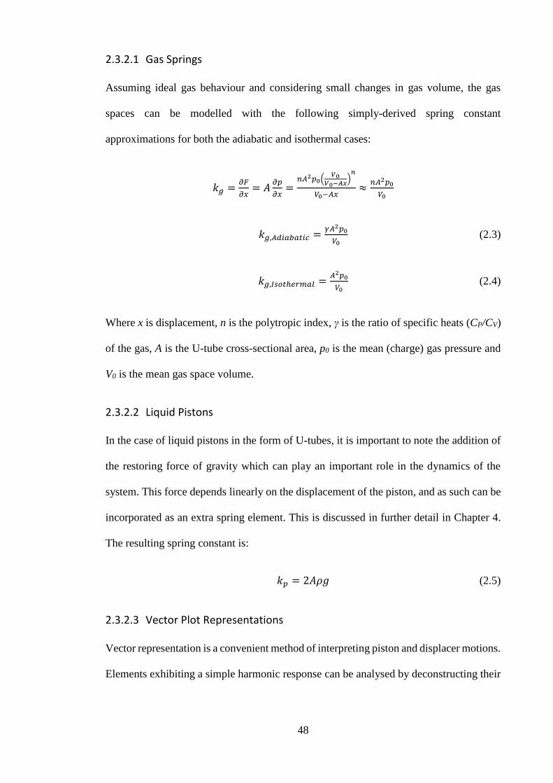
48

2.3.2.1 Gas Springs

Assuming ideal gas behaviour and considering small changes in gas volume, the gas

spaces can be modelled with the following simply-derived spring constant

approximations for both the adiabatic and isothermal cases:

𝑘𝑔 =𝜕𝐹

𝜕𝑥= 𝐴

𝜕𝑝

𝜕𝑥=

𝑛𝐴2𝑝0(𝑉0

𝑉0−𝐴𝑥)𝑛

𝑉0−𝐴𝑥≈

𝑛𝐴2𝑝0

𝑉0

𝑘𝑔,𝐴𝑑𝑖𝑎𝑏𝑎𝑡𝑖𝑐 =𝛾𝐴2𝑝0

𝑉0 (2.3)

𝑘𝑔,𝐼𝑠𝑜𝑡ℎ𝑒𝑟𝑚𝑎𝑙 =𝐴2𝑝0

𝑉0 (2.4)

Where x is displacement, n is the polytropic index, γ is the ratio of specific heats (CP/CV)

of the gas, A is the U-tube cross-sectional area, p0 is the mean (charge) gas pressure and

V0 is the mean gas space volume.

2.3.2.2 Liquid Pistons

In the case of liquid pistons in the form of U-tubes, it is important to note the addition of

the restoring force of gravity which can play an important role in the dynamics of the

system. This force depends linearly on the displacement of the piston, and as such can be

incorporated as an extra spring element. This is discussed in further detail in Chapter 4.

The resulting spring constant is:

𝑘𝑝 = 2𝐴𝜌𝑔 (2.5)

2.3.2.3 Vector Plot Representations

Vector representation is a convenient method of interpreting piston and displacer motions.

Elements exhibiting a simple harmonic response can be analysed by deconstructing their

49

displacement, velocity and acceleration functions. Earlier, the general solution for the

displacement of a mass element within a linear vibrating system was:

𝑥(𝑡) = 𝑋 cos(𝜔𝑡 + 𝜑)

By differentiating with respect to time, the following equations for velocity and

acceleration are obtained as:

�̇�(𝑡) = −𝜔𝑋 sin(𝜔𝑡 + 𝜑) (2.6)

�̈�(𝑡) = −𝜔2𝑋 cos(𝜔𝑡 + 𝜑) (2.7)

These functions can be plotted as rotating vectors with lengths equal to the coefficient

terms, X, ωX and ω2X, which represent the amplitudes of displacement, velocity and

acceleration respectively. The angle (ωt + φ) is measured anticlockwise from the positive

x-axis. As time, t, increases, the vectors rotate anti-clockwise about the origin, with each

revolution encapsulating the pistons’ progression through one cycle of physical

oscillation. Figure 2.11 shows the vector plot for the generic case described above.

Figure 2.11 – Vector representation of the generic solutions for piston or displacer motion.

50

Projecting the vectors onto the x-axis for any particular time yields their instantaneous

value, while the amplitudes provide maximum values, and the phase angles between

vectors can provide interesting insights into system dynamics. For example, in the above

case the acceleration vector leads the velocity vector by 90º, which also leads

displacement by 90º. This notation will be used extensively in the results and discussion

section of this thesis.

2.3.3 Power Estimation

At the beginning of any engine design process, it is important to attain rough estimates

for the power and efficiency of a machine based on general dimensions and operating

conditions. The ideal Stirling cycle pictured earlier in Figure 2.5 yields the following

formula for the cyclic work:

𝑊 = ∮𝑝𝑑𝑉 = 𝑚𝑅(𝑇𝐻 − 𝑇𝐶) ln (𝑉1

𝑉2)

where m is the gas mass, R is the gas constant, TH is the heat source temperature, TC is the

heat sink temperature, and V1 and V2 are the gas volumes at states 1 and 2 respectively.

Knowing the machine’s operating frequency, f, would therefore yield the power output

as:

𝑃 = 𝑓𝑊

Unfortunately, for the reasons previously mentioned in Section 2.2.4, the real Stirling

cycle is unable to match this level of performance. Work was conducted by Martini (1978)

in identifying an ‘experience factor’, F, which could be used to scale this power estimate

and account for the various real world losses. His work was taken further by William

Beale, who observed that the real power output of a number of machines was also

proportional to mean pressure, p0, and swept volume, VS. Walker (1979), West (1981),

51

and Senft (1982) then further expanded on Beale’s relationship to include temperature

dependence. The result was:

𝑃 = 𝐹𝑓𝑉𝑆𝑝0𝑇𝐻−𝑇𝐶

𝑇𝐻+𝑇𝐶 (2.8)

It should be noted that, in general, specific Stirling engine configurations share similar F

values, so designing unique or significantly different engines may require the

identification of more suitable F values. The average value of F is 0.25, but can be as

high as 0.35.

2.3.4 Frequency Estimation

In kinematic engines the frequency can be the most difficult parameter to estimate

accurately prior to the design process. The frequency depends on many factors that are as

yet undetermined, for example, the external loading profile. In the case of the FPSE,

however, since the frequency is essentially held constant by the overarching dynamics of

the system, it is possible to attain a good estimate for most configurations relatively

simply. The machine is approximated as a series of springs and masses, as previously

described in Section 2.3.2, and the natural frequency of the system obtained by evaluating

the system’s natural undamped response. An example of this is shown below for the

simple spring and mass system mentioned earlier. From Equation 2.7, the piston’s

acceleration is:

�̈�(𝑡) = −𝜔2𝑋 cos(𝜔𝑡 + 𝜑)

Substituting the above into the undamped equation of motion gives:

−𝑚𝜔2𝑋 cos(𝜔𝑡 + 𝜑) + 𝑘𝑋 cos(𝜔𝑡 + 𝜑) = 0

52

which simplifies to:

𝜔 = √𝑘

𝑚 or 𝑓 =

1

2𝜋√

𝑘

𝑚

Although this gives a good estimate for the operational frequency, in reality the true

frequency will vary depending on any loading, damping and the true nature of gas

expansion. Also, information about the piston amplitude is currently unknown and

requires more sophisticated analysis techniques to identify. These points are further

discussed in the following sections.

2.3.5 First Order Analysis

Stirling engine analysis methods are categorized into three tiers: first order, second order

and third order. The categorisation of these tiers is based on the level of complexity

employed in the analysis technique. First order analysis, being the simplest, utilises a

large number of assumptions intended to idealise the system. Numerous first order

analysis schemes have been proposed throughout the literature, however, they all utilise

a number of key assumptions first employed by Gustav Schmidt at the German

Polytechnic Institute of Prague in 1871 (Schmidt, 1871).

2.3.5.1 Schmidt Analysis

The Schmidt analysis considers the following simplifying assumptions:

1. The working fluid behaves as an ideal gas

2. The working fluid mass remains constant

3. The instantaneous gas pressure is uniform throughout each gas space

4. The gas space is comprised of isothermal sections

5. The mass elements (pistons and displacers) motion is sinusoidal or reflects simple

harmonic motion.

53

It is important to consider the validity of these assumptions. Assumptions 1 and 2 are

reasonable, especially in the case of FPSEs where the extent of sealing required can be

non-existent. Assumption 3 neglects fluid-friction-induced pressure drops across the

working space. These losses are usually more pronounced in high speed engines, so in

the case of lower frequency liquid piston engines the assumption is more acceptable.

The fourth assumption is where the most significant deviations from real systems occurs.

This step involves dividing the gas space into regions of constant temperature—for

example, a typical approach is to have three separate regions for the expansion,

compression and regenerator spaces—which essentially neglects any transient heat

transfer phenomenon occurring within these spaces, and assumes isothermal gas

behaviour throughout. This assumption also implies instantaneous temperature change

for mass flows to (and from) adjacent zones. Although this assumption considerably

decreases the potential accuracy of this analysis method, an important analytical

advantage is attained in its place. The pressure profile of the gas space is linearized with

respect to piston (and displacer) displacement, as the only factors affecting instantaneous

workspace pressure are the relative positions of associated mass elements. The workspace

pressure is given by the following equation:

𝑃 = 𝑚𝑅 (𝑉𝐸

𝑇𝐸+

𝑉𝑅

𝑇𝑅+

𝑉𝐶

𝑇𝐶)−1

(2.9)

where the subscripts E, R and C, refer to the expansion, regenerator and compression

spaces respectively. In the above case, the only variable quantities are the volumes in the

compression and expansion space, which depend on the mass element displacement

variables. Coupled with assumption 5, it is possible to integrate over a complete cycle

and obtain a closed-form expression for the cyclic work estimate. Assumption 5 is

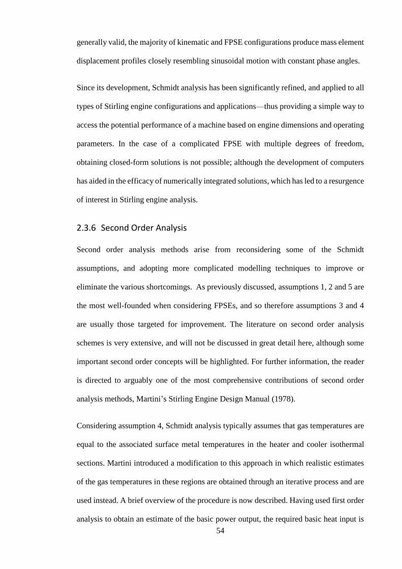
54

generally valid, the majority of kinematic and FPSE configurations produce mass element

displacement profiles closely resembling sinusoidal motion with constant phase angles.

Since its development, Schmidt analysis has been significantly refined, and applied to all

types of Stirling engine configurations and applications—thus providing a simple way to

access the potential performance of a machine based on engine dimensions and operating

parameters. In the case of a complicated FPSE with multiple degrees of freedom,

obtaining closed-form solutions is not possible; although the development of computers

has aided in the efficacy of numerically integrated solutions, which has led to a resurgence

of interest in Stirling engine analysis.

2.3.6 Second Order Analysis

Second order analysis methods arise from reconsidering some of the Schmidt

assumptions, and adopting more complicated modelling techniques to improve or

eliminate the various shortcomings. As previously discussed, assumptions 1, 2 and 5 are

the most well-founded when considering FPSEs, and so therefore assumptions 3 and 4

are usually those targeted for improvement. The literature on second order analysis

schemes is very extensive, and will not be discussed in great detail here, although some

important second order concepts will be highlighted. For further information, the reader

is directed to arguably one of the most comprehensive contributions of second order

analysis methods, Martini’s Stirling Engine Design Manual (1978).

Considering assumption 4, Schmidt analysis typically assumes that gas temperatures are

equal to the associated surface metal temperatures in the heater and cooler isothermal

sections. Martini introduced a modification to this approach in which realistic estimates

of the gas temperatures in these regions are obtained through an iterative process and are

used instead. A brief overview of the procedure is now described. Having used first order

analysis to obtain an estimate of the basic power output, the required basic heat input is

55

obtained by dividing by the Carnot efficiency. Estimates of various losses such as gas

conduction, radiation, shuttle losses, regenerator losses, flow losses and others are then

added to this basic heat input to yield the net heat input, which is the total heat supply

required per cycle. The heat transfer coefficient for the high temperature heat exchanger

is then calculated, and used to equate the gas-to-metal temperature difference required to

achieve the aforementioned net heat input. A similar approach is taken for the cooler side.

The newly identified gas temperatures can then be used in the Schmidt analysis to obtain

a more realistic basic power output, and the process repeated until the gas temperatures

converge. In the modern era, iterative calculations like that described above are trivial

and essentially instantaneous when carried out by computers. The majority of time is

spent on establishing the algorithms necessary. For this reason, it can be desirable to

consider third order analysis schemes, as they can demand a similar amount of setting up,

but produce more accurate results.

2.3.7 Third Order Analysis

Third order analysis is the most intricate approach to the simulation of Stirling systems,

and aims to remove the need for many of the simplifying assumptions employed for first

and second order analysis. This is done by attempting to evaluate the entire spectrum of

thermo-fluid interactions experienced by the working gas throughout the operation of the

machine, as well as the energy flows existing through and into the machine components.

Computational modelling has become popular in number of mechanical engineering

fields, and most undergraduate programs offer specialised courses on computational fluid

mechanics and computational solid mechanics. Third order analysis essentially employs

aspects of these fundamental modelling techniques, while also incorporating the specifics

associated with Stirling engine processes. As with second order analysis schemes, the

literature on third order methods is very extensive and is not critically important in the

56

context of this thesis. A brief summary of the general approach is outlined here, with

further detail of the specific modelling software and approach used in this project

presented in Section 4.2.

The procedure begins by discretising the gas space volume into a number of individual

cells. The fundamental conservation equations of mass, energy and momentum are

constructed for each cell, and continuity conditions established between adjacent cells to

create a network of interconnected equations for fluid properties. By applying certain

boundary conditions based on the real-life machine configurations and empirical

correlations when necessary, the vast system of equations can be solved numerically over

a predefined time interval. The resolution of the matrix of cells can be increased along

with the time increment until the solution becomes independent of both, resulting in

numerically assessable profiles for the gas pressure(s) and mass element motion(s). From

these functions, the machine performance indicators can be evaluated and operating

parameters adjusted for the purposes of design improvements or general understanding.

In recent decades a number of specialised software entities have been developed for

conducting the complex analysis described above, some specifically for Stirling engines

(Dyson, Wilson, & Tew, 2004).

57

3 Heat-powered Liquid Piston Stirling Cooler Test-rig

3.1 Preliminary Design

The initial LPSC test-rig was designed and commissioned at FH Rosenheim, Germany.

Figure 3.1 shows the test-rig assembly when the experimental investigation began in late

2013.

Figure 3.1 – First liquid piston Stirling cooler (LPSC) set-up with U-tubes.

58

The image shows each of the four gas spaces, embodied by the ‘H’ shaped housings,

resting above the wooden support structure, two in the foreground and two in the

background. Each of these is connected in series to the adjacent housing sections via a

steel U-tube, which completes the desired geometry of the system, as portrayed in Figure

3.2. Also shown are the designations of each of the four gas spaces (GS1–GS4) and

pistons (Pistons A–D), which are frequently referred to throughout the rest of this thesis.

Figure 3.2 – Liquid piston Stirling cooler Schematic.

It was anticipated that the machine’s performance would be sensitive to small changes in

certain system parameters, such as the diameter or volume of liquid pistons, the clearance

between the liquid piston surface and the entrance to the heat exchangers, the mean

pressure (or charge pressure) in the gas spaces or the number of absorbers versus heaters.

For this reason, the design of the test-rig allowed changes in the geometry of the system

so that its performance across a range of operating conditions could be analysed. For

example, the liquid piston U-tubes can be exchanged with others of different diameters.

Figure 3.3 shows an indicative schematic of a quarter section of the overall system and

identifies where the measurement equipment takes readings for data collection. The

arrangement is the same for each of the four subsystems. Since the primary interest is in

the behaviour of the liquid piston Stirling system, the heat input does not come from a

59

solar source but instead is supplied by electric heating cartridges used in conjunction with

a heat exchanger. This enables more efficient, simplified experimentation with a constant

and reliable heat source. An integrated solar collector system will potentially be

considered for future research.

Figure 3.3 – Subsystem composition. The LPSC machine is comprised of four of these units connected in series.

In terms of data collection, eight thermocouples are installed in the gas spaces directly

under each heat exchanger. These provide real-time temperatures of the gas in each of the

compression and expansion spaces. Four pressure transducers are installed on the cold

side of each gas space below the temperature sensor ports. All of these measurement

devices are used in conjunction with LabVIEW to monitor, organise and collect the data

for analysis. The engineering design software SolidWorks was employed to design the

heat exchanger, regenerator and housing components.

60

3.1.1 Heat Exchangers

All eight heat exchangers used in the LPSC machine are identical in design and were

manufactured in Rosenheim, Germany. Figures 3.4 and 3.5 show the annular finned

design employed in the system.

Figure 3.4 – Brass heat exchanger showing side view of the annular fins and protrusion for heating cartridge access (RHS).

Figure 3.5 – Brass heat exchanger end showing a view of the annular fins (note that the large channel is for temperature probe installation access).

61

These components were designed prior to the commencement of this investigation, and

as such, will not be discussed in great detail. Brass was the chosen material, because of

its favourable heat transfer properties and malleability for the intricate component

geometry. Each heat exchanger incorporates an internal bored section which is exposed

to atmosphere and not connected to the hermetically sealed gas space. In the case of the

four ‘hot’ heat exchangers, this bore is fitted with a cylindrical electric heating cartridge,

which provides the heat input to the system. Each heater can be individually isolated, and

when one of the heaters is not activated that space then becomes a potential absorber, i.e.

as a result of the relative motions of adjacent liquid pistons, the working gas is forced to

expand, drawing heat from the surrounding housing, and lowering its temperature. The

four ‘cold’ heat exchangers have an internal cold water fitting, and during operation this

provides a steady flow of cooling water into (and out of) the cavity, in order to transport

the rejected heat. Each of the four fittings is connected in series with a PVC tube and fed

by a single water supply.

3.1.2 Housing and Regenerator

The housing components are constructed out of stainless steel. They encapsulate the gas

space around the heat exchangers, and provide the structural support for the regenerator

matrix occupying the space between the hot and cold sides. There are eight individual

housing components—one for each heat exchanger. They are connected via vacuum seals

and clamped together to form a hermetically sealed space. Figure 3.6 shows an individual

housing component, and Figure 3.7 shows a version preassembled with a heat exchanger.

62

Figure 3.6 – Stainless Steel housing component.

Figure 3.7 – Stainless Steel housing component assembled with brass heat exchanger and vacuum clamp.

63

The space between the top surface of the heat exchanger fins on the hot side and the top

surface of the heat exchanger fins on the cold side is filled with regenerator material. In

order to permit swift assembly and disassembly the material used was steel shot: small

steel spheres approximately 1 mm in diameter. Each half of the ‘H’ housing is filled

separately before covering the open surface with a thin steel mesh to contain the steel

shot, then clamping both faces of the regenerator together. Figure 3.8 shows the steel shot

regenerator material.

Figure 3.8 – Steel shot material used in the regenerators (with an average diameter of 1 mm).

3.1.3 Liquid Pistons

Standard steel tubing was selected as the material for the piston tubes. This material was

selected over other potential options primarily to allow for the potential variation in piston

tube dimension. Each U-tube is divided into two parts. The largest of these two parts

comprises 75% of the whole U-tube, and attaches to the underside of the hot heat

64

exchanger housing via an expansion flange—which also incorporates the pressure and

temperature sensor ports shown in Figure 3.9.

Figure 3.9 – Liquid piston housing U-tubes with expansion flange fittings.

The same vacuum seal and clamp attachments (common to the whole set-up) are used to

fix the flange to the heat exchanger housings. To complete the U-tube assembly, a smaller

section of straight tube extends from the underside of the cold heat exchanger with the

same expansion flange, and both U-tube openings are connected via a clear PVC tube

section. This provides viewing access to the liquid piston surface, which is crucial in

assessing system operation and troubleshooting. When installed, the PVC tube is heated

in hot water and slid over the ends of both tube sections before being fixed in place via

ring clamps. The initial steel tube size utilised was 15 mm outer diameter, with 1 mm wall

thickness, whereas the PVC had an average internal diameter of 12.3 mm. Liquid water

is measured out and added to each of the U-tubes, resulting in functional U-shaped liquid

pistons.

3.1.4 PID Controller

The power supplied to the heating cartridges is regulated by a PID controller, in

conjunction with a Solid State Relay (SSR) that is linked to a thermocouple in contact

65

with the interior surface of one of the heat exchanger’s fins. The circuit diagram for this

configuration is shown below in Figure 3.10.

Figure 3.10 – Controller Circuit for regulating the power supply to the heaters.

This arrangement allows for the heat source temperature to be set and remain constant

over the course of each experiment. It should be noted that out of the four potential heaters

only one heat exchanger fin temperature is monitored and controlled. The other heater(s)

are connected in parallel so that they are all supplied with the same amount of power, and

thus heat input (assuming similar thermal resistances, etc.). Figure 3.11 shows the PID

controller installation, including an isolation box containing all of the associated circuitry

and the SSR. The user interface displays the set-point temperature (green) and the current

temperature (red).

66

Figure 3.11 – PID controller and SSR housing images.

3.1.5 Temperature and Pressure Sensors

Aside from the temperature sensor that was used to measure the fin surface temperature

of the primary hot heat exchanger, eight additional temperature sensors were employed

for data collection. All eight sensors were installed through ¼-inch compression fittings

in the walls of the liquid piston expansion flanges (situated just below the gas entry points

into the hot and cold heat exchangers). This was identified clearly in Figure 3.3 in

Section 3.1 and also shown in Figure 3.12. The purpose of these temperature sensors was

to collect gas temperature data on both the hot and cold sides of the gas space. The types

of thermocouples used were J-type sheathed thermocouples. The sizes used were either

the 1.5 mm × 150 mm or the 1.5 mm × 100 mm variety, as these were readily available

within the laboratory. The thermocouples where calibrated using single point calibration

at the boiling point of water.

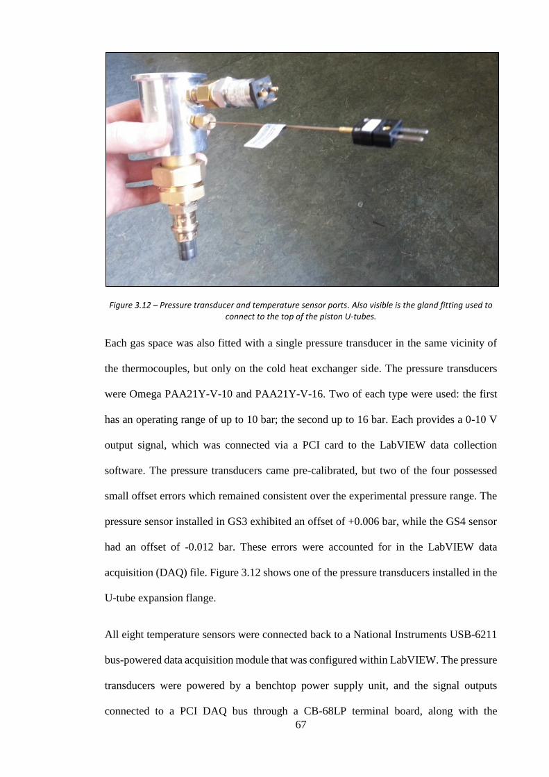
67

Figure 3.12 – Pressure transducer and temperature sensor ports. Also visible is the gland fitting used to connect to the top of the piston U-tubes.

Each gas space was also fitted with a single pressure transducer in the same vicinity of

the thermocouples, but only on the cold heat exchanger side. The pressure transducers

were Omega PAA21Y-V-10 and PAA21Y-V-16. Two of each type were used: the first

has an operating range of up to 10 bar; the second up to 16 bar. Each provides a 0-10 V

output signal, which was connected via a PCI card to the LabVIEW data collection

software. The pressure transducers came pre-calibrated, but two of the four possessed

small offset errors which remained consistent over the experimental pressure range. The

pressure sensor installed in GS3 exhibited an offset of +0.006 bar, while the GS4 sensor

had an offset of -0.012 bar. These errors were accounted for in the LabVIEW data

acquisition (DAQ) file. Figure 3.12 shows one of the pressure transducers installed in the

U-tube expansion flange.

All eight temperature sensors were connected back to a National Instruments USB-6211

bus-powered data acquisition module that was configured within LabVIEW. The pressure

transducers were powered by a benchtop power supply unit, and the signal outputs

connected to a PCI DAQ bus through a CB-68LP terminal board, along with the

68

displacement sensors discussed in the next section. The same LabVIEW file was used to

configure the sensor outputs for data acquisition.

3.1.6 Piston Displacement Sensors

A capacitive sensor was used to measure the displacement of the liquid pistons. The

capacitance of a parallel-plate capacitor is given in the following equation:

𝐶𝑝 = 𝜀𝑟𝜀0𝐴𝑝

𝑑𝑝 (3.1)

where ɛr is the dielectric constant of the material between the plates, ɛ0 is the electric

constant, Ap is the plate area and dp is the separation distance between the plates.

The capacitor enshrouds the displacement range of one surface of a liquid piston. Since

water is a far better dielectric than air (or helium/hydrogen), the capacitance of the

capacitor changes significantly as the piston surface moves up and down. Based on the

above equation, this change should be close to linear and can be used to measure liquid

piston displacement during operation. This approach was chosen to combat the potential

irregularities in the liquid surface during oscillation since the measured capacitance

would primarily depend on the volume of water encased within the measurement space.

Figure 3.13 – Capacitive sensor setup for measuring piston displacement.

69

In the original set-up two capacitors were used for each piston in the manner shown in

Figure 3.13. One would be installed across a lower section of the U-tube where the liquid

surface never crossed in order to act as a reference capacitance. The second capacitor

would be installed so that its centre was bisected by the resting position of the liquid

piston surface. During operation, as the surface moved up and down, the changing volume

of liquid contained within the capacitor would vary its capacitance. Figure 3.14, shows

the initial set-up of the capacitive sensors.

Figure 3.14 – First generation capacitive sensors used for measuring liquid piston displacements.

70

The sensors were constructed from copper film which could be cut and shaped to fit the

shape of the piston tubes being used. The electrodes were then connected in pairs via a

Wheatstone bridge which compared the variable capacitance to the reference

capacitance—and led back to a common circuit board which included amplification,

filtering and rectification procedures, before providing 0–10 V output signals for the PCI

board and DAQ system. A circuit diagram of this system can be found in Appendix I.

This technique was employed in the initial experiments and was found to have a very high

sensitivity, and a capability to tolerate high oscillation frequencies. The capacitive sensors

went through many iterations and ended up causing substantial delays in the experimental

process. Their commissioning, calibration and performance is discussed further in

Sections 3.2.3 and 6.1.

3.2 Commissioning and Modifications

Before experimentation began, it was unknown whether the system would be capable of

self-starting, or indeed starting at all. It was also unclear over what range of operating

conditions the liquid piston surfaces would remain stable, as this would depend on the

frequency and amplitude of any oscillation. Fortunately, the system did prove to be self-

starting when preliminary testing began. A period of practical problem-solving followed

the initial testing, which involved making alterations to the test-rig in order to improve

its functionality, usability and controllability. These alterations are summarised below.

3.2.1 Piston Floats

One of the major adaptations was the inclusion of piston floats. At the beginning of the

project it was unclear as to whether some form of piston float would be required. In the

ideal scenario, piston surface instability would be mitigated through indirect means, i.e.

via geometric design and the prevailing operating conditions such as frequency, charge

pressure and piston dimensions. Unfortunately, in order to determine whether such

71

operating conditions existed, the system first needed to be well understood and optimised.

Preliminary results revealed that the liquid pistons became unstable (and their surfaces

would disintegrate) at charge pressures above 2 bar. With the scope of the investigation

including pressures up to 6 bar, some form of surface stability measure was required. It

was decided that piston floats would be therefore incorporated into the test-rig—in order

to limit the disintegration of the liquid piston surfaces as piston amplitude and frequency

increased with charge pressure beyond stable limits.

Very little research has been conducted in the field of liquid piston float design and any

mention of them is vague and unspecific. Therefore, the floats incorporated were of an

original design. As previously mentioned, however, optimisation of float design would

likely prove redundant as the piston geometry is varied throughout the experimental

investigation. For this reason, the development of the optimised piston floats was

identified as being of secondary importance to the main objective of evaluating

performance trends.

A number of potential float options were considered and tested. Submerged floats were

selected over above-surface floats for simplicity reasons. The two main factors of float

design are geometry and material. The material must be water and heat resistant and have

a density lower than that of water, while the geometry must be simple to produce. It was

theorized that the most suitable material would have a density relatively close to that of

water, so that during operation the float would retain its vertical position relative to the

liquid surface as it moved up and down—as opposed to oscillating above and below the

surface due to buoyancy and inertial effects. The different materials tested included wood,

polystyrene, and polyethylene.

Following a number of trial experiments—using various float prototypes—polyethylene

cylindrical floats were eventually selected as they outperformed the other options, and

72

could be easily machined to varying dimensions in the workshop. The density of the

polyethylene used was also the closest to that of water—being one of the only plastics

with a relative density of less than one.

Initially, 10 mm × 20 mm cylindrical polyethylene floats were installed. But at the higher

end of the temperature and pressure ranges to be investigated, a significant amount of

piston water was still able to by-pass the floats, and interfere with the temperature sensors

above. It became apparent that an optimal float diameter would exist, where the clearance

created would be sufficiently small to reduce piston leakage, whilst remaining large

enough not to increase the annular fluid friction too much. Eventually piston floats of

diameter 11.5 mm (PVC tube side) and 12 mm (steel tube side) and 20 mm in length were

settled upon. An example of the floats used can be seen in Figure 3.15.

Figure 3.15 – Cylindrical polyethylene liquid piston float for improved surface stability.

73

Figure 3.16 – Gas temperature stability comparison for different float diameters. Experiments were conducted with the 3HEAT configuration with 150 °C heaters and 4 bar charge pressure.

Figure 3.16 shows how the change from 11 mm floats on both sides of the U-tubes (to

11.5 mm and 12 mm floats) improved piston stability. The irregular readings from the

11 mm experiment are presumed to result from water droplets bypassing the piston floats

and interfering with the thermocouple installed above. By increasing float diameter, the

clearance gap was reduced, increasing the effects of surface tension and limiting the

possibility for water droplets to escape. The 11.5 mm and 12 mm floats resulted in more

stable temperature readings and the stability improvements were also visually apparent

when observed through the PVC tube section. The larger floats did hinder the self-starting

ability of the system, particularly at lower charge pressures. This meant that ‘jump starts’

were required more frequently1. Conversely, operation was now stable for higher

pressures and temperatures, which was of greater importance.

1 Jump starting the system involved manually exciting a small piston amplitude by pulsating the piston

housing at close to the expected frequency.

90

92

94

96

98

100

102

104

0 50 100 150 200 250 300 350 400 450 500

Ho

t si

de

gas

te

mp

era

ture

(ºC

)

Time (s)

12 mm & 11.5 mm OD floats 11 mm OD floats

74

Figure 3.17 – The impact of piston float diameter on the development of pressure amplitudes within the gas spaces.

Figure 3.17 shows how the pressure amplitude was affected by the change in piston float

diameter. At lower charge pressures, the larger floats have more of an impact on stifling

operation; however, as mean pressure or temperature increases, this effect is less evident.

In this case the additional benefits on piston and temperature stability become more

relevant. For this reason, the subsequent experimental investigation continued with the

11.5 mm (PVC side) and 12 mm (steel side) floats installed within the 15 mm piston

tubes. A more substantive investigation into float design could be of value to the future

of this system (or any similar liquid piston machines) and is discussed in Chapter 8.

3.2.2 Pressure Manifold

A pressure manifold was installed as an interface between the main compressed air line

and the feed lines of the individual gas spaces. During the commissioning phase it became

apparent that each of the four gas spaces required independent control and isolation valves

0

0.02

0.04

0.06

0.08

0.1

0.12

0.14

0.16

0.18

0 1 2 3 4 5 6 7

Pre

ssu

re a

mp

litu

de

(b

ar)

Charge pressure (bar)

12 mm floats (150 °C) 12 mm floats (120 °C)

11 mm floats (150 °C) 11 mm floats (120 °C)

75

in order to manage charging/discharging as well as for isolating each space during

operation and locating pressure leakages. A schematic of the manifold is shown in Figure

3.18.

Figure 3.18 – Pressure manifold with individual control valves for each subsystem.

3.2.3 Displacement Sensors

The displacement sensors proved to be the most time-consuming and troublesome of all

aspects of the experimental investigation. Numerous iterations of the sensors were tested

and modified following the establishment of the basic principles of operation (using the

set-up outlined in Section 3.1.6). The largest obstacles faced in commissioning the

76

displacement sensors to a satisfactory level were those of signal noise and calibration. It

was discovered that the output signal from the displacement sensors was very sensitive

to any handling of the sensor wires—and also their proximity to any other sensor wires.

An extensive trial and error procedure was initiated in order to solve this problem. Some

examples of the attempted fixes included moving the reference capacitor sensors from the

test-rig to an entirely separate duplicate set of U-tubes situated nearby, as well as

reconfiguring the circuity of the sensor system multiple times in order to eliminate

potential ground loop interference. Eventually, the noise issue was mitigated by installing

shielded cable wires of exactly equal length for the sense and drive electrodes—and

disconnecting the reference sensors entirely, and replacing them with a miniature

breadboard equipped with an array of small ceramic capacitors. Since the reference

capacitance does not change during normal operation, it can be provided by a separate

input source. Figure 3.19 shows the breadboard and capacitive sensor circuit set-up prior

to its installation on the test-rig stand.

Figure 3.19 – Capacitive sensor circuit with reference capacitors.

77

In this form, each reference capacitor is represented by two 30 µF capacitors in parallel,

creating a total capacitance of 60 µF. This arrangement was found to produce the highest

signal resolution for the 15 mm piston tubes through the LabVIEW interface. It should

be noted that the reference capacitance required is specific to each piston diameter and

U-tube material in use. By removing the reference capacitor from the sensor installation

on the piston tube, the measurement stroke range is effectively doubled since the sense

electrode can be increased in length to match that of the drive electrode. A beneficial

consequence of this modification is that the range of piston masses available for testing

for each set of U-tubes is increased. Following the successful elimination of signal noise,

the displacement sensors could now be calibrated. Figure 3.20 shows the typical

displacement sensor output data over a period of one second.

Figure 3.20 – Piston displacement profiles over one second interval during a typical experiment. This experiment was at 3 bar and 105ºC with 100 ml liquid pistons.

From this information, the piston phase angles and amplitudes can be determined. It

should be noted that the difference in vertical offsets of the data is due to the differences

2.5

3

3.5

4

4.5

5

5.5

0 200 400 600 800 1000

Dis

pla

cem

en

t se

nso

r o

utp

ut

(V)

Time (ms)

Piston A Piston B Piston C Piston D

78

in physical sensors and their positioning on the U-tubes themselves. The phase angles are

calculated by using the least mean squares method to approximate the displacement

profiles as sine functions, as shown in Figure 3.21.

Figure 3.21 – Example of phasor representation and optimisation for Piston A displacement profile using least mean squares approximation.

The phasor approximation of the piston displacement profile thus developed shows good

agreement with the actual displacement profile measured by the capacitive sensors—

indicating that the assumption of simple harmonic motion is valid. The final requirement

was to calibrate the sensor voltage output with actual piston amplitude. Due to the slight

geometric and spatial differences, each of the four sensors needed to be calibrated

separately. In order to calibrate the sensors, 8-times slow motion video of the piston

motion was recorded at increasing levels of piston amplitude and frequency. Each piston

U-tube was fitted with an external scale covering the PVC tube section where the piston

surface oscillates, as shown in Figure 3.22.

2.5

3

3.5

4

4.5

5

5.5

0 200 400 600 800 1000

Dis

pla

cem

en

t se

nso

r o

utp

ut

(V)

Time (ms)

Sensor measurements Phasor approximation

79

Figure 3.22 – Scales for calibrating displacement sensors with slow motion video recordings.

Figure 3.23 – Displacement sensor 4 calibration curve comparing sample experiment readings with slow motion video displacements.

The piston amplitudes obtained from the slow motion videos were compared with the

output signals from the capacitive sensors. Each sensor behaved similarly during

y = 5.8504x2 + 3.2769xR² = 0.9934

0

1

2

3

4

5

6

0 0.1 0.2 0.3 0.4 0.5 0.6 0.7 0.8

Pis

ton

am

plit

ud

e (

cm)

Sensor amplitude (V)

2Bar 3Bar 4Bar 5Bar 6Bar Poly. (Sensor 4)

80

calibration with slight differences in the calibration coefficients. Figure 3.23 shows the

relationship between piston amplitude and sensor output for one of the four sensors. In

each of the four cases, the correlation between observed piston amplitude and sensor

output appeared to closely resemble the quadratic form. When the idea of using capacitive

displacement sensors was first discussed, it was theorized that this relationship would be

linear. The capacitance of the section of the U-tube enclosed between the copper plates

does increase linearly with an increase in water level as long as the piston surface is not

in motion. This can be seen in Equation 3.1 from section 3.1.6 where capacitance is

proportional to the dielectric constant. Since the dielectric constant of water is far greater

than air, the aggregate dielectric constant is proportional to the volume of liquid water

within the sensor. The problem is that this equation is only valid for materials with

symmetric material thickness through all vertical cross sections. As the liquid piston

oscillates, a thin layer of water develops on the inner surface of the U-tube. This has the

effect of increasing the average overall capacitance measured by the sensor.

Figure 3.24 – Comparison of surface profiles between moving and stationary liquid pistons.

81

It is easiest to understand how this happens by considering the two capacitive limits

measured by the sensor, these are shown in Figure 3.24. At top dead centre (TDC) the

piston surface is roughly flat and the maximum capacitance is measured. At bottom dead

centre (BDC) however, a layer of water film remains on a section of the U-tube above the

piston surface. The capacitance measured at this position is higher than that which would

be measured if the piston was given time to settle and acquire a flat surface, i.e. as per the

stationary piston on the right hand side. Since the measured capacitance is higher at BDC,

but roughly the same at TDC, the total range measured by the sensors is less than a

corresponding set of flat surfaces (despite the same change in volume). This phenomenon

becomes more pronounced as piston amplitude and frequency increase, thickening and

spreading out the water layer. As a result, the capacitive sensors underestimate piston

amplitude by larger and larger degrees as the actual amplitude increases, resulting in the

quadratic relationship pictured earlier.

Fortunately, the correlation appears to be predictable, and does not appear to depend

significantly on system charge pressure (although a slight dependence was observed).

Quadratic trend lines were fitted to the calibration data. The quadratic trend lines fitted to

the calibration data were used in all subsequent testing involving the 15 mm U-tubes, and

are shown in table 3.1.

Table 3.1 – Displacement Sensor Calibration Coefficients. Fitted for y = Ax2 + Bx, where y is piston amplitude (cm) and x is the sensor output (V).

Sensor Calibration coefficients

A B

A 5.501 3.140

B 6.337 3.040

C 5.381 3.057

D 5.850 3.277

82

3.2.4 Minor Alterations

Many minor improvements were also implemented throughout the commissioning and

experimentation phase. The previously used PVC hose sections were increased in length

by a factor of three to encompass the majority of one side of the U-tube. This allowed the

displacement sensors to cover a greater potential amplitude range, and also enabled a

larger range of liquid piston volumes/masses to be investigated. The clear PVC hose was

replaced by fibre-reinforced PVC hose capable of withstanding up to 10 bar at 60ºC. The

previous un-reinforced hose’s structural integrity became compromised due to heat

conduction from the hot side of the U-tube after prolonged use. Gland fittings (¾-inch)

were installed at the top of each U-tube connection to facilitate piston access. This

allowed each piston to be removed in isolation, without needing to take apart the housing

components. It also allowed for the potential of easily installing piston U-tubes of

different diameters, without altering the housing connections.

3.2.5 Experimental Accuracy

The main sources of error in the experimentation process come from the pressure,

temperature, and displacement sensors. The pressure transducers have a stated total error

range of ± 1%, however as described in Section 3.1.5, all four were calibrated together

and resulting pressure tests showed agreement to 4 significant figures over the entire

testing range. Although this does not necessarily guarantee true accuracy, it does indicate

that the measured pressure amplitudes are very accurate and consistent across the four

subsystems. Similarly, the stated error range of the thermocouples was ± 0.75%, however

these were also recalibrated in the lab using a single point calibration test at the boiling

point of water. In the case of the capacitive displacement sensors, the calibration method

(outlined in Section 3.2.3) showed that a calibration curve could be fitted to the

experimental data with a high R2 value. The experimental error involved in their use was

83

conservatively estimated to be ± 10%, although for reasons discussed further in

Section 6.1, the use of the capacitive sensors for piston displacement information was not

continued for the second iteration of the experimental investigation. Instead an optical

method was used, with an estimated error of ± 2.5 mm.

During the commissioning and early experimentation processes, it was identified that the

system’s behaviour was very transient in nature. Aside from the modal behaviour

discussed in Chapter 5, the pressure amplitudes, piston displacements, and other

measured variables showed gradual cyclic variation, even well after sufficient time had

been allowed for the system to reach steady-state operation. This cyclic variation is not

unexpected for a complex system such as the LPSC, where each of the four subsystems

has direct, uncontrolled influence over its neighbouring subsystems. In order to collect

data points for the experimental analysis, a time period of steady-state behaviour was

identified for each experiment (of at least 5 minutes in length), and the parameters of

interest were averaged over this period (see Section 5.1). In the majority of experiments,

the cyclic variations contributed more significantly to the experimental uncertainty of the

data than the accuracy of the data collection instrumentation itself. For this reason, and

considering the current stage of the research project, the inclusion of a thorough error

analysis in this thesis was decided against. With future test-rig and model refinement, the

inclusion of error analysis will be re-evaluated.

3.2.6 Commissioned Test-rig Setup

After completing all of the necessary test-rig upgrades and commissioning procedures,

the test-rig was ready for the primary data collection phase. Figure 3.25 shows the final

state of the test-rig.

84

Figure 3.25 – Fully commissioned 15 mm OD piston tube test-rig.

3.3 Operating Configurations

The performance of the LPSC system can be evaluated in four different configurations.

Operation with either 4, 3, 2 or 1 of the installed heaters can be selected, resulting in either

0, 1, 2 or 3 potential absorption spaces respectively. It was decided that the first three of

85

these would be investigated. These operating configurations will be referred to frequently

throughout this document and as such are given the following abbreviations:

4HEAT – 4 Heaters, 0 Absorbers

3HEAT – 3 Heaters, 1 Absorber

2HEAT – 2 Heaters, 2 Absorbers

It should be noted that the reason the one-heater configuration is not considered is because

it is unlikely that only one heater would be able to sustain operation of the other three

subsystems—especially in light of the relatively low heat source temperatures being

investigated within the scope of this research project. The results and discussions in later

sections of this document will rely on this terminology, and schematics and descriptions

clarifying the three configurations are shown below for reference. As identified in the

literature review, and stated in Section 1.4, only the 3HEAT configuration has been

successfully tested by other research groups.

3.3.1 4HEAT Configuration

Figure 3.26 shows the ‘4HEAT’ configuration. The 4HEAT configuration occurs when

all four heaters are turned on during operation. In this state, the system essentially

becomes four forward heat engines in series—with the work produced only needing to

overcome system friction in order to sustain operation. As a result, the 4HEAT

configuration requires the lowest heater temperatures in order to achieve stable operation.

Although obviously lacking any potential for cooling, this configuration is very useful for

the purposes of computer model validation, and checking for inconsistencies in the

behaviour of the four subsystems.

86

Figure 3.26 – 4HEAT configuration (4 Heaters, 0 Absorbers).


The second configuration to be tested was termed ‘3HEAT’ and is where all but one

heater is powered. The remaining unpowered hot heat exchanger space then becomes the

only absorber, and experiences any cooling that the system is able to produce. The

3HEAT configuration is shown in Figure 3.27.

Figure 3.27 – 3HEAT configuration (3 Heaters, 1 Absorber).

87


The final configuration, ‘2HEAT’ is the same as that displayed earlier in Figure 1.6, with

two adjacent heaters being powered, and the two remaining unpowered heaters behaving

as absorbers. It should be noted that with two powered heaters there is a choice: (a)

alternate in series between heater/absorber, or (b) couple the two heaters next to each

other. Both configurations are shown below in Figures 3.28 and 3.29.

Figure 3.28 – 2HEAT configuration (a) with alternating heaters and absorbers (2 Heaters, 2 Absorbers).

Figure 3.29 – 2HEAT configuration (b) with adjacent heaters (2 Heaters, 2 Absorbers).

88

Somewhat paradoxically, only arrangement (b) was operable, an explanation for why this

was the case is suggested in Section 8.1.2. Unless otherwise specified, the term 2HEAT

will be used when referring to the adjacent configuration.

3.4 Experimental Parameters

The key design parameters chosen for variation in this investigation were heater

temperature, piston mass, and mean operating pressure. Initially only one piston diameter

was tested. The aim of the first investigation was to validate the computer models and to

identify piston dimensions for the next stage, which would hopefully improve system

performance. Table 3.2 shows the range of independent variables which were employed

for the first set of experiments.

Table 3.2 – Set of parameters for first experimental investigation.

Piston tube outer diameter (mm)

Configuration Liquid piston volume (ml)

Heater surface temperature (°C)

Gas charge pressure (bar)

15 4HEAT 100 95, 100, 105 1-6

15 4HEAT 115 95, 100, 105 1-6

15 3HEAT 100 130, 140, 150 1-6

15 3HEAT 115 130, 140, 150 1-6

15 2HEAT 115 190 1-6

Two different piston masses were investigated, without any other changes to the system

geometry, i.e. when adding piston mass (liquid water), the resulting working gas volume

necessarily reduced so that the total internal volume of the system remained constant. For

each operating configuration, experiments were carried out by varying the charge

pressure by 0.5 bar increments, starting from atmospheric pressure (1 bar) up to the

maximum pressure attainable with the local compressed air line (6 bar). The heater

temperatures at which operation would begin were initially unknown, and as such were

arrived upon by trial and error. The lowest corresponded to the situation where just

enough heat was supplied for self-sustaining operation at the lower charge pressures; the

89

highest corresponded to higher charge pressures where the pistons become borderline

unstable. A third temperature directly in between these two limits was added to help with

experimental consistency. Encouragingly, the temperature ranges identified are similar to

that which can be supplied by various forms of solar collectors (IEA, 2011). The 2HEAT

experiments were only conducted at a temperature of 190°C. Notably missing from the

table are the 2HEAT experiments with 100 ml pistons. For this configuration and piston

mass, operation was unable to be achieved within the allowable maximum heater

temperature of 200°C.

3.5 Experimental Procedure

A sequential list summarising the individual experimental procedure is outlined below.

1. A visual check over of the test-rig is conducted—the PVC hose ring clamps and the

cooling water supply hoses are checked for water leaks. The compressed air regulation

valve is set at 0-gauge pressure, and the gas spaces decompressed from the previous

experiment. The isolation valve for each subsystem is opened, and a check is made that

the visible liquid piston surfaces are level with each other. The piston floats are checked

for air bubbles or any level of unusual submergence. The grounding cables connecting all

four housing compartments are checked to ensure a common ground. The number of

connected heaters is checked against the desired configuration (4HEAT, 3HEAT or

2HEAT) and the hot heat exchangers are noted for safety reasons. The DAQ computer is

booted and LabVIEW initialised. The neutral outputs from the pressure, temperature and

displacement sensors are checked.

2. The cooling water supply is turned on—this is done first to give time for the

temperature on the rejection side to stabilise.

90

3. The gas spaces are pressurised—the main isolation valve on the manifold is opened

and—if this is the first experiment of the day—a pressure test is conducted at 6 bar;

otherwise the pressure is gradually increased to the required level. Close attention is paid

to the surfaces of the liquid pistons, as any sudden motion may indicate a leak. The main

isolation valve is closed.

4. The heaters are powered—the heater control unit is plugged in and the heater

temperature set on the PID interface. The gas temperatures are monitored through

LabVIEW until they reach the range known to sustain operation. This can take up to 5

minutes.

5. The system’s temperatures are normalised—the four isolation valves are closed, and

the system coaxed into motion via manual jump start if necessary. This initial operation

moves gas through the heat exchangers and regenerator, and allows for the temperature

profiles of the gas and housing to regulate to a level close to steady state. At this time,

quite often the piston neutral positions will become offset as more of the gas in the hot

spaces expands. (Note: if the piston oscillation becomes too unstable the isolation valves

can be swiftly opened to stop the system.)

6. The gas spaces are equalised—following the system warm up, the isolation valves are

reopened to allow the pistons to return to their neutral positions, and each subsystem to

reset to equal gas volumes.

7. The data acquisition is conducted—the isolation valves are closed again and the data

collection initiated. The main data file collects averaged data every 5 seconds, while

supplementary 1-second pressure and displacement profile recordings can be taken at any

time. The experiment is typically conducted for 30 minutes, with two or three profiles

taken at intermittent times throughout. During the course of the experiment, the piston

91

tubes and sensor outputs are monitored for any unusual behaviour. Data acquisition is

terminated when the experiment is complete.

8. The experiment is concluded—following the successful acquisition of experimental

data, the isolation valves are opened, and piston oscillation ceases. Experiments are

continued by proceeding from step 3, and investigating the range of charge pressures

required, before changing the heater set temperature and repeating the process.

92

4 System Modelling

4.1 Analytical Modelling

4.1.1 Natural Frequency

In the context of system analysis via Sage modelling software, the most important

characteristic parameter needed for the LPSC machine is its operational frequency. After

experimenting with the test-rig during the commissioning phase, it was noticed that the

system frequency was very consistent and predictable, regardless of the configuration

being tested or what heater temperature was used. This is plausible given that the LPSC

system comprises a series of mass elements (pistons) and springs (gas spaces and piston

gravity) connected end on end in a loop. As identified in Section 2.3, once excited, such

a system’s natural vibrational behaviour has little dependence on factors other than

geometry, mass and spring constant values. Unlike a machine exhibiting a work coupling

mechanism, the frequency of the operation cannot be manipulated manually, and instead

will settle at the natural frequency of the prevailing conditions and geometry.

As previously shown in Section 2.3.4, it is a simple task to derive the natural frequency

of a single U-tube column open to the atmosphere at both ends. The same approach is

now used to find an approximate analytical solution for the natural frequency of the LPSC

system. Since all four pistons are connected to each other via gas spaces, the LPSC must

be considered a MDOF system. Figure 4.1 gives a spring and mass representation of the

LPSC.

93

Figure 4.1 – Spring and mass representation of the LPSC.

In Figure 4.1 the restoring force of gravity is applied to the pistons via the springs denoted

by the subscript p, while the gas springs are denoted by their corresponding gas space

number. Applying Newton’s second law, the equations of motion for each of the four

pistons are deduced as follows:

0)( 1221 DBAPA xkxkxkkkxm (4.1)

0)( 2332 ACBPB xkxkxkkkxm (4.2)

0)( 3443 BDCPC xkxkxkkkxm (4.3)

0)( 4114 CADPD xkxkxkkkxm (4.4)

Written in matrix form, the equations become:

0

0

0

0

0

000

000

000

000

1441

4433

3322

1221

D

C

B

A

P

P

P

P

D

C

B

A

x

x

x

x

kkkkk

kkkkk

kkkkk

kkkkk

x

x

x

x

m

m

m

m

or

𝑀�̈� + 𝐾𝒙 = 0

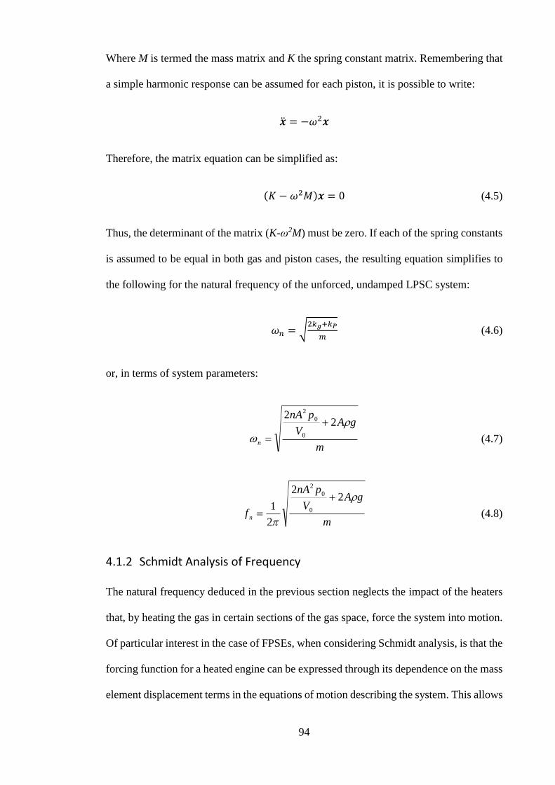
94

Where M is termed the mass matrix and K the spring constant matrix. Remembering that

a simple harmonic response can be assumed for each piston, it is possible to write:

�̈� = −𝜔2𝒙

Therefore, the matrix equation can be simplified as:

(𝐾 − 𝜔2𝑀)𝒙 = 0 (4.5)

Thus, the determinant of the matrix (K-ω2M) must be zero. If each of the spring constants

is assumed to be equal in both gas and piston cases, the resulting equation simplifies to

the following for the natural frequency of the unforced, undamped LPSC system:

𝜔𝑛 = √2𝑘𝑔+𝑘𝑃

𝑚 (4.6)

or, in terms of system parameters:

m

gAV

pnA

n

22

0

0

2

(4.7)

m

gAV

pnA

f n

22

2

1 0

0

2

(4.8)

4.1.2 Schmidt Analysis of Frequency

The natural frequency deduced in the previous section neglects the impact of the heaters

that, by heating the gas in certain sections of the gas space, force the system into motion.

Of particular interest in the case of FPSEs, when considering Schmidt analysis, is that the

forcing function for a heated engine can be expressed through its dependence on the mass

element displacement terms in the equations of motion describing the system. This allows

95

a method for investigating frequency dependence on both operating configuration and

heater temperature, which is useful in ensuing discussions in Chapters 6, 7 and 8. The

following is a simplified Schmidt analysis, similar to that presented by Urieli &

Berchowitz (1984), conducted for the sole purpose of investigating heater temperature

influence on operating frequency.

Taking the equations of motion obtained for the LPSC machine’s spring and mass

equivalent system in the previous section (Equations 4.1–4.4), then by replacing gas

springs with pressure forces, the following set of equations for the undamped piston

motions is obtained:

0)( 12 ppAxkxm APA (4.9)

0)( 23 ppAxkxm BPB (4.10)

0)( 34 ppAxkxm CPC (4.11)

0)( 41 ppAxkxm DPD (4.12)

where the pressures are denoted by the p terms and A is the piston cross-sectional area.

Assuming the pressures oscillate around a mean value of pressure given by p0, a linear

approximation would have the form:

)1(0 DCBA dxcxbxaxpp (4.13)

It is an expression of this form which is required for the pressures in Equations 4.9–4.12.

From the assumptions for Schmidt analysis earlier described in Chapter 2, with isothermal

gas space sections and uniform gas space pressure, Equation 2.9 gives:

𝑝 = 𝑚𝑅 (𝑉𝐸𝑇𝐸

+𝑉𝑅𝑇𝑅

+𝑉𝐶𝑇𝐶)−1

96

Extending this equation to include separate regions for the expansion/compression spaces

and the heat exchangers, the pressure becomes:

1

)/ln(

C

C

C

HX

CH

CHR

H

HX

H

E

T

V

T

V

TT

TTV

T

V

T

VMRp (4.14)

where M is the gas mass, R is the gas constant and V is volume, with subscripts E, HX, R,

C, H and K representing the expansion, heat exchanger, regenerator and compression

spaces respectively. TH and TC are the hot and cold side temperatures. Note that the

temperature assumed in the regenerator is determined from the well-known mean

effective temperature equation for a regenerator, which assumes a linear temperature

profile. Also note that the only variable terms in this expression are the expansion and

compression space volumes. Considering the first gas space, and substituting in with the

following displacement dependent expressions for compression and expansion space

volumes:

)( 11 DE xEAV

)( 11 AC xCAV

where E1 and C1 are the characteristic lengths of the neutral expansion and compression

spaces respectively. Each gas pressure can be written as a function of displacements in

the form:

1

111

)()/ln()(

C

A

C

HX

CH

CHR

H

HX

H

D

T

xCA

T

V

TT

TTV

T

V

T

xEAMRp


97

1

1

H

D

C

A

T

Ax

T

AxSMRp

where:

CC

HX

CH

CHR

H

HX

H T

AC

T

V

TT

TTV

T

V

T

AES 11 )/ln(

(4.15)

Factoring out the S variable gives:

1

1 1

ST

Ax

ST

Ax

S

MRp

H

D

C

A

Noting that the MR/S term is equivalent to the charge pressure of the system (and therefore

also the mean operating pressure) yields:

1

01 1

ST

Ax

ST

Axpp

H

D

C

A (4.16)

The final step in obtaining linear approximations for the gas pressures is to use binomial

expansion, and neglect second order terms to invert the fraction in Equation 4.16. When

performed for each gas space in the 4HEAT configuration, this yields:

ST

Ax

ST

Axpp

H

D

C

A101 (4.17)

ST

Ax

ST

Axpp

H

A

C

B102 (4.18)

ST

Ax

ST

Axpp

H

B

C

C103 (4.19)

98

ST

Ax

ST

Axpp

H

C

C

D104 (4.20)

These expressions now are in the form of the desired general linearized pressure equation

described earlier, Equation 4.13. Substituting into the EOMs (4.9–4.12) and simplifying

into matrix form gives:

0

1110

1

11110

01111

10

111

000

000

000

000

0

2

0

2

0

2

0

2

0

2

D

C

B

A

CH

P

HC

CCH

P

H

CCH

P

H

HCCH

P

D

C

B

A

x

x

x

x

TTpA

Sk

TT

TTTpA

Sk

T

TTTpA

Sk

T

TTTTpA

Sk

S

pA

x

x

x

x

m

m

m

m

Assuming similar piston spring constants, rearranging into the form of Equation 4.5 and

solving for the zero determinant of the matrix (K-ω2M), results in the following quartic

equation (if ω2 is considered the variable):

02

2

0

22

0

24

0

24

0

24

20

2

0

2

ST

pA

ST

pA

ST

pA

ST

pAmk

ST

pA

ST

pA

CHCH

P

CH

Assuming the terms on the right cancel each other out, or at least are insignificant

compared to the leftmost term (for low temperature systems this is justifiable as TH and

TC are relatively close), the equation for the forced frequency becomes:

m

kTTS

pAP

CH

f

110

2

(4.21)

or

m

kTTS

pA

f

P

CH

f

11

2

1

0

2

(4.22)

99

4.1.3 Frequency Dependence on Heater Temperature

Equation 4.22 shows that for a particular machine, geometry and operating pressure, the

forced frequency is dependent only on the heat source and sink temperatures, TH and TC.

A natural inclination is to wonder how sensitive the forced frequency is to changes in

these temperatures. For this, the ratio of forced frequency (Equation 4.22) to natural

frequency (Equation 4.8) can be analysed:

m

gAV

pnA

m

gATTS

pA

f

ff

CH

n

f

n

f

ratio

22

211

0

0

2

0

2


gAV

pnA

gATTS

pA

fCH

ratio

22

211

0

0

2

0

2

2

Noting that the influence of the right hand terms in the above ratio can only contribute to

a value closer to unity, they can be neglected for a conservative frequency ratio estimate:

0

0

2

0

2

2

2

11

V

pnA

TTS

pA

fCH

ratio

CH

ratioTTnS

Vf

11

2

02

100

Recalling that p0=MR/S and letting V0=MRT0/p0 (where T0 represents the equivalent

average temperature of the unforced system i.e. TC). The preceding equation simplifies

to:

CHf

nratio

TTnM

TMf

11

2

02

where Mn and Mf are the gas space masses in the natural and forced response cases. From

the ideal gas law, the mass ratio can be replaced with a temperature ratio, since charge

pressure p0, gas space volume V0 and the gas constant R, are the same in both scenarios:

CHn

f

ratioTTnT

TTf

11

2

02 (4.23)

As previously identified, the equivalent average temperature T0 in the unforced case is

the same as Tn. The polytropic index can be assumed to be 1 since isothermal behaviour

is assumed in Schmidt analysis. Finally, neglecting the nonlinear temperature distribution

through the heat exchangers, it is reasonable to approximate the average gas temperature

in the forced case, Tf, as halfway between the sink and source temperatures, TH and TC.

Substituting these conditions into Equation 4.23 and simplifying gives:

C

H

H

Cratio

T

T

T

Tf

4

1

2

1 (4.24)

Considering that the sink temperature is in general close to ambient temperature, then

using a value of TC = 300 K, Equation 4.24 can be rewritten as a function only dependent

on the heater temperature:

H

Hratio

T

Tf

300

900002

2

1 2 (4.25)

101

To gauge the sensitivity of this approximate frequency ratio to heater temperature change,

the percentage difference between the forced and natural frequencies can be graphed for

a range of heater temperatures.

Figure 4.2 – Graph showing how little the heater temperature affects the operational frequency of the LPSC system.

Figure 4.2 shows a plot of this function over the temperature range of -100°C to 500°C.

From the graph it can be inferred that the heater temperature has little impact on the

operational frequency of the overall system. With heater temperatures of 450ºC, the

change in operating frequency is less than 10%. In the investigation undertaken in this

thesis, the heater temperatures being considered are in the order of 150ºC, which

corresponds to a maximum difference in operating frequency of less than 2%.

It is important to remember that the frequency analysis summarised in Figure 4.2 is an

approximation based on a number of simplifying assumptions and is not intended for

precise quantification. A frequency comparison with the experimental results is

0

2

4

6

8

10

12

-200 -100 0 100 200 300 400 500 600

Dif

fere

nce

be

twe

en

fo

rce

d a

nd

un

forc

ed

fre

qu

en

cie

s (%

)

Heater temperaure (°C)

102

conducted in Section 6.2. Also worth mentioning is that the approximation for the

frequency ratio given in Equation 4.25 considers the difference between the natural

response or ‘0HEAT’ configuration and the forced response of the 4HEAT

configuration—thus the expected frequency differences are even less in the 2HEAT and

3HEAT configurations.

4.2 Sage Modelling

4.2.1 Description of Sage Modelling Software

With the advent of computers, the complex behaviour of oscillating thermodynamic

systems has become open to investigation with unprecedented precision. Notorious for

its deviation from ideal behaviour, the Stirling cycle has been one such target of dedicated

computer simulation efforts. Developed by David Gedeon, Sage simulation software is

specifically designed for modelling oscillating systems, such as Stirling engines and

coolers, pulse-tube cryocoolers and other types of cryocoolers (Gedeon, 2010). Much

more limited in terms of scope, user-friendliness and commercial development compared

with software packages such as MATLAB, Sage makes up for this with its accuracy and

fast solving speeds and has become one of the most reliable modelling tools for oscillating

thermodynamic systems in higher education institutions and industry. Sage treats the

working gas as one-dimensional and solves the governing equations implicitly in space

and time. The grid includes all time values since a periodic solution is assumed. Hence,

Sage is incapable of modelling transient cyclic processes, such as start-up behaviour.

Unlike traditional modelling approaches where a model is made up of a set of user-

defined parameters and equations, Sage models are built component by component,

allowing the geometry of the model to evolve with relative ease. Components

representing different sections of the modelled system are added one by one and

interconnected to build a complete system model. Each individual component is divided

103

into a user-defined number of cells, across which the three conservation equations of

mass, momentum and energy are solved at each time increment. This is explained in more

detail in Section 4.2.1.1. Components can be linked to each other through user-created

boundary conditions, embodying their physical relationships with their surroundings. For

example, fluid mass flow between a heat exchanger and a regenerator, or a force

connection between a piston and adjacent gas space. Sage also encapsulates gas flow

effects and heat transfer between and through components to determine realistic

performance characteristics. In its ability to model heat transfer processes and fluid

friction of oscillating flow, even through porous media such as the regenerator matrix,

Sage can be regarded as a very powerful third order modelling tool.

Figure 4.3 – Example showing the graphical interface of Sage. Mass and heat flow connections are embodied by arrow symbols indicating the axial direction of the connector.

Figure 4.3 shows part of a basic model subsystem in Sage. Model components are

organized logically in a hierarchical tree structure, and sub-levels of each component are

accessible in order to allow for parameter manipulation and the connection of different

model components. These are shown in more detail for the LPSC model, later in this

chapter. Each component of the system is subdivided into a user-defined number of

spatial increments and analysed in a one-dimensional form. While Sage primarily models

the thermodynamic behaviour of the working gas, it also takes into account the interaction

of the gas with the adjacent walls, as well as heat transfer by conduction in the canister

walls in both axial and radial directions. In this respect, Sage is somewhere between a

one-dimensional and two-dimensional modelling tool.

104

Sage operates in a frequency domain and solves all fundamental conservation equations

for each cell until it converges to a solution. Further features of this software package are

a mapping tool, which allows a parameter study over a user-defined number of variables

in a user-defined number of increments, and an optimisation tool. The components

available range from different types of heat exchangers to pistons, cylinders, canisters,

dashpots, springs and more. They are selected from an appropriate menu and connected

via characteristic variables. For instance, various gas volumes are connected via a mass

flow variable; a piston face is connected to the adjacent gas space via a pressure variable.

In the context of the LPSC, an apparent disadvantage of Sage is its requirement for cycle

frequency and piston amplitudes as input parameters. These must therefore initially be

obtained from the MATLAB model and then used as inputs in Sage to evaluate the system

performance1. The resulting outputs from Sage include pressure and temperature profiles

of each working space, as well as piston and gas pressure amplitudes and phase angles.

The following descriptions about gas domain theory and the solution method are

summarised from Sage’s user manual, which should be consulted for further information.

4.2.1.1 Gas Domain Theory

The equations used by Sage are somewhat non-standard in the computational fluid-

dynamics literature because they are designed specifically for one-dimensional internal

flows with space-variable and time-variable flow area. Most CFD textbooks use a more

general approach. Instead of merely stating the equations, an overview of their derivation

is provided. Starting with the general Navier-Stokes equations in integral form, as found

in Peyret and Taylor (1983), body forces shall be neglected and the prevailing convention

of a fixed control volume is relaxed. Instead it is assumed that the control volume has

1 As previously alluded to, this intermediate step was circumvented via a procedure which is explained in

more detail in Section 4.2.9.

105

fixed inlet and exit boundaries, but the side boundaries can move. This results in a time-

variable flow area. The side boundaries are impermeable so that flow enters and leaves

only through the inlet and exit boundaries. A rubber tube with space-variable and time-

variable cross-section is a useful thought picture, with the principal flow axis being the

tube axis. In this control volume the integral gas dynamic equations are:

Continuity: 𝑑

𝑑𝑡∫ 𝜌𝑑𝑣𝑣

+ ∫ 𝜌𝒏𝑠

· 𝑽𝑟𝑑𝑠 = 0

Momentum: 𝑑

𝑑𝑡∫ 𝜌𝑽𝑑𝑣𝑣

+ ∫ [(𝒏𝑠

· 𝑽𝑟)𝜌𝑽 − 𝒏𝝈]𝑑𝑠 = 0

Energy: 𝑑

𝑑𝑡∫ 𝜌𝑒𝑑𝑣𝑣

+ ∫𝒏𝑠

· (𝜌e𝑽𝑟 − 𝝈𝑽 − 𝒒)𝑑𝑠 = 0

Where, e = ε + u2/2 (mass-specific total gas energy), n = unit outward normal of s, q =

heat flux vector, s = surface of υ, t = time, υ = control volume, V = Newtonian-frame flow

velocity vector, Vr = boundary-relative flow velocity vector, ε = mass-specific internal

gas energy, ρ = gas density and σ = stress tensor.

The continuity equation states that the time rate of change of mass in the control volume

equals the rate at which mass leaves through its surface boundaries. The momentum

equation is a statement of Newton’s second law of motion: the time rate of change of

control-volume momentum, less the momentum leaving through its surface boundaries,

equals the net force acting on all surfaces. The energy equation states that the time rate of

change of control-volume internal energy plus kinetic energy—minus that leaving

through its surface boundaries—is equal to the net heat flux through its boundaries, plus

the mechanical work done on its boundaries.

The equations are then converted into one-dimensional differential equations in

conservative form: where dv in the time integrals is replaced with Axdx, and where Ax is

flow area and x is the principal flow direction. Taking the limit ∆x→ dx then dividing

106

through by dx and making some simplifications, the three equations take the following

form. Note that for the surface integrals in each case the inlet and outlet boundaries are

considered separately from the side boundaries. The stress tensor is empiricised as

thermodynamic pressure, p, and as a viscous flow resistance term, RF, which can be

thought of as the force per unit length per unit flow area due to surface shear stress. The

empirical film heat transfer per unit length, Qw, is introduced to represent the integral for

the negative z boundary in the energy equation, and q represents the axial heat flux.

The gas dynamic equations are therefore:

Continuity: 𝜕𝜌𝐴𝑥

𝜕𝑡+

𝜕𝜌𝑢𝐴𝑥

𝜕𝑥= 0,

Momentum: 𝜕𝜌𝑢𝐴𝑥

𝜕𝑡+

𝜕𝑢𝜌𝑢𝐴𝑥

𝜕𝑥+

𝜕𝑝

𝜕𝑥𝐴𝑥 − 𝑅𝐹𝐴𝑥 = 0, and

Gas energy: 𝜕𝜌𝑒𝐴𝑥

𝜕𝑡+ 𝑝

𝜕𝐴𝑥

𝜕𝑡+

𝜕

𝜕𝑥(𝑢𝜌𝑒𝐴𝑥 + 𝑢𝑝𝐴𝑥 + 𝑞) − 𝑄𝑤 = 0

The purpose of these equations is to determine three implicit solution variables, which

are chosen to be ρ, ρuAx and ρe. The reason for making this choice is that all are roughly

continuous across area discontinuities and, except for the factor Ax in the second, are

standard in the field. Empirical terms RF, Qw and q are explained in further detail in the

user manual.

The gas dynamic equations are tied together with an equation of state that serves to

evaluate the dependent variables, pressure, p, and temperature, T, as functions of

independent variables ρ, ρuAx and ρe (p(ρ,T) and T(ρ,ρuAx,ρe)). The gas-property objects

defined in the Stirling root model section of the user manual provide these functions.

107

4.2.1.2 Solution Method

The gas dynamic equations are discretized over a grid of points uniformly spaced

throughout the domain and over the cycle period. On this grid, the three solution variables

(highlighted earlier) are solved implicitly or interpolated explicitly according to the logic

of a staggered-grid formulation. The underlying idea is to solve ρuAx at alternate nodes

from ρe and ρ to avoid solution instability and produce global conservation of mass,

momentum and energy. Solution staggering is only carried out in the spatial direction.

The concept of control volumes can be used to aid with the interpretation of the staggered-

grid scheme. The boundaries of these control volumes can be imagined as lying on

alternating nodes. At these boundaries, ρuAx is solved, while ρ and ρe are solved at the

midpoints. By using first-order central differencing in the continuity and energy

equations, the global conservation of energy and mass automatically holds for the solved

variables ρ and ρe. In other words, quantities leaving one control volume enter the

adjacent one. The reason higher order differentiation is not used is that it would destroy

this global conservation property, or complicate it greatly.

When the model is ready so be solved, a large system of nonlinear equations and their

associated implicit variables will exist based on the model hierarchy. A nonlinear solver

is employed and solves a sequence of linear approximations to the nonlinear equations.

The coefficients of the linearized equations result from numerical partial derivatives of

the evaluation functions taken with respect to the model’s implicit variables. The result

is a sparse matrix, solved with a special sparse-matrix solver. The solution becomes a

search direction along which to seek the nonlinear solution. This process repeats until the

nonlinear model equations are all satisfied within some given tolerance.

For a more in depth explanation of the inner workings of the Sage software, the reader is

directed to the Sage user manual. The manual contains more than 400 pages of

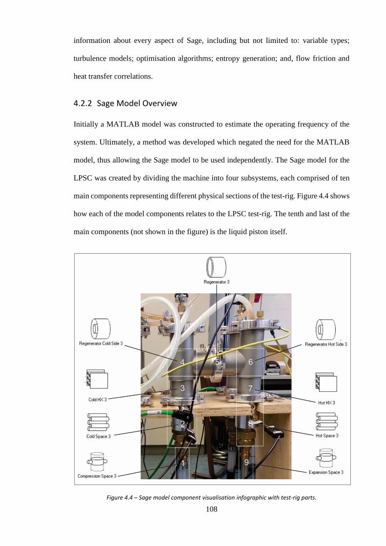
108

information about every aspect of Sage, including but not limited to: variable types;

turbulence models; optimisation algorithms; entropy generation; and, flow friction and

heat transfer correlations.

4.2.2 Sage Model Overview

Initially a MATLAB model was constructed to estimate the operating frequency of the

system. Ultimately, a method was developed which negated the need for the MATLAB

model, thus allowing the Sage model to be used independently. The Sage model for the

LPSC was created by dividing the machine into four subsystems, each comprised of ten

main components representing different physical sections of the test-rig. Figure 4.4 shows

how each of the model components relates to the LPSC test-rig. The tenth and last of the

main components (not shown in the figure) is the liquid piston itself.

Figure 4.4 – Sage model component visualisation infographic with test-rig parts.

109

Figure 4.5 shows the corresponding graphical interface within Sage. Along with the main

model components there are also some supplementary ones, such as the pressure source,

which provides the gas charge pressure setting, the sink and source heat reservoir

components, and the liquid piston accessories.

Figure 4.5 – Sage model of a liquid piston Stirling cooler subsystem.

Depicted in Figure 4.5 is only one of the four subsystems, with the complete model

comprising all four connected in series. The components are arranged in the approximate

shape of the actual housing and are connected in series using heat and mass flow linkages

within Sage to construct the continuous loop of the enclosed space (these can be seen as

the numbered arrows in the preceding figure). All of the components have internal

geometric variables and material properties that were altered to resemble the desired

physical system as closely as possible. The model necessarily incorporates simplifying

assumptions relating to the heat transfer within the heat exchangers, and approximations

for the viscous frictional effects in the liquid pistons as discussed later. The assumptions

include a perfectly sealed system; no heat transfer losses to the surroundings; constant

heat source and sink temperatures; and no evaporation of liquid from the surfaces of the

pistons. The last assumption is almost certainly not valid and the limitations of this

assumption are discussed later in Section 8.2.4. A brief explanation of the details of each

of the main components is now outlined.

110

4.2.3 Compression and Expansion Spaces

The compression and expansion spaces, denoted by numbers 1 and 9 in Figure 4.4

represent the variable gas volumes that exist above the liquid piston surface within the U-

tubes. The boundary of this space is the threaded connection with the gland fitting, and it

thus encompasses the entire permissible piston stroke range. Figure 4.6 shows the

hierarchical structure of the compression space model-component in the third subsystem.

Figure 4.6 – Structure of the compression space model-component within Sage.

Two child components are required: the duct gas and a conductive surface element

resembling the U-tube. These are some of the most basic Sage model components—only

a small number of connections are required, including a pressure link to the adjacent

piston, mass flow and heat conduction links to the space above, and the aforementioned

charge pressure linkage (in the expansion space only). The majority of the geometric and

material properties are defined at the root-component level by changing the input

111

parameters of the individual components. Table 4.1 summarises the parameters used in

the compression and expansion spaces.

Table 4.1 – Compression and expansion space model-component input parameters

Description Value Component level

Number of spatial cells 2 Root

Mean-flow length (m) 8x10-2 Root

Initial temperature (K) 300 Root

Wetted surface area (m2) 7.5x10-3 Root

Baseline volume (m3) 2.382x10-5 Root (recast)

Tube wall thickness (m) (PVC = 3.5 mm, Steel = 1 mm) 3.5x10-3 Child

Tube material (PVC or Steel) Steel (SS304) Child

Mean-flow length is a parameter that corresponds to the swept distance of the piston.

Sage uses the mean flow length to calculate the cross-sectional area of the generic

cylinder element when regarding the cylinder as a passage. The length may vary by an

order of magnitude without producing much effect on the simulation outputs (Gedeon,

2010), since nothing in the variable-volume gas domain model depends on length or flow

area. The Sage manual advises using a rough value of length scaled to the modelled

machine. In this case the average stroke expected, approximately 80 mm, in the

compression and expansion spaces is selected. On the hot side, the material selected is

stainless steel; on the cold side, polyester is selected (PVC is not a material option within

Sage).

The most important parameters specified for these components are that of baseline

volume and wetted surface area. Baseline volume is the component volume when all

volume-displacement attachments are zero. It is critical because it directly effects the

pressure ratio of the machine. Relative accuracy within a few per cent is recommended in

the Sage manual. The value is derived from the dimensions of the U-tube and the

measured distances to the hot and cold spaces above the pistons. It is also recast to the

root component level so that all eight spaces can be manipulated with a single user defined

112

variable. The wetted surface area is the time-mean inner surface area of the tube, and not

excessively critical since it has only a secondary effect on the cycle pressure through the

heat transfer between the gas and wall. A value within 50% is recommended. The

accuracy of this value is even less important in the case of low temperature machines. An

area of 7500 mm2 is calculated from the U-tube inner diameter and the straight-line

distance separating the piston from the entrance to the cold and hot spaces.

4.2.4 Cold and Hot Spaces

Components 2 and 8 from Figure 4.4 are termed the cold and hot spaces respectively.

These components serve to model the relatively complex geometry of the housing

between the gland fitting and the entrance to the heat exchangers. This space includes a

number of changes in cross-sectional area as well as the pressure and temperature sensor

ports. Since the volume of these components remains constant, they are approximated as

a single cylindrical tube, whose cross-section is a weighted average of the actual test-rig

geometry in this section. The tube length is then established from the actual volume.

Figure 4.7 depicts the hierarchical structure of these components.

Figure 4.7 – Structure of the hot and cold space component within Sage.

113

As in the case of the compression and expansion spaces, only two child components are

needed: the duct gas and a conductive surface element. Five continuity connections are

required for these components: mass flows through the inlet and exits, conductive heat

flows to the two neighbouring components, and a heat flow from the gas to the interior

surface of the tube. Table 4.2 summarises the parameters used in the compression and

expansion spaces. The material selected is brass, as the gland fitting takes up the majority

of the total length.

Table 4.2 – Hot and cold space model-component input parameters.



Duct-length (m) 1.42x10-1 Root

Mean wall roughness/Dhydraulic (non-dimensional) 1x10-3 Root

Wall thickness (m) 2.5x10-3 Root


Tube inner diameter (m) 1.941x10-2 Root

Number of tubes 1 Root

Material brass Child

4.2.5 Heat Exchangers

The heat exchanger model components, 3 and 7 from Figure 4.4, encompass the

cylindrical housing section that contains the heat exchangers. Based on information

within the Sage manual the appropriate arrangement and type of child components were

incorporated to resemble an annular finned heat exchanger. Figure 4.8 shows their typical

hierarchical structure, including heat and mass flow interconnections.

The heat exchangers are some of the more complicated model components. The second

level of the hierarchy shows the four child components of the heat exchanger: duct gas,

inner heat exchanger wall, heat exchanger fins and outer heat exchanger wall. The duct

gas is connected via a heat flow path to the heat exchanger fins, which also share a heat

flow path with the inner heat exchanger wall. Within the heat exchanger components of

114

the Sage model, heat transfer from the gas can only occur with one contact surface. The

heat transfer from the gas to the outer wall was neglected in this section of the model,

although the outer wall retains conductive heat transfer connections to the adjacent

components. The remaining connections were exported to the root-component level as

they required connections to the adjacent model components, hence all of the connecting

arrows surrounding the root component, Cold HX 3, in the lower left of the Figure 4.8.

Figure 4.8 – Structure of the heat exchanger model-component within Sage.

By hovering over each connection it is possible to identify the child component to which

it relates. The two mass flows, denoted by the mGt arrows, pertain to the duct gas flows

through both inlet and exit boundaries of the neighbouring regenerator and cold space

components. The inner walls of the hot heat exchangers are connected to heat sources that

remain at constant temperature—for example, as ‘Heater 3 Temperature’ in Figure 4.5.

Similarly, the cold heat exchangers are connected to a common heat sink, which is pre-

set to the desired ambient temperature. The remaining heat flow connections include

conduction paths through housing boundaries, and also from the top surfaces of the fins

115

into the regenerator matrix. Since all heat exchangers are identical, they all have the

component inputs shown in Table 4.3.

Table 4.3 – Heat exchanger model-component input parameters.

Description Value Component level Number of spatial cells 3 Root

Duct length (m) 6x10-2 Root

Mean wall roughness (non-dimensional) 1x10-3 Root


Channel width (m) 5x10-4 Root

Channel height (m) 5x10-3 Root

Number of channels 90 Root

Fin thickness (m) 7x10-4 Root

Fin conduction length (m) 4.5x10-3 Child

Fin material brass Child

Inner HX wall circumference (m) 9.425x10-2 Child

Inner HX wall thickness (m) 8.75x10-3 Child

Inner HX wall material brass Child

Outer HX wall circumference (m) 1.335x10-1 Child

Outer HX wall thickness (m) 2.5x10-3 Child

Outer HX wall material Aluminium Child

The Sage user guide provides an appropriate method for relating an annular finned heat

exchanger to the depicted rectangular-finned model component. The input values used in

the heat exchanger components are self-explanatory, and are determined from the

geometry of the components themselves. The reader is directed to the manual for further

information about this procedure.

4.2.6 Regenerators

Three separate components are used to model the regenerators (identified in Figure 4.4

as numbers 4, 5 and 6). These components were used in order to account for the unusual

and changing geometry of the regenerator spaces. The side sections have a cylindrical

brass tube passing down and through their centres so as to provide access to the internal

heat exchanger for the heating cartridges or cooling water. As a result, these spaces

resemble a concentric tube configuration, whereas the central regenerator space is purely

cylindrical and entirely filled with regenerator material. Also, the spaces are not

116

connected end on end, which complicates the model requirements. Figure 4.9 shows a

graphical representation of the hierarchical structure of the centre regenerator component.

Figure 4.9 – Structure of the central regenerator model-component within Sage.

The centre regenerator component is modelled as a tubular canister with two child

components: the packed sphere matrix and the outer wall. The matrix child component

contains two further child components of its own: the duct gas and the steel shot material.

Further information on why regenerators are modelled this way can be found in the Sage

manual. The duct gas exhibits the familiar mass flow connections with the regenerator

sides, and also shares a heat flow connection with the steel shot material, which can

117

conduct heat to the surface of the outer wall. Conductive heat flow paths exist for the

outer wall’s contact with the side regenerator components. Table 4.4 summarises the

parameters used in the central regenerator component. The porosity of the regenerator

material was estimated to be 0.39, based on loosely poured sphere packing void fractions.

Table 4.4 – Input parameter values for the central regenerator model-components.



Canister length (m) 8x10-2 Root

Canister inner diameter (m) 4x10-2 Root

Canister material Alum6063 Root


Canister wall thickness (m) 2.5x10-3 Root

Matrix porosity 0.39 Child

Matrix sphere diameter (m) 1x10-3 Child

Matrix material Steel Child

Figure 4.10 – Structure of the side regenerator model-component within Sage.

118

Figure 4.10 shows the structure of the side regenerator components. The side sections are

modelled as annular canisters, with three child components: the inner and outer walls,

both of which are conductive surface elements, and the packed sphere matrix material.

As with the centre regenerator component, the matrix child component includes the duct

gas and steel shot material. Heat flow paths exist between both walls and the matrix

material. All three of these child components share conductive heat flow connections with

the adjacent components, although it should be noted that since no inner wall exists in the

centre regenerator, the flow paths are made to its outer wall instead. As with most gas

space components, two mass flow connections exist for the inlet and outlets. Table 4.5

displays the input parameters used for the side regenerator model components.

Table 4.5 – Input parameters for regenerator side model-components.



Canister length (m) 4x10-2 Root

Canister inner wall inner diameter (m) 1.3x10-2 Root

Canister material brass Root


Canister outer wall outer diameter (m) 6.5x10-2 Root

Canister inner wall thickness (m) 2.5x10-3 Root

Canister outer wall thickness (m) 1.25x10-2 Root

Matrix porosity 0.39 Child

Matrix sphere diameter (m) 1x10-3 Child

Matrix material Steel Child

Matrix radial thickness (m) 5.5x10-3 Child

The Sage model deviates from the actual geometry in that it does not account for the

elbow bends in the regenerator spaces, but this is considered to have negligible relevance

given the early stage of research and development of this project. As the physical system

is optimised with greater precision, so too can the computer models be improved and

modified to better replicate its performance.

119


On the right side of Figure 4.5 are the three components used to model the liquid piston:

spring D, Liquid Piston D, and damper D. The piston itself is modelled as a solid free-

piston, and is connected to the expansion and compression components of the adjacent

gas spaces. In reality, the liquid piston’s behaviour will deviate from that of a solid free-

piston, and for this reason a spring and damper are also added to the model and connected

to the piston. The spring is used to represent the restoring force imposed by gravity on

the U-shaped piston as it oscillates back and forth, while the damper is used to account

for fluid friction and kinetic losses (also commonly known as minor pipe flow losses)

associated with the flow of the liquid during motion. The spring constant is simply derived

from a force balance conducted on the liquid piston as a free body as identified in

Section 2.3.2.2:

𝑘𝑝 = 2𝐴𝜌𝑔

The damping coefficient of the viscous damper, CDamper, is calculated by determining

equivalent damping coefficients for the viscous and kinetic losses, CVis and CKin, in the

fluid and summing them together. The average rate of viscous and kinetic energy loss for

liquid pistons was estimated by West as:

3

22

t

S

VisR

VLffE

and:

4

33

242.0

t

SKin

R

VfKE

where ΣK represents the sum of the kinetic flow loss coefficients and VS, being the swept

volume, is equal to:

120

XRV tS

22

As identified in Section 2.2.7, the theory and experimentation for oscillatory flow

problems is lacking, therefore the above equations are derived from well-known steady

flow formulas. The limitations of assessing oscillatory flow losses with standard steady

flow formulas is discussed further in Section 8.2.3.

In order to obtain the equivalent damping values, one can compare the average rate of

energy lost through both viscous and kinetic mechanisms to that of a viscous damper,

shown below. The average rate of energy loss for a damper is equal to the work done by

the damping force per cycle multiplied by the frequency of oscillation:

fWE cycledamper

fXCE damperdamper

2

2222 fXCE damperdamper

Equating the viscous losses to damping losses and rearranging the following expression

for the equivalent viscous damping coefficient can be obtained as:

fLRC tVis 5.12

Similarly, an expression for the equivalent kinetic damping can be derived as:

XfRKC tKin

2284.0

Now these effects are able to be incorporated into the model. The total damping

coefficient used in the model is then:

KinVisDamper CCC

121

CDamper is recast as a user variable within Sage, which allows for it to be written as a

function—and, as a result, it can vary with corresponding changes to its dependent

variables during the solving process (piston radius, frequency, amplitude, etc.). While the

majority of variables influencing the damping coefficient are the same for each piston,

the kinetic component is influenced by piston amplitude. For this reason, each piston

damper is designated its own damping coefficient variable.

The K values associated with the minor pipe losses in the U-shaped liquid piston are

estimated to total 0.5, which includes two smooth 90° bends (0.15–0.25 each) and one

small expansion/contraction (of negligible value) at the interface between the PVC and

steel tube. The model sensitivity to this parameter is evaluated in Section 5.2.1. The effect

of the floats is also expected to increase the cyclic power losses, but there is no research

to indicate by how much, and hence is not currently included in the model. With the

geometric and physical traits of the ‘real-life’ test-rig approximated, the model is almost

complete. The final noteworthy characteristic of the model is that although three of the

four pistons are modelled as free-pistons, the fourth is modelled as a constrained piston.

This was found to be a necessity as the software would not converge on a solution with

four free-pistons. The justification for constraining this piston is that its amplitude is

found by optimising for a negligible net-work output, meaning the piston is essentially

free, with its phase being pre-set to anchor the solver. This is explained in more detail in

Section 4.2.9.

The diameter value used in the Sage model with 15 mm OD steel tubes is set to 12.65 mm.

Although the manufacturer’s specification for the PVC tube indicated that its internal

diameter was 13.5 mm, a volumetric test concluded that the average internal diameter was

actually 12.3 mm. On the steel side the internal diameter was measured to be accurate at

13 mm. Within the model only a single average diameter is used on both sides of the U-

122

tube to simplify the analysis. Therefore, the cross-sectional area assumed to take part in

the force balance is provided by the average of these two diameters, 12.65 mm. It could

be argued that the float diameters also need to be considered in this situation, since (due

to the fluid boundary layers) their surface may be more representative of the area through

which pressure and force are transmitted from the gas to the liquid. At this stage,

speculating on the most accurate approximation for the effective cross-sectional area of

the liquid pistons is unwarranted. It is a topic that could be revisited as the design is

refined, and the model uncertainties reduced in other areas. Table 4.6 summarises the

input parameters associated with the piston components.

Table 4.6 – Piston input parameters used in the Sage model for 100 ml pistons.


Spring constant (N/m) variable Root

Damping coefficient (Ns/m) variable Root

Piston mass (kg) 1x10-1 Root (recast)

Piston face area (m2) 1.257x10-4 Child (recast)

4.2.8 Sage Model Input Requirements

Table 4.7 – General input parameters for LPSC Sage model.

Input Name Description Value

NTnode Number of time nodes 9

Lnorm Length scale (m) 2.5x10-2

Freqnorm Frequency scale (Hz) 4

Pnorm Pressure scale (Pa) 4x105

Tnorm Temperature scale (K) 300

Qnorm Heat-flow scale (W) 100

Freq Operational frequency (Hz) -

Gas Working gas Ideal air

Xamp Constrained piston amplitude (m) -

Pmean Charge pressure (Pa) -

Theaters Heater temperature (K) -

Tcooling Rejection temperature (K) 297

Rho Liquid density (kg/m3) 1000

Mew Liquid viscosity (Ns/m2) 1x10-3

Ksum Sum of minor pipe loss coefficients 5x10-1

Pmass Piston mass (kg) 1x10-1

Vvariable Expansion and compression space volumes (m3) 2.382x10-5

Dpiston Piston diameter (m) 1.265x10-2

123

Sage requires a number of general inputs for the Stirling machine before a simulation can

be solved. The inputs window can be accessed separately and also includes the variables

recast from model components, allowing for the manipulation of multiple system

parameters from one location. For the LPSC model constructed for this project, these

variables are listed in Table 4.7.

NTnode is the number of time nodes in the computational grids of all underlying model

components containing grids. The influence of this value is discussed in the grid

independence section, 4.2.11. The parameters, Lnorm, Freqnorm, Pnorm, Tnorm and

Qnorm represent the normalisation constants for different system variables and influence

the convergence of the solver. The most important of these is Lnorm, which is set to the

approximate cube root of the largest stroke volume amplitude in the model. Advice for

selecting appropriate values can be found in the Sage manual.

Of the remaining parameters, many have been recast to system level from model

components (such as the piston mass); others include user created variables, such as Ksum

and mew (for determining the piston damping constant). The four unspecified values in

the table include the operation frequency, charge pressure, constrained piston amplitude

and heater temperature. The charge pressure and heater temperatures are free to be varied

depending on the operating range(s) of interest. For a conventional Stirling engine the

frequency and piston amplitude would be known and available as inputs, however (as

previously discussed), for the LPSC machine these are unknowns. This is, of course,

precisely why modelling the LPSC is extremely complicated.

4.2.9 Frequency Deduction

It was initially intended that a computer model constructed in MATLAB would be used

to predict the system frequency. The aim was primarily to obtain predictive results for the

oscillation frequency, which could then be used as inputs for the more sophisticated Sage

124

model in order to analyse trends in the system’s performance. Unfortunately, however,

the Sage model was found to be extremely sensitive to the frequency input, and would

generate vastly different results for small changes in the frequency input. A large amount

of time was spent working with the Sage model, and it was thought that Sage’s

dependence on frequency as an input could not be circumvented. Despite this, after

experimenting with many different model modifications, eventually a method was created

which used Sage itself to provide the operating frequency for the 4HEAT configuration.

This was a major breakthrough which allowed the model to be used independently for all

LPSC simulations. The method is outlined below.

The process was developed by recognising the symmetric traits associated with the

4HEAT configuration. In the 4HEAT case where all four heaters are powered and

supplied the same amount of energy, the resulting steady state amplitude of the liquid

pistons must theoretically be equal as all four subsystems are identical and symmetrical.

Furthermore, the relative phase angles between the pistons should also be 90º. Using these

properties, and knowing the approximate range of permissible amplitude values, it was

found that the in-built optimisation function1 in Sage could converge on the frequency—

if the objective function was carefully selected, and the starting estimates were already in

close vicinity to the solution. An iterative process was employed, whereby either

frequency or piston amplitude was selected as a floating variable, and the system

optimised for either the smallest differences in piston amplitudes (objective function 1):

𝑂𝑏𝑗1 = |𝑋𝐴 − 𝑋𝐵| + |𝑋𝐴 − 𝑋𝐶| + |𝑋𝐴 − 𝑋𝐷|

1 Within Sage, the optimiser’s goal is to drive the pseudo-Lagrangian step-change to a small negative value.

The pseudo-Lagrangian step-change is a measure of the relative change over the current step of the

objective function. The value generally starts out large and negative and grows smaller as the optimisation

converges to the minimum. The reader is directed to the user manual for more information about the

optimisation process employed by Sage.

125

or minimal net-work output by the constrained piston (objective function 2):

𝑂𝑏𝑗2 = |𝑊𝑛𝑒𝑡,𝐴|

Initially the natural frequency provided by Equation 4.8 for the spring-mass system in

Section 4.1 was used to provide the optimiser’s frequency estimate. After recognising

patterns in the frequency solutions, this was later modified to be the natural frequency

determined using a polytropic index of 1.2 in the same equation. This was an essential

step as the solver would converge on false solutions with near-zero piston amplitudes if

the starting point was outside a certain local turning point. The process would continue

with the piston amplitude being set and the frequency found, and then the frequency

would be set, and the model optimised to find a more accurate piston amplitude.

Eventually, the piston amplitudes would all be equal to within 0.1%, and the piston phase

angles would be within the range 90° ± 0.5º. Both objective functions would converge to

the same solutions—although objective function 1 was much more stable and generally

converged more quickly (so it was used in the 4HEAT case1). Via this method both the

piston amplitudes and frequency of operation for the 4HEAT configuration for any charge

pressure and heater temperature set points could be determined.

Since the operating frequencies have shown very little dependence on heater temperature,

they are almost identical when comparing 4HEAT, 3HEAT, and 2HEAT configurations

with the same charge pressure. Therefore, the frequency obtained via this method can be

used in the 3HEAT and 2HEAT simulations, despite the fact that the piston amplitude

symmetry no longer applies.

1 Another method involving optimising for 90º phase angles was also attempted, but the optimisation

problem seemed to be ill-conditioned and the solver was unable to converge.

126

As a test for this, it is possible to assess the Sage model’s frequency dependence on heater

temperature, similar to the analysis in Section 4.1.2. Using the frequency deduction

procedure described above, the operational frequency was obtained for the 15 mm

4HEAT system using two heater temperatures at the limits of the functional range. The

highest charge pressure of 6 bar was used to produce the largest differences. The values

obtained were 5.050 Hz and 5.076 Hz for 100°C and 150°C heater temperatures,

respectively, which have a difference of 0.026 Hz or 0.51 % relative to the value at 100°C.

The estimates obtained from Equation 4.25 for the percentage differences between

unforced and forced frequencies are 0.59% and 1.48% at 100°C and 150°C respectively—

a difference between the two of 0.89%. These values of 0.51% from Sage and 0.89% from

the analytical approximation are very small and similar in magnitude, and therefore

contribute to the validity of using the 4HEAT Sage model frequencies for 3HEAT and

2HEAT Sage simulations.

4.2.10 Solving 3HEAT and 2HEAT models

For reasons already discussed in relation to model convergence, one of the pistons must

be modelled as a constrained piston. Within the model this component provides a number

of referenceable outputs. Those of primary interest are the forcing function and net-work

output. For the 3HEAT and 2HEAT simulations the second objective function is used to

find the amplitude of Piston A. A user variable is created in Sage and recast to equal the

net work of the piston. The piston amplitude is then optimized for a minimal absolute

value in this variable. This corresponds to the case where the piston is behaving as a free

piston, with no external influence, exactly as the other three pistons in the model

automatically behave. An example of this optimisation process can be seen in Figure 4.11.

127

Figure 4.11 – Piston A work output mapped against piston displacement. Simulation was conducted for 3HEAT configuration at 4 bar and 150ºC heaters with 100 ml pistons.

The work output from the constrained piston, Piston A, crosses the x-axis at

approximately 0.0675 m, corresponding to an amplitude of 6.75 cm. This represents the

amplitude at which the piston behaves as a free piston, requiring negligible external

influence (aside from the spring and damper attached in the model). For displacements

lower than this 6.75 cm, the piston provides a work output, as if it were connected to a

coupling mechanism or linear generator. For values above 6.75 cm, the piston requires a

net work input, as if it were a driven component. The amplitudes of the other three pistons

automatically adjust, as they are inherently unconstrained, and always have a zero net

work output. The figure above also explains why a number of convergence issues are

associated with objective function 2. When optimising for minimal absolute piston work,

the solver can converge towards zero amplitude if the initial value is to the left of the

turning point at 0.045 m. For comparison, Figure 4.12 shows objective function 1 when

mapped against piston displacement for a 4HEAT simulation.

-0.06

-0.04

-0.02

0.00

0.02

0.04

0.06

0.08

0.10

0.00 0.01 0.02 0.03 0.04 0.05 0.06 0.07 0.08

Pis

ton

A w

ork

ou

tpu

t (W

)

Piston A amplitude (m)

128

Figure 4.12 – Objective function 1 mapped against Piston A amplitude. Simulation was conducted for 4HEAT configuration at 4 bar and 100ºC heaters with 100 ml pistons.

Convergence issues are sometimes encountered with objective function 1; but they are

much more infrequent. This may be related to the shape of the two objective functions.

Objective function 1, in Figure 4.12, appears to transition past the slope towards zero

amplitude earlier than the net work of Piston A (objective function 2), in Figure 4.11.

4.2.11 Grid Independent Solutions

The sensitivity of Sage to a number of model-specific parameters was investigated in

order to ensure simulation solutions were independent. These parameters were those not

related to the physical test-rig dimensions or other properties, but model variables within

Sage components. The relevant parameters are defined below.

NTnode—Number of time nodes in the computational grids of all underlying model

components containing grids. This is an important parameter because it can significantly

affect the solution time, accuracy and memory requirements. It can be likened to a mesh

0.000

0.002

0.004

0.006

0.008

0.010

0.012

0.014

0.016

0.00 0.01 0.02 0.03 0.04 0.05 0.06 0.07 0.08

Ob

ject

ive

fu

nct

ion

1 v

alu

e

Piston A amplitude (m)

129

size for the harmonic variables in the time domain. This value determines the number of

harmonic terms output in the Fourier series solutions of system variables such as gas

pressure and temperature. Changing this variable recreates all time grids in the model and

initializes solution values by interpolating between solved values of the previous grid.

The Sage manual advises using an odd value for this parameter. Table 4.8 shows how the

model solution accuracy was affected by the NTnode parameter. A value of 9 was

employed for the NTnode parameter since the increases in precision beyond this value

were negligible.

Table 4.8 – Sage model sensitivity to NTnode parameter. (Example 3HEAT simulations at 4 bar with 150ºC heaters and 100 ml pistons)

NTnode parameter Piston A amplitude solution (cm) Change (%)

3 7.598 -

5 6.830 10.11

7 6.852 0.32

9 6.783 1.01

11 6.768 0.22

13 6.771 0.04

15 6.774 0.04

Ncells—The Ncells parameter is the number of spatial cells that a single component is

divided into for the solution and is specific to each component. It is similar to the number

of elements in a finite element model. The Ncells parameter was checked for each model

component containing the working gas. Table 4.9 shows how the Ncells parameter

affected the piston amplitude solution quantities when changed in a number of different

components. The simulations were with the 4HEAT configuration and used parameters

of 4 bar charge pressure and 100ºC heater temperatures. As a result of the investigation

only one Ncells parameter was changed from the default value and that was in the

compression and expansion spaces, where the value was increased from 1 to 2.

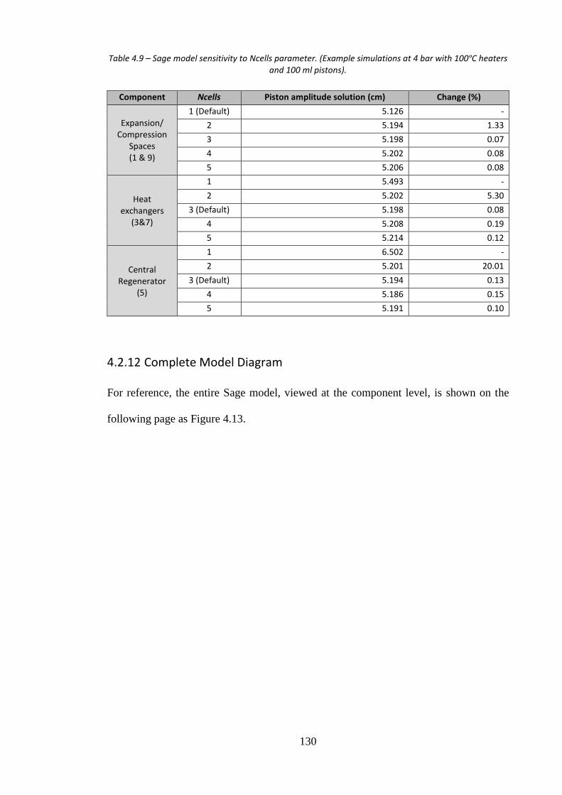
130

Table 4.9 – Sage model sensitivity to Ncells parameter. (Example simulations at 4 bar with 100ºC heaters and 100 ml pistons).

Component Ncells Piston amplitude solution (cm) Change (%)

Expansion/ Compression

Spaces (1 & 9)

1 (Default) 5.126 -

2 5.194 1.33

3 5.198 0.07

4 5.202 0.08

5 5.206 0.08

Heat exchangers

(3&7)

1 5.493 -

2 5.202 5.30

3 (Default) 5.198 0.08

4 5.208 0.19

5 5.214 0.12

Central Regenerator

(5)

1 6.502 -

2 5.201 20.01

3 (Default) 5.194 0.13

4 5.186 0.15

5 5.191 0.10

4.2.12 Complete Model Diagram

For reference, the entire Sage model, viewed at the component level, is shown on the

following page as Figure 4.13.

131

Figure 4.13 – Complete Sage model diagram

132

5 Results for 15 mm OD Piston Tubes

5.1 Experimental Results

The parameters included for the experimental investigation were summarised in Table 3.2

(in Section 3.4), and are reproduced here in Table 5.1.

Table 5.1 – Set of parameters for first experimental investigation (reproduced from Section 3.4).

Piston tube outer diameter (mm)



Gas charge pressure (bar)

15 4HEAT 100 95, 100, 105 1-6

15 4HEAT 115 95, 100, 105 1-6

15 3HEAT 100 130, 140, 150 1-6

15 3HEAT 115 130, 140, 150 1-6

15 2HEAT 115 190 1-6

Examples of experimental results that were typical for each configuration tested are

presented, in this section, and then the results for each parameter set from the table above

are summarised (along with any interesting observations made during the experimental

process). The results for the 4HEAT configuration are shown first—followed by 3HEAT

and 2HEAT. The reader is encouraged to note that due to the early stage in the

development of the LPSC machine, the emphasis is more on behavioural, trends and less

on specific numerical evaluation.


As previously mentioned in Section 3.3.1, although the 4HEAT configuration has no

cooling potential, its symmetry makes it very useful as a benchmark comparison for the

modelling techniques (it was also very useful when testing out different modifications

during the commissioning of the system). Understanding the 4HEAT system allows for a

better understanding of the differences seen in the 3HEAT and 2HEAT configurations.

The results presented here aim to familiarise the reader with the behaviour of the 4HEAT

133

configuration and how its performance is influenced by changes in the key design

parameters in the table above.

Example results of a representative 4HEAT experiment are presented in Figures 5.1 and

5.2, and show the pressure amplitudes and heater temperature trends for a typical 4HEAT

experiment lasting about 30 minutes. Figures 5.3 and 5.4 show the pressure and

displacement profiles during a one second snapshot taken during the experiment. The

experiment considered in this example case used heaters set at 105ºC, 115 ml liquid

pistons, and a gas charge pressure of 4.75 bar. The snapshot was taken at time, t = 1665

seconds (27 minutes and 45 seconds into the experiment).

Figure 5.1 – Gas pressure amplitude variations during a typical 4HEAT experiment. The experiment was at 4.75 bar with 105ºC set heater temperature and 115 ml liquid pistons.

0

0.02

0.04

0.06

0.08

0.1

0.12

0.14

0.16

0.18

0.2

0 200 400 600 800 1000 1200 1400 1600 1800

Pre

ssu

re a

mp

litu

de

(b

ar)

Elapsed time (s)

Gas Space 1 (Heater) Gas Space 2 (Heater)


134

Figure 5.2 – Heater gas temperature variations during a typical 4HEAT experiment. The experiment was at 4.75 bar with 105ºC set heater temperature and 115 ml liquid pistons.

Figure 5.3 – Gas pressure profiles over one second interval during a typical 4HEAT experiment. The experiment was at 4.75 bar and 105ºC with 115 ml liquid pistons. Snapshot time was 1665 seconds (27

minutes 45 seconds) into the experiment.

50

55

60

65

70

75

80

85

0 200 400 600 800 1000 1200 1400 1600 1800

Gas

te

mp

era

ture

(°C

)

Elapsed Time (s)

Gas Space 1 Gas Space 2 Gas Space 3 Gas Space 4

4.55

4.6

4.65

4.7

4.75

4.8

4.85

4.9

4.95

5

0 200 400 600 800 1000

Gas

pre

ssu

re (

bar

)

Time (ms)


135

Figure 5.4 – Piston displacement profiles over one second interval during a typical 4HEAT experiment. The experiment was at 4.75 bar and 105ºC with 115 ml liquid pistons. Snapshot was 1665 seconds (27


The pressure amplitudes seen in Figure 5.1 are approximately equal for each of the four

gas spaces and oscillate around 0.16 bar throughout the duration of the experiment. This

is expected for the 4HEAT configuration as each sub-system would be identical were it

not for small geometric and physical property differences associated with the real test-

rig. The pressure amplitudes were always roughly equal to each other in the 4HEAT

experiments. The average pressure ratio in the example experiment equates to 1.07, which

is in the expected realm for a low temperature Stirling machine (Kolin, 1991). The hot

side gas temperatures are seen in Figure 5.2 and span the range 66°C–79°C. The

differences seen here are more unexpected, with each heater being supplied the same

power via the PID heater controller. The cause of this is currently unknown, but possible

explanations include differing thermal resistances in the heat exchanger to heating

cartridge interface. The gas pressure profiles depicted in Figure 5.3 exhibit the expected

2

2.5

3

3.5

4

4.5

5

0 200 400 600 800 1000

Dis

pla

cem

en

t se

nso

r o

utp

ut

(V)

Time (ms)


136

sinusoidal forms and look to have approximate relative phase angles of 90º, which is

another expected characteristic of the symmetric 4HEAT configuration.

The displacement profiles in Figure 5.4 appear less uniform and consistent when

compared with the pressure profiles. It is important to note that with liquid pistons the

surface is prone to behave irregularly depending on frequency and amplitude.

Considering the relatively high frequency (~4 Hz) and pressure in this case, the sensor

outputs are acceptably accurate. The stability of the liquid pistons is a major topic

throughout the results, and is investigated and discussed in further detail in Section 5.1.5

and thereafter. Although harder to infer, the phase angles of the pistons also appear to be

approximately 90º, which was a consistent outcome of 4HEAT experiments. The

displacement profiles show the output from the sensors in volts. These displacement

profiles were fitted with sinusoidal functions by way of a least mean squares optimisation

in Microsoft Excel as described earlier in Section 3.2.3. The calibration coefficients were

then implemented to obtain the amplitudes and phase angles of each piston. This process

was repeated for each piston, gas space pressure, and net pressure acting on the pistons,

which allowed their behaviours to be interpreted as phasors.

With phasor representations obtained for the pistons and gas space pressures it is possible

to conduct vector analysis and to quantify the volumetric changes for each gas space—

and therefore investigate the performance of the machine. Table 5.2 shows the summary

of the phasor expressions for the example experiment. The gas space and piston

designations were made in Figure 3.2 (from Chapter 3). The phase angles are referenced

to the Gas Space 1 pressure phasor. Visualising the values in the following table can be

difficult, so it is often beneficial to construct the following graphics. Figure 5.5 shows the

pressure and displacement phasors described in Table 5.2.

137

Table 5.2 – Phasor representations of gas pressure and piston displacement amplitudes for example 4HEAT experiment. The experiment was at 4.75 bar with 105ºC with 115 ml liquid pistons. Snapshot was

at 1665 seconds (27 minutes 45 seconds into experiment).

Phasor Amplitude (bar or cm) Phase angle (°)

Pressure 1 (P1) 0.161 0

Pressure 2 (P2) 0.151 94.0

Pressure 3 (P3) 0.155 179.7

Pressure 4 (P4) 0.152 272.0

Displacement A (XA) 3.49 138.1

Displacement B (XB) 3.16 232.4

Displacement C (XC) 3.37 321.7

Displacement D (XD) 3.32 43.8

Figure 5.5 – Phasor plot of example 4HEAT experiment pressure and displacement profiles. Note the symmetry of the 4HEAT configuration results.

P1

P2

P3

P4

XA

XB XC

XD

-0.2

-0.15

-0.1

-0.05

0

0.05

0.1

0.15

0.2

-0.2 -0.15 -0.1 -0.05 0 0.05 0.1 0.15 0.2

Pressure/displacement amplitude (bar or m)

Pressure 1 (P1) Pressure 2 (P2)


Displacement A (XA) Displacement B (XB)

Displacement C (XC) Displacement D (XD)

138

Figure 5.6 – Phasor plot of example 4HEAT experiment pressure and displacement profiles. The phasor magnitudes have been scaled for more clarity.

The phasor magnitudes can be scaled by dividing by the magnitudes of P1 and XA to

produce the scaled phasor plot of Figure 5.6. In this form the phasor and their

interrelationships are easier to interpret. As expected for the 4HEAT configuration, the

phasor plot is quite symmetrical, with close to 90º angles separating the pressures and

displacements from each other, as well as roughly 45º differences between piston

displacements and pressures. The exact phase angles are shown in Figure 5.7.

P1

P2

P3

P4

XA

XB

XC

XD



Displacement A (XA) Displacement B (XB)

Displacement C (XC) Displacement D (XD)

139

Figure 5.7 – Pressure and displacement phase angles for 4HEAT example experiment.

Comparing Figures 5.6 and 5.7 it is possible to review the associated phase angle values

between different pressure and displacement phasors. The values in yellow boxes relay

the phase angle difference between adjacent pressure phasors. Those in green relate to the

piston phases and the single value in the blue box compares Piston A to Pressure 1. With

this combination, any relative phase angle can be deduced. For example, subtracting the

relative phase angle between pistons A & D (94.3°) from the angle between Pressure 1

and Piston A (138.1°), yields the phase difference between Pressure 1 and Piston D

(43.8°). All remaining interrelationships of interest can be assessed using this method.

5.1.1.1 100 ml Piston Results

The results presented here summarise the experiments conducted with 100 ml piston

volumes, using the 4HEAT configuration at three heater temperatures of 95°C, 100°C

and 105°C, and across the charge pressure range of 2 bar–6 bar. Figures 5.8–5.15 show

some of the key variables dependence on charge pressure and heater temperature—

namely pressure amplitudes, piston displacements, phase angles and gas space

temperature differentials.

94.0

Pressure 1 138.1 Piston A Pressure 2

94.3 94.4

88.1 Piston D Piston B 85.7

82.1 89.3

Pressure 4 Piston C Pressure 3

92.3

140

Figure 5.8 – Frequency variation with mean operating pressure for all 4HEAT configuration experiments using 100 ml liquid pistons

Figure 5.8 shows how the frequency of operation of the system changes with increasing

gas pressure and for different heater temperatures. Experiments below 2 bar charge

pressure did not achieve stable operation. As expected from the analytical approximation

for frequency derived in Section 4.1, the shape of the above trend implies that frequency

has a dependence on the square root of charge pressure (this will become more obvious

when a direct comparison is made in Section 6.2). The changes in heater temperature in

this case do not influence the operational frequency, which is an expected outcome based

on the analysis conducted in Section 4.1.3. Figure 5.9 displays the pressure amplitude

variations measured against increasing charge pressure for the 105°C heater temperature.

As previously identified in the example experiment, the pressure amplitudes of each of

the gas spaces are very similar, and they maintain this similarity across the entire charge

pressure range investigated. The pressure amplitudes increase with charge pressure and

appear to be converging towards a potential maximum value.

0

1

2

3

4

5

6

0 1 2 3 4 5 6 7

Fre

qu

en

cy (

Hz)


95 °C 100 °C 105 °C

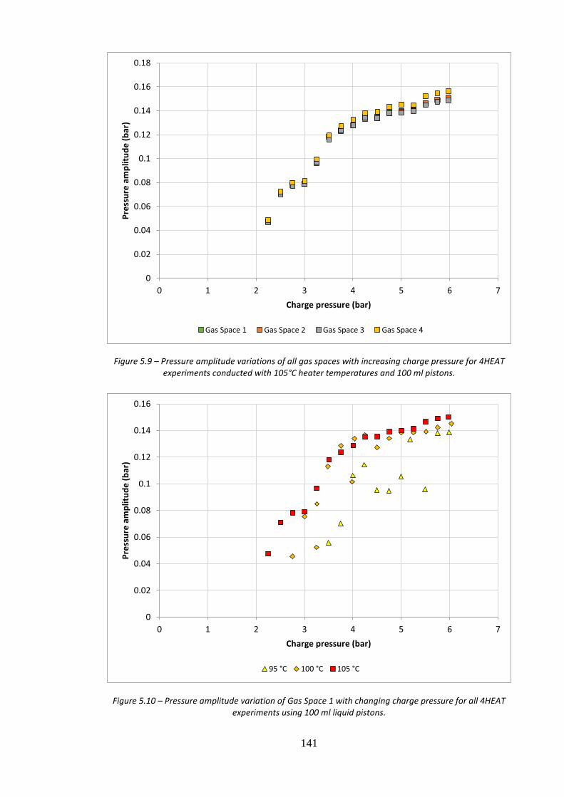
141

Figure 5.9 – Pressure amplitude variations of all gas spaces with increasing charge pressure for 4HEAT experiments conducted with 105°C heater temperatures and 100 ml pistons.

Figure 5.10 – Pressure amplitude variation of Gas Space 1 with changing charge pressure for all 4HEAT experiments using 100 ml liquid pistons.

0

0.02

0.04

0.06

0.08

0.1

0.12

0.14

0.16

0.18

0 1 2 3 4 5 6 7

Pre

ssu

re a

mp

litu

de

(b

ar)



0

0.02

0.04

0.06

0.08

0.1

0.12

0.14

0.16

0 1 2 3 4 5 6 7

Pre

ssu

re a

mp

litu

de

(b

ar)


95 °C 100 °C 105 °C

142

Similar to Figure 5.9, Figure 5.10 displays the pressure amplitude variations with charge

pressure, but for all three heater temperatures investigated. Due to the symmetry within

the 4HEAT configuration, only Gas Space 1 measurements are graphed. The general

influence of higher heater temperatures producing larger pressure amplitudes is evident.

More interesting is the apparent separation of the data points into a number of ridges. This

indicates the possibility of different stable regions of operation, which are subsequently

referred to as modes. All of the 105°C results occupy the highest energy modes, with

perhaps one existing between 2 bar–3 bar and another from 3 bar–6 bar. The 100°C data

points occupy both the higher energy and lower energy modes, which seem to converge

at approximately 4.5 bar. The 95°C series include some data points in-line with the lower

energy mode seen in the 100°C results, as well as what appear to be either outliers or a

lower energy mode between 4.5 bar and 5.5 bar. The phenomenon of these different

operational modes was something consistently observed in the 15 mm U-tube

experiments and is discussed in more detail in section 8.2.5.

Figure 5.11 shows the difference in gas temperatures between the compression and

expansion spaces. Although relatively close in magnitude, a consistent trend is evident in

the data—with the temperature difference in GS2 being the largest, GS1 and GS3

occupying similar middle values, and GS4 having the lowest difference. The compression

space temperatures were all very similar for each sub-system as they were regulated by

the cooling water, which was near ambient. The variance in these gas space temperature

differentials is therefore attributed to different expansion space temperatures, which

implies potentially different heater surface temperatures. As discussed in Section 3.1.4,

the experimental set-up regulates the fin temperature of one heater (GS2), and each heater

is supplied the same quantity of power. Therefore, there are two potential causes of these

differences: either they are due to the variations in the thermal resistances within each hot

heat exchanger sub-assembly; or, alternatively, due to other imperfections in the

143

geometric/thermal symmetry of the sub-systems, which causes the system to reach a

stable operating point that does not reflect the precisely symmetrical behaviour of the

theoretical 4HEAT system. In practice, achieving a perfectly symmetrical system is

difficult, and unnecessary for a preliminary research endeavour akin to this one.

Figure 5.11 – Gas space temperature differentials and their variation with charge pressure for the 4HEAT experiments with 105°C heater temperatures.

The largest variance seen in Figure 5.11 is approximately 5ºC and occurs at 4.25 bar,

between GS2 and GS4—however, this magnitude of inconsistency is still considered to

be acceptable for the purposes of this project. Section 8.2.2 reviews the design of the

experimental set-up and discusses recommendations for future experimental work.

Interestingly, the local peak in gas space temperature difference (seen above at 4.25 bar)

closely corresponds to the maximum piston amplitudes across the range of charge

pressures tested. These are shown in Figure 5.12. The average piston amplitudes for each

of the three heater temperatures are then shown in Figure 5.13.

47

48

49

50

51

52

53

54

55

56

0 1 2 3 4 5 6 7

Gas

te

mp

era

ture

(°C

)


Gas Space 1 (TC1-TC2) Gas Space 2 (TC3-TC4) Gas Space 3 (TC5-TC6) Gas Space 4 (TC7-TC8)

144

Figure 5.12 – Piston amplitude variation with charge pressure for the 105ºC, 4HEAT configuration experiments using 100 ml liquid pistons.

Figure 5.13 – Average piston amplitude variation with mean operating pressure for all 4HEAT configuration experiments using 100 ml liquid pistons.

0

0.5

1

1.5

2

2.5

3

3.5

4

4.5

5

0 1 2 3 4 5 6 7

Pis

ton

am

plit

ud

e (

cm)



0

0.5

1

1.5

2

2.5

3

3.5

4

4.5

5

0 1 2 3 4 5 6 7

Pis

ton

am

plit

ud

e (

cm)


95 °C 100 °C 105 °C

145

The piston amplitudes increase with mean pressure from 2 bar–4 bar, before reaching

their maximum at approximately 4 bar, and begin to decline as the charge pressure is

increased from 4 bar–6 bar. An interesting characteristic of the behaviour of the system

was that the ease with which the system started loosely followed the distribution of piston

amplitude. At charge pressures close to 4 bar, the system was easy to start, requiring

minimal manual excitation before the piston motion would self-amplify. The system

became more and more difficult to start as the charge pressure moved away from 4 bar,

requiring more vigorous manual excitation before reaching self-sustaining motion.

The average piston amplitudes in Figure 5.13 show that the other heater temperatures

behave similarly, with the exception of the lowest temperature of 95ºC. The 100ºC results

are very similar to the 105ºC results except for the experiments below 3 bar. The 100ºC

experiments were not able to achieve stable operation below this point. A clear peak is

seen at approximately 4 bar. It is worth noting that the same modal behaviour identified

in the pressure amplitude plot of Figure 5.11 is evident in these results as well. Excluding

some of the lower energy 95ºC results, the amplitudes for the different heater

temperatures appear to converge along some form of an upper limit for charge pressures

of 4.5 bar and higher. The shape of this limit resembles an inverse proportionality, where

the product of pressure and piston amplitude is equal to some constant. This is

investigated further and discussed in section 5.1.5.

The final graphs presented for the 4HEAT configuration in this general results section

concern the pressure and piston displacement phase angles. Figure 5.14 shows how the

phase angles of the pressure amplitude phasors vary with charge pressure. For clarity, the

only experiments plotted are those at 105ºC heater temperature.

146

Figure 5.14 – Pressure phasor relative phase angles' variation with gas charge pressure for the 105ºC 4HEAT experiments with 100 ml liquid pistons.

The most striking feature of Figure 5.14 is the clear distinction between experiments

below 3 bar charge pressure and experiments with 3 bar (and higher) charge pressure.

The modal behaviour suspected earlier in the 105ºC experiments is confirmed by the

differences in these phasor plots. The reasons why the different operational modes would

have different phase angle relationships is not as obvious, however, and is discussed in

later sections. Beyond 3 bar, the relative phase angles between the gas pressure amplitude

phasors appears relatively consistent. Figure 5.15 shows the relative phase angles of the

pistons across the charge pressure range. The phase angles oscillate around the expected

value of 90°, but diverge further away from this value as charge pressure is increased,

particularly in the range 5 bar–6 bar. Interestingly, this is also the range at which jump-

starting the system becomes increasingly difficult, and the pistons’ behaviour appears

more unstable.

82

84

86

88

90

92

94

96

0 1 2 3 4 5 6 7

Re

lati

ve p

has

e a

ngl

e (

°)


Gas Space 1-2 Gas Space 2-3 Gas Space 3-4 Gas Space 4-1

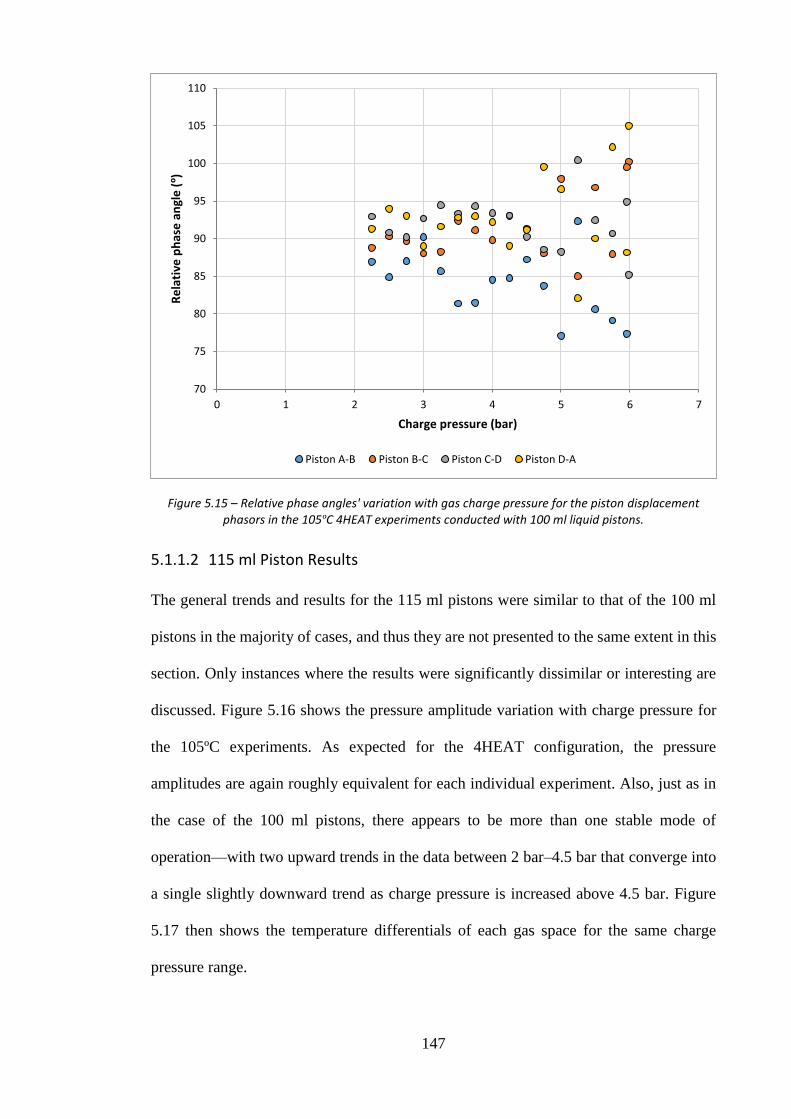
147

Figure 5.15 – Relative phase angles' variation with gas charge pressure for the piston displacement phasors in the 105ºC 4HEAT experiments conducted with 100 ml liquid pistons.


The general trends and results for the 115 ml pistons were similar to that of the 100 ml

pistons in the majority of cases, and thus they are not presented to the same extent in this

section. Only instances where the results were significantly dissimilar or interesting are

discussed. Figure 5.16 shows the pressure amplitude variation with charge pressure for

the 105ºC experiments. As expected for the 4HEAT configuration, the pressure

amplitudes are again roughly equivalent for each individual experiment. Also, just as in

the case of the 100 ml pistons, there appears to be more than one stable mode of

operation—with two upward trends in the data between 2 bar–4.5 bar that converge into

a single slightly downward trend as charge pressure is increased above 4.5 bar. Figure

5.17 then shows the temperature differentials of each gas space for the same charge

pressure range.

70

75

80

85

90

95

100

105

110

0 1 2 3 4 5 6 7

Re

lati

ve p

has

e a

ngl

e (º)


Piston A-B Piston B-C Piston C-D Piston D-A

148

Figure 5.16 – Pressure amplitude variation with charge pressure for the 105ºC 4HEAT experiments using 115 ml liquid pistons.

Figure 5.17 – Temperature differentials between the expansion and compression spaces for each gas space and their variation with charge pressure for the 105ºC 4HEAT experiments with 115 ml liquid

pistons.

0

0.02

0.04

0.06

0.08

0.1

0.12

0.14

0.16

0.18

0 1 2 3 4 5 6 7

Pre

ssu

re a

mp

litu

de

(b

ar)



40

42

44

46

48

50

52

54

56

58

0 1 2 3 4 5 6 7

Tem

pe

ratu

re d

iffe

ren

ce (

ºC)



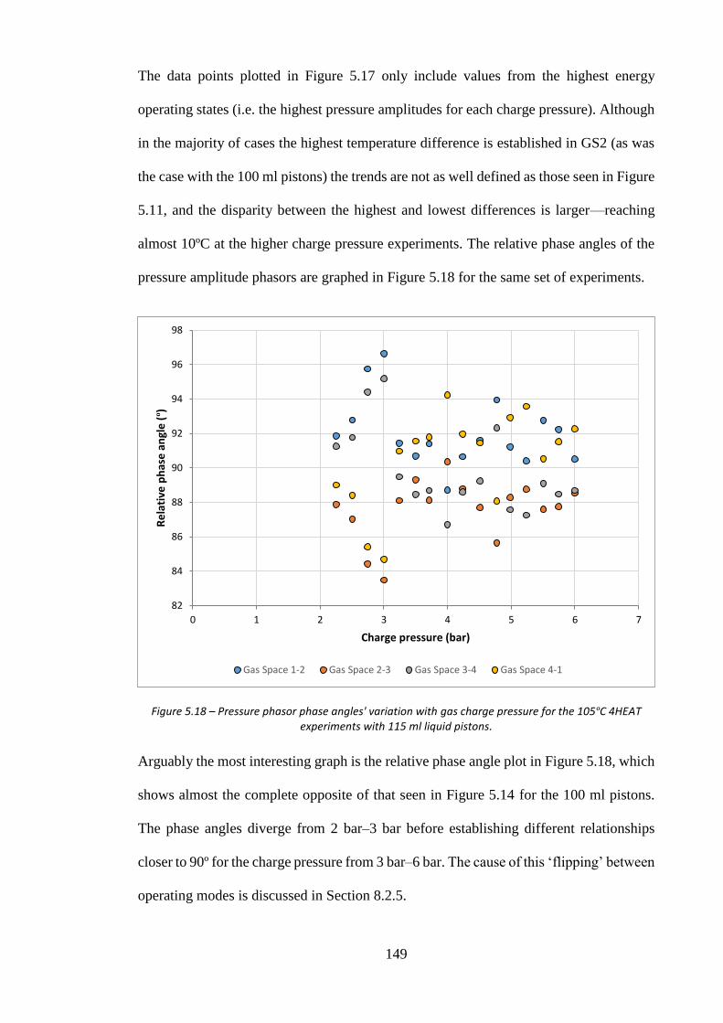
149

The data points plotted in Figure 5.17 only include values from the highest energy

operating states (i.e. the highest pressure amplitudes for each charge pressure). Although

in the majority of cases the highest temperature difference is established in GS2 (as was

the case with the 100 ml pistons) the trends are not as well defined as those seen in Figure

5.11, and the disparity between the highest and lowest differences is larger—reaching

almost 10ºC at the higher charge pressure experiments. The relative phase angles of the

pressure amplitude phasors are graphed in Figure 5.18 for the same set of experiments.

Figure 5.18 – Pressure phasor phase angles' variation with gas charge pressure for the 105ºC 4HEAT experiments with 115 ml liquid pistons.

Arguably the most interesting graph is the relative phase angle plot in Figure 5.18, which

shows almost the complete opposite of that seen in Figure 5.14 for the 100 ml pistons.

The phase angles diverge from 2 bar–3 bar before establishing different relationships

closer to 90º for the charge pressure from 3 bar–6 bar. The cause of this ‘flipping’ between

operating modes is discussed in Section 8.2.5.

82

84

86

88

90

92

94

96

98

0 1 2 3 4 5 6 7

Re

lati

ve p

has

e a

ngl

e (

º)



150

5.1.1.3 4HEAT summary

The important findings and observations from the 4HEAT section are summarised and

outlined here for clarity: (a) The phasor analysis shows that the symmetrical behaviour

expected is evident which is verified by the pressure amplitude magnitude and phase

angle similarities; (b) The experimental frequency trend has a dependence on the square

root of pressure as predicted by the analytical solution obtained for the natural frequency

of the LPSC system; (c) Increased heater temperature generally leads to higher pressure

amplitudes, but the results imply that a number of stable modes of operation are present

and can be occupied by different heater temperatures. Some of the phase angle data

analysis shows a clear distinction between these modes; (d) The pressure amplitudes tend

to increase with charge pressure until reaching an as yet unexplained threshold where

experiments with different heater temperatures converge.


The 3HEAT configuration is one of the two configurations which has the potential to

produce a cooling effect. With three subsystems producing work and one subsystem

consuming work, the 3HEAT configuration has the desirable characteristic of containing

only one absorption space—but it is not known how the dynamics of the three adjacent

power-producing subsystems will impact the dynamics of the machine. The results

presented here aim to illustrate the behaviour of the 3HEAT configuration, and how its

performance is influenced by changes in the key design parameters in Table 5.2. As in

the 4HEAT case, example results of a representative 3HEAT experiment are presented

first. Figures 5.19 and 5.20 show the pressure amplitudes and heater temperature trends

for a typical 3HEAT experiment.

151

Figure 5.19 – Gas pressure amplitude variations during a typical 3HEAT experiment. The experiment was at 4 bar with 150ºC set heater temperature and 100 ml liquid pistons.

Figure 5.20 – Heater gas temperature variations during a typical 4HEAT experiment. The experiment was at 4 bar with 150ºC set heater temperature and 100 ml liquid pistons.

0

0.02

0.04

0.06

0.08

0.1

0.12

0.14

0.16

0.18

0 500 1000 1500 2000 2500

Pre

ssu

re a

mp

litu

de

(b

ar)

Elasped time (s)

Gas Space 1 (Absorber) Gas Space 2 (Heater)


88

90

92

94

96

98

100

102

104

106

108

0 500 1000 1500 2000 2500

Gas

te

mp

era

ture

(ºC

)

Elapsed time (s)

Gas Space 2 Gas Space 3 Gas Space 4

152

The experiment considered in this example case used heaters set at 150ºC, 100 ml liquid

pistons and a gas charge pressure of 4 bar. Unlike the 4HEAT configuration, the pressure

amplitudes in Figure 5.20 vary significantly in magnitude. The pressure amplitudes

developed in GS1 and GS3 are close to equal at approximately 0.1 bar. These two spaces

are opposite each other in the series of four subsystems, with GS1 containing the absorber

and GS3 a heater. With substantially higher pressure amplitudes of 0.155 and 0.140 bar,

respectively, GS2 and GS4 contain the second and third heater, and are also opposite each

other. These ratios in magnitude between the developed pressure amplitudes in each of

the four gas spaces was something that occurred consistently during the majority of

3HEAT experiments and is later quantified. To some extent, the heater gas temperatures

shown in Figure 5.20 reflect the differences in pressure amplitudes; the highest

temperatures align with the highest pressure amplitudes, although the differences between

GS2 and GS4 are much more pronounced in the temperature case. GS3 registers the

lowest heater gas temperature of approximately 95°C, compared with GS2 (the highest),

with approximately 105°C. These temperatures are higher than in the 4HEAT

experiments, primarily because of the higher heater temperatures needed to account for

the unpowered fourth subsystem, GS1.

Figures 5.21 and 5.22 show the pressure and displacement profiles during a one second

snapshot taken during the experiment. The snapshot was taken at time, t = 1210 seconds

(20 minutes and 10 seconds into the experiment). The pressure profiles graph shows a

number of interesting characteristics. Firstly, all four pressure profiles appear to be

roughly 90° out of phase with each other. The two lowest pressure amplitude profiles seen

in spaces GS1 and GS3 appear very similar in maximum and minimum values, and are

180° out of phase; while the two larger pressure amplitudes, GS2 and GS4, are slightly

different in terms of magnitude.

153

Figure 5.21 – Gas pressure profiles over one second interval during a typical 3HEAT experiment. The experiment was at 4 bar and 150ºC with 100 ml liquid pistons. Time taken was at 1210 seconds (20


Figure 5.22 – Piston displacement profiles over one second interval during a typical 3HEAT experiment. The experiment was at 4 bar and 150ºC with 100 ml liquid pistons. Time taken was at 1210 seconds (20


3.8

3.85

3.9

3.95

4

4.05

4.1

4.15

4.2

0 200 400 600 800 1000

Gas

pre

ssu

re (

bar

)

Time (ms)


2.5

3

3.5

4

4.5

5

5.5

0 200 400 600 800 1000

Dis

pla

cem

en

t se

nso

r o

utp

ut

(V)

Time (ms)


154

As in the case of the 4HEAT experiments, the piston displacement profiles seen in Figure

5.22 appear less consistent from cycle to cycle—although they clearly have different

phase angle relationships when compared with the pressure profiles. Despite pistons

opposite to each other appearing to have 180° phase differences, the phase angles between

adjacent pistons is not uniformly close to 90°. Applying the least mean squares

approximation and calibration procedure described in Section 3.2.3, phasor expressions

of the gas pressure and displacement profiles were obtained. Table 5.3 shows the values

obtained for the example 3HEAT experiment. As previously carried out in the 4HEAT

case, the unscaled and scaled phasor plots can then be constructed from the tabulated

values (but for discussion purposes only the scaled phasor plots need to be shown). Figure

5.23 shows the scaled phasor plot for the example 3HEAT experiment.

Table 5.3 – Phasor representations of gas pressure and piston displacement amplitudes for example 3HEAT experiment.


Pressure 1 (P1) 0.096 0

Pressure 2 (P2) 0.156 93.7

Pressure 3 (P3) 0.098 177.1

Pressure 4 (P4) 0.139 273.1





It is clear from Figure 5.23 that the behaviour of the 3HEAT system deviates from the

symmetrical 45° phasor separations seen in the 4HEAT configuration. The two large

pressure phasors P2 and P4 ‘stretch’ the system out vertically, which causes the piston

phasors to gravitate towards the larger magnitude pressure amplitudes. In the case of

Piston A (phasor XA), for example, the displacement of this piston is influenced by the

pressures P1 and P2. P2 has the greater amplitude which forces the motion of the piston

to be more similar in phase with this pressure than the lower amplitude pressure, P1. This

explains why each piston displacement phasor is closer in phase to the adjacent gas space

155

with the highest pressure amplitude. Even with this effect, every pair of opposite phasors

remains approximately 180° out of phase with each other, which is evidence of how the

symmetry of the system is imposed on the dynamic response.

Figure 5.23 – Phasor plot of the pressure and displacement profiles for the example 3HEAT experiment. The phasor magnitudes have been scaled for more clarity. The experiment was at 4 bar and 150ºC with

100 ml liquid pistons.

Figure 5.24 presents the phase angle values relating to the pressure and displacement

phasors in Figure 5.23.

P1

P2

P3

P4

XA

XB XC

XD

Pressure 1 (P1) Pressure 2 (P2) Pressure 3 (P3) Pressure 4 (P4)

Displacement A (XA) Displacement B (XB) Displacement C (XC) Displacement D (XD)

156

Figure 5.24 – Pressure and displacement phase angles for 3HEAT example experiment.

The relative phase angles between the pressure phasors is close to 90° as was seen in the

case of the 4HEAT system. The most significant difference is seen in the relative phase

angle differences between the piston displacements. The differences between

neighbouring pistons alternate from approximately 110° to 70°.


The results presented here cover the experiments conducted with 100 ml piston volumes,

using the 3HEAT configuration at three heater temperatures of 130°C, 140°C and 150°C,

and across the charge pressure range of 2 bar–6 bar. A number of figures are shown to

highlight how some of the key variables depend on charge pressure and heater

temperature—namely pressure amplitudes, piston displacements, phase angles and gas

space temperature differentials. The figures are accompanied by brief assessments and

general observations about the behaviour of the 3HEAT configuration.

Figure 5.25 shows how the operational frequency of the system changes with increased

charge pressure. The frequency trends of the 3HEAT experiments resemble that of the

4HEAT experiments. The frequency increases with charge pressure and, as predicted,

shows a square root dependence. The experimental dependence on temperature is

assessed for all 3 configurations in Section 5.1.4.

93.7


68.8 112.3


109.0 69.9


96.0

157

Figure 5.25 – Frequency variation with mean operating pressure for all 3HEAT configuration experiments using 100 ml liquid pistons.


0

1

2

3

4

5

6

0 1 2 3 4 5 6 7

Fre

qu

en

cy (

Hz)


130 °C 140 °C 150 °C

0

0.02

0.04

0.06

0.08

0.1

0.12

0.14

0.16

0.18

0.2

0 1 2 3 4 5 6 7

Pre

ssu

re a

mp

litu

de

(b

ar)


Gas Space 1 (Absorber) Gas Space 2 (Heater) Gas Space 3 (Heater) Gas Space 4 (Heater)

158

Figure 5.26 shows the pressure amplitudes developed for 3HEAT experiments conducted

at 150°C heater temperatures. The pressure amplitude seen in each of the gas spaces retain

their characteristic differences in magnitude first identified in the example 3HEAT

experiment, with GS2 and GS3 achieving the highest values, and GS1 and GS3 the

lowest. The pressure amplitude ratios of the three heater spaces to the absorber space

remain close to constant across the charge pressure range. The mean ratios (and associated

standard deviations) are 1.62 (s = 0.7%), 1.02 (s = 0.6%) and 1.44 (s = 0.7%) for GS2,

GS3 and GS4, respectively. With standard deviations less than 1%, it can be inferred that

the pressure amplitude ratios are an important behavioural trait, which can be used to

assess the performance of each configuration. As a method for evaluating the

effectiveness of the 3HEAT configuration, the conversion of pressure amplitudes

developed in the heated spaces to those in the absorber space can be assessed. Summing

the relative pressure ratios gives a conversion ratio of 4.08:1 (three significant figures).

This ratio is used as a measure of the potential suitability of a particular configuration,

and is referred to in subsequent analysis as the conversion ratio.

As the charge pressure is increased, the pressure amplitudes increase and appear to peak

at the upper end of the tested range of 6 bar. This is very similar to that which occurred

for the 4HEAT experiments with 100 ml pistons, except the maximum amplitudes

achieved are higher in magnitude in the 3HEAT case—the largest being 0.188 bar

compared with 0.156 bar from the 4HEAT experiments. The average values for the

3HEAT experiments are similar to (but slightly lower than) the 4HEAT experiments at

the same charge pressure, e.g. 0.148 bar compared with 0.152 bar at 6 bar. When

comparing the 4HEAT and 3HEAT experiments in this manner, it should be noted that

the different heater temperatures probably imply very different heat inputs; although this

comparison is still of interest considering that the heater temperatures selected are close

to the minimum necessary for stable operation. Figure 5.27 shows how the other heater

159

temperature experiments compared in respect to the pressure amplitudes. The graph

shows the data for GS1, which contained the absorption space.


Again evident is the possibility for different operational modes to exist; although fewer

experiments exhibited bi-modal behaviour when compared with the 4HEAT case. Some

of the experiments attempted at lower charge pressures and temperatures were unable to

achieve steady operation. Hence, results for 130°C heaters below 4 bar and 140°C heaters

below 3 bar are missing. With these pressure amplitudes being generated in the absorption

space, an obvious question arises with regard to evidence of cooling. Figure 5.28 shows

the temperature difference between the expansion (absorption) and compression

(rejection) spaces in GS1. For the values displayed, positive values can be interpreted as

the expansion space having a higher temperature than the compression space, implying

that a cooling effect has not been developed. Negative values show that the absorption

space has a lower temperature than the water-cooled compression space.

0

0.02

0.04

0.06

0.08

0.1

0.12

0.14

0 1 2 3 4 5 6 7

Pre

ssu

re a

mp

litu

de

(b

ar)


130 °C 140 °C 150 °C

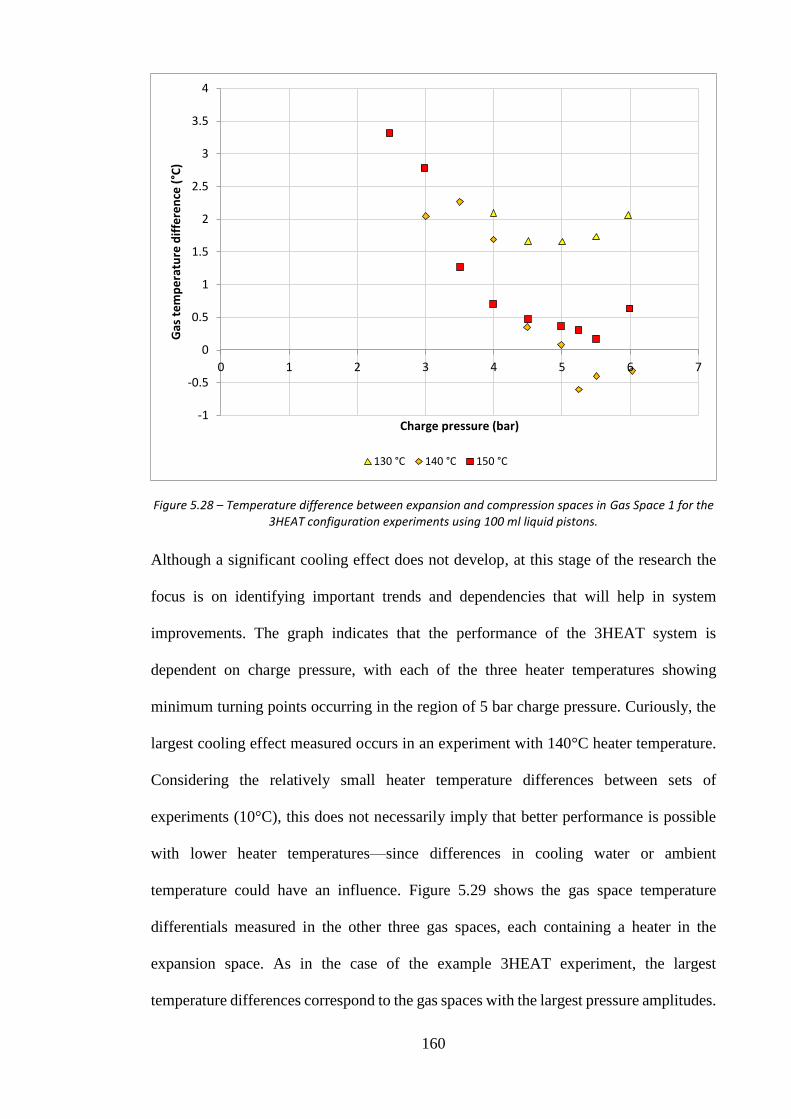
160

Figure 5.28 – Temperature difference between expansion and compression spaces in Gas Space 1 for the 3HEAT configuration experiments using 100 ml liquid pistons.

Although a significant cooling effect does not develop, at this stage of the research the

focus is on identifying important trends and dependencies that will help in system

improvements. The graph indicates that the performance of the 3HEAT system is

dependent on charge pressure, with each of the three heater temperatures showing

minimum turning points occurring in the region of 5 bar charge pressure. Curiously, the

largest cooling effect measured occurs in an experiment with 140°C heater temperature.

Considering the relatively small heater temperature differences between sets of

experiments (10°C), this does not necessarily imply that better performance is possible

with lower heater temperatures—since differences in cooling water or ambient

temperature could have an influence. Figure 5.29 shows the gas space temperature

differentials measured in the other three gas spaces, each containing a heater in the

expansion space. As in the case of the example 3HEAT experiment, the largest

temperature differences correspond to the gas spaces with the largest pressure amplitudes.

-1

-0.5

0

0.5

1

1.5

2

2.5

3

3.5

4

0 1 2 3 4 5 6 7

Gas

te

mp

era

ture

dif

fere

nce

(°C

)


130 °C 140 °C 150 °C

161

Figure 5.29 – Heater gas space temperature differentials and their variation with charge pressure for the 3HEAT experiments with 150°C heater temperatures and 100 ml liquid pistons.


60

65

70

75

80

85

90

0 1 2 3 4 5 6 7

Gas

te

mp

era

ture

dif

fere

nce

(°C

)


Gas Space 2 (Heater) Gas Space 3 (Heater) Gas Space 4 (Heater)

0

0.5

1

1.5

2

2.5

3

3.5

4

4.5

0 1 2 3 4 5 6 7

Pis

ton

am

plit

ud

es

(cm

)



162

Figure 5.30 shows the piston amplitudes for the 3HEAT experiments at 150°C heater

temperature. A peak occurs at 4 bar, with amplitudes decreasing in the direction of both

higher and lower charge pressure from this point. Reviewing the 4HEAT piston amplitude

plots from earlier, the maximum piston amplitudes occur at roughly the same charge

pressure as these tests. There does not appear to be very much difference between the

amplitudes of each piston. The largest difference occurs between Piston A and Piston D

and equates to 6.9 mm at 4 bar charge pressure. Apart from an increase in amplitude of

Piston D relative to the other pistons at higher charge pressure, not much more can be

inferred from this graph. The average piston amplitudes for each of the three heater

temperatures are shown in Figure 5.31. The multi-modal characteristics are seen again,

with lower energy states occurring for experiments below 5 bar, and the results for the

three temperatures converging upon an apparent excitation limit above this point.

Figure 5.31 – Average piston amplitude variation with charge pressure for all of the 3HEAT experiments conducted using 100 ml liquid pistons.

0

0.5

1

1.5

2

2.5

3

3.5

4

0 1 2 3 4 5 6 7

Pis

ton

am

plit

ud

e (

cm)


130 °C 140 °C 150 °C

163

The final graphs presented for the 3HEAT configuration in this general results section

again concern the phase angles on the system. Figure 5.32 shows how the phase angles

of the pressure amplitude phasors vary with charge pressure. Again, the only experiments

plotted are those at the highest heater temperature of 150ºC. The results appear relatively

consistent and within a similar range to the relative phase angles seen in the 4HEAT

experiments above 3 bar. A clear separation of each relative phase angle occurs with the

pairs of GS1–GS2 and GS4–GS1 having phase angles closer to 90°, while the other two

pairs are ± 7° from 90°.

Figure 5.32 – Relative phase angle variations with gas charge pressure for the pressure phasors in the 150ºC 3HEAT experiments using 100 ml liquid pistons.

Figure 5.33 shows the relative phase angles for the piston displacements. As identified in

the example 3HEAT experiment, the piston phase angles are significantly different when

comparing 3HEAT to the 4HEAT operation. These differences remain across the charge

pressure range tested—although towards the higher end of 5 bar–6 bar, the phase angles

82

84

86

88

90

92

94

96

98

0 1 2 3 4 5 6 7

Ph

ase

an

gle

(°)



164

appear to flare inward in contrast to the 4HEAT phase angles which flared outward. The

3HEAT system becomes more difficult to jump-start in this range as well.

Figure 5.33 – Relative phase angle variations with gas charge pressure for the piston displacement phasors in the 150ºC 3HEAT experiments using 100 ml liquid pistons.


As per the 4HEAT results, the 115 ml 3HEAT results are not presented with as much

detail as the 100 ml piston results because of the significant similarities. Instead, instances

where the results were significantly dissimilar or interesting are presented.

Figure 5.34 shows the pressure amplitude variation with charge pressure for Gas Space 1

(absorber) and all heater temperatures. The 115 ml experiments exhibited the same

consistent pressure amplitude ratios seen with the 100 ml pistons, where GS2 and GS4

achieved higher values than GS1 and GS3. The range of successful experiments is larger

in the 115 ml case, with stable operation starting at 2 bar for 150°C and 2.5 bar for 140°C

heater temperatures. The pressure amplitudes reflect similar behaviour to that seen in both

50

60

70

80

90

100

110

120

130

0 1 2 3 4 5 6 7

Re

lati

ve p

has

e a

ngl

e (

°)



165

3HEAT and 4HEAT experiments up to this point. The heater temperatures have more

influence at lower pressure, with the behaviour of the system essentially identical for all

three heater values above 5 bar charge pressure. The pressure amplitudes developed in

the 115 ml experiments were slightly higher than their 100 ml counterparts.

Figure 5.34 – Gas pressure amplitude variations for Gas Space 1 in the 3HEAT experiments conducted using 115 ml liquid pistons.

The gas temperature difference between the expansion and compression spaces in Gas

Space 1 is shown in Figure 5.35. The trend for the temperature difference generated in

Gas Space 1 suggests that the best performance occurs in the region of 4.5 bar–5 bar,

although as in the 100 ml case, the level of cooling attained is not significant. Despite the

higher pressure amplitudes developed in the 115 ml experiments, the temperature

differences measured were not significantly larger.

0

0.02

0.04

0.06

0.08

0.1

0.12

0.14

0.16

0 1 2 3 4 5 6 7

Pre

ssu

re a

mp

litu

de

(b

ar)


130 °C 140 °C 150 °C

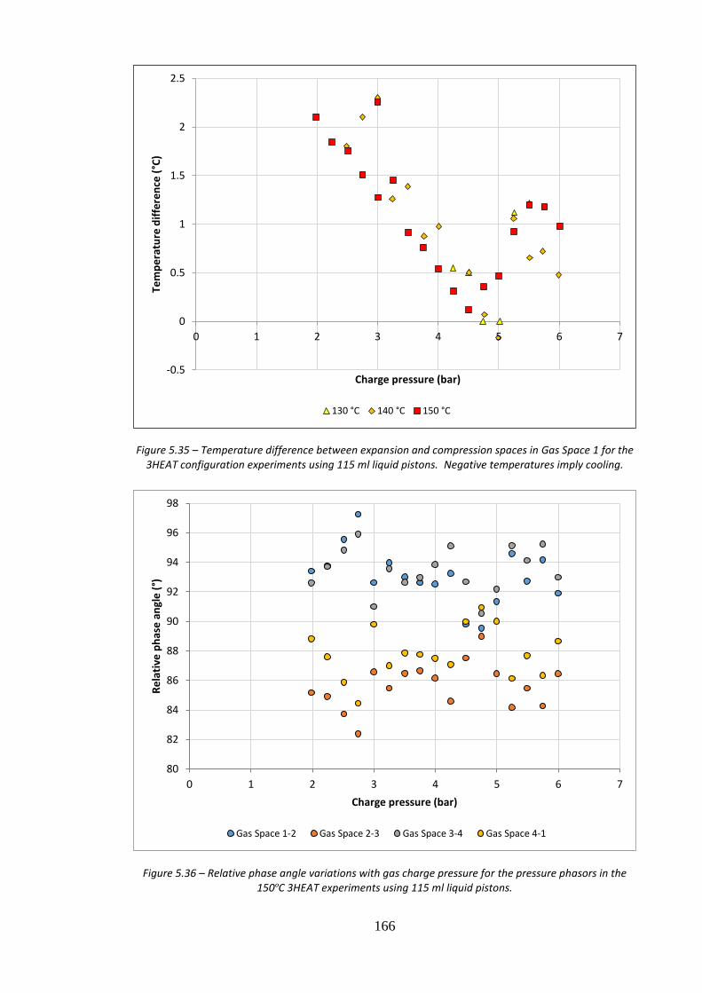
166

Figure 5.35 – Temperature difference between expansion and compression spaces in Gas Space 1 for the 3HEAT configuration experiments using 115 ml liquid pistons. Negative temperatures imply cooling.

Figure 5.36 – Relative phase angle variations with gas charge pressure for the pressure phasors in the 150ºC 3HEAT experiments using 115 ml liquid pistons.

-0.5

0

0.5

1

1.5

2

2.5

0 1 2 3 4 5 6 7

Tem

pe

ratu

re d

iffe

ren

ce (

°C)


130 °C 140 °C 150 °C

80

82

84

86

88

90

92

94

96

98

0 1 2 3 4 5 6 7

Re

lati

ve p

has

e a

ngl

e (

°)



167

Figure 5.36 shows the phase angles of the pressure phasors for 3HEAT experiments at

150°C with the 115 ml pistons. Interestingly, the graph shows the same divergence when

the charge pressure approaches 3 bar, as was seen for the 4HEAT experiments with 115

ml pistons. The result at 4.75 bar is also intriguing, with all phase angles being very close

to 90º, unlike the rest of the results which have similar trends to the 100 ml phase angle

results. Figure 5.37 presents the relative phase angle trends for the piston displacement

phasors.

Figure 5.37 – Relative phase angle variations with gas charge pressure for the piston displacement phasors in the 150ºC 3HEAT experiments using 115 ml liquid pistons.

Apart from the two groups at 5 bar and 6 bar, the phase angles of the liquid pistons are

very consistent across the pressure range. The differences between the close pairs and

further away pairs are also larger in magnitude, with the relative phase angles for pistons

A–B and C–D generally between 110°–120°, and for pistons B–C and D–A between 60°–

70º—whereas these values were closer to 70º and 110º with the 100 ml pistons. Also of

note is that the same convergence/divergence of the relative phase angles seen in the

50

60

70

80

90

100

110

120

130

0 1 2 3 4 5 6 7

Re

lati

ve p

has

e a

ngl

es

(°)



168

trends for the gas pressures is not seen in the piston phase angle plots for the 115 ml

pistons.

5.1.2.3 3HEAT Summary


outlined here for clarity: (a) Similar to the 4HEAT configuration, the experimental

frequency trend with charge pressure follows the analytical prediction; (b) Increased

heater temperatures generally lead to higher pressure amplitudes; although increases seem

to get closer to a possible maximum as the charge pressure nears 6 bar (perhaps tests at

higher pressure would confirm this); (c) The pressure amplitudes developed are not equal

for all gas spaces. The two opposite gas spaces containing heaters, GS2 and GS4, record

the highest values—with maximum global values of 0.211 bar and 0.185 bar respectively.

The other pair of opposite gas spaces, GS1 and GS3, consistently recorded equal pressure

amplitudes with the global maximum being 0.136 bar. The ratios of these pressure

amplitudes remained consistent across the charge pressure and temperature range

investigated. This means that the lowest pressure amplitude is always developed in the

absorber space, which may hinder the cooling potential of this configuration; (d) The

relative phase angles between the pressure phasors at approximately 90° were very similar

to the 4HEAT configuration. This was not the case for the piston displacement phase

angles where the differences in magnitude of the pressure amplitudes influenced the

piston phases, and aligned them closer to the higher pressure amplitude spaces. The result

was phase angles between pistons of approximately 70º or 110º; (e) The temperature

difference developed in the absorber gas space seemed to depend on charge pressure,

indicating an optimal charge pressure existed between 4.5 bar–5.5 bar for both piston

masses, although no significant cooling capability was measured for any experiment1.

1 It is worth reiterating that at this stage of the research, the primary objective is understanding the dynamics

of the system, and not necessarily targeting the largest temperature difference.

169

The largest temperature difference achieved in Gas Space 1 was 0.5ºC; (f) Multi-modal

behaviour was again witnessed at the lower charge pressure experiments (below 5 bar),

with the developed pressure and piston amplitudes converging above this threshold, and

being independent of heater temperature.


The 2HEAT configuration is the second of the two configurations which has the potential

to produce a cooling effect. With two subsystems producing work and two subsystem

consuming work, the 2HEAT configuration contains two heaters (GS2 and GS3), and two

absorbers (GS1 and GS4). Two possible configurations exist for the 2HEAT scenario, the

alternating and adjacent configurations. These were described in Section 3.3.3. After

extensive efforts to operate the alternating configuration with no success, the adjacent

configuration was found to function, but only with 115 ml pistons. It is probable that

100 ml pistons would have worked with higher heater temperatures, but an upper limit of

190ºC was set to protect elements of the test-rig. The results presented here aim to

illustrate the behaviour of the 2HEAT configuration, and how its performance is

influenced by changes in the key design parameters in Table 5.2. The results cover only

one heater temperature, 190ºC, and one piston size, 115 ml. Figure 5.38 shows the

pressure amplitudes trends for a typical 2HEAT. The experiment considered in this case

was with a gas charge pressure of 4 bar.

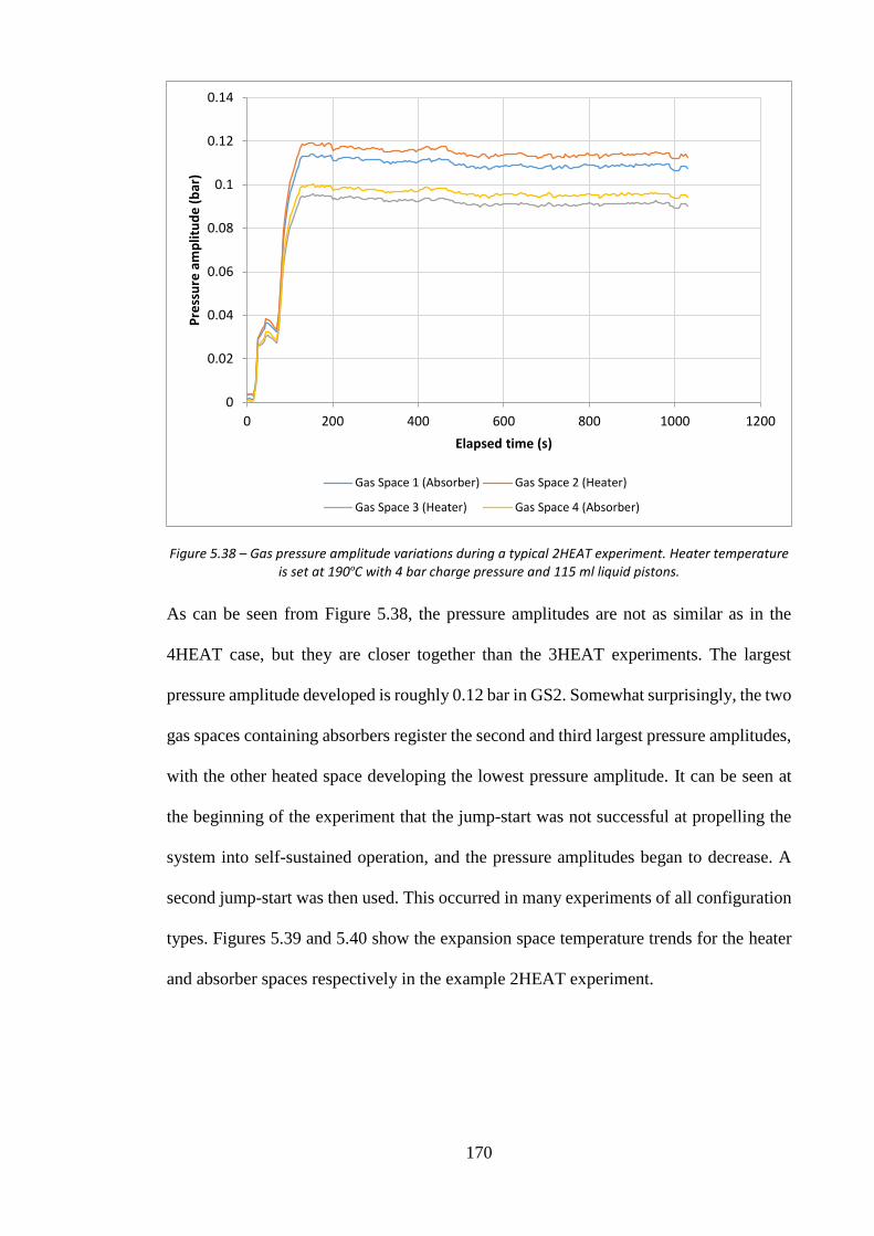
170

Figure 5.38 – Gas pressure amplitude variations during a typical 2HEAT experiment. Heater temperature is set at 190ºC with 4 bar charge pressure and 115 ml liquid pistons.

As can be seen from Figure 5.38, the pressure amplitudes are not as similar as in the

4HEAT case, but they are closer together than the 3HEAT experiments. The largest

pressure amplitude developed is roughly 0.12 bar in GS2. Somewhat surprisingly, the two

gas spaces containing absorbers register the second and third largest pressure amplitudes,

with the other heated space developing the lowest pressure amplitude. It can be seen at

the beginning of the experiment that the jump-start was not successful at propelling the

system into self-sustained operation, and the pressure amplitudes began to decrease. A

second jump-start was then used. This occurred in many experiments of all configuration

types. Figures 5.39 and 5.40 show the expansion space temperature trends for the heater

and absorber spaces respectively in the example 2HEAT experiment.

0

0.02

0.04

0.06

0.08

0.1

0.12

0.14

0 200 400 600 800 1000 1200

Pre

ssu

re a

mp

litu

de

(b

ar)

Elapsed time (s)


Gas Space 3 (Heater) Gas Space 4 (Absorber)

171

Figure 5.39 – Heater space gas temperature variations during a typical 2HEAT experiment. The experiment was at 4 bar with 190ºC set heater temperature and 115 ml liquid pistons.

Figure 5.40 – Absorber space gas temperature variations during a typical 2HEAT experiment. The experiment was at 4 bar with 190ºC set heater temperature and 115 ml liquid pistons.

100

105

110

115

120

125

130

135

0 200 400 600 800 1000 1200

Gas

te

mp

era

ture

(°C

)

Elapsed time (s)

Gas Space 2 Gas Space 3

25

25.5

26

26.5

27

27.5

28

28.5

29

29.5

30

0 200 400 600 800 1000 1200

Gas

te

mp

era

ture

(°C

)

Elapsed time (s)


172

As can be seen from the Figures 5.39 and 5.40, the largest pressure amplitudes correspond

to the more pronounced expansion space temperatures. Gas Space 2 exhibits the largest

pressure amplitude and the gas approaches 130ºC, while in Gas Space 3 the temperature

approaches 120ºC. In the case of the absorbers, the lowest temperature is achieved by the

space with the higher pressure amplitude, GS1. There is a noticeable drop in the absorber

gas temperatures once the system achieves self-sustained operation (at approximately 150

seconds). Figures 5.41 and 5.42 show the pressure and displacement profiles during a one

second snapshot taken midway through the experiment. The snapshot was taken at time,

t = 450 seconds (7 minutes and 30 seconds into the experiment).

Figure 5.41 – Gas pressure profiles over a one second interval during a typical 2HEAT experiment. The experiment was at 4 bar and 190ºC with 115 ml liquid pistons. Time taken was at 450 seconds (7 minutes

30 seconds) into the experiment.

3.85

3.9

3.95

4

4.05

4.1

4.15

0 200 400 600 800 1000

Gas

pre

ssu

re (

bar

)

Time (ms)


Gas Space 3 (Heater) Gas Space 4 (Absorber)

173

Figure 5.42 – Piston displacement profiles over a one second interval during a typical 2HEAT experiment. The experiment was at 4 bar and 190ºC with 115 ml liquid pistons. Time taken was at 450 seconds (7


The relative phase angles of the pressure profiles and displacement profiles appear to be

approximately 90º; they appear much more regularly spaced than the 3HEAT

configuration. Applying the same least mean squares approximation and calibration

procedure from earlier will yield the phasor expressions of the gas pressure and

displacement profiles. Table 5.4 shows the phasor values obtained for the example

2HEAT experiment. Figure 5.43 then shows the associated scaled phasor plot.



Pressure 1 (P1) 0.112 0

Pressure 2 (P2) 0.118 90.0

Pressure 3 (P3) 0.0936 180.0

Pressure 4 (P4) 0.0982 270.0





2

2.5

3

3.5

4

4.5

0 200 400 600 800 1000

Dis

pla

cem

en

t se

nso

r o

utp

ut

(V)

Time (ms)


174

Figure 5.43 – Phasor plot of example 2HEAT experiment pressure amplitude and displacement profiles. The phasor magnitudes have been scaled for more clarity.

The pressure phasors are positioned in a very similar manner to both the 4HEAT and

3HEAT scenarios previously examined. The P2 phasor’s relative phase angle to P1 is

slightly greater than 90º, the P3 phasor’s relative phase angle to P1 is slightly less than

180º and the P4 phasor’s relative phase angle is slightly more than 270º. It seems as

though the phase angles of the pressures are unaffected by the configuration of the system.

The magnitudes of the phasors are different, however, and in this case the arrangement

with P1 and P2 being dominant seems to have a favourable influence on the piston phases.

Unlike the 3HEAT configuration, the relative phase angles between piston displacements

P1

P2

P3

P4

XA

XB XC

XD



175

look much closer to the desirable 90º value for a Stirling machine. Another important

feature of this plot is that it shows that opposite pistons are not constrained to having 180º

phase differences, which appeared to be the case for the 3HEAT experiments. Figure 5.44

presents the phase angle values relating to the pressure and displacement phasors in

Figure 5.43.

Figure 5.44 – Pressure and piston displacement phasor phase angles for 2HEAT example experiment.

As observed, the relative phase angles of the pistons are much closer to 90º than in the

3HEAT case. Understandably, they are not as close as the values seen in the symmetrical

4HEAT experiments; although for a system which has two forward and two reverse heat

engines connected in series the values are encouraging. The absorber gas spaces are

particularly interesting with the relative phase angles of the adjacent pistons next to gas

spaces 1 and 4 at 88.0º and 96.2º respectively. This suggests that the dynamic constraints

of this configuration may be more suitable for cooling than the 3HEAT configuration.


The results presented here cover the experiments conducted with 115 ml piston volumes,

using the 2HEAT configuration at a heater temperature of 190°C, and across the charge

pressure range of 2 bar–6 bar. Similar to the general overview of the previous

configurations, a number of figures are shown to highlight how some of the key variables

95.5


88.0 99.2


96.2 76.6


95.5

176

depend on charge pressure and heater temperature. The figures are accompanied by brief

assessments and general observations about the behaviour of the 2HEAT configuration.

Figure 5.45 shows how the operational frequency of the system changes with increased

charge pressure.

Figure 5.45 – Shows the frequency variation with mean operating pressure for all 2HEAT configuration experiments using 115 ml liquid pistons.

As expected, the results for the frequency trend are similar to the previous configurations.

They appear to exhibit the same dependence on charge pressure as previously identified.

The 2HEAT configuration was unable to achieve self-sustaining operation below 3 bar

charge pressure; although it is likely that with increased heater temperatures, operation at

lower pressures would occur (as previously explained, heater temperatures above 190ºC

were not considered). The missing data point between 4 and 4.5 bar (i.e. the 4.25 bar

experiment) is due to the data being accidentally corrupted and lost. Figure 5.46 presents

the pressure amplitudes developed in the 2HEAT experiments.

0

0.5

1

1.5

2

2.5

3

3.5

4

4.5

5

0 1 2 3 4 5 6 7

Fre

qu

en

cy (

Hz)



177


The pressure amplitudes increase with charge pressure, and appear to approach a local

maximum in the region of 6 bar—with the largest value of 0.147 bar being recorded in

Gas Space 2 at 5.75 bar. The relative magnitudes of the pressure amplitudes developed in

each of the four gas spaces remains consistent across the range tested. The mean ratios

with respect to GS1 are 1.05 (s = 0.6%), 0.84 (s = 0.3%) and 0.88 (s = 0.6%) for GS2,

GS3 and GS4 respectively. Adding up the unrounded ratios obtained for the heater and

absorber spaces gives 1.884 for the heater spaces, and 1.879 for the absorber spaces,

which equates to a conversion ratio of 1.003:1 (to three significant figures).

The gas temperatures measured in the expansion spaces of each subsystem are displayed

in the following graphs. Figure 5.47 shows the temperatures of the heated spaces 2 and 3,

while Figure 5.48 shows the absorber temperatures in 1 and 4. The temperature

differences correspond with the relative magnitudes of the pressure amplitudes in each

space.

0

0.02

0.04

0.06

0.08

0.1

0.12

0.14

0.16

0 1 2 3 4 5 6 7

Pre

ssu

re a

mp

litu

de

(b

ar)



178

Figure 5.47 – Heater gas space temperature differentials and their variation with charge pressure for the 2HEAT experiments with 190°C heater temperatures and 115 ml liquid pistons.

Figure 5.48 – Temperature difference between expansion and compression spaces in gas spaces 1 and 4 for the 2HEAT configuration experiments using 115 ml liquid pistons.

80

85

90

95

100

105

0 1 2 3 4 5 6 7

Gas

te

mp

era

ture

dif

fere

nce

(°C

)


Gas Space 2 (TC3-TC4) Gas Space 3 (TC5-TC6)

0

0.5

1

1.5

2

2.5

3

3.5

4

4.5

5

0 1 2 3 4 5 6 7

Gas

te

mp

era

ture

dif

fere

nce

(°C

)



179

The behaviour of the hot spaces is similar to that expected (i.e. as charge pressure

increases so does the measured gas temperature). This is a consequence of the increased

frequency, density and gas velocity, which influences the heat transfer coefficients. In the

absorber spaces, Gas Space 1 exhibits the lowest temperature differences. With the higher

of the two pressure amplitudes, the gas is forced expand to a greater degree than in the

absorber of Gas Space 4.


The piston displacements for the 2HEAT experiments are shown in Figure 5.49. The

amplitudes exhibit the same general trends as those seen in earlier configurations with a

gradual increase towards a peak near 4.5 bar—before decreasing marginally as charge

pressure is increased further. A significant difference, however, is that the piston

amplitudes seem to be grouped into two pairs with pistons A and C recording similar

amplitudes to each other. Pistons B and D also demonstrate similar amplitudes, but these

-0.5

0

0.5

1

1.5

2

2.5

3

3.5

4

0 1 2 3 4 5 6 7

Pis

ton

am

plit

ud

es

(cm

)



180

are consistently in the range of 10 mm larger than A and C, and often within a few

millimetres of each other.

The final graphs of interest for the 2HEAT configuration are the phase angles trends of

the system. Figure 5.50 shows how the phase angles of the pressure amplitude phasors

vary with charge pressure, and Figure 5.51 shows the same for the phase angles of the

displacement phasors.

Figure 5.50 – Relative phase angle variations with gas charge pressure for the pressure phasors in the 190°C 2HEAT experiments using 115 ml liquid pistons.

As mentioned in the assessment of the example experiment phasor plot, the values of the

relative phase angles between the pressure phasors are similar to the results for the other

configurations. They are all close to 90º, but consistently GS1–GS2 and GS3–GS4 values

are above 90º, while GS2–GS3 and GS4–GS1 values are below 90º. This differs from the

other configuration plots in the uniformity of the relative phase angles across the entire

charge pressure range. Each relative phase angle varies (at most) by 1º across the range

82

84

86

88

90

92

94

96

98

0 1 2 3 4 5 6 7

Re

lati

ve p

has

e a

ngl

e (

º)



181

of 3 bar–6 bar, whereas the other configurations exhibit differences of up to 7º. This

highlights an important characteristic of the 2HEAT adjacent configuration that was

noticed during the experimental procedure. The 2HEAT experiments were always very

stable; none resulted in any multi-modal behaviour, and the pressure amplitudes

fluctuated to a lesser degree than the other configurations. Unfortunately, since results

from other heater temperatures are absent in the 2HEAT case, it is unknown whether this

trait is inherent. This is addressed in the second set of experimental parameters

investigated in Section 6.2, where additional 2HEAT experiments are evaluated.

Figure 5.51 – Relative phase angle variations with gas charge pressure for the piston displacement phasors in the 190°C 2HEAT experiments using 115 ml liquid pistons.

5.1.3.2 2HEAT Summary


outlined here for clarity: (a) In a similar manner to the 3HEAT and 4HEAT

configurations, the experimental frequency follows the expected trend with charge

pressure; (b) Increased heater temperatures generally lead to higher pressure amplitudes;

70

75

80

85

90

95

100

105

0 1 2 3 4 5 6 7

Re

lati

ve p

has

e a

ngl

e (

°)



182

although the increases seem to get closer to a possible maximum as the charge pressure

nears 6 bar. The pressure amplitudes developed are not equal for all gas spaces, but they

are much closer in magnitude than the 3HEAT experiments. (c) Interestingly, the larger

pressure amplitudes are not exclusively held by heated spaces. GS2 still registers the

largest, with a global maximum of 0.147 bar at 5.75 bar charge pressure. The next largest

is an absorber space, GS1, with 0.141 bar, followed by the second absorber space, GS4,

with 0.124 bar. The second heated space, GS3, consistently records the lowest pressure

amplitude with a maximum of 0.118 bar; (d) The relative magnitudes of these pressure

amplitudes remains consistent across the charge pressure range 3 bar–6 bar, resulting in

a consistent conversion ratio of 1.003:1. This distribution is potentially much more

favourable for producing a cooling effect; (e) At approximately 90°, the relative phase

angles between the pressure phasors were very similar to both the 3HEAT and 4HEAT

configurations. Unlike the 3HEAT results, the relative phase angles of the piston phasors

were much closer to the desired 90º target. The values related to the absorber spaces, C–

D and D–A, were particularly promising and consistently within 85º–95º; (f) The

temperature difference developed in the absorber gas spaces again showed a dependence

on charge pressure, with an optimal charge pressure existing between 4.5 bar–5 bar.

Despite no significant cooling effect being measured for any experiment, the dynamic

behaviour of the 2HEAT system is very encouraging, with both desirable phase angle and

pressure amplitude distributions; (g) Multi-modal behaviour was not witnessed for any

2HEAT experiments; (h) The experimental investigation into the 2HEAT configuration

was limited because of the high heater temperatures required to achieve self-sustained

operation. Sustained operation was not possible with the 100 ml pistons.

183

5.1.4 Configuration Comparisons

After assessing the results of each configuration’s experiments, it is possible to compare

their general behavioural characteristics, as well as the influence of the additional piston

mass in the 115 ml experiments. Figure 5.52 shows the operational frequency

measurements for all sets of experiments conducted with 100 ml, while Figure 5.53 shows

the same graph for all 115 ml liquid piston experiments. As predicted, the temperature

increases in the heater spaces have very little influence on the resulting frequency of the

LPSC system, independent of which configuration is being considered. The primary

dynamic differences between the configurations are the gas temperatures in the expansion

spaces, which have a small effect on gas spring constant and therefore frequency.

Figure 5.52 – Operational frequency variation with mean operating pressure for all experiments using 100 ml liquid pistons.

0

1

2

3

4

5

6

0 1 2 3 4 5 6 7

Fre

qu

en

cy (

Hz)


100 ml 3HEAT (130 °C) 100 ml 3HEAT (140 °C) 100 ml 3HEAT (150 °C)


184

Figure 5.53 – Operational frequency variation with mean operating pressure for all experiments using 115 ml liquid pistons.

Figure 5.54 – Operational frequency differences between 100 ml and 115 ml liquid pistons.

0

1

2

3

4

5

6

0 1 2 3 4 5 6 7

Fre

qu

en

cy (

Hz)


115 ml 3HEAT (130 °C) 115 ml 3HEAT (140 °C) 115 ml 3HEAT (150 °C) 115 ml 4HEAT (95 °C)


0

1

2

3

4

5

6

0 1 2 3 4 5 6 7

Fre

qu

en

cy (

Hz)


100 ml pistons 115 ml pistons

185

Figure 5.54 compares the frequency trends of the 100 ml piston with the 115 ml pistons.

The frequency is only slightly affected by the increase in piston mass. A 15% increase in

the mass of the piston resulted in the frequency reducing by a maximum of 3.9%—with

this percentage difference decreasing further with increased charge pressure. This limited

influence is a consequence of the fact that—for the particular geometry of the test-rig—

the natural frequency of the system is dominated by the gas spring component, which has

a much larger magnitude than the piston gravitational term. Figure 5.55 shows the

influence that the larger piston mass has on the pressure amplitudes developed in the

4HEAT configuration experiments. Similarly, the pressure amplitudes developed in the

absorber spaces of the 3HEAT configuration experiments are compared in Figure 5.56.

Figure 5.55 – Differences in pressure amplitudes between 100 ml and 115 ml liquid pistons for the 4HEAT, 105ºC experiments.

0

0.02

0.04

0.06

0.08

0.1

0.12

0.14

0.16

0.18

0 1 2 3 4 5 6 7

Pre

ssu

re a

mp

litu

de

(b

ar)



186

Figure 5.56 – Differences in pressure amplitudes between 100 ml and 115 ml liquid pistons for the 3HEAT 150ºC experiments.

The larger piston masses produce larger pressure amplitudes at the same charge pressures

in comparison to the smaller pistons. This is more obvious in the 3HEAT experiments

where multi-modal behaviour at the temperatures selected is less evident. The pressure

amplitude is consistently roughly 0.02 bar higher for the 115 ml piston experiments,

although in both graphs the pressure amplitudes appear to converge at the higher charge

pressures between 5 bar–6 bar.

Table 5.5 (shown on the following page) is a summary table listing some of the key

performance data from both 100 ml and 115 ml experiments for the 15 mm piston LPSC

test-rig.

0

0.02

0.04

0.06

0.08

0.1

0.12

0.14

0.16

0 1 2 3 4 5 6 7

Pre

ssu

re a

mp

litu

de

(b

ar)



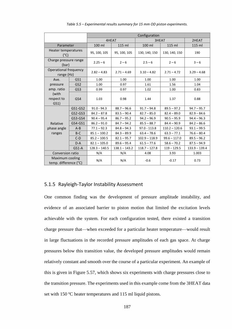
187

Table 5.5 – Experimental results summary for 15 mm OD piston experiments.

Configuration

4HEAT 3HEAT 2HEAT

Parameter 100 ml 115 ml 100 ml 115 ml 115 ml

Heater temperatures (°C)

95, 100, 105 95, 100, 105 130, 140, 150 130, 140, 150 190

Charge pressure range (bar)

2.25 – 6 2 – 6 2.5 – 6 2 – 6 3 – 6

Operational frequency range (Hz)

2.82 – 4.83 2.71 – 4.69 3.10 – 4.82 2.71 – 4.72 3.29 – 4.68

Ave. pressure

amp. ratio (with

respect to GS1)

GS1 1.00 1.00 1.00 1.00 1.00

GS2 1.00 0.97 1.61 1.56 1.04

GS3 0.99 0.97 1.02 1.00 0.83

GS4 1.03 0.98 1.44 1.37 0.88

Relative phase angle

ranges

GS1-GS2 91.0 - 94.3 88.7 – 96.6 91.7 – 94.8 89.5 – 97.2 94.7 – 95.7

GS2-GS3 84.2 – 87.8 83.5 – 90.4 82.7 – 85.0 82.4 – 89.0 82.9 – 84.6

GS3-GS4 90.4 – 95.4 86.7 – 95.2 94.2 – 96.9 90.5 – 95.9 94.4 – 96.3

GS4-GS1 86.2 – 91.0 84.7 – 94.2 85.5 – 88.7 84.4 – 90.9 84.2 – 86.6

A-B 77.1 – 92.3 84.8 – 94.3 97.0 - 113.8 110.2 – 120.6 93.1 – 99.5

B-C 85.1 – 100.2 84.3 – 89.9 63.4 – 78.6 63.3 – 77.1 76.6 – 80.4

C-D 85.2 – 100.5 82.1 – 95.7 102.9 – 118.9 99.6 – 117.0 89.5 – 96.2

D-A 82.1 – 105.0 89.6 – 95.4 61.5 – 77.6 58.6 – 70.2 87.5 – 94.9

GS1-A 128.3 – 140.5 138.1 – 143.2 118.7 – 127.8 119 – 129.5 133.9 – 139.4

Conversion ratio N/A N/A 4.08 3.93 1.003

Maximum cooling temp. difference (°C)

N/A N/A -0.6 -0.17 0.73

5.1.5 Rayleigh-Taylor Instability Assessment

One common finding was the development of pressure amplitude instability, and

evidence of an associated barrier to piston motion that limited the excitation levels

achievable with the system. For each configuration tested, there existed a transition

charge pressure that—when exceeded for a particular heater temperature—would result

in large fluctuations in the recorded pressure amplitudes of each gas space. At charge

pressures below this transition value, the developed pressure amplitudes would remain

relatively constant and smooth over the course of a particular experiment. An example of

this is given in Figure 5.57, which shows six experiments with charge pressures close to

the transition pressure. The experiments used in this example come from the 3HEAT data

set with 150 ºC heater temperatures and 115 ml liquid pistons.

188

Figure 5.57 – Pressure amplitude stability for different charge pressures. Experiments are all from 3HEAT 150ºC data set with 115 ml pistons.

The experiments at 3.5 bar (or below) produce pressure amplitudes that are relatively

stable, while those at 3.75 bar (or above) are much more volatile, and show sudden and

large fluctuations around a mean value. This same pattern is found when analysing the

results of all of the data sets for the 15 mm experiments: that is, every configuration and

heater temperature produced a similar occurrence of a transition from stability to

instability. The charge pressures corresponding to this transition point were dependent on

the heater temperature—with higher temperatures leading to lower transition pressures.

In order to understand the cause of this phenomenon, the stability of the liquid pistons

and their surfaces must be assessed. Figures 5.58 and 5.59 show the piston displacement

profiles produced by the capacitive sensors for two of the experiments from the Figure

5.57. The first is from the 3.25 bar charge pressure experiment, and the second from the

5 bar experiment.

0

0.02

0.04

0.06

0.08

0.1

0.12

0.14

0.16

300 400 500 600 700 800 900 1000

Pre

ssu

re a

mp

litu

de

(b

ar)

Elapsed time (s)

2.75 bar 3.25 bar 3.5 bar 3.75 bar 4 bar 5 bar

189

Figure 5.58 – Piston displacement profiles over a one second interval at 3.25 bar charge pressure. The experiment was with 3HEAT and 150°C heaters, using 115 ml liquid pistons.

Figure 5.59 – Piston displacement profiles over a one second interval at 5 bar charge pressure. The experiment was with 3HEAT and 150°C heaters, using 115 ml liquid pistons.

1.5

2

2.5

3

3.5

4

4.5

5

0 200 400 600 800 1000

Dis

pla

cem

en

t se

nso

r o

utp

ut

(V)

Time (ms)


1.5

2

2.5

3

3.5

4

4.5

0 200 400 600 800 1000

Dis

pla

cem

en

t se

nso

r o

utp

ut

(V)

Time (ms)


190

Despite some slight flattening of the minimum turning points in the readings from the

3.25 bar experiment, the profiles themselves are very smooth and closely follow

sinusoidal motion. This means that the liquid within the measurement volume is changing

steadily (and in a repeatable way) each cycle, i.e. the piston oscillation is stable. The

measurements from the 5 bar experiment are quite different. Three of the four piston

profiles show irregular behaviour between cycles. The profiles retain the general

sinusoidal shape, but exhibit periods of sudden accelerated or decelerated changes in

capacitance. Although not noticeable from an observer’s standpoint during the

experiment, the liquid pistons are not perfectly stable in the 5 bar profile. It is likely that

the instability is reducing the levels of excitation that would be achievable for an identical

configuration with different liquid pistons—or, indeed, possibly solid pistons.

The Rayleigh-Taylor (RT) instability was considered as a potential explanation for the

development of this piston instability. The RT instability, which is outlined in

Appendix II, imposes an acceleration limit on the interface of two fluids having different

densities, i.e. before the exponential growth of surface perturbations. It is possible to

check whether the RT instability is causing the piston instability by evaluating the

maximum piston accelerations that are experienced during each experiment. Figure 5.60

shows the average maximum piston accelerations sustained for the 115 ml experiments

using the 15 mm piston tubes. The maximum accelerations that are sustained by the

pistons begin to rise at pressures of 2 bar–4 bar—a region that normally exhibit stable

pressure amplitude and piston displacement profiles. Beyond the transition pressures

associated with each data set, the maximum accelerations do not show significant

increases. None of the experiments were able to sustain accelerations above 30 ms-2.

Observing the two highest temperature data sets for each configuration, 105ºC for 4HEAT

and 150ºC for 3HEAT, the maximum accelerations rose at a close to linear rate before

abruptly plateauing at 4 bar, and staying within the range of 25ms-2–30 ms-2.

191

Figure 5.60 – Average maximum piston acceleration for experiments with 115 ml pistons and 15 mm piston tubes.

This would also potentially explain why the profiles of different heater temperatures seem

to merge at higher operating pressure. With increased heater temperatures it is expected

that the gap between excitation levels would remain across the entire spectrum of

considered charge pressures; however, as seen previously, some of the pressure

amplitudes developed at higher charge pressures are the same for different temperatures.

If a physical limit on piston motion exists, then these results (i.e. with different data sets

converging on the same values) would be an expected outcome. This is not conclusive

evidence that an acceleration limit exists, but it does provide a basis for exploring this

possibility when considering the Sage model predictions, and the second experimental

investigation in later chapters.

0

5

10

15

20

25

30

35

0 1 2 3 4 5 6 7

Max

imu

m p

isto

n a

cce

lera

tio

n (

ms-2

)


95 °C 4HEAT 115 ml 100 °C 4HEAT 115 ml 105 °C 4HEAT 115 ml

130 °C 3HEAT 115 ml 140 °C 3HEAT 115 ml 150 °C 3HEAT 115 ml

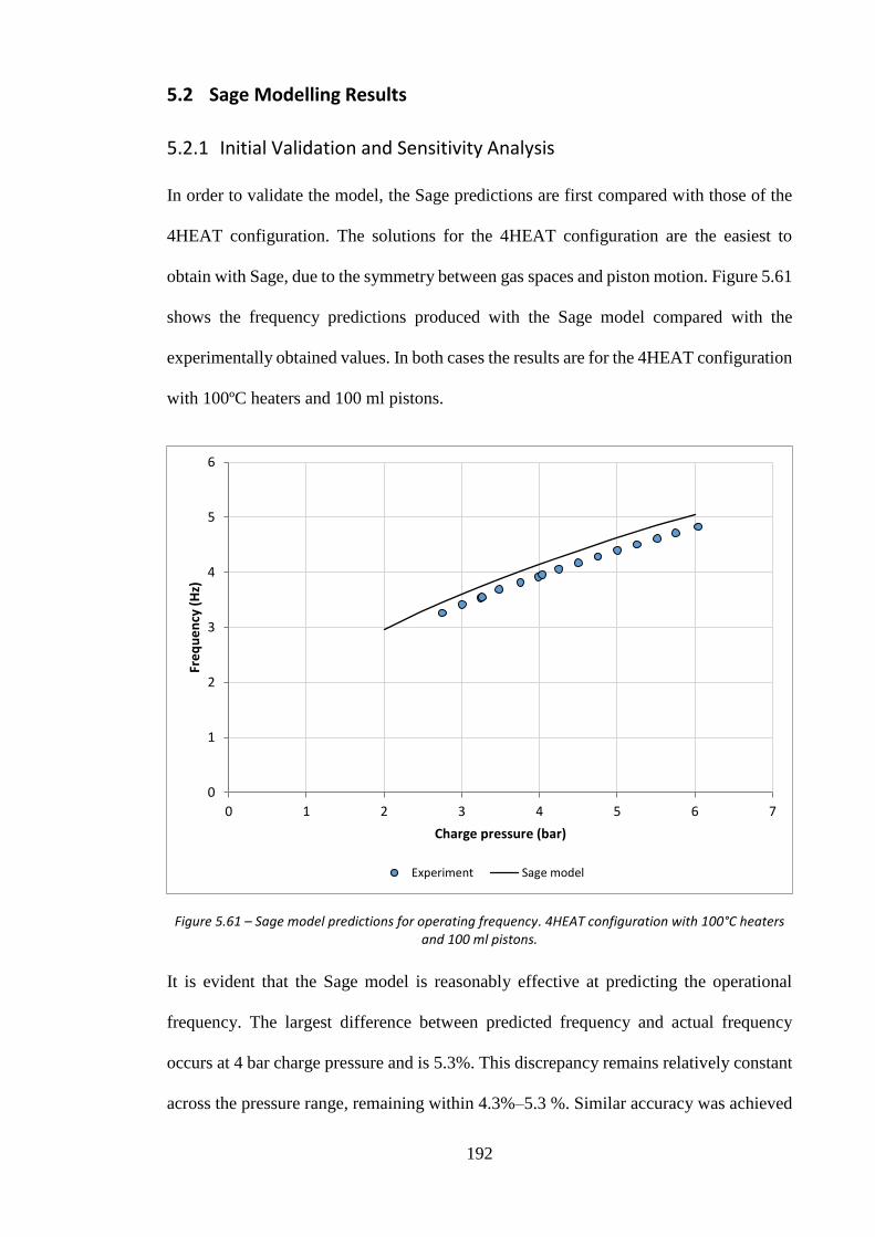
192

5.2 Sage Modelling Results

5.2.1 Initial Validation and Sensitivity Analysis

In order to validate the model, the Sage predictions are first compared with those of the

4HEAT configuration. The solutions for the 4HEAT configuration are the easiest to

obtain with Sage, due to the symmetry between gas spaces and piston motion. Figure 5.61

shows the frequency predictions produced with the Sage model compared with the

experimentally obtained values. In both cases the results are for the 4HEAT configuration

with 100ºC heaters and 100 ml pistons.

Figure 5.61 – Sage model predictions for operating frequency. 4HEAT configuration with 100°C heaters and 100 ml pistons.

It is evident that the Sage model is reasonably effective at predicting the operational

frequency. The largest difference between predicted frequency and actual frequency

occurs at 4 bar charge pressure and is 5.3%. This discrepancy remains relatively constant

across the pressure range, remaining within 4.3%–5.3 %. Similar accuracy was achieved

0

1

2

3

4

5

6

0 1 2 3 4 5 6 7

Fre

qu

en

cy (

Hz)


Experiment Sage model

193

when modelling the 115 ml pistons. Figure 5.62 shows the piston amplitudes predicted

for the same set of simulations compared with the measured quantities from experiment.

Figure 5.62 – Sage model predictions for piston amplitude. 4HEAT configuration with 100ºC heaters and 100 ml pistons.

The Sage model does not predict piston amplitudes as accurately as frequency. It

consistently overestimates piston amplitude, and although the model follows the same

trend, and seems to agree reasonably well with the profile of the experimental results at

the lower operating pressures (<4 bar), the predictions begin to diverge at higher charge

pressure. This was a very interesting discovery that was not initially explainable. It

seemed likely that the underlying cause is associated with the differences between liquid

pistons (as used in the experiments) and solid pistons (upon which the Sage model bases

its liquid piston approximation). This is further evidence of a potential physical limitation

affecting the liquid pistons, which only materialises upon reaching some threshold of

operation. At this stage it is inconclusive, but aside from this discrepancy, the Sage model

was more accurate than expected, and capable of assessing potential performance

improvements. A number of physical parameters used in the model are subject to

0

1

2

3

4

5

6

0 1 2 3 4 5 6 7

Pis

ton

am

plit

ud

e (

cm)


Sage model Experiment

194

variation in reality. It is important to know how sensitive the model is to changes in these

parameters, and therefore a sensitivity analysis (that, for the time being, ignores the

discrepancies in piston amplitude) was carried out as follows:

Liquid piston viscosity – The dynamic viscosity of the water being used as liquid pistons

influences the calculation of the viscous damping coefficient within the Sage model. As

explained in Section 4.2.7, this value attempts to approximate the viscous energy losses

associated with piston motion. The viscosity of water is not constant; it depends primarily

on temperature. Since one side of the water column is in close proximity to heated gas

then the water temperature can gradually change over the course of an experiment or a

set of experiments. Figure 5.63 shows what happens to the Sage simulation results when

the viscosity within the model is changed to reflect 20°C, 25°C and 30ºC water. The

viscosity of water at these temperatures was taken to be 1.0 × 10-3 Nsm-2, 8.9 × 10-4 Nsm-2

and 8.0 × 10-4 Nsm-2, respectively.

Figure 5.63 – Sage model predictions of piston amplitude for different water viscosities. 4HEAT, 100ºC and 100 ml simulation.

0

1

2

3

4

5

6

7

0 1 2 3 4 5 6 7

Pis

ton

am

plit

ud

e (

cm)


20 °C Water 25 °C Water 30 °C Water

195

For an increase in water temperature of 10°C, the model predicts the piston amplitude can

rise by roughly 10 mm, regardless of charge pressure. This effect is more significant at

lower pressure, doubling the amplitude for simulations at 2 bar—while at 6 bar the

difference is 14.6% between 20°C and 30°C water.

Sum of kinetic flow loss coefficients – The sum of the minor flow loss coefficients is

used to estimate the energy dissipation caused by geometric changes in the flow path of

the piston. The U-tube housing of the piston can be thought of as having two smooth 90º

bends at its base (or a single 180º bend) and being otherwise straight. At the position

where the steel tube transitions to PVC tube there is also a small change in cross-section;

although the change in diameter produces a negligible flow loss coefficient compared to

the other features. The contribution of these effects is estimated with a ΣK sum of 0.5 (see

Section 4.2.7). Figure 5.64 shows the sensitivity of the model predictions with ΣK values

of 0.5, 0.75 and 1.0.

Figure 5.64 – Sage model predictions for piston amplitude with different values for the sum of the minor pipe flow loss coefficients. 4HEAT simulations with 100ºC heaters and 100 ml pistons.

0

1

2

3

4

5

6

0 1 2 3 4 5 6 7

Pis

ton

am

plit

ud

e (

cm)


ΣK = 0.5 ΣK = 0.75 ΣK = 1.0 Experiment

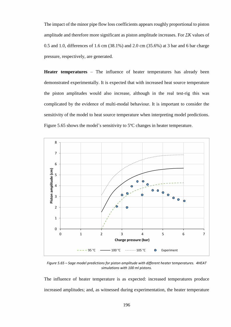
196

The impact of the minor pipe flow loss coefficients appears roughly proportional to piston

amplitude and therefore more significant as piston amplitude increases. For ΣK values of

0.5 and 1.0, differences of 1.6 cm (38.1%) and 2.0 cm (35.6%) at 3 bar and 6 bar charge

pressure, respectively, are generated.

Heater temperatures – The influence of heater temperatures has already been

demonstrated experimentally. It is expected that with increased heat source temperature

the piston amplitudes would also increase, although in the real test-rig this was

complicated by the evidence of multi-modal behaviour. It is important to consider the

sensitivity of the model to heat source temperature when interpreting model predictions.

Figure 5.65 shows the model’s sensitivity to 5ºC changes in heater temperature.

Figure 5.65 – Sage model predictions for piston amplitude with different heater temperatures. 4HEAT simulations with 100 ml pistons.

The influence of heater temperature is as expected: increased temperatures produce

increased amplitudes; and, as witnessed during experimentation, the heater temperature

0

1

2

3

4

5

6

7

8

0 1 2 3 4 5 6 7

Pis

ton

am

plit

ud

e (

cm)


95 °C 100 °C 105 °C Experiment

197

directly impacts the lower limits of charge pressure at which the system is capable of

achieving self-sustained operation. But the magnitude of the influence of heater

temperature is very surprising—a 1.5% change in heater temperature is capable of

producing a 23.9% difference in piston amplitude even at the high operating pressure of

6 bar.

Heat rejection temperatures – As with heater temperature, the heat sink temperatures

also play a role in influencing the performance of the LPSC machine. In the model, the

heat sink (or rejector) temperature is set at 24ºC. Figure 5.66 displays the model

sensitivity to changes in the ambient temperature value of ± 5ºC.

Figure 5.66 – Sage model sensitivity to heat rejection temperature. 4HEAT simulations with 100ºC heaters and 100 ml pistons.

The effect of altering the rejection temperature has the reverse impact of changing the

heater temperatures—with higher temperatures decreasing piston amplitude. This is as

one would expect for any thermodynamic machine: the output being dependent on the

0

1

2

3

4

5

6

7

8

0 1 2 3 4 5 6 7

Pis

ton

am

plit

ud

e (

cm)


19 °C 24 °C 29 °C

198

temperature difference between the sink and source temperatures. In this case, the same

change of ± 5ºC produces a more significant change in the piston amplitudes than for the

heater temperature. At 6 bar the difference between 24ºC and 29ºC is 28.8%.

In summary, the model has been shown to be relatively sensitive to liquid viscosity, minor

pipe flow loss coefficients, heat source and heat sink temperatures. Small changes in

these parameters (1%–10%) can produce larger differences in the piston amplitude

predictions (20%–40%). When considering the LPSC system dynamics, this type of

outcome is what one would expect from a complicated multi-system, MDOF free-piston

machine in which the dynamic and thermodynamic behaviour feeds back into itself. Small

changes in important system parameters can produce larger fluctuations that compound

and give rise to different levels of operation. This was shown experimentally (and

previously discussed in Section 5.1) with multi-modal behaviour of the system arising in

many different experiments and with no perceptual change in the governing parameters.

Fortunately, these sensitivities seem limited to the outputs of the machine that are

associated with the level of excitation, and not the characteristic dynamic traits such as

phase angles and relative piston/pressure amplitudes that define each configuration.

Obtaining an understanding of these traits will provide a direction for improving the

fundamental system performance.

5.2.2 4HEAT Model

The Sage model predictions for frequency and piston amplitude for the 4HEAT system

were briefly compared to experimental results in the preceding section on validation and

sensitivity. The remaining variables of general significance are now compared with the

results from Section 5.1.1. Table 5.6 shows the pressure and displacement amplitude

phasors generated by Sage at 4 bar, 100ºC and 100 ml pistons. Figure 5.67 then displays

the scaled versions of these phasors.

199

Table 5.6 – Sage model phasors predictions for 4HEAT experiment at 4 bar with 100ºC heaters and 100 ml pistons.


Pressure 1 (P1) 0.194 0

Pressure 2 (P2) 0.195 90.0

Pressure 3 (P3) 0.194 180.0

Pressure 4 (P4) 0.195 270.0





Figure 5.67 – Phasor plot of example 4HEAT Sage simulation pressure and displacement profiles. The phasor magnitudes have been scaled for more clarity. Simulation is at 4 bar charge pressure with 100ºC

heater temperatures and 100 ml pistons.

P1

P2

P3

P4

XA

XB

XC

XD



200

The phasor plot has many similarities to the example 4HEAT phasor plot from Figure

5.6. As expected in the 4HEAT configuration: (a) the pressure phasors are spaced exactly

90º apart, and (b) the displacement phasors a spaced exactly 90° apart—although the

displacement phasors are not exactly spaced at 45º angles to the pressure phasors. Instead,

all four appear to have a 5º anti-clockwise offset from the 45º bisector. In the case of the

net pressure phasor acting on Piston A, this would have the form P1 minus P2 and would

have a phase angle of -45º relative to P1. Since all four pressure phasors have the same

magnitude then they should not skew the piston displacements. The 5° differences are a

consequence of friction acting on the pistons from the damper within the Sage model. As

discussed in Section 2.3.2, the friction phasor contributes to the phase of the net force

acting on the piston, meaning it is skewed slightly from the 45° angle of the net pressure

phasor. Figure 5.68 quantifies the phase angles for the phasor plot.

Figure 5.68 – Pressure and displacement phase angles for 4HEAT Sage simulation.

The relative phase angles of 90º are confirmed in Figure 5.68. The value highlighted in

blue, 139.3º, represents the relative phase angle between the pressure in GS1 and piston

A’s displacement. Figure 5.69 shows the Sage model predictions for pressure amplitude

compared with the experimental results over the 2 bar–6 bar range. Figures 5.70 and 5.71

show the trends for the relative phase angles between pressure and displacement phasors.

90.0


90.0 90.0


90.0 90.0


90.0

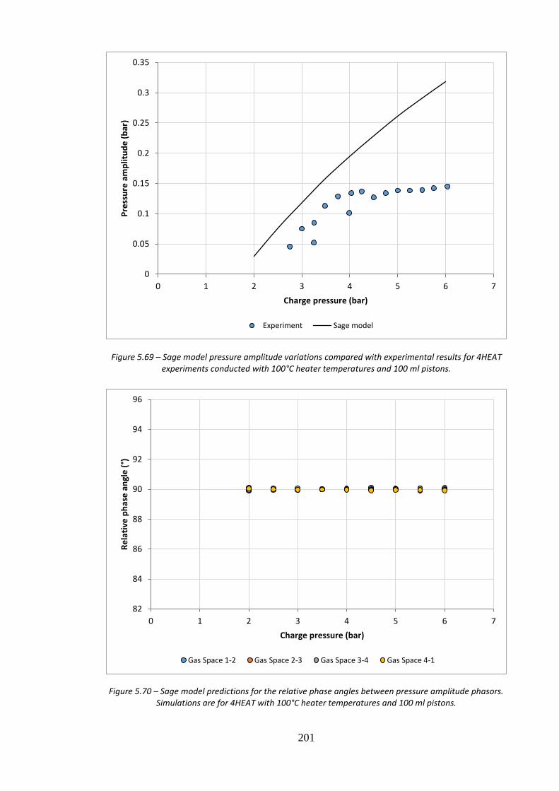
201

Figure 5.69 – Sage model pressure amplitude variations compared with experimental results for 4HEAT experiments conducted with 100°C heater temperatures and 100 ml pistons.

Figure 5.70 – Sage model predictions for the relative phase angles between pressure amplitude phasors. Simulations are for 4HEAT with 100°C heater temperatures and 100 ml pistons.

0

0.05

0.1

0.15

0.2

0.25

0.3

0.35

0 1 2 3 4 5 6 7

Pre

ssu

re a

mp

litu

de

(b

ar)



82

84

86

88

90

92

94

96

0 1 2 3 4 5 6 7

Re

lati

ve p

has

e a

ngl

e (

°)



202

Figure 5.71 – Sage model predictions for the relative phase angles between piston amplitude phasors. Simulations are for 4HEAT with 100°C heater temperatures and 100 ml pistons.

Figure 5.69 shows a similar trend to the comparison with piston amplitudes; the behaviour

of the model and the test-rig are offset but similar up until approximately 4 bar, when the

experiment trend changes considerably and appears to plateau, not exceeding 0.15 bar

pressure amplitude. The phase angle trends in both cases are as anticipated: they remain

roughly constant and are independent of charge pressure. Results that are not shown

include the temperature difference trends between expansion and compression spaces,

which exhibited less than 1ºC change across the entire pressure range.

5.2.3 3HEAT Model

The true test of the Sage model is how it handles the 3HEAT and 2HEAT configurations,

which are no longer constrained by symmetry. This section shows the characteristics of

the 3HEAT configuration as predicted by the Sage model. Table 5.7 shows the pressure

and displacement amplitude phasors generated by Sage at 4 bar, 150ºC heater temp and

100 ml pistons. Figure 5.72 then displays the scaled phasor plot for the same simulation.

70

75

80

85

90

95

100

105

110

0 1 2 3 4 5 6 7

Re

lati

ve p

has

e a

ngl

e (

°)



203

Table 5.7 – Sage model phasors predictions for 3HEAT experiment at 4 bar with 150°C heaters and 100 ml pistons.

Phasor variable Amplitude (bar or cm) Phase angle (°)

Pressure 1 (P1) 0.195 0.0

Pressure 2 (P2) 0.322 90.4

Pressure 3 (P3) 0.199 180.3

Pressure 4 (P4) 0.268 270.4







P1

P2

P3

P4

XA

XB

XC

XD



204

The first impression from this phasor plot is that phasor orientations look very similar to

the experimentally obtained versions (see Figure 5.23 in Section 5.1.2). The pressure

phase angles remain close to the 4HEAT predictions, which in Sage’s case is almost

exactly 90º. The P2 and P4 phasors have the largest magnitudes, and the displacement

phasors are skewed vertically in the same manner as seen experimentally. Similarly, the

magnitudes of P1 and P3 are almost identical to each other. The difference in magnitude

between the largest (P2) and the smallest (P1) is 0.127 bar or 39.4%. The relative phase

angles are again quantified in Figure 5.73 for better comparison with the experiment.

Figure 5.73 – Sage model predictions for the relative phase angles between pressure and displacement phasors in the example 3HEAT simulation. Simulation is at 4 bar charge pressure with 150ºC heater

temperatures and 100 ml pistons.

The first comparison can be made for the relative phase angle between P1 and Piston A

(highlighted in the blue box). The example experiment recorded a value of 124.0º, while

Sage predicts 125.6º. These values are very similar, differing by only 1.3%. The values

in the yellow boxes differ more significantly, with discrepancies of up to 6.2º. However,

it is important to note that the pressure phase angle differences remained approximately

constant across the entire experimental investigative range, and were independent of

changes in configuration, temperature or pressure. This implies that their deviation from

90º resulted from physical imperfections in the symmetry between all four subsystems.

90.4


66.3 118.1


108.0 67.6


90.2

205

The Sage model pressure amplitude phase angles do retain their similarities to the model

predictions for the 4HEAT pressure, which is of primary importance.

The final point of comparison for the phase angles is the piston displacements. The

experimental results showed that relative phase angles of between 60°–80° could be

expected for pistons B–C and D–A, and 100°–120° for pistons A–B and C–D.

Specifically, at 4 bar the results were within 3º of the predictions, except for pistons A-B

which differed by 5.8º.

Figure 5.74 – Sage predictions for pressure amplitudes developed in all four gas spaces with increasing charge pressure for 3HEAT configuration. Simulations are with 150ºC heaters and 100 ml pistons.

The predicted pressure amplitudes for each of the gas spaces (shown in Figure 5.74)

follow a similar pattern to the experimental results. The ratios between the magnitudes

remain consistent from 2 bar–6 bar charge pressure. The ratios calculated and averaged

over the simulation range are 1.65 (s = 1.1%), 1.02 (s = 0.04%) and 1.38 (s = 0.8%) for

GS2, GS3 and GS4 respectively. The main differences compared with the experimental

results from Section 5.1.2, are higher pressure amplitude magnitudes, and a less rapid

0

0.1

0.2

0.3

0.4

0.5

0.6

0 1 2 3 4 5 6 7

Pre

ssu

re a

mp

litu

de

(b

ar)




206

tapering off at higher charge pressure. This can be seen in Figure 5.75, which shows a

direct comparison between Sage and experiment for the pressure amplitudes of GS1. The

predicted amplitudes exceed the experimental values by a significant margin, even at

lower pressure.

Figure 5.75 – Sage model predictions for pressure amplitude in Gas Space 1 compared with experimental results for 3HEAT configuration. 150ºC heaters with 100 ml pistons.

At 4 bar, the predicted amplitude is 0.195 bar, which is 103% larger than the experiment

value of 0.096 bar. This might seem like a large discrepancy (and it is) but as previously

emphasised, the quantitative accuracy of the model is not of critical importance at this

stage. It is much more important that the model predictions reflect the correct

characteristics of each configuration and show similar trends. As demonstrated in the

sensitivity analysis, small changes in the heater temperature, liquid viscosity and other

variables can produce large changes in the pressure and displacement amplitudes—

therefore a number of model variables could easily be altered in order to match the

experimental results more precisely (but with no objective justification this might

jeopardise the model validity when extrapolating the model to analyse different piston

0

0.05

0.1

0.15

0.2

0.25

0.3

0.35

0 1 2 3 4 5 6 7

Pre

ssu

re a

mp

litu

de

(b

ar)



207

sizes in later chapters). Once more results are obtained using different piston sizes then

some of these sensitive parameters can be identified with greater certainty. Figures 5.76

and 5.77 show the piston amplitude versions of Figures 5.74 and 5.75. Unlike the piston

amplitudes obtained from the experiments, the Sage model predicts distinctive

differences in their magnitudes. Piston A and Piston B are predicted to have the largest

amplitudes, which are very close in magnitude to each other. Piston C and D are predicted

to have lower amplitudes—by almost 10 mm at 6 bar. This is explained by the magnitudes

of the pressure phasors. With GS1 and GS3 having approximately the same magnitude,

the significant contributions come from GS2 and GS4. The magnitude of GS2 is larger

than GS4, therefore the pistons adjacent to that space (A and B) exhibit larger

displacement amplitudes. The comparison between the average displacements in Figure

5.77 shows the same discrepancy seen between the pressure amplitude comparison in

Figure 5.75, i.e. a significant overestimation by Sage.

Figure 5.76 – Sage predictions for piston amplitudes with increasing charge pressure for 3HEAT configuration. Simulations are with 150ºC heaters and 100 ml pistons.

0

1

2

3

4

5

6

7

8

0 1 2 3 4 5 6 7

Pis

ton

am

plit

ud

e (

cm)



208

Figure 5.77 – Sage model predictions for Piston A amplitude compared with experimental results for 3HEAT configuration. 150ºC heaters with 100 ml pistons.

Figure 5.78 – Sage model predictions for the relative phase angles between pressure amplitude phasors. Simulations are for 3HEAT with 150°C heater temperatures and 100 ml pistons.

0

1

2

3

4

5

6

7

8

0 1 2 3 4 5 6 7

Pis

ton

am

plit

ud

e (

cm)


Sage model Experiment

82

84

86

88

90

92

94

96

0 1 2 3 4 5 6 7

Re

lati

ve p

has

e a

ngl

e (

°)



209

Figure 5.79 – Sage model predictions for the relative phase angles between piston amplitude phasors. Simulations are for 3HEAT with 150°C heater temperatures and 100 ml pistons.

The relative pressure and displacement phase angles are shown in Figures 5.78 and 5.79.

As seen in the 4HEAT simulations, the Sage model predicts very little deviation in these

values with increased charge pressure. This implies that the cause of the variation seen in

the experimental values may either result from the piston instability or another physical

phenomenon affecting the test-rig. This phenomenon, and why it might relate to the multi-

modal behaviour, is discussed in Section 8.2.5.

There are a number of other performance indicators which can be identified with the

model results that are not available from the experimental data. For now, only one will

be assessed. That is the cooling efficiency or overall coefficient of performance of the

machine based on heat input and heat absorbed. Figure 5.72 shows the COP predicted for

the 3HEAT configuration with the same parameters outlined earlier.

50

60

70

80

90

100

110

120

130

0 1 2 3 4 5 6 7

Re

lati

ve p

has

e a

ngl

e (

°)



210

Figure 5.80 – Sage model coefficient of performance predictions for the 3HEAT configuration. Simulations are with 150 ºC heaters and 100 ml pistons.

The COP values are relatively low and do not cross 0.2. The COP peaks at a charge

pressure very close to what was found experimentally to be the ‘sweet spot’ of the system.

It remains to be seen whether this is coincidental or if there is something linking these

system traits.

5.2.4 2HEAT Model

This section shows the characteristics of the 2HEAT configuration as predicted by the

Sage model. Unlike the experiments, the Sage model does predict functionality with

100 ml pistons at 190ºC. For consistency with the other Sage model results, these are

presented instead of the simulations with 115 ml pistons. Table 5.8 shows the pressure

and displacement amplitude phasors generated by Sage at 4 bar, 190ºC heater temp and

100 ml pistons. Figure 5.81 then displays the scaled phasor plot for the same simulation.

0

0.05

0.1

0.15

0.2

0.25

0 1 2 3 4 5 6 7

CO

P


211


Phasor variable Amplitude (bar or cm) Phase angle (°)

Pressure 1 (P1) 0.168 0.0

Pressure 2 (P2) 0.176 90.6

Pressure 3 (P3) 0.138 180.4

Pressure 4 (P4) 0.138 270.7







P1

P2

P3

P4

XA

XB

XC

XD



212

Again, the phasor plot produced from the Sage simulation looks very similar to the

experimental phasor plot for the 2HEAT configuration with the pressure phasors retaining

their similar phase angle interrelationships. The relative magnitudes of the pressure

phasors are also similar to the experimental results, with P1 and P2 being the largest and

closest to each other, P3 and P4 smaller but also very similar. The difference between the

largest pressure amplitude, P2, and the smallest, P4, is much less than in the 3HEAT case,

being only 21.6%. The relative phase angles between the phasors are given in Figure 5.82.



The angle between the pressure phasor of GS1 and the displacement phasor of Piston A

is 138.0º, which is close to the experimental value of 133.9º. The angles between the

pressure phasors are very close to 90º value, all are within the range 90º ± 0.7º. Comparing

the angles between the pistons, the largest discrepancy from the experiment (of 12.1°)

occurs for the angle between Piston C and Piston D, where 84.1º is predicted by Sage and

the value from the experiment is 96.2º. It is not worth inferring too much from precise

comparison with the experiments since the 100 ml piston Sage results are being compared

to 115 ml piston experiment results. Figures 5.83 and 5.84 show the Sage model pressure

amplitude and piston displacement predictions across the charge pressure range.

90.6


94.4 98.7


84.1 82.8


90.3

213

Figure 5.83 – Sage predictions for pressure amplitudes with increasing charge pressure for 2HEAT configuration. Simulations are with 190ºC heaters and 100 ml pistons.

Figure 5.84 – Sage predictions for piston amplitudes with increasing charge pressure for 2HEAT configuration. Simulations are with 190ºC heaters and 100 ml pistons.

0

0.05

0.1

0.15

0.2

0.25

0.3

0.35

0 1 2 3 4 5 6 7

Pre

ssu

re a

mp

litu

de

(b

ar)



0

1

2

3

4

5

6

0 1 2 3 4 5 6 7

Pis

ton

am

plit

ud

e (

cm)


Piston A Piston B Piston C Piston C

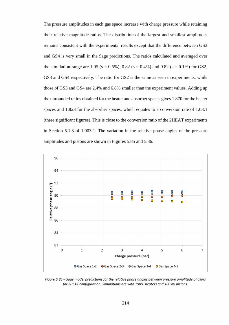
214

The pressure amplitudes in each gas space increase with charge pressure while retaining

their relative magnitude ratios. The distribution of the largest and smallest amplitudes

remains consistent with the experimental results except that the difference between GS3

and GS4 is very small in the Sage predictions. The ratios calculated and averaged over

the simulation range are 1.05 (s = 0.5%), 0.82 (s = 0.4%) and 0.82 (s = 0.1%) for GS2,

GS3 and GS4 respectively. The ratio for GS2 is the same as seen in experiments, while

those of GS3 and GS4 are 2.4% and 6.8% smaller than the experiment values. Adding up

the unrounded ratios obtained for the heater and absorber spaces gives 1.870 for the heater

spaces and 1.823 for the absorber spaces, which equates to a conversion rate of 1.03:1

(three significant figures). This is close to the conversion ratio of the 2HEAT experiments

in Section 5.1.3 of 1.003:1. The variation in the relative phase angles of the pressure

amplitudes and pistons are shown in Figures 5.85 and 5.86.

Figure 5.85 – Sage model predictions for the relative phase angles between pressure amplitude phasors for 2HEAT configuration. Simulations are with 190ºC heaters and 100 ml pistons.

82

84

86

88

90

92

94

96

0 1 2 3 4 5 6 7

Re

lati

ve p

has

e a

ngl

e (

°)



215

Figure 5.86 – Sage model predictions for the relative phase angles between piston phasors for 2HEAT configuration. Simulations are with 190ºC heaters and 100 ml pistons.

The relative pressure phase angles are again very close to the 90° value and show little

variation with increased charge pressure. The relative phase angles between piston

displacements also remain close to those discussed previously for Figure 5.82, and show

variations of less than 1° with charge pressures up to 6 bar.

As done for the 3HEAT simulations, Figure 5.87 shows how the COP predicted for the

2HEAT configuration varies with charge pressure. The COP values are much higher than

the 3HEAT configuration. The COP peaks at 5.5 bar with a value of 0.46, which is more

than twice the maximum COP achieved in the 3HEAT simulations analysed earlier. This

is in line with the promising traits identified experimentally for the 2HEAT configuration.

With pressure amplitudes much closer to each other in magnitude, relative piston phase

angles closer to 90° and far superior conversion ratios, it would be expected that the

2HEAT configuration should outperform the 3HEAT configuration.

80

85

90

95

100

105

0 1 2 3 4 5 6 7

Re

lati

ve p

has

e a

ngl

e (

°)



216

Figure 5.87 – Sage model predictions for the coefficient of performance for the 2HEAT configuration. Simulations are with 190ºC heaters and 100 ml pistons.

5.2.5 Validation Summary

The development of the Sage model and the relevant procedures associated with its use

not only in the 4HEAT configuration, but also in the 3HEAT and 2HEAT configurations

proved very successful. Aside from lacking the inclusion of restrictions imposed by the

RT instability, the model has shown the ability to independently predict the complex

dynamic behaviour of the LPSC machine to a relatively high degree of similarity with

experiments for all three configurations. This contributes significantly to the validity of

the model’s use in subsequent optimisations. The sensitivity of the model was

investigated for a number of important constants including liquid viscosity, minor flow

loss coefficients, as well as the heat source and sink temperatures. Model outputs related

to the level of excitation, such as piston amplitudes, were found to have relatively high

sensitivity to these parameters. Changes of 1%–10% in the inputs resulted in 20%–40%

changes in the outputs. Whereas the model outputs which distinguish the dynamic

0

0.05

0.1

0.15

0.2

0.25

0.3

0.35

0.4

0.45

0.5

0 1 2 3 4 5 6 7

Co

eff

icie

nt

of

Pe

rfo

rman

ce (

CO

P)


217

patterns of behaviour such as frequency, relative phase angles and relative magnitudes of

excitation were found to have very little sensitivity to these changes. Also of note is that

the Sage model predicts a far superior COP for the 2HEAT configuration (0.46) over the

3HEAT configuration (0.20).

Based on the model predictions for the 100 ml piston LPSC test-rig, and the sensitivity

analysis conducted, it was decided that the model had been validated to a suitable level

and was ready for investigating system modifications in order to achieve improved

performance. One component in particular stands out as the prime candidate for

adjustment—the liquid piston dimensions.

5.3 Preliminary Piston Investigation

As a consequence of the geometrical complexity of the test-rig gas spaces (in addition to

containing the sensor ports, etc.) it is logical to first investigate the influence of different

piston dimensions on the behaviour and performance of the LPSC machine test-rig—

since the piston U-tubes are relatively easy to interchange. After validating the accuracy

of the Sage model to an acceptable level, it was possible to run simulations with different

piston masses and diameters (and any other related variations) without making changes

to the physical test-rig. The Sage model is easy to alter for pistons of different length and

cross-sectional area; and once improved piston dimensions are identified, it is much easier

to implement them in the physical test-rig, thanks to the modular nature of the set-up. By

testing new piston dimensions, and comparing the results with the Sage model

predictions, the accuracy of the model can be improved as well. This could potentially be

repeated for further improvements and lead to the design of a prototype.

There are two parameters associated with the liquid pistons which can be easily

manipulated: the piston length and diameter. For the first piston redesign, it was decided

that only changes in the diameter would be investigated. The diameter was chosen over

218

the length for a number of reasons—primarily that changes in the diameter have a much

larger influence on the resulting piston mass, and do not take up as much space as

equivalent changes in the piston length. This allows for a much wider scope of feasible

piston masses, that can be potentially implemented. Once an optimal (or, at least, better)

piston diameter was identified and tested with the test-rig, the Sage model would also

now have another important reference point for comparison purposes, and this would

allow for the model to be further refined (at which point it could be used to identify the

optimal piston dimensions of both length and diameter).

A very simple approach was taken for this piston diameter investigation. The key

performance indicator was selected as being the lowest heater temperature required for

the system to achieve self-sustained operation. Although this parameter does not exhibit

any specific performance data, it does highlight which systems are the easiest to start, and

therefore which are the most well-balanced in terms of the vibrational dynamics and

thermodynamics. This also allows the investigative process to proceed with the 4HEAT

configuration model, for which identifying the frequency and solving for piston

amplitudes is much simpler. The Sage model was used to assess the performance of the

LPSC test-rig with six piston diameters in the range of 12.65 mm (current installation) to

25 mm. Table 5.9 outlines the specifications of each of the piston sizes investigated.

Table 5.9 – Operating frequencies and starting temperatures for 94 cm pistons of varying diameter.

Piston diameter (mm)

Piston mass (ml)

Frequency of operation (Hz)

Functional temperature ranges (°C)

12.65 100.0 4.141 87.5-100

15.00 140.6 4.890 82.0-100

17.50 191.4 5.690 79.5-100

20.00 250.0 6.487 79.0-100

22.50 316.4 7.285 79.5-100

25.00 390.6 8.083 81.0-100

219

A single charge pressure of 4 bar was used in the analysis, and the heater temperatures

were initially set to 100ºC—before being reduced to the point at which operation ceased

and no solution was found. Figure 5.88 shows the results of the simulations with the

pressure amplitudes developed in the gas spaces for the operational temperature range

below 100ºC.

Figure 5.88 – Piston diameter influence on the heater temperatures needed for self-sustained operation. Simulations are conducted with 4HEAT configuration at 4 bar charge pressure with constant piston

length.

The systems associated with the leftmost graphed functions are the easiest to start,

requiring lower heater temperatures to achieve the same pressure amplitude development

as those further to the right. The best predictions arise from the 20 mm diameter pistons—

with piston diameters above and below leading to increased heater temperatures. The

12.65 mm pistons exhibit the worst performance, requiring heater temperatures at least

5ºC higher than the other pistons to achieve the same pressure amplitudes. Another

noticeable characteristic is that as the temperature is increased, the separation between

each set of predictions remains constant, which allows the relative performance of each

0

0.05

0.1

0.15

0.2

0.25

0.3

0.35

75 80 85 90 95 100 105

Pre

ssu

re a

mp

litu

de

(b

ar)

Heater temperature (°C)

12.65mm 15 mm 17.5 mm 20 mm 22.5 mm 25 mm

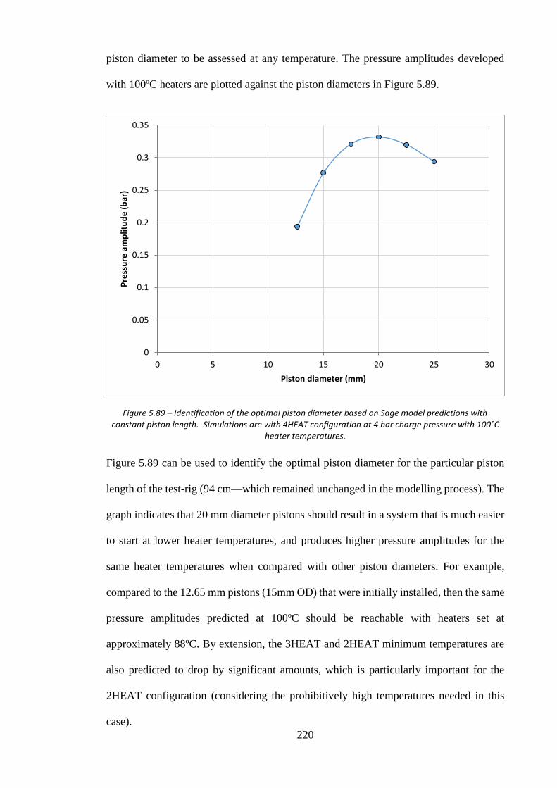
220

piston diameter to be assessed at any temperature. The pressure amplitudes developed

with 100ºC heaters are plotted against the piston diameters in Figure 5.89.

Figure 5.89 – Identification of the optimal piston diameter based on Sage model predictions with constant piston length. Simulations are with 4HEAT configuration at 4 bar charge pressure with 100°C

heater temperatures.

Figure 5.89 can be used to identify the optimal piston diameter for the particular piston

length of the test-rig (94 cm—which remained unchanged in the modelling process). The

graph indicates that 20 mm diameter pistons should result in a system that is much easier

to start at lower heater temperatures, and produces higher pressure amplitudes for the

same heater temperatures when compared with other piston diameters. For example,

compared to the 12.65 mm pistons (15mm OD) that were initially installed, then the same

pressure amplitudes predicted at 100ºC should be reachable with heaters set at

approximately 88ºC. By extension, the 3HEAT and 2HEAT minimum temperatures are

also predicted to drop by significant amounts, which is particularly important for the

2HEAT configuration (considering the prohibitively high temperatures needed in this

case).

0

0.05

0.1

0.15

0.2

0.25

0.3

0.35

0 5 10 15 20 25 30

Pre

ssu

re a

mp

litu

de

(b

ar)


221

6 Results for 22 mm OD Piston Tube

6.1 Test-rig Modifications and Commissioning

After identifying the optimal piston diameter, new piston U-tubes were constructed for a

new set of experiments. Conveniently, the optimum diameter identified in the preceding

section (20 mm) is in line with a standard steel tube size. The piston length was kept

similar, but its diameter was increased from 15 mm to 22 mm, resulting in a new piston

mass of 275 ml. The 22 mm OD steel tubes have a wall thickness of 1.2 mm, meaning

the inner diameter is 19.6 mm on the steel side. As in the case of the first set-up, fibre

reinforced PVC tube was used on the side where the displacement sensors were installed.

This time ¾-inch (19.05 mm ID) tube was employed. The new pistons were implemented

and after some commissioning, a secondary set of experiments was carried out. Table 6.1

shows the set of experimental parameters which were tested for the larger pistons.

Table 6.1 – Set of parameters for second experimental investigation.

Piston tube OD (mm)



Gas pressure (bar)

22 4HEAT 275 75, 80 1-6

22 3HEAT 275 105, 110, 115 1-6

22 2HEAT 275 160, 165 1-6

As predicted by the Sage model, the heater temperatures required for the system to

achieve stable operation were significantly reduced, and hence the tested heater

temperatures are lower than in the previous experiments. Some of the experiments at

lower pressure did not produce usable results because the degree of ovality of the 19 mm

PVC tube was too high and the piston floats were in direct contact with parts of the tube

walls, which introduced static friction. At charge pressures above 2.5 bar this was usually

overcome as the PVC tube cross-section would become more circular with the increase

in internal pressure. The experiments were conducted using a similar procedure to the

222

earlier experiments, except that a number of additional improvements were made, as

follows:

New test-rig stand – Due to the increased piston diameters, a new support structure had

to be built for the modified test-rig. The 22 mm diameter steel tube required a larger

bending radius when forming the new U-tube components, which consequently increased

the separation distances needed for the gas space housing components. The structure also

needed to be able to withstand the machine’s increased mass, since the piston volumes

had increased almost by a factor of three. The new structure is shown in Figure 6.1.

Figure 6.1 – New support structure created for larger pistons.

Video footage for piston amplitudes – After the many difficulties associated with the

capacitive sensors and their calibration for piston amplitude data, it was decided that

video footage would be used instead. Slow motion video was used to capture snapshots

of the piston oscillations at different intervals during each experiment. The time at which

the videos were taken was recorded, and the videos were later analysed to provide the

relevant piston amplitude data. The uncertainty in the piston amplitude data was ± 0.25

223

cm. The capacitive displacement sensors were still employed for collection of the piston

phase angle data. The reference capacitors were modified to account for the change in

baseline piston readings.

New piston floats – With the increased piston diameter, new floats were manufactured

in the workshop. They were designed with the same length-to-diameter aspect ratio and

made from a similar material (Polyethylene 300) to previous experiments. The new floats

were also coloured green to aid in their visual identification—as the previous white

versions were sometimes obscured by the fibre reinforcing in the PVC tube walls, which

made it difficult to distinguish their outline. Roughly the same clearance was kept

between the piston floats and the tube walls, although the larger PVC tube had a higher

ovality which meant that the floats in the PVC sections were required to be 0.5 mm

smaller. The float sizes used were 18.5 mm OD in the steel side, and 18 mm OD in the

PVC side. Additionally, a number of experiments were conducted without any floats at

all. This was done to allow for a more objective measure of their impact on system

performance, and also to test the Rayleigh-Taylor instability theory further. The no-float

results are compared and evaluated in Section 6.2.1.

Piston stabilisers – An unexpected discovery was made after conducting a number of

experiments with the new 22 mm set-up. As the charge pressure was increased a lull in

operation was found. At pressures above and below this point, the system would achieve

much higher pressure amplitudes; and, in some cases, the machine would cease to achieve

self-sustained operation entirely. It was discovered that the natural frequency of vibration

of the support structure itself was close to the operational frequency of the LPSC system

in the vicinity of these problematic charge pressures. To combat this, the bottoms of the

U-tubes were fastened to rigid stabilisers to prevent relative motion between them. This

effectively increased the rigidity and natural frequency of the test-rig stand, which

224

prevented resonance with the LPSC machine. This resolved the issue, and the developed

pressure amplitudes were restored to their expected values. It should be noted, however,

that during some experiments it was necessary to disconnect a single stabiliser in order to

jump-start the system; after reaching stable operation it would then be reconnected. Figure

6.2 shows the final set-up of the upgraded 22 mm piston tube test-rig.

Figure 6.2 – Fully commissioned 22 mm piston test-rig.

225

All other system geometry was kept the same as in the first set of experiments, although

some minor inconsistencies were present in the final installation. The gas volumes of each

space were increased slightly, because the length of dead gas volume above the liquid

piston (and within the U-tubes) now had a much larger cross-sectional area. These values

were quantified and incorporated into the updated Sage model, which is discussed in more

detail in the Section 6.3.

6.2 Experiment Results

Presented here are the results from the second iteration of the LPSC experimental

investigation. The piston U-tube diameter has been increased from 15 mm (13 mm ID) to

22 mm (19.6 mm ID) steel tube. Because of the large number of experiments conducted

(more than 100) and their similarities with the 15 mm piston experiments, the results

presented here are not as comprehensive as those in Section 5.1. Instead, it is assumed the

reader is familiar with the concepts and system behaviours identified in the earlier results

sections, and only the key distinguishing or critical information will be presented. Typical

examples of experiments for each of the three configurations are again presented with the

associated phasor analysis. The results for the 4HEAT configuration are shown first—

followed by 3HEAT and 2HEAT. The first comparison includes experiments from all

three configurations. Figure 6.3 shows the frequency of operation of the LPSC system

and its variation with charge pressure. As with the results from the smaller 15 mm pistons,

the operational frequency of the system is the same for each configuration when tested

with the same charge pressure. This provides further justification for using the same

frequencies for different configurations within the Sage modelling procedure. Figure 6.4

compares the frequencies obtained from the 22 mm experiments with those from the 100

ml, 15 mm experiments. Included are the predicted frequencies from Equation 4.8 (from

the earlier section on theoretical analysis) assuming isothermal gas behaviour.

226

Figure 6.3 – Frequency variation of the 22 mm piston experiments with 275 ml pistons for all configurations.

Figure 6.4 – Experimental frequencies of both piston sizes compared with predictions from natural frequency derivation.

0

1

2

3

4

5

6

7

0 1 2 3 4 5 6 7

Fre

qu

en

cy (

Hz)


2HEAT 160 °C 2HEAT 165 °C 3HEAT 105 °C 3HEAT 110 °C

3HEAT 115 °C 4HEAT 75 °C 4HEAT 80 °C

0

1

2

3

4

5

6

7

0 1 2 3 4 5 6 7

Fre

qu

en

cy (

Hz)


15 mm Experiment 15 mm Isothermal

22 mm Experiment 22 mm Isothermal

227

It can be seen that the estimate of operational frequency based on isothermal gas

behaviour is very similar to the values measured experimentally. Knowing the form of

Equation 4.8 and its dependence on charge pressure, the close-to square root dependence

observed in the experimental results is plausible. The differences remain small across the

entire charge pressure range. At 5 bar for example, the predicted frequency is 3.3% lower

than the value measured for the 15 mm U-tubes with 100 ml pistons. In the case of the 22

mm U-tubes with 275 ml pistons, the predicted frequency is 2.7% higher than the

experiment. It is not known why the formula overestimates in one instance and

underestimates in the other. It is possible that the gas is behaving less isothermally in one

setup compared with the other; or there could be some small discrepancies in the

quantities used for gas volume or other contributing variables.


After commissioning the new test-rig setup it was discovered that the system was capable

of operating with much lower heat source temperatures than the 15 mm setup. In

Section 6.3 the Sage model predicted that 250 ml pistons with 20 mm internal diameter

would start at approximately 80ºC. The new setup with 275 ml, 19.3 mm diameter

(average) pistons was found to operate at temperatures as low as 75ºC. The 4HEAT

experiments were conducted with heater temperatures of 75ºC and 80ºC. Heater

temperatures of 70ºC were attempted, although self-sustained operation was not

established. Temperatures above 80ºC produced too much piston instability for useful

data collection. An example experiment with 80ºC heaters at 4 bar charge pressure is

considered for the phasor analysis. The phasor parameters obtained using the same

procedure described earlier are listed in Table 6.2. Figure 6.5 then shows the scaled

pressure and displacement phasor plot for the experiment.

228



Pressure 1 (P1) 0.173 0.0

Pressure 2 (P2) 0.178 90.7

Pressure 3 (P3) 0.174 179.4

Pressure 4 (P4) 0.181 270.4





Figure 6.5 – Scaled phasor plot of pressure and displacement profiles for the example 4HEAT experiment with 22 mm piston tubes. The experiment was with 80ºC heaters and 4 bar charge pressure.

P1

P2

P3

P4

XA

XB

XC

XD



229

The relative phase angles between the pressure phasors are much closer to 90º than any

of the 15 mm piston experiments. This is in accordance with the model predictions and

implies that the 22 mm test-rig has a higher aspect of symmetry. Figure 6.6 shows the

corresponding chart for the relative phase angles between phasors. All four pressure

phasors are within ± 1.3º of perfect symmetry. The displacement phasors show greater

variation with the range being within ± 5.2º of 90º. The relative phase angle between

Piston A and GS1 pressure at 140.8º is also similar to previous 4HEAT experiments and

their Sage predictions.

Figure 6.6 – Relative phase angles for the example 4HEAT experiment with 22 mm piston tubes. The experiment was with 80ºC heaters and 4 bar charge pressure.

Figure 6.7 shows the pressure amplitudes developed for both sets of heater temperature

experiments. The pressure amplitudes developed with 80ºC heater temperature rise

steeply from the first measurements at 2.5 bar until plateauing at 4 bar where they remain

for all higher charge pressures. This evidence of a barrier preventing higher excitation

levels is similar to that seen in the 15 mm results. Figure 6.8 presents the pressure

amplitude progressions of three separate tests from the above data set: one at 3.5 bar, one

at 4 bar and the other at 4.25 bar.

90.7


89.8 89.9


95.2 85.1


91.0

230


Figure 6.8 – Pressure amplitude progressions of experiments conducted at or near the transition pressure of 4 bar for the 4HEAT configuration.

0

0.02

0.04

0.06

0.08

0.1

0.12

0.14

0.16

0.18

0.2

0 1 2 3 4 5 6 7

Pre

ssu

re a

mp

litu

de

(b

ar)


75 °C 80 °C

0

0.02

0.04

0.06

0.08

0.1

0.12

0.14

0.16

0.18

0.2

0 200 400 600 800 1000 1200

Pre

ssu

re a

mp

litu

de

(b

ar)

Elapsed time (s)

3.5 bar 4 bar 4.25 bar

231

Figure 6.8 shows the pressure amplitude from the 3.5 bar experiment remaining relatively

constant at 0.15 bar after its initial rise, with very little fluctuation as the experiment

continues. Being below the threshold pressure then the small changes in magnitude are

gradual and smooth. The 4.25 bar measurements are much more erratic and show the

pressure amplitude rising steeply and immediately becoming unstable. The amplitude

rises and falls continuously as though constantly re-establishing itself and building up

(before again becoming unstable); the average pressure amplitude recorded is below the

average for the 4 bar experiment. The 4 bar experiment is very close to the transition

point: the results exhibit both operation modes from the 3.5 bar and 4.25 bar experiments.

It is stable and smooth for long periods while also experiencing some sudden fluctuations

similar to the 4.25 bar behaviour (albeit less extreme). This behavioural pattern was

identical for all of the experiments above 4 bar—with the fluctuations in pressure

amplitude becoming even more significant at higher pressure.

Figure 6.9 – Pressure amplitude progressions for 75ºC heater experiments.

0

0.02

0.04

0.06

0.08

0.1

0.12

0.14

0 100 200 300 400 500 600 700 800

Pre

ssu

re a

mp

litu

de

(b

ar)

Elapsed time (s)

4.25 bar 4.6 bar 4.75 bar

232

When considering the 75ºC results from Figure 6.7 it becomes evident that none of the

developed pressure amplitudes are large enough to reach the threshold encountered by

the 80ºC experiments. It should be expected then that the pressure amplitude progressions

for these experiments should resemble the stable behaviours highlighted by the 3.5 bar

experiment in Figure 6.8. Figure 6.9 shows the pressure amplitudes measured for three

experiments from the 75ºC data set. Despite the pressures being above 4 bar, the same

instability is not evident in these experiments; in fact, none of the 75ºC experiments

exhibited unstable behaviour. This suggests that the pressure amplitudes developed are

not hindered by any piston stability limitations (as those suspected for the 80ºC

experiments), and were the maximum achievable for that particular pressure and

temperature. This is explored further when considering the modified Sage predictions for

the same set of experiments in Section 6.3. Figure 6.10 shows the piston amplitudes

measured for the 75ºC and 80ºC experiments.

Figure 6.10 – Piston amplitude variation with charge pressure for the 4HEAT configuration experiments using 275 ml liquid pistons.

0

0.5

1

1.5

2

2.5

3

3.5

0 1 2 3 4 5 6 7

Pis

ton

am

plit

ud

e (

cm)


Piston A (75 °C) Piston B (75 °C) Piston C (75 °C) Piston D (75 °C)


233

The new video-based method of obtaining the piston amplitudes is justified by these

results. Unlike the 15 mm experiments, the piston amplitude measurements here reflect

what is expected for the 4HEAT configuration, with very similar amplitudes for all 4

pistons at every experiment (except at 6 bar and 80ºC).

Experiments without floats were also conducted to highlight their necessity and impact.

Figure 6.11 shows the pressure amplitudes developed in the no-float experiments in

comparison to those already analysed with floats. Both sets of experiments were

conducted with 80ºC heater temperatures.

Figure 6.11 – Performance of LPSC 4HEAT system with and without piston surface floats. Experiments are with 80°C heater temperature.

The system is much easier to start without the floats, and consequently requires lower

starting pressures. However, the pistons quickly become unstable when increasing the

charge pressure and reach their threshold at 2.5 bar, where the developed pressure

amplitudes plateau at roughly 0.12 bar. With the piston floats installed, the pistons are

0

0.02

0.04

0.06

0.08

0.1

0.12

0.14

0.16

0.18

0.2

0 1 2 3 4 5 6 7

Ave

rage

pre

ssu

re a

mp

litu

de

(b

ar)


No floats Floats

234

able to sustain higher pressure amplitudes and accelerations, and hence retain their

stability for charge pressures up to 4 bar. The pistons with floats installed perform better

for all pressures above 3 bar. Unfortunately, because of the levels of instability of the

piston surfaces in the no-float experiments, it was not possible to determine piston

amplitudes. These results confirm that the RT instability acceleration threshold can be

influenced by the use of piston floats; although at a cost in terms of increased friction and

self-starting potential.


The 3HEAT experiments were conducted with heater temperatures of 105°C, 110°C and

115ºC. The experiments at 115ºC were too unstable above pressures of 4 bar, and

therefore have a limited range. Temperatures below 105ºC did not produce continuous

operation. Figure 6.12 shows the scaled pressure and displacement phasor plot for an

example experiment with 110ºC at 4 bar charge pressure. The same relative phase angle

chart is then shown in Figure 6.13. The phasor values are also listed in Table 6.3 for

reference.



Pressure 1 (P1) 0.121 0.0

Pressure 2 (P2) 0.202 90.7

Pressure 3 (P3) 0.124 179.4

Pressure 4 (P4) 0.182 271.0





235

Figure 6.12 – Scaled phasor plot of pressure and displacement profiles for the example 3HEAT experiment with 22 mm piston tubes. The experiment used 110ºC heaters and 4 bar charge pressure.

Figure 6.13 – Relative phase angles for the example 3HEAT experiment with 22 mm piston tubes. The experiment was with 110ºC heaters and 4 bar charge pressure.

P1

P2

P3

P4

XA

XB

XC

XD



90.7


62.4 118.7


114.1 64.8


91.5

236

The shape of the phasor plot is again very similar to those of the 15 mm experiments. As

in the 22 mm 4HEAT case, the pressure phasors are much closer to the 90º mark, with

the largest deviation in this instance of 1.5º. The piston phasors are influenced by the two

largest pressure phasors, which results in relative phase angles in the ranges of

63.6° ± 1.2° and 116.4° ± 2.3º for the displacements. The pressure amplitude trends of

GS1 (the absorber space) for each of the three heater temperatures are shown in Figure

6.14. Both the 110ºC and 115ºC experiments produced results which transitioned into

unstable pressure amplitude oscillations. The transition pressure for the 115ºC

experiments was between 3 bar and 3.25 bar, whereas for the 110ºC experiments the

transition pressure was at approximately 4.25 bar. The results at 105ºC remained below

the threshold, and all experiments produced smooth pressure amplitude progression

trends as those shown in Figure 6.9 (for the 75°C 4HEAT dataset).


0

0.02

0.04

0.06

0.08

0.1

0.12

0.14

0.16

0 1 2 3 4 5 6

Pre

ssu

re a

mp

litu

de

(b

ar)


105 °C 110 °C 115 °C

237


The pressure amplitudes of all four gas spaces are plotted in Figure 6.15 for the 110ºC

heater temperature experiments. The pressure amplitudes of each space exhibit very

similar ratios of magnitude to the 3HEAT experiments conducted for the 15 mm piston

tubes. The relative ratios in this case are 1.66 (s = 0.4%), 1.02 (s = 0.1%) and 1.50

(s = 0.4%) for GS2, GS3 and GS4 respectively (recalling that from Section 5.1.2, the

relative ratios of 1.62 (s = 0.7%), 1.02 (s = 0.6%) and 1.44 (s = 0.7%) were measured for

GS2, GS3 and GS4 respectively). Calculating the percentage changes in the relative

pressure ratios gives 2.3% and 3.8% increases for GS2 and GS4 respectively, with no

change in the GS3 ratio. This means that despite the improvements made to the system’s

performance with the new pistons, the pressure amplitudes developed in the absorber

space for the 3HEAT configuration are a smaller percentage of the total. Calculating the

conversion ratio from the ratios above yields 4.17:1 (three significant figures). The piston

displacements recorded for the experiments are shown in Figure 6.16.

0

0.05

0.1

0.15

0.2

0.25

2 2.5 3 3.5 4 4.5 5 5.5 6

Pre

ssu

re a

mp

litu

de

(b

ar)



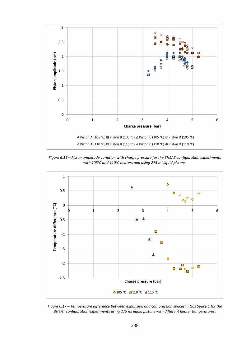
238

Figure 6.16 – Piston amplitude variation with charge pressure for the 3HEAT configuration experiments with 105ºC and 110ºC heaters and using 275 ml liquid pistons.

Figure 6.17 – Temperature difference between expansion and compression spaces in Gas Space 1 for the 3HEAT configuration experiments using 275 ml liquid pistons with different heater temperatures.

0

0.5

1

1.5

2

2.5

3

0 1 2 3 4 5 6

Pis

ton

am

plit

ud

e (

cm)




-2.5

-2

-1.5

-1

-0.5

0

0.5

1

0 1 2 3 4 5 6

Tem

pe

ratu

re d

iffe

ren

ce (°C

)


105 °C 110 °C 115 °C

239

Figure 6.17 presents the evidence of cooling obtained for the 3HEAT configuration

experiments with the new piston size. The measured difference between the expansion

space temperature minus the compression space temperature of GS1 are plotted for all

three data sets. The expansion space is where the temperature will drop if the system is

producing a cooling effect. Examining the 110°C and 115°C measurements, the first

unequivocal evidence of cooling for the project is witnessed. The 110°C values drop

steadily until reaching the transition pressure of 4.25 bar, where they plateau. The largest

cooling effect recorded is a temperature difference of -2.3°C. The limited data from the

115°C experiments also suggests larger temperature differences would be achievable if

the pistons remained stable.


The 2HEAT experiments were conducted with heater temperatures of 160ºC and 165ºC.

Temperatures below 160ºC did not produce significant results. Figure 6.18 shows the

scaled pressure and displacement phasor plot for an example experiment with 165ºC at 4

bar charge pressure. The relevant relative phase angle chart is then shown in Figure 6.19.

The absolute quantities of the phasors are also listed in Table 6.4 for reference.



Pressure 1 (P1) 0.192 0.0

Pressure 2 (P2) 0.188 87.4

Pressure 3 (P3) 0.166 179.9

Pressure 4 (P4) 0.155 268.5





240

Figure 6.18 – Scaled phasor plot of pressure and displacement profiles for the example 2HEAT experiment with 22 mm piston tubes. The experiment was with 165°C heaters and 4 bar pressure.

Figure 6.19 – Relative phase angles for the example 2HEAT experiment with 22 mm piston tubes. The experiment was with 165 °C heaters and 4 bar charge pressure.

P1

P2

P3

P4

XA

XB

XC

XD



87.4


97.4 89.2


80.7 92.7


88.6

241

Although the general shape of the phasor plot is quite similar to the previous 15 mm

example, there are some notable differences. The first significant difference is that the

largest pressure amplitude is now developed in one of the absorber spaces, GS1, whereas

previously it was in the heated space, GS2. The lowest amplitude developed is also now

the other absorber space GS4; previously it was in the heated space GS3. Because of these

changes in the relative pressure amplitudes, the relative phase angles between the pistons

have also been affected. The two phase angles separating the pistons on either side of the

absorber spaces are not as close to the 90º as before. Even so, all relative piston phase

angles are within ± 9.3º of 90º, which is an improvement over the 15 mm case where the

phase angle between Piston B and C was 76.6º.

The pressure amplitude trends of GS1 for both heater temperatures are shown in Figure

6.20. Both the 160ºC and 165ºC experiments experienced transitions from stable pressure

amplitude oscillations into unstable oscillations. The transition pressure for both occurred

between 3.75 bar and 4.25 bar. It can be seen that the pressure amplitudes developed for

both sets of experiments reach a plateau at this point, and actually decrease slightly as the

charge pressure is increased up to 6 bar. Figure 6.21 shows the pressure amplitude

progressions of all four gas spaces for the 165ºC experiments. The observations made

about the changes in the relative pressure amplitude hierarchy for the example 2HEAT

experiment, are shown to be repeated consistently across all charge pressures. Despite the

GS1 and GS2 magnitudes being very similar, GS1 is always approximately 2% larger.

The mean pressure amplitude ratios with respect to GS1 are 0.98 (s = 0.9%), 0.87 (s =

0.3%) and 0.81 (s = 0.7%) for GS2, GS3 and GS4, respectively. Adding up the unrounded

ratios obtained for the heater and absorber spaces gives 1.851 for the heater spaces and

1.809 for the absorber spaces, which equates to a conversion ratio of 1.02:1 (three

significant figures).

242



0

0.02

0.04

0.06

0.08

0.1

0.12

0.14

0.16

0.18

0 1 2 3 4 5 6

Pre

ssu

re a

mp

litu

de

(b

ar)


160 °C 165 °C

0

0.05

0.1

0.15

0.2

0.25

0 1 2 3 4 5 6

Pre

ssu

re a

mp

litu

de

(b

ar)


Gas Space 1 (Absorber) Gas Space 2 (Heater) Gas Space 3 (Heater) Gas Space 4 (Absorber)

243

Figure 6.22 – Piston amplitude variation with charge pressure for the 2HEAT configuration experiments with 160ºC heaters and using 275 ml liquid pistons.

The piston amplitudes for the 160ºC experiments are presented in Figure 6.22. The

amplitudes increase steadily until they reach maximums of 2.6 cm at the transition

pressure of 4 bar, beyond which point they reduce with increased charge pressure. Of the

piston amplitudes, pistons A, B and D are very similar in magnitude for the majority of

the experiments. The amplitude of Piston C constantly measures in the range of 0.2 cm–

0.5 cm below the other three pistons. The reason for this is that the two gas spaces in

contact with Piston C (i.e. gas spaces 3 and 4) exhibit the two lowest pressure amplitudes;

with the smallest contributing pressure amplitudes, the net pressure phasor acting on

Piston C thus has the smallest magnitude of all of the four net pressure phasors. By the

same measure, it could be expected that the amplitude of Piston A would be the largest,

since the two gas spaces contributing to its motion are gas spaces 1 and 2, which have the

two largest pressure amplitudes. However the relative phase angles also play a role in

determining the magnitude of the net pressure phasor, and in this case the relative phase

0

0.5

1

1.5

2

2.5

3

0 1 2 3 4 5 6

Pis

ton

am

plit

ud

e (

cm)



244

angle is 87.4°, which is less than 90º. Subtracting one from the other for the net pressure

phasor will therefore involve a degree of counteraction, reducing the resultant magnitude

compared with the case of 90º separation. This normally would not be enough to reduce

the piston amplitude to those values expected from pistons B and D, but the relative phase

angles between the gas spaces contributing to the motion of pistons B and D are 91.5º and

92.6º, which are above 90º, and therefore boost their amplitudes slightly. Hence, it is easy

to see how small differences in the relative phase angles between the gas space pressures

can be quite influential in the resultant piston amplitudes and phase angles.

Figure 6.23 – Shows the temperature difference between expansion and compression spaces in the two absorber spaces for the 2HEAT configuration experiments using 275 ml liquid pistons with different

heater temperatures.

The temperature differences between the expansion spaces and the compression spaces

in the two absorber gas spaces, GS1 and GS4, are shown in Figure 6.23. The temperature

differences achieved are the most significant of any experiments up until this point. The

largest developed over the entire experimental range is -5ºC and occurs in the 165ºC

-6

-5

-4

-3

-2

-1

0

1

2

0 1 2 3 4 5 6

Tem

pe

ratu

re d

iffe

ren

ce (°C

)


Gas Space 1 (160 °C) Gas Space 1 (165 °C) Gas Space 2 (160 °C) Gas Space 2 (165 °C)

245

experiments at 4.5 bar charge pressure. The largest temperature difference developed in

Gas Space 4 is -2.2ºC, which is very similar to the maximum achieved in the 3HEAT

experiments in the previous section. Both sets of results show similar trends, with steadily

declining values (or increased cooling potential) until reaching the transition pressures of

approximately 4 bar. From 4 bar onwards, the rate of change of the temperature reduction

slows down, and at 4.5 bar most of the temperature differences start to decrease in

magnitude. Unlike the 15 mm experiments, the 2HEAT configuration has proven to be

more effective at producing a temperature difference than the 3HEAT configuration,

which is in agreement with the Sage model COP predictions from the 15 mm piston

analysis.

6.2.4 Summary

Increasing the piston diameter from 15 mm to 22 mm resulted in significantly better

performance of the LPSC system. Large reductions were achieved for the minimum

heater temperatures required to achieve self-sustained operation. The 4HEAT

configuration experiments were able to be conducted at temperatures as low as 75ºC,

which equates to a 20ºC reduction compared with the 15 mm experiments. For the

3HEAT configuration a reduction of approximately 25ºC was achieved, from 130 ºC to

105 ºC, and for the 2HEAT configuration a reduction of 30ºC was realised, 190ºC to

160ºC. Reducing this minimum temperature is an important factor in determining the

feasibility of such a system for use with a solar thermal energy supply due to the

restrictions on the heat source temperature of many solar collectors.

The results for all three 22 mm configurations produced similar scaled phasor plots to the

15 mm experiments. The 4HEAT pressure phasors were closer to what was expected for

a perfectly symmetrical system, with all of the relative phase angles between gas space

pressures residing in the range of 90º ± 1.3º. When considering the 3HEAT and 2HEAT

246

configurations, the patterns found in the pressure amplitude ratios between the four gas

spaces were found to be very similar to those identified from the earlier 15 mm

experiments. The 3HEAT ratios were at most 3.8% different between the two piston sizes,

while for the 2HEAT case they were up to 8.0% different. Similarly, the conversion ratios

for the development of pressure amplitudes in the heated spaces to the absorber space(s)

showed little change, registering 4.17:1 and 1.02:1 for the 3HEAT and 2HEAT

configurations, which corresponds to changes of 2.2% and 2.1% respectively.

Although both 3HEAT and 2HEAT configurations showed improved performance

compared with their 15 mm piston versions, the 2HEAT configuration was able to

outperform the 3HEAT system on this occasion. The 2HEAT configuration produced the

largest cooling effect measured for any experiments up to this point with temperature

differences of -5ºC and -2.2ºC developed in the absorber spaces.

The 4HEAT experiments were able to show further evidence of piston instability limiting

the magnitude of the pressure amplitudes developed in each gas space. There existed a

threshold charge pressure for which the measured pressure amplitudes would transition

from being smooth and stable into irregular and volatile. This transition pressure was

different depending on the heater temperature of the experiment set; in some instances

the heater temperature was low enough to avoid reaching the threshold (in a similar

manner to the 75ºC experiments). The transition pressure phenomenon was encountered

in the 3HEAT and 2HEAT experiments as well—with the temperature achieved in the

absorber spaces plateauing in close proximity to this threshold pressure. Understanding

the circumstances which induce this piston instability is critical in the successful design

of an LPSC machine.

The multi-modal behaviour of the system was not witnessed with the larger diameter

pistons. It is possible that the inclusion of the piston stabilisers was a factor in this regard.

247

The new method of using slow motion video for obtaining the piston amplitudes provided

more consistent estimates than the capacitive sensors used previously, and the results

were correlated more highly with the net pressure magnitudes. The capacitive sensors

were still the preferred option for obtaining the piston phase angle data.

6.3 Sage Modelling Results

The Sage model required a number of small changes in order to better represent the new

test-rig setup with 22 mm pistons. These changes included the piston dimensions, but also

other changes to Sage model components. With the 22 mm U-tubes each filled with

275 ml of liquid water, the total volume of each gas space was increased slightly when

compared with the 15 mm 100 ml piston installation. The volume of the compression and

expansion spaces, as well as the hot and cold spaces, were increased within the model to

account for this. A summary of the changes made to model parameters is given by

Table 6.5. Note that the rejection temperature was changed from 24ºC to 21ºC to reflect

the change in the prevailing average ambient temperature measured during the 22 mm

experiments. The multitude of other variable changes happen automatically within the

model based on the user defined and recast variables.

Table 6.5 – Sage parameter adjustments for 22 mm, 275 ml liquid piston test-rig.

Parameter Name Description Value Component, level

Pmass Piston mass (kg) 2.75x10-1 System

Vvariable Expansion and compression space volumes (m3)

2.414x10-5 System

Dpiston Piston diameter (m) 1.93x10-2 System

Tcooling Rejection temperature (K) 294 System

Swet Compression and expansion space wetted surface area (m2)

5x10-3 Compression and expansion Spaces,

Root

Dtube Cold and hot Space weighted average tube inner diameter (m)

2.141x10-2 Cold and hot spaces, Root

Length Cold and hot Space weighted average duct-length (m)

1.355x10-1 Cold and hot Spaces, Root

248

Figure 6.24 – Frequency comparison between Sage predictions, experiment and natural estimates.

Figure 6.24 shows the frequency predicted by Sage and how it compares with the

experimental measurements and the analytical estimates (both isothermal and adiabatic).

As with the 15 mm case, the Sage model overestimates the test-rig frequency. The trends

are very similar, but the measured frequencies are much closer to isothermal gas

behaviour than those predicted by the Sage model, which typically reside halfway in

between isothermal and adiabatic gas behaviour. The Sage model does not account for

the presence of liquid water vapour and evaporation of water from the piston surface.

Both of these factors would contribute to greater isothermal heat transfer occurring in the

gas spaces. The experimental measurements also register slightly below the isothermal

line, which implies that there may be a small discrepancy between the model and the test-

rig, most likely associated with precise gas space volumes (due to their complex geometry

and the uncertainties resulting from the regenerator material), sensor ports and other

fittings. The volumes used in the model were checked to ensure that the best estimates of

the real system geometry were used; although without sophisticated technology capable

0

1

2

3

4

5

6

7

8

0 1 2 3 4 5 6 7

Fre

qu

en

cy (

Hz)


Sage model Isothermal Adiabatic Experiment

249

of measuring the gas volumes exactly, it is inevitable that there are slight differences in

the model’s approximation.

The Sage model results are now compared directly to the experimental results for each of

the three configurations. As with the experimental results section for the 22 mm, 275 ml

pistons, the scope of the analysis presented here is restricted to the most significant

findings and basic understanding of the three configurations, and their traits identified in

chapter 5 is assumed.


The phasor plot for the 4HEAT Sage model results is not shown because of its similarities

to the previous 15 mm 4HEAT Sage model results. The pressure and piston amplitudes

were predicted to be equal in each of the four subsystems. All of the relative phase angles

between pressure phasors are 90º ± 0.1º, as are the relative phase angles between piston

displacements. The only distinguishing parameter is the relative phase angle between

pistons and pressure phasors: for the angle between P1 and XA an average value of 138.1º

was obtained. An example of the Sage solutions in phasor form is presented in Table 6.6

for the simulations at 4 bar charge pressure and 80ºC heater temperature.



Pressure 1 (P1) 0.185 0.0

Pressure 2 (P2) 0.185 89.9

Pressure 3 (P3) 0.185 179.9

Pressure 4 (P4) 0.185 270.0





250

Figure 6.25 – Gas pressure amplitudes predicted by Sage compared with the experimental results for the 22 mm 275 ml pistons.

Figure 6.25 compares the pressure amplitudes predicted by the Sage model and the

experimental measurements for the two heater temperatures 75ºC and 80ºC. This graph

shows some very intriguing results. For the 75ºC case, the Sage predictions are quite

similar to the experimentally measured values. In these experiments the heater

temperature was not high enough to cause excitation levels that would approach

instability (as previously explained in Section 6.2.1). The 80ºC case also shows agreement

between the model and experiment, although only up until the transition pressure of 4 bar,

where the model predictions continue to grow and the experimental measurements

plateau. This transition pressure was shown experimentally to occur at the same point

where the pistons progress from stable to unstable oscillations in Sections 5.1.5 and 6.2.1.

If the cause of this transition is the onset of the RT instability, it would be expected that

the same limitations would be imposed on maximum piston acceleration. Figure 6.26

presents the maximum piston accelerations predicted by Sage and compared with the

0

0.05

0.1

0.15

0.2

0.25

0.3

0 1 2 3 4 5 6 7

Pre

ssu

re a

mp

litu

de

(b

ar)


Sage (80 °C) Sage (75 °C) Experiment (80 °C) Experiment (75 °C)

251

experiment data. The shaded band in green represents the potential acceleration limit

identified for the 15 mm pistons (with floats installed), between 25 ms-2 and 30 ms-2.

Figure 6.26 – Average maximum piston acceleration for 22 mm experiments with 275 ml pistons when compared with Sage model.

As suspected, the 75ºC results from both Sage and the experiments do not achieve high

enough maximum accelerations to reach the theorised maximum piston acceleration limit.

The 80ºC experiment results follow the Sage predictions until the maximum piston

accelerations move into the range of 25 ms-2 to 30 ms-2, where they remain for all higher

charge pressure experiments.


An example of the Sage solutions in phasor form is presented in Table 6.7 for the 3HEAT

simulations at 4 bar charge pressure and 80ºC heater temperature. Figure 6.27 then

displays the scaled phasor plot for the same simulation compared with the phasor plot

from the experiment with the same conditions.

0

5

10

15

20

25

30

35

40

0 1 2 3 4 5 6

Max

imu

m p

isto

n a

cce

lera

tio

n (

ms-

2)


Acceleration limit Sage (80 °C) Sage (75 °C)

Experiment (80 °C) Experiment (75 °C)

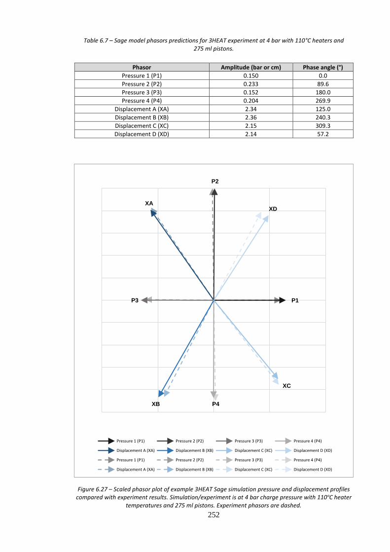
252



Pressure 1 (P1) 0.150 0.0

Pressure 2 (P2) 0.233 89.6

Pressure 3 (P3) 0.152 180.0

Pressure 4 (P4) 0.204 269.9





Figure 6.27 – Scaled phasor plot of example 3HEAT Sage simulation pressure and displacement profiles compared with experiment results. Simulation/experiment is at 4 bar charge pressure with 110ºC heater

temperatures and 275 ml pistons. Experiment phasors are dashed.

P1

P2

P3

P4

XA

XB

XC

XD





253

The phasors generated from the Sage model simulations are very similar to the experiment

results in this scaled comparison. The primary differences result from the slightly larger

relative pressure amplitudes of gas spaces 1 and 3 in the Sage phasors. They have the

effect of attracting the displacement phasors, which is why all of the Sage displacement

phasors are aligned slightly closer to the horizontal axis. The relative phase angles

between the phasors are shown in Figure 6.28. The angle between the pressure phasor of

Gas Space 1 and Piston A’s displacement phasor is 125º, which is very close to the

experimental value of 124.1º. The angles between the pressure phasors are very close to

90º—all are within the range 90º ± 0.4º. The angles between the pistons show greater

deviation when compared to the experiment values in the same figure (the phasors with

dashed arrow-lines). The largest discrepancy of 6.2° occurs for the angle between Piston

C and Piston D (where 107.9º is predicted by Sage and the value from the experiment is

114.1º).



Figure 6.29 shows the pressure amplitudes predicted for each gas space for Sage

simulations using the 3HEAT configuration with 110ºC heater temperatures. The pressure

amplitudes in each gas space increase with charge pressure while retaining their relative

89.6


67.8 115.3


107.9 69.0


89.9

254

magnitude ratios. The distribution of the largest and smallest amplitudes remains

consistent with both the experimental results and the previous analysis for the 15 mm

pistons. The ratios calculated and averaged over the simulation range are 1.54 (s = 0.5%),

1.01 (s = 0.1%) and 1.35 (s = 0.3%) for GS2, GS3 and GS4 respectively. The ratios for

GS2 and GS4 are 6.7% and 9.6% smaller than the experiment values. Adding up the

unrounded ratios obtained for the heater spaces gives a conversion rate of 3.91:1 (three

significant figures).

Figure 6.29 – Sage predictions for pressure amplitudes developed in all four gas spaces with increasing charge pressure for 3HEAT configuration. Simulations are with 110ºC heaters and 275 ml pistons.

Figure 6.30 compares the Sage model pressure amplitudes for the absorber space (GS1)

for both 105ºC and 110ºC heater temperature against the experiment results. For the

4HEAT simulations it was shown that the Sage model was capable of predicting not only

the relative phasor magnitudes and phase angle relationships of the pistons and gas

spaces, but also the absolute values for the pressure amplitudes and piston accelerations.

In the 3HEAT simulations, the model overestimates the level of excitation resulting from

the exact heater temperatures of 105ºC and 110ºC used in the experiments. The

0

0.05

0.1

0.15

0.2

0.25

0.3

0.35

0 1 2 3 4 5 6 7

Pre

ssu

re a

mp

litu

de

(b

ar)



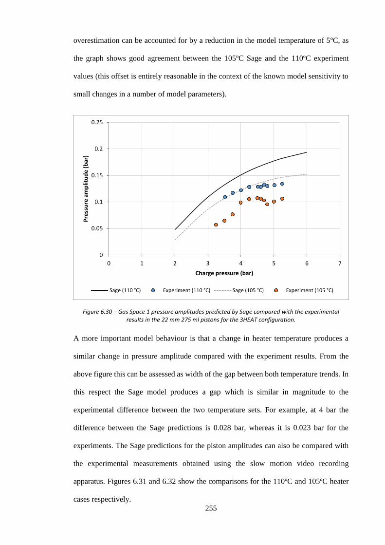
255

overestimation can be accounted for by a reduction in the model temperature of 5ºC, as

the graph shows good agreement between the 105ºC Sage and the 110ºC experiment

values (this offset is entirely reasonable in the context of the known model sensitivity to

small changes in a number of model parameters).

Figure 6.30 – Gas Space 1 pressure amplitudes predicted by Sage compared with the experimental results in the 22 mm 275 ml pistons for the 3HEAT configuration.

A more important model behaviour is that a change in heater temperature produces a

similar change in pressure amplitude compared with the experiment results. From the

above figure this can be assessed as width of the gap between both temperature trends. In

this respect the Sage model produces a gap which is similar in magnitude to the

experimental difference between the two temperature sets. For example, at 4 bar the

difference between the Sage predictions is 0.028 bar, whereas it is 0.023 bar for the

experiments. The Sage predictions for the piston amplitudes can also be compared with

the experimental measurements obtained using the slow motion video recording

apparatus. Figures 6.31 and 6.32 show the comparisons for the 110ºC and 105ºC heater

cases respectively.

0

0.05

0.1

0.15

0.2

0.25

0 1 2 3 4 5 6 7

Pre

ssu

re a

mp

litu

de

(b

ar)


Sage (110 °C) Experiment (110 °C) Sage (105 °C) Experiment (105 °C)

256

Figure 6.31 – Piston amplitudes predicted by Sage compared with the experimental results in the 22 mm 275 ml pistons for the 3HEAT configuration with 110ºC heaters.

Figure 6.32 – Piston amplitudes predicted by Sage compared with the experimental results in the 22 mm 275 ml pistons for the 3HEAT configuration with 105°C heaters.

0

0.5

1

1.5

2

2.5

3

0 1 2 3 4 5 6 7

Pis

ton

am

plit

ud

e (

cm)


Piston A (experiment) Piston B (experiment) Piston C (experiment) Piston D (experiment)

Piston A (Sage) Piston B (Sage) Piston C (Sage) Piston D (Sage)

0

0.5

1

1.5

2

2.5

0 1 2 3 4 5 6 7

Pis

ton

am

plit

ud

e (

cm)




257

The measurements taken with the video have a potential error of ± 0.25 cm, therefore it

is not necessary to infer too much from their relative magnitudes when compared with

each other. The experimental values show some similarities with the Sage model

predictions—pistons C and D consistently record smaller amplitudes, as the model would

suggest, and the spread from largest amplitude to smallest is also approximately equal for

both sets. Unlike the pressure amplitude predictions earlier, the Sage model

underestimates the piston amplitude by a small margin of (at most) 0.5 cm. The reason

for this apparent inconsistency comes from the differences between the model and

experiment frequencies. As identified at the beginning of this section, the Sage model

converges at frequencies which are typically in the region of 0.5 Hz faster than the

experiments, which means the pistons have less development time per cycle to achieve

maximum displacement.

A similar explanation can be used to understand why the maximum piston accelerations

are higher in the case of the Sage predictions. Figure 6.33 shows the piston acceleration

trend comparison for the 3HEAT configuration. Due to the higher frequencies in the Sage

predictions, the piston accelerations are higher for the same amplitude. The lower

amplitude predictions in combination with higher frequencies result in maximum

acceleration predictions that are in close vicinity to the experimental observations. The

predictions for 110ºC pass through the theorised acceleration limit at approximately 4 bar,

which is where the experiments begin to produce unstable results. As with the 4HEAT

results, the maximum accelerations plateau and remain at 27 ms-2 at charge pressures

above 4 bar. The 105ºC experiments do not reach the excitation threshold where the

theorised acceleration limit exists and follow the predicted behaviour of a Sage simulation

between 100ºC and 105ºC Sage trends.

258

Figure 6.33 – Average maximum piston acceleration for 22 mm experiments with 275 ml pistons when compared with Sage model for 3HEAT configuration.

Figure 6.34 – Temperature difference between expansion and compression spaces in Gas Space 1 for the 3HEAT Sage simulations compared with experiments.

0

5

10

15

20

25

30

35

40

0 1 2 3 4 5 6

Max

imu

m a

cce

lera

tio

n (

ms-2

)


Acceleration limit Experiment (110 °C) Experiment (105 °C)

Sage (110 °C) Sage (105 °C) Sage (100 °C)

-5

-4

-3

-2

-1

0

1

2

0 1 2 3 4 5 6 7

Tem

pe

ratu

re d

iffe

ren

ce (

°C)



Experiment (110 °C) Experiment (105 °C)

259

Figure 6.34 shows the temperature difference between the expansion and compression

spaces in Gas Space 1 for both Sage and experiment. The Sage model predicts the largest

temperature difference should occur between 4 bar–5 bar charge pressure, which is what

the experimental results show. The turning points appear to depend on the heater

temperature; higher temperatures lead to higher optimum charge pressures.

Figure 6.35 – Sage model coefficient of performance predictions for the 3HEAT configuration. Simulations are with 275 ml pistons.

Figure 6.35 shows the COP values obtained from the Sage model for the 3HEAT

simulations at 110°C, 105°C and 100°C heater temperatures. The higher temperature

simulations produce higher coefficients of performance. The peak coefficient of

performance occurs at lower charge pressures than the maximum temperature difference

in the absorber space. The COP values are relatively low, and do not suggest the 3HEAT

configuration is particularly useful as a heat-powered cooling configuration. The

maximum COP attained is less than 0.2, which is similar to that identified in the 15 mm

investigation.

0

0.05

0.1

0.15

0.2

0.25

0 1 2 3 4 5 6 7

Co

eff

icie

nt

of

pe

rfo

rman

ce, C

OP



260


Figure 6.36 displays the scaled phasor plot for an example 2HEAT Sage simulation

compared with the phasor plot from the experiment with the same parameters (4 bar

charge pressure and 165ºC heater temperature). Table 6.8 then presents the absolute Sage

model solutions for the pressure and displacement phasors of the same simulation.

Figure 6.36 – Scaled phasor plot of example 2HEAT Sage simulation pressure and displacement profiles compared with experiment results. Simulation/experiment is at 4 bar charge pressure with 165ºC heater

temperatures and 275 ml pistons. Experiment phasors are dashed.

P1

P2

P3

P4

XA

XB

XC

XD





261



Pressure 1 (P1) 0.241 0.0

Pressure 2 (P2) 0.255 90.8

Pressure 3 (P3) 0.200 180.6

Pressure 4 (P4) 0.205 270.8





Except for the displacement of Piston B, the phasors generated from the Sage model

simulations are very similar to the experimental results in this scaled comparison. As was

the case in the 3HEAT comparison, the primary differences result from the slightly larger

relative pressure amplitudes of gas spaces 1 and 3, this time from the experiment side.

Due to their larger relative magnitudes, they have more influence over the piston phasor

orientations, which is why all of the displacement phasors from the experiment are

aligned closer to the horizontal axis.



The relative phase angles between the phasors are shown in Figure 6.37. The angle

between the pressure phasor of Gas Space 1 and the displacement phasor of Piston A is

90.8


93.0 99.3


85.6 82.1


90.2

262

136.8º, which is close to the experimental value of 139.1º. The angles between the

pressure phasors are very close to a value of 90º; all are within the range 90º ± 0.8º.

Comparing the angles between the pistons, the largest discrepancy from experiment (of

10.6°) occurs for the angle between Piston B and Piston C, 82.1º is predicted by Sage and

the value from the experiment is 92.7º. Figure 6.38 shows the pressure amplitudes

predicted for each gas space for Sage simulations using the 2HEAT configuration with

165ºC heater temperatures.

Figure 6.38 – Sage predictions for pressure amplitudes developed in all four gas spaces with increasing charge pressure for 2HEAT configuration. Simulations are with 165°C heaters and 275 ml pistons.

The pressure amplitudes in each gas space increase with charge pressure while retaining

their relative magnitude ratios. The distribution of where the largest and smallest

amplitudes are developed remains consistent with both the experimental results and the

previous analysis for the 15 mm pistons. The ratios calculated and averaged over the

simulation range are 1.06 (s = 0.6%), 0.83 (s = 0.6%) and 0.85 (s = 0.3%) for GS2, GS3

and GS4 respectively. The ratios for GS2 and GS4 are 8.2% and 4.9% larger than the

0

0.05

0.1

0.15

0.2

0.25

0.3

0.35

0.4

0 1 2 3 4 5 6 7

Pre

ssu

re a

mp

litu

de

(b

ar)



263

experiment values, while the GS3 ratio is 4.6% smaller. Adding up the unrounded ratios

obtained for the heater and absorber spaces gives 1.891 for the heater spaces and 1.852

for the absorber spaces, which equates to a conversion rate of 1.02:1 (three significant

figures). This is the same conversion ratio as the 2HEAT experiment in section 6.2.3.

Figure 6.39 – Gas Space 1 pressure amplitudes predicted by Sage compared with the experimental results in the 22 mm 275 ml pistons for the 2HEAT configuration.

Figure 6.39 compares the Sage model pressure amplitudes for one of the absorber spaces,

GS1, for both 165ºC and 160ºC heater temperatures against the experiment results. Again

it is evident that the Sage model is overestimating the pressure amplitude development.

In the 3HEAT cases from the previous section, the overestimation could be quantified by

a heater temperature difference of approximately 5ºC, whereas here it is approximately a

10ºC difference (until both of the experiment sets reach the transition pressures and

plateau from 4 bar and above). The 5ºC difference between the two heater temperatures

analysed in Sage produces a similar amplitude change to that which was measured

0

0.05

0.1

0.15

0.2

0.25

0.3

0.35

0 1 2 3 4 5 6 7

Pre

ssu

re a

mp

litu

de

(b

ar)


Sage (165 °C) Sage (160 °C) Experiment (165 °C) Experiment (160 °C)

264

between the experimental data sets1. This reinforces the model validity inferred from the

same observation made for the 3HEAT comparison.

Figures 6.40 and 6.41 compare the Sage predictions for the piston amplitudes with the

experimental measurements obtained from slow motion video for the 165ºC and 160ºC

heater cases respectively. The trends, magnitudes and relative magnitudes predicted by

Sage agree well with the experimental measurements. The displacement of Piston C is

consistently evaluated at the lowest magnitude, and while the exact magnitudes of the

other pistons’ displacements are closer to each other in the experiments (than those

predicted by Sage), they are still very close in magnitude. The amplitudes in the

experiments decrease beyond the transition pressure at a faster rate than predicted, which

may again be explained by the RT instability.


1 That is for charge pressures below the transition pressure, before the pistons become unstable and the

resulting pressure amplitudes converge.

0

0.5

1

1.5

2

2.5

3

3.5

0 1 2 3 4 5 6 7

Pis

ton

am

plit

ud

e (

cm)




265


Figure 6.42 – Average maximum piston acceleration for 22 mm experiments with 275 ml pistons when compared with Sage model for 2HEAT configuration.

0

0.5

1

1.5

2

2.5

3

0 1 2 3 4 5 6 7

Pis

ton

am

plit

ud

e (

cm)




0

5

10

15

20

25

30

35

40

45

50

0 1 2 3 4 5 6

Max

imu

m a

cce

lera

tio

n (

ms-2

)


Acceleration limit Experiment (165 °C) Experiment (160 °C)


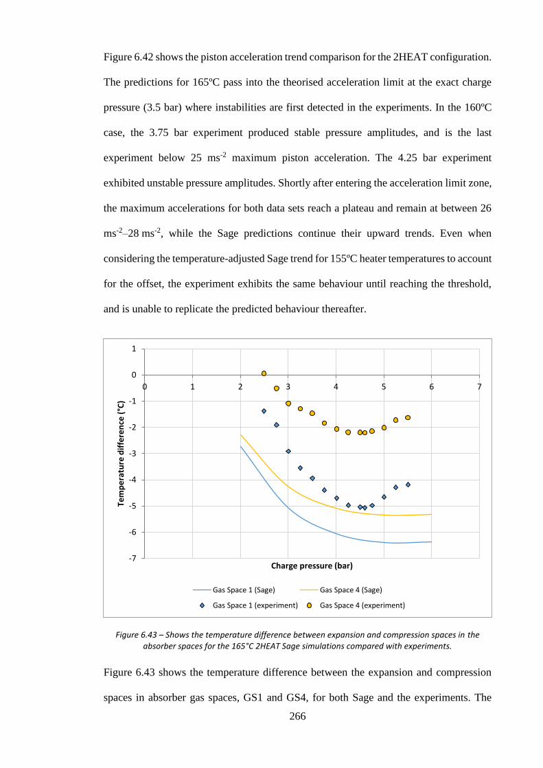
266

Figure 6.42 shows the piston acceleration trend comparison for the 2HEAT configuration.

The predictions for 165ºC pass into the theorised acceleration limit at the exact charge

pressure (3.5 bar) where instabilities are first detected in the experiments. In the 160ºC

case, the 3.75 bar experiment produced stable pressure amplitudes, and is the last

experiment below 25 ms-2 maximum piston acceleration. The 4.25 bar experiment

exhibited unstable pressure amplitudes. Shortly after entering the acceleration limit zone,

the maximum accelerations for both data sets reach a plateau and remain at between 26

ms-2–28 ms-2, while the Sage predictions continue their upward trends. Even when

considering the temperature-adjusted Sage trend for 155ºC heater temperatures to account

for the offset, the experiment exhibits the same behaviour until reaching the threshold,

and is unable to replicate the predicted behaviour thereafter.

Figure 6.43 – Shows the temperature difference between expansion and compression spaces in the absorber spaces for the 165°C 2HEAT Sage simulations compared with experiments.

Figure 6.43 shows the temperature difference between the expansion and compression

spaces in absorber gas spaces, GS1 and GS4, for both Sage and the experiments. The

-7

-6

-5

-4

-3

-2

-1

0

1

0 1 2 3 4 5 6 7

Tem

pe

ratu

re d

iffe

ren

ce (

°C)


Gas Space 1 (Sage) Gas Space 4 (Sage)

Gas Space 1 (experiment) Gas Space 4 (experiment)

267

Sage model predicts the largest temperature difference should occur between 5 bar–6 bar

charge pressure. The experimental results follow a similar downward trend until the

effects of the piston instability begin to influence system behaviour. The differences

between the two gas spaces is larger than predicted by the Sage model. One contributing

factor towards this is the different relative pressure ratios. The ratio between GS4 and

GS1 is 0.85 for Sage and 0.81 for the example experiment. A larger difference in pressure

ratios will result in a larger difference in the temperature differences within the associated

gas space.

Figure 6.44 – Sage model coefficient of performance predictions for the 2HEAT configuration. Simulations are with 275 ml pistons.

Figure 6.44 shows the COP values obtained from the Sage model for the 2HEAT

simulations at 165°C, 160°C and 155°C heater temperatures. The higher temperature

simulations produce higher coefficients of performance. The peak coefficient of

performance occurs at approximately 3.25 bar, which again is lower than where the

maximum temperature differences occur. The COP values are much higher than their

0

0.1

0.2

0.3

0.4

0.5

0.6

0 1 2 3 4 5 6 7

Co

eff

icie

nt

of

pe

rfo

rman

ce, C

OP



268

3HEAT counterparts. The maximum COP predicted is 0.53, which is higher than the

maximum of 0.46 identified in the 15 mm piston 2HEAT investigation.

6.3.4 Summary

The Sage model was updated to reflect the changes made to the physical test-rig when

installing and commissioning the new 22 mm U-tubes with 275 ml liquid pistons. The

frequency predicted by the Sage model was found to lie between the analytical estimates

for adiabatic and isothermal gas behaviour. The corresponding average polytropic index

was found to vary between 1.19–1.20 depending on the charge pressure. The frequency

of the test-rig has consistently been much closer to what would be expected for isothermal

gas behaviour. Due to the model’s sensitivity to frequency as an input parameter, it is

very important to identify the correct value for the model despite the fact it may differ

from the experiment.

The Sage model showed high levels of accuracy in predicting system behaviours for all

three configurations. In the 4HEAT case, the pressure amplitude trends were closely

aligned with the measurements for all experiments conducted at both 75°C and 80°C

(except for the experiments which were above the transition pressure and exhibited piston

instability). For these experiments the pressure amplitude reached a plateau that was

shown to correspond with the same maximum piston accelerations that were identified in

the 15 mm experiments. The Sage model, unhindered by liquid piston instability and the

implications of the RT instability, predicted increased pressure amplitudes and

accelerations above the threshold encountered experimentally. The behaviours were

observed in the 3HEAT and 2HEAT comparisons. Both sets included experiments which

encountered the theorised acceleration limit, and in each case the Sage model showed

similar behavioural trends within the stable operating range before diverging at the point

of transition into instability.

269

The relative magnitudes and phase angles of the pressure and piston displacement phasors

were shown to be very similar to the phasors constructed from experimental

measurements. The phase angles between the pressure phasors were consistently close to

90° for all configurations. The largest differences between the relative pressure

magnitudes were found to be 9.6% and 8.2% for the 3HEAT and 2HEAT configurations

respectively, whereas for the relative piston phase angles they were 6.2° and 10.6°

respectively. The conversion ratios for the 3HEAT and 2HEAT simulations were

calculated as 3.91:1 and 1.02:1 respectively.

The highest COP values for the 3HEAT and 2HEAT configurations were estimated to be

0.2 and 0.53 respectively (for the particular heater temperatures analysed). The COP of

each configuration is predicted to increase for higher heater temperatures. The COP

values rise steeply from 2 bar charge pressure before peaking at 3.5 bar and gradually

decreasing for higher charge pressures. The experimentally-measured temperature

differences achieved in the absorber spaces were found to follow similar trends predicted

by the Sage model, although they were consistently overestimated by 1°C–3°C.

After initial validation attempts with the 15 mm test-rig, the model was used to identify

an improved piston diameter and accurately predicted the fall in starting temperature of

the system for all three configurations. The model was used to determine pressure and

displacement phasor representations that matched the experimentally measured and

observed behaviour. Considering the complex nature of the physical system—and the

difficulties in not only constructing a perfectly symmetrical test-rig, but also replicating

it within the confines of the Sage modelling software—the ability to produce phasor

approximations for the LPSC machine with the degree of accuracy demonstrated in the

preceding sections is probably one of the most significant outcomes of this research

project. The model’s ability to accurately replicate the test-rig performance has helped to

270

identify a physical limitation associated with the use of liquid pistons. The deviation of

the experimental results from Sage-predicted excitation levels (during and after the onset

of piston instability) provides support for the theorised RT instability phenomenon and

the existence of a maximum sustainable piston acceleration. Knowledge of this effect will

aid in the design and optimisation processes of future work with the LPSC machine.

6.4 Results Summary Table

Table 6.9 summarises some of the key performance data from both experiments and Sage

simulations for the 22 mm piston LPSC.

Table 6.9 – 22 mm piston tube results summary for 275 ml pistons.

Configuration

4HEAT 3HEAT 2HEAT

Parameter Experiment Sage Experiment Sage Experiment Sage

Heater temperatures (°C) 75, 80 75, 80 105, 110,

115

100, 105, 110

160, 165 155, 160, 165

Charge pressure range (bar)

2.6 – 6 2 – 6 2.5 – 5.25 2 – 6 2.5 – 5.5 2 – 6

Operational frequency range (Hz)

4.03 - 6.12 3.99 – 6.87

4.00 – 5.73 3.99 – 6.87

3.97 – 5.88 3.99 – 6.87

Ave. pressure amp ratio

(with respect to GS1)

GS1 1.00 1.00 1.00 1.00 1.00 1.00

GS2 1.03 1.00 1.66 1.54 0.98 1.06

GS3 1.00 1.00 1.02 1.01 0.87 0.83

GS4 1.05 1.00 1.50 1.35 0.81 0.85

Relative phase angles, (for

example experiments)

GS1-GS2 90.7 89.9 90.7 89.6 87.4 90.8

GS2-GS3 88.7 90.0 88.7 90.4 92.6 89.9

GS3-GS4 91.0 90.1 91.5 89.9 88.6 90.2

GS4-GS1 89.6 90.0 89.0 90.1 91.5 89.2

A-B 89.9 89.9 118.7 115.3 89.2 99.3

B-C 85.1 90.1 64.8 69.0 92.7 82.1

C-D 95.2 89.9 114.1 107.9 80.7 85.6

D-A 89.8 90.1 62.4 67.8 97.4 93.0

GS1-A 140.8 138.1 124.1 125.0 139.1 136.8

Conversion ratio N/A N/A 4.17 3.91 1.02 1.02

Maximum cooling temp. difference (°C)

N/A N/A -2.3 -4.0 -5.0 -6.4

Maximum Coefficient of Performance

N/A N/A - 0.20 - 0.53

271

7 Liquid Piston Optimisation

On the basis of the Sage model validation conducted in Chapters 5 and 6 (for the 15 mm

and 22 mm experiments) the model is considered ready for use in further test-rig

optimisation. This chapter investigates the optimal piston dimensions which lead to the

best test-rig performance possible. The aim is to identify the level of performance that is

achievable by solely manipulating the piston dimensions, since modifications to the gas

space componentry are more difficult. The resulting identification of optimised piston

sizes could then lead to their implementation in a future stage of the research project.

7.1 Mapping Piston Dimensions

In Section 5.3 it was shown that there existed an optimal piston diameter for the particular

piston length of 94 cm that was used in the 15 mm experiments. Figure 5.89 showed that

this optimal piston diameter was approximately 20 mm. In the second set of experiments,

piston tubes of 19.3 mm average ID were implemented to test the model’s predictive

capabilities. The results obtained from the new test-rig experiments confirmed the

predicted improvements in system performance, and validated the Sage model’s

accuracy. The next logical step is to identify the optimal overall piston dimensions in

terms of length and diameter, and what role the RT instability plays in deciding which to

implement.

In this investigation lower starting temperatures are considered to be the key performance

indicator; although identifying the starting temperatures of each particular piston size is

a time-consuming and tedious endeavour. Recalling that in Section 5.3 it was shown that

higher pressure amplitudes for simulations at the same heater temperature are predictive

of lower starting temperatures, it is much more efficient to select a single heater

temperature and assess the performance of each piston size based on the developed gas

272

pressure amplitudes. A manual optimisation process was conducted whereby the Sage

model was altered to reflect different piston lengths and diameters, and simulations

carried out with the results being collected and analysed. The 4HEAT configuration was

used with a single heater temperature of 90ºC and charge pressure of 6 bar. A charge

pressure of 6 bar was chosen to allow for the potential implementation of the optimised

pistons in the current lab space where the compressed air line is limited to 6.4 bar. The

design of a prototype system would likely involve significantly higher charge pressures.

Table 7.1 summarises the piston dimensions used in the mapping process. All model

parameters not directly affected by the pistons remained constant for all simulations.

Table 7.1 – Piston dimension variations and resulting volumes

Piston volumes (ml) Piston Diameter (mm)

19.3 22.5 25.0 27.5 30.0 32.5 35.0

Pis

ton

Le

ng

th (

cm

) 94 275 374 461 558 664 780 904

140 410 557 687 832 990 1160 1350

200 585 795 982 1190 1410 1660 1920

300 878 1190 1470 1780 2120 2490 2890

400 1170 1590 1960 2380 2830 3320 3850

500 1460 1990 2450 2970 3530 4150 4810

Figure 7.1 – Pressure amplitude predictions for pistons of different diameter and length. Simulations are conducted with 4HEAT configuration with 90ºC heaters and 6 bar charge pressure.

0

0.2

0.4

0.6

0.8

1

1.2

0 100 200 300 400 500 600

Pre

ssu

re a

mp

litu

de

(b

ar)

Piston length (cm)

19.3 mm 22.5 mm 25 mm 27.5 mm 30 mm 32.5 mm 35 mm

273

Figure 7.1 shows the pressure amplitudes predicted from the Sage simulations with piston

dimensions from Table 7.1. The graph shows that increasing piston length generally has

the effect of increasing the pressure amplitude developed in the gas space. Some

simulations were conducted for pistons above 5 m in length, however, as can be seen, the

performance improvement reduces for every meter added, and at some point it becomes

unrealistic to consider extremely long pistons. For now, the practicalities associated with

accommodating excessively long pistons are ignored, and a maximum of 5 m length is

considered in this investigation. Five-metre-long pistons are already extremely large

pistons, and solutions for using such lengths are discussed in Chapter 8.

Another result of increasing the piston length is that the frequency of operation of the

system is reduced. This is good for the maximum piston acceleration, but can also reduce

the power density of the machine. A crude measure of power output can be taken as the

product of frequency and pressure amplitude. Figure 7.2 shows the variation of this

performance indicator, termed objective function 3, for the same set of simulations.

For each diameter, there exists an optimal piston length which produces the highest power

output. This length is longer for larger diameter pistons, with the peaks for 19.3 mm and

30 mm occurring at approximately 175 cm and 350 cm respectively. These lengths do

not necessarily align with the optimal performance of the machine in terms of coefficient

of performance and low starting temperature. In terms of the maximum power output,

there is little gain available above 300 cm piston lengths. Another important consideration

(in light of the RT instability effects) is the maximum piston accelerations sustained in

achieving these pressure amplitudes. Figure 7.3 then shows the maximum accelerations

for the set of piston parameters investigated.

274

Figure 7.2 – Variation of the product of frequency and pressure amplitude (objective function 3) with increasing piston length for different piston diameters.

Figure 7.3 – Maximum piston accelerations sustained for variations in piston length and diameter.

0

1

2

3

4

5

6

0 100 200 300 400 500 600

Ob

ject

ive

fu

nct

ion

3 (

bar

/s)

Piston length (cm)

19.3 mm 22.5 mm 25 mm 27.5 mm 30 mm 32.5 mm 35 mm

0

10

20

30

40

50

60

70

0 100 200 300 400 500 600

Max

imu

m a

cce

lera

tio

n (

ms-2

)

Piston length (cm)

19.3 mm 22.5 mm 25 mm 27.5 mm 30 mm 32.5 mm 35 mm

275

For pistons within the range of 0 m–3 m the larger diameter pistons have significantly

lower maximum piston accelerations, whereas for longer pistons the accelerations

converge to similar values for all piston diameters. The absolute values in the above graph

may seem problematic considering the theorised acceleration limit of 25 ms-2–30 ms-2

previously identified—but the heater temperature used in these simulations is relatively

high (90ºC for 4HEAT) and lower excitation levels would be targeted for the 2HEAT

configuration.

7.2 Selection of Piston Length and Diameter

Considering all of the available information so far presented for the piston optimisation,

the optimal piston size is not immediately apparent (or, indeed, if there even is one). It

can be said, however, that the pressure amplitudes are predicted to rise steadily for

increased piston length, and that piston accelerations reduce with increased length.

Conversely, the estimations for relative power output appear to show little increase above

piston lengths of 3 m. Since it is generally desirable to decrease both piston acceleration

and length to realistic levels (while increasing gas pressure amplitude and power output)

it is logical to consider pistons in the area of 3 m length. Figures 7.4 and 7.5 show the

pressure amplitudes and objective function 3 variations for 3 m pistons with different

piston diameters. Figure 7.4 suggests that using pistons of 23 mm diameter and 3 m in

length will result in the highest pressure amplitude development, and therefore lowest

starting temperature—while Figure 7.5 suggests that increasing the piston diameter to

above 30 mm will result in significant power output gains. For these reasons, two separate

piston diameters, 23 mm and 30 mm, are selected and compared in more detail in the

subsequent section.

276

Figure 7.4 – Predicted pressure amplitudes developed for 3 m pistons with varying piston diameters.

Figure 7.5 – Product of pressure amplitude and frequency (objective function 3) for 3 m pistons with varying piston diameters.

0.6

0.65

0.7

0.75

0.8

0.85

17 19 21 23 25 27 29 31 33 35 37

Pre

ssu

re a

mp

litu

de

(b

ar)


2.5

3

3.5

4

4.5

5

17 19 21 23 25 27 29 31 33 35 37

Ob

ject

ive

fu

nct

ion

3 (

bar

/s)


277

7.3 Comparison Between 23 mm and 30 mm Diameter 3 m Pistons

In the previous section, the scope of piston sizes under consideration was narrowed to

pistons 3 m in length. In this section, the performance of the LPSC machine is evaluated

for two potential system prototypes: one with 3 m long, 23 mm diameter pistons; and the

other with 3 m long, 30 mm diameter pistons. Separate Sage models were constructed for

each case and numerous simulations conducted to map the performance. The charge

pressure was kept constant at 6 bar. Table 7.2 summarises the distinguishing properties

between both prototypes.

Table 7.2 – Prototypes considered for performance assessment.

Properties Prototype 1 Prototype 2

Piston length (m) 3 3

Piston diameter (mm) 23 30

Piston volume (ml) 1246 2121

Piston mass (kg) 1.246 2.121

Operational frequency range (Hz) 4.56 – 4.59 5.95 – 5.98

7.3.1 Simulation Results Overview

From the preliminary piston investigation in Section 5.3, it was concluded that the starting

temperature of the machine could be reduced by varying the piston diameter. The lowest

starting temperatures for the 94 cm pistons were estimated to occur at approximately 79ºC

(with 20 mm diameter pistons). The lower starting temperatures predicted were verified

during the experimental investigation in Section 6.2. Figure 7.6 shows a similar starting

temperature analysis for the 4HEAT configuration comparison between the 23 mm and

30 mm diameter, 3 m long pistons. Interestingly, although the 23 mm pistons produce

larger pressure amplitudes when assessing higher heater temperatures, both sizes exhibit

similar starting temperatures, which are just slightly above 64ºC. This equates to a 15ºC

improvement over the 22 mm OD, 94 cm long pistons used in the second experimental

investigation.

278

Figure 7.6 – Heater temperature influence on the pressure amplitudes developed with 3 m long pistons of diameter 23 mm and 30 mm. Simulations are conducted with 4HEAT configuration at 6 bar charge

pressure.

The LPSC systems are now compared in terms of their ability to achieve the target

objective, i.e. using heat input to produce a cooling effect. The configuration chosen for

this objective is the 2HEAT configuration since it has consistently outperformed the

3HEAT configuration in terms of predicted COP and indicates the most promise based

on the favourable phase angle relationships identified through the phasor analysis of both

configurations.

Both models were found to produce 2HEAT configuration solutions with heater

temperatures at 117ºC and above. Simulations were conducted for a number of different

heater temperatures in the range of 117ºC to 160ºC. The charge pressure was kept constant

at 6 bar (as were all other model parameters). The frequencies were identified from

4HEAT simulations in the same manner as described earlier in Section 4.2.9. The results

from this analysis is summarised in Table 7.3.

0

0.1

0.2

0.3

0.4

0.5

0.6

0.7

0.8

0.9

60 65 70 75 80 85 90 95

Pre

ssu

re a

mp

litu

de

(b

ar)


23 mm 30 mm

279

Table 7.3 – LPSC performance summary for 2HEAT simulations at 6 bar and various heater temperatures.

Heater Temp.

(°C)

Ave. pressure amplitude

(bar)

Ave. piston amplitude

(cm)

Max piston acceleration

(ms-2)

Total heater heat

input (W)

Total absorber

heat input (W)

COP

23 mm

30 mm

23 mm

30 mm

23 mm

30 mm

23 mm

30 mm

23 mm

30 mm

23 mm

30 mm

117 0.119 0.134 0.68 0.45 5.6 6.3 1.5 2.2 0.6 1.0 0.403 0.435

120 0.177 0.178 1.01 0.59 8.3 8.3 2.6 3.4 1.3 1.7 0.491 0.492

125 0.239 0.232 1.35 0.77 11.2 10.8 4.3 5.2 2.3 2.8 0.541 0.531

130 0.290 0.277 1.64 0.91 13.6 12.8 5.9 7.0 3.4 3.9 0.565 0.550

135 0.336 0.317 1.90 1.05 15.7 14.7 7.7 8.9 4.4 5.0 0.577 0.560

140 0.378 0.355 2.13 1.17 17.7 16.4 9.5 10.9 5.5 6.2 0.583 0.564

145 0.418 0.391 2.36 1.28 19.5 18.0 11.3 12.9 6.6 7.3 0.586 0.565

150 0.456 0.424 2.56 1.39 21.3 19.6 13.3 15.0 7.8 8.4 0.585 0.564

155 0.491 0.456 2.76 1.49 22.9 21.0 15.2 17.1 8.9 9.6 0.583 0.561

160 0.525 0.486 2.95 1.59 24.5 22.4 17.2 19.2 10.0 10.7 0.580 0.557

Figure 7.7 – Gas Space 1 pressure amplitude comparison for 2HEAT simulations with different heater temperatures. Charge pressure is 6 bar and piston length is 3 m.

Figure 7.7 shows the comparison for the pressure amplitude predicted in GS1 for both

Sage models across the aforementioned heater temperature range. The pressure

amplitudes developed in GS1 share similar trends to those observed for the 4HEAT

0

0.1

0.2

0.3

0.4

0.5

0.6

110 120 130 140 150 160 170

Pre

ssu

re a

mp

litu

de

(b

ar)


23 mm (GS1) 30 mm (GS1)

280

simulations in the previous section—they begin very close to each other near the lower

starting temperature before diverging slightly as the heater temperature is increased. The

total difference for a heater temperature of 150ºC is 0.034 bar or 6.9% of the 23 mm

model prediction. This difference is relatively small considering the large difference in

piston masses between both systems. The average piston amplitudes are now compared

for both models in Figure 7.8, and Figure 7.9 shows the corresponding average maximum

piston accelerations predicted. As one would expect, the piston amplitudes are larger in

the case of the narrower piston tubes. For reference, the length of the expansion and

compression spaces are 5.81 cm and 3.42 cm for the 23 mm and 30 mm models

respectively.

Figure 7.8 – Average piston amplitude comparison for 2HEAT simulations with different heater temperatures. Charge pressure is 6 bar and piston length is 3 m.

0

0.5

1

1.5

2

2.5

3

3.5

110 120 130 140 150 160 170

Ave

rage

pis

ton

am

plit

ud

e (

cm)


23 mm 30 mm

281

Figure 7.9 – Average maximum piston acceleration comparison for 2HEAT simulations with different heater temperatures. Charge pressure is 6 bar and piston length is 3 m.

Despite the large differences in piston amplitude, the maximum piston accelerations are

comparatively similar, which is due in part to the higher frequency of operation of the

30 mm system. The 30 mm diameter pistons produce accelerations that are consistently

lower than the 23 mm pistons above 120ºC heater temperature. For simulations at 150ºC

the difference is 1.69 ms-2—or roughly 8% of the 23 mm value. Similar acceleration

predictions are expected when recalling Figure 7.3 in the mapping section (this was also

the rationale used in selecting the new piston sizes). Neither system produces

accelerations which exceed 25 ms-2 or enter into the theorised acceleration limit for the

heater temperature range assessed—meaning the conditions for liquid piston surface

stability should be less demanding, and therefore alternatives to the submerged

polyethylene floats could be considered.

0

5

10

15

20

25

30

110 120 130 140 150 160 170

Ave

rage

max

imu

m p

isto

n a

cce

lera

tio

n (

ms-2

)


23 mm 30 mm

282

7.3.2 Cooling Potential

The performance of both systems in terms of their ability to produce the desired cooling

effects are now compared. Figure 7.10 shows the COP values predicted for both systems

when varying the heater temperatures (charge pressure is kept at 6 bar in this analysis).

Figure 7.10 – Coefficient of performance comparison for 2HEAT simulations with different heater temperatures. Charge pressure is 6 bar and piston length is 3 m.

The 23 mm pistons outperform the 30 mm pistons in this comparison. Both experience a

peak COP value at approximately 145ºC; although the rate of decrease of these COP

values with respect to heater temperatures is relatively small after this point. At 150ºC,

the COP values are 0.5853 and 0.5635 for the 23 mm and 30 mm diameter pistons

respectively. It was expected that the 23 mm diameter pistons would show better

performance in this regard considering Figure 7.4 from Section 7.2 (where the highest

pressure amplitude was achieved at the 23 mm diameter for the 4HEAT simulations). Of

course, coefficient of performance is not the only important performance measure. The

0

0.1

0.2

0.3

0.4

0.5

0.6

0.7

110 120 130 140 150 160 170

Co

eff

icie

nt

of

pe

rfo

rman

ce, C

OP


23 mm 30 mm

283

30 mm diameter pistons were included in this comparison to identify the differences

achieved in cooling capacity.

Figure 7.11 – Average absorber heat exchanger fin temperatures achieved for 23 mm and 30 mm diameter pistons in 2HEAT configuration at 6 bar charge pressure. Ambient temperature is 21ºC.

Figure 7.11 shows the absorber heat exchangers’ average fin temperatures achieved by

both systems. The lowest temperatures are achieved by the 30 mm liquid pistons, which

implies greater cooling capacity for this system despite the lower COP values. With

150ºC heaters, the temperatures achieved in the GS1 absorber are 13.1ºC and 12.4ºC for

the 23 mm and 30 mm pistons respectively. Figure 7.12 shows the corresponding heat

flow through the absorber heat exchanger fins for the same set of simulations. The heat

flows correlate with the absorber fin temperatures; heat transfer to the 30 mm absorbers

is greater than the 23 mm system absorbers. The heat input required for the 30 mm

absorbers has necessarily increased to accommodate the higher capacity cooling

potential.

0

5

10

15

20

25

110 120 130 140 150 160 170

Ab

sorb

er

HX

fin

te

mp

era

ture

(°C

)


23 mm (GS1) 23 mm (GS4) 30 mm (GS1) 30 mm (GS4)

284

Figure 7.12 – Heat flow through absorber heat exchanger fins achieved for 23 mm and 30 mm diameter pistons in 2HEAT configuration at 6 bar charge pressure.

It must be remembered that the absorbers within Sage are modelled as if they were

perfectly insulated from the internal heating cartridge (installed in each of the four

expansion spaces in the physical test-rig). For a prototype system, the internal heating

cartridge currently within the absorbers would be replaced with methods for utilising the

cooling effect. This may involve the use of a coolant system—repositioning the absorber

heat exchangers to expose the heat transfer site to an external surface. In either case, the

capacity of the absorber to withdraw heat from the surroundings would be increased since

there would exist a greater heat flow cross-sectional area and decreased total thermal

resistance. This approach can be approximated within the Sage model by reconnecting

the heat flow connections from the heat sources in the absorbers and choosing a target

cooling temperature to replace the high temperature heat sources. The reduction in

resistance on the absorber side could also potentially increase the overall capacity of the

system since, the heaters would be able to regulate their supply to match the increased

0

1

2

3

4

5

6

7

110 120 130 140 150 160 170

He

at f

low

th

rou

gh a

bso

rbe

r H

X f

ins

(W)


23 mm (GS1) 23 mm (GS4) 30 mm (GS1) 30 mm (GS4)

285

absorber capacity. For the 23 mm and 30 mm proposed systems, a number of absorber

heat source temperatures were simulated in order to estimate the significance of this

effect. Table 7.4 summarises the results from the Sage simulations with these new

conditions. A heater temperature of 150ºC was chosen to reflect a realistic solar thermal

collector heat source. The charge pressure remained unchanged at 6 bar with ambient

temperature of 21ºC.

Table 7.4 – LPSC performance summary for simulations with 150ºC heaters at 6 bar and various pre-set absorber temperatures.

Absorber Temp.

(°C)

Ave. pressure amplitude

(bar)

Ave. piston amplitude

(cm)

Max piston acceleration

(ms-2)

Total heater

heat input (W)

Total absorber

heat input (W)

COP

23 mm

30 mm

23 mm

30 mm

23 mm

30 mm

23 mm

30 mm

23 mm

30 mm

23 mm

30 mm

20 0.555 0.521 3.12 1.70 25.9 24.0 18.6 21.2 12.3 13.7 0.661 0.648

18 0.524 0.494 2.94 1.62 24.4 22.7 16.8 19.3 10.9 12.3 0.646 0.634

16 0.492 0.465 2.77 1.53 23.0 21.5 15.1 17.5 9.5 10.8 0.631 0.618

14 0.460 0.436 2.59 1.43 21.5 20.1 13.5 15.7 8.3 9.5 0.613 0.601

12 0.426 0.406 2.40 1.34 19.9 18.8 11.9 14.0 7.0 8.1 0.594 0.582

10 0.392 0.376 2.21 1.24 18.3 17.4 10.3 12.3 5.9 6.9 0.571 0.560

8 0.357 0.344 2.01 1.13 16.7 15.9 8.8 10.6 4.8 5.7 0.544 0.535

Comparing the results to the 150ºC simulation results from the previous analysis, it

appears that the performance of the system does improve slightly when the additional

absorber heat flow potential is added. For absorber temperatures at 14ºC, the total heat

flows are 13.5 W and 8.3 W (COP = 0.613) for the heaters and absorbers in the 23 mm

system respectively; whereas with an average absorber temperature of 13.8ºC, the 23 mm

system produced heat flows totalling 13.3 W and 7.8 W (COP = 0.585). The performance

of both systems increases as the absorber temperature nears the ambient temperature.

Figures 7.13 and 7.14 show how the COPs and predicted heat flow quantities change

depending on the absorber temperature. This type of analysis would be useful when

attempting to size and select an appropriate solar collector system for integration with an

optimised LPSC machine.

286

Figure 7.13 – Predicted COP values depending on the absorber temperature achieved.

Figure 7.14 – Predicted heat flows into the system through the heaters and absorbers for different pre-set absorber temperatures.

0.5

0.55

0.6

0.65

0.7

0 5 10 15 20 25

Co

eff

icie

nt

of

pe

rfo

rman

ce, C

OP

Absorber temperature (°C)

23 mm 30 mm

0

5

10

15

20

25

0 5 10 15 20 25

He

at f

low

(W

)

Absorber temperature (°C)

23 mm (Heaters) 23 mm (Absorbers)

30 mm (Heaters) 30 mm (Absorbers)

287

8 Discussion

8.1 LPSC Configurations


Although obviously incapable of being used in cooling applications, the 4HEAT

configuration proved extremely useful in linking the behaviours of the other

configurations and providing a baseline for comparison. The procedure for using the Sage

model to analyse the 3HEAT and 2HEAT configurations relies on first evaluating 4HEAT

results by virtue of this configuration’s symmetrical properties. The 4HEAT

configuration could be considered for alternative power generation applications by

utilising the developed piston motion alongside linear generators or similar external

power extraction methods. With the addition of an external load, however, the dynamics

of the resulting system would differ significantly from the free behaviour of the LPSC.

8.1.2 3HEAT and 2HEAT Configurations

The 2HEAT configuration is expected to produce better cooling performance based on

the relative pressure amplitudes and the relative phase angles that are established from

the dynamic behaviour of the system. This was verified using the Sage model, with

superior COP values being predicted over the 3HEAT configuration. The highest COP

value predicted for the 3HEAT configuration was 0.20, which was for the 22 mm piston

tube simulations with 275 ml liquid pistons. The corresponding 2HEAT COP prediction

was 0.53 for the exact same set-up.

The 2HEAT opposite configuration previously described in Section 3.3.3, was found not

to function within the experimental range investigated, and the Sage model simulations

showed that even with much higher heater temperatures, self-sustained operation was not

possible. The suspected reason for this is a consequence of the dynamics that result from

288

the positioning of the two heaters—with any motion they induce causing a negating

counteraction. During experimentation, this was noted in the attempts at self-starting the

machine; after generating a significant piston amplitude manually and then releasing the

U-tube, the piston amplitudes would decay to zero almost instantaneously, and much

faster than would be expected of an individual free liquid piston with both surfaces open

to the atmosphere.

One way to think of the 3HEAT system is that it is the 2HEAT opposite configuration

except with an extra heater in place of one of the absorbers, this additional heater breaks

the symmetrical constraints and allows the system to achieve self-sustained operation—

but since the other two heaters are still attempting to cancel out the majority of each

other’s influence, the pressure amplitudes developed in the absorber space are

significantly reduced.

8.1.3 Alternative Configurations

Aside from the configurations discussed and analysed up to this point, there are a number

of other potential arrangements which could be employed for the LPSC. These

arrangements are defined by the different number of subsystems they contain. In this

research project only the 4-subsystems arrangements were considered, due in part to the

goal of achieving phase angles of close to 90°. It is possible, however, to construct the

machine with three, five, six or more subsystems, each of the double-acting alpha Stirling

type connected in series. Each of these machines would have their own operating

configurations, with different combinations of heaters and absorbers occupying the

expansion spaces. Since this research was able to identify the 2HEAT adjacent

configuration as having a conversion ratio of very close to 1:1, and relative phase angles

of close to 90°, it would seem unlikely that a superior set-up could be identified from the

multitude of other potential configurations; but it is not impossible and could be a future

289

avenue of research. With the validation of the Sage model, this process could be

conducted solely through simulation.

8.2 Limitations of Research Presented

8.2.1 Frequency Considerations

The frequencies used in the Sage models are currently identified from the symmetrical

properties of the 4HEAT configuration and its resulting behaviour. Using a procedure

outlined in Section 4.2.9, the piston amplitude and frequency of operation of the 4HEAT

system can be found through an iterative optimisation process for any particular heater

temperature (as long as it is high enough to excite sustained operation, but not too high

to exceed the allowable volumes of the compression and expansion spaces). The heater

temperature value is usually chosen to be in the range which generates piston and pressure

amplitudes close in magnitude to that expected or targeted for the 3HEAT or 2HEAT

configurations. The resulting frequency is then used in the 3HEAT and 2HEAT models

to determine the piston and gas pressure phasors, and generally solve for the behaviour

of the LPSC machine when operating at various heater temperatures of interest for those

configurations. In reality, since the frequency has some small dependence on heater

temperature, it cannot be ensured that the frequency used is exactly the same as that which

would naturally result in the 3HEAT or 2HEAT systems. It was shown that the potential

error range for this frequency is very small across the heater temperatures being

considered; although at the same time, the sensitivity of the model to changes in frequency

is very high. In future work, this aspect of the modelling procedure could be improved.

One possible improvement would be to create a function which attempts to relate the

excitation achieved with the 4HEAT system to the 2HEAT system for different heater

temperatures. Selecting a 2HEAT heater temperature would then produce the

corresponding 4HEAT heater temperature which best approximates similar gas space

290

dynamics. This 4HEAT temperature could then be used to identify the frequency for use

in the 4HEAT model.

The Sage model also predicts a different operating frequency than that of the experiments.

The same difference was observed in the 15 mm and 22 mm piston tube experiments. The

Sage predicted frequencies lie in between the theoretical adiabatic and isothermal gas

spring limits (with an approximate average polytropic index of 1.2); whereas the

experimental results are much closer to the isothermal gas behaviour limit. This difference

could result from the influences of liquid water evaporation, which due to increases in

heat capacity tend to produce behaviour that is closer to isothermal. However the research

is at a too early stage to draw conclusions from this observation. Another potential source

of this error is the average volumes of each gas space being significantly different from

the model, although this was checked on multiple occasions. A method for measuring gas

space volume could be used to rule out this source of error.

8.2.2 Test-rig Asymmetries

The Test-rig contains a number of physical asymmetries, which cannot be accounted for

by the Sage model. Since the volume of each gas space cannot change, the gas masses of

each space are always slightly different. Whether this is due to different operating

configurations (some spaces being heated and others not) or from the small differences in

geometry between the gas spaces, the differences in gas mass will always have an

influence on the behaviour of the system—shifting relative phase angles and/or

amplitudes. The different thermal conductivities resulting from the assembly of the

heating cartridges within the heat exchangers potentially has a similar influence; although

as described in Section 3.1.4, attempts at mitigating this by regulating power flow to each

heater were implemented. To a lesser extent the heat rejection heat exchangers are

subjected to small differences in the heat sink temperatures due to the single cooling line

291

connecting them in series. There are a number of other minor differences associated with

the real test-rig set-up—many are similar to any experimental endeavour—but the final

one highlighted here is the test-rig stand itself. The test-rig stand was shown to influence

the behaviour of the system when the operational frequency approached the stand’s own

natural frequency of vibration. The movement of the stand behaved like a damper to

system motion, and prevented sustained operation at some charge pressures in the 22 mm

experiments (where its influence was identified). It is likely that the stand used in the 15

mm experiments also had some influence on the results attained, since stabilisers were

not implemented in this first set of experiments.

The design of the stand is an interesting challenge, considering that for the interests of

jump-starting the system it is necessary to be able to induce piston motion manually, but

once self-sustained operation is achieved, the stand should then be transitioned into a state

of high rigidity. Perhaps with the reduction in piston amplitudes associated with longer

pistons, and the resulting reduced importance of piston floats, the self-starting properties

of the LPSC machine will be restored and jump-starting will not be necessary. Until this

is confirmed, the design of the test-rig stand should be kept in a non-rigid state to allow

some form of manual excitation (if needed).

These differences between the real system and a computer model are unavoidable when

using a test-rig whose purpose is to function with a number of configurations and heater

temperatures (although they are worth considering in the development of a prototype).

8.2.3 Fluid Friction

The fluid friction present in the gas spaces is relatively well-known and accounted for by

the correlations built into the Sage modelling software. Sage does not have the capability

of selecting liquid pistons as a form of model component, however, and therefore the

differences between solid pistons and liquid pistons had to be manually accounted for

292

within the Sage model. The fluid friction correlations used for the liquid pistons were

outlined in Section 4.2.7, where formulae derived for steady flow situations were used to

approximate an equivalent variable damping coefficient for use in the Sage model. This

was due to the lack of experimental data in the literature on flow losses for reciprocating

liquid flows. The results of the Sage simulations and their comparisons with the

experimental results suggest that the approximations made were reasonably accurate; but

it is not known how accurate they will remain, or how the loss relationships might differ

for vastly differently-sized machines, or those with liquid pistons made up of alternative

liquids. The correlations also have no dependence on the stability of the liquid surface or

the RT instability, which may have an influence on the frictional losses unique to

reciprocating flows. The presence of piston floats (and their influence on overall frictional

flow losses) is another area which may become more relevant depending on the float

requirements for an optimised prototype. It was shown in Section 6.2.1 that the presence

of the polyethylene floats had a significant effect on the performance of the machine; they

increased the minimum charge pressures capable of achieving self-sustained operation,

which is an indication of the increased frictional losses and barrier to motion they present.

8.2.4 Liquid Evaporation

An important characteristic of this machine, which will undoubtedly have an impact on

the level of performance attainable, is that of liquid evaporation at the piston surface and

the resulting role the liquid vapour plays in the thermodynamic processes in the gas space.

At this stage no attempts have been made to mitigate this factor, other than the inclusion

of the polyethylene floats, which also function as piston stabilisers. In the present context

of research into the LPSC machine (as with the piston floats) liquid evaporation and its

impact on system performance does not qualify as being of primary importance. As the

LPSC machine is refined and improved closer to its optimal operating parameter set, the

293

effects of evaporation will be able to be assessed with greater certainty. The use of liquid

water as the piston fluid was made because of its abundance and simple handling

requirements; however, as discussed further in Section 8.6.2, many other fluids are

available for consideration and—as such—evaporation is considered outside of the

present research scope. As the project progresses, a greater amount of consideration

should be given to the effects of liquid evaporation and methods for mitigating it.

8.2.5 Multi-modal Behaviour

During the experimental investigation (particularly with the 15 mm piston tubes) multi-

modal system behaviour was frequently observed. This behaviour was more prevalent in

the 4HEAT and 3HEAT configuration experiments—possibly due to the higher degrees

of dynamic instability associated with having a larger number of ‘engine’ subsystems.

The multi-modal behaviour did not occur very frequently with the 22 mm test-rig. There

are a number of physical differences between the 15 mm and 22 mm test-rigs, so it is not

possible to definitively identify why multi-modal experiments were not witnessed with

the 22 mm test-rig; although there is one main difference which is suspected to play the

most important role—the test-rig stand. As discussed in Section 6.1, when the 22 mm

test-rig experiments were first begun, the vibration of the newly created test-rig stand was

found to interfere with the operation of the LPSC machine within a particular charge

pressure range. It was discovered that the natural frequency of vibration of the stand

coincided with the operational frequency of the LPSC machine near this point, and thus

was damping the motion of the pistons. The interference was so significant that at charge

pressures near 3.5 bar the machine was unable to achieve self-sustained operation

entirely. In order to combat this effect, stabilisers were added to the test-rig stand. The

stabilisers increased the rigidity of the stand and prevented the piston U-tubes from

294

entering into oscillatory motion of their own1. With these stabilisers installed, the

experiments conducted in the affected charge pressure range now behaved consistently

with the expected trends in pressure amplitude and piston displacement.

In the first experimental investigation (using 15 mm OD U-tubes) the effects of test-rig

stand vibration were not as significant, and their detrimental impact on operation not yet

appreciated. As a result, all of the 15 mm experiments were conducted using a test-rig

stand without specialised stabilisers restricting the motion of the piston U-tubes. The

100 ml and 115 ml liquid pistons associated with the 15 mm test-rig did not produce

forces as large as with the 275 ml pistons, which is one reason why the vibration of the

test-rig stand was not as noticeable. It is likely that the vibration of the test-rig stand, and

how this vibration changed in magnitude for different LPSC frequencies, had some

influence on the development of pressure amplitudes and piston displacements during the

15 mm experiments. The multi-modal behaviour of the machine could have been caused

by fluctuations in the damping from test-rig vibration—with multiple semi-stable

oscillatory regimes possible since the stand can provide a variable level of energy

dissipation based on its own motion. With stabilisers installed, the test-rig stand is

restricted in its ability to dissipate energy, and therefore the machine behaves more like

the closed dynamic system intended (and that which was modelled analytically and in

Sage). The design of the test-rig stand will become more important as the liquid piston

mass is increased further, since the reaction forces will increase in magnitude proportional

to piston mass.

8.3 Rayleigh-Taylor Instability and Piston Floats

At the beginning of the project, it was unknown what role the behaviour unique to liquid

pistons would play in the progression of the research. As the investigation progressed, it

1 Or at least they prevented the U-tubes from entering large scale oscillations visible to an observer.

295

was discovered that the liquid surface would become unstable and turbulent at relatively

low charge pressures in the heater temperature range being considered. In order to

mitigate this instability, polyethylene floats were eventually employed, which allowed

experiments to be conducted over the entire range of operating conditions targeted. When

the experimental results were analysed in more detail, evidence of a transition between

stable and unstable behaviour was found, and traced to the liquid pistons based on the

capacitive sensor readings. The cause of the piston instability was not immediately

obvious during the experimental investigation, but in a subsequent literature review the

Rayleigh-Taylor instability was identified as a potential cause.

The RT instability phenomenon was not widely cited in Fluidyne research papers and

texts—the reason for this is speculated to be predominantly due to the much lower

frequencies (typically in the order of 1 Hz) of most Fluidyne machines. The lower

frequencies correspond to lower liquid piston accelerations and therefore less instances

of RT instability. It is only due to the Siemens-Stirling configuration of the LPSC, which

employs the double-acting alpha configuration of the Stirling cycle, that the natural

frequency of the machine is raised to levels which coincide with RT instability. This has

led to some instances of the RT instability being overlooked—for example, in a paper

assessing the potential of a thermoacoustic Stirling engine utilising liquid pistons (Zhang

& Luo, 2015), operational frequencies of 25 Hz were being analysed, which for their

50 mm diameter, 1.5 m long liquid pistons, imposes a maximum piston amplitude of

approximately 1 mm (using an acceleration limit of 25 ms-2).

With the polyethylene floats employed during the experimental process of this research

project, the maximum piston accelerations capable of being sustained were in the range

of 25 ms-2–30 ms-2. The experimental measurements consistently showed that the

behaviour of the system transitioned from stable to unstable liquid surfaces and pressure

296

amplitudes when the maximum acceleration reached this threshold level. The Sage

simulations did not predict the same acceleration plateau as that observed experimentally.

Without the floats, the transition occurred much earlier and at much lower maximum

pressure amplitudes; therefore, much lower maximum piston accelerations were able to

be sustained. Piston floats have proven useful in extending the experimental range of the

test-rig and attaining more evidence of the RT instability phenomenon.

It seems that a major reason why the polyethylene floats outperformed other types was

because their density is very similar to that of water. There is still a lot of room for

improvement in terms of float design; although with the current research focus being on

determining the key design parameters (such as piston length and diameter, etc.) the

geometry of the system is subject to change, and these changes will govern the float

design constraints. It was shown that the optimal performance predictions from the Sage

model tended to coincide with lower piston accelerations, which suggests that as further

improvements are made then the need for submerged floats may be eliminated entirely.

Therefore, any attempt at optimising their presence in the test-rig may prove redundant.

The floats will and should remain an important design consideration for the test-rig in its

current form and future iterations—although with a possible shift in focus from surface

stability to minimising evaporation effects. With the LPSC system becoming more

refined and optimised, some of the less significant considerations become more

important, and float design could be used to mitigate other sources of performance

degradation. As an example, shuttle heat losses between the liquid piston and the

surrounding U-tube and working gas can be reduced by using an above-surface float with

a length comparable to the piston stroke.

297

8.4 Design Considerations

8.4.1 Working Fluids

In this research project, air was used as the working gas for experimentation. Air was

chosen because of its ease of use and handling when compared with the other candidates:

helium and hydrogen. Both helium and hydrogen result in superior performance for

Stirling engines due to their advantageous heat transfer and fluid-dynamic properties.

When designing a prototype LPSC machine it is highly likely that one of these gases

would be selected for use. Hydrogen does outperform helium, but its use does result in a

number of other design considerations and restraints due to its flammable nature and its

ability to diffuse into metal housings. Helium is disadvantaged due to its status as a finite

resource.

As an indication for the increased performance possible with the use of these two working

gases, the Sage model constructed for the 23 mm diameter, 3 m long liquid pistons was

modified to replicate the use of hydrogen instead of air. The results are summarised below

in Table 8.1. The simulations were conducted with the 2HEAT configuration, 150°C

heater temperatures, 6 bar charge pressure and with all other model parameters

unchanged.

Table 8.1 – Sage model predictions for air and hydrogen with the 23 mm diameter, 3 m long liquid piston test-rig.

Property Air Hydrogen

Frequency (Hz) 4.583 4.568

Average pressure amplitude (bar) 0.456 0.611

Heat input from heaters (W) 13.25 20.54

Heat absorbed through absorbers (W) 7.76 12.35

Absorber 1 fin temperature (°C) 13.1 7.0

Absorber 4 fin temperature (°C) 14.5 9.4

Coefficient of performance 0.5853 0.6013

Second law efficiency 5.3% 9.9%

298

Immediately it can be seen that the performance of the LPSC is predicted to improve

significantly with the use of hydrogen. The COP has increased by 2.7% to 0.6013. The

cooling capacity of the machine has increased by 59.1% from 7.76 W to 12.35 W, and

the temperatures developed in the absorbers have also significantly lowered, from 13.1°C

to 7.0°C and 14.5°C to 9.4°C for the fin temperatures of absorbers 1 and 4 respectively.

As a result, the second law efficiency is observed to increase significantly from 5.3% to

9.9%1. It is also important to recognise that these improvements have resulted from the

implementation of hydrogen in a prototype that was optimised for the use of air as the

working fluid. It is likely that with hydrogen the optimal piston dimensions would differ

from the 23 mm diameter, 3 m long ones used in the model. Identifying these would

undoubtedly result in performance improvements exceeding those in the preceding table.

As previously discussed, however, pursuing the optimisation of the LPSC machine with

multiple geometric and physical alterations is not advised at this stage due to the

uncertainty surrounding the Sage model predictions. The results for the use of hydrogen

are nonetheless very encouraging, and could be considered (along with helium) during

the next research phase.

8.4.2 Piston Sizing

As previously identified, the experimental results indicate that an acceleration limit is

imposed on the liquid pistons. It is currently theorised that the RT instability phenomenon

is responsible for this limit and that the absolute value of the limit is influenced by surface

tension and the presence of surface floats (such as the polyethylene floats used in this

research project). If it is assumed that the acceleration limit is independent of any other

system parameters, it is possible to investigate the design implications imposed by this

1 The second law efficiencies are calculated by comparing the Carnot efficiencies for a tri-thermal system

(see Equation 2.1), with the low temperature selected as the absorber 1 fin temperature.

299

limitation. From Equation 4.7, the natural angular frequency of the LPSC machine can be

found:

𝜔𝑛 =√

2𝑛𝐴2𝑝0𝑉0

+2𝐴𝜌𝑔

𝑚

In general, p0 will be increased as much as possible, in order to obtain the ‘free’

performance benefits associated with doing so. When this is done, the right-hand (RH)

term (within the square root function in the above equation) becomes increasingly less

significant. In other words, the gas spring constant begins to dominate the piston spring

constant in terms of dictating the natural frequency of operation. For example, assuming

a V0/A ratio of 1 (which is a generous effective gas space length), the RH term becomes

less than 10% of the left-hand (LH) term at a charge pressure of 7 bar. As the charge

pressure is increased further, this percentage continues to reduce. It is reasonable,

therefore, to neglect the RH term and use:

𝜔𝑛 = √2𝑛𝐴2𝑝0

𝑚𝑉0

as an approximation for the system angular frequency. Assuming a constant cross-

sectional liquid piston area, the equation simplifies to:

𝜔𝑛 = √2𝑛𝐴𝑝0

𝜌𝐿𝑉0 (8.1)

where L is the length of the liquid piston. The acceleration limit:

𝜔2𝑋 ≤ 𝛼𝑀𝑎𝑥

will provide a design constraint, where αMax is the acceleration limit. Substituting in for

the angular frequency from Equation 8.1 and rearranging gives:

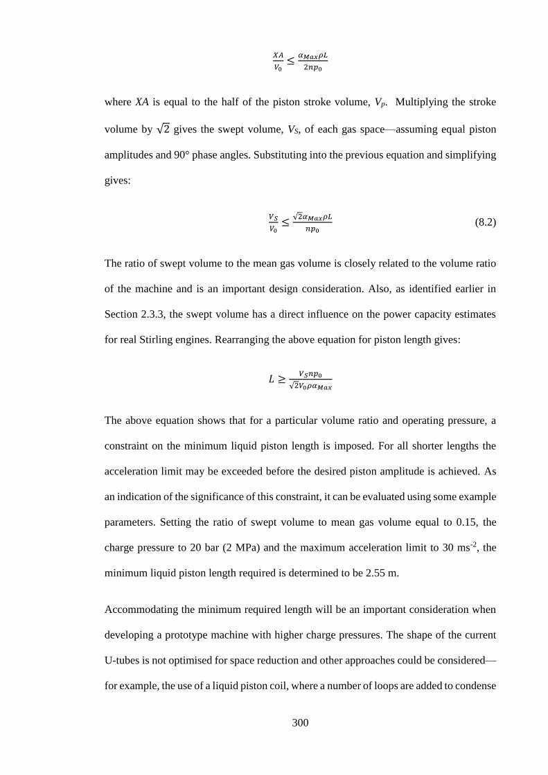
300

𝑋𝐴

𝑉0≤

𝛼𝑀𝑎𝑥𝜌𝐿

2𝑛𝑝0

where XA is equal to the half of the piston stroke volume, Vp. Multiplying the stroke

volume by √2 gives the swept volume, VS, of each gas space—assuming equal piston

amplitudes and 90° phase angles. Substituting into the previous equation and simplifying

gives:

𝑉𝑆

𝑉0≤

√2𝛼𝑀𝑎𝑥𝜌𝐿

𝑛𝑝0 (8.2)

The ratio of swept volume to the mean gas volume is closely related to the volume ratio

of the machine and is an important design consideration. Also, as identified earlier in

Section 2.3.3, the swept volume has a direct influence on the power capacity estimates

for real Stirling engines. Rearranging the above equation for piston length gives:

𝐿 ≥𝑉𝑆𝑛𝑝0

√2𝑉0𝜌𝛼𝑀𝑎𝑥

The above equation shows that for a particular volume ratio and operating pressure, a

constraint on the minimum liquid piston length is imposed. For all shorter lengths the

acceleration limit may be exceeded before the desired piston amplitude is achieved. As

an indication of the significance of this constraint, it can be evaluated using some example

parameters. Setting the ratio of swept volume to mean gas volume equal to 0.15, the

charge pressure to 20 bar (2 MPa) and the maximum acceleration limit to 30 ms-2, the

minimum liquid piston length required is determined to be 2.55 m.

Accommodating the minimum required length will be an important consideration when

developing a prototype machine with higher charge pressures. The shape of the current

U-tubes is not optimised for space reduction and other approaches could be considered—

for example, the use of a liquid piston coil, where a number of loops are added to condense

301

a longer liquid piston into a smaller vertical space. The use of a higher density liquid

would also result in minimum length reductions. This is discussed further in Section 8.6.2.

8.5 Overall Feasibility

8.5.1 Cooling Potential

The 2HEAT configuration with adjacent heaters has been identified as the most promising

configuration for heat-activated cooling. This configuration is shown again in Figure 8.1

for clarity.

Figure 8.1 – Optimal configuration for cooling (2HEAT with adjacent heaters)

This configuration resulted in relative phase angles between adjacent pistons which were

closest to the ideal region of 90°. The magnitudes of the pressure amplitudes developed

in each of the four gas spaces were also relatively close, and the conversion ratios of

pressure amplitudes in the heated spaces to those in the absorber spaces consistently very

close to 1:1. The combination of these behavioural traits resulted in the largest

temperature differences generated experimentally, and the highest predicted overall COP

values of any simulations.

302

The COP value predicted for the test-rig in Chapter 7, with piston dimensions optimised

for efficiency, was 0.585. This also included a maximum temperature difference of 7.9°C

below ambient. By merely switching between air and hydrogen (as was assessed in

Section 8.4.1) the COP of the same Sage model increased to 0.601, with a maximum

temperature difference of 14°C below ambient, and a cooling capacity increase of 59.1%.

Recalling the observations made in Section 2.1, and (in particular) Figure 2.4, it can be

seen that a COP of approximately 0.6 would be very close in terms of competitiveness

with the sorption technologies currently prevailing as the market-leading solar cooling

options. There are a number of other important factors which affect the COP (so it is not

wise to rely excessively on direct comparisons made in this manner)—although it is a

clear indication that such an LPSC machine is feasible, if not commercially viable. This

is reaffirmed when considering the large parasitic losses not accounted for in the sorption

machine COPs in Figure 2.4, as well as the relatively un-optimised LPSC test-rig being

analysed and considered here. With the entire set of heat exchangers, regenerators, and

all other gas space components un-optimised, it is likely that significant performance

improvements over the current LPSC machine can be obtained.

8.5.2 Capacity limitations

Traditional Stirling engines have always suffered from capacity limitations. This arises

from the requirement for external heat input into the system. Unlike combustion cycles,

the Stirling engines typically receive their heat input through a solid interface separating

the heat source from the working gas. These interfaces impose limitations on the rates at

which heat can be transferred into the working gas. The result is that Stirling engines

generally have relatively low power densities. As was described in Equation 2.8 in

Section 2.3.3, the power output of a real Stirling machine depends linearly on a number

303

of factors. If we consider unchanging temperature regimes, these factors reduce to the

frequency, f, the charge pressure, p0, the swept volume, Vs, and the experience factor, F.

The swept volume is the only extensive property out of the four, i.e. it has direct

implications for the size of any machine. The experience factor is known to typically vary

between 0.25–0.35 for well-designed machines. Of the remaining two, frequency and

pressure, only pressure is directly controllable. As discussed already, increasing the

charge pressure also increases the frequency. With the limitations imposed on frequency

by the RT instability, the capacity of a particular sized machine must therefore also be

limited. It is possible to analyse the design constraints associated with these limitations

since approximations for the system frequency and swept volume have already been

obtained. Beginning with Equation 2.8, which provides an estimate of the power output

of a real Stirling engine we have:

𝑃 = 𝐹𝑓𝑉𝑆𝑝0𝑇𝐻−𝑇𝐶

𝑇𝐻+𝑇𝐶.

Rearranging Equation 8.2 for the swept volume, VS, and substituting into the above

equation (along with Equation 8.1 for the system frequency) gives the following when

simplified:

𝑃 ≤𝐹𝛼𝑀𝑎𝑥

𝜋√𝐴𝑝0𝑉0𝜌𝐿

𝑛(𝑇𝐻−𝑇𝐶

𝑇𝐻+𝑇𝐶)

This equation can be further simplified by assuming isothermal gas behaviour (n = 1) and

replacing AL with the liquid piston volume, Vlp. This results in the following expression

for the estimated power producing capacity of one of the driving subsystems:

𝑃 ≤𝐹𝛼𝑀𝑎𝑥

𝜋√𝑝0𝑉0𝜌𝑉𝑙𝑝 (

𝑇𝐻−𝑇𝐶

𝑇𝐻+𝑇𝐶) (8.3)

304

If it is assumed that the heat source and sink temperatures remain unchanged, along with

the acceleration limit and the density of the liquid pistons, the dependent variables reduce

to the charge pressure, the mean gas volume, and the liquid piston volume. In Chapter 7,

the liquid piston dimensions were optimised for the test-rig in its current form. It is

possible to use the same ratio of gas space volume to liquid piston volume in order to

obtain a crude approximation for the size of the machine necessary to achieve the stated

goal at the beginning of this project. This goal was to develop a LPSC capable of

producing a cooling effect in the vicinity of 5 kW. Using the Sage model parameters for

prototype 1 (in Chapter 7) the ratio of gas space volume, V0, to piston volume, Vlp, is

calculated to be approximately 5:1. Therefore V0 ≈ 0.2Vlp. Substituting this into Equation

8.3 and assuming an experience factor of 0.25, an acceleration limit of 30 ms-2, a charge

pressure of 20 bar (2 MPa), a water density of 1000 kgm-3, a heat source temperature of

150°C (423 K), and a heat sink temperature of 25°C (298 K), the expression becomes:

𝑃 ≤ 8278√𝑉𝑙𝑝.

For a cooling effect of approximately 5 kW, it is reasonable to estimate that the power

output of each of the two driving subsystem should be in the vicinity of 1 kW. Thus,

solving the above equation for a 1 kW power output results in a minimum piston volume

of 0.0146 m3, or approximately 15 L. Four 15 L liquid pistons would result in a machine

housing 60 L of liquid water, weighing approximately 60 kg, and with a rough estimate

of 40 kg for other housing componentry. This results in a machine which is roughly 100

kg in total weight; a machine of this size is certainly feasible for low capacity cooling

applications.

305

8.6 Future Research

8.6.1 Piston Floats

The piston friction and float incorporation topics were partially explored during this

project, however, as discussed in Section 8.3, a considerable amount of additional work

is required to establish whether they are necessary, and—if so—in what physical

embodiment are they required, i.e. are they needed purely for surface stability,

evaporation mitigation, heat transfer restrictions or for another purpose.


In this research project only liquid water was considered (and used) in the experiments

and modelling procedures. This was primarily due to its availability, stability and ease of

handling. There are, however, many other potential liquids that can be considered for use

in the LPSC machine. Assessing the suitability of these liquids would be another

interesting avenue for further research. On the surface it appears that higher density

liquids with low viscosity would be the preferred choice. By using higher density liquids,

the machine’s power density can be increased, since a larger amount of energy is capable

of being stored in the motion of the liquid pistons. With higher density typically comes

higher viscosity; although if the total volume required for the liquid piston is significantly

reduced, the increase in viscosity may still result in cumulative reductions in piston

friction. It seems likely that kinematic viscosity (µ/ρ) will be an important property of any

potential liquid.

Related to the preceding speculation on alternative liquids is the need for experimentally

verified correlations for fluid friction and kinetic flow losses in reciprocating fluid flow.

The correlations currently used are for steady flow scenarios only—if the true behaviour

of the liquid deviates significantly from the correlations used, then the Sage model’s

accuracy suffers, when extrapolating (after validation) during the design optimisation

306

process. Perhaps the influence of surface tension and other properties affecting flow

direction change also play a role, in which case the correlations may need to be altered

for different types of liquid.

8.6.3 Thermal Energy Storage

The field of Thermal Energy Storage (TES) is extensive and covers a large range of

applications, including those involving solar thermal collection (Tian & Zhao, 2013).

Since, the target heat source being considered is variable and inconsistent in nature, TES

will need to be considered at a later stage of project development. The challenge of TES

as it relates to this research project is in identifying an optimal storage method (and

integrating it into the collector and LPSC design) so as to create a complete and

independently operable final system prototype. This would be one of the final stages in

producing a machine for commercial implementation and is not suggested for immediate

consideration.

8.6.4 Solid Pistons

Although this research project has focussed solely on the implementation of liquid

pistons, much of the analysis would potentially apply to solid piston machines of a similar

design. Unlike liquid pistons, the solid piston machines would not be constrained by the

acceleration limit imposed by the RT instability. Similarly, since the solid pistons could

be fitted with custom spring supports (for example flexure bearings) their contribution to

the operating frequency (see equation 4.6) would be more significant and controllable

from a design perspective. This would potentially allow for machines with much higher

frequencies, and therefore power densities, when compared with a similar sized LPSC.

Considerable work has been conducted on solid piston heat-activated heat pumps,

including machines based on the Stirling cycle (Walker & Senft, 2012). This is another

research avenue that could be pursued.

307

9 Conclusions and Recommendations

This research presents the liquid piston Stirling cooler or LPSC—which is a 4-cylinder

double-acting alpha-type Stirling test-rig capable of utilising heat input to produce a

cooling effect. The objective of this research project was to establish the feasibility of

such a machine. Based on the findings presented, it is clear that such a system is feasible

both technically and commercially, although to what extent in either regard is still

unknown. The main conclusions and recommendations are summarised as follows:

9.1 Design, Construction and Testing of the LPSC Machine

The successful development of an experimental test-rig has shown that it is possible to

produce a cooling effect using the LPSC concept in conjunction with a thermal heat

source. In its current un-optimised state the LPSC test-rig has proven to be functional

over a wide range of relatively low mean gas pressures (1 bar–6 bar), relatively low heat

source temperatures (80°C–150°C), and with air as a working gas. The (previously

untested) 2HEAT adjacent configuration (with two adjacent heated spaces connected in

series with two adjacent absorber spaces) proved to be the optimal configuration for

cooling performance—with relative phase angles close to 90°, and a conversion ratio of

heater gas pressure amplitude to absorber gas pressure amplitude of 1.02:1.

9.2 System Modelling and Performance Evaluation

A third order model of the LPSC was constructed in the computer modelling software,

Sage. The model encompasses the complex system dynamics and heat transfer

characteristics, and has been validated against experimental results. An approximation for

the natural frequency of the system was derived analytically, and an independent

procedure was developed to determine the operating frequency needed for the Sage

model. These frequencies were found to have very minimal dependence on the machine’s

308

configuration type and heat source temperatures. Some limitations of the model require

further investigation, such as reciprocating flow losses in the liquid pistons and piston

surface instability; although its use in predicting system performance enabled the

installation of more optimised piston geometry which led to the first tangible cooling

effect in the range of 5°C below ambient. When considering test-rig performance at

150°C heater temperature and 6 bar charge pressure, the Sage model predicts a thermal

COP value of 0.53 for the current set-up with 19.3 mm diameter, 94 cm long liquid water

pistons. This rises to 0.59 with the installation of 23 mm diameter, 3 m long liquid pistons.

When the working gas in the model is replaced with hydrogen, the performance of the

LPSC increases significantly: the COP increases by 2.7%, to 0.6, the cooling capacity

increases by 59.1%, the cold-side temperature in the primary absorber is decreased by

77.2% (with respect to 21°C ambient) from 13.1°C to 7°C, and the second law efficiency

increases from 5.3% to 9.9%.

9.3 Liquid Piston Acceleration Limit and Design Implications

Evidence of a liquid piston acceleration limit (likely resulting from the Rayleigh-Taylor

instability phenomenon) was consistently observed during the experiments. The use of

submerged polyethylene piston floats was found to increase surface stability and enable

accelerations of 25 ms-2–30 ms-2. A number of design considerations for the LPSC have

been explored. The existence of a potential piston acceleration limit due to the RT

instability imposes a constraint on the minimum piston length, which is quantified for use

as a design tool. A crude capacity evaluation was also conducted, which indicated that a

LPSC capable of generating a cooling effect of approximately 5 kW was feasible with

15 L liquid water pistons and a total machine weight of roughly 100 kg.

309

9.4 Recommendations

The predicted COPs for the modified test-rig are close to current market-leading solar

cooling options, i.e. sorption systems. With a gap in the market for low capacity machines

(<5 kW) a more thorough and targeted optimisation effort is recommended. The

successful validation of a third order Sage model of the LPSC provides an avenue for

theoretical development and optimisation. Many aspects of the LPSC are capable of being

improved, including manipulation of the gas space component dimensions such as heat

exchangers and regenerators. Different working gases and piston liquids can be

modelled—with higher charge pressures to advance plans for an optimised LPSC

prototype. If successful, an integrated solar refrigeration system could be developed,

although this particular heat-activated cooling machine would not be limited to the solar

market (it could also find use in other waste heat applications).

A number of specific topics are also recommended for future research (summarised in

Section 8.6). These include: (a) an assessment of the design requirements and

implications of piston floats—if needed; (b) research into potential liquid piston fluid

options (and their associated frictional losses, etc.) with respect to reciprocating motion

specifically; (c) thermal energy storage options for integration with solar (or other) heat

sources; and finally, (d) an investigation into the development of a similar machine using

solid pistons instead of liquid pistons.

310

References

Albers, J., Kühn, A., Petersen, S., & Ziegler, F. (2011). Development and progress in

solar cooling technologies with sorption systems. Chemie-Ingenieur-Technik,

83(11), 1853-1863. doi:10.1002/cite.201100116

Anyanwu, E. E. (2003). Review of solid adsorption solar refrigerator I: An overview of

the refrigeration cycle. Energy Conversion and Management, 44(2), 301-312.

doi:10.1016/s0196-8904(02)00038-9

Anyanwu, E. E. (2004). Review of solid adsorption solar refrigeration II: An overview

of the principles and theory. Energy Conversion and Management, 45(7-8), 1279-

1295. doi:10.1016/j.enconman.2003.08.003

Balaras, C. A., Grossman, G., Henning, H. M., Infante Ferreira, C. A., Podesser, E.,

Wang, L., & Wiemken, E. (2007). Solar air conditioning in Europe-an overview.

Renewable and Sustainable Energy Reviews, 11(2), 299-314.

doi:10.1016/j.rser.2005.02.003

Bocquet-Appel, J. P. (2011). When the world's population took off: The springboard of

the neolithic demographic transition. Science, 333(6042), 560-561.

doi:10.1126/science.1208880

Carlsen, H. (1994). Results from 20 kW Vuilleumier heat pump test program.

Proceedings of the 29th Intersociety Energy Conversion Engineering Conference,

2, 927–932. doi: 10.2514/6.1994-3837

Choudhury, B., Saha, B. B., Chatterjee, P. K., & Sarkar, J. P. (2013). An overview of

developments in adsorption refrigeration systems towards a sustainable way of

cooling. Applied Energy, 104, 554-567. doi:10.1016/j.apenergy.2012.11.042

Cook-Yarborough, E. H. (1982). Multi-cylinder Stirling Engine Heat Pumps with

Double-acting Free Pistons. Proceedings of the Intersociety Energy Conversion

Engineering Conference, 4, 1790-1795.

311

Dyson, R. W., Wilson, S. D., & Tew, R. C. (2004). Review of computational Stirling

analysis methods. Proceedings of the 2nd International Energy Conversion


Fan, Y., Luo, L., & Souyri, B. (2007). Review of solar sorption refrigeration

technologies: Development and applications. Renewable and Sustainable Energy

Reviews, 11(8), 1758-1775. doi:10.1016/j.rser.2006.01.007

Fauvel, O. R., Reader, G., & Walker, G. (1989). Tuning line excitation of displacer

motion in a fluidyne. Proceedings of the 24th Intersociety Energy Conversion


Fauvel, O. R., & West, C. D. (1990). Excitation of displacer motion in a fluidyne:

Analysis and experiment. Proceedings of the 25th Intersociety Energy Conversion


Gedeon, D. (2010). Sage User's Guide. Retrieved from www.sageofathens.com

Gerstmann, J., & Friedman, Y. (1979). US Patent No. 4148195. Washington, DC: U.S.

Patent and Trademark Office.

Goswami, D. Y., Kreith, F., & Kreider, J. F. (1999). Principles of Solar Engineering.

Philadelphia, USA: Taylor & Francis.

Harboe-Hansen, H. (1995). Sweden scores a first with AIP submarine. Naval Architect,

March 1995, p E175. London, England: Royal Institution of Naval Architects.

Hargreaves, C. M. (1991). The Philips Stirling engine. New York, NY: Elsevier Science

Publishing Compnay Inc.

Henning, H. M. (2007). Solar assisted air conditioning of buildings - an overview.

Applied Thermal Engineering, 27(10), 1734-1749.

doi:10.1016/j.applthermaleng.2006.07.021

Hong, W. J., Alhussan, K., Zhang, H., & Garris Jr, C. A. (2004). A novel thermally

driven rotor-vane/pressure-exchange ejector refrigeration system with

environmental benefits and energy efficiency. Energy, 29(12-15), 2331-2345.

doi:10.1016/j.energy.2004.03.050

312

International Energy Agency. (2007). Renewables for Heating and Cooling. Retrieved

from http://www.iea.org/

International Energy Agency. (2009). Renewable Energy Essesntials - Solar Heating

and Cooling. Retrieved from http://www.iea.org/

International Energy Agency. (2011). Solar Energy Perspectives. Retrieved from

http://www.iea.org/

International Energy Agency. (2012). Technology Roadmap: Solar Heating and

Cooling. Retrieved from http://www.iea.org/

International Energy Agency. (2016). Our mission. Retrieved from http://www.iea.org/

Kim, D. S., & Infante Ferreira, C. A. (2008). Solar refrigeration options – a state-of-the-

art review. International Journal of Refrigeration, 31(1), 3-15.

doi:10.1016/j.ijrefrig.2007.07.011

Kolin, I. (1991). Stirling motor: history, theory, practice; contributions to the 5th

International Stirling Engine Conference, Inter University Center, Dubrovnik

1991. Zagreb: University Publications.

Kongtragool, B., & Wongwises, S. (2003). A review of solar-powered Stirling engines

and low temperature differential Stirling engines. Renewable and Sustainable

Energy Reviews, 7(2), 131-154. doi:10.1016/s1364-0321(02)00053-9

Kruskal, M., & Schwarzschild, M. (1954). Some Instabilities of a Completely Ionized

Plasma. Proceedings of the Royal Society of London. Series A. Mathematical and

Physical Sciences, 223(1154), 348. doi:10.1098/rspa.1954.0120

Lamp, P., & Ziegler, F. (1998). European research on solar-assisted air conditioning.

International Journal of Refrigeration, 21(2), 89-99. doi:10.1016/S0140-

7007(98)00008-5

Martini, W. R. (1978). Stirling Engine Design Manual: U.S. Department of Energy,

Office of Conservation and Solar Applications, Division of Transportation Energy

Conservation.

313

Martini, W. R. (1983). Test on a 4U tube heat operated heat pump. Proceedings from

the 18th Intersociety Energy Conversion Engineering Conference, 2, 872-874.

Mason, J. W., & Stevens, J. W. (2011). Design and construction of a solar-powered

fluidyne test bed. ASME 2011 International Mechanical Engineering Congress

and Exposition, 4(A&B), 9-20. doi:10.1115/IMECE2011-62194

Nguyen, V. M., Doherty, P. S., & Riffat, S. B. (2001). Development of a prototype low-

temperature Rankine cycle electricity generation system. Applied Thermal

Engineering, 21(2), 169-181. doi:10.1016/s1359-4311(00)00052-1

Nkwetta, D. N., & Sandercock, J. (2016). A state-of-the-art review of solar air-

conditioning systems. Renewable and Sustainable Energy Reviews, 60, 1351-

1366. doi:10.1016/j.rser.2016.03.010

Orda, E., & Mahkamov, K. (2004). Development of "low-tech" solar thermal water

pumps for use in developing countries. Journal of Solar Energy Engineering,

Transactions of the ASME, 126(2), 768-773. doi:10.1115/1.1668015

Otanicar, T., Taylor, R. A., & Phelan, P. E. (2012). Prospects for solar cooling - An

economic and environmental assessment. Solar Energy, 86(5), 1287-1299.

doi:10.1016/j.solener.2012.01.020

Özdemir, M., & Özgüç, A. F. (2003). A simple mathematical model to analyse a

fluidyne heat machine. Proceedings of the Institution of Mechanical Engineers,

Part A: Journal of Power and Energy, 217(1), 91-100.

doi:10.1243/095765003321148736

Perlin, J. (1999). From Space to Earth: The Story of Solar Electricity. Ann Arbor, MI:

Aatec Publications.

Peyret, R., & Taylor, T. D. (1983). Computational Methods for Fluid Flow. The

University of California: Springer-Verlag.

Schmidt, G. (1871). The theory of Lehmann's calorimetric machine. Z. Ver. Dtsch. Ing.,

15(1), 1-12.

Scott, R. (2005). Japan signs up for Stirling AIP. Jane's Navy International (JUL.).

London, England: Jane's Information Group.

314

Senft, J. R. (1982). Simple Derivation of the Generalized Beale Number. Proceedings of

17th the Intersociety Energy Conversion Engineering Conference, 4, 1652-1655.

Slavin, V. S., Bakos, G. C., & Finnikov, K. A. (2009). Conversion of thermal energy

into electricity via a water pump operating in Stirling engine cycle. Applied

Energy, 86(7–8), 1162-1169.

doi:http://dx.doi.org/10.1016/j.apenergy.2008.10.018

Smil, V. (2010). Energy Transitions. Santa Barbara, USA: ABC-CLIO.

Stebnovskii, S. V. (2003). Structural stability of unsteadily accelerated liquid pistons.

Fluid Dynamics, 38(6), 832-838. doi:10.1023/B:FLUI.0000015222.32547.dd

Stephan, K. (1983). History of absorption heat pumps and working pair developments in

Europe. International Journal of Refrigeration, 6(3), 160-166.

Stevens, J. W. (2010). Low capital cost renewable energy conversion with liquid piston

stirling engines, ASME 2010 4th International Conference on Energy

Sustainability, 1, 479-484. doi:10.1115/ES2010-90129

Sunpower. (n.d.). Engines. Retrieved from

http://www.sunpowerinc.com/services/technology/engines.php

Tchanche, B. F., Lambrinos, G., Frangoudakis, A., & Papadakis, G. (2011). Low-grade

heat conversion into power using organic Rankine cycles - A review of various

applications. Renewable and Sustainable Energy Reviews, 15(8), 3963-3979.

doi:10.1016/j.rser.2011.07.024

Tchernev, D. I. (1980). Solar Refrigeration Utilizing Zeolites. Proceedings of the

Intersociety Energy Conversion Engineering Conference, 2, 2070-2073.

Stirling Technology (n.d.). Total Energy Independence. Retrieved from

http://www.stirling-tech.com/energy.shtml

Thombare, D. G., & Verma, S. K. (2008). Technological development in the Stirling

cycle engines. Renewable and Sustainable Energy Reviews, 12(1), 1-38.

doi:10.1016/j.rser.2006.07.001

315

Tian, Y., & Zhao, C. Y. (2013). A review of solar collectors and thermal energy storage

in solar thermal applications. Applied Energy, 104, 538-553.

doi:10.1016/j.apenergy.2012.11.051

Urieli, I., & Berchowitz, D. M. (1984). Stirling cycle engine analysis. Bristol, England:

A. Hilger.

Van de Ven, J. D. (2009). Mobile hydraulic power supply: Liquid piston Stirling engine

pump. Renewable Energy, 34(11), 2317-2322. doi:10.1016/j.renene.2009.01.020

Walker, G. (1979). Elementary Design Guidelines for Stirling Engines. Proceedings of

the Intersociety Energy Conversion Engineering Conference, 1, 1066-1068.

Walker, G., Reader, G., Fauvel, O. R., & Bingham, E. R. (1994). The Stirling

Alternative: Power Systems, Refrigerants and Heat Pumps. Yverdon, Switzerland:

Gordon and Breach Science Publishers.

Walker, G., & Senft, J. R. (2012). Free Piston Stirling Engines. Berlin, Germany:

Springer Berlin Heidelberg.

Wang, K., Sanders, S. R., Dubey, S., Choo, F. H., & Duan, F. (2016). Stirling cycle

engines for recovering low and moderate temperature heat: A review. Renewable

and Sustainable Energy Reviews, 62, 89-108. doi:10.1016/j.rser.2016.04.031

West, C. D. (1971). The Fluidyne heat engine. United Kingdom Atomic Energy

Authority Research Group Report AERE R6775.

West, C. D. (1981). Theoretical Basis for the Beale Number. Proceedings of the

Intersociety Energy Conversion Engineering Conference, 2, 1886-1887.

West, C. D. (1983). Liquid piston Stirling engines. New York, USA: Van Nostrand

Reinhold Company Inc.

West, C. D. (1984). Liquid-piston Stirling Machines. 2nd International Conference on

Stirling Engines, Shanghai, China.

West, C. D. (1986). Principles and applications of Stirling engines. New York, USA:

Van Nostrand Reinhold Compnay Inc.

WhisperGen Ltd. (n.d.). Retrieved April 1, 2013, from http://www.whispergen.com

316

Wurm, J., Kinast, J.A., Roose, T.R., Staats, W.R. (1991) Stirling and Vuilleumier heat-

pumps. New York, USA: McGrawHill, Inc.

Yu, L., & Fauvel, O. R. (1994a). Development of a composite Fluidyne regenerator.

Proceedings of Intersociety Energy Conversion Engineering Conference, 4,

1908-1910.

Yu, L., & Fauvel, O. R. (1994b). Displacer design and testing for a barrel Fluidyne.

Proceedings of Intersociety Energy Conversion Engineering Conference, 4,

1950-1953.

Zhai, X. Q., Qu, M., Li, Y., & Wang, R. Z. (2011). A review for research and new

design options of solar absorption cooling systems. Renewable and Sustainable

Energy Reviews, 15(9), 4416-4423. doi:10.1016/j.rser.2011.06.016

Zhang, S., & Luo, E. (2015). The thermodynamic performance of a double-acting

traveling-wave thermoacoustic engine with liquid-water piston. International

Journal of Green Energy, 12(3), 198-206. doi:10.1080/154350

317

Appendix I – Displacement Sensor Circuit Diagram

318

Appendix II – Rayleigh-Taylor Instability

The Rayleigh-Taylor (RT) instability describes the unstable behaviour of the surface

between a dense fluid supported by another of lower density and subjected to some form

of acceleration. The phenomenon was first theoretically analysed by Lord Rayleigh in

1882 (Rayleigh, 1882), who assessed the everyday scenario of water suspended above

oil. Later, G. I. Taylor experimentally investigated the topic following World War II

(Taylor, 1950). Taylor recognised that the phenomenon applied to liquids under any

acceleration regime—not just those affected by gravity. Following Taylor’s work, the RT

instability received a considerable amount of research in various directions including

surface tension and viscosity effects (Bellman & Pennington, 1954), as well as other areas

such as magnetic fields (Kruskal & Schwarzschild, 1954), spherical geometries (Birkhoff,

1954) and bubble theories (Garabedian, 1957). More recently, the topic has expanded

with developments in CFD to include numerous research focusses such as Inertial

Confinement Fusion (ICF) devices. The range of applications of the RT instability is

extensive—from underwater reactions to cloud stratification, and the aftermath of

supernova.

The RT instability can also be applied to oscillating liquid pistons in order to access the

stability of the liquid surface during operation. The derivation of the RT instability

equations is relatively involved and not necessary in the context of this discussion. The

reader is directed to the literature for further information. Figure A2.1 shows the case

where two homogeneous incompressible fluid planes are separated by a common

interface.

319

Figure A2.1 – Rayleigh-Taylor Instability interface between fluid planes of varying densities

The following equations describe the RT instability for the interface with a small

sinusoidal perturbation profile imposed. Neglecting fluid friction and surface tension

effects the perturbation function is given by:

𝐴(𝑥, 𝑧, 𝑡) = 𝐴(𝑧)𝑒(𝑛𝑡+𝑖𝑘𝑥)

where k is the wavenumber and n is given by:

𝑛 = √𝑘𝛼 (𝜌1 − 𝜌2𝜌1 + 𝜌2

)

where α is the acceleration in the positive z direction. The density fraction within the

above equation is sometimes referred to as the Atwood number. So for instances where

ρ1 > ρ2, i.e. positive Atwood numbers, the growth of the perturbation amplitude is

exponential. Therefore, the instability only occurs in the scenario where the acceleration

is in the direction of the denser fluid. In the case of the U-tube configuration of a liquid

piston, this occurs when the liquid surface is above its neutral position, and the

acceleration vector is pointed down—with peak acceleration occurring at top dead centre

when velocity is zero.

320

It is important to note, however, that any experiments conducted on the surface of the

earth will constantly experience the gravitational acceleration in the positive vertical

direction equal to 9.81 ms-2. Therefore, the RT instability will only become applicable in

Fluidyne machines when the piston acceleration exceeds this quantity. Whether this

occurs (or not) will depend on the frequency and amplitude of oscillation as shown in

Section 2.3.2 of the main work. Since the surface motions on both sides of the U-tube are

directionally opposite then the RT instability has two windows of potential influence per

period of oscillation.

Although referenced as early as 1984 in relation to liquid piston Stirling engines (West,

1984), the relevance and significance of RT instability in liquid pistons has not been

heavily investigated. The main reason for this appears to result from the relatively low

frequencies typical of the majority of Fluidyne systems (as a consequence of their

frequency having primary dependence on liquid piston dimensions). In order for the RT

instability to potentially occur then the piston acceleration must exceed gravity. With

typical frequencies on the order of 1 Hz (as documented by West) this corresponds to a

minimum stroke of 20 cm before the onset of RT instability is possible. In the case of

Fluidyne machines in the Siemens-Stirling configurations, however, the operational

frequencies have a greater dependence on charge pressure—meaning RT instability can

be an important consideration.

The effects of surface tension have also been investigated. Theoretically, they can lead to

stabilization of perturbations with wavenumbers larger than a certain cut-off value:

𝑘𝑐 = √𝜌𝛼

𝜎

where σ is the surface tension (N/m). In 2003, the structural stability of liquid pistons

subjected to unsteady acceleration was investigated (Stebnovskii, 2003). RT instability

321

was observed for water liquid-pistons accelerating inside a cylindrical channel. The same

experiments were also conducted with glycerine liquid-pistons, where the higher

viscosity liquid counteracted the surface perturbation growth, and remained stable for the

particular loading scheme investigated.

References

Bellman, R., & Pennington, R. H. (1954). Effect of surface tension and viscosity on

Taylor Instability. Quart. Appl. Math., 12 (1954), 151-162. Retrieved from

http://www.rand.org/pubs/papers/P403.html.

Birkhoff, G. (1954). Note on Taylor instability. Quart. Appl. Math., 12, 306-309.

Garabedian, P. R. (1957). On steady state bubbles generated by Taylor instability.

Proceedings of the Royal Society of London. Series A. Mathematical and Physical

Sciences, 241(1226), 423-431. doi:10.1098/rspa.1957.0137

Kruskal, M., & Schwarzschild, M. (1954). Some Instabilities of a Completely Ionized

Plasma. Proceedings of the Royal Society of London. Series A. Mathematical and

Physical Sciences, 223(1154), 348. doi:10.1098/rspa.1954.0120

Rayleigh. (1882). Investigation of the character of the equilibrium of an incompressible

heavy fluid of variable density. Proceedings of the London Mathematical Society,

s1-14(1), 170-177. doi:10.1112/plms/s1-14.1.170

Taylor, G. (1950). The Instability of Liquid Surfaces when Accelerated in a Direction

Perpendicular to their Planes. I. Proceedings of the Royal Society of London.

Series A. Mathematical and Physical Sciences, 201(1065), 192.

doi:10.1098/rspa.1950.0052

Stebnovskii, S. V. (2003). Structural stability of unsteadily accelerated liquid pistons.

Fluid Dynamics, 38(6), 832-838. doi:10.1023/B:FLUI.0000015222.32547.dd

West, C. D. (1984). Liquid-piston Stirling Machines. 2nd International Conference on

Stirling Engines, Shanghai, China.

Feasibility Study of a Heat-powered Liquid Piston Stirling Cooler

Documents

Transcript of Feasibility Study of a Heat-powered Liquid Piston Stirling Cooler