FE Model of Moisture Absorption by Adhesive Joints between ...

MASTER’S THESIS

FE Model of Moisture Absorption byAdhesive Joints between Composites

Author:Verónica Bonilla Mora

Supervisor:Magdalena Mieloszyk

Ph.D., Eng.

A thesis submitted in fulfillment of the requirements for theErasmus Mundus Double Master’s Degree Programme in

Mathematical Modelling in Engineering: Theory, Numerics, Applications

in the

Faculty of Applied Physics and MathematicsDepartment of Solid State Physics

October, 2016

http://researchgroup.university.com

http://ftims.pg.edu.pl/fizyki-ciala-stalego/strona-glowna

POLITECHNIKA GDAŃSKA UNIVERSITÀ DEGLI STUDI

DELL’AQUILA

Erasmus Mundus Consortium “MathMods”

Double Master’s Degree Programme in Mathematical Modelling in Engineering: Theory, Numerics, Applications

Master of Science in

Technical Physics

Specialization Advanced Computational

Methods in Materials Science

Laurea Magistrale in

Ingegneria Matematica

POLITECHNIKA GDAŃSKA UNIVERSITÀ DEGLI STUDI DELL’AQUILA

In the framework of the

Consortium Agreement and Award of a Joint/Multiple Degree 2013-2019

Master’s thesis

FE Model of Moisture Absorption by Adhesive Joints between Composites

Supervisor

Candidate

Magdalena Mieloszyk Verónica Bonilla Mora Ph.D., Eng. Matricola: 238831

2014/2016

Student’s name and surname: Verónica Bonilla Mora

ID: 164308

Second cycle studies

Mode of study: Full-time studies

Field of study: Technical Physics

Specialization: Advanced Computational Methods in Materials Science

MASTER'S THESIS

Title of thesis:


Title of thesis (in Polish):

Modelowanie metodą elementów skończonych absorpcji wilgoci w połączeniach klejowych między elementami kompozytowymi

Supervisor

signature

Head of Department

signature

Date of thesis submission to faculty office:

vii

STATEMENT

First name and surname: Verónica Bonilla Mora

Date and place of birth: 30.01.1988, San José

ID: 164308

Faculty: Faculty of Applied Physics and Mathematics

Field of study: technical physics

Cycle of studies: postgraduate studies

Mode of studies: Full-time studies

I, the undersigned, agree that my diploma thesis entitled: “FE Model of Moisture Absorption by Adhesive Joints between Composites” may be used for scientific or didactic purposes.1

Gdańsk, ................................. ................................................ signature of the student

Aware of criminal liability for violations of the Act of 4th February 1994 on Copyright and Related Rights (Journal of Laws 2006, No. 90, item 631) and disciplinary actions set out in the Law on Higher Education (Journal of Laws 2012, item 572 with later amendments),2 as well as civil liability, I declare that the submitted diploma thesis is my own work.

This diploma thesis has never before been the basis of an official procedure associated with the awarding of a professional title.

All the information contained in the above diploma thesis which is derived from written and electronic sources is documented in a list of relevant literature in accordance with art. 34 of the Copyright and Related Rights Act.

I confirm that this diploma thesis is identical to the attached electronic version.


I authorise the Gdańsk University of Technology to include an electronic version of the above diploma thesis in the open, institutional, digital repository of the Gdańsk University of Technology and for it to be submitted to the processes of verification and protection against misappropriation of authorship.


1

Decree of Rector of Gdańsk University of Technology No. 34/2009 of 9th November 2009, TUG archive instruction

addendum No. 8.

2

Act of 27th July 2005, Law on Higher Education:

Art. 214, section 4. Should a student be suspected of committing an act which involves the appropriation of the authorship of a major part or other elements of another person’s work, the rector shall forthwith order an enquiry.

Art. 214 section 6. If the evidence collected during an enquiry confirms that the act referred to in section 4 has been

committed, the rector shall suspend the procedure for the awarding of a professional title pending a judgement of the disciplinary committee and submit formal notice of the committed offence.

ix

GDANSK UNIVERSITY OF TECHNOLOGY

AbstractFaculty of Applied Physics and Mathematics

Department of Solid State Physics

Erasmus Mundus Double Master’s Degree inMathematical Modelling in Engineering


by Verónica Bonilla Mora

Adhesive joints offer many advantages over traditional mechanical joiningsystems. Nonetheless, their use is limited since they can be adversely affectedby extreme temperatures and humidity conditions. Moisture absorption in anadhesive can alter its tensile strength and compromise the structural integrity ofthe joint. Thus, moisture absorption and moisture-induced strain monitoring isan area of high interest in the field of structural health monitoring (SHM).

In the present project, several finite element models were created to analysethe thermal response, diffusion dynamics and strain development of two ad-hesive joints with different thickness size between composites; and serve as amethodology for future studies in the area. The project was motivated by ex-perimental results obtained by the Institute of Fluid-Flow Machinery, in whichFiber-Bragg grating sensors were used to monitor the moisture-induced strainson the adhesive joints.

Three main analyses were performed: a thermal analysis, a mass diffusionanalysis and a hygro-mechanical analysis. All three were developed throughthe use of the FE software Abaqus. Simulation results were validated by experi-mental data.

HTTP://PG.EDU.PL/EN/

http://ftims.pg.edu.pl/en

http://ftims.pg.edu.pl/fizyki-ciala-stalego/strona-glowna

xi

AcknowledgementsThe completion of any project invariably involves the collaboration of many

helping hands at different stages. This project wasn’t the exception, and I waslucky to count on wonderful people along the way.

A special thanks to my supervisor, for always taking the time to promptlyrespond my many, many emails and patiently answering my, also, many, manyquestions. And my eternal gratitude to Rohan Soman, part of the IMP PANteam, for taking the time to discuss my models and results.

My sincerest thanks to professor Jerzy Bobinski, for helping me pass the firsttechnical hurdles of this project.

And Adwait, your positivism and excitement to learn was always a sourceof motivation throughout this whole experience. Thank you for helping me "seethe light" despite being miles and miles away, in true MathMods fashion. Toogood, man!

The work in this thesis was inspired by and conducted in collaboration withthe IMP PAN team realising the project entitled: ’Quality assurance conceptsfor adhesive bonding of aircraft composite structures by advanced NDT’ (Com-BoNDT). This project has received funding from the European Union’s Horizon2020 research and innovation programme under grant agreement No 636494.

The research was supported by the project entitled: Non-invasive Methodsfor Assessment of Physicochemical and Mechanical Degradation (PBS1/B6/8/2012) granted by National Centre for Research and Development in Poland.

xiii

Contents

Abstract ix

Acknowledgements xi

1 Moisture-induced strain monitoring 11.1 Introduction . . . . . . . . . . . . . . . . . . . . . . . . . . . . . . . 11.2 Fiber-Bragg Grating Sensors . . . . . . . . . . . . . . . . . . . . . . 2

1.2.1 Strain sensitivity . . . . . . . . . . . . . . . . . . . . . . . . 31.2.2 Temperature Sensitivity . . . . . . . . . . . . . . . . . . . . 4

1.3 Experimental Results . . . . . . . . . . . . . . . . . . . . . . . . . . 51.3.1 Moisture Content . . . . . . . . . . . . . . . . . . . . . . . . 51.3.2 Temperature-Induced Strains . . . . . . . . . . . . . . . . . 71.3.3 Moisture-Induced Strain Results . . . . . . . . . . . . . . . 8

1.4 Hypothesis and Main Objectives . . . . . . . . . . . . . . . . . . . 10

2 Thermal Analysis 112.1 Introduction . . . . . . . . . . . . . . . . . . . . . . . . . . . . . . . 112.2 Mathematical Model . . . . . . . . . . . . . . . . . . . . . . . . . . 112.3 Thermal Simulation . . . . . . . . . . . . . . . . . . . . . . . . . . . 13

2.3.1 Simulation - Dry Conditions . . . . . . . . . . . . . . . . . 162.3.2 Simulation - Wet Conditions . . . . . . . . . . . . . . . . . 17

2.4 Conclusions . . . . . . . . . . . . . . . . . . . . . . . . . . . . . . . 19

3 Mass Diffusion Analysis 213.1 Introduction . . . . . . . . . . . . . . . . . . . . . . . . . . . . . . . 213.2 Moisture Diffusion . . . . . . . . . . . . . . . . . . . . . . . . . . . 22

3.2.1 Time-Varying Boundary Conditions . . . . . . . . . . . . . 243.2.2 Dual-Stage Model . . . . . . . . . . . . . . . . . . . . . . . 25

3.3 Weak form discretization . . . . . . . . . . . . . . . . . . . . . . . . 263.4 Diffusion Model . . . . . . . . . . . . . . . . . . . . . . . . . . . . . 27

3.4.1 Material Properties . . . . . . . . . . . . . . . . . . . . . . . 27Time-Varying Boundary Conditions . . . . . . . . . . . . . 27Dual-Stage . . . . . . . . . . . . . . . . . . . . . . . . . . . . 28

3.4.2 Boundary Conditions . . . . . . . . . . . . . . . . . . . . . 29Time-Varying Boundary Conditions . . . . . . . . . . . . . 29Dual-Stage Model . . . . . . . . . . . . . . . . . . . . . . . 30

3.4.3 Model Mesh . . . . . . . . . . . . . . . . . . . . . . . . . . . 313.5 Results . . . . . . . . . . . . . . . . . . . . . . . . . . . . . . . . . . 32

3.5.1 Average Concentration - Whole Sample . . . . . . . . . . . 333.5.2 1 mm vs 0.5 mm Mesh . . . . . . . . . . . . . . . . . . . . . 34

xiv

3.5.3 Average Concentration - Sample A and B . . . . . . . . . . 353.5.4 Average Concentration - Sensor Areas . . . . . . . . . . . . 353.5.5 Concentration Distribution . . . . . . . . . . . . . . . . . . 36

3.6 Conclusions . . . . . . . . . . . . . . . . . . . . . . . . . . . . . . . 37

4 Hygro-Mechanical Analysis 414.1 Introduction . . . . . . . . . . . . . . . . . . . . . . . . . . . . . . . 414.2 Hygroscopic and Thermal Strain . . . . . . . . . . . . . . . . . . . 424.3 Hygro-Mechanical Model . . . . . . . . . . . . . . . . . . . . . . . 43

4.3.1 Coupling the Mass Diffusion Analysis . . . . . . . . . . . . 434.3.2 Material Properties . . . . . . . . . . . . . . . . . . . . . . . 434.3.3 Boundary Conditions and Loads . . . . . . . . . . . . . . . 454.3.4 Interactions . . . . . . . . . . . . . . . . . . . . . . . . . . . 464.3.5 Model Mesh . . . . . . . . . . . . . . . . . . . . . . . . . . . 46

4.4 Analysis Results . . . . . . . . . . . . . . . . . . . . . . . . . . . . . 474.4.1 Time-Varying BC Strain Profiles . . . . . . . . . . . . . . . 484.4.2 Dual-Stage Strain Profiles . . . . . . . . . . . . . . . . . . . 494.4.3 1 mm vs 0.5 mm Mesh . . . . . . . . . . . . . . . . . . . . . 504.4.4 Water Pressure Effect . . . . . . . . . . . . . . . . . . . . . . 51

4.5 Conclusions . . . . . . . . . . . . . . . . . . . . . . . . . . . . . . . 53

5 Summary 575.1 Introduction . . . . . . . . . . . . . . . . . . . . . . . . . . . . . . . 57

5.1.1 Thermal Analysis . . . . . . . . . . . . . . . . . . . . . . . . 575.1.2 Mass Diffusion Analysis . . . . . . . . . . . . . . . . . . . . 58

5.2 Hygro-mechanical Analysis . . . . . . . . . . . . . . . . . . . . . . 595.3 Future Works . . . . . . . . . . . . . . . . . . . . . . . . . . . . . . 60

A User Subroutine - UFIELD 61

B Average Concentration - Python Script 63

C Record Key Change Code 65

Bibliography 69

xv

Dedicated to my loving parents,

Raúl and Sylvia

"It’s away from home when you realize the true meaning of aparent’s love and the significance of family."

Anonymous

1

Chapter 1

Moisture-induced strainmonitoring

1.1 Introduction

Composites are, like their name suggests, materials composed of two or moredifferent materials joined together to create a new material with special andunique characteristics. They have been widely used by mankind for centuries,with the earliest composites being plywood, cartonnage, concrete, and mortar;among others [1].

In recent years, composite manufacturing has evolved to create materials bymerging several different layers of fibres and resins. The layers can be chosen toobtain materials with the required structural and mechanical qualities for spe-cific applications. Most notably, to create materials that possess higher strength,more corrosion resistance and better stiffness-to-weight ratios than other tradi-tional materials like metals [2, 3]. As such, the market of composite materialshas bloomed and their use can be found in almost all industries in the world,from aeronautics to construction, to medicine, to the oil and gas industry [4,5]. Clearly, the study of composites as well as their structures is of utmost im-portance for designers and manufacturers to guarantee needed safety standardsand increase reliability.

A widely used method for composite structure manufacturing is the useof high strength adhesive joining. Adhesive joints are preferable to traditionalmethods like mechanical fasteners that may require the drilling of the compos-ite. Drilling holes could be a source of damage for the material and it intro-duces undesired stress concentrations near the hole [6]. Adhesive bonds arealso lighter than riveting or welding methods, present higher fatigue resistanceand can distribute loads over larger areas [7].

2 Chapter 1. Moisture-induced strain monitoring

Of course, when employing these types of joints, care has to be given tothe type of adhesives used, surface preparation and environmental conditionswhere the structure will be used. Due to the polymeric nature of adhesives,adhesive joints present limited resistance to extreme temperature and humidityconditions [8]. As several studies have shown [3, 9–11], moisture can be a majorcontributing factor to adhesive joint and composite failure. Moisture absorptionby an adhesive leads to several changes in its physical and mechanical structure.It reduces the transition temperature Tg, reduces tensile strength and lowersthe ultimate elongation of the adhesive [11]. Thus, moisture absorbtion andmoisture-induced strain monitoring is an area of high interest in the field ofstructural health monitoring (SHM).

The present project was motivated by experimental results obtained at theInstitute of Fluid-Flow Machinery in Gdansk, Poland. The experiment madeuse of fiber Bragg grating sensors to quantify developed strains caused by mois-ture absorption of an epoxy paste adhesive used to join two composite materials[12]. In the present project, a finite element model was generated to simulatethe thermal response, diffusion dynamics and strain development of the testedcomponents and serve as a methodology for future studies in the area.

1.2 Fiber-Bragg Grating Sensors

Fiber Bragg Grating sensors are optical sensors whose core index of refractionhas been altered by optical absorption of UV light. Their use has become wide-spread due to the many advantages they possess: small dimensions, light weight,insensitivity to electromagnetic interference, multiplexing capabilities and resis-tance to corrosion [13].

The core index of refraction is changed in a periodic pattern along the core ofthe fibers creating phase structures, or phase gratings [14]. When light interactswith the gratings created inside the fiber core, only a small part of the lightspectrum will be reflected back. The reflected spectrum is centred on the Bragg-wavelength (λB) and depends on the effective index of refraction (neff ) andon the spacing between gratings, the Bragg period (Λ), as stated by the Braggcondition [13]:

λB = 2neffΛ (1.1)

1.2. Fiber-Bragg Grating Sensors 3

Applied mechanical strains and temperature changes affect FBG wavelengthmeasurements, which is why it is possible and have been regularly used forstrain and temperature monitoring [13, 15–17]. Parting from equation 1.1, thechange of the Bragg-wavelength due to strain and temperature changes is,

∆λB = 2

(Λ∂n

∂ε+ n

∂Λ

∂ε

)∆ε+ 2

(Λ∂n

∂T+ n

∂Λ

∂T

)∆T (1.2)

FIGURE 1.1: Fiber Bragg Grating Sensor Diagram [18]

1.2.1 Strain sensitivity

The first term of equation 1.2 is related to the strain contribution to the wave-length measurement. The change in the refractive index of the fibre due to strainin the longitudinal axis is the following

∂n3′ = −n2eff

2[ρ13ε1′ + ρ23ε2′ + ρ33ε3′ ] (1.3)

where ρ13, ρ23 and ρ33 are the elements of the strain-optic tensor of a ho-mogeneous orthotropic material [19] following the coordinate system shown onfigure 1.1. The change in the Bragg period is ∂Λ = Λ0(1 + ε3′) [17], therefore, thewavelength response to axial strains can be expressed as follows [20]

∆λBλB

=

[1− 1

2n2eff [ρ12 − ν(ρ11 + ρ12)]

]ε3′ = (1− ρε)ε3′ (1.4)

where ρε is an effective strain-optic coefficient of the fiber optic materialwhich can be measured experimentally and is defined on equation 1.5.

ρε =n2eff

2[ρ12 − ν(ρ11 + ρ12)] (1.5)

where ρ11 and ρ12 are components of the strain-optic tensor, neff is the indexof the fiber core, and ν is Poisson’s ratio [13]


For silica fiber sensors, the wavelength-strain sensitivities of 800 nm and1550 nm FBGs have been measured as ∼0.64 pm µε−1 and ∼ 1.15 pm-1 µε [21].The manufacturer of the FBG sensors used in the experiment states that (1− ρε)has a value of 0.890 [12].

1.2.2 Temperature Sensitivity

The rest of equation 1.2 corresponds to the effect of temperature on the wave-length measurements. It can be rewritten as follows,

∆λBλB

=

[1

neff

∂neff∂T

+1

Λ

∂Λ

∂T

]∆T (1.6)

The first term in the brackets is known as the thermal expansion coefficient,αf , of the fiber core (equation 1.7) . For silica it has an approximate value of 0.55

x 10−6 1/K [18]. The second term represents the thermo-optic coefficient, αn,(equation 1.8). It is dependant on the type and concentration of dopants in thesensor [18]. For germanium-doped, silica-core fibers values have been found tobe between 3.0 x 10−6 [22] and 8.6 x 10−6 1/K [13].

αf =1

neff

∂neff∂T

(1.7)

αn =1

Λ

∂Λ

∂T(1.8)

Sometimes in the literature, the thermal expansion coefficient and the thermo-optic coefficient can be found combined as the so-called temperature coefficient,β = αf + αn. Equation 1.6 then, can be rewritten as,

∆λBλB

= β∆T (1.9)

For a silica fiber, the wavelength-temperature sensitivities of 800 nm and 1.5µm FBGs have been measured with values of∼6.8 and∼13 pm/oC, respectively[21].

1.3. Experimental Results 5

1.3 Experimental Results

One of the focus areas of the Mechanics of Intelligent Structures Department atthe Institute of Fluid-Flow Machinery is the static and dynamics of compositestructures and possible failure modes [23]. As part of those investigation ef-forts, experimental results were obtained for the moisture-induced strains on anadhesive joint between composites.

1.3.1 Moisture Content

The main purpose of the investigation was to determine the applicability andfeasibility of using FBG (Fiber Bragg Grating) sensors for structural health mon-itoring of moisture contamination of adhesive bonds in composite structures[12].

The experiment consisted of three different samples denominated A, B andC. Each sample was made up of two GFRP (Glass Fiber Reinforced Plastic)composites with a stacking sequence of (0/90/0/90/90/0/90/0) and sizes of250x50x1 mm (figure 1.2).

FIGURE 1.2: Sample Dimensions [12]

The composites were bonded together by a 0.2 mm layer of adhesive (in thecase of sample B, the adhesive layer had a thickness of 0.4 mm). FBG sensorswere placed in the adhesive layer, with their placement varying within samplesas shown on figure 1.3.

FIGURE 1.3: FBG sensor placement [12]


The adhesive used was a two-part structural epoxy paste adhesive producedby Henkel Corporation and commercially known as Loctite EA 9394 Aero orHysol EA 9394. Its main properties as listed by the manufacturer [24] are givenon Table 1.1.

TABLE 1.1: Adhesive Properties

Parameter Value Units

Tg (dry) 78 oCTg (wet) 68 oCTensile Strength at 25oC 46 MPaTensile Modulus at 25oC 4.237 GPaElongation at 25oC at break 0.017 %Compressive Strength at 25oC 68.9 MPaCure Temperature 25-93 oCCure Time 3-5 day

After proper curing, the assembled samples were placed into individualboxes and submerged in demineralized water. The samples were kept insidea temperature chamber at 60oC ± 2oC for approximately 2 weeks. During thattime, the moisture content was regularly monitored by weighing the samplesand calculating it by the following equation,

M(t) =W (t)−Wo

Wo· 100 (1.10)

where W(t) is the measured weight at a given time and Wo is for the initiallydry weight of the sample.

After the two weeks, the moisture content of the samples was around 2.26%.Figure 1.4 shows the moisture weight-gain against time.

0

0.5

1

1.5

2

2.5

0 50 100 150 200 250 300 350

Mois

ture

Weig

ht

Gain

(%

)

Time (h)

Experimental Results

FIGURE 1.4: Moisture Weight Gain (%)


1.3.2 Temperature-Induced Strains

As mentioned earlier, FBG sensors are very sensitive to temperature changes.In order to experimentally quantify only the moisture-induced strains (ε) on theadhesive bond, it was necessary to determine the temperature contribution, εT ,to the total values measured, εC .

εC = εT + ε (1.11)

To do so, dry samples were placed in a heating chamber at 60 ± 2 oC. Thetemperature was monitored using a temperature probe (os4200, Micron Optics).Figure 1.5 shows the temperature measurements of both, the 1 mm and 10 mmFBG sensors.

FIGURE 1.5: FBG sensors temperature measurements [12]

The total strain values, εC , can be determined from the FBG readings usingequation 1.12 [12].

εC(t) =λmi(t)− λb(1− ρε)λb

(1.12)

where λB is the base Bragg wavelength, λmi is the Bragg wavelength fromthe i-th measurement and ρε is the effective strain-optic coefficient.

In this case, since the measurements are on dry samples, the total measuredstrains correspond to the temperature-induced strains. The relationship be-tween strain and temperature is given by equation 1.13, where p is the volumet-ric expansion coefficient that depends on the fiber optic and adhesive materials.The value of p for the samples used was determined to be 9.15 µε/oC with theexperimental data gathered.

εT = p∆T (t) (1.13)


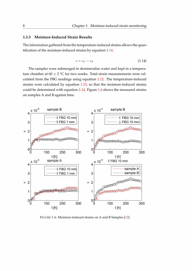
1.3.3 Moisture-Induced Strain Results

The information gathered from the temperature-induced strains allows the quan-tification of the moisture-induced strains by equation 1.14.

ε = εC − εT (1.14)

The samples were submerged in demineralise water and kept in a tempera-ture chamber at 60 ± 2 oC for two weeks. Total strain measurements were cal-culated from the FBG readings using equation 1.12. The temperature-inducedstrains were calculated by equation 1.13, so that the moisture-induced strainscould be determined with equation 1.14. Figure 1.6 shows the measured strainson samples A and B against time.

FIGURE 1.6: Moisture-induced strains on A and B Samples [12]


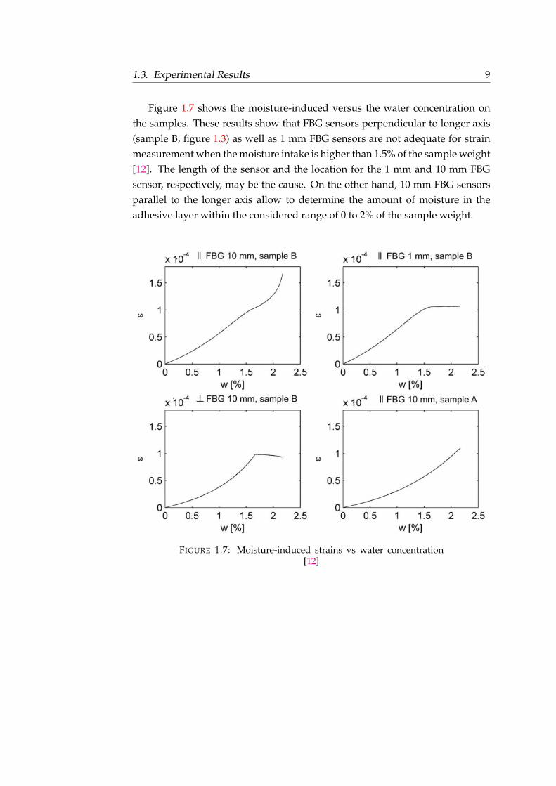
Figure 1.7 shows the moisture-induced versus the water concentration onthe samples. These results show that FBG sensors perpendicular to longer axis(sample B, figure 1.3) as well as 1 mm FBG sensors are not adequate for strainmeasurement when the moisture intake is higher than 1.5% of the sample weight[12]. The length of the sensor and the location for the 1 mm and 10 mm FBGsensor, respectively, may be the cause. On the other hand, 10 mm FBG sensorsparallel to the longer axis allow to determine the amount of moisture in theadhesive layer within the considered range of 0 to 2% of the sample weight.

FIGURE 1.7: Moisture-induced strains vs water concentration[12]


1.4 Hypothesis and Main Objectives

The absorption of moisture by an adhesive joint, may greatly affect the adhe-sive’s chemical composition and mechanical strength; compromising the assem-bly’s structural integrity. The use of embedded FBG sensors adhesive jointscould help determine working conditions in real time, preventing mechanicalfailures and allowing the use of adhesive joints in a wider array of applicationswhere they haven’t been used due to safety concerns.

Based on literature review, experimental investigations conducted at the IMPPAN, as well as my own observations; the hypothesis for the present project isthat:

Numerical simulations, in particular finite element (FE) models, can be used tobetter understand the complex dynamics between moisture absorption and hygroscopicstrain distribution in an adhesive layer.

The aim of project is to perform three different numerical analyses to simu-late the different conditions the experimental samples presented: a thermal anal-ysis, a mass diffusion analysis and a hygro-mechanical analysis. Another goal ofthe project is to serve as a methodology for future research in the field. All threeanalyses will be conducted through the use of the finite element method usingthe commercial code Abaqus as the main computational tool. Experimental re-sults from samples A and B, as classified in figure 1.3, will be used to compareand validate the numerical findings.

11

Chapter 2

Thermal Analysis

2.1 Introduction

A thermal analysis is the analysis of a system using the laws of heat transfer. Itallows to quantify the heat transfer rate and temperature distribution in the sys-tem. As previously mentioned, during the experiment, each sample was placedin an individual box inside a temperature chamber. Hence, it was important toestimate the amount of time taken by the samples to reach their thermal equilib-rium and the temperature effect on the FBG sensor’s readings.

Thermal analysis can be performed under different approaches: experimen-tally, analytically or numerically. Analytical solutions for conduction heat trans-fer are available for cases in which the geometry and the boundary conditionsare simple. For most cases, however, it is necessary and more practical to usea numerical approach since the geometry and the case loads in real life tend tobe more complex. Some numerical methods include: the Finite Difference, theFinite Volume and the Finite Element method [25].

In this case, a numerical approach was chosen for its simplicity, reliabilityand relative accuracy. A finite element analysis was implemented using thecommercially available FE software: AbaqusTM. With the help of this software,it was possible to estimate the temperature distribution on each sample withrespect to time.

2.2 Mathematical Model

The first step for any analysis is to identify the physical conditions in which thesystem is in. Three different samples were used in the experiment, however,measurements relevant to this project were done on only two: Sample A and B,as shown on figure 1.3. The samples were first at a room temperature of 31± 0.5oC and then placed inside the temperature chamber which was kept at 60±2 oC

12 Chapter 2. Thermal Analysis

[12]. Measurements were taken for sample A in dry conditions inside the cham-ber, and another set of measurements were performed with both samples in wetconditions. Thus, the mathematical model for the analysis involves heat convec-tion between water or air and the corresponding sample, and heat conductionwithin the sample.

The basic general energy balance is [26]:∫VρUdV =

∫SqdS +

∫VrdV (2.1)

where V is the volume of the solid material, with surface area S; ρ is thedensity of the material; U is the material time rate of the internal energy; q is theheat flux per unit area of the body; and r is the heat supplied internally into thebody per unit volume. It is assumed that U = U(θ), where θ is the temperatureof the material.

c(θ) =dU

dθ(2.2)

Heat conduction in a body is governed by the Fourier law,

f = −k ∂θ∂x

(2.3)

where k is the conductivity matrix, k = k(θ); f is the heat flux; and x is theposition. If the material is isotropic then k = k · I , where I is the identity matrix.

Heat transfer by convection is described by Newton’s cooling law, equation2.4, where h is the convection coefficient and θ0 is the sink temperature.

q = h(θ − θ0) (2.4)

Considering equations 2.3 and 2.4; and since there is no internal heat gener-ation, the energy balance for the present problem is given in equation 2.5∫

VρUdV +

∫Vk∂θ

∂xdV =

∫Sh(θ − θ0)dS (2.5)

AbaqusTMemploys the Galerkin method to solve heat transfer problems [27].Therefore, by applying it to equation 2.5, it becomes,

δθN{∫

VρUNNdV +

∫V

∂NN

∂xk∂θ

∂xdV −

∫SNNh(θ − θ0)dS

}= 0 (2.6)

2.3. Thermal Simulation 13

With respect to the time integration, the backward difference operator (equa-tion 2.7) is employed by AbaqusTM[27] due to its stability. Plugging equation 2.7into 2.6 gives rise to equation 2.8. These type of systems are then solved throughthe modified Newton method by the software.

Ut+∆t =Ut+∆t − Ut

∆t(2.7)

δθN{∫

Vρ(Ut+∆t − Ut)NNdV +

∫V

∂NN

∂xk∂θ

∂xdV −

∫SNNh(θ − θ0)dS

}= 0

(2.8)

2.3 Thermal Simulation

The main focus of the analysis was the adhesive layer where the FBG sensorswere embedded. However, since both composites have an active role in theheat transfer process, they were both taken into account on the 3D-model of thesample. This consideration requires more computational time but is preferredsince it gives a more accurate representation.

The only difference between Sample A and B is that the adhesive layer insample A has a thickness of 0.2 mm and sample B has a thickness of 0.4 mm. Allother aspects are equal for both specimens. Given the symmetric properties ofeither one of the samples, it was possible to consider only one fourth of the totalsize of each, as shown on figure 2.1.

FIGURE 2.1: Section of Sample Considered


Table 2.1 lists the values for the density, thermal conductivity and specificheat used in the simulation, for both, the adhesive and the composite.

TABLE 2.1: Material Properties - Thermal Analysis

Material Parameter Value Units

AdhesiveDensity 0.00136 g/mm3

Thermal Conductivity 0.000331 W/mmKSpecific Heat 1.00 J/gK

CompositeDensity 0.00187 g/mm3

Thermal Conductivity 0.00035 W/mmKSpecific Heat 1.17 J/gK

The adhesive used was Loctite EA 9394 Aero (a.k.a. Hysol EA 9394), thedensity and thermal conductivity were given by the manufacturer [24]. It wasassumed that the adhesive behaves isotropically. Its specific heat was takenfrom Lai et al.’s article [28] in which a similar epoxy was employed. The GlassFiber Reinforced Polymer (GFRP) composites were considered as homogeneous,isotropic materials with properties assumed similar as those stated by Keller etal. [29] and Bai et al.[30] in their works.

Three simulations were carried out. One simulation for when sample A isintroduced in the temperature chamber in dry conditions. The second and thirdcorrespond to when each sample is submerged in water, respectively. In allcases, there’s heat transfer through natural convection with laminar flow. Thecorresponding convective heat transfer coefficients for air and water were calcu-lated using the correlation equation for natural convection on a flat plate shownon equation 2.9 [31, 32], where Nu, Gr, Pr and Ra stand for Nusselt, Grashof,Prandtl and Rayleigh numbers respectively.

Nu = C(Gr · Pr)n = 0.54Ra14

h · Lk

= 0.54

(ρ2gcβ∆TL3

µ2· µcPk

) 14

(2.9)

The meaning of each parameter and its corresponding value for each case islisted on Table 2.2. Properties for both water and air were taken at the averagetemperature value, T = (Tf + Tp)/2, from [33, 34]. The characteristic length fora horizontal plate is defined as L = surface area/perimeter [35].


TABLE 2.2: Parameters for Equation 2.9

Symbol Parameter Air Water Units

ρ Density 1.109E00 9.901E02 kg/m3

cp Specific heat constant pressure 1.007E03 4.181E03 J/(kgK)k Thermal conductivity 2.699E-02 6.370E-01 W/mKµ Dynamic viscosity 1.941E-05 5.960E-04 Pa sβ Coefficient of thermal expansion 3.200E-03 4.150E-04 1/Kg Gravitational acceleration 9.81 m/s 2

L Characteristic Length 10,42 mTf Temperature of fluid 333,25 KTp Temperature of plate 304,15 K∆T Temperature difference 29.1 K

With the parameter values and equation 2.9, the heat convection coefficientswere estimated to be 4.93 and 819 W/Km2 for air and water, respectively. Thesevalues are within the expected ranges for natural convection in gases (5 - 30W/Km2) and in liquids (20 - 1000 W/Km2) [32].

The convection boundary conditions were imposed in the model through asurface film condition interaction only on the top surfaces and external faces.The bottom was considered as insulated since it’s in direct contact with the floorof the chamber, and the remaining faces are omitted because of symmetry prop-erties. A tie condition was also used between the adhesive and the compositesas it was assumed that there is no thermal resistance between both materials.The tie condition equates temperatures at the matching nodes.

The model was meshed using elements with an approximate global size of1, and a constraint was placed to have three elements across the thickness ofthe adhesive. The geometry of the sample enabled the use of 20-node quadraticheat transfer bricks (DC3D20) as elements. Figure 2.2 depicts the mesh on theadhesive as well as the composites. Overall, a total of 15 625 elementd and 93788nodes were employed.

FIGURE 2.2: Refined mesh on model


2.3.1 Simulation - Dry Conditions

In the course of the experiment, measurements with sample A in dry conditionswere gathered as a way to study the temperature influence on the FBG sensorsand determine the volumetric expansion coefficient as described on equation1.13. Figure 2.3 shows the temperature distribution on the sample under theseconditions.

(A) After 1 min (B) After 3 min

(C) After 5 min (D) After 10 min

(E) After 20 min (F) After 30 min

FIGURE 2.3: Sample A - Dry Conditions

The temperature profile for the sample was obtained by monitoring the tem-perature of a node during the simulation. This node was located in the areawhere the FBG sensors were placed in the actual sample. Figure 2.4 shows: (a)the temperature profile obtained by the simulation, and (b) the actual measure-ments, for comparison. The higher curve at the beginning of the experimentalresults is due to the fact that the temperature chamber needs to go to a highertemperature than the input setting before it can stabilize at the correct tempera-ture.


300

305

310

315

320

325

330

335

0 2 4 6 8 10

Tem

pera

ture

(K

)

Time (h)

(A) Simulation Results

(B) Experimental Results [12]

FIGURE 2.4: Temperature Profiles

2.3.2 Simulation - Wet Conditions

Figure 2.5 shows the temperature distribution of sample A and B at differenttimes when in wet conditions. As was expected, the surfaces of the adhesivethat are in contact with the water display a higher temperature during the firstmoments of the simulation. The temperature of the sample continues to riseuntil it finally reaches thermal equilibrium, an average temperature of 333.15 K,around 5 min after being exposed to the liquid.


(A) A - 5 s (B) B - 5 s

(C) A - 15 s (D) B - 15 s

(E) A - 30 s (F) B - 30 s

(G) A - 40 s (H) B - 40 s

(I) A - 60 s (J) B - 60 s

FIGURE 2.5: Sample A and B - Wet Conditions

2.4. Conclusions 19

Graphically, the temperature profile of both samples can be seen on figure2.6. The chart was created by monitoring a node in the center of the adhesivethroughout the simulations. From figure 2.6, one can see that sample B takes abit longer to reach an equilibrium state due to its higher thickness than sampleA. Nonetheless, both samples are able to reach a temperature of 333 K (60 oC)during the first minutes of the experiment.

300

305

310

315

320

325

330

335

0 2 4 6 8 10

Tem

pera

ture

(K

)

Time (min)

Sample ASample B

FIGURE 2.6: Sample A and B Temperature Comparison

2.4 Conclusions

The main objective of the thermal analysis was to determine the time it took forthe sample to achieve thermal equilibrium in the case in which the sample wasplaced dry inside the temperature chamber, as well for when the sample wasimmersed in water.

The main mechanisms for heat transfer in the system were convection be-tween the sample and the fluid, and conduction through the composites andadhesives in the sample. The effects of radiation were assumed to be minimaland thus, neglected. The heat convection coefficients were calculated through acorrelation formula for a horizontal flat plate (equation 2.9). In the case of air,the coeffient had a calculated value of 4.93 W/Km2. This value is just a littlebelow the lower limit of the typical range for gases which is between 5 and 30W/Km2, but was considered acceptable. For water, the calculated coefficientwas 819 W/Km2, well between the typical range of 20 - 1000 W/Km2.


While in dry conditions, the sample reached thermal equilibrium within thefirst 40 min, as seen on figure 2.3. A temperature profile was created by moni-toring a node in the area where the FBG sensors were located. The simulationresults were very similar to the experimental values (figure 2.4). Profiles differonly during the first couple of hours where the experimental values show a tem-perature spike. This behaviour is due to the temperature chamber which has toinduce a higher temperature to be able to stabilise at the desired input setting.

The simulations for the wet conditions, show that samples A and B are ableto reach thermal equilibrium during the first 60 seconds (figure 2.5), much morefaster than in air. This is not surprising given the magnitude difference be-tween the calculated convection coefficients. Samples A and B were constructedequally, the only difference is that sample B has double the thickness of A.The extra material causes B to take a bit longer to reach thermal equilibrium.Nonetheless, the difference is negligible and by the the first 5 minutes both sam-ples reach thermal equilibrium.

Given both samples’ temperature profiles when underwater, it is possible tocorrectly assume both samples in isothermal states during the first sensor mea-surement, which was done after 6 hours of immersion; and all other measure-ments, which were done with hour-differences from each other.

21

Chapter 3

Mass Diffusion Analysis

3.1 Introduction

Many applications have preferred the use of adhesive bonds over traditionalmechanical joints due to advantages such as a more homogeneous stress distri-bution, aesthetic appeal, higher stiffness, high fatigue strength, low weight, thepossibility to join dissimilar materials and corrosion prevention [8]. Nonethe-less, their use is still limited since many of its properties are negatively affectedby environmental conditions.

One of the most important causes for loss of mechanical strength in an ad-hesive is moisture absorption [28]. By virtue of its polymeric nature, the ingressof water in an epoxy is associated with an increased separation between themolecular chains which cause expansional strains. This phenomenon is referredto as plasticization and it can alter the chemical structure of the component [36].Studies have shown that moisture intake can be just as damaging as temperaturechanges in some polymeric structures [37].

The moisture distribution inside an epoxy component is necessary to fullyassess the adhesive joint’s mechanical response under known environmentalconditions. The diffusion characteristics of moisture in an epoxy adhesive arecritical factors to predict the moisture profile [11]. Numerical simulations havebeen successfully used to predict the mass gained by water intake and the mech-anisms of diffusion through polymeric materials [38].

In the current project, a diffusion analysis with a finite element model wascreated to simulate the water ingress inside the epoxy joint of the samples usedin the experiment. Two different models for non-Fickian diffusion were usedand compared. The progression of the average concentration across the samplewith time was calculated and compared to experimental results. The resultsfor the distribution of the water concentration will later be used to quantify thehygro-mechanical behaviour in the following chapter.

22 Chapter 3. Mass Diffusion Analysis

3.2 Moisture Diffusion

In his book "The Mathematics of Diffusion", J. Crank defines diffusion as "theprocess by which matter is transported from one part of a system to another as a resultof random molecular motions." [39]. Heat transfer can also be described in thesame manner, so it is not surprising that both phenomena are analogous to oneanother.

Adolf Eugen Fick, was one of the first to make the analogy of diffusion withheat transfer, and in 1855 published his equations. They are now referred to asFick’s first and second law of diffusion.

Fick’s first law of diffusion (equation 3.1) describes the overall mass diffusionphenomenon, and it’s comparable to the law of heat conduction or Fourier’s law(equation 2.3). In it, C is the moisture concentration, J is the mass flux and D isthe coefficient of diffusion.

J = −D · ∇C (3.1)

Considering the conservation of mass for the system leads to Fick’s secondlaw, also known as the general diffusion law. If one considers uniform diffusiv-ity then equation 3.2 becomes 3.3 [40].

∂C

∂t= −∇ · J (3.2)

∂C

∂t= D

(∂2C

∂x2+∂2C

∂y2+∂2C

∂z2

)(3.3)

In the case of a one-dimensional diffusion process, i.e. a thin layer of materialwith a 2h thickness and both surfaces exposed to a constant moisture concentra-tion, C0; the analytical solution for the total moisture is given by equation 3.4[39]. M∞ is the amount of solute at saturation.

M(t)

M∞= 1− 8

π2

∞∑n=0

1

(2n+ 1)2exp

[−D(2n+ 1)2π2t

4h2

](3.4)

A simple approximation to equation 3.4 is the following [41].

M(t)

M∞≈ 1− exp

[−7.3

(Dt

4h2

)3/4]

(3.5)

3.2. Moisture Diffusion 23

As can be seen from the previous equations, the diffusivity coefficient, D, andthe concentration at saturation, Csat, are important parameters to characterizediffusion in a material. Respectively, they determine the rate of diffusion andthe absorption capacity [9]. Both can be obtained by experimental data. In thecase of the diffusivity coefficient, it is given by the initial slope when plottingthe weight gain, M(t), versus the square root of the time (equation 3.6) [41].

D = π

(2h

4M∞

)2( M2 −M1√t2 −

√t1

)2

(3.6)

Fick’s laws are the basis for understanding diffusion processes in differentmedia. They accurately help quantify the concentration to be expected in manymaterials. However, it has been noted in multiple studies [36, 42–45] that themajority of polymers show a non-Fickian nature, often named as anomalousdiffusion.

Figure 3.1 shows schematic curves for non-Fickian weight-gain absorptiondata in polymers and polymeric composites [36]. Linear Fickian diffusion isdesignated by the solid line "LF". Several models have been proposed for thestudy of diffusion in polymeric materials. Two different models were used andcompared in this project: the Time-Varying Boundary Conditions and the Dual-Stage model.

FIGURE 3.1: Schematic curves non-Fickian diffusion in polymers[36]


3.2.1 Time-Varying Boundary Conditions

The viscoelastic nature of polymers can affect the diffusion process by increasingthe concentration of moisture at the exposed surfaces of the material with time[44]. In order to take into account this viscoelastic effect, Weitsman and Cai [46]introduced a model with time-varying boundary conditions using Prony series(equation 3.7). Ci and Cr are Prony coefficients, while τr is the rth time constantcontrolling how the concentration is allowed to vary at the boundaries [44].

C0(t) = Ci +∑r

Cr[1− exp(−t/τr))] (3.7)

Considering the one-dimensional case of equation 3.3, with an initial concen-tration, C(x, 0) = 0, and boundary conditions equal to equation 3.7 with Ci = 0

and one exponential term; the solution is given by equations 3.8 and 3.9 [39].Both equations will be denoted by C and M , respectively, for future reference.

C(x, t)

C∞= 1− exp(−βt)cos[x(β/D)0.5]

cos[h(β/D)0.5]...

− 16βh2

π

∞∑n=0

(−1)n

2n+ 1

exp[−D(2n+ 1)2π2t/4h2]

[4βh2 −Dπ2(2n+ 1)2]cos

(2n+ 1)πx

2h(3.8)

M(t)

M∞= 1− [exp(−βt)(D/βh2)0.5tan(βh2/D)0.5...

− 8

π2

∞∑n=0

1

(2n+ 1)2

exp[−D(2n+ 1)2π2t/(4h2)]

1− (2n+ 1)2[Dπ2/(4βh2)](3.9)

For the general case with time-varying conditions, the solution is given by alinear combination of C, M , CH and MH , as can be seen on equations 3.10 and3.11 [46]. The last two terms correspond to the solution of the one-dimensionalFick equation with an initial condition of zero and uniform boundary concentra-tions equal to one. Both are given in equations 3.12 and 3.13 [39]. The variablesC0, C∞ and M∞ stand for the concentration at the boundary, concentration atsaturation and total amount of solute at saturation, respectively.

C(x, t)

C∞=CiCH(x, t)

C∞+

R∑r=1

CrC∞

C(x, t;βr) (3.10)

3.2. Moisture Diffusion 25

M(t)

M∞=

CiC∞

MH(t) +

R∑r=1

CrC∞

M(t;βr) (3.11)

CH(x, t)

C0= 1− 4

π

∞∑n=0

(−1)n

2n+ 1exp

[−D(2n+ 1)2π2

4h2

]cos

(2n+ 1)πx

2h(3.12)

MH(t)

M∞= 1− 8

π2

∞∑n=0

1

(2n+ 1)exp

[−D(2n+ 1)2π2t

4h2

](3.13)

Experimental results can be used to obtain the parameters used on equation3.13. Keep in mind that βr = 1/τr. Weistman and Cai [46] give a detailed accounton how to go about this particular fitting. In their investigation, LaPlante et. al.[44] concluded that the time-varying model with one exponential term was themodel that showed a better approximation to their experimental results whencompared to other models.

3.2.2 Dual-Stage Model

Non-Fickian behaviour is observed in polymers when their temperature is lessthan the glass transition temperature (Tg), as it is in this case. This anomalousbehaviour could be the consequence of the relaxation process and/or chemicalinteraction between the water molecules and the polymer chains [47]. Under theglass transition temperature, many properties of polymers are time-dependent,e.g. the stress may be slow to decay after the polymer has been stretched [39].Anomalous diffusion occurs when the diffusion and relaxation rates are com-parable, i.e. the polymer chains don’t adjust as quickly to the presence of thepenetrant.

The dual-stage model is characterized by the schematic curve labelled as"B" on figure 3.1. Some studies have been able to model this behaviour by theuse of two parallel Fickian processes, others have used two sequential Fickianprocesses instead. For their study, Shirangi and Michel [48] compared both ap-proaches and found that the two sequential Fickian processes adapted better toexperimental data. As such, this approach was chosen for the current project.

The main parameters of the dual-stage model are: diffusion coefficients forthe first and second stage, D1 D2, concentrations of saturation at the first andsecond stage, Minf 1 Minf 2 and the time at which the change is made. All of this


information can be obtained from the experimental data directly and by usingequation 3.6 for the diffusivity coefficients.

3.3 Weak form discretization

The diffusion analysis was made through the mass diffusion analysis options inAbaqus/CAE. On the grounds of mass conservation, the diffusion analysis isstated in equation 3.14. In it, V is the volume with surface S, n is the outwardnormal to S, J is the flux of concentration of the diffusing phase, and n · J is theconcentration flux leaving S [49].∫

V

dC

dtdV +

∫Sn · JdS = 0 (3.14)

Applying the divergence theorem, it can be simplified to,

∫V

(dC

dt+

∂

∂x· J)dV = 0 (3.15)

To be able to handle cases between dissimilar materials, Abaqus takes thenormalized concentration, φ, as the solution variable. The normalized concen-tration is defined in equation 3.16, where C is the concentration of the diffusingmaterial and s stands for the solubility in the base material [49].

φ =C

s(3.16)

The flux of concentration, J, is defined according to Fick’s law (equation 3.3),which is slightly modified to accommodate the use of the normalized concen-tration. In equation 3.17, D stands for the diffusivity coefficient.

J = −D ·(s∂φ

∂x+ φ

∂s

∂x

)(3.17)

In this project, solubility is assumed to remain constant. Hence, equation3.17 is simplified to equation 3.18.

J = −sD · ∂φ∂x

(3.18)

3.4. Diffusion Model 27

Applying the variational principle to equation 3.14 and considering J as givenby equation 3.18, the weak form of the diffusion problem is obtained (equation3.19) [50].

∫V

[δφ

(sdφ

dt

)+∂δφ

∂x· sD · ∂φ

∂x

]dV =

∫Sδφ− n ·

(−sD · ∂φ

∂x

)dS (3.19)

The variable δφ is an arbitrary, scalar field as per the variational principle.Abaqus considers the Galerkin method, therefore δφ is defined as equation 3.20,where N N are the interpolation functions [50].

δφ = NNδφN (3.20)

For transient analysis, like in this project, the backward Euler scheme is usedfor the time integration. Therefore, the discretize version of equation 3.19 is asfollows [50],

∫V

[NN

(sdφ

dt

)+∂NN

∂x· sD ·

(∂φ

∂x

)]dV =

∫SNNn ·

(−sD · ∂φ

∂x

)dS (3.21)

3.4 Diffusion Model

As in the thermal analysis, the geometric and loading symmetries allow the useof just one part of the model for the diffusion analysis. In this case, one fourth ofthe model was considered. The main focus of the analysis was the evolution ofthe moisture distribution within the adhesive with time. Two different modelswere used for this purpose: Time-Varying Boundary Conditions and Dual-Stage.

3.4.1 Material Properties

Time-Varying Boundary Conditions

The material properties considered for the analysis are given on table 3.1. Thedensity is given by the manufacturer [24]. The diffusion coefficient was deter-mined by conducting a linear fit on the first four points of the experimental dataand using equation 3.6. The experimental data corresponds to sample A only,hence the thickness to be considered is 0.2 mm.


Solubility is defined as the concentration at saturation, which is the maxi-mum amount of a substance that can be dissolved per the amount of a solvent[3]. Abaqus uses solubility to calculate the normalized concentration (equation3.16), and all boundary conditions must be given as normalized concentrationsas well. This means that if a surface is in full contact with the penetrant a bound-ary condition equal to one should be applied. In this project, due to the nature ofthe boundary conditions used, it was preferable to choose a solubility of 1 andboundary concentrations as concentration at saturation when necessary.

TABLE 3.1: Material Properties - Time-Varying BC


Density 0.00136 g/mm3

Diffusion 0.00018325 mm2/hSolubility 1.00

Dual-Stage

At first glance, the weight-gain data for sample A (figure 1.4 ) might not givethe impression of a dual stage diffusion. However, by taking a closer look, itis possible to distinguish two stages with different saturation points. Both ofthese stages are pointed out on figure 3.2, where the first three points of theexperimental data were omitted.

1.75

1.8

1.85

1.9

1.95

2

2.05

2.1

2.15

2.2

2.25

2.3

0 50 100 150 200 250 300 350

First Stage

Second Stage

Mass

Conce

ntr

ati

on (

%)

Time (h)

Partial Experimental Results

FIGURE 3.2: Dual-Stage on Experimental Data


The mass saturation concentrations for each stage are 0.0211 and 0.0226, re-spectively. The corresponding diffusion coefficients were calculated by equation3.6, doing a linear fit on each of the two slopes. It’s important to note that forthe second stage, the concentration used in the equation is 0.0015, the differencebetween both saturation concentrations.

In order to allow the change of diffusion properties in the model, it was nec-essary to create a time dependency in Abaqus. To do so, the diffusion coefficientswere defined as dependant to a field variable; and then this field variable wasdefined equal to the total time of the simulation. This was done through usersubroutine UFIELD. Appendix A shows the respective Fortran code. The timechosen for the change of properties was 140 hours.

As for the solubility, it was preferred to keep it as unity and account for thedifferent saturation concentrations through the boundary conditions. Table 3.2lists the material properties for this analysis.

TABLE 3.2: Material Properties - Dual Stage


Density 0.00136 g/mm3

Diffusivity1st Stage (0-140h) 0.00021023 mm2/h2nd Stage (140-336h) 0.00022764 mm2/h

Solubility 1.00

3.4.2 Boundary Conditions

Time-Varying Boundary Conditions

Given the fact that the adhesive is a polymeric material, it was clear that it wouldnot follow a Fickian diffusion. To take into account the non-Fickian nature of theadhesive, the time-varying boundary conditions model was used (section 3.2.1).Thus, all the surfaces of the adhesive in contact with water were given boundaryconditions following equation 3.7.

Abaqus allows the definition of an amplitude function to be applied withits loads and boundary conditions. This amplitude can be chosen from a listof in-built functions or it can be user-defined through a user subroutine. Inthis case, the in-built function for exponential decay (equation 3.22) was chosensince, with just minor adjustments of constants, it equals the desired boundary


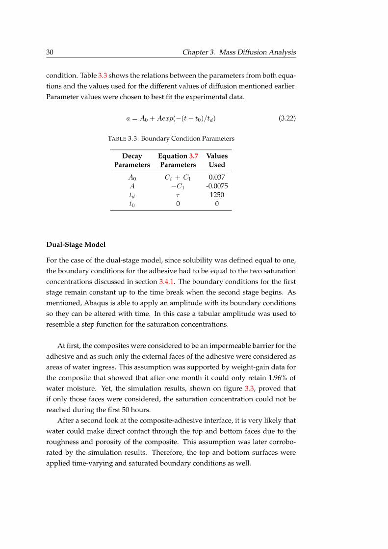
condition. Table 3.3 shows the relations between the parameters from both equa-tions and the values used for the different values of diffusion mentioned earlier.Parameter values were chosen to best fit the experimental data.

a = A0 +Aexp(−(t− t0)/td) (3.22)

TABLE 3.3: Boundary Condition Parameters

Decay Equation 3.7 ValuesParameters Parameters Used

A0 Ci + C1 0.037A −C1 -0.0075td τ 1250t0 0 0

Dual-Stage Model

For the case of the dual-stage model, since solubility was defined equal to one,the boundary conditions for the adhesive had to be equal to the two saturationconcentrations discussed in section 3.4.1. The boundary conditions for the firststage remain constant up to the time break when the second stage begins. Asmentioned, Abaqus is able to apply an amplitude with its boundary conditionsso they can be altered with time. In this case a tabular amplitude was used toresemble a step function for the saturation concentrations.

At first, the composites were considered to be an impermeable barrier for theadhesive and as such only the external faces of the adhesive were considered asareas of water ingress. This assumption was supported by weight-gain data forthe composite that showed that after one month it could only retain 1.96% ofwater moisture. Yet, the simulation results, shown on figure 3.3, proved thatif only those faces were considered, the saturation concentration could not bereached during the first 50 hours.

After a second look at the composite-adhesive interface, it is very likely thatwater could make direct contact through the top and bottom faces due to theroughness and porosity of the composite. This assumption was later corrobo-rated by the simulation results. Therefore, the top and bottom surfaces wereapplied time-varying and saturated boundary conditions as well.


0

0.01

0.02

0.03

0.04

0.05

0.06

0.07

0.08

0.09

0 50 100 150 200 250 300 350

Avera

ge C

once

ntr

ati

on (

%)

Time (h)

Only External Faces

FIGURE 3.3: Diffusion Analysis - Only External Faces

3.4.3 Model Mesh

One of the main goals of the mass diffusion analysis was to use the concentra-tion results in the following mechanical analysis. To be able to import the resultsproperly it was necessary for both, the mass diffusion and the mechanical ana-lyses, to have the exact same mesh. In the mechanical analysis, the main areasof interest were the locations of the FBG sensors to compare the measurementswith the simulation results. Hence, it was necessary to have elements at the cen-ter of the adhesive. With this in mind, a constraint was placed on the thicknessof both sample models so that there would be three elements through it. As forthe rest of the sample a uniform mesh was chosen.

Mass diffusion analyses can be performed using only the two-dimensional,three-dimensional, and axisymmetric solid elements that are included in theAbaqus/Standard heat transfer/mass diffusion element library [49]. The type ofelements chosen were first-order brick elements (type DC3D8). At first a globalsize mesh of 1 mm was used, but then it was refined to a 0.5 mm mesh to im-prove the aspect ratio of the elements. Results with both meshes were compared.In total, with the 1 mm mesh, 9375 elements (13104 nodes) were used; with the0.5 mm mesh the number increased to 37 500 elements (51 204 nodes). Figure3.4 shows a detail of both meshes.

(A) 1 mm Mesh (B) 0.5 mm Mesh

FIGURE 3.4: Sample mesh


3.5 Results

The experimental data was given as a percentage of weight gain, M(t). How-ever, the analysis is ran using average concentration, C(t), as the main variable.To be able to compare the simulation results with the experimental data, theweight-gain data was converted to average concentration. The average concen-tration was calculated through equation 3.23 [28, 51], where ρepoxy = 0.00136 ,

g/mm3 [24] and ρwater = 0.0009832 g/mm3 [33] are the densities of the epoxyand water at 60oC , respectively. The experimental results for average concen-tration are shown on figure 3.5, where one can see that the concentration at sat-uration is 3.126%.

C(t) =ρepoxyρwater

M(t) (3.23)

0

0.5

1

1.5

2

2.5

3

3.5

0 50 100 150 200 250 300 350

Avera

ge C

once

ntr

ati

on (

%)

Time (h)


FIGURE 3.5: Average Concentration - Experimental results

The finite element model calculates the concentration percentage at each in-tegration point. Thus, to compare results, the average concentration of the wholesample at each time increment was calculated using equation 3.24 [52]. Ci andVi stand for the concentration and the volume at the integration point, respec-tively. The formula was implemented through a simple Python script that readsthrough the Abaqus results database and extracts the pertinent information. Anexample of such a script is presented in Appendix B.

Cave =

n∑i=1

CiVi

n∑i=1

Vi

(3.24)

3.5. Results 33

3.5.1 Average Concentration - Whole Sample

Two different approaches for the modelling of the concentration distributionacross the samples were used: the Time-Varying Boundary Condition and theDual-Stage model. The weight-gain experimental data is given for Sample Aonly. The average concentration from the FEA results was calculated with equa-tion 3.24. Figure 3.6 shows the comparison between the experimental measure-ments and the results for both models.

0

0.5

1

1.5

2

2.5

3

3.5

0 50 100 150 200 250 300 350

Avera

ge C

once

ntr

ati

on (

%)

Time (h)


Sample A: Time-Varying BC 1 mm Mesh

(A) Time-Varying BC

0

0.5

1

1.5

2

2.5

3

3.5

0 50 100 150 200 250 300 350

Avera

ge C

once

ntr

ati

on (

%)

Time (h)


Sample A: Dual-Stage 1 mm Mesh

(B) Dual-Stage

FIGURE 3.6: Average Concentration - Whole Sample

Since the adhesive is below its glass transition temperature, it shows a non-Fickian behaviour. This behaviour is taken into account by both of the modelsused. Had this not been the case, the model would have followed a Fickianprofile. For comparison, figure 3.7 shows the average concentrations obtainedby the models and the analytical solution for Fickian diffusion.

0

0.5

1

1.5

2

2.5

3

3.5

0 50 100 150 200 250 300 350

Avera

ge C

once

ntr

ati

on (

%)

Time (h)


Time-Varying BC

Dual-Stage

Fickian Diffusion

FIGURE 3.7: Comparison Fickian Profile


3.5.2 1 mm vs 0.5 mm Mesh

Two different meshes were used for the simulations; a uniform mesh with aglobal element size of 1 and a more refined mesh with a global element size of0.5. Usually, the use of more and finer elements leads to a more precise result atthe cost of more computational time. The concentration profiles obtained fromsimulations with each mesh and with each model are compared in figure 3.8.

0

0.5

1

1.5

2

2.5

3

3.5

0 50 100 150 200 250 300 350

Avera

ge C

once

ntr

ati

on (

%)

Time (h)


Sample A: Time-Varying BC 1 mm Mesh

Sample A: Time-Varying BC 0.5 mm Mesh

(A) Time-Varying BC

0

0.5

1

1.5

2

2.5

3

3.5

0 50 100 150 200 250 300 350

Avera

ge C

once

ntr

ati

on (

%)

Time (h)


Sample A: Dual-Stage 1 mm Mesh

Sample A: Dual-Stage 0.5 mm Mesh

(B) Dual-Stage

FIGURE 3.8: Mesh Comparison

In both cases, it is clear that the use of the 1 mm mesh is sufficient enoughto get a reliable concentration profile. A refined mesh is not necessary since thedesired result is not focused on a particular section of the adhesive but rather theaverage concentration across the whole sample. For the subsequent mechanicalanalysis, however, results are wanted from specific areas of the sample where amore refined mesh might prove more accurate. The difference in computationaltime between each mesh for each case is presented in table 3.4.

TABLE 3.4: Computational Times per Mesh Size

Sample A Sample B1 mm 0.5 mm 1 mm 0.5 mm

Time-Varying 15 s 44 s 18 s 55 sDual-Stage 17 s 47 s 16 s 48 s

Problem Size9 375 elem.(13 104 n.)

37 500 elem.(51 204 n.)

9 375 elem.(13 104 n.)

37 500 elem.(51 204 n.)

3.5. Results 35

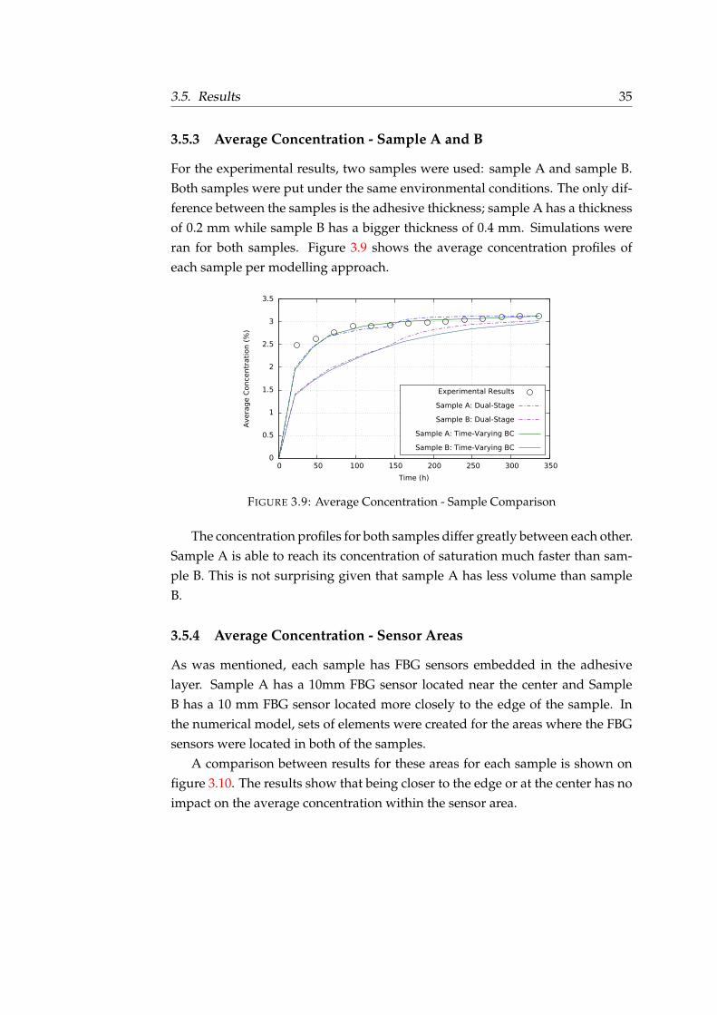
3.5.3 Average Concentration - Sample A and B

For the experimental results, two samples were used: sample A and sample B.Both samples were put under the same environmental conditions. The only dif-ference between the samples is the adhesive thickness; sample A has a thicknessof 0.2 mm while sample B has a bigger thickness of 0.4 mm. Simulations wereran for both samples. Figure 3.9 shows the average concentration profiles ofeach sample per modelling approach.

0

0.5

1

1.5

2

2.5

3

3.5

0 50 100 150 200 250 300 350

Avera

ge C

once

ntr

ati

on (

%)

Time (h)


Sample A: Dual-Stage

Sample B: Dual-Stage

Sample A: Time-Varying BC

Sample B: Time-Varying BC

FIGURE 3.9: Average Concentration - Sample Comparison

The concentration profiles for both samples differ greatly between each other.Sample A is able to reach its concentration of saturation much faster than sam-ple B. This is not surprising given that sample A has less volume than sampleB.

3.5.4 Average Concentration - Sensor Areas

As was mentioned, each sample has FBG sensors embedded in the adhesivelayer. Sample A has a 10mm FBG sensor located near the center and SampleB has a 10 mm FBG sensor located more closely to the edge of the sample. Inthe numerical model, sets of elements were created for the areas where the FBGsensors were located in both of the samples.

A comparison between results for these areas for each sample is shown onfigure 3.10. The results show that being closer to the edge or at the center has noimpact on the average concentration within the sensor area.


0

0.5

1

1.5

2

2.5

3

3.5

0 50 100 150 200 250 300 350

Avera

ge C

once

ntr

ati

on (

%)

Time (h)

Sample A: Center Sensor

Sample A: Edge Sensor

(A) Sample A

0

0.5

1

1.5

2

2.5

3

0 50 100 150 200 250 300 350

Avera

ge C

once

ntr

ati

on (

%)

Time (h)

Sample B: Center Sensor

Sample B: Edge Sensor

(B) Sample B

FIGURE 3.10: Sensor Area Comparison

3.5.5 Concentration Distribution

The average concentration of the sample was calculated in order to comparesimulation results with the experimental results. Nonetheless, the most impor-tant result from the analysis is the concentration distribution on the sample andits progression with time. Figure 3.11 shows the distribution across the thicknessof sample A and B.

(A) Sample A (B) Sample B

FIGURE 3.11: Concentration Distribution at 336 h

As was expected, areas in contact with water show a higher concentrationvery early in the simulation. In the case of sample A, the saturation concen-tration is reached rapidly with only slight differences in the third and fourthdecimals of the concentration values. On the other hand, sample B is only ableto reach a saturation state towards the end of the simulation.

The concentration progression with time in each sample is depicted on figure3.12. The limits of each frame were kept the same for a fair comparison. Afterthe 140th hour, for sample A, there are no visible changes across the sample sincethe concentration differences are minimal.

3.6. Conclusions 37

3.6 Conclusions

A diffusion analysis by means of a finite element model was executed in order toobtain the concentration distribution of the moisture absorbed by the adhesivein sample A and B. This allowed a better understanding of the diffusion pro-cess within the material. Comparison with the experimental results was possi-ble by converting the experimental weight-gain data into average concentration3.23 and by calculating the average concentration at the integration points of thewhole model with equation 3.24.

Several models for non-Fickian diffusion can be found in the literature. Inthis project, two were chosen: Time-Varying boundary conditions and the Dual-Stage model. The average concentration for each model was compared to theexperimental results as is shown on fig 3.6. From the two, the time-varying BCshows a good fit with the data. However, this is expected since the parametersin equation 3.10 are chosen to provide the best fit.

The parameters for the dual-stage model are the saturation concentrationsand the diffusion coefficients at each stage, the latter are calculated theoreticallythrough equation 3.6. The Dual-Stage model provides a reasonable fit to thedata overall. However, it tends to underestimate the concentration during thefirst stage and overestimate concentrations for the second stage. This relatesdirectly to the diffusion coefficients and the error when calculating them fromvery few data points.

In any case, both models account for the viscoelastic nature of the adhesiveand how it can slow down the diffusion process. When compared to a com-pletely Fickian diffusion (figure 3.7), it is clear that the Fickian diffusion overes-timates the concentration, especially during the first hours of the simulation.

The main drawback of either one of the models used for anomalous diffusionis that the parameters have to be obtained through experimental data which, ofcourse, limits its implementation.

As in any finite element model, the way a continuum is discretize can greatlyaffect the whole analysis. If a mesh is too course, the results may be unreliableand too fine a mesh may lead to a very high computation cost and a lengthyanalysis. During this analysis, two meshes were implemented. The first onewas a uniform mesh with a global element size of 1 mm; and a finer mesh with0.5 elements.

The results obtained, figure 3.8, show that the use of the more refined meshdoesn’t have an impact on the predicted average concentration values across thewhole sample. Nonetheless, it may have an impact when focusing on a smallerarea of the sample which is the case for the subsequent mechanical analysis.


Computational times are increased three times when using the finer mesh, butsince times are still under a minute it’s not considered a limitation. Both mesheswere used for the following mechanical analysis and results compared.

Experimental results used two different samples. The samples differ fromeach other only by their thickness; sample A has an adhesive thickness of 0.2mm and sample B a 0.4 mm thickness. Models for both samples were createdand average concentrations results from both samples are shown on figure 3.9.The results show that the thickness difference has a very strong influence onthe concentration across the sample. Clearly, Sample A has less volume and isable to reach a saturated state within the first 140 h. The concentration acrosssample B is increasing steadily up to the last few hours of the simulation whenconcentration values differ slightly between each other.

FBG sensors were embedded into the adhesive layer of each of the sample.In sample A, a 10 mm FBG sensor was located at the center and in sample B thesensor was located closer to the edge. It was believed that the sensor located atthe edge would be subjected to a higher moisture concentration than the one inthe center. As figure 3.10 shows, that is not the case. The amount of moistureentering the sample from the external faces is negligible when compared to thetop and bottom faces. Hence, the main contributor for the differences in con-centrations between the sensors is not their location but the fact that they areembedded in samples with different thicknesses.

3.6. Conclusions 39

(A) Sample A 22h (B) Sample B 22h

(C) Sample A 44h (D) Sample B 44h

(E) Sample A 140h (F) Sample B 140h

(G) SampleA 184h (H) Sample B 184h

(I) Sample A 336h (J) Sample B 336h

FIGURE 3.12: Concentration Distribution Progression

41

Chapter 4

Hygro-Mechanical Analysis

4.1 Introduction

The ingress of water molecules into a polymeric material leads to the chemicalinteraction between the water molecules and the polymer chain. This interactionleads to two different stages of water that can be found in the polymeric mate-rial. A percentage of the water molecules group in the voids and cavities withinthe material, these are referred to as the "free" or "unbounded" molecules. Incontrast, the rest of the molecules are called "bounded" since they interact withthe polymer chains and form hydrogen bonds [37]. These states have been de-tected through the use of spectroscopic methods [53, 54].

The absorption of water by an adhesive produces an overall expansion in thematerial’s volume. This behaviour is known as hygroscopic swelling. Studieshave observed that the ratio between the hygroscopic swelling volume and thevolume of absorbed water is less than one [55, 56]. Hence, not all the absorbedwater molecules have an active role in the expansion. It is very likely that onlythe "bounded" molecules contribute to the expansion. When water moleculesform hydrogen bonds with the hydroxyl groups found in polymers, it causesa disruption in the inter-chain hydrogen bonding leading to an increase in theinter-segmental hydrogen bond length [56] which leads to swelling.

The hygroscopic swelling of a polymer can produce hygroscopic stresses ifthere’s a material response mismatch in the structure. These stresses are similarto the stresses caused by thermal expansion [57]. Both effects can add up andaffect the total mechanical response of the adhesive joint. Hygroscopic stressesare related to moisture content very similarly to how thermal stresses are relatedto thermal distributions. The stress distribution caused by hygroscopic swellinghas been successfully calculated through the use of finite element techniques[58–62].

42 Chapter 4. Hygro-Mechanical Analysis

In this project a sequentially coupled hygro-mechanical analysis was per-formed. The concentration profiles calculated in 3, were used in a mechanicalanalysis in Abaqus. The strain distribution and evolution against time due tomoisture concentration was obtained. Results were compared to those obtainedby the FBG readings done in the base experiment.

4.2 Hygroscopic and Thermal Strain

The absorption of water by a polymer causes a swelling in the material knownas hygroscopic swelling and the deformation of the material referred to as hy-groscopic strains. It has been found that hygroscopic strains, εhygro, follow alinear relationship with the change in concentration in the material ∆C. Thebehaviour is in analogy to how thermal strains, εthermal, linearly depend on thetemperature difference, ∆T . Both dependencies are mathematically shown onequations 4.1 and 4.2 [62].

εhygro = β ·∆C (4.1)

εthermal = α ·∆T (4.2)

The symbols β and α stand for the coefficients of hygroscopic swelling andthermal expansion, respectively. Both can be determined experimentally. In thecase of α, it can be found listed for many materials.

Under normal conditions, a material can be subjected to temperature changes,differences in moisture concentration and mechanical loads. Thus, the total de-formation in the material is given by the sum of all three induced strains (equa-tion 4.3 [62]).

εtotal = εmechanical + εthermal + εhygro (4.3)

In this particular experiment, the samples were exposed to thermal and mois-ture concentrations changes only. As was explained in chapter 1, thermal strainswere measured in a separate experiment and hygroscopic strains were calcu-lated through equation 1.14.

This linear superposition of the mentioned strains is applicable when the to-tal resulting stress is below the material’s elastic limit [62]. Experimental resultsshow that the strains are small enough so that this is the case at all times.

4.3. Hygro-Mechanical Model 43

4.3 Hygro-Mechanical Model

4.3.1 Coupling the Mass Diffusion Analysis

In order to quantify the deformation suffered by the material due to moistureabsorption, a mass diffusion analysis was carried out on models for both of theexperimental samples (Chapter 3). The spatial moisture concentration profile ofeach was then sequentially combined with a mechanical deformation analysis.Both analyses were executed through the Abaqus/CAE finite element software.

Abaqus doesn’t offer the possibility to directly use the concentration distri-bution for a hygro-mechanical analysis. It does, however, offer the option to per-form a thermo-mechanical analysis. Given the close similarities between bothphenomena, it was possible to use this capabilities for the hygro-mechanicalanalysis.

The normalized concentration values at each node were imported into themechanical analysis as temperature values. This was achieved through the For-tran code developed by S. Yoon, C. Jang and B. Han [58]. The code is presentedon Appendix C. It reads the record key of the mass diffusion results databaseand changes it from normalized concentration (key 221) to nodal temperature(key 201). Then, the results can be imported into the mechanical analysis as apredefined temperature field using the usual Abaqus commands directly in theinput file or through the graphical interface.

During the mechanical analysis, the hygro-mechanical strain is calculatedas a thermal strain by specifying the coefficient of hygroscopic swelling as thethermal expansion coefficient in the material properties, as it was done in thiscase. If one desires to conduct a coupled hygro-thermal mechanical analysis,that is also possible by importing the concentration values as a predefined fieldand using the user subroutine UEXPAN to define the coefficient of hygroscopicswelling and thermal expansion. An example of this approach is given in S.Yoon et. al.’s article [58].

4.3.2 Material Properties

In a finite element analysis is usual to take advantage of the symmetric prop-erties, geometric and load-wise, to simplify the model and the computationaleffort. In this case, it was possible to only consider one fourth of the sampleas shown on figure 4.1. The composites were also taken into account since theinteraction between them and the adhesive was important for the mechanicalanalysis.


(A) Whole Model(B) Detail View

FIGURE 4.1: Model for Hygro-Mechanical Analysis

Table 4.1 lists the material properties for both the adhesive and the compos-ites. The coefficient of hygroscopic swelling was determined by experimentaldata, since it is given by the slope when plotting strains values against concen-tration, as given by equation 4.1 and shown on figure 1.7.

The coefficient of hygroscopic swelling (CHS) is a material property, and assuch, doesn’t depend on the geometry. The experimental data shows, however,very different CHS values for Sample A and Sample B. It is still unclear whythis is the case. For the analysis, in order to compare computed strains withexperimental results, it was decided to use the corresponding theoretical CHSvalues for each sample as well.

Viscoelastic properties of the adhesive were not contemplated in the analysis.Expected tensile strain values are small enough that the material is kept in theelastic range, as shown by the stress-strain curve for Hysol EA-9394 adhesive[63].

TABLE 4.1: Material Properties - Hygro-Mechanical

Material Parameter Value Units

Adhesive

Density 0.00136 [24] g/mm3

Young’s Modulus 5.49 E+16 [24] (g ·mm/s2)/ mm2

Poisson’s Ratio 0.4 [63]Coeff. HygroscopicSwelling

0.004030 (A)0.007685 (B)

CompositeDensity 0.00187 [30] g/mm3

Young’s Modulus 4.17E+17 [29] (g ·mm/s 2)/ mm2

Poisson’s Ratio 0.3 [29]

4.3. Hygro-Mechanical Model 45

4.3.3 Boundary Conditions and Loads

Since only one fourth of the sample was used, symmetric boundary conditionswere applied on the corresponding faces. Also, a condition of zero displacementin the y-axis was applied to the bottom surface since it’s simply supported bythe tray. Figure 4.2 shows the model with the faces where the conditions wereapplied.

FIGURE 4.2: Boundary Conditions - Hygro-Mechanical

The weight of the composites on the adhesive was included in the analysisthrough the use of a gravity load. This is an in-built load in Abaqus. It is used torepresent the gravitational acceleration. Abaqus applies the weight according tothe geometry and density of the material. The inputs are the direction and themagnitude. In this case, since milimeters and hours were the units used, it has avalue of -1.27008E+11 mm/h2 (9.81 m/s2).

Another external force considered was the water pressure on top of the sam-ple. As was explained on chapter 1 and 3, the samples were submerged in atray with demineralised water. The column of water on top of the samples hada maximum height of 5 mm. Thus, the water pressure on top of the sample hada magnitude of 6.24E+08 g/mm h2.

The moisture concentration distribution within the sample is the main driverfor the deformation. This load was imported as a predefined field in the model.Concentration values are applied on each node according to the previously per-formed mass diffusion analysis. Two approaches were used for the concen-tration distribution: Time-Varying Boundary Conditions and the Dual-Stagemodel. Both results were used for the sequential mechanical analysis in sep-arate simulations.


4.3.4 Interactions

The interaction between the composites and the adhesive was very importantin the mechanical analysis. This interaction was defined as a contact interac-tion with tangential behaviour using a high frictional coefficient (0.9). The in-teraction was defined between the top surface of the bottom composite and thebottom surface of the adhesive; and between the bottom surface of the top com-posite and the top surface of the adhesive. This interaction was preferred overa tie constraint, since the latter would prove very restrictive. A frictional inter-action was deemed more representative and since there’s is a chance of slippagebetween the surfaces, the composites were modelled as slightly larger than theadhesive.

4.3.5 Model Mesh

When a predefined field is imported, nodes in the mesh are assigned the re-spective values. To this end, it is advisable to keep the meshes between theanalyses as similar as possible. If there’s a mismatch between the meshes, thealgorithm tries to interpolate values between nodes. Of course, this can intro-duce more variability in the study. For this analysis, it was preferred to keepidentical meshes for the adhesive between analyses.

The mass diffusion analysis only considered the adhesive. In the hygro-mechanical analysis three part instances were considered: the adhesive, the topcomposite and the bottom composite. The use of more or less instances betweenanalyses is not a problem when importing results for a predefined field. Theprogram assigns the nodal values according to the name of the part. As long aseach instance has the same name in both analysis, the use of other instances willnot affect the results.

For the adhesive, two uniform meshes were used in the mass diffusion anal-ysis, a coarse mesh of 1 mm elements and a finer mesh of 0.5 mm elements.During the mass diffusion analysis, the coarse mesh proved sufficient to obtainaccurate results. In the case of the hygro-mechanical analysis, the finer 0.5 meshprovides a better element aspect ratio, 7.5 for Sample A and 3.5 for Sample B,which could lead to an improvement in results. Both meshes were used andresults were compared.

Both meshes had a constraint of 3 elements for the thickness. This was donein order to have central elements where the FBG sensors were embedded in thesamples. Element sets for both sensors were created in both samples to com-pare simulation results with experimental measurements. Figure 4.3 shows thelocation of the element sets defined on the 1 mm mesh.

4.4. Analysis Results 47

(A) Top View (B) Side-view Detail

FIGURE 4.3: Sensor Element Sets - 1 mm Mesh

As for the composites, a coarse uniform mesh of 1 mm was imposed on bothparts. The composites were not areas of interest in the analysis and a 1 mm meshprovides a good aspect ratio since both have a thickness of 1 mm.

All part instances were assigned 8-node linear brick elements with reducedintegration (type C3D8R). Given the geometry of the sample, in which two di-mensions are much larger than the third, the use of shell elements would havebeen, perhaps, more appropriate. However, the use of shell elements is not sup-ported for a mass diffusion analysis, and so, it limited the use in the mechanicalanalysis since respective nodes were desired to be equal for the assigning ofthe predefined field. An alternative, would have been to use continuum shellelements, which take their thickness from the element nodal geometry, for themechanical analysis only. Unfortunately, the constitutive relations for contin-uum shell elements in Abaqus are not equipped to handle temperature changesunless it is in a coupled thermal-displacement analysis [64].

4.4 Analysis Results

Fibre-Bragg Grating (FBG) sensors are sensitive to mechanical strains as well asto temperature changes. For this reason, their use has proliferated in structuralhealth monitoring applications. In this experiment, FBG sensors were embed-ded in the adhesive layer of the sample and the wavelength measurements wereused to calculate hygroscopic strains through equation 1.4. It’s important to notethat FBG sensors measure strains in the direction parallel to their axis.

A sequentially-coupled hygro-mechanical analysis was performed throughthe use of the finite element method. Two different approaches were used forthe mass diffusion analysis: Time-Varying BC and Dual-Stage. Results fromboth mass diffusion approaches were implemented for the hygro-mechanicalanalysis. Strain profiles for each FBG sensor were compared to the experimentalones.


4.4.1 Time-Varying BC Strain Profiles

The Time-Varying Boundary Condition model takes into account the visco-elasti-city effect on the diffusion mechanism through the use of time-dependent bound-ary condition based on a Prony series given on equation 3.7.

Two different samples were used for the experiment, Sample A and SampleB. Sample A has a thickness of 0.2 mm and a 10-mm FBG sensor placed near thecenter of the sample. Sample B has a thickness of 0.4 mm and a 10-mm FBG sen-sor closer to the edge of the sample. Strain profiles for the sensors correspondingto each sample are shown on figure 4.4.

0

0.2

0.4

0.6

0.8

1

1.2

1.4

1.6

0 50 100 150 200 250 300 350

Hyg

rosc

op

ic S

train

s (1

0-4

)

Time (h)

FBG-A: Experimental ValuesFBG-A: Time-Varying BC Strains

(A) Sample A Sensor - Time-Varying BC

0

0.5

1

1.5

2

2.5

0 50 100 150 200 250 300 350

Hyg

rosc

op

ic S

train

s (1

0-4

)

Time (h)

FBG-B: Experimental ValuesFBG-B: Time-Varying BC Strains

(B) Sample B Sensor - Time-Varying BC

FIGURE 4.4: Time-Varying BC - Strain Profiles


4.4.2 Dual-Stage Strain Profiles

The Dual-Stage model proposes the analysis of the anomalous diffusion by char-acterizing it as the product of two sequential Fickian diffusion profiles with dis-tinct saturation concentrations and diffusion coefficients. The strain profiles es-timated for this approach and for each FBG sensor are displayed on figure 4.5.Figure 4.6 shows a comparison between the different approaches and differentsensor areas.

0

0.2

0.4

0.6

0.8

1

1.2

1.4

1.6

0 50 100 150 200 250 300 350

Hyg

rosc

op

ic S

train

s (1

0-4

)

Time (h)

FBG-A: Experimental ValuesFBG-A: Dual-Stage Strains

(A) Sample A Sensor - Dual-Stage

0

0.5

1

1.5

2

2.5

0 50 100 150 200 250 300 350

Hyg

rosc

op

ic S

train

s (1

0-4

)

Time (h)

FBG-B: Experimental ValuesFBG-B: Dual-Stage Strains

(B) Sample B Sensor - Dual-Stage

FIGURE 4.5: Dual-Stage - Strain Profiles


0

0.5

1

1.5

2

2.5

0 50 100 150 200 250 300 350

Hyg

rosc

op

ic S

train

s (1

0-4

)

Time (h)

FBG-A: Experimental ValuesFBG-A: Time-Varying BC Strains

FBG-A: Dual-Stage StrainsFBG-B: Experimental Values

FBG-B: Time-Varying BC StrainsFBG-B: Dual-Stage Strains

(A)

FIGURE 4.6: Strain Profile Comparison

4.4.3 1 mm vs 0.5 mm Mesh

The finite element method is a numerical method which tries to approximatethe response of a continuum solid through the analysis of discrete sections ofit. It is a numerical approximation, and as such, it is evident that the finer youdiscretize, the better the approximation. Of course, the use of more elementscomes with an additional cost: computational time. In this case, two differentmeshes to partition the sample were used: 1 mm mesh and a 0.5 mm mesh. Theresults for the strain profiles for each different mesh per diffusion approach areshown on figure 4.6.

0

0.5

1

1.5

2

2.5

0 50 100 150 200 250 300 350

Hyg

rosc

op

ic S

train

s (1

0-4

)

Time (h)

FBG-A: Experimental ValuesFBG-A: Time-Varying BC 1 mm Mesh

FBG-A: Time-Varying BC 0.5 mm MeshFBG-B: Experimental Values

FBG-B: Time-Varying BC 1 mm MeshFBG-B: Time-Varying BC 0.5 mm Mesh

(A) Time-Varying BC Strains - Mesh Comparison


0

0.5

1

1.5

2

2.5

0 50 100 150 200 250 300 350

Hyg

rosc

op

ic S

train

s (1

0-4

)

Time (h)

FBG-A: Experimental ValuesFBG-A: Dual-Stage 1 mm Mesh

FBG-A: Dual-Stage 0.5 mm MeshFBG-B: Dual-Stage Experimental Values

FBG-B: Dual-Stage 1 mm MeshFBG-B: Dual-Stage 0.5 mm Mesh

(B) Dual-Stage Strains - Mesh Comparison

FIGURE 4.6: Strain Profiles - Mesh Comparison

The computational time required by each analysis is detailed on table 4.2.Information is also given on the number of elements and nodes involved witheach mesh size.

TABLE 4.2: Computational Times per Mesh Size

Sample A Sample B1 mm 0.5 mm 1 mm 0.5 mm

Time-Varying 16 min 1 h 36 min 10 min 1 h 8 minDual-Stage 24 min 1 h 22 min 12 min 1 h

Problem Size15 927 elem.(26 820 n.)

44 052 elem.(64 920 n.)

15 927 elem.(26 820 n.)

44 052 elem.(64 920 n.)

4.4.4 Water Pressure Effect

Both samples were placed inside a box and submerged in demineralise water.The column of water on top of both samples had a height of 5 mm. The pressureexerted by this column was considered as a load in the hygro-mechanical model.A separate set of simulations were ran without this pressure load to quantify theeffect of the water pressure on the strain profiles. Results are shown on figures4.7 and 4.8 .


0

0.2

0.4

0.6

0.8

1

1.2

1.4

1.6

0 50 100 150 200 250 300 350

Hyg

rosc

op

ic S

train

s (1

0-4

)

Time (h)

FBG-A: Experimental ValuesFBG-A: With Pressure 1 mm

FBG-A: Without Pressure 1 mmFBG-A: With Pressure 0.5 mm

FBG-A: Without Pressure 0.5 mm

(A) Time-Varying BC Strains - Pressure Effect on A

0

0.5

1

1.5

2

2.5

0 50 100 150 200 250 300 350

Hyg

rosc

op

ic S

train

s (1

0-4

)

Time (h)

FBG-B: Experimental ValuesFBG-B: With Pressure 1 mm

FBG-B: Without Pressure 1 mmFBG-B: With Pressure 0.5 mm

FBG-B: Without Pressure 0.5 mm

(B) Time-Varying BC Strains - Pressure Effect on B

FIGURE 4.7: Time-Varying BC - Pressure Effect

4.5. Conclusions 53

0

0.2

0.4

0.6

0.8

1

1.2

1.4

1.6

0 50 100 150 200 250 300 350

Hyg

rosc

op

ic S

train

s (1

0-4

)

Time (h)

FBG-A: Experimental ValuesFBG-A: With Pressure 1 mm

FBG-A: Without Pressure 1 mmFBG-A: With Pressure 0.5 mm

FBG-A: Without Pressure 0.5 mm

(A) Dual-Stage Strains - Pressure Effect on A

0

0.5

1

1.5

2

2.5

0 50 100 150 200 250 300 350

Hyg

rosc

op

ic S

train

s (1

0-4

)

Time (h)

FBG-B: Experimental ValuesFBG-B: With Pressure 1 mm

FBG-B: Without Pressure 1 mmFBG-B: With Pressure 0.5 mm

FBG-B: Without Pressure 0.5 mm

(B) Dual-Stage Strains - Pressure Effect on B

FIGURE 4.8: Dual-Stage Strains - Pressure Effect

4.5 Conclusions

The strains caused by moisture absorption in an adhesive joint between com-posites were determined by a sequentially-coupled hygro-mechanical analysisusing a finite element model. The simulation results were compared to experi-mental values obtained through Fiber Bragg grating sensors embedded in adhe-sive layers with thicknesses of 0.2 and 0.4 mm.

The diffusion process through the polymeric material was modelled by twodifferent approaches: the Time-Varying Boundary Condition and the Dual-Stagemodel. Figures 4.4 and 4.5 show the strains profiles from each approach, respec-tively; and figure 4.6 compares both approaches.


With the time-varying boundary condition approach, the mechanical strainsshow slightly higher values than the experimental results for the sensor in Sam-ple A. The profile trend, nonetheless, does resemble the experimental strain pro-file during the first 150 hours. The difference could be attributed to the error in-volved in calculating the value for the coefficient of hygroscopic swelling (CHS),which was done by estimating the slope of the strain-concentration curve shownon figure 1.7. The strain profile for the sensor in Sample B with this approach,4.4b, gives a better correlation with the experimental results.

In the case of the dual-stage model, strain profiles obtained for Samples Aand B demonstrate a good correlation with the experimental results, during thefirst 200 hours. Both approaches used the same CHS values. The time betweenthe stages in the dual-stage diffusion model, coincides with the increase of theexperimental values. In this way, the dual-stage model is able to adapt better tothe results than the time-varying boundary condition model.

Neither approach, however, follows the experimental profile trends on eitherone of the samples after the 200th hour of the simulation. In sample A, theexperimental values show a steady increase from an approximate strain value of0.00012 to 0.00014; with a slight decrease towards the end of the measurements.A much more quick increase is observed in Sample B, where the maximum strainvalue reached is 0.00024; followed immediately by a decrease.

During the experiment, all external conditions were kept constant. The onlyload varying with time was the amount of moisture entering the sample. Thehygroscopic strains follow a linear relationship with the concentration differ-ence, as stated in equation 4.1. A strain value of 0.00014 in sample A, wouldthen imply a concentration of 3.47%, which is higher than the 3.126% measuredfrom weight-gain absorption data (figure 3.5). The sudden increase and decreaseshown by sample B, would imply a sudden higher diffusivity followed by a des-orption process. Both samples were kept submerged for all measurements.

A change in temperature could affect the diffusivity coefficient in the sam-ples and provoke thermal strains that weren’t accounted for during the mea-surements with the dry sample (section 2.3.1). The samples were placed in atemperature chamber controlled and monitored at 60 ± 2 oC, throughout theexperiment. Thermal strains can be calculated by equation 1.13. A 2oC increasein the temperature would account for an increase of only 0.0000183 in the strainvalue.

Experimental strain values were calculated by the changes in wavelengthmeasured by the FBG sensors (equation 1.4). It is possible that during a wave-length measurement, the spectrum recorded by the FBG is not composed of onlyone clear peak but rather several peaks. The measurement equipment used,

4.5. Conclusions 55

takes the highest of the peaks and presents that as the measurement. This high-est peak may not be representative of the sample. A comparison between spectraand wavelength could help determine if this is the case for the odd measure-ments presented in the strain profiles. Unfortunately, the measuring unit is ableto record either wavelength or spectra only, not both simultaneously, so such acomparison was not available.

Simulations were performed using two different meshes for each sample: a1 mm and a 0.5 mm mesh. The 0.5 mm mesh was thought to be better sinceit provided a better aspect ratio for the elements. However, as can be seen onfigure 4.6, for the time-varying boundary condition simulations the obtainedstrain profiles from both meshes are basically identical. The same holds true forthe strain profile for the sensor in sample B with the dual-stage approach. Theonly case where the use of a finer mesh is justified is with sample A with the dualstage approach. There’s a noticeable difference between measurements. Thefiner mesh shows lower strain values that provide a better correlation with theexperimental values during the first hours. Sample A with the dual-stage modelcould be more susceptible to a finer mesh than sample B because of its thinness.When compared to sample A with the time-varying boundary condition, theconcentration profiles from both samples (figure 3.9) shows that the dual-stagemodel has more drastic changes in concentration that a finer mesh is able toadapt to better.

The use of a finer mesh always implies a higher computational time. Table4.2 shows that the use of the 0.5 mm mesh increases the computational cost byan average factor of 5. This computational cost was only justified for one case,when the sample’s focus area is closer to interaction zones and there’s morevariability in the loading conditions.

Lastly, the effects of the water column on the measurements were estimatedby running simulations with and without considering it and then comparingthe results. Results were obtained for different size meshes as well. When usingthe time-varying approach on sample A, figure 4.7a, the water column showsto have an effect with either size mesh, lowering the strain values. Differencesbetween meshes are negligible if the water pressure is disregarded. If the watercolumn is considered, the mesh size does play an important role showing higherstrain values with a coarser mesh than with the finer mesh. Neglecting the watercolumn effect with a 1 mm mesh shows a maximum difference of 0.000011691(10.49 % increase).


For sample B, with the time-varying approach, mesh sizes don’t create anydifferences as seen on figure 4.7b. The water pressure on the sample does lowerthe magnitude of the strain values from 0.000227176 to 0.000221605 (2.51 % de-crease), most notably during the last hours of the simulation.

With the dual-stage approach, similar behaviours between same size sam-ples are seen. When using the time-varying approach on sample A, figure 4.8a,the water column doesn’t show any effect with a 0.5 mm mesh. On the otherhand, with the 1 mm mesh, the effect is considerable. Disregarding the waterpressure with a 1 mm mesh can lead to estimate strains 9.77% higher than inreality. Sample B remains unchanged with different meshes but is affected bythe water column on top. Nonetheless, the water effect on sample B creates asmall difference of 5.62E-06 (2.49 % decrease) between strain values.

57

Chapter 5

Summary

5.1 Introduction

This project was motivated by the experimental results obtained by a researchteam at the Institute of Fluid-Flow Machinery in Gdansk, Poland. The experi-ment consisted of three samples of adhesive joints between composites that weresubmerged in water for a period of 336 hours. The goal of the research was toquantify the moisture-induced strains on the adhesive joint and prove the feasi-bility of using Fiber Bragg Grating (FBG) sensors for such a purpose.

Due to the polymeric nature of adhesives, moisture content in the surround-ings of an adhesive joint can be absorbed and have a detrimental effect on themechanical strength of the bond. Lack of a complete understanding of thesedynamics, limits the use of adhesive joints in many applications where a faultyadhesion may pose a safety hazard.

FBG sensors embedded in adhesive joints could be used in structural healthmonitoring applications, as a way to profit from the versatility and many ad-vantages of adhesives in a manner that won’t risk public safety.

The goal of the present project was successfully reached by creating numer-ical models that could represent the thermal response, mass diffusion dynam-ics and moisture-induced strain propagation of the samples used. Three sepa-rate finite-element models were created: a transient thermal analysis, a transientmass diffusion analysis and a hygro-mechanical analysis.

5.1.1 Thermal Analysis

FBG sensors are both sensitive to mechanical strains as well as temperaturechanges. Since the moisture-induced strains, also referred to as hygroscopicstrains, were the focus of the experiment, temperature’s effect on the measure-ments had to be quantified and considered.

One sample, labelled as sample A, was placed in a temperature chamberat 60oC in dry conditions, to quantify the strains produced by the temperature

58 Chapter 5. Summary

change and assess the time it took the sample to reach thermal equilibrium. Af-terwards, samples A and B were placed in the same temperature chamber com-pletely immersed in water. Temperature was kept constant so that all followingmeasurements could be associated directly to hygroscopic strains.

The thermal model was constructed to simulate the temperature distributionof Sample A when inside the chamber in dry conditions and also when samplesA and B were inside the chamber in wet conditions.

When in dry conditions, the thermal model was able to accurately simulatethe temperature profile obtained by the FBG sensor embedded in the sample.Experimental values were not collected for the temperature profiles for whenthe samples A and B were submerged.

During the experiment, the samples had to be taken out of the water and beweighed outside of the temperature chamber. Mathematical models for this situ-ation were created in order to verify the assumption that all strain measurementswere done under an isothermal state. Simulations results show that both sam-ples, in spite of the difference in thickness, are able to reach thermal equilibriumwithin the first 5 minutes. There were hours of difference between the weightmeasurements and the strain readings. Thus, one can conclude that, even whenconsidering the error involved in the calculation of the convection coefficient,both samples were in an isothermal state when the strain measurements wererecorded.

5.1.2 Mass Diffusion Analysis

At the moment the samples are submerged, a diffusion process is started inwhich water penetrates inside the sample until it reaches a saturation point. Theconcentration distribution of moisture inside the adhesive of both samples wasessential to properly simulate the hygroscopic strains.

During the experiment, sample A was periodically weighed to determine theoverall level of moisture concentration and determine the saturation point.

Mass diffusion processes, in many materials, can be mathematically anal-ysed through Fick’s equations of diffusion, which hold a strong analogy to heattransfer equations. Polymeric materials, however, have shown not to follow thediffusion profiles predicted by Fickian equations.

Different mathematical models have been created to better understand thediffusion dynamics in polymers such as adhesives. In the present project, twodifferent approaches were implemented: time-varying boundary conditions andthe dual stage model. Results from both approaches used in samples A and B,were produced and compared.

5.2. Hygro-mechanical Analysis 59

The main drawback from either one of these approaches, and also from Fick-ian equations, is that they all use variables obtained from experimental values.When comparing the overall concentration of sample A from both approacheswith experimental data, the time-varying boundary condition shows a bettercorrelation than the dual-stage model. However, the time-varying boundarycondition model requires the adjustment of variables to provide the best fit. Thedual-stage model requires less information from experimental results. Nonethe-less, the dual-stage model also presents a good correlation with results.

5.2 Hygro-mechanical Analysis

The main focus of the project was to predict the hygroscopic strains inside theadhesive layers in samples A and B. To this effect, a sequentially coupled hygro-mechanical analysis was conducted.

With the mass diffusion analysis, average concentration of the whole samplewas calculated to compare with experimental results. Yet, the most importantresult was the concentration distribution within the sample and its progressionwith time. These spatial-concentration results were imported into a mechanicalanalysis to simulate the swelling effect of moisture absorption. Results fromboth mass diffusion approaches were used.

Strain measurements taken by the FBG sensors correspond to very localisedareas inside the adhesive. Sets of elements from the FE model were taken fromthese areas in the samples and results were compared to experimental values.

Both approaches are able to follow the strain profile up to the 200th hour. Thedual-stage model shows better correlation with results in general, especially forthe strain increase in sample B around the 150th hour of simulation.

Unfortunately, after the 200th hours, experimental values show a profile thatneither model can simulate. Experimental strain values show an unlikely in-crease. Considering the linear relationship between hygroscopic strains andmoisture, experimental strain results on sample A seem to indicate a concen-tration value of 3.47%, much higher than the saturation point of 3.126 %.

All loading conditions were kept constant throughout the experiment. Tem-perature was controlled by the temperature chamber and kept at 60 ± 2oC. Atemperature variation could affect diffusivity and create thermal strains. How-ever, a 2oC variation would only account for an increase of 0.0000183 in the strainvalues which is not enough for the results obtained.

Experimental strain values were calculated by the changes in wavelengthmeasured by the FBG sensors. It’s a possibility that during a wavelength mea-surement, the spectrum recorded by the FBG was not composed of only one

60 Chapter 5. Summary

clear peak but rather several peaks. The measurement equipment used, takesthe highest of the peaks and presents that as the measurement. This highestpeak may not be representative of the sample. A comparison between spectraand wavelength could help determine if this is the case for the odd measure-ments presented in the strain profiles. Unfortunately, the measuring unit is ableto record either wavelength or spectra only, not both simultaneously, so such acomparison is not available.

The FE models created for the hygro-mechanical show a good correlationwith experimental results for 60% of the simulation time. The reasons for the in-congruences towards the end of the simulation remain unknown. It may be thatthe mathematical models used for moisture diffusion in the sample are not ableto completely represent the diffusion process, yet, good correlation with sampleconcentration was obtained with both approaches. Unaccounted loading con-ditions during experimental measurements could have also affected the strainprofiles, or perhaps variabilities within the measuring equipment. Nonetheless,in both those cases, there’s lack of information to corroborate.

5.3 Future Works

All the analyses conducted to study the thermal, mass diffusion and hygro-mechanical responses of the samples are explained thoroughly in the presentproject so the methodology followed can be implement in further experiments.

Given the fact that the simulation results weren’t able to explain the exper-imental strain profiles for the last hours of the experiment; new experimentaldata is needed to verify if the erratic behaviour is due to the model or to unac-counted factors during the measurement of this particular set of values.

Within the context of the research efforts at the Institute of Fluid-Flow Ma-chinery, the 3D finite element models created give an approximation to the dif-fusion and swelling effects that are taking place along the whole sample as op-posed to only focalized areas where experimental values can be obtained. Therepresentation of the concentration distribution provides good guidance as towhere would be best to place sensors for future experiments. Also, the finiteelements models, will serve as a basis for furthering the research into the spe-cial dynamics taking place between the adhesive and composite layers and thedegradation of the joint in these areas.

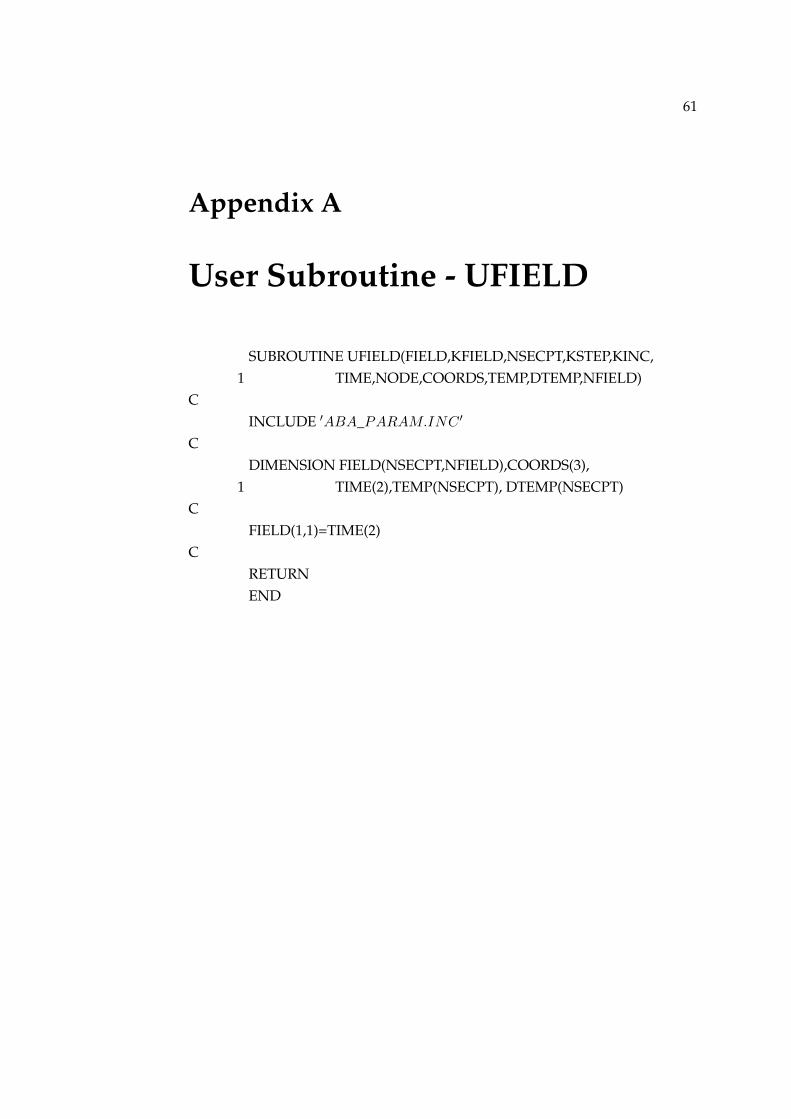
61

Appendix A

User Subroutine - UFIELD

SUBROUTINE UFIELD(FIELD,KFIELD,NSECPT,KSTEP,KINC,1 TIME,NODE,COORDS,TEMP,DTEMP,NFIELD)

CINCLUDE ′ABA_PARAM.INC ′

CDIMENSION FIELD(NSECPT,NFIELD),COORDS(3),

1 TIME(2),TEMP(NSECPT), DTEMP(NSECPT)C

FIELD(1,1)=TIME(2)C

RETURNEND

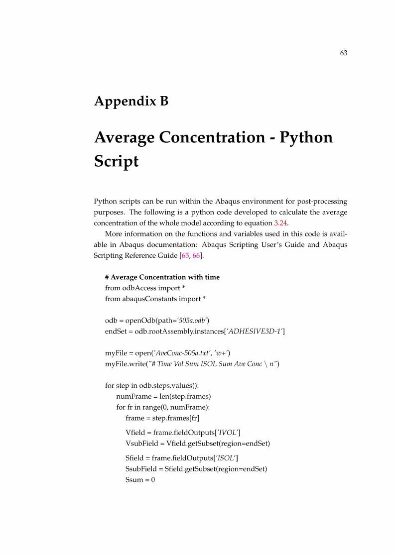
63

Appendix B

Average Concentration - PythonScript

Python scripts can be run within the Abaqus environment for post-processingpurposes. The following is a python code developed to calculate the averageconcentration of the whole model according to equation 3.24.

More information on the functions and variables used in this code is avail-able in Abaqus documentation: Abaqus Scripting User’s Guide and AbaqusScripting Reference Guide [65, 66].

# Average Concentration with timefrom odbAccess import *from abaqusConstants import *

odb = openOdb(path=’505a.odb’)endSet = odb.rootAssembly.instances[’ADHESIVE3D-1’]

myFile = open(’AveConc-505a.txt’, ’w+’)myFile.write("# Time Vol Sum ISOL Sum Ave Conc \ n")

for step in odb.steps.values():numFrame = len(step.frames)for fr in range(0, numFrame):

frame = step.frames[fr]

Vfield = frame.fieldOutputs[’IVOL’]VsubField = Vfield.getSubset(region=endSet)

Sfield = frame.fieldOutputs[’ISOL’]SsubField = Sfield.getSubset(region=endSet)Ssum = 0

64 Appendix B. Average Concentration - Python Script

Vsum = 0

for num in range(len(VsubField.values)):Vval = VsubField.values[num].dataVsum = Vsum + VvalSval = SsubField.values[num].dataSsum = Ssum + Sval

ave = Ssum / VsumframetotalTime = step.totalTime + frame.frameValue

myFile.write(str(frametotalTime))myFile.write(" ")myFile.write(str(Vsum))myFile.write(" ")myFile.write(str(Ssum))myFile.write(" ")myFile.write(str(ave))myFile.write("text\ n")

myFile.close()

65

Appendix C

Record Key Change Code

The following code was taken from the article by S. Yoon, C. Jang and B. Hanentitled "Nonlinear stress modeling scheme to analyze semiconductor packagessubjected to combined thermal and hygroscopic loading" [58].

SUBROUTINE ABQMAIN

INCLUDE ’aba_param.inc’DIMENSION ARRAY(513), JRRAY(NPRECD,513)EQUIVALENCE (ARRAY(1),JRRAY(1,1))

PARAMETER (MXUNIT = 21)INTEGER LRUNIT(2,MXUNIT),LUNIT(10)CHARACTER FNAME*80DATA LUNIT/1,5,6,7,9,11,12,13,20,28/

NRU=1LOUTF=2LRUNIT(1,1)=8LRUNIT(2,1)=2

WRITE(6,60)60 FORMAT(1X,’Enter the name of the input file(s) (w/o extension):’)

READ(5, ’(A)’) FNAMECALL INITPF(FNAME, NRU, LRUNIT, LOUTF)JUNIT = 8KEYPRV = 0

DO 110 INRU = 1, NRUJUNIT = LRUNIT(1,INRU)

66 Appendix C. Record Key Change Code

CALL DBRNU (JUNIT)I2001 = 0DO 100 IXX2 = 1, 100

DO 80 IXX = 1, 99999CALL DBFILE(0,ARRAY,JRCD)

C WRITE(6,*)’KEY/RECORD LENGTH=’, JRRAY(1,2), JRRAY(1,1)IF (JRCD .NE. 0 .AND. KEYPRV .EQ. 2001) THEN

WRITE(6,*) ’END OF FILE # ’, INRUCLOSE (JUNIT)GOTO 110

ELSE IF (JRCD .NE. 0) THENWRITE(6,*) ’ERROR READING FILE # ’, INRUCLOSE(JUNIT)GOTO 110

ENDIF

LWRITE = 1

IF (INRU.GE.1) THENIF (JRRAY(1,2).GE.1900 .AND. JRRAY(1,2).LE.1909) LWRITE=0IF (JRRAY(1,2).GE.1912 .AND. JRRAY(1,2).LE.1922) LWRITE=0IF (JRRAY(1,2).EQ.2001 .AND. I2001.EQ.0) THEN

I2001= 1LWRITE=0

ENDIFENDIF

IF(INRU .EQ. 1 .OR. LWRITE .EQ. 1) THENKEY = JRRAY(1,2)

IF ((KEY.EQ.1900) .OR. (KEY.EQ.1901) .OR. (KEY.EQ.1902) .OR.1 (KEY.EQ.1910) .OR. (KEY.EQ.1911) .OR. (KEY.EQ.1921) .OR.2 (KEY.EQ.1922) .OR. (KEY.EQ.1980) .OR. (KEY.EQ.2000) .OR.3 (KEY.EQ.2001) .OR. (KEY.EQ.1)) THEN

CALL DBFILW (1, ARRAY,JRCD)IF (JRCD .NE. 0) THEN

WRITE (6,*) ’ERROR WRITING FILE’CLOSE (JUNIT)GOTO 110

Appendix C. Record Key Change Code 67

ENDIFCC If a current RECORD KEY is 221, the key is changedC into 201 and the associated dataC are written to an output file.C

ELSE IF ( (KEY.EQ.221 )) THENJRRAY (1,2 ) =201CALL DBFILW (1, ARRAY, JRCD )IF (JRCD .NE. 0) THEN

WRITE (6,*) ’ERROR WRITING FILE’CLOSE (JUNIT )GOTO 110

ENDIFENDIF

ENDIFKEYPRV = JRRAY(1,2)

80 CONTINUE100 CONTINUE110 CONTINUE

CLOSE(9)C

RETURNEND

69

Bibliography

[1] Mar-Bal Incorporated. History of Composites. 2016. URL: http://www.mar - bal . com / language / en / applications / history - of -composites/ (visited on 07/07/2016).

[2] C. Mitchell, L. Dangora, and J. Sherwood. “Investigation into a robust fi-nite element model for composite materials”. In: Finite Elements in Analysisand Design 115 (2016), pp. 1–8.

[3] S. Eslami, A. Honarbakhsh-Raouf, and S. Eslami. “Effects of moisture ab-sorption on degradation of E-glass fiber reinforced Vinyl Ester compositepipes and modelling of transient moisture diffusion using finite elementanalysis”. In: Corrosion Science 90 (2015), pp. 168–175.

[4] P.D. Mangalgiri. “Composite materials for aerospace applications”. In:Bulletin of Materials Science 22.3 (1999), pp. 657–664.

[5] M. Scholz et al. “The use of composite materials in modern orthopaedicmedicine and prosthetic devices: a review”. In: Composites Science and Tech-nology 71.16 (2011), pp. 1791–1803.

[6] W.C. De Goeij, M.J.L. Van Tooren, and A. Beukers. “Composite adhesivejoints under cyclic loading”. In: Materials & design 20.5 (1999), pp. 213–221.

[7] J.K. Kim, H.S. Kim, and D. Lee. “Investigation of optimal surface treat-ments for carbon/epoxy composite adhesive joints”. In: Journal of adhesionscience and technology 17.3 (2003), pp. 329–352.

[8] L. da Silva, A. Öchsner, and R. Adams. Handbook of adhesion technology.Springer Science & Business Media, 2011.

[9] X.J. Fan, S.W.R. Lee, and Q. Han. “Experimental investigations and modelstudy of moisture behaviors in polymeric materials”. In: MicroelectronicsReliability 49.8 (2009), pp. 861–871.

[10] C.E. Browning, G.E. Husman, and J.M. Whitney. “Moisture effects inepoxy matrix composites”. In: Composite Materials: Testing and Design(Fourth Conference). ASTM International. 1977.

[11] R.J. Morgan, J.E. O’neal, and D.L. Fanter. “The effect of moisture on thephysical and mechanical integrity of epoxies”. In: Journal of Materials Sci-ence 15.3 (1980), pp. 751–764.

[12] M. Mieloszyk and W. Ostachowicz. “Moisture contamination detection inadhesive bond using embedded FBG sensors”. In: Mechanical Systems andSignal Processing (2016).

[13] A. Othonos and K. Kalli. Fiber Bragg gratings: fundamentals and applicationsin telecommunications and sensing. Artech House, 1999.

http://www.mar-bal.com/language/en/applications/history-of-composites/



70 BIBLIOGRAPHY

[14] A. Othonos. “Fiber bragg gratings”. In: Review of scientific instruments 68.12(1997), pp. 4309–4341.

[15] L. da Silva, P. Moreira, and A. Loureiro. “Determination of the strain dis-tribution in adhesive joints using fiber Bragg grating (FBG)”. In: Journal ofAdhesion Science and Technology 28.14-15 (2014), pp. 1480–1499.

[16] K. Hill and G. Meltz. “Fiber Bragg grating technology fundamentals andoverview”. In: Journal of lightwave technology 15.8 (1997), pp. 1263–1276.

[17] J.A. Guemes and J.M. Menendez. “Response of Bragg grating fiber-opticsensors when embedded in composite laminates”. In: Composites scienceand technology 62.7 (2002), pp. 959–966.

[18] G Luyckx et al. “Strain measurements of composite laminates with em-bedded fibre Bragg gratings: Criticism and opportunities for research”.In: Sensors 11.1 (2010), pp. 384–408.

[19] G.B. Hocker. “Fiber-optic sensing of pressure and temperature”. In: Ap-plied optics 18.9 (1979), pp. 1445–1448.

[20] F. Bosia et al. “Characterization of the response of fibre Bragg grating sen-sors subjected to a two-dimensional strain field”. In: Smart materials andStructures 12.6 (2003), p. 925.

[21] Y-J Rao. “Fiber Bragg grating sensors: principles and applications”. In: Op-tical fiber sensor technology. Springer, 1998, pp. 355–379.

[22] K. Sugden et al. “Fabrication and characterization of bandpass filtersbased on concatenated chirped fiber gratings”. In: Journal of LightwaveTechnology 15.8 (1997), pp. 1424–1432.

[23] Institute of Fluid-Flow Machinery. Centre of Mechanics of Machines. 2016.URL: http://www.imp.gda.pl/en/o4/ (visited on 07/07/2016).

[24] Henkel Corporation. LOCTITE EA 9394 AERO. 2013. URL: http://na.henkel-adhesives.com/product-search-1554.htm?nodeid=8797801054209 (visited on 03/26/2016).

[25] P. Nithiarasu, R. Lewis, and K. Seetharamu. Fundamentals of the finite ele-ment method for heat and mass transfer. John Wiley & Sons, 2016.

[26] A.E. Green and P.M. Naghdi. “A general theory of an elastic-plastic con-tinuum”. In: Archive for rational mechanics and analysis 18.4 (1965), pp. 251–281.

[27] Dassault Systèmes Simulia Corp. “2.11 Heat Transfer”. In: Abaqus TheoryGuide ().

[28] M. Lai et al. “An experimental–numerical study of moisture absorptionin an epoxy”. In: Composites Part A: Applied Science and Manufacturing 43.7(2012), pp. 1053–1060.

[29] T. Keller, C. Tracy, and A. Zhou. “Structural response of liquid-cooledGFRP slabs subjected to fire–Part I: Material and post-fire modeling”. In:Composites Part A: Applied Science and Manufacturing 37.9 (2006), pp. 1286–1295.

http://www.imp.gda.pl/en/o4/

http://na.henkel-adhesives.com/product-search-1554.htm?nodeid=8797801054209



BIBLIOGRAPHY 71

[30] Y. Bai, T. Vallée, and T. Keller. “Modeling of thermal responses for FRPcomposites under elevated and high temperatures”. In: Composites Scienceand Technology 68.1 (2008), pp. 47–56.

[31] R. Simons. “Simplified formula for estimating natural convection heattransfer coefficient on a flat plate”. In: Electronics Cooling Magazine 8.1(2002).

[32] L. Jiji. Heat convection. Springer, 2006.

[33] The Engineering Toolbox. Water - Thermal properties. 2016. URL: http://www.engineeringtoolbox.com/water-thermal-properties-d_162.html (visited on 07/26/2016).

[34] The Engineering Toolbox. Air Properties. 2016. URL: http : / / www .engineeringtoolbox.com/air-properties-d_156.html (vis-ited on 07/26/2016).

[35] A. Jaffer. Convection from a rectangular plate. 2016. URL: http://people.csail . mit . edu / jaffer / SimRoof / Convection/ (visited on07/26/2016).

[36] Y. Weitsman. Fluid effects in polymers and polymeric composites. Springer Sci-ence & Business Media, 2011.

[37] E. Stellrecht, B. Han, and M. Pecht. “Characterization of hygroscopicswelling behavior of mold compounds and plastic packages”. In: IEEETransactions on components and Packaging Technologies 27.3 (2004), pp. 499–506.

[38] L. Canal and V. Michaud. “Micro-scale modeling of water diffusion in ad-hesive composite joints”. In: Composite Structures 111 (2014), pp. 340–348.

[39] J. Crank. The mathematics of diffusion. Oxford university press, 1979.

[40] S. Yoon, B. Han, and Z. Wang. “On moisture diffusion modeling usingthermal-moisture analogy”. In: Journal of Electronic Packaging 129.4 (2007),pp. 421–426.

[41] F. Ellyin and R. Maser. “Environmental effects on the mechanical prop-erties of glass-fiber epoxy composite tubular specimens”. In: CompositesScience and Technology 64.12 (2004), pp. 1863–1874.

[42] F. Müller-Plathe, S. Rogers, and W.F. van Gunsteren. “Computational ev-idence for anomalous diffusion of small molecules in amorphous poly-mers”. In: Chemical physics letters 199.3-4 (1992), pp. 237–243.

[43] A. Mubashar et al. “Modelling cyclic moisture uptake in an epoxy adhe-sive”. In: The Journal of Adhesion 85.10 (2009), pp. 711–735.

[44] G. LaPlante, A. Ouriadov, and B.J. Lee-Sullivan P. Balcom. “Anomalousmoisture diffusion in an epoxy adhesive detected by magnetic resonanceimaging”. In: Journal of applied polymer science 109.2 (2008), pp. 1350–1359.

[45] H. Carter and K. Kibler. “Langmuir-type model for anomalous moisturediffusion in composite resins”. In: Journal of Composite Materials 12.2 (1978),pp. 118–131.

http://www.engineeringtoolbox.com/water-thermal-properties-d_162.html



http://www.engineeringtoolbox.com/air-properties-d_156.html

http://www.engineeringtoolbox.com/air-properties-d_156.html

http://people.csail.mit.edu/jaffer/SimRoof/Convection/

http://people.csail.mit.edu/jaffer/SimRoof/Convection/

72 BIBLIOGRAPHY

[46] L-W Cai and Y. Weitsman. “Non-Fickian moisture diffusion in polymericcomposites”. In: Journal of composite materials 28.2 (1994), pp. 130–154.

[47] H Shirangi et al. “Characterization of dual-stage moisture diffusion, resid-ual moisture content and hygroscopic swelling of epoxy molding com-pounds”. In: Thermal, Mechanical and Multi-Physics Simulation and Experi-ments in Microelectronics and Micro-Systems, 2008. EuroSimE 2008. Interna-tional Conference on. IEEE. 2008, pp. 1–8.

[48] MH Shirangi and B Michel. “Mechanism of moisture diffusion, hy-groscopic swelling, and adhesion degradation in epoxy molding com-pounds”. In: Moisture Sensitivity of Plastic Packages of IC Devices. Springer,2010, pp. 29–69.

[49] Dassault Systèmes Simulia Corp. “6.9.1 Mass Diffusion Analysis”. In:Abaqus Analysis User’s Guide (2016).

[50] Dassault Systèmes Simulia Corp. “2.13 Mass Diffusion”. In: Abaqus TheoryGuide (2016).

[51] D. Karalekas, J. Cugnoni, and J. Botsis. “Monitoring of hygrothermal age-ing effects in an epoxy resin using FBG sensor: A methodological study”.In: Composites science and technology 69.3 (2009), pp. 507–514.

[52] J. Zhou. “Sequentially-coupled finite element transient analysis with hy-groscopic swelling”. In: EuroSime 2006-7th International Conference on Ther-mal, Mechanical and Multiphysics Simulation and Experiments in Micro-Electronics and Micro-Systems. IEEE. 2006, pp. 1–6.

[53] D.L. Vanderhart, M.A. Schen, and G.T. Davis. “Partitioning of water be-tween voids and the polymer matrix in a polymer compound by protonNMR: the role of larger voids in the phenomena of popcorning and de-lamination”. In: Int. J. Microcircuits Electron. Packag 22.4 (1999), pp. 423–441.

[54] C. Toprak, J.N. Agar, and M. Falk. “State of water in cellulose acetate mem-branes”. In: Journal of the Chemical Society, Faraday Transactions 1: PhysicalChemistry in Condensed Phases 75 (1979), pp. 803–815.

[55] L. El-Sa’ad, M.I. Darby, and B. Yates. “Moisture absorption by epoxyresins: the reverse thermal effect”. In: Journal of Materials Science 25.8(1990), pp. 3577–3582.

[56] M.J. Adamson. “Thermal expansion and swelling of cured epoxy resinused in graphite/epoxy composite materials”. In: Journal of Materials Sci-ence 15.7 (1980), pp. 1736–1745.

[57] H. Ardebili, E.H. Wong, and M. Pecht. “Hygroscopic swelling and sorp-tion characteristics of epoxy molding compounds used in electronic pack-aging”. In: IEEE Transactions on Components and Packaging Technologies 26.1(2003), pp. 206–214.

[58] S. Yoon, C. Jang, and B. Han. “Nonlinear stress modeling scheme to ana-lyze semiconductor packages subjected to combined thermal and hygro-scopic loading”. In: Journal of Electronic Packaging 130.2 (2008), p. 024502.

BIBLIOGRAPHY 73

[59] M.Y. Tsai et al. “An approach to determining residual strains and mois-ture diffusion coefficients of cured adhesives in electronic packaging”. In:ASME 2007 InterPACK Conference collocated with the ASME/JSME 2007 Ther-mal Engineering Heat Transfer Summer Conference. American Society of Me-chanical Engineers. 2007, pp. 711–717.

[60] A. Lucantonio, P. Nardinocchi, and L. Teresi. “Transient analysis ofswelling-induced large deformations in polymer gels”. In: Journal of theMechanics and Physics of Solids 61.1 (2013), pp. 205–218.

[61] J-B Pyo et al. “Prediction of time-dependent swelling of flexible polymersubstrates using hygro-mechanical finite element simulations”. In: Softmatter 12.18 (2016), pp. 4135–4141.

[62] S. Yoon et al. “Experimental verification of non-linear finite element anal-ysis for combined hygroscopic and thermo-mechanical stresses”. In: Pro-ceedings of 2005 SEM Annual Conference. 2005.

[63] TR Guess, ED Reedy, and ME Stavig. “Mechanical properties of hysol EA-9394 structural adhesive”. In: SAND95-0229, Sandia National Laboratories,Albuquerque, New Mexico (1995).

[64] Dassault Systèmes Simulia Corp. “29.6 Shell Elements”. In: Abaqus Analy-sis User’s Guide (2016).

[65] Dassault Systèmes Simulia Corp. Abaqus Scripting Reference Guide. 2016.URL: http://50.16.225.63/v2016/books/ker/default.htm.

[66] Dassault Systèmes Simulia Corp. Abaqus Scripting User’s Guide. 2016. URL:http://50.16.225.63/v2016/books/cmd/default.htm.

http://50.16.225.63/v2016/books/ker/default.htm

http://50.16.225.63/v2016/books/cmd/default.htm

75

List of Figures

1.1 Fiber Bragg Grating Sensor Diagram [18] . . . . . . . . . . . . . . 31.2 Sample Dimensions [12] . . . . . . . . . . . . . . . . . . . . . . . . 51.3 FBG sensor placement [12] . . . . . . . . . . . . . . . . . . . . . . . 51.4 Moisture Weight Gain (%) . . . . . . . . . . . . . . . . . . . . . . . 61.5 FBG sensors temperature measurements [12] . . . . . . . . . . . . 71.6 Moisture-induced strains on A and B Samples [12] . . . . . . . . . 81.7 Moisture-induced strains vs water concentration [12] . . . . . . . 9

2.1 Section of Sample Considered . . . . . . . . . . . . . . . . . . . . . 132.2 Refined mesh on model . . . . . . . . . . . . . . . . . . . . . . . . 152.3 Sample A - Dry Conditions . . . . . . . . . . . . . . . . . . . . . . 162.4 Temperature Profiles . . . . . . . . . . . . . . . . . . . . . . . . . . 172.5 Sample A and B - Wet Conditions . . . . . . . . . . . . . . . . . . . 182.6 Sample A and B Temperature Comparison . . . . . . . . . . . . . 19

3.1 Schematic curves non-Fickian diffusion in polymers [36] . . . . . 233.2 Dual-Stage on Experimental Data . . . . . . . . . . . . . . . . . . . 283.3 Diffusion Analysis - Only External Faces . . . . . . . . . . . . . . . 313.4 Sample mesh . . . . . . . . . . . . . . . . . . . . . . . . . . . . . . . 313.5 Average Concentration - Experimental results . . . . . . . . . . . . 323.6 Average Concentration - Whole Sample . . . . . . . . . . . . . . . 333.7 Comparison Fickian Profile . . . . . . . . . . . . . . . . . . . . . . 333.8 Mesh Comparison . . . . . . . . . . . . . . . . . . . . . . . . . . . . 343.9 Average Concentration - Sample Comparison . . . . . . . . . . . . 353.10 Sensor Area Comparison . . . . . . . . . . . . . . . . . . . . . . . . 363.11 Concentration Distribution at 336 h . . . . . . . . . . . . . . . . . . 363.12 Concentration Distribution Progression . . . . . . . . . . . . . . . 39

4.1 Model for Hygro-Mechanical Analysis . . . . . . . . . . . . . . . . 444.2 Boundary Conditions - Hygro-Mechanical . . . . . . . . . . . . . . 454.3 Sensor Element Sets - 1 mm Mesh . . . . . . . . . . . . . . . . . . . 474.4 Time-Varying BC - Strain Profiles . . . . . . . . . . . . . . . . . . . 484.5 Dual-Stage - Strain Profiles . . . . . . . . . . . . . . . . . . . . . . . 494.6 Strain Profile Comparison . . . . . . . . . . . . . . . . . . . . . . . 504.6 Strain Profiles - Mesh Comparison . . . . . . . . . . . . . . . . . . 514.7 Time-Varying BC - Pressure Effect . . . . . . . . . . . . . . . . . . 524.8 Dual-Stage Strains - Pressure Effect . . . . . . . . . . . . . . . . . . 53

77

List of Tables

1.1 Adhesive Properties . . . . . . . . . . . . . . . . . . . . . . . . . . 6

2.1 Material Properties - Thermal Analysis . . . . . . . . . . . . . . . . 142.2 Parameters for Equation 2.9 . . . . . . . . . . . . . . . . . . . . . . 15

3.1 Material Properties - Time-Varying BC . . . . . . . . . . . . . . . . 283.2 Material Properties - Dual Stage . . . . . . . . . . . . . . . . . . . . 293.3 Boundary Condition Parameters . . . . . . . . . . . . . . . . . . . 303.4 Computational Times per Mesh Size . . . . . . . . . . . . . . . . . 34

4.1 Material Properties - Hygro-Mechanical . . . . . . . . . . . . . . . 444.2 Computational Times per Mesh Size . . . . . . . . . . . . . . . . . 51

FE Model of Moisture Absorption by Adhesive Joints between ...

Documents

Transcript of FE Model of Moisture Absorption by Adhesive Joints between ...