Fatigue Behaviour of Steel Reinforcement Bars at Very High ...

POUR L'OBTENTION DU GRADE DE DOCTEUR ÈS SCIENCES

acceptée sur proposition du jury:

Prof. N. Geroliminis, président du juryProf. E. Brühwiler, Prof. A. Nussbaumer, directeurs de thèse

Dr S. Michel, rapporteur Dr A. Pipinato, rapporteur Dr C. Zeltner, rapporteur

Fatigue Behaviour of Steel Reinforcement Bars at Very High Number of Cycles

THÈSE NO 6382 (2014)

ÉCOLE POLYTECHNIQUE FÉDÉRALE DE LAUSANNE

PRÉSENTÉE LE 22 OCTOBRE 2014

À LA FACULTÉ DE L'ENVIRONNEMENT NATUREL, ARCHITECTURAL ET CONSTRUITLABORATOIRE DE MAINTENANCE, CONSTRUCTION ET SÉCURITÉ DES OUVRAGES

PROGRAMME DOCTORAL EN GÉNIE CIVIL ET ENVIRONNEMENT

Suisse2014

PAR

Marina ROCHA PINTO PORTELA NUNES

“In fatigue and solitudemen emanate the divine.”— Louis-Ferdinand Celine, Journey to the End of the Night

Foreword

Today’s engineeringmethods of fatigue safety veriûcation of existing civil structureslike reinforced concrete bridges are still based on conservativemethodologies usedfor the design of new structures and on incomplete knowledge on the fatigue be-haviour of steel rebars in particular in the relevant domain of very high number ofcycles at relatively low fatigue stresses, as experienced by reinforced concrete bridgedeck slabs.

his situation oen leads to the unsatisfactory situation that the fatigue safetyof existing bridges cannot be veriûed “on paper” although there are no signs ofany fatigue damage. his situation may lead to costly unnecessary interventionsfor strengthening or even replacement of bridges. Consequently, there is an obvi-ous need to improve knowledge about the fatigue behaviour of reinforced concreteelements subjected to very high number of stress cycles, in particular for steel rein-forcing bars which are the fatigue vulnerable part of reinforced concrete.

In her doctoral thesis,Marina Rocha investigates the fatigue behaviour of steelreinforcement bars at very high number of stress cycles using concepts ofmechan-ics ofmaterials including micro andmacro structural material aspects and fracturemechanics. By an increase in knowledge about the fatigue behaviour of reinforcedconcrete,more realisticmethods for the examination of existing bridges will be de-veloped contributing to devise novel ways how to “getmore out of an existing struc-ture subjected to fatigue”. his thesis contributes to this ambitious goal and is thusmuch relevant from a socio-economic viewpoint and sustainability of civil struc-tures.

he doctoral thesis by Marina Rocha contains a signiûcant amount of new dataand information on the fatigue behaviour of steel reinforcement bars subjected tovery high number of stress cycles. he research includes fatigue test results at veryhigh number of stress cycles, micro-macro structural material characterisation of

v

steel rebars as well as numerical and analytical modelling to investigate the mainparameters inuencing the fatigue behaviour and fatigue strength of steel rebars.

With her doctoral thesis, Marina Rocha provides the proof of her capabilitiesto conduct a signiûcant scientiûc study and to solve complex scientiûc questionsby applying scientiûc approaches. he present thesis delivers results and ûndingsthat are useful and applicable to improve structural engineering methods for thefatigue safety veriûcation of existing reinforced concrete structures. In the name ofthe wholeMCS Team, I thank Marina for her constant and thorough investment inthe thesis topic as well as for her professional skills and personal qualities.

Lausanne, September 2014 Professor Eugen Bruhwiler

vi

Acknowledgements

My gratitude ûrstly goes to Prof. Eugen Bruhwiler (MCS Lab.), director ofmy thesisand Prof. Alain Nussbaumer (ICOM Lab.), co-director, for their support, patienceand valuable advices and interesting discussions on a broad range of topics. I wouldalso like to thank Prof. Bruhwiler who gaveme the opportunity to work in a high-quality research environment.

I would like to thank MCS and Vale for funding this research, Dr. Zeltner andMr. Opatz, from Stahl Gerlaûngen, for the donation of the specimens analysed inthe thesis as well as for the information provided on the rebars.

My sincere thanks go to the examining committee for their valuable input: Dr.Silvain Michel (EMPA) who also helpedme with the fatigue tests, Dr. Alessio Pip-inato (University of Padova) Dr. Christoph Zeltner (Stahl Gerlaûngen) and Prof.Nikolas Geroliminis (chairman).

Iwish to expressmy gratitude to SylvainDemierre, FrederiqueDubugnon, Danie-leLaub (CIME), CyrilDenereaz (LMM), Dr. EmmanuelleBoehm-Courjault (LSMX),Dr. Cayron (CEA-Grenoble) who greatly helped me with the experimental workand analysis.

I have spent amemorable time atMCS thanks toDr. Denarie, Christine,Hamid,Florence, Alexis, Talayeh, Hadi, Tohru, Mark, Malena, Vasileios, Christophe andalso other friends: Paulo, Francisco andMaria, Farshid, Toktam and Parastoo, Lucaand Fran-cesca, Jose and Adriana, Alessandro, Jose Pedro, Manuel, Raphael, Mo-hadeseh, Petra and the rest ofmy peers in doctoral school. hank you for the timewe spent together inside as well as outside of the EPFL.

vii

I oòer my most sincere thanks to my family, specially my parents, for their sup-port and encouragement. his work couldn’t have been done without the uncondi-tional support of Julien whom I am deeply grateful to.

viii

Abstract

A large portion of reinforced concrete (RC) bridges in the western world were builtin the second half of the last century. RC bridge deck slabs are nowadays oen sub-jected to increased traõc loading and volume than originally designed for and thus,steel reinforcement bars (rebars) aremore susceptible to fatigue damage. Fatigue lifeof rebars can be largely aòected by the crack initiation phase characterised by thegrowth of short cracks. he approaches available for fatigue damage evaluation ofrebars fail to predict the crack initiation phase. Microstructural barriers controlthe short crack behaviour which can be signiûcantly diòerent from the stable longcrack growth described by Paris’ law. he stochastic nature of the fatigue life comesmainly from the scatter of these short cracks. Research on this domain is attractivesince it can help to understand more accurately the fatigue behaviour of rebars. Abetter understanding can result in more accurate fatigue damage evaluation of RCelements.

he aim of this thesis is to predict the scatter and fatigue behaviour of hot rolled(HR), coldworked (CW) as well as quenched and self-tempered (QST) rebars incor-porating the crack initiation phase. he research commences with an experimentalinvestigation on the fatigue strength of QST rebars under high and very high cyclefatigue (HCF-VHCF) at constant amplitude (R=0.1). A non-destructive inspectiontechnique was applied for surface crack detection based on the frequency changemonitored during the tests.

Surface and near surface macro residual stresses on QST rebars were deter-mined by X-ray diòraction and Cut Compliance techniques. Surface imperfectionsand roughness were identiûed with Scanning Electron Microscopy mainly near theribs. A parametric study of the rebar geometry, using 3D Finite ElementModels, al-lowed to determine the inuence of rib inclination and rebar diameter on the stressconcentration factors.

ix

A short crack growth model was developed to study the scatter resulting fromthe interaction between short crack and microstructural barriers. he model in-cludes dispersion of grain orientation ratio, grain size variation and diòerent phases(ferrite-pearlite andmartensite). his model was then modiûed to include the sur-face roughness eòects and long crack propagation. he stress concentration factorwas considered as a constant parameter. hemodel predicted the fatigue behaviourofHR-CW and QST rebars.

Keywords: Steel reinforcement bars; Fatigue tests underHCF-VHCF;Micro-macrostructural surface characterisation; Constant amplitude; Short crack growthmodel;Scatter; Fatigue behaviour prediction.

x

Resume

Une grande partie des ponts en beton arme (BA) dans lemonde occidental ont eteconstruits au cours de la secondemoitie du siecle dernier. Les dalles en BA de pontssont aujourd’hui soumises a des charges et volumes accrus vis-a-vis de leur concep-tion initiale et par consequent, les barres d’armature en acier sont plus sensibles auxdommages de fatigue resultants de l’augmentation du traûc. La resistance a la fatiguedes armatures peut-etre en grande part inuencee par la phase d’initiation des ûs-sures—caracterisee par la croissance de ûssures courtes. Les approches disponiblespour l’evaluation des dommages en fatigue des armatures ne parviennent pas apredire la phase d’initiation des ûssures. Les barrieres microstructurelles controlentle comportement desûssures courtes qui diòere de celui desûssures longues decritespar la loi de Paris en regime stable. La nature stochastique de la vie en fatigue pro-vient principalement de la dispersion generee par les ûssures courtes. La recherchedans ce domaine est interessante, car elle peut aider a apprehender plus precisementle comportement en fatigue des armatures.Unemeilleure comprehension entraıneraune plus grande precision de l’evaluation des dommages en fatigue des elements enBA.

L’objectif de cette these est de predire la dispersion et le comportement des es-sais de fatigue des barres d’armature laminees a chaud (HR), travaillees a froid (CW)ainsi que des barres trempees et revenues (QST) en considerant la phase d’initia-tion des ûssures. Le projet de recherche debute par une etude experimentale de laresistance a la fatigue des armatures QST a grand et tres grand nombre de cycles(HCF-VHCF) a amplitude constante (R=0.1). Une technique d’inspection non des-tructive a ete appliquee pour la detection des ûssures de surface se basant sur lavariation de la frequencemesuree pendant les essais.

Les contraintes residuelles macroscopiques de surface et pres de la surface desarmatures QST ont ete determinees par diòraction des rayons X et par lamethode

xi

”Cut Compliance”. Les imperfections de surface et la rugosite ont ete identiûeesprincipalement pres des nervures par microscopie electronique a balayage. Uneetudeparametrique de la geometrie des barresd’armature, a l’aide demodeles 3Dparelements ûnis, a permis de determiner l’inuence de l’inclinaison de la nervure etdu diametre des barres d’armature sur les facteurs de concentration des contraintes.

Un modele de propagation des ûssures courtes a ete developpe pour etudier ladispersion resultant de l’interaction entre les ûssures courtes et les barrieres micro-structurelles. Le modele inclut la dispersion liee a l’orientation cristallographiquedes grains, a la variation de la taille des grains et des phases (ferrite-perlite et mar-tensite). Ce modele a ensuite ete ameliore pour inclure les eòets de la rugosite desurface ainsi que la phase de propagation lineaire des ûssures longues. Le facteurde concentration de contrainte a ete considere comme un parametre constant. Lemodele a predit le comportement en fatigue des armatures HR-CW et QST.

Mots-cles :Barresd’armature en acier ;Essais en fatigueHCF-VHCF ;Caracterisationmicrostructurale etmacrostructurale de surface ;Modele de propagation de ûssurescourtes ; Dispersion ; Prevision du comportement en fatigue.

xii

Resumo

Uma grande parte das pontes de concreto armado (CA) no mundo ocidental foiconstruıda na segunda metade do seculo passado. Atualmente, as lajes em CA daspontes estao sujeitas a um aumento de carga e volume de trafego em relacao aoprojeto inicial e, consequentemente, as barras de aco estao mais suscetıveis a da-nos por fadiga. A vida a fadiga das barras pode ser, em grande parte, inuencidadapela fase de iniciacao das ûssuras caracterizada pelo crescimento de microûssuras.Os metodos utilizados para avaliacao dos danos por fadiga em barras de aco saoincapazes de prever essa fase de iniciacao. Barreiras microestruturais controlamos comportamento das microûssuras o qual pode diferenciar signiûcantemente docrescimento estavel das ûssuras descrito pela lei de Paris. A natureza estocatica davida a fadiga e principalemente inuenciada pela dispersao gerada pelas microûs-suras. Pesquisa nessa area e relevante pois contribui para um melhor entendimentodo comportamento a fadiga das barras e, portanto, uma avaliacao mais precisa dodano por fadiga em elementos de CA.

O objetivo desta tese e prever a dispersao e comportamento a fadiga das barrasde aco laminadas a quente (HR) , trabalhadas a frio (CW) assim como temperadase revenidas (QST) considerando a fase de iniciacao das ûssuras. Este projeto de pes-quisa inicia-se por uma investigacao experimental da resistencia a fadiga das barrasQST sujeitas a alto e muito alto ciclos a amplitude constante (R=0.1). Uma tecnicade inspecao nao destrutiva foi utilizada para identiûcacao de ûssuras na superfıcieda barra baseada na variacao da frequenciamonitorada durante os ensaios.

Tensoes residuais macroscopicas foram determinadas na superfıcie e subsu-perfıcie das barrasQST por difracao de raio X e ometodo “CutCompliance”. Imper-feicoes e rugosidade da superfıcie foram identiûcadas principalmente proximas aosdentesdasbarraspelomicroscopio eletronicode varredura. Um estudoparametricoda geometria das barras usando modelos 3D de elementos ûnitos permitiu deter-

xiii

minar a inuencia da inclinacao dos dentes e do diametro das barras nos fatores deconcentracao de tensao.

Um modelo de crescimento de microûssuras foi desenvolvido para estudo dadispersao resultante da interacao entre ûssuras e barreiras microestruturais. O mo-delo inclui a dispersao da razao de orientacao dos graos, variacao do tamanho dograo e diferentes fases (ferrita-perlita emartensita). Estemodelo foi posteriormentemodiûcado para inclusao dos efeitos da rugosidade da superfıcie e propagacao demacroûssuras. O fatorde concentracaode tensao foi considerado comoumparame-tro constante. O modelo previu o comportamento a fadiga das barras HR, CW eQST.

Palavras-chave: Barras de aco; Ensaios de fadiga aHCF-VHCF;Caracterizacaomi-cro e macroestrutural da superfıcie; Amplitude constante; Modelo de crescimentodas microûssuras; Dispersao; Previsao do comportamento a fadiga.

xiv

Contents

Foreword v

Acknowledgements vii

Abstract ix

Resume xi

Resumo xiii

Contents xviii

List of Figures xxiv

List of Tables xxv

1 Introduction 11.1 Objectives of thesis . . . . . . . . . . . . . . . . . . . . . . . . . . . . 31.2 Scope of thesis . . . . . . . . . . . . . . . . . . . . . . . . . . . . . . . 31.3 Structure of thesis . . . . . . . . . . . . . . . . . . . . . . . . . . . . . 4

2 Very high cycle fatigue tests of quenched and self-tempered steel rein-forcement bars 92.1 Introduction . . . . . . . . . . . . . . . . . . . . . . . . . . . . . . . . 112.2 Material properties . . . . . . . . . . . . . . . . . . . . . . . . . . . . 122.3 Test details . . . . . . . . . . . . . . . . . . . . . . . . . . . . . . . . . 14

2.3.1 Grip arrangement and specimen preparation. . . . . . . . . 142.3.2 Test method . . . . . . . . . . . . . . . . . . . . . . . . . . . . 16

2.4 Results and discussions . . . . . . . . . . . . . . . . . . . . . . . . . . 18

xv

2.4.1 Test results . . . . . . . . . . . . . . . . . . . . . . . . . . . . . 182.4.2 Non-destructive inspection . . . . . . . . . . . . . . . . . . . 192.4.3 Fractured surface analyses . . . . . . . . . . . . . . . . . . . 21

2.5 Conclusions . . . . . . . . . . . . . . . . . . . . . . . . . . . . . . . . 262.6 Acknowledgements . . . . . . . . . . . . . . . . . . . . . . . . . . . . 26

3 Material andgeometrical characterisationofquenched and self-temperedsteel reinforcement bars 293.1 Introduction . . . . . . . . . . . . . . . . . . . . . . . . . . . . . . . . 313.2 Material characteristics . . . . . . . . . . . . . . . . . . . . . . . . . . 323.3 Fabrication process . . . . . . . . . . . . . . . . . . . . . . . . . . . . 333.4 Microstructure . . . . . . . . . . . . . . . . . . . . . . . . . . . . . . . 34

3.4.1 Metallographic analysis . . . . . . . . . . . . . . . . . . . . . 343.4.2 Grain size and area fraction . . . . . . . . . . . . . . . . . . . 353.4.3 Microhardness test . . . . . . . . . . . . . . . . . . . . . . . . 36

3.5 Residual stresses . . . . . . . . . . . . . . . . . . . . . . . . . . . . . . 373.5.1 Residual stress on QST rebars . . . . . . . . . . . . . . . . . 373.5.2 Cut Compliance technique . . . . . . . . . . . . . . . . . . . 383.5.3 X-ray diòraction technique . . . . . . . . . . . . . . . . . . . 413.5.4 Results and discussion . . . . . . . . . . . . . . . . . . . . . . 43

3.6 Surface imperfections . . . . . . . . . . . . . . . . . . . . . . . . . . . 443.7 Stress concentration . . . . . . . . . . . . . . . . . . . . . . . . . . . . 46

3.7.1 Stress concentration on the ribbed proûle . . . . . . . . . . . 463.7.2 Numerical analysis . . . . . . . . . . . . . . . . . . . . . . . . 463.7.3 Kt determined on the rib . . . . . . . . . . . . . . . . . . . . 50

3.8 Conclusions . . . . . . . . . . . . . . . . . . . . . . . . . . . . . . . . 563.9 Acknowledgements . . . . . . . . . . . . . . . . . . . . . . . . . . . . 57

4 Microstructural inuence on the scatter in the fatigue life of steel rein-forcement bars 634.1 Introduction . . . . . . . . . . . . . . . . . . . . . . . . . . . . . . . . 654.2 Reconstruction of parent austenite grains . . . . . . . . . . . . . . . 68

4.2.1 Experimental analysis . . . . . . . . . . . . . . . . . . . . . . 684.3 Short crack growth model . . . . . . . . . . . . . . . . . . . . . . . . 70

4.3.1 Grain structure . . . . . . . . . . . . . . . . . . . . . . . . . . 704.3.2 Grain orientation . . . . . . . . . . . . . . . . . . . . . . . . . 754.3.3 Material properties . . . . . . . . . . . . . . . . . . . . . . . . 77

xvi

4.4 Results and Discussion . . . . . . . . . . . . . . . . . . . . . . . . . . 784.5 Conclusion . . . . . . . . . . . . . . . . . . . . . . . . . . . . . . . . . 814.6 Acknowledgements . . . . . . . . . . . . . . . . . . . . . . . . . . . . 82

5 Fatiguebehaviourpredictionof steel reinforcementbars using an adaptedNavarro and De Los Rios model 895.1 Introduction . . . . . . . . . . . . . . . . . . . . . . . . . . . . . . . . 915.2 Crack growth model . . . . . . . . . . . . . . . . . . . . . . . . . . . . 92

5.2.1 hreshold for short crack growth . . . . . . . . . . . . . . . . 945.2.2 f function . . . . . . . . . . . . . . . . . . . . . . . . . . . . . 95

5.3 Surface roughness . . . . . . . . . . . . . . . . . . . . . . . . . . . . . 955.3.1 3D surface roughness proûle . . . . . . . . . . . . . . . . . . 965.3.2 Fatigue stress concentration factor . . . . . . . . . . . . . . . 98

5.4 Stress concentration factor-rib geometry . . . . . . . . . . . . . . . . 995.5 Results and discussion . . . . . . . . . . . . . . . . . . . . . . . . . . 1005.6 Conclusion . . . . . . . . . . . . . . . . . . . . . . . . . . . . . . . . . 102

6 Conclusion 1096.1 Introduction . . . . . . . . . . . . . . . . . . . . . . . . . . . . . . . . 1096.2 Response to research questions . . . . . . . . . . . . . . . . . . . . . 109

6.2.1 Fatigue testing . . . . . . . . . . . . . . . . . . . . . . . . . . 1096.2.2 Micro-macro structural characterisation . . . . . . . . . . . 1106.2.3 Analytical model-part I . . . . . . . . . . . . . . . . . . . . . 1116.2.4 Analytical model-part II . . . . . . . . . . . . . . . . . . . . . 112

6.3 Future work . . . . . . . . . . . . . . . . . . . . . . . . . . . . . . . . . 1136.3.1 Fatigue crack detection . . . . . . . . . . . . . . . . . . . . . 1136.3.2 Grain orientation ratio . . . . . . . . . . . . . . . . . . . . . . 1136.3.3 Surface roughness . . . . . . . . . . . . . . . . . . . . . . . . 1136.3.4 Fatigue behaviour modelling-other methods . . . . . . . . . 113

A Stress-Strain curve 117

B Rebar Kt 119B.1 D10h03r02 . . . . . . . . . . . . . . . . . . . . . . . . . . . . . . . . . 120B.2 D10h08r02 . . . . . . . . . . . . . . . . . . . . . . . . . . . . . . . . . 121B.3 D10h08r04 . . . . . . . . . . . . . . . . . . . . . . . . . . . . . . . . . 122B.4 D10h15r04 . . . . . . . . . . . . . . . . . . . . . . . . . . . . . . . . . . 123B.5 D10h08 . . . . . . . . . . . . . . . . . . . . . . . . . . . . . . . . . . . 124

xvii

B.6 D16h03r02 . . . . . . . . . . . . . . . . . . . . . . . . . . . . . . . . . 125B.7 D16h08r02 . . . . . . . . . . . . . . . . . . . . . . . . . . . . . . . . . 126B.8 D16h08r04 . . . . . . . . . . . . . . . . . . . . . . . . . . . . . . . . . 127B.9 D16h08r08 . . . . . . . . . . . . . . . . . . . . . . . . . . . . . . . . . 128B.10 D16h08 . . . . . . . . . . . . . . . . . . . . . . . . . . . . . . . . . . . 129B.11 D16h08r04c04 . . . . . . . . . . . . . . . . . . . . . . . . . . . . . . . 130B.12 D16h08r04c12 . . . . . . . . . . . . . . . . . . . . . . . . . . . . . . . 131B.13 D26h03r02 . . . . . . . . . . . . . . . . . . . . . . . . . . . . . . . . . 132B.14 D26h08r02 . . . . . . . . . . . . . . . . . . . . . . . . . . . . . . . . . 133B.15 D26h08r04 . . . . . . . . . . . . . . . . . . . . . . . . . . . . . . . . . 134B.16 D26h15r04 . . . . . . . . . . . . . . . . . . . . . . . . . . . . . . . . . 135B.17 D26h15r08 . . . . . . . . . . . . . . . . . . . . . . . . . . . . . . . . . 136

C Model 137C.1 File experiment.m . . . . . . . . . . . . . . . . . . . . . . . . . . . . . 138C.2 FilemainNR.m . . . . . . . . . . . . . . . . . . . . . . . . . . . . . . . 140C.3 File classTM.m . . . . . . . . . . . . . . . . . . . . . . . . . . . . . . . 159C.4 File classFP.m . . . . . . . . . . . . . . . . . . . . . . . . . . . . . . . . 167

D 3D Surface 175

E S-N-P fatigue curves using maximum likelihood 177E.1 Statistical evaluation of S-N-P curves . . . . . . . . . . . . . . . . . . 178

E.1.1 Statistical evaluation of S-N-P curves based on EN back-ground documentation . . . . . . . . . . . . . . . . . . . . . 178

E.1.2 Statistical evaluation of S-N-P curves based on maximumlikelihood approach . . . . . . . . . . . . . . . . . . . . . . . 179

E.2 Results of statistical analysis . . . . . . . . . . . . . . . . . . . . . . . 181E.3 Discussion of statistical analysis results . . . . . . . . . . . . . . . . . 185

F Curriculum Vitae 189

xviii

LISTOFFIG

URES

List of Figures

1.1 Structure of the thesis. . . . . . . . . . . . . . . . . . . . . . . . . . . . 5

2.1 Etched cross section of a 16 mm diameter QST rebar. . . . . . . . . . 142.2 (a) Initial grip system used for the fatigue tests. Rebar failure in the

grip areawith (b)Aluminium sheet; (c) Shot peened rebar ends; (d)Welded andmachined rebar. . . . . . . . . . . . . . . . . . . . . . . . 15

2.3 (a) Conical grip system used for the fatigue tests; (b) Detail of theconical grip. . . . . . . . . . . . . . . . . . . . . . . . . . . . . . . . . . 16

2.4 Rib patterns at both sides of the tested QST rebars. . . . . . . . . . . 162.5 Representative frequency drop (%) of a failed specimen during the

fatigue test. . . . . . . . . . . . . . . . . . . . . . . . . . . . . . . . . . 172.6 Frequency drop versus number of cycles obtained for specimens 7,

14 & 15. . . . . . . . . . . . . . . . . . . . . . . . . . . . . . . . . . . . 192.7 (a) Specimen 15: Two dots of penetrant ink indicating the fatigue

crack tips on the specimen surface; (b) Crack on the specimen sur-face when the test was stopped. . . . . . . . . . . . . . . . . . . . . . 20

2.8 Frequency drop versus number of cycles obtained for specimens 1,2 & 3. . . . . . . . . . . . . . . . . . . . . . . . . . . . . . . . . . . . . . 20

2.9 Frequency drop versus number of cycles obtained for specimens 4,5 & 6. . . . . . . . . . . . . . . . . . . . . . . . . . . . . . . . . . . . . 21



xix

LISTOFFIG

URES

2.12 (a)Location where fatigue crack initiates on the surface of specimen7; (b)OM image (10×) of the fractured cross section; (c) SEMimage(65×) of the imperfection from where fatigue crack initiated. . . . . 23

2.13 (a) Location where fatigue crack initiates on the surface of speci-men 14; (b)OM image (10×) of the fractured cross section; (c) SEMimage (65×) of the imperfection from where fatigue crack initiated. 24

2.14 (a) Location where fatigue crack initiates on the surface of speci-men 15; (b) OM image (10×) of the fractured cross section; (c) SEMimage (65×) of the imperfections from where fatigue crack initiated. 25

3.1 (a) Etched cross section of theQST rebar; (b) Temperedmartensite(TM); (c) Transition zone (TZ) of acicular ferrite (light areas) andpearlite (darker areas); (d) Quasi-equiaxed ferrite (light areas) andpearlite (dark areas) (F-P). . . . . . . . . . . . . . . . . . . . . . . . . 35

3.2 Hardness map of theQST rebars with diameters of 16, 26 and 34 mm. 373.3 Cut Compliance technique. . . . . . . . . . . . . . . . . . . . . . . . . 383.4 Location and orientation of cuts and strain gauges aer measure-

ments. . . . . . . . . . . . . . . . . . . . . . . . . . . . . . . . . . . . . 393.5 Longitudinal residual stress proûle determined on the rebar subsur-

face. . . . . . . . . . . . . . . . . . . . . . . . . . . . . . . . . . . . . . 403.6 Path diòerence. . . . . . . . . . . . . . . . . . . . . . . . . . . . . . . . 413.7 Locations of the X-ray measurements between non-uniform ribs. . 423.8 Locations of the X-ray measurements between uniform ribs. . . . . 423.9 Longitudinal residual stresses obtained on the rebar surface and

subsurface by X-ray diòraction technique. . . . . . . . . . . . . . . . 433.10 Surface imperfections identiûed on QST rebars with diameter of

16 mm (a) Marks near the transversal rib; (b) Semi-circular marksnear the transversal rib. . . . . . . . . . . . . . . . . . . . . . . . . . . 44

3.10 Surface imperfections identiûed on QST rebars with diameter of 16mm (c) Marks and cracks near the transversal rib; (d) Cracks nearthe transversal rib; (e)Cracks perpendicular to the longitudinal rib;(f) Location of the analysed imperfections on the QST rebar surface. 45

3.11 Illustration of the ribbed proûle. . . . . . . . . . . . . . . . . . . . . . 463.12 Illustration of the rib geometry and the paths along and perpendic-

ular to the ribs where stress concentrations were investigated. . . . . 483.13 Typical mesh considered in themodels. . . . . . . . . . . . . . . . . 493.14 Mesh convergence for rib radius r=0.2 mm. . . . . . . . . . . . . . . 49

xx

LISTOFFIG

URES

3.15 Stress concentration proûle obtained in a perpendicular to the ribaxis of D26h08r02 model. . . . . . . . . . . . . . . . . . . . . . . . . . 50

3.16 Kt curves obtained for diòerent rib inclinations θ of D16h08r04 andD16h08r04θ90 models. . . . . . . . . . . . . . . . . . . . . . . . . . . 51

3.17 Example of the peak positions (PP)s and peak zones (PZ)s along therib of an original model. . . . . . . . . . . . . . . . . . . . . . . . . . 53

3.18 Inuence of the rib inclination θ on Kt . . . . . . . . . . . . . . . . . 533.19 Inuence of the rib radius r on Kt . . . . . . . . . . . . . . . . . . . . 543.20 Inuence of the rib height h on Kt . . . . . . . . . . . . . . . . . . . . 553.21 Inuence of the rebar diameter D on Kt . . . . . . . . . . . . . . . . . 553.22 Inuence of the rib spacing c on Kt . . . . . . . . . . . . . . . . . . . . 56

4.1 Two-zone [6], [7] and three-zone [10]models. . . . . . . . . . . . . . 674.2 Reconstruction of the austenite grains in theQST rebar: (a)Marten-

site grains obtained fromEBSDanalyses; (b)Reconstructed austen-ite grains determined from Arpge soware. . . . . . . . . . . . . . . 69

4.3 Example of a simulation result obtained in F-P with a crack length2a ≈ 8Dm at N = 2 × 106 cycles: (a) Illustration of a surface shortcrack growth in ferrite (dark grey) and pearlite (ligth gray) grainsrepresented by Voronoi cells; (b) Short crack growth rate as a func-tion of the crack length. . . . . . . . . . . . . . . . . . . . . . . . . . . 71

4.4 Schematic diagram of the crack with its plastic zones in the grains. . 734.5 Illustration of a subsurface crack growth and variation of the grain

orientation ratio mi/m1: (a) A crack length 2a reaches 7 grains onthe surface, the subsurface crack tip extends over N = 14 grains;(b) he graph represents the evolution ofmi/m1 scatter as the crackgrows using Eq. 4.10; To illustrate this scatter, it was computed 1000mi/m1 values for each step. he greyscale represents the amount ofmi/m1 with same values in a region. In the ûrst step, mi/m1=1 andthere is no dispersion. In the second step, a higher dispersion isobtained compared to the 10th step when the dispersion decreases.he red lines represent the evolution of mi/m1 obtained by Eq. 4.9. 76

4.6 Scatter obtained for diòerent area fractions % of pearlite in the F-Pmodel. . . . . . . . . . . . . . . . . . . . . . . . . . . . . . . . . . . . . 79

xxi

LISTOFFIG

URES

4.7 Distribution of failures points obtained in the model and experi-mental data: (a) For F-P model with an area fraction of 53% ofpearlite and HR-CW rebars [43, 44]; (b) For TM model and QSTrebars [45–47]. . . . . . . . . . . . . . . . . . . . . . . . . . . . . . . . 80

5.1 Flowchart of the adapted N-R model used in this work. . . . . . . . 935.2 Roughness on the surface of a QST rebar near the rib. . . . . . . . . 965.3 3D proûle of the surface roughness of the QST rebar obtained by

photometric stereo technique. . . . . . . . . . . . . . . . . . . . . . . 975.4 Illustration of a surface roughness proûle obtained for the QST re-

bar and the surface roughness parameters. . . . . . . . . . . . . . . . 975.5 Dispersion determined for the stress concentration fatigue factor

K f from the surface roughness proûle obtained for the QST rebar. . 995.6 Illustration of the critical zone along the ribs considered in this work. 995.7 Data points including the crack initiation phase (green marks: fa-

tigue crack size = 1 grain; bluemarks: fatigue crack size = 0.2 mm)in the F-P model and experimental data (black marks) of HR-CWrebars with diameter D ≤ 16 mm [14, 15]. . . . . . . . . . . . . . . . . 102

5.8 Data points including the crack propagation phase (red marks) inthe F-P model and experimental data (black marks) ofHR-CW re-bars with diameter D ≤ 16 mm [14, 15]. . . . . . . . . . . . . . . . . . 103

5.9 Data points including the crack initiation phase (green marks: fa-tigue crack size = 1 grain; bluemarks: fatigue crack size =0.2mm) inthe TM model and experimental data (black marks) of QST rebarswith diameter D ≤ 16 mm [9, 16, 17]. . . . . . . . . . . . . . . . . . . . 104

5.10 Data points including the crack propagation phase (red marks) inthe TM model and experimental data (black marks) of QST rebarswith diameter D ≤ 16 mm [9, 16, 17]. . . . . . . . . . . . . . . . . . . . 104

5.11 Inuence of the - 1) Microstructure and roughness together (all);2) Microstructure, including grain orientation ratio mi/m1, grainsize variation, phases (ferrite-pearlite); 3)Each parameter of themi-crostructure separately and 4) Surface roughness - on the scatterobtained in the F-P model. . . . . . . . . . . . . . . . . . . . . . . . . 105

xxii

LISTOFFIG

URES

5.12 Inuence of the - 1) Microstructure and roughness together (all); 2)Microstructure, including grain orientation ratio mi/m1, grain sizevariation, phases (martensite); 3)Eachparameterof themicrostruc-ture separately and 4) Surface roughness - on the scatter obtainedin the TM model. . . . . . . . . . . . . . . . . . . . . . . . . . . . . . 106

A.1 Stress × Strain curve of a QST rebar analysed in this thesis. . . . . . 117

B.1 Paths (darker lines) where Kt evolution was determined. . . . . . . 119B.2 D10h03r02 model: (a) 3D FE mesh (b) Top view (c) Kt plot (d)

Bottom view. . . . . . . . . . . . . . . . . . . . . . . . . . . . . . . . . 120B.3 D10h08r02 model: (a) 3D FE mesh (b) Top view (c) Kt plot (d)


Bottom view. . . . . . . . . . . . . . . . . . . . . . . . . . . . . . . . . 122B.5 D10h15r04model: (a) 3D FEmesh (b) Top view (c) Kt plot (d) Bot-

tom view. . . . . . . . . . . . . . . . . . . . . . . . . . . . . . . . . . . 123B.6 D10h08model: (a) 3DFEmesh (b)Top view (c) Kt plot (d) Bottom

view. . . . . . . . . . . . . . . . . . . . . . . . . . . . . . . . . . . . . . 124B.7 D16h03r02 model: (a) 3D FE mesh (b) Top view (c) Kt plot (d)




Bottom view. . . . . . . . . . . . . . . . . . . . . . . . . . . . . . . . . 128B.11 D16h08model: (a) 3DFEmesh (b)Top view (c) Kt plot (d) Bottom

view. . . . . . . . . . . . . . . . . . . . . . . . . . . . . . . . . . . . . . 129B.12 D16h08r04c04 model: (a) 3D FEmesh (b) Top view (c) Kt plot (d)

Bottom view. . . . . . . . . . . . . . . . . . . . . . . . . . . . . . . . . 130B.13 D16h08r04c12 model: (a) 3D FEmesh (b) Top view (c) Kt plot (d)



Bottom view. . . . . . . . . . . . . . . . . . . . . . . . . . . . . . . . . 133

xxiii

LISTOFFIG

URES

B.16 D26h08r04 model: (a) 3D FE mesh (b) Top view (c) Kt plot (d)Bottom view. . . . . . . . . . . . . . . . . . . . . . . . . . . . . . . . . 134

B.17 D26h15r04model: (a) 3DFEmesh (b) Top view (c) Kt plot (d) Bot-tom view. . . . . . . . . . . . . . . . . . . . . . . . . . . . . . . . . . . 135

B.18 D26h15r08model: (a) 3DFEmesh (b) Top view (c) Kt plot (d) Bot-tom view. . . . . . . . . . . . . . . . . . . . . . . . . . . . . . . . . . . 136

C.1 Model ûles: (a) ûle containing the input function to run an experi-ment; (b) the process will occur simultaneously in parallel on eachcore; (c) ûle containing all the function for the Voronoi structureand the propagation algorithm; (d) two ûles containing a class withproperties for each of the two steels: TM & FP. . . . . . . . . . . . . 137

D.1 3D surface reconstruction using photometric stereo technique: (a)-(d) source SEM images. . . . . . . . . . . . . . . . . . . . . . . . . . . 175

D.1 3D surface reconstruction using photometric stereo technique: (e)3D reconstructed surface. . . . . . . . . . . . . . . . . . . . . . . . . . 176

xxiv

LISTOF

TABLES

List of Tables

2.1 Chemical composition of the QST rebar with diameter of 16 mm. . 132.2 Mechanical properties of the QST rebar with diameter of 16 mm. . 132.3 Fatigue test results of 16 mm rebar. . . . . . . . . . . . . . . . . . . . 18

3.1 Chemical composition of the QST rebars with diameters of 16, 26 and 34mm. . . . . . . . . . . . . . . . . . . . . . . . . . . . . . . . . . . . . . 33

3.2 Mechanical properties of QST rebars. . . . . . . . . . . . . . . . . . . . . 333.3 Average grain size of ferrite and area fraction of pearlite obtained

in the core of QST rebars. . . . . . . . . . . . . . . . . . . . . . . . . . 363.4 Geometrical parameters of the analysedmodels. . . . . . . . . . . . 473.5 Peak values (PV)s and Peak positions (PP)s determined along the

transition line (TL). . . . . . . . . . . . . . . . . . . . . . . . . . . . . 52

4.1 Material properties used in themodel. . . . . . . . . . . . . . . . . . 78

E.1 Summary of characteristic values ofML-based linearized S-N curves 184

xxv

LISTOF

TABLES

xxvi

Chapter1

INTRO

DUCTIO

N

Chapter 1

Introduction

Context andmotivation

In the second half of the last century, a signiûcant increase in bridge constructionwas observed. his event was accompanied by the change from steel to reinforcedconcrete (RC) as the dominant structural material [1].

A survey performed on approximately 50 000 concrete bridges, (RC, prestressedand post-tensioned), by the railway administration in 17 European countries (in-cluding Switzerland), showed that about 80% of these bridges are classiûed as RC.From all concrete bridge types, 25% are less than 20 years old, 55% are between 20and 50 years old, 16% are between 50 and 100 years old and 4% are over 100 yearsold [2].

In the United States, bridges have been mostly built in the last 50 years withRCmaterial being predominant. RC bridges correspond to approximately 30% (ormore than 140 000) of all bridge types in the United States [3].

Bridges are nowadays oen subjected to increased traõc loading and volumesthan originally designed for. RC bridge deck slabs can experience very high num-ber of signiûcant stress cycles during their service life i.e., exceeding 10 million cy-cles [3]. hus, they are more susceptible to fatigue damage with a likely ultimatestrength reduction of the building materials due to fatigue. Despite this fact, rein-forced concrete deck slabs were commonly not designed for fatigue [4]. RC bridgesbuilt before 1989 in Switzerland, for example, oen do not meet the current fatiguecode requirements [5].

[4] and [6] showed that fatigue failure in slab-likemembers is always inducedby the fracture of steel reinforcement bars (rebars). hey are signiûcantly more fa-tigue vulnerable than concretewhich shows no orminor local fatigue damaging [4].herefore, the knowledge on the fatigue behaviour of rebars is of fundamental im-

1

Chapter1

INTRO

DUCTIO

N

portance for safety evaluation of RC elements.Research on the fatigue strength of rebars was intensely carried out up to the

1980’s on hot rolled (HR) and cold worked (CW) steels [7], [8] and [9]. Axial andbending fatigue tests were performed, under constant stress amplitude, on HR andCW rebars in air and embedded in concrete, respectively. hese test results formedthe basis of the standard S-N curves used still nowadays for fatigue safety veriûca-tion. In the last decades, straigthHR andCW steels have been replaced by quenchedand self-tempered (QST) rebars. In some European countries,QST rebars were in-troduced in 1974 [10]. Straigth QST rebars correspond to approximately 1/3 of theSwiss rebarmarket. Rebars withdiameter greater than 20mm aremainly QST steels;rebars with diameter smaller than 20 mm are mainly cold worked steels with verysmall diameters consisting of smooth cold worked bars. QST rebars are hot rolledsteels followed by rapidwater quenching. his process results in a harder outer sur-face layer compared to HR and CW rebars.

Although a large amount of experimental data of QST rebars is available, thetest results are oen limited to 2 million stress cycles with rarely tests exceeding5 million cycles. hese rebars have mostly shown improved fatigue strength andsmaller scatter in the tests compared to HR and CW rebars.

he fatigue damage in rebars develops in two stages: crack initiation with nu-cleation and growth of short (micro) cracks followed by a linear long (macro) crackpropagation until failure occurs. Rebar surface is a preferential site for fatigue crackinitiation. Surface conditions may signiûcantly inuence the behaviour of shortcracks. he understanding of the mechanisms of crack initiation is therefore a keyissue.

In a damage-tolerance approach, it is assumed that a rebar contains an initiallong crack. his crack propagates according to the Paris’ law and since failure of onerebar is not failure of the slab, a diòerent resistance factor is used. However, shortcracks can behave signiûcantly diòerent from the long crack propagation predictedby Paris’ law [11]. In addition, S-N curve approach used for fatigue life assessment,although relative simple andwidely used, doesn’t separate crack initiation and prop-agation phases.

Short crack growth models have been widely used to predict the fatigue be-haviour ofmetals. he signiûcance ofmicrostructural features on the fatigue dam-age process is considered by thesemodels. hey can predict the behaviour of shortcracks by simulating the interactions between crack andmicrostructural barriers.

2

Chapter1

INTRO

DUCTIO

N

1.1 Objectives of thesis

hemain objectives of this thesis are summarised as follows:1. Investigate experimentally the fatigue strength ofQST rebars at high and very

high number of constant amplitude stress cycles.2. Characterisemicro-macro structural aspects of QST rebars.3. Investigate the inuence of surface microstructure on the scatter above the

fatigue limit ofHR-CW and QST rebars.4. Predict the scatter and fatigue behaviour ofHR-CW and QST rebars.

1.2 Scope of thesis

his thesis focuses on the inuence of surface microstructural features on the fa-tigue behaviour of rebars in the high and very high cycle domain. Both initiation(nucleation and short crack growth) and propagation of long fatigue cracks are im-portant in understanding their behaviour. However, the prime importance of thecrack initiation phase is addressed in this thesis.

In this research, microcracks or cracks coalescence are not considered. heanalyses are restricted to fatigue under constant amplitude loadings (sequence, in-teraction eòects are not studied). his research includes only straight rebars with-out concrete; no welding (rebarsmeshes) are analysed. he study covers only rebarstested under positive R-ratio (R=0 to 0.2). he QST rebars analysed in this thesiswere produced by Stahl Gerlaûngen AG.

Fatigue tests withQST rebars carried out at high and very high number of stresscycles are discussed. It is followed by an experimental investigation ofmicro-macrostructural surface conditions on QST rebars. A parametric study allowed to deter-mine the inuence of rib geometry on the stress concentration factors at the rebarsurface. A model was then developed to quantify the contribution of microstruc-tural parameters on the scatter found in fatigue tests. Although the experimentalanalyses were performed only on QST rebars, themodel was also adapted to studythe scatter onHR-CW rebars, present in older RC bridges. hismodel simulates theinteractions between short crack andmicrostructural barriers. It considers stochas-tic crack initiation and long crack propagation phases. he model was applied forfatigue behaviour prediction ofHR-CW andQST rebars and to investigate the scat-ter in fatigue tests. hemodel results were compared to experimental data.

3

Chapter1

INTRO

DUCTIO

N

1.3 Structure of thesis

he structure of this thesis and its contents are presented in Fig. 1.1. he thesis isdivided in three parts: 1) Experimental, with fatigue test results and rebar charac-terisation 2) heoretical, where a short crack model is developed 3) Application ofthemodel to the scatter and fatigue behaviour prediction on experimental data.

his research consists of four journal papers, to be submitted, and appendicespresented in an extended format.

Chapter 2 presents axial fatigue test results of QST rebars between 106 and 108

stress cycles under constant amplitude, R=0.1. Gripping methods are investigatedand a non-destructive inspection technique is proposed to detect surface cracks.

Chapter 3provides experimental investigation on surface andnear surface resid-ual stresses and surface imperfections on QST rebars. A parametric study using 3DFinite Element models is developed to determine the stress concentrations factorson the rebar surface.

Chapter 4 presents a short crack growth model, adapted from Navarro and DeLos Rios [12], which considers the dispersion in the grain orientation ratio, grainsize variation and diòerent phases on the scatter observed in experimental data asobtained above the fatigue limit.

Chapter 5 presents modiûcations on the model developed in Chapter 4 to in-clude surface roughness dispersion and long crack propagation. he stress concen-tration factor from the rib geometry is considered in the calculations. he modelresults are compared to experimental data.

Finally, Chapter 6 summarises the main conclusions of the four previous ormain chapters and suggests areas for future work in this ûeld.

Supplementary information are presented in Appendices A to D which consist of:

• 3D Finite Element Models of the rebar geometry and stress concentrationsanalyses for diòerent rib geometries;

• the algorithm developed for the short crack growthmodel presented inChap-ters 3 and 4;

• the 3D roughness proûle determined from the surface of the QST rebar;

• a Conference paper where an approach was proposed to determine S-N curvefrom fatigue test results including run-out results.

4

Chapter1

INTRO

DUCTIO

N

Chapter I: Introduction

Chapter II: Fatigue tests at high-very high number of stress cycles Chapter IV:

Short crack growth model to determine the inuence of microstructure on the scatter

Chapter V: Fatigue behaviour prediction of hot rolled/cold worked and quenched/self-tempered rebars

Experimental part eoretical part

Chapter VI: Conclusion

Chapter III: Micro-macrostructural surface analyses

Figure 1.1 – Structure of the thesis.

5

Chapter1

INTRO

DUCTIO

N

6

BIBLIOGRA

PHY

Bibliography

[1] Branco, F. A., & De Brito, J. (2004). Handbook of concrete bridge manage-ment. ASCE Publications.

[2] Bell, B., & Rail, N. (2004). European railway bridge demography. EuropeanFP, 6.

[3] Das, P., G. (1999). Management of highway structures. homas Telford, Lon-don.

[4] Schlai, M., & Bruhwiler, E. (1997). Fatigue considerations in the evaluationof existing reinforced concrete bridge decks. IABSE reports, Rapports AIPC,IVBH Berichte, 76, 25-33.

[5] Fehlmann, P., & Vogel, T. (2009). Experimental investigations on the fatiguebehavior of concrete bridges. In IABSE Symposium Report, 96(5), 45-54. In-ternational Association for Bridge and Structural Engineering.

[6] Johansson, U. (2004). Fatigue tests and analysis of reinforced concrete bridgedeck models. Royal Institute of Technology, Stockholm.

[7] Hanson, J. M., Somes, N. F., Helgason, T., Corley, W. G., & Hognestad, E.(1970). Fatigue strength of high-yield reinforcing bars. National CooperativeHighway Research program (NCHRP). Final report-Project n°4-7. Illinois.

[8] Tilly, G. P. (1979). Fatigue of steel reinforcement bars in concrete: a review.Fatigue & Fracture of Engineering Materials & Structures, 2(3), 251-268.

[9] Tilly,G. P. (1984). Fatigue testing and performance of steel reinforcement bars.Materiaux et Construction, 17(1), 43-49.

7

BIBLIOGRA

PHY

[10] Virmani, Y. P.,Wright,W., &Nelson, R. N. (1991). Fatigue testing for hermexreinforcing bars. Public Roads, 55(3), 72-78.

[11] Tokaji, K., & Ogawa, T. (1992). he growth behaviour of microstructurallysmall fatigue cracks in metals. Short fatigue cracks, ESIS, 13, 85-99.

[12] Navarro, A., & De Los Rios, E. R. (1992). Fatigue crack growth modelling bysuccessive blocking of dislocations. Proceedings of the Royal Society of Lon-don. Series A:Mathematical and Physical Sciences, 437(1900), 375-390.

8

Chapter2

PAPER

I

Chapter 2

Paper I

Very high cycle fatigue tests of quenched andself-tempered steel reinforcement bars— Marina Rocha, Silvain Michel, Eugen Bruhwiler, Alain Nussbaumer

Abstract: Investigations on the fatiguestrength of steel reinforcement bars (re-bars) mainly involves fatigue tests withhot rolled (HR) and and cold worked(CW) steels. However, in the last fewdecades, HR and CW rebars were re-placed by quenched and self-tempered(QST) rebars with hardened surface layer.here still remains a lack of research on fa-tigue strength of QST rebars especially inthe very high cycle domain i.e., numberof stress cycles surpassing 5 million. hiswork aims to investigate the fatigue per-formance of QST rebars axially tested atnumber of stress cycles in the range of 106

to 108. A preliminary study of the gripping

method is followed by fatigue test resultsincluding non-destructive inspection ofthe rebar surface and fractographic anal-yses. he rebar surface is examined withliquid penetrant to reveal fatigue crack lo-cation and size in speciûc frequency inter-val monitored during the tests. Fracturedsurface analyses are performed by Scan-ning Electron Microscopy (SEM) to detectthe location from where fatigue cracks ini-tiate. Cross sectional area reduction re-sulting from fatigue crack propagation isalso determined. Fractographic investiga-tions are comparedwith the fractured sur-faces ofHR, CW andQST rebars from theliterature.

Keywords: Quenched and self-tempered rebars; High and very high cycle fatigue;Gripping method; Non-destructive inspection; Fractured surface analysis.

9

Chapter2

PAPER

I

10

Chapter2

PAPER

I

Contents2.1 Introduction . . . . . . . . . . . . . . . . . . . . . . . . . . . . 11

2.2 Material properties . . . . . . . . . . . . . . . . . . . . . . . . . 12

2.3 Test details . . . . . . . . . . . . . . . . . . . . . . . . . . . . . 14

2.3.1 Grip arrangement and specimen preparation. . . . . . . 14

2.3.2 Test method . . . . . . . . . . . . . . . . . . . . . . . . . . 16

2.4 Results and discussions . . . . . . . . . . . . . . . . . . . . . . 18

2.4.1 Test results . . . . . . . . . . . . . . . . . . . . . . . . . . . 18

2.4.2 Non-destructive inspection . . . . . . . . . . . . . . . . . 19

2.4.3 Fractured surface analyses . . . . . . . . . . . . . . . . . 21

2.5 Conclusions . . . . . . . . . . . . . . . . . . . . . . . . . . . . . 26

2.6 Acknowledgements . . . . . . . . . . . . . . . . . . . . . . . . 26

2.1 Introduction

Reinforced concrete structures such asbridges arenowadays subjected tohigher andmore frequent traõc loads and thus they are more susceptible to fatigue damage.One of the key elements contributing to the bridge deck slab service life is the fatiguestrength of steel reinforcement bars (rebars). Fatigue loading may lead to failure ofrebars in the reinforced concrete without any sign of external structural distressexcept local concrete cracking.

Axial and bending tests of plain rebars and within concrete beams respectivelyare the two test methods commonly used to study the fatigue strength of rebars.Generally, fatigue tests on rebars are carried out as repetitive loading with stressratio between 0 and 0.2 [1–3]. Axial fatigue tests on rebars are usually conductedon electromagnetic resonance machines at frequencies up to 150 Hz [4]. he dis-advantage of these tests is related to the method of gripping the rebar. It tends tocause local stress concentration and premature failure of the rebar in the grippingarea which are not characteristic of the rebar itself. Bending fatigue tests have theadvantage of simulating the service conditions at the steel-concrete interface. How-ever, concrete beams are usually tested by hydraulicmachines at frequency smallerthan 10 Hz,with few tests conducted for number of cycles more than 107, due to thehigh costs [1].

11

Chapter2

PAPER

I

Fatigue tests carried out up to the 1980’s weremainly onhot rolled (HR) and coldworked (CW) rebars. However,HR andCW rebars were replaced inmost Europeancountries by quenched and self-tempered (QST) rebars [5, 6]. hese rebars have ahard outer layer ofmartensite as a result of the speciûcQST treatment. his processknown as hermex or Tempcore has been introduced in Western Europe since 1974[7].

Axial and bending fatigue tests performed onQST rebars have been reported inthe literature. handavamoorthy [8] conducted fatigue tests with Tempcore rebarsin eight concrete beams up to 2 million cycles; fatigue strength of QST rebars wasfound to be comparable to HR and CW rebars. In [3], Tempcore rebars survivedto stress levels as high as 40% of the tensile strength σu and in some cases reached60% up to 2 millions cycles. Surface imperfections and stress concentrations aris-ing from the rib geometry were signiûcant factors aòecting the fatigue lifetime ofthe fractured rebars. Axial fatigue tests with Tempcore rebars were performed to amaximum of 5 million cycles [9]. he test results showed small scatter for rebarswith diòerent diameters. In [10], fatigue tests with HR, CW and Tempcore rebarswere run to utmost 2 million cycles. Tempcore rebars showed considerably smallerscatter and higher fatigue strength than HR and CW rebars. In [11], concrete beamswith embedded 12 mm diameter hermex rebars were tested to utmost 10 millioncycles. Rebars survived at stress levels higher than 40% of their yield strength σy.

Fatigue tests performed on QST rebars are mostly limited to utmost 5 millioncycles. hus, fatigue resistance of QST rebars based on these test data can lead toincoherent resistance estimation in the very high cycle regime [12] i.e., beyond 5million cycles. his paper presents an experimental investigation carried out onQST rebars in the very high cycle fatigue regime. he gripping arrangement usedin the axial fatigue tests are discussed. he test frequency is monitored for fatiguecrack detection using liquid penetrant testing. he fractured surfaces are analysedby Scanning Electron Microscopy (SEM) and sites where fatigue cracks initiate areidentiûed. Crack propagation region is estimated aer test stopping.

2.2 Material properties

he chemical composition and mechanical properties of QST (hermex) rebarswith diameter of 16 mm were provided by the manufacturer and are summarisedin Tables 2.1 and 2.2.

12

Chapter2

PAPER

I

Table 2.1 – Chemical composition of the QST rebar with diameter of 16 mm.

Elements %

C 0.186Si 0.22Mn 0.86P 0.023S 0.040Cr 0.14Mo 0.02Ni 0.13Cu 0.40Sn 0.018V 0.002Nb 0.002Al 0.004Ceq∗ 0.398

Notes:(∗) Ceq: Carbon Equivalent Ceq (%)= C (%)+ Mn

6 (%)+ Cr+Mo+V5 (%) + Ni+Cu

15 (%)

Table 2.2 –Mechanical properties of the QST rebar with diameter of 16 mm.

σy (MPa) σu (MPa) εu (%)M SD M SD M SD

518 8.29 613 1.63 16.7 1.40

Notes:

σy : yield strength;σu : tensile strength;εu : strain at maximum force;M:mean;SD: standard deviation.

13

Chapter2

PAPER

I

hemicrostructure consists of a hardened outer layer ofmartensite as indicatedin Fig. 2.1 with a thickness of approximately 1.2mm and a so core of ferrite-pearlite.Vicker’s hardness,measured in the cross section, varied from 265HV in themarten-sitic layer to 160 HV in the core; these values are expected for QST rebars as givenin [3,6].

ferrite -pearlite

martensite

Figure 2.1 – Etched cross section of a 16 mm diameter QST rebar.

2.3 Test details

2.3.1 Grip arrangement and specimen preparation.

Axial fatigue tests are sensitive to the high stress concentration induced by the grip-ping pressure preventing the rebar from slipping. Some techniques were investi-gated to avoid premature failure of the rebar in the grip area.

he initial grip system used in the testing machine is shown in Fig. 2.2a. hegrip has an inner-circular cross section of 20 mm. hree types of gripping arrange-ment were usedwith the initial system in order to obtain the failure in the rebar freelength: 1) A 1 mm aluminium sheet was wrapped around the rebar ends within thegrip area with the aim to distribute the force evenly over the surface of the rebar asshown in Fig. 2.2b; 2) Shot peening the rebar ends (see Fig. 2.2c) to induce compres-sive residual stresses on the surface and 3) Welding and machining the rebar endsto create a gradual and smooth transition between the grips and the ribbed surfaceFig. 2.2d. he cross section diameter of thewelded andmachined rebar ends was 20mm. However, all thesemethods were ineòective to prevent failure in the grip area.

herefore, the initial grip system was replaced by a conical grip with maximum18 mm diameter (see Figs. 2.3a and 2.3b) in the testing machine. Diòerent conical

14

Chapter2

PAPER

I

(a) (b)

(c) (d)

Figure 2.2 – (a) Initial grip system used for the fatigue tests. Rebar failure in the grip areawith (b) Aluminium sheet; (c) Shot peened rebar ends; (d) Welded and ma-chined rebar.

arrangements have been shown to be eòective for fatigue tests with rebars. Howeverit required casting the rebar ends in alloys as given in [3,9]. In [7], QST rebar endsembedded in high strengthmetallic grout within a conical grip system showed 40%of the failures in the grips and 60% within a distance of 1 diameter outside the griparea.

In this work, three specimens were initially testedwith the conical gripping sys-tem to verify its eòectiveness. Failures occurred at least 39 mm away from the gripedges without modifying the rebar ends.

he specimen preparation was as follows: 16 mm raw material was ûrst exam-ined for defects, scratches andmanufacturer’s identiûcation marks. hen it was cutinto pieces of 400 mm length. 80 mm on each side were necessary for clamping;therefore the free length was 240 mm. he specimen free length considered in tests

15

Chapter2

PAPER

I

conicalgrip

(a) (b)

Figure 2.3 – (a) Conical grip system used for the fatigue tests; (b)Detail of the conical grip.

(a) (b)

Figure 2.4 – Rib patterns at both sides of the tested QST rebars.

is in accordancewith standard recommended procedures [13]where the rebar’s freelength in axial tests should be at least 140 mm or 14 times the specimen diameter,whichever is greater. Care was taken to ensure that the free length was free ofman-ufacturer’s identiûcation marks. he rib patterns on both rebar sides are shown inFigs. 2.4a and 2.4b.

2.3.2 Test method

Axial fatigue tests were performed on a RUMUL Testonic 100 kN 8601 resonancemachine at 85 Hz and force-ratio of 0.1. A total of 21 specimens were tested; 6 testedspecimens were considered as non-valid results since the failure occurred in thegrip area. he valid tests i.e, rebars with failure in the free length were run to atleast 1.89 × 106 cycles but not longer than 66.2 × 106 cycles as given in Table 2.3.he failure within the rebar’s free length occurred in more than 70% of the tested

16

Chapter2

PAPER

I

rebars. Whenever the specimen survived the test, it was termed ”run-out”. Two run-outs were retested under higher forces. It was assumed fatigue damage in the testedrebars for a surface crack length of at least 5 mm. his is theminimum crack lengththat can be detected by the non-destructive inspection technique used in this work.

During all the tests that were carried out, the resonance frequency was moni-tored. he frequency changewas used as an indication of cracking in the specimen.A typical evolution of the frequency drop obtained during the fatigue tests is shownin Fig. 2.5. he frequency drop versus number of cycles can be separated in threestages. In stage I, the frequency drops continuously from the beginning of the testsup to approximately 106 cycles. he frequency drop in the beginning of the test wasprobably caused by the settlement of the specimen in the clamping area. A stabi-lization of the frequency is observed at stage II with the frequency variation beingsmaller than 0.1%. An abrupt frequency change occurs at stage III caused by fatiguecrack propagation followed by failure of the specimen.

he test was interrupted just aer the abrupt frequency change fornon-destructiveinspection by liquid penetrant for detection of fatigue cracks. he specimen re-mainedmounted in themachine and loaded at themean forcewhile the liquid pen-etrant was applied on the surface. he liquid penetrant was applied only once. hetest was stopped at a frequency drop of approximately 2.2%.

0

2.2

application of the liquidpenetrant

0.1% of the frequency drop

N (cycles)

Frequency drop (%)

I II III

Figure 2.5 – Representative frequency drop (%) of a failed specimen during the fatigue test.

17

Chapter2

PAPER

I

Table 2.3 – Fatigue test results of 16 mm rebar.

Specimen Stress range Number of Failure x Failure location(1)number (MPa) cycles (×106) Run-out o (mm)

1 225 30 o -2 235 30 o -3 235 35 o -4 243 36 o -5 243 51 o -6 243 49 o -7 245 1.89 x 928 247 30 o -9 247 30 o -10 247 30 o -

11(2) 251 64.5 o -12 251 66.2 o -

13(2) 255 34.6 o -14 255 2.71 x 6015 255 1.97 x 39

Notes:(1) Failure location: distance from the grip’s edge to the failure in the free length.(2) Specimens 11 and 13 correspond to the retested 8 and 9 specimens at 251MPa and255 MPa respectively.

2.4 Results and discussions

2.4.1 Test results

Table 2.3 shows the fatigue test results of the 16 mm rebars. Two specimens wereretested at higher stresses aer run-outs. hree rebars showed a failure and all theothers were run-outs. he failure location on the rebars are given in Table 2.3. Run-outs represented 80% of the test results with one rebar surviving to a total of 94.5 ×106 cycles for a stress level of approximately 48% of themean yield strength σy.

Fatigue strength of rebars are traditionally expressed by S-N curves. S-N curvesare obtained by linear regression applied only to failed data points; run-outs areneglected in the analysis. In the standard S-N curves, aminimumof 12 specimens isrequired for characteristic allowable and reliability data as given in [14]. he 3 failedspecimens in this present work don’t ût theminimum specimen size requirementsfor linear regression analysis. herefore, the S-N curve for the present test resultscouldn’t be determined. In [12], an alternative approach is proposed for statisticaltreatment of the data including run-out specimens.

18

Chapter2

PAPER

I

2.4.2 Non-destructive inspection

Non-destructive inspection allowed identifying the fatigue crack location and sizeon the surface of the failed specimens. he liquid penetrant was applied at the be-ginning of stage III as indicated in Fig. 2.5.

he frequency changemeasured from the beginning of stage I until applicationof the liquid penetrant on the 3 failed specimens varied between 0.15 and 0.18%.Fig. 2.6 shows the frequency evolution obtained for the failed specimens 7, 14 and 15.Twodots ofpenetrant ink shown inFig. 2.7a indicated the surface crack tipsdetectedjust aer the abrupt frequency change in specimen 15. he distance between thecrack tips was approximately 8 mm. Similar crack length was also detected on thesurface of specimens 7 and 14. he crack propagated away from the non-uniformribs and perpendicular to the longitudinal specimen axis. Fig. 2.7b shows the crackaer the test stopping when the frequency dropped by 2.2%. he crack area wasapproximately 50% of the specimen cross section.

0.5 1 1.5 2 2.5

⋅106

0

0.5

1

1.5

2

2.5

Fig.2.7(a)

Fig.2.7(b)

N (cycles)

Frequency drop (%)

specimen 7specimen 15specimen 14

Figure 2.6 – Frequency drop versus number of cycles obtained for specimens 7, 14 & 15.

he frequency drop versus number of cycles obtained for run-out specimensis given in Figs. 2.8 to 2.11. he frequency evolution of run-out specimens showeda similar tendency for stages I and II: A continuous frequency drop followed by anstabilization period until test stopping. he liquid penetrant was applied on the run-outsmounted in themachine at the end of the tests. However, no crack was detected

19

Chapter2

PAPER

I

crack tips

(a) (b)

Figure 2.7 – (a) Specimen 15: Two dots of penetrant ink indicating the fatigue crack tipson the specimen surface; (b) Crack on the specimen surface when the test wasstopped.

on the surface of any surviving specimen, even for specimen 13 which showed afrequency drop of nearly 0.5%.

0 1 2 3

⋅107

0

5 ⋅ 10−2

0.1

N (cycles)

Frequency drop (%)



20

Chapter2

PAPER

I

0 1 2 3 4 5

⋅107

0

5 ⋅ 10−2

0.1

0.15

N (cycles)

Frequency drop (%)



0 0.5 1 1.5 2 2.5 3

⋅107

0

2 ⋅ 10−2

4 ⋅ 10−2

6 ⋅ 10−2

8 ⋅ 10−2

0.1

N (cycles)

Frequency drop (%)



2.4.3 Fractured surface analyses

Fractography analysis was performed by Optical Microscopy (OM) and XL30-FEGSEM in order to determine the location where fatigue cracks initiate. Since the testswere stopped before complete fractureof the specimens, it was required to split themand prepare the fractured surfaces beforemicroscopic analysis. Aer test stopping,

21

Chapter2

PAPER

I

0 1 2 3 4 5 6 7

⋅107

0

0.1

0.2

0.3

0.4

0.5

N (cycles)

Frequency drop (%)



the specimen was put in liquid nitrogen in order to split them in a brittle mannerusing an actuator. he average temperaturemeasured on the specimen surfaces wasapproximately -65°C aer 30 min immersed in liquid nitrogen. QST rebars tends tohave a brittle fracture at this temperature [15]. he frozen specimen surfaces weredried using ethanol and compressed air and then le in desiccator under vacuum forone day. he fractured surfaces were then immersed in a beaker containing meltedparaõn at 55°C to protect them from damage. A cut was made at approximately 5cm away from the fractured surfaces by Electric DischargeMachining.

he paraõn around the specimen’s cross section was manually removed. hecross sections were then immersed in an ultrasonic cleaner containing Xylene for 10minutes in order to remove the residual paraõn. Since some corrosion was visibleon the fractured surfaces, two methods of removing corrosion were used: 1) Oneside of the cross section was immersed in a beaker with Alconox solution heatedup to 90°C for 1 hour and 2) he other side was immersed in an ultrasonic cleanerfor 10s containing an acid solution, consisting of 3 mL of hydrochloric acid, 4 mL of2-butyne-l, 4-diol (35% aqueous solution) and 50 mL of deionized water [16]. Bothmethods were eòective to remove the corrosion on the surface. Aer corrosion re-moval, the fractured surfaces were cleaned with ethanol, dried with compressed airand le in desiccator under vacuum to protect it from any damage before micro-scopic analysis.

22

Chapter2

PAPER

I

crack initiationpoint

(a)

crackpropagation

area


(b)

240:imperfection

500 µm

(c)

Figure 2.12 – (a) Location where fatigue crack initiates on the surface of specimen 7; (b)OM image (10×) of the fractured cross section; (c) SEM image (65×) of theimperfection from where fatigue crack initiated.

he site from where fatigue cracks initiate on the specimen surface is indicatedin Figs. 2.12a, 2.13a and 2.14a. he crack initiated at or very near the base of the trans-verse non-uniform ribs. Figs. 2.12b, 2.13b and 2.14b show the fatigue crack propa-gation region determined from fractography images obtained with OM. he brightrough area is the brittle fracture caused by the actuator whereas the smooth area isthe fatigue crack region. he diòerent surface texture allows determining the ûnalfatigue crack area.

Imperfections on the fractured cross section from where fatigue cracks initiatedare indicated in Figs. 2.12c, 2.13c and 2.14c. he cracks (white lines in the SEM im-ages) emerging from the imperfections conûrm the crack initiation site previouslyidentiûed in the OM images. A single fatigue crack initiation site is identiûed onthe cross sections of specimens 7 and 14: Cracks start to propagate from a imper-

23

Chapter2

PAPER

I


(a)

crackpropagation

area


(b)

500 µm

imperfection

(c)

Figure 2.13 – (a) Location where fatigue crack initiates on the surface of specimen 14; (b)OM image (10×) of the fractured cross section; (c) SEM image (65×) of theimperfection from where fatigue crack initiated.

fection size of approximately 1 mm and 0.8mm in specimens 7 and 14 respectivelyas indicated in Fig. 2.12c and 2.13c. In specimen 15, fatigue cracks initiated from twoimperfections on the cross section of approximately 0.3 mm and 0.45 mm as shownin Fig. 2.14c. Imperfections identiûed on theQST cross sections are originated fromthemanufacturing process.

Fractured surface analyses onHR, CW andQST rebars tested at high number offatigue cycles have been reported in the literature [3,4,17]. According to [4], fatiguelifetime of HR and CW rebars axially tested at high number of cycles was mainlyaòected by surface defects ranging from 5 to 100 µm. HR rebars mostly had a singlefatigue crack initiation site and plane fractured surface. CW rebars had multipleinitiation sites and helical fractured surfaces.

In [3], fatigue cracks on QST rebars initiated from surface defects and at theroot of the transverse ribs from where arise the highest stress concentration [18].

24

Chapter2

PAPER

I


(a)

crackpropagation

area


(b)

500 µm

imperfections

(c)

Figure 2.14 – (a) Location where fatigue crack initiates on the surface of specimen 15; (b)OM image (10×) of the fractured cross section; (c) SEM image (65×) of theimperfections from where fatigue crack initiated.

he plane fractured surface showed single or multiple initiation sites: Higher stressrange and lower ratio between rib radius and rib height r/h led tomultiple initiationsites.

In [17], fatigue tests performed on HR rebars embedded in concrete beams re-sulted in fatigue cracks starting at the base of transverse ribs and plane fractured sur-face. he fractured surface of CW rebars embedded in concrete was plane inclinedat an angle of approximately 45° and fatigue cracks initiated near to the transversalribs.

Comparisons between the fractured surface investigations given in the literature[3,4,17] and the fractured surfaces analysed in this present work showed that fatiguelife ofHR, CW andQST was signiûcantly aòected by surface imperfections in axialfatigue tests at high cycle regime. In bending fatigue tests, the rib geometry had a

25

Chapter2

PAPER

I

signiûcant eòect on the fatigue lifetime of rebars. Beside,HR andQST rebars testedat high cycle fatigue tended to have a single crack initiation site and a similar planefractured surface while CW rebars show a helical fractured surface.

2.5 Conclusions

Fatigue tests were performed on QST rebars between 106 and 108 cycles and underconstant amplitude loading. Non-destructive inspection using liquid penetrant al-lowed to determine the surface crack size and location just aer the abrupt drop ofthe frequency. Fractured surfaces were analysed aer test stopping by OM and SEMand compared to fractographic analysis from the literature. he following conclu-sions can be drawn from the present study:

• Conical grip arrangement was the only eòectivemethod to prevent failure inthe grip area. he method provided more than 70% of the failures on rebarfree length without requiring any modiûcation at the rebar ends.

• QST rebars survived at least 30 million cycles in 80% of the tests and at stresslevels of approximately 50% of themean yield strength.

• Due to the small frequency change at almost the entire fatigue life of the rebarsand the limitation of the penetrant liquid testing in detect surface cracks fromfew mm, fatigue cracks could only be detected when the rebar approachedfracture.

• he fatigue lifetime ofQST rebars was signiûcantly controlled by manufactur-ing imperfections extending from surface to the depth cross section; fatiguecracks initiated from imperfections located at and very near the base of thetransversal ribs.

2.6 Acknowledgements

he authors are grateful toDaniele Laub from the InterdisciplinaryCentre For Elec-tron Microscopy (CIME) at EPFL for her advices and help with the sample prepa-ration for themicroscopic analyses. We are also grateful to Prof. Francesco Stellaccifrom the Supramolecular Nanomaterials and Interfaces Laboratory (SuNMIL) whoprovided the laboratory space for the chemical attack and preparation of the sam-ples.

26

BIBLIOGRA

PHY

Bibliography

[1] Tilly, G. P. (1979). Fatigue of steel reinforcement bars in concrete: A review.Fatigue & Fracture of Engineering Materials & Structures, 2(3), 251-268.


[3] Zheng, H., & Abel, A. A. (1999). Fatigue properties of reinforcing steel pro-duced by Tempcore process. Journal of Materials in Civil Engineering, 11(2),158-165.

[4] Mallett, G. P. (1991). Fatigue of reinforced concrete. Transport and Road Re-search laboratory,HMSO, London.

[5] Economopoulos, M., Respen, Y., Lessel, G. & Steòes, G. (1975). Applicationof the Tempcore process to the fabrication of high yield strength concrete-reinforcing bars. Metallurgical reports CRM, (45), 3–19.

[6] Rehm, G., & Russwurm, D. (1977). Assessment of concrete reinforcing barsmade by the Tempcore process. Metallurgical reports CRM, (51), 3-16.


[8] handavamoorthy, T. S. (1999). Static and fatigue of high-ductility bars rein-forced concrete beams. Journal ofMaterials in Civil Engineering, 11(1), 41-50.

[9] Donnell,M. J., Spencer,W., &Abel, A. (1986). Fatigue ofTempcore reinforcingbars - the eòect of galvanizing. In Australasian Conference on theMechanicsof Structures andMaterials, 10th, 1986, Adelaide, Australia (Volume 2).

27

BIBLIOGRA

PHY

[10] Fehlmann P. (2012). Zur Ermudung von Stahlbetonbrucken. ETH thesis, n°20231, Zurich.

[11] Schlai M. (1999). Ermudung von Bruckenfahrbahnplatten aus Stahlbeton.EPFL thesis n° 1998, Lausanne.

[12] D’Angelo, L.,Rocha,M.,Nussbaumer, A.&Bruhwiler, E. (2014). S-N-P fatiguecurves usingMaximumLikelihood:Method for fatigue resistance curves withapplication to straight and welded rebars. EUROSTEEL, Naples, Italy.

[13] EN ISO 15630-1. (2010). Steel for the reinforcement and prestressing ofconcrete-test methods - part 1: Reinforcing bars, wire rod and wire.

[14] ASTM E739-10. (2010). Standard practice for statistical analysis of linear orlinearized stress-life (S-N) and strain-life (є-N) fatigue data.

[15] Nikolaou, J., & Papadimitriou, G. D. (2005). Impact toughness of reinforcingsteels produced by (i) the Tempcore process and (ii) microalloying with vana-dium. International journal of Impact Engineering, 31(8), 1065-1080.

[16] ASM Handbook: Fractography (1992). ASM International.

[17] Hanson, J. M., Burton, K. T., & Hognestad, E. (1968). Fatigue tests of rein-forcing bars-eòect of deformation pattern. Journal of the PCA Research andDevelopment Laboratories, 10, 2-13.

[18] Zheng, H., & Abel, A. (1998). Stress concentration and fatigue of proûled re-inforcing steels. International Journal of Fatigue, 20(10), 767-773.

28

Chapter3

PAPER

II

Chapter 3

Paper II

Material and geometrical characterisation ofquenched and self-tempered steel reinforce-ment bars— Marina Rocha, Eugen Bruhwiler, Alain Nussbaumer

Abstract: Quenched and self-tempered(QST) steel reinforcement bar (rebar) ismanufactured by hermex or Tempcoreprocess. Characterisation studies of QSTrebars are mostly limited to reveal thehardened outer layer and some improvedmechanical properties compared to hotrolled (HR) and cold worked (CW) re-bars. However, investigations on resid-ual stresses and imperfections originatedfrom the manufacturing process as wellas stress concentrations arising from theribbed proûle are rarely found in the liter-ature. Surface residual stress may be ben-eûcial or detrimental to the fatigue perfor-mance of rebars although they have beenstudied only on the subsurface of QST re-bars. Surface imperfections are zones ofstress concentration from where fatiguecracks may initiate. Imperfections areusually identiûed in the fractured crosssection resultant from fatigue tests of re-

bars. Stress concentrations can also arisefrom the rib geometry. While the rib geo-metric parameters aòect the stress concen-tration factor Kt on rebars, stress concen-tration analysis are restricted to 2D FiniteElement Models (FEM)s. In this presentwork, characterisation analyses of QSTrebars include: 1) Experimental investi-gation of surface and subsurface residualstresses onQST rebars byCutComplianceand X-ray diòraction techniques. Resid-ual stresses from both techniques are dis-cussed. 2) Identiûcation of surface imper-fections by Scanning Electron Microscopy(SEM) analysis. 3) 3D Finite ElementAnalysis of stress concentrations on theribbed proûle. he inuence of the rib ge-ometry such as radius, width, height andinclination as well as the rebar diameteron Kt values are analysed. he criticalzones are determined along the ribs.

Keywords: Quenched and self-tempered rebars; Microstructure; Residual stress;Surface imperfection; Stress concentration factors.

29

Chapter3

PAPER

II

30

Chapter3

PAPER

II

Contents3.1 Introduction . . . . . . . . . . . . . . . . . . . . . . . . . . . . 313.2 Material characteristics . . . . . . . . . . . . . . . . . . . . . . 323.3 Fabrication process . . . . . . . . . . . . . . . . . . . . . . . . 333.4 Microstructure . . . . . . . . . . . . . . . . . . . . . . . . . . . 34

3.4.1 Metallographic analysis . . . . . . . . . . . . . . . . . . . 34

3.4.2 Grain size and area fraction . . . . . . . . . . . . . . . . . 35

3.4.3 Microhardness test . . . . . . . . . . . . . . . . . . . . . . 36

3.5 Residual stresses . . . . . . . . . . . . . . . . . . . . . . . . . . 373.5.1 Residual stress on QST rebars . . . . . . . . . . . . . . . 37

3.5.2 Cut Compliance technique . . . . . . . . . . . . . . . . . 38

3.5.3 X-ray diòraction technique . . . . . . . . . . . . . . . . . 41

3.5.4 Results and discussion . . . . . . . . . . . . . . . . . . . . 43

3.6 Surface imperfections . . . . . . . . . . . . . . . . . . . . . . . 443.7 Stress concentration . . . . . . . . . . . . . . . . . . . . . . . . 46

3.7.1 Stress concentration on the ribbed proûle . . . . . . . . . 46

3.7.2 Numerical analysis . . . . . . . . . . . . . . . . . . . . . . 46

3.7.3 Kt determined on the rib . . . . . . . . . . . . . . . . . . 50

3.8 Conclusions . . . . . . . . . . . . . . . . . . . . . . . . . . . . . 563.9 Acknowledgements . . . . . . . . . . . . . . . . . . . . . . . . 57

3.1 Introduction

Concrete structures show typically three types of steel reinforcement bars (rebars):hot rolled (HR), cold worked (CW) and quenched and self-tempered (QST) steels.HR rebars are produced through hot rolling followed by a slow cooling. Billetsheated up to about 1200°C pass through rollers which squeeze them into the re-quired diameter. he bars are then air cooled to ambient temperatures aer emergefrom the last rolling mill with a temperature of about 1000°C. As the rolling ûnishis above 900°C before the steel is allowed to naturally cool, the resulting propertiesare similar to those obtained by normalisation process [1]. CW rebars are submit-ted to strain hardening aer hot rolling; cold twisted deformed rebars are producedby stretching and twisting of mild steel, beyond the elastic limit and subsequentlyreleasing of the load [2].

31

Chapter3

PAPER

II

HR and CW rebars were replaced by QST rebars in some European countries[3–5] i.e., hot rolled steels followed by a special thermal treatment. his thermalprocess known ashermex is similar to theTempcore process developed in 1974 [6].QST rebars show advantages with respect to weldability, bendability and ductilitycompared to HR and CW rebars [4, 5,7, 8].

hermexprocess combines the conventional hot rollingwith rapidwater quench-ing which results in a hardened outer layer ofmartensite; HR and CW rebars showductile ferritic-pearlitic microstructure [9]. he biggest temperature gradients areproduced in the quenching stage and hence the greatest residual stresses. As freshlyquenched steel tend to crack, the tempering process starts just aer quenching tominimize distortion, cracking and residual stresses [10].

he residual stresses pattern in QST steels aremainly inuenced by the combi-nation of thermal andmicrostructural changes in the cross section during the fabri-cation process [10]. Residual stresses on rebars act in addition to the stresses due toservice loading. Tensile residual stresses are detrimental while compressive stressesare beneûcial to the rebar performance. In [11], residual stresses onQST rebars wereexperimentally determined by hole drilling method; compressive residual stresseswere found to improve their fatigue strength. In this present study, residual stressesare determined on surface and subsurface of QST rebars by Cut Compliance andX-ray diòraction techniques. Results obtained from both techniques are discussed.

he ribs introduced in the rolling mill as well as the surface imperfections orig-inated from themanufacturing process are zones of stress concentration. he inho-mogeneous stress distribution at the ribbed proûle and imperfections may initiatea failure and it should bemitigated or if possible avoided.

In this present work, Scanning Electron Microscopy (SEM) analyses were per-formed on the surface of QST rebars to detect imperfections near the ribs. Similarstudies have not been reported in the literature. Moreover, a parametric study wasdeveloped to analyse the inuence of the rib geometry, including rib inclination, andrebar diameter on the stress concentration factors Kt . Kt values were determinedalong the ribs by 3D Finite Element Analyses (FEA)s.

3.2 Material characteristics

he chemical composition of QST rebars analysed in this work, with diameters of16, 26 and 34 mm, is given in Table 3.1. QST rebar is a low alloy carbon steel since itcontains aCarbon contentC< 0.3% andCu content which can exceed themaximum

32

Chapter3

PAPER

II

Table 3.1 – Chemical composition of the QST rebars with diameters of 16, 26 and 34 mm.

Elements1 Sample diameter (mm)% 16 26 34

Carbon C 0.186 0.185 0.198Silicon Si 0.22 0.20 0.24

ManganeseMn 0.86 0.74 0.97Chromium Cr 0.14 0.18 0.10

Nickel Ni 0.13 0.13 0.14Copper Cu 0.40 0.38 0.48Ceq2 0.397 0.383 0.423

(1) It includes only elements with content equal or greater than0.1%.(2) Ceq: Carbon EquivalentCeq (%)= C (%)+ Mn

6 (%)+ Cr+Mo+V5 (%) + Ni+Cu

15 (%)

Table 3.2 –Mechanical properties of QST rebars.

σy σu/σy εuMPa MPa %

>500 >1.15 >7.5<600 <1.25

Notes:

σy : yield strength;σu : tensile strength;εu : strain at maximumforce.

of 0.40% [12]. Mechanical properties are given in Table 3.2.

3.3 Fabrication process

QST rebars analysed in this work were produced by the hermex process. Billetswith cross section of 170× 130 mm and length of 12.5 m are reheated up in furnacesat about 1200-1300°C. hese billets pass through the rollers which squeeze theminto the required diameter. Aer pass by the ûrst rolling the temperature of the barsis between 1140-1180°C. he end rolling temperature is approximately 1050°C. heribs are introduced on the surface of the bars at the last rolling. he rebars are thenslitted in two strands.

Hot rolled steels are then quenchedwith water in tubes providing intensive cool-ing of the surface. he rapid quenching leads to the formation ofmartensite at the

33

Chapter3

PAPER

II

surface layer and a hot corewhich remains austenitic. hemartensite start tempera-tureMs, i.e., the temperature at which the transformation of austenite tomartensitebegins, can be estimated by Eq. 3.1 [13]:

Ms(°) = 539 − 423 ⋅ (%C) − 30.4 ⋅ (%Mn)− 17.7 ⋅ (%Ni) − 12.1 ⋅ (%Cr) − 7.5 ⋅ (%Mo) (3.1)

where Ms is approximately 430°C for QST rebars.When the rebar emerges from the quenching zone, the thermal gradient across

the rebar section causes heat to ow from the core toward the surface. his resultsin a temperedmartensitic surface and an equalization of both surface and core tem-peratures at approximately 670°C [14]. During atmospheric cooling of the rolled baron the cooling bed, the austenitic core is gradually transformed to a ferrite-pearlitemicrostructure.

3.4 Microstructure

3.4.1 Metallographic analysis

hemicrostructureofQST rebars was revealed bymetallography analysis. Transver-sal and longitudinal sections were cut with Electrical DischargeMachining (EDM)and polished with abrasive papers and diamond paste [15] up to 0.25 µm. he sur-faces were then polished on cloth synthetic suede with alumina up to 0.05 µm for60 seconds. Aer polishing, the sections were etched with a fresh solution ofMar-shall’s reagent [16] for 4 seconds. he sections were completely immersed in thissolution where an eòervescent etching reaction was observed. he etched surfaceswere then rinsed with ethanol, dried with compressed air and analysed under anOptical Microscopy (OM).

Fig. 3.1a shows the transverse etched section of theQST rebar with 16mm diam-eter. Fig. 3.1b consists of tempered martensite (TM) within prior austenite grains.Transition zone (TZ) with acicular ferrite and pearlite is shown in Fig. 3.1c and corewith quasi-equiaxed ferrite and pearlite (F-P) is given in Fig. 3.1d. he longitudinalsection showed similar grain shape to themicrostructure of the transversal sectionin the three TM, TZ and F-P zones.

34

Chapter3

PAPER

II

TM

TZ

F-P

(a) (b)

(c) (d)

Figure 3.1 – (a) Etched cross section of the QST rebar; (b) Temperedmartensite (TM); (c)Transition zone (TZ) of acicular ferrite (light areas) and pearlite (darker areas);(d) Quasi-equiaxed ferrite (light areas) and pearlite (dark areas) (F-P).

3.4.2 Grain size and area fraction

he Abram’s hree Circlemethod [17]was used to estimate the ferrite average grainsize in the core of QST rebars. Cross sections with diameter of 16, 26 and 34 mmwere analysed by OM. he area fraction of pearlite was also estimated according tothe procedures given in [18].

he images of the microstructure were taken on the core centre. he averagegrain size of ferrite and area fraction of pearlite are given in Table 3.3.

he microstructure of the QST rebars became coarser with the increase of thediameter. Similar behaviour was observed by [19] for Tempcore rebars with diame-ter ranging from 10 to 16 mm.

HR and CW rebars show low (C ≤ 0.3%) or medium Carbon content (0.3% <C < 0.6%) [20, 21]. he microstructure in the entire cross section consists of du-

35

Chapter3

PAPER

II

Table 3.3 – Average grain size of ferrite and area fraction of pearlite obtained in the core ofQST rebars.

Cross section Ferrite 95% CI∗ Pearlite 95% CI∗mm ASTM number [17] % %

16 11 (7.9 µm) 0.20 11 3.3326 10.5 (9.4 µm) 0.19 13 2.0434 10 (11.2 µm) 0.30 25 4.62

(∗) Conûdence interval determined according to the procedures givenin [17, 18].

plex ferrite-pearlite [3, 9]. HR rebars can show coarser microstructure in the corecompared to QST rebars with similar or greater diameter. In [9], HR rebars with12 mm diameter showed an average ferrite grain size of 43 µm which is higher thanthe values given in Table 3.3. In [22], the average grain size of approximately 25 µmwas determined in the centre ofHR rebars with diameter of 25 mm.

3.4.3 Microhardness test

Hardness may be related to the tensile strength of the steels and it is helpful to de-termine if the steel has been heat treated in accordance to a speciûcation [10].

Vickers hardness testing was conducted on the QST cross sections with diam-eters of 16, 26 and 34 mm according to [23]. A hardness map was obtained in thethree zones i.e., rim, intermediate and core as given in Fig. 3.1a. A 1 kg-force wasapplied for 12-15 seconds on the cross sections. he minimum distance of 2.5 t (tis the indenter diagonal) between indentations was respected to ensure that amea-surement was not aòected by the previous one. his distance was approximately0.35 mm. he hardness maps are graphically shown in Fig. 3.2.

heminimum andmaximum hardness values measured in the rim of the threecross sections were approximately 263 and 285 HV respectively. Similar hardnessvalues can be found in [24] for Tempcore rebars. he hardness decreased continu-ously from the transition zone to the core where a small variation of the hardnessvalues was measured. As it was expected, the hardness of QST cross sections de-creased as the distance from the rim increased.

he core of the cross section with 34 mm showed considerable higher values ofhardness compared to both 16 and 26 mm cross sections as shown in Fig. 3.2. hismay be explained by the higher amount of pearlite determined in the core of the 34mm diameter; the hardness increases with increasing pearlite content [25].

36

Chapter3

PAPER

II

0 0.2 0.4 0.6 0.8 1

150

200

250

Normalized radius x/r

Hardness HV

16 mm26 mm34 mm

M TZ FP

Figure 3.2 –Hardness map of the QST rebars with diameters of 16, 26 and 34 mm.

CW and HR rebars show an entire cross section of ferrite-pearlite and homo-geneous hardness. For HR rebars, the hardness can vary between 160 and 290 HVdepending on the steel grade [26,27].

3.5 Residual stresses

3.5.1 Residual stress on QST rebars

Residual stresses are those which remain in the material with no external appliedforce. hese stresses are in self-equilibrium and consequently the resultant forceproduced by residual stresses must be zero.

Residual stress pattern on QST rebars result from combination of thermal andmicrostructural changes in themanufacturing process. he formation ofmartensitefrom austenite in the quenching process results in volume expansion at the surfacewhereas the remainder part is still austenitic. When the remainder austenite trans-forms to martensite, its volumetric expansion is restricted by the hardened surfacelayer. his restrain results in tensile residual stress at the surface and compressiveresidual stress in the interior [10]. At the same time, the interior contraction inthe ûnal cooling process is inhibited by the martensitic layer. his restrain gen-erates tensile residual stress in the interior and compressive residual stress at thesurface [10]. he tempering process starts just aer quenching to minimize these

37

Chapter3

PAPER

II

residual stresses.Residual stress pattern of rebars are hardly found in the literature. Residual

stress acts as a preloading when the rebar is subjected to fatigue loading and it canaòect its fatigue strength: compressive residual stresses determined on Tempcorerebars were found to improve their fatigue strength [11] at R=0.

In this work, residual stresses at and near the surface of QST rebars were de-termined by Cut Compliance (CC) [28] and X-ray diòraction [29, 30] techniques.Since the X-ray diòraction technique is limited to amaximum depth of about 5 µmfrom the surface of steels, it requires a layer removal at greater depth due to the lowlevels of penetration of approximately Angstrom wavelength X-ray beams [30].

As-receivedQST rebars used for residual stress analyses were slightly distorted.hismay aòect the results obtained from bothCC andX-ray diòraction techniques.

3.5.2 Cut Compliance technique

CC (also called CrackCompliance) is a destructive technique to determine residualstresses from thematerial subsurface [28]. A cut is progressively introduced in thespecimen using EDM. Strain gauges are glued on the specimen surface and near thecut (see Fig. 3.3) and the strain change is measured at each increment of depth.

a

strain gauge Dz

y

cut

Figure 3.3 – Cut Compliance technique.

he residual stress is numerically estimated from the strain change measuredduring cutting. Since the cut is assumed as a crack [28], equations of Linear Elas-tic Fracture Mechanics are used for the residual stress calculation. Stress Intensityfactor KIrs due to the residual stress ûeld at the cut tip is given by [31]:

KIrs(a) =E′

Z(a)dεda

(3.2)

where ε is the strainmeasured during the cutting process, E′ is theYoung’sModulus(E′ =E for plane stress and E′ = E/(1-ν2) for plane strain) and Z(a) is called ”inu-

38

Chapter3

PAPER

II

ence function” which depends on the specimen geometry, cut plane and location ofthemeasurement point. Eq. 3.2 is restricted to theMode I case. KIrs(a) is related tothe normal residual stresses, σrs(y), as given in Eq. 3.3.

KIrs(a) = ∫ a

0f (y, a)σrs(y)dy (3.3)

Where f (y, a) is aweight function and σrs(y) can be obtained by inversion of Eq. 3.3[31].

Experimental description

Residual stresses were determined in a QST rebar with 16 mm diameter. A cut wasincrementally introduced at the base of the transversal rib by EDM. Strain changesweremeasured by surfacemounted strain gauges placed about 1.5 mm from the cutrim. Strain measurements were used to determine the residual stresses normal tothe cut plane as a function of the cut depth. hemeasurements were taken near thesurface up to 2 mm depth in 40 steps of 0.05 mm.

Location 1 Location 2 Location 3

cutcutcut

Figure 3.4 – Location and orientation of cuts and strain gauges aer measurements.

Position and orientation of cuts and strain gauges aermeasurements are shownin Fig. 3.4. Cuts were introduced parallel to the uniform rib and also perpendicularto the rebar axis. In this case, the stresses are at the same direction as the fatigueloading on rebars. he elastic constants E=205 GPa and ν=0.3 given in [32] were

39

Chapter3

PAPER

II

used for the residual stress calculations.

Results and discussion

he average of the residual stresses evaluated from the strain gauge signals is givengraphically in Fig. 3.5. All three proûles showed tensile residual stresses in the regioncovered by the measurements. he measurements show an imprecision from 5 to10% up to 1 mm and from 10 to 20% up to 2 mm.

0 0.5 1 1.5 20

50

100

150

Distance from the surfacemm

Residual Stress MPa

Location 1Location 2Location 3

Figure 3.5 – Longitudinal residual stress proûle determined on the rebar subsurface.

A peak of stress near the surface is expected in all cases because of the notcheòect at the rib base. he stress peak at the surface could not be obtained experi-mentally since the measurements required the introduction of a minimum cut of0.05 mm. his peak is expected to be from 10 to 20% higher than the maximumvalues given at locations 1 and 3 since the rib removal may also release stress. heabsence of near surface-stress peak at location 3 may be caused during rib removalby grinding. If the removal was somewhat too deep then the stress peak was elimi-nated. Moreover, the position of the strain gauge should be at 90° to the cut rim butthis angle was not precisely deûned.

he combination of these diõculties led to measurement uncertainties. It islikely that the more representative stress peak is at location 2 since the diõcultiesduring themeasurements could only reduce the stress peak but not amplify it. Max-imum tensile residual stress of 120 MPa can be expected on the surface ofQST rebar

40

Chapter3

PAPER

II

based on CCmeasurement results at locations 1, 2 and 3.

3.5.3 X-ray diòraction technique

Bragg’s law

When X-ray beam irradiates the surface of a crystallinematerial,with wavelength λof same order ofmagnitude as the lattice spacing d of thematerial, Bragg diòractionoccurs if scattered waves interfere constructively in accordance to the Bragg’s law:the extra path 2dsin(β) travelled by the deepest wave is equal to integer n mul-tiples of wavelengths [29] (see Fig. 3.6). When scattered waves satisfy the Bragg’slaw, a sharp intensity peak, known as Bragg peak, is produced at those diòracteddirections. his intensity peak is observable by the X-ray detector.

βd

2d.sin(β)

Figure 3.6 – Path diòerence.

he Bragg‘s law is given by Eq. 3.4 [29].

nλ = 2dsin(β) (3.4)

where β is the angle between the incident beam and the diòracting lattice planes.When the elastic properties of the material and the angular position of the Braggpeak 2β are known, then stresses can be calculated [29]. he sin2ψmethod is usuallyused to determine the residual stresses; d is plotted versus sin2ψ and a straight slopem is ûtted by least squares regression [29]. ψ is the angle between the normal of thespecimen and the normal of the diòraction lattice planes.

Experimental description

Residual stresses were determined on the surface and subsurface of aQST rebar with16 mm diameter. Material was removed by electrolytic polishing for measurementsat depths of 0.02 and 0.05 mm. he electro polishing minimizes a possible alter-ation of the residual stress distribution as a result of material removal [33]. X-ray

41

Chapter3

PAPER

II

measurements were performed between non-uniform ribs at locations MP1, MP2andMP3 as indicated in Fig. 3.7 and between uniform ribs at locations MP4, MP5andMP6 as shown in Fig. 3.8.

0

MP1

Figure 3.7 – Locations of the X-ray measurements between non-uniform ribs.

0

Figure 3.8 – Locations of the X-ray measurements between uniform ribs.

CrKa beam was irradiated on the rebar surface over an area between 2 and 3mm diameter. he X-ray penetration depth was about 5-7 µm. Measurements wereperformed on the (211) plane with λ of 0.22897 nm. hese parameters are recom-mended for ferritic and martensitic steels [29]. Measurements were taken underfour tilt angles ψ of -5°, 5°, -39°, 39° and 2β of 156.4°. Young’smodulus of E=205 GPaand Poisson’s ratio of ν=0.3 were considered for stress calculations. hese values arein the range of E and ν values in the (211) atomic plane of steels given in [34]. Resid-ual stresses were determined by the XStress soware using the sin2ψ method [29].

X-ray elastic constants, such as the Young’s modulus, can produce systematicerrors in themeasured stresses [29]. Residual stress is proportional to E which canbemeasured or taken from the literature. However, E values found in the literaturedon’t always provide the uncertainties around the measured values. herefore, theuncertainties in E and ν values were set to zero.

42

Chapter3

PAPER

II

3.5.4 Results and discussion

Longitudinal residual stressesdetermined betweenuniform andnon-uniform transver-sal ribs are given in Fig. 3.9. Measurement uncertainties varied from 2 to 9 MPa.hese uncertainties are related to the peak ûtting and the ût of d versus sin2ψ plot.

0 1 2 3 4 5

⋅10−2

−150

−100

−50

0

50

Distance from the surfacemm

Residual stress MPa

MP 1MP 2MP 3MP 4MP 5MP 6

Figure 3.9 – Longitudinal residual stresses obtained on the rebar surface and subsurface byX-ray diòraction technique.

Surface compressive residual stresses were obtained in all measurements. heyvaried from 48 to 147 MPa between non-uniform ribs and from 26 to 61 MPa be-tween uniform ribs. In [24], compressive longitudinal residual stress values werealso obtained for Tempcore rebars with diameters of 16, 24 and 32 mm. Surfacecompressive residual stresses of approximately 90 MPawere obtained by extrapola-tion of near surfacemeasurements performed by the hole drilling method.

Tensile residual stresses varying between 4 to 52 MPawere determined at depthof 0.05 mm from the rebar surface (see Fig. 3.9); only ameasurement taken betweenuniform ribs showed compressive residual stress value of 50 MPa at this depth.

Based on the X-ray diòraction measurements, tensile and compressive residualstresses can be found on the martensitic layer of QST rebars. Since fatigue cracksusually initiate on themartensitic surface layer of rebars and propagates in the pres-ence of tensile stress ûelds, tensile residual stresses on the surface and near-surfacemay be detrimental to their fatigue performance.

43

Chapter3

PAPER

II

3.6 Surface imperfections

Imperfections are introduced in themanufacturing process and create a local stressconcentration eòect (notch eòect). hey can act as crack initiator and thereby, it isimportant to quantify them.

In this work, surface imperfections on QST rebars were analysed by XL30-FEGSEM.Five sections were cut, from four as-receivedQST rebars with 16mmdiameter,by EDM. Size and orientation of these imperfections were determined.

Marks were identiûed near the transversal ribs as shown in Figs. 3.10a, 3.10band 3.10c.hese marks are introduced in the last rolling mill of the manufactur-ing process, when the ribs are formed, and they can show semi-circular shape (seeFig. 3.10b).

Cracks were identiûed near themarks as shown in Figs. 3.10c and 3.10d. Some ofthese cracks were perpendicular to the rebar axis; their length ranged from few mi-crometers to approximately 200 µm (see Fig. 3.10d). hey may result from thewaterquenching process which produces rapid cooling and also high residual stresses thatcan lead to cracks on thematerial surface [10].

Cracks were also detected near the longitudinal ribs with similar length to thecracks identiûed at the vicinity of the transversal ribs. hese cracks are perpendic-ular to the longitudinal ribs (see Fig. 3.10e).

rib

bar

rebar axis direction

1 mm

(a)

100 µm

(b)

Figure 3.10 – Surface imperfections identiûed on QST rebars with diameter of 16 mm (a)Marks near the transversal rib; (b) Semi-circular marks near the transversalrib.

44

Chapter3

PAPER

II

200 µm

(c)

100 µm

(d)

rib bar

200 µm

(e)

(a)

(b c)

(d)

(e)

,

(f)

Figure 3.10 – Surface imperfections identiûed on QST rebars with diameter of 16 mm (c)Marks and cracks near the transversal rib; (d) Cracks near the transversal rib;(e) Cracks perpendicular to the longitudinal rib; (f) Location of the analysedimperfections on the QST rebar surface.

45

Chapter3

PAPER

II

3.7 Stress concentration

3.7.1 Stress concentration on the ribbed proûle

A sudden change in the geometrical formof amember section produces local stressdistribution. Stress concentration on rebars arises from the ribbed proûle (see Fig.3.11); they can be related to the rib geometry by the stress concentration factor Kt .his factor is deûned as the ratio between the local stress at the rib and the stressassumed to be uniformly distributed over the total cross section.

wα r

h

Figure 3.11 – Illustration of the ribbed proûle.

Fatigue performance of rebars can be aòected by the stress concentration onthe rib geometry. In [22,27], fatigue life of ribbed bars was considerable lower thansmooth bars produced from the same steel. [22] associated the reduction in the fa-tigue strength of ribbed bars to the stress concentration on the ribs.

2D Finite Element Models FEMs have been used to investigate the inuence ofthe rib geometry on Kt values. [35] concluded that Kt increases as the rib radius rdecreases and as the rib width w and ank angle α increases. Kt was found to beindependent of the rebar diameter D when D/h ratio ranges from 10 to 20. [36]arrived at similar conclusions as [35]. he highest Kt values were obtained at theroot of the ribs.

3.7.2 Numerical analysis

3D Finite Element Model

Kt values were determined for the rib geometry of QST rebars by Finite ElementAnalyses (FEA)s. Stress analyses were performed using Abaqus/CAE 6.12 soware[38]. A parametric study was proposed and a script was developed to generate the3D rib geometries. he geometrical rib details were provided by themanufacturer.A total of 24 models with diòerent rebar diameters and rib geometries analysed inthis paper is given in Table 3.4.

he ank angle α of 47.5° and the shape of the ribs were kept constant in allmodels. Models without rib radius r were also investigated. Six models represent

46

Chapter3

PAPER

II

Table 3.4 – Geometrical parameters of the analysedmodels.

D r h w/h c Models

10 0.2 0.03D 4.67 0.65D D10h03r0210 0.2 0.075D 2.97 0.65D D10h08r02(1)10 0.4 0.075D 2.97 0.65D D10h08r04(1)10 0.2 0.15D 2.40 0.65D D10h15r0210 0.4 0.15D 2.40 0.65D D10h15r0410 - 0.075D 2.97 0.65D D10h0816 0.2 0.03D 4.67 0.6D D16h03r0216 0.2 0.075D 2.97 0.6D D16h08r02(1)16 0.4 0.075D 2.97 0.6D D16h08r04(1)16 0.8 0.075D 2.97 0.6D D16h08r0816 0.2 0.15D 2.40 0.6D D16h15r0216 0.4 0.15D 2.40 0.6D D16h15r0416 0.8 0.15D 2.40 0.6D D16h15r0816 - 0.075D 2.97 0.6D D16h0816 0.4 0.075D 2.97 0.4D D16h08r04c0416 0.4 0.075D 2.97 1.2D D16h08r04c1216 0.4 0.075D 2.97 0.6D D16h08r04θ90(2)26 0.2 0.03D 4.67 0.6D D26h03r0226 0.2 0.075D 2.97 0.6D D26h08r02(1)26 0.4 0.075D 2.97 0.6D D26h08r04(1)26 0.8 0.075D 2.97 0.6D D26h08r0826 0.4 0.15D 2.40 0.6D D26h15r0426 0.8 0.15D 2.40 0.6D D26h15r08

Notes:(1) Models which represent the original geometry of the QSTrebars. hey are referred as original models.(2) Model with rib inclinations of 90°.

47

Chapter3

PAPER

II

the original geometry of the QST rebars i.e., the geometry as provided by theman-ufacturer. hesemodels are indicated in Table 3.4.

Fig. 3.12 illustrates the typical rib geometry on both sides of theQST rebar anal-ysed in this work. Four ribs were modelled on both sides of the bar and the Kt ’swere analysed on the centre ribs (see Fig. 3.12) . QST rebar shows uniform ribs withinclination θ1 of 54° and non-uniform ribs with inclinations θ2 of 46° and θ3 of 64°as given in Fig. 3.12. Stress analyses were performed for paths 1) along the transitionline between theweld toe radius and the rebar cylinder, referred in this paper as TL,and 2) perpendicular to the rib axis as indicated in blue color in Fig. 3.12. he in-uence of the rib geometry on the bond characteristics between concrete and rebarwas not considered in this work. However, the parameter variations of the origi-nal models such as rib height h (0.03D, 0.15D) and rib spacing c (0.4D, 1.2D) werechosen according to recommendations given in [37].

θ3θ2

z

x

c

θ1

Figure 3.12 – Illustration of the rib geometry and the paths along and perpendicular to theribs where stress concentrations were investigated.

A freemeshwas generatedusing 10-nodequadratic tetrahedral elements (C3D10).he rib radius r, which is the critical region on the ribbed proûle, was meshed ûner.he location away from this region was coarser to save computing time. An uni-form tensile stress was applied to themodels and thematerial was considered elasticand isotropic. Material properties E=205 GPa and ν=0.3 were considered as givenin [32].

hemesh convergence was veriûed to obtain an optimum mesh density. Aver-age element sizes e ranging from 0.8 to 0.05 mm were created for r equal to 0.2, 0.4

48

Chapter3

PAPER

II

and 0.8mm. A resulting mesh is given in Fig. 3.13.

-1.304e-01+7.412e-02+2.786e-01+4.831e-01+6.876e-01+8.921e-01+1.097e+00+1.301e+00+1.506e+00+1.710e+00+1.915e+00+2.119e+00+2.323e+00

y

z x

Figure 3.13 – Typical mesh considered in themodels.

Fig. 3.14 shows the mesh convergence obtained for r=0.2 mm. Kt curves ob-tained along r=0.2 mm converged for e ⩽ 0.1 mm. hemesh convergence for bothr=0.4 and 0.8mm was veriûed for e ⩽ 0.2 mm.

0 0.2 0.4 0.6 0.8 1

1

1.5

2

Normalised distance along OR

Kt

0.80 mm0.40 mm0.20 mm0.10 mm0.05 mm

Figure 3.14 –Mesh convergence for rib radius r=0.2 mm.

49

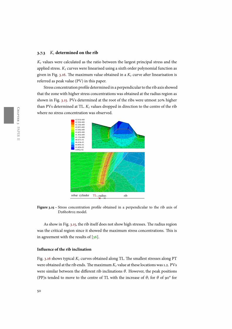
Chapter3

PAPER

II

3.7.3 Kt determined on the rib

Kt values were calculated as the ratio between the largest principal stress and theapplied stress. Kt curves were linearised using a sixth order polynomial function asgiven in Fig. 3.16. hemaximum value obtained in a Kt curve aer linearisation isreferred as peak value (PV) in this paper.

Stress concentration proûle determined in aperpendicular to the rib axis showedthat the zone with higher stress concentrations was obtained at the radius region asshown in Fig. 3.15. PVs determined at the root of the ribs were utmost 20% higherthan PVs determined at TL. Kt values dropped in direction to the centre of the ribwhere no stress concentration was observed.

-8.092e-02+1.600e-01+4.009e-01+6.418e-01+8.827e-01+1.124e+00+1.364e+00+1.605e+00+1.846e+00+2.087e+00+2.328e+00+2.569e+00+2.810e+00

rebar cylinder TL radius rib

Figure 3.15 – Stress concentration proûle obtained in a perpendicular to the rib axis ofD26h08r02 model.

As show in Fig. 3.15, the rib itself does not show high stresses. he radius regionwas the critical region since it showed the maximum stress concentrations. his isin agreement with the results of [36].

Inuence of the rib inclination

Fig. 3.16 shows typical Kt curves obtained along TL. he smallest stresses along PTwere obtained at the rib ends. hemaximumKt value at these locations was 1.2. PVswere similar between the diòerent rib inclinations θ. However, the peak positions(PP)s tended to move to the centre of TL with the increase of θ; for θ of 90° for

50

Chapter3

PAPER

II

example, PP was at the centre of TL as shown in Fig. 3.16.

0 0.2 0.4 0.6 0.8 1

1

1.2

1.4

1.6

1.8

Normalised distance along OR

Kt

46°54°64°90°

Figure 3.16 – Kt curves obtained for diòerent rib inclinations θ of D16h08r04 andD16h08r04θ90 models.

PVs and PPs determined along TL for diòerent θ are given in Table 3.5.Zones along TL with Kt equal or higher than 95% of PVs were analysed. hese

zones are referred as peak zones (PZ)s in this paper. PZs of the original modelswere anti-symmetrically located along TL and they showed similar sizes as given inFig. 3.17. Fig. 3.18 shows PZ sizes obtained for diòerent θ. PZ sizes increased alongTL as θ increased; θ of 64°, for example, showed higher PZ sizes compared to theribs with inclination of 46° and 54°. However, the increase of θ from 64° to 90° hada negligible inuence on the PZ sizes.

Inuence of the radius

he increase of r resulted in the reduction of the PVs of the original models (seeTable 3.5). PVs decreased in 14 to 21% with the increase of r from 0.2 to 0.4 mmand dropped by 15% with the change of r from 0.4 to 0.8 mm. he maximum PVobtained along TL for the original models was 2.50. In the models with no radius,PVs was utmost 20% higher than PVs of themodels with r=0.2 mm.

Fig. 3.19 shows the PPs and PZs obtained along TL with the change of r. Smallvariation on the PPs of the original models was obtained with the increase of r. heincrease of r led to an increase of the PZ sizes: the change of r from 0.2 to 0.4 mm,

51

Chapter3

PAPER

II

Table 3.5 – Peak values (PV)s and Peak positions (PP)s determined along the transition line(TL).

Rib inclination θModels 46° 54° 64°

PV PP PV PP PV PP

D10h03r02 1.56 0.82 1.61 0.71 1.63 0.64D10h08r02 1.90 0.82 1.90 0.73 1.89 0.63D10h08r04 1.59 0.79 1.61 0.73 1.64 0.64D10h15r02 2.44 0.76 2.36 0.73 2.37 0.67D10h15r04 2.19 0.74 1.92 0.70 2.13 0.55D10h08 2.15 0.81 2.27 0.75 2.25 0.65D16h03r02 1.72 0.82 1.79 0.71 1.83 0.63D16h08r02 2.09 0.81 2.15 0.76 2.15 0.68D16h08r04 1.76 0.80 1.78 0.72 1.80 0.63D16h08r08 1.53 0.79 1.54 0.73 1.56 0.63D16h15r02 2.79 0.77 2.68 0.72 2.74 0.62D16h15r04 2.28 0.76 2.18 0.70 2.26 0.53D16h15r08 1.99 0.74 1.87 0.67 1.97 0.47D16h08 2.45 0.81 2.48 0.76 2.48 0.68

D16h08r04c04 1.95 0.76 1.81 0.67 1.98 0.35D16h08r04c12 1.74 0.82 1.75 0.75 1.77 0.68D26h03r02 1.95 0.80 2.04 0.72 2.09 0.62D26h08r02 2.46 0.82 2.45 0.75 2.50 0.68D26h08r04 1.95 0.80 1.98 0.73 1.97 0.61D26h08r08 1.66 0.80 1.70 0.72 1.71 0.65D26h15r04 2.53 0.77 2.48 0.71 2.50 0.58D26h15r08 2.19 0.75 2.07 0.67 2.15 0.52

Notes:D16h08r04θ90 model: all ribs with the same inclination of 90°;PV = 1.85 and PP = 0.5.

for example, resulted to an increase up to 11% on the PZ sizes.

Inuence of the height

he reduction of h resulted in the decrease of PVs as shown in Table 3.5. he changeof h from 0.075D to 0.03D reduced PVs from 14 to 21%. he maximum PV de-termined for the models with h=0.3D was 2.09. Fig. 3.20 shows the PPs and PZsobtained for models with diòerent h. Small variation on the PPs was observed; PZsizes increased up to 15% with h reduction from 0.075D to 0.03D. he increase ofr from 0.2 to 0.4 mm had similar eòect on PVs as the change of h from 0.075D to0.03D.

he maximum PV of 2.79 was determined between all analysed models (see

52

Chapter3

PAPER

II

PP

PZ

PP

PZ

Figure 3.17 – Example of the peak positions (PP)s and peak zones (PZ)s along the rib of anoriginal model.

0 0.2 0.4 0.6 0.8 11.5

2

2.5

3

PPs along the normalised distance of TL

PVs

D16h08r04θ46°D16h08r04θ54°D16h08r04θ64°D16h08r04θ90°PZs

Figure 3.18 – Inuence of the rib inclination θ on Kt .

Table 3.5). his value resulted from a combination of highest h=0.15D and smallestr= 0.2. Models with h=0.15D combinedwith r=0.4 or 0.8mm aòected both PVs and

53

Chapter3

PAPER

II

0 0.2 0.4 0.6 0.8 11.5

2

2.5

3


PVs

D16h08D16h08r02D16h08r04D16h08r08PZs

Figure 3.19 – Inuence of the rib radius r on Kt

PPs of the non-uniform ribs. As the ank angle α was kept constant in all models,the increase of h was followed by the increase of the ribwidthw. Beside, the increaseof r and the diòerent rib inclination θ reduced signiûcantly the distance betweenthe non-uniform ribs. As a consequence, it created a region of stress concentrationsmoving the PPs of the ribs to this zone. he reduction of the distance between non-uniform ribs increased PVs of these ribs. herefore, these rib geometries should beavoided.

Inuence of the diameter

he increase of D resulted in the increase of PVs as shown in Table 3.5. PVs of theoriginal the models increased up to 14% as D changed from 10 to 16 mm and toutmost 18% for D increasing from 16 to 26 mm.

Fig. 3.21 shows PPs and PZs obtained for the original models with 10, 16 and26 mm diameters. Small variation on the PPs and PZ sizes was obtained with thechange of D from 10 to 16 mm and from 16 to 26 mm.

Inuence of the rib spacing

Rib spacing c change had small inuence on thePVs andPZ sizes alongTL as shownin Fig. 3.22. he c parameter had smaller inuence on the Kt values and PZ sizes

54

Chapter3

PAPER

II

0 0.2 0.4 0.6 0.8 11.5

2

2.5

3


PVs

D16h03r02D16h08r02D16h15r02PZs

Figure 3.20 – Inuence of the rib height h on Kt .

0 0.2 0.4 0.6 0.8 11.5

2

2.5

3


PVs

D10h08r02D16h08r02D26h08r02PZs

Figure 3.21 – Inuence of the rebar diameter D on Kt .

compared to other analysed parameters.However, the reduction of c from 0.6D to 0.4D aòected the PVS and PPs of

the non-uniform ribs (see Table 3.5). Similar case was obtained for models withh=0.15D combined with r=0.4 or 0.8mm.

55

Chapter3

PAPER

II

0 0.2 0.4 0.6 0.8 11.5

2

2.5

3


PVs

D16h08r04c04D16h08r04D16h08r04c12PZs

Figure 3.22 – Inuence of the rib spacing c on Kt .

3.8 Conclusions

In this work, characterisation studies of QST rebars included 1) Identiûcation ofthe microstructure and hardness measurements in the cross section of rebars withdiòerent diameters. he average grain size of the core microstructure was quanti-ûed and compared to the grain size of QST and HR rebars given in the literature.1) Residual stresses were experimentally determined on surface and subsurface ofQST rebars with 16 mm diameter by Cut Compliance and X-ray diòraction tech-niques. Results obtained from both techniques were discussed and compared toresidual stresses ofQST rebars found in the literature. 2) SEM analyses on the rebarsurface allowed to identify and quantify imperfections originated in the manufac-turing process. 3) A parametric study was developed to analyse the inuence of therib geometry and rebar diameter on the stress concentration factors Kt along therib. he ûndings of this study suggest that:

• he average grain size in the core of QST rebars increase with the increaseof diameter. However, themicrostructure ofQST rebars is ûner than themi-crostructure of hot rolled rebars with higher diameter.

• Random tensile and compressive residual stresses are expected on the surfaceand subsurface ofQST rebars. hese stresses are no higher than 20% of theiryield strength.

56

Chapter3

PAPER

II

• Surface imperfections originated in the manufacturing process are near thetransversal and longitudinal ribs. As imperfections are zones of stress con-centration and may aòect the performance of rebars in service, they shouldbe avoided.

• he highest stress concentrations arising from the ribbed proûle are locatedat radius region. hemain parameters of the rib geometry aòecting themax-imum Kt ’s are the radius and height; maximum Kt values at the radius regioncan be signiûcantly reduced with the increase of the radius and reduction ofthe height.

• he rib inclination is the main parameter aòecting the position of the max-imum Kt ’s as well as the critical zone sizes along the rib. he critical zonescorrespond to the zones where Kts are at least 95% of the maximum values.hese critical zones are located anti-symmetrically along the rib. As near therib inclination is to a perpendicular of the rebar axis, themaximum Kt ’s tendsto move to the rib centre and the critical zone sizes increase.

• Maximum Kt ’s along the ribs increasewith the rebar diameter increasing andits inuence in themaximumKt is comparable to the changes in the rib radiusand height. However, the eòect of the diameter on the critical zone size is lesssigniûcant than those parameters.

• he reduction of the rib spacing should be avoided for non-uniform ribs sinceit increases themaximum Kt values.


he authors are grateful toDaniele Laub from the InterdisciplinaryCentre For Elec-tron Microscopy (CIME) at EPFL for her help with the sample preparation for themicroscopic analyses. We are also grateful to Cyril Denereaz from theMechanicalMetallurgy Laboratory (LMM) for the hardness measurements.

57

Chapter3

PAPER

II

58

BIBLIOGRA

PHY

Bibliography

[1] Domone, P., & Illston, J. (2010). Construction materials: heir nature and be-haviour. CRC Press.

[2] Basu, P. C., Shyiamoni, P., & Roshan, A. D. (2004). Characterisation of steelreinforcement for RC structures: An overview and related issues. IndianCon-crete Journal, 78(1), 19-30.

[3] Ray, A.,Mukerjee, D., Sen, S. K., Bhattacharya, A., Dhua, S. K., Prasad,M. S.,& Sahu, A. K. (1997). Microstructure and properties of thermomechanicallystrengthened reinforcement bars: A comparative assessment of plain-carbonand low-alloy steel grades. Journal ofMaterials Engineering and Performance,6(3), 335-343.

[4] Economopoulos, M., Respen, Y., Lessel, G. & Steòes, G. (1975). Applicationof the Tempcore process to the fabrication of high yield strength concrete -reinforcing bars. Metallurgical reports CRM, (45), 3–19.

[5] Rehm, G., & Russwurm, D. (1977). Assessment of concrete reinforcing barsmade by the Tempcore process. Metallurgical reports CRM, (51), 3-16.


[7] Simon, P., Economopoulos,M., &Nilles, P. (1984a). Tempcore: A new processfor the production of high-quality reinforcing bars. Iron Steel Engineer, 61(3),53-57.

[8] Simon, P., Economopoulos,M., & Nilles, P. (1984b). Tempcore: An economi-cal process for the production of high quality rebars. Metallurgical Plant andTechnology 1984b, (3), 80–93.

59

BIBLIOGRA

PHY

[9] Kelestemur, O., Kelestemur, M. H., & Yildiz, S. (2009). Improvement of me-chanical properties of reinforcing steel used in the reinforced concrete struc-tures. Journal of Iron and Steel Research, International, 16(3), 55-63.

[10] Totten,G., E. (2006). Steel heat treatment:Metallurgy and technologies. CRCPress.

[11] Zheng,H., &Abel, A.A. (1997).Residual stress eòects on the fatiguepropertiesof Tempcore reinforcing steel. Technology Transfer Series, 177-182.

[12] ISO 4948-1 (1982). Steels - classiûcation - part 1: Classiûcation of steels intounalloyed and alloy steels based on chemical composition.

[13] Bhadeshia,H., &Honeycombe, R. (2006). Steels:Microstructure and proper-ties. Butterworth - Heinemann, p. 117.

[14] Russwurm, D., & Martin, H. (1993). Betonstahle fur den Stahlbetonbau:Eigenschaen und Verwendung. Wiesbaden: Bauverlag, p. 53.

[15] ASTM E3-11 (2011). Standard guide for preparation of metallographic speci-mens.

[16] Bramûtt, B. L., & Benscoter, A. O. (2002). Metallographer’s guide: Practicesand procedures for iron and steels, ASM International.

[17] E112-12 (2012) Standard test methods for determining average grain size.

[18] E562-11 (2011). Standard test method for determining volume fraction by sys-tematicmanual point count.

[19] Mukherjee, M., Dutta, C., & Haldar, A. (2012). Prediction of hardness of thetemperedmartensitic rim of TMT rebars. Materials Science and Engineering:A, 543, 35-43.

[20] Tilly, G. P. (1979). Fatigue of steel reinforcement bars in concrete: A review.Fatigue & Fracture of Engineering Materials & Structures, 2(3), 251-268.

[21] Hanson, J. M., Burton, K. T., & Hognestad, E. (1968). Fatigue tests of rein-forcing bars - eòect of deformation pattern. Journal of the PCA Research andDevelopment Laboratories, 10, 2-13.

[22] Jhamb, I. C., & Mac Gregor, J. G. (1974). Eòect of surface characteristics onfatigue strength of reinforcing steel. ACI Special Publication, 41-7, 139-168.

60

BIBLIOGRA

PHY

[23] ISO 6507-1 (2005). Metallic materials - Vickers hardness test-part 1: Testmethod.


[25] Tisza M. (2001). Physical metallurgy for engineers. ASM International, pp.280-281.

[26] Baydogan, M., Uysal, A., Kayali, E. S., & Cimenoglu, H. (2005). 4698 - In-vestigation on cyclic deformation behaviour of reinforced steel bars. In ICF11,Italy.

[27] Hanson, J. M., Somes, N. F., Helgason, T., Corley, W. G., & Hognestad, E.(1970). Fatigue strength of high-yield reinforcing bars. National CooperativeHighway Research program (NCHRP). Final report - Project n°4-7. Illinois.

[28] Schindler, H. J., Bertschinger, P., & Semenov, B. Near-surface stress measure-ment in 2D and 3D by the cut compliance technique. In Materials ScienceForum, 404, 515-520.

[29] Lu, J. (1996). Handbook ofmeasurement of residual stresses.

[30] Withers, P. J., Turski, M., Edwards, L., Bouchard, P. J., & Buttle, D. J. (2008).Recent advances in residual stressmeasurement. International Journal ofPres-sure Vessels and Piping, 85(3), 118-127.

[31] Schindler,H. J. (2000). Residual stress measurement in cracked components:Capabilities and limitations of the cut compliance method. In Materials Sci-ence Forum, 347, 150-155. Transtec Publications, 1999.

[32] Standard SIA 262 (2003). Concrete structures. Swiss Society of Engineers andArchitects, Zurich.

[33] Fitzpatrick, M. E., Fry, A. T., Holdway, P., Kandil, F. A., Shackleton, J., &Suominen, L. (2002). Determination of residual stresses by X-ray diòraction.Measurement good practice guide n°52. National Physical Laboratory, Ted-dington,Middlesex, UK.

61

BIBLIOGRA

PHY

[34] Wimpory, R. C., & Ohms, C. (2010). A step towards a complete uncertaintyanalysis of residual stress determination using neutron diòraction. In Materi-als Science Forum, 638, 2487-2492.

[35] Jhamb, I. C., &MacGregor, J. G. (1974). Stress concentrations caused by rein-forcing bar deformations. ACI Special Publication, 41-8, 169-182.


[37] EN 10080 (2005) Steel for the reinforcement of concrete, weldable, ribbed re-inforcing steel.

[38] Abaqus (2012)Analysis user’s manual version 6.12, Dassault Systemes SimuliaCorp., Providence, USA.

62

Chapter4

PAPER

III

Chapter 4

Paper III

Microstructural inuence on the scatter in thefatigue life of steel reinforcement bars— Marina Rocha, Eugen Bruhwiler, Alain Nussbaumer

Abstract: Fatigue test results with steelreinforcement bars (rebars) is a stochas-tic process. Scatter can be inuenced bythe sensitivity of the short crack growthto the microstructural features, especiallynear the fatigue limit. his work inves-tigates the scatter inherent to the micro-scopic conditions near the fatigue limitof ferrite-pearlite and martensite mi-crostructures found in the outer layer ofrebars. An adapted Navarro-De Los Rios

model within a Monte-Carlo frameworkis used to simulate the short crack growthin material grains. Grain size varia-tion, grain orientation factor and multi-ple phases were considered in the model.he results are compared with the scatterfound in fatigue tests on hot-rolled-coldworked as well as quenched and temperedrebars. It is shown that microstructuraleòects explains part of the observed scat-ter in the fatigue tests.

Keywords: Short fatigue crack growth; Ferrite-pearlite; Temperedmartensite; Scat-ter above the fatigue limit.

63

Chapter4

PAPER

III

64

Chapter4

PAPER

III


4.2 Reconstruction of parent austenite grains . . . . . . . . . . . 68

4.2.1 Experimental analysis . . . . . . . . . . . . . . . . . . . . 68

4.3 Short crack growth model . . . . . . . . . . . . . . . . . . . . . 70

4.3.1 Grain structure . . . . . . . . . . . . . . . . . . . . . . . . 70

4.3.2 Grain orientation . . . . . . . . . . . . . . . . . . . . . . . 75

4.3.3 Material properties . . . . . . . . . . . . . . . . . . . . . . 77

4.4 Results and Discussion . . . . . . . . . . . . . . . . . . . . . . 78

4.5 Conclusion . . . . . . . . . . . . . . . . . . . . . . . . . . . . . 81

4.6 Acknowledgements . . . . . . . . . . . . . . . . . . . . . . . . 82

4.1 Introduction

Fatigue life assessment of engineering structures depends on the knowledge ofma-terial properties. Fatigue limit is amacroscopic property of thematerial that is sen-sitive to microscopic conditions. Since metal fatigue is a random process, fatiguedata from testing always exhibit scatter for specimens of the same geometry, un-der same loading condition, especially near the fatigue limit. Besides, for metal-lic materials, the crack initiation period oen dominates the fatigue life just abovethis limit. Since fatigue crack initiation is mainly a surface phenomenon, specimensurface roughness, protrusions and microscopic aspects such as grain size, grainorientation, dislocation density can inuence the scatter in fatigue lives and fatiguelimit stress range. he large scatter observed in fatigue tests lead to high values ofconûdence intervals (CI)s to get the design S-N curves. Further scatter result fromthe damage accumulation models used in fatigue life veriûcations. In most designcodes, including those for steel reinforcement bars (rebars), usually considers 95%CIs.

Furthermore, one single design S-N curve regroup rebars produced from hotrolling, cold working and quenching and self-tempering with diòerent surfacemi-crostructures, rib patterns and surface roughness, all of which increase the scatternear the fatigue limit and lead to very conservative design values. In order to under-stand the scatter inherent to microscopic aspects in the fatigue behaviour of rebars,this work proposes a short crack growth model to simulate the initiation period

65

Chapter4

PAPER

III

in ferrite-pearlite and temperedmartensite grains found on the surface of diòerenttypes of rebars.

Fatigue crack initiation period in metallicmaterial consists of cyclic slip, cracknucleation and short crack growth [1]. hese cracks can behave signiûcantly diòer-ent from the (long) crack propagation as described by Paris’ law [2,3] . Short crackscan grow faster than corresponding long cracks at the same value of stress intensityfactor range, ∆K. hey can also grow at signiûcant rates for ∆K value smaller thanthe threshold for long cracks [4].

Surfacemicroscopic investigations in steel specimenshas shown that short cracksform on slip bands and propagates along them [3]. he short crack propagationstops when the applied stress is below the fatigue limit; when the stress is just abovethis limit, the crack accelerates and decelerates due to the interactions with mi-crostructural barriers until it reaches a long crack regime with apparent continu-ous propagation rate. he crack growth rate decreases as approaching the grain orphase boundary; the crack then accelerates when a slip band is initiated in the ad-jacent grain [2, 5].

Navarro and De Los Rios (N-R) [6, 7] proposed a short crack growth modelwhere a crack initiates from slip bands. his model is particularly appropriate tostudy fatigue limit problems which involve microstructurally short cracks. N-Rmodel considers the interaction between crack andmicrostructural barriers. It as-sumes that dislocations are constrained to remain on their original plane and pileup when blocked by grain boundaries. hey propagate along slip bands extendingthrough successive grains.

N-R model can be considered as a further development of research in [3, 8, 9].Bilby et al. [8] were the ûrst to obtain a bounded solution for the dislocation distri-bution function representing the crack and the plastic zone (slip band ahead of thecrack tip). [3,9] showed that the crack tip plastic zone interacts withmicrostructuralbarriers, such as grain boundaries, when the crack is of the order of microstruc-tural features. [9] developed the unbounded solution for the dislocation distributionfunction.

In its original form,N-R model considers inûnitesimal dislocations distributedwithin two zones: the crack itself a (half crack length) and the plastic zone c asshown in Fig. 4.1. In this two-zone model, an inûnite stress level is sustained bythe grain boundary. In [10], the model was extended by considering an additionalsmall zone of length r0 << D, (D is the, uniform, grain diameter) representing theinterface between neighbouring grains or phases (see Fig. 4.1). his model elimi-

66

Chapter4

PAPER

III

nates the singularity of the stress ûeld associated to the distribution of dislocations.In physical terms, the three-zone system was argued to be more realistic since theplastic zone is blocked by the grain boundary i.e., its two boundaries, and it remainsblocked until the stress in the third zone i.e., the grain boundary, attains a criticallevel for dislocations to cross this zone.

initiation point plastic zonecrack

ac

Two-zone model

initiation point extra zonecrack

a r₀c

Three-zone model

Figure 4.1 – Two-zone [6], [7] and three-zone [10]models.

N-R model has been extensively used (or extended) to predict the fatigue life-time of metals. In [11], N-R model was applied to predict the short fatigue crackgrowth behaviour in mild steel. In [12], N-R model was applied for fatigue life pre-diction of commercially pure aluminium. hemodel prediction was in good agree-ment with experimental results. In [13], the eòect of textures was investigated in theshort fatigue crack growth in Al-Li alloy. An equation for the grain orientation fac-tor was proposed depending on the load axis, slip plane normal and slip direction.N-R model was extended for biaxial fatigue loading case in low and medium Car-bon steels; the crack initiation orientation was close to the experimental results [14].he inuence of the grain size variation was introduced in the N-R model by [15]where Voronoi cells were used to represent the grain structure. In [16], amicrome-chanical model for short crack growth based on successive blocking of monotonicplastic zone and cyclic plastic zone of a crack at grain boundaries was proposed. hismodel was based on the N-R approach [10]. hesemodels successfully reproducedthe short crack growth pattern where the crack decelerates at a grain boundariesand it accelerates when crossing a grain.

67

Chapter4

PAPER

III

his irregular behaviour of short cracks due to the interactions with the mi-crostructure can aòect the scatter found near the fatigue limit. Factors such as grainsize variation [3], grain orientation [13] and diòerent phases [2] aremore prominentat low stress levels and consequently inuence the fatigue crack initiation period.

In this study, the inuence of themicrostructure on the scatter observed in ex-perimental data as obtained above the fatigue limit is investigated using an adaptedN-R model within aMonte-Carlo framework. he short crack growth is simulatedin ferrite-pearlite (F-P) and tempered martensite (TM) grains found on the outerlayer of rebars. he grain structure is represented by Voronoi tesselation. In the F-Pmodel, the two phases, pearlite and ferrite, weremodelled separately with the areafraction of each phase being obtained from the literature. On the other hand, theparent austenite grain is considered for short crack growth modelling in TM. heparent grain is experimentally determined using Electron Back Scattered Diòrac-tion (EBSD) and Arpge soware. he scatter obtained in the crack initiation phaseis compared to experimental data from the literature.

4.2 Reconstruction of parent austenite grains

he laths of (daughter) martensite are organized within the parent austenite grains.he austenite grain size represents an essential characteristic of martensite steels;ûne austenite grain results in the formation of ûne martensite and consequentlyimprovement in the mechanical properties of martensite steels [17]. In this work,slip band and short crack growth is simulated in the austenite grains of TM steel.

With the martensite transformation, also called displacive transformation, avestige of the austenite grain boundary remains in the microstructure [18] and itcan be revealed by etching [19]. However, it can be time consuming to ûnd a suc-cessful etching to correctly identify the austenite grain boundaries. Instead, in [20],parent grains were successfully reconstructed by post-processing of EBSD data onthe daughter grains. his techniquewas applied in this work to reconstruct the par-ent austenite grains in the cross section of quenched and self-tempered (QST) rebarfrom EBSD data obtained on martensite laths. he Arpge soware [21] was usedfor reconstruction of the parent grains.

4.2.1 Experimental analysis

EBSD analyses were performed on a polished cross section of QST rebar with 16mm diameter. he cross section was prepared by mechanical grinding and polishing

68

Chapter4

PAPER

III

(a)

50 µm

(b)

Figure 4.2 – Reconstruction of the austenite grains in theQST rebar: (a) Martensite grainsobtained from EBSD analyses; (b) Reconstructed austenite grains determinedfrom Arpge soware.

69

Chapter4

PAPER

III

up to 1 µm followed by polishing with a Vibromet table containing non-crystallinecolloidal silica for approximately 3.5 hours. ESBD analyses were then conductedusing XL30-FEG Scanning Electron Microscopy (SEM) at 20 KV. he cross sectionwas tilted at 70° in the SEM. EBSDmap of themartensite grains was obtained fromthe surface edge to 200 µm towards the centre. A map size of 200 × 200 µm wasconsidered with ameasurement step size of 0.2 µm.

EBSD map of the martensite laths is given in Fig. 4.2a. he orientation of themartensite grains is coded by colors representing the Euler angles; they are a set ofthree angles which describe the crystallographic orientation of grains relative to areference (sample) coordinate system.

he austenite grains reconstructed by theArpge soware are shown in Fig. 4.2b.he reconstruction was performed in three steps: identiûcation of the martensitegrains in the EBSDmapping; nucleation of austenite grains based on a selected ori-entation relationship (OR); growth of the austenite grains up to a deûned toleranceangle [20]. he OR between austenite and martensite was the Greninger-Troiano(GT) relationship [18]. he white areas in the image (see Fig. 4.2b) correspond tothe areas that could not be reconstructed by Arpge. his may result from no in-dexed pixels in the EBSD map, martensite with ORs that are far from the GT-OR,martensite laths that could belong to two parent austenite grains and for which itwas impossible to decide [20]. he color of each austenite grain represents the colorof onemartensite lath into this grain.

4.3 Short crack growth model

he short fatigue crack growth model is adapted from the three-zone microme-chanical N-R model [10]. he interaction between crack and grain-phase boundaryis characterized. It is assumed that when slip is initiated in a grain, the whole grainundergoes slip being blocked by the grain boundary. Slip propagates to the adjacentgrain when the stress ahead of the plastic zone reaches a required value. his stressdepends on the position of the crack tip to the grain boundary.

4.3.1 Grain structure

In N-R model, all grains are assumed to have equal sizes. In this work, the grainstructure with diòerent sizes was represented by Voronoi tessellation. Voronoi hasbeen extensively used to reproduce the grain geometry of polycrystallinematerialsin short fatigue crack initiation models [15,22].

70

Chapter4

PAPER

III

-5 0 5 10 15-5

15

× 10-5

× 10-5 (mm)

(mm)

0

5

10

(a)

10-9

10-8

crack length (m)

crack growth rate da/dN (mm/cycle)

0 5 10 15× 10-5

(b)

Figure 4.3 – Example of a simulation result obtained in F-P with a crack length 2a ≈ 8Dmat N = 2 × 106 cycles: (a) Illustration of a surface short crack growth in ferrite(dark grey) and pearlite (ligth gray) grains represented by Voronoi cells; (b)Short crack growth rate as a function of the crack length.

71

Chapter4

PAPER

III

Fig. 4.3a illustrates a short crack in F-P steel where the two phases, ferrite andpearlite, are modelled separately by Voronoi cells. he crack grows along a prefer-ential slip direction randomly distributed in the model. In TM steel, Voronoi cellsrepresent the parent austenite grains.

Voronoi tessellation is a cell structure generated from a random set of pointsas shown in Fig. 4.3a. Voronoi tesselation is a good approximation to represent apolycrystalline structure assuming that, in the crystallization process of ametal, allgrains start to grow from random points and grow uniformly in all directions. hegrains will then collide and a grain boundary will be created. In geometric aspects,the resulting grain structure would be a Voronoi.

In the Voronoi tessellation, the set of points is speciûed beforehand and eachpoint will be enclosed by an area. Each Voronoi area (or cell) represents one grain.Voronoi tessellation was generated using Matlab.

Crack initiation in the ûrst grain

Short fatigue cracks in steel specimen under uniaxial loading initiate along slipplanes closer to the plane of maximum shear stress [24]. he angle between theslip plane and the applied load axis is close to 45° (mode II loading). Moreover,crack initiates in relatively coarse grains in steel [2]. hus, it was assumed in themodel that a crack initiates in a large grain along the slip plane closer to the plane ofmaximum shear stress. he crack always starts from a Voronoi point. To decide inwhich grain the crack will start, a compromise between slip size and direction wasconsidered. A new length lcr it was calculated for each grain as given in Eq. 4.1:

lcr it = l cos 2θ (4.1)

where l is the length of all slip planes passing through the Voronoi point and θ isthe angle between the slip plane and the plane ofmaximum shear stress. he crackinitiates in the grain with maximum lcr it .

Short crack growth

he schematic diagram given in Fig. 4.4 represents a half crack length a and itsplastic zone c in a polycrystalline material. he crack grows in mode II loadingand the applied shear stress component is assumed as ∆τ = ∆σ/2, where ∆σ is theapplied uniaxial cyclic loading. In thismodel, a single crack is assumed to propagateuntil it reaches a given length of 10Dmean (Dmean is themean grain diameter) [2,25]

72

Chapter4

PAPER

III

aa

c

c

initiation point

plastic zone

crack

Figure 4.4 – Schematic diagram of the crack with its plastic zones in the grains.

and the simulation is stopped. Dmean=20 µm as obtained from Fig. 4.2b using theAbram’s hree Circlemethod [23].

he crack growth is calculated for each crack tip separately.he crack grows at a rate of:

dadN

= f ϕ (4.2)

where N is the number of cycles, f is the fraction of dislocations ahead of the cracktip that contributes to the crack growth process and ϕ is the crack tip plastic dis-placement.

he factor f varies between 0 and 1 and it depends on the applied stress: thesmallest f values are obtained when the applied stress level approaches the fatiguelimit [24]. It represents the degree of irreversibility of slip per cycle. In this work,f was assumed constant and equal to 5.64 × 10−4 since the scatter is analysed atconstant stress amplitude and near the fatigue limit. his value was obtained fromfatigue tests with low carbon steels subjected to uniaxial loading [24].

he plastic displacement ϕ can be written as [26]:

ϕ = 2(1 − ν)√

1 − n2∆τaµn

(4.3)

where ν is the Poisson’s ratio and µ is the shearmodulus. he dimensionless param-eter n = a/c deûnes the position of the crack tip relative to the grain boundary (seeFig. 4.4).

73

Chapter4

PAPER

III

he crack growth rate as a function of the crack length obtained for F-P is givenin Fig. 4.3b. he growth rate decreases as the crack approaches the grain boundaryand then increases as the plastic zone propagates into the next grain. he dottedlines in Fig. 4.3b represent the plastic zone size at every propagation step in eachgrain.

he slip propagates from grain i to the neighbouring grain i + 1 when n reachesa critical value n = nc . his critical value nc is given by [10]:

nic = cos [

π2(∆τ − ∆τLi

2τ f r)] (4.4)

where τ f r is the ”friction stress” which represents the resistance of the grain to thedislocation motion in the plastic zone. ∆τLi is theminimum stress required for slippropagation determined as [15]:

∆τLi = ∆τFLmim1

√di2ci

(4.5)

where ∆τFL is the fatigue limit, di is the mean of the crack length in each grainand mi/m1 is the grain orientation ratio. ∆τFL represents a macroscopic propertyof thematerial and ∆τLi represents a condition for local plastic deformation at themicroscopic level. he mi/m1 ratio will be discussed in Section 4.3.2. he crackpropagation stops if ∆τ is smaller than ∆τLi .

When a slip band starts in the next grain, the plastic zone spans this entire grain.hus, ni

c decreases to nis expressed as:

ni+1s = c

ci+1 nic (4.6)

he number of cycles to propagate the crack in a grain can be obtained by inte-gration of Eq. 5.3 which gives:

∆Ni =µ

f (1 − ν)∆τ(sin−1 ni

c − sin−1 nis) (4.7)

he number of cycles Nd1 and Nd2 spent to propagate each crack tip separatelyare determined from the sum of ∆Ni . he total number of cycles NTotal , when thecrack length is equal to 10Dmean, is given by:

NTotal = max(Nd1,Nd2) (4.8)

74

Chapter4

PAPER

III

4.3.2 Grain orientation

An equation for the grain orientation ratiomi/m1, used inN-Rmodel,wasproposedby [27] and it is given as:

mim1

= 1 + 2.07 [ 2π

tan−1(0.522(i − 1)2)]1.86

(4.9)

where m1 is the orientation factor of the ûrst grain and mi is the orientation factorof successive grains. Eq. 4.9 was developed based on fatigue test results ofmild steeland then applied for randomly oriented fccmaterials. mi/m1 increasesprogressivelyas the crack grows over several grains (see Fig. 4.5b) andmi→∞ tends to the averageTaylor factor MT=3.07.

In reality, the short crack growth depends on the individual grain orientations.Since the objective of the present work is to analyse the scatter due to microstruc-tural features including the grain orientation, a new equation mi/m1 was proposedwhere this factor isn’t forced to increase continuously with the crack length; it candecrease or increase as the crack propagates through successive grains which aremore or less favourably oriented for slip. his allows to consider how the statisticalvariations of the grain orientation can aòect the crack growth.

mi/m1 orientation ratio

he crack initiation in the ûrst grain is governed by the stress required to sustainplastic deformation along the slip direction with the most favourable orientation,which results in the smallest orientation factor. his factor measures the deforma-tion compatibility between the current crack and the slip direction in the adjacentgrain. Since the need to maintain the compatibility between adjacent grains in thisstage is small, the orientation factor is close to the Sachs factor for single crystal.his factor MS is equal to 2.24 (Sachs factor) for fcc and body centered cubic (bcc)materials [28].

With further crack propagation over several grains with diòerent orientations(see Fig. 4.5a), the deformation compatibility between all these grains moves theorientation factor value from Sachs to Taylor type. When the crack becomes suf-ûciently large i.e., insensitive to the material microstructure, the orientation factorreaches a maximum value similar to the Taylor factor, mi→∞= MT=3.07 for ran-domly oriented fcc and bcc crystals [28].

heoretically, the grain orientation ratio mi/m1, for m1 = 2.24 andmi→∞ = 3.07,

75

Chapter4

PAPER

III

a

aa

aa

a

surface initiation point

crack

(a)

4

3.5

3

2.5

2

1.5

1

0.5

01 2 3 4 5 6 7 8 9 10

100

200

300

400

500

600

700

800

900

1000

0

orientation factor mi/m1

grain number

(b)

Figure 4.5 – Illustration of a subsurface crack growth and variation of the grain orientationratio m i/m1: (a) A crack length 2a reaches 7 grains on the surface, the subsur-face crack tip extends overN= 14 grains; (b)he graph represents the evolutionof m i/m1 scatter as the crack grows using Eq. 4.10; To illustrate this scatter, itwas computed 1000 m i/m1 values for each step. he greyscale represents theamount of m i/m1 with same values in a region. In the ûrst step, m i/m1=1 andthere is no dispersion. In the second step, a higher dispersion is obtained com-pared to the 10th step when the dispersion decreases. he red lines representthe evolution of m i/m1 obtained by Eq. 4.9.

76

Chapter4

PAPER

III

varies between 1 and 1.4. However, as given in [29,30],mi→∞/m1 can tend to a valueof approximately 3 for mild steels. [29] suggests that this diòerence is attributed tocrack closure eòects; as the crack grows, it progressively increases to a steady peakvalue for large crack. Other factors such as microcrack initiation at several pointsandmicrocrack coalescencemay also contribute to the value of 3.

Eq. 4.10 gives mi/m1 which simulates the variance for steels with randomly ori-ented crystals:

mim1

= 1 + 2(Ωi − 2.3) + 2.07 [ 2π

tan−1(0.522(i − 1)2)]1.86

(4.10)

where Ωi , the average value of the grain orientations, is calculated as:

Ωi =1N

N

∑j=1 ω j (4.11)

N represents the number of grains which contains the crack tip as shown in Fig.4.5a.

ω j = mink=1 to 12

( 1(L ⋅ nk)(L ⋅ sk)

) (4.12)

where L, nk and sk are unit vectors along the loading axis, slip plane normal and slipdirection respectively. he k values represent themain slip system in bcc crystals: 6slip planes and 2 slip directions in each plane.

Fig. 4.5b shows the mi/m1 behaviour obtained for 1000 simulation runs at eachstep of the short crack growth. When the crack propagates in the ûrst grain, thegrain orientation ratio is 1. As the crack grows in few grains, mi/m1 variation in-creases due to the higher dispersion in grain orientations. Asmore grains are incor-porated to the crack growth, this variation decreases and mi/m1 tends to the valueof 3 when the crack length 2a ≈ 10Dm.

4.3.3 Material properties

he parameters used for ferrite, pearlite and martensite in the model are given inTable 4.1.

Ferrite and pearlite properties

Fatigue limit ∆σFL of ferrite steels, i.e., with very low amount of pearlite, is ap-proximately 0.6σu [31], where σu is the tensile strength. his results in ∆σFL=260

77

Chapter4

PAPER

III

Table 4.1 –Material properties used in themodel.

Parameters Ferrite Pearlite Martensite

τ f r (MPa) 70 134 142∆σFL (MPa) 260 385 368µ (GPa) [40] 82 82 79ν [40] 0.28 0.28 0.29

MPa [32]. τ f r for ferrite is 70 MPa as given in [33].Fatigue limit ∆σFL of fully pearlite steels is approximately 0.4σu [31]. he value

of 385 MPa was obtained [34] as shown in Table 4.1. he τ f r value of 134 MPa isgiven in [35]. he area fraction of pearlite for hot rolled (HR) rebars was found tovary from approximately 15 to 55% [36, 37]. his variation was considered in themodel.

Since in fatigue tests with F-P steels, cracks usually start in the soer ferritegrain [24, 38, 39], the crack was assumed always to start in a ferrite grain in themodel.

Temperedmartensite properties

Fatigue limit ∆σFL of TM steels was found to be approximately 0.6σu [31]. Sinceσu=613 MPa for the TM steel studied in this work, ∆σFL was then determined asapproximately 368MPa (see Table 4.1). he τ f r values given in [41,42] for TM steelsvaries from approximately 0.25 to 0.30σy with σy being the yield strength. τ f r =142MPa was calculated from 0.275σy with σy =518MPa for the studied TM steel.

4.4 Results and Discussion

Fig. 4.6 shows the scatter obtained in the F-P model for diòerent area fractions ofpearlite i.e., varying approximately between 15 and 55%, as found in HR rebars [36],[37]. he scatter in F-P model is aòected by the presence of two phases and diòerentarea fractions of ferrite and pearlite. As the crack grows into pearlite from soerferrite phase, the crack growth rate decreases at phase interface. Since pearlite isa harder microstructure, the boundary between two phases tended to impede thecrack propagation. Similar crack behaviour was experimentally observed in fatiguetests with F-P steels [38]. As the area fraction of ferrite varies considerably betweenHR rebars, the duration of fatigue crack initiation was aòected with this area varia-tion and consequently, the scatter at the analysed stress level. Smaller area fraction

78

Chapter4

PAPER

III

area fraction of pearlite (%)

N number of cycles to failure

15 20 25 30 35 40 45 50 551

1.5

2

2.5

3

3.5

4

4.5

(× 106)

Figure 4.6 – Scatter obtained for diòerent area fractions % of pearlite in the F-P model.

of pearlite, for example, tended to decrease scatter since the crack grows predomi-nantly in one phase i.e., in ferrite grains.

Figs. 4.7a and 4.7b show the scatter determined from simulations of the shortcrack growth in F-P (with 53% of pearlite) and TM steels. he model results werecompared to experimental data including rebars with diameter d ⩽ 16 mm andtested at stress-ratio between 0 and 0.2 as given in [43–47]. Model and experimentalresults given in Figs. 4.7a and 4.7b include only failure data points. hemodel resultsinclude the inuence ofmicrostructural features on the scatter in the fatigue crackinitiation phase. his phase includes short crack propagation to amaximum lengthof 0.2 mm. he long crack propagation phase will be treated in another paper.

hemodel datawere generated from 1000 simulations run at 24 MPa above thefatigue limit of both F-P and TM steels. he scatter at this stress level was comparedto the scatter found in HR-CW and QST rebars with similar local conditions. hevalue of 24 MPa was considered in the simulations since 1) he smallest f valueexperimentally given in [24] was determined for a stress range at 24 MPa above thefatigue limit of the material; 2) here were no or few experimental data for HR-CW and, especially for QST rebars, at lower stress ranges and with the same testconditions as considered in this work.

he experimentaldata inFig. 4.7a includeHR andCW rebarsof low andmediumCarbon content with diòerent area fractions of pearlite. Information on the crystal-lographic textureofHR, CW andQST rebars isn’tprovided in the literature. Crystal-

79

Chapter4

PAPER

III

N number of cycles to failure

number of failures

1 2 3 4 5 6 7 8 90

10

20

30

40

50

60

70

80

90

× 106

model

experimental data

(a)

1 1.5 2 2.5 30

20

40

60

80

100

120

× 106N number of cycles to failure

number of failures

model

experimental data

(b)

Figure 4.7 –Distribution of failures points obtained in the model and experimental data:(a) For F-P model with an area fraction of 53% of pearlite and HR-CW rebars[43,44]; (b) For TM model and QST rebars [45–47].

80

Chapter4

PAPER

III

lographic texture is deûned as the grain (crystal) orientation in a specimen. In [48],nearly random texture was found on the surface of hot rolled low-alloyed steelswith bcc structure; during hot rolling, the steel undergoes several passes where thetexture is randomized by dynamic recrystallization and phase transformation fromaustenite to ferrite. Randomly oriented grains were then assumed for F-P and TMin themodel as a ûrst approximation.

Fig. 4.7b shows the scatter of failure data obtained from the model and QSTrebar test results. With themodel, higher scatter was obtained in F-P compared toTM which is in agreement to what has been observed in fatigue tests with HR, CWandQST rebars. In [49], for example,QST rebars showed smaller scatter comparedto HR and CW rebars. In [45], small scatter was observed in fatigue tests with QSTrebars near the fatigue limit. he fatigue behaviour of these rebars was consideredessentially as a function of the surface layer ofmartensite.

Moreover, as shown in Figs. 4.7a and 4.7b, the scatter determined in both F-P and TM is smaller than the scatter observed in experimental data; it representsabout 50% of the scatter from fatigue tests. his diòerence between model and ex-perimental results may be inuenced by stress concentrators on the rebar surface,such as roughness and the presence of the ribs, giving rise to local plastic deforma-tion and aòecting fatigue crack propagation. [50], for example, suggests that scatternear the fatigue limit of QST rebars may result from variations in stress concentra-tions arising from ribs as well as surfacemicrostructural features.

4.5 Conclusion

N-R model including grain structurewith diòerent sizes and grain orientation vari-ations was used to simulate the propagation of a single fatigue short crack in ferrite-pearlite and temperedmartensite steels within aMonte-Carlo framework. he scat-ter determined above but near the fatigue limit was compared to the scatter foundon experimental data of rebars. Grain size variation using Voronoi tessellation, ran-domly oriented grains and diòerent phases were considered in the analyses. hiswork suggests that:

Martensiticmicrostructure contributes to the scatter reduction in rebars at stressrange levels above the fatigue limit compared to ferrite-pearlite. he grain and phaseboundaries as well as diòerent area fractions of ferrite-pearlite aòects the short crackgrowth rate and thus increase the scatter in the fatigue crack initiation period.

hemicrostructure on the rebar surface is responsible for about half of the scat-

81

Chapter4

PAPER

III

ter found in fatigue tests with rebars used as reference. Since fatigue crack initiationis mainly a surface phenomena, it is likely that surface roughness and ribs may alsocontribute to the dispersion in the tests.

For further studies, it is recommended to consider:

• More experimental data, especially on QST rebars, is needed near the fatiguelimit. Few data were found in the literature with similar test conditions asconsidered in this work.

• he crystallographic orientation of hot rolled, coldworked and quenched andself-tempered rebars, considered in this work, should be conûrmed. Randomtexturewas assumed in themodel based on texture analyses on hot rolled bccsteels found in the literature.

• For future simulations, it is suggested to use the formulation proposed byVallellano et al. [51] for unequal grain sizes. N-R model used in this paper isstrictly applicable to symmetric conditions including equal grain sizes. Be-side,

• In fatigue tests with steel,multiple short cracks can grow simultaneously andform amain crack that propagates until failure. However, in this work, it wasassumed that only a single crack initiates and grows until the end of initiationlife, deûned as a crack size of 10 grains. herefore, nomacrocrack growth andcrack coalescence, which can occur in reality, were considered in themodel,although many initiation spots can occur at the diòerent ribs and only theworst combination leads to a dominating crack and failure.


We are grateful to Dr. Emmanuelle Courjault from the Computational MaterialsLaboratory (LSMX) at EPFL for the EBSD analysis. We are also grateful also to Dr.Cayron from the Nanocharacterisation group of LITEN at CEA-Grenoble for theparent austenite reconstruction.

82

BIBLIOGRA

PHY

Bibliography

[1] Schijve, J. (2001). Fatigue of structures andmaterials.Dordrecht: KluwerAca-demic, p. 9.


[3] Taira, S., Tanaka, K., & Hoshina, M. (1979). Grain size eòect on crack nu-cleation and growth in long-life fatigue of low-carbon steel. ASTM STP, 675,135-173.

[4] Milne, I., Ritchie, R. O., & Karihaloo, B. L. (2003). Comprehensive structuralintegrity: Cyclic loading and fatigue. Elsevier, 4, 129-154.

[5] Ray, K. K., Narasaiah, N., & Sivakumar, R. (2004). Studies on short fatiguecrack growth behavior of a plain carbon steel using a new specimen conûgu-ration. Materials Science and Engineering: A, 372(1), 81-90.

[6] Navarro, A., & Rios, E. (1987). A model for short fatigue crack propagationwith an interpretation of the short-long crack transition. Fatigue & Fractureof Engineering Materials & Structures, 10(2), 169-186.

[7] Navarro, A., & De Los Rios, E. R. (1988). Short and long fatigue crack growth:A uniûedmodel. Philosophical Magazine A, 57(1), 15-36.

[8] Bilby, B.A., Cottrell, A. H., & Swinden,K.H. (1963).he spread of plastic yieldfrom a notch. Proceedings of the Royal Society of London. Series A. Mathe-matical and Physical Sciences, 272(1350), 304-314.

[9] Taira, S.,Tanaka,K., &Nakai,Y. (1978).Amodel of crack-tip slip band blockedby grain boundary. Mechanics Research Communications, 5(6), 375-381.

83

BIBLIOGRA

PHY

[10] Navarro, A., & De Los Rios, E. R. (1992). Fatigue crack growth modelling bysuccessive blocking of dislocations. Proceedings of the Royal Society of Lon-don. Series A:Mathematical and Physical Sciences, 437(1900), 375-390.

[11] De Los Rios, E. R., & Navarro, A. (1990). Considerations of grain orientationand work hardening on short-fatigue-crack modelling. Philosophical Maga-zine A, 61(3), 435-449.

[12] Turnbull, A., & De Los Rios, E. R. (1995). Predicting fatigue life in commer-cially pure aluminium using a short crack growth model. Fatigue & Fractureof Engineering Materials & Structures, 18(12), 1469-1481.

[13] Wilkinson, A. J. (2001). Modelling the eòects of texture on the statistics ofstage I fatigue crack growth. Philosophical Magazine A, 81(4), 841-855.

[14] Chaves, V., Navarro, A., Madrigal, C., & Vallellano, C. (2014). Calculatingcrack initiation directions for in-phase biaxial fatigue loading. InternationalJournal of Fatigue, 58, 166-171.

[15] Andersson, J. (2005). he inuence of grain size variation on metal fatigue.International Journal of Fatigue, 27(8), 847-852.

[16] Vallellano, C., Vazquez, J., Navarro, A., & Dominguez, J. (2009). Amicrome-chanical model for small fatigue crack growth: An approach based on twothreshold conditions. Fatigue & Fracture of Engineering Materials & Struc-tures, 32(6), 515-524.

[17] Davis, J.R. (2002). Surfacehardening of steels: Understanding the basics.ASMinternational.

[18] Bhadeshia,H., &Honeycombe, R. (2006). Steels:Microstructure and proper-ties. Butterworth-Heinemann, pp. 97-98.

[19] Bramûtt, B. L., & Benscoter, A. O. (2002). Metallographer’s guide: Practicesand procedures for iron and steels, ASM International.

[20] Cayron, C., Artaud, B., & Briottet, L. (2006). Reconstruction of parent grainsfrom EBSD data. Materials Characterization, 57(4), 386-401.

[21] Cayron, C. (2007).ARPGE: a computer program to automatically reconstructtheparent grains from electron backscatterdiòractiondata. Journal of AppliedCrystallography, 40(6), 1183-1188.

84

BIBLIOGRA

PHY

[22] Bruckner-Foit, A., &Huang, X. (2006). Numerical simulation ofmicro-crackinitiation of martensitic steel under fatigue loading. International Journal ofFatigue, 28(9), 963-971.

[23] E112-12. (2012) Standard test methods for determining average grain size.

[24] Hussain, K., De Los Rios, E. R., & Navarro, A. (1993). A two-stage mi-cromechanics model for short fatigue cracks. Engineering FractureMechan-ics, 44(3), 425-436.

[25] Tokaji,K.,Ogawa, T.,Harada, Y., & Ando, Z. (1986). Limitations of linear elas-tic fracture mechanics in respect of small fatigue cracks and microstructure.Fatigue & Fracture of Engineering Materials & Structures, 9(1), 1-14.

[26] Navarro, A., & Rios, E. R. (1988). A microstructurally short fatigue crackgrowth equation. Fatigue & Fracture of Engineering Materials & Structures,11(5), 383-396.

[27] De Los Rios, E. R., Xin, X. J., & Navarro, A. (1994). Modelling microstruc-turally sensitive fatigue short crack growth. Proceedings of the Royal Societyof London. Series A:Mathematical and Physical Sciences, 447(1929), 111-134.

[28] Shetty, M. (2013). Dislocations and mechanical behaviour of materials. PHILearning Pvt.

[29] Vallellano, C., Navarro, A., Garcıa-Lomas, F. J., & Domınguez, J. (2008). Onthe estimation ofmicrostructural eòects in the near-threshold fatigue of smallcracks. he Journal of Strain Analysis for Engineering Design, 43(5), 337-347.

[30] Kuroda,M., &Marrow, T. J. (2008). Modelling the eòects of surface ûnish onfatigue limit in austenitic stainless steels. Fatigue & Fracture of EngineeringMaterials & Structures, 31(7), 581-598.

[31] Boyer,H. E. (Ed.). (1985). Atlas of fatigue curves. ASM International, p. 31.

[32] Tokaji, K., Ogawa, T., & Aoki, T. (1990). Small fatigue crack growth in a lowcarbon steel under tension-compression and pulsating-tension loading. Fa-tigue & Fracture of Engineering Materials & Structures, 13(1), 31-39.

[33] Gladman,T.,McIvor, I.D., &Pickering, E.B. (1972). Some aspects of the struc-ture— property relationships in high-carbon ferrite-pearlite steels. Journal ofthe Iron and Steel Institute, 210, 916–930.

85

BIBLIOGRA

PHY

[34] Dollar,M., Bernstein, I. M., &hompson, A. W. (1988). Inuence of deforma-tion substructure on ow and fracture of fully pearlitic steel. Acta Metallur-gica, 36(2), 311-320.

[35] Elwazri, A. M., Wanjara, P., & Yue, S. (2005). he eòect of microstructuralcharacteristics ofpearlite on themechanical properties ofhypereutectoid steel.Materials Science and Engineering: A, 404(1), 91-98.

[36] Jhamb, I. C., & Mac Gregor, J. G. (1974). Eòect of surface characteristics onfatigue strength of reinforcing steel. ACI Special Publication, 41-7, 139-168.

[37] Kelestemur, O., Kelestemur, M. H., & Yildiz, S. (2009). Improvement of me-chanical properties of reinforcing steel used in the reinforced concrete struc-tures. Journal of Iron and Steel Research, International, 16(3), 55-63.

[38] Tokaji, K., Ogawa, T., & Osako, S. (1988). he growth of microstructurallysmall fatigue cracks in a ferritic-pearlitic steel. Fatigue & Fracture of Engi-neering Materials & Structures, 11(5), 331-342.

[39] Tokaji, K., Ogawa, T., &Harada, Y. (1986). he growth of small fatigue cracksin a low carbon steel; the eòect ofmicrostructure and limitations of linear elas-tic fracturemechanics. Fatigue & Fracture of Engineering Materials & Struc-tures, 9(3), 205-217.

[40] Kim, S. A., & Johnson, W. L. (2007). Elastic constants and internal frictionof martensitic steel, ferritic-pearlitic steel, and α-iron. Materials Science andEngineering: A, 452, p. 636.

[41] Daigne, J., Guttmann,M., & Naylor, J. P. (1982). he inuence of lath bound-aries and carbide distribution on the yield strength of 0.4% C temperedmartensitic steels. Materials Science and Engineering, 56(1), 1-10.

[42] Malik, L., & Lund, J. A. (1972). A study of strengthening mechanisms in tem-pered martensite from a medium carbon steel. Metallurgical Transactions,3(6), 1403-1406.



86

BIBLIOGRA

PHY



[47] Rocha,M.,Michel, S., Bruhwiler, E., &NussbaumerA. Very high cycle fatiguetests of quenched and self-tempered steel reinforcement bars.

[48] Raabe, D., & Lucke, K. (1992). Texture andmicrostructure of hot rolled steel.ScriptaMetallurgica et Materialia, 26(8), 1221-1226.

[49] Fehlmann P. (2012). Zur Ermudung von Stahlbetonbrucken. ETH thesis, n°20231, Zurich, pp. 46-47.


[51] Vallellano, C.,Navarro, A., & Domınguez, J. (2002).Compact formulation formodelling cracks in inûnite solids using distributed dislocations. Philosophi-cal magazine A, 82(1), 81-92.

87

BIBLIOGRA

PHY

88

Chapter5

PAPER

IV

Chapter 5

Paper IV

Fatigue behaviourprediction of steel reinforce-ment bars using an adapted Navarro and DeLos Rios model— Marina Rocha, Eugen Bruhwiler, Alain Nussbaumer

Abstract: Fatigue cracks tend to initi-ate on the rebar surface and therefore,the surface conditions may control theirfatigue behaviour. his study investi-gates the inuence of surface microstruc-ture and roughness dispersion on the scat-ter and fatigue life of hot rolled (HR)-coldworked (CW) and quenched and self-tempered (QST) rebars. he stochasticnature of the fatigue life is mainly af-

fected by the scatter of short cracks in thecrack initiation phase. A model adaptedfrom Navarro and De Los Rios was de-veloped to predict the crack initiation, in-cluding short crack growth, and long crackpropagation phases. he stress concentra-tion factor determined near the ribs wasconsidered as a constant parameter. hemodel results were compared to experi-mental data from the literature.

Keywords: Steel reinforcement bars;Crack growthmodel; Surface conditions; Scat-ter; Fatigue behaviour prediction.

89

Chapter5

PAPER

IV

90

Chapter5

PAPER

IV


5.2 Crack growth model . . . . . . . . . . . . . . . . . . . . . . . . 92

5.2.1 hreshold for short crack growth . . . . . . . . . . . . . . 94

5.2.2 f function . . . . . . . . . . . . . . . . . . . . . . . . . . . 95

5.3 Surface roughness . . . . . . . . . . . . . . . . . . . . . . . . . 95

5.3.1 3D surface roughness proûle . . . . . . . . . . . . . . . . 96

5.3.2 Fatigue stress concentration factor . . . . . . . . . . . . . 98

5.4 Stress concentration factor-rib geometry . . . . . . . . . . . . 99

5.5 Results and discussion . . . . . . . . . . . . . . . . . . . . . . . 100

5.6 Conclusion . . . . . . . . . . . . . . . . . . . . . . . . . . . . . 102

5.1 Introduction

Fatigue life of structural metallic components until failure can be split into initiationand propagation periods. Initiation is generally deûned as the smallest crack thatcan be detected by non-destructive inspection technique. Propagation follows andin a cracked component, Paris’ law is usually applied for fatigue life assessment de-scribing the growth rate from the detected initial-crack. In reinforced concrete ele-ments,where crack detection is impracticable on the embedded steel reinforcementbars (rebars), S-N curve-method is used for fatigue life prediction. However, thismethod doesn’t provide any information on the presence, or not, of fatigue cracks.Paris’ law is only applied when amore detailed investigation is required with a longor conservative initial crack size being assumed in the calculations.

Fatigue strengthofmetallicmaterialsmaybe controlled by the short crack growthbehaviour as a consequence of the strength oòered by the barriers, such as grain-phase boundaries, to the plastic slip. Short cracks can behave signiûcantly diòerentfrom long cracks predicted by Paris’ law [1]. hese cracks may propagate during alarge fraction of the component life and therefore, Paris’ law would fail to predicttheir fatigue life.

Fatigue cracks tend to initiate at stress raisers on thematerial surface. As a con-sequence, the conditions of the surface layer such as roughness and geometricalfeatures is signiûcant for the fatigue behaviour of the material. hese stress raisers

91

Chapter5

PAPER

IV

are introduced in the fabrication process and they can be, in some cases, essentialto a component perform its function.

Surface conditions aòect primarily the crack initiation period, especially nearthe fatigue limit. Initiation, in this case, includes crack nucleation and short crackgrowth controlled by material barriers. Nucleation can be dependent on local sur-face irregularities which vary from specimen to specimen and can aòect the dura-tion of the crack initiation period. As a consequence,more scatter is found at highnumber of stress cycles [2].

he stress concentration on a surface irregularity (notch) is usually quantiûed interms of stress concentration factor K. As K increases, the stress required to initiatea crack at the notch decreases. It has been observed that the short crack growth rateat the notch root of steels, for example, can increase with the increase of K valuesalthough these cracks can arrest or become non-propagating at the notch root aerovercoming few barriers [3, 4]. his suggests that the initiation of the crack itselfisn’t the key point in the fatigue behaviour of notched steels but rather the capacityof the (short) crack to propagate over successivemicrostructural barriers.

In this work, the fatigue behaviour of hot rolled (HR), cold worked (CW) andquenched and self-tempered (QST) rebars is investigated using an adaptedNavarroand De Los Rios (N-R) model as given in [2]. he model includes the inuenceof the microstructure as well as the K dispersion obtained from surface roughnessanalysis. he K value determined for the rib geometry at the critical zone i.e., fromwhere fatigue cracks usually initiate, is considered as a constant. he results arecompared to experimental data for HR-CW and QST rebars.

5.2 Crack growth model

he algorithm used in this work is adapted from theN-R model described in [2] forplain specimens and represented in Fig. 5.1. he present model includes the rough-ness dispersion determined on the rebar surface as well as the long crack propaga-tion phase to theN-R model [2] to investigate the fatigue behaviour ofHR-CW andQST rebars.

As shown in Fig. 5.1, the crack initiation phase consists of a stochastic processwhich includes the dispersion inherent to:

• grain size variation;

• grain orientation ratio (for randomly oriented grains);

92

Chapter5

PAPER

IV

STARTGeneration of the

random Voronoi grain

Isσ > σLi ?

yes

no

Increment the plastic zone size ci

Compute σLi

Determination of the rst grain & slip band orientation to

initiate a crack

Is 2ai > 10 Dmean ?

Compute nci

Compute ai, when n = nci

e crack is now a "long" crack

Find the next grain in the Voronoi

structure

Select the preferentially

oriented slip band

ENDe crack stops

i++

yesno

INITIATIONStochastic part of the

model.

PROPAGATIONLinear part of the model.

ComputeΔNi

Increment the plastic zone size ci by Dmean

Is 2ai > 6 mm ?

ENDRebar failure :

N = max(Σ ΔNi)of the two sides

Compute nci, aci and ΔNi

i++

no

yes

Simulations run independently for the two sides of the crack

Figure 5.1 – Flowchart of the adapted N-R model used in this work.

93

Chapter5

PAPER

IV

• diòerent phases (ferrite-pearlite andmartensite);

• stress concentration factors determined from surface roughness analysis.

In the long crack propagation phase, there is no dispersion of the microstruc-tural features and therefore, it is assumed equal grain sizes and consequently equalincrements of the plastic zone. he plastic zone size is negligible compared to thecrack size.

5.2.1 hreshold for short crack growth

he short crack growth model for plain specimens [2] deûnes the condition to acti-vate a plastic slip in terms of applied stress level and crack size; short cracks are un-able to overcomemicrostructural barriers, such as grain-phase boundaries, at stresslevels below the fatigue limit ∆τFL. his interpretation is in agreement to what hasbeen observed by [3, 5].

he applied stress ∆τLi required to propagate a short crack over i grains is givenby [2]:

∆τLi = ∆τFLmim1

√di2ci

(5.1)

where ∆τFL is the fatigue limit of the plain specimen, di is the mean of the cracklength in each grain, ci is the position of the plastic zone and mi/m1 is the grainorientation ratio.

When irregularities (notches) arepresenton the specimen surface, the crack andits plastic zone growth are controlled by the resistance oòered by the grain boundaryas it occurs in plain specimens. However, the main diòerence in the short crackgrowth behaviour between plain and notched cases is the stress gradient relatedto the notch: the driving stress can vary signiûcantly as the crack confronts eachgrain boundary. Depending on the applied stress level and the severity of the stressgradient, a short crack may grow over few grains and then stop as the stress leveldecreases. he crack propagates to the next grain only if the plastic slip is activatedbeyond the grain boundary.

he applied stress ∆τnotchLi required for the crack to overcome the i-th barrier in

a notched specimen is given as [6]:

∆τnotchLi = ∆τLiK f (5.2)

where K f is the fatigue stress concentration factor. K f values determined from sur-

94

Chapter5

PAPER

IV

face roughness analysis on QST rebar is discussed in Section 5.3.2.

5.2.2 f function

he crack propagation rate da/dN in the N-R model depends on the f functionand it is given by:

dadN

= f ϕ (5.3)

where f represents the fraction of dislocations ahead of the crack tip that con-tributes to the crack growth process. N is the number of cycles and ϕ is the cracktip plastic displacement. Since f varies as a function of the applied stress (it de-creases as the applied stress level decreases) and the fatigue behaviour of rebars inthis work is analysed at diòerent stress levels, f functions were then proposed forferrite, pearlite andmartensite depending on the applied stress.

In the N-R model, f is constant at each stress level and is always obtained ex-perimentally. In this work, three equations for the diòerent phases were deduced onthe experimental data with low Carbon steel under uniaxial loading as given in [7].Depending on the fatigue limit of each phase, it was then assumed the same growthrate as found in the literature.

f functionsdetermined for ferrite, pearlite andmartensite are given inEqs. 5.4, 5.5and 5.6 respectively:

f = 4.89 × 10−16∆τ5.49 (5.4)

f = 1.93 × 10−20∆τ7.03 (5.5)

f = 8.30 × 10−20∆τ6.81 (5.6)

5.3 Surface roughness

Surface roughness is usually associated with the geometric topography of materialsurface. It depends greatly on the production techniquewhere each fabrication pro-cess generates its own characteristic surface. Surface roughness manifests as a se-quence of micronotches from where slip bands can emerge. he stress concentra-tion arising from these micronotches may accelerate the fatigue crack nucleation

95

Chapter5

PAPER

IV

and lead to early short crack growth. In rebars, these micronotches are on the freesurface andmainly concentrated near the ribs (see Fig. 5.2).

rib bar

rebar axis direction

1 mm

Figure 5.2 – Roughness on the surface of a QST rebar near the rib.

5.3.1 3D surface roughness proûle

Aphotometric stereo technique applied toXL30-FEG ScanningElectronMicroscopy(SEM) was used to reconstruct the 3D surface roughness proûle of the QST rebarwith diameter of 16 mm. An area of 1500 × 1500 µm, close to a transversal rib, wasconsidered in the analysis. Four images were captured from the same area. he3D surface reconstruction was then obtained by post-processing of all images basedon photometric stereo technique. Fig. 5.3 shows the 3D surface roughness proûlereconstructed by photometric stereo technique using SEM images.

he eòect of the surface roughness on the fatigue strength of rebars can be ob-tained as a function of Ra, Ry and Rz parameters. hey were obtained from theroughness proûle height distribution (z) recorded over a length (L) and calculatedas [8]:

Ra =1L ∫ L

0∣z∣ dx (5.7)

where Ra is the average deviation in surface height from the roughness proûlemeanline.

Ry = ∣zmax − zmin∣ (5.8)

Ry is themaximum peak-to-valley height roughness over the evaluated length.

Rz =15(

5∑r=1(zr)max +

5∑s=1 ∣(zs)min∣) (5.9)

Rz is the ten-point roughness i.e., the average height from the ûve highest peaks

96

Chapter5

PAPER

IV

500

250

0

10001500

500

1000

1500

y (µm)

x (µm)

-250

Figure 5.3 – 3D proûle of the surface roughness of the QST rebar obtained by photometricstereo technique.

and ûve lowest valleys. Fig. 5.4 illustrates a surface roughness proûle determinedfor the QST rebar over a length L=1500 µm. he dash line represents the meanof the roughness proûle. he circles correspond to the ûve highest peaks and ûvelowest valleys considered in the Rz calculations.

0 500 1000 1500-30

-20

-10

0

10

20

30

x (µm)

z (µm)

Figure 5.4 – Illustration of a surface roughness proûle obtained for the QST rebar and thesurface roughness parameters.

97

Chapter5

PAPER

IV

5.3.2 Fatigue stress concentration factor

he fatigue stress concentration factor K f , imposed by the surface roughness andconsidered in themodel, was calculated as [8]:

K f = 1 + q [n (Raρ

)(Ry

Rz) − 1] (5.10)

where q is the notch sensitivity, n=2 for uniform tension stress and ρ is the eòectiveproûle valley radius. It represents the average radius obtained from the dominantproûle valleys. he parameter q is determined as:

q = 1(1 + γ/ρ) (5.11)

where γ is a material constant and deûned as a function of the ultimate tensilestrength σu for steels [8]:

γ = 0.025(2070MPaσu

)1.8

(5.12)

Since there are no studies in the literature on the surface roughness proûle of rebars,the K f values determined in this work for theQST rebar were applied in themodelforHR-CW rebars. hemean σu ofQST rebars [9]was then used in the calculationsof K f . For more accurate results, it is suggested to determine the roughness proûleofHR-CW rebars and other QST rebars.

he K f values, calculated according to Eq. 5.10, were determined from the 3Dsurface roughness proûle given in Fig. 5.3. he K f dispersion is shown in Fig. 5.5with amean value of 1.3.

he surface roughness of rebars is aòected by the introduction of the ribs duringthe fabrication process; a higher surface roughness is observed near the transversalribs (see Fig. 5.2). he material properties considered in the model are based on aliterature review and they include implicitly unknown surface roughness K f greaterthan 1. he use of amean K f value equal to 1.3 in themodel could therefore under-estimate the fatigue life predictions. For this reason, it is proposed to replace themean K f = 1.3 by 1, but keeping the scatter. he distribution of the K f values, givenin Fig. 5.5, was approximated to a normal law with amean value of 1 and a standarddeviation of 0.1.

98

Chapter5

PAPER

IV

1 1.1 1.2 1.3 1.4 1.5 1.6 1.7 1.80

5

10

15

20

25

30

Kf

Figure 5.5 –Dispersion determined for the stress concentration fatigue factor K f from thesurface roughness proûle obtained for the QST rebar.

5.4 Stress concentration factor-rib geometry

Fatigue cracks in rebars usually initiate at the transversal rib base region (a zonebetween the weld toe radius and the rebar cylinder) [9, 10]. his critical region,illustrated in Fig. 5.6, is located along the ribs and it shows high stress concentrationfactors Kt values on the rebar surface [11].

Figure 5.6 – Illustration of the critical zone along the ribs considered in this work.

he rib geometrydetails and the respective stress concentration factors aremostlyunknown for the experimental data considered in this paper. However, these data,especially for QST rebars, consist mainly of specimens with similar rib patterns.Moreover, an average Kt= 1.6 can be expected on the zone along the transversal

99

Chapter5

PAPER

IV

ribs [11]where fatigue cracks can initiate. For this reason, the eòect of the rib geom-etry was considered by a constant 1/Kt factor multiplied by each stress range levelin themodel for HR-CW and QST rebars. A similar approach is given in [12].

5.5 Results and discussion

he inuence ofmicrostructure, surface roughness (K f ) and rib geometry (Kt) onthe scatter and fatigue behaviour of HR-CW and QST rebars was analysed in thiswork. A total of 1000 simulations were run for diòerent stress range levels. hematerial properties considered in this model are given in [2]. Ferrite-pearlite (F-P)and tempered martensite (TM) refers to the models for HR-CW and QST rebars,respectively.

hemodel included both crack initiation and propagation phases. he initiationphase is a stochastic process which includes the growth of microstructurally shortcracks. Short cracks are allowed to grow to a maximum length of 2a equal to 10grains from where the macro crack propagation phase starts [13] (see Fig. 5.1). Ashort crack propagates if ∆τnotch

Li is greater than ∆τ. If this condition is not satisûed,the short crack stops to propagate and a run-out result is obtained in the model.Run-out result is, therefore, a non-propagating micro crack in an analysed regionnear the rib; if the short crack growth stops, it will no longer propagates. Since thesimulations were run to utmost 100 million cycles, run-out results obtained at anynumber of cycles in the simulations represent run-outs at 100 million cycles as well.

he propagation phase in the model shows a macro crack growth where theinuence ofmicrostructural features such as grain-phase boundaries and grain ori-entation ratio is negligible. For this reason, similar grain sizes were consideredwithconstant increments of the plastic zone ci=Dmean. In fatigue testing of rebars withd=16 mm, when a surface crack length 2a of approximately 8 mm was detected, arapid failure was in process [9]. Since rebars with d ≤ 16 mm are also considered inthe experimental data, the fatigue behaviour prediction would be overestimated fora crack length of 8mm. For this reason, rebar failure was assumed, in all cases, fora surface crack length 2a= 6 mm in themodel.

Figs. 5.7 to 5.10 show the F-P and TM model results obtained for the crack initi-ation and propagation phases compared to experimental data. Experimental data isalways represented in black andmodel results is represented in other colors. hesedata consist ofHR-CW and QST rebars with diameter d≤16 mm [9, 14–17].

100

Chapter5

PAPER

IV

Figs. 5.7 and 5.9 show the model data points obtained for the crack initiationphase predicted for HR-CW and QST rebars, respectively. he green marks rep-resent the number of cycles for a crack to overcome the ûrst grain boundary at anapplied stress range level. he blue marks correspond to the fatigue life of a shortcrack that propagated over 10 grains. Since the average grain size considered in themodel for HR-CW and QST rebars is about 20 µm [2, 18], the crack length at theend of the initiation phase is approximately 0.2 mm.

he model results given in Figs. 5.7 to 5.10 show that a large fraction of the fa-tigue life ofHR-CW andQST rebars is occupied by the crack initiation phase. hisphase consists of the short crack growth to a maximum length of 0.2 mm and itcovers approximately 80 (± 10) % and 60 (± 10) % near the fatigue limit ofHR-CWandQST rebars, respectively. Paris’ law is, therefore, not appropriate for fatigue lifepredictions of rebars since it misses a signiûcant part of the fatigue life prediction.

he diòerence between experimental andmodel data at high stress range levels(see Fig. 5.7) may be explained by the diòerent pearlite area fractions that can befound in HR-CW rebars; their area fractions can vary between 15 and 55% while inthemodel a pearlite fraction of 53% was considered as given in [18]. Moreover, thehigher scatter obtained in the initiation phase, especially for the crack to overcomethe ûrst grain boundary, is likely inuenced by the presence of two diòerent phases:the stress required to propagate in a pearlite grain, for example, is greater than thestress to overcome a (soer) ferrite grain [2].

he scatter trend obtained in the F-P and TM models, (see Figs. 5.7 to 5.10 wassimilar to the scatter obtained from experimental results,with an increase of scatteras the applied stress approaches the fatigue limit.

Figs. 5.11 and 5.12 shows the dispersion of the analysed parameters includingonly failure data points. To analyse the eòect of a parameter in the model, the dis-persion inherent to the other parameters was kept constant. he black points inFigs. 5.11 and 5.12 represent the inuence of each parameter independently and thelight grey points represent the dispersion of all the other parameters together. F-PandTMmodel results show that the inuence ofmi/m1 and grain size variation havesimilar eòect on the scatter (see Figs. 5.11 and 5.12). Microstructure and roughnessshow approximately the same inuence, near the fatigue limit, in both F-P and TMmodels; each parameter aòects in about 50% the scatter at this region.

101

Chapter5

PAPER

IV

104 105 106 107 108 109

150

200

300

400

N (cycles)

Stress Range (MPa)

FailureRun-out

Figure 5.7 –Data points including the crack initiation phase (green marks: fatigue cracksize = 1 grain; blue marks: fatigue crack size = 0.2 mm) in the F-P model andexperimental data (black marks) of HR-CW rebars with diameter D ≤ 16 mm[14, 15].

5.6 Conclusion

he fatigue behaviour of HR-CW and QST rebars was predicted using an adaptedN-R short crack growth model which includes stochastic crack initiation and lin-ear propagation phases. he model takes into account the inuence of the surfacemicrostructure (grain orientation, grain size variation and phase) and roughness onthe crack growth. he stress concentration factor from the rib geometry was consid-ered as a constant parameter: it covers a critical region along the ribs which mostlyshow similar patterns. Based on the work presented in this paper, the followingconclusions can be drawn:

• he main aspects inuencing the fatigue behaviour of rebars, used as refer-ence,were likely treated in this study using the F-Pmodel and theTMmodels,since the scatter and fatigue behaviour predictions obtained from themodelswere similar to the experimental results. However, since fatigue test resultsfrom the literature include rebars with diòerent rib patterns as well as resid-ual stress at/near surface, the variation of these parametersmay also inuencetheir fatigue behaviour.

102

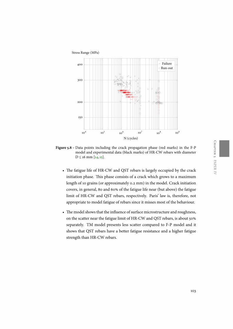
Chapter5

PAPER

IV

104 105 106 107 108 109

150

200

300

400

N (cycles)

Stress Range (MPa)

FailureRun-out

Figure 5.8 –Data points including the crack propagation phase (red marks) in the F-Pmodel and experimental data (black marks) of HR-CW rebars with diameterD ≤ 16 mm [14, 15].

• he fatigue life of HR-CW and QST rebars is largely occupied by the crackinitiation phase. his phase consists of a crack which grows to a maximumlength of 10 grains (or approximately 0.2 mm) in themodel. Crack initiationcovers, in general, 80 and 60% of the fatigue life near (but above) the fatiguelimit of HR-CW and QST rebars, respectively. Paris’ law is, therefore, notappropriate to model fatigue of rebars since it misses most of the behaviour.

• hemodel shows that the inuence of surfacemicrostructure and roughness,on the scatter near the fatigue limit ofHR-CW andQST rebars, is about 50%separately. TM model presents less scatter compared to F-P model and itshows that QST rebars have a better fatigue resistance and a higher fatiguestrength than HR-CW rebars.

103

Chapter5

PAPER

IV

104 105 106 107 108 109

150

200

300

400

N (cycles)

Stress Range (MPa)

FailureRun-out

Figure 5.9 –Data points including the crack initiation phase (green marks: fatigue cracksize = 1 grain; blue marks: fatigue crack size = 0.2 mm) in the TM model andexperimental data (black marks) of QST rebars with diameter D ≤ 16 mm [9,16, 17].

104 105 106 107 108 109

150

200

300

400

N (cycles)

Stress Range (MPa)

FailureRun-out

Figure 5.10 –Data points including the crack propagation phase (red marks) in the TMmodel and experimental data (black marks) ofQST rebars with diameterD ≤16 mm [9, 16, 17].

104

Chapter5

PAPER

IV

−4 −2 0 2 4

⋅106

180

200

220

240260

280∆σ

all

−4 −2 0 2 4

⋅106

180

200

220

240260

280microstructure

−4 −2 0 2 4

⋅106

180

200

220

240260

280

∆σ

m i/m1

−4 −2 0 2 4

⋅106

180

200

220

240260

280grain size

−4 −2 0 2 4

⋅106

180

200

220

240260

280

∆N

∆σ

roughness

−4 −2 0 2 4

⋅106

180

200

220

240260

280

∆N

phases

Figure 5.11 – Inuence of the - 1) Microstructure and roughness together (all); 2) Mi-crostructure, including grain orientation ratio mi/m1, grain size variation,phases (ferrite-pearlite); 3) Each parameter of the microstructure separatelyand 4) Surface roughness - on the scatter obtained in the F-P model.

105

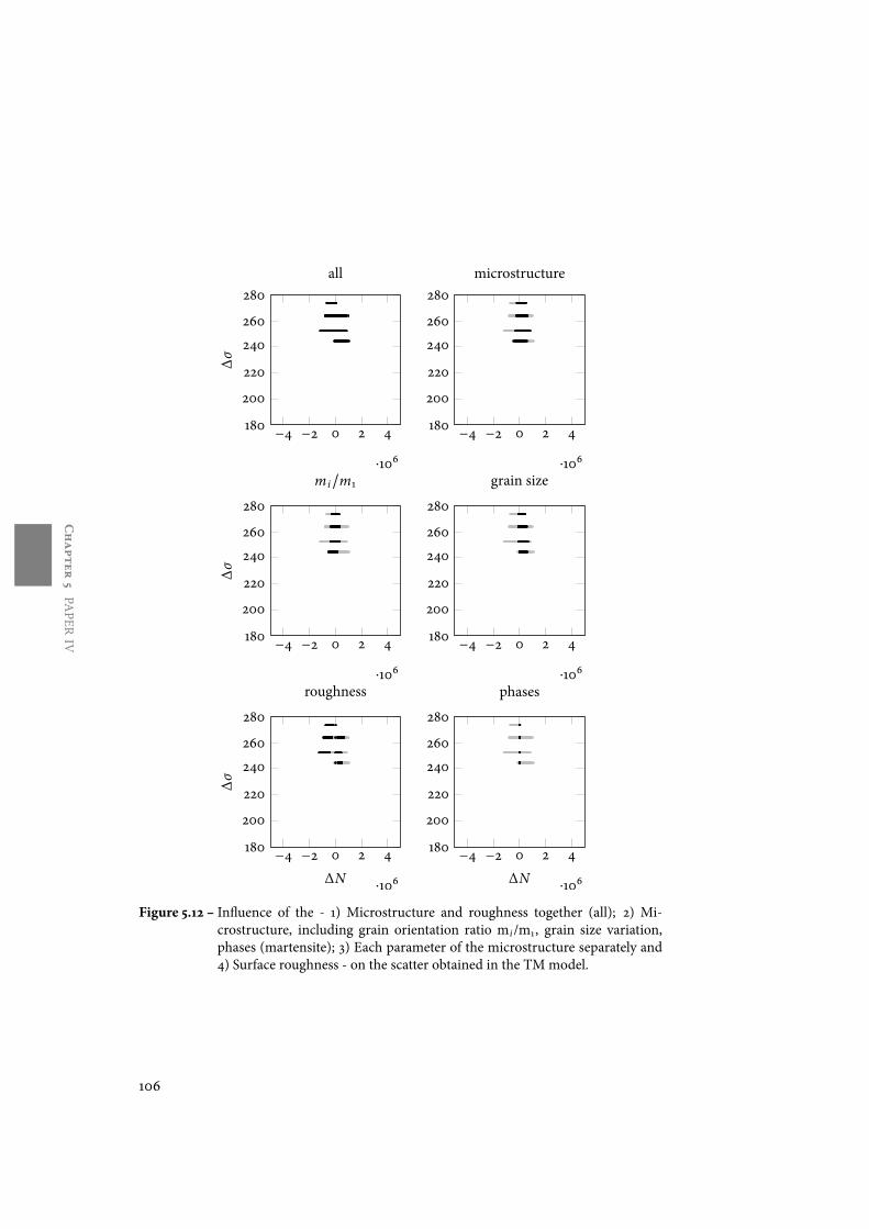
Chapter5

PAPER

IV

−4 −2 0 2 4

⋅106

180

200

220

240260

280

∆σ

all

−4 −2 0 2 4

⋅106

180

200

220

240260

280microstructure

−4 −2 0 2 4

⋅106

180

200

220

240260

280

∆σ

m i/m1

−4 −2 0 2 4

⋅106

180

200

220

240260

280grain size

−4 −2 0 2 4

⋅106

180

200

220

240260

280

∆N

∆σ

roughness

−4 −2 0 2 4

⋅106

180

200

220

240260

280

∆N

phases

Figure 5.12 – Inuence of the - 1) Microstructure and roughness together (all); 2) Mi-crostructure, including grain orientation ratio mi/m1, grain size variation,phases (martensite); 3) Each parameter of the microstructure separately and4) Surface roughness - on the scatter obtained in the TM model.

106

BIBLIOGRA

PHY

Bibliography

[1] Milne, I., Ritchie, R. O., & Karihaloo, B. L. (2003). Comprehensive structuralintegrity: Cyclic loading and fatigue. Elsevier.

[2] Rocha,M., Bruhwiler, E., & Nussbaumer A. Microstructural inuence on thescatter in the fatigue life of steel reinforcement bars.

[3] Frost,N. E., & Dugdale, D. S. (1957). Fatigue tests on notchedmild steel plateswith measurements of fatigue cracks. Journal of the Mechanics & Physics ofSolids, 5(3), 182-192.

[4] Yates, J.R., & Brown,M. W. (1987). Prediction of the length of non propagatingfatigue cracks. Fatigue& Fracture of EngineeringMaterials& Structures,10(3),187-201.

[5] Taira, S., Tanaka, K., & Hoshina, M. (1979). Grain size eòect on crack nu-cleation and growth in long-life fatigue of low-carbon steel. ASTM STP, 675,135-173.

[6] Vallellano, C., Navarro, A., & Dominguez, J. (2000). Fatigue crack growththreshold conditions at notches-Part I: heory. Fatigue & Fracture of Engi-neering Materials & Structures, 23(2), 113-122.

[7] Hussain, K., De Los Rios, E. R., & Navarro, A. (1993). A two-stage mi-cromechanics model for short fatigue cracks. Engineering FractureMechan-ics, 44(3), 425-436.

[8] Arola, D., &Williams, C. L. (2002).Estimating the fatigue stress concentrationfactor ofmachined surfaces. International Journal of Fatigue, 24(9), 923-930.


107

BIBLIOGRA

PHY


[11] Rocha,M., Bruhwiler, E., &Nussbaumer A. Material and geometrical charac-terisation of quenched and self-tempered steel reinforcement bars.

[12] Schijve, J. (2001). Fatigue of structures andmaterials.Dordrecht: KluwerAca-demic.






[18] Jhamb, I. C., &MacGregor, J. G. (1974). Stress concentrations caused by rein-forcing bar deformations. ACI Special Publication, 41-8, 169-182.

108

Chapter6CO

NCLU

SION

Chapter 6

Conclusion

6.1 Introduction

his thesis applies concepts of the mechanics of materials and material engineer-ing to deûne micro and macro structural aspects aòecting the fatigue strength ofdiòerent type of steel reinforcement bars (rebars). It provides advancements in thestructural engineering methods used for fatigue life prediction. his research in-cludes fatigue tests at very high number of stress cycles, micro-macro structuralcharacterisation of rebars and an analytical model which predicts themain param-eters inuencing the fatigue behaviour of rebars.

6.2 Response to research questions

he main thesis contribution and ûndings to the research questions raised in Sec-tion 1.1 are concluded in this sub-chapter.

6.2.1 Fatigue testing

Experimental test data are used as reference to predict the fatigue behaviour of re-bars in concrete structures. Axial tests of rebars alone have the advantage to beperformed at very high number of stress cycles, i.e., greater than 10 million, at re-duced time – and consequently costs – compared to fatigue tests with rebars em-bedded in concrete. However, axial fatigue tests are very sensitive to the grip ar-rangement which can lead to a rebar failure which isn’t characteristic of the properfatigue searched behaviour. his research shows that conical grip is the most ef-fectivemethod preventing premature failure of the rebar inside the grip area. QSTrebars mostly survived to a number of cycles exceeding 30 million at stress rangelevels of approximately 50% of their mean yield strength.

109

Chapter6CO

NCLU

SION

hemethod used for fatigue crack detection on these survival rebars, based onthe application of the liquid penetrant testing (LPT) with an abrupt monitored fre-quency change (representative of fractured rebars), was ineòective. Survival rebarsdon’t show any abrupt frequency change; indeed, the frequency reaches a stabiliza-tion regime from about 1 million cycles on and kept nearly constant during thewhole test. Moreover, LPT is a conservative method that can only detect ratherlarge surface cracks of at least 5 mm length.

Surface imperfections were the determinant factor that led to the fracture ofrebars, at similar stress ranges as applied for survival rebars. hese imperfectionsare produced during the manufacturing process and located near the transversalribs, in the zone of highest stress concentrations. Precisions regarding these surfaceimperfections are given in the next section.

6.2.2 Micro-macro structural characterisation

Conditions of the surface layer aremost signiûcant for the fatigue behaviour of re-bars since fatigue cracks tend to initiate on the surface. his study provides newinformation on micro and macro surface aspects of QST rebars including experi-mental analyses of surface residual stresses and imperfections. he inuence of ge-ometric parameters on the stress concentration factors Kt at the rebar surface wasinvestigated by 3D Finite Element (FE) analyses. A parametric study using 3D FEmodels allowed to determine the inuence of rib inclination and rebar size on theKt values of the critical zones. here were no references with similar studies of thesurface residual stress, imperfections and 3D FE analysis of the geometric Kt in theliterature.

In this research, themicrostructure ofQST rebars was identiûed under OpticalMicroscopy and quantiûed for diòerent rebar diameters. he analyses showed thatthe average grain size tends to increase with the increase of the rebar diameter.

Macroscopic residual stresses (type I) were experimentally determined on sur-face and subsurface of QST rebars by X-ray diòraction and Cut Compliance tech-niques. Residual stresses were found to be random tensile and compressive stresseswith values no higher than 20% of their yield strength.

Surface imperfections and roughness, analysed under Scanning Electron Mi-croscopy (SEM), are mainly located near the transversal ribs. he imperfectionscan be of diòerent type:

• Marks near the transversal ribs;

110

Chapter6CO

NCLU

SION

• Marks with semi-circular shape near the transversal ribs;

• Cracks near the marks with some cracks perpendicular to the rebar axis.Cracks were also ûnd perpendicular to the longitudinal ribs.

hese imperfections are introduced in the rollingmill when the ribs are formed andthey may also result from the water quenching process.

his research shows how the rib geometry and rebar diameter aòects Kt valueson the rebar surface. hehighestKt are located at the rib radius zone. hemaximumKt values at this zone aremainly aòected by the rib radius and height.

he highest Kt values determined along the rib base increase with increasingrebar. he inuence of the rebar diameter on these Kt values is comparable to thechanges in the rib radius and height. he maximum Kt for QST rebars geometrywith diameters of 10 and 26 mm are approximately 1.6 and 2.5, respectively. heeòect of the rebar diameter on the size of the critical zone is less signiûcant than theinuence of rib radius and height.

he rib inclination is themain parameter aòecting the position of themaximumKt and size of the critical zone along the rib. he critical zones (deûned as zoneswhere Kt are at least 95% of the maximum values) are located anti-symmetricallyalong the rib. However, the position of the maximum Kt tends to move to the ribcentre and the size of the critical zone increases if the rib inclination becomes moreandmore perpendicular to the rebar axis.

6.2.3 Analytical model-part I

he scatter present in fatigue test results of rebars can be inuenced by the sensitiv-ity of the short crack growth to themicrostructural features. his thesis proposes anadaptedNavarro andDe Los Rios (N-R) model within aMonte-Carlo framework toinvestigate the scatter above and near the fatigue limit on HR, CW andQST rebars.he N-R model, adapted in this work, incorporates the dispersion of the grain ori-entation ratiomi/m1, grain size variation and two phases (ferrite and pearlite) in thecase of HR-CW rebars. A mi/m1 equation is developed to take into account crackclosure eòects and the variation of the grain orientations. Although N-R model hasbeen extensively used for fatigue life prediction of metals, there are no referencesin the literature where the dispersion ofmicrostructural features have been consid-ered to analyse scatter in fatigue. Moreover, there are no references where a shortcrack growth model have been applied to study the scatter found in fatigue testingof rebars.

111

Chapter6CO

NCLU

SION

he developed approach shows that surface martensite contributes to reducethe scatter in fatigue tests with rebars compared to ferrite-pearlite microstructurefound on the surface ofHR-CW rebars. Surfacemicrostructure aòects to about 50%the scatter present in the fatigue tests for both HR-CW and QST rebars.

6.2.4 Analytical model-part II

he adapted N-R model in Section 6.2.3 is modiûed to include:

• the surface roughness eòect in order to explain the diòerence in the scatterfound in the analyses with the surfacemicrostructure;

• a linear crack propagation phase where the eòect ofmicrostructural featuresis negligible in the crack growth.

he stress concentration factor from the rib geometry is considered as a constantparameter. his approach allowsmore realistic comparisons betweenmodel and ex-perimental data. hemodel predicts the fatigue behaviour ofHR-CW andQST re-bars including fatigue crack initiation (cyclic slip, nucleation and short crack growth)and propagation (macro crack) phases.

his model shows fatigue behaviour predictions similar to test results for HR-CW and QST rebars. he main ûnding is that the fatigue life of rebars is largelyoccupied by the crack initiation phase during which the application of Paris’ law isinfeasible.

his modelling demonstrates that QST rebars have a better fatigue resistanceand a higher fatigue strength than HR-CW rebars. he standard S-N curves [1],used for safety veriûcation, are nowadays classiûed according to the rebar size butthere is no distinction between the fatigue strength ofHR-CW andQST rebars. hisapproach is conservative and it is recommended to classify S-N curves according tothe rebar type and size.

Fatigue cracks tend to initiate at the zone close to the ribs [2], [3], where thehighest stress concentrations are present. he stress concentrations resulting fromthe rib geometry combined with the surface roughness near the ribs lead to a sig-niûcant reduction on the fatigue strength of rebars. As a consequence, this ûndingsuggests the use of plain rebars with surface martensite microstructure for fatiguerelevant structures.

112

Chapter6CO

NCLU

SION

6.3 Future work

6.3.1 Fatigue crack detection

One of the greatest challenges in fatigue testing of rebars is the detection of cracksor microcracks, during or aer the tests, in particular run-out tests. he methodsused for crack detection are not eõcient and therefore investigations are requiredin this area. One possible solution is to investigate the use of nanoparticles, in lowsurface tension solution, with further X-ray micro computed tomography analyses.

6.3.2 Grain orientation ratio

In this study, the equation proposed for the grain orientation ratio mi/m1 was de-veloped for randomly oriented grains. However, it is possible thatHR, CW andQSTrebars may show a preferential crystallographic orientation in the rolling direction.To provide more accurate microstructural information for the short crack growthmodelling, the crystallographic texture of HR, CW and QST rebars could be de-termined by X-ray diòraction technique. Further research is needed on the eòectof R-ratio in the fatigue behaviour of rebars. As given in [4], the mi/m1 factor isaòected by crack closure which partially governs the material resistance to fatiguedamage. However, experimental data in the literature is still rather scarce for R-ratiogreater than 0.2. he crack closure eòect could be included in the mi/m1 equationin the N-R model as proposed in this thesis.

6.3.3 Surface roughness

Further work is required in generating more information on the surface roughnessproûle near and between the ribs. his information could providemore accuracy onthe eòect of the surface roughness on the scatter present in fatigue tests and improvethe fatigue behaviour prediction.

6.3.4 Fatigue behaviour modelling-other methods

For further modelling of fatigue behaviour, it is suggested to use the formulationproposed by Vallellano et al. [5] for non-symmetric conditions. Finite element (FE)modelling could be another promising method for amore detailed investigation onthe stress ûeld at each step of the short crack propagation, including the eòect oflocal microresidual stresses, into and at the grain boundary. FEmethod has also theadvantage to allow for the study of crack coalescence since the stress distribution of

113

Chapter6CO

NCLU

SION

the grains, of an analysed area, would not be uniform andmicro cracks could startsimultaneously at diòerent grains.

he eòect of variable amplitude loading could be studied by detailedmodellingin parallel with lab tests to give a better understanding on the fatigue behaviour ofrebars under the condition representative for structures subjected to fatigue.

114

BIBLIOGRA

PHY

Bibliography

[1] Model code 2010-ûnal dra, ûb, Bulletin N°65, Vol.1.



[4] Vallellano, C., Navarro, A., Garcıa-Lomas, F. J., & Domınguez, J. (2008). Onthe estimation ofmicrostructural eòects in the near-threshold fatigue of smallcracks. he Journal of Strain Analysis for Engineering Design, 43(5), 337-347.

[5] Vallellano, C.,Navarro, A., & Domınguez, J. (2002).Compact formulation formodelling cracks in inûnite solids using distributed dislocations. Philosophi-cal magazine A, 82(1), 81-92.

115

BIBLIOGRA

PHY

116

Appendix

ASTRESS-STRA

INCU

RVE

Appendix A

Stress-Strain curve

Figure A.1 – Stress × Strain curve of a QST rebar analysed in this thesis.

117

Appendix

ASTRESS-STRA

INCU

RVE

118

Appendix

BREBA

RK

T

Appendix B

Rebar Kt

Appendix A presents 3D Finite Element Models of the rebar geometry consideredin the parametric study. he graphs given in this Appendix shows the evolution ofthe stress concentration factor, Kt , determined for the paths illustrated in Fig. B.1.Finite Element analyses were performed with Abaqus/CAE 6.12.

46°

64°54°

Figure B.1 – Paths (darker lines) where Kt evolution was determined.

119

Appendix

BREBA

RK

T

B.1 D10h03r02

(a) (b)

0 0.2 0.4 0.6 0.8 1

1.2

1.4

1.6

Normalized distance along OR

Kt

46o

54o

64o

(c) (d)

Figure B.2 –D10h03r02 model: (a) 3D FEmesh (b) Top view (c) Kt plot (d) Bottom view.

120

Appendix

BREBA

RK

T

B.2 D10h08r02

(a) (b)

0 0.2 0.4 0.6 0.8 1

0.8

1

1.2

1.4

1.6

1.8

2


Kt

46o

54o

64o

(c) (d)


121

Appendix

BREBA

RK

T

B.3 D10h08r04

(a) (b)

0 0.2 0.4 0.6 0.8 1

1

1.2

1.4

1.6


Kt

46o

54o

64o

(c) (d)


122

Appendix

BREBA

RK

T

B.4 D10h15r04

(a) (b)

0 0.2 0.4 0.6 0.8 1

1

1.5

2


Kt

46o

54o

64o

(c) (d)


123

Appendix

BREBA

RK

T

B.5 D10h08

(a) (b)

0 0.2 0.4 0.6 0.8 1

0.5

1

1.5

2


Kt

46o

54o

64o

(c) (d)

Figure B.6 –D10h08model: (a) 3D FEmesh (b) Top view (c) Kt plot (d) Bottom view.

124

Appendix

BREBA

RK

T

B.6 D16h03r02

(a) (b)

0 0.2 0.4 0.6 0.8 1

1.2

1.4

1.6

1.8


Kt

46o

54o

64o

(c) (d)


125

Appendix

BREBA

RK

T

B.7 D16h08r02

(a) (b)

0 0.2 0.4 0.6 0.8 1

1

1.5

2


Kt

46o

54o

64o

(c) (d)


126

Appendix

BREBA

RK

T

B.8 D16h08r04

(a) (b)

0 0.2 0.4 0.6 0.8 1

1

1.2

1.4

1.6

1.8


Kt

46o

54o

64o

(c) (d)


127

Appendix

BREBA

RK

T

B.9 D16h08r08

(a) (b)

0 0.2 0.4 0.6 0.8 11

1.2

1.4

1.6


Kt

46o

54o

64o

(c) (d)

Figure B.10 –D16h08r08model: (a) 3D FEmesh (b) Top view (c) Kt plot (d) Bottom view.

128

Appendix

BREBA

RK

T

B.10 D16h08

(a) (b)

0 0.2 0.4 0.6 0.8 1

0.5

1

1.5

2

2.5


Kt

46o

54o

64o

(c) (d)

Figure B.11 –D16h08model: (a) 3D FEmesh (b) Top view (c) Kt plot (d) Bottom view.

129

Appendix

BREBA

RK

T

B.11 D16h08r04c04

(a) (b)

0 0.2 0.4 0.6 0.8 1

1

1.2

1.4

1.6

1.8

2


Kt

46o

54o

64o

(c) (d)

Figure B.12 –D16h08r04c04 model: (a) 3D FE mesh (b) Top view (c) Kt plot (d) Bottomview.

130

Appendix

BREBA

RK

T

B.12 D16h08r04c12

(a) (b)

0 0.2 0.4 0.6 0.8 1

1

1.2

1.4

1.6

1.8


Kt

46o

54o

64o

(c) (d)

Figure B.13 –D16h08r04c12 model: (a) 3D FE mesh (b) Top view (c) Kt plot (d) Bottomview.

131

Appendix

BREBA

RK

T

B.13 D26h03r02

(a) (b)

0 0.2 0.4 0.6 0.8 11

1.2

1.4

1.6

1.8

2


Kt

46o

54o

64o

(c) (d)


132

Appendix

BREBA

RK

T

B.14 D26h08r02

(a) (b)

0 0.2 0.4 0.6 0.8 1

1

1.5

2

2.5


Kt

46o

54o

64o

(c) (d)


133

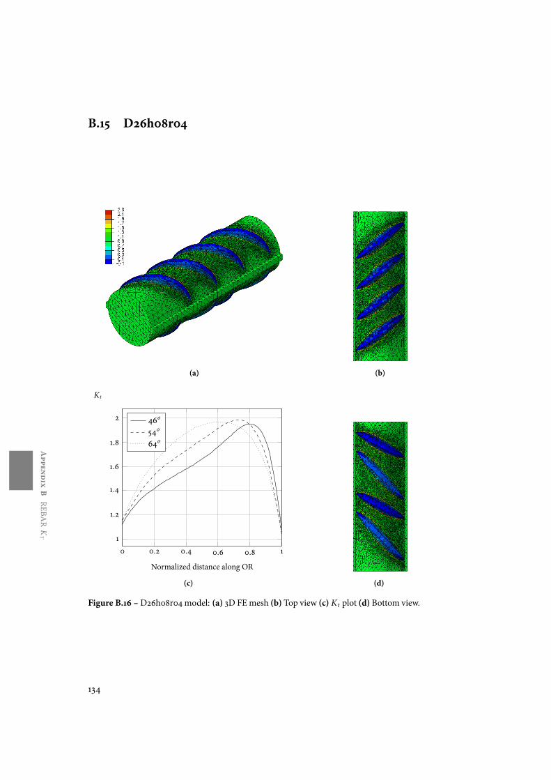
Appendix

BREBA

RK

T

B.15 D26h08r04

(a) (b)

0 0.2 0.4 0.6 0.8 11

1.2

1.4

1.6

1.8

2


Kt

46o

54o

64o

(c) (d)


134

Appendix

BREBA

RK

T

B.16 D26h15r04

(a) (b)

0 0.2 0.4 0.6 0.8 1

1

1.5

2

2.5


Kt

46o

54o

64o

(c) (d)


135

Appendix

BREBA

RK

T

B.17 D26h15r08

(a) (b)

0 0.2 0.4 0.6 0.8 1

1

1.5

2


Kt

46o

54o

64o

(c) (d)


136

Appendix

CM

ODEL

Appendix C

Model

ContentsC.1 File experiment.m . . . . . . . . . . . . . . . . . . . . . . . . . 138

C.2 FilemainNR.m . . . . . . . . . . . . . . . . . . . . . . . . . . . 140

C.3 File classTM.m . . . . . . . . . . . . . . . . . . . . . . . . . . . 159

C.4 File classFP.m . . . . . . . . . . . . . . . . . . . . . . . . . . . . 167

Appendix B presents the algorithm developed for the analytical model used inthe analyses given in Chapters 4 and 5.

experiment.m

.m mainNR.m.m.m

.mclassTM.m

.mclassFP.m

.m.m.ma

b

c

d

Figure C.1 –Model ûles: (a) ûle containing the input function to run an experiment; (b) theprocess will occur simultaneously in parallel on each core; (c) ûle containingall the function for the Voronoi structure and the propagation algorithm; (d)two ûles containing a class with properties for each of the two steels: TM& FP.

137

Appendix

CM

ODEL

C.1 File experiment.m

1 % experiment.m file

2 % this is the main input function

3 % Examples:

4 % experiment(10,400,[180:200],1);

5 % experiment(10,400,linspace(180,200,1),1);

6

7 function matrix = experiment( N, points, applied stress, is martensite )

8

9 matlabpool local;

10

11 number of tests = N*numel(applied stress);

12 matrix = zeros(8,number of tests);

13

14 value time1 = clock;

15

16 value ten = applied stress(1);

17 parfor i = 1:3*3

18 mainNR( value ten,points, is martensite );

19 end

20

21 value time2 = clock;

22 print estimation time(number of tests,value time1,value time2);

23

24 tic

25

26 % parallel for loop (each step is an experiment)

27 parfor i = 1:number of tests

28 current stress = return stress(applied stress,i,N);

29

30 [mem,~] = mainNR( current stress,points , is martensite );

31

32 matrix(:,i) = [current stress rot90(mem)];

33 end

34

35 figure;

36 scatter(log10(matrix(2,:)),matrix(1,:),20);

37

38 figure;

39 %plot run-outs by applied stress

40 B=matrix(1:2,:);

41 B=(B==100000000);

42 %get N values

43 Ns=matrix(B);

44 %get S values

45 m1=B(2,:);

46 m2=zeros(7,length(B(2,:)));

47 matrix select=cat(1,m1,m2);

48 Ss=matrix( matrix select==1 );

138

Appendix

CM

ODEL

49 %plot S-N curve

50 hist(cat(1,rot90(Ss)));

51

52 toc

53

54 matrix = rot90(matrix);

55

56 matlabpool close;

57 end

58

59 function result = return stress(app,i,N)

60 result = app(ceil(i/N));

61 end

62

63 function print estimation time(number of tests,value time1,value time2)

64 init = value time1(5)*60 + value time1(6);

65 stop = value time2(5)*60 + value time2(6);

66

67 time int = (stop - init)/(3*3);

68 total = floor(time int*number of tests);

69

70 value time3 = value time2;

71 value time3(4) = floor(total/3600)+value time3(4);

72 value time3(5) = floor(mod(total,3600)/60+value time3(5));

73 value time3(6) = floor(mod(mod(total,3600),60)+value time3(6));

74

75 if value time3(6) >= 60

76 value time3(5) = value time3(5) + floor(value time3(6)/60);

77 value time3(6) = mod(value time3(6),60);

78 end

79


81 value time3(4) = value time3(4) + floor(value time3(5)/60);


83 end

84



87 end

88

89 disp(['-> It will take ',num2str(total),' seconds, for ...

',num2str(number of tests),' essays.']);

90 disp(['-> from ',num2str(value time2(4)), ':', ...

num2str(value time2(5)), ':', num2str(floor(value time2(6))), ...

' to ', num2str(value time3(4)), ':', num2str(value time3(5)), ...

':', num2str(floor(value time3(6)))]);

91 end

139

Appendix

CM

ODEL

C.2 FilemainNR.m

1 % mainNR.m file

2 % this is the main input function

3 % Examples:

4 % [NumberCycles, Structure] = mainNR(49, 1000);5 % and to use an already made "Structure":

6 % [NumberCycles, Structure] = mainNR(Structure);

7

8 function [result navarro, structure data] = mainNR( varagin, ...

is martensite )

9

10 %constants

11 global calculus error;

12 global print slipbands during propagation;

13 global plot result;

14 global load orientation;

15 global global dmean;

16 global number of grains to break;

17 global propagation model;

18 global scale structure;

19

20 result navarro = zeros(7,1);

21

22 load orientation = 0;

23 calculus error = 1.0e-10;

24

25 plot result = false;

26 print slipbands during propagation = false;

27 number of grains to break = 10;

28 global dmean = [0 0];

29 scale structure = 1;

30

31 linear propagation=true;

32 second grain limit=300;

33

34 %experiment statistics

35 statistics matrix=ones(2,15,4);

36

37 %tic

38

39 if length(varagin) == 2

40 applied stress = varagin1; point number = varagin2;41 %create the grain structure

42 [V, C, points, sb, maxgrainx, maxgrainy, maxgrain, maxfirstsb] = ...

create structure(point number);

43 elseif length(varagin) == 11

44 applied stress = varagin1; point number = varagin2; V = ...

varagin3;C = varagin4; points = varagin5; sb = ...

varagin6; maxgrainx = varagin7; maxgrainy = varagin8; ...

140

Appendix

CM

ODEL

maxgrain = varagin9; maxfirstsb = varagin10; global dmean ...

= varagin11;45 else

46 return;

47 end

48

49 if is martensite==1

50 propagation model = classTM(applied stress, load orientation);

51 else

52 propagation model = classFP(applied stress, load orientation);

53 end

54

55 PL Structure = containers.Map( - 1, 1, struct('grain id', maxgrain, ...

'slipband id', maxfirstsb, 'init point', points(maxgrain, :), ...

'end point', [maxgrainx(1) maxgrainy(1)], 'length', ...

distance segment(points(maxgrain, 1), points(maxgrain, 2), ...

maxgrainx(1), maxgrainy(1)), 'total length', ...


maxgrainx(1), maxgrainy(1)), 'angle', ...

get angle with coordinates(points(maxgrain, 1), points(maxgrain, ...

2), maxgrainx(1), maxgrainy(1)), 'is border', false), ...

struct('grain id', maxgrain, 'slipband id', maxfirstsb, ...

'init point', points(maxgrain, :), 'end point', [maxgrainx(2) ...

maxgrainy(2)], 'length', distance segment(points(maxgrain, 1), ...

points(maxgrain, 2), maxgrainx(2), maxgrainy(2)), 'total length', ...


maxgrainx(2), maxgrainy(2)), 'angle', ...

get angle with coordinates(points(maxgrain, 1), points(maxgrain, ...

2), maxgrainx(2), maxgrainy(2)), 'is border', false));56 Crack Structure = containers.Map(0, struct('c', 0, 'd mean', 0, ...

'nc', 0, 'ac', 0, 'ns', 0, 'dN', 0, 'N', 0, 'is blocked', false));57

58 if plot result

59 if length(get(0, 'children'))>1

60 figure(2);

61 clf;

62 figure(1);

63 clf;

64 end

65 plot structure(V, C, points);

66 %plot initial point

67 plot(PL Structure(1).init point(1), PL Structure(1).init point(2), ...

'*', 'Color', 'black', 'linewidth', 4);%, 'LineSmoothing', 'on');

68 %plot slipbands(V, C, points, sb);

69 end

70

71 side ok = [true true];

72 current a = [0 0];

73 current plastified grain step = [0 0];

74 lastminDaDN = - 1;

75

76 d mean stop = global dmean(1, 1);

141

Appendix

CM

ODEL

77

78 while sum(current a) < number of grains to break*d mean stop && ...

(side ok(1, 1) == true | | side ok(1, 2) == true)

79

80 if (Crack Structure(current plastified grain step(1, 1)).N <= ...

Crack Structure(current plastified grain step(1, 2)).N && ...

(side ok(1, 1) == true && side ok(1, 2) == true)) | | ...

(side ok(1, 1) == true && side ok(1, 2) == false)

81 index = 1;

82 current plastified grain step(1, index) = ...

current plastified grain step(1, index)+1;

83 else

84 index = 2;


current plastified grain step(1, index)-1;

86 end

87

88 if plot result

89 plot plastic zone(current plastified grain step(1, index), ...

PL Structure);

90 end

91

92 PL Structure = preferential line(V, C, sb, PL Structure, ...

current plastified grain step(1, index));

93 [propagation model, Crack Structure, side ok res, matrix disp] = ...

propagation model.is propagating(current plastified grain step(1, ...

index), current plastified grain step(1, mod(index, 2)+1), ...

side ok, Crack Structure, PL Structure);

94

95 %statistics

96 statistics matrix(index,abs(current plastified grain step(1, ...

index)),:)=matrix disp;

97

98 if plot result

99 disp(['PLASTIC ZONE: ', ...

num2str(current plastified grain step(1, index))]);

100 disp(PL Structure(current plastified grain step(1, index)));

101 disp(['CRACK INCREMENT: ', ...


102 disp(Crack Structure(current plastified grain step(1, index)));

103 end

104

105 %when dN<=0, don't compute the dadN function

106 if plot result && side ok(1, index) == true && ...

Crack Structure(current plastified grain step(1, index)).dN<=0

107 side ok(1, index) = false;

108 if index == 1;


current plastified grain step(1, index)-1;

110 else


current plastified grain step(1, index)+1;

142

Appendix

CM

ODEL

112 end

113 end

114

115 if ((Crack Structure(current plastified grain step(1, 1)).N<= ...

Crack Structure(current plastified grain step(1, 2)).N) && ...

(side ok(1, 1) == true && side ok(1, 2) == true)) | | ~...(side ok(1, 1) == true && side ok(1, 2) == true)

116 current a(1, 1) = ...

Crack Structure(current plastified grain step(1, 1)).ac;

117 end

118 if ((Crack Structure(current plastified grain step(1, 2)).N<= ...

Crack Structure(current plastified grain step(1, 1)).N) && ...

(side ok(1, 1) == true && side ok(1, 2) == true)) | | ~...(side ok(1, 2) == true && side ok(1, 1) == true)

119 current a(1, 2) = ...

Crack Structure(current plastified grain step(1, 2)).ac;

120 end

121

122 if plot result && abs(current plastified grain step(1, 1))>0 && ...

abs(current plastified grain step(1, 2))>0

123 lastminDaDN = plotdadN(current plastified grain step, ...

Crack Structure, PL Structure, lastminDaDN);

124 end

125

126 %update here for the next step only (when the fracture stops or

127 %arrives at the border

128 side ok = side ok res;

129 if plot result && side ok(1, index) == false

130 disp(['The crack stops at step ', ...


131 end

132 if PL Structure(current plastified grain step(1, index)).is border ...

== true

133 side ok(1, index) = false;

134 if plot result

135 disp(['The crack arrives at the border at step ', ...


136 end

137 end

138

139 if plot result && abs(current plastified grain step(1, 1))>0 && ...

abs(current plastified grain step(1, 2))>0

140 d mean stop = (abs(current plastified grain step(1, ...

1))*Crack Structure(current plastified grain step(1, ...

1)).d mean+abs(current plastified grain step(1, ...

2))*Crack Structure(current plastified grain step(1, ...

2)).d mean)/(abs(current plastified grain step(1, ...

1))+abs(current plastified grain step(1, 2)));

141 end

142

143 %store the value when the first grain breakes

144 if abs(current plastified grain step(1, 1))==1 && ...

143

Appendix

CM

ODEL

abs(current plastified grain step(1, 2))==1

145 result navarro(2) = ...

max([Crack Structure(current plastified grain step(1, ...

1)).dN Crack Structure(current plastified grain step(1, ...

2)).dN]);

146 end

147 end

148

149 if PL Structure(current plastified grain step(1, 1)).is border

150 side ok(1, 1) = true;

151 elseif PL Structure(current plastified grain step(1, 2)).is border

152 side ok(1, 2) = true;

153 end

154

155 Ntotal = max([Crack Structure(current plastified grain step(1, 1)).N ...

Crack Structure(current plastified grain step(1, 2)).N]);

156

157 if side ok(1, 1) == true | | side ok(1, 2) == true

158 if plot result

159 disp(['Propagation part: it breakes at N propa = ', ...

num2str(Ntotal, '%10.5e\n')]);160 end

161 else

162 Ntotal = 10ˆ8;

163 if plot result

164 disp(['Propagation part: the cracks stops before N = ', ...

num2str(Ntotal, '%10.5e\n')]);165 end

166 end

167

168 %statistics

169 result navarro(1) = Ntotal;

170 result navarro(3) = Ntotal;

171 if(Crack Structure(current plastified grain step(1, ...

1)).N>Crack Structure(current plastified grain step(1, 2)).N)

172 stat mat=statistics matrix(1,1:abs(current plastified grain step(1, ...

1)),:);

173 stat mat=reshape(stat mat,[abs(current plastified grain step(1, ...

1)) 4]);

174 else

175 stat mat=statistics matrix(2,1:abs(current plastified grain step(1, ...

2)),:);

176 stat mat=reshape(stat mat,[abs(current plastified grain step(1, ...

2)) 4]);

177 end

178 result navarro(4)=sum(stat mat(:,1));




182

183 structure data = applied stress, point number, V, C, points, sb, ...

maxgrainx, maxgrainy, maxgrain, maxfirstsb, global dmean;

144

Appendix

CM

ODEL

184 %toc

185

186 %linear propagation

187 if linear propagation==true && (side ok(1, 1) == true | | side ok(1, 2) ...

== true)

188 c=[Crack Structure(current plastified grain step(1, 1)).c ...

Crack Structure(current plastified grain step(1, 2)).c];

189 nc=[Crack Structure(current plastified grain step(1, 1)).nc ...

Crack Structure(current plastified grain step(1, 2)).nc];

190 ns=[0 0];

191 dN=[0 0];

192 while abs(current plastified grain step(1, ...

1))+abs(current plastified grain step(1, ...

2))<second grain limit && (side ok(1, 1) == true | | side ok(1, ...

2) == true)

193

194 for t=[-1 1]

195 index side = 1+(1-sign(t))/2;

196 if side ok(1, index side) == true

197 ns(index side)=c(index side)/(c(index side) + ...

d mean stop)*nc(index side);

198 c(index side)=c(index side)+d mean stop;

199 current plastified grain step(1, index side) = ...

current plastified grain step(1, index side)+t;

200 [dnRes,ncRes] = propagation model.compute long crack( ...

current plastified grain step( 1, index side ), c( ...

index side ), d mean stop,ns(index side) );

201 dN(index side)=dN(index side)+dnRes;

202 nc(index side)=ncRes;

203

204 if plot result

205 disp(['CRACK INCREMENT: ', ...

num2str(current plastified grain step(1, ...

index side))]);

206 end

207 end

208 end

209

210 end

211 result navarro(1)=result navarro(1)+max(dN);

212

213 if plot result

214 disp(['Linear part: N linear = ', num2str(max(dN), '%10.5e\n')]);215 end

216

217 end

218

219 end

220

221 function plot plastic zone(k, PL Structure)

222 if ~isempty(get(0, 'children'))

223 figure(1);

145

Appendix

CM

ODEL

224 else

225 figure('Name', 'Grain structure');

226 end

227

228 %for step 1 or - 1, the plastic zone is all the grain.

229 if abs(k) == 1

230 plot([PL Structure(1).end point(1) PL Structure(-1).end point(1)], ...

[PL Structure(1).end point(2) PL Structure(-1).end point(2)], ...

'Color', [0 0 0], 'linewidth', 4);%, 'LineSmoothing', 'on');

231 else

232 plot([PL Structure(k).init point(1) PL Structure(k).end point(1)], ...

[PL Structure(k).init point(2) PL Structure(k).end point(2)], ...

'Color', [0 0 0], 'linewidth', 4);%, 'LineSmoothing', 'on');

233 end

234 end

235

236 function plot crack(a p, a m, PL Structure)


238 figure(1);

239 else


241 end

242

243 for i = [1 -1]

244 current length = 0;

245 if i == 1

246 a = a p;

247 grain id = 1;

248 else

249 a = a m;

250 grain id = - 1;

251 end

252 if numel(a)>1

253 while current length<a(2)

254 new length = current length+PL Structure(grain id).length;

255 if a(1)<= new length

256 if a(1)>= current length && a(1)<new length

257 prop coef = (a(1) - ...

current length)/PL Structure(grain id).length;

258 points1 = [( PL Structure(grain id).end point(1) - ...

PL Structure(grain id).init point(1) ...

)*prop coef + ...

PL Structure(grain id).init point(1) ( ...

PL Structure(grain id).end point(2) - ...


)*prop coef + ...

PL Structure(grain id).init point(2)];

259 else

260 points1 = PL Structure(grain id).init point;

261 end

262 if a(2)>= current length && a(2)<new length

263 prop coef = (a(2) - ...

146

Appendix

CM

ODEL

current length)/PL Structure(grain id).length;

264 points2 = [( PL Structure(grain id).end point(1) - ...


)*prop coef + ...

PL Structure(grain id).init point(1) ( ...

PL Structure(grain id).end point(2) - ...


)*prop coef + ...

PL Structure(grain id).init point(2)];

265 else

266 points2 = PL Structure(grain id).end point;

267 end

268 if sign(i) == - 1, color = 'red'; else color = 'blue'; ...

end;

269 plot([points1(1) points2(1)], [points1(2) points2(2)], ...

'Color', 'white');

270 end

271 current length = current length+PL Structure(grain id).length;

272 grain id = grain id+1*i;

273 end

274 end

275 end

276 end

277

278 function mindaDN = plotdadN(steps, Crack Structure, PL Structure, mindaDN)

279

280 global propagation model;

281


283 figure(2);

284 else

285 figure('Name', 'da/dN');

286 end

287

288 offset alone = 0;%when the loop is only k

289

290 minX = [0 0];

291 maxX = [0 0];

292

293 if Crack Structure(steps(1, 1)).N >= Crack Structure(steps(1, 2)).N

294 k = steps(1, 1);l = steps(1, 2);

295 else

296 k = steps(1, 2);l = steps(1, 1);

297 end

298

299 %lap length computations

300 if Crack Structure(k - sign(k)).N > Crack Structure(l).N

301 loop = k;

302 %when a crack stops, fill the gap

303 if Crack Structure(k - 2*sign(k)).N <= Crack Structure(l).N

304 [propagation model, minX(1)] = ...

propagation model.crack position by dN(Crack Structure(l).N ...

147

Appendix

CM

ODEL

- Crack Structure(k - 2*sign(k)).N , Crack Structure(k - ...

sign(k)).ns, Crack Structure(k - sign(k)).c, k - sign(k), ...

l, Crack Structure, PL Structure);

305 else

306 minX(1) = Crack Structure(k - sign(k)).ac;

307 end

308 maxX(1) = Crack Structure(k).ac;

309 offset alone = Crack Structure(l).ac;

310 else

311 loop = [k l];

312 if Crack Structure(k - sign(k)).N>= Crack Structure(l - sign(l)).N

313 minX(1) = Crack Structure(k - sign(k)).ac;

314 maxX(2) = Crack Structure(l).ac;

315 %compute minX for l, when N = N(k - 1)


propagation model.crack position by dN(Crack Structure(k - ...

sign(k)).N - Crack Structure(l - sign(l)).N , ...

Crack Structure(l).ns, Crack Structure(l).c, l, k - ...

sign(k), Crack Structure, PL Structure);

317 %compute maxX for k, when N = N(l)

318 [propagation model, maxX(1)] = ...


- Crack Structure(k - sign(k)).N , Crack Structure(k).ns, ...

Crack Structure(k).c, k, l, Crack Structure, PL Structure);

319 else %all l - N segments are inside the k - N segment

320 minX(2) = Crack Structure(l - sign(l)).ac;

321 maxX(2) = Crack Structure(l).ac;


propagation model.crack position by dN(Crack Structure(l - ...

sign(l)).N - Crack Structure(k - sign(k)).N , ...

Crack Structure(k).ns, Crack Structure(k).c, k, l - ...

sign(l), Crack Structure, PL Structure);

323 [propagation model, maxX(1)] = ...


- Crack Structure(k - sign(k)).N , Crack Structure(k).ns, ...

Crack Structure(k).c, k, l, Crack Structure, PL Structure);

324 end

325 end

326

327 numb int points = 10;

328 X = [1:numb int points];

329 Y = zeros(numb int points, 1);

330 if size(loop) == 1

331 if sign(k) == 1, color = 'blue'; else color = 'red'; end;

332 else

333 if sign(k) == 1, color = 'red'; else color = 'blue'; end;

334 end

335

336 factorToMeterByCycle = 10ˆ-3; %because unity in Mpa (N/mm2)

337

338 if sum(maxX) ~= 0

339 for p = 1:numel(loop)

148

Appendix

CM

ODEL

340 i = loop(p);

341 step = (maxX(p) - minX(p))/(numb int points - 1);

342 for j = 1:numb int points

343 a = minX(p)+(j - 1)*step;

344 [propagation model, newdadn] = propagation model.dadN(a, ...

a/Crack Structure(i).c, k, l, Crack Structure, ...

PL Structure);

345 Y(j) = Y(j)+newdadn;

346 end

347 end

348 plot(sum(minX)+(sum(maxX) - sum(minX))/(numb int points - 1)*(X - ...

1) +offset alone, (Y*factorToMeterByCycle), 'black');

349 end

350

351 if mindaDN>0

352 plot([sum(minX)+offset alone sum(minX)+offset alone], ([mindaDN ...

Y(1)]*factorToMeterByCycle), 'black');

353 end

354

355 %grain boundaries

356 hold on;

357 X2 = (([Crack Structure(k).c+Crack Structure(l).c ...

Crack Structure(k).c+Crack Structure(l).c]));

358 Y2 = ([min(Y) max(Y)]*factorToMeterByCycle);

359 plot(X2, Y2, '--', 'Color', color);

360

361 %plot crack

362 if sign(k) == 1

363 plot crack([minX(1) maxX(1)], [minX(2) maxX(2)], PL Structure);

364 else

365 plot crack([minX(2) maxX(2)], [minX(1) maxX(1)], PL Structure);

366 end

367

368 mindaDN = min(Y);

369 end

370

371 %create the voronoi structure

372 function [V, C, points, sb, first slip band x, first slip band y, ...

init grain id, maxfirstsb angle index] = ...

create structure(point number)

373

374 points = zeros(point number, 2);

375 maxfirstsb angle index = -1;

376

377 %here to change the grain strucure

378 for a = 1:point number

379 %pointx(a) = random('norm', 0.5, 0.2);

380 %random

381 points(a, 1) = random('unif', -0.5, 1.5);

382 points(a, 2) = random('unif', -0.5, 1.5);

383 %hexa

384 %offset = mod(floor(a/sqrt(point number)), 2)/sqrt(point number);

149

Appendix

CM

ODEL

385 %points(a, 2) = 2.0*floor(a/sqrt(point number))/sqrt(point number) ...

- 0.5+1/sqrt(point number);

386 %points(a, 1) = 2.0*mod(a, sqrt(point number))/sqrt(point number) ...

- 0.5+offset;

387 %square


- 0.5;


- 0.5;

390 %web


- ...

0.5+2.0*floor(a/sqrt(point number))/sqrt(point number)/2.0*mod(a, ...

sqrt(point number));


- 0.5;

393 end

394

395 global scale structure;

396 %scale structure = 10ˆ - 3;

397 points = points*scale structure;

398

399 [V, C] = voronoin(points);

400

401 %sb = slip bands

402 %psb = first slip band

403 number of slip band = 3;

404 sb = zeros(point number, number of slip band);

405 for a = 1:point number

406 %psb = 0;

407 psb = random('unif', 0.0, pi/number of slip band);

408 for k = 1:number of slip band

409 sb(a, k) = psb+(k - 1)*pi/number of slip band;

410 end

411 end

412

413 maxlc = 0;

414 init grain id = 0;

415

416 first slip band x = 0;

417 first slip band y = 0;

418

419 for grain = 1:point number

420 if points(grain, 1)>0 && points(grain, 2)>0 && points(grain, ...

1)<1*scale structure && points(grain, 2)<1*scale structure

421 [grainx, grainy, sb index, sb angle] = find slip band( V, C, ...

grain, sb(grain, :), points(grain, 1), points(grain, 2), ...

[], 0 );

422 if numel(grainx)>1

423

424 sb length = distance segment(grainx(1), grainy(1), ...

grainx(2), grainy(2));

150

Appendix

CM

ODEL

425

426 %compute lc

427 lc = abs(sb length*cos(2*(pi/4 - (sb(grain, sb index)))));

428

429 if lc>maxlc

430 maxlc = lc;

431 init grain id = grain;

432 first slip band x = grainx;

433 first slip band y = grainy;

434 maxfirstsb angle index = sb index;

435 end

436 end

437 end

438 end

439

440 %compute the global grain mean size here


442 global dmean(1, 1) = global dmean(1, 1)/global dmean(1, 2);

443

444 end

445

446 %plot the voronoi structure

447 function plot structure(V, C, points)

448

449 %global scale structure;


451


453 figure(1);

454 else


456 end

457

458 for a = 1:length(points(:, 1))

459 hold on;

460 if (a>1)

461 %plot(pointx(a - 1:a), pointy(a - 1:a));

462 end

463 %text(points(a, 1), points(a, 2), num2str(a), 'FontSize', 8, ...

'Color', 'black');

464 end

465

466 hold on;

467 %plot(points(:, 1), points(:, 2), '*', 'Color', 'k', 'MarkerSize', 2);

468

469 %plot grain: if convhull raises an error, other method to draw the points.

470 try

471 for k = 1:length(C)

472 if all(Ck~= 1)

473 VertCell = V(Ck, :);

474 KVert = convhulln(VertCell);

475 patch('Vertices', VertCell, 'Faces', KVert, ...

151

Appendix

CM

ODEL

'FaceVertexCData', hsv(1), 'FaceColor', 'flat', ...

'EdgeColor', [0 0 0], 'LineWidth', ...

0.1);%'LineSmoothing', 'on');

476 end

477 end

478 catch errN

479 for j = 1:length(C)

480 b = Cj, :;481 number vert = size(b);

482 for i = 1:number vert(2)

483 hold on;

484 if (i>1)

485 plot([V(b(i-1), 1) V(b(i), 1)], [V(b(i-1), 2) V(b(i), ...

2)], 'Color', [0 0 0], 'LineWidth', 0.1);

486 else

487 plot([V(b(1), 1) V(b(number vert(2)), 1)], [V(b(1), 2) ...

V(b(number vert(2)), 2)], 'Color', [0 0 0], ...

'LineWidth', 0.1);

488 end

489 end

490 end

491 end

492

493 axis equal;

494 axis([ -0.5 1.5 -0.5 1.5]*scale structure);

495 end

496

497 %plot the slipbands

498 function plot slipbands(V, C, points, sb)

499 for grain = 1:length(points(:, 1))

500 find slip band( V, C, grain, sb(grain, :), points(grain, 1), ...

points(grain, 2), [], true );

501 end

502 end

503

504 %find the equation of the line

505 function [A, B] = line equation( X, Y )

506 A = (Y(1) - Y(2))/(X(1) - X(2));

507 B = Y(2) - A*X(2);

508 end

509

510 %give the length of the segment

511 function length seg = distance segment(x1, y1, x2, y2)

512 length seg = sqrt((x1 - x2)ˆ2 + (y1 - y2)ˆ2);

513 end

514

515 %give the next grain

516 function boundary grain = find next grain( V, C, grain, x inter, ...

y inter )

517


519

152

Appendix

CM

ODEL

520 boundary grain = 0;

521

522 test = Cgrain, :;523 tamanho = size(test);

524

525 %loop on vertices

526 for i = 1:tamanho(2)

527

528 x1 = V(test(i), 1);

529 y1 = V(test(i), 2);

530 first point = test(i);

531

532 if i == tamanho(2)

533 x2 = V(test(1), 1);

534 y2 = V(test(1), 2);

535 second point = test(1);

536 else

537 x2 = V(test(i+1), 1);

538 y2 = V(test(i+1), 2);

539 second point = test(i+1);

540 end

541

542 %check if the line is/not vertical

543 if abs(x1 - x2) < calculus error

544 erro = abs(x inter - x1);

545 else

546 [A, B] = line equation([x1 x2], [y1 y2]);

547 erro = abs(A*x inter+B - y inter);

548 end

549

550 %disp(['erro ' , num2str(erro)]);

551

552 if erro < calculus error

553

554 for j = 1:length(C)

555 tem first point = 0;

556 tem second point = 0;

557 vertices list = Cj, :;558 tamanhoc = size(vertices list);

559 for k = 1:tamanhoc(2)

560 if vertices list(k) == first point

561 tem first point = 1;

562 elseif vertices list(k) == second point

563 tem second point = 1;

564 end

565 end

566 if tem first point == 1 && tem second point == 1 && grain ~...= j

567 boundary grain = j;

568 end

569

570 end

153

Appendix

CM

ODEL

571

572 end

573

574 end

575

576 end

577

578 %choose the next slipband

579 function [maxgrainx, maxgrainy, slip band index, ...

slip band oriented angle] = find slip band( V, C, grain, anglesb, ...

x init, y init, first step sb, print )

580

581 maxlc = 0;

582 minlc = pi;

583 slip band index = 0;

584 slip band oriented angle = 0;

585


587 global load orientation;


589 %global scale structure;


591

592 maxgrainx = 0;

593 maxgrainy = 0;

594

595 b = Cgrain, :;596 tamanho = size(b);

597 tamanho = tamanho(2);

598

599 vgx = zeros(tamanho+1, 1);

600 vgy = zeros(tamanho+1, 1);

601

602 for i = 1:tamanho

603 vgx(i) = V(b(i), 1);

604 vgy(i) = V(b(i), 2);

605 end

606

607 %close the grain

608 vgx(tamanho+1) = V(b(1), 1);

609 vgy(tamanho+1) = V(b(1), 2);

610

611 for sbg = 1:length(anglesb)

612 linex = [cos(anglesb(sbg))+x init cos(anglesb(sbg)+pi)+x init];

613 liney = [sin(anglesb(sbg))+y init sin(anglesb(sbg)+pi)+y init];

614

615 [xi, yi] = polyxpoly(vgx, vgy, linex, liney);

616

617 if length(xi)>1 && max(abs(max(vgx - 0.5*scale structure)), ...

abs(min(vgx - 0.5*scale structure))) <= 1.0*scale structure && ...

max(abs(max(vgy - 0.5*scale structure)), abs(min(vgy - ...

0.5*scale structure))) <= 1.0*scale structure %p assegurar que ...

154

Appendix

CM

ODEL

todas as linhas formam um pol??gono fechado

618

619 if abs(xi(2) - x init) < calculus error

620 %disp(['need to invert the matrix init (', ...

num2str(x init), ', ', num2str(y init), ') and ...

xi(2):', num2str(xi(2))]);

621 tempx = [xi(2) xi(1)];

622 tempy = [yi(2) yi(1)];

623 xi = tempx;

624 yi = tempy;

625 end

626

627 %plot(vgx, vgy, 'Color', 'green');

628 if print == true

629 if isempty(first step sb) == true

630 plot(xi, yi, ':', 'Color', [1 1 1]);%, ...

'LineSmoothing', 'on');

631 else

632 plot(xi, yi, '--', 'Color', [0.5 0.5 0.5]);%, ...

'LineSmoothing', 'on');

633 end

634 end

635

636 if isempty(first step sb) == true %draw slipband from the ...

center of the grain

637

638 sb length = distance segment(xi(1), yi(1), xi(2), yi(2));

639

640 lc = abs(sb length*cos(2*(pi/4 - (anglesb(sbg) - ...

load orientation))));

641

642 global dmean(1, 2) = global dmean(1, 2)+1;

643 global dmean(1, 1) = global dmean(1, 1)+sb length;

644

645 if lc>maxlc

646 maxlc = lc;

647 maxgrainx = xi;

648 maxgrainy = yi;

649 slip band index = sbg;

650 slip band oriented angle = anglesb(sbg);

651 end

652

653 else

654

655 macroangle = get angle with coordinates(xi(1), yi(1), ...

xi(2), yi(2));

656 ref angle = get angle with coordinates(first step sb(1), ...

first step sb(2), first step sb(3), first step sb(4));

657

658 %find the closest shear stress plane

659 shear stress dir = [ -3*pi/4-load orientation ...

-pi/4-load orientation pi/4-load orientation ...

155

Appendix

CM

ODEL

3*pi/4-load orientation ];

660 [C, I] = min(compute angle diff(shear stress dir, ref angle));

661 ref angle = shear stress dir(I);

662

663 lc = compute angle diff(ref angle, macroangle);

664

665 if lc>pi

666 lc = 2*pi - lc;

667 end

668

669 if lc<= minlc

670 minlc = lc;

671 maxgrainx = xi;

672 maxgrainy = yi;

673 slip band index = sbg;

674 slip band oriented angle = macroangle;

675 end

676

677 end

678 end

679 end

680

681 end

682

683 function result = compute angle diff(angle1, angle2)

684 result = abs(sin(angle1) - sin(angle2))+abs(cos(angle1) - cos(angle2));

685 end

686

687 function angle = get angle with coordinates(x1, y1, x2, y2)

688 angle = atan((y2 - y1)/(x2 - x1));

689 % as atan give result between pi/2 and - pi/2, update here:

690 if y1<y2 && x1>x2

691 angle = angle+pi;

692 elseif y1>= y2 && x1>x2

693 angle = angle - pi;

694 end

695 end

696

697 %find the preferential line ie composed by several grains

698 function PL Structure = preferential line(V, C, sb, PL Structure, step)

699 global print slipbands during propagation;

700 global plot result;

701

702 if plot result


704 figure(1);

705 else


707 end

708 end

709

710 function [next grain id, sb id, pointx, pointy, sb length, ...

156

Appendix

CM

ODEL

sb angle, will pro] = next grain slipband(current grain, ...

current pointx, current pointy)

711 will pro = true;

712 sb id = 0;

713 pointx = 0;

714 pointy = 0;

715 sb length = 0;

716 sb angle = 0;

717

718 next grain id = find next grain( V, C, current grain, ...

current pointx, current pointy );

719

720 if next grain id ~= 0

721 [pointx, pointy, sb id, sb angle] = find slip band( V, C, ...

next grain id, sb(next grain id, :), current pointx, ...

current pointy, ...

[PL Structure(1*sign(step)).init point(1), ...

PL Structure(1*sign(step)).init point(2), ...

PL Structure(1*sign(step)).end point(1), ...

PL Structure(1*sign(step)).end point(2)], ...

print slipbands during propagation );

722 else

723 will pro = false;

724 end

725

726 if numel(pointx)>1 && numel(pointy)>1 && will pro == true

727 sb length = distance segment(pointx(1), pointy(1), ...

pointx(2), pointy(2));

728 else

729 will pro = false;

730 end

731 end

732

733 [next grain, next sb id, next points x, next points y, next sb length, ...

next sb angle, lado ok] = next grain slipband( ...

PL Structure(step).grain id, PL Structure(step).end point(1), ...

PL Structure(step).end point(2) );

734 if next grain~= 0 && numel(next points x)>1 && numel(next points y)>1

735 PL Structure(step+sign(step)) = struct('grain id', next grain, ...

'slipband id', next sb id, 'init point', [next points x(1) ...

next points y(1)], 'end point', [next points x(2) ...

next points y(2)], 'length', next sb length, 'total length', ...

PL Structure(step).total length+next sb length, 'angle', ...

next sb angle, 'is border', next grain == 0);

736 else

737 PL Structure(step) = struct('grain id', ...

PL Structure(step).grain id, 'slipband id', ...

PL Structure(step).slipband id, 'init point', ...

PL Structure(step).init point, 'end point', ...

PL Structure(step).end point, 'length', ...

PL Structure(step).length, 'total length', ...

PL Structure(step).total length, 'angle', ...

157

Appendix

CM

ODEL

PL Structure(step).angle, 'is border', true);

738 end

739

740 end

158

Appendix

CM

ODEL

C.3 File classTM.m

1 % classTM.m class

2 % this is the class for Martensite

3

4 classdef classTM

5

6 properties (SetAccess = private, GetAccess = public)

7

8 applied stress ;

9 load direction;

10

11 materialDist = [100];

12

13 sigFL = [368/2];

14 surfRoughnessVariance = normrnd(1.0,0.1);

15

16 sigComp = [284];%Martensite: medium carbon steel 0.4C, 142*2

17 nu = [0.29];%Martensite

18 G = [79*10ˆ3];%Martensite

19

20 propertiesArray = ones(350,8)*(-1);

21

22 end

23

24 methods ( Access = private )

25

26 function [self,res] = getValueByDist(self,i,propertyIndex)

27 current index=1+(1-sign(i))/2;

28 if ...

self.propertiesArray(abs(i),(propertyIndex-1)*2+current index)==-1

29 %for the first time, compute and store the value

30 if propertyIndex==1

31 matrixValue=self.sigFL ;

32 elseif propertyIndex==2

33 matrixValue=self.sigComp ;


35 matrixValue=self.nu ;


37 matrixValue=self.G ;

38 end

39 %half the crack for both side

40 grainNumber=ceil(1+3*(abs(i)-1)/2);

41 r = randi(100,1,grainNumber);

42 a = self.materialDist;

43 c = cell2mat(arrayfun(@(a,matrixValue) ...

matrixValue+zeros(1,a), a, matrixValue, 'unif', 0));

44 self.propertiesArray(abs(i),(propertyIndex-1)*2 + ...

current index) = mean(c (r ));

45 if (abs(i)==1)%for the first grain, the values are the ...

159

Appendix

CM

ODEL

same

46 self.propertiesArray(abs(i),(propertyIndex-1)*2 + ...

1 + (1-sign(-i))/2) = mean(c (r ));

47 end

48 res = self.propertiesArray(abs(i),(propertyIndex-1)*2 ...

+ current index);

49 else

50 %get the value if it was already computed

51 res = self.propertiesArray(abs(i),(propertyIndex-1)*2 ...

+ current index);

52 end

53 end

54

55 function [self,res] = sigFL(self,i)

56 %disp(['sigFL',num2str(i)]);

57 [self,res]=self.getValueByDist(i,1);

58 end

59

60 function [self,res] = sigComp(self,i)

61 %disp(['sigComp',num2str(i)]);


63 end

64

65 function [self,res] = nu(self,i)

66 %disp(['nu',num2str(i)]);


68 end

69

70 function [self,res] = G(self,i)

71 %disp(['G',num2str(i)]);


73 end

74

75 function [self,res] = f(self,i)

76 [self,sigFLTemp] = self.sigFL(i);

77 [self,sigCompTemp] = self.sigComp(i);

78

79 if self.applied stress >sigFLTemp

80 res = 8.3044*10ˆ(-20)*(self.applied stress )ˆ6.8132;

81 else

82 res=0;

83 end

84 end

85

86 function res = applied stress(self,i)

87 res = self.applied stress ;

88 end

89

90 function [self,res] = phi(self,a,n,i)

91 [self,nuTemp] = self.nu(i);

92 [self,GTemp] = self.G(i);

93 res = ...

160

Appendix

CM

ODEL

2*(1-nuTemp)*sqrt(1-nˆ2)*self.applied stress(i)*a/(GTemp*n);

94 end

95

96 function res = f 1(self,b)

97 if(abs(b)<10)

98 res=(10-abs(b))/9;

99 else

100 res=0;

101 end

102 end

103

104 function res = f 2(self,b)

105 if(abs(b)<10)

106 res=(abs(b)-1)/9;

107 else

108 res=1;

109 end

110 end

111

112 function [self,res] = mim1(self,i)

113

114 function res = mi (t)

115

116 direction vectors = [

117 [1 0 -1],%(1 1 1)

118 [0 -1 1],

119 [-1 1 0],

120 [0 -1 -1],%(1 -1 1)

121 [-1 0 1],

122 [1 1 0],

123 [1 1 0],%(-1 1 1)

124 [-1 0 -1],

125 [0 -1 1],

126 [0 -1 -1],%(-1 -1 1)

127 [-1 1 0],

128 [1 0 1]

129 ];

130

131 normal direction vectors = [

132 [1 1 1],%(1 1 1)

133 [1 1 1],

134 [1 1 1],

135 [1 -1 1],%(1 -1 1)

136 [1 -1 1],

137 [1 -1 1],

138 [-1 1 1],%(-1 1 1)

139 [-1 1 1],

140 [-1 1 1],

141 [-1 -1 1],%(-1 -1 1)

142 [-1 -1 1],

143 [-1 -1 1]

144 ];

161

Appendix

CM

ODEL

145

146 function res = normalize(vector)

147 length vec = sqrt(vector(1)ˆ2 + vector(2)ˆ2 + ...

vector(3)ˆ2);

148 res = [vector(1)/length vec vector(2)/length vec ...

vector(3)/length vec];

149 end

150

151 function res = scalar product(vector1,vector2)

152 res = vector1(1)*vector2(1) + ...

vector1(2)*vector2(2) + vector1(3)*vector2(3);

153 end

154

155 angle=0;

156 grain number=ceil(1+3*(abs(t)-1)/2);

157

158 if abs(i) > 1

159 for a = 1:grain number

160 %random load direction

161 load direction vec = [random('unif',0.0,2.0)-1 ...

random('unif',0.0,2.0)-1 ...

random('unif',0.0,2.0)-1];

162

163 orient matrix=zeros(length(direction vectors(:,1)),1);

164 for k = 1:length(direction vectors(:,1))

165 load v=normalize(load direction vec);

166 norm v=normalize(normal direction vectors(k,:));

167 dire v=normalize(direction vectors(k,:));

168 value=abs( 1/( scalar product( load v, ...

norm v )*scalar product( load v, ...

dire v ) ) );

169 orient matrix(k)=value;

170 end

171

172 [m,mi]=sort(orient matrix);

173 lowest5index = mi(1:1);

174 angle=angle+mean(orient matrix(lowest5index));

175 end

176 res = angle/grain number;

177 else

178 res = 2.3;

179 end

180

181 end

182

183 res = 1 + 2*(mi (abs(i)) - 2.3) + 2.07*( 2/pi*atan(0.522*( ...

abs(i) - 1 )*2) )ˆ1.86;

184

185 end

186

187 %constant mim1

188 function res = mim1 (self,i)

162

Appendix

CM

ODEL

189 res = 1+2.07*(2/pi*atan( 0.522*(abs(i)-1)*2))ˆ1.86;

190 end

191

192 function [self,res] = sigLi(self,mim1,dmean,c,i)


194 res = sigFLTemp*mim1*sqrt(dmean/(2*c)) * ...

self.surfRoughnessVariance ;

195 end

196

197 function [self,res] = nc(self,sigLi,i)


199 res = cos(pi/2*((self.applied stress(i)-sigLi)/sigCompTemp));

200 end

201

202 function [self,res] = ns(self,cm1,c,nc)

203 res = cm1/c*nc;

204 end

205

206 function [self,res] = dN(self,ns,nc,i)



209 [self,fTemp] = self.f(i);

210 if fTemp== 0

211 res = 0;

212 else

213 res = ( GTemp/(fTemp*(1 - ...

nuTemp)*2*self.applied stress(i)) )*( asin(nc) - ...

asin(ns) );

214 end

215 end

216

217 end

218

219 methods ( Access = public )

220

221 %constructor

222 function self = classTM(app stress,load direction)

223 self.applied stress = app stress;

224 self.load direction = load direction;

225 end

226

227 %i is the current plastic zone side & j the opposite

228 function [self,res] = ...

crack position by dN(self,dN,ns,c,i,j,Crack Structure,PL Structure)

229

230 %the plastic zone is in the entire grain for the first step

231 if j==0

232 j=-sign(i);

233 end

234



163

Appendix

CM

ODEL


238

239 res = abs(c*sin( ...

dN/(GTemp/(fTemp*(1-nuTemp)*2*self.applied stress(i))) ...

+ asin(ns) ));

240 end

241



dadN(self,a,n,i,j,Crack Structure,PL Structure)

244


246 if j==0

247 j=-sign(i);

248 end

249

250 [self,phiTemp] = self.phi(a,n,i);


252

253 res = fTemp*phiTemp;

254 end

255

256 function [dN,nc] = compute long crack(self,i,c,dmean,ns)

257 mim1 = self.mim1 (i);


259 sigLi = sigFLTemp*mim1*sqrt(dmean/(2*c)) * ...



261 nc = cos(pi/2*((self.applied stress(i)-sigLi)/sigCompTemp));




265

266 dN = ( GTemp/( fTemp*( 1 - nuTemp ...

)*2*self.applied stress(i) ) )*( asin(nc) - asin(ns) );

267 end

268

269 function matrix = statistics( self, i, ns, mim1 c, length c, ...

roughness c, mim1 v, length v, roughness v )

270 matrix=zeros(4,1);

271

272 function value = dN(grain,m,l,r)

273 [self,sigFLTemp] = self.sigFL(grain);

274 sigLi = sigFLTemp*m*l/r;

275 [self,sigCompTemp] = self.sigComp(grain);

276 nc = cos( pi/2*(( self.applied stress(grain) - sigLi ...

)/sigCompTemp) );

277 [self,GTemp] = self.G(grain);

278 [self,nuTemp] = self.nu(grain);

279 [self,fTemp] = self.f(grain);

280

281 value = (GTemp/( fTemp*(1 - ...

164

Appendix

CM

ODEL

nuTemp)*2*self.applied stress(grain) ) ...

)*(asin(nc ) - asin(ns));

282 end

283

284 without disp=dN(i,mim1 c,length c,roughness c);

285

286 matrix(1,1)=dN(i,mim1 v,length c,roughness c)-without disp;

287 matrix(2,1)=dN(i,mim1 c,length v,roughness c)-without disp;

288 matrix(3,1)=dN(i,mim1 c,length c,roughness v)-without disp;

289 matrix(4,1)=0;

290

291 end

292

293 %does the crack propagate?


295 function [self,Crack Structure,will pro,disp matrix] = ...

is propagating(self,i,j,will pro,Crack Structure,PL Structure)

296


298 if j==0

299 j=-sign(i);

300 end

301

302 dc = PL Structure(i).length;

303 if abs(i)==1

304 %ddm = PL Structure(1).length+PL Structure(-1).length;

305 ddm = PL Structure(i).length*2;

306 else

307 ddm = dc;

308 end

309

310 %global global dmean;

311 %global dmean(1,1) OR ...

(Crack Structure(i-1*sign(i)).d mean*(abs(i)-1)+ddm)/abs(i)

312 current step = struct('c', Crack Structure(i - ...

1*sign(i)).c+dc,'d mean', (Crack Structure(i - ...

1*sign(i)).d mean*(abs(i) - 1)+ddm)/abs(i), 'nc', 0, ...

'ac', 0, 'ns', 0, 'dN', 0, 'N', 0, 'is blocked', false);

313

314 [self,mim1] = self.mim1(i);

315 [self,sigLi] = ...

self.sigLi(mim1,current step.d mean,current step.c,i);

316 [self,current step.nc] = self.nc(sigLi,i);

317

318 current step.ac = current step.c*current step.nc;

319 [self,current step.ns] = self.ns( Crack Structure( i - ...

1*sign(i) ).c,current step.c,Crack Structure( i - ...

1*sign(i) ).nc );

320 [self,current step.dN] = ...

self.dN(current step.ns,current step.nc,i);

321

322 current step.N = ...

165

Appendix

CM

ODEL

Crack Structure(i-1*sign(i)).N+current step.dN;

323


325 will pro(1,current index) = true;

326 [self,sigFLTemp]=self.sigFL(i);

327

328 %statistics

329 disp matrix=zeros(4,1);

330 disp matrix=self.statistics(i, current step.ns, ...

self.mim1 (i), sqrt(1/(2*abs(i)-1)), 1, mim1, ...

sqrt(current step.d mean/(2*current step.c)), ...

self.surfRoughnessVariance );

331

332 % stop the crack if ... OR if dN==0 or dN<0

333 if self.applied stress(i)<sigLi | | ...

self.applied stress <sigFLTemp | | current step.dN<=0

334 will pro(1,current index) = false;

335 end

336

337 current step.is blocked = ~will pro(1,current index);

338 Crack Structure(i) = current step;

339

340 end

341

342 end

343

344 end

166

Appendix

CM

ODEL

C.4 File classFP.m

1 % classFP.m class

2 % this is the class for Ferrite-Pearlite

3

4 classdef classFP

5

6 properties (SetAccess = private, GetAccess = public)

7

8 applied stress ;

9 load direction;

10

11 materialDist = [47 53];%Ferrite & Pearlite

12

13 sigFL = [260/2 385/2];%Ferrite & Pearlite

14 surfRoughnessVariance = normrnd(1.0,0.1);

15

16 sigComp = [140 268];%Ferrite: 70*2 & Pearlite: 134*2

17 nu = [0.28 0.28];%Ferrite & Pearlite

18 G = [82*10ˆ3 82*10ˆ3];%Ferrite & Pearlite

19

20 propertiesArray = ones(350,10)*(-1);

21 AVERAGE = 100;

22

23 end

24

25 methods ( Access = private )

26

27 function [self,res] = getValueByDist(self,i,propertyIndex)


29 if ...

self.propertiesArray(abs(i),(propertyIndex-1)*2+current index)==-1

30 %for the first time, compute and store the value

31 if propertyIndex==1

32 matrixValue=self.sigFL ;


34 matrixValue=self.sigComp ;


36 matrixValue=self.nu ;


38 matrixValue=self.G ;



41 if self.applied stress >sigFLTemp

42 matrixValue=[ ...

4.8938*10ˆ(-16)*(self.applied stress )ˆ5.4884 ...

1.9279*10ˆ(-20)*(self.applied stress )ˆ7.0320 ...

];

43 else

44 matrixValue=[0 0];

167

Appendix

CM

ODEL

45 end

46 end

47 %half the crack for both side

48 grainNumber=ceil(1+3*(abs(i)-1)/2);

49 valueToStore=-1;

50

51 % /!\ always start inside a ferrite grain

52 if abs(i)==1

53 valueToStore = matrixValue(1);

54 elseif abs(i)<self.AVERAGE

55 r = randi(100,1,grainNumber);

56 a = self.materialDist;

57 c = cell2mat(arrayfun(@(a,matrixValue) ...

matrixValue+zeros(1,a), a, matrixValue, ...

'unif', 0));

58 valueToStore = mean(c (r ));

59 else%the material properties are the average values.

60 valueToStore = ( ...

matrixValue(1)*self.materialDist(1) + ...

matrixValue(2)*self.materialDist(2) )/100;

61 end

62

63 self.propertiesArray( abs(i), ( propertyIndex - 1 )*2 ...

+ current index ) = valueToStore;

64 if (abs(i)==1)%for the first grain, the values are the ...

same

65 self.propertiesArray( abs(i), (propertyIndex-1)*2 ...

+ 1 + (1-sign(-i))/2 ) = valueToStore;

66 end

67

68 res = self.propertiesArray( abs(i), ...

(propertyIndex-1)*2 + current index );

69 else

70 %get the value if it was already computed

71 res = self.propertiesArray( abs(i), ...

(propertyIndex-1)*2 + current index );

72 end

73 end

74

75 function [self,res] = sigFL(self,i)

76 %disp(['sigFL',num2str(i)]);


78 end

79

80 function [self,res] = sigComp(self,i)

81 %disp(['sigComp',num2str(i)]);


83 end

84

85 function [self,res] = nu(self,i)

86 %disp(['nu',num2str(i)]);


168

Appendix

CM

ODEL

88 end

89

90 function [self,res] = G(self,i)

91 %disp(['G',num2str(i)]);


93 end

94

95 function [self,res] = f(self,i)

96 %[self,sigFLTemp] = self.sigFL(i);


98 end

99

100 function res = applied stress(self,i)

101 res = self.applied stress ;

102 end

103

104 function [self,res] = phi(self,a,n,i)



107 res = ...

2*(1-nuTemp)*sqrt(1-nˆ2)*self.applied stress(i)*a/(GTemp*n);

108 end

109

110 function [self,res] = mim1(self,i)

111

112 function res = mi (t)

113

114 direction vectors = [

115 [1 0 -1],%(1 1 1)

116 [0 -1 1],

117 [-1 1 0],

118 [0 -1 -1],%(1 -1 1)

119 [-1 0 1],

120 [1 1 0],

121 [1 1 0],%(-1 1 1)

122 [-1 0 -1],

123 [0 -1 1],

124 [0 -1 -1],%(-1 -1 1)

125 [-1 1 0],

126 [1 0 1]

127 ];

128

129 normal direction vectors = [

130 [1 1 1],%(1 1 1)

131 [1 1 1],

132 [1 1 1],

133 [1 -1 1],%(1 -1 1)

134 [1 -1 1],

135 [1 -1 1],

136 [-1 1 1],%(-1 1 1)

137 [-1 1 1],

138 [-1 1 1],

169

Appendix

CM

ODEL

139 [-1 -1 1],%(-1 -1 1)

140 [-1 -1 1],

141 [-1 -1 1]

142 ];

143

144 function res = normalize(vector)

145 length vec=sqrt(vector(1)ˆ2+vector(2)ˆ2+vector(3)ˆ2);

146 res=[vector(1)/length vec vector(2)/length vec ...

vector(3)/length vec];

147 end

148

149 function res = scalar product(vector1,vector2)

150 res=vector1(1)*vector2(1) + vector1(2)*vector2(2) ...

+ vector1(3)*vector2(3);

151 end

152

153 angle=0;

154 grain number=ceil(1+3*(abs(t)-1)/2);

155

156 if abs(i) > 1

157 for a = 1:grain number

158 %random load direction

159 load direction vec = [random('unif',0.0,2.0)-1 ...

random('unif',0.0,2.0)-1 ...

random('unif',0.0,2.0)-1];

160

161 orient matrix=zeros(length(direction vectors(:,1)),1);

162 for k = 1:length(direction vectors(:,1))

163 load v=normalize(load direction vec);

164 norm v=normalize(normal direction vectors(k,:));

165 dire v=normalize(direction vectors(k,:));

166 value = abs(1/( scalar product( load v, ...

norm v )*scalar product( load v, ...

dire v ) ) );

167 orient matrix(k)=value;

168 end

169

170 [m,mi]=sort(orient matrix);

171 lowest5index = mi(1:1);

172 angle=angle+mean(orient matrix(lowest5index));

173 end

174 res = angle/grain number;

175 else

176 res = 2.3;

177 end

178

179 end

180

181 res = 1 + 2*( mi (abs(i)) - 2.3 ) + 2.07*( ...

2/pi*atan(0.522*( abs(i) - 1 )*2) )ˆ1.86;

182

183 end

170

Appendix

CM

ODEL

184

185 %constant mim1

186 function res = mim1 (self,i)

187 res = 1+2.07*(2/pi*atan( 0.522*(abs(i)-1)*2))ˆ1.86;

188 end

189

190 function [self,res] = sigLi(self,mim1,dmean,c,i)


192 res = sigFLTemp*mim1*sqrt(dmean/(2*c)) * ...


193 end

194

195 function [self,res] = nc(self,sigLi,i)


197 res = cos(pi/2*((self.applied stress(i)-sigLi)/sigCompTemp));

198 end

199

200 function [self,res] = ns(self,cm1,c,nc)

201 res = cm1/c*nc;

202 end

203

204 function [self,res] = dN(self,ns,nc,i)




208 if fTemp== 0

209 res = 0;

210 else

211 res = ( GTemp/(fTemp*( 1 - nuTemp ...

)*2*self.applied stress(i)) )*( asin(nc) - ...

asin(ns) );

212 end

213 end

214

215 end

216

217 methods ( Access = public )

218

219 %constructor

220 function self = classFP(app stress,load direction)

221 self.applied stress = app stress;

222 self.load direction = load direction;

223 end

224



crack position by dN(self,dN,ns,c,i,j,Crack Structure,PL Structure)

227


229 if j==0

230 j=-sign(i);

231 end

171

Appendix

CM

ODEL

232




236

237 res = abs(c*sin( ...

dN/(GTemp/(fTemp*(1-nuTemp)*2*self.applied stress(i))) ...

+ asin(ns) ));

238 end

239



dadN(self,a,n,i,j,Crack Structure,PL Structure)

242


244 if j==0

245 j=-sign(i);

246 end

247

248 [self,phiTemp] = self.phi(a,n,i);


250

251 res = fTemp*phiTemp;

252 end

253

254 function [dN,nc] = compute long crack(self,i,c,dmean,ns)

255 mim1 = self.mim1 (i);

256 %here i=self.AVERAGE to have average values

257 [self,sigFLTemp] = self.sigFL(self.AVERAGE);

258 sigLi = sigFLTemp*mim1*sqrt(dmean/(2*c)) * ...


259 [self,sigCompTemp] = self.sigComp(self.AVERAGE);

260 nc = cos(pi/2*((self.applied stress(i)-sigLi)/sigCompTemp));

261 [self,GTemp] = self.G(self.AVERAGE);

262 [self,nuTemp] = self.nu(self.AVERAGE);

263 [self,fTemp] = self.f(self.AVERAGE);

264

265 dN = (GTemp/(fTemp*(1 - ...

nuTemp)*2*self.applied stress(i)))*( asin(nc) - ...

asin(ns) );

266 end

267

268 function matrix = statistics(self, i, ns, mim1 c, length c, ...

roughness c, mim1 v, length v, roughness v)

269 matrix=zeros(4,1);

270

271 function value = dN(grain,m,l,r)

272 [self,sigFLTemp] = self.sigFL(grain);

273 sigLi = sigFLTemp*m*l/r;

274 [self,sigCompTemp] = self.sigComp(grain);

275 nc = cos( pi/2*((self.applied stress(grain) - ...

sigLi )/sigCompTemp) );

172

Appendix

CM

ODEL

276 [self,GTemp] = self.G(grain);

277 [self,nuTemp] = self.nu(grain);

278 [self,fTemp] = self.f(grain);

279

280 value = (GTemp/(fTemp*( 1 - nuTemp ...

)*2*self.applied stress(grain)))*( asin(nc ) - ...

asin(ns) );

281 end

282

283 without disp=dN(self.AVERAGE,mim1 c,length c,roughness c);

284

285 matrix(1,1)=dN(self.AVERAGE,mim1 v,length c,roughness c)-without disp;

286 matrix(2,1)=dN(self.AVERAGE,mim1 c,length v,roughness c)-without disp;

287 matrix(3,1)=dN(self.AVERAGE,mim1 c,length c,roughness v)-without disp;

288 matrix(4,1)=dN(i,mim1 c,length c,roughness c)-without disp;

289

290 end

291

292 %does the crack propagate?


294 function [self,Crack Structure,will pro,disp matrix] = ...

is propagating(self,i,j,will pro,Crack Structure,PL Structure)

295


297 if j==0

298 j=-sign(i);

299 end

300

301 dc = PL Structure(i).length;

302 if abs(i)==1

303 %ddm = PL Structure(1).length+PL Structure(-1).length;

304 ddm = PL Structure(i).length*2;

305 else

306 ddm = dc;

307 end

308

309 %global global dmean;

310 %global dmean(1,1) OR ...

(Crack Structure(i-1*sign(i)).d mean*(abs(i)-1)+ddm)/abs(i)

311 current step = struct('c', Crack Structure(i - ...

1*sign(i)).c+dc,'d mean', (Crack Structure(i - ...

1*sign(i)).d mean*(abs(i) - 1)+ddm)/abs(i), 'nc', 0, ...

'ac', 0, 'ns', 0, 'dN', 0, 'N', 0, 'is blocked', false);

312

313 [self,mim1] = self.mim1(i);

314 [self,sigLi] = ...

self.sigLi(mim1,current step.d mean,current step.c,i);

315 [self,current step.nc] = self.nc(sigLi,i);

316

317 current step.ac = current step.c*current step.nc;

318 [self,current step.ns] = self.ns( Crack Structure( i - ...

1*sign(i) ).c,current step.c,Crack Structure( i - ...

173

Appendix

CM

ODEL

1*sign(i) ).nc );

319 [self,current step.dN] = ...

self.dN(current step.ns,current step.nc,i);

320

321 current step.N = ...

Crack Structure(i-1*sign(i)).N+current step.dN;

322


324 will pro(1,current index) = true;

325 [self,sigFLTemp]=self.sigFL(i);

326

327 %statistics

328 disp matrix=zeros(4,1);

329 disp matrix=self.statistics(i, current step.ns, ...

self.mim1 (i), sqrt(1/(2*abs(i)-1)), 1, mim1, ...

sqrt(current step.d mean/(2*current step.c)), ...

self.surfRoughnessVariance );

330

331 % stop the crack if ... OR if dN==0 or dN<0

332 if self.applied stress(i)<sigLi | | ...

self.applied stress <sigFLTemp | | current step.dN<=0

333 will pro(1,current index) = false;

334 end

335

336 current step.is blocked = ~will pro(1,current index);

337 Crack Structure(i) = current step;

338

339 end

340

341 end

342

343 end

174

Appendix

D3D

SURFACE

Appendix D

3D Surface

Appendix C presents Scanning Electron Microscopy (SEM) images used for the 3Dreconstruction of the surface roughness proûle with photometric stereo technique.

(a) (b)

(c) (d)

Figure D.1 – 3D surface reconstruction using photometric stereo technique: (a)-(d) sourceSEM images.

175

Appendix

D3D

SURFACE

500

250

0

10001500

500

1000

1500

y (µm)

x (µm)

-250

(e)

Figure D.1 – 3D surface reconstruction using photometric stereo technique: (e) 3D recon-structed surface.

176

Appendix

EPA

PERV

Appendix E

Paper V

S-N-P fatigue curves using maximum likelihoodMethod for fatigue resistance curves with application to straight and welded rebars

— Luca D’Angelo1,Marina Rocha2, Alain Nussbaumer1, Eugen Bruhwiler2

Published in EUROSTEEL 2014, September 10-12, 2014,Naples, Italy

Introduction

When checking the fatigue life of steel bridges with concrete deck slabs, both steeldetails and embedded reinforcing steel bars (rebars) must be considered. In thispaper a method for estimation of fatigue resistance curves is presented with appli-cation to straight and welded rebars. Rebar fatigue resistance is traditionally pre-sented in the form of S-N-P curves which relate the applied stress range, S, to thep-quantile of fatigue life,N.hese S-N-P curves are obtained from rebar fatigue testsat constant stress amplitudes. Test results for hot rolled (HR), cold worked (CW)and quenched and self-tempered (QST) rebars can be found in [1–7]. Both HR andCW rebars show a ductile cross section consisting of pearlite-ferritemicrostructureand low or medium Carbon content [8,9]; however, HR and CW rebars have beenmainly replaced by QST rebars since the 1970’s. QST rebars are produced from aspeciûc thermal treatment called hermex or Tempcore [10, 11] which results in adiòerentmicrostructure at the surface and in the core. Typically the surface is a hardmartensite, whereas the core consists of pearlite-ferrite. Fatigue datasets for diòer-ent rebar connections such as lapping, coupling or welding as well as for corrodedrebars can be found from tests performed in the 1970’s.

1Ecole Polytechnique Federale de Lausanne, Steel Structures Laboratory (ICOM), Switzerland2Ecole Polytechnique Federale de Lausanne, Structural Safety and Maintenance Laboratory

(MCS), Switzerland

177

Appendix

EPA

PERV

In the EN standards, characteristic S-N curves are created by ûtting a linear re-gression to the experimental failure data points and translating the linear regressionmean curve to the p-lower hyperbolic prediction bound (typically p=0.05), at 1 mil-lion cycles [12]. his approach has several limitations: 1) run-out test results areneglected; 2) a constant amplitude fatigue limit (CAFL) (stress below which testedbars experience no fatigue damage) is arbitrarily chosen to begin at 1 million cyclesfor straight rebars and at 10 million cycles for welded rebars [13]; and 3) S-N curvesare based on fatigue data scatter in the ûnite-life region (N less than 1million cycles)resulting in less accuracy in the high cycle fatigue (HCF) region (N over 1 millioncycles). he statistical method recommended by the EN standards is currently usedin the standards for concrete structures [14]. Analysing the fatigue data using morestatistically robust approaches may overcome some of these issues.

In this paper aMaximum Likelihood (ML) method-based approach is used to-gether with Monte-Carlo Simulations (MCS) to estimate S-N-P curves of straightand welded rebars. Run-out test results are considered and particular attention isgiven to the position of the CAFL.he inuence of rebar size and rebar type is stud-ied. Comparisons between ML-based S-N-P curves and EN-based characteristicS-N curves are made. he approach proposed in this study is presented with ap-plication to straight and welded rebars but it has generic applicability for estimat-ing fatigue S-N-P curves of fatigue sensitive details of steel bridges like welded andbolted connections.

E.1 Statistical evaluation of S-N-P curves

his section presents the statisticalmethod for estimation of characteristic S-N curvesrecommended by the EN standards [12], and presents the formulation for theML-based approach.

E.1.1 Statistical evaluation of S-N-P curves based on EN backgrounddocumentation

A linear statistical model is used to deûne the relationship between the logarithm ofthe number of cycles to failure, Y = ln(N), and the logarithm of the nominal stressrange, X = ln(S):

Y = β0 + β1 ⋅ X + ε (0, σ) (E.1)

In Eq. 1, β0 and β1 are respectively the intercept and the slope of the S-N curve in

178

Appendix

EPA

PERV

the log-log plane. It is assumed that themodel error є can bemodeledwith a normalrandom variable,with an expected value equal to zero and standard deviation equalto σ . hemodel E(Y) = β0 + β1 ⋅ X, which represents themean value of ln(N) foran assigned stress range, is ûtted to the experimental dataset (y1, x1)...(yn, xn) usingthe least squaremethod (LSM). Only failure points are considered.

According to the LSM, the unbiased, normally distributed estimators ofmodelparameters are:

β1 =n∑i=1

(xi − x) (yi − y)(xi − x)2 =

Sx y

Sxx(E.2)

β0 = y − β1x (E.3)

Since β0 and β1 are normally distributed in repeated sampling, it follows thatY = β0+ β1 ⋅X is also normally distributed. In order to obtain the characteristic S-Ncurve, a 100(α)% lower hyperbolic prediction bound can be determined around themean regression line, using the following expression:

β0 + β1 ⋅ x∗ + tα,n−2 ⋅ StD ⋅

¿ÁÁÀ1 + 1

n+ (x∗ − x)

Sxx

2(E.4)

In Eq. 4, StD is the sample standard deviation, tα,n−2 is the a-quantile of the Stu-dent’s T distribution with n-2 degrees of freedom and x∗ is the natural logarithmof the reference stress range. Characteristic S-N curves are determined by translat-ing themean regression line to the corresponding point of the 5% lower hyperbolicprediction bound, at 1 million cycles. he constant amplitude fatigue limit (CAFL)is arbitrarily chosen to begin at 1 million cycles for straight bars and at 10 millioncycles for welded bars [13].

E.1.2 Statistical evaluation of S-N-P curves based on maximum likeli-hood approach

As previously mentioned, this EN standard approach is limited because: 1) run-outtest results are neglected (loss of information) 2) the CAFL position is arbitrarilychosen; and 3) prediction bounds of linear regression curves are based on fatiguedata scatter in the ûnite-life region resulting in less accuracy in the HCF region.To overcome these limitations, Pascual et al. [15] proposed a 5-parameter randomfatigue limit (RFL) model that ût a nonlinear S-N curve having a random CAFL, toa complete fatigue dataset using ML estimation. In [15], characteristic S-N curves

179

Appendix

EPA

PERV

were determined by ûnding lower α-conûdence bounds of p-quantile S-N curves(typically α=75% and p=0.05). his ML model proposed by Pascual is still aòectedby two limitations: 1) the choice of the α-conûdence level for the lower bound ofthe p-quantiles is arbitrary; and 2) RFL-based S-N curves are nonlinear and are noteasily comparable to the current standard linear S-N curves from the EN method.

his study proposes a bi-linear random fatigue limit (BLRFL) model that ûts abi-linear median S-N curve to a complete fatigue dataset, using again ML estima-tion. S-N-P curves are computed using Monte-Carlo Simulations (MCS), wherebythe arbitrary choice of the α-conûdence level for the lower bound of the p-quantilesis not required.

he dependence between fatigue life and stress range is modeled as follows:

Y = β0 + β1 ⋅ XH (X − V) + ε (0, exp(σY)) (E.5)

Where H(⋅) is the unit step function and V is the natural logarithm of CAFL.Y and V are assumed to be normal distributed random variables:

Y = Normal (µY , exp (σY)) (E.6)

V = Normal (µV , exp(σV)) (E.7)

he location parameter of the Y distribution is:

µY = (β0 + β1 ⋅ X)H (X − V) (E.8)

he conditional probability density function of Y ∣V is:

fY ∣V = 1σY

ϕY ∣V (x , y, v; β0, β1, σY) (E.9)

hemarginal probability density function of Y is:

fY =x

∫−∞1

σYσVϕY ∣V (x , y, v; β0, β1, σY) ϕV (v; µV , σV) dv = fY (x , y; θ) (E.10)

Similarly themarginal cumulative distribution function of Y is:

FY =x

∫−∞1σV

ϕY ∣V (x , y, v; β0, β1, σY) ϕV (v; µV , σV) dv = FY (x , y; θ) (E.11)

180

Appendix

EPA

PERV

Where themodel parameter vector is indicated as:

θ = (β0, β1, σY , µV , σV) (E.12)

he sample likelihood is:

L (θ) =Ntot

∏i=1 [ fY (xi , yi ; θ)]δ i [1 − FY (xi , yi ; θ)]1−δ i (E.13)

where δi = 1 for the failure points and δi = 0 for run-out points. he negativesample log-likelihood is:

− ln (L (θ)) = −⎛⎝

Nfail

∑i=1 ln( fY (xi , yi ; θ)) +

Nrunouts

∑i=1 ln(1 − FY (xi , yi ; θ))

⎞⎠

(E.14)

hemaximum likelihood estimate of the parameters vector θ is the vector thatminimizes the negative sample log-likelihood.

E (θ) = [E(β0), E(β1), E(σY), E(µV), E(σV)] (E.15)

he inverse of the Fisher informationmatrix is the asymptotic covariancematrixC and gives information on the uncertainty of the stochasticmodel. Once the vectorE (θ) and the covariance matrix C have been computed, following MCS approachis used to estimate S-N-P curves:

- A stress range S is selected- 106 values of Y are sampled using E (θ) and C information- Pf is computed for each value of the sample- the p-quantile of the fatigue life, N that gives E(Pf)= p, for the selected stress

range- the process is repeated

E.2 Results of statistical analysis

Five diòerent experimental datasets were analysed using both the EN- and ML-based approaches. he ûve diòerent data sets represent:

- HRCW straight rebars with diameter, d, smaller than 20 mm [1,2]- HRCW straight rebars with d greater than 20 mm [1–3,7]- QST straight rebars with d smaller than 20 mm [4][anonymous industrial

dataset]

181

Appendix

EPA

PERV

- QST straight rebars with d greater than 20 mm [4, 5]- HR butt welded rebars (60-degree single-v weld joint) [6]Figs. 1 to 3 (b) show theML-basedmedian S-N curves, theML-based 5th quantile

S-N curves and EN-based characteristic curves for the ûve considered datasets. ML-based 5th quantile nonlinear S-N curves were linearized (dotted lines) for directcomparison withEN-based characteristic S-N curves, using the following approach:1) a horizontal line at CAFL5% is traced; 2) a straight line with slope equal to theslope of the median line and starting at the lower abscissa point of the nonlinearcurve is intersectedwith the CAFL5% horizontal line; 3) the intersection point is theknee point. For all considered datasets, theML-based 5th quantile S-N curves andEN-based characteristic curves are almost identical while N<106 cycles.

Fig. 1. S-N curves for HRCW straight rebars; (a) diameter<20mm; (b) diameter>20mm

Figs. 1 and 2 show that for HRCW and QST straight rebars ML-approach givesconsiderably lower estimation of the CAFL with respect to the EN-based approach:

182

Appendix

EPA

PERV

ML-approach gives estimates of the knee point between 1.4 and 3.4 million cycles(see Table E.1).

Fig. 3 (a) shows that for HR welded rebars the EN-based approach gives an overconservative estimate of the CAFL of the characteristic curve with respect to theML-based approach: ML-approach gives estimate of the knee point at 5.5 millioncycles (see Table E.1).

For HRCW andQST straight rebars the fatigue resistance increases by decreas-ing the diameter of the section; for HRCW straight rebars the CAFL of the ML-based 5th quantile S-N curve decreases from 162 MPa (d<20 mm) to 134 MPa (d>20mm) while the fatigue resistance of the ML-based 5th quantile curve at 106 cyclesdecreases from 224 MPa (d<20 mm) to 152 MPa (d>20 mm). For QST straight re-bars, the CAFL of the ML-based 5th quantile S-N curve decreases from 214 MPa(d<20 mm) to 188MPa (d>20 mm) while the fatigue resistance of theML-based 5th

quantile curve at 106 cycles decreases from 234 MPa (d<20 mm) to 107 MPa (d>20mm) (see Table E.1).

Fig. 2. S-N curves for QST straight rebars; (a) diameter<20 mm; (b) diameter>20 mm

183

Appendix

EPA

PERV

Table E.1 – Summary of characteristic values ofML-based linearized S-N curves

Type of rebars Slope CAFL50% CAFL5% knee point S (N=106)5%HRCW d<20 mm -5.17 219 MPa 162 MPa (200 MPa)3 3.4 × 106 224 MPaHRCW d>20 mm -4.72 146 MPa 134 MPa (144 MPa) 1.4 × 106 152 MPaQST d<20 mm -4.46 279 MPa 214 MPa (240 MPa) 1.8 × 106 258MPaQST d>20 mm -4.39 233 MPa 188MPa (225 MPa) 2.3 × 106 234 MPa

Welded -2.71 123 MPa 48MPa (34 MPa) 5.5 × 106 107 MPa

Fig. 3. (a) S-N curves for HR welded rebars (b) ML 5th quant. linearized S-N curvesfor all experimental datasets

ML-based 5th quantile S-N curves were plotted in Fig. 3 for the ûve considereddatasets: both for d<20 mm and for d>20 mm QST straight rebars show higherfatigue resistance with respect to HRCW straight rebars. HR welded rebars havethe by far lowest fatigue resistance both in terms of CAFL and of stress range at 106

cycles.

184

Appendix

EPA

PERV

Figs. 2 and 3 (a) show that QST straight rebars and HR welded rebars have asmall deviation of 5th quantile curve from the median curve in the ûnite life re-gion and higher deviation in HCF region. Fig. 1 (a) shows that HRCW (d>20 mm)straight rebars have high deviation both in ûnite life region and in HCF region;HRCW (d>20 mm) straight rebars have high deviation in ûnite life region and asmaller deviation in HCF region.

E.3 Discussion of statistical analysis results

Comparison of the ML-based S-N curves and the EN-based characteristic curvesin the HCF region for HRCW and QST straight rebars, indicates that the arbitraryassumption of having the CAFL at 106 cycles is unsafe sinceML estimates of the S-Ncurve knee point lie between 1.4 and 3.4million cycles. On the contrary, comparisonofML-based S-N curves and EN-based characteristic curves in theHCF region forHR welded rebars, indicate that the arbitrary assumption of having the CAFL at 107

cycles seems is over conservative since the ML estimate of knee point of the S-Ncurve lies at 5.5 million cycles.

ML-based linearized 5th quantile S-N curves indicate that fatigue resistance ofHRCW and QST straight rebars decreases as the diameter increases. For a givendiameter interval,QST straight rebars have higher fatigue resistancewith respect toHRCW straight rebars. HR welded rebars have the lowest fatigue resistance withinall analysed datasets.

High deviation of theML-based 5th quantile curve from themedian curve wasobserved in HCF region for QST straight rebars, HRCW (d<20 mm) straight re-bars and HR welded rebars: this is due to the fact that the experimental datasetsare highly dispersed in the HCF region. On the contrary a small standard devia-tion was observed in HCF region for HRCW straight (d>20 mm) rebars, which isprobably due to the fact that only run-out points exist at lowest stress ranges in theexperimental datasets.

In conclusion the ûndings of this paper suggest that the limitations includedin the current EN recommendations for statistical evaluations of characteristic S-N curves lead to incoherent fatigue resistance estimation in the HCF region for alltypes of analysed rebars. he ML-approach proposed herein constitutes a power-ful tool that can be used to re-deûne the characteristic S-N curves for straight andwelded rebars by taking in account both rebar type and size eòect. he estimation ofthe characteristic S-N curves in the HCF region is directly related to experimental

185

Appendix

EPA

PERV

data and the coherence of the estimates can be ameliorated by increasing the sig-niûcance of the dataset information in the HCF region. Furthermore it has to benoted that the ML-approach is presented with application to straight and weldedrebars but it has generic applicability for estimating fatigue S-N-P curves of fatiguesensitive details of steel bridges like welded and bolted connections.

Acknowledgements

he authors wish to thank Professor Michael Havbro Faber for his suggestions ondevelopment of statistical method.

186

BIBLIOGRA

PHY

Bibliography

[1] Tilly G.P., Oct. 1979, Fatigue of Steel Reinforcement Bars in Concrete: a Re-view, Fatigue & Fracture of Engineering Materials and Structures, vol. 2, no. 3,pp. 251-268.

[2] Tilly G.P., Jan. 1984, Fatigue testing and performance of steel reinforcementbars,Materiaux et Constructions, vol. 17, no. 97, pp. 43-49.

[3] Rabbat B.G., Corley W.G., 1984, Long-time fatigue properties of high yieldreinforcing bars,Materiaux et Constructions, vol. 17, no. 97, pp. 35-38.

[4] Zheng H., Abel A., 1999, Fatigue properties of reinforcing steel produced byTEMPCORE process, Journal of Materials in Civil Engineering, vol. 11, no. 2,pp. 158-165.

[5] Donnel M.J., Spencer W., Abel A., Fatigue of Tempcore reinforcing bars - theeòect of galvanizing, 10th Australasian Conference on the Mechanics of Struc-tures andMaterials,1986, pp. 327-332.

[6] BaroneM.R., Cannon J.P.,MunseW.H., 1974, “Fatigue behavior of reinforcingsteel bars”, IHR-64

[7] Hanson J.M., Burton K.T., Hognestad E., 1968, Fatigue Tests of ReinforcingBars - Eòect of Deformation Pattern, Journal of PCA Research and Develop-ment Laboratories, vol. 10, no. 3, pp. 2-13.

[8] Ray A., Mukerjee D., Sen S.K., Bhattacharya A., Dhua S.K., Prasad M.S.,BanerjeeN., Popli A.M., Sahu A.K., June 1997,Microstructure and Propertiesof hermomechanically Strengthened Reinforcement Bars : A ComparativeAssessment of Plain-Carbon and Low-Alloy Steel Grades, Journal ofMaterialsEngineering and Performance, vol. 6, pp. 335-343.

187

BIBLIOGRA

PHY

[9] MacGregor J.G., Jhamb I.C., Nuttal N., 1971, Fatigue Strength of Hot RolledDeformed Reinforcing Bars, ACI Journal, pp. 169-179.

[10] RehmG., RusswurmD., 1977, Assessment of Concrete Reinforcing Bars madeby Tempcore Process, Betonwers + Fertigteil-Technik, vol. 6, pp. 300-307.

[11] Virmani Y.P., Wright W., Nelson R.N., 1991, Fatigue Testing for hermex Re-inforcing Bars, Public Roads, vol. 55, no. 3, pp. 72-78.

[12] Eurocode EN 1993 - Part 1 - Background Documentation, EuropeanCommit-tee for Standardization, Bruxelles, 1989.

[13] Eurocode 1992: Design of concrete structures - Part 1-1: General rules andrules for buildings.EuropeanCommittee for Standardization, Bruxelles, 2005.

[14] ûbModel Code for Concrete Structures, Federation internationale du beton,2013.

[15] Pascual F.G.,Meeker W.Q., 1999, Estimating Fatigue Curves With theRandomFatigue-Limit Model, Technometrics.

188

Appendix

FCV

Appendix F

Curriculum Vitae

Marina Rocha Pinto Portela Nunes

Born: 1983Nationality: Brazilian

- [email protected]

Education2010-2014 PhD in Structural Engineering, Swiss Federal Institute of Technology in Lausanne – EPFL,

Lausanne, Switzerlandhesis entitled: Fatigue Behaviour of Steel Reinforcement Bars at Very High Number ofCyclesDirectors: Prof. E. Bruhwiler and Prof. A. Nussbaumer

2007-2010 Master of Science in Structural Engineering, Polytechnic School at the University of Sao

Paulo – EPUSP, Sao Paulo - SP, Brazilhesis entitled: A new algorithm for themodeling of FractureMechanics using BoundaryElement MethodDirector: Prof. Dr. Marcos Aurelio Marques Noronha

2002-2007 Bachelor in Civil Engineering, Federal University of Piauı – UFPI, Teresina - PI, BrazilGraduate Research: Structural analysis of plane frames for infrastructure project - com-parison between classical methods and Finite Element Method.

Teaching and Professional Experiences2011-2013 Teaching EPFL, Lausanne, Switzerland

Description: Teaching assistant for courses in Existing structures, structural safety & re-liability and aesthetics of structures at the School of Architecture, Civil and Environmen-tal Engineering (ENAC) of EPFL. Supervision ofmaster and undergraduate projects atEPFL.

189

mailto:[email protected]

http://www.epfl.ch

http://www.poli.usp.br

http://www.poli.usp.br

http://www.ufpi.br

Appendix

FCV

2008 Structural Engineer Celenge Engenharia, Sao Paulo - SP, BrazilDescription: Structural calculation of bridges ; design of slabs, beams and calculation offorms. Checking of conditions of stability and design of retaining walls.

2006 Internship as SiteManager Construtora CAXE, Teresina - PI, BrazilDescription: Supervision of building sites such as schools, squares and housing estates.Update schedules of work with the physical and ûnancial progress and reporting of thework week.

2005-2006 Internship as Structural Engineer Maloca Arquitetura e Estruturas, Teresina - PI, BrazilDescription: Structural calculation of infrastructure projects such as houses, with de-sign of slabs, beams. Structural calculation of bridges with design of foundations.

Honors and Awards2014 3rd prize ENAC Doctoral Poster, EPFL

2008-2009 Postgraduate research scholarship FAPESP

2005-2006 Graduate research scholarship Institutional Program of Scientific Initiation

2006 Poster selected for presentation XV Seminar of Scientific Initiation, UFPI

Journal Papers

2014 Rocha, M., Michel, S., Bruhwiler, E. & Nussbaumer, A. Very high cycle fatigue tests ofquenched and self-tempered steel reinforcement bars. Materials and Structures (subm-mited).

2014 Rocha,M., Bruhwiler, E. & Nussbaumer, A. Geometrical andmaterial characterisationof quenched and self-tempered steel reinforcement bars. Journal of Materials in CivilEngineering (submmited).

2014 Rocha,M., Bruhwiler, E. & Nussbaumer, A. Microstructural inuence on the scatter inthe fatigue life of steel reinforcement bars. International Journal of Fatigue (submmited).

2014 Rocha,M., Bruhwiler, E. & Nussbaumer, A. Fatigue behaviour prediction of steel rein-forcement bars using an adaptedNavarro and De Los Rios model. International Journalof Fatigue (submmited).

190

Appendix

FCV

Conference Proceedings2014 D’Angelo, L.; Rocha, M.; Nussbaumer, A. & Bruhwiler, E. S-N-P fatigue curves using

maximum likelihood. 7th Conference on Steel and Composite Structures, Napoli, Italy(accepted).

2012 Bruhwiler, E.; Rocha, M., Treacy; M. A., Bittencourt, T. N.; & Neto, A. P. C. Updat-ing existing railway bridges based on monitoring data. Proceedings BridgeMaintenance,Safety,Management, Resilience and Sustainability (Vol. 1, No. EPFL-CONF-180269, pp.2820-2826). CRC Press/Balkema.

2012 Rocha,M.;&Bruhwiler, E. Prediction of fatigue life of reinforced concrete bridges usingFracture Mechanics. Proceedings Bridge Maintenance, Safety, Management, Resilienceand Sustainability (Vol. 1,No. EPFL-CONF-180270, pp. 3755-3761). CRCPress/Balkema.

2009 Nunes,M.R. P. P.; Noronha,M.A. M.Umnovo algoritmo paramodelagem deMecanicada Fratura usando o Metodo dos Elementos de Contorno. XXX Iberian Latin AmericanCongress on Computational Methods in Engineering (CILAMCE), Buzios, Brazil.

LanguagesPortuguese,mother tongueEnglish, uentFrench, intermediate

Computer SkillsDocument Preparation System: LATEX,Microso Oõce (Word, Excel, PowerPoint)Finite Element Soware: AbaqusComputer Programming: Java, Visual Basic& VBA, Delphi, Netbeans, Eclipse, UMLNumerical Computing: MatlabComputer-Aided Design: AutoCADVector Graphics Editor Application: Inkscape

191

Appendix

FCV

192

Fatigue Behaviour of Steel Reinforcement Bars at Very High ...

Documents

Transcript of Fatigue Behaviour of Steel Reinforcement Bars at Very High ...