Fast computation of incomplete elliptic integral of first kind by half argument transformation

This article was published in the above mentioned Springer issue.The material, including all portions thereof, is protected by copyright;all rights are held exclusively by Springer Science + Business Media.

The material is for personal use only;commercial use is not permitted.

Unauthorized reproduction, transfer and/or usemay be a violation of criminal as well as civil law.

ISSN 0029-599X, Volume 116, Number 4

Numer. Math. (2010) 116:687–719DOI 10.1007/s00211-010-0321-8

NumerischeMathematik

Fast computation of incomplete elliptic integral of firstkind by half argument transformation

Toshio Fukushima

Received: 25 October 2009 / Revised: 20 April 2010 / Published online: 1 July 2010© Springer-Verlag 2010

Abstract We developed a new method to calculate the incomplete elliptic integralof the first kind, F(ϕ|m), by using the half argument formulas of Jacobian ellipticfunctions. The method reduces the magnitude of ϕ by repeated usage of the formulaswhile fixing m. The method is sufficiently precise in the sense that the maximumrelative error is 3–5 machine epsilons at most. Thanks to the simplicity of the halfargument formulas, the new procedure is significantly faster than the existing proce-dures. For example, it runs 20–60% faster than Bulirsch’ function, el1, and 1.9–2.2times faster than the method using Carlson’s function, RF .

Mathematics Subject Classification (2000) 33E05

1 Introduction

The incomplete elliptic integral of the first kind, F(ϕ|m), frequently appears in vari-ous fields of mathematical physics and engineering [6]. As for practical examples inastrophysics and celestial mechanics, consult with the references of our latest work[20]. The integral is defined in Legendre’s form [1] as

F(ϕ|m) ≡ϕ∫

0

dθ√1 − m sin2 θ

, (1)

where ϕ is the amplitude and m is the parameter. It is real for arbitrary value of ϕ ifm < 1 and for |ϕ| < sin−1(1/

√m) if m ≥ 1. There are various transformations and

T. Fukushima (B)National Astronomical Observatory of Japan, 2-21-1,Ohsawa, Mitaka, Tokyo 181-8588, Japane-mail: [email protected]

123

Author's personal copy

688 T. Fukushima

special value formulas with respect to ϕ and/or m as explained in the literature [6]. Bymeans of these, the problem is finally reduced to find numerical values of the integralfor the input arguments in their standard domain;

0 < ϕ <π

2, 0 < m < 1. (2)

Hereafter, we assume that the input arguments are in the above domain. Refer toAppendix A for a practical procedure to realize this condition. Under this condition,the integral is further expressed in different ways;

F(ϕ|m) =sin ϕ∫

0

ds√(1 − s2

) (1 − ms2

) , (3)

is the well known Jacobi’s form [1],

F(ϕ|m) =tan ϕ∫

0

dξ√(1 + ξ2

) (1 + mcξ2

) , (4)

is the form Bulirsch used in developing his algorithms [2], and

F(ϕ|m) = sin ϕ

2

∞∫

0

dt√(t + cos2 ϕ

) (t + 1 − m sin2 ϕ

)(t + 1)

, (5)

is the form Carlson based in redefining elliptic integrals in symmetric manner [7,8].In the above,

mc ≡ 1 − m, (6)

is the complementary parameter. From the viewpoint of applications, the integral is ofmore importance than the incomplete elliptic integrals of the second and the third kind,E(ϕ|m) and Π(n;ϕ|m), respectively. This is because F(ϕ|m) is inevitably requiredin computing the inverse functions of the Jacobian elliptic functions as

sn−1(s|m) = F(

sin−1 s∣∣∣m)

, cn−1(c|m) = F(

cos−1 c∣∣∣m)

, (7)

since

sn(u|m) = sin ϕ, cn(u|m) = cos ϕ, (8)

if the argument u is given as

u = F(ϕ|m). (9)

123


Fast computation of incomplete elliptic integral 689

The existing methods to compute incomplete elliptic integrals are classified into threecategories [26,27]; (1) the methods using various series expansion formulas whichare generally obtained by binomial expansion of the integrand and its quadrature termby term [1,15,28,6,25], (2) the methods using the descending Landen transforma-tion represented by Bulirsch’ routines, el1, el2, and el3 [24,2–5], and (3) themethods using the duplication theorems in Carlson’s standard form of elliptic inte-grals, RF , RD, RJ , and RC [8–11]. Recently we unified Bulirsch’ three routines intoa single routine, el [21]. At any rate, there are no significant differences among theexisting procedures as for the computing precision of F(ϕ|m). This will be reportedlater in Sect. 4. On the other hand, Bulirsch’el1 is the fastest among the three existingmethods. Nevertheless, it still requires some amount of computational time, say 6–10times that of the sine function. This is a significant computational load if we note itsfrequent use in applications [20].

Triggered by practical needs to implement recently-developed formulations to studyrotational motions of a general tri-axial rigid body [16,17,19], we started seeking fastermethods to compute elliptic functions and integrals. Our first result [18] is a fast butlimited algorithm to compute the Jacobian elliptic functions and the incomplete ellipticintegrals of the second and third kind regarded as functions of that of the first kind;

en(u|m) ≡ E(am(u|m)|m), pn(n; u|m) ≡ Π(n; am(u|m)|m). (10)

Here am(u|m) is the Jacobian amplitude function defined as a sort of the inversefunction of F(ϕ|m) with respect to ϕ as

u = F(am(u|m)|m). (11)

The developed method is based on the addition theorems of these elliptic functionsand runs quite fast when compared with the existing methods. However, the obtainedformulation is restrictive in the sense that it can be used only for the computation ofmany function values for different values of u while m and n are kept the same. Thenext achievements of ours [20] are new procedures to compute the complete ellipticintegral of the first and/or the second kind,

K (m) ≡ F(π

2

∣∣∣m)

, E(m) ≡ E(π

2

∣∣∣m)

. (12)

The new method consists of an assembly of polynomial approximations obtained bythe Taylor expansions of the complete integrals. Refer to Appendix B for its algo-rithm for K (m) in the single precision environment. This is rather an employment ofbrute force than the development of a sophisticated theory. At any rate, the resultingalgorithm is very fast. In fact, it runs more-than-twice faster than Cody’s Chebyshevpolynomial expressions of Hastings type [23,12–14], which has been regarded as thede facto standard. Further, we created a new algorithm to compute three Jacobianelliptic functions, sn(u|m), cn(u|m), and dn(u|m), simultaneously [20]. The new for-mulation is based on the combination of Maclaurin series expansion and the repeatedusage of double argument formulas of these functions. It runs 25–70% faster than

123


690 T. Fukushima

Bulirsch’ routine, sncndn [2]. During the construction of the latter algorithm, werealized the effectiveness of the double argument formulas. In order to improve thesituation on the numerical computation of F(ϕ|m) as described in the above, wedeveloped a new procedure to compute it by utilizing their inverse transformations,i.e. the half argument formula of sn(u|m) and/or cn(u|m). The resulting method issufficiently precise as the existing methods. Meanwhile the new method runs signifi-cantly faster than Bulirsch’ and other procedures. Further, in a combination with ourfast procedure to compute K (m), the new approach runs much faster than the pairs ofexisting formulations. In this article, we explain this new method to compute F(ϕ|m)

in details. First, we describe our new method in Sect. 2. Next, we provide primitiveFortran implementation of the new method in Sect. 3. Finally, we compare the costand performance of the new method with those of the existing procedures in Sect. 4.

2 New method

2.1 Strategy

Throughout this section, we assume that the input arguments are reduced such that0 < ϕ < π/2 and 0 < m < 1. Then, we compute F(ϕ|m) by selecting one of thefollowing four expressions depending on the values of ϕ and m;

F(ϕ|m) =

⎧⎪⎪⎨⎪⎪⎩

sn−1(s|m),

K (m) − sn−1(z|m),

cn−1(c|m),

K (m) − cn−1(w|m),

(13)

where

s ≡ sin ϕ, z ≡ sin ϕc√mc + m sin2 ϕc

, c ≡ sin ϕc, w ≡(√

mc)

sin ϕ√1 − m sin2 ϕ

. (14)

Both the second and the last expressions of Eq. 13 are rewritings of the special addi-tion formula of sn−1(s|m) and cn−1(c|m), i.e. Formula 117.01 of [6]. Hereafter, wefrequently refer to the formulas in this textbook. Then, we abbreviate their referencesas BF117.01. A fast method to compute K (m) in the double precision environment isgiven in Ref. [20]. Also Appendix B explains its single precision version. The meaningof the switch structure in the above is understood from its limit to the circular case;m → 0 as

ϕ =

⎧⎪⎪⎨⎪⎪⎩

sin−1 s.π/2 − sin−1 c.cos−1 c.π/2 − cos−1 s.

(15)

The detail of the selection rule will be described later in Sect. 2.8. The computationof sn−1(s|m) is the main engine of our approach. We conduct this process by (1)

123



successive applications of the half argument formula of sn(u|m) so as to reduce swhile keeping m the same, (2) the evaluation of sn−1(s|m) for the reduced s by acertain approximate formula based on its Maclaurin series expansion with respect tos, and (3) the recovery of the inverse function value for the original s by a multiplica-tion of a power of 2. As will be remarked later in Sect. 2.7, this approach is effectiveas long as the initial value of s is not so large, say less than a certain critical valuebeing around 0.95. Otherwise, the second expression to compute K (m) − sn−1(z|m)

becomes suitable if z is similarly not so large, say less than the same critical value.Under the conditions 0 < ϕ < π/2 and 0 < m < 1, however, there are possibilitieswhen both s and z are greater than this critical value. In that case, we apply the thirdoption to compute cn−1(c|m). This option becomes less adequate when c > w. Inthat case, we choose the last expression to calculate K (m) − cn−1(w|m). In a similarmanner to compute sn−1(s|m), we calculate cn−1(c|m) by (1) applying successivelythe half argument formula of cn(u|m) in order to increase c while keeping m the same,(2) calling the routine to compute sn−1(s|m) described in the above once the increasedc is sufficiently large, say when c > 1/

√2 ∼ 0.71, by translating c into s = √

1 − c2,and (3) recovering the function value for the original c by multiplying by anotherpower of 2. This process is assured to converge effectively as long as the initial valueof c is not so large, say less than 1/

√2.

The present approach is different from Bulirsch’ method. His method uses a trans-formation modifying ϕ and m simultaneously named the descending Landen trans-formation. On the other hand, both the new and Carlson’s methods rely on the samekind of transformation that keeps m unchanged. Actually, the duplication theoremon RF is nothing but the half argument formulas of Jacobian elliptic functions aswill be explained in Appendix C. The main differences between them are in (1)the complexity of transformation, (2) the variety of different cases considered andthe rule of their selection, and (3) the precision of approximate formula applied afterthe transformations are terminated.

In the below, we will (1) describe the half argument transformation in Sect. 2.2, (2)explain the approximate formula to compute the inverse sine amplitude function inSect. 2.3, (3) discuss the convergence of the transformation in Sect. 2.4, (4) state thecriterion to terminate the application of the transformations in Sect. 2.5, (5) optimizethe termination condition by measuring the CPU times through numerical experimentsin Sect. 2.6, (6) illustrate treatments to reduce the information loss caused by the trans-formation in Sect. 2.7, and (7) present our selection policy on the four expressions ofEq. 13 in Sect. 2.8.

2.2 Half argument transformation

Let us consider to compute the inverse sine amplitude function,

u ≡ sn−1(s|m), (16)

under the condition that the input arguments are in their standard domain, 0 < s < 1and 0 < m < 1. To do this, we use the half argument formula of the sine amplitude

123


692 T. Fukushima

function given as BF124.02;

sn2(u

2

∣∣∣m)

= 1 − cn(u|m)

1 + dn(u|m), (17)

where cn(u|m) and dn(u|m) are the cosine and the delta amplitude functions, respec-tively. They are written in terms of s and m as

cn(u|m) =√

1 − s2, dn(u|m) =√

1 − ms2. (18)

The original form of the half argument formula, Eq. 19, faces a loss of informationwhen u is small. In that case, s is small and cn(u|m) is close to unity. Then, we rewriteit into a robust form as

sn2(u

2

∣∣∣m)

= sn2(u|m)

[1 + cn(u|m)] [1 + dn(u|m)]. (19)

Noting this rewritten form, we introduce new variables

y ≡ sn2(u|m), y∗ = sn2 (u∗∣∣m) , (20)

where

u∗ = u

2. (21)

Then the above rewriting of the half argument formula can be regarded as a transfor-mation from y to y∗ as

y → y∗ = y(1 + √

1 − y) (

1 + √1 − my

) . (22)

Let us name it the half argument transformation. The computational labor of thistransformation is small; two square roots, one division, two multiplications, and fouradditions/subtractions. The reason why we adopt not s but y as the main variable isthat we can save one square root operation during the repeated application of the trans-formation. On the other hand, the associate transformation of u is already expressed asEq. 21. Once u∗ is given, u is computed by a multiplication by 2. Namely, the backwardtransformation on u is a bit shift operation. It runs fast and causes no round-off.

2.3 Series expansion in terms of y

Once y becomes small, we approximate the value of u corresponding to the reducedy by the Maclaurin series of the inverse sine amplitude function as

u ≈L∑

�=0

u�(m)s2�+1 = √y

L∑�=0

u�(m)y�. (23)

123



Table 1 Polynomial coefficients of series expansion of sn−1(s|m) in y ≡ s2 and m

� (Numerators)/denominator

0 1/1

1 1/6

2 (3,2)/40

3 (5,3)/112

4 (35,20,18)/1152

5 (63,35,30)/2816

6 (231,126,105,100)/13312

7 (429,231,189,175)/30720

8 (6435,3432,2772,2520,2450)/557056

9 (12155,6435,5148,4620,4410)/1245184

10 (46189,24310,19305,17160,16170,15876)/5505024

11 (88179,46189,36465,32175,30030,29106)/12058624

12 (676039,352716,277134,243100,225225,216216,213444)/104857600

13 (1300075,676039,529074,461890,425425,405405,396396)/226492416

Listed are the numerators and the common denominator of the polynomial coefficients, u�j . They appear

in the Maclaurin series expansion of sn−1(s|m) in terms of y ≡ s2. The coefficients are nonzero onlywhen j ≤ � and symmetric with respect to the second index as u�j = u�,�− j . Then, we show the numer-ators only when the second index is in the domain, 0 ≤ j ≤ [�/2]. Thus, the table should be read asu00 = 1, u10 = u11 = 1/6, u20 = u22 = 3/40, u21 = 2/40, u30 = u33 = 5/112, u31 = u32 =3/112, u40 = u44 = 36/1152, u41 = u43 = 20/1152, u42 = 18/1152, etc

Here the �-th expansion coefficient is an �-th order polynomial of m as

u�(m) =�∑

j=0

u�j mj . (24)

The polynomial coefficients are explicitly given as

u�j = (2 j − 1)!!(2� − 2 j − 1)!!2�(2� + 1) j !(� − j)! . (25)

The series expansion is derived by expanding the integrand of Jacobi’s form of theintegral definition, Eq. 3, as a Maclaurin series in terms of s by using the binomialtheorem and integrating them term by term. Refer to Appendix D for the details. Fromthe viewpoints of the ease in implementation and of the computational speed, we rec-ommend to provide the coefficients as explicit constants in computational codes suchas illustrated later in Sect. 3.4. For this purpose, we present some low order coefficientsin Table 1.

123


694 T. Fukushima

2.4 Convergence of half argument transformation

We use the half argument transformation in order to reduce y. Then, it is important toexamine the magnitude of reduction scale,

r ≡ y∗

y= 1(

1 + √1 − y

) (1 + √

1 − my) . (26)

Under the assumed conditions 0 < m < 1 and 0 < ϕ < π/2, the domain of y becomes0 < y < 1. Then r moves in the domain 1/4 < r < 1. The typical value of r is thatcorresponding to the mean values of m and ϕ as

r |m=1/2,ϕ=π/4 = r |m=y=1/2 = 1

/[(1 +

√1

2

)(1 +

√3

4

)]∼ 0.31. (27)

On the other hand, its asymptotic value is

r |y=0 = 1

4. (28)

If m = 1 and ϕ = π/2 initially, then y = 1 and r = 1. In this case, no reduction ofthe amplitude is expected. This means that our algorithm fails. Of course, this extremecase, m = y = 1, is out of the domain we will deal with. In fact, it leads to the infinitevalue of the inverse sine amplitude function as

sn−1(1|1) = K (1) = +∞. (29)

However, there remains a doubt whether similar situations occur when m ≈ 1 and/ory ≈ 1. In order to investigate this issue, we rewrite the half argument transformationinto the transformation in terms of the complementary variable,

x ≡ 1 − y = cos2 ϕ, (30)

as

x → x∗ =√

x + d

1 + d, (31)

where

d = √mc + mx . (32)

This is nothing but a translation of the half argument formula of cn(u|m),

cn2(u

2

∣∣∣m)

= cn(u|m) + dn(u|m)

1 + dn(u|m), (33)

123



4

5

6

7

8

0 4 8 12 16 20 24 28 32

j

−log10mc

Necessary Number of Half Argument Transformations

Starting from x0=10−32

Terminated after when yj<0.04

Fig. 1 Necessary number of half argument transformations. Shown are the necessary number of the halfargument transformations in the worst cases where the initial value of the complementary variable is assmall as x0 = 10−32. The terminating condition is y < 0.04

given as the second part of BF124.02. When both mc and x are small, the reductionscale in terms of the complementary variable is approximated as

rc ≡ x∗

x≈

√x + √

mc + x

x≥ max

(2√

x,√

mc)

x� 1. (34)

One application of the half argument transformation inflates x by the rate of√

mc/xuntil x grows to be comparable with mc. Then the rate roughly slows down to 2/

√x .

Yet, x keeps growing until x becomes of the order of unity. The slowest case is whenthe initial value of x and mc are as tiny as the square of machine epsilon. In the doubleprecision it becomes as ε2 ∼ 10−32. Refer to Fig. 1. It illustrates the necessary numberof half argument transformations as a function of mc when x0 = 10−32. Even in thisextreme case, eight iterations of the half argument transformation makes y sufficientlysmall, say less than 0.04, such that the Maclaurin series expansion is well applicableas will be shown later.

2.5 Criterion to terminate half argument transformations

Now that the convergence of the half argument transformation is assured, we willexamine the criteria to terminate the transformation in order to evaluate the truncatedMaclaurin series. When we truncate the series so as to include up to the term � = L ,the leading term in relative error becomes

uL+1(m)s2L+3

u0(m)s= uL+1(m)yL+1, (35)

123


696 T. Fukushima

Table 2 Critical values to truncate series expansion of inverse sine amplitude function

L Single Double

yC (0) yC (1) yC (0) yC (1)

4 8.817E-02 6.661E-02 1.378E-03 1.041E-03

5 1.379E-01 1.076E-01 4.309E-03 3.362E-03

6 1.888E-01 1.510E-01 9.678E-03 7.741E-03

7 2.381E-01 1.943E-01 1.769E-02 1.444E-02

8 2.845E-01 2.359E-01 2.823E-02 2.341E-02

9 3.275E-01 2.753E-01 4.094E-02 3.442E-02

10 3.671E-01 3.122E-01 5.543E-02 4.714E-02

11 4.033E-01 3.464E-01 7.129E-02 6.123E-02

Listed are the critical values at two end points, yC (0) and yC (1) where yC (m) ≡ (ε/uL+1(m)

)1/(L+1).Using them, we construct the approximate linear functions as yA(m) = yC (0)(1 − m) + yC (1)m. Theseare used in judging the application of Maclaurin series expression in evaluating the inverse sine amplitudefunction. The cases of single and double precision computation are provided. An example is yA(m) =0.1888(1 − m) + 0.1510m = 0.1888 − 0.0378m to let the truncation error of the first six terms of theseries expansion be less than the machine epsilon in the single precision. Another example is yA(m) =0.04094(1 − m) + 0.03442m = 0.04094 − 0.00652m to let the truncation error of the first nine terms ofthe series expansion be less than the machine epsilon in the double precision

since u0(m) is unity independently on the value of m. By equating this quantity withε and solving it with respect to y, we obtain a critical value in terms of y as a functionof m for the order L as

yC (m) ≡(

ε

uL+1(m)

)1/(L+1)

. (36)

This is a complicated function of m. Its exact evaluation requires a significant amountof computational time. For the purpose to suppress efficiently the truncation errorbelow a certain level, we need a fast procedure to compute a lower bound of yC (m).Then, we approximate it by a linear function of m. The polynomial coefficients, u�j ,are all positive definite. As a result, u�(m) is a monotonically increasing function ofm and is convex downward. Thus, yC (m) is monotonically decreasing and convexupward with respect to m. One of its lower bounds is provided by a linear functionconnecting the two end points of the curve. It is connecting those at m = 0 and m = 1as

yA(m) ≡ yC (0)(1 − m) + yC (1)m ≤ yC (m). (37)

In conclusion, if y < yA(m), then the series expansion up to the L-th term is expectedto approximate the integral with a relative error less than ε (Table 2).

123



3

3.5

4

4.5

5

5.5

6

6.5

7

7.5

4 5 6 7 8 9 10 11 12

CP

U T

ime

(Uni

t: S

ine

Fun

ctio

n)

L

Order Dependence of CPU Time

Single Precision

Double Precision

0<y<1/2

0<y<1/2

0<y<1

0<y<1

Fig. 2 Order dependence of CPU times. Shown are the same averaged CPU times of the new method aslisted in Table 3 but depicted as functions of the order of approximate polynomials, L . The minimum valuesare indicated by arrows

2.6 Optimization of termination condition

As described in the previous subsection, the relative precision of the truncated series isexpected to be at the machine epsilon level as long as an appropriate critical conditionis adopted such as y < yA(m). The rest question is which value of L is most preferablein the sense to minimize the total computing time. If L is too small, then the numberof applications of the half argument transformation becomes large. Thus, the totalcomputing time increases. On the other hand, if L is too large, the truncated series istoo lengthy. Then, the total computing time becomes large. Therefore, we expect thatthere is an optimal solution in the sense of computational time. In order to investigatethis issue, we prepared Fig. 2 showing the L-dependence of the averaged CPU timesof the new method. For each L , we adopt yA(m) as the criterion to terminate the halfargument transformations. In the figure, we illustrated the averaged results for twodifferent domains of y; 0 < y < 1/2, and 0 < y < 1. In the former case, only theexpression F(ϕ|m) = sn−1(sin ϕ|m) is used. On the other hand, the latter case dealswith the finally adopted selection rule as will be described in Sect. 2.8. The domainof m is the same in both cases; 0 < m < 1. At any rate, the figure indicates that theoptimal order in the sense of computational time is 6 and 9 for the single and doubleprecision environments, respectively.

2.7 Care for round-off errors

The half argument transformation in terms of y given in Eq. 19 is fragile against round-off errors when y is large, say significantly close to 1. In that case, the computationof

√1 − y faces a loss of information amounting one bit or more. Further, if m ≈ 1,

another source of round-off errors emerges in the computation of√

1 − my. In orderto avoid this phenomenon, we consider three alternatives. The first is to replace the

123


698 T. Fukushima

-16

-15

-14

-13

-12

Before

-16

-15

0.35 0.4 0.45 0.5

Log1

0 |R

elat

ive

Err

ors|

ϕ/π

Effect of Care for Round-Off

After

Fig. 3 Effect of care for round-off error. Shown are the relative errors of F(ϕ|m) obtained by the newmethod before and after the introduction of the switch of half argument transformations between those ofsine and cosine amplitude functions. The errors are measured as the difference from the quadruple precisioncomputation obtained by qel1, the quadruple precision extension of Bulirsch’ el1. In order to cover thewide dynamic range of the errors, we illustrate the magnitude of errors in a logarithmic manner. From thefigure, the introduction of the switch structure seems to be needed only when ϕ is sufficiently large, sayϕ > 0.40π ∼ 1.249

expression of the transformation from that in terms of y to that in terms of x givenin Eq. 31. In other words, we compute the inverse cosine amplitude in place of theinverse sine amplitude as

u = cn−1(c|m). (38)

From the viewpoint of avoiding round-off errors, this alternative becomes more effec-tive than the original method when y > 1/2. As seen in Fig. 3, this care can suppressthe round-off errors causing a loss of more than three digits. The second alternative isto utilize the special addition formula of the inverse sine amplitude function;

u = K (m) − sn−1(z|m), (39)

where K (m) is the complete elliptic integral of the first kind and

z ≡√

x

mc + mx, (40)

is a transformed sine amplitude. The above expression is a rewriting of the first partof BF134.01. Of course, this alternative becomes practically feasible only when a fastprocedure to evaluate K (m) is available as such given in Ref. [20]. Refer to AppendixB for its single precision version. At any rate, the inverse sine amplitude functionagain appears in this option. From the viewpoint to reduce round-off errors, this alter-native becomes effective when the new sine amplitude satisfies the same condition as

123



0

0.1

0.2

0.3

0.4

0.5

0.6

0.7

0.8

0.9

1

0 0.1 0.2 0.3 0.4 0.5 0.6 0.7 0.8 0.9 1

y

m

Selection Rule in Priority of Precision

<sn−1(s|m)>

<cn−1(c|m)>

<K(m)−sn−1(z|m)>

<K(m)−cn−1(w|m)>

y=1/2y=yB(m)

y=yH(m)

Fig. 4 Selection rule in priority of precision. Illustrated is a m-y diagram showing the regions wheremostly suitable is one of four expressions to compute F(ϕ|m); (1) sn−1(s|m), (2) cn−1(c|m), (3) K (m) −cn−1(w|m), and (4) K (m) − sn−1(z|m). The first and the second regions are separated by a straight line,y = 1/2. Next, the second and the third ones are separated by a curve y = yB (m), which is a translationof the condition s = z, and therefore c = w. Meanwhile, the third and the last are separated by a curvey = yH (m), which represents the condition z2 = 1/2. The separations are determined only from theviewpoint to minimize the round-off errors

s, namely z < 1/√

2. The critical condition z = 1/√

2 is solved with respect to y as

y = yH (m) ≡ 1

2 − m. (41)

If y > yH (m), the second option becomes preferable. The last alternative is a combi-nation of the first and the second ones; to utilize the special addition formula of theinverse cosine amplitude function,

u = K (m) − cn−1(w|m), (42)

where

w ≡√

1 − z2 =√

mc y

1 − my, (43)

is a transformed cosine amplitude. This alternative becomes superior to the first optionwhen w > c. The critical condition w = c is equivalent with the condition z = s,which is solved in terms of y as

y = yB(m) ≡ 1

1 + √1 − m

. (44)

If y > yB(m), then the last alternative is more suitable than the first one. Figure 4summarizes the rule of preference among the four expressions in Eq. 13 from the

123


700 T. Fukushima

4

5

6

7

8

9

0.25 0.3 0.35 0.4 0.45 0.5

CP

U T

ime

(Uni

t: S

ine

Fun

ctio

n)

ϕ/π

Selection Rule Dependence of CPU Time

Priority in Precision

sn−1(s|m) only

Fig. 5 Selection rule dependence of CPU time. Shown are two curves of the CPU times of the newmethod; (1) that computed by the selection rule shown in Fig. 4, and (2) that calculated by the expression,u = sn−1(s|m), only. We omit the features for ϕ < π/4 where the two curves become the same. The CPUtimes are obtained by averaging with respect to m in its standard domain, 0 < m < 1, for each ϕ. The twocurves intersect with each other at around ϕ/π = 0.4

viewpoint to minimize the round-off errors. However, we do not adopt this rule becauseit lacks the consideration on the computational speed.

2.8 Selection rule

Let us examine the selection rule among the four expressions in Eq. 13 from theviewpoint to minimize the computational time while maintaining the precision belowa certain level, say around five machine epsilons in the relative sense. The secondand the last expressions require additional labor to compute K (m). Then, these twoexpressions are less favorable in terms of speed than the first and the third ones if thenumber of half argument transformations are the same. On the other hand, the num-ber of transformations needed before the Maclaurin series approximation is appliedmainly depends on the initial magnitude of the sine amplitude. Therefore, the sec-ond and the last expressions are more favorable in terms of speed than the first andthe third if z is smaller than s, and therefore, w is greater than c. For each m, thiscondition is satisfied when y > yB(m). In other words, the second and the last expres-sions are preferred when y is relatively large, namely when being closer to 1. Sincethese two tendencies are in the opposite sense, we experimentally compare the CPUtimes for two extreme cases of the selection rule; (1) the rule in priority of precisiondescribed in the previous subsection, and (2) a simple rule to adopt the first expres-sion, u = sn−1(s|m). Figure 5 shows the amplitude dependence of the CPU times ofthe new method using the above two selection rules. Apparently there is a crossoverpoint between the two rules at ϕ ≈ 0.3976π ≈ 1.249. When ϕ is smaller than thiscritical value, the simple rule to compute the inverse sine amplitude function is thefaster. Otherwise, the rule constructed in priority of precision is the better. Keepingthese facts in mind, we reexamine Fig. 3 and find that the care for round off errors arenot needed until when y is sufficiently large, say y > 0.9. This critical value roughly

123



0.88

0.9

0.92

0.94

0.96

0.98

1

0.98 0.984 0.988 0.992 0.996 1

y

m

Selection Rule in Priority of Speed: Close-Up

<sn−1(s|m)>

<cn−1(c|m)>

<K(m)−sn−1(z|m)>

<K(m)−cn−1(w|m)>

y=0.9

z2=0.9

y=yB(m)

9

Fig. 6 Selection rule in priority of speed: close-up. same as Fig. 4 but the separation is done from theviewpoint to minimize the computational time while keeping the round-off errors being less than a tolerablelevel, say around five machine epsilons. We show the essential part only

coincides with the crossover point since sin2(1.249) ≈ 0.9000. Then, we decide toselect the first expression, u = sn−1(s|m), as long as y ≤ yS ≡ 0.9. If y > yS , onthe other hand, we adopt the second expression, u = K (m) − sn−1(z|m), as longas z2 ≤ yS by the same reason. Let us consider the rest case where both y and z2

are greater than yS . The computational cost of the half argument transformation isroughly the same whether it is of the sine amplitude function or of the cosine ampli-tude function. In fact, the total number of half argument transformations is dependentonly on the values of m and ϕ and has no relation with whether each transformationis conducted in the form of sine or cosine amplitudes. In other words, when the directcomputation of the inverse sine amplitude function is inappropriate, we can shift to theusage of the inverse cosine amplitude function at any time. Therefore, we select thethird expression, u = cn−1(c|m), if c > w. If not, we choose the fourth expression,u = K (m) − cn−1(w|m). The resulting selection rule becomes as follows:

If y ≤ yS then u = sn−1(s|m),elseif z2 ≤ yS then u = K (m) − sn−1(z|m),elseif c > w then u = cn−1(c|m),else u = K (m) − cn−1(w|m).

This rule is depicted in Fig. 6. It is applicable in both the single and the double precisionenvironments. As will be seen later in Sect. 3.1, the judgment y ≤ yS should be donebefore the evaluation of s = sin ϕ. Then, we translate the determination condition intothat in terms of ϕ as ϕ ≤ ϕS ≡ 1.249 ≈ sin−1 √

yS .

3 Algorithm

3.1 Incomplete elliptic integral of first kind

In order to present the new method more clearly, we provide elf, a primitive doubleprecision Fortran function to compute F(ϕ|m). We assume that the input arguments

123


702 T. Fukushima

satisfy the conditions 0 < ϕ < π/2 and 0 < mc < 1. In order to avoid the loss ofinformation for ϕ, we require its complementary value, ϕc ≡ π/2−ϕ, as an additionalinput argument. Further, as the input argument to specify the parameter, we adopt notm but mc ≡ 1 − m in order to avoid its loss of information when m ≈ 1.

real*8 function elf( phi, phic, mc )!! double precision function to compute F( phi | 1-mc )!! ’phi’, ’phic’, and ’mc’ must satisfy ’phi + phic = pi/2’,! ’0 < phi < pi/2’, and ’0 < mc < 1’!real*8 phi, phic, mcreal*8 m, phiS, c, x, d2, yS, vreal*8 asn, elk, acnparameter ( phiS = 1.249d0 )parameter ( yS = 0.9d0 )m = 1.d0 - mcif( phi .lt. phiS ) thenelf = asn( sin( phi ), m )elsec = sin( phic )x = c * cd2 = mc + m * xif( x .lt. yS * d2 ) thenelf = elk( mc ) - asn( c / sqrt( d2 ), m )elsev = mc * ( 1.d0 - x )if( v .lt. x * d2 ) thenelf = acn( c, mc )elseelf = elk( mc ) - acn( sqrt( v / d2 ), mc )endifendifendifreturnend

In the above, the input variables are (1) phi = ϕ, (2) phic = ϕc, and (3) mc = mc.The internal variables are (1) m = m, (2) c = cos ϕ, (3) x = x , (4) d2 = 1−m sin2 ϕ,and (5) v = mc y. The constants are (1) phiS = ϕS and (2) yS = yS . In order to showthe main body only, we omit all the decorative parts such as the check of input argu-ments. This routine calls three functions; (1) asn(s,m), that to compute sn−1(s|m)

described later in Sect. 3.2, (2) acn(c,mc), that to compute cn−1(c|m) describedlater in Sect. 3.3, and (3) elk(mc), that to compute K (m) described in Ref. [20]

123



and in Appendix B. In case of the single precision version, there will be no essentialchanges in the above code. Also we may skip the call of elk if K (m) is alreadycomputed before entering this routine. This situation frequently occurs since the valueof K (m) is required in reducing the domain of ϕ when |ϕ| > π/2. Refer to AppendixA.2.

3.2 Inverse sine amplitude function

Next, we show asn, a Fortran function to compute the inverse sine amplitude.

real*8 function asn( s, m )

!

! double precision function to compute inverse sine amplitude

!

! ’s’ and ’m’ must be in the range ’0 < s < 1’ and ’0 < m < 1’

!

real*8 s, m

real*8 yA, y, p

real*8 serf

integer j

yA = 0.04094d0 - 0.00652d0 * m

y = s * s

if( y .lt. yA ) then

asn = s * serf( y, m )

return

endif

p = 1.d0

do j = 1, 10

y = y / (( 1.d0 + sqrt( 1.d0 - y )) * ( 1.d0 + sqrt( 1.d0 - m *

y )))

p = p * 2.d0

if( y .lt. yA ) then

asn = p * sqrt( y ) * serf( y, m )

return

endif

enddo

pause "(asn) too many half argument transformations of sn"

end

The input variables are (1) s = s and (2) m = m. The internal variables are (1)yA = yA, (2) y = y, and (3) p as the power of 2 to be multiplied to the func-tion value. This routine calls serf(y,m). It is a function to calculate the truncatedseries,

∑L�=0 u�(m)y�. Its computation code will be given in Sect. 3.4. In case of the

single precision version, the critical value yA shall be replaced as yA = 0.1888 −0.0378 * m. From the viewpoint of round-off errors, we do not recommend the

123


704 T. Fukushima

usage of asn when s > 0.95. In that case, the inverse cosine amplitude function mustbe computed or the special addition formula should be used as described in Sect. 3.1.

3.3 Inverse cosine amplitude function

Third, we present acn, a Fortran function to compute the inverse cosine amplitude.

real*8 function acn( c, mc )

!

! double precision function to compute inverse cosine amplitude

!

! ’c’ and ’mc’ must be in the range ’0 < c < 1’ and ’0 < mc < 1’

!

real*8 c, mc

real*8 m, p, x, d

real*8 asn

integer j

m = 1.d0 - mc

p = 1.d0

x = c * c

do j = 1, 10

if( x .gt. 0.5d0 ) then

acn = p * asn( sqrt( 1.d0 - x ), m )

return

endif

d = sqrt( mc + m * x )

x = ( sqrt( x ) + d ) / ( 1.d0 + d )

p = p * 2.d0

enddo

pause "(acn) too many half argument transformations of cn"

end

The input variables are (1) c = c and (2) mc = mc. The internal variables are (1)m = m, (2) p as another power of 2 to be multiplied to the function value, (3) x = x ,and (4) d = d as the intermediate values of Jacobian delta amplitude function. Thisroutine callsasn, the routine to compute the inverse sine amplitude function explainedin Sect. 3.2. In case of the single precision version, there will be no essential changesin the above code. From the viewpoint of round-off errors, we do not recommend theusage of acn when c > 0.5. In that case, the inverse sine amplitude function must becomputed as described in Sect. 3.1.

3.4 Truncated series expansion of inverse sine amplitude function

Finally, we provide serf. It computes an approximate polynomial of y and mappeared in asn.

123



real*8 function serf( y, m )!! double precision function to compute truncated seriesneeded in ’asn’!real*8 y, mreal*8 u1, u2, · · ·, u9real*8 u10, u20, · · ·, u94parameter (u10=1.d0/6.d0)parameter (u20=3.d0/40.d0)...

parameter (u94=4410.d0/1245184.d0)u1=u10+m*u10u2=u20+m*(u21+m*u20)...

u9=u90+m*(u91+m*(u92+m*(u93+m*(u94+m*(u94+m*(u93+m*(u92+m*(u91+m*u90))))))))serf=1.d0+y*(u1+y*(u2+y*(u3+y*(u4+y*(u5+y*(u6+y*(u7+y*(u8+y*u9))))))))returnend

In the above, we skipped most of the statements (1) declaring internal constants/vari-ables, (2) assigning numerical values to the internal constants, which can be takenfrom Table 1, and (3) calculating numerical values of the internal variables. In case ofthe single precision version, enough are the terms up to u6.

4 Comparison with existing methods

4.1 Summary of existing methods

Let us compare the cost and performance of the new method with those of existingthree categories explained in Sect. 1. There are variety of the algorithms in the firstcategory. As its representative, we adopt ellpi. It is Morris’ Fortran 90 implemen-tation of the algorithm of Ref. [15] with his improvements. It is found in the NSWCmathematical library of special functions [25] accessible through Glynn’s web site[22]. Since the routine gives the value of the incomplete elliptic integrals of the firstand second kinds simultaneously, we simplified it to compute only the first kind andnamed ellpif. In our simplification of Morris’ procedure, the integral is evaluatedby the following calling sequence;

ellpif (ϕ, ϕc, k, kc,F,ERR),

123


706 T. Fukushima

where

ϕc ≡ π

2− ϕ, (45)

is the complementary amplitude,

k ≡ √m, (46)

is the modulus,

kc ≡ √mc, (47)

is the complementary modulus, F = F(ϕ|m), and ERR is an integer variable returningthe error status. The reason why this routine requires redundant input arguments, ϕ

and ϕc, or, k and kc, is in order to minimize round-off errors. This is true especially inthe so-called critical region where ϕ ≈ π/2 and m ≈ 1. Meanwhile, we find that theintegral is effectively expressed in Bulirsch’ function el1 [2,21] as

F(ϕ|m) ={

el1 (tan ϕ, kc) , (0 < ϕ ≤ π/4)

el1 (1/ tan ϕc, kc) , (0 < ϕc < π/4)(48)

where

el1 (t, kc) ≡t∫

0

dξ√(1 + ξ2

) (1 + k2

c ξ2) . (49)

Bulirsch prefers kc to k as an input argument in order to reduce round-off errors. Thisis eminent especially when m ≈ 1. We add a switch between two mathematicallyequivalent but computationally different forms in the above expression. This is inorder to avoid a loss of information when ϕ ≈ π/2 and m ≈ 1. Since the compu-tational labor of two forms are practically the same, the introduction of the switchcauses insignificant increase in the CPU time. See the amplitude dependence of theCPU time for Bulirsch’ routine in Figure 9 later. On the other hand, we learn that theintegral is precisely expressed in Carlson’s form [8] as

F(ϕ|m)={

(sin ϕ) RF(1−sin2 ϕ, 1−m sin2 ϕ, 1

), (0 < ϕ ≤ π/4)(√

1 − sin2 ϕc

)RF(sin2 ϕc, mc + m sin2 ϕc, 1

), (0 < ϕc < π/4)

(50)

where

RF (α, β, γ ) = 1

2

∞∫

0

dt√(t + α) (t + β) (t + γ )

, (51)

123



-505 Morris

-505

Bulirsch

-505 Carlson

-5

0

5

0 0.1 0.2 0.3 0.4 0.5

Rel

ativ

e E

rror

s (U

nit:

)

ϕ/π

Amplitude Dependence of Relative Errors: F(ϕ|m)

New

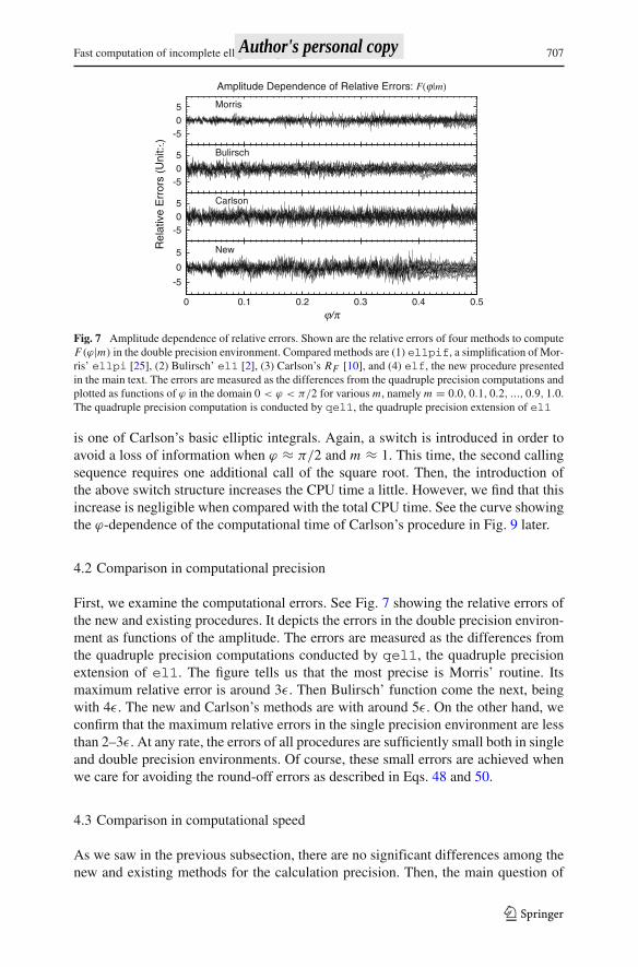
Fig. 7 Amplitude dependence of relative errors. Shown are the relative errors of four methods to computeF(ϕ|m) in the double precision environment. Compared methods are (1) ellpif, a simplification of Mor-ris’ ellpi [25], (2) Bulirsch’ el1 [2], (3) Carlson’s RF [10], and (4) elf, the new procedure presentedin the main text. The errors are measured as the differences from the quadruple precision computations andplotted as functions of ϕ in the domain 0 < ϕ < π/2 for various m, namely m = 0.0, 0.1, 0.2, ..., 0.9, 1.0.The quadruple precision computation is conducted by qel1, the quadruple precision extension of el1

is one of Carlson’s basic elliptic integrals. Again, a switch is introduced in order toavoid a loss of information when ϕ ≈ π/2 and m ≈ 1. This time, the second callingsequence requires one additional call of the square root. Then, the introduction ofthe above switch structure increases the CPU time a little. However, we find that thisincrease is negligible when compared with the total CPU time. See the curve showingthe ϕ-dependence of the computational time of Carlson’s procedure in Fig. 9 later.

4.2 Comparison in computational precision

First, we examine the computational errors. See Fig. 7 showing the relative errors ofthe new and existing procedures. It depicts the errors in the double precision environ-ment as functions of the amplitude. The errors are measured as the differences fromthe quadruple precision computations conducted by qel1, the quadruple precisionextension of el1. The figure tells us that the most precise is Morris’ routine. Itsmaximum relative error is around 3ε. Then Bulirsch’ function come the next, beingwith 4ε. The new and Carlson’s methods are with around 5ε. On the other hand, weconfirm that the maximum relative errors in the single precision environment are lessthan 2–3ε. At any rate, the errors of all procedures are sufficiently small both in singleand double precision environments. Of course, these small errors are achieved whenwe care for avoiding the round-off errors as described in Eqs. 48 and 50.

4.3 Comparison in computational speed

As we saw in the previous subsection, there are no significant differences among thenew and existing methods for the calculation precision. Then, the main question of

123


708 T. Fukushima

Table 3 Averaged CPU time to compute incomplete elliptic integral of first kind only

Method Procedure Single Double

Morris ellpif 9.13 16.12

Carlson RF 7.63 13.65

Bulirsch el1 6.25 7.33

New elf 3.95 6.25

Listed are the averaged CPU times to compute F(ϕ|m) in the single and double precision environments,respectively. They are the results uniformly averaged in the standard domain of input arguments, 0 < ϕ <

π/2 and 0 < m < 1. The unit of CPU time is that to compute the sine function in the double precisionenvironment. Compared methods are those using (1) ellpif, a simplification of Morris’ ellpi [25], (2)Carlson’s RF [10], (3) Bulirsch’ el1 [2], and (4) elf, the new procedure presented in the main text

Table 4 Averaged CPU time to compute incomplete and complete elliptic integrals of first kind simulta-neously

Method Procedures Single Double

Morris ellpif & eklk 38.68 77.75

Carlson RF 17.13 28.65

Bulirsch el1 & cel1 8.40 9.78

New elf & elk 4.46 7.01

Same as Table 3 but for the simultaneous computation of F(ϕ|m) and K (m). The methods we used incomputing K (m) are (1) Bulirsch’ cel1 [2], (2) eklk, a modification and simplification of Morris’ ekl[25], (3) Carlson’s RF [10], and (4) our fast procedure elk [20]

concern is their speed. Tables 3 and 4 compare the CPU times of the new and existingprocedures to compute F(ϕ|m) and the pair of F(ϕ|m) and K (m) in the single anddouble precision environments, respectively. The listed CPU times are those uniformlyaveraged with respect to ϕ and m in their standard domains and normalized by thatto compute the sine function in the double precision environment. More specificallyspeaking, we measured the CPU times as simple means of the results for 4095 × 4095equally spaced grid points in the domain, 0 < ϕ < π/2 and 0 < m < 1. The com-puter used in the measurement was a PC with an Intel Pentium M processor. All thecomputation codes were written in Fortran 77/90, compiled by the Intel Visual Fortran8.0, and executed under Windows XP. As for the computation of K (m), we used (1)cel1, Bulirsch’ function to compute the complete elliptic integral of the first kind[2], (2) eklk, a modification of ekl, (3) RF , the same Carlson’s function as thecase of incomplete integral [10], and (4) elk, our fast procedure to compute K (m)

[20]. Here ekl is Morris’ routine to return complex-valued complete integral of thefirst and second kinds [25]. We modified it so as to calculate real-valued completeintegral of the first kind only. The value of K (m) is required in calculating F(ϕ|m)

when |ϕ| > π/2. Refer to Appendix A. In this sense, Table 4 provides a more realisticcomparison than Table 3. At any rate, the new method is significantly faster than theexisting procedures.

123



0

2

4

6

8

10

12

14

16

18

20

22

0 0.1 0.2 0.3 0.4 0.5 0.6 0.7 0.8 0.9 1

CP

U T

ime

(Uni

t: S

ine

Fun

ctio

n)

m

Parameter Dependence of CPU Time

New

Morris

Carlson

Bulirsch

Fig. 8 Parameter dependence of CPU time. Illustrated are the CPU times, being averaged with respect tothe amplitude, of various methods to compute the incomplete elliptic integral of the first kind in the doubleprecision environment

0

2

4

6

8

10

12

14

16

18

20

22

24

0 0.1 0.2 0.3 0.4 0.5

CP

U T

ime

(Uni

t: S

ine

Fun

ctio

n)

ϕ/π

Amplitude Dependence of CPU Time

New

Bulirsch

Carlson

Morris

Fig. 9 Amplitude dependence of CPU Time. Same as Fig. 8 but for the dependence on the amplitude ϕ

4.4 Dependence of computational speed on input arguments

Figures 8 and 9 illustrate the averaged CPU time in the double precision environmentas functions of m and ϕ, respectively. More specifically speaking, we illustrated Fig. 8by taking simple means of the CPU times for the values of ϕ at 224 − 1 ∼ 1.68 × 107

equally spaced grid points in its standard domain for a fixed m. Again we scaledthem in the unit of that to compute the sine function. In Morris’ case, the change ofcharacteristics near m ∼ 0.57 is due to the internal shift of series expansions fromthat around m = 0 to that around m = 1. In the curve of Carlson’s method, a subtlekink at m = 0.5 is caused by the switch between two expressions given in Eq. 50.In case of Bulirsch’ results, the step-function-like jumps at m ∼ 0.091, 0.712, and0.993 are resulted by the increase in the number of Landen transformations. Namely

123


710 T. Fukushima

the corresponding numbers before and after the jumps are 0, 1, 2, and 3 in average. Onthe other hand, the CPU time of the new method is slightly increasing with respect tom. At any rate, the new method is the fastest for any value of m. Similarly, we createdFig. 9 by plotting the CPU times averaged for 224 − 1 equally spaced grid points ofthe parameter m in its standard domain for each ϕ. In Morris’ case, the change ofcurves near ϕ/π ∼ 0.3 is again due to the internal shift of series expansions. In thecurve of Carlson’s method, the step-function-like jumps near ϕ/π = 0.04, 0.08, 0.16,and 0.32 are due to the increase in the number of duplication transformations. Namelythe corresponding numbers before and after the jumps are 0, 1, 2, 3, and 4. On theother hand, Bulirsch’ results do not depend on ϕ. In case of the new procedure, thegradual jumps near ϕ/π = 0.06, 0.12, and 0.23 are caused by the increase in the totalnumber of half argument transformations. Namely the numbers before and after thejumps are 0, 1, 2, and 3. We confirmed these numbers by counting them during theactual computations. This feature remains roughly the same in the single precisionenvironment although the total numbers are reduced by one. This averaged decreaseroughly corresponds to the decrease in the CPU time of the new method from thedouble to the single precision results. Meanwhile, the change of manner in the newmethod at ϕ/π = 0.4 is due to the switch of expressions described in Eq. 13. At anyrate, the new method runs the fastest for almost all values of ϕ. The exception is asmall region around ϕ/π = 0.4, say 0.38 < ϕ/π < 0.42. In that case, Bulirsch’method is the best.

5 Conclusion

Using the half argument formulas of the sine and/or cosine amplitude functions, wedeveloped a new method to calculate F(ϕ|m) when 0 < ϕ < π/2 and 0 < m < 1.While keeping the parameter m the same, the method reduces the amplitude ϕ byrepeated usage of the formulas until y ≡ sin2 ϕ becomes less than a certain smallvalue. It is around 0.15–0.19 and 0.034–0.041 in case of the single and double precisionarithmetics, respectively. Then, the integral corresponding to the reduced amplitude iscomputed by the product of

√y and a polynomial of y. The order of the polynomial is

6 and 9 in the single and double precision arithmetics, respectively. The total numberof applications of the half argument formulas is 0–3 typically and 8 at most in thedouble precision arithmetics. These numbers decrease by one in the single precisionenvironment. Finally, the integral of the original amplitude is obtained by multiply-ing that of the reduced one by a power of 2. The power is the same as the numberof applications of the half argument formulas. The resulting method is sufficientlyprecise in the sense that the maximum relative error is 3–5 machine epsilons at most.Thanks to the simplicity of the half argument formulas and their inverse, the new pro-cedure is significantly faster than the existing procedures. For example, in the doubleprecision computation, it runs 17% faster than Bulirsch’ el1, 2.2 times faster than themethod using Carlson’s RF , and 2.6 times faster than Morris’ ellpi based on theseries expansion method of Didonato and Hershey. This superiority is mainly due to(1) the simplicity of the half argument transformations, (2) an optimal balance of thetransformation process and the Maclaurin series approximation, and (3) an efficient

123



rule to select one of four mathematically equivalent but computationally differentexpressions of F(ϕ|m) depending on the value of ϕ and m. When the amplitude is ingeneral domain as −∞ < ϕ < ∞, the computation of K (m) is required. In this case,the above ratios of computational times are significantly increased. As an illustration,our combination of elf and elk runs 40–90 % faster than the corresponding pairof Bulirsch’ el1 and cel1. As by-products, we present fast algorithms to computethe inverse sine and cosine amplitude functions. We anticipate that this new approachwill help to accelerate the computation of the incomplete elliptic integrals of two otherkinds.

Acknowledgments The author appreciates the referees’ valuable comments and suggestions to improvethe readability and quality of the present article.

Appendix A: Reduction of input arguments

The incomplete elliptic integral of the first kind, F(ϕ|m), is real-valued as long as1 − m sin2 ϕ > 0. Namely, it is real for arbitrary value of ϕ if m < 1 and for|ϕ| < sin−1(1/

√m) if m ≥ 1. Under this condition, we reduce the domain of ϕ and

m into the standard one, 0 < ϕ < π/2 and 0 < m < 1. In the below, we will (1)provide procedures to reduce the domain of m such that 0 < m < 1 in Appendix A.1,and (2) show procedures to reduce the domain of ϕ such that 0 < ϕ < π/2 under thecondition 0 < m < 1 in Appendix A.2.

A.1 Reduction of parameter domain

We begin with the domain reduction of the parameter m. First, if m = 0, the integralis simply expressed as

F(ϕ|0) = ϕ, (52)

which is the second part of BF111.01. Next, if m = 1, the integral is written in termsof elementary functions as

F(ϕ|1) = tanh−1(sin ϕ) = log

(1 + sin ϕ

cos ϕ

)= log

[tan(π

4+ ϕ

2

)], (53)

which shows three different expressions of the second part of BF111.04. Third, ifm > 1, we reduce the domain of m into the standard one, 0 < m < 1, by thereciprocal parameter transformation as shown in the second part of BF114.01 as,

F(ϕ|m) = (√m R)

F (ϕR | m R) , (54)

where

ϕR ≡ sin−1 [(√m)

sin ϕ], m R ≡ 1

m. (55)

123


712 T. Fukushima

Note that ϕR is uniquely determined since the condition |ϕ| < sin−1(1/√

m) is satis-fied. Finally, if m < 0, we reduce the domain of m into the standard one, 0 < m < 1,by the negative parameter transformation, or the imaginary modulus transformationin classic notation, as shown in the first part of BF160.02,

F(ϕ|m) =(√

1 − m N

)F (ϕN | m N ) , (56)

where

ϕN ≡ sin−1

[(√1 − m

1 − m sin2 ϕ

)sin ϕ

], m N ≡ −m

1 − m, (57)

Note that ϕN is well-defined since 1 − m ≤ 1 − m sin2 ϕ, and therefore the argumentof the inverse sine is less than or equal to unity. Thus, we can reduce the domainof m into the standard one, 0 < m < 1. In the last two cases, the computationallabor of the transformation can be reduced significantly. In fact, we can translate thetransformations in terms of ϕ into those in terms of y ≡ sin2 ϕ as

yR = my, yN = mc y

1 − my, (58)

which are simply calculated. Therefore, the extra computational labor mainly consistsof one square root to calculate the factor

√m R or

√1 − m N .

A.2 Reduction of amplitude domain

Let us move to the reduction of amplitude, ϕ, under the condition that m is in thestandard domain, 0 < m < 1. First, if |ϕ| > π/2, we reduce the domain of ϕ from(−∞,+∞) to [−π/2, π/2) by utilizing the amplitude modulus transformation asshown in the second part of BF113.02 as,

F(ϕ|m) = 2 j K (m) + F(ϕ − jπ |m), (59)

where j is an integer such that |ϕ− jπ | < π/2 and K (m) is the complete elliptic inte-gral of the first kind, the fast computation of which is described in Ref. [20]. Second,if ϕ < 0, we reduce the domain of ϕ to be non-negative by the negative amplitudetransformation

F(ϕ|m) = −F(−ϕ|m), (60)

which is the second part of BF113.01. Finally, if ϕ = 0, the integral reduces to simplerforms as

F(0|m) = 0, (61)

which is the second part of BF111.00. In conclusion, excluding some special casesreducible to elementary functions and the complete integral, and using various trans-

123



formations described so far, we can reduce the domain of ϕ and m into the standardone, 0 < ϕ < π/2 and 0 < m < 1.

Appendix B: Fast computation of complete elliptic integral of the first kind insingle precision environment

Below, we summarize the single precision version of our fast algorithm to computeK (m). The details of the double precision version was given in Ref. [20].

B.1 Case of small parameter

We compute K (m) by a piecewise polynomial of m. By truncating its Taylor expan-sion around m = m0 at certain orders, we obtain the approximate polynomials asexpressed as

K (m) ≈JK∑j=0

K j (m − m0)j , (62)

where the coefficients are defined as

K j ≡ 1

j !

[(d

dm

) j

K (m)

]

m=m0

. (63)

It is easy to show that all K j are positive definite. Practically, the coefficients K j

can be directly computed by formula processors such as Mathematica [29]. Exceptthe case when m is close to 1, say when m ≥ 0.9, we experimentally learn that thisapproach works well.

For simplicity, we fix the intervals of the piecewise polynomials as [0, 0.1), [0.1,

0.2), [0.2, 0.3), [0.3, 0.4), [0.4, 0.5), [0.5, 0.6), [0.6, 0.7), [0.7, 0.8), [0.8, 0.85), and[0.85, 0.9). The reason why the last two intervals are of the half length is to make theorders of polynomial reasonably small, say less than 8. Then, we set m0 as the cen-ter of each intervals; 0.05, 0.15, 0.25, 0.35, 0.45, 0.55, 0.65, 0.75, 0.825, and 0.875,respectively. Finally, we seek for JK , the minimum order satisfying the condition thatthe truncation error of the Taylor expansions is less than the error tolerance. We set it as1 machine epsilon in the single precision environment, ∼ 1.19 × 10−7. The resultingsets of coefficients are listed in Table 5.

B.2 Case of large parameter

When m is large, say m ≥ 0.9, we first compute the associate complete elliptic integralof the first kind by the approximate polynomial described in the previous subsectionas,

123


714 T. Fukushima

Tabl

e5

Coe

ffici

ents

ofTa

ylor

expa

nsio

npo

lyno

mia

lsof

K(m

)

m0

K0

K1

K2

K3

K4

K5

K6

K7

0.05

1.59

1003

450.

4160

0074

0.24

5791

510.

1794

8148

0.14

4556

06

0.15

1.63

5256

730.

4711

9063

0.30

9728

410.

2522

0831

0.22

6725

62

0.25

1.68

5750

350.

5417

3185

0.40

1524

440.

3696

4247

0.37

6060

72

0.35

1.74

4350

600.

6348

6428

0.53

9842

560.

5718

9271

0.67

0295

140.

8325

8659

0.45

1.81

3883

940.

7631

6325

0.76

1928

610.

9510

7465

1.31

5180

681.

9285

6069

0.55

1.89

8924

910.

9505

2179

1.15

1077

591.

7502

3911

2.95

2676

815.

2858

0040

0.65

2.00

7598

401.

2484

5723

1.92

6234

663.

7512

8964

8.11

9944

5518

.665

7213

44.6

0392

48

0.75

2.15

6515

651.

7918

0564

3.82

6751

2910

.386

7247

31.4

0331

4110

0.92

3704

337.

3268

2811

58.7

0793

0.82

52.

3181

2262

2.61

6920

157.

8979

3508

30.5

0239

7213

1.48

6937

602.

9847

6428

77.0

2462

0.87

52.

4735

9617

3.72

7624

2415

.607

3930

84.1

2850

8450

6.98

1820

3252

.277

0621

713.

2424

1490

37.0

45

Show

nar

eth

eTa

ylor

expa

nsio

nco

effic

ient

sof

K(m

),th

eco

mpl

ete

ellip

ticin

tegr

alof

the

first

kind

,for

the

dom

ain

0≤

m<

0.9.

For

the

para

met

erm

ina

sub

dom

ain,

m0

−Δ

m≤

m<

m0

+Δ

m,

K(m

)is

appr

oxim

atel

yco

mpu

ted

as

K(m

)≈

J K ∑ j=0

Kj(m

−m

0)

j.

The

orde

rJ K

is4

for

the

case

sm

0is

0.05

,0.1

5,an

d0.

25,5

for

the

case

sm

0is

0.35

,0.4

5,an

d0.

55,6

for

the

case

sm

0is

0.65

and

0.82

5,an

d7

for

the

case

sm

0is

0.75

and

0.87

5.M

eanw

hile

,Δm

is0.

025

for

the

case

sm

0is

0.08

25an

d0.

0875

,and

0.05

othe

rwis

e

123



K ′(m) ≡ K (mc) ≈JK∑j=0

K j (mc − 0.05) j , (64)

where the coefficients are those listed in the first row of Table 5. Then, we transformK ′(m) into K (m) by a formula

K (m) = (− log qc)

(K ′(m)

π

). (65)

This is a rewriting of the definition of complementary nome as

qc ≡ exp

(−π K ′(m)

K (m)

). (66)

We compute qc by using its Maclaurin series expansion with respect to mc as

qc ≈(

1

16

)mc +

(1

32

)m2

c +(

21

1024

)m3

c +(

31

2048

)m4

c +(

6257

524288

)m5

c

+(

10293

1048576

)m6

c (67)

The coefficients can be obtained by formula processors such as Mathematica [29]. Weconfirm that the first six terms as shown in the above are enough to calculate qc in thesingle precision environment for the interval considered, 0 ≤ mc ≤ 0.1.

B.3 Computational precision and computational speed

By comparing with the result of double precision computations, we confirmed thatthe maximum error of K (m) computed by the method described in the previous sub-sections is as small as 2.0 × 10−7. This is 1.5 times the machine epsilon in the singleprecision environment. On the other hand, the new method runs very fast. Its averagedCPU time is 0.51 times that of the sine function in the double precision environment.This value is obtained by taking the difference of CPU times of F(ϕ|m) only andthe combination of F(ϕ|m) and K (m) in the single precision environment given inTables 3 and 4, respectively.

Appendix C: Equivalence of duplication theorem and half argument formulas

The duplication theorem of Carlson’s elliptic integral of the first kind is expressed as

RF (α, β, γ ) = RF

(α + λ

4,β + λ

4,γ + λ

4

), (68)

123


716 T. Fukushima

where

λ ≡ √αβ +√βγ + √γα. (69)

An identity relation of RF is written as

RF (α, β, γ ) = 1√γ

RF

(α

γ,β

γ, 1

). (70)

This is proven as

RF (α, β, γ ) = 1

2

∞∫

0

dt√(t + α) (t + β) (t + γ )

= 1

2√

γ 3

∞∫

0

dt√[(t + α)/γ ][(t + β)/γ ][(t/γ ) + 1]

= 1

2√

γ

∞∫

0

dt ′√[t ′ + (α/γ )

] [t ′ + (β/γ )

](t ′ + 1)

= 1√γ

RF

(α

γ,β

γ, 1

), (71)

where t ′ ≡ t/γ . Using this relation, we obtain a rewriting of the duplication theoremby letting γ = 1 as

RF (α, β, 1) = RF

(α + ρ

4,β + ρ

4,

1 + ρ

4

)

= 2√1 + ρ

RF

(α + ρ

1 + ρ,β + ρ

1 + ρ, 1

), (72)

where

ρ ≡ √α +√β +√αβ. (73)

Therefore, the argument u ≡ F(ϕ|m) is transformed by the duplication theorem as

u = F(ϕ|m) = s RF

(c2, d2, 1

)= 2s√

1 + σRF

(c2 + σ

1 + σ,

d2 + σ

1 + σ, 1

), (74)

where

s ≡ sin ϕ = sn(u|m), c ≡ cos ϕ = cn(u|m), d ≡√

1 − ms2 = dn(u|m), (75)

123



and

σ ≡ c + d + cd. (76)

On the other hand, the half argument formulas of the sine, cosine, and delta amplitudefunctions given in BF124.02 are written as

sn(u

2

∣∣∣m)

= s√(1 + c)(1 + d)

= s√1 + σ

, (77)

cn2(u

2

∣∣∣m)

= 1 − sn2(u

2

∣∣∣m)

= 1 − s2

(1 + c)(1 + d)= c2 + c + d + cd

(1 + c)(1 + d)

= c2 + σ

1 + σ, (78)

dn2(u

2

∣∣∣m)

= 1 − m sn2(u

2

∣∣∣m)

= 1 − ms2

(1 + c)(1 + d)= d2 + c + d + cd

(1 + c)(1 + d)

= d2 + σ

1 + σ. (79)

These lead to another expression of u as

u = 2(u

2

)= 2 sn

(u

2

∣∣∣m)

RF

(cn2(u

2

∣∣∣m)

, dn2(u

2

∣∣∣m)

, 1)

= 2s√1 + σ

RF

(c2 + σ

1 + σ,

d2 + σ

1 + σ, 1

), (80)

which is exactly the same as Eq. 74. This means that the duplication theorem on RF

is equivalent with the half argument formulas of Jacobian elliptic functions.

Appendix D: Derivation of Maclaurin series expansion

Using the Jacobi’s form of the incomplete elliptic integral of the first kind, Eq. 3, weexpress the argument u as

u =s∫

0

ds√(1 − s2

) (1 − ms2

) . (81)

By assuming that y ≡ s2 is small, we can expand a factor in the integrand, 1/√

1 − y,by the general binomial expansion theorem as

1√1 − y

=∞∑

n=0

(− 12

n

)(−y)n =

∞∑n=0

(2n − 1)!!n!

( y

2

)n. (82)

123


718 T. Fukushima

Similarly, we expand the other factor as

1√1 − my

=∞∑j=0

(2 j − 1)!!j !

(my

2

) j. (83)

Then the whole integrand is expanded as

1√(1 − y) (1 − my)

=∞∑

�=0

⎛⎝ �∑

j=0

((2 j − 1)!!(2� − 2 j − 1)!!

j !(� − j)!)

m j

⎞⎠ y�

2�. (84)

where we set � = n + j . Substituting this into the integral definition and noting thaty = s2, we rewrite u as

u =s∫

0

⎡⎣ ∞∑

�=0

⎛⎝ �∑

j=0

((2 j − 1)!!(2� − 2 j − 1)!!

j !(� − j)!)

m j

⎞⎠ s2�

2�

⎤⎦ ds. (85)

Exchanging the integration and the summation operation, we finally obtain

u =∞∑

�=0

⎛⎝ �∑

j=0

((2 j − 1)!!(2� − 2 j − 1)!!

j !(� − j)!)

m j

⎞⎠ s2�+1

2�(2� + 1)

=⎛⎝ �∑

j=0

u�j mj

⎞⎠ y�, (86)

where

u�j ≡ (2 j − 1)!!(2� − 2 j − 1)!!2�(2� + 1) j !(� − j)! . (87)

This expression is the same as Eq. 25 in the main text.

References

1. Abramowitz, M. Stegun, I.A. (eds.): Handbook of Mathematical Functions with Formulas, Graphs,and Mathematical Tables, Chapter 17. National Bureau of Standards, Washington (1964)

2. Bulirsch, R.: Numerical computation of elliptic integrals and elliptic functions. Numer. Math. 7,78–90 (1965a)

3. Bulirsch, R.: Numerical computation of elliptic integrals and elliptic functions II. Numer. Math. 7,353–354 (1965b)

4. Bulirsch, R.: An extension of the Bartky-transformation to incomplete elliptic integrals of the thirdkind. Numer. Math. 13, 266–284 (1969a)

5. Bulirsch, R.: Numerical computation of elliptic integrals and elliptic functions III. Numer.Math. 13, 305–315 (1969b)

6. Byrd, P.F., Friedman, M.D.: Handbook on Elliptic Integrals for Engineers and Physicists, 2ndedn. Springer, Berlin (1971)

123



7. Carlson, B.C.: On computing elliptic integrals and functions. J. Math. Phys. 44, 332–345 (1965)8. Carlson, B.C.: Elliptic integrals of the first kind. SIAM J. Math. Anal. 8, 231–242 (1977)9. Carlson, B.C.: Short proofs of three theorems on elliptic integrals. SIAM J. Math. Anal. 9,

524–528 (1978)10. Carlson, B.C.: Computing elliptic integrals by duplication. Numer. Math. 33, 1–16 (1979)11. Carlson, B.C., Notis, E.M.: Algorithm 577. Algorithms for incomplete elliptic integrals. ACM Trans.

Math. Software 7, 398–403 (1981)12. Cody, W.J.: Chebyshev approximations for the complete elliptic integrals K and E. Math.

Comp. 19, 105–112 (1965a)13. Cody, W.J.: Chebyshev polynomial expansions of complete elliptic integrals K and E. Math.

Comp. 19, 249–259 (1965b)14. Cody, W.J.: Corrigenda: Chebyshev approximations for the complete elliptic integrals K and E. Math.

Comp. 20, 207 (1966)15. Didonato, A.R., Hershey, A.V.: New formulas for computing incomplete elliptic integrals of the first

and second kind. J. Assoc. Comput. Mach. 6, 515–526 (1959)16. Fukushima, T.: Gaussian element formulation of short-axis-mode rotation of a rigid body. Astron.

J. 136, 649–653 (2008a)17. Fukushima, T.: Canonical and universal elements of rotational motion of triaxial rigid body. Astron.

J. 136, 1728–1735 (2008b)18. Fukushima, T.: Fast computation of Jacobian elliptic functions and incomplete elliptic integrals for

constant values of elliptic parameter and elliptic characteristic. Celest. Mech. Dyn. Astron. 105,245–260 (2009a)

19. Fukushima, T.: Efficient solution of initial-value problem of torque-free rotation. Astron. J. 137,210–218 (2009b)

20. Fukushima, T.: Fast computation of complete elliptic integrals and Jacobian elliptic functions. Celest.Mech. Dyn. Astron. 105, 305–328 (2009c)

21. Fukushima, T., Ishizaki, H.: Numerical computation of incomplete elliptic integrals of a generalform. Celest. Mech. Dyn. Astron. 59, 237–251 (1994)

22. Glynn, E.F.: efg’s Computer Lab and Reference Library. http://www.efg2.com/Lab/Library/mathematics.htm (2009)

23. Hastings, C. Jr.: Approximations for Digital Computers. Princeton University Press, Princeton (1955)24. Hofsommer, D.J., van de Riet, R.P.: On the Numerical Calculation of Elliptic Integrals of the First and

Second Kind and Elliptic Functions of Jacobi. Numer. Math. 5, 291–302 (1963)25. Morris, A.H. Jr.: NSWC Library of Mathematics Subroutines, Tech. Rep. NSWCDD/TR-92/425,

107-110. Naval Surface Warfare Center, Dahlgren (1993)26. Press, W.H., Flannery, B.P., Teukolsky, S.A., Vetterling, W.T.: Numerical Recipes: the Art of Scientific

Computing. Cambridge University Press, Cambridge (1986)27. Press, W.H., Teukolsky, S.A., Vetterling, W.T., Flannery, B.P.: Numerical Recipes: the Art of Scientific

Computing, 3rd edn. Cambridge University Press, Cambridge (2007)28. Vande Vel, H.: On the series expansion method for computing incomplete elliptic integrals of the first

and second kinds. Math. Comp. 23, 61–69 (1969)29. Wolfram, S.: The Mathematica Book, 5th edn. Wolfram Research Inc./Cambridge University

Press, Cambridge (2003)

123


http://www.efg2.com/Lab/Library/mathematics.htm

http://www.efg2.com/Lab/Library/mathematics.htm

Fast computation of incomplete elliptic integral of first kind by half argument transformation

Documents

Transcript of Fast computation of incomplete elliptic integral of first kind by half argument transformation