Farm-level impacts of prolonged drought: is a multiyear event more than the sum of its parts

Farm-level impacts of prolonged drought: is amultiyear event more than the sum of its parts?

Dannele E. Peck and Richard M. Adams†

A multiyear discrete stochastic programming model with uncertain water supplies andinter-year crop dynamics is developed to determine: (i) whether a multiyear drought’simpact can be more than the sum of its parts, and (ii) whether optimal response to1 year of drought can increase a producer’s vulnerability in subsequent years ofdrought. A farm system that has inter-year crop dynamics, but lacks inter-annualwater storage capabilities, is used as a case study to demonstrate that dynamics unre-lated to large reservoirs or groundwater can necessitate a multiyear model to estimatedrought’s impact. Results demonstrate the importance of analysing individual years ofdrought in the context of previous and future years of drought.

Key words: crop rotations, inter-year dynamics, multiyear drought,stochastic integer programming.

1. Introduction

Multiyear drought is prominent throughout the world (Dai et al. 2004).Nearly half of all droughts in the U.S., for example, are multiyear events(Diaz 1983). Australia’s Murray Darling Basin experienced 23 years ofdrought between 1952 and 2002, 16 of which comprised multiyear events(Nicholls 2004). Multiyear drought is expected to become even more frequentin many parts of the world, because of global climate change, populationgrowth, and land use change (Rosenzweig and Hillel 1993; Gleick 2000; Wilh-ite et al. 2006; Meehl et al. 2007).Despite the historical frequency of multiyear drought, such events have

been the focus of relatively few economic studies. Studies that do addressmultiyear drought tend to focus on livestock grazing (Toft and O’Hanlon1979; Thompson et al. 1996; McKeon et al. 2000), rather than crops (Iglesiaset al. 2003). Studies of drought in crop systems focus primarily on single-yearevents instead (e.g. Bernardo et al. 1987; Bryant et al. 1993; Keplinger et al.1998; Chen et al. 2001; Mejias et al. 2004). The lack of multiyear droughtanalyses for crop systems leaves readers wondering if multiyear drought canbe modelled as a series of single-year events, or if multiyear analyses mightprovide unique insights about drought impacts in cropping systems.

† Dannele E. Peck (email: [email protected]) is an Assistant Professor at the Department ofAgricultural and Applied Economics, University of Wyoming, Laramie, WY, USA andRichard M. Adams is Professor Emeritus at the Department of Agricultural and ResourceEconomics, Oregon State University, Corvallis, OR, USA.

� 2010 The AuthorsJournal compilation � 2010 Australian Agricultural and Resource Economics Society Inc. and Blackwell Publishing Asia Pty Ltddoi: 10.1111/j.1467-8489.2009.00478.x

The Australian Journal of Agricultural and Resource Economics, 54, pp. 43–60

The Australian Journal of

Journal of the AustralianAgricultural and ResourceEconomics Society

The potential for multiyear drought to generate more complex impactsthan a series of independent single-year events has been raised in the literature(e.g. Clawson et al. 1980; Thompson et al. 1996; Iglesias et al. 2003). Claw-son et al., in particular, hypothesizes that a producer’s response to, or recov-ery from, 1 year of drought may impair their ability to endure subsequentyears of drought. They neglect, however, to test their hypothesis. If Clawsonet al. is correct, producers’ decisions during a multiyear drought, as well asthe resulting impact, may be more dynamic and complex than previouslyacknowledged.To test hypotheses about the economic impacts of single versus multiyear

droughts, we develop and solve a multiyear, stochastic and dynamic pro-gramming model for a hypothetical irrigated row-crop farm. The farm faceswater supply uncertainty; both the occurrence and duration of drought areknown only probabilistically. Decision-making under uncertainty is mademore complex by cropping decisions that generate inter-year dynamics. Theproducer must therefore consider not only how crops chosen in the currentyear will perform under alternative states of nature, but also how they willaffect cropping options, and hence vulnerability to drought, in subsequentyears.Optimal farm activities (crop choice, irrigation technology, and deficit irri-

gation) are identified for each stage and state of the multiyear planning hori-zon, given uncertainty about the timing and duration of drought. Optimalfarm activities and returns to land and management for various single andmultiyear drought scenarios are then compared to determine: (i) whether amultiyear drought’s impact is more complex than the sum of its componentyears’ impacts, i.e. whether the impact of drought in 1 year affects the impactof drought in subsequent years, and (ii) whether optimal response to 1 yearof drought leaves the producer more vulnerable to subsequent years ofdrought, i.e. whether a producer’s effort to mitigate drought in 1 yearincreases the economic impact of subsequent years of drought. The economicimpact of drought is measured as the difference in returns between a droughtscenario and a drought-free scenario. Because an optimization approach isused in this study, rather than simulation, drought impacts reflect the pro-ducer’s ability to make optimal decisions under uncertainty, and respondoptimally when drought is revealed.

2. Case study

2.1 Overview

The farm-level decision model is based on irrigated row-crop farms in theVale Oregon Irrigation District, located in a semi-arid region of the U.S.Pacific Northwest. Drought is a major source of production risk in the Dis-trict; multiyear droughts have occurred there most recently from 1990 to1992 and 2001 to 2003. The District’s primary source of irrigation water is

44 D.E. Peck and R.M. Adams

� 2010 The AuthorsJournal compilation � 2010 Australian Agricultural and Resource Economics Society Inc. and Blackwell Publishing Asia Pty Ltd

snowmelt stored in small reservoirs that provide essentially no inter-annualcarryover capacity. Reliable groundwater is not widely available in the Dis-trict, and state laws deter water transfers. Producers therefore rely primarilyon crop and irrigation management to prepare for and respond to drought.Several studies address reservoir and aquifer management under inter-

annual water supply uncertainty (Dudley 1988; Iglesias et al. 2003; Chenet al. 2006; Iglesias et al. 2007). Few, however, explore multiyear drought incrop systems that lack inter-annual water storage (Weisensel et al. 1991). Inthe absence of inter-annual water storage, a dynamic multiyear model mayseem unnecessary to investigate optimal drought management. Other sourcesof inter-year dynamics that have important implications during a multiyeardrought may exist, however, such as crop rotations, which are discussed next.

2.2 Crop rotations and inter-year dynamics

A wide variety of crops can be grown in the study area, including onions,sugar beets, winter wheat, corn, alfalfa, and potatoes. Crop rotations aretherefore diverse and flexible. Rather than adhering to a rigid crop rotation,producers in the study area have a suite of eligible crops from which tochoose each year. The suite of eligible crops for a particular field depends onthe field’s crop history, and a set of agronomic ‘rules’ that producers followto reduce pest and disease outbreaks. Example agronomic ‘rules’ include thefollowing: onions are typically grown only once every 6 years in each field;sugar beets once every 5 years; wheat is not grown in consecutive years, andcorn is grown consecutively for no more than 2 years. Constrained by a set ofeligible crops for each field in a given year, the producer chooses one crop perfield, taking into consideration relative profitability, probabilistic informationabout the upcoming growing season’s water supply, and their goal to maxi-mize the farm’s discounted stream of expected returns. These crop decisionsare made each year.Agronomic rules (as opposed to rigid crop rotations) enable the producer

to flexibly adjust crop plans after the water supply is revealed; however, theyalso generate inter-year dynamics. Crop choice for an individual field in agiven year restricts the set of feasible crops in subsequent years. Thisrestricted set of feasible crops might, in turn, reduce the producer’s futuredrought-preparedness and response options. Inter-year dynamics arisingfrom agronomic rules therefore create the need for a dynamic multiyearmodel, as well as the potential for more complex drought management deci-sions and impacts.

2.3 Water supply uncertainty and intra-year dynamics

Water supplies in a given year are finite, so the producer must carefully con-sider crop water requirements and drought tolerances when making theircrop, irrigation technology, and deficit irrigation decisions. Furthermore, the

Farm-level impacts of prolonged drought 45


producer’s water allotment for the upcoming growing season is uncertain atthe time most crop-irrigation combinations must be chosen (in fall, winter,and early spring, i.e. stage 1). After the water allotment is revealed in mid-spring1 (i.e. stage 2), the producer can respond by planting or abandoningfields that were prepared in stage 1, and deficit irrigating.Division of the crop year into two decision stages, because of water supply

uncertainty, creates intra-year dynamics between stages 1 and 2. The numberof fields prepared for sugar beets in stage 1, for example, creates an upperbound on the number of fields that can be planted to sugar beets in stage 2.Additional sugar beet fields cannot be prepared after the water supply isrevealed because of labour and machinery constraints (which are capturedimplicitly through agronomic rules, rather than explicitly). Winter wheat, as asecond example, is both prepared and planted in stage 1; therefore, the num-ber of fields planted to winter wheat in stage 1 creates an upper bound on thenumber of fields of winter wheat harvested in stage 2. Similar intra-yeardynamics exist for nearly all other crops, with the exception of corn, which isboth prepared and planted in stage 2.

2.4 Decision problem

The producer faces a stochastic and dynamic decision problem. They mustchoose the current year’s crop plan, and make initial resource investments init, before the growing season’s water allotment is known (stage 1), and revisethat plan in response to the revealed water allotment (stage 2). In doing so,the producer must consider the implication of stage 1 decisions for stage 2activities (because of intra-year dynamics arising from water supply uncer-tainty), and stage 2 activities for future crop years (because of inter-yeardynamics arising from agronomic rules). The producer’s decision problem ismodelled empirically as a multiyear discrete stochastic program, as describednext (see Appendix S1 for the theoretical model; all supplementary appendi-ces are available at http://agecon.lib.umn.edu/).

3. Empirical model

3.1 Primer on DSP

Discrete stochastic programming (DSP) is a method for solving decisionproblems that have random variables in the objective function and/or con-straints (Cocks 1968). DSP is also known as discrete sequential stochasticprogramming or stochastic programming with recourse, but should not be

1 The District allocates water using a shares system, so each producer receives the same vol-ume of water per hectare. Water shortages are therefore shared equally per hectare. The Dis-trict manager’s announcement of the upcoming growing season’s water allotment is sometimesrevised as spring progresses and snowmelt is fully realized. We assume for simplicity that theallotment is announced with certainty each spring, just before the planting season.



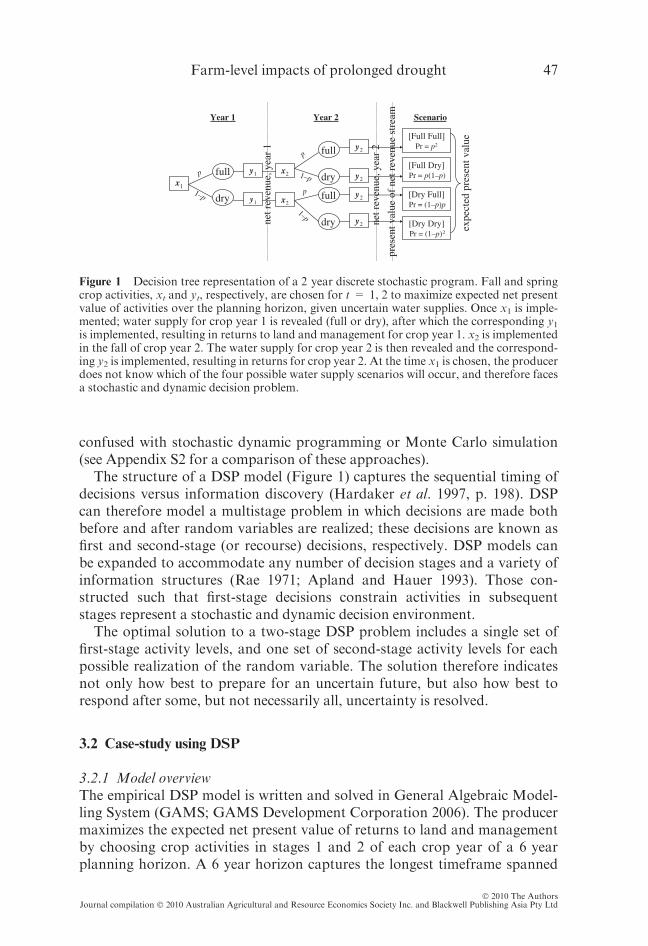
confused with stochastic dynamic programming or Monte Carlo simulation(see Appendix S2 for a comparison of these approaches).The structure of a DSP model (Figure 1) captures the sequential timing of

decisions versus information discovery (Hardaker et al. 1997, p. 198). DSPcan therefore model a multistage problem in which decisions are made bothbefore and after random variables are realized; these decisions are known asfirst and second-stage (or recourse) decisions, respectively. DSP models canbe expanded to accommodate any number of decision stages and a variety ofinformation structures (Rae 1971; Apland and Hauer 1993). Those con-structed such that first-stage decisions constrain activities in subsequentstages represent a stochastic and dynamic decision environment.The optimal solution to a two-stage DSP problem includes a single set of

first-stage activity levels, and one set of second-stage activity levels for eachpossible realization of the random variable. The solution therefore indicatesnot only how best to prepare for an uncertain future, but also how best torespond after some, but not necessarily all, uncertainty is resolved.

3.2 Case-study using DSP

3.2.1 Model overviewThe empirical DSP model is written and solved in General Algebraic Model-ling System (GAMS; GAMS Development Corporation 2006). The producermaximizes the expected net present value of returns to land and managementby choosing crop activities in stages 1 and 2 of each crop year of a 6 yearplanning horizon. A 6 year horizon captures the longest timeframe spanned

net r

even

ue, y

ear

2

Scenario

[Dry Dry]Pr = (1–p)2

[Dry Full]Pr = (1–p)p

[Full Dry]Pr = p(1–p)

[Full Full]Pr = p2

x2

x2

full

dry

full

dry

y2

y2

y2

y2

Year 2

x1

y1

y1

full

dry

net r

even

ue, y

ear

1

Year 1

p

1–p

p

1–p

p

1–p

pres

ent v

alue

of

net r

even

ue s

trea

m

expe

cted

pre

sent

val

ue

Figure 1 Decision tree representation of a 2 year discrete stochastic program. Fall and springcrop activities, xt and yt, respectively, are chosen for t = 1, 2 to maximize expected net presentvalue of activities over the planning horizon, given uncertain water supplies. Once x1 is imple-mented; water supply for crop year 1 is revealed (full or dry), after which the corresponding y1is implemented, resulting in returns to land and management for crop year 1. x2 is implementedin the fall of crop year 2. The water supply for crop year 2 is then revealed and the correspond-ing y2 is implemented, resulting in returns for crop year 2. At the time x1 is chosen, the producerdoes not know which of the four possible water supply scenarios will occur, and therefore facesa stochastic and dynamic decision problem.



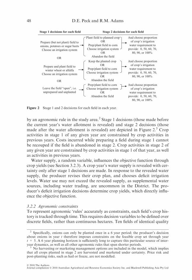
by an agronomic rule in the study area.2 Stage 1 decisions (those made beforethe current year’s water allotment is revealed) and stage 2 decisions (thosemade after the water allotment is revealed) are depicted in Figure 2.3 Cropactivities in stage 1 of any given year are constrained by crop activities inprevious years. Costs incurred while preparing a field during stage 1 cannotbe recouped if the field is abandoned in stage 2. Crop activities in stage 2 ofany given year are constrained by crop activities in stage 1 of that year, as wellas activities in previous years.Water supply, a random variable, influences the objective function through

crop yields (see Section 3.2.3). A crop year’s water supply is revealed with cer-tainty only after stage 1 decisions are made. In response to the revealed watersupply, the producer revises their crop plan, and chooses deficit irrigationlevels. Water use may not exceed the revealed supply, as supplemental watersources, including water trading, are uncommon in the District. The pro-ducer’s deficit irrigation decisions determine crop yields, which directly influ-ence the objective function.

3.2.2 Agronomic constraintsTo represent agronomic ‘rules’ accurately as constraints, each field’s crop his-tory is tracked through time. This requires decision variables to be defined overdiscrete fields, rather than continuous hectares. Ten fields of identical quality

Prepare (but not plant) field toonions, potatoes or sugar beets

Choose an irrigation system

OR

Prepare and plant field towinter wheat or alfalfa

Choose an irrigation system

OR

Leave the field “open”, i.e.unprepared and unplanted

Keep the planted cropOR

Prep/plant field to cornChoose irrigation system

ORAbandon the field

Plant field to planned cropOR


ORAbandon the field

Stage 2 decisions for each field


ORAbandon the field

Stage 1 decisions for each field

And choose proportionof crop’s irrigation

water requirement toprovide: 0, 50, 60, 70,

80, 90, or 100%



80, 90, or 100%



80, 90, or 100%

Figure 2 Stage 1 and 2 decisions for each field in each year.

2 Specifically, onions can only be planted once in a 6 year period; the producer’s decisionabout onions in year t therefore imposes constraints on the feasible crop set through yeart + 5. A 6 year planning horizon is sufficiently long to capture this particular source of inter-year dynamics, as well as all other agronomic rules that span shorter periods.

3 No harvesting or marketing management options are included in the model, which impliesthat all crops planted in stage 2 are harvested and marketed under certainty. Price risk andpost-planting risks, such as hail or freeze, are not modelled.



and size (86.5 hectares, or 35 acres, based on aerial photographs of the studyarea) are assumed. In any given decision period, the producer chooses one cropto plant in each field. For each field, a crop is therefore assigned either a valueof 0 (if not chosen for that particular field) or 1 (if chosen). This contrasts tomodelling crop choice as a continuous variable, in which the producer choosesthe number of hectares of each crop, with no indication of the field(s) in whichthey will be located. Modelling crop choice as a discrete decision for individualfields allows crop history to be tracked at the field-level, rather than the farm-level; agronomic rules are captured more realistically as a result (as demon-strated in Appendix S3). One drawback of discrete decision variables is thatthe model becomes a stochastic integer program, which is difficult to solvebecause of the absence of convenient convexity properties (Schultz 2003).The set of eligible crops for each field in a given year is a function of that

field’s crop history; therefore, crop choices in the previous planning horizonaffect initial opportunities in the current planning horizon. The model accom-modates an exogenously-defined crop history for the preceding planning hori-zon.4 A crop history that imposes no constraints on the current planninghorizon is assumed. This generates the largest set of eligible crops, the mostflexibility in current crop decisions, and hence more conservative droughtimpact estimates.Similarly, cropping activities in the current planning horizon affect oppor-

tunities in subsequent planning horizons. A terminal value function is there-fore defined to relate cropping activities in the current planning horizon toland rental values in the subsequent planning horizon. More specifically, if aparcel of land is capable of supporting high-value crops during the next plan-ning horizon (because of activities in the current planning horizon), the pro-ducer receives a relatively large rental payment to reflect their ability to leasethat parcel for a premium. The producer otherwise receives a small rentalpayment because their parcel can only support low-value crops.

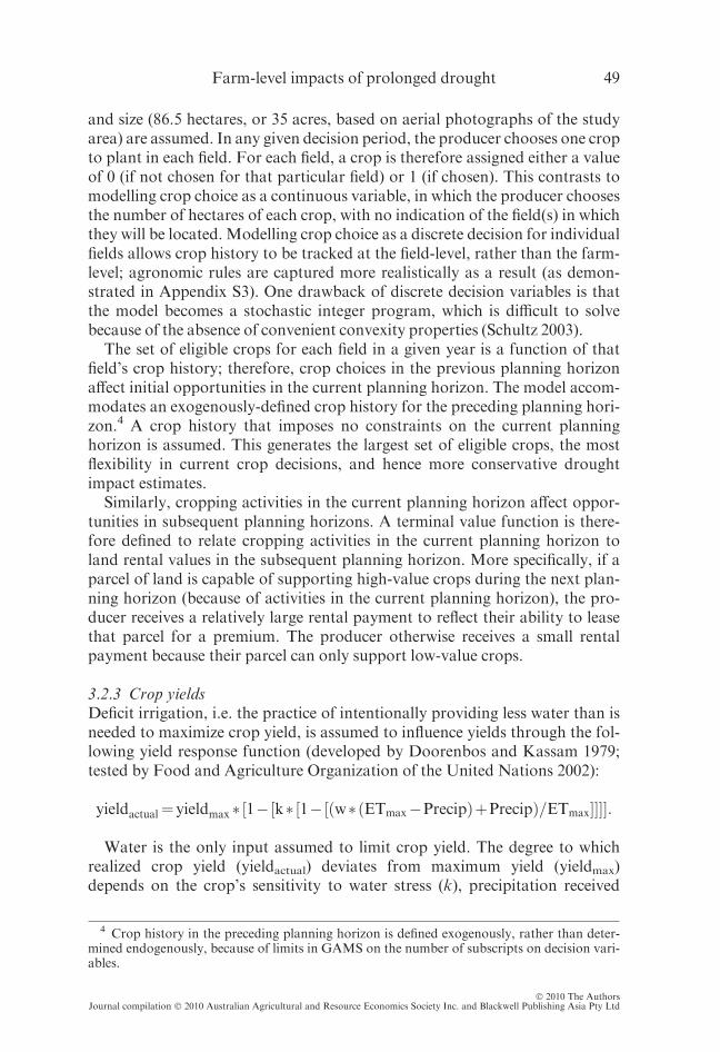
3.2.3 Crop yieldsDeficit irrigation, i.e. the practice of intentionally providing less water than isneeded to maximize crop yield, is assumed to influence yields through the fol-lowing yield response function (developed by Doorenbos and Kassam 1979;tested by Food and Agriculture Organization of the United Nations 2002):

yieldactual¼yieldmax �½1�½k�½1�½ðw�ðETmax�PrecipÞþPrecipÞ=ETmax��:

Water is the only input assumed to limit crop yield. The degree to whichrealized crop yield (yieldactual) deviates from maximum yield (yieldmax)depends on the crop’s sensitivity to water stress (k), precipitation received

4 Crop history in the preceding planning horizon is defined exogenously, rather than deter-mined endogenously, because of limits in GAMS on the number of subscripts on decision vari-ables.



during the growing season (Precip), which is assumed constant and certain at10.2 cm, and the proportion (w) provided of the crop’s maximum irrigationwater requirement (ETmax).This function assumes water deficits occur in equal proportions throughout

the growing season, i.e. season-long deficit irrigation. Strategic deficit irriga-tion, in which crops are deficit-irrigated during their least sensitive growthstages, is preferable; however, data for the study area are insufficient to applyit. Yield estimates under season-long deficit irrigation likely underestimateyields under strategic-deficit irrigation, and therefore underestimate the useof deficit irrigation in the study area.

3.2.4 Irrigation technologyAvailable irrigation technologies include furrow, reuse furrow, solid set sprin-kler, wheel line sprinkler, centre pivot sprinkler, and subsurface drip. Feasi-bility varies by crop (e.g. corn is too tall for wheel line sprinklers); AppendixS4 reports parameter values for feasible crop-irrigation combinations.Simplifying assumptions about irrigation technology adoption are made

because of the decision model’s inherent complexity. An irrigation technologyis chosen in stage 1 for each field (except those left unprepared), and cannot bechanged in stage 2. Irrigation technology in a given field can, however, be chan-ged between years. This simplifying assumption implies that the producer iseither able to use the irrigation system on another field (technological advanceshave made some drip, sprinkler and reuse furrow systems portable), sell it forthe balance of the principal, or idle it at no opportunity cost. A variety of irri-gation systems used in the study area can be easily moved or idled, however. Itwould therefore be overly-restrictive to impose a single irrigation system onindividual fields for the entire planning horizon. Our simplified treatment ofirrigation technology adoption overestimates the producer’s year-to-year flexi-bility, and therefore reduces the model’s drought impact estimates.

3.2.5 Water allotmentsA producer’s annual water allotment is, in reality, a continuous random vari-able, and therefore best represented by a probability density function. Unfor-tunately, the decision problem becomes unreasonably difficult to solve whenwater is defined as a continuous variable, because of the large number of deci-sion variables and stages in the model (Birge and Louveaux 1997, p. 91). Adiscrete probability distribution is therefore used to approximate the waterallotment’s density function. Nonetheless, dimensionality increases quicklywith the number of water allotment categories (i.e. states of nature). Twostates of nature, in each year of a 6 year planning horizon, for example, gen-erates 64 unique water supply scenarios. Three states of nature, in contrast,generates 729 unique water supply scenarios, and four states of nature gener-ates 4096 unique scenarios. A Gaussian quadrature procedure (Miller andRice 1983; Preckel and Devuyst 1992) is used to help identify a small butmeaningful number of water allotment categories for the District.



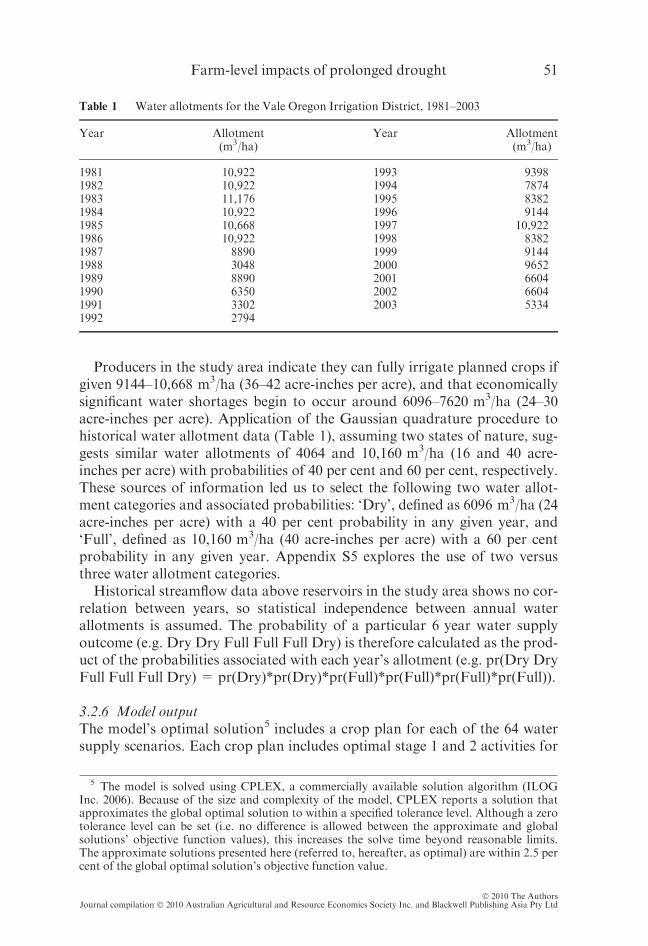
Producers in the study area indicate they can fully irrigate planned crops ifgiven 9144–10,668 m3/ha (36–42 acre-inches per acre), and that economicallysignificant water shortages begin to occur around 6096–7620 m3/ha (24–30acre-inches per acre). Application of the Gaussian quadrature procedure tohistorical water allotment data (Table 1), assuming two states of nature, sug-gests similar water allotments of 4064 and 10,160 m3/ha (16 and 40 acre-inches per acre) with probabilities of 40 per cent and 60 per cent, respectively.These sources of information led us to select the following two water allot-ment categories and associated probabilities: ‘Dry’, defined as 6096 m3/ha (24acre-inches per acre) with a 40 per cent probability in any given year, and‘Full’, defined as 10,160 m3/ha (40 acre-inches per acre) with a 60 per centprobability in any given year. Appendix S5 explores the use of two versusthree water allotment categories.Historical streamflow data above reservoirs in the study area shows no cor-

relation between years, so statistical independence between annual waterallotments is assumed. The probability of a particular 6 year water supplyoutcome (e.g. Dry Dry Full Full Full Dry) is therefore calculated as the prod-uct of the probabilities associated with each year’s allotment (e.g. pr(Dry DryFull Full Full Dry) = pr(Dry)*pr(Dry)*pr(Full)*pr(Full)*pr(Full)*pr(Full)).

3.2.6 Model outputThe model’s optimal solution5 includes a crop plan for each of the 64 watersupply scenarios. Each crop plan includes optimal stage 1 and 2 activities for

Table 1 Water allotments for the Vale Oregon Irrigation District, 1981–2003

Year Allotment(m3/ha)

Year Allotment(m3/ha)

1981 10,922 1993 93981982 10,922 1994 78741983 11,176 1995 83821984 10,922 1996 91441985 10,668 1997 10,9221986 10,922 1998 83821987 8890 1999 91441988 3048 2000 96521989 8890 2001 66041990 6350 2002 66041991 3302 2003 53341992 2794

5 The model is solved using CPLEX, a commercially available solution algorithm (ILOGInc. 2006). Because of the size and complexity of the model, CPLEX reports a solution thatapproximates the global optimal solution to within a specified tolerance level. Although a zerotolerance level can be set (i.e. no difference is allowed between the approximate and globalsolutions’ objective function values), this increases the solve time beyond reasonable limits.The approximate solutions presented here (referred to, hereafter, as optimal) are within 2.5 percent of the global optimal solution’s objective function value.



each year of the 6 year planning horizon. All 64 crop plans are solved forsimultaneously, which enables DSP to mimic forward-looking behaviour,rather than naıve or recursive behaviour. Each water supply scenario’s associ-ated crop plan generates a net present value of returns to land and manage-ment (assuming a 5 per cent discount rate, and a 7 per cent interest rate(American Agricultural Economics Association Task Force 1998)). Given theprobability and net present value of returns associated with each water supplyscenario, the producer’s expected net present value of returns (i.e. objectivefunction value) is calculated. Optimal crop plans and associated returns forvarious water supply scenarios are then compared to address the researchquestions.

4. Results and discussion

4.1 Is a multiyear drought’s impact more than the sum of its parts?

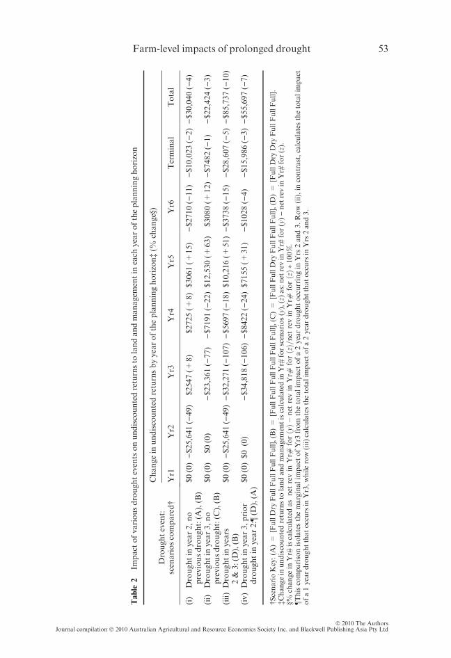
A multiyear drought is comprised of individual years of drought whose eco-nomic impacts may not necessarily be independent, particularly for farm sys-tems with inter-year dynamics. If the economic impacts of individual years ofdrought are interdependent, it may be incorrect to examine an individual yearof drought independent of events and decisions in preceding and subsequentyears. The following four scenarios’ crop plans and associated returns arecompared to determine if the economic impact of a 2 year drought (occurringin years 2 and 3 of a 6-year planning horizon) can be deconstructed into inde-pendent parts, or is more than the sum of its component years’ impacts: (A)[Full Dry Full Full Full Full], (B) [Full Full Full Full Full Full], (C) [Full FullDry Full Full Full], and (D) [Full Dry Dry Full Full Full]. Scenario (A) repre-sents a single-year drought in year 2. Scenario (B) represents the case of noyears of drought, and serves as a baseline to which the other scenarios’ cropplans and returns are compared. Scenario (C) represents a single-yeardrought in year 3. Scenario (D) represents a 2 year drought in years 2 and 3.A comparison of scenarios (A) and (B) reveals that a single-year drought in

year 2 generates a total loss of returns over the 6 year planning horizon of$30,040 (4 per cent of total undiscounted returns) (Table 2, row-i). A similarcomparison of scenarios (C) and (B) shows that a single-year drought in year3 generates a total loss of $22,424 (3 per cent of total undiscounted returns)(Table 2, row-ii). If the impacts of these single-year events are in fact indepen-dent (i.e. confined within the years in which the droughts occurred), the fol-lowing two outcomes are expected: (i) the economic impact of a 2 yeardrought that occurs in years 2 and 3 should approximately equal the sum ofthe individual droughts’ impacts ($52,464 or 6 per cent), and (ii) losses attrib-utable to a year 3 drought should be the same regardless of whether it is pre-ceded by drought or not.Comparison of scenarios (D) and (B) reveals that a 2 year drought that

occurs in years 2 and 3 generates a total loss of $85,737 (10 per cent of total



Table

2Im

pact

ofvariousdroughteventsonundiscountedreturnsto

landandmanagem

entin

each

yearoftheplanninghorizon

Droughtevent:

scenarioscompared†

Changein

undiscountedreturnsbyyearoftheplanninghorizon‡(%

change§)

Yr1

Yr2

Yr3

Yr4

Yr5

Yr6

Terminal

Total

(i)

Droughtin

year2,no

previousdrought:(A

),(B)

$0(0)

)$25,641()49)

$2547(+

8)

$2725(+

8)$3061(+

15)

)$2710()11)

)$10,023()2)

)$30,040()4)

(ii)

Droughtin

year3,no

previousdrought:(C

),(B)

$0(0)

$0(0)

)$23,361()77)

)$7191()22)$12,530(+

63)

$3080(+

12)

)$7482()1)

)$22,424()3)

(iii)Droughtin

years

2&

3:(D

),(B)

$0(0)

)$25,641()49)

)$32,271()107)

)$5697()18)$10,216(+

51)

)$3738()15)

)$28,607()5)

)$85,737()10)

(iv)Droughtin

year3,prior

droughtin

year2:¶(D

),(A

)$0(0)$0(0)

)$34,818()106)

)$8422()24)$7155(+

31)

)$1028()4)

)$15,986()3)

)$55,697()7)

†ScenarioKey:(A

)=

[FullDry

FullFullFullFull],(B)=

[FullFullFullFullFullFull],(C

)=

[FullFullDry

FullFullFull],(D

)=

[FullDry

Dry

FullFullFull].

‡Changein

undiscountedreturnsto

landandmanagem

entiscalculatedin

Yr#

forscenarios(y),(z)as:net

revin

Yr#

for(y))net

revin

Yr#

for(z).

§%changein

Yr#

iscalculatedasnet

revin

Yr#

forðyÞ�

net

revin

Yr#

forðzÞ=net

revin

Yr#

forðzÞ�

100%.

¶Thiscomparisonisolatesthemarginalim

pact

ofYr3

from

thetotalim

pact

ofa2yeardroughtoccurringin

Yrs

2and3.Row(ii),in

contrast,calculatesthetotalim

pact

ofa1yeardroughtthatoccurs

inYr3,whilerow(iii)calculatesthetotalim

pact

ofa2yeardroughtthatoccurs

inYrs

2and3.



undiscounted returns) (Table 2, row-iii), which is 63 per cent more than thehypothesized loss of $52,464. The economic impact of this multiyear droughtis indeed more than the sum of its parts. This result is also found in a compar-ison of the impact of a year 3 drought that is preceded by a year 2 droughtversus a year 3 drought that is not. The marginal impact of a year 3 droughtwhen preceded by a year 2 drought (obtained by comparing scenarios (D)and (A); see Table 2, row-iv) is $55,697 (7 per cent), as compared to $22,424(3 per cent) when not preceded by drought (Table 2, row-ii). That is, the mar-ginal impact of a year 3 drought is 150 per cent larger when preceded bydrought in year 2. The underlying explanation of this result is discussed in thenext subsection.Similar results are found for other multiyear drought scenarios (see Appen-

dix S6), including a 2 year drought that occurs in years 2 and 4, i.e. scenario[Full Dry Full Dry Full Full]. In this case, a single-year drought in year 2 gen-erates a total loss over the 6 year planning horizon of $30,040 (4 per cent oftotal undiscounted returns). A single-year drought in year 4 generates a totalloss of $17,198 (2 per cent). If the economic impacts of the two events wereindependent, the 2 year drought’s impact should approximately equalthe sum of the individual years’ impacts ($47,238 or 5.8 per cent). Instead, the2 year drought generates a total loss of $72,336 (8.8 per cent). It may betempting to analyse this particular drought scenario as two independent yearsof drought, because a wet year separates them. It is clear, however, that theeconomic impacts of the non-consecutive years of drought are interdependent;the impact of drought in year 4 is conditional on the impact of drought in year2. Therefore, even the total impact of non-consecutive years of droughtcannot necessarily be estimated as the sum of two independent events.

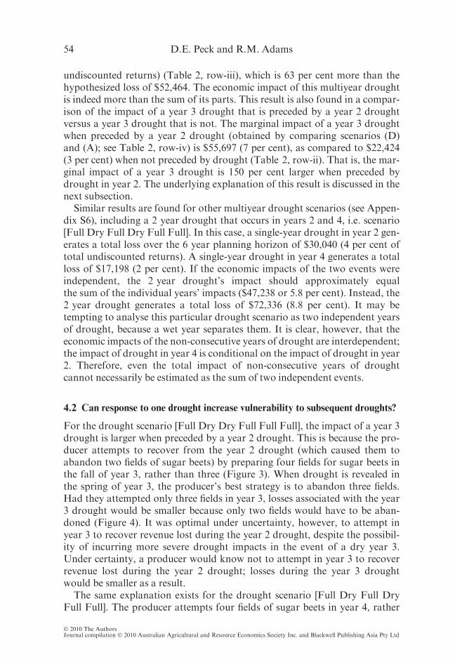
4.2 Can response to one drought increase vulnerability to subsequent droughts?

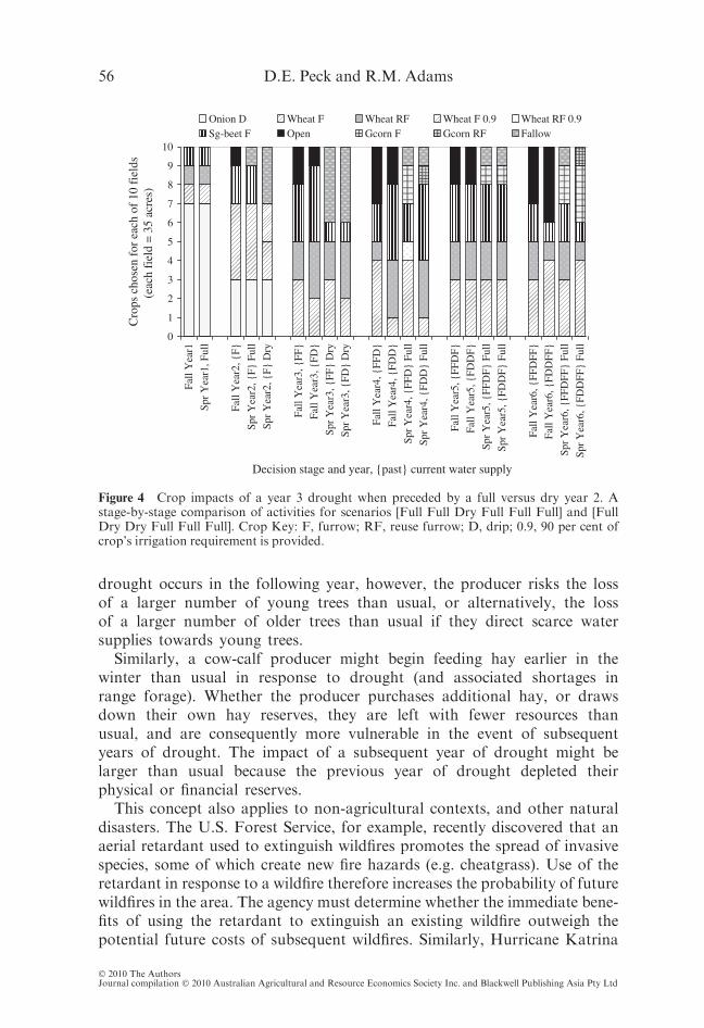
For the drought scenario [Full Dry Dry Full Full Full], the impact of a year 3drought is larger when preceded by a year 2 drought. This is because the pro-ducer attempts to recover from the year 2 drought (which caused them toabandon two fields of sugar beets) by preparing four fields for sugar beets inthe fall of year 3, rather than three (Figure 3). When drought is revealed inthe spring of year 3, the producer’s best strategy is to abandon three fields.Had they attempted only three fields in year 3, losses associated with the year3 drought would be smaller because only two fields would have to be aban-doned (Figure 4). It was optimal under uncertainty, however, to attempt inyear 3 to recover revenue lost during the year 2 drought, despite the possibil-ity of incurring more severe drought impacts in the event of a dry year 3.Under certainty, a producer would know not to attempt in year 3 to recoverrevenue lost during the year 2 drought; losses during the year 3 droughtwould be smaller as a result.The same explanation exists for the drought scenario [Full Dry Full Dry

Full Full]. The producer attempts four fields of sugar beets in year 4, rather



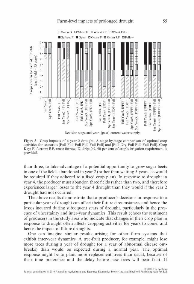
than three, to take advantage of a potential opportunity to grow sugar beetsin one of the fields abandoned in year 2 (rather than waiting 5 years, as wouldbe required if they adhered to a fixed crop plan). In response to drought inyear 4, the producer must abandon three fields rather than two, and thereforeexperiences larger losses to the year 4 drought than they would if the year 2drought had not occurred.The above results demonstrate that a producer’s decisions in response to a

particular year of drought can affect their future circumstances and hence thelosses incurred during subsequent years of drought, particularly in the pres-ence of uncertainty and inter-year dynamics. This result echoes the sentimentof producers in the study area who indicate that changes in their crop plan inresponse to drought often affects cropping activities for years to come, andhence the impact of future droughts.One can imagine similar results arising for other farm systems that

exhibit inter-year dynamics. A tree-fruit producer, for example, might losemore trees during a year of drought (or a year of abnormal disease out-breaks) than would be expected during a normal year. The optimalresponse might be to plant more replacement trees than usual, because oftheir time preference and the delay before new trees will bear fruit. If

0

1

2

3

4

5

6

7

8

9

10Fa

ll Y

ear1

Spr

Yea

r1, F

ull

Fall

Yea

r2, {

F}

Spr

Yea

r2, {

F} F

ull

Spr

Yea

r2, {

F} D

ry

Fall

Yea

r3, {

FF}

Fall

Yea

r3, {

FD}

Spr

Yea

r3, {

FF}

Full

Spr

Yea

r3, {

FD}

Full

Fall

Yea

r4, {

FFF}

Fall

Yea

r4, {

FDF}

Spr

Yea

r4, {

FFF}

Ful

l

Spr

Yea

r4, {

FDF}

Ful

l

Fall

Yea

r5, {

FFFF

}

Fall

Yea

r5, {

FDFF

}

Spr

Yea

r5, {

FFFF

} Fu

ll

Spr

Yea

r5, {

FDFF

} Fu

ll

Fall

Yea

r6, {

FFFF

F}

Fall

Yea

r6, {

FDFF

F}

Spr

Yea

r6, {

FFFF

F} F

ull

Spr

Yea

r6, {

FDFF

F} F

ull

Decision stage and year, {past} current water supply

Onion D Wheat F Wheat RF Wheat F 0.9

Sg-beet F Open Gcorn F Gcorn RF Fallow

Cro

ps c

hose

n fo

r ea

ch o

f 10

fie

lds

(eac

h fi

eld

= 3

5 ac

res)

Figure 3 Crop impacts of a year 2 drought. A stage-by-stage comparison of optimal cropactivities for scenarios [Full Full Full Full Full Full] and [Full Dry Full Full Full Full]. CropKey: F, furrow; RF, reuse furrow; D, drip; 0.9, 90 per cent of crop’s irrigation requirement isprovided.



drought occurs in the following year, however, the producer risks the lossof a larger number of young trees than usual, or alternatively, the lossof a larger number of older trees than usual if they direct scarce watersupplies towards young trees.Similarly, a cow-calf producer might begin feeding hay earlier in the

winter than usual in response to drought (and associated shortages inrange forage). Whether the producer purchases additional hay, or drawsdown their own hay reserves, they are left with fewer resources thanusual, and are consequently more vulnerable in the event of subsequentyears of drought. The impact of a subsequent year of drought might belarger than usual because the previous year of drought depleted theirphysical or financial reserves.This concept also applies to non-agricultural contexts, and other natural

disasters. The U.S. Forest Service, for example, recently discovered that anaerial retardant used to extinguish wildfires promotes the spread of invasivespecies, some of which create new fire hazards (e.g. cheatgrass). Use of theretardant in response to a wildfire therefore increases the probability of futurewildfires in the area. The agency must determine whether the immediate bene-fits of using the retardant to extinguish an existing wildfire outweigh thepotential future costs of subsequent wildfires. Similarly, Hurricane Katrina

0

1

2

3

4

5

6

7

8

9

10

Fall

Yea

r1

Spr

Yea

r1, F

ull

Fall

Yea

r2, {

F}

Spr

Yea

r2, {

F} F

ull

Spr

Yea

r2, {

F} D

ry

Fall

Yea

r3, {

FF}

Fall

Yea

r3, {

FD}

Spr

Yea

r3, {

FF}

Dry

Spr

Yea

r3, {

FD}

Dry

Fall

Yea

r4, {

FFD

}

Fall

Yea

r4, {

FDD

}

Spr

Yea

r4, {

FFD

} Fu

ll

Spr

Yea

r4, {

FDD

} Fu

ll

Fall

Yea

r5, {

FFD

F}

Fall

Yea

r5, {

FDD

F}

Spr

Yea

r5, {

FFD

F} F

ull

Spr

Yea

r5, {

FDD

F} F

ull

Fall

Yea

r6, {

FFD

FF}

Fall

Yea

r6, {

FDD

FF}

Spr

Yea

r6, {

FFD

FF}

Full

Spr

Yea

r6, {

FDD

FF}

Full

Decision stage and year, {past} current water supply

Onion D Wheat F Wheat RF Wheat F 0.9 Wheat RF 0.9Sg-beet F Open Gcorn F Gcorn RF Fallow

Cro

ps c

hose

n fo

r ea

ch o

f 10

fie

lds

(eac

h fi

eld

= 3

5 ac

res)

Figure 4 Crop impacts of a year 3 drought when preceded by a full versus dry year 2. Astage-by-stage comparison of activities for scenarios [Full Full Dry Full Full Full] and [FullDry Dry Full Full Full]. Crop Key: F, furrow; RF, reuse furrow; D, drip; 0.9, 90 per cent ofcrop’s irrigation requirement is provided.



changed the city of New Orleans’ vulnerability to subsequent hurricanes.Because Katrina damaged levees and coastal wetlands, subsequent hurricanesmay be more likely to cause flooding and generate damages.

5. Conclusions

Producers whose farm systems exhibit inter-year dynamics weigh the immedi-ate benefits of a particular drought response against potential future costs inthe event of subsequent droughts. Even when producers behave optimally,management decisions in response to drought can worsen the impacts of sub-sequent years of drought. The marginal economic impact of a given year ofdrought was shown to increase by as much as 150 per cent when preceded byprevious years of drought. This highlights the importance of evaluating theimpacts of an individual year of drought in the context of preceding and sub-sequent years. It also confirms Clawson et al.’s (1980) hypothesis, and pro-ducers’ assertion, that the form of recovery from one drought might affect aproducer’s ability to cope with subsequent droughts.Inter-year dynamics and uncertainty about a drought’s duration make it

more difficult for producers to determine how best to respond to a particularyear of drought. Economists can assist producers by (i) being cognizant ofthe increased complexity of drought preparedness and response decisionswhen inter-year dynamics and the potential for multiyear drought exist, and(ii) developing multiyear stochastic and dynamic simulation models that canbe used in consultation with producers to explore the intra- and inter-yearconsequences of alternative responses to drought under various water supplyscenarios.Similarly, farm policymakers and administrators need to understand that a

year of drought can change a producer’s crop plan for years to come, therebygenerating impacts long after the drought itself subsides, and potentiallyexacerbating the impact of drought in subsequent years. They also need tointerpret drought impact estimates carefully, particularly if derived in a man-ner that disregards water supply conditions in preceding years, and considerthe ability of alternative risk management tools to reduce producers’ vulnera-bility during future drought events.Disaster assistance and crop insurance (including prevented planting provi-

sions), for example, provide payments based on the current year’s crop activi-ties, and therefore inherently account for the influence of past droughts onthe current drought’s impact. They do not, however, necessarily reduce pro-ducers’ vulnerability to future droughts. Producers might still attempt torecover lost revenue opportunities during what is revealed to be another yearof drought. Water supply forecasts with longer lead-times, in contrast, wouldhelp producers avoid failed recovery attempts, and thereby reduce vulnerabil-ity to future droughts. The value of forecasts with longer lead-time is rela-tively well-studied (e.g. Carberry et al. 2000), so an estimate using this study’smultiyear stochastic framework is left for future investigation.



Supporting Information

Additional Supporting Information may be found in the online version of thisarticle:Appendix S1. Theoretical decision model.Appendix S2. Discrete stochastic programming versus simulation and sto-

chastic dynamic programming.Appendix S3. Continuous versus discrete crop choice variables.Appendix S4. Parameter values assumed for various crop-irrigation tech-

nology combinations.Appendix S5. Consideration of three states of nature.Appendix S6. Profit impact of alternative multiyear drought scenarios.Please note: Wiley-Blackwell is not responsible for the content or function-

ality of any supporting materials supplied by the authors. Any queries (otherthan missing material) should be directed to the corresponding author for thearticle.

References

American Agricultural Economics Association Task Force (1998). Conceptual issues in costand return estimates, in Eidman, V. (ed.), Commodity Costs and Returns Estimation Hand-book. American Agricultural Economics Association, Ames, IA, pp. 1–84.

Apland, J. and Hauer, G. (1993). Discrete stochastic programming: concepts, examples and areview of empirical applications, Staff Paper P93-21, University of Minnesota, St. Paul,MN.

Bernardo, D.J., Whittlesey, N.K., Saxton, K.E. and Bassett, D.L. (1987). An irrigation modelfor management of limited water supplies, Western Journal of Agricultural Economics 12,164–173.

Birge, J.R. and Louveaux, F. (1997). Introduction to Stochastic Programming. Springer-VerlagNew York, Inc., New York.

Bryant, K.J., Mjelde, J.W. and Lacewell, R.D. (1993). An intraseasonal dynamic optimizationmodel to allocate irrigation water between crops, American Journal of Agricultural Econom-

ics 75, 1021–1029.Carberry, P., Hammer, G., Meinke, H. and Bange, M. (2000). The potential value of seasonalclimate forecasting in managing cropping systems, in Hammer, G.L., Nicholls, N. and Mit-

chell, C. (eds.), Applications of Seasonal Climate Forecasting in Agricultural and NaturalEcosystems. Kluwer Academic Publishers, Boston, pp. 167–181.

Chen, C., McCarl, B.A. and Adams, R.M. (2001). Economic implications of potential ENSO

frequency and strength shifts, Climatic Change 49, 147–159.Chen, C., McCarl, B.A. and Williams, R.L. (2006). Elevation dependent management of theEdwards Aquifer: linked mathematical and dynamic programming approach, Journal ofWater Resources Planning & Management 132, 330–340.

Clawson, M., Ottoson, H.W., Duncan, M. and Sharp, E.S. (1980). Task group on economics, inRosenberg, N.J., Hoffman, R.O., Quinn, M.L. and Wilhite, D.A. (eds.),Drought in the GreatPlains: Research on Impacts and Strategies. BookCrafters, Inc., Chelsea,MI, pp. 43–59.

Cocks, K.D. (1968). Discrete stochastic programming,Management Science 15, 72–79.CPLEX (2006). Computer Program. ILOG Inc., Sunnyvale, CA.Dai, A., Trenberth, K.E. and Qian, T. (2004). A global dataset of Palmer Drought Severity

Index for 1870–2002: relationship with soil moisture and effects of surface warming, Journalof Hydrometeorology 5, 1117–1130.



Diaz, H.F. (1983). Drought in the United States: some aspects of major dry and wet periods inthe contiguous United States, 1895–1981, Journal of Climate and Applied Meteorology 22,3–16.

Doorenbos, J. and Kassam, A.H. (1979). Yield Response to Water. Food and Agriculture

Organization of the United Nations, Rome.Dudley, N.J. (1988). A single decision-maker approach to irrigation reservoir and farm man-agement decision making,Water Resources Research 24, 633–640.

Food and Agriculture Organization of the United Nations (2002). Deficit Irrigation Practices.Water Reports No. 22, Food and Agriculture Organization of the United Nations, Rome.

General Algebraic Modeling System (2006). Computer Program. GAMS Development Corpo-

ration, Washington, DC.Gleick, P.H. (2000). Water: the potential consequences of climate variability and change forthe water resources of the United States, Pacific Institute for Studies in Development, Envi-

ronment, and Security, Oakland.Hardaker, J.B., Huirne, R.B.M. and Anderson, J.R. (1997). Coping with Risk in Agriculture.CABI Publishing, New York.

Iglesias, E., Garrido, A. and Gomez-Ramos, A. (2003). Evaluation of drought management in

irrigated areas, Agricultural Economics 29, 211–229.Iglesias, E., Garrido, A. and Gomez-Ramos, A. (2007). Economic drought management indexto evaluate water institutions’ performance under uncertainty, Australian Journal of Agricul-

tural and Resource Economics 51, 17–38.Keplinger, K.O., McCarl, B.A., Chowdhury, M.E. and Lacewell, R.D. (1998). Economic andhydrologic implications of suspending irrigation in dry years, Journal of Agricultural and

Resource Economics 23, 191–205.McKeon, G., Ash, A., Hall, W. and Stafford Smith, M. (2000). Simulation of grazing strategiesfor beef production in north-east Queensland, in Hammer, G.L., Nicholls, N. and Mitchell,C. (eds.), Applications of Seasonal Climate Forecasting in Agricultural and Natural Ecosys-

tems. Kluwer Academic Publishers, Boston, pp. 227–252.Meehl, G.A., Stocker, T.F., Collins, W.D., Friedlingstein, P., Gaye, A.T., Gregory, J.M.,Kitoh, A., Knutti, R., Murphy, J.M., Noda, A., Raper, S.C.B., Watterson, I.G., Weaver,

A.J. and Zhao, Z.-C. (2007). Global climate projections, in Solomon, S., Qin, D., Manning,M., Chen, Z., Marquis, M., Averyt, K.B., Tignor, M. and Miller, H.L. (eds.), ClimateChange 2007: The Physical Science Basis. Cambridge University Press, New York, pp.

747–845.Mejias, P., Varela-Ortega, C. and Flichman, G. (2004). Integrating agricultural policies andwater policies under water supply and climate uncertainty, Water Resources Research 40,

W07S03, doi: 10.1029/2003WR002877.Miller, A.C. and Rice, T.R. (1983). Discrete approximations of probability distributions,Man-agement Science 29, 352–362.

Nicholls, N. (2004). The changing nature of Australian droughts, Climatic Change 63,

323–336.Preckel, P.V. and Devuyst, E. (1992). Efficient handling of probability information for deci-sion-analysis under risk, American Journal of Agricultural Economics 74, 655–662.

Rae, A.N. (1971). An empirical application and evaluation of discrete stochastic programmingin farm management, American Journal of Agricultural Economics 53, 625–638.

Rosenzweig, C. and Hillel, D. (1993). The Dust Bowl of the 1930s-analog of greenhouse-effect

in the Great-Plains, Journal of Environmental Quality 22, 9–22.Schultz, R. (2003). Stochastic programming with integer variables,Mathematical ProgrammingSeries B 97, 285–309.

Thompson, D., Jackson, D., Tapp, N., Milham, N., Powell, R., Douglas, B., Kennedy, G.,

Jack, E. and White, G. (1996). Analysing drought strategies to enhance farm financial viabil-ity, Final Report, University of New England, Armidale, New South Wales, Australia.



Toft, H.I. and O’Hanlon, P.W. (1979). A dynamic programming model for on-farm decisionmaking in a drought, Review of Marketing and Agricultural Economics 47, 5–16.

Weisensel, W.P., Van Kooten, G.C. and Schoney, R.A. (1991). Relative riskiness of fixed vs.flexible crop rotations in the dryland cropping region of western Canada, Agribusiness 7,

551–560.Wilhite, D.A., Diodato, D.M., Jacobs, K., Palmer, R., Raucher, B., Redmond, K., Sada, D.,Helm-Smith, K., Warwick, J. and Wilhelmi, O. (2006). Managing drought: a roadmap for

change in the United States, Paper presented at Managing drought and water scarcity in vul-nerable environments: creating a roadmap for change in the United States; The GeologicalSociety of America, 18–20 September, Longmont, CO.



Farm-level impacts of prolonged drought: is a multiyear event more than the sum of its parts

Documents

Transcript of Farm-level impacts of prolonged drought: is a multiyear event more than the sum of its parts