Faramarz E. Seraji, "Dynamic response of a fiber-optic ring resonator: Analysis with influences of...

ARTICLE IN PRESS

Progress in Quantum Electronics 33 (2009) 110–125

0079-6727/$ -

doi:10.1016/j

E-mail ad

www.elsevier.com/locate/pquantelec

Review

Dynamic response of a fiber-optic ring resonator:Analysis with influences of light-source parameters

Faramarz E. Seraji

Optical Communication Group, Iran Telecom Research Center, Tehran, Iran

Abstract

In practice, dynamic behavior of fiber-optic ring resonator (FORR) appears as a detrimental

factor to influence the transmission response of the FORR. This paper presents dynamic response

analysis of the FORR by considering phase modulation of the FORR loop and sinewave modulation

of input signal applied to the FORR from a laser diode. The analysis investigates the influences of

modulation frequency and amplitude modulation index of laser diode, loop delay time of the FORR,

phase angle between FM and AM response of laser diode, and laser diode line-width on dynamic

response of the FORR. The analysis shows that the transient response of the FORR strongly

depends on the product of modulation frequency and loop delay time, coupling and transmission

coefficients of the FORR. The analyses presented here may have applications in optical systems

employing an FORR with a laser diode source.

r 2009 Elsevier Ltd. All rights reserved.

Keywords: Dynamic response; Fiber-optic ring resonator; Loop phase modulation; FM deviation

Contents

1. Introduction . . . . . . . . . . . . . . . . . . . . . . . . . . . . . . . . . . . . . . . . . . . . . . . . . . . . . . 111

2. Dynamic behavior of FORR . . . . . . . . . . . . . . . . . . . . . . . . . . . . . . . . . . . . . . . . . . 112

2.1. Phase modulation of the loop of FORR . . . . . . . . . . . . . . . . . . . . . . . . . . . . . . 113

.

2.1.1. Conditions for dynamic responses . . . . . . . . . . . . . . . . . . . . . . . . . . . . 114

2.2. Sinewave modulation of the input signal to FORR . . . . . . . . . . . . . . . . . . . . . . 115

3. Numerical computations . . . . . . . . . . . . . . . . . . . . . . . . . . . . . . . . . . . . . . . . . . . . . 119

3.1. Influence of modulation frequency of laser diode . . . . . . . . . . . . . . . . . . . . . . . . 119

3.2. Influence of loop delay time of the FORR . . . . . . . . . . . . . . . . . . . . . . . . . . . . 120

see front matter r 2009 Elsevier Ltd. All rights reserved.

pquantelec.2009.05.001

dress: [email protected]

www.elsevier.com/locate/pquantelec

dx.doi.org/10.1016/j.pquantelec.2009.05.001

mailto:[email protected]

ARTICLE IN PRESSF.E. Seraji / Progress in Quantum Electronics 33 (2009) 110–125 111

3.3. Influence of amplitude modulation index. . . . . . . . . . . . . . . . . . . . . . . . . . . . . . 120

3.4. Influence of phase angle between FM and AM responses of laser diode. . . . . . . . 120

3.5. Influence of laser diode line-width . . . . . . . . . . . . . . . . . . . . . . . . . . . . . . . . . . 122

4. Measurement of FM deviation of a laser diode . . . . . . . . . . . . . . . . . . . . . . . . . . . . . 122

5. Conclusion . . . . . . . . . . . . . . . . . . . . . . . . . . . . . . . . . . . . . . . . . . . . . . . . . . . . . . . 123

References . . . . . . . . . . . . . . . . . . . . . . . . . . . . . . . . . . . . . . . . . . . . . . . . . . . . . . . 124

1. Introduction

In recent years, fiber-optic ring resonator (FORR) has been utilized in severalapplications in optical communication [1–14], sensing [15–20], and gyro systems [21–29].In utilization of the FORR, the loop-length is to be modulated by a phase modulator tosweep the loop phase with time to establish a resonance condition in the output of theFORR [30,31]. When the loop phase is modulated, the analysis based on a steady-stateresponse will be inaccurate, particularly, if the modulation frequency is high [32]. In theliterature, however, several authors used only steady-state analysis [33,34], and such ananalysis will be acceptable when the modulation in the loop is performed at a very slowrate. Recently, Ying et al., analyzed dynamic characteristics of the FORR. They showedexperimentally that the sweep rate would shift the oscillating behavior and deteriorate theresponse curve [31].

The FORR behaves quite different from the steady-state response at high modulationrates of light source applied to the FORR [30,35]. However, in Ref. [35] an analysis waspresented by assuming an ideal ramped modulation of the loop phase which did not givethe information about the maximum modulation frequency above which the FORRresponse deviated from the steady-state response. In fact, in practice a phase modulatorcan be made from a piezoelectric transducer (PZT) that usually oscillates at its mechanicalresonance frequency and introduces a sinewave modulation in the loop fiber of FORR.Usually, to obtain a maximum modulation response from the PZT, a sinewave modulatingvoltage is used at the PZT resonance frequency.

In this paper, by considering the influences of light-source parameters, a theoreticalanalysis of dynamic responses of the FORR is presented for two cases: (a) when FORRloop is phase modulated and (b) when input signal to the FORR is sinewave modulated. Infirst case, we find lower limits on the modulation frequency over which the response of theFORR does deviate from the steady-state response and will behave in dynamic regime[31,32]. It is shown that the response of the FORR will be in dynamic state if the productof the modulating frequency fm and the loop delay time t (i.e., fmt) exceeds a certain value(in the range 0.0004–0.06 that depends on the finesse of the FORR). The lower limits of fmtrequired for a dynamic-state response of the FORR are obtained for different conditionsof the FORR.

In second case, the results of the analysis are given for different parameters, namely, themodulating frequency of the laser diode (LD) used as input source to the FORR,amplitude modulation index, power-coupling coefficient k of the coupler used in theFORR, loop delay time t, and the phase angle between FM and AM response of the LD. Itis shown that the dynamic response of the device appears when fmt exceeds a certain value,similar to the first case. Also, when the value of fmt is increased further beyond unity, theresonance of the FORR is shown to be totally lost, where the output simply corresponds to

ARTICLE IN PRESSF.E. Seraji / Progress in Quantum Electronics 33 (2009) 110–125112

the amplitude modulation (AM) of the LD [31,32]. The sinewave-based analysis also givesa possible application of the FORR to measure the optical FM characteristics of laserdiodes. The analysis is also expected to be useful in other applications of the FORR inoptical communication systems and sensors when using an LD as a source [36].

2. Dynamic behavior of FORR

Let us consider an FORR of loop-length L and loop delay time t defined as t ¼ L/v,where v is the phase velocity of the light in the loop fiber, as shown in Fig. 1. It consists of aphase modulator (PZT) to impose a phase delay of Df ¼ f(t) in the loop, where f(t) is ageneral time function. Let Ein, Er2, Er1, and E0 be the complex amplitudes of electric fieldsof optical signals at ports 1, 2, 3, and 4, respectively. It is assumed that the input light islinearly polarized and that the polarization remains constant along the ring. Let k and gdenote the power-coupling coefficient and excess intensity loss of the coupler, respectively.During a time interval 0rtot, the complex electric field amplitudes at different ports of

FORR will be from the first principle as follows:

E0r1

E0r2

E00

264

375 ¼

ffiffiffiffiffiffiffiffiffiffiffiffiffiffiffiffiffiffiffiffiffiffiffiffiffiffiffiffið1� gÞð1� kÞ

p0ffiffiffiffiffiffiffiffiffiffiffiffiffiffiffiffiffi

kð1� gÞp

expð�jp=2Þ

264

375Ein ð1Þ

where the superscript (0) on Er1, Er2, and E0 indicates the number of signal round-trips inthe loop.Before commencement of the first round-trip in the loop, the electric field at port 3

would be phase-shifted by the PZT and the resulting field just after the PZT is

E0r ¼ E0

r1 exp½�jf ðtÞ� ð2Þ

Now, during the time period trto2t, i.e., just after the first round-trip is completed, theelectric field at port 2 would be

E1r2 ¼

ffiffiffiap

E0r expð�joctÞ ð3Þ

By substituting Eqs. (1) and (2) in Eq. (3) will result in

E1r2 ¼

ffiffiffiffiffiffiffiffiffiffiffiffiffiffiffiffiffiffiffiffiffiffiffiffiffiffiffiffiffiffiffiað1� gÞð1� kÞ

pEin expf�j½f ðt� tÞ þ oct�g ð4Þ

Fig. 1. Schematic diagram of an FORR with a phase modulator (PZT) in the loop.


where a is the power transmission coefficient of the loop fiber and oc the angular opticalfrequency. The output of the FORR during this time interval will be

E10 ¼

ffiffiffiffiffiffiffiffiffiffiffiffiffiffiffiffiffikð1� gÞ

pEin expð�jp=2Þ þ

ffiffiffiffiffiffiffiffiffiffiffiffiffiffiffiffiffiffiffiffiffiffiffiffiffiffiffiffið1� gÞð1� kÞ

pE1

r2 ð5Þ

By inserting the value of Er21, Eq. (5) reduces to

E10 ¼


pEin expð�jp=2Þ

þ ð1� gÞð1� kÞffiffiffiap

Ein expf�j½f ðt� tÞ þ oct�g ð6Þ

Similarly, considering n number of round-trips of the fields in the loop, i.e., during atime interval (n�1)trtont, (assuming the integer n tending to infinity) the complex, time-dependent amplitude transmittance can be derived as

En0

Ein

¼ � jffiffiffiffiffiffiffiffiffiffiffiffiffiffiffiffiffikð1� gÞ

pþ jð1� gÞð1� kÞ

ffiffiffiap

�X1n¼1

½akð1� gÞ�ðn�1Þ=2 expf�j½noctþ np=2

(

þ f ðt� tÞ þ � � � þ f ðt� ntÞ�gg ð7Þ

2.1. Phase modulation of the loop of FORR

If we consider a ramped phase modulation, i.e., f(t) ¼ st, where s is the rate of phaseshift, Eq. (7) will change to

En0

Ein



ffiffiffiap

�X1n¼1

½akð1� gÞ�ðn�1Þ=2 expf�j½nðoctþ p=2Þ þ nst� stnðnþ 1Þ=2�g

( )ð8Þ

Now, if a sinusoidal phase modulation f(t) ¼ fm sin(omt) is considered, where fm is themaximum phase shift and om the angular modulation frequency, then from Eq. (7) we canwrite

En0

Ein



ffiffiffiap

�X1n¼1

½akð1� gÞ�ðn�1Þ=2 expf�j½nðoctþ p=2Þ

(

þfm

X1n¼1

sin½omðt� ntÞ��g

)ð9Þ

Eq. (9) is the normalized complex electric field at the output port of the FORR for n

number of signal round-trips in the loop. The normalized output intensity (NOI) fromEq. (9) can be obtained as

Inout ¼

En0

Ein

��2

ð10Þ


2.1.1. Conditions for dynamic responses

The steady-state response of the FORR is achieved when the phase-modulationfrequency fm ( ¼ om/2p) is very low. In fact, the value 1/fm should be very small whencompared to loop delay time (t) of the FORR [32].The simulated responses of the FORR for different values of the product fmt, above

which the ring response starts deviating from the steady-state response, have beendetermined and illustrated in Fig. 2. The typical results are tabulated in Table 1 for fm ¼ p,g ¼ 0.01, and different values of k and a. If a ¼ k ¼ 0.1, the dynamic response appearswhen the value of fmt is just higher than 0.06 and if a ¼ k ¼ 0.9, fmt40.0004. Whena ¼ 0.99 (for almost no loss and maximum transmission in the loop), the minimum value offmt should be 0.0014 for k ¼ 0.1 and 0.00003 for k ¼ 0.9. From Table 1, for the steady-stateoperation of the FORR, the product fmt should be kept as small as possible, depending onvalue of k. That is, the period of the modulating signal should be very large as compared tothe loop delay time t. In the FORR, due to multiple round-trips of the light in the loop,dynamic effects are observable for low values of fmt (as low as 0.00835 for Fig. 2).The data given in Table 1 are expected to be useful in making an approximate estimate

of any given FORR whether it will have a steady-state operation or not.Fig. 2 shows the intensity transmission of the FORR when k ¼ a ¼ 0.88, fm ¼ 334 kHz,

fm ¼ p, g ¼ 0.01, t ¼ 25 ns, and t ¼ 1250 nm [35]. The dynamic response exhibits anoscillatory behavior which is not predicted by steady-state analysis.

Fig. 2. Simulated intensity transmissions of the FORR for k ¼ a ¼ 0.88, fm ¼ 334 kHz, fm ¼ p, and g ¼ 0.01. (a)

ac modulating signal, (b) t ¼ 25 ns, and (c) t ¼ 1250ns.

ARTICLE IN PRESS

Table 1

Condition for dynamic response of the FORR with phase modulation of the loop.

k a ¼ k a ¼ 0.99

fmt� 10�5

0.1 46000 4140

0.2 43300 4100

0.3 42400 468

0.4 41400 448

0.5 4870 435

0.6 4500 427

0.7 4280 418

0.8 4130 410

0.9 440 43

fm ¼ p and g ¼ 0.01

F.E. Seraji / Progress in Quantum Electronics 33 (2009) 110–125 115

In Fig. 2(b), for k ¼ a ¼ 0.88, the value of fmt is 0.00835, where the response is found tobe oscillatory. When fmt is increased further by a factor of 50 (by increasing the value of tto 1250 nm) the resulting response curve will look complex with no proper development ofthe resonance dips, as shown in Fig. 2(c).

Fig. 3 shows the simulated results of the FORR for different modulating frequencieswith k ¼ 0.47, t ¼ 1125 ns, fm ¼ 1.15p, g ¼ 0.49, and a ¼ 0.13. When the modulatingsignal frequency (Fig. 3a) increases, the response from steady-state condition (Fig. 3b)changes to dynamic regime with an overshoot at the leading edge (Fig. 3c). A furtherincrease of fm will render the overshoot to switch to falling edge (Fig. 3d).

2.2. Sinewave modulation of the input signal to FORR

In this section, the dynamic analysis is presented for a case when the optical frequency ofinput signal to FORR in Fig. 1 is injected from a sinewave-modulated laser diode. Theoptical frequency of a single-mode laser diode can be directly modulated by modulatingthe injection current. In fact, the injection current changes both the intensities as well as thefrequency of LD, producing a simultaneous amplitude modulation and frequencymodulation (FM) on the electric field of the optical source [37–40]. The transient analysisthen considers the effects of both AM and FM.

Generally, the electric field of optical FM signal from an LD can be expressed as [37–40]

EðtÞ ¼ emðtÞ sin octþZ t

t0

OðgÞ dgþ y0

� �ð11Þ

where O(g) is frequency of modulating signal, em(t) the time-varying amplitude of theelectric field of the optical signal, oc the angular optical frequency, and y0 an arbitraryphase constant.

By choosing to properly, we can cancel out the phase constant y0. Let, for the sake ofsimplicity, y0 ¼ 0. Then, from Eq. (11) the instantaneous phase can be denoted by

yðtÞ ¼ octþ y0 þZ t

t0

OðgÞ dg ð12Þ

ARTICLE IN PRESS

Fig. 3. Simulated intensity transmission of the FORR for k ¼ 0.47, t ¼ 1125 ns, fm ¼ 1.15p, g ¼ 0.49, and

a ¼ 0.13 when (a) ac modulating signal, (b) fm ¼ 6 kHz, fmt ¼ 0.00675, (c) fm ¼ 66.7 kHz, fmt ¼ 0.075, and (d)

fm ¼ 340 kHz, fmt ¼ 0.382.

F.E. Seraji / Progress in Quantum Electronics 33 (2009) 110–125116

The instantaneous angular frequency will be

oðtÞ ¼dyðtÞ

dt¼ oc þ OðtÞ ð13Þ

where O(t) is the instantaneous angular frequency deviation. Let i(t) be the instantaneousinjection current of the LD expressed as

iðtÞ ¼ I0 þ Im sinðomtÞ ð14Þ

where I0 is the bias current of the LD and Im the peak value of the ac modulating current.The instantaneous frequency deviation from the unmodulated frequency of the LD isrelated to the sinewave-modulated injection current i(t) as

oðtÞ � oc ¼ 2pkf Im sinðomtþ fFM Þ ð15Þ


where kf is the optical frequency deviation in Hz per mA current, and fFM the phase anglebetween the optical frequency deviation and the amplitude modulating drive current of thegiven LD. fFM and kf are the functions of the modulating frequency and the bias currentof the LD [38]. From Eqs. (13) and (15) the instantaneous angular frequency deviation canbe written as

OðtÞ ¼ 2pkf Im sinðomtþ fFM Þ ð16Þ

By using Eq. (15), Eq. (11) becomes

EðtÞ ¼ emðtÞ sin oct�2pImkf

om

cosðomtþ fFM Þ

� �ð17Þ

The maximum frequency deviation from the frequency of the unmodulated carrier will be

Df ¼ Imkf ð18Þ

Then from Eq. (17) we can write

EðtÞ ¼ emðtÞ sin oct�Df

f m

cosðomtþ fFMÞ

� �¼ emðtÞ sin½oct� b cosðomtþ fFMÞ� ð19Þ

where b is the frequency modulation index expressed as

b ¼Df

f m

¼kmkf ðI0 � I thÞ

f m

ð20Þ

where km is the amplitude modulation index for the drive current defined as

km ¼Im

ðI0 � I thÞð21Þ

with Ith as the threshold current of the LD. The corresponding time-varying optical powerof the LD with P0 as the unmodulated power, will be

p0ðtÞ ¼ P0½1þ km sinðomtÞ� ð22Þ

Then, the time-varying electric field amplitude of the optical signal can be expressed as

emðtÞ ¼ �ffiffiffiffiffiffiP0

p ffiffiffiffiffiffiffiffiffiffiffiffiffiffiffiffiffiffiffiffiffiffiffiffiffiffiffiffiffiffiffiffiffi1þ km sinðomtÞ

pð23Þ

where e is a proportionality constant relating the value of electric field to the average valueof optical power. Thus, by substituting Eq. (23) in Eq. (19), the electric field of the opticalsignal from the LD can be written as

EðtÞ ¼ Em

ffiffiffiffiffiffiffiffiffiffiffiffiffiffiffiffiffiffiffiffiffiffiffiffiffiffiffiffiffiffiffiffiffi1þ km sinðomtÞ

psin½oct� b cosðomtþ fFMÞ�

¼ Em


psin oct�

kmkf ðI0 � I thÞ

f m

cosðomtþ fFMÞ

� �ð24Þ

where Em ¼ eOPo is the electric field amplitude of the unmodulated light.Let us now consider the FORR shown in Fig. 1 with the same parameters’ definitions.

We assume that the state of linearly polarized input optical signal em(t) (see Eq. (23))from the LD applied to the FORR remains constant along the loop of the FORR. If weconsider time intervals 0rtot, trto2t,y, ntrto(n+1)t, where n is the number ofsignal round-trips along the ring), the output electric field at port 4 of the FORR can


be derived.

En0 ¼ � j


pemðtÞ exp½jf ðtÞ� þ jð1� gÞð1� kÞ

ffiffiffiap

�X1n¼1

½akð1� gÞ�ðn�1Þ=2emðt� ntÞ expfj½f ðt� ntÞ � nðoctþ p=2Þ�g

( )ð25Þ

where

emðtÞ ¼ Em


pð26aÞ

emðt� ntÞ ¼ Em

ffiffiffiffiffiffiffiffiffiffiffiffiffiffiffiffiffiffiffiffiffiffiffiffiffiffiffiffiffiffiffiffiffiffiffiffiffiffiffiffiffiffiffiffiffiffi1þ km sin½omðt� ntÞ�

pð26bÞ

f ðtÞ ¼ �b cosðomtþ fFM Þ ð26cÞ

f ðt� ntÞ ¼ �b cos½omðt� ntÞ þ fFM Þ� ð26dÞ

We note that Eq. (24) is considered as the input electric field amplitude of the FORR.Using Eqs. (26a)–(26d) in Eq. (25), the amplitude ratio will result in

En0

Em

¼ � jAffiffiffiffiffiffiffiffiffiffiffiffiffiffiffiffiffiffiffiffiffiffiffiffiffiffiffiffiffiffiffiffiffi1þ km sinðomtÞ

psin½�jb cosðomtþ fFM Þ�

þ jBX1n¼1

ðCÞðn�1Þffiffiffiffiffiffiffiffiffiffiffiffiffiffiffiffiffiffiffiffiffiffiffiffiffiffiffiffiffiffiffiffiffiffiffiffiffiffiffiffiffiffiffiffiffiffiffi1þ km sin½ðomðt� ntÞ�

p(

� expfj½�b cos½omðt� ntÞ� þ fFM � � nðoctþ p=2Þ�gg ð27Þ

where A ¼ffiffiffiffiffiffiffiffiffiffiffiffiffiffiffiffiffikð1� gÞ

p, B ¼ ð1� kÞð1� gÞ

ffiffiffiap

, and C ¼ffiffiffiffiffiffiffiffiffiffiffiffiffiffiffiffiffiffiffiakð1� gÞ

pare constants.

Fig. 4. Theoretical intensity transmission of FORR for k ¼ a ¼ 0.8, km ¼ 0.2, kf ¼ 250� 106Hz/mA, and

t ¼ 1 ns. (a) ac modulating signal, (b) fm ¼ 0.5� 106Hz, (c) fm ¼ 5� 106Hz, and (d) fm ¼ 1.0� 109Hz.


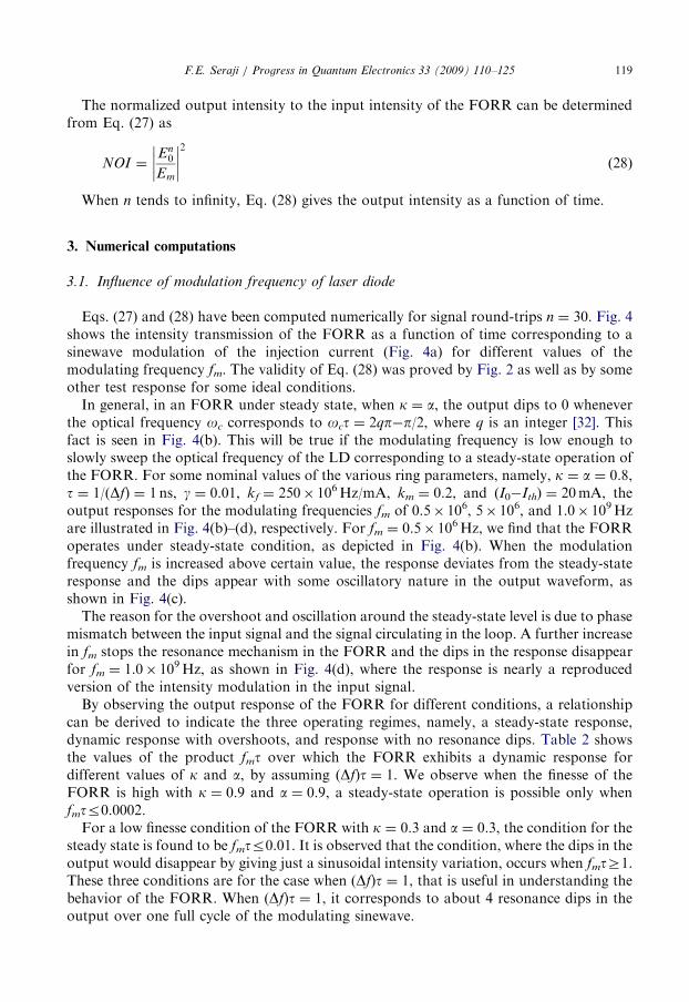
The normalized output intensity to the input intensity of the FORR can be determinedfrom Eq. (27) as

NOI ¼En

0

Em

��2

ð28Þ

When n tends to infinity, Eq. (28) gives the output intensity as a function of time.

3. Numerical computations

3.1. Influence of modulation frequency of laser diode

Eqs. (27) and (28) have been computed numerically for signal round-trips n ¼ 30. Fig. 4shows the intensity transmission of the FORR as a function of time corresponding to asinewave modulation of the injection current (Fig. 4a) for different values of themodulating frequency fm. The validity of Eq. (28) was proved by Fig. 2 as well as by someother test response for some ideal conditions.

In general, in an FORR under steady state, when k ¼ a, the output dips to 0 wheneverthe optical frequency oc corresponds to oct ¼ 2qp�p/2, where q is an integer [32]. Thisfact is seen in Fig. 4(b). This will be true if the modulating frequency is low enough toslowly sweep the optical frequency of the LD corresponding to a steady-state operation ofthe FORR. For some nominal values of the various ring parameters, namely, k ¼ a ¼ 0.8,t ¼ 1/(Df) ¼ 1 ns, g ¼ 0.01, kf ¼ 250� 106Hz/mA, km ¼ 0.2, and (I0�Ith) ¼ 20mA, theoutput responses for the modulating frequencies fm of 0.5� 106, 5� 106, and 1.0� 109Hzare illustrated in Fig. 4(b)–(d), respectively. For fm ¼ 0.5� 106Hz, we find that the FORRoperates under steady-state condition, as depicted in Fig. 4(b). When the modulationfrequency fm is increased above certain value, the response deviates from the steady-stateresponse and the dips appear with some oscillatory nature in the output waveform, asshown in Fig. 4(c).

The reason for the overshoot and oscillation around the steady-state level is due to phasemismatch between the input signal and the signal circulating in the loop. A further increasein fm stops the resonance mechanism in the FORR and the dips in the response disappearfor fm ¼ 1.0� 109Hz, as shown in Fig. 4(d), where the response is nearly a reproducedversion of the intensity modulation in the input signal.

By observing the output response of the FORR for different conditions, a relationshipcan be derived to indicate the three operating regimes, namely, a steady-state response,dynamic response with overshoots, and response with no resonance dips. Table 2 showsthe values of the product fmt over which the FORR exhibits a dynamic response fordifferent values of k and a, by assuming (Df)t ¼ 1. We observe when the finesse of theFORR is high with k ¼ 0.9 and a ¼ 0.9, a steady-state operation is possible only whenfmtr0.0002.

For a low finesse condition of the FORR with k ¼ 0.3 and a ¼ 0.3, the condition for thesteady state is found to be fmtr0.01. It is observed that the condition, where the dips in theoutput would disappear by giving just a sinusoidal intensity variation, occurs when fmtZ1.These three conditions are for the case when (Df)t ¼ 1, that is useful in understanding thebehavior of the FORR. When (Df)t ¼ 1, it corresponds to about 4 resonance dips in theoutput over one full cycle of the modulating sinewave.

ARTICLE IN PRESS

Table 2

Conditions for dynamic responses of the FORR with sinewave-modulated input.

k a ¼ k a ¼ 0.90

fmt� 10�4

0.3 4100 410

0.5 450 48

0.6 430 46

0.7 410 44

0.8 45 43

0.9 42 42


3.2. Influence of loop delay time of the FORR

Fig. 5 shows response of the FORR for k ¼ a ¼ 0.5, km ¼ 0.2, fm ¼ 0.5� 106Hz, andkf ¼ 250� 106Hz/mA, when the value of t is changed by altering the length of the loop ofthe FORR. By increasing the value of t, the number of resonance dips will increase.Fig. 5(a) shows the intensity transmission when t ¼ 1 ns (loop-length of about 20 cm). Thenumber of resonance dips in one cycle in this case is 4, assuming Df ¼ 1GHz. As t isincreased by a factor of 2 and 6, respectively, the corresponding output response will havethe number of resonance dips multiplied by the same factors, as shown in Fig. 5(b) and (c).In Fig. 4(c), the multiplying factor of t with respect to Fig. 5(a) is 6 and the correspondingnumber of resonance dips in one cycle will be 6� 4 ¼ 24. It should be noted that variationof t may cause the output response to exhibit an oscillatory dynamic response when theproduct fmt exceeds a certain limit, as shown in Fig. 5(c).

3.3. Influence of amplitude modulation index

Fig. 6 shows the intensity transmission when the only variable parameter is theamplitude modulation index km and all other parameters are kept constant so as to have asteady-state operation of the FORR. It is observed that when km ¼ 0.2 (Fig. 6a), thenumber of resonance dips in the output in one full cycle of the modulating sine waveformis 4. As the value of km is doubled to 0.4, the number of dips in the output also doubles to8, as shown in Fig. 6(a) and (b). Similarly, for km ¼ 0.8, as indicated in Fig. 6(c), thenumber of dips increases correspondingly to 16. On the basis of this relationship betweenthe amplitude modulation index and the number of resonance dips in the output ofthe resonator, it is possible to estimate the optical frequency deviation per unit current(Eq. (18)) of any given LD. Observe that the amplitude modulation in the output intensityincreases when km is increased.

3.4. Influence of phase angle between FM and AM responses of laser diode

As illustrated in Fig. 7, the intensity transmission of the FORR is plotted for differentvalues of the phase angle fFM between the FM and AM responses of the LD. By applyingthe input modulation signal of Fig. 7(a), the response curves for fFM values of 0, p/2, and p

ARTICLE IN PRESS

Fig. 6. Theoretical intensity transmission of FORR for k ¼ a ¼ 0.5, fm ¼ 0.5� 106Hz, kf ¼ 250� 106Hz/mA,

and t ¼ 1 ns. (a) km ¼ 0.2, (b) km ¼ 0.4, and (c) km ¼ 0.8.

Fig. 5. Theoretical intensity transmission of FORR for k ¼ a ¼ 0.5, km ¼ 0.2, fm ¼ 0.5� 106Hz, and

kf ¼ 250� 106Hz/mA. (a) t ¼ 1 ns, (b) t ¼ 2 ns, and (c)t ¼ 6 ns.


radians are obtained as shown in Fig. 7(b)–(d), respectively. From these output responsecurves we see that the variation of fFM does not alter the nature of the response, ratheronly shifts the response by the same angle through which fFM is varied.

ARTICLE IN PRESS

Fig. 7. Theoretical intensity transmission of FORR for k ¼ a ¼ 0.5, fm ¼ 0.5� 106Hz, kf ¼ 250� 106Hz/mA,

t ¼ 1 ns, and km ¼ 0.2. (a) ac modulating current signal applied to laser diode, (b) fFM ¼ 0 rad, (c) fFM ¼ p/2 rad, and (d) fFM ¼ p rad.


3.5. Influence of laser diode line-width

The analysis presented above is valid when the line-width of LD is ideally zero or smallcompared to the free spectral range (1/t) of the FORR. The condition for the line-width(lw) required can be stated as lw51/t and typically we should have lwo0.001/t.Experimentally, the later condition is a stringent case. For example, for a practical case if

we have a loop-length of about 10 cm corresponding to t ¼ 0.5 ns, the line-width required forthe LD works out to be smaller than 2MHz. When the condition lw51/t is not satisfied, theoutput response may contain beat noise corresponding to the beating of the differentiallydelayed spectral components of the LD. To implement this condition, a multimode LD withone dominant mode at 1300nm is used as an input source applied to an FORR with a 3dBcoupler and a loop-length of 1m. Fig. 8 shows the experimental response [41–43]. The outputresponse contains the resonance dips in the presence of excessive beat noise. For a givenpractical length of the loop fiber, low finesse FORR can accommodate somewhat larger line-width of LD. The beat noise, if any in the output, gives some information about the line-width of a given LD. An application where the line-width of an LD is controlled in closedloop by use of an FORR was reported [36]. When using LD’s, to obtain a noise-free outputresponse, a short loop-length is needed. Practically, micro-ring resonator with a small loop-length in mm and mm ranges has been reported [44,45].

4. Measurement of FM deviation of a laser diode

Figs. 4–6 indicate that when the value of (Df)t is kept equal to unity, it results in 4resonance dips in the output of FORR over one full cycle of the modulating sinewave

ARTICLE IN PRESS

x-scale: 10 µµs/divy-scale: 50 mV/div

Fig. 8. Experimental response of the FORR showing resonance dips in presence of beat noise when using a

multimode laser diode, a loop-length of 1m, and a coupler with k ¼ 0.5. Bottom trace: modulating signal at

11 kHz [after 41]. x-scale: 10ms/div; y-scale: 50mV/div.


applied to the input source LD. This can be a basis for measuring the FM deviation of anLD. If the peak value of the modulating current Im is adjusted for a given FORR toproduce 4 resonance dips, then we have (Df)t ¼ 1. For a general value of the current Im,if there are N resonance dips (N44), we can approximately write (Df)t ¼ N/4. Thenthe optical frequency deviation per unit current of the LD can be derived as(Df) ¼ Im ¼ (N/4tIm).

The phase angle between FM and AM can be estimated by measuring the shift in theoutput waveform (see Fig. 7) of the FORR with respect to the modulating sinewave asexplained in Section 3.4.

Use of an FORR to measure FM deviation when has an advantage over usualMach–Zehnder FM discriminator [46] where in FORR the FM signal (measured asnumber of resonance dips) is not mixed up with the AM signal as it occurs in case ofMach–Zehnder FM discriminator. In the later case, a network analyzer would be neededto separate the FM signal. Also, the FORR is simple to construct and will not require anypiezoelectric transducer stabilization. Moreover, in the FORR method, if the loop delay tis known, the FM deviation per unit current can be directly calculated, as per the aboverelation, with no need of calibration. However, major disadvantages of using the FORRmethod are poor accuracy and resolution in the measurement (due to counting of dips),and the limit on the maximum allowable value of modulating frequency fm for a givenvalue of t.

5. Conclusion

This paper presented the dynamic behavior of an FORR by considering a sinusoidalphase modulation of the FORR loop and sinewave-modulation of the input signal appliedto the FORR. It is shown that when the period of the modulating waveform (1/fm)becomes comparable to the loop delay time t, the FORR operates in dynamic regime by


deviating from the steady-state condition. The lower limits on the value of fmt required fora dynamic behavior of the FORR were tabulated for different values of k and a.The analysis also dealt with the influences of modulation frequency of laser diode, loop

delay time of FORR, amplitude modulation index, phase angle between FM and AMresponses of laser diode, and laser diode line-width on the over all response of the FORR.There is an upper limit for the operating modulation frequency of the source above whichthe FORR deviates from an ideal steady-state response and enters into dynamic regime. Inthis case, to obtain a steady-state response, the value of the product fmt should typically beless than about 0.0002 for a high-finesse FORR. When fmt exceeds unity, the resonancedips in the output response disappear and the output of the FORR approximates to thesinewave intensity modulation in the input light from the LD.The number of resonance dips in the FORR response is a function of (Df)t that should

be greater than (or equal to) unity for obtaining more than (or equal to) about 4 dips inone cycle of the modulating sinewave input. When the amplitude modulation index of theLD drive is increased, the number of resonance dips increases along with a sinusoidalmodulation in the output corresponding to the intensity modulation of the laser output.The effect of the phase angle between the FM and AM characteristic of the LD is alsostudied. A method of measuring the FM characteristics of the LD is suggested. The effectof line-width of the LD source is described. To satisfy coherence conditions, it was shownthat the line-width of the source should be very small when compared to the free spectralrange (1/t) of the FORR.The analysis presented will have applications in optical systems employing an FORR

with a laser-diode source. Also, a method is proposed to measure an unknown optical FMmagnitude and phase response of a laser diode.

References

[1] G. Soundra Pandian, Faramarz E. Seraji, IEE Proc. Pt. J. 138 (3) (1991) 235–239.

[2] Sai T. Chu, B.E. Little, Wugen Pan, Taro Kaneko, Shinay Sato, Yasuo Kokubun, IEEE Photonic Technol.

Lett. 11 (6) (1999) 691–693.

[3] D.G. Rabus, M. Hamacher, H. Heidrich, Active and passive microring resonator filter applications on

GaInAsP/InP, in: Proceedings of the 13th International Conference on Indium Phosphide and Related

Materials, IPRM 14–18 May, Nara, Japan, Pap. ThA1-3, 2001, pp. 477–480.

[4] Fufei Pang, Feng Liu, Xiuyou Han, Haiwen Cai, Ronghui Qu, Zujie Fang, Opt. Commun. 260 (2006)

567–570.

[5] Sanjoy Mandal, Kamal Dasgupta, T.K. Basak, S.K. Ghosh, Opt. Commun. 264 (2006) 97–104.

[6] P.P. Yupapin, P. Saeung, C. Li, Opt. Commun. 272 (2007) 81–86.

[7] P. Saeung, P.P. Yupapin, Optik 119 (10) (2008) 465–472.

[8] Otto Schwelb, Opt. Commun. 265 (2006) 175–179.

[9] S. Dilwali, G.S. Pandian, IEEE Photonic Technol. Lett. 4 (8) (1992) 942–944.

[10] Hao Shen, Jian-Ping Chen, Xin-Wan Li, Yi-Ping Wang, Opt. Commun. 262 (2006) 200–205.

[11] Junqing Li, Li Li, Jiaqun Zhao, Chunfei Li, Opt. Commun. 256 (2005) 319–325.

[12] A. Rostami, Microelectron. J. 37 (2006) 976–981.

[13] P.P. Yupapin, P. Chunpang, Opt. Laser Technol. 40 (2008) 273–277.

[14] J.L.S. Lima, K.D.A. Saboia, J.C. Sales, J.W.M. Menezes, W.B. deFraga, G.F. Guimaraes, A.S.B. Sombra,

Opt. Fiber Technol. 14 (2008) 79–83.

[15] Y. Ohtsuka, Y. Imai, Opt. Acta 33 (12) (1986) 1529–1537.

[16] K. Kyuma, S. Tai, K. Kojima, and M. Takahashi, Fibre-optic resonant ring sensors: system and device

technology, optical fibre sensor, in: Proceeding of the sixth International Conference OFS ‘89, Paris, France,

18–20 September, 1989.


[17] A.D. Kersey, Fibre-optic current sensor based on Faraday rotation in a resonant fibre ring, in: Proceeding of

Conference. LEOS-‘88, Santa Clara, CA, USA, November, 1988, pp. 281–282.

[18] G.A. Sanders, G.F. Rouse, L.K. Strandjord, N.A. Demma, K.A. Miesel, and Q.Y. Chen, Resonator fiber-

optic gyro using LiNbO3 integrated optics at 1.5 mm wavelength, in: Proceeding of SPIE, 985, 1989,

pp. 202–210. (Fiber optic and laser sensors VI, Boston, MA, USA, 6–7 September, 1988).

[19] F. Farahi, K. Kalli, and D.A. Jackson, An all fibre ring resonator gyroscope using a low coherence length

source, in: Proceeding of sixth International Conference OFS ‘89, Paris, France, September 18–20, 1989.

[20] R.W. Boyd, J.H. Heebner, Appl. Opt. 40 (2001) 5742–5747.

[21] S.L. McCall, A.F.J. Levi, R.E. Slusher, S.J. Pearton, R.A. Logan, Appl. Phys. Lett. 60 (1992) 289–291.

[22] D. Garus, R. Hereth, F. Schliep, Design considerations for Brillouin–Ringlaser gyroscopes, in: Proceedings

of Symposium on Gyro Technology (DGON), Stuttgart, 1994, p. 2.0.

[23] K. Kalli, D.A. Jackson, Opt. Lett. 17 (15) (1992) 1090–1092.

[24] B.E. Little, S.T. Chu, J.V. Hryniewicz, P.P. Absil, Opt. Lett. 25 (5) (2000) 344–346.

[25] T. Kominato, Y. Ohmori, N. Takato, H. Okazaki, M. Yasu, IEEE J. Lightwave Technol. 12 (1992)

1781–1788.

[26] R. Adar, Y. Shani, C.H. Henry, R.C. Kistler, G.E. Blonder, N.A. Olsson, Appl. Phys. Lett. 58 (5) (1991)

444–445.

[27] K. Oda, S. Suzuki, H. Takahashi, H. Toba, IEEE Photon. Technol. Lett. 6 (8) (1994) 1031–1034.

[28] Y. Dumeige, C. Arnaud, P. Feron, Opt. Commun. 250 (2005) 376–383 (Erratum: Opt. Commun. 272 (2007)

279).

[29] P.P. Yupapin, Optik 119 (10) (2008) 492–494.

[30] Faramarz E. Seraji, G. Soundra Pandian, J. Mod. Opt. 38 (4) (1991) 671–676.

[31] D.Q. Ying, H.L. Ma, Z.H. Jin, Appl. Opt. 46 (2007) 4890–4895.

[32] Faramarz E. Seraji, Prog. Quantum Electron. 33 (2009) 1–16.

[33] B. Crosignani, A. Yariv, P. Di-Porto, Opt. Lett. 11 (1986) 251–253.

[34] M. Nazarathy, S.A. Newton, Appl. Opt. 25 (7) (1986) 1051–1055.

[35] Z.K. Ioannidis, P.M. Radmore, I.P. Giles, Opt. Lett. 13 (5) (1988) 422–424.

[36] S. Tai, K. Kyuma, K. Hamanaka, T. Nakayama, Opt. Acta 33 (12) (1986) 1539–1551.

[37] S. Kobayashi, T. Kimura, Laser, IEEE J. Quantum Electron. QE-18 (10) (1982) 1662–1669.

[38] H. Olesen, G. Jacobsen, IEEE J. Quantum Electron. QE-18 (12) (1982) 2069–2080.

[39] M.C. Carvalho, A.J. Seeds, Electron. Lett. 24 (7) (1988) 428–429.

[40] K. Kikuchi, IEEE J. Quantum Electron. 26 (1) (1990) 45–49.

[41] G. Soundra Pandian, Faramarz E. Seraji, Jpn. J. Appl. Phys. 29 (10) (1990) 1967–1973.

[42] K. Kalli, D.A. Jackson, Opt. Lett. 18 (1993) 465–467.

[43] H.L. Ma, Z.H. Jin, C. Ding, Y.L. Wang, Chin. J. Lasers 30 (2003) 731–734.

[44] C. Caspar, E. -J. Bachus, Electron. Lett. 25 (22) (1989) 1506–1508.

[45] Chun-Sheng Ma, Yuan-Zhe Xu, Xin Yan, Zheng-Kun Qin, Xian-Yin Wang, Opt. Commun. 262 (2006)

41–46.

[46] G. Soundra Pandian, N.E. Jolly, A. Hadjifotiou, Measurement of FM deviation of DFB lasers using a

Mach–Zehnder type of optical FM discriminator, Unpublished Report, STC Technology Ltd., England,

June 1989.

Faramarz E. Seraji, "Dynamic response of a fiber-optic ring resonator: Analysis with influences of...

Documents

Transcript of Faramarz E. Seraji, "Dynamic response of a fiber-optic ring resonator: Analysis with influences of...