arX

iv:1

009.

4313

v2 [

mat

h.A

G]

1 J

ul 2

011

Fano 3-folds in codimension 4,

Tom and Jerry. Part I

Gavin Brown Michael Kerber Miles Reid

Abstract

This work is part of the Graded Ring Database project [GRDB],and is a sequel to [A0] and [ABR]. We introduce a strategy based onKustin–Miller unprojection that allows us to construct many hundredsof Gorenstein codimension 4 ideals with 9× 16 resolutions (that is, 9equations and 16 first syzygies). Our two basic games are called Tomand Jerry; the main application is the biregular construction of mostof the anticanonically polarised Mori Fano 3-folds of Altınok’s thesis[A0]. There are 115 cases whose numerical data (in effect, the Hilbertseries) allow a Type I projection. In every case, at least one Tomand one Jerry construction works, providing at least two deformationfamilies of quasismooth Fano 3-folds having the same numerics butdifferent topology.MSC: 14J45 (13D40 14J28 14J30 14Q15)Keywords: Mori theory, Fano 3-fold, unprojection, Sarkisov program

1 Introduction and the classification of

Fano 3-folds

A Fano 3-fold X is a normal projective 3-fold whose anticanonical divisor−KX = A is Q-Cartier and ample. We eventually impose additional condi-tions on the singularities and class group of X , such as terminal, Q-factorial,quasismooth, prime (that is, class group ClX of rank 1) or ClX = Z · A,but more general cases occur in the course of our arguments.

We study X via its anticanonical graded ring

R(X,A) =⊕

m∈N

H0(X,mA).

1

Choosing generators of R(X,A) embeds X as a projectively normal sub-variety X ⊂ P(a1, . . . , an) in weighted projective space. The anticanonicalring R(X,A) is known to be Gorenstein, and we say that X ⊂ P(a1, . . . , an)is projectively Gorenstein. The codimension of X refers to this anticanonicalembedding. The discrete invariants of a Fano 3-foldX are its genus g (definedby g + 2 = h0(X,−KX)) together with a basket of terminal cyclic quotientsingularities; for details see 3.1 and [ABR].

In small codimension we can write down hypersurfaces, codimension 2complete intersections and codimension 3 Pfaffian varieties fluently. Thisunderlies the classification of Fano 3-folds in codimension ≤ 3 (see [C3f], [F]and [A0]): the famous 95 weighted hypersurfaces, 85 codimension 2 families,and 70 families in codimension 3, of which 69 are 5 × 5 Pfaffians. Goren-stein in codimension 4 remains one of the frontiers of science: there is noautomatic structure theory, and deformations are almost always obstructed.Type I projection and Kustin–Miller unprojection (see [KM], [PR], [Ki]) is asubstitute that is sometimes adequate. This paper addresses codimension 4Fano 3-folds in this vein.

The analysis of [A0], [A], [ABR], [GRDB] provides 145 numerical can-didates for codimension 4 Fano 3-folds. This paper isolates 115 of thesethat can be studied using Type I projections, hence as Kustin–Miller un-projections. Our main result is Theorem 3.2: each of these 115 numericalcandidates occurs in at least two ways (the Tom and Jerry of the title), thatgive rise to topologically distinct varieties X .

The reducibility of the Hilbert scheme of Fano 3-folds is a systematicfeature of our results, that goes back to Takagi’s study of prime Fano 3-foldswith basket of 1

2(1, 1, 1) points ([T], Theorem 0.3). He describes families of

varieties having the same invariants, but arising from different “Takeuchiprograms”, that is, different Sarkisov links. Four of his numerical cases havecodimension 4. The first, No. 1.4 in the tables of [T], is our initial caseX ⊂ P7(17, 2); it projects to the (2, 2, 2) complete intersection, so has 7× 12resolution and is unrelated to Tom and Jerry. Takagi’s three other pairs ofcodimension 4 cases correspond to our Tom and Jerry families as follows:

X ⊂ P7(14, 24) : Tom1 = No. 2.2 (8 nodes), Jer45 = No. 3.3 (9 nodes),X ⊂ P7(15, 23) : Tom1 = No. 5.4 (7 nodes), Jer23 = No. 4.1 (8 nodes),X ⊂ P7(16, 22) : Tom1 = No. 4.4 (6 nodes), Jer15 = No. 1.1 (7 nodes).

Each of these is prime. In our treatment, each of these numerical cases admitsone further Jerry family consisting of Fano 3-folds of Picard rank ≥ 2.

2

Section 2 traces the origin of Tom and Jerry back to the geometry oflinear subspaces of Grass(2, 5) and associated unprojections to twisted formsof P2 × P2 and P1 × P1 × P1; for more on this, see Section 9. Section 3is a detailed discussion of our Main Theorem 3.2, whose proof occupies therest of the paper. Flowchart 3.5 maps out the proof, which involves manythousand computer algebra calculations. Section 9 discusses the wider issueof codimension 4 formats, and serves as a mathematical counterpart to thecomputer algebra of Sections 5–8. We do not elaborate on this point, but Tomand Jerry star in many other parallel or serial unprojection stories beyondFano 3-folds or codimension 4, notably the diptych varieties of [BR].

We are indebted to a referee for several pertinent remarks that led toimprovements, and to a second referee who verified our computer algebracalculations independently. This research is supported by the Korean gov-ernment WCU Grant R33-2008-000-10101-0.

2 Ancestral examples

2.1 Linear subspaces of Grass(2, 5)

A del Pezzo variety of degree 5 is an n-fold Y n5 ⊂ Pn+3 of codimension 3,

defined by 5 quadrics that are Pfaffians of a 5 × 5 skew matrix of linearforms. Thus Y is a linear section of Plucker Grass(2, 5) ⊂ P(

∧2 V ) (hereV = C5). We want to unproject a projective linear subspace Pn−1 containedas a divisor in Y to construct a degree 6 del Pezzo variety Xn

6 ⊂ Pn+4. Thecrucial point is the following.

Lemma 2.1 The Plucker embedding Grass(2, 5) contains two families ofmaximal linear subspaces. These arise from

(I) The 4-dimensional vector subspace v ∧ V ⊂∧2 V for a fixed v ∈ V .

(II) The 3-dimensional subspace∧2 U ⊂

∧2 V for a fixed 3-dimensionalvector subspace U ⊂ V .

Thus there are two different formats to set up Pn−1 ⊂ Y . Case I givesP3v ⊂ Grass(2, 5). A section of Grass(2, 5) by a general P7 containing P3

v is a4-fold Y 4 whose unprojection is P2 × P2 ⊂ P8. Case II gives Grass(2, U) =P2U ⊂ Grass(2, 5). A section of Grass(2, 5) by a general P6 containing P2

U isa 3-fold Y 3 whose unprojection is P1 × P1 × P1 ⊂ P7.

3

The proof is a lovely exercise. Hint: use local and Plucker coordinates

(1 0 a1 a2 a30 1 b1 b2 b3

)and

1 a1 a2 a3b1 b2 b3

m12 m13

m23

(2.1)

with Plucker equations m12 = a1b2 − a2b1, etc.; permute the indices andchoose signs pragmatically to make this true. Prove that in Plucker P9, thetangent plane m12 = m13 = m23 = 0 intersects Grass(2, 5) in the cone overthe Segre embedding of P1 × P2.

2.2 Tom1 and Jer12 in equations

Tom1 is

y1 y2 y3 y4m23 m24 m25

m34 m35

m45

(2.2)

with y1...4 arbitrary elements, and the six entries mij linear combinations ofa regular sequence x1...4 of length four. Expressed vaguely, there are “twoconstraints on these six entries”; these two coincidences take the simplestform when m23 = m45 = 0. In this case, the Pfaffian equations all reduce tobinomials, and can be seen as the 2× 2 minors of an array: as a slogan,

4× 4 Pfaffians of

(y1 y2 y3 y4

0 m24 m25m34 m35

0

)= 2× 2 minors of

(∗ y3 y4y1 m24 m25y2 m34 m35

). (2.3)

That is, the 4×4 Pfaffians on the left equal the five 2×2 minors of the arrayon the right. To see the Segre embedding of P2×P2 and its linear projectionfrom a point, replace the star entry by the unprojection variable s.

In a similar style, Jer12 is

m12 m13 m14 m15

m23 m24 m25

y34 y35y45

(2.4)

with y34, y35, y45 arbitrary, and the seven entries mij linear combinations ofx1...4. Vaguely, “three constraints on these seven entries”; most simply, these

4

take the form m15 = m23 = 0, m24 = m14. We leave you to see this as thelinear projection of P1 × P1 × P1, starting from the hint:

4× 4 Pfaffians of

t z1 z2 00 z2 z3

y3 y2y1

= 2× 2 minors of

∗ y2| |y1 z3

y3 z1| |z2 t

(2.5)that is, on the right, take 2 × 2 minors of the three square faces out of t,together with the “diagonal” minors y1z1 = y2z2 = y3z3, then replace thestar by an unprojection variable. Compare (9.6).

2.3 General conclusions

Definition 2.2 Tomi and Jerij are matrix formats that specify unprojec-tion data, namely a codimension 3 scheme Y defined by a 5 × 5 Pfaffianideal, containing a codimension 4 complete intersection D. Given a regularsequence x1...4 in a regular ambient ring R generating the ideal ID, the idealof Y is generated by the Pfaffians of a 5 × 5 skew matrix M with entries inR, subject to the conditions

Tomi: the 6 entries mjk ∈ ID for all j, k 6= i; in other words, the 4 entriesmij of the ith row and column are free choices, but the other entries ofM are required to be in ID. See (4.6) for an example.

Jerij : the 7 entries mkl ∈ ID if either k or l equals i or j. See (4.7) for anexample. The bound entries are the pivot mij and the two rows andcolumns through it. The 3 free entries are the Pfaffian partners mkl,mkm, mlm of the pivot, where {i, j, k, l,m} = {1, 2, 3, 4, 5}. In Y , thepivot vanishes twice on D.

Case I in 2.1 is the ancestor of our Tom constructions and II that ofJerry. Our main aim in what follows is to work out several hundred appli-cations of the same formalism to biregular models of Fano 3-folds, when our“constraints”

mij = linear combination of x1...4 (2.6)

are not linear, do not necessarily reduce to a simple normal form, and displaya rich variety of colourful and occasionally complicated behaviour.

5

Nevertheless, the same general tendencies recur again and again. Tomtends to be fatter than Jerry. Jerry tends to have a singular locus of biggerdegree than Tom, and the unprojected varieties X have different topologies,in fact different Euler numbers. For example, Y 4 in Case I has two lines oftransversal nodes; the Y 3 in Case II has three nodes. If we only look at 3-foldsin 2.1 (cutting Y 4 by a hyperplane), the unprojected varieties X are then thefamiliar del Pezzo 3-folds of index 2, namely the flag manifold of P2 versusP1 × P1 × P1; see Section 7 (especially Remark 7.2) for the number of nodes(2 and 3 in the two cases) via enumerative geometry. Tom equations oftenrelate to extensions of P2 × P2 such as the “extrasymmetric 6 × 6 format”;Jerry equations often relate to extensions of P1×P1×P1 such as the “rollingfactors format” (an anticanonical divisor in a scroll) or the “double Jerryformat”; Section 9 gives a brief discussion.

3 The main result

3.1 Numerical data of Fano 3-folds

Let X be a Fano 3-fold. As explained in [ABR], the numerical data ofX consists of an integer genus g ≥ −2 plus a basket B = {1

r(1, a, r − a)}

of terminal cyclic orbifold points; this data determines the Hilbert seriesPX(t) =

∑a≥0 h

0(X, nA)tn of R(X,A), and is equivalent to it. At present weonly treat cases when the ring is generated as simply as possible, and not (say)cases that fall in a monogonal or hyperelliptic special case. The database[GRDB] lists cases of small codimension, including 145 candidate cases incodimension 4 from Altınok’s thesis [A0]. We sometimes say Fano 3-foldto mean numerical candidate; the abuse of terminology is fairly harmless,because practically all the candidates in codimension ≤ 5 (possibly all ofthem) give rise to quasismooth Fano 3-folds; in fact usually more than onefamily, as we now relate.

3.2 Type I centre and Type I projection

An orbifold point P ∈ X of type 1r(1, a, r − a) with r ≥ 2 is a Type I centre

if its orbinates are restrictions of global forms x ∈ H0(A), y ∈ H0(aA),z ∈ H0((r − a)A) of the same weight. The condition means that afterprojecting, the exceptional locus of the projection is a weighted projective

6

plane P(1, a, r − a) that is embedded projectively normally.One may view a projection P ∈ X 99K Y ⊃ D in simple terms: in

geometry, as the map (x1, . . . , xn) 7→ (x1, . . . , xi, . . . , xn) analogous to lin-ear projection Pn

99K Pn−1 from centre Pi = (0, . . . , 1, . . . , 0); or in alge-bra, as eliminating a variable, corresponding to passing to a graded subringk[x1, . . . , xi, . . . , xn]; to be clear, the distinguishing characteristic is not theeliminated variable xi, rather the point Pi and the complementary system ofvariables xj that vanish there.

We take the more sophisticated view of [CPR], 2.6.3 of a projection as anintrinsic biregular construction of Mori theory; namely a diagram

P ∈ X ⊂ P(a0, . . . , an)ր

E ⊂ X1

ցD ⊂ Y ⊂ P(a0, . . . , ak, . . . , an)

(3.1)

consisting of an extremal extraction σ : X1 → X centred at P followed by theanticanonical morphism ϕ : X1 → Y . In more detail, we have the followingresult.

Lemma 3.1 The Type I assumption implies that −KX1 is semiample. Theanticanonical morphism ϕ : X1 → Y contracts only curves C with −KX1C =0 meeting the exceptional divisor E = P(1, a, r− a) ⊂ X1 transversely in onepoint.

Proof A theorem of Kawamata [Ka] (discussed also in [CPR], 3.4.2) saysthat the (1, a, r−a) weighted blowup σ : X1 → X is the unique Mori extremalextraction whose centre meets the 1

r(1, a, r− a) orbifold point P ∈ X . It has

exceptional divisor the weighted plane E = P(1, a, r − a) with discrepancy1r. Thus −KX1 = −KX −

1rE, and the anticanonical ring of X1 consists

of forms of weight d in R(X,−KX) vanishing to order ≥ dron E. The

homogenising variable xk of degree r with xk(P ) = 1 does not vanish at all,so is eliminated. By assumption, the orbinates x, y, z at P are global formsof weights 1, a, r − a vanishing to order exactly 1

r, ar, r−a

r, so these extend to

regular elements of R(X1,−KX1). Locally at P , appropriate monomials inx, y, z base the sheaves OX(d) modulo any power of the maximal ideal mP ,so we can adjust the remaining generators xl of R(X,−KX) to vanish to

7

order ≥ wtxl

r, and so they lift to R(X1,−KX1). It follows that −KX1 is semi-

ample and the anticanonical morphism ϕ : X1 → Y takes E isomorphicallyto D ⊂ Y . QED

In our cases, ϕ contracts a nonempty finite set of flopping curves tosingular points of Y on D, and Y is a codimension 3 Fano 3-fold. Theanticanonical model Y is not Q-factorial because the divisor D ⊂ Y is notQ-Cartier. It is the midpoint of a Sarkisov link (compare [CPR], 4.1 (3)); wedevelop this idea in Part II. The ideal case is when each Γi ⊂ X1 is a copyof P1 with normal bundle O(−1,−1), or equivalently, Y has only ordinarynodes on D. We prove that this happens generically in all our families.

In other situations, Type I allows ϕ to be an isomorphism, typically forX of large index. At the other extreme, the Type I condition on its own doesnot imply that −KX1 is big, and ϕ could be an elliptic Weierstrass fibrationover D = P(1, a, r− a), although this never happens for codimension 4 Fano3-folds. Also ϕ might contract a surface to a curve of canonical singularitiesof Y ; then X 99K Y is a “bad link” in the sense of [CPR], 5.5. We knowexamples of this if X is not required to be Q-factorial and prime, but nonewith these conditions.

Example Consider the general codimension 2 complete intersection

X12,14 ⊂ P(1, 1, 4, 6, 7, 8)〈x,a,b,c,d,e〉. (3.2)

The coordinate point Pe = (0, . . . , 0, 1) is necessarily contained in X : nearit, the two equations f12 : be = F12 and g14 : ce = G14 express b and c asimplicit functions of the other variables, so that X is locally the orbifoldpoint 1

8(1, 1, 7) with orbinates x, a, d.

Eliminating e from f12, g14 projects X12,14 birationally to the hypersurfaceY18 : (bG− cF = 0) ⊂ P(1, 1, 4, 6, 7)〈x,a,b,c,d〉. Note that Y contains the planeD = P(1, 1, 7)〈x,a,d〉 = V (b, c), and has in general 24 = 1

7× 12 × 14 ordinary

nodes at the points F = G = 0 of D.In this case, the Kustin–Miller unprojection of the “opposite” divisor

(b = F = 0) ⊂ Y completes the 2-ray game on X1 to a Sarkisov link, inthe style of Corti and Mella [CM]: the flop X1 → Y ← Y + blows this upto a Q-Cartier divisor, and the unprojection variable z2 = c/b = G/F thencontracts it to a nonorbifold terminal point Pz ∈ Z14 ⊂ P(1, 1, 4, 7, 2)〈x,a,b,d,z〉.

8

3.3 Main theorem

Write P ∈ X for the numerical type of a codimension 4 Fano 3-fold ofindex 1 marked with a Type I centre. There are 115 or 116 candidates forX (depending on how you count the initial case); some have two or threecentres, and treating them separately makes 162 cases for P ∈ X .

Theorem 3.2 Let P ∈ X be as above; then the projected variety is realisedas a codimension 3 Fano Y ⊂ wP6, and Y can be made to contain a coor-dinate stratum D = P(1, a, r − a) of wP6 in several ways.

For every numerical case P ∈ X, there are several formats, at least oneTom and one Jerry (see Definition 2.2) for which the general D ⊂ Y onlyhas nodes on D, and unprojects to a quasismooth Fano 3-fold X ⊂ wP7. Indifferent formats, the resulting Y have different numbers of nodes on D, sothat the unprojected quasismooth varieties X have different Betti numbers.Therefore in each of the 115 numerical cases for X, the Hilbert scheme hasat least two components containing quasismooth Fano 3-folds.

3.4 Discussion of the result

The theorem constructs around 320 different families of quasismooth Fano3-folds. We do not burden the journal pages with the detailed lists, theBig Table in the Graded Ring Database [GRDB]; the case worked out inSection 4 may be adequate for most readers. Our data and the softwaretools for manipulating them are available from [GRDB].

Our 162 cases for P ∈ X project to D ⊂ Y ⊂ wP6; of the 69 codimen-sion 3 families of Fanos Y that are 5 × 5 Pfaffians, 67 are the images ofprojections, each having up to four candidate planes D ⊂ Y . For each of the162 candidate pairs D ⊂ Y , we study 5 Tom and 10 Jerry formats, of whichat least one Tom and one Jerry succeeds (often one more, occasionally two),so that Theorem 3.2 describes around 450 constructions of pairs P ∈ X ofquasismooth Fano 3-folds with marked centre of projection, giving around320 different families of X .

Theorem 3.2 covers codimension 4 Fano 3-folds of index 1 for which thereexists a Type I centre. If one believes the possible conjecture raised in [ABR],4.8.3 that every Fano 3-fold in the Mori category (that is, with terminalsingularities) admits a Q-smoothing, this also establishes the components ofthe Hilbert scheme of codimension 4 Fano 3-folds in these numerical cases.

9

The main novelty of this paper (and this was a big surprise to us) is that inevery case, the moduli space has 2, 3 or 4 different components.

An important remaining question is which X are prime. In some cases,our Tom or Jerry matrices have a zero entry, possibly after massaging. Then3 of the Pfaffian equations are binomial, which implies that X has class groupof rank ρ ≥ 2. This happens in the ancestral examples of Section 2 and theeasier cases 4.2–4.3 of Section 4. Our Big Table confirms that if we set asideall these cases with a zero, each of our numerical possibilities for Type Icentres P ∈ X admits exactly one Tom and one Jerry construction that ispotentially prime. Compare Takagi’s cases discussed in Section 1. We returnto this question in Part II.

3.5 Flowchart

Our proof in Sections 5–8 applies computer algebra calculations and veri-fications to a couple of thousand cases; any of these could in principle bedone by hand. We go to the database for candidates for P ∈ X , figure outthe weights of the coordinates of D ⊂ Y ⊂ wP6 and the matrix of weights,and list all inequivalent Tom and Jerry formats. Section 5 gives criteria fora format to fail. In the cases that pass these tests, Section 6 contains analgorithm to produce D ⊂ Y in the given format, and to prove that it hasonly allowed singularities (that is, only nodes on D). Section 7 contains theChern class calculation for the number of nodes, so proving that the differ-ent constructions build topologically distinct varieties. Section 8 gives “quickstart-up” instructions; do not under any circumstances read the README file.

3.6 Further outlook

The reducibility phenomenon appearing in this paper is characteristic ofGorenstein in codimension 4; we have several current preprints and workin progress addressing different aspects of this. See for example [Ki].

This paper concentrates on 115 numerical cases of codimension 4 Fano3-folds of index 1. Most of the remaining numerical cases from Altınok’s listof 145 [A0] can be studied in terms of more complicated Type II or Type IVunprojections, when the unprojection divisor is not projectively normal; see[Ki] for an introduction. We believe that codimension 5 is basically similar:most cases have two or more Type I centres that one can project to smallercodimension, leading to parallel unprojection constructions.

10

The methods of this paper apply also to other categories of varieties, mostobviously K3 surfaces and Calabi–Yau 3-folds. K3 surfaces are includedas general elephants S ∈ |−KX | in our Fano 3-folds, although the K3 isunobstructed, so that passing to the elephant hides the distinction betweenTom and Jerry. We can also treat some of the Fano 3-folds of index > 1of Suzuki’s thesis [S], [BS]; we have partial results on the existence of someof these families, and hope eventually to cover the cases not excluded byProkhorov’s birational methods [Pr].

This paper uses Type I projections X 99K Y to study the biregular ques-tion of the existence and moduli of X ; however, in each case, the Kawamatablowup X1 → X initiates a 2-ray game on X1, with the anticanonical modelX1 → Y and its flop Y ← Y + as first step. In many cases, we know howto complete this to a Sarkisov link using Cox rings, in the spirit of [CPR],[CM], [BCZ] and [BZ]; we return to this in Part II.

4 Extended example

The case g = 0 plus basket{

12(1, 1, 1), 1

3(1, 1, 2), 1

4(1, 1, 3), 1

5(1, 1, 4)

}gives the

codimension 4 candidate X ⊂ P7(1, 1, 2, 3, 3, 4, 4, 5) with Hilbert numerator

1− 2t6 − 3t7 − 3t8 − t9 + t9 + 4t10 + 6t11 + · · ·+ t22. (4.1)

It has three different possible Type I centres, namely the 13, 1

4or 1

5points.

We project away from each of these, obtaining consistent results; each caseleads to four unprojection constructions for X , two Toms and two Jerries:

from 13: gives P(1, 1, 2) ⊂ Y ⊂ P(1, 1, 2, 3, 4, 4, 5) with matrix of weights

2 2 3 43 4 5

4 56

and

Tom2 has 13 nodesTom1 has 14 nodesJer45 has 16 nodesJer25 has 17 nodes

(4.2)

from 14: gives P(1, 1, 3) ⊂ Y ⊂ P(1, 1, 2, 3, 3, 4, 5) with matrix of weights

2 3 3 43 3 4

4 55

and

Tom3 has 9 nodesTom1 has 10 nodesJer35 has 12 nodesJer15 has 13 nodes

(4.3)

11

from 15: gives P(1, 1, 4) ⊂ Y ⊂ P(1, 1, 2, 3, 3, 4, 4) with matrix of weights

2 2 3 33 4 4

4 45

and

Tom4 has 8 nodesTom2 has 9 nodesJer24 has 11 nodesJer14 has 12 nodes

(4.4)

Specifically, we assert that in each of these 12 cases, if we pour generalelements of the ideal ID and general elements of the ambient ring into theTom or Jerry matrix M as specified in Definition 2.2, the Pfaffians of Mdefine a Fano 3-fold Y having only the stated number of nodes on D, and theresulting X is quasismooth. Section 6 verifies this claim by cheap computeralgebra, although we work out particular cases here without such assistance.Section 7 computes the number of nodes in each case from the numericaldata. Imposing the unprojection plane D on the general quasismooth Yt

introduces singularities on Y = Y0, nodes in general, which are then resolvedon the quasismooth X1. Each node thus gives a conifold transition, replacinga vanishing cycle S3 by a flopping line P1, and therefore adds 2 to the Eulernumber of X ; so the four different X have different topology.

The unprojection formats and nonsingularity algorithms establish theexistence of four different families of quasismooth Fano 3-folds X . The restof this section analyses these in reasonably natural formats; an ideal wouldbe to free ourselves from unprojection and computer algebra, although wedo not succeed completely.

For illustration, work from 13; take X ⊂ P7(1, 1, 2, 3, 3, 4, 4, 5)〈x,a,b,c,d,e,f,g〉,

and assume that Pd = (0, 0, 0, 0, 1, 0, 0, 0) is a Type 1 centre on X of type13(1, 1, 2). The assumption means that P ∈ X is quasismooth with orbinates

x, a, b. The cone over X is thus a manifold along the d-axis, and therefore,by the implicit function theorem, four of the generators of IX form a regularsequence locally at Pd, with independent derivatives, say cd = · · · , de = · · · ,df = · · · , dg = · · · of degrees 6, 7, 7, 8. Eliminating d gives the Type Iprojection X 99K Y where Y ⊂ P6(1, 1, 2, 3, 4, 4, 5) has Hilbert numerator

1− t6 − t7 − 2t8 − t9 + t10 + 2t11 + t12 + t13 − t19. (4.5)

Let Y be a 5× 5 Pfaffian matrix with weights as in (4.2). Since rows 2 and3 have the same weights, we can interchange the indices 2 and 3 throughout;thus Tom2 is equivalent to Tom3, Jer25 to Jer35, and so on.

12

4.1 Failure

Some Tom and Jerry cases fail, either for coarse or for more subtle reasons;for example, it sometimes happens that for reasons of weight, one of thevariables xi cannot appear in the matrix, so the variety is a cone, which wereject. Section 5 discusses failure systematically.

In the present case D = P(1, 1, 2)〈x,a,b〉, the generators of ID = (c, e, f, g)all have weight ≥ 3, but wtm12, m13 = 2. Thus requiring m12, m13 ∈ IDforces them to be zero, making the Pfaffians Pf12.34 and Pf12.35 reducible.This kills Tom4, Tom5, Jer1i for any i and Jer23. The same argument saysthat Tom2 hasm13 = 0 and Jer25 hasm12 = 0, a key simplification in treatingthem: a zero in M makes three of the Pfaffians binomial.

We see below that Jer24 fails for an interesting new reason. The othercases all work, as we could see from the nonsingularity algorithm of Section 6.Tom2 and Jer25 are simpler, and we start with them, whereas Tom1 and Jer45involve heavier calculations; they are more representative of constructionsthat possibly lead to prime X .

4.2 Tom2

The analysis of the matrix proceeds as:

K2 0 c eL3 M4 N5

f g〈c, e, f, g〉6

7→

b 0 c eL3 M4 N5

f g0

7→

b c ed M NL f g

(4.6)

here m13 = 0 is forced by low degree, K2, L3, M4, N5 are general forms ofthe given degrees, that we can treat as tokens (independent indeterminates),and the four entries m14, m15, m34, m35 are general elements of ID that wewrite c, e, f, g by choice of coordinates. Next, m45 can be whittled away to 0by successive row-column operations that do not harm the remaining format;seeing this is a “crossword puzzle” exercise that uses the fact that m13 = 0and all the entries in Row 2 are general forms. For example, subtracting asuitable multiple of Row 1 from Row 5 (and then the same for the columns)kills the c in m45, while leaving m15 and m35 unchanged (because m11 =m13 = 0) and modifying N5 by a multiple of K2, which is harmless becauseN5 is just a general ring element of weight 5.

13

The two zeros imply that all the Pfaffians are binomial, and, as in 2.2,putting in the unprojection variable d of weight 4 gives the 2×2 minors of thematrix on the right. The equations describe X inside the projective cone overw(P2×P2) ⊂ P(2, 33, 43, 52) with vertex P1

〈x,a〉 as the complete intersection ofthree general forms of degree 3, 4, 5 expressing L,M,N in terms of the othervariables. (It is still considerably easier to do the nonsingularity computationafter projecting to smaller codimension.)

4.3 Jer25

We start from

0 b L3 fc e g

M4 λ1eµ3c + ν2e

(4.7)

where m12 = 0 is forced by low degree, and we put tokens b, L,M in place ofthe free entries m13, m14, m34. We have cleaned out m35 and m45 as much aswe can; the quantities b, L,M, λ, µ, ν are general ring elements of the givenweights.

We have to adjoin d together with unprojection equations for dc, de, df, dg.There are various ways of doing this, including the systematic method ofwriting out the Kustin–Miller homomorphism between resolution complexes,that we use only as a last resort. An ad hoc parallel unprojection method isto note that g appears only as the entry m25, so we can project it out to acodimension 2 c.i. containing the plane c = e = f = 0:

(µb νb− λL ML −b 0

)cef

= 0. (4.8)

The equations for dc, de, df come from Cramer’s rule, and we can write theunprojection in rolling factors format:

2∧(b L f dc e g M

)and

µb2 + νbL − λL2 + df,µbc+ νcL− λeL+Mf,µc2 + νce− λe2 +Mg.

(4.9)

The first set of equations of (4.9), with the entries viewed as indeterminates,defines w(P1 × P3) ⊂ P(2, 3, 3, 3, 4, 4, 4, 5)〈b,c,d,L,e,f,M,g〉; the second set is a

14

single quadratic form evaluated on the rows, so defines a divisor in the coneover this with vertex P1

〈x,a〉. Finally, setting L,M general forms gives X as acomplete intersection in this.

4.4 Jer24 fails

The matrix has the form

0 b c L4

c f ge M5

〈c, e, f, g〉6

7→

0 b c L4

c f ge M5

0

(4.10)

The entries in the rows and columns through the pivot m24 = f are generalelements of the ideal ID = (c, e, f, g). As before, m12 = 0 is forced bydegrees. Although 5.2, (5) fails this for a mechanical reason, we discuss it inmore detail as an instructive case, giving a perfectly nice construction of theunprojected variety X , that happens to be slightly too singular. First, pleasecheck that the entry m45 can be completely taken out by row and columnoperations. For example, to get rid of the e term in m45, add α3 times Row 3to Row 5; in m25 this changes g to g + αc, that we rename g.

One sees that the equations of the unprojected variety X take the form

2∧(b c e fd L M g

)= 0 and

bf = c2,bg = cL,dg = L2.

(4.11)

(exercise, hint: project out f or g). In straight projective space, these equa-tions define P1 × Q ⊂ P1 × P3 where Q ⊂ P3 is the quadric cone. This issingular in codimension 2, so the 3-fold X cannot have isolated singularities.

4.5 Tom1

The matrix and its clean form are

b K2 L3 M4

c e gf 〈c, e, f, g〉5〈c, e, f, g〉6

7→

b K L Mc e g

f λ1eµ3c+ ν2e

(4.12)

15

where K,L,M and λ, µ, ν are general forms, that we treat as tokens. Weadd a multiple of Column 2 to Column 5 to clear c from m35, so we cannotuse the same operation to clear e from m45. The nonsingularity algorithm ofSection 6 ensures that for general choices this has only nodes on D.

We show how to exhibit X as a triple parallel unprojection from a hyper-surface in the product of three codimension 2 c.i. ideals (compare 9.1). Sinceg only appears as m25, it is eliminated by writing the two Pfaffians Pf12.34and Pf13.45 as:

(L −K bµK νK − λL M

)cef

= 0; (4.13)

in the same way, Pf12.45 and Pf12.35 eliminate f :

(M λb −Kµb M + νb −L

)ceg

= 0. (4.14)

Cramer’s rule applied to these gives the unprojection equations for d:

dc = KM + νbK − λbL,de = LM − µbK,

df = −µK2 + νKL− λL2,dg = M2 + νbM − λµb2.

(4.15)

The combination eliminating d, f and g is

eKM − cLM − λbeL+ µbcK + νbeK = 0. (4.16)

This is a hypersurface Z10 ⊂ P4(1, 1, 2, 3, 4)〈x,a,b,c,e〉 contained in the productideal of Id = (c, e), If = (b,M4), Ig = (K2, L3). The unprojection planes Πd,Πf , Πg are projectively equivalent to P(1, 1, 2), P(1, 1, 3), P(1, 1, 4), but wecannot normalise all three of them to coordinate planes at the same time.Their pairwise intersection is:

Πd ∩Πf = the 4 zeros of M4 on the line b = c = e = 0,

Πd ∩Πg = the 3 zeros of L3 on the line c = e = K = 0,

Πf ∩Πg = the 2 zeros of K2 on the line b = L = M = 0.

Nonsingularity based on (4.16) All the assertions we need for Y and Xare most simply derived from (4.16). The linear system |Id · If · Ig · OP(10)|of hypersurfaces through the three unprojection planes has base locus the

16

planes themselves, together with the curve (b = c = K2 = 0), which is inthe base locus because the term eLM ∈ Id · If · Ig has degree 11 and so doesnot appear in the equation of Z. This curve is a pair of generating lines(K = 0) ⊂ P(1, 1, 4)〈x,a,e〉. One sees that for general choices, one of the termscLM or λbeL in Z provides a nonzero derivative LM or λeL at every pointalong this curve away from the three planes.

The singular locus of Z on Πd = P(1, 1, 2) is given by

∂Z

∂c= −LM + µbK = 0,

∂Z

∂e= KM − λbL+ νbK = 0. (4.17)

For general choices, these are 21 = 7×62

reduced points of P(1, 1, 2), includingthe 4 points of Πd∩Πf and the 3 points of Πd∩Πg; after unprojecting Πf andΠg, this leaves 14 nodes of Tom1, as we asserted in (4.2). The calculationsfor the other planes are similar.

We believe that Z10 ⊂ P4(1, 1, 2, 3, 4) has class group Z4 generated by thehyperplane section A = −KZ and the three planes Πd, Πf , Πg, so that X isprime.

4.6 Jer45

The tidied up matrix is

b −L2 c eM3 e g

f λ2cm45

, (4.18)

with pivot m45 = δ3c + γ2e + β2f + α1g; we use row and column operationsand changes of coordinates in ID = (c, e, f, g) to clean c and f out of m24,but we cannot modify the pivot m45 without introducing multiples of b, L,Minto Row 4 or Row 5, spoiling the Jer45 format.

We get parallel unprojection constructions for X by eliminating f or g orboth. First, subtract α times Row 2 from Row 4, and ditto with the columns,to take g out of m45. This spoils the format by c 7→ c− αb /∈ ID in m14, butdoes not change the Pfaffian ideal. The new matrix only contains g in m25;the two Pfaffians not involving it are Pf12.34 and the modified Pf13.45, giving

(M L b

δL+ λc− αλb γL− αM βL− e

)cef

= 0. (4.19)

17

Eliminating f = m34 is similar, with Pf12.35 and modified Pf12.45 giving

(λb M L

δb− βM γb+ e− βL αb− c

)ceg

= 0. (4.20)

We derive the unprojection equations for d using Cramer’s rule:

dc = −L(e− βL)− γLb+ αMb,de = M(e− βL) + λb(c− αb) + δLb,df = −λL(c− αb)− δL2 + γLM − αM2,dg = λb(e− βL) +M(g − δb) + γλb2 + βM2.

(4.21)

This is also a triple parallel unprojection, but with a difference: thehypersurface Z10 ⊂ P(1, 1, 2, 3, 4) obtained by eliminating f from (4.19) or gfrom (4.20) or d from the first two rows of (4.21) is now

e(e− βL)L+ δcbL+ γebL+ λbc(c− αb) +M(ce− βcL− αbe) = 0. (4.22)

It is in the intersection of the three codimension 2 c.i. unprojection idealsId = (c, e), If = (b, e − βL), Ig = (c − αb, L), but not in their product: thefirst 4 terms are clearly in the product ideal. The interesting part is thebracket in the last term, which cannot be in the product since it has termsof degree 2, but is in Id ∩ If ∩ Ig, because

c(e− βL)− αbe = e(c− αb)− βLc. (4.23)

The slogan is like lines on a quadric; the three ideals have linear combinationsof b, c as first generator, and of e, L as second generator, like three disjointlines x = z = 0, y = t = 0 and x = t, y = z on Q : (xy = zt). Oneanalyses the singularities of Z10 from this much as before; we believe thatClZ = 〈A,D1, D2, D3〉, so that the triple unprojection X is prime.

5 Failure

We give reasons for failure following the introductory discussion in Section 4;we don’t need to treat all the possible tests in rigorous detail, or the logicalrelations between them. For the structure of our proof, the point of thissection is merely to give cheap preliminary tests to exclude all the candidatesD ⊂ Y that will not pass the nonsingularity algorithm in Section 6.

18

5.1 Easy fail at a coordinate point

Consider a coordinate point Pi = Pxi∈ Y . In either of the following cases,

Pi cannot be a hyperquotient point, let alone terminal, and we can safely failthe candidate D ⊂ Y :

(1) xi does not appear in the matrix M .

(2) xi does not appear as a pure power in any entry of M , which thus hasrank zero at Pi.

5.2 Fishy zero in M and excess singularity

Suppose we can arrange that m12 = 0, if necessary after row and columnoperations; then the subscheme Z = V ({m1i, m2i | i = 3, 4, 5}) is in thesingular locus of Y . Indeed, the three Pfaffians Pf12,ij are in I2Z , so do notcontribute to the Jacobian at points of Z. The case that dimZ = 0 andZ ⊂ D is perfectly acceptable and happens in a fraction of our successfulconstructions (see Tom2 and Jer25 in Section 4). Notice that dimZ = 0 ifand only if the 6 forms m1i, m2i make up a regular sequence for P6; in thecontrary case, the zero is fishy. Thus any little coincidence between the sixm1i, m2i fails D ⊂ Y . The tests we implement are:

(3) Two collinear zeros in M ; see 4.1 for an example.

(4) Two of the m1i, m2i coincide; see Section 4, Jer24.

(5) An entry m1i or m2i is in the ideal generated by the other five.

In fact, the tricky point here is how to read our opening “Suppose wecan arrange that m12 = 0”. The row and column operations clearly needa modicum of care to preserve the format (i.e., the entries we require tobe in ID). The harder point is that we may need a particular change ofbasis in ID for the zero to appear. For example, in the Tom5 format for

P2 ⊂ Y ⊂ P(16, 2), with matrix of weights1 1 1 21 1 21 22, the lowest degree Pfaffian

is quadratic in three variables of weight 1, so we can write it xy−z2. Mountingthis as a Pfaffian in these coordinates, we can force a fishy zero, with two equalentries z arising from the term z2. (The same applies to several candidates,but this is the only one that fails solely for this reason.)

19

5.3 More sophisticated and ad hoc reasons for failure

For the unprojected X to have terminal singularities, Y itself must also:it is the anticanonical model of the weak Fano 3-fold X1. We can test forthis at a coordinate point P of index r > 1: by Mori’s classification, Y iseither quasismooth at P , or a hyperquotient singularity with local weights1r(1, a, r − a, 0) or 1

4(1, 1, 3, 2). Thus we can fail the candidate D ⊂ Y if:

(6) A coordinate point off D is a nonterminal hyperquotient singularity.

(7) A coordinate point on D is a nonterminal hyperquotient singularity.

These tests dispatch most of the remaining failing candidates.

(8) Ad hoc fail. Just two cases have nonisolated singularities not revealedby the elementary tests so far:

(a) Tom4 for P(1, 2, 3) ⊂ Y ⊂ P(12, 2, 32, 42) with weights2 2 3 33 4 44 45;

(b) Jer12 for P(1, 2, 3) ⊂ Y ⊂ P(12, 22, 32, 4) with weights2 2 2 33 3 43 44.

Each of these has a 12(1, 1, 1, 0; 0) hyperquotient singularity at the 1

2

point of D. Such a point may be terminal if it is an isolated doublepoint, but the format of the matrix prevents this. The second case alsofails at the index 4 point P7 lying offD: it is a hyperquotient singularityof the exceptional type 1

4(1, 1, 3, 2; 2) with the right quadratic part to

be terminal. However, it lies on a curve of double points along the lineP(2, 4) joining P7 to the 1

2point on D: in local coordinates x, a, e, b at

P7, the equation is xa = e2 + b× terms in (x, a, e)2.

6 Nonsingularity and proof of Theorem 3.2

To prove Theorem 3.2, we need to run through a long list of candidate 3-foldsD ⊂ Y ⊂ wP6 with choice of format Tomi or Jerij . We exclude many of theseby the automatic methods of Section 5. In every remaining case, we run anonsingularity algorithm to confirm that the candidate can be unprojectedto a codimension 4 Fano 3-fold X with terminal singularities (in fact, weconclude also quasismooth). For the proof of Theorem 3.2, we check that atleast one Tom and one Jerry works for each case D ⊂ Y .

20

We outline the proof as a pseudocode algorithm; our implementation isdiscussed in Section 8. The justification of the algorithm is that it works inpractice. A priori, it could fail, e.g., the singular locus of Y on D could bemore complicated than a finite set of nodes, or all three coordinate lines ofD could contain a node, but by good luck such accidents never happen.

6.1 Nonsingularity analysis

We work with any D ⊂ Y not failed in Section 5. The homogeneous idealIY is generated by the 4× 4 Pfaffians of M . Differentiating the 5 equationsPf with respect to the seven variables gives the 5×7 Jacobian matrix J(Pf).Its ideal ISing Y =

∧3 J(Pf) of 3 × 3 minors defines the singular locus of Y ;more precisely, it generates the ideal sheaf ISing Y ⊂ OP6 . Our claim is thatthe only singularities of Y lie on D, and are nodes. For this, we check that

(a) Sing Y ⊂ D, or equivalently ID ⊂ Rad(ISing Y ).

(b) The restriction ISing Y · OD defines a reduced subscheme of D.

In fact (b) together with Lemma 7.1 imply that Y has only nodes. In practice,we may work on a standard affine piece ofD containing all the singular points:it turns out in every case that some 1-strata of D is disjoint from the singularlocus.

6.2 Proof of Theorem 3.2

We start with the data for a candidate P ∈ X ⊂ wP7: a genus g ≥ −2 anda basket B of terminal quotient singularities, or equivalently, the resultingHilbert series (see [ABR]). We give a choice of 8 ambient weights WX of wP7

and a choice of Type I centre P = 1r(1, a, r− a) from the basket. The Type I

definition predicts that the ambient weights of Y ⊂ wP6 are WX \ {r} andthat D = P(1, a, r−a) can be chosen to be a coordinate stratum of wP6. Weanalyse all possible Tom and Jerry formats for D ⊂ Y ⊂ wP6.

Step 1 Set up coordinates x1, x2, x3, x4, y1, y2, y3 on wP6; here x1...4 is aregular sequence generating ID, and y1, y2, y3 are coordinates on D.

Step 2 The numerics of [CR] determine the weights dij of the 5 × 5 skewmatrix M from the Hilbert numerator of Y ⊂ wP6.

21

Step 3 Set each entry mij of M equal to a general form, respectively ageneral element of the ideal ID of the given degree dij, according to thechosen Tom or Jerry format (see Definition 2.2).

Tidy up the matrix M as much as possible while preserving its Tomor Jerry format. Some entries of M may already be zero. Use coordinatechanges on wP6 to set some entries of M equal to single variables. If possible,use row and column operations to simplify M further. Check every zero of Mfor failure for the mechanical reasons discussed in 5.2, followed by the otherfailing conditions of 5.1. Now any candidate that passes these tests actuallyworks.

Step 4 Carry out the singularity analysis of 6.1.

Step 5 Calculate the number of nodes as in Section 7; check that no twosets of unprojection data give the same number of nodes.

Step 6 (optional) Apply the Kustin–Miller algorithm [KM] to constructthe equations of X . This is not essential to prove that X exists, but know-ing the full set of equations is useful if we want to put the equations in acodimension 4 format, for example by projecting from another Type I centre.

7 Number of nodes

The unprojection divisor D = V (x1...4) ⊂ P6 is a codimension 4 c.i., withconormal bundle ID/I2D the direct sum of four orbifold line bundles OD(−xi)on D. The ideal sheaf IY is generated by 5 Pfaffians that vanish on D, soeach is Pf i =

∑aijxj . Thus the Jacobian matrix Jac restricted to D is the

5 × 4 matrix (aij), where bar is restriction mod ID = (x1...4); the inducedhomomorphism to the conormal bundle

J :⊕

5

OP(−Pf i) ։ IY /(ID · IY )→ ID/I2D (7.1)

has generic rank 3. Its cokernel N is the conormal sheaf to D in Y . It is arank 1 torsion free sheaf on D whose second Chern class c2(N ) counts thenodes of Y on D. The more precise result is as follows:

22

Lemma 7.1 (I) The cokernel N is an orbifold line bundle at points of Dwhere rankJ = 3, that is, at quasismooth points of Y .

(II) Assume that P ∈ D is a nonsingular point (not orbifold), and thatrankJ = 2 at P and = 3 in a punctured neighbourhood of P in D;then N is isomorphic to a codimension 2 c.i. ideal (f, g) locally at P .This coincides locally with the ideal

∧3 Jac ·OD generated by the 3 × 3minors of the Jacobian matrix.

(III) Assume that∧3 Jac ·OD is reduced (locally the maximal ideal mP at

each point). Then Y has an ordinary node at P .

(IV) If this holds everywhere then c2(N ) is the number of nodes of Y on D.

Proof The statement is the hard part; the proof is just commutative alge-bra over a regular local ring. The rank 1 sheaf N is the quotient of a rank 4locally free sheaf by the image of the 5 × 4 matrix Jac = (aij), of genericrank 3. It is a line bundle where the rank is 3, and where it drops to 2, we canuse a 2×2 nonsingular block to take out a rank 2 locally free summand. Thecokernel is therefore locally generated by 2 elements, so is locally isomorphicto an ideal sheaf (f, g), a c.i. because the rank drops only at P .

The minimal free resolution of N is the Koszul complex of f, g; now (7.1)is also part of a free resolution of N , so covers the Koszul complex. Thismeans that the matrix Jac = (aij) can be written as its 2 × 2 nonsingularblock and a complementary 2 × 3 block of rank 1, whose two rows are g · vand −f · v for v a 3-vector with entries generating the unit ideal. Therefore∧3 Jac generates the same ideal (f, g).

If (f, g) = (y1, y2) is the maximal ideal at P ∈ D then the shape of∧3 Jac

says that two of the Pfaffians Pf1,Pf2 express two of the variable x1, x2 asimplicit functions; then a linear combination p of the remaining three has∂p/∂x3 = y1 and ∂p/∂x4 = y2, so that Y is a hypersurface with an ordinarynode at P . QED

We now show how to resolve N by an exact sequence involving directsums of orbifold line bundles on D, and deduce a formula for c2(N ).

23

Tom1 The matrix is

M =

K L M Nm23 m24 m25

m34 m35

m45

(7.2)

where mij are linear forms in x1...4 ∈ ID with coefficients in the ambient ring.When we write out Jac = (aij), the only terms that contribute are the deriva-tives ∂/∂x1...4, with the xi set to zero; thus only the terms that are exactlylinear in the xi contribute. Since Pf1 is of order ≥ 2 in the xi, the correspond-ing row of the matrix J is zero and we omit it in (7.3). Moreover, the first rowK,L,M,N of M provides a syzygy Σ1 = K Pf2+LPf3+M Pf4+N Pf5 ≡ 0between the 4 remaining Pfaffians. Hence we can replace J by the resolution

N ←∑

1...4

O(−di)←∑

j 6=1

O(−aj)← O(−σ1)← 0 (7.3)

where di = wt xi, aj = wtPfj and σ1 = wtΣ1, and leave the reader to thinkof names for the maps. Therefore N has total Chern class

4∏

i=1

(1− dih)× (1− σ1h)/∏

j 6=1

(1− ajh) (7.4)

The number of nodes c2(N ) is then the h2 term in the expansion of (7.4);recall that we view h = c1(OD(1)) as an orbifold class, so that h2 = 1/ab forD = P(1, a, b).

Jer12 The pivot m12 appears in three Pfaffians Pf i = Pf12,jk for {i, j, k} ={3, 4, 5} as the term m12mjk, together with two other terms m1jm2k of order≥ 2 in x1...4. The Jacobian matrix restricted to D thus has three correspond-ing rows that are mjk times the same vector ∂m12/∂x1...4. This proportion-ality gives three syzygies Σl between these three rows, yoked by a secondsyzygy T in degree t = adjunction number − wtm12. In other words, theconormal bundle has the resolution

N ←⊕

4

O(−di)←⊕

5

O(−aj)←⊕

3

O(−σl)← O(−t)← 0, (7.5)

24

so that the total Chern class of N is the alternate product∏

4(1− dih)∏

3(1− σlh)∏5(1− ajh)(1− th)

, (7.6)

with c2(N ) equal to the h2 term in this expansion.

Example 7.2 We read the number of nodes mechanically from the Hilbertnumerator, the matrix of weights and the choice of format. As a baby ex-ample, the “interior” projections of the two del Pezzo 3-folds of degree 6discussed in 2.2 have 2 and 3 respective nodes. These numbers are the coef-ficient of h2 in the formal power series

(1− h)4(1− 3h)

(1− 2h)4= 1+h+2h2 and

(1− h4)(1− 3h)3

(1− 2h)5(1− 4h)= 1+h+3h2. (7.7)

As a somewhat more strenuous example, in (4.2),

Tom1 has wt x1...4 = 3, 4, 4, 5, wt Pf2...5 = 8, 8, 7, 6, Σ1 = 10, so that

c(N ) =

∏a∈[3,4,4,5,10](1− ah)∏

b∈[6,7,8,8](1− bh)= 1+ 3h+28h2, giving 28

1·1·2= 14 nodes.

Jer25 has the same xi, Pf1...5 = 9, 8, 8, 7, 6, Σl = 10, 11, 12, adjunction num-

ber = 19, wtm25 = 5, so c(N ) =∏

a∈[3,4,4,5,10,11,12](1−ah)∏

b∈[6,7,8,8,9,14](1−bh)= 1+ 3h+34h2,

giving 341·1·2

= 17 nodes.

Try the other cases in (4.2)–(4.4) as homework.

8 Computer code and the GRDB database

A Big Table with the detailed results of the calculations proving Theorem 3.2is online at the Graded Ring Database webpage

http://grdb.lboro.ac.uk + Downloads.

This website makes available computer code implementing our calculationssystematically, together with the Big Table they generate. The code is forthe Magma system [Ma], and installation instructions are provided; at heart,it only uses primary elements of any computer algebra system, such as poly-nomial ideal calculations and matrix manipulations. The code runs online inthe Magma Calculator

25

http://magma.maths.usyd.edu.au/calc

All the data on the codimension 4 Fano 3-folds we construct is available onwebloc. cit.: follow the link to Fano 3-folds, select Fano index f = 1 (thedefault value), codimension = 4 and Yes for Projections of Type I, thensubmit. The result is data on the 116 Fano 3-folds with a Type I projection(the 116th is an initial case with 7 × 12 resolution, that projects to thecomplete intersection Y2,2,2 ⊂ P6 containing a plane, so is not part of ourstory here). The + link reveals additional data on each Fano.

The computer code follows closely the algorithm outlined as the proofof Theorem 3.2. For each Tom and Jerry format, we build a matrix withrandom entries; some of these can be chosen to be single variables, since weassume Y is general for its format. We use row and column operations tosimplify the matrix further without changing the format. The first failuretests (fishy zeroes, cone points and points of embedding dimension 6) are noweasy, and inspection of the equations on affine patches at coordinate pointson Y is enough to determine whether their local quotient weights are those ofterminal singularities. An ideal inclusion test checks that the singularities lieon D. By good fortune, in every case that passes the tests so far, the singularlocus lies on one standard affine patch of D. We pass to this affine patch andcheck that ISing Y ·OD defines a reduced scheme there. We calculate the lengthof the quotient OD/(ISing Y · OD) on this patch, providing an alternative tothe computation of Section 7 (and a comforting sanity check).

The random entries in the matrix are not an issue: our nonsingularityrequirements are open, so if one choice leads to a successful D ⊂ Y , anygeneral choice also works. The only concern is false negative reports, forexample, an alleged nonreduced singular locus on D. To tackle such hiccups,if a candidate fails at this stage (in practice, a rare occurrence), we simplyrerun the code with a new random matrix; the fact that the code happensto terminate justifies the proof.

The conclusion is that every possible Tom and Jerry format for everynumerical Type I projection either fails one of the human-readable tests ofSection 5 (and we have made any number of such hand calculations), or isshown to work by constructing a specific example.

To complete the proof of Theorem 3.2, we check that the final outputsatisfies the following two properties:

(a) Every numerical candidate admits at least one Tom and one Jerryunprojection.

26

(b) Whenever a candidate has more than one Type I centre, the successfulTom and Jerry unprojections of any two correspond one-to-one, withcompatible numbers of nodes: the difference in Euler number computedby the nodes is the same whichever centre we calculate from; compare(4.2)–(4.4).

The polynomial ideal calculations of Nonsingularity analysis 6.1 (that is,the inclusion ID ⊂ Rad(ISing Y ) and the statement that ISing Y ·OD is reduced)are the only points where we use computer power seriously (other than tohandle hundreds of repetitive calculations accurately). In cases with 2 or 3centres, even this could be eliminated by projecting to a complete intersectionand applying Bertini’s theorem, as in Section 4.

9 Codimension 4 Gorenstein formats

The Segre embeddings P2 × P2 ⊂ P8 and P1 × P1 × P1 ⊂ P7 are well knowncodimension 4 projectively Gorenstein varieties with 9 × 16 resolution. Sin-gularity theorists consider the affine cones over them to be rigid, becausethey have no nontrivial infinitesimal deformations or small analytic deforma-tion. Nevertheless, both are sections of higher dimensional graded varietiesin many different nontrivial ways. Each of these constructions appears atmany points in the study of algebraic surfaces by graded rings methods.

9.1 Parallel unprojection and extrasymmetric format

The extrasymmetric 6 × 6 format occurs frequently, possibly first in Dicks’thesis [D]. It is a particular case of triple unprojection from a hypersurface inthe product of three codimension 2 c.i. ideals. Start from the “undeformed”6× 6 skew matrix

M0 =

b3 −b2 x1 a3 a2b1 a3 x2 a1

a2 a1 x3

−b3 b2−b1

(9.1)

with the “extrasymmetric” property that the top right 3 × 3 block is sym-metric, and the bottom right 3× 3 block equals minus the top left block. So

27

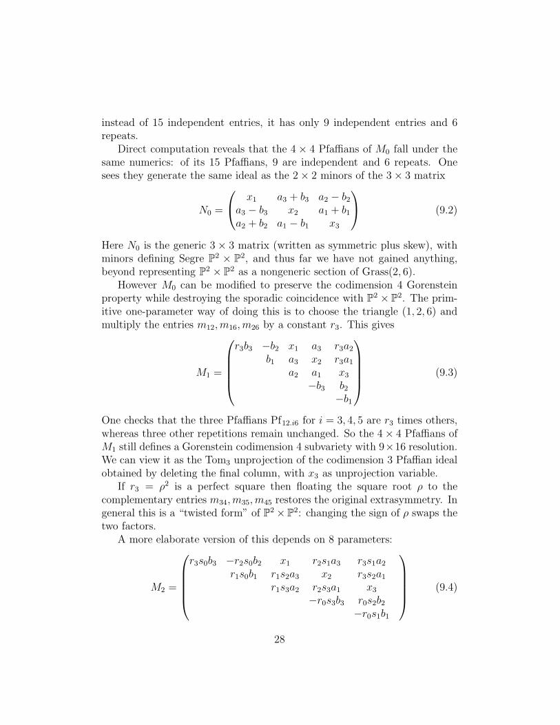
instead of 15 independent entries, it has only 9 independent entries and 6repeats.

Direct computation reveals that the 4 × 4 Pfaffians of M0 fall under thesame numerics: of its 15 Pfaffians, 9 are independent and 6 repeats. Onesees they generate the same ideal as the 2× 2 minors of the 3× 3 matrix

N0 =

x1 a3 + b3 a2 − b2a3 − b3 x2 a1 + b1a2 + b2 a1 − b1 x3

(9.2)

Here N0 is the generic 3 × 3 matrix (written as symmetric plus skew), withminors defining Segre P2 × P2, and thus far we have not gained anything,beyond representing P2 × P2 as a nongeneric section of Grass(2, 6).

However M0 can be modified to preserve the codimension 4 Gorensteinproperty while destroying the sporadic coincidence with P2 × P2. The prim-itive one-parameter way of doing this is to choose the triangle (1, 2, 6) andmultiply the entries m12, m16, m26 by a constant r3. This gives

M1 =

r3b3 −b2 x1 a3 r3a2b1 a3 x2 r3a1

a2 a1 x3

−b3 b2−b1

(9.3)

One checks that the three Pfaffians Pf12.i6 for i = 3, 4, 5 are r3 times others,whereas three other repetitions remain unchanged. So the 4× 4 Pfaffians ofM1 still defines a Gorenstein codimension 4 subvariety with 9×16 resolution.We can view it as the Tom3 unprojection of the codimension 3 Pfaffian idealobtained by deleting the final column, with x3 as unprojection variable.

If r3 = ρ2 is a perfect square then floating the square root ρ to thecomplementary entries m34, m35, m45 restores the original extrasymmetry. Ingeneral this is a “twisted form” of P2× P2: changing the sign of ρ swaps thetwo factors.

A more elaborate version of this depends on 8 parameters:

M2 =

r3s0b3 −r2s0b2 x1 r2s1a3 r3s1a2r1s0b1 r1s2a3 x2 r3s2a1

r1s3a2 r2s3a1 x3

−r0s3b3 r0s2b2−r0s1b1

(9.4)

28

Now the same three Pfaffians Pf12.i6 are divisible by r3, and the comple-mentary three are divisible by s3 with the same quotient, so one has to doa little cancellation to see the irreducible component. The necessity of can-celling these terms (although cheap in computer algebra as the colon ideal)has been a headache in the theory for decades, since it introduces apparentuncertainty as to the generators of the ideal.

The right way to view this is as the triple parallel unprojection of thehypersurface

V (a1a2b3r3s3 + a1a3b2r2s2 + a2a3b1r1s1 + b1b2b3r0s0) (9.5)

in the product ideal∏3

i=1(ai, bi). Then

x1 =a2a3r1s1 + b2b3r0s0

a1= −

a2b3r2s2 + a2b3r3s3b1

,

etc., and the ideal is generated by the Pfaffians of the three matrices(

x2 b1r0s0 a1r3s3 a3−a1r2s2 −b1r1s1 b3

x3 a2b2

),

(x1 b3r0s0 a3r2s2 a2

−a3r1s1 −b3r3s3 b2x2 a1

b1

),

(x3 b2r0s0 a2r1s1 a1

−a2r3s3 −b2r2s2 b1x1 a3

b3

).

If the ri and si are nonzero constants, one still needs the square root of thediscriminant

∏3i=0(risi) to get back to P2 × P2.

9.2 Double Jerry

The equations of Segre P1 × P1 × P1 ⊂ P7 are the minors of a 2 × 2 × 2array; they admit several extensions, and it seems most likely that there isno irreducible family containing them all. One family consists of various“rolling factors” formats discussed below; here we treat “double Jerry”.

Start from the equations written as

syi = xjxk for {i, j, k} = {1, 2, 3},txi = yjyk for {i, j, k} = {1, 2, 3},st = xiyi for i = 1, 2, 3.

(9.6)

corresponding to a hexagonal view of the cube centred at vertex s (with threesquare faces �sxiykxj , and t behind the page, cf. (2.5)):

y2x3 x1

sy1 y3

x2

(9.7)

29

Eliminating both s and t gives the codimension 2 c.i.

(x1y1 = x2y2 = x3y3) ⊂ P5, (9.8)

containing the two codimension 3 c.i.s x = 0 and y = 0 as divisors. We canview x as a row vector and y a column vector, and the two equations (9.8)as the matrix products

xAy = xBy = 0, where A =(

1 0 00 −1 00 0 0

), B =

(0 0 00 1 00 0 −1

). (9.9)

The unprojection equations for s and t separately take the form

tx = (Ay)× (By) and sy = (xA)× (xB), (9.10)

where × is cross product of vectors in C3, with the convention that the crossproduct of two row vectors is a column vector and vice versa. For example,xA = (x1,−x2, 0), xB = (0, x2,−x3) and the equations sy = (xA) × (xB)giving the first line of (9.6) are deduced via Cramer’s rule from (9.8).

We can generalise this at a stroke to A,B general 3×3 matrices. That is,for x a row vector and y a column vector, xAy = xBy = 0 is a codimension 2c.i.; since these are general bilinear forms in x and y, it represents a universalsolution to two elements of the product ideal (x1, x2, x3) · (y1, y2, y3). It hastwo single unprojections:

xAy = xBy = 0 and sy = (xA)× (xB), (9.11)

xAy = xBy = 0 and tx = (Ay)× (By), (9.12)

either of which is a conventional 5 × 5 Pfaffian, and a parallel unprojectionputting those equations together with a 9th long equation

st = something complicated. (9.13)

The equation certainly exists by the Kustin–Miller theorem. It can be ob-tained easily in computer algebra by coloning out any of x1, x2, x3, y1, y2, y3from the ideal generated by the eight equations (9.11) and (9.12). Its some-what amazing right hand side has 144 terms, each bilinear in x, y and bi-quadratic in A,B. Taking a hint from 144 = 12× 12, we suspect that it mayhave a product structure of the form

x(A ∧B)× (A ∧ B)y, (9.14)

30

with “×” and “∧” still requiring elucidation.If the entries of A and B are constants, one gets back to P1 × P1 × P1

after coordinate changes based on the three roots (λi : µi) of the relativecharacteristic equation det(λA − µB) = 0 and the three eigenvectors vi =ker(λiA− µiB). Swapping the roots permutes the three factors.

The significance of the double Jerry parallel unprojection format is that itcovers any Jerry case where the pivot is one of the generators of ID. Indeed,if the regular sequence generating ID is s, x1, x2, x3, a Jerry matrix for D is

s m13 m14 m15

m23 m24 m25

y3 −y2y1

where

(m13, m14, m15) = xA,

(m23, m14, m15) = xB.(9.15)

for some 3× 3 matrices A,B. Unprojecting D gives a double Jerry.

9.3 Rolling factors format

Rolling factors view a divisor X ⊂ V on a normal projective variety V ⊂ Pn

as residual to a nice linear system. This phenomenon occurs throughout theliterature, with typical cases a divisor on the Segre embedding of P1×P3, oron a rational normal scroll F, or on a cone over a Veronese embedding. Adivisor X ⊂ P1 × P3 in the linear system |ah1 + (a + 2)h2| = |−KV + bH|is of course defined by a single bihomogeneous equation in the Cox ring ofP1 × P3, but to get equations in the homogeneous coordinate ring of SegreP1×P3 ⊂ P7 we have to add |2h1|. This is a type of hyperquotient, given byone equation in a nontrivial eigenspace.

Dicks’ thesis [D] discussed the generic pseudoformat

2∧(a1 a2 a3 a4b1 b2 b3 b4

)= 0, and

m1a1 +m2a2 +m3a3 +m4a4 = 0m1b1 +m2b2 +m3b3 +m4b4 ≡ n1a1 + n2a2 + n3a3 + n4a4 = 0

n1b1 + n2b2 + n3b3 + n4b4 = 0.

(9.16)

One sees that under fairly general assumptions the “scroll” V defined by thefirst set of equations of (9.16) is codimension 3 and Cohen–Macaulay, withresolution

OV ← R← 6R← 8R← 3R← 0.

31

On the right, the identity is a preliminary condition on quantities inthe ambient ring. If we assume (say) that R is a regular local ring andai, bi, mi, ni ∈ R satisfy it (and are “fairly general”), the second set definesan elephant X ∈ |−KV | (anticanonical divisor) which is a codimension 4Gorenstein variety with 9× 16 resolution.

The identity in (9.16) is a quadric of rank 16. It is a little close-up view ofthe “variety of complexes” discussed in [Ki], Section 10. To use this methodto build genuine examples, we have to decide how to map a regular ambientscheme into this quadric; there are several different solutions. If we take theai, bi to be independent indeterminates, the first set of equations gives thecone on Segre P1×P3 ⊂ P7, and the second set consists of a single quadraticform q in 4 variables evaluated on the two rows, so that X ⊂ V is given byq(a) = ϕ(a,b) = q(b) = 0, with ϕ the associated symmetric bilinear form (cf.(4.9)). This format seems to be the only commonly occurring codimension 4Gorenstein format that tends not to have any Type I projection.

On the other hand, if there are coincidences between the ai, bi, there maybe other ways of choosing the mi, ni to satisfy the identity in (9.16) withoutthe need to take mi, ni quadratic in the ai, bi: for example, if a2 = b1, we canroll a1 → a2 and b1 → b2.

References

[A0] Selma Altınok, Graded rings corresponding to polarised K3 sur-faces and Q-Fano 3-folds, Univ. of Warwick PhD thesis, Sep. 1998,vii+93 pp., get from

www.maths.warwick.ac.uk/∼miles/doctors/Selma

[A] Selma Altınok, Constructing new K3 surfaces, Turkish J. Math. 29(2005) 175–192

[ABR] S. Altınok, G. Brown and M. Reid, Fano 3-folds, K3 surfacesand graded rings, in Topology and geometry: commemoratingSISTAG (National Univ. of Singapore, 2001), Ed. A. J. Berrickand others, Contemp. Math. 314, AMS, 2002, pp. 25–53, preprintmath.AG/0202092, 29 pp.

[BCZ] Gavin Brown, Alessio Corti and Francesco Zucconi, Birational ge-ometry of 3-fold Mori fibre spaces, in The Fano Conference, Pro-

32

ceedings, A. Collino, A. Conte, M. Marchisio (eds.), Universita diTorino (2005), 235–275

[BR] Gavin Brown and Miles Reid, Diptych varieties and Mori flips ofType A, in preparation

[BS] Gavin Brown and Kaori Suzuki, Fano 3-folds with divisible anti-canonical class, Manuscripta Math. 123 1 (2007) 37–51

[BZ] Gavin Brown and Francesco Zucconi, The graded ring of a rank 2Sarkisov link, Nagoya Math J. 197 (2010) 1–44

[GRDB] G. Brown, A.M. Kasprzyk and others, Graded Ring Database,http://grdb.lboro.ac.uk

[CM] A. Corti and M. Mella, Birational geometry of terminal quartic3-folds, I. Amer. J. Math. 126 (2004) 739–761

[CPR] A. Corti, A. Pukhlikov and M. Reid, Birationally rigid Fano hy-persurfaces, in Explicit birational geometry of 3-folds, A. Corti andM. Reid (eds.), CUP 2000, 175–258

[CR] Alessio Corti and Miles Reid, Weighted Grassmannians, in Alge-braic geometry, de Gruyter, Berlin (2002), pp. 141–163

[D] Duncan Dicks, Surfaces with pg = 3, K2 = 4 and extension-deformation theory, Univ. of Warwick PhD thesis, 1988, vi+125pp.

[F] A. Iano-Fletcher, Working with weighted complete intersections, inExplicit birational geometry of 3-folds, A. Corti and M. Reid (eds.),CUP 2000, pp. 101–173

[Ka] KAWAMATA Yujiro, Divisorial contractions to 3-dimensional ter-minal quotient singularities, in Higher-dimensional complex vari-eties (Trento, 1994), 241–246, de Gruyter, Berlin, 1996

[KM] A. Kustin and M. Miller, Constructing big Gorenstein ideals fromsmall ones, J. Algebra 85 (1983) 303–322

[Ma] Magma (John Cannon’s computer algebra system): W. Bosma,J. Cannon and C. Playoust, The Magma algebra system I: Theuser language, J. Symb. Comp. 24 (1997) 235–265. See alsohttp://magma.maths.usyd.edu.au/magma

33

[PR] Stavros Argyrios Papadakis and Miles Reid, Kustin–Miller unpro-jection without complexes, J. Algebraic Geom. 13 (2004) 563–577,Preprint math.AG/0011094

[Pr] Yuri Prokhorov, Q-Fano threefolds of large Fano index, I. preprint:arXiv:0812.1695, 29 pp.

[C3f] M. Reid, Canonical 3-folds, Journees de Geometrie Algebriqued’Angers, 1979, Sijthoff & Noordhoff (1980), pp. 273–310

[Ki] M. Reid, Graded rings and birational geometry, in Proc. of algebraicgeometry symposium (Kinosaki, Oct 2000), K. Ohno (Ed.), 1–72,get from www.maths.warwick.ac.uk/∼miles/3folds

[S] SUZUKI Kaori, On Fano indices of Q-Fano 3-folds, ManuscriptaMath., 114 (2004) 229–246

[T] TAKAGI Hiromichi, On classification of Q-Fano 3-folds of Goren-stein index 2. I, II, Nagoya Math. J., 167 (2002) 117–155, 157–216

Gavin BrownSchool of Mathematics, Loughborough UniversityLE11 3TU, UKG.D.Brown@lboro.ac.uk

Michael KerberInstitute of Science and Technology (IST) Austria3400 Klosterneuburg, Austriamichael.kerber@ist.ac.at

Miles ReidMathematics Institute, University of WarwickCoventry CV4 7AL, UKMiles.Reid@warwick.ac.uk

34