Families of Legendrians and Lagrangians with unbounded ...
32
J. Fixed Point Theory Appl. (2022) 24:43 https://doi.org/10.1007/s11784-022-00964-7 c The Author(s) 2022 Journal of Fixed Point Theory and Applications Families of Legendrians and Lagrangians with unbounded spectral norm Georgios Dimitroglou Rizell Abstract. Viterbo has conjectured that any Lagrangian in the unit co- disc bundle of a torus which is Hamiltonian isotopic to the zero-section satisfies a uniform bound on its spectral norm; a recent result by Shelukhin showed that this is indeed the case. The modest goal of our note is to explore two natural generalisations of this geometric setting in which the bound of the spectral norm fails: first, passing to Legen- drian isotopies in the contactisation of the unit co-disc bundle (recall that any Hamiltonian isotopy can be lifted to a Legendrian isotopy) and, second, considering Hamiltonian isotopies but after modifying the co-disc bundle by attaching a critical Weinstein handle. Mathematics Subject Classification. 53D40, 53D42. Keywords. Spectral norm, Boundary depth, Spectral invariants for Leg- endrians, Floer homology for Legendrians. Contents 1. Introduction and results 1.1. Why the proofs of uniform bounds fail for Legendrians 2. Background 2.1. Contact geometry of jet-spaces and contactisations 2.1.1. The cotangent bundle and jet-space 2.1.2. The punctured torus 2.2. Barcode of a filtered complex and notions from spectral invariants 2.3. Outline of Floer homology and generating family homology for Legendrians 2.4. Floer complex as the linearised Chekanov–Eliashberg algebra The author is supported by the Grant KAW 2016.0198 from the Knut and Alice Wallenberg Foundation. This article is part of the topical collection “Symplectic geometry - A Festschrift in honour of Claude Viterbo’s 60th birthday” edited by Helmut Hofer, Alberto Abbondandolo, Urs Frauenfelder and Felix Schlenk. 0123456789().: V,-vol
-
Upload
khangminh22 -
Category
Documents
-
view
4 -
download
0
Transcript of Families of Legendrians and Lagrangians with unbounded ...

J. Fixed Point Theory Appl. (2022) 24:43 https://doi.org/10.1007/s11784-022-00964-7c© The Author(s) 2022
Journal of Fixed Point Theoryand Applications
Families of Legendrians and Lagrangianswith unbounded spectral norm
Georgios Dimitroglou Rizell
Abstract. Viterbo has conjectured that any Lagrangian in the unit co-disc bundle of a torus which is Hamiltonian isotopic to the zero-sectionsatisfies a uniform bound on its spectral norm; a recent result byShelukhin showed that this is indeed the case. The modest goal of ournote is to explore two natural generalisations of this geometric settingin which the bound of the spectral norm fails: first, passing to Legen-drian isotopies in the contactisation of the unit co-disc bundle (recallthat any Hamiltonian isotopy can be lifted to a Legendrian isotopy)and, second, considering Hamiltonian isotopies but after modifying theco-disc bundle by attaching a critical Weinstein handle.
Mathematics Subject Classification. 53D40, 53D42.
Keywords. Spectral norm, Boundary depth, Spectral invariants for Leg-endrians, Floer homology for Legendrians.
Contents
1. Introduction and results1.1. Why the proofs of uniform bounds fail for Legendrians
2. Background2.1. Contact geometry of jet-spaces and contactisations
2.1.1. The cotangent bundle and jet-space2.1.2. The punctured torus
2.2. Barcode of a filtered complex and notions from spectral invariants
2.3. Outline of Floer homology and generating family homology forLegendrians
2.4. Floer complex as the linearised Chekanov–Eliashberg algebra
The author is supported by the Grant KAW 2016.0198 from the Knut and Alice WallenbergFoundation.
This article is part of the topical collection “Symplectic geometry - A Festschrift in
honour of Claude Viterbo’s 60th birthday” edited by Helmut Hofer, Alberto Abbondandolo,
Urs Frauenfelder and Felix Schlenk.
0123456789().: V,-vol

43 Page 2 of 32 G. Dimitroglou Rizell
2.5. Maslov potential and grading3. Examples that exhibit unbounded spectral norms
3.1. Legendrian isotopy of the unknot (Proof of Part (2) of TheoremA)
3.2. Legendrian isotopy of the zero-section (Proof of Part (1) ofTheorem A)
3.3. Hamiltonian isotopy on the punctured torus (Proof of TheoremD)
4. Proof of Theorem CReferences
1. Introduction and results
Spectral invariants were introduced in Viterbo’s seminal work [31]. Sincetheir appearance they have become one of the most fundamental tools ofquantitative symplectic topology. We do not intend to give an overview ofits development and many applications here; instead we direct the reader towork by Oh [23] for a thorough introduction to the subject from a modernperspective.
Very briefly, spectral invariants in the symplectic case consist of func-tions from the group of Hamiltonian diffeomorphisms
c : Ham(X,ω) → R
that take values in the real numbers, and which satisfy a list of axioms thatwill be omitted. The spectral invariants that we consider here are constructedas follows. For a pair of exact Lagrangian submanifolds L0, L1 ⊂ (X, dλ) (thesymplectic manifold is thus necessarily exact) one can associate the Floercomplex CF (L0, φ(L1)) to any Hamiltonian diffeomorphism φ ∈ Ham(X,ω)endowed with its canonical action filtration. Spectral invariants are certainreal numbers that encode information about this filtered chain complex. Tomake this precise, we utilise the language of the barcode from the theory ofpersistent homology in topological data analysis, which goes back to work byCarlsson–Zomorodian–Collins–Guibas [8]. This theory has been proven to bevery useful in quantitative symplectic topology, where it was introduced byPolterovich–Shelukhin [25] and Usher–Zhang [30]; also see the recent work[24] by Polterovich–Rosen–Samvelyan–Zhang for a systematic introduction.Here we give a quick definition of the barcode of a filtered complex that willsuit our needs in Sect. 2.2.
The barcode can be defined for any chain complex (C, ∂, a) with a fil-tration by subcomplexes
C<c∗ := a−1[−∞, c) ⊂ C∗
defined by an “action” function
a : C → {−∞} ∪ R,

Families of Legendrians and Lagrangians... Page 3 of 32 43
where a−1(−∞) = {0}. Phrased in this language, the spectral invariantsare the values of the starting points of the semi-infinite bars of the barcodeassociated to the Floer complex. In fact, the main interest here is not thespectral invariants themselves, but rather the following derived quantities(see Definition 2.7):
• The spectral range of a filtered complex, denoted by
ρ(C, ∂, a) ∈ {−∞} ∪ [0,+∞].
This quantity is defined as the supremum of the distances between thestarting points of two semi-infinite bars in the corresponding barcode.(It takes the value −∞ if and only if there are no semi-infinite bars.)
• The boundary depth of a filtered complex, denoted by
β(C, ∂, a) ∈ {−∞} ∪ [0,+∞].
This quantity is defined as the supremum of the lengths of a finite bar inthe corresponding barcode. (It takes the value −∞ if and only if thereare no bars of finite length.)
For the Floer complex CF (L, φ1H(L)) of a closed embedded exact Lagrangian
and its Hamiltonian deformation, the spectral range coincides with a quantitycalled the spectral norm. This can be seen using Leclercq’s results from [20,Corollary 1.7], after relating the spectral invariants used in that article tothe endpoints of semi-infinite bars in the relevant barcode. Since we will notuse any of the particular features satisfied by the spectral norm here, we willgloss over the difference between these two concepts and simply define thespectral norm as
γ(CF (Λ, φ1H(Λ))) := ρ(CF (Λ, φ1
H(Λ))),
i.e. we prescribe it to be equal to the spectral range.
Remark 1.1. The correct way to define the spectral norm in the setting ofLegendrians would be to define γ as the difference of action levels of theclasses that correspond to the unit for the cup-product and its image underPoincare duality. We do not go into details of products and Poincare dualityhere, but when Λ is a Legendrian without Reeb chords, we again expect anequality between spectral norm and spectral range. In general there shouldbe an inequality γ ≤ ρ.
We also need a generalisation of the above spectral invariants to contactmanifolds. Since we will only consider contact manifolds of a very particulartype, namely contactisations
(Y, α) = (X × R, dz + λ)
of exact symplectic manifolds (X, dλ) (see Sect. 2.1), this can be done byrelying on well-established techniques. From our point of view, the spectralinvariants of a contact manifold are defined for the group of contactomor-phisms which are contact-isotopic to the identity, and yield functions
c : Cont0(Y, α) → R.
43 Page 4 of 32 G. Dimitroglou Rizell
Note that the value does depend on the choice of contact form α here, andnot just on the contact structure kerα ⊂ TY . It should be noted thatspectral invariants in the contact setting are much less studied and devel-oped than the symplectic version. However, the original formulation of thespectral invariants, which appeared in [31] for symplectic cotangent bundles(X,ω) = (T ∗M,d(p dq)), admits a straightforward generalisation to the stan-dard contact jet-space
(J1M = T ∗M × R, dz − p dq),
as shown by Zapolsky [33]. In fact, the spectral invariants in [31] are basedon a version of Floer homology defined using generating families, and thistheory can be generalised to invariants of Legendrian isotopies inside jet-spaces by work of Chekanov [7]. Note that jet-spaces are particular cases ofcontactisations.
The spectral invariants considered here can be defined either by usinggenerating families as in [33], or using a Floer homology constructed using theChekanov–Eliashberg algebra as first done in [13] by Ekholm–Etnyre–Sabloff;also see work [4] by the author together with Chantraine–Ghiggini–Golovko.The Chekanov–Eliashberg algebra is a Legendrian isotopy invariant in theform of a unital differential graded algebra (DGA) that is freely generatedby the Reeb chords on the Legendrian, which are all assumed to be trans-verse. Given a pair of Legendrians Λ0 and Λ1, the spectral invariants that weconsider are associated to the barcode of the Floer complex CF (Λ0, φ(Λ1))where φ is a contactomorphism that is contact isotopic to the identity. SeeSect. 2.3 for the definition of this Floer complex.
Viterbo conjectured in [32] that the spectral norm γ(CF (0Tn , φ(0Tn)))of the Floer complex of the zero section 0Tn ⊂ T ∗Tn satisfies a uniformbound whenever φ ∈ Ham(T ∗Tn) maps the zero section φ(0Tn) ⊂ DT ∗Tn
into the unit-disc cotangent bundle. In recent work by Shelukhin [28,29] thisproperty was finally shown to be the case, even for a wide range of cotangentbundles beyond the torus case. The main point of our work here is to giveexamples of geometric settings beyond symplectic co-disc bundles, where theanalogous boundedness of the spectral norm fails. It should be stressed that,in the time of writing of this article, there are still many cases of cotangentbundles for which the problem remains open: does the spectral norm of anexact Lagrangian inside DT ∗M which is Hamiltonian isotopic to the zero-section satisfy a uniform bound for an arbitrary closed smooth manifold M?
As a first result, in Part (1) of Theorem A, we show that the spectralnorm of Legendrians inside the contactisation D∗S1 × R ⊂ J1S1 which areLegendrian isotopic to the zero section does not satisfy a uniform bound.Recall that any Hamiltonian isotopy of 0S1 ⊂ DT ∗S1 lifts to a Legendrianisotopy of the zero section j10 ⊂ J1S1 (see Lemma 2.1); consequently, oneway to formulate Part (1) of Theorem A is by saying that Viterbo’s conjecturecannot be generalised to Legendrian isotopies.
Below we denote by
Fθ0,z0 := {θ = θ0, z = z0} ⊂ J1S1

Families of Legendrians and Lagrangians... Page 5 of 32 43
a Legendrian lift of the Lagrangian cotangent fibre T ∗θ0
S1.
Theorem A.
(1) There exists a contact isotopy φt : J1S1 → J1S1 that satisfies
φt|j10 : j10 ↪→ DT ∗S1 × R = (S1 × [−1, 1]) × R,
and for which CF (j10, φt(j10)) all are generated by precisely two mixedReeb chords, whose difference in length grows indefinitely as t → +∞.In particular, the spectral norm γ(CF (j10, φt(j10))) becomes arbitrarilylarge as t → +∞.
(2) There exists a contact isotopy φt : J1S1 → J1S1 that satisfies
φt|Λst : Λst ↪→ DT ∗S1 × R>0 = (S1 × [−1, 1]) × R>0 ⊂ J1S1,
where Λst ⊂ J1S1 is the standard Legendrian unknot shown in Fig. 1,and for which the boundary depth β(CF (φt(Λst), Fθ0,0)) becomes arbi-trarily large as t → +∞. In addition, we may assume that φt is sup-ported inside some subset {z ≥ c}, where c > 0, and for which theinclusion {z ≥ c} ∩ Λst � Λst is a strict subset.
In recent work [2, Section 6.2] Biran–Cornea showed that a boundγ(CF (0M , L)) ≤ C on the spectral norm of the Floer complex of a LagrangianL ⊂ T ∗M , where L is Hamiltonian isotopic to the zero section, implies thebound β(CF (L, T ∗
ptM)) ≤ 2C on the boundary depth of the Floer complex ofL and a cotangent fibre. The Legendrians produced by Part (2) of TheoremA can be used to show that the analogous result cannot be generalised toLegendrian isotopies. More precisely,
Corollary B. There exists a contact isotopy φt : J1S1 → J1S1 that satisfies
φt|j10 : j10 ↪→ DT ∗S1 × R = (S1 × [−1, 1]) × R,
and for which the spectral norm γ(CF (j10, φ1(j10))) is uniformly bounded forall t ≥ 0, while the boundary depth β(CF (φ1(0S1), Fθ0,z0)) becomes arbitrarilylarge as t → +∞.
Proof. Take a cusp-connected sum of a C1-small perturbation of the zero-section j10 and any unknot Λt
st from the family produced by Part (2) ofTheorem A; the case of Λst is shown in Fig. 1. We refer to [9] for the definitionof cusp-connected sum (also called ambient Legendrian 0-surgery) along aLegendrian arc (the so-called surgery disc). We perform the cusp-connectedsum along a Legendrian arc contained inside the region {z < c}, and which isdisjoint from the support of the Legendrian isotopy of the unknots. Note thatthe Legendrian resulting from the cusp-connected sum is Legendrian isotopicto the zero-section, as shown in Fig. 1. It follows that the same is true forthe cusp-connected sum of j10 and any Legendrian Λt
st from the family.Finally, to evaluate the effect of the ambient surgery on the barcodes
of the Floer complexes we apply Theorem C. To that end, the following twofacts are needed. First, CF (Λst, j
10) is acyclic, and thus its barcode consistsof only finite bars. The acyclicity of the Floer complex is a consequence of the
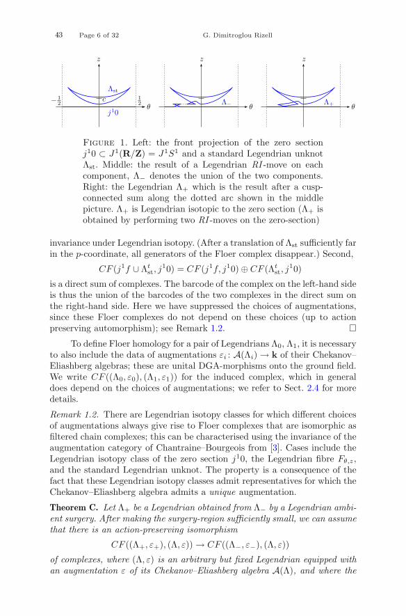
43 Page 6 of 32 G. Dimitroglou Rizell
Λst
j10Λ− Λ+
zzz
θθθc 1
2− 12
Figure 1. Left: the front projection of the zero sectionj10 ⊂ J1(R/Z) = J1S1 and a standard Legendrian unknotΛst. Middle: the result of a Legendrian RI -move on eachcomponent, Λ− denotes the union of the two components.Right: the Legendrian Λ+ which is the result after a cusp-connected sum along the dotted arc shown in the middlepicture. Λ+ is Legendrian isotopic to the zero section (Λ+ isobtained by performing two RI -moves on the zero-section)
invariance under Legendrian isotopy. (After a translation of Λst sufficiently farin the p-coordinate, all generators of the Floer complex disappear.) Second,
CF (j1f ∪ Λtst, j
10) = CF (j1f, j10) ⊕ CF (Λtst, j
10)
is a direct sum of complexes. The barcode of the complex on the left-hand sideis thus the union of the barcodes of the two complexes in the direct sum onthe right-hand side. Here we have suppressed the choices of augmentations,since these Floer complexes do not depend on these choices (up to actionpreserving automorphism); see Remark 1.2. �
To define Floer homology for a pair of Legendrians Λ0, Λ1, it is necessaryto also include the data of augmentations εi : A(Λi) → k of their Chekanov–Eliashberg algebras; these are unital DGA-morphisms onto the ground field.We write CF ((Λ0, ε0), (Λ1, ε1)) for the induced complex, which in generaldoes depend on the choices of augmentations; we refer to Sect. 2.4 for moredetails.
Remark 1.2. There are Legendrian isotopy classes for which different choicesof augmentations always give rise to Floer complexes that are isomorphic asfiltered chain complexes; this can be characterised using the invariance of theaugmentation category of Chantraine–Bourgeois from [3]. Cases include theLegendrian isotopy class of the zero section j10, the Legendrian fibre Fθ,z,and the standard Legendrian unknot. The property is a consequence of thefact that these Legendrian isotopy classes admit representatives for which theChekanov–Eliashberg algebra admits a unique augmentation.
Theorem C. Let Λ+ be a Legendrian obtained from Λ− by a Legendrian ambi-ent surgery. After making the surgery-region sufficiently small, we can assumethat there is an action-preserving isomorphism
CF ((Λ+, ε+), (Λ, ε)) → CF ((Λ−, ε−), (Λ, ε))
of complexes, where (Λ, ε) is an arbitrary but fixed Legendrian equipped withan augmentation ε of its Chekanov–Eliashberg algebra A(Λ), and where the

Families of Legendrians and Lagrangians... Page 7 of 32 43
augmentation ε+ of A(Λ+) is induced by pulling back the augmentation ε− ofA(Λ−) under the unital DGA-morphism induced by the standard Lagrangianhandle-attachment cobordism. In particular, the barcodes of the two Floercomplexes coincide.
In the setting of exact Lagrangian cobordisms in the sense of Arnol’dbetween exact Lagrangian submanifolds similar results were found in [2, Sec-tion 5.3] .
Finally we present a Hamiltonian isotopy of a closed exact Lagrangianinside a Liouville domain for which the spectral norm becomes arbitrarilylarge. The simplest examples of such a Liouville domain is the 2-torus withan open ball removed; we denote this space by (Σ1,1, dλ) and depict it inFig. 13. The detailed construction is given in Sect. 2.1.2. As kindly pointedout to the author by the anonymous referee, this fact is not new. The samephenomenon was exhibited in, e.g. Zapolsky’s work [34, Lemma 1.10], as wellas the more recent [19, Remark 6] by Kislev–Shelukhin.
Theorem D. There exists a closed exact Lagrangian submanifold L ⊂ (Σ1,1, ω)and a compactly supported Hamiltonian H : Σ1,1 → R for which the inducedcompactly supported Hamiltonian isotopy φt
H : (Σ1,1, ω) → (Σ1,1, ω) satisfiesthe property that the spectral norm γ(CF (L, φt
H(L))) becomes arbitrarily largeas t → +∞.
1.1. Why the proofs of uniform bounds fail for Legendrians
The techniques that are used in [29] and [2] to prove the results in the case ofthe cotangent bundle are not yet fully developed in the case of Legendrians incontactisations. This includes the closed-open map, which is a crucial ingre-dient in [29], and a unital A∞-structure on the Floer complex with relevantPSS-isomorphisms, which is crucial in [2]. Nevertheless, we still do expectthat these operations can be defined also for the Floer homology of Legendri-ans in contactisations. In fact the A∞-structure was recently extended to thissetting by Legout [21]. Assuming the possibility to define these operationsin the Legendrian setting, what goes wrong when one tries to generalise theproofs to the Legendrian case?
First we recall the properties of the Floer homology complex of a Leg-endrian and itself; see, e.g. [13] for the details. To define CF (Λ,Λ) one mustfirst make the mixed Reeb chords transverse by a Legendrian perturbationof the second copy of Λ. We do this by replacing Λ with a section j1f in itsstandard contact jet-space neighbourhood, where f : Λ → R is a C1-smallMorse function. In this manner, we obtain
CF (Λ,Λ) = CMorse(f ;k) ⊕⊕
c∈Q(Λ)
kpc ⊕ kqc
where Q(Λ) denotes the set of Reeb chords on Λ, and CMorse(f ;k) is theMorse homology complex with basis given by the critical points of the func-tion f : Λ → R. The action of the former chords are approximately equalto a(pc) = (c) and a(qc) = − (c) while the action of the latter is equalto a(x) = f(x). What is important to notice here is that the generators of

43 Page 8 of 32 G. Dimitroglou Rizell
CMorse(f ;k) may be assumed to have arbitrarily small action, while this isnot the case for the generators that correspond to pure Reeb chords. WhenΛ is the Legendrian lift of a Lagrangian embedding, there are of course onlygenerators of the type CMorse(f ;k). This turns out to be the crucial differencebetween the symplectic and the contact case.
Example in Part (1) of Theorem A: The proof in [29] uses the closed-open map. More precisely, a crucial ingredient in the proof is the action-preserving property of the operations P ′
a on the Floer homology CF (0M , φ1H
(0M )), which are defined using the length-0 part φ0(a) and length-1 partφ1(a, ·) of the closed open map for certain elements a ∈ SH(T ∗M) in sym-plectic cohomology (by this we mean the unital version of the symplecticinvariant, which is contravariant with respect to inclusion of exact Liouvillesubdomains). In the case when the Legendrian has pure Reeb chords (i.e. it isnot the lift of an exact Lagrangian embedding), the chain φ0(a) ∈ CF (Λ,Λ)may consist of generators whose action does not vanish (since they do notcorrespond to Morse generators). In this case the action-preserving propertyof P ′
a can no longer be determined from the aciton of a ∈ SH(T ∗M) alone.Example in Part (2) of Theorem A: The proof in [2, Section 6.2] uses
the fact that there are continuation elements a ∈ CF (φ1H(0M ), 0M ) and
b ∈ CF (0M , φ1H(0M )) for which μ2(a, b) ∈ CF (φ1
H(0M ), φ1H(0M )) is the
unique maximum of a suitable Morse function. In the Legendrian case theelement μ2(a, b) ∈ CF (φ1(j10), φ1(j10)) is still a homology unit; however, itnot necessarily a sum of Morse chords, and can, therefore, have significantaction. In particular, multiplication with the element μ2(a, b) is not necessar-ily identity on the chain level, nor is it necessarily homotopic to the identityby a chain homotopy of small action. The geometrically induced chain homo-topy μ3(a, b, ·) between μ2(a, μ2(b, ·)) and μ2(μ2(a, b), ·) increases action byat most the spectral norm, and is used in [2] for establishing the bound onthe boundary depth. However, this chain homotopy does not do the job anymore, since we also need an additional chain-homotopy (of unknown actionproperties) to take us from the map μ2(μ2(a, b), ·) to the chain level identity.
2. Background
2.1. Contact geometry of jet-spaces and contactisations
An exact symplectic manifold is a smooth 2n-dimensional manifold (X2n, dλ)equipped with a choice of a primitive one-form λ for an exact symplectic two-form ω = dλ, i.e. ω is skew-symmetric, non-degenerate, and closed. Note thatthe primitive λ should be considered as part of the data describing the exactsymplectic manifold. A compact exact symplectic manifold with boundary(W,dλ) is a Liouville domain if the Liouville vector field, i.e. the vector fieldζ given as the symplectic dual of λ via the equation ιζdλ = λ, is transverseto the boundary ∂W . The flow generated by ζ is called the Liouville flowand satisfies (φt
ζ)∗λ = etλ. An open exact symplectic manifold (W,dλ) is
a Liouville manifold if the all critical points of the Liouville vector field are

Families of Legendrians and Lagrangians... Page 9 of 32 43
contained inside some compact Liouville domain W ⊂ (W,dλ), and if theLiouville flow is complete.
A Hamiltonian isotopy is a smooth isotopy of X which is generated bya time-dependent vector field Vt ∈ Γ(TX) that satisfies ιVt
dλ = −dHt forsome smooth time-dependent function
H : X × Rt → R
which is called the Hamiltonian; a diffeomorphism of X which is the time-tflow generated by such a vector field preserves the symplectic form (but notnecessarily the primitive) and is denoted by
φtH : (X,ω) → (X,ω);
we call such a map a Hamiltonian diffeomorphism, and the correspondingflow a Hamiltonian isotopy. Conversely, any choice of Hamiltonian functioninduces a Hamiltonian isotopy φt
H in the above manner. Since we considerexact symplectic manifolds, a smooth isotopy φt : X → X is a Hamiltonianisotopy if and only if (φt)∗λ = λ + dGt ∈ Ω1(X) holds for some smoothfunction
G : X × Rt → R.
Note that the Hamiltonian function that corresponds to a Hamiltonian iso-topy is determined only up to the addition of a function that only dependson t.
Any exact 2n-dimensional symplectic manifold (X2n, dλ) gives rise to a2n + 1-dimensional contact manifold (X × Rz, dz + λ) called its contactisa-tion, which is equipped with the canonical contact one-form αst := dz + λ.The contactisations induced by choices of primitives of the symplectic formλ and λ′ = λ + df that differ by the exterior differential of f : X → R areisomorphic via the coordinate change z �→ z − f . Recall that the contactcondition is equivalent to dαst being non-degenerate on the contact planesker αst ⊂ T (X × R). A contact isotopy is a smooth isotopy which preservesthe distribution kerαst (but not necessarily the contact form). The contrac-tion ιVt
αst of the contact form and the infinitesimal generator gives a bijectivecorrespondence between contact isotopies and smooth time-dependent func-tions on X × R, the latter are called contact Hamiltonians. We refer to [18]for more details.
Lemma 2.1. A Hamiltonian isotopy φtH : (X, dλ) → (X, dλ) with a choice of
Hamiltonian Ht : X → R lifts to a contact isotopy
X × R → X × R,
(x, z) �→ (φtH(x), z − Gt(x)),
where the function G : X × Rt → R is defined by
Gt(x) =∫ t
0
λ(Vs(φsH(x))) − Hs(φs
H(x))ds
and satisfies the property
(φtH)∗λ = λ + dGt.

43 Page 10 of 32 G. Dimitroglou Rizell
Moreover, this contact isotopy preserves the contact form αst and is generatedby the time-dependent contact Hamiltonian Ht ◦ prX : X × Rz → R.
A smooth immersion of an n-dimensional manifold
Λ � (X2n × R, dz + λ)
in the contactisation is Legendrian if it is tangent to kerαst, while a smoothn-dimensional immersion L � (X2n, λ) in an exact symplectic manifold isexact Lagrangian if λ pulls back to an exact one-form. The following relationbetween Legendrians and exact Lagrangians is immediate:
Lemma 2.2. The canonical projection of a Legendrian immersion to (X,λ) isan exact Lagrangian immersion. Conversely, any exact Lagrangian immer-sion lifts to a Legendrian immersion of the contactisation X ×R. Moreover,the lift is uniquely determined by the choice of a primitive f : L → R of thepull-back λ|TL = df , via the formula z = −f .
Transverse double points of Lagrangian immersions are stable. On theother hand, generic Legendrian immersions are in fact embedded. However,there are stable self-intersections of Legendrians that appear in one-parameterfamilies. Recall the following standard fact; again we refer to, e.g. [18] fordetails.
Lemma 2.3. A compactly supported smooth isotopy φt(Λ) ⊂ X × R throughLegendrian embeddings, also called a Legendrian isotopy, can be generated byan ambient contact isotopy.
2.1.1. The cotangent bundle and jet-space. There is a canonical exact sym-plectic two-form −d(p dq) on any smooth cotangent bundle T ∗M , whose prim-itive −p dq is the tautological one-form with a minus sign. The cotangentbundle is a Liouville manifold and any co-disc bundle is a Liouville domain.The zero-section 0M ⊂ T ∗M is obviously an exact Lagrangian embedding.
The contactisation of T ∗M is the one-jet space J1M = T ∗M ×Rz withthe canonical contact one-form dz − p dq. The zero-section in T ∗M lifts tothe one-jet j1c of any constant function c (obviously the one-jet j1f of anarbitrary function f : M → R is Legendrian isotopic to j10). For us the mostrelevant example is actually the two-dimensional symplectic cotangent bundleT ∗S1 = S1 ×Rp equipped with the exact symplectic two-form −d(p dθ), andits corresponding contactisation, i.e. the three-dimensional contact manifold
(J1S1 = T ∗S1 × Rz, dz − p dθ)
(note the sign convention for the Liouville form).To describe Legendrians in J1M we will make use of the front-projection,
by which one simply means the canonical projection
ΠF : J1M → M × Rz.
A Legendrian immersion can be uniquely determined by its post-compositionwith the front projection. A generic Legendrian knot in J1S1 has a frontprojection whose singular locus consists of
• non-vertical cubical cusps and

Families of Legendrians and Lagrangians... Page 11 of 32 43
zz
RI
xx
Figure 2. RI: the first Legendrian Reidemeister move inthe front projection
zz
RII
xx
Figure 3. RII: the second Legendrian Reidemeister movein the front projection
• transverse self-intersections.
Note that the front projection cannot be tangent to ∂z by the Legendriancondition (i.e. there are no vertical tangencies).
Two sheets of the front projection that have the same slopes (i.e. p-coordinates) above some given point in the base, project to a double-pointinside T ∗M . There is a bijection between double points of this projectionand Reeb chords, where a Reeb chord is an integral curve of ∂z with bothendpoints on the Legendrian. The difference of z-coordinate of the endpointand starting point of a Reeb chord c is called its length and is denoted by (c) ≥ 0.
Double-points of the Legendrian immersion itself correspond to self-tangencies of the front projection. This is not a stable phenomenon, anddouble-points of Legendrians generically arise only in one-parameter families.These double-points can be considered as Reeb chords of length zero.
Two Legendrian knots inside J1R or J1S1 with generic fronts are Leg-endrian isotopic if and only if their front projections can be related by asequence of Legendrian Reidemeister moves [26] together with an ambientisotopy of the front inside S1 ×Rz; see [15] for an introduction to Legendrianknots.
For convenience we will also introduce a composite move that we willmake repeated use of; this is the one shown in Fig. 5, which involves takingtwo cusp edges with different slopes, and making them cross each other (it isimportant that the cusps have different slopes).

43 Page 12 of 32 G. Dimitroglou Rizell
zz
RIII
xx
Figure 4. RIII: the third Legendrian Reidemeister move inthe front projection
zz
2 × RII
xx
Figure 5. A composite move: the front to the right is ob-tained by performing two consecutive RII -moves on the frontto the left together with an isotopy
2.1.2. The punctured torus. Here we construct an example of a two-dimensional non-planar Liouville domain: the two torus minus an open ball, whichwe denote by (Σ1,1, dλ).
First, consider the primitive
λ0 = −12(p dq − q dp)
of the standard linear symplectic form dq ∧ dp on R2. We have the identities
λ0 + d(pq
2
)= q dp,
λ0 − d(pq
2
)= −p dq.
Take a smooth function σ : R2 → R which in the standard coordinates la-belled by (p, q) ∈ R2 is given by
• σ(p, q) = pq/2 on {|q| ≤ 1, |p| > 2}, while it is of the form g(p)q/2 forsome smooth function g that satisfies g(p), g′(p) ≥ 0 on {|q| ≤ 1, |p| ≥1};
• σ(p, q) = −pq/2 on {|q| > 2, |p| ≤ 1}, while it is of the form −g(q)p/2 forsome smooth function g that satisfies g(q), g′(q) ≥ 0 on {|q| ≥ 1, |p| ≤1};
• σ(p, q) = 0 on {|q| < 1, |p| < 1}; and

Families of Legendrians and Lagrangians... Page 13 of 32 43
Consider the exact symplectic manifold (X, dλ) which is obtained by takingthe cross-shaped domain
{p ∈ [−2, 2], q ∈ [−1, 1]} ∪ {q ∈ [−2, 2], p ∈ [−1, 1]} ⊂ R2
and identifying {p = 2} with {p = −2}, and {q = −2} with {q = 2} in theobvious manner. Topologically the result is a punctured torus. The Liouvilleform λ0 + dσ on R2 extends to a Liouville form λ on this punctured torus.The punctured torus has a skeleton Sk ⊂ X which is the image of the cross{pq = 0} under the quotient; in other words, Sk ⊂ X is the union of twosmooth Lagrangian circles that intersect transversely in a single point. Notethat
Sk =∞⋂
T=1
φ−T (X).
We claim that the sought Liouville domain (Σ1,1, dλ) can be realised as asuitable subset of this exact symplectic manifold, simply by smoothing itscorners; see Fig. 13.
Since (Σ1,1, λ) is a surface with non-empty boundary, it admits a sym-plectic trivialisation of its tangent bundle. This implies that the all La-grangian submanifolds of Σ1,1 have a well-defined Maslov class; see Sect.2.5 for more details. We will make heavy use of the fact that the Maslov classdepends on the choice of a symplectic trivialisation; in this case, symplectictrivialisations up to homotopy can be identified with homotopy classes ofmaps
Σ1,1 → S1
i.e. cohomology classes H1(Σ1,1;Z).
2.2. Barcode of a filtered complex and notions from spectral invariants
A (strict) filtered complex over some field k is a chain complex (C, ∂, a) inwhich each element is endowed with an action a(c) ∈ R � {−∞} and suchthat the following properties are satisfied:
• a(c) = −∞ if and only if c = 0,• a(r · c) = a(c) for any r ∈ k∗,• a(a + b) ≤ max{a(a), a(b)}, and• a(∂(a)) < a(a) for any a �= 0.
The subset
C<a = a−1({−∞} ∪ (−∞, a))
is a k-subspace by the first three bullet points; this subspace is a subcomplexby the last bullet point.
We say that a basis {ei} is compatible with the filtration, if the actionof a general element c ∈ C is given by
a(r1e1 + · · · + rnen) = max{a(ei); ri �= 0}, ri ∈ k, (2.1)
i.e. the action function is determined by its values on elements in the basis.

43 Page 14 of 32 G. Dimitroglou Rizell
Remark 2.4. The non-trivial condition in the definition is the equality “=”in Formula (2.1); for a general basis the above equality gets replaced with aninequality “≤”.
The existence of a compatible basis for any filtered complex was provenby Barannikov [1]; see [30] for a more general version (in that article they arecalled “orthogonal bases”), as well as [24]. For proof adapted to the notationused here, see [10, Lemma 2.2].
Given a basis with a specified action on each basis element, one canalso use the above formula to construct a filtration on the entire complex,under the assumption that the differential decreases action. The Floer com-plexes described below get endowed with filtrations in precisely this manner,i.e. by specifying an action for each canonical and geometrically induced basiselement.
For every filtered complex there is a notion of a barcode; we refer to[10, Section 2] for the details of the presentation that we rely on here. Thebarcode is a set of intervals of the form [a, b) and [a,+∞), where a, b ∈ R, andwe allow multiplicities. Instead of giving the usual definition of the barcode,we give it the following alternative characterisation.
Lemma 2.5. (Lemma 2.6 in [10]) The barcode can be recovered from the fol-lowing data:(1) For any basis which is compatible with the action filtration, there is a
bijection between the set of actions of basis elements and the union ofstart and endpoints of bars (counted with multiplicities).
(2) For any two numbers a < b, the number of bars of C∗ whose endpointse satisfy e ∈ (b,+∞] and starting points s satisfy s ∈ [a, b) is equal todim H(C<b/C<a).
Corollary 2.6. Assume that the barcode contains a finite bar [a, b). Then, forany compatible basis {ei}, we can deduce the existence of basis elements ei
and ej with a(ei) = b, a(ej) = a, such that 〈∂ei, ej〉 �= 0.Conversely, if there exists a compatible basis {ei} for which ∂ei = rej for
some coefficient r �= 0, then the barcode contains the finite bar [a(ej), a(ei)).
Note that the barcode considered here is independent of the grading.An efficient way to deduce properties of the barcode is thus to find (possiblyseveral different) gradings for the complex, for which the differential remainsan operation of degree −1. The existence of such gradings imposes restrictionson the differential, which in view of the previous corollary imposes restrictionson the barcode. This technique will be used in the proofs given in Sects. 3.1and 3.3.
For a filtered complex as above we can associate the following importantnotions.
Definition 2.7.
(1) The spectral range ρ(C, ∂, a) ∈ {−∞} ∪ [0,+∞] is the supremum ofthe distances between starting points of the semi-infinite bars in thebarcode.

Families of Legendrians and Lagrangians... Page 15 of 32 43
(2) The boundary depth β(C, ∂, a) ∈ {−∞} ∪ [0,+∞] is supremum of thelengths of the finite bars in the barcode.
Note that the above quantities automatically are equal to −∞ in thecase when the supremum is taken over the empty set (i.e. when there are nosemi-infinite and finite bars, respectively).
An important feature of the barcode is that remains invariant undersimple bifurcations of the complex, i.e. action preserving handle-slides andbirth/deaths. Legendrian isotopies induce one-parameter families of the Floercomplex considered here, which undergoes bifurcations of precisely this type;hence the corresponding barcode undergoes continuous deformations underLegendrian isotopies. Since this property will not be needed, we do not givemore details here, but instead direct the interested reader to [10].
2.3. Outline of Floer homology and generating family homology for Legen-drians
Floer homology for pairs (L0, L1) of closed exact Lagrangian submanifoldsof cotangent bundles was originally defined by Floer [16]. For any such pairone obtains the Floer chain complex CF (L0, L1) with a basis given by theintersections L0 ∩ L1, which here are assumed to be transverse. Floer alsoshowed that the homology of the complex—the so-called Floer homologyHF (L0, L1)—is invariant under Hamiltonian isotopy of either LagrangianLi. Moreover, in the case when L1 is a C1-small Hamiltonian perturbationof L0 the Floer complex CF (L0, L1) = CMorse(f) is the Morse complex for aC1-small Morse function f : L0 → R and suitable auxiliary data; see Floer’soriginal computation [17]. (This property might not hold for the Floer ho-mology of a Legendrian, due to additional generators corresponding to Reebchords; see Sect. 1.1.)
Nowadays there are several different techniques available for construct-ing Floer homology. Here we will consider the setting of Legendrian submani-folds of contactisations (W ×R, αst) of a Liouville manifold (W,dλ), in whichFloer homology associates a chain complex CF (Λ0,Λ1) to a pair of Legen-drian submanifolds equipped with additional data. In this case, the homologyof the complex is invariant under Legendrian isotopy of either Legendrian Λi.This is the version that we will use also in the case of exact Lagrangian em-beddings in (W,dλ). To that end, recall that exact Lagrangians admit lifts toLegendrians by Lemma 2.2, and that a Hamiltonian isotopy of the Lagrangianinduces a Legendrian isotopy of the Legendrian lift by Lemma 2.1.
In the case when W = T ∗M , and thus W × R = J1M , in [33] Zapol-sky relied on generating family homology defined for generating families dueto Chekanov [7] to define spectral invariants. Generating family homologyis a Hamiltonian isotopy invariant obtained by Morse functions on finite-dimensional spaces, which behaves very similarly to Floer homology. In cer-tain cases these two invariants have even been shown to be equivalent. Sincewe will work with contactisations that are more general than jet-spaces, weinstead follow the techniques from [13] by Ekholm–Etnyre–Sabloff, wherethe Floer chain complex is constructed as the linearised Legendrian contact-homology complex associated to the Chekanov–Eliashberg algebra [6], [12].

43 Page 16 of 32 G. Dimitroglou Rizell
First we outline the general set-up Floer homology in the setting ofLegendrians, which applies equally well to either the version used here or theversion defined using generating families (when applicable). Given a pair ofLegendrians Λ0,Λ1 ⊂ W × R, equipped with additional data denoted by εi
to be specified below (in the version defined using generating families, theseadditional data are simply the choice of a generating family), one obtains agraded (grading is in Z or Z/μZ depending on the Maslov class as describedin Sect. 2.5) filtered chain complex
(CF∗((Λ0, ε0), (Λ1, ε1)), ∂, a)
with a canonical compatible basis as a k-vector space given by the• Reeb chords c from Λ0 to Λ1 of action a(c) = (c) equal to the Reeb
chord length; together with the• Reeb chords c from Λ1 to Λ0 of action a(c) = − (c) equal to minus the
Reeb chord length.
We assume that all Reeb chords are transversely cut out, and hence thatthey form a discrete subset, which thus is finite whenever the Legendriansare closed. With our conventions the differential is strictly action decreasingand of degree −1. In the case of generating family homology, the differential isthe Morse homology differential for a Morse function on a finite-dimensionalmanifold that is constructed using the generating family. Below we give moredetails of the Floer complex defined via the Chekanov–Eliashberg algebra, forwhich the differential counts pseudoholomorphic strips in W with boundaryon the Lagrangian projections ΠW (Λi) ⊂ W (these are exact Lagrangian im-mersions with transverse self-intersections). In this case the strips are more-over allowed to have corners that map to the double points of the Lagrangianprojections; the strips are then counted with weights given by the value ofthe augmentations on the corresponding pure Reeb chords. More details aregiven in Sect. 2.4 below.
The Floer complex satisfies the following important properties; see [13]for details.
• A Legendrian isotopy of the Legendrian Λi induces a canonical continua-tion of the additional data εi, and the resulting one-parameter family ofFloer complexes undergoes only simple bifurcations, i.e. handle-slidesand births/deaths. In particular, the homology of the complex is notchanged under such a deformation.
• In the case when Λ ⊂ W ×R has no Reeb chords (i.e. it is the lift of anexact Lagrangian embedding), and when Λ′ is a C1-small Legendrianperturbation, then the induced Floer complex
(CF ((Λ, ε), (Λ′, ε′)), ∂, a) = CMorse(f ;k)
is the Morse homology complex of some C1-small Morse function f : Λ →R.
Again we refer to Sect. 1.1 for a description of the complex under the presenceof pure Reeb chords; in this case the Morse complex is only realised as aquotient complex of a subcomplex.
Families of Legendrians and Lagrangians... Page 17 of 32 43
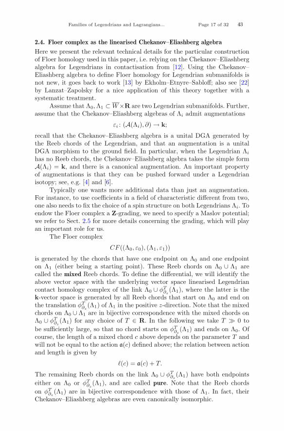
2.4. Floer complex as the linearised Chekanov–Eliashberg algebra
Here we present the relevant technical details for the particular constructionof Floer homology used in this paper, i.e. relying on the Chekanov–Eliashbergalgebra for Legendrians in contactisation from [12]. Using the Chekanov–Eliashberg algebra to define Floer homology for Legendrian submanifolds isnot new, it goes back to work [13] by Ekholm–Etnyre–Sabloff; also see [22]by Lanzat–Zapolsky for a nice application of this theory together with asystematic treatment.
Assume that Λ0,Λ1 ⊂ W ×R are two Legendrian submanifolds. Further,assume that the Chekanov–Eliashberg algebras of Λi admit augmentations
εi : (A(Λi), ∂) → k;
recall that the Chekanov–Eliashberg algebra is a unital DGA generated bythe Reeb chords of the Legendrian, and that an augmentation is a unitalDGA morphism to the ground field. In particular, when the Legendrian Λi
has no Reeb chords, the Chekanov–Eliashberg algebra takes the simple formA(Λi) = k, and there is a canonical augmentation. An important propertyof augmentations is that they can be pushed forward under a Legendrianisotopy; see, e.g. [4] and [6].
Typically one wants more additional data than just an augmentation.For instance, to use coefficients in a field of characteristic different from two,one also needs to fix the choice of a spin structure on both Legendrians Λi. Toendow the Floer complex a Z-grading, we need to specify a Maslov potential;we refer to Sect. 2.5 for more details concerning the grading, which will playan important role for us.
The Floer complex
CF ((Λ0, ε0), (Λ1, ε1))
is generated by the chords that have one endpoint on Λ0 and one endpointon Λ1 (either being a starting point). These Reeb chords on Λ0 ∪ Λ1 arecalled the mixed Reeb chords. To define the differential, we will identify theabove vector space with the underlying vector space linearised Legendriancontact homology complex of the link Λ0 ∪ φT
∂z(Λ1), where the latter is the
k-vector space is generated by all Reeb chords that start on Λ0 and end onthe translation φT
∂z(Λ1) of Λ1 in the positive z-direction. Note that the mixed
chords on Λ0 ∪ Λ1 are in bijective correspondence with the mixed chords onΛ0 ∪ φT
∂z(Λ1) for any choice of T ∈ R. In the following we take T � 0 to
be sufficiently large, so that no chord starts on φT∂z
(Λ1) and ends on Λ0. Ofcourse, the length of a mixed chord c above depends on the parameter T andwill not be equal to the action a(c) defined above; the relation between actionand length is given by
(c) = a(c) + T.
The remaining Reeb chords on the link Λ0 ∪ φT∂z
(Λ1) have both endpointseither on Λ0 or φT
∂z(Λ1), and are called pure. Note that the Reeb chords
on φT∂z
(Λ1) are in bijective correspondence with those of Λ1. In fact, theirChekanov–Eliashberg algebras are even canonically isomorphic.

43 Page 18 of 32 G. Dimitroglou Rizell
The differential is the Linearised Legendrian contact homology differ-ential induced by a choice of almost complex structure, together with theaugmentations εi for the Chekanov–Eliashberg algebras A(Λi) generated bythe pure chords. This version of a Floer complex defined via the Chekanov–Eliashberg algebra was originally considered in [13]; also see [4] for a morerecent realisation. We now give a sketch of the definition of the differential.It is roughly speaking defined by counts of rigid pseudoholomorphic discs in(W,dλ), for some choice of compatible almost complex structure, where thedisc has
• boundary on the exact Lagrangian immersion ΠW (Λ0 ∪ φT∂z
(Λ1)) ⊂(W,λ);
• precisely one positive puncture at a double point which corresponds toa mixed chord—this is the input;
• precisely one negative puncture at a double point which corresponds toa mixed chord—this is the output; and
• several additional negative punctures at double points which correspondto pure chords.
By positive (resp. negative) boundary puncture, one means a point wherethe boundary of the pseudoholomorphic disc makes a jump that increases(resp. decreases) the z-value of the Legendrian Λ0 ∪φT
∂z(Λ1) ⊂ W ×Rz when
following the boundary according to the orientation of the disc induced by thealmost complex structure. When counting the strip, one weighs the count bythe value of the augmentation εi on the pure chords from the last point. Thisis a part of the so-called linearised differential induced by the augmentation,as defined in [6]; also see the notion of the bilinearised Legendrian contacthomology as defined by Bourgeois–Chantraine in [3].
From positivity of symplectic area of such pseudoholomorphic discs to-gether with Stokes’ theorem one obtains that the Reeb chord length of theinput chord must be larger than the Reeb chord of the output. In other words,the complex is strictly filtered in the sense defined in Sect. 2.2, and the Reebchords constitute a compatible basis.
From the index formula for the expected dimension of the moduli spaceof pseudoholomorphic discs, it follows that the degree of the input is onegreater than the degree of the output; i.e. the differential is of degree −1.
2.5. Maslov potential and grading
The Maslov potential is a useful framework for introducing gradings in La-grangian Floer homology which originally is due to Seidel [27]. The choice ofa Maslov potential gives a well-defined grading in Z. In general the potentialis only well-defined modulo the Maslov number μ ∈ Z (the positive generatorof the subgroup of Z which is the image of the Maslov class); in that case thegrading is only defined in Z/μZ. Here we describe a grading for which thedifferential of the Floer complex considered above becomes a map of degree−1, i.e. it decreases the degree.

Families of Legendrians and Lagrangians... Page 19 of 32 43
Assume that W has vanishing first Chern class; this is, e.g. the case whenW has a symplectic trivialisation, which is automatic when dimR W = 2. TheZ–grading of the generators is defined as follows.
Consider the determinant bundle
C∗ → detC TW → W
induced by some choice of a compatible almost complex structure. The quo-tient
C∗/R∗ = (R2\{0})/R∗ = RP 1 = R/πZ
gives rise to an induced RP 1-bundle that we denote by
L = (detC TW )/R∗ → W.
Note that the bundle L is trivial when W has vanishing first Chern class(actually, the first Chern class being two-torsion is sufficient). In this casethere might be several choices of homotopy classes of trivialisations.
First, we make the choice of a trivialisation of the above determinantbundle. This choice gives rise to a trivialisation L = RP 1 × W → W of theRP 1-bundle as well. Then, taking the fibre-wise universal cover of this trivialRP 1-bundle, we obtain the affine R-bundle L = R × W → W . The fibre ofthis bundle is thus the choice of an R-lift of the angle in RP 1 = R/πZ of anunoriented real line.
Second, one makes the choice of a Maslov potential for each of theLegendrians Λi. This is the lift of the canonically defined section
(detR TΠW (Λi))/R∗ ⊂ (detC TW )/R∗
along Λi of the above RP 1-bundle L to the associated R-bundle L. Recallthat a non-zero Maslov class is the obstruction to the existence of such a lift.When a Maslov potential exists and the Legendrian is connected, there is anatural free and transitive Z-action on its Maslov potentials.
Given choices of Maslov potentials, the grading of a generator c ∈CF∗((Λ0, ε0), (Λ1, ε1)) is finally obtained in the following manner. Denoteby ϕi ∈ Lc the R-lift of the angle of the real determinant line
(detR TcΠW (Λi))/R∗ ⊂ (detC TcW )/R∗
specified by the choices of Maslov potentials. Consider a compatible almostcomplex structure J on TcW for which J · TcΠW (Λ0) = TcΠW (Λ1) to-gether with the induced family of Lagrangian planes eitTcΠW (Λ0) ∈ TcW ,t ∈ [0, π/2], that joins TcΠW (Λ0) to
eiπ/2TcΠW (Λ0) = J · TcΠW (Λ0) = TcΠW (Λ1).
There is a continuous path of real determinant lines ϕt0 ∈ Lc; denote by
ϕt0 ∈ Lc the continuous lift to the fibre-wise universal cover R → RP 1, where
ϕ00 = ϕ0. In particular, ϕ
π/20 is a lift of the determinant line ϕ1. The degree
of the generator c is finally defined by
|c| = (ϕπ/20 − ϕ1)/π ∈ Z.

43 Page 20 of 32 G. Dimitroglou Rizell
In the below examples we provide some useful techniques for specifyingMaslov potentials and computing degrees in the cases that we are interestedin here.
Example 2.8.(1) In the case of W = T ∗M there is a trivialisation of detC T (T ∗M) in
which the tangent planes to the zero section all coincide with the realpart R∗ ⊂ C∗ of the fibres. The zero-section Λ0 = j10 can be inducedwith the Maslov potential ϕ0 which is zero in each R-fibre of L.
(2) A choice of Maslov potential for a general Legendrian Λ1 ⊂ J1M forthe trivialisation from Part (1) above (if it exists) can be described bycomparing it to the canonical Maslov potential for the zero section j10.More precisely, the difference between the Maslov potential at a pointx ∈ Λ1 for which TxΠW (Λ1) is transverse to the Lagrangian fibre ofT ∗M and the canonical Maslov potential for j10 = Λ0 at the pointp(x) ∈ Λ0, where p : J1M → M is the bundle projection, can be de-scribed by an integer m(x) ∈ Z in the following manner.The fibre-wise rescaling of J1M induces an isotopy of Legendrian tan-gent planes that isotopes any tangent plane TxΛ1 which is transverse tothe fibre to the tangent plane Tp(x)j
10 of the zero section. There is aninduced continuous path of determinant lines ϕt
1 ∈ L where
ϕ01 = (detR TxΠW (Λ1))/R∗ ⊂ (detC Tx(T ∗M))/R∗,
and ϕ11 is the determinant line of the zero-section at the point p(x).
Consider the continuous choice of lifts ϕt1 ∈ L that extend the choice of
Maslov potential for Λ1. The difference
m(x) = (ϕ11 − ϕ0)/π ∈ Z
is an integer that uniquely recovers the choice of Maslov potential atx ∈ Λ1 (for x where the Lagrangian projection is transverse to thefibre).The integer m(x) is locally constant in the open subsets of Λ1 for whichthe Lagrangian projection is transverse to the fibres, and changes by +1as one traverses a cusp-edge in the direction of decreasing z-value. Thisis illustrated in Fig. 6.
(3) In the case when detC TW is trivial, the homotopy classes of trivial-isations of detC TW are in bijection with homotopy classes of mapsW → C∗, which is the same as classes in H1(W ;Z). In the particularcase W = T ∗S1, the description of the Maslov potential given in Part (2)is only valid above a simply connected subset, e.g. T ∗(−π, π) ⊂ T ∗S1.The Maslov potential for a general Legendrian in this setting can be de-scribed by the choice of numbers m(x) as above, that, however, satisfythe additional property that they make a jump by a fixed value l ∈ 2Zwhen traversing the hypersurface {θ = π} in the direction of increasingθ-value. (The case l = 0 corresponds to the canonical trivialisation forwhich the zero-section admits a Maslov potential.) This is illustrated inthe top of Fig. 7.

Families of Legendrians and Lagrangians... Page 21 of 32 43
(4) Let Λi ⊂ J1M , i = 0, 1, be two Legendrians with choices of Maslovpotentials that have the form j1fi over some subset in M (i.e. the La-grangian projections are transverse to the fibre there), where the Maslovpotentials are determined by integers mi ∈ Z in the manner describedabove. If f1 −f0 has a non-degenerate critical point at p ∈ M (i.e. thereis a transverse Reeb chord c there), then the above degree formula be-comes
|c| = indexMorsep (f1 − f0) + m0 − m1
where the first term on the right-hand side is the Morse index of thecritical point. We refer to [11, Lemma 3.4] for the computation.
Lemma 2.9.
(1) Let φ1 : W ×R → W ×R be the time-one map of a compactly supportedcontact isotopy. For any choice of Maslov potential on the Legendrian Λthere an induced Maslov potential on its image φ1(Λ) ⊂ W ×R uniquelydefined by the property that the Maslov potentials extend over the exactLagrangian cobordism from Λ to φ1(Λ) induced by the isotopy.
(2) If φ1 is a generic C1-small contact isotopy, then the small chords ofΛ ∪ φ1(Λ) are in bijective correspondence with the critical points of aC1-small Morse function f : Λ → R, and the above grading coincideswith the Morse index, if φ1(Λ) is endowed with the Maslov potentialinduced from Λ via the isotopy φt as in Part (1).
Proof. (1) The trace of the Legendrian isotopy can be made into a Lagrangiancylinder inside the symplectisation
(Rt × W × Rz, d(etαst))
with cylindrical ends over the initial and final Legendrian; see work [5] byChantraine. The Maslov potential of Λ induces a Maslov potential on thenegative end of this cobordism. This Maslov potential can be extended to theentire cobordism by elementary topology (it is a Lagrangian cylinder). Theinduced Maslov potential on the positive end is the sought Maslov potentialon φ1(Λ).
(2) This computation is standard, and can be performed in a smallneighbourhood of Λ. In particular, for a small perturbation of the zero-sectionj10 ⊂ J1M by a section j1f , this is an immediate consequence of Part(4) of Example 1. In general, recall that any Legendrian Λ has a standardneighbourhood which is contactomorphic to a neighbourhood of the zerosection j10 ⊂ J1Λ, under which Λ, moreover, is identified with j10; see [18].The perturbation can be assumed to be given by the one-jet j1f of someC1-small smooth function f : Λ → R in the same neighbourhood. �
3. Examples that exhibit unbounded spectral norms
The following basic auxiliary results facilitate our computations, and will beinvoked repeatedly.
43 Page 22 of 32 G. Dimitroglou Rizell
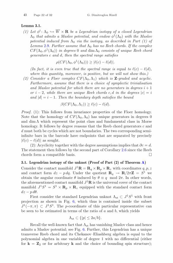
Lemma 3.1.
(1) Let φt : Λ0 ↪→ W × R be a Legendrian isotopy of a closed LegendrianΛ0 that admits a Maslov potential, and endow φ1(Λ0) with the Maslovpotential induced from Λ0 via the isotopy, as described in Part (1) ofLemma 2.9. Further assume that Λ0 has no Reeb chords. If the complexCF (Λ0, φ
1(Λ0)) in degrees 0 and dim Λ0 consists of unique Reeb chordgenerators c and d, then the spectral range satisfies
ρ(CF (Λ0, φ1(Λ0))) ≥ | (c) − (d)|.
(In fact, it is even true that the spectral range is equal to (c) − (d),where this quantity, moreover, is positive, but we will not show this.)
(2) Consider a Floer complex CF (Λ0,Λ1) which is Z-graded and acyclic.Furthermore, assume that there is a choice of symplectic trivialisationand Maslov potential for which there are no generators in degrees i + 1or i − 2, while there are unique Reeb chords c, d in the degrees |c| = iand |d| = i − 1. Then the boundary depth satisfies the bound
β(CF (Λ0,Λ1)) ≥ (c) − (d).
Proof. (1): This follows from invariance properties of the Floer homology.Note that the homology of CF (Λ0,Λ0) has unique generators in degrees 0and dim Λ which represent the point class and fundamental class in Morsehomology. It follows by degree reasons that the Reeb chord generators c andd must both be cycles which are not boundaries. The two corresponding semi-infinite bars in the barcode have endpoints that are separated by precisely| (c) − (d)| as sought.
(2): Acyclicity together with the degree assumptions implies that ∂c = d.The statement then follows by the second part of Corollary 2.6 since the Reebchords form a compatible basis. �
3.1. Legendrian isotopy of the unknot (Proof of Part (2) of Theorem A)
Consider the contact manifold J1R = Rq ×Rp ×Rz with coordinates q, p, zand contact form dz − p dq. Under the quotient Rq → R/2πZ = S1 weobtain the angular coordinate θ induced by θ ≡ q mod 2π. In other words,the aforementioned contact manifold J1R is the universal cover of the contactmanifold J1S1 = S1 × Rp × Rz equipped with the standard contact formdz − p dθ.
First consider the standard Legendrian unknot Λst ⊂ J1S1 with frontprojection as shown in Fig. 6, which thus is contained inside the subsetJ1(−π, π) ⊂ J1S1. The p-coordinate of this particular representative canbe seen to be estimated in terms of the ratio of a and b, which yields
Λst ⊂ {|p| ≤ 2a/b}.
Recall the well-known fact that Λst has vanishing Maslov class and henceadmits a Maslov potential; see Fig. 6. Further, this Legendrian has a uniquetransverse Reeb chord and its Chekanov–Eliashberg algebra is equal to thepolynomial algebra in one variable of degree 1 with no differential (eitherfor k = Z2 or for arbitrary k and the choice of bounding spin structure);

Families of Legendrians and Lagrangians... Page 23 of 32 43
see [14]. In particular, its Chekanov–Eliashberg algebra admits the trivialaugmentation.
We also fix a Legendrian fibre
F = F(π/4,0) = {π/2} × Rp × {0} ⊂ J1(−π, π) ⊂ J1S1.
Note that the Reeb chords between any Legendrian Λ and F are in bijectivecorrespondence with the intersection points of Λ and the hypersurface {θ =π/4}. Note that the image of F under the front projection is given by thepoint {(π/4, 0)}; Reeb chords correspond to lines contained inside {θ = π/4}in the front projection that have one endpoint on {(π/4, 0}) and one endpointon the projection of Λ. These chords are depicted in Fig. 6.
Since F that has no Reeb chords, its Chekanov–Eliashberg algebratrivially admits an augmentation. We can thus define the Floer homologycomplex CF (Λst, F ) which is generated by two Reeb chords c and d, where0 > (c) > (d) and |c| = |d| + 1. Note that CF (Λst, F ) is an acyclic complexby invariance under Legendrian isotopy; after shrinking the unknot suffi-ciently, all mixed chords disappear.
The goal is to construct a Legendrian isotopy Λtst ⊂ J1S1 of the unknot
confined to the subset
{|p| ≤ 2a/b} ⊂ J1S1
for which the boundary depth of CF (ΛTst, F ) becomes arbitrarily large as
t → +∞. This isotopy will be constructed as the projection of an isotopyΛt
st ⊂ J1R of the unknot inside the universal cover J1R → J1S1. In fact,the Legendrian isotopy Λt
st is very simple; it is the rescaling of
Λst = Λst ⊂ J1(−π, π) ⊂ J1R
under the contact isotopy (q, p, z) �→ (et · q, p, et · z) defined on the universalcover; note that this contact isotopy simply rescales the front projection.
It is easy to check that CF (Λtst, F ) satisfies the property that the bound-
ary depth goes to +∞ as t → +∞. Indeed, these complexes are generatedby the two unique transversely cut out Reeb chords ct and dt between Λt
st
and F for all values t > 0. These chords, moreover, satisfy the property that (ct) − (dt) becomes arbitrarily large as t → +∞; c.f. Part (2) of Lemma3.1.
What remains to prove is the following two claims for the projectionΛt
st ⊂ J1S1 of the Legendrian rescaling Λt ⊂ J1R. First, we claim that Λtst
indeed is a Legendrian isotopy. Second, we show that the boundary depth ofCF (Λt
st, F ) goes to +∞ as t → +∞The fact that Λt
st is a Legendrian isotopy can be seen by consideringthe sequence of front projections; see Figs. 7 and 8. Except for an isotopy ofthe front, the front also undergoes a sequence RIII -moves together with thecomposite move shown in Fig. 5. The Lagrangian projection of Λ2 is shownin Fig. 9.
Then we need to estimate the boundary depth of the sequence of Floercomplexes CF (Λt
st, F ). In addition to Reeb chords ct and dt, which corre-spond to the Reeb mixed Reeb chords on the lift and have exactly the same

43 Page 24 of 32 G. Dimitroglou Rizell
a
b
Λstd0
m − 1
m
c0F
z
θπ−π
Figure 6. The standard Legendrian unknot Λst and theLegendrian fibre F . Note that there are precisely two trans-verse Reeb chords c0, d0 between F and Λst. The choice ofm ∈ Z determines a Maslov potential on Λst as described inPart (2) of Example 1
actions, there are additional Reeb chords between Λtst and F that appear as
t → +∞. Nevertheless, we claim that the boundary depth of CF (Λtst, F ) still
is bounded from below by the boundary depth β(CF (Λtst, F )).
To see the last claim, we will consider different gradings of the complexesCF (Λt
st, F ), obtained by changing the symplectic trivialisation of T ∗S1. Notethat Λst is null-homotopic inside J1S1 and thus has a vanishing Maslov classindependently of the choice of symplectic trivialisation. Moreover, the chordsct and dt always satisfy |ct| − |dt| = 1 regardless of the choice of Maslovpotential and symplectic trivialisation; see the top of Fig. 7.
We claim that, after changing the symplectic trivialisation of T ∗S1 byintroducing a sufficiently large number l/2 � 0 of full rotations of the stan-dard symplectic frame as one traverses the hypersurface {θ = π} in thedirection of increasing θ-coordinate, all generators c′ in the complex exceptdifferent from ct and dt acquire degrees that satisfy
|c′| − |ct| /∈ [−10, 10].
To see this, we note that the Maslov potential of these sheets acquire anadditional term kl where k ∈ Z\{0}; see Parts (3) and (4) of Example 1.
Since these degree properties can be achieved, the statement now followsdirectly by Part (2) of Lemma 3.1. �3.2. Legendrian isotopy of the zero-section (Proof of Part (1) of Theorem A)
We use the same coordinates as in the above Sect. 3.1. In fact, the soughtLegendrian isotopy is also constructed in a manner similar to the constructionof Λt given there, by performing a rescaling of a part of the front inside theuniversal cover J1R (and then projecting back to J1S1). The isotopy is shownin Figs. 10 and 11. One starts by considering a Legendrian perturbation

Families of Legendrians and Lagrangians... Page 25 of 32 43
Λ2st
m +m l− l
m − 1 − l m − 1 + l
F
F
Λ2st
d2
c2
d2
c2
z
z
θ
qπ
m
m − 1
−π
π−π
Figure 7. Above: Λ2st has a front which is a linear rescaling
of the front of Λst inside J1R. The number m defines achoice of Maslov potential for Λ2
st, where l ∈ 2Z depends onthe homotopy class of the trivialisation of detC(T (T ∗S1)).Below: Λ2
st is the projection of Λ2st inside J1S1. Except for
the mixed chords ct and dt that exist for the lift, there arenow additional mixed chords
j1f of j10 which has precisely two chords. Then one performs a RII -move.Rescaling the front of the Legendrian introduced by the RII -move in theuniversal cover R2 and then projecting back to S1 ×R is again a Legendrianisotopy. In Fig. 11 one sees that there are exactly two chords between j10and the produced Legendrians, while the difference in action between thesetwo generators grows indefinitely as t → +∞. �
3.3. Hamiltonian isotopy on the punctured torus (Proof of Theorem D)
Here we consider the exact Lagrangian embedding L ⊂ (Σ1,1, dλ) of S1 whichis given as the image of {p = 0} ⊂ R2 under the quotient construction in Sect.2.1.2; see Fig. 13. We perform a Hamiltonian perturbation L′ that intersectsthe original Lagrangian transversely in precisely two points c and d. Thespectral norm is thus γ(CF (L,L′)) = (c) − (d).

43 Page 26 of 32 G. Dimitroglou Rizell
Λtst
dt
ct
z
θπ−π
Figure 8. This shows the projection Λtst of the rescaling
Λtst under the universal cover J1R → J1S1
Λ2st
p
qπ−π
Figure 9. The figure depicts the Lagrangian projection ofΛ2
st to T ∗R. The Lagrangian projection of Λ2st to T ∗S1 is
induced by the quotient projection R → S1. The Lagrangianprojection of Λt
st is obtained by rescaling the q-coordinate ofT ∗R followed by the canonical projection to T ∗S1
Then consider the autonomous Hamiltonian
ρ : Σ1,1 → R≤0
with support inside {q ∈ [−δ, δ]} for some small δ > 0, and which is equal tothe smooth bump-function ρ(q) ≤ 0 in one variable of the form
• ρ(q) ≡ −1 in a neighbourhood of q = 0;• ρ(q) = ρ(−q);• and ρ′(q) ≤ 0 for q < 0.

Families of Legendrians and Lagrangians... Page 27 of 32 43
z
θ
z
θπ−π π−π
d d
c
d d
c0
Λ Λ0
Figure 10. Left: a Legendrian perturbation of the zero sec-tion. The vertical chords denote the two Reeb chords be-tween the zero-section j10 and the perturbation. Right: theperturbed version of the zero-section after a suitable Legen-drian RI -move
The Hamiltonian isotopy φtρ wraps the region q ∈ (−δ, 0) in the negative
p-direction, while it wraps the region q ∈ (0, δ) in the positive p-direction.We claim that CF (L, φt
ρ(L′)) has a spectral norm which becomes arbi-
trarily large as t → +∞. What is clear is that (c)− (d) → +∞ as t → +∞.(Use, e.g. Lemma 2.1.) Again there are additional generators that appear ast → +∞, so knowing that (c) − (d) → +∞ is not sufficient.
As in Sect. 3.1 a change of symplectic trivialisation can again give uswhat we need. First consider the canonical symplectic trivialisation, inducedby the trivialisation of R2 and the quotient projection. Then deform thistrivialisation by adding a number l/2 � 0 of full rotations of the standardsymplectic frame (relative the constant one) as one traverses the {p = 1}.Note that the Lagrangian corresponding to {p = 0} still has a Maslov poten-tial after this change of trivialisation. Similarly to the computation in Sect.3.1, it is now readily seen that all generators c′ different from c and d satisfythe property that
|c′| − |c| /∈ [−10, 10],
after we have chosen l � 0 sufficiently large. In the meantime, |c| − |d| = 1is always satisfied.
The spectral norm can now finally be computed by invoking Part (1) ofLemma 3.1.
4. Proof of Theorem C
By definition, our two Floer complexes are the linearised Legendrian contacthomology complexes generated as a k-vector space by the mixed Reeb chordson the Legendrian link
Λ± ∪ φT∂z
(Λ).
Here T � 0 is fixed but sufficiently large.

43 Page 28 of 32 G. Dimitroglou Rizell
π 2π−2π −π
z
z
θ
q
π−π
d d
ct
d dΛt
Figure 11. Λt is obtained from Λ0 by a linear rescaling ofthe front inside {z ≥ 0} in the universal cover J1R2 followedby the canonical projection J1R → J1S1. The front of Λt
undergoes the composite move shown in Fig. 5 consisting oftwo consecutive RII -moves along with RIII -moves
The cusp-connected sum performed on Λ− ∪ φT∂z
(Λ) produces Λ+ ∪φT
∂z(Λ) (of course, only the first component is affected). There is an associated
exact standard Lagrangian handle-attachment cobordism
L ⊂ (Rt × W × Rz, d(etαst))
inside the symplectisation as constructed in [9]. This is a cobordism withcylindrical ends from
Λ− ∪ φT∂z
(Λ) to Λ+ ∪ φT∂z
(Λ),
i.e. from the Legendrian link before surgery (at the concave end) to the linkafter surgery (at the convex end). One component of this cobordism is simplythe trivial cylinder R× φT
∂z(Λ). This Lagrangian cobordism induces a unital
DGA-morphism
ΦL : A(Λ+ ∪ φT∂z
(Λ)) → A(Λ− ∪ φT∂z
(Λ))

Families of Legendrians and Lagrangians... Page 29 of 32 43
Λt
p
qπ 2π−π−2π
Figure 12. The Lagrangian projection in T ∗R of the uni-versal cover Λ ⊂ J1R of Λt ⊂ J1S1 shown in Fig. 11, whereΛt
∼= R. The interval shown in dark blue is a fundamentaldomain for Λt
q
p
d cL
L′
Σ1,1
L′L
Figure 13. The left depicts a domain in R2 with piecewisesmooth boundary. After identifying the two horizontal piecesof the boundary, as well as the two vertical pieces, one ob-tains the Liouville domain shown on the right, with Liouvilleform described in Sect. 2.1.2. The closed exact LagrangianL is the image of {p = 0} and L′ is a small Hamiltonianperturbation of L
of the Chekanov–Eliashberg algebras. In particular, the choice of augmenta-tion ε− of the Chekanov–Eliashberg algebra of Λ− pulls back to an augmen-tation ε+ = ε− ◦ ΦL of the Chekanov–Eliashberg algebra of Λ+.

43 Page 30 of 32 G. Dimitroglou Rizell
q
p
q
p
d c LL
φtρ(L
′) φt′ρ (L′)
Figure 14. A Hamiltonian isotopy that wraps the La-grangian {p = 0} around the one-handle with core {q = 0},while fixing a neighbourhood of the latter core. Note thatthe Hamiltonian function is positive but constant near q = 0.Here t′ > t
The above DGA-morphism ΦL of the Chekanov–Eliashberg algebrasafter and before the surgery was computed in [9, Theorem 1.1] under the as-sumption that the handle-attachment is sufficiently small. This computationsin particular shows that the mixed chords c on Λ+ ∪ φT
∂z(Λ) are mapped to
ΦL(c) = c +∑
i
ridi, ri ∈ k,
where di are words of Reeb chords that each contain an odd number of mixedchords of Λ−∪φT
∂z(Λ), and in which every mixed chord, moreover, is of lengthstrictly less than (c). It now follows by pure algebraic considerations thatthe map
CF∗((Λ+, ε+), (Λ, ε)) → CF∗((Λ−, ε−), (Λ, ε))
induced by linearising the DGA-morphism ΦL using the augmentations ε,ε+, and ε− (see [3] and [4]) is an action-preserving isomorphism of the Floercomplexes as claimed. �
Acknowledgements
The author is grateful to Remi Leclercq for teaching him the basics aboutspectral invariants and Viterbo’s conjecture, in a cafe somewhere on the RiveGauche. The author would also like to thank the anonymous referee for care-fully reading the manuscript.
Funding Open access funding provided by Uppsala University.

Families of Legendrians and Lagrangians... Page 31 of 32 43
Publisher’s Note Springer Nature remains neutral with regard to jurisdic-tional claims in published maps and institutional affiliations.
References
[1] Barannikov, S.A.: The framed Morse complex and its invariants. In: Singu-larities and Bifurcations, Volume 21 of Advances in Soviet Mathematics, pp.93–115. American Mathematical Society, Providence (1994)
[2] Biran, P., Cornea, O.: Bounds on the Lagrangian spectral metric in cotangentbundles. https://arxiv.org/abs/2008.04756 [math.SG] (2020)
[3] Bourgeois, F., Chantraine, B.: Bilinearized Legendrian contact homology andthe augmentation category. J. Symplectic Geom. 12(3), 553–583 (2014)
[4] Chantraine, B., Dimitroglou Rizell, G., Ghiggini, P., Golovko, R.: Floer theoryfor Lagrangian cobordisms. J. Differ. Geom. 114(3), 393–465 (2020)
[5] Chantraine, B.: Lagrangian concordance of Legendrian knots. Algebr. Geom.Topol. 10(1), 63–85 (2010)
[6] Chekanov, Y.: Differential algebra of Legendrian links. Invent. Math. 150(3),441–483 (2002)
[7] Chekanov, Yu.V.: Critical points of quasifunctions, and generating families ofLegendrian manifolds. Funktsional. Anal. i Prilozhen. 30(2), 56–69 (1996). (96)
[8] Carlsson, G., Zomorodian, A., Collins, A., Guibas, L.: Persistence barcodes forshapes. In: Scopigno, R., Zorin, D. (eds.) Symposium on Geometry Processing.The Eurographics Association (2004)
[9] Dimitroglou Rizell, G.: Legendrian ambient surgery and Legendrian contacthomology. J. Symplectic Geom. 14(3), 811–901 (2016)
[10] Dimitroglou Rizell, G., Sullivan, M.G.: The persistence of the Chekanov–Eliashberg algebra. Selecta Math. (N.S.) 26(5), 69 (2020)
[11] Ekholm, T., Etnyre, J., Sullivan, M.: Non-isotopic Legendrian submanifolds inR2n+1. J. Differ. Geom. 71(1), 85–128 (2005)
[12] Ekholm, T., Etnyre, J., Sullivan, M.: Legendrian contact homology in P × R.Trans. Am. Math. Soc. 359(7), 3301–3335 (2007). ((electronic))
[13] Ekholm, T., Etnyre, J.B., Sabloff, J.M.: A duality exact sequence for Legen-drian contact homology. Duke Math. J. 150(1), 1–75 (2009)
[14] Etnyre, J.B., Ng, L.L.: Legendrian contact homology in R3. https://arxiv.org/
abs/1811.10966 [math.SG] (2019)
[15] Etnyre, J.B.: Legendrian and transversal knots. In: Menasco W, ThistlethwaiteM (eds) Handbook of Knot Theory, pp. 105–185. Elsevier B. V., Amsterdam(2005)
[16] Floer, A.: Morse theory for Lagrangian intersections. J. Differ. Geom. 28(3),513–547 (1988)
[17] Floer, A.: Witten’s complex and infinite-dimensional Morse theory. J. Differ.Geom. 30(1), 207–221 (1989)
[18] Geiges, H.: An introduction to contact topology. In: Bollobas B, Fulton W,Katok A, Kirwan F, Sarnak P, Simon B, Totaro B (eds) Cambridge Studies
43 Page 32 of 32 G. Dimitroglou Rizell
in Advanced Mathematics, vol. 109. Cambridge University Press, Cambridge(2008)
[19] Kislev, A., Shelukhin, E.: Bounds on spectral norms and barcodes. Geom.Topol. 25(7), 3257–3350 (2021)
[20] Leclercq, R.: Spectral invariants in Lagrangian Floer theory. J. Mod. Dyn. 2(2),249–286 (2008)
[21] Legout, N.: A-infinity category of Lagrangian cobordisms in the symplectiza-tion of PxR. https://arxiv.org/abs/2012.08245 [math.SG] (2020)
[22] Lanzat, S., Zapolsky, F.: On the contact mapping class group of the contacti-zation of the Am-Milnor fiber. Ann. Math. Que. 42(1), 79–94 (2018)
[23] Oh, Y.-G.: Spectral Invariants: Applications, Volume 2 of New MathematicalMonographs, pp. 348–407. Cambridge University Press, Cambridge (2015)
[24] Polterovich, L., Rosen, D., Samvelyan, K., Zhang, J.: Topological Persistencein Geometry and Analysis, Volume 74 of University Lecture Series. AmericanMathematical Society, Providence (2020)
[25] Polterovich, L., Shelukhin, E.: Autonomous Hamiltonian flows, Hofer’s geom-etry and persistence modules. Selecta Math. (N.S.) 22(1), 227–296 (2016)
[26] Swiatkowski, J.: On the isotopy of Legendrian knots. Ann. Glob. Anal. Geom.10(3), 195–207 (1992)
[27] Seidel, P.: Graded Lagrangian submanifolds. Bull. Soc. Math. France 128(1),103–149 (2000)
[28] Shelukhin, E.: Viterbo conjecture for Zoll symmetric spaces. https://arxiv.org/abs/1811.05552 [math.SG] (2018)
[29] Shelukhin, E.: Symplectic cohomology and a conjecture of Viterbo. https://arxiv.org/abs/1904.06798 [math.SG] (2019)
[30] Usher, M., Zhang, J.: Persistent homology and Floer-Novikov theory. Geom.Topol. 20(6), 3333–3430 (2016)
[31] Viterbo, C.: Symplectic topology as the geometry of generating functions.Math. Ann. 292(4), 685–710 (1992)
[32] Viterbo, C.: Symplectic homogenization. https://arxiv.org/abs/0801.0206[math.SG] (2014)
[33] Zapolsky, F.: Geometry of contactomorphism groups, contact rigidity, and con-tact dynamics in jet spaces. Int. Math. Res. Not. IMRN 20, 4687–4711 (2013)
[34] Zapolsky, F.: On the Hofer geometry for weakly exact Lagrangian submani-folds. J. Symplectic Geom. 11(3), 475–488 (2013)
Georgios Dimitroglou RizellDepartment of MathematicsUppsala UniversityBox 480751 06 UppsalaSwedene-mail: [email protected]
Accepted: April 20, 2021.