Well-Posed Solvability of Functional-Differential Equations with Unbounded Operator Coefficients

ISSN 0012-2661, Differential Equations, 2014, Vol. 50, No. 9, pp. 1161–1172. c© Pleiades Publishing, Ltd., 2014.Original Russian Text c© R.Kh. Akylzhanov, V.V. Vlasov, 2014, published in Differentsial’nye Uravneniya, 2014, Vol. 50, No. 9, pp. 1175–1186.

INTEGRAL EQUATIONS

Well-Posed Solvability of Functional-DifferentialEquations with Unbounded Operator Coefficients

R. Kh. Akylzhanov and V. V. VlasovMoscow State University, Moscow, Russia

e-mail: [email protected] July 15, 2013

Abstract—We study functional-differential equations with unbounded variable operator coef-ficients and variable delays in a Hilbert space. We prove the well-posed solvability of initial–boundary value problems for the above-mentioned equations in Sobolev spaces of vector func-tions on the positive half-line.

DOI: 10.1134/S0012266114090043

1. INTRODUCTION

At present, there are numerous papers dealing with various aspects of the theory of functional-differential equations (FDE) (see the monographs [1–3] and the bibliography therein). Many ofthese papers contain results on the well-posed solvability of initial–boundary value problems forFDE in various function spaces. The same topic includes the study of FDE with unboundedoperator coefficients in Banach spaces, in particular, in Hilbert spaces. (In this connection, notethe papers [4–15].)

The aim of the present paper is to prove the well-posed solvability of an initial–boundary valueproblem for FDE of neutral type with unbounded variable operator coefficients and variable de-lays in a Hilbert space. It is important to note that we weaken the conditions imposed on thedelays as much as possible. This result is apparently new even for FDE in a finite-dimensionalspace. The present paper develops the corresponding results published in [4–6].

2. DEFINITIONS, NOTATION, AND STATEMENT OF RESULTS

Let H be a separable Hilbert space, and let I be the identity operator on H.

Definition 1. A closed linear densely defined operator A in a Banach space X is said to besectorial (with angle δ) if there exists a δ, 0 < δ ≤ π/2, such that the sector

Σπ/2+δ := {λ ∈ C : | arg λ| < π/2 + δ}\{0}

lies in the resolvent set �(−A) and, for each ε ∈ (0, δ), there exists a number Mε such that

‖(A + λI)−1‖ ≤ Mε

1 + |λ| for arbitrary 0 �= λ ∈ Σπ/2+δ−ε. (1)

Let B(H) be the algebra of bounded operators on the space H.By L2,γ = L2,γ(R+,H) we denote the space of measurable vector functions ranging in H equipped

with the norm

‖u‖L2,γ (R+,H) =

( +∞∫0

e−2γt‖u(t)‖2 dt

)1/2

, γ ≥ 0.

1161

1162 AKYLZHANOV, VLASOV

By W 12,γ = W 1

2,γ(R+, A) we denote the space of vector functions ranging in H such thatApu(1−p) ∈ L2,γ (p = 0, 1) equipped with the norm

‖u‖W 12,γ (R+,A) = (‖u(1)‖2

L2,γ(R+,H) + ‖Au‖2L2,γ (R+,H))

1/2.

Here and in the following, u(1)(t) =d

dtu(t). A more complete description of the spaces W 1

2,γ

for the case in which A is an unbounded self-adjoint positive operator can be found in the mono-graph [7, Chap. I]. In the following, we omit the subscript γ if γ = 0.

On the half-line R+ = (0,+∞), consider the following problem for a FDE:

Cu =du

dt+ Au(t) +

∞∑j=1

[Bj(t)Sgj((−A)βu)(t) + Dj(t)Spj

(u(1)(t))]

+

t∫0

(K(t − s)Au(s) + Q(t − s)u(1)(s)) ds = f(t), 0 ≤ β <12, t ∈ R+, (2)

u(+0) = θ. (3)

Here Bj(t), Dj(t), K(t), and Q(t), j ∈ N, are operator functions ranging in B(H), and θ isthe zero vector of the space H. The definition of fractional powers (−A)β can be found, e.g., in themonograph [16, p. 140] (see also [17, p. 281]). We require that the operator functions K(t) andQ(t) be Bochner integrable on R+ with weight e−κt,

+∞∫0

e−κt‖K(t)‖ dt < +∞,

+∞∫0

e−κt‖Q(t)‖ dt < +∞. (4)

The operators Sgjand Spj

are defined as follows:

(Sgju)(t) =

{u(gj(t)) for t ∈ {s : gj(s) ≥ 0},0 for t ∈ {s : gj(s) < 0},

(Spju)(t) =

{u(pj(t)) for t ∈ {s : pj(s) ≥ 0},0 for t ∈ {s : pj(s) < 0}.

The functions gj(t) are scalar real-valued Borel functions on R+ such that gj(t) ≤ t, and the pj(t)are scalar real-valued continuously differentiable functions on R+ with the properties

pj(t) ≤ t, p(1)j (t) > 0, t ∈ [0,+∞).

We denote the inverse functions of pj by p−1j and set hk(t) = t−gk(t) and qk = t−pk(t). We assume

that the function f belongs to L2,γ0(R+,H) for some γ0 ∈ R+. Equation (2) is called an FDE ofneutral type.

Definition 2. A function u is called a strong solution of problem (2), (3) if it belongs to thespace W 1

2,γ for γ ≥ 0 and satisfies Eq. (2) a.e. on R+ and the initial condition (3).

The main result of the present paper is stated in the following assertion.

Theorem 1. Suppose that A is a sectorial operator with bounded inverse and there existsa γ0 ∈ R such that the series

∞∑k=1

( +∞∫0

e−2γ0hk(t)‖Bk(t)‖2 dt

)1/2

< +∞, (5)

∞∑k=1

supt∈R+

e−γ0(t−pk(t))

(sup

t∈[p−1k (0),+∞)

‖Dk(t)‖2 1

p(1)k (t)

)1/2

< +∞ (6)

DIFFERENTIAL EQUATIONS Vol. 50 No. 9 2014

WELL-POSED SOLVABILITY OF FUNCTIONAL-DIFFERENTIAL EQUATIONS 1163

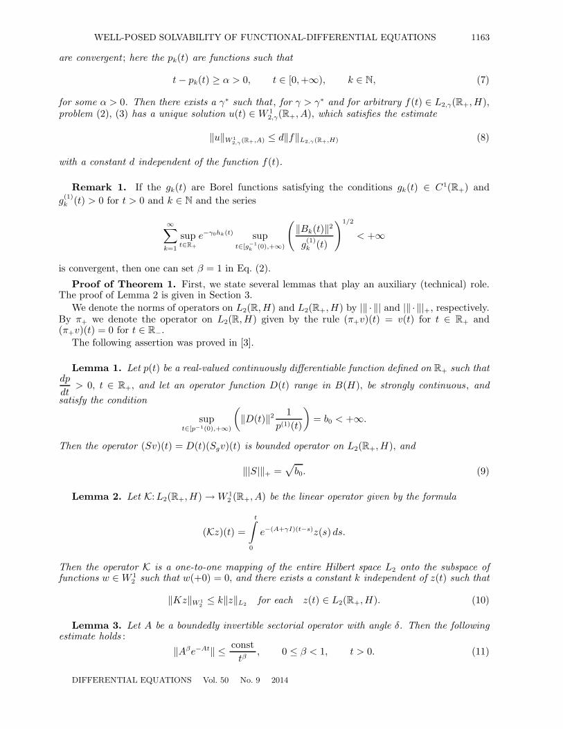
are convergent ; here the pk(t) are functions such that

t − pk(t) ≥ α > 0, t ∈ [0,+∞), k ∈ N, (7)

for some α > 0. Then there exists a γ∗ such that , for γ > γ∗ and for arbitrary f(t) ∈ L2,γ(R+,H),problem (2), (3) has a unique solution u(t) ∈ W 1

2,γ(R+, A), which satisfies the estimate

‖u‖W 12,γ (R+,A) ≤ d‖f‖L2,γ (R+,H) (8)

with a constant d independent of the function f(t).

Remark 1. If the gk(t) are Borel functions satisfying the conditions gk(t) ∈ C1(R+) andg

(1)k (t) > 0 for t > 0 and k ∈ N and the series

∞∑k=1

supt∈R+

e−γ0hk(t) supt∈[g−1

k (0),+∞)

(‖Bk(t)‖2

g(1)k (t)

)1/2

< +∞

is convergent, then one can set β = 1 in Eq. (2).

Proof of Theorem 1. First, we state several lemmas that play an auxiliary (technical) role.The proof of Lemma 2 is given in Section 3.

We denote the norms of operators on L2(R,H) and L2(R+,H) by |‖ · ‖| and |‖ · ‖|+, respectively.By π+ we denote the operator on L2(R,H) given by the rule (π+v)(t) = v(t) for t ∈ R+ and(π+v)(t) = 0 for t ∈ R−.

The following assertion was proved in [3].

Lemma 1. Let p(t) be a real-valued continuously differentiable function defined on R+ such thatdp

dt> 0, t ∈ R+, and let an operator function D(t) range in B(H), be strongly continuous, and

satisfy the condition

supt∈[p−1(0),+∞)

(‖D(t)‖2 1

p(1)(t)

)= b0 < +∞.

Then the operator (Sv)(t) = D(t)(Sgv)(t) is bounded operator on L2(R+,H), and

‖|S|‖+ =√

b0. (9)

Lemma 2. Let K:L2(R+,H) → W 12 (R+, A) be the linear operator given by the formula

(Kz)(t) =

t∫0

e−(A+γI)(t−s)z(s) ds.

Then the operator K is a one-to-one mapping of the entire Hilbert space L2 onto the subspace offunctions w ∈ W 1

2 such that w(+0) = 0, and there exists a constant k independent of z(t) such that

‖Kz‖W 12≤ k‖z‖L2 for each z(t) ∈ L2(R+,H). (10)

Lemma 3. Let A be a boundedly invertible sectorial operator with angle δ. Then the followingestimate holds :

‖Aβe−At‖ ≤ consttβ

, 0 ≤ β < 1, t > 0. (11)



The proof of Lemma 3 is technical and can be carried out by analogy with that of Theorem 4.3in [16, p. 97] and Theorem 14.11 in [17].

Let us return to the proof of Theorem 1. We seek a solution of problem (2), (3) in the formu(t) = eγtw(t). Then the vector function w(t) satisfies the equation

dw

dt+ (A + γI)w(t) +

∞∑k=1

e−γhk(t)

(Bk(t)Sgk

((−A)βu)(t) + Dk(t)Spk

(dw

dt+ γw(t)

))

+

t∫0

e−γ(t−s)(K(t − s)Aw(s) + Q(t − s)(w(1)(s) + γw(s))) ds = e−γtf(t) (12)

and the initial conditionw(+0) = θ. (13)

In turn, we seek a solution of problem (12), (13) in the form

w(t) =

t∫0

e−(A+γI)(t−s)z(s) ds (14)

with a new unknown vector function z(t) ∈ L2(R+,H). By Lemma 2, to the vector function z(t),there corresponds a vector function w(t) that belongs to the space W 1

2 (R+, A) and satisfies theinequality

‖w‖W 12 (R+,A) ≤ k‖z‖L2(R+,H)

with a constant k independent of z(t).By substituting the function (14) into Eq. (12), for the vector function z(t), we obtain the

equationz(t) + (Hγz)(t) + (Gγz)(t) + (Uγz)(t) + (Wγz)(t) = F (t), (15)

where the operators Hγ , Gγ , Uγ, and Wγ and the vector function F (t) are defined as follows:

(Jγz)(t) =

t∫0

(−A)βe−(A+γI)(t−s) ds, (16)

(Fγz)(t) =

t∫0

Ae−(A+γI)(t−s) ds, (17)

(Hγz)(t) =∞∑

k=1

e−γ(t−gk(t))Bk(t)(SgkJγz)(t), (18)

(Gγz)(t) =∞∑

k=1

e−γhk(t)Dk(t)(Spk(I − Fγ)z)(t), (19)

(Uγz)(t) =

t∫0

e−γ(t−s)K(t − s)(Fγz) ds, (20)

(Wγz)(t) =

t∫0

e−γ(t−s)Q(t − s)((I − Fγ)z) ds, (21)

F (t) = e−γtf(t). (22)



Let us show that the norm of the operator Hγ satisfies the inequality

‖|Hγ |‖+ ≤ C

γ(1−2β)/2(γ > 0). (23)

By using the relatione−(A+γI)(gk(t)−s) = e−A(gk(t)−s)−γ(gk(t)−s)

and the fact that the operators −A(gk(t) − s) and −γ(gk(t) − s)I commute, we obtain

e−(A+γI)(gk(t)−s) = e−A(gk(t)−s)e−γ(gk(t)−s). (24)

By using relation (24), we rewrite formula (18) as

(Hγz)(t) =∞∑

k=1

e−γ(t−gk(t))Bk(t)

gk(t)∫0

(−A)βe−A(gk(t)−s)e−γ(gk(t)−s)z(s) ds. (25)

Since e−γ(t−gk(t)) is a scalar function, it follows that formula (25) can be reduced to the form

(Hγz)(t) =∞∑

k=1

Bk(t)

gk(t)∫0

(−A)βe−A(gk(t)−s)e−γ(t−s)z(s) ds.

By using Lemma 3, we find that there exists a constant C1 = C1(A) such that

‖(−A)βe−A(gk(t)−s)‖ ≤ C1

|gk(t) − s|β .

We introduce the notation

L(t) ={

e−γt/tβ for t ≥ 0,0 for t < 0.

Let us extend the function z(t) by zero for t < 0 and estimate the norm of the operator

Bk(t)

gk(t)∫0

(−A)βe−A(gk(t)−s)e−γ(t−s)z(s) ds

in the space H. We have the chain of inequalities

∥∥∥∥∥Bk(t)

gk(t)∫0

(−A)βe−A(gk(t)−s)e−γ(t−s)z(s) ds

∥∥∥∥∥≤ ‖Bk(t)‖

gk(t)∫0

‖(−A)βe−A(gk(t)−s)e−γ(t−s)z(s)‖ ds

≤ ‖Bk(t)‖gk(t)∫0

‖(−A)βe−A(gk(t)−s)‖ ‖e−γ(t−s)z(s)‖ ds

≤ C1‖Bk(t)‖gk(t)∫0

e−γ(t−s)

(gk(t) − s)β‖z(s)‖ ds = C1e

−γhk(t)‖Bk(t)‖gk(t)∫0

L(gk(t) − s)‖z(s)‖ ds. (26)



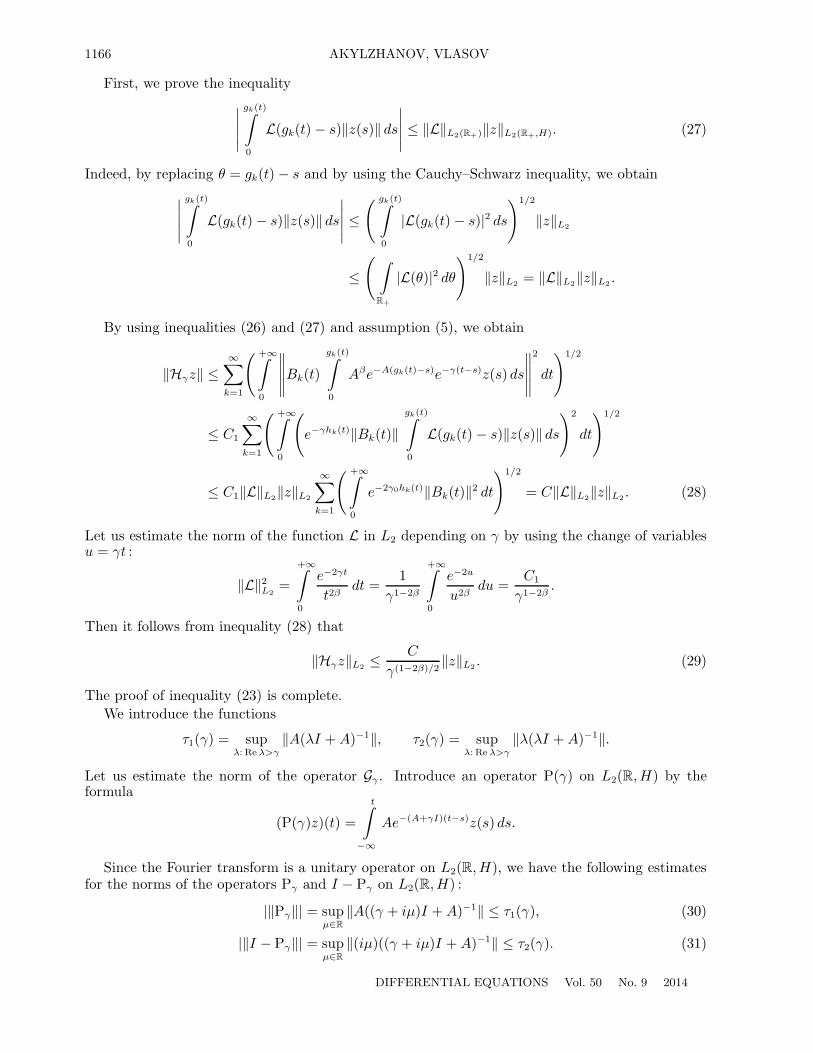
First, we prove the inequality∣∣∣∣∣gk(t)∫0

L(gk(t) − s)‖z(s)‖ ds

∣∣∣∣∣ ≤ ‖L‖L2(R+)‖z‖L2(R+,H). (27)

Indeed, by replacing θ = gk(t) − s and by using the Cauchy–Schwarz inequality, we obtain∣∣∣∣∣gk(t)∫0


∣∣∣∣∣ ≤( gk(t)∫

0

|L(gk(t) − s)|2 ds

)1/2

‖z‖L2

≤( ∫

R+

|L(θ)|2 dθ

)1/2

‖z‖L2 = ‖L‖L2‖z‖L2 .

By using inequalities (26) and (27) and assumption (5), we obtain

‖Hγz‖ ≤∞∑

k=1

( +∞∫0

∥∥∥∥∥Bk(t)

gk(t)∫0

Aβe−A(gk(t)−s)e−γ(t−s)z(s) ds

∥∥∥∥∥2

dt

)1/2

≤ C1

∞∑k=1

( +∞∫0

(e−γhk(t)‖Bk(t)‖

gk(t)∫0


)2

dt

)1/2

≤ C1‖L‖L2‖z‖L2

∞∑k=1

( +∞∫0

e−2γ0hk(t)‖Bk(t)‖2 dt

)1/2

= C‖L‖L2‖z‖L2 . (28)

Let us estimate the norm of the function L in L2 depending on γ by using the change of variablesu = γt :

‖L‖2L2

=

+∞∫0

e−2γt

t2βdt =

1γ1−2β

+∞∫0

e−2u

u2βdu =

C1

γ1−2β.

Then it follows from inequality (28) that

‖Hγz‖L2 ≤ C

γ(1−2β)/2‖z‖L2 . (29)

The proof of inequality (23) is complete.We introduce the functions

τ1(γ) = supλ: Re λ>γ

‖A(λI + A)−1‖, τ2(γ) = supλ: Re λ>γ

‖λ(λI + A)−1‖.

Let us estimate the norm of the operator Gγ . Introduce an operator P(γ) on L2(R,H) by theformula

(P(γ)z)(t) =

t∫−∞

Ae−(A+γI)(t−s)z(s) ds.

Since the Fourier transform is a unitary operator on L2(R,H), we have the following estimatesfor the norms of the operators Pγ and I − Pγ on L2(R,H) :

|‖Pγ‖| = supμ∈R

‖A((γ + iμ)I + A)−1‖ ≤ τ1(γ), (30)

|‖I − Pγ‖| = supμ∈R

‖(iμ)((γ + iμ)I + A)−1‖ ≤ τ2(γ). (31)



Note that we have the representations

(Fγz)(t) = (π+Pγπ+z)(t), (I − Fγz)(t) = (π+(I − Pγ)π+z)(t) (32)

for t ∈ R+, where π+ is the operator on L2(R,H) defined by (π+, v)(t) = v(t) for t ∈ R+ and(π+, v)(t) = 0 for t ∈ R− = (−∞, 0). By taking into account the representations (32), the esti-mates (30) and (31), and the relation ‖|π+|‖ = 1, we obtain the inequalities

‖|Fγ |‖+ ≤ τ1(γ), (33)‖|I − Fγ |‖+ ≤ τ2(γ). (34)

This, together with Lemma 1 and the representation (16), implies the estimate

|‖Gγ‖|+ ≤ τ2(γ)∞∑

k=1

supt∈R+

e−γqk(t)

(sup

t∈[p−1k (0),+∞)

‖Dk(t)‖2 1

p(1)k (t)

)1/2

. (35)

Note that we have the inequalities

supt∈R+

e−γqk(t) = supt∈R+

e−γ1qk(t)e−(γ−γ1)qk(t) ≤ e−(γ−γ1)α supt∈R+

e−γ1qk(t), j = 1, 2, . . . , (36)

for γ ≥ γ1. By using conditions (7) and (6), the estimates (23) and (35), and the limit relation

limγ→∞

e−(γ−γ1)α = 0, (37)

hence we obtain‖|Hγ |‖+ → 0, ‖|Gγ |‖+ → 0, γ → +∞. (38)

Let us proceed to estimating the norms of the operators Uγ and Wγ on L2(R+,H). To this end,consider the operators Jγ and Mγ given by

(Jγz)(t) =

t∫−∞

e−γ(t−s)K(t − s)z(s) ds, (Mγz)(t) =

t∫−∞

e−γ(t−s)Q(t − s)z(s) ds.

Note that the representations

(Uγz)(t) = (π+Jγπ+Fγz)(t), (Wγz)(t) = (π+Mγπ+(I − Fγ)z)(t) (39)

hold for t ∈ R+. Since, as was mentioned above, the Fourier transform is a unitary operator onL2(R,H), we have the following estimates for the norms of the operators Jγ and Mγ on L2(R,H) :

‖|Jγ |‖+ ≤ supμ∈R

‖K(γ + iμ)‖, ‖|Mγ |‖+ ≤ supμ∈R

‖Q(γ + iμ)‖, (40)

where K(·) and Q(·) stand for the Laplace transforms of the operator functions K(·) and Q(·),γ ≥ κ. By the well-known properties of the Laplace transform, we have the relations

supμ∈R

‖K(γ + iμ)‖ → 0, supμ∈R

‖Q(γ + iμ)‖ → 0, γ → +∞. (41)

By taking into account the estimates for the norms of the operators Fγ and I−Fγ [see (33) and (34)]and the representations (39), we obtain

‖|Uγ |‖+ ≤ supμ∈R

‖K(γ + iμ)‖ × τ1(γ), ‖|Wγ |‖+ ≤ supμ∈R

‖Q(γ + iμ)‖ × τ2(γ). (42)



Let us complete the proof of the theorem. By combining the estimates (23), (35), and (42),we obtain the inequality

‖|Hγ + Gγ + Uγ + Wγ|‖+

≤ C

γ(1−2β)/2+ τ2(γ)

∞∑k=1

supt∈R+

e−γqk(t)

(sup

t∈[p−1k (0),+∞)

‖Dk(t)‖2 1

p(1)k (t)

)1/2

+ τ1(γ) supμ∈R

‖K(γ + iμ)‖ + τ2(γ) supμ∈R

‖Q(γ + iμ)‖. (43)

It follows from relations (38) and (41), conditions (5) and (6), and inequalities (43) that, for eachδ ∈ (0, 1), there exists a γ1 > max(γ0, κ) such that the inequality

‖|Hγ + Gγ + Uγ + Wγ |‖+ < δ < 1 (44)

holds for γ ≥ γ1. In turn, it follows from the last inequality that Eq. (15) is uniquely solvable inthe space L2(R+,H), and its solution z(t) satisfies the inequality

‖z(t)‖L2(R+,H) ≤ C‖F (t)‖L2(R+,H) (45)

with a constant C independent of F (t). One can show that, by Lemma 2, to the vector functionz(t) ∈ L2(R+,H), there corresponds a vector function w(t) that belongs to the space W 1

2 (R+, A)and satisfies the inequality

‖w‖W 12 (R+,A) ≤ C1‖F‖L2(R+,H) (46)

with a constant C1 independent of the function F (t). By using relation (22) and the definition ofthe norm on the space L2,γ(R+,H), we obtain

‖F‖L2(R+,H) = ‖f‖L2,γ(R+,H). (47)

By taking into account relations (46) and (47) and the definition of the norm on the spaceW 1

2,γ(R+, A), we derive the desired inequality (8) for γ > γ1 with a constant d independent of f(t).The proof of Theorem 1 is complete.

3. PROOF OF LEMMA 2

Let us estimate the norm of the vector function

w(t) =

t∫0

e−(A+γI)(t−s)z(s) ds

in W 12 (R+, A). We continue the function z(t) by zero for t < 0. By a straightforward verification,

one can show that

d

dt

( t∫−∞


)= z(t) − (A + γI)

t∫−∞

e−(A+γI)(t−s)z(s) ds.

For convenience, we introduce the notation

K(t) ={

Ae−(A+γI)t for t ≥ 0,0 for t < 0.

Let us estimate the vector function A∫ t

0e−(A+γI)(t−s)z(s) ds. Since the Fourier transform F is

a unitary operator on L2(R,H), we have

‖K ∗ z‖L2 = ‖F [K ∗ z]‖L2 = ‖F [K]F [z]‖L2 .



The Fourier transform F [K](μ) of the kernel K(t) can be represented in the form

F [K](μ) =1√2π

+∞∫0

Ae−(A+γI)te−iμt dt =1√2π

+∞∫0

Ae−(γ+iμ)e−At dt.

The operator (−A) is the generator of an analytic semigroup T (t) = e−At. Consequently, thereexist constants M and w such that ‖T (t)‖ ≤ Mewt, and the resolvent of the operator (−A) admitsthe representation

(λI + A)−1 =

∞∫0

e−λtT (t) dt.

Then the relationF [K](μ) =

1√2π

A((γ + iμ)I + A)−1

holds for λ = γ+ iμ, γ > ω. Since the Fourier transform is a unitary operator on L2(R,H), we havethe estimate∥∥∥∥∥A

t∫0


∥∥∥∥∥L2(R+,H)

≤ 1√2π

supμ∈R

‖A((γ + iμ)I + A)−1‖ ‖z‖L2(R+,H)

=1√2π

r1(γ)‖z‖L2(R+,H).

It follows from this estimate that

‖w(1)(t)‖L2 ≤(

1√2π

r1(γ) + γ + 1)‖z‖L2 ,

and consequently,

‖w‖2W 1

2 (R+,A) = ‖w(1)‖2L2

+ ‖Aw‖2L2

≤((

1√2π

r1(γ) + γ + 1)2

+r21(γ)2π

)‖z‖2

L2(R+,H). (48)

The proof of Lemma 2 is complete.

4. REMARKS

Along with problem (2), (3), consider the following problem, which is traditionally referred toas an initial value problem:

dv

dt+ (Av)(t) +

∞∑k=1

(Bk(t)(−A)βv(gk(t)) + Dk(t)v(1)(pk(t)))

+

t∫−∞

[K(t − s)Av(s) + Q(t − s)v(1)(s)] ds = f0(t), t > 0, (49)

v(m)(t) = ym(t), t ∈ R−(−∞, 0), m = 0, 1, (50)u(+0) = φ0. (51)

It is assumed that the vector functions Ay0(t) and y1(t) belong to the space L2,γ(R−,H) for someγ ≥ 0 and φ0 ∈ D(A1/2).



Let us introduce the operators T gkv,

(T gkv)(t) = 0 for gk(t) ≥ 0, (T gkv)(t) = v(gk(t)) for gk(t) < 0,(T pkv)(t) = 0 for pk(t) ≥ 0, (T pkv)(t) = v(pk(t)) for pk(t) < 0.

Taking into account the relations

v(gk(t)) = (Sgkv)(t) + (T gky0)(t), v(1)(gk(t)) = (Sgk(t)v

(1))(t) + (T gky1)(t),

note that problem (49)–(51) can be reduced to a problem for Eq. (2); here the function f(t) isdefined by the formula

f(t) = −∞∑

k=1

(Bk(t)(−A)βT gk(y0)(t) + Dk(t)T pk(y1)(t))

−0∫

−∞

(K(t − s)Ay0(s) + Q(t − s)y1(s)) ds + f0(t), (52)

and the initial condition is (51).In turn, one can pass from condition (51) to condition (2) if the solution is sought in the form

v(t) = u(t) + e−tAϕ0 with the new unknown function u(t). Then for the function u(t), we obtaina problem of the form (2), (3),

Lu =du

dt+ Au(t) +

∞∑j=1

[Bj(t)Sgj((−A)βu)(t) + Dj(t)Spj

(u(1)(t))]

+

t∫0

(K(t − s)Au(s) + Q(t − s)u(1)(s)) ds = f2(t), 0 ≤ β <12, t ∈ R+,

with the initial condition u(+0) = θ, where f2(t) = f(t) + f1(t) and

f1(t) =∞∑

j=1

[Bj(t)(−A)βSgj(e−tAϕ0)(t) + Dj(t)Spj

(Ae−tAϕ0)(t)]

+

t∫0

((K(t − s) − Q(t − s))Ae−tAϕ0) ds.

Therefore, problem (49)–(51) can be reduced to the form (2), (3) with right-hand side f2(t) de-pending on the initial data y0(t), y1(t), and ϕ0(t). This explains why problem (2), (3) was studiedin the present paper.

5. CONCLUSION

The step method for constructing the solution is sometimes used to study the solvability ofinitial-value problems. Some modifications of this method for the case of a differential-differenceequation of retarded type with a single delay in a Hilbert space on a finite interval with respect tot ∈ [0, T ] can be found in [10]. However, this method proves to be very cumbersome in use and oftenless efficient for the investigation of the asymptotic behavior of solutions as t → +∞ and for theanalysis of the solvability of equations with variable delay on the half-line. In the above-consideredcase, the investigation is further complicated by the presence of unbounded operator coefficientsmultiplying the delays. The reduction of the original problem (2), (3) to Eq. (15) used in the proofof the solvability (Theorem 1) turns out to be very useful, because Eq. (15) is an equation withbounded operators Hγ , Gγ , Uγ , and Wγ .



In the study of problem (49)–(51), we follow the approach in [2, Chap. I] (in the case of a finite-dimensional space H). With our definition of solution, this permits one to treat problem (49)–(51)as a special case of problem (2), (3) with a special right-hand side of the form (52). In this case,it is reasonable to consider the problem on the continuous matching of y0(t), y1(t), and φ0 at t = 0as a separate problem.

Let us dwell on certain aspects related to the presence of unbounded operator coefficientsin Eq. (2).

More restrictive conditions were imposed in [9, 10, 12, 14] on the coefficients multiplying thedelays Bk(t)A and Dk(t), j ∈ N. In particular, it was assumed in most papers (e.g., see [9, 15])that these coefficients [Bk(t)A and Dk(t), j ∈ N, in our notation] are bounded operators.

Let us describe closest results by some authors in more detail.The case of infinitely many delays was quite comprehensively studied in [9] (see also [8]). The fact

that bounded operator coefficients multiplying the delays were considered in [9] is the main differ-ence of the results obtained in [9] from ours. The same is true for the results in [15].

An FDE of neutral type with unbounded operator coefficients multiplying the delays was con-sidered in [14], but the study was carried out in the autonomous case, that is the case, in whichthe coefficients Bk(t) and Dk(t) are independent of t. The case of unbounded operator coefficientsmultiplying the delays was also considered in [10–13]. However, only equations of retarded type[Dk(t) ≡ 0, j ∈ N, Q(t) ≡ 0] were considered in these papers, and it was assumed that the operatorcoefficients multiplying the delays are independent of t.

The condition that the delays are constant, hk(t) ≡ hk ≡ const > 0, is also an importantdistinction of the papers [8–15], while in the present paper, we have considered FDE with variabledelays and unbounded operator coefficients depending on t.

Note that results on the well-posed solvability in the Sobolev space of vector functions con-structed on the basis of a self-adjoint operator A under the condition presented in Remark 1 aregiven and summarized in the monograph [6, Chap. 2].

ACKNOWLEDGMENTS

The authors are grateful to A.B. Antonevich, V.P. Maksimov, and H.-O. Walther (Giessen,Germany) for useful discussions of the results.

The research was supported by the Russian Foundation for Basic Research (projects nos. 14-01-00349, 13-01-12476-ofi-m-2013, and 13-01-00384).

REFERENCES

1. Hale, J., Theory of Functional Differential Equations, New York: Springer, 1977. Translated under thetitle Teoriya funktsional’no-differentsial’nykh uravnenii , Moscow: Mir, 1984.

2. Azbelev, N.V., Maksimov, V.P., and Rakhmatullina, L.F., Elementy sovremennoi teorii funktsional’no-differentsial’nykh uravnenii (Elements of Modern Theory of Functional-Differential Equations), Moscow,2002.

3. Antonevich, A.B., Lineinye funktsional’nye uravneniya. Operatornyi podkhod (Linear Functional Equa-tions. The Operator Approach), Minsk: Universitetskoe, 1988.

4. Vlasov, V.V., On the Solvability and Estimates for the Solutions of Functional-Differential Equations inSobolev Spaces, Tr. Mat. Inst. Steklova, 1999, vol. 227, no. 4, pp. 109–121.

5. Vlasov, V.V. and Medvedev, D.A., Functional-Differential Equations in Sobolev Spaces and RelatedProblems in Spectral Theory, Sovrem. Mat. Fundam. Napravl., 2008, vol. 30, pp. 3–173.

6. Vlasov, V.V., Medvedev, D.A., and Rautian, N.A., Functional-Differential Equations in Sobolev Spacesand Their Spectral Analysis, Sovrem. Probl. Mat. Mekh. Mat., 2011, vol. 8, no. 1.

7. Lions, J.-L. and Magenes, E., Problemes aux limites non homogenes et applications, Paris: Dunod, 1968.Translated under the title Neodnorodnye granichnye zadachi i ikh prilozheniya, Moscow: Mir, 1971.

8. Datko, R., Uniform Asymptotic Stability of Evolutionary Processes in a Banach Space, SIAM J. Math.Anal., 1973, vol. 3, pp. 428–445.

9. Datko, R., Representation of Solutions and Stability of Linear Differential-Difference Equation in a Ba-nach Space, J. Differential Equations, 1978, vol. 29, no. 1, pp. 105–166.



10. Di Blasio, G., Kunisch, K., and Sinestrari, E., L2-Regularity for Parabolic Partial Integro-DifferentialEquations with Delays in the Highest Order Derivatives, J. Math. Anal. Appl., 1984, vol. 102, pp. 38–57.

11. Di Blasio, G., Kunisch, K., and Sinestrari, E., Stability for Abstract Linear Functional DifferentialEquations, Israel J. Math., 1985, vol. 50, no. 3, pp. 231–263.

12. Kunisch, K. and Mastinsek, M., Dual Semigroups and Structural Operators for Partial DifferentialEquations with Unbounded Operators Acting on the Delays, Differential Integral Equations , 1990, vol. 3,no. 4, pp. 733–756.

13. Kunisch, K. and Schappacher, W., Necessary Conditions for Partial Differential Equations with Delayto Generate C0-Semigroups, J. Differential Equations, 1983, vol. 50, pp. 49–79.

14. Staffans, O.J., Some Well-Posed Functional Equations Which Generate Semigroups, J. Differential Equa-tions , 1985, vol. 58, no. 2, pp. 157–191.

15. Wu, J., Semigroup and Integral Form of Class of Partial Differential Equations with Infinite Delay,Differential Integral Equations , 1991, vol. 4, no. 6, pp. 1325–1351.

16. Engel, K.J. and Nagel, R., One Parameter Semigroups for Linear Evolution Equations , Springer, 1999.17. Krasnosel’skii, M.A., Zabreiko, P.P., Pustyl’nik, E.I., and Sobolevskii, P.E., Integral’nye operatory

v prostranstvakh summiruemykh funktsii (Integral Operators in Spaces of Integrable Functions), Moscow:Nauka, 1996.


Well-Posed Solvability of Functional-Differential Equations with Unbounded Operator Coefficients

Documents

Transcript of Well-Posed Solvability of Functional-Differential Equations with Unbounded Operator Coefficients