NEAR EAST UNIVERSITY

Faculty of Engineering

Department of Electrical & Electronic Engineering

BASE STATION & FREQUENCY INTERFACES

Graduation Project EE-400 _

Student:Tarek Eleisawi (981261)

Supervisor: Prof. Dr. Fakhreddin Mamedov

•

ACKNOWLEDGMENTS

. First I would to thank Prof Fakhreddin Mamedov to be my advisor . under

his guidence , I succesfully overcome many diffeculties and learn a lot from

him.

Special thanks to my friends that they were always help me a lot to

reach to this point and espacially Hani Agha and Hazem Abo Shaban

Finally , I would to thank my family ,espacially my parents . Without

their endless support and love for me , I would never achieve my current

position . I wish my mother lives happily always , and my father in the heaven

be proud of me .

• ABSTRACT

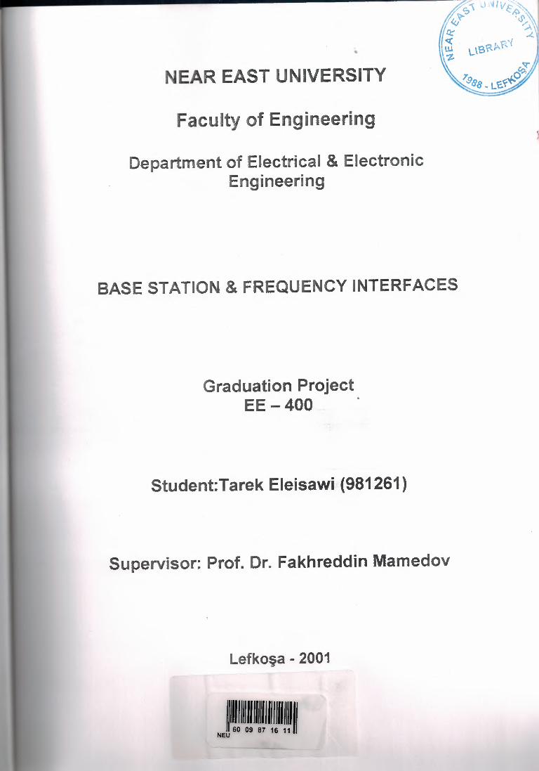
In this telecommunications environment of incompatible interfaces, the most

important technical goal of GSM was full roaming in all countries. Another goal was to

accommcxiate diverse service plans to conform to the separate needs and policies of

participating countries , GSM is a comprehensive standard, like the other standards

covered in this project, it specifies the air interface that links terminals and base

stations. However, it is unique in also prescribing open interfaces between infra

structure network elements, most notably between base stations and switches.

The traffic channels are both two-way channels with identical transmission

formats in the two directions. In this respect, GSM differs from NA-IDMA and CDMA).

Base stations use the broadcast control channel to transmit the information that

terminals need to set up a call, including the control channel BCCH transmits one

message segment, of length 184 bits, in every control multi frame ,a base station

subsystem (BSS) providing the interface between a mobile switching center (MSC) and

a mobile , A BSS consists of several base transceiver subsystems (BTS) and a base • station controller (BSC).

The primary aim of this study was to determine the RF EME level resulting

from all signal frequencies prcxiuced by the particular GSM base stations under survey.

Mobile -telephone communication signals are both transient and partly random in their

occurrence and distribution. In this context, we were interested in determining the RF

EME levels at many locations and more particularly .

INTRODUCTION

Mobile telephone base stations are low power radio transmitters with antennas

mounted on either freestanding towers or on buildings. Radio signals are fed through

cables to the antennas and then launched as radio waves into the area, or cell, around the

base station. Two types of antennas are used for the transmissions; pole-shaped

antennas are used to communicate with mobile telephones and dish antennas

communicate to other base stations and link the network together The transmissions

from any particular base station are variable and dependent upon the number of calls

and the number of transmitters in operatic.

The antennas are the sources of the radiated signals and operate at power levels

consistent with their aim of communicating over short distances. Typical power levels

are not more than a few tens of watts .

The mobile phone system has limitations, similar to the radio and television

systems, in that the number of frequencies available restricts the number of handsets or

users within each cell. To enable a large number of users, regions are divided up into

cells each with its own set of frequencies (GSM system). Adjacent cells have different

frequencies to prevent interference and power levels are kept to a minimum to ensure no

interference with non-adjacent cells, which use the same frequency. The size of the cell

varies depending on the number of users. In rural areas, which typically cover large

regions due to the sparse population, more power has to be generated to cover the larger

area. This can lead to higher radiation exposure .

Both sector antennas and radio link antennas bundle the waves they transmit,

sending them in just one specific direction or at one specific angle. This means the

waves can be sent only where they are actually required.

TABLE OF CONTENTS

ACKNOWLEDGMENT

ABSTRACT

INTRODUCTION

I.DIGITAL CELLULAR SYSTEM

1.1 Background and Goals

1.2 Architecture

1.3 Radio Transmission 1. 3. 1 Physical Channels

1.3 .2 GSM Bit Stream

1.3 .3 Slow Frequency Flopping

1.3 .4 Radiated Power

1.3.5 Spectrum Efficiency

2.LOGICAL CHANNELS 2.1 Introduction

2.2 Broadcast Channels and Common Control Channels

2.3 Frequency Correction Channel (FCCH)

2.4 Synchronization Channel (SCH)

2.5 Broadcast Control Channel (BCCH) 2.6 Paging Channel (PCH) and Access Grant Channel

2. 7 Random Access Channel (RACH)

2.8 Stand-Alone Dedicated Control Channel

2. 9 Traffic Channels (TCH)

2.10 Speech Coding and Interleaving

2.11 Slow Associated Control Channel

2.12 Fast Associated Control Channel

2 .13 Messages 2.14 Message Structure

2. 15 Message Content

I .

.. u. m.

1

1

4

8

9

14

16

17

19

20

20

21

22

23

25

25

26

28

30

30

33

33

35

36

38

3. BASE STATION SUBSYSTElVIS

3 .1 Introduction

3 .2 System Architectures

3 .3 Base Transceiver Subsystems (BTS)

3 .4 Base Station Controller (BSC).

3.5 Analysis of Call Handling Schemes

3.5.1 System Modeling

3. 6 Analysis of Call Handling Schemes

3.6.1 Call Handling Scheme with Guard channels (Scheme 1)

3 .6.2 Call Handling Schemes without Guard Channels

3. 7 Calling Examples

4.BASE STATIONS RADIO FREQUENCIES

4.1 Introduction

4.2 Measurement Locations

4.3 Nature And Type Of Measurements Required.

4.3.1 Fixed Site Environmental Measurements

4.4 GSM Base Station Activity Measurements

4.5 Mobile GSM Base Station Area Measurements

4.6 Equipment

4.7 RF EME Exposure And Activity Levels From GSM Base

Stations

4.8 Fixed Site Eenviromental RF EME Levels From Various

Signal Sources

CONCLUSION

REFERENCES

• 47

47

47

49

51

54

54

56

56

56

59

61

61

63

63

63

64

65

66

67

71

75

76

CHAPTERl

DIGITAL CELLULAR SYSTEM

1.1 Background and Goals

The Pan-European digital cellular system traces its origins to 1982, when analog

cellular services were in their earliest stages of commercial deployment. At that early date,

European authorities anticipated the long-term potential of mobile communications and

stimulated CEPT, the Conference of European Postal and Telecommunications

administrations, to study the creation of a mobile telephone standard to be adopted

throughout Western Europe. CEPT responded by forming the Group Special Mobile

(Special Mobile Group). Group members used the initials GSM to refer to their project.

Eventually, GSM produced a compatibility specification that was adopted as a European

standard. The system embodied in the standard acquired the name Global System for Mobile

Communications. During the GSM development period in the 1'980s, European economic

integration proceeded rapidly; the idea of a telecommunications system that could be used

conveniently by travelers throughout Europe was an exciting symbol of this integration. A

continental standard for mobile telephones stands in strong contrast to fixed telephone

networks in Europe, which have different dialing procedures and charging systems in each

country. Similar disparities exist in European analog cellular systems, which have five

incompatible analog air interfaces scattered around the continent [Mouly and Pautet, 1992].

In this telecommunications environment of incompatible interfaces, the most

important technical goal of GSM was full roaming in all countries. Another goal was to

accommodate diverse service plans to conform to the separate needs and policies of

participating countries. These characteristics of GSM make it possible for a subscriber to

carry one telephone throughout Europe, initiating and receiving phone calls in all locations,

without the burden of learning new dialing codes every time he crosses a national boundary.

Calling features and charges reflect the service plan of the subscriber's home service

provider. As an incentive for the diverse participants in GSM to reach an agreement,

authorities made new frequency bands available for Pan-European operation with the

requirement that all transmissions in these hands conform to a single standard. GSM reached

a major milestone in 1987 when all pa4icipants agreed on the framework of a compatibility

specification. Two principal technologies in the specification are an air interface based on

hybrid frequency division/Time-division multiple access and infrastructure communication

based on Signaling System Number. Over the sub-sequent three years, GSM produced a

complete standard that became the responsibility of ETSI, the European

Telecommunications Standards Institute. in addition, network operators signed a

memorandum of under standing that specifies how GSM systems are brought into

commercial service. The memorandum of understanding also governs the business

arrangements between different operators of GSM networks.

GSM is a comprehensive standard, like the other standards covered in this project, it

specifies the air interface that links terminals and base stations. However, it is unique in also

prescribing open interfaces between infra structure network elements, most notably between

base stations and switches. The development of GSM reflects a remarkable cooperative

effort undertaken over ninny years by dozens of people from fifteen countries. Many GSM

innovations were later embodied in other systems. Two examples of these innovations are

location-based mobility management and mobile assisted handover.

GSM stands apart in two respects. it is a purely digital system There is no provision

for dual mode operation with an analog cellular system. This difference reflects the contrast

between the diversity of analog cellular systems in Europe and the ubiquitous deployment of

AMPS systems in North America. Another difference is the large number of network inter

faces specified by GSM, in contrast with the CDMA standard and the NA-TDMA standard,

which specify only the air interface. The GSM open interfaces reflect the major influence of

network operators its the development of- GSM. Open interfaces favor network operators

by giving them flexibility in procurement. By contrast, equipment vendors take the lead in

the creation of North American standards. Compared with service providers, equipment

vendors have a stronger tendency to favor proprietary interfaces.

2

•

Although the principal goal of GSM is international roaming, the project formally

adopted a broad set of aims, which included :

• full international roaming.

• provision for national variations in charging and rates,

• efficient interoperation with ISDN systems,

• signal qua lily better than or equal to that of existing mobile systems,

• traffic capacity higher than or equal to that of present systems,

• subscriber costs lower than or equal to those of existing systems,

• accommodation of non-voice services, and

• accommodation of portable terminals.

GSM adopted this ambitious list of objectives in t 985. As the standardization

proceeded, it became clear that achieving them fully would not be consistent with the service

introduction (late of 199 t approved by the initial GSM network operators. lb reconcile the

performance and cost objectives with early deployment, GSM decided that the standard

would evolve through a set of "phases." This decision implicitly added the goats of early

deployment and adaptability to the list. The Phase 1 GSM specifications were divided into

more than 100 sections, 4 with a total length of 5,320 pages. Phase 2 specifications have

been developed section by section in the mid-I 990s. The main goat of Phase 2 is to enrich

the set of information services available to GSM subscribers [Mouly and Pautet, 1995).

The remainder of this chapter is a description of the principal properties of GSM, as

defined in Phase I of the specifications. The services specified in Phase 1 include

• telephony with some special features,

• emergency calls,

• data transmission at rates tip to 9,600 bl s, and

• a short message service for transmitting up to 160 alphanumeric characters

between terminalsand a network.

3

•

Phase 2 adds additional lion-voice services and enriched telephony features.

To present tile salient features of GSM. The focus is on Communications across the

air interface. For more details, readers can refer to tile excellent book by Mouly and Pautet,

The GSM System far Mobile Communications, which is a 700-page tutorial on GSM [ 1992]

Of course, tile ultimate authority is the GSM standard, but that consists of more than one

hundred documents published by ETSI, with a total length of more than 5,000 pages.

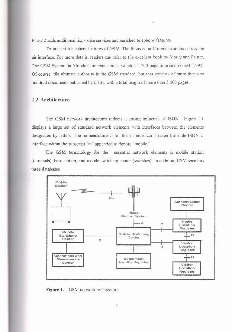
1.2 Architecture

The GSM network architecture reflects a strong influence of ISDN . Figure 1.1

displays a large set of standard network elements with interfaces between the elements

designated by letters. The nomenclature U for the air interface is taken from tile ISDN U

interface within the subscript "in" appended to denote "mobile."

The GSM terminology for the essential network elements is mobile station

(terminals), base station, and mobile switching center (switches). In addition, CSM specifies

three databases.

Mobile Station

Um

·1 Authentication Center

Base Station System

Home A C Location Register

D Mobile Mobile Switching Switching Center Center E

Visitor Location F B Register

G Operations and Equipment Maintenance

Identity Register Visitor

Center

Location Register

Figure 1.1: GSM network architecture

4

..

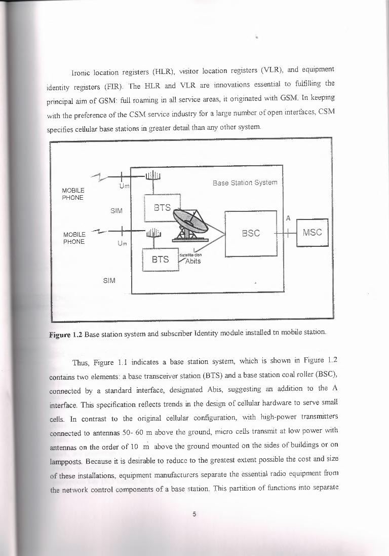
Ironic location registers (HLR), visitor location registers (VLR), and equipment

identity registers (FIR). The HLR and VLR are innovations essential to fulfilling the

principal aim of GSM: full roaming in all service areas, it originated with GSM. In keeping

with the preference of the CSM service industry for a large number of open interfaces, CSM

specifies cellular base stations in greater detail than any other system

Urn I I Base Station System MOBILE PHONE

SIM I i BTS ·-~..,,··"""''"'·---· ..

A

MOBILE -""1,...-- I I illlil.i ~ ')I ~ MSC . SSC PHONE Um

• "'I

srs_fAb;t: I

SIM

Figure 1.2 Base station system and subscriber Identity module installed tn mobile station.

Thus, Figure 1.1 indicates a base station system, which is shown in Figure 1.2

contains two elements: a base transceiver station (BTS) and a base station coal roller (BSC),

connected by a standard interface, designated Abis, suggesting an addition to the A

interface. This specification reflects trends in the design of cellular hardware to serve small

cells. In contrast to the original cellular configuration, with high-power transmitters

connected to antennas 50- 60 m above the ground, micro cells transmit at low power with

antennas on the order of 10 m above the ground mounted on the sides of buildings or on

lampposts. Because it is desirable to reduce to the greatest extent possible the cost and size

of these installations, equipment manufacturers separate the essential radio equipment from

the network control components of a base station. This partition of functions into separate

5

•

pieces of equipment is reflected in the GSM designation of distinct base transceiver stations

(BTS), consisting primarily of radio equipment, and base station: controllers (BSC), that

perform network control operations and signal processing functions, Typically, one BSC

controls several BTS. Another important GSM innovation appears in every mobile, station. GSM specifies

that every terminal contain a subscriber identify module (SIM). The SINI is a removable card

that stores essential subscriber information, including identification numbers, details of the

subscriber's service plan, and abbreviated dialing codes selected by the subscriber.

The SIM is the subscriber's link to a cellular system. By removing the SIM, the

subscriber disables the telephone, with the exception of an ability to vehicle emergency calls.

To change telephones for example, from a portable phone to a vehicle mounted phone the

subscriber simply moves the SIM from one telephone to the other, Using the new phone, the

subscriber retains her own telephone number, her special calling features, and the telephone

directory she has programmed into the SM. This situation differs substantially from the other cellular systems, which store

subscriber information in fixed hardware within a terminal. Thus in AMPS, CDMA, and NA­

TDMA, the telephone unit is part of the subscription. When a person changes telephone

equipment, the service provider gels involved, changing the subscription to reflect tire

identity of the new telephone. A GSM subscription, like a fixed telephone subscription, is

unaffected by the telephone instrument used try a subscriber, GSM specifies two types of

SIM distinguished by their physical characteristics. One is like a credit card and is easily

inserted into or removed from a terminal. The other is much smaller-comparable in size to

a postage stamp-and better suited to compact portable telephones. It is also harder to

insert and remove than the credit card type.

As in the other systems presented in this project, GSM base stations and telephones

store and transmit a variety of identification codes that participate in network operations.

Table 1.1 is a partial list of these codes. Some of the codes, including the IMEI and the class

mark, are properties of the telephone equipment and are stored in the terminal itself Other

codes, including the international mobile subscriber identifier (IMSI) and the secret

encryption key (Ki) belong to the subscriber. These codes are stored in the SIM and can be

6

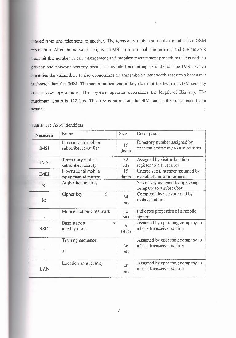
moved from one telephone to another. The temporary mobile subscriber number is a GSM

innovation. After the network assigns a TMSI to a terminal, the terminal and the network

transmit this number in call management and mobility management procedures. This adds to

privacy and network security because it avoids transmitting over the air the IMSI, which

identifies the subscriber. It also economizes on transmission bandwidth resources because it

is shorter than the IMSI. The secret authentication key (ki) is at the heart of GSM security

and privacy opera lions. The system operator determines the length of Ibis key. The

maximum length is 128 bits. This key is stored on the SIM and in the subscriber's home

system.

Table 1.1: GSM Identifiers.

Notation Name Size Description

International mobile 15 Directory number assigned by IMSI subscriber identifier digits operating company to a subscriber

TMSI Temporary mobile 32 Assigned by visitor location subscriber identity bits register to a subscriber

IMEI International mobile 15 Unique serial number assigned by equipment identifier digits manufacturer to a terminal

Ki Authentication key Secret key assigned by operating company to a subscriber

Cipher key 6' 64

Computed by network and by kc bits mobile station

Mobile station class mark 32 Indicates properties of a mobile - bits station

Base station 6 6 Assigned by operating company to

BSIC identity code BITS a base transceiver station

Training sequence Assigned by operating company to 26 a base transceiver station - 26 bits

Location area identity 40 Assigned by operating company to

LAN bits a base transceiver station

7

Terminals and the network use Ki to compute the cipher key, Kc, which protects user

information and network control information from unauthorized interception.

The 32-bit class mark describes the capabilities of a terminal. It has several

components three of which are essential: the revision level is the version of the GSM

standard to which the terminal conforms; the RF power capability indicates the power levels

available to the mobile transmitter, and the encryption algorithm indicates the manner in

which the terminal encrypts user information and network control information. These three

components comprise 8 bits of the class mark. In many network control procedures. only

this part of the class mark is transmitted. The remainder of the class mark indicates the frequency capability of the terminal

and whether the terminal is capable of operating a short message service. The base station

identity code and the training sequence serve the same purposes as the supervisory audio

tone in AMPS and the digital verification color code in NA-TDMA. They help a terminal

verify that it receives information from the correct base station rather than another base

station using the same physical channel. The base station uses these codes in the same

manner to verify that the received signal comes from the correct terminal. The location area

identity (LAI)has three components. A mobile country code and a mobile network code are

like the system identifier in North America. Together they identify the network to which a

cell belongs. The third component of the LAI is the location area code, which controls

mobility management operations.

1.3 Radio Transmission

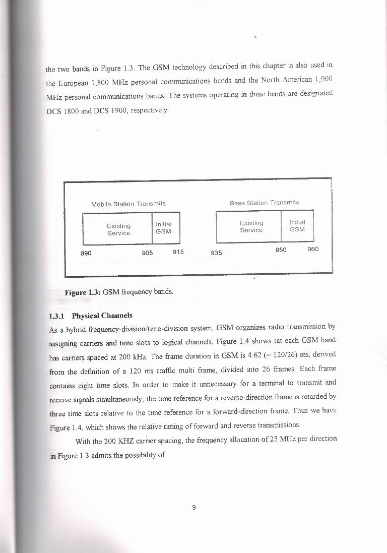
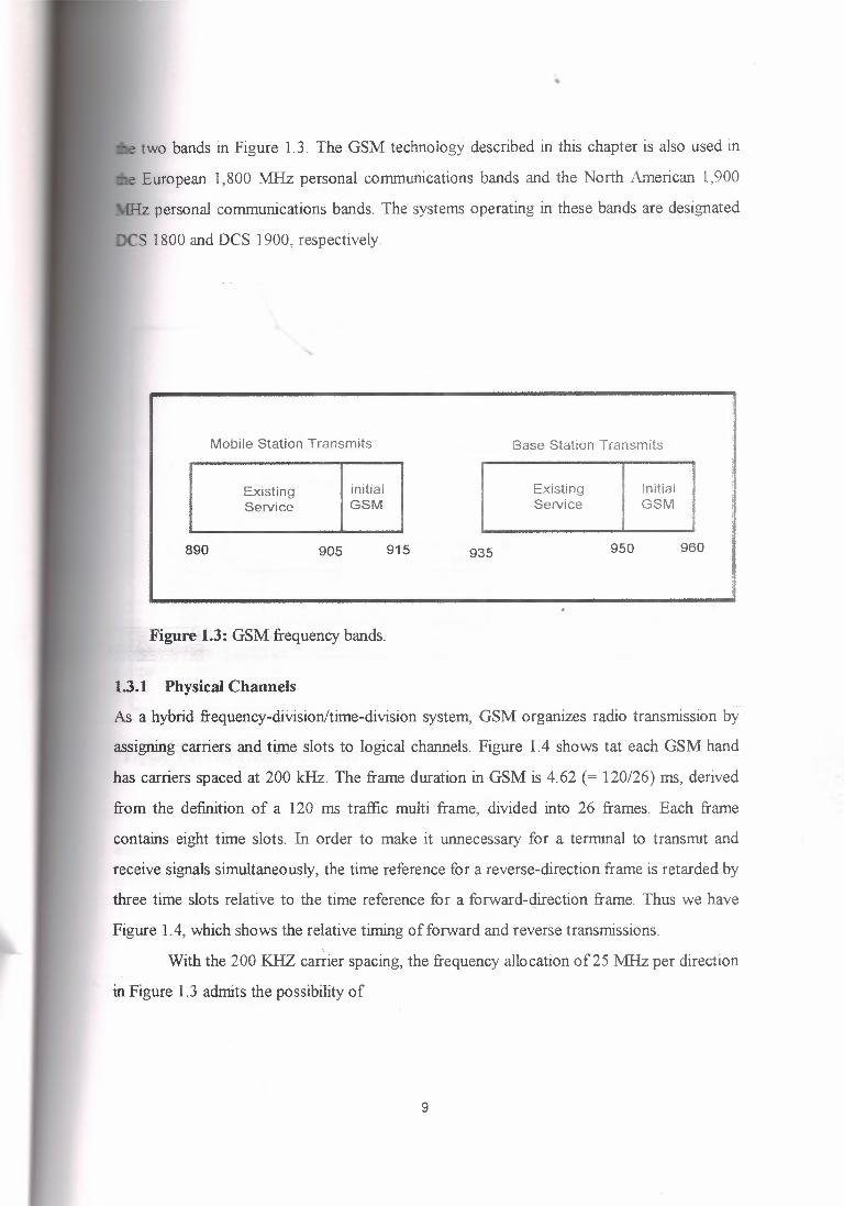
Figure 1.3 shows the GSM spectrum allocation. As in AMPS, there are two 25 Mlfz

bands separated by 45 MHz, with the lower hand used for transmissions from terminals to

base stations and the tipper band for transmissions from base stations to terminals. In some

countries, analog cellular systems occupy the lower 15 .MHz of each band. In these

countries, initial GSM systems operate in the upper 10 Mlfz. As the demand for GSM

grows, GSM channels gradually displace analog channels at the lower carrier frequencies.

Eventually, analog operations will be discontinued and GSM systems will completely occupy

8

•

the two bands in Figure 1.3. The GSM technology described in this chapter is also used in

the European 1,800 MHz personal communications bands and the North American 1,900

MHz personal communications bands. The systems operating in these bands are designated

DCS 1800 and DCS 1900, respectively.

Mobile Station Transmits Base Station Transmits

Existing Service

initial GSM

Existing Service

Initial GSM

890 905 915 950 960 935

Figure 1.3: GSM frequency bands.

1.3.1 Physical Channels

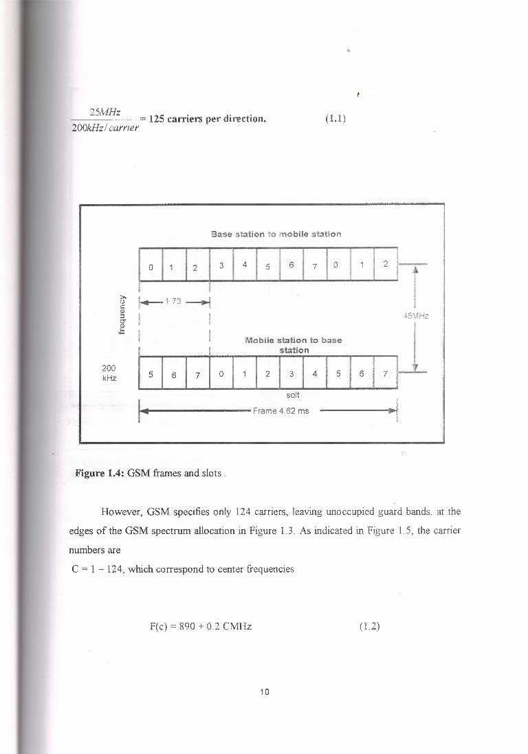
As a hybrid frequency-division/time-division system, GSM organizes radio transmission by.

assigning carriers and time slots to logical channels. Figure 1.4 shows tat each GSM hand

has carriers spaced at 200 kHz. The frame duration in GSM is 4.62 (= 120/26) ms, derived

from the definition of a 120 ms traffic multi frame, divided into 26 frames. Each frame

contains eight time slots. In order to make it unnecessary for a terminal to transmit and

receive signals simultaneously, the time reference for a reverse-direction frame is retarded by

three time slots relative to the time reference for a forward-direction frame. Thus we have

Figure 1.4, which shows the relative timing of forward and reverse transmissions. ' With the 200 KHZ carrier spacing, the frequency allocation of 25 MHz per direction

in Figure 1.3 admits the possibility of

9

two bands in Figure 1.3. The GSM technology described in this chapter is also used in

European 1,800 :MHz personal communications bands and the North American 1,900

lliz personal communications bands. The systems operating in these bands are designated

CS 1800 and DCS 1900, respectively.

Mobile Station Transmits Base Station Transmits

Existing Service

initial GSM

Existing Service

Initial GSM

890 950 960 915 905 935

Figure 1.3: GSM frequency bands.

1.3.1 Physical Channels

As a hybrid frequency-division/time-division system, GSM organizes radio transmission by

assigning carriers and time slots to .logical channels. Figure 1.4 shows tat each GSM hand

has carriers spaced at 200 kHz. The frame duration in GSM is 4.62 (= 120/26) ms, derived

from the definition of a 120 ms traffic multi frame, divided into 26 frames. Each frame

contains eight time slots. In order to make it unnecessary for a terminal to transmit and

receive signals simultaneously, the time reference for a reverse-direction frame is retarded by

three time slots relative to the time reference for a forward-direction frame. Thus we have

Figure 1.4, which shows the relative timing of forward and reverse transmissions. ' With the 200 KHZ carrier spacing, the frequency allocation of 25 :MHz per direction

in Figure 1.3 admits the possibility of

9

•

25MHz 200kHz I carrier= 125 carriers per direction. (1.1)

Base station to mobile station

1011 i213141sl617IO 1, 12

!..- 1. 73 --.j I 1 4"MH 1 f '._, Z

i 5 I 6 I 7 i O , ,M,·;:· 1:l: T: I 6 I 7 ~ solt

14 Frame 4.62 ms

200 kHz

Figure 1.4: GSM frames and slots .

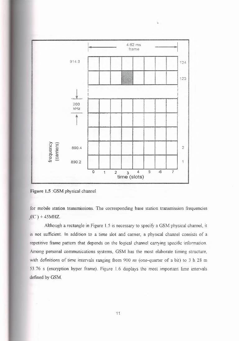
However, GSM specifies only 124 carriers, leaving unoccupied guard bands. at the

edges of the GSM spectrum allocation in Figure 1. 3. As indicated in Figure 1. 5, the carrier

numbers are

C = 1 - 124, which correspond to center frequencies

F(c) = 890 + 0.2 CMHz (1.2)

10

•

914.8

J_ 200 kHz

>, - () (/) C s... (I) .!:!2 :::, l:::::: O" (1:l (I) () I... - -

890.4

890.2

4.62 ms frame 1

124

123 '

i 2

1

0 2 3 4 5 time (slots)

7

Figure 1.5 :GSM physical channel

f(C) + 451\ffiZ. for mobile station transmissions. The corresponding base station transmission frequencies

Although a rectangle in Figure 1. 5 is necessary to specify a GSM physical channel, it

is not sufficient. In addition to a time slot and carrier, a physical channel consists of a

repetitive frame pattern that depends on the logical channel carrying specific information.

Among personal communications systems, GSM has the most elaborate timing structure,

with definitions of time intervals ranging from 900 ns (one-quarter of a bit) to 3 h 28 m

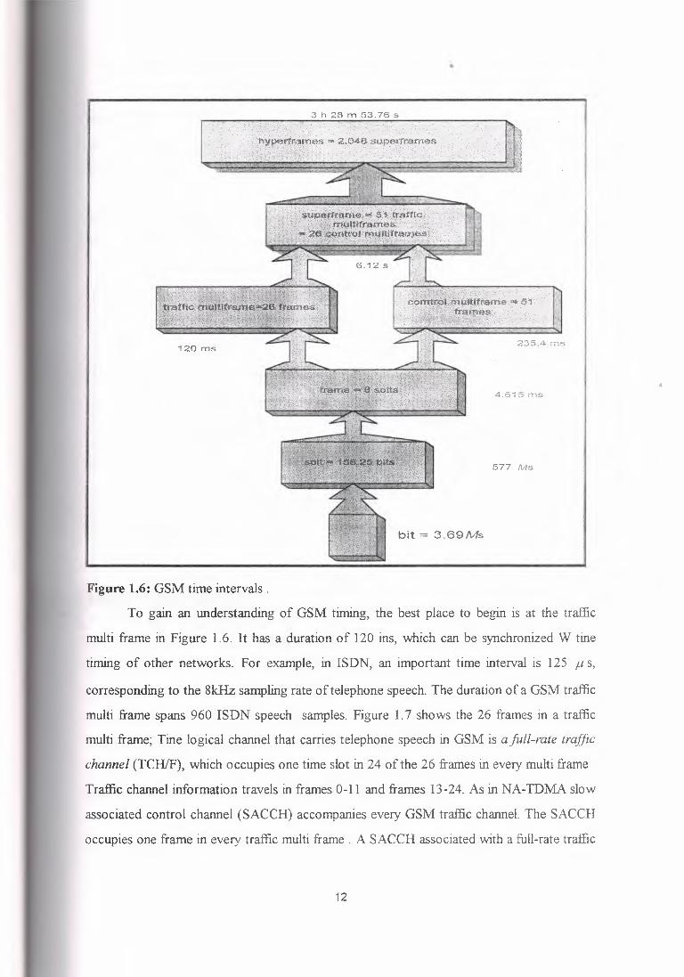
53.76 s (encryption hyper frame). Figure 1.6 displays the most important lime intervals

defined by GSM.

11

•

120 ms

4

4.615 ms

577 ii/ls

bit= 3.69Ms

Figure 1.6: GSM time intervals.

To gain an understanding of GSM timing, the best place to begin is at the traffic

multi frame in Figure 1.6. It has a duration of 120 ins, which can be synchronized W tine

timing of other networks. For example, in ISDN, an important time interval is 125 µ s,

corresponding to the 8kHz sampling rate of telephone speech. The duration of a GSM traffic

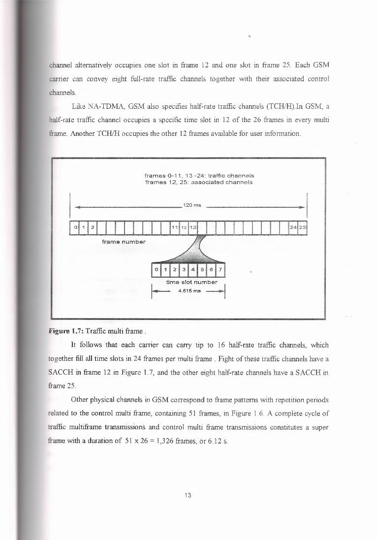
multi frame spans 960 ISDN speech samples. Figure 1. 7 shows the 26 frames in a traffic

multi frame; Tine logical channel that carries telephone speech in GSM is a full-rate traffic

channel (TCHIF), which occupies one time slot in 24 of the 26 frames in every multi frame .

Traffic channel information travels in frames 0-11 and frames 13-24. As in NA-TDMA slow

associated control channel (SACCH) accompanies every GSM traffic channel. The SACCH

occupies one frame in every traffic multi frame . A SACCH associated with a full-rate traffic

12

•

channel alternatively occupies one slot in frame 12 and one slot in frame 25. Each GSM

earner can convey eight full-rate traffic channels together with their associated control

channels.

Like NA-TDMA, GSM also specifies half-rate traffic channels (TCH/H).In GSM, a

half-rate traffic channel occupies a specific time slot in 12 of the 26 frames in every multi

frame. Another TCH/H occupies the other 12 frames available for user information.

frames 0-11, 13 -24: traffic channels frames 12, 25: associated channels

frame number

Lme slot num~ r--- 4.615 ms -1

Figure 1.7: Traffic multi frame.

It follows that each carrier can carry tip to 16 half-rate traffic channels, which

together fill all time slots in 24 frames per multi frame . Fight of these traffic channels have a

SACCH in frame 12 in Figure 1. 7, and the other eight half-rate channels have a SACCH in

frame 25.

Other physical channels in GSM correspond to frame patterns with repetition periods

related to the control multi frame, containing 51 frames, in Figure 1. 6. A complete cycle of

traffic multiframe transmissions and control multi frame transmissions constitutes a super

frame with a duration of 51 x 26 = 1,326 frames, or 6 .12 s.

13

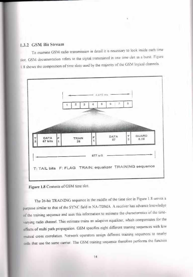
l.3.2 GSM Bit Stream To examine GSM radio transmission in detail it is necessary to look inside each time

slot. GSM documentation refers to the signal transmitted in one time slot as a burst. Figure

1.8 shows the composition of time slots used by the majority of the GSM logical channels.

4.615 ms

1 2 s I 7 I

8

T 3

DATA IF 67 bits 1

F 1

DATA 67

T 3

GUARD 8.26 TRAIN

26

677MS

T: TAIL bits F: FLAG TRAIN: equalizer TRAINING sequence

Figure 1.8 Contents of GSM time slot.

The 26-bit TRAINING sequence in the middle of the time slot in Figure 1.8 serves a

purpose similar to that of the SYNC field in NA-TDMA. A receiver has advance knowledge

of the training sequence and uses this information to estimate the characteristics of the time­

varying radio channel. This estimate trains an adaptive equalizer, which compensates for the

effects of multi path propagation. GSM specifies eight different training sequences with low

mutual cross correlation. Network operators assign different training sequences to nearby

cells that use the same carrier. The GSM training sequence therefore performs the function

14

of the AMPS Supervisory Audio Tone (SAT) and the NA-TDMA digital verification color

code (DVCC). It enables terminals and base stations to confirm that the received signal

conies from [lie correct transmitter and not a strong interfering transmitter.

The two DATA fields carry either user information or network control information.

Each of these fields is accompanied by a 1-bit FLAG and 3 TAIL bits. The FLAG indicates

whether the DATA field contains user information or network control information. The

TAIL bits, all set to 0, can be used to enhance equalizer performance. There is also a guard

time of 30.5 µ s (corresponding to 8.25 bits) when no information is transmitted. The guard

time includes ramp time for the transmitter to tum off at the end of one time slot and tum on

at the beginning of [lie next slot. It also prevents signals assigned to adjacent time slots from

arriving simultaneously at a base station receiver.

Figure 1.8 contains a total of 156.25 bits, which implies that the GSM

transmission rate is

26frames I multiframe x 8 slots /frame x 156.25 b/slot = l20ms I muliframe

270.833 .!_ kb/s 3

(1.3)

This transmission tale corresponds to a hit duration of 1 /0.270833t 3.69 µ s. GSM

specifies that each receiver be capable of equalizing signals that arrive over multiple

propagation paths with delay differences as high as 16 bits. This delay spread corresponds to

more than four bit periods. To unscramble the inter symbol interference caused by this large

spread, an adaptive equalizer is an essential component of every GSM receiver.

The modulation scheme in GSM is Gauss Ian minimum shift keying (GMSK), a form

of frequency shift keying (FSK). A GMSK modulator per- forms signal processing

operations to reduce (lie bandwidth occupied by an FSK signal. The principal operation is

linear filtering, with a Gaussian transfer function. The filter confines the modulated signal to '

the 200 kHz band allocated to cacti carrier, Thus the modulation efficiency of GSM is

270.833kb Is = 1.35b / s I Hz 200kHz

(1.4)

15

•

significantly higher than A.MIPS frequency shift keying with modulation efficiency 0.33

0.33b/s/Hz. (10 kb/s I 30kHz). However, it is lower than the modulation efficiency of NA­

TDMA (1,62 b/s/ Hz). In exchange for this lower modulation efficiency, GMSK has the

advantage of a constant signal envelope, which reduces the drain on the battery of a portable

telephone, relative to the NA-TDMA modulation scheme. The GMSK signal is also more

robust in [lie presence of channel impairments than its NA-TD MA counterpart.

Note that in contrast to NA-TDl\ilA , GSM has only one time-slot configuration for

transmission of riser information. Both base stations ;and mobile stations use this

configuration. Thus, a GSM base station turns off its transmitter at the end of each time slot.

When it has information to send to another terminal in the next time slot, the base station

resumes transmitting after a pause of 30. 5 µ s. Recall that NA-TDMA base stations transmit

continuously even if only a fraction of the time slots per frantic are assigner! to

conversations or digital control channels. In GSM, the base stations turns off its transmitter

in unassigned time slots. This has the effect of reducing interference to signals in nearby

cells using the same carrier. It is also essential when the system employs slow frequency

hopping.

1.3.3 Slow Frequency Flopping

GSM has two definitions of radio carriers. One is the conventional definition of a

sine wave at a single frequency (among the 124 carriers in the GSM band). Jim other

definition of a radio carrier is a frequency hopping pattern, consisting of a repetitive

sequence of frequencies occupied by a signal. When the radio carrier is a frequency hopping

pattern, the signal moves from one frequency to another in every frame. The purpose of

frequency hopping is to reduce the vulnerability of GSM signals to transmission

impairments. Without frequency hopping, the entire signal is subject to distortion whenever

the assigned carrier is impaired. When the distortion is severe and sustained, an error­

correcting code is incapable of recovering the transmitted hit stream. Many impairments are

frequency dependent. When a transmitter employs frequency hopping, it is likely that the

16

signal will encounter these impairments for only a fraction of the time (when it hops to a

frequency with a poor propagation path or high interference). In this situation, it is possible

that error-correcting codes applied to GSM signals will mitigate the sporadic effects of the

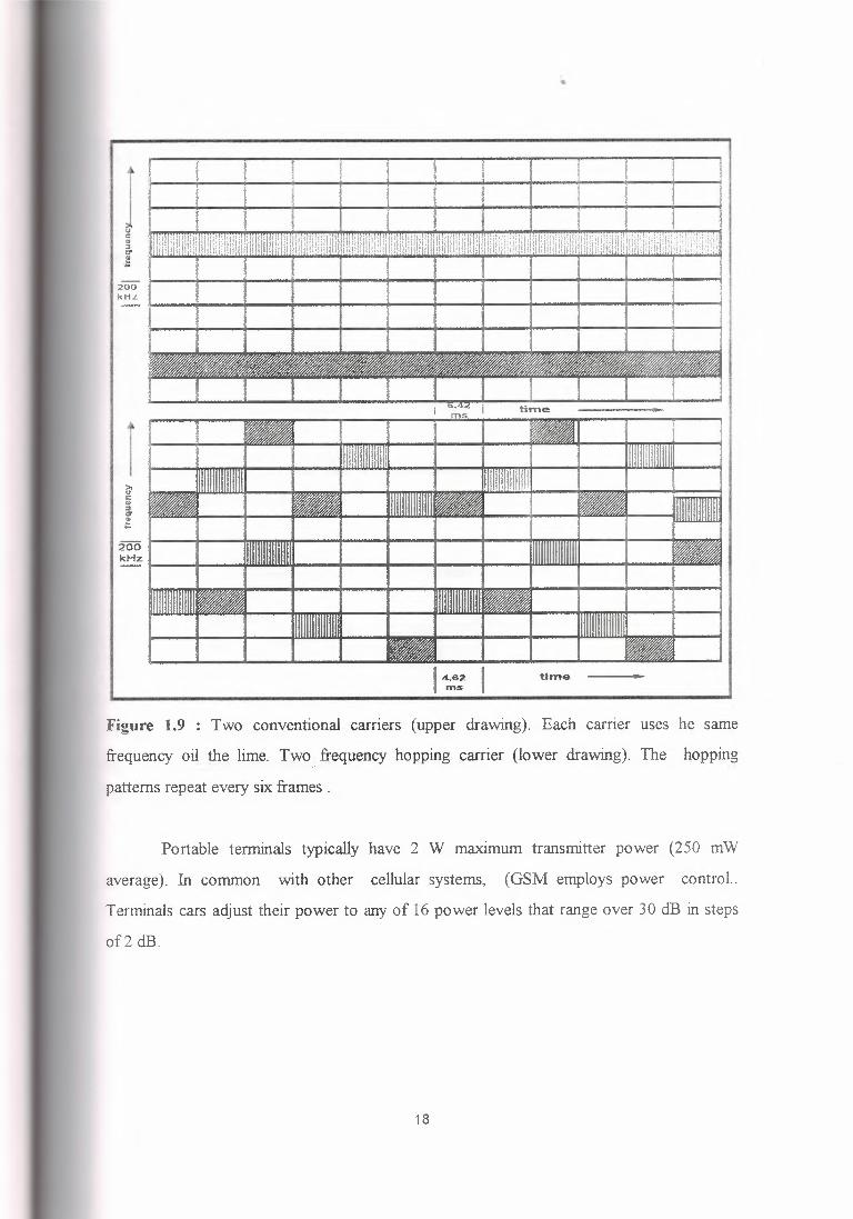
transmission impairments .Figure 1.9 shows, as a function of time, the frequency bands

occupied by two convention carriers and two frequency hopping carriers.

Frequency hopping can also reduce harmful effects of co-haoticl interference

between signals in nearby cells. The interference in a conversation depends on the location

of a mobile phone in another cell using the same carrier. If a network operator assigns

different hopping patterns to different cells, two mobile phones that are in vulnerable

positions with respect to one another will use the same carrier frequency for only a fraction

of the time. With only part of a signal subject to interference, error-correcting codes have a

chance of overcoming the effects of the interference. All GSM terminals are capable of frequency hopping. Network operators decide

whether the introduce frequency hopping, and if so, which patterns to use. To avoid

interference with one another, all of the signals in a cell have to hop in a coordinated

manner, so that two of theta do nut use the same frequency simu,ltaneously. Moreover, to

reduce the effects of interference from other cells, as described in the previous paragraph,

the hopping patterns in a group of cells have to be coordinated with one another. Frequency

hopping thus adds a new dimensions of complexly to cellular reuse planning.

1.3.4 Radiated Power

GSM specifies five classes of mobile stations distinguished by maximum transmitter

power, ranging from 20W (43 dBm) to 0.8 W (29 dBm). When a terminal _transmits in a

full-rate channel, the transmitter is active during only one time slot per frame ( one-eighth of

the time). This implies that the average radiated power is lower than the maximum in by a

factor of eight (9 dB). Typically, the maximum power capability of vehicle-muonted

terminals is 8 W (I W average).

17

200 kHz

i 200 kHz I I I

Figure 1.9 : Two conventional carriers (upper drawing). Each carrier uses he same

frequency oil the lime. Two_ frequency hopping carrier (lower drawing). The hopping

patterns repeat every six frames .

Portable terminals typically have 2 W maximum transmitter power (250 mW

average). In common with other cellular systems, (GSM employs power control..

Terminals cars adjust their power to any of 16 power levels that range over 30 dB in steps

of2 dB.

18

•

1.3.5 Spectrum Efficiency

the GMSK modulation technique, combined with error-correcting codes and

adaptive equalization, makes GSM less vulnerable than NA-TDMA to interference. The

system can meet signal-quality objectives with a signal interference ratio as low as 7 dB

[Mouly and Paulct, 1992]. This allows networks to operate with a reuse factor ofN=3 or

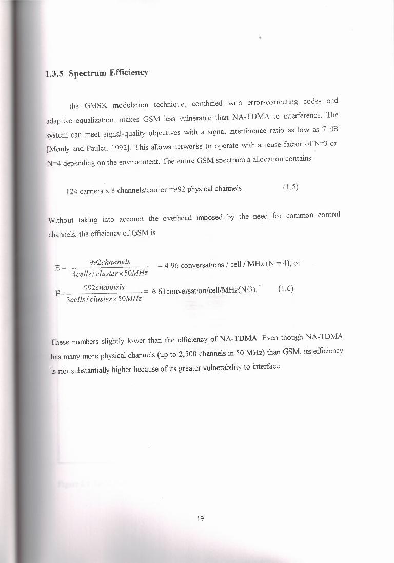
N=4 depending on the environment. The entire GSM spectrum a allocation contains:

124 carriers x 8 channels/ carrier =992 physical channels. ( 1. 5)

Without taking into account the overhead imposed by the need for common control

channels, the efficiency of GSM is

E= 992channels = 4.96 conversations I cell/ MHz (N = 4), or

4cells I clusterx 50MHz

E= 992channels 3cells I clusterx 50MHz = 6.6lconversation/cell/MHz(N/3).. (1.6)

These numbers slightly lower than the efficiency of NA-TDMA. Even though NA-TDMA

has many more physical channels (up to 2,500 channels in 50 MHz) than GSM, its efficiency

is riot substantially higher because of its greater vulnerability to interface.

19

•

CHAPTER2

LOGICAL CHANNELS

2.1 Introduction

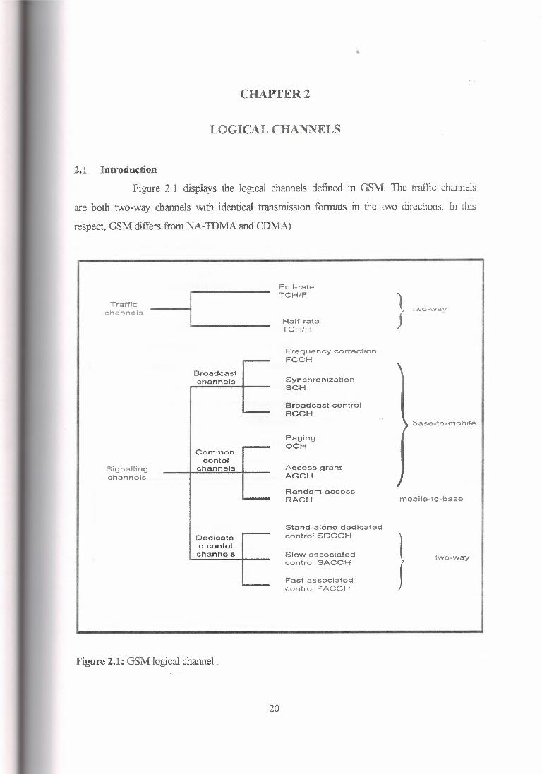
Figure 2.1 displays the logical channels defined in GSM. The traffic channels

are both two-way channels with identical transmission formats in the two directions. In this

respect, GSM differs from NA-IDMA and CDMA).

Traffic channels

Signalling channels

Broadcast channels

- ---- Common

contol channels

Dedicate d contol channels

Full-rate TCH/F

} ,wo-way Half-rate TCH/H

Frequency correction FCCH

Synchronization SCH

Broadcast control BCCH

base-to-mobile

Paging OCH

Access grant AGCH

Random access RACH mobile-to-base

Stand-alone dedicated control SOCCH

Slow associated control SACCH

two-way

Fast associated control FACCH

Figure 2.1: GSM logical channel.

20

•

In both of those systems, the multiplexing scheme on the forward traffic channel

differs from the multiplexing scheme on the reverse traffic channel. There are three

categories of control channels (in GSM terminology, they are together referred to as

signaling channels). A base station uses broadcast channels to transmit the same

information to all terminals in a cell. The common control channels carry information to

and from specific terminals. However, they use physical channels that are available to all

of the terminals in a cell.

The dedicated control channels use physical channels that are assigned to specific

terminals. The following paragraphs describe the GSM logical channels individually.

2.2 Broadcast Channels and Common Control Channels

Together the broadcast and common control channels serve the same purposes as

the digital control channel in NA-TDMA and the pilot, sync, paging, arid access channels

in CDMA. They make it possible for a terminal without a call in progress to synchronize

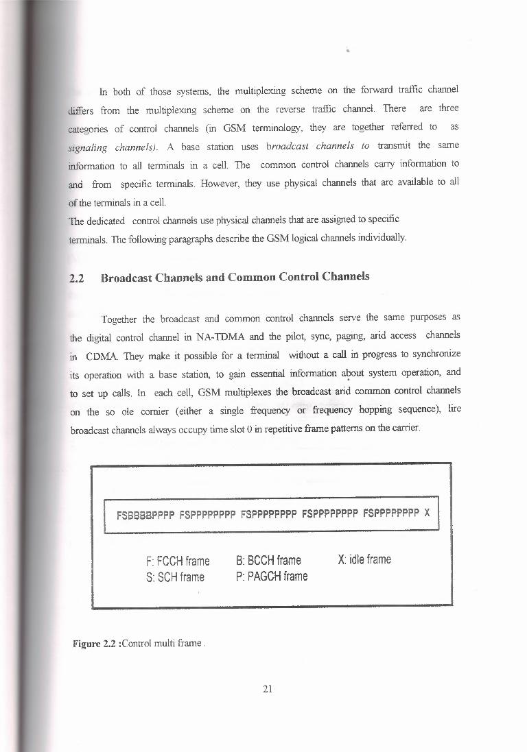
its operation with a base station, to gain essential information about system operation, and . to set up calls. In each cell GSM multiplexes the broadcast arid common control channels

on the so ale cornier ( either a single frequency or frequency hopping sequence), lire

broadcast channels always occupy time slot O in repetitive frame patterns on the carrier.

FS8888PPPP FSPPPPPPPP FSPPPPPPPP FSPPPPPPPP FSPPPPPPPP X

F: FCCH frame S: SCH frame

B: BCCH frame P: PAGCH frame

X: idle frame

Figure 2.2 :Control multi frame .

21

The common control channels also occupy time slot and if they need more capacity than

time slot O can provide they need, they can occupy time slots 2.4, or .6 or the same carrier.

The frames occupied by each channel are specified with respect to their positions

,within the 51 frame control multi frame in figure 1.6. figure 2.2 shows the contents of time

slot O in each of the 51 frames . in each multiframe there are five groups of frames, each

containing ten frames beginning with a frequency correction frame and a synchronization

frame. At the beginning of the multiframe, four broadcast control frames follow the FCCH

and SCH. With the exception of one idle frame at the end of the multi frame, all of the

remairnng frames carry and access grant information, referred to together as P AGCH

[Mouly and Paul, 1992] in figure 2. 2 .

The pattern illustrated in figure 2.2 applies to time slot O in one carrier in the

forward direction. In the reverse direction, time slot O of the corresponding carrier is

assigned to a random access channel in all 51 frames of the multiframe. All of the

terminals in a cell without a call in progress share this channel on a contention basis. The

other seven time slots on this carrier is independent of the one dedicated to control

channels. Typically, they carry traffic channels or stand done-alone dedicated control

channels. However, the even-numbered slots can also be used for common control channels

if the number of control message in a cell exceeds the capacity of a single physical channel.

2.3 Frequency Correction Channel (FCCH)

On beginning its operation in a cell, a terminal without a cell progress searches for

a frequency-correction channel. The FCCH is one of logical channels with a time-slot

structure that deviates from that shown in figure 1.8. instead of the DATA fields,

TRAINING fields, FLAG bits, and TAIL bits of figure 1.8. the FCCH simply transmits

148s. this causes the GMSK modulator to emit a constant sine wave, each terminal adjusts

its frequency reference to match that of the base station. The FCCH always occupies time

slot O in a frame of eight time slots. After a terminal detects

22

•

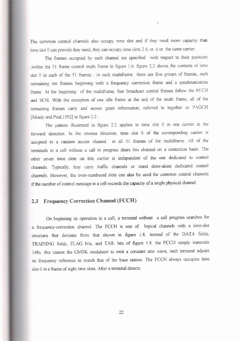
T:Tail bits

Figure 2.3 : Time-slot structure for the synchronization channel

the distinctive sine wave of an FCCH, it can keep of the number( between 1 and 7) of each

successive time slot. After finding an FCCH, a terminal obtains timing information.from a

synchronization channel that arrives eight slots after the arrival of the FCCH sine wave

2.4 Synchronization Channel (SCH)

A base station transmits SCH information in time slot O of every frame that

follows a frame containing FCCH. The SCH also has its own slof structure , shown in

figure 2.4 , that deviates from the one shown in figure 1.8. To help terminals synchronize

their operation to a new base station, the SCH containing a long TRAINING sequence ( 64

bits) that is the same in all cells. The DATA fields in the SCH containing the base station

identity code (BSIC) (see Table 1.1) and the present frame number. The frame number is

the position of the current frame within the 3.5 hour GSM hyper frame (Figure 1.6). The

hyper frame is a sequence of 2,048 x 26 x 51 = 2,715,648 frames.

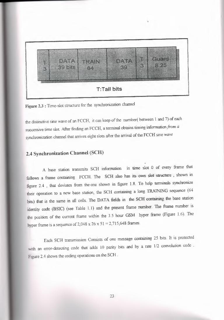
Each SCH transmission Consists of one message containing 25 bits. It is protected

with an error-detecting code that adds 10 parity bits and by a rate 1/2 convolution code .

Figure 2.4 shows the coding operations on the SCH .

23

•

data' fields

4 tail bits

Figure 2.4 coding on the SCH.

i84 bits

4 times slots

4 tail bits

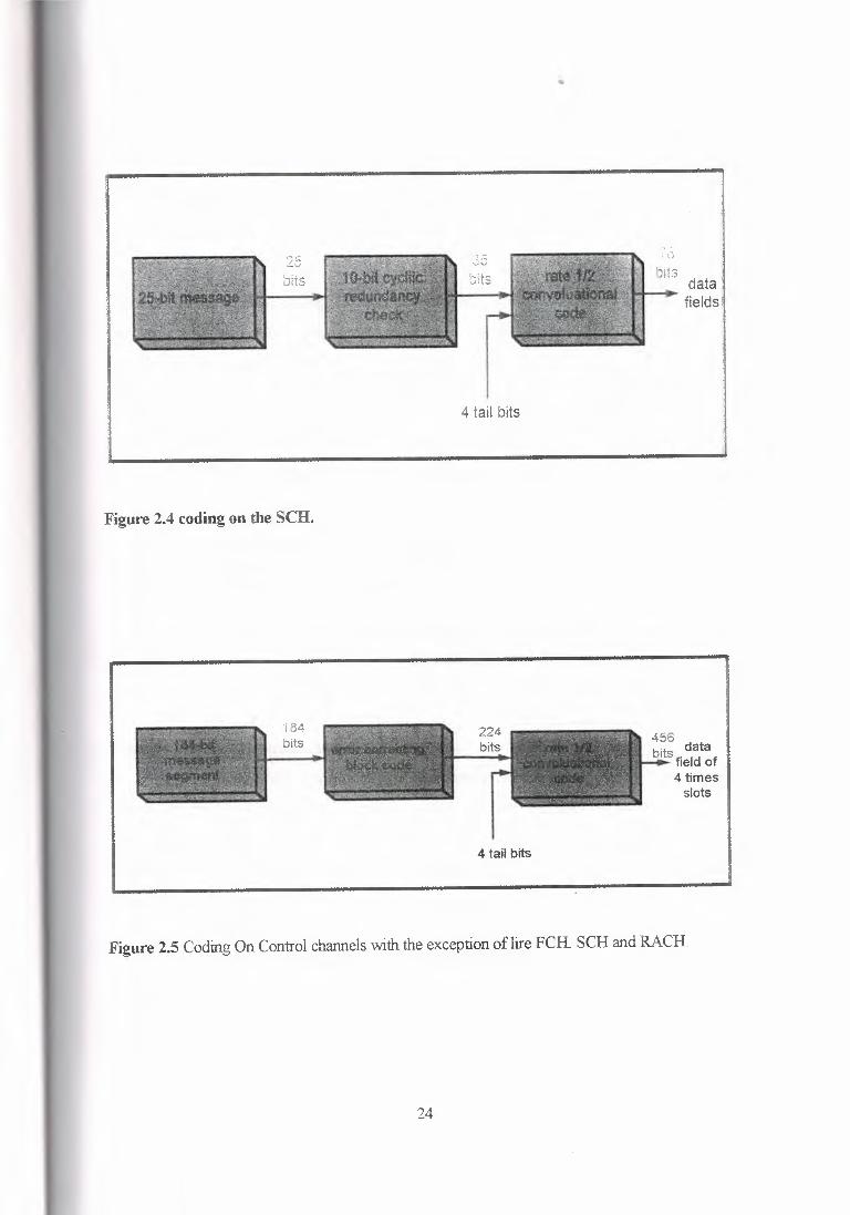
Figure 2.5 Coding On Control channels with the exception oflire FCH SCH and RACH.

24

•

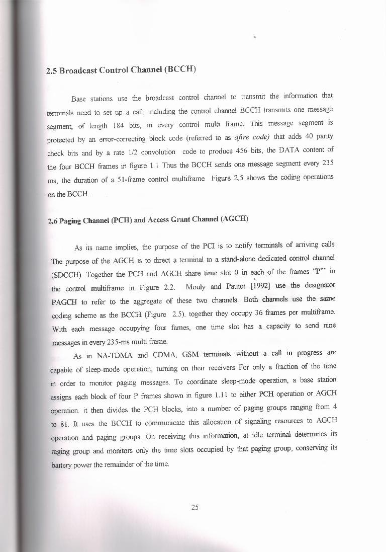
2.5 Broadcast Control Channel (BCCH)

Base stations use the broadcast control channel to transmit the information that

terminals need to set up a call, including the control channel BCCH transmits one message

segment, of length 184 bits, in every control multi frame. This message segment is

protected by an error-correcting block code (referred to as a.fire code) that adds 40 parity

check bits and by a rate 1/2 convolution code to produce 456 bits, the DATA content of

the four BCCH frames in figure 1.1 Thus the BCCH sends one message segment every 235

ms, the duration of a 51-frame control multiframe Figure 2.5 shows the coding operations

- on the BCCH .

2.6 Paging Channel (PCB) and Access Grant Channel (AGCH)

As its name implies, the purpose of the PCI is to notify terminals of arriving calls

The purpose of the AGCH is to direct a terminal to a stand-alone dedicated control channel

(SDCCH). Together the PCH and AGCH share time slot O in each of the frames "P"' in •

the control multiframe in Figure 2.2. Mouly and Pautet [1992] use the designator

PAGCH to refer to the aggregate of these two channels. Both channels use the same

coding scheme as the BCCH (Figure 2.5). together they occupy 36 frames per multiframe.

With each message occupying four fames, one time slot has a capacity to send nine

messages in every 235-rns multi frame. As in NA-TDMA and CDMA, GSM terminals without a call in progress are

capable of sleep-mode operation, turning on their receivers For only a fraction of the time

in order to monitor paging messages. To coordinate sleep-mode operation, a base station

assigns each block of four P frames shown in figure 1.11 to either PCH operation or AGCH

operation. it then divides the PCH blocks, into a number of paging groups ranging from 4

to 81. It uses the BCCH to communicate this allocation of signaling resources to AGCH

operation and paging groups. On receiving this information, at idle terminal determines its

raging group and monitors only the time slots occupied by that paging group, conserving its

battery power the remainder of the time.

25

•

2.7 Random Access Channel (RACH)

Terminals without a call in progress use this channel to initiate signaling dialogs

with the remainder of the system. GSM terminals send messages on the random access

channel to originate phone calls, initiate transmissions of short messages, respond to paging

messages, and register their locations. As in the counterparts to the RACH found in the

other systems described in this project, disperse terminals contend in an uncoordinated

manner for access to the RACH However, in GSM the contention is simpler than in other

systems and the information transmitted on the RACH is far more restricted. A RACH

occupies all of the reverse direction time slots of a common control channel ( one slot in

each frame of the 51-frame control Terminals with information to transmit use the slotted

ALOHA protocol [Tannenbaum, 1.988, Section 3.2] to gain access to these time slots.

A terminal with information to transmit simply chooses a time slot, transmits a

message, and waits for an acknowledgment. An acknowledgment contains, in place of

address, the total number in which the uplink message arrived, and a 5-bit code word

transmitted in. the RACH message. The acknowledgment directs the terminal to a stand­

alone dedicated control channel (SDCCH) to be used for further signaling messages

transmitted between the terminal and the base station. A terminal, after transmitting a

RACH message, waits for a fixed · time interval for an acknowledgment. If no

acknowledgment arrives, the terminal transmits another RACH message, and repeats the

procedure until it reaches a maximum number of attempts as specified by a message on the

BCCH. Transmissions on the RACH use shortened of a duration of 87-bit periods, to ensure

that they are confined to the boundaries of a single lime slot when they arrive at the base

station. Figure 1.15, which shows the time-slot structure of the RACH, indicates that the

guard time is 69.25 bits.

256 µs sufficient to allow transmissions from all parts of a cell to arrive within the

577 µs duration (156.25 bit periods) of a time slot. On observing the time of arrival of the

RACH message, a base station determines the correct timing (or subsequent transmissions

26

•

from the terminal and sends this "timing advance" information to the terminal in the

channel assignment message.

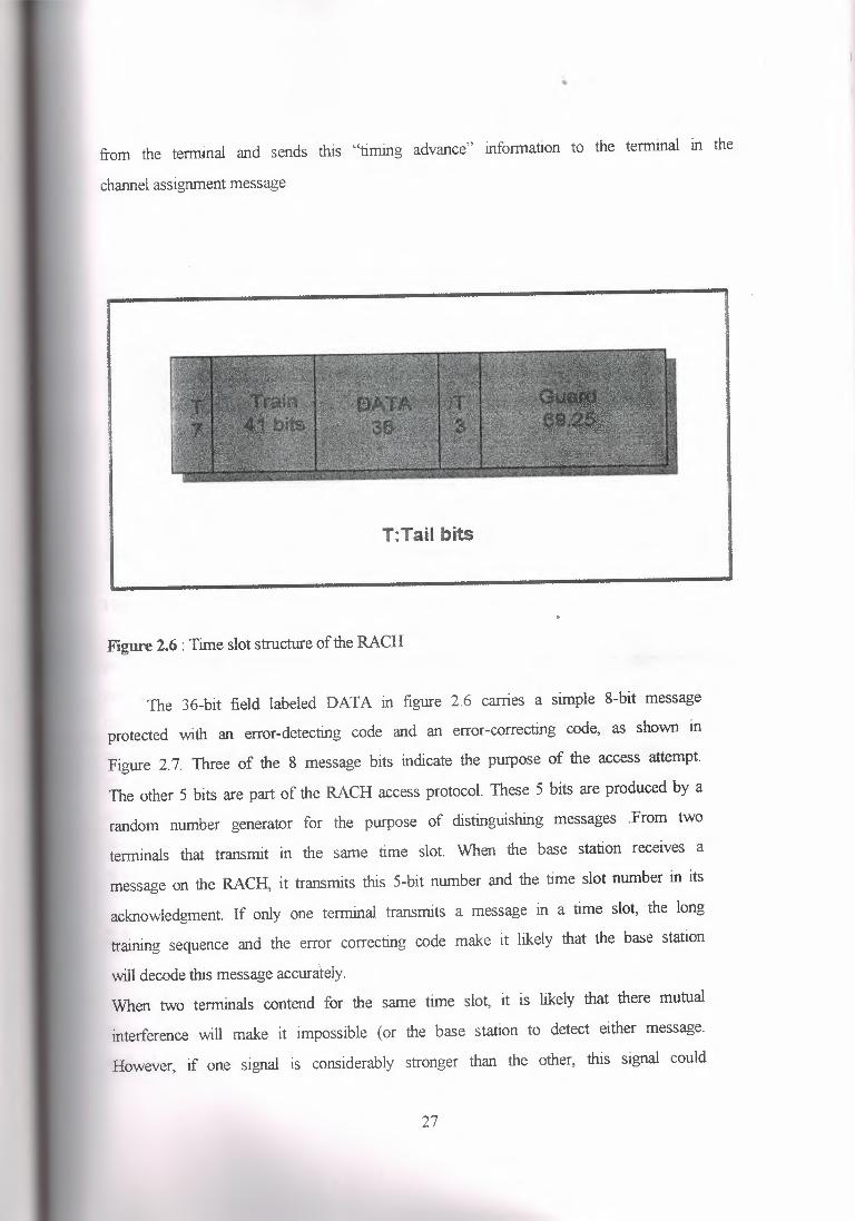
T:Tail bits

Figure 2.6: Time slot structure of the RACH

The 36-bit field labeled DATA in figure 2.6 carries a simple 8-bit message

protected with an error-detecting code and an error-correcting code, as shown in

Figure 2. 7. Three of the 8 message bits indicate the purpose of the access attempt.

The other 5 bits are part of the RACH access protocol. These 5 bits are produced by a

random number generator for the purpose of distinguishing messages .From two

terminals that transmit in the same time slot. When the base station receives a

message on the RACH, it transmits this 5-bit number and the time slot number in its

acknowledgment. If only one terminal transmits a message in a time slot, the long

training sequence and the error correcting code make it likely that the base station

will decode this message accurately.

When two terminals contend for the same time slot, it is likely that there mutual

interference will make it impossible ( or the base station to detect either message.

However, if one signal is considerably stronger than the other, this signal could

27

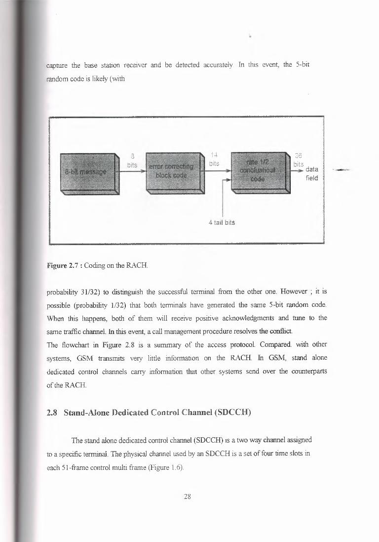
capture the base station receiver and be detected accurately. In this event, the 5-bit

random code is likely ( with

4 tail bits

Figure 2. 7 : Coding on the RACH

probability 31/32) to distinguish the successful terminal from the other one. However ; it is

possible (probability 1/32) that both terminals have generated the same 5-bit random code.

When this happens, both of them will receive positive acknowledgments and tune to the

same traffic channel. In this event, a call management procedure resolves the conflict.

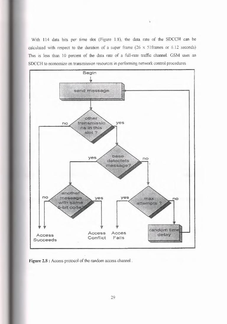
The flowchart · in Figure 2. 8 is a summary of the access protocol. Compared with other

systems, GSM transmits very little information on the RACH In GSM, stand alone

dedicated control channels carry information that other systems send over the counterparts

of the RACH

2.8 Stand-Alone Dedicated Control Channel (SDCCH)

The stand alone dedicated control channel (SDCCH) is a two way channel assigned

to a specific terminal. The physical channel used by an SDCCH is a set of four time slots in

each 51-frame control multi frame (Figure 1.6).

28

•

With 114 data bits per time slot (Figure 1.8), the data rate of the SDCCH can be

calculated with respect to the duration of a super frame (26 x 5lframes or 6.12 seconds)

This is less than 10 percent of the data rate of a full-rate traffic channel. GSM uses an

SDCCH to economize on transmission resources in performing network control procedures

Begin

yes

Access Succeeds

Access Conflict

Acces Fails

Figure 2.8 : Access protocol of the random access channel .

29

•

, including mobility management and call managementl that do not require a high average

data rate , The SDCCH is an efficient alternative to using a RACH or a traffic channel to

perform network control. The RACH is inefficient due to the contention that takes place in

the access protocol. A traffic channel has a data rate that is higher than necessary for the

control procedures. We have observed that in contrast to the other systems presented in this

book, not much network control information moves on the RACH in GSM. To transfer all

the information necessary to set up a call, GSM assigns a terminal 10 a SDCCH. After

performing the necessary transfer of network control information, the system commands

the terminal to move to a traffic channel.

Like traffic channels , each SDCCH has a slow associated control channel . In the case

of the SDCCH, the SACCH occupies an average of two time slots per control multi frame.

Therefore, its bit rate is one half that of the SDCCH (which occupies four time slots per

multi frame), or approximately 969 bis, which is about 2 percent higher than the bit rate of

a SACCH associated with a traffic channel (which is 950 b/s). Channel coding on the

SDCCH conforms to Figure 2. 5.

2.9 Traffic Channels (TCH)

GSM defines two traffic channels. a full rate channel (TCH I F) occupies 24 time

slots in every 26-fRAME traffic multi frame. A half rate channel (TCH/F) occupies 12

time slots in every multi frame. Both traffic channels use the time slot structure of Figure

1. 8 with 114 data bits. Therefore the bit rate of a full rate traffic channel is 22. 8b/s .

The bit rate of a half rate traffic channel is, as the name imp lies, half of this, or 11, 40 b/s.

2.10 Speech Coding andInterleaving

The principal purpose of GSM traffic channels is to carry conversational speech.

Initial implementations of GSM use only full rate traffic channels with the speech coding

technique described in this section. In later developments GSM has adopted standards for

two new speech coders , which performs enhanced full rate (EFR) coding, is used in full­

rate traffic channels. Like the advanced coder developed for NA-IDMA, it uses the

30

•

ACELP technique to achieve higher voice quality than the original GSM speech coder

achieves. The other coder operating at a lower bit rate, can he used to transmit speech in

half-rate traffic channels.

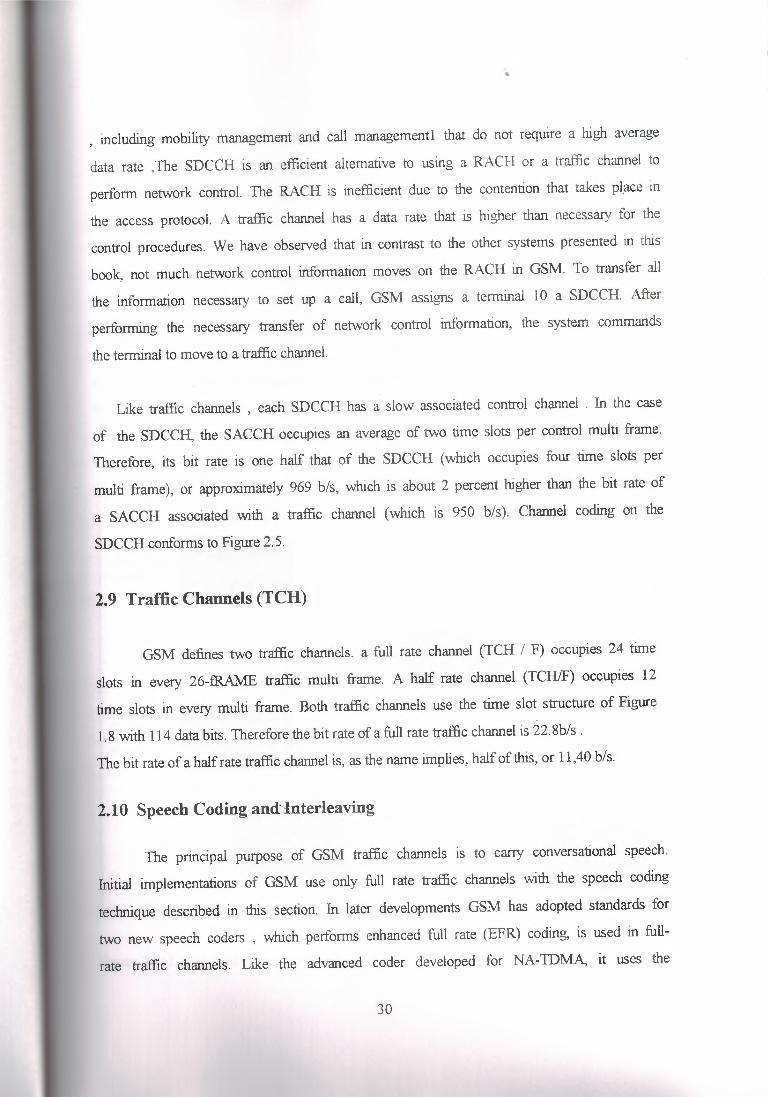
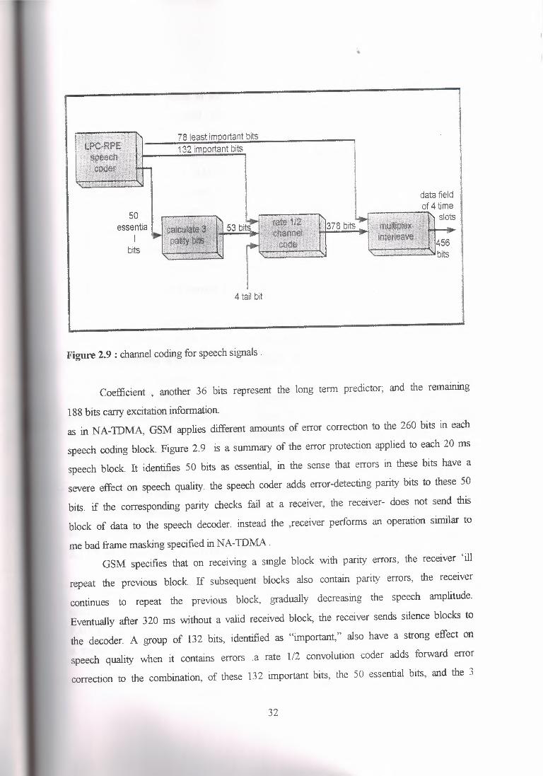
the original speech coding technique of GSM is referred to as linear prediction

coding with regular pulse excitation. As indicated in Figure 2.8, the LPC- RPE coder uses

36 + 188 + 36 = 260 bits to represent each block of 20 ms of speech (160 samples at the 8

kHz sampling rate).Therefore the speech coding rate is

260 bits/block+ 0.02 sec/block= 1.3,000 bis.

This is higher than the coding rates of NA-TOMA and CDMA. The higher bit rate

reflects the early date M which the GSM. coder was developed .For a given speech quality,

the required code rate predictably decreases with time, reflecting advances in signal

processing hardware technology. In the LPC-RPE coder, 36 bits per block carry

information about eight linear prediction

Terminal

analog

speech

8 kHz 13 bits

64 kb/s

speech

Base or MSC

LPC predictor 36 bits

excitation 188 bits long-term predictor 36 bits

Figure 2.8: Linear prediction coding with regular pulse excitation.

31

'•

78 least important bits 132 important bits

data field

50 essentia

I bits

4 tail bit

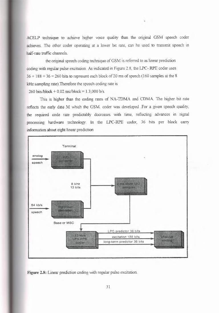
Figure 2.9 : channel coding for speech signals .

Coefficient , another 36 bits represent the long term predictor; and the remammg

188 bits cany excitation information. as in NA-TDMA, GSM applies different amounts of error correction to the 260 bits in each

speech coding block. Figure 2.9 is a summary of the error protection applied to each 20 ms

speech block. It identifies 50 bits as essential, in the sense that errors in these bits have a

severe effect on speech quality. the speech coder adds error-detecting parity bits to these 50

bits. if the corresponding parity checks fail at a receiver, the receiver- does not send this

block of data to the speech decoder. instead the ,receiver performs an operation similar to

me bad frame masking specified in NA-TDMA. GSM specifies that on receiving a single block with parity errors, the receiver 'ill

repeat the previous block. If subsequent blocks also contain parity errors, the receiver

continues to repeat the previous block, gradually decreasing the speech amplitude.

Eventually after 320 ms without a valid received block, the receiver sends silence blocks to

the decoder. A group of 132 bits, identified as "important," also have a strong effect on

speech quality when it contains errors .a rate 1/2 convolution coder adds forward error

correction to the combination, of these 132 important bits, the 50 essential bits, and the 3

32

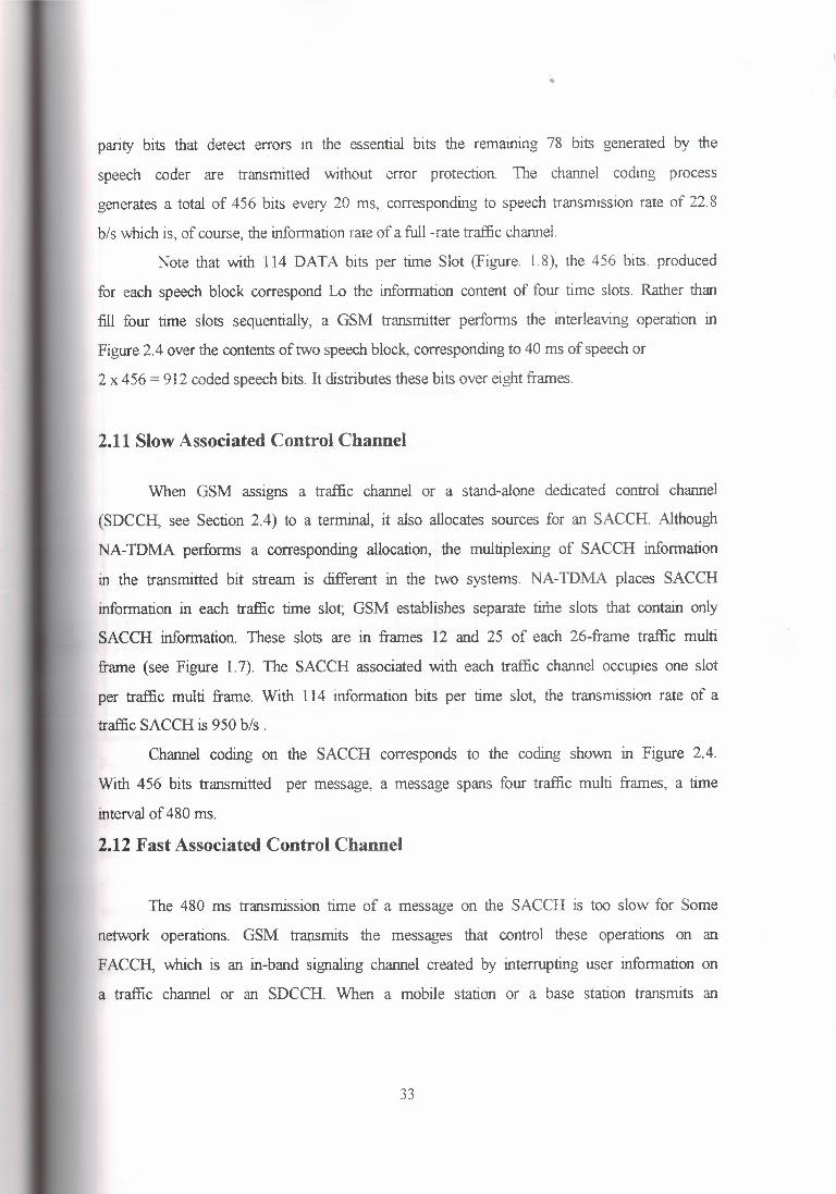
parity bits that detect errors in the essential bits the remammg 78 bits generated by the

speech coder are transmitted without error protection. The channel coding process

generates a total of 456 bits every 20 ms, corresponding to speech transmission rate of 22.8

b/s which is, of course, the information rate of a full -rate traffic channel.

Note that with 114 DATA bits per time Slot (Figure. 1.8), the 456 bits. produced

for each speech block correspond Lo the information content of four time slots. Rather than

fill four time slots sequentially, a GSM transmitter performs the interleaving operation m

Figure 2. 4 over the contents of two speech block, corresponding to 40 ms of speech or

2 x 456 = 912 coded speech bits. It distributes these bits over eight frames.

2.11 Slow Associated Control Channel

When GSM assigns a traffic channel or a stand-alone dedicated control channel

(SDCCH, see Section 2.4) to a terminal, it also allocates sources for an SACCH. Although

NA-TDMA performs a corresponding allocation, the multiplexing of SACCH information

in the transmitted bit stream is different in the two systems. NA-TDMA places SACCH

information in each traffic time slot; GSM establishes separate time slots that contain only

SACCH information. These slots are in frames 12 and 25 of each 26-frame traffic multi

frame (see Figure 1.7). The SACCH associated with each traffic channel occupies one slot

per traffic multi frame. With 114 information bits per time slot, the transmission rate of a

traffic SACCH is 950 b/s .

Channel coding on the SACCH corresponds to the coding shown in Figure 2.4.

With 456 bits transmitted per message, a message spans four traffic multi frames, a time

interval of 480 ms.

2.12 Fast Associated Control Channel

The 480 ms transmission time of a message on the SACCH is too slow for Some

network operations. GSM transmits the messages that control these operations on an

F ACCH, which is an in-band signaling channel created by interrupting user information on

a traffic channel or an SDCCH. When a mobile station or a base station transmits an

33

·.

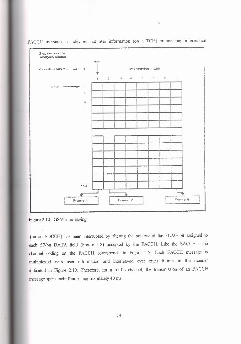
F ACCH message, it indicates that user information ( on a TCH) or signaling information

2 speech coder analysis blocks

2 00 456 bits = 8 00 11 4

read

! Interleaving matrix

2 3 5 6 7 8 4

write l '

I l j

I i r '

2

3

·- I 1

I I a, ... ••• I l I !__ ]

arrre 1 Frame 2 Frame 8 I ' •.. _ -k .

Figure 2.10 : GSM interleaving .

( on an SDCCH) has been interrupted by altering the polarity of the FLAG bit assigned to

each 57-bit DATA field (Figure 1.8) occupied by the FACCH Like the SACCH , the

channel coding on the FACCH corresponds to Figure 1.8. Each FACCH message is

multiplexed with user information and interleaved over eight frames in the manner

indicated in Figure 2.10. Therefore, for a traffic channel, the transmission of an F ACCH

message spans eight frames, approximately 40 ms.

34

•

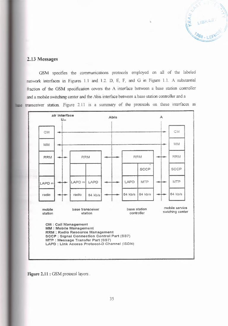
2.13 Messages

GSM specifies the communications protocols employed on all of the labeled

network interfaces in Figures 1.1 and 1.2. D, E, F, and G in Figure 1.1. A substantial

fraction of the GSM specification covers the A interface between a base station controller

and a mobile switching center and the Abis interface between a base station controller and a

transceiver station. Figure 2.11 is a summary of the protocols on these interfaces as

- air Interface Abis A

Um

I l l _ _L_ CM 1-I- ----1 CM

I I I I.

MM I-+- ---4-- I MM

I I J_ I RRM RRM I -f-- I RRM I •• .. I RRM ' SCCP SCCP

±I : MTP

164 kb/s

I

LAPD ml -+- ILAPD ml LAPD LAPD I MTP

radio ~ 64 kb/s I 64 kb/s radio 64 kb/s

mobile station

base transceiver station

base station controller

mobile servics swiching center

CM : Call Management MM : Mobile Management RRM : Radio Resource Management seep : Signal Connection Control Part (SS7) MTP : Message Transfer Part (SS7) LAPD : Link Access Protocol-0 Channel (ISDN)

Figure 2.11: GSM protocol layers.

35

well as on the GSM air interface. The figure indicates that the A interface uses Signaling

System 7 protocols and that. the Abis interface uses LAPD, the ISDN data link layer

protocol. On the air interface, the corresponding protocol is LAPD Like the Um

nomenclature, this terminology appends "m" denoting mobile ,to the name of an ISDN

protocol. Earlier sections of this chapter describe the physical layer (labeled "radio" in

Figure 2.12). Section 2.5 describes the GSM message structure specified in the LAPD

protocol. Section 2. 5 then examines message content, with messages classified

according to the network management operations they perform: radio resources

management, mobility management, or call management. Figure 2.11 indicates that the

base station system. participates in radio resources management. By contrast, the mobile

switching center and the terminal coordinate call management and mobility management

functions. for these two categories of system operations, the base station system simply

relays messages between terminals and switching centers.

2.14 Message Structure

All of the signaling channels listed in figure 1.10 , with the exception of the frequency

correction channel (FCCH), the synchronization channel (SCH), and the random access

channel (RACH), transmit information in the LAPD format. The physical layer carnes

these messages in segments of 184 bits, as shown in Figure 2. 5 . Most messages fit into a

single segment that spans four physical layer time slots. The exceptions are a few call

management messages that require multiple segments.

Figure 2.13 shows the five information fields that appear in LAPD messages. Although

every message contains a length indicator field, the

36

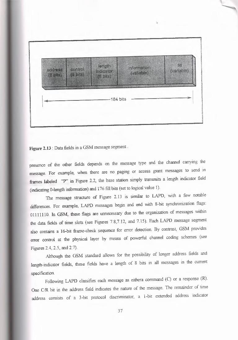
~-----------184 bits

Figure 2.13 : Data fields in a GSM message segment .

presence of the other fields depends on the message type and the channel canying the

message. For example, when there are no paging or access gsant messages to send in

frames labeled "P" in Figure 2.2, the base station simply transmits a length indicator field

(indicating 0-length information) and 17 6 fill bits ( set to logical value 1).

The message structure of Figure 2.13 is similar to LAPD, with a few notable

differences. For example, LAPD messages begin and end with 8-bit synchronization flags:

01111110. In GSM, these flags are unnecessary due to the organization of messages within

the data fields of time slots (see Figures 7.8,7.12, and 7.15). Each LAPD message segment

also contains a 16-bit frame-check sequence for error detection. By contrast, GSM provides

error control at the physical layer by means of powerful channel coding schemes (see

Figures 2.4, 2.5, and 2.7). Although the GSM standard allows for the possibility of longer address fields and

length-indicator fields, these fields have a length of 8 bits in all messages in the current

specification. Following LAPD classifies each message as eithera command (C) or a response (R).

One CIR bit in the address field indicates the nature of the message. The remainder of time

address consists of a 3-bit protocol discriminator, a 1-bit extended address indicator

37

•

(always set to O in the initial version of GSM), and a 3-bit service access point identifier

(SAPI). Anticipating revised versions of the GSM standard, the protocol discriminator

indicates to which revision the current message conforms. The SAPI allows a network

element to engage simultaneously in more than one type of communication. SAPI =0

corresponds to a network management message ( call control, mobility management, or

radio resources management) and SAPI= 3 corresponds to a short message service

message. Following the ISDN convention , GSM specifies three message types: information

(I), supervisory (s), and unnumbered (U). Information messages perform the main tasks of

GSM network management. S messages and U messages control the flow of I messages

between terminals and base stations. Message flow is also controlled by two message

sequence numbers in the control field of each information message. N(S) is the 3-bit

sequence number of the current message, and N(R) is the sequence number of a message

received by the network element that is sending the current message. For example, when a

terminal transmits an I message, the value of N(S) in the control field is the sequence

number of that message. The value of N(R) is the sequence number of the last message

received from the base station. When the base station observes N(R), it may infer that a

message transmitted to the terminal did not arrive successfully. this would cause the base

station to retransmit the lost message. The length indicator field contains a 6-bit field that specifies the number of octets in

the information field. Length=O indicates that the current message does not carry an

information field. There is 1 bit in the length indicator field that indicates whether or not

the present message segment is the final one in the current message. When the other fields

occupy less than 184 bits, the remainder of the message contains fill bits that are all logical

ls.

2.15 Message Content

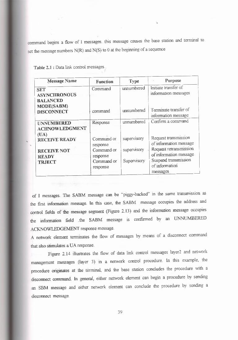
Table 2.1 is a list of the unnumbered (U) messages and supervisory (5) messages

that control the flow of information (I) messages. The unnumbered messages initiate and

terminate exchanges of information messages. The set asynchronous balanced mode

38

•

command begins a flow of I messages. this message causes the base station and terminal to

set the message numbers N(R) and N(S) to O at the beginning of a sequence

Table 2.1 : Data link control messages .

'

Message Name Function Type Purpose

SET .. Command unnumbered Initiate transfer of

ASYNCHRONOUS information messages

BALANCED MODE(SABM) DISCONNECT command unnumbered Terminate transfer of

information message

UNNUMBERED Response unnumbered Confirm a command ACHNOWLEDGMENT (UA) RECENE READY Command or supervisory Request transmission

response of information message

RECENENOT Command or supervisory . Request retransmission

RE;\l)Y response of information message

TRJECT Command or Supervisory Suspend transmission response of informatiori

messages

of I messages. The SABM message can be "piggy-backed" in the same transmission as

the first information message. In this case, the SABM message occupies the address and

control fields of the message segment (Figure 2.13) and the information message occupies

the information field . the SABM message is confirmed by an UNNUMBERED

ACKNOWLEDGEMENT response message.

A network element terminates the flow of messages by means of a disconnect command

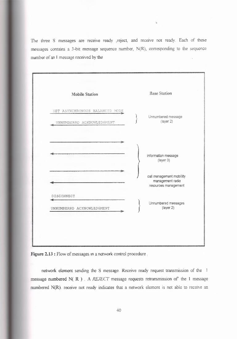
that also stimulates a UA response. Figure 2.14 illustrates the flow of data link control messages layer2 and network

management messages (layer 3) in a network control procedure. In this example, the

procedure originates at the terminal, and the base station concludes the procedure with a

disconnect command. In general, either network element can begin a procedure by sending

an SBM message and either network element can conclude the procedure by sending a

disconnect message.

39

•

The three S messages are receive ready ,reject, and receive not ready. Each of these

messages contains a 3-bit message sequence number, N(R), corresponding to the sequence

number of an I message received by the

Mobile Station Base Station

SET ASYNCHRONOUS BALAl"!CZD MODE

} Unnumbered message (layer 2) UNNUMBERRD ACKNOWLEDG~IBNT

information message (layer 3)

call management mobillity management radio

resources management

DISCONNECT

} Unnumbered messages (layer 2) UNNUMBERRD ACKNOWLEDGr1ENT

Figure 2.13 : Flow of messages in a network control procedure .

network element sending the S message. Receive ready request transmission of the 1

message numbered N( R ) . A REJECT message requests retransmission of the 1 message

numbered N(R). receive not ready indicates that a network element is not able to receive an

40

•

I message. When this condition changes. the network element sends a receive ready

message requesting transmission of message number N(R).

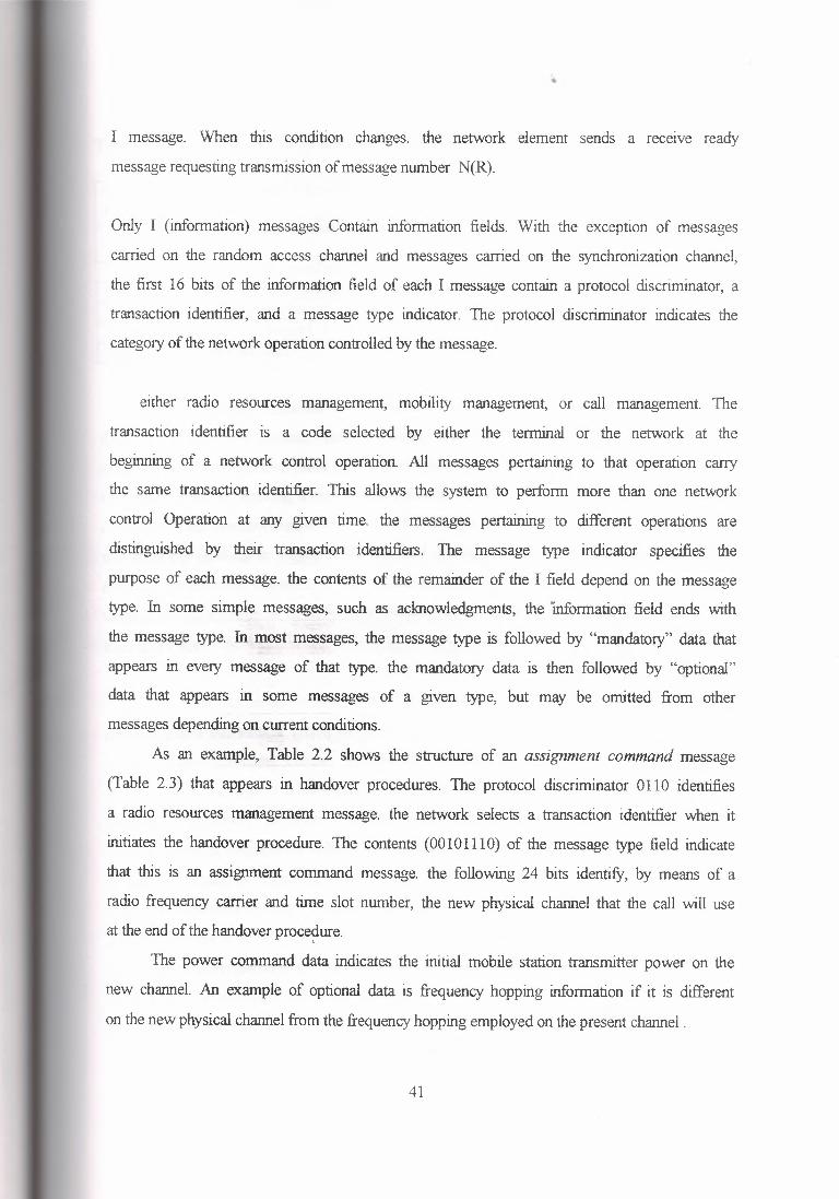
Only I (information) messages Contain information fields. With the exception of messages

carried on the random access channel and messages carried on the synchronization channel,

the first 16 bits of the information field of each I message contain a protocol discriminator, a

transaction identifier, and a message type indicator. The protocol discriminator indicates the

category of the network operation controlled by the message.

either radio resources management, mobility management, or call management. The

transaction identifier is a code selected by either the terminal or the network at the

beginning of a network control operation. All messages pertaining to that operation carry

the same transaction identifier. This allows the system to perform more than one network

control Operation at any given time. the messages pertaining to different operations are

distinguished by their transaction identifiers. The message type indicator specifies the

purpose of each message. the contents of the remainder of the I field depend on the message

type. In some simple messages, such as acknowledgments, the •. information field ends with

the message type. In most messages, the message type is followed by "mandatory" data that

appears in every message of that type. the mandatory data is then followed by "optional"

data that appears in some messages of a given type, but may be omitted from other

messages depending on current conditions.

As an example, Table 2.2 shows the structure of an assignment command message

(Table 2.3) that appears in handover procedures. The protocol discriminator 0110 identifies

a radio resources management message. the network selects a transaction identifier when it

initiates the handover procedure. The contents (00101110) of the message type field indicate

that this is an assignment command message. the following 24 bits identify, by means of a

radio frequency carrier and time slot number, the new physical channel that the call will use

at the end of the handover procedure.

The power command data indicates the initial mobile station transmitter power on the

new channel. An example of optional data is frequency hopping information if it is different

on the new physical channel from the frequency hopping employed on the present channel.

41

·.

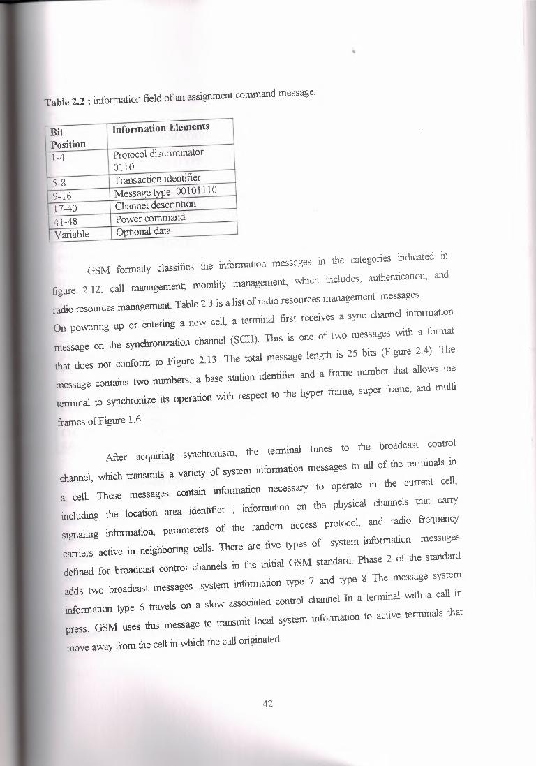
Table 2.2 : information field of an assignment command message.

Bit Position

Information Elements

1-4 Protocol discriminator 0110

5-8 Transaction identifier Message type 00101110 9-16 Channel description 17-40 Power command 41-48

Variable Optional data

GSM formally classifies the information messages in the categories indicated in

figure 2.12: call management; mobility management, which includes, authentication; and

radio resources management. Table 2.3 is a list of radio resources management messages.

On powering up or entering a new cell, a terminal first receives a sync channel information

message on the synchronization channel (SCH). This is one of two messages with a format

that does not conform to Figure 2.13. The total message length is 25 bits (Figure 2.4). The

message contains two numbers: a base station identifier and a frame number that allows the

terminal to synchronize its operation with respect to the hyper frame, super frame, and multi

frames of Figure 1.6.

After acqumng synchronism, the terminal tunes to the broadcast control

channel, which transmits a variety of system information messages to all of the terminals in

a cell. These messages contain information necessary to operate in the current cell,

including the location area identifier ; information on the physical channels that carry

signaling information, parameters of the random access protocol, and radio frequency

carriers active in neighboring cells. There are five types of system information messages

defined for broadcast control channels in the initial GSM standard. Phase 2 of the standard

adds two broadcast messages . system information type 7 and type 8 The message system

information type 6 travels on a slow associated control channel In a terminal with a call in

press. GSM uses this message to transmit local system information to active terminals that

move away from the cell in which the call originated.

42

'•

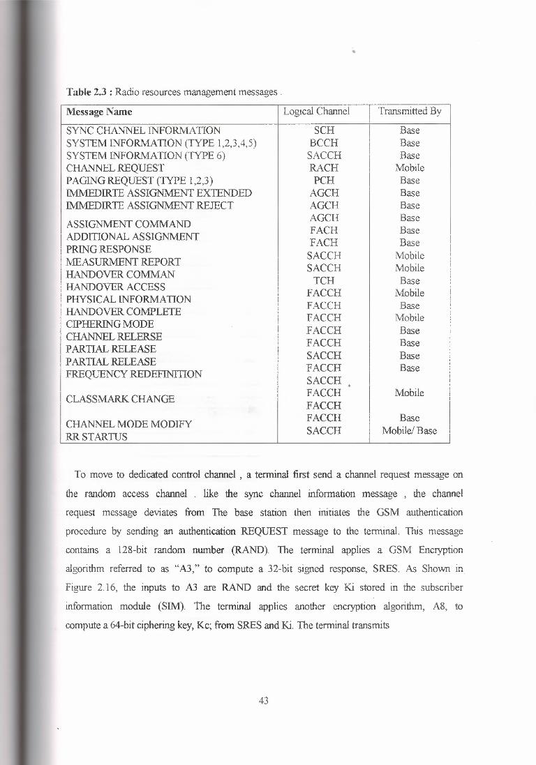
Table 2.3 : Radio resources management messages .

Message Name Logical Channel Transmitted By

SYNC CHANNEL INFORMATION SCH Base SYSTEM INFORMATION (TYPE 1,2,3,4,5) BCCH Base SYSTEM INFORMATION (TYPE 6) SAC CH Base CHANNEL REQUEST RACH Mobile PAGING REQUEST (TYPE 1,2,3) PCH Base IM1\1EDIRTE ASSIGNMENT EXTENDED AGCH Base IM1\1EDIRTE ASSIGNMENT REJECT AGCH Base

ASSIGNMENT COMMAND AGCH Base

ADDIDONAL ASSIGNMENT FACH Base

PRING RESPONSE FACH Base

MEASURMENT REPORT SAC CH Mobile

HANDOVER COMMAN SAC CH Mobile

HANDOVER ACCESS TCH Base

PHYSICAL INFORMATION FACCH Mobile

HANDOVER COMPLETE FACCH Base

CIPHERING MODE FACCH Mobile

CHANNEL RELERSE FACCH Base

PARTIAL RELEASE FACCH Base

PARTIAL RELEASE SAC CH Base

FREQUENCY REDEFINITION FACCH Base SAC CH .

CLASSMARK CHANGE FACCH Mobile FACCH

CHANNEL MODE MODIFY FACCH Base

RRSTARTUS SAC CH Mobile/ Base

To move to dedicated control channel , a terminal first send a channel request message on

the random access channel . like the sync channel information message , the channel

request message deviates from The base station then initiates the GSM authentication

procedure by sending an authentication REQUEST message to the terminal. This message

contains a 128-bit random number (RAND). The terminal applies a GSM Encryption

algorithm referred to as "A3," to compute a 32-bit signed response, SRES. As Shown in

Figure 2.16, the inputs to A3 are RAND and the secret key Ki stored in the subscriber

information module (SIM). The terminal applies another encryption algorithm, A8, to

compute a 64-bit ciphering key, Kc; from SRES and Ki. The terminal transmits

43

•

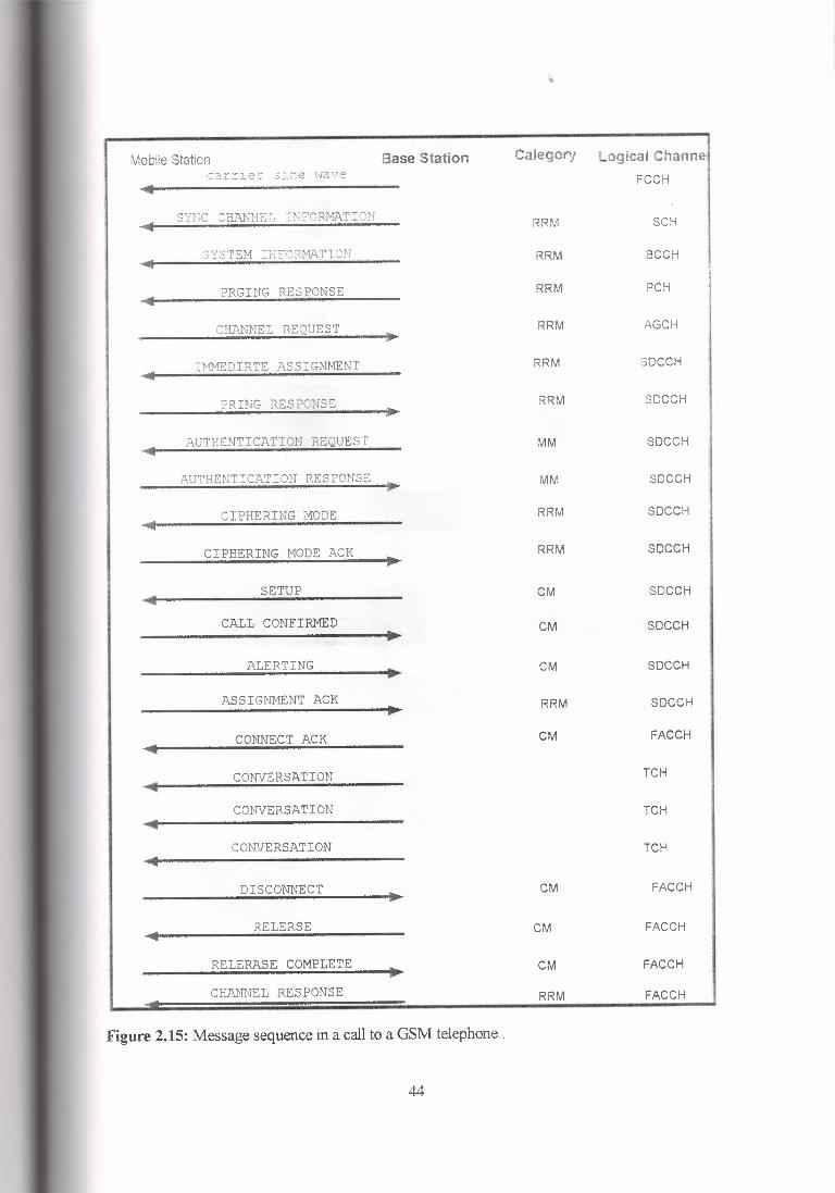
Mobile Station Base Station Calegory Logical Channe carrier 3i~e wave FCCH

SYNC CHANNEL INFORMATION RRM SCH

SYSTEM INFORMATION RRM BCCH

PRGING RESPONSE RRM PCH

CHANNEL REQUEST RRM AGCH ,. IMMEDIRTE ASSIGNMENT RRM SDCCH

PRING RESPONSE RRM SDCCH • AUTHENTICATION REOUEST MM SDCCH

AUTHENTICATION RESPONSE ,.. MM SDCCH

CIPHERING MODE RRM SOC CH

CIPHERING MODE ACK RRM SDCCH •• SETUP CM SDCCH

CALL CONFIRMED CM SOC CH

ALERTING 11s CM SOC CH

ASSIGNMENT ACK RRM SDCCH

CONNECT ACK CM FACCH

CONVERSATION TCH

C01'lVE RSAT I ON TCH

CONVERSATION TCH

DISCONNECT •• CM FACCH

RELERSE CM FACCH

RELERASE COMPLETE ~ CM FACCH

CHANNEL RESPONSE RRM FACCH

Figure 2.15: Message sequence in a call to a GSM telephone.

44

•

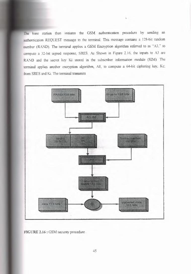
station then initiates the GSM authentication procedure by sending an

authentication REQUEST message to the terminal. This message contains a 128-bit random

number (RAND). The terminal applies a GSM Encryption algorithm referred to as "A3," to

compute a 32-bit signed response, SRES. As Shown in Figure 2.16, the inputs to A3 are

RAND and the secret key Ki stored in the subscriber information module (SII\.1). The

terminal applies another encryption algorithm, A8, to compute a 64-bit ciphering key, Kc;

from SRES and Ki. The terminal transmits

FIGURE 2.16 : GSM security procedure .

45

'•

SRES to the network in an authentication response message. The network also uses A3 to

compute SRES from RAND and Ki. If the two values of SRES are identical, the network

accepts the user as authorized subscriber. It then transmits ciphering mode message to the

terminal in order to establish the mode of encryption to be used in the remainder of the call.

To encrypt user information and network control information, the base station and network

derive a 114-bit mask to be added module 2 to the Two data fields (figure 1.8) in each time

slot. This mask is obtained from another GSM encryption algorithm, AS.the inputs to AS

are the 64-bit ciphering key, Kc , and the current 22-bit frame number.

The base station computes the same mask to decipher the encrypted data. Because

AS uses the frame number to compute the ciphering mask, the mask changes from frame to

frame. This property contributes to the security of the communication.

With the authenticity of the subscriber established and the ciphering arrangement

in place, the network proceeds to set up the call. To do so, it transmits a SETIJP message

to the terminal. The terminal acknowledges this message with a call confirmed message

and then proceeds to alert the subscriber When the subscriber accepts the call, the

terminal sends a connect message to the network. In response, the network moves the

call to a traffic channel by means of an assignment command message. At this point, the

network establishes a connection between the two parties to the conversation. in figure

2. IS, the mobile subscriber concludes the conversation. When this happens, the terminal

sends a disconnect message. to the network. the network responds with a release

command. After the terminal acknowledges this command, the network releases the

traffic channel by sending channel release message to the terminal .the terminal then

returns to monitoring its paging channel.

This example contains a procedure referred to as off air call setup (OACSU). With

OACSU, GSM assigns a traffic channel after the mobile subscriber accepts the call.

Compared to an earlier assignment of a traffic channel, this conserves transmission

resources while the network is setting up a call. OACSU is optional in GSM. It is also

possible to move the call to a traffic channel prior to alerting the subscriber. OACSU can

also be used when the mobile party initiates the call. In this situation, the network assigns a

traffic channel after the remote party accepts the call.

46

•

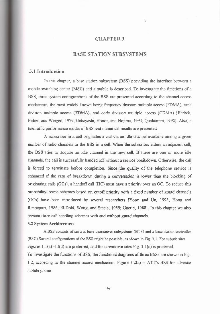
CHAPTER3

BASE ST A TION SUBSYSTEMS

3.1 Introduction

In this chapter, a base station subsystem (BSS) providing the interface between a

mobile switching center (MSC) and a mobile is described. To investigate the functions of a

BSS, three system configurations of the BSS are presented according to the channel access

mechanism, the most widely known being frequency division multiple access (FDMA), time

division multiple access (TDMA), and code division multiple access (CDMA) [Ehrlich,

Fisher, and Winged, 1979; Uebayashi, Honor, and Nojirna, 1993; Qualcomm, 1992]. Also, a

teletraffic performance model ofBSS and numerical results are presented.

A subscriber in a cell originates a call via an idle channel available among a given

number of radio channels to the BSS in a cell. When the subscriber enters an adjacent cell,

the BSS tries to acquire an idle channel in the new cell. If there are one or more idle

channels, the call is successfully handed off without a service breakdown. Otherwise, the call

is forced to terminate before completion. Since the quality of the telephone service is

enhanced if the rate of breakdown during a conversation is lower than the blocking of

originating calls (OCs), a handoff call (HC) must have a priority over an OC. To reduce this

probability, some schemes based on cutoff priority with a fixed number of guard channels

(GCs) have been introduced by several researchers [Yoon and Un, 1993; Hong and

Rappaport, 1986; El-DoW, Wong, and Steele, 1989; Guerin, 1988]. In this chapter we also

present three call handling schemes with and without guard channels.

3.2 System Architectures

A BSS consists of several base transceiver subsystems (BTS) and a base station controller

(BSC).Several configurations of the BSS might be possible, as shown in Fig. 3.1. For suburb sites

Figures 1.1 (a) -1. l( d) are preferred, and for downtown sites Fig. 3 .1 ( c) is preferred.

To investigate the functions ofBSS, the functional diagrams of three BSSs are shown in Fig.

1.2, according to the channel access mechanism Figure 1.2(a) is ATT's BSS for advance

mobile phone

47

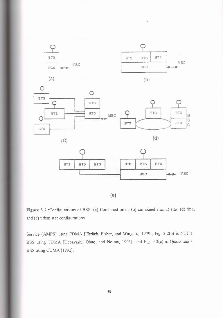
BTS I

3CS i........... 1'\JlSC

l 8TS l 3TS I BTS

~ l

(a)

BSC .14 MSC

~

(b}

•

BTS r'l-i 3-, ~:::1~

(d)

BTS STS MSC

BTS

(C)

SSC MSC

BTS BTS BTS BTS BTS

(e)

Figure 3.1 :Configurations of BSS: (a) Combined omni, (b) combined star, c) star, (d) ring,

and ( e) urban star configurations.

Service (AMPS) using FDMA [Ehrlich, Fisher, and Wingard, 1979], Fig. 3.2(b) is NTT's

BSS using TDMA [Uebayashi, Ohno, and Nojma, 1993], and Fig. 3.2(c) is Qualcornni's

BSS using CDMA [1992].

48

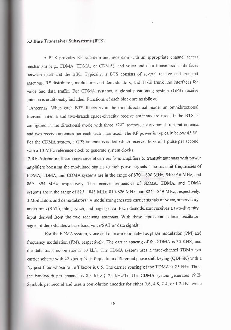
3.3 Base Transceiver Subsystems (BTS)

A BTS provides RF radiation and reception with an appropriate channel access

mechanism (e.g., FDMA, TDMA, or CDMA), and voice and data transmission interfaces

between itself and the BSC. Typically, a BTS consists of several receive and transmit

antennas, RF distributor, modulators and demodulators, and Tl/El trunk line interfaces for

voice and data traffic. For CDMA systems, a global positioning system (GPS) receive

antenna is additionally included. Functions of each block are as follows.

I .Antennas: When each BTS functions in the omnidirectional mode, an omnidirectional

transmit antenna and two-branch space-diversity receive antennas are used. If the BTS is

configured in the directional mode with three 120° sectors, a directional transmit antenna

and two receive antennas per each sector are used. The RF power is typically below 45 W.

For the CDMA system, a GPS antenna is added which receives ticks of 1 pulse per second

with a 10-MHz reference clock to generate system clocks.

2.RF distributor: It combines several carriers from amplifiers to transmit antennas with power

amplifiers boosting the modulated signals to high-power signals. The transmit frequencies of

FDMA, TDMA, and CDMA systems are in the range of 870-:-~90 MHz, 940-956 MHz, and

869-894 MHz, respectively. The receive frequencies of FDMA, TDMA, and CDMA

systems are in the range of 825-845 MHz, 810-826 MHz, and 824-849 MHz, respectively.

3.Modulators and demodulators: A modulator generates carrier signals of voice, supervisory

audio tone (SAT), pilot, synch, and paging data. Each demodulator receives a two-diversity

input derived from the two receiving antennas. With these inputs and a local oscillator

signal, it demodulates a base band voice/SAT or data signals.

For the FDMA system, voice and data are modulated as phase modulation (PM) and

frequency modulation (FM), respectively. The carrier spacing of the FDMA is 30 KHZ, and

the data transmission rate is 10 kb/s. The TDMA system uses a three-channel TDMA per

carrier scheme with 42 kb/s 1r /fl.-shift quadrate differential phase shift keying (QDPSK) with a

Nyquist filter whose roll off factor is 0.5. The carrier spacing of the TDMA is 25 kHz. Thus,

the bandwidth per channel is 8.3 kHz (=25 kHz/3). The CDMA system generates 19.2k

Symbols per second and uses a convolution encoder for either 9.6, 4.8, 2.4, or 1.2 kb/s voice

49

•

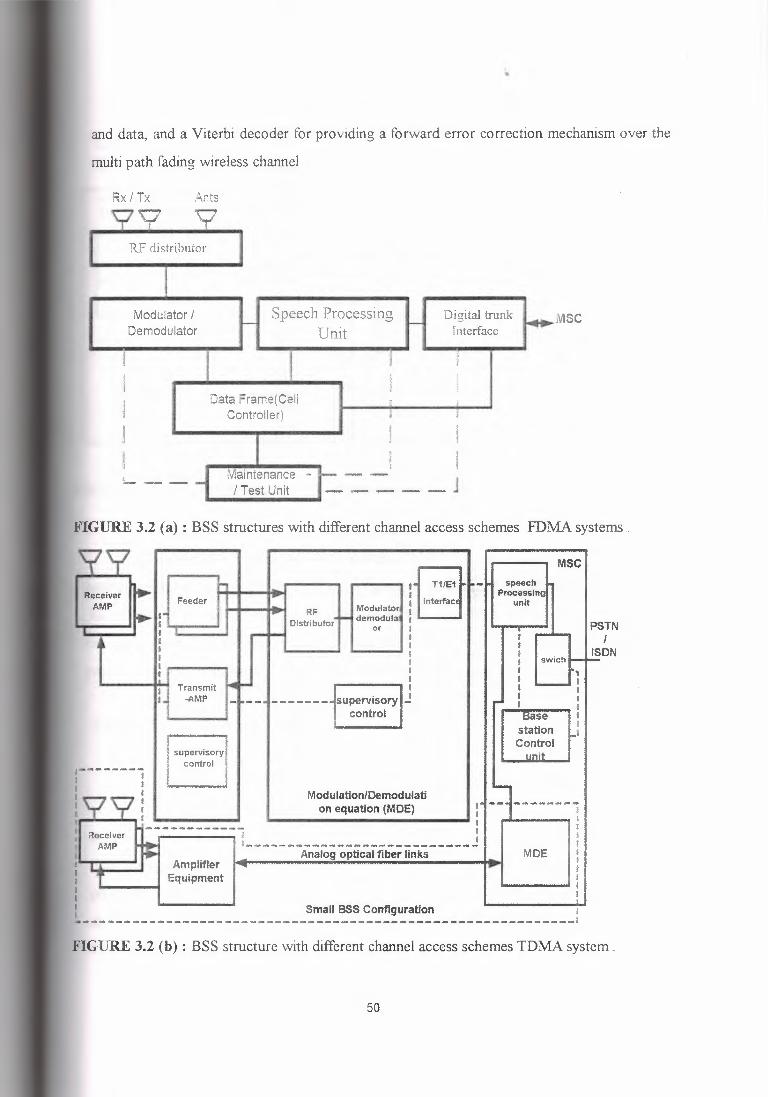
and data, and a Viterbi decoder for providing a forward error correction mechanism over the

multi path fading wireless channel

Rx I Tx Ants

Modulator I Demodulator

Speech Processing Unit

MSC Digital trunk Interface

Data Frame(Cell Controller)

__ J !..- -- -- Maintenance - I Test Unit

FIGURE 3.2 (a): BSS structures with different channel access schemes FDMA systems.

MSC

RF Distributor PSTN

I ISDN

T1/E1 speech Processing

unit

I I

Modulatori : demodula I ~--..i

or l I I I ! l ----- .. ·

isupervisory I J control se

station Control

Receiver AMP Feeder intertac

swich

Transmit -AMP

supervisory control

Receiver AMP

Modulatlon/Demodulati I on equation (MOE) I : I

------------ I ~~~~-.I I

1--------------------------- Analog optical fiber links MOE ! ••• ••

I l I I l Small BSS Configuration ! ------------------------------------------------------------·

Amplifier Equipment

FIGURE 3.2 (b) : BSS structure with different channel access schemes TDMA system .

50

•

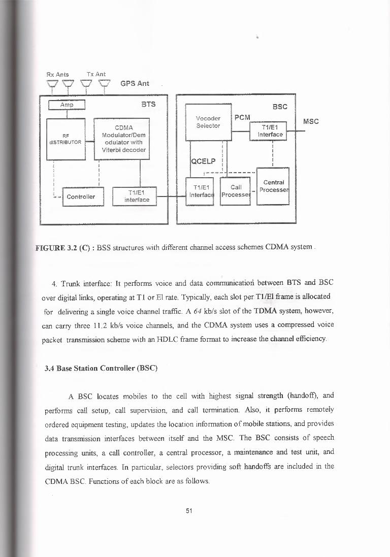
Rx Ants Tx Ant

I Amp BTS SSC I Vocoder PCM

CDMA Selector H T1/E1 L ~ RF Modulator/Dem Interface I

dlSTRIBUTOR -- odulator with ' 1

Viterbi decoder l I i I l I

J • QCELP I I I I I I ! I I J g ,----· ------ l I Central I I Call L _, Controller I I I T1/E1 - Processer T1/E1 Interface Processe

interface I

MSC

FIGURE 3.2 (C): BSS structures with different channel access schemes CDMA system.

4. Trunk interface: It performs voice and data communication between BTS and BSC

over digital links, operating at Tl or El rate. Typically, each slot per Tl/El frame is allocated

for delivering a single voice channel traffic. A 64 kb/s slot of the TDMA system, however,

can carry three 11.2 kb/s voice channels, and the CDMA system uses a compressed voice

packet transmission scheme with an HDLC frame format to increase the channel efficiency.

3.4 Base Station Controller (BSC)

A BSC locates mobiles to the cell with highest signal strength (handofl), and

performs call setup, call supervision, and call termination. Also, it performs remotely

ordered equipment testing, updates the location information of mobile stations, and provides

data transmission interfaces between itself and the MSC. The BSC consists of speech

processing units, a call controller, a central processor, a maintenance and test unit, and

digital trunk interfaces. In particular, selectors providing soft handoffs are included in the

CDMA BSC. Functions of each block are as follows.

51

•

1. Speech processing unit/vocoder: It provides the per channel audio-level speech and data

paths interface between MSC and RF. Certain orders and request data signals can beadded

on the transmitter path before the modulator, and these data signals must be removed from

the receiver path after the demodulator.

The speech-processing unit employs one of two signaling methods for sending the

orders and requests signaling over a voice channel without interfering with voice

conversation. The two methods are the blank-and-burst and dim-and-burst modes. With the

blank-and-burst mode, the signals are sent in the form of a binary data message over the

voice channel by momentarily muting the voice and inserting a binary data sequence. The

data sequence requires approximately one-tenth of a second. However, the blank-and-burst

signal is sent and replaces voice traffic temporarily. For the CDMA system, the dim-and­

burst as well as the blank-and-burst mode can be used. When a vocoder desires to transmit

at its maximum rate under the dim-and-burst mode, it is permitted to supply data at half of

this rate. The remaining rate is used for signaling and overhead.

For the digital cellular system, both pulse code modulation (PCM) digitized voice

and data suffer from the coding used to increase the whole system capacity. The TDMA

system uses a 11.2 kb/s vector sum excited linear prediction (VSELP) transmission code,

which consists of 6. 7kb/s source traffic and additional preamble bits, sync bits, and control

bits.

In the CDMA system, the vocoder handles variable rate vocoding [transforms the

Qualcomm developed code excited linear prediction code (QCELP) to PCM, or vice versa].

The vocoder has a variable rate that supports 8, 4, 2, and 1 kb/s operation and corresponds

to channel rates of 9. 6, 4. 8, 2.4, and 1.2 kb/s. For example, a low-rate vocoder, running at

4kb/s would increase the system capacity by a factor of 1. 7 times with some degraded voice

quality.

For the TDMA and CDMA systems, echo cancellors are added, which eliminate

echo due to a 2-W/4--W hybrid transformer in the public· switch telephone network.

52

•

2. Data frame/call controller: It maintains an independent setup channel for the shared use

of the BTS in communicating with all mobiles within its zone. Only data traffic is transmitted

on the setup channel. Any mobile wishing to initiate a call monitors the forward setup

channel (land to mobile). If the channel is idle, the mobile can transmit a call request or a

page response. Otherwise, the mobile must wait a short time interval and monitor the

channel again, until the forward channel is idle.

The call processor of the FD~lA system initiates the hard handoff procedure with

the MSC. To determine when and if a handoff is necessary, signal-strength measurement or

a phase range measurement in the speech-processing unit is made once every few seconds on

each active voice channel. The soft handoffs between BTSs of the CDMA system are

handled in selectors.

The call processors must also detect and control the signaling tone, off and on

hooks, and transmitter power control. In addition, the processor provides a pagmg

procedure to find a mobile station when a land-originating call is initiated.

3. Central controller: It allocates or de-allocates voice and data channels, communicates with

the MSC and BTS, and controls the maintenance and test unit.

4. Digital trunk interface: It performs voice and data communication between BTS and BSC

or between BSC and MSC over digital links, operating at Ti or El rate.

5.Selector for the CDMA system: The selector handles soft handoffs between BTSs. The soft

handoff allows both the original call and new to serve the call temporarily during the

handoff transition. The transition is from the originating cell to both cells and then to the new

cell. Thus, it provides the make-before-break switching function.

After a cell is initiated, the mobile continues to scan neighboring cells to determine if

the signal from another cell becomes comparable to that of the original cell. Then, it sends a

control message to the MSC, which states that the new cell is now strong and identifies the

new cell. The MSC indicates the handoff by establishing a link to the mobile through the

new cell while maintaining the old link. While the mobile is located in the transition region

53

•

between the two cells, the call is supported by both cells until the mobile notifies the MSC

that one of the links is no longer useful. This decision is performed by the selector, which

selects an appropriate BTS among the current three engaged BTSs.

3.5 Analysis of Call Handling Schemes

3.5.1 System Modeling

Here, three call handling schemes for a BSS are presented and analyzed. It is

assumed that the BSS can handle two types of calls (originating and prioritized handoff

calls) and store these calls in a finite storage buffer. One scheme is a prioritized handoff

scheme with GCs to reduce the blocking probability of HCs with a penalty on OCs. Under

this scheme, handoff calls can be stored exclusively and access all free channels without

restriction, whereas OCs have access to idle channels, except for a fixed number of guard

channels. The other two schemes are prioritized handoff schemes without GCs to increase

the total grade of service by reducing the blocking probability of OCs without a severe

penalty on the grade of service for HCs. Under these two schemes without guard channels, both types of calls are allowed

to be stored, and prioritized handoff calls push out originating calls if the buffer is full.

Figure 3.3 shows a BSS which has a set of C duplex channels with a finite call storage buffer

of size K - C, C ~ K. Prioritized HCs and ordinary OCs are handled in the BSS. We

assume that these calls have the same exponential service time distribution with rate of µ ,

but different arrival rates of the Poisson process, Al and r.2, respectively. Here, Al is

assumed to be proportional to )...2 such that Al == Ph )...2, where Ph is the probability of having

an HC. Then, the total and arrival rate 21 is )...1 + )...2, and the total traffic load per channel p , is )..TICµ. A

hexagonal cell shape is assumed for the system. The cell radius R for a hexagonal cell is

defined as the maximum distance from the BSS to the cell boundary With the cell radius,

54

•

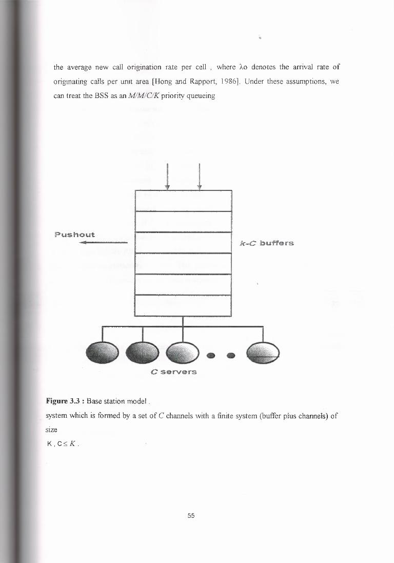
the average new call origination rate per cell , where 11,0 denotes the arrival rate of

originating calls per unit area [Hong and Rapport, 1986]. Under these assumptions, we

can treat the BSS as an M/MICIK priority queueing

Pushout k-C buffers

• • C servers

Figure 3.3 : Base station model .

system which is formed by a set of C channels with a finite system (buffer plus channels) of

size

K,C::;K.

55

•

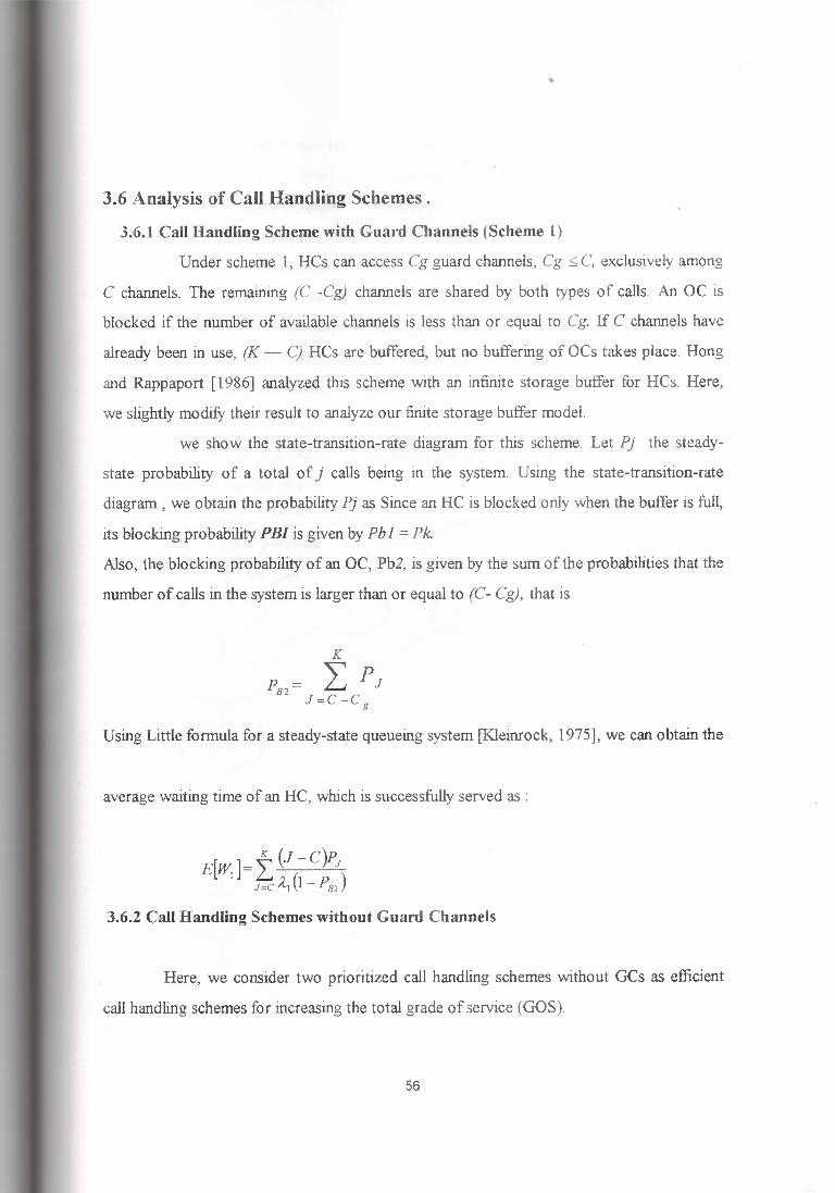
3.6 Analysis of Call Handling Schemes .

3.6.1 Call Handling Scheme with Guard Channels (Scheme 1)

Under scheme 1, HCs can access Cg guard channels, Cg ::;; C, exclusively among

C channels. The remaining (C -Cg) channels are shared by both types of calls. An OC is

blocked if the number of available channels is less than or equal to Cg. If C channels have

already been in use, (K - C) HCs are buffered, but no buffering of OCs takes place. Hong

and Rappaport [1986] analyzed this scheme with an infinite storage buffer for HCs. Here,

we slightly modify their result to analyze our finite storage buffer model.

we show the state-transition-rate diagram for this scheme. Let Pj the steady­

state probability of a total of j calls being in the system. Using the state-transition-rate

diagram, we obtain the probability Pj as Since an HC is blocked only when the buffer is full,

its blocking probability PB! is given by Pbl = Pk. Also, the blocking probability of an OC, Pb2, is given by the sum of the probabilities that the

number of calls in the system is larger than or equal to (C- Cg), that is

K

PB2= L pl l=C-C g

Using Little formula for a steady-state queueing system [Kleinrock, 1975], we can obtain the

average waiting time of an HC, which is successfully served as :

3.6.2 Call Handling Schemes without Guard Channels

Here, we consider two prioritized call handling schemes without GCs as efficient

call handling schemes for increasing the total grade of service (GOS).

56

•

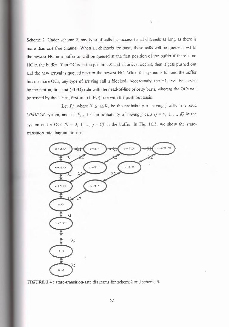
Scheme 2. Under scheme 2, any type of calls has access to all channels as long as there is

more than one free channel. When all channels are busy, these calls will be queued next to

the newest HC in a buffer or will be queued at the first position of the buffer if there is no

HC in the buffer. If an QC is in the position Kand an arrival occurs, then it gets pushed out

and the new arrival is queued next to the newest HC. When the system is full and the buffer

has no more OCs, any type of arriving call is blocked. Accordingly, the HCs will be served

by the first-in, first-out (FIFO) rule with the head-of-line priority basis, whereas the OCs will

be served by the last-in, first-out (LIFO) rule with the push out basis.

Let Pj, where O ::; j::; K, be the probability of having j calls in a basic

MIMICIK system, and let PJ,K be the probability of having j calls O = 0, 1, ... , K) in the

system and k OCs (k = 0, 1, ... , j - C) in the buffer. In Fig. 16.5, we show the state­

transition-rate diagram for this

FIGURE 3.4 : state-transition-rate diagrams for scheme2 and scheme 3.

57

•

Scheme 3. Under scheme 3, any type of call has access to all channels as long as

there is more than one free channel. When all channels are busy, HCs are served as. under

scheme 2. However, OCs will be queued next to the newest OC in a buffer or will be queued

at the first position of the buffer, if the buffer is empty.

When the system is full, an arriving OC is blocked. In addition, if an OC is in the

position K and an HC arrives, then the OC gets pushed out and the new arrival is queued

next to the newest HC. Thus, the HCs will be served by the FIFO rule with the head-of-line

priority basis as done under scheme 2, whereas the OCs will be served by the FIFO rule with

the push out basis.

The state-transition-rate diagram for scheme 3 is the same as scheme 2. Thus, the

blocking probabilities of HCs and OCs for scheme 3 are the same as scheme 2. Since the

waiting time distribution of an HG is independent of the service rule of Ocs,However, the

waiting time distribution of an OC is different from the result of scheme 2 as follows.

Noting that an HC arriving only forces a move of the position of OC in i to the new position

i + I, we can obtain the probability of Ui,n that an OC arrives at position i in the system and

gets served after n transitions with q = >..11( >..I + Cµ). Also, since the number of transitions

in the buffer depends on the arrival rate of HCs and the service rate, the probability that an

OC is in position I and the OC gets served after tis obtained as :

When the system size is j, j < K, an OC arrrvmg can jom at position j + 1 without

considering the number of OCs in the buffer.

58

•

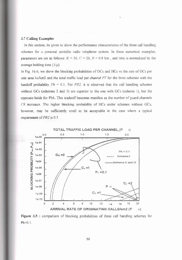
3.7 Calling Examples

In this section, its given to show the performance characteristics of the three call handling

schemes for a personal portable radio telephone system In these numerical examples,

parameters are set as follows: K = 30, C = 20, R = 0.8 km, and time is normalized by the

average holding time (1/µ)

In Fig. 16. 6, we show the blocking probabilities of OCs and HCs vs the rate of OCs per

unit area t-.o/km2 and the total traffic load per channel PT for the three schemes with the

handoff probability Ph = 0.1. For PB2, it is observed that the call handling schemes

without GCs (schemes 2 and 3) are superior to the one with GCs (scheme 1), but the

opposite holds for Pbl. This tradeoff becomes manifest as the number of guard channels

C8 increases. The higher blocking probability of HCs under schemes without GCs,

however, may be sufficiently small to be acceptable in the case where a typical

requirement of PB2 is 0.5

TOTAL TRAFFIC LOAD PER CHANNEL.(P r) 0.0

1e-OO 0.5 1.0 2.0 1.5

1i 1e-01 0. "' 1e-02 "' 0. > 1e-03

!::: ..J 1e04 ai ~ 1e-05 0. (!) 1e06 z 5 1e-07 0 ...J 1 e-08 CD

1 e-09

1e-10 .. 0

Ph= 0.1 .. , ,, .... ,, 2 ,, Cg= ~, , , ,,,, , , , , , , 1 /,, I cg= I'• , , , ,' ,,,, 1· ,,

I I ,, ,, , , ', I I I I . I I I I

: : 1· I I I I I I ! I . I I

Scheme-I

---Scheme-II and Ill

14 16 18 20 2 4 6 8 10 12

ARRIVAL RATE OF ORIGINATING CALLS/km2 (P o)

Figure 3.5 : comparison of blocking probabilities of three call handling schemes for

Ph=O.l.

59

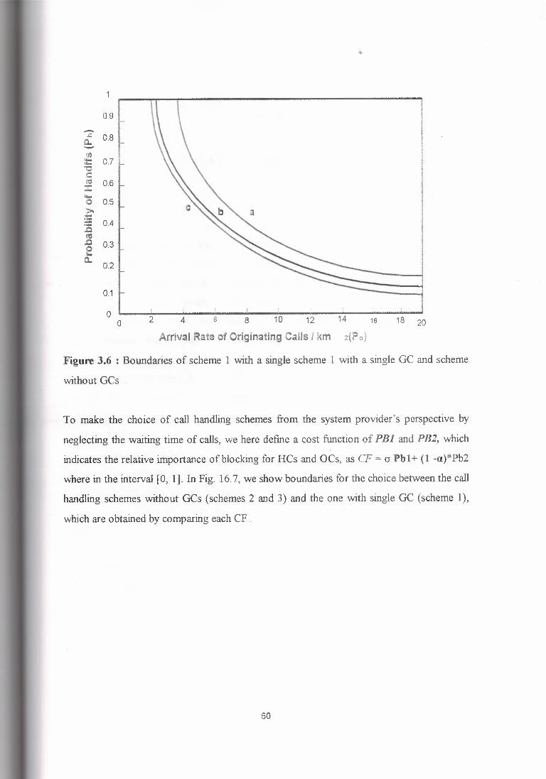
0.9

- s: 0.8 c.. - f/J lt: 0.7 "O

t: "' 0.6 ::c - 0 0.5 >. ~ :.s 04

"' .c 0.3 e a, 0.2

0.1

0 2 10 0 4 6 8 12 16 18 20

Arrival Rate of Originating Calls I km 2(Po)

Figure 3.6 : Boundaries of scheme 1 with a single scheme 1 with a single GC and scheme

without GCs .

To make the choice of call handling schemes from the system provider's perspective by

neglecting the waiting time of calls, we here define a cost function of PBJ and PB2, which

indicates the relative importance of blocking for HCs and OCs, as CF= a Pbl+ (1 -a)*Pb2

where in the interval [O, 1]. In Fig. 16.7, we show boundaries for the choice between the call

handling schemes without GCs (schemes 2 and 3) and the one with single GC (scheme 1),

which are obtained by comparing each CF .

60

•

CHAPTER4

BASE STATIO~S RADIO FREQUENCIES

4.1 Introduction

·•'

In recent years there has been a proliferation of base station towers designed to meet

increased demands placed on mobile telephone networks by the growing number of mobile

phone users .In parallel with the construction of these base station towers there has been an

increase in community concern about possible health effects from the radio frequency (RF)

radiation emissions from the towers. The Australian Government Committee on

Electromagnetic Energy (EME) Public Health Issues (CEMEPID), as part of the public

information component of its RF EME program, considers it important that the general

public be informed about the RF EME levels to which they may be exposed. Accordingly,

the CEMEPID requested the Australian Radiation Protection and Nuclear Safety Agency

- (ARP ANSA) to carry out a survey of the RF EME levels in the vicinity of mobile .s:

telephone base stations.

This report provides information on the levels of RF radiation from RF transmitter

towers (base stations) to which members of the public may be exposed. Reviews on the

potential health risks of RF radiation are available elsewhere (e.g., UNEP/WHO/IRPA,

1993; Barnett, 1994; McKinley etal., 1996; ICNIRP, 1998; Repacholi, 1998; Byrus et al.,

1999).

A survey on RF EME in and around five Vancouver schools by Thansandote et al.

(1999), both at indoor and outdoor sites, yielded power density measurements well within

Canada's safety code limits (Safety Code 6, 1990). Signal sources investigated in the

Thansandote et al survey incl:1ded base station frequency bands for analog cellular phones

and personal communication services (PCS - the new generation of digital cellular phone),

as well as AM radio, FM radio and TV broadcasts. A US study by Petersen and Testagrossa

(1992) characterized RF EME fields in the vicinity of several frequency modulated (FM)

61

•

cellular radio antennae towers, at heights varying from 46 to 82 meters. They reported

maximum power densities considered representative of public exposure levels to be less

than 0.0001 W/m 2 per transmitter. Hence, in a worst-case scenario of 96 transmitters

operating at an

effective radiated power (ERP) of 100 watts per transmitter, the aggregate

maximum power density was estimated by Petersen and Testagrossa to be below 0.01 W/m

2 . In Poland, where the maximum permissible power density value is 0.1 W/m 2 at

relevant base station frequencies, measurements of electromagnetic fields (EMF) in the

surrounds of 20 GSM base stations showed that 'admissible EMF intensities at the level of

people's presence, in existing buildings, in surroundings of base stations and inside

buildings with antennas, were not exceeded' (Aniolczyk, 1999, p.57).

The purpose of the work reported here is to provide data on RF EME levels at

independently nominated sites, over the range of the digital Global System for Mobile

communication (GSM) mobile telephone base stations frequency band (935 - 960 MHz),

and to make comparisons with the limit for non-occupational exposure specified in the

relevant Australian exposure standard. The Radio communications (Electromagnetic

. Radiation Human Exposure) Standard 1999 adopted by the Australian Communications

Authority (ACA) requires mobile phones and mobile phone base stations to comply with

the exposure limits in the interim Australian and New Zealand Standard 2772. l(Int):1998

which has now been withdrawn by Standards Australia.

The ACA standard is subsequently abbreviated as ACAS in this publication. The

non-occupational exposure limit specified in the ACAS, expressed in terms of power flux

density, is 2 W/m 2 (equivalent to 200 µW/cm 2) for frequencies between 10 MHz and 300

GHz, averaged over a 6 minute period. It should be noted that the exposure limits in the

ACAS were 'developed on the basis of there being a threshold of 4 W /kg whole body

specific absorption rate (SAR) before any adverse health consequences are likely to appear

However, because the SAR (units W/kg) is difficult and often impractical to measure, the

ACAS provides derived levels of electric (E) and magnetic (H) field strengths, as well as

the equivalent plane wave power flux densities (S), which are more readily measured.

62

•

Although the primary focus of the ARP ANSA study was to measure the RF EME

emission levels from GSM base stations, fixed site environmental measurements from other

RF EME sources were also recorded, including the analog mobile phone system (AMPS),

VHF TV UHF TV, AM radio, FM radio and Paging.

4.2 Measurement Locations

Measurements were performed at fourteen different locations throughout Australia

Two localities were chosen from each state, and the Northern Territory. In most instances

the sites were chosen by local governments, who were asked to nominate two mobile

telephone base stations sites in major population centers that were of concern to local

communities. Security of monitoring equipment for the 24 hour data logging component

was taken into account in the final selection of the measurement sites. Table 1 lists the RF

measurement survey sites.

4.3 Nature And Type Of Measurements Required.

4.3.1 Fixed Site Environmental Measurements

Broadcast communication sources such as television, and both AM radio and FM

radio, are usually transmitted at high powers from a single base facility. Such sources have

very extensive areas of effective reception frequently extending to many hundreds of

kilometers from a single station transmitter. Furthermore, for such sources and considering

their necessary broadcast design requirements, we do not expect to encounter significant or

strong variations in signal strength in relatively open areas surrounding a mobile telephone

base station. Given the nature and emphasis of our study we therefore adopted a protocol of

making a single set of static environmental measurements for all broadcast sources other

than mobile telephone base stations. Buildings or other likely objects may significantly

attenuate or scatter the RF signal. Hence, where possible, measurements were made in

locations that maintained direct line-of-sight with known RF sources, at a height of 1. 7

metres above ground, in open areas in the near vicinity of the GSM base station of interest.

Measurement antennae were oriented to obtain a maximum signal strength for the particular

frequency band being measured. The environmental RF EME signals were measured at a

location within 500 metres of the base station.

63

•

Measurement of such fixed site environmental RF EME levels involved

investigating a number of different RF EME sources. These included GSN1, AlvlPS, VHF

TV, UHF TV, AM radio, FM radio and paging. All signals with power densities greater

than 1 % of the observed maximum for each frequency band were recorded individually.

Other signals, such as emergency services (police, ambulance, etc.) and taxis, were rarely

detected and are not included in this summary report. To measure the environmental RF

EME levels the average RF EME levels over a six minute scanning period during the day

was determined. The time taken to record all the relevant sources of environmental RF

EME at each site was approximately one hour. A spectrum analyzer was used and some

transient signal sources, such as paging services, may have gone undetected if by chance

the relevant frequency band was not swept by the spectrum analyzer when the signal was

transmitted.

4.4 GSM Base Station Activity Measurements

The primary aim of this study was to determine the RF EME level resulting from all signal

frequencies produced by the particular GSM base stations under survey. Mobile telephone

communication signals are both transient and partly random in their occurrence and

distribution. In this context, we were interested in determining the RF EME levels at many

locations and more particularly, we wanted to estimate both maximum and minimum levels

and also the long term average value for each location and to map such levels in the area

surrounding the base station.

Because telephone communications are based on human activity, a diurnal signal

pattern is generally observed. Site specific GSM mobile telephone exposure levels were

therefore monitored over a 24 hour period. Relevant spectrum analyser data were recorded

automatically under PC control and subsequently analysed to determine both the temporal

and daily average activity. Measurements were performed within a single sector, at a fixed

location close to the base station, by continuously scanning the frequency bands and

logging the signal level for the GSM mobile phone systems.

The recorded data were used to determine the temporal activity for the GSM

systems over the 24 hour period The activity level of the data samples was determined by

counting the number of simultaneous active time slots for a single carrier base station. For

64

•

the majority of GSM base stations there is a possible minimum of eight and a possible

maximum of thirty two time slots for any given sector.

Hence, eight time slots will amount to 25% of the total activity possible from the

transmitting antenna of a single carrier GSM base station.

The digital GSM base stations produce carrier frequencies between 93 5 to 960 MHz

(analog AMPS system operates at 870 to 890 MHz). The GSM system transmits data in

bursts of 0. 6 sec with a repetition rate of 217 Hz. The temporal RF EME levels of the

transmitting antennae at GSM base stations were analyzed to identify control frequencies or

additional carrier frequencies. For GSM the frequency range investigated was divided up

into three sub-bands, with the sampling order of each sub-band and frequency randomized

to avoid bias. The system was optimized to gather as much data as possible by sampling more

often when fewer frequencies were detected. Post logging data analysis was performed to

determine the average activity over a six minute scanning period, yielding an activity value

for every six minutes of the day. The analysis software included only the signals identified

as belonging to the base station in question. Where more than one carrier (Telstra, Optus or

Vodafone) shared the same tower, the combined activity from all • carriers was determined.

A diurnal correction factor was derived from analysis of the 24 hour activity measurements

for use in mobile measurements.

4.5 Mobile GSM Base Station Area Measurements

A fixed antenna was roof mounted on a car and automated mobile measurements

were made whilst driving around the streets near the GSM base station under survey. Both

signal data· and position information [using Global Positioning System (GPS)] were

recorded. For technical reasons, we were not able to make simultaneous measurements of

all frequencies at each particular mobile measurement sample location. However, for each

base station sector there is always a single "control frequency" present and this frequency is

produced at a constant transmitter power. The control frequency is broadcast from the same

antennae as additional transient carrier frequencies. In addition, the control frequency will

have similar propagation characteristics to those of any additional frequencies. Hence, to

determine the RF EME area levels, only the control frequency ( surrogate for all

frequencies) was measured. Application of the diurnal correction factor obtained by

65

previous activity data analysis yielded an estimate of the average RF EN1E over 24 hours at

each measured point in the mapping area Maps of each survey area displaying the

distribution of the 24 hour average RF EME levels at each measured point are presented in

the individual reports for each survey site .

4.6 Equipment

All RF EME measurements were recorded using a portable Tektronix Model 2712

Spectrum Analyzer. This instrument is essentially a radio receiver with the capacity to

measure the power distribution of a received signal as a function of frequency. Signal

amplitude was usually measured in dB relative to a mill watt ( dBm). Calculation of field

strength requires knowledge of the receiving antenna properties and system losses. Because

the dBm measurements were all recorded in the far-field of the transmitting antennae, the

measurements results could be converted to equivalent electric field strength in dB relative

to micro volt per meter (dBµ Vim) using the following equation:

Field strength (dBµV/m) = dBm measurement + 107 + receiving antenna factor + cable

loss factor + spectrum analyzer calibration factor

The field strength values (in dBµV/m) were subsequently converted to power flux density.

Power flux density (S) is commonly expressed in units of microwatt per square centimeter

(µW/cm 2 ) and, in the far-field of a transmitting antenna, can be calculated from the plane

wave relationship:

£2 =Z*S

where E is the electric field strength (units V/m) and Z is the characteristic Impedance of

free space ( 377ohms). The spectrum analyser was interfaced to and controlled, via a communication card,

by a portable lap-top computer based data logging system utilizing a portable GPS receiver.

The receiver was operated in differential mode. GSM and AMPS power density measurements were recorded from the signals

radiated by the mobile telephone base stations. The signals measured by the spectrum

analyser, over the frequency ranges specified below, were received using a variety of

66

antennae. Each receiving antenna was calibrated at relevant frequencies, and the calibration

factors were used in the calculations of the RF EME levels. The overall uncertainty of the

measurement results is estimated to be± 6dB. The following receiving antennae were used:

1- Low frequency signals (AM radio); 0.01 MHz - 30 MHz loop antenna; EMCO model

6502 active loop. This antenna was used for the stationary environmental measurements;

2-Very High Frequencies (FM radio, VHF TV, paging); 20 MHz - 320 MHz bi-conical

antenna; A.H. Systems model SAS 200/541. This antenna was used for the stationary

environmental measurements.

3-Ultra High Frequency (UHF TV, mobile telephone, paging); 300 MHz - 1000 MHz log

periodic antenna; A.H. Systems model SAS 200/510. This antenna was used in the

environmental and base station activity measurements; and Mobile phone frequencies; 870

l\1Hz - 960 MHz magnetic base vehicle roof mount antenna; supplied by Telstra Shop. This

antenna was used to determine 24 hour base station activity levels and mobile area survey

measurements.

4. 7 RF EME Exposure And Activity Levels From GSM Base Stations

Table below lists the RF EME power flux density (DW/cm 2 ) and activity levels

for the GSM base stations at the 13 relevant locations. The reference to RF EME levels

always implies power flux density levels (DW/cm 2 ). When comparing the RF EME

power flux · density levels with that of the ACAS, the comparison will be given as, for

example, "the limit specified in the ACAS is at least X times greater than this level." At the

bottom of Table 2 the mean and SD are given, as well as the number of sites (N) where

measurements were made. No activity levels were measured from any single GSM base

station in Leichhardt, and so no measurements for Leichhardt were reported in Table 2.

Also, for technical reasons the activity

levels at Bulleen were only recorded over a 12 hour period, between late morning and late

everung.

67

"

The RF EME measurements at each locality were each adjusted to represent the

mean RF EME level for the 24 hour recording period at each particular measurement

position. Column 2 in Table 2 gives the 'highest average' RF EME levels (i.e., the highest

of all the 24 hour mean RF EME readings in the surveyed area), whilst Column 3 lists the

'area average' RF EME levels (i.e., the average of all the 24 hour mean RF EME readings

in the surveyed area). The surveyed area at each site was restricted to a radius of a few kilometers from

the GSM base station. For illustrations of the spatial variation in the 24-hour mean RF

EME measurements at a particular site refer to the survey map of the report for that

locality. Column 4, Column 5 and Column 6 in Table 2 lists the minimum, maximum and

average activity levels respectively over a 24hour period. These activity levels were

obtained by recording the telephone activity of the GSM base station over a 24hour period

from one position. Figure 1 illustrates the overall changes in activity at each measurement

locality. The three symbols in the graph correspond to the minimum activity, average

activity and maximum activity over the 24 hour period. The full names for the locality

abbreviations given in Figure L are as follows: Bulleen (Bul), Bunbury (Bun), South

Melbourne (SMe ), Repatriation Hospital (Rep), Rapid Creek (Rap), Palmerston (Pal),

Nerang (Ner), Launceston (Lau), Kenmore (Ken), Jolimont (Jol), Hobart (Hob), Fulham

(Ful) and Engadine (Eng). For graphs displaying the temporal variation in activity over the

24 hour period at each individual site refer to the specific report for that locality.

Across all GSM base stations the average of the 24 hour variation in telephone

activity was 32% of the total available capacity (a factor of 1.27 compared with the

minimum operational capacity of 25% ), with the maximum base station activity averaging

48% of the total available capacity. The largest change possible is an increase by a factor of

four, which occurs when four transmitters are operating at full power. B ulleen, Vic. had the

largest measured variation in activity. For this site there was a change in activity of 40%

with respect to the total available capacity (a factor of 2.6 compared with the minimum

operational capacity of25%). The smallest variation in activity was at Bunbury and Fulham, where no change in

activity over the 24 hour period was recorded (i.e., it remained at 25% capacity ).

68

•

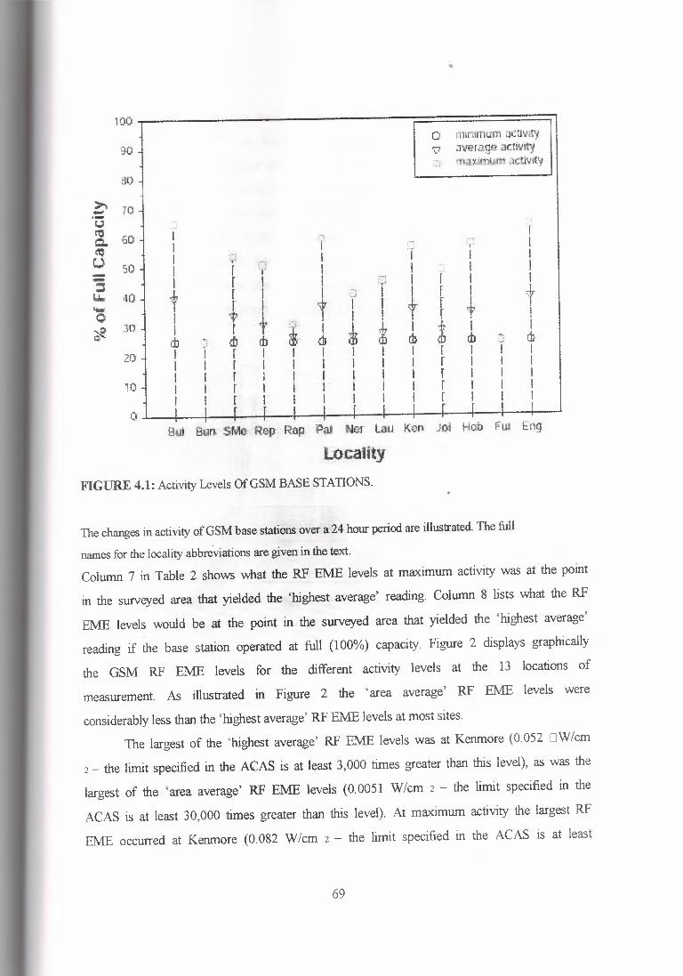
100

90

so ~ 70 - - C.) 11'- 60 a. ~ o 50- - - ~ I.I,.; ,10 ;_, 0

* ~()

20

io

Q

o m1t1ifr1uin .ieuv1iy 'v' mrerag:e acti•lit)' :r rr\tt:w;olthtl i'.lttl~11t1,

1 I I I I l r J I I I

· 1 I

·"'·"· ·r I I I I

I' I I I I t I I ili I I I I I

I I I I I t I I d) I I I I I

;~ T I I I k r I r.h I I I I I

I I I I

+ I iD I I I I I

!._i '<-i'"

f r r '1' r dJ r f r r r

9 I I I

+ d) I I l I r

r r r r t r r r r r

P1

T r I * .d) I I I I I

,] r I i I I I i I

l I I I I

. .. B.ul E!iu.1 :SJv1~··RC\P:·RafJ fl,a,i Ner Lau Ken ~- Hoo Fua Eng

:L-····o< ··-~a:iitt, . ·. )··_ ... _· .. -'.~' _ .. ~~-~,,-.

FIGURE 4.1: Activity Levels Of GSM BASE STATIONS.

The changes in activity of GSM base stations over a 24 hour period are illustrated The full

names for the locality abbreviations are given in the text. Column 7 in Table 2 shows what the RF EME levels at maximum activity was at the point

in the surveyed area that yielded the 'highest average' reading. Column 8 lists what the RF

EME levels would be at the point in the surveyed area that yielded the 'highest average'

reading if the base station operated at full (100%) capacity. Figure 2 displays graphically

the GSM RF EME levels for the different activity levels at the 13 locations of

measurement. As illustrated in Figure 2 the 'area average' RF EME levels were

considerably less than the 'highest average' RF EME levels at most sites.

The largest of the 'highest average' RF EME levels was at Kenmore (0.052 OW/cm

2 - the limit specified in the ACAS is at least 3,000 times greater than this level), as was the

largest of the 'area average' RF EME levels (0.0051 W/cm 2 - the limit specified in the

ACAS is at least 30,000 times greater than this level). At maximum activity the largest RF

EME occurred at Kenmore (0.082 W/cm 2 - the limit specified in the ACAS is at least

69

•

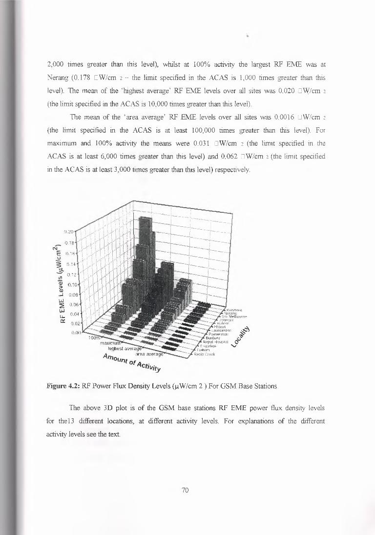
2,000 times greater than this level), whilst at 100% activity the largest RF EME was at

Nerang (0.178 OW/cm 2 - the limit specified in the ACAS is 1,000 times greater than this

level). The mean of the 'highest average' RF EME levels over all sites was 0.020 OW/cm 2

(the limit specified in the ACAS is 10,000 times greater than this level).

The mean of the 'area average' RF EME levels over all sites was 0.0016 OW/cm 2

( the limit specified in the ACAS is at least 100,000 times greater than this level). For

maximum and 100% activity the means were 0.031 OW/cm 2 (the limit specified in the

ACAS is at least 6,000 times greater than this level) and 0.062 OW/cm 2 (the limit specified

in the ACAS is at least 3,000 times greater than this level) respectively.

Figure 4.2: RF Power Flux Density Levels (µ W /cm 2 ) For GSM Base Stations.

The above 3D plot is of the GSM base stations RF EME power flux density levels

for the13 different locations, at different activity levels. For explanations of the different

activity levels see the text.

70

•

4.8 Fixed Site Eenviromental RF EME Levels From Various Signal Sources

Table 3 lists the average fixed site environmental RF EME power flux density

levels over a six minute scanning period for the different signal sources at the 14 base

stations. In this report the reference to RF EME levels always implies power flux density

levels µ W/cm 2 .

The RF EME power flux density levels in Table 3 are given to four decimal places

to make it easier for comparison of signal levels.

At the bottom of Table 3 the mean levels and standard deviation (SD) are given, as

well as the number of sites (N) where signals were detected. It is emphasized that the

environmental RF EME levels are only given as a guide. Except for GSM, the distances

from the signal sources of the RF EME power flux density measurements were not known

or considered. Hence, if the TV or Radio broadcasting transmitter was very distant then this

may underestimate the typical population exposure to those RF sources.

Likewise, if the broadcasting transmitters were very close, such as the FM

transmitter at Palmerston, then this may overestimate the typical population exposure to

those RF sources. Generally, transmitter TV and radio towers tend to be much higher and

further away from population areas than base stations. Also, with these other RF sources

the wavelength of the RF EME radiation is longer and there is a more uniform distribution

of the signal. Figure 3 is a presentation of the environmental RF EME levels of all the

signal sources, at the 14 locations of measurements.

Figure 4 shows the same data as in Figure 3, except that the RF EME levels for AM

radio have been excluded so as to show more clearly the RF EME levels produced by high

frequency sources. As is illustrated in Figure 3, AM radio signals were the dominant signal

source over all the other signal sources combined in 11 of the 14 sites of measurement, and

m seven of these localities AM radio contributed >95% of the total RF EME (i.e., at

Bulleen, Bunbury, Fulham, Jolimont, Launceston, Repatriation Hospital, South

Melbourne).

At Palmerston the FM radio RF EME level was considerably greater than the AM

radio RF EME level, ontributing 93% of the total RF EME. At Nerang and Engadine the

GSM base stations contributed 67% and 63% respectively of the total RF EME at these

71

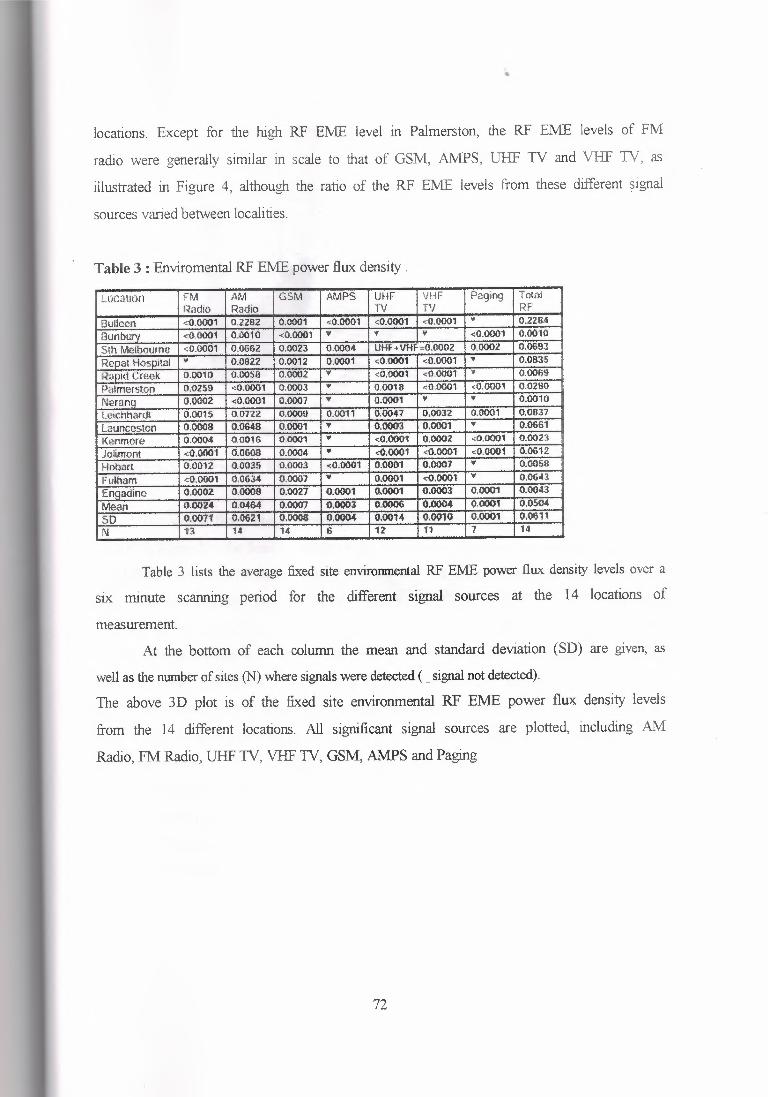
locations. Except for the high RF E.ME level in Palmerston, the RF EME levels of FM

radio were generally similar in scale to that of GSM, AMPS, UHF TV and VHF TV, as

illustrated in Figure 4, although the ratio of the RF EME levels from these different signal

sources varied between localities.

Table 3: Enviromental RF EME power flux density.

Locaunn FM AM GSM AMPS UHF VHF Pnging Total Radio Radio rv TV RF

Bu Ileen <0.0001 0.2282 0.0001 -e0.0001 -~0.0001 -<.0.0001 ..• 0228.4

Bunb-Uf'I <:0.0001 0.0010 <0.0001 • 'f ., <0.0001 0.0010

Slh Melbourne r.0.0001 0.060.2 0.0023 0.0004, UHF +-VHF :0;0002 0.0002 0.0693

Renat Hosaital •• 0.0822 0.0012 OJ)001 <0.0001 <0.0001 " 0.0835

R,mid Cm<ik 0.0010 0.0058 0.000.: ... <'.0,0001 <:.Q.0001 ... 0.0069

Palmer5ton 0.0259 ,:0.000"1 0.0003 • 0.0018 <11.0001 <0.0001 0.0280

Neranq 0.0002 <0.0001 0.0007 ... 0.0001 • ... 0.0010

Leiehhardt 0.0015 0.0722 0.0009 0.0011 0.0047 0.0032 0.0001 0.0837

Launceston 0.0008 0.0648 0.0001 .,. 0.0003 0.0001 " 0.0661

Ke·nm.om 0.0004 0.0016 0.000, " <O.OO<tl 0.0002 ,:0,0001 0.0023

Jolimont <0.0001 0.0008 0.0004 • <0.0001 <0.0001 <0.0001 0.0012

Hobart 0.0012 0.0035 0.0003 <0:0001 0.0001 0.0007 ... 0.0058

Fl:llham d).()001 0.0634 0.0007 ,; 0.0001 ,cQ,00()1 ... 0,0643

Enqadine 0.0002 0.0008 0.0027 ,0.0001 0.0001 0.0003 0.0001 0.0043

Mean 0.0024 0.04l>4 0.0007 0.0003 0.0006 0.0004 0.0001 Q,0504

so o.oon 0;{)621 0.0008 0,00(),f o:oot-4 O.WIO 0.0001 0.0011

N 13 14 14 6 12 11 7 14

Table 3 lists the average fixed site enviromnental RF EME power flux density levels over a

six minute scanning period for the different signal sources at the 14 locations of

measurement.

At the bottom of each column the mean and standard deviation (SD) are given, as

well as the mnnber of sites (N) where signals were detected (_signal not detected).

The above 3D plot is of the fixed site environmental RF EME power flux density levels

from the 14 different locations. All significant signal sources are plotted, including AM

Radio, FM Radio, UHF TV, VHF TV, GSM, AMPS and Paging

72

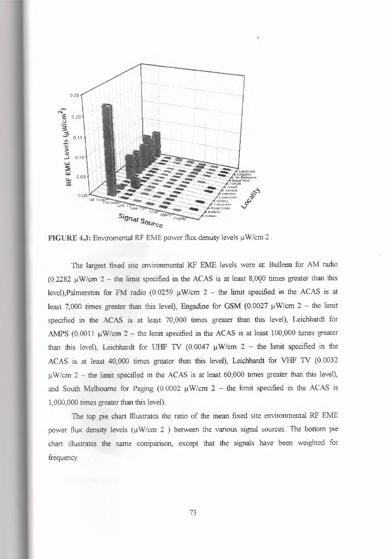
FIGURE 4.3: Enviromental RF EME power flux density levels µ W /cm 2 .

The largest fixed site environmental RF EME levels were at: Bulleen for AM radio

(0.2282 µ W/cm 2 - the limit specified in the ACAS is at least 8,0QO times greater than this

level),Palmerston for FM radio (0.0259 µW/cm 2 - the limit specified in the ACAS is at

least 7,000 times greater than this level), Engadine for GSM (0.0027 µW/cm 2 - the limit

specified in the ACAS is at least 70,000 times greater than this level), Leichhardt for

AMPS (0.0011 µW/cm 2 - the limit specified in the ACAS is at least 100,000 times greater

than this level), Leichhardt for UHF TV (0.0047 µ W/cm 2 - the limit specified in the

ACAS is at. least 40,000 times greater than this level), Leichhardt for VHF TV (0.0032

µ W/cm 2 - the limit specified in the ACAS is at least 60,000 times greater than .this level),

and South Melbourne for Paging (0.0002 µW/cm 2 - the limit specified in the ACAS is

1,000,000 times greater than this level).

The top pie chart Illustrates the ratio of the mean fixed site environmental RF EME

power flux density levels (µW/cm 2 ) between the various signal sources. The bottom pie

chart illustrates the same comparison, except that the signals have been weighted for

frequency.

73

"

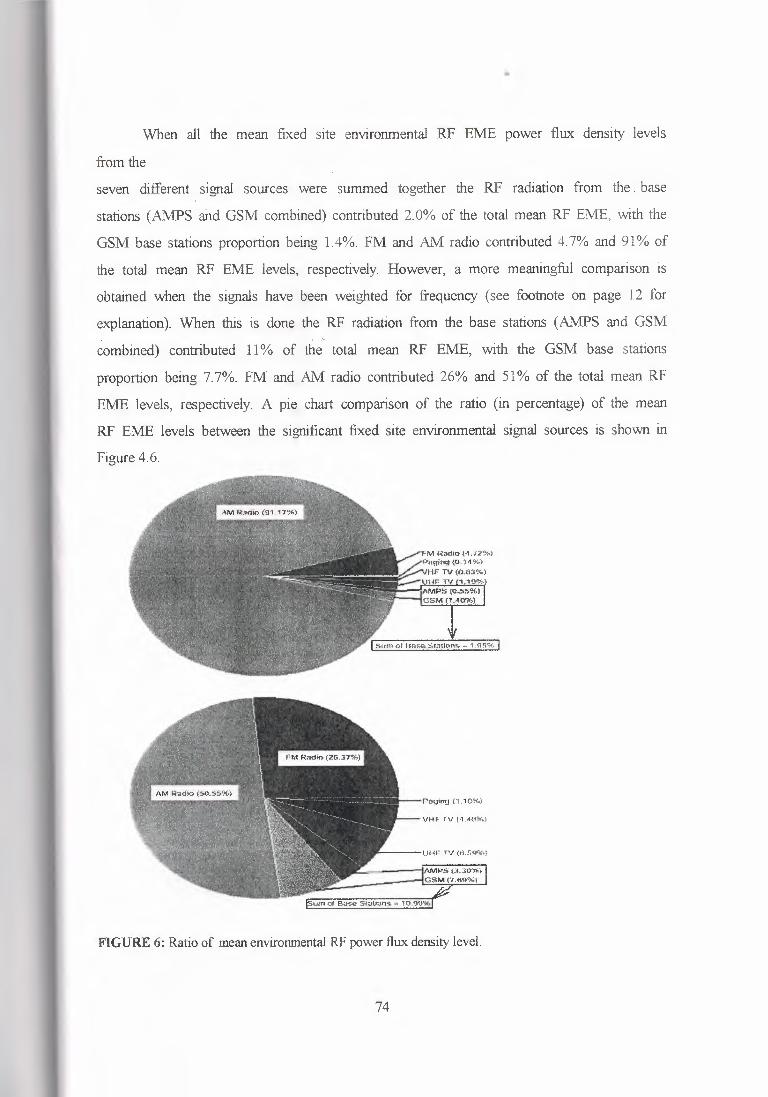
When all the mean fixed site environmental RF E.ME power flux density levels

from the

seven different signal sources were summed together the RF radiation from the . base

stations (AMPS and GSM combined) contributed 2.0% of the total mean RF EME, with the

GSM base stations proportion being 1.4%. FM and AM radio contributed 4.7% and 91% of

the total mean RF E.ME levels, respectively. However, a more meaningful comparison is

obtained when the signals have been weighted for frequency (see footnote on page 12 for

explanation). When this is done the RF radiation from the base stations (AMPS and GSM ., .

combined) contributed 11 % of the total mean RF EME, with the GSM base stations

proportion being 7.7%. FM and AM radio contributed 26% and 51 % of the total mean RF

EME levels, respectively. A pie chart comparison of the ratio (in percentage) of the mean

RF EME levels between the significant fixed site environmental signal sources is shown in

Figure 4.6.

VHF TV [•1.-<0%)

.fu\i'\PS (3-.30%) GSM(7.n9%i

FIGURE 6: Ratio of mean environmental RF power flux density level.

74

CONCLUSION

Base stations use the broadcast · control channel to transmit the information that

terminals need to set up a call, including the control channel BCCH transmits. one

message segment ,Adjacent cells have different frequencies to prevent interference and

power levels are kept to a minimum to ensure no interference with non-adjacent cells,

which use the same frequency. The size of the cell varies depending on the number of

users. In rural areas, which typically cover large regions due to the sparse population,

more power has to be generated to cover the larger area.

The goal of this study was to determine the RF EME level resulting from all signal

frequencies produced by the particular GSM base stations under survey. Mobile

telephone communication signals are both transient and partly random in their

occurrence and distribution. we were interested in determining the RF EME levels at

many locations and more particularly .

75

REFERENCES

1. Chia ( Second generation mobile radio systems) november 1994.

2. ( cellular system ) , gardiner . j .D .

3. Joseph Schiller. (2000). Mobile communication . Prentice Hall.

4. Vigay Gag, (1996). Wireless and personal communication systems.

5. Theodores S.Rappaport .Wireless communication systems.

6. Mertin Nemzow .(1989).Implementing wireless networks.Mc Graw-Hill.

7. Mehrorta , A Celluler Radio Analog & Digital systems , Boston -London :

Artech House. 1994.

8. · Viterbi. AJ ( Base Stations and wireless systems) IEEE commmunication

magazine (December 1992) 30 no.

76