Factors affecting the evolution of mimicry

Matthew John Wheelwright

Thesis submitted for the degree of Doctor of Philosophy

Centre for Behaviour and Evolution

Biosciences Institute

Newcastle University

February 2020

i

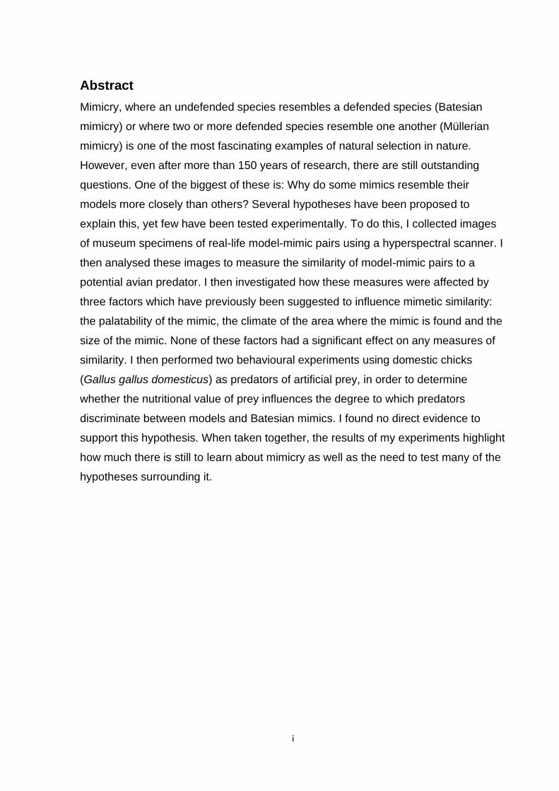
Abstract

Mimicry, where an undefended species resembles a defended species (Batesian

mimicry) or where two or more defended species resemble one another (Müllerian

mimicry) is one of the most fascinating examples of natural selection in nature.

However, even after more than 150 years of research, there are still outstanding

questions. One of the biggest of these is: Why do some mimics resemble their

models more closely than others? Several hypotheses have been proposed to

explain this, yet few have been tested experimentally. To do this, I collected images

of museum specimens of real-life model-mimic pairs using a hyperspectral scanner. I

then analysed these images to measure the similarity of model-mimic pairs to a

potential avian predator. I then investigated how these measures were affected by

three factors which have previously been suggested to influence mimetic similarity:

the palatability of the mimic, the climate of the area where the mimic is found and the

size of the mimic. None of these factors had a significant effect on any measures of

similarity. I then performed two behavioural experiments using domestic chicks

(Gallus gallus domesticus) as predators of artificial prey, in order to determine

whether the nutritional value of prey influences the degree to which predators

discriminate between models and Batesian mimics. I found no direct evidence to

support this hypothesis. When taken together, the results of my experiments highlight

how much there is still to learn about mimicry as well as the need to test many of the

hypotheses surrounding it.

ii

Acknowledgments

This thesis would not have been possible without the help and support of so

many people, so I would like to take the opportunity to thank all of them here. First, I

would like to thank my supervisors: John Skelhorn, Candy Rowe and Julie Harris

whose endless support, guidance and patience have been a blessing throughout my

PhD. Thank you to Christina Halpin, Diana Umeton, Grace Holmes, Thomas Carle

and Jasmine Clarkson for making me feel so welcome in the lab and special thanks

to Christina, Diana, Grace and Vicky Comer for helping me to collect my

hyperspectral scans. I would also like to thank Olivier Penacchio who, not only

helped to collect scans, but also provided me with the code to allow me to carry out

the energy-isotropy analysis and whose advice on how to use it was invaluable. On

top of this, I would also like to thank Cassie Stoddard for allowing me to use and

providing me with the code to carry out the NaturePatternMatch analysis. Thank you

to Jenny Read and Daniel Nettle for their advice during progression panel meetings

and George Lovell and Innes Cuthill for their advice during grant meetings. Thank

you to Terri-Ann Badcock, Julie Lees and Michelle Waddle for helping me to look

after the chicks and for their advice on how to best care for them. I must also express

my gratitude to the curatorial staff from all of the collections I worked with, for not only

taking the time to find the specimens I needed but also finding space for me to scan

on site when I needed to, so thank you to: Dan Gordon and Erin Slack at the

Discovery Museum, Geoff Martin at the Natural History Museum, London, Dmitri

Logunov and Phil Rispin at the Manchester Museum and to Courtney Richenbacher

and David Grimaldi of the American Museum of Natural History. I would also like to

thank Ann Fitchett and Beckie Hedley for being able to answer every question I had

about administration and general day-to-day life in the Institute. I would also like to

thank Léa, Ismet, Alban, Coline, Beshoy, Janire, Stu, Thomas, Matthieu and

everyone in the Lunch Group for keeping me sane these past three years and for

making this a truly fantastic place to work, I have made many wonderful friends whilst

working here and this has made it a truly special experience. Last but by no means

least, I would like to thank my family and friends back home, particularly my parents,

for their love, support and encouragement and above all else putting up with my love

of bugs throughout my life, even when that meant that they ended up in the house!

iii

iv

Contents

Abstract .................................................................................................................................................... i

Acknowledgments ................................................................................................................................... ii

Contents ................................................................................................................................................. iv

List of tables, figures and equations ....................................................................................................... vii

Chapter 1: What do we know about mimicry? ....................................................................................... 1

1.1: Introduction .................................................................................................................................. 1

1.2: The evolution of Batesian mimicry ............................................................................................... 3

1.3: The evolution of Müllerian mimicry ............................................................................................. 6

1.4: Has mimicry been proven to reduce predation? ....................................................................... 11

1.5 Why are some mimics imperfect? ............................................................................................... 12

1.6: What factors might influence similarity between models and mimics? .................................... 14

1.7: What features have been shown to be important to mimic in order for a mimic to be

“successful”? ..................................................................................................................................... 16

Chapter 2: Techniques for measuring pattern similarity ...................................................................... 18

2.1: Introduction ................................................................................................................................ 18

2.2: Measures of colour similarity ..................................................................................................... 19

2.2.1: The Receptor Noise-Limited (RNL) model ........................................................................... 20

2.3: Measures of pattern similarity ................................................................................................... 23

2.3.1: Measures based on absolute similarity ............................................................................... 24

2.3.2: Measures based on early visual processing ........................................................................ 29

2.3.3: Measures based on higher visual processing ...................................................................... 32

2.4: Measures of spatiochromatic similarity ..................................................................................... 34

2.4.1: Adjacency analysis and Boundary Strength Analysis ........................................................... 34

2.4.2: HMAX with Colour Opponency............................................................................................ 37

2.5: Conclusions and future questions .............................................................................................. 37

Chapter 3: General Methods ................................................................................................................. 38

3.1: Introduction ................................................................................................................................ 38

3.2: Selection of study species for image analyses ........................................................................... 39

3.2.1: Selection of models and mimics .......................................................................................... 39

3.2.2: Selection of sympatric, non-mimicked, aposematic species ............................................... 39

3.3: Scanning the specimens ............................................................................................................. 41

3.3.1: Locating the specimens to scan ........................................................................................... 41

3.3.2: Selecting the specimens to scan .......................................................................................... 42

3.3.3: Scanning the specimens ...................................................................................................... 43

v

3.3.4: Calibrating the hyperspectral camera ................................................................................. 44

3.3.5: Additional data for each specimen ..................................................................................... 46

3.4: Image analysis ............................................................................................................................ 46

3.4.1: Colour analysis .................................................................................................................... 46

3.4.2: Pattern analysis ................................................................................................................... 47

3.5: Selecting diagnostics for study ................................................................................................... 49

3.5.1: Methods .............................................................................................................................. 50

3.5.2: Results ................................................................................................................................. 50

Chapter 4: The effect of palatability on the evolution of mimics and models ..................................... 53

4.1: Introduction ............................................................................................................................... 53

4.2: Methods ..................................................................................................................................... 56

4.2.1: Is there a difference in mimetic similarity between Batesian and Müllerian mimicry? ..... 56

4.2.2: Do Batesian mimics affect the evolution of their models? ................................................. 58

4.3: Results ........................................................................................................................................ 59

4.3.1: Is there a difference in similarity between Batesian and Müllerian mimics? ..................... 59

4.3.2: Do Batesian mimics affect the evolution of their models? ................................................. 61

4.4: Discussion ................................................................................................................................... 63

4.4.1: The effect of palatability on the evolution of mimics ......................................................... 63

4.4.2: The effect of mimics on the evolution of their models ....................................................... 67

4.4.3: Overall conclusions ............................................................................................................. 69

Chapter 5: The effect of ambient temperature on the evolution of mimicry ...................................... 70

5.1: Introduction ............................................................................................................................... 70

5.2: Methods ..................................................................................................................................... 72

5.3: Results ........................................................................................................................................ 77

5.4: Discussion ................................................................................................................................... 82

Chapter 6: The effect of size on mimetic similarity .............................................................................. 88

6.1: Introduction ............................................................................................................................... 88

6.1.1: The absolute size of a mimic affects the degree of pattern similarity between mimics and

their models .................................................................................................................................. 90

6.1.2: The size of a mimic relative to its model affects the degree of pattern similarity between

mimics and their models ............................................................................................................... 90

6.1.3: The difference in size between mimics and their models affects the degree of pattern

similarity between mimics and their models ................................................................................ 91

6.2: Methods ..................................................................................................................................... 92

6.2.1: Measuring the size of the mimics ....................................................................................... 93

6.3: Results ........................................................................................................................................ 95

6.3.1: Does the absolute size of a mimic affect the degree of pattern similarity between mimics

and their models? ......................................................................................................................... 95

vi

6.3.2: Does the size of a mimic relative to its model affect the degree of pattern similarity

between mimics and their models? .............................................................................................. 97

6.3.3: The difference in size between mimics and their models affects the degree of pattern

similarity between mimics and their models ................................................................................ 99

6.4: Discussion ................................................................................................................................. 101

Chapter 7: The effect of nutritive value on predation risk for a mimic ............................................... 105

7.1: Introduction .............................................................................................................................. 105

7.2: Methods ................................................................................................................................... 107

7.2.1: Chick husbandry ................................................................................................................ 107

7.2.2: Experimental arena ........................................................................................................... 108

7.2.3: Artificial Prey ..................................................................................................................... 109

7.2.4: Experiment 1 training trials ............................................................................................... 110

7.2.5: Experiment 1 test trials ..................................................................................................... 110

7.2.6: Experiment 1 statistical analyses....................................................................................... 111

7.2.7: Experiment 2 training trials ............................................................................................... 112

7.2.8: Experiment 2 test trials ..................................................................................................... 112

7.2.9: Experiment 2 statistical analyses....................................................................................... 113

7.3: Results ...................................................................................................................................... 114

7.3.1: Experiment 1 ..................................................................................................................... 114

7.3.2: Experiment 2 ..................................................................................................................... 117

7.4: Discussion ................................................................................................................................. 120

7.5: Conclusions ............................................................................................................................... 123

Chapter 8: General conclusions ........................................................................................................... 124

8.1: What makes an effective mimetic signal? ................................................................................ 124

8.2: Which abiotic and biotic factors affect how closely mimics evolve to resemble their

aposematic models? ........................................................................................................................ 125

8.3: Do palatable mimics affect the evolution of the pattern of their aposematic models? .......... 127

8.4: Future research directions ....................................................................................................... 128

8.5: Concluding remarks .................................................................................................................. 129

References ........................................................................................................................................... 131

Appendix A .......................................................................................................................................... 166

Appendix B ........................................................................................................................................... 173

Appendix C ........................................................................................................................................... 180

vii

List of tables, figures and equations

List of Tables

Table 3.1. Trios of models, mimics and sympatric, non-mimicked species which I scanned. …………………………………………………………………………………………………………….……….… 42

Table 5.1. The minimum monthly temperatures for the regions where the mimics are found. ………………….………………………………………………………………………………………….……………. 75

Table 5.2. The mean monthly temperatures for the regions where the mimics are found. ………………………………………………………………………………………………………………………………….……. 76

Supplementary Table 1. Experimentally proven mimics. ……………………………………… 166

Supplementary Table 2. All of the pattern diagnostics which I looked at as potential measures of similarity……………………………………………………………………………………….…………. 173

Supplementary Table 3. Sizes of the hoverflies and models studied in Penney et al. (2012). ……………………………………………………………………………………………………………………….. 180

List of Figures

Figure 1.1. A comparison of a) advergent evolution and b) convergent evolution in mimicry systems. …………………………………………………………………………………………………………. 9

Figure 1.2. A graphical representation of the relative abundance of models and mimics

over time. ………………………………………………………………………………………………………................. 10

Figure 2.1. An example of distance transform based on Figure 2 of Taylor et al. (2013).

………………………………………………………………………………………………………………………………………… 27

Figure 2.2. The box-counting method demonstrated on the monarch butterfly (Danaus

plexippus). ……………………………………………………………………………………………………………………. 28

Figure 2.3. An image of Thermidarctia thermidoides and its corresponding amplitude

spectrum. ……………………………………………………………………………………………………………………… 29

Figure 2.4. Example of a) a low isotropy pattern and b) a high isotropy pattern ……. 31

Figure 2.5. A zone map based on the pattern of Thermidarctia thermidoides. ………. 36

Figure 2.6. The transition matrix based on the sampling grid from Figure 2.5. ……… 36

Figure 3.1. A flow-chart depicting the method used to decide whether or not to classify a species as a sympatric, non-mimicked, aposematic species. …………………………….. 41

Figure 3.2. A photo of the hyperspectral camera and the stage. .………………………….. 44

Figure 3.3. An illustration for the method of estimating the importance of a given pattern

diagnostic for mimicry. ……………………………………………………………………………………………..… 52

viii

Figure 4.1. The degree of difference (based on the standard deviation of the blue-

yellow ((L+M) vs S) opponent channel response) between models and Batesian

mimics and Müllerian mimics. ..………………………………………………………………………….……….. 60

Figure 4.2. The degree of difference (based on the mean pattern energy from cells of

Scale 10) between models and Batesian mimics and Müllerian mimics. ………………. 60

Figure 4.3. The degree of similarity (based on NaturePatternMatch) between models

and Batesian mimics and Müllerian co-mimics. …………………………………………….…………. 61

Figure 4.4. The mean pattern energy of Batesian models and their sympatric, non-

mimicked aposematic species (SNMAS). ………………………………………………………………... 62

Figure 4.5. The standard deviation of isotropy departure of Batesian models and their

sympatric, non-mimicked aposematic species (SNMAS). ……………………………………… 62

Figure 5.1. The relationship between the difference in the standard deviation of the blue-yellow ((L+M) vs S) opponent channel between models and mimics and the mean flight temperature of the mimic. …………………………………………………………………….………..... 78

Figure 5.2. The relationship between the difference in the mean energy differences (for cells of Scale 10) between models and mimics and the mean flight temperature of the mimic. …………………………………………………………………………………………………………………….……. 78

Figure 5.3. The relationship between the similarity scores of models and mimics (based on NaturePatternMatch) and the mean flight temperature of the mimic. ………………. 79

Figure 5.4. The relationship between the difference in the standard deviation of the blue-yellow ((L+M) vs S) opponent channel between models and mimics and the minimum flight temperature of the mimic. …………………………………………………………….…. 79

Figure 5.5. The relationship between the difference in the mean energy differences (for cells of Scale 10) between models and mimics and the minimum flight temperature of the mimic. ………………………………………………………………………………………………………………...….. 80

Figure 5.6. The negative correlation between the similarity scores of models and mimics (based on NaturePatternMatch) and the minimum flight temperature of the mimic. ………………………………………………………………………………………………………………………….. 80

Figure 5.7. The relationship between the difference in the standard deviation of the blue-yellow ((L+M) vs S) opponent channel between models and mimics and the control minimum flight temperature of the mimic. ………………………………………….……….. 81

Figure 5.8. The relationship between the difference in the mean energy differences (for cells of Scale 10) between models and mimics and the control minimum flight temperature of the mimic. ……………………………………………………………………………………….…. 81

Figure 5.9. The negative correlation between the similarity scores of models and mimics (based on NaturePatternMatch) and the control minimum flight temperature of the mimic. ………………………………………………………………………………………………….……………….… 82

Figure 6.1. The correlation between mean wing area (mm2) and the mean body volume (mm3) of each mimic. ……………………………………………………………………………………….……….... 94

ix

Figure 6.2. The correlation between mean wing area (mm2) and the difference in the standard deviation of the blue-yellow ((L+M) vs S) opponent channel response. …. 95

Figure 6.3. The correlation between the mean wing area (mm2) and the difference in mean energy (for cells of Scale 10). …………………………………………………….…………………….. 96

Figure 6.4. The correlation between the mean wing area (mm2) and the similarity score (based on NaturePatternMatch). ……………………………………………………….……..………………. 96

Figure 6.5. The correlation between the wing area of the mimic relative to its model (%) and the difference in the standard deviation of the blue-yellow ((L+M) vs S) opponent channel response. …………………………………………………………………………...….……. 97

Figure 6.6. The correlation between the wing area of the mimic relative to its model (%) and the difference in mean energy (for cells of Scale 10). ……………………..………. 98

Figure 6.7. The correlation between the wing area of the mimic relative to its model (%) and the similarity score (based on NaturePatternMatch). …………………………...….. 98

Figure 6.8. The correlation between the percentage difference in wing area between mimics and their models (%) and the difference in the standard deviation of the blue-yellow ((L+M) vs S) opponent channel response. …………………………………………...……… 99

Figure 6.9. The correlation between the percentage difference in wing area between mimics and their models (%) and the difference in the mean energy (for cells of Scale 10). ……………………………………………………………………...………………………………………………………. 100

Figure 6.10. The correlation between the percentage difference in wing area between mimics and their models (%) and the similarity score (based on NaturePatternMatch). ……………………………………………………………………………………..………………………………………………… 100

Figure 7.1. The artificial prey used in this experiment: a) Training stimulus, b) Profitable “control”, c) Unprofitable “model” and d) the Imperfect “mimic”. …………………………….. 110

Figure 7.2. The mean percentage of prey attacked which belonged to each type in each trial during Experiment 1. ……………………………………………………………………………………….…. 115

Figure 7.3. The mean difference between the percentage of mimics and models attacked during Experiment 1 and how this differed between the two reward groups. ……………………………………………………………………………………………………………………….………………. 116

Figure 7.4. The mean difference between the percentage of controls and mimics

attacked during Experiment 1 and how this differed between the two reward groups.

………………………………………………………………………………………………………………………….…….……... 117

Figure 7.5. The mean percentage of prey attacked which belonged to each type in each trial during the discrimination training period of Experiment 2. ……………………………….. 119

Figure 7.6. The mean percentage of prey attacked which belonged to each type in each trial during the test period of Experiment 2. …………………………………………………….……….. 119

x

Figure 7.7. The mean difference between a) the percentage of mimics and models attacked and (b) the percentage of controls and mimics attacked during the test period of Experiment 2 and how this differed between the two reward groups. ………….…… 120

List of equations

Equation 2.1. Equation to calculate the quantum catch of a photoreceptor. ……….…. 21

Equation 2.2. Equation to calculate von Kries adaptation coefficient of a photoreceptor.

…………………………………………………………………………………………………………………………………….…... 21

Equation 2.3. Equation to calculate the difference between two colours in a trichromatic

colour space based on the RNL model. …………………………………………………………..…………. 21

Equation 2.4. Equation to calculate the standard deviation of noise in a photoreceptor.

……………………………………………………………………………………………………………………………….………… 22

Equation 2.5. Equation to calculate the fractal dimension of a pattern. ………………….. 25

Equation 2.6. Equation to calculate the similarity of two images based on

NaturePatternMatch……………………………………………………………………………………………………….. 33

Equation 6.1. Equation to estimate body volume of a Lepidopteran. ……………...………. 93

1

Chapter 1: What do we know about mimicry?

Batesian and Müllerian mimicry provide beautiful examples of co-evolution and

provide insight into many areas of research from genetics and evolutionary ecology

to behavioural ecology and predator cognition. As such, mimicry has fascinated

scientists for over a century, and has been the subject of hundreds of studies. The

aim of this chapter is to introduce the concepts of Batesian and Müllerian mimicry, to

summarise what has been discovered about mimicry in the past 150 years and to

highlight some of the questions which have yet to be answered.

1.1: Introduction

Many animals have evolved colour patterns which help them to avoid

predation; they can achieve this through several different strategies. The first, and

most obvious, is to be camouflaged. This can be achieved in two ways: by using

cryptic patterns that make prey difficult to detect when viewed against their natural

background (Stevens and Merilaita 2009; Skelhorn and Rowe 2016; Merilaita et al.

2017), or by masquerading as inedible objects found in the local environment, such

as stones, dead leaves or sticks (Skelhorn et al. 2010a; Skelhorn et al. 2010b;

Skelhorn et al. 2015). An alternative approach is to use aposematism, a strategy

whereby prey use conspicuous and colourful patterns to advertise the presence of

secondary defences (Poulton 1890), such as distasteful and/or toxic chemicals

(Eisner and Eisner 1991) or physical defences like hard elytra (Wang et al. 2018),

spines (Inbar and Lev-Jadun 2005; Speed and Ruxton 2005) or irritating hairs

(Sandre et al. 2007). For example, the dazzling array of different colour patterns

seen in poison dart frogs advertise the fact that they possess potent toxins (Wang

and Shaffer 2008), and the yellow and black stripes seen in several species of

Hymenoptera advertise their painful stings and distasteful venom (Marchini et al.

2017). These bright colours benefit prey because they help to improve avoidance

learning by predators (Gittleman et al. 1980; Roper and Redston 1987), are more

memorable (Roper and Redston 1987) and even elicit innate aversions in naïve

predators (Schuler and Hesse 1985; Penacchio et al. in prep.).

Around 150 years ago, Henry Walter Bates realised that some species of

Amazonian butterflies were completely palatable despite having these bright warning

colours. He hypothesised that these species had evolved to resemble sympatric

2

aposematic species and, in doing so, benefited from reduced predation due to the

local predators mistaking them for the defended prey they resembled (Bates 1862).

This phenomenon later became known as Batesian mimicry. Some 16 years later,

Fritz Müller discovered that it was not just palatable species that mimicked

aposematic species. He realised that some groups of aposematic species had also

evolved to share the same colour pattern. In one of the first mathematical models

used in evolutionary ecology, he demonstrated that this resemblance could benefit

all of the species involved, because the cost of educating a predator to avoid the

colour pattern was shared by the co-mimics (Müller 1878). This defensive strategy

was named in his honour and became known as Müllerian mimicry. While the

palatability of the mimic may seem like a subtle difference between these two kinds

of mimicry, it is thought to lead to major differences in the evolutionary dynamics of

the two types of mimetic complexes (Sections 1.2 and 1.3) since models of Batesian

mimics should evolve away from their mimics (Fisher 1930), while Müllerian co-

mimics should evolve towards one another (Turner 1987) (Figure 1.1). This

difference in dynamics could, in turn, lead to differences in the mimetic similarity

between Batesian mimics and their models and Müllerian mimics and their co-

mimics (Rettenmeyer 1970) (This idea is tested in Chapter 4), although this idea is

complicated somewhat by quasi-Batesian mimics, which are mimics which are

defended but to a lesser extent than their model which means that their evolutionary

dynamics more closely resemble Batesian mimics than true Müllerian mimics (Speed

1993) (this is also discussed further in Chapter 4).

Despite these differences, both Batesian and Müllerian mimicry have sparked

the interests of researchers from a range of disciplines across biology. This is partly

due to the fact that mimicry provides an excellent system in which to study both

evolution and coevolution. As such, it can provide insight into a range of topics from

the genes (Nadeau et al. 2016) and pigments (Kikuchi and Pfennig 2012; Kikuchi et

al. 2014) involved in controlling pattern phenotypes to the kinds of cues predators

use when discriminating between profitable and unprofitable prey items. Moreover,

mimicry has been observed not only in the visual domain (Kikuchi and Pfennig

2010a) but also in other sensory modalities such as olfaction (Malcicka et al. 2015)

and audition (Barber and Conner 2007). However, due to the fact that most mimicry

research focuses on mimicry in the visual domain, this will be the focus of my thesis.

3

I have three main aims: (1) To understand what makes an effective mimetic signal,

(2) to explore which biotic and abiotic factors affect how closely a mimic evolves to

resemble its model and (3) to find out whether palatable mimics affect the evolution

of their aposematic models. But in order to do this, we must first understand how

mimicry evolves.

1.2: The evolution of Batesian mimicry

There are three main ways hypotheses that seek to explain how Batesian

mimicry evolves. The first states that the patterns of mimics evolve in one major

evolutionary step (Punnett 1915). The second assumes that such a leap would be

incredibly unlikely, and so posits that it is much more plausible that the patterns of

mimics gradually evolve to match their models over time (Fisher 1927). The third,

which is known as the two-step hypothesis (Nicholson 1927), suggests that a cryptic

species experiences a major phenotypic shift in its pattern which makes it more

similar to a sympatric aposematic species thus making it an imperfect mimic of that

species. Then the pattern gradually evolves in such a way that the mimic resembles

the model much more closely over time (Nicholson 1927). This suggests that

Batesian mimicry evolves via a combination of the first two proposed mechanisms.

This final hypothesis is currently the most widely accepted model for the

evolution of Batesian mimicry. One reason for this is that the two alternative

hypotheses are implausible. As stated above, the chances of a single mutation

resulting in perfect mimicry are infinitesimally small. Moreover, it also seems unlikely

that mimicry could evolve gradually. If a species were to gradually evolve from a

cryptic ancestral state to a mimetic state, individuals would likely experience an initial

decline in their survival known as a ‘fitness valley’ (Balogh et al. 2010; Kikuchi and

Pfennig 2010b). This is because if a cryptic species becomes gradually more

conspicuous (as it must do if it is to resemble the brightly-coloured model), it will

initially experience higher levels of predation because it is both easier to find than its

cryptic ancestors but it does not resemble the model closely enough to gain any

protection from mimicry. Indeed, this has been demonstrated in laboratory-based

behavioural experiments where avian predators search for artificial prey (Mappes

and Atalato 1997). In these experiments, birds were presented with a set of 5

artificial prey types which varied from background-matching “cryptic stimuli” to stimuli

which were a “perfect mimic” of a conspicuous defended model which the birds had

4

previously learned to avoid. The birds attacked the imperfectly cryptic prey (i.e. those

that had become more conspicuous but did not yet resemble models) more often

than any other prey type (Mappes and Atalato 1997), indicating that the initial

mimetic mutants would have to show a reasonable degree of resemblance to their

models in order to be favoured by selection. This lends support to the two-step

model whereby initial mimetic mutants show a large jump in phenotype towards a

sympatric aposematic species and consequently should avoid the fitness valley. This

phenotypic leap is known as feature saltation (Balogh and Leimar 2005; Balogh et al.

2010; Gamberale-Stille et al. 2012). This idea was further supported by the fact that

genetic studies of Papilio polyxenes have led researchers to believe that the

evolution of its mimetic pattern was due to a mutation at one locus which controls the

melanisation of wing (Clarke and Sheppard 1959). This would cause the initial

mimics to be darker than the non-mimetic form but they would lack the further

refinement of the pattern seen in modern individuals. Artificial hybridization studies

backed this up by showing that, not only do hybrids between mimetic Papilio

polyxenes and non-mimetic Papilio machaon butterflies showed higher levels of

melanisation compared to their non-mimetic parent (Kazemi et al. 2018), but also

that this increased melanisation was enough to reduce predation of the hybrids after

an avian predator (blue tits (Cyanistes caeruleus) had learned to avoid the proposed

model of P. polyxenes (Battus philenor) (Kazemi et al. 2018). On the other hand,

field experiments have shown that fitness valleys may not be present if a model is

extremely abundant as this causes predators to generalise more widely between

these models and their mimics which, in turn, can then facilitate the gradual evolution

of a Batesian mimic (Kikuchi and Pfennig 2010b). Therefore, while there is some

evidence that Batesian mimicry can evolve through the mechanism proposed by

Fisher (1927), most theoretical and experimental evidence would suggest that,

under most circumstances, Batesian mimicry evolves in the manner predicted by the

two-step hypothesis (Nicholson 1927).

When thinking about the evolution of Batesian mimicry it is not only important

to consider the evolution of the mimics themselves but also the evolution of their

models. Batesian mimics have a parasitic relationship with their models (Franks and

Noble 2004) because the presence of a Batesian mimic weakens the effectiveness

of the warning signal of the model: when predators attack mimics, they start to

5

associate the pattern with profitable, rather than unprofitable, prey and so increase

their attack rates on both models and mimics. As a result, selection should cause the

colour pattern of the model to evolve away from that of the mimic (Fisher 1930)

(Figure 1.1a). However, it has been suggested that the selection on mimics may be

stronger than selection on models. This is because the evolution of a Batesian mimic

changes the optimal pattern for its model because models which are dissimilar from

a Batesian mimic should have a selective advantage. Since mimics which resemble

their models more closely have a selective advantage, this also changes the optimal

pattern for the mimic and, since the model is likely to be closer to this new optimum

than the mimic, selection acts more strongly on the pattern of the mimic than the

model (Turner 1987; Turner 1995).

The fact that Batesian mimics weaken the association between an

aposematic pattern and unprofitability also has interesting implications for the mimics

themselves. Batesian mimics are under what is known as negative frequency-

dependent selection (Turner 1972): the benefit of mimicry decreases as the

frequency of mimics relative to that of their model increases (Lindström et al. 1997).

This is because the higher the relative abundance of mimics, the more likely

predators are to associate their pattern profitability rather than unprofitability

(Sheppard 1959). As a consequence of this, we might expect to see selection for

mimicry breaking down when Batesian models become common in relation to their

models (Harper and Pfennig 2008; Ries and Mullen 2008). Moreover, all else being

equal, we might expect Batesian mimics to evolve to resemble locally abundant

aposematic species. However, this is a difficult hypothesis to validate as the local

abundance of a model can vary throughout the year. For example, if the model of a

Batesian mimic is a holometabolous insect (an insect which undergoes complete

metamorphosis, (e.g. butterflies, moths, wasps and beetles (Gullan and Cranston

2010))), then it will show a peak abundance when the adults emerge from their

pupae and then a subsequent decline throughout the rest of the year. This can have

interesting implications on the life history of the mimic because if a mimic is also a

holometabolous insect then, theory predicts that, selection favour mimics that

emerge at a time when their models are most abundant so that a predator is more

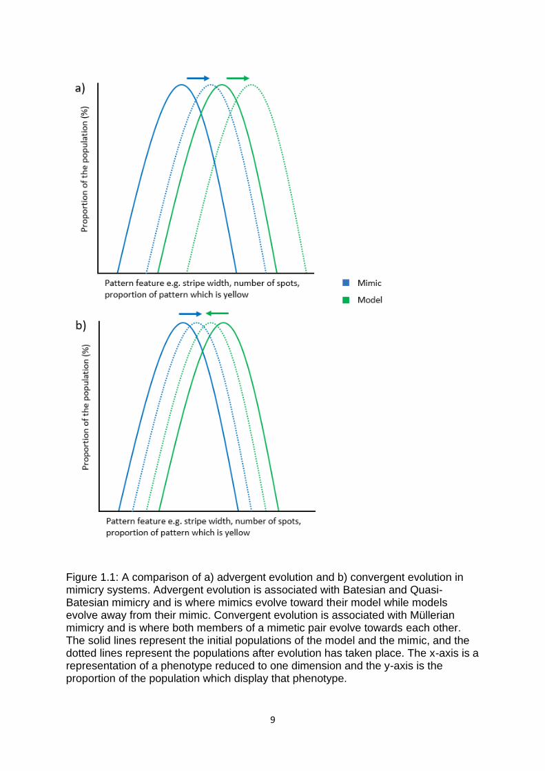
likely to encounter a model than a mimic (Waldbauer 1988) (Figure 1.2). This

hypothesis has been supported by data from the field (Howarth and Edmunds 2000).

6

However, in some regions the temporal relationship is a lot more complex. For

example, hoverflies show a peak abundance early in the spring before birds start to

fledge. This means that they avoid naïve predators, which have not yet learned to

avoid their hymenopteran models and consequently show no avoidance of

hoverflies. They also avoid predation by adult birds because these birds will have

learned to avoid the hymenopteran models in the previous year (Waldbauer 1988)

(Figure 1.2).

Another factor that makes the evolution of Batesian mimicry interesting to

consider, is that Batesian mimics are often only distantly related to their models. For

instance, hoverflies are in the order Diptera, while their models tend to be in the

order Hymenoptera (Howarth and Edmunds 2000). This raises the question: how

does a species evolve to resemble another with such a large degree of phylogenetic

separation? One answer comes from the fact that, despite not being closely related,

some mimics share the same colour production mechanisms as their models e.g.

scarlet kingsnakes Lampropeltis elapsoides and their coral snake models (Kikuchi

and Pfennig 2012). Moreover, these colour production measures are also highly

conserved among non-mimetic snakes which may mean that mimicry can be

facilitated by the developmental similarities of the model and a potential mimic

(Kikuchi et al. 2014). Alternatively, the evolution of a Batesian mimic may also be

facilitated by the evolvability of the pattern of the model. A study by Marchini et al.

(2017) suggests that the mimicry of wasps by hoverflies is due, in part, to the fact

that their patterns are so easy to evolve. This may explain why some aposematic

species have several mimics while others lack them entirely.

1.3: The evolution of Müllerian mimicry

The three hypotheses that seek to explain the evolution of Batesian mimicry

can also be applied to the evolution of Müllerian mimicry. However, as with Batesian

mimicry, the evidence seems to support the two-step hypothesis (Nicholson 1927).

This is because aposematic species are under positive frequency-dependent

selection (Chouteau et al. 2016) whereby the more unprofitable individuals there are

which share the aposematic colour pattern, the more likely each individual is to

survive: if predators attack a fixed number of prey during avoidance learning, then

the more individuals, the lower the chances of being eaten (Greenwood et al. 1989;

Mallet and Joron 1999). Therefore, when an individual of an aposematic species is

7

born with a slightly different pattern it experiences a decrease in fitness compared to

its conspecifics because a predator will not have learned to avoid that pattern. This

causes purifying selection on the aposematic patterns and suggests that Müllerian

mimicry does not evolve gradually. An exception to this is when an aposematic

species is already reasonably similar to another, for example if the pattern has

undergone feature saltation (the first part of the two-step hypothesis). Under these

circumstances, it has been observed that aposematic species in an area will evolve

towards the most common aposematic species in that region. This was

demonstrated by Mérot et al. (2016) who showed that individuals of Heliconius

timareta thelxinoe collected from regions where Heliconius erato and Heliconius

melpomene are present are more similar to those species than individuals collected

from regions where those species are absent. This suggests that H. t. thelxinoe is

slowly evolving towards H. erato and H. melpomene in those regions. In this case,

the initial step in the two-step process is thought to have come from the appearance

of alleles of the optix gene in the genome of H. t. thelxinoe (Pardo-Diaz et al. 2012).

These alleles are associated with the presence of the red forewing patch (Pardo-

Diaz et al. 2012).

In addition to the three hypotheses mentioned above, a fourth has been

suggested that relates exclusively to the evolution of Müllerian mimicry. This

hypothesis, which was first suggested by Brower et al. (1963), states that Müllerian

mimicry could evolve through divergence of one aposematic species into several

distinct species, each of which shares the ancestral pattern. Some of the first

evidence supporting this idea came from a phylogenetic study by Machado et al.

(2004) which showed that the black and yellow patterns used in the putative mimicry

ring consisting of Chauliognathus beetles, emerged once in a common ancestor of

the species involved (Machado et al. 2004). However, due to the absence of

evidence showing an adaptive benefit to maintaining this colour pattern, it is

impossible to tell whether these patterns are maintained due to selection for

Müllerian mimicry or whether they are just similar because of their shared ancestry.

In contrast, a study by Wright (2011) showed, not only that the shared pattern of

Tanganyikan catfish came from one common ancestor, but also that (in at least two

species (Synodontis multipunctata and Synodontis petricola)) this had an adaptive

benefit because a model predator (largemouth bass (Micropterus salmoides))

8

avoided each species significantly more often after having previous experience of

the other, thus proving that they are involved Müllerian mimicry ring (Wright 2011).

Moreover, this mimetic relationship seemingly causes maintenance of the pattern

because this study also showed that the patterns of Synodontis living in Lake

Tanganyika have diverged much less than Synodontis from other regions (Wright

2011).

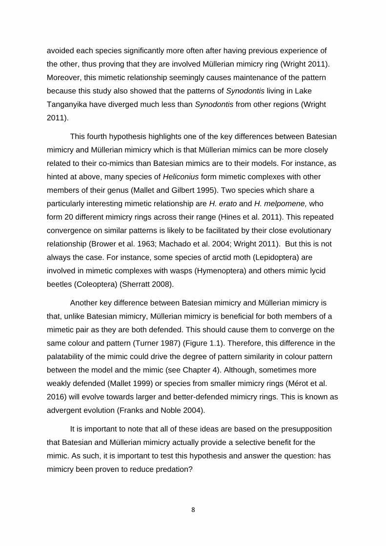
This fourth hypothesis highlights one of the key differences between Batesian

mimicry and Müllerian mimicry which is that Müllerian mimics can be more closely

related to their co-mimics than Batesian mimics are to their models. For instance, as

hinted at above, many species of Heliconius form mimetic complexes with other

members of their genus (Mallet and Gilbert 1995). Two species which share a

particularly interesting mimetic relationship are H. erato and H. melpomene, who

form 20 different mimicry rings across their range (Hines et al. 2011). This repeated

convergence on similar patterns is likely to be facilitated by their close evolutionary

relationship (Brower et al. 1963; Machado et al. 2004; Wright 2011). But this is not

always the case. For instance, some species of arctid moth (Lepidoptera) are

involved in mimetic complexes with wasps (Hymenoptera) and others mimic lycid

beetles (Coleoptera) (Sherratt 2008).

Another key difference between Batesian mimicry and Müllerian mimicry is

that, unlike Batesian mimicry, Müllerian mimicry is beneficial for both members of a

mimetic pair as they are both defended. This should cause them to converge on the

same colour and pattern (Turner 1987) (Figure 1.1). Therefore, this difference in the

palatability of the mimic could drive the degree of pattern similarity in colour pattern

between the model and the mimic (see Chapter 4). Although, sometimes more

weakly defended (Mallet 1999) or species from smaller mimicry rings (Mérot et al.

2016) will evolve towards larger and better-defended mimicry rings. This is known as

advergent evolution (Franks and Noble 2004).

It is important to note that all of these ideas are based on the presupposition

that Batesian and Müllerian mimicry actually provide a selective benefit for the

mimic. As such, it is important to test this hypothesis and answer the question: has

mimicry been proven to reduce predation?

9

Figure 1.1: A comparison of a) advergent evolution and b) convergent evolution in mimicry systems. Advergent evolution is associated with Batesian and Quasi-Batesian mimicry and is where mimics evolve toward their model while models evolve away from their mimic. Convergent evolution is associated with Müllerian mimicry and is where both members of a mimetic pair evolve towards each other. The solid lines represent the initial populations of the model and the mimic, and the dotted lines represent the populations after evolution has taken place. The x-axis is a representation of a phenotype reduced to one dimension and the y-axis is the proportion of the population which display that phenotype.

10

Figure 1.2: A graphical representation of the relative abundance of models and mimics over time. Figure (a) shows the relationship seen in the study by Howarth and Edmunds (2000) where the peak abundance of mimics matches the peak abundance of models, (b) shows the relationship seen in the study by Waldbauer (1988) where the peak abundance of mimics occurs while the abundance of naïve predators is low (the percentage of brood fledged (purple line) is an indicator of the number of naïve predators in the local population).

11

1.4: Has mimicry been proven to reduce predation?

A particularly clear example of a gap in the knowledge of mimicry versus

theory is the huge difference in the number of species which are thought to be

involved in mimicry complexes and those have actually been proven to be mimics.

Despite the fact that between 1990 and 2018, over 2,100 species of insects alone

were suggested to be involved in mimicry complexes, only around 50 species of

animal have been experimentally proven to be mimics (37 Batesian mimics, 10

Müllerian rings; Supplementary Table 1). I defined studies which have experimentally

proven mimetic relationships to be those which showed that predators showed an

increased avoidance of a putative mimic after gaining experience with its model/ co-

mimic or where a predator was shown to be unable to discriminate between models

and mimics.

I used this as the definition because the only way to truly establish whether

mimics gain a selective advantage from their colouration is to observe a predator

showing an increased avoidance of a mimic after being exposed to the model (e.g.

Long et al. 2014) or to show that a predator is unable to discriminate between a

putative mimic and a sympatric aposematic species which is its proposed model

(e.g. Prudic et al. 2002). Most experiments of this kind take place under laboratory

conditions using naïve predators to ensure that they haven’t had prior experience

with the model. For instance, Long et al. (2014) tested the palatability of three

species of butterfly (Chlosyne palla (red form and black form), Chlosyne hoffmanni

and Euphydryas chalcedona (red form and black form)) using European starlings

(Sturnus vulgaris) as a model predator. These starlings had been caught outside the

range of any of the three species to try and ensure that they had no prior experience

with any of the butterflies. Long et al. (2014) found that of those species, only

Euphydryas chalcedona was distasteful. Next, they compared the predation rates of

the black form of Chlosyne palla by starlings which had no experience with the black

form of Euphydryas chalcedona and those which had learned to avoid it and found

that experienced birds were significantly more likely to avoid Chlosyne palla which

showed that it is a Batesian mimic of Euphydryas chalcedona (Long et al. 2014).

Such experiments are important as they allow researchers to control

experimental conditions and predator experience much more easily. However, it is

also important to test if any reduced predation also occurs in natural settings in order

12

to ensure that this is not just an artefact created by the exclusion of potentially

important factors experienced by animals in the field (e.g. Candolin and Voigt 2001).

Importantly some such studies have been performed, and have found similar results

to the laboratory-based studies. For instance, Slobodchikoff (1987) tested the

mimetic relationship between the unpalatable tenebrionid beetle (Eleodes longicollis)

and the palatable cerambycid beetle (Moneilema appressum) under field conditions

by setting up buckets in two grid-like patterns. In the first of these grids, the buckets

either contained an individual of E. longicollis, an individual of M. appressum or

nothing at all. In the second grid, which was placed adjacently to the first, buckets

either contained an individual of a palatable scarab beetle (Polyphilla decemlineata)

or nothing at all. The contents of the buckets within each grid were randomised so

that wild predators did not associate the position of the bucket with its contents.

Slobodchikoff found that predators showed a generalised avoidance of E. longicollis

and M. appressum after they had eaten E. longicollis whereas predation of P.

decemlineata remained high throughout the experiment. This showed that the lack of

predation was not due to an absence of predators. On the other hand it could be

argued that the predators were avoiding the buckets in the first grid while maintaining

predation of beetles in the second grid due to their relative position rather than

because of the visual similarity between models and mimics.

So both lab and field experiments have shown that several species do indeed

experience reduced predation due to sharing their appearance with an aposematic

species. What is perhaps more interesting is that some of these experiments

suggest that, while some mimics look quite different from their models to human

observers, non-human predators show generalisation between them and the model

and as a consequence they still experience a reduction in predation despite the fact

they do not show a perfect resemblance to the model based on similarity ratings

from human observers (Dittrich et al. 1993). These species are termed imperfect

mimics (Kikuchi and Pfennig 2013) and their existence raises several interesting

questions about the evolution of both Batesian and Müllerian mimicry.

1.5 Why are some mimics imperfect?

Mimicry theory would suggest that mimics should evolve to resemble their

models as closely as possible to reduce the likelihood that a predator would be able

to discriminate between them (Taylor et al. 2016): So how does imperfect mimicry

13

arise? This question has led to a multitude of potential explanations, which can be

broadly divided into four categories (Kikuchi and Pfennig 2013). The first of these is

the idea that some species are simply unable to evolve to more closely resemble

their model, either because they lack the genetic architecture necessary to evolve

that pattern (the developmental constraints hypothesis (Maynard Smith et al. 1985))

or because their model is evolving away from them at the same rate that they are

evolving towards the model (the chase-away hypothesis (Franks et al. 2009)).

The second category deals with the idea that seemingly imperfect mimicry

may be the best evolutionary strategy for that particular habitat. This could be for a

variety of reasons, for instance a mimic may have adopted a “jack-of-all trades”

strategy where it has a pattern which is intermediate between several different

aposematic patterns and so benefit from a predator’s prior experience with several

models (the “multi-model” hypothesis (Edmunds 2000)). This strategy is thought to

work because if a Batesian mimic resembles several aposematic models, this means

that effectively there is a higher ratio of models to that mimic in that area than if it just

mimicked one of those species. Since Batesian mimics are under negative

frequency-dependent selection (as discussed in Section 1.2) it means that an

imperfect Batesian mimic should receive an equal level of protection from predation

at a given abundance as a perfect Batesian mimic which just mimics one of those

species (Edmunds 2000). Alternatively, some predators may be specialise on an

aposematic species, for example, bee-eaters predominantly eat stinging

Hymenoptera, which can make-up up to 95% of their diet (Calver et al. 1987).

Therefore, any mimics which live in the same region as these specialists will not

receive as much protection from their colouration as the same mimic living in an area

full of generalist predators which avoid the model. In fact, if the predatory guild of the

region is mainly composed of specialists, then the mimics may experience selection

against perfect mimicry. However, resembling the model to a lesser degree may still

provide a selective advantage due to any generalists avoiding them which will mean

that the optimal level of defence will come from imperfect mimicry. This idea is

termed the multiple predator hypothesis (Pekár et al. 2011). Another idea is that

mimicry may be imperfect because the specific pattern adopted represents the

optimum trade-off between selection for protection and selection for another adaptive

advantage (Taylor et al. 2016). An example of this would be a trade-off between

14

mimetic accuracy and thermoregulation. Taylor et al. (2016) suggest that some

species of hoverfly are imperfect mimics of Hymenoptera because selection has

favoured individuals with more black in their pattern than their models. They reason

that whilst these individuals probably suffer more predation than perfect mimics, this

is more than compensated for by increased dark areas making thermoregulation

easier. This kind of trade-off is already known to occur in aposematic species from

colder regions where selection acts in opposing directions, with patterns that allow

for improved thermoregulation being less effective as aposematic signals (Lindstedt

et al. 2009). I tested whether a similar tradeoff can be seen in the evolution of

mimetic patterns of Lepidoptera in Chapter 5.

The third set of hypotheses suggest that imperfect mimics are not in fact

imperfect to the predators which they are trying to fool, and that the apparent

dissimilarity is due to the fact that the humans differ from these species in terms of

their the visual capabilities and cognition (the eye of the beholder hypothesis (Cuthill

and Bennett 1993)). There is some behavioural evidence which supports this idea.

For example, Dittrich et al. (1993) carried out a behavioural study with pigeons

(Columba livia) as a model predator and found that when trained to avoid pecking at

images of wasps and then shown a series of images of hoverflies of various species,

they showed the strongest avoidance towards images of hoverflies from the genera

Syrphus and Episyrphus and so treated them as being the most similar to wasps,

even though humans rate them as being imperfect mimics.

The final category suggests that imperfect mimicry occurs because some

species of mimic experience a reduced predation rate, for example if they have a low

nutritive value (Penney et al. 2012). Under these circumstances, the predators

generalise more widely between models and mimics, therefore predators do not

pose a strong enough selection pressure on the mimics to cause them to evolve

closer to their model. This is known as the relaxed selection hypothesis (Duncan and

Sheppard 1965). This raises yet further questions because we then have to identify

the factors which could cause a mimic to experience this relaxed selection.

1.6: What factors might influence similarity between models and mimics?

A simple explanation of aposematism would suggest that predators simply

attack palatable and reject unpalatable prey, however, in reality, it is much more

15

complicated. When a predator encounters a prey which it knows to be distasteful, the

decision of whether or not to attack it is complex. This decision is affected by a

multitude of factors, including the nutritive value of the prey (Halpin et al. 2014; Smith

et al. 2016), the amount of defensive chemicals it contains (Barnett et al. 2012), the

amount of toxin which the predator has already consumed (Skelhorn and Rowe

2007) and how easy it is to find alternative palatable prey (Carle and Rowe 2014).

When a predator encounters a mimic, it likely takes into account not only these

factors, but also how certain it is that the mimic is/is not the model. Moreover, the

decision of whether or not a mimic is likely to be a mimic or a model is also affected

by several factors. For example, the similarity between the models and mimics

(Mappes and Alatalo 1997) and their relative frequency and likelihood of encounter

(Lindström et al. 1997).

Since a more nutritionally-valuable model is more likely to be attacked than a

less-nutritionally-valuable one (Halpin et al. 2014; Smith et al. 2016) and nutritive

value tends to increase with body size (Sutherland 1982), it seems likely that

predators will be more likely to attack larger mimics than smaller mimics.

Consequently, smaller mimics should experience relaxed selection and so for a

given model, a small imperfect mimic should hypothetically gain as much protection

from its colouration as a larger mimic with a closer resemblance to the model. This

hypothesis is supported by the fact that larger species of hoverflies tend to resemble

their models much more closely in terms of their pattern than smaller ones (Penney

et al. 2012). However, such correlations are not found in all Batesian mimicry

complexes. In fact larger, erythristic red-backed salamanders (Plethodon cinereus)

have been found to be poorer mimics of red-spotted newts (Notophthalmus

viridescens) than smaller individuals (Kraemer et al. 2015a).This was explained by

the fact that predators are likely to generalise more widely after encountering larger

newts because they contain more toxins. As a consequence of this, larger

salamanders are likely to experience relaxed selection on their mimetic patterns

(Kraemer et al. 2015a). Given these conflicting findings, it is unclear what effect size

has on the evolution of mimicry. Therefore in Chapter 6, I aimed to test this by

investigating how the size of mimics and models affects mimetic similarity in

lepidopteran mimetic pairs. Then, in Chapter 7, I tested Penney et al.’s (2012)

hypothesis of the effect of nutritive value on mimicry by carrying out a behavioural

16

experiment with avian predators to investigate how the value of a mimic affects

generalisation between models and mimics.

1.7: What features have been shown to be important to mimic in order for a

mimic to be “successful”?

Given the prevalence of seemingly imperfect mimicry, recent research has

attempted to understand what makes an effective mimetic signal. Work in this area

has focused on understanding whether there are specific features that are

particularly important to mimic, and whether these key features are consistent across

a range of mimicry complexes. In fact, there is good reason to believe that this may

be the case. Evidence from the animal cognition literature suggests that many

species display hierarchical learning when learning a complex signal which means

that if particularly salient features of a pattern remain the same then small changes

in other aspects may be ignored (Pavlov 1927). These highly-attended-to features

overshadow those which seem to play a smaller role in discrimination (Kazemi et al.

2014).

Most experiments performed with birds (Kazemi et al. 2014), humans

(Sherratt et al. 2015) and fish (Newport et al. 2017) suggest that predators do not

attend equally to all aspects of mimetic patterns: colour seems to be the feature

which is most attended to during discrimination learning of models and mimics. This

is based on the evidence that birds can learn to discriminate more quickly between

rewarded and unrewarded stimuli when they differ only in colour than when they

differ only in shape or pattern (Kazemi et al. 2014). In addition, birds, fish and

humans seemed to avoid mimics which matched models in terms of their colour but

differed in pattern or shape more than those which matched their models in terms of

shape or pattern but not colour (Kazemi et al. 2014; Sherratt et al. 2015; Newport et

al. 2017). Therefore one would expect other aspects of the patterns, such as the

spatial arrangement of different colour patches within the pattern, to be under

weaker selection. However, this may not always be the case. Predators from other

taxa may primarily attend to other features. Moreover, these studies should be

interpreted with some caution. Since colour, pattern and shape are measured on

different scales, the degree of difference in these measures could not be equalised.

Thus the fact that colour seems to be the most important cue, could also be because

the difference in colour was larger than the difference in shape or pattern.

17

Once we have identified which features are most important we then have to

be able to quantify how similar they are in models and mimics. Fortunately, there has

been a recent explosion in the number of methods we can use to do this. However,

the usefulness of these techniques in the study of mimicry varies greatly and is

reviewed in the next chapter.

18

Chapter 2: Techniques for measuring pattern similarity

An essential part of mimicry research is the ability to accurately measure the

similarity of mimics to their models. In the last 20 years, there have been a huge

number of techniques which have been developed to allow us to do just that. In this

chapter, I describe how some of these measurement models work and discuss how

suitable they are for studying mimicry.

2.1: Introduction

When studying mimicry, the ability to compare patterns is essential. Many

early studies in mimicry did this qualitatively by describing patterns based on their

constituent pattern elements (such as spots or stripes) and stating which colours

featured in the pattern. This is a problem for three reasons: firstly, it makes

experiments incredibly difficult to repeat. Although, researchers did try to avoid this

limitation by giving the exact ink/paint used in their experiments and providing

diagrams to show the spatial arrangement of the different colours within the pattern

(e.g. Brower et al. 1967). Secondly, it is very difficult to get a qualitative measure of

pattern similarity when comparing colours or patterns of two different categories i.e.

How similar are spots to stripes? At what point does a stripe become a spot? Are

intermediate markings more similar to stripes or spots? Finally, and arguably most

importantly, it is incredibly subjective and leads to an assessment of similarity based

on human observation rather than on how the receiver the mimic has evolved to

deceive perceives the patterns. This problem of subjectivity has been recently noted

for the study of signals as whole (Caves et al. 2019). In fact, the idea that the

difference between how humans and animals perceive visual stimuli led some

researchers to believe that mimics which have been classified as imperfect could be

identical to their intended signal recipient (eye of the beholder hypothesis (Cuthill

and Bennett 1993)).

These shortcomings of qualitative descriptions of colour patterns have led to a

proliferation of models and algorithms which allow for the quantification of pattern

similarity. While some of these are based on absolute pattern similarity (e.g. Taylor

et al. 2013), many are based on the physiology of the intended receiver (e.g.

Vorobyev and Osorio 1998). In this chapter, I will discuss many of the methods from

the literature and discuss how useful each of them are for studying mimicry by

examining both their strengths and weaknesses.

19

2.2: Measures of colour similarity

The initial idea of the eye of the beholder hypothesis of imperfect mimicry

stems from the fact that human colour vision is very different from that of potential

predators of mimics (Cuthill and Bennett 1993). This is because most humans are

trichromats (Bowmaker and Dartnall 1980) and so they have three types of cone

photoreceptor which are used for colour discrimination: the long-wavelength-

sensitive cone (LWS), the medium-wavelength-sensitive cone (MWS) and the short-

wavelength-sensitive cone (SWS). These cones are so-named due to the different

wavelengths of light to which they have maximal sensitivity. The spectral sensitivity

of a cone can be thought of as the response to a given wavelength of light relative to

other wavelengths at a given intensity (Schnapf et al. 1987). For example, a human

LWS cone will show a maximal response to light with a wavelength of 560nm but a

much lower response to light with a wavelength of 400nm with the same intensity

(Schnapf et al. 1987).These different cone types with different spectral sensitivities

are one of the components of the visual system necessary to allow us to see colours

in the visible spectrum. On the other hand, birds (which are often thought of as the

main selective agent on the patterns of mimetic insects) are tetrachromats

(Bowmaker et al. 1997). This means that alongside the three cone types that

humans have, they have a fourth kind of cone. In some species, this is sensitive to

UV light and hence it is called the ultraviolet-sensitive (UVS) cone, whereas in other

species it is sensitive to slightly longer wavelengths of light, in which case it is called

the violet-sensitive (VS) cone (Bowmaker et al. 1997). This means that birds can

detect not only light in the visible spectrum, but also light in the UV range. Therefore,

if a mimic differs from a model in terms of the amount of UV it reflects then it could

appear very different from its model to an avian predator but still be relatively similar

in the eyes of a human observer.

In order to perceive differences in colour, not only do animals need several

types of cones which are maximally sensitive to different wavelengths, they also

need a way of comparing the response of these different cones. This occurs via

colour opponency (Conway et al. 2010; Kelber 2016). The way this works in

mammals is that several cones connect to a retinal ganglion cell, one or more of

these cones excite the ganglion cell and one or more inhibit it. For instance, humans

have four opponent channels: Red-ON/Green-OFF, Red-OFF/Green-ON, Blue-

20

ON/Yellow-OFF and Blue-OFF/Yellow-ON (Conway et al. 2010). The number and

types of opponent channel differ between different species, for example, red-eared

sliders (Trachemys scripta) have been found to have 12 opponent channels (Rocha

et al. 2008), this also leads to differences in colour perception between humans and

non-human animals.

Because of this, it is vital that when comparing the colours of models and

mimics that it is done with the appropriate receiver in mind. Normally, this involves

the creation of “colour spaces” (Renoult et al. 2017), which are diagrammatic

representations made up of several dimensions which contain all of the colours

which are theoretically perceivable by a given organism based on its visual system

where the distance between two points in the space gives a measure of how

different two colours are to the organism for which the space was made. In order to

do this, researchers must use a technique in which the visual properties of a

theoretical predator can be mathematically defined. The most commonly-used model

which has this flexibility is the Receptor Noise-Limited model (Vorobyev and Osorio

1998; Vorobyev et al. 2001).

2.2.1: The Receptor Noise-Limited (RNL) model

The method used most frequently to quantify differences between colours is

the Receptor Noise-Limited (RNL) model (Vorobyev and Osorio 1998; Vorobyev et

al. 2001). As its name suggests, the model works on the assumption that the main

factor which affects the discrimination between two colours is the amount of

photoreceptor noise. Photoreceptor noise is defined as the random variation in the

response of a photoreceptor that is independent of a signal and it arises due to the

fact that photons do not arrive at the receptor at a constant rate (in fact the rate at

which they arrived can be closely modelled by a Poisson distribution) (Faisal et al.

2008) and due to signal noise from receptor cells themselves which is termed

“transducer noise” (Lillywhite 1978). To use this model, one must first work out the

quantum catch of each receptor in the modelled visual system when viewing a

certain colour. This gives a measure of the amount of light captured by the receptor

underspecified lighting conditions by multiplying the sensitivity of the receptor (Ri

(where i is the identity of the receptor in question)) by the spectrum of the light

entering the eye from the target colour (IS) (which in itself is a product of the

spectrum of ambient light and the reflectance spectrum of the colour being viewed).

21

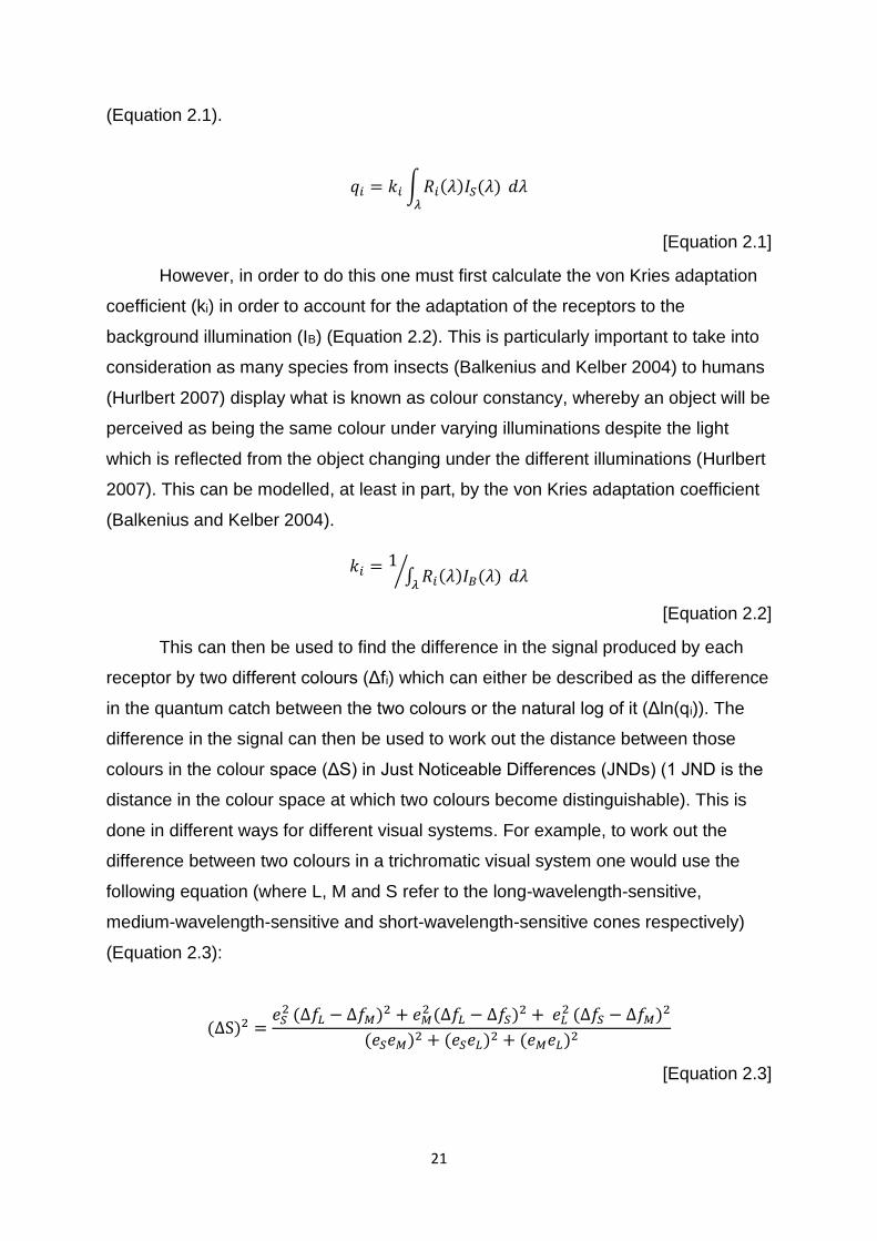
(Equation 2.1).

𝑞𝑖 = 𝑘𝑖 ∫ 𝑅𝑖(𝜆)𝐼𝑆(𝜆)

𝜆

𝑑𝜆

[Equation 2.1]

However, in order to do this one must first calculate the von Kries adaptation

coefficient (ki) in order to account for the adaptation of the receptors to the

background illumination (IB) (Equation 2.2). This is particularly important to take into

consideration as many species from insects (Balkenius and Kelber 2004) to humans

(Hurlbert 2007) display what is known as colour constancy, whereby an object will be

perceived as being the same colour under varying illuminations despite the light

which is reflected from the object changing under the different illuminations (Hurlbert

2007). This can be modelled, at least in part, by the von Kries adaptation coefficient

(Balkenius and Kelber 2004).

𝑘𝑖 = 1∫ 𝑅𝑖(𝜆)𝐼𝐵(𝜆)

𝜆 𝑑𝜆⁄

[Equation 2.2]

This can then be used to find the difference in the signal produced by each

receptor by two different colours (Δfi) which can either be described as the difference

in the quantum catch between the two colours or the natural log of it (Δln(qi)). The

difference in the signal can then be used to work out the distance between those

colours in the colour space (ΔS) in Just Noticeable Differences (JNDs) (1 JND is the

distance in the colour space at which two colours become distinguishable). This is

done in different ways for different visual systems. For example, to work out the

difference between two colours in a trichromatic visual system one would use the

following equation (where L, M and S refer to the long-wavelength-sensitive,

medium-wavelength-sensitive and short-wavelength-sensitive cones respectively)

(Equation 2.3):

(ΔS)2 =𝑒𝑆

2 (Δ𝑓𝐿 − Δ𝑓𝑀)2 + 𝑒𝑀2 (Δ𝑓𝐿 − Δ𝑓𝑆)2 + 𝑒𝐿

2 (Δ𝑓𝑆 − Δ𝑓𝑀)2

(𝑒𝑆𝑒𝑀)2 + (𝑒𝑆𝑒𝐿)2 + (𝑒𝑀𝑒𝐿)2

[Equation 2.3]

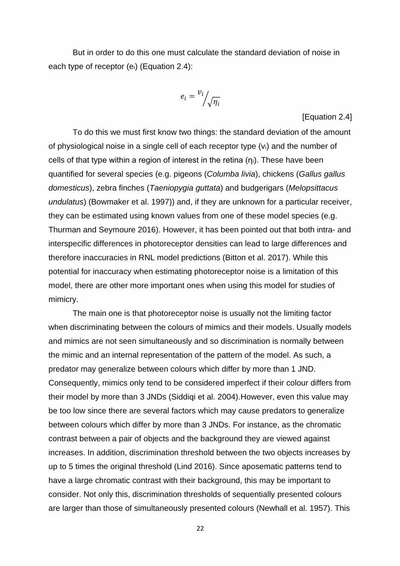
22

But in order to do this one must calculate the standard deviation of noise in

each type of receptor (ei) (Equation 2.4):

𝑒𝑖 =𝑣𝑖

√𝜂𝑖⁄

[Equation 2.4]

To do this we must first know two things: the standard deviation of the amount

of physiological noise in a single cell of each receptor type (vi) and the number of

cells of that type within a region of interest in the retina (ηi). These have been

quantified for several species (e.g. pigeons (Columba livia), chickens (Gallus gallus

domesticus), zebra finches (Taeniopygia guttata) and budgerigars (Melopsittacus

undulatus) (Bowmaker et al. 1997)) and, if they are unknown for a particular receiver,

they can be estimated using known values from one of these model species (e.g.

Thurman and Seymoure 2016). However, it has been pointed out that both intra- and

interspecific differences in photoreceptor densities can lead to large differences and

therefore inaccuracies in RNL model predictions (Bitton et al. 2017). While this

potential for inaccuracy when estimating photoreceptor noise is a limitation of this

model, there are other more important ones when using this model for studies of

mimicry.

The main one is that photoreceptor noise is usually not the limiting factor

when discriminating between the colours of mimics and their models. Usually models

and mimics are not seen simultaneously and so discrimination is normally between

the mimic and an internal representation of the pattern of the model. As such, a

predator may generalize between colours which differ by more than 1 JND.

Consequently, mimics only tend to be considered imperfect if their colour differs from

their model by more than 3 JNDs (Siddiqi et al. 2004).However, even this value may

be too low since there are several factors which may cause predators to generalize

between colours which differ by more than 3 JNDs. For instance, as the chromatic

contrast between a pair of objects and the background they are viewed against

increases. In addition, discrimination threshold between the two objects increases by

up to 5 times the original threshold (Lind 2016). Since aposematic patterns tend to

have a large chromatic contrast with their background, this may be important to

consider. Not only this, discrimination thresholds of sequentially presented colours

are larger than those of simultaneously presented colours (Newhall et al. 1957). This

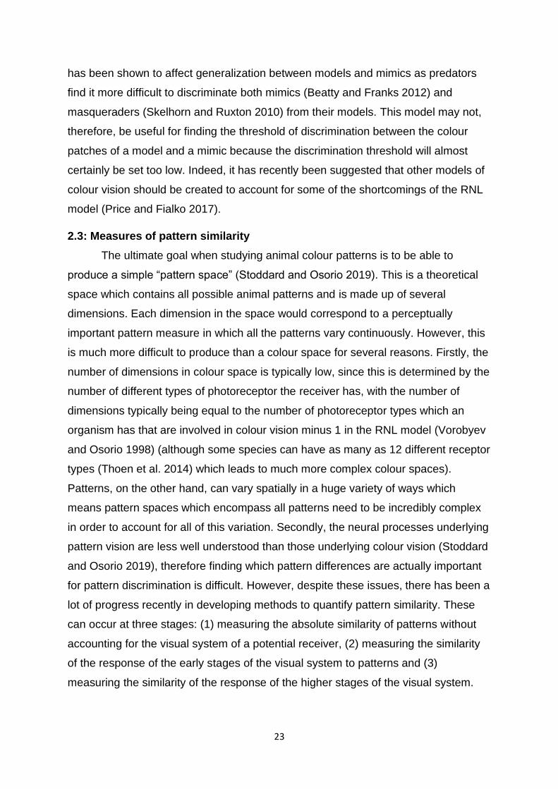
23

has been shown to affect generalization between models and mimics as predators

find it more difficult to discriminate both mimics (Beatty and Franks 2012) and

masqueraders (Skelhorn and Ruxton 2010) from their models. This model may not,

therefore, be useful for finding the threshold of discrimination between the colour

patches of a model and a mimic because the discrimination threshold will almost

certainly be set too low. Indeed, it has recently been suggested that other models of

colour vision should be created to account for some of the shortcomings of the RNL

model (Price and Fialko 2017).

2.3: Measures of pattern similarity

The ultimate goal when studying animal colour patterns is to be able to

produce a simple “pattern space” (Stoddard and Osorio 2019). This is a theoretical

space which contains all possible animal patterns and is made up of several

dimensions. Each dimension in the space would correspond to a perceptually

important pattern measure in which all the patterns vary continuously. However, this

is much more difficult to produce than a colour space for several reasons. Firstly, the

number of dimensions in colour space is typically low, since this is determined by the

number of different types of photoreceptor the receiver has, with the number of

dimensions typically being equal to the number of photoreceptor types which an

organism has that are involved in colour vision minus 1 in the RNL model (Vorobyev

and Osorio 1998) (although some species can have as many as 12 different receptor

types (Thoen et al. 2014) which leads to much more complex colour spaces).

Patterns, on the other hand, can vary spatially in a huge variety of ways which

means pattern spaces which encompass all patterns need to be incredibly complex

in order to account for all of this variation. Secondly, the neural processes underlying

pattern vision are less well understood than those underlying colour vision (Stoddard

and Osorio 2019), therefore finding which pattern differences are actually important

for pattern discrimination is difficult. However, despite these issues, there has been a

lot of progress recently in developing methods to quantify pattern similarity. These

can occur at three stages: (1) measuring the absolute similarity of patterns without

accounting for the visual system of a potential receiver, (2) measuring the similarity

of the response of the early stages of the visual system to patterns and (3)

measuring the similarity of the response of the higher stages of the visual system.

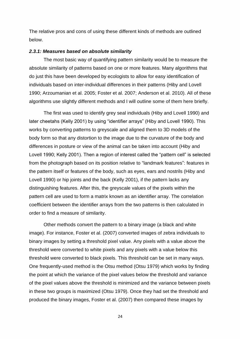
24

The relative pros and cons of using these different kinds of methods are outlined

below.

2.3.1: Measures based on absolute similarity

The most basic way of quantifying pattern similarity would be to measure the

absolute similarity of patterns based on one or more features. Many algorithms that

do just this have been developed by ecologists to allow for easy identification of

individuals based on inter-individual differences in their patterns (Hiby and Lovell

1990; Arzoumanian et al. 2005; Foster et al. 2007; Anderson et al. 2010). All of these

algorithms use slightly different methods and I will outline some of them here briefly.

The first was used to identify grey seal individuals (Hiby and Lovell 1990) and

later cheetahs (Kelly 2001) by using “identifier arrays” (Hiby and Lovell 1990). This

works by converting patterns to greyscale and aligned them to 3D models of the

body form so that any distortion to the image due to the curvature of the body and

differences in posture or view of the animal can be taken into account (Hiby and

Lovell 1990; Kelly 2001). Then a region of interest called the “pattern cell” is selected

from the photograph based on its position relative to “landmark features”: features in

the pattern itself or features of the body, such as eyes, ears and nostrils (Hiby and

Lovell 1990) or hip joints and the back (Kelly 2001), if the pattern lacks any

distinguishing features. After this, the greyscale values of the pixels within the

pattern cell are used to form a matrix known as an identifier array. The correlation

coefficient between the identifier arrays from the two patterns is then calculated in

order to find a measure of similarity.

Other methods convert the pattern to a binary image (a black and white

image). For instance, Foster et al. (2007) converted images of zebra individuals to

binary images by setting a threshold pixel value. Any pixels with a value above the

threshold were converted to white pixels and any pixels with a value below this

threshold were converted to black pixels. This threshold can be set in many ways.

One frequently-used method is the Otsu method (Otsu 1979) which works by finding

the point at which the variance of the pixel values below the threshold and variance

of the pixel values above the threshold is minimized and the variance between pixels

in these two groups is maximized (Otsu 1979). Once they had set the threshold and

produced the binary images, Foster et al. (2007) then compared these images by

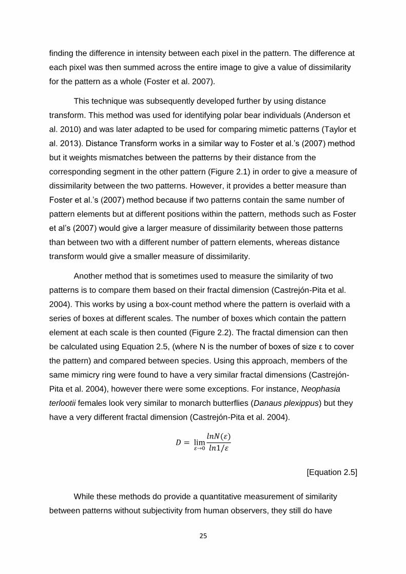
25

finding the difference in intensity between each pixel in the pattern. The difference at

each pixel was then summed across the entire image to give a value of dissimilarity

for the pattern as a whole (Foster et al. 2007).

This technique was subsequently developed further by using distance

transform. This method was used for identifying polar bear individuals (Anderson et

al. 2010) and was later adapted to be used for comparing mimetic patterns (Taylor et

al. 2013). Distance Transform works in a similar way to Foster et al.’s (2007) method

but it weights mismatches between the patterns by their distance from the

corresponding segment in the other pattern (Figure 2.1) in order to give a measure of

dissimilarity between the two patterns. However, it provides a better measure than

Foster et al.’s (2007) method because if two patterns contain the same number of

pattern elements but at different positions within the pattern, methods such as Foster

et al’s (2007) would give a larger measure of dissimilarity between those patterns

than between two with a different number of pattern elements, whereas distance

transform would give a smaller measure of dissimilarity.

Another method that is sometimes used to measure the similarity of two

patterns is to compare them based on their fractal dimension (Castrejón-Pita et al.

2004). This works by using a box-count method where the pattern is overlaid with a

series of boxes at different scales. The number of boxes which contain the pattern

element at each scale is then counted (Figure 2.2). The fractal dimension can then

be calculated using Equation 2.5, (where N is the number of boxes of size ε to cover

the pattern) and compared between species. Using this approach, members of the

same mimicry ring were found to have a very similar fractal dimensions (Castrejón-

Pita et al. 2004), however there were some exceptions. For instance, Neophasia

terlootii females look very similar to monarch butterflies (Danaus plexippus) but they

have a very different fractal dimension (Castrejón-Pita et al. 2004).

𝐷 = lim𝜀→0

𝑙𝑛𝑁(𝜀)

𝑙𝑛1/𝜀

[Equation 2.5]

While these methods do provide a quantitative measurement of similarity

between patterns without subjectivity from human observers, they still do have

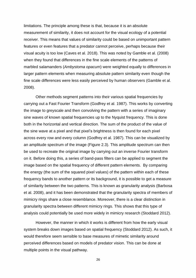
26

limitations. The principle among these is that, because it is an absolute

measurement of similarity, it does not account for the visual ecology of a potential

receiver. This means that values of similarity could be based on unimportant pattern

features or even features that a predator cannot perceive, perhaps because their

visual acuity is too low (Caves et al. 2018). This was noted by Gamble et al. (2008)

when they found that differences in the fine scale elements of the patterns of

marbled salamanders (Ambystoma opacum) were weighted equally to differences in

larger pattern elements when measuring absolute pattern similarity even though the

fine scale differences were less easily perceived by human observers (Gamble et al.

2008).

Other methods segment patterns into their various spatial frequencies by

carrying out a Fast Fourier Transform (Godfrey et al. 1987). This works by converting

the image to greyscale and then convolving the pattern with a series of imaginary

sine waves of known spatial frequencies up to the Nyquist frequency. This is done

both in the horizontal and vertical direction. The sum of the product of the value of

the sine wave at a pixel and that pixel’s brightness is then found for each pixel

across every row and every column (Godfrey et al. 1987). This can be visualized by

an amplitude spectrum of the image (Figure 2.3). This amplitude spectrum can then

be used to recreate the original image by carrying out an inverse Fourier transform

on it. Before doing this, a series of band-pass filters can be applied to segment the

image based on the spatial frequency of different pattern elements. By comparing

the energy (the sum of the squared pixel values) of the pattern within each of these

frequency bands to another pattern or its background, it is possible to get a measure

of similarity between the two patterns. This is known as granularity analysis (Barbosa

et al. 2008), and it has been demonstrated that the granularity spectra of members of

mimicry rings share a close resemblance. Moreover, there is a clear distinction in

granularity spectra between different mimicry rings. This shows that this type of

analysis could potentially be used more widely in mimicry research (Stoddard 2012).

However, the manner in which it works is different from how the early visual

system breaks down images based on spatial frequency (Stoddard 2012). As such, it

would therefore seem sensible to base measures of mimetic similarity around

perceived differences based on models of predator vision. This can be done at

multiple points in the visual pathway.

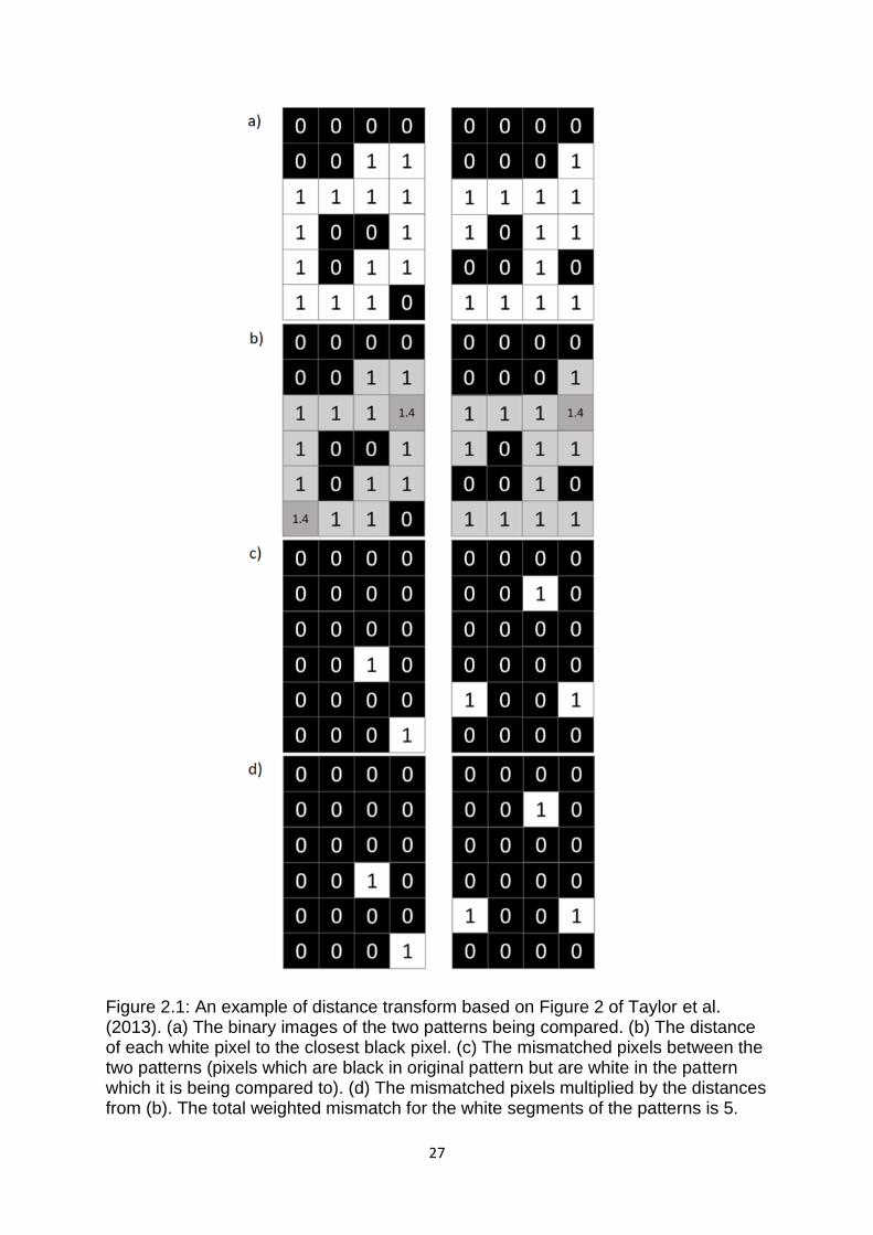
27

Figure 2.1: An example of distance transform based on Figure 2 of Taylor et al. (2013). (a) The binary images of the two patterns being compared. (b) The distance of each white pixel to the closest black pixel. (c) The mismatched pixels between the two patterns (pixels which are black in original pattern but are white in the pattern which it is being compared to). (d) The mismatched pixels multiplied by the distances from (b). The total weighted mismatch for the white segments of the patterns is 5.

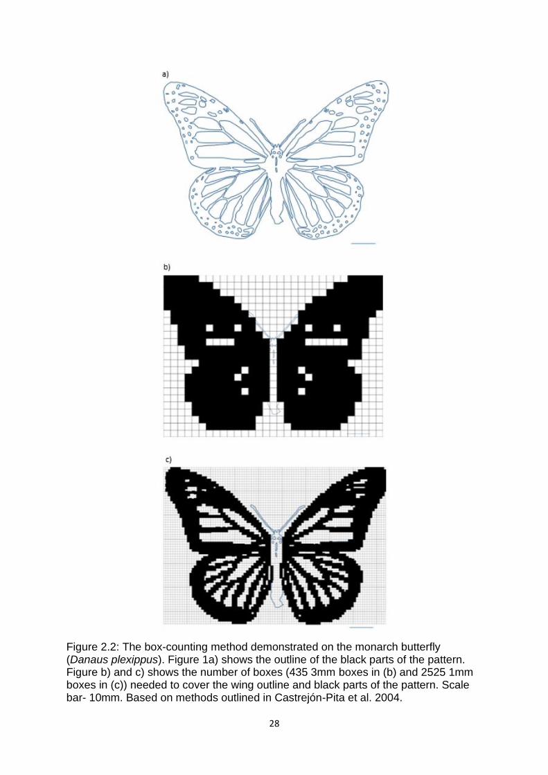
28

Figure 2.2: The box-counting method demonstrated on the monarch butterfly (Danaus plexippus). Figure 1a) shows the outline of the black parts of the pattern. Figure b) and c) shows the number of boxes (435 3mm boxes in (b) and 2525 1mm boxes in (c)) needed to cover the wing outline and black parts of the pattern. Scale bar- 10mm. Based on methods outlined in Castrejón-Pita et al. 2004.

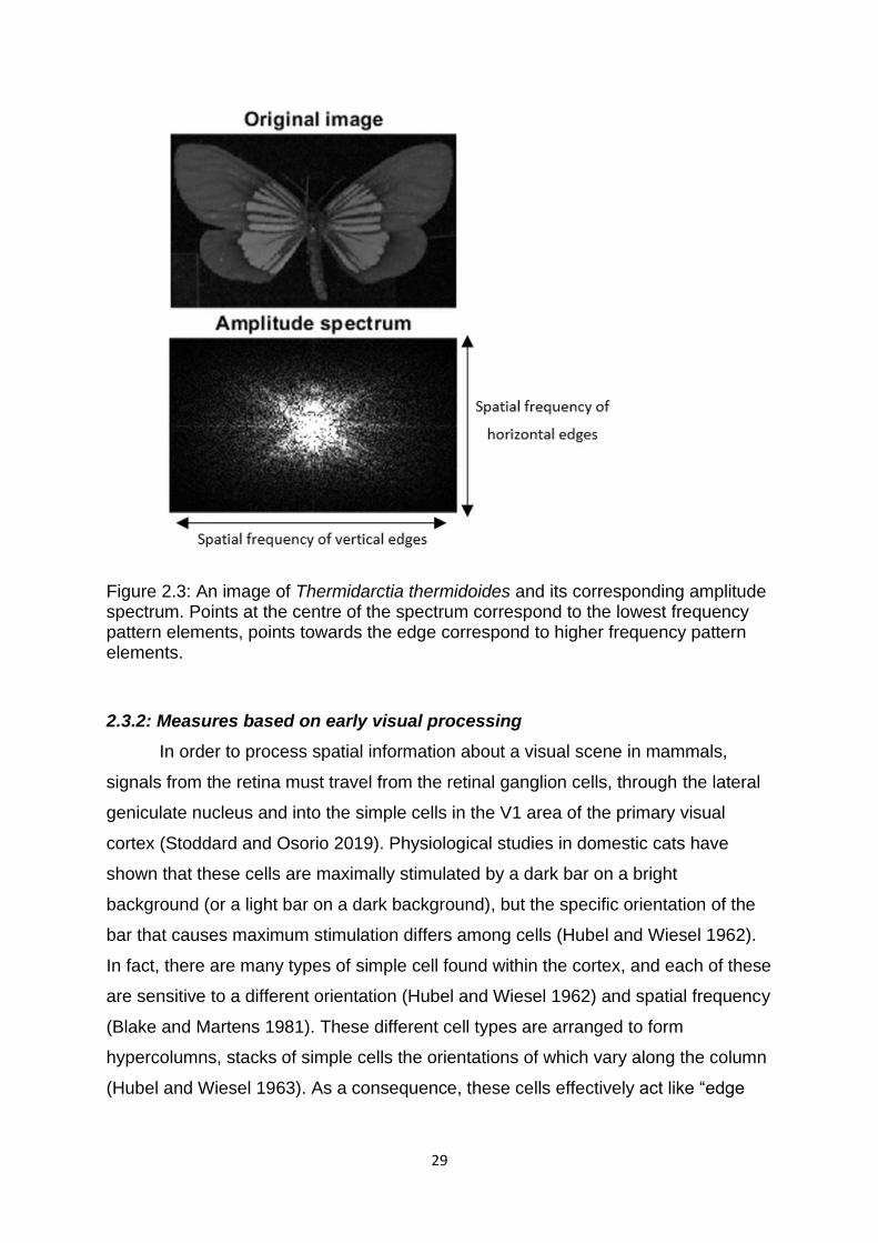
29

Figure 2.3: An image of Thermidarctia thermidoides and its corresponding amplitude spectrum. Points at the centre of the spectrum correspond to the lowest frequency pattern elements, points towards the edge correspond to higher frequency pattern elements.

2.3.2: Measures based on early visual processing

In order to process spatial information about a visual scene in mammals,

signals from the retina must travel from the retinal ganglion cells, through the lateral

geniculate nucleus and into the simple cells in the V1 area of the primary visual

cortex (Stoddard and Osorio 2019). Physiological studies in domestic cats have

shown that these cells are maximally stimulated by a dark bar on a bright

background (or a light bar on a dark background), but the specific orientation of the

bar that causes maximum stimulation differs among cells (Hubel and Wiesel 1962).

In fact, there are many types of simple cell found within the cortex, and each of these

are sensitive to a different orientation (Hubel and Wiesel 1962) and spatial frequency

(Blake and Martens 1981). These different cell types are arranged to form

hypercolumns, stacks of simple cells the orientations of which vary along the column

(Hubel and Wiesel 1963). As a consequence, these cells effectively act like “edge

30

detectors” and so are sensitive to luminance boundaries in a pattern (Marr and

Hildreth 1980).

The response of the simple cells in the V1 to an image can be modelled by

convolving the image in question with a series of Gabor filters of various orientations

and spatial frequencies (Jones and Palmer 1987). Comparing the responses of

these cells to images to prey, with the responses of the cells to images of the prey’s

background has been used to assess how similar/different both cryptic and

aposematic species are to their backgrounds (Troscianko et al. 2017; Barnett et al.

2018). Moreover, this approach could be used to compare the similarity of models

and mimics.

This method has recently been built upon to not only provide a measure of the

energy of the pattern, which captures the total response of the simulated visual

system (the more boundaries between areas with a difference in luminance there are

within the pattern, the higher the energy of the pattern will be), but also the isotropy

of the pattern, which gives a measure of how the size of the response varies

depending on the orientation of the Gabor cell (an example of a low isotropy pattern

and a high isotropy pattern can be seen in Figure 2.4). (Penacchio et al. in prep.).

The more the response of the Gabor cells varies depending on their orientation, the

lower the isotropy of the pattern, therefore a high isotropy pattern will be made up of

dots, low isotropy patterns will be made of stripes and a medium patterns will either

be a clouded pattern or be made up of dots and stripes. The difference in these

measures between models and mimics could then be used to give a measure of

similarity for these diagnostics. This method works by using a series of Gabor filters

to simulate the response of V1 simple cells from the primary visual cortex to a

pattern. This works because Gabor filters are orientation-specific, band-pass filters

which allow for local edge detection and as explained in Chapter 2 can be used to

model the responses of the cells in V1. While this technique is based on the way in

which mammals process visual information (Hubel and Wiesel 1962), it can also be

applied to birds because the receptive fields of cells in the nucleus isthmi par

magnocellularis and the nucleus isthmi par parvocellularis of birds seem to be similar

to those of V1 cells (Wang and Frost 1991; Li et al. 2007). Consequently, they

should respond to patterns in a similar way.

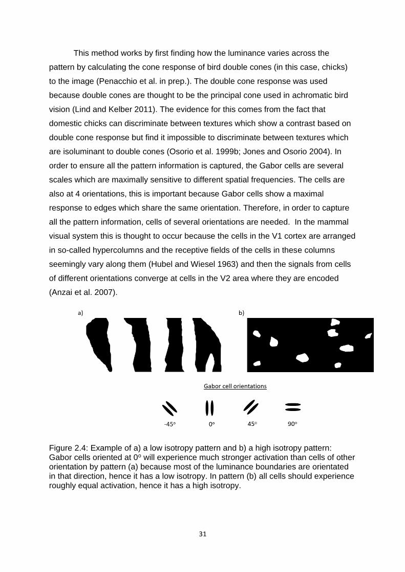
31

This method works by first finding how the luminance varies across the

pattern by calculating the cone response of bird double cones (in this case, chicks)

to the image (Penacchio et al. in prep.). The double cone response was used

because double cones are thought to be the principal cone used in achromatic bird

vision (Lind and Kelber 2011). The evidence for this comes from the fact that

domestic chicks can discriminate between textures which show a contrast based on

double cone response but find it impossible to discriminate between textures which

are isoluminant to double cones (Osorio et al. 1999b; Jones and Osorio 2004). In

order to ensure all the pattern information is captured, the Gabor cells are several

scales which are maximally sensitive to different spatial frequencies. The cells are

also at 4 orientations, this is important because Gabor cells show a maximal

response to edges which share the same orientation. Therefore, in order to capture

all the pattern information, cells of several orientations are needed. In the mammal

visual system this is thought to occur because the cells in the V1 cortex are arranged

in so-called hypercolumns and the receptive fields of the cells in these columns

seemingly vary along them (Hubel and Wiesel 1963) and then the signals from cells

of different orientations converge at cells in the V2 area where they are encoded

(Anzai et al. 2007).

Figure 2.4: Example of a) a low isotropy pattern and b) a high isotropy pattern: Gabor cells oriented at 0o will experience much stronger activation than cells of other orientation by pattern (a) because most of the luminance boundaries are orientated in that direction, hence it has a low isotropy. In pattern (b) all cells should experience roughly equal activation, hence it has a high isotropy.

32

2.3.3: Measures based on higher visual processing

When processing images for identification, in mammals, signals travel from

the retina to the lateral geniculate nucleus (LGN), then signals from the LGN travel to

the V1 area of the visual cortex then the signals from V1 travel to the V2 area, then

the V4 area before arriving in the inferior temporal (IT) cortex, this is known as the

ventral stream (Stoddard and Osorio 2019) or the geniculocortical pathway (Li et al.

2007). Meanwhile, birds rely on a visual pathway which is functionally very similar

but structurally very different. This is known as the tectofugal pathway (Li et al.

2007). In this pathway, signals travel from the retina to the tectal cells in the optic

tectum, then signals from there travel to the nucleus rotundus and from there to the

entopallium. Finally, the signals from the entopallium split and travel to different

areas of the brain such as the nidopallium frontolaterale, the mesopallium

ventrolaterale, the area temporo-parieto-occipitalis and the nidopallium intermediate

par lateralis (Stacho et al. 2016). It is much more difficult to model the response of

cells at this level and any mistakes would lead to inaccuracies in the conclusions

drawn from these models (Pérez-Rodríguez et al. 2017). However, there have been

a couple of models which have been developed for image recognition which work by

simulating the response of cells at this stage: these are known as HMAX

(Riesenhuber and Poggio 1999) and SIFT (Lowe 1999).

HMAX uses a hierarchical method which adds to the early-visual models

based on Gabor filters. It works by first passing a bank of Gabor filters over the

images with a range of spatial frequencies and of 4 orientations, this is termed the

S1 layer. The responses of cells are then pooled using a MAX response function to

make up the next layer (C1). Each cell in this layer is made up of the pooled

responses of the cells in an area which span all of the spatial scales but that share

the same orientation. Cells in this layer are then combined in two ways. Firstly, pairs

of C1 cells from the same area but tuned to different orientations are combined to

create S2 cells which are then be summed across a wider area to form C2 cells.

Secondly, C1 cells which are tuned to the same orientation are combined across a

wider area to form C2 cells (Riesenhuber and Poggio 1999). It is these so-called

“complex composite cells” which then feed into the view-tuned cells. These are cells

tuned to respond maximally to a particular object/pattern feature which give the

response of the model.

33

SIFT (Scale-Invariant Feature Transform) works in a slightly different way.

First, a series of Gaussian filters of different scales are applied to the image to blur it

to different extents. Filtered images of neighbouring scales are then compared to

one another to give a series of images called the difference-of-Gaussian images.

Local points of maximum and minimum differences are found between these images

(local maxima and minima). A series of Laplacians are then used to detect the edges

of the pattern features detected by the difference-of-Gaussian method. This

algorithm forms the basis of pattern comparison methods such as

NaturePatternMatch (Stoddard et al. 2014). In NaturePatternMatch, information

about each feature that is extracted by SIFT is encoded in a 128-dimensional vector,

then all the features in two images are compared to see how many match (Stoddard

et al.2014). This is done by pairing each feature in one pattern (x) with the nearest

feature to it in the other pattern (y) based on the Euclidean distance between the two

features in the 128-dimensional vector space. “True” matches are then identified by

only accepting pairs of features for which the distance between a pair is less than

0.85 times the distance between each feature in the pair and its next nearest

neighbour in the other image (Stoddard et al. 2014). The number of features that

match is then divided by the largest number of features in either of the two patterns

to give a similarity score. This is then normalized so that the score is scaled between

0 and 1 where 0 is a total mismatch and 1 is a pair of two identical patterns

(Equation 2.6).

𝑆𝑐𝑜𝑟𝑒 (𝑥, 𝑦) =∑ 𝑊𝑛

𝑁𝐹𝑥.𝐹𝑦

𝑛=1

max(|𝐹𝑥|, |𝐹𝑦|)

[Equation 2.6]

Both algorithms mimic the response of neurons in the inferior temporal cortex

but in very different ways however neither one is better under all circumstances.

HMAX was found to perform better than SIFT when attempting to detect particular

objects in target images (Moreno et al. 2007), however SIFT was found to be a

better predictor of the time taken to find a camouflaged object than HMAX

(Troscianko et al. 2017). Therefore, the choice of which model to use depends on

the task. So far only SIFT has been used in studies of mimicry (egg mimicry)

34

(Stoddard et al. 2019) but an extended model of HMAX described below does seem

like it would also be useful.

2.4: Measures of spatiochromatic similarity

Although the models mentioned previously quantify differences in colour and

differences in spatial pattern separately, information about the colour and form of

objects in the visual field travels mainly through the parvocellular pathway (the visual

pathway associated with the red-green opponent channels) (with some colour

information travelling through the koniocellular pathway (the visual pathway

associated with the blue-ON-yellow-OFF opponent channel)) (Nassi and Callaway

2009). However, the way that information from these characteristics is integrated is

not entirely certain, although there is evidence that this happens as early as in the

retina and the integration continues into the cortex (Clery et al. 2013) with some cells

in the primate cortex in V1 both responding to colour and showing orientation

selectivity (Garg et al. 2019). In addition to this, colour and pattern can affect the

perception of one another (reviewed in Moutoussis 2015). For example, the position

of luminance boundaries along a colour gradient can affect the perception of the

colour between the boundaries (Vergeer et al. 2015). Therefore, models which

integrate colour and pattern information would provide a useful next step to using

models which examine colour and pattern differences separately. Several models

have been developed to do just that and I will review them here.

2.4.1: Adjacency analysis and Boundary Strength Analysis

The first pattern-matching method which is based on this is adjacency

analysis (Endler 2012). Adjacency analysis works by first constructing a “zone map”

by segmenting the pattern into its constituent colours. In the original paper this was

done by using k-means clustering to assign each pixel to the correct colour class

(Endler 2012). The pattern is then sampled in a grid pattern which gives a measure

of the proportion of the pattern that is made up of each colour class (Figure 2.5).

Once all the grid points have been sampled, a transition matrix is constructed (Figure

2.6). To do this, the colour that one point is sampled from is compared to the colours

which adjacent points are sampled from. This can give several pattern statistics to

describe the pattern. The first of these is transition density, this gives a measure of

how frequently adjacent points are sampled from two different colour patches and

hence a measure of pattern complexity. The second is the transition aspect ratio, this

35

gives a measure of the kind of pattern. This is calculated by finding the number of

transitions in the vertical axis divided by the number of transitions in the horizontal

axis, the more this value differs from 1, the more striped the pattern is. This

technique was then built upon with Boundary Strength Analysis (BSA) (Endler et al.

2018). Boundary Strength Analysis works in an almost identical way to adjacency

analysis however it also takes the chromatic contrast between adjacent colour

patches into account. To do this a measure of chromatic contrast is given at every

boundary between two colours (the boundary strength). This is done by using the

RNL model (Vorobyev and Osorio 1998) to measure the chromatic contrast of

adjacent colour patches. This not only provides information about the different colour

patches within the pattern relate to another spatially, it also tells us how similar these

patches are to one another. Some of the pattern statistics are very useful when

studying mimetic patterns. For instance, one might expect mimics and models to

share similar proportions of colours in their patterns. However, they may not

necessary share similar proportions of transition types. For instance, North American

milk snakes and their coral snake models would have entirely different frequencies of

black-red and red-yellow transitions (Endler 2012) but yet predators still generalize

between them (Kikuchi and Pfennig 2010).

36

Figure 2.5: A zone map based on the pattern of Thermidarctia thermidoides. Grey points represent sampling points. Actual sampling would occur on a much finer scale to ensure that all the fine details in the pattern are sampled. (This figure is based on Figure 2 of Endler 2012).

Figure 2.6: The transition matrix based on the sampling grid from Figure 2.5. Diagonals give a measure of the number of transitions within the same colour. Off-diagonals give a measure of the number of transitions between different colours.

37

2.4.2: HMAX with Colour Opponency

The most recent model for spatiochromatic similarity was developed by

Renoult et al. (2019). This basically takes the HMAX model described in Section

2.3.3 and adds a layer which allows for the modelling of colour opponency alongside

it (Renoult et al. 2019). This technique has not yet been used for studies of mimicry

but it seems promising as a useful tool in the future.

2.5: Conclusions and future questions

There are now a number of methods available to measure the similarity of

colour and patterns. However, as this chapter has shown, the best one to use

depends on the task it has being used for. In terms of mimicry, sometimes combining

several methods can provide a much better explanation of likelihood of being a

successful mimic than one method on its own. For instance, a study of the eggs of

host-parasites showed that adding a measure of the similarity of higher-level pattern

features provided a more accurate model of egg rejection behaviour by hosts than

using measures of low-level pattern features and colour alone (Stoddard et al. 2019).

However, there is still a lot of work can be done to develop models which allow

people to find the point at which a mimic is no longer discriminable from its model as

shown by the fact that even using three measures together only explains 37% of the

variance in behaviour (Stoddard et al. 2019). As this is currently the best way of

predicting the response of receivers, this is the method I will use throughout this

thesis. I will find a measure of colour similarity, a measure of the low-pattern feature

similarity and a measure of high-level pattern feature similarity for all of my image

analysis, the details of which are explained in the next chapter.

38

Chapter 3: General Methods

The aim of this chapter is to summarise the general methods I used to acquire and

analyse the images of the specimens of real life model-mimic pairs. In this chapter, I

will outline the methods used to (1) select species to scan, (2) acquire scans of the

specimens and (3) analyse the scans to obtain quantitative measures of mimetic

similarity between models and mimics. I will also cover the methods used for each of

the chick experiments in their respective chapter since the methodologies differ

substantially between these experiments.

3.1: Introduction

My thesis has three main aims: (1) to determine what makes an effective

mimetic signal; (2) to identity the abiotic and biotic factors which can affect how

closely mimics evolve to resemble their aposematic models; and, (3) to determine

whether or not palatable mimics affect the evolution of the pattern of their

aposematic models. To better understand mimetic signalling, I used mimicry in

lepidopterans as my model system for two reasons. First, mimicry in Lepidoptera has

been studied extensively, with many mimetic relationships having been identified.

Second, the hyperspectral camera used to collect the hyperspectral images needed

for the image analysis has a narrow plane of focus, meaning that it is difficult to

capture a single image in which an entire animal is in focus unless (as is the case

with butterflies and moths) the animals is relatively flat. In addition to this, butterflies

and moths are easy to find in good condition in museum collections.

In this chapter, I will cover all the methods used (1) in the selection of the

study species, (2) the scanning of museum specimens and (3) the analysis of the

images I acquired as these are consistent throughout Chapters 4, 5 and 6. I will

discuss how I gathered information about each of the factors which is thought to

affect mimicry in Chapters 5 and 6 as these methods are specific to those chapters. I

will also cover the methods used for each of the chick experiments in their respective

chapter since the methodologies differ substantially between these experiments.

39

3.2: Selection of study species for image analyses

3.2.1: Selection of models and mimics

I first searched Google Scholar for papers published between 1990 and 2016

using the search term “Batesian Mimicry”, I did this in 2-year increments so that no

results were missed (because Google Scholar displays a finite number of results). In

total, this gave around 3,170 publications, 256 of which were used to find species. I

used the search term “Batesian mimicry” in order to filter out papers about other

forms of mimicry such as vocal mimicry by birds and mimicry of natural materials by

engineers. However, this allowed me to retain papers about Müllerian mimics

because they were also among these results since many papers about Müllerian

mimicry also refer to Batesian mimicry. These searches were repeated several times

over the course of my PhD to ensure that the list was up to date (the final update

took place on January 2018). This gave me a total of 331 papers which listed

mimetic species. From these, I identified suitable species for study. From these

papers, I created a table which listed all the mimetic species mentioned.

I only included mimics and models from mimicry rings consisting of just two

species. The reason for this is because in larger, more complex mimicry rings (in

particular, those which have several Müllerian mimics), it is difficult to designate one

member as the “focal” species as the one which the other mimics are evolving

towards, therefore focusing on mimicry rings which contain only two species allowed

me to avoid having to carry out multiple comparisons within the same ring. From the

331 papers, which included details of 253 model species and over 2,000 mimic

species, I identified 102 of these simple mimetic pairs.

3.2.2: Selection of sympatric, non-mimicked, aposematic species

For each of the model-mimic pairs, I found an example of an aposematic

species which is found in the same region as the pair but which lacks mimics of its

own. I did this for two reasons. Firstly, it provided me with a control species which

allowed me to see how similar mimics are to their models compared to other

aposematic species within their habitat. Secondly, it also allowed me to see if the

presence of Batesian mimics affects the efficacy of the patterns of their models

compared to species which lack mimics (Chapter 4).

Identifying these sympatric, non-mimicked, aposematic species was a multi-

step process (Figure 3.1). First, I found species which were sympatric with the

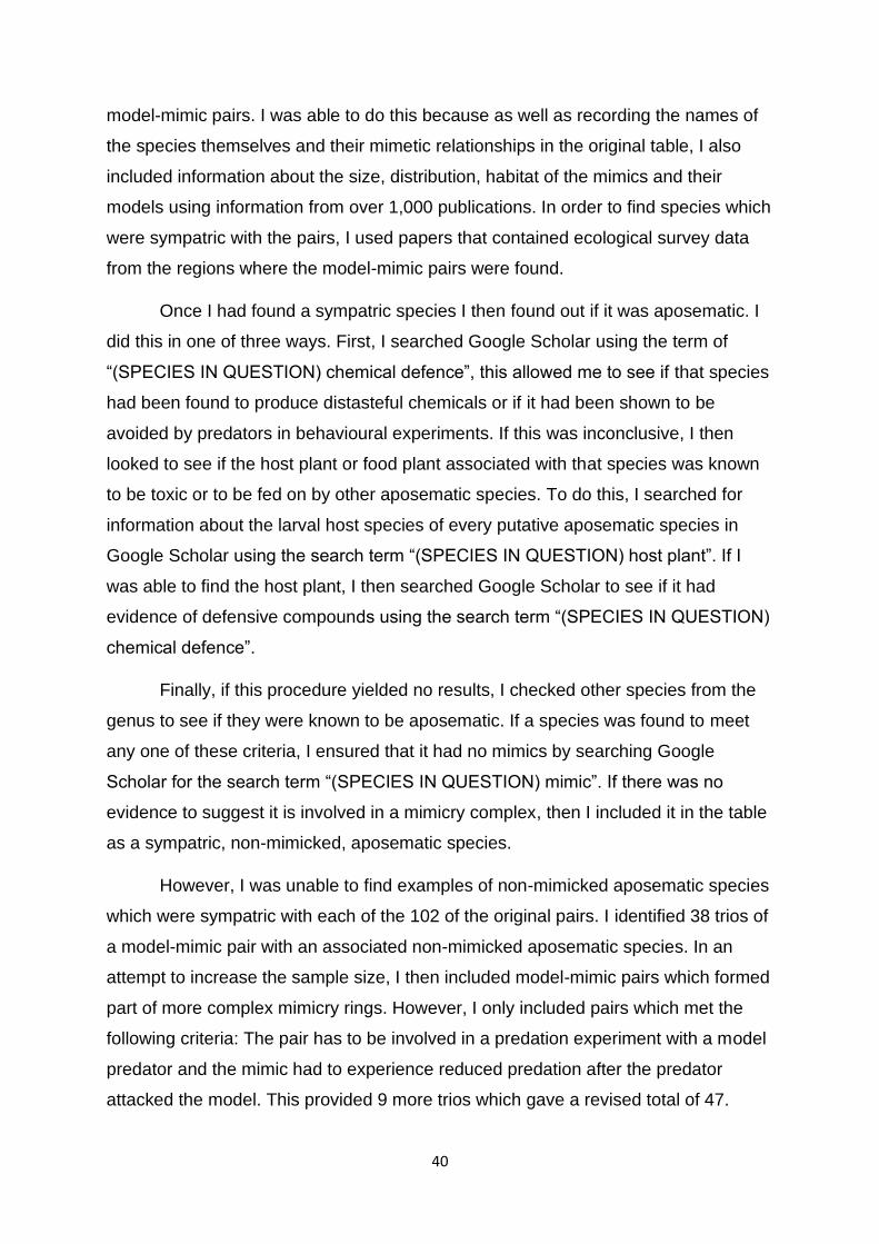
40

model-mimic pairs. I was able to do this because as well as recording the names of

the species themselves and their mimetic relationships in the original table, I also

included information about the size, distribution, habitat of the mimics and their

models using information from over 1,000 publications. In order to find species which

were sympatric with the pairs, I used papers that contained ecological survey data

from the regions where the model-mimic pairs were found.

Once I had found a sympatric species I then found out if it was aposematic. I

did this in one of three ways. First, I searched Google Scholar using the term of

“(SPECIES IN QUESTION) chemical defence”, this allowed me to see if that species

had been found to produce distasteful chemicals or if it had been shown to be

avoided by predators in behavioural experiments. If this was inconclusive, I then

looked to see if the host plant or food plant associated with that species was known

to be toxic or to be fed on by other aposematic species. To do this, I searched for

information about the larval host species of every putative aposematic species in

Google Scholar using the search term “(SPECIES IN QUESTION) host plant”. If I

was able to find the host plant, I then searched Google Scholar to see if it had

evidence of defensive compounds using the search term “(SPECIES IN QUESTION)

chemical defence”.

Finally, if this procedure yielded no results, I checked other species from the

genus to see if they were known to be aposematic. If a species was found to meet

any one of these criteria, I ensured that it had no mimics by searching Google

Scholar for the search term “(SPECIES IN QUESTION) mimic”. If there was no

evidence to suggest it is involved in a mimicry complex, then I included it in the table

as a sympatric, non-mimicked, aposematic species.

However, I was unable to find examples of non-mimicked aposematic species

which were sympatric with each of the 102 of the original pairs. I identified 38 trios of

a model-mimic pair with an associated non-mimicked aposematic species. In an

attempt to increase the sample size, I then included model-mimic pairs which formed

part of more complex mimicry rings. However, I only included pairs which met the

following criteria: The pair has to be involved in a predation experiment with a model

predator and the mimic had to experience reduced predation after the predator

attacked the model. This provided 9 more trios which gave a revised total of 47.

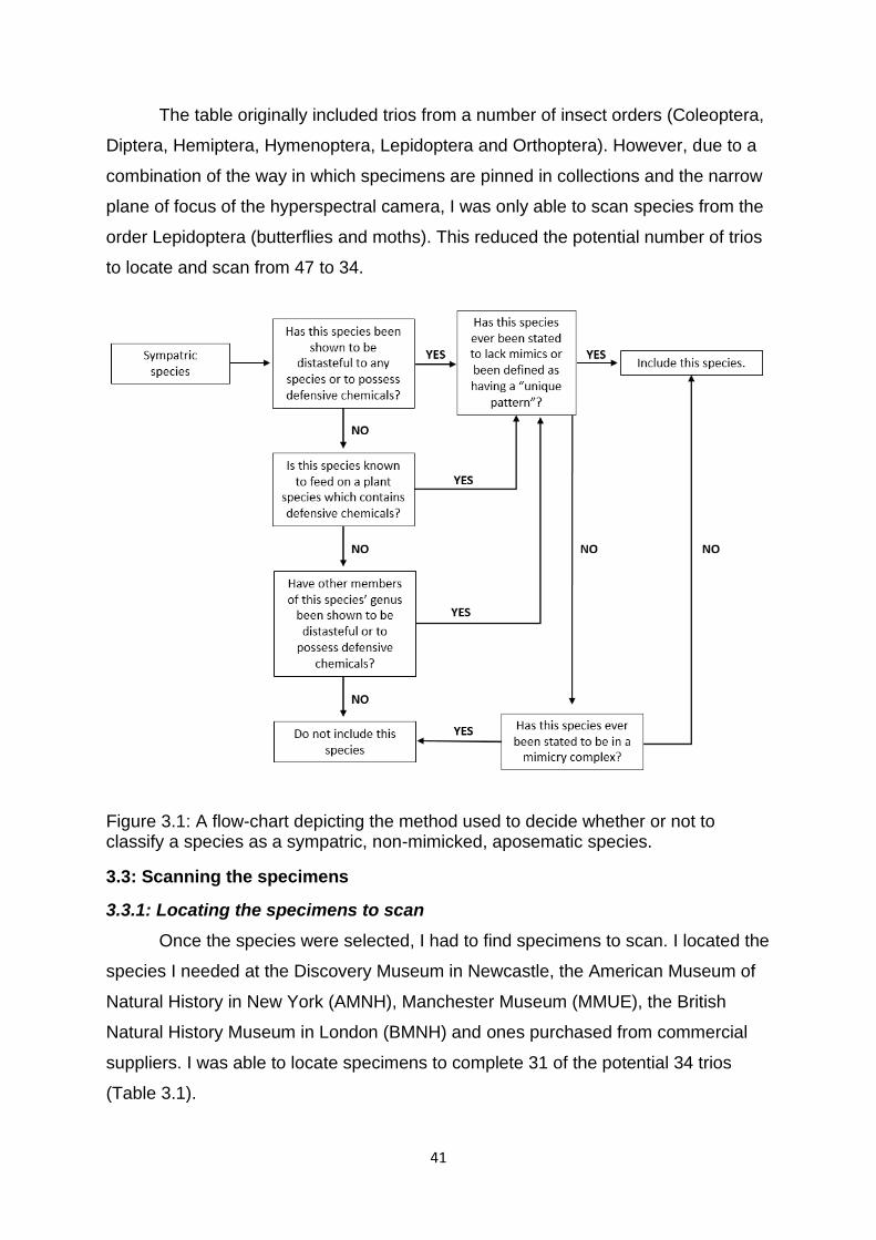
41

The table originally included trios from a number of insect orders (Coleoptera,

Diptera, Hemiptera, Hymenoptera, Lepidoptera and Orthoptera). However, due to a

combination of the way in which specimens are pinned in collections and the narrow

plane of focus of the hyperspectral camera, I was only able to scan species from the

order Lepidoptera (butterflies and moths). This reduced the potential number of trios

to locate and scan from 47 to 34.

Figure 3.1: A flow-chart depicting the method used to decide whether or not to classify a species as a sympatric, non-mimicked, aposematic species.

3.3: Scanning the specimens

3.3.1: Locating the specimens to scan

Once the species were selected, I had to find specimens to scan. I located the

species I needed at the Discovery Museum in Newcastle, the American Museum of

Natural History in New York (AMNH), Manchester Museum (MMUE), the British

Natural History Museum in London (BMNH) and ones purchased from commercial

suppliers. I was able to locate specimens to complete 31 of the potential 34 trios

(Table 3.1).

42

Mimic Model/ Co-mimic Sympatric, non-mimicked aposematic species

Agraulis vanillae vanillae Dryas iulia iulia Batesia hypochlora

Amerila bipartita Amerila brunnea Balacra flavimacula

Amesia apoensis Euploea blossomae Delias ottonia

Arichanna gaschkevitchii Arichanna melanaria Miltochrista miniata

Atrophaneura varuna Papilio protenor Papilio polyctor

Callicore astarte Callicore texa Battus ingenuus

Cheimas opalinus Lymanopoda marianna Lymanopoda dietzi

Chlosyne palla Euphydryas chalcedona Hypoprepia miniata

Cyclosia notabilis Parantica sita Cethosia biblis

Elymnias nesaea Ideopsis vulgaris Losaria neptunus

Epicopeia mencia Byasa confusus Elcysma westwoodii

Gynautocera philomela Troides dohertyi Danaus ismare

Heliconius ethilla ethilla Eueides isabella isabella Histioea cepheus

Heraclides astyalus Papilio androgeus Heliconius charithonia

Hestina mimetica Parantica pseudomelaneus

Delias periboea

Laparus doris doris Heliconius sara thamar Calonotos craneae

Limenitis archippus archippus

Danaus plexippus Poladryas minuta

Limenitis arthemis Battus philenor Eurytides marcellus

Limenitis lorquini Adelpha bredowii Parnassius clodius

Mimoides ilus Parides panares Urania leilus

Mynes doubledayi Delias duris Acraea moluccana

Mynes plateni Delias funerea Troides hypolitus

Papilio bootes Byasa polyeuctes Acraea issoria

Papilio glaucus (dark form)

Battus philenor Eurytides marcellus

Papilio laglaizei Alcides agathyrsus Milionia dohertyi

Papilio polyxenes Battus philenor Eurytides marcellus

Papilio troilus Battus philenor Eurytides marcellus

Prioneris cornelia Delias singhapura Delias eumolpe

Prioneris philonome Delias descombesi Idea agamarschana

Prioneris sita Delias eucharis Acraea terpsichore

Scea discinota Thermidarctia thermidoides

Scotura annulata

Table 3.1: Trios of models, mimics and sympatric, non-mimicked species which I scanned.

3.3.2: Selecting the specimens to scan

For each species, two specimens were scanned where possible (in some

cases there was only one specimen present in the collection). However, in cases

where a species was polymorphic, two specimens were selected per morph. When

selecting specimens to scan, where possible, I used a random number generator to

select the row and column of the specimens in the drawer in order to avoid bias

43

when choosing specimens. If the specimen selected was damaged or I was unable

to remove it safely from the drawer without damaging it or the other specimens, the

nearest suitable specimen was scanned instead. Damaged specimens were avoided

as the pattern measurements would be affected by being incomplete. In cases where

this was not possible, such as when the species were too valuable for us to get from

the drawers ourselves, the curator of the collection chose the specimens from the

drawers and brought them to us. Therefore, even in these cases, I did not bias the

selection by choosing specimens myself.

3.3.3: Scanning the specimens

The specimens were scanned using a bespoke hyperspectral camera

(Resonon Pika NUV), this differs from a normal camera because it allows us to

collect an image outside the range of visual light (the camera I used had a spectral

range of 350nm to 800nm, while most commercial cameras have a spectral range of

around 400nm to 700nm (Stevens et al. 2007)). The camera samples wavelengths

from this range via 196 spectral channels as opposed to the 3 seen in standard

cameras (the R, G and B channels) (Stevens et al. 2007) which gives it a spectral

resolution of 2.3nm. It differs from a standard camera in other ways because, rather

than taking a single image like a standard camera, the hyperspectral camera works

by taking a series of pixel-wide images which are then put together to make one

continuous scan. Each of these images is 1600 pixels wide and each pixel is 5.8μm

in size which means that the images produced have both a high spatial resolution as

well as a high spectral resolution. This method of producing images means that the

camera had to be moved across the specimens on a motorized stage. This was

done in the x direction of the image i.e. from left to right. Both the camera and the

stage were controlled using the program SpectrononPro (Resonon inc.) (Figure 3.2).

This is a good method of measuring the colour of models and mimics as it provides

full spectral information from across the entire specimen which means that any

boundaries in colour patches which are visible to potential predators (such as birds)

but not to humans (i.e. differences in the UV) can be found. This means that it

provides more spectral information than a standard camera while also providing a

higher spatial resolution than a spectrophotometer which makes it an incredibly

useful device for studying colour patterns.

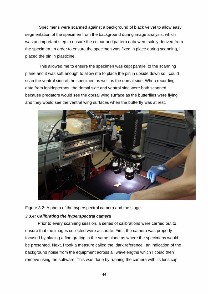
44

Specimens were scanned against a background of black velvet to allow easy

segmentation of the specimen from the background during image analysis, which

was an important step to ensure the colour and pattern data were solely derived from

the specimen. In order to ensure the specimen was fixed in place during scanning, I

placed the pin in plasticine.

This allowed me to ensure the specimen was kept parallel to the scanning

plane and it was soft enough to allow me to place the pin in upside down so I could

scan the ventral side of the specimen as well as the dorsal side. When recording

data from lepidopterans, the dorsal side and ventral side were both scanned

because predators would see the dorsal wing surface as the butterflies were flying

and they would see the ventral wing surfaces when the butterfly was at rest.

Figure 3.2: A photo of the hyperspectral camera and the stage.

3.3.4: Calibrating the hyperspectral camera

Prior to every scanning session, a series of calibrations were carried out to

ensure that the images collected were accurate. First, the camera was properly

focused by placing a fine grating in the same plane as where the specimens would

be presented. Next, I took a measure called the ‘dark reference’, an indication of the

background noise from the equipment across all wavelengths which I could then

remove using the software. This was done by running the camera with its lens cap

45

on to stop any light from entering the lens. Because there was no light hitting the

sensor, I knew that any response seen was an artefact due to background noise

from the camera and I could then remove this using Spectronon. By doing this, I then

had a baseline for the minimum reflectance across all wavelengths. After that, a light

reference spectrum was taken by scanning a Spectralon white standard, this

material has a spectrally flat reflectance and reflects 98% of light (Labsphere,

Congleton, UK) which provides a set of values across all wavelengths for maximum

reflectance. To account for any possible changes in illumination in the room

throughout the day, this step was repeated frequently (roughly once an hour).

The reflectance of an object or colour is a measure of the proportion of light

that hits an object which is then reflected by it across all wavelengths. This can be

visualised by what is known as a reflectance spectrum. Objects which are different

colours will therefore have a different reflectance spectrum to one another. This is

why I have to take a measure of the minimum and maximum reflectance across all

wavelengths in order to get a measure of the reflectance of the pattern at every pixel

across the pattern. These values then feed into the various visual models explained

later in this chapter to give an idea of how these patterns will be perceived by

predators. In order to ensure that lighting was consistent in all images and that there

was UV light present for the patterns to potentially reflect, the only light in the room

when the scans were taking place came from 4 lights positioned around the camera

(See Figure 3.2) which were fitted with bulbs which emitted light in the visual and

ultraviolet spectrum (Eiko Q35MR16/CG/47/36- Solux, 12V, 35W, 4700K).

Finally, I spatially calibrated the setup to make sure that the camera was not

moving too quickly or too slowly. This had to be done because the camera works by

taking a series of pixel-wide images as it moves across the specimen, these are then

put together to make one continuous scan. Therefore, if the camera moves too

quickly or too slowly for a given frame-rate then the image will be distorted. In order

to avoid these distortions, I scanned a sheet which had a series of right-angle pairs

at various orientations; this scan was then sent to MATLAB (MATLAB r2016b, The

MathWorks Inc., Natick, MA, 2000) with a custom script to measure how close the

angles in the image were to 90o, the script then calculated the change in stage

speed and framerate needed in order to make the scanned angles into right angles

because any distortions of the images would cause the angle in the image to deviate

46

from 90o. I then measured a second image with the suggested parameters and

repeated the process until the difference between the image and the ideal was less

than 2%.

3.3.5: Additional data for each specimen

After each scan with the hyperspectral camera, I took a photograph of the

specimen alongside a CameraTrax 24 colour card using a DSLR camera (Basler

acA1300-200ac) to produce calibrated digital photographs. These were used to

calculate the size of each specimen.

I also recorded the details from specimen labels, including the date it was

collected, and its origin (where it was collected from and whether it was captive

bred). This provided detailed information about each specimen that allowed me to

explore how other factors, such as the effect of temperature, might affect the

evolution of mimicry (Chapter 5).

3.4: Image analysis

3.4.1: Colour analysis

As previously stated, hyperspectral imaging is a very powerful technique

as it provides full spectral information for every pixel of the scan, therefore it is

possible to use various techniques to attempt to model how an image would be

interpreted by the visual system of an animal without it first having lost spectral

information, as is the case with photographs taken by normal digital photographs, or

spatial information, as is the case with measurements taken by a spectrometer.

Because of this, once the hyperspectral images were collected, I was able to

analyse them using a variety of methods. In order to analyse the colour, I used code

developed by collaborator Olivier Penacchio (MATLAB r2018a, The MathWorks Inc.,

Natick, MA, 2000). This code takes the hyperspectral scan and calculates the

theoretical response of each cone type (long-wavelength-sensitive (LWS), medium-

wavelength-sensitive (MWS), short-wavelength-sensitive (SWS) and violet-sensitive

(VS)) of the domestic chick (Gallus gallus domesticus) visual system for every pixel

in the scan. The chick visual system was used because the physiology of the

photoreceptors is well understood (Olsson et al. 2015) and it was necessary

because processing of colour in a bird’s visual pathway will be based on the signals

from excited cones, it is also frequently used as a representative species for

47

modelling the visual systems of violet-sensitive birds (e.g. Finkbeiner et al. 2017).

These cone responses were then used to find a variety of pattern descriptors of the

chromatic features of the pattern. Two measures of the variation in each cone type

response from across the image were used. These were the standard deviation of

each cone response, which provides a measure of the variability of each cone

response from across the scan, and the Gini coefficient. This is a measure that is

often used in economics and provides a measure of the equality of the cone

response from across the image (values closer to 0 show more equal responses,

values closer to 1 show less equal responses) (Penacchio et al. in prep). These

measures are important because the mean cone response is not a very informative

measure alone. The cone responses were also used to calculate the response of the

different opponent channels (L-M channel, S-U channel (S-V in this instance since

chicks are violet-sensitive) and the (L+M)-S channel) which gave a measurement of

the variation of colour contrast within the pattern. The theoretical colour channels

computed from this code were based on those which were experimentally validated

by Osorio et al. (1999a). In this experiment, domestic chicks were trained to

discriminate between rewarded and unrewarded stimuli which had colours which a

chromatic axis created by one of the three colour channels: L-M, (L+M)-S or S-V

(Osorio et al. 1999a). Since chicks were able to use all of three of these channels to

discriminate between different colours, it shows that they use all three opponent

mechanisms. Along with the mean, the code also gives values of the standard

deviation and Gini coefficient of each channel response because, as with the cone

responses, knowing the mean alone is not that useful therefore a measure of colour

variation was also provided.

3.4.2: Pattern analysis

In order to analyse the spatial characteristics of the pattern, I carried out two

additional analyses, one which allowed me to look at the similarity of the models and

mimics at an early stage of visual processing (the energy-isotropy analysis) and one

which allowed me to look at similarity at a later stage of the visual pathway

(NaturePatternMatch). This is important because birds seem to use information from

both pattern features which are processed early in the visual pathway (low-level

features) and those which are processed later (high-level features) when deciding

whether or not to reject host-parasite eggs from their nests (Stoddard et al. 2019),

48

and it seems likely that birds would use both when deciding whether or not to attack

mimetic prey. Similarly, birds could also use this information when discriminating

between different mimetic complexes so it could be used to discriminate between

mimics and models from sympatric aposematic species.

The first method I used was energy-isotropy analysis, which was also

developed by Olivier Penacchio to model the response of the early visual system

(see Chapter 2). This method works by first finding how the luminance varies across

the pattern by calculating the cone response of bird double cones (in this case,

chicks) to the image (Penacchio et al. in prep.). The double cone response was used

because double cones are thought to be the principal cone used in achromatic bird

vision (Lind and Kelber 2011). The evidence for this comes from the fact that

domestic chicks can discriminate between textures which show a contrast based on

double cone response but find it impossible to discriminate between textures which

are isoluminant to double cones (Osorio et al. 1999b; Jones and Osorio 2004). In

order to ensure all the pattern information is captured, the Gabor cells were at 16

scales which are maximally sensitive to different spatial frequencies: Scale 1 is the

smallest, with each cell at this scale having a receptive field of 7 x 7 pixels, and is

maximally stimulated by high frequency pattern elements, Scale 16 is the largest

scale, with each cell having a receptive field of 32 x 32 pixels, and is maximally

stimulated by low frequency pattern elements. The cells which were used to form the

basis of the energy analysis were also at 4 orientations (22.5o, 45o, 67.5o and 90o),

this is important because Gabor cells show a maximal response to edges which

share the same orientation, therefore to capture all the pattern information, cells of

several orientations are needed. In the mammal visual system this is thought to

occur because the cells in the V1 cortex are arranged in so-called hypercolumns and

the receptive fields of the cells in these columns seemingly vary along them (Hubel

and Wiesel 1963) and then the signals from cells of different orientations converge at

cells in the V2 area where they are encoded (Anzai et al. 2007).

The second method I used to analyse the pattern used the

NaturePatternMatch algorithm (Stoddard et al. 2014) on the double cone response

images produced in the first analysis. This gave a measure of similarity of the

patterns of models and mimics based on the response of cells at a later stage of the

visual pathway. NaturePatternMatch works by using Scale-Invariant Feature

49

Transform (SIFT) in order to extract potentially recognisable elements from the

pattern in a similar way to how the cells in the inferior temporal cortex of a primate

would (Stoddard et al. 2014) (See Section 2.3.3). Once the features of a pattern

have been extracted, they are then compared between models and mimics which

gives a similarity score which ranges between 0 (complete mismatch) and 1 (perfect

match) (See Section 2.3.3). The idea is that elements which are potentially easily

recognised by an observer should be theoretically important for mimicry and

therefore they should occur in the patterns of both models and their mimics.

I did not include any measures of absolute pattern similarity because, these

techniques have previously been shown to give a disproportionately low measure of

similarity between patterns which, to a human observer, were quite similar (Gamble

et al. 2008). This was due to equal weighting of differences between pattern features

which are highly salient and differences in features which were barely perceivable

(Gamble et al. 2008). Therefore, although using methods which do not take into

account the visual system of a theoretical predator would seemingly avoid measures

of mimetic similarity being based on the visual system of a non-ecologically relevant

predator and thus lead to a potentially incorrect assessment of whether or not a

mimic is imperfect (Cuthill and Bennett 1993), using a measure which does not take

into account any theoretical visual capabilities at all can lead to the same problem.

3.5: Selecting diagnostics for study

It would be unfeasible to look at how all of the diagnostics (measures of

different aspects of the pattern) produced by these analyses vary with the factors

which are thought to affect mimetic similarity due to the sheer number of them (the

energy-isotropy analysis alone gives measures for over 100 pattern diagnostics). In

addition, it would be redundant since many of these measures are correlated or

provide different measurements of the same pattern feature. For instance, the

energy- isotropy analysis gives three measures of pattern contrast (including pattern

energy) which are calculated in different ways. In order to avoid this redundancy, and

to make the data analysis more manageable, I attempted to find the pattern features

which seemed to be the most important for mimicry.

50

3.5.1: Methods

To do this, I used a novel approach to measure how much more similar the

various features of the patterns of the mimics are to those of their models compared

to a sympatric non-mimicked aposematic species. I carried out a series of robust

mixed model ANOVAs on trimmed means using the package WRS2 in R (V.0.10-0;

Mair and Wilcox 2018). The difference in a given pattern diagnostic between a mimic

and an aposematic species was the outcome variable (the aposematic species in

question was either the model or the sympatric aposematic species). The

aposematic species the mimic was being compared to (its model or its sympatric,

non-mimicked aposematic species) and whether the mimic was palatable or not (i.e.

whether it is a Batesian pair or a Müllerian pair) were used as the predictor variables.

Finally, the trio to which the mimic belonged was the random factor. I used a robust

mixed model ANOVA because the data did not fit the assumptions of a parametric

test. From this, I took the F-value of how the size of the difference in the pattern

diagnostic varies depending on whether the mimic was being compared to the model

or to the sympatric aposematic species and used it to predict how important that

pattern diagnostic is for mimicry (Figure 3.3).

The idea behind this method is that a high F-value would indicate that mimics

are more similar to their models than the sympatric aposematic species (as

measured by this particular diagnostic), and the larger the F-value is the more similar

mimics are to their models than to the sympatric non-mimicked aposematic species.

Therefore, this would suggest that selection has favoured mimics that match their

models in the particular aspect of their appearance measured by that diagnostic,

which would suggest that it is important in mimicry. This has been shown to be the

case in egg mimicry because pattern diagnostics which are similar in host and

parasitic eggs have been shown to be important when birds are discriminating

between their own eggs and those of brood parasites (Spottiswoode and Stevens

2010).

3.5.2: Results

From this analysis, I found that the standard deviation of the response of the

blue-yellow opponent channel (F-value = 16.647) had the highest F-value out of all

measures of colour, the similarity score from NaturePatternMatch (F-value = 12.604)

had the highest F-value of the high-level pattern diagnostics and the mean energy of

51

the pattern at Scale 10 (F-value = 14.653) had the highest F-value of the low-level

pattern diagnostics, respectively (Supplementary Table 2). This suggests that these

measures of pattern similarity were more similar between models and mimics than

they were between mimics and sympatric aposematic species. This suggests that

they are important for discriminating between different aposematic species in a

region and so these should be features which mimics evolve to match. In addition to

this, a series of Pearson correlations revealed no correlations between any of my

measures, indicating that all three are statistically independent of one another

(Difference in the standard deviation of blue-yellow opponent channel response vs

NaturePatternMatch Score: r = 0.073, p =0.812; Difference in the standard deviation

of blue-yellow opponent channel response vs Difference in mean energy (Scale 10):

r = -0.339, p =0.257; NaturePatternMatch Score vs Difference in mean energy (Scale

10): r = -0.298, p =0.322). Therefore, I used these measures to test my hypotheses

in Chapters 4, 5 and 6. The reason why I used a measure of energy at one scale

rather than the mean of the energy at all scales is because when I included multiple

scales, the F-value decreased. I hypothesize that this is potentially because pattern

elements at some scales are not used by birds during object classification, or may

not be seen by a predator under natural conditions. Therefore, including them would

give a non-ecologically relevant measure of similarity. One potential consideration

that should be taken is the fact that the images are different sizes (the scans range

from 432 pixels wide to 2080 pixels wide with the largest difference between a mimic

and its model being 410 pixels: 1512 pixels wide vs 1102 pixels wide) as such any

measures based on the spatial frequency of the pattern may be subject to

confounding noise.

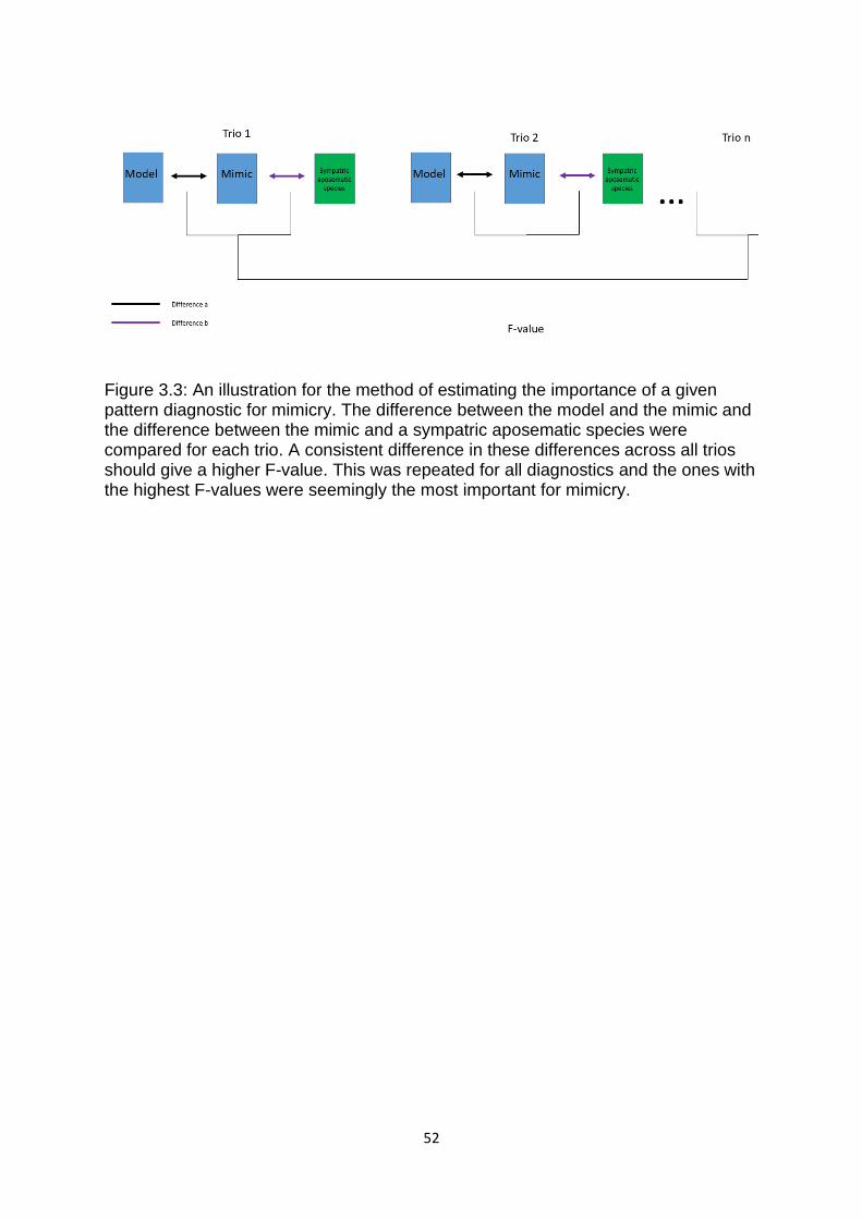
52

Figure 3.3: An illustration for the method of estimating the importance of a given pattern diagnostic for mimicry. The difference between the model and the mimic and the difference between the mimic and a sympatric aposematic species were compared for each trio. A consistent difference in these differences across all trios should give a higher F-value. This was repeated for all diagnostics and the ones with the highest F-values were seemingly the most important for mimicry.

53

Chapter 4: The effect of palatability on the evolution of mimics and

models

As discussed in Chapter 1, the evolutionary dynamics of Batesian and

Müllerian mimicry are very different. This could lead to mimetic similarity differing

between Batesian and Müllerian mimics. It could also cause the aversiveness of

aposematic patterns to differ between defended species with Batesian mimics and

those without mimics. To test the first hypothesis, I used the images outlined in

Chapter 3 to compare the degree of similarity between Batesian mimics and their

models, with the degree of similarity between Müllerian co-mimics using the three

measures of similarity I use throughout the thesis (See Chapter 3). In order to test

the second hypothesis, I compared the aversiveness of the patterns of aposematic

species which have Batesian mimics with those which lack mimics entirely, using two

measures of pattern aversiveness (mean pattern energy and the standard deviation

of isotropy). I found no significant differences in any of the measures used to

compare either the mimetic similarity between Batesian and Müllerian mimicry, or the

aversiveness of aposematic species with and without Batesian mimics. When taken

together, these findings could suggest that the presence of Batesian mimics does

not cause their models to evolve away from their optimally effective aposematic

patterns, at least in Lepidoptera.

4.1: Introduction

Though, on the face of it, the difference between Batesian and Müllerian

mimicry may seem inconsequential, the fact that Batesian mimics are palatable

whereas Müllerian mimics are unpalatable has huge implications for their

evolutionary dynamics (Turner 1987). In Batesian mimicry, it is thought that as the

palatable mimics evolve to resemble their models, the models, in turn, evolve away

from them: this is known as advergent evolution (Franks and Noble 2004; See Figure

1.1 and Chapter 1 for a more detailed discussion of this phenomenon). The reason

for this is that the presence of a Batesian mimic weakens the association that

predators makes between the unprofitability of the model and its pattern, although

there are some circumstances where Batesian mimicry is mutually beneficial for both

the mimics and their models, see Polnaszek et al. (2017) and Holen and Johnstone

(2018) for details. As a result, Batesian mimicry is beneficial for the mimic but costly

for the model (Franks and Noble 2004). It has been suggested that in some

54

circumstances this could lead to imperfect mimicry since the model continually

evolves away from the mimic (this is known as the “chase-away hypothesis” (Franks

et al. 2009)). However, this is not always the case, and in other circumstances we

might expect the mimics to ‘win’ the race because they are under stronger selection:

evolution has presumably favoured models with “optimal” patterns, so evolving away

from this to avoid mimics could well be associated with costs as well as benefits

(Turner 1987).

In contrast, traditionally, Müllerian co-mimics are classically believed to evolve

towards one another in order to benefit from a shared aposematic pattern. If a

predator takes a fixed number of encounters to learn to associate a pattern with

unprofitability, then if two species share a pattern they also share the cost of

educating predators, meaning the per capita predation rate is lower for both species

(Müller 1878). This type of relationship (where two species converge on a single

pattern) is known as convergent evolution (Franks and Noble 2004; Figure 1.1).

However, some putative Müllerian mimics may share similar evolutionary

dynamics to those commonly associated with Batesian mimicry (Mallet 1999). This

could occur when one Müllerian co-mimic is less well defended than another. Under

these circumstances, the relationship between co-mimics could be parasitic if a

predator attacks the less-defended mimic, learns to associate its colour pattern with

a lower toxin content and increases attack rates on the mimicry complex in the

future. This so-called “quasi-Batesian mimicry” (Speed 1993) should lead to

advergence of the less well-defended mimic to the more defended one. However,

evidence for such relationships are equivocal. Some behavioural experiments have

shown that defended mimics can either improve or be detrimental to the survival of a

co-mimic, depending on their relative unpalatability (Speed et al. 2000; Rowland et

al. 2010). However, this is not always the case, some experiments have shown that

Müllerian mimics can have a mutually beneficial relationship even if one is less

defended than the other (Rowland et al. 2007). Moreover, recent mathematical

models suggest that mimicry between unequally defended species is likely to be

mutually beneficial under a wide range of conditions; and that, while Quasi-Batesian

mimics are possible, these would only be predicted under very restricted

circumstances (Aubier et al. 2017).

55

The difference between advergent and convergent evolution is important

when thinking about mimetic similarity. Since, on the whole, Müllerian co-mimics are

both likely to converge on the same pattern whereas Batesian mimics are likely to

cause their models to evolve away from them (Figure 1.1). We might expect mimetic

similarity to be greater in Müllerian than Batesian mimicry because when Batesian

mimics evolve towards the pattern of a model, the model may subsequently evolve

away from that pattern thus causing the mimic to share a less close resemblance

with it (Rettenmeyer 1970).

Alternatively, it has also been suggested that Batesian mimics should be

under stronger selection to resemble their models than Müllerian mimics due to the

fact that they lack defences of their own (Nur 1970). This is because the decision a

predator makes when determining whether or not to attack a mimic depends on the

cost of attacking the model (Goodale and Sneddon 1977), the reward for eating the

mimic (Penney et al. 2012) and how sure the predator is that the prey being attacked

is the mimic (i.e. the degree of similarity between the model and the mimic (Duncan

and Sheppard 1965)). Because attacking a Müllerian mimic is less rewarding than

attacking a Batesian mimic due to the fact that the predator still incurs a cost from

the Müllerian mimic’s defences, in order to gain the same level of protection, a

Batesian mimic should theoretically resemble its model more closely. However, there

have been no studies to examine whether there is a difference in mimetic similarity

between Batesian and Müllerian pairs. In order to answer to address this, in the first

part of this chapter I compare the degree of similarity between Batesian mimics and

their models with the degree of similarity between Müllerian co-mimics (For

simplicity, I will refer to mimetic pairs involving two defended species as Müllerian

pairs as in the classical sense as described by Müller (1879)).

The difference in palatability between Batesian mimics and Müllerian mimics

should also affect the selection pressures on the patterns of the models (Nur 1970).

This could lead to a change in the aversiveness of the pattern, which could be in one

of two directions for models of Batesian mimics. Firstly, the presence of a Batesian

mimic may make a model evolve a less-effective aposematic signal since the

“optimal” pattern for an aposematic species changes once a palatable species

evolves to mimic it (Turner 1987; Turner 1995). Therefore, a model may have

evolved an “optimally-aversive” pattern prior to the appearance of the mimic may

56

evolve away from this pattern and, in doing so, its new pattern might be less visually

aversive. Alternatively, if a Batesian mimic evolves to resemble an aposematic

species, the pattern of the new model may be selected to become more conspicuous

to disengage from the Batesian mimic and avoid the parasitic relationship

(Rettenmeyer 1970; Franks et al. 2009; Kraemer et al. 2015b). Becoming more

conspicuous could allow a model to evolve away from a Batesian mimic because

mimics which are more conspicuous are likely to experience increased predation

(because they are more likely to be detected) and therefore will not gain as much of

a benefit from mimicry (Speed and Ruxton 2010). Since pairs of equally defended

Müllerian mimics and species which lack mimics do not experience selection

pressure due to the presence of a palatable mimic, they are both unlikely to differ in

terms of their pattern effectiveness. In the past, the main way in which the

effectiveness of an aposematic pattern has been measured is either through its

conspicuousness (i.e. luminance contrast (Prudic et al. 2006), its chromatic contrast

with the background (Kraemer et al. 2015b)) or its distinctiveness (i.e. the difference

between it and the profitable prey in the area (Merilaita and Ruxton 2007; Polnaszek

et al. 2017)). Recently, it has been shown that the patterns of aposematic and non-

aposematic Lepidoptera can be reliably separated by certain pattern diagnostics

(Penacchio et al. in prep.) which are also good indicators of the aversiveness of a

pattern to a predator (Penacchio et al. in prep.). Hence, in this study, I use these

measures as an indicator of how effective the aposematic patterns are and explore

how they differ between aposematic species with a Batesian mimic and sympatric

aposematic species which lack mimics entirely. Therefore, the two questions I hope

to answer with this chapter are: (1) is there a difference in similarity between

Batesian and Müllerian mimics and their models? (2) Do Batesian mimics affect the

evolution of their models?

4.2: Methods

4.2.1: Is there a difference in mimetic similarity between Batesian and

Müllerian mimicry?

In order to investigate whether mimetic similarity differs between Batesian and

Müllerian mimicry, I initially established which of the 31 pairs I scanned could be

considered examples of Batesian mimicry, and which could be considered to be

examples of Müllerian mimicry. In order to classify a pair as an example of Batesian

57

mimicry, one of the individuals had to be shown to be palatable and one had to be

shown to be unpalatable, whereas to classify a pair as an example of Müllerian

mimicry, both species involved had to be shown to be unpalatable. I considered

individuals as palatable if they had been shown to be palatable to a predator in a

behavioural experiment, or if they were found in the same genus as another species

which had been shown to be palatable. I considered individuals as unpalatable if

they met at least one of the three following criteria: they had been shown to be

unpalatable to a predator in a behavioural experiment, they contained a known

defensive chemical or they were in the same genus as a species which was known

to be unpalatable. If a pair did not fit these criteria, the type of mimicry was recorded

as unknown. Using these criteria, I determined that out of my 31 pairs, 13 were

examples of Batesian mimicry, 10 were examples of Müllerian and 8 were unknown.

I then calculated the similarity between the two species involved in each of the

Batesian and Müllerian mimic pairs. I did this in three different ways, using the 3

pattern diagnostics which were predicted to be the most important for mimicry: the

difference in the standard deviation of the blue-yellow channel response, the

difference in mean energy for cells of Scale 10 and the NaturePatternMatch score

(See Chapter 3). Unfortunately, I was only able to use 9 of the 10 Müllerian pairs

when calculating pattern similarity based on the score from NaturePatternMatch

because I only scanned 1 specimen of Amerila brunnea and 1 specimen of Amerila

bipartita and the algorithm did not provide a value of similarity between the two

specimens.

I used independent t-tests to compare two of the measures of mimetic

similarity between Batesian and Müllerian mimics (NaturePatternMatch Score and

the mean pattern energy for cells of Scale 10). This approach was chosen because

the data met the assumptions for parametric tests: the residuals were normally

distributed (Shapiro-Wilk Test: NaturePatternMatch Score: W = 0.967, p = 0.630,

mean pattern energy for cells of Scale 10: W = 0.928, p = 0.0997) and their variance

was homogeneous (Levene test: NaturePatternMatch: F1, 20 = 0.0582, p = 0.812,

Mean energy of the pattern (Scale 10): F1, 21 = 0.628, p = 0.437, Standard deviation

of blue-yellow channel response: F1, 21 = 0.449, p = 0.510). However, the residuals of

the standard deviation of blue-yellow channel response were not normally distributed

58

(Shapiro-Wilk Test: W: 0.895, p = 0.02), and so I used a Mann Whitney-U test when

comparing this measure.

4.2.2: Do Batesian mimics affect the evolution of their models?

To investigate the effect of the presence of a Batesian mimic on the

effectiveness of the pattern of the model, I calculated (i) the mean energy of the

patterns, and (ii) the standard deviation of the isotropy departure of the patterns, for

both aposematic species with models and those without using the energy-isotropy

analysis described in Sections 2.3.2 and 3.4.2. I chose these measures because

they have been demonstrated to affect how aversive a pattern is (Penacchio et al. in

prep.).

I then established whether these measures differed between aposematic

species with Batesian mimics and those without mimics. I used a paired sample t-

test to compare the mean energy of the patterns of Batesian models with that of

aposematic species which lack mimics. I used a paired method because each model

species with a Batesian mimic was associated with a sympatric non-mimicked

species. This approach was appropriate because the data showed homogeneity of

variance (Levene’s test- F1,18 = 0.324, p = 0.576) and were normally distributed

(Shapiro-Wilk Test: Models: W= 0.956, p = 0.743, non-mimicked species: W = 0.949,

p = 0.661). The residuals were also normally distributed (W = 0.955, p = 0.447). In

contrast, when comparing the standard deviation of isotropy departure between the

two groups, I used a Wilcoxon signed-rank test. This was chosen because although

these data also showed homogeneity of variance (Levene’s test- F1,18 = 1.355, p

=0.260), the data for Batesian models were not normally distributed (Shapiro-Wilk

test: models: W = 0.749, p = 0.003, non-mimicked species: W = 0.897, p = 0.204).

The residuals were also non-normally distributed (W = 0.819, p = 0.002). For all of

these tests, the number of pairs studied was reduced from 13 to 10 as there were

only 10 Batesian models, (four of the Batesian mimics mimicked Battus philenor).

This was not a problem in the previous study because the measures of similarity

differ between every model-mimic pair. Whilst there is evidence to suggest that

larger species tend to have more conspicuous patterns (Hagman and Forsman

2003), this is not true for all taxa (Cheney et al. 2014). Moreover, I found no

evidence that aposematic species with and without mimics differed in size between

groups (Mann-Whitney U test: W=59, p = 0.5288). Consequently, I did not include

59

size as a factor in the analyses. All analyses were conducted in R 3.5.3 (R

Development Core Team, 2019) and visualised by RStudio 1.2.1335 (RStudio Team,

2018).

4.3: Results

4.3.1: Is there a difference in similarity between Batesian and Müllerian

mimics?

None of the measures of mimetic similarity differed significantly between

Batesian and Müllerian mimics (Standard deviation of blue-yellow colour channel

response: W = 67.5, p =0.901 (Figure 4.1); Mean Energy for Scale 10 cells: t17.47 =

0.319, p =0.753 (Figure 4.2); NaturePatternMatch Scores: t18.888 = 0.479, p =0.638

(Figure 4.3)). Furthermore, the differences remained non-significant even after the

outliers were removed (Standard deviation of blue-yellow colour channel response:

t19.528 = 0.662, p = 0.516, Mean Energy for Scale 10 cells: W =30, p = 0.581,

NaturePatternMatch Scores: t13.937 = 0.383, p =0.707). Outliers were defined as

points which were either less than the first quartile minus 1.5 times the interquartile

range or more than the third quartile plus 1.5 times the interquartile range. This is

sometimes termed the 1.5-IQR rule (Ghosh-Dastidar and Schafer 2003).

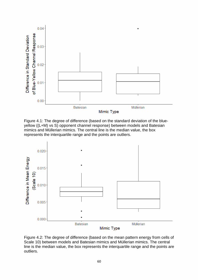
60

Figure 4.1: The degree of difference (based on the standard deviation of the blue-yellow ((L+M) vs S) opponent channel response) between models and Batesian mimics and Müllerian mimics. The central line is the median value, the box represents the interquartile range and the points are outliers.

Figure 4.2: The degree of difference (based on the mean pattern energy from cells of Scale 10) between models and Batesian mimics and Müllerian mimics. The central line is the median value, the box represents the interquartile range and the points are outliers.

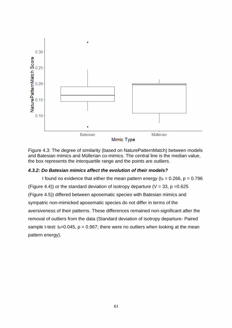
61

Figure 4.3: The degree of similarity (based on NaturePatternMatch) between models and Batesian mimics and Müllerian co-mimics. The central line is the median value, the box represents the interquartile range and the points are outliers.

4.3.2: Do Batesian mimics affect the evolution of their models?

I found no evidence that either the mean pattern energy (t9 = 0.266, p = 0.796

(Figure 4.4)) or the standard deviation of isotropy departure (V = 33, p =0.625

(Figure 4.5)) differed between aposematic species with Batesian mimics and

sympatric non-mimicked aposematic species do not differ in terms of the

aversiveness of their patterns. These differences remained non-significant after the

removal of outliers from the data (Standard deviation of isotropy departure- Paired

sample t-test: t6=0.045, p = 0.967; there were no outliers when looking at the mean

pattern energy).

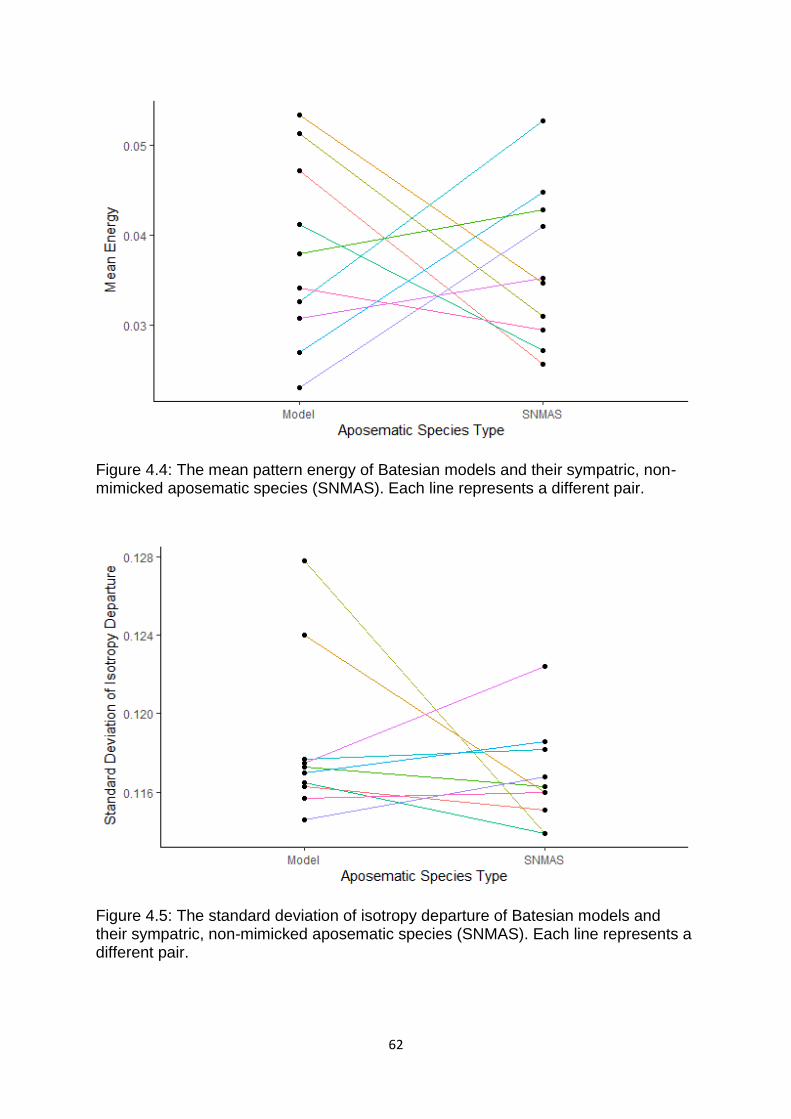
62

Figure 4.4: The mean pattern energy of Batesian models and their sympatric, non-mimicked aposematic species (SNMAS). Each line represents a different pair.

Figure 4.5: The standard deviation of isotropy departure of Batesian models and their sympatric, non-mimicked aposematic species (SNMAS). Each line represents a different pair.

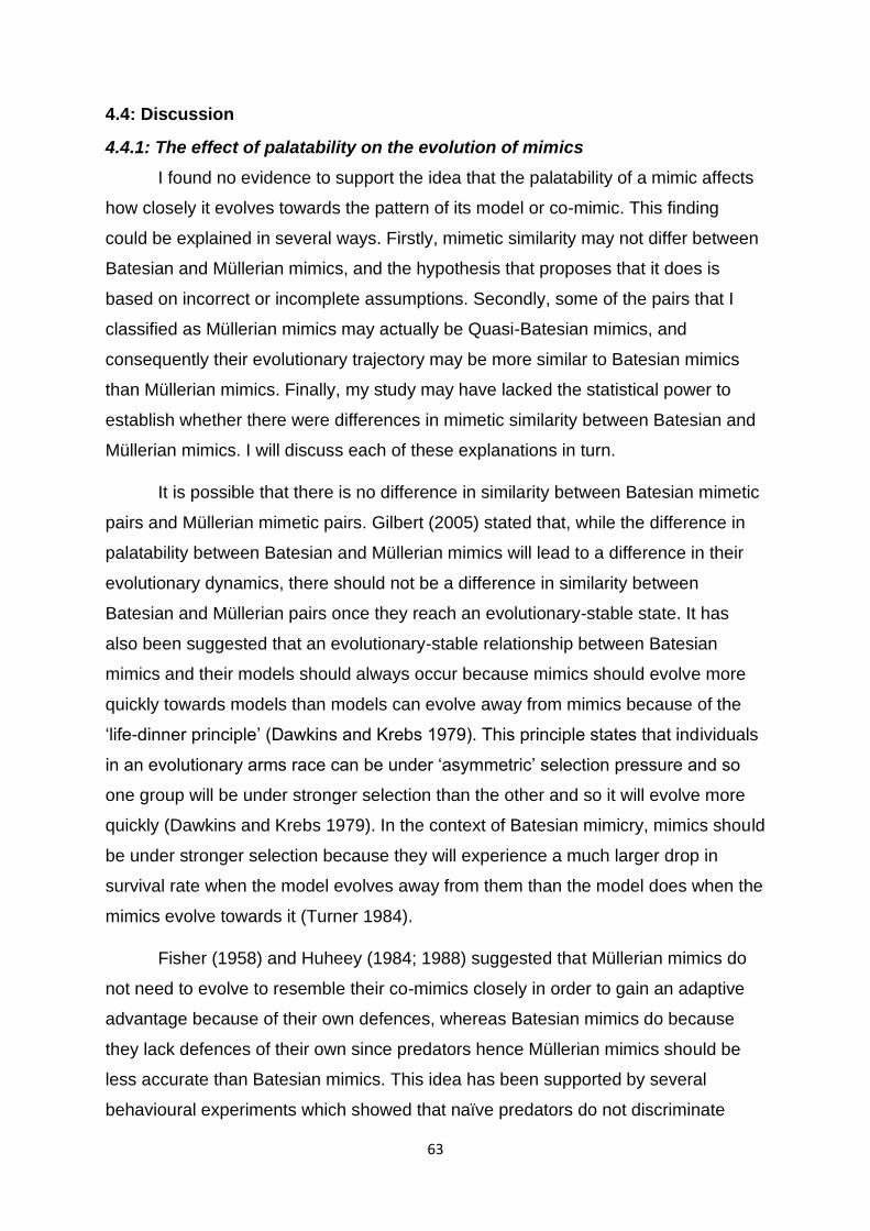
63

4.4: Discussion

4.4.1: The effect of palatability on the evolution of mimics

I found no evidence to support the idea that the palatability of a mimic affects

how closely it evolves towards the pattern of its model or co-mimic. This finding

could be explained in several ways. Firstly, mimetic similarity may not differ between

Batesian and Müllerian mimics, and the hypothesis that proposes that it does is

based on incorrect or incomplete assumptions. Secondly, some of the pairs that I

classified as Müllerian mimics may actually be Quasi-Batesian mimics, and

consequently their evolutionary trajectory may be more similar to Batesian mimics

than Müllerian mimics. Finally, my study may have lacked the statistical power to

establish whether there were differences in mimetic similarity between Batesian and

Müllerian mimics. I will discuss each of these explanations in turn.

It is possible that there is no difference in similarity between Batesian mimetic

pairs and Müllerian mimetic pairs. Gilbert (2005) stated that, while the difference in

palatability between Batesian and Müllerian mimics will lead to a difference in their

evolutionary dynamics, there should not be a difference in similarity between

Batesian and Müllerian pairs once they reach an evolutionary-stable state. It has

also been suggested that an evolutionary-stable relationship between Batesian

mimics and their models should always occur because mimics should evolve more

quickly towards models than models can evolve away from mimics because of the

‘life-dinner principle’ (Dawkins and Krebs 1979). This principle states that individuals

in an evolutionary arms race can be under ‘asymmetric’ selection pressure and so

one group will be under stronger selection than the other and so it will evolve more

quickly (Dawkins and Krebs 1979). In the context of Batesian mimicry, mimics should

be under stronger selection because they will experience a much larger drop in

survival rate when the model evolves away from them than the model does when the

mimics evolve towards it (Turner 1984).

Fisher (1958) and Huheey (1984; 1988) suggested that Müllerian mimics do

not need to evolve to resemble their co-mimics closely in order to gain an adaptive

advantage because of their own defences, whereas Batesian mimics do because

they lack defences of their own since predators hence Müllerian mimics should be

less accurate than Batesian mimics. This idea has been supported by several

behavioural experiments which showed that naïve predators do not discriminate

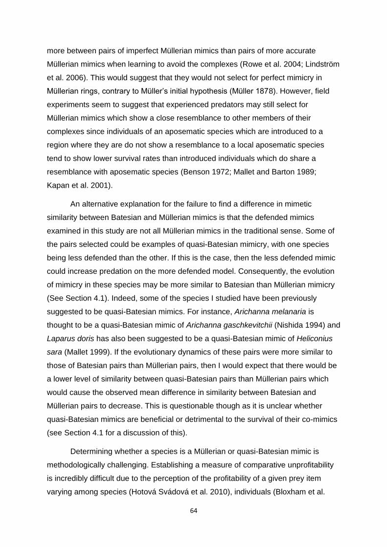
64

more between pairs of imperfect Müllerian mimics than pairs of more accurate

Müllerian mimics when learning to avoid the complexes (Rowe et al. 2004; Lindström

et al. 2006). This would suggest that they would not select for perfect mimicry in

Müllerian rings, contrary to Müller’s initial hypothesis (Müller 1878). However, field

experiments seem to suggest that experienced predators may still select for

Müllerian mimics which show a close resemblance to other members of their

complexes since individuals of an aposematic species which are introduced to a

region where they are do not show a resemblance to a local aposematic species

tend to show lower survival rates than introduced individuals which do share a

resemblance with aposematic species (Benson 1972; Mallet and Barton 1989;

Kapan et al. 2001).

An alternative explanation for the failure to find a difference in mimetic

similarity between Batesian and Müllerian mimics is that the defended mimics

examined in this study are not all Müllerian mimics in the traditional sense. Some of

the pairs selected could be examples of quasi-Batesian mimicry, with one species

being less defended than the other. If this is the case, then the less defended mimic

could increase predation on the more defended model. Consequently, the evolution

of mimicry in these species may be more similar to Batesian than Müllerian mimicry

(See Section 4.1). Indeed, some of the species I studied have been previously

suggested to be quasi-Batesian mimics. For instance, Arichanna melanaria is

thought to be a quasi-Batesian mimic of Arichanna gaschkevitchii (Nishida 1994) and

Laparus doris has also been suggested to be a quasi-Batesian mimic of Heliconius

sara (Mallet 1999). If the evolutionary dynamics of these pairs were more similar to

those of Batesian pairs than Müllerian pairs, then I would expect that there would be

a lower level of similarity between quasi-Batesian pairs than Müllerian pairs which

would cause the observed mean difference in similarity between Batesian and

Müllerian pairs to decrease. This is questionable though as it is unclear whether

quasi-Batesian mimics are beneficial or detrimental to the survival of their co-mimics

(see Section 4.1 for a discussion of this).

Determining whether a species is a Müllerian or quasi-Batesian mimic is

methodologically challenging. Establishing a measure of comparative unprofitability

is incredibly difficult due to the perception of the profitability of a given prey item

varying among species (Hotová Svádová et al. 2010), individuals (Bloxham et al.

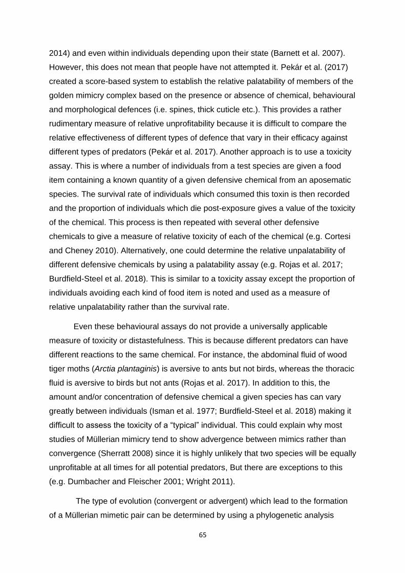
65

2014) and even within individuals depending upon their state (Barnett et al. 2007).

However, this does not mean that people have not attempted it. Pekár et al. (2017)

created a score-based system to establish the relative palatability of members of the

golden mimicry complex based on the presence or absence of chemical, behavioural

and morphological defences (i.e. spines, thick cuticle etc.). This provides a rather

rudimentary measure of relative unprofitability because it is difficult to compare the

relative effectiveness of different types of defence that vary in their efficacy against

different types of predators (Pekár et al. 2017). Another approach is to use a toxicity

assay. This is where a number of individuals from a test species are given a food

item containing a known quantity of a given defensive chemical from an aposematic

species. The survival rate of individuals which consumed this toxin is then recorded

and the proportion of individuals which die post-exposure gives a value of the toxicity

of the chemical. This process is then repeated with several other defensive

chemicals to give a measure of relative toxicity of each of the chemical (e.g. Cortesi

and Cheney 2010). Alternatively, one could determine the relative unpalatability of

different defensive chemicals by using a palatability assay (e.g. Rojas et al. 2017;

Burdfield-Steel et al. 2018). This is similar to a toxicity assay except the proportion of

individuals avoiding each kind of food item is noted and used as a measure of

relative unpalatability rather than the survival rate.

Even these behavioural assays do not provide a universally applicable

measure of toxicity or distastefulness. This is because different predators can have

different reactions to the same chemical. For instance, the abdominal fluid of wood

tiger moths (Arctia plantaginis) is aversive to ants but not birds, whereas the thoracic

fluid is aversive to birds but not ants (Rojas et al. 2017). In addition to this, the

amount and/or concentration of defensive chemical a given species has can vary

greatly between individuals (Isman et al. 1977; Burdfield-Steel et al. 2018) making it

difficult to assess the toxicity of a “typical” individual. This could explain why most

studies of Müllerian mimicry tend to show advergence between mimics rather than

convergence (Sherratt 2008) since it is highly unlikely that two species will be equally

unprofitable at all times for all potential predators, But there are exceptions to this

(e.g. Dumbacher and Fleischer 2001; Wright 2011).

The type of evolution (convergent or advergent) which lead to the formation

of a Müllerian mimetic pair can be determined by using a phylogenetic analysis

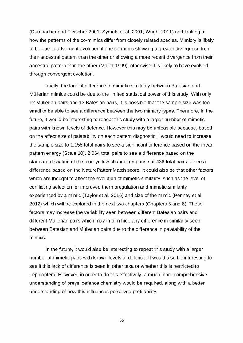
66

(Dumbacher and Fleischer 2001; Symula et al. 2001; Wright 2011) and looking at

how the patterns of the co-mimics differ from closely related species. Mimicry is likely

to be due to advergent evolution if one co-mimic showing a greater divergence from

their ancestral pattern than the other or showing a more recent divergence from their

ancestral pattern than the other (Mallet 1999), otherwise it is likely to have evolved

through convergent evolution.

Finally, the lack of difference in mimetic similarity between Batesian and

Müllerian mimics could be due to the limited statistical power of this study. With only

12 Müllerian pairs and 13 Batesian pairs, it is possible that the sample size was too

small to be able to see a difference between the two mimicry types. Therefore, In the

future, it would be interesting to repeat this study with a larger number of mimetic

pairs with known levels of defence. However this may be unfeasible because, based

on the effect size of palatability on each pattern diagnostic, I would need to increase

the sample size to 1,158 total pairs to see a significant difference based on the mean

pattern energy (Scale 10), 2,064 total pairs to see a difference based on the

standard deviation of the blue-yellow channel response or 438 total pairs to see a

difference based on the NaturePatternMatch score. It could also be that other factors

which are thought to affect the evolution of mimetic similarity, such as the level of

conflicting selection for improved thermoregulation and mimetic similarity

experienced by a mimic (Taylor et al. 2016) and size of the mimic (Penney et al.

2012) which will be explored in the next two chapters (Chapters 5 and 6). These

factors may increase the variability seen between different Batesian pairs and

different Müllerian pairs which may in turn hide any difference in similarity seen

between Batesian and Müllerian pairs due to the difference in palatability of the

mimics.

In the future, it would also be interesting to repeat this study with a larger

number of mimetic pairs with known levels of defence. It would also be interesting to

see if this lack of difference is seen in other taxa or whether this is restricted to

Lepidoptera. However, in order to do this effectively, a much more comprehensive

understanding of preys’ defence chemistry would be required, along with a better

understanding of how this influences perceived profitability.

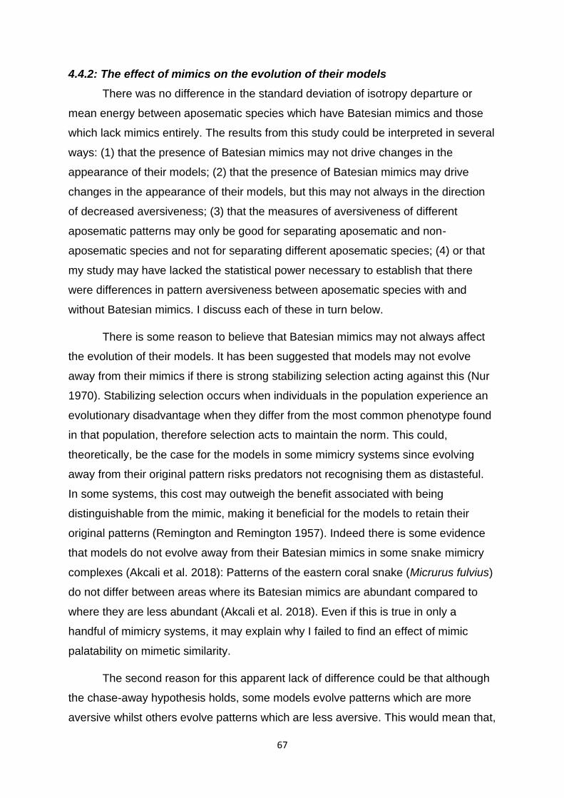
67

4.4.2: The effect of mimics on the evolution of their models

There was no difference in the standard deviation of isotropy departure or

mean energy between aposematic species which have Batesian mimics and those

which lack mimics entirely. The results from this study could be interpreted in several

ways: (1) that the presence of Batesian mimics may not drive changes in the

appearance of their models; (2) that the presence of Batesian mimics may drive

changes in the appearance of their models, but this may not always in the direction

of decreased aversiveness; (3) that the measures of aversiveness of different

aposematic patterns may only be good for separating aposematic and non-

aposematic species and not for separating different aposematic species; (4) or that

my study may have lacked the statistical power necessary to establish that there

were differences in pattern aversiveness between aposematic species with and

without Batesian mimics. I discuss each of these in turn below.

There is some reason to believe that Batesian mimics may not always affect

the evolution of their models. It has been suggested that models may not evolve

away from their mimics if there is strong stabilizing selection acting against this (Nur

1970). Stabilizing selection occurs when individuals in the population experience an

evolutionary disadvantage when they differ from the most common phenotype found

in that population, therefore selection acts to maintain the norm. This could,

theoretically, be the case for the models in some mimicry systems since evolving

away from their original pattern risks predators not recognising them as distasteful.

In some systems, this cost may outweigh the benefit associated with being

distinguishable from the mimic, making it beneficial for the models to retain their

original patterns (Remington and Remington 1957). Indeed there is some evidence

that models do not evolve away from their Batesian mimics in some snake mimicry

complexes (Akcali et al. 2018): Patterns of the eastern coral snake (Micrurus fulvius)

do not differ between areas where its Batesian mimics are abundant compared to

where they are less abundant (Akcali et al. 2018). Even if this is true in only a

handful of mimicry systems, it may explain why I failed to find an effect of mimic

palatability on mimetic similarity.

The second reason for this apparent lack of difference could be that although

the chase-away hypothesis holds, some models evolve patterns which are more

aversive whilst others evolve patterns which are less aversive. This would mean that,

68

on average, there was no apparent change in the pattern aversiveness. It is

commonly assumed that if, in the absence of any mimics, selection favours the

aposematic patterns which are optimally aversive, the evolution of a Batesian mimic

which resembles a species with such a pattern will cause the most optimal pattern

for that species to change as models which resemble the mimic will be selected

against (Turner 1987; Turner 1995) and this selection will cause them to evolve

towards this new optimum and away from their old pattern. As they do, their patterns

should theoretically become less aversive since they are “chased away” from an

optimally aversive pattern. However, this is not likely to be true if a wide range of

patterns are equally effective at providing a warning to would-be predators. In

addition, the patterns that models possess may not be optimal for deterring

predators, but may instead reflect an optimal trade-off between deterring predators

and some other function (e.g. thermoregulation). If this is the case, then the

presence of mimics may shift the optimal trade-off and cause patterns to become

more aversive in the presence of mimics.

A third reason why there may not be a difference in pattern aversiveness

between mimicked and non-mimicked species is due to the measures used in this

study. The two measures used in this study were developed to distinguish between

aposematic and non-aposematic species (Penacchio et al. in prep.). Because of this,

most aposematic species, regardless of whether or not they have mimics, are likely

to have a high mean pattern energy and a large standard deviation of isotropy

departure. Therefore, these measures may not be well-suited to distinguish between

different groups of aposematic species.

It is also possible that the small number of pairs means that I was not able to

find a difference between mimicked and non-mimicked species, and it would be

interesting to repeat this experiment in the future with more species. But this may be

also be unfeasible as the effect size is so small that it would require 1,392 pairs of

mimics and sympatric, non-mimicked species before there would be a significant

difference in mean pattern energy but it would only require 100 pairs of mimics and

sympatric, non-mimicked species to see a significant difference in the standard

deviation of isotropy.

69

It would also be interesting to do this in a phylogenetically-controlled manner

to see if the presence of mimics alters the pattern aversiveness from an ancestral

state i.e. do species which gain a mimic after evolving from ancestrally-non-

mimicked species have less aversive patterns than their ancestors? This would

require a lot of work to construct the phylogenies of the model species, but this task

will be slightly easier than in previous years due to recent advancements in the

phylogenomics of butterflies (Espeland et al. 2018) and Lepidoptera as a whole

(Kawahara et al. 2019).

4.4.3: Overall conclusions

Taken together, my results suggest that the difference in the evolutionary

dynamics between Batesian mimics and Müllerian mimics do not lead to significant

differences in how closely they evolve to resemble their model. It seems that the

more palatable species evolves so that its pattern resembles the less palatable

species and the less palatable species do not evolve away from that mimic. Whether

this is due to all Müllerian mimicry being quasi-Batesian or Batesian models not

evolving away from their mimics due to stabilizing selection (or a mixture of the two)

remains to be seen. However, this lack of difference is certainly interesting especially

when considering the traditional view of the dichotomy of Batesian and Müllerian

mimicry and perhaps, instead, supports the idea of a mimicry spectrum (Balogh et al.

2008).

This chapter has focused on exclusively on how patterns of mimics are

shaped based on how predators generate selection for mimicry. However, animal

patterns often several several functions (e.g. sexual signalling (Finkbeiner et al.

2014), thermoregulation (Taylor et al. 2016) etc.) and often several pressures are

acting on one pattern simultaneously. Therefore, in the next chapter, I will focus on

how selection by one of these factors (selection for increased thermoregulatory

efficiency) may interact with selection for increased mimetic similarity and therefore

how it may influence the evolution of mimicry.

70

Chapter 5: The effect of ambient temperature on the evolution of

mimicry

Colour patterns are often under selection pressures to fulfil multiple functions,

and features which allow a pattern to perform better in one respect would cause it to

perform worse in another. This is known as an evolutionary trade-off. In this study, I

investigated whether there is a trade-off between selection for improved

thermoregulation and selection for improved mimetic accuracy as suggested by

Taylor et al. (2016). Specifically, I tested if there was a correlation between the three

measures of mimetic similarity I have used throughout this thesis and both the

minimum temperature and mean temperature experienced by a mimic during its

flight period. I found that there was no significant correlation between any measure

of mimetic similarity and the mean temperature experienced by a mimic, although I

did find a significant negative correlation with one measure (NaturePatternMatch

score) and the minimum temperature experienced. This could be due to the more

diverse prey communities associated with tropical regions causing predators to

generalise their aversions to models more widely, which could in turn lead to relaxed

selection for mimetic similarity in these areas.

5.1: Introduction

The colour patterns of animals have many functions even for a single animal.

They can be used for attracting mates (Finkbeiner et al. 2014), thermoregulation

(Zeuss et al. 2014; Xing et al. 2016) and (as detailed in this thesis) anti-predator

defence: with aposematic (Lee et al. 2018), cryptic (Cuthill et al. 2005) and, of

course, mimetic (Prudic et al. 2002) patterns all reducing the likelihood of an

organism being eaten. However, research into animal colouration tends to consider

each function of a colour pattern in isolation without considering how they may

interact. This is an important factor to consider, particularly for studies of mimicry,

since patterns which improve one function often do so to the detriment of another.

One clear example of this can be seen with the patterns of Heliconius

butterflies which are used for intersexual communication as well as for anti-predator

defence (Finkbeiner et al. 2014). This is potentially problematic because several

Heliconius species use mimicry as a form of defence, and whilst this could deter

predators it could also cause males to court females of the wrong species (Estrada

71

and Jiggins 2008). In order to avoid this, some species of Heliconius butterflies

evolved to have a different yellow pigment to their Müllerian co-mimics. The pigment

used by Heliconius reflects UV light, while the pigment used by their co-mimics does

not (Bybee et al. 2012). The butterflies can better discriminate between these two

pigments than their predators which allows them to identify conspecifics while

maintaining the benefits of being part of a Müllerian mimicry ring (Bybee et al. 2012).

However, it is not always possible to find a solution that simultaneously optimises all

functions of an animal’s colour pattern. In some cases, these trade-offs between the

different pressures can lead to selection for improved efficacy of one function to the

detriment of the efficacy of the other.

One such conflict is the trade-off faced by animals with patterns which have

been selected to allow for efficient thermoregulation while also serving mimetic

function. The ability to control body temperature efficiently is vital for insects

(particularly those living in temperate climates) because their bodies need to reach a

minimum temperature for the enzymes involved in metabolic processes to function

(Neven 2000). Insects’ flight muscles also need to reach a minimum temperature

before they will work. If this is not reached, insects are unable to fly and, therefore, to

forage and escape potential predators (Heinrich 1993). Since many species of

insects are ectotherms meaning that their body temperature largely depends on

climatic factors (although some endothermic insects can control their own

temperature using physiological processes (Casey 1988)), they usually warm up by

basking in the sun (Hodkinson 2005). Species with darker colouration heat up more

quickly due to their ability to absorb radiation more efficiently, this is why insects

which live in cooler climates tend to be darker (Zeuss et al. 2014; Xing et al. 2016).

However, if insects are involved in mimetic relationships, they may need to trade-off

the benefit of being dark with the benefit of accurately resembling their model

(unless, of course, their model is also dark).

Recently, it has been suggested that selection for improved thermoregulation

acts in opposition to selection for improved mimetic accuracy, and that this result in

the evolution of imperfect mimicry (Taylor et al. 2016). This hypothesis was based on

the fact that hoverflies that demonstrate imperfect mimicry, tend to have a higher

proportion of black in their patterns than their models, suggesting that they have

increased melanisation to allow them to heat up more quickly (Willmer and Unwin

72

1981). However, this hypothesis does not explain why models are not under similar

selection to improve their ability to thermoregulate. Indeed, it implicitly assumes that

either the costs of increased melanisation are higher for models than mimics or the

benefits are lower. This hypothesis is further called into question by the fact that

there are mimicry rings where the correlation between melanisation and mimetic

accuracy is not seen. For instance, some imperfect coral snake mimics do have a

large amount of black in their dorsal colouration, whereas other equally imperfect

mimics do not (Akcali and Pfennig 2017). Moreover, the proposed trade-off seen in

the hoverflies does not seem to improve their thermoregulatory capabilities. Daňková

et al. (in prep.) found that there was no correlation between the internal body

temperature of hoverflies relative to the ambient temperature and their mimetic

accuracy.

Given the uncertainty surrounding this hypothesis, I decided to test it

empirically using the lepidopteran images I had collected and analysed. I predicted

that, if this hypothesis holds, there would be a positive relationship between the

measures of mimetic similarity previously outlined in this thesis (so a positive

relationship with NaturePatternMatch score and a negative relationship with the

difference in the mean pattern energy for cells of Scale 10 and the difference in the

standard deviation of blue-yellow channel response) and the temperature of the

regions where the mimics are found during their flight periods. This would be

expected because selection for patterns that optimise the absorption of heat when

basking should be stronger in areas where temperatures are lower.

5.2: Methods

I used two measures of environmental temperature in this study: the mean

and minimum temperatures experienced by mimics during their flight periods. The

mean temperature was used as a measure of the temperature that mimics typically

encounter during their flight season, and the minimum temperature was used as a

measure of the lowest temperature that a species has to endure in order to survive in

that region. The latter is important because it is at these temperatures that colour

patterns that enhance individuals’ abilities to maintain body temperatures sufficiently

high enough to allow flight, are likely to have the biggest effect on survival.

73

In order to find mean and minimum temperatures for each species, I first used

the labels from the scanned museum specimens to find the exact location where

they had been collected, and, determined the latitude and longitude of these

locations.

I then used several methods to establish the months when adults of each

species of mimic are on the wing. First, I checked the labels for any record of the

month when a specimen was collected. If the labels lacked the relevant information, I

consulted relevant field guides and searched Google Scholar for species surveys for

regions where the mimics were found. If these methods were not successful, I

searched for photographs of the mimic online and noted the months in which any

photos were taken. There was only species for which I found no flight data (Papilio

laglaizei) and, in this case, I used the flight dates of its model (Alcides agathyrsus)

instead. In addition to this, there were four species where the data on flight dates

were incomplete (Hestina mimetica, Mimoides ilus, Mynes doubledayi and Mynes

plateni), and I detail how I dealt with this below. I used information about the mimics

because the hypotheses primarily focus on selection acting on mimics. However,

there should be little difference between the flight times of model and mimic: whilst

there are instances where models (Fordyce 2000) or even mimics (Pfennig and

Mullen 2010) can be found in areas where the other is absent, and other cases

where models and mimics have a slightly different phenology (Howarth and

Edmunds 2000), most models and mimics share a similar spatial and temporal

distributions.

Once I had found the habitat and the flight dates of the mimics, I then found

the average monthly minimum temperature (Table 5.1) and average monthly mean

temperature (Table 5.2) for those locations during the months that adults would be

on the wing using the WorldClim 2 dataset (Fick and Hijmans 2017). This provides

measures of global land temperatures which have a very high degree of spatial

precision based the average of data collected between 1970 and 2000. The regions

where P. laglaizei and the four species for which I could not find complete flight

periods were unavailable are found, shows little variation in average temperature

across the year. As such these regions have a very small range of possible average

monthly mean temperatures (Papilio laglaizei: 1.0oC, Hestina mimetica: 1.3oC,

Mimoides ilus: 1.3oC, Mynes doubledayi: 1.6oC, Mynes plateni: 1.2oC) and monthly

74

minimum temperatures throughout the year (Papilio laglaizei: 1.4oC, Hestina

mimetica: 1.3oC, Mimoides ilus: 1.6oC, Mynes doubledayi: 2.0oC, Mynes plateni:

1.4oC) therefore I still included these species in my analysis since such small

variations in temperature had no effect on my analyses (See Section 5.3). I did not

look at the effect of maximum experienced temperature on mimicry because the

original hypothesis from Taylor et al. (2016) proposed that the trade-off occurs

because insects show competing selection for patterns which allow them to warm up

efficiently and patterns which are similar to their models, consequently the maximum

temperature is unlikely to affect this trade-off. Additionally, although some species of

insect have evolved very pale patterns to avoid overheating (Wilson et al. 2020),

which could prevent perfect mimicry due to opposing selection for patterns that allow

a reduced chance of overheating, none of the species I investigated are from the

desert and so it is unlikely that they would experience such selection.

To find determine whether there was a correlation between the environmental

temperature measures and each of the three measures of mimetic similarity, I used a

series of Kendall Tau Correlations. I used this approach because neither the mean

temperatures nor the minimum temperatures experienced by the mimics were

normally distributed (Shapiro-Wilk: Mean Temperature: W = 0.851, p = 0.029;

Minimum Temperature: W = 0.831, p = 0.017) and the assumptions of a parametric

test were not met. Given that the flight period data was incomplete for 5 species, I

first ran the correlations with the mean and minimum temperatures that the

incomplete data demonstrated they (or their models in the case of P. laglaizei)

experienced (i.e. I calculated the means using only the months they were known to

fly). I then ran the correlations again, replacing these values with the minimum

possible values that the 5 species could experience in the region if they flew year-

round.

75

Month

Mimic Jan. Feb. Mar. Apr. May Jun. Jul. Aug. Sep. Oct. Nov. Dec.

Chlosyne palla

-2.1 -0.7 0.7 3.2 7.3 11.4 16.5 16.2 13.6 8.8 2.6 -0.6

Elymnias nesaea

18.2 18.6 18.8 19.1 19.0 18.5 18.5 18.5 18.9 19.4 19.4 19.1

Hestina mimetica

1.6 1.5 1.2 1.6 1.5 1.4 1.5 1.1 0.9 1.6 2.2 2.2

Limenitis arthemis

-8.5 -7.1 -2.0 3.6 9.4 14.0 17.5 16.7 12.8 6.6 1.0 -4.4

Limenitis lorquini

-0.3 1.2 2.4 4.6 7.7 10.3 14.0 14.3 11.8 7.3 3.4 1.3

Mimoides ilus

18.9 19.3 20.0 20.1 20.0 20.1 20.5 20.4 20.2 19.8 19.6 19.4

Mynes doubledayi

22.0 21.9 22.0 21.9 21.8 21.1 20.2 20.0 20.5 21.1 21.5 21.6

Mynes plateni

23.4 23.3 23.4 23.3 23.3 22.8 22.1 22.0 22.3 22.9 23.2 23.2

Papilio bootes

13.6 15.6 19.2 21.8 23.1 24.5 23.6 23.7 23.0 21.0 17.3 13.4

Papilio glaucus

-7.0 -4.6 0.8 6.2 11.4 16.0 18.9 18.1 14.4 7.9 2.0 -3.6

Papilio laglaizei

24.4 24.2 24.4 24.4 24.5 23.9 23.1 23.1 23.6 24.0 24.1 24.0

Papilio polyxenes

19.1 19.3 20.4 21.6 23.0 24.4 25.0 25.2 24.7 23.3 21.2 19.5

Papilio troilus

10.6 13.6 19.4 25.0 29.4 28.7 21.9 20.7 20.5 18.2 12.8 9.1

Table 5.1: The minimum monthly temperatures for the regions where the mimics are found. Green cells are months where the adults of the mimics have been found to be on the wing.

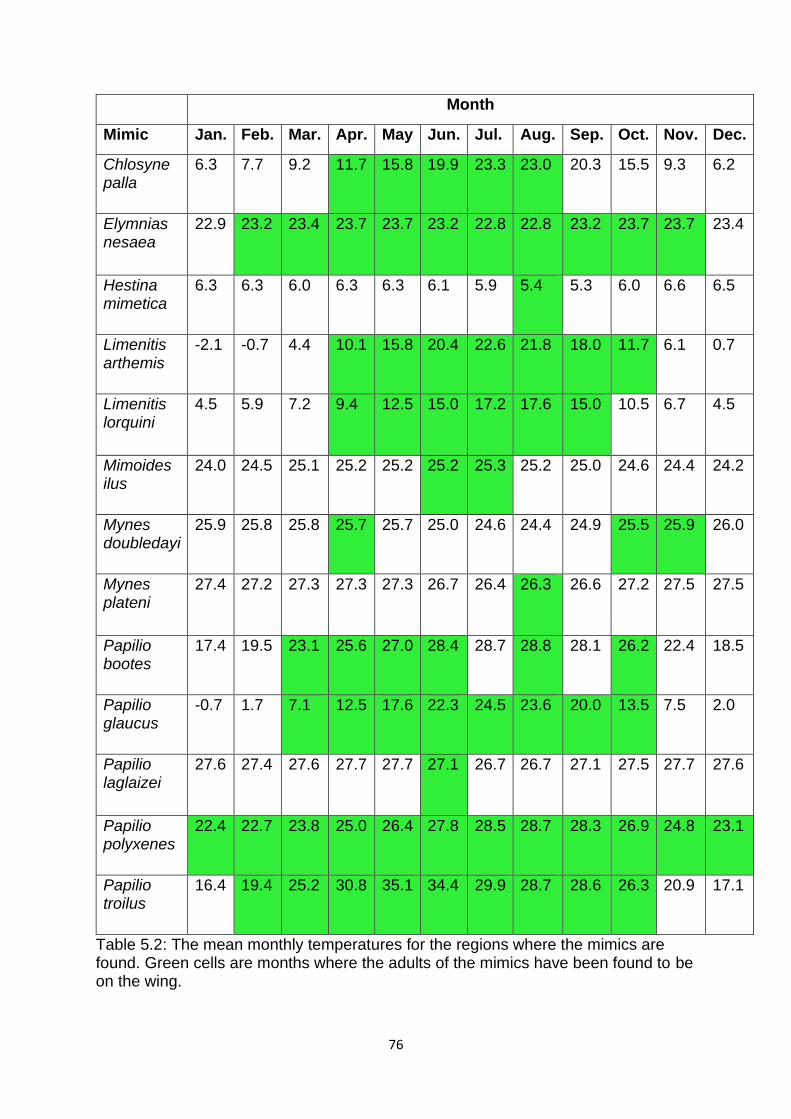
76

Month

Mimic Jan. Feb. Mar. Apr. May Jun. Jul. Aug. Sep. Oct. Nov. Dec.

Chlosyne palla

6.3 7.7 9.2 11.7 15.8 19.9 23.3 23.0 20.3 15.5 9.3 6.2

Elymnias nesaea

22.9 23.2 23.4 23.7 23.7 23.2 22.8 22.8 23.2 23.7 23.7 23.4

Hestina mimetica

6.3 6.3 6.0 6.3 6.3 6.1 5.9 5.4 5.3 6.0 6.6 6.5

Limenitis arthemis

-2.1 -0.7 4.4 10.1 15.8 20.4 22.6 21.8 18.0 11.7 6.1 0.7

Limenitis lorquini

4.5 5.9 7.2 9.4 12.5 15.0 17.2 17.6 15.0 10.5 6.7 4.5

Mimoides ilus

24.0 24.5 25.1 25.2 25.2 25.2 25.3 25.2 25.0 24.6 24.4 24.2

Mynes doubledayi

25.9 25.8 25.8 25.7 25.7 25.0 24.6 24.4 24.9 25.5 25.9 26.0

Mynes plateni

27.4 27.2 27.3 27.3 27.3 26.7 26.4 26.3 26.6 27.2 27.5 27.5

Papilio bootes

17.4 19.5 23.1 25.6 27.0 28.4 28.7 28.8 28.1 26.2 22.4 18.5

Papilio glaucus

-0.7 1.7 7.1 12.5 17.6 22.3 24.5 23.6 20.0 13.5 7.5 2.0

Papilio laglaizei

27.6 27.4 27.6 27.7 27.7 27.1 26.7 26.7 27.1 27.5 27.7 27.6

Papilio polyxenes

22.4 22.7 23.8 25.0 26.4 27.8 28.5 28.7 28.3 26.9 24.8 23.1

Papilio troilus

16.4 19.4 25.2 30.8 35.1 34.4 29.9 28.7 28.6 26.3 20.9 17.1

Table 5.2: The mean monthly temperatures for the regions where the mimics are found. Green cells are months where the adults of the mimics have been found to be on the wing.

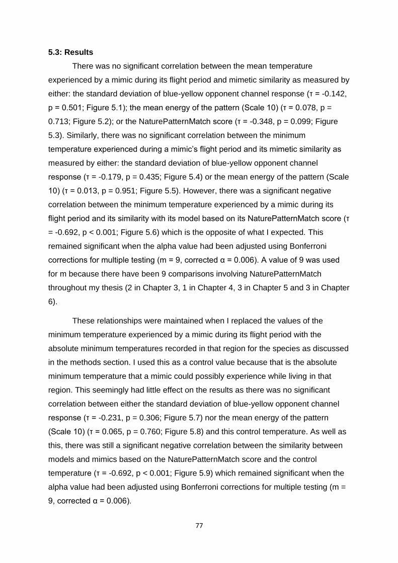
77

5.3: Results

There was no significant correlation between the mean temperature

experienced by a mimic during its flight period and mimetic similarity as measured by

either: the standard deviation of blue-yellow opponent channel response (τ = -0.142,

p = 0.501; Figure 5.1); the mean energy of the pattern (Scale 10) (τ = 0.078, p =

0.713; Figure 5.2); or the NaturePatternMatch score (τ = -0.348, p = 0.099; Figure

5.3). Similarly, there was no significant correlation between the minimum

temperature experienced during a mimic’s flight period and its mimetic similarity as

measured by either: the standard deviation of blue-yellow opponent channel

response (τ = -0.179, p = 0.435; Figure 5.4) or the mean energy of the pattern (Scale

10) (τ = 0.013, p = 0.951; Figure 5.5). However, there was a significant negative

correlation between the minimum temperature experienced by a mimic during its

flight period and its similarity with its model based on its NaturePatternMatch score (τ

= -0.692, p < 0.001; Figure 5.6) which is the opposite of what I expected. This

remained significant when the alpha value had been adjusted using Bonferroni

corrections for multiple testing (m = 9, corrected α = 0.006). A value of 9 was used

for m because there have been 9 comparisons involving NaturePatternMatch

throughout my thesis (2 in Chapter 3, 1 in Chapter 4, 3 in Chapter 5 and 3 in Chapter

6).

These relationships were maintained when I replaced the values of the

minimum temperature experienced by a mimic during its flight period with the

absolute minimum temperatures recorded in that region for the species as discussed

in the methods section. I used this as a control value because that is the absolute

minimum temperature that a mimic could possibly experience while living in that

region. This seemingly had little effect on the results as there was no significant

correlation between either the standard deviation of blue-yellow opponent channel

response (τ = -0.231, p = 0.306; Figure 5.7) nor the mean energy of the pattern

(Scale 10) (τ = 0.065, p = 0.760; Figure 5.8) and this control temperature. As well as

this, there was still a significant negative correlation between the similarity between

models and mimics based on the NaturePatternMatch score and the control

temperature (τ = -0.692, p < 0.001; Figure 5.9) which remained significant when the

alpha value had been adjusted using Bonferroni corrections for multiple testing (m =

9, corrected α = 0.006).

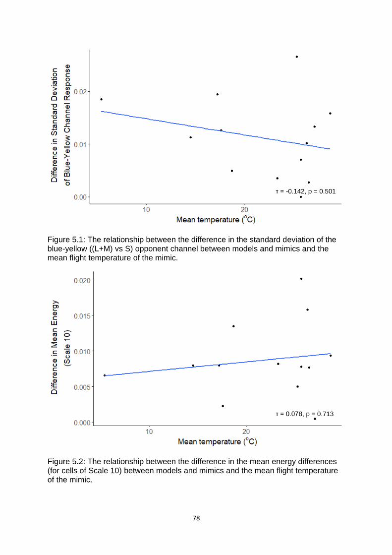
78

Figure 5.1: The relationship between the difference in the standard deviation of the blue-yellow ((L+M) vs S) opponent channel between models and mimics and the mean flight temperature of the mimic.

Figure 5.2: The relationship between the difference in the mean energy differences (for cells of Scale 10) between models and mimics and the mean flight temperature of the mimic.

τ = 0.078, p = 0.713

τ = -0.142, p = 0.501

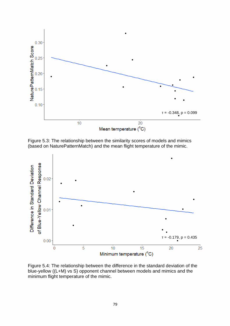
79

Figure 5.3: The relationship between the similarity scores of models and mimics (based on NaturePatternMatch) and the mean flight temperature of the mimic.

Figure 5.4: The relationship between the difference in the standard deviation of the blue-yellow ((L+M) vs S) opponent channel between models and mimics and the minimum flight temperature of the mimic.

τ = -0.179, p = 0.435

τ = -0.348, p = 0.099

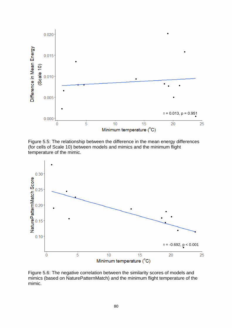
80

Figure 5.5: The relationship between the difference in the mean energy differences (for cells of Scale 10) between models and mimics and the minimum flight temperature of the mimic.

Figure 5.6: The negative correlation between the similarity scores of models and mimics (based on NaturePatternMatch) and the minimum flight temperature of the mimic.

τ = -0.692, p < 0.001

τ = 0.013, p = 0.951

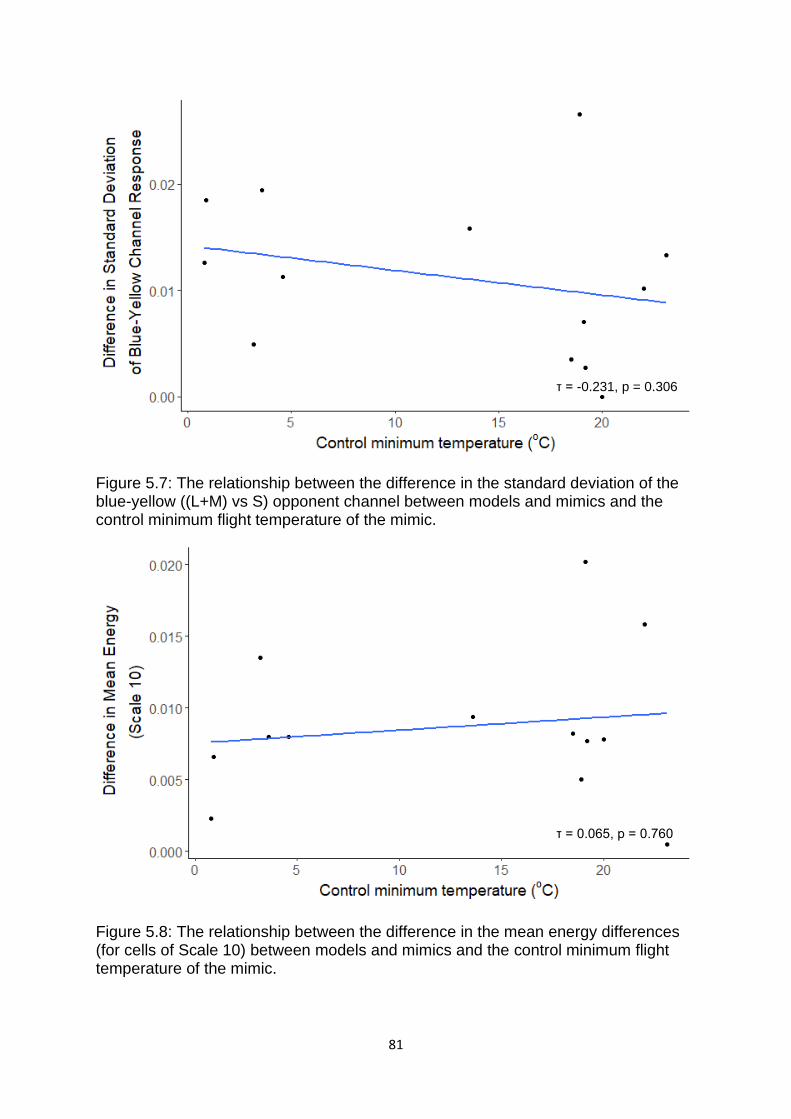
81

Figure 5.7: The relationship between the difference in the standard deviation of the blue-yellow ((L+M) vs S) opponent channel between models and mimics and the control minimum flight temperature of the mimic.

Figure 5.8: The relationship between the difference in the mean energy differences (for cells of Scale 10) between models and mimics and the control minimum flight temperature of the mimic.

τ = 0.065, p = 0.760

τ = -0.231, p = 0.306

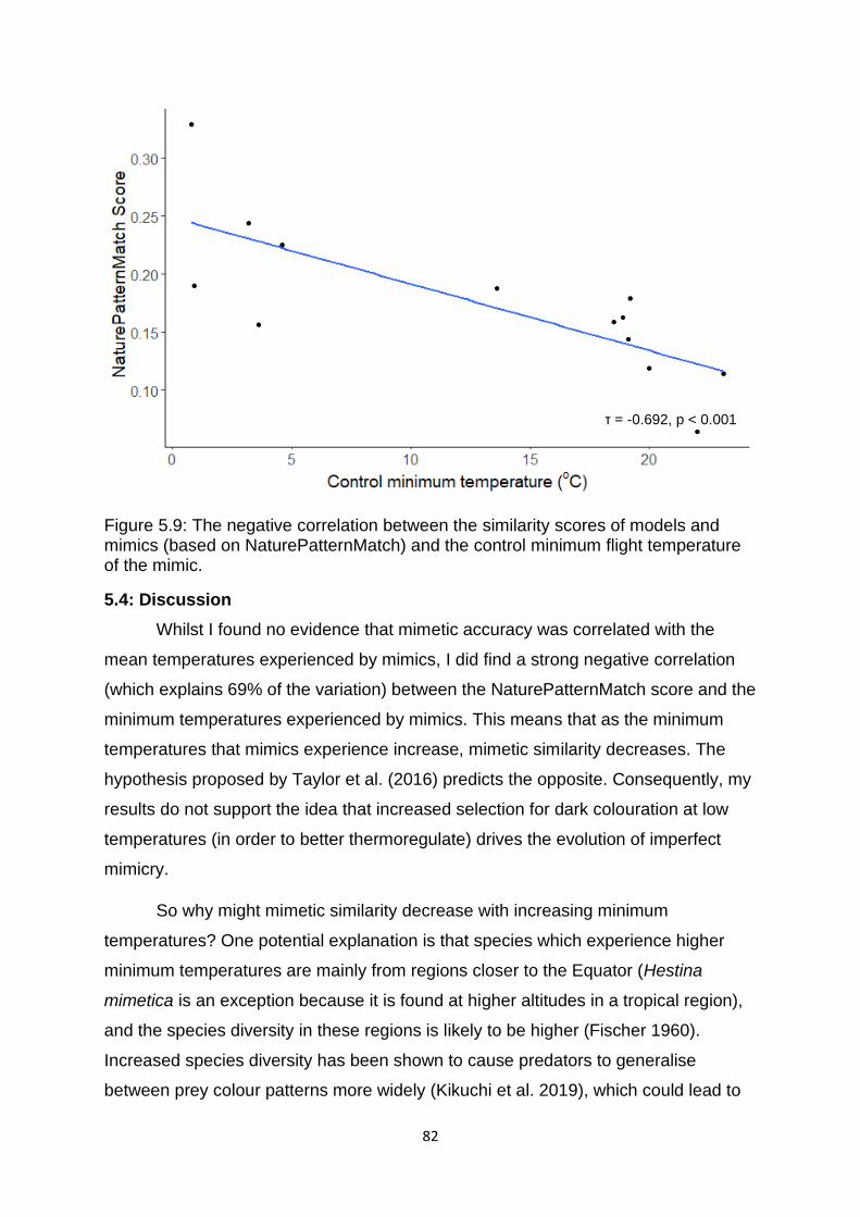
82

Figure 5.9: The negative correlation between the similarity scores of models and mimics (based on NaturePatternMatch) and the control minimum flight temperature of the mimic.

5.4: Discussion

Whilst I found no evidence that mimetic accuracy was correlated with the

mean temperatures experienced by mimics, I did find a strong negative correlation

(which explains 69% of the variation) between the NaturePatternMatch score and the

minimum temperatures experienced by mimics. This means that as the minimum

temperatures that mimics experience increase, mimetic similarity decreases. The

hypothesis proposed by Taylor et al. (2016) predicts the opposite. Consequently, my

results do not support the idea that increased selection for dark colouration at low

temperatures (in order to better thermoregulate) drives the evolution of imperfect

mimicry.

So why might mimetic similarity decrease with increasing minimum

temperatures? One potential explanation is that species which experience higher

minimum temperatures are mainly from regions closer to the Equator (Hestina

mimetica is an exception because it is found at higher altitudes in a tropical region),

and the species diversity in these regions is likely to be higher (Fischer 1960).

Increased species diversity has been shown to cause predators to generalise

between prey colour patterns more widely (Kikuchi et al. 2019), which could lead to

τ = -0.692, p < 0.001

83

mimics from these regions experiencing relaxed selection for mimetic accuracy. This

explanation could also help us understand why there was no significant correlation

between mean temperature and NaturePatternMatch score. This is because the

mean minimum temperature is a better predictor of whether species live in temperate

or tropical regions. Consequently, it is a better predictor of species richness.

In addition to this, species in warmer climates could be facing a trade-off

between selection for increased melanization and selection for increased mimetic

similarity as suggested by Gloger’s Rule (Gloger 1833). This rule, as simplified by

Rensch (1929), suggests that species from warm and humid regions are darker than

species from drier and cooler regions. This trend is thought to be mainly driven by

the humidity of the region (Delhey 2019). This correlation between melanization and

environmental humidity is thought to be due to selection for increased protection

from parasites and pathogens (Burtt and Ichida 2004). This is because these

organisms tend to be more abundant in areas with high humidity, which means that

the risk of parasitization or bacterial infection is higher in those regions, therefore

species from those regions should invest more energy into the production of melanin

since it plays an integral role in the immune defense system (Burtt and Ichida 2004).

Intriguingly, the trend for decreased mimetic similarity at higher temperature

was not seen in my other measures of mimetic similarity (the difference in mean

energy, and the difference in the standard deviation of the blue-yellow channel). The

reason for this is probably due to the fact that NaturePatternMatch score provides a

more relevant measure of mimetic similarity. Predators probably more likely to

generalise between prey based on the shared presence of specific pattern features

(which is what NaturePatternMatch measures) rather than on the mean energy of

pattern features or the similarity of the variation in chromatic contrast in one

opponent channel. Moreover, patterns which have very similar mean energy scores

can actually appear quite different (e.g. stripes and spots) because this measure was

developed to distinguish between aposematic and non-aposematic patterns rather

than between different types of aposematic pattern (see Section 4.2.2). As such, it

may not be useful for quantifying how accurately a mimic resembles its model.

It seems, therefore, that there are scientifically feasible explanations for the

patterns observed in my data. However, we must also consider why the trends I

84

observed in Lepidoptera are different from those previously observed in hoverflies.

One explanation for this is that the need to thermoregulate has a stronger influence

on the patterns of hoverflies than those of Lepidoptera.

While lepidopterans are ectotherms and are often used in studies

investigating the link between colouration and thermoregulation (e.g. Zeuss et al

2014; Munro et al. 2019). It has been shown that the ability for butterflies to

efficiently thermoregulate is determined largely by their wing posture rather than their

wing colour (Wasserthal 1975; Heinrich 1986; Kemp and Krockenberger 2002): wing

position affects the amount of warm air trapped under the wing (Wasserthal 1975).

Furthermore, there is reason to believe that butterflies’ abilities to thermoregulate are

disproportionately influenced by the colour of a subset of body parts. The most

important areas for thermoregulation are the dorsal surface of the thorax and basal

areas of the wing (the areas of the wings closest to the thorax) (Wasserthal 1975).

This means that the colouration of the majority of the wing surface will be mainly

affected by selection from other sources such as selection for effective anti-predator

colouration. As such, the pattern of the wings, as a whole, may be unlikely to be

under strong selection to allow improved thermoregulation. However, some studies

have shown that the trade-off between selection for improved thermoregulation and

selection for increased anti-predator colouration influence the colour of the whole

wing (e.g. Hegna et al. 2013).

Another explanation for the discrepancy seen between my study and the

study by Taylor et al. (2016) could be that hoverflies and hymenopterans provide a

unique case due to the thermal ecology of bees and wasps. This is because

honeybees and social wasps live in hives and so they have regular access to a

microhabitat which is often maintained at a temperature which is well above the

ambient temperature of the surrounding area (Heinrich 1993). In addition to this, both

honeybees (Stabentheiner et al. 1995) and social wasps (Schmolz et al. 1993) seem

to display a degree of endothermy. While hoverflies are also endothermic to some

extent, these processes are less efficient for them than their models (Morgan and

Heinrich 1987). This may mean that hoverflies rely more on basking to warm up than

bees and wasps and so they may experience stronger selection for thermoregulatory

colouration compared to their models in order to make this process more efficient. In

contrast, Lepidopteran models and mimics are likely to have similar thermal

85

ecologies meaning that there is no mismatch in selection for colouration that

optimises thermoregulation between them. Thus, in the patterns of Lepidoptera,

there may be no trade-off between mimetic similarity and thermoregulation because

both can be optimised simultaneously.

Finally, it could be that mimics (including hoverflies) never experience a trade-

off between selection for improved thermoregulation and mimetic similarity. This is

supported by the fact that, in some mimicry rings, both models and mimics have

been shown to evolve colouration which improves thermoregulation in colder

climates. The key example of this is seen a series of mimicry rings from New

Zealand (Harris 1974). These rings are based around defended Priocnemis spider

wasps (Family Pompilidae) which show a marked shift in their colouration with

latitude. Individuals found below 45o tend to be black and yellow, whereas those

found above the 45o line tend to show a lighter red and gold colouration (Harris

1974). It is likely that this difference in colouration is caused by selection for

improved thermoregulation because it is colder at more extreme latitudes and the

degree of melanism in several Priocnemis wasps is known to be affected by rearing

temperature (Harris 1974). Crucially, this change is mirrored by several of their

Batesian and Müllerian mimics (Harris 1974). This suggests that the selection on

colour patterns to improve thermoregulatory efficiency is the same for both models

and mimics and so there should be little trade-off between selection for mimetic

accuracy and for improved thermoregulation.

This raises the question: if there is no trade-off between mimetic similarity and

thermoregulation, then why were imperfect mimics more highly melanised than their

models in the study by Taylor et al. (2016)? One potential explanation for this, is that

the effect is an artefact caused by the history of Hymenoptera in the UK, in

particularly the history of the honeybee (Apis mellifera). The native subspecies of

honeybee to the UK (A. m. mellifera) reportedly experienced a population crash in

the early 20th century (Adam 1983). This led beekeepers to start importing other

subspecies of honeybee (e.g. Italian honeybees (A. m. ligustica) and Carniolan

honeybees (A. m. carnica)) or breeding hybrids (e.g. the Buckfast bee) to use in

apiculture (Jensen et al. 2005). These differ phenotypically from A. m. mellifera and

tend to have a lower proportion of black in their pattern than the native subspecies

(Woyke 1998). This means that, in the last 100 years, the phenotype of the model

86

that these hoverflies have been selected to resemble will have shifted, not just in

areas where apiaries are present but also in regions where escaped populations

have become established or where captive bees have hybridised with the native

population (Jensen et al. 2005). Therefore, the hoverflies examined by Taylor et al.

could be experiencing selection away their ancestral form (which would have been

selected to resemble A. m. mellifera), and towards the appearance of lighter modern

bees, and the patterns seen currently may be an intermediate between the two.

This would only explain part of the data though, as most of the hoverflies in

Taylor et al.’s (2016) study were classified as wasp mimics. However, their results

could also have been influenced by the fact that they only identified four

Hymenopteran species as models in their study (Taylor et al. 2016). This was

because, while other species of Hymenoptera were present at the study sites, they

were so rare that the authors concluded that they were not abundant enough to

affect the evolution of mimics. I would argue that it is not appropriate to exclude

these potential models because despite them appearing to be too scarce to act as a

model for mimics, ancestrally they could have been more common and therefore

could have acted as a model for some of the hoverfly species. Moreover, when these

rarer aposematic species were included in the analyses, the previously seen

association between mimetic accuracy and the proportion of black in the pattern was

weakened (Taylor et al. 2016). When taken together, these results could explain why

a subsequent study has found no significant correlation between mimetic accuracy

and body temperature in hoverflies (Daňková et al. in prep.).

In conclusion, while this study provides some tentative evidence that the

diversity of the prey community could affect mimetic similarity, further studies are

required to assess this directly. More research is also necessary to determine

whether selection for improved thermoregulation does indeed lead to decreased

mimetic similarity. If the diversity of the prey community has a strong effect on

mimetic similarity, then it may mask any trade-off between mimetic similarity and

thermoregulation. Perhaps the best approach would be to see if mimics from

complexes which exhibit climate-based melanism, such as the two mimicry rings

described by Harris (1974) or the Müllerian mimicry complex of ladybirds and soldier

beetles described by Brakefield (1985), differ in terms of their mimetic accuracy

when they exhibit higher levels of melanism compared to when they exhibit lower

87

levels of melanism. Since each of these rings have morphs with different levels of

melanism, and all morphs are likely to be exposed to a similar suite of predators,

they should experience a very similar selection pressure from predation. Therefore, if

there is a trade-off between thermoregulation and mimicry then we would expect

mimics which exhibit higher levels of thermal melanism to be poorer mimics than

those which exhibit lower levels of thermal melanism. If there is no trade-off, there

should be no difference between the two rings. This would be a good approach to

use as it reduces the number of confounding variables which may affect the

difference in mimetic accuracy, such as differences in toxicity of the models or

differences in nutritive value seen between different mimetic species.

This does not mean that it is not important to explore the effect of these other

factors on the evolution of mimicry, they are crucial to consider in their own right.

One particularly noteworthy factor which has garnered a lot of attention is the

nutritional value of the mimic. This is thought to have an effect on mimetic similarity

because when mimics are small and of a low value to predators, selection for

mimetic accuracy may be weaker, and this could result in the evolution of imperfect

mimicry (Penney et al. 2012). This is the focus of the next chapter.

88

Chapter 6: The effect of size on mimetic similarity

The size of an organism affects its life history in many ways, and it has also

been suggested to influence the evolution of mimicry. However, there have been

conflicting hypotheses about how size affects the evolution of mimicry and each of

these have received some empirical support. In this chapter, I used the measures of

mimetic similarity taken from the butterfly images outlined in previous chapters to

test three hypotheses which predict how mimic size affects mimetic similarity. I found

a significant positive correlation between mimetic similarity and the difference in size

between mimics and models. However, I found no significant correlation between

mimetic similarity and either the absolute size of the mimic or the size of the mimic

relative to its model. This indicates that predators generalise more widely between

the patterns of mimics and models when the mimic matches its model in terms of

size.

6.1: Introduction

The size of an organism has a huge impact on its entire life history. For

example, it can affect lifespan (Speakman 2005), fecundity (Honěk 1993; Tammaru

et al.1996; Tammaru et al. 2002) and predation risk (Shine et al. 2001; Taylor and

Cox 2019). As such, the size of an individual can have important ramifications on the

selection pressures acting on it. Recent work has suggested that body size may play

an important role in determining the type of anti-predator defences that a prey

species evolves. This is because the efficacy of a number of defensive strategies are

known to be size-dependent. Larger organisms are by their very nature easier to

detect (Mänd et al. 2007) which can reduce the efficacy of cryptic colouration. This is

one of the reasons why larger species tend to adopt other strategies such as

eyespots (Hossie et al. 2015), deimatic displays (Kang et al. 2017) or a chemical

defence paired with aposematic colouration (Hagman and Forsman 2003). In

addition to this, some anti-predator strategies are more effective when the individuals

which have evolved them are larger: eyespots are more “intimidating” when found on

larger individuals (Hossie et al. 2015). However, size does not only affect the

conspicuousness of a prey item, it also affects its profitability. This is because the

nutritive value of a prey item often increases with body size (Cummins and

Wuycheck 1971; Brooks et al. 1996). Furthermore, in the case of defended species,

the amount of defensive chemicals produced by an individual can increase with body

89

size (Holloway et al. 1993), sometimes in a non-linear fashion (Phillips and Shine

2006). However this is not always the case, in some species there is a trade-off

between investment in growth and investment in costly chemical defences (Brower

and Moffitt 1974; Cohen 1985; Björkman and Larsson 1991).

The relationship between size and anti-predator colouration is particularly

interesting in mimicry systems because predators’ decisions to attack aposematic

prey are known to be affected by the prey’s nutritional value (Smith et al. 2014) and

toxin content (Barnett et al. 2011), both of which could potentially be inferred from

prey size. If predators treat mimics in the same way as aposematic prey, then these

factors may also influence the benefit of mimicry. This is important because it will

determine which species are able to evolve mimicry (Pyron and Burbrink 2009), and

influence the evolutionary dynamics of those species for which mimicry is beneficial

(Penney et al. 2012).

The importance of size in the evolution of mimicry can be seen in mimics

which display “transformational mimicry” (Mathew 1935). Transformational mimicry is

where a mimic only mimics a given model for part of its life (normally as a juvenile)

before displaying an ontogenetic colour change which causes it to either resemble a

different model (e.g. Mantoida maya mimics ants during its earliest nymphal instars

and wasps during the later nymphal stages; Jackson and Drummond 1974), or

switch to a different form of defence (e.g. juvenile Eremias lugubris are thought to

mimic oogpister beetles Anthias sp. while the adults are more cryptically coloured;

Huey and Pianka 1977). This phenomenon is seen in species from a range of taxa,

including insects (Mathew 1935; Jackson and Drummond 1974), fish (Randall and

Randall 1960; Eagle and Jones 2014), reptiles (Huey and Pianka 1977) and even

birds (Londoño et al. 2015). Moreover, in all cases, the change in colour seems to

occur when the individuals reach a certain size suggesting that the efficacy of

mimicry is size-dependent.

This relationship between size and mimicry can also be seen on a genetic

level in the mimetic butterfly Hypolimnas misippus as the genes controlling wing size

and wing colouration are very closely linked (Gordon and Smith 1998). This close

genetic link leads to a close phenotypic link between size and colour pattern in this

species. However, despite it being apparent that size is an important factor to

90

consider when studying mimicry, it is still unclear how the size of an individual affects

the evolution of its colour pattern. In fact, there are three main ways in which size is

thought to affect selection on mimetic similarity.

6.1.1: The absolute size of a mimic affects the degree of pattern similarity

between mimics and their models

The first hypothesis is that the strength of selection for mimetic similarity will

depend solely on the size of the mimic. However, this is thought to work in one of

two ways. Some authors have suggested that smaller mimics should be less

accurate than larger mimics (Penney et al. 2012). This stems from the idea that

since smaller mimics have a lower nutritional value, predators should be less

motivated to invest time discriminating between small mimics and their models.

Consequently, small mimics should experience relaxed selection for mimetic

accuracy: this idea is known as the small bodied hypothesis (Wilson et al. 2013). In

contrast to this, other authors have proposed that larger mimics should be less

accurate than smaller mimics. They argue that larger models (and so larger mimics)

should experience relaxed selection because they are more conspicuous, which

should cause predators to show increased innate aversions to them (Nur et al.

1970). In addition to this, larger models tend to contain more toxins than smaller

ones (although there are exceptions to this (Isman 1977; Tuskes and Brower 1978))

and therefore predators should show a more generalised avoidance of larger mimics

(Kraemer et al. 2015a). Despite their conflicting nature, both of these hypotheses

have been supported by empirical evidence. The work of Penney et al. (2012)

showed that smaller species of hoverfly are less accurate mimics of Hymenoptera.

While Kraemer et al. (2015a) found that larger erythristic red-backed salamanders

(Plethodon cinereus) are less similar to their models (the red-spotted newt

(Notophthalmus viridescens)) than smaller ones.

6.1.2: The size of a mimic relative to its model affects the degree of pattern

similarity between mimics and their models

The second hypothesis is that mimics which are smaller relative to their model

will be less accurate than mimics which are larger relative to their model. Rothschild

(1963) argued that, since birds tend to ignore smaller prey in favour of larger prey,

Batesian mimics should evolve to remain smaller than their models in order to further

reduce predation. This suggests that mimics which are smaller than their model

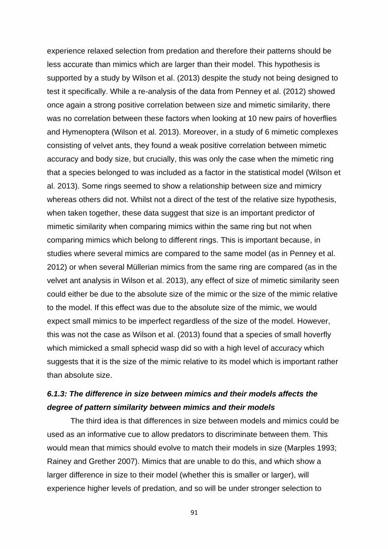
91

experience relaxed selection from predation and therefore their patterns should be

less accurate than mimics which are larger than their model. This hypothesis is

supported by a study by Wilson et al. (2013) despite the study not being designed to

test it specifically. While a re-analysis of the data from Penney et al. (2012) showed

once again a strong positive correlation between size and mimetic similarity, there

was no correlation between these factors when looking at 10 new pairs of hoverflies

and Hymenoptera (Wilson et al. 2013). Moreover, in a study of 6 mimetic complexes

consisting of velvet ants, they found a weak positive correlation between mimetic

accuracy and body size, but crucially, this was only the case when the mimetic ring

that a species belonged to was included as a factor in the statistical model (Wilson et

al. 2013). Some rings seemed to show a relationship between size and mimicry

whereas others did not. Whilst not a direct of the test of the relative size hypothesis,

when taken together, these data suggest that size is an important predictor of

mimetic similarity when comparing mimics within the same ring but not when

comparing mimics which belong to different rings. This is important because, in

studies where several mimics are compared to the same model (as in Penney et al.

2012) or when several Müllerian mimics from the same ring are compared (as in the

velvet ant analysis in Wilson et al. 2013), any effect of size of mimetic similarity seen

could either be due to the absolute size of the mimic or the size of the mimic relative

to the model. If this effect was due to the absolute size of the mimic, we would

expect small mimics to be imperfect regardless of the size of the model. However,

this was not the case as Wilson et al. (2013) found that a species of small hoverfly

which mimicked a small sphecid wasp did so with a high level of accuracy which

suggests that it is the size of the mimic relative to its model which is important rather

than absolute size.

6.1.3: The difference in size between mimics and their models affects the

degree of pattern similarity between mimics and their models

The third idea is that differences in size between models and mimics could be

used as an informative cue to allow predators to discriminate between them. This

would mean that mimics should evolve to match their models in size (Marples 1993;

Rainey and Grether 2007). Mimics that are unable to do this, and which show a

larger difference in size to their model (whether this is smaller or larger), will

experience higher levels of predation, and so will be under stronger selection to

92

accurately resemble the patterns of their models. This differs from the previous

hypothesis in two ways. Firstly, it predicts that mimics that are less similar to their

models in terms of size should be more similar in terms of pattern, whereas in the

previous hypothesis predicts that individuals that are less similar to their models in

terms of size should also be less similar in terms of pattern. Secondly, this

hypothesis predicts that the direction of the difference is not important: mimics that

are 10% larger than the model should have the same level of pattern similarity as

mimics that are 10% smaller. This is in stark contrast to the previous hypothesis,

which predicts that mimetic similarity should be greater in mimics that are 10% larger

than their models than in mimics which are 10% smaller than their models. This idea

is supported by the fact that masqueraders which are either smaller or larger than

their models show reduced survival compared to masqueraders that are the same

size as their models; and, importantly, the reduction in survival caused by size

mismatches is similar for masqueraders that are smaller or larger than their models

(Skelhorn et al. 2010c). However, behavioural experiments investigating Batesian

mimicry have found conflicting results. Marples (1993) showed that birds could use

size cues to discriminate between palatable and unpalatable prey whereas Terhune

(1977) found that, when birds were offered artificial models and mimics which

differed colour, pattern or size, only 2 out of 7 birds were able to use size cues to

successfully discriminate between models and mimics. In addition to this, Taylor et

al. (2017) found that humans were unable to discriminate between models and

mimics based on size alone.

In order to see test whether the predictions arising from each of these

hypotheses hold for mimetic Lepidoptera, I tested whether mimetic similarity (defined

using the three measures of mimetic similarity used throughout this thesis), was

correlated with the three different size metrics outlined above.

6.2: Methods

Size measurements were taken from calibrated digital photographs using

ImageJ (Schneider et al. 2012). The photos were taken using either a DSLR camera

(Basler acA1300-200ac) or a digital camera (Canon Ixus 140). I used these photos

because I was able to include a CameraTrax 24 colour card to provide a reference

object for the scale of objects in the photo. Only Batesian mimic pairs were used for

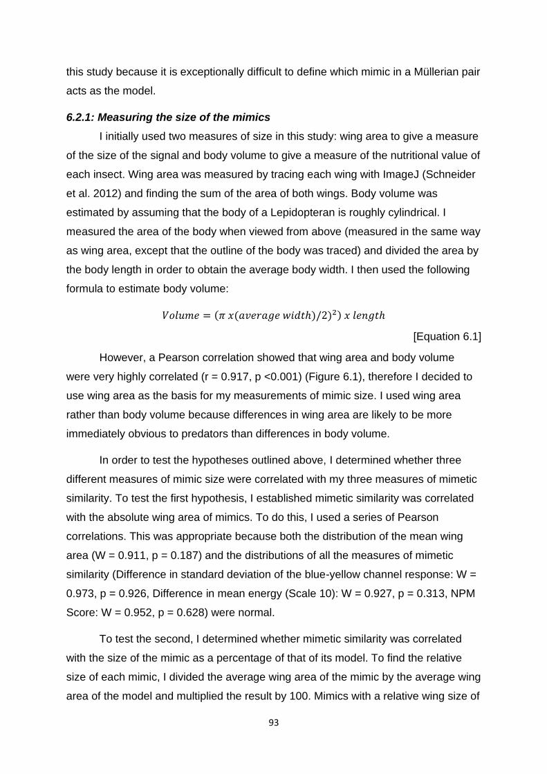
93

this study because it is exceptionally difficult to define which mimic in a Müllerian pair

acts as the model.

6.2.1: Measuring the size of the mimics

I initially used two measures of size in this study: wing area to give a measure

of the size of the signal and body volume to give a measure of the nutritional value of

each insect. Wing area was measured by tracing each wing with ImageJ (Schneider

et al. 2012) and finding the sum of the area of both wings. Body volume was

estimated by assuming that the body of a Lepidopteran is roughly cylindrical. I

measured the area of the body when viewed from above (measured in the same way

as wing area, except that the outline of the body was traced) and divided the area by

the body length in order to obtain the average body width. I then used the following

formula to estimate body volume:

𝑉𝑜𝑙𝑢𝑚𝑒 = (𝜋 𝑥(𝑎𝑣𝑒𝑟𝑎𝑔𝑒 𝑤𝑖𝑑𝑡ℎ)/2)2) 𝑥 𝑙𝑒𝑛𝑔𝑡ℎ

[Equation 6.1]

However, a Pearson correlation showed that wing area and body volume

were very highly correlated (r = 0.917, p <0.001) (Figure 6.1), therefore I decided to

use wing area as the basis for my measurements of mimic size. I used wing area

rather than body volume because differences in wing area are likely to be more

immediately obvious to predators than differences in body volume.

In order to test the hypotheses outlined above, I determined whether three

different measures of mimic size were correlated with my three measures of mimetic

similarity. To test the first hypothesis, I established mimetic similarity was correlated

with the absolute wing area of mimics. To do this, I used a series of Pearson

correlations. This was appropriate because both the distribution of the mean wing

area (W = 0.911, p = 0.187) and the distributions of all the measures of mimetic

similarity (Difference in standard deviation of the blue-yellow channel response: W =

0.973, p = 0.926, Difference in mean energy (Scale 10): W = 0.927, p = 0.313, NPM

Score: W = 0.952, p = 0.628) were normal.

To test the second, I determined whether mimetic similarity was correlated

with the size of the mimic as a percentage of that of its model. To find the relative

size of each mimic, I divided the average wing area of the mimic by the average wing

area of the model and multiplied the result by 100. Mimics with a relative wing size of

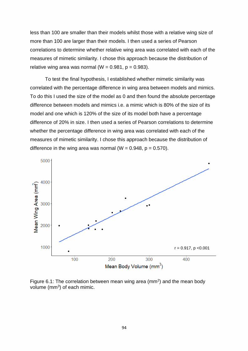
94

less than 100 are smaller than their models whilst those with a relative wing size of

more than 100 are larger than their models. I then used a series of Pearson

correlations to determine whether relative wing area was correlated with each of the

measures of mimetic similarity. I chose this approach because the distribution of

relative wing area was normal (W = 0.981, p = 0.983).

To test the final hypothesis, I established whether mimetic similarity was

correlated with the percentage difference in wing area between models and mimics.

To do this I used the size of the model as 0 and then found the absolute percentage

difference between models and mimics i.e. a mimic which is 80% of the size of its

model and one which is 120% of the size of its model both have a percentage

difference of 20% in size. I then used a series of Pearson correlations to determine

whether the percentage difference in wing area was correlated with each of the

measures of mimetic similarity. I chose this approach because the distribution of

difference in the wing area was normal (W = 0.948, p = 0.570).

Figure 6.1: The correlation between mean wing area (mm2) and the mean body volume (mm3) of each mimic.

r = 0.917, p <0.001

95

6.3: Results

6.3.1: Does the absolute size of a mimic affect the degree of pattern similarity

between mimics and their models?

There was no significant correlation between mean wing area and any of the

three measures of mimetic similarity (Difference in the standard deviation of blue-

yellow channel response: r = -0.063, p =0.839, Figure 6.2; Difference in mean

energy (Scale 10): r = -0.296, p = 0.326, Figure 6.3; NaturePatternMatch Score: r =

0.107, p =0.727, Figure 6.4). This indicates that smaller mimics do not experience

relaxed selection for mimetic accuracy compared to larger mimics.

Figure 6.2: The correlation between mean wing area (mm2) and the difference in the

standard deviation of the blue-yellow ((L+M) vs S) opponent channel response.

r = -0.063, p =0.839

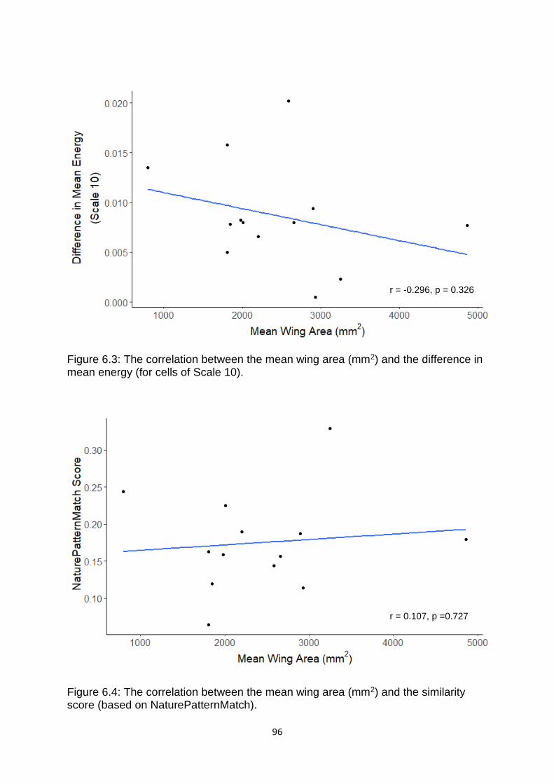
96

Figure 6.3: The correlation between the mean wing area (mm2) and the difference in mean energy (for cells of Scale 10).

Figure 6.4: The correlation between the mean wing area (mm2) and the similarity score (based on NaturePatternMatch).

r = 0.107, p =0.727

r = -0.296, p = 0.326

97

6.3.2: Does the size of a mimic relative to its model affect the degree of pattern

similarity between mimics and their models?

There was no significant correlation between the area of the wings of the

mimics relative to the model and any of the three measures of mimetic similarity

(Difference in the standard deviation of blue-yellow channel response: r = 0.522, p =

0.067, Figure 6.5; Difference in mean energy (Scale 10): r = -0.156, p = 0.610,

Figure 6.6; NaturePatternMatch Score: r = 0.457, p =0.116, Figure 6.7). This

indicates that mimics that are smaller than their model do not experience relaxed

selection for mimetic similarity compared to mimics that are the same size or larger

than their model.

Figure 6.5: The correlation between the wing area of the mimic relative to its model (%) and the difference in the standard deviation of the blue-yellow ((L+M) vs S) opponent channel response.

r = 0.522, p = 0.067

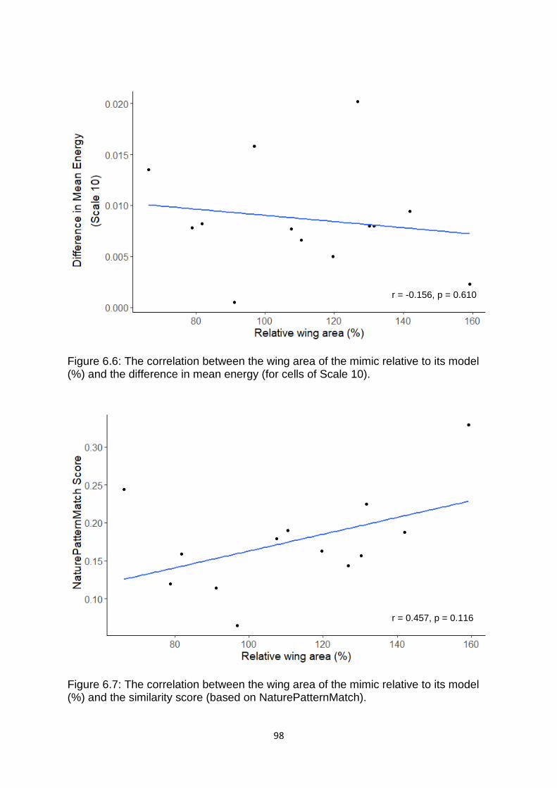
98

Figure 6.6: The correlation between the wing area of the mimic relative to its model (%) and the difference in mean energy (for cells of Scale 10).

Figure 6.7: The correlation between the wing area of the mimic relative to its model (%) and the similarity score (based on NaturePatternMatch).

r = 0.457, p = 0.116

r = -0.156, p = 0.610

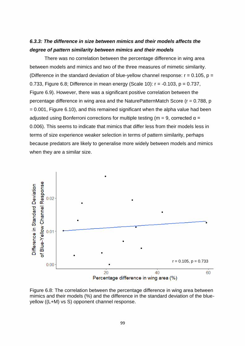
99

6.3.3: The difference in size between mimics and their models affects the

degree of pattern similarity between mimics and their models

There was no correlation between the percentage difference in wing area

between models and mimics and two of the three measures of mimetic similarity.

(Difference in the standard deviation of blue-yellow channel response: r = 0.105, p =

0.733, Figure 6.8; Difference in mean energy (Scale 10): r = -0.103, p = 0.737,

Figure 6.9). However, there was a significant positive correlation between the

percentage difference in wing area and the NaturePatternMatch Score (r = 0.788, p

= 0.001, Figure 6.10), and this remained significant when the alpha value had been

adjusted using Bonferroni corrections for multiple testing (m = 9, corrected α =

0.006). This seems to indicate that mimics that differ less from their models less in

terms of size experience weaker selection in terms of pattern similarity, perhaps

because predators are likely to generalise more widely between models and mimics

when they are a similar size.

Figure 6.8: The correlation between the percentage difference in wing area between mimics and their models (%) and the difference in the standard deviation of the blue-yellow ((L+M) vs S) opponent channel response.

r = 0.105, p = 0.733

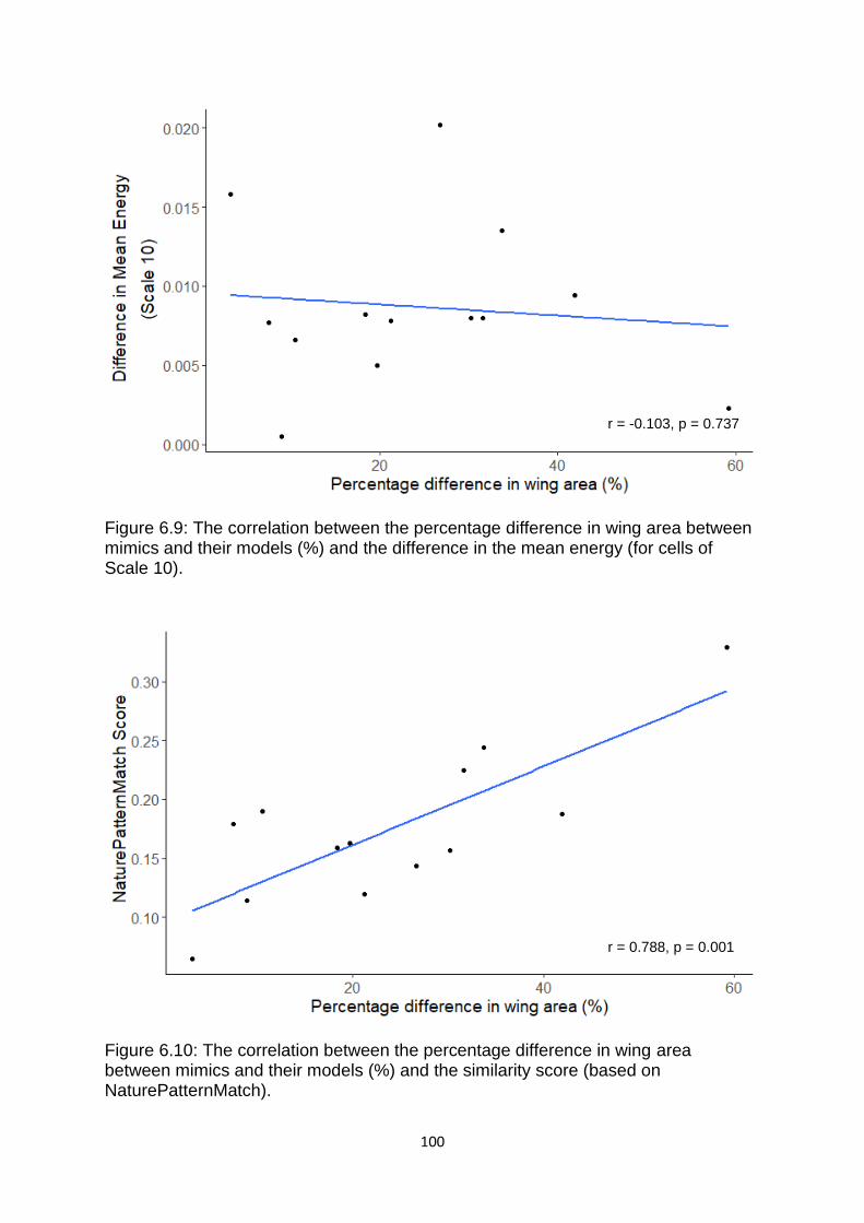
100

Figure 6.9: The correlation between the percentage difference in wing area between mimics and their models (%) and the difference in the mean energy (for cells of Scale 10).

Figure 6.10: The correlation between the percentage difference in wing area between mimics and their models (%) and the similarity score (based on NaturePatternMatch).

r = 0.788, p = 0.001

r = -0.103, p = 0.737

101

6.4: Discussion

I found a strong positive correlation between mimetic similarity based on

NaturePatternMatch scores and the percentage difference in wing area between

models and mimics. However, there were no significant correlations between the

other measures of mimetic similarity and the percentage difference in wing area; or

between any measure of mimetic similarity and either the absolute size of the mimic,

or the size of the mimic relative to its model. Taken together, these findings support

the my third hypothesis: that the difference in size between mimics and their models

affects the degree of pattern similarity between them. This is interesting because

humans show size invariance in their recognition of objects (Biederman and Cooper

1992; Cooper et al. 1992) which allows us to generalise between objects of different

sizes and recognize the same object at different distances. This trait has also been

shown shared by birds (Peissig et al. 2006; Castro and Wasserman 2010). However,

birds show a weaker generalization between objects which differ more in size

(Peissig et al. 2006), this means that object size is used in object recognition, which

also lends support the third hypothesis. However, the birds must also show size

invariance in the recognition of the pattern of the mimics in order for those mimics to

gain a selective advantage from their pattern. The reason why this correlation was

seen when mimetic similarity was measured using NaturePatternMatch and not

when using the other two measures of similarity could be because the

NaturePatternMatch score is likely to be a more ecologically relevant measure of

mimetic similarity (see Chapter 5 for a discussion of why this is likely the case).

My findings suggest that prey size is an informative cue for predators, since

mimics that match their models more closely in terms of size seemingly experience

relaxed selection for pattern similarity. This is particularly interesting because most

experiments investigating the relationship between size and mimicry have claimed to

support the small bodied hypothesis (i.e. that small mimics are under relaxed

selection for similarity irrespective of model size) (Penney et al. 2012; Wilson et al.

2013). This raises the question as to why the relationship between size and mimetic

accuracy seen here differs from what has been previously found in the literature.

One reason could be neither of these previous studies were designed to

discriminate between the small bodied hypothesis and the idea that it is the size-

102

match between models and mimics that influence mimetic similarity. These studies

used absolute mimic size in their analyses but did not consider the difference in size

between models and mimics. This was because the specific model associated with

each mimic was not known as the mimics were part of a complex mimicry ring

(Penney et al. 2014). However, it is possible to make inferences about what these

studies could tell us about how size difference might influence mimetic similarity.

Most hoverflies are the same size or smaller than the sympatric Hymenoptera that

they are thought to mimic (Supplementary Table 3).This would suggest that if

Penney et al. (2012) had looked at relative size, they probably would have found that

the hoverflies which were less similar to their models in terms of size were also less

similar in terms of pattern. This makes it difficult to be sure whether it is absolute

mimic size, or the difference in size between models and mimics that is responsible

for the observed differences in mimetic similarity. However, even it is the difference

in size, the correlation is in the opposite direction to the one found in my study.

So why might there be a negative correlation between difference in size and

mimetic similarity in previous studies? In both the study by Penney et al. (2012) and

the study by Wilson et al. (2013), the images shown to human observers were all

presented in such a way that all models and mimics had the same apparent size.

This was necessary to ensure that all ratings of similarity were based on colour and

pattern alone because, while size alone cannot be used by humans to discriminate

between models and mimics (Taylor et al. 2017), the ratings of mimetic similarity

given in the experiments could have differed if a measure of relative size had been

provided. But it could have also introduced bias into these ratings. This is because,

in order to have the same apparent size, photos of the smaller mimics would be

presented at a higher magnification than those of larger mimics. As a consequence

of this, the human observers would have been able to see finer details of the

patterns of smaller mimics meaning that elements of the patterns of the smaller

mimics which would be barely visible in natural scenarios could have been used to

discriminate between models and mimics. This could potentially lead to small mimics

being rated as less accurate mimics than larger ones, and could lead to the trends

seen in the studies by Penney et al. (2012) and Wilson et al. (2013).

Alternatively, the difference in findings could due a difference in the

complexity of the mimicry rings studied (Wilson et al. 2013). The mimicry rings

103

studied by Wilson et al. (2013) are much larger and more complex than the ones in

this experiment. In addition to this, these rings contain several Müllerian mimics.

Under these circumstances, size may not be an informative cue for discriminating

between defended and undefended members of those rings, particularly if the

Müllerian mimics show a large variation in size between species. If this is the case, it

is conceivable that the predation strategies of local predators may change from

avoiding mimics which closely match the size of their models to avoiding smaller

mimics due to their lower nutritive value.

The correlation found by Penney et al. (2012) may also be limited to the

system they looked at since larger models in those rings are not only more

nutritionally valuable but also potentially less well-defended (making smaller

individuals more aversive). This is because the sting seen in Hymenoptera is a

modified ovipositor (Dotimas and Hider 1987. As such only females possess the

sting, and female workers also tend to be smaller than males (Hrassnigg and

Crailsheim 2005; Archer 2014). Because of this, males are potentially Batesian

automimics of the smaller, defended worker females (Mallet 1999). Thus, Penney et

al. (2012) may have found a negative correlation between size and similarity

because predators generalise their avoidance of models more widely when they are

smaller because, in contrast to most model species, smaller models are both less

valuable and less defended.

One factor which may be interesting to consider when interpreting the findings

of my study is the effect of phylogenetic autocorrelation, i.e. the fact that there may

be an apparent link between two factors due to a shared evolutionary history

between the organisms studied. This has previously been accounted-for in several

studies investigating the effect of body size on the evolution of anti-predator

colouration (e.g. Penney et al. 2012; Hossie et al. 2015). Although this has been

shown to have little effect in some of these studies (Penney et al. 2012). However, I

chose not to correct for phylogeny. Whilst there is an incredibly strong effect of

phylogeny on adult body size in Lepidoptera (Freckleton et al. 2002), there should be

no effect of phylogeny on the effect of absolute size on mimetic similarity. This is

because, in contrast to previous studies, the mimics were compared to a wide variety

of models, therefore there should be no effect of relatedness on the similarity of

mimics of a particular size to their models unless species in a particular genus show

104

particularly strong mimicry or particularly weak mimicry. On the other hand,

phylogenetic autocorrelation may affect the effect of the difference in size on mimetic

similarity.

However, if this is the case, we would expect a negative correlation since

relatedness is correlated with adult body size in Lepidoptera (Freckleton et al. 2002)

and is likely to be correlated with mimetic similarity which is the opposite to what is

seen in this study. Therefore, it is likely that controlling for phylogeny would not

weaken the relationship seen between the difference in size and mimetic similarity.

Furthermore, it would be incredibly difficult to control for phylogeny in my

study because, unlike in previous studies, some of the phylogenetic comparisons

occur across different families rather than all being within the same family (as is the

case in the studies by both Penney et al. (2012) and Hossie et al. (2015)). Although,

this may have recently become more feasible because of recent advancements in

the phylogenomics of butterflies (Espeland et al. 2018) and Lepidoptera (Kawahara

et al. 2019.

Although I found no support for the small bodied hypothesis, previous studies

have. Therefore, in order to test this more directly, I decided to perform behavioural

experiments to determine whether predators generalise more widely between

models and mimics when the mimics have a higher nutritive value. This is the

subject of the next chapter.

105

Chapter 7: The effect of nutritive value on predation risk for a mimic

While measuring the pattern similarity between mimics and models provides

an estimate of the level of selection from predation experienced by a mimic, it is also

useful to carry out behavioural experiments to empirically test how different factors

affect the way in which predators generalise between models and mimics. Therefore,

in order to test Penney et al.’s (2012) hypothesis that predators are more likely to

discriminate between models and imperfect mimics when mimics are more

nutritionally valuable, I carried out a series of two behavioural experiments using

domestic chicks (Gallus gallus domesticus) as a model predator. In each of these

experiments, chicks were split into two groups: the large-reward group (where

mimics were highly rewarding) and the small reward group (where mimics were less

rewarding). Chicks in both of these groups had to discriminate between rewarding

“control” stimuli (which contained one mealworm) and a mimetic complex consisting

of non-rewarding “model” stimuli (which contained no food reward) and “mimic”

stimuli (which contain one mealworm during trials involving chicks in the small-

reward group and two mealworms during trials involving chicks in the large-reward

group). In Experiment 1, chicks were presented with all three stimuli simultaneously

whereas in Experiment 2, chicks were given the opportunity to discriminate between

the rewarding controls and the non-rewarding models prior to being introduced to

mimics. In both experiments, there was no significant difference in the proportion of

each prey type attacked between groups. However, chicks in the large reward group

learned to attack controls more quickly than chicks in the small reward group during

Experiment 1. This suggests that the predation rate of mimics is not significantly

affected by their nutritive value alone.

7.1: Introduction

As discussed in the previous chapter, size seems to have an important impact

on the evolution of mimics. However, since the size of a prey item can affect

predation risk in numerous ways, it is important to understand how each of them

could affect the evolution of mimicry separately. The first, and most obvious, way

that size can impact predation risk is the ability of predators to handle large prey

items: many predators have an upper limit for the size of prey they can consume.

Some prey take advantage of this by adopting postures that make them too large to

eat (e.g. Honma et al. 2006), or that gives them the appearance of an organism

106

which is too big to attack safely (Shine 1990). Secondly, the size of an organism can

affect its conspicuousness. Larger animals tend to be inherently more conspicuous

than smaller animals. This may be why cryptic species tend to be smaller than

aposematic species: it is harder for larger species to avoid detection via crypsis and

aposematism may be more effective for larger species (Mänd et al. 2007). Finally,

the size of a prey item will affect its nutritional value to a predator. On the whole,

larger individuals are more valuable to predators because they contain more

nutrients and energy (Sutherland 1982). This is presumably why birds often find

larger insects to be more acceptable than smaller ones (Jones 1932) (However,

larger insects can be less profitable if the increased energy or time expenditure

required to handle them outweighs the increased energy gained by consuming them

(Davies 1977; Sherry and McDade 1982)).

This last effect of size is of particular importance when thinking about mimicry.

Since, predators are more likely to attack aposematic prey when they are more

nutritionally valuable (Halpin et al. 2014; Smith et al. 2016) and when the alternative

undefended prey available in the area are less nutritionally valuable (Halpin et al.

2013), it is likely that the predators’ decisions to attack an imperfect Batesian mimic

are also likely to depend on the nutritive value of the mimic and the availability of

alternative prey (Lindström et al. 2004). Therefore, it would seem reasonable to

predict that a predator would also be more likely to risk attacking a mimic if it was

potentially more rewarding. This idea is supported by the fact that there is a positive

correlation between size and mimetic similarity in hoverflies (Penney et al. 2012),

with smaller species being more likely to be imperfect mimics than larger ones. This

is thought to be because selection for mimetic similarity should be less intense for

smaller mimics than for larger mimics due to their low nutritive value. However, one

study investigating whether this trend held within a single species found the opposite

result: larger erythristic red-backed salamanders (Plethodon cinereus) were found to

be less accurate mimics of red spotted newts (Notophthalmus viridescens) than

smaller ones (Kraemer et al. 2015a). This discrepancy between the two studies may

be due to larger individuals in this species containing more toxin and being more

costly to attack (Kraemer et al. 2015a). This causes predators to generalise their

aversions more widely, relaxing selection for mimetic similarity (Kraemer et al.

2015a). In contrast to both of these studies, the results from the last chapter suggest

107

that the absolute size of a mimic only has a weak effect on the evolution of mimetic

similarity. (See also Wilson et al. (2013)).

These mixed results found in the literature may be because size affects other

attributes of a prey item, including its conspicuousness (Mänd et al. 2007) and time

required to handle and consume it (Davies 1977; Sherry and McDade 1982). So,

whilst size may be a good proxy for the profitability of a prey item in some cases, this

may not be true in all instances. This makes it important to test this correlative link

between size and mimicry experimentally in the absence of other confounding

variables. As yet, there have not been any behavioural tests of this. My aim in this

chapter was to empirically test how the nutritional value of mimics affects predation

risk and selection for mimicry. I did this by performing two experiments, each

representing a distinct evolutionary scenario. In Experiment 1, naïve predators were

introduced to models, mimics and alternative prey simultaneously. This experiment

represents the situation encountered by predators migrating into an area where

models and mimics are already present or when birds fledge at a time when models

and mimics are present concurrently. In Experiment 2, naïve predators were allowed

to learn to discriminate between models and alternative prey before they

encountered mimics. This experiment represents the conditions seen when a new

mimic evolves in an area where the model and predator are already present, or

when a mimic emerges after a naïve predator has fledged and had a chance to

encounter and learn to avoid its model. In both experiments, one group encountered

mimics of low nutritional value, and another encountered mimics with a high

nutritional value. I hypothesise that, in Experiment 1, chicks in the small-reward

group will show greater avoidance of models and mimics than chicks in the large-

reward group i.e. chicks in the large-reward group will show a greater ability to

discriminate between mimics and models. I then hypothesise that, in Experiment 2,

chicks in the large-reward group will learn to attack mimics more quickly than chicks

in the small-reward group.

7.2: Methods

7.2.1: Chick husbandry

72 Ross Strain domestic chicks (Gallus gallus domesticus) were collected

from a commercial hatchery on the day they hatched and transported to the

university by car. They were obtained in two batches for use in these separate

108

experiments (36 chicks were used in Experiment 1 and 36 were used in Experiment

2). For each experiment, each batch was further split into 24 experimental chicks

and 12 “buddy” chicks. Chicks were housed in one laboratory and tested in another.

The floor of the home laboratory was covered in wood shavings, and both

commercial chick starter crumbs and water were available ad libitum from four

plastic hoppers (two containing food, two containing water). The laboratory also

contained a small shelter (41 x 37 x 54.5cm) and enrichment in the form of small

bales of hay which were replaced every few days. The temperature of the laboratory

was maintained at 23.6 – 33.8oC and the lighting was maintained on a 12:12

light:dark cycle. All chicks were marked using non-toxic markers so that they could

be individually identified, and were weighed and visually-inspected daily to ensure

that they were healthy. All chicks gained weight throughout the experiment. Prior to

every training and test trial (see below), each chick was food-deprived for one hour

to ensure it was motivated to attack artificial prey. In order to achieve this, chicks

were placed in a separate food deprivation pen located in the test laboratory. The

food-deprivation pen measured 120 x 60 x 60cm and contained a water hopper from

which water was available ad libitum. At least two chicks were present in this pen at

any one time to ensure that they did not become stressed during this time.

7.2.2: Experimental arena

The experiments took place in an arena measuring 60 x 120 x 180cm. The

floor of the arena was covered with laminated 20% grey paper (Mean luminance:

36.22cd/m2-Luminance measured by a Minolta LS100 luminance meter) with an anti-

slip backing to reduce the likelihood of it shifting during the trial. 45 petri dishes

(Diameter: 35mm, depth: 5mm) were painted to match this background using non-

toxic acrylic paint (Crawford & Blacks Black Acrylic Paint and White Acrylic Paint

mixed to resemble the background, mean luminance: 25.53cd/m2) and were glued to

the floor in a grid-like pattern. This grid consisted of 5 rows and 9 columns of petri

dishes with 17cm between the centres of dishes in adjacent columns and 20cm

between the centres of dishes in adjacent rows. Mealworms were placed into these

petri dishes during the experiment, and these were then covered with circular

cardboard (see later) in order to create artificial prey. On either side of the

experimental arena were two buddy areas (60 x 120 x 30 cm) each of which

contained two “buddy” chicks (four in total). These chicks did not take part in the

109

experiment but they were in areas adjacent to the arena which allowed the

experimental chicks to be in visual contact through a wire mesh but not in physical

contact with the buddy chicks. These chicks were present to ensure that the

experimental chicks did not get stressed during training and experimental trials.

Buddy chicks were rotated every hour, and had free access to water from a dish but

no food was presented. Above the experimental arena was a digital camera (JVC

Everio FullHD Quad Proof) which was used to record the experimental trials.

7.2.3: Artificial Prey

Each artificial prey was a petri dish stuck to the arena floor and covered with a

printed paper lid that was reinforced with cardboard. These lids were circular and

45mm in diameter. The paper component of the lids was printed using a HP Color

LaserJet Enterprise M651 printer. It was then stuck to cardboard (WHSmith A4

White Card, 240g/m2) to provide structural stability, and laminated to ensure that the

pattern did not become soiled during the trials. The pattern was present on both

sides of the lid so as not to confuse the chick when it removed the lid.

By altering what was printed on the lids, I created four visually distinct prey

types. Training lids were patterned with checkerboards made up of equal amounts of

black, white and 70% grey so that chicks did not develop a preference for any one of

those three luminances (see Figure 7.1a). During each experimental trial, birds were

presented with three types of artificial prey: those covered with black lids (Mean

luminance: 20.50cd/m2; Figure 7.1b), those covered with white lids (278.99cd/m2;

Figure 7.1c) and those covered with lids which were 70% grey (Mean luminance:

157.43cd/m2; Figure 7.1d).

The dishes covered by white lids were empty and acted as the unprofitable

“models”. Empty dishes rather than dishes with mealworms treated with quinine were

used for two reasons. Firstly, so that the dishes did not become contaminated with

the quinine and, in turn, contaminate mealworms which were meant to be palatable

in subsequent trials and, secondly, because birds can find a lack of reward more

aversive than a weakly unpalatable one (Alcock 1970). Dishes covered by the black

lids contained one mealworm and acted as the profitable “control”. The dishes

covered by the grey lids acted as imperfect “mimics”, and their contents varied

between experimental groups. During trials for chicks in one group (hereafter termed

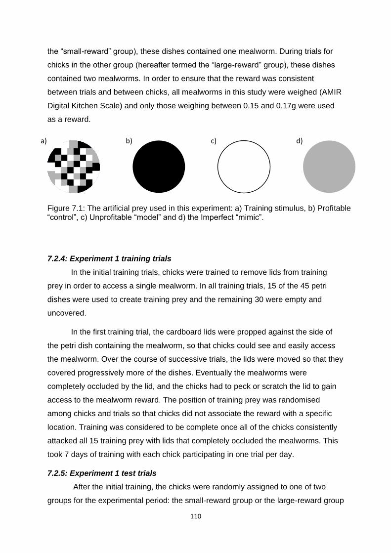
110

the “small-reward” group), these dishes contained one mealworm. During trials for

chicks in the other group (hereafter termed the “large-reward” group), these dishes

contained two mealworms. In order to ensure that the reward was consistent

between trials and between chicks, all mealworms in this study were weighed (AMIR

Digital Kitchen Scale) and only those weighing between 0.15 and 0.17g were used

as a reward.

7.2.4: Experiment 1 training trials

In the initial training trials, chicks were trained to remove lids from training

prey in order to access a single mealworm. In all training trials, 15 of the 45 petri

dishes were used to create training prey and the remaining 30 were empty and

uncovered.

In the first training trial, the cardboard lids were propped against the side of

the petri dish containing the mealworm, so that chicks could see and easily access

the mealworm. Over the course of successive trials, the lids were moved so that they

covered progressively more of the dishes. Eventually the mealworms were

completely occluded by the lid, and the chicks had to peck or scratch the lid to gain

access to the mealworm reward. The position of training prey was randomised

among chicks and trials so that chicks did not associate the reward with a specific

location. Training was considered to be complete once all of the chicks consistently

attacked all 15 training prey with lids that completely occluded the mealworms. This

took 7 days of training with each chick participating in one trial per day.

7.2.5: Experiment 1 test trials

After the initial training, the chicks were randomly assigned to one of two

groups for the experimental period: the small-reward group or the large-reward group

Figure 7.1: The artificial prey used in this experiment: a) Training stimulus, b) Profitable “control”, c) Unprofitable “model” and d) the Imperfect “mimic”.

a) b) c) d)

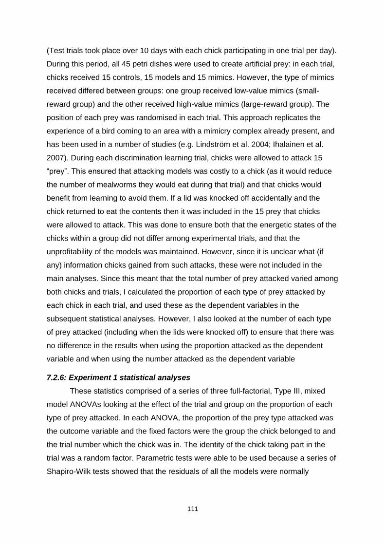
111

(Test trials took place over 10 days with each chick participating in one trial per day).

During this period, all 45 petri dishes were used to create artificial prey: in each trial,

chicks received 15 controls, 15 models and 15 mimics. However, the type of mimics

received differed between groups: one group received low-value mimics (small-

reward group) and the other received high-value mimics (large-reward group). The

position of each prey was randomised in each trial. This approach replicates the

experience of a bird coming to an area with a mimicry complex already present, and

has been used in a number of studies (e.g. Lindström et al. 2004; Ihalainen et al.

2007). During each discrimination learning trial, chicks were allowed to attack 15

“prey”. This ensured that attacking models was costly to a chick (as it would reduce

the number of mealworms they would eat during that trial) and that chicks would

benefit from learning to avoid them. If a lid was knocked off accidentally and the

chick returned to eat the contents then it was included in the 15 prey that chicks

were allowed to attack. This was done to ensure both that the energetic states of the

chicks within a group did not differ among experimental trials, and that the

unprofitability of the models was maintained. However, since it is unclear what (if

any) information chicks gained from such attacks, these were not included in the

main analyses. Since this meant that the total number of prey attacked varied among

both chicks and trials, I calculated the proportion of each type of prey attacked by

each chick in each trial, and used these as the dependent variables in the

subsequent statistical analyses. However, I also looked at the number of each type

of prey attacked (including when the lids were knocked off) to ensure that there was

no difference in the results when using the proportion attacked as the dependent

variable and when using the number attacked as the dependent variable

7.2.6: Experiment 1 statistical analyses

These statistics comprised of a series of three full-factorial, Type III, mixed

model ANOVAs looking at the effect of the trial and group on the proportion of each

type of prey attacked. In each ANOVA, the proportion of the prey type attacked was

the outcome variable and the fixed factors were the group the chick belonged to and

the trial number which the chick was in. The identity of the chick taking part in the

trial was a random factor. Parametric tests were able to be used because a series of

Shapiro-Wilk tests showed that the residuals of all the models were normally

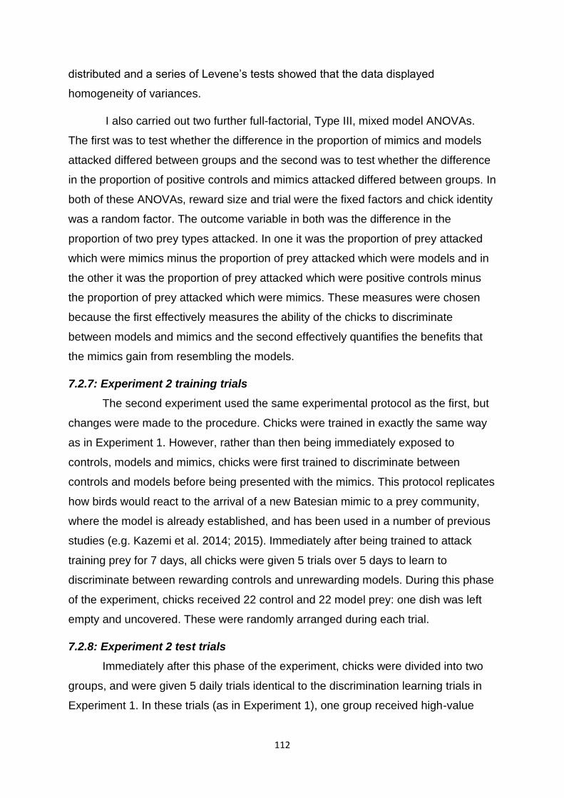
112

distributed and a series of Levene’s tests showed that the data displayed

homogeneity of variances.

I also carried out two further full-factorial, Type III, mixed model ANOVAs.

The first was to test whether the difference in the proportion of mimics and models

attacked differed between groups and the second was to test whether the difference

in the proportion of positive controls and mimics attacked differed between groups. In

both of these ANOVAs, reward size and trial were the fixed factors and chick identity

was a random factor. The outcome variable in both was the difference in the

proportion of two prey types attacked. In one it was the proportion of prey attacked

which were mimics minus the proportion of prey attacked which were models and in

the other it was the proportion of prey attacked which were positive controls minus

the proportion of prey attacked which were mimics. These measures were chosen

because the first effectively measures the ability of the chicks to discriminate

between models and mimics and the second effectively quantifies the benefits that

the mimics gain from resembling the models.

7.2.7: Experiment 2 training trials

The second experiment used the same experimental protocol as the first, but

changes were made to the procedure. Chicks were trained in exactly the same way

as in Experiment 1. However, rather than then being immediately exposed to

controls, models and mimics, chicks were first trained to discriminate between

controls and models before being presented with the mimics. This protocol replicates

how birds would react to the arrival of a new Batesian mimic to a prey community,

where the model is already established, and has been used in a number of previous

studies (e.g. Kazemi et al. 2014; 2015). Immediately after being trained to attack

training prey for 7 days, all chicks were given 5 trials over 5 days to learn to

discriminate between rewarding controls and unrewarding models. During this phase

of the experiment, chicks received 22 control and 22 model prey: one dish was left

empty and uncovered. These were randomly arranged during each trial.

7.2.8: Experiment 2 test trials

Immediately after this phase of the experiment, chicks were divided into two

groups, and were given 5 daily trials identical to the discrimination learning trials in

Experiment 1. In these trials (as in Experiment 1), one group received high-value

113

mimics (large-reward group) and the other received low-value mimics (small-reward

group).

7.2.9: Experiment 2 statistical analyses

Since chicks in both experimental groups received the same prey types during

the discrimination learning phase, I predicted that they should learn to discriminate

between models and controls at similar rates. I tested this using a full factorial, mixed

model, Type III ANOVA with the difference in proportion of prey attacked during the

discrimination learning trials which were positive controls as the outcome variable,

the group the chick belonged to and the trial number as the fixed factors and chick

identity as the random factor.

In contrast, I predicted that the behaviour of the chicks in the test trials should

differ between the experimental groups. In order to test this, I carried out a series of

three bootstrapped full-factorial, Type III, mixed model ANOVAs (number of

bootstraps = 1000), I used 1000 bootstraps because it is over the minimum number

of bootstraps for general use as suggested by Wilcox (2010) which was 599. Much

like in Experiment 1, the outcome variable was the proportion of prey attacked of

each type, the fixed factors were the group the chick belonged to and the trial

number and the random factor was the chick identity. I used non-parametric tests

because a series of Levene’s tests showed that the residuals were not normally

distributed.

Again, I carried out two further ANOVAS: one full-factorial, Type III, mixed

model ANOVA to test whether the difference in the proportion of mimics and models

attacked differed between groups and one bootstrapped full-factorial, Type III, mixed

model ANOVA (number of bootstraps = 1000) to test whether the difference in the

proportion of positive controls and mimics attacked differed between groups. In both

of these ANOVAs, reward size and trial were the fixed factors and chick identity was

a random factor. The outcome variable in both was the difference in the proportion of

two prey types attacked. In one it was the proportion of prey attacked which were

mimics minus the proportion of prey attacked which were models and in the other it

was the proportion of prey attacked which were controls minus the proportion of prey

attacked which were mimics.

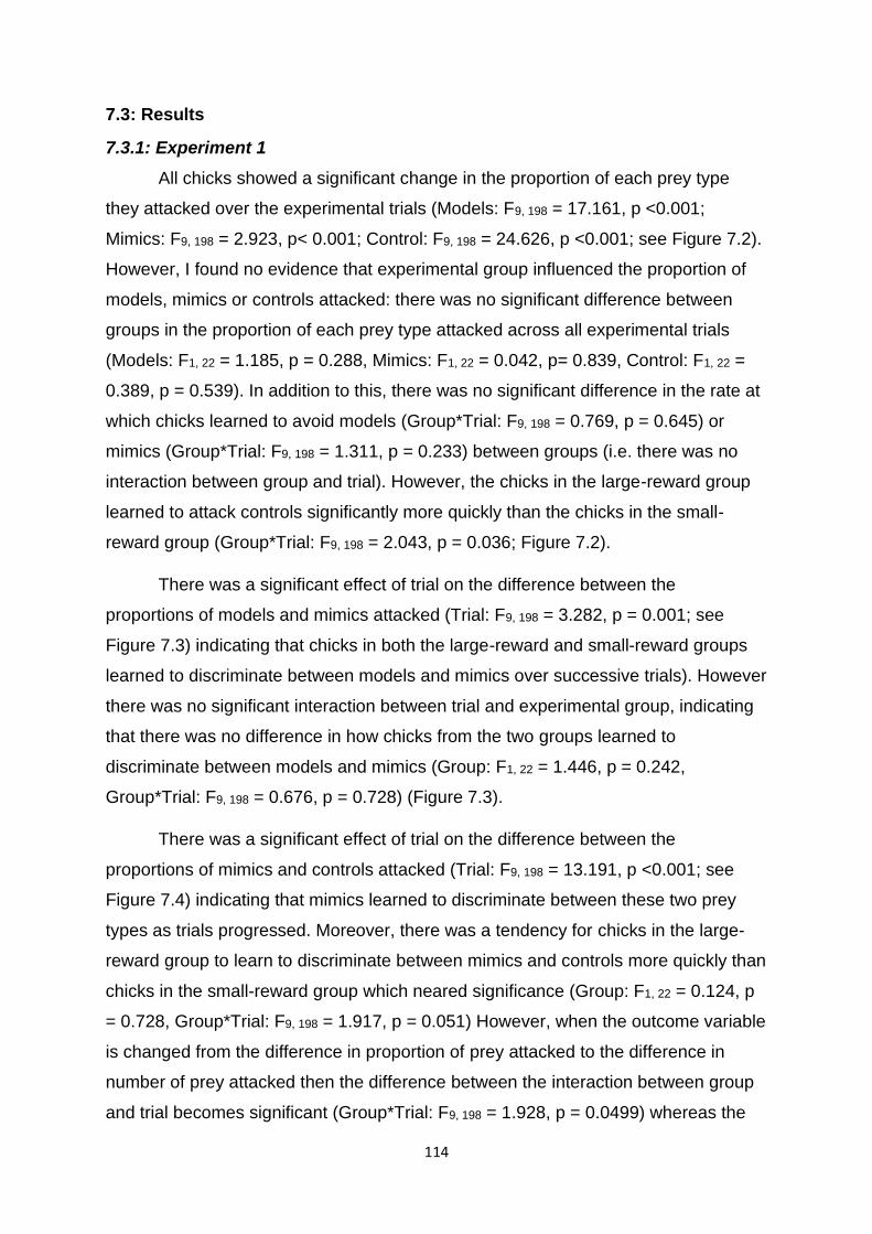
114

7.3: Results

7.3.1: Experiment 1

All chicks showed a significant change in the proportion of each prey type

they attacked over the experimental trials (Models: F9, 198 = 17.161, p <0.001;

Mimics: F9, 198 = 2.923, p< 0.001; Control: F9, 198 = 24.626, p <0.001; see Figure 7.2).

However, I found no evidence that experimental group influenced the proportion of

models, mimics or controls attacked: there was no significant difference between

groups in the proportion of each prey type attacked across all experimental trials

(Models: F1, 22 = 1.185, p = 0.288, Mimics: F1, 22 = 0.042, p= 0.839, Control: F1, 22 =

0.389, p = 0.539). In addition to this, there was no significant difference in the rate at

which chicks learned to avoid models (Group*Trial: F9, 198 = 0.769, p = 0.645) or

mimics (Group*Trial: F9, 198 = 1.311, p = 0.233) between groups (i.e. there was no

interaction between group and trial). However, the chicks in the large-reward group

learned to attack controls significantly more quickly than the chicks in the small-

reward group (Group*Trial: F9, 198 = 2.043, p = 0.036; Figure 7.2).

There was a significant effect of trial on the difference between the

proportions of models and mimics attacked (Trial: F9, 198 = 3.282, p = 0.001; see

Figure 7.3) indicating that chicks in both the large-reward and small-reward groups

learned to discriminate between models and mimics over successive trials). However

there was no significant interaction between trial and experimental group, indicating

that there was no difference in how chicks from the two groups learned to

discriminate between models and mimics (Group: F1, 22 = 1.446, p = 0.242,

Group*Trial: F9, 198 = 0.676, p = 0.728) (Figure 7.3).

There was a significant effect of trial on the difference between the

proportions of mimics and controls attacked (Trial: F9, 198 = 13.191, p <0.001; see

Figure 7.4) indicating that mimics learned to discriminate between these two prey

types as trials progressed. Moreover, there was a tendency for chicks in the large-

reward group to learn to discriminate between mimics and controls more quickly than

chicks in the small-reward group which neared significance (Group: F1, 22 = 0.124, p

= 0.728, Group*Trial: F9, 198 = 1.917, p = 0.051) However, when the outcome variable

is changed from the difference in proportion of prey attacked to the difference in

number of prey attacked then the difference between the interaction between group

and trial becomes significant (Group*Trial: F9, 198 = 1.928, p = 0.0499) whereas the

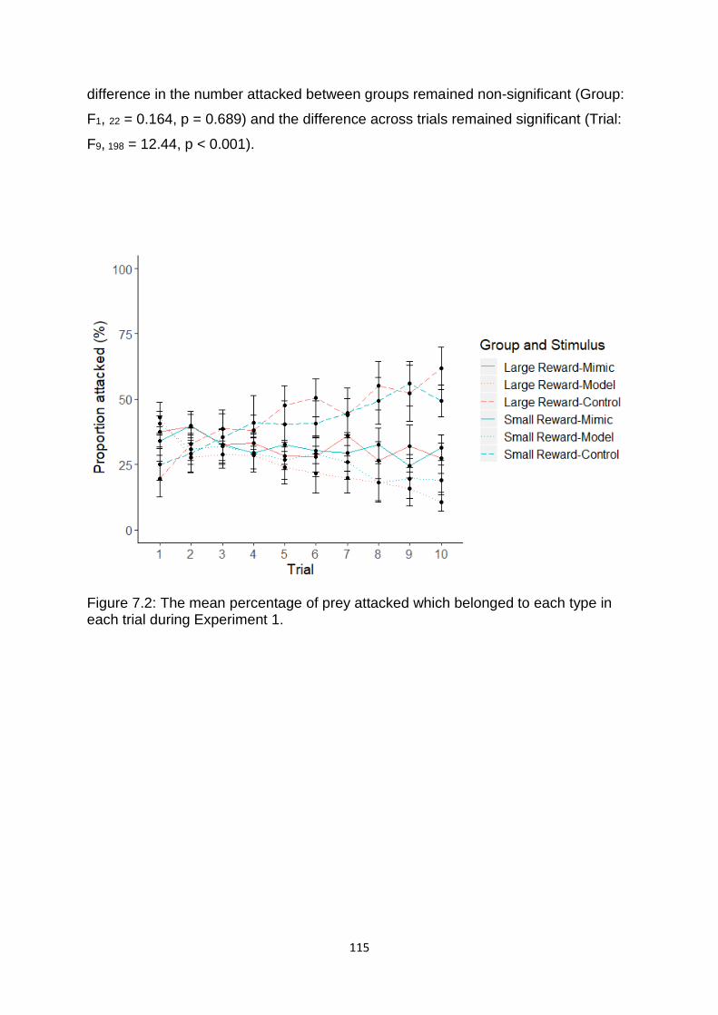
115

difference in the number attacked between groups remained non-significant (Group:

F1, 22 = 0.164, p = 0.689) and the difference across trials remained significant (Trial:

F9, 198 = 12.44, p < 0.001).

Figure 7.2: The mean percentage of prey attacked which belonged to each type in each trial during Experiment 1.

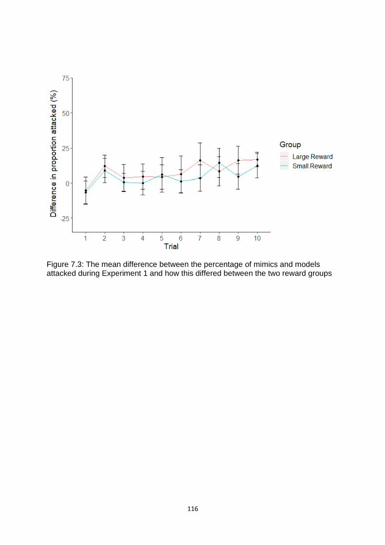
116

Figure 7.3: The mean difference between the percentage of mimics and models attacked during Experiment 1 and how this differed between the two reward groups

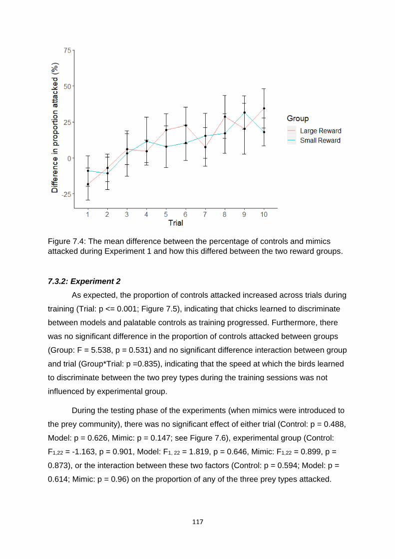
117

Figure 7.4: The mean difference between the percentage of controls and mimics

attacked during Experiment 1 and how this differed between the two reward groups.

7.3.2: Experiment 2

As expected, the proportion of controls attacked increased across trials during

training (Trial: p <= 0.001; Figure 7.5), indicating that chicks learned to discriminate

between models and palatable controls as training progressed. Furthermore, there

was no significant difference in the proportion of controls attacked between groups

(Group: F = 5.538, p = 0.531) and no significant difference interaction between group

and trial (Group*Trial: p =0.835), indicating that the speed at which the birds learned

to discriminate between the two prey types during the training sessions was not

influenced by experimental group.

During the testing phase of the experiments (when mimics were introduced to

the prey community), there was no significant effect of either trial (Control: p = 0.488,

Model: p = 0.626, Mimic: p = 0.147; see Figure 7.6), experimental group (Control:

F1,22 = -1.163, p = 0.901, Model: F1, 22 = 1.819, p = 0.646, Mimic: F1,22 = 0.899, p =

0.873), or the interaction between these two factors (Control: p = 0.594; Model: p =

0.614; Mimic: p = 0.96) on the proportion of any of the three prey types attacked.

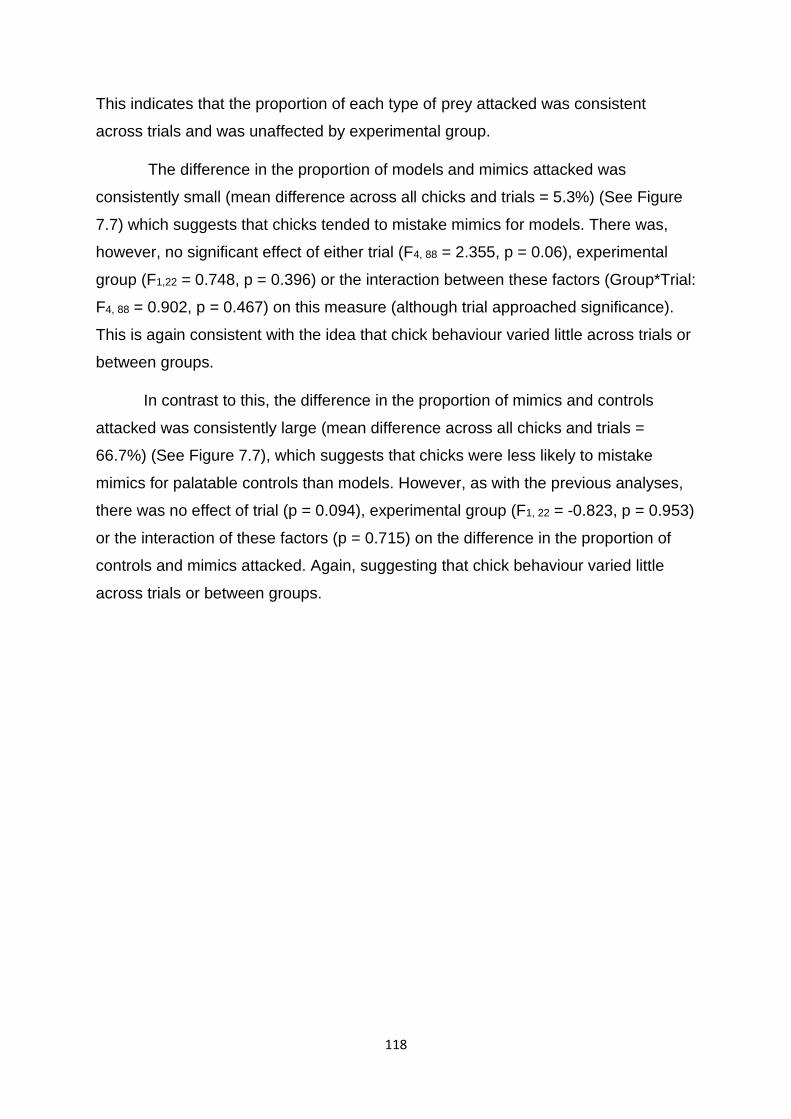
118

This indicates that the proportion of each type of prey attacked was consistent

across trials and was unaffected by experimental group.

The difference in the proportion of models and mimics attacked was

consistently small (mean difference across all chicks and trials = 5.3%) (See Figure

7.7) which suggests that chicks tended to mistake mimics for models. There was,

however, no significant effect of either trial (F4, 88 = 2.355, p = 0.06), experimental

group (F1,22 = 0.748, p = 0.396) or the interaction between these factors (Group*Trial:

F4, 88 = 0.902, p = 0.467) on this measure (although trial approached significance).

This is again consistent with the idea that chick behaviour varied little across trials or

between groups.

In contrast to this, the difference in the proportion of mimics and controls

attacked was consistently large (mean difference across all chicks and trials =

66.7%) (See Figure 7.7), which suggests that chicks were less likely to mistake

mimics for palatable controls than models. However, as with the previous analyses,

there was no effect of trial (p = 0.094), experimental group (F1, 22 = -0.823, p = 0.953)

or the interaction of these factors (p = 0.715) on the difference in the proportion of

controls and mimics attacked. Again, suggesting that chick behaviour varied little

across trials or between groups.

119

Figure 7.5: The mean percentage of prey attacked which belonged to each type in each trial during the discrimination training period of Experiment 2.

Figure 7.6: The mean percentage of prey attacked which belonged to each type in each trial during the test period of Experiment 2.

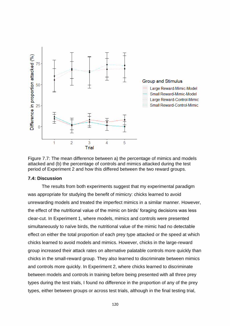
120

Figure 7.7: The mean difference between a) the percentage of mimics and models attacked and (b) the percentage of controls and mimics attacked during the test period of Experiment 2 and how this differed between the two reward groups.

7.4: Discussion

The results from both experiments suggest that my experimental paradigm

was appropriate for studying the benefit of mimicry: chicks learned to avoid

unrewarding models and treated the imperfect mimics in a similar manner. However,

the effect of the nutritional value of the mimic on birds’ foraging decisions was less

clear-cut. In Experiment 1, where models, mimics and controls were presented

simultaneously to naïve birds, the nutritional value of the mimic had no detectable

effect on either the total proportion of each prey type attacked or the speed at which

chicks learned to avoid models and mimics. However, chicks in the large-reward

group increased their attack rates on alternative palatable controls more quickly than

chicks in the small-reward group. They also learned to discriminate between mimics

and controls more quickly. In Experiment 2, where chicks learned to discriminate

between models and controls in training before being presented with all three prey

types during the test trials, I found no difference in the proportion of any of the prey

types, either between groups or across test trials, although in the final testing trial,

121

there was a difference in the ability of chicks in different groups to discriminate

between models and mimics which neared significance.

Contrary to the prediction of Penney et al. (2012), there was no effect of the

nutritional value of the mimic on the total proportions of any of the prey types

attacked in either of my experiments. One explanation for this is that chicks paid little

attention to reward value (beyond establishing whether prey was rewarded and

unrewarded). This could be because I varied the number rather than the size of the

reward. In the wild, predators will experience prey of a variety of sizes and since wild

birds will often eat the most profitable prey items available to them (Barnard and

Stephens 1981; Sutherland 1982) and there is evidence that they do this using visual

cues (Sutherland 1982), they presumably use size as a cue for profitability. Using a

single signal to indicate differences in reward number (as in m experiments) may be

less ecologically realistic, and may be more difficult for birds to learn. Therefore if

this experiment was repeated mimics that varied in size then perhaps we might see

predation rates which echo those suggested by the literature. This idea is further

supported by the results from Chapter 6 which suggest that the difference in size

between models and mimics affects the predation risk for mimics.

An alternative explanation as to why there was no difference in the proportion

of each prey type attacked between the large-reward group and the small-reward

group could be due to the fact that the mimicry complexes in these experiments have

the same coefficient of variation despite having a different mean reward. The

coefficient of variation is defined as the standard deviation of the size of the reward

divided by the mean reward and has been shown to be a strong predictor of risk-

aversion in experiments investigating risk sensitivity (Shafir 2000; Weber et al. 2004;

Drezner-Levy and Shafir 2007). Since the coefficient of variation of the model and

mimic stimuli for both groups was 1 (Small-reward group: mean reward = 0.5,

standard deviation of reward = 0.5; Large-reward group: mean reward = 1, standard

deviation of reward = 1), it makes sense that chicks in both groups are equally risk-

averse.

Whilst I found no evidence that the total proportion of prey attacked differed

between groups, Experiment 1 provided some evidence that the speed at which

predators learned about prey types differed among groups. However, these data are

122

difficult to interpret. Whilst there is evidence that predators faced with high-value

mimics increase their attack rates on alternative prey more quickly that those faced

with low-value mimics, I found no corresponding increase in the speed at which

predators decreased their attack rates on either models or mimics. Given that I

analysed the proportion of prey attacked that were from each of the three prey types,

an increase in the speed at which predators attacked controls should be

accompanied by an increase in the speed at which they decreased attacks on other

prey types. However, this was not seen. This could be because the reduction was

shared across these two prey types. However, this was not seen. This could be

because the reduction was shared across these two prey types and so was too small

to detect: if I had analysed the combined proportion of models and mimics attacked, I

would have perhaps found a difference.

So why might chicks learn to discriminate between mimetic complexes and

alternative palatable prey more quickly when mimics have a higher nutritive value?

This is perplexing because this is the opposite of what I initially hypothesised. There

are two potential explanations for this. Firstly, my high-reward prey may have been

less rewarding than the low-reward prey. This could be the case if the handling time

was higher for high-reward prey. However, whilst it clearly took birds longer to eat

two mealworms than one, the difference in handling time was very small and is

unlikely to have exceeded the benefits of the additional nutrients of high-value prey.

Alternatively, chicks in the large-reward group may have payed closer attention to

the different types of prey due to their differing reward values. Hence, they could

have learned the initial discrimination between the controls and the mimetic complex

faster than the chicks in the small-reward group. This, however, raises the question

of why such an increase in attention did not allow chicks to better discriminate

between models and mimics. Again, this is difficult to answer, but perhaps birds were

not given sufficient time to make this discrimination or perhaps making this

discrimination was not worthwhile. This could be the case if this discrimination was

difficult and required a significant time investment. Under such circumstances relying

on the alternative prey that could be identified quickly may have proved the optimal

foraging option.

When considering my results, it is also worth noting that the model was

associated with a lack of reward rather than a distasteful food reward. This is

123

contrary to many mimicry systems and may have affected avoidance learning. The

results of Alcock (1979) suggested that the mimics of artificial non-rewarding models

are more likely to be attacked than mimics of artificial mildly-unpalatable models by

white-throated sparrows (Zonotrichia albicollis). This indicates that the chicks in this

experiment should have been more likely to learn that the mimics were rewarded

and so this should be more likely to lead to a difference between groups based on

the difference in the size of the reward. Regardless, this experiment is still

ecologically-relevant since there are some mimicry rings which are based around

models whose only defence is being completely unrewarding. For instance, weevils

of the genus Pachyrrhynchus are aposematic, predators quickly learn to avoid them

(Tseng et al. 2014) and they are seemingly mimicked by longhorn beetles of the

genus Doliops (Barševskis 2013). However, their only apparent defence is their

incredibly hard elytra which makes them inedible to sympatric lizards (Wang et al.

2018) and thus they are unrewarding rather than distasteful, much like the stimuli

used in my study. Even so, it would be interesting to carry out studies in the future

where the model stimulus is associated with an unprofitable prey item rather than a

lack of reward to see if the relationship is still seen

7.5: Conclusions

The results of this experiment suggest that the nutritive value of an imperfect

mimic has no effect on how predators discriminate between it and its model in the

absence of size cues. When combined with the results of Chapter 6, this suggests

that the size of a prey item may be an informative visual cue for predators which not

only allows predators to discriminate between models and mimics but also potentially

provides an indication of the nutritive value of a prey item. In the future, it would be

interesting to carry out further experiments to see if the lack of relationship between

nutritive value and predation risk seen here is still seen if the size of the stimulus is

used to provide an informative cue about the nutritive value of the associated reward

and if this lack of effect would still be seen if models are unpalatable rather than

unrewarded.

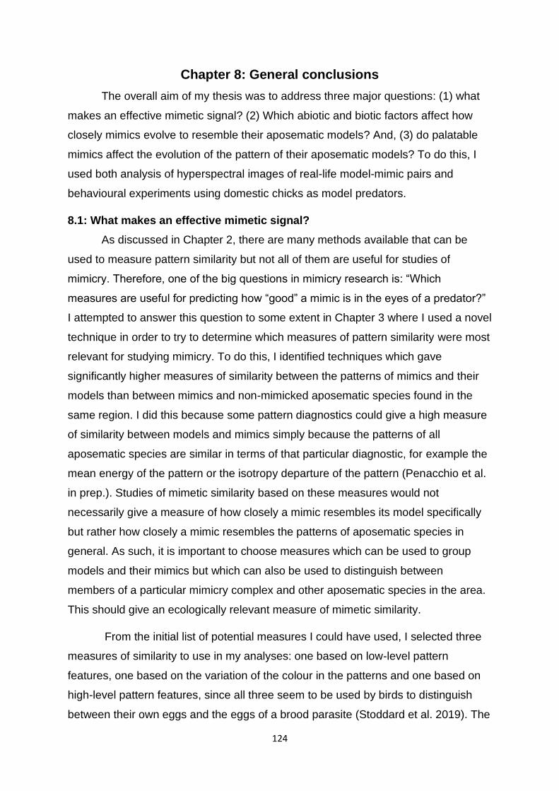
124

Chapter 8: General conclusions

The overall aim of my thesis was to address three major questions: (1) what

makes an effective mimetic signal? (2) Which abiotic and biotic factors affect how

closely mimics evolve to resemble their aposematic models? And, (3) do palatable

mimics affect the evolution of the pattern of their aposematic models? To do this, I

used both analysis of hyperspectral images of real-life model-mimic pairs and

behavioural experiments using domestic chicks as model predators.

8.1: What makes an effective mimetic signal?

As discussed in Chapter 2, there are many methods available that can be

used to measure pattern similarity but not all of them are useful for studies of

mimicry. Therefore, one of the big questions in mimicry research is: “Which

measures are useful for predicting how “good” a mimic is in the eyes of a predator?”

I attempted to answer this question to some extent in Chapter 3 where I used a novel

technique in order to try to determine which measures of pattern similarity were most

relevant for studying mimicry. To do this, I identified techniques which gave

significantly higher measures of similarity between the patterns of mimics and their

models than between mimics and non-mimicked aposematic species found in the

same region. I did this because some pattern diagnostics could give a high measure

of similarity between models and mimics simply because the patterns of all

aposematic species are similar in terms of that particular diagnostic, for example the

mean energy of the pattern or the isotropy departure of the pattern (Penacchio et al.

in prep.). Studies of mimetic similarity based on these measures would not

necessarily give a measure of how closely a mimic resembles its model specifically

but rather how closely a mimic resembles the patterns of aposematic species in

general. As such, it is important to choose measures which can be used to group

models and their mimics but which can also be used to distinguish between

members of a particular mimicry complex and other aposematic species in the area.

This should give an ecologically relevant measure of mimetic similarity.

From the initial list of potential measures I could have used, I selected three

measures of similarity to use in my analyses: one based on low-level pattern

features, one based on the variation of the colour in the patterns and one based on

high-level pattern features, since all three seem to be used by birds to distinguish

between their own eggs and the eggs of a brood parasite (Stoddard et al. 2019). The

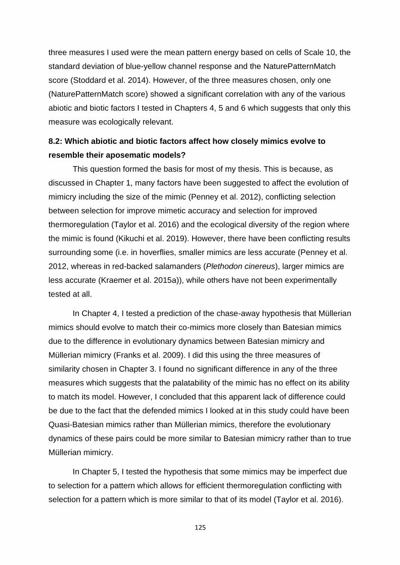
125

three measures I used were the mean pattern energy based on cells of Scale 10, the

standard deviation of blue-yellow channel response and the NaturePatternMatch

score (Stoddard et al. 2014). However, of the three measures chosen, only one

(NaturePatternMatch score) showed a significant correlation with any of the various

abiotic and biotic factors I tested in Chapters 4, 5 and 6 which suggests that only this

measure was ecologically relevant.

8.2: Which abiotic and biotic factors affect how closely mimics evolve to

resemble their aposematic models?

This question formed the basis for most of my thesis. This is because, as

discussed in Chapter 1, many factors have been suggested to affect the evolution of

mimicry including the size of the mimic (Penney et al. 2012), conflicting selection

between selection for improve mimetic accuracy and selection for improved

thermoregulation (Taylor et al. 2016) and the ecological diversity of the region where

the mimic is found (Kikuchi et al. 2019). However, there have been conflicting results

surrounding some (i.e. in hoverflies, smaller mimics are less accurate (Penney et al.

2012, whereas in red-backed salamanders (Plethodon cinereus), larger mimics are

less accurate (Kraemer et al. 2015a)), while others have not been experimentally

tested at all.

In Chapter 4, I tested a prediction of the chase-away hypothesis that Müllerian

mimics should evolve to match their co-mimics more closely than Batesian mimics

due to the difference in evolutionary dynamics between Batesian mimicry and

Müllerian mimicry (Franks et al. 2009). I did this using the three measures of

similarity chosen in Chapter 3. I found no significant difference in any of the three

measures which suggests that the palatability of the mimic has no effect on its ability

to match its model. However, I concluded that this apparent lack of difference could

be due to the fact that the defended mimics I looked at in this study could have been

Quasi-Batesian mimics rather than Müllerian mimics, therefore the evolutionary

dynamics of these pairs could be more similar to Batesian mimicry rather than to true

Müllerian mimicry.

In Chapter 5, I tested the hypothesis that some mimics may be imperfect due

to selection for a pattern which allows for efficient thermoregulation conflicting with

selection for a pattern which is more similar to that of its model (Taylor et al. 2016).

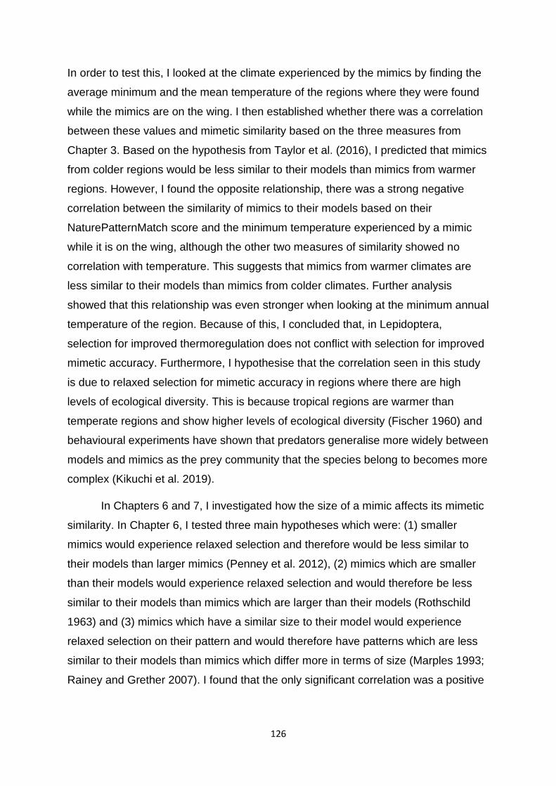
126

In order to test this, I looked at the climate experienced by the mimics by finding the

average minimum and the mean temperature of the regions where they were found

while the mimics are on the wing. I then established whether there was a correlation

between these values and mimetic similarity based on the three measures from

Chapter 3. Based on the hypothesis from Taylor et al. (2016), I predicted that mimics

from colder regions would be less similar to their models than mimics from warmer

regions. However, I found the opposite relationship, there was a strong negative

correlation between the similarity of mimics to their models based on their

NaturePatternMatch score and the minimum temperature experienced by a mimic

while it is on the wing, although the other two measures of similarity showed no

correlation with temperature. This suggests that mimics from warmer climates are

less similar to their models than mimics from colder climates. Further analysis

showed that this relationship was even stronger when looking at the minimum annual

temperature of the region. Because of this, I concluded that, in Lepidoptera,

selection for improved thermoregulation does not conflict with selection for improved

mimetic accuracy. Furthermore, I hypothesise that the correlation seen in this study

is due to relaxed selection for mimetic accuracy in regions where there are high

levels of ecological diversity. This is because tropical regions are warmer than

temperate regions and show higher levels of ecological diversity (Fischer 1960) and

behavioural experiments have shown that predators generalise more widely between

models and mimics as the prey community that the species belong to becomes more

complex (Kikuchi et al. 2019).

In Chapters 6 and 7, I investigated how the size of a mimic affects its mimetic

similarity. In Chapter 6, I tested three main hypotheses which were: (1) smaller

mimics would experience relaxed selection and therefore would be less similar to

their models than larger mimics (Penney et al. 2012), (2) mimics which are smaller

than their models would experience relaxed selection and would therefore be less

similar to their models than mimics which are larger than their models (Rothschild

1963) and (3) mimics which have a similar size to their model would experience

relaxed selection on their pattern and would therefore have patterns which are less

similar to their models than mimics which differ more in terms of size (Marples 1993;

Rainey and Grether 2007). I found that the only significant correlation was a positive

127

correlation between mimetic similarity based on NaturePatternMatch score and

percentage difference in wing area which supports the third hypothesis.

In Chapter 7, I again tested the hypothesis that smaller mimics experience

relaxed selection due to their lower nutritive value (Penney et al. 2012). However,

this time I did it by carrying out a series of behavioural experiments using domestic

chicks as model predators. In these experiments, chicks had to choose between a

rewarded control stimulus, an unrewarded “model” stimulus and an imperfect,

rewarded “mimic” stimulus. In Experiment 1, chicks were introduced to all three

stimuli at the same time, whereas in Experiment 2, chicks were given the opportunity

to learn to discriminate between positive control stimuli and model stimuli before

being introduced the mimics. In both of these experiments, chicks were split into two

groups: the large-reward group and the small-reward group. Chicks in the large-

reward group were rewarded with two mealworms for attacking mimics, whereas

chicks in the small-reward group where only rewarded with one mealworm for

attacking mimics. I then compared the following between groups: (1) the proportion

of each prey type attacked, (2) the difference in proportion of models and mimics

attacked and (3) the difference in proportion of positive controls and mimics

attacked. In both experiments, there was no difference in the proportion of any type

of prey attacked between groups. However, in Experiment 1, chicks in the large-

reward group learned to avoid the models and mimics more quickly than chicks in

the small-reward group. This suggests that, in the absence of size cues, the nutritive

value of a mimic has no effect on how predators discriminate between models and

mimics. However, this could also be due to the fact that the mimetic complex in the

large-reward group had the same coefficient of variation as the mimetic complex in

the small-reward group: this has been shown to be an important predictor of risk-

aversion in feeding behaviour (Shafir 2000; Weber et al. 2004; Drezner-Levy and

Shafir 2007).

8.3: Do palatable mimics affect the evolution of the pattern of their aposematic

models?

It has been hypothesised that, due to the chase-away hypothesis (Franks et

al. 2009), models of palatable mimics should evolve to disengage from the Batesian

mimetic relationship due to the associated costs. I had hypothesised that this

proposed change in pattern would lead to a change in the efficacy of the aposematic

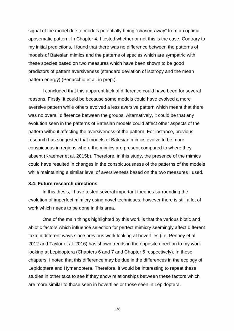
128

signal of the model due to models potentially being “chased-away” from an optimal

aposematic pattern. In Chapter 4, I tested whether or not this is the case. Contrary to

my initial predictions, I found that there was no difference between the patterns of

models of Batesian mimics and the patterns of species which are sympatric with

these species based on two measures which have been shown to be good

predictors of pattern aversiveness (standard deviation of isotropy and the mean

pattern energy) (Penacchio et al. in prep.).

I concluded that this apparent lack of difference could have been for several

reasons. Firstly, it could be because some models could have evolved a more

aversive pattern while others evolved a less aversive pattern which meant that there

was no overall difference between the groups. Alternatively, it could be that any

evolution seen in the patterns of Batesian models could affect other aspects of the

pattern without affecting the aversiveness of the pattern. For instance, previous

research has suggested that models of Batesian mimics evolve to be more

conspicuous in regions where the mimics are present compared to where they

absent (Kraemer et al. 2015b). Therefore, in this study, the presence of the mimics

could have resulted in changes in the conspicuousness of the patterns of the models

while maintaining a similar level of aversiveness based on the two measures I used.

8.4: Future research directions

In this thesis, I have tested several important theories surrounding the

evolution of imperfect mimicry using novel techniques, however there is still a lot of

work which needs to be done in this area.

One of the main things highlighted by this work is that the various biotic and

abiotic factors which influence selection for perfect mimicry seemingly affect different

taxa in different ways since previous work looking at hoverflies (i.e. Penney et al.

2012 and Taylor et al. 2016) has shown trends in the opposite direction to my work

looking at Lepidoptera (Chapters 6 and 7 and Chapter 5 respectively). In these

chapters, I noted that this difference may be due in the differences in the ecology of

Lepidoptera and Hymenoptera. Therefore, it would be interesting to repeat these

studies in other taxa to see if they show relationships between these factors which

are more similar to those seen in hoverflies or those seen in Lepidoptera.

129

It would be particularly interesting to test the hypothesis that the relationship

between temperature and mimetic similarity observed in Chapter 5 is due to the

ecological diversity found in warmer regions. To do this, I could investigate the

relationship between actual measures of the ecological diversity and measures of

pattern similarity. This would be difficult to carry out because arthropod diversity in

some regions is still unknown (Basset et al. 2012), however this problem could be

somewhat overcome since arthropod diversity can be accurately predicted from plant

diversity (Basset et al. 2012; Zhang et al. 2016, as such I could use that as the basis

of my measurements of the diversity of that region. Alternatively, the diversity of

Lepidoptera alone could be quantified by using species checklists from these

regions. This study would be incredibly useful to carry out as it could be a way of

establishing whether the results of the experiments of Kikuchi et al. (2019) accurately

reflect how predators select for mimetic patterns in the wild.

It would also be interesting to carry out further studies to investigate the

relationship between size and mimicry. It which would be useful to repeat the

experiments from Chapter 7 with unpalatable, rather than unrewarding, models. This

would allow us to determine whether this affects how predators discriminate between

models and mimics as the reward associated with the mimic changes.

In addition to this, one could determine whether the relationship between size

and mimetic similarity seen in Chapter 6 is also observed in mimetic complexes

based around unprofitable rather than unpalatable models. Examples of complexes

that could be studied are rings based around Pachyrrhynchus weevils (e.g. those

discussed by Barševskis 2013) or species which exhibit escape mimicry (also known

as evasive mimicry) i.e. species which mimic aposematic species whose colouration

has been proposed to advertise unprofitability due to their fast and erratic flight

pattern rather than due to them being toxic or unpalatable (Ruxton et al. 2004;

Pinheiro and Freitas 2014).

8.5: Concluding remarks

Overall, the results of my thesis have provided novel insights into the

evolution of mimicry. Moreover, these data have highlighted the complex nature of

mimicry by demonstrating the sheer number of factors which can affect its evolution.

In addition to this, my results suggest that these factors can seemingly have different

130

effects on the evolution of mimicry in different taxa. Finally, I have shown the

importance of empirically testing the theories associated with the evolution of

mimicry using behavioural experiments.

131

References

Adam, Brother. 1983. In search of the best strains of bees. Northern Bee Books.

Hebden Bridge, UK. 206 pp.

Akcali, C. K. and D. W. Pfennig. 2017. Geographic variation in mimetic precision

among different species of coral snake mimics. Journal of Evolutionary Biology 30:

1420-1428. doi: 10.1111/jeb.13094

Akcali, C. K., Kikuchi, D. W. and D. W. Pfennig. 2018. Coevolutionary arms races in

Batesian mimicry? A test of the chase-away hypothesis. Biological Journal of the

Linnean Society 124(4): 668-676. doi: 10.1093/biolinnean/bly075

Alcock, J. 1970. Punishment levels and the response of white-throated sparrows

(Zonotrichia albicollis) to three kinds of artificial models and mimics. Animal

Behaviour 18: 733-739. doi: 10.1016/0003-3472(70)90019-9

Anderson, C. J. R., Lobo, N. D. V., Roth, J. D. and J. M. Waterman. 2010.

Computer-aided photo-identification system with an application to polar based on

whisker spot patterns. Journal of Mammalogy 91(6): 1350-1359. doi: 10.1644/09-

MAMM-A-425.1

Anzai, A., Peng, X. and D. C. Van Essen. 2007. Neurons in monkey visual area V2

encode combinations of orientations. Nature Neuroscience 10(10): 1313-1321. doi:

10.1038/nn1975

Archer, M. E. 2014. The Vespoid Wasps (Tiphiidae, Mutillidae, Sapygidae, Scoliidae

and Vespidae) of the British Isles. The Royal Entomological Society 82 pp

Arzoumanian, Z., Holmberg, J. and B. Norman. 2005. An astronomical pattern-

matching algorithm for computer-aided identification of whale sharks Rhincodon

typus. Journal of Applied Ecology 42(6): 999-1011. doi: 10.1111/j.1365-

2664.2005.01117.x

Aubier, T. G., Joron, M. and T. N. Sherratt. 2017. Mimicry among Unequally

Defended Prey Should Be Mutualistic When Predators Sample Optimally. The

American Naturalist 189(3): 267-282. doi: 10.1086/690121

132

Bain, R. S., Rashed, A., Cowper, V. J., Gilbert, F. S. and T. N. Sherratt. 2007. The

key mimetic features of hoverflies through avian eyes. Proceedings of the Royal

Society B 274: 1949-1954. doi: 10.1098/rspb.2007.0458

Balkenius, A. and A. Kelber. 2004. Colour constancy in diurnal and nocturnal

hawkmoths. Journal of Experimental Biology 207: 3307-3316. doi:

10.1242/jeb.01158

Ball, S. and R. Morris. 2015. Britain’s Hoverflies: A Field Guide, Revised and

Updated Second Edition. Princeton University Press. Princeton, New Jersey, USA.

312 pp.

Balogh, A. C. V. and O. Leimar. 2005. Müllerian mimicry: an examination of Fisher’s

theory of gradual evolutionary change. Proc. R. Soc. B 272: 2269-2275. doi:

10.1098/rspb.2005.3227

Balogh, A. C. V., Gamberale-Stille, G. and O. Leimar. 2008. Learning and the

mimicry spectrum: from quasi-Bates to super-Müller. Animal Behaviour 76: 1591-

1599. doi: 10.1016/j.anbehav.2008.07.017

Balogh, A. C., Gamberale-Stille, G., Tullberg, B. S. and O. Leimar. 2010. Feature

theory and the two-step hypothesis of Müllerian mimicry evolution. Evolution 64(3):

810-822. doi: 10.1111/j.1558-5646.2009.00852.x

Barber, J. R. and W. E. Conner. 2007. Acoustic mimicry in predator-prey interaction.

PNAS 104(22): 9331-9334. doi: 10.1073/pnas.0703627104

Barbosa, A., Mäthger, L. M., Buresch, K. C., Kelly, J., Chubb, C., Chiao, C-C and R.

T. Hanlon. 2008. Cuttlefish camouflage: The effect of substrate contrast and size in

evoking uniform, mottle or disruptive body patterns. Vision Research 48: 1242-1253.

doi: 10.1016/j.visres.2008.02.011

Barnard, C. J. and H. Stephens. 1981. Prey size selection by lapwings in

lapwing/gull associations. Behaviour 77(1-2): 1-22. doi: 10.1163/156853981X00130

Barnett, C. A., Bateson, M. and C. Rowe. 2007. State-dependent decision making:

educated predators strategically trade off the costs and benefits of consuming

aposematic prey. Behavioral Ecology 18(4): 645-651. doi: 10.1093/beheco/arm027

133

Barnett, C. A., Skelhorn, J., Bateson, M. and C. Rowe. 2012. Educated predators

make strategic decisions to eat defended prey according to their toxin content.

Behaviorial Ecology 23(2): 418-424. doi: 10.1093/beheco/arr206

Barnett, J. B., Michalis, C., Scott-Samuel, N. E. and I. C. Cuthill. 2018. Distance-

dependent defensive colouration in the poison frog Dendrobates tinctorius,

Dendrobatidae. PNAS 115(25): 6416-6421. doi: 10.1073/pnas.1800826115

Barševskis, A. 2013. Contribution to the knowledge of the genus Doliops

Waterhouse, 1841 (Coleoptera: Cerambycidae). Baltic Journal of Coleopterology 13:

73-89.

Basset, Y., Cizek, L., Cuénoud, P., Didham, R. K., Guilhaumon, F., Missa, O.,

Novotny, V., Ødegaard, F., Roslin, T., Schmidl, J., Tishechkin, A. K., Winchester, N.

N., Roubik, D. W., Aberlanc, H-P., Bail, J., Barrios, H., Bridle, J. R., Castaño-

Meneses, G., Corbana, B., Curletti, G., Duarte da Rocha, W., Bakker, D. D., Delabie,

J. H. C., Dejean, A., Fagan, L. L., Floren, A., Kitching, R. L., Medianero, E., Miller, S.

E., Gama da Oliveira, E., Orivel, J., Pollet, M., Rapp, M., Ribeiro, S. P., Roisin, Y.,

Schmidt, J. B., Sørensen, L. and M. Leponce. 2012. Arthropod Diversity in a Tropical

Forest. Science 338: 1481-1484. doi: 10.1126/science.1226727

Bates, H. W. 1862. XXXII. Contributions to an Insect Fauna of the Amazon Valley.

Lepidoptera: Heliconidae. Transactions of the Linnean Society of London 23(3): 495-

566

Beatty, C. D. and D. W. Franks. 2012. Discriminative predation: Simultaneous and

sequential encounter experiments. Current Zoology 58(4): 649-657. doi:

10.1093/czoolo/58.4.649

Benson, W. W. 1972. Natural Selection for Müllerian mimicry in Heliconius erato in

Costa Rica. Science 176(4037): 936-939. doi: 10.1126/science.176.4037.936

Biederman, I. and E. E. Cooper. 1992. Size invariance in visual object priming.

Journal of Experimental Psychology: Human Perception and Performance 18(1):

121-133. doi:10.1037/0096-1523.18.1.121

134

Bitton, P-P., Janisse, K. and S. M. Doucet. 2017. Assessing sexual dichromatism:

The Importance of Proper Parameterization in Tetrachromatic Visual Models. PLoS

ONE 12(1): e0169810. doi: 10.1371/journal.pone.0169810

Björkman, C. and S. Larsson. 1991. Pine sawfly defence and variation in host plant

resin acids: a trade-off with growth. Ecological Entomology 16: 283-289. doi:

10.1111/j.1365-2311.1991.tb00219.x

Blake, R. and W. Martens. 1981. Critical bands in cat spatial vision. J. Physiol. 314:

175-187. doi: 10.1113/jphysiol.1981.sp013699

Bloxham, L., Bateson, M., Bedford, T., Brilot, B. and D. Nettle. 2014. The memory of

hunger: developmental plasticity of dietary selectivity in the European starling,

Sturnus vulgaris. Animal Behaviour 91(100): 33-40. doi:

10.1016/j.anbehav.2014.02.025

Bowers, M. D. 1983. Mimicry in North American checkerspot butterflies: Euphydryas

phaeton and Chlosyne harrisii (Nymphalidae). Ecological Entomology 8(1): 1-8. doi:

10.1111/j.1365-2311.1983.tb00475.x

Bowmaker J. K. and H. J. A. Dartnall. 1980. Visual pigments of rods and cones in a

human retina. J. Physiol. 298: 501-511. doi: 10.1113/jphysiol.1980.sp013097

Bowmaker, J. K., Heath, L. A., Wilkie, S. E. and D. M. Hunt. 1997. Visual Pigments

and Oil Droplets from Six Classes of Photoreceptor in the Retinas of Birds. Vision

Res. 37(6): 2183-2194. doi: 10.1016/S0042-6989(97)00026-6

Brakefield, P. M. 1985. Polymorphic Müllerian mimicry and interactions with thermal

melanism in ladybirds and a soldier beetle: a hypothesis. Biological Journal of the

Linnean Society 26(3): 243-267. doi: 10.1111/j.1095-8312.1985.tb01635.x

Brooks, S. J., Calver, M. C., Dickman, C. R., Meathrel, C. E. and J. S. Bradley. 1996.

Does intraspecific variation in the energy value of a prey species to its predators

matter in studies of ecological energetics? A case study using insectivorous

vertebrates. Ecoscience 3(3): 247-251. doi: 10.1080/11956860.1996.11682338

Brower, J. V. Z. 1958a. Experimental Studies of Mimicry in Some North American

Butterflies: Part I. The Monarch, Danaus plexippus, and Viceroy, Limenitis archippus

archippus. Evolution 12(1): 32-47. doi: 10.1111/j.1558-5646.1958.tb02926.x

135

Brower, J. V. Z. 1958b. Experimental Studies of Mimicry in Some North American

Butterflies: Part II. Battus philenor and Papilio troilus, P. polyxenes and P. glaucus.

Evolution 12(2): 123-136. doi: 10.1111/j.1558-5646.1958.tb02939.x

Brower, J. V. Z. 1958c. Experimental Studies of Mimicry in Some North American

Butterflies: Part III. Danaus gilippus Berenice and Limenitis archippus floridensis.

Evolution 12(3): 273-285. doi: 10.1111/j.1558-5646.1958.tb02959.x

Brower, L. P., Brower, J. V. Z. and P. W. Westcott. 1960. Experimental Studies of

Mimicry. 5. The Reactions of Toads (Bufo terrestris) to Bumblebees (Bombus

americanorum) and Their Robberfly Mimics (Mallophora bomboides), with a

Discussion of Aggressive Mimicry. The American Naturalist 94(878): 343-355. doi:

10.1086/282137

Brower, J. V. Z. and L. P. Brower. 1962. Experimental studies of mimicry. 6. The

reaction of toads (Bufo terrestris) to honeybees and their dronefly mimics (Eristalis

vinetorum). American Naturalist 96: 297-307. doi: 10.1086/282237

Brower, L. P., Brower, J. V. Z. and C. T. Collins. 1963. Experimental studies of

mimicry. 7. Relative palatability and Müllerian mimicry among neotropical butterflies

of the subfamily Heliconiinae. Zoologica N. Y. 48(7): 65-84

Brower, J. V. Z. and L. P. Brower. 1965. Experimental studies of mimicry. 8. Further

investigations of honeybees (Apis mellifera) and their dronefly mimics (Eristalis spp.).

American Naturalist 99: 173-187. doi: 10.1086/282365

Brower, L. P., Cook, L. M. and H. J. Croze. 1967. Predator Responses to Artificial

Batesian Mimics Released in a Neotropical Environment. Evolution 21(1): 11-23. doi:

10.2307/2406736

Brower, L. P. and C. M. Moffitt. 1974. Palatability dynamics of cardenolides in the

monarch butterfly. Nature 249: 280-283. doi: 10.1038/249280b0

Burdfield-Steel, E., Brain, M., Rojas, B. and J. Mappes. 2018. The price of safety:

food deprivation in early life influences the efficacy of chemical defence in an

aposematic moth. Oikos 128(2): 245-253. doi: 10.1111/oik.05420

136

Burtt, E. H. and J. M. Ichida. 2004. Gloger’s rule, feather-degrading bacteria and

colour variation among song sparrows. The Condor 106: 681-686. doi:

10.1093/condor/106.3.681

Bybee, S. M., Yuan, F., Ramstetter, M. D., Llorente-Bousquets, J., Reed, R. D.,

Osorio, D. and A. D. Briscoe. 2012. UV Photoreceptors and UV-Yellow Wing

Pigments in Heliconius Butterflies Allow a Color Signal to Serve both Mimicry and

Intraspecific Communication. The American Naturalist 179(1): 38-51. doi:

10.1086/663192

Calver, M. C., Saunders, D. A. and B. D. Porter. 1987. The Diet of Nestling Rainbow

Bee-Eaters, Merops ornatus, on Rottnest Island, Western Australia, and

Observations on a Non-Destructive Method of Diet Analysis. Wildlife Research 14(4):

541-550. doi: 10.1071/WR9870541

Candolin, U. and H. –R. Voigt. 2001. No effect of a parasite on reproduction in

stickleback males: a laboratory effect? Parasitology 122(4): 457-464. doi:

10.1017/S0031182001007600

Carle, T. and C. Rowe. 2014. Avian predators change their foraging strategy on

defended prey when undefended prey are hard to find. Animal Behaviour 93: 97-103.

doi: 10.1016/j.anbehav.2014.04.030

Casey, T. M. 1988. Thermoregulation and Heat Exchange. Advances in Insect

Physiology 20: 119-146. doi: 10.1016/S0065-2806(08)60024-7

Castrejón-Pita, A. A., Sarmiento-Galán, A., Castrejón-Pita, J. R. and R. Castrejón-

Garcia. 2004. Fractal Dimension in Butterflies’ Wings: A novel approach to

understanding wing patterns? Journal of Mathematical Biology 50(5): 584-594. doi:

10.1007/s00285-004-0302-6

Castro, L. and E. A. Wasserman. 2010. Effects of stimulus size and spatial

organization on pigeons’ conditional same-different discrimination. Behavioural

Processes 83: 162-171. doi: 10.1016/j.beproc.2009.10.007

Caves, E. M., Brandley, N. C. and S. Johnsen. 2018. Visual Acuity and the Evolution

of Signals. Trends in Ecology & Evolution 33(5): 358-372. doi:

10.1016/j.tree.2018.03.001

137

Caves, E. M., Nowicki, S. and S. Johnsen. 2019. Von Uexküll Revisited: Addressing

Human Biases in the Study of Animal Perception. Integrative and Comparative

Biology icz073: 1-12. doi: 10.1093/icb/icz073

Chai, P. and R. B. Srygley. 1990. Predation and the Flight, Morphology, and

Temperature of Neotropical Rain-Forest Butterflies. The American Naturalist 135(6):

748-765. doi: 10.1086/285072

Cheney, K. L., Cortesi, F., How, M. J., Wilson, N. G., Blomberg, S. P., Winters, A. E.,

Umanzör, S. and N. J. Marshall. 2014. Conspicuous visual signals do not coevolve

with increased body size in marine slugs. Journal of Evolutionary Biology 27(4): 676-

687. doi: 10.1111/jeb.12348

Chittka, L. 1992. The colour hexagon: a chromaticity diagram based on

photoreceptor excitations as a generalized representation of colour opponency. J

Comp Physiol A 170: 533-543. doi: 10.1007/BF00199331

Chouteau, M., Arias, M. and M. Joron. 2016. Warning signals are under positive

frequency-dependent selection in nature. PNAS 113(8): 2164-2169. doi:

10.1073/pnas.1519216113

Clark, R. C., Santer, R. D. and J. S. Brebner. 2017. A generalized equation for the

calculation of receptor noise limited colour distances in n-chromatic visual systems.

Royal Society Open Science 4: 170712. doi: 10.1098/rsos.170712

Clarke, C. A. and P. M. Sheppard. 1959. The genetics of some mimetic forms of

Papilio dardanus, Brown, and Papilio glaucus. Linn. Journal of Genetics 56(2): 236-

259. doi: 10.1007/BF02984747

Clery, S. Bloj, M. and J. M. Harris. 2013. Interactions between luminance and colour

signals: Effects on shape. Journal of Vision 13(5)16: 1-23. doi: 10.1167/13.5.16

Cohen, J. A. 1985. Differences and similarities in cardenolide contents of queen and

monarch butterflies in Florida and their ecological and evolutionary implications.

Journal of Chemical Ecology 11(1): 85-103. doi: 10.1007/BF00987608

Conway, B. R., Chatterjee, S., Field, G. D., Horwitz, G. D., Johnson, E. N., Koida, K.

and K. Mancuso. 2010. Advances in Color Science: From Retina to Behavior. J.

Neurosci. 30(45): 14955-14963. doi: 10.1523/JNEUROSCI.4348-10.2010

138

Cooper, E. E., Biederman, I. and J. E. Hummel. 1992. Metric Invariance in Object

Recognition: A Review and Further Evidence. Canadian Journal of Psychology

46(2): 191-214. doi: 10.1037/h0084317

Cortesi, F. and K. L. Cheney. 2010. Conspicuousness is correlated with toxicity in

marine opisthobranchs. Journal of Evolutionary Biology 23(7): 1509-1518.

doi:10.1111/j.1420-9101.2010.02018.x

Cummins, K. W. and J. C. Wuycheck. 1971. Caloric Equivalents for Investigations in

Ecological Energetics. Internationale Vereinigung für Theoretische und Angewandte

Limnologie: Mitteilungen 18(1): 1-158. doi: 10.1080/05384680.1971.11903918

Cuthill, I. C. and A. T. D. Bennett. 1993. Mimicry and the eye of the beholder.

Proceedings of the Royal Society B 253: 203-204. doi: 10.1098/rspb.1993.0103

Cuthill, I. C., Stevens, M., Sheppard, J., Maddocks, T., Párraga, C. A. and T. S.

Troscianko. 2005. Disruptive coloration and background pattern matching. Nature

454: 72-74. doi: 10.1038/nature03312

Cutler, B. 1991. Reduced Predation on the Antlike Jumping Spider Synageles

occidentalis (Araneae: Salticidae). Journal of Insect Behavior 4(3): 401-407. doi:

10.1007/BF01048287

Daňková, K. et al. In Prep. Mimicry of hoverflies (Diptera: Syrphidae) in the context

of selection pressures from predators, thermoregulation and sexual selection.

Davies, N. B. 1977. Prey Selection and Social Behaviour in Wagtails (Aves:

Motacillidae). Journal of Animal Ecology 46(1): 37-57. doi: 10.2307/3945

Dawkins, R. and J. R. Krebs. 1979. Arms races between and within species. Proc. R.

Soc. Lond. B 205: 489-511. doi: 10.1098/rspb.1979.0081

Del-Claro, K. 1991. Notes on Mimicry between Two Tropical Beetles in South-

Eastern Brazil. Journal of Tropical Ecology 7(3): 407-410. doi:

10.1017/S0266467400005733

Delhey, K. 2019. A review of Gloger’s rule, an ecogeographical rule of colour:

definitions, interpretations and evidence. Biol. Rev. 94: 1294-1316. doi:

10.1111/brv.12503

139

Dittrich, W., Gilbert, F., Green, P., McGregor, P. and D. Grewcock. 1993. Imperfect

mimicry: a pigeon’s perspective. Proceedings of the Royal Society B 251: 195-200.

doi: 10.1098/rspb.1993.0029

Dotimas, E. M. and R. C. Hider. 1987. Honeybee Venom. Bee World 68(2): 51-70.

doi: 10.1080/0005772X.1987.11098915

Drezner-Levy, T. and S. Shafir. 2007. Parameters of variable reward distributions

that affect risk sensitivity of honey bees. Journal of Experimental Biology 210: 269-

277. doi: 10.1242/jeb.02656

Dumbacher, J. P. and R. C. Fleischer. 2001. Phylogenetic evidence for colour

pattern convergence in toxic pitohuis: Müllerian mimicry in birds? Proc. R. Soc. B

268(1480): 1971-1976. doi: 10.1098/rspb.2001.1717

Duncan, C. J. and P. M. Sheppard. 1965. Sensory discrimination and its role in the

evolution of Batesian mimicry. Behaviour. 24: 269-282. doi:

10.1163/156853965X00066

Eagle, J. V. and G. P. Jones. 2004. Mimicry in coral reef fishes: ecological and

behavioural responses of a mimic to its model. Journal of Zoology 264(1): 33-43. doi:

10.1017/S0952836904005473

Edmunds, M. 2000. Why are there good and poor mimics? Biological Journal of the

Linnean Society 70(3): 459-466. doi: 10.1006/bijl.1999.0425

Eisner, T. and M. Eisner. 1991. Unpalatability of the pyrrolizidine alkaloid-containing

moth Utetheisa ornatrix, and its larva, to wolf spiders. Psyche 98(1): 111-118. doi:

10.1155/1991/95350

Endler, J. A. 2012. A framework for analyzing colour pattern geometry: adjacent

colours. Biological Journal of the Linnean Society 107: 233-253. doi: 10.1111/j.1095-

8312.2012.01937.x

Endler, J. A., Cole, G. L. and A. Kranz. 2018. Boundary Strength Analysis:

Combining colour pattern geometry and coloured patch visual properties for use in

predicting behaviour and fitness.

Espeland, M., Breinholt, J., Willmott, K. R., Warren, A. D., Vila, R., Toussaint, E. F.

A., Maunsell, S. C., Aduse-Poku, K., Talavera, G., Eastwood, R., Jarzyna, M. A.,

140

Guralnick, R., Lohman, D. J., Pierce, N. E. and A. Y. Kawahara. 2018. A

Comprehensive and Dated Phylogenomic Analysis of Butterflies. Current Biology

28(5): 770-778. doi: 10.1016/j.cub.2018.01.061

Estrada, C. and C. D. Jiggins. 2008. Interspecific sexual attraction because of

convergence in warning colouration: is there conflict between natural and selection in

mimetic species? Journal of Evolutionary Biology 21: 749-760. doi: 10.1111/j.1420-

9101.2008.01517.x

Evans, D. L., Castoriades, N. and H. Badruddine. 1987. The Degree of Mutual

Resemblance and its Effect on Predation in Young Birds. Ethology 74: 335-345. doi:

10.1111/j.1439-0310.1987.tb00943.x

Faisal, A. A., Selen, L. P. J. and D. M. Wolpert. 2008. Noise in the nervous system.

Nat. Rev. Neurosci. 9(4): 292-303. doi: 10.1038/nrn2258

Feltwell, J., Porter, K. and A. Wootton. 1982. Field guide to the butterflies and other

insects of Britain. Reader’s Digest. London, UK. 351 pp

Fick, S. E. and R. J. Hijmans. 2017. WorldClim 2: new 1-km spatial resolution

climate surfaces for global land areas. International Journal of Climatology 37(12):

4302-4315. doi: 10.1002/joc.5086

Finkbeiner, S. D., Briscoe, A. D. and R. D. Reed. 2014. Warning signals are

seductive: Relative contributions of colour and pattern to predator avoidance and

mate attraction in Heliconius butterflies. Evolution 68(12): 3410-3420. doi:

10.1111/evo.12524

Finkbeiner, S. D., Fishman,D. A., Osorio, D. and A. D. Briscoe. 2017. Ultraviolet and

yellow reflectance but not fluorescence is important for visual discrimination of

conspecifics by Heliconius erato. Journal of Experimental Biology 220: 1267-1276.

doi: 10.1242/jeb.153593

Fischer, A. G. 1960. Latitudinal variations in organic diversity. Evolution 14: 64-81.

doi: 10.1111/j.1558-5646.1960.tb03057.x

Fisher, R. A. 1927. On some objections to mimicry theory; statistical and genetic.

Trans. R. Entomol. Soc. 75: 269-278. doi: 10.1111/j.1365-2311.1927.tb00074.x

141

Fisher, R. A. 1930. The Genetical Theory of Natural Selection. Oxford University

Press, Oxford, UK. 304 pp.

Fisher, R. A. 1958. The Genetical Theory of Natural Selection. Revised 2nd Edition.

Dover Publications Inc. New York, USA. 291 pp.

Fordyce, J. A. 2000. A model without a mimic: Aristolochic acids from the California

pipevine swallowtail, Battus philenor hirsuta, and its host plant, Aristolochia

californica. Journal of Chemical Ecology 26(11): 2567-2578. doi:

10.1023/A:1005588829864

Foster, G., Krijger, H. and S. Bangay. 2007. Zebra fingerprints: towards a computer-

aided identification system for individual zebra. African Journal of Ecology 45(2):

225-227. doi: 10.1111/j.1365-2028.2006.00716.x

Franks, D. W. and J. Noble. 2004. Batesian mimics influence mimicry ring evolution.

Proceedings of the Royal Society B 271: 191-196. doi: 10.1098/rspb.2003.2582

Franks, D. W., Ruxton, G. D. and T. N. Sherratt. 2009. Warning signals evolve to

disengage Batesian mimics. Evolution 63(1): 256-267. doi: 10.1111/j.1558-

5646.2008.00509.x

Freckleton, R. P., Harvey, P. H. and M. Pagel. 2002. Phylogenetic Analysis and

Comparative Data: A Test and Review of Evidence. The American Naturalist 160(6):

712-726. doi: 10.1086/343873

Gamberale-Stille, G., Balogh, A. C. V., Tullberg, B. S. and O. Leimar. Feature

saltation and the evolution of mimicry. Evolution 6693): 807-817. doi:10.1111/j.1558-

5646.2011.01482.x

Gamble, L., Ravela, S. and K. McGarigal. 2008. Multi-scale features for identifying

individuals in large biological databases: an application of pattern recognition

technology to the marbled salamander Ambystoma opacum. Journal of Applied

Ecology 45(1): 170-180. doi: 10.1111/j.1365-2664.2007.01368.x

Garg, A.K., Li, P., Rashid, M. S. and E. M. Callaway. 2019. Color and orientation are

jointly coded and spatially organized in primate primary visual cortex. Science

364(6447): 1275-1279. doi: 10.1126/science.aaw5868

142

Ghosh-Dastidar, B. and J. L. Schafer. 2003. Multiple Edit/Multiple Imputation for

Multivariate Continuous Data. Journal of the American Statistical Association

98(464): 807-817. doi: 10.1198/016214503000000738

Gibbons, B. 1999. Insects (Collins Wild Guide). Harper Collins. London, UK. 255 pp.

Gilbert, F. 2005. The evolution of imperfect mimicry. p231-288 in Insect evolutionary

ecology (eds. M. D. E. Fellowes, G. J. Holloway and J. Rolff). Wallingford, CT: CABI

Gittleman, J. L., Harvey, P. H. and P. J. Greenwood. 1980. The evolution of

conspicuous coloration: Some experiments in bad taste. Animal Behaviour 28: 897-

899. doi: 10.1016/S0003-3472(80)80150-3

Gloger, C. W. L. 1833. Das Abändern der Vogel durch Einfluss des Klimas. August

Schulz. Breslau. 194 pp.

Godfrey, D., Lythgoe, J. N. and D. A. Rumball. 1987. Zebra stripes and tiger stripes:

the spatial frequency distribution of the pattern compared to that of the background is

significant in display and crypsis. 32: 427-433. doi: 10.1111/j.1095-

8312.1987.tb00442.x

Goodale, M. A. and I. Sneddon. 1977. The effect of distastefulness of the model on

the predation of artificial Batesian mimics. Animal Behaviour 25: 660-665. doi:

10.1016/0003-3472(77)90117-8

Gordon, I. J. and D. A. S. Smith. 1998. Body size and colour-pattern genetics in the

polymorphic mimetic butterfly Hypolimnas misippus (L.) Heredity 80: 62-69. Doi:

10.1046/j.1365-2540.1998.00259.x

Greenwood, J. J. D., Cotton, P. A. and D. M. Wilson. 1989. Frequency-dependent

selection on aposematic prey: some experiments. Biological Journal of the Linnean

Society 36: 213-226. doi: 10.1111/j.1095-8312.1989.00491.x

Gullan, P. J. and P. S. Cranston. 2010. Insects: An outline of entomology. Fourth

Edition. Wiley-Blackwell, West Sussex, UK.

Hagman, M. and A. Forsman. 2003. Correlated evolution of conspicuous colouration

and body size in poison frogs (Dendrobatidae). Evolution 57(12): 2904-2910. doi:

10.1111/j.0014-3820.2003.tb01531.x

143

Halpin, C. G., Skelhorn, J. and C. Rowe. 2013. Predators’ decisions to eat defended

prey depend on the size of undefended prey. Animal Behaviour 85: 1315-1321.

doi:10.1016/j.anbehav.2013.03.021

Halpin, C. G., Skelhorn, J. and C. Rowe. 2014. Increased predation of nutrient-

enriched aposematic prey. Proceedings of the Royal Society B 281: 20133255. doi:

10.1098/rspb.2013.3255

Harper, G. R. and D. W. Pfennig. 2008. Selection overrides gene flow to break down

maladaptive mimicry. Nature 451: 1103-1106. doi: 10.1038/nature06532

Harris, A. C. 1974. A systematic revision of the New Zealand Pompilidae

(Hymenoptera) with studies on larvae, life histories, distribution, variation,

paleogeography, hybrid-zones, mimicry, and environmental melanism. Masters

Thesis. Victoria University, Wellington.

Heinrich, B. 1993. The Hot-Blooded Insects: Strategies and Mechanisms of

Thermoregulation. Harvard University Press 612 pp.

Hegna, R. H., Nokelainen, O., Hegna, J. R. and J. Mappes. 2013. To quiver or to

shiver: increased melanisation benefits thermoregulation, but reduces warning signal

efficacy in the wood tiger moth. Proc. R. Soc. B 280: 20122812. doi:

10.1098/rspb.2012.2812

Heinrich, B. 1986. Comparative thermoregulation of four montane butterflies of

different mass. Physiol. Zool. 59(6): 616-626. doi: 10.1086/physzool.59.6.30158609

Hetz, M. and C. N. Slobodchikoff. 1988. Predation pressure on an imperfect

Batesian mimicry complex in the presence of alternative prey. Oecologia 76: 570-

573. doi: 10.1007/BF00397872

Hiby, L. and P. Lovell. 1990. Computer Aided Matching of Natural Markings: A

Prototype System for Grey Seals. Report of the International Whaling Commission

12: 57-61

Hines, H. M., Counterman, B. A., Papa, R., de Moura, P. A., Cardosa, M. Z., Linares,

M., Mallet, J., Reed, R. D., Jiggins, C. D., Kronsforst, M. R. and W. O. McMillan.

2011. Wing patterning gene redefines the mimetic history of Heliconius butterflies.

PNAS 108(49): 19666-19671. doi: 10.1073/pnas.11110096108

144

Hodkinson, I. D. 2005. Terrestrial insects along elevation gradients: species and

community responses to altitude. Biol. Rev. 80: 489-513. doi:

10.1017/S1464793105006767

Holen, Ø. H. and R. A. Johnstone. 2018. Reciprocal mimicry: kin selection can drive

defended prey to resemble their Batesian mimics. Proceedings of the Royal Society

B 285: 20181149. doi: 10.1098/rspb.2018.1149

Holloway, G. J., de Jong, P. W. and M. Ottenheim. 1993. The genetics and cost of

chemical defence in the two-spot ladybird (Adalia bipunctata L.). Evolution 47(4):

1229-1239. doi: 10.1111/j.1558-5646.1993.tb02149.x

Honěk, A. 1993. Intraspecific Variation in Body Size and Fecundity in Insects: A

General Relationship. Oikos 66(3): 483-492. doi:10.2307/3544943

Honma, A., Oku, S. and T. Nishida. 2006. Adaptive significance of death feigning

posture as a specialized inducible defence against gape-limited predators.

Proceedings of the Royal Society B 273(1594): 1631-1636. doi:

10.1098/rspb.2006.3501

Hossie, T. J., Skelhorn, J., Breinholt, J. W., Kawahara, A. Y. and T. N. Sherratt.

2015. Body size affects the evolution of eyespots in caterpillars. PNAS 112(21):

6664-6669. doi: 10.1073/pnas.1415121112

Hotová Svádová, K., Exnerová, A., Kopečková, M. and P. Štys. 2010. Predator

dependent mimetic complexes: Do passerine birds avoid Central European red-and-

black Heteroptera? Eur. J. Entomol. 107: 349-355. doi: 10.14411/eje.2010.044

Hotová Svádová, K., Exnerová, A., Kopečková, M. and P. Štys. 2013. How Do

Predators Learn to Recognize a Mimetic Complex: Experiments with Naïve Great

Tits and Aposematic Heteroptera. Ethology 119: 814-830. doi: 10.1111/eth.12121

Howard, R. R. and E. D. Brodie. 1971. Experimental Study of Mimicry in

Salamanders involving Notophthalmus viridescens viridescens and Pseudotriton

ruber schenki. Nature 233: 277. doi: 10.1038/233277a0

Howarth, B. and M. Edmunds. 2000. The phenology of Syrphidae (Diptera): are they

Batesian mimics of Hymenoptera? Biological Journal of the Linnean Society 71: 437-

457. doi: 10.1006/bijl.2000.0455

145

Hrassnigg, N. and K. Crailsheim. 2005. Differences in drone and worker physiology

in honeybees (Apis mellifera). Apidologie 36: 255-277. doi: 10.1051/apido:2005015

Hubel, D. H. and T. N. Wiesel. 1962. Receptive fields, binocular interaction and

functional architecture in the cat’s visual cortex. J. Physiol. 160: 106-154. doi:

10.1113/jphysiol.1962.sp006837

Huey, R. B. and E. R. Pianka. 1977. Natural selection for juvenile lizards mimicking

noxious beetles. Science 195(4274): 201-203. doi: 10.1126/science.831272

Huheey, J. E. 1984. Warning coloration and mimicry. p 257-297 in Chemical ecology

of insects (eds. W. J. Bell and R. T. Cardé). Chapman and Hall, London

Huheey, J. E. 1988. Mathematical models of mimicry. The American Naturalist 131:

S22-S41. doi: 10.1086/284765

Hubel, D. H. and T. N. Wiesel. 1963. Shape and arrangement of columns in cat’s

striate cortex. J. Physiol. 165: 559-568. doi: 10.1113/jphysiol.1963.sp007079

Hurlbert, A. 2007. Colour constancy. Current Biology 17(21): R206-207. doi:

10.1016/j.cub.2007.08.022

Ihalainen, E., Lindström, L. and J. Mappes. 2007. Investigating Müllerian mimicry:

predator learning and variation in prey defences. Journal of Evolutionary Biology

20(2): 780-791. doi: 10.1111/j.1420-9101.2006.01234.x

Inbar, M. and S. Lev-Yadun. 2005. Conspicuous and aposematic spines in the

animal kingdom. Naturwissenschaften 92: 170-172. doi: 10.1007/s00114-005-0608-2

Isman, M. B., Duffey, S. S. and G. G. E. Scudder. 1977. Variation in cardenolide

content of the lygaeid bugs, Oncopeltus fasciatus and Lygaeus kalmii kalmii and of

their milkweed hosts (Asclepias spp.) in Central California. Journal of Chemical

Ecology 3(6): 613-624. doi: 10.1007/BF009880761

Jackson, J. F. and B. A. Drummond. 1974. A Batesian Ant-Mimicry Complex from

the Mountain Pine Ridge of British Honduras, with an Example of Transformational

Mimicry. The American Midland Naturalist 91(1): 248-251. doi: 10.2307/2424528

Jensen, A. B., Palmer, K. A., Boomsma, J. J. and B. V. Pedersen. 2005. Varying

degrees of Apis mellifera ligustica introgression in protected populations of the black

146

honeybee, Apis mellifera mellifera, in northwest Europe. Molecular Ecology 14: 93-

106. doi: 10.1111/j.1365-294X.2004.02399.x

Jones, C. D. and D. Osorio. 2004. Discrimination of oriented visual textures by

poultry chicks. Vision Research 44: 83-89. doi: 10.1016/j.visres.2003.08.014

Jones, F. M.1932. Insect Coloration and the relative acceptability of insects to birds.

Proceedings of the Royal Entomology Society 80(2): 345-371. doi: 10.1111/j.1365-

2311.1932.tb03313.x

Jones, J. P. and L. A. Palmer. 1987. An Evaluation of the Two-Dimensional Gabor

Filter Model of Simple Receptive Fields in Cat Striate Cortex. Journal of

Neurophysiology 58(6): 1233-1258. doi: 10.1152/jn.1987.58.6.1233

Kang, C., Zahiri, R. and T. N. Sherratt. 2017. Body size affects the evolution of

hidden colour signals in moths. Proceedings of the Royal Society B 284: 20171287.

doi: 10.1098/rspb.2017.1287

Kapan, D. D. 2001. Three-butterfly system provides a field test of Müllerian mimicry.

Nature 409(6818): 338-340. doi: 10.1038/35053066

Kawahara, A. Y., Plotkin, D., Espeland, M., Meusemann, K., Toussaint, E. F. A.,

Donath, A., Gimnich, F., Frandsen, P. B., Zwick, A., dos Rei, M., Barber, J. R.,

Peters, R. S., Liu, S., Zhou, X., Mayer, C., Podsiadlowski, L., Storer, C., Yack, J. E.,

Misof, B. and J. W. Breinholt. 2019. Phylogenomics reveals the evolutionary timing

and pattern of butterflies and moths. PNAS pii: 201907847. doi:

10.1073/pnas.1907847116

Kazemi, B., Gamberale-Stille, G., Tullberg, B. S. and O. Leimar. 2014. Stimulus

Salience as an Explanation for Imperfect Mimicry. Current Biology 24: 965-969. doi:

10.1016/j.cub.2014.02.061

Kazemi, B., Gamberale-Stille, G. and O. Leimar. 2015. Multi-trait mimicry and the

relative salience of individual traits. Proc. R. Soc. B 282: 20152127. doi:

10.1098/rspb.2015.2127

Kazemi, B., Gamberale-Stille, G., Wåtz, T., Wiklund, C. and O. Leimar. 2018.

Learning of salient prey traits explains Batesian mimicry evolution Evolution 72(3):

531-539. doi: 10.1111/evo.13418

147

Kelber, A. 2016. Colour in the eye of the beholder: receptor sensitivities and neural

circuits underlying colour opponency and colour perception. Current Opinion in

Neurobiology 41: 106-112. doi: 10.1016/j.conb.2016.09.007

Kelly, M. J. 2001. Computer-Aided Photograph Matching in Studies Using Individual

Identification: An Example from Serengeti Cheetahs. Journal of Mammalogy 82(2):

440-449. doi: 10.1644/1545-1542(2001)082

Kemp, D. J. and A. K. Krockenberger. 2002. A novel method of behavioural

thermoregulation in butterflies. J. Evol. Biol. 15: 922-929. doi: 10.1046/j.1420-

9101.2002.00470.x

Kikuchi, D. W. and D. W. Pfennig. 2010a. Predator cognition permits imperfect coral

snake mimicry. American Naturalist 176(6): 830-834. doi: 10.1086/657041

Kikuchi, D. W. and D. W. Pfennig. 2010b. High-model abundance may permit the

gradual evolution of Batesian mimicry: an experimental test. Proceedings of the

Royal Society B. 277: 1041-1048. doi: 10.1098/rspb.2009.2000

Kikuchi, D. W. and D. W. Pfennig. 2012. A Batesian mimic and its model share color

production mechanisms. Current Zoology 58(4): 658-667. doi:

10.1093/czoolo/58.4.658

Kikuchi, D. W. and D. W. Pfennig. 2013. Imperfect mimicry and the limits of natural

selection. The Quarterly Review of Biology 88(4): 297-315. doi: 10.1086/673758

Kikuchi, D. W., Seymoure, B. M. and D. W. Pfennig. 2014. Mimicry’s palette:

widespread use of conserved pigments in the aposematic signals of snakes.

Evolution & Development 16(2): 61-67. doi: 10.1111/ede.12064

Kikuchi, D. W., Dornhaus, A., Gopeechund, V. and T. N. Sherratt. 2019. Signal

categorization by foraging animals depends on ecological diversity. eLife 8: e43965.

doi: 10.7554/eLife.43965

Kraemer, A. C., Serb, J. M. and D. C. Adams. 2015a. Model toxin level does not

directly influence the evolution of mimicry in the salamander Plethodon cinereus.

Evolutionary Ecology 29: 511-523. doi: 10.1007/s10682-015-9765-8

148

Kraemer, A. C., Serb, J. M. and D. C. Adams. 2015b. Batesian mimics influence the

evolution of conspicuousness in an aposematic salamander. Journal of Evolutionary

Biology 28(5): 1016-1023. doi:10.1111/jeb.12622

Kuchta, S. R., Krakauer, A. H. and B. Sinervo. 2008. Why does the yellow-eyed

ensatina have yellow eyes? Batesian mimicry of pacific newts (Genus Taricha) by

the salamander Ensatina eschscholtzii xanthoptica. Evolution 62(4): 984-990. doi:

10.1111/j.1558-5646.2008.00338.x

Larsen, T. B. 2006. Aposematism, mimicry, chameleons and butterflies – a

challenging research opportunity. Metamorphosis 17(3): 99-107

Lee, C-Y., Yo, S-P., Clark, R. W., Hsu, J-Y., Liao, C-P., Tseng, H-Y. and W-S.

Huang. 2018. The role of different visual characters of weevils signalling

aposematism to sympatric lizard predators. Journal of Zoology 306(1): 1-12. doi:

10.1111/jzo.12567

Li, D-P., Xiao, Q. and S-R. Wang. 2007. Feedforward Construction of the Receptive

Field and Orientation Selectivity of Visual Neurons in the Pigeons. Cerebral Cortex

17(4): 885-893. doi: 10.1093/cercor/bhk043

Lillywhite, P. G. 1977. Single Photon Signals and Transduction in an Insect Eye. J.

comp. Physiol. 122: 189-200. doi: 10.1007/BF00611889

Lind, O. and A. Kelber. 2011. The spatial tuning of achromatic and chromatic vision

in budgerigars. Journal of Vision 11(7)2: 1-9. doi: 10.1167/11.7.2

Lind, O. 2016. Colour vision and background adaptation in a passerine bird, the

zebra finch (Taeniopygia guttata). R. Soc. Open sci. 3: 160383. doi:

10.1098/rsos.160383

Lindstedt, C., Lindström, L. and J. Mappes. 2009. Thermoregulation constrains

effective warning signal expression. Evolution 63(2): 469-478. doi: 10.1111/j.1558-

5646.2008.00561.x

Lindström, L., Alatalo, R. V. and J. Mappes. 1997. Imperfect Batesian mimicry – the

effects of the frequency and the distastefulness of the model. Proceedings of the

Royal Society B 264(1379): 149-153. doi: 10.1098/rspb.1997.0022

149

Lindström, L., Alatalo, R. V., Lyytinen, A. and J. Mappes. 2004. The effect of

alternative prey on the dynamics of imperfect Batesian and Müllerian mimicries.

Evolution 58(6): 1294-1302. doi: 10.1111/j.0014-3820.2004.tb01708.x

Lindström, L., Lyytinnen, A., Mappes, J. and K. Ojala. 2006. Relative importance of

taste and visual appearance for predator education in Müllerian mimicry. Animal

Behaviour 72(2): 323-333. doi: 10.1016/j.anbehav.2005.10.015

Londoño, G. A., García, D. A. and M. A. Sánchez Martínez. 2015. Morphological and

behavioral evidence of Batesian mimicry in nestlings of a lowland Amazonian bird.

American Naturalist 185(1): 135-141. doi: 10.1086/679106.

Long, E. C., Hahn, T. P. and A. M. Shapiro. 2014. Variation in wing pattern and

palatability in a female-limited polymorphic mimicry system. Ecology and Evolution

4(23): 4543-4552. doi: 10.1002/ece3.1308

Lowe, D. G. 1999. Object Recognition from Local Scale-Invariant Features. The

Proceedings of the Seventh IEEE International Conference on Computer Vision

(IEEE) 2: 1150-1157. doi: 10.1109/ICCV.1999.790410

Machado, V., Araujo, A. M., Serrano, J. and J. Galián. 2004. Phylogenetic

relationships and the evolution of mimicry in the Chauliognathus yellow-black

species complex (Coleoptera: Cantharidae) inferred from mitochondrial COI

sequences. Genetics and Molecular Biology 27(1): 55-60. doi: 10.1590/S1415-

47572004000100010

Mair, P. and R. Wilcox. 2018. WRS2: Wilcox robust estimation and testing. R

package version 0.10-0. https://CRAN.R-project.org/package=WRS2

Malcicka, M., Bezemer, T. M., Visser, B., Bloemberg, M., Snart. C. J. P., Hardy, I. C.

W. and J. A. Harvey. 2015. Multi-trait mimicry of ants by a parasitoid wasp. Scientific

Reports 5(8043): 1-6. doi: 10.1038/srep08043

Mallet, J. and N. H. Barton. 1989. Strong natural selection in a warning-color hybrid

zone. Evolution 43(2): 421-431. doi: 10.1111/j.1558-5646.1989.tb04237.x

Mallet, J. and L. E. Gilbert. 1995. Why are there so many mimicry rings? Correlations

between habitat, behaviour and mimicry in Heliconius butterflies. Biological Journal

of the Linnean Society 55: 159-180. doi: 10.1111/j.1095-8312.1995.tb01057.x

150

Mallet, J. 1999. Causes and consequences of a lack of coevolution in Müllerian

mimicry. Evolutionary Ecology 13(7-8): 777-806. doi: 10.1023/A:1011060330515

Mallet, J. and M. Joron. 1999. Evolution of Diversity in Warning Color and Mimicry:

Polymorphisms, Shifting Balance, and Speciation. Annual Review of Ecology and

Systematics 30: 201-233. doi: 10.1146/annurev.ecolsys.30.1.201

Mänd, T., Tammaru, T. and J. Mappes. 2007. Size dependent predation risk in

cryptic and conspicuous insects. Evolutionary Ecology 21: 485-498. doi:

10.1007/s10682-006-9130-z

Mappes, J. and R. V. Alatalo. 1997. Batesian mimicry and signal accuracy. Evolution

51(6): 2050-2053. doi: 10.2307/2411028

Marchini, M., Sommaggio, D. and A. Minelli. 2017. Playing with Black and Yellow:

The Evolvability of a Batesian Mimicry. Evol. Biol. 44: 100-112. doi: 10.1007/s11692-

016-9397-0

Marples, N. M. 1993. Do wild birds use size to distinguish palatable and unpalatable

prey types? Animal Behaviour 46: 347-354. doi: 10.1006/anbe.1993.1196

Marr, D. and E. Hildreth. 1980. Theory of edge detection. Proc. R. Soc. Lond. 207:

187-217. doi: 10.1098/rspb.1980.0020

Mathew, A. P. 1935. Transformational deceptive resemblance as seen in the life

history of a plant bug (Riptortus pedestris), and of a mantis (Evantissa pulchra).

Journal of the Bombay Natural History Society 37: 803-813

Maynard Smith, J., Burian, R., Kauffman, S., Alberch, P., Campbell, J., Goodwin, B.,

Lande, R., Raup, D. and L. Wolpert. 1985. Developmental Constraints and Evolution:

A Perspective from the Mountain Lake Conference on Development and Evolution.

The Quarterly Review of Biology 60(3): 265-287. doi: 10.1086/414425

McCallum, M. L., Beharry, S. and S. E. Trauth. 2008. A Complex Mimetic

Relationship between the Central Newt and Ozark Highlands Leech. Southeastern

Naturalist 7(1): 173-179. doi: 10.1656/1528-7092(2008)7

McIver, J. D. 1987. On the myrmecomorph Coquillettia insignis Uhler (Hemiptera:

Miridae): arthropod predators as operators in an ant-mimetic system. Zoological

151

Journal of the Linnean Society 90(2): 133-144. doi: 10.1111/j.1096-

3642.1987.tb01352.x

McLain, D. K. 1984. Coevolution: Müllerian Mimicry between a Plant Bug (Miridae)

and a Seed Bug (Lygaeidae) and the Relationship between Host Plant Choice and

Unpalatability. Oikos 43(2): 143-148. doi: 10.2307/3544761

McMillan, W. O. and C. D. Jiggins. 2016. The gene cortex controls mimicry and

crypsis in butterflies and moths. Nature 534: 106-110. doi: 10.1038/nature17961

Merilaita, S. and G. D. Ruxton. 2007. Aposematic signals and the relationship

between conspicuousness and distinctiveness. Journal of Theoretical Biology

245(2): 268-277. doi: 10.1016/j.jtbi.2006.10.022

Merilaita, S., Scott-Samuel, N. E. and I. C. Cuthill. 2017. How camouflage works.

Phil. Trans. R. Soc. B. 372: 2016.0341. doi: 10.1098/rstb.2016.0341

Mérot, C., Le Poul, Y., Théry, M. and M. Joron. 2016. Refining mimicry: phenotypic

variation tracks the local optimum. Journal of Animal Ecology 85(4): 1056-1069. doi:

10.1111/1365-2656.12521

Milne, L. and M. Milne. 1980. National Audubon Society Field Guide to North

American Insects and Spiders. Fieldstone Publishing. Norwich, Vermont, USA. 989

pp.

Mitchell, T. B. 1962. Bees of the eastern United States. II. Technical Bulletin (North

Carolina Agricultural Experiment Station) 152: 1-557

Moreno, P., Marín-Jiménez, M. J., Bernardino, A., Santos-Victor, J. and N. P. de la

Blanca. 2007. A comparative study of Local Descriptors for Object Category

Recognition: SIFT. p. 515-522 in Pattern Recognition and Image Analysis, Berlin,

Heidelberg: Springer eds. Marti, J., Benedi, J. M., Mendonça A. M. and J. Serrat.

Morgan, K. R. and B. Heinrich. 1987. Temperature regulation in bee- and wasp-

mimicking syrphid flies. Journal of Experimental Biology 133: 59-71

Moutoussis, K. 2015. The physiology and psychophysics of the colour-form

relationship: a review. 6(1407): 1-17. doi: 10.3389/fpsyg.2015.01407

152

Mostler, G. 1935. Beobachtungen zur frage der wespenmimikry. Zeitschrift für

Morphologie und Ökologie der Tiere 29(3): 381-454. doi: 10.1007/BF00403719

Müller, F. 1878. Über die Vortheile der Mimicry bei Schmetterlingen. Zoologischer

Anzeiger 1: 54-55

Munro, J. T., Medina, I., Walker, K., Moussalli, A., Kearney, M. R., Dyer, A. G.,

Garcia, J., Rankin, K. J. and D. Stuart-Fox. 2019. Climate is a strong predictor of

near-infrared reflectance but a poor predictor of colour in butterflies. Proc. R. Soc. B

286: 20190234. doi: 10.1098/rspb.2019.0234

Nadeau, N. J., Pardo-Diaz, C., Whibley, A., Supple, M. A., Saenko, S. V., Wallbank,

R. W. R., Wu, G. C., Maroja, L., Ferguson, L., Hanly, J. J., Hines, H., Salazar, C.,

Merill, R. M., Dowling, A. J., ffrench-Constant, R. H., Llaurens, V., Joron, M.,

Nassi, J. J. and E. M. Callaway. 2009. Parallel Processing Strategies of the Primate

Visual System. Nat Rev Neurosci. 10(5): 360-372. doi: 10.1038/nrn2619

Nelson, X. J. and R. R. Jackson. 2006. Vision-based innate aversion to ants and ant

mimics. Behavioral Ecology 17(4): 676-681. doi: 10.1093/beheco/ark017

Nelson, X. J., Li, D. and R. R. Jackson. 2006a. Out of the Frying Pan and into the

Fire: a Novel Trade-Off for Batesian Mimics. Ethology 112: 270-277. doi:

10.1111/j.1439-0310.2006.01155.x

Nelson, X. J., Jackson, R. R., Li, D., Barrion, A. T. and G. B. Edwards. 2006b. Innate

aversion to ants (Hymenoptera: Formicidae) and ant mimics: experimental findings

from mantises (Mantodea). Biological Journal of the Linnean Society 88: 23-32. doi:

10.1111/j.1095-8312.2006.00598.x

Nelson, X. J. 2012. A Predator’s Perspective of the Accuracy of Ant Mimicry in

Spiders. Psyche 168549: 1-5. doi: 10.1155/2012/168549

Neven, L. G. 2000. Physiological responses of insects to heat. Postharvest Biology

and Technology 21: 103-111. doi: 10.1016/S0925-5214(00)00169-1

Newhall, S. M., Burnham, R. W. and J. R. Clark. 1957. Comparison of Successive

with Simultaneous Color Matching. Journal of the Optical Society of America 47(1):

43-56. doi: 10.1364/JOSA.47.000043

153

Newport, C., Green, N. F., McClure, E. C., Osorio, D. C., Vorobyev, M., Marshall, N.

J. and K. L. Cheney. 2017. Fish use colour to learn compound visual signals. Animal

Behaviour 125: 93-100. doi: 10.1016/j.anbehav.2017.01.003

Nicholson, A. J. 1927. A new theory of mimicry in insects. The Australian Zoologist 5:

10-104

Nishida, R. 1994. Sequestration of plant secondary compounds by butterflies and

moths. Chemoecology 5(3-4): 127-138

Nur, U. 1970. Evolutionary Rates of Models and Mimics in Batesian Mimicry. The

American Naturalist 104(939): 477-486. doi: 10.1086/282682

Ohsaki, N. 2005. A common mechanism explaining the evolution of female-limited

and both-sex Batesian mimicry in butterflies. Journal of Animal Ecology 74(4): 728-

734. doi: 10.1111/j.1365-2656-2005-00972.x

Oliveira, P. S. 1985. On the mimetic association between nymphs of Hyalomenus

spp. (Hemiptera: Alydidae) and ants. Zoological Journal of the Linnean Society 83:

371-384. doi: 10.1111/j.1096-3642.1985.tb01182.x

Olsson, P., Lind, O. and A. Kelber. 2015. Bird colour vision: behavioural thresholds

reveal receptor noise. Journal of Experimental Biology 218: 184-193. doi:

10.1242/jeb.111187

Osorio, D., Vorobyev, M. and C. D. Jones. 1999a. Colour vision of domestic chicks.

The Journal of Experimental Biology 202: 2951-2959

Osorio, D., Miklósi, A. and Zs. Gonda. 1999b. Visual ecology and perception of

coloration patterns by domestic chicks. Evolutionary Ecology 13: 673-689. doi:

10.1023/A:1011059715610

Otsu, N. 1979. A Threshold Selection Method from Gray-Level Histograms. IEEE

Transactions of Systems, Man, and Cybernetics 9(1): 62-66. doi:

10.1109/TSMC.1979.4310076

Pardo-Diaz, C., Salazar, C., Baxter, S. W., Mérot, C., Figueirado-Ready, W., Joron,

M., McMillan, W. O. and C. D. Jiggins. 2012. Adaptive Introgression across Species

Boundaries in Heliconius butterflies. PLoS Genetics 8(6): e1002752. doi:

10.1371/journal.pgen.1002752

154

Pavlov, I. P. 1927. Conditioned Reflexes: an investigation of the physiological activity

of the cerebral cortex. Oxford University Press, Oxford, UK. 450 pp.

Peissig, J. J., Kirkpatrick, K., Young, M. E. and I. Biederman. 2006. Effects of

Varying Stimulus Size on Object Recognition in Pigeons. Journal of Experimental

Psychology: Animal Behaviour Processes 32(4): 419-430. Doi: 10.1037/0097-

7403.32.4.419

Pekár, S., Jarab, M., Fromhage, L. and M. E. Herberstein. 2011. Is the evolution of

inaccurate mimicry a result of selection by a suite of predators? A case study using

myrmecomorphic spiders. American Naturalist 178(1): 124-134. doi: 10.1086/660287

Pekár, S., Petrákova, L., Bulbert, M. W., Whiting, M. J. and M. E. Herberstein. 2017.

The golden mimicry complex uses a wide spectrum of defence to deter a community

of predators. eLife 6:e22089. doi: 10.7554/eLife.22089

Penacchio, O., Halpin, C. G., Wheelwright, M., Skelhorn, J., Lovell, P. G., Cuthill, I.

C., Rowe, C. and J. M. Harris. In Prep. Predicting the design of salient features in

natural environments.

Penney, H. D., Hassall, C., Skevington, J. H., Abbott, K. R. and T. N. Sherratt. 2012.

A comparative analysis of the evolution of imperfect mimicry. Nature 483(7390): 461-

464. doi: 10.1038/nature10961

Penney, H. D., Hassall, C., Skevington, J. H., Lamborn, B. and T. N. Sherratt. 2014.

The Relationship between Morphological and Behavioral Mimicry in Hover Flies

(Diptera: Syrphidae). The American Naturalist 183(2): 281-289. doi: 10.1086/674612

Pérez-Rodríguez, L., Jovani, R. and M. Stevens. 2017. Shape matters: animal colour

patterns as signals of individual quality. Proc. R. Soc. B. 284: 20162446. doi:

10.1098/rspb.2016.2446

Pfennig, D. W. and S. P. Mullen. 2010. Mimics without models: causes and

consequences of allopatry in Batesian mimicry complexes. Proc. R. Soc. B 277:

2577-2585. doi: 10.1098/rspb.2010.0586

Phillips, B. L. and R. Shine. 2006. Allometry and selection in a novel predator-prey

system: Australian snakes and the invading cane toad. Oikos 112(1): 122-130. doi:

10.1111/j.0030-1299.2006.13795.x

155

Pinheiro, C. E. G. and A. V. L. Freitas. 2014. Some Possible Cases of Escape

Mimicry in Neotropical Butterflies. Neotropical Entomology 43: 393-398. doi:

10.1007/s13744-014-0240-y

Platt, A. P., Coppinger, R. P. and L. P. Brower. 1971. Demonstration of the Selective

Advantage of Mimetic Limenitis Butterflies Presented to Caged Avian Predators.

Evolution 25(4): 692-701. doi: 10.2307/2406950

Polnaszek, T. J., Rubi, T. L. and D. W. Stephens. 2017. When it’s good to signal

badness: using objective measures of discriminability to test the value of being

distinctive. Animal Behaviour 129: 113-125. doi: 10.1016/j.anbehav.2017.05.009

Poulton, E. B. 1890. The colours of animals: their meaning and use. Especially

considered in the case of insects. The international scientific series, 2nd edition. D.

Appleton and co., New York, USA. 368 pp.

Price, T. and K. Fialko. 2017. Receptor noise models: time to consider alternatives? :

a comment on Olsson et al. Behavioral Ecology 29(2): 284-285. doi:

10.1093/beheco/arx155

Prudic, K. L., Shapiro, A. M. and N. S. Clayton. 2002. Evaluating a putative mimetic

relationship between two butterflies, Adelpha bredowii and Limenitis lorquini.

Ecological Entomology 27: 68-75. doi: 10.1046/j.0307-6946.2001.00384.x

Prudic, K. L., Skemp, A. K. and D. R. Papaj. 2006. Aposematic coloration, luminance

contrast, and the benefits of conspicuousness. Behavioral Ecology 18(1): 41-46.

doi:10.1093/beheco/arl046

Punnett, R. C. 1915. Mimicry in butterflies. Cambridge University Press, Cambridge,

UK. 244 pp.

Pyron, R. A. and F. T. Burbrink. 2009. Body size as a primary determinant of

ecomorphological diversification and the evolution of mimicry in the lampropeltinine

snakes (Serpentes: Colubridae). Journal of Evolutionary Biology 22: 2057-2067. doi:

10.1111/j.1420-9101.2009.01820.x

R Core Team. 2019. R: A language and environment for statistical computing. R

Foundation for Statistical Computing, Vienna, Austria. https://www.r-project.org/

156

Rainey, M. M. and G. F. Grether. 2007. Competitive mimicry: Synthesis of a

neglected class of mimetic relationships. Ecology 88(10): 2440-2448. doi:

10.1890/06-1717.1

Randall, J. E. and H. A. Randall. 1960. Examples of mimicry and protective

resemblance in tropical marine fishes. Bulletin of Marine Science of the Gulf of the

Caribbean 10(4): 444-480

Raske, A. G. 1967. Morphological and Behavioral Mimicry Among Beetles of the

genus Moneilema. Pan- Pacific Entomologist 43: 239-244

Reimchen, T. E. 1989. Shell colour ontogeny and tubeworm mimicry in a marine

gastropod Littorina mariae. Biological Journal of the Linnean Society 36: 97-109. doi:

10.1111/j.1095-8312.1989.tb00485.x

Remington J. E. and C. L. Remington. 1957. Mimicry, a test of evolutionary theory.

Yale Scientific Magazine 32: 10-21

Renoult, J. P., Kelber, A. and H. M. Schaefer. 2017. Colour spaces in ecology and

evolutionary biology. Biological Reviews 92: 292-315. doi: 10.1111/brv.12230

Renoult, J. P., Guyl, B., Mendelson, T. C., Percher, A., Dorignac, J., Geniet, F. and

M. François. 2019. Modelling the Perception of Colour Patterns in Vertebrates with

HMAX. BioRxiv 1-27. doi: 10.1101/552307

Rensch, B. 1929. Das Prinzip geographischer Rassenkreise und das Problem der

Artbildung. Gebruder Borntraeger. Berlin. 206 pp.

Rettenmeyer, C. W. 1970. Insect mimicry. Annual Review of Entomology 15: 43-74.

doi: 10.1146/annurev.en.15.010170.000355

Ries, L. and S. P. Mullen. A rare model limits the distribution of its more common

mimic: a twist on frequency-dependent Batesian mimicry. Evolution 62(7): 1798-

1803. doi: 10.1111/j.1558-5646.2008.00401.x

Riesenhuber, M. and T. Poggio. 1999. Hierarchical models of object recognition in

cortex. Nature Neuroscience 2(11): 1019-1025. doi: 10.1038/14819

157

Rocha, F. A., Saito, S. A., Silveira, L. C., de Souza, J. M. and D. F. Ventura. 2008.

Twelve chromatically opponent ganglion cell types in turtle retina. Vis Neurosci.

25(3): 307-315. doi: 10.1017/S0952523808080516

Rojas, B., Burdfield-Steel, E., Pakkanen, H., Suisto, K., Maczka, M., Schulz, S. and

J. Mappes. 2017. How to fight multiple enemies: target-specific chemical defences in

an aposematic moth. Proceedings of the Royal Society B 284: 20171424.

doi:10.1098/rspb.2017.1424

Roper, T. J. and S. Redston. 1987. Conspicuousness of distasteful prey affects the

strength and durability of one-trial avoidance learning. Animal Behaviour 35: 739-

747. doi: 10.1016/S0003-3472(87)080110-0

Rothschild, M. 1963. Is the Buff Ermine (Spilosoma lutea (Huf.)) A mimic of the

White ermine (Spilosoma lubricipeda (L.))? Proceedings of the Royal Entomological

Society of London 38(7-9): 159-164. doi: 10.1111/j.1365-3032.1963.tb00772.x

Rowe, C., Lindström, L. and A. Lyytinen. 2004. The importance of pattern similarity

between Müllerian mimics in predator avoidance learning. Proc. R. Soc. B

271(1537): 407-413. doi: 10.1098/rspb.2003.2615

Rowland, H. M., Ihalainen, E., Lindström, L., Mappes, J. and M. P. Speed. 2007. Co-

mimics have a mutualistic relationship despite unequal defences. Nature 448: 64-67.

doi: 10.1038/nature05899

Rowland, H. M., Mappes, J., Ruxton, G. D. and M. P. Speed. 2010. Mimicry between

unequally defended prey can be parasitic: evidence for quasi-Batesian mimicry.

Ecology Letters 13: 1494-1502. doi: 10.1111/j.1461-0248.2010.01539.x

RStudio Team. 2018. RStudio: Integrated Development for R. RStudio, Inc., Boston,

MA. http://www.rstudio.com/

Ruxton, G. D., Speed, M. and T. N. Sherratt. 2004. Evasive mimicry: when (if ever)

could mimicry based on difficulty of capture evolve? Proc. R. Soc. Lond. B 271:

2135-2142. doi: 10.1098/rspb.2004.2816

Sandre, S-L., Tammaru, T., Esperk, T., Julkunen-Tiitto, R. and J. Mappes. 2007.

Carotenoid-based colour polyphenism in a moth species: search for fitness

158

correlates. Entomologia Experimentalis et Applicata 124: 269-277. doi:

10.1111/j.1570-7458.2007.00579.x

Schmolz, E., Lamprecht, I. and B. Schricker. 1993. Calorimetric investigations on

social thermogenesis in the hornet Vespa crabro. Thermochimica Acta 229: 173-180.

doi: 10.1016/0040-6031(93)80324-4

Schnapf, J. L., Kraft, T. W. and D. A. Baylor. 1987. Spectral sensitivity of human

cone photoreceptors. Nature 325: 439-441. doi: 10.1038/325439a0

Schneider, C. A., Rasband, W. S. and K. W. Eliceiri. 2012. NIH Image to ImageJ: 25

years of image analysis. Nature methods 9(7): 671-675. PMID: 22930834

Schuler, W. and E. Hesse. 1985. On the Function of Warning Coloration: A Black

and Yellow Pattern Inhibits Prey-Attack by Naïve Domestic Chicks. Behavioral

Ecology and Sociobiology 16(3): 249-255. doi: 10.1007/BF00310988

Shafir, S. 2000. Risk-sensitive foraging: the effect of relative variability. Oikos 88(3):

663-669. doi: 10.1034/j.1600-0706.2000.880323.x

Sheppard, P. M. 1959. The evolution of mimicry; a problem in ecology and genetics.

Cold Spring Harbor Symp. Quant. Biol. 24: 131-140. doi:

10.1101/SQB.1959.024.01.013

Sherratt, T. N. 2008. The evolution of Müllerian mimicry. Naturwissenschaften 95:

681-695. doi: 10.1007/s00114-008-0403-y

Sherratt, T. N., Whissell, E., Webster, R. and D. W. Kikuchi. 2015. Hierarchical

overshadowing of stimuli and its role in mimicry evolution. Animal Behaviour 108: 73-

79. doi: 10.1016/j.anbehav.2015.07.011

Sherry, T. W. and L. A. McDade. 1982. Prey Selection and Handling in Two

Neotropical Hover-Gleaning Birds. Ecology 63(4): 1016-1028. doi: 10.2307/1937241

Shine, R. 1990. Function and evolution of the frill of the frillneck lizard,

Chlamydosaurus kingii (Sauria: Agamidae). Biological Journal of the Linnean Society

40: 11-20. doi: 10.1111/j.1095-8312.1990.tb00531.x

Shine, R., LeMaster, M. P., Moore, I. T., Olsson, M. M. and R. T. Mason. Bumpus in

the snake den: effects of sex, size and body condition on mortality of red-sided

159

garter snakes. Evolution 55(3): 598-604. doi: 10.1554/0014-

3820(2001)055[0598:BITSDE]2.0.CO;2

Siddiqi, A., Cronin, T. W., Loew, E. R., Vorobyev, M. and K. Summers. 2004.

Interspecific and intraspecific views of color signals in the strawberry poison frog

Dendrobates pumilio. Journal of Experimental Biology 207: 2471-2485. doi:

10.1242/jeb.01047

Skelhorn, J. and C. Rowe. 2007. Predators’ Toxin Burdens Influence Their Strategic

Decisions to Eat Toxic Prey. Current Biology 17: 1479-1483. doi:

10.1016/j.cub.2007.07.064

Skelhorn, J. and G. D. Ruxton. 2010. Predators are less likely to misclassify

masquerading prey with their models are present. Biology Letters 6: 597-599. doi:

10.1098/rsbl.2010.0226

Skelhorn, J., Rowland, H. M., Speed, M. P. and G. Ruxton. 2010a. Masquerade:

Camouflage Without Crypsis. Science 327(5961): 51. doi: 10.1126/science.1181931

Skelhorn, J., Rowland, H. M. and G. D. Ruxton. 2010b. The evolution and ecology of

masquerade. Biological Journal of the Linnean Society 99: 1-8. doi: 10.1111/j.1095-

8312.2009.01347.x

Skelhorn, J., Rowland, H. M., Speed, M. P., de Wert, L., Quinn, L., Delf, J. and G. D.

Ruxton. 2010. Size-dependent misclassification of masquerading prey. Behavioral

Ecology 21(6): 1344-1348. doi: 10.1093/beheco/arq159

Skelhorn, J. 2015. Masquerade. Current Biology 25:R643-644. doi:

10.1016/j.cub.2015.02.069

Skelhorn, J. and C. Rowe. 2016. Cognition and the evolution of camouflage. Proc. R.

Soc. B 283: 20152890. doi: 10.1098/rspb.2015.2890

Skevington, J. H., Locke, M. M., Young, A. D., Moran, K., Crins, W. J. and S. A.

Marshall. 2019. Field Guide to the Flower Flies of Northeastern North America.

Princeton University Press. Princeton, New Jersey, USA. 512 pp.

Slobodchikoff, C. N. 1987. Aversive conditioning in a model-mimic system. Animal

Behaviour 35(1): 75-80. doi: 10.1016/S0003-3472(87)80212-9

160

Smith, K. E., Halpin, C. G. and C. Rowe. 2016. The benefits of being toxic to deter

predators depends on prey body size. Behavioral Ecology 27(6): 1650-1655. doi:

10.1093/beheco/arw086

Speakman, J. R. 2005. Body size, energy metabolism and lifespan. Journal of

Experimental Biology 208: 1717-1730. doi: 10.1242/jeb.01556

Speed, M. P. 1993. Müllerian mimicry and the psychology of predation. Animal

Behaviour 45: 571-580. doi: 10.1006/anbe.1993.1067

Speed, M. P., Anderson, N. J., Hardman, C. and G. D. Ruxton. 2000. Testing

Müllerian mimicry: an experiment with wild birds. Proceedings of the Royal Society B

267: 725-731. doi: 10.1098/rspb.2000.1063

Speed, M. P. and G. D. Ruxton. 2005. Warning displays in spiny animals: one (more)

evolutionary route to aposematism. Evolution 59(12): 2499-2508. doi:

10.1111/j.0014-3820.2005.tb00963.x

Speed, M. P. and G. D. Ruxton. 2010. Imperfect Batesian Mimicry and the

Conspicuous Costs of Mimetic Resemblance. The American Naturalist 176(1): 1-14.

doi: 10.1086/652990

Spottiswoode, C. N. and M. Stevens. 2010. Visual modeling shows that avian host

parents use multiple visual cues in rejecting parasitic eggs. PNAS 107(19): 8672-

8676. doi: 10.1073/pnas.0910486107

Springer, V. G. and W. F. Smith-Vaniz. 1972. Mimetic Relationship Involving Fishes

of the Family Blenniidae. Smithsonian Contributions to Zoology 112: 1-36. doi:

10.5479/si.00810282.112

Stabentheiner, A., Kovac, H. and K. Hagmüller. 1995. Thermal behavior of round

and wagtail dancing honeybees. J. Comp. Physiol. B 165: 433-444. doi:

10.1007/BF00261297

Stacho, M., Ströckens, F., Xiao, Q. and O. Güntürkün. 2016. Functional organization

of telencephalic visual association fields in pigeons. Behavioural Brain Research

303: 93-102. doi: 10.1016/j.bbr.2016.01.045

161

Stevens, M., Párraga, C. A., Cuthill, I. C., Partridge, J. C. and T. S. Troscianko.

2007. Using digital photography to study animal colouration. Biological Journal of the

Linnean Society 90: 211-237. doi: 10.1111/j.1095-8312.2007.00725.x

Stevens, M. and S. Merilaita. 2009. Animal camouflage: current issues and new

perspectives. Phil. Trans. R. Soc. B 364: 423-427. doi: 10.1098/rstb.2008.0217

Stoddard, M. C. 2012. Mimicry and masquerade from the avian visual perspective.

Current Zoology 58(4): 630-648. doi: 10.1093/czoolo/58.4.630

Stoddard, M. C., Kilner, R. M. and C. Town. 2014. Pattern recognition algorithm

reveals how birds evolve individual egg pattern signatures. Nature Communications

5: 4117. doi: 10.1038/ncomms5117

Stoddard, M. C. and D. Osorio. 2019. Animal Coloration Patterns: Linking Spatial

Vision to Quantitative Analysis. The American Naturalist 193(2): 164-186. doi:

10.1086/701300

Stoddard, M. C., Hogan, B. G., Stevens, M. and C. N. Spottiswoode. 2019. Higher-

level pattern features provide additional information to birds when recognizing and

rejecting parasitic eggs. Phil. Trans. R Soc. 374: 20180197. doi:

10.1098/rstb.2018.0197

Sutherland, W. J. 1982. Do oystercatchers select the most profitable cockles?

Animal Behaviour 30(3): 857-861. doi: 10.1016/S0003-3472(82)80159-0

Symula, R., Schulte, R. and K. Summers. 2001. Molecular phylogenetic evidence for

a mimetic radiation in Peruvian poison frogs supports a Müllerian mimicry

hypothesis. Proc. R. Soc. B 268(1484): 2415-2421. doi: 10.1098/rspb.2001.1812

Tagawa, K., Watanabe, M. and T. Yahara. 2018. Hoverflies can sense the risk of

being trapped by carnivorous plants: An empirical study using Sphaerophoria

menthastri and Drosera toyoakensis. Journal of Asia-Pacific Entomology 21: 944-

946. doi: 10.1016/j.aspen.2018.07.014

Tammaru, T., Kaitaniemi, P. and K. Ruohomäki. 1996. Realized Fecundity in Epirrita

autumnata (Lepidoptera: Geometridae): Relation to Body Size and Consequences to

Population Dynamics. Oikos 77(3): 407-416. doi: 10.2307/3545931

162

Tammaru, T., Esperk, T. and I. Castellanos. 2002. No evidence for costs of being

large in females of Orgyia spp. (Lepidoptera, Lymantriidae): larger is always better.

Oecologia 133(3): 430-438. doi: 10.1007/s00442-002-1057-7

Taniguchi, K., Maruyama, M., Ichikawa, T. and F. Ito. 2005. A case of Batesian

mimicry between a myrmecophilous staphylinid beetle, Pella comes, and its host ant,

Lasius (Dendrolasius) spathepus: an experiment using the Japanese treefrog, Hyla

japonica as a real predator. Insect. Soc. 52: 320-322. doi: 10.1007/s00040-005-

0813-1

Taylor, C. H., Gilbert, F. and T. Reader. 2013. Distance transform: a tool for the

study of animal colour patterns. Methods in Ecology and Evolution 4: 771-781. doi:

10.1111/2041-210X.12063

Taylor, C. H., Reader, T. and F. Gilbert. 2016. Why many Batesian mimics are

inaccurate: evidence from hoverfly colour patterns. Methods in Ecology and

Evolution 4(8): 771-781. doi: 10.1111/2041-210X.12063

Taylor, C. H., Warrin, J. Gilbert, F. and T. Reader. 2017. Which traits do observers

use to distinguish Batesian mimics from their models? Behavioral Ecology 28(2):

460-470. doi: 10.1093/beheco/arw166

Taylor, Q. and C. L. Cox. 2019. Evidence of predation risk increases with body size

in a diminutive snake. Journal of Zoology 307(2): 141-148. doi: 10.1111/jzo.12627

Terhune, E. C. 1977. Components of a visual stimulus used by scrub jays to

discriminate a Batesian model. The American Naturalist 111(979): 435-451

Thoen, H. H., How, M. J., Chiou, T. - H. and J. Marshall. A Different Form of Color

Vision in Mantis Shrimp. Science 343(6169): 411-413. doi: 10.1126/science.1245824

Thurman, T. J. and B. M. Seymoure. 2016. A bird’s eye view of two mimetic tropical

butterflies: colouration matches predator’s sensitivity. Journal of Zoology 298: 159-

168. doi: 10.1111/jzo.12305

Troscianko, J., Skelhorn, J. and M. Stevens. 2017. Quantifying camouflage: how to

predict detectability from appearance. BMC Evolutionary Biology 17(7): 1-13. doi:

10.1186/s12862-016-0854-2

163

Tseng, H-Y., Lin, C-P., Hsu, J-Y., Pike, D. A. and W-S. Huang. 2014. The Functional

Significance of Aposematic Signals: Geographic Variation in the Responses of

Widespread Lizard Predators to Colourful Invertebrate Prey. PLoS ONE 9(3):

e91777. doi: 10.1371/journal.pone.0091777

Turner, J. R. G. 1972. Why male butterflies are non-mimetic: natural selection,

sexual selection, group selection, modification and sieving. Biological Journal of the

Linnean Society 10: 385-432. doi: 10.1111/j.1095-8312.1978.tb00023.x

Turner, J. R. G. 1984. Darwin’s coffin and Doctor Pangloss- Do adaptationist models

explain mimicry? p313-362 in Evolutionary Ecology: the 23rd Symposium of the

British Ecological Society, Leeds 1982 (ed. B. Shorrocks). Oxford, London,

Edinburgh, Boston, Melbourne: Blackwell Scientific Publications

Turner, J. R. G. 1987. The evolutionary dynamics of Batesian and Müllerian mimicry:

Similarities and differences. Ecological Entomology 12: 81-85. doi: 10.1111/j.1365-

2311.1987.tb00987.x

Turner, J. R. G. 1995. Mimicry as a Model for Coevolution. p131-152 in Biodiversity

and Evolution (ed. R. Arai, M. Kato and Y. Doi). The National Science Museum

Foundation, Tokyo.

Tuskes, P. M. and L. P. Brower. 1978. Overwintering ecology of the monarch

butterfly, Danaus plexippus L., in California. Ecological Entomology 3(2): 141-153.

doi: 10.1111/j.1365-2311.1978.tb00912.x

Uesugi, K. 1996. The Adaptive Significance of Batesian Mimicry in the Swallowtail

Butterfly, Papilio polytes (Insecta, Papilionidae): Associative Learning in a Predator.

Ethology 102: 762-775. doi: 10.1111/j.1439-0310.1996.tb01165.x

Vergeer, M., Anstis, S. and R. van Lier. 2015. Flexible color perception depending on

the shape and positioning of achromatic contours. Front. Psychol. 6(620): 1-7. doi:

10.3389/fpsyg.2015.00620

Vockeroth, J. R. 1990. Revision of the Nearctic species of Platycheirus (Diptera,

Syrphidae). The Canadian Entomologist 122(4): 659-766. doi: 10.4039/Ent122659-7

Vorobyev, M. and D. Osorio. 1998. Receptor noise as a determinant of colour

thresholds. Proc. R. Soc. Lond. B 265: 351-358. doi: 10.1098/rspb.1998.0302

164

Vorobyev, M., Brandt, R., Peitsch, D., Laughlin, S. B. and R. Menzel. 2001. Colour

thresholds and receptor noise: behaviour and physiology. Vision Research 41: 639-

653. doi: 10.1016/S0042-6989(00)00288-1

Waldbauer, G. P. 1970. Mimicry of Hymenopteran Antennae by Syrphidae. Psyche

77(1): 45-49. doi: 10.1155/1970/28967

Waldbauer, G. P. 1988. Asynchrony between Batesian Mimics and Their Models.

The American Naturalist 131: 103-121. doi: 10.1086/284768

Wang, I. J. and H. B. Shaffer. 2008. Rapid color evolution in an aposematic species:

A phylogenetic analysis of color variation in the strikingly polymorphic strawberry

poison-dart frog. Evolution 62(11): 2742-2759. doi: 10.1111/j.1558-

5646.2008.00507.x

Wang, L. Y., Huang, W. S., Tang, H. C., Huang, L. C. and C. P. Lin. 2018. Too hard

to swallow: a secret secondary defence of an aposematic insect. Journal of

Experimental Biology 221: jeb172486. doi: 10.1242/jeb.172486

Wang, Y-C. and B. J. Frost. 1991. Visual response characteristics of neurons in the

nucleus isthmi magnocellularis and nucleus isthmi parvocellularis of pigeons. Exp.

Brain Res. 87: 624-633. doi: 10.1007/BF00227087

Wasserthal, L. T. 1975. The role of butterfly wings in regulation of body temperature.

J. Insect. Physiol. 21: 1921-1930. doi: 10.1016/0022-1910(75)90224-3

Weber, E. U., Shafir, S. and A. R. Blais. 2004. Predicting risk sensitivity in humans

and lower animals: risk as variance or coefficient of variation. Psychological Review

111(2): 430-445. doi: 10.1037/0033-295X.111.2.430

Wilcox, R. R. 2010. Fundamentals of Modern Statistical Methods: Substantial

Improving Power and Accuracy. Springer. New York, USA. 268 pp. doi:

10.1007/978-1-4419-5525-8

Willmer, P. G. and D. M. Unwin. 1981. Field Analyses of Insect Heat Budgets:

Reflectance, Size and Heating Rates. Oecologia 50: 250-255. doi:

10.1007/BF00348047

165

Wilson, J. S., Jahner, J. P., Williams, K. A. and M. L. Forister. 2013. Ecological and

Evolutionary Processes Drive the Origin and Maintenance of Imperfect Mimicry.

PLoS ONE 8(4): e61610. doi: 10.1371/journal.pone.0061610

Wilson, J. S., Sidwell, J. S., Forister, M. L., Williams, K. A. and J. P. Pitts. 2020.

Thistledown velvet ants in the Desert Mimicry Ring and the evolution of white

colouration: Müllerian mimicry, camouflage and thermal ecology. Biol. Lett. 16:

20200242. doi: 10.1098/rsbl.2020.0242

Woyke, J. 1998. Difference in body colour expression between European and Asian

honeybees. Proceeding of Fourth Asian Apicultural Association International

Conference, Kathmandu, March 23-28, 1998. pp 20-23

Wright, J. J. 2011. Conservative coevolution of Müllerian mimicry in a group of rift

lake catfish. Evolution 65(2): 395-407. doi: 10.1111/j.1558-5646.2010.01149.x

Xing, S., Bonebrake, T. C., Tang, C. C., Pickett, E. J., Cheng, W., Greenspan, S. E.,

Williams, S. E. and B. R. Scheffers. 2016. Cool habitats support darker and bigger

butterflies in Australian tropical forests. Ecology and Evolution 6: 8062-8074. doi:

10.1002/ece3.2464

Zeuss, D., Brandl, R., Brändle, M., Rahbek, C. and S. Brunzel. 2014. Global

warming favours light-coloured insects in Europe. Nature Communications 5 (3874):

1-9. doi: 10.1038/ncomms4874

Zhang, K., Lin, S., Ji, Y., Yang, C., Wang, X., Yang, C., Wang, H., Jiang, H.,

Harrison, R. D. and D. W. Yu. 2016. Plant diversity accurately predicts insect

diversity in two tropical landscapes. Molecular Ecology 25: 4407-4419. doi:

10.1111/mec.13770

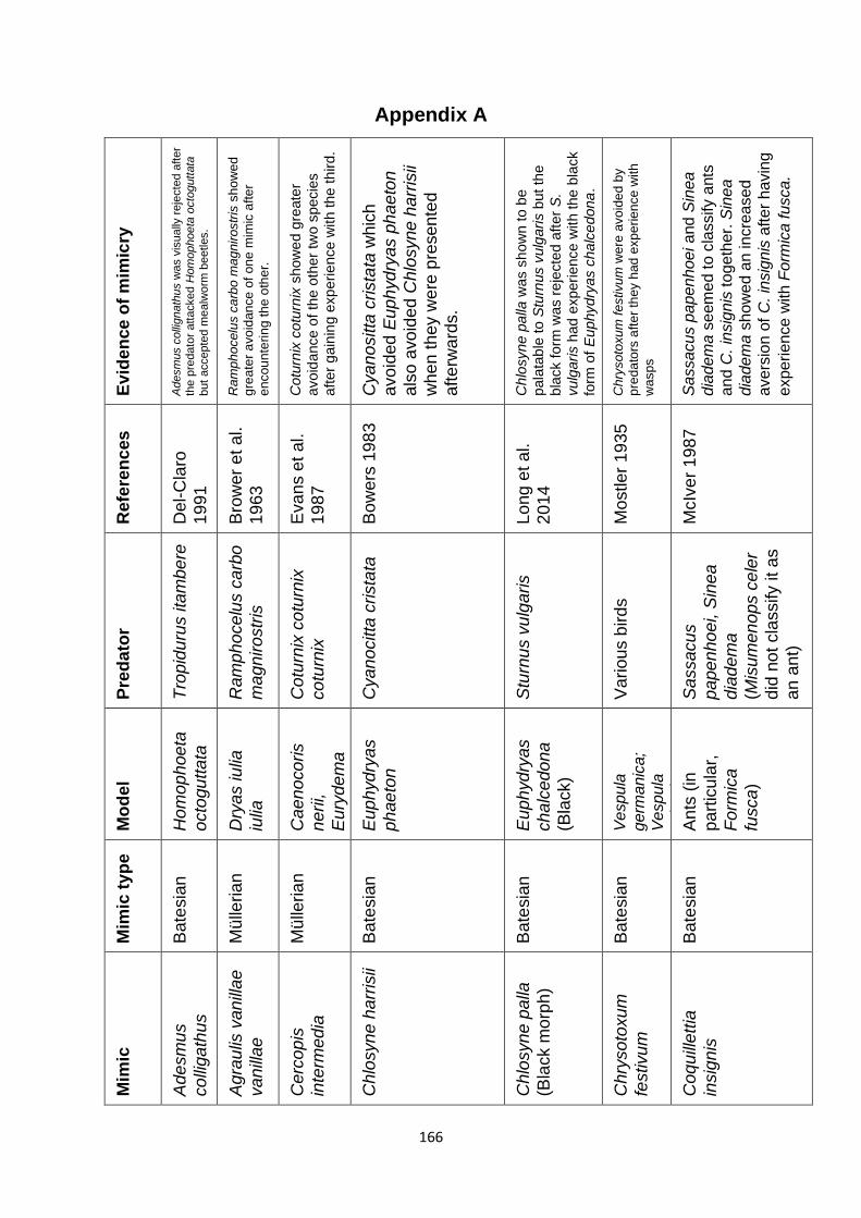
166

Appendix A E

vid

en

ce

of

mim

icry

Adesm

us c

olli

gnath

us w

as v

isually

reje

cte

d a

fter

the p

redato

r attacked H

om

ophoeta

octo

gutt

ata

but

accepte

d m

ealw

orm

beetles.

Ra

mp

ho

celu

s c

arb

o m

ag

nir

ostr

is s

ho

we

d

gre

ate

r a

vo

idan

ce

of o

ne

mim

ic a

fte

r

en

cou

nte

rin

g th

e o

the

r.

Cotu

rnix

cotu

rnix

show

ed g

reate

r

avoid

ance o

f th

e o

ther

two s

pecie

s

after

gain

ing e

xp

erie

nce w

ith the

th

ird.

Cyan

ositta

crista

ta w

hic

h

avo

ided

Eu

ph

yd

ryas p

ha

eto

n

als

o a

vo

ide

d C

hlo

syne h

arr

isii

whe

n th

ey w

ere

pre

sen

ted

aft

erw

ard

s.

Chlo

syne

pa

lla w

as s

how

n t

o b

e

pala

tab

le t

o S

turn

us v

ulg

ari

s b

ut th

e

bla

ck form

was r

eje

cte

d a

fter

S.

vulg

ari

s h

ad

experi

ence w

ith the

bla

ck

form

of

Eu

phydry

as c

ha

lce

dona

.

Ch

rysoto

xu

m f

estivu

m w

ere

avo

ide

d b

y

pre

da

tors

aft

er

they h

ad

exp

erie

nce w

ith

wa

sp

s

Sa

ssacu

s p

ap

en

ho

ei a

nd

Sin

ea

dia

de

ma

se

em

ed to

cla

ssify a

nts

and C

. in

sig

nis

to

ge

ther.

Sin

ea

dia

de

ma

sh

ow

ed a

n in

cre

ase

d

avers

ion o

f C

. in

sig

nis

afte

r h

avin

g

expe

rien

ce w

ith F

orm

ica

fu

sca.

Refe

ren

ces

Del-C

laro

19

91

Bro

wer

et a

l.

19

63

Eva

ns e

t a

l.

19

87

Bo

wers

19

83

Lo

ng

et a

l.

20

14

Mo

stle

r 1

935

McIv

er

19

87

Pre

da

tor

Tro

pid

uru

s ita

mb

ere

Ram

ph

oce

lus c

arb

o

ma

gn

iro

str

is

Cotu

rnix

co

turn

ix

co

turn

ix

Cyan

ocitta

crista

ta

Stu

rnu

s v

ulg

aris

Va

rio

us b

ird

s

Sa

ssa

cu

s

pa

pe

nho

ei, S

ine

a

dia

de

ma

(Mis

um

en

op

s c

ele

r

did

no

t cla

ssify it a

s

an

an

t)

Mo

del

Hom

op

hoe

ta

octo

gu

tta

ta

Dry

as iu

lia

iulia

Cae

no

co

ris

ne

rii,

Eu

ryde

ma

de

co

ratu

m

Eu

ph

yd

ryas

ph

ae

ton

Eu

ph

yd

ryas

ch

alc

edo

na

(Bla

ck)

Ve

spu

la

germ

anic

a;

Ve

spu

la

vu

lgaris

An

ts (

in

pa

rtic

ula

r,

Fo

rmic

a

fusca

)

Mim

ic t

yp

e

Ba

tesia

n

Mü

lleria

n

Mü

lleria

n

Ba

tesia

n

Ba

tesia

n

Ba

tesia

n

Ba

tesia

n

Mim

ic

Ad

esm

us

co

lliga

thu

s

Ag

rau

lis v

an

illae

va

nill

ae

Cerc

op

is

inte

rme

dia

Chlo

syn

e h

arr

isii

Chlo

syn

e p

alla

(Bla

ck m

orp

h)

Chry

so

toxu

m

festivu

m

Coq

uill

ett

ia

insig

nis

167

Ev

ide

nce

of

mim

icry

Fis

h w

hic

h lea

rned

to

re

ject

Me

iaca

nth

us

nig

rolin

ea

tus s

ho

we

d s

om

e a

ve

rsio

n t

o

Ecsen

ius g

ravie

ri

Aphelo

com

a c

alif

orn

ica w

as m

ore

hesitant to

att

ack E

nsatin

a e

schscholtzii

xanth

opic

a t

han E

.

e.

ore

gonensis

aft

er

exposure

to T

aricha t

oro

sa.

Pre

dato

rs a

te few

er

Erista

lis a

fter

encounte

rin

g

inta

ct A

pis

me

llife

ra c

om

pare

d to w

hen t

hey

encounte

red s

tin

gle

ss o

nes o

r none a

t all.

Eri

sta

lis t

ena

x w

as a

vo

ide

d b

y p

red

ato

rs

aft

er

the

y h

ad

exp

eri

en

ce

with

ho

neyb

ees

Pre

da

tors

ate

fe

we

r E

rista

lis a

fte

r

en

cou

nte

rin

g in

tact

Ap

is m

elli

fera

co

mp

are

d t

o w

he

n th

ey e

nco

un

tere

d

sting

less o

nes o

r n

on

e a

t a

ll (B

row

er

an

d

Bro

we

r 1

962

; B

row

er

an

d B

row

er

19

65

).

Ra

mp

ho

celu

s c

arb

o m

ag

nir

ostr

is s

ho

we

d

gre

ate

r a

vo

idan

ce

of o

ne

mim

ic a

fte

r

en

cou

nte

rin

g th

e o

the

r.

Ra

mp

ho

celu

s c

arb

o m

ag

nir

ostr

is s

ho

we

d

gre

ate

r a

vo

idan

ce

of o

ne

mim

ic a

fte

r

en

cou

nte

rin

g th

e o

the

r.

Refe

ren

ces

Sp

ring

er

and

Sm

ith

-Va

niz

197

2

Ku

ch

ta e

t a

l.

20

08

Bro

wer

and

Bro

wer

196

5

Mo

stle

r 1

935

Bro

wer

and

Bro

wer

196

2;

Bro

wer

and

Bro

wer

196

5

Bro

wer

et a

l.

19

63

Bro

wer

et a

l.

19

63

Pre

da

tor

Se

ve

ral sp

ecie

s o

f

pre

da

tory

fis

h

Ap

he

loco

ma

ca

lifo

rnic

a

An

olis

ca

rolin

en

sis

;

Bu

fo te

rre

str

is

Mu

scic

ap

a

atr

ica

pill

a

Bu

fo t

err

estr

is (

Bro

wer

and

Bro

wer

19

62

; B

row

er

an

d

Bro

wer

19

65

); A

no

lis

ca

rolin

en

sis

(B

row

er

and

Bro

wer

19

65

)

Ram

ph

oce

lus c

arb

o

ma

gn

iro

str

is

Ram

ph

oce

lus c

arb

o

ma

gn

iro

str

is

Mo

del

Me

iacanth

us

nig

rolin

eatu

s;

Pla

gio

trem

us tow

nsendi

Ta

rich

a t

oro

sa

Ap

is m

elli

fera

Ap

is m

elli

fera

Ap

is m

elli

fera

Helic

on

ius s

ara

tha

ma

r

Helic

on

ius

me

lpo

me

ne

eu

ryade

s

Mim

ic t

yp

e

Ba

tesia

n

Ba

tesia

n

Ba

tesia

n

Ba

tesia

n

Ba

tesia

n

Mü

lleria

n

Mü

lleria

n

Mim

ic

Ecse

niu

s g

ravie

ri

En

sa

tin

a e

sch

sch

oltzii

xa

nth

op

ica

Erista

lis a

gro

rum

Erista

lis t

en

ax

(Re

ferr

ed

to a

s

Erista

lom

ya

ten

ax in M

ostle

r

19

35

)

Erista

lis

vin

eto

rum

Helic

on

ius d

oris

do

ris

Helic

on

ius e

rato

hyd

ara

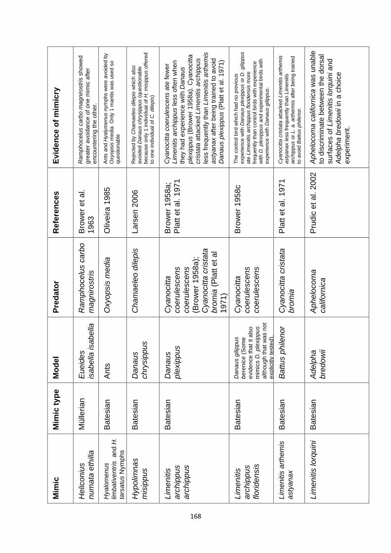
168

Ev

ide

nce

of

mim

icry

Ra

mp

ho

celu

s c

arb

o m

ag

nir

ostr

is s

ho

we

d

gre

ate

r a

vo

idan

ce

of o

ne

mim

ic a

fte

r

en

cou

nte

rin

g th

e o

the

r.

Ants

and H

yaly

me

nus n

ym

phs w

ere

avoid

ed b

y

Oxyopsis

me

dia

. O

nly

1 m

antis w

as u

sed s

o

questio

nable

Reje

cte

d b

y C

ham

aele

o d

ilepis

whic

h a

lso

avoid

ed D

anaus c

hry

sip

pus (

questio

nable

because o

nly

1 in

div

idual of

H. m

isip

pus o

ffere

d

to o

ne in

div

idual of

C.

dile

pis

)

Cyanocitta

coeru

lescens a

te few

er

Lim

en

itis

arc

hip

pus less o

ften w

hen

they h

ad e

xp

erie

nce w

ith D

anaus

ple

xip

pus (

Bro

wer

195

8a).

Cyanocitta

crista

ta a

ttacked L

imenitis

arc

hip

pus

less fre

qu

ently tha

n L

imenitis

art

he

mis

asty

anax a

fter

be

ing tra

ine

d to a

void

Dana

us p

lexip

pus (

Pla

tt e

t al. 1

97

1)

Th

e c

ontr

ol bird w

hic

h h

ad n

o p

revio

us

experie

nce w

ith D

anaus p

lexip

pus o

r D

. gili

ppus

ate

Lim

enitis

arc

hip

pus f

lorid

ensis

mo

re

frequently t

han c

ontr

ol birds w

ith e

xperie

nce

with D

. ple

xip

pus a

nd e

xperim

enta

l birds w

ith

experie

nce w

ith D

anaus g

ilip

pus.

Cyanocitta

crista

ta a

ttacked L

imenitis

art

hem

is

asty

anax le

ss f

requently than L

imenitis

arc

hip

pus o

r L.

a.

art

herm

is a

fter

bein

g t

rain

ed

to a

void

Batt

us p

hile

nor.

Ap

he

locom

a c

alif

orn

ica w

as u

na

ble

to d

iscrim

inate

betw

een

th

e d

ors

al

su

rfa

ces o

f L

ime

nitis

lo

rqu

ini and

Ad

elp

ha

bre

do

wii

in a

cho

ice

expe

rim

ent.

Refe

ren

ces

Bro

wer

et a

l.

19

63

Oliv

eira

19

85

La

rse

n 2

00

6

Bro

wer

195

8a;

Pla

tt e

t a

l. 1

97

1

Bro

wer

195

8c

Pla

tt e

t a

l. 1

97

1

Pru

dic

et a

l. 2

002

Pre

da

tor

Ram

ph

oce

lus c

arb

o

ma

gn

iro

str

is

Oxyo

psis

me

dia

Cha

ma

ele

o d

ilep

is

Cyan

ocitta

co

eru

lescen

s

co

eru

lescen

s

(Bro

we

r 1

958

a);

Cyan

ocitta

crista

ta

bro

mia

(P

latt

et a

l

19

71

)

Cyan

ocitta

co

eru

lescen

s

co

eru

lescen

s

Cyan

ocitta

crista

ta

bro

mia

Ap

he

loco

ma

ca

lifo

rnic

a

Mo

del

Eu

eid

es

isab

ella

isab

ella

An

ts

Dan

au

s

ch

rysip

pu

s

Dan

au

s

ple

xip

pu

s

Dan

au

s g

ilip

pu

s

be

ren

ice

(S

om

e

evid

en

ce

tha

t it a

lso

mim

ics D

. ple

xip

pu

s

alth

ou

gh

th

at

wa

s n

ot

exp

licitly

teste

d).

Ba

ttu

s p

hile

no

r

Ad

elp

ha

bre

do

wii

Mim

ic t

yp

e

Mü

lleria

n

Ba

tesia

n

Ba

tesia

n

Ba

tesia

n

Ba

tesia

n

Ba

tesia

n

Ba

tesia

n

Mim

ic

Helic

on

ius

nu

ma

ta e

thill

a

Hyalo

men

us

limbativentr

is

an

d H

.

tars

atu

s N

ym

phs

Hypo

limn

as

mis

ipp

us

Lim

en

itis

arc

hip

pu

s

arc

hip

pu

s

Lim

en

itis

arc

hip

pu

s

flo

rid

en

sis

Lim

enitis

art

hem

is

asty

an

ax

Lim

en

itis

lorq

uin

i

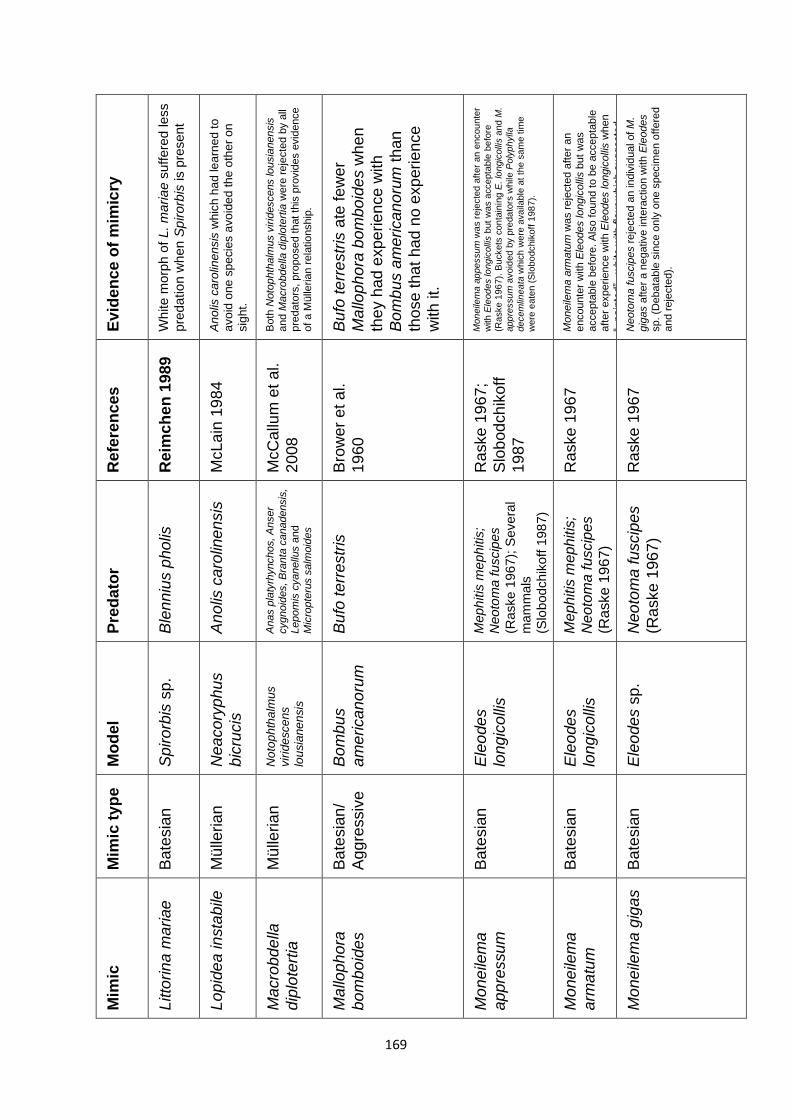
169

Ev

ide

nce

of

mim

icry

Wh

ite m

orp

h o

f L. m

aria

e s

uffere

d less

pre

datio

n w

hen S

pirorb

is is p

resent

An

olis

ca

rolin

ensis

wh

ich

ha

d le

arn

ed t

o

avo

id o

ne

sp

ecie

s a

vo

ide

d th

e o

the

r o

n

sig

ht.

Both

Noto

phth

alm

us v

irid

escens lousia

nensis

and M

acro

bdella

dip

lote

rtia

were

reje

cte

d b

y a

ll pre

dato

rs,

pro

posed t

hat

this

pro

vid

es e

vid

ence

of

a M

ülle

ria

n r

ela

tio

nship

.

Bu

fo te

rre

str

is a

te fe

wer

Ma

llop

ho

ra b

om

bo

ide

s w

he

n

the

y h

ad e

xpe

rie

nce w

ith

Bo

mb

us a

me

rica

no

rum

th

an

tho

se t

ha

t ha

d n

o e

xp

erie

nce

with

it.

Mon

eile

ma

ap

pessu

m w

as r

eje

cte

d a

fter

an e

ncou

nte

r

with E

leod

es lo

ngic

olli

s b

ut

was a

ccepta

ble

be

fore

(R

aske 1

96

7).

Buckets

con

tain

ing

E. lo

ngic

olli

s a

nd M

.

app

ressu

m a

void

ed b

y p

reda

tors

while

Poly

ph

ylla

decem

linea

ta w

hic

h w

ere

availa

ble

at

the s

am

e tim

e

were

eate

n (

Slo

bo

dchik

off

198

7).

Mo

neile

ma

arm

atu

m w

as r

eje

cte

d a

fter

an

encounte

r w

ith E

leodes lo

ngic

olli

s b

ut

was

accepta

ble

befo

re. A

lso f

ound to b

e a

ccepta

ble

aft

er

experie

nce w

ith E

leodes lo

ngic

olli

s w

hen

“pain

ted”

white w

ith flo

ur

whic

h s

uggeste

d

reje

ctio

n w

as d

ue t

o v

isual m

imic

ry.

Neoto

ma

fuscip

es r

eje

cte

d a

n in

div

idual of

M.

gig

as a

fter

a n

egative inte

ractio

n w

ith E

leodes

sp. (D

ebata

ble

sin

ce o

nly

one s

pecim

en o

ffere

d

and r

eje

cte

d).

Refe

ren

ces

Reim

ch

en

19

89

McL

ain

19

84

McC

allu

m e

t a

l.

20

08

Bro

wer

et a

l.

19

60

Raske

19

67

;

Slo

bod

ch

ikoff

19

87

Raske

19

67

Raske

19

67

Pre

da

tor

Ble

nn

ius p

ho

lis

An

olis

ca

rolin

en

sis

Anas p

laty

rhynchos, A

nser

cygnoid

es, B

ranta

canadensis

, Lepom

is c

yanellu

s a

nd

Mic

ropte

rus s

alm

oid

es

Bu

fo te

rre

str

is

Meph

itis

me

phitis

;

Neoto

ma f

uscip

es

(Raske 1

96

7);

Severa

l

mam

mals

(Slo

bodch

ikoff 1

98

7)

Me

ph

itis

me

ph

itis

;

Ne

oto

ma f

uscip

es

(Ra

ske

19

67)

Neo

tom

a fu

scip

es

(Ra

ske

196

7)

Mo

del

Sp

iro

rbis

sp

.

Nea

co

ryphu

s

bic

rucis

Noto

ph

tha

lmus

vir

ide

sce

ns

lou

sia

ne

nsis

Bo

mb

us

am

erica

no

rum

Ele

ode

s

lon

gic

olli

s

Ele

ode

s

lon

gic

olli

s

Ele

ode

s s

p.

Mim

ic t

yp

e

Ba

tesia

n

Mü

lleria

n

Mü

lleria

n

Ba

tesia

n/

Ag

gre

ssiv

e

Ba

tesia

n

Ba

tesia

n

Ba

tesia

n

Mim

ic

Litto

rin

a m

ariae

Lo

pid

ea

in

sta

bile

Ma

cro

bd

ella

dip

lote

rtia

Ma

llop

ho

ra

bo

mb

oid

es

Mo

ne

ilem

a

ap

pre

ssu

m

Mo

ne

ilem

a

arm

atu

m

Mo

ne

ilem

a g

iga

s

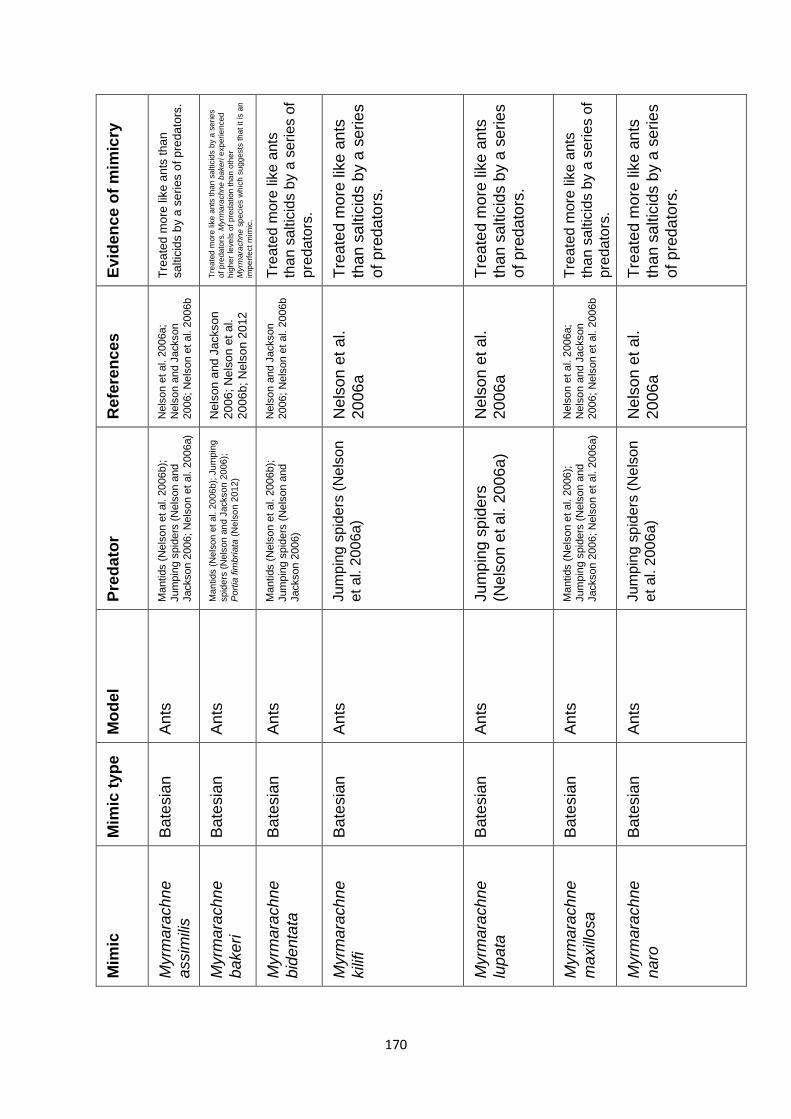
170

Ev

ide

nce

of

mim

icry

Tre

ate

d m

ore

lik

e a

nts

tha

n

sa

ltic

ids b

y a

se

ries o

f p

reda

tors

.

Tre

ate

d m

ore

lik

e a

nts

th

an

sa

ltic

ids b

y a

serie

s

of

pre

da

tors

. M

yrm

ara

chn

e b

akeri

exp

eri

en

ced

hig

he

r le

ve

ls o

f p

red

atio

n th

an

oth

er

Myrm

ara

ch

ne

sp

ecie

s w

hic

h s

ug

ge

sts

th

at

it is a

n

imp

erf

ect m

imic

.

Tre

ate

d m

ore

lik

e a

nts

than

sa

ltic

ids b

y a

se

ries o

f

pre

da

tors

.

Tre

ate

d m

ore

lik

e a

nts

tha

n s

altic

ids b

y a

se

rie

s

of

pre

da

tors

.

Tre

ate

d m

ore

lik

e a

nts

tha

n s

altic

ids b

y a

se

rie

s

of

pre

da

tors

.

Tre

ate

d m

ore

lik

e a

nts

than

sa

ltic

ids b

y a

se

ries o

f

pre

da

tors

.

Tre

ate

d m

ore

lik

e a

nts

tha

n s

altic

ids b

y a

se

rie

s

of

pre

da

tors

.

Refe

ren

ces

Nels

on e

t al. 2

006a;

Nels

on a

nd J

ackson

2006;

Nels

on e

t al. 2

006b

Ne

lson

and

Jackson

20

06

; N

els

on

et

al.

20

06

b;

Ne

lso

n 2

012

Nels

on a

nd J

ackson

2006;

Nels

on e

t al. 2

006b

Nels

on

et

al.

20

06

a

Nels

on

et

al.

20

06

a

Nels

on e

t al. 2

006a;

Nels

on a

nd J

ackson

2006;

Nels

on e

t al. 2

006b

Nels

on

et

al.

20

06

a

Pre

da

tor

Ma

ntids (

Nels

on e

t al. 2

006b);

Jum

pin

g s

pid

ers

(N

els

on a

nd

Jackson 2

006; N

els

on e

t al. 2

006a)

Man

tids (

Nels

on

et

al. 2

006

b);

Ju

mpin

g

spid

ers

(N

els

on a

nd J

ackson 2

006);

Port

ia fim

bri

ata

(N

els

on 2

01

2)

Ma

ntids (

Nels

on e

t al. 2

006b);

Jum

pin

g s

pid

ers

(N

els

on a

nd

Jackson 2

006)

Ju

mp

ing s

pid

ers

(N

els

on

et

al. 2

00

6a

)

Ju

mp

ing

sp

ide

rs

(Ne

lson

et a

l. 2

006

a)

Mantids (

Nels

on e

t al. 2

006);

Jum

pin

g s

pid

ers

(N

els

on a

nd

Jackson 2

006; N

els

on e

t al. 2

006a)

Ju

mp

ing

sp

iders

(N

els

on

et

al. 2

00

6a

)

Mo

del

An

ts

An

ts

An

ts

An

ts

An

ts

An

ts

An

ts

Mim

ic t

yp

e

Ba

tesia

n

Ba

tesia

n

Ba

tesia

n

Ba

tesia

n

Ba

tesia

n

Ba

tesia

n

Ba

tesia

n

Mim

ic

Myrm

ara

ch

ne

assim

ilis

Myrm

ara

ch

ne

ba

ke

ri

Myrm

ara

ch

ne

bid

enta

ta

Myrm

ara

ch

ne

kili

fi

Myrm

ara

ch

ne

lup

ata

Myrm

ara

ch

ne

ma

xill

osa

Myrm

ara

ch

ne

na

ro

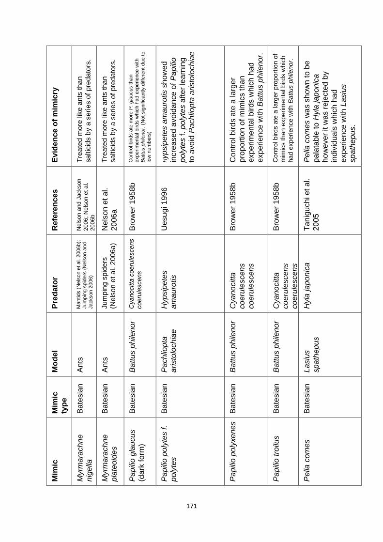
171

Ev

ide

nce

of

mim

icry

Tre

ate

d m

ore

lik

e a

nts

tha

n

sa

ltic

ids b

y a

se

ries o

f p

reda

tors

.

Tre

ate

d m

ore

lik

e a

nts

tha

n

sa

ltic

ids b

y a

se

ries o

f p

reda

tors

.

Contr

ol birds a

te m

ore

P.

gla

ucus than

experim

enta

l birds w

hic

h h

ad e

xperie

nce w

ith

Batt

us p

hile

nor.

(N

ot sig

nific

antly d

iffe

rent due t

o

low

num

bers

)

Hyp

sip

ete

s a

ma

uro

tis s

ho

wed

incre

ase

d a

vo

ida

nce

of

Pa

pili

o

po

lyte

s f.

po

lyte

s a

fte

r le

arn

ing

to a

vo

id P

ach

liopta

aristo

loch

iae

Con

tro

l b

ird

s a

te a

la

rge

r

pro

po

rtio

n o

f m

imic

s th

an

exp

erim

en

tal b

ird

s w

hic

h h

ad

exp

erie

nce

with

Ba

ttu

s p

hile

no

r.

Contr

ol b

irds a

te a

larg

er

pro

port

ion o

f

mim

ics tha

n e

xperi

me

nta

l b

irds w

hic

h

had e

xperi

ence w

ith B

attus p

hile

nor.

Pe

lla c

om

es w

as s

ho

wn t

o b

e

pa

lata

ble

to

Hyla

jap

onic

a

ho

weve

r it w

as r

eje

cte

d b

y

ind

ivid

ua

ls w

hic

h h

ad

exp

erie

nce

with

La

siu

s

sp

ath

ep

us.

Refe

ren

ces

Nels

on

and

Jackson

20

06

; N

els

on

et

al.

20

06

b

Nels

on

et

al.

20

06

a

Bro

we

r 1

95

8b

Uesu

gi 19

96

Bro

we

r 1

95

8b

Bro

we

r 1

95

8b

Ta

nig

uch

i e

t a

l.

20

05

Pre

da

tor

Ma

ntids (

Nels

on e

t al. 2

006b);

Jum

pin

g s

pid

ers

(N

els

on a

nd

Jackson 2

006)

Ju

mp

ing s

pid

ers

(Ne

lso

n e

t a

l. 2

00

6a

)

Cyanocitta

coeru

lescens

coeru

lescens

Hypsip

ete

s

am

au

rotis

Cyan

ocitta

co

eru

lescen

s

co

eru

lescen

s

Cyan

ocitta

co

eru

lescen

s

co

eru

lescen

s

Hyla

jap

on

ica

Mo

del

An

ts

An

ts

Ba

ttu

s p

hile

no

r

Pa

ch

liopta

aristo

loch

iae

Ba

ttu

s p

hile

no

r

Ba

ttu

s p

hile

no

r

La

siu

s

sp

ath

ep

us

Mim

ic

typ

e

Ba

tesia

n

Ba

tesia

n

Ba

tesia

n

Ba

tesia

n

Ba

tesia

n

Ba

tesia

n

Ba

tesia

n

Mim

ic

Myrm

ara

ch

ne

nig

ella

Myrm

ara

ch

ne

pla

teo

ide

s

Pa

pili

o g

lau

cu

s

(da

rk fo

rm)

Pa

pili

o p

oly

tes f.

po

lyte

s

Pa

pili

o p

oly

xene

s

Pa

pili

o t

roilu

s

Pe

lla c

om

es

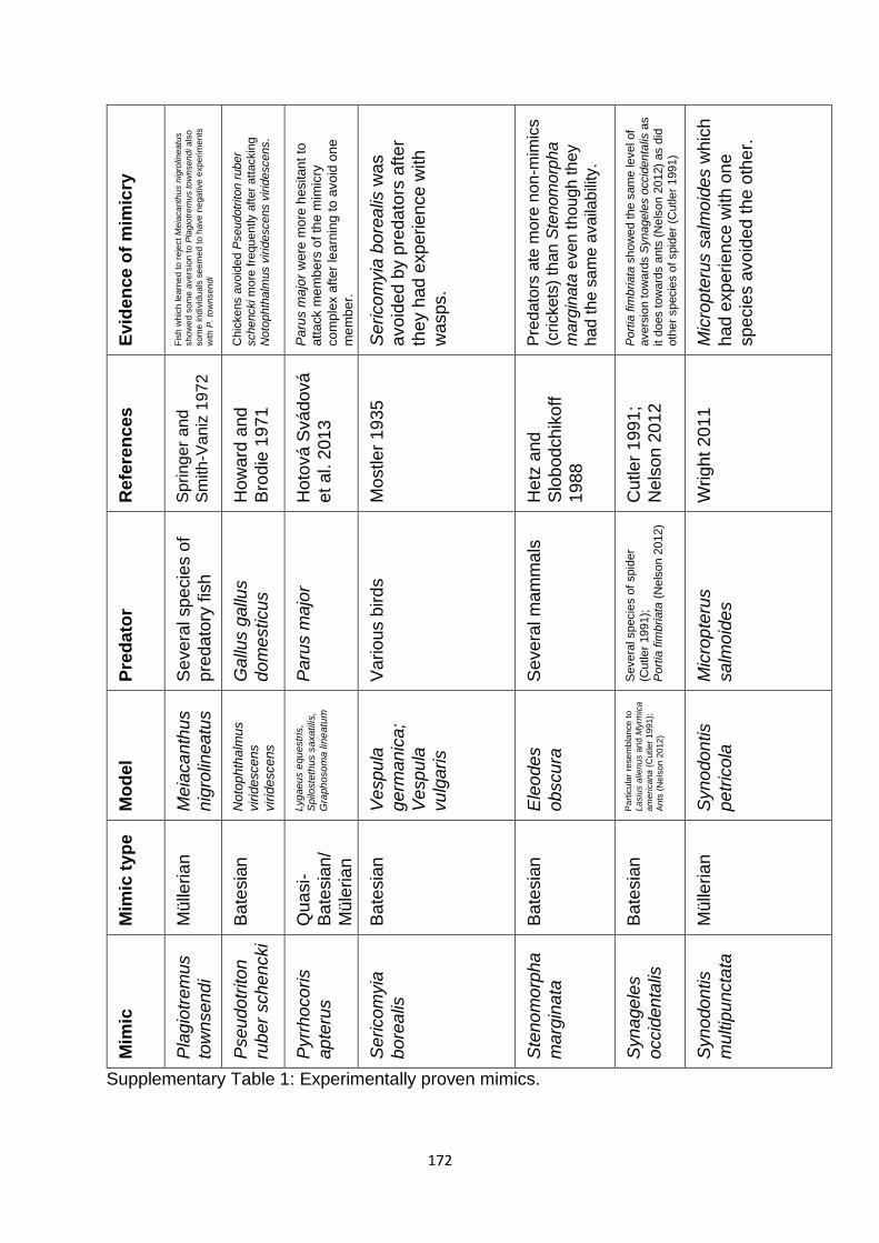
172

Ev

ide

nce

of

mim

icry

Fis

h w

hic

h le

arn

ed

to

re

ject M

eia

ca

nth

us n

igro

line

atu

s

sh

ow

ed

so

me a

ve

rsio

n t

o P

lag

iotr

em

us to

wnse

nd

i a

lso

so

me

in

div

idu

als

se

em

ed

to

ha

ve

ne

ga

tive

exp

eri

me

nts

with

P.

tow

nse

nd

i

Chic

kens a

void

ed P

seudotr

iton r

uber

schencki m

ore

fre

quently a

fter

att

ackin

g

Noto

phth

alm

us v

irid

escens v

irid

escens.

Pa

rus m

ajo

r w

ere

mo

re h

esitan

t to

att

ack m

em

be

rs o

f th

e m

imic

ry

co

mp

lex a

fte

r le

arn

ing

to

avo

id o

ne

me

mb

er.

Se

rico

myia

bo

rea

lis w

as

avo

ided

by p

reda

tors

aft

er

the

y h

ad e

xpe

rie

nce w

ith

wasp

s.

Pre

da

tors

ate

mo

re n

on

-mim

ics

(crickets

) th

an S

tenom

orp

ha

ma

rgin

ata

even t

hou

gh th

ey

had

th

e s

am

e a

vaila

bili

ty.

Port

ia fim

briata

show

ed t

he s

am

e level of

avers

ion tow

ard

s S

ynagele

s o

ccid

enta

lis a

s

it d

oes tow

ard

s a

nts

(N

els

on 2

012)

as d

id

oth

er

specie

s o

f spid

er

(Cutle

r 1991)

Mic

rop

teru

s s

alm

oid

es w

hic

h

ha

d e

xp

erien

ce

with o

ne

sp

ecie

s a

vo

ided

th

e o

the

r.

Re

fere

nc

es

Sp

ring

er

and

Sm

ith

-Va

niz

197

2

Ho

wa

rd a

nd

Bro

die

19

71

Ho

tová

Svá

do

vá

et

al. 2

01

3

Mo

stle

r 1

935

He

tz a

nd

Slo

bod

ch

ikoff

19

88

Cu

tler

199

1;

Ne

lso

n 2

01

2

Wrig

ht

20

11

Pre

da

tor

Se

ve

ral sp

ecie

s o

f

pre

da

tory

fis

h

Ga

llus g

allu

s

do

me

sticu

s

Pa

rus m

ajo

r

Va

rio

us b

ird

s

Se

ve

ral m

am

ma

ls

Severa

l specie

s o

f spid

er

(Cutle

r 1991);

P

ort

ia fim

briata

(N

els

on 2

012)

Mic

rop

teru

s

sa

lmo

ide

s

Mo

del

Me

iaca

nth

us

nig

rolin

eatu

s

Noto

ph

tha

lmus

vir

ide

sce

ns

vir

ide

sce

ns

Lyg

aeu

s e

qu

estr

is,

Spilo

ste

thus s

axatilis

,

Gra

ph

oso

ma lin

eatu

m

Ve

sp

ula

ge

rma

nic

a;

Ve

sp

ula

vu

lga

ris

Ele

ode

s

ob

scu

ra

Pa

rtic

ula

r re

se

mb

lan

ce

to

La

siu

s a

lien

us a

nd

Myrm

ica

am

eri

cana

(C

utler

19

91);

An

ts (

Nels

on

20

12

)

Syn

odo

ntis

pe

tric

ola

Mim

ic t

yp

e

Mü

lleria

n

Ba

tesia

n

Qu

asi-

Ba

tesia

n/

Mü

leria

n

Ba

tesia

n

Ba

tesia

n

Ba

tesia

n

Mü

lleria

n

Mim

ic

Pla

gio

trem

us

tow

nsen

di

Pse

udo

trito

n

rub

er

sche

ncki

Pyrr

ho

co

ris

ap

teru

s

Se

rico

myia

bo

rea

lis

Ste

no

mo

rpha

ma

rgin

ata

Syn

age

les

occid

enta

lis

Syn

odo

ntis

mu

ltip

un

cta

ta

Supplementary Table 1: Experimentally proven mimics.

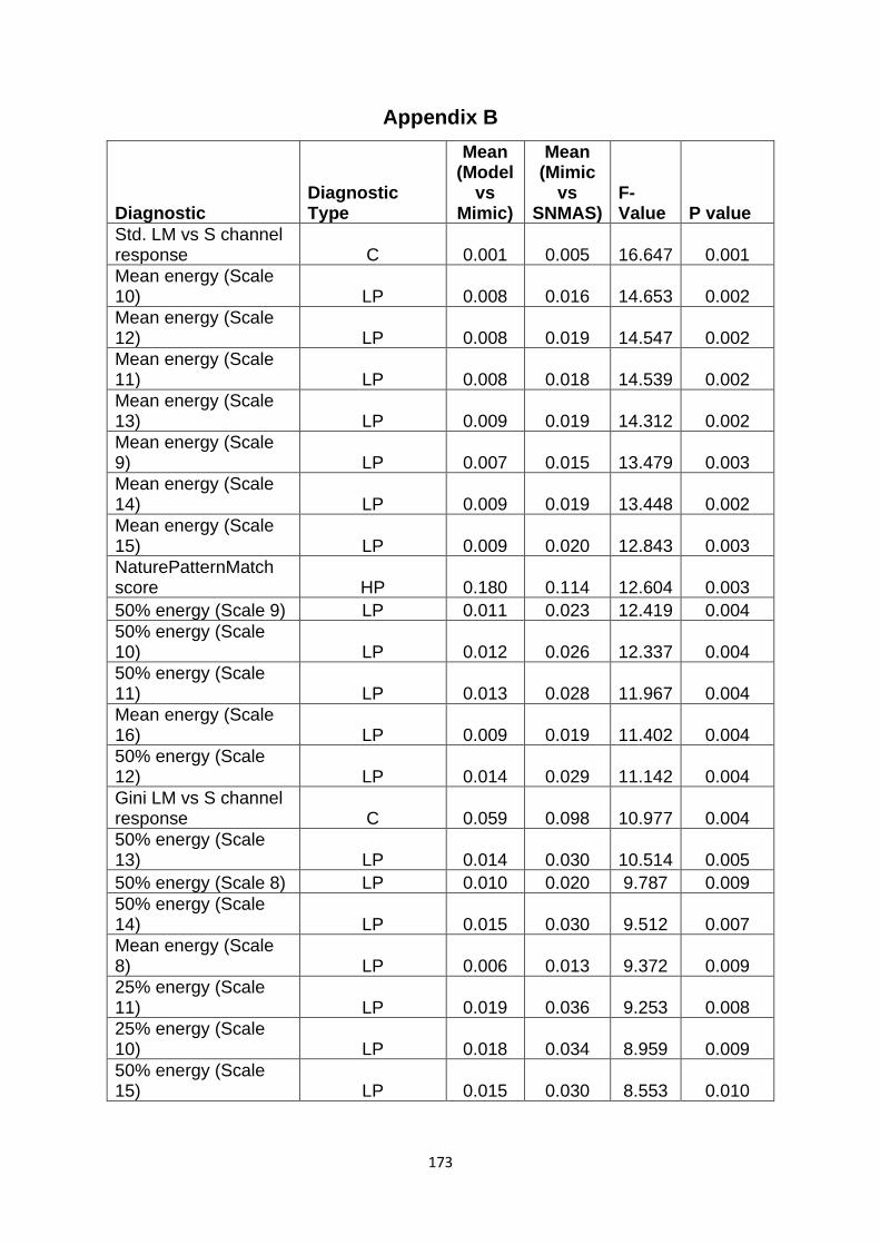
173

Appendix B

Diagnostic Diagnostic Type

Mean (Model

vs Mimic)

Mean (Mimic

vs SNMAS)

F-Value P value

Std. LM vs S channel response C 0.001 0.005 16.647 0.001

Mean energy (Scale 10) LP 0.008 0.016 14.653 0.002

Mean energy (Scale 12) LP 0.008 0.019 14.547 0.002

Mean energy (Scale 11) LP 0.008 0.018 14.539 0.002

Mean energy (Scale 13) LP 0.009 0.019 14.312 0.002

Mean energy (Scale 9) LP 0.007 0.015 13.479 0.003

Mean energy (Scale 14) LP 0.009 0.019 13.448 0.002

Mean energy (Scale 15) LP 0.009 0.020 12.843 0.003

NaturePatternMatch score HP 0.180 0.114 12.604 0.003

50% energy (Scale 9) LP 0.011 0.023 12.419 0.004

50% energy (Scale 10) LP 0.012 0.026 12.337 0.004

50% energy (Scale 11) LP 0.013 0.028 11.967 0.004

Mean energy (Scale 16) LP 0.009 0.019 11.402 0.004

50% energy (Scale 12) LP 0.014 0.029 11.142 0.004

Gini LM vs S channel response C 0.059 0.098 10.977 0.004

50% energy (Scale 13) LP 0.014 0.030 10.514 0.005

50% energy (Scale 8) LP 0.010 0.020 9.787 0.009

50% energy (Scale 14) LP 0.015 0.030 9.512 0.007

Mean energy (Scale 8) LP 0.006 0.013 9.372 0.009

25% energy (Scale 11) LP 0.019 0.036 9.253 0.008

25% energy (Scale 10) LP 0.018 0.034 8.959 0.009

50% energy (Scale 15) LP 0.015 0.030 8.553 0.010

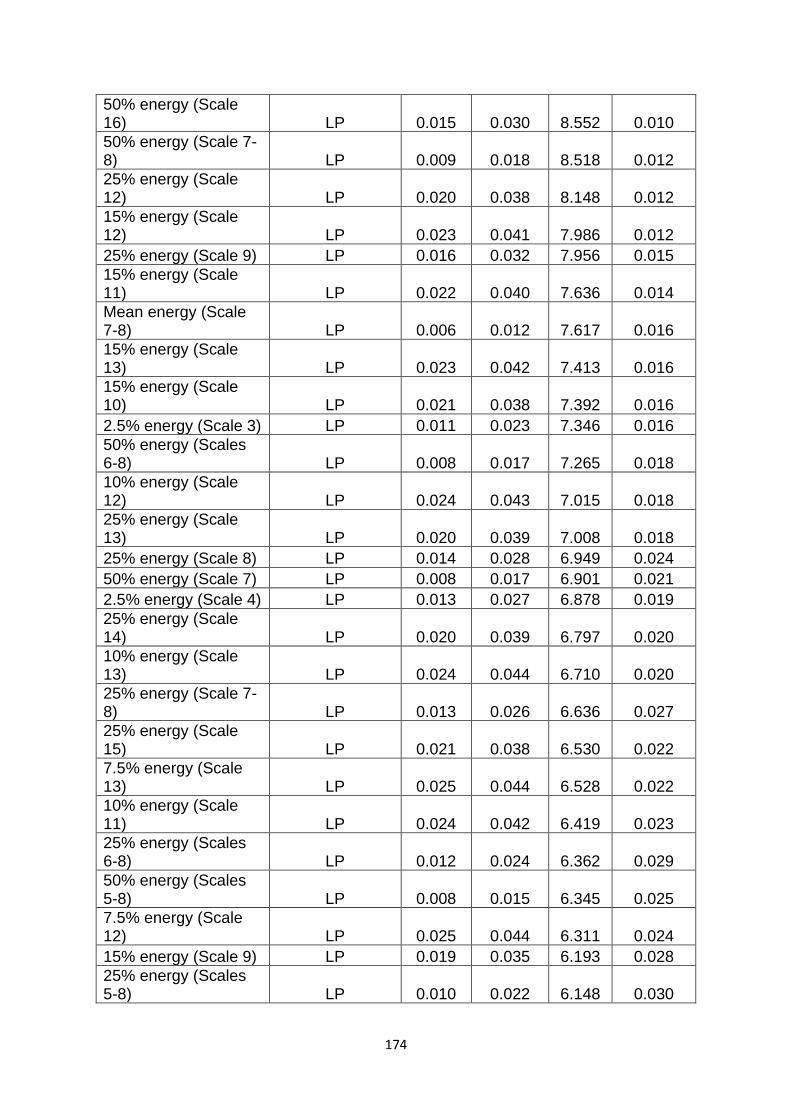
174

50% energy (Scale 16) LP 0.015 0.030 8.552 0.010

50% energy (Scale 7-8) LP 0.009 0.018 8.518 0.012

25% energy (Scale 12) LP 0.020 0.038 8.148 0.012

15% energy (Scale 12) LP 0.023 0.041 7.986 0.012

25% energy (Scale 9) LP 0.016 0.032 7.956 0.015

15% energy (Scale 11) LP 0.022 0.040 7.636 0.014

Mean energy (Scale 7-8) LP 0.006 0.012 7.617 0.016

15% energy (Scale 13) LP 0.023 0.042 7.413 0.016

15% energy (Scale 10) LP 0.021 0.038 7.392 0.016

2.5% energy (Scale 3) LP 0.011 0.023 7.346 0.016

50% energy (Scales 6-8) LP 0.008 0.017 7.265 0.018

10% energy (Scale 12) LP 0.024 0.043 7.015 0.018

25% energy (Scale 13) LP 0.020 0.039 7.008 0.018

25% energy (Scale 8) LP 0.014 0.028 6.949 0.024

50% energy (Scale 7) LP 0.008 0.017 6.901 0.021

2.5% energy (Scale 4) LP 0.013 0.027 6.878 0.019

25% energy (Scale 14) LP 0.020 0.039 6.797 0.020

10% energy (Scale 13) LP 0.024 0.044 6.710 0.020

25% energy (Scale 7-8) LP 0.013 0.026 6.636 0.027

25% energy (Scale 15) LP 0.021 0.038 6.530 0.022

7.5% energy (Scale 13) LP 0.025 0.044 6.528 0.022

10% energy (Scale 11) LP 0.024 0.042 6.419 0.023

25% energy (Scales 6-8) LP 0.012 0.024 6.362 0.029

50% energy (Scales 5-8) LP 0.008 0.015 6.345 0.025

7.5% energy (Scale 12) LP 0.025 0.044 6.311 0.024

15% energy (Scale 9) LP 0.019 0.035 6.193 0.028

25% energy (Scales 5-8) LP 0.010 0.022 6.148 0.030

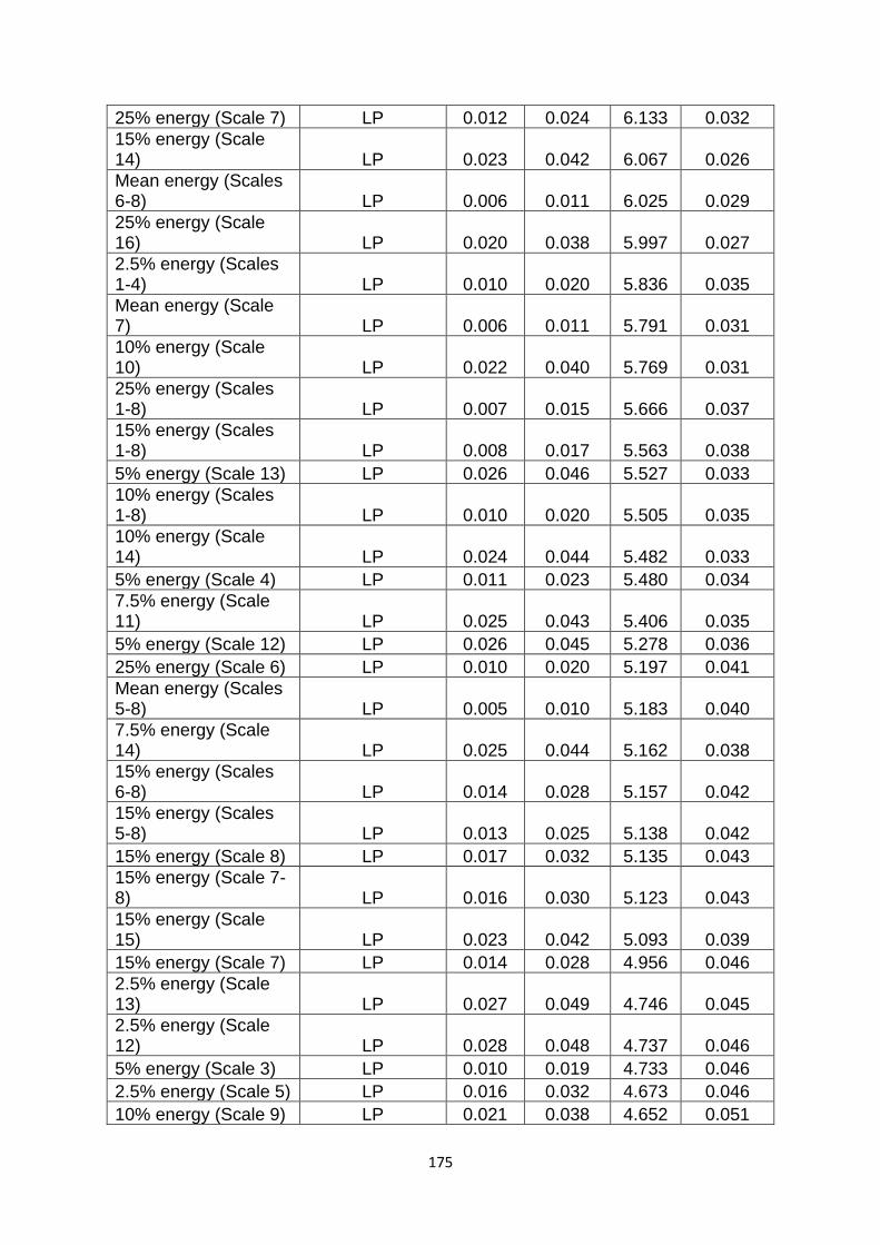
175

25% energy (Scale 7) LP 0.012 0.024 6.133 0.032

15% energy (Scale 14) LP 0.023 0.042 6.067 0.026

Mean energy (Scales 6-8) LP 0.006 0.011 6.025 0.029

25% energy (Scale 16) LP 0.020 0.038 5.997 0.027

2.5% energy (Scales 1-4) LP 0.010 0.020 5.836 0.035

Mean energy (Scale 7) LP 0.006 0.011 5.791 0.031

10% energy (Scale 10) LP 0.022 0.040 5.769 0.031

25% energy (Scales 1-8) LP 0.007 0.015 5.666 0.037

15% energy (Scales 1-8) LP 0.008 0.017 5.563 0.038

5% energy (Scale 13) LP 0.026 0.046 5.527 0.033

10% energy (Scales 1-8) LP 0.010 0.020 5.505 0.035

10% energy (Scale 14) LP 0.024 0.044 5.482 0.033

5% energy (Scale 4) LP 0.011 0.023 5.480 0.034

7.5% energy (Scale 11) LP 0.025 0.043 5.406 0.035

5% energy (Scale 12) LP 0.026 0.045 5.278 0.036

25% energy (Scale 6) LP 0.010 0.020 5.197 0.041

Mean energy (Scales 5-8) LP 0.005 0.010 5.183 0.040

7.5% energy (Scale 14) LP 0.025 0.044 5.162 0.038

15% energy (Scales 6-8) LP 0.014 0.028 5.157 0.042

15% energy (Scales 5-8) LP 0.013 0.025 5.138 0.042

15% energy (Scale 8) LP 0.017 0.032 5.135 0.043

15% energy (Scale 7-8) LP 0.016 0.030 5.123 0.043

15% energy (Scale 15) LP 0.023 0.042 5.093 0.039

15% energy (Scale 7) LP 0.014 0.028 4.956 0.046

2.5% energy (Scale 13) LP 0.027 0.049 4.746 0.045

2.5% energy (Scale 12) LP 0.028 0.048 4.737 0.046

5% energy (Scale 3) LP 0.010 0.019 4.733 0.046

2.5% energy (Scale 5) LP 0.016 0.032 4.673 0.046

10% energy (Scale 9) LP 0.021 0.038 4.652 0.051

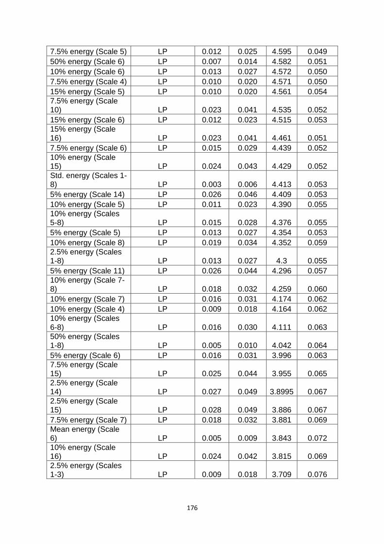
176

7.5% energy (Scale 5) LP 0.012 0.025 4.595 0.049

50% energy (Scale 6) LP 0.007 0.014 4.582 0.051

10% energy (Scale 6) LP 0.013 0.027 4.572 0.050

7.5% energy (Scale 4) LP 0.010 0.020 4.571 0.050

15% energy (Scale 5) LP 0.010 0.020 4.561 0.054

7.5% energy (Scale 10) LP 0.023 0.041 4.535 0.052

15% energy (Scale 6) LP 0.012 0.023 4.515 0.053

15% energy (Scale 16) LP 0.023 0.041 4.461 0.051

7.5% energy (Scale 6) LP 0.015 0.029 4.439 0.052

10% energy (Scale 15) LP 0.024 0.043 4.429 0.052

Std. energy (Scales 1-8) LP 0.003 0.006 4.413 0.053

5% energy (Scale 14) LP 0.026 0.046 4.409 0.053

10% energy (Scale 5) LP 0.011 0.023 4.390 0.055

10% energy (Scales 5-8) LP 0.015 0.028 4.376 0.055

5% energy (Scale 5) LP 0.013 0.027 4.354 0.053

10% energy (Scale 8) LP 0.019 0.034 4.352 0.059

2.5% energy (Scales 1-8) LP 0.013 0.027 4.3 0.055

5% energy (Scale 11) LP 0.026 0.044 4.296 0.057

10% energy (Scale 7-8) LP 0.018 0.032 4.259 0.060

10% energy (Scale 7) LP 0.016 0.031 4.174 0.062

10% energy (Scale 4) LP 0.009 0.018 4.164 0.062

10% energy (Scales 6-8) LP 0.016 0.030 4.111 0.063

50% energy (Scales 1-8) LP 0.005 0.010 4.042 0.064

5% energy (Scale 6) LP 0.016 0.031 3.996 0.063

7.5% energy (Scale 15) LP 0.025 0.044 3.955 0.065

2.5% energy (Scale 14) LP 0.027 0.049 3.8995 0.067

2.5% energy (Scale 15) LP 0.028 0.049 3.886 0.067

7.5% energy (Scale 7) LP 0.018 0.032 3.881 0.069

Mean energy (Scale 6) LP 0.005 0.009 3.843 0.072

10% energy (Scale 16) LP 0.024 0.042 3.815 0.069

2.5% energy (Scales 1-3) LP 0.009 0.018 3.709 0.076

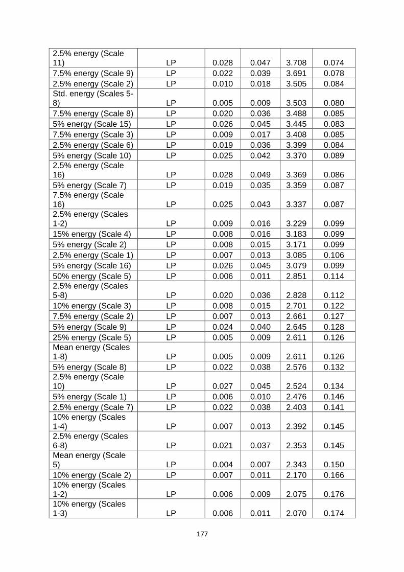
177

2.5% energy (Scale 11) LP 0.028 0.047 3.708 0.074

7.5% energy (Scale 9) LP 0.022 0.039 3.691 0.078

2.5% energy (Scale 2) LP 0.010 0.018 3.505 0.084

Std. energy (Scales 5-8) LP 0.005 0.009 3.503 0.080

7.5% energy (Scale 8) LP 0.020 0.036 3.488 0.085

5% energy (Scale 15) LP 0.026 0.045 3.445 0.083

7.5% energy (Scale 3) LP 0.009 0.017 3.408 0.085

2.5% energy (Scale 6) LP 0.019 0.036 3.399 0.084

5% energy (Scale 10) LP 0.025 0.042 3.370 0.089

2.5% energy (Scale 16) LP 0.028 0.049 3.369 0.086

5% energy (Scale 7) LP 0.019 0.035 3.359 0.087

7.5% energy (Scale 16) LP 0.025 0.043 3.337 0.087

2.5% energy (Scales 1-2) LP 0.009 0.016 3.229 0.099

15% energy (Scale 4) LP 0.008 0.016 3.183 0.099

5% energy (Scale 2) LP 0.008 0.015 3.171 0.099

2.5% energy (Scale 1) LP 0.007 0.013 3.085 0.106

5% energy (Scale 16) LP 0.026 0.045 3.079 0.099

50% energy (Scale 5) LP 0.006 0.011 2.851 0.114

2.5% energy (Scales 5-8) LP 0.020 0.036 2.828 0.112

10% energy (Scale 3) LP 0.008 0.015 2.701 0.122

7.5% energy (Scale 2) LP 0.007 0.013 2.661 0.127

5% energy (Scale 9) LP 0.024 0.040 2.645 0.128

25% energy (Scale 5) LP 0.005 0.009 2.611 0.126

Mean energy (Scales 1-8) LP 0.005 0.009 2.611 0.126

5% energy (Scale 8) LP 0.022 0.038 2.576 0.132

2.5% energy (Scale 10) LP 0.027 0.045 2.524 0.134

5% energy (Scale 1) LP 0.006 0.010 2.476 0.146

2.5% energy (Scale 7) LP 0.022 0.038 2.403 0.141

10% energy (Scales 1-4) LP 0.007 0.013 2.392 0.145

2.5% energy (Scales 6-8) LP 0.021 0.037 2.353 0.145

Mean energy (Scale 5) LP 0.004 0.007 2.343 0.150

10% energy (Scale 2) LP 0.007 0.011 2.170 0.166

10% energy (Scales 1-2) LP 0.006 0.009 2.075 0.176

10% energy (Scales 1-3) LP 0.006 0.011 2.070 0.174

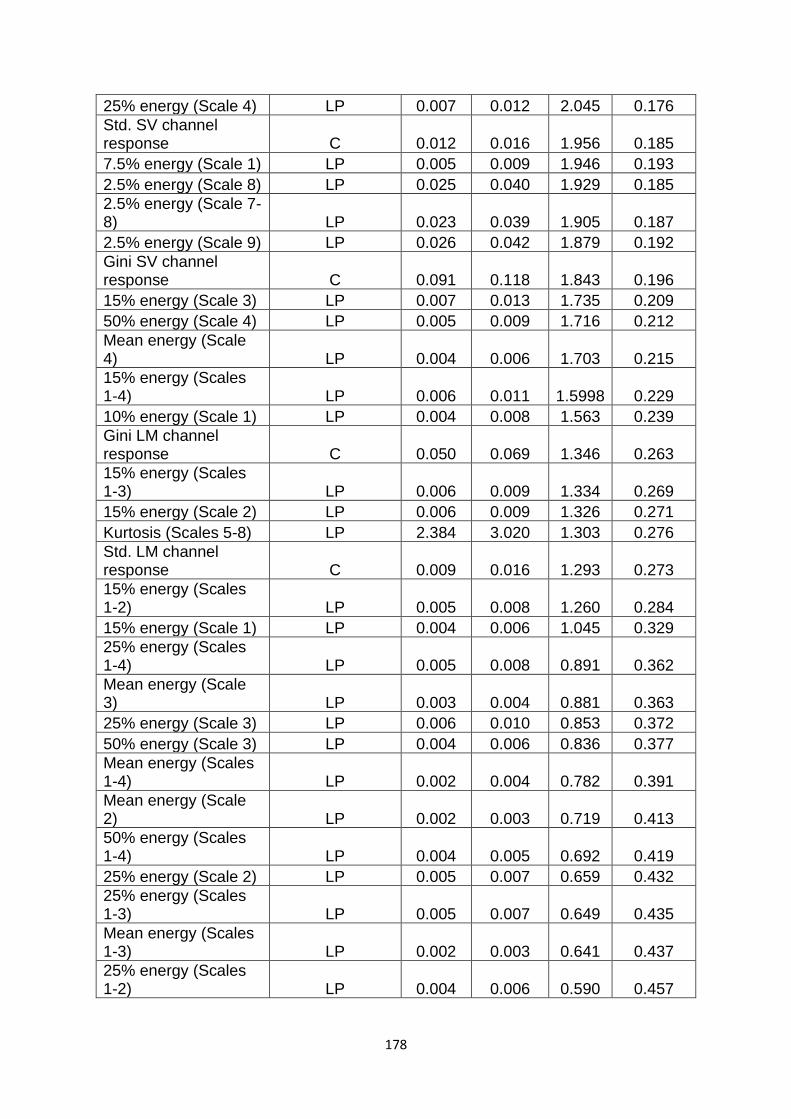
178

25% energy (Scale 4) LP 0.007 0.012 2.045 0.176

Std. SV channel response C 0.012 0.016 1.956 0.185

7.5% energy (Scale 1) LP 0.005 0.009 1.946 0.193

2.5% energy (Scale 8) LP 0.025 0.040 1.929 0.185

2.5% energy (Scale 7-8) LP 0.023 0.039 1.905 0.187

2.5% energy (Scale 9) LP 0.026 0.042 1.879 0.192

Gini SV channel response C 0.091 0.118 1.843 0.196

15% energy (Scale 3) LP 0.007 0.013 1.735 0.209

50% energy (Scale 4) LP 0.005 0.009 1.716 0.212

Mean energy (Scale 4) LP 0.004 0.006 1.703 0.215

15% energy (Scales 1-4) LP 0.006 0.011 1.5998 0.229

10% energy (Scale 1) LP 0.004 0.008 1.563 0.239

Gini LM channel response C 0.050 0.069 1.346 0.263

15% energy (Scales 1-3) LP 0.006 0.009 1.334 0.269

15% energy (Scale 2) LP 0.006 0.009 1.326 0.271

Kurtosis (Scales 5-8) LP 2.384 3.020 1.303 0.276

Std. LM channel response C 0.009 0.016 1.293 0.273

15% energy (Scales 1-2) LP 0.005 0.008 1.260 0.284

15% energy (Scale 1) LP 0.004 0.006 1.045 0.329

25% energy (Scales 1-4) LP 0.005 0.008 0.891 0.362

Mean energy (Scale 3) LP 0.003 0.004 0.881 0.363

25% energy (Scale 3) LP 0.006 0.010 0.853 0.372

50% energy (Scale 3) LP 0.004 0.006 0.836 0.377

Mean energy (Scales 1-4) LP 0.002 0.004 0.782 0.391

Mean energy (Scale 2) LP 0.002 0.003 0.719 0.413

50% energy (Scales 1-4) LP 0.004 0.005 0.692 0.419

25% energy (Scale 2) LP 0.005 0.007 0.659 0.432

25% energy (Scales 1-3) LP 0.005 0.007 0.649 0.435

Mean energy (Scales 1-3) LP 0.002 0.003 0.641 0.437

25% energy (Scales 1-2) LP 0.004 0.006 0.590 0.457

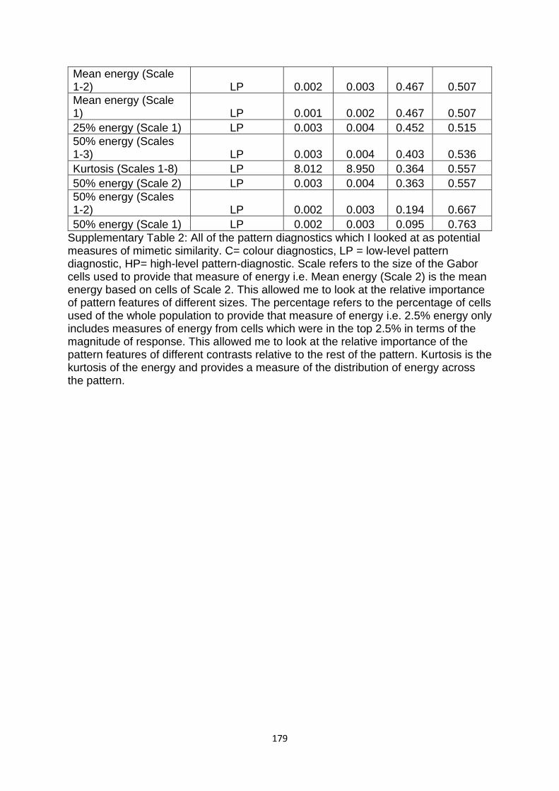
179

Mean energy (Scale 1-2) LP 0.002 0.003 0.467 0.507

Mean energy (Scale 1) LP 0.001 0.002 0.467 0.507

25% energy (Scale 1) LP 0.003 0.004 0.452 0.515

50% energy (Scales 1-3) LP 0.003 0.004 0.403 0.536

Kurtosis (Scales 1-8) LP 8.012 8.950 0.364 0.557

50% energy (Scale 2) LP 0.003 0.004 0.363 0.557

50% energy (Scales 1-2) LP 0.002 0.003 0.194 0.667

50% energy (Scale 1) LP 0.002 0.003 0.095 0.763

Supplementary Table 2: All of the pattern diagnostics which I looked at as potential measures of mimetic similarity. C= colour diagnostics, LP = low-level pattern diagnostic, HP= high-level pattern-diagnostic. Scale refers to the size of the Gabor cells used to provide that measure of energy i.e. Mean energy (Scale 2) is the mean energy based on cells of Scale 2. This allowed me to look at the relative importance of pattern features of different sizes. The percentage refers to the percentage of cells used of the whole population to provide that measure of energy i.e. 2.5% energy only includes measures of energy from cells which were in the top 2.5% in terms of the magnitude of response. This allowed me to look at the relative importance of the pattern features of different contrasts relative to the rest of the pattern. Kurtosis is the kurtosis of the energy and provides a measure of the distribution of energy across the pattern.

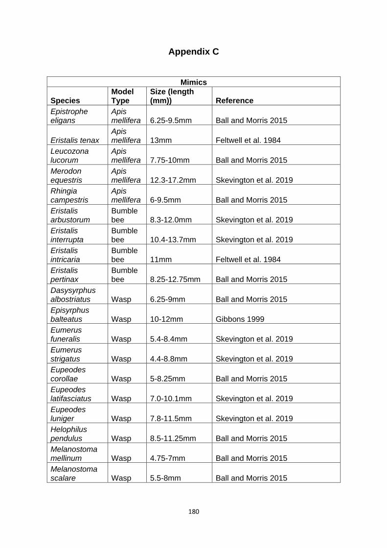
180

Appendix C

Mimics

Species Model Type

Size (length (mm)) Reference

Epistrophe eligans

Apis mellifera 6.25-9.5mm Ball and Morris 2015

Eristalis tenax Apis mellifera 13mm Feltwell et al. 1984

Leucozona lucorum

Apis mellifera 7.75-10mm Ball and Morris 2015

Merodon equestris

Apis mellifera 12.3-17.2mm Skevington et al. 2019

Rhingia campestris

Apis mellifera 6-9.5mm Ball and Morris 2015

Eristalis arbustorum

Bumble bee 8.3-12.0mm Skevington et al. 2019

Eristalis interrupta

Bumble bee 10.4-13.7mm Skevington et al. 2019

Eristalis intricaria

Bumble bee 11mm Feltwell et al. 1984

Eristalis pertinax

Bumble bee 8.25-12.75mm Ball and Morris 2015

Dasysyrphus albostriatus Wasp 6.25-9mm Ball and Morris 2015

Episyrphus balteatus Wasp 10-12mm Gibbons 1999

Eumerus funeralis Wasp 5.4-8.4mm Skevington et al. 2019

Eumerus strigatus Wasp 4.4-8.8mm Skevington et al. 2019

Eupeodes corollae Wasp 5-8.25mm Ball and Morris 2015

Eupeodes latifasciatus Wasp 7.0-10.1mm Skevington et al. 2019

Eupeodes luniger Wasp 7.8-11.5mm Skevington et al. 2019

Helophilus pendulus Wasp 8.5-11.25mm Ball and Morris 2015

Melanostoma mellinum Wasp 4.75-7mm Ball and Morris 2015

Melanostoma scalare Wasp 5.5-8mm Ball and Morris 2015

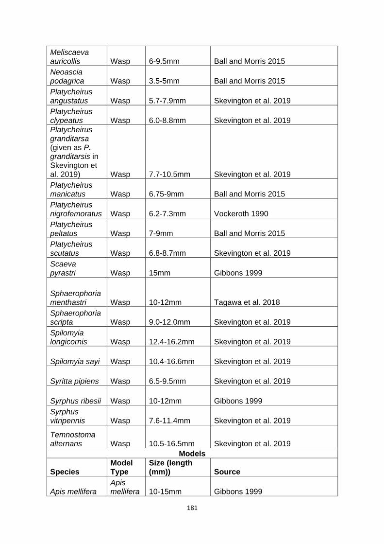
181

Meliscaeva auricollis Wasp 6-9.5mm Ball and Morris 2015

Neoascia podagrica Wasp 3.5-5mm Ball and Morris 2015

Platycheirus angustatus Wasp 5.7-7.9mm Skevington et al. 2019

Platycheirus clypeatus Wasp 6.0-8.8mm Skevington et al. 2019

Platycheirus granditarsa (given as P. granditarsis in Skevington et al. 2019) Wasp 7.7-10.5mm Skevington et al. 2019

Platycheirus manicatus Wasp 6.75-9mm Ball and Morris 2015

Platycheirus nigrofemoratus Wasp 6.2-7.3mm Vockeroth 1990

Platycheirus peltatus Wasp 7-9mm Ball and Morris 2015

Platycheirus scutatus Wasp 6.8-8.7mm Skevington et al. 2019

Scaeva pyrastri Wasp 15mm Gibbons 1999

Sphaerophoria menthastri Wasp 10-12mm Tagawa et al. 2018

Sphaerophoria scripta Wasp 9.0-12.0mm Skevington et al. 2019

Spilomyia longicornis Wasp 12.4-16.2mm Skevington et al. 2019

Spilomyia sayi Wasp 10.4-16.6mm Skevington et al. 2019

Syritta pipiens Wasp 6.5-9.5mm Skevington et al. 2019

Syrphus ribesii Wasp 10-12mm Gibbons 1999

Syrphus vitripennis Wasp 7.6-11.4mm Skevington et al. 2019

Temnostoma alternans Wasp 10.5-16.5mm Skevington et al. 2019

Models

Species Model Type

Size (length (mm)) Source

Apis mellifera Apis mellifera 10-15mm Gibbons 1999

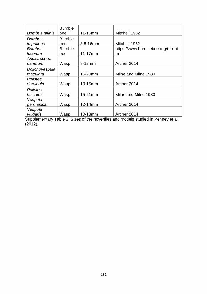
182

Bombus affinis Bumble bee 11-16mm Mitchell 1962

Bombus impatiens

Bumble bee 8.5-16mm Mitchell 1962

Bombus lucorum

Bumble bee 11-17mm

https://www.bumblebee.org/terr.htm

Ancistrocerus parietum Wasp 8-12mm Archer 2014

Dolichovespula maculata Wasp 16-20mm Milne and Milne 1980

Polistes dominula Wasp 10-15mm Archer 2014

Polistes fuscatus Wasp 15-21mm Milne and Milne 1980

Vespula germanica Wasp 12-14mm Archer 2014

Vespula vulgaris Wasp 10-13mm Archer 2014

Supplementary Table 3: Sizes of the hoverflies and models studied in Penney et al. (2012).