arX

iv:c

ond-

mat

/011

1246

v1 [

cond

-mat

.sta

t-m

ech]

13

Nov

200

1

FACING NON-STATIONARY CONDITIONS WITH A NEW

INDICATOR OF ENTROPY INCREASE: THE CASSANDRA

ALGORITHM

P. ALLEGRINI

Istituto di Linguistica Computazionale del Consiglio Nazionale delle Ricerche,

Area della Ricerca di Pisa–S. Cataldo, Via Moruzzi 1, 56124, Pisa, Italy

P. GRIGOLINI

Center for Nonlinear Science, University of North Texas, P.O. Box 5368,

Denton, TX 76203;

Istituto di Biofisica del Consiglio Nazionale delle Ricerche,

Area della Ricerca di Pisa–S. Cataldo, Via Moruzzi 1, 56124, Pisa, Italy

P. HAMILTON

Center for Nonlinear Science, Texas Woman’s University, P.O. Box 425498, Denton,

Texas 76204

L. PALATELLA, G. RAFFAELLI, M. VIRGILIO

Dipartimento di Fisica dell’Universita di Pisa and INFM Piazza Torricelli 2, 56127 Pisa,

Italy

We address the problem of detecting non-stationary effects in time series (in particularfractal time series) by means of the Diffusion Entropy Method (DEM). This means thatthe experimental sequence under study, of size N , is explored with a window of sizeL << N . The DEM makes a wise use of the statistical information available and,consequently, in spite of the modest size of the window used, does succeed in revealinglocal statistical properties, and it shows how they change upon moving the windows alongthe experimental sequence. The method is expected to work also to predict catastrophicevents before their occurrence.

1 Introduction

The main aim of this paper is to illustrate a promising strategy to study non-stationary processes. We prove that the method is efficient by means of the jointstudy of real and artificial sequences, and we reach a conclusion that makes it plau-sible to imagine the method at work to successfully predict the time of occurrenceof catastrophic events.

The method here illustrated is a suitable extension of the Diffusion EntropyMethod (DEM). The DEM is discussed in details in other publications1,2,3. Herewe limit ourselves to give a concise illustration of this technique so as to allow thereader to understand the spirit of the method of this paper, at least through afirst reading, without consulting these earlier publications. The first step of thistechnique is the same as that of the pioneering work of Refs. 4,5. This means thatthe experimental sequence is converted into a kind of Brownian-like trajectory. Thesecond step aims at deriving many distinct diffusion trajectories with the techniqueof moving windows of size l. The reader should not confuse the mobile vindow of sizel with the mobile window of value L that will be used later on in this paper to detectnon-stationary properties. For this reason we shall refer to the mobile windows of

1

size L as large windows, even if the size of L is relatively small, whereas the mobilewindows of size l will be called small windows. The large mobile window has to beinterpreted as a sequence with statistical properties to reveal, and will be analyzedby means of small windows of size l, with l < L. The success of the method dependson the fact that the DE makes a wise use of the statistical information available.In fact, the small windows overlap among themselves and are obtained by locatingtheir left border on the first site of the sequence, on the second second site, andso on. The adoption of overlapping windows is dictated by the wish to establisha connection with the Kolomogorov-Sinai (KS)6,7 method. This yields also, as afurther beneficial effect, many more trajectories than the widely used method ofDetrended Fluctuation Analysis (DFA)4,5.

In conclusion, we create a conveniently large number of trajectories by graduallymoving the small window from the first position, with the left border of the smallwindow coinciding with the first size of the sequence, to the last position, with theright border of the small window coinciding with the last site of the sequence. Atfterthis stage, we utilize the resulting trajectories, all of them with the initial positionlocated at x = 0, to produce a probability distribution at “time” l. We evaluate theShannon entropy of this distribution, Sd(l), and with easy mathematical argumentswe prove that, if the diffusion process undergoes a scaling of intensity δ, then

Sd(l) = A+ δln(l). (1)

Thus the parameter δ of the scaling condition, if this condition applies, can bemeasured without recourse to any form of detrending.

This is the original motivation for the DEM1,2,3. In this paper we want to provethat the DEM does much more than detecting scaling. In a stationary conditionthe DEM not only detects with accuracy the final scaling but it also affords a wayto monitor the regime of transition to the final thermodynamic condition. If thesequence under study is affected by biases and non-stationary perturbations, theattainment of the final regime of steady scaling can be cancelled, and replaced by anout of equilibrium regime changing in time under the influence of time dependentbiases. We want to prove that the DEM can be suitably extended to face thischallenging non-stationary condition.

The outline of the paper is as follows. In Section 2 we shortly review the maintenets of the DEM so as to make this paper, as earlier mentioned, as self-containedas possible. In Section 3 we illustrate the extension of the DEM and we discussthe fundamental problem of assessing which is the shortest portion, of size L, ofthe sequence under study, which is still large enough as to make the DEM work.In Section 3 we express our hope that this new method might serve predictionpurposes.

2 Diffusion Entropy

Let us consider a sequence of M numbers ξi , with i = 1, . . . ,M . The purpose ofthe DEM algorithm is to establish the possible existence of a scaling, either normalor anomalous, in the most efficient way as possible, without altering the data withany form of detrending. Let us select first of all an integer number l, fitting the

2

condition 1 ≤ l ≤ M . As earlier mentioned, we shall refer ourselves to l as ”time”.For any given time l we can find M − l + 1 sub-sequences defined by

ξ(s)i ≡ ξi+s, s = 0, . . . ,M − l. (2)

For any of these sub-sequences we build up a diffusion trajectory, labelled with theindex s, defined by the position

x(s)(l) =l

∑

i=1

ξ(s)i =

l∑

i=1

ξi+s. (3)

Let us imagine this position as referring to a Brownian particle that at regularintervals of time has been jumping forward or backward according to the prescrip-tion of the corresponding sub-sequence of Eq.(2). This means that the particlebefore reaching the position that it holds at time l has been making l jumps. The

jump made at the i-th step has the intensity |ξ(s)i | and is forward or backward

according to whether the number ξ(s)i is positive or negative.

We are now ready to evaluate the entropy of this diffusion process. To do thatwe have to partition the x-axis into cells of size ǫ(l). When this partition is madewe have to label the cells. We count how many particles are found in the same cellat a given time l. We denote this number by Ni(l). Then we use this number todetermine the probability that a particle can be found in the i-th cell at time l,pi(l), by means of

pi(l) ≡Ni(l)

(M − l + 1). (4)

At this stage the entropy of the diffusion process at the time l is determined andreads

Sd(l) = −∑

i

pi(l)ln[pi(l)]. (5)

The easiest way to proceed with the choice of the cell size, ǫ(l), is to assume itindependent of l and determined by a suitable fraction of the square root of thevariance of the fluctuation ξ(i).

Before proceeding with the illustration of how the DEM method works, it isworth making a comment on the way we use to define the trajectories. The methodwe are adopting is based on the idea of a moving window of size l that makes thes− th trajectory closely correlated to the next, the (s+ 1)− th trajectory. The twotrajectories have l − 1 values in common. A motivation for our choice is given byour wish to establish a connection with the Kolmogorov Sinai (KS) entropy6,7. TheKS entropy of a symbolic sequence is evaluated by moving a window of size l alongthe sequence. Any window position corresponds to a given combination of symbols,and, from the frequency of each combination, it is possible to derive the Shannonentropy S(l). The KS entropy is given by the asymptotic limit liml→∞S(l)/l. Webelieve that the same sequence, analyzed with the DEM method, at the large valuesof l where S(l)/l approaches the KS value, must yield a well defined scaling δ. Torealize this correspondence we carry out the determination of the Diffusion Entropyusing the same criterion of overlapping windows as that behind the KS entropy.

3

Details on how to deal with the transition from the short-time regime, sensitiveto the discrete nature of the process under study, to the long-time limit where bothspace an time can be perceived as continuous, are given in Ref. 1,3. Here we makethe simplifying assumption of considering so large times as to make the continuousassumption valid. In this case the trajectories, built up with the above illustratedprocedure, correspond to the following equation of motion:

dx

dt= ξ(t), (6)

where ξ(t) denotes the value that the time series under study gets at the l− th site.This means that the function ξ(l) is depicted as a function of t, thought of as acontinuous time t = l. In this case the Shannon entropy reads

Sd(t) = −

∫

∞

−∞

dx p(x, t)ln[p(x, t)]. (7)

We can derive with a simple treatment an analytical solution for Diffusion Entropywhen the process is characterized by scaling, namely when

p(x, t) =1

tδF

( x

tδ

)

. (8)

Let us plug Eq.(8) into Eq.(7). After a simple algebra, we get:

Sd(τ) = A+ δ(τ)τ, (9)

where

A ≡ −

∫

∞

−∞

dy F (y) ln[F (y)] (10)

andτ ≡ ln(t). (11)

It is evident that this kind of technique to detect scaling does not imply anyform of detrending, and this is one of the reasons why some attention should bedevoted to it. It is also worth mentioning, as we prove now, that it yields the correctscaling values even for the so-called Levy walks, where the time dependence of thesecond moment with respect to time has an exponent which is different from thescaling exponent of the Levy process.

We therefore check the efficiency of this technique by the studying the artificialsequence of Refs. 8,9. This sequence is built up in such a way as to realize longsequences of either +’s or −’s. The probability of finding a sequence of only +’s oronly −’s of length t is given by

ψ(t) = (µ− 1)T µ−1

(t+ T )µ. (12)

Here we focus our attention on the condition µ < 3 and we raise the reader’sattention on the interval 2 ≤ µ ≤ 3. In fact, this kind of sequence is the same asthat adopted in earlier work 9 for a dynamic derivation of Levy diffusion, which

4

shows up when the condition 2 < µ < 3 applies. It corresponds to a particletravelling with constant velocity throughout the whole time interval correspondingto either only +’s or only -’s, and changing direction with no rest, at the end of anystring with the same symbols.

We will refer to this model as Symmetric Velocity Model (SVM). We know fromthe theory of Ref.9 that the scaling of the resulting diffusion process when 2 < µ < 3is

δ =1

µ− 1. (13)

Note, however, that this diffusion process has a finite propagation front, with bal-listic peaks showing up at both x = t and x = −t. The intensity of these peaks isproportional to the correlation function

Φξ(t) =

(

T

T + t

)µ−2

. (14)

As a consequence of this fact, the whole distribution does not have a single rescaling.In fact, the distribution enclosed between the two peaks rescales with δ of Eq.(13)while the peaks are associated to δ = 1. Furthermore, it is well known9 that thescaling of the second moment is given by

δH =4 − µ

2. (15)

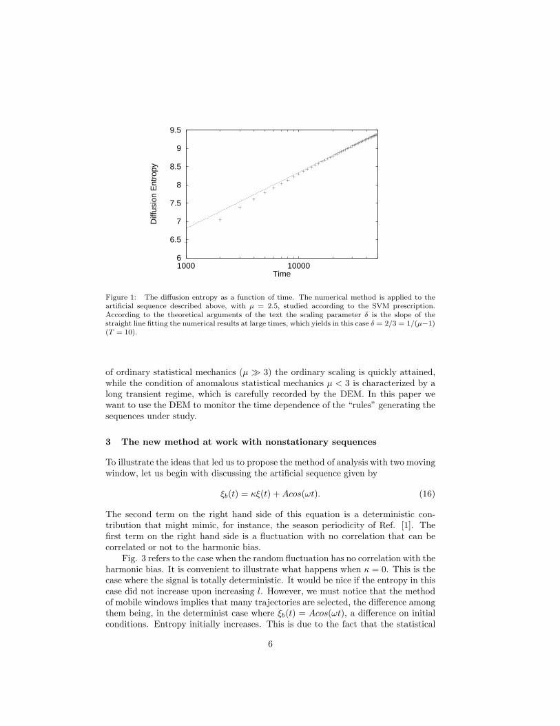
Thus, it is expected that the scaling detected by the DE method might not coincidewith the prediction of Eq.(13) for the whole period of time corresponding to thepresence of peaks of significant intensity. We think that the Levy scaling of Eq.(13)will show up at long times, when the peak intensity is significantly reduced. Thisconjecture seems to be supported by the numerical results illustrated in Fig.1. Wesee in fact that the scaling predicted by Eq.(13) is reached after an extended tran-sient, of the order of about 20,000 in the scale of Fig.1. This time interval is about2000 larger than the value assigned to the parameter T, of Eq.(12), which is, infact, in the case of Fig.1, T= 10.

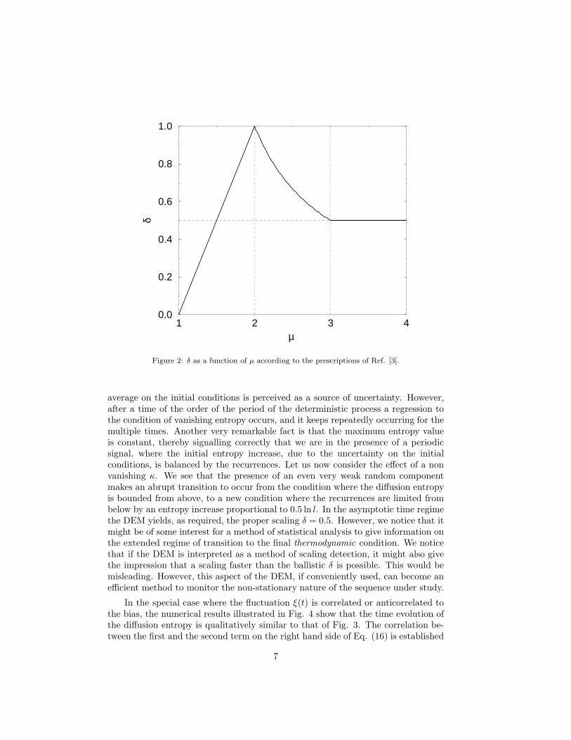
In conclusion, this section proves that the DE method applied to the SVMyields, for the scaling parameter δ, the correct value of Eq.(13), rather than thevalue that would be obtained measuring the variance of the diffusion process,Eq.(15). However, the time necessary to make this correct value emerge is verylarge. Furthermore, as shown in Fig. 2, the adoption of SVM would make thescaling parameter δ insensitive to µ in the whole interval 1 ≤ µ ≤ 2. This meansthat the adoption of the DE method would not allow us to distinguish a processwith µ very close to 1 from one with µ very close to 2. This problem can be solvedusing different rules for the diffusion process 3: the random walker can, for instance,walk always in the same direction, and at the “time” when there is a passage froma laminar region of ’s to one of -’s and vice-versa. If this latter rule is adopted, thenit is easy to prove 3 that the resulting p(x, t) is an asymmetric Levy distribution,with a scaling δ = µ− 1 for 1 ≤ µ ≤ 2.

Throughout this paper, however, apply the DEM with the rule correspondingto the symmetric velocity model, with δ depending on µ as in Fig. 2. In the regime

5

6

6.5

7

7.5

8

8.5

9

9.5

1000 10000

Diff

usio

n E

ntro

py

Time

Figure 1: The diffusion entropy as a function of time. The numerical method is applied to theartificial sequence described above, with µ = 2.5, studied according to the SVM prescription.According to the theoretical arguments of the text the scaling parameter δ is the slope of thestraight line fitting the numerical results at large times, which yields in this case δ = 2/3 = 1/(µ−1)(T = 10).

of ordinary statistical mechanics (µ ≫ 3) the ordinary scaling is quickly attained,while the condition of anomalous statistical mechanics µ < 3 is characterized by along transient regime, which is carefully recorded by the DEM. In this paper wewant to use the DEM to monitor the time dependence of the “rules” generating thesequences under study.

3 The new method at work with nonstationary sequences

To illustrate the ideas that led us to propose the method of analysis with two movingwindow, let us begin with discussing the artificial sequence given by

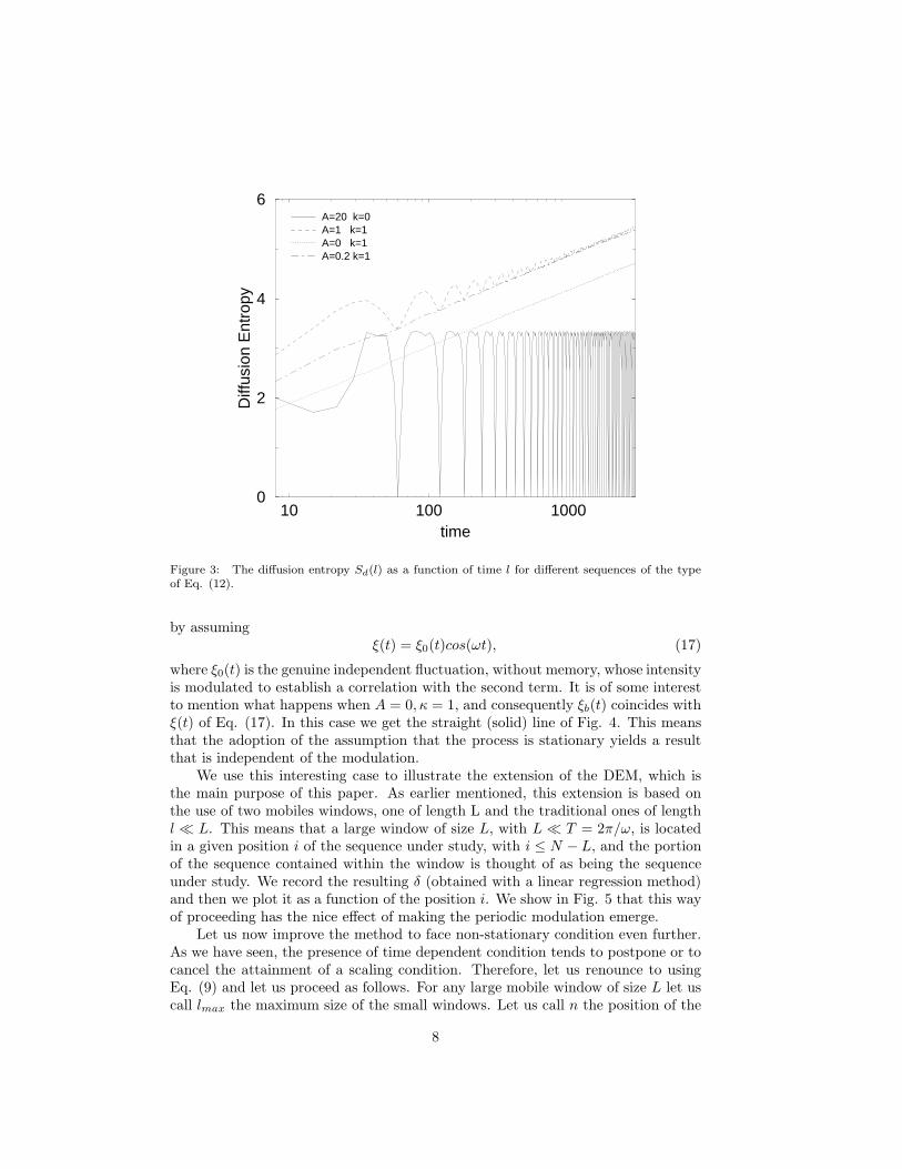
ξb(t) = κξ(t) +Acos(ωt). (16)

The second term on the right hand side of this equation is a deterministic con-tribution that might mimic, for instance, the season periodicity of Ref. [1]. Thefirst term on the right hand side is a fluctuation with no correlation that can becorrelated or not to the harmonic bias.

Fig. 3 refers to the case when the random fluctuation has no correlation with theharmonic bias. It is convenient to illustrate what happens when κ = 0. This is thecase where the signal is totally deterministic. It would be nice if the entropy in thiscase did not increase upon increasing l. However, we must notice that the methodof mobile windows implies that many trajectories are selected, the difference amongthem being, in the determinist case where ξb(t) = Acos(ωt), a difference on initialconditions. Entropy initially increases. This is due to the fact that the statistical

6

1 2 3 4µ

0.0

0.2

0.4

0.6

0.8

1.0

δ

Figure 2: δ as a function of µ according to the prescriptions of Ref. [3].

average on the initial conditions is perceived as a source of uncertainty. However,after a time of the order of the period of the deterministic process a regression tothe condition of vanishing entropy occurs, and it keeps repeatedly occurring for themultiple times. Another very remarkable fact is that the maximum entropy valueis constant, thereby signalling correctly that we are in the presence of a periodicsignal, where the initial entropy increase, due to the uncertainty on the initialconditions, is balanced by the recurrences. Let us now consider the effect of a nonvanishing κ. We see that the presence of an even very weak random componentmakes an abrupt transition to occur from the condition where the diffusion entropyis bounded from above, to a new condition where the recurrences are limited frombelow by an entropy increase proportional to 0.5 ln l. In the asymptotic time regimethe DEM yields, as required, the proper scaling δ = 0.5. However, we notice that itmight be of some interest for a method of statistical analysis to give information onthe extended regime of transition to the final thermodynamic condition. We noticethat if the DEM is interpreted as a method of scaling detection, it might also givethe impression that a scaling faster than the ballistic δ is possible. This would bemisleading. However, this aspect of the DEM, if conveniently used, can become anefficient method to monitor the non-stationary nature of the sequence under study.

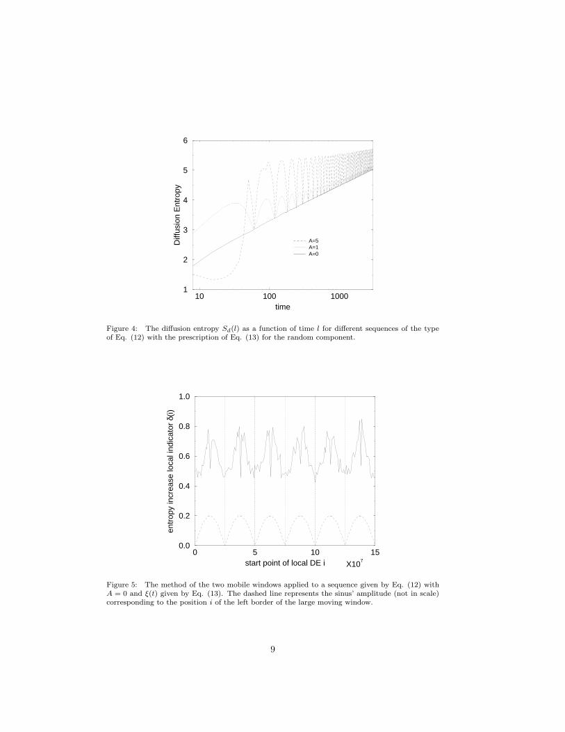
In the special case where the fluctuation ξ(t) is correlated or anticorrelated tothe bias, the numerical results illustrated in Fig. 4 show that the time evolution ofthe diffusion entropy is qualitatively similar to that of Fig. 3. The correlation be-tween the first and the second term on the right hand side of Eq. (16) is established

7

10 100 1000time

0

2

4

6

Diff

usio

n E

ntro

py

A=20 k=0A=1 k=1A=0 k=1A=0.2 k=1

Figure 3: The diffusion entropy Sd(l) as a function of time l for different sequences of the typeof Eq. (12).

by assumingξ(t) = ξ0(t)cos(ωt), (17)

where ξ0(t) is the genuine independent fluctuation, without memory, whose intensityis modulated to establish a correlation with the second term. It is of some interestto mention what happens when A = 0, κ = 1, and consequently ξb(t) coincides withξ(t) of Eq. (17). In this case we get the straight (solid) line of Fig. 4. This meansthat the adoption of the assumption that the process is stationary yields a resultthat is independent of the modulation.

We use this interesting case to illustrate the extension of the DEM, which isthe main purpose of this paper. As earlier mentioned, this extension is based onthe use of two mobiles windows, one of length L and the traditional ones of lengthl ≪ L. This means that a large window of size L, with L ≪ T = 2π/ω, is locatedin a given position i of the sequence under study, with i ≤ N − L, and the portionof the sequence contained within the window is thought of as being the sequenceunder study. We record the resulting δ (obtained with a linear regression method)and then we plot it as a function of the position i. We show in Fig. 5 that this wayof proceeding has the nice effect of making the periodic modulation emerge.

Let us now improve the method to face non-stationary condition even further.As we have seen, the presence of time dependent condition tends to postpone or tocancel the attainment of a scaling condition. Therefore, let us renounce to usingEq. (9) and let us proceed as follows. For any large mobile window of size L let uscall lmax the maximum size of the small windows. Let us call n the position of the

8

10 100 1000time

1

2

3

4

5

6

Diff

usio

n E

ntro

py

A=5A=1A=0

Figure 4: The diffusion entropy Sd(l) as a function of time l for different sequences of the typeof Eq. (12) with the prescription of Eq. (13) for the random component.

0 5 10 15start point of local DE i

0.0

0.2

0.4

0.6

0.8

1.0

entr

opy

incr

ease

loca

l ind

icat

or δ

(i)

X107

Figure 5: The method of the two mobile windows applied to a sequence given by Eq. (12) withA = 0 and ξ(t) given by Eq. (13). The dashed line represents the sinus’ amplitude (not in scale)corresponding to the position i of the left border of the large moving window.

9

0 2000 4000 6000 8000 10000period (base pairs)

0

0.1

0.2

four

ier

coef

ficie

nts

0 10000 20000 30000 40000n (start point of local DE)

−0.25

0.25

0.75

1.25

I(n)

(lo

cal c

orre

latio

n in

dica

tor)

Figure 6: The method of the two moving windows with lmax = 30 applied to the analysis ofan artificial CMM sequence with periodic parameter ǫ. The period of the variation of ǫ is 5000bps and the analysis is carried out with moving windows of size 2000 bps. Inset: Fourier spectralanalysis of I(n).

left border of the large window, and and let us evaluate the following property

I(n) ≡

lmax∑

l=2

Sd(l) − [Sd(1) + 0.5 ln l]

l. (18)

The quantity I(n) detects the deviation from the condition of increase that thediffusion entropy would have in the random case. Since in the regime of transitionthe entropy increase can be much slower than in the corresponding random case,the quantity I(n) can also bear negative values. This indicator affords a satisfactoryway to detect local properties. As an example, Fig. 6 shows a case based on theDNA model of Ref. [8], called Copying Mistake Map (CMM). This is a sequenceof symbols 0 and 1 obtained from the joint action of two independent sequences,one equivalent to tossing a coin and the other equivalent to establishing randomly asequence of patches whose length is distributed as an inverse power law with indexµ fitting the condition 2 < µ < 3. The probability of using the former sequence is1 − ǫ and that of using the latter is ǫ. We choose a time dependent value of ǫ

ǫ = ǫ0[1 − cos(ωt)]. (19)

In Fig. 6 we show how this periodicity is perceived by using the two-windowsgeneralization, proposed in this paper, of the DEM.

As a final example to show the efficiency of the new method of analysis, letus address the problem of the search of hidden periodicities in DNA sequences.

10

0 1000 2000period (base pairs)

0

0.02

0.04

four

ier

coef

ficie

nts

0 990 1980 2970 3960 4950 5940 6930 7920n (start point of local DE)

−0.2

0

0.2

0.4

0.6

0.8

I(n)

(lo

cal c

orre

latio

n in

dica

tor)

990

Figure 7: The method of two mobile windows applied to the analysis of the human DNA sequence.The method of two mobile windows (lmax = 20 L = 512) detects a periodicity of 990 bps. Inset:Fourier spectral analysis of I(n).

Fig. 7 shows a distinct periodic behavior for the human T-cell receptor alpha/deltalocus. A period of about 990 base pairs is very neat in the first part of the sequence(promoter region), while several periodicities of the order of 1000 base pairs aredistributed along the whole sequence.

These periodicities, probably due to DNA-proteins interactions in active eukary-otic genes, are expected by biologists, but the current technology is not yet adequateto deal with this issue, neither from the experimental nor from the computationalpoint of view: such a behavior cannot be analyzed by means of crystallographic orstructural NMR methods, nor would the current (or of the near future) computingfacilities allow molecular dynamics studies of systems of the order of 106 atoms ormore.

4 Conclusions

The research work illustrated in this paper shows that the DEM is a very efficientway to detect the departure from ordinary Brownian motion with the shortest se-quence as possible. On the basis of these results we are confident that it will bepossible to predict the occurrence of catastrophic events, heart-quakes, heart at-tacks, stock-market crashes, and so on. We think that if all these misfortune eventsare anticipated by a correlation change, lasting for a fairly extended time period,then the DEM, within the double window procedure here illustrated, will signalin time their later occurrence. We refer to this method of analysis as Complex

11

Analysis of Sequences via Scaling AND Randomness Assessment (CASSANDRA),and we hope to prove by means of future research work that its prophetic power isworth of consideration. We wish that the CASSANDRA algorithm will have morefortune and will receive more credit than the daughter of Priam and Hecuba.

References

1. N. Scafetta, P. Hamilton, P. Grigolini, Fractals, 9, 193 (2001).2. N. Scafetta, V. Latora, P. Grigolini, cond-mat/0105041.3. P. Grigolini, L. Palatella, G. Raffaelli, cond-mat/0104166, in press on Fractals.4. C.-K. Peng, S.V. Buldyrev, S. Havlin, M. Simons, H.E. Stanley, and A.L.

Goldberger, Phys. Rev. E, 49, 1685 (1994).5. C.-K. Peng, S. Havlin, H.E. Stanley, A.L. Goldberger, Chaos 5, 82 (1995).6. C. Beck, F. Schlogl, Thermodynamics of Chaotic Systems, Cambdridge Uni-

versity Press, Cambridge (1993)7. J.R. Dorfman, An Introduction to Chaos in Nonequilibrium Statistical Me-

chanics, Cambridge University Press, Cambridge (1999).8. M. Buiatti, P. Grigolini, L. Palatella, Physica A 268, 214 (1999).9. P. Allegrini, P. Grigolini, B.J. West, Phys. Rev. E 54, 4760 (1996).

10. P. Allegrini, M. Barbi, P. Grigolini and B.J. West, Phys. Rev. E 52, 5281(1995).

12