Extreme Point Characterizations forInfinite Network Flow Problems∗

H. Edwin Romeijn† Dushyant Sharma‡ Robert L. Smith§

June 12, 2006

Abstract

We study capacitated network flow problems with supplies and demands defined

on a countably infinite collection of nodes having finite degree. This class of network

flow models includes, for example, all infinite horizon deterministic dynamic programs

with finite action sets since these are equivalent to the problem of finding a shortest

path in an infinite directed network. We derive necessary and sufficient conditions for

flows to be extreme points of the set of feasible flows. Under an additional regularity

condition met by all such problems with integer data, we show that a feasible solution

is an extreme point if and only if it contains neither a cycle nor a doubly-infinite path

consisting of free arcs (an arc is free if its flow is strictly between its upper and lower

bounds). We employ this result to show that the extreme points can be characterized

by specifying a basis. Moreover, we establish the integrality of extreme point flows

whenever demands and supplies and arc capacities are integer valued. We illustrate

our results with an application to an infinite horizon economic lot-sizing problem.

Keywords: Network flow problems, infinite horizon optimization, extreme point so-

lutions, basic solutions.

∗This work was supported in part by NSF Grants DMI-0322114 and DMI-9713723.†Department of Industrial and Systems Engineering, University of Florida, 303 Weil Hall, P.O. Box

116595, Gainesville, Florida 32611-6595; e-mail: romeijn@ise.ufl.edu.‡Department of Industrial and Operations Engineering, The University of Michigan, Ann Arbor, Michigan

48109-2117; e-mail: dushyant@umich.edu.§Department of Industrial and Operations Engineering, The University of Michigan, Ann Arbor, Michigan

48109-2117; e-mail: rlsmith@umich.edu.

1

1 Introduction

An important class of optimization problems in operations research is formed by planning

problems over time. Many of these planning problems can quite naturally be formulated

as network flow problems. When, as is often the case, there is no natural study horizon

that can be specified a priori, these planning problems are formulated as problems over an

infinite horizon. Some notable examples of such problems include capacity expansion under

nonlinear demand (Bean and Smith [7]), equipment replacement under technological change

(Bean, Lohmann, and Smith [5], Jones, Zydiak, and Hopp [12]), and production planning

under non-stationary cost and demand data (Smith and Zhang [15]). Such problems then give

rise to minimum cost network flow problems in networks with infinitely many nodes and arcs.

The usual attack to solving such an infinite horizon problem is through a planning horizon

approach which seeks solutions to finite horizon versions that arbitrarily well approximate

optimal solutions to the original infinite horizon problem (see, e.g., Bean and Smith [6],

Schochetman and Smith [14]). Our intent in this paper however is to study properties, and

in particular extreme point properties, of the infinite horizon versions of such problems,

including more broadly, general infinite network flow problems.

Network flow problems form a very well-studied area. The excellent book by Ahuja, Mag-

nanti, and Orlin [1] describes the state of the art in designing algorithms for various types

of network flow problems. To date, however, attention has almost exclusively been focused

on network flow problems in a network containing only a finite number of nodes and arcs

(notable exceptions being the works by Anderson and Philpott [4], Fuchssteiner and Morisse

[10], and Gomory and Hu [11], who studied network flow problems in networks with an un-

countable number of nodes). Many optimization algorithms for finite network flow problems,

in particular for linear and concave minimum cost network flow problems, employ a char-

acterization of extreme points and basic solutions of such problems using spanning trees.

Although the theory of optimization problems in infinite dimensional spaces is quite well

developed (see, e.g., Anderson and Nash [3]), application of this theory for developing algo-

rithms for concrete problems and obtaining important insights into the behavior of extreme

2

point and basic and optimal solutions has been thwarted by the mathematical pathologies

inherent in infinite dimensional optimization problems. Although Anderson and Nash [3]

provided a characterization of extreme point solutions for general infinite linear programs,

the abstract nature of their results prevented their further exploitation. Cross, Romeijn and

Smith [8] attempted to circumvent this problem by indirectly characterizing extreme points

of infinite dimensional convex sets by showing they are arbitrarily well approximated by the

extreme points of their finite dimensional projections.

In this paper, we return to the challenging problem of directly characterizing extreme

points within the infinite dimensional space itself and in particular through basic variables.

More precisely, the lack of and need for concrete characterizations of extreme points and

basic solutions to infinite network flow problems motivated our work. Our structural results

will provide an essential building block towards the characterization of extreme points for

general doubly-infinite linear programming problems as well as towards the development of

a (network) simplex method for infinite dimensional linear programming problems.

We will study capacitated network flow problems with supplies and demands defined

on a countably infinite collection of nodes having finite degree. This class of network flow

models includes, for example, all infinite horizon deterministic dynamic programs with finite

action sets since these are equivalent to the problem of finding a shortest infinite path in

an infinite directed network. We extend concepts and structural properties of solutions to

network flow problems from the finite to the infinite case. We derive properties of the set

of all feasible solutions (i.e., flows that satisfy all flow balance and bound constraints) and

establish a relationship between extreme point solutions to the network flow problem and

trees in the network, generalizing an analogous property of the finite version of the problem.

In particular, we provide necessary and sufficient conditions for a feasible solution to be an

extreme point. Under an additional non-vanishing support assumption on arc flows in ex-

treme point solutions we show that all extreme point solutions can be uniquely characterized

via a specification of a set of free variables. This then enables us to characterize extreme

points through a decomposition of the flow variables into basic and nonbasic variables. We

find that, as in finite networks, in infinite networks in which all node demands and supplies

3

and all arc capacities are integer valued, all extreme points have integral flows, which in turn

guarantees that the non-vanishing support assumption is met. As an example, we study a

capacitated economic lot-sizing problem with concave costs, and extend the finite-horizon

characterization of all (including the optimal) extreme point solutions to such problems.

The paper is organized as follows. In Section 2 we introduce the necessary notation

for the network flow problem, and extend some concepts from finite graph theory to the

infinite case. In Section 3 we derive structural properties of feasible flows as well as flows

corresponding to extreme points of the set of all feasible flows. In Section 4 we study a

production planning problem over an infinite horizon with concave costs. We end in Section

5 with some concluding remarks and directions for future research.

2 Notation and Definitions

In this section, we introduce the notation and some basic definitions used throughout the

paper. While most of the definitions introduced here are commonly used for finite networks,

some definitions are extended or introduced to specifically deal with infinite networks.

2.1 Network definitions

Let G = (N,A) be a directed network consisting of a countable set N = {1, 2, 3, . . .} of

nodes and a set A ⊆ N × N of arcs. Let d ∈ R|N | with typical element d(i) represent the

demand for each node, i.e., d(i) is the demand associated with node i ∈ N . We assume that

the in and out degree of each node i ∈ N is finite, i.e., |{j ∈ N : (j, i) ∈ A}| < ∞ and

|{j ∈ N : (i, j) ∈ A}| < ∞. Let `, u ∈ R|A| ∪ {−∞,∞} with typical elements `(i, j) and

u(i, j) be the vectors of lower and upper bounds, respectively, for the flows on arcs in A.

Without loss of generality, we assume that `(i, j) < u(i, j) for all (i, j) ∈ A.

We define a path P in the graph G to be a collection of arcs P ⊆ A in G representing

a sequence of nodes i1 − i2 − i3 − · · · such that no node is repeated in the sequence and for

each k, either (ik, ik+1) ∈ P or (ik+1, ik) ∈ P . If the path contains finitely many arcs (and

nodes) then it is called a finite path. Two infinite paths that share their endpoints is called a

4

doubly-infinite path. A cycle C in the graph G is defined as a finite path with corresponding

sequence of nodes i1 − i2 − i3 − · · · − ik whose endpoints are connected by an additional arc

(ik, i1) or (i1, ik). Given a cycle C (or a path P ), we shall use A(C) (or A(P )) to denote the

set of arcs in the cycle (or path). We say that two vertices i, j ∈ N are connected if there

exists a finite path i1 − i2 − · · · − ik in G with i1 = i and ik = j. The graph G is called

connected if every pair of nodes in G is connected. In this paper, we shall assume that the

graph G is connected.

A subgraph T = (N ′, A′) of G is called a tree if T is connected and it does not contain

any cycles. Note that there must be a unique finite path connecting each pair of nodes in

T . We can designate some node r ∈ N ′ to be the root of T . In this case, the tree T is called

a rooted tree and is denoted by T = (N ′, A′, r). The designation of a node as a root node

allows us to associate additional properties with the nodes in a tree. If (j, i) or (i, j) is the

arc on the unique path connecting node i and node r then j is called the parent of i, denoted

by pT (i), and i is called a child of j. For a node i ∈ N ′, we define CT (i) as the set of children

of i. The set NT (i) of descendants of a node i ∈ T consists of node i, its children, children of

its children, and so on. We say that node i is a leaf node if it is the only descendant of itself.

We define the subtree T (i) = (NT (i), AT (i), i) rooted at a node i ∈ N ′ to be the subgraph

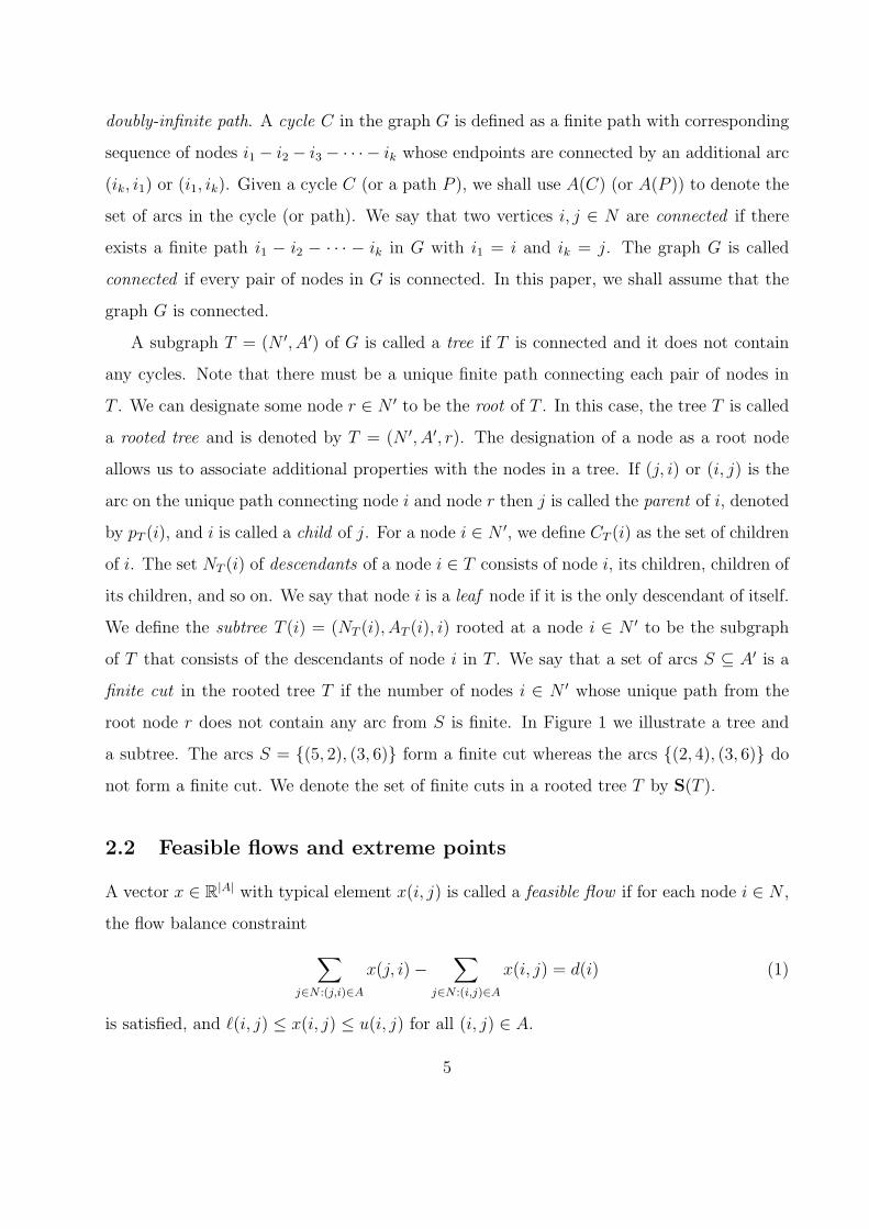
of T that consists of the descendants of node i in T . We say that a set of arcs S ⊆ A′ is a

finite cut in the rooted tree T if the number of nodes i ∈ N ′ whose unique path from the

root node r does not contain any arc from S is finite. In Figure 1 we illustrate a tree and

a subtree. The arcs S = {(5, 2), (3, 6)} form a finite cut whereas the arcs {(2, 4), (3, 6)} do

not form a finite cut. We denote the set of finite cuts in a rooted tree T by S(T ).

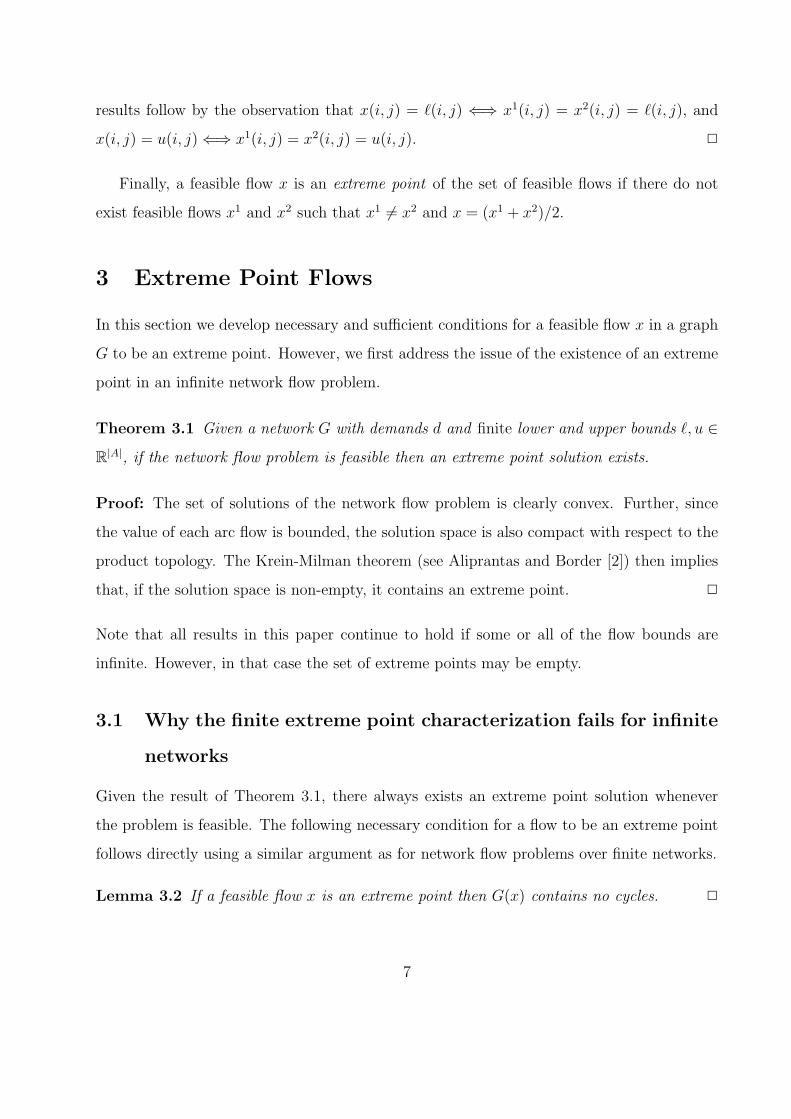
2.2 Feasible flows and extreme points

A vector x ∈ R|A| with typical element x(i, j) is called a feasible flow if for each node i ∈ N ,

the flow balance constraint

∑

j∈N :(j,i)∈A

x(j, i)−∑

j∈N :(i,j)∈A

x(i, j) = d(i) (1)

is satisfied, and `(i, j) ≤ x(i, j) ≤ u(i, j) for all (i, j) ∈ A.

5

1

2 3

54 6

(a)

2

54

(b)

Figure 1: (a) A tree T , and (b) its subtree T (2).

Given a feasible flow x, we define r(i, j) = min{x(i, j) − `(i, j), u(i, j) − x(i, j)} as the

maximum amount by which the flow on (i, j) can be increased or decreased without violating

bounds. We define the free arc graph of x as the graph G(x) = (N, A(x)) where A(x) =

{(i, j) ∈ A : r(i, j) > 0} is the set of free arcs, i.e., arcs whose flow can be increased as

well as decreased. We define the set of arcs with their flow equal to their upper bound as

U(x) = {(i, j) ∈ A : x(i, j) = u(i, j)} and arcs with flow equal to their lower bound as

L(x) = {(i, j) ∈ A : x(i, j) = `(i, j)}. We note that A(x), U(x), and L(x) are pairwise

disjoint and A(x) ∪ U(x) ∪ L(x) = A. The following proposition provides some important

properties of feasible flows that will be useful later in this paper.

Proposition 2.1 Let x1 and x2 be two feasible flows and x = (x1 + x2)/2. Then,

1. A(x1) ∪ A(x2) ⊆ A(x).

2. L(x) = L(x1) ∩ L(x2).

3. U(x) = U(x1) ∩ U(x2).

Proof: The first result follows by noting that for any arc (i, j) ∈ A if `(i, j) < x1(i, j) <

u(i, j) or `(i, j) < x2(i, j) < u(i, j) then `(i, j) < x(i, j) < u(i, j). The second and third

6

results follow by the observation that x(i, j) = `(i, j) ⇐⇒ x1(i, j) = x2(i, j) = `(i, j), and

x(i, j) = u(i, j) ⇐⇒ x1(i, j) = x2(i, j) = u(i, j). 2

Finally, a feasible flow x is an extreme point of the set of feasible flows if there do not

exist feasible flows x1 and x2 such that x1 6= x2 and x = (x1 + x2)/2.

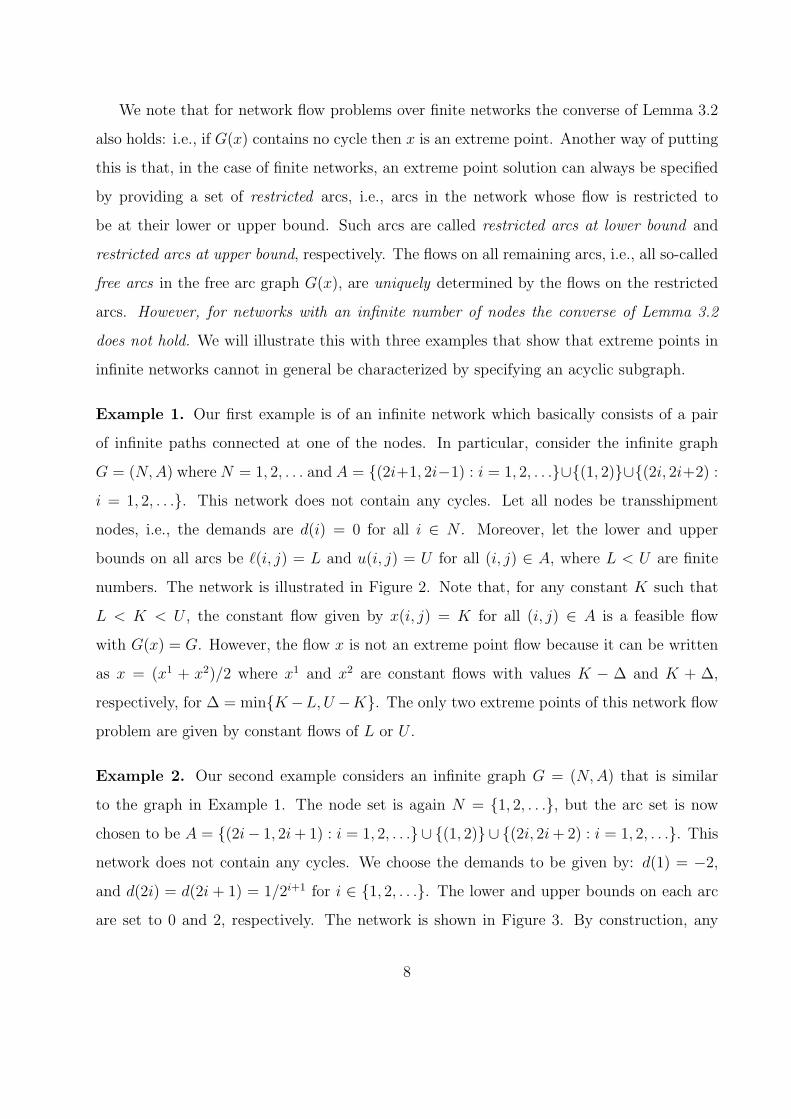
3 Extreme Point Flows

In this section we develop necessary and sufficient conditions for a feasible flow x in a graph

G to be an extreme point. However, we first address the issue of the existence of an extreme

point in an infinite network flow problem.

Theorem 3.1 Given a network G with demands d and finite lower and upper bounds `, u ∈R|A|, if the network flow problem is feasible then an extreme point solution exists.

Proof: The set of solutions of the network flow problem is clearly convex. Further, since

the value of each arc flow is bounded, the solution space is also compact with respect to the

product topology. The Krein-Milman theorem (see Aliprantas and Border [2]) then implies

that, if the solution space is non-empty, it contains an extreme point. 2

Note that all results in this paper continue to hold if some or all of the flow bounds are

infinite. However, in that case the set of extreme points may be empty.

3.1 Why the finite extreme point characterization fails for infinite

networks

Given the result of Theorem 3.1, there always exists an extreme point solution whenever

the problem is feasible. The following necessary condition for a flow to be an extreme point

follows directly using a similar argument as for network flow problems over finite networks.

Lemma 3.2 If a feasible flow x is an extreme point then G(x) contains no cycles. 2

7

We note that for network flow problems over finite networks the converse of Lemma 3.2

also holds: i.e., if G(x) contains no cycle then x is an extreme point. Another way of putting

this is that, in the case of finite networks, an extreme point solution can always be specified

by providing a set of restricted arcs, i.e., arcs in the network whose flow is restricted to

be at their lower or upper bound. Such arcs are called restricted arcs at lower bound and

restricted arcs at upper bound, respectively. The flows on all remaining arcs, i.e., all so-called

free arcs in the free arc graph G(x), are uniquely determined by the flows on the restricted

arcs. However, for networks with an infinite number of nodes the converse of Lemma 3.2

does not hold. We will illustrate this with three examples that show that extreme points in

infinite networks cannot in general be characterized by specifying an acyclic subgraph.

Example 1. Our first example is of an infinite network which basically consists of a pair

of infinite paths connected at one of the nodes. In particular, consider the infinite graph

G = (N, A) where N = 1, 2, . . . and A = {(2i+1, 2i−1) : i = 1, 2, . . .}∪{(1, 2)}∪{(2i, 2i+2) :

i = 1, 2, . . .}. This network does not contain any cycles. Let all nodes be transshipment

nodes, i.e., the demands are d(i) = 0 for all i ∈ N . Moreover, let the lower and upper

bounds on all arcs be `(i, j) = L and u(i, j) = U for all (i, j) ∈ A, where L < U are finite

numbers. The network is illustrated in Figure 2. Note that, for any constant K such that

L < K < U , the constant flow given by x(i, j) = K for all (i, j) ∈ A is a feasible flow

with G(x) = G. However, the flow x is not an extreme point flow because it can be written

as x = (x1 + x2)/2 where x1 and x2 are constant flows with values K − ∆ and K + ∆,

respectively, for ∆ = min{K−L,U −K}. The only two extreme points of this network flow

problem are given by constant flows of L or U .

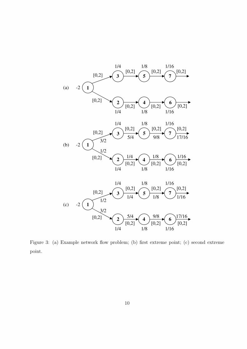
Example 2. Our second example considers an infinite graph G = (N, A) that is similar

to the graph in Example 1. The node set is again N = {1, 2, . . .}, but the arc set is now

chosen to be A = {(2i− 1, 2i + 1) : i = 1, 2, . . .} ∪ {(1, 2)} ∪ {(2i, 2i + 2) : i = 1, 2, . . .}. This

network does not contain any cycles. We choose the demands to be given by: d(1) = −2,

and d(2i) = d(2i + 1) = 1/2i+1 for i ∈ {1, 2, . . .}. The lower and upper bounds on each arc

are set to 0 and 2, respectively. The network is shown in Figure 3. By construction, any

8

2 4 6 8

1 3 5 7

[L,U] [L,U] [L,U] [L,U]

[L,U] [L,U] [L,U] [L,U]

[L,U]

K K K K

K K K K

K

Figure 2: A network with no cycles.

feasible flow x would satisfy 0 < x(i, j) ≤ 3/2 for all (i, j) ∈ A. Hence, for any feasible

flow x we have that G(x) = G. However, there are only two feasible solutions that are

extreme points. The first solution is given by x(2i− 1, 2i + 1) = 1 + 1/2i for i ∈ {1, 2, . . .},x(1, 2) = 1/2, and x(2i, 2i+2) = 1/2i+1 for i ∈ {1, 2, . . .}. The second extreme point is given

by x(2i − 1, 2i + 1) = 1/2i for i ∈ {1, 2, . . .}, x(1, 2) = 3/2, and x(2i, 2i + 2) = 1 + 1/2i+1

for i ∈ {1, 2, . . .}. Note that the total demand of all demand nodes is equal to 1, whereas

the supply of the only supply node is equal to 2. Therefore, there is one unit of flow that is

shipped from the supply node for which no demand exists. An extreme point in the network

corresponds to a solution in which the excess unit supplied flows through either the infinite

path 1− 2− 4− 6− · · · or the infinite path 1− 3− 5− 7− · · ·. Any feasible flow in which

the excess unit supplied is shared by these two infinite path is not an extreme point.

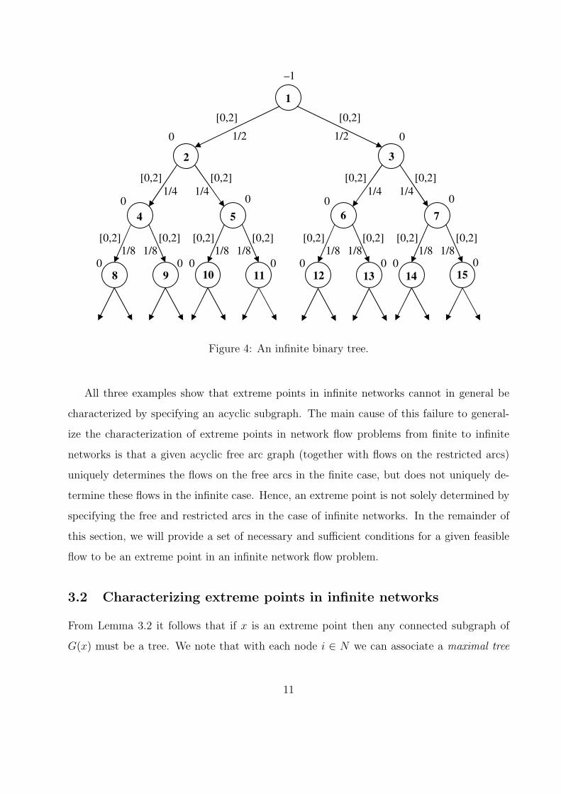
Example 3. Our third example is the case of an infinite binary tree (see Figure 4). In

this network, we assume that the root node has a supply of 1 unit (i.e., d(1) = −1), and

all other nodes are transshipment nodes (d(i) = 0 for all i ∈ N \ {1}. Furthermore, let the

lower and upper bounds on the arc flows be 0 and 2 units, respectively. Figure 4 shows a

feasible solution with positive flow on all arcs in the network. Moreover, it is clear that the

free arc graph corresponding to any feasible flow does not contain any cycles. However, the

only extreme points in this network flow problem are feasible flows that carry a single unit

along a single infinite path from the root node 1.

9

2 4 6

1

3 5 7 [0,2] [0,2] [0,2] [0,2]

[0,2]

[0,2] [0,2] [0,2]

-2

1/4 1/8 1/16

1/4 1/8 1/16

(a)

2 4 6

1

3 5 7 [0,2] [0,2] [0,2] [0,2]

[0,2]

[0,2] [0,2] [0,2]

-2

1/4 1/8 1/16

1/4 1/8 1/16

(b) 3/2

1/2

5/4 9/8 17/16

1/4 1/8 1/16

2 4 6

1

3 5 7 [0,2] [0,2] [0,2] [0,2]

[0,2]

[0,2] [0,2] [0,2]

-2

1/4 1/8 1/16

1/4 1/8 1/16

(c) 1/2

3/2

1/4 1/8 1/16

5/4 9/8 17/16

Figure 3: (a) Example network flow problem; (b) first extreme point; (c) second extreme

point.

10

1

2

4 5

3

6 7

9 8 11 10 13 12 15 14

–1

0

0 0 0 0

0

0 0 0 0 0 0 0

[0,2] [0,2]

[0,2] [0,2] [0,2] [0,2]

[0,2] [0,2] [0,2] [0,2] [0,2] [0,2] [0,2] [0,2]

0

1/2 1/2

1/4 1/4 1/4 1/4

1/8 1/8 1/8 1/8 1/8 1/8 1/8 1/8

Figure 4: An infinite binary tree.

All three examples show that extreme points in infinite networks cannot in general be

characterized by specifying an acyclic subgraph. The main cause of this failure to general-

ize the characterization of extreme points in network flow problems from finite to infinite

networks is that a given acyclic free arc graph (together with flows on the restricted arcs)

uniquely determines the flows on the free arcs in the finite case, but does not uniquely de-

termine these flows in the infinite case. Hence, an extreme point is not solely determined by

specifying the free and restricted arcs in the case of infinite networks. In the remainder of

this section, we will provide a set of necessary and sufficient conditions for a given feasible

flow to be an extreme point in an infinite network flow problem.

3.2 Characterizing extreme points in infinite networks

From Lemma 3.2 it follows that if x is an extreme point then any connected subgraph of

G(x) must be a tree. We note that with each node i ∈ N we can associate a maximal tree

11

T = (N ′, A′) in the graph G(x) given by the node set N ′ = {i′ ∈ N : i and i′ are connected in

G(x)}. It can be easily shown that the maximal trees associated with any pair of nodes

i, j ∈ N that are connected are identical. Therefore, the graph G(x) consists of one or

more (and possibly countably infinitely many) maximal trees such that there are no arcs in

A(x) connecting two different maximal trees. Given a maximal tree T = (N ′, A′, r) in G(x)

(rooted at a node r ∈ N ′) we define, for every node i ∈ N ′,

RT (i) = infS∈S(T (i))

∑

(i′,j′)∈S

r(i′, j′).

The value RT (i) provides a measure of the maximum amount by which the flow on the arc

connecting node i and its parent in T , pT (i), could be changed when we are only allowed

to balance that change by modifying arc flows in the subtree T (i). Note that if T (i) is a

finite tree, the empty cut is a valid finite cut, and we immediately obtain that RT (i) = 0.

Intuitively, this can be seen by observing that the flow balance constraints prohibit changing

the flow on any given arc when we may only balance that change using changes in the subtree

T (i). The following lemma provides a key property of the functions RT (i).

Lemma 3.3 Given a rooted tree T = (N ′, A′, r), the function RT (i) for i ∈ N ′ is given by

RT (i) =∑

j∈CT (i)

min{αij, RT (j)}

where

αij =

r(i, j) if (i, j) ∈ A′

r(j, i) otherwise.

Proof: See the Appendix. 2

We will next illustrate the measure RT (i) for infinite networks through the three examples

presented in Section 3.1.

Example 1. Consider a solution of the form x(i, j) = K for all (i, j) ∈ A where L < K < U ,

so that G(x) = G. Thus G(x) contains a single maximal tree: G(x) itself. If we consider this

tree, say T , rooted at node 1, we obtain that RT (i) = ∆ for i ∈ N \ {1} and RT (1) = 2∆.

12

Since node 1 has 2 children in T with positive RT (i) we can reroute flow by the amount ∆

in the tree T in two directions. Therefore, the solution x is not an extreme point.

Example 2. In this example, any feasible flow has G(x) = G which, in turn, is equal to the

single maximal tree in G(x). We consider this tree, say T , rooted at node 1. Now consider the

midpoint of the two solutions illustrated in Figures 3(b) and (c): x(2i−1, 2i+1) = 1/2+1/2i

for i ∈ {1, 2, . . .}, x(1, 2) = 1, and x(2i, 2i + 2) = 1/2 + 1/2i+1 for i ∈ {1, 2, . . .}. For this

solution, we have that RT (2i) = RT (2i + 1) = 1/2 for i ∈ {1, 2, . . .} and RT (1) = 1. Since

node 1 has 2 children in T with positive RT (i), we can reroute flow in the tree T by 1/2 in

two directions and thus the solution x is not an extreme point. However, for the solution in

Figure 3(b) we have that RT (2i + 1) = 1 for i ∈ {1, 2, . . .}, RT (2i) = 0 for i ∈ {1, 2, . . .},and RT (1) = 1. In this case, each node has at most a single child in T with positive RT (i)

so that we cannot reroute flow by any positive amount in the tree T so the solution x is an

extreme point.

Example 3. Consider the feasible flow, say x, illustrated in Figure 4. For this flow we have

that G(x) = G which, in turn, is equal to the single maximal tree in G(x). We consider this

tree, say T , rooted at node 1. Then RT (i) = 1/2 for i ∈ {2, 3} and RT (1) = 1. Since node

1 has 2 children in T with positive RT (i), we can reroute flow in the tree T by 1/2 in two

directions and the solution x is not an extreme point. It is easy to see that any feasible flow

except a flow that sends 1 unit along a single infinite directed path from node 1 is not an

extreme point either.

The definition of RT (i) and the three examples now motivate the following condition

which, as we will show in the remainder of this section, is necessary and sufficient for a

feasible flow x in G to be an extreme point.

Condition 3.4

(a) G(x) contains no cycles.

(b) Every maximal tree T = (N ′, A′) in G(x) can be rooted at some node r ∈ N ′ such that

any node i ∈ N ′ with RT (i) > 0 has at most one child j ∈ CT (i) such that RT (j) > 0.

13

We will refer to this condition as Extreme Point Condition 3.4. Although Extreme Point

Condition 3.4(b) requires the existence of some root node with the desired property for

each maximal tree, it is in fact equivalent to the (seemingly more restrictive and sometimes

more convenient) condition that the desired property holds for all choices of root node, as

is formally proven in Lemma A.1 in the Appendix. That is, we can replace Extreme Point

Condition 3.4(b) by

(b′) In every maximal tree T = (N ′, A′, r) in G(x) rooted at any node r ∈ N ′, any node

i ∈ N ′ with RT (i) > 0 has at most one child j ∈ CT (i) such that RT (j) > 0.

We first establish the sufficiency of Extreme Point Condition 3.4 for a feasible flow x to

be an extreme point.

Proposition 3.5 A feasible flow x is an extreme point if it satisfies Extreme Point Condition

3.4.

Proof: Suppose that the feasible flow x satisfies Extreme Point Condition 3.4 but it is not an

extreme point. Let x1 and x2 be feasible flows such that x = (x1 +x2)/2 and x1 6= x2. Using

Proposition 2.1, it follows that L(x) = L(x1)∩L(x2) and U(x) = U(x1)∩U(x2). Therefore,

x1 and x2 can only differ over the arcs in the set A(x). Since G(x) contains no cycles by

Extreme Point Condition 3.4(a), every arc in A(x) must belong to a maximal tree in G(x).

Let (i, j) be an arc in some maximal tree T = (N ′, A′) in G(x) such that x1(i, j) 6= x2(i, j).

Since x, x1, and x2 are feasible flows, they each satisfy the flow balance constraint (1) at i.

Therefore one of the following two must happen (otherwise the flow balance at i would not

be satisfied):

(i) there is an arc (i, ) ∈ A′ such that 6= j and x1(i, ) 6= x2(i, ).

(ii) there is an arc (, i) ∈ A′ such that 6= j and x1(, i) 6= x2(, i).

Consider the maximal tree T rooted at node i, i.e., T = (N ′, A′, i). By observations above,

j, ∈ CT (i) when i is the root node. If RT (i) = 0, then by Lemma 3.3 it follows that

RT (j) = RT () = 0. If RT (i) > 0 then either RT (j) = 0 or RT () = 0 by Extreme Point

14

Condition 3.4(b′) (which must be satisfied since it is equivalent to Extreme Point Condition

3.4(b)).

Without loss of generality, let RT (j) = 0 and ∆ > 0 be such that x1(i, j) = x(i, j) −∆

(and thus x2(i, j) = x(i, j) + ∆). Since RT (j) = 0, by definition there must exist a finite cut

S ∈ S (T (j)) such that∑

(i′,j′)∈S r(i′, j′) < ∆. Using Lemma A.2 from the Appendix with

flows x and x1 over the finite cut S, we obtain that

∆ = |x(i, j)− x1(i, j)| ≤∑

(i′,j′)∈S

|x(i′, j′)− x1(i′, j′)|.

We note that for any arc (i′, j′) ∈ S

x(i′, j′)− x1(i′, j′) = x2(i′, j′)− x(i, j).

Using the fact that `(i′, j′) ≤ x1(i′, j′) ≤ u(i′, j′) and `(i′, j′) ≤ x2(i′, j′) ≤ u(i′, j′), it follows

that

|x(i′, j′)− x1(i′, j′)| ≤ min{x(i′, j′)− `(i′, j′), u(i′, j′)− x(i′, j′)} = r(i′, j′)

which implies that

∆ ≤∑

(i′,j′)∈S

r(i′, j′).

However, this contradicts the choice of S to be such that∑

(i′,j′)∈S r(i′, j′) < ∆. Therefore,

our assumption that x1(i, j) 6= x2(i, j) must be incorrect. Since the arc (i, j) was chosen

arbitrarily in A(x), it follows that x1 and x2 are identical on the set A(x), and we conclude

that x is an extreme point. 2

We next show that Extreme Point Condition 3.4 is necessary for a feasible flow to be an

extreme point.

Proposition 3.6 If a feasible flow x is an extreme point then it satisfies Extreme Point

Condition 3.4.

Proof: Let x be a feasible flow, and suppose that it is an extreme point. From Lemma 3.2,

it follows that G(x) contains no cycles. Suppose that there exists a maximal rooted tree

T = (N ′, A′, r) in G(x) such that there is a node i ∈ N ′ with two children j, ∈ CT (i) and

15

RT (i), RT (j), RT () > 0. We shall construct two feasible flows x1 and x2 such that x1 6= x2

and x = (x1 + x2)/2, providing contradiction to the assumption that x is an extreme point.

In particular, we will let the flows x1 and x2 be identical to x on all arcs except the arcs

between node i and nodes j, , and the arcs in sets Aj and A. For any of these remaining

arcs, say (i′, j′), we set the value of the flow x2(i′, j′) equal to 2x(i′, j′) − x1(i′, j′), so it

remains to specify the flow x1. For simplicity of the argument, we will show the construction

when (i, j), (i, ) ∈ A′; the other cases can be handled in a similar manner. Let

∆ = min {r(i, j), r(i, ), RT (j), RT ()}.

We set

x1(i, j) = x(i, j) + ∆

x1(i, ) = x(i, )−∆

(and thus x2(i, j) = x(i, j)−∆ and x2(i, ) = x(i, )+∆). Clearly, the flow balance constraint

(1) at node i and the bounds on the flow on arcs (i, j) and (i, ) are satisfied for both x1

and x2. The flow x1 on the arcs in Aj will be specified in a recursive manner as follows. By

definition, Lemma 3.3 says that

∆ ≤ RT (j) =∑

k∈CT (j)

min {αjk, RT (k)} .

It is easy to see that there exist non-negative numbers γ(k) for k ∈ CT (j) such that 0 ≤γ(k) ≤ min{αjk, RT (k)} and

∑k∈CT (j) γ(k) = ∆. For each child k ∈ CT (j) we now set

the flow on the arc connecting j with k. If (j, k) ∈ A′, we set x1(j, k) = x(j, k) + γ(k).

Otherwise, (k, j) ∈ A′ and we set x1(k, j) = x(k, j)−γ(k). This assignment ensures that the

flow balance at node j as well as the bounds on the arcs between node j and its children are

satisfied. The assignment also ensures that the flow x2 will satisfy both the flow balance and

the bound constraints. Note that the values γ(k) satisfy the condition γ(k) ≤ RT (k), so the

method used to determine the flows x1 on arcs between j and its children can be recursively

applied to find the flows on arcs between its children and their children. Also, note that the

recursive application of this procedure yields the flow x1 for all arcs in Aj so that the flow

16

balance constraints for the nodes in N j and the bounds on all arcs are satisfied. A similar

recursion can be used to determine an appropriate set of flow values x1 for the arcs in Ak.

The construction shows that if the flow x violates Extreme Point Condition 3.4 then

there exist flows x1 and x2 such that x1 6= x2 and x = (x1 + x2)/2. 2

Combining Propositions 3.5 and 3.6 we conclude the major result of this section that

Extreme Point Condition 3.4 is a necessary and sufficient condition for any feasible point x

to be an extreme point.

Theorem 3.7 A feasible flow x is an extreme point if and only if it satisfies Extreme Point

Condition 3.4.

3.3 A class of problems for which extreme points can be charac-

terized through free arcs or basic variables

In this section we will discuss an important class of network flow problems in infinite networks

for which the extreme points can be characterized through the free arc graph. In addition,

we will show that for this class of problems we can extend the concept of basic and non-basic

variables, and thus the concept of basic solutions, to the network flow problem. While it

seems unlikely that one can develop a simplex like method for general minimum linear cost

network flow problems in infinite networks, it may be possible to develop such a method for

network flow problems from the class discussed in this section.

3.3.1 Network flow problems with non-vanishing support

Consider the following extreme point condition that is stronger than Extreme Point Condi-

tion 3.4.

Condition 3.8

(a) G(x) contains no cycles.

(b) For any node i ∈ N there exists at most one infinite path i− i1 − i2 − · · · in G(x).

17

We will refer to this condition as Extreme Point Condition 3.8. If we informally think of

two paths to infinity as forming a doubly-infinite path, then we may rephrase Extreme Point

Condition 3.8 as the requirement that G(x) contains neither cycles nor doubly-infinite paths.

We will show in this section that Extreme Point Condition 3.8 is a necessary and sufficient

condition for a feasible flow x to be an extreme point if the network flow problem satisfies

the following assumption:

Assumption 3.9 For any extreme point x there exists a value θ > 0 such that if `(i, j) <

x(i, j) < u(i, j) for some (i, j) ∈ A then `(i, j) + θ ≤ x(i, j) ≤ u(i, j) − θ or, equivalently,

inf(i,j)∈A(x) r(i, j) > 0.

We will refer to this assumption as Non-Vanishing Support Assumption 3.9. The following

theorem provides the main result of this section.

Theorem 3.10 Suppose that the network flow problem given by G = (N,A), `, u, and d

satisfies Non-Vanishing Support Assumption 3.9. Then, a feasible flow x is an extreme point

if and only if Extreme Point Condition 3.8 is satisfied.

Proof: We prove the theorem by showing that if the network flow problem satisfies Non-

Vanishing Support Assumption 3.9, then Extreme Point Condition 3.8(b) is equivalent to

Extreme Point Condition 3.4(b′).

Suppose that the flow x satisfies conditions (a) and (b) in the theorem. Consider any

maximal rooted tree T = (N ′, A′, r) in G(x). Extreme Point Condition 3.8(b) along with

the assumption that any node has finite degree implies that for any node i ∈ N ′, at most

one subtree T (j) rooted at a child j ∈ CT (i) contains infinitely many nodes as otherwise

there would be two distinct infinite paths from node i. By definition, the value RT (j) is zero

if T (j) is finite because S = Ø is a finite cut of T (j) in this case. Therefore, for any node

i ∈ N ′, at most one child j ∈ CT (i) can have RT (j) > 0. In other words, the flow x satisfies

Extreme Point Condition 3.4(b).

Now suppose that the flow x satisfies Extreme Point Condition 3.4(b) and thus also

Extreme Point Condition 3.4(b′). Consider any node i ∈ N . Since G(x) contains no cycle,

node i must be part of a maximal tree. Let T = (N ′, A′, i) be the maximal tree containing

18

node i rooted at node i. Suppose that there are two distinct infinite paths P 1 = i−i1−i2−· · ·and P 2 = i− ı1− ı2−· · · in T . Then, i1 ∈ CT (i) and ik+1 ∈ CT (ik) for k = 1, 2, . . .. Similarly,

ı1 ∈ CT (i) and ık+1 ∈ CT (ık) for k = 1, 2, . . .. We note that every finite cut S ∈ S (T (i1))

must contain an arc from the path P 1. Since A(P 1) ⊆ A(x), r(i′, j′) ≥ θ for (i′, j′) ∈ A(P 1).

Therefore, by definition, RT (i1) ≥ θ > 0. Using a similar argument, RT (ı1) ≥ θ > 0.

However, this contradicts the assumption that the flow satisfies Extreme Point Condition

3.4(b′) because i1, ı1 ∈ CT (i). Hence, there cannot be two distinct infinite paths starting at

node i, and the flow x must satisfy Extreme Point Condition 3.8(b). 2

We note that the proof of Theorem 3.10 shows that Extreme Point Condition 3.8 is

sufficient for a feasible flow x to be an extreme point in general. In the special case where

the network flow problem satisfies Non-Vanishing Support Assumption 3.9 the conditions are

necessary as well, as the theorem states. Note that, in contrast Extreme Point Condition 3.4,

Extreme Point Condition 3.8 is dependent only on the graph G(x) and not the actual value

of the flow x. We use this observation to prove that if the network flow problem satisfies

Non-Vanishing Support Assumption 3.9 then any extreme point x can be expressed in terms

of its restricted arcs.

Theorem 3.11 Suppose that the network flow problem given by G = (N,A), `, u, and d

satisfies Non-Vanishing Support Assumption 3.9. Then, any extreme point x for the problem

is uniquely characterized by the sets L(x) and U(x).

Proof: Suppose that x1 and x2 are two extreme points such that L(x1) = L(x2), U(x1) =

U(x2), and x1 6= x2. Given our observation, G(x1) and G(x2) must be identical. Now

consider the feasible flow x = (x1 + x2)/2. By Proposition 2.1, L(x) = L(x1) = L(x2) and

U(x) = U(x1) = U(x2). We observe that for any feasible flow x, the graph G(x) can be

specified by providing the sets L(x) and U(x) because L(x)∪U(x)∪A(x) = A. This implies

that G(x), G(x1), and G(x2) are identical. Since x1 is an extreme point, G(x) = G(x1)

satisfies the conditions of Theorem 3.10. However this leads to a contradiction because

Theorem 3.10 then implies that x is an extreme point. Therefore, we can not have two

extreme points x1 6= x2 such that L(x1) = L(x2) and U(x1) = U(x2). 2

19

In Section 3.4 we will show that the class of network flow problems satisfying Non-

Vanishing Support Assumption 3.9 is large and significant: infinite network flow problems

where the demand and lower and upper bound data are integral always have integral valued

extreme points. Moreover, such problems satisfy Non-Vanishing Support Assumption 3.9

with θ = 1. However, we will first show that for this class of problems each extreme point

can be characterized by partitioning of the flow variables into basic variables and non-basic

variables.

3.3.2 Characterization of extreme points through basic and nonbasic variables

In the spirit of Extreme Point Condition 3.8, we will define a set of basic arcs or variables

as a set B ⊆ A with the following properties:

Condition 3.12

(a) The graph GB = (N,B) contains no cycles.

(b) For each node i ∈ N there exists exactly one infinite path i− i1 − i2 − · · · in GB.

Now consider a set B satisfying Condition 3.12. Note that this set is maximal in the

sense that there does not exist a set B′ such that B ⊂ B′ ⊆ A that satisfies Condition

3.12. Moreover, suppose we fix the flow on all arcs in A\B to an arbitrary value, say xij

for (i, j) ∈ A \ B. Then it follows immediately that the flows on all other arcs that satisfy

the flow balance constraints are uniquely defined. This can be seen as follows. Consider any

arc in B, say (i, j). This arc is on exactly one infinite path. Therefore, this infinite path

must have a leaf node, since it is, by definition, only infinite in one direction. The value of

the arc adjacent to the leaf node can then be found through the flow balance equation for

that node. (Note that the value of the flow on this arc may violate the bound constraints,

in which case the solution that we are constructing is infeasible.) Now remove the arc from

GB and proceed with the reduced network.

In summary, we will call any set B satisfying Condition 3.12 a set of basic variables

(and its complement will be the corresponding set of nonbasic variables). In analogy with

20

the concept of basic and nonbasic variables in finite-dimensional linear programming, any

solution satisfying the flow balance constraints that is found by choosing a basic set B and

fixing the corresponding nonbasic variables to either their lower or upper bound is a basic

solution. If this solution also satisfies all bound constraints it is a basic feasible solution;

otherwise, it is a basic infeasible solution. Note that this immediately implies that any basic

feasible solution is an extreme point.

It remains to be shown that for each extreme point solution x there exists an associated

set B(x) ⊇ A(x) satisfying Condition 3.12. If this is the case, it immediately follows that x

is a basic feasible solution. We will show that this is the case when the network flow problem

satisfies Non-Vanishing Support Assumption 3.9.

Theorem 3.13 Suppose that the network flow problem given by G = (N,A), `, u, and d

satisfies Non-Vanishing Support Assumption 3.9. Then any extreme point solution is a basic

feasible solution.

Proof: It is clear that an extreme point x is a basic feasible solution if G(x) happens to

satisfy Condition 3.12. If it does not, this means that there are some nodes in N that are

not in any infinite path – we therefore need to show that we can enlarge G(x) with such a

path for all such nodes without creating any cycles or doubly infinite paths. To this end, we

apply the following procedure:

Step 0. Initialize B = A(x).

Step 1. Let G′ = (N ′, B) be the graph induced by B, i.e.,

N ′ = {i ∈ N : ∃j ∈ N such that (i, j) ∈ B or (j, i) ∈ B}

and let G′′ = (N\N ′, A′′) be the graph induced by N\N ′, i.e.,

A′′ = {(i, j) ∈ A : i, j ∈ N\N ′}.

Step 2. If G′′ contains an infinite path then identify one, add all its arcs to the set B, and

return to Step 1. Otherwise, stop.

21

This procedure produces some set B. Note that this set B will contain exactly one infinite

path from each node in its node set N ′. Moreover, it will not contain any cycles since it is

the union of an acyclic subnetwork and a set of disjoint infinite paths. If N ′ = N , i.e., B

contains an arc adjacent to all nodes in N , it follows that B is the basic set corresponding

to x.

However, suppose that G′ 6= G. Then the corresponding set G′′ must be a countable

collection of disjoint finite subgraphs. In that case we perform the following procedure:

Step 1. Choose one of the finite subgraphs of G′′.

Step 2. Find a spanning tree, say T , in this subgraph.

Step 3. Find an arc (i, j) that connects T to G′ (note that such an arc indeed exists).

Step 4. Add the arcs in T as well as the connecting arc (i, j) to B and remove the subgraph

chosen in Step 1 from G′′.

Step 5. If G′′ 6= Ø, return to Step 1.

This procedure produces a new set B. We claim that this set satisfies Condition 3.12.

First, observe that the first procedure ensures that an infinite path exists from all nodes in

the graph G′ that results from this procedure. Furthermore, Step 4 in the second procedure

ensures that such a path exists for all other nodes. Therefore, each node in N contains a

path to infinity only consisting of arcs in B. Second, note that the graph G′ that results

from the first procedure is acyclic and the second procedure connects finite acyclic graphs

to this graph. This means that the second procedure cannot create a cycle or a doubly

infinite path. Therefore, the set B does not contain any cycles nor a node with more than

one infinite paths. 2

3.4 Integral network flow problems

In this section, we discuss a class of network flow problems where the demands d and the arc

capacities u can only take integral values. It is well-known (see for example, Ahuja et al. [1])

22

that in the case of finite networks, if the demands and the arc capacities are integral, then

any extreme point must have integral values for arc flows. We extend this result to infinite

network flow problems.

In order to prove this result we need to introduce some new notation. For any real

number a, we define af = min{a − bac, dae − a}. For a given flow x ∈ R|A|+ , we define its

rounding vector xf ∈ [0, 0.5]|A| through xf (i, j) = (x(i, j))f for (i, j) ∈ A.

Theorem 3.14 If the demands d as well as the lower and upper bounds ` and u in a network

flow problem only take integer values, then any extreme point of the problem is integral.

Proof: We will show that any feasible flow x which has a fractional value for some arc in

A does not satisfy Extreme Point Condition 3.4, so it can not be an extreme point. Hence,

the extreme points must have integral values for all arcs.

From Lemma 3.2, if the graph G(x) contains a cycle then x can not be an extreme point.

So suppose that we have a feasible flow x such that G(x) contains no cycle and for some

(i, j) ∈ A(x), x(i, j) has a fractional value (i.e., xf (i, j) > 0). Let T = (N ′, A′, i) be the

maximal tree containing the arc (i, j) rooted at i. Since the flow x satisfies the flow balance

equation (1) at node i and d(i) is an integer, there must exist another arc incident to node

i (different from (i, j)) that has fractional flow. There are two possible cases:

(i) there is an arc (i, ) in A′ such that 6= j and x(i, ) is fractional;

(ii) there is an arc (, i) in A′ such that 6= j and x(, i) is fractional.

We deal with case (i); case (ii) can be handled similarly. We observe that if the upper bounds

u only takes integer values, then for any feasible flow x, r(i, j) ≥ xf (i, j) for (i′, j′) ∈ A.

By definition, RT (j) = infS∈S(T (j))

∑(i′,j′)∈S r(i′, j′). From our observation it follows that

RT (j) ≥ infS∈S(T (j))

∑(i′,j′)∈S xf (i′, j′). We now use Lemma A.3 in the Appendix to conclude

that RT (j) ≥ xf (i, j) > 0 as i = pT (j) in T . By a similar argument, we can conclude

that RT () ≥ xf (i, ) > 0. This means that node i has two children j and such that

RT (j), RT () > 0 and therefore x does not satisfy Extreme Point Condition 3.4(b′), which is

equivalent to Extreme Point Condition 3.4(b). 2

23

The integrality of the extreme points in case the problem data are integral immediately

implies that Non-Vanishing Support Assumption 3.9 is satisfied:

Corollary 3.15 If the demands d as well as the lower and upper bounds ` and u in a

network flow problem only take integer values, then Non-Vanishing Support Assumption 3.9

is satisfied with θ = 1.

In turn, this then implies that Extreme Point Condition 3.8 characterizes all extreme points

to network flow problems with integral data.

4 An Application to the Infinite Horizon Capacitated

Economic Lot-Sizing Problem

In this section we will study the extreme point structure of the infinite horizon variant of

the classical capacitated economic lot-sizing problem with backordering. In this problem,

the uncapacitated version of which dates back to Wagner and Whitin [16] and Zangwill [17],

a producer faces a deterministic demand stream for a single product over a sequence of time

periods. This demand needs to be satisfied from production, which may be held in inventory

until demand occurs or used to satisfy past demands through backordering. The problem

is then to decide how much to produce in each time period to ensure that all demands are

satisfied at minimum production, inventory holding, and backordering costs. To formulate

this problem as an optimization problem, let us denote the time periods by t = 1, 2, . . ., and

the (integral) demand in time period t by dt. Furthermore, let ct(·), h+t (·), and h−t (·) denote

the production, inventory holding, and backlogging cost functions in period t, and assume

that they are concave and nondecreasing, where we assume that inventory and backordering

costs are charged against end of period inventory and backorder levels. Let pt, I+t , and

I−t denote the (integral and finite) production, inventory, and backorder limits in period t.

Finally, denote the quantity produced in period t by pt, the quantity in inventory at the end

of period t by I+t , and the quantity backordered at the end of period t by I−t . The problem

24

can then be formulated as:

minimize∞∑

t=1

(ct(pt) + h+

t (I+t ) + h−t (I−t )

)

subject to

p1 + I−1 = d1 + I+1

pt + I+t−1 + I−t = dt + I−t−1 + I+

t t = 2, 3, . . .

pt ≤ pt t = 1, 2, . . .

I+t ≤ I+

t t = 1, 2, . . .

I−t ≤ I−t t = 1, 2, . . .

pt, I+t , I−t ≥ 0 t = 1, 2, . . . .

When viewed as a subset of the product space∏∞

i=1R3, the feasible region is clearly compact.

Due to the concavity of the cost functions, we then know that if the lot-sizing problem has

an optimal solution, an extreme point optimal solution exists by Bauer’s Minimum Principle

(see Roy [13]). An optimal solution, in turn, exists if there exists a feasible solution with

finite cost value. (This is the case if, for example, (i) the cost functions are linear and

discounted at a rate in (0, 1) and dt ≤ pt ≤ p < ∞ for all t = 1, 2, . . . ,.) It is therefore of

interest to study the extreme point structure of the feasible region of the economic lot-sizing

problem.

When the horizon is finite, say T periods, the first step is usually to formulate the problem

as a minimum-cost network flow problem. In the most common network flow formulation (see

Figure 5), each period t is represented by a demand node with demand dt, and production is

represented by a source node with supply equal to the sum of all demands, i.e., the demand

of the source node is equal to −∑Tt=1 dt. Production in period t is represented by a directed

arc from the source node to node t with capacity pt, inventory carried from period t to

period t + 1 is represented by a directed arc from node t to node t + 1 with capacity I+t , and

backorders carried from period t + 1 to period t are represented by a directed arc from node

t + 1 to node t with capacity I−t . In this network, each feasible solution to the lot-sizing

problem is represented by a feasible flow.

25

1 2 3 … T

[0, 1p ] [0, 2p ] [0, 3p ] [0, Tp ]

0

1=

−∑T

t

t

d

d1

d2

d3

dT

[0, 1

+−TI ] [0, 3

+I ] [0, 2

+I ] [0, 1

+I ]

[0, 1

−I ] [0, 2

−I ] [0, 3

−I ] [0, 1

−−TI ]

Figure 5: A network representation of the finite-horizon economic lot-sizing problem.

This network flow formulation of the finite-horizon economic lot-sizing problem can be

used to derive properties of the extreme point solutions to this problem. It is well-known

that any extreme point solution satisfies the following conditions (see, e.g., Denardo [9]):

(i) All production and inventory quantities are integral-valued.

(ii) In no period t = 1, 2, . . . do we have that 0 < I+t < I+

t and 0 < I−t < I−t .

(iii) Consider two periods, say t1 and t2, in which the inventory and backorder levels are

either at zero or their capacity, while 0 < I+t < I+

t or 0 < I−t < I−t for all t =

t1 +1, . . . , t2−1 (such a sequence is often called a block or subplan). Then at most one

of the production quantitites pt, t = t1 + 1, . . . , t2 satisfies both its upper and lower

bound strictly, i.e., there exists at most one t = t1 + 1, . . . , t2 such that 0 < pt < pt.

The goal of this section is to generalize these properties to the infinite-horizon case. In fact,

we will show that, in addition, the following condition holds as well:

(iv) Consider a period, say t1, in which the inventory and backorder levels are either at

zero or their capacity, while 0 < I+t < I+

t or 0 < I−t < I−t for all t = t1 + 1, t1 + 2, . . .

26

(i.e., such a sequence generalizes the concept of a block or subplan). Then at most one

of the production quantitites pt, t = t1 + 1, t1 + 2, . . . satisfies both its upper and lower

bound strictly, i.e., there exists at most one t = t1 + 1, t1 + 2, . . . such that 0 < pt < pt.

When attempting to generalize the network-flow approach to the infinite-horizon eco-

nomic lot-sizing problem, it is immediate that we cannot use a network of the same form

as in the finite-horizon case. Since all demands are integral, total demand will be infinite if

we are dealing with a truly infinite-horizon problem. This implies that the total production

over the infinite horizon should be infinite as well. However, this means that the supply

of the source node is not well-defined in the straightforward generalization of the network.

Another complication is that the total out degree of the source node in this generalization

would be infinite, while the results on the structure of extreme points of infinite network

flow problems derived in this paper require that the in and out degrees of all nodes in the

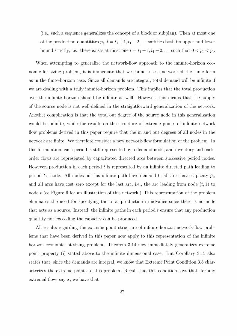
network are finite. We therefore consider a new network-flow formulation of the problem. In

this formulation, each period is still represented by a demand node, and inventory and back-

order flows are represented by capacitated directed arcs between successive period nodes.

However, production in each period t is represented by an infinite directed path leading to

period t’s node. All nodes on this infinite path have demand 0, all arcs have capacity pt,

and all arcs have cost zero except for the last arc, i.e., the arc leading from node (t, 1) to

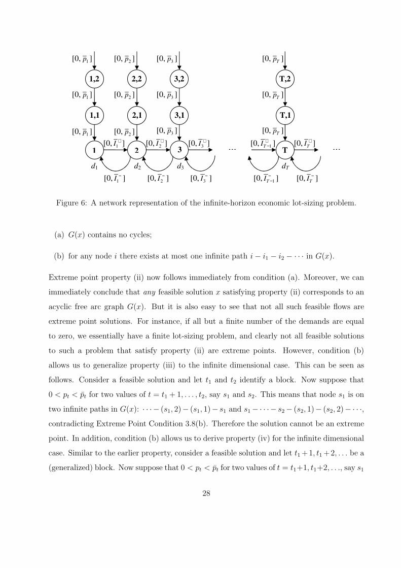
node t (ee Figure 6 for an illustration of this network.) This representation of the problem

eliminates the need for specifying the total production in advance since there is no node

that acts as a source. Instead, the infinite paths in each period t ensure that any production

quantity not exceeding the capacity can be produced.

All results regarding the extreme point structure of infinite-horizon network-flow prob-

lems that have been derived in this paper now apply to this representation of the infinite

horizon economic lot-sizing problem. Theorem 3.14 now immediately generalizes extreme

point property (i) stated above to the infinite dimensional case. But Corollary 3.15 also

states that, since the demands are integral, we know that Extreme Point Condition 3.8 char-

acterizes the extreme points to this problem. Recall that this condition says that, for any

extremal flow, say x, we have that

27

…

[0, 2p ]

1 2 3 T

d1

d2

d3

dT

1,1

1,2

[0, 1p ]

[0, 1p ]

[0, 1p ]

…

2,2

[0, 2p ]

[0, 2p ]

2,1

3,2

[0, 3p ]

[0, 3p ]

3,1

T,2

[0, Tp ]

[0, Tp ]

T,1

[0, Tp ] [0, 3p ]

[0, 1

+I ] [0, 2

+I ] [0, 3

+I ] [0, 1

+−TI ] [0, +

TI ]

[0, 1

−I ] [0, −

TI ] [0, 1

−−TI ] [0, 3

−I ] [0, 2

−I ]

Figure 6: A network representation of the infinite-horizon economic lot-sizing problem.

(a) G(x) contains no cycles;

(b) for any node i there exists at most one infinite path i− i1 − i2 − · · · in G(x).

Extreme point property (ii) now follows immediately from condition (a). Moreover, we can

immediately conclude that any feasible solution x satisfying property (ii) corresponds to an

acyclic free arc graph G(x). But it is also easy to see that not all such feasible flows are

extreme point solutions. For instance, if all but a finite number of the demands are equal

to zero, we essentially have a finite lot-sizing problem, and clearly not all feasible solutions

to such a problem that satisfy property (ii) are extreme points. However, condition (b)

allows us to generalize property (iii) to the infinite dimensional case. This can be seen as

follows. Consider a feasible solution and let t1 and t2 identify a block. Now suppose that

0 < pt < pt for two values of t = t1 + 1, . . . , t2, say s1 and s2. This means that node s1 is on

two infinite paths in G(x): · · · − (s1, 2)− (s1, 1)− s1 and s1− · · ·− s2− (s2, 1)− (s2, 2)− · · ·,contradicting Extreme Point Condition 3.8(b). Therefore the solution cannot be an extreme

point. In addition, condition (b) allows us to derive property (iv) for the infinite dimensional

case. Similar to the earlier property, consider a feasible solution and let t1 +1, t1 +2, . . . be a

(generalized) block. Now suppose that 0 < pt < pt for two values of t = t1+1, t1+2, . . ., say s1

28

and s2. This again means that node s1 is in two infinite paths in G(x): · · ·−(s1, 2)−(s1, 1)−s1

and s1 − · · · − s2 − (s2, 1)− (s2, 2)− · · ·, contradicting Extreme Point Condition 3.8(b).

Finally, we would like to remark that a similar approach to the one in this section may

be used to show that any extreme point to the uncapacitated infinite horizon economic lot-

sizing problem without backordering satisfies the standard zero-inventory ordering property

that production can only take place when there is no inventory, that is, It−1xt = 0 for all

t = 1, 2, . . ..

5 Conclusions and Future Research

In this paper, we studied the structure of the extreme points of infinite network flow problems.

Our results show that, unlike in the finite dimensional case, an extreme point for an infinite

network flow problem can, in general, not be uniquely represented in terms of free arcs.

Nevertheless, we developed necessary and sufficient conditions for a feasible flow to be an

extreme point that generalize this result. Moreover, under a regularity condition that is

met by network flow problems with integral data, we show that an extreme point can be

uniquely characterized by a set of free arcs corresponding to a subnetwork containing no finite

or infinite cycles. Finally, we showed that, when all problem data is integral, the extreme

points always have integral values, extending a result for finite network flow problems to the

infinite case.

In our future research we hope to generalize our structural results on extreme points

and basic feasible solutions to infinite dimensional network flow problems to larger classes

of doubly-infinite linear programming problems. Moreover, we intend to use the results of

this paper and their extensions to develop generalizations of the network simplex method

for solving linear minimum cost infinite network flow problems and the simplex method for

solving doubly-infinite linear programming problems.

29

References

[1] R.K. Ahuja, T.L. Magnanti, and J.B. Orlin, Network flows: theory, algorithms, and

applications, Prentice-Hall, Englewood Cliffs, New Jersey, 1993.

[2] C.D. Aliprantis and K.C. Border, Infinite dimensional analysis: A hitchhiker’s guide,

Springer-Verlag, Heidelberg, Germany, 1994.

[3] E.J. Anderson and P. Nash, Linear programming in infinite dimensional spaces, Wiley,

New York, New York, 1987.

[4] E.J. Anderson and A.B. Philpott, A continuous-time network simplex algorithm, Net-

works 19 (1989), 394–425.

[5] J.C. Bean, J.R. Lohmann, and R.L. Smith, A dynamic infinite horizon replacement

economy decision model, Eng Economist 30 (1985), 99–120.

[6] J.C. Bean and R.L. Smith, Conditions for the existence of planning horizons, Math

Oper Res 9 (Aug. 1984), 391–401.

[7] J.C. Bean and R.L. Smith, Optimal capacity expansion over an infinite horizon, Manage

Sci 31 (Dec. 1985), 1523–1532.

[8] W.P. Cross, H.E. Romeijn, and R.L. Smith, Approximating extreme points in infinite

dimensional convex sets, Math Oper Res 23 (1994), 433–442.

[9] E.V. Denardo, Dynamic programming: Models and applications, Prentice-Hall, Engle-

wood Cliffs, New Jersey, 1982.

[10] B. Fuchssteiner and K. Morisse, Infinite networks: minimal cost flows, Appl Math Lett

9 (1996), 89–93.

[11] R. Gomory and T.C. Hu, “Flows in continua,” Integer programs and network flows,

T.C. Hu, Addison Wesley, Reading, Massachusetts, 1969.

30

[12] P. Jones, J. Zydiak, and W. Hopp, Stationary dual prices and depreciation, Math Pro-

gram 41 (1988), 357–366.

[13] N.M. Roy, Extreme points of convex sets in infinite dimensional spaces, American Math

Monthly 94 (1987), 409–422.

[14] I.E. Schochetman and R.L. Smith, Infinite horizon optimization, Math Oper Res 14

(1989), 559–574.

[15] R.L. Smith and R.Q. Zhang, Infinite horizon production planning in time varying sys-

tems with convex production and inventory costs, Manage Sci 44 (1998), 1313–1320.

[16] H.M. Wagner and T.M. Whitin, Dynamic version of the economic lot size model, Manage

Sci 5 (1958), 89–96.

[17] W.I. Zangwill, A backlogging model and a multi-echelon model of a dynamic economic

lot sizing problem, Manage Sci 15 (1969), 506–527.

Appendix

Lemma 3.3 Given a rooted tree T = (N ′, A′, r), the function RT (i) for i ∈ N ′ is given by

RT (i) =∑

j∈CT (i)

min{αij, RT (j)}

where

αij =

r(i, j) if (i, j) ∈ A′

r(j, i) otherwise.

Proof: We observe that a finite cut S ∈ S (T (i)) can be partitioned into |CT (i)| disjoint

sets Sj (j ∈ CT (i)) where Sj either contains a finite cut of the subtree T (j) or contains the

arc between node j and i in T . Conversely, if we choose sets Sj for j ∈ CT (i) such that Sj is

either a finite cut of subtree T (j) or contains only the arc between node j and node i, then

31

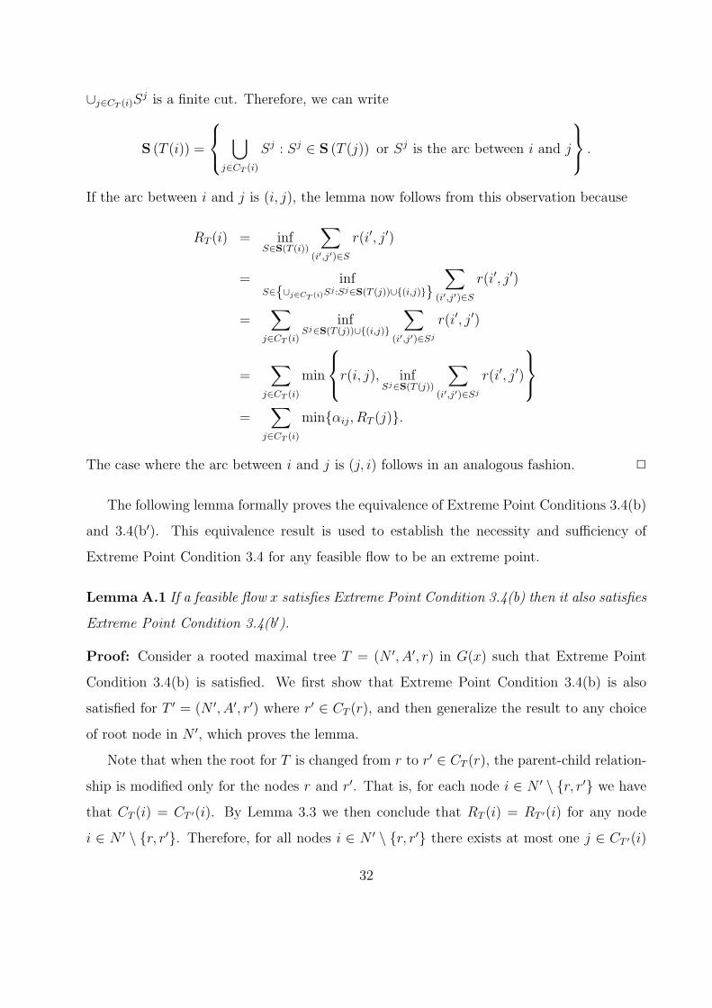
∪j∈CT (i)Sj is a finite cut. Therefore, we can write

S (T (i)) =

⋃

j∈CT (i)

Sj : Sj ∈ S (T (j)) or Sj is the arc between i and j

.

If the arc between i and j is (i, j), the lemma now follows from this observation because

RT (i) = infS∈S(T (i))

∑

(i′,j′)∈S

r(i′, j′)

= infS∈{∪j∈CT (i)S

j :Sj∈S(T (j))∪{(i,j)}}∑

(i′,j′)∈S

r(i′, j′)

=∑

j∈CT (i)

infSj∈S(T (j))∪{(i,j)}

∑

(i′,j′)∈Sj

r(i′, j′)

=∑

j∈CT (i)

min

r(i, j), inf

Sj∈S(T (j))

∑

(i′,j′)∈Sj

r(i′, j′)

=∑

j∈CT (i)

min{αij, RT (j)}.

The case where the arc between i and j is (j, i) follows in an analogous fashion. 2

The following lemma formally proves the equivalence of Extreme Point Conditions 3.4(b)

and 3.4(b′). This equivalence result is used to establish the necessity and sufficiency of

Extreme Point Condition 3.4 for any feasible flow to be an extreme point.

Lemma A.1 If a feasible flow x satisfies Extreme Point Condition 3.4(b) then it also satisfies

Extreme Point Condition 3.4(b′).

Proof: Consider a rooted maximal tree T = (N ′, A′, r) in G(x) such that Extreme Point

Condition 3.4(b) is satisfied. We first show that Extreme Point Condition 3.4(b) is also

satisfied for T ′ = (N ′, A′, r′) where r′ ∈ CT (r), and then generalize the result to any choice

of root node in N ′, which proves the lemma.

Note that when the root for T is changed from r to r′ ∈ CT (r), the parent-child relation-

ship is modified only for the nodes r and r′. That is, for each node i ∈ N ′ \ {r, r′} we have

that CT (i) = CT ′(i). By Lemma 3.3 we then conclude that RT (i) = RT ′(i) for any node

i ∈ N ′ \ {r, r′}. Therefore, for all nodes i ∈ N ′ \ {r, r′} there exists at most one j ∈ CT ′(i)

32

such that RT ′(j) > 0. Next, consider node r. Note that r′ is a child of r in T but not in

T ′, so that CT ′(r) = CT (r) \ {r′}. Since RT (i) = RT ′(i) for all i ∈ CT ′(r) ⊂ CT (r), node

r has at most one child j ∈ CT ′(r) such that RT ′(j) > 0. Finally, consider node r′. Note

that r is a child of r′ in T ′ but not in T , so that CT ′(r′) = CT (r′) ∪ {r}. Since Extreme

Point Condition 3.4(b) is satisfied for T , we have that if there exists some j ∈ CT (r) \ {r′}with RT (j) > 0 then RT (r′) = 0. In that case, by Lemma 3.3 we obtain that all j ∈ CT (r′)

must have RT (j) = 0 and therefore RT ′(j) = 0 for all j ∈ CT ′(r′) \ {r}. On the other hand,

if RT (r′) > 0 then RT (j) = 0 for all j ∈ CT (r) \ {r′}. In that case, RT ′(j) = RT (j) = 0

for all j ∈ CT ′(r) = CT (r) \ {r′} so that Lemma 3.3 implies that RT ′(r) = 0. Therefore,

since RT ′(j) = RT (j) for all j ∈ CT ′(r′) \ {r} there exists at most one j ∈ CT ′(r

′) such that

RT ′(j) > 0. Hence Extreme Point Condition 3.4(b) is satisfied for T ′.

Now consider an arbitrary node r′ ∈ N ′ and let again T ′ = (N ′, A′, r′). Let r =

i1, . . . , ik = r′ be the nodes on the unique finite path between r and r′ in T for some

k ≥ 2. Since i1 is a child of r in T rooted at r we can apply the result above to conclude that

Extreme Point Condition 3.4(b) is satisfied for T ′′ = (N ′, A′, i1). By repeatedly applying

the earlier result in this proof a finite number of times we conclude that Extreme Point

Condition 3.4(b) is satisfied for T ′. 2

The next lemma is a direct consequence of the flow balance equations satisfied by feasible

flows.

Lemma A.2 Let x and x′ be two feasible flows such that L(x) ⊆ L(x′), U(x) ⊆ U(x′),

and G(x) contains no cycles. Let T = (N ′, A′, r) be a maximal tree in G(x) rooted at node

r ∈ N ′. Then, for any node i ∈ N ′:

• if (i, pT (i)) ∈ A′ then |x(i, pT (i)) − x′(i, pT (i))| ≤ ∑(i′,j′)∈S |x(i′, j′) − x′(i′, j′)| for all

S ∈ S (T (i))

• if (pT (i), i) ∈ A′ then |x(pT (i), i) − x′(pT (i), i)| ≤ ∑(i′,j′)∈S |x(i′, j′) − x′(i′, j′)| for all

S ∈ S (T (i)).

Proof: We deal explicitly with the case (i, pT (i)) ∈ A′; the result for the other case can be

33

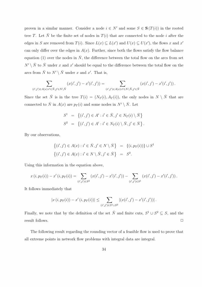
proven in a similar manner. Consider a node i ∈ N ′ and some S ∈ S (T (i)) in the rooted

tree T . Let N be the finite set of nodes in T (i) that are connected to the node i after the

edges in S are removed from T (i). Since L(x) ⊆ L(x′) and U(x) ⊆ U(x′), the flows x and x′

can only differ over the edges in A(x). Further, since both the flows satisfy the flow balance

equation (1) over the nodes in N , the difference between the total flow on the arcs from set

N ′ \ N to N under x and x′ should be equal to the difference between the total flow on the

arcs from N to N ′ \ N under x and x′. That is,

∑

(i′,j′)∈A(x):i′∈N,j′∈N\N(x(i′, j′)− x′(i′, j′)) =

∑

(i′,j′)∈A(x):i′∈N\N,j′∈N

(x(i′, j′)− x′(i′, j′)) .

Since the set N is in the tree T (i) = (NT (i), AT (i)), the only nodes in N \ N that are

connected to N in A(x) are pT (i) and some nodes in N i \ N . Let

S1 ={(i′, j′) ∈ Ai : i′ ∈ N , j′ ∈ NT (i) \ N

}

S2 ={(i′, j′) ∈ Ai : i′ ∈ NT (i) \ N , j′ ∈ N

}.

By our observations,

{(i′, j′) ∈ A(x) : i′ ∈ N , j′ ∈ N \ N

}= {(i, pT (i))} ∪ S1

{(i′, j′) ∈ A(x) : i′ ∈ N \ N , j′ ∈ N

}= S2.

Using this information in the equation above,

x (i, pT (i))− x′ (i, pT (i)) =∑

(i′,j′)∈S2

(x(i′, j′)− x′(i′, j′))−∑

(i′,j′)∈S1

(x(i′, j′)− x′(i′, j′)) .

It follows immediately that

|x (i, pT (i))− x′ (i, pT (i))| ≤∑

(i′,j′)∈S1∪S2

|(x(i′, j′)− x′(i′, j′))| .

Finally, we note that by the definition of the set N and finite cuts, S1 ∪ S2 ⊆ S, and the

result follows. 2

The following result regarding the rounding vector of a feasible flow is used to prove that

all extreme points in network flow problems with integral data are integral.

34

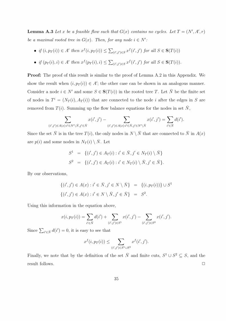
Lemma A.3 Let x be a feasible flow such that G(x) contains no cycles. Let T = (N ′, A′, r)

be a maximal rooted tree in G(x). Then, for any node i ∈ N ′:

• if (i, pT (i)) ∈ A′ then xf (i, pT (i)) ≤ ∑(i′,j′)∈S xf (i′, j′) for all S ∈ S(T (i))

• if (pT (i), i) ∈ A′ then xf (pT (i), i) ≤ ∑(i′,j′)∈S xf (i′, j′) for all S ∈ S(T (i)).

Proof: The proof of this result is similar to the proof of Lemma A.2 in this Appendix. We

show the result when (i, pT (i)) ∈ A′; the other case can be shown in an analogous manner.

Consider a node i ∈ N ′ and some S ∈ S(T (i)) in the rooted tree T . Let N be the finite set

of nodes in T i = (NT (i), AT (i)) that are connected to the node i after the edges in S are

removed from T (i). Summing up the flow balance equations for the nodes in set N ,

∑

(i′,j′)∈A(x):i′∈N ′\N,j′∈N

x(i′, j′)−∑

(i′,j′)∈A(x):i′∈N,j′∈N ′\Nx(i′, j′) =

∑

i′∈N

d(i′).

Since the set N is in the tree T (i), the only nodes in N \ N that are connected to N in A(x)

are p(i) and some nodes in NT (i) \ N . Let

S1 = {(i′, j′) ∈ AT (i) : i′ ∈ N , j′ ∈ NT (i) \ N}S2 = {(i′, j′) ∈ AT (i) : i′ ∈ NT (i) \ N , j′ ∈ N}.

By our observations,

{(i′, j′) ∈ A(x) : i′ ∈ N , j′ ∈ N \ N} = {(i, pT (i))} ∪ S1

{(i′, j′) ∈ A(x) : i′ ∈ N \ N , j′ ∈ N} = S2.

Using this information in the equation above,

x(i, pT (i)) =∑

i′∈N

d(i′) +∑

(i′,j′)∈S1

x(i′, j′)−∑

(i′,j′)∈S2

x(i′, j′).

Since∑

i′∈N d(i′) = 0, it is easy to see that

xf (i, pT (i)) ≤∑

(i′,j′)∈S1∪S2

xf (i′, j′).

Finally, we note that by the definition of the set N and finite cuts, S1 ∪ S2 ⊆ S, and the

result follows. 2

35