Extracting Complex Structural Geological Data from Outcrops ...

University of Wollongong University of Wollongong

Research Online Research Online

Faculty of Science, Medicine & Health - Honours Theses University of Wollongong Thesis Collections

2016

Extracting Complex Structural Geological Data from Outcrops Using Extracting Complex Structural Geological Data from Outcrops Using

Photogrammetry : Case Studies from Ladakh, Himalaya and the South Photogrammetry : Case Studies from Ladakh, Himalaya and the South

Coast, NSW Coast, NSW

Jacob Noblett Follow this and additional works at: https://ro.uow.edu.au/thsci

University of Wollongong University of Wollongong

Copyright Warning Copyright Warning

You may print or download ONE copy of this document for the purpose of your own research or study. The University

does not authorise you to copy, communicate or otherwise make available electronically to any other person any

copyright material contained on this site.

You are reminded of the following: This work is copyright. Apart from any use permitted under the Copyright Act

1968, no part of this work may be reproduced by any process, nor may any other exclusive right be exercised,

without the permission of the author. Copyright owners are entitled to take legal action against persons who infringe

their copyright. A reproduction of material that is protected by copyright may be a copyright infringement. A court

may impose penalties and award damages in relation to offences and infringements relating to copyright material.

Higher penalties may apply, and higher damages may be awarded, for offences and infringements involving the

conversion of material into digital or electronic form.

Unless otherwise indicated, the views expressed in this thesis are those of the author and do not necessarily Unless otherwise indicated, the views expressed in this thesis are those of the author and do not necessarily

represent the views of the University of Wollongong. represent the views of the University of Wollongong.

Recommended Citation Recommended Citation Noblett, Jacob, Extracting Complex Structural Geological Data from Outcrops Using Photogrammetry : Case Studies from Ladakh, Himalaya and the South Coast, NSW, BSci Hons, School of Earth & Environmental Sciences, University of Wollongong, 2016. https://ro.uow.edu.au/thsci/122

Research Online is the open access institutional repository for the University of Wollongong. For further information contact the UOW Library: [email protected]

https://ro.uow.edu.au/

https://ro.uow.edu.au/thsci

https://ro.uow.edu.au/thsci

https://ro.uow.edu.au/thesesuow

https://ro.uow.edu.au/thsci?utm_source=ro.uow.edu.au%2Fthsci%2F122&utm_medium=PDF&utm_campaign=PDFCoverPages

Extracting Complex Structural Geological Data from Outcrops Using Extracting Complex Structural Geological Data from Outcrops Using Photogrammetry : Case Studies from Ladakh, Himalaya and the South Coast, Photogrammetry : Case Studies from Ladakh, Himalaya and the South Coast, NSW NSW

Abstract Abstract Rendering high-definition 3D models is becoming a commonly requested task for scientific simulation, visualization and computer graphics. Many research areas generate extremely complex 3D models, such as industrial CAD models (e.g. airplanes, ships and architectures), composed of more than hundreds of millions of geometric primitives. However, these complex datasets cannot be rendered efficiently using brute-force methods on a desktop workstation. Desktop computer technology has recently reached a point where it has advanced sufficiently to calculate and process a number of photographs of an object from different perspectives to produce an accurate three-dimensional (3D) high-definition digital model. This project explores the potential applications of 3D digital models in terms of extracting complex geological data. Different methods of data acquisition and the scale of outcrops are compared between difficult to access rock outcrops in a remote High Himalayan region of Photoksar, Ladakh to more accessible, low lying coastal areas on the NSW South Coast at Bingie Bingie Point, Narooma, Wolumla and Eden. Archaeological sites and ultra-high resolution aerial photographs are also applied to the methods outlined. The application of photogrammetry at each site is assessed and compared to determine the benefit of it is applicable in any or all regions. The methods are assessed for efficiency, convenience and relevance of extracting complex structural geological data with emphasis on developing the highest quality digital 3D models possible. Any data extracted is tested for accuracy by comparing it with structural geological measurements obtained on the field by traditional methods using the trusted Field Move mobile application as a compass and clinometer equivalent. The results aim to provide a reliable and informative source of information outlining the methods used, what equipment is needed and what information can be extracted.

Degree Type Degree Type Thesis

Degree Name Degree Name BSci Hons

Department Department School of Earth & Environmental Sciences

Advisor(s) Advisor(s) Solomon Buckman

Keywords Keywords Photogrammetry, Unmanned Aerial vehicle, rendering

This thesis is available at Research Online: https://ro.uow.edu.au/thsci/122

https://ro.uow.edu.au/thsci/122

A thesis submitted in part fulfilment of the requirements of the Honours degree of Bachelor of Science in the School of Earth and Environmental Sciences

University of Wollongong, 2015

Extracting Complex Structural Geological Data from Outcrops Using

Photogrammetry: Case Studies from Ladakh, Himalaya and the South Coast,

NSW

Jacob Noblett

By

i

Abstract

Rendering high-definition 3D models is becoming a commonly requested task for scientific

simulation, visualization and computer graphics. Many research areas generate extremely

complex 3D models, such as industrial CAD models (e.g. airplanes, ships and architectures),

composed of more than hundreds of millions of geometric primitives. However, these

complex datasets cannot be rendered efficiently using brute-force methods on a desktop

workstation. Desktop computer technology has recently reached a point where it has

advanced sufficiently to calculate and process a number of photographs of an object from

different perspectives to produce an accurate three-dimensional (3D) high-definition digital

model. This project explores the potential applications of 3D digital models in terms of

extracting complex geological data. Different methods of data acquisition and the scale of

outcrops are compared between difficult to access rock outcrops in a remote High

Himalayan region of Photoksar, Ladakh to more accessible, low lying coastal areas on the

NSW South Coast at Bingie Bingie Point, Narooma, Wolumla and Eden. Archaeological sites

and ultra-high resolution aerial photographs are also applied to the methods outlined. The

application of photogrammetry at each site is assessed and compared to determine the

benefit of it is applicable in any or all regions. The methods are assessed for efficiency,

convenience and relevance of extracting complex structural geological data with emphasis

on developing the highest quality digital 3D models possible. Any data extracted is tested for

accuracy by comparing it with structural geological measurements obtained on the field by

traditional methods using the trusted Field Move mobile application as a compass and

clinometer equivalent. The results aim to provide a reliable and informative source of

information outlining the methods used, what equipment is needed and what information

can be extracted.

ii

Acknowledgements

I would like to express my sincere gratitude to my supervisor Dr Solomon Buckman for the

opportunity to work on this project and extensive fieldwork in Himalayas. Your guidance and help,

constructive feedbacks and expertise are greatly appreciated, thank you.

Sincere thank you is also dedicated to Associate Professor Brian G. Jones for guidance and help

throughout the year, your comments and opportunities to further broaden this project are greatly

appreciated.

I would also like to thank Dr Gert van den Bergh and Dr Alex MacKay for supplying site images and

research materials that were used in this project, your help, involvement and comments allowed to

broaden this project, thank you.

Sincere thank you goes to my loving family and friends who have put up with me and always

supported me when I needed help, thank you!

iii

Table of Contents

1 Chapter 1 - Introduction ........................................................................................................ 1

1.1. Aims and Objectives ........................................................................................................ 4

2 Chapter 2 - Literature Review Photogrammetry .................................................................. 6

2.1 3D Digital Models ................................................................................................................ 7

2.2 History of Photogrammetry ................................................................................................ 9

2.2.1 First Generation ........................................................................................................ 11

2.2.2 Analog Photogrammetry ........................................................................................... 11

2.2.3 Analytical Photogrammetry ...................................................................................... 11

2.2.4 Digital Photogrammetry ............................................................................................ 12

3 Chapter 3 - Methodology Creating 3D Models .................................................................... 13

3.1 Digital Photogrammetry .................................................................................................... 13

3.1.1 Phase 1- Reconnaissance .......................................................................................... 15

3.1.1.2 Field equipment .................................................................................................... 16

The equipment used in this project is outlined below. .......................................................... 16

3.1.2 Phase 2 - Photography .............................................................................................. 17

3.1.3 Phase 3 – Photoshop ................................................................................................. 22

3.1.4 Phase 4 – Digital Photogrammetry ............................................................................. 4

3.1.5 Phase 5 - Photogrammetric Products ....................................................................... 11

4 Chapter 4 - Field Work Methods and Results ...................................................................... 13

4.1 Project Applications .......................................................................................................... 13

iv

4.2 Camera Calibration – Julian Rocks .................................................................................... 14

4.3 Photoksar, Himalayas - High Alpine Photogrammetry ..................................................... 21

4.3.1 Photoksar, Ladakh, West Himalayas (high alpine) .................................................... 22

4.4 South Coast, NSW – Coastal Photogrammetry ................................................................. 33

4.4.1 Bingie Bingie Point .................................................................................................... 35

4.4.2 Narooma, South Coast of NSW ................................................................................. 40

4.4.3 Haycocks Point .......................................................................................................... 56

4.4.4 The Pinnacles ............................................................................................................ 60

4.4.5 Eagles Claw, NSW - Boat ........................................................................................... 64

4.4.6 Quarantine Bay ......................................................................................................... 70

4.4.7 Wolumla Cuttings ...................................................................................................... 74

4.5 Archaeological Application ............................................................................................... 79

4.5.1 The Hobbit - Mata Menge, Island of Flores, Indonesia (Drone) ............................... 79

4.5.2 Evolution of Early Man – Rocklands, South Africa .................................................... 86

4.6 Ultra-High Resolution Aerial Photographs – Uluru ........................................................... 92

5 Chapter 5 - Synthesis and Discussion .................................................................................. 97

5.1 Camera Calibration ........................................................................................................... 97

5.2 High Alpine vs Coastal Photogrammetry .......................................................................... 98

5.3 Digitization – The Photogrammetric Work Station (PWS) .............................................. 101

5.3.1 High versus Low Resolution Photographs ............................................................... 102

5.3.2 Windows 8GB RAM vs MacPro 32GB RAM ............................................................. 103

5.3.3 Colour Enhanced Photographs and Image Format Compatibilities ........................ 106

v

5.4 Archaeological Application ............................................................................................. 107

5.5 Extracting Structural Geological Data With PhotoScan .................................................. 109

5.5.1 KMZ Files and GeoVis 3D Developed by Dr Michael Roach .................................... 110

5.5.2 Orthophotograph .................................................................................................... 115

5.5.3 Animated Three Dimensional PDF Files .................................................................. 116

5.5.4 Blender .................................................................................................................... 118

6 Chapter 6 - Conclusion and Recomendations .................................................................... 120

References……………………………………………………………………………………………………………………….123

Appendix A …………………………………………………………………………………………………………………….131

Appendix B …………………………………………………………………………………………………………………….138

Appendix C …………………………………………………………………………………………………………………….140

Appendix D ……………………………………………………………………………………………………………………..USB

Appendix E ……………………………………………………………………………………………………………………..USB

Appendix F ………………………………………………………………………………………………………………………USB

Appendix G ……………………………………………………………………………………………………………………..142

vi

List of Figures

Figure 1-1: product of photogrammetry with digitised strike and dip measurements…………………. 2

FIGURE 2-1: BASIC SYSTEM FUNCTIONALITY OF A DIGITAL PHOTOGRAMMETRIC WORKSTATION (SCHENK 2005). ......................... 6

FIGURE 2-2: PHASE DEVELOPMENT THROUGH HISTORY OF PHOTOGRAMMETRY ..................................................................... 10

FIGURE 3-1: PHOTOGRAPHY WITH SELFIE POLE. ............................................................................................................... 17

FIGURE 3-2: PHOTOGRAPHY CHEAT SHEET (MERCER 2012). ............................................................................................ 19

FIGURE 3-3: SHOOTING PATTERNS RECOMMENDED BY AGISOFT (2015). ............................................................................. 20

FIGURE 3-4: A FLOW DIAGRAM OF PHOTOGRAMMETRIC PRODUCTS ABLE TO BE GENERATED FROM DIGITAL 3D MODELS. ............... 12

FIGURE 4-1: LOCATION OF JULIAN ROCKS ON THE BANKS OF BOMADERRY CREEK, BOMADERRY. ............................................... 15

FIGURE 4-2: EXAMPLES OF CAMERA SETTINGS: A) ISO 400, F-STOP 3. B) ISO 250, F-STOP 6. C) ISO-100, F-STOP 9. ............... 16

FIGURE 4-3: LOCATION OF PHOTOGRAPH EXTRACTION RELATIVE TO OUTCROP AT JULIAN ROCKS. .............................................. 17

FIGURE 4-4: SCREEN IMAGE OF PHOTOSCAN HIGH-RESOLUTION 3D MODEL OF JULIAN ROCKS ................................................. 20

FIGURE 4-5: LEFT; GEOMETRY OF POINTS (P) ON A DIPPING GEOLOGIC SURFACE REFERENCED TO A HORIZONTAL PLANE. ................ 21

FIGURE 4-6 LOCATION OF SITE 1, PHOTOKSAR, LADAKH, GPS: 34ᵒ4’11.01”N, 76ᵒ50’29.25”E ........................................... 23

FIGURE 4-7: GEOLOGICAL MAP OF LADAKH, NW HIMALAYAS, INDICATING THE STUDY SITE (CORFIELD 2001, P.12). ................... 25

FIGURE 4-8: PHOTOGRAPH COMPARISON. ..................................................................................................................... 27

FIGURE 4-9: LOCATION OF PHOTOGRAPH EXTRACTION RELATIVE TO THE OUTCROP IN: 1. ......................................................... 28

FIGURE 4-10: PHOTOGRAPH ADJUSTMENTS MADE. .......................................................................................................... 29

FIGURE 4-11: SCREEN IMAGE OF PHOTOSCAN HIGH-RESOLUTION 3D MODEL OF PHOTOKSAR.. ................................................ 32

FIGURE 4-12: GOOGLE EARTH MAP WITH YELLOW TAGS INDICATING THE LOCATION OF STUDY SITES. ......................................... 34

FIGURE 4-13: LOCATION OF PHOTOGRAPH EXTRACTION RELATIVE TO THE OUTCROP IN PHOTOSETS 1 AND 2 COMBINED. ............... 37

FIGURE 4-14: PHOTOGRAPH ADJUSTMENTS MADE.. ......................................................................................................... 37

FIGURE 4-15: SCREEN IMAGE OF PHOTOSCAN HIGH-RESOLUTION 3D MODEL OF BINGIE BINGIE POINT. .................................... 39

FIGURE 4-16: LOCATION OF SITE 2, NAROOMA ............................................................................................................... 40

FIGURE 4-17: DIAGRAM OF COAST AND SHORELINE ZONES AND DESCRIPTIVE BOUNDARIES. ..................................................... 41

FIGURE 4-18: GEOLOGICAL MAP OF THE NSW, SOUTH COAST INDICATING STUDY SITE AT NAROOMA, SURF BEACH ...................... 42

vii

FIGURE 4-19: LOCATION OF PHOTOGRAPH EXTRACTION RELATIVE TO THE OUTCROP .............................................................. 45

FIGURE 4-20: LOCATION OF PHOTOGRAPH EXTRACTION RELATIVE TO THE OUTCROP ............................................................... 46

FIGURE 4-21: PHOTOGRAPHS FROM SITE A DID NOT REQUIRE ANY ADJUSTMENTS ONLY CONVERSION FROM RAW TO JPG. .......... 47


FIGURE 4-23: SCREEN IMAGE OF HIGH-RESOLUTION 3D MODEL OF SITE C MODEL 1. ............................................................. 50

FIGURE 4-24: SCREEN IMAGE OF PHOTOSCAN HIGH-RESOLUTION 3D MODEL OF SITE A ......................................................... 52

FIGURE 4-25: SCREEN IMAGE OF PHOTOSCAN HIGH-RESOLUTION 3D MODEL OF SITE B,. ........................................................ 53

FIGURE 4-26: SCREEN IMAGE OF PHOTOSCAN HIGH-RESOLUTION 3D MODEL OF SITE D. ........................................................ 54

FIGURE 4-27: SCREEN IMAGE OF PHOTOSCAN HIGH-RESOLUTION 3D MODEL OF SITE E .......................................................... 55

FIGURE 4-28: LOCATION OF PHOTOGRAPH EXTRACTION RELATIVE TO THE OUTCROP IN PHOTOSET 2. ......................................... 57

FIGURE 4-29: PHOTOGRAPH ADJUSTMENTS MADE.. ......................................................................................................... 58

FIGURE 4-30: SCREEN IMAGE OF PHOTOSCAN HIGH-RESOLUTION 3D MODEL OF HAYCOCKS POINT, ......................................... 59


FIGURE 4-32: PHOTOSHOP ADJUSTMENTS ..................................................................................................................... 62

FIGURE 4-33: SCREEN IMAGE OF PHOTOSCAN HIGH-RESOLUTION 3D MODEL OF THE PINNACLES .............................................. 63

FIGURE 4-34: GEOLOGICAL MAP OF THE SOUTH EASTERN CORNER OF NSW (NSW GOVERNMENT, 1995). ............................... 65

FIGURE 4-36: LOCATION OF PHOTOGRAPH EXTRACTION BY BOAT RELATIVE TO THE SHORELINE OUTCROP IN PHOTOSET 1. .............. 67


FIGURE 4-37: SCREEN IMAGE OF PHOTOSCAN HIGH-RESOLUTION 3D MODEL OF EAGLES CLAW, .............................................. 69



FIGURE 4-40: SCREEN IMAGE OF PHOTOSCAN HIGH-RESOLUTION 3D MODEL OF QUARANTINE BAY, MODEL 2. ........................... 73

FIGURE 4-41: LOCATION OF PHOTOGRAPH EXTRACTION RELATIVE TO THE OUTCROP IN PHOTOSET 1, SITE B. ............................... 76

FIGURE 4-42: PHOTOGRAPH ADJUSTMENTS. ................................................................................................................... 77

FIGURE 4-43: SCREEN IMAGE OF PHOTOSCAN HIGH-RESOLUTION 3D MODEL OF WOLUMLA CULLTINGS, ................................... 78

FIGURE 4-44: LOCATION OF PHOTOGRAPH EXTRACTION RELATIVE TO THE OUTCROP IN: A) PHOTOSET 1. B) PHOTOSET 2. ............. 82

FIGURE 4-45: A) PHOTOGRAPH FROM UAV IN PHOTOGRAPH INSIDE TRENCH CAPTURE BY SAMSUNG GALAXY S5. ...................... 83

FIGURE 4-46: SCREEN IMAGE OF PHOTOSCAN HIGH-RESOLUTION 3D MODEL OF MATA MENGE DEVELOPED FROM DRONE. .......... 85

FIGURE 4-47: SCREEN IMAGE OF PHOTOSCAN HIGH-RESOLUTION 3D MODEL OF MATA MENGE, ............................................. 86

viii

FIGURE 4-48: LOCATION OF PHOTOGRAPH EXTRACTION RELATIVE TO THE OUTCROP IN:........................................................... 89

FIGURE 4-49: NO PHOTOGRAPH ADJUSTMENTS REQUIRED AS PHOTOGRAPHS WERE CAPTURED IN JPG FORMAT. ......................... 90

FIGURE 4-50: SCREEN IMAGE OF PHOTOSCAN HIGH-RESOLUTION 3D MODEL OF ROCKLANDS CAVE. ......................................... 92


FIGURE 4-52: NO PHOTOGRAPH ADJUSTMENTS MADE. THERE ARE 6 IMAGES SHOWN MANUALLY OVERLAPPED. .......................... 95

FIGURE 4-53: SCREEN IMAGE OF PHOTOSCAN HIGH-RESOLUTION 3D MODEL OF ULURU, MODEL 1. ......................................... 96

FIGURE 5-1: A) LOWEST QUALITY (DETAIL) MESH .......................................................................................................... 104

FIGURE 5-2: A FIGURE CREATED BY DR GERT VAN DEN BERGH INCLUDING MODEL 5 ............................................................ 108

FIGURE 5-3: TOP; BEDDING LAYER IDENTIFIED BY DIFFERENCE IN COLOUR ON A CORNER OF THE OUTCROP. ............................... 111

FIGURE 5-4: TOP: A NUMBER OF ‘BEST FIT PLANES’ ARE PLACES ON THE 3D MODEL IN GEOVIS 3D CREATED IN PHOTOSCAN.. ..... 112

FIGURE 5-5: TOP; IDENTIFIED EXPOSED BEDDING PLANES FOR PLACING ‘BEST FIT PLANES’. ..................................................... 113

FIGURE 5-6: TOP, MIDDLE: A NUMBER OF ‘BEST FIT PLANES’ ARE PLACES ON THE 3D MODEL IN GEOVIS 3D ............................ 114

FIGURE 5-7 : TOP: HIGH-RESOLUTION DIGITAL ORTHOPHOTO MOSAIC OF HAYCOCKS POINT CAPTURED FROM FRONT ................. 115

FIGURE 5-8: HIGH-RESOLUTION DIGITAL ORTHOPHOTO MOSAIC OF QUARANTINE BAY. ......................................................... 116

FIGURE 5-9: SCREEN IMAGE OF BINGIE BINGIE POINT ANIMATED PDF FILE WITH 3D MEASUREMENTS IN CENTIMETRES .............. 117

FIGURE 5-10: SCREEN IMAGE OF MATA MENGE ANIMATED PDF FILE WITH 3D COMMENTS OF TRENCH SITES (APPENDIX E6). ... 117

FIGURE 5-11: BINGIE BINGIE POINT HIGH-RESOLUTION 3D MODEL OBJ FILE IMPORT INTO BLENDER AND MODIFIED. ................ 118

ix

List of Tables

TABLE 3-1: PHOTOGRAMMETRY BROADLY PORTRAYED AS A SYSTEMS APPROACH. .................................................................. 14

TABLE 3-2: CAMERAS TRIALLED IN THIS PROJECT. ............................................................................................................. 18

TABLE 3-3: FORMATS ACCEPTED BY AGISOFT PHOTOSCAN................................................................................................. 22

TABLE 4-1: CAMERA SPECIFICATIONS AND SETTINGS OF PHOTOSETS CAPTURED AT JULIAN ROCKS. ............................................. 16

TABLE 4-2: PHOTOSHOP ADJUSTMENTS AND MODELS MADE FROM EACH PHOTOSET. .............................................................. 18

TABLE 4-3: SETTINGS AND SPECIFICATIONS USED IN PHOTOSCAN TO CREATE HIGH-DEFINITION 3D MODELS OF JULIAN ROCKS. ....... 19

TABLE 4-4: CAMERA SPECIFICATIONS AND SETTINGS OF PHOTOSETS CAPTURED AT PHOTOKSAR, LADAKH, HIGH HIMALAYAS. ......... 26


TABLE 4-6: SETTINGS AND SPECIFICATIONS USED IN PHOTOSCAN TO CREATE HIGH-DEFINITION 3D MODELS OF PHOTOKSAR. ......... 31

TABLE 4-7: CAMERA SPECIFICATIONS AND SETTINGS OF PHOTOSETS CAPTURED AT BINGIE BINGIE POINT. ................................... 36


TABLE 4-9: SETTINGS AND SPECIFICATIONS USED TO CREATE HIGH-DEFINITION 3D MODELS OF BINGIE BINGIE POINT. ................... 39

TABLE 4-10: CAMERA SPECIFICATIONS AND SETTINGS OF PHOTOSETS CAPTURED AT NAROOMA, NSW. ..................................... 44

TABLE 4-11: PHOTOSHOP ADJUSTMENTS AND MODELS MADE FROM EACH PHOTOSET. ............................................................ 49

TABLE 4-12: SETTINGS AND SPECIFICATIONS USED IN PHOTOSCAN TO CREATE HIGH-DEFINITION 3D .......................................... 51

TABLE 4-13: CAMERA SPECIFICATIONS AND SETTINGS OF PHOTOSETS CAPTURED AT HAYCOCKS POINT, EDEN, NSW. ................... 56

TABLE 4-14: PHOTOSHOP ADJUSTMENTS AND MODELS MADE FROM EACH PHOTOSET. ............................................................ 58

TABLE 4-15: SETTINGS AND SPECIFICATIONS USED IN PHOTOSCAN TO CREATE HIGH-DEFINITION 3D MODELS OF HAYCOCKS POINT. 59

TABLE 4-16: CAMERA SPECIFICATIONS AND SETTINGS OF PHOTOSETS CAPTURED AT THE PINNACLES, EDEN, NSW. ...................... 61

TABLE 4-17: SETTINGS AND SPECIFICATIONS USED IN PHOTOSCAN TO CREATE HIGH-DEFINITION 3D MODELS OF THE PINNACLES. ... 63

TABLE 4-18: CAMERA SPECIFICATIONS AND SETTINGS OF PHOTOSETS CAPTURED AT EAGLES CLAW, EDEN, NSW. ........................ 66

TABLE 4-19: PHOTOSHOP ADJUSTMENTS AND MODELS DEVELOPED FROM EACH PHOTOSET. .................................................... 68

TABLE 4-20: SETTINGS AND SPECIFICATIONS USED IN PHOTOSCAN TO CREATE HIGH-DEFINITION 3D MODELS OF EAGLES CLAW. ..... 69

TABLE 4-21: CAMERA SPECIFICATIONS AND SETTINGS OF PHOTOSETS CAPTURED AT QUARANTINE BAY, EDEN, NSW. ................... 71


x

TABLE 4-23: SETTINGS AND SPECIFICATIONS USED IN PHOTOSCAN TO CREATE HIGH-DEFINITION 3D MODELS OF QUARANTINE BAY. 73

TABLE 4-24: CAMERA SPECIFICATIONS AND SETTINGS OF PHOTOSETS CAPTURED AT WOLUMLA ROAD CUTTING, WOLUMLA, NSW. 75


TABLE 4-26: SETTINGS AND SPECIFICATIONS USED IN PHOTOSCAN TO CREATE HIGH-DEFINITION 3D MODELS OF WOLUMLA .......... 78

TABLE 4-27: CAMERA SPECIFICATIONS AND SETTINGS OF PHOTOSETS CAPTURED AT MATA MENGE, FLORESE, INDONESIA. ............ 81


TABLE 4-29: SETTINGS AND SPECIFICATIONS USED IN PHOTOSCAN TO CREATE HIGH-DEFINITION 3D MODELS OF MATA MENGE. .... 84

TABLE 4-30: CAMERA SPECIFICATIONS AND SETTINGS OF PHOTOSETS CAPTURED AT PAKHUIS PASS, CLANWILLIAM, SOUTH AFRICA. 87


TABLE 4-32: HIGH-DEFINITION 3D MODELS OF EXCAVATION SITES AT THE ROCKLANDS, SOUTH AFRICA. ..................................... 91

TABLE 4-33: CAMERA SPECIFICATIONS AND SETTINGS OF PHOTOSETS CAPTURED AT ULURU, MUTITJULU, NORTHERN TERRITORY. .. 93


TABLE 4-35: SETTINGS AND SPECIFICATIONS USED IN PHOTOSCAN TO CREATE HIGH-DEFINITION 3D MODELS OF ULURU. .............. 96

TABLE 5-1: CAMERAS TRIALLED IN THIS PROJECT AND THEIR RESOLUTION OUTPUT. ............................................................... 103

TABLE 5-2: BUILDING MODEL IN ARBITRARY MODE FROM 24MP PHOTOGRAPHS CAPTURED BY THE NIKON D610. .................. 105

1

1 Chapter 1 - Introduction

This project evaluates methods of digital photogrammetry and applications of high-resolution

3D digital models in the extraction of geological data from virtual outcrops. Three dimensional

models of outcrops are created for the purpose of extracting geological measurements remotely

without any physical contact with the rock. Thompson (1958) has defined photogrammetry as

the science or art of obtaining reliable measurements by means of photography.

Photogrammetry as a science is among the earliest techniques of remote sensing since the

invention of the photograph in the 1850s (Schenk 2005). The invention of the digital camera has

progressed photogrammetry from the analogue to the digital phase (Burtch 2005). There have

been rapid advances made in digital photogrammetry during recent years with the availability of

faster hardware and more sophisticated software, such as powerful image processing

workstations and vastly increased storage capacity (Carrivick 2013, Geological Survey of NSW

2015). Research and development efforts have resulted in operational products, such as AgiSoft

Photomodeller, give a few software examples, that are increasingly being used by government

organizations and private companies (ICSM 2008) to solve practical photogrammetric problems.

As technologies associated with photogrammetry improve, including the increasing availability

and affordability of drone aircraft carrying high resolution digital cameras, the potential

applications of photogrammetric methods in fields like geology will expand and become more

common place. Thus it is important that disciplines like Earth sciences stay up to date with the

pace of technological advances and regularly review and test current technologies and test

them against traditional methods of data collection. Currently, there are but a few recent

studies regarding geological applications of photogrammetry. Recent advances in hardware and

software, particularly advanced photographic positioning algorithms, mean that methods used

only 5 years ago are now redundant and out-dated. Photogrammetry and three dimensional

models are becoming increasingly useful in industries such as mining where visual inspection of

steep mine faces is dangerous and impractical but also in recreational pursuits such as golf or

trekking where people want to visualise golf courses or summit paths before attempting a shot

or climb. – maybe give a link to the AgiSoft Photomodeller website where they give examples of

applications?

2

Dr Matthew Cracknell and Dr Michael Roach have developed the most recent methods of

photogrammetry for creating high-resolution digital elevation models (DEM) at the University of

Tasmania. This project implements the method developed at the University of Tasmania

(Cracknel et al. 2013), investigating the applications of digital photogrammetry and 3D

modelling software for extracting complex geological data from outcrops that may be difficult or

expensive to access. The realistic high-resolution, 3D virtual models of sites of rock outcrops

give researchers the advantage of being able to “revisit” the site in a virtual sense and

potentially extract more useful data, such as bedding, foliation, fold axes, slope, aspect,

elevation and more from the outcrop (Cracknel et al. 2013). Dr Michael Roach from the

University of Tasmania has set up an online repository of freely available models of key outcrops

across Australia (see - http://www.utas.edu.au/earth-sciences/whats-new/news-

item/geological-visualisation ).

Figure 1-1: High-resolution 3D model, a product of photogrammetry with digitised strike and dip measurements.

Individual field applications were trialled at a number of different sites to develop and assess a

number of different methods for the application of digital photogrammetry in geology. Sites

include; 1) Nowra Sandstone, Bomaderry Creek, Bomaderry, to trial camera calibration in

manual setting, 2) high Himalayan mountains along the Indus Suture Zone at Photoksar, Ladakh

to experiment with large scale outcrop, 3) outcrops of the Wagonga Group at Narooma to trial

coastal outcrop digitization, 4) several outcrops of Merimbula Group formations at Eden used in

http://www.utas.edu.au/earth-sciences/whats-new/news-item/geological-visualisation

http://www.utas.edu.au/earth-sciences/whats-new/news-item/geological-visualisation

3

teaching undergraduate field geology at UOW, 5) an exposure of the Mutitjulu Arkose (Uluru) in

central Australia to trial aerial photography, and 6) archaeological sites at the Island of Floreses

in Indonesia and at the Rocklands in South Africa to trial archaeological application. The

extensive variety of geological sites was selected to assess and compare the methods used to

create DEMs at each one. Methods were also varied to incorporate assessment and evaluation

of using different cameras at different settings (manual versus automatic), cameras of different

resolutions (high versus low), different types of weather (sunny versus cloudy), a variety of

obstacles (alpine versus coastal) and to investigate what can be achieved from the results.

Dr Michael Roach states, small errors created by low resolution DEMs can significantly affect

measurements from bed planes with dip estimation being more susceptible than dip

orientation. Agisoft (2015) state, the accuracy of a model depends on effective image resolution

of a photoset, accuracy of GPS coordinates, quality of model reconstruction and images overlap.

Emphasis is made throughout the methods in this project to create the highest resolution model

possible at each site by processing photosets with the highest settings achievable by PhotoScan

likely to be limited by the processing power of the two computers used.

High-resolution 3D digital models were created primarily for evaluating the expediency and

efficiency of their application in geology to extract structural geological data. A secondary

advantage of creating high-resolution models is for addition to an online database to be freely

available for future studies by creating a record of 3D outcrops, including the date the images

were taken. Potential future studies include the study of rates of rock decay, downslope

movement or soil erosion over time as a function of wave action, sea level rise, and rates of rock

decay compared to rainfall on a particular escarpment by comparing the features of interest

with those created years afterwards. In laboratory and field conditions the use for these

methods is proving to be highly valuable (Gessesse et al. 2010, Morris et al. 2012, Rieke-Zapp

and Nearing 2005). If climate change is real it could be especially useful to have a database to

study what we have now as there may be a need for this information in the future as a result of

inundated coast lines (Li et al. 2009). This present project investigates what is possible with

photogrammetry and suggests potential uses for the technology. Methods are based on data

extraction techniques, the appropriate software programs available and focus on determining

the nature of the information that can be obtained from the results.

4

1.1. Aims and Objectives

The overarching aim of this project is to compare several methods of data extraction required to

create 3-D models of outcrops and to identify the methods most suitable to extract geologic

information from the model. Fieldwork will be at the high Himalayas near Photoksar in Ladakh and

the low lying coastal outcrops along the NSW south coast. Three other sites were also incorporated

to assess a variety of other applications. This project has been broken down into several achievable

objectives, which include:

I. Collect necessary photographs and structural geologic information using traditional methods

from selected study areas near the remote, difficult to access region of Himalayan village of

Photoksar and compare with relatively easy to access regions of Narooma on the south coast

of NSW.

II. Compare and contrast various cameras (Samsung Galaxy S5 versus Nikon DSLR) and camera

settings (auto versus manual exposures) to determine the best method of capturing multiple

images from which the Agisoft Photomodeller software will best match overlapping pixels

and build the best image.

III. Examine the most efficient way to store and post-process batches of photos (IrfanView

versus Adobe RawTherapee) in order to produce as much uniformity as possible between

images and assessing the models produced with colour enhanced photographs versus

natural colour photographs.

IV. Look at the effects of patchy cloud cover and contrasts in light and dark conditions on the

ability of the software to match photos and render 3D models.

V. Produce different scale 3D models from different environments (Ladakh versus South Coast)

to assess the usefulness and practicalities of photogrammetry in terms of extracting

geological information.

VI. Assess results of a standard low powered computer run by Windows with 8 GB of RAM to a

moderate to high powered computer, the MacPro with 32 GB of RAM.

VII. Compare the accuracy of structural geological data extracted from digital models with

structural measurements recorded using traditional methods.

5

VIII. Evaluate the types of geologic information that can be extracted from constructed 3-D

digital models and the practicalities of obtaining the data and using it in learning and

teaching environments such as geological fieldtrips.

IX. Consider the advantages and disadvantages of digital photogrammetry compared with

traditional methods of extracting geological information.

It is anticipated that this project will show that structural geologic data can be extracted quite

readily from detailed, high-resolution 3-D digital models and can be used to compliment traditional

structural geology methods. However, with studies documented by Haneberg (2006), measurements

from 3-D models have an expected error related to the scale of the measurements being taken.

Extracting data from 3-D digital models is also expected to be more convenient for outcrops that are

difficult to access for manual measurements as seen in studies of Westboy, et al. (2006). It is also

expected that working in the high Himalayas will have more implications than working on a coastal

outcrop.

6

2 Chapter 2 - Literature Review Photogrammetry

The name “photogrammetry" is derived from the three Greek words phos or phot which means

light, gramma which means letter or something drawn, and metrein, the noun of measure (Ghosh

1981). There is no universally accepted definition of photogrammetry (Schenk 2005). Kasser and

Egles (2003) defined photogrammetry as ‘any measuring technique allowing the modelling of a 3D

space using 2D images’. Geoscience Australia (1985) defines photogrammetry as a form of art and

science useful for making accurate measurements by means of aerial and terrestrial photography.

Photogrammetry is independent of the image type and is not restricted to photographs; it may

include radar or scanning devices, for example Lidar and CT scanners. It may vary from macro scale,

where planets are modelled from satellite imagery, to micro scale, where images from electron

microscopes may be used to create 3D images. This present project is based solely on the acquisition

of digital photographs that were processed through a photogrammetric software program (Agisoft

Photoscan) at a digital photogrammetric workstation (DPW) (Figure2-1) to recreate features selected

from a number of different types of terrain and to trial different methods to create them. While the

definition of photogrammetry is based on the use of film-based photographs to generate 3D

imagery, models within this project were created digitally from digital photographs and are better

defined for this project as digital photogrammetry.

3D viewing

CPU/OS Graphics

3D measuring

Memory Network

Printer

Storage Periphery

Plotter

Figure 2-1: Basic System Functionality of a Digital Photogrammetric Workstation (Schenk 2005).

7

5 Steps of System Functionality of Digital Photogrammetry

1. Archiving: recording and storing in separate files suitable sets of digital photographs for

creating 3D images.

2. Processing: formatting and adjusting visual settings of photographs if required then

importing them into photogrammetric software for creating 3D images.

3. Display and Roam: the purpose of creating models is to study their visual aspects. Models

can be exported as a number of different file formats and imported into other program, for

example Blender, to use views such as flight and walk modes.

4. 3D Measurement: Models that are scaled or georeferrenced correctly may be used to obtain

a number of different measurements.

5. Super positioning: by rotating models, bedding layers can be lined up or models of different

locations can be overlain for comparisons. This can also be achieved with orthophotos

(perspective adjusted photographs suitable for making accurate measurements).

2.1 3D Digital Models

Complete integration of high-resolution color photographs into the 3-D models, in particular, is

useful for geologic interpretation because it can convey information about non-geometric attributes

such as the distribution of alteration or weathering, locations of seeps, and some variations in rock

type. The result is a virtual outcrop that provides more information for geologic interpretation than

an unadorned point cloud or mesh from Terrestrial laser scanners (Heno 2014).

Over the last decade Westboy (2012) has identified evidence of a technological revolution in

geomatics that is transforming digital elevation modelling and geomorphological terrain analysis.

The extraction of topographic data has been transformed by a new generation of remote sensing

technologies. Airborne and, more recently, terrestrial laser scanning and soft-copy photogrammetry

in particular, have improved the quality of digital elevation models (DEMs) by extending their spatial

extent, resolution, and accuracy (Westboy 2012). Photogrammetry is the fastest and cheapest way

to extract topographic data having only an error of +/- 8% (Haneberg 2006), inspiring the focus of

the present project to be mainly on digital photogrammetry which is due to take over traditional

methods.

High-resolution topographic surveying is traditionally associated with high capital and logistical

costs, so that data acquisition is often passed on to specialist third party organisations. The high

8

costs of data collection are, for many applications in the earth sciences, made harder by the

remoteness and inaccessibility of many field sites, rendering cheaper, more portable surveying

platforms more desirable (Westboy 2012).

Traditional methods for characterising high mountain rock slopes are often constrained by

accessibility and safety issues. Consequently, terrestrial remote-sensing techniques represent

promising alternatives to supplement traditional rock engineering scanline or window mapping

methods (Sturzenegger 2009).

High-resolution digital photogrammetry provided a fast, safe, and economical characterization

alternative for a fast-track rock slope remediation design project conducted under challenging

conditions. Three dimensional models can be created using photographs taken from a moving

aircraft or watercraft with low cost and readily available cameras and software compared to

terrestrial laser scanners. The ability to export results in a variety of formats and amenable to

quantitative methods such as cluster analysis or eigenvalue fabric analysis is of direct interest to

engineering geologists (Haneberg 2006).

In educational settings, mapping exercises can be established during which students collect their

own aerial images and then interpret them. Unlike Google Earth or regular aerial photos,

structures imaged by UAVs provide greater detail at small scales (Helmke et al. 2007). Such

exercises also provide students with experience in using technical instrumentation, data

collection, data analysis, and interpretation being all critical career skills. The use of unmanned

aerial vehicles (UAVs) is also expanding in industry, making familiarity with them a résumé skill

(Helmke et al. 2007). Because of the ease of use and accessibility, they can be especially useful

in undergraduate research.

The past few years have seen the rapid development and availability of UAVs. Unmanned aerial

vehicles also known as “drones” are remotely operated vehicles that can be fixed-wing aircraft

or helicopters. Drones provides great maneuverability, stability, and control (Carrivick et al.

2013). Low cost drones may provide the most effective method of capturing images compared

to hand held photography which can encounter difficulties of access. In addition, with the ever-

shrinking sizes of sensors and an expanding range of instruments, there is greater potential for

use of micro UAVs (Jordan 2015).

9

2.2 History of Photogrammetry

Photogrammetry has increased exponentially in importance with the invention of the photograph,

aeroplane and the computer. Computers initiated the current phase of digital based

photogrammetry. The events that have helped to develop photogrammetry are outlined in the

following timeline:

1595- First mention of photogrammetry was in the late 15th century by De Vinci using a glass

pane to draw what was seen on the other side and using the picture to make

measurements.

1851- After the invention of photography, the art of Photogrammetry, or Metrophotography as

it was originally termed by its inventor Laussedat, was developed to be able to find the

correct metrical representations of the object photographed from ordinary photographs.

1901- Invention of steriophotogrammetry in by Pulfrich.

1908- First sterioplotter in by Orel.

1930- There was a boom in aerial surveying techniques between the world wars. The

techniques that were developed are still used today. The most significant developments

were the analog rectification and sterioplotting instruments which became widely

available. Photogrammetry was then able to establish itself as an efficient survey and

mapping technique (McCaw, G., Cazalet 1932).

1950- The invention of the computer created the beginning of the 3rd generation: analytical

photogrammetry.

1955- The first photogrammetist to access a computer was Schmidt, who then went on to

develop the basis of analytical photogrammetry in the 50’s using matrix algebra.

1968- Several years later, in the late 60’s, Brown developed the first block adjustment program.

1969- Shortly after Brown, Ackerman was the first to identify and report a new program that

improved aerial triangulation by a factor of 10. This led to two major breakthroughs in

photogrammetry; aerial triangulation, and analytical plotters.

1972- While Helava invented the analytical plotter in the 50’s it was not broadly available until

the 70’s. This 20 year delay between invention and broad based production is a typical

example of the history for all new developments/inventions for photogrammetry.

1990- Finally, the fourth, and most recent generation to emerge, is digital photogrammetry.

Digital images are rapidly replacing the use of aerial analog photography. The use of

digital images has been made possible by the availability of storage devices (which permit

10

rapid access to digital imagery) and by the development of special microprocessor chips

that allow higher speed random access memory (RAM).

2005- The photograph was the most widely used detector system for photogrammetric

applications.

2015- There are currently 14 programs available worldwide for photogrammetry where

photographs are automatically orientated for the purpose of making a 3D model. After

experimenting with some of these programs at the University of Tasmania it was decided

that Agisoft’s program PhotoScan produces the best detail, texture and accuracy for

application in geology and is easy to use. Therefore this program was used for this

present project.

There are four major phases in the development of photogrammetry that are directly related to the

technological inventions of photography, airplanes, computers and electronics. These are the first

generation, analogue photogrammetry, analytical photogrammetry and digital photogrammetry and

each is defined according to particular inventions responsible for changing the methods of

photogrammetry (Figure 2-2).

Figure 2-2: Phase development through history of photogrammetry related to particular inventions changing the basic

methods used in photogrammetry, (Schenk 2005, p.8).

11

2.2.1 First Generation

Photogrammetry had its beginning with the invention of photography by Daguerre and Niepce in

1839. The first generation, from the middle to the end of last century, was very much a pioneering

and experimental phase with remarkable achievements in terrestrial and balloon photography

(Moffit 1980).

2.2.2 Analog Photogrammetry

Originally, metric cameras were used to create steriopairs mostly as aerial images. If topographic

measurements could be recorded simultaneously it enabled the establishment of a good ground

control point network for photogrammetric use of images. Final products produced by analog

photogrammetry could be used for observing elevations, making plans, constructing cross-sections

and to develop contour maps (Hassani 1992). Development of the principles of optics and mechanics

allowed contour lines to be traced by hand with a pencil (Wolf 1980, Kraus 1994). In analog

photogrammetry the procedures and instruments require mechanical and optical manipulation. The

stereo plotter is the instrument used to measure 3D positions of points in a stereo model. Aerial

photographs contain date-time, altimeter data, photo number and a level bubble. Topographic

measurements could be recorded simultaneously to enable better establishment of a ground control

point network for photogrammetric use of images (Moffit 1980).

2.2.3 Analytical Photogrammetry

Analytical photogrammetry replaced analogue in the 1970s. Equipment was enhanced by

incorporating computers that enabled the implementation of an image formula for modelling the

relationship between a point and its image on the photograph (Kraus 1994, Moffit 1980). An

analytical plotter established the transformation of images computationally. Digital detection was

not the most widely used in photogrammetry until 2005 as analogue systems have unique properties

that make it, in many cases, superior to earlier digital detectors (Schenk 2005).

12

2.2.4 Digital Photogrammetry

During the 1990s, the first digital photographic equipment became available. This expanded the

possibilities for photogrammetric surveying. Methods were rapidly implemented by

photogrammetrists who saw the possibilities of using the high-quality images which were instantly

recorded in digital format extracting the need to scan analogue photographs (Hassani 1992).

Automatic measurement algorithms were also implemented into their production processes. Three

dimensional manual plotting is now largely replaced by new automated 3D reconstruction programs.

Today a digital photographic workstation is a standard computer (Heno 2014). Current

photogrammetric software is now able to calculate all of a camera’s geometric characteristics (focal

length and law of optical distortion) and automatically orientate the position the camera was in at

moment of capture and identify the object to be modelled because of the consistent overlap of

adjacent images (Heno 2014). Recent trends towards opened-sourced software means

photogrammetry is no longer a privilege for only a select few specialists at South Africa, Indonesia

and Uluru in the Northern Territory.

13

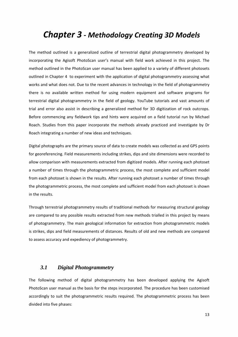
3 Chapter 3 - Methodology Creating 3D Models

The method outlined is a generalized outline of terrestrial digital photogrammetry developed by

incorporating the Agisoft PhotoScan user’s manual with field work achieved in this project. The

method outlined in the PhotoScan user manual has been applied to a variety of different photosets

outlined in Chapter 4 to experiment with the application of digital photogrammetry assessing what

works and what does not. Due to the recent advances in technology in the field of photogrammetry

there is no available written method for using modern equipment and software programs for

terrestrial digital photogrammetry in the field of geology. YouTube tutorials and vast amounts of

trial and error also assist in describing a generalized method for 3D digitization of rock outcrops.

Before commencing any fieldwork tips and hints were acquired on a field tutorial run by Michael

Roach. Studies from this paper incorporate the methods already practiced and investigate by Dr

Roach integrating a number of new ideas and techniques.

Digital photographs are the primary source of data to create models was collected as and GPS points

for georeferencing. Field measurements including strikes, dips and site dimensions were recorded to

allow comparison with measurements extracted from digitized models. After running each photoset

a number of times through the photogrammetric process, the most complete and sufficient model

from each photoset is shown in the results. After running each photoset a number of times through

the photogrammetric process, the most complete and sufficient model from each photoset is shown

in the results.

Through terrestrial photogrammetry results of traditional methods for measuring structural geology

are compared to any possible results extracted from new methods trialled in this project by means

of photogrammetry. The main geological information for extraction from photogrammetric models

is strikes, dips and field measurements of distances. Results of old and new methods are compared

to assess accuracy and expediency of photogrammetry.

3.1 Digital Photogrammetry

The following method of digital photogrammetry has been developed applying the Agisoft

PhotoScan user manual as the basis for the steps incorporated. The procedure has been customised

accordingly to suit the photogrammetric results required. The photogrammetric process has been

divided into five phases:

14

Phase 1 – Reconnaissance

- Site allocation

- Prerequisites

- Field equipment

Phase 2 – Photography

- Camera

- Format

- Photographic pattern

Phase 3 – Photoshop

- IrfanView: for non GPS referenced photographs

- RawTherapee: for GPS referenced photographs.

Phase 4 – Digital Photogrammetry

- PhotoScan

Phase 5 – Analysis

- Orthophoto

- PDF

- Blender

- GeoVis 3D

Table 3-1: Photogrammetry broadly portrayed as a systems approach.

Data Acquisition Photogrammetric Procedures Photogrammetric Products

Camera Photographs

Scanner

Sensor Digital imagery

Hardware

- Windows 2.5GHz

Intel dual core i7 processor

8GB RAM

- MacPro 3.5GHz 6-

Core Intel Xeon E5 processor

32GB RAM

Softcopy workstation

- Photoshop

- PhotoScan

- GeoVis 3D

- Blender

Photographic products

- Rectifications

- Orthophotos

DEMs, profiles, surfaces, points

- XML

- PDF

- OBJ

- 3DS

- PSL

Input

Procedures and Instruments

Output

15

3.1.1 Phase 1- Reconnaissance

3.1.1.1 Site Allocation

Prior to making a model it is necessary to consider the sites that are best suited for digital

photogrammetric reconstruction. Depending on the type of study, any geological outcrop can, in

some way, be reconstructed in digital form to create useful data. Digital models can be studied to

investigate such things as structural data, to measure slope movement, and to measure volume of a

land mass.

In this study, outcrops have been selected based on their physical appearance and location. The

focus has been to extract measurements of strikes and dips from digital photogrammetric outcrops

and to compare them with measurements taken on the field. It is necessary that outcrops not only

display stratigraphic layering but can also be accessed and measured by traditional methods with a

brunton or phone application such as field move (used in this project) so that results can be

compared to test the accuracy of measurements from digitised outcrops.

For greater efficiency, it is necessary to visit the site in advance to define the elements of digitization

and to decide on required resolution and accuracy of georeferencing needed. It is often necessary

for the projects sponsor to be present and available for questioning.

- Access authorisations should have been investigated prior to this stage including any possible

diversions of the public for a given period.

- Plan position of various measuring instruments by access limits, arranging as few as needed to

save time.

- Resolution required will determine type of camera needed and its distance from object.

- It is best to arrange georeferencing points at obvious natural features likely to be long lasting.

It is also necessary to have a sufficient numbers for accurate positioning.

- The number of visits may depend on budget, accessibility, weather limitations and project

size.

- Depending on the complexity of the site, it may be better accomplished in parts and later put

together.

Himalayan Photoksar is the first site where the digital photogrammetric method was trialled. It was

selected due to its complex folded structure, but also to trial photogrammetric methods in a high

alpine region. The second site selected was a coastal area at Narooma to make a direct comparison

between methods in high alpine and coastal regions. Narooma was chosen as it has complex folded

16

structures of chert outcropped at its shores which have similar fold structures to those in the

Himalayas but on a larger scale. Five different outcrops were selected to trial digitisation methods as

explained further in (Chapter 3). Eight sites at Eden were trialled to create models to be displayed as

learning guides for students doing the EESC 250 field geology subject. A number of other sites were

chosen at different locations around the world to create a broader variety of models at different

locations and with digital photographs produced from several different cameras to assess the

difference between their different characteristics (such as high/low resolution). The sites were

incorporated primarily to test the capabilities and limitations of Agisoft PhotoScan and what one can

expect in closely replicated situations. The sites incorporated for variety included Flores Island

(Indonesia), Rock Lands (South Africa), Nowra Sandstone (Bomaderry) and Uluru (Northern

Territory). Sites at Flores and the Rock Lands are archaeological sites allowing assessment of

photogrammetry for its application in archaeology.

3.1.1.2 Field equipment (Picture of each as appendix)

The equipment used in this project is outlined below.

- Camera: Higher resolution cameras produce better images requiring more processing

power. This is ideal when few photographs are needed or pictures need to be taken from a

distance. Low resolution cameras are best when there are a large number of photographs

that need to be taken. This is usually where a large area is required to be covered or where

there is a complex surface area involving many objects that need to be photographed at a

number of angles.

- 9m selfie stick: Necessary when pictures need to be taken at a higher angle of up to 10 m.

- Boat: Necessary where outcrops need to be photographed along a shoreline or where access

by land is difficult or impossible.

- Four wheel drive vehicle: Necessary for remote locations where roads are not accessible by

two wheel drive vehicles.

- Unmanned aerial vehicle (UAV): Necessary for high outcrops where camera angles above 10

m are required or foot and boat access are not possible or too dangerous.

- Scale, compass and level: A good scale is an item that is large enough to be recreated in 3D

and incorporated into the model so that its known dimensions can be used to give the

model a scale. Straight flat objects are ideal so that they can also show the direction of north

17

(aligned with a compass) and made level to show the orientation of a surface horizontal to

the force of gravity (aligned with leveling device).

- GPS with altimeter: Necessary when a model is required to be georeferenced. The high

accuracy of a GPS will produce a more precisely georeferenced model. Obvious land marks

that will also be displayed in the model (but not on a vertical surface such as a cliff) should

be used so that the location for each GPS point can easily be identified in the model and

placed with a marker in PhotoScan in the correct position.

- Computer with a large amount of RAM: PhotoScan can produce models at a number of

different resolutions. The higher the resolution the more accurate and detailed the model

will be. The greater the amount of processing power available the higher resolution a model

can produce. Anything less than 8GB of RAM will produce poor results with models created

from over 20 photographs.

3.1.2 Phase 2 - Photography

After completion of a site plan, the photography phase

should be as simple as following the plan and managing

any outside constraints that may occur. Operations are

carried out as planned in accordance to:

• Geometric information: spatial position and shape

of object.

• Physical information: refers to properties of

electromagnetic radiation, e.g. polarisation.

• Semantic information: meaning of an image, e.g.

interpretation.

• Temporal information: how an object has changed

over time when compared to previous images.

3.1.2.1 Camera

Agisoft PhotoScan is capable of processing images shot with both metric and non-metric cameras.

This means that it is possible to carry out true photogrammetric research with the help of an

ordinary digital consumer-level camera. No special photogrammetry equipment is required.

Figure 3-1: Photography with selfie pole.

18

Resolution: Agisoft PhotoScan does not set any requirements concerning the image resolution.

However, it is reasonable to remember that the resolution of the input data influences the quality of

the processed results. That is why it is strongly recommended to employ a camera with at least 5 MP

resolution. To produce professional quality orthophotomaps it is better to opt for 12 MP resolution

photography.

Lens: since the software applies the Brown model to simulate lens assembly, automatic calibration

works perfectly well for “standard” optics (that is with 50 mm focal length (35 mm film equivalent)).

To process data collected with “fish eye” lenses, you need to indicate corresponding camera type in

the program settings*. The software is also capable of spherical camera data processing, providing

that it implements equirectangular projection. If the source data was captured with ultra-wide angle

lenses, the operation is likely to fail. In this case, one should enter calibration data to the program to

achieve good reconstruction results.

Table 3-2: Cameras trialled in this project.

Camera Resolution Megapixels

Aerial photographic camera 14,430 x 9,420 136

Nikon D610 6,016 x 4,016 24

Panasonic 4,896 x 3,672 18

Samsung Galaxy s5 5,148 x 3,456 18

GoPro 4,000 x 3,000 12

Nikon D7000 3,872 x 2,592 10

iPhone 4s 3,264 x 2,448 8

19

3.1.2.2 Shooting

A basic knowledge of photography can assist in

capturing good quality photographs. Figure 3-2

outlines visually the basic functions of camera

settings. The better quality of a photoset the better

the results of Agisoft PhotoScan will be. Blurry

photographs and wrong ISO, F-stop and shutter

speed setting can prevent correct alignment of

photographs. It is possible that, after an entire day

of photography at a remote site, the photosets are

of no use for obtaining suitable results from

PhotoScan if the setting are not adjusted correctly.

If you do not have any experience in photography,

or do not know how to correctly use the manual

settings on a SLR camera, you would benefit from

doing at least a short course in photography from a

professional photographer or someone who has a

good understanding in how to use the manual

settings on a digital camera.

Aperture: large aperture (such as f/2.0, f/2.8) lets in more light to the camera shutter for an

exposure but gives poor depth of field, while small aperture (f/11, f/16, f/22) has a smaller opening

in the lens diaphragm to let in less light for a given exposure resulting in greater depth of field. The

size of an aperture in a lens can either be fixed or adjustable (as in an SLR camera). Aperture size is

usually calibrated in f-numbers or f-stops.

Shutter speed: or exposure time is the length of time that the film or digital sensor inside the

camera is exposed to light when taking a photograph. The amount of light that reaches the film or

image sensor is proportional to the exposure time. Longer exposure gives lighter photographs with

any movement being blurred. Shorter exposure times produce darker photographs with motion less

blurred.

ISO: The lower the ISO number, the less sensitive it is to the light which is better in sunny weather. A

higher ISO number increases the sensitivity of your camera and is better in darker conditions. The

component within your camera that can change sensitivity is called “image sensor” or simply

“sensor”.

Figure 3-2: Photography cheat sheet (Mercer 2012).

20

Shooting Pattern and Planning: Note; if a feature is not overlapping in at least two photographs it

will not be incorporated correctly into the model. Figure 3-3 below illustrates the basic ideas about

proper shooting scenarios.

Figure 3-3: Shooting patterns recommended by Agisoft (2015).

For the successful completion of the photo reconstruction task it is important to guarantee enough

image overlap across the input dataset. In the case of aerial photography the requirement can be

summarised as at least 60% of side overlap and 80% of forward overlap.

Take care with object texture and invent tricks to avoid plain/monotonous and glittering surfaces.

For example, talc can be spread over a shiny surface to change it from a glittering to a dull surface.

Photoscan has difficulty correctly orientating shiny surfaces.

To build a texture map of the object that has been prepared before shooting (as in the examples

above) you need to capture two sets of images of the same object; one of the “natural” texture of

the object and the other of the prepared object. The key point is that you need to take both sets of

images from the same camera positions. This requires the organisation of a fixed set of cameras for the

shoot to be successful.

21

To carry out any measurements based on the reconstructed model, it is important to locate at least

two markers with a known distance between them. Alternatively, you can place a ruler within the

shooting area.

To fulfil a georeferencing task, an even spread of at least 10 ground control points (GCPs) across the

area is required to achieve results of highest quality; both in terms of the geometrical precision and

georeferencing accuracy. Nonetheless, Agisoft PhotoScan is also able to complete the reconstruction

and georeferencing tasks without GCPs.

Trial and Error

After having been familiarised with the basic camera settings and having decided on a shooting

pattern, the next step is to trial some photography. Points to consider when taking photographs

include:

- Go to an area that is easy to access to practise shooting; preferably similar to where you are

planning your major project.

- Trial both sunny and cloudy conditions to see which settings work the best in different

conditions (Figure 3-2).

- Put camera into manual mode; usually an uppercase M on the cameras scene selector.

- Adjust ISO and F-stop settings so that the object of interest has the clearest lighting and

correct exposure (Figure 3-2). If you wish to study shady areas in any details, it may be best

to have the sky over-exposed and burnt out so that the object of interest shows more colour

and detail and less shadow effect. Shadows can also be reduced in photoshop programs

(Chapter 3.1.3).

- After correct lighting settings have been selected it is time to start shooting.

- When pressing the trigger it is important to hold the camera as steady as possible (more so

when there is poor lighting and when using higher ISO settings) to avoid any blurring.

- Inspect photographs closely on a large screen or computer after shooting to compare the

results and see which settings worked the best.

- Go through the procedure again if the pictures could be improved in any way. Blurry

photographs can ruin parts of the model alignment phase so it is important that

photographs are as clear as possible.

22

Considerations:

• Number of workers and their ability to work together without anyone being an inconvenience.

• Number of instruments available and how to use them most efficiently.

• Weather forecast and best time of day for lighting.

• Possible presence of the general public who may need to be diverted during the shoot.

• Conformity with requirements specified, are resolution and stereoscopic overlap specifications

satisfactory?

Field work for this project acquired data primarily by hand-held photography using a 7 m pole to extend

the camera’s height when high angle shots were required. In areas inaccessible by foot, a boat has been

used. This also provided the opportunity to compare the quality of a model created by images from a

boat with images taken by hand held devices.

For more detailed and less specific guidelines and cautions on camera choice and shooting scenarios refer

to Chapter 2 in Agisoft PhotoScan User Manual available at: http://www.agisoft.com/downloads/user-

manuals/

3.1.3 Phase 3 – Photoshop

3.1.3.1 Format

Table 3-3: Formats accepted by Agisoft Photoscan.

Format Script

JPEG *.jpg *.jpeg

TIFF *.tif *.tiff

PNG *.png

BMP *.bmp

OpenEXR *.exr

Portible Bit Map *.pgm *.ppm

Multi-Picture Object *.mpo

Norpix Sequential Files *.seq

http://www.agisoft.com/downloads/user-manuals/

http://www.agisoft.com/downloads/user-manuals/

23

Photograph formating is an essential stage of digital photogrammetry when using Agisoft Photoscan

if the photographs were recorded in RAW format. If the photographs are recorded in a format

compatible with photoscan (see Table 3.3) it is possible to skip to photo adjustments or upload

digital photographs directly to photoscan. In this project, trials were run to test results from

photographs left as their original colour and for comparison with results (3D images) created by

photographs where colours were modified to emphasise the different coloured bedding layers.

3.1.3.2 IrfanView – For non-GPS referenced photographs

IrfanView is a freeware/shareware image viewer for Microsoft Windows that can view, edit, and convert image

files and play video/audio files. The program is small size, fast, easy to use, and able to handle a wide variety of

graphic file formats (Appendix A). It also has some image creation and painting capabilities. The software was

first released in 1996. IrfanView is free for non-commercial use; commercial use requires paid registration.

IrfanView is a compact graphic viewer compatible with:

Windows 9x, ME, NT

Windows 2000

Windows XP

Windows 2003

Windows 2008

Windows Vista

Windows 7

Windows 8

Windows 10

Its design is simple for beginners and can be powerful for professionals. A program like Adobe

Photoshop (not used in this project) may be more suited for application with a Mac.

IrfanView features:

32 and 64 bit version

Many supported file formats

(Appendix A)

Multi language support

Thumbnail/preview option

Paint option - to draw lines,

circles, arrows, straighten

image etc.

Toolbar skins option

Slideshow (save slideshow as

EXE/SCR or burn it to CD)

Show EXIF/IPTC/Comment

text in Slideshow/Fullscreen

etc.

Support for Adobe Photoshop

Filters

2

Fast directory view (moving

through directory)

Batch conversion (with

advanced image processing)

Multipage TIF editing

File search

Email option

Multimedia player

Print option

Support for embedded color

profiles in JPG/TIF

Change color depth

Scan (batch scan) support

Cut/crop

Add overlay text/image

(watermark)

IPTC editing

Effects (Sharpen, Blur, Adobe

8BF, Filter Factory, Filters

Unlimited, etc.)

Screen Capturing

Extract icons from

EXE/DLL/ICLs

Lossless JPG rotation

Shell Extension PlugIn

Unicode support

Many hotkeys

Many command line options

Many PlugIns

Only one EXE-File, no DLLs, no

Shareware messages like "I

Agree" or "Evaluation

expired"

No registry changes without

user action/permission

When editing photographs, most photo editing software programs will add additional data by

masking a layer over the top of the original photograph increasing the file size. IrfanView recreates

the photograph while incorporating the changes so that no extra data is added and each pixel carries

its original file size unless compressed to a lower quality and smaller file size.

3.1.3.3 RawTherapee – For GPS referenced photographs.

RawTherapee provides the user with a file browser, a queue, and an image editing tab.

File browser: shows photo thumbnails along with a caption of the shooting information metadata.

The browser includes 5-star rating, flagging, and an Exif-based filter. It can be used to apply a profile,

or parts of a profile, to a whole selection of photos in one operation.

Queue tab: allows one to put exporting photos on hold until adjusting them in the Editor is

complete. This means that CPU is fully available to the user while tweaking a photo instead of

3

processing photos while the user is trying to tweak new ones; which could result in a sluggish

interface. Alternatively, the queue tab can be used to process photos alongside tweaking new ones if

one has a CPU capable of handling the workload.

Editor tab: is where the user tweaks photos. While the image is opened for editing, the user is

provided with a preview window with pan and zoom capabilities. A color histogram is also present

offering linear and logarithmic scales, and separate R, G, B and L channels. All adjustments are

reflected in the history queue and the user can reverse any of the changes at any time. There is also

the possibility of taking multiple snapshots of the history queue, allowing for various versions of the

image to be shown. These snapshots are not written to the sidecar file and are subsequently lost

once the photo has been closed; however, work is underway to migrate the PP3 sidecar system to

XMP which already supports storage of snapshots. By copying the settings used on a photograph the

settings can then be pasted to other selected photos for batch conversion.

The viewing space for adjusting visual settings of a photograph in RawTherapee was found to be

better than that in IrfanView.

Input File Formats

RawTherapee can work with both raw files from digital cameras as well as usual images. It also

supports high dynamic-range, 16/24/32 bit raw DNG images.

While reading raw files RawTherapee relies on the dcraw code, but only for parsing formats; not for

processing. Thus, RawTherapee supports all the formats supported by dcraw.

Additionally, RawTherapee supports the following image formats:

• JPEG

• TIFF

• PNG

Models tested for natural versus enhanced colours included Julian Rocks, Mod 2 Narooma, Mod 3

Narooma, Mod 4.5 Narooma, Mod 5 Narooma, Shale Cutting, Haycock West,

4

3.1.4 Phase 4 – Digital Photogrammetry

3.1.4.1 Agisoft PhotoScan

Agisoft PhotoScan was the software chosen for the photogrammetric processing of digital

photographs in this project. PhotoScan uses well implemented algorithms to analyze each input

image for special features in order to create a relation between the images of the entire scene

(Remondino et al. 2014). It is a stand-alone software product that performs photogrammetric

processing of digital images and generates 3D spatial data that can be used in GIS applications,

cultural heritage documentation, and visual effects production (Agisoft 2015). It can also be used for

indirect measurements of rock outcrops of various scales (Cracknel et al. 2013). It has a wisely

implemented digital photogrammetry technique enforced with computer vision methods which

results in a smart automated processing system that can be managed by a new-comer to the field of

photogrammetry. On the other hand, Agisoft PhotoScan has a lot to offer to a specialist who can

adjust the workflow to numerous specific tasks and different types of data. For the various case

studies, PhotoScan produced quality and accurate results.

3.1.4.2 Photo Preparation

The following instructions are a broad tutorial for using PhotoScan to process a single photoset in

Agisoft PhotoScan Professional, version 1.2.2.

1. Eliminate any blurry, out-of-focus or non-significant photos unrelated to the model from your

photoset.

2. If you have GPS track data for your photos, use a program like RawTherapee or GeoSetter to

geotag your photos before processing. IrfanView is a more suitable program for non-GPS

tracked photos (Chapter 3.1.3).

a. With geotagged photos, the coordinates are usually Latitude and Longitude (in degrees). Use

the convert tool in the ‘ground control’ pane to convert to UTM.

b. Never use geotagged photos as the sole source of georeferencing information. The errors in

consumer grade GPS units (handheld or in camera) are too large for anything more than

helping with photo alignment.

5

3. Agisoft PhotoScan estimates camera calibration parameters automatically. Consequently,

generally there is no need to run pre-calibration procedures manually.

3.1.4.3 Photo Alignment

1. Load your photo set for a single model

a. The masking tools can be used to create a mask over any features (such as the sky, people or

trees) not needed in the model.

2. Align Photos Settings:

a. Accuracy:

i. High: is best for smaller photosets

ii. Medium: is best for larger photosets

b. Pair Selection:

i. Disabled: default, works for most datasets

ii. Generic: use this one if there is any trouble getting photos to align

iii. Ground Control: If photos are geotagged, this will use the GPS positions to speed up

processing.

c. Advanced:

i. Point Limit: 40,000 is the default. Smaller numbers can speed up processing, but you run

the risk of not having enough points to align photos.

ii. Constrain features by mask: You can use masks to exclude parts of the images you do

not want to model, check this box if you have masks.

3. Fixing misaligned or unaligned photos

a. After the initial pass of photo alignment there may be photos that are misaligned or

unaligned. You can force the program to try again; usually this works (but not always).

6

i. Select all of the photos that are causing trouble, right-click and select ‘Reset Alignment’

ii. Right-click again, select ‘Align Selected Cameras’

iii. If that does not work, select a smaller batch of problem photos and try again by working

in small batches.

iv. If none of that works, you need to disable or exclude the photos that will not align.

3.1.4.4 Georeferencing

1. Prepare your control point data

a. Double-check your projection and vertical datum; do any conversions outside of Photoscan.

b. Load your data points into Excel and delete all but the NAME, LAT (Northing), LONG (Easting),

and ELEV to simplify things.

c. Save as a text file (tab delimited).

d. Use the Import tool in the ‘Ground Control’ pane, set the import settings, say ‘Yes to all’

when it asks to add points.

e. If you import a larger file, you should delete any points that are not present in the photoset.

2. Set your projection with the ‘Settings’; the other settings are default.

3. Find the first photo with a ground control point.

a. Double-click the photo to open it, zoom in on the control point, right-click on the centre of

the control point marker, select ‘Place Marker’ and select the appropriate marker.

b. Find the next photo with the same GCP as the first, set the marker.

i. Once you have a marker placed in two photos the software starts to guess where they

should be in other photos.

ii. Right-click on the marker you have been working on, select ‘Filter Photos by Marker’.

This will show just the photos that the marker is in.

7

iii. Click through all of the photos and place the markers.

iv. If a photo has a marker flag in it, but the GCP is not visible, you can leave it as a grey flag

and it will not be used, or you can right-click on it and ‘Remove Marker’.

c. In the photos pane, select ‘Reset Filter’ to get back to the full photoset.

d. Repeat the above steps for the next two GCPs.

4. After you have three GCP markers set, you can ‘Update’ the georeferencing in the ground

control pane.

a. This will roughly georeference the model and make finding the remaining GCPs easier.

b. If your first three points are close together, this may not work very well; In this case you may

have to manually find and mark an additional GCP.

5. Right-click on the next GCP in the list and ‘Filter Photos by Marker’.

a. Run through all of the photos and place the markers.

b. ‘Update’ again to refine the georeferencing.

c. Repeat this step for the rest of the GCPs.

6. Double-check that all of your GCP markers are placed.

a. Right-click on all of the GCPs and ‘Filter Photos by Marker’.

b. Double-check that all of the photos have little blue flags above them in the photo pane.

c. Update one last time.

3.1.4.5 Optimize the alignment

1. Double-check that you have a camera calibration applied to all of the photos.

2. Click on ‘Optimize’ in the ground control pane.

a. Make sure the ‘Fit k4’ box is checked.

8

b. This optimizes the camera alignment based on the camera calibration and control points.

3. Check your error for each GCP.

a. In the georeferencing pane, the point with the worst error is highlighted in red.

i. You can also click on ‘View Errors’ to view the X, Y, and Z components of the error.

b. If you have points with errors that are higher than you would like, you can uncheck the box

on the left to exclude the points from the georeferencing calculations.

c. Update the georeferencing and repeat for any other bad points if necessary.

d. If you change or exclude a lot of points, re-optimizing is a good thing to do.

3.1.4.6 Building Dense Point Clouds

1. Settings

a. Quality:

i. This is the super memory intensive part of the process; photosets that are large (lots of

photos) can take a long time to complete. Too many photos cause the program to run out

of memory. The quality that is achievable and the time it takes depend on your processor

(CPU), RAM, and video card (GPU).

ii. High: great for smaller photosets (up to ≈150 photos)

iii. Medium: good for larger datasets (over 150 photos)

b. Advanced

i. Depth Filtering: limits points that are too far from the surface. For models with a lot of

vegetation, aggressiveessive (default) may be the most suitable setting. For more flat and

smooth rock surfaces the setting may be better set to moderate or mild.

9

3.1.4.7 Point Cloud Editing

1. If there are any points in the dense point cloud needing to be eliminated, they can be deleted

manually. To do this use the ‘Rectangle Selection’, ‘Circle Selection’, or ‘Free-form Selection’

tools on the toolbar to select and delete errant points.

2. Check the bounding box (the light grey box with a red bottom) size and orientation.

a. Use the ‘Resize Region’ and ‘Rotate Region’ tools on the toolbar if the bounding box looks

like it is going to cut off any parts of the model.

3.1.4.8 Build Mesh

1. Settings

a. Surface Type:

i. Height Field: only builds a mesh surface orthogonal to the reference system Z-axis (i.e. no

undercuts will be modelled). This is the fastest mesh procedure and excellent if DEMs are

going to be your final product.

ii. Arbitrary: Will model every nook and cranny of the object. It is best used for oblique

imagery when point clouds or complex mesh surfaces are going to be the final product.

1. For geography applications, a height field would normally be modelled orthogonal to the Z-axis

of the coordinate system. In Photoscan, the height field is actually modelled against the

orientation of the bounding box (the light grey box with a red bottom) of the model. You can

run this Python script (Align Bounding Box Tool) in the console to align the bounding box to the

reference system. You will need to

b. Source Data:

i. Dense cloud: default, incorporates all point within the bounding box.

ii. Sparse cloud: You could use this, however, it serves no benefit.

10

c. Polygon Count: The number of polygons that the model will be decimated to after

processing.

i. The software has High, Medium, Low values.

ii. Or you can specify a custom number (entering 0 will not decimate the final model).

d. Interpolation

i. Enabled: default, will interpolate over small holes in the surface

ii. Extrapolation: will leave holes in the final surface where there are no dense points

e. Point Classes:

i. There is a point classification tool in Photoscan. If you used it to classify the dense point cloud,

you could specify which point classes you want to use for the mesh.

3.1.4.9 Texture

1. Settings

a. Quality:

i. This is the memory intensive part of the process; photosets that are large (lots of photos) can

take a long time to complete. Too many photos cause the program to run out of memory. The

quality that is achievable and the time it takes depend on your processor (CPU), RAM, and

video card (GPU)

ii. High: great for smaller photosets (up to ≈150 photos).

iii. Medium: good for larger datasets (over 150 photos).

3.1.4.10 Exporting DEM / Orthophotos

1. File…Export DEM…Export TIFF/BIL/XYZ…

a. Settings

11

i. Choose your projection.

ii. Crop invalid DEM: checked by default.

iii. No-data value: Use -9999 for ArcGIS.

iv. Pixel Size: Photoscan estimates an appropriate pixel size and can be changed to match your requirements.

v. Split in blocks: segment the DEM into X by X rasters (only needed for large datasets).

vi. Set boundaries:

1. Check the box and click ‘Estimate’; this limits extra no-data values on the edges:

vii. Write world file: not necessary if you export a TIFF.

viii. Choose your output location, file name, and type.

2. File…Export Orthophoto…Export JPEG/TIFF/PNG:

a. Settings

i. Choose your projection.

ii. Blending mode: Mosaic (default).

iii. Enable Colour Correction: not usually necessary; but if you need the colour to be evened out feel free to select this option.

iv. Pixel Size: same as above.

v. Split in Blocks: same as above.

vi. Set boundaries: same as above.

vii. Write world file: not necessary if you export a TIFF.

viii. Choose your output location; file name, and type.

3.1.5 Phase 5 - Photogrammetric Products

PhotoScan supports model export in the following formats:

Wavefront OBJ

3DS file format

VRML

COLLADA

12

Stanford PLY

Autodesk DXF

U3D

Adobe PDF

Some file formats (OBJ, 3DS, VRML, COLLADA, PLY) save texture image in a separate file. The texture

file should be kept in the same directory as the main file describing the geometry. If the texture atlas

was not built only the model geometry is exported. (Agisoft 2015).

Figure 3.4 outlines the type of products one may hope to obtain from photogrammetric processes.

Products range from simple stitching of photographs to complex, georeferenced models that cater

for a large number of applications for use in geology and many other areas. A flow chart (figure 3-5)

shows the way one may hope to reach such results.

Figure 3-4: A flow diagram of photogrammetric products able to be generated from digital 3d models.

13

4 Chapter 4 - Field Work Methods and Results

To test the expediency of digital photogrammetry in geology the following field sites were visited to

trial photogrammetry determining the feasibility of the results obtained. Utilizing the methods

outlined above from the hardware and software described a number of image processing and

photogrammetric applications can be integrated to create files for export from PhotoScan. The

method developed for each section is briefly outlined from the general methodology described

above in Chapter 3. Tables 4.1 to 4.35 were generated from the Table of Methods (Appendix C).

4.1 Project Applications

This project has been limited to focus on the comparison of methods used for application of

photogrammetry in the field of geology. Because there is little existing research utilising the more

recent available technology for extracting geological measurements, two different landscapes were

selected for a comparative study. The methods required in a high alpine region were compared to

the methods required in a comparatively low lying coastal area. One site has been chosen for

research in a high alpine region because of the difficulty of access to the study site and time

constraints. Four regions (Narooma, Bingie Bingie Point, Wolumla and Eden on the NSW south coast)

were chosen as the coastal research sites. Study sites were selected based on professional

observations made by Dr Solomon Buckman and Associate Professor Dr Brian Jones from the

University of Wollongong, 2015. The geology exposed at outcrops is presumed to be ideal for this

project as there are clear stratigraphic and structural features available. Each site can also have a

number of obstacles for acquiring the photographs necessary to produce the 3D images. In addition,

each site was expected to produce a different type of information because of their variation in

geology. The data collected was then taken back to laboratories at the University of Wollongong for

analysis and comparison.

Other side studies were added to the project to test further the capabilities of PhotoScan. These

included a camera tuning exercise, trials of photogrammetry for the purpose of archaeology, high

resolution photographs vs low resolution photographs, natural colour of photographs vs enhanced

colour of photographs, Windows with 8 GB RAM compared to a MacPro with 32 GB RAM and

Photoscan exports. The coastal sites of Narooma and Eden were also used as experiments in side

studies by running each as separate case studies. Sites at Eden, Bega and Bingie Bingie point were

trialled as sites used to create educational media for the purpose of the EESC 250 Eden field geology

subject.

14

The following list outlines the extent of this project in the areas that are focused on trialling the

applications possible for digital photogrammetry. These are discussed in detail in Chapter 5.

Camera Calibration

High alpine region versus Coastal Photogrammetry

Digitization – The Photogrammetric Work Shop (PWS)

Archaeological application

Extracting Structural Measurements

4.2 Camera Calibration – Julian Rocks This is a small exercise required to develop familiarity with the basic functions of the Nikon (DSLR)

D610 which was the primary camera used to create sets of photographs for creating models in this

project. The main aim of the experiment is to practise and become familiar with operating the

camera in manual mode and to understand the effects of adjusting the ISO, f-stop and shutter

speed. The site chosen is known as Julian Rocks which is a small sedimentary outcrop 7 m high and

52 m long displaying a number of cross bed features that can be useful for measuring the amount of

detail captured by the models. The site is only a 10 minute drive from home making it ideal for a trial

and error exercise as it could be easily revisited if any errors were found or if any improvements

were tried.

The quality of the photographs taken will determine the quality of the model being produced

(Agisoft 2016). It is important to take advantage of the time allowed for the photography phase of

photogrammetry. The quality of the photoset determines the quality of the 3D image produced from

the photographs. It is important to capture the photographs correctly so there is no need to return

to a site as they can be remote and returning can be costly and time consuming.

Method

This is a simple exercise where only the Nikon D610 is required on the field for taking photographs.

The D610 has been selected to be the primary camera for the project because of its versatility in

manual model and the ability to change the lens. Once captured, the photographs were taken back

to the University’s photogrammetric work station, known as the spatial analysis lab to be processed

through the photogrammetric method outlined in Chapter 3.

15

Site Details:

Photoset 1 – Julian Rocks

Date: 5th, October, 2015 at 4:30pm

GPS coordinates: 34°51'11.27"S, 150°35'41.60"E

Weather: Clear, sunny day

Cliff aspect: facing west

Modelled features: Nowra sandstone, trees, ferns, grass

Figure 4-1: Location of Julian Rocks on the banks of Bomaderry Creek, Bomaderry.

Photography

A number of shots were taken to establish the settings that work most appropriately for use in

photogrammetry. Figure 4-2 shows 3 different photographs captured by 3 different ISO and f-stop

settings (Table 4.1). It can be difficult to see clearly the quality of a photograph while on the field as

there is only a 6.5cm viewing screen to inspect a highly resolution photograph. The simplest way to

solve this problem is to zoom into the photographs while in playback mode on the cameras viewing

screen and carefully inspect key details, such as colour, depth of field, focal point and lighting, which

are import to the final model.

16

Figure 4-2: Examples of camera settings: A) ISO 400, f-stop 3. B) ISO 250, f-stop 6. C) ISO-100, f-stop 9.

The settings adjusted are as follows:

Aperture: referred to as f-stop on the Nikon D610. A higher f-stop is required for a greater depth of

field. Higher depth of field is important for the model as this will enable any part of the outcrop

caught in the photograph to be potentially used. This will increase the model’s level of detail and

accuracy (Agisoft, 2016). Any blurring in the photograph, even due to depth of field, can lead to

reduced detail in parts of the model.

ISO: adjusting the light exposure. A burnt out sky may seem to be poor photography when shooting

a landscape, however, for the requirements of photographs in photogrammetry the sky will be cut

out so it is of no importance to the model. A burnt out sky can even assist when using the masking

tools in PhotoScan to crop the sky out from the photographs. For darker or shadowed rocks, using a

higher ISO setting may lead to a burnt sky however the rock colour can be enhanced with more

detail visible in the image. It is important to get the correct balance so that any rock is not burnt out

and the edges outlining the model from the sky or any other features are not blurred.

Shutter speed: Shorter exposure times produce darker photographs with less chance of blurring

from movement. Long exposure times expose the film to light longer and create lighter images with

a higher chance of blurring from any movement.

Table 4-1: Camera specifications and settings of photosets captured at Julian Rocks.

Camera Photoset Resolution Number of photos GPS ISO F-Stop Shutter

Nikon D610 Set 1 6016x4016 33 No 200 7 1/200

Nikon D610 Set 2 6016x4016 33 No 200 5.6-8 1/(125-

250)

17

Photographic Pattern

Having clear and colourful photographs is important. If any details are not photographed they will

not be included in the model. The greater the number and higher consistency of points formed in

the high dense cloud the greater the overall resolution and accuracy of the final model (Agisoft

2016). The development of the point cloud is dependent on the consistency of features throughout

the entire model being captured in at least two photographs to ensure sufficient overlap. Every

photograph should have a minimum overlap of 50% to 60% of visual features of adjacent

photographs. A set of photographs that only overlap between themselves and not with any of the

photographs from the main bulk of the model will not be incorporated into the final model.

Figure 4-3: Location of photograph extraction relative to outcrop at Julian Rocks.

The aim of this exercise was to practise with the application of different settings of the D610 in

manual mode. Only one photographic pattern was trialled for this model. To see more on

photographic patterns refer to Chapter 3.1.2. The pattern used in this experiment is shown in Figure

4.3. This pattern was used as it has a large overlap for a relatively flat surface and captures many

angles to cover the three dimensional features that require some obscure angles to capture them

entirely. A total of 33 photographs were taken in RAW format.

IrfanView was used to process the single set of photographs for Julian Rocks. IrfanView program

was chosen as there are no GPS tags available to be attached to exported photographs. Images were

converted from NEF (RAW) to JPEG. No colour adjustments were made to photoset on. The auto

enhance function was used for photoset 2 to experiment with processing photographs through

PhotoScan and each individual photograph varies in colour.

18

Table 4-2: Photoshop adjustments and models made from each photoset.

Photoset Program Model ID Conversion Colour enhance

Set 1 IrfanView Mod 1, 2 & 4 RAW to JPG No Set 2 IrfanView Mod 3 RAW to JPG Auto enhance

Photoscan settings

Four models were from the two photosets (Table 4.2).

From photoset 1, seven attempts were made to process the photoset. Three models were created

successfully. There were some issues with the photo alignment phase until the setting was changed

to high and all 33 images aligned correctly. Low setting was trialled first to create the density cloud.

The run was successful but not completed. The medium setting was then trialled again and the trial

was successful. Images were not masked. The model was completed with an extrapolated mesh so

that all the gaps were filled in. The next model was run with all the same settings only this time

images were masked so as to remove trees and sky that were outside the area of the outcrop and

the mesh was not extrapolated so that the mesh was created only where the dense cloud was

accurate. Another run was made using the same settings as model 2 but this time the density cloud

setting was increased to high. The computer lacked processing power to complete the model. A final

run was made with photoset 1 this time on the Mac to determine the highest resolution that can be

achieved with 32 GB of RAM compared to 8 GB of RAM. The settings were the same as model 1

changing only the density cloud to ultra-high. The model was successfully created with the highest

setting possible for the density cloud which is the primary control limiting a model’s resolution.

Photoset two was run once using exactly the same settings as model 2 so that the two models could

be compared directly to investigate any differences between the results of photographs taken in

manual mode and photographs captured in automatic and run with the auto enhance function in

IrfanView.

19

Table 4-3: Settings and specifications used in PhotoScan to create high-definition 3D models of Julian Rocks.

Computer Model ID Cropped Alignment Photos Aligned # Tie Points Dense Cloud #Points Mesh #Faces Texture Comments

Windows, 8 GB RAM No Medium poorly

Windows, 8 GB RAM No High 33/33 92,387 Low, mod 2,765,344 Low 358.654 End

Windows, 8 GB RAM Mod 1 No High 33/33 92,387 Medium, mod 7,470,087 High 1,480,628 10,000 Extrapolated

Windows, 8 GB RAM Mod 2 Yes High 33/33 92,560 Medium, mod 7,532,365 High 1,389,332 10,000 Not extrapolated

Windows, 8 GB RAM Mod 3 Yes High 33/33 92,560 Medium, mod 7,532,365 High 1,389,332 10,000 Not extrapolated

Windows, 8 GB RAM Yes High 33/33 92,560 High, mod fail

MacPro, 32 GB RAM Mod 4 Yes High 33/33 92,560 Ultra-high, mod 19,186,725 High 19,186,725 20,000 Extrapolated

20

Results: of Julian Rocks from the Methods in Table 4.3 – see also Appendices D8 and E1

Figure 4-4: Screen image of PhotoScan high-resolution 3D model of Julian Rocks refer to Table 4-3 for model

specifications. A) Model 1. B) Model 3. C) model 4.

21

4.3 Photoksar, Himalayas - High Alpine Photogrammetry

In many cases rock outcrops can be situated in a position where access to the rock for taking strike

and dip measurements s is dangerous or impossible. Examples of these areas are recognised in

mountain ranges and along coastal cliff lines. For this reason, digital photogrammetry can be

advantageous in acquiring strikes and dips (and other possible forms of data) by taking clear and

reliable photographs (chapter 3.1.2) remotely and safely. Hasbergen (2012) outlines a method

described as the three-point-method to extract geologic information from digital aerial images

(Figure 4.5). This same method can be applied to vertically down orientated orthophotographs

extracted from georeferenced or correctly orientated models created in this project.

Figure 4-5: left; Geometry of points (P) on a dipping geologic surface referenced to a horizontal plane. Right;

Components of the pole (U) to the dipping geologic surface with the coordinate directions (north, east) and

elevation (z) (Hasbargen 2012, p.24).

Little information is available for application of digital photogrammetry in geology and there is no

information available for extracting strikes and dips from 3D images. Therefore, it is necessary to

create a method for extracting geological data from 3D images. Methods developed for

photogrammetry in a mountain region were compared to methods developed for low lying coastal

cliffs for creating 3D images of outcrops for the purpose of extracting complex geological data.

22

The sites selected for comparison were:

Photoksar, Ladakh, West Himalayas (high alpine)

Narrooma, South Coast of NSW (low coastal)

Eden, NSW (low coastal)

Outline

o Acquire photographs in the Himalayan region from scree slope on the opposing side of the

valley to the subject outcrop approximately 100 m in height using a Nikon D610 and a

Panasonic Lumix DMC-TZ60.

o Acquire photographs from a coastal outcrop at sea-level using a Nikon D610 and a Panasonic

Lumix DMC-TZ60. Photographs to be taken from the ocean by boat at site 3.

o Record structural geologic information using traditional methods from the same outcrops

using the application ‘Field Move’.

o Process collected photographs from rock outcrops of interest in 3-D digital models using a

software program called PhotoScan developed by Agisoft.

o Evaluate the geologic information that can be extracted from 3-D digital models

o Asses the accuracy of information extracted from digital model compared to measurements

taken using traditional methods

o Compare methods of digital photogrammetry in the remote high Himalayas to low-lying

coastal outcrops on the South Coast, NSW

o Consider the advantages and disadvantages digital photogrammetry compared with

tradition methods of extracting geologic information

4.3.1 Photoksar, Ladakh, West Himalayas (high alpine)

Photoksar is a small Himalayan mountain village residing 22 mountain families. It is situated on the

side of a large mountain where study site one is (Figure 4.6). The site was been chosen for study due

to its remote locality and it being situated in a high alpine region at an elevation greater than 4,500

m requiring methods that can implemented in regions of a similar standing. Access to the site

23

involved a 6 hour drive from the airport at Leh, India by a Himalayan taxi driver on rough, narrow,

elevated roads through numerous steep valleys between the massive Himalayan mountain ranges.

Accommodation involved a two-man team of Ladakhi guides to set up and run a camp site for Dr

Solomon Buckman and myself. Enough food was carried to last 4 people 9 days. Photographs were

taken on foot and by car focused on an objective mountain and including some surrounding

mountains. Along the base of the mountain at study site 1 where the cliffs are accessible by foot,

strikes and dips were extracted manually so that their measurements could be compared to any

measurements extracted digitally.

Figure 4-6 Location of site 1, Photoksar, Ladakh, GPS: 34ᵒ4’11.01”N, 76ᵒ50’29.25”E

Regional geology of Photoksar

There are three main units throughout the High Himalaya:

• The Crystalline Nappes, which form the Central Crystalline of the Great Himalaya and the

partly extensive outliers in the Lesser Himalaya.

24

• The Tibetan Zone builds up the sedimentaries which overlie the Central Crystalline in the

north.

• South from here there are the Synclinoria of Kashmir, Chamba and a smaller sequence

known as the Indus zone.

Units studied in this project were of in the Indus Zone. The Indus zone is a complex belt consisting of

several tectonic units including The Northern Zanskar Unit, Lamayuru Unit, Dras Unit, Indus Flysch

and Indus Molasse. Along the boundaries of these units ophiolitic melanges and larger peridotite

masses are found (Fuchs, 1981). Overall the Indus Zone is a complicated belt of flysch and volcanics

that result from a squeezed ocean.

Geologically, Site 1 is on the Indian continental plate situated 84 km south west of the Indus Suture

Zone. Four kilometres further to the south west of site 1 is a block of ophiolite approximately 15 km

in diameter (Figure 4.7) that has been pinched out during the closing of the Tethys Ocean 55 to 35

million years ago. Between study site 1 and the ophiolite is the Lamayaru molase, a mudstone slate

type melange with a number of large inclusions of cherts, ophiolites and sandstones. This is met to

the north east by the folded, multicoulored limestones that have been squashed and folded

underneath the ophiolite. Site 1 is at the contact where the Lamayuru molase is to the south and the

multi-coloured limestones are to the north. The contact is described as a thrust fault by Fuchs (1981)

that dips to the west. The Spong River flows toward the east cutting a valley perpendicular to the

fold axes of the multicoloured limestones and exposing the detail and complexity of the fold

structures that have formed in the region as a consequence of crustal shortening.

Research at site was used to develop a basic method for using digital photogrammetry as a means

for creating georeferenced 3D images of large mountainous features. The models need to show

enough detail so that as many bedding layers as possible can be clearly seen and identified.

Measurement were taken on the large scale features from the digital images and compared to

measurements taken in the field.

25

Figure 4-7: Geological map of Ladakh, NW Himalayas, indicating the study site (Corfield 2001, p.12).

Methods

The typical alpine landscape in the Himalayan region of Ladak at Photoksar was a suitable location to

trial the methods of digital photogrammetry to digitise a mountain range that is at high altitude. The

valley surrounding the mountain of Photoksar was formed by the Spong River and played a key role

in how photographs were taken to capture the mountain at a sufficient number of angles so that it

can be recreated in 3D. The primary aim was to create a model where bedding layers can be

identified and tracked through fold structures enabling strikes and dips to be measured from the 3D

images.

26

Site Details:

Model – Photoksar

Date: 12th, June, 2015 at 12:00pm


Weather: Cloudy and minor showers

Cliff aspect: a corner facing south with 90 degree turn around to the west

Modelled features: Folded layers of mud stone and limestones, mountain village, river

Photography

The small digital Panasonic camera was used for photo set 1. It is not an SLR camera so photographs

were captured with the cameras set to the automatic function. A number of photographs were

taken with the Nikon D610 to calibrate the camera and find the settings that work most effectively

for photogrammetry at site 1 due to the conditions at the time the photographs were taken. Three

different sets of photographs were captured primarily to trial different patterns of photography. A

forth photo set was assembled from photosets 1 and 3 to trial the creation of a model with

photographs from two completely different cameras (the Nikon D610 (SLR) with the Panasonic point

and shoot) (Table 4.4).

Table 4-4: Camera specifications and settings of photosets captured at Photoksar, Ladakh, High Himalayas.

Camera Photoset Resolution Number of photos

GPS ISO F-Stop Shutter

speed (s)

Model ID

Panasonic LUMIX DMC-TZ70

Set 1 4896x3672 109 yes Auto Auto Auto Mod 1-2

Nikon D610 Set 2 6016x4016 285 Only on 14pics

100 8 1/250 Mod 3

Nikon D610 Set 3 6016x4016 167 yes, some 100 9 1/320 Mod 5

Panasonic + Nikon Set 4 As above

193 Panasonic only

As above

As above

As above Mod 6

27

Figure 4-8: Photograph comparison. A) Photograph capture with Nikon D610. B) Photograph captured with Panasonic.


A different photographic pattern was used for each of the photosets 1, 2 and 3 to trial the different

methods that can be used to capture photographs in an alpine region. The various photographic

patterns can be seen in Figure 4.9. Figure 4.9,A shows the straight line of photographs with a

number of elevated photographs. Figure 4.9, B shows photographs spread out and skated through

mountain range to create a 3D model including 12 km of outcrop from 285 images. Figure 4.9, C

shows the multi-level height layering pattern used when capturing images with the Panasonic LUMIX

DMC-TZ70.

28

Figure 4-9: Location of photograph extraction relative to the outcrop in: A) Photoset 3. B) Photoset 2. C) Photoset 1.

29

Photoshop

IrfanView and RawTherapee were both used to process photosets in this exercise using each of the

programs batch conversion functions. Photoset 1 did not require photoshop as the photographs

were recorded in JPEG format. IrfanView was used to process photo set 2 as there were 271 of the

total 285 photographs that did not have GPS tags. No picture adjustments were made to photoset 2.

Images were converted from NEF (RAW) format to JPEG. RawTherapee was required for photo sets

3 and 4 to keep the photograph GPS tags attached. RawTheraee is the preferred program to use

when making image adjustments because it has a clear, large viewing pane and useful software

picture controls. The image adjustments can be seen in Figure 4.10 and Table 4.5.

Figure 4-10: Photograph adjustments made. A) RAW format. B) JPG conversion with colour adjustments made in

RawTherapee



Set 1 Not needed Mod 1 N/A N/A

Mod 2

Set 2 IrfanView Mod 3 RAW to JPG No

Mod 4

Set 3 RawTherapee Mod 5 RAW to JPG Yes

Set 4 RawTherapee Mod 6 RAW to JPG Yes

30

PhotoScan settings

Combined, the 4 photo sets were run through Agisoft PhotoScan a total of 12 times with an outcome

of 6 successful models. The settings that worked and the settings that failed can be seen in Table 4.6.

Photoset one was made to trial simple photographs using the automatic function on the Panasonic

LUMIX DMC-TZ70 Digital Camera. Photoset 2 trials very few photographs over a 10 km long section

of mountain side (Figure 4.9,B) with a section in the middle of the model 2 km long that has a high

concentration of photographs to see if the resolution of the model changes within different

segments of the model depending on the photographs distance from the mountain. Photoset 3 is a

set of photographs selected from the condensed 2km midsection of photoset 2. These photographs

were selected to create a high resolution model of the main section of mountain under study with

the MacPro 32 GB RAM (Table 4.6). Photoset 4 tested PhotoScan’s ability to create a model from

photographs from two completely different cameras (different brands, lenses, resolution and mode

settings).

31

Table 4-6: Settings and specifications used in PhotoScan to create high-definition 3D models of Photoksar.

Photoset Computer Model ID Cropped Alignment #Aligned Tie Points Dense Cloud #Points Mesh #Faces Texture Comments Set 1 Windows, 8 GB RAM Mod 1 No Medium 109/109 233,497 Low, mod 2,489,486 High 501,095 9,000 Not extrapolated Windows, 8 GB RAM Mod 2 No Medium 109/109 233,497 Medium, mod 10,084,537 High 2,027,253 9,000 Extrapolated Windows, 8 GB RAM No Medium 109/109 233,497 High, mod Fail Set 2 Windows, 8 GB RAM Yes Low 146/285 120,654 End

Windows, 8 GB RAM Mod 3 Yes High 279/285 207,965 Low, mod 6,389,523 High 1,806,894 12,500 Windows, 8 GB RAM Yes High 279/285 259,227 Medium, mod 24,249,184 Fail MacPro, 32 GB RAM Mod 4 Yes High 279/285 259,227 Medium, mod 24,732,283 High 10,412,341 16,000 Extrapolated MacPro, 32 GB RAM Yes High 279/285 259,227 High, mod 114,732,283 Low Fail Set 3 MacPro, 32 GB RAM Mod 5 Yes High 165/167 198,650 Medium, mod 15,218,740 High 8,822,516 16,000 Extrapolated Set 4 Windows, 8 GB RAM Yes Low poorly Windows, 8 GB RAM Yes High poorly 94,215

Windows, 8GB RAM Mod 6 Yes Medium 193/193 231,215 Medium, mod 13,121,857 High 2,479,852 10,000

Windows, 8 GB RAM Yes Medium 193/193 231,215 High, mod Fail

32

Results: of Himalayas from the methods in Table 4.6 – see also Appendices (D9 – 11) and E(2 -3)

Figure 4-11: Screen image of PhotoScan high-resolution 3D model of Photoksar. Refer to Table 4-6 for model

specifications. A) Model 2. B) Model 4. C) Model 5. D) Model 6.

33

4.4 South Coast, NSW – Coastal Photogrammetry

Outcrops of the NSW south coast span across nearly half a billion years of geological time. Stretching

and compression of the earth's crust, formation and splitting of supercontinents, and movements of

tectonic plates over millions of years have produced three very different time-rock groups along the

coast from Bermagui to Eden. This geo-diversity attracts researchers and students who visit every

year on field trips to 'time travel', work out the range of environments recorded in the region's

rocks, and trace the evolution of this place from deep ocean to stable continent.

Stratigraphic Hierarchy (Hill, D., 1967)

• Merrimbula Group: Group, Suite

o Bellbird Creek Formation: Formation, beds

Ettrema Limestone Member: Member, phase

o Ben Boyd Formation: Formation, beds

o Twofold Bay Formation: Formation, beds

Wolumla Conglomerate Member: Member, phase

o Worange Point Formation: Formation, beds

Rocks indicate their stories and tell how they were formed and what has happened to them during

the ages that have passed since they were created. Looking at the outcrops exposed in the region,

geologists can start to understand the very different past environments of their creation and the role

played by the rocks forming the landscape. It is possible to also imagine the unseen changes in the

earth and oceans that have left no visible rock record in this region.

Fieldwork can be time consuming and expensive and certain features may be overlooked or missed.

To revisit a site can be a problem when there is no time or funding available. Visually observing a site

on the field can also be limited to the angles viewed. These issues can be resolved by taking a

number of photographs of an outcrop and running them through the digital photogrammetric

process to create a realistic 3D model that can be viewed at any time on a computer. A 3D model

also allows the ability to view the outcrop from any angle and at any distance with the

34

orthoperspective mode function that changes the view slightly to eradicate any distortion from the

standard perspective mode having a 30 degree field of view. This is discussed in more detail later in

the chapter.

Example Sites:

Because of their significance to the EESC250 field geology subject run by Dr Brian Jones (associate

professor), the following sites were chosen. All of these sites are included as part of the field work to

be studied by students. Each outcrop was recreated into 3D models by methods of digital

photogrammetry outlined in Chapter 3. The methods used at each site vary slightly with adjustments

being made to accommodate the different settings (such as lighting, photography and computer

processing requirements) at each site.

Figure 4-12: Google Earth map with yellow tags indicating the location of study sites.

35

4.4.1 Bingie Bingie Point

While Bingie Bingie Point is not close to Eden it consists of outcrops displaying significant evidence

relating to geological events that help to explain the geological setting at Eden. The plutonic rocks

that occur at Bingie Bingie Point form part of the northern exposure of the Early Devonian Bega

Batholith. The Bega Batholith has an outcrop area of about 9,000 square kilometres and is the

largest in the Lachlan Fold Belt. It consists of more than 130 separate plutons which range in area up

to approximately 1,000 square kilometres and which intrude many Late Ordovician sandstone and

shale to produce contact aureoles about 1km in width. The batholith is unconformably overlain by

younger Middle to Late Devonian units that can be found at Eden including the Boyd Volcanic

Complex at Eagles Claw and the Merrimbula Group at Two Fold Bay.

Some of the plutons of the Bega Batholith are heterogeneous and range from mafic to felsin in

composition. Most plutons contain hornblend-bearing mafic zenoliths that commonly show a very

strong preferred orientation defining a foliation. These zenoliths are more common in the relatively

mafic rocks. Several younger Tertiary basalt dykes also crop out at Bingie Bingie Point.

Site Details:


Weather: Clear sunny day

GPS coordinates: 36° 0'44.97"S, 150° 9'45.50"E

Cliff aspect: flat horizontal surface with some boulder features

Modelled features: Granite, basaltic dykes, enclaves, grass, shrubs and water.

Dimensions: length x width x height = 50 m x 20 m x 2 m

Method

The coastal outcrop has a low relief less than 2 metres high covering an area of 1,000 square metres.

Because of the complexity of the geology at the site it can be overwhelming to understand the

bigger picture of what is happening. By recreating the outcrop in 3D form it is then possible to zoom

out from the model to get a bird’s eye view of the area. This will help to gain a faster understanding

of the key geological features and how they have formed. Explanations are also made easier by

being able to point out where features are precisely and more quickly than can be shown in the field.

36

Photography

One set of photographs was taken for this site using the Nikon D610 in manual mode. The camera

was first switched to automatic mode and pointed at a number of key components in the darkest

and lightest areas of the outcrop. The average of the ISO, f-stop and shutter speed was noted and an

estimation was made to calculate the correct settings. From these settings the ISO was then

adjusted to a slightly higher setting so that shadows were less dark (more exposed) and the sky

slightly over-exposed. This adjustment was necessary because the clear sunny weather caused the

shadowed areas to be automatically darker as a consequence of the large contrast between the light

and shadowed areas. The final settings chosen in manual mode can be seen in Table 4.7.

Photographs were recorded in RAW format.

Table 4-7: Camera specifications and settings of photosets captured at Bingie Bingie Point.

Camera Photoset Resolution Number of photos GPS ISO F-Stop Shutter Model ID

Nikon D610 Set 1 6016x4016 84 No 320 11 1/320 Mod 1-3

Nikon D610 Set 2 6016x4016 188 No 100 7.1 1/400 Mod 1-3


A loosely disciplined grid pattern was used to cover the area (Figure 4.13) with a total of 272

photographs being taken (Table 4.7). Adjustments were made to the grid pattern to compensate for

any irregularities such as boulders, corners, crevasses and raised platforms. Care was taken when

taking the photographs to capture every visible part of the selected area of rock exposure. There

were no GPS points attached to the photographs.

37

Figure 4-13: Location of photograph extraction relative to the outcrop in photosets 1 and 2 combined.

Photoshop

IrfanView was used to process the single photoset. Photographs were converted from the RAW

format to JPEG with colour, contrast and sharpness being increased by 20% (Figure 4.14, Table 4.14)

Figure 4-14: Photograph adjustments made. A) Raw format. B) IrfanView 20% colour, contrast and sharpness

adjustments made with JPG conversion.


Photo set Program Model ID Conversion Colour enhance

Set 1

IrfanView Mod 1-3 RAW to JPG 20% extra

38

PhotoScan settings

The photoset was run a total of 7 times; 4 runs through Windows and 3 runs through the Mac. The

photographs were run through the alignment process with 270 of 272 photographs being aligned on

both machines to create a sparse density cloud. The dense cloud was first run on a medium setting

with depth filtering set to aggressive. This step was successful; however, all attempts to create an

arbitrary mesh failed. A second attempt was made again setting the dense cloud to medium and

changing only the depth filtering to the mild setting. Again all attempts to create an arbitrary mesh

failed. The dense cloud was created a third time and set to low with aggressive depth filtering. All

attempts to create a mesh this time were successful with the mesh being created with 6 million

faces (Model 1, Table 4.9) which is the maximum number of faces limited by the computer’s RAM.

The model was important and so the same photoset was reprocessed on the MacPro in an attempt

to create the model with a higher resolution. After running the photo alignment phase, the dense

cloud was set to medium with moderate depth filtering. All attempts to create a mesh were

successful with 12 million faces, the maximum number of faces possible with the computer’s

processing power. A final run was made with the photoset adjusting the dense cloud to high with

aggressive depth filtering. This phase was successful; however, all attempts to create an arbitrary

mesh failed (Table 4.9).

39

Table 4-9: Settings and specifications used in PhotoScan to create high-definition 3D models of Bingie Bingie Point.

Photoset Computer Model ID Cropped Alignment #Aligned Tie Points Dense Cloud #Points Mesh #Faces Texture Comments

Set 1 Windows, 8 GB RAM No High 270/272 448,308 Medium, aggressive 40,904,835 Low Fail Windows, 8 GB RAM No High 270/272 448,307 Medium, mild 34,544,371 low Fail Windows, 8 GB RAM Mod 1 No High 270/272 448,307 Low, aggressive 10,595,128 Custom 6,000,000 12,000 Windows, 8 GB RAM No High 270/272 448,308 High, mod Fail MacPro, 32 GB RAM Mod 2 Yes High 270/272 448,308 Medium, mod 37,063,941 Custom 12,000,000 16,000 Extrapolated MacPro, 32 GB RAM Mod 3 Yes High 270/272 448,308 Medium, mod 37,063,941 Decimated 4,967,030 9,000 Extrapolated MacPro, 32 GB RAM Yes High 270/272 448,308 High, aggressive 155,925,646 Low Fail

Results: of Bigie Bingie Point from the methods in Table 4.9 – see also Appendices D1 and E6

Figure 4-15: Screen image of PhotoScan high-resolution 3D model of Bingie Bingie Point. Refer to Table 4-9 for model specifications. A) Model 1. B) Model 2.

40

4.4.2 Narooma, South Coast of NSW

Figure 4-16: Location of site 2, Narooma, including the locations of the 5 digitized outcrops, NSW, GPS:

36ᵒ13’12.69”S, 150ᵒ8’28.87”E

Narooma is a coastal town on the south coast of New South Wales, Australia. Study site 2 looks at

outcrops along the coastal rock platforms from Australia Rock near the southern bar of the inlet and

down south to Kangaroo Rock at the southern end of Cemetery beach. This site was chosen as it has

a number of outcrops accessible by foot and displays fold structures similar to those found at study

site one in the Himalayas. Five separate outcrops were digitised along the coast to run a number of

different photosets with varying numbers of photographs to assess the consistency of the methods.

Figure 4.17 defines terms used to explain model boundaries. Access to the site is simple requiring

only a 5 minute walk from either of three car parks. At a maximum height of 7 m, the outcrops at

site 2 are far smaller than the mountainous 200 m tall outcrop at site 1. Photographs were taken on

foot. Because of the absence of a topographic rise opposing the outcrops a 9 m pole was used to

elevate the camera for high angle shots. Some strikes and dips were taken at outcrops; however, the

focus at this site was more about trialling in more detail the photogrammetric methods applied. In

this section, only the method for developing 3D images of outcrops is discussed. Refer to Figure 4.16

to see the locations of the Narooma projects.

41

Figure 4-17: Diagram of coast and shoreline zones and descriptive boundaries (Flanders Marine Institute 2015).

Regional geology of Narooma

The geology at Narooma is described (Foster et al. 1999) to be of an accretionary prism and part of

the south-eastern Paleozoic Lachlan Orogen that formed during cratonisation of the eastern margin

of the Australian continent. Within this complex is the Wagonga Group that contains the Narooma

Chert, Bogolo Formation (including undifferentiated chert, basalt and parautochtonous limestone

units, undifferentiated turbidites) and interfingering lenses of Adaminaby Group sandstones (Powell

1983). Conodonts indicate that the lower, more massive (ribbon chert) part of the Narooma Chert

ranges are Middle to Late Cambrian to Darriwilian–Gisbornian (Middle to Late Ordovician). The

upper Narooma Chert consists of shale, containing Eastonian (Late Ordovician) graptolites,

interbedded with chert. Where there is no deformation by later faulting, the boundary between the

Narooma Chert and Bogolo Formation is gradational. At map scale, the Narooma Terrane consists of

a stack of imbricate thrust slices caught between two thrust faults that juxtaposed the terrane

against the coeval Adaminaby Superterrane in Early Silurian time. These slices are best defined

where Narooma Chert is thrust over the Bogolo Formation. The soles of such slices contain multiple

foliated cherts. Late extensional shear bands indicate a strike-slip component to the faulting. The

Narooma Terrane, with chert overlain by muddy ooze, is interpreted to be an oceanic terrane that

accumulated remote from land for about 50 million years. The upward increase in the terrigenous

component at the top of the Wagonga Group (shale, argillite, siltstone and sandstone of the upper

Narooma Chert and Bogolo Formation) records the approach of the terrane towards the Australian

sector of the Gondwana margin. Blocks of chert, argillite and sandstone reflect extensional/strike-

slip disruption of the terrane as it approached the transform trench along the Gondwana–proto-

42

Pacific plate boundary. Blocks of basalt and basalt breccia represent detritus from a seamount that

was also entering the trench.

Outcrops at site 2 consist of exposed units from the Wogonga and Bogolo Formations. The focus of

digital photogrammetry at this site was primarily on the chert components of each formation with a

small examination of a breccia layer of the Wogonga Formation. Four models of the outcrops were

created from the Wongonga Formation (three outcrops of chert to examine its variation along the

coast and one outcrop of volcanic breccia to show its texture and orientation with the chert). Only

one model of the outcrop was created from the Bogolo Formation displaying the ribbon chert. It was

then compared to cherts of the Wogonga formation with the 3D digital visual models as they exist in

the field.

Figure 4-18: Geological map of the NSW, south coast indicating study site at Narooma, surf beach (Geological Survey of

NSW, 2015).

Method

Outcrops digitized at Narooma are of a larger scale than those in the Himalayas and so have a

greater resolution. Models created of the Himalayas range from 2 km to 10 km in length compared

to large scale models created at Narooma ranging from 5 m to 30 m. Without the presence of valleys

43

opposing the outcrops at Narooma, photographs needed to be taken up close to the rock. In comparison,

distant photographs were taken from the rocks in the Himalayas. Five different sections of outcrop were

digitised from Narooma (Figure 4.23, 4.24, 4.25, 4.26, 4.27) to experiment with consistency of creating

models relating to small variations in the digitisation process to account for variations such as weather,

camera settings, photoshop and photographic pattern. Objects were placed on the outcrops to show

scale and orientation.

Site Details:

Site A – Photoset 1

Date: 19th, November, 2015 at 4:00pm

GPS coordinates: 36°12'41.08"S, 150° 8'3.03"

Weather: Cloudy and overcast

Cliff aspect: facing north with a three-dimensional rock protrusion facing all directions

Modelled features: Folded layers of chert, shrubs, water

Site B – Photoset 1


GPS coordinates: 36°12'41.56"S, 150° 8'6.80"E


Cliff aspect: Flat rock platform with a vertical three-dimensional rock protrusion facing all directions

Modelled features: Folded layers of chert, water

Site C – Photoset 1




Cliff aspect: facing south

Modelled features: Conglomerates, shrubs

Site D – Photoset 1 and 2

Date: Set 1 on 19th and set two on the 24th, November, 2015 both at 8:00am


Weather: partly cloudy

Cliff aspect: facing east with jagged features facing north and south

Modelled features: Folded layers of chert, shrubs, water

44

Site E – Photoset 1




Cliff aspect: three sides facing south, east and north

Modelled features: Chevron folded chert, sand, trees, shrubs

Photography

One photoset was captured for each site except for site D for which two photosets were taken.

Photoset 1 is large, consisting of 453 images, and photoset 2 is smaller, consisting of 83 images. The

Nikon D610 was used to capture photographs for all photosets of the Narooma outcrops. The 9 m

carbon fibre selfie pole was used at each location to acquire photographs from high angles. The

number of photographs and customised camera settings chosen for each set can be seen in Table

4.10.

Table 4-10: Camera specifications and settings of photosets captured at Narooma, NSW.



Speed (s)

Model ID

Nikon D610 Set 1, site A 6016x4016 246 No 100 9 1/250 Mod 1-4

Nikon D610 Set 1, site B 6016x4016 98 No 140 8 1/250 Mod 1-7

Nikon D610 Set 1, site C 6016x4016 49 No 400 14 1/400 Mod 1

Nikon D610 Set 1, siteD 6016x4016 453 No 400 14 1/400 Mod 1

Nikon D610 Set 2, site D 6016x4016 83 No 320 11 1/250 Mod 1-10

Nikon D610 Set 1, site E 6016x4016 114 No 100 9 1/250 Mod 1-4


All photosets were captured using a scattered grid pattern from one end of the selected area to the

other (Figure 4.19, 4.20). The grid patterns were captured first by walking around holding the

camera and then by using the selfie pole to capture any surface missed that required the camera to

be elevated.

45

Figure 4-19: Location of photograph extraction relative to the outcrop in: A) Photoset 1, site A. B) Photoset 1, site B.

C) Photoset 1, site C

46

Figure 4-20: Location of photograph extraction relative to the outcrop in: A) Photoset 1, site D. B) Photoset 2, site D. C)

photoset 1, site E.

47

Photoshop

IrfanView and RawTherapee were both used to process photosets for sites at Narooma. Refer to

Table 4.11 to follow details of photoshop processes. IrfanView was required to reformat

photographs to be compatible with PhotoScan with no colour adjustments being made.

RawTherapee was used for photosets requiring colour adjustments as well as for reformatting.

RawTherapee is the preferred program to use when making image colour adjustments. Except for

two photosets, one at site B model 5 and site D model 7 where formats were changed from RAW to

TIFF to trial functionality of TIFF versus JPEG images, the images were converted from RAW to JPEG

format with some different amounts of compression (Figure 4.21, 4.22, Table 4.11).

Figure 4-21: Photographs from Site A did not require any adjustments only conversion from RAW to JPG.

48

Figure 4-22: Photograph adjustments made. A,B) RAW to JPG conversion with extreme colour adjustments of Site B in

RawTherapee. C,D) RAW to JPG conversion with auot-enhance function used of Site C in IrfanView. E,F) RAW to JPG

conversion colour adjutments madeof Site D in RawTherapee. G) RAW format Site E. H) Conversion to JPG with minor

adjutments made in RawTherapee. i) Conversion to JPG with extreme adjustments made in RawTherapee.

49



Set 1, site A Irfanview Mod 1-4 RAW to JPG No

Set 1, site B Irfanview Mod 1-3 RAW to JPG No RawTherapee Mod 4 RAW to JPG 60% Yes, extreme Irfanview Mod 5 RAW to TIF No RawTherapee Mod 6-7 RAW to JPG Yes Set 1, siteC IrfanView Fail RAW to JPG No IrfanView Mod 1 RAW to JPG Auto enhance Set 1, site D IrfanView Failed RAW to JPG No IrfanView Failed RAW to JPG 60% No Set 2, site D RawTherapee Mod 1-2 and 8-10 RAW to JPG 80% Yes RawTherapee Mod 3-5 RAW to JPG Yes RawTherapee Mod 6 RAW to JPG No RawTherapee Mod 7 RAW to TIF Yes Set 1, site E RawTherapee Mod 1-2 and 4 RAW to JPG 90% Yes RawTherapee Mod 3 RAW to JPG 80% Yes, extreme

PhotoScan settings

Site A: Four models were successfully made from the single photoset with all photographs being

masked at the start of each run before being processed through PhotoScan. Using Windows with 8

GB of RAM as the digital photogrammatic workstation, 230 of 246 photographs aligned successfully.

The low setting for the density cloud is the highest achievable setting with the Windows system. Two

models, one with and one without extrapolation, having a low density cloud were completed.

Following assessment of the results from the Windows system, the extrapolated model was chosen

as the setting to be used when processing the photoset with the MacPro 32 GB of RAM system. Two

models were created with the MacPro. The first one was created in a batch process so the model

could progress through each phase automatically overnight. From the first model, the work space

box was resized to crop out the outer distorted, messy parts of the model caused by lack of cloud

points and over-extrapolation. The mesh in model 4 was extended to 9 million face from the high

setting of 6.5 million of the batch process run (Table 4.12).

Site B: The first coastal site modelled for this project. Ten runs were processed with the Windows

system of which seven were successful. Different photosets were trialled with model 5 created with

TIFF images failing at the photo alignment phase. Model 4 was created following 60% compression

and excessively colour enhanced photographs to experiment with colour alterations to make

contiguous stratigraphic layers of similar colour more easily distinguishable. The images were

compressed to 60% of their original size. This appeared to increase the processing speed; however,

fewer points were created in the dense cloud. The MacPro aligned 93 of 98 images (Table 4.12). No

50

masks were placed over unwanted features in the photographs. The dense cloud was created with the

high, moderate setting and a custom extrapolated mesh.

Site C: Images were processed to investigate results created for a conglomerate layer. A number of

attempts were made to align the images; however, 26 of 49 images was the maximum that would align

(Table 4.12). It is suspected that insufficient overlap was the cause for the poor alignment results.

However, from the 26 aligned photographs a sufficient model, model 1, was created to examine the

application of digital photogrammetry to a conglomerate layer.

Site D: Two photosets were created for site D. Set 1 contained 453 photographs. After masking out the

sky and other unnecessary features only Windows crashed and the MacPro systems aligned 403 of the

photographs. Set 2 contained only 83 images of only a portion of the area captured in photoset 1. All 83

images aligned with both systems except for model 7, created from TIFF images, where 82 images

aligned. The highest resolution image created was from the MacPro processed with dense cloud set to

high, aggressive and a high extrapolated mesh of 6.6 million faces (Table 4.12).

Site E: Using the Windows system, a trial of both masked and non-masked images was run at the highest

setting achievable of a medium dense cloud and high, extrapolated mesh from 112 images. From the

results it was decided to use the non-masked images to be processed by the MacPro. Because of the

complex folds of the outcrop and thin multi-coloured layers, an experiment was run to assess natural

colour versus enhanced coloured images to increase ease of geologic interpretation. From the Windows

system model 6 was the clearest and most realistic image (Table 4.12).

Results: of Site C from the methods in Table 4.12 – see also Appendix E9

Figure 4-23: Screen image of high-resolution 3D model of Site C Model 1. Refer to Table 4-12 for model specifications.

51

Table 4-12: Settings and specifications used in PhotoScan to create high-definition 3D models of Sites A to E at Narooma.

Photo set Computer Model ID Mask Alignment #Aligned Tie Points Dense Cloud #Points Mesh #Faces Textur Comments Set 1, site A Windows, 8 GB RAM Mod 1 Yes High 230/246 460,090 Low, mod 8,082,226 High 1,764,581 12,000 Not extrapolated Windows, 8 GB RAM Mod 2 Yes High 230/246 460,090 Low, mod 8,082,226 Custom 6,208,367 12,000 Extrapolated Windows, 8 GB RAM Yes High 230/246 460,090 Medium, mod 32,852,580 Low Fail MacPro, 32 GB RAM Mod 3 Yes High 228/233 476,702 Medium, aggressive 32,625,974 High 6,525,177 16,000 Extrapolated MacPro, 32 GB RAM Mod 4 Yes High 228/233 476,702 Medium, aggressive 32,625,974 Custom 8,960,023 16,000 Best, extrapolated MacPro, 32 GB RAM Yes High 228/233 476,702 High, aggressive Fail Set 1, site B Windows, 8 GB RAM No Med 85/98 97,547 End Windows, 8 GB RAM Mod 1 Yes High 90/98 99,877 Low, mod 3,654,321 High 744,288 12,000 Windows, 8 GB RAM Mod 2 Yes High 90/98 99,877 Medium, mod 14,204,692 High 2,849,798 12,000 Not extrapolated Windows, 8 GB RAM Mod 3 Yes High 90/98 99,877 Medium, mod 14,204,692 High 2,840,935 12,000 Extrapolated, bent Windows, 8 GB RAM Yes High 90/98 99,877 High, mod Fail Windows, 8 GB RAM Mod 4 Yes High 92/98 87,191 Medium, mod 12,835,148 High 2,574,678 12,000 JPG 60%, Extreme colour Windows, 8 GB RAM Mod 5 No High 14/98 7,236 low, mod 901,926 High 2,555,310 13,000 TIFF Windows, 8 GB RAM No Med 13/98 6,688 End MacPro, 32 GB RAM Mod 6 No High 93/98 81,357 High, mod 51,935,219 Custom 11,920,674 17,000 Almost perfect, Extrapolated MacPro, 32 GB RAM Mod 7 No High 93/98 81,357 High, mod 51,935,219 Decimated 999,999 17,000 Set 1, siteC Windows, 8 GB RAM No Low 19/49 11,449 End Windows, 8 GB RAM No High 18/49 35,820 End Windows, 8 GB RAM Yes Medium 24/49 34,013 End Windows, 8 GB RAM Mod 1 Yes High 26/49 39,166 Medium, mod 7,596,465 High 1,936,592 12,000 Set 1, site D Windows, 8 GB RAM No Med Fail Windows, 8 GB RAM No Med Fail MacPro, 32 GB RAM Mod 1 No High 403/454 345,089 Low, moderate 18,168,516 Custom 10,000,000 16,000 Extrapolated Set 2, site D Windows, 8 GB RAM Mod 1 No High 83/83 149,967 Medium, aggressive 9,139,248 Custom 5,999,999 12,000 Bad, workflow Windows, 8 GB RAM Mod 2 No High 83/83 143,426 Medium, aggressive 8,890,841 Custom 6,000,000 12,000 Good, manually Windows, 8 GB RAM No High 83/83 143,426 High, aggressive Fail Windows, 8 GB RAM Mod 3 Yes High 83/83 125,276 Medium, aggressive 9,195,804 High 3,678,893 13,000 Bent, not extrapolated Windows, 8 GB RAM Mod 4 Yes Med 83/83 124,910 Medium, aggressive 8,904,890 Custom 5,978,401 12,000 Extrapolated Windows, 8 GB RAM Mod 5 Yes Med 83/83 124,910 Medium, aggressive 8,904,890 Custom 5,940,827 12,000 Not extrapolated Windows, 8 GB RAM Mod 6 No High 83/83 159,402 Medium, aggressive 8,886,894 Custom 6,000,000 14,000 Best. No Windows, 8 GB RAM Mod 7 No High 82/83 89,073 Medium, aggressive 6,430,866 Custom 5,999,999 13,000 Terrible, TIFF MacPro, 32 GB RAM Mod 8 No High 83/83 143,408 High, aggressive 33,481,156 High 6,284,843 16,000 Not extrapolated MacPro, 32 GB RAM Mod 9 No High 83/83 143,408 High, aggressive 33,481,156 High 6,617,030 16,000 Extrapolated MacPro, 32 GB RAM Mod 10 No High 83/83 143,408 High, aggressive 33,481,156 Decimated 2,000,000 9,000 Set 1, site E Windows, 8 GB RAM Mod 1 No High 111/114 183,011 Medium, aggressive 13,723,576 High 2,565,760 12,000 Best Windows, 8 GB RAM Mod 2 Yes High 112/114 185,593 Medium, aggressive 14,658,645 Custom 4,737,641 13,000 Rough Windows, 8 GB RAM Yes High 112/114 185,593 High, aggressive Fail Windows, 8 GB RAM Mod 3 No High 119/120 183,976 Medium, aggressive 12,969,876 Custom 5,730,665 12,000 MacPro, 32 GB RAM Mod 4 No High 111/114 183,011 High, aggressive 54,552,419 High 10,713,575 16,000 Extrapolated

52

Results: of Site A from the methods in Table 4.12 – see also Appendix E7

Figure 4-24: Screen image of PhotoScan high-resolution 3D model of Site A, refer to Table 4-12 for model

specifications. A) Model 2. B) Model 4.

53

Results: of Site B from the methods in Table 4.12 – see also Appendix E8

Figure 4-25: Screen image of PhotoScan high-resolution 3D model of Site B, refer to Table 4-12 for model

specifications. A) Model 3. B) Model 5. C) Model 4. D) Model 6.

54

Results: of Site D from the methods in Table 4.12 – see also Appendices E10 and E11

Figure 4-26: Screen image of PhotoScan high-resolution 3D model of Site D, refer to Table 4-12 for model specifications.

A) Model 1. B) Model 3. C) Model 7. D) Model 9.

55

Results: of Site E from the methods in Table 4.12 – see also Appendices D4, E12 and E13

Figure 4-27: Screen image of PhotoScan high-resolution 3D model of Site E, refer to Table 4-12 for model specifications.

A) Model 2. B) Model 3. C) Model 4.

56

4.4.3 Haycocks Point

The middle section of the Worange Formation of the Late Devonian Merrimbula Group crops out at

Haycocks Point. Changes in sea level can be easily identified at the site with sediments alternating in

colour as they change from mudstone to sandstone. Two photosets were made at the site. Photoset

1 was captured for a purpose unrelated to this present study. Photoset 2 was designed to capture

500 m of the rocky coastline visually displaying the orientation of bedding layers and their folded

state. The coastline is very jagged with many three-dimensional features including caves, rock walls

and large boulders.

Site Details:

Photosets 1 and 2 – Haycocks Point (north west)




Cliff aspect: facing north

Modelled features: sandstone, mudstone, boulders, grass, shrubs, water

Photography

Photosets 1 and 2 were captured at midday on the same day and in full sunlight. Midday was

chosen as the time to take the photographs so that there would be minimal shadows from sun light

around jagged features. Shadows cause outcrop discolouration that can affect the ability to follow

bed layers continually along the coastline. Photographs were taken in manual mode with settings

shown in Table 4.13 found to be most suited. Both photosets were captured using the same setting

to assist the recognition algorithm if attempting to join the chunks together. No GPS points were

recorded with the photographs.

Table 4-13: Camera specifications and settings of photosets captured at Haycocks Point, Eden, NSW.


Nikon D610 Set 1 6016x4016 156 No 100 8.0 1/250 Not run


57


Due to the jagged features of the section of coastline it would not be possible to photograph all of

the appropriate angles by boat required to create a complete model of the coastline. The section of

coastline is accessible by foot along the platform as well as along the top of the headland allowing

photographs to also be captured from a higher angle. Photographs were taken in a scattered pattern

to cover as much of the visible outcrop as possible (Figure 4.28).

Figure 4-28: Location of photograph extraction relative to the outcrop in photoset 2.

Photoshop

Photoset 1 was run through RawTherapee with small adjustments made to increase colour, contrast

and sharpness. The format was changed from RAW to JPEG. Photographs were not processed any

further through the phases of photogrammetry due to time constraints.

Photoset two was converted into three different layouts with two different formats of JPEG and PNG

(Figure 4.29, Table 4.14). The first two layouts each had a different format of PNG and JPEG with the

same settings made to make a small increase to colour, contrast and sharpness settings. The third

layout was created to experiment with large adjustments to increase colour, contrast and sharpness

(Figure 4.29).

58

Figure 4-29: Photograph adjustments made. A) RAW format. B) Minor colour adjustments made in RawTherapee.

C) Extreme colour adjustments made in RawTherapee.



Set 1 RawTherapee Not run RAW to JPG Yes

Set 2 RawTherapee Mod 1-2 RAW to JPG Yes

IrfanView Mod 3-4 RAW to PNG Yes

RawTherapee Mod 5-7 RAW to JPG Yes,extreme

PhotoScan settings

Photoset 2 was processed through PhotoScan 9 times; 3 times with windows and 6 times on the Mac

(Table 4.15). Windows was used to identify the limit of its 8 GB RAM processor processing 318

photographs of 24 megapixels with PhotoScan. Running the program with the density cloud set to

medium was found to exceed the computer’s capabilities so the photoset was run twice with the

cloud density to low and depth filtering set to aggressive. Only the mesh was changed with one

being extrapolated and the other not extrapolated. It was found that the extrapolated model looked

more complete because it filled in the gaps left behind by the non-extrapolated model. As a result,

all runs using the Mac had the mesh set to be extrapolated.

Model 3 was run to trial results of PNG format photographs with those of JPEG format in models 5

and 6. The photoset for model 3 had only small adjustment made to increase the colour, contrast

and sharpness. Photographs from photoset 2 for models 5 to 7 had large colour, contrast and

sharpness adjustments made to see if making colours appear more different would help to make

reading the visual aspects of the geology easier to read. Models 3 and 6 were decimated to create

simplified models more import-friendly when transferred to other software programs such as

Blender.

59

Table 4-15: Settings and specifications used in PhotoScan to create high-definition 3D models of Haycocks Point.

Photoset Computer Model ID Cropped Alignment #Aligned Tie Points Dense Cloud #Points Mesh #Faces Texture Comments Set 1 Not run Set 2 Windows, 8 GB RAM Mod 1 Yes Medium 297/318 388,310 Low,aggressive 9,434,970 Custom 6,000,000 12,000 Not extrapolated Windows, 8 GB RAM Mod 2 Yes Medium 297/318 388,310 Low,aggressive 9,434,970 Custom 6,000,000 12,000 Extrapolated Windows, 8 GB RAM Yes Medium 297/318 388,310 Medium,aggressive Fail MacPro, 32 GB RAM Mod 3 Yes High 305/306 471,440 Medium,mod 34,844,039 Custom 9,710,308 16,000 Extrapolated MacPro, 32 GB RAM Mod 4 Yes High 305/306 471,440 Medium,mod 34,844,039 Decimated 3,000,000 16,000 Extrapolated MacPro, 32 GB RAM Mod 5 Yes Medium 289/289 398,631 Medium,mod 38,469,465 Custom 12,000,000 16,000 Extrapolated MacPro, 32 GB RAM Mod 6 Yes Highest 284/284 262,815 Medium,mod 37,009,302 Custom 12,000,000 16,000 Extrapolated MacPro, 32 GB RAM Mod 7 Yes Highest 284/284 262,815 Medium,mod 37,009,302 Decimated 1,999,999 16,000 Extrapolated MacPro, 32 GB RAM Yes Highest 284/284 262,815 High,mod Fail

Results: of Haycocks Point from the methods in Table 4.15 – see also Appendices D5, D6, D7, E14 and E15

Figure 4-30: Screen image of PhotoScan high-resolution 3D model of Haycocks Point, refer to Table 4-15 for model specifications. A) Model 4. B) Model 6.

60

4.4.4 The Pinnacles

The Pinnacles are located to the north in Ben Boyd National Park. The Pinnacles is a formation which

dates back some 65 million years when the soft white sand and its cap of red clay laid the

foundations for the subsequent feature which now exists. The geology of this section is mainly

sedimentary rock (ironstone and clay) laid down in the Paleogene, with some quartzite outcrops.

The Pinnacles is a multi-coloured erosion gully with white sands overlaying rusty red clay. The

boundary of the two colours indicates the paleo groundwater level. This boundary line can be clearly

identified and shown in a single photograph; however, by recreating it as a 3D image it may be

possible to extract more complex information such as angle of repose and ground erosion processes

that are not possible to measure in 2D images. For example, an understanding of the formation of

rills and gullies can be studies in more detail at selected sites. Wind and salt-wedging erosion can be

observed around slope areas. The foliage cover can be observed, looking at the physical and thermal

barriers that influence surface erosion including patterns of rainfall erosion (Figure 4.54).

Figure 4.54: Typical Puget Sound Coastal Slope Processes (Downing 1983, p.31)

61

Site Details:

Photoset 1 – The Pinnacles




Cliff aspect: facing north

Modelled features: N/A

Photography

Images were captured with the Nikon D610. Global positioning system tags were not attached to the

photographs. Because of the high light exposure on a highly reflective white surface, the ISO, f-stop

and shutter speed settings in Table 4.16 worked best. The 24 megapixel images were recorded in

RAW format.

Table 4-16: Camera specifications and settings of photosets captured at the Pinnacles, Eden, NSW.


Nikon D610 Set 1 6016x4016 177 No 100 10.0 1/400 Mod 1


The site was photographed on foot in an attempt to capture the entire surface with a sufficient

overlap. Although the selfie pole would have been useful for capturing a number of angles that were

not possible on foot, so as to avoid damaging the camera when crawling under and walking through

thick scrub the selfie pole was not used. The main purpose of the photographic pattern was to

capture a set of images overlapping around the entire perimeter of the exposure at a distance of 2 m

to 3 m from the outcrop. A number of scattered photographs were also taken to increase the

percentage of image overlap (Figure 4.31).

62


Photoshop

While there were no GPS points recorded to the images they were converted with RawTherapee

because of its favoured image enhancement display and functions. Photographs were converted

from RAW format to JPEG. Some colour adjustments were made to increase contrast, colour and

sharpness (Figure 4.32, Table 4.36).

Figure 4-32: Photoshop adjustments of B) RAW format to A) JPG format with colour adjustments made in RawTherapee.

Table 4.36: Photoshop adjustments and models developed from each photoset.


Set 1 RawTherapee Not run RAW to JPG Yes

63

PhotoScan settings

With knowledge acquired from processing previous models the Pinnacles photosets was run through

Agisoft PhotoScan once with a successful model developed. The settings that were used are shown

in Table 4.17.

Table 4-17: Settings and specifications used in PhotoScan to create high-definition 3D models of the Pinnacles.

Photoset Computer Model ID Cropped Alignment #Aligned Tie Points

Set 1 MacPro Mod 1 No High 174/177 287, 884

Dense Cloud

#Points Mesh #Faces Texture Comments

Medium 24,177,696 Custom 9,000,000 16,000 Extrapolated

Results: of The Pinnacle from the methods in Table 4.17 – see also Appendix E16

Figure 4-33: Screen image of PhotoScan high-resolution 3D model of the Pinnacles, Model 1. Refer to Table 4-17 for

model specifications.

64

4.4.5 Eagles Claw, NSW - Boat

Figure 3: Eagles Claw, Eden, NSW, Google Earth (2016).

Eagles claw is a headland situated 1.2 km south east from the town centre of Eden on the south

coast of New South Wales, Australia. Site 3 spans 3 km from outcrops at the south end of Aslings

Beach following the coastline south along Two Fold Bay and around eagles claw to outcrops at the

eastern end of Shelly’s Beach. This site was chosen primarily to trial methods of extracting digital

photographs by boat for use in photogrammetry. The geology at this site is complex and clearly

visible at the water’s edge for almost the entire shoreline of the study site. While many sections of

the outcrops are accessible by foot, there are some sections that are not and make it highly difficult

and dangerous to gather a set of continuous overlapping photographs covering the entire 3 km of

shoreline.

Regional Geology of Eagles Claw

The geology of the Eagles Claw area consists essentially of a Middle Devonian sequence of the

volcanic (Boyd Volcanic Complex) and sedimentary rocks (the Merimbula Group). The basal exposure

of the Middle Devonian Boyd Volcanic Complex unconformably overlies the Late Ordovician

Mallacoota Beds which can be seen at the north western corner of the headland towards Shelly’s

Beach. In the region of the “slot” at Eagles Claw, the exposed units of the volcanic complex show a

65

variety of compositions, internal features and emplacement mechanisms within layers of ash units,

crystal tuff layers, co-ignumbrites and a mafic lava flow. The Merimbula Group can be subdivided

into the Twofold Bay Formation (base), Bellbird Creek Formation and the Worange Point Formation

(top). At study site 3 of the Merrimbula Group, only the Twofold Bay Formation consisting of a

number of sedimentary layers is included. A volcanic plug made up of rhyolite is located at the

southern end of Twofold Bay underlying the sedimentary units.

Stratigraphic Hierarchy of Eden, NSW (Hill, D., 1967)

• Merrimbula Group: Group, Suite

o Bellbird Creek Formation: Formation, beds

Ettrema Limestone Member: Member, phase

o Ben Boyd Formation: Formation, beds

o Twofold Bay Formation: Formation, beds

Wolumla Conglomerate Member: Member, phase

o Worange Point Formation :Formation, beds

Figure 4-34: Geological map of the south eastern corner of NSW (NSW Government, 1995).

66

Method

Coastal shorelines are often inaccessible by foot leaving the only options for capturing images to be

by air or by water. A small aluminium boat of 4.2 m was used in this exercise to trial the potential of

photogrammetry following acquisition of images by boat and to note any complications with the

process. The boat was safely navigated by the captain as the images were taken during forward

movement. Three kilometres of shoreline was photographed from the boat to create a continuous

image of the coastline.

Site Details:

Date: 28th, November, 2015 at 10:00am

GPS coordinates: 37° 4'22.29"S, 149°55'1.20"E


Cliff aspect: 3 km of coastline all directions favouring the east

Modelled features: Cliff, trees and other vegetation, houses, beaches.

Photography

Photographs were taken by hand standing in a 4.2 m aluminium runabout to help with satiability as

the boat motored forward at a speed of 20 km/hr. Pictures were captured with the Nikon D610 in

manual mode with the settings outlined in Table 4.18.

Table 4-18: Camera specifications and settings of photosets captured at Eagles Claw, Eden, NSW.

Camera Photo set Resolution Number of photos GPS ISO F-Stop Shutter

speed (s)

Model ID

Nikon D610 Set 1 6016x4016 300 Yes 100 8 1/250 Mod 1-3


During photography, the direction varied from slightly forward facing to perpendicular with the cliffs

and then to facing slightly backwards (Figure 4.36). This pattern was repeated as the boat continued

moving forwards and was necessary to capture images covering angles around jagged pieces of land

sticking out from the shoreline. If photographs were captured by only taking them perpendicular to

the shoreline a large number of visible outcrop would be missed. Being on a single platform boat

67

limits any change of elevation and, because of dangerous shallow waters, limits the minimum

distance that can be reached to the outcrop. An image was captured every 10 m resulting in 300

images over 3 km.

Figure 4-35: Location of photograph extraction by boat relative to the shoreline outcrop in photoset 1.

Photoshop

The single image set was processed with RawTherapee to retain GPS tags attached to photographs

once processed. Photographs were converted from RAW format to JPEG. Some colour adjustments

were made to increase contrast, colour and sharpness (Figure 4.35, Table 4.19).

68

Figure 4-36: Photograph adjustments made. A) RAW format. B) JPG conversion with colour adjustments made in

RawTherapee.

Table 4-19: Photoshop adjustments and models developed from each photoset.


Set 1 RawTherapee Mod 1-3 RAW to JPG Yes

PhotoScan settings

The single photoset was processed 4 times with the MacPro from GPS referenced images. The sky

and water were masked out of the images. A maximum of 205 of 300 photographs would align.

Alignment was trialled with GPS tags turned on and off and results were the same whether the GPS

tags were on or off. Global positioning system (GPS) tags do not appear to improve the alignment

phase. The 95 photographs that did not align with any settings were all of the first 95 images

captured. It is uncertain why they would not align as there appears to be sufficient overlap of the

images and all settings and adjustments were the same as the 205 images that successfully aligned

(Table 4.20).

69

Table 4-20: Settings and specifications used in PhotoScan to create high-definition 3D models of Eagles Claw.

Photo set

Computer Model ID Cropped Alignment #Aligned Tie Points Dense Cloud #Points Mesh #Faces Texture Comments

Set 1 MacPro, 32 GB RAM Mod 1 Yes High 205/205 365,480 Medium,aggressive 28,848,703 Custom 8,999,999 16,000 Not extrapolated MacPro, 32 GB RAM Mod 2 Yes High 205/205 365,480 High,mod 107,102,667 Custom 8,999,999 16,000 Best,Not extrapolated MacPro, 32 GB RAM Mod 3 Yes Highest 196/205 231,998 High,mod 97,102,667 High 19,532,949 16,000 Not extrapolated MacPro, 32 GB RAM Mod 3 Yes Highest 196/205 231,998 Ultra-high, mod Fail

Results: of boat photographs at Eagles Claw from the methods in Table 4.20 – see also Appendices D2, D3 and E17

Figure 4-37: Screen image of PhotoScan high-resolution 3D model of Eagles Claw, model 2. Refer to Table 4-20 for model specifications

70

4.4.6 Quarantine Bay

The Late Ordovician Adaminaby Group (Mallacoota Beds) comprises an undifferentiated sequence of

sedimentary strata that have a widespread occurrence in southern New South Wales and

northeastern Victoria. The part of the sequence exposed at Quarantine Bay unconformably underlies

a basal conglomerate of the Middle to Late Devonian Boyd Volcanic Complex. The turbidites outcrop

at Quarantine Bay is the best example available within the Mallacoota Beds making it important for

education and research.

Site Details:

Photoset 1 – Quarantine Bay

Date: 26th and 28th, November, 2015 both at 4:30pm

GPS coordinates: 37° 4'38.76"S, 149°53'20.55"E

Weather: Overcast

Cliff aspect: facing east

Modelled features: Turbidites, trees, shrubs, boulders, shallow rock pools

Photography

The complete photoset was captured on two different days at 4:30pm. This time was chosen

because this is when the tide was low. Most of the rock platform is covered at high tide and so it was

important to do the shoot at low tide. On the first day 280 of 331 photographs were taken in

overcast conditions. Towards the end of the photo shoot the clouds disappeared and the sun came

out permanently until sunset. This caused a significant change to the lighting at the site and so the

remainder of the shot was postponed until the clouds blocked the sun out again. An attempt was

made the next day to return to the site at the same time, however, the sky continued to be clear.

The following day, two days after the first photo shoot, the clouds returned and it was cloudy in the

afternoon. A final 51 photographs were taken to complete the photoset. All photographs were taken

with the Nikon D610 in manual mode with the same ISO, f-stop and shutter speed settings as listed

in Table 4.21.

71

Table 4-21: Camera specifications and settings of photosets captured at Quarantine Bay, Eden, NSW.



speed (s)

Model ID



A vague grid pattern was used to capture the 331 photographs Figure 4.38. The grid pattern is ideal

when covering a large area because it the grid makes it easier to keep track of where photographs

have already been taken.


Photoshop

Due to no GPS tags being attached to the photographs they were manipulated with IrfanView to

convert the RAW format to JPEG and to increase colour, contrast and sharpness by 20% (Table 4.22,

Figure 4.39).

72

Figure 4-39: Photograph adjustments made. A) RAW format. B) JPG conversion with 20% increase of colour,

contrast and sharpness adjustments made in IrfanView.



Set 1 IrfanView Mod 1-3 RAW to JPG 20% extra

PhotoScan settings

After uploading the photographs, the ocean, sky and distant land features were cropped out before

running the photo alignment. A maximum of 269 photographs could be aligned. Of the photographs

that did not align, 95% were the pictures taken facing out to the ocean. PhotoScan’s algorithms were

unable to align these pictures even with the ocean masked out. This is likely caused by lack of

overlap with other photographs facing the other direction. The photographs were first run with

dense cloud set to medium. After successful completion of the model, the photoset was run a

second time with the dense cloud set to high. Surprisingly, the model was also completed at this

setting (Table 4.23). The model was processed a third time to decimate model 2 from 12 million

faces to 5 million so that it could be exported into a OBJ file format and imported into Blender.

73

Table 4-23: Settings and specifications used in PhotoScan to create high-definition 3D models of Quarantine Bay.

Photo set

Computer Model ID Cropped Alignment #Aligned Tie Points Dense Cloud #Points Mesh #Faces Texture Comments

Set 1 MacPro, 32 GB RAM Mod 1 Yes High 269/331 290,762 Medium,aggressive 31,577,369 Custom 8,919,392 16,000 Extrapolated MacPro, 32 GB RAM Mod 2 Yes High 269/331 290,762 High,aggressive 106,940,231 Custom 12,000,000 16,000 Extrapolated MacPro, 32 GB RAM Mod 3 Yes High 269/331 290,762 High,aggressive 106,940,231 Decimated 5,000,000 16,000 Extrapolated

Results: of Quarantine Bay from the methods in Table 4.23 – see also Appendices D12 and E18

Figure 4-40: Screen image of PhotoScan high-resolution 3D model of Quarantine Bay, model 2. Refer to Table 4-23 for model specifications.

74

4.4.7 Wolumla Cuttings

Most of the Late Devonian Merimbula Group, which conformably overlies the Boyd Volcanic

Complex, can be subdivided into three major stratigraphic units comprising the Twofold Bay

Formation (base), Bellbird Creek Formation (middle) and Worange Point Formation (top). The

Wolumla cuttings are the basal unit of the group consisting of undifferentiated conglomerate

overlain by sandstone that is equivalent to the Twofold Bay Formation. These facies are of a high-

energy depositional environment.

Site-A Details:

Photoset 1 - Conglomerate cutting (north)




Cliff aspect: facing west

Modelled features: Successive conglomerate layers interrupted by car width ledges, trees,

vegetation, grass

Site-B Details:

Photoset 2 and 3 – Shale Cutting (south)




Cliff aspect: canyon type road cutting with one slope facing west and the opposing slope facing east.

Modelled features: steep rocky slopes separated by ledges and joined by a road, trees, vegetation,

grass, fence

75

Methods

Road cuttings can offer a lot of visual geological information. The Wolumla cuttings show significant

similarities to outcrops along the coast between Aslings Beach and Eagles Claw (Chapte 4.4.5)

providing visual evidence that both outcrops belong to the Two-Fold Bay Formation. Because of the

variations in colour, many of the bedding layers are clearly visible and recognisable. However,

because they are spread over 30 km, it is difficult to make detailed comparisons of all the visible

features that can be identified. Creating 3D images of either side of the road cutting similarities can

be more easily made. Because it is easy to make comparisons, comparisons may be made that have

not been thought of previously so making it more likely to make new discoveries. The focus of the

Wolumla cuttings is to capture the entirety of outcrops visible with minimum change in lighting so

that colours do not visually differ.

Photography

Two sets of photographs were taken; one from site A and one from site B. For both sites, all

photographs were captured by the Nikon D610 with the same ISO, f-stop and shutter speed settings

(Table 4.24). The same settings were used as there was only half an hour time different between

photographing the two sites under the same light conditions.

Table 4-24: Camera specifications and settings of photosets captured at Wolumla road cutting, Wolumla, NSW.

Camera Photoset Resolution Number of photos GPS ISO F-Stop Shutter

Speed (s)

Model ID

Nikon D610 Set 1, site A 6016x4016 40 Yes 110 8.0 1/250 Not run

Nikon D610 Set 1, site B 6016x4016 136 Yes 110 8.0 1/250 Mod 1-2

Nikon D610 Set 2, site B 6016x4016 136 No 110 8.0 1/250 Mod 3


At site A, 40 photographs were taken on foot at two different distances from the outcrop. With

reference to Figure 4.41, it can be seen that the photographs were all by pointing the camera

parallel to the rocky slope. The first line of photographs was taken 3 m to 4 m away from the base of

76

the slope and the second line of photographs was taken 14 m to 15 m away (Figure 4.41). Fewer

photographs were needed on the second line as they were not required to create sufficient overlap

at this distance.

Figure 4-41: Location of photograph extraction relative to the outcrop in photoset 1, site B.

Photoshop

Photographs for site A were captured to recreate a 3D image of the single-sided road cutting; however,

they were not processed through the final phases of the photogrammetric work flow due to time

restraints and because it lacked sufficient distinctive features.

Photographs from site B were processed into two photosets (Table 4.25, Figure 4.42):

Photoset one was processed through RawTherapee so that when the photographs were converted from

RAW to JPEG format the GPS tags were kept with the photographs. Small adjustments were made to

increase the strength of the colour and the contrast so that different coloured beds were more

distinguishable.

Photoset 2 was processed through IrfanView so that GPS tags were removed when the format was

converted from RAW to JPEG. Global positioning system tags were removed to trial the difference when

compared to photoset 1 where GPS tags were kept. No colour adjustments were made to this photoset.

77

Figure 4-42: photograph adjustments. A) RAW format. B) JPG conversion with colour adjustments made in

RawTherapee



Set 1, site A Mod not run Set 1, site B RawTherapee Mod 1-2 RAW to JPG Yes

Set 2, site B IrfanView Mod 3 RAW to JPG No

PhotosScan settings

Three successful models were made at site B with two from photoset 1 and one from photoset 2

(Table 4.26).

The two models created from photoset 1 were processed using the same settings of a medium

density cloud. The difference between the two models allowed the analysis of the difference

between the extrapolated and non-extrapolated models. The primary aim of the extrapolated model

was to include the road so that it could be used to identify visually the orientation of each side of the

road cutting.

Only one complete model was created from photoset 2. A number of attempts were made to align

photographs taken of the road cutting on both sides of the road. However, all attempts failed and

the larger rock slope on the western side of the road would not align without the GPS tags.

78

Table 4-26: Settings and specifications used in PhotoScan to create high-definition 3D models of Wolumla Cuttings.

Photo set Computer Model ID Cropped Alignment #Aligned Tie Points Dense Cloud #Points Mesh #Faces Texture Comments Set 1, site A Not run Set 1, site B Windows, 8 GB RAM No Medium 113/136 57,499 End Windows, 8 GB RAM Mod 1 No High 113/136 57,499 Medium, mod 9,815,454 Custom 5,829,451 12,000 Not extrapolated Windows, 8 GB RAM Mod 2 No High 113/136 57,499 Medium, mod 9,815,454 Custom 5,971,479 12,000 Extrapolated Set 2, site B Windows, 8 GB RAM Mod 3 No High 65/136 36,421 Medium, mod 6,845,910 Custom 5,999,999 12,000 Only half worked

Results: of Wolumla Cutting from the methods in Table 4.26 – see also Appendix E19

Figure 4-43: Screen image of PhotoScan high-resolution 3D model of Wolumla Culltings, refer to Table 4-26 for model specifications. A) Model 2. B) Model 3.

79

4.5 Archaeological Application

To investigate firsthand the application of digital photogrammetry in archaeology, two research sites

were investigated through sets of photographs. The photographs in both cases were captured by the

leading archaeologist at each site. The first site was on the island of Flores in Indonesia. Aerial

photographs were taken at the site from a drone with the focus being to display the distribution of

trenches that have been excavated in the area over the past 25 years. The drone captured images

when the camera was aimed directly downwards (at exactly 90 degrees to the plane of the earth’s

surface) and covered an area of one square kilometre. The second site was located at the Rocklands

in South Africa. Two individual archaeological sites were photographed with photosets trialled using

the photogrammetric process.

4.5.1 The Hobbit - Mata Menge, Island of Flores, Indonesia (Drone)

Associations of stone artefacts and fossil vertebrate remains, notably of an extinct dwarfed

elephant, Stegodon florensis, have been known since the 1950s from the So’a Basin on the island of

Flores (East Nusatenggara Province, Indonesia) (Hooijer, 1957; Maringer and Verhoeven, 1970;

Sondaar et al., 1992; van den Bergh et al., 1996; Morwood et al., 1997; van den Bergh, 1999). The

oldest stone tools so far recorded from the So’a Basin are 1.02 million year old (Brumm et al., 2010),

and are thought to have been made by the putative ancestor of Homo floresiensis, the diminutive

hominin that was found in 2003 in the cave Liang Bua on Flores (Brown et al., 2004; Morwood et al.,

2004). In 2010 a new research project was started aiming at finding Early to Middle Pleistocene

hominin fossils of the maker of the So’a Basin stone artefacts. Large-scale ongoing excavations were

initiated at the site Mata Menge, in 1978. In 2015, a photogrammetric model of the site Mata

Menge was constructed based on aerial photographs of the site obtained with a drone. The model is

presented in a paper under review with the journal Nature (Brumm et al., in prep.). A second set of

photographs taken by mobile phone from the ground of a single trench were also run through the

photogrammetric process to trial recreation of a trench from phone photographs.

80

Site Details:

Model – Flores landscape and trench

Date: 3rd , November, 2015 at 12:00pm

GPS coordinates: 32° 4'18.16"S, 19° 7'48.04"E

Weather: Partly cloudy

Cliff aspect: photoset 1; terrain surface, photoset 2; square shaped trench

Modelled features: Vegetation, grass plains, sandstone, mudstone and regolith

Method

The research site on the island of Flores is a savanna type landscape consisting of dry open plains

with gentle sloping hills and valleys. A number of trenches have been excavated across the site over

the past 25 years (Brumm et al., 2010). To map out the location of the trenches visually in high

detail, a drone was used to capture aerial photographs to digitize the landscape. The model is

compared to maps created from satellite images available in google earth,

A second photoset was captured on the ground to recreate a 3D image of the main trench currently

in operation on the island. A mobile phone was used to capture the images to trial the potential for a

simple method to create 3D images.

Photography

Two photosets were captured for this exercise:

Photoset 1 (Figure 4.45, Table 4.27) consists of 108 photographs captured by GoPro 3. The GoPro

had been installed onto a drone, the DJI Phantom 2, and operated in the air to take aerial

photographs. An Indonesian team was hired by Gert van den Bergh, the sites coordinator, to operate

the drone and to take the photographs. The weather was partly cloudy creating patchy lighting. The

initial photo set consists of 102 photographs, however, the trench in photoset 2 (the main feature to

be shown in the map) was covered by a blue tarpaulin. The next day the trench was photographed

again to provide an additional set of photographs with the tarpaulin removed. Six pictures were

taken of the exposed trench to replace those from the original set with the blue tarpaulin. These

pictures were taken at the same time of day so that shadows and lighting would be the same. The

team originally stitched the 108 photographs together manually. The end result was not satisfactory

81

because of the very poor 3D topographic relief. The drone photographs were then passed on to the

present researcher and run through methods outlined in Chapter 3. The pictures showing the trench

covered by a blue tarpaulin were kept and processed with the blue tarpaulin cropped out (Figure

4.46 versus Figure 5.2).

Table 4-27: Camera specifications and settings of photosets captured at Mata Menge, Florese, Indonesia.



speed

Model ID

GoPro 3 Set 1 4000x3000

108 Yes 100 2.8 1/250 Mod 1-8

Samsung s5 Set 2 5184x3456

47 No 125 8.0 1/160 Mod 1-4

Photoset 2 consist of 47 photographs captured by Gert van den Bergh. The pictures were taken on

his mobile phone device, the Samsung Galaxy S5. Photographs were taken on the same day as the

first drone launch while the tarpaulin was blocking out the majority of sunlight. The walls of the

trench were photographed on automatic setting at chest height without GPS points (Figure 4.44).


For photoset 1, photographs were captured by the drone in a grid pattern at a constant elevation of

30 m above the point of take-off (Figure 4.44). For photoset 2, the area surrounding the trench and

the majority of the trench floor were not photographed. Photographs were captured in an assorted

pattern pointing in all directions facing the trench at a distance of approximately 1.5 m to 2 m away

from the trench wall.

82

Figure 4-44: Location of photograph extraction relative to the outcrop in: A) Photoset 1. B) Photoset 2.

Photoshop

Photoshop was not used on photographs in this section as images were recorded in JPEG format

valid for use in PhotoScan. No colour adjustments were made to the photographs (Figure 4.45, Table

4.28).

83

Figure 4-45: A) Photograph from UAV in JPG format. B) Photograph inside trench capture by Samsung Galaxy S5.



Set 1 Not needed Mod 1-8

Already JPEG No

Set 2 Not needed Mod 1-4

Already JPG No

PhotoScan settings

The drone photographs (photoset 1) were processed through PhotoScan a total of 9 times with one

attempt failing. Models 1 and 2 were the only trials run in the project using the ‘height field’ function

to create a mesh. Comparisons between arbitrary and height field are made in the results (Figure

4.46). Models 1-6 were run through PhotoScan on Windows with 8 GB RAM. Models 7 and 8 were

processed through PhotoScan on a MacPro 32 GB RAM (Table 4.29).

The simple phone photographs (photoset 2) were processed through PhotoScan 4 times, all on the

Windows 8GB RAM system, to assess aggressive versus moderate dense cloud (models 1 and 3) and

extrapolated versus not extrapolated (models 2 and 3). Model 4 is a reproduction of model 3 with a

lower texture setting for export as a PDF file. Clouds cause a dark patch in model.

84

Table 4-29: Settings and specifications used in PhotoScan to create high-definition 3D models of Mata Menge.

Photoset Computer Model ID Cropped Alignment #Aligned Tie Points Dense Cloud #Points Mesh #Faces Texture Comments Set 1 Windows, 8

GB RAM Mod 1 Yes High 102/102 251,636 Medium,

aggressive 13,535,587 HF, custom 5,998,439 13,000 Hieght field-

Windows, 8 GB RAM

Mod 2 Yes High 102/102 251,636 Medium, aggressive

13,535,587 HF, custom 5,996,350 9,000 distorted, cropped

Windows, 8 GB RAM


13,535,587 Custom 6,499,999 14,000 not extrapolated

Windows, 8 GB RAM


13,535,587 Custom 6,499,999 14,000 Extrapolated worked best filling in cloud hole

Windows, 8 GB RAM


13,847,409 Custom 4,983,806 13,000 Added 6 photos, no tarpaulin

Windows, 8 GB RAM


13,847,409 Custom 4,983,806 9,000 cropped to square

Windows, 8 GB RAM

Yes High 102/102 272,300 High, aggressive Fail

MacPro, 32 GB RAM

Mod 7 Yes High 102/102 251,636 High, aggressive 47,860,101 Custom 11,905,301 16,000 Extrapolated

MacPro, 32 GB RAM

Mod 8 Yes High 102/102 251,636 High, aggressive 47,860,101 Decimated 2,000,000 16,000 Extrapolated

Set 2 Windows, 8 GB RAM

Mod 1 No High 45/47 106,681 Medium, mod 7,194,465 Custom 5,779,974 13,000 Not extrapolated

Windows, 8 GB RAM

Mod 2 No High 45/47 106,681 Medium, aggressive

7,194,465 Custom 5,779,974 13,000 Not extrapolated

Windows, 8 GB RAM


7,196,642 Custom 6,000,000 13,000 Extrapolated

Windows, 8 GB RAM


7,194,465 Custom 5,779,974 9,000 Not extrapolated

85

Results: of Drone Images at Mata Menge from the methods in Table 4.29 – see also Appendix E20

Figure 4-46: Screen image of PhotoScan high-resolution 3D model of Mata Menge developed from drone

photographs. Refer to Table 4-29 for model specifications. A) Model 1, height field. B) Model 7, arbitrary.

86

Results: of Samsung Galaxy S5 Images from the methods in Table 4.29 – see also Appendix E21

Figure 4-47: Screen image of PhotoScan high-resolution 3D model of Mata Menge, trench developed frpm smart

phone photographs. Refer to Table 4-29 for model specifications. A) Model 2. B) Model 3.

4.5.2 Evolution of Early Man – Rocklands, South Africa

For the last five years Dr Alex McKay and his team have inspected caves and open air sites around

the Doring River in the eastern Cederberg area located in the south-west of South Africa. This is

about 6000 km south-west from the typical Nubian belt. As part of the project, Dr McKay’s aim is to

understand when, and by what routes, early modern humans left Africa. While the scientific

community is increasingly certain that Homo sapiens evolved in Africa 200,000 years ago, it is still

not known how long humans have remained an exclusively African species. It appears humans had

entered Europe by 40,000 years ago and Australia probably 50,000 years ago, but these are, at best,

youngest ages and not all are accepted (McKay, 2015). By excavating rock artefacts, McKay hopes to

87

answer a number of questions such as do the Nubian artefacts reflect a great migration of north-east

Africans to the continent’s southern tip? Or are they the result of convergence in the face of finite

possibilities? Photosets from two of the trenches currently under excavation were incorporated into

this present project to assess the possible uses and benefits photogrammetry may have in the field

of archaeology.

Site Details:

Model – Rocklands

Date of Photography: 5th, October, 2015 at 4:30pm



Modelled Features: soil pit, sandstone cave, prehistoric rock paintings, field equipment.

Method

Three photosets from two sites A and B at the Rocklands were trialled in this exercise aimed

primarily at creating 3D images of two different trenches; one at each site. The two trenches were

under excavation at the time the photographs were taken. A secondary aim was to recreate and

include the surrounding cave containing the recent sediment deposits covering the area where the

trenches are situated and to include the rock art visible on the cave walls.

Photography

All three photosets were captured using the Nikon D7000 set to automatic mode (Table 4.30).

Photographs were taken by Dr Alex Mckay, the site coordinator.

Table 4-30: Camera specifications and settings of photosets captured at Pakhuis Pass, Clanwilliam, South Africa.

Camera Photoset/ Site Resolution Number of photos GPS ISO F-Stop Shutter Model ID

Nikon D7000 Set 1, Site A 3872x2592 53 No 400 3.0 - 6.0 1/(60-500) Mod 1-2

Nikon D7000 Set 2, Site A 4928x3264 1,133 No 400 3.0 - 6.0 1/(60-320) Mod 1

Nikon D7000 Set 1, Site B 3648x2736 37 No 400 2.0 - 4.0 1/60 Fail

88

Photoset 1 from both’ sites A’ and ‘B’ were taken with the cameras resolution set to the medium

setting (Table 4.30) to increase the processing speed of PhotoScan. Only a relatively small number of

photographs were taken for each photoset as only the walls for the inside of the two trenches were

intended to be recreated in 3D digital form from this photoset.

Photoset 2 for ‘site A’ was captured in high resolution to increase the detail of features in the model

and to create a more realistic 3D image. Many photographs (1,139) were taken to create a complete

3D image of the cave and its trench and so that every surface was photographed with a sufficient

overlap.


Site A was captured with two different photosets to trial processing both a large and small photoset.

Photoset 1 consisted of 53 photographs taken in a fan type sequence from 4 points; one at each side

of the trench (Figure 4.48). Photoset 2 consisted of 1,139 photographs to ensure every part of the

surface area intended to be recreated within the boundaries of the model was covered (Figure 4.48,

B).

Site B was captured with one photoset. Photoset 1 consisted of 37 photographs in a fan pattern

similar to that used for photoset 1 at site A (Figure 4.48, A).

89

Figure 4-48: Location of photograph extraction relative to the outcrop in: A) Photoset 1, site A. B) Photoset 2, site A.

Photoshop

Photoshop was not used on photographs in this section as images were recorded in JPEG format

valid for use in PhotoScan. There were no colour adjustments made to the photographs (Figure 4.49,

Table 4.31).

90

Figure 4-49: No photograph adjustments required as photographs were captured in JPG format.



Set 1 Not needed Mod 1-2 JPG No Set 2 Not needed Fail JPG No

Set 1 Not needed Fail JPG No

PhotoScan settings

Photoset 1 at site A was run three times with all of the 53 photographs being aligned on the ‘high’

setting. The first run with the dense cloud was set to ‘medium’ and with each consecutive run the setting

of the density cloud was increased until the program failed. This happened because of insufficient RAM

when the setting was changed to ‘ultra-high’ (Table 4.32).

Photoset 2 at site A was run a number of times on both the Windows system with all attempts failing. The

MacPro was capable of aligning and developing the photoset taking a total of 26 hours with a low quality

dense cloud. Because of the excessive amount of overlap due to the dense photographic pattern the final

model appeared as though it had been developed at a higher quality setting. There were almost no

imperfections in the mesh making it appear very continuous (Figure 4-48 B).

Photoset 1 at site B was run a number of times at different photo alignment settings with all attempts

failing (Table 4.32). Failure was due to excessive colour differences from radical changes in light exposure

with the camera set in automatic mode. Photographs looking into the dark cave caused the soil in the

trench to appear very dark brown. Photographs looking out towards the bright sunlight caused soil to

appear a very light coloured brown. The trench also lacked variety in lines and colours that assist

algorithms within PhotoScan to align the photographs.

91

Table 4-32: Settings and specifications used in PhotoScan to create high-definition 3D models of excavation sites at the Rocklands, South Africa.

Photo set Computer Model ID Cropped Alignment #Aligned Tie Points Dense Cloud #Points Mesh #Faces Texture Comments Set 1 Windows, 8 GB RAM Mod 1 No High 53/53 94,366 Medium, aggressive 3,128,265 High 625,434 12,000 Added in panorama Windows, 8 GB RAM Mod 2 No High 53/53 94,366 High, aggressive 11,444,345 Custom 5,916,067 12,000 Windows, 8 GB RAM No High 53/53 94,366 Ultra high, aggressive 37,733,171 Custom Fail Set 2 Windows, 8 GB RAM No Medium 1133 pics Fail To many photos MacPro, 32 GB RAM No Medium 1133 pics 1124/1133 To many photos Set 1 Windows, 8 GB RAM No Low 15/37 85,366 Unsatisfactory Windows, 8 GB RAM No Medium 16/37 88,512 Unsatisfactory Windows, 8 GB RAM No High 18/37 92,306 Unsatisfactory

92

Results: of Rocklands, Cave images from Table 4.32 – see also Appendices E22 and E23.

Figure 4-50: Screen image of PhotoScan high-resolution 3D model of Rocklands cave. Refer to Table 4-32 for model

specifications. A) Model 2 showing open pit. B) Model 1 showing pit after back fill.

4.6 Ultra-High Resolution Aerial Photographs – Uluru

Uluru is an inselberg (Island Mountain). An inselberg is a prominent isolated residual knob or hill that

rises abruptly from extensive surroundings of flat erosion lowlands. Uluru is also often referred to as

a monolith, although this is a somewhat ambiguous term that is generally avoided by geologists

93

(Sweet, 1992). The remarkable feature of Uluru is its homogeneity and lack of jointing and parting at

bedding surfaces, leading to the lack of development of scree slopes and soil. These characteristics

led to its survival while the surrounding rocks were eroded. For the purpose of mapping and

describing the geological history of the area, geologists refer to the rock strata making up Uluru as

the Mutitjulu Arkose, and it is one of many sedimentary formations filling the Amadeus Basin

(Young, 2002).

Method

Uluru has been mapped out so that the entire rock can be visualised to assist with geological

research of Uluru currently underway by Dr Solomon Buckman.

Site Details:

Photoset - Uluru

Date: 12th, June, 2015 at 12:00pm


Weather: Cloudy and minor showers

Cliff aspect: facing south around west capturing 90 degree turn

Rock type: Folded layers of mudstone and limestones

Photography

Aerial photographs used in this exercise were purchased from the Australian government. They are

the highest resolution images processed in the project. Each photograph has a resolution of 14,430

x 9,420 which is 136 megapixels (Table 4.33). Thirty three photographs were included in the

photoset.

Table 4-33: Camera specifications and settings of photosets captured at Uluru, Mutitjulu, Northern Territory.


Aerial photograph

Set 1 9420x14430 33 Yes Mod 1

94


Three different patterns were selected for this experiment to trial the different methods that could

be used to capture photographs when only on foot in an alpine region. These patterns can be seen

as follows (Figure 4.51):


Photoshop

No photoshop was required as the photographs are already in JPEG format (Table 4.34). Figure 4.52

shows raw JPG aerial photograph.

95

Figure 4-52: No photograph adjustments made. There are 6 images shown manually overlapped.



Set 1 Not needed Mod 1 Already JPG No

PhotoScan settings

The photoset did not work at all with PhotoScan on Windows with 8 GB RAM. The photoset was run

through PhotoScan on the Mac with 32 GB RAM and all photographs were successfully aligned. The

photoset was then run through PhotoScan to test each setting of the density cloud; at low, medium

and high. With 33 photographs and 32 GB of RAM, low was the only setting that would work

successfully (Table 4.35).

96

Table 4-35: Settings and specifications used in PhotoScan to create high-definition 3D models of Uluru.

Photo set Computer Model ID Cropped Alignment #Aligned Tie Points Dense Cloud #Points Mesh #Faces Texture Comments Set 1 Windows, 8 GB RAM No Low Fail MacPro, 32 GB RAM Mod 1 No High 33/33 111, 113 Low, aggressive 20,420,357 Custom 12,000,000 16,000 Extrapolated MacPro, 32 GB RAM No High 33/33 111, 113 Med, aggressive 76,164,285 Medium Fail MacPro, 32 GB RAM No High 33/33 111, 113 High, aggressive 328,763,165 Medium Fail

Results: of ultra-high resolution aerial photographs of Uluru from the methods in Table 4.35 – see also Appendix E24

Figure 4-53: Screen image of PhotoScan high-resolution 3D model of Uluru, model 1. Refer to Table 4-35 for model specifications. A) Model

97

5 Chapter 5 - Synthesis and Discussion

5.1 Camera Calibration

One of the most important aspects of creating maps (McCaw and Cazalet 1932, p454-455) and

digital photogrammetric models (Agisoft 2015) from photographs is to capture a good quality

photoset. Prior to commencing field work at the research locations it is important to become

familiar with the equipment required for extracting data (Uysal et al. 2015). For digital

photogrammetry the primary source of data is the photographs used for providing images to create

the 3D images. Hence, the better the quality of the photographs the better the quality the digitized

models will be. Good quality photographs are obtained by the correct use of the aperture, ISO and

shutter speed functions in manual mode. For this research, the automatic setting for taking

photographs was avoided as it was found to create confusion in PhotoScans photograph alignment

algorithms. For this project, the Nikon D610 was the only camera available with manual mode,

therefore, being the only camera used for this exercise. A rock outcrop close to home known as

Julian Rocks was chosen to practise taking photographs. Using the photography cheat sheet (figure

3.2) proved an effective source of information for understanding how each of the functions in

manual mode will work. Each function has a diagrammatic visual description for outlining the effect

changing each setting will have.

The exercise proved to be helpful by creating a good understanding of how to use the Nikon D610 in

manual mode. However, a more in depth understanding could have been developed by trialling the

camera in more than one light setting of sunny weather. The basic functionality of aperture, ISO and

shutter speed was understood by the end of the exercise, however, by rerunning the exercise in

overcast or cloudy conditions would have helped to better prepare for a wider range of weather

conditions. The weather can be unpredictable and allocated time allowed to perform field work can

be limited and it is important to be prepared for any type of weather. Depending on one’s level of

understanding and application of photography, doing a course in photography would be beneficial

for capturing good quality photographs quickly and efficiently to create the highest quality images

possible as recommended by Agisoft (2015).

98

5.2 High Alpine vs Coastal Photogrammetry

To initiate experimentation to assess the relevance of photogrammetry as a tool in the field of

geology, a comparison was made of the application of photogrammetry in the Himalayas to

photogrammetry in coastal locations. It was found that the method required for photograph

extraction from each area varied according to the different environments and geography of the

outcrops.

Because the Himalayas are remote means a lot of time and money was required to access the site.

Two flights (one flight on a large aircraft from Sydney to New Delhi, India and a smaller aircraft from

New Delhi to Leh, India) were required to reach the nearest airport at the Himalayan city of Leh at

an altitude of 3,500 m.. Three days of climatisation were required in Leh before being able to safely

ascend to the romote high himalayan villiage of photoksar where the maximum altitude reached was

5,000m. A two man team of local Himalayan guides was required to take us on the 7 hour drive from

the cityof Leh to the village of Photoksar and set up camp, provide food, water, local translation and

local information to ensure our safety and well being in the foreign and unfamiliar landscape. This

method of accessing the research area is very involved when compared to accessing the coastal

areas of NSW where a 3 to 5 hour drive from home, and accommodation in a caravan park, is all that

is required.

The amount of equipment required and the methods required for photographic extraction of an

alpine versus coastal region must be assessed . The Himalayan mountain required only a camera to

being used to capture the images (although two cameras were used at this site for experimentation

of the difference in results between the cameras), an object of known size to scale the digitized

image (the village of Photoksar measured on Google Earth) and an object to show the bearing of

north. A smart phone to record strikes/dips and to take notes was required only to gather

information to confirm the accuracy of geological measurements extracted from the

photogrammetric models. Capturing the photographs involved walking along the scree slopes on the

opposing side of the valley to the mountain being photographed. One hour was required to capture

167 photographs. Photographs were captured 200 mm to 300 m from the outcrop by walking along

the scree slope at one elevations for 1.6km. Photographs were taken every 10 metres to 20 metres

apart horizontaly to digitize 2.1 km of the mountain side (Figure 4.9,A). All photographs were taken

with the camera pointing directly at the mountain. As an addition to this photoset, a second set of

photographs was captured of a more distant slope opposing the mountain 1-3 km from the outcrop

on the side of a larger, more distant valley. A car was driven along a poorly maintained dirt road

stopping every 100-200m to take 4 photographs in a fan pattern (Figure 4.9, B). One hundred and

99

eighteen photographs were taken in total and combined with the 167 images to form a photoset of

285 images (Table 4.4). The combined set of photographs produced a digitzed imaged of 14 km of

cliff line. The detail of the model formed from this photoset is much lower than the detail that can

be seen in the model produced from the first photoset. A separate set of photographs was taken

with the Panasonic to capture the same 2 km of mountain side as the first set of images from the

Nikon (Figure 4.9). Results between the two images were very similar. The Nikon was prefered due

to its veritility of control using the settings available in manual mode.

The coastal outcrops were photographed using only the Nikon D610 as it was the prefered camera

from experiments run in the himalayas. Two 2 m long pieces of dowel with a diameter of 2 cm were

used to create a scale and orientation in the models, however, their diameter was found to be too

small to create an effective scale. A square piece of drift wood 5 cm x 5 cm x 60 cm was used in the

models created for Narooma and were large enough to be digitized to create a valid scale and

orientation. As the travel to coastal outcrops was much less involved, more convenient and less

costly than travelling to Photoksar, a total of eleven outcrops were photographed and digitized. As

outlined in chapter 4 each outcrop was digitized to experiment with what is possibilities and to

assess the capabilities of extracting complex geological data. A number of different methods were

used to extract the photographs from the rocky outcrops including walking around by foot as in the

Himalayas, using a 9m selfie pole to capture elevated angles and taking photographs from the water

by boat moving along the shoreline. Taking photographs by foot is ideal for convinience when

accessing distant outcrops or for a difficult approach (such as narrow or steep terrain similar to

accessing the base of the Pinnacles or Haycocks Point) as less equipment is required. However,

camera angles are limited when traversing on foot, and assessment of whether every critical angle

can be covered by this method alone should be carefully considered. Haycocks Point, the Pinnacles,

Quarantine Bay, Wolumla cuttings and site C at Narooma are examples of the models that can be

created by capturing photographs exclusively on foot (Apendicies E1, E9, E14, E15, E16, E18 and

E19). As shoreline outcrops are rarely opposed by an elevated land mass it is often not possible to

capture high angled images without the assistance of specialised equipment. To solve this problem a

9m selfie pole has been used at a number of outcrops including sites A, C and E at Narooma and

Bingie Bingie Point (Appendices E7, E8, E10, E11, E12, E13 and E6). Photographs were first taken on

foot and then the selfie pole was used to fill in the gaps by setting the camera to take a photograph

every 15 seconds while walking around. It was important to keep the camera as steady as possible

while each shot was taken to avoid blurring with 15 seconds to move inbetween each take. These

methods worked very well where there is a continual rock platform to walk on. The shoreline

outcrop at Eagles Claw did not have a continual platform along the shoreline. To extract

100

photographs from this type of terain a 4.2 m aluminium runabout was used to create a versatile

photographic platform on the water. With nearly any outdoor photogrammatic project (unless

in a protected cave) the weather has to be considered. When using a boat or unmanned aerial

vehicle (UAV) the weather becomes a bigger factor by limiting the days of which these methods

can be used so more time with respect to the number of days allowed for a project may be

required. Any winds above 10 to 15 knots can be consider impracticle for a UAV or boat from

experience on the field, creating to much movement resulting in blurred images. Large sea

swell and rain are also not ideal for photography by boat. Results of GPS referenced

photographs by boat at Eagles Claw proved successful with 2.5km of coastline being digitized

with only one trial being run. Photgraphs from an aditional 1 km of coastline from the same

photoset would not stitch together at all for reasons unknown.

This research has made clear that the best methods of photogrammetry will be determined by

the altitude and the nature of the terrain but camera opperations and methods for creating a

scale for reference are likely to be the same. For example, the Himalayan landscape requires a

lot of hiking with out the requirement of boats or 9 m selfie poles where as the coastal areas do

require them. However, methods of operation of the camera and using objects for scale remain

the same for both regions.

Studies by Gini et al. (2013), Remondino et al. (2014), Ryan et al. (2015) and Uysal et al. (2015)

reveal that development of new platforms and sensors and improvement of data acquisition

devices such as UAV technology has the potential to replace all methods of photography in

both regions. From UAVs almost any required angle can be captured providing the weather will

permit UAVs to operate safely. Automated photographic patterns can be planned and calculated

by modern UAV opperating systems. However, opperating a UAVs is not only limited by weather

but also by battery power. Large, high input solar panels and a number of secondary batteries

would be required to allow consistant use of a UAV at remote areas such as Photoksar where

there is no localy generated electricity.

Different regions will have different access issues. For example, alpine regions are more costly

and required more time and money for preperation and execution where the coastal areas

proved more accessible. Each region has its dangers and the high alpine regions require serious

consideration as emergency response can take a number of hours and even days to arrive

depending on weather and snow conditions. Coastal areas also have a number of dangers

101

elating to high cliffs and dangerous waters; however, reliable medical care is much closer and

more promptly accessible.

To perfect the method of photogrammetry in both regions the methods outlined in this project

could be repeated and adjusted by revisiting the same location a number of times and by

compensating for any error found in previous photorealistic 3D representations made (Gini 2013).

Improvements may include capturing areas not photographed previously shown as imperfections in

high-resolutiond 3D images or by adding and subtracting photographs to create sufficient overlap, or

to reduce the number of photographs to increase processing speed. Blurred photographs should be

replaced and better weather or more suitable times of day may be chosen to create photosets of

better or more consistent lighting. By recapturing entire photosets with different ISO, aperture and

shutter speed settings can also help to increase the quality of the final model by eliminating

shadows or any excessive exposure.

5.3 Digitization – The Photogrammetric Work Station (PWS)

Methods for processing photographs through the photogrammetric work station (PWS) were the

same for all sets of photographs from both alpine and coastal regions. Variations in methods were

determined by the number of images in a photoset, the resolution of photographs, the amount of

image adjustment required, the desired output resolution and the final product to be exported. The

number of photographs was the main variable in this project so as to determine the maximum

settings that could be used to create the highest resolution possible. For this reason the same

camera was used for 18 out of the 27 photosets processed (Appendix C). Other variables that

determined the maximum setting to be used in PhotoScan that were trialled in this project include

the resolution of photographs and the processing power of the computer being used. Dahl (2004)

explains that the speed of a computer system is primarily determined by the amount of random

access memory (RAM) with the type of computer processor and graphics cards within the computer

also influencing the computers speed. A number of experiments were run to assess and compare the

computers’ processing capacities with PhotoScan by; high versus low resolution photographs,

Windows with 8GB RAM versus Macintosh with 32GB RAM and natural versus enhanced

photographs.

102

5.3.1 High versus Low Resolution Photographs

A number of experiments were run using different types of cameras that captured photographs at

different resolutions. A significant finding is that the resolution of an image has as much significance

for the maximum settings to be used in PhotoScan and its processing speed as the number of

photographs within the photoset. For example, Appendix B outlines that the number of photographs

determines the RAM required to process a photoset for 12 MP images. Findings in Table 5.1 show

that by doubling the number of megapixels (MP) and halving the number of photographs, photosets

of 24 MP would comply with RAM and quality settings (see Appendix B) calculated with 12 MP

images). Chapter 4 discusses the dense cloud quality setting as the controlling factor behind the

output resolution of the final model with the alignment and mesh settings working on any setting

providing the dense cloud is not too high. For example, the photoset at Julian Rocks used as the

subject for the camera calibration exercise (see Chapter 4.2) contained 33 photographs captured

with the Nikon D610 with a resolution of 6,016 x 4,016 pixels (24 MP) (table 5.1). When the photoset

was processed through PhotoScan on the Windows system, photogrammetric work station (PWS)

comprising 8GB RAM the maximum dense cloud that could be created was at the ‘medium’ setting

producing 7,532,365 points (table 4.3). Photoset 1 at South Africa of trench 1 using the Nikon D7000

had a resolution of 3,264 x 2,448 pixels (8 MP) (table 4.29) contained 53 photographs. This photoset

was processed through the Windows 8GB Ram PWS also, however, was capable of processing at a

maximum setting of ‘high’ dense cloud producing 11,444,345 (table 4.29) points. With the photoset

captured by the Nikon D7000 in South Africa containing 20 photographs more than that of the

photoset captured by the Nikon D610, the Nikon D700 was able to run at a higher quality dense

cloud setting consisting of more matched points in the dense cloud.

A second example can be identified between the 33 aerial photographs captured of Uluru at a

resolution of 14,430 x 9,420 pixels (136 MP) (table 5.1) and again being compared with the photoset

of Julian Rocks where 33 images were captured by the Nikon D610 with a resolution of 6,016 x 4,016

pixels (24 MP) (table 5.1). Both photosets were run this time using the MacPro 32GB RAM as the

Windows 8GB RAM system failed to process the 136 MP images at any setting. The highest setting

achieved by the 136 megapixel aerial photographs was at the low dense cloud setting producing

20,420,357 (table 4.35) points. The highest quality setting achieved with PhotoScan by the 24

megapixel images was an ultra-high dense cloud which is three settings higher producing 19,186,725

points (table 4.3). While the dense cloud settings are of much higher quality setting for Julian Rocks,

similar to the results of the previous example for the Windows 8 GB system, the number of points

produced is again very similar defining a relationship between the number of photographs and the

103

resolution where lower resolution photographs and higher settings are equal to higher resolution

photographs and lower settings.

When planning to digitize an outcrop, the choice of resolution should be considered in accordance

with the number of camera angles required or the distance the camera is away from the subject. If

the surface is detailed and relatively flat then fewer angles may be needed. The results in chapter 4

(Appendix C) show that the resolution of photographs will digitize the details more efficiently

although a high powered computer is required. If the images are captured from a large distance

(such as the aerial images of Uluru (Chapter 4.6)) digitized details will be similar to lower resolution

photographs captured closer to the outcrop. If an outcrop has many bends, corners and hidden

surfaces, or images can only be taken close to the subject, then a large number of angles may be

required so a camera capturing photographs at a lower resolution should be used (example Site D,

Figure 4.20,A,B).

Table 5-1: Cameras trialled in this project and their resolution output.

Camera Resolution Megapixels

Aerial photographic camera 14,430 x 9,420 136

Nikon D610 6,016 x 4,016 24

Panasonic 4,896 x 3,672 18

Samsung Galaxy s5 5,148 x 3,456 18

GoPro 4,000 x 3,000 12

Nikon D7000 3,872 x 2,592 10

iPhone 4s 3,264 x 2,448 8

5.3.2 Windows 8GB RAM vs MacPro 32GB RAM

A model with a low dense cloud commonly has blurred and poorly defined lines where the same

model produced with a high dense cloud will have clearer more easily defined lines in-between

colours (Figure 5.1). This is particularly important when attempting to trace out stratigraphic layers

to make geological assessments of boundaries where it can be difficult to distinguish between

similar colours which are made more distinguishable by higher quality 3D models.

104

Initially, high-resolution 3D models were developed by processing photosets with PhotoScan using a

Windows 2.5GHz Intel dual core i7 processor with 8GB RAM. From results in chapter 4, it is evident

the Windows computer had enough processing power to produce models from all photosets aside

from the 33, 136MP ultra-high resolution aerial photographs of Uluru, photoset 1 from site D at

Narooma containing 453 photographs of 24MP and photoset 2 of trench 1 in South Africa which

contained 1,139 photographs of 16 MP. All other photosets could produce 3D models with

Photoscan. However, any photosets captured by the Nikon D610 (24MP) containing more than 200

photographs (Table 5.2) could only be processed to a maximum dense cloud setting of low.

According to the developers of PhotoScan, the higher the settings that a photoset can be produced

at, the more accurate the model will be (Agisoft 2015) with low settings not ideal for models

requiring data acquisition of strikes and dips. This is also evident when observing the difference

between a model developed by a high and a low setting of the dense cloud (Figure 5.1).

Figure 5-1: A) Lowest quality (detail) mesh (without texture) to be produced by a computer with low processing power. B) High texture over the lowest quality mesh. C) Highest quality (detail) mesh (without texture) to be produced by a computer with high processing power. D) High texture over highest quality mesh appears the same as high texture over low mesh.

To overcome the issue of low quality high-resolution 3D models developed by the Windows system,

models were reprocessed by a MacPro consisting of 3.5GHz 6-Core Intel Xeon E5 processor running with

32GB of RAM which has four times the amount of RAM of the Windows system. Table 5.2 outlines the

maximum performance output of each computer relative to the number of photographs contained in

105

each photoset captured by the Nikon D610. Models created by the Windows 8 GB RAM system consisting

of photosets with 33 to 136 photographs of 24 MP could be created with up to a medium dense cloud

and photosets with 228 to 290 photographs of 24 MP could be created with a low dense cloud (Table

5.2). A photoset containing 453 photographs of 24 MP exceeded the computer’s capacity to complete the

first phase of aligning the photographs at any setting. The photoset containing 453 photographs also

initially exceeded the processing capabilities of the MacPro. However, by adjusting the tie point and

match point limits to half of the original default setting and by turning pair selection from ‘default’ to

‘generic’, the alignment worked and a 3D image was successfully created (Table 4.12). The same scenario

is described in Chapter 4.5.2 with the 1,139 photographs of 14 MP in photoset 2 at site A at the

Rocklands, South Africa (Table 4.32). This was the highest number of photographs to be stitched into a

single high-resolution 3D model in this project. Each of the dense cloud settings limited by the Windows

system could be processed to a minimum of one setting higher with the MacPro. From the MacPro

photosets containing 228 to 290 photographs of 24 MP could be processed at a dense cloud setting of

medium. Photosets with 83 to 205 photographs of 24 MP could be processed at dense cloud setting of

high and where the Windows system could process 33 photographs of 24 MP at a ‘medium’ setting the

MacPro could process 33 photographs at ‘ultra-high’. The MacPro was also able to process the 136MP

aerial photographs at a low dense cloud and also photosets of 453 images with 24 MP and 1,139 images

with 14 MP setting where the 8GB RAM Windows system was unable to process any of these photosets

(Appendix C).

Table 5-2: Building Model in Arbitrary Mode from 24MP Photographs Captured by the Nikon D610.

Location Images Max Windows 8GB RAM Max Macintosh 32GB RAM

Julian rocks 33 Medium Ultra-High

Site D(2), Narooma 83 Medium High

Site B, Narooma 98 Medium High

Site E, Narooma 114 Medium High

Wolumla Cuttings 136 Medium

Eagles Claw 205 High

Site A, Narooma 228 Low Medium

Quarantine Bay 269 Medium

Bingie Bingie Point 272 Low Medium

Photoksar 285 Low Medium

Haycocks Point 290 Low Medium

Site D(1), Narooma 453 Fail Fail

106

In conclusion, it is highly beneficial to have the highest powered computer possible to produce the

highest quality models possible in order to gain the greatest accuracy possible. This is important

when the models are required for extracting geological measurements. The web page

http://www.agisoft.com/support/tips-tricks/ created by Agisoft (2015) provides tables under the

heading ‘Memory Requirements Tips’ (Appendix B) and is similar to Table 5.2. Appendix B shows

how the approximate memory consumption peaks depend on the processing stage, settings of

dense cloud quality used and the number and resolution of images (or, simply, the limitations of

PhotoScan which depends on the available RAM). Tables in Appendix B are based on images having a

resolution of 12MP. Table 5.2 is based on images of 24MP, therefore, if the number of photographs

are doubled in Table 5.2 an equal comparison can be made to the ‘Build Model (Arbitrary mode)’

table in Appendix B suggesting the tables are nearly identical. This suggests Appendix B to be a

reliable source for planning the size of desirable photosets in accordance with the dense cloud

quality required.

5.3.3 Colour Enhanced Photographs and Image Format Compatibilities

As a side study, photographs were duplicated into a number of different photosets to experiment

with variations in colour and format. Extreme colour adjustments were made at sites B (Figures

4.22,A,B and 4.25,A,C) and E (Figures 4.22,G,I, 4.27,A,B, Appendices E12, E13) at Narooma and also

at Haycocks Point (Figures 4.29,A,C, 4.30,A,B, Appendices E14, E15, D5, D6) in Eden to assess

whether the colour adjustments would assist in making it easier to distinguish between different

coloured stratigraphic layers of high-resolution 3D models. It is evident that the different coloured

stratigraphic layers of the colour enhanced models are more easily distinguished. However, as the

colours are very different to how they appear in reality, the general comprehension of the model is

made more difficult. Batch processing photographs through photo shop programs does work

successfully and is a viable option when digitizing 3D models with the photogrammetric process

outlined in this project. Colour enhanced models may not be beneficial in all geological

presentations, however, they do show potential in making geological interpretation easier and may

be suited for certain projects where bedding layers are required to be more distinguishable.

PhotoScan will import several different image formats (Table 3.3). The most common to be used are

JPG, PNG and TIF.It is uncertain whether JPG or PNG format images can create the highest quality

models and more experiments are needed to make an accurate and final decision. It can be

suggested that both PNG and JPG are compliable formats and it is recommended that TIF images be

http://www.agisoft.com/support/tips-tricks/

107

avoided if possible. Images in JPG format are the preferred format as JPG files require approximately

60% of the disk space compared to PNG files from the same photosets.

Photosets of JPG, PNG and TIF were each trialled to assess if either one will produce better quality

models. All except three photosets were run in JPG format as was recommended by Dr Michael

Roach at the University of Wollongong (2015). Photoset 2 at Haycocks Point (Chapter 4.4.3) was

captured in RAW format and converted into PNG and JPG format. Models 3 and 4 were created by

PNG images and compared to models 5 and 6 which were created by JPG images (Table 4.14). From

the PNG images 305 of the 318 images aligned when compared to JPG where 284 of the 318 aligned

(Table 4.15). Mores images were successfully aligned by PNG images with nearly double the number

of tie points being created compared to the JPG images. However, an extra 20,000 points where

formed in the JPG dense cloud when compared to the PNG dense cloud (Table 4.15). Overall there

was no distinguishable difference when observing the final 3D models (Figures 4.30,A,B, Appendices

E14, E15, D5, D6). Photoset 1 from site B and photoset 2 from site D at Narooma each had

conversions into both TIF and JPG format images (Table 4.11). The models produced from the JPG

images at both sites developed normal, well replicated models with 90 out of 98 images aligning at

site B and 83 out of 83 images aligning at site D (Table 4.12). When the two photosets were

processed with the TIF images both models failed having unusual formations (Figures 4.25,B, 4.26,C).

Photoset 1 at site B had only 14 of the 98 TIF images align and site D had 82 of the 83 TIF images

align. It may be possible to manipulate the TIF images to create adequate models however, JPG and

PNG format images have proven to be less problematic and therefore less time consuming.

5.4 Archaeological Application

Photogrammetry has recently seen increased use in archaeological studies as it allows rapid and

cost-effective formation of models of archaeological sites, excavation surfaces, and individual finds

(Gonzalez-Aguilera, Munoz-Nieto et al. 2009; Sturzenegger and Stead 2009; Lerma, Navarro et al.

2010; De Reu, Plets et al. 2013; Ashton, Lewis et al. 2014; De Reu, De Smedt et al. 2014; Magnani

2014, Olson, Gordon et al. 2014' Stal, Van Liefferinge et al. 2014; Fisher, Akkaynak et al. 2015). The

advantages are numerous.

In cave sites, complex sedimentation processes are sensitive to the physical structure of the cave

and can be time consuming to map with traditional total station methods. The combination of

photogrammetry and rectification to local or global grid systems also allows the integration of time

108

lapse sequences spanning the period and process of excavation into the broader cave model. Figure

4-48 shows images of two 3D models: A) created at the peak of pit excavation and B) the cave floor

on completion of pit back fill.

Figure 5-2: A Figure created by Dr Gert van den Bergh including model 5 (Figure 4-44,B) created in this project, for

publication in the first edition of Nature Paprer 2016.

109

Also, in caves, photogrammetry can be used as a tool to archive and preserve rock art, allowing

the creation of models and virtual tourism that limits the need for large numbers of visitors to

sensitive locations (Figure 4-48,B).

In open air sites, photogrammetry from local flyovers by unmanned aerial vehicles (UAVs) can

be used to develop high-resolution local terrain models across which sediment bodies and

artefact distributions can be mapped (Figure 5.2). This allows the integration of geological and

archaeological data, and also allows the creation of time-series studies of the effects of

processes, such as erosion, on both land-surfaces and the archaeological debris which rests on

them. Figure 5.2 is a Figure that was created to be published in the first Nature Paper of 2016

(Brumm et al. in prep) including a high-resolution 3D photogrammetric digital elevation model

created in this paper.

Three dimensional (3D) LiDAR scanning of individual artefacts in the field is often impractical

given constraints on the portability and operating conditions required by most scanning

systems. Yet in-field recording of artefacts with traditional ‘metric and characteristic-systems’ is

invariably insufficient to capture all detail of current and potential interest. In-field

photogrammetry allows the creation of a digital archive of artefact forms which allow for

subsequent (ex-field) analysis of shape and other characteristics of interest. Photogrammetry

can thus reduce the analytic constraints that arise from finite field time.

5.5 Extracting Structural Geological Data With PhotoScan

PhotoScan provides a number of built in measuring tools to measure distance, area and volume

for georeferenced 3D models. However, measurements cannot be stored or exported in anyway

and required the installation of PhotoScan software to be utilized in this way. PhotoScan

provides a number of options for exporting files from high-resolution 3D models created by

PhotoScan in different formats (Table_). After investigating the options of file formats available

for export four formats were selected to be analysed and assessment in this project to

investigated methods available for extracting geological measurements from high-resolution 3D

models. The formats selected were Google Earth KMZ files, 2D orthophotos, 3D PDF documents

and OBJ files to be imported into Blender.

110

5.5.1 KMZ Files and GeoVis 3D Developed by Dr Michael Roach

Anon (2015) points out that KMZ stands for Keyhole Markup language Zipped. It is a compressed

version of a KML (Keyhole Markup Language) file. The KMZ file extension is for a placemark file used

by Google Earth and can only be created by PhotoScan from georeferenced 3D models. KMZ files can

contain placemarks featuring a custom name, the latitudinal and longitudinal coordinates for the

location, and 3D model data. KMZ files can be opened by Google Earth, or unzipped with a

compression utility, such as WinZip on Windows, MacZip for Macintosh users, and Zip and UnZip for

UNIX systems.

Roach (2015), developed an interactive gaming platform called GeoVis 3D. GeoVis 3D requires KMZ

files containing georeferenced 3D model data to be imported. After a KMZ file is imported into the

software program a number of tools are provided to make strike and dip measurements which are

then plotted on a stereonet. Measurement options include point, multi-point and neighbouring

point measurements, lineation by digitising two successive points, best fit plane requiring selection

of a minimum of three points to trace out a bedding plane, and multi-line to place coloured

annotations on the models surface. The measuring tools can be used for interaction with the

model’s surface only. The measurements made by the GeoVis 3D measuring tools can be exported

into a Microsoft Excel file. An instruction manual written by Roach is provided with the software. The

following examples outline the results obtained from the GeoVis 3D interface of one alpine and one

coastal 3D model developed by PhotoScan and exported as a KMZ file. Stereonets produced

111

Eample 1: Photoksar, Ladakh, High Himalayas. Using ‘best fit plane’ tool with linear indicators.

Figure 5-3: Top; bedding layer identified by difference in colour on a corner of the outcrop. Middle; points selected to

trace out bedding plane. Bottom; A number of best fit planes can be made to measure the average.

112

Figure 5-4: Top: A number of ‘best fit planes’ are places on the 3D model in GeoVis 3D created in PhotoScan. Bottom:

Stereonet and legend for measurements extracted on the field using the phone application field move.

When strikes and dips of the Zanskar Limestones and Lamayuru Shales are plotted on the stereonet

of field measurements and are compared with the stereonet of strikes and dips extracted from the

3D model many similarities can be identified (Figure 5.4). As the results of the stereonets from the

Himalayan experiment shown in Figure 5.4 are very similar, there is strong evidence to suggest

extracting strikes and dips from high-resolution 3D models created from photographs capture by

walking around the mountain on land has high potential to be a valid method for extracting reliable

structural geological measurements.

113

Example 2: Folded chert, Narooma. Using ‘best fit plane’ tool on exposed bedding plane.

Figure 5-5: Top; identified exposed bedding planes for placing ‘best fit planes’. Middle; points selected to mark out

bedding plane. Bottom; A number of best fit planes can be placed to measure the average.

114

Figure 5-6: Top, Middle: A number of ‘best fit planes’ are places on the 3D model in GeoVis 3D created in PhotoScan.

Bottom: Stereonet and legend for measurements extracted on the field using the phone application, field move. Field

measurements for stereonet were taken from the same positions as 3D measurements.

115

When strikes and dips of the folded chert that are plotted on the stereonet of field measurements

are compared with the stereonet of strikes and dips extracted from the 3D model many similarities

can be identified (Figure 5.6). As the results of stereonets from the outcrop of folded chert shown in

Figure 5.6 are very similar, there is strong evidence to suggest that extracting strikes and dips from

high-resolution 3D models created from photographs captured by walking around the coastal

outcrop on land and using the 9 m selfie pole without physical contact to measures exposed bedding

planes has high potential as a valid method for extracting reliable structural geological

measurements.

5.5.2 Orthophotograph

An orthophoto is a high-resolution image also referred to as a digital orthophoto or orthophoto

mosaics from created by raw aerial survey photography and digital image capture that has been

geometrically corrected or 'ortho-rectified' such that the scale of the photograph is uniform and

utilised in the same manner as a map. An ortho-photograph can be used to measure true distances

of features within the photograph (Spatial Solutions 2015).

Figure 5-7 : Top: High-resolution digital orthophoto mosaic of Haycocks Point captured from front view of PhotoScan 3D

model. Middle: High-resolution digital orthophoto mosaic of Haycocks Point captured from top view of PhotoScan 3D

model. Bottom: Google Earth image for comparison (Google Earth 2015).

116

High-resolution digital orthophoto mosaics were captured from several 3D models created in

PhotoScan (Appendices D(1-12)). High-resolution digital orthophoto mosaics captured from high-

resolution digital 3D models of Haycocks Point (Figure 5.7) and Quarantine Bay (Figure 5.8) were

used to assess their practical uses. Jones (2015) found the high-resolution digital orthophoto

mosaics suitable for marking out fold axis interpretations on the coastal outcrops which are

incorporated in annual field exercises. The image interpretations can then be shown to students to

assist with explanations in the class room. Studies by Doneus (2001) and Welch et al. (2002) suggest

that by calculating a scale for the digital orthophoto mosaics accurate measurements can be made

from the images.

Figure 5-8: High-resolution digital orthophoto mosaic of Quarantine Bay.

5.5.3 Animated Three Dimensional PDF Files

Animated 3D PDF (portable document format) files provide a broad range of interactivity, as opposed to

2D images and movies, as the perspective can be chosen and varied. Unlike the animated 3D PDF file,

almost all other software applications providing these functions require the installation of specific

software (van de Kamp 2014). By exporting high-resolution 3D models from PhotoScan into an animated

3D PDF file (Figures 5.9, 5.10, Appendicies E(1-24)) possibilities were discovered to be available to

analyse, illustrate and describe complex structural geological and archaeological data. This is

accomplished by animating 3D mesh models of static land formations with the help of the 3D animation

software. The main advantage is that 3D PDF files do not require additional software to be installed for

modern operating systems as most systems have Adobe software pre-installed. However, there are

disadvantages: the files are limited by resolution as 3D PDF files are not yet capable of being exported at

the resolution of the original 3D model created in PhotoScan (Figures 4.4, 4.11, 4.15, 4.23, 4.24, 4.25,

4.26, 4.27, 4.30, 4.33, 4.37, 4.40, 4.43, 4.46, 4.47, 4.50, 4.53), older, slower computers have a high

amount of lag when attempting to manipulate 3D models within the animated PDF files, the tools for

117

making measurements are limited to straight lines, circles, angles and 3D comments, and georeferenced

information is not recognised (meaning, therefore, that any measurements made are not geographically

orientated with GPS coordinates). The following examples, one of geology and one of archaeology

applications, reveal how the animated 3D PDF files can be utilized in these fields.

Example 1: Bingie Bingie Point, NSW, South Coast geological application.

Figure 5-9: Screen image of Bingie Bingie Point animated PDF file with 3D measurements in centimetres (Appendix E6).

Example 2: Rocklands, South Africa archaeological application.

Figure 5-10: Screen image of Mata Menge animated PDF file with 3D comments of trench sites (Appendix E6).

118

5.5.4 Blender

Blender is a professional free and open-source 3D computer graphics software product used for

modelling, rigging, animation, simulation, rendering, compositing and motion tracking, video editing

and game creation. Advanced users employ Blender’s API for Python scripting to customize the

application and write specialized tools (Blender Foundation, 2015). To import high-resolution 3D

models into blender, the 3D models were first required to be exported from PhotoScan in OBJ file

format after having decimated the mesh to 3 million faces and reducing the texture to a setting no

greater than 9,999 (Chapter 3.1.5). The Blender software is complex and tutorials in the operation of

the program may be required before proficiency is achieved. Appendix G outlines the control

functions available for operating the program. Once a PhotoScan generated mesh has been

imported into the program many operations are possible possible; from expanding the thin mesh

into a block to give it a cubic appearance making it look as though the land formation has been

neatly cut out in a prism and raised out of the earth (Figure 5.11) to implementing physics and giving

life-like interactive animated motion to the static mesh.

Figure 5-11: Bingie Bingie Point high-resolution 3D model OBJ file import into Blender and modified.

119

Blender was originally implemented into the project as an attempt to 3D print high-resolution digital

3D land formations. The mesh created in PhotoScan of Bingie Bingie Point (Chapter 4.4.1, Figure

4.15) was selected for the experiment. It required almost 7 days of YouTube tutorials and trial and

error experiments with smaller models to expand the Bingie Bingie Point mesh into a rectangular

block. The Blender file of the Bingie Bingie Point block model was then exported as a STL file

required for 3D printing. The STL file was processed for 3D printing at the University of Wollongongs

Engineering 3D printing laboratory, however, the attempt failed as the block model had not been

programmed with a 3D density. More time was required to program the 3D block with a density, so

the experiment was aborted to focus on directions more suited to extracting geo-orientated

structural measurements. Other functions, such as model lighting, sculpting and texture rendering

were experimented with to assess the program’s potential for future projects. By applying physics

3D models in Blender tectonic simulations can be created for crustal processes including volcanism,

plate tectonics, land surface erosion processes, human intervention to land structures and many

more. Animated simulations of walk through tours can be created as well as creating figures such as

people or geological instruments to give models recognisable features for scale.

120

6 Chapter 6 - Conclusion and Recomendations

The advances made in terms of the algorithms that match various photos from various camera

sources by Agisoft Photoscan and other photogrammetry programs has made making high-

resolution digital 3D models much simpler and potentially added a new and easy way in which

geologists can extract more geological information from the outcrop. It is possible to extract

accurate geological data such as bedding plane, foliation and fold axis orientations from detailed

three dimensional digital models of geological outcrops. The main conclusions drawn from this study

are as follows:

o It can be concluded that 3D models of different scales can be used to extract important

structural data from both large mountain sides (small scale) to detailed outcrops (large scale)

as the application of digital photogrammetry has proven to be successful for all study sites and

rock types trialled in this project from large Himalayan Mountains to small isolated coastal

outcrops. This is useful in remote regions like the Himalaya where it is difficult to access the

field site. Models from the south coast of NSW of individual outcrops and were also used to

extract structural data that matched the field measurements well. These local models would

be particularly useful for teaching purposes, enable large cohorts of students access before

and after visiting key geological sites and the ability to check their field observations.

o A key finding of this study is the importance of developing as high a resolution model as

possible initially by capturing as much of the outcrop as possible from as many orientations as

possible with greater image overlap ensuring more complete models. The use of a high-

resolution DSLR camera when initially capturing the images will give the potential to create a

high resolution model. Lower resolution images from smart phones will certainly produce a

model but it will be limited by the resolution of the camera and doesn’t allow for manual

settings image capture. It was found that high resolution images captured with a DSLR camera

gave the best results in terms of having the potential to produce extremely detailed, high-

resolution 3D models.

o Using manual settings on a DSLR provided consistency between overlapping images that

helped the software identify and match overlapping pixels. The ideal manual settings vary

depending on light conditions of the day and partly cloudy days or full sunshine with heavy

shadows were not ideal in terms of obtaining consistency between overlapping images.

Overcast days provide the perfect lighting without the development of strongly contrasting

shadows which is ideal for photogrammetry. Shadows created by sunlight were found to assist

121

PhotoScans alignment algorithms in creating a greater depth of field with rock detail,

especially with lower resolution photosets.

o Both IrfanView and RawTherapee proved to be successful image editing programs for

reformatting images from RAW format into PNG and JPG files. However, photographs

reformatted with IrfanView would lose any attatched GPS coordinates. Photographs

converted into TIF format proved consistently problematic in 3 separate photosets at the

photograph alignment phases in PhotoScan for reason unknown. RawTherapee proved to be

more user friendly than IrfanView for making image colour, contrast and sharpness

adjustments.

o Experiments of photosets run by two different computers systems (Windows 8 GB of RAM to

MacPro 32 GB of RAM) confirmed (Figure 5.2, Appendix B) to be accurate with processing

power creating a very large difference in the amount of detail and resolution of 3D models

produced. This is an important factor as recommended by Agisoft (2015) as higher settings

require greater RAM to produce more accurate and detailed 3D models. This is of great

significance for the required application of models produced in this project as models are

created specifically for the purpose of extracting measurements where the highest accuracy

obtainable is required.

o There are a wide variety of possible model output types from which measurements can be

extracted. High-resolution 3D models created in PhotoScan can be exported as KMZ files, PDF

files, digital orthophoto mosaics and OBJ files. Each type of file proved to be useful in some

way for geological application. From the production of GeoVis 3D by Dr Michael Roach, KMZ

files were found to be the most appropriate type of file to be exported and used for extracting

complex geological data. GeoVis 3D requires 3D models to be imported as as KMZ files. Two

models created in this project, one of a large Himalayan Mountain and one of a small coastal

outcrop were analysed in GeoVis 3D. Strike and dip measurements made on the field were

plotted in stereonets and compared to stereonets of strikes and dips extracted from the high-

resolution 3D models created with PhotoScan. Measurements extracted from GeoVis 3D were

found to be very similar to measurements extracted on the field. 3D PDF files are the most

versatile due to the widespread use of PDF related software.

o 3D models produced are found to be a new comparative technology that has the ability to

change the way in which field geology is carried out. It is still necessary to test and compare

the capabilities of different systems, in order to further assess the accuracies of final products

and be aware in the choice of the system, which should be the most suitable for the survey

purpose.

122

The ease at which high-resolution digital models can be created now compared to only 5 years ago

(Westboy 2012) has the potential to change the way in which field geology is carried out. More

emphasis may be put on capturing digital images of the outcrop and its orientation with only a few

structural measurements for ground trothing due to the ability to extract more data points from the

digital model any time after the field visit. It enables measurements to be taken on a computer from

difficult or dangerous to access or cliffs or open cut walls. Creating detailed, high definition virtual

models that are located and orientated accurately could change the way in which field geology is

approached. A strong example of this is with the Two-Fold Bay Formation being able to compare two

3D models. The 3D models can be used to construct and check stratigraphic logs recorded by

students on the day. The ability to virtually revisit a site after the fieldwork has been completed

allows students to check their recorded observations in the case that they have conflicting

observations with other people in their group. A calibrated 3D model also allows students to

measure the true thickness of unit outcrops and check against their own field measurements.

Sometimes it is impossible to measure the true thickness of a unit because the contacts are not

accessible with a tape measure whereas 3D models enable those measurements to be made. If all

the bedding information that is included in a stratigraphic log is added to the 3D models it can open

a wide range of possibilities to how easily complex geological data can be read.

123

References

Agisoft LLC, 2015. Articles. [online] Agisoft.com. Available at:

<http://www.agisoft.com/community/articles/> [Accessed 1 Apr. 2016].

Ahmed, M., 2000. Development of Autonomous Photogrammetric Feature Extraction Technique.

Proceedings of Al Azhar International Conference, Egypt.

Ashton, N., S. G. Lewis, I. De Groote, S. M. Duffy, M. Bates, R. Bates, P. Hoare, M. Lewis, S. A. Parfitt,

S. Peglar, C. Williams and C. Stringer 2014. "Hominin footprints from early Pleistocene

deposits at Happisburgh, UK." PLoS One 9(2): p.e88329.

van den Bergh, G., Mubroto, B., Aziz, F., Sondaar, P. and Vos, J., 1996. Did Homo erectus reach the

island of Flores?. BIPPA, 14(0).

van den Bergh GD., 1999. The Late Neogene elephantoid-bearing faunas of Indonesia and their

palaeozoogeographic implications: a study of the terrestrial faunal succession of Sulawesi,

Flores and Java, including evidence for early hominid dispersal east of Wallace’s Line. Scripta

Geologica, 117, 1-419.

Blender Foundation, 2015. blender.org - Home of the Blender project - Free and Open 3D Creation

Software. [online] blender.org. Available at: <https://www.blender.org/> [Accessed 12 Dec.

2015].

Brasington, J. & Smart, R.M.A., 2003. Close range digital photogrammetric analysis of experimental

drainage basin evolution. Earth Surface Processes and Landforms, 28, 231-247.

Brown, P., Sutikna, T., Morwood, M., Soejono, R., Jatmiko, Wayhu Saptomo, E. and Awe Due, R.,

2004. A new small-bodied hominin from the Late Pleistocene of Flores, Indonesia. Nature,

431(7012), 1055-1061.

Brumm, A., Moore M.W., Van den Bergh, G.D., Kurniawan, I., Morwood, M.J. and Aziz, F., 2010.

Stone technology at the Middle Pleistocene site of Mata Menge, Flores, Indonesia. Journal of

Archaeological Science, 37, 451-473.

124

Brumm A, Van den Bergh, G., Storey, M., Kurniawan, I., Alloway, B.V., Setiawan, R., Setiyabudi, E.,

Grün, R., Moore, M.W. and Yurnaldi, D. (in prep.), Stratigraphic context and age of hominin

fossils from Middle Pleistocene Flores. Nature.

Burtch, R., 2004. History of photogrammetry: Notes of the Center for Photogrammetric Training.

Ferris State University, USA.

Burtch, R., 2009. Class notes Sure340: History of Photogrammetry. Academic Program Review Ferris

State University, USA.

Carrivick, J., Smith, M., Quincey, D., and Carver, S., 2013. Developments in budget remote sensing

for the geosciences. Geology Today, 29(4), 138–143.

Collins, A. & Walling, E., 2004. Documenting catchment suspended sediment sources: problems,

approaches and prospects. Progress in Physical Geography, 28, 159-196.

Corfield, R. I., & Searle, M. P., 2000. Crustal shortening estimates across the north Indian

continentalmargin, Ladakh, NW India. Geological Society Londom Special Publication, 170(1),

395-410.

Cracknell, M., Roach, M., Green, D. and Lucieer, A., 2013. Estimating Bedding Orientation From High-

Resolution Digital Elevation Models. IEEE Trans. Geosci. Remote Sensing, 51(5), 2949-2959.

Dahl, E., 2004. 'Memory: Get the Most You Can. (Cover story)'. PC World, 22(9), 81.

De Reu, J., P. De Smedt, D. Herremans, M. Van Meirvenne, P. Laloo and W. De Clercq., 2014. On

introducing an image-based 3D reconstruction method in archaeological excavation practice.

Journal of Archaeological Science, 41, 251-262.

De Reu, J., Plets, G., Verhoeven, G., De Smedt, P., Bats, M., Cherretté, B., De Maeyer, W., Deconynck,

J., Herremans, D., Laloo, P., Van Meirvenne, M. and De Clercq, W., 2013. Towards a three-

dimensional cost-effective registration of the archaeological heritage. Journal of

Archaeological Science, 40(2), 1108-1121.

Doneus, M., 2001. Precision mapping and interpretation of oblique aerial photographs.

Archaeological Prospection, 8(1), 13-27.

125

Downing, J., 1983. The Coast of Puget Sound: Its Processes and Development. University of

Washington Press, Seattle.

Fischer, M. & Keating, D., 2005. Photogrammetric techniques for analyzing displacement, strain, and

structural geometry in physical models: Application to the growth of monoclinal basement

uplifts. Geol Soc America Bull, 117(3), p.369.

Fisher, E., Akkaynak, D., Harris, J., Herries, A., Jacobs, Z., Karkanas, P., Marean, C. and McGrath, J.

2015. Technical considerations and methodology for creating high-resolution, color-

corrected, and georectified photomosaics of stratigraphic sections at archaeological

sites. Journal of Archaeological Science, 57, 380-394.

Flanders Marine Institute, 2015. Definitions of coastal terms - Coastal Wiki. [online] Coastalwiki.org.

Available at: <http://www.coastalwiki.org/wiki/definitions_of_coastal_terms> [Accessed 5

Dec. 2015].Foster, D. & Gray, D., 2000. Evolution and structure of the Lachlan Fold Belt

(Orogen) of eastern Australia. Annual Review Earth and Planetary Sciences, 28, 47–80.

Fuchs, G., 1981. The geology of western Zanskar. Jahrb. Geol. Bundesaust, Austria.

Geological Survey of NSW., 2015. Geological sheet 1975, Geological map overlay © New

Gini, R., Pagliari, D., Passoni, D., Pinto, L., Sona, G. and Dosso, P., 2013. UAV Photogrammetry: Block

Triangulation Comparisons. Int. Arch. Photogramm. Remote Sens. Spatial Inf. Sci., XL-1/W2,

157-162.

Glen, R. A., Stewart, I. R., and Percival, I. G., 2004. The Narooma Terrane: implications for the

construction of the outboard part of the Lachlan Orogen, Australian Journal of Earth

Sciences, 51(6), 859–884.

Gessesse, G., Fuchs, H., Mansberger, R., Klik, A. and Rieke-Zapp, D., 2010. Assessment of erosion,

deposition and rill development on irregular soil surfaces using close range digital

photogrammetry. Photogrammetric Record, 25, 299-318.

Gosh, S., 1981. History of Photogrammetry, Laval University, Canada.

126

González-Aguilera, D., Muñoz-Nieto, A., Gómez-Lahoz, J., Herrero-Pascual, J. and Gutierrez-Alonso,

G., 2009. 3D Digital Surveying and Modelling of Cave Geometry: Application to Paleolithic

Rock Art. Sensors, 9(2), 1108-1127.

Haneberg, W.C., Norrish, N.L., Findley, D.P., 2006. Digital Outcrop Characterization for 3-D Structural

Mapping and Rock Slope Design Along Interstate 90 Near Snoqualmie Pass, Washington,

Annual Highway Geology Symposium, 5,27-29.

Hasbargen, L., 2012. A test of three-point vector method to determine strike and dip utilizing digital

aerial imagery and topography, The Geological Society of America, State University of New

York, USA.

Hassani, M. & Carswell, J., 1992. Transition from Anolog to Digital Photogrammetry, EARSeL

Advances in RS, The Netherlands.

Hill, D., 1967. Devonian of Eastern Australia, In Oswald. International Symposium on the Devonian

System, 1, 613-630.

Helmke, M., Coughlin, M., Potter, N. and Sevon, W., 2007. Hickory Run Boulder Field (2): Collecting

high-resolution, low-altitude aerial photographs by UAV: Geological Society of America

Abstracts with Programs, 39(1), 43.

Heno, R., Chandelier, L., 2014. Focus: 3D Modeling of Buildings: Outstanding sites, Wiley, USA.

Hooijer D., 1957. A Stegodon from Flores. Treubia, 24, 119-129.

Hudec, P., 2011, Analysis of accuracy of digital elevation models created from captured data by

digital photogrammetry method. Slovak Journal of Civil Engineering, XIX(4), 28-36.

ICSM., 2012, Guidelines for Digital Elevation Data, Anslic Committee on Surveying and Mapping

Version 1, Canberra, Australia.

Jordan, B., 2015. A bird’s-eye view of geology: The use of micro drones/UAVs in geologic fieldwork

and education, Brigham Young University, Hawaii.

van de Kamp, T., dos Santos Rolo, T., Vagovič, P., Baumbach, T. and Riedel, A., 2014. Three-

Dimensional Reconstructions Come to Life – Interactive 3D PDF Animations in Functional

Morphology. PLoS ONE, 9(2), 1108-1127.

127

Kasser, M. & Egels, Y., 2003. Digital Photogrammetry, Taylor and Frances, London and New York.

Koppel, P., 2015. Agisoft PhotoScan: Point Cloud accuracy in close range configuration.

Kraus, K., 1994. Photogrammetry, Verd. Dümmler Verlag, Bonn.

Lane, S.N., Richards, K.S. and Chandler, J.H., 1993. Developments in Photogrammetry - the

Geomorphological Potential. Progress in Physical Geography, 17(3), 306-328.

Lerma, J. L., Navarro, S., Cabrelles, M. and Villaverde, V., 2010. Terrestrial laser scanning and close

range photogrammetry for 3D archaeological documentation: the Upper Palaeolithic Cave of

Parpalló as a case study. Journal of Archaeological Science, 37(3), 499-507.

Li, X., 2009. GIS Analysis of Global Impacts from Sea Level Rise, Photogrammetric Engineering and

Remote sensing, University of Kansas, USA.

Loughran, R., 1989. The Measurement of Soil-Erosion. Progress in Physical Geography, 13, 216-233.

Magnani, M., 2014. Three-Dimensional Alternatives to Lithic Illustration. Advances in Archaeological

Practice, 2(4), 285-297.

Maringer, J. & Verhoeven T., 1970. Die steinartefakte aus der Stegodon-fossilschicht von Mengeruda

auf Flores, Indonesien. Anthropos, 65, 229-247.

McCaw, G. & Cazalet, F., 1932, Mapping From Photographs, Chapman and Hall Ltd, London, pp. 454-

455.

Merce, D., et al., 2012. The Ultimate Photography Cheat Sheet Every Photography Lover Needs.

[online] Lifehack.org. Available at: <http://www.lifehack.org/articles/technology/the-ultimate-

photography-cheat-sheet-every-photography-lover-needs.html> [Accessed 5 Dec. 2015].

Mikhail, E., Bethel, J. and McGlone, J., 2001. Introduction to Modern Photogrammetry, John Wiley &

Sons,Inc., New York.

Moffit, F.H. & E. Mikhail, 1980. Photogrammetry, 3rd Ed., Harper & Row Publishers, NY.

Morris, R., 2012. The Dirt on Assessing Post-fire Erosion in the Mount Lofty Ranges: Comparing

Methods, School of Geosciences, University of Sydney, NSW, Australia.

128

Morwood, M., Soejono, R., Roberts, R., Sutikna, T., Turney, C., Westaway, K., Rink, W., Zhao, J., Van

Den Bergh, G.. and Due, R., 2004. Archaeology and age of a new hominin from Flores in

eastern Indonesia. Nature, 431, 1087-1091.

Morwood, M., Aziz, F., Van den Bergh, G., Sondaar, P. and De Vos, J., 1997. Stone artefacts from the

1994 excavation at Mata Menge, west central Flores, Indonesia. Australian Archaeology, 44,

26-34.

NSW Government, 1995. Bega - Mallacoota 1:250,000 Geological Map, Department of Industry,

Resources and Energy, Canberra.

NSW Government, 2015. Home - NSW Resources and Energy. [online]

Resourcesandenergy.nsw.gov.au. Available at:

<http://www.resourcesandenergy.nsw.gov.au> [Accessed 18 Nov. 2015].

Ohnishi, Y., Nishiyama, S., Yano, T., Matsuyama, H. and Amano, K., 2006. A study of the application

of digital photogrammetry to slope monitoring systems, International Journal of Rock

Mechanics and Mining Sciences, 43(5), 756-766.

Olson, B. R., Gordon, J. M., Runnels C. and Chomyszak, S., 2014. Experimental Three-Dimensional

Printing of a Lower Palaeolithic Handaxe: An Assessment of the Technology and Analytical

Value. Lithic Technology, 39(3), 162-172.

Powell C. M., 1983. Geology of the New South Wales south coast and adjacent Victoria with

emphasis on the pre-Permian structural history, Geological Society of Australia, Specialist

Group in Tectonics and Structural Field Guide. 1, pp.118.

Prendergast, E., Offler, R. and Zwingmann, H., 2012. Adaminaby Group west of Batemans Bay:

Deformation and metamorphism of the Narooma accretionary complex, NSW, Australian

Journal of Earth Science, 59, 1049-1066.

Remondino, F., Spera, M., Nocerino, E., Menna, F. and Nex, F., 2014. State of the art in high density

image matching. The Photogrammetric Record, 29(146), 144-166.

Rieke-Zapp, D. & Nearing, M., 2005. Digital close range photogrammetry for measurement of soil

erosion, Photogrammetric Record, 20, 69-87.

129

Ryan, J., Hubbard, A., Box, J., Todd, J., Christoffersen, P., Carr, J., Holt, T. and Snooke, N., 2015. UAV

photogrammetry and structure from motion to assess calving dynamics at Store Glacier, a

large outlet draining the Greenland ice sheet. The Cryosphere, 9(1), 1-11.

Schenk, T., 2005. Introduction to photogrammetry, Department of Civil and Environmental

Engineering and Geodetic Sciences, The Ohio State University, USA.

Solidworks, 2015. Blender Cheat Sheet • /r/3Dprinting. [online] reddit. Available at:

<https://www.reddit.com/r/3Dprinting/comments/36ipie/blender_cheat_sheet/> [Accessed

7 Oct. 2015].

Sondaar, P., Van den Bergh, G., Mubroto, B., FACHROEL, A., De Vos, J. and Batu,. U., 1994. Middle

Pleistocene faunal turnover and colonization of Flores (Indonesia) by Homo erectus.

Comptes rendus de l'Académie des sciences Série 2 Sciences de la terre et des planets,

319(10), 1255-1262.

Spatial Solutions, 2015. Orthophoto, Digital Orthophoto. Ortho-Rectified. [online]

Photomapping.com.au. Available at: <http://www.photomapping.com.au/digital-

orthophoto> [Accessed 12 Dec. 2015].

Stal, C., Van Liefferinge, K., De Reu, J., Docter, R., Dierkens, G., De Maeyer, P., Mortier, S., Nuttens,

T., Pieters, T., van den Eijnde, F., van de Put, W. and De Wulf, A., 2014. Integrating geomatics

in archaeological research at the site of Thorikos (Greece). Journal of Archaeological Science,

45, 112-125.

Sturzenegger, M. & Stead, D., 2009. Quantifying discontinuity orientation and persistence on high

mountain rock slopes and large landslides using terrestrial remote sensing techniques,

Natural Hazards and Earth System Sciences, 9 (2), 267-287.

Sturzenegger, M. & Stead, D., 2009. Close-range terrestrial digital photogrammetry and terrestrial

laser scanning for discontinuity characterization on rock cuts. Engineering Geology, 106(3-4),

163-182.

Sweet, I. & Crick, I., 1993. Uluru & Kata Tjuta: A Geological History (Monograph). Canberra:

Australian Geological Survey Organisation.

130

Tech Target, 2015. What is KMZ? What Opens a KMZ? File Format List from WhatIs.com. [online]

Whatis.techtarget.com. Available at: <http://whatis.techtarget.com/fileformat/KMZ-Google-

Earth-Saved-Working-Session-file> [Accessed 3 December. 2015].

Thompson, E., 1958. Sign conventions in photogrammetry, Photogrammetria, 15, 12-13.

Uysal, M., Toprak, A. and Polat, N., 2015. DEM generation with UAV Photogrammetry and accuracy

analysis in Sahitler hill. Measurement, 73, 539-543.

Welch, R., Madden, M. and Jordan, T., 2002. Photogrammetric and GIS techniques for the

development of vegetation databases of mountainous areas: Great Smoky Mountains

National Park. ISPRS Journal of Photogrammetry and Remote Sensing, 57(1-2), 53-68.

Westoby, M., Et al., 2012. ‘Structure-from-Motion’ photogrammetry: A low-cost, effective tool for

geoscience applications, Institute of Geography and Earth Sciences, Penglais Campus,

Aberystwyth University, UK.

Wolf, P., 1980. Elements of Photogrammetry, McGraw Hill Book Co, NY.

Young, D.; Duncan, N.; Camacho, A.; Ferenczi, P.A. and Madigan, T.L.A. , 2002. Ayers Rock, Northern

Territory, Map Sheet GS52-8 (2nd edition) (Map). 1:250 000. Northern Territory Geological

Survey. Geological Map Series Explanatory Notes.

131

Appendix A - Supported file formats in IrfanView

Extension Format Name R

ead

S

ave

Graphic formats:

ANI, CUR Animated Cursor X

AWD* Artweaver format X

B3D* BodyPaint 3D format X

BMP, DIB Windows Bitmap X X

CAM* Casio digital camera format (JPG

version only) X

CLP Windows Clipboard X

CPT CorelDraw Photopaint format (CPT

version 6 only) X

CRW/CR2* Canon RAW format X

DCM/ACR/IMA* Dicom/ACR/IMA file format for

medical images X

132

DCX Multipage PCX format X

DDS* Direct Draw Surface format X

DJVU, IW44* DjVu File Format X

DXF* Drawing Interchange Format, CAD

format X

DXF, DWG, HPGL,

CGM, SVG* CAD Formats (Shareware PlugIns) X

ECW* Enhanced Compressed Wavelet X X

EMF Enhanced Metafile Format X X

EPS, PS, PDF, AI* PostScript Formats (Ghostscript

required) X

EXR* EXR format X X

FITS* Flexible Image Transport System X

FPX* FlashPix format X

G3* Group 3 Facsimile Apparatus format X

GIF Graphics Interchange Format X X

HDR* High Dynamic Range format X

HDP, JXR, WDP* JPEG-XR/Microsoft HD Photo format X

http://sourceforge.net/projects/ghostscript/

http://sourceforge.net/projects/ghostscript/

133

ICL, EXE, DLL Icon Library formats X

ICO Windows Icon X X

ICS* Image Cytometry Standard format X

IFF, LBM* Interchange File Format X

IMG* GEM Raster format X

JP2, JPC, J2K* JPEG 2000 format X X

JPG, JPEG Joint Photographic Experts Group X X

JLS* JPEG-LS, JPEG Lossless X X

JPM* JPEG2000/Part6, LuraDocument.jpm X X

KDC* Kodak digital camera format X

Mac PICT, QTIF* Macintosh PICT format (Apple

Quicktime required) X

MNG, JNG* Multiple Network Graphics X

MRC* MRC format X

MrSID, SID* LizardTech's SID Wavelet format X

DNG, EEF, NEF, MRW,

ORF, RAF, DCR,

SRF/ARW, PEF, X3F,

Digital camera RAW formats (Adobe,

Epson, Nikon, Minolta, Olympus, Fuji,

Kodak, Sony, Pentax, Sigma)

X

134

RW2, NRW*

PBM Portable Bitmap format X X

PCD Kodak Photo CD X

PCX PC Paintbrush format from ZSoft

Corporation X X

PDF* Portable Document format X X

PDN* Paint.NET file format X

PGM Portable Greymap format X X

PNG Portable Network Graphics X X

PPM Portable Pixelmap format X X

PSD Adobe PhotoShop format X

PSP* Paint Shop Pro format X

PVR* DreamCast Texture format X

RAS, SUN* Sun Raster format X

RAW, YUV* Raw (binary) data X

RLE* Utah RLE format X

SFF* Structured Fax File X

135

SFW* Seattle Film Works format X

SGI, RGB* Silicon Graphics format X

SIF* SIF format X

SWF, FLV* Macromedia Flash format X

TGA Truevision Advanced Raster Graphics

Adapter (TARGA) X X

TIF, TIFF Tagged Image File Format X X

TTF* True Type Font X

TXT Text (ASCII) File (as image) X

VTF* Valve Texture format X

WAD* WAD3 Game format X

WAL* Quake 2 textures X

WBC, WBZ* Webshots formats X

WBMP* WAP Bitmap format X

WebP* Weppy file format X X

WMF Windows Metafile Format X

WSQ* Wavelet Scaler Quantization format X

136

XBM* X11 Bitmap X

XCF* GIMP file format X

XPM* X11 Pixmap X

old formats* Amiga, Atari, C64, ZX Spectrum etc.

formats X

Video/Audio:

AIF Sound file, Audio Interchange

Format X

AU, SND Audio format used by Sun and NeXT

machines X

MED* MED/OctaMED sound format X

MID Musical Instrument Digital Interface

(MIDI) X

MP3* MPEG audio layer 3 format X

OGG* OGG Vorbis sound format X

RA* Real Audio sound format (Real

Player required) X

WAV Windows audio file X

137

ASF Advanced Systems Format X

AVI Audio Video Interleaved X

MKV*, M4V*,

M2T/MTS/TS/M2TS/M2V*,

MOV*, MP4*, WEBM*

Movie formats X

MOV*, MP4*

QuickTime Movie format (Apple

Quicktime required if Quicktime

option activated)

X

MPG, MPEG Moving Pictures Experts Group

format X

WMA, WMV Windows Media Audio/Video format X

138

Appendix B – PhotoScan System Specifications

Agisoft PhotoScan

Building geometry (Dense cloud and Mesh generation) step usually has the largest memory

footprint, especially if the model is constructed in the Medium or High quality, and should be

carefully taken into account. For aerial photography processing PhotoScan implements a special

Height-field processing mode, which is highly optimized for this kind of data. It allows to process

much more photos (several hundreds or thousands), than it is possible using Arbitrary mode.

Memory consumption during photo alignment is typically lower, but can be comparable or even

exceed the amount of memory required for model building in Point Cloud mode, or in Low quality.

•Aligning Photos

Memory consumption during photo alignment depends mainly on the number of photos being

aligned, and practically does not depend on the resolution of individual photos.

Photos 100 200 500 1000 2000 5000 10000 Memory consumption 500 MB 1 GB 2.5 GB 5 GB 10 GB 25 GB 50 GB

•Building Model (Height-field mode)

Memory consumption in Height-field mode depends on the number of photos, their resolution,

selected quality and overlap. Dependency on the number of photos and their resolution is

approximately linear.

In the following table approximate memory consumption for 12 MPix photo resolution is listed.

Photos 100 200 500 1000 2000 5000 10000 Lowest quality 25 MB 50 MB 125 MB 250 MB 500 MB 1.25 GB 2.5 GB Low quality 100 MB 200 MB 500 MB 1 GB 2 GB 5 GB 10 GB

Medium quality 400 MB 800 MB 2 GB 4 GB 8 GB 20 GB 40 GB

High quality 1.6 GB 3.2 GB 8 GB 16 GB 32 GB 80 GB 160 GB

Ultra high quality 6.4 GB 12.8 GB 32 GB 64 GB 128 GB 320 GB 640 GB

•Building Model (Arbitrary mode)

139

Arbitrary processing mode is designed for processing of compact objects, mainly captured from the

ground level. It can be used to process data sets containing up to several hundreds of photos, but

typically much less. Memory consumption in arbitrary mode depends on the number of photos, their

resolution and overlap, selected quality level and also on the shape of the object. Dependency on

the photo resolution is approximately linear.

In the following table approximate memory consumption for 12 MPix photo resolution is listed.

Please note that memory consumption depends significantly on the kind of object being processed.

Photos 20 - 50 100 200 500 Lowest quality 100 MB - 300 MB 150 MB - 450 MB 300 MB - 1 GB 1 GB - 3 GB Low quality 500 MB - 1.5 GB 750 MB - 2.2 GB 1.5 GB - 4.5 GB 4 GB - 12 GB

Medium quality 2 GB - 6 GB 3 GB - 9 GB 6 GB - 18 GB 15 GB - 45 GB

High quality 8 GB - 24 GB 12 GB - 36 GB 24 GB - 72 GB 60 GB - 180 GB

Ultra high quality 32 GB - 96 GB 48 GB - 144 GB 96 GB - 288 GB 240 GB - 720 GB

•Decimating Model

Amount of memory required for model decimation depends on the initial polygon count only. It

does not depend on the target face count, and thus breaking decimation in small steps will not help

to reduce memory consumption.

Faces (millions) 1 5 10 20 50 100 200 500 Memory consumption 128 MB 640 MB 1.3 GB 2.5 GB 6.2 GB 12.5 GB 25 GB 63 GB

140

Appendix C – Table of Methods

Project/Application Location Setting Photographs Photo Shop PhotoscanDate of Photos Time of day Geology Weather Camera Photo set Resolution Number of photos GPS Program Conversion Colour enhance Computer Model ID Cropped Alignmen#Aligned Tie Points Dense Cloud #Points Mesh #Faces Texture Comments

High alpine region Photoksar 12/06/2015 Midday Limestone shales Cloudy + showers Panasonic Set 1 4896x3672 109 yes N/A N/A N/A Windows, 8GB RAM Mod 1 No Medium 109/109 233,497 Low, mod 2,489,486 High 501,095 9,000 Not extrapolatedWindows, 8GB RAM Mod 2 No Medium 109/109 233,497 Medium, mod 10,084,537 High 2,027,253 9,000 ExtrapolatedWindows, 8GB RAM No Medium 109/109 233,497 High, mod Fail

12,14/06/2015 Midday and 4pm Limestone shales Cloudy + showers Nikon D610 Set 2 6016x4016 285 Only on 14pics Irfanview RAW to JPG No Windows, 8GB RAM Yes Low 146/285 120,654 EndWindows, 8GB RAM Mod 3 Yes High 279/285 207,965 Low, mod 6,389,523 High 1,806,894 12,500Windows, 8GB RAM Yes High 279/285 259,227 Medium, mod 24,249,184 FailMacPro, 32GB RAM Mod 4 Yes High 279/285 259,227 Medium, mod 24,732,283 High 10,412,341 16,000 ExtrapolatedMacPro, 32GB RAM Yes High 279/285 259,227 High, mod 114,732,283 Low Fail

12,14/06/2015 Midday and 4pm Limestone shales Cloudy + showers Nikon D610 Set 3 6016x4016 167 yes, some Raw Therapee RAW to JPG Yes MacPro, 32GB RAM Mod 5 Yes High 165/167 198,650 Medium, mod 15,218,740 High 8,822,516 16,000 Extrapolated

12/06/2015 only Midday Limestone shales Cloudy + showers Panasonic + Nikon Set 4 193 Panasonic only As above As above Windows, 8GB RAM Yes Low poorly Windows, 8GB RAM Yes High poorly 94,215Windows, 8GB RAM Mod 6 Yes Medium 193/193 231,215 Medium, mod 13,121,857 High 2,479,852 10,000Windows, 8GB RAM Yes Medium 193/193 231,215 High, mod Fail

Camera tuning Julian Rocks 4/10/2015 4:30pm Nowra sandstone Sunny, tree shade Nikon D610 Set 1 6016x4016 33 No Irfanview RAW to JPG No Windows, 8GB RAM No Medium poorly Windows, 8GB RAM No High 33/33 92,387 Low, mod 2,765,344 Low FailWindows, 8GB RAM Mod 1 No High 33/33 92,387 Medium, mod 7,470,087 High 1,480,628 10,000 ExtrapolatedWindows, 8GB RAM Mod 2 Yes High 33/33 92,560 Medium, mod 7,532,365 High 1,389,332 10,000 Not extrapolated

Auto enhance Windows, 8GB RAM Mod 3 Yes High 33/33 92,560 Medium, mod 7,532,365 High 1,389,332 10,000 Not extrapolatedWindows, 8GB RAM Yes High 33/33 92,560 High, mod fail

No MacPro, 32GB RAM Mod 4 Yes High 33/33 92,560 Ultra high, mod 19,186,725 High 19,186,725 20,000 Extrapolated

Panotour project Narooma-site 1 8/10/2015 5pm Folded chert Partly cloudy Nikon D610 Set 1 6016x4016 246 No Irfanview RAW to JPG No Windows, 8GB RAM Mod 1 Yes High 230/246 460,090 Low, mod 8,082,226 High 1,764,581 12,000 Not extrapolatedWindows, 8GB RAM Mod 2 Yes High 230/246 460,090 Low, mod 8,082,226 Custom 6,208,367 12,000 ExtrapolatedWindows, 8GB RAM Yes High 230/246 460,090 Medium, mod 32,852,580 Low FailMacPro, 32GB RAM Mod 3 Yes High 228/233 476,702 Medium, aggr 32,625,974 High 6,525,177 16,000 ExtrapolatedMacPro, 32GB RAM Mod 4 Yes High 228/233 476,702 High, aggr 32,625,974 Custom 8,960,023 16,000 Best, extrapolated

Narooma-site 2 8/10/2015 1pm Folded chert Cloudy Nikon D610 Set 1 6016x4016 98 No Irfanview RAW to JPG No Windows, 8GB RAM No Med 85/98 97,547 EndWindows, 8GB RAM Mod 1 Yes High 90/98 99,877 Low, mod 3,654,321 High 744,288 12,000Windows, 8GB RAM Mod 2 Yes High 90/98 99,877 Medium, mod 14,204,692 High 2,849,798 12,000 Not extrapolatedWindows, 8GB RAM Mod 3 Yes High 90/98 99,877 Medium, mod 14,204,692 High 2,840,935 12,000 Extrapolated, bentWindows, 8GB RAM Yes High 90/98 99,877 High, mod Fail

Raw Therapee RAW to JPG 60% Yes, extreme Windows, 8GB RAM Mod 4 Yes High 92/98 87,191 High, mod 12,835,148 High 2,574,678 12,000Irfanview RAW to TIF No Windows, 8GB RAM Mod 5 No High 14/98 7,236 Medium, mod 901,926 High 2,555,310 13,000

Windows, 8GB RAM No Med 13/98 6,688 EndRaw Therapee RAW to JPG Yes MacPro, 32GB RAM Mod 6 No High 93/98 81,357 High, mod 51,935,219 Custom 11,920,674 17,000 Almost perfect, ExtrapolatedRaw Therapee RAW to JPG Yes MacPro, 32GB RAM Mod 7 No High 93/98 81,357 High, mod 51,935,219 Decimate 999,999 17,000

Narooma-site 3 9/10/2015 5pm Folded chert Partly cloudy Nikon D610 Set 1 6016x4016 49 No IrfanView RAW to JPG No Windows, 8GB RAM No Low 19/49 11,449 EndWindows, 8GB RAM No High 18/49 35,820 End

IrfanView RAW to JPG Auto enhance Windows, 8GB RAM No Low 15/49 11,487 EndWindows, 8GB RAM Yes Medium 24/49 34,013 EndWindows, 8GB RAM Mod 1 Yes High 26/49 39,166 Medium, mod 7,596,465 High 1,936,592 12,000

Narooma-site 4 9/10/2015 9:30am Folded chert Partly cloudy Nikon D610 Set 1 6016x4016 453 No IrfanView RAW to JPG No Windows, 8GB RAM No Med FailIrfanView RAW to JPG 60% No Windows, 8GB RAM No Med FailIrfanView RAW to JPG No MacPro, 32GB RAM No Med Fail

25/11/2015 7:30am Folded chert Sunny Nikon D610 Set 2 6016x4016 83 No Raw Therapee RAW to JPG 80% Yes Windows, 8GB RAM Mod 1 No High 83/83 149,967 Medium, aggr 9,139,248 Custom 5,999,999 12,000 Bad, workflow ExtrapolatWindows, 8GB RAM Mod 2 No High 83/83 143,426 Medium, aggr 8,890,841 Custom 6,000,000 12,000 Good, manually ExtrapolatWindows, 8GB RAM No High 83/83 143,426 High, aggr Fail

Raw Therapee RAW to JPG Yes Windows, 8GB RAM Mod 3 Yes High 83/83 125,276 Medium, aggr 9,195,804 High 3,678,893 13,000 Bent, not extrapolatedWindows, 8GB RAM Mod 4 Yes Med 83/83 124,910 Medium, aggr 8,904,890 Custom 5,978,401 12,000 ExtrapolatedWindows, 8GB RAM Mod 5 Yes Med 83/83 124,910 Medium, aggr 8,904,890 Custom 5,940,827 12,000 Not extrapolated

Raw Therapee RAW to JPG No Windows, 8GB RAM Mod 6 No High 83/83 159,402 Medium, aggr 8,886,894 Custom 6,000,000 14,000 Best ExtrapolatedRaw Therapee RAW to TIF Yes Windows, 8GB RAM Mod 7 No High 82/83 89,073 Medium, aggr 6,430,866 Custom 5,999,999 13,000 Terrible Not extrapolatedRaw Therapee RAW to JPG 80% Yes MacPro, 32GB RAM Mod 8 No High 83/83 143,408 High, aggr 33,481,156 High 6,284,843 16,000 Not extrapolatedRaw Therapee RAW to JPG 80% Yes MacPro, 32GB RAM Mod 9 No High 83/83 143,408 High, aggr 33,481,156 High 6,617,030 16,000 ExtrapolatedRaw Therapee RAW to JPG 80% Yes MacPro, 32GB RAM Mod 10 No High 83/83 143,408 High, aggr 33,481,156 ecimated 2,000,000 9,000

Narooma-site 5 30/11/2015 4:30pm Folded chert Partly cloudy Nikon D610 Set 1 6016x4016 114 No Raw Therapee RAW to JPG 90% Yes Windows, 8GB RAM Mod 1 No High 111/114 183,011 Medium, aggr 13,723,576 High 2,565,760 12,000 BestWindows, 8GB RAM Mod 2 Yes High 112/114 185,593 Medium, aggr 14,658,645 Custom 4,737,641 13,000 RoughWindows, 8GB RAM Yes High 112/114 185,593 High, aggr Fail

Raw Therapee RAW to JPG 80% Yes, extreme Windows, 8GB RAM Mod 3 No High 119/120 183,976 Medium, aggr 12,969,876 Custom 5,730,665 12,000Raw Therapee RAW to JPG 90% Yes MacPro, 32GB RAM Mod 4 No High 111/114 183,011 High, aggr 54,552,419 High 10,713,575 16,000 Extrapolated

Archiological application Indonesia Drone 3/11/2015 2pm Sandstone + siltstone Partly cloudy GoPro Set 1 4000x3000 108 Yes Not needed JPG Windows, 8GB RAM Mod 1 Yes High 102/102 251,636 Medium, aggr 13,535,587 HF, custo 5,998,439 13,000 Hieght field-Windows, 8GB RAM Mod 2 Yes High 102/102 251,636 Medium, aggr 13,535,587 HF, custo 5,996,350 9,000 distorted, croppedWindows, 8GB RAM Mod 3 Yes High 102/102 251,636 Medium, aggr 13,535,587 Custom 6,499,999 14,000 not extrapolatedWindows, 8GB RAM Mod 4 Yes High 102/102 251,636 Medium, aggr 13,535,587 Custom 6,499,999 14,000 Extrapolated worked best filli Windows, 8GB RAM Mod 5 Yes High 108/108 272,300 Medium, aggr 13,847,409 Custom 4,983,806 13,000 Added 6 photos, no tarpWindows, 8GB RAM Mod 6 Yes High 108/108 272,300 Medium, aggr 13,847,409 Custom 4,983,806 9,000 cropped to squareWindows, 8GB RAM Yes High 102/102 272,300 High, aggr FailMacPro, 32GB RAM Mod 7 Yes High 102/102 251,636 High, aggr 47,860,101 Custom 11,905,301 16,000 ExtrapolatedMacPro, 32GB RAM Mod 8 Yes High 102/102 251,636 High, aggr 47,860,101 Decimate 2,000,000 16,000 Extrapolated

Indonesia Trench 27/10/2015 9:30am, 2:30pm & 5pm Sandstone + siltstone Sunny Samsung s5 Set 2 5184x3456 47 No Not needed JPG Windows, 8GB RAM Mod 1 No High 45/47 106,681 Medium, mod 7,194,465 Custom 5,779,974 13,000 Not extrapolatedWindows, 8GB RAM Mod 2 No High 45/47 106,681 Medium, aggr 7,194,465 Custom 5,779,974 13,000 Not extrapolatedWindows, 8GB RAM Mod 3 No High 45/47 106,681 Medium, aggr 7,196,642 Custom 6,000,000 13,000 ExtrapolatedWindows, 8GB RAM Mod 4 No High 45/47 106,681 Medium, aggr 7,194,465 Custom 5,779,974 9,000 Not extrapolated

South Africa T1 30/10/2015 Midday Regolith Under cave Nikon D7000 Set 1 3872x2592 53 No Not needed JPG Windows, 8GB RAM Mod 1 No High 53/53 94,366 Medium, aggr 3,128,265 High 625,434 12,000 Added in panoramaWindows, 8GB RAM Mod 2 No High 53/53 94,366 High, aggr 11,444,345 Custom 5,916,067 12,000Windows, 8GB RAM No High 53/53 94,366 Ultra high, aggr 37,733,171 Custom Fail

4/08/2015 3pm Sandstone Cloudy Nikon D7000 Set 2 4928x3264 1,139 No Not needed JPG Windows, 8GB RAM No Medium 1106 pics Fail To many photosMacPro, 32GB RAM No Medium 1106 pics Fail To many photos

South Africa T2 29,30/10/2015 2pm & 8am Regolith Under cave Nikon D7000 Set 1 3648x2736 37 No Not needed JPG Windows, 8GB RAM No Low 15/37 85,366 UnsatisfactoryWindows, 8GB RAM No Medium 16/37 88,512 UnsatisfactoryWindows, 8GB RAM No High 18/37 92,306 Unsatisfactory

Eden educational tools Bingie Bingie Point 24/11/2015 2pm Granite Partly cloudy Nikon D610 Set 1 6016x4016 272 No IrfanView RAW to JPG 20% extra Windows, 8GB RAM No High 270/272 448,308 Medium, aggr 40,904,835 Low FailWindows, 8GB RAM No High 269/272 448,307 Medium, mild 34,544,371 low FailWindows, 8GB RAM Mod 1 No High 269/272 448,307 Low, aggr 10,595,128 Custom 6,000,000 12,000Windows, 8GB RAM No High 270/272 448,308 High, mod FailMacPro, 32GB RAM Mod 2 Yes High 270/272 448,308 Medium, mod 37,063,941 Custom 12,000,000 16,000 ExtrapolatedMacPro, 32GB RAM Mod 3 Yes High 270/272 448,308 Medium, mod 37,063,941 Decimate 4,967,030 9,000 ExtrapolatedMacPro, 32GB RAM Yes High 270/272 448,308 High, aggr 155,925,646 Low Fail

Eagles Claw 28/11/2015 10am Eden sucsesion Cloudy Nikon D610 Set 1 6016x4016 300 Yes Raw Therapee RAW to JPG Yes MacPro, 32GB RAM Mod 1 Yes High 205/205 365,480 Medium,aggr 28,848,703 Custom 8,999,999 16,000 Not extrapolatedMacPro, 32GB RAM Mod 2 Yes High 205/205 365,480 High,mod 107,102,667 Custom 8,999,999 16,000 Best,Not extrapolatedMacPro, 32GB RAM Mod 3 Yes Highest 196/205 231,998 High,mod 97,102,667 High 19,532,949 16,000 Not extrapolated

Wollumla Cuttings 25/11/2015 4pm Conglomerate Sunny Nikon D610 Set 1 6016x4016 40 Yes

25/11/2015 3pm Shale & sandstone Sunny Nikon D610 Set 2 6016x4016 136 Yes Raw Therapee RAW to JPG Yes Windows, 8GB RAM No Medium 113/136 57,499 EndWindows, 8GB RAM Mod 1 No High 113/136 57,499 Medium, mod 9,815,454 High 5,829,451 12,000 Not extrapolatedWindows, 8GB RAM Mod 2 No High 113/136 57,499 Medium, mod 9,815,454 High 5,971,479 12,000 Extrapolated

Nikon D610 Set 3 6016x4016 136 No Irfanview RAW to JPG No Windows, 8GB RAM Mod 3 No High 65/136 36,421 Medium, mod 6,845,910 Custom 5,999,999 12,000 Only half worked

Haycocks 27/11/2015 10am Shale & sandstone Sunny Nikon D610 Set 1 6016x4016 156 No Raw Therapee RAW to JPG Yes

27/11/2015 11am Shale & sandstone Sunny Nikon D610 Set 2 6016x4016 318 No Raw Therapee RAW to JPG Yes Windows, 8GB RAM Mod 1 Yes Medium 297/318 388,310 Low,aggr 9,434,970 Custom 6,000,000 12,000 Not extrapolatedWindows, 8GB RAM Mod 2 Yes Medium 297/318 388,310 Low,aggr 9,434,970 Custom 6,000,000 12,000 Extrapolated Messy

Irfanview RAW to PNG Yes MacPro, 32GB RAM Mod 3 Yes High 305/306 471,440 Medium,mod 34,844,039 Custom 9,710,308 16,000 ExtrapolatedIrfanview RAW to PNG Yes MacPro, 32GB RAM Mod 4 Yes High 305/306 471,440 Medium,mod 34,844,039 Decimate 3,000,000 16,000 ExtrapolatedRaw Therapee RAW to JPG Yes,extreme MacPro, 32GB RAM Mod 5 Yes Medium 289/289 398,631 Medium,mod 38,469,465 Custom 12,000,000 16,000 ExtrapolatedRaw Therapee RAW to JPG Yes,extreme MacPro, 32GB RAM Mod 6 Yes Highest 284/284 262,815 Medium,mod 37,009,302 Custom 12,000,000 16,000 Extrapolated

MacPro, 32GB RAM Mod 7 Yes Highest 284/284 262,815 Medium,mod 37,009,302 Decimate 1,999,999 16,000 ExtrapolatedMacPro, 32GB RAM Yes Highest 284/284 262,815 High,mod Fail

Quarantine Bay 26/11/2015 5:30pm Turbidites Cloudy Nikon D610 Set 1 6016x4016 331 No IrfanView RAW to JPG 20% extra MacPro, 32GB RAM Mod 1 Yes High 269/331 290,762 Medium,aggr 31,577,369 Custom 8,919,392 16,000 ExtrapolatedMacPro, 32GB RAM Mod 2 Yes High 269/331 290,762 High,aggr 106,940,231 Custom 12,000,000 16,000 ExtrapolatedMacPro, 32GB RAM Mod 3 Yes High 269/331 290,762 High,aggr 106,940,231 Decimate 5,000,000 16,000 Extrapolated

The Pinacle 27/11/2015 1pm Sandy regolith Sunny Nikon D610 Set 1 6016x4016 177 No Raw Therapee RAW to JPG Yes

High and low resolution Uluru 28/06/2010 5:30pm Sandstone Sunny Aerial photograph Set 1 9420x14430 33 Yes Not needed JPG No Windows, 8GB RAM No Low Failcamera trialing MacPro, 32GB RAM Mod 1 No High 33/33 111, 113 Low, aggr 20,420,357 Custom 12,000,000 16,000 Extrapolated

MacPro, 32GB RAM No High 33/33 111, 113 Med, aggr 76,164,285 Medium FailMacPro, 32GB RAM No High 33/33 111, 113 High, aggr 328,763,165 Medium Fail

Broughton Creek iPhone Set 1 3264x2448

141

Appendix D (1-12) – see folder provided in USB

Appendix E (1-24) – see folder provided in USB

Appendix F – see file provided in USB

142

Appendix G – Blender Short Cuts

(Solidworks 2015)

Extracting Complex Structural Geological Data from Outcrops ...

Documents

Transcript of Extracting Complex Structural Geological Data from Outcrops ...