Exploring unconventional approaches to Molecular Replacement in Protein

Crystallography with AMPLE

Thesis submitted in accordance with the requirements of the University of Liverpool

for the degree of Doctor in Philosophy

by

Jens Max Haydn Thomas

September 2016

Institute of Integrative Biology

University of Liverpool

Abstract

Exploring unconventional approaches to Molecular Replacement in Protein Crystallography with AMPLE

Jens Thomas

This thesis is concerned with the development and application of AMPLE, a software pipeline for macromolecular crystallographic Molecular Replacement, to different classes of proteins. The ability of AMPLE to solve protein structures via Molecular Replacement was first explored with two new classes of proteins: coiled-coils and transmembrane helical proteins. The results were very positive, with AMPLE solving 75 of 94 (80%) of the coiled-coil and 10 of 15 (67%) of the transmembrane protein test cases. In both cases the performance of AMPLE was benchmarked against a library of ideal helices. The performance of idea helices was found to be surprisingly good (solving 44 of the coiled-coil and 7 of the transmembrane test cases), but the performance of AMPLE was significantly better. AMPLE's truncation and ensembling pipeline was then applied to the solution of protein structures using very distant homologs, and compared with the performance of the current state-of-the-art in automated Molecular Replacement in MRBUMP. The AMPLE pipeline was able to solve structures that could be be solved using MRBUMP, showing how AMPLE is able to find the evolutionarily conserved structural core from homologs that cannot be accessed using existing protocols. Work was also carried out to optimise AMPLE's cluster and truncate procedure. This has resulted in a significant improvement on AMPLE's ability to solve the structures in a difficult set of test cases (solving 11 of 18 test cases compared with 6 for the original protocol), despite only a modest increase in processing time. As part of this work, AMPLE has been extended from a prototype piece of software consisting of a collection of independent scripts, to a coherent, modularised program incorporating a range of software best practice. AMPLE is also now available as a server as part of CCP4 online at: https://www.ccp4.ac.uk/ccp4online.

Acknowledgments I would like to thank my supervisor Dr. Daniel Rigden for his support, and for always being available and making time to talk through any issues that I encountered. I would also like to thank him for being so understanding of the demands on my time that my other activities made and allowing me to manage my own time to accommodate them. It is often said that the experience of a PhD is determined by the choice of supervisor and the overwhelmingly positive experience I have had during this PhD is a testament to my having chosen the right supervisor.

I would like to thank Ronan Keegan and Martyn Winn at CCP4 for their help and support during the development of AMPLE. Ronan in particular was a great help, inaugurating me into the arcane mysteries of crystallographic structure solution and clearing up the confusions that I often encountered.

Thanks also go to my co-supervisor Olga Mayans who somehow found time to talk to me and help me despite the myriad demands on her time.

I would also like to thank my business partner Paul Myers for his understanding during the write up and carrying the burden of Farm Urban while I was otherwise occupied.

Thanks are also due to my viva assessors Charlotte Dean and Svetlana Antonyuk for taking the time to give this thesis (and me) a thorough examination and their very helpful comments and suggestions, which will improve the work going forward from this thesis.

Finally I would like to thank my parents, Isa and Graham Thomas. Particular thanks go to my Dad for his work on reading through this weighty tome and spotting all the spelling and grammar errors that had eluded me.

4

1 Introduction ................................................................................................................................... 11

1.1 General Introduction .............................................................................................................. 11

1.2 Macromolecular Crystallography ........................................................................................... 12

1.2.1 X-ray scattering ............................................................................................................... 12

1.2.1.1 Atomic scattering ...................................................................................................... 12

1.2.1.2 Molecular Scattering ................................................................................................. 14

1.2.2 Crystallography ............................................................................................................... 15

1.2.2.1 The Structure Factor Equation .................................................................................. 17

1.2.2.2 Fourier Transforms and Electron Density from the Structure Factor ........................ 18

1.2.2.3 The Phase Problem .................................................................................................. 19

1.2.2.4 Experimental methods for recovering phase information ......................................... 20

1.2.3 Molecular replacement .................................................................................................... 20

1.2.3.1 Placement of the Structure in the Unit Cell ............................................................... 21

1.2.3.1.1 Brute-force methods ........................................................................................... 21

1.2.3.1.2 Rotation/Translation searches ........................................................................... 22

1.2.3.1.3 Patterson maps .................................................................................................. 22

1.2.3.1.4 Maximum Likelihood .......................................................................................... 24

1.2.3.1.5 Bayes Theorem .................................................................................................. 25

1.2.3.2 PHASER ................................................................................................................... 26

1.2.3.3 Ensemble Models in MR ........................................................................................... 27

1.2.3.4 Refinement ............................................................................................................... 27

1.2.3.5 The R-Factor ............................................................................................................. 28

1.2.3.6 Model bias and RFREE ............................................................................................ 28

1.2.3.7 REFMAC ................................................................................................................... 29

1.2.3.8 Density modification, chain tracing and SHELXE ..................................................... 29

1.2.3.9 Model building with BUCCANEER and ARPWARP ................................................. 31

1.2.3.10 MR Pipelines ........................................................................................................... 32

5

1.2.3.10.1 MRBUMP ......................................................................................................... 32

1.2.3.10.2 ARCIMBOLDO ................................................................................................. 34

1.2.4 Problems with Molecular Replacement ........................................................................... 35

1.3 Ab Initio Modelling .................................................................................................................. 36

1.3.1 The Protein Folding Problem ........................................................................................... 36

1.3.2 Ab Initio Protein Structure Prediction .............................................................................. 37

1.3.2.1 ROSETTA modelling protocol ................................................................................... 37

1.3.2.1.1 Decoy Generation .............................................................................................. 38

1.3.2.1.2 Decoy clustering ................................................................................................. 39

1.3.2.1.3 All-atom refinement ............................................................................................ 40

1.3.3 Evolutionary Contact Prediction ...................................................................................... 40

1.4 AMPLE ................................................................................................................................... 41

1.5 Structure of the thesis ............................................................................................................ 44

2 Software Developments ............................................................................................................... 46

2.1 Software Development Approaches ...................................................................................... 46

2.1.1 Issues with the first version of AMPLE ............................................................................ 46

2.1.2 Software Development Approaches ................................................................................ 46

2.1.2.1 Object-oriented programming ................................................................................... 47

2.1.2.2 Functional programming ........................................................................................... 47

2.2 Restructuring the code and adding new features .................................................................. 47

2.2.1 Adding logging functionality ............................................................................................. 47

2.2.2 Saving State and restarting ............................................................................................. 48

2.2.3 A job-running framework ................................................................................................. 49

2.2.3.1 Running jobs locally .................................................................................................. 49

2.2.3.2 Running jobs on a cluster ......................................................................................... 50

2.2.4 Using CCTBX .................................................................................................................. 51

2.3 An analysis/benchmarking framework ................................................................................... 52

2.3.1 Analysis of the target PDB .............................................................................................. 53

6

2.3.2 Analysis of the ab initio models ....................................................................................... 53

2.3.2.1 Comparison of native structures with ab initio models .............................................. 53

2.3.2.1.1 Metrics for comparing protein structures ............................................................ 56

2.3.2.1.1.1 Root Mean Square Deviation (RMSD) ........................................................ 56

2.3.2.1.2 TM-score ............................................................................................................ 57

2.3.2.1.3 Software for comparing models ......................................................................... 58

2.3.3 Analysing the results of Molecular Replacement ............................................................ 58

2.3.3.1 Alternate Origins ....................................................................................................... 58

2.3.3.2 REFORIGIN .............................................................................................................. 60

2.3.3.3 RIO score .................................................................................................................. 61

2.3.3.3.1 Problems with get_cc_mtz_pdb ......................................................................... 64

2.3.3.3.2 Using SHELXE to determine the origin shift ...................................................... 65

2.4 Testing the code .................................................................................................................... 65

2.4.1 Unit tests ......................................................................................................................... 65

2.4.2 Integration testing ............................................................................................................ 66

2.4.2.1 Framework Structure ................................................................................................ 67

2.5 Server Development .............................................................................................................. 69

2.6 Ideal Helices .......................................................................................................................... 72

3 Coiled-Coils .................................................................................................................................. 74

3.1 Introduction ............................................................................................................................ 74

3.1.1 Problems with Molecular Replacement ........................................................................... 76

3.2 Methods ................................................................................................................................. 77

3.2.1 Test Case Selection ........................................................................................................ 77

3.2.2 Running the test cases .................................................................................................... 78

3.3 Results ................................................................................................................................... 81

3.3.1 Analyses of the solved targets ........................................................................................ 81

3.3.2 Analysis of the search models ......................................................................................... 85

3.3.3 Analysis of the MR results ............................................................................................... 87

7

3.3.3.1 MR and model-building/refinement scores ............................................................... 96

3.3.4 Timing analyses .............................................................................................................. 98

3.3.5 Why do these search models succeed? .......................................................................... 99

3.3.5.1 The ensemble effect ............................................................................................... 100

3.3.5.2 Solving structures with ideal polyalanine helices .................................................... 102

3.3.5.3 Comparison of the different methods ...................................................................... 106

3.3.6 Exploiting coiled-coils for structure solution of complexes ............................................ 107

3.4 Discussion ............................................................................................................................ 110

4 Transmembrane Proteins ........................................................................................................... 114

4.1 Introduction .......................................................................................................................... 114

4.2 Methods ............................................................................................................................... 115

4.2.1 ROSETTA modelling ..................................................................................................... 115

4.2.1.1 RosettaMembrane Protocol .................................................................................... 115

4.2.1.2 ROSETTA Modelling with GREMLIN evolutionary contacts ................................... 118

4.2.2 Test set Selection .......................................................................................................... 119

4.2.3 Model Generation .......................................................................................................... 123

4.2.3.1 Fragment Generation .............................................................................................. 123

4.2.3.2 Modelling ................................................................................................................ 123

4.3 Results ................................................................................................................................. 124

4.3.1 Ideal helices and RosettaMembrane ............................................................................. 124

4.3.2 PCONSC2 Contacts ...................................................................................................... 129

4.3.3 GREMLIN contacts ........................................................................................................ 133

4.4 Discussion ............................................................................................................................ 137

5 Distant Homologs ....................................................................................................................... 141

5.1 Introduction .......................................................................................................................... 141

5.1.1 Homologs as MR models .............................................................................................. 141

5.1.2 Structural Superposition ................................................................................................ 142

5.1.3 Histidine Phosphatase Superfamily ............................................................................... 143

8

5.2 Methods ............................................................................................................................... 143

5.2.1 AMPLE Homologs Pipeline ........................................................................................... 143

5.2.1.1 Test Case Selection ................................................................................................ 144

5.2.1.2 Running the test cases ........................................................................................... 148

5.3 Results ................................................................................................................................. 149

5.3.1 Solution with fewer search models ................................................................................ 153

5.4 Discussion ............................................................................................................................ 154

6 Algorithm Developments ............................................................................................................ 157

6.1 Introduction .......................................................................................................................... 157

6.1.1 Selection of stage to test and parameters to explore .................................................... 157

6.2 Methods ............................................................................................................................... 158

6.2.1 Truncation ..................................................................................................................... 158

6.2.2 Sub-clustering ............................................................................................................... 158

6.2.2.1 Slicing sub-clusters ................................................................................................. 158

6.2.2.2 Increasing sub-cluster radii ..................................................................................... 159

6.2.3 Clustering ...................................................................................................................... 160

6.2.3.1 Clustering algorithms and distance metrics ............................................................ 160

6.2.3.2 Multiple Clusters ..................................................................................................... 161

6.2.4 Test set Selection .......................................................................................................... 162

6.2.5 Model generation and MR ............................................................................................. 164

6.2.6 Ideal Helices .................................................................................................................. 164

6.3 Results ................................................................................................................................. 165

6.3.1 Truncation ..................................................................................................................... 165

6.3.2 Sub-clustering ............................................................................................................... 166

6.3.3 Clustering Algorithms .................................................................................................... 167

6.3.4 Exploring additional clusters .......................................................................................... 170

6.3.5 Pruning the clusters ....................................................................................................... 171

6.3.5.1 Q-scoring and random clusters ............................................................................... 177

9

6.4 Discussion ............................................................................................................................ 189

6.4.1 Truncation ..................................................................................................................... 189

6.4.2 Sub-clustering ............................................................................................................... 189

6.4.3 Clustering ...................................................................................................................... 190

6.5 Conclusion ........................................................................................................................... 192

7 Conclusion and Outlook ............................................................................................................. 194

7.1 Conclusion ........................................................................................................................... 194

7.2 Outlook ................................................................................................................................. 197

References .................................................................................................................................... 199

10

Chapter 1: Introduction

11

1 Introduction

1.1 General Introduction This thesis is concerned with the development and application of AMPLE, a software pipeline for

Macromolecular Crystallographic Molecular Replacement, to different classes of proteins. AMPLE

is a program that works at the boundary of three academic disciplines: macromolecular

crystallography, bioinformatics and molecular modelling. As such, this thesis will need to at least

touch on these areas in order to explain and contextualise the work.

The primary context for this work is Macromolecular Crystallography, a discipline concerned with

determining the three-dimensional structure of biological macromolecules such as proteins. One of

the main techniques within Macromolecular Crystallography is Molecular Replacement, which is

the use of a similar model to help solve a novel structure. AMPLE uses methods from

Bioinformatics and Molecular Modelling to overcome some of the problems within Molecular

Replacement. This thesis will therefore begin with an introduction to crystallography to explain

what Molecular Replacement is and why it often encounters difficulties.

AMPLE is developed as a collaboration with CCP4 (Winn et al. 2011). CCP4 is the Collaborative

Computational Project Number 4, a U. K.-based organisation and associated community that exists

to "produce and support a world-leading, integrated suite of programs that allows researchers to

determine macromolecular structures by X-ray crystallography, and other biophysical techniques"

(“CCP4: Software for Macromolecular Crystallography” 2016). As AMPLE is developed within

CCP4 and uses CCP4 programs internally, the different programs that are used by AMPLE will be

introduced and brief explanations given. The introduction will then move on to explore Molecular

Modelling and Bioinformatics and show how AMPLE applies these to Molecular Replacement. The

final section will then give an overview of the structure and function of AMPLE.

12

1.2 Macromolecular Crystallography In our everyday world we use light to see the things around us. The wavelength of visible light

extends from about 400 to 700nm and so with the help of optical microscopes, structures down to

about one micrometer in size can be resolved. In light microscopy, the object of interest is

illuminated with light, which diffracts off the object. The diffracted light is then focussed by the

microscope lenses (which have a high refractive index and so bend the light) onto a small area

using a lens, and it is the focussed beam that creates the image.

Proteins range in size from a few tens of amino acids (Hobbs et al. 2011) to the monster Titin at

more than 30,000 amino acids (3000 kDa) (Erickson 2009). However, the atoms in proteins are of

the order of an Angstrom (Å) apart (0.1nm), which is far too small to resolve with visible light. In

order to resolve structures of this size a form of radiation with a wavelength of a similar size needs

to be used. The wavelength of x-ray radiation is of the correct order of magnitude, but unfortunately

the refractive index of x-rays is 1 in almost all materials (i.e. the x-rays are hardly deflected and

pass through most materials unchanged). This means that a lens that could bend x-rays to form an

image would be so large that it would be effectively impractical.

X-rays are however reflected by electrons, and the physical shape of atomic matter is dominated

by electrons, so the scattering of x-rays by electrons can provide a route into the determination of

protein structure, although the methods will be far more complex than if x-rays could be focussed.

1.2.1 X-ray scattering There are two types of scattering from electrons: elastic and inelastic. In inelastic scattering the x-

ray photons either impart or absorb energy from the electron and depart with a different energy. In

elastic scattering they are considered to bounce off with their energy unchanged. For this

discussion only elastic scattering will be considered.

1.2.1.1 Atomic scattering The simplest form of scattering to consider is the scattering of a single x-ray photon by a single

electron. The Thomson formula gives this scattering probability and the picture it paints is of non-

13

isotropic scattering with significant scattering both in forward and backward directions, but only 0.1-

1% scattered transversely to the path of the incoming x-ray photon (Rupp 2009). For elastic

scattering the wavelength of the scattered photon is coherent with the incoming x-rays so most of

the photons effectively pass through the material unchanged. This explains why x-rays have such

a low refractive index.

The picture of scattering by a single electron needs to be expanded to consider scattering from an

entire atom. An atom consists of a nucleus surrounded by one or more electrons, and the

scattering will depend on the arrangement of the electrons around the nucleus. This arrangement

is given by their quantum mechanical wave function and it is the square of the wave function that

gives the probability distributions of the electrons, and consequently the electron density at a

particular point. Rather than considering scattering from individual electrons the scattering from the

electron density will now be considered.

To a first approximation, the electron density of a single atom is spherical. The incoming x-ray

photons are scattered by the electron density at all points in space within the atom and the photons

scattered from different points will interact and interfere.

The equation describing the phase difference between waves scattered from different points in

space is:

(1.1)

Where Δφ is the phase difference, r the distance between the two scattering elements 0 and 1. s0

is the vector of the scattered wave from element 0, s1 the vector of the scattered wave from

element 1,and S the vector of the resultant wave. Where Δφ is in phase the scattering will be

enhanced, and where it is out of phase it will be reduced.

14

If it is assumed that an atom is spherical and centrosymmetric then integration over the volume of

a sphere will elicit the scattering factor for a single atom:

(1.2)

Where ρ(r) is the electron density (as calculated from the quantum mechanical wavefunction) at

point r from the centre of the atom (Rupp 2009).

When the sum runs over the entire volume of the atom the total scattering factor is again non-

isotropic with most scattering forward and backwards and only some transverse to the incoming

photons. The intensity of the scattering is proportional to the number of electrons in the atom, with

more electrons leading to increased scattering.

The scattering from a single isolated atom is called its atomic scattering factor f and can be derived

quantum mechanically for isolated atoms. In reality however, the atomic scattering factor will

depend to some extent on the environment of the atom in the molecule. To a first approximation

though it is proportional to the number of electrons in the atom. The atomic scattering factor of an

atom is the Fourier Transform (see below) of the atom's real-space electron density.

1.2.1.2 Molecular Scattering If the discussion is expanded to include molecules, atoms of different sizes arranged at

(reasonably) fixed positions in space are being considered. The scattered waves emanating from

different atoms can now be considered to be interfering with each other due to the separation of

the atoms in space leading to a path difference between the waves. The constructive and

destructive interference of these waves leads to varying intensities of the x-ray photon wave at

different points in space around the molecule.

15

Considering a molecule, each atom will scatter in proportion to its atomic scattering power f. The

total scattering from a molecule is therefore the sum of the scattering from all the atoms, which can

be determined from the sum:

(1.3)

Where the symbols are as for equation 1.2, but with Fs the total scattering, f the atomic scattering

power for atom j, and i is a complex number related to the phase (Rupp 2009).

The three-dimensional pattern of the scattered waves in space is determined by the three-

dimensional arrangement of the atoms in the molecule. If therefore the position, phase and

intensity of the diffraction from a single molecule could be accurately measured, all the information

required to determine its three-dimensional structure would be available.

Unfortunately, the diffraction from a single molecule is so weak that it is not feasible to measure the

diffraction above that of the background radiation. With the advent of electron lasers, it may

become possible to blast a molecule with enough coherent radiation that a diffraction pattern could

be measured before the molecule was ripped apart by the radiation, but this is the subject of

ongoing research (Chapman et al. 2011).

1.2.2 Crystallography In order to enable the measurement of the diffraction of a molecule, some method of amplifying

that diffraction is required. In x-ray crystallography, the method used to achieve this amplification is

to crystallise the molecule so that millions of atoms are arranged in a periodic repeating lattice. The

repeating unit of this lattice is the unit cell, and if it contains a single molecule, moving one unit

cell's direction from an atom in any particular direction encounters another identical atom.

The maximum scattering from a crystal occurs when there is maximum constructive interference

between the waves diffracted from the related atoms in different unit cells. The Laue equations

16

relate the maximal scattering to the unit cell dimensions. For the phase to be a maximum, the

phase difference is required to be an integer (n) multiple of the wavelength, so:

(1.4)

In a crystal, the distances between related atoms are the unit cell dimensions (a,b,c), so:

S.a = n1, S.b=n2, S.c = n3 (1.5)

which are the Laue equations (Rupp 2009).

In order to quantitatively understand the diffraction from a periodic system, the Bragg Equation,

developed by William Lawrence Bragg (Bragg and Bragg 1913) is used. The theoretical

interpretation of the Bragg equation relies on having different scattering elements arranged

vertically above each other with the incoming beam entering from the side and the resultant

scattering vector pointing directly up. In this interpretation the scattering from two planes separated

by a distance d is considered. In this view, scattering will be a maximum when:

(1.6)

Where n is an integer, λ the wavelength, dhkl the spacing between the scattering elements and θ

the angle of the incoming radiation. The subscripts hkl refer to the Miller indices, which can be

defined as points in reciprocal space, or as the inverse of the fractional intercept of a plane with the

unit cell lattice vectors. Figure 1.1 illustrates Bragg scattering in two dimensions.

17

Figure 1.1. Schematic of Bragg scattering from planes of spacing d and incoming radiation at an angle θ.

This states that given a particular spacing of repeated atomic planes, incoming radiation will diffract

maximally depending on the angle of the incoming radiation and its wavelength. If the molecules

are arranged in a periodic crystal, so that the separation of the lattice planes of the crystal is

commensurate with the wavelength of the incoming radiation, then the diffraction from different

planes can reinforce and lead to increased scattering.

The combined scattering from all of the molecules in crystalline lattice now needs to be considered.

1.2.2.1 The Structure Factor Equation Bragg's Law requires that the phase difference between the waves scattered by successive unit

cells must be equal to an integral multiple of 2π / λ. The coordinates of the atoms are usually

represented in fractional coordinates; i.e. fractions of the unit cell edges. The coordinate r in

equation 1.4, can therefore be written as:

rj = axj + byj + czj (1.7)

The product rj . S, can therefore be written as:

rj . S = axj .S + byj .S + czj . S = hxj + kyj + lzj (1.8)

18

where h, k and l are the Miller indices of the planes from which diffraction is taking place. If this is

applied to equation 1.3, the canonical form of the structure factor equation is achieved, which is

therefore:

(1.9)

Where F(hkl) is the intensity of the reflection from the plane with Miller indices hkl, the sum is over

the n atoms in the unit cell, fn is the scattering factor of atom n, and x, y, z are the fractional

coordinates of the atom n. This allows the calculation of the phase and intensity for a diffracted

wave.

It should be noted that the above structure factor equation is 'ideal'; the simple picture is

complicated by the fact that not all of the molecules in the crystal will be identical, and the single

'crystal' may actually be 'mosaic' and made up of many different crystals arranged in a more or less

regular alignment to each other. In addition, there are a number of effects that must be taken into

account, namely:

l multiplicity, j

l the polarisation factor, P

l the Lorentz factor, L

l X-ray absorption, A

l temperature

These are accounted for by applying additional terms to the structure factor equation. However, for

the purposes of this general explanation, these will be eschewed.

1.2.2.2 Fourier Transforms and Electron Density from the Structure Factor The structure factor equation relates the information in one domain (real-space electron density) to

that in a reciprocal domain (diffraction space). This means that the structure factor equation is a

form of equation known as a Fourier Transform. Fourier Transforms have the fortunate property

that they are their own inverse: if you apply a Fourier Transform to the Fourier Transform of a

function you get the original function back.

19

This allows the calculation the electron density directly from the measured structure factors, simply

by applying a Fourier Transform to the structure factor equations (Rupp 2009). The sum needs to

run over all structure factors and a normalisation factor needs to be applied, but with this the

equation becomes:

(1.10)

1.2.2.3 The Phase Problem Unfortunately, although diffraction from a molecule, and how this is related to the electron density

is now clear, a problem is encountered in that only the intensity can be measured, not the phase of

the diffracted x-ray photons. Current measurement devices such as Charge-Coupled Devices or

Silicon Pixel Detectors such as the Pilatus (Henrich et al. 2009), can only effectively count the

number of photons they encounter; they cannot measure their energy. This is a consequence of

Heisenberg's Uncertainty Principle in Quantum Mechanics, which states that the location and

energy of a quantum mechanical particle cannot be determined at the same time.

X-ray diffraction experiments are therefore only able to measure the intensity part of the

information required to reconstruct the electron density. The phase, which actually contains the

bulk of the information is not recovered in a single diffraction experiment and alternative

approaches must therefore be considered.

In order to take account of phase the structure factor equation can be separated into a phase-

dependent and phase-independent parts by separating it into real and imaginary, or sine and

cosine, parts:

(1.11)

20

The cosine part determines the intensity of the diffraction spot, but the phase part is described by

the sine part and as this cannot be measured, alternative methods are required for its

determination.

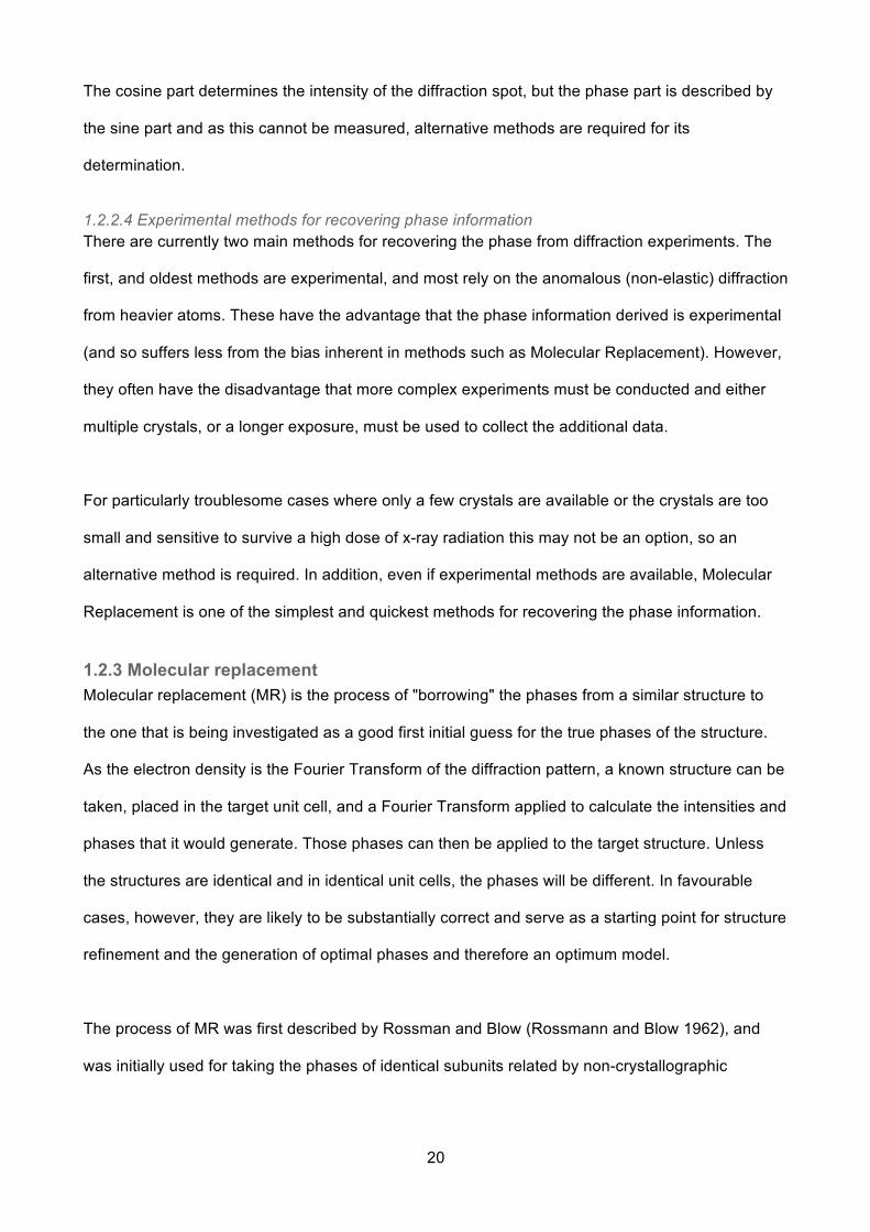
1.2.2.4 Experimental methods for recovering phase information There are currently two main methods for recovering the phase from diffraction experiments. The

first, and oldest methods are experimental, and most rely on the anomalous (non-elastic) diffraction

from heavier atoms. These have the advantage that the phase information derived is experimental

(and so suffers less from the bias inherent in methods such as Molecular Replacement). However,

they often have the disadvantage that more complex experiments must be conducted and either

multiple crystals, or a longer exposure, must be used to collect the additional data.

For particularly troublesome cases where only a few crystals are available or the crystals are too

small and sensitive to survive a high dose of x-ray radiation this may not be an option, so an

alternative method is required. In addition, even if experimental methods are available, Molecular

Replacement is one of the simplest and quickest methods for recovering the phase information.

1.2.3 Molecular replacement Molecular replacement (MR) is the process of "borrowing" the phases from a similar structure to

the one that is being investigated as a good first initial guess for the true phases of the structure.

As the electron density is the Fourier Transform of the diffraction pattern, a known structure can be

taken, placed in the target unit cell, and a Fourier Transform applied to calculate the intensities and

phases that it would generate. Those phases can then be applied to the target structure. Unless

the structures are identical and in identical unit cells, the phases will be different. In favourable

cases, however, they are likely to be substantially correct and serve as a starting point for structure

refinement and the generation of optimal phases and therefore an optimum model.

The process of MR was first described by Rossman and Blow (Rossmann and Blow 1962), and

was initially used for taking the phases of identical subunits related by non-crystallographic

21

symmetry (NCS) to solve larger structures. The method has since been developed and extended

and can now be used to solve structures that are substantially different from the target structure.

MR is currently the most popular method for x-ray structure solution. At the time of writing, there

were 105,912 x-ray structures in the PDB (Rose et al. 2013), of which 82 percent (70007 structures

and 16102 ligands) were solved with MR. The proportion of structures solved with MR in the PDB

has been increasing with time because the more structures that there are in the PDB the greater

the chances are that there is something similar which can be used for MR.

For successful MR, the structure used to generate the phases must be sufficiently similar to the

target structure. Experience with standard MR has shown that it is expected to be unlikely to

succeed when the sequence identity (a proxy for structural similarity) is between 20 and 30%

(Abergel 2013) and impossible when it is lower than 20%.

1.2.3.1 Placement of the Structure in the Unit Cell For MR to work the spatial transformation required to position the MR search model in the unit cell

needs to be determined so that it is optimally aligned with the target structure and the phases that

are generated will be as applicable to the target as possible. It is methods of solving this problem

that constitute the field of Molecular Replacement.

1.2.3.1.1 Brute-force methods The naive method of solving this problem would be to run a grid-search through the entire unit cell,

placing the structure at each grid point and then calculating the intensities of the diffraction pattern

to see how they compare with the measured intensities (using an R-factor - see section 2.3.5). In

addition to sampling all grid points (at a suitable density), all possible rotations would also have to

be tested as it is both the position and the orientation of the structure that determines the diffraction

pattern.

Although there are some programs that attempt this approach (such as Queen of Spades and

BEAST (Glykos and Kokkinidis 2000; Read 2001) ), it is in general prohibitively expensive. For

22

each position and orientation, the structure factor for all reflections must be calculated, and as all

atoms contribute to each structure factor, the number of calculations is extremely high.

1.2.3.1.2 Rotation/Translation searches As brute-force methods are largely impractical, alternatives have been developed, which generally

rely on separating out the rotation and translation searches. This separation greatly reduces the

number of searches that need to be made, as rather than having to compute all rotations for each

translation search, the rotation search only needs to be completed once. The correctly rotated

molecule can then be used in the translation search. This, however, requires that the correct

orientation of the search model can be determined. To understand conceptually how this is done a

brief foray into the subject of Patterson maps is required.

1.2.3.1.3 Patterson maps The Patterson map is named after Arthur Patterson (Patterson 1934), and can be considered as a

convolution integral of the electron density with its inverse:

(1.12)

Where P is the Patterson function, ρ the density and r a position vector.

This form shows that the Patterson map contains peaks for all of the position vectors between

each pair of atoms, weighted by the product of the electron density at those positions. The

Patterson map therefore contains N2 peaks, but if self-peaks are excluded (which appear at the

origin), N(N-1) peaks remain. Even excluding the self-peaks means that the Patterson is a very

crowded and hard to interpret map, particularly for large protein structures. Figure 1.2 shows a

schematic of a highly simplified Patterson map.

23

Figure 1.2. Schematic of a Patterson Map

The major advantage of the Patterson map is that it can be computed directly from the

intensities of the diffraction pattern without requiring any phase information, using the equation:

(1.13)

This is the Fourier Transform of the diffraction data using the intensities as the amplitudes and

setting the phases to zero. It is also possible, to some extent, to separate the Patterson map into

inter- and intra-molecular vectors. There will always be an extremely large peak at the centre that

contains all of the self-peaks. Further out the peaks gradually become dominated by inter-

molecular peaks.

For a known structure, placing the model in a unit cell far larger than the model effectively

separates the inter and intra-molecular peaks, with the inter-molecular peaks crowding near the

origin and the inter-molecular peaks separated from them by the distance of the unit cell. For a

crystal structure in a unit cell with dimensions commensurate with the size of the molecule there is

no clean separation of the peaks, but those closer to the origin will again be dominated by the

inter-molecular peaks.

The advantage of being able to separate the intra- and inter-molecular peaks is that the intra-

molecular peaks are invariant under translation of the molecule and depend entirely on its

24

orientation. Therefore, by comparing the intra-molecular Patterson peaks of the search model in

all orientations with those of the diffraction pattern (usually using least-square methods), it should

be possible to determine the correct orientation of the search model. With the orientation

determined a similar procedure can be carried out to determine the translation vector.

These types of methods are called Patterson Methods and were the methods first used to solve

structures using Molecular Replacement. They provide a convenient theoretical explanation of the

types of procedures employed, but are not an accurate portrayal of the algorithms the current

state-of-the-art programs employ, most of which are based on Maximum Likelihood.

1.2.3.1.4 Maximum Likelihood Most of the current methods employed in crystallography now use variations on Maximum

Likelihood and Bayesian Inference both in order to account for the highly noisy and statistical

nature of crystallographic experiments, and to more easily combine these with existing knowledge

about molecular structures (Airlie J. McCoy 2004).

Maximum Likelihood is a way of determining the best hypothesis to explain an observation. For

example, given two dice, one with 4 sides and one with 10 sides, if an 8 is rolled, the likelihood of

the hypothesis that it was the 4-sided dice is zero. The likelihood can however be increased by

changing the hypothesis to it being the 10-sided dice that was rolled, in which case the likelihood

becomes one. Within crystallography Maximum Likelihood is used to determine the optimum model

(molecular structure) that explains the data (measured diffraction pattern) with the highest

probability.

Maximum Likelihood therefore provides a way of generating an optimum model to explain the data,

but it takes no account of the overall viability of the model; it is quite possible to generate a

molecular model that accounts for a diffraction pattern, but is completely impossible in reality (i.e. it

contains an arrangement of atoms that would not be adopted by any known structure).

25

In order to incorporate prior knowledge of physics, chemistry and biology into the model recourse

to Bayesian Inference is required.

1.2.3.1.5 Bayes Theorem The Bayes Theorem makes it possible to determine whether an hypothesis formulated to interpret

a set of evidence offers the most likely explanation, by linking with it the prior knowledge of the

conditions pertaining to that hypothesis (Bayes and Price 1763).

Bayes Theorem can be written as:

(1.14)

This states that, given the data, the probability of the model (the posterior probability; how well the

model can explain the data) is the product of the probability of the data given the model (the

likelihood of the data given the model), with the probability of the model (called the prior probability;

basically the viability of the model) divided by the prior probability of the data, or the probability of

measuring the data. In other terms:

𝑝𝑜𝑠𝑡𝑒𝑟𝑖𝑜𝑟 =𝑙𝑖𝑘𝑒𝑙𝑖ℎ𝑜𝑜𝑑 ∗ 𝑝𝑟𝑖𝑜𝑟

𝑒𝑣𝑖𝑑𝑒𝑛𝑐𝑒

(1.15)

The denominator is the prior probability of the data and is constant in experimental situations so

can either be converted to a constant or ignored when probabilities are being compared. With the

prior for the evidence constant, the crystallographic version of Bayes Theorem becomes:

P(model | data) = P(data | model) P(model) (1.16)

which states that the likelihood of the model structure explaining the diffraction data is maximised

by optimising the likelihood of the model explaining the data (altering the model to best fit the data),

whilst at the same time ensuring that the model is maximally viable.

Maximum Likelihood has become the preferred method of solving MR (and indeed of refining

structures following MR) as it enables the inclusion of error estimates (such as the RMS errors in

the model coordinates), something that cannot be included in Patterson Methods.

26

Within crystallography the application of Maximum Likelihood involves the multiplication of many

small probabilities, which is a problem as computers struggle to represent very small floating point

numbers, leading to an accumulation of rounding errors. For this reason the log of the likelihood is

used, rather than the likelihood itself (something that is possible because log functions are

monotonic, so that if a < b, log(a) < log(b)). Additionally, as most computational optimisation

algorithms tend to minimise functions, it is usually the negative of the log likelihood that is

optimised.

1.2.3.2 PHASER Within CCP4, there the two main programs that are used for Molecular Replacement are PHASER

and MOLREP (A. J. McCoy et al. 2007; Vagin and Teplyakov 1997). For most of the calculations

within this work, PHASER was used.

PHASER is a program for both Molecular Replacement and experimental phasing that comes out

of the group of Randy Read at the Cambridge Institute for Medical Research, and is developed

primarily by Airlie McCoy. Unlike earlier programs that relied on Patterson methods, PHASER

relies heavily on maximum likelihood methods and multivariate statistics. PHASER contains a

number of modules for performing the different steps of MR, and in automatic mode, these are all

marshalled to run the entire MR pipeline, which consists of the following steps:

l Cell Content Analysis

l Anisotropy correction

l Translational NCS correction

l Rotation Function

l Translation Function

l Packing

l Refinement

Within PHASER, the results of MR are scored using an LLG and Z-score. The LLG score is the

Log-Likelihood Gain, which is the difference between the likelihood calculated for the model and

27

the likelihood calculated from a Wilson Distribution (a distribution calculated for random distribution

of atoms in a unit cell), and the Z-score, which is the number of standard deviations that the LLG

score differs from the mean of a random set of translation and rotation scores. A LLG score of >=

120 and a TFZ score of >=8 are usually very reliable indicators of success.

1.2.3.3 Ensemble Models in MR When MR was first developed, a single homologous structure would be used as the search model.

The effectiveness of using several similar superimposed models was demonstrated when NMR

models were first used to try and solve crystal structures. In 1987 Brunger et al. (Brünger et al.

1987) first demonstrated the ability to solve crystal structures using the average structure derived

from an NMR ensemble, where no individual structure could achieve solution.

The use of ensembles is now a standard technique in MR although the method differs from the

average structure approach used in the NMR method. Within PHASER, the variance between the

ensembles is used to weight the structure factors generated from the ensembles, thereby feeding

into the maximum likelihood target.

1.2.3.4 Refinement Unless repeating an experiment with the optimum model that best explains the diffraction data,

then the model used in MR is necessarily incorrect to some extent and needs to be improved. The

improving of an existing model to best fit the diffraction data is termed refinement.

Refinement involves taking an existing model and altering its structure to best fit the diffraction

data. It does not involve adding or removing residues to the model as this is something that is done

in model building. Combining the phases calculated from the model positioned by MR with the

intensities measured in the experiment using the structure factor equation, the electron density for

the experiment can be calculated. The model can then be altered in real space to make it better fit

into the density whilst maintaining a chemically sensible structure (in Maximum Likelihood terms

adhering to the prior probabilities of a molecular structure). The changes to the model will change

the phases and hence the density, so the alteration to the model in real space is an iterative

28

process. However, at some point this process will stall, and then most programs will switch to a

stage of refinement in reciprocal space. In this stage the positions of the atoms (which contribute to

the phase) and the B-factors (which affect the intensity of the structure factors) are altered to best

fit the measured diffraction pattern whilst ensuring the model obeys stereochemical restraints. This

process will generate a new model and phases, and hence new density, so the model can now be

refined in realspace in the new density.

Most refinement involves cycling between refinement in real space and reciprocal space until the

overall refinement has converged. The success of refinement is usually quantified with an R-factor.

1.2.3.5 The R-Factor The R-factor is a measure of how well the model can explain the diffraction data. The R-factor is a

global linear residual that can be written as:

(1.17)

Where the summation runs over the structure factors with Miller indices h,k,l, and Fobs(h,k,l) are the

observed structure factors, and Fcalc(h,k,l) the calculated structure factors. The R-factor would be

zero for a model that perfectly explained the diffraction data and one for one that had no explaining

power. For an initial refinement after MR, anything below 0.5 is considered a good indication that

MR has succeeded.

1.2.3.6 Model bias and RFREE As the phases dominate the structure factor equation and the experiment only measures

intensities, adding phases from a partial model will heavily skew the electron density in favour of

the model, regardless of how correct the model is. In order to guard against this model bias, Axel

Brunger introduced the idea of the Rfree set (Brunger 1992). This is a small selection (of the order

of a few per cent) of the reflections that are set aside and not used in refinement to ensure that the

model has not been refined against these reflections. An R-factor can then be calculated for these

29

reflections. If the refinement is unbiased, the R-factor for this subset should be similar to those

against which the model has been refined. If they are significantly different, and particularly if they

diverge over the course of a refinement, then it is an indication of model bias.

1.2.3.7 REFMAC The refinement program used within CCP4 is REFMAC (Murshudov et al. 2011), the development

of which is led by Garib Murshudov, and this is the program that is used within the AMPLE pipeline

itself and many of the programs that it runs. REFMAC implements a number of techniques to aid

refinement, including TLS (Translation, Libration, Screw), bulk solvent techniques, such as solvent

masking, and jelly body restraints.

Within the MrBUMP (Keegan and Winn 2007) and therefore AMPLE pipelines, REFMAC is run by

default for 30 macrocycles with jelly body restraints with a weight of sigma 0.02. Jelly body

restraints are a form of rigid-body restraints applied to the second-derivative matrix of the overall

maximum likelihood refinement function. The restraints effectively serve to dynamically rigidify all

atom pairs within a radius (currently 4.2Å), with the weight determining the contribution to the

function. The weight is inversely proportional to sigma, so smaller sigmas indicate a larger weight

and a more rigid-body type approach. With a weight of 1, jelly body refinement would effectively be

full rigid-body refinement.

1.2.3.8 Density modification, chain tracing and SHELXE Once a model has been refined, a common step is to use density modification to improve the

phases. Density modification is a technique for altering the phases so that the electron density

better matches what is known about the structure of protein molecules in solvent. Experience has

shown that the density within solvent regions of a protein crystal is lower and less ordered than the

regions where there is protein. Modifying the density to better demarcate these regions has been

shown to be a powerful technique for improving phases. A number of techniques can be used for

density modification, such as solvent flattening and flipping, histogram matching and density

averaging.

30

Within the AMPLE pipeline, SHELXE (G. M. Sheldrick 2007; Thorn and Sheldrick 2013) is used for

both density modification, chain tracing to expand the small fragments generated by AMPLE and

also to determine if the MR step has succeeded. A brief explanation of the operation of SHELXE

will therefore be provided.

SHELXE is part of the SHELX suite of programs developed by George Sheldrick, and was initially

developed to aid the experimental phasing of macromolecules by improving the phases from a

heavy-atom substructure. However, it has since proved to be of great utility for expanding small

MR solutions as generated by AMPLE, ARCIMBOLDO (Millán, Sammito, and Usón 2015) and

Auto-Rickshaw (Panjikar et al. 2005).

Crucial to the operation of SHELXE it the CC score, which is the correlation coefficient of the

partial structure of the native data. The CC score was formulated by Fujinaga and Read (Fujinaga

and Read 1987) and is calculated as:

(1.18)

where EO are the normalised observed structure factors and EC the normalised structure factors for

the partial structure.

Experience has shown that the CC score is a powerful metric for determining whether MR has

worked, with a CC score of >= 25% usually being a clear indication that MR has been successful

(for data of resolution <= 2.5Å). However, a good CC score can arise due to an physically

unreasonable arrangement of atoms, so in most practical cases an average traced chain length

(see below) of >= 10 is added as an additional requirement.

31

The CC score is used in an optional first stage of the SHELXE algorithm called CC-trimming,

where the initial MR fragment is pruned by removing each residue in turn to see if this improves the

CC score. If the CC score increases then the residue is removed.

The heart of the SHELXE 'sphere of influence' algorithm, which is based on the idea that the

average 1,3 interatomic distance between carbon atoms (i.e. the distance between carbon atoms

separated by two bonds) in macromolecules is 2.42Å. The algorithm works by taking each point on

a grid in the density map and looking at the variance of the density of a sphere of radius 2.42Å. If

the density on the surface of the sphere is highly variable it indicates the point may be a main

chain atom and the density is left unchanged. If the variance of the density is low the point is

assumed to be in solvent and the density is flipped (i.e the sign of the density is changed whilst

leaving the magnitude unchanged). By default, 20 cycles of density-modification are carried out

before there is a cycle of autotracing.

Autotracing involves extending out from any initial tri-peptides, using a simplex search with a two-

residue look-ahead, and allowing a limited variation of the N-Cα-Cτ torsion angles. A number of

searches are trialled and when they cannot be extended any further, those that meet the criteria for

the figure of merit (based on trace length, fit to the density and various structural parameters) are

kept and, where appropriate, spliced together.

By default 15 cycles of autotracing, each with 20 cycles of density modification are undertaken and

the cycle with the best CC score is kept for additional model building. If the CC score is >= 25%

and the average traced chain length is >= 10, then the structure is deemed to have been solved.

1.2.3.9 Model building with BUCCANEER and ARPWARP In many MR cases, the search model will only contain a subset of the residues expected in the

final structure. Therefore, following refinement (and possible chain tracing by SHELXE), the

missing parts of the structure need to be built into the density. The way that this usually proceeds

is that where the sequence of the model is known and the density for one or more missing residue

32

can be seen, the residues are built into the density. The structure with the new residues is then

subject to one or more rounds of refinement, which should improve the density allowing additional

residues to be built into the structure. This process is iterated until all residues, ligands and

potentially waters, etc. have been added to the structure and the building and refinement are

deemed to have converged (exactly when this has happened is still a hotly debated topic in

crystallography).

Previously this was done manually, but today, automated programs are able to carry out most if not

all of these steps. Within CCP4 the two main model building programs are BUCCANEER (Cowtan

2006), developed by Kevin Cowtan and ARPWARP (Langer et al. 2008), developed by the group

of Victor Lamzin. As they perform similar tasks both programs have similar workflows, alternating

between cycles of finding atom and residue positions, linking adjacent residues to form chains and

then attempting to sequence the chains, with cycles of refinement with REFMAC. They differ

primarily in their approach to interpreting the electron density to find structures of interest.

BUCCANEER uses a reference map of known protein features that it modifies based on the target

density, and then searches for those features using a likelihood function, whereas ARPWARP

inserts pseudo-atoms into the density and then attempts to join and merge pseudo-atoms to build

up residues.

1.2.3.10 MR Pipelines Within CCP4 there are a number of MR pipelines that automate the process of structure solution,

from model selection, MR, refinement, density modification and model building. These include

BALBES, MRBUMP and ARCIMBOLDO (Long et al. 2008; Keegan and Winn 2007; Rodríguez et

al. 2009). MRBUMP is used extensively by AMPLE, and AMPLE and ARCIMBOLDO share a

similar approach, so both will be examined below.

1.2.3.10.1 MRBUMP MRBUMP is a MR pipeline written in PYTHON and developed by Ronan Keegan that automates

the entire process of MR, from model selection through to final model building. The MRBUMP

pipeline involves the following steps:

33

1. Search for model templates: using the sequence of the target protein, a sequence search

of online databases is made using one or more of PSIBLAST (Altschul et al. 1997),

PHMMER (Finn, Clements, and Eddy 2011) or HHPRED (Söding, Biegert, and Lupas

2005) in order to select homologs (subsequently referred to as templates) of the target.

2. Domain search: a search is made of the SCOP database to determine if any of the

templates can be split into domains, in which case additional templates are generated by

splitting the parent template into separate domains.

3. Multiple sequence alignment (MSA): a MSA of the templates to the target is made using

either PHMMER or MAFFT (Katoh et al. 2002), in order to aid the subsequent search

model preparation stage and also to score and rank the various templates.

4. Single search model preparation: using the MSA from step 3, each template is prepared

in four different ways, using the programs PDBCLIP, MOLREP, CHAINSAW (Stein 2008),

and SCULPTOR (Bunkóczi and Read 2011). PDBCLIP just removes any waters and

selects the most probable conformation, whereas the others all prune or modify the side

chains of the template based on the alignment to the target. In addition to these four

models, an` unmodified template, and another where all side chains are mutated to

polyalanine are used.

5. Ensemble search model preparation: In addition to the six templates above an additional

ensemble search model is prepared by creating an ensemble from all templates using

either GESAMT (Evgeny Krissinel 2012) or SUPERPOSE (E. Krissinel and Henrick 2004).

6. Molecular Replacement: MR is then run on all search models using either PHASER or

MOLREP.

7. Refinement: following MR, the models are refined with REFMAC. Following refinement,

MRBUMP will rate each model according to the following criteria:

a. good: the final RFREE is < 0.35 or is < 0.5 and has dropped by 20%.

b. marginal: final RFREE is < 0.48 or < 0.52 and has dropped by 5%.

c. poor: anything else.

34

8. Model building and density modification: the refined model may then either be

submitted directly to ARPWARP or BUCCANEER for model building, or may first be

submitted to SHELXE for chain tracing, followed by optional submission to ARPWARP or

BUCCANEER for final model building.

The latter stages of the MRBUMP pipeline, from steps 6 to 8, are used within AMPLE to drive the

MR and model building stages.

1.2.3.10.2 ARCIMBOLDO Of the MR pipelines in CCP4, ARCIMBOLDO is most similar in philosophy to AMPLE, and has

driven a number of the developments to PHASER and SHELXE that have aided AMPLE.

ARCIMBOLDO, is developed by the group of Isabel Uson and attempts MR solution with small

fragments and then builds up to full structures from these fragments.

ARCIMBOLDO derives its inspiration from direct solutions methods, such as the Shake-and-Bake

algorithm as implemented in the SnB and SHELXD programs (George M. Sheldrick 1998). These

all start from the assumption that a structure is composed of atoms, and then attempt to locate the

atoms as peaks in the density map and join them together to create full structures (Millán,

Sammito, and Usón 2015). This approach can only be successful with atomic-resolution data,

something that is still extremely rare in macromolecular crystallography. ARCIMBOLDO uses small

fragments to extend this approach beyond atomic resolution, placing and combining small

fragments to build up larger structures.

The first version of ARCIMOBOLDO used 14-residue ideal polyalanine helices to solve the

structure of PRD-II (Rodríguez et al. 2009), placing 3 copies of the helix with PHASER and then

using SHELXE to trace the final structure. This resulted in three successful solutions from the

1,473 trials attempted by PHASER. As so many attempts are explored, the early versions of

ARCIMOBOLDO required a supercomputer or computational grid in order to achieve solution.

35

Since the first version was developed, the developers have extended their approach to use the

PHASER rotation search to prioritise solutions. A rotation search is made for each fragment and

the rotations grouped to find the most promising candidates. For each candidate rotation a

translation search is then made and the resulting placement submitted to SHELXE for CC-

trimming, density modification and main-chain tracing. For multiple fragments these stages are

repeated for each candidate rotation peak.

ARCIMBOLDO has since expanded to comprise a suite of four programs.

l ARCIMBOLDO and ARCIMBOLDO_LITE (Sammito et al. 2015): these use small, user-

selected fragments (usually ideal α-helices) to attempt solution as described above.

ARCIMBOLDO_LITE is a version that is parallelised to run on multi-core desktop machines

l ARCIMBOLDO BORGES (Sammito et al. 2013): this relies on an existing library of small

structural motifs extracted from the PDB. Fragments from the library are selected based on

a geometrical description and are then geometrically clustered, before being clustered

again via the rotation function and submitted to the ARCIMBOLDO pipeline.

l ARCIMBOLDO SHREDDER (Sammito et al. 2014): this takes a distant homolog and

successively removes residues based on their Shred-LLG function, which is calculated from

the rotation function. A selection of the best-scoring shredded models are then submitted to

the ARCIMBOLDO pipeline.

1.2.4 Problems with Molecular Replacement The previous sections have explored Macromolecular Crystallography with a focus on Molecular

Replacement. As has been mentioned, Molecular Replacement is the most popular technique for

solving Macromolecular Crystal structures, but usually relies on the existence of a similar structure.

When no suitable similar structure exists in the PDB, or structures expected to be similar are not

(such as coiled-coil proteins, in which similar proteins can pack very differently), alternatives need

to be found. AMPLE's first and still primary role, is the use of Ab Initio Molecular Modelling to

generate novel structures where none can be found, and to prepare these in a form suitable for

36

MR. The following section will therefore look into Ab Initio Molecular Modelling as it applies to

AMPLE.

1.3 Ab Initio Modelling

1.3.1 The Protein Folding Problem Determining the tertiary (folded) structure of a protein from its amino acid sequence is known as

the 'Protein Folding Problem' and has been an active area of research for more than 40 years. The

nature of the problem was demonstrated by Cyrus Levinthal, in a 1969 paper (Levinthal 1969),

which was concerned with a theoretical protein of 150 amino acids and considered only the 450

degrees of freedom that arise from rotations of the main chain and side chain rotamers. If the

rotations were determined to a tenth of a radian, there would be 10300 possible conformations that

would have sampled in order to determine the lowest energy conformation of the protein;

something that would take a protein longer than the lifetime of the universe to accomplish.

A similar problem afflicts computational protein folding and means that a brute-force

conformational search will never be feasible (at least with non-quantum computers). For this

reason, a variety of methods that severely curtail the conformational space that needs to be

sampled have been developed. Nearly all of these methods rely in some way on using existing

structures (i.e. those in the PDB). Some methods use general information derived from all

structures (such as common bond lengths, and favoured rotamer angles), others use either entire

structures, or structural fragments, and some use a combination of both.

Examples of using an entire structure are protein 'threading' or homology modelling. These involve

overlaying a novel amino acid sequence over an existing structure, which serves as a guide for the

overall fold. The novel structure can then be refined and minimised to determine the correct final

structure. Although often very successful and capable of generating structures that differ from

native structures by only a few Angstroms, these methods are hampered by the fact that they

require a largely complete model of a similar protein fold. For novel structures, or structures where

37

similar sequences can form quite different folds, these methods may not be applicable, and this is

where ab initio folding protocols come into play

1.3.2 Ab Initio Protein Structure Prediction Ab Initio Protein Structure Prediction, is the process of determining the tertiary structure of a

protein starting purely from the protein sequence, and not relying on the structure of an existing

model as a template.

There are a number of methods and protocols that have been developed to accomplish this. In the

2014 CASP Community Wide Experiment on the Critical Assessment of Techniques for Protein

Structure Prediction (Taylor et al. 2014), for example, 22 separate groups used distinct methods to

determine the structures of the submitted proteins (Taylor et al. 2014). Although all distinct, the

methods are predominantly variations on ways of incorporating and permuting data from known

structures to generate models.

The ROSETTA suite of programs (Simons et al. 1997; Rohl et al. 2004) is one of the best

established and widely used methods, and is also the one that has been used most within AMPLE,

so a brief explanation of how it works follows.

1.3.2.1 ROSETTA modelling protocol The ROSETTA modelling protocol (Simons et al. 1997; Rohl et al. 2004) is a mixture of knowledge-

based (i.e. using information from known structures) and first-principles physics-based

approaches. It starts from the idea that the overall structure of a protein arises from the interplay of

the forces derived from local structure, together with those arising from the global conformation of

the protein. The local structure guides the initial folding, but it is the larger features such as the

burying of hydrophobic residues or the pairings of β-strands that determine the overall fold.

38

The overall ROSETTA protocol can be separated into three parts:

l an initial decoy generation stage where many (typically tens of thousands) of relatively

computationally inexpensive molecular structures are generated.

l a clustering stage where the decoys are clustered to determine the centroid models.

l a computationally expensive optimisation stage, where the centroid models are refined to

produce final models.

1.3.2.1.1 Decoy Generation The protocol starts with a search for short protein fragments (3 or 9 residues in length) with

identical or related residue composition for every position along the length of the protein. The

positions are overlapping, so that for the triplet fragments, there is a fragment starting at the first

residue, another at the second and so forth. The fragments are collected from a non-redundant

database of fragments that have been assembled from known structures, but with their bond

lengths and angles set at idealised values. This is required because the fragments are represented

in a simplified form using the heavy atoms of the main chain and the C-β atom of the side chain,

with bond lengths and angles held constant according to the ideal geometry of alanine. The

fragments are described both by their φ, ψ and ω backbone torsional angles, and their secondary

structure content.

The protocol uses a search through torsional space starting from a fully extended protein, with the

fragments defining the conformational space to be searched. A position is selected at random in

the protein, and the torsional angles from a randomly selected fragment from the top 25 for that

position are applied to the protein. The energy is then evaluated according to a scoring function

and the move is either accepted if it lowers the energy, or accepted according to the Metropolis

(Metropolis and Ulam 1949) criteria if it raises it.

Simulated annealing is incorporated by lowering the temperature over the course of the simulation.

In addition, terms are progressively added to the scoring function used to assess moves as the

simulation progresses and the structure nears a supposedly more native-like conformation. Side

39

chain conformations are added to the backbone using a Monte-Carlo simulated annealing search

with a rotamer library. Following the 9-fragment assembly stage, the structure is refined with a

short stage of 3-residue insertions using the full energy function to score the resulting models.

The full energy function for evaluating the structures during the fragment-assembly strategy

contains the following terms (Rohl et al. 2004):

l residue environment (solvation)

l residue pair interactions (electrostatics, disulfides)

l strand pairing (hydrogen bonding)

l strand arrangement into sheets

l helix-strand packing

l radius of gyration (van der Waals attraction, solvation)

l Cβ density (solvation; correction for excluded volume effect introduced by simulation)

l steric repulsion (van der Waals)

l The energy function operates on a reduced representation of the side chains, in which they

are represented by a centroid located at the centre of mass of the side chain (defined as

the atoms including and beyond Cβ).

Once they have been generated, the decoys are clustered.

1.3.2.1.2 Decoy clustering The rationale for clustering the decoys is the hypothesis that the native state of a protein is the

minimum of the folding energy landscape, and that there are numerous low-energy states

clustered around this state, the folding being largely dictated by long-range hydrophobic effects

(Shortle, Simons, and Baker 1998). As such, in a large selection of energy-minimised models, the

majority should approximate the native state. If the models are clustered by structural similarity

then the largest cluster often contains the best model, and the centroid of the cluster is likely to be

the best prediction for that model.

40

In the ROSETTA protocol the models are clustered using the CLUSTER application. This takes a

subset of the models (usually 400) and finds the model with the highest number of neighbours

within the cluster radius. This is considered the centroid, and then all the models that are within the

specified radius of this cluster from all the models are added to the cluster and removed from the

list of available models. The process is then repeated until all the models have been claimed by a

cluster. By working with subsets of models, this algorithm avoids the need to calculate the large

and expensive all-by-all distance matrix.

1.3.2.1.3 All-atom refinement Decoys may either be generated as low-resolution models without side chains, or, more time-

consumingly, as fully refined models. If low-resolution models have been used, following clustering,

centroid representatives of the top 5-10 clusters may be sent forward for a more computationally

expensive all-atom refinement.

1.3.3 Evolutionary Contact Prediction A major development in the field of bioinformatics and protein structure prediction has been the

rapid progress made in the prediction of residue-residue contacts from patterns of co-evolution of

residues in related families of proteins (de Juan, Pazos, and Valencia 2013). Accurate information

about which residues are likely to be in contact vastly reduces the conformational space that needs

to be sampled and can lead to more rapid and accurate modelling.

The hypothesis behind contact prediction is that residues that are in contact with one another, and

particularly those that have important structural and functional roles, will need to vary in concert

with each other in order to preserve the function or structure. For example, for two residues with an

important structural role, if one residue mutates to become larger, then the other will need to be

mutated to something smaller in order to maintain the structure, so their changes will be correlated.

A multiple sequence alignment (MSA) of a protein family shows how the residues vary through the

family, but this information is of limited value without a probabilistic model that relates the changes

at one position to any other in the alignment. A key problem is how to separate direct (A-B and B-

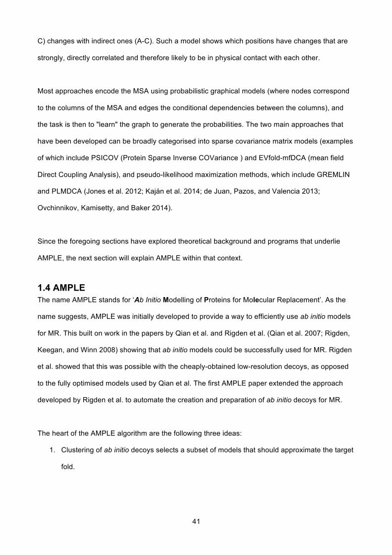
41

C) changes with indirect ones (A-C). Such a model shows which positions have changes that are

strongly, directly correlated and therefore likely to be in physical contact with each other.

Most approaches encode the MSA using probabilistic graphical models (where nodes correspond

to the columns of the MSA and edges the conditional dependencies between the columns), and

the task is then to "learn" the graph to generate the probabilities. The two main approaches that

have been developed can be broadly categorised into sparse covariance matrix models (examples

of which include PSICOV (Protein Sparse Inverse COVariance ) and EVfold-mfDCA (mean field

Direct Coupling Analysis), and pseudo-likelihood maximization methods, which include GREMLIN

and PLMDCA (Jones et al. 2012; Kaján et al. 2014; de Juan, Pazos, and Valencia 2013;

Ovchinnikov, Kamisetty, and Baker 2014).

Since the foregoing sections have explored theoretical background and programs that underlie

AMPLE, the next section will explain AMPLE within that context.

1.4 AMPLE The name AMPLE stands for ‘Ab Initio Modelling of Proteins for Molecular Replacement’. As the

name suggests, AMPLE was initially developed to provide a way to efficiently use ab initio models

for MR. This built on work in the papers by Qian et al. and Rigden et al. (Qian et al. 2007; Rigden,

Keegan, and Winn 2008) showing that ab initio models could be successfully used for MR. Rigden

et al. showed that this was possible with the cheaply-obtained low-resolution decoys, as opposed

to the fully optimised models used by Qian et al. The first AMPLE paper extended the approach

developed by Rigden et al. to automate the creation and preparation of ab initio decoys for MR.

The heart of the AMPLE algorithm are the following three ideas:

1. Clustering of ab initio decoys selects a subset of models that should approximate the target

fold.

42

2. Structurally aligning the clustered decoys and measuring the inter-residue structural

variance of the aligned decoys provides a proxy for the accuracy of the modelling.

Removing residues based on the degree of structural variance should therefore remove

less accurately modelled regions leaving a more accurate core that may be suitable for MR.

3. Even if small relative to the native structure, an ensemble of structurally similar truncated

decoys may contain enough information for MR to work and allow auto-tracing and auto-

building programs such as SHELXE and BUCCANEER to construct a largely full model

from a correctly placed search model.

AMPLE is a pipeline that automates the entire process, from the creation of the ab initio decoys,

through the creation of the ensembles, to the MR and autobuilding steps. Figure 1.2 below depicts

the ensemble creation pipeline.

Figure 1.2. The AMPLE ensemble preparation pipeline

43

The AMPLE ensemble preparation pipeline consists of the following steps:

1. Clustering of the 1000 ab initio decoys with SPICKER (Y. Zhang and Skolnick 2004) and selection of up to 200 decoys from the top cluster.

2. Truncation of the decoys at 20 different levels (5% intervals by default), based on the inter-

residue variance score calculated by THESEUS (Theobald and Wuttke 2006).

3. Sub-clustering of the decoys in each truncation level under 1, 2 or 3Å RMSD thresholds (as calculated by MAXCLUSTER (“MaxCluster - A Tool for Protein Structure Comparison and Clustering,” n.d.)), and the creation of a structurally aligned ensemble from up to 30 of the resulting models using THESEUS.

4. Three different side chain treatments of the final ensemble:

� retention of all side chains. � retention of only those side chains that are usually well-modelled by SCWRL

(Krivov, Shapovalov, and Dunbrack 2009). � removal of all side chains to polyalanine.

From the initial 1000 decoys, up to 180 ensembles, each containing anywhere from 2 to 30 decoys

are generated. The ensembles are then sent for processing to MRBUMP, which undertakes steps

6-8 of the MRBUMP pipeline described above.

A key part of the success of the AMPLE (and MRBUMP) pipelines is that every putatively MR-

positioned model produced by PHASER is submitted blindly to SHELXE, regardless of whether the

statistics indicate that the job has succeeded. Any model that is traced by SHELXE to a CC of >=

20 and an average chain length of >= 8 is then submitted for autobuilding by BUCCANEER and

ARPWARP. This is important, because, as with ARCIMBOLDO, AMPLE often uses such small

fragments that the LLG and TFZ statistics generated by PHASER (particularly with earlier versions

of the program) are often not a reliable indicator of success and it is only the CC score following

SHELXE autotracing that provides this.

Runtime for AMPLE is highly variable as it depends on the length of the target (which affects the

time required for ab initio modelling), the resolution of the data (which affects the runtime for

SHELXE, with higher-resolution data significantly slowing things down), the number of ensembles

generated and the ratio of successful (if any) ensembles generated by the pipeline. In most use

cases AMPLE takes of the order of 24 hours on a single processor. However run times can vary

44

from a few hours for simple cases to several days for the most difficult cases. AMPLE is

extensively parallellised and as most parts of the pipeline can be split into independent jobs, the

time taken reduces almost linearly with the number of processors. On a modern desktop with 4-8

processors, AMPLE should run to completion in considerably less than 24 hours.

When it was first developed, AMPLE's primary focus was on ab initio models generated by

ROSETTA. However, since then AMPLE has been extended to work with QUARK ab initio models,

NMR ensembles and distant homologs.

1.5 Structure of the thesis The work undertaken for this thesis falls into three parts:

l the first is covered in chapter two, which focuses on the software developments that

have been made to the AMPLE code to improve it and make it easier to maintain,

extend and distribute on different platforms.

l the second is treated in chapters three to five, which explore the use of AMPLE on

three different types of protein targets, namely coiled-coil and transmembrane proteins,

and distant homologs.

l the third is dealt with in chapter six, which covers the improvements to the original

AMPLE ensembling and truncation algorithm that were made in the light of the insights

gained in the second section.

45

Chapter 2: Software

Developments

46

2 Software Developments

2.1 Software Development Approaches

2.1.1 Issues with the first version of AMPLE As with most prototype scientific software, AMPLE was initially developed as a piecemeal series of

scripts for carrying out particular tasks, that were pulled together by a single monolithic script to

implement the pipeline. As time progressed, more functionality was added, including the ability to

run either on a local machine or submitting to a queueing system to run on a

cluster/supercomputer. These two paths through the code were implemented separately, and led

to duplication of code and the possibility of errors. In addition, there were no tests implemented, so

it wasn't clear whether all parts of the code were working as expected.

AMPLE quickly became incorporated and distributed with CCP4. As a piece of software

responsible for wider scientific research and used by the general crystallographic community, it

became even more necessary to ensure that it was easy to maintain and to ensure the correctness

of its results. As a result of this, the first task that was completed as part of this PhD was to

extensively refactor and rewrite AMPLE in best accord with current software development best

practice.

2.1.2 Software Development Approaches AMPLE is written in PYTHON (“Welcome to Python.org” 2016), which is a powerful multi-purpose

language. PYTHON is quick and easy to learn, and it is often mis-represented as 'just' a scripting

language, but it's simplicity belies its great power.

Within software development, there are two main types of approach employed: object-oriented and

functional programming.

47

2.1.2.1 Object-oriented programming With this approach, the code contains 'objects', which encapsulate all the code and data to

represent a particular facet of the problem at hand. So for example, a molecular model might be an

object and have methods to rotate or translate the object. Object orientation is a powerful method

of organising code, and also permits easy extension of code, using the inheritance approach,

whereby a new object can use all of the code from its parent object and just add or alter the

methods that it alone requires. So for example, a transmembrane protein model would be able to

use all of the methods of the molecular model object but might have additional methods to define

its relation to the cell membrane.

Object-orientation is a successful and widely used approach. However, it can have the

disadvantage that it can obfuscate the operation of the objects through multiple inheritance, and

the objects also have a 'state', which can become very complex and difficult to manage.

2.1.2.2 Functional programming This is a way of programming where almost all interactions with the code happen through

functions. The functions take a set of parameters as inputs and return a result. The advantage of

functional programming is that it is often clear to see what is happening, as the code has to be

broken down into defined chunks, and the output of a function is entirely determined by its input;

there is no complicated internal state to account for, as there might be in object-oriented

programming. This makes it particularly easy to test functional programs as the inputs and outputs

for each operation are completely deterministic. PYTHON permits both forms of programming, and

as far as possible AMPLE has been written to apply the most suitable paradigm where possible.

2.2 Restructuring the code and adding new features

2.2.1 Adding logging functionality The first version of AMPLE relied on using print statements to output data to the terminal to inform

the user of its ongoing operations. It then created several files to hold information regarding the

results and progress of the run. This had the problem that each individual print statement would

48

have to be changed if the print format needed to be changed, or the information from the print

statement also needed to appear in a file. Additionally, it was almost impossible to follow the flow

of the program to determine the source of the errors as there was no chronological log of what the

program was doing when.

One of the first changes that was made was therefore to add a logger. A logger is an object that is

given a series of messages from a variety of code sources, each tagged with a level (such as

WARNING, INFO, or DEBUG) and can then output them to a variety of different sources (usually

files or terminals). Loggers allow the sequence of events within a program to be tracked

chronologically, but that information to be filtered so that only certain portions of it end up in

different sources.

To facilitate logging within AMPLE, any time an external program is called, the call is made through

a wrapper function that logs all the details of the call, such as the arguments, working directory,

output files etc. In addition, numerous logging statements have been added to the code with the

'debug' level, describing the in-depth operations of the program. With these changes, the entire

flow of the program is tracked and logged, something that has saved countless hours in

determining the cause of errors.

General log statements of interest to the users are tagged with a level of INFO or higher, and the

logger outputs these to a standard log file and also to the text terminal where the program is run

from. In addition a file called 'debug.log' is created which contains all logged statements. This isn't

expected to be viewed by the user, but serves as a complete record of an AMPLE run and can be

sent to the developers if any problems are encountered.

2.2.2 Saving State and restarting Issues that have plagued AMPLE since its inception are the huge quantities of data that are

generated, the need to extract and analyse those data, and the problems of restarting failed or

49

incomplete jobs, and then tracking the data between the initial and restarted run. To deal with

these issues, a data structure has been added to the code in the form of a python dictionary that

holds all of the inputs and outputs relating to the running of the code. As programs are run and

data are parsed from files generated by them, the dictionary is updated, and is also periodically

serialised and written out as a file.

To a large extent, the dictionary completely encapsulates the state and outputs of the program and

contains all of the data that are required to analyse an AMPLE run. This has meant that the

analysis of an AMPLE run can now be an integral part of the normal running of the program, rather

than something that takes weeks to do, as was the case previously. In addition, the file can be

used to trivially restart a job that has failed, or carry out additional steps on an existing job, as all of

the information required to run the job, and the results of any intermediate calculations are already

present in the file.

As AMPLE relies heavily on MRBUMP, and requires information from it, a similar data structure

has been added to MRBUMP. AMPLE is now only required to collect these data rather than

reprocess all of the files itself, something that took considerable time and effort previously.

2.2.3 A job-running framework As AMPLE is a pipeline, it relies heavily on running other programs. For the modelling and MR

steps with MRBUMP, large numbers of jobs are generated. In the case of modelling, up to 1000

separate ROSETTA ab initio jobs may be required. AMPLE is also required to run both on

standard desktop computers and cluster- and super-computers. This adds an order of complexity

to the task of managing the jobs, as at each stage that a program is run, it needs to be determined

whether the job should be run locally or submitted to a cluster queueing system.

2.2.3.1 Running jobs locally The initial version of AMPLE had a simple script for running jobs on a local multi-core machine that

split the jobs into as many groups as there were processors, and then distributed a group to each

50

processor. Although effective, this method took no account of the time taken to run a job, so if a

particular processor received more than its fair share of long-running jobs, it would be running long

after all the other processors had finished and were sat idle. This was a particular problem with

AMPLE as the MR jobs in particular can take anywhere from a few minutes to many hours to

complete, so a single processor could often be running for many hours after the others had

finished.

To address this, a dynamically load-balanced job running framework was developed using the

PYTHON multiprocessing module.

For each job a script (BASH on Unix, DOS batch file on Windows) is created with the commands

required to run the job. A queue object is created which holds a list of all the jobs, and as many

worker processes are created as there are processors. Each processor takes a job from the

queue, and then once it has finished, it queries the queue for any subsequent jobs. The

multiprocessing module ensures that all the queue operations happen in a defined order and

avoids any race conditions.

This means that as long as there are jobs and available processors, all the processors will be

active. In addition, the structure of the worker module means that the jobs are periodically queried

to determine their state. This has made it possible to stop the other processors if a particular job

has succeeded or if an error has occurred, something that has significantly reduced the average

runtime for AMPLE on a multicore machine. In addition, the creation of the scripts means that it is

easy to re-run any individual job if there are any issues or the job needs to be debugged.

2.2.3.2 Running jobs on a cluster For running jobs on a cluster, previously the code to run on a desktop was duplicated and there

was a separate path through the code. This has now been rationalised so that there is only a single

path through the code for both desktop and cluster submission.

51

As mentioned above, AMPLE generates batch scripts for all the jobs it will run; these are the same

both for desktop and cluster submission. On a cluster however, the scripts are given to the cluster

submission engine. This takes the scripts and adds the queue directives for the clustering

queueing system (currently Sun Grid Engine and Loadleveller are supported), submits them to the

queue, and monitors the queue until all jobs are completed. For SGE, the scripts are run in batch

mode, something that is required for large numbers of jobs in some supercomputer centres. This

also facilitates the management of jobs in the queue.

The advantage of the new job submission framework is that the way the job is run is completely

decoupled from the nature of the job. The code in the desktop or cluster cases is identical. It is only

when the job is executed that the job submission framework decides how to run it. This has made

the code far simpler and allowed a significant proportion of the old code to be removed, as it was

just duplicating the steps in the desktop or cluster mode.

2.2.4 Using CCTBX Over the course of an AMPLE run, a variety of crystallographic data files (mmcif, mtz) need to be

examined, and numerous protein structure pdb files queried and manipulated. In the first version,

the pdb editing was carried out by simple text manipulations of the files, and the crystallographic

data files queried with the command-line CCP4 programs.

Although this worked, it was both inefficient and error-prone. In particular, simple text search-and-

replace, or selection of particular lines with matching patterns from a pdb file can easily be

hampered by the file containing unexpected features such as multiple chains/models, alternate

configurations, incompatible residue sequence numbering, etc.

In order to avoid these sorts of errors, a framework was developed to read in a pdb and maintain a

hierarchical structure of the models/chains/residues, and allow manipulations on them. This

52

framework was useful, but constantly needed to be updated as additional unexpected features of

pdb files were learnt about, and errors discovered.

Fortunately, a year or so after starting this work, research into different software packages

uncovered the CCTBX. The CCTBX is the Computational Crystallographic Toolbox, and was a

project originally started as part of the PHENIX project by Ralph Grosse-Kunstleve and Paul

Adams (Grosse-Kunstleve et al. 2002). The CCTBX provides tools for working in all areas of

crystallography, and has a particularly well thought-out model for manipulating crystallographic and

pdb data files.

Although started within PHENIX, the CCTBX is an open-source project and many of its libraries

and modules are used as core components within the PHASER and DIALS (Waterman et al.

2013)projects, that form core components of the CCP4 package. As such, CCTBX is included with

CCP4 and built on all the platforms supported by it.

It was therefore decided to use CCTBX within AMPLE, as it would allow the leveraging of all the

development effort that had gone into the creation of the library and just focus on what was

required, rather than worry about how it would be done. Currently, almost all manipulations of pdb

files are carried out with the CCTBX, and it is also used to query MTZ files to determine what data

they contain, if they have a valid RFREE set etc.

2.3 An analysis/benchmarking framework As AMPLE has been extended and then extensively benchmarked on a range of different

structures, a large quantity of data have been generated that needs to be analysed. Previously this

was done in a separate step requiring considerable effort. Now however, as mentioned previously,

all the data required to analyse an AMPLE run are collected during its execution, and so can be

analysed as part of the run.

53

An analysis framework was developed to analyse this data. The analysis primarily attempts to

answer the following questions:

l what is the nature of the target structure for which solution is being attempted (resolution,

size, etc.)?

l how good are any ab initio models that have been generated? How do they compare to the

target structure?

l how successful has the MR step been? Even for jobs where the MR step does not pass

any of the statistical criteria for a successful job , has any part of the model been placed

correctly or incorrectly?

A description of the different parts of the analysis framework that attempts to answer these

questions will follow.

2.3.1 Analysis of the target PDB All of the data on the nature of the target PDB are contained within the PDB file, mostly in the

header section. Code was initially written to manually parse this data out, but with the adoption of

the CCTBX (see above), this has been used instead. However, much of the data that are required

from the PDB is not trivially available within the CCTBX, so a number of wrapper functions have

been written to extract this information.

2.3.2 Analysis of the ab initio models There are a number of programs that can be used to compare models within crystallography (such

as REFORIGIN (“CCP4: Software for Macromolecular Crystallography” 2016)), but most assume a

one-to-one correspondence of the residues between the two models. This, unfortunately is not

always the case for the target structure and the ab initio models that are generated.

2.3.2.1 Comparison of native structures with ab initio models The first problem is that the PDB file is the record of a crystallographic experiment, and, as such,

the structure contained within it will reflect the nature of the experiment, leading to issue such as:

54

l alternate conformations for atoms, entire residues and even whole models, meaning that

there is not a single defined position for many residues.

l atoms and residues for which no electron density could be ascertained, and so have been

left out of the structure, thus leading to gaps.

l residues for which there may be density for a Cβ residue, but not a Cα residue (and most

structure comparison programs only use Cα), so a missing Cα is the same as a residue

being missing.

l purification tags such as HIS tags that are present in the crystal, but are not part of the

original protein sequence.

An additional issue is to do with the residue sequence. The PDB files are stored in the PDB

repository together with their sequence in the form of a FASTA file. The FASTA file (which is the

same as the SEQRES section of the PDB header) is usually assumed to reflect the sequence in

the PDB. However, this is not always the case. In some cases the FASTA file reflects the

sequence that the structure is derived from although the construct that was used to crystallise the

structure may have been different (usually being shorter), so that the FASTA sequence is longer

than that in the PDB. This is in addition to any gaps due to experimental issues described above.

A final concern is that the numbering of the residues in the PDB frequently does not start from one,

as the numbering may reflect the numbering of the original gene sequence from which the

numbering was derived. In some cases this leads to the first residue starting with a number in the

hundreds. In cases where the protein has a HIS tag, the numbering may even be negative. This

has meant that the structure and model files may need to be altered in order to allow them to be

successfully compared to each other. The following pipeline was developed in order to do this:

1. Remove all solvent and HETATMS from the native structure, and select the most probable

conformation/model for all chains.

55

2. Determine the actual sequence from the native PDB (this is not the sequence from the

SEQRES header, but the sequence for all residues where at least a Cα residue was

observed).

3. Align the observed sequence and the model sequence. This cannot be done using

standard alignment software as the alignment must also account for the residue numbering.

For example, in figure 2.1 below with two C residues missing, a pure sequence alignment

could not determine which of the two C residues were missing, and therefore which of the

two C residues of the second sequence align with which two of the four from the first

sequence.

Figure 2.1. Graphical representation of the alignment of two sequences, together with their residue numbers, showing that without the residue numbers, it is not clear whether residue 4 in the lower sequence aligns with residue 3, 4 or 5 in the upper sequence.

A custom aligner was therefore written that uses both the sequence and residue numbering

information.

4. With the models aligned a 'residue sequence map' is created. This stores the result of the

alignment and can be used to map the residues between the two structures, and also to list

any atoms that are not present in both structures and so cannot be compared.

5. The information in the residue sequence map is then used to create two new PDB files, one

for the native and one for the model, where any atoms that are not present in both

56

structures have been removed, and the residue numbering has been brought into

correspondence.

2.3.2.1.1 Metrics for comparing protein structures There are a number of ways that two protein structures can be compared. The two that are used

predominantly in the AMPLE analysis will be described here.

2.3.2.1.1.1 Root Mean Square Deviation (RMSD) The RMSD is the square root of the squared deviations between two (equally numbered) sets of

values. It is calculated using the formula:

(2.1)

Where v and w, are two structures, each containing n positional coordinates and vi and wi are the

individual positional coordinate vectors. The RMSD shows how far, on average, all of the positions

differ from each other.

In order to calculate the RMSD, the two structures must be brought into an optimal alignment (as

otherwise, if, for example they were aligned head to tail, even two identical structures would have

terrible RMSD values). This is usually done using Wolfgang Kabsch's 1976 algorithm (W. Kabsch

1976).

The RMSD is a powerful metric for comparing sequence identical structures, but it is less effective

for comparing structures that are substantially similar, but have widely different sections. For

example, if a structure has a large rigid core, but contains a long, floppy loop, two configurations

might have an identical core configuration, but the loop in different positions. Despite these

structures being substantially similar, the RMSD comparison would identify them as being widely

different.

It is considerations like this, particularly in the context of having to compare models submitted as

part of the CASP (Critical Assessment of Protein Structure Prediction (Taylor et al. 2014)), that

57

have led to a number of different metrics being developed, such as the Template Modelling (TM)

score, Global Distance Threshold (GDT) and Maxsub score (Yang Zhang and Skolnick 2004). The

approach taken by many of these metrics is similar, so focus will be restricted to the TM score, as

that is the one that is used most within AMPLE.

2.3.2.1.2 TM-score The TM-score algorithm was developed by Yang Zhang and Jeffrey Skolnick. It consists of an

iterative search where a small number (Lint) of corresponding residues in the two structures are

selected and superimposed using the Kabsch algorithm. All residues that are with a distance of d0

of each other are then collected and the superposition is repeated with the collected residues, and

the process repeated until the collected residues do not change. This can be written as:

(2.2)

Where Max denotes the maximum value after the optimum superposition, LN is the number of

residues in the native structure, and di the distance between the aligned residues i in the set of

maximally aligned residues containing LT residues.

The value d0 is calculated using the formula:

(2.3)

where Ln is as in equation 2.2. This was determined based on the comparison of randomly

superposed structures from the PDB.

The TM-score is on a scale of 0-1 and has the advantage that the score is not length-dependent.

This was one of the primary motivations behind the creation of the TM score, as the significance of

a GDT or Maxsub score is different depending on the length of the structure being investigated (a

GDT score of 0.4 is highly significant for 400 residues, but would indicate a random alignment of

40 residues) (Xu and Zhang 2010).

58

In their 2010 paper (Xu and Zhang 2010), Zhang and Xu determine that structures with a TM-score

of greater than 0.5 have a P-value of 5.5 x 10-7. The P-value was calculated by fitting an Extreme

Value Distribution to 71 583 085 random protein pairs from 6684 non-homologous protein

structures, and then integrating the resulting distribution from the TM-score value (0.5 in this case)

to 1. This means that at least 1.8 million random protein pairs need to be considered to generate a

TM-score greater than 0.5. A TM score of 0.5 is therefore a good indication that two structures are

similar, so would probably be considered in the same fold in the classification databases such as

SCOP and CATH (Murzin et al. 1995; Sillitoe et al. 2015). However, with AMPLE highly truncated

structures are being processed, so care needs to be taken with the extent of reliance on overall TM

scores.

2.3.2.1.3 Software for comparing models For comparing the models to each other and to the native structure the MAXCLUSTER software

was used (“MaxCluster - A Tool for Protein Structure Comparison and Clustering,” n.d.). This is a

C++ program that can either make a comparison between two structures using RMSD, GDT and

TM metrics, or do an all-by-all comparison of a large number of structures. MAXCLUSTER was

chosen because, although there are a number of programs that can compare individual structures,

it was the only one that could compare up to a thousand structures in just a few minutes.

2.3.3 Analysing the results of Molecular Replacement The final main question for the analysis is how the MR step has fared. The way this is usually done

is to compare the RMSD of the MR solution overlaid with the native structure. This would be trivial

problem were it not for the complication of crystal symmetry and the related problem of alternative

origins of the crystal axes.

2.3.3.1 Alternate Origins MR programs such as PHASER are working with data that span real space and reciprocal space.

The data from the experiment are in reciprocal space, and there is no set way of relating this to a

fixed point in real space. When these programs start work in real space, they just pick a point,

which then becomes the origin of the real space. For MR, refinement and the like, this is fine as it

59

is just the relation of real space to reciprocal space that is relevant. However, if comparing real

space solutions is it essential to compare the same origin as otherwise the structures will be in

different frames of reference.

Considering a unit cell in a space group such as P212121 with three orthogonal 2-fold rotation

axes, then there are 8 places where the asymmetric unit could be placed (and hence fix the origin)

within the unit cell, and the entire unit cell could then be reconstructed by applying the 2-fold

rotation symmetry operators. Figure 2.2 below demonstrates this for the protein 1PZ4.

Figure 2.2. PDB 1PZ4, with the 4 copies of the P212121 asymmetric unit displayed, two coloured blue and two green. The unit cell is shown as the blue surrounding box and the red ellipses show the 8 possible positions for the origin.

This choice of origin is entirely arbitrary and there is no way of knowing a-priori which origin has

been selected. The only way to compare a native structure and a search model that have been

placed in unit cells with alternate origins is try the overlap of the two structures in all origins and

select the one that has the best overlap. This of course assumes that the native model accurately

60

describes the electron density within the unit cell and that the MR program has placed the search

model so that it best describes the density.

This problem is relatively simple to solve for non-polar space groups, as there are only a defined

number of alternate origins that need to be tested. For polar space groups, the problem becomes

much harder because one or more of the origins is 'floating' and hence can appear at any point

along the axis. The only way to determine the origin along a floating axis is to run a fine-grained

search along that axis until the optimum overlap has been determined.

2.3.3.2 REFORIGIN The CCP4 program REFORIGIN can be used to compare a MR solution with a native structure for

all space groups, generating an RMSD score of the maximal overlap. REFORIGIN assumes that

the two structures are sequence identical, so if the search model is from an ab initio structure, the

input files must be treated using the same procedure as for the direct comparison of an ab initio

model with a native structure, to make sure that there is a one-to-one correspondence between the

residues.

After using REFORIGIN on a number of MR results from AMPLE, it quickly became clear that

there was a problem with using REFORIGIN with the small, highly truncated models generated by

AMPLE. Many of the MR solutions that generated very high RMSD scores with REFORIGIN still

went on to solve, indicating that the search models had been well-placed within the unit cell (i.e.

the model was placed in valid electron density).

The problem traced to the models being placed incorrectly with regards to sequence, but correctly

with regards to the electron density. An example of this is shown in figure 2.3, where a 25-residue

helix has been placed to correctly overlap with the native structure along residues 187-212,

although the modelled helix was actually from residues 40-65.

61

Figure 2.3. PYMOL cartoon rendering showing a helical fragment (blue) correctly overlaid on the native structure (green), although placed incorrectly with regards to sequence.

REFORIGIN is scoring this poorly because when it is calculating the RMSD score, it is looking at

how far residue Z in the model is from residue Z in the native; it is a large distance away despite

the good overall position of the helix.

2.3.3.3 RIO score An alternative scoring method that is able to quantify the placement of an MR search model with

respect to a native structure is therefore required. The method needs to:

l determine the correct origin.

l provide a simple metric of how the MR has performed.

l indicate whether fragments have been placed correctly with regard to the sequence (in-

register), or incorrectly with regard to the sequence, but correctly into the electron density

(out-of-register).

62

It should be noted that there is an existing metric that could be applied in this situation, which is the

phase difference between two structures, such as can be calculated with the CCP4 program

CPHASEMATCH (“CCP4: Software for Macromolecular Crystallography” 2016). This calculates

the difference in phases between those calculated from the native structure and those calculated

from the MR result, taking into account all possible origin shifts.

Although this is a useful metric and shows how well the overall MR step has performed, it does not

indicate whether fragments have been placed in-, or out-of-register. This is of interest with regards

to AMPLE as it provides insight into how the ab initio modelling is working to solve the structures.

The Residue-Independent Overlap (RIO) and Atom-Independent Overlap (AIO) scores were

therefore developed to fulfill these needs.

The RIO score counts the number of Cα atoms in the MR result that are less than 1.5 Å from a Cα

in the native structure (regardless of how the Cα atoms are related in sequence), including only

stretches where at least three consecutive Cα atoms of the MR result overlie matching Cα atoms in

the native structure. This quantifies how well the MR result maps onto the native, without making

any assumptions on the correctness of the model or placement with respect to register. The total

RIO score is composed of an in-register RIO_in component and a second RIO_out figure summing

out of register overlays.

The AIO score counts how many non-hydrogen atoms between the native and MR result are within

0.5 Å of each other. Pairs of atoms that are within 0.5 Å of each other are counted towards a final

score. An atom in one structure may contribute to more than one of the enumerated pairs if it is

closer than 0.5 Å to more than one atom in the other. This makes no assumptions as to what types

of atoms have matched; it just quantifies the number of MR solution atoms positioned close to

native atoms.

63

When the RIO score was first developed, the only program that we were aware of that could

determine the origin shift for both polar and non-polar space groups was Tom Terwilliger's

get_cc_mtz_pdb, which is part of the PHENIX package.

An initial RIO pipeline using get_cc_mtz_pdb was therefore developed, which consisted of the

following steps:

l the MR PDB is renumbered to bring the residue numbers into correspondence with the

native structure.

l the MTZ file containing the crystallographic data is parsed to determine the F, SIGFP and

FREE column labels.

l REFMAC is run using the native PDB file and the MTZ file to generate a density map for

the native structure.

l the PHENIX tool get_cc_mtz_pdb uses the density map and the MR result to determine the

origin of the MR result with respect to the native structure.

l the MR result is moved onto the same origin as the native structure.

l the MR result and the native structure are concatenated into a single PDB file (with the

chains renamed in order to distinguish the two structures).

l CCP4 NCONT is used to count all contacts between the native and MR structures; once for

Cα atoms within 1.5Å and once for all atoms within 0.5 Å.

l the output of NCONT is parsed with a PYTHON script to determine the RIO and AIO

scores, as well as determining how many Cα atoms are positioned in- and out-of-register.

l optionally the CCP4 tool CSYMMATCH (“CCP4: Software for Macromolecular

Crystallography” 2016) can be used to overlay the chains in the MR result onto the native

structure providing a visual representation of how well the MR result has worked.

The RIO algorithm itself can be described in pseudo-code in table 2.1.

64

Table 2.1. Pseudo-code for RIO classification algorithm # split the contacts into chunks >= 3 residues:

FOREACH NCONT contact pair

IF the residue numbering of both atoms is +/- 1 the previous residue number AND each

residue is part of the same chain as the previous residue:

THEN add the atom pair to the current chunk

ELSE:

IF the current chunk is >3 residues long:

THEN add the chunk to the list of chunks

# Classify each chunk

IF the residue numbering for both atoms pairs matches:

THEN increase in-register count by chunk size

ELSE:

increase out-of-register count by chunk size

IF the residue numbering is backwards:

THEN increase backwards count by chunk size

2.3.3.3.1 Problems with get_cc_mtz_pdb As an initial test, the RIO pipeline was run on a range of the coiled-coil targets, which had

generated 15,000 MR solutions. Of these, approximately 400 gave incorrect origins (i.e. origins

that were not acceptable alternative origins as defined by the website:

http://www.ccp4.ac.uk/html/alternate_origins.html). Tom Terwilliger, author of get_cc_mtz_pdb was

contacted and he confirmed that this was a problem due to the algorithm for finding the local

maximum failing if the starting point had a density less than all the neighboring points. The author

was fortunately quickly able to fix this in a subsequent release.

65

2.3.3.3.2 Using SHELXE to determine the origin shift Although the RIO implementation with get_cc_mtz_pdb worked it was relatively slow and required

an AMPLE user also to have PHENIX installed. It was thus not something that could be included in

a solely CCP4 environment.

Following discussions with George Sheldrick, the author of the SHELX suite of programs, he

indicated that he had recently introduced an option to SHELXE, whereby if a native structure was

given to SHELXE with the '-x' option, SHELXE would calculate the origin shift. The new method not

only gives the correct origin shift, but is orders of magnitude faster than get_cc_mtz_pdb. The

current RIO implementation therefore uses SHELXE to determine the origin shift.

2.4 Testing the code Testing of software is essential to ensure that it works as expected and that the results it generates

can be trusted. Testing is taken extremely seriously within most professional software development

companies, which employ entire departments purely to test a code and make sure it is working.

Unfortunately, within academia, time and manpower constraints, and also the fact that most code

is a research exercise and so rapidly changing and without a formal specification, mean that

testing of code is often very minimal or completely non-existent.

This is a serious problem as it means that errors within academic software are frequently not

spotted and an indeterminate amount of research will have been carried out with software that was

not functioning properly.

2.4.1 Unit tests Within software development practice, Test Driven Development (TDD) is a well respected practice

that is encouraged. Within TDD, before any functional code is written, a small piece of code (called

a unit test) is created that tests the functionality that is about to be implemented. The code is then

written to implement the functionality, and provided that the unit test (or tests) fully exercise that

functionality, one can be reasonably confident that the code is working.

66

The unit tests are then maintained alongside the code and are run regularly to ensure that no new

changes to the code, or even related libraries, cause unforeseen errors within existing code.

As unit testing is so fundamental to software development best practice, the standard PYTHON

library contains a fully functioning unit-testing framework. When the work to rewrite and refactor

AMPLE was started, the first job was to develop a set of unit tests that exercised the basic

functionality of the core program. Once the testing framework had been developed, then it was

possible to refactor the code with confidence, as it was immediately obvious if the changes had

broken any of existing functionality.

As a result, there is now an extensive set of unit tests for the code, and a framework to run them all

with a single command. All new developments are made using the TDD approach, and the unit

tests are run on all new platforms that the code is run on to ensure that it is functioning correctly.

2.4.2 Integration testing Although they are an essential part of reliable software development, unit tests by themselves are

not sufficient to ensure that software is functioning correctly. By their very nature unit tests only test

a small atomic piece of the code and do not test the overall functionality of the code or how the

various pieces interact with each other. This is the role of integration testing, which either tests the

entire program, or large pieces of it that exercise a substantial section of interacting pieces of code.

As integration testing is usually very specific to a particular piece of code, and there wasn't an

existing framework that we were aware of that could be used for AMPLE, one was developed.

The design requirements of the integration testing framework were that:

l it must be trivial to run on a range of platforms to ensure that it is run frequently to ensure

the correctness of the code.

67

l it should integrate well with the existing AMPLE examples, so that any changes are

reflected in the examples to ensure that users always have valid example inputs to test.

l it must be easy to maintain and add new examples, so that developers can easily add tests

for any functionality that they develop.

l it must be easy to test different options with existing examples so that new functionality can

be tested on many different paths through the code.

l as far as possible it should integrate with the existing PYTHON testing framework to

leverage its utility and also to make it easier for new developers and adopt.

With these requirements in mind, the following framework was developed.

2.4.2.1 Framework Structure As part of the initial rewrite of AMPLE, an example directory had been created, with each

subdirectory containing a script and input data for running a particular type AMPLE run (such as ab

initio ROSETTA modelling, or from ideal helices).

A single script called 'test_cases.py' is created in each example directory, which already contains

all of the data required to run the example. The script contains all the command-line arguments to

run the test case, together with the test code required to confirm that the test case has worked.

The test code is called AMPLETest and is a subclass of the standard python unit test TestCase

class, so all methods of that class are available. In addition, the class provides access to the

AMPLE results dictionary of the job so that the user can query the dictionary to ensure that all

results are as expected. An example of a file is in table 2.2.

68

Table 2.2. Example code for an AMPLE test case

#SpecifytheargumentstoAMPLEtorunthistestcase

args_homologs=[

['-fasta',os.path.join(INPUT_DIR,'3DCY.fasta')],

['-mtz',os.path.join(INPUT_DIR,'3dcy-sf.mtz')],

['-homologs','True'],

['-models',INPUT_DIR]

]

classAMPLETest(AMPLEBaseTest):

deftest_homologs(self):

self.assertTrue(self.AMPLE_DICT['AMPLE_finished'])

self.assertIn('mrbump_results',self.AMPLE_DICT)

self.assertGreater(len(self.AMPLE_DICT['mrbump_results']),0,"NoMRBUMPresults")

self.assertTrue(self.AMPLE_DICT['success'])

self.assertGreater(self.AMPLE_DICT['mrbump_results'][0]['SHELXE_CC'],25,"SHELXE_CCcriteria

notmet")

return

#Addeverythingtothetest_dict-thekeyisusedtonamethescriptandrundirectory

TEST_DICT['homologs']={'args':args_homologs,

'test':AMPLETest,

}

++ highlighting provided by http://markup.su/highlighter

Once the file has been created it is accessed by the testing framework, which uses the arguments

to generate an input file suitable for the platform, and can also add any additional options that may

need to be tested. The input file can be saved and used as an example of how to run this mode of

AMPLE on a particular platform, ensuring that the example files are always kept up to date. The

testing framework then calls the job submission framework (see above) to run the jobs, so the jobs

can either be run on multiple cores of a desktop, or submitted to a cluster to further speed up the

process. Once all jobs have completed, the framework runs all of the tests and reports the results

back to the user.

Together, the unit testing and integration framework mean that there is increased confidence that

AMPLE is running as expected on all platforms, and also provides a way of quickly verifying the

integrity of the code before any new releases are made.

69

2.5 Server Development In order to facilitate the use of AMPLE and encourage greater uptake, a web-service version of

AMPLE been developed so that users can run AMPLE without having it installed on their local

machines, and also so that they can take advantage of the greater processing power of the server

that powers the web-service. The web service is accessed on the CCP4 website at:

http://www.ccp4.ac.uk/ccp4online

The web service front-end has been developed by Ville Uski at CCP4 with guidance from

ourselves. The front-end is written in Java and is responsible for providing a submission interface

to the user, collecting the input and files, and then staging the files to the server where the job is

run. All other functionality of the server is maintained within AMPLE itself.

The server that runs the jobs and where AMPLE is installed is the cluster morrigan.rc-

harwell.ac.uk, situated at the Rutherford Appleton Laboratory. The cluster consists of 160 cores

spread across 10 nodes. Each node has 16 cores in the form of two 8-core Intel Xeon E5640

2.67GHz processors. Submission of jobs to the cluster is controlled by a Sun Grid Engine queuing

system, and the AMPLE queue allows 20 concurrent AMPLE jobs to run. Each AMPLE job is

allowed 10 subjob slots in the queuing system meaning that AMPLE can occupy 20*10 + 20 slots

in the queue when fully utilised.

A number of changes were required to AMPLE in order to make it suitable for the web service. The

first was to restrict the disk usage. By default, AMPLE keeps all the intermediary files from a run to

aid debugging in problem cases and so that users can see how the ensembles have been derived.

However, for a large run, this can lead to many GB of data, and this isn't acceptable on a server

with limited disk space where there may be many dozens of users running jobs at the same time.

A 'purge' option was therefore added to AMPLE to delete all intermediary files. However, even with

these files removed, disk usage was still too high due to the large quantity of data generated by

70

MRBUMP. Simply removing the files was not acceptable, as even the data for failing jobs could be

of interest and could indicate possible avenues for structure solution. Code was therefore added to

remove all of the data files from all MRBUMP jobs that were not successful, while maintaining a

data structure with all of the relevant information from the job. This could then be displayed to the

user, together with a script that could be executed to re-run the job and generate any data files.

The final stage in the creation of the server was to develop a Graphical User Interface (GUI) for the

output from AMPLE. It was decided to use the RVAPI code for the interface that has been

developed by Eugene Krissinel at CCP4. RVAPI is a C++ code based on the Qt library that creates

an HTML/JAVASCRIPT output that can be displayed in any browser, and also has an interface to

PYTHON (PYRVAPI), making it easy to use from within AMPLE. It has the advantage that it

creates an interface that can be displayed on a user's browser for the server, but also can be used

within the desktop version of CCP4 with its own built-in browser. This enables the creation of a

single GUI for AMPLE that can be used both for the server and the desktop versions.

The GUI has been developed with three tabs:

l a log tab that displays the detailed stdout from AMPLE and displays any error or warning

messages.

l a summary tab that displays two tables showing all of data associated with the ensembling

and MRBUMP stages of an AMPLE run.

l a results tab that displays the top three MRBUMP jobs as scored by the SHELXE score, as

well as the top three results as scored by the PHASER TFZ score, together with a display

of all of the files generated and buttons to open the files in the relevant CCP4 program.

An example of the results tab is shown in figure 2.5.

71

Figure 2.5. Results tab from the AMPLE Pyrvapi interface

72

2.6 Ideal Helices As AMPLE has developed it has been found increasingly useful to use ideal helices as models for

MR. Ideal helices provide a useful benchmark for determining whether the modelling carried out by

AMPLE is adding additional structural information beyond the selection of small helical fragments.

For the work on coiled-coil proteins, it was necessary to generate a large number of ideal helices

with different sequences and side chains. This is not something that is feasible to accomplish

manually, but there did not appear to be a scriptable or command-line program that could

accomplish the task.

The Python/C++molecular modelling program AVOGADRO (Hanwell et al. 2012) is built on top of

the OPENBABEL (O’Boyle et al. 2011) libraries and has the functionality to generate ideal helices,

but only via the graphical interface. As AVOGADRO and OPENBABEL are open source, it was

possible to isolate the source code that generated the ideal helices and create a small command-

line program to automate the preparation of the ideal helices. This program has been included

within the AMPLE source code. For all work involving ideal helices in this thesis, the helices were

built with phi=-57.8º, psi=-47.0º and SCWRL (Krivov, Shapovalov, and Dunbrack 2009) was used

to add the side chains where appropriate. In order to enable an ideal helices mode within AMPLE,

a library of 8 ideal polyalanine helices were created with residue lengths of 5, 10, 15, 20, 25, 30, 35

and 40 respectively.

73

Chapter 3: Coiled-coil proteins

74

3 Coiled-Coils The work in this chapter has been published in a less extended form as the paper:

Thomas, Jens M. H., Ronan M. Keegan, Jaclyn Bibby, Martyn D. Winn, Olga Mayans, and

Daniel J. Rigden. 2015. “Routine Phasing of Coiled-Coil Protein Crystal Structures

with AMPLE.” IUCrJ 2 (Pt 2): 198–206. doi:10.1107/S2052252515002080

3.1 Introduction Coiled-coil protein folds are both pervasive and abundant in nature despite being some of the

simplest proteins known (Kuhn, Hyman, and Beyer 2014). They are known to mediate the self- and

hetero-association of proteins into functional quaternary assemblies (Robson Marsden and Kros

2010).

Coiled-coils consist typically of two to five amphipathic α-helices wound around each other to form

a supercoil. This distinct fold is achieved by protein sequences consisting of characteristic seven

(heptad) or eleven residue repeats, which lead to left- or right-handed coils, respectively (Lupas

and Gruber 2005). The heptad repeat is made up of hydrophobic (h) and charged (c) residues in

the sequence hxxhcxc. These seven residues are labelled abcdefg, with a and d being the

hydrophobic positions, usually occupied by isoleucine, leucine, or valine. It takes approximately 3.6

residues to complete a turn in an α-helix, so being four residues apart, the two hydrophobic

residues form a pair that are packed against each other. The slight offset from the ideal of 3.5

residues per turn means that the adjacent hydrophobic pairs above and below any given pair are

slightly offset, so that there is a hydrophobic stripe that coils around an alpha helix. It is the packing

of the two stripes of α-helices that allows them to pack together. Figures 3.1 and 3.2 show the

packing of 1ZIK, an Interleucine Zipper, and the classic example of a coiled-coil.

75

Figure 3.1. PYMOL rendering of two chains of 1ZIK, with the hydrophobic residues coloured orange and represented in both cartoon and as sticks, and all others rendered purely as cartoon in blue.

Figure 3.2. Helical wheel diagram from (http://www.grigoryanlab.org/drawcoil) showing the packing of 1ZIB, with the hydrophobic residues at positions a and d.

Figure 3.1 shows the 'hydrophobic stripe' in orange and how for two chains of 1ZIB, the stripes lie

against each other. Figure 3.2 shows the same in a helical wheel diagram.

Coiled-coil folds are found ubiquitously in Nature and adopt a variety of sizes and oligomeric

states. Their scaffolding function underlies many fundamental processes in biology, including

transcription, ATP synthesis, intracellular transport, transmembrane signalling, membrane fusion

and remodelling, proteostasis, the formation of the extracellular matrix and several cytoskeletal and

nuclear structures of the eukaryotic cell (Kuhn, Hyman, and Beyer 2014). Accordingly, mutations of

coiled-coil proteins have been associated with significant human diseases such as progeria

(Verstraeten et al. 2006), motor neurone disease (Puls et al. 2003), cancer (McClatchey 2003),

and several myopathies (Oldfors et al. 2004). Furthermore, the associative properties of coiled-

coils are exploited in biotechnology for the biofabrication of self-assembled and bioactive polymeric

materials (Pechar and Pola 2013). The use of coiled-coils in biotechnology includes drug delivery,

76

synthetic matrices for cell growth and differentiation, biosensors, and antigen display particles for

vaccination (Apostolovic, Danial, and Klok 2010). They are therefore of substantial physiological,

biomedical and biotechnological significance and their structural characterisation is essential to the

rapid development of these fields.

3.1.1 Problems with Molecular Replacement Despite the apparent simplicity of the coiled-coil architecture they are notoriously difficult to solve

with MR (Blocquel et al. 2014). This is due to several factors that work in combination to

complicate the phasing of these proteins. Firstly, coiled-coil proteins are filamentous in nature and

their highly elongated shapes can lead to unusual, tightly-packed crystalline lattices, where

molecules are laterally associated resulting in minimal interstitial bulk solvent. This complicates the

separation of self and cross Patterson vectors in MR. Secondly, coiled-coil folds can exhibit

notable levels of diversification, displaying both distinct superhelical parameters and local helical

distortions caused by deviations from the idealised heptad repeat (examples of this are often called

'stutters' (Lupas and Gruber 2005)). These helical and superhelical irregularities can cause long-

range deviations in the fold that trouble MR.

Finally, MR approaches suffer from the frequency with which coiled-coil folds differ from

expectations, with the assembly of the constituent chains being highly sensitive to experimental

conditions, such as crystallographic media and construct design (Franke et al. 2014). This can

drastically and unpredictably alter their self-association and through this the overall fold. MR of

coiled-coil proteins is therefore rarely straightforward and often requires crystallographers to

undertake a bespoke and time-consuming screening of potential search models. The alternative

approach of phasing using MAD data often suffers from the generally low frequency of methionine

and cysteine residues in repetitive coiled-coil sequences.

As coiled-coils are such difficult targets for MR, but are largely helical, it was reasonable to expect

that they might make promising candidates for AMPLE.

77

3.2 Methods

3.2.1 Test Case Selection A test set of coiled-coil crystal structures was obtained by a search of the PDB for structures with

>70% helical content and diffraction data to better than 3Å resolution containing 1–4 helices and

sharing no more than 50% sequence identity. Manual removal of globular proteins resulted in the

following 94 crystal structures:

Table 3.1: list of PBD codes for coiled-coil crystal structures. PDB codes: 1BYZ 1D7M 1DEB 1ENV 1EZJ 1G1J 1GMJ 1JCD 1K33 1KQL 1KYC

1M3W 1M5I 1MI7 1N7S 1NKD 1P9I 1S35 1S9Z 1T6F 1UII 1UIX 1USD 1WT6 1X8Y 1Y66 1YBK 1YOD 1ZV7 1ZVB 2AKF 2B22 2BEZ 2EFR 2FXM 2IC6 2IC9 2NO2 2OVC 2PNV 2Q5U 2Q6Q 2QIH 2V71 2W6A 2W6B 2WPQ 2XU6 2XUS 2XV5 2YKT 2ZZO 3A2A 3AJW 3AZD 3BAS 3CVE 3CVF 3ETW 3H00 3H7Z 3HFE 3HRN 3K29 3K9A 3LJM 3M91 3MQC 3NI0 3OKQ 3P7K 3PP5 3Q8T 3QH9 3RA3 3S0R 3S4R 3S9G 3SWF 3SWK 3SWY 3T97 3TRT 3TWE 3TYY 3U1A 3U1C 3V86 3VGY 3VIR 3VP9 4DZK 4DZN 4E61

This set still contains several instances where multiple targets were derived from the same protein

or from clearly homologous proteins, often corresponding to overlapping fragments or

subfragments. Such targets are common in coiled-coil protein research, where long coiled-coil

domains are split into shorter sections for structural work.

These were not eliminated by the PDB clustering algorithm for 50% identity redundancy removal

since it requires that the alignment must cover at least 90% of the length of both sequences. All of

these cases were retained since it is common for coiled-coil substructures to pack differently to

their parents (intramolecularly and intermolecularly) so that they should not necessarily be

considered as redundant in terms of their crystal structure solution. Of the set of 94 structures, 50

were originally solved by MR and 44 by experimental methods.

78

3.2.2 Running the test cases We were granted early-access time on the Blue Wonder HPC cluster at the Science and

Technology Facilities Council's Hartree Centre at Daresbury Laboratory. This is an IBM System

iDataPlex cluster comprising 8,192 Intel Xeon E5-2670 processor cores connected by FDR

Infiniband interconnects, and high speed IBM GPFS Storage. The default operating system is 64

bit CentOS, with each IBM CPU compute node comprising two Intel SandyBridge E5-2670 8-core

CPUs with either 36Gb or 128Gb of RAM.

In order to take advantage of the processing power available on Blue Wonder, rather than use the

default strategy of running the model generation through AMPLE as a single-processor job,

ROSETTA was compiled using both MPI (“Message Passing Interface (MPI) Forum Home Page”

2016) and the BOOST threads (“Boost C++ Libraries” 2016). MPI and BOOST threads are

software libraries that provide an easy way for a developer to parallelise a program without writing

the low-level code to accomplish the parallelisation. ROSETTA has been written to take potential

advantage of both MPI and BOOST, although they are not default options when compiling the

code. Compiling with MPI allows the modelling to be run on multiple nodes, and in the current

case, each modelling job was run on two, 16 processor nodes. The fragment picking is only

parallelised with threads, which can only run within a node where all processors can access the

same shared memory, so fragment picking was run on 16 cores within a single node. 1000 models

were generated for each target. An example of a modelling script is shown in figure 3.3.

79

#!/bin/bash # Output - don't specify error to include in this file #BSUB -oo models_2YKT.log.%J # Use 16 processors per node #BSUB -R "span[ptile=16]" # Total number of processors (16 per node) #BSUB -n 16 # Job name #BSUB -J models_2YKT #BSUB -W 12:00 mpirun -np 16 \ AbinitioRelax.mpiboostboost_thread.linuxgccrelease \ -in:path:database rosetta-3.5/rosetta_database \ -in:file:fasta 2YKT_1.fasta \ -in:file:frag3 t001_.200.3mers \ -in:file:frag9 t001_.200.9mers \ -nstruct 1000 \ -out:pdb \ -out:file:silent silent.out \ -abinitio:return_full_atom true \ -abinitio:relax \ -relax::fast \ -abinitio::rg_reweight 0.5 \ -abinitio::rsd_wt_helix 0.5 \ -abinitio::rsd_wt_loop 0.5 \ -use_filters true \ -psipred_ss2 t001_.psipred_ss2 \ -in:file:native 2YKT_clean.pdb \ -mute core.io.database

Figure 3.3. Example of a ROSETTA modelling script.

The native structure was provided to ROSETTA, which resulted in the RMSD of the native to each

model being output in the ROSETTA score.fsc file. In addition, MAXCLUSTER was used to

compare the model to the native using the TM score. AMPLE 0.1.0 in CCP4 suite 6.4.0-008 was

used to create the ensembles and run the MR steps with MRBUMP.

The 94 targets generated 15,244 search ensembles, with an average of 162 ensembles per target

(varying from 18 for 1KYC to 297 for 3AZD). Under normal usage, AMPLE would stop as soon as a

successful structure solution was produced, using well-established statistics from SHELXE to

detect success, but here all search models were processed in order to assess their performance.

The established measure for success of MR with SHELXE main chain tracing and electron density

modification, is a correlation coefficient (CC) score of >=25 and an average traced chain length of

>=10 residues (see introduction chapter). The generally accepted operating parameters for

80

SHELXE include a resolution better than around 2.1 Å. As the targets examined extended to

resolutions as low as 2.91 Å, the success criteria were tightened by requiring that the SHELXE

trace could be rebuilt by either BUCCANEER or ARPWARP} with a resulting RFREE value of ≤

0.45. By these criteria, 64 of 94 targets (68%) were successful in a single run of AMPLE.

Since each AMPLE run builds a specific set of ROSETTA decoys, which though similar between

runs differ in their details, there is an element of chance in structure solution with AMPLE: a few

borderline cases will solve in one run but not in another. Thus, targets that did not solve by the

above criteria in the first run were run twice more. These runs added nine cases (1MI7, 2BEZ,

2Q5U, 2ZZO, 3H00, 3H7Z, 3TYY, 3U1A and 3U1C) to the tally of successes. Finally, since

successful MR placements may not immediately be refinable to the Rfree criterion, the top model

(i.e. that with the best SHELXE CC score) was manually inspected for targets that had not

achieved an Rfree ≤ 0.45. For two targets (3BAS and 3CVF) density suggested successful solution

and, indeed, further cycles of rebuilding in Buccaneer lowered Rfree values to 0.44 and 0.32,

respectively. These further cases give a total of 75 of 94 successes (80% of the set).

81

The test cases were all run with the software versions detailed in table 3.2.

Table 3.2: Software versions used in run.

Software Version

ROSETTA 3.5

CCP4 suite 6.3

PHASER 2.5.6

REFMAC 5.8.0049

SHELXE 2014/1

3.3 Results

3.3.1 Analyses of the solved targets The successfully solved cases covered the full range of chain lengths in the test set, from the

smallest (1BYZ, a designed protein with 13 residues) to the largest (2YKT, the complex of the N-

terminal I-BAR domain of IRSp53 with a bacterial peptide; 253 residues) as shown in figure 3.4. It

is believed that 2YKT is the largest protein structure solved to date using ab initio predictions for

MR phasing.

82

Figure 3.4. Target success mapped against resolution and target chain length. Each circle

represents a target with the radius of the outer circle proportional to the number of models

generated for that target, and the colour indicating whether the target solved (blue) or not

83

(red). The filled blue circles within the open circles indicate the proportion of successful

models. The crystal structures of selected targets are shown, with each chain coloured

differently. Asymmetric unit contents are shown except for 2N02, where the biological

assembly is displayed, with the second chain generated by crystallographic symmetry in

light grey.

Similarly, in terms of asymmetric unit content, success over a wide range was seen as shown in

figure 3.5, the largest target being 3U1A with four chains in the asymmetric unit totalling 334

residues. Interestingly, 3U1A corresponds to a recently elucidated structure of a fragment of

smooth-muscle tropomyosin alpha that was originally phased using SAD on selenium because

conventional MR approaches were unsuccessful (Rao et al. 2012).

84

Figure 3.5. Target success mapped against resolution and number of residues in the ASU. Each circle represents a target with the radius of the outer circle proportional to the number of models generated for that target, and the colour indicating whether the target solved (blue) or not (red). The filled blue circles within the open circles indicate the proportion of successful models.

The resolution of the diffraction data also had little impact on the likelihood of success or failure:

the mean resolution of the failures was 2.03Å, that of the successes 1.88Å. The lowest resolution

structure (3V86 at 2.91Å) failed to solve, but three of the lower resolution cases in the set (3CVF at

2.90Å, 2W6B and 2NO2 both 2.80Å) all solved; a notable outcome given that SHELXE, which is

used to assess success, is only generally considered to work well up to 2.4Å and is reported to

require better than 2.1Å data for expansion from small fragments (Thorn and Sheldrick 2013).

85

These low-resolution successes are remarkable, in particular 2NO2, a domain of Huntingtin-

interacting protein 1, that contains a long, unconventional coiled-coil-like assembly (figure 3.4) that

was originally phased experimentally using MAD. Similar to the other parameters evaluated, the

solvent content of crystals of successfully solved cases (mean 46.6%) was not significantly

different to that of the failures (mean 50.4%). The fact that some targets solved only with small

numbers of search models (e.g. 1KQL solved only with one from a set of 234), demonstrates the

value of AMPLE’s extensive sampling.

These results indicate that AMPLE is an universal tool for the phasing of coiled-coil-like assemblies

that can resolve structures over a broad range of sizes, not being limited a priori by resolution or

crystallographic parameters. Most importantly, AMPLE does not require previous knowledge of the

arrangement of chains (parallel/antiparallel) or their level of oligomerization and, thus, can succeed

in unconventional cases that remain challenging for classical MR approaches. For example, both

the two unusual right-handed coiled-coils in the test set solved, namely the structures of the

bacterial surface layer protein tetrabrachion (1YBK; see figure 3.4) and the vasodilator-stimulated

phosphoprotein tetramerization domain (1USD). Also successful were the two other structures in

the set containing both right- and left-handed coiled-coils (human lamin (2XV5) and bacterial

autotransporter segments (3H7Z)).

3.3.2 Analysis of the search models In order to understand AMPLE's successes, the respective performance of the search was

examined. Analysis of the length distributions of successful search models (figures 3.6 and 3.7)

indicated that search models of all lengths were capable of solving structures, but the majority

tended to be relatively short, approx. 20-30 residues in length.

86

Figure 3.6. Size distribution of successful (blue) or failing (red) search models by length in residues.

Figure 3.7. Size distribution of successful (blue) or failing (red) search models by percentage of the modelled chain.

Some of the targets here solved with most or all of the derived search models (eg all 180 in the

case of 3TWE) yet eight (1D7M, 1KQL, 1MI7, 2BEZ, 2Q5U, 3CVE, 3M91 and 3U1A) were solvable

only with a single model; in the case of 1KQL from a pool of 234 models.

Remarkably, some successful search models contained only minimal portions of the target. The

structure of a phospholamban variant (1YOD) was solved with a search ensemble with the

smallest number of residues, five, representing 16% of the target chain length. This reiterates the

value of sampling over a range of truncations, from mild to substantial. Some of these small

fragments were successfully expanded in SHELXE at resolutions worse than the 2.1Å currently

considered to be required eg. the structure of a designed protein (3S0R with a resolution of 2.45Å)

solved with an ensemble with nine residues.

As in previous work, the overall success rates for search models derived from three different

modes of side chain treatment (all side chains, only a more reliably predictable subset, or no side

chains i.e. polyalanine - see section 1.4) and from the three different sub-clustering radii (1, 2 and

3Å) were broadly similar (figures 3.8 and 3.9). There was complementarity between the treatments:

87

certain search models were only successful with one or two modes, not with the other(s). For

example, 3M91 only solved with the more reliably predicted subset of side chains, and 2Q5U only

solved with 3Å sub-clustering.

Figure 3.8. Number of successes (blue) and failures (red) for different ensemble side chain treatments.

Figure 3.9. Number of successes (blue) and failures (red) for different ensemble sub-clustering radii.

3.3.3 Analysis of the MR results Probing the accuracy of the MR using the CCP4 tool REFORIGIN (figure 3.10) shows that many

search models were succeeding despite a high RMSD of the placed model to the crystal structure,

indicating that the model had been placed "incorrectly".

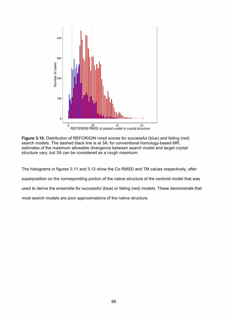
88

Figure 3.10. Distribution of REFORIGIN rmsd scores for successful (blue) and failing (red) search models. The dashed black line is at 3Å; for conventional homology-based MR, estimates of the maximum allowable divergence between search model and target crystal structure vary, but 3Å can be considered as a rough maximum.

The histograms in figures 3.11 and 3.12 show the Cα RMSD and TM values respectively, after

superposition on the corresponding portion of the native structure of the centroid model that was

used to derive the ensemble for successful (blue) or failing (red) models. These demonstrate that

most search models are poor approximations of the native structure.

89

Figure 3.11. Distribution of RMSD values for the centroid model compare to the crystal structure used for deriving the ensemble for the successful (blue) and failing (red) search models.

Figure 3.12. Distribution of TM-scores for the centroid model used for deriving the ensemble for the successful (blue) and failing (red) search models.

It is striking how little correlation between model quality and success there is, indicating that

AMPLE can compose successful search models from unpromising starting material. Examination

of cases quickly revealed that helical segments in search models were frequently overlaid on

different helical portions of the native structure. In such cases the local structure of the search

model, especially the backbone, matched the native structure well despite the incorrect sequence

register. To probe this effect further, the models were examined with the RIO and AIO scores

described earlier.

90

Figure 3.13. Distribution of RIO scores for successes (blue) and failures (red)

Figure 3.14. Distribution of RIO scores for successes (blue) and failures (red) omitting the large failure peak with RIO=0.

Figure 3.13 shows the RIO distribution for all test cases. The major peak is for failing models with a

RIO score of zero. As this peak is so large and obscures other details, figure 3.14 shows the RIO

distribution omitting the large peak at RIO=0. Figure 3.13 shows that the distribution of RIO scores

for successes has four broad peaks separated by roughly 20 residues. As most successful search

models are 25 residues in length, this indicates that many structures are solved by placement of

multiple copies of the same fragment.

The above analysis shows the number of RIO contacts that contributed to success, but

amalgamates all the contacts and therefore does not provide any information on the length of the

individual helical segments. The plot below displays the length distribution of the longest individual

RIO helical segments, with any single-residue gaps included in the overall length.

91

Figure 3.15. Length distribution of the longest RIO helices with any single-residue gaps included in the overall length.

Figure 3.15 shows that there is a peak in the length distribution at about 20 residues. This confirms

that most structures were solved with one or more placements of fragments of approximately 20

residues in length.

Figure 3.16. Comparison of RIO_in and RIO_out scores for successful (blue) or failing (red) search models.

Figure 3.17. Comparison of RIO_in and RIO_out scores for successful (blue) or failing (red) search models. Cases with no contacts omitted.

92

Figures 3.16 and 3.17 compare the distribution of in- and out-of-register RIO scores. These show

that the majority of cases were solved with out-of-register placements. With some cases, there is a

mix of in- and out-of-register placements; these are cases where a helical fragment has been

placed correctly, but then additional copies of the same helical fragment have been placed at

different points in the ASU.

Figure 3.18. The percentage of out-of-register RIO scores for successful models.

Figure 3.18 shows the percentage of out-of-register RIO scores for successful models . The vast

majority (85.19%) solved with exclusively out-of-register contacts, whereas only 3.45% solved with

exclusively in-register. The remaining search models solved with a mixture of in- and out-of-

register, and for 28 models (0.74%), the RIO score was zero.

Notably, figure 3.18 shows some success from search models with placements that have a RIO

score of zero i.e. positions in which three consecutive Cα atoms are not overlaid within 1.5Å, even

disregarding register. Figure 3.20d below exemplifies cases of this kind, in which the search model

93

was translated and rotated about its helical axis such that Cα positions are too far apart to be

counted by this metric. There is, nevertheless, overlay of heavy atoms (carbon, oxygen or nitrogen)

in the search model upon other heavy atoms in the target.

Cases like these were captured by the Atom-Independent Overlap (AIO) which counts overlaid

heavy atoms irrespective of their being O, C or N. Figure 3.19 examines the number of non-AIO

contacts (i.e. number of atoms that were not placed within viable density) against the RIO score as

a percentage of the native structure.

Figure 3.19. RIO score as a percentage of the number of Cα in the ASU against the

94

number of non-AIO atoms. The graphs are faceted by resolution to disentangle any effects from resolution.

Figure 3.19 shows that as more atoms are placed out of viable density (increasing number of non-

AIO atoms), the chances of solution decrease. However, as more of the structure is placed

correctly (as measure by the percentage of RIO scores), solution is more likely, and this can even

overcome a substantial number of atoms being placed incorrectly. Successes are almost

guaranteed if more than 50% of the Cα atoms are placed correctly. Interestingly, solution is still

possible even with negligible RIO and AIO scores.

Figure 3.20 shows actual solutions that illustrate a number of these cases, from almost perfect

solutions (3.20a) to solutions that had very low RIO and AIO scores (3.20d and e).

95

Figure 3.20. Illustrative examples of successful coiled-coil structure solution with AMPLE. In each case, the target chain of the crystal structure is shown on the left as a green cartoon, MR-placed model(s) as blue lines and, where appropriate, cartoon; and the ensemble search model is displayed on the right in blue. MR-placed model ensembles (panels a-d, g-h) are represented here, for clarity, by their first member a) In-register placement (i.e. the sequence of the search model correctly aligns with that of the substrate) of two copies of a mildly truncated centroid structure as search model solves

96

the coiled-coil domain structure of the Sin Nombre Virus Nucleocapsid Protein (2IC9); b) Out-of-register placement (backbone structures of search model and target coincide closely, but their sequences do not match) of eight copies of a heavily truncated search model ensemble with polyalanine side chain treatment solves a coiled-coil fragment from the HIV-1 protein gp41 (3H00); c) Four copies of an ensemble with reliable side chain treatment solves the coiled-coil domain structure from the replication regulator geminin (1UII); d) A heavily truncated polyalanine search model solves the structure of adhesin UspA1 (2QIH) with a RIO score of zero; e) Two copies of a 5 residue ideal polyalanine helix solved a de novo designed assembly protein (3S0R; 2.45Å); f) Two copies of a 20 residue ideal polyalanine helix solved a dynamin adaptor protein (2XU6; 2.7Å); g) Five copies of a mildly truncated polyalanine search model ensemble solved the complex of GGA1 GAT domain (yellow) with the GAT-binding domain of Rabaptin5 (green) (1X79; 2.4Å); h) Four copies of a polyalanine search model ensemble solved a transcription regulation complex (1H8A; 2.23Å) containing a coiled-coil domain (green), an additional helical protein (yellow) and duplex DNA (brown).

3.3.3.1 MR and model-building/refinement scores AMPLE's strategy of submitting all PHASER solutions to SHELXE, regardless of the PHASER

statistics was also reinforced in the current work (figure 3.21), where solutions were found with

PHASER LLG scores as low as -833, and TFZ scores as low as 2.1.

Figure 3.21. PHASER LLG and TFZ scores for successful (blue) and failing (red) search models.

97

In fact, some successes were seen from initial PHASER placements in runs where the program

declined to produce a final result; solution was still possible as PHASER produces PDB files for the

intermediate results. These intriguing new observations come to light because AMPLE employs no

statistical cut-off of any kind after MR, attempting SHELXE tracing of the top placement regardless

of the score.

As mentioned, an additional criterion for automatic definition of success - refinement of SHELXE -

traced structure to Rfree ≤0.45 by BUCCANEER or ARP/wARP - was applied. For comparison,

placements defined as failures were also treated in the same way.

Figure 3.22. SHELXE CC score against BUCCANEER Rfree score. Successful jobs are coloured blue and failing ones red,

As figure 3.22 shows, a large majority of successes (95.3%) could be refined to Rfree ≤ 40 %.

Interestingly, a very few placements classified as failures after SHELXE were refined to low Rfree

values. These were cases where the SHELXE CC was greater than 25 but mean chain length was

98

less than 10. The key predictor of success, SHELXE CC ≥ 25, is therefore reinforced by the results

in figure 3.22.

Figure 3.23. BUCCANEER and ARP/wARP Rfree scores for successful models i.e. SHELXE CC ≥ 25 and mean chain length ≥ 10.

Figure 3.23 shows the Rfree for the models after rebuilding with ARP/wARP and BUCCANEER.

This shows that the two programs are broadly comparable, although a few models that rebuild and

refine with ARP/wARP could not be processed by BUCCANEER.

3.3.4 Timing analyses The time taken per target can be split into search model generation and the processing of these by

MrBUMP. For search model generation (including fragment generation, ab initio modelling, search

model ensembling), each target took on average 13.0 CPU hours as shown in table 3.3. This

reduces to 9.0 CPU hours if fragment generation is done on the ROBETTA server.

99

Figure 3.24. Average timing breakdown across all jobs in CPU seconds.

Table 3.3: average time for each step of the AMPLE pipeline.

Step Average Time per target (CPU hours)

Fragment generation 3.0

Model generation 9.9

Ensemble generation 0.07

MrBUMP processing 2.6

On average, 162 search models are generated per target. The time taken for MR and tracing will

obviously depend on how many search models are successful for the target in question. On

average, a search model takes 2.6 CPU hours to process with MRBUMP, and one third of the

search models were successful. On average three search models would have to be processed

before a job was successful, so the processing step takes around 8 hours. Typically, therefore,

successful AMPLE runs terminate well within 24 hours and this is what is observed in practice.

3.3.5 Why do these search models succeed? It is proposed that the power of AMPLE derives from several factors. The first is the ability of rapid

ROSETTA ab initio modelling to accurately recapitulate at least local features of the native

structure and sometimes the global fold. Secondly, AMPLE progressively truncates clusters of

ROSETTA predictions using structural variance within the clusters (THESEUS) as a predictor of

inaccuracy. Finally, AMPLE treats side chains three different ways and constructs search models

as ensembles derived from sub-clustering of truncated superpositions.

100

3.3.5.1 The ensemble effect Ensembles are considered to be particularly effective MR search models and so their contribution

to success in MR was tested by rerunning AMPLE with single-structure search models instead of

the normal ensembles of 2-30 structures. AMPLE constructs ensembles by sub-clustering the

truncated decoys under 3 clustering radii (1, 2 and 3Å). The first cluster in the ensemble is the

centroid of the ensemble and so is the same for all three ensembles. A comparison of the

performance of the centroid structure to the 1Å sub-clustering radius ensemble (the sub-clustering

radius that performed best) was therefore undertaken. Figure 3.25 plots the SHELXE CC scores

for the ensemble and single-structure cases.

101

Figure 3.25. Comparison of performance (SHELXE CC score) for single centroid structures and the 1Å sub-clustering radius ensembles. Points are coloured as follows - blue, both the single centroid structure and the 1Å ensemble were classified as successes (by both SHELXE and refinement criteria); yellow, the ensemble but not its centroid structure succeeded; orange, the centroid structure alone succeeded; red, both were classified as failures. The large point on the origin represents the cases in which neither single centroid structure nor the ensemble achieved a non-zero SHELXE CC score.

In terms of targets solved, ensembles are more successful than single centroid structures, solving

66 against the latter’s 59. There is a similar disparity in number of successful search models - 1494

successes (28%) against 1171 (22%) for the single structures. This suggests that ensembling, a

key characteristic of AMPLE, is generally an efficient strategy for gainfully combining information

from a number of predictions into a single search model. Despite the overall greater success of

ensembles, five targets (2Q5U, 3Q8T, 3TYY, 3U1C and 4DZK) were solved with single structure

102

search models, but not with a single run of the ensembles. Of these, four were all solved in

subsequent reruns of the ensembles, but 4DZK only solved with the single-structure search model.

165 single structures succeeded despite the failure of their corresponding 1Å ensemble search

model. This suggests that while ensembling is an efficient strategy for gainfully combining

information from a number of models, in a small minority of cases, potential success that would be

achieved with a single structure is masked by the ensembling.

Figure 3.26. Target success mapped against resolution and target chain length for single-conformer (centroid) search models. Each circle represents a target with the radius of the outer circle proportional to the number of models generated for that target, and the colour indicating whether the target solved (blue) or not (red). The filled blue circles within the open circles indicate the proportion of successful models.

3.3.5.2 Solving structures with ideal polyalanine helices The success of short, out-of-register helical fragments raises the question of the extent to which

AMPLE's success derived from its ability to select promising fragments of the ROSETTA decoys

and whether these models have advantages over simpler, ideal α-helices.

103

A comparison of ROSETTA-derived search models with ideal helices was therefore carried out in

order to shed light on the contribution to success of the modelling by ROSETTA. As a first step in

untangling the effect of the modelling, ideal α-helices were created from the sequences of the

largest α-helical segment that contributed to successful structure solution in the full ensemble run.

This restricts the analyses only to those targets that were solved successfully with an ensemble,

but selects MR jobs that are likely to be solvable with an α-helical segment.

In order to construct the sequence of residues for the α-helical segment, the RIO results and DSSP

secondary structure analyses were used to determine where the α-helices between the native

structure and ensemble MR solution overlapped. DSSP is a program developed by Wolfgang

Kabsch and Chris Sander and uses the three-dimensional structure of a protein, in particular the

hydrogen bond energies and geometries, to determine the secondary structure (Wolfgang Kabsch

and Sander 1983). This resulted in one or more α-helical fragments, at least three residues long,

with the fragments potentially separated by one or more residues. The native sequence was then

used to fill in any gap between fragments that was smaller than 4 residues. For example, if

residues 10-30 in the native structure comprised a helix then the largest helical region in the

search model could be residues 12-15, 19-22 and 25-26. In that case, an ideal helix of residues

12-26 would be built. The sequence of the largest segment resulting after any gaps had been filled

was then used to create the ideal α-helix. In this way, for all bar five of the successful ensemble

search models it was possible to derive an α-helical segment at least three residues long.

As the ideal α-helices are single structures (not ensembles), they were compared against the

single structure search model set. Ideal helices and single structures can be paired, since each

helix derives from a search model ensemble, allowing for a direct comparison. Furthermore, the

helices and single structures each inherit the same side chain treatment as their parent ensemble:

for the single structures side chains are already present and for the helices they were generated

using SCWRL.

104

Figure 3.27. Comparison of performance (SHELXE CC score) for search models comprising a single centroid structures or an idealised helix. Points are coloured as follows - blue, both the single centroid structure and the idealised helix were classified as successes (by both SHELXE and refinement criteria); yellow, the single structure but not the idealised helix deriving from the same search models ensemble succeeded; orange, the idealised helix alone succeeded; red, both were classified as failures. The large point on the origin represents the cases in which neither the single centroid structure nor the idealised helix counterpart achieved a non-zero SHELXE CC score.

Figure 3.27 shows that single structures succeed somewhat more often than idealised helices: for

all pairs of search models compared, both were successful in 617 cases. In 398 further cases

where the idealised helix failed the single structure was successful, although in 127 cases, the

idealised helix succeeded where the single structure failed. This comparison clearly underlines the

value of employing explicit tertiary structure prediction. This can be rationalised here by

105

consideration of the variable but typically significant distortions from α-helix ideality found in coiled-

coil structures. Figure 3.19a shows the significant α-helical twist seen in one of the successful

search models that solved the structure of PDB entry 2IC9. Examination of the ROSETTA outputs

confirms that it picked out fragments deriving from other similarly twisted coiled-coil structures and

used them to build a search model of appropriate local structure and, in this case, correct register

after MR placement.

As the foregoing idealised helices were derived from the structures of the single-models, they

assumed knowledge about what could actually solve the structure. In order to be of utility for

solving novel structures, it is of interest to know if structures could be solved using ideal

polyalanine helices. Solution of the original test set using ideal polyalanine α-helices as search

models was therefore attempted. As the most successful search ensembles were between 20 and

30 residues in length, eight ideal α-helices were generated, starting at five residues in length and

extending to 40, in five-residue increments, with ideal backbone torsion angles of phi=-57.8º and

psi=-47.0º.

These simple polyalanine helices solved 52 of the targets (55%), including PDB entry 2QIH with

278 residues (2 chains) in the ASU and PDB entry 2W6B, with a resolution of 2.8 Å (figure 3.27).

The success covered almost the entire breadth of the test set. However, AMPLE with ab initio

prediction-derived search models performed considerably better, solving an additional 23 targets.

In particular, the success of ideal helices in the lower resolution range - data to worse than 2.5Å -

was notably lower than with ensembles: only two targets in this set of 15 solved with ideal helices.

Considering the effort often devoted to preparing search models for MR, it is surprising to discover

that many coiled-coil structures, including those with long chains and limited resolution, could be

solved solely with these simple helical models. Despite the successes of the polyalanine helices,

the data confirm the added value of the AMPLE pipeline.

106

Figure 3.28. Ideal polyalanine helices solve around half of coiled-coil targets in AMPLE. Targets are coloured blue (solved) or red (failed) and are plotted by the target chain length and diffraction data resolution.

3.3.5.3 Comparison of the different methods The following section compares the results of three of the methods attempted: full ensembles,

single models and the 8 ideal polyalanine helices (the idealised helices constructed from the

sequence of the first model in the ensemble have been omitted).

Figure 3.29. Ab initio model-derived search model ensembles solve more coiled-coil targets than either single structures or ideal helices. a) Overall successes with a single run of ensemble (green), single structure (blue) or ideal polyalanine helix (purple) search models. A single structure, 3H00, solved with ideal helices that did not solve with a single run of ab initio prediction-derived search models

107

Figure 3.29 shows that 44 of the models can be considered 'easy' as they were solvable with all

the different methods. AMPLE ensembles were by far the most successful, solving 64 cases, but

were unable to solve all the cases that were solvable, as both ideal helices and single structures

were able to solve structures that could not be solved with either of the other methods. Figure 3.30

summarises the results by chain length and resolution.

Figure 3.30. Detailed breakdown of targets solved with ensembles, single structures and/or polyalanine helices. Red triangles - failures; filled blue circles - solved with each search model (ensemble, single-structure and helices); empty blue circles - solved with one or more of the above; blue circle with a cross - only solved with the single-structure run (4DZK); purple circles - solved with a re-run of the ensemble (1MI7, 2BEZ, 2Q5U, 2ZZO, 3H00, 3H7Z, 3TYY, 3U1A and 3U1C); purple square - manual inspection indicated success (3BAS and 3CVF).

3.3.6 Exploiting coiled-coils for structure solution of complexes Coiled-coil proteins are often involved in the formation of protein complexes due to their biological

roles in scaffolding, transcription and cell signalling (Burkhard, Stetefeld, and Strelkov 2001). The

conspicuous success of AMPLE in solving coiled-coil targets indicated that sufficient phasing

108

information might be obtainable through MR with AMPLE when applied to coiled-coil components

of complexes, that could then permit tracing protein or polynucleotide partners in biological

assemblies. Phasing with AMPLE and coiled-coil subunit sequences was attempted for two such

complexes ( PDB entries 1X79 and 1H8A) identified using the SCOP database (Andreeva et al.

2004).

PDB entry 1X79 contains 322 residues and comprises a dimeric coiled-coil domain in complex

with a small, helical GAT domain (Fig. 3.20g). The structure solved with an ensemble search

model of the coiled-coil chain, 112 residues long, ultimately tracing and refining at 2.41Å resolution

to R=0.25, Rfree=0.29 after ARPWARP. The backbone structure was accurately traced in the final

result, although there were errors in the assignment of sequence to the trace (figure 3.20a). 1H8A

contains 284 residues - a dimeric coiled-coil domain (2 x 78 residues) from CCAAT/enhancer-

binding protein beta and a Myb DNA-binding domain - in complex with a 26-base long DNA duplex

(figure 3.20h). The DNA contributes about a third of the scattering matter of the crystal.

Nevertheless, search models deriving from predictions of the coiled-coil sequence solved the

structure. Taking the AMPLE-produced SHELXE Cα trace as a starting point, a rough initial model

for the target could be built using a combination of BUCCANEER for the protein molecules and the

CCP4 program NAUTILUS for the DNA. Phases from this initial model were then further improved

in SHELXE. With these improved phases a more complete model could be built with

BUCCANEER/NAUTILUS achieving R=0.39 and Rfree=0.42 at 2.23Å resolution (figure 3.31b).

109

a)

b)

Figure 3.31. Electron density maps of 1H8A a) immediately post-AMPLE and b) after phase improvement with SHELXE and further model building with BUCCANEER/NAUTILUS (see text for details). In blue, the (2Fo-Fc)αc map is contoured at 2σ: positive difference map (Fo-Fc)αc contoured at 2σ is shown in green. The crystal structure is shown as a ribbon (black with blue used for its symmetry mates) while the structure built at each stage is indicated in magenta. The density in a) supported the correctness of the MR solution, for example revealing density resembling elements of a DNA duplex backbone, later shown (b) to indeed correspond to this missing component.

110

3.4 Discussion MR is the dominant route to protein structure solution, and as more structures are determined and

the chance of a homologous structure existing in the PDB becomes greater, this position becomes

more entrenched. For coiled-coiled proteins however, homology is not a sufficient condition to

guarantee success. Unless experimental phasing is attempted, there are two routes available. The

first is to search the PDB to find homologous structures, and/or to use experience and intuition to

select models that might be suitable and then undertake extensive and laborious work to prepare

these structures for MR; standard preparation techniques will often not be suitable as coiled-coils

with similar sequences can crystallise in such different forms. The second possibility is to use the

approach pioneered by ARCIMBOLDO of using small fragments and expanding up to a full

solution. The first comes with extensive human labour time, and the second with extensive CPU

time. The work completed here demonstrates that AMPLE can provide a computationally efficient

route that bridges these two approaches.

The study of small, idealised polyalanine helices shows that many coiled coils (55% - more than

half of the test set) are actually trivially solvable with the powerful combination of PHASER,

SHELXE, REFMAC and then either Arp/WARP or BUCCANEER. However, this still leaves a large

minority that cannot be solved in this way and require a more sophisticated approach.

The power of AMPLE to select salient features from ab initio models and construct MR search

ensembles enables the solution of the majority of those not solvable with ideal helices. The in-

depth analyses of the results indicates that this ability derives from three main factors.

The first is the ability to exploit the modelling capabilities of ROSETTA and the structural

information contained within its fragment database. Since the 9-residue fragments that contribute

to ROSETTA model building are long enough to detect the classical coiled-coil heptad repeat, the

resulting models will include helices with distortions from ideality reflecting those naturally

111

occurring in the PDB. Given the poor overall quality of the modelling it is unreasonable to expect

the decoys produced to faithfully reproduce the fold-specific bends and twists of the target.

However, by assembling fragments from naturally occurring distorted helices, and favouring

structures containing plausible helical packing modes, the ab initio modelling provides sets of

structures from which usefully non-ideal helical search models, suitable for solving coiled-coil

structures, can be derived. Fig. 2.19a demonstrates the significant α-helical bend seen in one of

the successful search models that solved the 2IC9 structure.

However, just selecting plausible fragments is not enough, as the weaker performance of the

single-models as compared with the ensembles demonstrates. It is AMPLE's ability to

progressively truncate models down to a smaller chunks, and then create ensembles that indicate

which parts of the search model are likely to be most accurate, that enables solution of the

additional cases not solvable with ideal helices or single-models. Indeed AMPLE is so effective at

solving coiled-coil structures, that they can even be used as a route to solving coiled-coil

complexes, as shown by the solution of 1H8A and 1X79.

An interesting facet of this work has been the discovery that most of the models were solved with

smaller search models, approximately 20-residues in length, that often only consisted of a single

helix. PHASER is often able to place these fragments correctly, although the 'standard' LLG and

TFZ scores are often not a reliable indicator of success, as can be seen from figure 3.21. However,

SHELXE is able to undertake density modification and main-chain tracing to turn these

unpromising fragments into largely complete models, with the SHELXE CC being a largely reliable

indicator of whether the MR step has succeeded. As smaller search models are often successful,

these have now been prioritised within AMPLE, so that they are run earlier, increasing the chances

of an early success. The somewhat poor performance of the PHASER LLG and TFZ scores with

this version of PHASER (2.5.6) was raised with the developers, and with later versions of PHASER

the LLG and TFZ score are now more reliable indicators of success.

112

Additionally, the importance of using different side chain treatments and sub-clustering radii was

reinforced by the fact that a small subset of models only solved with one particular side chain

treatment or sub-clustering radii. This has been explored further in the work that was carried out in

chapter 6.

In summary, this work demonstrates that AMPLE should be the first tool of choice for a

crystallographer working with coiled-coils proteins. The use of ideal helices (which has now been

added as an option within AMPLE) should be attempted first, as it may provide a quick route to

solution. If this fails, then one or more modelling runs should be attempted with ROSETTA or

QUARK, as there is a very good chance that the structure will be solvable without the need of

having to resort to much manual computational work, or further experimental work to collect

anomalous data.

113

Chapter 4: Transmembrane

Proteins

114

4 Transmembrane Proteins

4.1 Introduction Transmembrane proteins are an important class of proteins, that are estimated to comprise about

30% of all proteins (Tusnády, Dosztányi, and Simon 2004). As their name suggests,

transmembrane proteins tend to be located primarily within the hydrophobic cell membrane,

sandwiched between the aqueous cell interior and exterior. Their primarily hydrophobic nature

means that transmembrane proteins are particularly difficult to work with and produce poorly

diffracting crystals. As a result, of the more than 80,000 protein structures currently in the PDB,

fewer than 1800 are classified as transmembrane proteins by the TMDET algorithm (Tusnády,

Dosztányi, and Simon 2004).

Transmembrane proteins come in two main forms: α-helical and β-barrel, with the overwhelming

majority being of the α-helical form. Studies have proposed that 27% of all human proteins are α-

helical transmembrane proteins (Almén et al. 2009). β-barrel proteins by contrast, are found in the

cell walls of gram-positive bacteria, and in mitochondria and chloroplasts (Wimley 2003/8).

The portion of an alpha-helical transmembrane protein that is located within the cell membrane is

almost always exclusively alpha-helical and is constrained by the surrounding membrane. The

structural constraints that are placed on proteins within the membrane limit the conformational

space available to them and can be used to guide protein modelling protocols. The more focussed

modelling and smaller conformational space increases the size of protein that is amenable for

modelling. Conversely, most current protein modelling protocols rely heavily on either entire known

structures (as is the case for homology modelling), or fragments as is the case for the ROSETTA.

The relatively small number of transmembrane protein structures mean that these protocols have a

115

much smaller pool of data to draw on, which is likely to have a negative impact on their

effectiveness.

However, the α-helical form of transmembrane proteins, and the paucity of homologous structures

within the PDB that would be candidates for homology modelling, mean that ab initio modelling

could be a valuable option for generating models and indicate that these will be interesting

candidates to explore with AMPLE.

4.2 Methods

4.2.1 ROSETTA modelling There are currently two protocols within ROSETTA for modelling transmembrane proteins.

4.2.1.1 RosettaMembrane Protocol The original RosettaMembrane protocol was initially developed by V. Yarov-Yarovoy (Yarov-

Yarovoy, Schonbrun, and Baker 2005). The first step in this method is the prediction of the

transmembrane regions. This is done using the online Octopus server (Viklund and Elofsson

2008), which uses a combination of Hidden-Markov models and artificial neural networks that have

been trained to recognise transmembrane regions to predict which residues are part of the

membrane. For each residue within the protein, Octopus will classify it as o (outside), i (inside) or

M (membrane).

A lipophilicity prediction is then made using the run_lips.pl perl script supplied with ROSETTA that

combines the data from the OCTOPUS prediction with a PSIBLAST multiple sequence alignment

of the target sequence against the NR database (McEntyre and Ostell 2002). This requires that the

user has the large (~100GB) NR database installed locally, together with the BLAST version 2

executables, something that is not part of a standard ROSETTA installation.

As part of this work it was discovered that there is a error in the run_lips.pl script, as it attempts to

use the server script http://gila.bioengr.uic.edu/cgi-bin/lips/script.cgi to calculate the lipophilicity.

116

The server is no longer maintained, but the script can be downloaded and run locally. This issue

was reaised with the RosettaMembrane developers on the Rosetta Commons forum, but none of

the developers have responded. despite several other people encountering the same error.

Fortunately it was possible to ammend run_lips.pl to use the script locally, but this indicates that

RosettaMembrane is no longer actively maintained.

The final preparatory stage is the generation of the fragments for the modelling. In their original

paper, Yarov-Yarovoy recommend only using SAM (Sequence Alignment and Modeling System)

(Katzman et al. 2008) to predict the secondary structure, as, in their experience, the default JUFO

and PSIPRED (Jones 1999) predictors often have problems predicting the secondary structure for

transmembrane proteins.

The modelling of the protein is then carried out using the fragments, predicted membrane regions

and lipophilicity and a modified ROSETTA modelling protocol. In the modified protocol, the

membrane is represented by two parallel planes 60Å apart, which is subdivided into five regions as

shown in figure 4.1.

117

Figure 4.1. Partitioning of the transmembrane profile in the ROSETTA transmembrane

modelling protocol.

A modified scoring term is used, which contains the following terms:

Etotal = Eenv + Epair + Eclash + Edensity + Estrand

The terms are as follows:

l Eenv - environment term. Accounts for the different amino acid propensities for the 5 layers,

together with the burial state, which is the number of amino acids with centroids within 10Å.

l Epair - amino acid pair propensities; the tendencies for particular amino acids to be close

together in either polar or hydrophobic regions, based on their separation and position with

the hydrophobic or polar regions.

l Eclash - penalty for steric overlaps.

l Edensity - accounts for both close-range residue packing and overall protein density for both

polar and hydrophobic regions.

l Estrand - term to favour strand pairings.

The membrane modeling protocol is also modified in that the protein is built up helix by helix,

starting from the middle of the membrane. After each move, a search is made for the optimal

118

embedding of the helix within the membrane. This protocol is thought to capture some of the

features of how a physical protein folds to its native state.

The second ROSETTA protocol uses the GREMLIN (Ovchinnikov, Kamisetty, and Baker 2014)

server to predict evolutionary contacts.

4.2.1.2 ROSETTA Modelling with GREMLIN evolutionary contacts The ROSETTA team have developed the GREMLIN protocol to predict residue-residue contacts.

GREMLIN uses a pseudo-likelihood method coupled with block-L1 regularisation and quasi-

Newton optimisation methods (Kamisetty, Ovchinnikov, and Baker 2013). This avoids the need to

implement some of the assumptions about the statistical distribution of the underlying Multiple

Sequence Alignment, and is also highly parallelisable, so computationally very tractable.

Work by Ovchinnikov et al (Ovchinnikov et al. 2015) has demonstrated that the contact information

from the GERMLIN server alone is sufficient to model Transmembrane Proteins with a slightly

modified form of the ROSETTA modelling protocol. In their work, they benchmarked this method

on 13 Transmembrane Proteins, ranging in size from 188 to 434 residues and predicted structures

with an overall RMSD of less than 4.0 Å (the RMSDs over the structurally aligned regions were all

below 2.8 Å). Their method presents an attractive alternative to the original RosettaMembrane

protocol, as it only requires a user to generate the contact information using the GREMLIN server,

and then run the standard ROSETTA executables. There is no need to perform the lipophilicity

prediction, and associated need for BLAST and the NR database to be installed, as there is with

RosettaMembrane.

GREMLIN is made available as a server that accepts a fasta sequence as input and then performs

a Multiple Sequence Alignment using the HHBLITS (Remmert et al. 2011) database search

program (this is the default, there is also an option to use JACKHMMER (Eddy 2011)). The

GREMLIN protocol is then run on the Multiple Sequence Alignment to determine the residue-

residue covariance, and the server has the option to download a file of restraints for ROSETTA

119

modelling. By default, the server generates Cβ-Cβ sigmoid restraints with a cutoff for the scaled

score of 1.0 for the contact to be included as a restraint. The scaled score is raw score for the

contact divided by the average of all the raw scores for the contacts. The ROSETTA sigmoid

restraint is of the form:

(5.1)

where the limits are hard-coded at 0.5, x0 is the centre of the sigmoid function and m its slope.

The only change required to the modelling protocol is a modification of the ROSETTA energy

function to reflect the exposure of non-polar residues in the membrane-spanning regions. This

requires the Lazaridis-Karplus solvation energy term weight to be set to zero, and to compensate

for the short-range repulsion implicit in the solvation model, the Lennard-Jones repulsive and

attractive terms being given equal weights. This requires the creation of a ROSETTA weights file

with the following flags:

fa_atr = 0.8

fa_rep = 0.8

fa_sol = 0.0

The weights file is then supplied to ROSETTA with the '-score:patch' command-line flag.

The second change is for the normalized GREMLIN score to be multiplied by three to give the

contact restraints roughly the same total dynamic range as the ROSETTA energy. This requires

the addition of the '-constraints:cst_weight 3' and '-constraints:cst_fa_weight 3' flags.

Both methods will be contrasted and compared in this work.

4.2.2 Test set Selection A set of 15 transmembrane structures was selected using the following procedure:

l a list of all the α-helical proteins from the PDBTM (Tusnády, Dosztányi, and Simon 2004)

120

was created.

l an advanced query was run against the PDB to extract all structures from this list

containing a single protein entity (i.e. distinct chemical entities, regardless of the number of

copies), with a sequence length less than 250 and where the structure was resolved to a

resolution of better than 2.5Å.

l the list of structures was then clustered with CD-HIT (Li and Godzik 2006) using a

sequence identity threshold of 0.4 and a word length of 2. For each cluster with more than

one structure, the shortest, highest resolution structure was selected, where there was a

viable MTZ file (a binary file containing the reflection data from a crystallography

experiment in CCP4 format).

l PDB entries 2BL2 and 2X2V were removed from the list of structures as the unit cell

contained 10 and 13 copies of the chain respectively, so that an individual chain was only

10% or 7% of the scattering mass. Although successes have been seen with as little as 4%

of a structure, solving such small cases are the exceptions, and an initial test with 2BL2 and

2X2V showed that the PHASER search for these two exceed the time for the rest of the

targets, making it difficult to run the cases in a reasonable amount of time.

l PDB entry 3LBW was removed from the list as it was too short (22 residues) to enable

lipophilicity prediction by ROSETTA; a key step in the RosettaMembrane protocol.

l PDB entry 2UUI had been used for initial testing, but was not included in the list after

clustering as it was closely related to PDB entry 3PCV. It was however included in the list of

structures analysed to add to the data and also to check the results for reproducibility.

The final test set is listed in table 4.1.

121

Table 4.1. The final list of selected structures with data collated from the PDB and thumbnail

images generated by PYMOL.

PDB Title Chain Length

Chains Resolution (Å)

Thumbnail

1GU8 Sensory Rhodopsin II 239 1 2.27

2BHW Pea light-harvesting complex II 232 3 2.5

2EVU Crystal structure of Aquaporin AQPM

246 1 2.3

2O9G Crystal structure of AQPZ mutant L170C complexed with mercury.

234 1 1.9

2UUI Crystal structure of human leukotriene C4 synthase

156 1 2.0

2WIE High-resolution structure of the rotor ring from a proton-dependent ATP synthase

82 5 2.13

2XOV Crystal structure of e.coli rhomboid protease glpg, native enzyme

181 1 1.65

3GD8 Crystal Structure of Human Aquaporin 4 at 1.8 and its Mechanism of Conductance

223 1 1.8

3HAP Crystal structure of bacteriorhodopsin mutant L111A crystallized from bicelles

249 1 1.6

3LDC High resolution open MthK pore structure crystallized in 100 mM K+

82 1 1.45

122

3OUF Structure of a K+ selective NaK mutant

97 2 1.55

3PCV Crystal structure analysis of human leukotriene C4 synthase.

156 1 1.9

3RLB Crystal structure at 2.0 A of the S-component for thiamin from an ECF-type ABC transporter

192 2 2.0

3U2F ATP synthase c10 ring in proton-unlocked conformation at pH 8.3

76 5 2.0

4DVE Crystal structure at 2.1 Å of the S-component for biotin from an ECF-type ABC transporter

198 3 2.09

123

4.2.3 Model Generation

4.2.3.1 Fragment Generation The recommended way to generate fragments for the RosettaMembrane protocol is to use SAM

(Katzman et al. 2008) only for the secondary structure prediction. In the initial work on

transmembrane proteins that was undertaken for the MRes project, SAM was compiled from

source and only used this to predict the original fragments. However, SAM is no longer supported

by the authors for stand-alone compilation and to get a working version required alteration of the

source code, which entailed considerable effort. Additionally, the online ROBETTA server has no

option to generate fragments specifically for transmembrane proteins, and as this is the

recommended way for AMPLE users to generate fragments, there is no obvious route for AMPLE

users to generate transmembrane-specific fragments. Therefore any methods developed using

transmembrane-specific fragments would not be available to AMPLE users and so of limited utility.

The decision was therefore taken to use standard fragments with the RosettaMembrane modelling

protocol. This has the added advantage that as the ROSETTA GREMLIN protocol uses standard

fragments, the same fragments can be used in both cases, making comparison of the two methods

easier. In both cases, the fragments were generated with close homologs excluded from the

fragment picking.

4.2.3.2 Modelling All of the computation for this was undertaken on the cluster badb.rc-harwell.ac.uk based at the

Research Complex at Harwell at Rutherford Appleton Laboratory. The machine is made up of 16

Xeon E5-2640v3 processors, each with 8 cores, giving a total of 128 cores. The machine consists

of 4 separate boxes each with 2 processors. Each box has 64Gb of RAM, giving a total of 4GB per

core. The interconnect is a 1 Gb ethernet switch. The operating system is CentOS Linux 6.5, with

the Rocks cluster management software and Sun Grid Engine queueing system. The test cases

were all run with the software versions detailed in table 4.2.

124

Table 4.2. Software versions used in run.

Software Version

ROSETTA 2015.22.57859

CCP4 suite 6.5.13

PHASER 2.5.7

REFMAC 5.8.0124

SHELXE 2014/4

4.3 Results

4.3.1 Ideal helices and RosettaMembrane As with the coiled-coil work, an initial attempt was made to solve the test cases with ideal helices to

provide a baseline of cases which can be trivially solved with ideal helices, and which require

additional structural information from the modelling. The test cases were then run using the

RosettaMembrane protocol.

Previous work as part of my MRes had investigated this set of transmembrane proteins with the

RosettaMembrane protocol, but with earlier versions of the various software and databases. The

software versions detailed in table 4.3 were used.

Table 4.3. Software versions used in the earlier MRes run.

Software Version

ROSETTA 3.5

CCP4 suite 6.3

PHASER 2.5.4

REFMAC 5.7.0032

SHELXE 2013/2

When that work was undertaken, the criterion for success was solely whether the SHELXE CC

score was >= 25 and the SHELXE average chain length >= 10. In all subsequent work, these

criteria have been tightened to include a successful rebuild of the SHELXE trace with either

125

ARP/WRAP or BUCCANEER to an RFREE of <= 0.5. As it is relevant to this work, the results from

the MRes run have been included below.

Table 4.4 below shows the number of successful search ensembles when attempting to solve the

test cases with ideal helices and RosettaMembrane. The table includes both a run with the latest

version of the software, and the earlier versions used in the MRes. As the earlier work only

included the SHELXE criteria, the table shows the success both for SHELXE as well as the

augmented rebuild criteria.

126

Table 4.4. The number of successful/unsuccessful search models (columns 5-9) achieved in

the three runs.

PDB Resolution (Å)

Residues in ASU

Chain Length

Rosetta Membrane

Rosetta MembraneSHELXE

Ideal Helices

Ideal Helices SHELXE

MRes Rosetta Membrane SHELXE

1GU8 2.27 436 239 0/66 3/66 0/8 0/8 5/150 2BHW 2.5 669 232 0/33 0/33 0/8 0/8 0/36 2EVU 2.3 245 246 0/30 /300 0/8 0/8 0/54 2O9G 1.9 234 234 0/21 0/21 2/8 2/8 0/66 2UUI 2 167 156 29/93 29/93 6/8 6/8 31/246 2WIE 2.13 406 82 0/180 0/180 0/8 0/8 0/204 2XOV 1.65 182 181 0/105 0/105 3/8 3/8 1/210 3GD8 1.8 225 223 4/45 4/45 0/8 0/8 1/114 3HAP 1.6 261 249 0/99 0/99 3/8 3/8 0/138 3LDC 1.45 82 82 30/180 30/180 1/8 1/8 21/354 3OUF 1.55 189 97 22/171 22/171 1/8 1/8 38/384 3PCV 1.9 160 156 6/105 6/105 5/8 5/8 8/276 3RLB 2 354 192 0/72 0/72 0/8 0/8 0/252 3U2F 2 391 76 0/171 0/171 0/8 0/8 0/228 4DVE 2.09 567 198 0/81 0/81 0/8 0/8 0/174 Cases with successful ensembles are coloured green. Column headers with SHELXE appended show the results solely for the SHELXE criteria without the additional rebuild criteria. The MRes results have higher number of search models due to an error in the earlier version of AMPLE that led to duplicate search models being created.

Table 4.4 shows that ideal helices are the most successful method, solving seven of the 15 test

cases. 2O9G and 3HAP solve only with ideal helices. 2XOV didn't solve with the standard

RosettaMembrane with the most current run, although it did solve (under the SHELXE criteria) with

the earlier run. 3GD8 is not solvable with ideal helices, although it did solve with both the current

and previous versions of the RosettaMembrane protocol. 2UUI, 3LDC, 3OUF and 3PCV all solve

with both RosettaMembrane and ideal helices, so seem to be relatively easy to solve. All of the test

cases that solved with ideal helices were at 2Å resolution or better, and tended to be the smaller

cases, the largest solved being 3HAP with 261 residues in the asymmetric unit.

127

3GD8 was the only structure that was not solvable with ideal helices but was solvable with the

RosettaMembrane protocol. The highest scoring successful search model from the latest

RosettaMembrane run is shown below in figure 4.2.

Figure 4.2. PYMOL cartoon rendering of 3GD8 (green) with the top-rated MR model c1_tl11_r3_polyAla (blue) overlaid on it. This was a helical fragment of 25 residues and solved with a RIO score of 16.

Figure 4.2 shows that the successful search model is a single, largely straight helix of length 25

residues with polyalanine side chains. That this was able to solve 3GD8, whereas the ideal helix of

25 residues was not, shows that even the very minor deviations from ideal helicity that the

ROSETTA modelling confers can be the determinant of success or failure.

Comparison of the two RosettaMembrane runs show that the significant differences were that

2XOV solved with a single search model in the previous run, but failed to solve in the latest one,

and that 3GD8 solved with four search models in the current run but only one in the previous run.

These differences are more likely to be due to the inherent variability within different AMPLE runs

128

(due to the stochastic nature of the ab initio modelling) rather than the differences in the ROSETTA

software or database of structures and fragments that were used. This effect was clearly apparent

in the work on coiled-coil protein study, where nine additional targets out of the 94 solved when

subjected to two additional runs.

Manual inspection of the top solution for 1GU8 for the earlier run with RosettaMembrane revealed

reasonably high PHASER LLG and TFZ scores of 77.0 and 5.1 respectively, and a single copy of

the MR model placed so as to overlap reasonably well with three of the helices of the native

structure, as shown in figure 4.3.

Figure 4.3. PYMOL cartoon rendering of 1GU8 (green) with the top-rated MR model tl25_r2_polyAla (blue) overlaid on it, showing the overlap of the helices.

Unfortunately, the resolution of 1GU8 is 2.27Å, the third lowest of the test set, and above the 2.1Å

limit where SHELXE is expected to work with small fragments. It is possible that 1GU8 could be

rebuilt with manual work, but this has not been attempted as the goal of this work is to develop

automatic protocols within AMPLE.

129

4.3.2 PCONSC2 Contacts In order to see if an improvement could be made on the initial results, a run was attempted with the

standard ROSETTA modelling protocol, but using contact information derived from PCONSC2.

PCONSC2 is a contact metapredictor that combines contact prediction from PSICOV and

PLMDCA (Skwark et al. 2014). The contacts generated by PCONSC2 were then implemented as

Cβ constraints within ROSETTA using the FADE energy function, and the standard ROSETTA

modelling protocol was used. The FADE function is a smoothed square well energy function that in

this case lowers the energy by -15 ROSETTA Energy Units for residue pairs where the Cβ atoms

are closer than 9Å, but has no effect on residues further apart than this. This has the effect of

rewarding contacts that are satisfied, whilst not permitting false contacts for residues that are far

apart from distorting the structure. The results are displayed in table 4.5.

130

Table 4.5. Number of successful/unsuccessful search models for the RosettaMembrane and

PCONSC2 runs.

PDB Neff* Number of Contacts used

Native PPV**

Rosetta Membrane PCONSC2

1GU8 184 244 0.312 0/66 0/18 2BHW 229 232 0.186 0/33 0/6 2EVU 820 246 0.694 0/30 0/12 2O9G 836 240 0.687 0/21 0/15 2UUI 434 156 0.419 29/93 0/33 2WIE 288 82 0.432 0/180 0/180 2XOV 1142 181 0.533 0/105 0/42 3GD8 851 223 0.707 4/45 0/21 3HAP 183 249 0.274 0/99 0/60 3LDC 942 82 0.481 30/180 4/141 3OUF 1065 97 0.323 22/171 15/147 3PCV 444 156 0.444 6/105 0/36 3RLB 374 192 0.529 0/72 0//36 3U2F 254 76 0.417 0/171 0/171 4DVE 682 198 0.660 0/81 0/102 Cells with successful models are coloured green. * Neff: Number of Effective Sequences for PCONSC2 run ** PPV: Positive Predictive Value of the native structure.

Table 4.5 shows that the addition of the contacts has significantly reduced the ability of the models

to solve the structures. This raises a number of questions. The first is whether the contact

information is correct and whether it can provide useful information to ROSETTA.

Column two in table 4.5 shows the Number of Effective Sequences (Neff) for the different targets.

Neff is generated by generating an Multiple Sequence Alignment (MSA) with HHblits v.2.0.15

against the UniProt20 database v.2013.03 (“UniProt” 2016) (Jones et al. 2015). The MSA is then

clustered with CD-HIT v.4.6.3 at 63% sequence identity and the reciprocal of the number of

sequences in each cluster is summed. Neff is calculated as:

131

(5.2)

where N is the number of clusters and ni is the number of sequences in cluster i. An Neff of > 100 is

considered to be the minimum for accurate contact predictions. Column 2 of table 4.5 shows that

the Neff values vary significantly, but that all targets have a sufficient number of effective

sequences for some predictive power, so that the contact information should be improving the

quality of the models.

Column three in table 4.5 shows the Positive Predictive Value of the predicted contacts against the

native structure. The PPV is calculated as:

(5.3)

Where Ntrue is the number of true predicted contacts and Nfalse is the number of false predicted

contacts. The PPV is on a scale of zero to one and shows how well the contact information

correctly predicts the intermolar contacts, with a value of one indicating all contacts are correct.

The PPV values in table 4.5 show that the contact information is in general quite poor, with the

majority of the predicted contacts being wrong for eight out of the fifteen targets. Despite this one

would expect slightly better results with the contacts included, particularly for cases such as 3GD8

and 2EVU, where there are a significant majority of correctly predicted contacts.

This second question that the poor result of the contact-guided modelling raises is whether the

contact information was correctly incorporated by ROSETTA. Figure 4.4 below shows the PPV of

the centroid of the top SPICKER cluster for the RosettaMembrane Models and the Contact models.

This shows that the PPV for the PCONSC2 models is significantly higher than for the

RosettaMembrane models and demonstrates that the contact information has been successfully

incorporated into the ROSETTA modelling.

132

Figure 4.4. Positive Predictive Value (PPV) scores for the PCONSC2 and RosettaMembrane models.

Figure 4.5. Median Template Modelling (TM) scores for the PCONSC2 and RosettaMembrane models.

Figure 4.5 shows the median TM score of top SPICKER cluster for the PCONSC2 and

RosettaMembrane models. This shows that the addition of the contact information has in almost all

cases altered the models, but there does not appear to be a trend in the results, with some models

becoming better and others worse.

133

4.3.3 GREMLIN contacts As the contact information from PCONSC2 did not improve the results, it was decided to attempt

the solution of the targets using GREMLIN contacts and the ROSETTA modelling procedure with

the modified Lazaridis-Karplus solvation energy and Lennard-Jones repulsive and attractive terms

described by Ovchinnikov et al. Table 4.6 shows the results, together with the previous attempts

for comparison.

Table 4.6. Number of successful/unsuccessful search models for GREMLIN using the 0.0

and 1.0 cutoffs, RosettaMembrane and Ideal Helix runs.

PDB Resolution (Å)

Residues in ASU

Chain Length

Solvent (%)

GREMLIN 1.0

GREMLIN 0.0

Rosetta Membrane

Ideal Helices

1GU8 2.27 436 239 53 4/78 20/135 0/66 0/8 2BHW 2.5 669 232 69 0/18 0/27 0/33 0/8 2EVU 2.3 245 246 63.57 0/24 0/54 0/30 0/8 2O9G 1.9 234 234 63.19 0/9 0/54 0/21 2/8 2UUI 2 167 156 72.83 11/105 80/147 29/93 6/8 2WIE 2.13 406 82 68 0/180 0/180 0/180 0/8 2XOV 1.65 182 181 64.92 0/54 8/207 0/105 3/8 3GD8 1.8 225 223 54.97 0/36 0/81 4/45 0/8 3HAP 1.6 261 249 54.99 0/96 23/132 0/99 3/8 3LDC 1.45 82 82 50.44 0/180 0/180 30/180 1/8 3OUF 1.55 189 97 48.76 17/171 0/171 22/171 1/8 3PCV 1.9 160 156 74.77 14/99 60/162 6/105 5/8 3RLB 2 354 192 68.39 0/27 0/90 0/72 0/8 3U2F 2 391 76 46.92 0/171 0/171 0/171 0/8 4DVE 2.09 567 198 62.4 0/99 0/96 0/81 0/8 Cells with successful models are coloured green. Successes are defined as a SHELXE CC score of >= 25, a SHELXE average chain length of >= 10, and an RFREE for the rebuilding of the SHELXE trace with either ARPWARP or BUCCANEER being <= 0.5.

After an initial run with the test set, it was discovered that the GREMLIN authors had altered the

default settings on the server from the cutoff of zero for contact inclusion used in their paper, to

1.0. On discovering this, a second run was attempted using a cutoff of zero as per the original

paper. Unfortunately by this time the version of SHELXE had expired, so that rather than using the

SHELXE version 2014/4 that had been used in the previous run, SHELXE version 2016/1 was

used. However subsequent testing has shown that there are no significant differences between the

two versions.

134

The results in table 5.6 show that GREMLIN with a cutoff of 0.0 performs better than with a cutoff

of 1.0, although again the results are mixed, with 3OUF only solving with the cutoff of 1.0, but

2XOV and 3HAP only solving with a cutoff of 0.0. Both GREMLIN runs are able to solve 1GU8,

which was not solvable with any of the previous runs.

Table 4.7 below lists the median TM score of the models in the top SPICKER cluster for the

GREMLIN models with a 0.0 cutoff and the original RosettaMembrane models, together with the

number of effective sequences for the different targets.

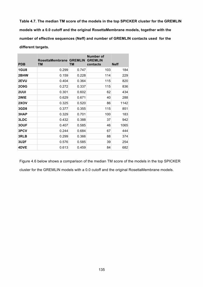
135

Table 4.7. The median TM score of the models in the top SPICKER cluster for the GREMLIN

models with a 0.0 cutoff and the original RosettaMembrane models, together with the

number of effective sequences (Neff) and number of GREMLIN contacts used for the

different targets.

PDB RosettaMembrane TM

GREMLIN TM

Number of GREMLIN contacts Neff

1GU8 0.299 0.747 103 184 2BHW 0.159 0.228 114 229 2EVU 0.404 0.364 115 820 2O9G 0.272 0.337 115 836 2UUI 0.301 0.602 62 434 2WIE 0.629 0.671 40 288 2XOV 0.325 0.520 86 1142 3GD8 0.377 0.355 115 851 3HAP 0.329 0.701 100 183 3LDC 0.432 0.388 37 942 3OUF 0.407 0.585 46 1065 3PCV 0.244 0.684 67 444 3RLB 0.299 0.366 88 374 3U2F 0.576 0.585 39 254 4DVE 0.613 0.459 84 682

Figure 4.6 below shows a comparison of the median TM score of the models in the top SPICKER

cluster for the GREMLIN models with a 0.0 cutoff and the original RosettaMembrane models.

136

Figure 4.6. Median TM sores for the top SPICKER cluster for the GREMLIN models with a cutoff of 0.0 and the RosettaMembrane models.

Figure 4.6 and table 4.7 show that in almost all cases the GREMLIN models are more accurate

with respect to the native structure. The only exceptions are for 2EVU, 3GD8, and 3LDC, where

there is a small decrease in the TM score, and 4DVE where the TM score drops from 0.613 to

0.459. Interestingly, this does not correlate with the number of effective sequences. It might be

expected that the cases for which the GREMLIN contact-assisted modelling was better would be

those that had a lower number of effective sequences, and where the contact information was

therefore presumably of lower quality.

137

4.4 Discussion This work has involved the application of AMPLE to Transmembrane Proteins; a difficult class of

proteins for crystallographers. Figure 4.7 below summarises the results as a Venn diagram.

Figure 4.7. Venn diagram summarising the success and failures of the three main methods attempted.

A primary point of interest arising from this work has been the discovery that many transmembrane

proteins are solvable with ideal helices. Ideal helices solved seven of the 15 test cases, although

the successes were limited to 2Å resolution or better, and with fewer than 262 residues in the unit

cell. This is encouraging because ideal helices require no modelling (a significant portion of the

time of an AMPLE run), and also because, with the current ideal helix configuration in AMPLE, only

138

eight MR jobs are attempted, as opposed to the maximum of 180 that was generated by AMPLE

from the ROSETTA models. As such, solution with AMPLE on a standard desktop should only take

a few hours. This suggests that attempting solution with ideal helices should be the initial choice for

an AMPLE user.

The only additional target that the RosettaMembrane protocol was able to solve beyond what was

solvable with ideal helices, was 3GD8. That only one additional target could be solved appears to

be at least in part a consequence of the generally poor quality of the models, as shown by the low

TM scores depicted in figure 4.2. However, considering that the RosettaMembrane protocol is

lengthy, involves the installation of the NR database and is unsupported, the overall poor

performance is not such a negative. Unfortunately 1GU8 was not solvable with any other method,

indicating that the RosettaMembrane protocol may be of use in particularly challenging cases.

The run with models using the PCONSC2 contacts performed particularly poorly, only solving

3LDC and 3OUF, both of which solved with ideal helices. Again, the poor performance seems to

be a consequence of poor models, which could in turn be related to the poor quality of the contact

information, as demonstrated by the generally low PPV values against the native structures as

shown in column 3 in table 4.5. Additionally, the PCONSC2 models were generated with the

standard ROSETTA modelling protocol. The developers of the GREMLIN modelling protocol

modified the electrostatic terms for the ROSETTA modelling for their contact-assisted modelling of

transmembrane proteins, so it is possible that the PCONSC2 might perform better with this altered

modelling protocol. This is something that will be explored in future work.

The GREMLIN transmembrane modelling protocol solves the same number of targets as the

RosettaMembrane protocol, although the identity of the individual targets solved is different, so it

was able to solve 1GU8, which was not solved with any other protocol. The GREMLIN protocol has

the advantage that the online server for generating the contacts is relatively quick and easy to use,

and the modelling then just uses the standard ROSETTA binaries with some modified flags that

139

have been implemented within AMPLE. This means that it is relatively easy for AMPLE users to

adopt this approach. The success of this approach seems to be sensitive to the handling of the

contacts, as there is a marked difference in the performance when the cut-off is changed from 1.0

to 0.0. In general the results are much better with 0.0, although 3OUF only solved with the cutoff of

1.0. This suggests that better parameterisation of GREMLIN could lead to better results.

On the basis of this work, a crystallographer with a transmembrane protein would be

recommended to attempt solution of the protein first with ideal helices. AMPLE using ideal helices

is far quicker than its other modes of operation, as no modelling is undertaken and only eight MR

jobs are generated. As such, most runs complete in a few hours.

If solution with ideal helices is not successful, then solution with GREMLIN contacts would be the

next logical step. Contacts can be calculated by the GREMLIN server with results being returned in

the order of a day, and then AMPLE can be run either on the user's workstation or via the AMPLE

webserver, with an expected runtime of the order of 1-2 days. In particularly challenging cases

where ideal helices and GREMLIN contacts fail, an attempt could be made to solve the structure

using the RosettaTransmembrane protocol.

Future work will explore different ways of using and combining contact information from different

sources and also using a modified AMPLE protocol that will be explored in chapter 6. The modified

protocol uses a modified version of SPICKER that clusters models based on TM scores, rather

than RMSD scores. AMPLE then sparsely samples all 10 clusters, as opposed to a deeper

sampling of the top cluster. The work in chapter 6 shows that this approach is able to considerably

improve the performance of AMPLE, particularly with difficult-to-solve cases.

140

Chapter 5: Distant Homologs

141

5 Distant Homologs

5.1 Introduction

5.1.1 Homologs as MR models Experience with standard MR has shown that it is expected to be unlikely to succeed when the

sequence identity is between 20% and 30% and impossible when it is lower than 20% (Abergel

2013). However, tools such as HHPRED (Söding, Biegert, and Lupas 2005) are constantly

improving and able to discover ever more distant homologs, which although sequentially and

structurally diverse should still contain useful structural information that could aid MR. In addition,

PHASER's maximum likelihood algorithms are also constantly being improved and are better able

to use the structural information from an ensemble composed of superimposed structures to weight

different parts of a search model. An individual homolog might not contain sufficient high-quality

structural information to derive valid phases from, but it is conceivable that by combining the

information from a number of remote homologs, sufficient information could be gathered to enable

successful MR.

As mentioned in the introduction, the use of structurally superimposed homologs is a standard

technique in MR, and is part of the standard pipeline for MrBUMP. However, by their very nature

distant homologs are very diverse, and this diversity could degrade and mask the structural

information. Structurally superimposing a set of distant homologs, and subjecting them to AMPLE's

truncation strategy to prune back to a structurally conserved core could potentially improve the

signal-to-noise ratio from a geometrically conserved core by pruning away the more diverse

regions.

142

The strategy in this work is to select a sequence-diverse set of homologs, ascertain whether

conventional MR can solve them, and then establish whether AMPLE ensembles formed from a

subset of those models enables solutions that would not otherwise be possible.

5.1.2 Structural Superposition The first task in creating the ensembles from a diverse set of homologs is to structurally

superimpose the homologs so that THESEUS (Theobald and Wuttke 2006) can determine the

variance between the residues required for the truncation procedure.

THESEUS uses a maximum likelihood approach to superposing structures which is able to

downweight variable regions of the structures and correct for correlations among atoms. This is

generally superior to a least squares superposition. Although THESEUS can superimpose diverse

homologs, it bases its superposition on an initial sequence alignment. The sequence alignment

determines which atoms are CORE (i.e shared amongst all structures) and these are then used to

guide the structural superposition (Douglas Theobald, personal communication). As the structural

alignment is restricted to the core atoms found from the sequence alignment, it can never be as

effective as a pure structural alignment. This is because sequence is only a proxy for structure, and

the best structural alignment will be one that only considers structure.

MUSTANG (Konagurthu et al. 2006) and GESAMT (Evgeny Krissinel 2012) are two programs that

undertake a purely structural alignment based entirely on the position of the Cα atoms. Both

programs adopt the approach of sequentially determining small fragments that superimpose and

then extending these fragments to build up a larger superposition. However, they differ in their

scoring metrics and approaches to selecting, collating and extending the fragments. As the

algorithms are somewhat different, both programs were used and their relative performance

assessed.

143

5.1.3 Histidine Phosphatase Superfamily The histidine phosphatase superfamily is a large and functionally diverse set of proteins. Although

functionally diverse, they all share a conserved catalytic core centred on histidine, which is usually

involved in a phosphorylation reaction. Although a single superfamily, the proteins can be

separated into two branches. Branch 1 is primarily composed of bacterial, usually intracellular

proteins and Branch 2, predominantly of eukaryotic extracellular proteins. The two branches are so

diverse that sensitive sequence and structural analyses are required to show the shared heritage.

Even within the branches there is considerable sequence, structural and functional diversity

(Rigden 2008).

The diversity in sequence and structure makes this family an interesting candidate for investigating

the effectiveness of distant homologs in MR. Although sharing a functional core and related

structural features that suggest that diverse members of the family could be suitable as MR search

models for each other, the diversity in sequence and structure means that conventional routes to

preparing MR models from related family members will not usually succeed. In this work, an

investigation of the potential for using AMPLE's cluster and truncate approach to prepare search

ensembles from homologous models was undertaken.

5.2 Methods

5.2.1 AMPLE Homologs Pipeline A number of changes were required to AMPLE to enable the use of homologous proteins as

models. AMPLE was initially written to work with ab initio decoys, all of which are of the same

length and have identical sequences and residue numbering. This made it very easy to handle the

models, as the only changes between the different PDB files was the coordinates. This meant that

the truncation stage could use the residue sequence number field of the pdb to identify a particular

residue across all models, since this number would always be the same. Considering a collection

of diverse homologs, the residue sequence number would no longer be the same between files.

144

The pipeline was therefore altered to use the position index of a residue, something which required

a number of changes to the internal architecture.

The following steps are carried out by the homolog module:

1. Take selection of homologs and standardise them by selecting the most probable

conformation and removing any solvent/HETATMS and ANISOU records.

2. Perform a structural alignment with either MUSTANG or GESAMT and generate a FASTA

format alignment file describing the alignment.

3. Align the homologs with THESEUS using the alignment file as a guide to which are the

CORE atoms, and record the variances at each residue position.

4. Remove all non-core atoms to generate a set of models that are all the same length.

5. Subject the core models to the standard AMPLE truncation procedure using the residue

positions instead of the residue sequence number.

5.2.1.1 Test Case Selection Seven examples from branch one of the histidine phosphatase family were selected to serve as

test cases. In each case chain A was selected. The seven structures are listed in table 5.1, and the

sequence identity matrix of all the structures is shown in table 5.2.

Table 5.1. Seven histidine phosphatases structures used as test cases.

PDB PDB Title Resolution (Å)

Length

1UJB Structure of the protein histidine phosphatase SixA 2.06 161

2A6P Structure Solution to 2.2 Angstrom of the Open Reading Frame Rv3214 from Mycobacterium tuberculosis

2.2 208

3C7T Crystal structure of the ecdysone phosphate phosphatase, EPPase, from Bombix mori in complex with tungstate

1.76 263

1E59 E.Coli cofactor-dependent phosphoglycerate mutase complexed with vanadate

1.3 249

1EBB Bacillus Stearothermophilus YHFR 2.3 202

2QNI Crystal structure of uncharacterized protein Atu0299 1.8 219

3DCY Crystal Structure a TP53-induced glycolysis and apoptosis regulator protein from Homo sapiens sapiens

1.75 275

145

Table 5.2. PDB eFold {REF} Secondary Structure Matching (SSM) sequence identity matrix for the seven members of the histidine phosphatase family.

1UJB:A 2A6P:A 3C7T:A 1E59:A 2QNI:A 1EBB:A 3DCY:A

1UJB:A 0.171 0.225 0.178 0.070 0.186 0.163

2A6P:A 0.171 0.202 0.240 0.171 0.279 0.240

3C7T:A 0.225 0.202 0.178 0.140 0.194 0.178

1E59:A 0.178 0.240 0.178 0.124 0.279 0.271

2QNI:A 0.070 0.171 0.140 0.124 0.202 0.140

1EBB:A 0.186 0.279 0.194 0.279 0.202 0.264

3DCY:A 0.163 0.240 0.178 0.271 0.140 0.264

The structures are structurally aligned using the SSM algorithm and then the sequence identity using this alignment is calculated. The cells showing the identity of the three structures (1UJB, 2A6P and 3C7T) that will be combined to attempt to solve the other four are highlighted in grey.

As can be seen in table 5.2, the sequence identity varies from 0.07 to 0.279, which indicates that

these are all likely to be either hard or impossible to solve with conventional MR.

The three structures 1UJB, 2A6P and 3C7T were selected at random to serve as the distant

homologs that would be used to try and solve the structures of the other members of the family

(1E59, 1EBB, 2QNI and 3DCY). Figure 5.1 shows the sequence alignment of all seven structures

based on a structural alignment with GESAMT. The 'Conservation' line graph in the figure shows

the degree of conservation of residue type where there is an aligned residue at that position for

each structure. As there is only a value in the conservation graph where there are aligned residues

for all the structures, this also corresponds to the position of the CORE residues.

146

Figure 5.1. JALVIEW display of GESAMT alignment of 1E59, 1EBB, 1UJB, 2A6P, 2QNI, 3C7T and 3DCY, with ClustalX colouring. Structurally aligned residues are in UPPER CASE whereas lower case letters are not part of the structural alignment.

Figure 5.2 shows a similar alignment just for the three structures that will be used as the models for

MR.

147

Figure 5.2. JALVIEW display of GESAMT alignment of 1UJB, 2A6P and 3C7T with ClustalX colouring. Structurally aligned residues are in UPPER CASE whereas lower case letters are not part of the structural alignment.

Figures 5.3 and 5.4 show the GESAMT structural alignment of all seven structures.

Figure 5.3. GESAMT superposition of 1UJB, 2A6P and 3C7T.

Figure 5.4. GESAMT superposition of 1E59, 1EBB, 1UJB, 2A6P, 2QNI, 3C7T and 3DCY

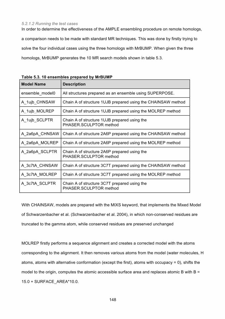
148

5.2.1.2 Running the test cases In order to determine the effectiveness of the AMPLE ensembling procedure on remote homologs,

a comparison needs to be made with standard MR techniques. This was done by firstly trying to

solve the four individual cases using the three homologs with MrBUMP. When given the three

homologs, MrBUMP generates the 10 MR search models shown in table 5.3.

Table 5.3. 10 ensembles prepared by MrBUMP Model Name Description

ensemble_model0 All structures prepared as an ensemble using SUPERPOSE.

A_1ujb_CHNSAW Chain A of structure 1UJB prepared using the CHAINSAW method

A_1ujb_MOLREP Chain A of structure 1UJB prepared using the MOLREP method

A_1ujb_SCLPTR Chain A of structure 1UJB prepared using the PHASER.SCULPTOR method

A_2a6pA_CHNSAW Chain A of structure 2A6P prepared using the CHAINSAW method

A_2a6pA_MOLREP Chain A of structure 2A6P prepared using the MOLREP method

A_2a6pA_SCLPTR Chain A of structure 2A6P prepared using the PHASER.SCULPTOR method

A_3c7tA_CHNSAW Chain A of structure 3C7T prepared using the CHAINSAW method

A_3c7tA_MOLREP Chain A of structure 3C7T prepared using the MOLREP method

A_3c7tA_SCLPTR Chain A of structure 3C7T prepared using the PHASER.SCULPTOR method

With CHAINSAW, models are prepared with the MIXS keyword, that implements the Mixed Model

of Schwarzenbacher et al. (Schwarzenbacher et al. 2004), in which non-conserved residues are

truncated to the gamma atom, while conserved residues are preserved unchanged

MOLREP firstly performs a sequence alignment and creates a corrected model with the atoms

corresponding to the alignment. It then removes various atoms from the model (water molecules, H

atoms, atoms with alternative conformation (except the first), atoms with occupacy = 0), shifts the

model to the origin, computes the atomic accessible surface area and replaces atomic B with B =

15.0 + SURFACE_AREA*10.0.

149

PHASER.SCULPTOR undertakes main-chain deletion, side chain pruning and B-factor

modification of the model based on a refined version of the Schwarzenbacher algorithm that makes

decisions based on the similarity scores from the sequence alignment of the model with the target

sequence using a binary score matrix combined with the BLOSUM62 matrix. (Bunkóczi and Read

2011).

The full ensemble is created using the SUPERPOSE program in CCP4, which aligns models using

a graph-theoretical approach based on secondary structure elements (E. Krissinel and Henrick

2004). The results of the MrBUMP run were then compared with AMPLE using the distant homolog

pipeline described above, once using MUSTANG to perform the initial alignment, and once using

GESAMT.

During this work, two errors were discovered with MUSTANG, one of which caused it to generate

an incorrect structural alignment when given a relatively diverse set of homologs, and another

which caused it to hang indefinitely. The developers were contacted regarding these problems, but

they stated that, the primary developer having left the group, they lacked the expertise to fix the

problem themselves. While the bug fortunately did not affect the cases used in this work, all future

work will be undertaken solely with GESAMT. For both MrBUMP and AMPLE, the software

versions as detailed in table 5.4 were used:

Table 5.4: Software versions used in run. Software Version Settings

CCP4 suite 6.5.15 Default

PHASER 2.5.7 Default

REFMAC 5.8.0131 30 cycles of jelly-body refinement

SHELXE 2014/4 Default

5.3 Results Table 5.5 show the results of running AMPLE and MrBUMP with different structures.

150

Table 5.5. The results of attempting to solve 1E59, 1EBB, 2QNI and 3DCY with two or more of 1UJB, 2A6P and 3C7T, with MrBUMP and AMPLE. Structures in AMPLE superposition MrBUMP

PDB 1UJB 2A6P 3C7T

1UJB 2A6P

2A6P 3C7T

1UJB 3C7T

1UJB 2A6P 3C7T

2A6P 3C7T

1E59 Mustang

0/57 0/57 0/57 0/57

0/10 0/7 1E59 Gesamt

0/60 0/60 0/57 0/57

1EBB Mustang

11/57 0/57 1/63 14/63

3/10 0/7 1EBB Gesamt

13/60 0/60 2/57 6/57

2QNI Mustang

34/57 14/57 19/63 27/63

0/10 0/7 2QNI Gesamt

28/60 4/60 5/57 13/57

3DCY Mustang

45/57 41/57 40/57 45/57

2/10 0/7 3DCY Gesamt

45/60 37/60 35/57 37/57

The numbers in the table show the number of successful/unsuccessful ensembles for each case. Cells with successful runs are coloured green.

The second and sixth columns show the results of attempts to solve the four targets with structure

1UJB, 2A6P and 3C7T, with AMPLE and MrBUMP respectively. MrBUMP succeeds in solving

structures 1EBB and 3DCY with 3 and 2 of the 10 ensembles respectively, but fails with both

structures 1E59 and 2QNI. AMPLE is able to solve both structures 1EBB and 3DCY, but

additionally solves 2QNI. Neither approach is able to solve structure 1E59.

Comparing the AMPLE results with GESAMT and MUSTANG, the results with the two programs

are broadly similar. The different alignments, resulting residue variances, and hence the different

truncation parameters, mean that different programs generate different numbers of ensembles. For

structure 3DCY both programs were equally successful (although MUSTANG generated the same

number of successes with 3 fewer ensembles). For structure 1EBB GESAMT was more successful

151

(13 success versus MUSTANG's 11), but for structure 2QNI MUSTANG was more successful (34

successes versus GESAMT'S 28).

The results for attempting to solve structures 1E59, 1EBB, 2QNI and 3DCY with structures 1UJB,

2A6P and 3C7T using GESAMT were combined to provide an overall analysis.

Figure 5.5. Number of residues per chain in successful (blue) and unsuccessful (red) models for all ensemble search models for attempting to solve 1E59, 1EBB, 2QNI and 3DCY with 1UJB, 2A6P and 3C7T.

In previous work with ab initio models (Bibby et al. 2012; Thomas et al. 2015), the number of

residues per chain for successful ensembles had a maximum at about 25 residues. The successful

homolog ensembles have a maximum at about 80 residues, so are considerably larger.

152

Figure 5.6. Percentage of core ensemble in successful (blue) and unsuccessful (red) models for all ensemble search models for attempting to solve 1E59, 1EBB, 2QNI and 3DCY with 1UJB, 2A6P and 3C7T.

Similarly, the maximum for the percentage of the chain in the ensemble was at about 50% with ab

initio models, but is at about 65% here. However, it must be remembered that there is an additional

truncation step from full homolog models down to the structural core that is shared between all

models. As a result, the initial core ensemble is already somewhat smaller than the original

homologs. With this taken into account, the percentage of the original homolog model that is

successfully able to solve the crystal structure is similar to that in previous work.

153

Figure 5.7. Side chain treatments for successful (blue) and unsuccessful (red) models for all ensemble search models for attempting to solve 1E59, 1EBB, 2QNI and 3DCY with 1UJB, 2A6P and 3C7T.

An analysis of the side chain treatments show that all side chain treatments were capable of

generating successes, with poly-alanine being the most successful. All of the structures that were

solved were solved with at least two different side chain treatments as is shown in table 5.6. No

side chain treatments were exclusively successful, but polyalanine was the most successful and all

of the structures would have been solvable if only polyalanine side chains had been used.

Table 5.6: successful ensembles partitioned by side chain treatment.

PDB Num. Ensembles

Successful Ensembles

Success PolyAla

Success Reliable

Success Allatom

1E59 60 0 0 0 0 1EBB 60 8 3 5 0 2QNI 60 29 14 10 5 3DCY 60 41 16 14 11

5.3.1 Solution with fewer search models Looking at which search models solved for MRBUMP the following is observed:

154

Table 5.7. Successful MRBUMP search models for attempting to solve 1EBB and 3DCY with 1UJB, 2A6P and 3C7T Target PDB Successful search models

1EBB A_1ujb_CHNSAW A_1ujb_MOLREP A_1ujb_SCLPTR

3DCY A_1ujb_CHNSAW A_1ujb_SCLPTR

In both cases a search model derived from 1UJB alone was able to enable successful MR. Initially

this seems unexpected as it shares 0.186 sequence-identity with 1EBB and 0.163 with 3DCY,

seemingly too low to enable solution. However examination of the sequence and structural

alignments in figures 5.2 and 5.3 provide a possible explanation. Only a partial model may be

required for successful MR, particularly if that model is accurate. The whole philosophy of AMPLE

is to truncate models down to an accurate core that can solve the structure, and 1UJB is almost a

truncated core of 2A6P and 3C7T. Therefore, although the overall sequence diversity is large, the

structures share the conserved core, which is represented by 1UJB and means that solution with

1UJB alone is possible.

It was therefore interesting to see whether it was still possible to solve this structure without

including structure 1UJB. An additional run of MRBUMP was therefore carried out with just 2A6P

and 3C7T. As shown in the 7th column of table 5.5, none of the seven search models generated

was able to solve any of the targets.

Solution was then attempted with AMPLE with all pairs of 1UJB, 2A6P and 3C7T. As columns 3-5

of table 5.5 show, AMPLE was able to solve all the structures, with the exception of 1EBB when

3C7T was omitted from the ensemble.

5.4 Discussion This work has shown that AMPLE's truncation algorithm is able to automatically extract sufficient

structural information from distant homologs to enable structure solution where the individual

155

homologs, or a superposition of all of them cannot succeed, as demonstrated by the failure of

MRBUMP to succeed with the same search models.

Combining multiple homologs with a structural alignment and using THESEUS to determine the

inter-residue variance enables AMPLE to determine which parts of the structure are likely to be

conserved and which are likely to vary. Truncating the ensemble using this information creates a

series of ensemble search models that should successively better approximate the conserved core

(although only up to a point as excessive truncation can lead to a model too small to enable

successful solution)

When run with MRBUMP, PHASER is also given a structurally aligned ensemble of all the search

models, and hence has some information on how the models align and which parts are likely to be

more accurate. However it seems that the information from the more variable regions is masking

the signal from the core.

AMPLE is able extract this information so effectively that it is able to succeed with just two

structures, where solution with conventional methods is not even possible with three.

This work has presented an initial foray into the use of distant homologs within AMPLE. It has

shown that AMPLE holds great promise for extracting hitherto unavailable information from distant

homologs. Further work will explore the effectiveness of this approach.

156

Chapter 6: Algorithm

Developments

157

6 Algorithm Developments

6.1 Introduction The AMPLE pipeline can be divided into three largely separate stages:

l model generation.

l clustering and truncation of models to create ensembles for molecular replacement (MR).

l MR and automated model building.

For each stage there are a number of different parameters and options that can be selected; for

example, the number of models generated by ROSETTA, or the sub-clustering radius for the

ensemble creation. The parameters for the original pipeline were selected based on the best

available evidence at the time, but have not been extensively benchmarked to determine their

optimum values. The purpose of this work is to explore those parameters that are believed most

likely to have an effect on the success of the pipeline.

6.1.1 Selection of stage to test and parameters to explore In order to approach this in a systematic manner, and reduce the number of combinations of

parameters to be explored, the assumption was made that the three stages of the AMPLE pipeline

are mutually independent. This is based on the hypothesis that accurate models are likely to make

the best ensembles, which in turn are most likely to be more successful in MR It is conceivable that

a particular class of models (coiled-coil proteins, or β-sheet proteins for example), might fare better

under particular ensembling parameters and might favour parameters for MR that are different to

other classes of proteins. However, these are expected to be minor deviations from the norm and

can be explored in subsequent work if there are any indications that this may be the case.

The heart of the AMPLE algorithm is the preparation of the ensembles for MR from existing

models. As this stage is most specific to AMPLE and the one that the AMPLE pipeline has most

control over, it was decided to examine this "ensembling" stage first. Additionally, the optimal

158

ensembling strategy is likely to extract the greatest potential from even relatively poor models and

provide more data for the MR pipeline to work with. This should make it easier to determine an

optimal MR strategy.

6.2 Methods The optimal configuration of each step within the ensembling pipeline was assumed to be largely

independent of the others. Each was therefore examined in turn. The parameters available to be

explored for each stage will be discussed below. The different stages of the AMPLE ensemble

preparation pipeline are depicted in figure 1.1 in chapter 1.

6.2.1 Truncation Currently AMPLE truncates the models from the first cluster based on the residue variances across

different models as calculated by THESEUS. The truncation is currently at evenly-spaced 5%

intervals based on the number of residues in the protein chain.

As the truncation is based exclusively on the variance score the truncation often produces models

that have isolated residues. It is conceivable that these isolated residues would not contribute

usefully to the molecular replacement signal. The truncation algorithm was therefore amended to

remove any single residue remaining after the truncation step that was isolated from any other

residue by a gap of at least 2 residues in sequence.

6.2.2 Sub-clustering The truncated models are sub-clustered under three successively increasing RMSD thresholds (1,

2 and 3Å) and a maximum of 30 are then selected to create an ensemble. An ensemble is only

created for a sub-clustering radius if the list of models selected differs from previous ensembles.

6.2.2.1 Slicing sub-clusters On examining the code for this step some minor limitations were discovered. In the original code,

the comparison of the list of models was carried out based on the size of the list. However this

excludes potential ensembles, since if there were more than 30 models in the list, a different

ensemble could be created from it. In addition, the comparison was carried out before the list was

159

truncated to 30. Due to the nature of the sub-clustering algorithm it is very likely that two different

lists of sub-clustered models could share the first 30 members, which would lead to duplication of

the ensembles. This would not affect the overall success of the code, but would mean that more

ensembles would be generated than need be, which would waste CPU time. Finally, the sub-

clustering algorithm would return a random model even if no models could be sub-clustered under

a particular radius, and this single model would become the ensemble.

The code was therefore altered to use the following algorithm.

l if no models are sub-clustered under a given radius, no ensemble is created.

l if more than 30 models are sub-clustered for any given radius:

l if this is the first radius (1Å), the first 30 models from the list of sub-clustered models

are selected.

l if the radius is 2Å, a check is made to see if the first 30 are the same as that chosen

for 1Å

� if the list is the same, the slice of the list of length 30 is taken, starting at an

index of half of the remainder, when 30 is subtracted from the length of the

list.

l if the radius is 3Å, a check is made as to whether the first 30 are the same as that

chosen for 1 or 2Å

� if the list is the same, ta slice of the list of length 30 is taken from the end of

the list.

The test set was then run to examine the effect of this change.

6.2.2.2 Increasing sub-cluster radii If no models are selected for a particular sub-clustering radius, then the sub-clustering stage

would stop. However no examination had been undertaken previously to determine whether

increasing the sub-clustering radius until more models are selected could generate additional

solutions.

160

The code was therefore altered so that if no models are selected for a particular sub-clustering

radius, the radius will be increased until at least two models have been selected. This will be

referred to as sub-clustering with floating radii.

6.2.3 Clustering

6.2.3.1 Clustering algorithms and distance metrics Currently the clustering in AMPLE is carried out with SPICKER. SPICKER is developed by the

Zhang group at the University of Michigan and is a well-respected tool used in the I-TASSER and

QUARK ab initio modelling programs. SPICKER clusters models using the RMSD of the Cα atoms

as the distance metric to compare models. This makes it extremely fast, so that even for the

largest models used within AMPLE, the clustering time is of the order of about 15 minutes.

However, RMSD is a global distance metric, so that structural differences in flexible regions of two

proteins (such as loops), can cause large deviations in the RMSD even if the core regions of the

proteins are similar. For this reason a number of alternative metrics for comparing proteins, such

as the Template Modelling (TM) score, Longest Continuous Segment (LCS) and Global Distance

Test (GDT) have been developed to overcome this shortcoming (Yang Zhang and Skolnick 2004).

As AMPLE prunes back the most variable regions of its models to a conserved core to generate

the ensembles, it could be expected that clustering the models based on a distance metric that can

account for similar core regions would perform better than a global distance metric.

There are currently a number of protein model clustering programs that can compare models using

different distance metrics including Fast Protein Cluster (FPC) and ClusCo (Hung and Samudrala

2014; Jamroz and Kolinski 2013) . For this work, it was decided to use FPC, as it is available under

a permissive licence, was developed to work with many thousands of models, and so has been

parallelised for both CPUs and GPUs, which makes it very quick to use. FPC is able to cluster

161

using both RMSD and TM scores as distance metrics, and can also use a number of different

clustering methods, such as the k-means (default) and h-average.

The following strategy will therefore be attempted with FPC clustering:

l cluster with the default k-means clustering algorithm and RMSD scoring to provide a

baseline and comparison to the current SPICKER clustering.

l cluster with the default k-means clustering algorithm and TM scoring to elucidate the effect

of TM scoring.

6.2.3.2 Multiple Clusters The decoys are clustered on the hypothesis that, if the models are clustered by structural similarity,

then the largest cluster often contains the best model, and the centroid of the cluster is likely to be

the best prediction for that model. In the initial work that was done with AMPLE on globular

proteins up to 120 residues in size, it was found that this hypothesis held, with the vast majority of

success originating in the top (largest) cluster, and only a few in the second cluster.

The time for processing each cluster within AMPLE is the same, so analysing the second cluster

doubles the time, and a third triples it. As there were so few solutions in subsequent clusters, the

additional cost of processing additional clusters was deemed excessive, so most work on AMPLE

since then has involved processing only the top cluster and this is the default setting for users

running AMPLE on their own machines.

However, recent experience has indicated that successful solutions to problematic cases can

sometimes be found in clusters other than the first. This appears to be happening more frequently

now that larger targets that are at the limit of what the molecular modelling programs such as

ROSETTA are able to work with are being attempted. In these cases, it is often only a part of the

model that enables solution, with the accuracy of the overall modelled fold being insufficient to

enable a solution. In these cases it would appear to be more effective to sample a number of

162

different fold predictions, each of which may contain smaller structural elements that are accurately

modelled, rather than attempting to select the overall best structure.

This work was therefore an opportunity to explore the additional clusters and see whether an

algorithm could be developed that enables exploration of the additional clusters in a tractable way.

6.2.4 Test set Selection In order to systematically explore the effect of different parameters, a systematically varied test set

was required. The requirements of the test set are that it:

l be small enough to run multiple times without generating too much data or consuming

excessive CPU time.

l contain representative examples of the different diffraction resolutions, chain lengths and

classes of protein amenable to solution by AMPLE.

l be representative of cases that:

� did not previously solve in order to highlight if a particular change produces a

solution.

� only produced a few solutions, making it obvious if a change prevents solution or

creates additional solutions.

� have many solutions, to clearly show if a change alters the proportion of successes.

In total, 409 crystal structures have been benchmarked in previous AMPLE investigations. Fifteen

of these were selected for the test set. As the work with globular proteins only included chains of

up to 120 residues, and AMPLE has shown to be successful with considerably larger structures, an

additional three larger globular proteins were added to this list. Table 6.1 below lists the 18

structures together with the reason for their inclusion. Targets included for having the largest

percentage of β-sheet or number of residues whilst having failed in previous runs were included

because these were those most unlikely to succeed, and so their solution would provide a clear

indication of an improvement.

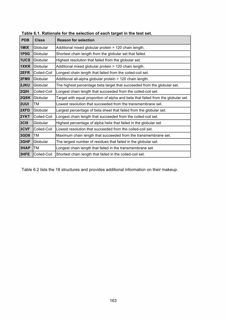
163

Table 6.1. Rationale for the selection of each target in the test set. PDB Class Reason for selection

1MIX Globular Additional mixed globular protein > 120 chain length. 1P9G Globular Shortest chain length from the globular set that failed.

1UCS Globular Highest resolution that failed from the globular set.

1XKR Globular Additional mixed globular protein > 120 chain length.

2EFR Coiled-Coil Longest chain length that failed from the coiled-coil set. 2FM9 Globular Additional all-alpha globular protein > 120 chain length.

2JKU Globular The highest percentage beta target that succeeded from the globular set.

2QIH Coiled-Coil Longest chain length that succeeded from the coiled-coil set.

2QSK Globular Target with equal proportion of alpha and beta that failed from the globular set. 2UUI TM Lowest resolution that succeeded from the transmembrane set.

2XFD Globular Largest percentage of beta sheet that failed from the globular set.

2YKT Coiled-Coil Longest chain length that succeeded from the coiled-coil set.

3CI9 Globular Highest percentage of alpha helix that failed in the globular set 3CVF Coiled-Coil Lowest resolution that succeeded from the coiled-coil set.

3GD8 TM Maximum chain length that succeeded from the transmembrane set.

3GHF Globular The largest number of residues that failed in the globular set.

3HAP TM Longest chain length that failed in the transmembrane set. 3HFE Coiled-Coil Shortest chain length that failed in the coiled-coil set.

Table 6.2 lists the 18 structures and provides additional information on their makeup.

164

Table 6.2. Description of the targets in the test set selection. PDB Class Resoln.

Å Solvent %

Space Group

Chain Length

Chains in ASU

Residues α % β %

1MIX Glob. 1.75 40.43 C 1 2 1 206 1 206 39 18

1P9G Glob. 0.84 20.89 P 1 21 1 41 1 41 0 43.9

1UCS Glob. 0.62 11.58 P 21 21 21 64 1 64 34.38 17.19 1XKR Glob. 1.75 63.5 P 42 21 2 206 1 206 44 27

2EFR Coiled-Coil 1.8 50.1 P 1 155 4 620 98 0

2FM9 Glob. 2.0 59.31 P 32 2 1 215 1 215 72 0

2JKU Glob. 1.5 65.53 P 64 2 2 94 1 94 0 45.74 2QIH Coiled-Coil 1.9 53.66 P 3 157 2 314 85 0

2QSK Glob. 1.0 46.02 P 21 21 21 95 1 95 12 12

2UUI TM 2.0 72.83 F 2 3 156 1 156 80 0

2XFD Glob. 1.19 41.0 P 21 21 21 112 1 112 0 59.82 2YKT Coiled-Coil 2.11 54.63 C 2 2 21 253 2 266 80 0

3CI9 Glob. 1.8 51.58 H 3 48 4 96 93.75 0

3CVF Coiled-Coil 2.9 85.71 P 65 79 4 316 81 0

3GD8 TM 1.8 54.97 P 4 21 2 223 1 223 69 0 3GHF Glob. 2.2 44.04 P 32 2 1 120 1 120 26.67 18.33

3HAP TM 1.6 54.99 C 2 2 21 249 1 249 70 4

3HFE Coiled-Coil 1.7 33.17 C 1 2 1 31 3 93 70 0

6.2.5 Model generation and MR A set of 1000 decoys was generated for each target, and the same models used for all subsequent

runs. The same version of CCP4 was also used for all MR stages as detailed in table 6.3.

Table 6.3. Software versions used in the run.

Software Version

ROSETTA 2014.35.57232

CCP4 suite 6.5.015

PHASER 2.5.7

REFMAC 5.8.0103

SHELXE 2014/4

6.2.6 Ideal Helices As in previous work, solution was first attempted with ideal helices. Although these would obviously

not be expected to work with a predominantly β-sheet protein with no α-helices, it does provide

165

some indication of which structures are relatively easy to solve and do not require the additional

information from the modelling to enable solution.

6.3 Results

6.3.1 Truncation Table 6.4 compares the results of the original AMPLE single-cluster run with that when isolated

residues are removed following truncation.

Table 6.4. Comparison of results for the default truncation and that with pruning.

Benchmark Pruning

PDB Search Models

Succeeded Search Models

Succeeded

1MIX 30 0 36 0

1P9G 162 0 156 0

1UCS 144 0 144 0

1XKR 21 0 15 0 2BL2 153 0 144 0

2EFR 21 0 24 0

2FM9 45 0 45 0

2JKU 114 5 111 6 2QIH 60 5 60 6

2QSK 15 0 15 0

2UUI 90 19 78 18

2XFD 126 0 120 0 2YKT 63 3 57 3

3CI9 177 88 174 84

3CVF 159 0 147 0

3GD8 21 0 15 0

3GHF 81 0 81 0 3HAP 81 3 78 2

3HFE 111 0 111 0

Total: 1674 123 1611 119

Table 6.4 shows that there is very little difference between the two runs, with the original run being

marginally more successful, with 123 successes against the truncation run with 119 successes.

166

Interestingly, two cases fare better with truncation (2JKU and 2QIH), whereas all the others fare

slightly worse.

6.3.2 Sub-clustering Table 6.5. Comparison of the results for different sub-clustering strategies.

Benchmark Sub-cluster slice Sub-cluster floating radii

PDB Search Models

Succeeded Search Models

Succeeded Search Models

Succeeded

1MIX 30 0 30 0 144 0

1P9G 162 0 168 0 180 0

1UCS 144 0 147 0 189 0

1XKR 21 0 21 0 189 0 2BL2 153 0 150 0 180 0

2EFR 21 0 21 0 174 0

2FM9 45 0 54 0 180 0

2QIH 60 5 60 5 180 15 2QSK 15 0 15 0 114 0

2UUI 90 19 93 21 180 18

2XFD 126 0 126 0 18 0

2YKT 63 1 63 1 180 5 3CI9 177 80 204 69 207 67

3CVF 159 0 159 0 180 0

3GD8 21 0 21 0 189 0

3GHF 81 0 81 0 63 0

3HAP 81 3 81 3 189 3 3HFE 111 0 132 0 135 0

Total: 1560 108 1626 99 2898 108

For this run, 2JKU has been excluded due to a technical problems, but all other data are valid.

Table 6.5 above shows that the new sub-cluster-slicing algorithm produces more ensembles than

the original benchmark code, but fewer successes. The creation of more ensembles overall is due

to the additional ensembles created when sub-clustering at a larger radius creates the same list of

ensembles and a different slice is selected. The drop in successes for 2UUI and 3CI9 is due to the

removal of duplicate ensembles due to the altering of the original sub-clustering implementation.

167

For sub-cluster floating, many more ensembles were created, as three ensembles were always

created for each sub-clustering step. However, despite the creation of more ensembles from sub-

clusters with larger radii. only two ensembles solved with radii greater than 3Å, which were two

ensembles sub-clustered under 4 and 5Å for 2YKT.

6.3.3 Clustering Algorithms Table 6.6 below shows the results of the different clustering algorithms for the decoys from the top

cluster, together with a run of AMPLE using ideal helices.

Table 6.6. Number of successful/total search models for the different clustering treatments.

PDB Class IDEAL HELICES

SPICKER RMSD

SPICKER TM

FPC K-means RMSD

FPC K-means TM

FPC H-complete TM

1MIX Globular 0/8 0/30 0/45 0/18 0/57 0/54

1P9G Globular 0/8 0/162 0/159 0/165 0/162 1/150

1UCS Globular 0/8 0/144 0/141 0/114 0/132 0/123

1XKR Globular 0/8 0/21 0/33 0/39 0/54 0/48 2EFR Coiled-Coil 0/8 0/21 0/63 0/48 0/54 0/51

2FM9 Globular 0/8 0/45 0/48 0/42 0/72 0/48

2JKU Globular 0/8 5/114 63/126 1/75 18/108 15/105

2QIH Coiled-Coil 7/8 5/60 52/87 16/81 35/81 48/78 2QSK Globular 0/8 0/15 0/12 0/9 0/15 0/9

2UUI TM 6/8 19/90 16/99 12/84 16/93 12/81

2XFD Globular 0/8 0/126 0/132 0/117 0/120 0/120

2YKT Coiled-Coil 4/8 3/63 2/66 3/60 7/72 6/75 3CI9 Globular 4/8 88/177 57/180 50/207 74/195 8/192

3CVF Coiled-Coil 0/8 0/159 1/165 0/156 0/159 0/159

3GD8 TM 0/8 0/21 0/54 0/18 2/60 0/24 3GHF Globular 0/8 0/81 0/102 0/78 0/87 0/69

3HAP TM 3/8 3/81 1/99 0/84 0/90 0/81

3HFE Coiled-Coil 0/8 0/111 0/114 0/135 0/129 0/132

Total: 24/144 123/1674 192/1881 82/1674 152/1881 90/1737 Cells with successful search models are coloured green.

168

The library of 8 ideal helices within AMPLE was able to solve 5 structures, including 3CI9 and

3HAP that had not been solvable with AMPLE when they were first selected (the transmembrane

protein 3HAP was subsequently solved with ROSETTA models using GREMLIN contacts, but this

was after the test set had been selected).

The default SPICKER/RMSD clustering solved 6 targets. In addition to the 5 that were solvable

with ideal helices, it also solved 2JKU, which had been solved in the first AMPLE paper (Bibby et

al. 2012).

The first run with FPC used the default k-means clustering algorithm and the model RMSD scores

for clustering. This solved only 4 targets, all of which were solvable with the SPICKER/RMSD

clustering. This demonstrates that the SPICKER clustering algorithm is well-optimised for its role.

The next step was to see if using TM scores to cluster, rather than RMSD scores would improve

the performance. FPC was run using the k-means clustering algorithm, but clustering on TM

scores. This run solved 6 targets, so was a substantial improvement on using the RMSD as the

scoring metric, but solved the same number as the SPICKER/RMSD clustering. This run solved

3GD8, which was not solvable with any of the preceding methods (but had been solved with

SPICKER/RMSD clustering with an earlier set of models). However, it was not able to solve 3HAP,

which solved with SPICKER/RMSD clustering. A notable feature of the TM scoring run, is that for

the models that solved with both RMSD scoring and TM scoring, there was a marked increase in

the number of solutions with TM scoring. This demonstrates that TM scoring provides a significant

improvement to RMSD scoring, although at the cost of the additional CPU time required to

calculate the TM scoring matrix.

As TM scoring seems to be superior, a run was made with FPC using TM scoring, but using the h-

complete clustering algorithm. This solved 6 structures (the same number as SPICKER/RMSD and

FPC/k-means), with 5 of the targets (2JKU, 2QIH, 2UUI, 2YKT and 3CI9) being the same as

169

solved with the other methods. This run managed to solve 1P9G with a single search model; a

significant result as it did not solve with any of the other methods and had not been solved with

AMPLE previously. This run did not solve 3GD8, which did solve with FPC/k-means

These results indicate that both the choice of clustering algorithm and scoring metric have a

significant effect on the success of AMPLE. TM scoring seems to be the most effective, but the

SPICKER clustering algorithm seems to be superior to both k-means and h-complete clustering, as

it solves the same number of targets using the seemingly weaker RMSD scoring metric.

It was therefore of interest to see how SPICKER clustering would perform when using TM scoring.

Unfortunately this option was unavailable in SPICKER. However, since the source code of

SPICKER is made freely available, the program was altered to read in the matrix of TM scores

generated by FPC to provide a direct comparison of the SPICKER clustering algorithm with k-

means and h-complete.

This SPICKER/TM run was the most successful of all runs, solving 7 targets. 6 of the targets

(2JKU, 2QIH, 2UUI, 2YKT, 3CI9 and 3HAP) had been solved with the other methods, but 3CVF

was solved for the first time with a single search model. Interestingly, although for 2JKU and 2QIH

there was a marked increase in the number of successful search models between

SPICKER/RMSD and SPICKER/TM, for all other cases, although the target solved, it did so with

fewer search models.

Through all the different runs, 9 out of 18 targets were solvable with this set of models, although no

individual clustering method was able to solve all of the targets. TM scoring appears to be most

effective and the SPICKER clustering algorithm the most effective overall, although it was unable

to select models that are able to solve 1P9G and 3GD8. However, as SPICKER is already included

in CCP4, and the source code is accessible, the TM scoring algorithm was added to it. The further

170

work on clustering was then carried out using the SPICKER clustering algorithm to explore what

role additional clusters can have.

6.3.4 Exploring additional clusters As mentioned previously, in most of the work completed with AMPLE only the top, or occasionally

the top three clusters have been used, but there has been no systematic attempt to explore the

possibility of solutions in the lower ranked clusters. In order to investigate this, two runs were

undertaken using all 10 clusters and treating them all to the full AMPLE truncation, sub-clustering

and side chain treatments. As this is an extremely compute- and data-intensive exercise (~150GB

of data when compressed), only two runs were attempted. One with SPICKER/RMSD clustering

and the other with SPICKER/TM clustering. The results are displayed in table 6.7.

Table 6.7. Successful/total search models with 10 full clusters.

PDB Class Resoln. Å

Chain Length

Chains in ASU

SPICKER RMSD

SPICKER TM

1MIX Glob. 1.75 206 1 0/186 0/384

1P9G Glob. 0.84 41 1 14/1506 16/1422

1UCS Glob. 0.62 64 1 0/1053 7/1134

1XKR Glob. 1.75 206 1 0/174 11/279 2EFR Coiled-Coil 1.8 155 4 0/180 0/360

2FM9 Glob. 2.0 215 1 0/303 1/504

2JKU Glob. 1.5 94 1 138/912 160/927

2QIH Coiled-Coil 1.9 157 2 184/531 310/792 2QSK Glob. 1.0 95 1 0/75 0/156

2UUI TM 2.0 156 1 153/786 136/870

2XFD Glob. 1.19 112 1 0/1002 0/1086

2YKT Coiled-Coil 2.11 253 2 17/588 17/723 3CI9 Glob. 1.8 48 4 279/1926 503/1911

3CVF Coiled-Coil 2.9 79 4 15/1476 1/1449

3GD8 TM 1.8 223 1 1/222 8/387

3GHF Glob. 2.2 120 1 0/609 0/696 3HAP TM 1.6 249 1 3/747 14/768

3HFE Coiled-Coil 1.7 31 3 2/1311 0/1338

Total: 806/13587 1184/15186 Cells with successful search models are coloured in green. Cells with only a single search models are coloured a lighter shade of green to indicate that this is a rare solution.

171

The results show a huge jump in the number of targets that can be solved. SPICKER/RMSD is

able to solve 10 targets, and SPICKER/TM is able to solve 12. This includes 4 targets (1UCS,

1XKR, 2FM9 and 3HFE) that had not been solved with any of the previous runs and had never

been solved by AMPLE with a different set of models.

Overall the performance of SPICKER/TM is better, solving 1UCS, 1XKR and 2FM9 that could not

be solved with SPICKER/RMSD. Of these 2FM9 and 3CVF, were only solved with a single model,

a result that could be attributed to chance, due to the large number of solutions attempted (504 and

1449 respectively).

SPICKER/RMSD was able to solve 3HFE which was not solvable with SPICKER/TM and also

solved 3CVF with 15 search models, a far more definitive solution then the single solution achieved

by SPICKER/TM. Conversely, SPICKER/TM is able to solve 3GD8 with 8 search models, as

opposed to the single solution generated with SPICKER/RMSD.

Overall SPICKER/TM with 10 clusters appears to be a more effective algorithm, enabling the

solution of 12 targets, double that which is possible with the original SPICKER/RMSD single-

cluster algorithm currently employed in AMPLE, and two more than SPICKER/RMSD with 10

clusters.

6.3.5 Pruning the clusters Although the SPICKER/TM algorithm with 10 clusters is able to solve 6 additional targets, the

additional processing of 10 clusters increases the total run time of AMPLE by a factor of roughly

10. Under normal use, AMPLE will stop as soon as soon as a solution is found, so the total run

time is related to the proportion of successful search models (assuming that the successful jobs

are randomly distributed within the clusters). Table 6.8 lists the proportion of successful/total jobs

for the different runs.

172

173

Table 6.8. Proportion of successful/total jobs for the different clustering algorithms. Run type : N clusters Successful/Total jobs Proportion

SPICKER/RMSD: 1 123/1674 0.073

SPICKER/RMSD: 10 806/13587 0.059

SPICKER/TM: 10 1184/15180 0.078

Overall the proportion of successful jobs is largely similar, so for a successful job, even with 10

clusters, the run time for a 10-cluster job (excluding modelling/clustering) would be similar to that

for a single cluster. However, for unsuccessful jobs, the run time will be 10 times that of a standard

AMPLE run, which could be many weeks, and is therefore not acceptable for most users. It is

therefore important to see if the number of search models can be reduced, whilst still maintaining

the success rate.

The following section will analyse the results to see the best way to sample the search ensembles.

Figure 6.1. Cluster distribution of successful (blue) and unsuccessful (red) search models for SPICKER/RMSD

Figure 6.2. Cluster distribution of successful (blue) and unsuccessful (red) search models for SPICKER/TM

Figures 6.1 and 6.2 show the distribution of successful and unsuccessful search models between

the different clusters for the 10-cluster SPICKER/RMSD and SPICKER/TM runs. They show that

174

solutions are scattered more or less evenly through the clusters, with little preference for the top

cluster.

Figure 6.3. Number of successful (blue) and unsuccessful (red) search models for different sub-clustering radii for SPICKER/RMSD.

Figure 6.4. Number of successful (blue) and unsuccessful (red) search models for different side chain treatments for SPICKER/RMSD.

Figure 6.5. Number of successful (blue) and unsuccessful (red) search models for different sub-clustering radii for SPICKER/TM.

Figure 6.6. Number of successful (blue) and unsuccessful (red) search models for different side chain treatments for SPICKER/TM.

175

Figures 6.4-6.6 show the distribution of successful and unsuccessful jobs for the different side

chain treatments and sub-clustering radii for the SPICKER/RMSD and SPICKER/TM runs. They

show that the successful jobs are largely evenly distributed amongst the different sub-clustering

radii and side chain treatments, with a very slight increase in the number of successes for

polyalanine side chains.

As the results gave no particular indication of a way to prune the ensembles, a number of different

strategies were attempted for the SPICKER/TM results as shown in table 6.9 below. The different

treatment strategies in the table are as follows:

l All: the original set with 5% truncation, 1, 2 & 3Å sub-clustering and all-atom, reliable and

polyalanine side chains.

l Full 1, 1+3Å/polyA: the original full treatment for the first cluster, and then 1 & 3Å sub-

clustering and only polyalanine side chains for all subsequent clusters.

l 1Å/polyA: 1Å sub-clustering and polyalanine side chains for all clusters.

l 2Å/polyA: 2Å sub-clustering and polyalanine side chains for all clusters.

l 3Å/polyA: 3Å sub-clustering and polyalanine side chains for all clusters.

l 1+3Å/polyA: 1 & 3Å sub-clustering and polyalanine side chains for all clusters.

l 10% Truncation: 10% truncation level, 1, 2 & 3Å sub-clustering and all-atom, reliable and

polyalanine side chains for all clusters.

l 10% Truncation: 10% truncation level, 1 & 3Å sub-clustering and polyalanine side chains

for all clusters.

176

Table 6.9:.Successful/total search models for the SPICKER/TM set under different pruning

strategies.

PDB All Full 1 1+3Å/ polyAla

1Å/ polyAla

2Å/ polyAla

3Å/ polyAla

1+3Å/ polyAla

10% Truncation

10% Truncation 1+3Å/polyAla

1MIX 0/384 0/129 0/19 0/42 0/67 0/86 0/159 0/38 1P9G 16/1422 5/435 3/125 2/169 2/180 5/305 8/696 2/150 1UCS 7/1134 4/368 2/84 1/123 2/171 4/255 3/534 0/121 1XKR 11/279 6/87 4/28 2/31 2/34 6/62 1/102 1/23 2EFR 0/360 0/119 0/34 0/46 0/40 0/74 0/162 0/34 2FM9 1/504 0/154 0/37 1/63 0/68 0/105 0/249 0/51 2JKU 160/927 88/306 15/85 22/108 22/116 37/201 89/429 21/93 2QIH 310/792 108/251 25/73 36/96 36/95 61/168 161/384 34/81 2QSK 0/156 0/36 0/7 0/18 0/27 0/34 0/69 0/15 2UUI 136/870 57/274 15/53 28/84 27/153 42/206 56/408 16/97 2XFD 0/1086 0/331 0/77 0/134 0/151 0/228 0/409 0/106 2YKT 17/723 8/218 2/64 5/81 4/96 6/160 8/435 4/96 3CI9 503/1911 181/577 62/204 77/221 82/212 144/416 250/990 63/213 3CVF 1/1449 1/449 1/117 0/172 0/194 1/311 1/711 1/153 3GD8 8/387 2/130 0/20 0/47 2/62 2/82 3/201 0/42 3GHF 0/696 0/239 0/39 0/75 0/118 0/157 0/327 0/72 3HAP 14/768 5/240 5/40 0/94 0/122 5/162 4/342 1/73 3HFE 0/1338 0/402 0/148 0/149 0/149 0/297 0/708 0/157 Totals: 1184/15186 465/4745 134/1254 174/1753 179/2055 313/3309 584/7401 143/1615 Cells with successful search models are coloured in green. Cells with only a single search models are coloured a lighter shade of green to indicate that this is a weak solution.

The original single cluster SPICKER/RMSD algorithm generated 1674 search ensembles and was

able to solve 6 targets. Table 6.9 shows that using 10 clusters with SPICKER/TM clustering, the

best pruning strategy is 1+3Å/polyA, as this is able to solve 11 targets with 3309 search

ensembles; this is almost double the number of targets solved with just under a doubling of the

number of search ensembles.

All the other treatments either significantly reduce the number of targets solved or do not lower the

number of search ensembles sufficiently to make the strategy tractable. The 1+3Å/polyA treatment

does lose the solution for 2FM9 (as the single solution for this target was under 2Å sub-clustering),

177

but as this is only a single solution and saving it would entail keeping so many redundant search

ensembles, it was deemed acceptable.

For all subsequent work, the clustering strategy of using 10 clusters, together with 1 and 3Å sub-

clustering and polyalanine side chains was adopted.

6.3.5.1 Q-scoring and random clusters The results above show that the current set of models contain enough information to solve at least

13 of the structures. Of the 18 test cases, only 5, namely 1MIX, 2EFR, 2QSK, 2XFD and 3GHF

could not be solved. Unfortunately no individual clustering algorithm was able to solve all solvable

structures. There was also variation in which structures the different algorithms were able to solve,

which indicates that different clustering algorithms are able to extract different information from the

models.

It is of interest to know whether the clustering and scoring algorithms are selecting relevant

structural information, or whether there is enough information contained within the models to allow

a randomly selected set of models to perform as well or even better. It is conceivable that selecting

random models would introduce more variation into a the set of models, which would enable the

AMPLE truncation algorithm to better prune away the more variable regions to leave a more

accurately conserved core. A run was therefore attempted using 10 clusters of randomly selected

models,.

After this work was started, we were made aware of the GESAMT program, which is able to rapidly

compare models using a metric known as the Q-score. The Q-score is defined as:

6.1

178

where Nalign is the number of aligned residues between the two structures, N1 and N2 are the

number of residues in the two structures, R0 is an empirical parameter set at 3Å, and RMSD the

RMSD between the Cα atoms of the two structures. GESAMT, which is developed by Eugene

Krissinel and part of CCP4, is extremely fast. If, therefore, the QSCORE is suitable as a metric for

clustering the models, it would provide an attractive alternative to calculating TM scores directly

with SPICKER. A run was therefore attempted using QSCORE calculated by GESAMT as the

metric, but with the SPICKER clustering algorithm.

Table 6.10 below therefore compares the results of the SPICKER/TM, SPICKER/RMSD and

SPICKER/QSCORE clustering algorithms with 10 random clusters of 200 models. The ideal

helices results are also included for comparison.

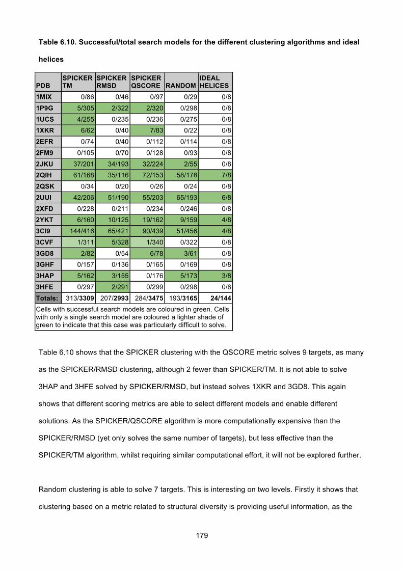
179

Table 6.10. Successful/total search models for the different clustering algorithms and ideal

helices

PDB SPICKER TM

SPICKER RMSD

SPICKER QSCORE RANDOM

IDEAL HELICES

1MIX 0/86 0/46 0/97 0/29 0/8

1P9G 5/305 2/322 2/320 0/298 0/8

1UCS 4/255 0/235 0/236 0/275 0/8 1XKR 6/62 0/40 7/83 0/22 0/8

2EFR 0/74 0/40 0/112 0/114 0/8

2FM9 0/105 0/70 0/128 0/93 0/8

2JKU 37/201 34/193 32/224 2/55 0/8 2QIH 61/168 35/116 72/153 58/178 7/8

2QSK 0/34 0/20 0/26 0/24 0/8

2UUI 42/206 51/190 55/203 65/193 6/8

2XFD 0/228 0/211 0/234 0/246 0/8 2YKT 6/160 10/125 19/162 9/159 4/8

3CI9 144/416 65/421 90/439 51/456 4/8

3CVF 1/311 5/328 1/340 0/322 0/8

3GD8 2/82 0/54 6/78 3/61 0/8 3GHF 0/157 0/136 0/165 0/169 0/8

3HAP 5/162 3/155 0/176 5/173 3/8

3HFE 0/297 2/291 0/299 0/298 0/8

Totals: 313/3309 207/2993 284/3475 193/3165 24/144 Cells with successful search models are coloured in green. Cells with only a single search model are coloured a lighter shade of green to indicate that this case was particularly difficult to solve.

Table 6.10 shows that the SPICKER clustering with the QSCORE metric solves 9 targets, as many

as the SPICKER/RMSD clustering, although 2 fewer than SPICKER/TM. It is not able to solve

3HAP and 3HFE solved by SPICKER/RMSD, but instead solves 1XKR and 3GD8. This again

shows that different scoring metrics are able to select different models and enable different

solutions. As the SPICKER/QSCORE algorithm is more computationally expensive than the

SPICKER/RMSD (yet only solves the same number of targets), but less effective than the

SPICKER/TM algorithm, whilst requiring similar computational effort, it will not be explored further.

Random clustering is able to solve 7 targets. This is interesting on two levels. Firstly it shows that

clustering based on a metric related to structural diversity is providing useful information, as the

180

best method (SPICKER/TM clustering) is able to solve an additional 4 targets (1P9G, 1UCS, 1XKR

and 3CVF). However, it also demonstrates that in more than half of the targets, no clustering is

required, as a random selection of models is enough to provide a solution. Random clustering is

able to solve all the targets solvable with ideal helices, with the addition of 2JKU and 3GD8.

In order to try and understand the performance of the different clustering algorithms, various data

relating to the decoys are tabulated in table 6.11 below, together with two columns indicating if the

target was solvable at all, and with random clustering. The column data within the table are:

l TM Median: the median TM score of all the decoys to the native

l TM std. dev.: the standard deviation of the TM scores of the decoys to the native.

l Cluster 1 size: the size of the first SPICKER cluster under TM scoring.

l Cluster 1 TM Median: the median TM score of the decoys to the native in the first

SPICKER cluster.

l TM Max: the maximum (best) TM score of all the decoys to the native.

l % Helical: the percentage of helical content of the native structure.

181

Table 6.11. Different data relating to the decoys, together with two columns indicating if the

targets were solvable with any method, and with random clustering.

PDB TM Median

TM std. dev.

Cluster 1 size

Cluster 1 TM Median

TM Max

HELICAL %

Structure could be solved?

Solved with Random Clusters

1MIX 0.22 0.03 10 0.22 0.3659 39 No No

1P9G 0.26 0.07 156 0.25 0.5127 0 Yes No

1UCS 0.21 0.03 146 0.2 0.3736 34.38 Yes No 1XKR 0.25 0.03 31 0.25 0.4103 44 Yes No

2EFR 0.2 0.03 14 0.21 0.3241 98 No No

2FM9 0.27 0.04 35 0.32 0.4156 72 No No

2JKU 0.34 0.12 79 0.41 0.8569 0 Yes Yes 2QIH 0.25 0.04 123 0.24 0.4186 85 Yes Yes

2QSK 0.17 0.02 3 0.18 0.3004 12 No No

2UUI 0.32 0.04 160 0.33 0.6018 80 Yes Yes

2XFD 0.24 0.02 158 0.23 0.3242 0 No No 2YKT 0.28 0.05 70 0.29 0.4822 80 Yes Yes

3CI9 0.39 0.04 162 0.4 0.58 93.75 Yes Yes

3CVF 0.33 0.06 157 0.32 0.609 81 Yes No

3GD8 0.27 0.03 89 0.28 0.4213 69 Yes Yes 3GHF 0.3 0.06 110 0.35 0.5549 26.67 No No

3HAP 0.43 0.07 138 0.5 0.6452 70 Yes Yes

3HFE 0.4 0.07 157 0.46 0.6017 70 Yes No

Cells coloured green are for solvable structures. Light blue cells are for targets where the TM median score is >= 0.3, which is indicative that the overall decoy modelling appears to have worked well.

Table 6.11 presents a range of different data on the models, the first five of which are metrics for

the quality of the decoys. With 1000 decoys, it is always difficult to judge the overall quality of the

decoys. A number of metrics were therefore compared to gain the best overall picture. The median

TM score of all the decoys to the native provides some indication as to whether the models are

generally similar to the native. The size of the first SPICKER cluster is generally taken as a good

indication of the quality of the modelling (Y. Zhang and Skolnick 2004), with a larger cluster (of up

to 200 decoys) indicating better modelling. These data are supplemented with the median TM

score of the top cluster, which should provide a somewhat better indication of the overall modeling

quality than the median TM score of all the models. The TM Max score is the score of the best

182

decoy compared to the native, so although not necessarily indicative of the overall modelling, it

does provide some indication of what the modelling is capable of.

Taking all the decoy modelling metrics together, it appears that an overall TM median score of

greater than 0.3 indicates good modelling. Figure 6.7 below plots the size of the top cluster against

the decoy median TM score.

Figure 6.7. The median TM score of all the decoys to the native plotted against the size of the first SPICKER cluster under TM scoring. Points are coloured according to whether the target was solvable under any method (blue) or not (red).

Figure 6.7 shows that, with the exception of one target (3GHF), any target where the overall

median TM score of the models was greater than 0.3 was solvable. 3GHF only just achieved a

median TM score of 0.3 and is one of the lowest resolution datasets, coupled with having the

lowest proportion of α-helicity of any of the targets. Resolution and the proportion of α-helicity are

183

two factors that are known to contribute heavily to AMPLE's ability to solve structures so this could

explain why this target could not be solved despite relatively good modelling.

Cluster size is a less clear indicator of success, but in general, most targets where the top cluster

was larger than 60 were solvable. The two exceptions are 2XFD and 3GHF. 3GHF has been dealt

with above. Despite the large cluster size, the modelling for 2XFD does not appear to have been

particularly successful as the median decoy TM score is considerably below 0.3, while the best

decoy only has a TM score of 0.3242. Additionally 2XFD has the highest proportion of β-sheet of

any of the targets, something that is known to make modelling less reliable and to affect the ability

of SHELXE to trace the main chain. Figure 6.8 plots the resolution and percentage of α-helicity of

the targets.

Figure 6.8. The proportion of the target that is α-helical plotted against resolution for the 18 targets. Points are coloured blue for solvable and red for unsolvable.

Figure 6.8 shows that there does not appear to be any particular trend in resolution or α-helicity

indicating whether targets are solvable, as both high resolution targets failed to solve, while the

184

lowest resolution was solvable. Moreover, the target with the lowest proportion of α-helix solved

while the target with the highest failed to solve. Taken together with figure 6.7, this would indicate

that the quality of the modelling appears to be the best indicator of success.

Of the targets where the modelling appears to have been good, only 3CVF and 3HFE were not

solvable with random clusters, which indicates that when the modelling is good, clustering may not

be required to select models of sufficient quality to enable solution. That 3CVF did not solve can be

explained by the fact that it has the poorest resolution (2.9Å) and is something of an anomaly in

being solvable at all with AMPLE, as it falls far outside of the optimal operating parameters of

SHELXE, which AMPLE relies on for its solutions. Based on the modelling and target data, there is

no clear indication as to why 3HFE did not solve, as it is relatively small, has high-resolution data,

is primarily α-helical and the modelling appears to have been good; all factors which indicate it

should have been easy to solve with AMPLE.

Figures 6.9 to 6.22 below show the top solution, as measured by the SHELXE CC score from

random clustering, and the top solution from SPICKER/TM clustering for comparison.

Figure 6.9. Top solution (blue) of 2JKY (green) with random clustering.

Figure 6.10. Top solution (blue) of 2JKY (green) with SPICKER/TM clustering.

185

Figure 6.11. Top solution (blue) of 2QIH (green) with random clustering.

Figure 6.12. Top solution (blue) of 2QIH (green) with SPICKER/TM clustering.

Figure 6.13. Top solution (blue) of 2UUI (green) with random clustering.

Figure 6.14. Top solution (blue) of 2UUI (green) with SPICKER/TM clustering.

186

Figure 6.15. Top solution (blue) of 2YKT (green) with random clustering.

Figure 6.16. Top solution (blue) of 2YKT (green) with SPICKER/TM clustering.

Figure 6.17. Top solution (blue) of 3CI9 (green) with random clustering.

Figure 6.18. Top solution (blue) of 3CI9 (green) with SPICKER/TM clustering.

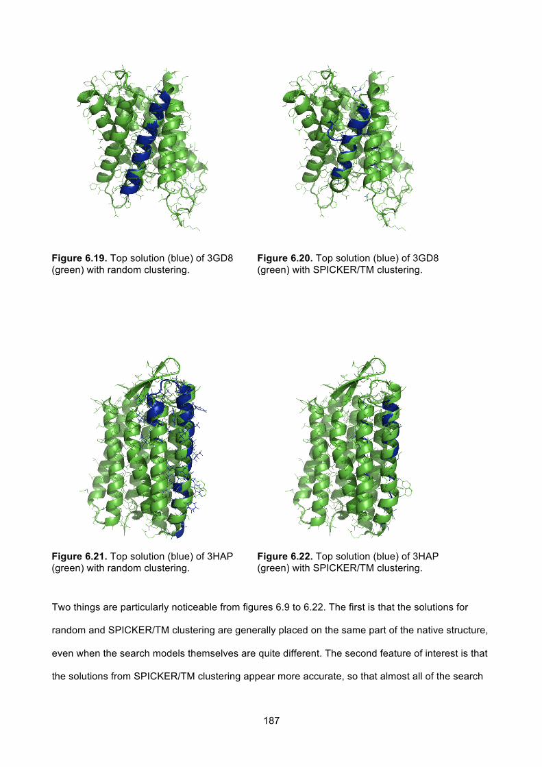
187

Figure 6.19. Top solution (blue) of 3GD8 (green) with random clustering.

Figure 6.20. Top solution (blue) of 3GD8 (green) with SPICKER/TM clustering.

Figure 6.21. Top solution (blue) of 3HAP (green) with random clustering.

Figure 6.22. Top solution (blue) of 3HAP (green) with SPICKER/TM clustering.

Two things are particularly noticeable from figures 6.9 to 6.22. The first is that the solutions for

random and SPICKER/TM clustering are generally placed on the same part of the native structure,

even when the search models themselves are quite different. The second feature of interest is that

the solutions from SPICKER/TM clustering appear more accurate, so that almost all of the search

188

model is placed on the native structure, whereas with random clustering (particularly for 2JKY,

2QIH and 3CI9) a substantial portion of the model is not overlaid on any part of the native

structure.

In order to investigate this more systematically, the RIO score was plotted as a proportion of the

number of Cα atoms in the search model(s) for the random and SPICKER/TM clustering. A

proportion of 1 would indicate that all atoms in the search model were overlaid on the native

structure, whereas lower proportions would indicate increasing numbers of residues placed

incorrectly.

Figure 6.23. RIO score as a proportion of the number of Cα atoms in the placed search models for random clustering.

Figure 6.24. RIO score as a proportion of the number of Cα atoms in the placed search models for SPICKER/TM clustering.

Figures 6.23 and 6.24 show quite clearly that the proportion of Cα atoms placed 'correctly' is higher

for the SPICKER/TM clustering than for the random clustering, as borne out by the models shown

in figures 6.9 to 6.22. This again confirms that the clustering of the decoys is helping to select

salient features that are enabling solutions and resulting in the better performance of the

SPICKER/TM clustering as opposed to the random clustering.

189

6.4 Discussion

6.4.1 Truncation Surprisingly, the truncation of isolated residues does not significantly alter the results. There are

two possible reasons for this. Firstly, the truncation is carried out based on the inter-residue

variance, which is considered a proxy for the quality of the modelling of that residue. Even if a

residue is isolated, it is possible that it has been well modelled and contributes positively to the

density.

A second possible reason, is that the truncation of the residues was carried out based on their

isolation in sequence. Although this is often correlated with their being isolated in space, this is not

necessarily the case (as residues can be packed against residues from a different part of the chain

due to flexibility of the chains). A better strategy might be to truncate isolated residues that are

isolated in space.

However, as residues that are isolated in space will necessarily be isolated in sequence (since,

being isolated in space they cannot be directly connected to any other residues), by removing

residues isolated in sequence, all of those isolated in space will also have been removed. That this

did not lead to any great change in the number of successes or failures suggests that this is

probably not a strategy worth pursuing further.

6.4.2 Sub-clustering The fixing of the errors in the sub-clustering algorithm, and the implementation of the slicing of

larger clusters to create additional ensembles, where clustering at a larger radius does not add any

more models, does not greatly change the number of successes or solve any additional targets. It

is therefore probably not worth adding the additional ensembles if clustering at a larger radius does

not change the number of models.

190

Sub-clustering under a larger radius than 3Å does not appear to bring any benefit, as only 2

ensembles with radii larger than 3Å solved, and this did not add any additional solutions, but did

greatly increase the number of ensembles overall.

The original AMPLE sub-clustering strategy was therefore retained, although the error that led to

the creation of duplicate ensembles had been fixed.

6.4.3 Clustering Of all the strategies attempted here, it is clustering that has demonstrated the best promise and

ability to enable AMPLE to solve harder targets. The exploration of different scoring metrics and

clustering algorithms has shown that 13 out of the 18 targets selected for the test set are solvable

with the current set of decoys. This is an interesting result as all of the test cases were chosen to

be hard for AMPLE to solve; even those that had been solved before were at the limits of what was

expected to be possible.

The original SPICKER/RMSD single cluster strategy was able to solve 6 targets, but this was

increased to 9 when using 10 clusters with 1 and 3Å sub-clustering and polyalanine side chains.

This came at a cost of doubling the number of search models, but with the same proportion of

successes, meaning that the time to solution in successful cases would be expected to be the

same as for the original strategy.

Using the 10-cluster strategy but with TM scoring enabled the solution of 11 targets. This

represented a near doubling of the number of solvable targets, but again with a corresponding

doubling of the number of search models. In addition, there is the additional time that is required to

calculate the all-by-all TM score matrix required by SPICKER. For the largest target, 2YKT, the

total time to run SPICKER with TM scoring was just under 8 hours; a huge increase on the 2-3

minutes required for RMSD scoring. However, as part of this work, SPICKER has been parallelised

with OPENMP, which has led to a linear increase in the time to run SPICKER with the number of

191

processors. With 4 processors (not unusual on most desktop or laptops at the time of writing), the

time for SPICKER/TM clustering drops to an average of 2 hours, something that is acceptable

when the average AMPLE run takes of the order of 24 hours, particularly given the large increase

in the number of successes.

As part of this work, the code to cluster with SPICKER with both RMSD and TM scoring, as well as

the code to FPC have all been made available within AMPLE, so users now have the possibility of

running different strategies for cases that are particularly difficult to solve.

192

6.5 Conclusion The examination of the truncation and sub-clustering stages of AMPLE indicates that these

parameters are largely optimal, and that there is little scope for improvement here. The

shortcomings in the original sub-clustering implementation have been remedied and this will now

become the default implementation.

This work has, however, demonstrated that there is considerable scope for improvement in the

AMPLE algorithm beyond the current default SPICKER/RMSD single-cluster approach. For most

users, if the protein has significant α-helical content, an attempt should be made to solve the

structure with ideal helices, as this is by far the quickest route to solution given that it requires no

modelling. If ideal helices do not work, or if the target contains no significant α-helical content, the

10-cluster SPICKER/TM algorithm with 1 and 3Å sub-clustering and polyalanine side chains should

be attempted, ideally on a multi-core machine to speed up the time to solution.

This work has also looked extensively at the core AMPLE cluster and truncate algorithm. It is

clear, however, that there is much scope for further investigation of the modelling and MR stages

to see if similar improvements can be made there. For example, evolutionary contact information

can be added at the modelling stage, and different MR approaches (e.g. using ACORN instead of

SHELXE for density modification) could be used at different x-ray resolutions.

193

Chapter 7: Conclusion and

Outlook

194

7 Conclusion and Outlook

7.1 Conclusion This thesis has been concerned with the development of the CCP4 MR pipeline AMPLE and its

application to different classes of macromolecules.

The software development work that was undertaken, has taken AMPLE from being a prototype

piece of software consisting of a collection of independent scripts, to a coherent, modularised

program incorporating a range of software best practice. This has brought a number of

advantages, including making it simpler to extend and develop the program, enabling new

developers to become involved, and making possible the acceleration of the testing cycle for new

CCP4 releases. In addition, the integration of the results analysis within a standard AMPLE run has

meant that benchmarking and testing AMPLE on new test cases will be an order of magnitude

faster in the future.

The experience of running AMPLE on different classes of proteins has demonstrated the

applicability of AMPLE across different protein classes and also provided a range of insights into

how it works. When AMPLE was first developed, its fundamental assumption was that clustering

would select a potentially correct overall fold, and that truncation would progressively remove the

most poorly modelled sections until a relatively large, but well-modelled core, would provide

enough information to enable MR.

In contrast, the coiled-coil work has shown that solution is often achieved by the placement of,

often very small, fragments that are placed out of register with regard to the section of the protein

that they are meant to model. If the resolution of crystallographic data are sufficiently high, then

195

AMPLE is able to use SHELXE to trace up from the small fragment in a manner similar to that

pioneered by ARCIMBOLDO.

The graphs of the percentage of the modelled chain that successfully solved structures (figures 3.6

and 4.6) show that AMPLE is effectively capable of working both with smaller fragments and with

more complete structures. For proteins that are smaller than about 150 residues, the modelling is

often good enough for largely complete structures to be successful, and, with the advent of

evolutionary contact information, this is likely to become possible for ever-larger proteins. When

the modelling is poor, or the case particularly difficult, then solving the structure with a small

fragment may still be possible.

Partly as a result of seeing the effectiveness of small fragments, but primarily to provide a reliable

benchmark of the utility and effectiveness of the modelling, an ideal helix mode has been

developed for AMPLE. This has demonstrated that modelling is required for difficult cases. The

ideal helix mode has also, however, provided a quick and easy method for the solution of helical

proteins. We have already been informed of a number of successes using this mode, both for

coiled-coil and globular proteins.

The work on transmembrane proteins has been a mixture of positive and slightly disappointing

results. That 10 of the 15 test cases could be solved is extremely positive and opens up another

class of proteins to solution by AMPLE. However, despite the good overall success rate, the fact

that several proteins expected to be solvable (based on size, resolution etc.) turned out not to be,

and that ideal helices were able to solve cases which AMPLE could not is disappointing. It is

possible that because of the difficulties of working with transmembrane proteins, crystallographers

may be more optimistic when defining the resolution than they would be when working with more

experimentally-forgiving water-soluble proteins. However, more work will need to be done to

determine if this is the case. The use of the GREMLIN mode for modelling of transmembrane

proteins also greatly simplifies the modelling by ROSETTA, as it no longer requires the installation

196

of the BLAST programs and (very large) NCBI NR database that were required by the original

RosettaMembrane protocol.

The work on applying the AMPLE cluster and truncate procedure to distant homologs has opened

up an exciting new avenue. The work has demonstrated that AMPLE is able to turn distant

homologs that would previously have been unsuccessful in MR into successful search models.

This has the advantage that no modelling is required, and so considerably reduces the

computational demands of the program. Although likely to be a popular approach to using AMPLE

(and considerable interest in its use at several workshops has already been demonstrated),

because it is limited to existing structures within the PDB, it lacks the ability to solve entirely novel

folds enabled by ab initio modelling programs such as ROSETTA and QUARK.

The final section of work on exploring the different parameters has provided several new modes of

running AMPLE that offer the promise of considerably increasing the success rate. The main

discovery was that there is valuable information contained in clusters other than the top one

returned by SPICKER. By sampling multiple clusters, there is no restriction to a single fold

prediction, thus increasing the possibility of using all elements of the modelling. The sub-clustering

and side chain treatment strategies, although effective with the single-cluster mode, have less of a

role to play when multiple clusters are sampled (previous work having shown that singleton

solutions were sometimes obtained with a single sub-clustering radius or side chain treatment). By

sampling all 10 clusters, only using 1 and 3Å sub-clustering, and restricting the side chain

treatment to polyalanine, the performance could be increased whilst only marginally increasing the

run time. Using TM scoring as a clustering metric again increases the performance, albeit at a

reasonably large increase in run time, which can, however, be largely amortised through the use of

multiple processors.

197

7.2 Outlook The work presented here has opened up a range of new avenues for both consolidating and

extending the research around AMPLE.

The work on transmembrane proteins will will be revisited using the latest methods for contact

prediction, together with the new AMPLE multi-cluster approach, which will become the default

mode for clustering. This promises to extend the successes to further targets and make AMPLE a

more viable approach for dealing with moderately high-resolution transmembrane proteins.

The multiple-homolog work has really been an initial foray into the potential for using AMPLE to

increase the utility of distant homologs for MR. Different ways of structurally aligning the proteins

using the variances calculated by GESAMT rather than those calculated by THESEUS are being

explored, to see if this improves the results. There is also the possibility of using not just the core of

all aligned homologs (i.e. the positions where all structures are aligned within the geometric

tolerance), but taking the overall alignment as a guide and then selecting subsets of it where there

are two or more proteins that are larger than the core, but nevertheless align well together.

Using single distant homologs and creating ensembles by using programs that create ensembles

based on the structure of the protein (such as CONCOORD), also offers a route to expand

AMPLE's capabilities with distant homologs.

The use of multiple clusters and TM-scoring with SPICKER (using the new OPENMP parallelised

version) will require the build system for SPICKER to be updated within CCP4. Once this has been

done, using AMPLE with TM-clustering will become possible for all CCP4 users.

Additional work that is planned will explore extending the capabilities of the server so that it is

better able to present the key capabilities of AMPLE in a simple way that does not require the

198

installation of large databases or software packages, and allows users to take advantage of the

large processing power of the cluster that lies behind it.

199

References Abergel, Chantal. 2013. “Molecular Replacement: Tricks and Treats.” Acta Crystallographica.

Section D, Biological Crystallography 69 (Pt 11): 2167–73. Almén, Markus, Karl J. V. Nordström, Robert Fredriksson, and Helgi B. Schiöth. 2009. “Mapping

the Human Membrane Proteome: A Majority of the Human Membrane Proteins Can Be Classified according to Function and Evolutionary Origin.” BMC Biology 7 (1): 50.

Altschul, S. F., T. L. Madden, A. A. Schäffer, J. Zhang, Z. Zhang, W. Miller, and D. J. Lipman. 1997. “Gapped BLAST and PSI-BLAST: A New Generation of Protein Database Search Programs.” Nucleic Acids Research 25 (17): 3389–3402.

Andreeva, Antonina, Dave Howorth, Steven E. Brenner, Tim J. P. Hubbard, Cyrus Chothia, and Alexey G. Murzin. 2004. “SCOP Database in 2004: Refinements Integrate Structure and Sequence Family Data.” Nucleic Acids Research 32 (Database issue): D226–29.

Apostolovic, Bojana, Maarten Danial, and Harm-Anton Klok. 2010. “Coiled Coils: Attractive Protein Folding Motifs for the Fabrication of Self-Assembled, Responsive and Bioactive Materials.” Chemical Society Reviews 39 (9): 3541–75.

Bayes, Mr, and Mr Price. 1763. “An Essay towards Solving a Problem in the Doctrine of Chances. By the Late Rev. Mr. Bayes, F. R. S. Communicated by Mr. Price, in a Letter to John Canton, A. M. F. R. S.” Philosophical Transactions 53 (January). The Royal Society: 370–418.

Bibby, Jaclyn, Ronan M. Keegan, Olga Mayans, Martyn D. Winn, and Daniel J. Rigden. 2012. “AMPLE: A Cluster-and-Truncate Approach to Solve the Crystal Structures of Small Proteins Using Rapidly Computed Ab Initio Models.” Acta Crystallographica. Section D, Biological Crystallography 68 (12): 1622–31.

Blocquel, David, Johnny Habchi, Eric Durand, Marion Sevajol, François Ferron, Jenny Erales, Nicolas Papageorgiou, and Sonia Longhi. 2014. “Coiled-Coil Deformations in Crystal Structures: The ıt Measles Virus Phosphoprotein Multimerization Domain as an Illustrative Example.” Acta Crystallographica. Section D, Biological Crystallography 70 (6): 1589–1603.

“Boost C++ Libraries.” 2016. Accessed September 13. http://www.boost.org/. Bragg, W. H., and W. L. Bragg. 1913. “The Reflection of X-Rays by Crystals.” Proceedings of the

Royal Society of London A: Mathematical, Physical and Engineering Sciences 88 (605). The Royal Society: 428–38.

Brünger, A. T., R. L. Campbell, G. M. Clore, A. M. Gronenborn, M. Karplus, G. A. Petsko, and M. M. Teeter. 1987. “Solution of a Protein Crystal Structure with a Model Obtained from NMR Interproton Distance Restraints.” Science 235 (4792): 1049–53.

Brunger, Axel T. 1992. “Free R Value: A Novel Statistical Quantity for Assessing the Accuracy of Crystal Structures.” Nature 355 (6359): 472–75.

Bunkóczi, Gábor, and Randy J. Read. 2011. “Improvement of Molecular-Replacement Models with ıt Sculptor.” Acta Crystallographica. Section D, Biological Crystallography 67 (4): 303–12.

Burkhard, P., J. Stetefeld, and S. V. Strelkov. 2001. “Coiled Coils: A Highly Versatile Protein Folding Motif.” Trends in Cell Biology 11 (2): 82–88.

“CCP4: Software for Macromolecular Crystallography.” 2016. Accessed September 12. http://www.ccp4.ac.uk/.

Chapman, Henry N., Petra Fromme, Anton Barty, Thomas A. White, Richard A. Kirian, Andrew Aquila, Mark S. Hunter, et al. 2011. “Femtosecond X-Ray Protein Nanocrystallography.” Nature 470 (7332): 73–77.

Cowtan, Kevin. 2006. “The ıt Buccaneer Software for Automated Model Building. 1. Tracing Protein Chains.” Acta Crystallographica. Section D, Biological Crystallography 62 (9): 1002–11.

Eddy, Sean R. 2011. “Accelerated Profile HMM Searches.” PLoS Computational Biology 7 (10): e1002195.

Erickson, Harold P. 2009. “Size and Shape of Protein Molecules at the Nanometer Level Determined by Sedimentation, Gel Filtration, and Electron Microscopy.” Biological Procedures Online 11 (May): 32–51.

Finn, Robert D., Jody Clements, and Sean R. Eddy. 2011. “HMMER Web Server: Interactive Sequence Similarity Searching.” Nucleic Acids Research 39 (Web Server issue): W29–37.

200

Franke, Barbara, Alexander Gasch, Dayté Rodriguez, Mohamed Chami, Muzamil M. Khan, Rüdiger Rudolf, Jaclyn Bibby, et al. 2014. “Molecular Basis for the Fold Organization and Sarcomeric Targeting of the Muscle Atrogin MuRF1.” Open Biology 4 (March): 130172.

Fujinaga, M., and R. J. Read. 1987. “Experiences with a New Translation-Function Program.” Journal of Applied Crystallography 20 (6): 517–21.

Glykos, N. M., and M. Kokkinidis. 2000. “A Stochastic Approach to Molecular Replacement.” Acta Crystallographica. Section D, Biological Crystallography 56 (Pt 2): 169–74.

Grosse-Kunstleve, Ralf W., Nicholas K. Sauter, Nigel W. Moriarty, and Paul D. Adams. 2002. “The ıt Computational Crystallography Toolbox: Crystallographic Algorithms in a Reusable Software Framework.” Journal of Applied Crystallography 35 (1): 126–36.

Hanwell, Marcus D., Donald E. Curtis, David C. Lonie, Tim Vandermeersch, Eva Zurek, and Geoffrey R. Hutchison. 2012. “Avogadro: An Advanced Semantic Chemical Editor, Visualization, and Analysis Platform.” Journal of Cheminformatics 4 (1): 17.

Henrich, B., A. Bergamaschi, C. Broennimann, R. Dinapoli, E. F. Eikenberry, I. Johnson, M. Kobas, P. Kraft, A. Mozzanica, and B. Schmitt. 2009. “PILATUS: A Single Photon Counting Pixel Detector for X-Ray Applications.” Nuclear Instruments & Methods in Physics Research. Section A, Accelerators, Spectrometers, Detectors and Associated Equipment 607 (1): 247–49.

Hobbs, Errett C., Fanette Fontaine, Xuefeng Yin, and Gisela Storz. 2011. “An Expanding Universe of Small Proteins.” Current Opinion in Microbiology 14 (2): 167–73.

Hung, Ling-Hong, and Ram Samudrala. 2014. “Fast_protein_cluster: Parallel and Optimized Clustering of Large-Scale Protein Modeling Data.” Bioinformatics 30 (12): 1774–76.

Jamroz, Michal, and Andrzej Kolinski. 2013. “ClusCo: Clustering and Comparison of Protein Models.” BMC Bioinformatics 14 (February): 62.

Jones, David T. 1999. “Protein Secondary Structure Prediction Based on Position-Specific Scoring Matrices.” Journal of Molecular Biology 292 (2): 195–202.

Jones, David T., Daniel W. A. Buchan, Domenico Cozzetto, and Massimiliano Pontil. 2012. “PSICOV: Precise Structural Contact Prediction Using Sparse Inverse Covariance Estimation on Large Multiple Sequence Alignments.” Bioinformatics 28 (2): 184–90.

Jones, David T., Tanya Singh, Tomasz Kosciolek, and Stuart Tetchner. 2015. “MetaPSICOV: Combining Coevolution Methods for Accurate Prediction of Contacts and Long Range Hydrogen Bonding in Proteins.” Bioinformatics 31 (7): 999–1006.

Juan, David de, Florencio Pazos, and Alfonso Valencia. 2013. “Emerging Methods in Protein Co-Evolution.” Nature Reviews. Genetics 14 (4): 249–61.

Kabsch, W. 1976. “A Solution for the Best Rotation to Relate Two Sets of Vectors.” Acta Crystallographica. Section A, Foundations of Crystallography 32 (5): 922–23.

Kabsch, Wolfgang, and Christian Sander. 1983. “Dictionary of Protein Secondary Structure: Pattern Recognition of Hydrogen-Bonded and Geometrical Features.” Biopolymers 22 (12): 2577–2637.

Kaján, László, Thomas A. Hopf, Matúš Kalaš, Debora S. Marks, and Burkhard Rost. 2014. “FreeContact: Fast and Free Software for Protein Contact Prediction from Residue Co-Evolution.” BMC Bioinformatics 15 (March): 85.

Kamisetty, H., S. Ovchinnikov, and D. Baker. 2013. “Assessing the Utility of Coevolution-Based Residue-Residue Contact Predictions in a Sequence- and Structure-Rich Era.” Proceedings of the National Academy of Sciences 110 (39): 15674–79.

Katoh, Kazutaka, Kazuharu Misawa, Kei-Ichi Kuma, and Takashi Miyata. 2002. “MAFFT: A Novel Method for Rapid Multiple Sequence Alignment Based on Fast Fourier Transform.” Nucleic Acids Research 30 (14): 3059–66.

Katzman, S., C. Barrett, G. Thiltgen, R. Karchin, and K. Karplus. 2008. “PREDICT-2ND: A Tool for Generalized Protein Local Structure Prediction.” Bioinformatics 24 (21): 2453–59.

Keegan, Ronan M., and Martyn D. Winn. 2007. “Automated Search-Model Discovery and Preparation for Structure Solution by Molecular Replacement.” Acta Crystallographica. Section D, Biological Crystallography 63 (4): 447–57.

Konagurthu, Arun S., James C. Whisstock, Peter J. Stuckey, and Arthur M. Lesk. 2006. “MUSTANG: A Multiple Structural Alignment Algorithm.” Proteins 64 (3): 559–74.

201

Krissinel, E., and K. Henrick. 2004. “Secondary-Structure Matching (SSM), a New Tool for Fast Protein Structure Alignment in Three Dimensions.” Acta Crystallographica. Section D, Biological Crystallography 60 (Pt 12 Pt 1): 2256–68.

Krissinel, Evgeny. 2012. “Enhanced Fold Recognition Using Efficient Short Fragment Clustering.” Journal of Molecular Biochemistry 1: 76–85.

Krivov, Georgii G., Maxim V. Shapovalov, and Roland L. Dunbrack Jr. 2009. “Improved Prediction of Protein Side-Chain Conformations with SCWRL4.” Proteins 77 (4): 778–95.

Kuhn, Michael, Anthony A. Hyman, and Andreas Beyer. 2014. “Coiled-Coil Proteins Facilitated the Functional Expansion of the Centrosome.” PLoS Computational Biology 10 (6): e1003657.

Langer, Gerrit, Serge X. Cohen, Victor S. Lamzin, and Anastassis Perrakis. 2008. “Automated Macromolecular Model Building for X-Ray Crystallography Using ARP/wARP Version 7.” Nature Protocols 3 (7): 1171–79.

Levinthal, C. 1969. “How to Fold Graciously.” Mossbauer Spectroscopy in. University of Illinois Press: Allerton ….

Li, Weizhong, and Adam Godzik. 2006. “Cd-Hit: A Fast Program for Clustering and Comparing Large Sets of Protein or Nucleotide Sequences.” Bioinformatics 22 (13): 1658–59.

Long, Fei, Alexei A. Vagin, Paul Young, and Garib N. Murshudov. 2008. “ıt BALBES: A Molecular-Replacement Pipeline.” Acta Crystallographica. Section D, Biological Crystallography 64 (1): 125–32.

Lupas, Andrei N., and Markus Gruber. 2005. “The Structure of α-Helical Coiled Coils.” In Advances in Protein Chemistry, Volume 70:37–38. Academic Press.

“MaxCluster - A Tool for Protein Structure Comparison and Clustering.” n.d. http://www.sbg.bio.ic.ac.uk/~maxcluster/index.html.

McClatchey, Andrea I. 2003. “Merlin and ERM Proteins: Unappreciated Roles in Cancer Development?” Nature Reviews. Cancer 3 (11): 877–83.

McCoy, Airlie J. 2004. “Liking Likelihood.” Acta Crystallographica. Section D, Biological Crystallography 60 (Pt 12 Pt 1): 2169–83.

McCoy, A. J., R. W. Grosse-Kunstleve, P. D. Adams, M. D. Winn, L. C. Storoni, and R. J. Read. 2007. “Phaser Crystallographic Software.” Journal of Applied Crystallography 40 (4): 658–74.

McEntyre, Jo, and Jim Ostell. 2002. The NCBI Handbook. National Center for Biotechnology Information (US).

“Message Passing Interface (MPI) Forum Home Page.” 2016. Accessed September 13. https://www.mpi-forum.org/.

Metropolis, N., and S. Ulam. 1949. “The Monte Carlo Method.” Journal of the American Statistical Association 44 (247): 335–41.

Millán, Claudia, Massimo Sammito, and Isabel Usón. 2015. “Macromolecular Ab Initio Phasing Enforcing Secondary and Tertiary Structure.” IUCrJ 2 (1): 95–105.

Murshudov, Garib N., Pavol Skubák, Andrey A. Lebedev, Navraj S. Pannu, Roberto A. Steiner, Robert A. Nicholls, Martyn D. Winn, Fei Long, and Alexei A. Vagin. 2011. “REFMAC 5 for the Refinement of Macromolecular Crystal Structures.” Acta Crystallographica. Section D, Biological Crystallography 67 (4): 355–67.

Murzin, A. G., S. E. Brenner, T. Hubbard, and C. Chothia. 1995. “SCOP: A Structural Classification of Proteins Database for the Investigation of Sequences and Structures.” Journal of Molecular Biology 247 (4): 536–40.

O’Boyle, Noel M., Michael Banck, Craig A. James, Chris Morley, Tim Vandermeersch, and Geoffrey R. Hutchison. 2011. “Open Babel: An Open Chemical Toolbox.” Journal of Cheminformatics 3 (October): 33.

Oldfors, A., H. Tajsharghi, N. Darin, and C. Lindberg. 2004. “Myopathies Associated with Myosin Heavy Chain Mutations.” Acta Myologica: Myopathies and Cardiomyopathies: Official Journal of the Mediterranean Society of Myology / Edited by the Gaetano Conte Academy for the Study of Striated Muscle Diseases 23 (2): 90–96.

Ovchinnikov, Sergey, Hetunandan Kamisetty, and David Baker. 2014. “Robust and Accurate Prediction of Residue-Residue Interactions across Protein Interfaces Using Evolutionary Information.” eLife 3 (May): e02030.

Ovchinnikov, Sergey, Lisa Kinch, Hahnbeom Park, Yuxing Liao, Jimin Pei, David E. Kim,

202

Hetunandan Kamisetty, Nick V. Grishin, and David Baker. 2015. “Large-Scale Determination of Previously Unsolved Protein Structures Using Evolutionary Information.” eLife 4 (September): e09248.

Panjikar, Santosh, Venkataraman Parthasarathy, Victor S. Lamzin, Manfred S. Weiss, and Paul A. Tucker. 2005. “Auto-Rickshaw: An Automated Crystal Structure Determination Platform as an Efficient Tool for the Validation of an X-Ray Diffraction Experiment.” Acta Crystallographica. Section D, Biological Crystallography 61 (Pt 4): 449–57.

Patterson, A. L. 1934. “A Fourier Series Method for the Determination of the Components of Interatomic Distances in Crystals.” Physics Review 46 (5). American Physical Society: 372–76.

Pechar, Michal, and Robert Pola. 2013. “The Coiled Coil Motif in Polymer Drug Delivery Systems.” Biotechnology Advances 31 (1): 90–96.

Puls, Imke, Catherine Jonnakuty, Bernadette H. LaMonte, Erika L. F. Holzbaur, Mariko Tokito, Eric Mann, Mary Kay Floeter, et al. 2003. “Mutant Dynactin in Motor Neuron Disease.” Nature Genetics 33 (4): 455–56.

Qian, Bin, Srivatsan Raman, Rhiju Das, Philip Bradley, Airlie J. McCoy, Randy J. Read, and David Baker. 2007. “High-Resolution Structure Prediction and the Crystallographic Phase Problem.” Nature 450 (7167): 259–64.

Rao, Jampani Nageswara, Roland Rivera-Santiago, Xiaochuan Edward Li, William Lehman, and Roberto Dominguez. 2012. “Structural Analysis of Smooth Muscle Tropomyosin α and β Isoforms.” The Journal of Biological Chemistry 287 (5): 3165–74.

Read, R. J. 2001. “Pushing the Boundaries of Molecular Replacement with Maximum Likelihood.” Acta Crystallographica. Section D, Biological Crystallography 57 (Pt 10): 1373–82.

Remmert, Michael, Andreas Biegert, Andreas Hauser, and Johannes Söding. 2011. “HHblits: Lightning-Fast Iterative Protein Sequence Searching by HMM-HMM Alignment.” Nature Methods 9 (2): 173–75.

Rigden, Daniel J. 2008. “The Histidine Phosphatase Superfamily: Structure and Function.” Biochemical Journal 409 (2): 333–48.

Rigden, Daniel J., Ronan M. Keegan, and Martyn D. Winn. 2008. “Molecular Replacement Using ıt Ab Initio Polyalanine Models Generated with ıt ROSETTA.” Acta Crystallographica. Section D, Biological Crystallography 64 (12): 1288–91.

Robson Marsden, Hana, and Alexander Kros. 2010. “Self-Assembly of Coiled Coils in Synthetic Biology: Inspiration and Progress.” Angewandte Chemie 49 (17): 2988–3005.

Rodríguez, Dayté D., Christian Grosse, Sebastian Himmel, César González, Iñaki M. de Ilarduya, Stefan Becker, George M. Sheldrick, and Isabel Usón. 2009. “Crystallographic Ab Initio Protein Structure Solution below Atomic Resolution.” Nature Methods 6 (9): 651–53.

Rohl, Carol A., Charlie E. M. Strauss, Kira M. S. Misura, and David Baker. 2004. “Protein Structure Prediction Using Rosetta.” In Methods in Enzymology, 383:66–93. Elsevier.

Rose, P. W., C. Bi, W. F. Bluhm, C. H. Christie, D. Dimitropoulos, S. Dutta, R. K. Green, et al. 2013. “The RCSB Protein Data Bank: New Resources for Research and Education.” Nucleic Acids Research 41 (D1): D475–82.

Rossmann, M. G., and D. M. Blow. 1962. “The Detection of Sub-Units within the Crystallographic Asymmetric Unit.” Acta Crystallographica 15 (1): 24–31.

Rupp, B. 2009. Biomolecular Crystallography: Principles, Practice, and Application to Structural Biology. Taylor & Francis Group.

Sammito, Massimo, Kathrin Meindl, Iñaki M. de Ilarduya, Claudia Millán, Cecilia Artola-Recolons, Juan A. Hermoso, and Isabel Usón. 2014. “Structure Solution with ARCIMBOLDO Using Fragments Derived from Distant Homology Models.” The FEBS Journal 281 (18): 4029–45.

Sammito, Massimo, Claudia Millán, Dawid Frieske, Eloy Rodríguez-Freire, Rafael J. Borges, and Isabel Usón. 2015. “ıt ARCIMBOLDO_LITE: Single-Workstation Implementation and Use.” Acta Crystallographica. Section D, Biological Crystallography 71 (9): 1921–30.

Sammito, Massimo, Claudia Millán, Dayté D. Rodríguez, Iñaki M. de Ilarduya, Kathrin Meindl, Ivan De Marino, Giovanna Petrillo, et al. 2013. “Exploiting Tertiary Structure through Local Folds for Crystallographic Phasing.” Nature Methods 10 (11): 1099–1101.

Schwarzenbacher, Robert, Adam Godzik, Slawomir K. Grzechnik, and Lukasz Jaroszewski. 2004.

203

“The Importance of Alignment Accuracy for Molecular Replacement.” Acta Crystallographica. Section D, Biological Crystallography 60 (Pt 7): 1229–36.

Sheldrick, George M. 1998. “SHELX Applications to Macromolecules.” In Direct Methods for Solving Macromolecular Structures, edited by Suzanne Fortier, 401–11. NATO ASI Series 507. Springer Netherlands.

Sheldrick, G. M. 2007. “A Short History of SHELX.” Acta Crystallographica. Section A, Foundations of Crystallography 64 (1): 112–22.

Shortle, D., K. T. Simons, and D. Baker. 1998. “Clustering of Low-Energy Conformations near the Native Structures of Small Proteins.” Proceedings of the National Academy of Sciences 95 (19): 11158–62.

Sillitoe, Ian, Tony E. Lewis, Alison Cuff, Sayoni Das, Paul Ashford, Natalie L. Dawson, Nicholas Furnham, et al. 2015. “CATH: Comprehensive Structural and Functional Annotations for Genome Sequences.” Nucleic Acids Research 43 (Database issue): D376–81.

Simons, K. T., C. Kooperberg, E. Huang, and D. Baker. 1997. “Assembly of Protein Tertiary Structures from Fragments with Similar Local Sequences Using Simulated Annealing and Bayesian Scoring Functions.” Journal of Molecular Biology 268 (1): 209–25.

Skwark, Marcin J., Daniele Raimondi, Mirco Michel, and Arne Elofsson. 2014. “Improved Contact Predictions Using the Recognition of Protein like Contact Patterns.” PLoS Computational Biology 10 (11): e1003889.

Söding, Johannes, Andreas Biegert, and Andrei N. Lupas. 2005. “The HHpred Interactive Server for Protein Homology Detection and Structure Prediction.” Nucleic Acids Research 33 (Web Server issue): W244–48.

Stein, Norman. 2008. “ıt CHAINSAW: A Program for Mutating Pdb Files Used as Templates in Molecular Replacement.” Journal of Applied Crystallography 41 (3): 641–43.

Taylor, Todd J., Hongjun Bai, Chin-Hsien Tai, and Byungkook Lee. 2014. “Assessment of CASP10 Contact-Assisted Predictions.” Proteins 82 Suppl 2 (February): 84–97.

Theobald, D. L., and D. S. Wuttke. 2006. “THESEUS: Maximum Likelihood Superpositioning and Analysis of Macromolecular Structures.” Bioinformatics 22 (17): 2171–72.

Thomas, Jens M. H., Ronan M. Keegan, Jaclyn Bibby, Martyn D. Winn, Olga Mayans, and Daniel J. Rigden. 2015. “Routine Phasing of Coiled-Coil Protein Crystal Structures with AMPLE.” IUCrJ 2 (Pt 2): 198–206.

Thorn, Andrea, and George M. Sheldrick. 2013. “Extending Molecular-Replacement Solutions with SHELXE.” Acta Crystallographica. Section D, Biological Crystallography 69 (Pt 11): 2251–56.

Tusnády, G. E., Z. Dosztányi, and I. Simon. 2004. “Transmembrane Proteins in the Protein Data Bank: Identification and Classification.” Bioinformatics 20 (17): 2964–72.

“UniProt.” 2016. Accessed September 13. http://www.uniprot.org/. Vagin, A., and A. Teplyakov. 1997. “MOLREP : An Automated Program for Molecular

Replacement.” Journal of Applied Crystallography 30 (6): 1022–25. Verstraeten, Valerie L. R. M., Jos L. V. Broers, Maurice A. M. van Steensel, Sophie Zinn-Justin,

Frans C. S. Ramaekers, Peter M. Steijlen, Miriam Kamps, et al. 2006. “Compound Heterozygosity for Mutations in LMNA Causes a Progeria Syndrome without Prelamin A Accumulation.” Human Molecular Genetics 15 (16): 2509–22.

Viklund, H., and A. Elofsson. 2008. “OCTOPUS: Improving Topology Prediction by Two-Track ANN-Based Preference Scores and an Extended Topological Grammar.” Bioinformatics 24 (15): 1662–68.

Waterman, D. G., G. Winter, J. M. Parkhurst, L. Fuentes-Montero, J. Hattne, A. Brewster, N. K. Sauter, and G. Evans. 2013. “The DIALS Framework for Integration Software.” CCP4 Newslett. Protein Crystallogr 49: 13–15.

“Welcome to Python.org.” 2016. Python.org. Accessed September 13. https://www.python.org/. Wimley, William C. 2003/8. “The Versatile β-Barrel Membrane Protein.” Current Opinion in

Structural Biology 13 (4): 404–11. Winn, Martyn D., Charles C. Ballard, Kevin D. Cowtan, Eleanor J. Dodson, Paul Emsley, Phil R.

Evans, Ronan M. Keegan, et al. 2011. “Overview of the CCP 4 Suite and Current Developments.” Acta Crystallographica. Section D, Biological Crystallography 67 (4): 235–42.

Xu, Jinrui, and Yang Zhang. 2010. “How Significant Is a Protein Structure Similarity with TM-Score

204

= 0.5?” Bioinformatics 26 (7): 889–95. Yarov-Yarovoy, Vladimir, Jack Schonbrun, and David Baker. 2005. “Multipass Membrane Protein

Structure Prediction Using Rosetta.” Proteins: Structure, Function, and Bioinformatics 62 (4): 1010–25.

Zhang, Yang, and Jeffrey Skolnick. 2004. “Scoring Function for Automated Assessment of Protein Structure Template Quality.” Proteins 57 (4): 702–10.

Zhang, Y., and J. Skolnick. 2004. “SPICKER: A Clustering Approach to Identify near-Native Protein Folds.” Journal of Computational Chemistry 25 (6): 865–71.