�����������������

Citation: Yan, G.; Jin, Z.; Zhang, T.;

Zhang, C.; Ai, C.; Chen, G. Exploring

the Essence of Servo Pump Control.

Processes 2022, 10, 786. https://

doi.org/10.3390/pr10040786

Academic Editors: Wen-Jer Chang

and Mohd Azlan Hussain

Received: 16 February 2022

Accepted: 12 April 2022

Published: 16 April 2022

Publisher’s Note: MDPI stays neutral

with regard to jurisdictional claims in

published maps and institutional affil-

iations.

Copyright: © 2022 by the authors.

Licensee MDPI, Basel, Switzerland.

This article is an open access article

distributed under the terms and

conditions of the Creative Commons

Attribution (CC BY) license (https://

creativecommons.org/licenses/by/

4.0/).

processes

Article

Exploring the Essence of Servo Pump ControlGuishan Yan 1, Zhenlin Jin 1,*, Tiangui Zhang 1, Cheng Zhang 1, Chao Ai 1 and Gexin Chen 1,2

1 School of Mechanical Engineering, Yanshan University, Qinhuangdao 066004, China;gsyan@stumail.ysu.edu.cn (G.Y.); tianguiz@stumail.ysu.edu.cn (T.Z.); chengz@stumail.ysu.edu.cn (C.Z.);aichao@ysu.edu.cn (C.A.); jygxchen@ysu.edu.cn (G.C.)

2 Mechanical and Electrical Engineering, Xinjiang Institute of Engineering, Urumqi 830023, China* Correspondence: zljin@ysu.edu.cn; Tel.: +86-335-8057100

Abstract: The electrohydraulic servo variable speed volume pump control system (hereinafter re-ferred to as ESPCS) is integrated with a permanent magnet synchronous motor (hereinafter referred toas servo motor), a fixed-displacement pump, and a hydraulic cylinder. By controlling the servo motorspeed, the output flow of the system can be controlled, as can the displacement, force, and speed of thehydraulic cylinder. Compared with the traditional electro-hydraulic servo valve control system, theESPCS has the advantages of high power-to-weight ratio, energy saving, and environmental friendli-ness. However, due to the extremely nonlinear flow output of the ESPCS, further improvement ofsystem control performance is greatly hindered. This paper focuses on the nonlinear characteristics ofservo motor, fixed-displacement pump, hydraulic cylinder, and other key components in the system.A compensation method based on nonlinear characteristic mapping is proposed. Compared with thetraditional PID control method (pressure control accuracy ± 0.12 MPa), the pressure control accuracyof the system is greatly improved (pressure control accuracy ± 0.037 MPa), which opens up a newway to improve the pressure control accuracy of the ESPCS.

Keywords: electrohydraulic servo; pump control system; flow characteristic; nonlinearity mappingmodel; experimental research

1. Introduction

We look at the nature of servo pump control from the perspective of system energytransfer, as shown in Figure 1. The servo motor drives the flow required by the fixeddisplacement pump output system and then controls the displacement, force, and speed ofthe hydraulic cylinder output. In this process, the system flow is used as the medium ofenergy transfer and conversion. Therefore, the essence of ESPCS to achieve high precisioncontrol of hydraulic cylinder lies in the accurate control of system flow.

Figure 1. Schematic of servo pump-controlled energy transfer.

Processes 2022, 10, 786. https://doi.org/10.3390/pr10040786 https://www.mdpi.com/journal/processes

Processes 2022, 10, 786 2 of 24

The ESPCS is composed of electrical, hydraulic and mechanical parts. Due to thelarge inertia of the servo motor and the fixed-displacement pump and the time lag of thevolumetric servo response, the static accuracy of the system is not high and the dynamicperformance is limited [1,2]. System response speed, bandwidth and positioning accuracyare at a disadvantage compared with traditional valve-controlled system, which bringscertain challenges to high-performance control of the system [3,4]. A pump control systemis a typical strongly nonlinear system [5–7]. There are several parameter uncertainties anduncertain nonlinearities in the system [8,9]. The study of the nonlinear characteristics ofthe system flow output is a key factor in realizing high-precision control of the system.In recent years, experts and scholars in the industry have done relevant research on thehigh-performance control of ESPCS.

Quan Long (Taiyuan University of Technology) and other researchers, aiming at theproblem of poor dynamic and static characteristics in existing pump-controlled differentialcylinder technology, used an asymmetric pump to balance the asymmetric flow of thedifferential cylinder and proposed a nonlinear dynamic feedforward compensation controlstrategy. The results show that the control strategy can effectively improve the staticand dynamic characteristics of the stretching and retraction speeds of the differentialcylinder [10]. Jiawei of the Northwest Institute of Mechanical and Electrical Engineeringand other researchers established the concept and mathematical model of flow pulsationvolume in response to the problem of the flow pulsation of the electrohydraulic servosystem on the adjustment accuracy of the pitch gun system. Finally, the influence law of theplunger pump swash plate inclination angle and input shaft speed on the plunger pumpflow pulsation is obtained [11]. Wang et al. of Beijing Special Engineering Design andResearch Institute proposed a method of using wavelet analysis to extract fault features andbuilding a classifier using a backpropagation neural network for the problem of leakagefault diagnosis in hydraulic cylinders. The results show that the proposed method iseffective for fault diagnosis. Diagnosis has high recognition accuracy [12]. Li et al. ofthe School of Automation Science and Electric Engineering, Beihang University designedan SMC-fuzzy controller for high nonlinearity and external interference in an electro-hydrostatic actuator system. The simulation results show that the SMC-fuzzy controllerhas better tracking performance than the traditional PID controller, and the system controlinput is smoother, reducing the occurrence of system chattering [13]. Jiao Zongxia of BeijingAerospace and Astronautics conducted a theoretical analysis of the pressure loss of anaircraft hydraulic power system, established a flow and pressure loss model of typicalhydraulic components and hydraulic pipelines, and verified it with experimental data. Theresults demonstrated that the model can accurately analyze the available pressure and flowrate of the hydraulic system during the flight phase of an aircraft [14].

The investigation of high-precision control of the pump control system has shownthat most scholars have focused on the use of fuzzy control strategy [15–18], robust controlstrategy [19–21], synovial control strategy [22,23], adaptive backstepping control [24,25],and other control algorithms [26], without systematically and comprehensively analyzingthe methods for improving the control accuracy from the perspective of flow characteristics.This study mainly focuses on improving the pressure control precision of the ESPCS.

In order to improve the system pressure control precision, the main factors restrictingthe system pressure control precision improvement are analyzed. We raise the followingquestion: when the system is given a pressure command, and the system shown in Figure 1has reached the set steady-state pressure, what is the state of the system at this time? Wethen propose the following hypothesis: owing to the internal leakage of the hydrauliccylinder, to retain the pressure of the hydraulic cylinder constant, we need a continuousflow to balance the leakage of the cylinder. The fixed-displacement pump has to contin-uously output flow, but the fixed-displacement pump has a dead flow zone and leakage;therefore, the servo motor must continuously output speed to balance the leakage of thefixed-displacement pump and ensure that the flow exceeds the dead-zone boundary andcontinues to be supplied to the hydraulic cylinder. This assumption was ideal. The internal

Processes 2022, 10, 786 3 of 24

leakage and flow dead zone of the fixed-displacement pump are affected by many factors,and the low-speed jitter of servo motor makes it difficult to improve the pressure controlprecision of the system. Therefore, accurately characterizing nonlinear phenomena in thesystem is necessary.

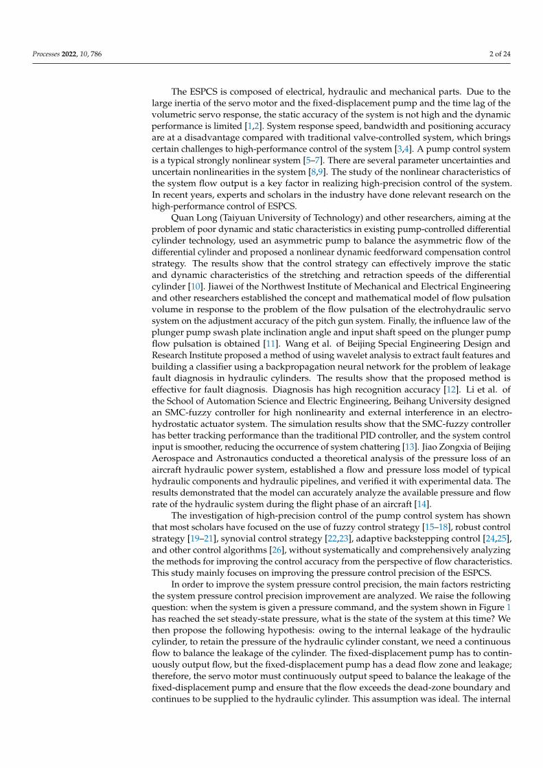
In this study, the mechanism prediction model was combined with the experimentalmapping model. The mechanism prediction model establishes an accurate mathematicalmodel of the system components at the component level. Through the mathematical model,the internal characteristics of the system are described, and the predicted value of the requiredflow of the system is provided in real time. Through the experimental mapping model, thenonlinear phenomena in the system are mapped and compensated to realize precise controlof the system flow, as shown in Figure 2.

Figure 2. ESPCS pressure control chart.

2. Introduction of ESPCS

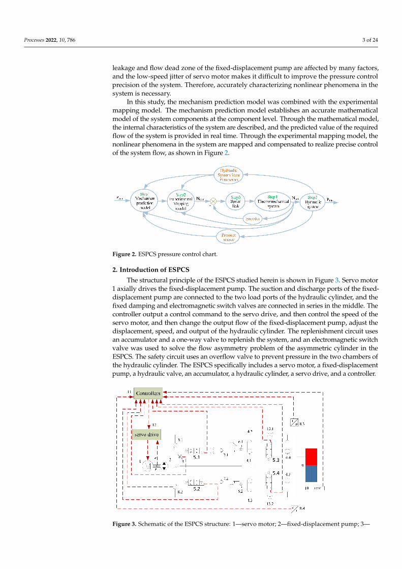
The structural principle of the ESPCS studied herein is shown in Figure 3. Servo motor1 axially drives the fixed-displacement pump. The suction and discharge ports of the fixed-displacement pump are connected to the two load ports of the hydraulic cylinder, and thefixed damping and electromagnetic switch valves are connected in series in the middle. Thecontroller output a control command to the servo drive, and then control the speed of theservo motor, and then change the output flow of the fixed-displacement pump, adjust thedisplacement, speed, and output of the hydraulic cylinder. The replenishment circuit usesan accumulator and a one-way valve to replenish the system, and an electromagnetic switchvalve was used to solve the flow asymmetry problem of the asymmetric cylinder in theESPCS. The safety circuit uses an overflow valve to prevent pressure in the two chambers ofthe hydraulic cylinder. The ESPCS specifically includes a servo motor, a fixed-displacementpump, a hydraulic valve, an accumulator, a hydraulic cylinder, a servo drive, and a controller.

Figure 3. Schematic of the ESPCS structure: 1—servo motor; 2—fixed-displacement pump; 3—

Processes 2022, 10, 786 4 of 24

low pressure pressure sensor; 4.1/4.2/4.3/4.4/4.5—accumulator; 5.1/5.2/5.3/5.4—solenoid switchvalve; 6.1/6.2—safety relief valve; 7.1/7.2—check valve; 8.1/8.2/8.3/8.4—high pressure sensor;9—hydraulic cylinder; 10—displacement sensor; 11—controller; 12—servo driver; 13.1/13.2—hydraulic damping.

The system detects the actual position and pressure signal output from the hydrauliccylinder through the sensor and transmits it to the controller. Through the integratedprocessing of the pressure information, it outputs the speed control signal of the servo motorand then controls the output flow of the fixed-displacement pump to control the pressurechange of the hydraulic cylinder. In this study, the fixed-displacement pump adopted anaxial piston pump, and the servo motor used was a permanent magnet synchronous motor.

3. Mechanism Prediction Mathematical Model Establishment3.1. Servo Motor Load–Speed Characteristic Mathematical Model

The servo motor is the core component of the system control as the execution terminalof the control algorithm.

The stator flux linkage equation of the servo motor is as follows:{ψd = Ldid + ψ f

ψq = Lqiq(1)

Servo motor stator voltage equation:{Ud = Rsid +

ddt ψd −ωeψq

Uq = Rsiq + ddt ψq + ωeψd

(2)

Servo motor electromagnetic torque equation:

Te =32

δn

[ψ f iq +

(Ld − Lq

)idiq

](3)

Servo motor motion equation:

Te − TL = JLdωm

dt+ Dωm (4)

where ψd, ψq are the d-q axis components of the stator flux linkage, Ld, Lq are the d-q axisequivalent inductance of the stator inductances, id, iq are the d-q axis components of thestator current, ψ f is the permanent magnet flux linkage, Ud, Uq are the d-q axis componentsof the stator voltage, Rs is the stator resistance, ωe is the motor rotor angular speed, Te isthe electromagnetic torque of the motor, δn is the number of pole pairs of the motor, TL isthe load torque of the motor, JL is the equivalent converted moment of inertia of the rotorshaft, ωm is the mechanical angular velocity of the motor, and D is the damping coefficientof the motor.

3.2. Mathematical Model of Generalized Dead-Zone Characteristics of Fixed-Displacement Pump

The pump used herein was an axial plunger pump. According to the principle ofthe axial plunger pump, if an accurate model of the pump output flow is obtained, anaccurate mathematical model must be established for each plunger suction and dischargeprocess. Schematics of the working principle of the plunger pump and the single plungeroil discharge principle are shown in Figures 4 and 5, respectively.

Processes 2022, 10, 786 5 of 24

Figure 4. Schematic of the working principle of the plunger pump.

Figure 5. Schematic of single plunger oil discharge principle.

According to the Bernoulli equation, the classic orifice flow equation for a singleplunger is derived as follows:

Qn = sign(Pn − Pd)Cd Ao

√2ρ| Pn − Pd | (5)

The flow generated by the multi-plunger of the fixed-displacement pump is as follows:

∧Q = (

π

NAp tan(α)w)

n′

∑n=1

sign(Pn − Pd)Cd Ao

√2ρ| Pn − Pd | (6)

where Ap is the compression area of a single piston, A0 is the cross-sectional flow dischargearea for the nth piston chamber, Cd is the flow coefficient, N is the number of pistonsin the pump body, n′ is the number of plungers above the oil discharge port, Pn is thepressure of the nth piston chamber, Pd is the pressure of the oil outlet of the pump, Q isthe instantaneous flow of the fixed-displacement pump, ρ is the fluid density, w is therotational angular velocity of the pump body, and α is the swash plate angle.

However, in the actual working process of the plunger pump, the cylinder bodyrotates at a high speed, and the oil between the cylinder body and the plunger is also ina fast-switching state of high and low pressure. In addition, owing to the manufacturingprecision, there are inevitable leaks between each structural part; however, the amount ofleakage has a positive correlation with the system pressure to a certain extent. Based onthese factors, the fixed-displacement pump itself has a dead-zone characteristic of flow,and this dead-zone characteristic is mainly related to leakage, and we mainly analyze theleakage of the fixed-displacement pumps below. The internal leakage of the disc-type axialpiston pump mainly occurs between the three main friction pairs; therefore, carrying outaccurate modeling of the leakage model of the three friction pairs is necessary.

3.2.1. Shoe Pair Leakage Model

The leakage of the sliding shoe pair of the plunger pump can be regarded as the flowof the gap between the parallel disks. The oil flows through the center oil cavity of the

Processes 2022, 10, 786 6 of 24

sliding shoe and along the gap between the supporting surface of the swash plate, as shownin Figure 6.

Figure 6. Sketch of the pair of skates.

As shown in Figure 6, the pressure difference flow is formed under the action of thepressure difference between the oil cavity pressure in the center of the shoe and the shellpressure. The relative movement between the shoe and the swash plate generates shearflow, but for the shear generated at this time, the flow will not affect the leakage of the shoepair, and the leakage of the shoe swash plate can be expressed as:

QL11 =πh3(pr − p0)

6µ ln r2r1

(7)

where h is the oil film thickness between the stator and the slipper, r1 is the inner radiusof the slipper oil sealing belt, r2 is the outer radius of the slipper oil sealing belt, pr is theslipper chamber pressure, and p0 is the shell pressure.

3.2.2. Plunger Pair Leakage Model

The leakage model of the plunger pair is shown in Figure 5. The leakage flow rate ofthe plunger pair is expressed as:

QL12 =πdδ3

1 P1

12µL1(1 + 1.5ε3) (8)

where P1 is the pressure difference inside and outside the plunger cavity, µ is the dynamicviscosity of the oil, L1 is the contact length between the plunger and the cylinder block, d isthe diameter of the plunger, δ1 is the gap between the plunger and the inner wall of theplunger hole of the rotor, and ε is the eccentricity.

3.2.3. Port Flow Leakage Plate Model

Port flow leakage plate model is expressed as:

QL13 =aδ3

36µCe

[1

ln(r12/r11)+

1ln(r14/r13)

]P3 (9)

where α is the covering angle of the valve plate waist groove, δ3 is the gap between thevalve plate and the cylinder surface, r12 is the pore size of the valve plate, r11 is the innerradius of the valve plate waist groove, r14 is the outer diameter of the valve plate, r13 is theouter radius of the valve plate waist groove, Ce is the flow coefficient of the valve plate,and P3 is the pressure difference between the pores of the valve plate.

Processes 2022, 10, 786 7 of 24

Therefore, the flow rate output by the pump port can be expressed as:

∧Q = ( π

NAp tan(α)w )n′

∑n=1

sign(Pn − Pd)Cd Ao

√2ρ | Pn − Pd | −QL11 −QL12 −QL13

= ( πNAp tan(α)w )

n′

∑n=1

sign(Pn − Pd)Cd Ao

√2ρ | Pn − Pd | −

πh3(pr−p0)

6µ ln r2r1

−(πdδ3

1 P112µL1

(1 + 1.5ε3)

)− aδ3

36µCe

[1

ln(r12/r11)+ 1

ln(r14/r13)

]P3

(10)

3.3. Mathematical Model of Energy Storage Characteristics of Accumulator

In hydraulic systems, irregular pressure pulsation significantly affects the transmissionperformance of the hydraulic system, and pressure pulsation is widely present in hydraulicsystems. The structure principle of the servo motor and axial piston pump changes thedischarge flow with the internal operation of the pump body, i.e., there is a phenomenon offlow pulsation. Owing to the existence of liquid resistance, the flow pulsation will furtherevolve into pressure pulsation. Therefore, the source of the pressure pulsation is the flowpulsation. The flow pulsation phenomenon is more serious in the ESPCS under low-speedworking conditions. When there is flow pulsation in the hydraulic system, the accumulatorcan absorb the peak flow in the hydraulic pipeline to compensate for the trough flow in thepipeline to reduce the flow pulsation, thereby effectively reducing the pressure pulsationin the pipeline. Therefore, an in-depth study of the energy storage characteristics of theaccumulator is crucial for analyzing the nonlinear characteristics of the system flow. Themathematical model of the accumulator is established as follows:

To obtain an accurate description of the outlet flow of the accumulator, it is firstnecessary to accurately model the gas model pre-charged in the accumulator. A functiondiagram of the accumulator is shown in Figure 7.

Figure 7. Function diagram of the accumulator.

The nonlinear model of the DDVC electro-hydraulic servo system has the characteris-tics of strong nonlinearity and many other characteristic parameters. Consequently, it isdifficult to directly solve the problem. Therefore, it is necessary to linearize the nonlinearmodel of the system.

First, we provide the state equation of the ideal gas:

PgVkg

T= R (11)

where Pg denotes the absolute pressure of the gas, Vg is the volume of the gas, k is thethermal insulation coefficient, T is the thermodynamic temperature of the gas, and R is thegas constant.

Processes 2022, 10, 786 8 of 24

When the accumulator is used to absorb flow and pressure fluctuations, it can be under-stood as an adiabatic process. Therefore, the ideal gas state equation can be expressed as:

P1V1 = P2V2 = R (12)

where V1, V2 are the instantaneous gas volumes at any two moments, and P1, P2 are theinstantaneous gas pressures at any two moments.

According to Figure 7, we establish the force equation of the system.

(Ph − Pg)A = kgVg

A+ Cg

1A

.Vg (13)

where kg is the gas stiffness coefficient of the bladder at any time, and Cg is the gas dampingcoefficient of the bladder at any time.

kg = A2 dPdV

= A2 kPgVkg

Vk+1g

(14)

where Pg is the instantaneous pressure of the gas in the accumulator and Vg is the instanta-neous volume of the gas in the accumulator.

Cg = 8πµgVg

A(15)

where µg is the gas viscosity coefficient.The oil flow rate at the outlet end of the accumulator is QS, and the change in the oil

flow rate at the outlet end is negatively related to the rate of change in the gas volume.

Qs = −.

Vg =kg A3PgVk+1

g − (Ph − Pg)AVk+1

8πµgVgVk+1 (16)

3.4. Mathematical Model of Friction and Leakage Characteristics of Hydraulic Cylinder

To accurately describe the load flow of the hydraulic cylinder, we first need to accu-rately analyze the working principle of the hydraulic cylinder and subsequently establishan accurate mathematical model of the hydraulic cylinder. Although there are many typesof existing hydraulic cylinders, their working principles are essentially the same. Basedon the double-acting single-piston rod servo hydraulic cylinder, this study establishes adynamic model. A schematic of its working principle is shown in Figure 8.

Figure 8. Schematic of hydraulic cylinder.

Taking the piston moving to the right as an example, the flow equation of the rodlesscavity and rod cavity of the hydraulic cylinder can be expressed as

QL8i = V1 + Cip(p1 − p2) + (V1/βe)p1 (17)

QL8o = −V2 + Cip(p1 − p2)− Cep p2 − (V2/βe)p2 (18)

Processes 2022, 10, 786 9 of 24

where V1 is the volume of the rodless cavity (V1 = V10+A1y), V2 is the rod cavity volume,y is the piston displacement, V10 is the initial volume of the rodless cavity oil, V20 is theinitial volume of oil with rod cavity, Cip is is the internal leakage coefficient of the hydrauliccylinder, Cep is is the external leakage coefficient of the hydraulic cylinder, and βe is theeffective volumetric elastic modulus of hydraulic oil.

According to the definition of load traffic QL = QL8i, the load traffic can be deduced:

QL = A1y− Csp ps + Ctp pL + Ve pL/4βe (19)

where Csp is the additional leakage factor (Csp = (1− n)Cip/(1 + n)), Ctp is the equivalentleakage coefficient (Ctp = 2Cip/(1 + n)), Ve is the equivalent volume (V10 = 4V1/(1 + n));generally, the equivalent volume is the volume when the piston is in the middle position,Ve = 2(2V0 + A1L)/(1 + n), L is the stroke of the piston.

QL8i = Cip(p1 − p2) + Cep p1 +V1

βe

dp1

dt+ A1

dydt

(20)

QL8o = Cip(p1 − p2)− Cep p2 −V2

βe

dp2

dt+ A2

dydt

(21)

3.5. Flow Mechanism Prediction Model of Electrohydraulic Servo Pump-Control System

We established a mechanism prediction model for the core components of the system.Based on the schematic shown in Figure 9, we need to build a mechanism prediction modelfor the entire system.

Figure 9. Schematic of ESPCS.

According to the flow characteristics of the small hole, Equation (22) is obtained.Qs1 = Cds1 As1

√2ρ (P1 − PL)

Qo1 = Cdo1 Ao1

√2ρ (P2 − P1)

Qo2 = −Cd02 A02

√2ρ (P3 − P4)

(22)

According to the flow continuity equation, Equation (23) is obtained.Qo −Qs1 −Qs2 = dV1

dt + V1βe

dP1dt

Qo1 −Qs3 −QL8 = dV2dt + V2

βe

dP2dt

QL8 −Qo2 −Qs6 = dV3dt + V3

βe

dP3dt

Qo2 −Qs5 = dV4dt + V4

βe

dP4dt

(23)

Processes 2022, 10, 786 10 of 24

V1, V2, V3, V4 can also be defined in the form shown in Equation (24).V1 = V10 + A1y1V2 = V20 + AR1y + A2y2V3 = V30 − AR2y + A6y6V4 = V40 + A5y5

(24)

Now let us define the state of the system as:

x1 = y, x2 =.y, x3 = P1, x4 = P2, x5 = P3, x6 = P4

The equation of state for the whole system is:

.x1 = x2.

x2 = AR1x4−AR2x5−Cx2−Kx1−Fm.

x3 = Qo−Qs1−Qs2−A1V1(V10+A1y1)/βe.

x4 = Qo1−Qs3−QL8−A2V2−AR1x2(V20+AR1x1+A2y2)/βe.

x5 = QL8+Qo2−Qs6−A6V6−AR2x2(V40+A5y5)/βe

(25)

4. Experimental Study

We herein explore the influence of the nonlinear characteristics of the various com-ponents of the ESPCS on the nonlinear characteristics of the system flow, as well as theinfluence of the coupling characteristics between the system components on the systempressure control. We conducted experimental research on the strong nonlinearity in thesystem, such as the load–speed characteristics of the servo motor, generalized dead-zonecharacteristics of the hydraulic pump, energy storage characteristics of the accumulator,and the friction characteristics of the hydraulic cylinder, and subsequently obtained thecorresponding mapping model. Finally, the experimental research on the pressure controlaccuracy based on the nonlinear flow prediction and mapping model is carried out, and itis verified that the model can significantly improve the pressure control accuracy.

4.1. Experimental Research Conditions

Based on the experimental platform of pump-controlled hydraulic actuators, we hereinconducted experimental research on the nonlinear characteristics of the system flow. Thehydraulic experiment platform included motor pump units, functional valve blocks, andhydraulic cylinders. The electrically integrated cabinet includes electrical components suchas axis controllers and servo drives. The mechanism prediction model and experimentalmapping mathematical model can be imported into the axis controller using MATLAB. Thecomposition of the experimental platform is shown in Figure 10.

4.2. Experimental Curve Analysis and Research4.2.1. Experimental Study on Load–Speed Characteristics of Servo Motor

In the actual control process, the coincidence degree between the actual speed andthe target speed of the servo motor will affect the control precision of the system to a greatextent. There are two main factors causing the fluctuation of servo motor speed: on the onehand, the fluctuation of servo motor speed will be significantly different under differentspeeds. On the other hand, the disturbance of external load will also cause the fluctuationof servo motor speed. These two factors are difficult to express by means of microscopicmechanism modeling at present. So, we established the experimental mapping model ofservo motor speed fluctuation through two groups of experiments.

Processes 2022, 10, 786 11 of 24

Figure 10. Schematic of the experimental platform. (a) Control system test platform; (b) hydraulicelectrical system test platform.

First, at a constant speed, the fluctuation of the servo motor speed under differentloads was obtained by adjusting the load sizes, as shown in Figure 11.

Processes 2022, 10, 786 12 of 24

Figure 11. Fluctuation of servo motor speed (constant speed/variable load).

According to the experimental data in Figure 11, the speed fluctuation of the servomotor is shown to be positively correlated with the load and approximately linear. Wedefine the speed fluctuation of the servo motor as Vvolatility, and we then establish the linearmapping equation of the speed fluctuation of the servo motor and the load as follows.

Vvolatility = Kl Fload (26)

where Kl is the correlation coefficient of speed, and Fload is the servo motor shaft-end load.In addition, at a constant pressure of 6 MPa, we obtained the fluctuation of the servo

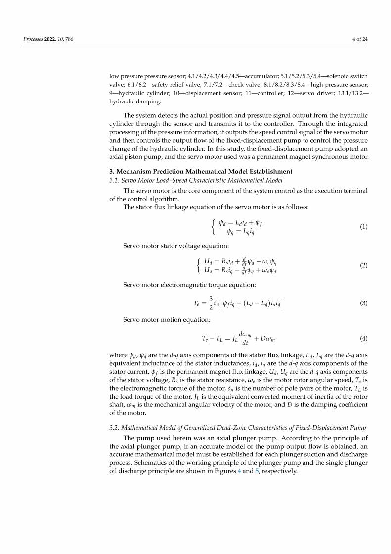
motor speed at different speeds by adjusting the speed, as shown in Figure 12.

Processes 2022, 10, 786 13 of 24

Figure 12. Fluctuation of servo motor speed (constant load/variable speed).

According to the above experimental data, the fluctuation of the servo motor speedalso positively correlated with that of the speed, which can also be approximated as a linearrelation. Therefore, we establish the linear mapping equation of the servo motor speedfluctuation and speed as follows.

Vvolatility = KaVactual (27)

where Ka is the servo motor speed correlation coefficient and Vactual is the servo motorshaft-end speed.

4.2.2. Experimental Study on Generalized Dead-Zone Characteristics ofFixed-Displacement Pump

A fixed-displacement pump is a direct output flow element of the hydraulic system,and the output flow is extremely nonlinear. From the perspective of high-precision control,the factors that affect the control accuracy mainly include the dead zone of the fixed-displacement pump and the flow attenuation of the fixed-displacement pump. From abroad perspective, the attenuation of the output flow of the fixed-displacement pump canbe seen as a result of the dead zone of the fixed-displacement pump flow, and the role of the

Processes 2022, 10, 786 14 of 24

dead zone exists anytime and anywhere. Therefore, we conducted a generalized dead-zoneexperimental study for this aspect.

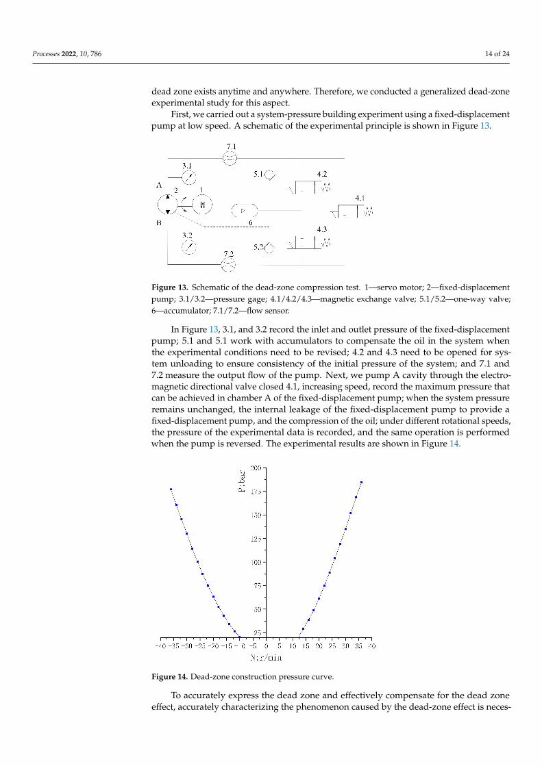
First, we carried out a system-pressure building experiment using a fixed-displacementpump at low speed. A schematic of the experimental principle is shown in Figure 13.

Figure 13. Schematic of the dead-zone compression test. 1—servo motor; 2—fixed-displacementpump; 3.1/3.2—pressure gage; 4.1/4.2/4.3—magnetic exchange valve; 5.1/5.2—one-way valve;6—accumulator; 7.1/7.2—flow sensor.

In Figure 13, 3.1, and 3.2 record the inlet and outlet pressure of the fixed-displacementpump; 5.1 and 5.1 work with accumulators to compensate the oil in the system whenthe experimental conditions need to be revised; 4.2 and 4.3 need to be opened for sys-tem unloading to ensure consistency of the initial pressure of the system; and 7.1 and7.2 measure the output flow of the pump. Next, we pump A cavity through the electro-magnetic directional valve closed 4.1, increasing speed, record the maximum pressure thatcan be achieved in chamber A of the fixed-displacement pump; when the system pressureremains unchanged, the internal leakage of the fixed-displacement pump to provide afixed-displacement pump, and the compression of the oil; under different rotational speeds,the pressure of the experimental data is recorded, and the same operation is performedwhen the pump is reversed. The experimental results are shown in Figure 14.

Figure 14. Dead-zone construction pressure curve.

To accurately express the dead zone and effectively compensate for the dead zoneeffect, accurately characterizing the phenomenon caused by the dead-zone effect is neces-

Processes 2022, 10, 786 15 of 24

sary. Through the analysis of the experimental data, we applied a Gaussian function to fitthe experimental data and obtained the following Equation (28). The fitting effect of theexperimental data is shown in Figure 15. From this, we also obtained an accurate mappingmathematical model of the dead-zone effect. The parameter values of Formula 28 can befound in the Appendix A.

f (x) = a11 exp(−((x− b11)/c11)2) + a12 exp(−((x− b12)/c12)

2)+

a13 exp(−((x− b13)/c13)2) + a14 exp(−((x− b14)/c14)

2)+

a15 exp(−((x− b15)/c15)2) + a16 exp(−((x− b16)/c16)

2)

(28)

Figure 15. Dead-zone build pressure mapping.

Given the attenuation problem of the fixed-displacement pump flow, we measuredthe experimental data of the system output flow under different speeds and pressures, asshown in Figure 16.

Figure 16. Experimental diagram of pump flow envelope surface.

The experimental data shows that if we accurately describe the envelope surface of theoutput flow of the hydraulic pump, then we can perfectly provide real-time and accurateflow mapping compensation for high-precision control. Next, we express the output flow

Processes 2022, 10, 786 16 of 24

envelope surface of the hydraulic pump obtained from the experiment through a third-order polynomial, as shown in Equation (29), and the envelope surface of the mappingmathematical model is shown in Figure 17. From this, we obtain a mapping model of theoutput flow of the hydraulic pump. The parameter values of Formula 29 can be found inthe Appendix A.

f (x, y) = p00 + p10x + p01y + p20x2 + p11xy + p02y2+p30x3 + p21x2y + p12xy2 + p03y3 (29)

Figure 17. Pump flow mapping.

4.2.3. Experimental Study on Accumulator Energy Storage Characteristics

The accumulator is the key component of a system that absorbs pressure fluctuations.To obtain the performance of the accumulator to absorb pressure fluctuations, we simulatedpressure fluctuations of different amplitudes and frequencies. Under the same inflationpressure, the accumulator’s ability to absorb different amplitudes and frequencies wasexperimentally studied. The hydraulic principle is shown in Figure 18. We adjust theopening size of the throttle valve 7, and by setting the sinusoidal speed signal of the servomotor (the sinusoidal speed here, the direction of the speed is not allowed to change), theflow exhibits sinusoidal fluctuations owing to the existence of damping, and the pressurealso presents sinusoidal fluctuations. A control experiment for the accumulator to absorbpressure fluctuations was obtained by controlling the on and off switch of the solenoidvalve 4.3. The experimental data are shown in Figure 19.

Figure 18. Schematic of accumulator experiment exploration. 1—servo motor; 2—fixed-displacementpump; 3.1/3.2—pressure gage; 4.1/4.2/4.3—magnetic exchange valve; 5.1/5.2—one-way valve;6.1/6.2—accumulator; 7—throttling valve; 7.1/7.2—flow sensor.

Processes 2022, 10, 786 17 of 24

H o:l

..0 ' 0...

H o:l

..0 ' 0...

H o:l

..0 ' 0...

135

130

125

120

115

110

105

100

95

90

85

80

75

70

65

60

55

50

45

-1 •••••• I

-2

. 2

-3 -4

•••••• 3 •••••• 4

102. 00

101. 75

101. 50

IOI. 25

IOI. 00

100. 75

100. 50

100. 25

100. 00

99. 75

40 +--�-�----�-�-�-�--�-�--+ 99. 50

0 1000 2000 3000 4000 5000

Tis

(a) -B -c -D -E ..•... F ...... G •..... H •...•• I

130

125

120

115

110

105

100

95

90

85

80

75

70 :;\.::\�_:::::}f ' .. ::<\\::_:·_,_<�"1</':::-,\.'.'.s;_:;y/f ·,,,:::\\;,::;-z/1/:.' � �/

\·:) 60-+--�-�----�-�-�----�-�---i

102. 00

101. 75

101. 50

101. 25

101. 00

100. 75

100. 50

100. 25

100. 00

99. 75

0 1000 2000 3000 4000 5000

-B -c ..•... F ...••. G

125

120

115

110

105

100

95

90

85

80

75

70

65

Tis

(b)

Tit

(c)

-D -E ·•···• H .....• I

102. 00

IOI. 75

IOI. 50

IOI. 25

IOI. 00

100. 75

100. 50

100. 25

100. 00

99. 75

4000 5000

H o:l

..0 ' 0...

H o:l

..0

0...

H o:l

..0 ' 0...

Figure 19. Schematic of accumulator experiment exploration. (a) Pressure wave absorption effectdrawing (0.6 Hz); (b) pressure wave absorption effect drawing (0.8 Hz); (c) pressure wave absorptioneffect drawing (1 Hz). 1, 2, 3, and 4 represent pressure fluctuations of different amplitudes while 5, 6,7, 8 represent the performance control experiment of the accumulator to resume pressure pulsation.

Processes 2022, 10, 786 18 of 24

In Figure 19, the pressure fluctuation frequencies of the three experimental groupsfrom left to right are 0.6 Hz, 0.8 Hz, and 1 Hz. The experimental results show that under thesame charging pressure, the accumulator has a significant effect on the absorption capacityof high-frequency pressure fluctuations but not on the absorption capacity of low-frequencypressure fluctuations.

4.2.4. Experimental Study on the Friction Characteristics of Hydraulic Cylinder

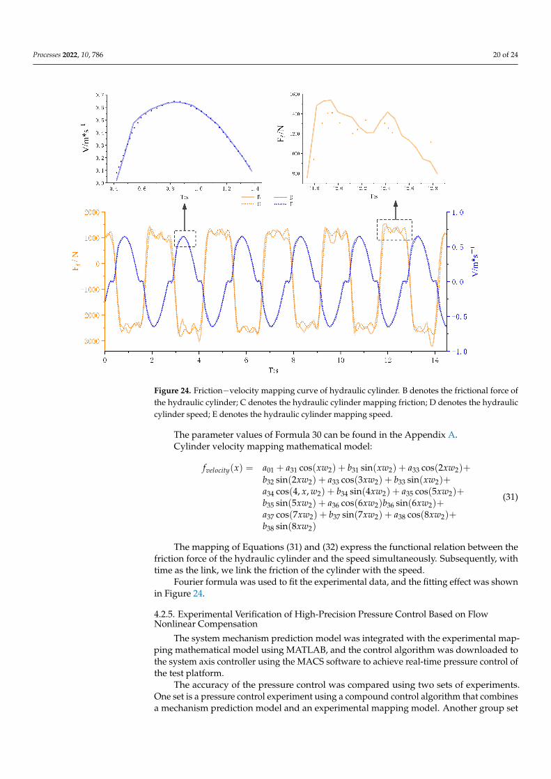
We built a pump-controlled hydraulic cylinder friction characteristics test bench toaccurately describe the friction characteristics of a hydraulic cylinder. The hydraulicprinciple is shown in Figure 20. Given the servo motor speed sinusoidal signal, the outputflow of the fixed-displacement pump shows sinusoidal periodic changes, and it then drivesthe reciprocating motion of the hydraulic cylinder. The data of the hydraulic cylinder inletand outlet pressure, hydraulic cylinder displacement, hydraulic cylinder acceleration, andhydraulic cylinder speed are shown in Figures 21 and 22, respectively, and the data curveof the friction force of the hydraulic cylinder is obtained through the force equation of thehydraulic cylinder. The curve of hydraulic cylinder friction varying with velocity is shownin Figure 23.

Figure 20. Hydraulic schematic of the friction characteristics test of pump-controlled hydrauliccylinder. 1—servo motor; 2—fixed-displacement pump; 3.1/3.2—pressure sensor; 4.1/4.2—one-way valve; 5—accumulator; 6—hydraulic cylinder.

Figure 21. Hydraulic cylinder displacement–velocity–acceleration test curve. x denotes hy-draulic cylinder displacement; v denotes the hydraulic cylinder speed; a denotes the hydrauliccylinder acceleration.

Processes 2022, 10, 786 19 of 24

Figure 22. Pressure test curve of the two chambers of the hydraulic cylinder. Pa denotes the hydrauliccylinder rod’s cavity pressure; Pb denotes the pressure of the piston chamber of the hydraulic cylinder.

Figure 23. Friction–speed test curve of hydraulic cylinder. Ff denotes the frictional force of thehydraulic cylinder; V denotes the speed of the hydraulic cylinder.

The pressure signals of the two cavities of the hydraulic cylinder are collected by thesine speed instruction of the servo motor, and the position information of the hydrauliccylinder is also collected by the external displacement sensor

By collecting and processing the displacement information of the hydraulic cylinder,the real-time velocity and acceleration of the hydraulic cylinder are obtained respectively.

The Fourier equation is used to express the friction characteristics, and the mathe-matical expression of the friction force of the cylinder and the cylinder speed with thetime-independent variable is obtained as the mapping mathematical model of the frictionand velocity of the hydraulic cylinder. Figure 24 shows the fitting effect between themapping model and actual friction characteristics.

Mathematical model of cylinder friction mapping:

f f riction(x) = a00 + a21 cos(xw1) + b21 sin(xw1) + a22 cos(2xw1)+b22 sin(2xw1) + a23 cos(3xw1) + b23 sin(3xw1)+a24 cos(4xw1) + b24 sin(4xw1) + a25 cos(5xw1)+b25 sin(5xw1)

(30)

Processes 2022, 10, 786 20 of 24

Figure 24. Friction−velocity mapping curve of hydraulic cylinder. B denotes the frictional force ofthe hydraulic cylinder; C denotes the hydraulic cylinder mapping friction; D denotes the hydrauliccylinder speed; E denotes the hydraulic cylinder mapping speed.

The parameter values of Formula 30 can be found in the Appendix A.Cylinder velocity mapping mathematical model:

fvelocity(x) = a01 + a31 cos(xw2) + b31 sin(xw2) + a33 cos(2xw2)+b32 sin(2xw2) + a33 cos(3xw2) + b33 sin(xw2)+a34 cos(4, x, w2) + b34 sin(4xw2) + a35 cos(5xw2)+b35 sin(5xw2) + a36 cos(6xw2)b36 sin(6xw2)+a37 cos(7xw2) + b37 sin(7xw2) + a38 cos(8xw2)+b38 sin(8xw2)

(31)

The mapping of Equations (31) and (32) express the functional relation between thefriction force of the hydraulic cylinder and the speed simultaneously. Subsequently, withtime as the link, we link the friction of the cylinder with the speed.

Fourier formula was used to fit the experimental data, and the fitting effect was shownin Figure 24.

4.2.5. Experimental Verification of High-Precision Pressure Control Based on FlowNonlinear Compensation

The system mechanism prediction model was integrated with the experimental map-ping mathematical model using MATLAB, and the control algorithm was downloaded tothe system axis controller using the MACS software to achieve real-time pressure control ofthe test platform.

The accuracy of the pressure control was compared using two sets of experiments.One set is a pressure control experiment using a compound control algorithm that combinesa mechanism prediction model and an experimental mapping model. Another group set

Processes 2022, 10, 786 21 of 24

up a PID control algorithm to perform a control experiment. The experimental results areshown in Figure 25.

Figure 25. Experimental curve of pressure control.

Through the given pressure instructions, the traditional PID algorithm and the opti-mized algorithm are respectively used for experiments. The experimental results show thatthe method adopted herein has considerably improved the accuracy of pressure followingcompared with the PID control algorithm. There was no overshoot phenomenon. Theaccuracy of the PID control algorithm is ±0.12 MPa. The test accuracy of the method usedin this study was 0.037 MPa, and the steady-state control accuracy greatly improved.

5. Conclusions

To improve the pressure control accuracy of the ESPCS, in this study, we use a combi-nation of a mechanism prediction model and an experimental mapping model to accuratelydescribe the flow nonlinear phenomenon in the ESPCS and achieve accurate and fasttracking of the target trajectory. The steady-state pressure control accuracy of the systemwas considerably improved. In addition, in this paper, the relation between the dead zoneof the hydraulic pump, flow attenuation of the full speed range, friction of the hydrauliccylinder and the speed, through experimental research, has obtained an accurate mappingmathematical model. We have ensured that the control algorithm accurately compensatesfor nonlinear phenomena in the system. A comparison with the traditional PID controlalgorithm shows that the method used herein to improve the pressure control accuracy cansignificantly increase the pressure control accuracy. The results of this study have broadapplication prospects in the fields of hydraulic quadruped robots and high-precision pres-sure control military industry in the future. However, our research also had shortcomings.It fails to express the relation between the accumulator’s energy storage characteristicsand its charging pressure and system pressure fluctuation characteristics with an accuratemapping mathematical model. In future follow-up research, we will rebuild a set of experi-mental platforms, to conduct a comprehensive experimental study on the energy storagecharacteristics of the accumulator. Finally, a more accurate experimental mapping modelis obtained.

Author Contributions: Conceptualization, G.Y. and T.Z.; methodology, Z.J.; experiment and analysis,T.Z. and C.Z.; software, Z.J.; investigation, G.Y.; writing—original draft preparation, G.Y. and T.Z.;writing—review and editing, C.A. and G.C.; project administration, C.A.; funding acquisition, C.A.and G.C. All authors have read and agreed to the published version of the manuscript.

Funding: This research was supported by the Key R&D Projects in Hebei Province (No. 20314402D),the Key Project of Science and Technology Research in Hebei Province (No. ZD2020166), the Key

Processes 2022, 10, 786 22 of 24

Project of Science and Technology Research in Hebei Province (No. ZD2021340), and the GeneralProject of Natural Science Foundation in Xinjiang Uygur Autonomous Region (No. 2021D01A63).

Institutional Review Board Statement: Not applicable.

Informed Consent Statement: Not applicable.

Data Availability Statement: The data generated and analyzed in this study are available. Requestsfor the data should be made to the author.

Conflicts of Interest: The authors declare no conflict of interest.

Appendix A

Parameter Definition Table

Variable Name Parameter Values Variable Name Parameter Values

a11 250.7 a00 −664

b11 47.38 a21 2120

c11 17.13 b21 −865.1

a12 10.06 a22 −116.6

b12 −28.34 b22 5.931

c12 8.063 a23 −267.9

a13 218.6 b23 593.3

b13 −45.57 a24 84.01

c13 18.57 b24 −78.01

a14 46.14 a25 −83.38

b14 27.08 b25 −284.8

c14 11.51 w1 2.52

a15 12.43 a01 2.831 × 10−5

b15 16.09 a31 −0.3626

c15 9.141 b31 0.482

a16 27.45 a32 −0.0002265

b16 −20.04 b32 5.446 × 10−5

c16 11.17 a33 0.07728

p00 0.07542 b33 −0.005133

p10 −0.011 a34 0.0001464

p01 0.007577 b34 −0.0001172

p20 0.0001085 a35 −0.008805

p11 −5.464 × 10−6 b35 0.05138

p02 −5.951 × 10−7 a36 −0.0001165

p30 −3.689 × 10−7 b36 3.717 × 10−5

p21 2.583 × 10−9 a37 −0.03001

p12 7.639 × 10−10 b37 −0.01099

p03 1.645 × 10−10 a38 0.000395

w2 2.523 b38 5.017 × 10−5

Processes 2022, 10, 786 23 of 24

References1. Luo, G.; Görges, D. Modeling and Adaptive Robust Force Control of a Pump-Controlled Electro-Hydraulic Actuator for an Active

Suspension System. In Proceedings of the 2019 IEEE Conference on Control Technology and Applications (CCTA), Hong Kong,China, 19–21 August 2019; pp. 592–597.

2. Li, X.; Jiao, Z.; Yan, L.; Cao, Y. Modeling and Experimental Study on a Novel Linear Electromagnetic Collaborative RectificationPump. Sens. Actuators A Phys. 2020, 309, 111883. [CrossRef]

3. Lee, S.R.; Hong, Y.S. A Dual EHA System for the Improvement of Position Control Performance Via Active Load Compensation.Int. J. Precis. Eng. Manuf. 2017, 18, 937–944. [CrossRef]

4. Yuan, H.B.; Na, H.C.; Kim, Y.B. Robust MPC–PIC force control for an electro-hydraulic servo system with pure compressiveelastic load. Control Eng. Pract. 2018, 79, 170–184. [CrossRef]

5. Zhu, Y.; Jiang, W.L.; Kong, X.D.; Zheng, Z. Study on nonlinear dynamics characteristics of electrohydraulic servo system. NonlinearDyn. 2015, 80, 723–737. [CrossRef]

6. Hao, Y.; Xia, L.; Ge, L.; Wang, X.; Qvan, L. Research on Position Control Characteristics of Hybrid Linear Drive System. Trans.Chin. Soc. Agric. Mach. 2020, 51, 379–385.

7. Jing, C.; Xu, H.; Jiang, J. Dynamic surface disturbance rejection control for electro-hydraulic load simulator. Mech. Syst. SignalProcess. 2019, 134, 106293. [CrossRef]

8. Zhang, L.; Guo, F.; Li, Y.; Lu, W. Global dynamic modeling of electro-hydraulic 3-UPS/S parallel stabilized platform by bondgraph. Chin. J. Mech. Eng. 2016, 29, 1176–1185. [CrossRef]

9. Yu, Z.; Leng, B.; Xiong, L.; Feng, Y.; Shi, F. Direct yaw moment control for distributed drive electric vehicle handling performanceimprovement. Chin. J. Mech. Eng. 2016, 29, 486–497. [CrossRef]

10. Wang, C.; Quan, L. Characteristic of Pump Controlled Single Rod Cylinder with Combination of Variable Displacement andSpeed. Trans. Chin. Soc. Agric. Mach. 2017, 48, 405–412.

11. Yue, J.; Dai, B.; Xu, W.U.; Yang, L. The Impact of Flow Pulsation of Axial Piston Pump on Gun Pitching Accuracy of a MultipleRocket Launcher. Acta Armamentarii 2019, 40, 1781.

12. Wang, L.; Wang, D.; Qi, J.; Xue, Y. Internal leakage detection of hydraulic cylinder based on wavelet analysis and backpropagationneural network. In Proceedings of the 2020 Global Reliability and Prognostics and Health Management (PHM-Shanghai),Shanghai, China, 16–18 October 2020; pp. 1–6.

13. Li, Y.; Shang, Y.; Jiao, Z. EHA position system simulation based on fuzzy sliding mode control. In Proceedings of the CSAA/IETInternational Conference on Aircraft Utility Systems (AUS 2018), Guiyang, China, 19–22 June 2018; pp. 1012–1016. [CrossRef]

14. Xia, H.; Yang, B.; Shang, Y.; Jiao, Z. Simulation and verification of pressure characteristics of aircraft hydraulic power system. InProceedings of the 2019 IEEE 8th International Conference on Fluid Power and Mechatronics (FPM), Wuhan, China, 10–13 April2019; pp. 1197–1202.

15. Li, J.; Fu, Y.; Zhang, G.; Gao, B.; Ma, J. Research on fast response and high accuracy control of an airborne brushless DC motor. InProceedings of the IEEE International Conference on Robotics & Biomimetics, Shenyang, China, 22–26 August 2004; pp. 807–810.

16. Guo, J.; Ye, C.; Wu, G. Simulation and Research on Position Servo Control System of Opposite Vertex Hydraulic Cylinder basedon Fuzzy Neural Network. In Proceedings of the 2019 IEEE International Conference on Mechatronics and Automation (ICMA),Tianjin, China, 4–7 August 2019; pp. 1139–1143.

17. Essa, M.E.S.M.; Aboelela, M.A.; Hassan, M.M.; Abdraboo, S.M. Fractional order fuzzy logic position and force control ofexperimental electro-hydraulic servo system. In Proceedings of the 2019 8th International Conference on Modern Circuits andSystems Technologies (MOCAST), Thessaloniki, Greece, 13–15 May 2019; pp. 1–4.

18. Essa ME, S.M.; Aboelela, M.A.; Hassan, M.M.; Abdrabbo, S.M. Control of hardware implementation of hydraulic servo applicationbased on adaptive neuro fuzzy inference system. In Proceedings of the 2018 14th International Computer Engineering Conference(ICENCO), Cairo, Egypt, 29–30 December 2018; pp. 168–173.

19. Milic, V.; Šitum, Ž.; Essert, M. Robust position control synthesis of an electro-hydraulic servo system. ISA Trans. 2010, 49, 535–542.[CrossRef] [PubMed]

20. Yin, X.; Zhang, W.; Jiang, Z.; Pan, L. Adaptive robust integral sliding mode pitch angle control of an electro-hydraulic servo pitchsystem for wind turbine. Mech. Syst. Signal Process. 2019, 133, 105704. [CrossRef]

21. Xu, G.; Chen, M.; He, X.; Pang, H.; Miao, H.; Cui, P.; Wang, W.; Diao, P. Path following control of tractor with an electro-hydrauliccoupling steering system: Layered multi-loop robust control architecture. Biosyst. Eng. 2021, 209, 282–299. [CrossRef]

22. Lin, Y.; Shi, Y.; Burton, R. Modeling and robust discrete-time sliding-mode control design for a fluid power electrohydraulicactuator (EHA) system. IEEE/ASME Trans. Mechatron. 2011, 18, 1–10. [CrossRef]

23. Zhang, H.; Liu, X.; Wang, J.; Karimi, H.R. Robust H∞ sliding mode control with pole placement for a fluid power electrohydraulicactuator (EHA) system. Int. J. Adv. Manuf. Technol. 2014, 73, 1095–1104. [CrossRef]

24. Kim, H.M.; Park, S.H.; Song, J.H.; Kim, J.S. Robust position control of electro-hydraulic actuator systems using the adaptiveback-stepping control scheme. Proc. Inst. Mech. Eng. 2010, 224, 737–746. [CrossRef]

Processes 2022, 10, 786 24 of 24

25. Ahn, K.K.; Nam, D.N.C.; Jin, M. Adaptive Backstepping Control of an Electrohydraulic Actuator. IEEE/ASME Trans. Mechatron.2013, 19, 987–995. [CrossRef]

26. Shen, Y.; Wang, X.; Wang, S.; Mattila, J. An Adaptive Control Method for Electro-hydrostatic Actuator Based on Virtual Decom-position Control. In Proceedings of the 2020 Asia-Pacific International Symposium on Advanced Reliability and MaintenanceModeling (APARM), Vancouver, BC, Canada, 20–23 August 2020; pp. 1–6.