Advances in Water Resources 64 (2014) 9–20

Contents lists available at ScienceDirect

Advances in Water Resources

journal homepage: www.elsevier .com/ locate/advwatres

Exploring the effects of hillslope-channel link dynamics and excessrainfall properties on the scaling structure of peak-discharge

0309-1708/$ - see front matter � 2013 Elsevier Ltd. All rights reserved.http://dx.doi.org/10.1016/j.advwatres.2013.11.010

⇑ Corresponding author. Tel.: +1 2675920623.E-mail address: tibebu-ayalew@uiowa.edu (T.B. Ayalew).

Tibebu B. Ayalew ⇑, Witold F. Krajewski, Ricardo Mantilla, Scott J. SmallIIHR-Hydroscience & Engineering, The University of Iowa, C. Maxwell Stanley Hydraulics Laboratory, Iowa City, IA 52242, USA

a r t i c l e i n f o

Article history:Received 22 December 2012Received in revised form 11 November 2013Accepted 20 November 2013Available online 1 December 2013

Keywords:StreamflowFloodsScalingRiver networksHillslope

a b s t r a c t

Several studies revealed that peak discharges (Q) observed in a nested drainage network following a run-off-generating rainfall event exhibit power law scaling with respect to drainage area (A) as Q(A) = aAh.However, multiple aspects of how rainfall-runoff process controls the value of the intercept (a) andthe scaling exponent (h) are not fully understood. We use the rainfall-runoff model CUENCAS and applyit to three different river basins in Iowa to investigate how the interplay among rainfall intensity, dura-tion, hillslope overland flow velocity, channel flow velocity, and the drainage network structure affectsthese parameters. We show that, for a given catchment: (1) rainfall duration and hillslope overland flowvelocity play a dominant role in controlling h, followed by channel flow velocity and rainfall intensity; (2)a is systematically controlled by the interplay among rainfall intensity, duration, hillslope overland flowvelocity, and channel flow velocity, which highlights that it is the combined effect of these factors thatcontrols the exact values of a and h; and (3) a scale break occurs when runoff generated on hillslopes runsoff into the drainage network very rapidly and the scale at which the break happens is determined by theinterplay among rainfall duration, hillslope overland flow velocity, and channel flow velocity.

� 2013 Elsevier Ltd. All rights reserved.

1. Introduction

An emerging approach to peak discharge estimation acrossscales is based on the statistical dependence of peak flow on wa-tershed area. While the statistical self-similarity of peak flow(flood) statistics has been well-established (e.g. regionalizationstudies), recent research has shown that, in a nested watershed,peak discharge scale as a power law of drainage area for individualevents, given by the form Q(A) = aAh, where Q(A) is peak discharge,A is the drainage area, a is the intercept, and h is the exponent.Empirical results by Goodrich et al. [1]; Ogden and Dawdy [2],Smith et al. [3], Gupta et al. [4], and Lima and Lall [5] offer clear evi-dence in support of the theory (e.g. Gupta [6]; Gupta et al. [7]) thatthe aggregated runoff response in a watershed, which is a result ofcomplex interactions of catchment physical processes that arehighly variable in space and time, exhibit scale invariance. Manda-paka et al. [8] showed that, by assuming the runoff generatingmechanism to be uniform in space, the spatial variability of rainfallleads to significant variability of peak discharge at smaller wa-tershed scales (�10 km2). However, the variability of peak dis-charge becomes insignificant at increasingly larger scales(�>150 km2), which demonstrates that the aggregated catchmentrunoff response resulting from spatially variable rainfall-runoff

processes in a nested watershed preserves scale invariance. Thisinteresting insight offers an avenue for peak discharge estimationacross scales without going through the rigors of calibration toestimate the spatially variable parameters that are required incomplex rainfall-runoff models. For other implications of peak-flow scaling, refer to Gupta [6] and Gupta et al. [7].

Earlier efforts were devoted to understanding the role of thedrainage network (e.g. Gupta and Waymire [9]; Menabde et al.[10]) and the spatial structure of rainfall (e.g. Gupta et al. [11];Menabde and Sivapalan [12]; Mandapaka et al. [8]) in controllingh. Recent research is geared towards understanding which aspectsof the rainfall-runoff processes control a and h (e.g. Furey and Gup-ta [13,14]; Di Lazzaro and Volpi [15]). We continue on this trajec-tory and devote the present study to further understanding therole of the drainage network and the interplay among rainfallintensity (I), duration (T), channel flow velocity (vc), and hillslopeoverland flow velocity (vh) in determining the scaling structure ofpeak discharges. Our approach involves simulation using the drain-age network based hydrologic model CUENCAS [16]. We systemat-ically altered catchment process variables to gain insight into theireffects on the scaling structure of peak discharges. To this end, wecarried out systematic simulation experiments across multiplewatersheds to determine whether our findings hold for watershedsthat have different shapes, sizes, and width functions.

The paper is organized as follows. In the next section we pro-vide a literature review of reported results on catchment runoff

10 T.B. Ayalew et al. / Advances in Water Resources 64 (2014) 9–20

response and scaling of peak flows. We then discuss the study areaand our methodology in greater detail in the following section. Thissection outlines the drainage network based hydrologic modelcalled CUENCAS and the three different watersheds we studied.We also discuss the physical assumptions we have made, the asso-ciated limitation of the study, and the systematic setup of our sim-ulation experiments. We follow this by presenting our results anddiscussing their implications on peak discharge estimation acrossscales. We conclude the paper with a summary of our findingsand recommendations for future research.

2. Literature review

Drainage area was first recognized as a peak discharge scalingparameter in the classical Rational Method [17]. In this method,for a given soil type (topography), rainfall intensity I and rainfallduration T, that is equal to the longest travel time in the watershed(‘‘time of concentration,’’ tc), peak discharge scales linearly withdrainage area at internal locations in the catchment and can beestimated using the formula Q(A) = cr � I � A, where cr is the runoffcoefficient. Under this method, a corresponds to Ie (Ie ¼ cr � I) andh = 1. The method is still being used in engineering practice forthe design of small drainage structures and is applicable to smallcatchments with drainage areas as large as 15 km2 [18]. Aroundthe same time the Rational Method was outlined, O’Connell [19]proposed the power law formula Q(A) = aA0.5 that linked peak dis-charge to drainage area, where a is a coefficient related to theregion.

In the early 1960s, the United States Geological Survey (USGS)adopted and popularized an empirical quantile regression methodfor regional flood frequency estimation that is used throughout theworld (see Dawdy et al. [20] for a comprehensive review). Thesequantile regressions often use drainage area as the only predictorvariable and follow the form Qp(A) = a(p)Au(p), where both theintercept a and the exponent u are functions of the probabilityof exceedance p. The flow quantile Qp(A) exhibits a log–log linearrelationship with drainage areas located in a homogeneous region.This means that streams that belong to different drainage net-works, and are therefore not nested but are located in a homoge-neous region, exhibit similar peak flow scaling structure. It isimportant to note here that the delineation of homogeneous re-gions is based on the residuals from regression analysis and onphysiographic characteristics of river basins [21].

Goodrich et al. [1] reported the first empirical evidence thatshowed peak discharges in nested watersheds exhibit self-similar-ity. They used empirical data from the semi-arid Walnut Gulchexperimental watershed in Arizona, whose nested watershedshave drainage areas that range from 0.0018 to 149 km2. Theirquantile-based empirical analysis revealed u values of 0.85 and0.90 for the 2-yr and 100-yr return periods and drainage areasup to 1 km2, whereas u equals 0.55 and 0.58 for the 2-yr and100-yr return periods and drainage areas greater than 1 km2,which suggests multiscaling. The fact that u assumes different val-ues for drainage areas above and below a certain critical drainagearea, in this case 1 km2, also suggests the existence of a scale break.They attributed the observed scale break to partial area storm cov-erage and ephemeral channel losses through infiltration as thestream flow propagates downstream.

The quantile-based estimates of u discussed thus far offer littlethat would enhance the understanding of which aspects of therainfall-runoff processes control h during a single event. This is be-cause peak flows used in the quantile regression approach likelycorrespond to different rainfall events which, in the case of USGS’sregional regression equations, may also come from different water-sheds that are not nested and, hence, belong to different drainage

networks. The first event-based empirical study of peak dischargecomes from Ogden and Dawdy [2], who studied the scaling struc-ture of peak discharges in a nested watershed where the spatialrainfall pattern is fairly uniform. They analyzed peak dischargedata from the 21.2 km2 Goodwin Creek experimental watershed(GCEW) located in Mississippi in the South-Central United States.They examined 16 yr of continuous rainfall and runoff data fromsubcatchments with drainage areas ranging from 0.172 to21.2 km2 at the outlet. Their estimate of u with the value of 0.77was independent of the return period, which suggests simple scal-ing. They also reported an event-based analysis of h in which theystudied basin-wide peak discharge data from 226 runoff events.Their results showed that the estimated h values were differentfor different events and generally varied between 0.6 and 1. Theevent-to-event variability of h was also shown to decrease as themagnitude of peak discharge at the outlet increases. This is be-cause, they argued, more intense rainfall events that are responsi-ble for larger peak discharge events have less spatial variabilitywhen compared with less intense rainfall events.

Motivated by the findings of Ogden and Dawdy [2], Furey andGupta [13] undertook an event-based analysis of peak dischargescaling structure in the GCEW with the main objective of under-standing which physical processes are responsible for the event-to-event variability of both a and h. Their study, which was basedon 148 rainfall-runoff events, showed that h depends on T, whereasa depends on excess rainfall depth (Pe). They found that the signif-icant event-to-event variability of h observed at smaller peak dis-charge values is due to the variability in the antecedent soilmoisture state and the increased spatial rainfall variability associ-ated with less intense rainfall events. In their follow up paper, Fur-ey and Gupta [14] further investigated the role of Pe and T indetermining a and h. They devised, based on the theory of a geo-morphic instantaneous unit hydrograph (GIUH) [22,23], an analyt-ical formula that relates the expected value of peak discharge to Pe,T , and A. Their results further confirmed the systematic depen-dence of a and h on Pe and T . Drawing from results of their preli-minary analysis of the effect of vc and vh on a and h, theyconcluded that both a and h can be affected by vc and vh. Their the-oretical estimates of the peak discharge are comparable withempirical data from GCEW only when realistic vh values wereused. This confirms the importance of the hillslope residence timein determining the scaling structure of peak discharges. It is alsoindependently confirmed by Saco and Kumar [24], and Botterand Rinaldo [25], that the runoff response at all scales is not onlyshaped by the drainage network and vc but also by vh.

Although our work is closely connected to that of Furey andGupta [14], we use a drainage network-based hydrologic modelsimulation to provide in-depth insight into the role of the interplayamong, T , vh, and vc in controlling a and h, which Furey and Gupta[14] did not fully address in their work, and which to our knowl-edge, has yet to be reported. A further understanding of this prob-lem is important because, in reality, these catchment processes areinterdependent, and understanding their relative roles in deter-mining the scaling structure provides further insight into our questto estimate a and h from catchment variables that can be either di-rectly measured or estimated.

3. Methodology

3.1. Study watersheds

We considered three different watersheds in Iowa: Clear Creek,Old Mans Creek, and Boone River, which have drainage areas of254, 520, and 1082 km2, respectively. We extracted their respec-tive drainage networks and hillslopes from a one arc-second

T.B. Ayalew et al. / Advances in Water Resources 64 (2014) 9–20 11

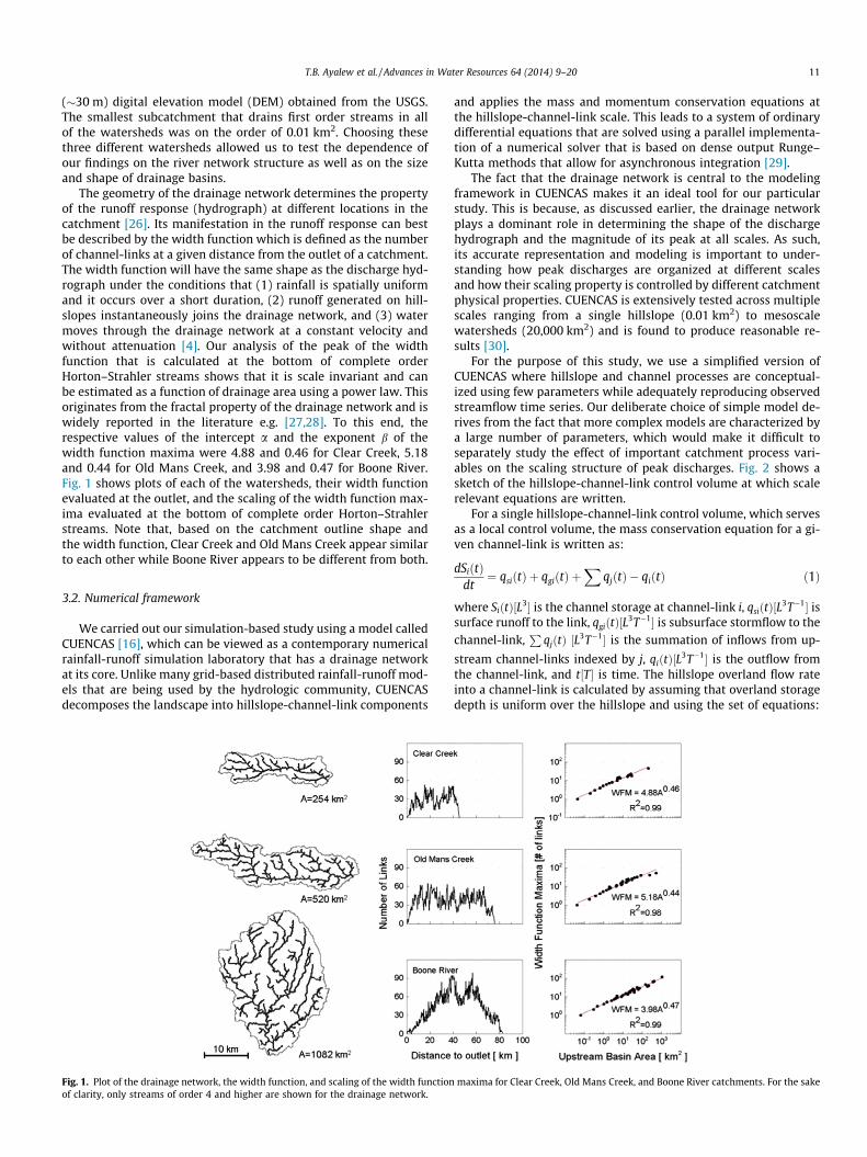
(�30 m) digital elevation model (DEM) obtained from the USGS.The smallest subcatchment that drains first order streams in allof the watersheds was on the order of 0.01 km2. Choosing thesethree different watersheds allowed us to test the dependence ofour findings on the river network structure as well as on the sizeand shape of drainage basins.

The geometry of the drainage network determines the propertyof the runoff response (hydrograph) at different locations in thecatchment [26]. Its manifestation in the runoff response can bestbe described by the width function which is defined as the numberof channel-links at a given distance from the outlet of a catchment.The width function will have the same shape as the discharge hyd-rograph under the conditions that (1) rainfall is spatially uniformand it occurs over a short duration, (2) runoff generated on hill-slopes instantaneously joins the drainage network, and (3) watermoves through the drainage network at a constant velocity andwithout attenuation [4]. Our analysis of the peak of the widthfunction that is calculated at the bottom of complete orderHorton–Strahler streams shows that it is scale invariant and canbe estimated as a function of drainage area using a power law. Thisoriginates from the fractal property of the drainage network and iswidely reported in the literature e.g. [27,28]. To this end, therespective values of the intercept a and the exponent b of thewidth function maxima were 4.88 and 0.46 for Clear Creek, 5.18and 0.44 for Old Mans Creek, and 3.98 and 0.47 for Boone River.Fig. 1 shows plots of each of the watersheds, their width functionevaluated at the outlet, and the scaling of the width function max-ima evaluated at the bottom of complete order Horton–Strahlerstreams. Note that, based on the catchment outline shape andthe width function, Clear Creek and Old Mans Creek appear similarto each other while Boone River appears to be different from both.

3.2. Numerical framework

We carried out our simulation-based study using a model calledCUENCAS [16], which can be viewed as a contemporary numericalrainfall-runoff simulation laboratory that has a drainage networkat its core. Unlike many grid-based distributed rainfall-runoff mod-els that are being used by the hydrologic community, CUENCASdecomposes the landscape into hillslope-channel-link components

Fig. 1. Plot of the drainage network, the width function, and scaling of the width functionof clarity, only streams of order 4 and higher are shown for the drainage network.

and applies the mass and momentum conservation equations atthe hillslope-channel-link scale. This leads to a system of ordinarydifferential equations that are solved using a parallel implementa-tion of a numerical solver that is based on dense output Runge–Kutta methods that allow for asynchronous integration [29].

The fact that the drainage network is central to the modelingframework in CUENCAS makes it an ideal tool for our particularstudy. This is because, as discussed earlier, the drainage networkplays a dominant role in determining the shape of the dischargehydrograph and the magnitude of its peak at all scales. As such,its accurate representation and modeling is important to under-standing how peak discharges are organized at different scalesand how their scaling property is controlled by different catchmentphysical properties. CUENCAS is extensively tested across multiplescales ranging from a single hillslope (0.01 km2) to mesoscalewatersheds (20,000 km2) and is found to produce reasonable re-sults [30].

For the purpose of this study, we use a simplified version ofCUENCAS where hillslope and channel processes are conceptual-ized using few parameters while adequately reproducing observedstreamflow time series. Our deliberate choice of simple model de-rives from the fact that more complex models are characterized bya large number of parameters, which would make it difficult toseparately study the effect of important catchment process vari-ables on the scaling structure of peak discharges. Fig. 2 shows asketch of the hillslope-channel-link control volume at which scalerelevant equations are written.

For a single hillslope-channel-link control volume, which servesas a local control volume, the mass conservation equation for a gi-ven channel-link is written as:

dSiðtÞdt¼ qsiðtÞ þ qgiðtÞ þ

XqjðtÞ � qiðtÞ ð1Þ

where SiðtÞ½L3� is the channel storage at channel-link i, qsiðtÞ½L3T�1� issurface runoff to the link, qgiðtÞ½L

3T�1� is subsurface stormflow to thechannel-link,

PqjðtÞ ½L3T�1� is the summation of inflows from up-

stream channel-links indexed by j, qiðtÞ½L3T�1� is the outflow from

the channel-link, and t½T� is time. The hillslope overland flow rateinto a channel-link is calculated by assuming that overland storagedepth is uniform over the hillslope and using the set of equations:

maxima for Clear Creek, Old Mans Creek, and Boone River catchments. For the sake

Fig. 2. Sketch depicting the decomposition of the Clear Creek catchment intohillslope-channel-link system. The hillslope-channel-link control volume is alsoshown.

12 T.B. Ayalew et al. / Advances in Water Resources 64 (2014) 9–20

SsiðtÞ ¼ AhdðtÞ ð2Þ

qsiðtÞ ¼ vhLdðtÞ ð3Þ

where SsiðtÞ½L3� is the proportion of rainfall that is stored on the sur-face of the hillslope at a given time, Ah½L2� is the hillslope area, dðtÞ isthe time dependent overland flow depth, vh½LT�1� is the hillslopeoverland flow velocity, L½L� is the length of the channel-link, andqsiðtÞ is as defined earlier. Solving Eqs. (2) and (3) simultaneouslyyields:

qsiðtÞ ¼ vhL

AhSsiðtÞ ð4Þ

Rewriting equations (2) and (3) for the subsurface flow case andsolving them simultaneously yields:

qgiðtÞ ¼ vgL

AhSgiðtÞ ð5Þ

where vg ½LT�1� is the subsurface flow velocity, and SgiðtÞ½L3� is theproportion of rainfall that is stored in the subsurface of the hillslope.The rate of change of surface and subsurface storage is further cal-culated by assuming that rainfall is partitioned into surface andsubsurface storage according to the runoff coefficient cr and usingthe following set of ordinary differential equations:

dSsi

dt¼ crAhIiðtÞ � qsiðtÞ ð6Þ

dSgi

dt¼ ð1� crÞAhIiðtÞ � qgiðtÞ ð7Þ

where cr is the runoff coefficient and IiðtÞ½LT�1� is the rainfallintensity.

The outflow from a channel-link, qiðtÞ, is calculated by assumingthat the channel cross-sectional area and flow depth is uniformover the channel-link and using the following set of equations:

SiðtÞ ¼ acL ð8Þ

qiðtÞ ¼ acvcðtÞ ð9Þ

where SiðtÞ½L3� is the channel storage at link i, ac½L2� is the channel-link cross-section area, vc½LT�1� is the channel flow velocity, and therest is as defined earlier. Combining equations (8) and (9) yields:

qiðtÞ ¼ vcðtÞ �SiðtÞ

Lð10Þ

Eq. (10) is not yet complete since vc is unknown. We used the fol-lowing equation to estimate vc:

vcðtÞ ¼ v r �qiðtÞQ r

� �k1

� AAr

� �k2

ð11Þ

where vr ½LT�1� is the reference channel velocity, qiðtÞ½L3T�1� is

the discharge from the link, A½L2� is the drainage area upstreamof the outlet of link i, and Qr ½L3T�1� and Ar ½L2� are the reference dis-charge and drainage area, whose values are taken in this study tobe 1 m3/s and 1 km2, respectively. The parameters k1 and k2 arethe scaling exponents for discharge and drainage area, respec-tively. The derivation of Eq. (11) is rooted in the assumption thatchannel velocity scales as a function of drainage area and dis-charge. The reader is encouraged to refer to Mantilla [31] for thetheoretical background and its detailed derivation.

Finally, the outflow from the link is calculated by combiningequations (10) and (11) and solving for qiðtÞ. The result leads to achannel storage–discharge relationship which can be consideredas a simplified form of momentum conservation equation and iswritten as follows:

qiðtÞ ¼ v rSiðtÞ

LAAr

� �k2 ! 1

1�k1

ð12Þ

Solving the above set of equations over the drainage network re-sults in channel flows that mimic the dispersion and attenuationof flows as the flood wave propagates downstream.

In order to illustrate the model’s capability to reproduce ob-served streamflow data we simulated observed rainfall-runoffevents in all the three study catchments using Stage-IV radar rain-fall data as input. The Stage-IV product is widely used in hydrologicapplications. It provides hourly radar-rainfall estimates that areadjusted by rain gauge data in real time; e.g. see Kitzmiller et al.[32] and Habib et al. [33]. While quality and accuracy of the prod-uct may vary across the US, over Iowa the multiplicative bias isclose to unity; see Seo and Krajewski [34]. For all the catchments,we also used a spatially uniform v r , k1, k2, vh, and cr values of0.25 m/s, 0.3, �0.1, 0.01 m/s, and 0.3, respectively. The simulationresults, which are shown in Fig. 3, indicate that the model is capa-ble of reproducing real events and hence fits the purpose of ourstudy.

3.3. Scope of our study

Our rainfall-runoff simulation-based study uses the assump-tions that: (1) rainfall is spatially uniform and its intensity I is con-stant over its duration T; (2) the entire watershed has the same soilmoisture deficit; (3) vh is constant both in space and time, and (4)vc is either constant both in space and time or variable as a nonlin-ear function of drainage area and discharge. Relevant theoreticalaccomplishments were advanced using similar assumptions atcomparable or even higher scales (e.g. [12,15,25]). The main limi-tation of our study derives from these simplifying assumptions be-cause spatially uniform and temporally constant I, cr , vh, and vc

seem unrealistic at the scale of the watersheds we investigated.However, these assumptions are helpful to separately study therole of these important process variables in shaping the scalingstructure of peak discharge. Thus, the results of this study shouldbe taken within the context of these assumptions.

3.4. Experimental setup

We systematically organized the simulation experiment intofour distinctive groups in order to separately study the effect ofvariation in one variable on both a and h by keeping the other vari-ables constant. We used both the constant and nonlinear channelvelocity formulations in each group. For the constant channelvelocity case, we set k1 ¼ k2 ¼ 0 and used vc ¼ v r values that rangefrom 0.1 to 2 m/s with a typical value of 0.5 m/s and applied it uni-formly both in space and time. When experimenting with nonlin-ear channel velocity as described by Eq. (11), we used vr values

Fig. 3. Plot of observed vs. simulated hydrographs.

T.B. Ayalew et al. / Advances in Water Resources 64 (2014) 9–20 13

that range from 0.1 to 2 m/s and set k1 ¼ 0:3 and k2 ¼ �0:1. Thesek1 and k2 values are supported by field data [30,31] and, as shownin Fig. 3, are also appropriate for our study catchments. For a givenv r , these k1 and k2 values generally lead to vc values that, in addi-tion to increasing with increasing rainfall intensity, increase in thedownstream direction. Fig. 4 shows the range vc values will as-sume at different scales and for different values of v r and I. For thisstudy, when experimenting with nonlinear channel velocity, wetake v r = 0.25 m/s as the typical value and the resulting vc valuesare in the range of 0.1–1 m/s. These scale dependent vc valuesare reported in the literature [35].

When modeling the hillslope response, we used a spatially uni-form and temporally constant vh value that range from 0.001 to0.1 m/s with a typical value of 0.01 m/s. These values are also

Fig. 4. Change of the channel velocity vc as a function of vr and A for a fixed I = 25 m

supported by results from field studies e.g. [15,25,36,37]. Guptaand Waymire [9] also reported that the maximum value vh couldattain is in the range of 0.03 m/s. In addition, we also assumed aconstant subsurface flow velocity value of vg ¼ 0:005 m=s whichis in the range of what is observed in tracer-based field studies[38,39]. Furthermore, a spatially uniform and temporally constantrunoff coefficient value of cr ¼ 0:5 was also used for all the simula-tions. This cr value was determined in an ad hoc fashion and isimmaterial for our study. A detailed summary of the simulationexperiments is outlined in Table 1.

Peak discharge estimates were extracted at the bottom of com-plete order Horton–Strahler streams whose drainage areas areknown from the analysis of the DEM in CUENCAS. We then usedthe ordinary least-squares (OLS) regression method in the log–log scale to parameterize the power law relationship between peakdischarge and drainage area. We used the OLS regression eventhough we recognize that the residuals are correlated in violationof one of the OLS regression assumptions. This arises because, ina nested watershed, peak discharges in higher order Horton–Strah-ler streams are dependent on peak discharges from lower orderstreams that drain into them. However, since the purpose of thepresent study is to identify systematic trends of a and h in responseto changes in the magnitude of important catchment physicalparameters (and not to develop a predictive model), OLS remainsa valid method of regression analysis.

4. Results and discussion

4.1. Effect of rainfall duration and intensity on the scaling structure

We began by investigating the effect of rainfall duration T onthe scaling exponent h. For this experiment, we used a spatiallyuniform rainfall depth of 25 mm, which is equivalent to the 1-yr,1-h rainfall for the study sites [40]. We applied this rainfall depthover the following values of T: 5-min, 10-min, 15-min, 30-min, 1-h,2-h, 3-h, 6-h, 12-h, 18-h, 1-day, and 2-day. This arrangementmeans that I decreases as T increases while the rainfall volume re-mains constant. Additionally, we used the constant channel veloc-ity formulation with vc and vh values of 0.5 and 0.01 m/s,respectively. In order to separately study the effect of rainfall dura-tion, we repeated the above experiment by keeping the rainfallintensity constant at 25 mm/h for all durations considered here.The result, which is presented in Fig. 5, shows how a and h system-atically change with I and T. It reveals that, under the assumptionswe employed here, h starts at a value greater than the scaling expo-nent of the width function maxima b for small values of T and sys-tematically converges to a value closer to 1 as T increases. Thisproperty is previously observed in empirical studies [13] and intheoretical results e.g. [9,14]. The value of h, under the present con-stant channel velocity assumption, is independent of the rainfallintensity and is determined solely by T , which is evident in Fig. 5

m/h (left) and its change as a function of I and A for a fixed vr = 0.25 m/s (right).

Table 1Summary of the simulation experiments.

Fig. 5. Systematic dependence of both the intercept a and the scaling exponent h on excess rainfall duration T and intensity I (top panels) for a fixed excess rainfall P whereI = P/T and (bottom panels) for a fixed I.

14 T.B. Ayalew et al. / Advances in Water Resources 64 (2014) 9–20

where I values of I ¼ 25=T mm/h (top panels) and I ¼ 25 mm/h forall T (bottom panels) lead to the same h values.

Plots of hydrographs at the bottom of selected complete orderHorton–Strahler streams (not shown here) revealed that h con-verges to 1 only when the rainfall duration equals or exceeds thetime of concentration for the subsurface stormflow. This durationis in the order of few weeks at the scale of catchments we studied.This long duration is the result of the considerably low subsurfaceflow velocity. The corresponding time of concentration for over-land flow calculated using the constant vc and vh values discussedabove was about 60-h, 80-h, and 100-h for the Clear Creek, OldMans Creek, and Boone River, respectively. Since a rainfall durationthat is in the order of few weeks is highly unrealistic, we concludethat h ¼ 1 is the upper bound value for the scaling exponent whenboth rainfall and catchment antecedent moisture state are spatiallyuniform and temporally constant. Furthermore, the fact that h in-creases with T convincingly lends itself to the argument that, un-der a given set of vc and vh, longer T values increase theproportion of subcatchments that contribute to the peak dischargeat the outlet, which is reflected in the increasing magnitude of h[9].

The result presented in Fig. 5 (top panels) also shows that, for afixed rainfall depth, a decreases with decreasing I. Moreover, Fig. 5(bottom panels) shows, for a fixed I, a increases with increasing T .These results clearly show that, for given vc and vh values, a is con-trolled by both I and T . Building on a similar results to those shownin Fig. 5 (top panels), Furey and Gupta [14] suggested a decreasingconcave relationship between a and T for a fixed P. However, weunderscore the observed decreasing concave relationship as dueto the resulting concave (inverse) relationship between I and Tfor a fixed P. Fig. 5 (bottom panels) clearly shows that if I is fixed,there is an increasing convex relationship between a and T. To fur-ther elucidate this, in the subsequent sections we demonstratethat, under realistic assumptions of vc and vh, a is an increasingfunction of I for a given rainfall duration T . This means that the de-crease in a with increasing T observed in empirical data [13] can bepartially explained by the generally decreasing relationship of Iwith increasing T , which is also observed in empirical data e.g. [40].

To further understand the effect of T and I on a and h, we set upsimulation experiments where we used a constant T ¼ 1 h and sys-tematically increased I. We used both the constant and nonlinearchannel velocity assumptions. We also experimented with a range

Fig. 6. Systematic dependence of the intercept a and the scaling exponent h on excess rainfall intensity I for both the constant channel velocity (top panels) and nonlinearchannel velocity cases (bottom panels). The rainfall had a constant duration of 1 h.

T.B. Ayalew et al. / Advances in Water Resources 64 (2014) 9–20 15

of other values of T and obtained the same result. The results pre-sented in Fig. 6 (top panels) show that, for the constant channelvelocity case, h is independent of I and remains constant despitethe increasing I. This means that the scaling structure follows sim-ple scaling when both hillslope overland flow and channel flowvelocity are assumed to be constant both in space and time. Wecan also see in the same figure (bottom panels) that, for the nonlin-ear channel velocity case, h increases with increasing I suggestingmultiscaling. This is due to the fact that, under nonlinear velocityassumption, channel velocity increases as I increases. And for agiven T, the increased vc further leads to an increase in theproportion of subwatersheds connected to the outlet which is inturn reflected in the increased h. More interestingly, h appears toasymptotically converge to some limiting value, determined byvc and T, as I increases. This suggests that even when vc is nonlin-ear and varies in both space and time, simple scaling is potentiallysufficient for explaining the scaling structure of extreme floodevents. Fig. 6 also shows that, when the rainfall duration is fixed,a is a linear function of I for both the constant and nonlinear chan-nel velocity cases. This is because of the increasing rainfall volumewhich is in turn reflected in the increasing peak discharge at allscales. The linearity of a as a function of I, irrespective of the chan-nel velocity formulation, is a direct consequence of the linear re-sponse of hillslopes in our model.

The results presented in this section also show that both theClear Creek and Old Mans Creek catchments exhibit similar aand h values that are significantly different from those estimatedfor Boone River (Figs. 5 and 6). This is explained by the shape ofthe boundaries and the width function of the respective catch-ments. Both Clear Creek and Old Mans Creek catchments haveelongated shapes and, as a result, exhibit quite similar widthfunctions, whereas the Boone River catchment has a circularshape and, consequently, a markedly different width function.Because the results for all three watersheds exhibit essentiallythe same trends and properties of a and h as a function of thecatchment physical variables we investigated, the rest of thepaper will only present (unless otherwise stated) the resultsfor the Clear Creek catchment.

4.2. Effect of channel velocity on the scaling structure

In a given catchment, vc varies from location to locationdepending on the local channel geometry, slope, roughness, anddischarge. In this section, we investigate how changes in vc affecth. We ignore the velocity fluctuations across the channel as well

as those at small scale (e.g. single channel-link). In the scenarioconsidered herein, we used a constant vh value of 0.01 m/s andconsidered two vc cases. In the first case, we used a constant vc

that was selected from the range of 0.1–2 m/s. We keptk1 ¼ k2 ¼ 0 which means that vc is constant both in space andtime. In the second case, we used the nonlinear channel velocityformulation (see Eq. (11)) and varied v r between 0.1 and 2 m/sand kept k1 ¼ 0:3 and k2 ¼ �0:1. In this case, as a result of the non-linear relationship between channel velocity and discharge, vc var-ies both in space and time with a generally increasing trend in thedownstream direction. In both cases, we applied a spatially uni-form rainfall depth of 25 mm over T values that ranged from 5-min to 12-h. This implies that I decreases as T increases.

Our results, shown in Fig. 7(a) and (c), reveal that increasing vc

leads to an increase in h with its effect being significant at shorter Tvalues. This is explained by the fact that vc reflects how the catch-ment retards the runoff response. To this end, for a given T, an in-crease in the magnitude of vc yields an increase in the proportionof subwatersheds contributing to the peak discharge at the outlet,which eventually leads to an increase in h. The effect of increasingvc is less significant for longer T because the catchment already hassufficient time for a larger proportion of the catchment to contrib-ute to the peak discharge regardless of the effect of increasing vc.An interesting finding here is that as vc increases, h converges toa certain limiting value that is largely determined by T . This is sim-ilar to the effect of increasing I under the assumption of nonlinearvc (Fig. 6 (bottom panels)).

Channel velocity also controls a in the same way it controls h,as discussed above. An increase in vc leads to an increase in themagnitude of a until a certain limiting value, with its effect par-ticularly significant as T gets shorter. This limiting value is asso-ciated with the maximum discharge the catchment can attainunder given values of I and T. As previously discussed, increasingvc leads to an increase in the proportion of the catchment thatcontributes to the peak discharge at larger scales. This causesan increase in the magnitude of the peak discharge that is re-flected in the increasing magnitude of a. When T is limiting,there is a maximum limit on the proportion of the catchmentthat contributes to peak discharge. This limiting value explainsthe asymptotic behavior of both a and h under increasing vc atshorter values of T . This finding highlights the dependence ofboth a and h on vc in addition to their already acknowledgeddependence on I and T . In the following section we also showthat hillslope dynamics play an even more significant role indetermining the magnitude of both a and h.

Fig. 7. Dependence of the intercept a and the scaling exponent h on channel velocity vc for the constant channel velocity case (a and b) and for the nonlinear channel velocitycase (c and d). The respective values of rainfall duration T shown here are 5-min, 10-min, 15-min, 30-min, 1-h, 2-h, 3-h, 6-h, and 12-h.

16 T.B. Ayalew et al. / Advances in Water Resources 64 (2014) 9–20

4.3. Effect of hillsope overland flow velocity on the scaling structure

Recent studies suggest that hillslopes play a significant role indetermining the runoff response of a catchment [14,24,25]. Fureyand Gupta [14] represent the only study that report the role of hill-slopes in determining the scaling structure of peak discharges fromnested watersheds during a single rainfall-runoff event. We con-tinue on this trajectory and further investigate the significant rolehillslopes play in determining the scaling structure of peak dis-charges. In this phase of our study, we first used a constant vc of0.5 m/s and varied vh in the range of 0.001 and 0.1 m/s among dif-ferent simulations. We followed this by repeating the simulationexperiment using the nonlinear channel velocity formulationwhere we set vr ¼ 0:25 m/s, k1 ¼ 0:3, and k2 ¼ �0:1. In both cases,we used a rainfall depth of 25 mm that is applied over T valuesranging from 5-min to 12-h. The results revealed how the interplaybetween T and vh affect the peak discharge scaling statistics.

The results presented in Fig. 8 reveal that, for the constant vc

case, h decreases with increasing vh when T < 1 h, whereas it in-creases with increasing vh when T P 1 h. This is because, althoughthe increase in vh leads to smaller catchments to discharge waterat a higher rate per unit area than larger catchments, their contri-

Fig. 8. Dependence of the intercept a and the scaling exponent on hillslope overland flochannel velocity case (c and d). The respective values of rainfall duration T shown here

bution to discharge at larger scales is determined by T , which con-trols the time available for peak discharges from smaller scales tobe transported and contribute to peak discharges at larger scales.This means that when T gets shorter, the impact of increasing vh

is reflected in the increased peak discharge rate per unit drainagearea at smaller subcatchments which is higher than the corre-sponding rate at larger scale subcatchments. Additionally, shorterrainfall durations and higher hillslope overland flow velocity val-ues will satisfy, as discussed in Section 3.1, the first two conditionsrequired for the discharge hydrograph to resemble the width func-tion of the catchment at all scales. Consequently, the exponent hdecreases with increasing vh and converges to the scaling expo-nent b of the width function maxima. This convergence to b isnot seen in Fig. 8 because we allowed for flow attenuation to occurin the drainage network, effectively invalidating the third condi-tion required for the discharge hydrograph to resemble the widthfunction of the catchment. Following the assumptions employedin this study, these results indicate that the lower limit of h is b.

We also see in Fig. 8 that h increases with increasing vh when Tget longer. This is because, as T gets longer, there will be sufficienttime available for a larger proportion of subcatchments tocontribute to peak discharges at larger scales. In this case, increas-

w velocity vh for the constant channel velocity case (a and b) and for the nonlinearare 5-min, 10-min, 15-min, 30-min, 1-h, 2-h, 3-h, 6-h, and 12-h.

T.B. Ayalew et al. / Advances in Water Resources 64 (2014) 9–20 17

ing vh further increases the proportion of the catchment that con-tributes to peak discharge at larger scales, which is reflected in theincreasing values of h. Furthermore, the value of T , above and be-low which we see contrasting effects of vh on h, is also controlledby the magnitude of vc . It can be seen that its value increased to2-h when the nonlinear vc was used (Fig. 8(c)). This is because,at smaller scales, the nonlinear channel velocity formulation leadsto vc values that are generally smaller than the correspondingvc ¼ 0:5 m/s we employed under the constant channel velocitycase (see Fig. 4). This simply means that higher vc and vh valuesshorten the time required for a larger proportion of the watershedto contribute to peak discharge at higher scales. Although notshown here, this magnitude of T is the same for all the three catch-ments. However, it is likely that it will assume higher values as thecatchment becomes bigger than those considered in this study.

As shown in Fig. 8(b) and (d), we also see that a increases withincreasing vh as well as with increasing I. We should note that, dueto the constant P applied, I increases with decreasing T . An impor-tant result here is that in addition to I, vh plays a more dominantrole in controlling a than vc does. This is because vh controls the

Fig. 9. Plot of peak-discharge as a function of drainage area in the three catchments focalculated using the rational formula for which h = 1. The red line is a regression line fitgreater than 1 km2. (For interpretation of the references to colour in this figure legend,

rate at which excess rainfall is delivered to the channel networkwhereas vc determines how the water traffic aggregates at succes-sively larger scales. This is evident in Fig. 7(b) and (d) where an in-crease in vc for a given vh leads to a smaller increase in a than theincrease of a due to the effect of vh for a given vc , as can be seen inFig. 8(b) and (d). We checked this for various combinations of vh

and vc and found similar results. This observation highlights thedominant role of hillslope processes in determining both a and h.

4.4. Hillslope overland flow velocity and scale break

In the context of statistical scaling of peak discharge, a scalebreak occurs when the log–log linear relationship between peakdischarge and drainage area exhibits different slopes (h) aboveand below a certain critical drainage area value. Empirical datasuggests the existence of scale break in some catchments. Usinga quantile-based analysis of annual peak discharge data, Goodrichet al. [1] showed the existence of scale break at about 1 km2 in theWalnut Gulch basin. Asquith and Slade [41], also using a quantile-based regional regression analysis, reported the existence of scale

r T = 1 h and different vh values. The solid black line represents the peak dischargeted to those peak discharge values coming from subcatchments with drainage areathe reader is referred to the web version of this article.)

18 T.B. Ayalew et al. / Advances in Water Resources 64 (2014) 9–20

break for watersheds in Texas (US) that happens at about 83 km2

for the 100 yr flood. Because these empirical studies were notevent based, it is difficult to physically describe the reasons forthe observed scale break. To this end, a number of event-based the-oretical studies have been conducted that either directly or indi-rectly addressed the issue of scale break [8,9,12,42]. All theseimportant theoretical contributions assume that runoff generatedon hillslopes instantaneously enters the river network and studiedthe property of the scale break as a function of rainfall durationonly. In this study, we relax the assumption of instantaneous run-off delivery to the river network by making use of appropriate hill-slope overland flow velocities and investigate the role the interplayamong vh, vc , and T play in determining the occurrence and prop-erty of scale break.

To separately study how hillslope overland flow velocity affectsthe scale break, we setup a simulation where we set the rainfallduration T ¼ 1 h, its intensity I ¼ 25 mm/h, and used the constantchannel velocity parameters vc ¼ 0:5 m/s, k1 ¼ 0 and k2 ¼ 0. Wethen varied the hillslope overland flow velocity vh between 0.01and 1 m/s per simulation. The results presented in Fig. 9 show

Fig. 10. Plot of peak-discharge as a function of drainage area in the Clear Creek catchmdischarge calculated using the rational formula for which h = 1. The red line is a regresinterpretation of the references to colour in this figure legend, the reader is referred to

how vh affect the scale break in each of the three catchments.For the sake of comparison, we superimposed peak discharge esti-mates (black lines) calculated using the rational formula(QpðAÞ ¼ cr � I � A) for which h ¼ 1. These results clearly show that,for a rainfall duration of T ¼ 1 h, a scale break occurs at around1 km2 and is caused when part of the catchment that is drainedby lower order streams achieves saturation, i.e. converge to theh ¼ 1 line. It can be seen that higher than average vh values areresponsible for the quick saturation of smaller subcatchmentsresulting in the decreasing scatter of peak discharge with increas-ing vh.

The same experiment was repeated where we investigated therole of the interplay among rainfall duration and channel velocityon the occurrence and property of scale break. In order to achievethis, we set vh ¼ 1 m/s and varied vc between 0.5 and 1.5 m/swhile always keeping k1 ¼ 0 and k2 ¼ 0. Moreover, the rainfalldepth was kept constant at 25 mm and was applied over durationsT between 5-min and 12-h. Since the results from the three catch-ments exhibit similar properties, we will only discuss those resultsfrom the Clear Creek catchment. Also, we only present the results

ent for vh = 1 m/s and different T and vc values. The solid black line represents peaksion line fitted through those peak discharges that depart from the h = 1 line. (Forthe web version of this article.)

T.B. Ayalew et al. / Advances in Water Resources 64 (2014) 9–20 19

for the constant channel velocity case since the results are similarto the case when the channel velocity is a nonlinear function of dis-charge and drainage area.

The results presented in Fig. 10 reveal that the critical catch-ment area at which the scale break was observed generally in-creases with increasing T . This is explained by the fact that,under a given set of vh and vc, subcatchments whose drainage areais less than the critical area have already achieved saturation, andas such an increase in T would only result in an increased propor-tion of the catchment achieving saturation. Although not presentedhere, under the present channel and hillslope overland flow veloc-ity values of vc ¼ 0:5 m=s and vh ¼ 1 m=s, the scale break disap-pears when T P 24 h, T P 36 h, and T P 32 h for the Clear Creek,Old Mans Creek, and Boone River, respectively. No noticeable scalebreak was observed when T ¼ 5 min which is because the rainfallduration is not long enough for smaller subcatchments to achievesaturation and, as previously discussed, the discharge hydrographat all scales resembles the corresponding width function. Anotherimportant feature of the results presented in Fig. 10 is that thechannel velocity also plays a role in determining the scale at whichthe scale break occurs. These results show that an increase in vc

also leads to an increase in the scale at which the scale break oc-curs. This happens because an increase in vc results in a decreasein tc , which means that more subcatchments achieve saturationfor a given T. In conclusion, the results discussed so far indicatethat the occurrence of a scale break is dictated by the interplayamong vh, vc, and T. Among these, vh plays the dominant role.

5. Conclusions and future work

We investigated the role of the interplay among rainfall inten-sity ðIÞ, duration ðTÞ, hillslope overland flow velocity ðvhÞ, andchannel velocity ðvcÞ in determining the scaling structure of peakdischarge. We used the drainage network-based hydrologic modelcalled CUENCAS [16], which decomposes a given catchment into ahillslope-channel-link system at which scale it solves the mass andmomentum conservation equations. We applied the model to threedifferent catchments in the state of Iowa in central US and system-atically set up approximately 1000 different event-based simula-tions per each catchment. These simulations were carried outunder the assumption that: (1) rainfall is spatially uniform and Iis constant over T; (2) the entire catchment has the same soil mois-ture deficit; (3) vh is constant both in space and time; and (4) vc iseither constant in space and time for the constant channel velocitycase or it varies in space and time for the nonlinear channel veloc-ity case. These assumptions were necessary prerequisites to gain afirst-order understanding of which catchment physical variablesdetermine the scaling structure of peak discharge observed inempirical data.

Analysis of the simulation results revealed that peak dischargeexhibits a log–log linear relationship with drainage area for allthe three catchments we investigated and for all combinations ofI, T, vh, and vc values we considered. We showed that when a spa-tially uniform and temporally constant vc was used, peak dischargefollows simple scaling. Moreover, we showed that the use of a non-linear channel velocity formulation, which leads to spatially andtemporally variable vc values, leads to exponents that are a func-tion of rainfall intensity, which provides an important insight intothe multiscaling of peak discharge generally observed in empiricalflood quantile data analyses. Another interesting result was thedependence of the intercept ðaÞ and the scaling exponent ðhÞ onthe spatial organization of the drainage network, which is reflectedin the catchment width function. We showed that under similarvalues of I, T , vh, and vc , our estimates of a and h for the Boone Riv-er catchment were significantly different from those we estimated

for the Clear Creek and Old Mans Creek catchments. This is becausethe width function of the Boone River catchment is significantlydifferent from the width functions of Clear Creek and Old MansCreek, which are similar to each other.

Our results further showed that a reflects the magnitude of thepeak discharge, whereas h reflects the proportion of the catchmentthat contributes to the peak discharge at the outlet. This meansthat a is controlled by the catchment’s physical properties that af-fect the magnitude of the peak discharge and h is controlled by thecatchment’s physical properties that affect the proportion of thecatchment that contribute to the peak discharge at the outlet irre-spective of its magnitude. To this end, we showed that, for a givencatchment, T and vh play a dominant role in controlling h, followedby vc and I. We also showed that, for a given catchment, a is con-trolled by the interplay among I, T , vh, and vc with vc playing theleast dominant role. These results reveal that, under the assump-tions we used, the scaling structure is controlled by the interplayamong I, T , vh, and vc . The variation of a and h observed in empir-ical data across multiple watersheds can therefore be explained bythe property of the catchment width function, the local climatethat determines the properties of I and T , the local topography, soiltype, land use, and land cover that controls vh and vc . The event-to-event variability of a and h can also be described based on theevent-to-event variability of rainfall, the antecedent catchmentmoisture state, and nonlinearities related to vh and vc.

Under the assumptions we used, our study also revealed theinterplay between T and vh determines if and when a scale breakhappens whereas the scale at which the break happens is con-trolled by the interplay among T , vh, and vc . Most importantly, ascale break happens when runoff generated on hillslopes quicklyenters the drainage network and that, for catchment scales weinvestigated, T 6 12 h. These results show the importance ofunderstanding the hillslope scale processes in order to predict botha and h in a physically meaningful way.

The main limitation of our study comes from the simplifyingassumptions we made in order to separately understand the effectof catchment process variables on the scaling structure of peak dis-charge. In doing so, we gained significant insight into their respec-tive roles. However, at the scales we investigated here, both rainfalland the catchment antecedent moisture state are neither spatiallyuniform nor temporally constant. The same goes for vh and vc. Wealready showed that the aggregated effect of a spatially and tempo-rally variable vc leads to a peak discharge scaling structure that isscale invariant. We are currently working on extending our presentunderstanding to the more realistic cases of spatially variable rain-fall, vh, and the catchment antecedent moisture state. Preliminaryresults suggest that scale invariance of peak discharge is preservedunder spatially variable rainfall intensity, runoff coefficient, vh andvc values. We will continue to report our results as we gain moreinsights in this line of research.

Acknowledgments

We thank the Iowa Flood Center (IFC) at The University of Iowafor the financial support of this research. We also thank threeanonymous reviewers whose comments helped us to significantlyimprove on the original manuscript.

References

[1] Goodrich DC, Lane LJ, Shillito RM, Miller SN, Syed KH, Woolhiser DA. Linearityof basin response as a function of scale in a semiarid watershed. Water ResourRes 1997;33:2951–65. http://dx.doi.org/10.1029/97WR01422.

[2] Ogden FL, Dawdy DR. Peak discharge scaling in small Hortonian watershed. JHydrol Eng 2003;8:64–73. http://dx.doi.org/10.1061/(ASCE)1084-0699(2003)8:2(64).

20 T.B. Ayalew et al. / Advances in Water Resources 64 (2014) 9–20

[3] Smith JA, Baeck ML, Villarini G, Krajewski WF. The hydrology andhydrometeorology of flooding in the Delaware River basin. J Hydrometeorol2010;11:841–59. http://dx.doi.org/10.1175/2010JHM1236.1.

[4] Gupta VK, Mantilla R, Troutman BM, Dawdy D, Krajewski WF. Generalizing anonlinear geophysical flood theory to medium-sized river networks. GeophysRes Lett 2010;37:L11402. http://dx.doi.org/10.1029/2009GL041540.

[5] Lima CHR, Lall U. Spatial scaling in a changing climate: a hierarchical Bayesianmodel for non-stationary multi-site annual maximum and monthlystreamflow. J Hydrol 2010;383:307–18. http://dx.doi.org/10.1016/j.jhydrol.2009.12.045.

[6] Gupta VK. Emergence of statistical scaling in floods on channel networks fromcomplex runoff dynamics. Chaos Solitons Fractals 2004;19:357–65. http://dx.doi.org/10.1016/S0960-0779(03)00048-1.

[7] Gupta VK, Troutman BM, Dawdy DR. Towards a nonlinear geophysical theoryof floods in river networks: an overview of 20 years of progress. Nonlinear DynGeosci 2007:121–51. http://dx.doi.org/10.1007/978-0-387-34918-3_8.

[8] Mandapaka PV, Krajewski WF, Mantilla R, Gupta VK. Dissecting the effect ofrainfall variability on the statistical structure of peak flows. Adv Water Resour2009;32:1508–25. http://dx.doi.org/10.1016/j.advwatres.2009.07.005.

[9] Gupta VK, Waymire E. Spatial variability and scale invariance in hydrologicregionalization. In: Sposito G, editor. Scale depend. Scale invariancehydrology. Cambridge: Cambridge University Press; 1998. p. 88–135. http://dx.doi.org/10.1017/CBO9780511551864.005.

[10] Menabde M, Veitzer S, Gupta V, Sivapalan M. Tests of peak flow scaling insimulated self-similar river networks. Adv Water Resour 2001;24:991–9.http://dx.doi.org/10.1016/S0309-1708(01)00043-4.

[11] Gupta VK, Castro SL, Over TM. On scaling exponents of spatial peak flows fromrainfall and river network geometry. J Hydrol 1996;187:81–104. http://dx.doi.org/10.1016/S0022-1694(96)03088-0.

[12] Menabde M, Sivapalan M. Linking space–time variability of river runoff andrainfall fields: a dynamic approach. Adv Water Resour 2001;24:1001–14.http://dx.doi.org/10.1016/S0309-1708(01)00038-0.

[13] Furey PR, Gupta VK. Effects of excess rainfall on the temporal variability ofobserved peak-discharge power laws. Adv Water Resour 2005;28:1240–53.http://dx.doi.org/10.1016/j.advwatres.2005.03.014.

[14] Furey PR, Gupta VK. Diagnosing peak-discharge power laws observed inrainfall–runoff events in Goodwin Creek experimental watershed. Adv WaterResour 2007;30:2387–99. http://dx.doi.org/10.1016/j.advwatres.2007.05.014.

[15] Di Lazzaro M, Volpi E. Effects of hillslope dynamics and network geometry onthe scaling properties of the hydrologic response. Adv Water Resour2011;34:1496–507. http://dx.doi.org/10.1016/j.advwatres.2011.07.012.

[16] Mantilla R, Gupta VK. A GIS numerical framework to study the process basis ofscaling statistics in river networks. IEEE Geosci Remote Sens Lett2005;2:404–8. http://dx.doi.org/10.1109/LGRS.2005.853571.

[17] Mulvany TJ. On the use of self-registering rain and flood gauges. In: Mak Obsrelations rain fall flood discharges a given catchment transactions minutes,Dublin, Ireland. Proc Inst Civ Eng Ireland, Sess 1850;1.

[18] Brutsaert W. Hydrology: an introduction. Cambridge University Press; 2005.[19] O’Connell P. On the relation of the freshwater floods of rivers to the areas and

physical features of their basins and on a method of classifying rivers andstreams with reference to the magnitude of their floods. Minutes Proc Inst CivEng 1868;27:204–17.

[20] Dawdy DR, Griffis VW, Gupta VK. Regional flood frequency analysis: how wegot here and where we are going. J Hydrol Eng 2012;17:953–9. http://dx.doi.org/10.1061/(ASCE)HE.1943-5584.0000584.

[21] Eash DA. Techniques for estimating flood-frequency discharges for streams inIowa. Water Resour Investig Report, United States Geol Surv 2001.

[22] Rodríguez-Iturbe I, Valdés JB. The geomorphologic structure of hydrologicresponse. Water Resour Res 1979;15:1409–20. http://dx.doi.org/10.1029/WR015i006p01409.

[23] Gupta VK, Waymire E, Wang CT. A representation of an instantaneous unithydrograph from geomorphology. Water Resour Res 1980;16:855–62. http://dx.doi.org/10.1029/WR016i005p00855.

[24] Saco PM, Kumar P. Kinematic dispersion effects of hillslope velocities. WaterResour Res 2004;40:W01301. http://dx.doi.org/10.1029/2003WR002024.

[25] Botter G, Rinaldo A. Scale effect on geomorphologic and kinematic dispersion.Water Resour Res 2003;39:1286. http://dx.doi.org/10.1029/2003WR002154.

[26] Rinaldo A, Rodríguez-Iturbe I. Geomorphological theory of the hydrologicalresponse. Hydrol Process 1996;10:803–29. http://dx.doi.org/10.1002/(SICI)1099-1085(199606)10:6<803::AID-HYP373>3.0.CO;2-N.

[27] Tarboton DG, Bras RL, Rodríguez-Iturbe I. The fractal nature of rivernetworks. Water Resour Res 1988;24:1317–22. http://dx.doi.org/10.1029/WR024i008p01317.

[28] Veitzer SA, Gupta VK. Statistical self-similarity of width function maxima withimplications to floods. Adv Water Resour 2001;24:955–65. http://dx.doi.org/10.1016/S0309-1708(01)00030-6.

[29] Small SJ, Jay LO, Mantilla R, Curtu R, Cunha LK, Fonley M, et al. Anasynchronous solver for systems of ODEs linked by a directed tree structure.Adv Water Resour 2013;53:23–32. http://dx.doi.org/10.1016/j.advwatres.2012.10.011.

[30] Cunha LK, Krajewski WF, Mantilla R. A framework for flood risk assessmentunder nonstationary conditions or in the absence of historical data. J Flood RiskManage 2011;4:3–22. http://dx.doi.org/10.1111/j.1753-318X.2010.01085.x.

[31] Mantilla R. Physical basis of statistical scaling in peak flows and stream flowhydrographs for topologic and spatially embedded random self-similarchannel networks. The University of Colorado; 2007.

[32] Kitzmiller D, Miller D, Fulton R, Ding F. Radar and multisensor precipitationestimation techniques in national weather service hydrologic operations. JHydrol Eng 2013;18:133–42. http://dx.doi.org/10.1061/(ASCE)HE.1943-5584.0000523.

[33] Habib E, Qin L, Seo D-J, Ciach GJ, Nelson BR. Independent assessment ofincremental complexity in NWS multisensor precipitation estimatoralgorithms. J Hydrol Eng 2013;18:143–55. http://dx.doi.org/10.1061/(ASCE)HE.1943-5584.0000638.

[34] Seo B-C, Krajewski WF. Investigation of the scale-dependent variability ofradar-rainfall and rain gauge error covariance. Adv Water Resour2011;34:152–63. http://dx.doi.org/10.1016/j.advwatres.2010.10.006.

[35] Leopold LB, Wolman MG, Miller JP. Fluvial processes in geomorphology. SanFrancisco: W.H. Freeman; 1964.

[36] Huff DD, O’Neill RV, Emanuel WR, Elwood JW, Newbold JD. Flow variabilityand hillslope hydrology. Earth Surf Process Landforms 1982;7:91–4. http://dx.doi.org/10.1002/esp.3290070112.

[37] Grimaldi S, Petroselli A, Alonso G, Nardi F. Flow time estimation with spatiallyvariable hillslope velocity in ungauged basins. Adv Water Resour2010;33:1216–23. http://dx.doi.org/10.1016/j.advwatres.2010.06.003.

[38] Anderson SP, Dietrich WE, Montgomery DR, Torres R, Conrad ME, Loague K.Subsurface flow paths in a steep, unchanneled catchment. Water Resour Res1997;33:2637–53. http://dx.doi.org/10.1029/97WR02595.

[39] Anderson AE, Weiler M, Alila Y, Hudson RO. Subsurface flow velocities in ahillslope with lateral preferential flow. Water Resour Res 2009;45:W11407.http://dx.doi.org/10.1029/2008WR007121.

[40] Huff FA, Angel JR. Rainfall frequency atlas of the Midwest. Midwestern ClimateCenter (Washington, DC and Champaign, Ill. 2204 Griffith Dr., Champaign61820–7495); 1992.

[41] Asquith WH, Slade RM. Regional equations for estimation of peak-streamflowfrequency for natural basins in Texas. US Department of the Interior, USGeological Survey; 1997.

[42] Mantilla R, Gupta VK, Mesa O J. Role of coupled flow dynamics and realnetwork structures on Hortonian scaling of peak flows. J Hydrol2006;322:155–67. http://dx.doi.org/10.1016/j.jhydrol.2005.03.022.