Exploration of trade-offs between steady-state and dynamic properties in signaling cycles

This article has been downloaded from IOPscience. Please scroll down to see the full text article.

2012 Phys. Biol. 9 045010

(http://iopscience.iop.org/1478-3975/9/4/045010)

Download details:

IP Address: 128.178.5.7

The article was downloaded on 15/08/2012 at 17:10

Please note that terms and conditions apply.

View the table of contents for this issue, or go to the journal homepage for more

Home Search Collections Journals About Contact us My IOPscience

IOP PUBLISHING PHYSICAL BIOLOGY

Phys. Biol. 9 (2012) 045010 (13pp) doi:10.1088/1478-3975/9/4/045010

Exploration of trade-offs betweensteady-state and dynamic propertiesin signaling cyclesA Radivojevic1,2, B Chachuat3, D Bonvin2 and V Hatzimanikatis1

1 Laboratory of Computational Systems Biotechnology, Ecole Polytechnique Federale de Lausanne(EPFL), Lausanne, Switzerland2 Automatic Control Laboratory, Ecole Polytechnique Federale de Lausanne (EPFL), Lausanne,Switzerland3 Centre for Process Systems Engineering (CPSE), Department of Chemical Engineering, ImperialCollege London, London, UK

E-mail: vassily.hatzimanikatis@epfl.ch

Received 14 March 2012Accepted for publication 22 May 2012Published 7 August 2012Online at stacks.iop.org/PhysBio/9/045010

AbstractIn the intracellular signaling networks that regulate important cell processes, the base patterncomprises the cycle of reversible phosphorylation of a protein, catalyzed by kinases andopposing phosphatases. Mathematical modeling and analysis have been used for gaining abetter understanding of their functions and to capture the rules governing system behavior.Since biochemical parameters in signaling pathways are not easily accessible experimentally,it is necessary to explore possibilities for both steady-state and dynamic responses in thesesystems. While a number of studies have focused on analyzing these properties separately, it isnecessary to take into account both of these responses simultaneously in order to be able tointerpret a broader range of phenotypes. This paper investigates the trade-offs between optimalcharacteristics of both steady-state and dynamic responses. Following an inverse sensitivityanalysis approach, we use systematic optimization methods to find the biochemical andbiophysical parameters that simultaneously achieve optimal steady-state and dynamicperformance. Remarkably, we find that even a single covalent modification cycle cansimultaneously and robustly achieve high ultrasensitivity, high amplification and rapid signaltransduction. We also find that the response rise and decay times can be modulatedindependently by varying the activating- and deactivating-enzyme-to-interconvertible-proteinratios.

S Online supplementary data available from stacks.iop.org/PhysBio/9/045010/mmedia

Introduction

In signaling networks, the basic units are covalentmodification cycles, which comprise the activation anddeactivation of proteins by other proteins. Proteinmodification in cell signaling—typically a phosphorylationand dephosphorylation—is a general mechanism responsiblefor the transfer of a wide variety of chemical signalsin biological systems. Although the concept does notseem to be complex from a biochemical point of view,

these simple systems can nevertheless provide a largediapason of dynamical responses and are therefore ubiquitousbuilding blocks of signaling pathways. Mitogen-activatedprotein kinase cascades (MAPK)—an example of chains ofinterconvertible proteins—have been shown to drive manydevelopmental processes and are also implicated in variousdiseases [1, 2].

Mathematical modeling and analysis of signaling unitsand networks have been used to understand the functions ofthese proteins (see [3–5] for review) and to study emergent

1478-3975/12/045010+13$33.00 1 © 2012 IOP Publishing Ltd Printed in the UK & the USA

Phys. Biol. 9 (2012) 045010 A Radivojevic et al

phenomena, such as switch-like input–output responses[6, 7], bistability [8–12] and oscillatory behavior [13, 14].A number of theoretical studies have elucidated some of thedesign principles of signaling networks and have proved usefulfor interpreting various experimental observations [15–20].

Parametric sensitivity analysis provides a powerfulframework to help relate the structure to the function incomplex networks. There exist two types of parametricsensitivity analyses, namely direct sensitivity analysisand inverse sensitivity analysis [21, 22]. These methodshave been used for the analysis of both metabolic andsignal transduction pathways. Direct sensitivity analysis—the consideration of changes in the system due to a variationin the model parameters—has been widely applied [23–28].Inverse sensitivity analysis—the identification of thecorresponding parameter values needed to achieve a desiredfunctional behavior—has also been occasionally used instudies of metabolic networks to identify the relationshipbetween model parameters and functions [29–31]. This secondtype involves solving constrained optimization problems andit is well adapted for studying biochemical networks, due toits ability to deal with large-scale models [32–34]. Moreover,the inverse approach leads to efficient parametric analysis andidentification, contrary to an exhaustive parameter search.

In this paper, we investigate multiple steady-state anddynamic properties and their combinations using an inverseparametric sensitivity formulation. We consider covalentmodification cycles with minimal number of degrees offreedom, and without assuming any feedback interaction ormultiple phosphorylation occurrences. We identify the bestcombinations of model parameter values, achieving desiredfunctional characteristics, such as high ultrasensitivity, lowsignal transduction time and high signal amplification. Thisapproach is found to be particularly well suited for translatingparameter values into design principles of signaling pathways.Furthermore, we account for inherent variability of cellcomponents and discuss the optimal design for covalentmodification cycles that are robust to such fluctuations.

Materials and methods

Mechanistic modeling framework

The system under consideration consists of three elements:(i) a kinase, (ii) an activating enzyme, which can be areceptor stimulated by a ligand or an activated kinase, and(iii) a deactivating enzyme, usually a phosphatase. The activereceptor initiates the internal signaling cascade, includinga series of protein phosphorylation state changes, whichrepresents the basic unit in signal transduction networks.

The development of our mathematical models relies on thefollowing assumptions that are commonly used in biochemicalnetworks:

• the activation step involves the reversible binding of theactivating enzyme to inactive kinase and the complex isirreversibly released;

• the inactivation step involves the reversible binding of thedeactivating enzyme to active kinase and the complex isirreversibly released;

Figure 1. Schematic representation of a covalent modification cycle.A cycle is composed of two states of the same protein, namely theinactive state X and the active state X

∗. The activation and

deactivation reactions are catalyzed by the enzymes S∗

and P,respectively.

• the total amount of kinase is taken to be constant for thesignaling time scale considered;

• the rates of the various processes follow mass-actionkinetics;

• the dynamics can be described by ordinary differentialequations.

A commonly used simplification considers that theconcentration in intermediate enzyme–substrate complex issmall compared to the substrate concentrations and cantherefore be neglected [6, 10, 13], leading to simplermathematical models. This simplification has been usedmainly to reduce the computational effort or to obtain an exactanalytical solution to the problem. However, it has been shown,and we found in our studies too, that if we neglect the so-calledsubstrate sequestration in the form of intermediate enzyme–substrate complexes, the analysis may lead to incorrect modelpredictions [35–37]. Besides its effect on model predictionaccuracy, substrate sequestration has been shown to induceboth positive and negative feedback mechanisms in signalingcascades [12, 19]. One key advantage of our computationalapproach is that it does not require such simplifications and,accordingly, substrate sequestration is fully considered here.

Mathematical models

The covalent modification cycle represented in figure 1comprises seven species S, S

∗, X, X

∗, P, X:S

∗and X

∗:P. The

receptor changes its own state from susceptible S to active S∗.

Since our focus is on the dynamics of the internal module,the activation/deactivation of the receptor is assumed to occurunder very fast kinetics. The kinetic mechanism and the initialconditions for the system are detailed in the appendix. Thevariables X and X

∗represent the two interconvertible forms of

one protein, e.g. the phosphorylated and dephosphorylatedforms of a kinase. The proteins S

∗and P catalyze the

activation and deactivation reactions and are both referred to asenzymes subsequently. The activation steps proceed throughthe formation of intermediate enzyme–substrate complexesX:S

∗and X

∗:P. The enzyme S

∗can be either the activating

2

Phys. Biol. 9 (2012) 045010 A Radivojevic et al

Table 1. Dimensionless variables and parameters in the dynamic model (7)–(12).

ConcentrationsInactive and active forms of interconvertibleprotein

x := [X][XT ] x∗ := [X∗]

[XT ]

Inactive and active forms of signaling enzyme,and enzyme–substrate complex

s := [S][ST ] s∗ := [S∗]

[ST ] {x : s∗} := [X :S∗][ST ]

Phosphatase, and phosphatase–substrate complex p := [P][PT ] {x∗ : p} := [X∗ :P]

[PT ]Kinetic parametersComplex dissociation rate constants dX := dX

kX∗ dX∗ := dX∗kX∗ kX := kX

kX∗Complex formation rate constants aX := aX

kX∗ [XT ] aX∗ := aX∗kX∗ [XT ]

Concentration ratiosInput signaling enzyme to interconvertibleprotein, and phosphatase to interconvertibleprotein

ρS/X := [ST ][XT ] ρP/X := [PT ]

[XT ]

Time τ := kX∗ t

kinase of an upstream cycle or the receptor responding to anexternal input signal (e.g. growth factor or hormone level),while the enzyme P corresponds to a phosphatase.

The total amount of interconvertible protein XT, as wellas the total amounts of the activation/deactivation proteinsST and PT, is considered to be constant in the time scaleconsidered. The corresponding conservation equations relatingthe concentrations of the seven species read

[XT ] = [X] + [X∗] + [X : S∗] + [X∗ : P],

withd[XT ]

dt= 0, (1)

[ST ] = [S] + [S∗] + [X : S∗], withd[ST ]

dt= 0, (2)

[PT ] = [P] + [X∗ : P], withd[PT ]

dt= 0. (3)

The conservation laws (1)–(3) relate the concentrations of thespecies in the system. Three additional (independent) relationscan be obtained by writing the mass-balance equations for X

∗,

X:S∗

and X∗:P as

d[X∗]

dt= −aX∗ [X∗][P] + kX [X : S∗] + dX [X∗ : P], (4)

d[X : S∗]

dt= aX [X][S∗] − (dX + kX )[X : S∗], (5)

d[X∗ : P]

dt= aX∗ [X∗][P] − (dX∗ + kX∗ )[X∗ : P], (6)

where aX, dX, kX, aX∗, dX∗ and kX∗ are the parameters of themass-action kinetic laws, as shown in figure 1.

The basic structure of signaling cycles is well conservedin cells, even though it can generate a high variety of biologicalresponses. In order to facilitate the discovery of such generalfeatures, it is useful to consider dimensionless parameters andvariables, rather than focussing on a particular system [6].Table 1 gives the dimensionless variables and parameters usedto conduct the analysis. The following dimensionless set ofdifferential algebraic equations (DAEs) is obtained:

dx∗

dτ= ρS/X kX {x : s∗} + ρP/X (dX∗ {x∗ : p} − aX∗x∗ p) (7)

d{x : s∗}dτ

= aX xs∗ − (dX + kX ){x : s∗} (8)

d[x∗ : p]

dτ= aX∗x∗ p − (dX∗ + 1){x∗ : p} (9)

1 = x + x∗ + ρS/X {x : s∗} + ρP/X {x∗ : p} (10)

1 = s + s∗ + {x : s∗} (11)

1 = p + {x∗ : p}. (12)

When the system is at steady state and assuming that all ofsignaling enzyme is in its active form s = 0, the dynamic model(7)–(12) reduces to the following set of algebraic equations:

0 = {x : s∗} − x

KX + x(13)

0 = {x∗ : p} − x∗

KX∗ + x∗ (14)

0 = {x∗ : p} − αX {x : s∗} (15)

1 = x + x∗ + ρS/X {x : s∗} + ρP/X {x∗ : p} (16)

1 = s∗ + {x : s∗} (17)

1 = p + {x∗ : p}, (18)

where (·) indicates a variable at steady state, and KX = aX +kX

dX,

KX∗ = aX∗ +1dX∗

and αX = kXρS/X

ρP/X are the new parameters.

Design parameters

The foregoing steady-state formulation (13)–(18) identifiestwo dimensionless Michaelis–Menten constants KX andKX∗ , which have been shown to determine the mostimportant features of steady-state responses. They are in turnnonlinear combinations of the dimensionless kinetic ratesaX , aX∗ , dX , dX∗ , kX , and thus provide the link between steady-state and dynamic responses.

Furthermore, the parameter αX represents the activationpotential of the cycle and describes the balance betweenactivation and deactivation of the kinase. It has been shownthat in the special case, when all the corresponding parametersof the upper and lower branch in the cycle are the same andαX = 1, the system is at or very close to its inflection point[6]. In the formulation above, we have included the balanceof the first signaling input (in this case the receptor) in orderto capture changes in the activating input due to changes inprotein amount.

3

Phys. Biol. 9 (2012) 045010 A Radivojevic et al

(a) (b)

(c) (d)

Figure 2. Design criteria. (a) The ultrasensitivity coefficient nH provides a measure of the sensitivity of substrate activity to changes in inputsignal activity, at steady state. (b) The amplification gain � is a measure of the relative strength of the response to a given input level, atsteady state. (c) The rise time τr is a measure of the speed at which a stimulation signal is transduced. (d) The decay time τd provides ameasure of the speed at which an activated state vanishes upon canceling the stimulation signal.

Design criteria

Several criteria have been considered to assess signaltransduction properties. Ultrasensitivity (figure 2(a)) and gainamplification (figure 2(b)) are steady-state criteria, whereasrise time (figure 2(c)), decay time (figure 2(d)) and signalduration are transient criteria. Since the last criterion is morerelevant in the analysis in the study of signaling cascades, wedo not consider it in this study.

Ultrasensitivity. Signaling pathways with ultrasensitiveinput–output characteristics convert gradual changes in all ornothing type decisions. This property is defined as the responseof a system that is more sensitive to the input concentrationthan a normal hyperbolic Michaelis–Menten response [6]. Forinstance, to increase the reaction rate 9-fold from 10% to90% of the maximum activation, a typical Michaelis–Mentenresponse requires 81-fold increase in input concentration. Anultrasensitive response should need less ligand concentrationchange to accomplish the same. The degree of ultrasensitivitydepends on the size of the input window within which theresponse changes from nothing to all.

The ability of signaling cycles to produce ultrasensitiveresponse has been observed experimentally, and it has beensuggested that many physiological phenomena such as cancerprogression and morphogenesis are associated with thisfeature (see, e.g., [7]). Several mechanisms can lead toswitch-like stimulus-response curves, examples of which arethe cooperative allosteric effect of multisite protein [38],saturation of enzymes [6] and positive feedback [9]. Whencombined with negative feedback, ultrasensitive modules canlead to oscillations [13], but these modules also add robustnessagainst stochastic fluctuations [39].

Goldbeter and Koshland [6] introduced a measure ofultrasensitivity in signaling cycles based on the similarity ofthe ultrasensitive response with the sigmoidal (Hill) kineticsof allosteric proteins. They quantified ultrasensitivity by theapparent Hill coefficient nH of the output response as

nH = ln(81)

ln(α90

X

) − (α10

X

) , (19)

where the variables α10X and α90

X are the activation potentialsof the signaling kinase required to achieve 10% and

4

Phys. Biol. 9 (2012) 045010 A Radivojevic et al

90%, respectively, of the maximal activation of the output(figure 2(a)),

α10X : x∗(α10

X

) = 0.1 limαX →∞ x∗(αX ) (20)

α90X : x∗(α90

X

) = 0.9 limαX →∞ x∗(αX ). (21)

In general, this measure does not require the response curve tobe point symmetric, and the larger the apparent Hill coefficientin (19), the more ultrasensitive the system.

Determining the apparent Hill coefficients in complexsignaling cycles can be computationally demanding, especiallyconsidering that the study of design criteria involvesexhaustive parameter search. To facilitate this computation,it is advantageous to transform the steady-state model (13)–(18) into a set of DAEs in αX —see model (A.3)–(A.8)in the appendix. This way, the values of α10

X and α90X

defined implicitly via relations (20) and (21) can be obtainedusing numerical continuation [40] and well-established eventdetection techniques in DAEs [41].

Amplification. The amplification gain in signaling cyclesdefines a measure of response strength. It is a relevantbiological characteristic because the response produced bya signaling cycle must exceed a certain magnitude in orderto trigger downstream reactions. However, a very largeamplification may not always be warranted for a signal tobe transmitted to its final target.

The amplification gain is defined as the ratio of activatedsubstrate concentration to input concentration at steady state.We consider that the relevant input concentration accountsfor the active form of the receptor, either in free orcomplexed form, thus giving the definition of a dimensionlessamplification gain,

� := x∗

ρS/X, (22)

where x∗ stands for the steady-state substrate activitycorresponding to a given level of signaling enzyme(figure 2(b)). From this definition, it is clear that higheramplification gains are favored by the smaller signalingenzyme-to-substrate ratios, ρS/X � 1. This also explains whythose models ignoring intermediate complex formation tendto overestimate amplification (see [6]).

Signaling times. The time needed for an output signal toreach a certain threshold with respect to a reference state inresponse to an input signal is an important characteristic ofsignaling cycles and, more generally, of signal transductionpathways. It has been proposed that short signaling time isa desirable characteristic in various biological pathways [15,42]. Here, we consider two different signaling times.

• The rise time τr is a measure of how fast an activationsignal propagates through a cycle. We specifically defineτr as the time needed to reach 90% of the steady-statesubstrate activation in response to sustained step activationof the input, starting from the reference (inactive) state(figure 2(c)):

τr : x∗(τr) = 0.9x∗, with x∗(0) = 0. (23)

Note that this definition of signaling time differs fromthe one in [15], which considers the average timeneeded to activate the substrate. This latter measurewould be inappropriate here, as the activation time growsunbounded in the case of a permanently activated pathway.

• The decay time τd is the time needed for the substrateactivity of interconvertible kinase, starting from thesteady-state activation level, to decrease to within 10%of this initial activity after the stimulus has been ceased(figure 2d):

τd : x∗(τd ) = 0.1x∗, with x∗(0) = x∗. (24)

The above definitions assume step inputs. Alternatively,one could also consider exponential, impulse or rectangularinputs, although this would require redefining (23) and (24).

Results and discussion

Optimal design for ultrasensitivity

The ultrasensitivity of covalent modification cycles has beenstudied extensively since its discovery by Goldbeter andKoshland [6]. Their classical results suggest that a monocycliccascade can display ultrasensitive responses even thoughthe interconversion steps follow Michaelis–Menten kinetics.Since then, a number of studies have elaborated further onthese results [43–45].

In this subsection, we apply the inverse sensitivity analysisin order to identify the subdomains of the parameter space thatlead to ultrasensitive responses. We vary the dimensionlessMichaelis–Menten constants KX , KX∗ and the concentrationratios ρS/X , ρP/X and measure how the input signal s∗ affectsthe relative concentration of protein in active state x∗ based onthe steady-state model (A.3)–(A.8).

Figure 3 illustrates how ultrasensitivity is determined bythe values of KX and KX∗ for fixed values of ρS/X and ρP/X .This behavior is in good agreement with the main conclusionsin [6], namely

• ultrasensitivity is promoted by low values of thedimensionless Michaelis–Menten constants KX and KX∗ ;

• ultrasensitivity is only possible when the totalconcentration in activating enzyme [ST] and the totalconcentration in deactivating enzyme [PT] are smallcompared to the total concentration in interconvertibleprotein [XT], i.e. ρS/X and ρP/X � 1;

• the stimulus response is point symmetric when KX = KX∗

and ρS/X , ρP/X → 0.

Next, we consider the inverse sensitivity approachand solve the following optimization problem in order todetermine optimal values of the dimensionless Michaelis–Menten constants KX and KX∗ ,

find KX , KX∗ thatmaximize nH (19)

subject to steady–state model (A.3)–(A.8). (P1)

The parameters KX and KX∗ are taken in the range [10−2, 102],which was found to be wide enough from comparisons with

5

Phys. Biol. 9 (2012) 045010 A Radivojevic et al

0.01 0.1 1 10 100 0.01

0.1

1

10

100

5

10

15

20

25

1 1 2 3 4 5 6 7 8 9 10

0.01 0.1 1 10 100 0.01

0.1

1

10

100

nH

K~

X*

K~

X

nH

K~

X*

K~

X

0.01 0.1 1 10 100 0.01

0.1

1

10

100

K~

X*

K~

X

1

1.04

1.08

1.12

1.16

nH(a) (b) (c)

Figure 3. Landscape of Hill coefficient value nH versus dimensionless Michaelis–Menten constants KX and KX∗ for the three different valuesof concentration ratios: (a) ρS/X = ρP/X = 10−2, (b) ρS/X = ρP/X = 10−1, (c) ρS/X = ρP/X = 1.

1

5

10

15

20

25

0.01

0.1

1

0.01 0.1 1 0.01

0.1

1

Michaelis-Menten constantMichaelis-Menten constantHill coefficient

0.01

0.1

1

0.01 0.1 1 0.01

0.1

1

0.01 0.1 1 0.01

0.1

1

P/XP/XP/X

K~

X*

S/XS/X S/X

K~

XnH

Figure 4. Design for maximal ultrasensitivity. The optimal Hill coefficient and Michaelis–Menten constants are computed by solving theoptimization problem (P1), for values of the concentration ratios ρS/X and ρP/X in the range [10−2, 1]. The largest possible Hill coefficientvalues nH (left plot), with the corresponding dimensionless Michaelis–Menten constant KX (middle plot) and the correspondingdimensionless Michaelis–Menten constant KX∗ (right plot), are displayed.

larger parameter ranges. Moreover, following the observationsin figure 3, the concentration ratios ρS/X and ρP/X are taken inthe range [10−2, 1].

The results shown in figure 4 lead to the followingobservations.

• Significant ultrasensitivity (nH > 6) can only be achieved(i) for values of the dimensionless Michaelis–Mentenconstants KX and KX∗ lower than 10−1 and (ii) for smallvalues of the two concentration ratios ρS/X , ρP/X � 1.

• Ultrasensitivity can accommodate higher phosphataselevels (ρP/X < 0.5) than activating enzyme levels (ρS/X <

0.1).

The first observation is not a new result for it wassuggested as a design criterion for ultrasensitivity already by[6]. On the other hand, the interplay and relative effect of theactivation and deactivation steps constitute a new observationthat follows from the proposed optimization methodology.In particular, this result also suggests that overexpression inactivating proteins, such as receptors relative to target kinases,might lead to (pathological) loss of ultrasensitivity.

Optimal design for signaling times under the amplificationconstraint

In this subsection, we follow the inverse approach andformulate an optimization problem to identify the kineticparameter values that minimize the response time, while at thesame time satisfying a given amplification level �. Separate

formulations are considered for the rise time τr (P2) and forthe decay time τd (P3),

find aX , aX∗ , dX , dX∗ , kX thatminimize rise time τr (23)

subject to amplification gain � (22)

transient model (7)–(12), (P2)

and

find aX , aX∗ , dX , dX∗ , kX thatminimize decay time τd (24)

subject to amplification gain � (22)

transient model (7)–(12). (P3)

The model parameters aX , aX∗ , dX , dX∗ , kX are all taken inthe range [10−3, 103] subsequently. Recall that model (7)–(12) was made dimensionless, and so a kinetic parameterwhose value is either at its lower bound 10−3 or at itsupper bound 103 reflects a very small or very large valuerelative to other parameters. To confirm that this parameterrange is large enough to reveal the actual set of behaviors,we performed similar computations with wider parameterranges as [10−5, 105] (see figure S1 in the supporting materialavailable at stacks.iop.org/PhysBio/9/045010/mmedia). It wasfound that the general trend is conserved in that the parametersthat were at their lower/upper bounds remained at theirbounds, and those taking intermediate values also remainedintermediate; moreover, optimization with wider parameterranges only leads to marginal improvements in signaling times.We also performed additional computations with more narrow

6

Phys. Biol. 9 (2012) 045010 A Radivojevic et al

0

20

40

60

80

100

120

0 10 20 30 40 50 60 70 80 90 100 0.0001

0.0010.01 0.1

110

100 1000

10000

1.5 1.6 1.7 1.8 1.9

2 2.1 2.2 2.3

0

2

4

6

8

10

12

0 1 2 3 4 5 6 7 8 9

kine

tic p

aram

eter

ski

netic

par

amet

ers

1.5

1.6

1.7

1.8

1.9

2

2.1

,

,

0 10 20 30 40 50 60 70 80 90 100 0 10 20 30 40 50 60 70 80 90 100

0.0001 0.001

0.01 0.1

110

100 1000

10000

0 1 2 3 4 5 6 7 8 9 0 1 2 3 4 5 6 7 8 9

kine

tic p

aram

eter

ski

netic

par

amet

ers

010

20 30 4050

6070

80 90

0 1 2 3 4 5 6 7 8 9

2 2.01 2.02 2.03 2.04 2.05 2.06 2.07 2.08

,,

0 10 20 30 40 50 60 70 80 90 100 0 10 20 30 40 50 60 70 80 90 100 0 10 20 30 40 50 60 70 80 90 100 0.0001

0.0010.01 0.1

110

100 1000

10000

0.0001 0.001

0.01 0.1

110

100 1000

10000

2 2.01 2.02 2.03 2.04 2.05 2.06 2.07

2.08

0 1 2 3 4 5 6 7 8 9 0 1 2 3 4 5 6 7 8 9 0 1 2 3 4 5 6 7 8 9

gain, Γ gain, Γ gain, Γ

gain, Γ gain, Γ gain, Γ

gain, Γ gain, Γ gain, Γ

gain, Γ gain, Γ gain, Γ

d~

X*

aX~

d~

X k~

X

a~

X*

d~

X k~

X

aX~

a~

X*

d~

X*

nH

nHr

r

d

d

d~

X*

d~

X*

aX~

aX~

a~

X* d~

X k~

X

,,a~

X* d~

X k~

X

nH

nH

(a)

(b)

(c)

(d)

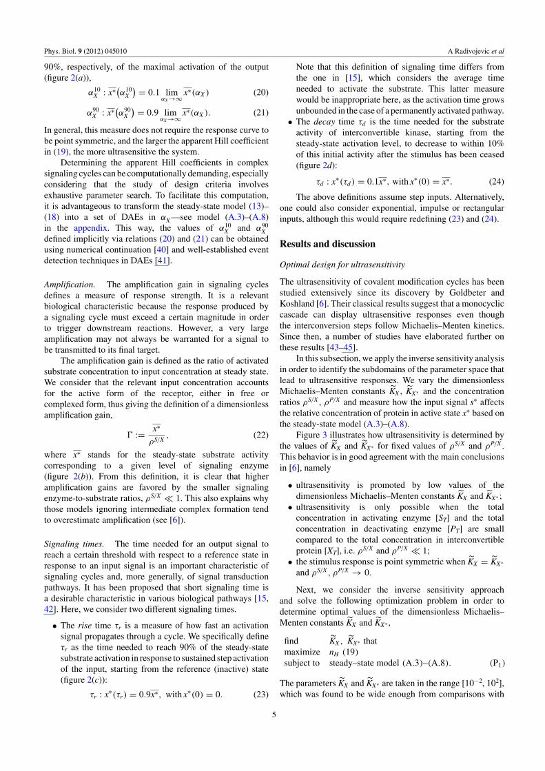
Figure 5. Design for minimal signaling times subject to given amplification. Optimal rise time τr (a and b) and decay time τd (c and d),corresponding kinetic parameters aX , aX∗ , dX , dX∗ , kX (middle plots) and Hill coefficient nH (right plots) versus amplification gain, for theconcentration ratio regime ρS/X = ρP/X = 10−2 (a and c) and concentration ratio regime ρS/X = ρP/X = 10−1 (b and d).

parameter ranges as [10−2, 102], which again led to essentiallythe same trade-offs and minor differences in signaling times.

Figure 5 (left plots) displays the optimal signaling timesas a function of the amplification gain �, for two differentregimes of concentration ratios ρS/X = ρP/X = 10−2 andρS/X = ρP/X = 10−1. Qualitatively, the optimization resultsappear to be very similar in both regimes. The feasible rangeof amplification gains is much wider with the lower valuesof concentration ratios—as expected from the relative gaindefinition in (22). The rise time τr (figures 5(a) and (b)) firstincreases monotonically with � for low amplification. Beyonda certain amplification threshold, the rise time then decreasesmonotonically with �, thus indicating that the system canrespond faster while achieving higher levels of amplification.This amplification threshold depends on the concentrationratios ρS/X and ρP/X ; it is close to � ≈ 40 in the operatingregime ρS/X = ρP/X = 10−2 (figure 5(a)) and around � ≈3.3 in the regime ρS/X = ρP/X = 10−1 (figure 5(b)). On theother hand, the decay time τd (figures 5(c) and (d)) increaseslinearly with the amplification gain �. This is due to the fact

that higher amplification leads to higher concentrations inactivated protein form, which in turn takes more time to returnto inactive state. Moreover, higher concentration ratios ρS/X

and ρP/X lead to lower maximal possible levels of free activeprotein and, consequently, decay times are almost ten timesshorter in the regime ρS/X = ρP/X = 10−1 compared to theregime ρS/X = ρP/X = 10−2 (figures 5(b), (d) versus (a), (c)).Such nonlinear relationships between various design criteriademonstrate the need for systematic optimization methods toanalyze signaling pathways in a comprehensive manner.

In order to better understand these relationships, figure 5(middle plots) displays the optimal kinetic parameter valuesaX , aX∗ , dX , dX∗ , kX leading to minimal signaling times as afunction of the amplification gain �. Both dissociation rateconstants dX and kX of the kinase complex X : S∗ into xand x∗, respectively, stay at their upper bounds and the rateconstant dX∗ of the phosphatase complex X∗ : P into x∗

remains at its lower bound in all cases and regardless ofthe amplification level �. Particularly counter-intuitive is thefinding that minimum response times are not achieved when

7

Phys. Biol. 9 (2012) 045010 A Radivojevic et al

the rate of formation aX of the kinase complex X : S∗ ismaximum, which suggests that faster signal propagation withamplification is promoted by a more unstable complex X : S∗.These findings are in good agreement with the computationalresults for a covalent modification cycle obtained in [34]. It isalso observed that higher levels of amplification together withshorter rise and decay times are achieved for an increasingvalue of the complex formation rate constant aX , whichsuggests that aX is the primary determining parameter forminimal signaling times under amplification constraints.

Nevertheless, signaling cycles so designed do not promotehigh ultrasensitivity as seen from figure 5 (right plots). Thisis because the constraints imposed on the kinetic parameterscorrespond to the values of KX and KX∗ at which the Hillcoefficient is no larger than nH ≈ 2. It is therefore critical totake the ultrasensitivity criterion into account simultaneouslywith the response time and amplification criteria in analyzingthe design of signaling cycles.

Optimal design for signaling times under amplification andultrasensitivity constraints

The ability of monocyclic cascades to achieve a high Hillcoefficient for small values of the Michaelis–Menten constantsis one of the most basic findings since their early studyin the 1980s [6]. But with such a design, the system mayexhibit excessively long response times as well as low signalamplification. In this subsection, we investigate whether asimple covalent modification cycle can simultaneously achievefast signaling, high amplification and high ultrasensitivity.

A previous analysis has underpinned the strongdependence of ultrasensitivity with respect to the parametersKX and KX∗ , which are themselves functions of the dynamicmodel parameters,

dX + kX

aX= KX and

dX∗ + 1

aX∗= KX∗ . (25)

Incorporating an ultrasensitivity objective in the optimizationproblems (P2) and (P3) can be done in either one of the twoways.

(1) Optimize the steady-state and transient kinetic parametersjointly and enforce constraints (25) directly. This requiresaccounting for both the transient model (7)–(12) andthe steady-state model (A.3)–(A.8) in the optimizationproblem.

(2) Optimize the transient kinetic parameters only, whileenforcing an ultrasensitivity target indirectly via fixingthe Michaelis–Menten constants to the values κX , κX∗

as

dX + kX − κX aX = 0 (26)

dX∗ + 1 − κX∗ aX∗ = 0. (27)

This no longer requires the steady-state model (A.3)–(A.8)in the optimization problem and, besides, the foregoingconstraints (26) and (27) are linear.

The second approach is considered next. Note that thereremains flexibility in the choice of the kinetic parametersafter enforcing constraints (26) and (27)—three remaining

degrees of freedom out of five, thereby leaving significantfreedom for optimization. As previously, separate optimizationformulations are considered for minimizing the rise time τr (P4)and the decay time τd (P5),

find aX , aX∗ , dX , dX∗ , kX thatminimize rise time τr (23)

subject to amplification gain � (22)

target nH (26)−(27)

transient model (7)−(12) (P4)

and

find aX , aX∗ , dX , dX∗ , kX

minimize decay time τd (24)

subject to amplification gain � (22)

target nH (26)−(27)

transient model (7)−(12). (P5)

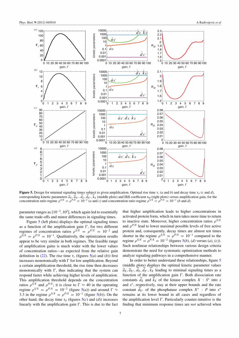
The Michaelis–Menten constant κX∗ is set to 10−3 andthe value of κX is then chosen in order to meet adesired ultrasensitivity target nH ∈ {3, 4, 6, 8, 10, 12, 16}(see figure S2 in the supporting material available atstacks.iop.org/PhysBio/9/045010/mmedia). The influence ofthe amplification and ultrasensitivity constraints on theminimal signaling times is considered in the operating regimeρS/X = ρP/X = 10−1 and for the kinetic parametersaX , aX∗ , dX , dX∗ , kX varying in the range [10−3, 103].

Figure 6 (left plots) displays the optimal signaling times asa function of the amplification gain �. The optimal rise time τr

exhibits a non-monotonic relationship with the amplificationgain and increases with the Hill coefficient target for a constantgain. In contrast, the ultrasensitivity requirement has a limitedeffect on the design for minimal decay time τd . It is alsofound that the kinetic parameters aX and aX∗ stay at theirupper bounds and dX∗ at its lower bound in all cases. On theother hand, the optimal values of the dissociation rate constantdX of the kinase complex X : S∗ decrease significantly withincreasing nH, unlike those of the dissociation rate constant kX .This is attributed to the fact that high ultrasensitivity requiressmall values of the Michaelis–Menten constant KX —the valueof the other Michaelis–Menten constant KX∗ being fixed at10−3, which requires that dX � aX − kX according to (25).

Perhaps the most striking finding from this inversesensitivity analysis is that simple covalent modification cyclescan be designed in such a way that they achieve highamplification and high ultrasensitivity, along with relativelyshort signaling times, on the order of 10 to 100 timesthe characteristic time (kX )−1 of the dissociation of theX∗ : P complex. It has often been postulated that multiplecycles in signaling cascades are needed to achieve multipleobjectives [15], but interestingly, our results show that evena single interconvertible cycle can already meet several goalssimultaneously.

Designing flexible covalent modification cycles

Due to the inherent variability of chemical reactions andcell components, the concentration levels in cells are subjectto large fluctuations. This subsection addresses the questionwhether simple covalent modification cycles can be designed

8

Phys. Biol. 9 (2012) 045010 A Radivojevic et al

0.001

0.01

0.1

1

10

100

1000

0.1

1

10

100

1000

0.01

0.1

1

10

100

1000

0 1 2 3 4 5 6 7 8 9 0 1 2 3 4 5 6 7 8 9 0 1 2 3 4 5 6 7 8 9

0.01

0.1

1

10

100

1000

0 1 2 3 4 5 6 7 8 9

0.001

0.01

0.1

1

10

100

1000

0 1 2 3 4 5 6 7 8 9 0 1 2 3 4 5 6 7 8 9 0 1 2 3 4 5 6 7 8 9

gain, Γ gain, Γ gain, Γ

gain, Γ gain, Γ gain, Γ

d

r

d~

X

d~

X k~

X

k~

X

nH

nH

nH

nH

nH

nH

(a)

(b)

Figure 6. Design for minimal signaling rise time τr (a) and decay time τd (b) subject to given amplification and ultrasensitivity. Theamplification gain � is in the range [0,9] and the Hill coefficient is in the set nH ∈ {3, 4, 6, 8, 10, 12, 16}. The concentration ratios areρS/X = ρP/X = 10−1.

5

21

0.5 50

20

10521

200

20

10050

10

500

200

100

= 7 nH = 6

S/X

P/X

0.001

0.01

0.1

1

0.001 0.01 0.1 1

r

S/X

P/X

0.001

0.01

0.1

1

0.001 0.01 0.1 1

= 7 nH = 6d

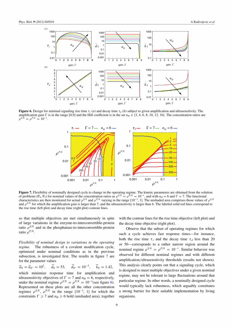
Figure 7. Flexibility of nominally designed cycle to change in the operating regime. The kinetic parameters are obtained from the solutionof problems (P4, P5) for nominal values of the concentration ratios as ρS/X = ρP/X = 10−1, and with nH = 6 and � = 7. The functionalcharacteristics are then monitored for actual ρS/X and ρP/X varying in the range [10−3, 1]. The unshaded area comprises those values of ρS/X

and ρP/X for which the amplification gain is larger than 7, and the ultrasensitivity is larger than 6. The labeled solid red lines correspond tothe rise time (left plot) and decay time (right plot) contour lines.

so that multiple objectives are met simultaneously in spiteof large variations in the enzyme-to-interconvertible-proteinratio ρS/X and in the phosphatase-to-interconvertible-proteinratio ρP/X .

Flexibility of nominal design to variations in the operatingregime. The robustness of a covalent modification cycle,optimized under nominal conditions as in the previoussubsection, is investigated first. The results in figure 7 arefor the parameter values

aX = aX∗ = 103, dX = 53, dX∗ = 10−3, kX = 1.42,

which minimize response time for amplification andultrasensitivity objectives of � = 7 and nH = 6, respectively,under the nominal regime ρS/X = ρP/X = 10−1(see figure 6).Represented on these plots are all the other concentrationregimes ρS/X , ρP/X in the range [10−3, 1] for which theconstraints � � 7 and nH � 6 hold (unshaded area), together

with the contour lines for the rise time objective (left plot) andthe decay time objective (right plot).

Observe that the subset of operating regimes for whichsuch a cycle achieves fast response times—for instance,both the rise time τ r and the decay time τ d less than 20or 50—corresponds to a rather narrow region around thenominal regime ρS/X = ρP/X = 10−1. Similar behavior wasobserved for different nominal regimes and with differentamplification/ultrasensitivity thresholds (results not shown).This analysis clearly points out that a signaling cycle, whichis designed to meet multiple objectives under a given nominalregime, may not be tolerant to large fluctuations around thatparticular regime. In other words, a nominally designed cyclewould typically lack robustness, which arguably constitutesa strong barrier for their suitable implementation by livingorganisms.

9

Phys. Biol. 9 (2012) 045010 A Radivojevic et al

= 7 nH = 6

S/X

P/X

0.001

0.01

0.1

1

0.001 0.01 0.1 1

r

S/X

P/X

0.001

0.01

0.1

1

0.001 0.01 0.1 1

= 7 nH = 6d

50 20 10 5 2 1 0.5 0.2

10

5

21

500

200

100

50

20

0.5

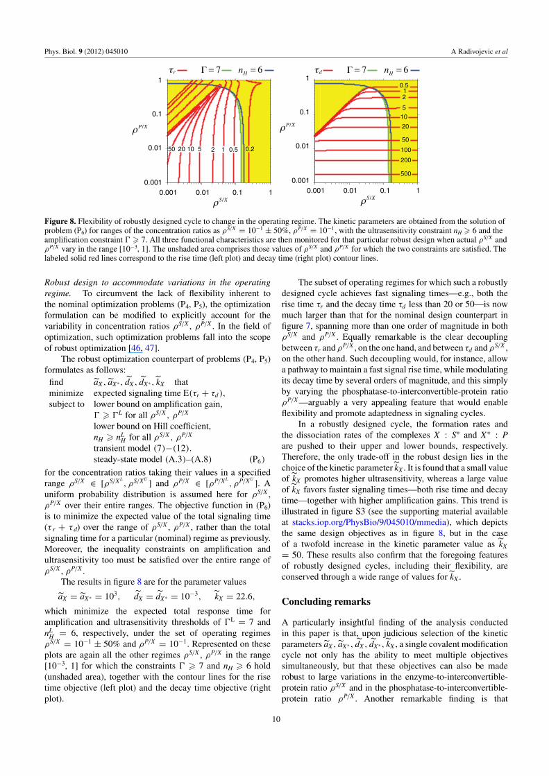
Figure 8. Flexibility of robustly designed cycle to change in the operating regime. The kinetic parameters are obtained from the solution ofproblem (P6) for ranges of the concentration ratios as ρS/X = 10−1 ± 50%, ρP/X = 10−1, with the ultrasensitivity constraint nH � 6 and theamplification constraint � � 7. All three functional characteristics are then monitored for that particular robust design when actual ρS/X andρP/X vary in the range [10−3, 1]. The unshaded area comprises those values of ρS/X and ρP/X for which the two constraints are satisfied. Thelabeled solid red lines correspond to the rise time (left plot) and decay time (right plot) contour lines.

Robust design to accommodate variations in the operatingregime. To circumvent the lack of flexibility inherent tothe nominal optimization problems (P4, P5), the optimizationformulation can be modified to explicitly account for thevariability in concentration ratios ρS/X , ρP/X . In the field ofoptimization, such optimization problems fall into the scopeof robust optimization [46, 47].

The robust optimization counterpart of problems (P4, P5)formulates as follows:find aX , aX∗ , dX , dX∗ , kX thatminimize expected signaling time E(τr + τd ),

subject to lower bound on amplification gain,� � �L for all ρS/X , ρP/X

lower bound on Hill coefficient,nH � nL

H for all ρS/X , ρP/X

transient model (7)−(12).

steady-state model (A.3)–(A.8) (P6)

for the concentration ratios taking their values in a specifiedrange ρS/X ∈ [ρS/XL

, ρS/XU] and ρP/X ∈ [ρP/XL

, ρP/XU]. A

uniform probability distribution is assumed here for ρS/X ,ρP/X over their entire ranges. The objective function in (P6)is to minimize the expected value of the total signaling time(τ r + τ d) over the range of ρS/X , ρP/X , rather than the totalsignaling time for a particular (nominal) regime as previously.Moreover, the inequality constraints on amplification andultrasensitivity too must be satisfied over the entire range ofρS/X , ρP/X .

The results in figure 8 are for the parameter values

aX = aX∗ = 103, dX = dX∗ = 10−3, kX = 22.6,

which minimize the expected total response time foramplification and ultrasensitivity thresholds of �L = 7 andnL

H = 6, respectively, under the set of operating regimesρS/X = 10−1 ± 50% and ρP/X = 10−1. Represented on theseplots are again all the other regimes ρS/X , ρP/X in the range[10−3, 1] for which the constraints � � 7 and nH � 6 hold(unshaded area), together with the contour lines for the risetime objective (left plot) and the decay time objective (rightplot).

The subset of operating regimes for which such a robustlydesigned cycle achieves fast signaling times—e.g., both therise time τr and the decay time τd less than 20 or 50—is nowmuch larger than that for the nominal design counterpart infigure 7, spanning more than one order of magnitude in bothρS/X and ρP/X . Equally remarkable is the clear decouplingbetween τr and ρP/X , on the one hand, and between τd and ρS/X ,on the other hand. Such decoupling would, for instance, allowa pathway to maintain a fast signal rise time, while modulatingits decay time by several orders of magnitude, and this simplyby varying the phosphatase-to-interconvertible-protein ratioρP/X —arguably a very appealing feature that would enableflexibility and promote adaptedness in signaling cycles.

In a robustly designed cycle, the formation rates andthe dissociation rates of the complexes X : S∗ and X∗ : Pare pushed to their upper and lower bounds, respectively.Therefore, the only trade-off in the robust design lies in thechoice of the kinetic parameter kX . It is found that a small valueof kX promotes higher ultrasensitivity, whereas a large valueof kX favors faster signaling times—both rise time and decaytime—together with higher amplification gains. This trend isillustrated in figure S3 (see the supporting material availableat stacks.iop.org/PhysBio/9/045010/mmedia), which depictsthe same design objectives as in figure 8, but in the caseof a twofold increase in the kinetic parameter value as kX

= 50. These results also confirm that the foregoing featuresof robustly designed cycles, including their flexibility, areconserved through a wide range of values for kX .

Concluding remarks

A particularly insightful finding of the analysis conductedin this paper is that, upon judicious selection of the kineticparameters aX , aX∗ , dX , dX∗ , kX , a single covalent modificationcycle not only has the ability to meet multiple objectivessimultaneously, but that these objectives can also be maderobust to large variations in the enzyme-to-interconvertible-protein ratio ρS/X and in the phosphatase-to-interconvertible-protein ratio ρP/X . Another remarkable finding is that

10

Phys. Biol. 9 (2012) 045010 A Radivojevic et al

the responsiveness of a robustly designed cycle—both itsrise time and decay time—can be modulated simply viaincreasing or decreasing ρS/X and ρP/X , while maintaininghigh ultrasensitivity and amplification gains. Such featuresof signaling cycles give them the ability to perform varioussignaling functions robustly and make them versatile andadaptable. In particular, this analysis could help explain whysignaling cycles are so ubiquitous in cell signaling.

This study also shows that optimization, and morespecifically robust optimization, is particularly well suitedfor studying signaling pathways and generating hypothesesregarding their underlying design principles. Although focusedon covalent modification cycles, there are no conceptualbarriers toward the application of the same methodology tomore complex signaling pathways, such as multi-level MAPKcascades or JAK-Stat pathways.

Appendix. Mathematical formulations of dynamicoptimization problems

For the dynamic model, we use the compact notation

F(ξ (τ ), ξ (τ ), p, r) = 0, (A.1)

where the vector of state variables is ξ :={x∗ s {x : s∗} {x∗ : p}}T , the vector of kinetic pa-rameters is p : = (aX aX∗ dX dX∗ kX )T and the vector ofconcentration ratios is r : = (ρS/X ρP/X )T.

In the same manner, the steady-state model is representedas

G(ξ , αX , q, r) = 0 (A.2)

with the vector of steady-state model parameters q : =(KX KX∗ )T.

In order to use a continuation approach [40], the steady-state equations (13)–(15) are differentiated with respect to αX ,

0 =•

{x : s∗}(αX ) + KX

(KX + x)2(

•x∗(αX )

+ ρS/X•

{x : s∗}(αX ) + ρP/X•

{x∗ : p}(αX )) (A.3)

0 =•

{x∗ : p}(αX ) − KX∗

(KX∗ + x∗)2

•x∗(αX ) (A.4)

0 =•

{x∗ : p}(αX ) − αX

•{x : s∗}(αX ) − {x : s∗} (A.5)

1 = x + x∗ + ρS/X {x : s∗} + ρP/X {x∗ : p} (A.6)

1 = s∗ + {x : s∗} (A.7)

1 = p + {x∗ : p}. (A.8)

The mathematical formulation of the optimization problem(P1), where the objective is to maximize ultrasensitivity subjectto the steady-state model (A.3)–(A.8), reads

maxq,α10

X ,α90X

nH = ln(81)

ln(α90X ) − (α10

X )(P1)

subject to∂G∂ξ

ξ (αX ) + ∂G∂αX

= 0,

0 � αX � α∞X , G(ξ (0), 0, q, r) = 0,

x∗(α10X ) = 0.1x∗(α∞

X ), x∗(α90X ) = 0.9x∗(α∞

X ),

0 � α10X � α90

X � α∞X , 10−2 � q � 102.

As noted, the initial conditions ξ (0) are determined fromG(ξ (0), 0, q, r) = 0. Equations (A.7) and (A.8) give x

∗(0) =

{x∗:p}(0) = 0 and p(0) = 1; the remaining initial concentrations

x(0), s∗(0) and {x:s

∗}(0) depend on the kinetic constant KX andthe concentration ratio ρS/X only and are given by

0 = x(0)2 + (KX + ρS/X − 1)x(0) − KX (A.9)

{x : s∗}(0) = 1 − x(0)

ρS/X(A.10)

s∗(0) = 1 − 1 − x(0)

ρS/X. (A.11)

The forward and backward step inputs in the transient studiesrequire two different formulations of the fraction of inactivereceptor as

s :={

1,

0,

τ � 0τ > 0,

(A.12)

and

s :={

0,

1,

τ � 0τ > 0.

(A.13)

Moreover, the activation/deactivation of the receptor isassumed to occur under very fast kinetics (i.e. v = 1000)and is modeled as

ds

dτ= −vs, (A.14)

andds

dτ= vs∗. (A.15)

We append (A.12) and (A.14) to the transient model whenanalyzing signaling rise time and (A.13) and (A.15) whenanalyzing signaling decay time.

The optimization problems (P2) and (P3) determine thekinetic parameter values that minimize the signaling times(the rise time τr and the decay time τd , respectively), subjectto a fixed amplification constraint �,

minp,τr

τr (P2)

subject to Fr(ξ (τ ), ξ (τ ), p, r) = 0,

0 � τ � τ∞, ξ (0) = ξr0 ,

x∗(τr) − 0.9x∗(τ∞) = 0,

�ρS/X − x∗(τ∞) = 0,

10−3 � p � 103,

and

minp,τd

τd (P3)

subject to Fd(ξ (τ ), ξ (τ ), p, r) = 0,

0 � τ � τ∞, ξ (0) = ξd0 ,

x∗(τd ) − 0.1x∗(τ∞) = 0,

�ρS/X − x∗(0) = 0,

10−3 � p � 103,

The previous optimization formulations are then extendedto include additional constraints. The goal of the resultingoptimization problems (P4) and (P5) is to determine the kinetic

11

Phys. Biol. 9 (2012) 045010 A Radivojevic et al

parameter values that minimize the signaling times, subject togiven amplification and ultrasensitivity thresholds,

minp,τr

τr (P4)

subject to Fr(ξ (τ ), ξ (τ ), p, r) = 0,

0 � τ � τ∞, ξ (0) = ξr0 ,

x∗(τr) − 0.9x∗(τ∞) = 0,

�ρS/X − x∗(τ∞) = 0,

dX + kX − κX aX = 0,

dX∗ + 1 − κX∗ aX∗ = 0,

10−3 � p � 103.

andminp,τd

τd (P5)

subject to Fd(ξ (τ ), ξ (τ ), p, r) = 0,

0 � τ � τ∞, ξ (0) = ξd0 ,

x∗(τd ) − 0.1x∗(τ∞) = 0,

�ρS/X − x∗(0) = 0,

dX + kX − κX aX = 0,

dX∗ + 1 − κX∗ aX∗ = 0,

10−3 � p � 103.

To account for the inherent variability of the concentrationratios r, we use a robust optimization framework. Theoptimization problem (P6) determines the kinetic parametervalues that minimize the expected signal propagation times,subject to lower bounds on amplification and ultrasensitivity,

minp,τr,τd ,q,α10

X ,α90X

∫ rU

rL

[τr(r) + τd (r)] dr (P6)

subject to Fr(ξ (τ ), ξ (τ ), p, r) = 0,

0 � τ � τ∞, ξ (0) = ξr0 ,

x∗r (τr) − 0.9x∗

r (τ∞) = 0,

Fd(ξ (τ ), ξ (τ ), p, r) = 0,

0 � τ � τ∞, ξ (0) = ξd0 ,

x∗d(τd ) − 0.1x∗

d (τ∞) = 0,

x∗r (τ

∞)

ρS/X� �L,∀r ∈ [rL, rU ],

∂G∂ξ

ξ (αX ) + ∂G∂αX

= 0,

0 � αX � α∞X , G(ξ (0), 0, q, r) = 0

x∗(α10X ) = 0.1x∗(α∞

X ), x∗(α90X ) = 0.9x∗(α∞

X ),

KX = dX + kX

aX, KX∗ = dX∗ + 1

aX∗,

ln(81)

ln(α90X ) − ln(α90

X )� nL

H ,∀r ∈ [rL, rU

],

0 � τr, τd � τ∞, 0 � α10X � α90

X � α∞X ,

10−3 � p � 103, 10−2 � q � 102.

Problems (P1)–(P5) are dynamic optimization problems. Thegoal of dynamic optimization (DO) is to find the optimalinput parameters and/or profiles of a dynamic system.Optimality is defined as the minimization or maximization ofan objective function, subject to specified constraints. Part ofthese constraints are given in the form of differential equations.

We solve these problems using the sequential methodof dynamic optimization. The NLP subproblems are solvedwith the SQP solver SNOPT [48]. We have used the solver

DSL48S [49], which is part of DAEPACK [50] and forsolving the initial-value problems (IVPs) in DAEs. Thispackage is well suited for large-scale problems. DAEPACKis also used for consistent initialization and for calculatingfirst-order parametric sensitivities. Finally, all the necessarydifferentiations (of the models, the objective functions and theconstraint functions) are generated using the capabilities ofDAEPACK. In order to avoid local solutions that can be verymisleading, we systematically perform the optimization frommultiple randomly generated starting points.

Problem (P6) is a robust dynamic optimization problem.The goal of robust optimization (RO) is to search for designsand solutions that are immune to the effect of parametricuncertainty.

We solve this problem by using the so-called DAEs insideDAE approach, where the inner set of DAEs describes thesystem and the outer set describes the uncertainty [51].

References

[1] Widmann C, Gibson S, Jarpe M B and Johnson G L 1999Mitogen-activated protein kinase: conservation of athree-kinase module from yeast to human Physiol. Rev.79 143–80

[2] Sebolt-Leopold J S and Herrera R 2004 Targeting themitogen-activated protein kinase cascade to treat cancerNature Rev. Cancer 4 937–47

[3] Vayttaden S J, Ajay S M and Bhalla U S 2004 A spectrum ofmodels of signaling pathways Chem. Biochem. 5 1365–74

[4] Klipp E and Liebermeister W 2006 Mathematical modeling ofintracellular signaling pathways BMC Neurosci. 7 S10

[5] Kiel C, Yus E and Serrano L 2010 Engineering signaltransduction pathways Cell 140 33–47

[6] Goldbeter A and Koshland D E Jr 1981 An amplifiedsensitivity arising from covalent modification in biologicalsystems Proc. Natl Acad. Sci. USA 78 6840–4

[7] Huang C Y and Ferrell J E Jr 1996 Ultrasensitivity in themitogen-activated protein kinase cascade Proc. Natl Acad.Sci. USA 93 10078–83

[8] Bhalla U and Iyengar R 1999 Emergent properties of networksof biological signaling pathways Science 283 381–7

[9] Ferrell J E Jr 2002 Self-perpetuating states in signaltransduction: positive feedback, double-negative feedbackand bistability Curr. Opin. Cell. Biol. 14 140–8

[10] Angeli D, Ferrell J E Jr and Sontag E D 2004 Detection ofmultistability, bifurcations, and hysteresis in a large class ofbiological positive-feed back systems Proc. Natl Acad. Sci.USA 101 1822–7

[11] Markevich N I, Hoek J B and Kholodenko B N 2004 Signalingswitches and bistability arising from multisitephosphorylation in protein kinase cascades J. Cell Biol.164 353–9

[12] Legewie S, Schoeberl B, Bluthgen N and Herzel H 2007Competing docking interactions can bring about bistabilityin the MAPK cascade Biophys. J. 93 2279–88

[13] Kholodenko B N 2000 Negative feedback and ultrasensitivitycan bring about oscillations in the mitogen-activated proteinkinase cascades Eur. J. Biochem. 267 1583–8

[14] Qiao L, Nachbar R B, Kevrekidis I G and Shvartsman S Y2007 Bistability and oscillations in the Huang–Ferrellmodel of MAPK signaling PLoS Comput. Biol. 3 1819–26

[15] Heinrich R, Neel B G and Rapoport T A 2002 Mathematicalmodels of protein kinase signal transduction Mol. Cell.9 957–70

12

Phys. Biol. 9 (2012) 045010 A Radivojevic et al

[16] Chapman S and Asthagiri A R 2004 Resistance to signalactivation governs design features of the MAP kinasesignaling module Biotechnol. Bioeng. 85 311–22

[17] Hornberg J J, Bruggeman F J, Binder B, Geest C R, Bij deVaate A J M, Lankelma J, Heinrich R and Westerhoff H V2005 Principles behind the multifarious control of signaltransduction—ERK phosphorylation andkinase/phosphatase control FEBS J. 272 244–58

[18] Gomez-Uribe C, Verghese G C and Mirny L A 2007 Operatingregimes of signaling cycle: statics, dynamics, and noisefiltering PLoS Comput. Biol. 3 2487–97

[19] Ventura A C, Sepulchre J A and Merajver S D 2008 A hiddenfeedback in signaling cascades is revealed PLoS Comput.Biol. 4 1–14

[20] Shvartsman S Y, Coppey M and Berezhkovskii A M 2009MAPK signaling in equations and embryos Fly 3 62–7

[21] Saltelli A, Ratto M, Andres T, Campolongo F, Cariboni J,Gatelli D, Saisana M and Tarantola S 2008 GlobalSensitivity Analysis: The Primer (Chichester: Wiley)

[22] Nocedal J and Wright S J 1999 Numerical Optimization (NewYork: Springer)

[23] Zak D E, Stelling J and Doyle F J III 2005 Sensitivity analysisof oscillatory (bio)chemical systems Comput. Chem. Eng.29 663–73

[24] Schwacke J H and Voit E O 2005 Computation and analysis oftime-dependent sensitivities in generalized mass actionsystems J. Theor. Biol. 236 21–38

[25] Zi Z, Cho K H, Sung M H, Xia X, Zheng J and Sun Z 2005In silico identification of the key components and steps inIFN-γ induced JAK-STAT signaling pathway FEBS Lett.579 1101–8

[26] van Riel N A W 2006 Dynamic modelling and analysis ofbiochemical networks: mechanism-based models andmodel-based experiments Briefings Bioinform. 7 364–74

[27] Yue H, Brown M, Knowles J, Wang H, Broomhead D Sand Kell D B 2006 Insights into the behaviour of systemsbiology models from dynamic sensitivity and identifiabilityanalysis: a case study of an NF-κB signalling pathwayMol. Biosyst. 2 640–9

[28] Chen W W, Schoeberl B, Jasper P J, Niepel M, Nielsen U B,Lauffenburger D A and Sorger P K 2009 Input–outputbehavior of ErbB signaling pathways as revealed by a massaction model trained against dynamic data Mol. Syst. Biol.5 239

[29] Heinrich R, Schuster S and Holzhutter H G 1991Mathematical analysis of enzymic reaction systems usingoptimization principles Eur. J. Biochem. 201 1–21

[30] Kikuchi S 2003 Dynamic modeling of genetic networks usinggenetic algorithm and S-system Bioinformatics 19 643–50

[31] Banga J R 2008 Optimization in computational systemsbiology BMC Syst. Biol. 2 47

[32] Goh C J and Teo K L 1988 Control parametrization: a unifiedapproach to optimal control problem with generalconstraints Automatica 24 3–18

[33] Biegler L T, Cervantes A and Waechter A 2002 Advances insimultaneous strategies for dynamic process optimizationChem. Eng. Sci. 57 575–93

[34] Adiwijaya B S, Barton P I and Tidor B 2006 Biologicalnetwork design strategies: discovery through dynamicoptimization Mol. Biosyst. 2 650–9

[35] Rieger T R 2005 Mathematical modeling of the eukaryoticheat shock response and associated ultrasensitive signalingcascades PhD Thesis Northwestern University, Evanston, IL

[36] Bluthgen N, Bruggeman F J, Legewie S, Herzel H,Westerhoff H V and Kholodenko B N 2006 Effects ofsequestration on signal transduction cascades FEBS J.273 895–906

[37] Millat T, Bullinger E, Rohwer J and Wolkenhauer O 2007Approximations and their consequences for dynamicmodelling of signal transduction pathways Math. Biosci.207 40–57

[38] Liu X, Bardwell L and Nie Q 2010 A combination of multisitephosphorylation and substrate sequestration producesswitchlike responses Biophys. J. 98 1396–407

[39] Thattai M and van Oudenaarden A 2002 Attenuation of noisein ultrasensitive signaling cascades Biophys. J.82 2943–50

[40] Allgower E L and Georg K 2003 Introduction to NumericalContinuation Methods (Philadelphia, PA: SIAM)

[41] Park T and Barton P I 1996 State event location indifferential-algebraic models ACM Trans. Model. Comput.Simul. 6 137–65

[42] Asthagiri A R and Lauffenburger D A 2001 A computationalstudy of feedback effects on signal dynamics in amitogen-activated protein kinase (MAPK) pathway modelBiotechnol. Prog. 17 227–39

[43] Ferrell J E Jr 1996 Tripping the switch fantastic: how a proteinkinase cascade can convert graded inputs into switch-likeoutputs Trends Biochem. Sci. 21 460–6

[44] Legewie S, Bluthgen N and Herzel H 2005 Quantitativeanalysis of ultrasensitive responses FEBS J. 272 4071–9

[45] Buchler N E and Cross F R 2009 Protein sequestrationgenerates a flexible ultrasensitive response in a geneticnetwork Mol. Syst. Biol. 5 272

[46] Zhang Y 2007 General robust-optimization formulation fornonlinear programming J. Optim. Theory Appl.132 111–24

[47] Diehl M, Gerhard J, Marquardt W and Moenigmann M 2008Numerical solution approaches for robust nonlinear optimalcontrol problems Comput. Chem. Eng. 32 1287–300

[48] Gill P E, Murray W and Saunders M A 2005 SNOPT: an SQPalgorithm for large-scale constrained optimization SIAMRev. 48 99–131

[49] Feehery W F, Tolsma J E and Barton P I 1997 Efficientsensitivity analysis of large-scale differential-algebraicsystems Appl. Numer. Math. 25 41–54

[50] Tolsma J E and Barton P I 2000 DAEPACK: an open modelingenvironment for legacy models Ind. Eng. Chem. Res.39 1826–39

[51] Chachuat B and Barton P I 2007 Numerical simulation of aclass of PDAEs with a separation of time scales Progress InIndustrial Mathematics at ECMI 2006, Mathematics inIndustry ed L L Bonilla et al (Berlin: Springer)vol 12 pp 512–7

13