Exploration of the MSSM with non-universal Higgs masses

hep-ph/0210205

CERN–TH/2002-238

UMN–TH–2113/02

TPI–MINN–02/42

Exploration of the MSSM with Non-Universal Higgs Masses

John Ellis1, Toby Falk2, Keith A. Olive2 and Yudi Santoso2

1TH Division, CERN, Geneva, Switzerland

2Theoretical Physics Institute, University of Minnesota, Minneapolis, MN 55455, USA

Abstract

We explore the parameter space of the minimal supersymmetric extension of the Standard

Model (MSSM), allowing the soft supersymmetry-breaking masses of the Higgs multiplets,

m1,2, to be non-universal (NUHM). Compared with the constrained MSSM (CMSSM) in

which m1,2 are required to be equal to the soft supersymmetry-breaking masses m0 of the

squark and slepton masses, the Higgs mixing parameter µ and the pseudoscalar Higgs mass

mA, which are calculated in the CMSSM, are free in the NUHM model. We incorporate ac-

celerator and dark matter constraints in determining allowed regions of the (µ, mA), (µ, M2)

and (m1/2, m0) planes for selected choices of the other NUHM parameters. In the examples

studied, we find that the LSP mass cannot be reduced far below its limit in the CMSSM,

whereas mA may be as small as allowed by LEP for large tan β. We present in Appendices

details of the calculations of neutralino-slepton, chargino-slepton and neutralino-sneutrino

coannihilation needed in our exploration of the NUHM.

CERN–TH/2002-238

October 2002

1 Introduction

The hierarchy of mass scales in physics is preserved in a natural way if supersymmetric

particles weigh less than about a TeV. Many supersymmetric models conserve the quantity

R = (−1)3B+L+2S , where B is the baryon number, L the lepton number and S the spin.

If this R parity is conserved, the lightest supersymmetric particle (LSP) is expected to be

absolutely stable. The most plausible candidate for the LSP is the lightest neutralino χ,

which is a good candidate [1] for the cold dark matter (CDM) that is thought to dominate

over baryonic and hot dark matter.

In this paper, we refine and extend the many previous calculations of the relic LSP

density in the framework of the minimal supersymmetric extension of the Standard Model

(MSSM). In particular, we expand the recent analysis of the MSSM parameter space in [2],

where we allowed non-universal input soft supersymmetry-breaking scalar masses for the

Higgs multiplets. Here we explore in more detail the constraints imposed by accelerator

experiments - including searches at LEP, b → sγ and gµ − 2 - and the cosmological bound

on the LSP relic density.

Before discussing our calculations in more detail, we first review the range of the relic LSP

density that we prefer in our calculations. An important new constraint on this is provided

by data on the cosmic microwave background (CMB), which have recently been used to

obtained the following preferred 95% confidence range: ΩCDMh2 = 0.12 ± 0.04 [3]. Values

much smaller than ΩCDMh2 = 0.10 seem to be disfavoured by earlier analyses of structure

formation in the CDM framework, so we restrict our attention to ΩCDMh2 > 0.1. However,

one should note that the LSP may not constitute all the CDM, in which case ΩLSP could

be reduced below this value. On the upper side, we prefer to remain very conservative, in

particular because the upper limit on ΩLSP sets the upper limit for the sparticle mass scale.

In this paper, we use ΩCDMh2 < 0.3, while being aware that the lower part of this range

currently appears the most plausible.

The parameter space of the MSSM with non-universal soft supersymmetry-breaking

masses for the two Higgs multiplets has two additional dimensions, beyond those in the

constrained MSSM (CMSSM), in which all the soft supersymmetry-breaking scalar masses

m0 are assumed to be universal. In the CMSSM, the underlying parameters may be taken

as m0, the soft supersymmetry-breaking gaugino mass m1/2 that is also assumed to be uni-

versal, the trilinear supersymmetry-breaking parameters A0 that we set to zero at the GUT

scale in this paper, the ratio tan β of Higgs vacuum expectation values, the Higgs superpo-

tential coupling µ and the pseudoscalar Higgs boson mass mA. Two relations between these

1

parameters follow from the electroweak symmetry-breaking vacuum conditions, which are

normally used in the CMSSM to fix the values of µ (up to a sign ambiguity) and mA in

terms of the other parameters (m0, m1/2, A0, tanβ).

In the more general MSSM with non-universal Higgs masses (NUHM), the parame-

ters µ and mA become independent again [4, 5, 6]. Thus one may use the parameters

(m0, m1/2, µ, mA, A0, tan β) to parametrize this more general NUHM. The underlying theory

is likely to specify the non-universalities of the Higgs masses: mi ≡ sign(m2i )|mi/m0| :

i = 1, 2, so it is important to know how the different values of the mi map into the

(m0, m1/2, µ, mA, A0, tan β) parameter space, a point we discuss in Section 2. Furthermore,

this non-universality leads to new coannihilation processes becoming important, which are

discussed in Section 3.

We review and update in Section 4 the experimental and phenomenological constraints

on the MSSM parameter space that we use, applying them to the CMSSM. Then, in Section

5, we explore the NUHM parameter space. Previously, we gave priority to a first scan of

the extra dimensions of the parameter space, and postponed a complete discussion of the

NUHM at large tanβ. Here we also show how our results in the (µ, mA), (µ, M2) and

(m1/2, m0) planes for tan β = 10 change at larger tanβ, concentrating on the behaviour of

the relic LSP density, but also incorporating constraints on the NUHM from accelerators. In

our discussions of these planes, we emphasize the novel features not present in the CMSSM,

such as the forms of the regions in which the LSP is charged, e.g., the lighter τ , regions where

the LSP is a sneutrino ν (thus necessitating the inclusion of additional χ− ν coannihilation

processes), and the potential importance of Higgsino coannihilation processes. These are

not usually relevant in the CMSSM, where the relic LSP is usually mainly a B. Section 6

summarizes some conclusions from our analysis, including comments on the range of LSP

and pseudoscalar Higgs masses allowed in the NUHM.

The Appendices provide the information needed to reproduce our calculations of coanni-

hilation processes relevant to this NUHM analysis. In particular, Appendix A lists the MSSM

couplings we use, Appendix B extends previous results on neutralino-slepton coannihilation

to include left-right (L-R) mixing, Appendix C discusses chargino-slepton coannihilation

processes, and Appendix D concerns neutralino-sneutrino coannihilation.

2 Vacuum Conditions for Non-Universal Higgs Masses

We assume that the soft supersymmetry-breaking parameters are specified at some large

input scale MX , that may be identified with the supergravity or grand unification scale.

2

The low levels of flavour-changing neutral interactions provide good reasons to think that

sparticles with the same Standard Model quantum numbers have universal soft scalar masses,

e.g., for the eL, µL and τL. Specific grand unification models may equate the soft scalar

masses of matter sparticles with different Standard Model quantum numbers, e.g., (d, s, b)L

and (e, µ, τ)L in SU(5), and all the Standard Model matter sparticles in SO(10). However,

there are no particularly good reasons to expect that the soft supersymmetry-breaking scalar

masses of the Higgs multiplets should be equal to those of the matter sparticles. This is,

however, the assumption made in the CMSSM, which we relax in the NUHM studied here 1.

One of the attractive features of the CMSSM is that it provides a mechanism for generat-

ing electroweak symmetry breaking via the running of the effective Higgs masses-squared m21

and m22 from MX down to low energies. We use this mechanism also in the NUHM, which

enables us to relate m21(MX) and m2

2(MX) to the Higgs supermultiplet mixing parameter

µ and the pseudoscalar Higgs mass mA. Therefore, we can and do choose as our indepen-

dent parameters µ(mZ) ≡ µ and mA(Q) ≡ mA, where Q ≡ (mtRmtL

)1/2; as well as the

CMSSM parameters (m0(MX), m1/2(MX), A0, tanβ). In fact, in this paper we set A0 = 0

for definiteness.

The electroweak symmetry breaking conditions may be written in the form:

m2A(Q) = m2

1(Q) + m22(Q) + 2µ2(Q) + ∆A(Q) (1)

and

µ2 =m2

1 −m22 tan2 β + 1

2m2

Z(1− tan2 β) + ∆(1)

µ

tan2 β − 1 + ∆(2)µ

, (2)

where ∆A and ∆(1,2)µ are loop corrections [8, 9, 10] and m1,2 ≡ m1,2(mZ). We incorporate

the known radiative corrections [8, 11, 12] c1, c2 and cµ relating the values of the NUHM

parameters at Q to their values at mZ:

m21(Q) = m2

1 + c1

m22(Q) = m2

2 + c2

µ2(Q) = µ2 + cµ . (3)

Solving for m21 and m2

2, one has

m21(1 + tan2 β) = m2

A(Q) tan2 β − µ2(tan2 β + 1−∆(2)µ )− (c1 + c2 + 2cµ) tan2 β

−∆A(Q) tan2 β − 1

2m2

Z(1− tan2 β)−∆(1)µ (4)

1For models with non-universality also in the sfermion masses, see [4, 7].

3

and

m22(1 + tan2 β) = m2

A(Q)− µ2(tan2 β + 1 + ∆(2)µ )− (c1 + c2 + 2cµ)

−∆A(Q) +1

2m2

Z(1− tan2 β) + ∆(1)

µ , (5)

which we use to perform our numerical calculations.

It can be seen from (4) and (5) that, if mA is too small or µ is too large, then m21 and/or

m22 can become negative and large. This could lead to m2

1(MX) + µ2(MX) < 0 and/or

m22(MX) + µ2(MX) < 0, thus triggering electroweak symmetry breaking at the GUT scale.

The requirement that electroweak symmetry breaking occurs far below the GUT scale forces

us to impose the conditions m21(MX) + µ(MX), m2

2(MX) + µ(MX) > 0 as extra constraints,

which we call the GUT stability constraint 2.

Specific models for the origin of supersymmetry breaking should be able to predict the

amounts by which universality is violated in m21,2, which can be read off immediately from

(4, 5). Alternatively, for a given amount of universality breaking, these equations may easily

be inverted to yield the corresponding values of µ and mA. In this paper, we plot quantities

in terms of µ and mA.

In the CMSSM, to obtain a consistent low energy model given GUT scale inputs, we

must run down the full set of renormalization group equations (RGE’s) from the GUT scale

and use the electroweak symmetry breaking constraints which fix µ and mA. Consistency

requires the RGE’s to be run back up to the GUT scale, where the input parameters are

reset and the RGE’s are run back down. Many models require running this cycle about 3

times, though in some cases convergence may be much slower, particularly at large tan β.

Indeed, there are no solutions for µ < 0 when tanβ is large (>∼ 40) because of diverging

Yukawas. In the NUHM case considered here, we have boundary conditions at both the

GUT and low-energy scales. Once again, the numerical calculations of the RGE’s must be

iterated until they converge. However, in this case, it is not always possible to arrive at

a solution, especially for large tan β. In our subsequent calculations, we start by making

guesses for the values of m1,2(MX) for use in the first run from MX down to mZ , and it can

happen that the iteration pushes the solution away from the convergence point instead of

towards it. Therefore, the first few iterations must be monitored for any potential blow-ups.

2For a different point of view, however, see [13].

4

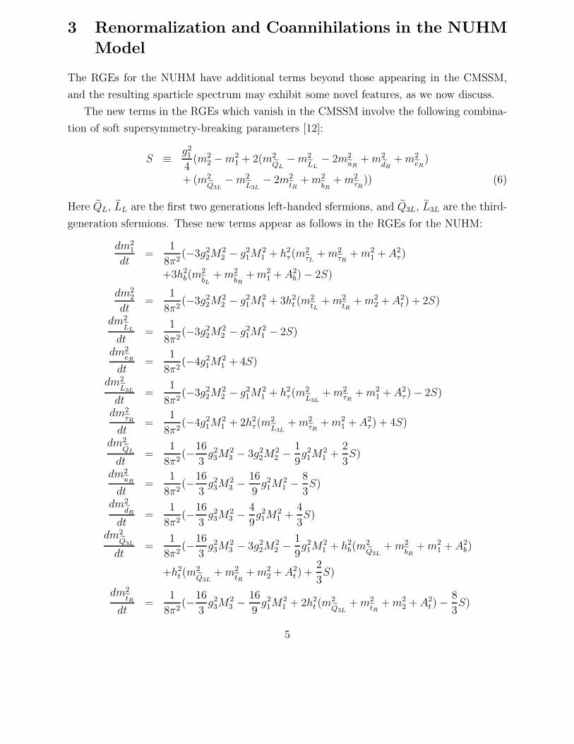
3 Renormalization and Coannihilations in the NUHM

Model

The RGEs for the NUHM have additional terms beyond those appearing in the CMSSM,

and the resulting sparticle spectrum may exhibit some novel features, as we now discuss.

The new terms in the RGEs which vanish in the CMSSM involve the following combina-

tion of soft supersymmetry-breaking parameters [12]:

S ≡ g21

4(m2

2 −m21 + 2(m2

QL−m2

LL− 2m2

uR+ m2

dR+ m2

eR)

+ (m2Q3L

−m2L3L

− 2m2tR

+ m2

bR+ m2

τR)) (6)

Here QL, LL are the first two generations left-handed sfermions, and Q3L, L3L are the third-

generation sfermions. These new terms appear as follows in the RGEs for the NUHM:

dm21

dt=

1

8π2(−3g2

2M22 − g2

1M21 + h2

τ (m2τL

+ m2τR

+ m21 + A2

τ )

+3h2b(m

2

bL+ m2

bR+ m2

1 + A2b)− 2S)

dm22

dt=

1

8π2(−3g2

2M22 − g2

1M21 + 3h2

t (m2tL

+ m2tR

+ m22 + A2

t ) + 2S)

dm2LL

dt=

1

8π2(−3g2

2M22 − g2

1M21 − 2S)

dm2eR

dt=

1

8π2(−4g2

1M21 + 4S)

dm2L3L

dt=

1

8π2(−3g2

2M22 − g2

1M21 + h2

τ (m2L3L

+ m2τR

+ m21 + A2

τ )− 2S)

dm2τR

dt=

1

8π2(−4g2

1M21 + 2h2

τ (m2L3L

+ m2τR

+ m21 + A2

τ ) + 4S)

dm2QL

dt=

1

8π2(−16

3g23M

23 − 3g2

2M22 −

1

9g21M

21 +

2

3S)

dm2uR

dt=

1

8π2(−16

3g23M

23 −

16

9g21M

21 −

8

3S)

dm2dR

dt=

1

8π2(−16

3g23M

23 −

4

9g21M

21 +

4

3S)

dm2Q3L

dt=

1

8π2(−16

3g23M

23 − 3g2

2M22 −

1

9g21M

21 + h2

b(m2Q3L

+ m2

bR+ m2

1 + A2b)

+h2t (m

2Q3L

+ m2tR

+ m22 + A2

t ) +2

3S)

dm2tR

dt=

1

8π2(−16

3g23M

23 −

16

9g21M

21 + 2h2

t (m2Q3L

+ m2tR

+ m22 + A2

t )−8

3S)

5

dm2

bR

dt=

1

8π2(−16

3g23M

23 −

4

9g21M

21 + 2h2

b(m2Q3L

+ m2

bR+ m2

1 + A2b) +

4

3S) (7)

where the M1,2,3 are gaugino masses that we assume to be universal at the GUT scale.

In the CMSSM, with all scalar masses set equal to m0 at the GUT scale, S = 0 initially

and remains zero at any scale [14], since S = 0 is a fixed point of the RGEs at the one-loop

level. However, in the NUHM, with m1 6= m2, as seen in Eq. (6) S 6= 0 and can cause the

low-energy NUHM spectrum to differ significantly from that in the CMSSM. For example,

if S < 0 the left-handed slepton can be lighter than the right-handed one. Also, m21 and m2

2

appear in the Yukawa parts of the RGEs for the third generation (Eq. (7)), so NUHM initial

conditions may cause their spectrum to differ from that in the CMSSM. In the NUHM case,

depending on the parameters, we may find the LSP to be either (i) the lightest neutralino

χ, (ii) the lighter stau τ1, (iii) the right-handed selectron eR and smuon µR3, (iv) the left-

handed selectron eL and smuon µL, (v) the electron and muon sneutrinos νe,µ, (vi) the tau

sneutrino ντ , or (vii) one of the squarks, especially the stop and the sbottom 4. Note that

in the cases that we consider here, the νe,µ are generally lighter than the ντ in the regions

in which they are the LSP (that is, when m21 < 0, cf. Eq. (7) and Fig. 2 of ref. [2]), unless

mA is very large (>∼ 1000 GeV).

We assume that R parity is conserved, so that the LSP is stable and is present in the

Universe today as a relic from the Big Bang. Searches for anomalous heavy isotopes tell

us that the dark matter should be weakly-interacting and neutral, and therefore eliminate

all but the neutralino and the sneutrinos as possible LSPs. LEP and direct dark-matter

searches together exclude a sneutrino LSP [15], at least if the majority of the CDM is the

LSP. Thus we require in our analysis that the lightest neutralino be the LSP.

Nevertheless there are new coannihilation processes to be considered when one or more

of these ‘wannabe’ LSPs is almost degenerate with the lightest neutralino. These include

χ − τ1, χ − eL − µL, χ − eR − µR, χ − νe,µ, χ − χ′ − χ± coannihilations and all possible

combinations 5. However, not all of these combinations are important as they are significant

only in very small regions for a particular set of parameters. For this reason we do not

include, for example, the sneutrino-slepton coannihilation in our calculations.

We include in our subsequent calculations neutralino-slepton χ − ˜ [17, 7, 18], χ − χ′ −3We neglect left-right (L-R) mixing for the first two generations of sfermions, so the right-handed selectron

and smuon are degenerate. Here and elsewhere, by ‘right-handed’ sfermion we mean the superpartner ofright-handed fermion.

4A squark LSP is possible only if |A0| is large, a possibility we do not study in this paper.5Again, because we set A0 = 0 here, squark coannihilations are not important, but see [16] for a calculation

of neutralino-stop coannihilation.

6

χ± [19], χ − νe,µ, χ′ − ˜ and χ± − ˜ coannihilations6. The χ′ (co)annihilation rates can

be derived from the corresponding χ (co)annihilations by appropriate mass and coupling

replacements. Details of our calculations are given in the Appendices. Following a summary

of the relevant couplings in Appendix A, in Appendix B we update the neutralino-slepton

coannihilation calculation of [17] to include L-R mixing. These are not very important at

relatively low tanβ but are potentially important for large values of tanβ. These improved

coannihilation calculations were in fact already used in [21], but no details were given there.

Appendix C provides chargino-slepton coannihilation processes, whilst Appendix D deals

with neutralino-sneutrino coannihilation processes.

4 Summary of Constraints and Review of the CMSSM

Parameter Space

We impose in our analysis the constraints on the MSSM parameter space that are provided

by direct sparticle searches at LEP, including that on the lightest chargino χ±: mχ± >∼ 103.5

GeV [22], and that on the selectron e: me>∼ 99 GeV [23]. Another important constraint is

provided by the LEP lower limit on the Higgs mass: mH > 114.4 GeV [24] in the Standard

Model7. The lightest Higgs boson h in the general MSSM must obey a similar limit, which

may in principle be relaxed for larger tanβ. However, as we discussed in our previous

analysis of the NUHM [2], the relaxation in the LEP limit is not relevant in the regions of

MSSM parameter space of interest to us. We recall that mh is sensitive to sparticle masses,

particularly mt, via loop corrections [25, 26], implying that the LEP Higgs limit constrains

the MSSM parameters.

We also impose the constraint imposed by measurements of b → sγ [27], BR(B →Xsγ) = (3.11 ± 0.42 ± 0.21) × 10−4, which agree with the Standard Model calculation

BR(B → Xsγ)SM = (3.29± 0.33)× 10−4 [28]. We recall that the b → sγ constraint is more

important for µ < 0, but it is also relevant for µ > 0, particularly when tanβ is large, as we

see again in this paper.

We also take into account the latest value of the anomalous magnetic moment of the

muon reported [29] by the BNL E821 experiment. The world average of aµ ≡ 12(gµ − 2)

now deviates by (33.9 ± 11.2) × 10−10 from the Standard Model calculation of [30] using

e+e− data, and by (17 ± 11)× 10−10 from the Standard Model calculation of [30] based on

6See [20] for recent work which includes all coannihilation channels.7In view of the theoretical uncertainty in calculating mh, we apply this bound with three significant

digits, i.e., our figures use the constraint mh > 114 GeV.

7

τ decay data. Other recent analyses of the e+e− data yield similar results. On some of

the subsequent plots, we display the formal 2-σ range 11.5 × 10−10 < δaµ < 56.3 × 10−10.

However, in view of the chequered theoretical history of the Standard Model calculations of

aµ, we do not impose this as an absolute constraint on the supersymmetric parameter space.

As a standard of comparison for our NUHM analysis, we first consider the impacts of the

above constraints on the parameter space of the CMSSM, in which the soft supersymmetry-

breaking Higgs scalar masses are assumed to be universal at the input scale. In this case, as

mentioned in the Introduction, one may use the parameters (m1/2, m0, A0, tanβ) and the sign

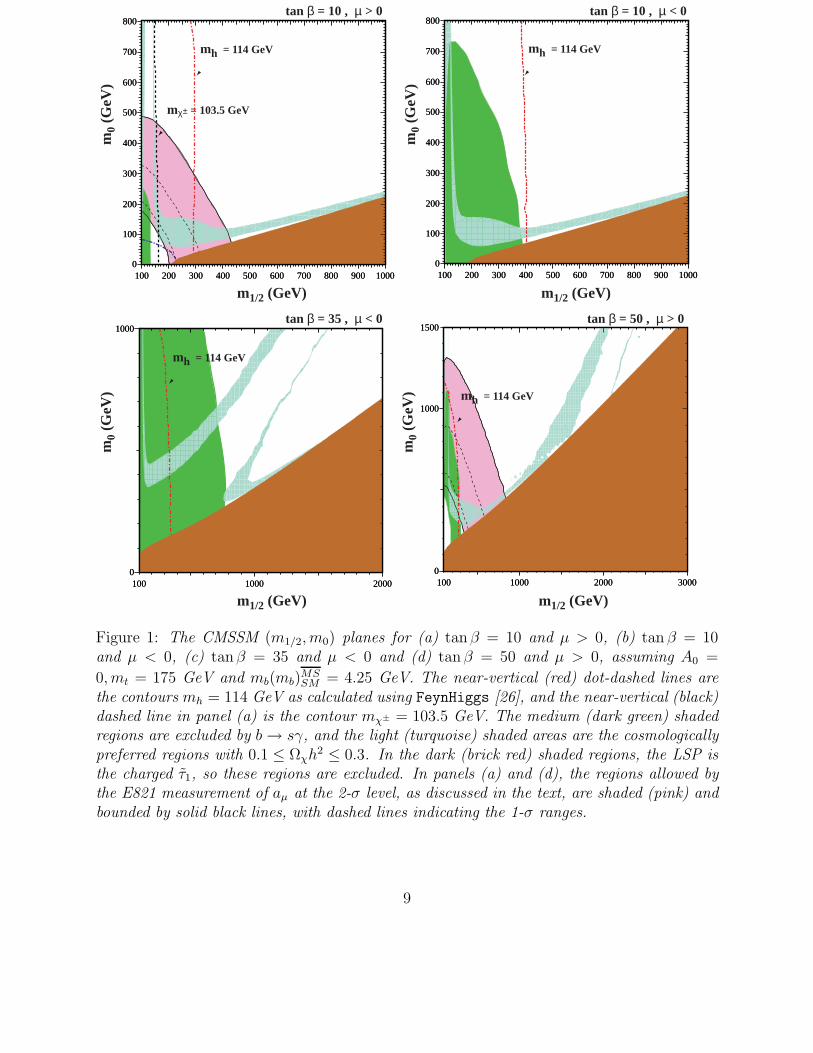
of µ. We assume for simplicity that A0 = 0, and plot in Fig. 1 the (m1/2, m0) planes for certain

choices of tanβ and the sign of µ. These plots are similar to those published previously [31],

but differ in using the latest version of FeynHiggs [26] and the latest information on aµ

discussed above.

The shadings and lines in Fig. 1 are as follows. The dark (brick red) shaded regions have

a charged LSP, i.e. τ1, so these regions are excluded. The b → sγ exclusion is presented

by the medium (dark green) shaded regions. The light (turquoise) shaded areas are the

cosmologically preferred regions with 0.1 ≤ Ωχh2 ≤ 0.3. The regions allowed by the E821

measurement of aµ at the 2-σ level, 11.5 × 10−10 < δaµ < 56.3 × 10−10, are shaded (pink)

and bounded by solid black lines. Only panel (a) and (d) have regions allowed by aµ. The

near-vertical (red) dot-dashed lines are the contours mh = 114 GeV, and the near-vertical

(black) dashed line in panel (a) is the contour mχ± = 103.5 GeV (though we do not plot

this constraint in panels (b,c,d), the position of the chargino contour would be very similar).

Regions on the left of these lines are excluded.

We see in panel (a) of Fig. 1 for tanβ = 10 and µ > 0 that all the experimental constraints

are compatible with the CMSSM for m1/2 ∼ 300 to 400 GeV and m0 ∼ 100 GeV, with larger

values of m1/2 also being allowed if one relaxes the aµ condition. In the case of tan β = 10

and µ < 0 shown in panel (b) of Fig. 1, valid only if one discards the aµ condition, the mh and

b → sγ constraints both require m1/2 >∼ 400 GeV and m0 >∼ 100 GeV. In the case tan β = 35

and µ < 0 shown in panel (c) of Fig. 1, the b → sγ constraint is much stronger than the mh

constraint, and imposes m1/2 >∼ 700 GeV, with the Ωχh2 constraint then allowing bands of

parameter space emanating from m0 ∼ 600, 300 GeV. Finally, in panel (d) for tanβ = 50

and µ > 0, we see again that the mh and b → sγ constraints are almost equally important,

imposing m1/2 >∼ 300 GeV for m0 ∼ 400 GeV. As in the case of panel (a), there is again a

region compatible with the aµ constraint, extending in this case as far as m1/2 ∼ 800 GeV

and m0 ∼ 500 GeV.

8

100 200 300 400 500 600 700 800 900 10000

100

200

300

400

500

600

700

800

100 200 300 400 500 600 700 800 900 10000

100

200

300

400

500

600

700

800

mh = 114 GeV

m0

(GeV

)

m1/2 (GeV)

tan β = 10 , µ > 0

mχ± = 103.5 GeV

100 200 300 400 500 600 700 800 900 10000

100

200

300

400

500

600

700

800

100 200 300 400 500 600 700 800 900 10000

100

200

300

400

500

600

700

800

mh = 114 GeV

m0

(GeV

)

m1/2 (GeV)

tan β = 10 , µ < 0

100 1000 20000

1000

100 1000 20000

1000

m0

(GeV

)

m1/2 (GeV)

tan β = 35 , µ < 0

mh = 114 GeV

100 1000 2000 30000

1000

1500

100 1000 2000 30000

1000

1500

mh = 114 GeVm

0 (G

eV)

m1/2 (GeV)

tan β = 50 , µ > 0

Figure 1: The CMSSM (m1/2, m0) planes for (a) tanβ = 10 and µ > 0, (b) tan β = 10and µ < 0, (c) tanβ = 35 and µ < 0 and (d) tanβ = 50 and µ > 0, assuming A0 =

0, mt = 175 GeV and mb(mb)MSSM = 4.25 GeV. The near-vertical (red) dot-dashed lines are

the contours mh = 114 GeV as calculated using FeynHiggs [26], and the near-vertical (black)dashed line in panel (a) is the contour mχ± = 103.5 GeV. The medium (dark green) shadedregions are excluded by b → sγ, and the light (turquoise) shaded areas are the cosmologicallypreferred regions with 0.1 ≤ Ωχh2 ≤ 0.3. In the dark (brick red) shaded regions, the LSP isthe charged τ1, so these regions are excluded. In panels (a) and (d), the regions allowed bythe E821 measurement of aµ at the 2-σ level, as discussed in the text, are shaded (pink) andbounded by solid black lines, with dashed lines indicating the 1-σ ranges.

9

5 Exploration of the NUHM Parameter Space

Following our discussion of the CMSSM parameter space in the previous Section, we now

discuss how that analysis changes in the NUHM. We extend our previous analysis [2] in two

ways: (i) fixing tanβ = 10 and µ > 0, but choosing different values of µ and mA, rather

than assuming the CMSSM values, and (ii) varying tanβ for representative fixed values of µ

and mA. We make such selections for three projections of the NUHM, onto the (m1/2, m0)

plane, the (µ, mA) plane and the (µ, M2) plane.

5.1 The (m1/2, m0) Plane

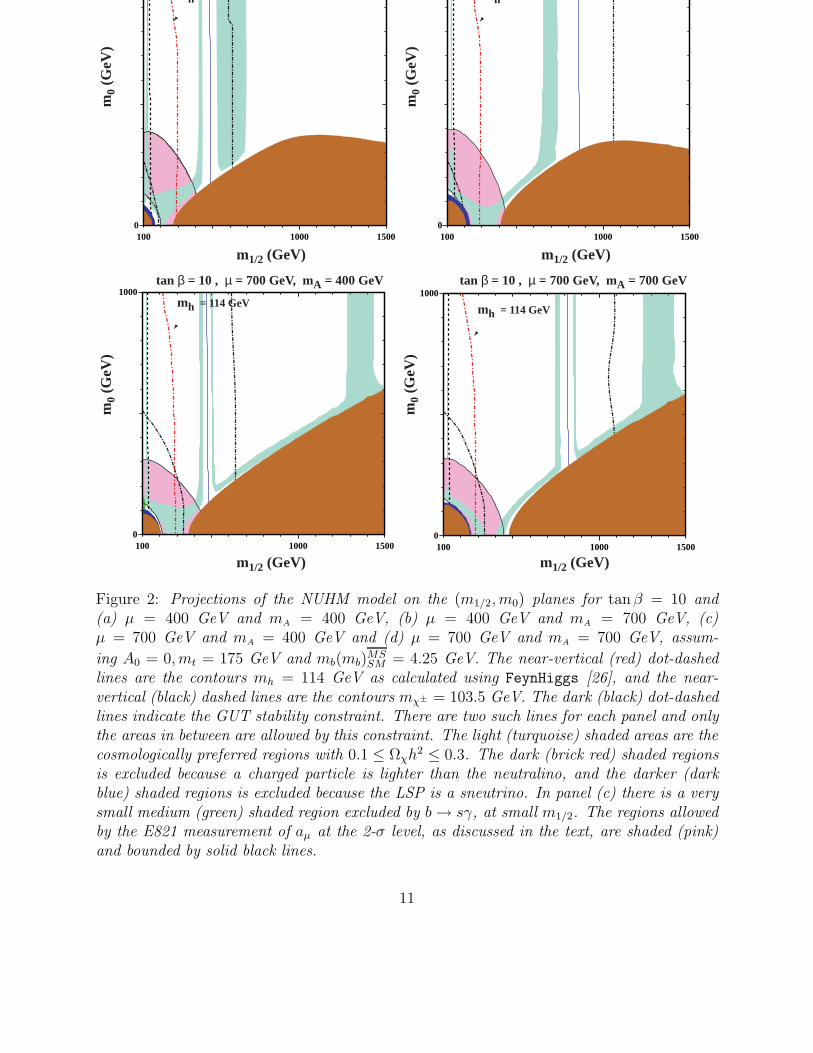
Panel (a) of Fig. 2 shows the (m1/2, m0) plane for tan β = 10 and the particular choice µ =

400 GeV and mA = 400 GeV, assuming A0 = 0, mt = 175 GeV and mb(mb)MSSM = 4.25 GeV as

usual. Again as usual, the light (turquoise) shaded area is the cosmologically preferred region

with 0.1 ≤ Ωχh2 ≤ 0.3. There is a bulk region satisfying this preference at m1/2 ∼ 50 GeV to

350 GeV, m0 ∼ 50 GeV to 150 GeV. The dark (red) shaded regions are excluded because a

charged sparticle is lighter than the neutralino. As in the CMSSM shown in Fig. 1, the τ1 is

the LSP in the bigger area at larger m1/2, and there are light (turquoise) shaded strips close

to these forbidden regions where coannihilation suppresses the relic density sufficiently to

be cosmologically acceptable. Further away from these regions, the relic density is generally

too high. However, for larger m1/2 there is another suppression, discussed below, which

makes the relic density too low. At small m1/2 and m0 the left handed sleptons, and also the

sneutrinos, become lighter than the neutralino. The darker (dark blue) shaded area is where

a sneutrino is the LSP. Within these excluded regions there are also areas with tachyonic

sparticles.

The near-vertical dark (black) dashed and light (red) dot-dashed lines in Fig. 2 are the

LEP exclusion contours mχ± > 104 GeV and mh > 114 GeV respectively. As in the CMSSM

case, they exclude low values of m1/2, and hence rule out rapid relic annihilation via direct-

channel h and Z0 poles. The solid lines curved around small values of m1/2 and m0 bound

the light (pink) shaded region favoured by aµ and recent analyses of the e+e− data.

A striking feature in Fig. 2(a) when m1/2 ∼ 500 GeV is a strip with low Ωχh2, which

has bands with acceptable relic density on either side. The low-Ωχh2 strip is due to rapid

annihilation via the direct-channel A, H poles which occur when mχ = mA/2 = 200 GeV,

indicated by the near-vertical solid (blue) line. Analogous rapid-annihilation strips have

been noticed previously in the CMSSM [32, 21], but at larger tanβ as seen in Fig. 1. There,

they are diagonal in the (m1/2, m0) plane, reflecting a CMSSM link between m0 and mA

10

100 1000 15000

m0

(GeV

)

m1/2 (GeV)

h

100 1000 15000

m0

(GeV

)

m1/2 (GeV)

h GeV

100 1000 15000

1000

m0

(GeV

)

m1/2 (GeV)

tan β = 10 , µ = 700 GeV, mA = 400 GeV

mh = 114 GeV

100 1000 15000

1000

m0

(GeV

)

m1/2 (GeV)

tan β = 10 , µ = 700 GeV, mA = 700 GeV

mh = 114 GeV

Figure 2: Projections of the NUHM model on the (m1/2, m0) planes for tanβ = 10 and(a) µ = 400 GeV and mA = 400 GeV, (b) µ = 400 GeV and mA = 700 GeV, (c)µ = 700 GeV and mA = 400 GeV and (d) µ = 700 GeV and mA = 700 GeV, assum-

ing A0 = 0, mt = 175 GeV and mb(mb)MSSM = 4.25 GeV. The near-vertical (red) dot-dashed

lines are the contours mh = 114 GeV as calculated using FeynHiggs [26], and the near-vertical (black) dashed lines are the contours mχ± = 103.5 GeV. The dark (black) dot-dashedlines indicate the GUT stability constraint. There are two such lines for each panel and onlythe areas in between are allowed by this constraint. The light (turquoise) shaded areas are thecosmologically preferred regions with 0.1 ≤ Ωχh2 ≤ 0.3. The dark (brick red) shaded regionsis excluded because a charged particle is lighter than the neutralino, and the darker (darkblue) shaded regions is excluded because the LSP is a sneutrino. In panel (c) there is a verysmall medium (green) shaded region excluded by b → sγ, at small m1/2. The regions allowedby the E821 measurement of aµ at the 2-σ level, as discussed in the text, are shaded (pink)and bounded by solid black lines.

11

that is absent in our implementation of the NUHM. The right-hand band in Fig. 2(a) with

acceptable Ωχh2 is broadened because the neutralino acquires significant Higgsino content,

and the relic density is suppressed by the increased W+W− production. Hereafter, we

will call this the ‘transition’ band, which in this case is incidentally coincident with the

right-hand rapid annihilation band 8. As m1/2 increases, the neutralino becomes almost

degenerate with the second lightest neutralino and the lighter chargino, and the χ−χ′−χ±

coannihilation processes eventually push Ωχh2 < 0.1 when m1/2 >∼ 700 GeV. We note that

chargino-slepton coannihilation processes become important at the junction between the

vertical bands in Fig. 2(a) and the neutralino-slepton coannihilation strip that parallels the

mχ = mτ1boundary of the forbidden (red) charged-LSP region.

There are two dark (black) dash-dotted lines in Fig. 2(a) that indicate where scalar

squared masses become negative at the input GUT scale for one of the Higgs multiplets,

specifically when either (m1(MX)2 + µ(MX)2) < 0 or (m2(MX)2 + µ(MX)2) < 0. One of

these GUT stability lines is near-vertical at m1/2 ∼ 600 GeV, and the other is a curved line

at m1/2 ∼ 150 GeV, m0 ∼ 200 GeV. We take the point of view that regions outside either of

these lines are excluded, because the preferred electroweak vacuum should be energetically

favoured and not bypassed early in the evolution of the Universe, but a different point of

view is argued in [13].

Thus, combining all the constraints, the allowed regions are those between the mh line

at m1/2 ∼ 300 GeV and the stability line at m1/2 ∼ 600 GeV, which include two rapid-

annihilation bands, some of the transition band and the junction between the bulk and

coannihilation regions around m1/2 ∼ 350 GeV, m0 ∼ 150 GeV. If one incorporates also the

putative aµ constraint, only the latter region survives. We note however, that if the τ data

were used in the g− 2 analysis, the constraint from aµ only excludes the lower left corner of

the plane and large values of m1/2 and m0 survive at the 2σ level.

Panel (b) of Fig. 2 is for µ = 400 GeV and mA = 700 GeV. We notice immediately that

the heavy Higgs pole and the right-hand boundary of the GUT stability region move out

to larger m1/2 ∼ 850, 1050 GeV, respectively, as one would expect for larger mA. At this

value of mA, the transition strip and and the rapid annihilation (‘funnel’) strip are separate.

However the latter would be to the right of the transition strip and hence the Ωχh2 bands on

both sides of the rapid-annihilation strip that was prominent in panel (a) have disappeared,

8As the neutralino acquires more Higgsino content, annihilation to W+W− production increases, whilstfermion-pair production decreases (except for tt). Around m1/2 ∼ 625 GeV, there is a threshold for hA, hHproduction, which decreases Ωχh2 to ∼ 0.08, not far below the preferred range. However, the decrease infermion production quickly raises Ωχh2 again for larger m1/2. There is a very narrow stripe with Ωχh2 < 0.1of width δm1/2 ∼ 2 GeV, which is not shown in the figure due to problems of resolution.

12

due to enhanced chargino-neutralino coannihilation effects. Panel (b) has the interesting

feature that there is a region of m1/2 ∼ 300 to 400 GeV where m0 = 0 is allowed. As

discussed in [33] this possibility, which would be favoured in some specific no-scale models of

supersymmetry breaking, is disallowed in the CMSSM. The small-m0 region is even favoured

in this variant of the NUHM by the putative aµ constraint.

Panel (c) of Fig. 2 is for µ = 700 GeV and mA = 400 GeV. In this case, we see that

the rapid-annihilation strip is back to m1/2 ∼ 500 GeV, reflecting the smaller value of mA,

whereas the transition band has separated off to large m1/2, reflecting the larger value of

µ. However, this band is excluded in this case by the GUT stability requirement. GUT

stability also excludes the possibility that m0 = 0. In this case, the putative aµ constraint

would restrict one to around m1/2 ∼ 400 GeV and m0 ∼ 100 GeV.

Finally, panel (d) of Fig. 2 is for µ = 700 GeV and mA = 700 GeV. In this case, the

rapid-annihilation strip has again moved to larger m1/2, related to the larger value of mA,

and the transition band at large m1/2 is again excluded by the GUT stability requirement.

The bulk region has disappeared in this panel, reflecting the fact that the values of µ and mA

here has strayed away from their values in the bulk region for the CMSSM. GUT stability no

longer excludes m0 = 0, and this possibility would be selected by the putative aµ constraint.

We now turn, in Fig. 3, to the impact of varying tan β, keeping µ = 400 GeV and

mA = 700 GeV. For convenience, panel (a) reproduces Fig. 2(b) with tan β = 10. In general

as tanβ is increased, two major trends are visible. One is for the region excluded by the

requirement that the LSP be neutral to spread up to larger values of m0, and the other is

for the aµ constraint to move out to larger values of m1/2 and m0.

Specifically, we see in panel (b) of Fig. 3 for tan β = 20 that, whereas the heavy Higgs

pole at m1/2 ∼ 850 GeV essentially does not move, the τ1 LSP and coannihilation strip lying

above the excluded charged-LSP region rise to larger m0. This has the effect of excluding

the m0 = 0 option that was present in panel (a). At low m1/2, the mh constraint is stronger

than the GUT stability and other constraints. The aµ constraint would allow a larger range

of m1/2 than in panel (a), extending up to ∼ 550 GeV.

Continuing in panel (c) of Fig. 3 to tan β = 35, we see that the minimum value of m0 has

now risen to ∼ 200 GeV. We also see that the b → sγ constraint is now important, enforcing

m1/2 > 300 GeV in the region preferred by the relic density. Because of this and the mh

constraint, the GUT stability constraint is now irrelevant at low m1/2, whereas at high m1/2

it has vanished off the screen, and is in any case also irrelevant because of chargino-neutralino

coannihilation. The aµ constraint would now allow part of the cosmological band on the left

side of the rapid-annihilation strip. These trends are strengthened in panel (d) of Fig. 3 for

13

100 1000 15000

1000

m0

(GeV

)

m1/2 (GeV)

tan β = 10 , µ = 400 GeV, mA = 700 GeV

mh = 114 GeV

100 1000 15000

1000

m0

(GeV

)

m1/2 (GeV)

tan β = 20 , µ = 400 GeV, mA = 700 GeV

mh = 114 GeV

100 1000 15000

1000

m0

(GeV

)

m1/2 (GeV)

tan β = 35 , µ = 400 GeV, mA = 700 GeV

mh = 114 GeV

100 1000 15000

1000

m0

(GeV

)

m1/2 (GeV)

tan β = 50 , µ = 400 GeV, mA = 700 GeV

mh = 114 GeV

Figure 3: The NUHM (m1/2, m0) planes for (a) tan β = 10 , (b) tanβ = 20, (c) tanβ = 35and (d) tanβ = 50, for µ = 400 GeV, mA = 700 GeV, assuming A0 = 0, mt = 175 GeV and

mb(mb)MSSM = 4.25 GeV. The shadings and line styles are the same as in Fig. 2.

14

tan β = 50, where we see that m0, m1/2 >∼ 400 GeV because of the b → sγ constraint, and

aµ would allow m0 <∼ 1100 GeV along the transition band.

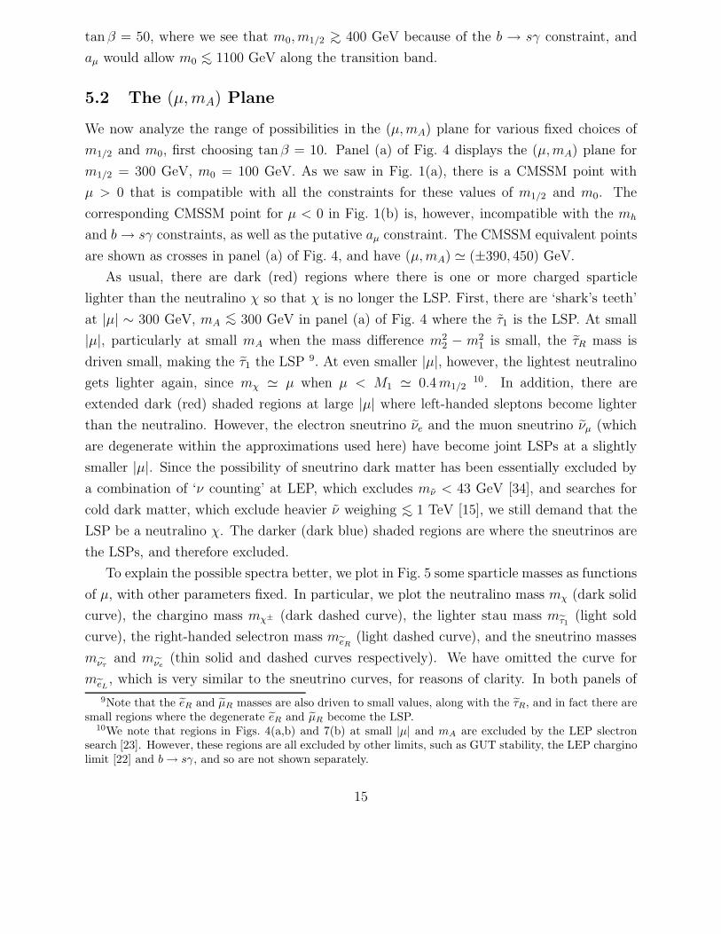
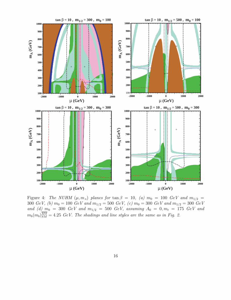
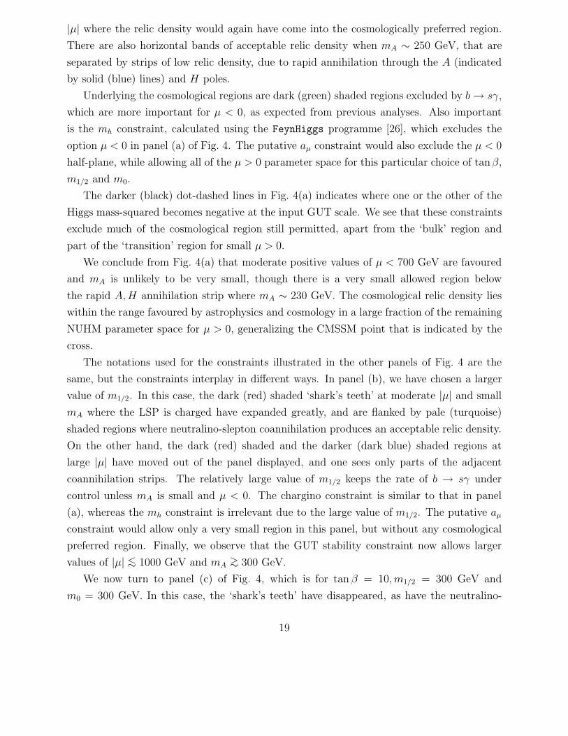
5.2 The (µ, mA) Plane

We now analyze the range of possibilities in the (µ, mA) plane for various fixed choices of

m1/2 and m0, first choosing tan β = 10. Panel (a) of Fig. 4 displays the (µ, mA) plane for

m1/2 = 300 GeV, m0 = 100 GeV. As we saw in Fig. 1(a), there is a CMSSM point with

µ > 0 that is compatible with all the constraints for these values of m1/2 and m0. The

corresponding CMSSM point for µ < 0 in Fig. 1(b) is, however, incompatible with the mh

and b → sγ constraints, as well as the putative aµ constraint. The CMSSM equivalent points

are shown as crosses in panel (a) of Fig. 4, and have (µ, mA) ' (±390, 450) GeV.

As usual, there are dark (red) regions where there is one or more charged sparticle

lighter than the neutralino χ so that χ is no longer the LSP. First, there are ‘shark’s teeth’

at |µ| ∼ 300 GeV, mA<∼ 300 GeV in panel (a) of Fig. 4 where the τ1 is the LSP. At small

|µ|, particularly at small mA when the mass difference m22 − m2

1 is small, the τR mass is

driven small, making the τ1 the LSP 9. At even smaller |µ|, however, the lightest neutralino

gets lighter again, since mχ ' µ when µ < M1 ' 0.4 m1/210. In addition, there are

extended dark (red) shaded regions at large |µ| where left-handed sleptons become lighter

than the neutralino. However, the electron sneutrino νe and the muon sneutrino νµ (which

are degenerate within the approximations used here) have become joint LSPs at a slightly

smaller |µ|. Since the possibility of sneutrino dark matter has been essentially excluded by

a combination of ‘ν counting’ at LEP, which excludes mν < 43 GeV [34], and searches for

cold dark matter, which exclude heavier ν weighing <∼ 1 TeV [15], we still demand that the

LSP be a neutralino χ. The darker (dark blue) shaded regions are where the sneutrinos are

the LSPs, and therefore excluded.

To explain the possible spectra better, we plot in Fig. 5 some sparticle masses as functions

of µ, with other parameters fixed. In particular, we plot the neutralino mass mχ (dark solid

curve), the chargino mass mχ± (dark dashed curve), the lighter stau mass mτ1(light sold

curve), the right-handed selectron mass meR(light dashed curve), and the sneutrino masses

mντand mνe

(thin solid and dashed curves respectively). We have omitted the curve for

meL, which is very similar to the sneutrino curves, for reasons of clarity. In both panels of

9Note that the eR and µR masses are also driven to small values, along with the τR, and in fact there aresmall regions where the degenerate eR and µR become the LSP.

10We note that regions in Figs. 4(a,b) and 7(b) at small |µ| and mA are excluded by the LEP slectronsearch [23]. However, these regions are all excluded by other limits, such as GUT stability, the LEP charginolimit [22] and b → sγ, and so are not shown separately.

15

-2000 -1000 0 1000 2000100

200

300

400

500

600

700

800

900

1000

mA

(G

eV)

µ (GeV)

tan β = 10 , m1/2 = 300 , m0 = 100

-2000 -1000 0 1000 2000100

200

300

400

500

600

700

800

900

1000

mA

(G

eV)

µ (GeV)

tan β = 10 , m1/2 = 500 , m0 = 100

-2000 -1000 0 1000 2000100

200

300

400

500

600

700

800

900

1000

mA

(G

eV)

µ (GeV)

tan β = 10 , m1/2 = 300 , m0 = 300

-2000 -1000 0 1000 2000100

200

300

400

500

600

700

800

900

1000

mA

(G

eV)

µ (GeV)

tan β = 10 , m1/2 = 500 , m0 = 300

Figure 4: The NUHM (µ, mA) planes for tan β = 10, (a) m0 = 100 GeV and m1/2 =300 GeV, (b) m0 = 100 GeV and m1/2 = 500 GeV, (c) m0 = 300 GeV and m1/2 = 300 GeVand (d) m0 = 300 GeV and m1/2 = 500 GeV, assuming A0 = 0, mt = 175 GeV and


16

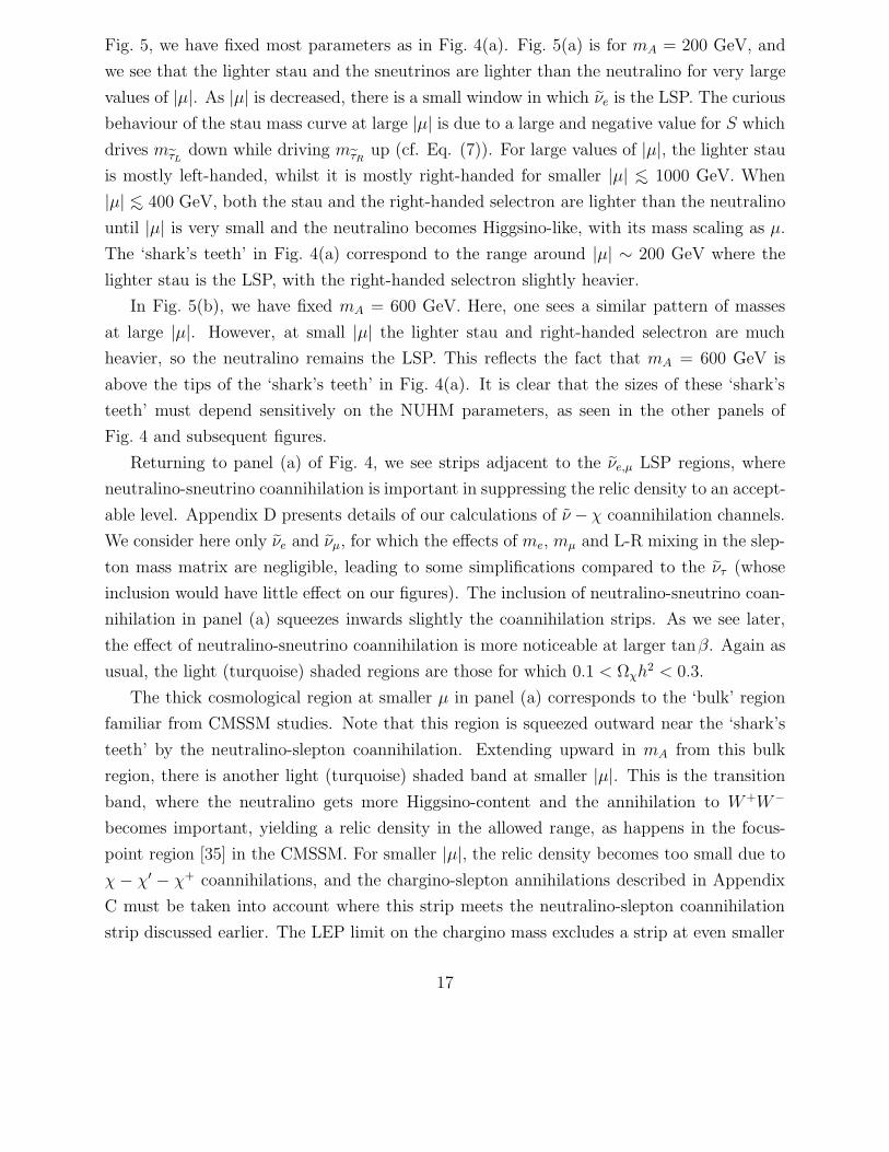
Fig. 5, we have fixed most parameters as in Fig. 4(a). Fig. 5(a) is for mA = 200 GeV, and

we see that the lighter stau and the sneutrinos are lighter than the neutralino for very large

values of |µ|. As |µ| is decreased, there is a small window in which νe is the LSP. The curious

behaviour of the stau mass curve at large |µ| is due to a large and negative value for S which

drives mτLdown while driving mτR

up (cf. Eq. (7)). For large values of |µ|, the lighter stau

is mostly left-handed, whilst it is mostly right-handed for smaller |µ| <∼ 1000 GeV. When

|µ| <∼ 400 GeV, both the stau and the right-handed selectron are lighter than the neutralino

until |µ| is very small and the neutralino becomes Higgsino-like, with its mass scaling as µ.

The ‘shark’s teeth’ in Fig. 4(a) correspond to the range around |µ| ∼ 200 GeV where the

lighter stau is the LSP, with the right-handed selectron slightly heavier.

In Fig. 5(b), we have fixed mA = 600 GeV. Here, one sees a similar pattern of masses

at large |µ|. However, at small |µ| the lighter stau and right-handed selectron are much

heavier, so the neutralino remains the LSP. This reflects the fact that mA = 600 GeV is

above the tips of the ‘shark’s teeth’ in Fig. 4(a). It is clear that the sizes of these ‘shark’s

teeth’ must depend sensitively on the NUHM parameters, as seen in the other panels of

Fig. 4 and subsequent figures.

Returning to panel (a) of Fig. 4, we see strips adjacent to the νe,µ LSP regions, where

neutralino-sneutrino coannihilation is important in suppressing the relic density to an accept-

able level. Appendix D presents details of our calculations of ν − χ coannihilation channels.

We consider here only νe and νµ, for which the effects of me, mµ and L-R mixing in the slep-

ton mass matrix are negligible, leading to some simplifications compared to the ντ (whose

inclusion would have little effect on our figures). The inclusion of neutralino-sneutrino coan-

nihilation in panel (a) squeezes inwards slightly the coannihilation strips. As we see later,

the effect of neutralino-sneutrino coannihilation is more noticeable at larger tanβ. Again as

usual, the light (turquoise) shaded regions are those for which 0.1 < Ωχh2 < 0.3.

The thick cosmological region at smaller µ in panel (a) corresponds to the ‘bulk’ region

familiar from CMSSM studies. Note that this region is squeezed outward near the ‘shark’s

teeth’ by the neutralino-slepton coannihilation. Extending upward in mA from this bulk

region, there is another light (turquoise) shaded band at smaller |µ|. This is the transition

band, where the neutralino gets more Higgsino-content and the annihilation to W+W−

becomes important, yielding a relic density in the allowed range, as happens in the focus-

point region [35] in the CMSSM. For smaller |µ|, the relic density becomes too small due to

χ − χ′ − χ+ coannihilations, and the chargino-slepton annihilations described in Appendix

C must be taken into account where this strip meets the neutralino-slepton coannihilation

strip discussed earlier. The LEP limit on the chargino mass excludes a strip at even smaller

17

0

100

200

300

400

-2000 -1000 0 1000 2000

Spar

ticl

e m

ass

µ (GeV)

mχ

mχ±

meR~

mντ~

mνe~

mτ1~

0

100

200

300

400

-2000 -1000 0 1000 2000

Spar

ticl

e m

ass

µ (GeV)

mχ

mχ±

meR~

mντ~

mνe~

mτ1~

Figure 5: The masses mχ (dark solid), mχ± (dark dashed), mτ1(light solid), meR

(lightdashed), mντ

(thin solid) and mνe(thin dashed) as functions of µ for tanβ = 10, m1/2 =

300 GeV, m0 = 100 GeV for (a) mA = 200 GeV and (b) mA = 600 GeV, assuming A0 =

0, mt = 175 GeV and mb(mb)MSSM = 4.25 GeV.

18

|µ| where the relic density would again have come into the cosmologically preferred region.

There are also horizontal bands of acceptable relic density when mA ∼ 250 GeV, that are

separated by strips of low relic density, due to rapid annihilation through the A (indicated

by solid (blue) lines) and H poles.

Underlying the cosmological regions are dark (green) shaded regions excluded by b → sγ,

which are more important for µ < 0, as expected from previous analyses. Also important

is the mh constraint, calculated using the FeynHiggs programme [26], which excludes the

option µ < 0 in panel (a) of Fig. 4. The putative aµ constraint would also exclude the µ < 0

half-plane, while allowing all of the µ > 0 parameter space for this particular choice of tanβ,

m1/2 and m0.

The darker (black) dot-dashed lines in Fig. 4(a) indicates where one or the other of the

Higgs mass-squared becomes negative at the input GUT scale. We see that these constraints

exclude much of the cosmological region still permitted, apart from the ‘bulk’ region and

part of the ‘transition’ region for small µ > 0.

We conclude from Fig. 4(a) that moderate positive values of µ < 700 GeV are favoured

and mA is unlikely to be very small, though there is a very small allowed region below

the rapid A, H annihilation strip where mA ∼ 230 GeV. The cosmological relic density lies

within the range favoured by astrophysics and cosmology in a large fraction of the remaining

NUHM parameter space for µ > 0, generalizing the CMSSM point that is indicated by the

cross.

The notations used for the constraints illustrated in the other panels of Fig. 4 are the

same, but the constraints interplay in different ways. In panel (b), we have chosen a larger

value of m1/2. In this case, the dark (red) shaded ‘shark’s teeth’ at moderate |µ| and small

mA where the LSP is charged have expanded greatly, and are flanked by pale (turquoise)

shaded regions where neutralino-slepton coannihilation produces an acceptable relic density.

On the other hand, the dark (red) shaded and the darker (dark blue) shaded regions at

large |µ| have moved out of the panel displayed, and one sees only parts of the adjacent

coannihilation strips. The relatively large value of m1/2 keeps the rate of b → sγ under

control unless mA is small and µ < 0. The chargino constraint is similar to that in panel

(a), whereas the mh constraint is irrelevant due to the large value of m1/2. The putative aµ

constraint would allow only a very small region in this panel, but without any cosmological

preferred region. Finally, we observe that the GUT stability constraint now allows larger

values of |µ| <∼ 1000 GeV and mA>∼ 300 GeV.

We now turn to panel (c) of Fig. 4, which is for tan β = 10, m1/2 = 300 GeV and

m0 = 300 GeV. In this case, the ‘shark’s teeth’ have disappeared, as have the neutralino-

19

slepton strips at large |µ| (due to the large value of m0). Negative values of µ are excluded

by mh and partially by b → sγ, as well as by the putative aµ constraint, which would permit

a strip with µ > 0. GUT stability enforces µ <∼ 800 GeV, and also provides a lower limit

on mA that is irrelevant because of the other constraints. In contrast, in panel (d) of Fig. 4

for m1/2 = 500 GeV and m0 = 300 GeV, we see a similar ‘cruciform’ pattern for the regions

allowed by cosmology, but b → sγ has only rather limited impact for µ < 0 and mh is

irrelevant: there is no region consistent with the putative aµ constraint. In this case, mA

could be as small as the ∼ 200 GeV allowed by the GUT stability constraint, and |µ| could

be as large as ∼ 1100 GeV.

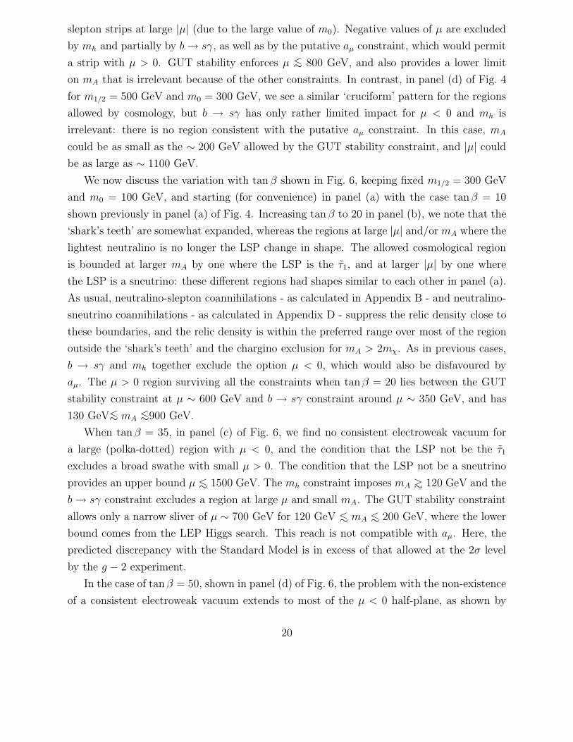
We now discuss the variation with tan β shown in Fig. 6, keeping fixed m1/2 = 300 GeV

and m0 = 100 GeV, and starting (for convenience) in panel (a) with the case tanβ = 10

shown previously in panel (a) of Fig. 4. Increasing tanβ to 20 in panel (b), we note that the

‘shark’s teeth’ are somewhat expanded, whereas the regions at large |µ| and/or mA where the

lightest neutralino is no longer the LSP change in shape. The allowed cosmological region

is bounded at larger mA by one where the LSP is the τ1, and at larger |µ| by one where

the LSP is a sneutrino: these different regions had shapes similar to each other in panel (a).

As usual, neutralino-slepton coannihilations - as calculated in Appendix B - and neutralino-

sneutrino coannihilations - as calculated in Appendix D - suppress the relic density close to

these boundaries, and the relic density is within the preferred range over most of the region

outside the ‘shark’s teeth’ and the chargino exclusion for mA > 2mχ. As in previous cases,

b → sγ and mh together exclude the option µ < 0, which would also be disfavoured by

aµ. The µ > 0 region surviving all the constraints when tanβ = 20 lies between the GUT

stability constraint at µ ∼ 600 GeV and b → sγ constraint around µ ∼ 350 GeV, and has

130 GeV<∼ mA<∼900 GeV.

When tanβ = 35, in panel (c) of Fig. 6, we find no consistent electroweak vacuum for

a large (polka-dotted) region with µ < 0, and the condition that the LSP not be the τ1

excludes a broad swathe with small µ > 0. The condition that the LSP not be a sneutrino

provides an upper bound µ <∼ 1500 GeV. The mh constraint imposes mA >∼ 120 GeV and the

b → sγ constraint excludes a region at large µ and small mA. The GUT stability constraint

allows only a narrow sliver of µ ∼ 700 GeV for 120 GeV <∼ mA <∼ 200 GeV, where the lower

bound comes from the LEP Higgs search. This reach is not compatible with aµ. Here, the

predicted discrepancy with the Standard Model is in excess of that allowed at the 2σ level

by the g − 2 experiment.

In the case of tanβ = 50, shown in panel (d) of Fig. 6, the problem with the non-existence

of a consistent electroweak vacuum extends to most of the µ < 0 half-plane, as shown by

20

-2000 -1000 0 1000 2000100

200

300

400

500

600

700

800

900

1000

mA

(G

eV)

µ (GeV)

tan β = 10 , m1/2 = 300 , m0 = 100

-2000 -1000 0 1000 2000100

200

300

400

500

600

700

800

900

1000

mA

(G

eV)

µ (GeV)

tan β = 20 , m1/2 = 300 , m0 = 100

-2000 -1000 0 1000 2000100

200

300

400

500

600

700

800

900

1000

mA

(G

eV)

µ (GeV)

tan β = 35 , m1/2 = 300 , m0 = 100

yyyyyyyyyyyyyyyyyyyyyyyyyyyyyyyyyyyyyyyyyyyyyyyyyyyyyyyyyyyyyyyyyyyyyyyyyyyyyyyyyyyyyyyyyyyyyyyyyy

-2000 -1000 0 1000 2000100

200

300

400

500

600

700

800

900

1000

mA

(G

eV)

µ (GeV)

tan β = 50 , m1/2 = 300 , m0 = 100


Figure 6: The NUHM (µ, mA) planes for m0 = 100 GeV and m1/2 = 300 GeV, for (a)tan β = 10, (b) tanβ = 20, (c) tan β = 35 and (d) tanβ = 50, assuming A0 = 0, mt =

175 GeV and mb(mb)MSSM = 4.25 GeV. The shadings and line styles are the same as in Fig. 2,

and there is no consistent electroweak vacuum in the polka-dotted region.

21

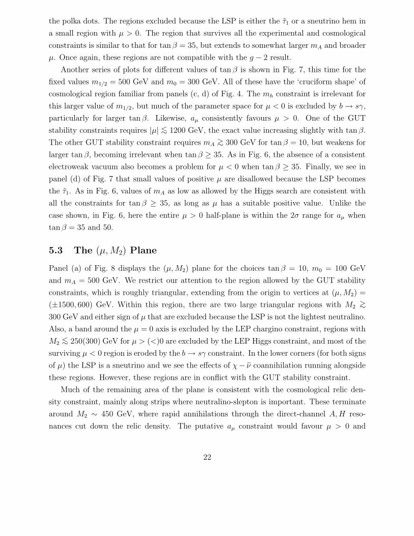
the polka dots. The regions excluded because the LSP is either the τ1 or a sneutrino hem in

a small region with µ > 0. The region that survives all the experimental and cosmological

constraints is similar to that for tanβ = 35, but extends to somewhat larger mA and broader

µ. Once again, these regions are not compatible with the g − 2 result.

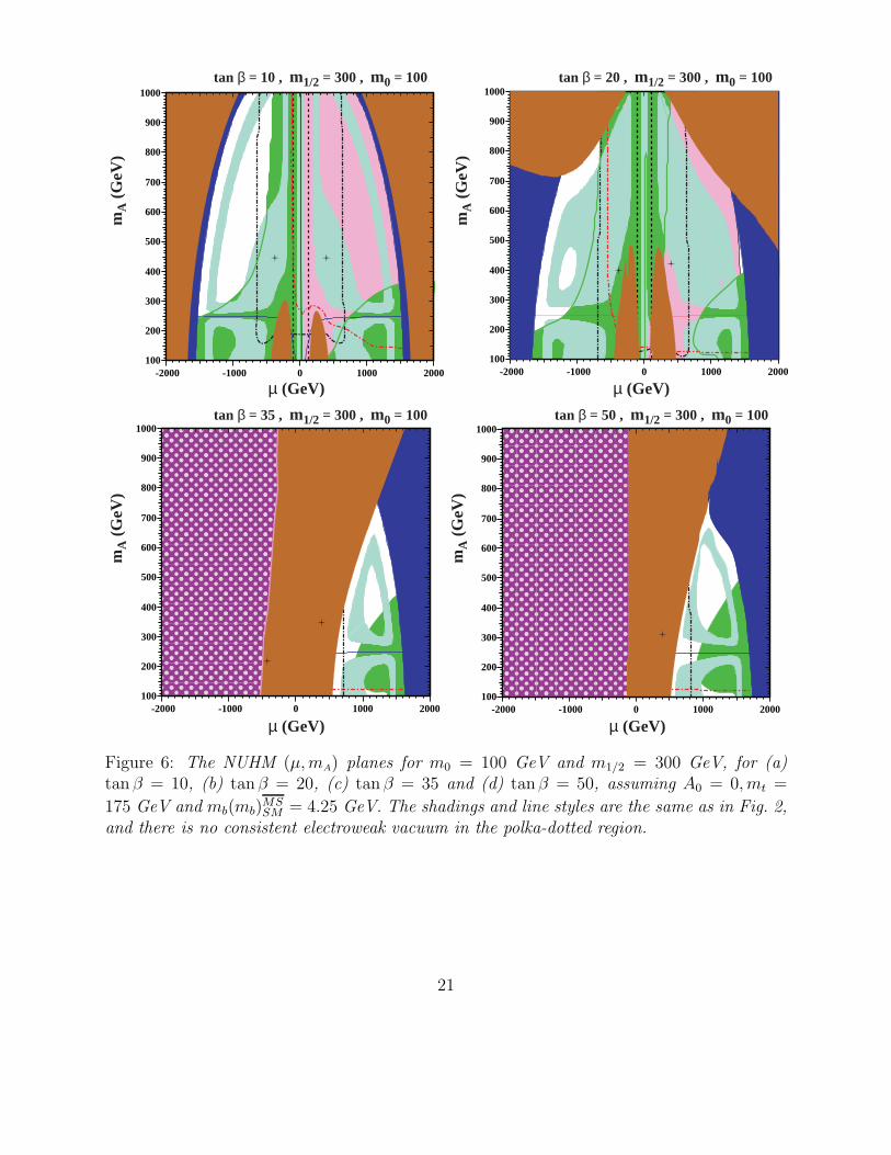
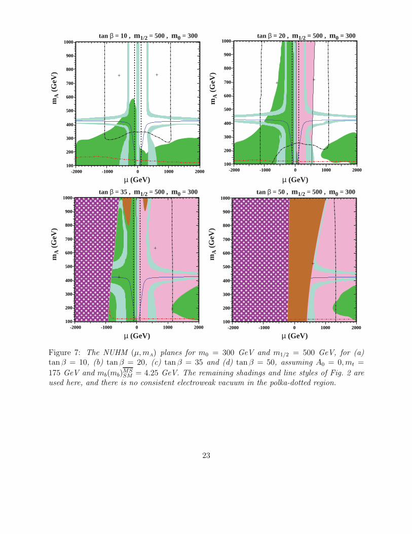
Another series of plots for different values of tan β is shown in Fig. 7, this time for the

fixed values m1/2 = 500 GeV and m0 = 300 GeV. All of these have the ‘cruciform shape’ of

cosmological region familiar from panels (c, d) of Fig. 4. The mh constraint is irrelevant for

this larger value of m1/2, but much of the parameter space for µ < 0 is excluded by b → sγ,

particularly for larger tan β. Likewise, aµ consistently favours µ > 0. One of the GUT

stability constraints requires |µ| <∼ 1200 GeV, the exact value increasing slightly with tan β.

The other GUT stability constraint requires mA>∼ 300 GeV for tanβ = 10, but weakens for

larger tan β, becoming irrelevant when tanβ ≥ 35. As in Fig. 6, the absence of a consistent

electroweak vacuum also becomes a problem for µ < 0 when tanβ ≥ 35. Finally, we see in

panel (d) of Fig. 7 that small values of positive µ are disallowed because the LSP becomes

the τ1. As in Fig. 6, values of mA as low as allowed by the Higgs search are consistent with

all the constraints for tan β ≥ 35, as long as µ has a suitable positive value. Unlike the

case shown, in Fig. 6, here the entire µ > 0 half-plane is within the 2σ range for aµ when

tan β = 35 and 50.

5.3 The (µ, M2) Plane

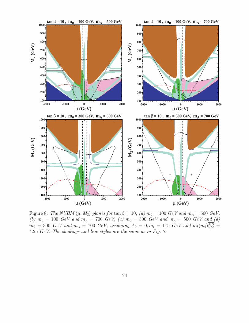
Panel (a) of Fig. 8 displays the (µ, M2) plane for the choices tan β = 10, m0 = 100 GeV

and mA = 500 GeV. We restrict our attention to the region allowed by the GUT stability

constraints, which is roughly triangular, extending from the origin to vertices at (µ, M2) =

(±1500, 600) GeV. Within this region, there are two large triangular regions with M2>∼

300 GeV and either sign of µ that are excluded because the LSP is not the lightest neutralino.

Also, a band around the µ = 0 axis is excluded by the LEP chargino constraint, regions with

M2<∼ 250(300) GeV for µ > (<)0 are excluded by the LEP Higgs constraint, and most of the

surviving µ < 0 region is eroded by the b → sγ constraint. In the lower corners (for both signs

of µ) the LSP is a sneutrino and we see the effects of χ− ν coannihilation running alongside

these regions. However, these regions are in conflict with the GUT stability constraint.

Much of the remaining area of the plane is consistent with the cosmological relic den-

sity constraint, mainly along strips where neutralino-slepton is important. These terminate

around M2 ∼ 450 GeV, where rapid annihilations through the direct-channel A, H reso-

nances cut down the relic density. The putative aµ constraint would favour µ > 0 and

22

-2000 -1000 0 1000 2000100

200

300

400

500

600

700

800

900

1000

mA

(G

eV)

µ (GeV)

tan β = 10 , m1/2 = 500 , m0 = 300

-2000 -1000 0 1000 2000100

200

300

400

500

600

700

800

900

1000

mA

(G

eV)

µ (GeV)

tan β = 20 , m1/2 = 500 , m0 = 300

-2000 -1000 0 1000 2000100

200

300

400

500

600

700

800

900

1000

yyyyyyyyyyyyyyyyyyyyyyyyyyyyyyyyyyyyyyyyyyyyyyyyyyyyyyyyyyyyyyyyyyyyyyyyyyyyyyyyyyyy

mA

(G

eV)

µ (GeV)

tan β = 35 , m1/2 = 500 , m0 = 300

-2000 -1000 0 1000 2000100

200

300

400

500

600

700

800

900

1000


mA

(G

eV)

µ (GeV)

tan β = 50 , m1/2 = 500 , m0 = 300

Figure 7: The NUHM (µ, mA) planes for m0 = 300 GeV and m1/2 = 500 GeV, for (a)tan β = 10, (b) tanβ = 20, (c) tan β = 35 and (d) tanβ = 50, assuming A0 = 0, mt =

175 GeV and mb(mb)MSSM = 4.25 GeV. The remaining shadings and line styles of Fig. 2 are

used here, and there is no consistent electroweak vacuum in the polka-dotted region.

23

-2000 -1000 0 1000 2000100

200

300

400

500

600

700

800

900

1000

M2

(GeV

)

µ (GeV)

tan β = 10 , m0 = 100 GeV, mA = 500 GeV

-2000 -1000 0 1000 2000100

200

300

400

500

600

700

800

900

1000

M2

(GeV

)

µ (GeV)

tan β = 10 , m0 = 100 GeV, mA = 700 GeV

-2000 -1000 0 1000 2000100

200

300

400

500

600

700

800

900

1000

M2

(GeV

)

µ (GeV)

tan β = 10 , m0 = 300 GeV, mA = 500 GeV

-2000 -1000 0 1000 2000100

200

300

400

500

600

700

800

900

1000

M2

(GeV

)

µ (GeV)

tan β = 10 , m0 = 300 GeV, mA = 700 GeV

Figure 8: The NUHM (µ, M2) planes for tan β = 10, (a) m0 = 100 GeV and mA = 500 GeV,(b) m0 = 100 GeV and mA = 700 GeV, (c) m0 = 300 GeV and mA = 500 GeV and (d)

m0 = 300 GeV and mA = 700 GeV, assuming A0 = 0, mt = 175 GeV and mb(mb)MSSM =

4.25 GeV. The shadings and line styles are the same as in Fig. 7.

24

M2<∼ 350 GeV.

The above constraints interplay analogously in panel (b) of Fig. 8, for m0 = 100 GeV and

mA = 700 GeV. We note, however, that the GUT stability limit has risen with mA to above

800 GeV, and that the tips of the non-neutralino LSP triangles have also moved up slightly.

The neutralino-slepton coannihilation strip now extends up to M2 ∼ 640 GeV, where it is

cut off by rapid A, H annihilations. We also see the ‘transition’ band at lower M2. In fact,

this region with µ > 0 is the one favoured by all constraints including aµ.

In panel (c) of Fig. 8, for m0 = 300 GeV and mA = 500 GeV, the triangular GUT

stability region is very similar to that in panel (a), whereas the non-neutralino LSP triangles

have moved to significantly higher M2, reflecting the larger value of m0. The regions where

the cosmological relic density falls within the preferred range are now narrow strips in the

neutralino-slepton coannihilation regions, on either side of the rapid A, H annihilation strips,

and the ‘transition’ bands. This tendency towards ‘skinnier’ cosmological regions is also

apparent in panel (d), where m0 = 300 GeV and mA = 700 GeV are assumed. In both

these panels, the b → sγ constraints disfavours µ < 0 and small mA, whilst the putative aµ

constraint would favour µ > 0 and small mA.

We now explore the variation of these results with tanβ, as displayed in Fig. 9 for the

choices m0 = 100 Gev and mA = 500 GeV. Panel (a) reproduces for convenience the case

tan β = 10 that was shown also in panel (a) of Fig. 8. When tanβ = 20, as seen in panel (b)

of Fig. 9, we first notice that the GUT stability region now extends to larger M2. Next, we

observe that the triangular non-neutralino LSP regions have extended down to lower M2. As

one would expect on general grounds and from earlier plots, the mh constraint at low M2 is

weaker than in panel (a), whereas the b → sγ constraint is stronger, ruling out much of the

otherwise allowed region with µ < 0. The allowed region with µ > 0 is generally compatible

with the putative aµ constraint.

Panel (c) for tanβ = 35 again shows the feature that no consistent electroweak vacuum

is found over much of the half-plane with µ < 0. The GUT stability constraint now allows

M2<∼ 1000 GeV. The non-neutralino LSP region is no longer triangular in shape, but now

requires µ >∼ 800 GeV. This happens as the regions with light left-handed slepton at low

M2 meet with the ones with light right-handed slepton at higher M2. There is a minuscule

allowed region for µ < 0. The residual regions with relic density in the preferred range for

µ > 0 are limited to strips in the neutralino-slepton coannihilation regions, and on either

side of the rapid A, H annihilation strip. All this preferred region is compatible with the

putative aµ constraint.

A rather similar pattern is visible in panel (d) of Fig. 9 for tan β = 50. The most

25

-2000 -1000 0 1000 2000100

200

300

400

500

600

700

800

900

1000

M2

(GeV

)

µ (GeV)

tan β = 10 , m0 = 100 GeV, mA = 500 GeV

-2000 -1000 0 1000 2000100

200

300

400

500

600

700

800

900

1000

M2

(GeV

)

µ (GeV)

tan β = 20 , m0 = 100 GeV, mA = 500 GeV

-2000 -1000 0 1000 2000100

200

300

400

500

600

700

800

900

1000

M2

(GeV

)

µ (GeV)

tan β = 35 , m0 = 100 GeV, mA = 500 GeV


-2000 -1000 0 1000 2000100

200

300

400

500

600

700

800

900

1000

M2

(GeV

)

µ (GeV)

tan β = 50 , m0 = 100 GeV, mA = 500 GeV


Figure 9: The NUHM (µ, M2) planes for m0 = 100 GeV and mA = 500 GeV, for (a) tan β =10, (b) tanβ = 20, (c) tanβ = 35 and (d) tan β = 50, assuming A0 = 0, mt = 175 GeV and


26

noticeable differences are that the absence of a consistent electroweak vacuum is even more

marked for µ > 0, and that the putative aµ constraint would suggest a lower limit M2>∼

350 GeV, whereas lower values would have been permitted in panel (c) for tanβ = 35.

6 Conclusions and Open Issues

We have provided in this paper the tools needed for a detailed study of the NUHM, in the

form of complete calculations of the most important coannihilation processes. However, in

this paper we have only been able to scratch the surface of the phenomenology of the NUHM.

Even this exploratory study has shown that many new features appear compared with the

CMSSM, as results of the two additional parameters in the NUHM, but much more remains

to be studied. For example, we have not studied the NUHM with a nonzero trilinear coupling

A0. Nevertheless, some interesting preliminary conclusions about the NUHM can be drawn,

though many questions remain open.

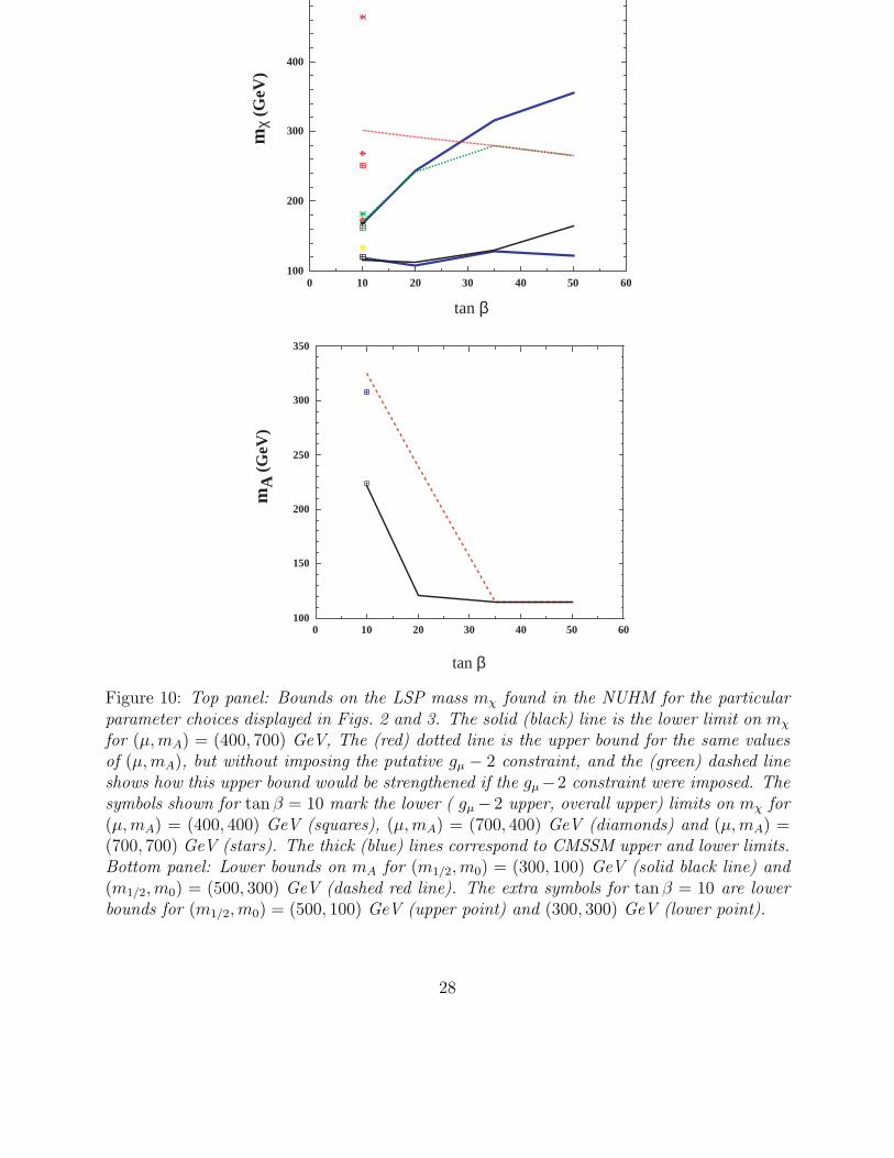
The lower limit on the LSP mass mχ in the CMSSM has been much discussed, and it is

interesting to consider whether this could be greatly reduced in the NUHM. The top panel

of Fig. 10 compiles the bounds on mχ for the various sample parameter choices explored

in this paper. We focus on the case µ > 0, which is favoured by mh and b → sγ as well

as the dubious gµ − 2 constraint. The solid (black) line connects the lower limits on mχ

for the particular choice µ = 400 GeV and mA = 700 GeV shown for the four choices of

tan β in Fig. 3. This lower limit is provided by mh for tanβ = 10, 20, but by b → sγ for

tan β = 35, 50. The CMSSM lower bound on mχ is indicated by a thick (blue) line. We see

that this CMSSM lower bound on mχ is similar to that in the NUHM when tanβ = 10, but

weaker when tanβ = 50 because of the different behaviour in the CMSSM of the b → sγ

constraint in this case.

For tan β = 10, we also indicate by different black symbols the lower bounds on mχ for

the other choices of (µ, mA) studied in Fig. 2, namely (µ, mA) = (400, 400) GeV (square),

(µ, mA) = (700, 400) GeV (diamond) and (µ, mA) = (700, 700) GeV (star). The two latter

lower bounds are significantly higher than in the default case (µ, mA) = (400, 700) GeV,

due to the impacts of the GUT stability condition and the Ωχh2 constraint, respectively.

In none of the NUHM examples studied was the lower limit on mχ relaxed compared with

the CMSSM, though this might be found possible in a more complete survey of the NUHM

parameter space.

We also show in the top panel of Fig. 10 the upper bounds on mχ found in the NUHM for

the various parameter choices explored in this paper. The (red) dot-dashed line is the upper

27

100

200

300

400

0 10 20 30 40 50 60

tan β

mχ

(GeV

)

100

150

200

250

300

350

0 10 20 30 40 50 60

tan β

mA

(GeV

)

Figure 10: Top panel: Bounds on the LSP mass mχ found in the NUHM for the particularparameter choices displayed in Figs. 2 and 3. The solid (black) line is the lower limit on mχ

for (µ, mA) = (400, 700) GeV, The (red) dotted line is the upper bound for the same valuesof (µ, mA), but without imposing the putative gµ − 2 constraint, and the (green) dashed lineshows how this upper bound would be strengthened if the gµ−2 constraint were imposed. Thesymbols shown for tan β = 10 mark the lower ( gµ− 2 upper, overall upper) limits on mχ for(µ, mA) = (400, 400) GeV (squares), (µ, mA) = (700, 400) GeV (diamonds) and (µ, mA) =(700, 700) GeV (stars). The thick (blue) lines correspond to CMSSM upper and lower limits.Bottom panel: Lower bounds on mA for (m1/2, m0) = (300, 100) GeV (solid black line) and(m1/2, m0) = (500, 300) GeV (dashed red line). The extra symbols for tanβ = 10 are lowerbounds for (m1/2, m0) = (500, 100) GeV (upper point) and (300, 300) GeV (lower point).

28

bound for µ = 400 GeV and mA = 400 GeV, as obtained without imposing the putative

gµ − 2 constraint. The upper bound on mχ is attained in the rapid-annihilation strip where

mχ < mA/2. Also shown in Fig. 10, as a (green) dashed line, is the strengthening of this

upper bound that would be found if the gµ − 2 constraint were imposed. This constraint

would not strengthen the upper limit for tanβ ≥ 35. We also show as a thick (blue) line the

CMSSM upper limit on mχ, implementing the gµ − 2 constraint. We see that it is similar

to that in the NUHM for tan β = 10, 20, but is weaker for higher tanβ. The CMSSM upper

bound would be much weaker still if the gµ − 2 constraint were relaxed, because of the

different behaviours of the rapid-annihilation strips in the NUHM and CMSSM, as seen by

comparing Figs. 1 and 3.

For tan β = 10, we also show in the top panel of Fig. 10 the upper bounds that hold with

and without gµ − 2 for the other three choices of (µ, mA) made in Fig. 2, using the same

symbols as for the lower bounds (squares, diamonds and stars, respectively). The largest

upper bound is for the choice (µ, mA) = (700, 700) GeV, for which there is an extension of

the allowed region along the coannihilation tail, extending up to the GUT stability line.

In the second panel of Fig. 10, we summarize the lower limits on mA found in the

NUHM models that we have studied. The solid (black) line is for the choice (m1/2, m0) =

(300, 100) GeV displayed previously in Fig. 7. The lower bounds shown for tanβ = 10, 20

are compatible with gµ − 2, but we find that no region would be allowed by gµ − 2 in the

cases tanβ = 35, 50, as seen in panels (c) and (d) of Fig. 7. The (red) dashed line in the

second panel of Fig. 10 is for the choice (m1/2, m0) = (500, 300) GeV shown previously in

Fig. 6. In this case, we find that no region would be allowed by gµ−2 for tan β = 10, whereas

the lower bounds for tanβ = 20, 35, 50 are compatible with gµ − 2. The extra symbols for

tan β = 10 correspond to the other choices (m1/2, m0) = (500, 100) GeV and (300, 300) GeV

shown in panels (b) and (c) of Fig. 4, at mA = 308 GeV and mA = 224 GeV, respectively.

We note that neither of these choices satisfies the g − 2 constraint.

An interesting feature of the second panel of Fig. 10 is the fact that the lower bounds coin-

cide for tanβ ≥ 35, and correspond to the lower limit established by direct searches at LEP.

For comparison, we note that in the CMSSM for (m1/2, m0) = (300, 100) GeV one would have

mA = 449, 424, 377, 315 GeV for tanβ = 10, 20, 35, 50, whilst for (m1/2, m0) = (500, 300) GeV

one would have mA = 762, 720, 639, 526 GeV for tanβ = 10, 20, 35, 50. We conclude that

the NUHM allows mA to be considerably smaller than in the CMSSM, particularly at large

tan β.

This brief survey is no substitute for a detailed study of the NUHM. However, we have

provided in the Appendices the technical tools required for such a study, and in this Section

29

we have presented some preliminary observations based on a cursory exploration of the

NUHM. This has already provided some interesting indications, for example that it may

prove difficult to relax significantly the CMSSM lower bound on the LSP, but that mA may

be greatly reduced. In our view, it would be interesting to pursue these questions more

deeply in a detailed study of the NUHM, a project that lies beyond the scope of this work.

Acknowledgments

The work of K.A.O. and Y.S. was supported in part by DOE grant DE–FG02–94ER–40823.

References

[1] J. Ellis, J.S. Hagelin, D.V. Nanopoulos, K.A. Olive and M. Srednicki, Nucl. Phys. B

238 (1984) 453; see also H. Goldberg, Phys. Rev. Lett. 50 (1983) 1419.

[2] J. R. Ellis, K. A. Olive and Y. Santoso, Phys. Lett. B 539 (2002) 107 [arXiv:hep-

ph/0204192].

[3] A. Melchiorri and J. Silk, Phys. Rev. D 66 (2002) 041301 [arXiv:astro-ph/0203200].

[4] V. Berezinsky, A. Bottino, J. R. Ellis, N. Fornengo, G. Mignola and S. Scopel, As-

tropart. Phys. 5 (1996) 1 [arXiv:hep-ph/9508249]; P. Nath and R. Arnowitt, Phys. Rev.

D 56 (1997) 2820 [arXiv:hep-ph/9701301]; A. Bottino, F. Donato, N. Fornengo and

S. Scopel, Phys. Rev. D 63, 125003 (2001) [arXiv:hep-ph/0010203]; V. Bertin, E. Nezri

and J. Orloff, arXiv:hep-ph/0210034.

[5] M. Drees, M. M. Nojiri, D. P. Roy and Y. Yamada, Phys. Rev. D 56 (1997)

276 [Erratum-ibid. D 64 (1997) 039901] [arXiv:hep-ph/9701219]; see also M. Drees,

Y. G. Kim, M. M. Nojiri, D. Toya, K. Hasuko and T. Kobayashi, Phys. Rev. D 63

(2001) 035008 [arXiv:hep-ph/0007202].

[6] J. R. Ellis, T. Falk, G. Ganis, K. A. Olive and M. Schmitt, Phys. Rev. D 58 (1998)

095002 [arXiv:hep-ph/9801445]; J. R. Ellis, T. Falk, G. Ganis and K. A. Olive, Phys.

Rev. D 62 (2000) 075010 [arXiv:hep-ph/0004169].

[7] R. Arnowitt, B. Dutta and Y. Santoso, Nucl. Phys. B 606 (2001) 59 [arXiv:hep-

ph/0102181].

30

[8] V. D. Barger, M. S. Berger and P. Ohmann, Phys. Rev. D 49 (1994) 4908 [arXiv:hep-

ph/9311269].

[9] W. de Boer, R. Ehret and D. I. Kazakov, Z. Phys. C 67 (1995) 647 [arXiv:hep-

ph/9405342].

[10] M. Carena, J. R. Ellis, A. Pilaftsis and C. E. Wagner, Nucl. Phys. B 625 (2002) 345

[arXiv:hep-ph/0111245].

[11] L. E. Ibanez, C. Lopez and C. Munoz, Nucl. Phys. B 256 (1985) 218.

[12] S. P. Martin and M. T. Vaughn, Phys. Rev. D 50 (1994) 2282 [arXiv:hep-ph/9311340].

[13] T. Falk, K. A. Olive, L. Roszkowski and M. Srednicki, Phys. Lett. B 367 (1996)

183 [arXiv:hep-ph/9510308]; A. Riotto and E. Roulet, Phys. Lett. B 377 (1996) 60

[arXiv:hep-ph/9512401]; A. Kusenko, P. Langacker and G. Segre, Phys. Rev. D 54

(1996) 5824 [arXiv:hep-ph/9602414]; T. Falk, K. A. Olive, L. Roszkowski, A. Singh and

M. Srednicki, Phys. Lett. B 396 (1997) 50 [arXiv:hep-ph/9611325].

[14] K. Inoue, A. Kakuto, H. Komatsu and S. Takeshita, Prog. Theor. Phys. 68 (1982)

927 [Erratum-ibid. 70 (1983) 330]; T. Falk, Phys. Lett. B 456 (1999) 171 [arXiv:hep-

ph/9902352].

[15] T. Falk, K. A. Olive and M. Srednicki, Phys. Lett. B 339 (1994) 248 [arXiv:hep-

ph/9409270].

[16] C. Boehm, A. Djouadi and M. Drees, Phys. Rev. D 62 (2000) 035012 [arXiv:hep-

ph/9911496]; J. R. Ellis, K. A. Olive and Y. Santoso, arXiv:hep-ph/0112113.

[17] J. R. Ellis, T. Falk, K. A. Olive and M. Srednicki, Astropart. Phys. 13 (2000) 181

[Erratum-ibid. 15 (2001) 413] [arXiv:hep-ph/9905481].

[18] J. Ellis, T. Falk and K. A. Olive, Phys. Lett. B 444 (1998) 367 [arXiv:hep-ph/9810360];

M. E. Gomez, G. Lazarides and C. Pallis, Phys. Rev. D 61 (2000) 123512 [arXiv:hep-

ph/9907261] and Phys. Lett. B 487 (2000) 313 [arXiv:hep-ph/0004028]; T. Nihei,

L. Roszkowski and R. Ruiz de Austri, JHEP 0207 (2002) 024 [arXiv:hep-ph/0206266].

[19] S. Mizuta and M. Yamaguchi, Phys. Lett. B 298 (1993) 120 [arXiv:hep-ph/9208251];

J. Edsjo and P. Gondolo, Phys. Rev. D 56 (1997) 1879 [arXiv:hep-ph/9704361];

A. Birkedal-Hansen and E. Jeong, arXiv:hep-ph/0210041.

31

[20] H. Baer, C. Balazs and A. Belyaev, JHEP 0203, 042 (2002) [arXiv:hep-ph/0202076];

G. Belanger, F. Boudjema, A. Pukhov and A. Semenov, arXiv:hep-ph/0112278.

[21] J. R. Ellis, T. Falk, G. Ganis, K. A. Olive and M. Srednicki, Phys. Lett. B 510 (2001)

236 [arXiv:hep-ph/0102098].

[22] Joint LEP 2 Supersymmetry Working Group, Combined LEP Chargino Results, up to

208 GeV,

http://lepsusy.web.cern.ch/lepsusy/www/inos moriond01/charginos pub.html.

[23] Joint LEP 2 Supersymmetry Working Group, Combined LEP Selectron/Smuon/Stau

Results, 183-208 GeV,

http://lepsusy.web.cern.ch/lepsusy/www/sleptons summer02/slep 2002.html.

[24] LEP Higgs Working Group for Higgs boson searches, OPAL Collaboration, ALEPH Col-

laboration, DELPHI Collaboration and L3 Collaboration, Search for the Standard Model

Higgs Boson at LEP, ALEPH-2001-066, DELPHI-2001-113, CERN-L3-NOTE-2699,

OPAL-PN-479, LHWG-NOTE-2001-03, CERN-EP/2001-055, arXiv:hep-ex/0107029;

Searches for the neutral Higgs bosons of the MSSM: Preliminary combined results us-

ing LEP data collected at energies up to 209 GeV, LHWG-NOTE-2001-04, ALEPH-

2001-057, DELPHI-2001-114, L3-NOTE-2700, OPAL-TN-699, arXiv:hep-ex/0107030;

LHWG Note/2002-01,

http://lephiggs.web.cern.ch/LEPHIGGS/papers/July2002 SM/index.html.

[25] Y. Okada, M. Yamaguchi and T. Yanagida, Prog. Theor. Phys. 85 (1991) 1; J. R. Ellis,

G. Ridolfi and F. Zwirner, Phys. Lett. B 257 (1991) 83; H. E. Haber and R. Hempfling,

Phys. Rev. Lett. 66 (1991) 1815.

[26] S. Heinemeyer, W. Hollik and G. Weiglein, Comput. Phys. Commun. 124 (2000) 76

[arXiv:hep-ph/9812320]; S. Heinemeyer, W. Hollik and G. Weiglein, Eur. Phys. J. C 9

(1999) 343 [arXiv:hep-ph/9812472].

[27] M.S. Alam et al., [CLEO Collaboration], Phys. Rev. Lett. 74 (1995) 2885 as updated

in S. Ahmed et al., CLEO CONF 99-10; BELLE Collaboration, BELLE-CONF-0003,

contribution to the 30th International conference on High-Energy Physics, Osaka, 2000.

See also K. Abe et al., [Belle Collaboration], [arXiv:hep-ex/0107065]; L. Lista [BaBar

Collaboration], [arXiv:hep-ex/0110010]; C. Degrassi, P. Gambino and G. F. Giudice,

JHEP 0012 (2000) 009 [arXiv:hep-ph/0009337]; M. Carena, D. Garcia, U. Nierste and

32

C. E. Wagner, Phys. Lett. B 499 (2001) 141 [arXiv:hep-ph/0010003]. D. A. Demir and

K. A. Olive, Phys. Rev. D 65 (2002) 034007 [arXiv:hep-ph/0107329].

[28] K. Chetyrkin, M. Misiak and M. Munz, Phys. Lett. B 400 (1997) 206 [Erratum-ibid. B

425, 414 (1997)] [hep-ph/9612313]; T. Hurth, hep-ph/0106050;

[29] G. W. Bennett et al. [Muon g-2 Collaboration], Phys. Rev. Lett. 89 (2002) 101804

[Erratum-ibid. 89 (2002) 129903] [arXiv:hep-ex/0208001].

[30] M. Davier, S. Eidelman, A. Hocker and Z. Zhang, arXiv:hep-ph/0208177; see also

K. Hagiwara, A. D. Martin, D. Nomura and T. Teubner, arXiv:hep-ph/0209187;

F. Jegerlehner, unpublished, as reported in M. Krawczyk, arXiv:hep-ph/0208076.

[31] J. R. Ellis, K. A. Olive and Y. Santoso, New Jour. Phys. 4 (2002) 32 [arXiv:hep-

ph/0202110].

[32] M. Drees and M. M. Nojiri, Phys. Rev. D 47 (1993) 376 [arXiv:hep-ph/9207234]; H. Baer

and M. Brhlik, Phys. Rev. D 53 (1996) 597 [arXiv:hep-ph/9508321] and Phys. Rev. D

57 (1998) 567 [arXiv:hep-ph/9706509]; H. Baer, M. Brhlik, M. A. Diaz, J. Ferrandis,

P. Mercadante, P. Quintana and X. Tata, Phys. Rev. D 63 (2001) 015007 [arXiv:hep-

ph/0005027]; A. B. Lahanas, D. V. Nanopoulos and V. C. Spanos, Mod. Phys. Lett. A

16 (2001) 1229 [arXiv:hep-ph/0009065].

[33] J. R. Ellis, D. V. Nanopoulos and K. A. Olive, Phys. Lett. B 525 (2002) 308 [arXiv:hep-

ph/0109288].

[34] J. R. Ellis, T. Falk, K. A. Olive and M. Schmitt, Phys. Lett. B 388 (1996) 97 [arXiv:hep-

ph/9607292].

[35] J. L. Feng, K. T. Matchev and T. Moroi, Phys. Rev. Lett. 84 (2000) 2322 [arXiv:hep-

ph/9908309]; J. L. Feng, K. T. Matchev and T. Moroi, Phys. Rev. D 61 (2000) 075005

[arXiv:hep-ph/9909334]; J. L. Feng, K. T. Matchev and F. Wilczek, Phys. Lett. B 482

(2000) 388 [arXiv:hep-ph/0004043].

33

Appendix A: Couplings used in the Calculations

Here we list the couplings used in the calculations. For clarity, we have not written fac-tors such as i, γ’s and momenta. These are taken into account in the calculations of theamplitudes squared in the other Appendices.

Couplings for chargino-slepton coannihilation:

CL˜1−ν`−χ−i= 0

CR˜1−ν`−χ−i= (g2 m`/(

√2 mW cos β))Ui2 sin θ` − g2 Ui1 cos θ`

CLχ+

1 −χ+i −Z

= g2/ cos θW (−Vi1V11 − Vi2V12/2 + δi1 sin2 θW )

CRχ+

1 −χ+i −Z = g2/ cos θW (−Ui1U11 − Ui2U12/2 + δi1 sin2 θW )

C˜1−Z−˜−1 = g2/(2 cos θW )(cos2 θ` − 2 sin2 θW )

C˜1−Z−˜−2 = g2/(2 cos θW ) sin θ` cos θ`

CL

χ−1 −ν`−˜i = 0

CR

χ−1 −ν`−˜1 = (g2m`/(√

2mW cos β))U12 sin θ` − g2U11 cos θ`

CR

χ−1 −ν`−˜2 = (g2m`/(√

2mW cos β))U12 cos θ` + g2U11 sin θ`

Cχ+i −χ+

i −γ = −e

C˜i−˜i−γ= e

CLχ+

1 −χ+i −H

= −g2(V11Ui2/√

2 cos α + V12Ui1/√

2 sin α)

CRχ+

1 −χ+i −H

= −g2(Vi1U12/√

2 cos α + Vi2U11/√

2 sin α)

CLχ+

1 −χ+i −h

= g2(V11Ui2/√

2 sin α− V12Ui1/√

2 cos α)

CRχ+

1 −χ+i −h

= g2(Vi1U12/√

2 sin α− Vi2U11/√

2 cos α)

C˜1−H−˜1 = g2mZ/ cos θW (1/2− sin2 θW ) cos(α + β) cos2 θ`

−g2mZ/ cos θW (−1) sin2 θW cos(α + β) sin2 θ`

−g2m2`/(mW cos β) cos α

+g2m`/(mW cos β)(µ sinα + A` cos α) sin θ` cos θ`

C˜1−H−˜2 = g2mZ/ cos θW (1/2− sin2 θW ) cos(α + β) cos θ`(− sin θ`)

−g2mZ/ cos θW (−1) sin2 θW cos(α + β) sin θ` cos θ`

+g2m`/(2mW cos β)(µ sinα + A` cos α)(cos2 θ` − sin2 θ`)

C˜1−h−˜1 = −g2mZ/ cos θW (1/2− sin2 θW ) sin(α + β) cos2 θ`

34

+g2mZ/ cos θW (−1) sin2 θW sin(α + β) sin2 θ`

+g2m2`/(mW cos β) sinα

+g2m`/(mW cos β)(µ cosα− A` sin α) sin θ` cos θ`

C˜1−h−˜2 = −g2mZ/ cos θW (1/2− sin2 θW ) sin(α + β) cos θ`(− sin θ`)

+g2mZ/ cos θW (−1) sin2 θW sin(α + β) sin θ` cos θ`

+g2m`/(2mW cos β)(µ cosα− A` sin α)(cos2 θ` − sin2 θ`)

CLχ+

1 −χ+i −A = g2(V11Ui2/

√2 sin β + V12Ui1/

√2 cos β)

CRχ+

1 −χ+i −A

= −g2(Vi1U12/√

2 sin β + Vi2U11/√

2 cos β)

C˜1−A−˜−2 = −g2m`/(2mW )(µ−A` tanβ)

CL˜1−`−χ0i

= cos θ`(g2/√

2(Ni2 + tan θW Ni1))

+ sin θ`(−g2/√

2m`Ni3/(mW cos β))

CR˜1−`−χ0i

= cos θ`(−g2/√

2m`Ni3/(mW cos β))

+ sin θ`(−g2/√

2(2) tan θW Ni1)

Cν`−`−W+ = −g2/√

2

CLW−χ−1 −χ0

i= g2(Ni2V11 −Ni4V12/

√2)

CRW−χ−1 −χ0

i= g2(Ni2U11 + Ni3U12/

√2)

Cν`−`−H+ = g2/(√

2mW )m` tanβ

CLH+−χ−1 −χ0

i= −g2(Ni4V11 + (Ni2 + Ni1 tan θW )V12/

√2) cos β

CRH+−χ−1 −χ0

i= −g2(Ni3U11 − (Ni2 + Ni1 tan β)U12/

√2) sin β

CL`−ν`−χ−1

= −g2V11

CR`−ν`−χ−1

= g2m`/(√

2mW cos β)U12

Cν`−˜1−W

= −g2/√

2 cos θ`

Cν`−˜1−H+ = −g2mW /

√2(sin(2β)−m2

` tanβ/m2W ) cos θ`

+g2m`/(√

2mW )(µ− A` tan β) sin θ`

Couplings for neutralino-sneutrino coannihilation:

CH−W−W = g2mW cos(β − α)

Ch−W−W = g2mW sin(β − α)

35

Cν−ν−H = −g2mZ/ cos θW (1/2) cos(β + α)

Cν−ν−h = g2mZ/ cos θW (1/2) sin(β + α)

Cν−ν−Z = −g2/ cos θW (1/2)

Cν−ν−W−W = g22/2

CZ−W−W = g2 cos θW

Cν−e−W = −g2/√

2

CH−Z−Z = g2mZ/ cos θW cos(β − α)

Ch−Z−Z = g2mZ/ cos θW sin(β − α)

Cν−ν−Z−Z = 2g22/(cos2 θW )(1/2)2

CLZ−f−f = −g2/ cos θW (T3f −Qf sin2 θW )

CRZ−f−f = g2/ cos θW Qf sin2 θW

CZ−ν−ν = −g2/(2 cos θW )

CH−f−f = −g2mf/(2mW ) sin α/ sin β

Ch−f−f = −g2mf/(2mW ) cos α/ sin β

Cν−χ+i −e = −g2Vi1

Cν−χ0i−ν = −g2/

√2(Ni2 − tan θW Ni1)

CH−W+−H− = −g2mZ/ cos θW (1/2) cos(α + β)

Ch−W+−H− = g2mZ/ cos θW (1/2) sin(α + β)

Cν−eL−H+ = −g2mW /√

2

CH−H+−H− = −g2(mW cos(β − α)−mZ/(2 cos θW ) cos(2β) cos(β + α))

Ch−H+−H− = −g2(mW sin(β − α) + mZ/(2 cos θW ) cos(2β) sin(β + α))

Cν−ν−H+−H− = g22/2 cos(2β)(−2(1/2) + (1/2)/ cos2 θW )

CH−H−H = −3g2mZ/(2 cos θW ) cos(2α) cos(β + α)

CH−H−h = g2mZ/(2 cos θW )(2 sin(2α) cos(β + α) + sin(β + α) cos(2α))

CH−h−h = −g2mZ/(2 cos θW )(2 sin(2α) sin(β + α)− cos(β + α) cos(2α))

Ch−h−h = −3g2mZ/(2 cos θW ) cos(2α) sin(β + α)

Cν−ν−H−H = g22/2((1/2)/ cos2 θW (− cos(2α)))

36

Cν−ν−h−h = g22/2((1/2)/ cos2 θW cos(2α))

Cν−ν−H−h = g22/2 sin(2α)((1/2)/ cos2 θW )

CH−A−A = g2mZ/(2 cos θW ) cos(2β) cos(β + α)

Ch−A−A = −g2mZ/(2 cos θW ) cos(2β) sin(β + α)

Cν−ν−A−A = g22/2((1/2)/ cos2 θW cos(2β))

CH−Z−A = g2 sin(β − α)/(2 cos θW )

Ch−Z−A = −g2 cos(β − α)/(2 cos θW )

CLχ0

1−χ0i−Z = g2/(2 cos θW )(Ni4N14 −Ni3N13)

CRχ0

1−χ0i−Z = −g2/(2 cos θW )(Ni4N14 −Ni3N13)

Cν−e−W = −g2/√

2

Cν−e−W = −g2/√

2

CLe1−χ0

1−e = −g2/√

2(sin θe2 tan θW N11)

CLe2−χ0

1−e = −g2/√

2(cos θe2 tan θW N11)

CRe1−χ0

1−e = −g2/√

(2(cos θe(−N12 − tan θW N11))

CRe2−χ0

1−e = −g2/√

2(− sin θe(−N12 − tan θW N11))

CLχ0

1−χ+i −W = g2(−1/

√2N14Vi2 + N12Vi1)

CRχ0

1−χ+i −W = g2(1/

√2N13Ui2 + N12Ui1)

CLχ0

1−χ0i−h = g2/2((N13(Ni2 −Ni1 tan θW ) + Ni3(N12 −N11 tan θW )) sin α

+(N14(Ni2 −Ni1 tan θW )Ni4(N12 −N11 tan θW )) cos α)

CRχ0

1−χ0i−h = g2/2((Ni3(N12 −N11 tan θW ) + N13(Ni2 −Ni1 tan θW )) sin α

+(Ni4(N12 −N11 tan θW ) + N14(Ni2 −Ni1 tan θW )) cos α)

CLχ0

1−χ0i−H = g2/2((N13(Ni2 −Ni1 tan θW ) + Ni3(N12 −N11 tan θW ))(− cos α)

+(N14(Ni2 −Ni1 tan θW )Ni4(N12 −N11 tan θW )) sin α)

CRχ0

1−χ0i−H = g2/2((Ni3(N12 −N11 tan θW ) + N13(Ni2 −Ni1 tan θW ))(− cos α)

+(Ni4(N12 −N11 tan θW ) + N14(Ni2 −Ni1 tan θW )) sin α)

CLχ0

1−χ0i−A = g2/2((N13(Ni2 −Ni1 tan θW ) + Ni3(N12 −N11 tan θW )) sin β

+(N14(Ni2 −Ni1 tan θW )Ni4(N12 −N11 tan θW ))(− cos β))

37

CRχ0

1−χ0i−A = g2/2((Ni3(N12 −N11 tan θW ) + N13(Ni2 −Ni1 tan θW ))(− sin β)

+(Ni4(N12 −N11 tan θW ) + N14(Ni2 −Ni1 tan θW )) cos β)

Cν−e−H+ = −g2/√

2 sin(2β)

CLχ0

1−χ−i −H+ = −g2(N14Vi1

√1/2(N12 + N11 tan θW )Vi2) cos β

CRχ0

1−χ−i −H+ = −g2(N13Ui1 −√

1/2(N12 + N11 tan θW )Ui2) sin β

Appendix B: Neutralino-Slepton Coannihilation with L-

R Mixing

We list below some modifications and additions to the slepton-slepton and neutralino-slepton

coannihilation channels previously given in the Appendix of [17]. There the lighter sleptons

were assumed to be pure partners of the right-handed leptons, which is a very good approxi-

mation for CMSSM when tanβ is small. Here, we include L-R mixing and denote the lighter

sleptons by ˜1, denoting ` ≡ e, µ, τ . The obvious change needed is then replacing τR in [17]

with ˜1. Furthermore, the presence of the left component entails some modifications in the

couplings and opens up some new channels. We note that L-R mixing had already been

included in some of our previous work [21, 2]. Our convention for the slepton mixing angle

is ( ˜1˜2

)=

(cos θ` sin θ`

− sin θ` cos θ`

)( ˜L˜R

)(B1)

The sign of mχ0i

must be kept in all of the formulae below.

˜1˜∗1 −→ W+W−

There are two additional channels:

III. t-channel ν` exchange

IV. point interaction

The couplings f1, f2 and f5 are modified, while f6 remains the same.

f1 = (−g2mW cos(β − α))(g2mZ/ cos θW ((1/2− sin2 θW ) cos(β + α) cos2 θ`

+ sin2 θW cos(β + α) sin2 θ`) + g2m2`/(mW cos β)(− cos α)

−g2m`/(mW cos β)(−A` cos α− µ sin α) sin θ` cos θ`)

f2 = (−g2mW sin(β − α))(g2mZ/ cos θW ((−1/2 + sin2 θW ) sin(β + α) cos2 θ`

38

− sin2 θW sin(β + α) sin2 θ`) + g2m2`/(mW cos β) sinα

−g2m`/(mW cos β)(A` sin α− µ cos α) sin θ` cos θ`)

f3 = (−g2 cos θ`/√

2)2

f4 = −g22 cos2 θ`/2

f5 = (g2 cos θW )(−g2/ cos θW (sin2 θW − cos2 θ`/2))

TIII×TIII = (m8˜1− 4m6

˜1m2

W + 6m4˜1m4

W − 4m2˜1m6

W + m8W − 4m6

˜1u + 4m4

˜1m2

W u

+4m2˜1m4

W u− 4m6W u + 6m4

˜1u2 + 4m2

˜1m2

W u2 + 6m4W u2 − 4m2

˜1u3

−4m2W

u3 + u4)/(m4W

(m2ν`− u)2)

TIV×TIV = (12m4W− 4m2

Ws + s2)/(4m4

W)

TI×TIII = (−6m4˜1m2

W− 20m2

˜1m4

W− 6m6

W+ m4

˜1s + 2m2

˜1m2

Ws + 5m4

Ws + 4m2

˜1m2

Wt

+4m4W

t + 8m2˜1m2

Wu + 8m4

Wu− 2m2

˜1su− 2m2

Wsu− 4m2

Wtu− 2m2

Wu2

+su2)/(2m4W

(m2H − s)(m2

ν`− u))

TII×TIII = (−6m4˜1m2

W− 20m2

˜1m4

W− 6m6

W+ m4

˜1s + 2m2

˜1m2

Ws + 5m4

Ws + 4m2

˜1m2

Wt

+4m4W

t + 8m2˜1m2

Wu + 8m4

Wu− 2m2

˜1su− 2m2

Wsu− 4m2

Wtu− 2m2

Wu2

+su2)/(2m4W

(m2h − s)(m2

ν`− u))

TIII×TIV = (−6m4˜1m2

W− 20m2

˜1m4

W− 6m6

W+ m4

˜1s + 2m2

˜1m2

Ws + 5m4

Ws + 4m2

˜1m2

Wt

+4m4W

t + 8m2˜1m2

Wu + 8m4

Wu− 2m2

˜1su− 2m2

Wsu− 4m2

Wtu− 2m2

Wu2

+su2)/(2m4W

(m2ν`− u))

TIII×TV = (64m4˜1m4

Wm2

Z+ 64m2

˜1m6

Wm2

Z− 16m4

˜1m2

Wm2

Zs− 32m2

˜1m4

Wm2

Zs

−16m6W m2

Zs + 4m2˜1m2

W m2Zs2 + 4m4

W m2Zs2 − 2m4

˜1m2

W m2Zt− 28m2

˜1m4

W m2Zt

−2m6W m2

Zt + m4˜1m2

Zst + 2m2˜1m2

W m2Zst + 5m4

W m2Zst + 2m4

˜1m2

W m2Zu

−36m2˜1m4

W m2Zu + 2m6

W m2Zu−m4

˜1m2

Zsu + 14m2˜1m2

W m2Zsu + 11m4

W m2Zsu

−4m2W m2

Zs2u + 4m2˜1m2

W m2Ztu + 4m4

Wm2Ztu− 2m2

˜1m2

Zstu− 2m2W m2

Zstu

−4m2˜1m2

W m2Zu2 − 4m4

W m2Zu2 + 2m2

˜1m2

Zsu2 + 2m2W m2

Zsu2 − 2m2W m2

Ztu2

+m2Zstu2 + 2m2

Wm2Zu3 −m2

Zsu3)/(2m4Wm2

Z(m2Z − s)(m2

ν`− u))

TIII×TVI = (−64m4˜1m4

W − 64m2˜1m6

W + 16m4˜1m2

W s + 32m2˜1m4

Ws + 16m6Ws− 4m2

˜1m2

W s2

−4m4W s2 + 2m4

˜1m2

W t + 28m2˜1m4

W t + 2m6W t−m4

˜1st− 2m2

˜1m2

W st− 5m4W st

39

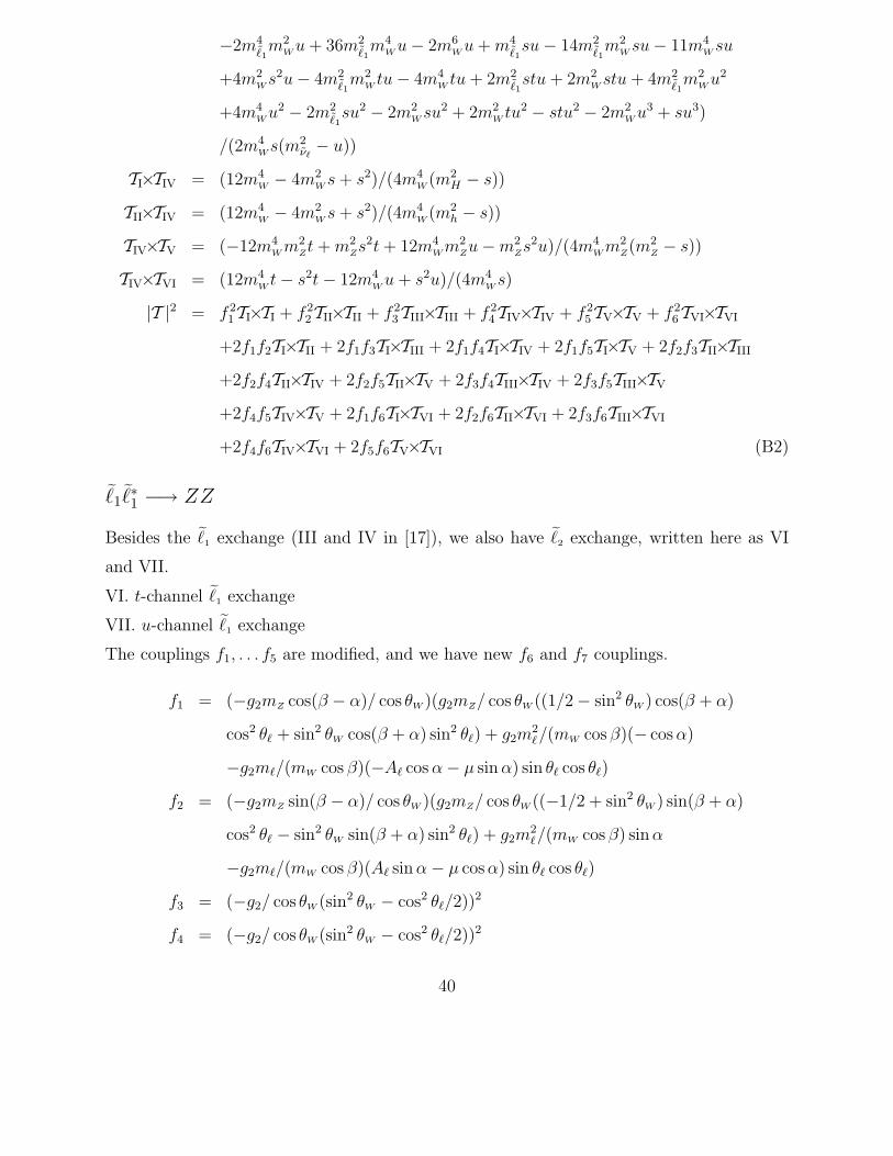
−2m4˜1m2

W u + 36m2˜1m4

W u− 2m6W u + m4

˜1su− 14m2

˜1m2

W su− 11m4W su

+4m2Ws2u− 4m2

˜1m2

W tu− 4m4W tu + 2m2

˜1stu + 2m2

W stu + 4m2˜1m2

W u2

+4m4Wu2 − 2m2

˜1su2 − 2m2

W su2 + 2m2W tu2 − stu2 − 2m2

Wu3 + su3)

/(2m4Ws(m2

ν`− u))

TI×TIV = (12m4W − 4m2

W s + s2)/(4m4W (m2

H − s))

TII×TIV = (12m4W − 4m2

W s + s2)/(4m4W (m2

h − s))

TIV×TV = (−12m4W m2

Zt + m2Zs2t + 12m4

Wm2Zu−m2

Zs2u)/(4m4Wm2

Z(m2Z − s))

TIV×TVI = (12m4W

t− s2t− 12m4W

u + s2u)/(4m4W

s)

|T |2 = f 21TI×TI + f 2

2TII×TII + f 23TIII×TIII + f 2

4TIV×TIV + f 25TV×TV + f 2

6TVI×TVI

+2f1f2TI×TII + 2f1f3TI×TIII + 2f1f4TI×TIV + 2f1f5TI×TV + 2f2f3TII×TIII

+2f2f4TII×TIV + 2f2f5TII×TV + 2f3f4TIII×TIV + 2f3f5TIII×TV

+2f4f5TIV×TV + 2f1f6TI×TVI + 2f2f6TII×TVI + 2f3f6TIII×TVI

+2f4f6TIV×TVI + 2f5f6TV×TVI (B2)

˜1˜∗1 −→ ZZ

Besides the ˜1 exchange (III and IV in [17]), we also have ˜2 exchange, written here as VI

and VII.

VI. t-channel ˜1 exchange

VII. u-channel ˜1 exchange

The couplings f1, . . . f5 are modified, and we have new f6 and f7 couplings.

f1 = (−g2mZ cos(β − α)/ cos θW )(g2mZ/ cos θW ((1/2− sin2 θW ) cos(β + α)

cos2 θ` + sin2 θW cos(β + α) sin2 θ`) + g2m2`/(mW cos β)(− cos α)

−g2m`/(mW cos β)(−A` cos α− µ sin α) sin θ` cos θ`)

f2 = (−g2mZ sin(β − α)/ cos θW )(g2mZ/ cos θW ((−1/2 + sin2 θW ) sin(β + α)

cos2 θ` − sin2 θW sin(β + α) sin2 θ`) + g2m2`/(mW cos β) sinα

−g2m`/(mW cos β)(A` sin α− µ cosα) sin θ` cos θ`)

f3 = (−g2/ cos θW (sin2 θW − cos2 θ`/2))2

f4 = (−g2/ cos θW (sin2 θW − cos2 θ`/2))2

40

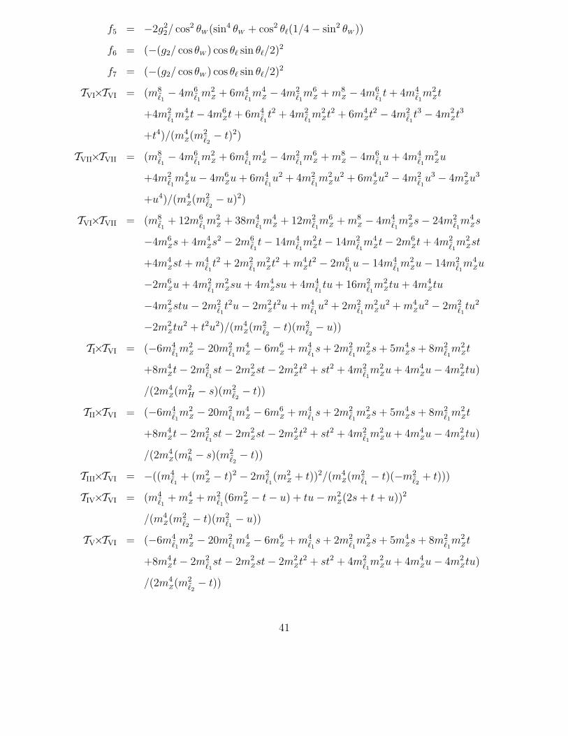
f5 = −2g22/ cos2 θW (sin4 θW + cos2 θ`(1/4− sin2 θW ))

f6 = (−(g2/ cos θW ) cos θ` sin θ`/2)2

f7 = (−(g2/ cos θW ) cos θ` sin θ`/2)2

TVI×TVI = (m8˜1− 4m6

˜1m2

Z + 6m4˜1m4

Z − 4m2˜1m6

Z + m8Z − 4m6

˜1t + 4m4

˜1m2

Zt

+4m2˜1m4

Zt− 4m6Zt + 6m4

˜1t2 + 4m2

˜1m2

Zt2 + 6m4Zt2 − 4m2

˜1t3 − 4m2

Zt3

+t4)/(m4Z(m2

˜2− t)2)

TVII×TVII = (m8˜1− 4m6

˜1m2

Z + 6m4˜1m4

Z − 4m2˜1m6

Z + m8Z − 4m6

˜1u + 4m4

˜1m2

Zu

+4m2˜1m4

Zu− 4m6

Zu + 6m4

˜1u2 + 4m2

˜1m2

Zu2 + 6m4

Zu2 − 4m2

˜1u3 − 4m2

Zu3

+u4)/(m4Z(m2

˜2− u)2)

TVI×TVII = (m8˜1+ 12m6

˜1m2

Z+ 38m4

˜1m4

Z+ 12m2

˜1m6

Z+ m8

Z− 4m4

˜1m2

Zs− 24m2

˜1m4

Zs

−4m6Zs + 4m4

Zs2 − 2m6

˜1t− 14m4

˜1m2

Zt− 14m2

˜1m4

Zt− 2m6

Zt + 4m2

˜1m2

Zst

+4m4Zst + m4

˜1t2 + 2m2

˜1m2

Zt2 + m4

Zt2 − 2m6

˜1u− 14m4

˜1m2

Zu− 14m2

˜1m4

Zu

−2m6Zu + 4m2

˜1m2

Zsu + 4m4

Zsu + 4m4

˜1tu + 16m2

˜1m2

Ztu + 4m4

Ztu

−4m2Zstu− 2m2

˜1t2u− 2m2

Zt2u + m4

˜1u2 + 2m2

˜1m2

Zu2 + m4

Zu2 − 2m2

˜1tu2

−2m2Ztu2 + t2u2)/(m4

Z(m2

˜2− t)(m2

˜2− u))

TI×TVI = (−6m4˜1m2

Z− 20m2

˜1m4

Z− 6m6

Z+ m4

˜1s + 2m2

˜1m2

Zs + 5m4

Zs + 8m2

˜1m2

Zt

+8m4Zt− 2m2

˜1st− 2m2

Zst− 2m2

Zt2 + st2 + 4m2

˜1m2

Zu + 4m4

Zu− 4m2

Ztu)

/(2m4Z(m2

H − s)(m2˜2− t))

TII×TVI = (−6m4˜1m2

Z− 20m2

˜1m4

Z− 6m6

Z+ m4

˜1s + 2m2

˜1m2

Zs + 5m4

Zs + 8m2

˜1m2

Zt

+8m4Zt− 2m2

˜1st− 2m2

Zst− 2m2Zt2 + st2 + 4m2

˜1m2

Zu + 4m4Zu− 4m2

Ztu)

/(2m4Z(m2

h − s)(m2˜2− t))

TIII×TVI = −((m4˜1+ (m2

Z − t)2 − 2m2˜1(m2

Z + t))2/(m4Z(m2

˜1− t)(−m2

˜2+ t)))

TIV×TVI = (m4˜1+ m4

Z + m2˜1(6m2

Z − t− u) + tu−m2Z(2s + t + u))2

/(m4Z(m2

˜2− t)(m2

˜1− u))

TV×TVI = (−6m4˜1m2

Z − 20m2˜1m4

Z − 6m6Z + m4

˜1s + 2m2

˜1m2

Zs + 5m4Zs + 8m2

˜1m2

Zt

+8m4Zt− 2m2

˜1st− 2m2

Zst− 2m2Zt2 + st2 + 4m2

˜1m2

Zu + 4m4Zu− 4m2

Ztu)

/(2m4Z(m2

˜2− t))

41

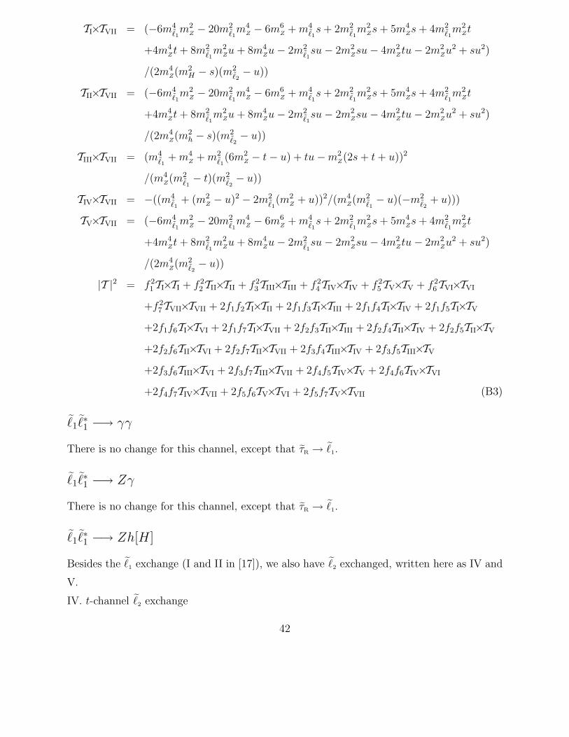
TI×TVII = (−6m4˜1m2

Z − 20m2˜1m4

Z − 6m6Z + m4

˜1s + 2m2

˜1m2

Zs + 5m4Zs + 4m2

˜1m2

Zt

+4m4Zt + 8m2

˜1m2

Zu + 8m4Zu− 2m2

˜1su− 2m2

Zsu− 4m2Ztu− 2m2

Zu2 + su2)

/(2m4Z(m2

H − s)(m2˜2− u))

TII×TVII = (−6m4˜1m2

Z − 20m2˜1m4

Z − 6m6Z + m4

˜1s + 2m2

˜1m2

Zs + 5m4Zs + 4m2

˜1m2

Zt

+4m4Zt + 8m2

˜1m2

Zu + 8m4Zu− 2m2

˜1su− 2m2

Zsu− 4m2Ztu− 2m2

Zu2 + su2)

/(2m4Z(m2

h − s)(m2˜2− u))

TIII×TVII = (m4˜1+ m4

Z + m2˜1(6m2

Z − t− u) + tu−m2Z(2s + t + u))2

/(m4Z(m2

˜1− t)(m2

˜2− u))

TIV×TVII = −((m4˜1+ (m2

Z− u)2 − 2m2

˜1(m2

Z+ u))2/(m4

Z(m2

˜1− u)(−m2

˜2+ u)))

TV×TVII = (−6m4˜1m2

Z− 20m2

˜1m4

Z− 6m6

Z+ m4

˜1s + 2m2

˜1m2

Zs + 5m4

Zs + 4m2

˜1m2

Zt

+4m4Zt + 8m2

˜1m2

Zu + 8m4

Zu− 2m2

˜1su− 2m2

Zsu− 4m2

Ztu− 2m2

Zu2 + su2)

/(2m4Z(m2

˜2− u))

|T |2 = f 21TI×TI + f 2



6TVI×TVI

+f 27TVII×TVII + 2f1f2TI×TII + 2f1f3TI×TIII + 2f1f4TI×TIV + 2f1f5TI×TV

+2f1f6TI×TVI + 2f1f7TI×TVII + 2f2f3TII×TIII + 2f2f4TII×TIV + 2f2f5TII×TV

+2f2f6TII×TVI + 2f2f7TII×TVII + 2f3f4TIII×TIV + 2f3f5TIII×TV

+2f3f6TIII×TVI + 2f3f7TIII×TVII + 2f4f5TIV×TV + 2f4f6TIV×TVI

+2f4f7TIV×TVII + 2f5f6TV×TVI + 2f5f7TV×TVII (B3)

˜1˜∗1 −→ γγ

There is no change for this channel, except that τR → ˜1.

˜1˜∗1 −→ Zγ

There is no change for this channel, except that τR → ˜1.

˜1˜∗1 −→ Zh[H]

Besides the ˜1 exchange (I and II in [17]), we also have ˜2 exchanged, written here as IV and

V.

IV. t-channel ˜2 exchange

42

V. u-channel ˜2 exchange

The couplings are modified.

f1 = (−g2/ cos θW (sin2 θW − cos2 θ`/2))(g2mZ/ cos θW ((−1/2 + sin2 θW )

sin[− cos](β + α) cos2 θ` − sin2 θW sin[− cos](β + α) sin2 θ`)

+g2m2`/(mW cos β) sin[− cos]α− g2m`/(mW cos β)(A` sin[− cos]α

−µ cos[sin]α) sin θ` cos θ`)

f2 = −(−g2/ cos θW (sin2 θW − cos2 θ`/2))(g2mZ/ cos θW ((−1/2 + sin2 θW )

sin[− cos](β + α) cos2 θ` − sin2 θW sin[− cos](β + α) sin2 θ`)

+g2m2`/(mW cos β) sin[− cos]α− g2m`/(mW cos β)(A` sin[− cos]α

−µ cos[sin]α) sin θ` cos θ`)

f3 = (−g2/ cos θW (sin2 θW − cos2 θ`/2))(−g2mZ sin[cos](β − α)/ cos θW )

f4 = (−g2 cos θ` sin θ`/(2 cos θW ))(g2mZ/ cos θW ((−1/2 + sin2 θW )

sin[− cos](β + α)(− cos θ` sin θ`)− sin2 θW sin[− cos](β + α) cos θ` sin θ`)

−g2m`/(2mW cos β)(A` sin[− cos]α− µ cos[sin]α) cos(2θ`))

f5 = (−)(−g2 cos θ` sin θ`/(2 cos θW ))(g2mZ/ cos θW ((−1/2 + sin2 θW )

sin[− cos](β + α)(− cos θ` sin θ`)− sin2 θW sin[− cos](β + α) cos θ` sin θ`)

−g2m`/(2mW cos β)(A` sin[− cos]α− µ cos[sin]α) cos(2θ`))

TIV×TIV = (m4˜1+ (m2

Z − t)2 − 2m2˜1(m2

Z + t))/(m2Z(m2

˜2− t)2)

TV×TV = (m4˜1+ (m2

Z − u)2 − 2m2˜1(m2

Z + u))/(m2Z(m2

˜2− u)2)

TI×TIV = −((m4˜1+ (m2

Z − t)2 − 2m2˜1(m2

Z + t))/(m2Z(m2

˜1− t)(−m2

˜2+ t)))

TI×TV = (m4˜1+ m4

Z + m2˜1(6m2

Z − t− u) + tu−m2Z(2s + t + u))

/(m2Z(m2

˜1− t)(m2

˜2− u))

TII×TIV = (m4˜1+ m4

Z + m2˜1(6m2

Z − t− u) + tu−m2Z(2s + t + u))

/(m2Z(m2

˜2− t)(m2

˜1− u))

TII×TV = −((m4˜1+ (m2

Z− u)2 − 2m2

˜1(m2

Z+ u))/(m2

Z(m2

˜1− u)(−m2

˜2+ u)))

TIII×TIV = (t(t− u) + m2˜1(−8m2

Z− t + u) + m2

Z(2s− t + u))

/(2m2Z(m2

Z− s)(m2

˜2− t))

43

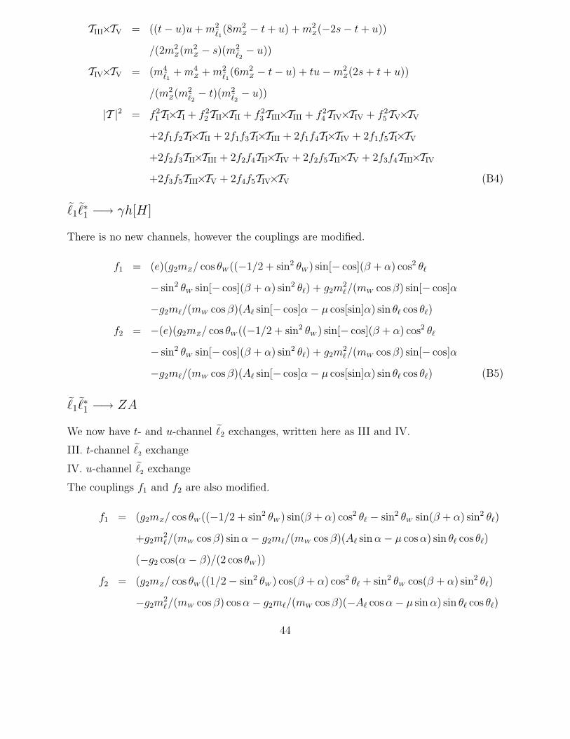
TIII×TV = ((t− u)u + m2˜1(8m2

Z − t + u) + m2Z(−2s− t + u))

/(2m2Z(m2

Z − s)(m2˜2− u))

TIV×TV = (m4˜1+ m4

Z + m2˜1(6m2

Z − t− u) + tu−m2Z(2s + t + u))

/(m2Z(m2

˜2− t)(m2

˜2− u))

|T |2 = f 21TI×TI + f 2


4TIV×TIV + f 25TV×TV

+2f1f2TI×TII + 2f1f3TI×TIII + 2f1f4TI×TIV + 2f1f5TI×TV

+2f2f3TII×TIII + 2f2f4TII×TIV + 2f2f5TII×TV + 2f3f4TIII×TIV

+2f3f5TIII×TV + 2f4f5TIV×TV (B4)

˜1˜∗1 −→ γh[H]

There is no new channels, however the couplings are modified.

f1 = (e)(g2mZ/ cos θW ((−1/2 + sin2 θW ) sin[− cos](β + α) cos2 θ`

− sin2 θW sin[− cos](β + α) sin2 θ`) + g2m2`/(mW cos β) sin[− cos]α

−g2m`/(mW cos β)(A` sin[− cos]α− µ cos[sin]α) sin θ` cos θ`)

f2 = −(e)(g2mZ/ cos θW ((−1/2 + sin2 θW ) sin[− cos](β + α) cos2 θ`

− sin2 θW sin[− cos](β + α) sin2 θ`) + g2m2`/(mW cos β) sin[− cos]α

−g2m`/(mW cos β)(A` sin[− cos]α− µ cos[sin]α) sin θ` cos θ`) (B5)

˜1˜∗1 −→ ZA

We now have t- and u-channel ˜2 exchanges, written here as III and IV.

III. t-channel ˜2 exchange

IV. u-channel ˜2 exchange

The couplings f1 and f2 are also modified.

f1 = (g2mZ/ cos θW ((−1/2 + sin2 θW ) sin(β + α) cos2 θ` − sin2 θW sin(β + α) sin2 θ`)

+g2m2`/(mW cos β) sinα− g2m`/(mW cos β)(A` sin α− µ cosα) sin θ` cos θ`)

(−g2 cos(α− β)/(2 cos θW ))

f2 = (g2mZ/ cos θW ((1/2− sin2 θW ) cos(β + α) cos2 θ` + sin2 θW cos(β + α) sin2 θ`)

−g2m2`/(mW cos β) cos α− g2m`/(mW cos β)(−A` cos α− µ sin α) sin θ` cos θ`)

44

(−g2 sin(α− β)/(2 cos θW ))

f3 = (−g2 cos θ` sin θ`/(2 cos θW ))(−g2m`/(2mW )(A` tanβ − µ))

f4 = (−g2 cos θ` sin θ`/(2 cos θW ))(−g2m`/(2mW )(A` tanβ − µ))

TIII×TIII = (m4˜1+ (m2

Z − t)2 − 2m2˜1(m2

Z + t))/(m2Z(m2

˜2− t)2)

TIV×TIV = (m4˜1+ (m2

Z − u)2 − 2m2˜1(m2

Z + u))/(m2Z(m2

˜2− u)2)

TIII×TIV = (m4˜1+ m4

Z + m2˜1(6m2

Z − t− u) + tu−m2Z(2s + t + u))

/(m2Z(m2

˜2− t)(m2

˜2− u))

TI×TIII = (−m4Z

+ m2Zs + m2

˜1(−3m2

Z+ s) + m2

Zt− st + m2

A(−m2

˜1− 3m2

Z+ t)

+2m2Zu)/(m2

Z(m2

h − s)(m2˜2− t))

TII×TIII = (−m4Z

+ m2Zs + m2

˜1(−3m2

Z+ s) + m2

Zt− st + m2

A(−m2

˜1− 3m2

Z+ t)

+2m2Zu)/(m2

Z(m2

H − s)(m2˜2− t))

TI×TIV = (−m4Z

+ m2Zs + m2

˜1(−3m2

Z+ s) + 2m2

Zt + m2

Zu− su + m2

A(−m2

˜1− 3m2

Z

+u))/(m2Z(m2

h − s)(m2˜2− u))

TII×TIV = (−m4Z

+ m2Zs + m2

˜1(−3m2

Z+ s) + 2m2

Zt + m2

Zu− su + m2

A(−m2

˜1− 3m2

Z

+u))/(m2Z(m2

H − s)(m2˜2− u))

|T |2 = f 21TI×TI + f 2


4TIV×TIV + 2f1f2TI×TII + 2f1f3TI×TIII

+2f1f4TI×TIV + 2f2f3TII×TIII + 2f2f4TII×TIV + 2f3f4TIII×TIV (B6)

˜1˜∗1 −→ `¯

The s-channel h and H annihilations are neglected, due to the small Yukawa couplings for

leptons. The t-channel χ exchange is modified, with more couplings introduced (K, K ′) →(Ka, Kb, K

′a, K

′b). The terms with m` were neglected in [17], but not here. The couplings f3c

and f3d are modified while f4c remains the same.

f3c = (−g2(sin2 θW − cos2 θ`/2)/ cos θW )(g2(1− 4 sin2 θW )/(4 cos θW ))

f3d = (−g2(sin2 θW − cos2 θ`/2)/ cos θW )(−g2/(4 cos θW ))

Ka = − sin θ`(g2m`/(2mW cos β)Ni3 + g1Ni1)/√

2

− cos θ`(g2m`/(2mW cos β)Ni3 − (g1Ni1 + g2/2(Ni2 −Ni1 tan θW )))/√

2

Kb = − sin θ`(g2m`/(2mW cos β)Ni3 − g1Ni1)/√

2

45

− cos θ`(−g2m`/(2mW cos β)Ni3 − (g1Ni1 + g2/2(Ni2 −Ni1 tan θW )))/√

2

K ′a = − sin θ`(g2m`/(2mW cos β)Nj3 + g1Nj1)/

√2

− cos θ`(g2m`/(2mW cos β)Nj3 − (g1Nj1 + g2/2(Nj2 −Nj1 tan θW )))/√

2

K ′b = − sin θ`(g2m`/(2mW cos β)Nj3 − g1Nj1)/

√2

− cos θ`(−g2m`/(2mW cos β)Nj3 − (g1Nj1 + g2/2(Nj2 −Nj1 tan θW )))/√

2

TIII×TV = (2f3dKbKa(−16m2˜1m2

` + 4m2˜1s + 4m2

`s− s2 + t2 − 2tu + u2)

+f3c(K2a(−4m2

˜1s + s2 − 4m2

` t− 4m`mχ0it− t2 + 4m2

ù + 4m`mχ0iu + 2tu− u2)

+K2b (−4m2

˜1s + s2 − 4m2

` t + 4m`mχ0it− t2 + 4m2

ù− 4m`mχ0iu + 2tu− u2)))

/((m2Z− s)(m2

χ0i− t))

TIV×TV = −(f4c(K2a(−4m2

˜1s + s2 − 4m2

`t− 4m`mχ0it− t2 + 4m2

ù + 4m`mχ0iu + 2tu

−u2) + K2b (−4m2

˜1s + s2 − 4m2

`t + 4m`mχ0it− t2 + 4m2

ù− 4m`mχ0iu + 2tu

−u2))/(s(m2χ0

i− t)))

TV×TV = (2(K ′2a K2

b (−m4˜1− 2m2

˜1m2

` + 3m4` −m3

`mχ0i− 3m3

`mχ0i+ m3

`mχ0j+ 3m3

`mχ0j

−2m2`mχ0

imχ0

j− 2m2

`mχ0imχ0

j+ m2

˜1s−m2

`s + m`mχ0is−m`mχ0

js

+mχ0imχ0

js + m2

˜1t + 2m2

` t + m2` t−m`mχ0

it + m`mχ0

jt + m2

˜1u−m2

ù

+m`mχ0iu−m`mχ0

ju− tu) + K ′

aKaK′bKb(−2m4

˜1− 4m2

˜1m2

` + 6m4` + 2m2

˜1s

−2m2`s + 2mχ0

imχ0

js + 2m2

˜1t− 4m2

`t + 2m2`t + 2m2

˜1u− 2m2

ù− 2tu)

+K2aK ′2

b (−m4˜1− 2m2

˜1m2

` + 3m4` + 4m3

`mχ0i− 4m3

`mχ0j− 4m2

`mχ0imχ0

j

+m2˜1s−m2

`s−m`mχ0is + m`mχ0

js + mχ0

imχ0

js + m2

˜1t + 3m2

` t + m`mχ0it

−m`mχ0jt + m2

˜1u−m2

ù−m`mχ0iu + m`mχ0

ju− tu)

+(KaK′a + KbK

′b)(KaK

′a + KbK

′b)(−m2

`s−mχ0imχ0

js + m2

˜1t + m2

` t

+m2˜1u−m2

ù− tu) + (KaK′a + KbK

′b)(KaK

′a −KbK

′b)(4m

3`mχ0

i

+4m3`mχ0

j−m`mχ0

is−m`mχ0

js + m`mχ0

it + m`mχ0

jt−m`mχ0

iu−m`mχ0

ju)

+(KaK′a −KbK

′b)(KaK

′a −KbK

′b)(2m

2`mχ0

imχ0

j+ 2m2

`t)))

/((m2χ0

i− t)(−m2

χ0j+ t))

|T |2 = TIII×TIII + TIV×TIV +∑i,j

TV×TV + 2TIII×TIV + 2∑

i

(TIII×TV + TIV×TV) (B7)

46

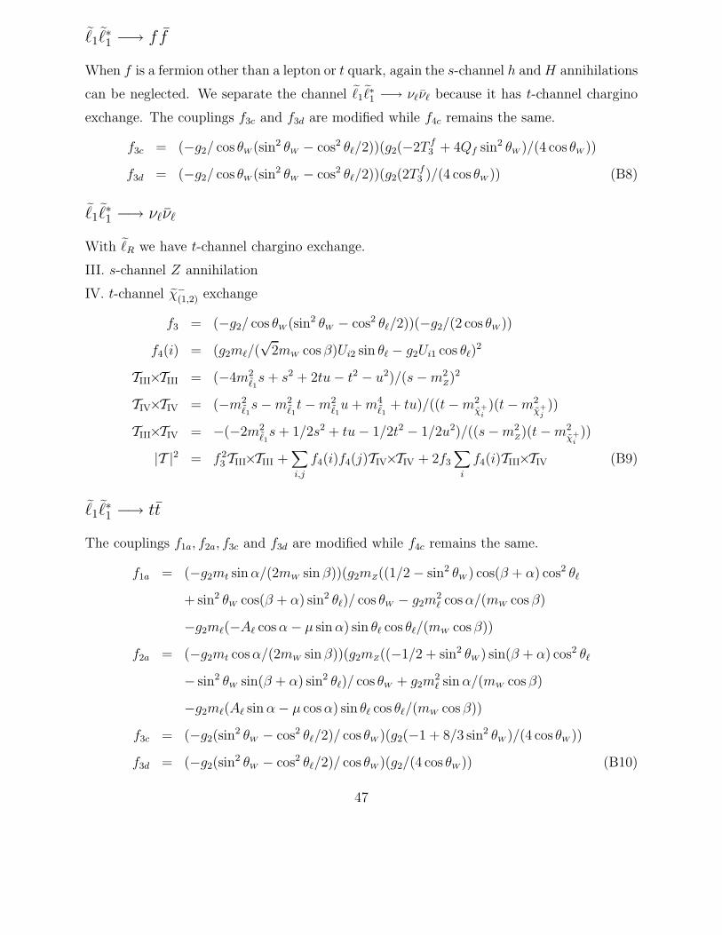
˜1˜∗1 −→ f f

When f is a fermion other than a lepton or t quark, again the s-channel h and H annihilations

can be neglected. We separate the channel ˜1 ˜∗1 −→ ν`ν` because it has t-channel chargino

exchange. The couplings f3c and f3d are modified while f4c remains the same.

f3c = (−g2/ cos θW (sin2 θW − cos2 θ`/2))(g2(−2T f3 + 4Qf sin2 θW )/(4 cos θW ))

f3d = (−g2/ cos θW (sin2 θW − cos2 θ`/2))(g2(2Tf3 )/(4 cos θW )) (B8)

˜1˜∗1 −→ ν`ν`

With ˜R we have t-channel chargino exchange.

III. s-channel Z annihilation

IV. t-channel χ−(1,2) exchange

f3 = (−g2/ cos θW (sin2 θW − cos2 θ`/2))(−g2/(2 cos θW ))

f4(i) = (g2m`/(√

2mW cos β)Ui2 sin θ` − g2Ui1 cos θ`)2

TIII×TIII = (−4m2˜1s + s2 + 2tu− t2 − u2)/(s−m2

Z)2

TIV×TIV = (−m2˜1s−m2

˜1t−m2

˜1u + m4

˜1+ tu)/((t−m2

χ+i)(t−m2

χ+j))

TIII×TIV = −(−2m2˜1s + 1/2s2 + tu− 1/2t2 − 1/2u2)/((s−m2

Z)(t−m2

χ+i))

|T |2 = f 23TIII×TIII +

∑i,j

f4(i)f4(j)TIV×TIV + 2f3

∑i

f4(i)TIII×TIV (B9)

˜1˜∗1 −→ tt

The couplings f1a, f2a, f3c and f3d are modified while f4c remains the same.

f1a = (−g2mt sin α/(2mW sin β))(g2mZ((1/2− sin2 θW ) cos(β + α) cos2 θ`

+ sin2 θW cos(β + α) sin2 θ`)/ cos θW − g2m2` cos α/(mW cos β)

−g2m`(−A` cos α− µ sin α) sin θ` cos θ`/(mW cos β))

f2a = (−g2mt cos α/(2mW sin β))(g2mZ((−1/2 + sin2 θW ) sin(β + α) cos2 θ`

− sin2 θW sin(β + α) sin2 θ`)/ cos θW + g2m2` sin α/(mW cos β)

−g2m`(A` sin α− µ cos α) sin θ` cos θ`/(mW cos β))

f3c = (−g2(sin2 θW − cos2 θ`/2)/ cos θW )(g2(−1 + 8/3 sin2 θW )/(4 cos θW ))

f3d = (−g2(sin2 θW − cos2 θ`/2)/ cos θW )(g2/(4 cos θW )) (B10)

47

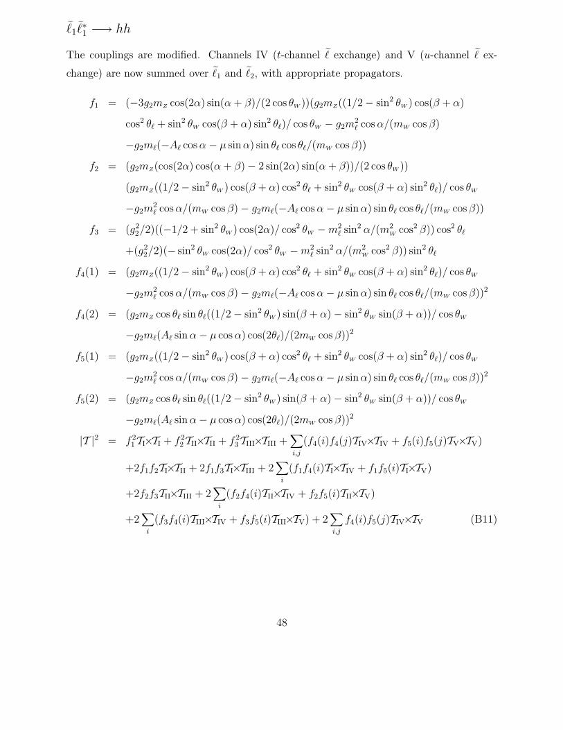
˜1˜∗1 −→ hh

The couplings are modified. Channels IV (t-channel ˜ exchange) and V (u-channel ˜ ex-

change) are now summed over ˜1 and ˜2, with appropriate propagators.

f1 = (−3g2mZ cos(2α) sin(α + β)/(2 cos θW ))(g2mZ((1/2− sin2 θW ) cos(β + α)

cos2 θ` + sin2 θW cos(β + α) sin2 θ`)/ cos θW − g2m2` cos α/(mW cos β)

−g2m`(−A` cos α− µ sinα) sin θ` cos θ`/(mW cos β))

f2 = (g2mZ(cos(2α) cos(α + β)− 2 sin(2α) sin(α + β))/(2 cos θW ))

(g2mZ((1/2− sin2 θW ) cos(β + α) cos2 θ` + sin2 θW cos(β + α) sin2 θ`)/ cos θW

−g2m2` cos α/(mW cos β)− g2m`(−A` cos α− µ sinα) sin θ` cos θ`/(mW cos β))

f3 = (g22/2)((−1/2 + sin2 θW ) cos(2α)/ cos2 θW −m2

` sin2 α/(m2W

cos2 β)) cos2 θ`

+(g22/2)(− sin2 θW cos(2α)/ cos2 θW −m2

` sin2 α/(m2W

cos2 β)) sin2 θ`

f4(1) = (g2mZ((1/2− sin2 θW ) cos(β + α) cos2 θ` + sin2 θW cos(β + α) sin2 θ`)/ cos θW

−g2m2` cos α/(mW cos β)− g2m`(−A` cos α− µ sinα) sin θ` cos θ`/(mW cos β))2

f4(2) = (g2mZ cos θ` sin θ`((1/2− sin2 θW ) sin(β + α)− sin2 θW sin(β + α))/ cos θW

−g2m`(A` sin α− µ cos α) cos(2θ`)/(2mW cos β))2


−g2m2` cos α/(mW cos β)− g2m`(−A` cos α− µ sinα) sin θ` cos θ`/(mW cos β))2

f5(2) = (g2mZ cos θ` sin θ`((1/2− sin2 θW ) sin(β + α)− sin2 θW sin(β + α))/ cos θW

−g2m`(A` sin α− µ cos α) cos(2θ`)/(2mW cos β))2

|T |2 = f 21TI×TI + f 2

2TII×TII + f 23TIII×TIII +

∑i,j

(f4(i)f4(j)TIV×TIV + f5(i)f5(j)TV×TV)

+2f1f2TI×TII + 2f1f3TI×TIII + 2∑

i

(f1f4(i)TI×TIV + f1f5(i)TI×TV)

+2f2f3TII×TIII + 2∑

i

(f2f4(i)TII×TIV + f2f5(i)TII×TV)

+2∑

i

(f3f4(i)TIII×TIV + f3f5(i)TIII×TV) + 2∑i,j

f4(i)f5(j)TIV×TV (B11)

48

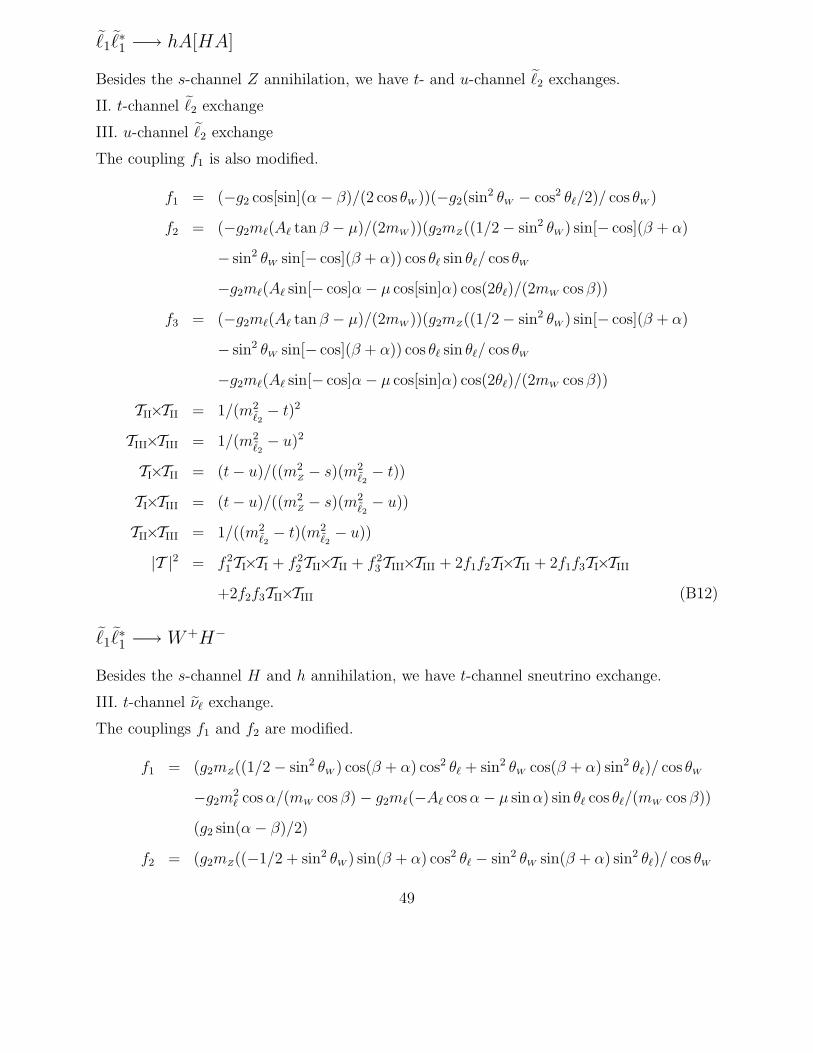
˜1˜∗1 −→ hA[HA]

Besides the s-channel Z annihilation, we have t- and u-channel ˜2 exchanges.

II. t-channel ˜2 exchange

III. u-channel ˜2 exchange

The coupling f1 is also modified.

f1 = (−g2 cos[sin](α− β)/(2 cos θW ))(−g2(sin2 θW − cos2 θ`/2)/ cos θW )

f2 = (−g2m`(A` tan β − µ)/(2mW ))(g2mZ((1/2− sin2 θW ) sin[− cos](β + α)

− sin2 θW sin[− cos](β + α)) cos θ` sin θ`/ cos θW

−g2m`(A` sin[− cos]α− µ cos[sin]α) cos(2θ`)/(2mW cos β))

f3 = (−g2m`(A` tan β − µ)/(2mW ))(g2mZ((1/2− sin2 θW ) sin[− cos](β + α)


−g2m`(A` sin[− cos]α− µ cos[sin]α) cos(2θ`)/(2mW cos β))

TII×TII = 1/(m2˜2− t)2

TIII×TIII = 1/(m2˜2− u)2

TI×TII = (t− u)/((m2Z− s)(m2

˜2− t))

TI×TIII = (t− u)/((m2Z− s)(m2

˜2− u))

TII×TIII = 1/((m2˜2− t)(m2

˜2− u))

|T |2 = f 21TI×TI + f 2

2TII×TII + f 23TIII×TIII + 2f1f2TI×TII + 2f1f3TI×TIII

+2f2f3TII×TIII (B12)

˜1˜∗1 −→ W+H−

Besides the s-channel H and h annihilation, we have t-channel sneutrino exchange.

III. t-channel ν` exchange.

The couplings f1 and f2 are modified.

f1 = (g2mZ((1/2− sin2 θW ) cos(β + α) cos2 θ` + sin2 θW cos(β + α) sin2 θ`)/ cos θW

−g2m2` cos α/(mW cos β)− g2m`(−A` cos α− µ sin α) sin θ` cos θ`/(mW cos β))

(g2 sin(α− β)/2)

f2 = (g2mZ((−1/2 + sin2 θW ) sin(β + α) cos2 θ` − sin2 θW sin(β + α) sin2 θ`)/ cos θW

49

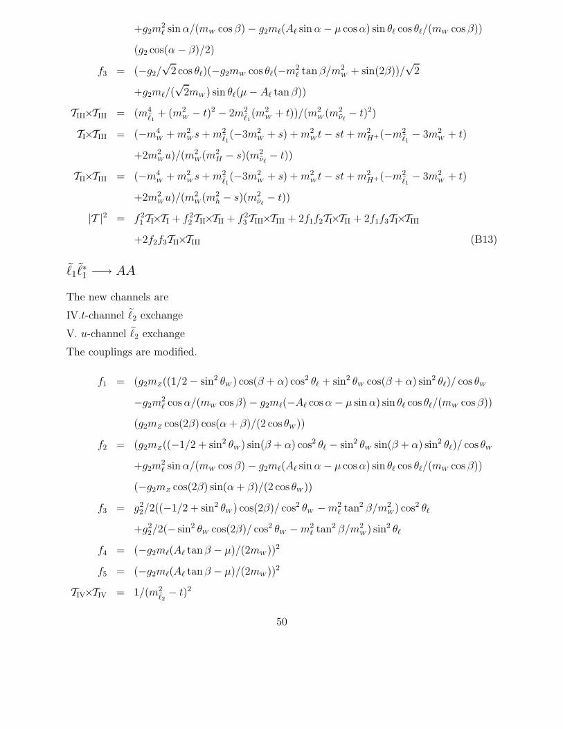
+g2m2` sin α/(mW cos β)− g2m`(A` sin α− µ cosα) sin θ` cos θ`/(mW cos β))

(g2 cos(α− β)/2)

f3 = (−g2/√

2 cos θ`)(−g2mW cos θ`(−m2` tan β/m2

W + sin(2β))/√

2

+g2m`/(√

2mW ) sin θ`(µ− A` tanβ))

TIII×TIII = (m4˜1+ (m2

W − t)2 − 2m2˜1(m2

W + t))/(m2W (m2

ν`− t)2)

TI×TIII = (−m4W + m2

W s + m2˜1(−3m2

W + s) + m2W t− st + m2

H+(−m2˜1− 3m2

W + t)

+2m2Wu)/(m2

W (m2H − s)(m2

ν`− t))

TII×TIII = (−m4W

+ m2W

s + m2˜1(−3m2

W+ s) + m2

Wt− st + m2

H+(−m2˜1− 3m2

W+ t)

+2m2W

u)/(m2W

(m2h − s)(m2

ν`− t))

|T |2 = f 21TI×TI + f 2


+2f2f3TII×TIII (B13)

˜1˜∗1 −→ AA

The new channels are

IV.t-channel ˜2 exchange

V. u-channel ˜2 exchange




(g2mZ cos(2β) cos(α + β)/(2 cos θW ))


+g2m2` sin α/(mW cos β)− g2m`(A` sin α− µ cos α) sin θ` cos θ`/(mW cos β))

(−g2mZ cos(2β) sin(α + β)/(2 cos θW ))

f3 = g22/2((−1/2 + sin2 θW ) cos(2β)/ cos2 θW −m2

` tan2 β/m2W

) cos2 θ`

+g22/2(− sin2 θW cos(2β)/ cos2 θW −m2

` tan2 β/m2W

) sin2 θ`

f4 = (−g2m`(A` tanβ − µ)/(2mW ))2

f5 = (−g2m`(A` tanβ − µ)/(2mW ))2

TIV×TIV = 1/(m2˜2− t)2

50

TV×TV = 1/(m2˜2− u)2

TI×TIV = 1/((m2H − s)(m2

˜2− t))

TI×TV = 1/((m2H − s)(m2

˜2− u))

TII×TIV = 1/((m2h − s)(m2

˜2− t))

TII×TV = 1/((m2h − s)(m2

˜2− u))

TIII×TIV = 1/(m2˜2− t)

TIII×TV = 1/(m2˜2− u)

|T |2 = f 21TI×TI + f 2


4TIV×TIV + f 25TV×TV

+2f1f2TI×TII + 2f1f3TI×TIII + 2f1f4TI×TIV + 2f1f5TI×TV

+2f2f3TII×TIII + 2f2f4TII×TIV + 2f2f5TII×TV + 2f3f4TIII×TIV

+2f3f5TIII×TV + 2f4f5TIV×TV (B14)

˜1˜∗1 −→ hH

The t- and u-channels ˜ exchanges are now summed over ˜1 and ˜2 with appropriate propa-

gators. The couplings are



(g2mZ(cos(2α) sin(α + β) + 2 sin(2α) cos(α + β))/(2 cos θW ))



(g2mZ(cos(2α) cos(α + β)− 2 sin(2α) sin(α + β))/(2 cos θW ))

f3 = g22 sin(2α)((−1/2 + sin2 θW )/ cos2 θW + m2

`/(2m2W

cos2 β)) cos2 θ`/2

+g22 sin(2α)(− sin2 θW / cos2 θW + m2

`/(2m2W

cos2 β)) sin2 θ`/2



(g2mZ((−1/2 + sin2 θW ) sin(β + α) cos2 θ` − sin2 θW sin(β + α) sin2 θ`)/ cos θW


f4(2) = (g2mZ((−1/2 + sin2 θW ) cos(β + α) + sin2 θW cos(β + α)) cos θ` sin θ`/ cos θW

51

−g2m`(−A` cos α− µ sin α) cos(2θ`)/(2mW cos β))

(g2mZ((1/2− sin2 θW ) sin(β + α)− sin2 θW sin(β + α)) cos θ` sin θ`/ cos θW

−g2m`(A` sin α− µ cosα) cos(2θ`)/(2mW cos β))





f5(2) = (g2mZ((−1/2 + sin2 θW ) cos(β + α) + sin2 θW cos(β + α)) cos θ` sin θ`/ cos θW

−g2m`(−A` cos α− µ sin α) cos(2θ`)/(2mW cos β))

(g2mZ((1/2− sin2 θW ) sin(β + α)− sin2 θW sin(β + α)) cos θ` sin θ`/ cos θW

−g2m`(A` sin α− µ cosα) cos(2θ`)/(2mW cos β))

|T |2 = f 21TI×TI + f 2


∑i,j



i

f1(f4(i)TI×TIV + f5(i)TI×TV)


i

f2(f4(i)TII×TIV + f5(i)TII×TV)

+2f3

∑i

(f4(i)TIII×TIV + f5(i)TIII×TV) + 2∑i,j


˜1˜∗1 −→ HH

The t- and u-channels ˜ exchanges are now summed over ˜1 and ˜2 with appropriate propa-

gators. The couplings are

f1 = (−3g2mZ cos(2α) cos(α + β)/(2 cos θW ))(g2mZ((1/2− sin2 θW ) cos(β + α) cos2 θ`

+ sin2 θW cos(β + α) sin2 θ`)/ cos θW − g2m2` cos α/(mW cos β)

−g2m`(−A` cos α− µ sinα) sin θ` cos θ`/(mW cos β))

f2 = (g2mZ(cos(2α) sin(α + β) + 2 sin(2α) cos(α + β))/(2 cos θW ))



f3 = g22/2(−(−1/2 + sin2 θW ) cos(2α)/ cos2 θW −m2

` cos2 α/(m2W

cos2 β)) cos2 θ`

+g22/2(sin2 θW cos(2α)/(cos2 θW )−m2

`(cos2 α)/(m2W

cos2 β)) sin2 θ`

52


−g2m2` cos α/(mW cos β)− g2m`(−A` cos α− µ sin α) sin θ` cos θ`/(mW cos β))2

f4(2) = (g2mZ((1/2− sin2 θW ) cos(β + α)(− cos θ` sin θ`) + sin2 θW cos(β + α) cos θ` sin θ`)

/ cos θW − g2m`(−A` cos α− µ sinα) cos(2θ`)/(2mW cos β))2


−g2m2` cos α/(mW cos β)− g2m`(−A` cos α− µ sin α) sin θ` cos θ`/(mW cos β))2

f5(2) = (g2mZ((1/2− sin2 θW ) cos(β + α)(− cos θ` sin θ`) + sin2 θW cos(β + α) cos θ` sin θ`)

/ cos θW − g2m`(−A` cos α− µ sinα) cos(2θ`)/(2mW cos β))2

|T |2 = f 21TI×TI + f 2


∑i,j



i

(f1f4(i)TI×TIV + f1f5(i)TI×TV)


i

(f2f4(i)TII×TIV + f2f5(i)TII×TV)

+2∑

i

(f3f4(i)TIII×TIV + f3f5(i)TIII×TV) + 2∑i,j


˜1˜∗1 −→ H+H−

We have one new channel,

VI. t-channel ν` exchange

The couplings, except f4, are modified



(−g2(mW cos(β − α)−mZ cos(2β) cos(β + α)/(2 cos θW )))


+g2m2` sin α/(mW cos β)− g2m`(A` sin α− µ cosα) sin θ` cos θ`/(mW cos β))

(−g2(mW sin(β − α) + mZ/(2 cos θW ) cos(2β) sin(β + α)))

f3 = (−g2(sin2 θW − cos2 θ`/2)/ cos θW )(g2 cos(2θW )/(2 cos θW ))

f5 = g22 cos(2β)(1 + (−1 + 2 sin2 θW )/(2 cos2 θW )) cos2 θ`/2

−(g22 cos(2β) sin2 θW /2 + g2

2m2` tan2 β/(2m2

W)) sin2 θ`

f6 = (−g2mW cos θ`(−m2` tan β/m2

W+ sin(2β))/

√2

53

+g2m` sin θ`(µ− A` tan β)/(√

2mW ))2

TVI×TVI = 1/(m2ν`− t)2

TI×TVI = 1/((m2H − s)(m2

ν`− t))

TII×TVI = 1/((m2h − t)(m2

ν`− t))

TIII×TVI = (t− u)/((m2Z − s)(m2

ν`− t))

TIV×TVI = (−t + u)/(s(m2ν`− t))

TV×TVI = 1/(m2ν`− t)

|T |2 = f 21TI×TI + f 2



6TVI×TVI

+2f1f2TI×TII + 2f1f3TI×TIII + 2f1f4TI×TIV + 2f1f5TI×TV + 2f1f6TI×TVI

+2f2f3TII×TIII + 2f2f4TII×TIV + 2f2f5TII×TV + 2f2f6TII×TVI

+2f3f4TIII×TIV + 2f3f5TIII×TV + 2f3f6TIII×TVI + 2f4f5TIV×TV

+2f4f6TIV×TVI + 2f5f6TV×TVI (B17)

˜1˜1 −→ ``

The channels I. t-channel χ exchange II. u-channel χ exchange are modified as follows.

Ka = − sin θ`(g2m`/(2mW cos β)Ni3 + g1Ni1)/√

2

− cos θ`(g2m`/(2mW cos β)Ni3 + (−g1Ni1 − g2/2(Ni2 −Ni1 tan θW )))/√

2

Kb = − sin θ`(g2m`/(2mW cos β)Ni3 − g1Ni1)/√

2

− cos θ`(−g2m`/(2mW cos β)Ni3 + (−g1Ni1 − g2/2(Ni2 −Ni1 tan θW )))/√

2

K ′a = − sin θ`(g2m`/(2mW cos β)Nj3 + g1Nj1)/

√2

− cos θ`(g2m`/(2mW cos β)Nj3 + (−g1Nj1 − g2/2(Nj2 −Nj1 tan θW )))/√

2

K ′b = − sin θ`(g2m`/(2mW cos β)Nj3 − g1Nj1)/

√2

− cos θ`(−g2m`/(2mW cos β)Nj3 + (−g1Nj1 − g2/2(Nj2 −Nj1 tan θW )))/√

2

TI×TI = (−2(4KaK′aKbK

′bmχ0

imχ0

js

+K2b K

′2a (−m4

˜1− 2m2

˜1m2

` + 3m4` − 4m3

`mχ0i+ 4m3

`mχ0j− 4m2

`mχ0imχ0

j

+m2˜1s−m2


js + mχ0

imχ0

js + m2

˜1t + 3m2

` t−m`mχ0it

+m`mχ0jt + m2

˜1u−m2

`u + m`mχ0iu−m`mχ0

ju− tu)

54

+K2b K

′2b (m4

˜1+ 2m2

˜1m2

` − 3m4` + 4m3

`mχ0i+ 4m3

`mχ0j− 4m2

`mχ0imχ0

j

−m2˜1s + m2

`s−m`mχ0is−m`mχ0

js + mχ0

imχ0

js−m2

˜1t− 3m2

` t + m`mχ0it

+m`mχ0jt−m2

˜1u + m2

ù−m`mχ0iu−m`mχ0

ju + tu)

+K2aK

′2b (−m4

˜1− 2m2

˜1m2

` + 3m4` + 4m3

`mχ0i− 4m3

`mχ0j− 4m2

`mχ0imχ0

j

+m2˜1s−m2


js + mχ0

imχ0

js + m2

˜1t + 3m2

` t + m`mχ0it

−m`mχ0jt + m2

˜1u−m2


ju− tu)

+K2aK

′2a (m4

˜1+ 2m2

˜1m2

` − 3m4` − 4m3

`mχ0i− 4m3

`mχ0j− 4m2

`mχ0imχ0

j

−m2˜1s + m2

`s + m`mχ0is + m`mχ0

js + mχ0

imχ0

js−m2

˜1t− 3m2

`t−m`mχ0it

−m`mχ0jt−m2

˜1u + m2

ù + m`mχ0iu + m`mχ0

ju + tu)))

/((m2χ0

i− t)(−m2

χ0j+ t))

TII×TII = (−2(4KaK′aKbK

′bmχ0

imχ0

js

+K2aK

′2b (−m4

˜1− 2m2

˜1m2

` + 3m4` + 4m3

`mχ0i− 4m3

`mχ0j− 4m2

`mχ0imχ0

j

+m2˜1s−m2


js + mχ0

imχ0

js + m2

˜1t−m2

` t−m`mχ0it

+m`mχ0jt + m2

˜1u + 3m2

ù + m`mχ0iu−m`mχ0

ju− tu)

+K2aK

′2a (m4

˜1+ 2m2

˜1m2

` − 3m4` − 4m3

`mχ0i− 4m3

`mχ0j− 4m2

`mχ0imχ0

j

−m2˜1s + m2

`s + m`mχ0is + m`mχ0

js + mχ0

imχ0

js−m2

˜1t + m2

` t + m`mχ0it

+m`mχ0jt−m2

˜1u− 3m2

ù−m`mχ0iu−m`mχ0

ju + tu)

+K2b K

′2a (−m4

˜1− 2m2

˜1m2

` + 3m4` − 4m3

`mχ0i+ 4m3

`mχ0j− 4m2

`mχ0imχ0

j

+m2˜1s−m2


js + mχ0

imχ0

js + m2

˜1t−m2

` t + m`mχ0it

−m`mχ0jt + m2

˜1u + 3m2


ju− tu)

+K2b K

′2b (m4

˜1+ 2m2

˜1m2

` − 3m4` + 4m3

`mχ0i+ 4m3

`mχ0j− 4m2

`mχ0imχ0

j

−m2˜1s + m2

`s−m`mχ0is−m`mχ0

js + mχ0

imχ0

js−m2

˜1t + m2

` t−m`mχ0it

−m`mχ0jt−m2

˜1u− 3m2

ù + m`mχ0iu + m`mχ0

ju + tu)))

/((m2χ0

i− u)(−m2

χ0j+ u))

TI×TII = (8KaK′aKbK

′bmχ0

imχ0

js +

K2a(−K ′2

b (2m4˜1+ 4m2

˜1m2

` − 6m4` − 8m3

`mχ0i+ 8m3

`mχ0j+ 8m2

`mχ0imχ0

j

+2m2˜1s + 2m2

`s + 2m`mχ0is− 2m`mχ0

js− 2mχ0

imχ0

js− s2 − 2m2

˜1t− 2m2

` t

55

+2m`mχ0it + 2m`mχ0

jt + t2 − 2m2

˜1u− 2m2

ù− 2m`mχ0iu− 2m`mχ0

ju + u2)) +

K2aK

′2a (2m4

˜1+ 4m2

˜1m2

` − 6m4` − 8m3

`mχ0i− 8m3

`mχ0j− 8m2

`mχ0imχ0

j

+2m2˜1s + 2m2

`s + 2m`mχ0is + 2m`mχ0

js + 2mχ0

imχ0

js− s2 − 2m2

˜1t− 2m2

` t

+2m`mχ0it− 2m`mχ0

jt + t2 − 2m2

˜1u− 2m2

ù− 2m`mχ0iu + 2m`mχ0

ju + u2) +

K2b K

′2b (2m4

˜1+ 4m2

˜1m2

` − 6m4` + 8m3

`mχ0i+ 8m3

`mχ0j− 8m2

`mχ0imχ0

j

+2m2˜1s + 2m2

`s− 2m`mχ0is− 2m`mχ0

js + 2mχ0

imχ0

js− s2 − 2m2

˜1t− 2m2

` t

−2m`mχ0it + 2m`mχ0

jt + t2 − 2m2

˜1u− 2m2

ù + 2m`mχ0iu− 2m`mχ0

ju + u2)−

K2b K

′2a (2m4

˜1+ 4m2

˜1m2

` − 6m4` + 8m3

`mχ0i− 8m3

`mχ0j+ 8m2

`mχ0imχ0

j

+2m2˜1s + 2m2

`s− 2m`mχ0is + 2m`mχ0

js− 2mχ0

imχ0

js− s2 − 2m2

˜1t− 2m2

` t

−2m`mχ0it− 2m`mχ0

jt + t2 − 2m2

˜1u− 2m2

ù + 2m`mχ0iu + 2m`mχ0

ju + u2))

/((m2χ0

i− t)(m2

χ0j− u))

|T |2 =∑i,j

(TI×TI + TII×TII + 2TI×TII) (B18)

Ã1˜B∗1 −→ À ¯B

I. t-channel χ exchange

Here mA,B ≡ mÀ,B and mA,B

≡ mÃ,B1

.

A(i) = −g2/√

2(cos θA(−Ni2 − tan θW Ni1) + sin θAmA/(mW cos β)Ni3)

B(i) = −g2/√

2(cos θAmA/(mW cos β)Ni3 + 2 sin θA tan θW Ni1)

C(i) = −g2/√

2(cos θBmB/(mW cos β)Ni3 + 2 sin θB tan θW Ni1)

D(i) = −g2/√

2(cos θB(−Ni2 − tan θW Ni1) + sin θBmB/(mW cos β)Ni3)

TI×TI = (A(i)C(i)A(j)C(j)(−m2Amχ0

imχ0

j−m2

Bmχ0imχ0

j+ mχ0

imχ0

js)

+A(i)C(i)A(j)D(j)(−m2AmBmχ0

i+ m2

AmBmχ0i+ mBmχ0

it)

+A(i)C(i)B(j)C(j)(m2AmAmχ0

i+ 2mAm2

Bmχ0i−mAmχ0

is−mAmχ0

iu + m3

Amχ0i)

+A(i)C(i)B(j)D(j)(−2mAmBmχ0imχ0

j)

+A(i)D(i)A(j)C(j)(−m2AmBmχ0

j+ m2

AmBmχ0j+ mBmχ0

jt)

+A(i)D(i)A(j)D(j)(2m2Am2

B −m2As−m2

At−m2

Au + m4

A− 2m2

Am2B + m2

As

+m2Au−m4

A −m2Bt + tu)

56

+A(i)D(i)B(j)C(j)(−2mAmBt)

+A(i)D(i)B(j)D(j)(m2AmAmχ0

j+ 2mAm2

Bmχ0j−mAmχ0

js−mAmχ0

ju + m3

Amχ0j)

+B(i)C(i)A(j)C(j)(m2AmAmχ0

j+ 2mAm2

Bmχ0j−mAmχ0

js−mAmχ0

ju + m3

Amχ0j)

+B(i)C(i)A(j)D(j)(−2mAmBt)

+B(i)C(i)B(j)C(j)(2m2Am2

B −m2As−m2

At−m2

Au + m4

A− 2m2

Am2B + m2

As

+m2Au−m4

A −m2Bt + tu)

+B(i)C(i)B(j)D(j)(−m2AmBmχ0

j+ m2

AmBmχ0j+ mBmχ0

jt)

+B(i)D(i)A(j)C(j)(−2mAmBmχ0imχ0

j)

+B(i)D(i)A(j)D(j)(m2AmAmχ0

i+ 2mAm2

Bmχ0i−mAmχ0

is−mAmχ0

iu + m3

Amχ0i)

+B(i)D(i)B(j)C(j)(−m2AmBmχ0

i+ m2

AmBmχ0i+ mBmχ0

it)

+B(i)D(i)B(j)D(j)(−m2Amχ0

imχ0

j−m2

Bmχ0imχ0

j+ mχ0

imχ0

js))

/((t−m2χ0

i)(t−m2

χ0j))

|T |2 =∑i,j

TI×TI (B19)

˜A1˜B1 −→ `A`B

I. t-channel χ exchange

A(i) = −g2/√

2(cos θA(−Ni2 − tan θW Ni1) + sin θAmA/(mW cos β)Ni3)

B(i) = −g2/√

2(cos θAmA/(mW cos β)Ni3 + 2 sin θA tan θW Ni1)

C(i) = −g2/√

2(cos θBmB/(mW cos β)Ni3 + 2 sin θB tan θW Ni1)

D(i) = −g2/√

2(cos θB(−Ni2 − tan θW Ni1) + sin θBmB/(mW cos β)Ni3)

TI×TI = (−A(i)(−B(j)mA(D(i)mχ0i(2C(j)mBmχ0

j+ D(j)(m2

A + 2m2B + m2

A− s− u))

+C(i)(2D(j)mBt + C(j)mχ0j(m2

A + 2m2B + m2

A− s− u)))

+A(j)(D(i)mχ0i(D(j)mχ0

j(m2

A + m2B − s) + C(j)mB(m2

A −m2A

+ t))

+C(i)(D(j)mBmχ0j(m2

A −m2A

+ t) + C(j)(m4A −m4

A+ m2

As + m2

At

+m2B(−2m2

A+ t) + m2

A(2m2B − s− u) + m2

Au− tu))))

−B(i)(C(i)mχ0i(B(j)(C(j)mχ0

j(m2

A + m2B − s) + D(j)mB(m2

A −m2A

+ t))

−A(j)mA(2D(j)mBmχ0j+ C(j)(m2

A + 2m2B + m2

A− s− u)))

57

+D(i)(C(j)mB(−2A(j)mAt + B(j)mχ0j(m2

A −m2A

+ t))

+D(j)(A(j)mAmχ0j(−m2

A − 2m2B −m2

A+ s + u) + B(j)(m4

A −m4A

+ m2As + m2

At

+m2B(−2m2

A+ t) + m2

A(2m2B − s− u) + m2

Au− tu)))))

/((t−m2χ0

i)(t−m2

χ0j))

|T |2 =∑i,j

TI×TI (B20)

˜1χ −→ Z`

Channel II (the t-channel ˜ exchange) is now summed over ˜1 and ˜

2, with appropriate

propagators. Also added is the neutralino u-channel exchange.

fA(1, i) = −g2/√

2(cos θ`(−Ni2 − tan θW Ni1) + sin θ`m`/(mW cos β)Ni3)

fA(2, i) = −g2/√

2(− sin θ`(−Ni2 − tan θW Ni1) + cos θ`m`/(mW cos β)Ni3)

fB(1, i) = −g2/√

2(cos θ`m`/(mW cos β)Ni3 + sin θ`(2 tan θW Ni1))

fB(2, i) = −g2/√

2(− sin θ`m`/(mW cos β)Ni3 + cos θ`(2 tan θW Ni1))

fC(1) = −g2/ cos θW ((−1/2) cos2 θ` − (−1) sin2 θW )

fC(2) = g2/ cos θW ((−1/2) cos θ` sin θ`)

fL = −g2/ cos θW ((−1/2)− (−1) sin2 θW )

fR = g2/ cos θW ((−1) sin2 θW )

fOL(i) = g2/(2 cos θW )(Ni4N14 −Ni3N13)

fOR(i) = −g2/(2 cos θW )(Ni4N14 −Ni3N13)

TI×TI = (1/2)(2fA(1, 1)fB(1, 1)mχm`(2m4Zf 2

L + 6m2`m

2ZfLfR + 2m4

Zf 2R

+m2χ(f 2

L + f 2R)(m2

` − s) + m2˜1(f 2

L + f 2R)(m2

` − s)− 2m2Zf 2

Ls + 6m2ZfLfRs

−2m2Zf 2

Rs−m2`f

2Lt−m2

`f2Rt + f 2

Lst + f 2Rst−m2

`f2Lu−m2

`f2Ru + f 2

Lsu + f 2Rsu)

+fA(1, 1)2(−m2`m

4Zf 2

R + m4˜1f 2

L(m2` − s)−m4

Zf 2

Ls− 6m2`m

2ZfLfRs

+m2`m

2Zf 2

Rs + m2Zf 2

Ls2 + m4χf 2

L(−m2` + s)−m2

`m2Zf 2

Rt + m2`f

2Lst

+m2Zf 2

Lst− f 2Ls2t + m4

`f2Ru + m2

`m2Zf 2

Ru−m2Zf 2

Lsu−m2`f

2Rsu

+m2˜1fL(2m4

ZfL + m2

Z(6m2

`fR − 2fLs)− fL(m2` − s)(s + t + u))

+m2χ(−2m4

Zf 2

L + 2m2ZfL(−3m2

`fR + fLs)− (m2` − s)(m2

`f2R − f 2

L(t + u))))

58

−fB(1, 1)2(m4χf 2

R(m2` − s)−m4

`f2Lu + m2

`(m4Zf 2

L −m4˜1f 2

R − f 2Rst + f 2

Lsu

+m2˜1f 2

R(s + t + u)−m2ZfL(6m2

˜1fR − 6fRs + fL(s− t + u)))

+m2χ(m4

`f2L + m2

`(6m2ZfLfR − f 2

Ls− f 2R(t + u)) + f 2

R(2m4Z

−2m2Zs + s(t + u)))− f 2

R(−m4˜1s− s(m4

Z + st−m2Z(s + t− u))

+m2˜1(2m4

Z − 2m2Zs + s(s + t + u)))))/(m2

Z(s−m2`)

2)

TII×TII = (1/2)((fA(i, 1)(−2fB(j, 1)mχm` + fA(j, 1)(m2χ + m2

` − t))

+fB(i, 1)(−2fA(j, 1)mχm`

+fB(j, 1)(m2χ + m2

` − t)))(m4˜1+ m4

Z− 2m2

Zt + t2 − 2m2

˜1(m2

Z+ t)))

/(m2Z(t−m2

˜i)(t−m2

˜j))

TIII×TIII = 1/2((1/m2Z)(fB(1, i)(fA(1, j)m`(m

4χ(mχ0

jfOL(i)fOL(j) + mχ0

ifOR(i)fOR(j))

+m2χ(mχ0

jfOL(i)fOL(j) + mχ0

ifOR(i)fOR(j))(m2

Z− 2u)

−6mχm2Z(mχ0

imχ0

jfOR(j)fOR(i) + fOL(i)fOR(j)u)− (mχ0

jfOL(i)fOL(j)

+mχ0ifOR(i)fOR(j))(2m4

Z−m2

Zu− u2)) + fB(1, j)(m6

χfOL(i)fOL(j)

−4m2`m

4ZfOL(i)fOL(j)− 2m6

ZfOL(i)fOL(j)−mχ0

imχ0

jm4

ZfOR(i)fOR(j)

−3m3χm2

Z(mχ0

ifOL(j)fOR(i) + mχ0

jfOL(i)fOR(j)) + 2m4

ZfOL(i)fOL(j)s

+mχ0imχ0

jm2

ZfOR(i)fOR(j)s− 3mχm2

Z(mχ0

ifOL(j)fOR(i)

+mχ0jfOL(i)fOR(j))(2m2

` + m2Z− s− t) + 2m4

ZfOL(i)fOL(j)t

−mχ0imχ0

jm2

ZfOR(i)fOR(j)t + m4

χfOL(i)fOL(j)(2m2` + 2m2

Z− s− t− 2u)

+2m2`m

2ZfOL(i)fOL(j)u + 2m4

ZfOL(i)fOL(j)u + m2

`mχ0imχ0

jfOR(i)fOR(j)u

+mχ0imχ0

jm2

ZfOR(i)fOR(j)u− 2m2ZfOL(i)fOL(j)su−mχ0

imχ0

jfOR(i)fOR(j)su

+m2`fOL(i)fOL(j)u2 − fOL(i)fOL(j)tu2 + m2

χ(−m4ZfOL(i)fOL(j)

+mχ0imχ0

jfOR(i)fOR(j)s + fOL(i)fOL(j)su + 2fOL(i)fOL(j)tu

+fOL(i)fOL(j)u2 −m2ZfOL(i)fOL(j)(s + t + u) + m2

`(2m2ZfOL(i)fOL(j)

−mχ0imχ0

jfOR(i)fOR(j)− 3fOL(i)fOL(j)u))))

+fA(1, i)(fB(1, j)m`(m4χ(mχ0

ifOL(i)fOL(j) + mχ0

jfOR(i)fOR(j))

+m2χ(mχ0

ifOL(i)fOL(j) + mχ0

jfOR(i)fOR(j))(m2

Z − 2u)

−6mχm2Z(mχ0

imχ0

jfOL(i)fOR(j) + fOL(j)fOR(i)u)− (mχ0

ifOL(i)fOL(j)

59

+mχ0jfOR(i)fOR(j))(2m4

Z −m2Zu− u2)) + fA(1, j)(m6

χfOR(i)fOR(j)

−3m3χm2

Z(mχ0jfOL(j)fOR(i) + mχ0

ifOL(i)fOR(j))− 3mχm2

Z(mχ0jfOL(j)fOR(i)

+mχ0ifOL(i)fOR(j))(2m2

` + m2Z − s− t)

+m4χfOR(i)fOR(j)(2m2

` + 2m2Z − s− t− 2u)

+mχ0imχ0

jfOL(i)fOL(j)(−m4

Z + (m2` − s)u + m2

Z(s− t + u))

+fOR(i)fOR(j)(−2m6Z − 2m2

Zsu− tu2 + 2m4Z(s + t + u)

+m2`(−4m4

Z + 2m2Zu + u2))−m2

χ(m4ZfOR(i)fOR(j)

−mχ0imχ0

jfOL(i)fOL(j)s− fOR(i)fOR(j)su− 2fOR(i)fOR(j)tu

−fOR(i)fOR(j)u2 + m2ZfOR(i)fOR(j)(s + t + u) + m2

`(mχ0imχ0

jfOL(i)fOL(j)

+fOR(i)fOR(j)(−2m2Z

+ 3u)))))))/((u−m2χ0

i)(u−m2

χ0j))

TI×TII = (1/2)(−fA(1, 1)(2fB(j, 1)mχm`(m4˜1fL + 2m4

ZfL − 3m2

`m2ZfR −m4

ZfR

−2m2ZfLs + m2

ZfRs + m2

χfL(m2˜1+ 3m2

Z− t)− 3m2

ZfLt + m2

`fRt + m2ZfRt

−fRst + fLt2 −m2ZfLu + 2m2

ZfRu + fLtu + m2

˜1(m2

Z(fL − 3fR)−m2

`fR + fRs

−2fLt− fLu)) + fA(j, 1)(−2m2`m

4ZfR + m2

`m2ZfLs + m4

ZfLs + 4m2

`m2ZfRs

−m2ZfLs2 + m2

`m2ZfLt + m4

ZfLt + 2m2

`m2ZfRt−m2

`fLst−m2ZfLst + fLs2t

−m2`fLt2 − 2m2

ZfLt2 + fLt3 + m4

˜1fL(−2m2

` + s + t− u)−m2`m

2ZfLu

−m4ZfLu + 2m2

`m2ZfRu + m2

`fLtu + m2ZfLtu− 2m2

`fRtu + m2ZfLu2 − fLtu2

+m2˜1(m2

`(2m2Z(fL − 3fR) + fL(s + 3t− u) + 2fRu) + fL(−s2 − st− 2t2

+2m2Z(s− t− u) + tu + u2)) + m2

χ(2m2`(fL − fR)(3m2

Z− t)

+m2˜1(2m2

`(fL − fR) + fL(8m2Z − s + t− u))− fL(t(−s + t− u)

+m2Z(s− t + 5u))))) + fB(1, 1)(−2fA(j, 1)mχm`(−m4

ZfL + m4˜1fR + 3m2

χm2ZfR

+2m4ZfR + m2

ZfLs− 2m2ZfRs + m2

ZfLt−m2χfRt− 3m2

ZfRt− fLst + fRt2

+m2`fL(−3m2

Z + t) + 2m2ZfLu−m2

ZfRu + fRtu + m2˜1(−m2

`fL + m2χfR

+m2Z(−3fL + fR) + fLs− 2fRt− fRu)) + fB(j, 1)(2m2

`m4ZfL − 4m2

`m2ZfLs

−m2`m

2ZfRs−m4

ZfRs + m2ZfRs2 − 2m2

`m2ZfLt−m2

`m2ZfRt−m4

ZfRt

+m2`fRst + m2

ZfRst− fRs2t + m2`fRt2 + 2m2

ZfRt2 − fRt3 − 2m2`m

2ZfLu

+m2`m

2ZfRu + m4

ZfRu + 2m2`fLtu−m2

`fRtu−m2ZfRtu−m2

ZfRu2 + fRtu2

60

+m4˜1fR(2m2

` − s− t + u) + m2˜1(−fR(−s2 − st− 2t2 + 2m2

Z(s− t− u) + tu

+u2) + m2`(m

2Z(6fL − 2fR)− 2fLu + fR(−s− 3t + u))) + m2

χ(2m2`(fL

−fR)(3m2Z − t) + m2

˜1(2m2

`(fL − fR) + fR(−8m2Z + s− t + u)) + fR(t(−s

+t− u) + m2Z(s− t + 5u))))))/(2m2

Z(s−m2`)(t−m2

˜j))

TI×TIII = 1/2((1/(2m2Z))(fA(1, i)(2fB(1, 1)m`(m

5χfRfOR(i) + m2

χmχ0ifOL(i)(−m2

`fL

−3m2ZfR + fLs) + m3

χfOR(i)(m2Z(−3fL + fR) + fR(m2

˜1− t− 2u))

+mχfOR(i)(−6m2`m

2ZfL −m4

Z(3fL + 4fR) + m2Z(−3m2

˜1fR + 3fL(s + t)

+fR(s + 2t)) + fRu(−m2˜1+ t + u)) + mχ0

ifOL(i)(−m4

ZfL + fL(m2

` − s)u

+m2Z(3m2

˜1fR − 3fRs + fL(s− t + u)))) + fA(1, 1)(2m3

χmχ0ifLfOL(i)(−m2

` + s)

+m4χfOR(i)(2m2

`fR − fL(s + t− u))− 2mχmχ0ifOL(i)(2m4

ZfL + m2

˜1fL(m2

` − s)

+m2Z(6m2

`fR − 2fLs)− fL(m2` − s)(t + u)) + m2

χfOR(i)(m2˜1fL(4m2

` + 8m2Z

−3s− t + u) + m2`(2m

2ZfR − 4fRu + fL(−s− 3t + u)) + fL(s2 + t2 + tu

−2u2 + s(2t + u)−m2Z(5s + t + 3u))) + fOR(i)(m2

˜1fL(4m4

Z− 4m2

Z(s + t)

+m2`(8m

2Z− 2u) + (s + t− u)u) + m2

`(−4m4ZfR + m2

Z(−8fLs + 2fRu)

+u(fL(s + t− u) + 2fRu)) + fL(−4m4Zs− u(s2 + t2 − u2)

+m2Z(4s2 + (t− u)u + s(4t + u)))))) + fB(1, i)(2fA(1, 1)m`(m

5χfLfOL(i)

+m2χmχ0

ifOR(i)(−3m2

ZfL + fR(−m2

` + s)) + mχfOL(i)(−m4Z(4fL + 3fR)

+m2Z(−6m2

`fR + 3fR(s + t) + fL(s + 2t))−m2˜1fL(3m2

Z+ u) + fLu(t + u))

+m3χfOL(i)(m2

˜1fL + m2

Z(fL − 3fR)− fL(t + 2u)) + mχ0

ifOR(i)(3m2

˜1m2

ZfL

−m4ZfR + fR(m2

` − s)u + m2Z(−3fLs + fR(s− t + u))))

+fB(1, 1)(2m3χmχ0

ifRfOR(i)(−m2

` + s) + m4χfOL(i)(2m2

`fL − fR(s + t− u))

−2mχmχ0ifOR(i)(m2

`(6m2ZfL + fR(m2

˜1− t− u)) + fR(2m4

Z − 2m2Zs + s(−m2

˜1

+t + u))) + m2χfOL(i)(m2

`(2m2ZfL + 4m2

˜1fR − fRs− 3fRt− 4fLu + fRu)

+fR(s2 + 2st + t2 + su + tu− 2u2 + m2˜1(8m2

Z − 3s− t + u)−m2Z(5s + t

+3u))) + fOL(i)(m2`(−4m4

ZfL + 2m2Z(4m2

˜1fR − 4fRs + fLu) + u(−2m2

˜1fR

+fR(s + t− u) + 2fLu)) + fR(−4m4Zs + m2

˜1(4m4

Z − 4m2Z(s + t) + (s + t

−u)u)− u(s2 + t2 − u2) + m2Z(4s2 + (t− u)u + s(4t + u))))))))

61

/((u−m2χ0

i)(s−m2

`))

TII×TIII = 1/2((1/m2Z)(fB(j, 1)(fA(1, i)m`(mχ0

ifOL(i) + mχfOR(i))(m4

Z − 2m2Zs

+m2χ(m2

˜1+ 3m2

Z − t)−m2Zt + m2

˜1(3m2

Z − u)−m2Zu + tu)

+fB(1, i)(m4χfOL(i)(m2

˜1+ 3m2

Z − t) + mχmχ0ifOR(i)(−m4

Z + m2Zs

+m2˜1(−m2

` − 3m2Z + s) + m2

Zt− st + m2`(−3m2

Z + t) + 2m2Zu)

+m2χfOL(i)(3m4

Z − 4m2Zs + m2

`(6m2Z − 2t)− 5m2

Zt + st + t2 + m2˜1(2m2

`

+5m2Z − s− t− u)− 2m2

Zu + tu) + fOL(i)(−m4Zs + m2

Zs2 −m4Zt + 2m2

Zst

+m2Zt2 + m4

Zu + m2

Ztu− t2u−m2

Zu2 + m2

`(−m2Z(3s + t) + tu)

+m2˜1(m2

`(4m2Z− u) + tu + m2

Z(−s− 3t + u)))))

+fA(j, 1)(fB(1, i)m`(mχfOL(i) + mχ0ifOR(i))(m4

Z− 2m2

Zs + m2

χ(m2˜1

+3m2Z− t)−m2

Zt + m2

˜1(3m2

Z− u)−m2

Zu + tu) + fA(1, i)(m4

χfOR(i)(m2˜1

+3m2Z− t) + mχmχ0

ifOL(i)(−m4

Z+ m2

Zs + m2

˜1(−m2

` − 3m2Z

+ s) + m2Zt

−st + m2`(−3m2

Z+ t) + 2m2

Zu) + m2

χfOR(i)(3m4Z− 4m2

Zs + m2

`(6m2Z− 2t)

−5m2Zt + st + t2 + m2

˜1(2m2

` + 5m2Z− s− t− u)− 2m2

Zu + tu)

+fOR(i)(−m4Zs + m2

Zs2 −m4

Zt + 2m2

Zst + m2

Zt2 + m4

Zu + m2

Ztu− t2u−m2

Zu2

+m2`(−m2

Z(3s + t) + tu) + m2

˜1(m2

`(4m2Z− u) + tu + m2

Z(−s− 3t + u)))))))

/((u−m2χ0

i)(t−m2

˜j))

|T |2 = TI×TI +∑i,j

fC(i)fC(j)TII×TII +∑i,j

TIII×TIII + 2∑j

fC(j)TI×TII

+2∑

i

TI×TIII + 2∑i,j

fC(j)TII×TIII (B21)

˜1χ −→ γ`


fA = −g2/√

2(cos θ`(−N12 − tan θW N11) + sin θ`m`/(mW cos β)N13)(e)

fB = −g2/√

2(cos θ`m`/(mW cos β)N13 + sin θ`(2 tan θW N11))(e)

TI×TI = (1/2)(2(4fAfBmχm`(−m2χ −m2

˜1+ 2s + t + u) + f 2

A(m4χ −m4

˜1+ m4

` − 3m2`s

−m2` t− su−m2

χ(m2` + t + u) + m2

˜1(2m2

` + s + t + u)) + f 2B(m4

χ −m4˜1+ m4

`

−3m2`s−m2

` t− su−m2χ(m2

` + t + u) + m2˜1(2m2

` + s + t + u))))/(s−m2`)

2

62

TII×TII = (1/2)(−2(−4fAfBmχm` + f 2A(m2

χ + m2` − t) + f 2

B(m2χ + m2

` − t))(m2˜1+ t))

/(t−m2˜1)2

TI×TII = (1/2)(1/2(−4fAfBmχm`(3m2χ − 3m2

˜1− 3m2

` − s− t + u) + f 2A(−5m2

`s + s2

−m2` t + t2 −m2

`u− u2 + m2˜1(2m2

` − s + 3t + u) + m2χ(−8m2

˜1+ s− t + 5u))

+f 2B(−5m2

`s + s2 −m2` t + t2 −m2

`u− u2 + m2˜1(2m2

` − s + 3t + u)

+m2χ(−8m2

˜1+ s− t + 5u))))/((s−m2

`)(t−m2˜1))

|T |2 = TI×TI + TII×TII + 2TI×TII (B22)

˜1χ −→ `h[H]

The s-channel τ annihilation was neglected in [17] due to the small Yukawa coupling.

However, at large tan β, these couplings are enhanced particularly for the h final state. The

t-channel ˜ exchange is now summed over ˜1 and ˜2. Also added is the neutralino u-channel

exchange.

I. s-channel ` annihilation

II. t-channel ˜1,2 exchange

III. u-channel χ1,2,3,4 exchange

f1 = −g2m` cos α/(2mW cos β)

f2(1) = g2mZ((−1/2 + sin2 θW ) sin[− cos](β + α) cos2 θ`

− sin2 θW sin[− cos](β + α) sin2 θ`)/ cos θW

+g2m2` sin[− cos]α/(mW cos β)

−g2m`(A` sin[− cos]α− µ cos[sin]α) sin θ` cos θ`/(mW cos β)

f2(2) = g2mZ((1/2− sin2 θW ) sin[− cos](β + α)


−g2m`(A` sin[− cos]α− µ cos[sin]α) cos(2θ`)/(2mW cos β)

fA(1, i) = −g2/√


fA(2, i) = −g2/√


fB(1, i) = −g2/√


fB(2, i) = −g2/√


63

fCL(i) = g2/2((N13(Ni2 −Ni1 tan θW ) + Ni3(N12 −N11 tan θW )) sin α

+(N14(Ni2 −Ni1 tan θW ) + Ni4(N12 −N11 tan θW )) cosα)

fCR(i) = g2/2((Ni3(N12 −N11 tan θW ) + N13(Ni2 −Ni1 tan θW )) sin α

+(Ni4(N12 −N11 tan θW ) + N14(Ni2 −Ni1 tan θW )) cosα)

TI×TI = 1/2(fA(1, 1)(2fB(1, 1)mχm`(m2χ + m2

˜1+ 3m2

` + s− t− u)

+fA(1, 1)(m4χ −m4

˜1+ m4

` + 3m2`s−m2

` t + m2χ(5m2

` − t− u)− su

+m2˜1(−4m2

` + s + t + u))) + fB(1, 1)(2fA(1, 1)mχm`(m2χ + m2

˜1+ 3m2

` + s

−t− u) + fB(1, 1)(m4χ −m4

˜1+ m4

` + 3m2`s−m2

` t + m2χ(5m2

` − t− u)− su

+m2˜1(−4m2

` + s + t + u))))/(s−m2`)

2

TII×TII = 1/2(fA(i, 1)(2fB(j, 1)mχm` + fA(j, 1)(m2χ + m2

` − t))

+fB(i, 1)(2fA(j, 1)mχm` + fB(j, 1)(m2χ + m2

` − t)))/((t−m2˜i)(t−m2

˜j))

TIII×TIII = 1/2(fA(1, i)(fB(1, j)m`(fCR(i)mχ0i(2fCL(j)mχmχ0

j+ fCR(j)(m2

χ −m2h[H] + u))

+fCL(i)(2fCR(j)mχu + fCL(j)mχ0j(m2

χ −m2h[H] + u)))

+fA(1, j)(fCR(i)mχ0i(fCR(j)mχ0

j(m2

χ + m2` − t) + fCL(j)mχ(m2

χ + m2h[H]

+2m2` − s− t)) + fCL(i)(fCR(j)mχmχ0

j(m2

χ + m2h[H] + 2m2

` − s− t)

+fCL(j)(m4χ −m4

h[H] + m2χ(2m2

` − s− t) + (m2` − s)u + m2

h[H](−2m2` + s + t

+u))))) + fB(1, i)(fA(1, j)m`(fCL(i)mχ0i(2fCR(j)mχmχ0

j+ fCL(j)(m2

χ −m2h[H]

+u)) + fCR(i)(2fCL(j)mχu + fCR(j)mχ0j(m2

χ −m2h[H] + u)))

+fB(1, j)(fCL(i)mχ0i(fCL(j)mχ0

j(m2

χ + m2` − t) + fCR(j)mχ(m2

χ + m2h[H] + 2m2

`

−s− t)) + fCR(i)(fCL(j)mχmχ0j(m2

χ + m2h[H] + 2m2

` − s− t) + fCR(j)(m4χ

−m4h[H] + m2

χ(2m2` − s− t) + (m2

` − s)u + m2h[H](−2m2

` + s + t + u))))))

/((u−m2χ0

i)(u−m2

χ0j))

TI×TII = 1/2(fB(1, 1)(fB(i, 1)m`(2m2χ −m2

˜1+ m2

` + s− t) + fA(i, 1)mχ(m2χ + m2

˜1

+4m2` − t− u)) + fA(1, 1)(fA(i, 1)m`(2m

2χ −m2

˜1+ m2

` + s− t)

+fB(i, 1)mχ(m2χ + m2

˜1+ 4m2

` − t− u)))/((s−m2`)(t−m2

˜i))

TI×TIII = 1/2((1/2)(fA(1, i)(2fA(1, 1)m`(fCR(i)mχ0i(2m2

χ −m2˜1+ m2

` + s− t)

+fCL(i)mχ(m2χ −m2

h[H] − 2m2˜1+ 2m2

` + u)) + fB(1, 1)(2fCR(i)mχmχ0i(m2

χ

64

+m2˜1+ 4m2

` − t− u) + fCL(i)(2m4χ + m2

˜1s + m2

`s− s2 −m2˜1t−m2

` t + t2

+m2χ(2m2

h[H] + 2m2˜1+ 6m2

` − s− 3t− u) + m2˜1u + 3m2

ù− u2 + m2h[H](−2m2

˜1

−2m2` + s− t + u)))) + fB(1, i)(2fB(1, 1)m`(fCL(i)mχ0

i(2m2

χ −m2˜1+ m2

` + s

−t) + fCR(i)mχ(m2χ −m2

h[H] − 2m2˜1+ 2m2

` + u))

+fA(1, 1)(2fCL(i)mχmχ0i(m2

χ + m2˜1+ 4m2

` − t− u) + fCR(i)(2m4χ + m2

˜1s

+m2`s− s2 −m2

˜1t−m2

` t + t2 + m2χ(2m2

h[H] + 2m2˜1+ 6m2

` − s− 3t− u)

+m2˜1u + 3m2

ù− u2 + m2h[H](−2m2

˜1− 2m2

` + s− t + u))))))

/((s−m2`)(u−m2

χ0i))

TII×TIII = 1/2(fB(j, 1)(fB(1, i)(fCL(i)mχ0i(m2

χ + m2` − t) + fCR(i)mχ(m2

χ + m2h[H]

+2m2` − s− t)) + fA(1, i)m`(2fCR(i)mχmχ0

i+ fCL(i)(m2

χ −m2h[H] + u)))

+fA(j, 1)(fA(1, i)(fCR(i)mχ0i(m2

χ + m2` − t) + fCL(i)mχ(m2

χ + m2h[H] + 2m2

`

−s− t)) + fB(1, i)m`(2fCL(i)mχmχ0i+ fCR(i)(m2

χ −m2h[H] + u))))

/((t−m2˜j)(u−m2

χ0i))

|T |2 = f 21TI×TI +

∑i,j

f2(i)f2(j)TII×TII +∑i,j

TIII×TIII + 2∑

i

f1f2(i)TI×TII

+2∑

i

f1TI×TIII + 2∑i,j

f2(j)TII×TIII (B23)

˜1χ −→ À

I. s-channel ` annihilation

II. t-channel ˜2 exchange

III. u-channel χ1,2,3,4 exchange

fA(1, i) = −g2/√


fA(2, i) = −g2/√


fB(1, i) = −g2/√


fB(2, i) = −g2/√


f1 = −(g2m` tan β)/(2mW )

f2 = −g2m`/(2mW )(A` tanβ − µ)

fCL(i) = g2/2((Ni3(N12 −N11 tan θW ) + N13(Ni2 −Ni1 tan θW )) sin β

65

−(Ni4(N12 −N11 tan θW ) + N14(Ni2 −Ni1 tan θW )) cos β)

fCR(i) = −g2/2((Ni3(N12 −N11 tan θW ) + N13(Ni2 −Ni1 tan θW )) sin β

−(Ni4(N12 −N11 tan θW ) + N14(Ni2 −Ni1 tan θW )) cos β)

TI×TI = 1/2(fA(1, )(2fB(1, 1)mχm`(−m2χ −m2

˜1−m2

` + s + t + u)

+fA(1, 1)(−m4χ + m4

˜1−m4

` + m2`s + m2

` t + su + m2χ(−m2

` + t + u)

−m2˜1(s + t + u))) + fB(1, 1)(2fA(1, 1)mχm`(−m2

χ −m2˜1−m2

` + s + t + u)

+fB(1, 1)(−m4χ + m4

˜1−m4

` + m2`s + m2

` t + su + m2χ(−m2

` + t + u)

−m2˜1(s + t + u))))/(s−m2

`)2

TII×TII = 1/2(fA(2, 1)(2fB(2, 1)mχm` + fA(2, 1)(m2χ + m2

` − t))

+fB(2, 1)(2fA(2, 1)mχm` + fB(2, 1)(m2χ + m2

` − t)))/((t−m2˜2)2)

TIII×TIII = 1/2(fA(1, i)(fB(1, j)m`(fCR(i)mχ0i(2fCL(j)mχmχ0

j+ fCR(j)(−m2

A+ m2

χ + u))

+fCL(i)(2fCR(j)mχu + fCL(j)mχ0j(−m2

A+ m2

χ + u)))

+fA(1, j)(fCR(i)mχ0i(fCR(j)mχ0

j(m2

χ + m2` − t) + fCL(j)mχ(m2

A+ m2

χ + 2m2`

−s− t)) + fCL(i)(fCR(j)mχmχ0j(m2

A+ m2

χ + 2m2` − s− t) + fCL(j)(−m4

A

+m4χ + m2

χ(2m2` − s− t) + (m2

` − s)u + m2A(−2m2

` + s + t + u)))))

+fB(1, i)(fA(1, j)m`(fCL(i)mχ0i(2fCR(j)mχmχ0

j+ fCL(j)(−m2

A+ m2

χ + u))

+fCR(i)(2fCL(j)mχu + fCR(j)mχ0j(−m2

A+ m2

χ + u)))

+fB(1, j)(fCL(i)mχ0i(fCL(j)mχ0

j(m2

χ + m2` − t) + fCR(j)mχ(m2

A+ m2

χ + 2m2`

−s− t)) + fCR(i)(fCL(j)mχmχ0j(m2

A+ m2

χ + 2m2` − s− t) + fCR(j)(−m4

A

+m4χ + m2

χ(2m2` − s− t) + (m2

` − s)u + m2A(−2m2

` + s + t + u))))))

/((u−m2χ0

i)(u−m2

χ0j))

TI×TII = 1/2(fA(1, 1)(fA(2, 1)m`(−m2˜1−m2

` + s + t) + fB(2, 1)mχ(m2χ + m2

˜1− t− u))

+fB(1, 1)(fB(2, 1)m`(m2˜1+ m2

` − s− t) + fA(2, 1)mχ(−m2χ −m2

˜1+ t + u)))

/((s−m2`)(t−m2

˜2))

TI×TIII = 1/2((1/2)(fB(1, i)(2fB(1, 1)m`(fCL(i)mχ0i(m2

˜1+ m2

` − s− t)

+fCR(i)mχ(3m2A + m2

χ + 2m2˜1+ 2m2

` − 2s− 2t− u))

+fA(1, 1)(2fCL(i)mχmχ0i(m2

χ + m2˜1− t− u) + fCR(i)(2m4

χ + m2˜1s + m2

`s

66

−s2 −m2˜1t−m2

` t + t2 + m2χ(2m2

˜1+ 2m2

` − s− 3t− u) + m2˜1u−m2

`u− u2

+m2A(2m2

χ − 2m2˜1+ 2m2

` + s− t + u))))

+fA(1, i)(−2fA(1, 1)m`(fCR(i)mχ0i(m2

˜1+ m2

` − s− t) + fCL(i)mχ(3m2A

+m2χ + 2m2

˜1+ 2m2

` − 2s− 2t− u)) + fB(1, 1)(2fCR(i)mχmχ0i(−m2

χ −m2˜1

+t + u) + fCL(i)(−2m4χ −m2

˜1s−m2

`s + s2 + m2˜1t + m2

`t− t2 −m2˜1u + m2

`u

+u2 −m2A(2m2

χ − 2m2˜1+ 2m2

` + s− t + u) + m2χ(−2m2

˜1− 2m2

` + s + 3t

+u))))))/((s−m2`)(u−m2

χ0i))

TII×TIII = 1/2(fB(2, 1)(fB(1, i)(fCL(i)mχ0i(m2

χ + m2` − t) + fCR(i)mχ(m2

A+ m2

χ + 2m2`

−s− t)) + fA(1, i)m`(2fCR(i)mχmχ0i+ fCL(i)(−m2

A+ m2

χ + u)))

+fA(2, 1)(fA(1, i)(fCR(i)mχ0i(m2

χ + m2` − t) + fCL(i)mχ(m2

A+ m2

χ + 2m2`

−s− t)) + fB(1, i)m`(2fCL(i)mχmχ0i+ fCR(i)(−m2

A+ m2

χ + u))))

/((t−m2˜2)(u−m2

χ0i))

|T |2 = f 21TI×TI + f 2

2TII×TII +∑i,j

TIII×TIII + 2f1f2TI×TII + 2∑

i

f1TI×TIII

+2∑

i

f2TII×TIII (B24)

Appendix C: Chargino-Slepton Coannihilation

Below is the list of the amplitudes squared for chargino-slepton coannihilation. Note that,

for identical-particle final states, one needs to divide them by two when performing the

momentum integrations.

˜1χ

+1 −→ ν`Z

I. t-channel χ−(1,2) exchange

II. u-channel ˜(1,2) exchange

f1LL(i) = CL˜1−ν`−χ−iCL

χ+1 −χ+

i −Z

f1LR(i) = CL˜1−ν`−χ−iCR

χ+1 −χ+

i −Z

f1RL(i) = CR˜1−ν`−χ−iCL

χ+1 −χ+

i −Z

f1RR(i) = CR˜1−ν`−χ−iCR

χ+1 −χ+

i −Z

67

f2L(i) = C˜1−Z−˜−i CLχ−1 −ν`−˜i

f2R(i) = C˜1−Z−˜−i CRχ−1 −ν`−˜i

TI×TI = (mχ+i(3f1LL(j)(f1LR(i) + f1RL(i))mχ+

1m2

Z(m2˜1− t)

+mχ+j(f1RL(i)f1RL(j)(m4

Z + s(−m2χ+

1+ t)−m2

Z(s + t− u))

+f1LR(i)f1LR(j)(m4Z + s(−m2

χ+1

+ t)−m2Z(s + t− u))))

+f1LL(i)(3(f1LR(j) + f1RL(j))mχ+1mχ+

jm2

Z(m2˜1− t)

−2f1LL(j)(−m4˜1t−m4

Zt−m2Zst + m2

Zt2 + m2Ztu− t2u

+m2˜1(2m4

Z− 2m2

Zt + st + t2 + tu) + m2

χ+1(m4

˜1+ tu−m2

˜1(s + t + u)))))

/(m2Z(m2

χ+i− t)(−m2

χ+j

+ t))

TII×TII = ((f2L(i)f2L(j) + f2R(i)f2R(j))(m2χ+

1− u)(m4

˜1+ (m2

Z− u)2

−2m2˜1(m2

Z+ u)))/(m2

Z(−m2˜i + u)(−m2˜j + u))

TI×TII = (−2(f1LR(j)f2L(i) + f1RL(j)f2R(i))mχ+1mχ+

j(m4

Z+ m2

˜1(3m2

Z− s) + su

−m2Z(s + 2t + u)) + f1LL(j)(f2L(i) + f2R(i))(m4

˜1(s− t− u)

+(m2Z− u)(−s2 + t2 + m2

Z(s− t− u) + u2)

+m2˜1(−s2 + t2 − su + tu + 2u2 + 2m2

Z(s− t + u))

+m2χ+

1(2m4

˜1− (m2

Z− u)(−s + t + u)−m2

˜1(2m2

Z− s + t + 3u))))

/(2m2Z(m2

χ+j− t)(m2˜i − u))

|T |2 =∑i,j

(TI×TI + TII×TII + 2TI×TII) (C1)

˜1χ

+1 −→ ν`γ

I. t-channel χ1 exchange

II. u-channel ˜1 exchange

f1L = CL˜1−ν`−χ−1Cχ+

1 −χ+1 −γ

f1R = CR˜1−ν`−χ−1Cχ+

1 −χ+1 −γ

f2L = C˜1−˜1−γCL

χ−1 −ν`−˜if2R = C˜1−˜1−γ

CR

χ−1 −ν`−˜iTI×TI = (2(f 2

1L + f 21R)(m4

χ+1−m4

˜1− st−m2

χ+1(6m2

˜1− 5t + u) + m2

˜1(s + t + u)))

68

/(m2χ+

1− t)2

TII×TII = −2(f 22L + f 2

2R)(m2χ+

1− u)(m2

˜1+ u)/(m2

˜1− u)2

TI×TII = ((f1Lf2L + f1Rf2R)(−s2 + t2 + u2 −m2χ+

1(6m2

˜1− 3s− 3t + u)

+m2˜1(s− t + 3u)))/(2(m2

χ+1− t)(m2

˜1− u))

|T |2 = TI×TI + TII×TII + 2TI×TII (C2)

˜1χ

+1 −→ ν`h [ν`H]

I. t-channel χ1,2 exchange

II. u-channel τ1,2 exchange


χ+1 −χ+

i −h [CL˜1−ν`−χ−iCL

χ+1 −χ+

i −H ]


χ+1 −χ+

i −h [CL˜1−ν`−χ−iCR

χ+1 −χ+

i −H ]


χ+1 −χ+

i −h[CR˜1−ν`−χ−i

CLχ+

1 −χ+i −H

]


χ+1 −χ+

i −h[CR˜1−ν`−χ−i

CRχ+

1 −χ+i −H

]

f2L(i) = C˜1−h−˜−i CL

χ−1 −ν`−˜i [C˜1−H−˜−i CL

χ−1 −ν`−˜i ]f2R(i) = C˜1−h−˜−i CR

χ−1 −ν`−˜i [C˜1−H−˜−i CR

χ−1 −ν`−˜i ]TI×TI = (mχ+

i(f1LL(i)(f1LR(j)mχ+

1(−m2

˜1+ t) + f1LL(j)mχ+

j(−m2

χ+1

+ u))

+f1RR(i)(f1RL(j)mχ+1(−m2

˜1+ t) + f1RR(j)mχ+

j(−m2

χ+1

+ u)))

+f1LR(i)(f1LL(j)mχ+1mχ+

j(−m2

˜1+ t) + f1LR(j)(m4

˜1+ m2

χ+1(2m2

˜1− t)

+st−m2˜1(s + t + u))) + f1RL(i)(f1RR(j)mχ+

1mχ+

j(−m2

˜1+ t)

+f1RL(j)(m4˜1+ m2

χ+1(2m2

˜1− t) + st−m2

˜1(s + t + u))))

/((m2χ+

i− t)(−m2

χ+j

+ t))

TII×TII = (f2L(i)f2L(j) + f2R(i)f2R(j))(m2χ+

1− u)/(−m2˜i + u)(−m2˜j + u)

TI×TII = (f1LR(i)f2L(j)mχ+1(m2

˜1− t) + f1RL(i)f2R(j)mχ+

1(m2

˜1− t)

+(f1LL(i)f2L(j) + f1RR(i)f2R(j))mχ+i(m2

χ+1− u))/((m2

χ+i− t)(m2˜j − u))

|T |2 =∑i,j

(TI×TI + TII×TII + 2TI×TII) (C3)

69

˜1χ

+1 −→ ν`A

I. t-channel χ1,2 exchange

II. u-channel ˜2 exchange


χ+1 −χ+

i −A


χ+1 −χ+

i −A


χ+1 −χ+

i −A


χ+1 −χ+

i −A

f2L = C˜1−A−˜−2 CL

χ−1 −ν`−˜2f2R = C˜1−A−˜−2 CR

χ−1 −ν`−˜2TI×TI = (mχ+

i(f1LL(i)(f1LR(j)mχ+

1(−m2

˜1+ t) + f1LL(j)mχ+

j(−m2

χ+1

+ u))

+f1RR(i)(f1RL(j)mχ+1(−m2

˜1+ t) + f1RR(j)mχ+

j(−m2

χ+1

+ u)))

+f1LR(i)(f1LL(j)mχ+1mχ+

j(−m2

˜1+ t) + f1LR(j)(m4

˜1+ m2

χ+1(2m2

˜1− t)

+st−m2˜1(s + t + u))) + f1RL(i)(f1RR(j)mχ+

1mχ+

j(−m2

˜1+ t)

+f1RL(j)(m4˜1+ m2

χ+1(2m2

˜1− t) + st−m2

˜1(s + t + u))))

/((m2χ+

i− t)(−m2

χ+j

+ t))

TII×TII = (f 22L + f 2

2R)(m2χ+

1− u)/(m2˜2 − u)2

TI×TII = (f1LR(i)f2Lmχ+1(m2

˜1− t) + f1RL(i)f2Rmχ+

1(m2

˜1− t) + (f1LL(i)f2L

+f1RR(i)f2R)mχ+i(m2

χ+1− u))/((m2

χ+i− t)(m2˜2 − u))

|T |2 =∑i,j

TI×TI + TII×TII + 2∑

i

TI×TII (C4)

˜1χ

+1 −→ `W+

I. s-channel ν` annihilation

II. t-channel χ0(1,2,3,4) exchange

Note the L-R switch for the neutralino couplings below.

f1L = CL˜1−ν`−χ−1Cν`−`−W+

f1R = CR˜1−ν`−χ−1Cν`−`−W+

f2LL(i) = CR˜1−`−χ0i

CLW−χ−1 −χ0

i

70

f2LR(i) = CR˜1−`−χ0i

CRW−χ−1 −χ0

i

f2RL(i) = CL˜1−`−χ0i

CLW−χ−1 −χ0

i

f2RR(i) = CL˜1−`−χ0i

CRW−χ−1 −χ0

i

TI×TI = 1/(m2W s2)(f 2

1R(m4˜1(m2

` − s) + m4χ+

1(−m2

` + s) + s(−m4W + (m2

` − s)u

+m2W (s− t + u)) + m2

χ+1(−2m4

W + 2m2Ws + (m2

` − s)(t + u))

+m2˜1(2m4

W − 2m2W s− (m2

` − s)(s + t + u))))

TII×TII = (mχ0i(f2RL(i)(3f2RR(j)mχ+

1m2

W (m2˜1−m2

` − t)

+mχ0j(6f2LR(j)mχ+

1m`m

2W

+ f2RL(j)(m4W

+ m2χ+

1(m2

` − s) + (−m2` + s)t

−m2W

(s + t− u)))) + f2LL(j)(3f2LR(i)mχ+1m2

W(m2

˜1−m2

` − t)

+f2RL(i)m`(−2m4W

+ 2m2W

t + t(m2˜1+ m2

` − s− u) + m2χ+

1(−m2

˜1−m2

`

+s + u))) + f2LR(i)(mχ0j(6f2RL(j)mχ+

1m`m

2W

+ f2LR(j)(m4W

+ m2χ+

1(m2

` − s)

+(−m2` + s)t−m2

W(s + t− u))) + f2RR(j)m`(−2m4

W+ 2m2

Wt + t(m2

˜1+ m2

`

−s− u) + m2χ+

1(−m2

˜1−m2

` + s + u)))) + f2LL(i)(3mχ+1m2

W(f2LR(j)mχ0

j(m2

˜1

−m2` − t) + 2f2RR(j)m`t) + f2RL(j)m`mχ0

j(−2m4

W+ 2m2

Wt + t(m2

˜1+ m2

`

−s− u) + m2χ+

1(−m2

˜1−m2

` + s + u)) + f2LL(j)(2m2`m

4W

+ m4˜1t−m4

` t

−2m2`m

2W

t + m4W

t + m2`st + m2

Wst−m2

Wt2 + m2

` tu−m2W

tu + t2u

+m2χ+

1(−m4

˜1+ m4

` − tu−m2`(s + u) + m2

˜1(s + t + u))−m2

˜1(2m4

W

−2m2W

t + t(s + t + u)))) + f2RR(i)(3mχ+1m2

W(f2RL(j)mχ0

j(m2

˜1−m2

` − t)

+2f2LL(j)m`t) + f2LR(j)m`mχ0j(−2m4

W+ 2m2

Wt + t(m2

˜1+ m2

` − s− u)

+m2χ+

1(−m2

˜1−m2

` + s + u)) + f2RR(j)(2m2`m

4W + m4

˜1t−m4

`t− 2m2`m

2W t

+m4W t + m2

`st + m2W st−m2

W t2 + m2` tu−m2

W tu + t2u

+m2χ+

1(−m4

˜1+ m4

` − tu−m2`(s + u) + m2

˜1(s + t + u))

−m2˜1(2m4

W − 2m2W t + t(s + t + u)))))

/(m2W (m2

χ0i− t)(−m2

χ0j+ t))

TI×TII = (f1R(−2f2LL(j)mχ+1m`(m

4˜1+ 4m4

W −m2Ws−m2

` t−m2W t + st

+m2˜1(m2

` + 4m2W − s− t− 2u) + m2

χ+1(m2

˜1+ m2

` − s− u)−m2`u

−3m2W u + su + tu + u2) + 2mχ0

j(3f2LR(j)m`m

2W (m2

χ+1−m2

˜1+ s)

71

+f2RL(j)mχ+1(2m4

W + m2χ+

1(m2

` − s) + m2˜1(m2

` − s)− 2m2W s−m2

`t + st

−m2`u + su)) + f2RR(j)(−5m2

`m2W s−m4

W s + m2W s2 −m2

`m2W t−m4

W t

−2m2W st + m2

W t2 −m4˜1(s + t− u) + m2

`m2W u + m4

W u + m2`su + m2

W su

−s2u + m2` tu + m2

W tu− t2u−m2`u

2 − 2m2W u2 + u3 + m2

χ+1((−2m2

` + s

+t− u)u + m2W (−s− 5t + u) + m2

˜1(4m2

` + 8m2W − 3s− t + u))

+m2˜1(4m4

W + s2 + 2st + t2 + su + tu− 2u2 + m2`(8m

2W − s− 3t + u)

−2m2W (s + t + u)))))/(2m2

Ws(m2χ0

j− t))

|T |2 = TI×TI +∑i,j

TII×TII + 2∑

i

TI×TII (C5)

˜1χ

+1 −→ `H+

I. s-channel ν` annihilation

II. t-channel χ0(1,2,3,4) exchange

Note the L-R switch for the neutralino couplings below.

f1L = CL˜1−ν`−χ−1Cν`−`−H+

f1R = CR˜1−ν`−χ−1Cν`−`−H+



i



i



i



i

TI×TI = (f 21R(m4

χ+1−m4

˜1+ s(m2

` − t) + m2χ+

1(2m2

` − t− u)

+m2˜1(−2m2

` + s + t + u)))/s2

TII×TII = (mχ0i(f2RR(i)(f2RL(j)mχ+

1(−m2

˜1+ m2

` + t)−mχ0j(2f2LL(j)mχ+

1m`

+f2RR(j)(m2χ+

1+ m2

` − u)) + f2LR(j)m`(2m2χ+

1+ m2

˜1+ m2

` − s− u))

+f2LL(i)(f2LR(j)mχ+1(−m2

˜1+ m2

` + t)−mχ0j(2f2RR(j)mχ+

1m`

+f2LL(j)(m2χ+

1+ m2

` − u)) + f2RL(j)m`(2m2χ+

1+ m2

˜1+ m2

` − s− u)))

+f2LR(i)(f2LL(j)mχ+1mχ0

j(−m2

˜1+ m2

` + t) + m`(−2f2RL(j)mχ+1t

+f2RR(j)mχ0j(2m2

χ+1

+ m2˜1+ m2

` − s− u)) + f2LR(j)(m4˜1−m4

` + m2`s

72

+m2χ+

1(2m2

˜1− 2m2

` − t) + st + m2`u−m2

˜1(s + t + u)))

+f2RL(i)(f2RR(j)mχ+1mχ0

j(−m2

˜1+ m2

` + t) + m`(−2f2LR(j)mχ+1t

+f2LL(j)mχ0j(2m2

χ+1

+ m2˜1+ m2

` − s− u)) + f2RL(j)(m4˜1−m4

` + m2`s

+m2χ+

1(2m2

˜1− 2m2

` − t) + st + m2`u−m2

˜1(s + t + u))))

/((m2χ0

i− t)(−m2

χ0j+ t))

TI×TII = −(f1R(mχ0j(f2RR(j)m`(m

2χ+

1−m2

˜1+ s) + f2LL(j)mχ+

1(m2

χ+1

+ m2˜1

+2m2` − t− u))− f2LR(j)(m4

˜1+ m2

χ+1(m2

˜1+ m2

`) + st

+m2˜1(m2

` − s− t− u)) + f2RL(j)mχ+1m`(−2m2

χ+1− 2m2

` + s + t + u)))

/(s(m2χ0

j− t))

|T |2 = TI×TI +∑i,j

TII×TII + 2∑

i

TI×TII (C6)

˜1χ

+1 −→ W−`+

I. t-channel ν` exchange

f1L = CL`−ν`−χ−1

Cν`−˜1−W

f1R = CR`−ν`−χ−1

Cν`−˜1−W

TI×TI = ((−4f1Lf1Rmχ+1m` + f 2

1L(m2χ+

1+ m2

` − t) + f 21R(m2

χ+1

+ m2` − t))(m4

˜1

+(m2W − t)2 − 2m2

˜1(m2

W + t)))/(m2W (m2

ν`− t)2)

|T |2 = TI×TI (C7)

˜1χ

+1 −→ H−`+

I. t-channel ν` exchange

f1L = CL`−ν`−χ−1

Cν`−˜1−H+

f1R = CR`−ν`−χ−1

Cν`−˜1−H+

TI×TI = (−4f1Lf1Rmχ+1m` + f 2

1L(m2χ+

1+ m2

` − t) + f 21R(m2

χ+1

+ m2` − t))/(t−m2

ν`)2

|T |2 = TI×TI (C8)

73

˜1χ−1 −→ `W−

I. t-channel χ0(1,2,3,4) exchange

II. u-channel ν` exchange

Note the L-R switch for the couplings below.


CLW−χ−1 −χ0

i


CRW−χ−1 −χ0

i


CLW−χ−1 −χ0

i


CRW−χ−1 −χ0

i

f2L = CR`−ν`−χ−1

Cν`−˜1−W

f2R = CL`−ν`−χ−1

Cν`−˜1−W

TI×TI = (mχ0i(f1RL(i)(3f1RR(j)mχ+

1m2

W(m2

˜1−m2

` − t)

+mχ0j(6f1LR(j)mχ+

1m`m

2W

+ f1RL(j)(m4W

+ m2χ+

1(m2

` − s)

+(−m2` + s)t−m2

W(s + t− u)))) + f1LL(j)(3f1LR(i)mχ+

1m2

W(m2

˜1−m2

` − t)

+f1RL(i)m`(−2m4W

+ 2m2W

t + t(m2˜1+ m2

` − s− u)

+m2χ+

1(−m2

˜1−m2

` + s + u))) + f1LR(i)(mχ0j(6f1RL(j)mχ+

1m`m

2W

+f1LR(j)(m4W

+ m2χ+

1(m2

` − s) + (−m2` + s)t−m2

W(s + t− u)))

+f1RR(j)m`(−2m4W

+ 2m2W

t + t(m2˜1+ m2

` − s− u)

+m2χ+

1(−m2

˜1−m2

` + s + u)))) + f1LL(i)(3mχ+1m2

W(f1LR(j)mχ0

j(m2

˜1−m2

`

−t) + 2f1RR(j)m`t) + f1RL(j)m`mχ0j(−2m4

W+ 2m2

Wt + t(m2

˜1+ m2

` − s− u)

+m2χ+

1(−m2

˜1−m2

` + s + u)) + f1LL(j)(2m2`m

4W + m4

˜1t−m4

`t

−2m2`m

2W t + m4

W t + m2`st + m2

W st−m2W t2 + m2

`tu−m2W tu + t2u

+m2χ+

1(−m4

˜1+ m4

` − tu−m2`(s + u) + m2

˜1(s + t + u))−m2

˜1(2m4

W

−2m2W t + t(s + t + u)))) + f1RR(i)(3mχ+

1m2

W (f1RL(j)mχ0j(m2

˜1−m2

` − t)

+2f1LL(j)m`t) + f1LR(j)m`mχ0j(−2m4

W + 2m2W t + t(m2

˜1+ m2

` − s− u)

+m2χ+

1(−m2

˜1−m2

` + s + u)) + f1RR(j)(2m2`m

4W + m4

˜1t−m4

` t

−2m2`m

2W t + m4

W t + m2`st + m2

W st−m2W t2 + m2

`tu−m2W tu + t2u

+m2χ+

1(−m4

˜1+ m4

` − tu−m2`(s + u) + m2

˜1(s + t + u))−m2

˜1(2m4

W

74

−2m2W t + t(s + t + u)))))/(m2

W(m2χ0

i− t)(−m2

χ0j+ t))

TII×TII = ((4f2Lf2Rmχ+1m` + f 2

2L(m2χ+

1+ m2

` − u) + f 22R(m2

χ+1

+ m2` − u))(m4

˜1

+(m2W − u)2 − 2m2

˜1(m2

W + u)))/(m2W (m2

ν`− u)2)

TI×TII = (2mχ0i(f1LR(i)(f2Rm`(m

4W − 2m2

W s + m2˜1(3m2

W − t)−m2W t

+m2χ+

1(m2

˜1+ 3m2

W − u)−m2W u + tu) + f2Lmχ+

1(−m4

W + m2W s

+m2˜1(−m2

` − 3m2W + s) + 2m2

W t + m2W u− su + m2

`(−3m2W + u)))

+f1RL(i)(f2Lm`(m4W − 2m2

Ws + m2˜1(3m2

W − t)−m2W t + m2

χ+1(m2

˜1+ 3m2

W

−u)−m2W

u + tu) + f2Rmχ+1(−m4

W+ m2

Ws + m2

˜1(−m2

` − 3m2W

+ s)

+2m2W

t + m2W

u− su + m2`(−3m2

W+ u)))) + f1LL(i)(2f2Rmχ+

1m`(m

4˜1

+2m4W−m2

Ws− 2m2

Wt + m2

˜1(m2

` + m2W− s− 2u) + m2

`(3m2W− u)

−3m2W

u + su + u2) + f2L(5m2`m

2W

s + m4W

s−m2W

s2 + m2`m

2W

t−m4W

t

+m2W

t2 + m4˜1(s− t− u)−m2

`m2W

u−m4W

u−m2`su−m2

Wsu + s2u

−m2` tu + m2

Wtu− t2u + m2

`u2 + 2m2

Wu2 − u3 + m2

˜1(−s2 + t2

+m2`(−8m2

W+ s + t− u)− su + tu + 2u2 + 2m2

W(s− t + u))

+m2χ+

1(2m4

˜1− (m2

W− u)(−s + t + u) + m2

`(−6m2W

+ 2u)

−m2˜1(2m2

` + 2m2W− s + t + 3u)))) + f1RR(i)(2f2Lmχ+

1m`(m

4˜1+ 2m4

W

−m2W

s− 2m2W

t + m2˜1(m2

` + m2W− s− 2u) + m2

`(3m2W− u)− 3m2

Wu + su

+u2) + f2R(5m2`m

2W

s + m4W

s−m2W

s2 + m2`m

2W

t−m4W

t + m2W

t2

+m4˜1(s− t− u)−m2

`m2W

u−m4W

u−m2`su−m2

Wsu + s2u−m2

` tu

+m2W tu− t2u + m2

`u2 + 2m2

W u2 − u3 + m2˜1(−s2 + t2

+m2`(−8m2

W + s + t− u)− su + tu + 2u2 + 2m2W (s− t + u))

+m2χ+

1(2m4

˜1− (m2

W − u)(−s + t + u) + m2`(−6m2

W + 2u)

−m2˜1(2m2

` + 2m2W − s + t + 3u)))))/(2m2

W (m2χ0

i− t)(m2

ν`− u))

|T |2 =∑i,j


i

TI×TII (C9)

75

˜1χ−1 −→ `H−

I. t-channel χ0(1,2,3,4) exchange

II. u-channel ν` exchange

Note the L-R switch for the couplings below.



i



i



i



i

f2L = CR`−ν`−χ−1

Cν`−˜1−H+

f2R = CL`−ν`−χ−1

Cν`−˜1−H+

TI×TI = (mχ0i(−f1RL(i)(f1RR(j)mχ+

1(m2

˜1−m2

` − t) + mχ0j(2f1LR(j)mχ+

1m`

+f1RL(j)(m2χ+

1+ m2

` − u))) + f1LL(j)(f1LR(i)mχ+1(−m2

˜1+ m2

` + t)

+f1RL(i)m`(2m2χ+

1+ m2

˜1+ m2

` − s− u))− f1LR(i)(mχ0j(2f1RL(j)mχ+

1m`

+f1LR(j)(m2χ+

1+ m2

` − u))− f1RR(j)m`(2m2χ+

1+ m2

˜1+ m2

` − s− u)))

+f1LL(i)(f1LR(j)mχ+1mχ0

j(−m2

˜1+ m2

` + t) + m`(−2f1RR(j)mχ+1t

+f1RL(j)mχ0j(2m2

χ+1

+ m2˜1+ m2

` − s− u)) + f1LL(j)(m4˜1−m4

` + m2`s

+m2χ+

1(2m2

˜1− 2m2

` − t) + st + m2`u−m2

˜1(s + t + u)))

+f1RR(i)(f1RL(j)mχ+1mχ0

j(−m2

˜1+ m2

` + t) + m`(−2f1LL(j)mχ+1t

+f1LR(j)mχ0j(2m2

χ+1

+ m2˜1+ m2

` − s− u)) + f1RR(j)(m4˜1−m4

` + m2`s

+m2χ+

1(2m2

˜1− 2m2

` − t) + st + m2`u−m2

˜1(s + t + u))))

/((m2χ0

i− t)(−m2

χ0j+ t))

TII×TII = (4f2Lf2Rmχ+1m` + f 2

2L(m2χ+

1+ m2

` − u) + f 22R(m2

χ+1

+ m2` − u))/(m2

ν`− u)2

TI×TII = (mχ0i(f1LR(i)(2f2Rmχ+

1m` + f2L(m2

χ+1

+ m2` − u)) + f1RL(i)(2f2Lmχ+

1m`

+f2R(m2χ+

1+ m2

` − u))) + f1RR(i)(f2Rmχ+1(m2

˜1−m2

` − t)

+f2Lm`(−2m2χ+

1−m2

˜1−m2

` + s + u)) + f1LL(i)(f2Lmχ+1(m2

˜1−m2

` − t)

+f2Rm`(−2m2χ+

1−m2

˜1−m2

` + s + u)))

/((m2χ0

i− t)(m2

ν`− u))

76

|T |2 =∑i,j


i

TI×TII (C10)

Appendix D: Neutralino-Sneutrino Coannihilation

Below is the list of the amplitudes squared for neutralino-sneutrino coannihilation. Note

that, for identical-particle final states, one needs to divide them by two when performing the

momentum integrations. Below, ν refers to νe,µ.

νν∗ −→ WW

I. s-channel H annihilation

II. s-channel h annihilation

III. u-channel eL exchange


V. s-channel Z annihilation

f1 = CH−W−W Cν−ν−H

f2 = Ch−W−W Cν−ν−h

f3 = (Cν−e−W )2

f4 = Cν−ν−W−W

f5 = CZ−W−W Cν−ν−Z

TI×TI = (12m4W − 4m2

W s + s2)/(4m4W (s−m2

H)2)

TII×TII = (12m4W − 4m2

W s + s2)/(4m4W (s−m2

h)2)

TIII×TIII = (m4ν + (m2

W− u)2 − 2m2

ν(m2W

+ u))2/(m4W

(u−m2eL

)2)

TIV×TIV = (12m4W− 4m2

Ws + s2)/(4m4

W)

TV×TV = (−32m6νm

2W− 24m6

Ws + (t2 − u2)2 − 8m4

W(s2 − 2(t− u)2 − s(t + u))

+2m2W

(s3 − 2s2(t + u)− 2(t− u)2(t + u)− s(t2 − 6tu + u2))

+4m4ν(16m4

W+ (t− u)2 + m2

W(−6s + 8(t + u)))

+4m2ν(24m6

W− (t− u)2(t + u) + 4m4

W(s− 2(t + u)) + 2m2

W(−4tu

+s(t + u))))/(4m4W

(s−m2Z)2)

77

TI×TII = (12m4W − 4m2

W s + s2)/(4m4W (s−m2

H)(s−m2h))

TI×TIII = (6m6W + m4

ν(6m2W − s)− su2 + 2m2

W u(s + 2t + u)−m4W (5s + 4t + 8u)

+2m2ν(10m4

W + su−m2W (s + 2t + 4u)))/(2m4

W(s−m2H)(u−m2

eL))

TI×TIV = −(12m4W − 4m2

W s + s2)/(4m4W (s−m2

H))

TI×TV = −((t− u)(16m4W + m2

ν(4m2W − 2s) + s(t + u)− 2m2

W (2s + t + u)))

/(4m4W (s−m2

H)(s−m2Z))

TII×TIII = (6m6W + m4

ν(6m2W − s)− su2 + 2m2

W u(s + 2t + u)−m4W (5s + 4t + 8u)

+2m2ν(10m4

W+ su−m2

W(s + 2t + 4u)))/(2m4

W(s−m2

h)(u−m2eL

))

TII×TIV = −(12m4W− 4m2

Ws + s2)/(4m4

W(s−m2

h))

TII×TV = −((t− u)(16m4W

+ m2ν(4m

2W− 2s) + s(t + u)− 2m2

W(2s + t + u)))

/(4m4W

(s−m2h)(s−m2

Z))

TIII×TIV = −(6m6W

+ m4ν(6m

2W− s)− su2 + 2m2

Wu(s + 2t + u)−m4

W(5s + 4t + 8u)

+2m2ν(10m4

W+ su−m2

W(s + 2t + 4u)))/(2m4

W(u−m2

eL))

TIII×TV = (t2u2 − u4 + 2m6ν(8m

2W− t + u) + 4m6

W(s− t + u) + m4

W(2s2 + 3t2

+4s(t− u) + 4tu− 7u2) + 2m2W

u(s2 − 2st− 2t2 + 2u2)− 2m2ν(8m

6W

+m4W

(4s + 5t− 5u) + u(t2 + tu− 2u2) + m2W

(s2 − 2st− 2t2 + 2su− 8tu

+2u2)) + m4ν(t

2 + 4tu− 5u2 + 4m2W

(s− 4(t + u))))

/(2m4W

(s−m2Z)(u−m2

eL))

TIV×TV = ((t− u)(16m4W

+ m2ν(4m

2W− 2s) + s(t + u)− 2m2

W(2s + t + u)))

/(4m4W (s−m2

Z))

|T |2 = f 21TI×TI + f 2


4TIV×TIV + f 25TV×TV + 2f1f2TI×TII

+2f1f3TI×TIII + 2f1f4TI×TIV + 2f1f5TI×TV + 2f2f3TII×TIII + 2f2f4TII×TIV

+2f2f5TII×TV + 2f3f4TIII×TIV + 2f3f5TIII×TV + 2f4f5TIV×TV (D1)

νν∗ −→ ZZ



III. u-channel ν exchange

78

IV. t-channel ν exchange

V. point interaction

f1 = CH−Z−Z Cν−ν−H

f2 = Ch−Z−Z Cν−ν−h

f3 = (Cν−ν−Z)2

f4 = (Cν−ν−Z)2

f5 = Cν−ν−Z−Z

TI×TI = (12m4Z− 4m2

Zs + s2)/(4m4

Z(s−m2

H)2)

TII×TII = (12m4Z− 4m2

Zs + s2)/(4m4

Z(s−m2

h)2)


Z− u)2 − 2m2

ν(m2Z

+ u))2/(m4Z(u−m2

ν)2)

TIV×TIV = (m4ν + (m2

Z− t)2 − 2m2

ν(m2Z

+ t))2/(m4Z(t−m2

ν)2)

TV×TV = (12m4Z− 4m2

Zs + s2)/(4m4

Z)

TI×TII = (12m4Z− 4m2

Zs + s2)/(4m4

Z(s−m2

H)(s−m2h))

TI×TIII = (6m6Z

+ m4ν(6m

2Z− s)− su2

+2m2Zu(s + 2t + u)−m4

Z(5s + 4t + 8u) + 2m2

ν(10m4Z

+ su−m2Z(s + 2t

+4u)))/(2m4Z(s−m2

H)(u−m2ν))

TI×TIV = (6m6Z + m4

ν(6m2Z − s)− st2 + 2m2

Zt(s + 2u + t)−m4Z(5s + 4u + 8t)

+2m2ν(10m4

Z + st−m2Z(s + 2u + 4t)))/(2m4

Z(s−m2H)(t−m2

ν))

TI×TV = −(12m4Z − 4m2

Zs + s2)/(4m4Z(s−m2

H))

TII×TIII = (6m6Z + m4

ν(6m2Z − s)− su2 + 2m2

Zu(s + 2t + u)−m4Z(5s + 4t + 8u)

+2m2ν(10m4

Z + su−m2Z(s + 2t + 4u)))/(2m4

Z(s−m2h)(u−m2

ν))

TII×TIV = (6m6Z + m4

ν(6m2Z − s)− st2 + 2m2

Zt(s + 2u + t)−m4Z(5s + 4u + 8t)

+2m2ν(10m4

Z + st−m2Z(s + 2u + 4t)))/(2m4

Z(s−m2h)(t−m2

ν))

TII×TV = −(12m4Z− 4m2

Zs + s2)/(4m4

Z(s−m2

h))

TIII×TIV = (m4ν + m4

Z+ m2

ν(6m2Z− t− u) + tu−m2

Z(2s + t + u))2

/(m4Z(t−m2

ν)(u−m2ν))

TIII×TV = −(6m6Z

+ m4ν(6m

2Z− s)− su2 + 2m2

Zu(s + 2t + u)−m4

Z(5s + 4t + 8u)

79

+2m2ν(10m4

Z + su−m2Z(s + 2t + 4u)))/(2m4

Z(u−m2ν))

TIV×TV = −(6m6Z + m4

ν(6m2Z − s)− st2 + 2m2

Zt(s + 2u + t)−m4Z(5s + 4u + 8t)

+2m2ν(10m4

Z + st−m2Z(s + 2u + 4t)))/(2m4

Z(t−m2ν))

|T |2 = f 21TI×TI + f 2


4TIV×TIV + f 25TV×TV + 2f1f2TI×TII

+2f1f3TI×TIII + 2f1f4TI×TIV + 2f1f5TI×TV + 2f2f3TII×TIII + 2f2f4TII×TIV

+2f2f5TII×TV + 2f3f4TIII×TIV + 2f3f5TIII×TV + 2f4f5TIV×TV (D2)

νν∗ −→ Zh [ZH]

I. s-channel Z annihilation

II. t-channel ν exchange

III. u-channel ν exchange

f1 = Cν−ν−Z Ch−Z−Z [Cν−ν−Z CH−Z−Z ]

f2 = Cν−ν−h Cν−ν−Z [Cν−ν−H Cν−ν−Z ]

f3 = Cν−ν−h Cν−ν−Z [Cν−ν−H Cν−ν−Z ]

TI×TI = (−16m2νm

2Z + 4m2

Zs + (t− u)2)/(4m2Z(s−m2

Z)2)

TII×TII = (m4ν + (m2

Z − t)2 − 2m2ν(m

2Z + t))/(m2

Z(t−m2ν)

2)


Z− u)2 − 2m2

ν(m2Z

+ u))/(m2Z(u−m2

ν)2)

TI×TII = −(t(t− u) + m2ν(−8m2

Z− t + u) + m2

Z(2s− t + u))/(2m2

Z(s−m2

Z)(t−m2

ν))

TI×TIII = −(u(u− t) + m2ν(−8m2

Z− u + t) + m2

Z(2s− u + t))/(2m2

Z(s−m2

Z)(u−m2

ν))

TII×TIII = (−m4ν + m4

Z+ tu−m2

ν(−6m2Z

+ t + u)−m2Z(2s + t + u))

/(m2Z(u−m2

ν)(t−m2ν))

|T |2 = f 21TI×TI + f 2


+2f2f3TII×TIII (D3)

νν∗ −→ Ah [AH]


f1 = Cν−ν−Z CZ−h−A [Cν−ν−Z CZ−H−A]

TI×TI = (t− u)2/(s−m2Z)2

80

|T |2 = f 21TI×TI (D4)

νν∗ −→ f f


fL = Cν−ν−Z CLZ−f−f

fR = Cν−ν−Z CRZ−f−f

TI×TI = −(f 2L + f 2

R)(4m2νs− s2 + (t− u)2)/(s−m2

Z)2

|T |2 = TI×TI (D5)

For quarks |T |2 is multiplied by 3 for color.

νν∗ −→ tt



III. s-channel H annihilation

f1L = Cν−ν−Z CLZ−t−t

f1R = Cν−ν−Z CRZ−t−t

f2 = Cν−ν−h Ch−t−t

f3 = Cν−ν−H CH−t−t

TI×TI = (−2m2t (f1L − f1R)2s + 4m2

ν(2m2t (f1L − f1R)2 − (f 2

1L + f 21R)s)

+(f 21L + f 2

1R)(s2 − (t− u)2))/(s−m2Z)2

TII×TII = 2(s− 4m2t )/(s−m2

h)2

TIII×TIII = 2(s− 4m2t )/(s−m2

H)2

TI×TII = −((f1L + f1R)2mt(t− u))/((s−m2Z)(s−m2

h))

TI×TIII = −((f1L + f1R)2mt(t− u))/((s−m2Z)(s−m2

H))

TII×TIII = 2(s− 4m2t )/((s−m2

H)(s−m2h))

|T |2 = 3(TI×TI + f 22TII×TII + f 2

3TII×TII + 2f2TI×TII + 2f3TI×TIII

+2f2f3TII×TIII) (D6)

81

νν∗ −→ ee


II. t-channel charginos exchange

f1L = Cν−ν−Z CLZ−e−e

f1R = Cν−ν−Z CRZ−e−e

f2(i) = (Cν−χ+i −e)

2

TI×TI = (−(f 21L + f 2

1R)(4m2νs− s2 + (t− u)2))/(s−m2

Z)2

TII×TII = f2(i)f2(j)(tu−m4ν)/((t−m2

χ+i)(t−m2

χ+j))

TI×TII = ((1/2)f2(j)f1L(4m2νs− s2 + (t− u)2))/((s−m2

Z)(t−m2

χ+j))

|T |2 = TI×TI +∑i,j

TII×TII + 2∑j

TI×TII (D7)

νν∗ −→ νν


II. t-channel neutralinos exchange

f1 = Cν−ν−Z CZ−ν−ν

f2(i) = (Cν−χ0i−ν)

2

TI×TI = (−4m2νs + s2 − (t− u)2)/(s−m2

Z)2

TII×TII = (−2m4ν + 2tu)/((t−m2

χ0i)(t−m2

χ0j))

TI×TII = −(1/2)(−4m2νs + s2 − (t− u)2)/((s−m2

Z)(t−m2χ0

i))

|T |2 = f 21TI×TI +

∑i,j

f2(i)f2(j)TII×TII + 2∑

i

f1f2(i)TI×TII (D8)

νν∗ −→ W+H−



III. t-channel eL exchange

f1 = CH−W+−H− Cν−ν−H

f2 = Ch−W+−H− Cν−ν−h

82

f3 = Cν−eL−W Cν−eL−H+

TI×TI = (m4H+ − 2m2

H+(2m2ν + 7m2

W + s− t− u) + (−2m2ν + m2

W − s + t + u)2)

/(4m2W (s−m2

H)2)

TII×TII = (m4H+ − 2m2

H+(2m2ν + 7m2

W + s− t− u) + (−2m2ν`

+ m2W − s + t + u)2)

/(4m2W (s−m2

h)2)


W − t)2 − 2m2ν(m

2W + t))/(m2

W (t−m2eL

)2)

TI×TII = (m4H+ − 2m2

H+(2m2ν + 7m2

W + s− t− u) + (−2m2ν + m2

W − s + t + u)2)

/(4m2W

(s−m2H)(s−m2

h))

TI×TIII = (2m4ν + m4

W−m2

Ws− 2m2

Wt− st + t2 + m2

H+(−m2ν − 3m2

W+ t)

+m2ν(m

2W

+ s− 3t− u) + m2W

u + tu)/(2m2W

(s−m2H)(t−m2

eL))

TII×TIII = (2m4ν + m4

W−m2

Ws− 2m2

Wt− st + t2 + m2

H+(−m2ν − 3m2

W+ t)

+m2ν(m

2W

+ s− 3t− u) + m2W

u + tu)/(2m2W

(s−m2h)(t−m2

eL))

|T |2 = f 21TI×TI + f 2



νν∗ −→ H+H−



III. t-channel eL exchange


f1 = CH−H+−H− Cν−ν−H

f2 = Ch−H+−H− Cν−ν−h

f3 = (Cν−eL−H+)2

f4 = Cν−ν−H+−H−

TI×TI = 1/(s−m2H)2

TII×TII = 1/(s−m2h)

2

TIII×TIII = 1/(t−m2eL

)2

TIV×TIV = 1

83

TI×TII = 1/((s−m2H)(s−m2

h))

TI×TIII = 1/((s−m2H)(t−m2

eL))

TI×TIV = −1/(s−m2H)

TII×TIII = 1/((s−m2h)(t−m2

eL))

TII×TIV = −1/(s−m2h)

TIII×TIV = −1/(t−m2eL

)

|T |2 = f 21TI×TI + f 2


4TIV×TIV + 2f1f2TI×TII

+2f1f3TI×TIII + 2f1f4TI×TIV + 2f2f3TII×TIII + 2f2f4TII×TIV

+2f3f4TIII×TIV (D10)

νν∗ −→ HH [hh] [hH]



III. t-channel ν exchange


f1 = CH−H−H Cν−ν−H [CH−h−h Cν−ν−H ] [CH−H−h Cν−ν−H ]

f2 = CH−H−h Cν−ν−h [Ch−h−h Cν−ν−h] [CH−h−h Cν−ν−h]

f3 = (Cν−ν−H)2 [(Cν−ν−h)2] [Cν−ν−h Cν−ν−H ]

f4 = Cν−ν−H−H [Cν−ν−h−h] [Cν−ν−H−h]

TI×TI = 1/(s−m2H)2


2

TIII×TIII = 1/(t−m2ν)

2

TIV×TIV = 1


h))

TI×TIII = 1/((s−m2H)(t−m2

ν))

TI×TIV = −1/(s−m2H)

TII×TIII = 1/((s−m2h)(t−m2

ν))

TII×TIV = −1/(s−m2h)

84

TIII×TIV = −1/(t−m2ν)

|T |2 = f 21TI×TI + f 2


4TIV×TIV + 2f1f2TI×TII

+2f1f3TI×TIII + 2f1f4TI×TIV + 2f2f3TII×TIII + 2f2f4TII×TIV

+2f3f4TIII×TIV (D11)

νν∗ −→ AA



III. point interaction

f1 = Cν−ν−H CH−A−A

f2 = Cν−ν−h Ch−A−A

f3 = Cν−ν−A−A

TI×TI = 1/(s−m2H)2


2

TIII×TIII = 1


h))

TI×TIII = −1/(s−m2H)

TII×TIII = −1/(s−m2h)

|T |2 = f 21TI×TI + f 2



νν∗ −→ AZ



f1 = Cν−ν−H CH−Z−A

f2 = Cν−ν−h Ch−Z−A

TI×TI = (m4A− 2m2

A(2m2

ν + 7m2Z

+ s− t− u) + (−2m2ν + m2

Z− s + t + u)2)

/(4m2Z(s−m2

H)2)

85

TII×TII = (m4A − 2m2

A(2m2ν + 7m2

Z + s− t− u) + (−2m2ν + m2

Z − s + t + u)2)

/(4m2Z(s−m2

h)2)

TI×TII = (m4A − 2m2

A(2m2ν + 7m2

Z + s− t− u) + (−2m2ν + m2

Z − s + t + u)2)

/(4m2Z(s−m2

H)(s−m2h))

|T |2 = f 21TI×TI + f 2

2TII×TII + 2f1f2TI×TII (D13)

νν −→ νν

I. t-channel neutralino exchange

II. u-channel neutralino exchange

f(i) = (Cν−χ0i−ν)

2

TI×TI = (2s mχ0imχ0

j)/((t−m2

χ0i)(t−m2

χ0j))

TII×TII = (2s mχ0imχ0

j)/((u−m2

χ0i)(u−m2

χ0j))

TI×TII = (2s mχ0imχ0

j)/((t−m2

χ0i)(u−m2

χ0j))

|T |2 =∑i,j

f(i)f(j) (TI×TI + TII×TII + 2TI×TII) (D14)

χν −→ νZ

I. s-channel ν annihilation

II. t-channel ν exchange

III. u-channel neutralino exchange

f1 = Cν−χ01−ν CZ−ν−ν

f2 = Cν−ν−Z Cν−χ01−ν

f3L(i) = Cν−χ0i−ν CL

χ01−χ0

i−Z

f3R(i) = Cν−χ0i−ν CR

χ01−χ0

i−Z

TI×TI = (1/2)(1/m2Z)(m4

χs−m4νs + s(−m4

Z− st + m2

Z(s + t− u))

−m2χ(2m4

Z− 2m2

Zs + s(t + u)) + m2

ν(2m4Z− 2m2

Zs + s(s + t + u)))/(s)2

TII×TII = (1/2)(m2χ − t)(m4

ν + (m2Z− t)2 − 2m2

ν(m2Z

+ t))/(m2Z(t−m2

ν)2)

TIII×TIII = (1/2)(−1)(mχ0if3L(i)(3(−mχ)m2

Zf3R(j)(−m2

χ −m2Z

+ s + t)

86

+mχ0jf3L(j)(m4

Z + s(−m2χ + u)−m2

Z(s− t + u)))

+f3R(i)(−3(−m3χ)mχ0

jm2

Zf3L(j)−m6χf3R(j)

+3(−mχ)mχ0jm2

Zf3L(j)(−m2Z + s + t) + m4

χf3R(j)(−2m2Z + s + t + 2u)

+f3R(j)(2m6Z + 2m2

Zsu + tu2 − 2m4Z(s + t + u))

+m2χf3R(j)(m4

Z + m2Z(s + t + u)− u(s + 2t + u))))

/(m2Z(u−m2

χ0i)(u−m2

χ0j))

TI×TII = (1/2)(−1/(2m2Z))(m4

ν(s + t− u) + (m2Z − t)(−s2 − t2 + m2

Z(s + t− u) + u2)

+m2ν(−s2 − st− 2t2 + 2m2

Z(s− t− u) + tu + u2) + m2

χ(m2Z(−s + t− 5u)

+m2ν(8m

2Z− s + t− u) + t(s− t + u)))/(s(t−m2

ν))

TI×TIII = (1/2)(1/(2m2Z))(−2(−m3

χ)mχ0jf3L(j)s−m4

χf3R(j)(s + t− u)

+2(−mχ)mχ0jf3L(j)(2m4

Z− 2m2

Zs + s(−m2

ν + t + u))

+m2χf3R(j)(s2 + 2st + t2 + su + tu− 2u2 + m2

ν(8m2Z− 3s− t + u)

−m2Z(5s + t + 3u)) + f3R(j)(−4m4

Zs + m2

ν(4m4Z− 4m2

Z(s + t) + (s + t− u)u)

−u(s2 + t2 − u2) + m2Z(4s2 + (t− u)u + s(4t + u))))/(s(u−m2

χ0j))

TII×TIII = (1/2)(1/m2Z)(m4

χf3R(j)(m2ν + 3m2

Z− t) + (−mχ)mχ0

jf3L(j)(m4

Z+ m2

ν(3m2Z− s)

+st−m2Z(s + t + 2u)) + m2

χf3R(j)(3m4Z

+ m2ν(5m

2Z− s− t− u)

+t(s + t + u)−m2Z(4s + 5t + 2u)) + f3R(j)(−m4

Z(s + t− u)− t2u

+m2Z(s2 + 2st + t2 + tu− u2) + m2

ν(tu + m2Z(−s− 3t + u))))

/((t−m2ν)(u−m2

χ0j))

|T |2 = f 21TI×TI + f 2

2TII×TII +∑i,j

TIII×TIII + 2f1f2TI×TII

+2∑j

(f1TI×TIII + f2TII×TIII) (D15)

χν −→ eW+

I. s-channel ν annihilation

II. t-channel e exchange

III. u-channel chargino exchange

f1 = Cν−e−W Cν−χ01−ν

87

f2L(i) = Cν−e−W CLei−χ0

1−e

f2R(i) = Cν−e−W CRei−χ0

1−e

f3L(i) = Cν−χ+i −e CL

χ01−χ+

i −W

f3R(i) = Cν−χ+i −e CR

χ01−χ+

i −W

TI×TI = (1/2)(m4χs−m4

νs + s(−m4W − st + m2

W (s + t− u))−m2χ(2m4

W − 2m2Ws

+s(t + u)) + m2ν(2m

4W − 2m2

W s + s(s + t + u)))/(m2Ws2)

TII×TII = (1/2)((f2R(i)f2R(j) + f2L(i)f2L(j))(m2χ − t)(m4

ν + (m2W − t)2

−2m2ν(m

2W

+ t)))/(m2W

(t−m2ei)(t−m2

ej))

TIII×TIII = (−1/2)((f3L(i)mχ+i(3(−mχ)m2

Wf3R(j)(−m2

χ −m2W

+ s + t)

+mχ+jf3L(j)(m4

W+ s(−m2

χ + u)−m2W

(s− t + u)))

+f3R(i)(−3(−mχ)3mχ+jm2

Wf3L(j)−m6

χf3R(j)

+3(−mχ)mχ+jm2

Wf3L(j)(−m2

W+ s + t) + m4

χf3R(j)(−2m2W

+ s + t + 2u)

+f3R(j)(2m6W

+ 2m2W

su + tu2 − 2m4W

(s + t + u))

+m2χf3R(j)(m4

W+ m2

W(s + t + u)− u(s + 2t + u)))))

/(m2W

(u−m2χ+

i)(u−m2

χ+j))

TI×TII = (−1/2)(f2R(j)(m4ν(s + t− u) + (m2

W− t)(−s2 − t2 + m2

W(s + t− u) + u2)

+m2ν(−s2 − st− 2t2 + 2m2

W(s− t− u) + tu + u2) + m2

χ(m2W

(−s + t− 5u)

+m2ν(8m

2W− s + t− u) + t(s− t + u))))/(2m2

Ws(t−m2

ej))

TI×TIII = (1/2)((−2(−mχ)3mχ+jf3L(j)s−m4

χf3R(j)(s + t− u)

+2(−mχ)mχ+jf3L(j)(2m4

W − 2m2Ws + s(−m2

ν + t + u))

+m2χf3R(j)(s2 + 2st + t2 + su + tu− 2u2 + m2

ν(8m2W − 3s− t + u)

−m2W (5s + t + 3u)) + fprj(−4m4

Ws + m2ν(4m

4W − 4m2

W (s + t)

+(s + t− u)u)− u(s2 + t2 − u2) + m2W (4s2 + (t− u)u + s(4t + u)))))

/(2m2Ws(u−m2

χ+j))

TII×TIII = (1/2)(f2R(i)(m4χf3R(j)(m2

ν + 3m2W − t) + (−mχ)mχ+

jf3L(j)(m4

W + m2ν(3m

2W

−s) + st−m2W (s + t + 2u)) + m2

χf3R(j)(3m4W + m2

ν(5m2W − s− t− u)

+t(s + t + u)−m2W (4s + 5t + 2u)) + f3R(j)(−m4

W (s + t− u)− t2u

88

+m2W (s2 + 2st + t2 + tu− u2) + m2

ν(tu + m2W (−s− 3t + u)))))

/(m2W (t−m2

ei)(u−m2

χ+j))

|T |2 = f 21TI×TI +

∑i,j

TII×TII +∑i,j

TIII×TIII + 2f1

∑j

TI×TII + 2f1

∑j

TI×TIII

+2∑i,j

TII×TIII (D16)

χν −→ hν [Hν]


II. u-channel ν exchange

f1L(i) = Cν−χ01−ν CL

χ01−χ0

i−h [Cν−χ01−ν CL

χ01−χ0

i−H ]

f1R(i) = Cν−χ01−ν CR

χ01−χ0

i−h [Cν−χ01−ν CR

χ01−χ0

i−H ]

f2 = Cν−χ01−ν Cν−ν−h [Cν−χ0

1−ν Cν−ν−H ]

TI×TI = (1/2)(f1R(i)mχ0i(f1R(j)mχ0

j(m2

χ − u) + f1L(j)(−mχ)(−m2χ −m2

h[H] + s + u))

+f1L(i)(f1R(j)(−mχ)mχ0j(−m2

χ −m2h[H] + s + u)

+f1L(j)(m4χ −m4

h[H] − st−m2χ(s + u) + m2

h[H](s + t + u))))

/((t−m2χ0

i)(t−m2

χ0j))

TII×TII = (1/2)(m2χ − u)/(u−m2

ν)2

TI×TII = (1/2)(f1R(i)mχ0i(m2

χ − u) + f1L(i)(−mχ)(−m2χ −m2

h[H] + s + u))

/((t−m2χ0

i)(u−m2

ν))

|T |2 =∑i,j

TI×TI + f 22TII×TII + 2

∑i

f2TI×TII (D17)

χν −→ Aν


fL(i) = Cν−χ01−ν CL

χ01−χ0

i−A

fR(i) = Cν−χ01−ν CR

χ01−χ0

i−A

TI×TI = (1/2)(fR(i)mχ0i(fR(j)mχ0

j(m2

χ − u) + fL(j)(−mχ)(−m2χ −m2

A+ s + u))

+fL(i)(fR(j)(−mχ)mχ0j(−m2

χ −m2A

+ s + u) + fL(j)(m4χ −m4

A− st−m2

χ(s + u)

+m2A(s + t + u))))/((t−m2

χ0i)(t−m2

χ0j))

89

|T |2 =∑i,j

TI×TI (D18)

χν −→ eH+

I. t-channel chargino exchange

II. u-channel eL exchange

f1aL(i) = CLχ0

1−χ−i −H+

f1aR(i) = CRχ0

1−χ−i −H+

f1bL(i) = CLν−χ+

i −e

f1bR(i) = CRν−χ+

i −e

f2 = Ce−χ01−e Cν−e−H+

TI×TI = (1/2)(f1bR(i)f1bR(j)(m4χf1aL(i)f1aL(j)−m4

H+f1aL(i)f1aL(j)

−(−mχ)3(mχ+jf1aL(i)f1aR(j) + mχ+

if1aL(j)f1aR(i))− f1aL(i)f1aL(j)st

−(−mχ)(mχ+jf1aL(i)f1aR(j) + mχ+

if1aL(j)f1aR(i))(m2

H+ − s− u)

−mχ+imχ+

jf1aR(j)f1aR(i)u + m2

H+f1aL(i)f1aL(j)(s + t + u)

+m2χ(mχ+

imχ+

jf1aR(j)f1aR(i)− f1aL(i)f1aL(j)(s + u))))/((t−m2

χ+i)(t−m2

χ+j))

TII×TII = (1/2)(m2χ − u)/(u−m2

eL)2

TI×TII = (1/2)(f1bR(i)(−(−mχ)3f1aL(i) + m2χmχ+

if1aR(i)−mχ+

if1aR(i)u

+(−mχ)f1aL(i)(−m2H+ + s + u)))/((t−m2

χ+i)(u−m2

eL))

|T |2 =∑i,j

TI×TI + f 22TII×TII + 2f2

∑i

TI×TII (D19)

νeν∗µ −→ νeνµ



2

TI×TI = f(i)f(j)(−2m4ν + 2tu)/((t−m2

χ0i)(t−m2

χ0j))

|T |2 =∑i,j

TI×TI (D20)

90

νeν∗µ −→ eµ

I. t-channel charginos exchange

f(i) = (Cν−χ+i −e)

2

TI×TI = f(i)f(j)(tu−m4ν)/((t−m2

χ+i)(t−m2

χ+j))

|T |2 =∑i,j

TI×TI (D21)

νeνµ −→ νeνµ



2

TI×TI = f(i)f(j)(2s mχ0imχ0

j)/((t−m2

χ0i)(t−m2

χ0j))

|T |2 = TI×TI (D22)

91

Exploration of the MSSM with non-universal Higgs masses

Documents

Transcript of Exploration of the MSSM with non-universal Higgs masses