This article was downloaded by: [Lanre Lawal]On: 30 April 2014, At: 01:21Publisher: Taylor & FrancisInforma Ltd Registered in England and Wales Registered Number: 1072954 Registeredoffice: Mortimer House, 37-41 Mortimer Street, London W1T 3JH, UK

Journal of Land Use SciencePublication details, including instructions for authors andsubscription information:http://www.tandfonline.com/loi/tlus20

Exploration of spatial morphometry andsocioeconomic variables in modellingurban land use changeOlanrewaju Lawalaa Centre for Applied Sciences, City and Islington College, London,UKPublished online: 22 Apr 2014.

To cite this article: Olanrewaju Lawal (2014): Exploration of spatial morphometry andsocioeconomic variables in modelling urban land use change, Journal of Land Use Science, DOI:10.1080/1747423X.2014.904939

To link to this article: http://dx.doi.org/10.1080/1747423X.2014.904939

PLEASE SCROLL DOWN FOR ARTICLE

Taylor & Francis makes every effort to ensure the accuracy of all the information (the“Content”) contained in the publications on our platform. However, Taylor & Francis,our agents, and our licensors make no representations or warranties whatsoever as tothe accuracy, completeness, or suitability for any purpose of the Content. Any opinionsand views expressed in this publication are the opinions and views of the authors,and are not the views of or endorsed by Taylor & Francis. The accuracy of the Contentshould not be relied upon and should be independently verified with primary sourcesof information. Taylor and Francis shall not be liable for any losses, actions, claims,proceedings, demands, costs, expenses, damages, and other liabilities whatsoever orhowsoever caused arising directly or indirectly in connection with, in relation to or arisingout of the use of the Content.

This article may be used for research, teaching, and private study purposes. Anysubstantial or systematic reproduction, redistribution, reselling, loan, sub-licensing,systematic supply, or distribution in any form to anyone is expressly forbidden. Terms &Conditions of access and use can be found at http://www.tandfonline.com/page/terms-and-conditions

Exploration of spatial morphometry and socioeconomic variables inmodelling urban land use change

Olanrewaju Lawal*

Centre for Applied Sciences, City and Islington College, London, UK

(Received 10 April 2013; final version received 4 March 2014)

The incorporation of land use (LU) data with socioeconomic data is a main issue inmodelling. This is as a result of difference in data model and scale. This studyproposed and tested the change–pattern approach, which allows the incorporation ofthese data sets in modelling LU change. Focusing on LU dynamics for a selected partof the Thames Gateway within the City of London, the approach tested two differentmethods of input selection for the modelling operations. Variables selected from thesetwo methods serve as inputs into several neural networks tested in order to identify thedirection of change for each of the LU types within the study area. The result showsthat direction of LU change across the study area could be identified when spatialmorphology of the area and socioeconomic variables are considered. Some classes ofchange could be identified fairly accurately using landscape metrics indicating level offragmentation, extent of LU patches, shape complexity of LU patches in combinationwith some socioeconomic variables.

Keywords: change–pattern approach; land use change; landscape metrics; ThamesGateway; neural networks; LUCC

1. Introduction

Analyses of land use (LU) changes are of great significance for research on environ-mental/global change. These changes have major implications for energy fluxes andecological balances, which consequently are essential for our survival on earth.

LU data are mostly derived from satellite images at pixel resolution, while socio-economic data are usually available over a range of administrative units. The main issue inincorporating these data sets in LU modelling is the differences in their data model (Irwin& Geoghegan, 2001; Mertens, Sunderlin, Ndoye, & Lambin, 2000; Van Der Veen &Otter, 2001). This problem starved LU research of fully integrated human–environmentalanalyses.

The structure of landscape is a function of distribution and composition of differentland use types (LUT) and affects the function of such a landscape within the larger scaleof the landmass. The function of the landscape and its structure bring about changes, andthe changes consequently over time bring about alterations in the structure and function ofthe landscape (Forman & Godron, 1986). Landscape heterogeneity and fragmentationprocesses are spatially measurable characteristics and processes. And landscape metricsenables these processes to be measured quantitatively.

By changing LUTs or introducing new ones, spatial configuration and processes alsochanges across any landscape. Therefore, patterns/configuration observed for a landscape

*Email: olalaw@hotmail.com

Journal of Land Use Science, 2014http://dx.doi.org/10.1080/1747423X.2014.904939

© 2014 Taylor & Francis

Dow

nloa

ded

by [

Lan

re L

awal

] at

01:

21 3

0 A

pril

2014

could be used to predict future landscape composition if appropriate indices and drivingfactors are collated. This research examines modelling of change using spatial morpho-logical characteristics and census-derived socioeconomic variables. This analysis willdraw upon the benefits of spatio-temporal analysis, the wealth of historical data availablecombined with the advancement in artificial intelligence for system analysis.

2. Data set and methods

2.1. Study area

The Thames Gateway (TG) area has been defined as comprising ‘a narrow band on eitherside of the River Thames (Figure 1), eastward from Deptford Creek and the Royal Docks,but also extending northwards up the Lea Valley’ (DOE, 1995, p. 5). The total land area isabout 80,600 ha.

The 1960s brought an increased inflow of investment, production and populationinto the areas of the old East End, which could be linked to the development of ‘the neweconomy’ (Cohen, 2004). With the decline of many land-extensive industries, ‘the neweconomy’ left a legacy of large scale dereliction and contaminated land. Consequently,the area is associated with some of the worst concentrations of poverty, crime and illhealth.

The study area (51°38’–51°22’N, 0°9’–0°19’W) is located within Greater London andrepresents a consistent unit area for which LU data can be obtained from 1971 through2000. The study area lies on the Thames basin and is made up of four major types oflandscapes of the South Eastern UK, namely Inner London, Thames Basin Lowlands,Northern Thames Basin, North Kent Plain and the Greater Thames Estuary (Countryside-Commission, 1996).

Figure 1. Thames Gateway in relation to London metropolitan area. © UKBORDERS. Reproducedby permission of UKBORDERS.

2 O. Lawal

Dow

nloa

ded

by [

Lan

re L

awal

] at

01:

21 3

0 A

pril

2014

2.2 Data set

On the basis of the data available, three time windows were selected: 1971, 1990 and2000 (Figure 2). The second Land Utilisation Survey maps constitute the 1971 LU data.Main categories of LU include settlements (residential and commercial), industry, trans-port, derelict land, open space, grassland, arable, market gardening, orchard, woodland,heath and rough land, water and marsh and unvegetated land. The measurement andanalysis were carried out using a systematic point sampling for abstraction of the requireddata (Best, 1981).

The 1990 Land Cover Map of Great Britain (LCMGB 1990) was sourced as the 1990LU data. The survey utilised both summer and winter data from the Landsat ThematicMapper sensor to enhance map accuracy (Fuller & Parsell, 1990). Acquired between 1988and 1991, the survey amounts to scenes with total area of about 185 km2 and wasregistered to the British National Grid using a 25 m output cell (Fuller & Parsell,1990). Further details on the process, methods and procedures are reported in works ofFuller, Groom, and Jones (1994), Fuller, Groom, and Wallis (1994), Fuller, Sheail, andBarr (1994), Wyatt, Greatorex-Davies, Bunce, Fuller, and Hill (1994).

The Land Cover Map 2000 (LCM 2000) was used to represent the 2000 LU data set.The LCM 2000 benefits from hindsight, and this led to the implementation of a segment-based mapping or vector-raster mapping. Within this system, procedures were developedfor segmenting satellite images to give vector outlines (Devereux, Amable, & Posada,2004). The segments were then classified by their spectral characteristics and registered tothe British National Grid using a 25 m output cell. Broad habitat classification wasadopted because of its determination as a comprehensive, exclusive, structured, nested,measurable and consistent scheme of classification (Jackson, 2000). There are 20 relevant

Figure 2. Land use data and ward boundaries for the study area. © UKBORDERS. Reproduced bypermission of UKBORDERS.

Journal of Land Use Science 3

Dow

nloa

ded

by [

Lan

re L

awal

] at

01:

21 3

0 A

pril

2014

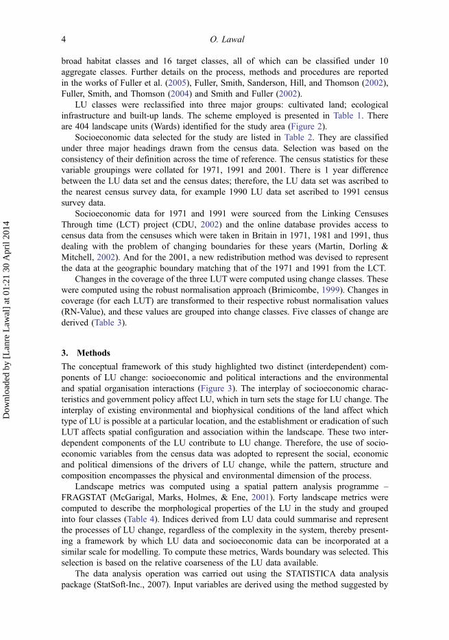
broad habitat classes and 16 target classes, all of which can be classified under 10aggregate classes. Further details on the process, methods and procedures are reportedin the works of Fuller et al. (2005), Fuller, Smith, Sanderson, Hill, and Thomson (2002),Fuller, Smith, and Thomson (2004) and Smith and Fuller (2002).

LU classes were reclassified into three major groups: cultivated land; ecologicalinfrastructure and built-up lands. The scheme employed is presented in Table 1. Thereare 404 landscape units (Wards) identified for the study area (Figure 2).

Socioeconomic data selected for the study are listed in Table 2. They are classifiedunder three major headings drawn from the census data. Selection was based on theconsistency of their definition across the time of reference. The census statistics for thesevariable groupings were collated for 1971, 1991 and 2001. There is 1 year differencebetween the LU data set and the census dates; therefore, the LU data set was ascribed tothe nearest census survey data, for example 1990 LU data set ascribed to 1991 censussurvey data.

Socioeconomic data for 1971 and 1991 were sourced from the Linking CensusesThrough time (LCT) project (CDU, 2002) and the online database provides access tocensus data from the censuses which were taken in Britain in 1971, 1981 and 1991, thusdealing with the problem of changing boundaries for these years (Martin, Dorling &Mitchell, 2002). And for the 2001, a new redistribution method was devised to representthe data at the geographic boundary matching that of the 1971 and 1991 from the LCT.

Changes in the coverage of the three LUT were computed using change classes. Thesewere computed using the robust normalisation approach (Brimicombe, 1999). Changes incoverage (for each LUT) are transformed to their respective robust normalisation values(RN-Value), and these values are grouped into change classes. Five classes of change arederived (Table 3).

3. Methods

The conceptual framework of this study highlighted two distinct (interdependent) com-ponents of LU change: socioeconomic and political interactions and the environmentaland spatial organisation interactions (Figure 3). The interplay of socioeconomic charac-teristics and government policy affect LU, which in turn sets the stage for LU change. Theinterplay of existing environmental and biophysical conditions of the land affect whichtype of LU is possible at a particular location, and the establishment or eradication of suchLUT affects spatial configuration and association within the landscape. These two inter-dependent components of the LU contribute to LU change. Therefore, the use of socio-economic variables from the census data was adopted to represent the social, economicand political dimensions of the drivers of LU change, while the pattern, structure andcomposition encompasses the physical and environmental dimension of the process.

Landscape metrics was computed using a spatial pattern analysis programme –FRAGSTAT (McGarigal, Marks, Holmes, & Ene, 2001). Forty landscape metrics werecomputed to describe the morphological properties of the LU in the study and groupedinto four classes (Table 4). Indices derived from LU data could summarise and representthe processes of LU change, regardless of the complexity in the system, thereby present-ing a framework by which LU data and socioeconomic data can be incorporated at asimilar scale for modelling. To compute these metrics, Wards boundary was selected. Thisselection is based on the relative coarseness of the LU data available.

The data analysis operation was carried out using the STATISTICA data analysispackage (StatSoft-Inc., 2007). Input variables are derived using the method suggested by

4 O. Lawal

Dow

nloa

ded

by [

Lan

re L

awal

] at

01:

21 3

0 A

pril

2014

Table

1.ReclassificationschemeforLU

data

sets.

New

classes

2ndLandutilisatio

nsurvey

(197

1)classes

1990

LCMGBclasses

2000

LCM

classes

Cultiv

ated

land

Arableland

,cereals,leylegu

mes,roots,green

fodder,industrial

crops,fallo

w,market

gardening,

fieldvegetables,mixed

market

gardening,

nurseries,allotm

entsgardens,

flow

ers,softfruits,ho

ps,orchards;with

grass,with

arable

land

,with

market

gardening

Tilled

land

mow

n/grazed

turf

Arable–cereals,ho

rticulture,Non

-rotational

horticulture,Im

prov

edgrassland

Ecological

infrastructures

Woo

dland,

forests–decidu

ous,coniferous,

mixed,copp

ice,

copp

icewith

standards,

woo

dlandshrub,

grassland,water

andmarsh,

freshwater

marsh,saltw

ater

marsh,heath,

moo

rland,

roug

hland

,op

enspace,

tend

edbu

tun

prod

uctiv

eland

Inland

water,saltm

arsh;grassheath,

meado

w/

verge/sem

i-natural;roug

h/marsh

grass;

bracken,

denseshrubheath,

decidu

ous

scrub;

decidu

ousandconiferous

woo

dland;

ruderalweed

Broad-leaved,

coniferous

woo

dland;

setaside,

neutral,calcareous,acid

grass;dw

arfshrub

heath,

open

dwarfshrubheath;

bracken,

fen,

marsh,sw

amp,

saltm

arsh;Water

Built-up

land

sSettlement,commercial

andresidential,

caravansites;un

vegetated,

indu

stry:

manufacturing

,extractiv

e,tip

s,pu

blic

utilities;transport:po

rtsareas,airfieldsand

soon

,major

roads;othermetalledroads;

derelictland

Sub

urban/ruraldevelopm

ent;continuo

usurban;

inland

bare

grou

ndInland

bare

grou

nd;subu

rban/rural

developed;

continuo

usurban

Journal of Land Use Science 5

Dow

nloa

ded

by [

Lan

re L

awal

] at

01:

21 3

0 A

pril

2014

Table

2.Socioecon

omic

data

grou

ping

sfrom

UK

census.

Group

Sub

grou

pDescriptio

n

Pop

ulation/spaceand

householdrelated

Num

berof

residents

Total

numberof

peop

leperWard(Totpo

p)Edu

catio

nallevel

Total

numberof

peop

lewith

high

erlevelof

education(H

iqual10)

Tenuretypes

Total

households

indifferenttype

oftenure

–Pub

licrenting(Pub

rnt),

Private

(Privrnt),Ownho

use(O

wnb

uy),Com

mun

alestablishm

ent(Com

estb),

Other

tenu

retypes(O

thrtenu)

Employ

mentrelated

Employ

mentstatus

Total

coun

tof

econ

omic

activ

eandno

n-activ

eindividu

als–Employ

edand

self-employ

ed(Empself),Retired

(Retrd),Student

(Studn

t),Unemploy

ed(U

nemply),Sick(Sick),Others(O

thremp)

Sectorof

employment

Total

numberof

individual

employed

perindustry

group–Agriculture,Fisheries

andForestry(A

gric),Services(Serv),Con

struction(Con

strc),Manufacturing

(Manuf),MiningUtilities

andTranspo

rt(M

utrans)

Transpo

rtationrelated

Mod

eof

travel

towork

Means

oftransportatio

nforecon

omically

activ

eindividu

al–Bus(Trvbu

s),

Foo

tandCycle

(Trvftcyc),Train(Trw

ktrn),Car

(Trvcar),Workfrom

home

(Wrkhm

),Others(O

thrtvw

rk)

Car

ownership

Total

coun

tof

carow

ned/nu

mberof

cars

ownedperho

usehold–Nocar(0car),

One

car(1car),twoor

morecars

(2mrcar)

6 O. Lawal

Dow

nloa

ded

by [

Lan

re L

awal

] at

01:

21 3

0 A

pril

2014

Table 3. Change classes derived from robust normalisation technique.

RN-Value Change class Interpretation

<−3.0 eDSC Very high decrease<−0.5 to >−3.0 DSC Decrease≥−0.5 to ≤0.5 NC No change>0.5 to ≤3 INCS Increase>3.0 eINCS Very high Increase

Figure 3. Conceptual framework of study.

Table 4. Selected landscape indices computed for modelling operations.

Class/Groupmembership Indices

Grain Total area (by landuse type) – TA; number of patches for each LUT – NP;patch density – PD; largest patch index – LPI; total edge – TE; edge density– ED;Landscape shape index – LSI; patch area distribution (Mean, area-weighted mean, standard deviation SD, coefficient of variation) – MPA,AWPA, SDPA, CVPA; radius of gyration distribution (mean, area-weightedmean, SD, CV) – MGYI, AWGYI, SDGYI, CVGYI

Shape Shape index distribution (mean, area-weighted mean, SD, CV) – MSI, AWSI,SDSI, CVSI; fractal dimension index distribution (mean, area-weightedmean, SD) – MFDI, AWFDI, SDFDI; perimeter-area ratio distribution(mean, area-weighted mean, SD, CV) – MPAR, SDPAR, CVPAR;contiguity index distribution (mean, area-weighted mean, SD, CV) – MCI,SDCI, CVCI

Contagion/interspersion(or connectivity)

Contagion (CONTAG); percentage of like adjacencies (PLADJ); landscapedivision index (LDI); effective mesh size (EMESH); splitting index(SPLITI); aggregation index (AGRIND); patch cohesion index (POCHES)

Diversity/richness Patch richness – PRICH; patch richness density – PRICHD; Simpson’sdiversity index – SIDI

Journal of Land Use Science 7

Dow

nloa

ded

by [

Lan

re L

awal

] at

01:

21 3

0 A

pril

2014

Riitters et al. (1995). Variables are termed high loading variables if they have the highestfactor load for dimensions identified from the factor analyses. To address any loss ofinformation which could be attributed to the use of factor analysis, a genetic algorithm(GA) feature selection method was also used to extract relevant variables for modellingLU changes. Data sets are entered into artificial neural networks (ANN) with changeclasses as output and landscape metrics and socioeconomic variables as inputs.

ANN are parallel, distributed information structures with a set of adaptive processingelements and unidirectional data connections (Fischer, 1998). ANN share some simila-rities with statistical methods such as regression analysis, but while regression analysismakes assumptions about the distribution and form of the variables used, ANN makes nosuch assumption, thus making them better predictors. ANN are made up of layers andneurons simulating the framework of learning and recollection of the human brain. Theyare well adapted to situations where relationships between inputs and outputs are complexbut do not give the functional form of relationship that exists between input and output.But their ability to handle spatially autocorrelated variables, poor and noisy data andaccount for non-linear relationships between input and output outweighs this shortcoming.The work of Gurney (2003) provides extensive details on ANN architecture, algorithmand classes.

The intelligent problem solver (IPS) module in STATISTICA package was adopted toidentify the optimal neural network design. IPS employs search algorithms to determinethe relevant set of inputs, number of hidden units and other key factors in the networkarchitecture (StatSoft-Inc., 2007). For the study, number of network to search through(200), number to retain (5), criteria for retention (error value), network design to search(see list below) were specified for the IPS. Search was carried out for multilayerperceptron (MLP) – three-layer and four-layer perceptron, radial basis function (RBF),linear (LNN), generalised regression (GRNN) and probabilistic (PNN) neural networkarchitectures. In selecting the best network to retain for further analysis, the system wasset to balance error against diversity. Networks were selected based on their complexity(number of inputs variables, hidden layers and units) and performance (selection error).Accuracy of the network was assessed using the sum-squared error function except forMLP (cross-entropy error function). Cross entropy has been reported to be better forclassification problem than sum-squared function for MLP when output classes are notbalanced (Rimer & Martinez, 2006).

4. Results and discussion

4.1. Dimension identification

A slight modification was made to the Riitters method (Riitters et al., 1995). And thisinvolved a two-staged correlation analysis – to eliminate intra-group and inter-grouprelationships among the landscape metrics. Metrics with high correlations with othermetrics are eliminated. With this process, 10 metrics were eliminated at the first stageand a further 6 at the second stage.

Factor analysis was carried out using the correlation matrix of the representativemetrics as inputs. Four factors derived from this analysis accounted for about 87% ofthe variation. A second factor analysis was carried out after removing six metrics that arenot loading highly into any of the four factors extracted. The results are similar to theprevious factor analysis, four factors were extracted from the 18 metrics (Table 5) and

8 O. Lawal

Dow

nloa

ded

by [

Lan

re L

awal

] at

01:

21 3

0 A

pril

2014

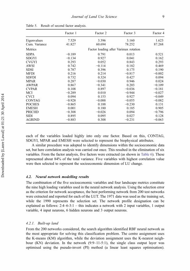
each of the variables loaded highly into only one factor. Based on this, CONTAG,SDGYI, MPAR and EMESH were selected to represent the biophysical attributes.

A similar procedure was adopted to identify dimensions within the socioeconomic dataset, but here correlation analysis was carried out once. This resulted in the elimination of sixvariables. From the factor analysis, five factors were extracted (as shown in Table 6). Theserepresented about 84% of the total variance. Five variables with highest correlation valuewere then selected to represent the socioeconomic dimension of LU change.

4.2. Neural network modelling results

The combination of the five socioeconomic variables and four landscape metrics constitutethe nine high loading variables used in the neural network analysis. Using the selection erroras the criterion for network acceptance, the best performing network from 200 test networkswere extracted and reported for each of the LUT. The 1971 data was used as the training set,while the 1990 represents the selection set. The network profile designation can beexplained as follows: 2:4–6-3:1 – this indicates a network with 2 input variables, 1 outputvariable, 4 input neurons, 6 hidden neurons and 3 output neurons.

4.2.1. Built-up land

From the 200 networks considered, the search algorithm identified RBF neural network asthe most appropriate for solving this classification problem. The centre assignment usesthe K-means (KM) algorithm, while the deviation assignment uses the K-nearest neigh-bour (KN) deviation. In the network (9:9–11-5:1), the single class output layer wasoptimised using the pseudo-invert (PI) method (a linear least squares optimisation).

Table 5. Result of second factor analysis.

Factor 1 Factor 2 Factor 3 Factor 4

Eigenvalues 7.529 3.396 3.160 1.623Cum. Variance 41.827 60.694 78.252 87.268

Metrics Factor loading after Varimax rotation

SDPA −0.189 0.791 0.013 0.521SDGYI −0.134 0.927 0.041 0.162CVGYI 0.293 0.052 0.843 0.293AWSI 0.742 −0.114 0.182 0.469SDSI 0.787 0.396 0.175 0.190MFDI 0.216 0.214 −0.817 −0.002SDFDI 0.732 0.324 0.427 0.094MPAR 0.287 −0.030 0.946 0.024AWPAR 0.867 −0.341 0.203 −0.109CVPAR 0.108 0.897 −0.036 −0.181MCI −0.289 0.010 −0.944 −0.027CVCI 0.094 0.153 0.927 −0.049CONTAG −0.928 −0.088 −0.055 −0.082POCHES −0.865 0.188 −0.230 0.131EMESH 0.001 0.180 0.185 0.905PRICHD −0.308 −0.026 0.094 −0.796SIDI 0.895 0.095 0.027 0.128AGRIND −0.883 0.308 −0.231 −0.063

Journal of Land Use Science 9

Dow

nloa

ded

by [

Lan

re L

awal

] at

01:

21 3

0 A

pril

2014

Furthermore, this network recorded 0.64 and 0.47 for the training and selection perfor-mance, respectively, while the error functions are reported as 0.33 (training error) and 0.37(selection error).

In the case of GA feature selection, RBF was also identified here as the mostappropriate network, and the GA identified 15 input variables (13 landscape metricsand 2 socioeconomic variables – Retrd and Constrc) with a network profile of 15:15–6-5:1. The training performance (0.62) was 2% worse off compared to the performancerecorded for the network using only factor representatives. The same observation wasmade for the selection performance (0.33), which declined by about 14%, while thenetwork was able to achieve only a 1% reduction in the training error (0.32) and aselection error of 0.39. The centre assignment (KM), deviation assignment (KN) andoutput layer optimisation (PI) are the same as observed for the high loading variable-derived model.

4.2.2. Cultivated land

PNN was found to be the best performer for cultivated land when factor representativesare used as inputs. The PNN network has a network profile designation of 9:9–404-5:1.The network training and selection performance was recorded as 0.59 and 0.41, respec-tively, while the errors in the network were quantified as 0.32 (training) and 0.38(selection). With these statistics, the overall performance of the network is fair.

Table 6. Results of factor analysis for socioeconomic variables.

Factor 1 Factor 2 Factor 3 Factor 4 Factor 5

Eigenvalues 7.807 11.356 14.533 16.605 17.720Cum. Variance 37.178 54.075 69.204 79.071 84.381

Variables Factor loading after Varimax rotation

0car 0.026 0.762 −0.164 0.530 0.2551car 0.266 0.294 0.833 0.170 0.1782mrcar 0.174 −0.161 0.905 −0.156 0.080Agric 0.745 −0.172 0.352 0.034 0.346Serv 0.758 −0.098 0.275 0.096 0.544Constrc 0.769 −0.180 0.426 0.043 0.163Manuf 0.877 0.083 0.273 0.082 0.239Empself 0.143 0.832 0.471 0.095 0.012Othremp −0.380 0.764 0.008 −0.016 −0.332Retrd −0.433 0.509 0.473 0.206 −0.352Studnt 0.354 0.168 0.162 0.230 0.731Unemply 0.095 −0.125 0.344 0.575 0.600Othrtenu 0.195 0.050 0.056 0.068 0.872Comestb −0.260 0.462 −0.176 −0.408 0.204Ownbuy 0.147 0.007 0.944 −0.158 0.031Privrnt 0.073 0.845 −0.198 −0.215 0.136Pubrnt 0.010 0.094 −0.225 0.902 0.161Othrtvwrk −0.801 −0.160 0.418 0.251 0.118Trvbus 0.727 0.010 0.034 0.289 0.451Trvftcyc 0.539 0.032 −0.044 0.097 0.686Trwktrn 0.732 −0.081 0.369 −0.034 0.088

10 O. Lawal

Dow

nloa

ded

by [

Lan

re L

awal

] at

01:

21 3

0 A

pril

2014

In the case of GA feature selection, RBF network (14:14–10-5:1) displayed a 6% and1% increase in training performance (0.66) and selection performance (0.42), respectively,over the PNN network retained for above. Furthermore, there was a reduction of about 2%in the training error (0.29) when compared with the PNN network identified earlier. Butthere was a slight increase (0.08%) in the selection error (0.38) for the RBF network overthe PNN. Overall, the current RBF network displayed an improvement over the pre-viously identified best network for cultivated land.

4.2.3. Ecological infrastructures

For ecological infrastructure, RBF neural network architecture was also found to be thebest performing network architecture. This network has a profile designation of 9:9–39-5:1, with the KM centre assignment, followed by the KN for deviation assignment. Thenetwork recorded a good training performance of 0.67 and a fair selection performance(0.47), while the lowest possible selection error out of the 200 networks tested was foundto be 0.36 coupled with a training error of 0.30.

The feature selection using GA identified 19 input variables – 4 socioeconomicvariable and 15 landscape metrics. With these input variables, the exploratory neuralnetwork analysis identified RBF as the best performing network with a profile of 15:15–20-5:1. There was no major improvement in the overall performance of the network whencompared to the network above. The network recorded a training and selection perfor-mance of 0.73 and 0.51, respectively, while errors are reported as 0.28 and 0.36,respectively.

By comparing the selection performance, it was possible to identify the best perfor-mance neural network for each of the LUT (Figure 4). The result from the modellingoperation shows that for built-up lands, the use of high loading variables provides a betterneural network performance. This is evident considering the number of variables entered

0

0.1

0.2

0.3

0.4

0.5

0.6

HL GA HL GA HL GA

Built Cultivate Land Ecol. Infra

Val

ues

Feature selection methods and LUT

PerformanceError

Figure 4. Neural network selection performance and error.

Journal of Land Use Science 11

Dow

nloa

ded

by [

Lan

re L

awal

] at

01:

21 3

0 A

pril

2014

and the overall performance of the GA-derived inputs neural network (i.e. no improve-ment in performance despite using more variables).

The difference was not so clear for cultivated lands, where the selection performanceof neural network using the GA feature extraction method was only marginally superior tothat of factor analysis method. But with the use of 14 variables compared to 9, it isdebatable that additional 5 variables is necessary to achieve a 1% improvement inperformance. It is, therefore, possible to posit that the use of factor analysis-derivedinputs is adequate, since it offers a simpler network (classification solution).

In the case of ecological infrastructures, the error rate remains the same for bothmethods. However, there was 9% increase (selection performance) over the factor analysisfeature extraction neural network – giving an indication of the better classificationperformance when GA is used for feature selection. A closer examination of the twoneural networks revealed that from the classification table (accuracy of classification byclasses), the improvement in performance is wholly attributable to 100% classificationaccuracy (and classification failure for the other four classes) obtained for landscape thatexperience decrease in ecological infrastructures.

Overall, the use of high loading variables (factor analysis-derived variables) providesa simpler model for the changes in LU across the study area. This implies that thedirection of change in LU within each ward across the study area could be identifiedwhen spatial morphology of the area and some socioeconomic variables are considered.And for the study area, it was found that the level of fragmentation (Contagion –connectivity, effective mesh – probability that two random points belong to the samepatch), extent of LU patches (Gyration index), shape complexity of LU patches (peri-meter–area ratio) when combined with the number of people employed in manufacturingsector and terms of house holding (public, private and other uncategorised tenure types)provide a slight indication of the direction of change in land use.

Furthermore, from the training performance, there is an indication that the conceptualframework for the study is valid. Across the entire modelling operation, the trainingperformance was consistently high, giving an indication that the use of spatial morphol-ogy and socioeconomic characteristics could be used in the identification of direction ofchange in land use. But as also shown in the results, for longitudinal studies using neuralnetwork, there are challenges in the identification data set for training the neural networkand also selecting the relevant input variables.

The accuracy of the model for the study area falls within an acceptable range,considering the fact that there are many other factors that could complicate futureprediction. It is opined that this performance could be enhanced with improvement inthe spatial and temporal resolution of the data set. Another factor that could improve theperformance is adjacency effect and, as it is well known, could have a significant effect onLU change. But essentially, the challenge is how this should be implemented within thecurrent modelling framework.

5. Conclusion

The conceptual framework of the study (Figure 3) has identified some of the relevantfactors that could contribute to changes in land use/cover. And it draws upon advances inlandscape ecology, wealth of information available and advances in pattern recognitionoffered by artificial neural networks to develop a link between human and natural factorsof land use/cover change.

12 O. Lawal

Dow

nloa

ded

by [

Lan

re L

awal

] at

01:

21 3

0 A

pril

2014

The results of the modelling operation revealed that this model is feasible and offers anew possibility for incorporation of socioeconomic data into LU models. The results showthe importance of pattern within landscape in modelling LU change and also demonstratedthat these patterns, when complemented with human factors, offer some solutions foridentifying the direction of change.

The methodology tested allows rapid evaluation of the direction of LU change, takinginto consideration relevant dimensions of LU dynamics. The study focused on LUdynamics of part of the TG within the City of London (Urban area). However, themodelling framework could also be applied to any other area where there is heterogeneityin the LUT, socioeconomic and biophysical characteristics.

The result of the study highlights the success of the approach in identifying thedirection of the change as evident from the interactions between the human and bio-physical factors. Landscape units with configurations and attributes that could causeundesirable changes could be identified from this study. It is, therefore, evident thatwhile the use of surrogate variables such as distance to facilities (transport, city centresetc.,) are prevalent as a way of incorporating socioeconomic characteristics in LU models,the use of data from census surveys and landscape metrics present a richer set ofinformation that are valuable in modelling LU change. While the outcome of this researchpresents a qualitative representation of the changes, there are possibilities for the output tobe quantitative, providing that the spatial and temporal resolution of the data are adequate.But this qualitative representation could still be used to understand and highlight regionaldirection and dynamics of LU.

With the data set used for this study, the modelling operation showed that someclasses of change could be identified when new data set were presented to the neuralnetwork after the initial training. For example, in the case of built-up LUT on the wardswith DSC and INCS change classes could be correctly identified in the selection phasesand in the case of ecological infrastructure only one change class showed consistentlygood classification (DSC – for both the factor analysis derived and GA derived inputvariable set). From the foregoing, it is evident that training the networks with the 1971data set, could not provide the network with appropriate centre and deviation calculationfor classification of all the five change classes, when new data set are presented to thenetwork. But the level of accuracy in classification showed that the approach is valuablefor rapid evaluation of possible LU change direction. Therefore, some questions that arisefrom this study include: what is the appropriate method for training the neural networkmodels? Could multi-output neural network model offer better classification solution thanthe current single output?

ReferencesBest, R. H. (1981). Land use and living space. London: Methuen & Co.Brimicombe, A. J. (1999). Small may be beautiful, but is simple sufficient? Geographical and

Environmental Modelling, 3, 9–33.CDU. (2002, February 15, 2006). Linking censuses through time. Retrieved from http://cdu.mimas.

ac.uk/lct/Cohen, P. (2004). Where is east London going? Discussion paper. London: London East Research

Institute.Countryside-Commission. (1996). The character of Engand’s natural and man-made landscape:

South East & London (Vol. 7). London: The Countryside Agency.Devereux, B. J., Amable, G. S., & Posada, C. C. (2004). An efficient image segmentation algorithm

for landscape analysis. International Journal of Applied Earth Observation andGeoinformation, 6(1), 47–61. doi:10.1016/j.jag.2004.07.007

Journal of Land Use Science 13

Dow

nloa

ded

by [

Lan

re L

awal

] at

01:

21 3

0 A

pril

2014

DOE. (1995). The Thames Gateway planning framework. London: HMSO.Fischer, M. M. (1998). Computational neural networks: A new paradigm for spatial analysis.

Environment and Planning A, 30(10), 1873–1891. doi:10.1068/a301873Forman, R. T. T., & Godron, M. (1986). Landscape ecology. New York, NY: Wiley.Fuller, R. M., Cox, R., Clarke, R. T., Rothery, P., Hill, R. A., Smith, G. M., … Stott, A. P. (2005).

The UK land cover map 2000: Planning, construction and calibration of a remotely sensed, user-oriented map of broad habitats. International Journal of Applied Earth Observation andGeoinformation, 7(3), 202–216. doi:10.1016/j.jag.2005.04.002

Fuller, R. M., Groom, G. B., & Jones, A. R. (1994). The land cover map of Great Britain: Anautomated classification of Landsat thematic mapper data. Photogrammetric Engineering andRemote Sensing, 60(5), 553–562.

Fuller, R. M., Groom, G. B., & Wallis, S. M. (1994). The availability of Landsat TM images of greatBritain. International Journal of Remote Sensing, 15(6), 1357–1362. doi:10.1080/01431169408954170

Fuller, R. M., & Parsell, R. J. (1990). Classification of TM imagery in the study of land use inlowland Britain: Practical considerations for operational use. International Journal of RemoteSensing, 11(10), 1901–1917. doi:10.1080/01431169008955137

Fuller, R. M., Sheail, J., & Barr, C. J. (1994). The land of Britain, 1930-1990: A comparative studyof field mapping and remote sensing techniques. The Geographical Journal, 160(2), 173–184.doi:10.2307/3060075

Fuller, R. M., Smith, G. M., Sanderson, J. M., Hill, R. A., & Thomson, A. G. (2002). The UK landcover map 2000: Construction of a parcel-based vector map from satellite images. TheCartographic Journal, 39(1), 15–25. doi:10.1179/caj.2002.39.1.15

Fuller, R. M., Smith, G. M., & Thomson, A. G. (2004). Contextual analyses of remotely sensedimages for the operational classification of land cover in Great Britain. In S. D. Jong, & F. V. D.Meer (Eds.), Contextual methods in image processing of remotely sensed data. Dordrecht:Kluwer Academics.

Gurney, K. (2003). An introduction to neural networks. Boca Raton, FL: CRC Press.Irwin, E. G., & Geoghegan, J. (2001). Theory, data, methods: Developing spatially explicit

economic models of land use change. Agriculture, Ecosystems and Environment, 85(1–3), 7–24. doi:10.1016/S0167-8809(01)00200-6

Jackson, D. L. (2000). Guidance on the interpretation of the biodiversity broad habitat classification(Terrestrial and freshwater types): Definitions and the relationships with other habitat classifica-tions JNCC Report No. 307. Peterborough: Joint Nature Conservation Committee.

Martin, D., Dorling, D., & Mitchell, R. (2002). Linking censuses through time: Problems andsolutions. Area, 34, 82–91. doi:10.1111/1475-4762.00059

McGarigal, K., Marks, B. J., Holmes, C., & Ene, E. (2001). Fragstats–spatial pattern analysisprogram for quantifying landscape structure (version 3.3 build 5). Amherst: University ofMassachusetts. Retrieved from http://www.umass.edu/landeco/research/fragstats/fragstats.html

Mertens, B., Sunderlin, W. D., Ndoye, O., & Lambin, E. F. (2000). Impact of macroeconomicchange on deforestation in South Cameroon: Integration of household survey and remotely-sensed data. World Development, 28(6), 983–999. doi:10.1016/S0305-750X(00)00007-3

Riitters, K. H., O’Neill, R. V., Hunsaker, C. T., Wickham, J. D., Yankee, D. H., Timmins, S. P., …Jackson, B. L. (1995). A factor analysis of landscape pattern and structure metrics. LandscapeEcology, 10, 23–39. doi:10.1007/BF00158551

Rimer, M., & Martinez, T. (2006). CB3: An adaptive error function for backpropagation training.Neural Processing Letters, 24(1), 81–92. doi:10.1007/s11063-006-9014-9

Smith, G. M., & Fuller, R. M. (2002). Land cover map 2000 and meta data at the land parcel level.In G. M. Foody & P. M. Atkinson (Eds.), Uncertainty in remote sensing and GIS. London:Wiley and Sons.

StatSoft-Inc. (2007, January 15, 2006). Electronic statistics textbook. Retrieved from http://www.statsoft.com/textbook/stathome.html

Van Der Veen, A., & Otter, H. S. (2001). Land use changes in regional economic theory.Environmental Modeling and Assessment, 6(2), 145–150. doi:10.1023/A:1011535221344

Wyatt, B. K., Greatorex-Davies, N. G., Bunce, R. G. H., Fuller, R. M., & Hill, M. O. (1994).Comparison of land cover definitions countryside 1990 series (Vol. 3). London: Department ofthe Environment.

14 O. Lawal

Dow

nloa

ded

by [

Lan

re L

awal

] at

01:

21 3

0 A

pril

2014