Exploiting the Potential Energy Landscape to Sample Free Energy

Andrew J. Ballard,1, ∗ Stefano Martiniani,1, † Jacob D. Stevenson,1, ‡

Sandeep Somani,1, 2, § and David J. Wales1, ¶

1Department of Chemistry, Lensfield Road, Cambridge CB2 1EW, UK

2Janssen Research and Development, LLC 1400 McKean Road, Spring House, PA 19477, USA

(Dated: March 2015)

Abstract

We review a number of recently-developed strategies for enhanced sampling of complex systems which

are based upon the energy landscape formalism. We describe five methods, Basin-Hopping, Replica Ex-

change, Kirkwood Sampling, Superposition-Enhanced Nested Sampling, and Basin-Sampling, and show

how each of these methods can exploit information contained in the energy landscape to enhance thermo-

dynamic sampling.

∗ ab2111@cam.ac.uk

† sm958@cam.ac.uk‡ js850@cam.ac.uk§ ssomani@its.jnj.com

¶ dw34@cam.ac.uk

1

I. INTRODUCTION

In this contribution we provide an overview of recent methods that all have their basis in en-

hancing the sampling of global thermodynamics using knowledge of the underlying potential en-

ergy landscape. Making these connections seems particularly timely, as a number of potentially

important advances have been made over the last few years, and they share some common charac-

teristics. In particular, the use of low-lying local minima obtained from methods based on global

optimisation (§ III), and the superposition approach (§ II), provide some common themes. Of

course, many other methods have been proposed for enhanced sampling [1–13], and these will not

be reviewed here. The procedures we describe, with foundations in potential energy landscape the-

ory [14–16] and geometry optimisation, are largely complementary to approaches based on more

conventional molecular dynamics and Monte Carlo schemes [17]. Future work will require bench-

marking comparisons of the most promising methods, to guide applications in different fields. For

the present purposes our main aim is to show what has been achieved in recent work based on the

potential energy landscape framework, and explain how these new tools are connected.

Most of the tests we have conducted employ atomic clusters of N atoms bound by the Lennard-

Jones (LJ) potential [18]

V = 4ǫ∑

i<j

[(σ

rij

)12

−

(σ

rij

)6], (1)

where ǫ and 21/6σ are the pair equilibrium well depth and separation, respectively. These systems

will be denoted LJN , and there are a number of sizes where low temperature solid-solid phase tran-

sitions have been identified in previous work [7, 8, 14, 19–26]. In each case there are competing

low energy morphologies separated by potential energy barriers that are large compared to kBT at

the transition temperature. The relatively simple potential makes these systems ideal benchmarks

for analysis of broken ergodicity issues, as well as for global optimisation [14, 19, 27] and rare

event dynamics [28–31]. In principle, the same improvements would be obtained for treatments

that explicitly consider electronic structure. However, the much greater computational expense of

computing energies and gradients that would be necessary mean that these opportunities have yet

to be exploited.

We begin by introducing the superposition approach (§ II), a key component in the methods

under review, which allows us to link thermodynamics to the basins of attraction of local minima

on the underlying energy landscape. With this background in place, we review in § III the basin-

2

hopping strategy for global optimisation. We then consider strategies for thermodynamic estima-

tion, including replica exchange (§ IV), Kirkwood sampling (§ V), nested sampling (§ VI), and

basin-sampling (§ VII). In these sections we emphasize the utility of the superposition approach

in enhancing these simulations, and provide evidence for gains in efficiency and convergence from

simulation results for benchmark systems.

II. THE SUPERPOSITION APPROACH

A common theme in several of the following sections is the superposition approach to ther-

modynamics, which represents a key component of the computational potential energy landscape

framework [14]. Here we write the total partition function or density of states as a sum over con-

tributions from the basins of attraction [14, 32, 33] of the local minima, which gives an explicitly

ergodic representation of the thermodynamics [8, 14, 34–37]. As a first approximation it is of-

ten convenient to use harmonic vibrational densities of states for the local minima. The resulting

superposition partition function is nevertheless anharmonic, owing to the distribution of local min-

ima in energy. We can therefore separate contributions to thermodynamic properties in terms of

the individual potential wells and the sum over minima. For example, we can identify well and

landscape anharmonicity [38, 39]. For low temperature solid-solid equilibria the harmonic nor-

mal mode approximation can be quantitatively accurate, but methods to sample anharmonicity are

generally required if an accurate picture of melting transitions is needed. Reweighting schemes

and temperature-dependent frequencies have been considered for this purpose in previous work

[35, 40–43]. The most recent basin-sampling scheme [44] will be outlined in § VII.

The underlying superposition representation for the canonical partition function is

Z(T ) =Nst∑

α=1

NPIα∑

ζ=1

Zζ(T ) =Nst∑

α=1

NPIα Zα(T ) = P

Nst∑

α=1

Zα(T )/oα, (2)

where Z(T ), is decomposed in terms of contributions from the catchment basin [14, 32] of each

of the N st distinct local minimum structures, with Zα(T ) the partition function of structure α

at temperature T , which is identical for each of the corresponding NPIα permutation-inversion

isomers. Here P is the number of permutation-inversion operations of the Hamiltonian, 2∏

β Nβ!,

and oα is the order of the rigid molecule point group [14, 45–47].

The great advantage of the superposition approach is that we can exploit efficient methods

for locating low-lying local minima based on global optimisation, as described in § III. Basin-

3

hopping approaches that incorporate a local minimisation [19, 48, 49] can employ arbitrary moves

through configuration space, which can circumvent the barriers that cause ergodicity breaking in

standard Monte Carlo and molecular dynamics procedures. Superposition methods employing

both harmonic and anharmonic approximations of the vibrational density of states have found

widespread applications in molecular science, and various examples are considered in the follow-

ing review. First we outline the basin-hopping global optimisation approach, which has been used

to obtain most of the samples of low-lying potential energy minima. We note that basin-hopping is

a stochastic procedure, so it is not guaranteed to find all the relevant low-lying minima. However,

the sampling of local minima, which does not require detailed balance, is much faster than for

thermodynamic sampling approaches, and is straightforward for the systems considered here.

III. BASIN-HOPPING GLOBAL OPTIMISATION

The thermodynamic sampling schemes described in the following sections are of particular

interest for systems involving broken ergodicity at low temperature, where the potential energy

landscape supports alternative low-lying morphologies separated by relatively high barriers. Here,

a ‘high’ barrier corresponds to a value that is large compared to kBT at the temperature, T , where

the structures would have equal occupation probabilities, and kB is Boltzmann’s constant. Basin-

hopping (BH) global optimisation [19, 48, 49] has been successfully employed to survey low-

lying minima in a wide range of systems of this type, including atomic and molecular clusters,

biomolecules, and soft and condensed matter [14, 49, 50]. These applications will not be reviewed

here; since the BH procedure is now well established an overview should be sufficient in the

present context.

The key point of the basin-hopping framework is to couple local energy minimisation to some

sort of step-taking procedure in configuration space. Random perturbations of the atomic coor-

dinates sometimes work quite well, but more efficient schemes can often be devised, which may

exploit characteristics of the system under consideration. For example, internal coordinate moves,

such as Kirkwood sampling, that respect connectivity are likely to work better for biomolecules

with a well-defined covalently bonded framework. Numerous BH variants with alternative step-

taking schemes have now been described, and parallel approaches using replicas at different effec-

tive temperatures have also been used [51]. In each case the potential energy for any configuration,

X, becomes the potential energy of the local minimum that the chosen minimisation procedure

4

converges to from X:

V (X) = minV (X), (3)

where X is a 3N-dimensional vector for a system of N atoms. The resulting minimum replaces

the previous structure in the chain if it satisfies a chosen acceptance condition, and again several

alternatives have been considered. A simple Metropolis scheme often works well, where the new

minimum with potential energy Enew is accepted if it lies below the potential energy of the starting

point, Eold. If Enew > Eold it is accepted if exp[(Eold−Enew)/kT ] is greater than a random number

drawn from the interval [0,1]. Schemes based on thresholding [52], downhill-only moves [53] and

non-Boltzmann weights [54] based on Tsallis statistics [55, 56] have also been described.

Much larger steps in configuration space can be taken than for conventional molecular dynam-

ics or Monte Carlo methods, since the energy becomes the value after minimisation, and there is

no requirement to satisfy detailed balance. Downhill barriers are therefore removed, and atoms

can pass through each other. In fact, there is a more subtle effect, which facilitates sampling when

broken ergodicity is prevalent. The occupation probabilities of competing regions of configuration

space for the transformed landscape V (X) have been found to overlap significantly over a wider

temperature range, where moves still have a good chance of being accepted [57, 58].

IV. REPLICA EXCHANGE APPROACHES

The local minima provided by BH can be very helpful to understand systems exhibiting bro-

ken ergodicity. However, if thermodynamic properties are required, then configurations within

the vicinity of each minimum become important, and increasingly so with higher temperature. At

temperatures where well anharmonicity becomes noticeable, alternative techniques are required

for sampling the thermodynamic state of interest. In contrast to BH, thermodynamic sampling

techniques generally require detailed balance to be satisfied in order to ensure the correct canon-

ical distribution is preserved. While many long-standing strategies exist for sampling stationary

distributions, the most notable being Monte Carlo and thermostatted molecular dynamics algo-

rithms, the restriction of detailed balance often renders such techniques inefficient or unpractical.

For instance, a Monte Carlo simulation with random perturbation moves often requires a small

displacement step in order to achieve a useful acceptance probability. As a result, the system

only explores its local configuration space on shorter timescales, with large-scale rearrangements,

which dominate simulation convergence, occurring on much larger timescales. This quite generic

5

problem necessitates advanced sampling strategies.

Replica exchange [59, 60] (REX) has emerged as a promising technique to sample such systems

exhibiting complex energy landscapes. REX refers to a family of methods in which M indepen-

dent copies or “replicas” of a system are simulated in parallel, typically at different temperatures,

with occasional moves that attempt to swap configurations between neighboring replicas. While

large energy barriers may prevent the system from exploring its configuration space at low temper-

atures, enhanced thermal fluctuations provide more rapid barrier crossings at high temperatures.

By means of the swap attempts, the low-temperature replicas are exposed to the wider reaches of

configuration space explored by the the high-temperature replicas, providing a means to sample

on both sides of the barrier without directly overcoming it. In this section we will focus primarily

on parallel tempering (PT) in which the replicas are defined by a progression of temperatures, but

methods with differing Hamiltonians exist as well [61].

The REX moves must satisfy detailed balance, which is enforced through an acceptance prob-

ability for the exchange attempt. For two replicas, A and B, having the same potential energy

function V but at different temperatures TA and TB , the acceptance probability takes the form

Pacc(X,Y) = min1, e∆β∆V . (4)

Here ∆β = 1/kBTB − 1/kBTA, and ∆V = V (Y) − V (X) is the difference in potential energy

of the swap configurations X and Y in question. Eq. 4 guarantees that each replica samples its

correct equilibrium state, despite the fact that configurations are being swapped between different

thermodynamic ensembles.

Just as detailed balance restricts the perturbation stepsize in a MC simulation, in REX it limits

the temperate spacings between neighboring replicas. To ensure a decent average acceptance rate

〈Pacc〉 the temperatures TA and TB must be spaced closely, yet still far enough apart not to waste

computational resources on an unnecessary number of replicas. This conflict has given rise to

numerous strategies to optimize various PT parameters, in particular the temperature spacings and

total number of replicas.

Understanding a system in terms of the underlying energy landscape can be particularly useful

in this respect, and recent developments have been made that enhance PT simulations by utilizing

information contained in the energy landscape. These developments, described below, exploit the

harmonic superposition approximation (HSA), a harmonic expansion of the landscape about the

known configurational minima. Through this approximation, an approximate energy landscape

6

can be constructed solely from a set of minima, and since the form is particularly convenient,

namely a series of multi-dimensional harmonic wells, thermodynamic predictions can be easily

made. In this way, thermodynamics from the HSA can be used to approximate the behaviour of

the true underlying system.

The HSA can be exploited to determine optimal PT temperature spacings, a crucial component

in the performance of PT simulations. In general a uniform acceptance profile is desired across all

neighboring replicas [62–67], which guarantees that replica round-trip times are not plagued by

bottlenecks as trajectories transition between temperatures. Ballard and Wales [68] have recently

demonstrated how knowledge of configurational minima can be utilized to optimize PT temper-

atures in this respect. By approximating the canonical distribution of each replica via the HSA,

they obtained analytic expressions for the average acceptance rate 〈Pacc〉 in terms of features of the

configurational minima. From these expressions, a set of optimal temperatures can be uniquely

determined by matching to a target acceptance rate, yielding a progression of replicas that has

a uniform acceptance within the approximation of the HSA. Simulations of systems undergoing

phase transformation have revealed that this strategy can yield uniform acceptance rates and effi-

ciency enhancements over a standard progression. Fig. 1 displays the uniform acceptance profile

achieved by the method on PT simulations of LJ31.

In addition to optimizing temperature spacings, the HSA can also be used as a replica in itself.

Mandelshtam and coworkers [7, 8] have devised a REX strategy whereby an auxiliary “reser-

voir” replica is coupled to an M-replica PT simulation. The reservoir replica samples the HSA

at a user-specified temperature, with reservoir-temperature swap moves occurring with a particu-

lar temperature replica. Because HSA samples can be drawn analytically, reservoir sampling is

essentially barrierless and enables rapid exploration of the system’s relevant configuration space

(defined by the known minima). In this way the reservoir reduces the need for high temperature

replicas to overcome barriers. Similar strategies for MC sampling employ analogous ideas by

generating trial moves near known configurational minima [1, 5].

V. KIRKWOOD SAMPLING

Kirkwood sampling [69] is a method for random (or non-Markovian) sampling of the confor-

mational space of molecules. The principal challenge in random conformational sampling is to

avoid steric clashes among the atoms. Kirkwood sampling addresses this problem by incorpo-

7

2 4 6 8 10

Temperature index

0.12

0.14

0.16

0.18

0.20

0.22

0.24

〈Pac

c〉

geometric

HSA-enhanced

target

FIG. 1. Acceptance profile for REX simulation of LJ31: The average REX acceptance probability for

pair (Ti, Ti+1) is plotted vs temperature index i, for temperature spacings chosen using standard geometric

progression (empty black circles), and chosen by HSA-optimization (filled blue circles). The dip in the

geometric case coincides with a heat capacity peak. At higher temperatures both profiles deviate from

uniform behavior, as the HSA becomes less accurate. Results replotted from Ref. [68]

rating correlations among internal coordinates, as captured by the joint probability distribution

function (pdf) between various sets of internal coordinates. Kirkwood sampling is based on the

generalization of the Kirkwood superposition approximation (KSA), originally developed in the

radial distribution function theory of liquids [70, 71]. Analogous approximations were later de-

veloped [72, 73] in the mutual information theory of correlations and provided expressions for a

multidimensional pdf in terms of its marginal pdfs corresponding to neglect of certain correlations.

The current application to conformational sampling was motivated by conformational entropy cal-

culation of small molecules using the mutual information expansion of entropy [74]. The simplest

approximation in this family, namely the Kirkwood superposition approximation, pKSA3 , expresses

a three-dimensional pdf, p3, in terms of its one- and two-dimensional marginal pdfs

p3(x1, x2, x3) ≈ pKSA3 (x1, x2, x3) =

p2(x1, x2)p2(x1, x3)p2(x2, x3)

p1(x1)p1(x2)p1(x3)(5)

8

where p1(.) and p2(., .) are the marginal pdfs, and the subscript indicates the dimensionality of the

pdf. Eq. 5 can be obtained from the mutual information expansion of Shannon entropy of p3 by

dropping the three-fold mutual information [69, 74]. The Kirkwood superposition approximation

can be generalized to express an N-dimensional pdf in terms of its marginals of highest order

l [74]. For instance, the doublet level (l=2) superposition approximation is given by the ratio of

the product of 2-D and 1-D marginal pdfs

pN ≈ p(2)N (x1, . . . , xN) =

∏i<j p2(xi, xj)∏

i p1(xi)(6)

where the superscript “(2)” denotes doublet level. Eq. 6 accounts for pairwise correlations among

all variables but ignores the higher order correlations. Approximations that account for selected

correlations of different orders can also be derived [75]. Eq. 6 is fully coupled and therefore exact

sampling would be computationally prohibitive for high-dimensional systems. The Kirkwood

approach addresses this issue by sequential sampling of the variables such that each one is selected

from a one-dimensional conditional distribution conditioned on the previously sampled variables.

The conditional distributions are obtained using the appropriate superposition approximation. For

example, given a sequence of variables, the conditional pdf for the k-th variable given values of

previous k-1 variables, using the doublet level approximation (Eq. 6), is

p(2)1 (xk |x1, .., xk−1 ) =

p(2)k (x1, .., xk−1, xk)

p(2)k−1(x1, .., xk−1)

=1

nk

∏1≤j≤k−1 p2 (xj , xk)

p1 (xk)k−2

(7)

where the normalization nk can be computed numerically. The doublet level Kirkwood scheme

effectively samples from the N-dimensional pdf

p(2)N (~x) = p2 (x1, x2)

∏

3≤k≤N

p(2)1 (xk |x1, x2, .., xk−1 ) , (8)

and not from Eq. 6. Thus, at the doublet level, the sequence of approximations for the true distri-

bution, pN , is

pN → p(2)N → p

(2)N . (9)

Note that both the doublet level Kirkwood approximation, p(2)N , and the doublet level sampling

distribution, p(2)N , involve a product of all singlet and doublet pdfs. Due to this product form,

a sampled conformation is guaranteed to fall in the non-zero probability cells of all input pdfs.

9

This construction ensures that all correlations are satisfied simultaneously. The computational

complexity of a Kirkwood sampling algorithm is proportional to the number of pdfs used. Since

the number of doublet level marginals are N(N + 1)/2, the doublet level sampling algorithm has

the complexity of O(N2).

Doublet and triplet level Kirkwood sampling has been applied to small drug-like molecules [69]

and small peptides [76] with up to 52 atoms. In these studies, bond-angle-torsion [77] internal co-

ordinate system was used and the input pdfs were populated using high temperature MD simulation

data and were effectively marginal pdfs of the Boltzmann distribution at the simulation tempera-

ture. Figure 2 shows that the majority of the conformations generated by doublet level sampling

for alanine tetrapeptide (N=150) had energies similar to those of conformations sampled by the

original MD simulation. In other words, the doublet level Kirkwood sampling distribution is a

good approximation of the original Boltzmann distribution. These studies suggest that accounting

for just the low order correlations is sufficient for avoiding steric clashes at the local level, for

example, between adjacent residues of a peptide.

We note that due to high dimensionality and neglect of the higher order correlations the con-

formational space accessible to Kirkwood sampling will be much larger than that sampled in the

original MD simulation. In Figure 2, this observation is reflected in the shift of the Kirkwood

energy distribution to higher energies since more conformations are available at higher energies.

Unlike MD simulations, Kirkwood sampling generates uncorrelated samples. Furthermore, it is

a geometrical sampling method, independent of the potential energy function, and therefore pro-

vides barrierless global sampling for any potential energy surface.

In the context of biomolecular simulations, performance of other methods described in this

contribution can be enhanced by employing Kirkwood sampling for step taking. For enhanced

sampling of local minima Kirkwood samples could be used for seeding independent basin-hopping

simulations. Kirkwood samples can also be used for generating the initial replicas for nested sam-

pling simulations. Since the normalized probability of generating a Kirkwood sample is available,

a key advantage over knowledge-based conformational samplers [78], Kirkwood sampling can

also be combined with thermodynamic sampling algorithms that require detailed balance to be

satisfied. We next discuss two approaches [79] for obtaining Boltzmann distributed conformations

from Kirkwood sampling.

The first approach utilizes the biased Monte Carlo [17] framework with the Kirkwood sam-

pling distribution as the biasing distribution. Here Kirkwood samples are used as trial moves and

10

the Metropolis acceptance function is modified to reweight according to the Boltzmann distribu-

tion. For example, if doublet level Kirkwood sampling is used (Eq. 8), the Metropolis acceptance

function is given by

Pacc(Xn,Xo) = min

(1,

e−βU(Xn;β)/p(2)N (Xn)

e−βU(Xo;β)/p(2)N (Xo)

), (10)

where Xn is the new trial conformation and Xo is the old conformation. The energy U(Xn; β)

includes a contribution due to the Jacobian, J(X), of transformation from internal to Cartesian

coordinate system

U(X; β) ≡ V (X)−1

βln J(X) (11)

where V is the potential energy, typically specified by a molecular mechanics forcefield. In con-

trast to standard perturbation move MC algorithms, which are sequential, the moves in biased

MC are independent of the current conformation. Consequently no equilibration is required and

the algorithm can be trivially parallelized in a distributed computing environment. Furthermore,

since Kirkwood sampling is a geometrical sampling approach, the same set of Kirkwood samples

may be reweighted to generate Boltzmann distributions for different potential energy functions

and temperatures.

We have applied [79] doublet Kirkwood biased MC simulation to a model system with nine

atoms and a bonded chain topology. The input pdfs were generated using data from a 500K

MD simulation and biased MC simulations were performed at successively lower temperatures of

500K, 400K, 300K and 200K. Biased MC simulations were able to generate Boltzmann distri-

butions at the MD temperature as well as at lower temperatures ( 3), though the acceptance ratios

fell with reduced temperatures, consistent with the lower overlap. One can imagine an iterative

scheme where the initial set of pdfs is constructed in a manner that provides coverage of a wide

conformational space. For instance, the pdfs could be populated using high temperature MD, or

using a database of conformations from structural databases [80, 81] or a pdf library for molecular

fragments. Given this initial set of pdfs and a potential energy function, one could potentially per-

form successive stages of biased MC simulations and repopulation of the pdfs to reach arbitrarily

low temperatures. Note that, for a given potential energy function and temperature, the acceptance

ratio of the Kirkwood biased MC simulation is completely determined by the input pdfs and pro-

vides a direct measure of the overlap between the Kirkwood sampling distribution and the target

Boltzmann distribution. A given acceptance ratio would impose a lower limit on the temperatures

for which biased MC simulations can be run.

11

Due to the product form of the Kirkwood sampling distribution, if there are zero probability

cells in the input pdfs then certain regions of the configurational space will not be accessible. As a

result Kirkwood sampling will not be ergodic, although the eliminated regions are likely to corre-

spond to conformations with atom clashes. For thermodynamic sampling, non-ergodicity can be

compensated by combining Kirkwood sampling with Markovian samplers, such as MD, or per-

turbation move Monte Carlo which explore the conformational space in the vicinity of the current

conformation. This exploration is accomplished using the Kirkwood sampler as a reservoir in a

reservoir replica exchange simulation. The acceptance function for exchanging between Kirkwood

reservoir and a temperature replica is given by

Pacc(Xβ,Xr) = min

(1,

p(2)N (Xβ)

p(2)N (Xr)

eβ(U(Xβ ;β)−U(Xr ;β))

), (12)

where Xβ is the conformation from a temperature replica and Xr is reservoir conformation, here

drawn from a Kirkwood sampling distribution. The doublet Kirkwood distribution is used in

Eq. 12 for illustration. Note that the acceptance function involves the reservoir probability of

the conformation from the temperature replica as well as the potential energy of the reservoir

conformation. Tests on the nine-atom model system show (Figure 4) improved convergence when

a Kirkwood reservoir is employed.

As in the case of biased MC, the acceptance ratio for exchanges with the reservoir is deter-

mined by the overlap of the Kirkwood distribution and the Boltzmann distribution for the coupled

temperature replica. Note that in the absence of a reservoir the highest temperature in a replica

exchange simulation needs to be high enough to overcome the energy barriers and avoid trapping.

By coupling to a Kirkwood reservoir the highest temperature would be dictated by the desired

exchange acceptance ratio. Depending on the input pdfs used, Kirkwood dictated highest replica

temperature may be lower than the highest temperature dictated by the barriers on the energy land-

scape. Indeed, if the reservoir has good overlap with the Boltzmann distribution corresponding to

the temperature of interest, then just a single replica would suffice. In this case, the temperature

replica essentially performs local sampling, while the reservoir facilitates global sampling of the

conformational space. One can also imagine a replica exchange simulation where the highest

temperature replica is coupled to a Kirkwood reservoir to facilitate global sampling and the lowest

temperature is coupled to a HSA reservoir constructed from the low energy minima to enable rapid

equilibration over the low energy regions of the energy landscape.

12

FIG. 2. Doublet level Kirkwood sampling results for 52-atom tetra alanine peptide. The input singlet

and doublet pdfs were populated using 5 million conformations from a 500 ns vacuum MD simulation

performed at 1000 K. (Top) shows the backbone (blue tube) of 100 Kirkwood sampled conformations

aligned on the backbone atoms; one conformation is also shown in licorice. Potential energy for a million

Kirkwood samples was computed using the MD energy function. (Bottom) shows the energy distribution

of the Kirkwood samples (crosses) overlaid on the Boltzmann energy distribution obtained from the MD

simulation (unmarked). The two distributions have substantial overlap indicating overlap of the Kirkwood

sampled and MD sampled conformational space.

13

FIG. 3. Biased MC simulations for a 9-atom chain molecule using doublet level Kirkwood sampling dis-

tribution as the biasing distribution. Distribution of energy from one million step biased MC simulations

(black unmarked line) performed at T = 500, 400, 300 and 200K, is overlaid on the corresponding refer-

ence Boltzmann distributions (in blue unmarked lines). The distribution of energy of the Kirkwood samples

is marked by boxes. The acceptance ratio for the different simulations were 0.29, 0.25, 0.07 and 0.009 for

T = 500, 400, 300 and 200K, respectively. These results show that this approach can generate Boltzmann

distributions even at temperatures lower than that of the original MD simulation used to populate the input

pdfs

VI. SUPERPOSITION ENHANCED NESTED SAMPLING

Nested sampling (NS) is an importance sampling method that was recently introduced in the

Bayesian statistics community [82] and has since been applied in a variety of fields, including

14

FIG. 4. (Color) Potential energy distributions (lines marked by circles) from the 5× 106 steps temperature

replica exchange simulations (a) without and (b) with a doublet level Kirkwood reservoir. The replica tem-

peratures are 20K (black), 30K (red), 50K (blue) and 100K (green). The distributions from the Kirkwood

reservoir simulation are much closer to the reference distributions (unmarked lines), indicating improved

convergence upon coupling to a reservoir.

astrophysics [83, 84], systems biology [85], and statistical physics [86–88]. NS was originally

described in the language of Bayesian statistics, but can equally be applied to thermodynamic

sampling. The Bayesian prior is the uniform distribution over all of phase space (every point in

phase space equally likely). The integral over phase space is performed, weighted by the likeli-

hood, which is simply the Boltzmann weight exp (−V (X)/T ). In the execution of NS the value of

the likelihood is unimportant; only the ordering matters, which means that the energy can be used

as a proxy for the Boltzmann weight, making NS independent of temperature. The primary output

15

FIG. 5. The nested sampling procedure is illustrated for a two-dimensional energy landscape where darker

colors indicate lower energies. The image is drawn after 26 iterations of the nested sampling procedure.

The circles represent the replica positions (K=15), which are distributed uniformly in the two-dimensional

space. The lines are constant energy contours at Emaxi for each iteration i. The cross gives the location

of the highest energy replica, which defines Emax for the next iteration. The dotted line is the path of the

MC walk of the newly generated replica, which is shown as a solid circle. The lower panel shows the

one-dimensional representation of phase space, which is used to derive the compression factor of equations

13 and 15. In this configuration there are no replicas in the basin with the global minimum, which will

cause the density of states to be overestimated. This major drawback of the NS algorithm can be overcome

by superposition enhanced nested sampling if the basin-hopping procedure correctly identifies the relevant

low-lying minima.

16

of NS is the density of states, from which it is possible to compute thermodynamic quantities at

any temperature.

Nested sampling proceeds by iteratively constructing a list of energy levels Emax1 , . . . , Emax

N

which are sorted so that Emaxi > Emax

i+1 . These energy levels have the special property that the

volume of phase space with energy below Emaxi satisfies, on average

Ω(E < Emaxi ) = αΩ(E < Emax

i−1) (13)

where 0 < α < 1 is determined by a parameter of the algorithm (equation 15). From this result,

the density of states, gi, the normalized phase space volume with energy between Emaxi and Emax

i−1

is constructed as

gi =Ω(E < Emax

i−1)− Ω(E < Emaxi )

Ω0= αi−1 − αi, (14)

where Ω0 is the total phase space volume.

The nested sampling algorithm begins by generating K configurations of the system (replicas)

distributed randomly and uniformly within phase space Ω0. For systems with infinite phase space

volume the system can be placed in a box. Alternatively, one can limit phase space by placing an

upper bound on the energy. Either way, the actual value of Ω0 is only a normalization constant and

does not come into the definition of the density of states. The energies of the replicas are computed

and stored in a list E1, . . . , EK. The key insight of nested sampling, is that the energy of the

replica with the maximum energy (Emax1 ) satisfies equation 13 as Ω(E < Emax

1 ) ≈ αΩ0 with the

compression factor

α =K

K + 1. (15)

This can be understood by laying out every point in phase space on a one dimensional line and

sorting them by energy. The “volume” of the line is just the length, and goes from 0 (leftmost) to

Ω0 (rightmost). The K replicas are distributed randomly and uniformly on that line. The replica

with the largest energy will be the rightmost replica. If K points are placed on a unit line, the

position of the point with the largest value will be distributed according to

pK(x) ∼ xK−1 (16)

with expectation value K/(K+1). Thus the mean position of the right-most replica is Ω0K/(K+

1), which also corresponds to Ω(E < Emax1 ).

We now remove the replica with the maximum energy and replace it with a new replica sampled

uniformly from with the volume Ω(E < Emax1 ). This is typically done by initializing the new

17

replica at the position of one of the others and walking it via a Monte Carlo Markov chain for

sufficient steps that it loses its memory of the starting location. We now again have K replicas

sampled uniformly from the volume Ω(E < Emax1 ). Thus, using the same arguments as before, the

energy of the maximum energy replica is saved as Emax2 , and satisfies equation 13. This procedure

is iterated until some stopping condition is met.

A major benefit of nested sampling is that, although phase space is divided into energy bins,

as in equation 14, the energy bins are determined adaptively via the constant compression factor

α = K/(K + 1). This stepping procedure automatically creates higher resolution for low energy

regions of phase space and in regions where phase space volume is changing most rapidly, which

usually applies near phase transitions. This feature of adaptively determined bin sizes is in contrast

with the energy bins in the Wang-Landau method [3], and the temperature spacing in parallel

tempering, which must be predetermined, although a method for choosing the temperature spacing

was presented in IV. In fact, Brewer et. al [88] introduced diffusive nested sampling, which uses

the energy bins and weights gi produced by NS as input to the Wang-Landau method to refine the

estimate for the density of states.

The vast majority of the computation time in NS is spent generating new configurations sam-

pled uniformly from the space Ω(E < Emaxi ). As discussed above, the standard way of achieving

this goal is using a Monte Carlo walk long enough so that the replica loses memory of where

it started. Uniform sampling is maintained by accepting every step subject only to the criterion

that the new energy is less than Emaxi . This technique can lead to serious sampling problems for

multi-modal energy landscapes. If two minima have energy less than Emaxi , but the minimum en-

ergy path between them lies above Emaxi , then a MC walk started in one basin will never reach

the other. This problem is partially alleviated by the fact that there are many independent replicas.

As long as there are sufficient replicas in each basin then the statistics should not be affected too

much. However if, through statistical fluctuations, one basin is devoid of replicas, it will never

become repopulated. This issue is most likely to cause serious problems in systems where the

basin with the global minimum is narrow and separated by large energy barriers from the rest of

phase space. Examples of such difficult systems are LJ31, LJ38, and LJ75 [87].

New methods for uniform sampling with a likelihood (or energy) constraint are actively being

developed [88]. Here we describe a recent method that uses ideas from potential energy landscape

theory to speed up sampling and overcome the problem of being locked out of basins, namely

superposition enhanced nested sampling (SENS) [89].

18

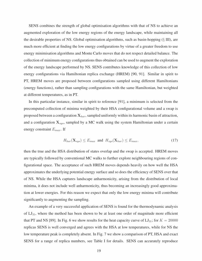
SENS combines the strength of global optimisation algorithms with that of NS to achieve an

augmented exploration of the low energy regions of the energy landscape, while maintaining all

the desirable properties of NS. Global optimisation algorithms, such as basin-hopping (§ III), are

much more efficient at finding the low energy configurations by virtue of a greater freedom to use

energy minimisation algorithms and Monte Carlo moves that do not respect detailed balance. The

collection of minimum energy configurations thus obtained can be used to augment the exploration

of the energy landscape performed by NS. SENS contributes knowledge of this collection of low

energy configurations via Hamiltonian replica exchange (HREM) [90, 91]. Similar in spirit to

PT, HREM moves are proposed between configurations sampled using different Hamiltonians

(energy functions), rather than sampling configurations with the same Hamiltonian, but weighted

at different temperatures, as in PT.

In this particular instance, similar in spirit to reference [91], a minimum is selected from the

precomputed collection of minima weighted by their HSA configurational volume and a swap is

proposed between a configuration Xhar, sampled uniformly within its harmonic basin of attraction,

and a configuration Xsys, sampled by a MC walk using the system Hamiltonian under a certain

energy constraint Emax. If

Hhar(Xsys) ≤ Emax and Hsys(Xhar) ≤ Emax, (17)

then the true and the HSA distribution of states overlap and the swap is accepted. HREM moves

are typically followed by conventional MC walks to further explore neighbouring regions of con-

figurational space. The acceptance of such HREM moves depends heavily on how well the HSA

approximates the underlying potential energy surface and so does the efficiency of SENS over that

of NS. While the HSA captures landscape anharmonicity, arising from the distribution of local

minima, it does not include well anharmonicity, thus becoming an increasingly good approxima-

tion at lower energies. For this reason we expect that only the low energy minima will contribute

significantly to augmenting the sampling.

An example of a very successful application of SENS is found for the thermodynamic analysis

of LJ31, where the method has been shown to be at least one order of magnitude more efficient

that PT and NS [89]. In Fig. 6 we show results for the heat capacity curve of LJ31; for K = 20000

replicas SENS is well converged and agrees with the HSA at low temperatures, while for NS the

low temperature peak is completely absent. In Fig. 7 we show a comparison of PT, HSA and exact

SENS for a range of replica numbers, see Table I for details. SENS can accurately reproduce

19

0.0 0.1 0.2 0.3 0.4 0.5kBT/ε

80

100

120

140

160

180

CV/k

B

HSA

SENS exact

SENS approx

NS

0.02 0.03 0.04kBT/ε

80

90

100

110

120

130

CV/k

B

FIG. 6. Heat capacity curves for LJ31. HSA corresponds to the harmonic superposition approximation. All

NS and SENS calculations were performed using K = 20000 replicas.

the low temperature features of the heat capacity for as low as K = 2500 replicas, representing

an improvement in performance of 20 times over PT [89]. The benefits are not as great for LJ75

where even reaching the region where the HSA becomes accurate enough for swaps to be accepted

is challenging.

An approximate version of the method has been proposed to alleviate this problem: similar in

spirit to the basin-sampling approach (§ VII), approximate-SENS interpolates between the high

energy density of states (DOS) obtained by NS and the low energy DOS provided by the HSA.

Once at low energy, this interpolation can be achieved by starting a fraction of the MC walks from

a local minimum configuration sampled from the precomputed collection of minima weighted by

their HSA volume. The transition from the conventional sampling at high energy to the enhanced

sampling at low energy is controlled by an onset function. The choice of the energy at which the

20

0.0 0.1 0.2 0.3 0.4 0.5kBT/ε

80

100

120

140

160

180

CV/k

B

PT

HSA

K= 2500

K= 5000

K= 10000

K= 200000.02 0.03 0.04

kBT/ε

80

90

100

110

120

130

CV/k

B

FIG. 7. Comparison of heat capacity curves for LJ31 obtained by exact SENS using different numbers of

replicas. The PT and HSA curves were obtained by parallel tempering and the harmonic superposition

approximation, respectively. Figure reproduced from [89].

transition should occur is practically the only additional parameter when compared to exact SENS

and NS. Approximate-SENS is easy to implement and generally yields equally good or better

results than exact SENS, although it is formally biased.

The thermodynamic analysis of LJ75 by approximate-SENS converges in about O(1011) en-

ergy evaluations, unlike PT, which has been shown to never converge on conventional simulation

timescales. The SENS methods are therefore another viable solution to tackle systems exhibiting

broken ergodicity.

21

LJ31

Method K N N(total)E

PT 1.9× 1011

NS ref.[87] 280000 3.4× 1012

SENS approx 20000 10000 1× 1011

SENS exact 20000 10000 1× 1011

SENS exact 10000 10000 5.2× 1010

SENS exact 5000 10000 2.6× 1010

SENS exact 2500 10000 1.3× 1010

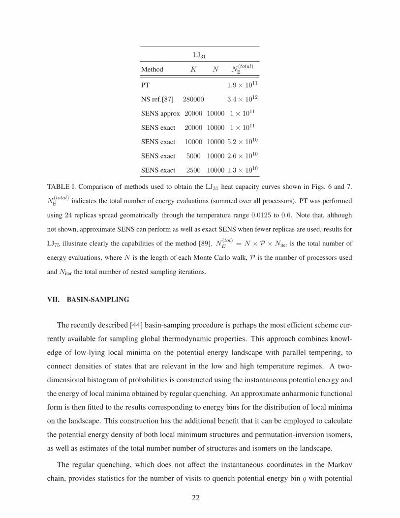
TABLE I. Comparison of methods used to obtain the LJ31 heat capacity curves shown in Figs. 6 and 7.

N(total)E indicates the total number of energy evaluations (summed over all processors). PT was performed

using 24 replicas spread geometrically through the temperature range 0.0125 to 0.6. Note that, although

not shown, approximate SENS can perform as well as exact SENS when fewer replicas are used, results for

LJ75 illustrate clearly the capabilities of the method [89]. N(tot)E = N × P × Niter is the total number of

energy evaluations, where N is the length of each Monte Carlo walk, P is the number of processors used

and Niter the total number of nested sampling iterations.

VII. BASIN-SAMPLING

The recently described [44] basin-samping procedure is perhaps the most efficient scheme cur-

rently available for sampling global thermodynamic properties. This approach combines knowl-

edge of low-lying local minima on the potential energy landscape with parallel tempering, to

connect densities of states that are relevant in the low and high temperature regimes. A two-

dimensional histogram of probabilities is constructed using the instantaneous potential energy and

the energy of local minima obtained by regular quenching. An approximate anharmonic functional

form is then fitted to the results corresponding to energy bins for the distribution of local minima

on the landscape. This construction has the additional benefit that it can be employed to calculate

the potential energy density of both local minimum structures and permutation-inversion isomers,

as well as estimates of the total number number of structures and isomers on the landscape.

The regular quenching, which does not affect the instantaneous coordinates in the Markov

chain, provides statistics for the number of visits to quench potential energy bin q with potential

22

230

250

270

290

100

200

300

400

500

600

700

800

0.05 0.15 0.25 0.35

0.04 0.08 0.12

Cv/k

kT/ǫ

HSA

BSPT+BSPT+

BSPT

BSPT

PT

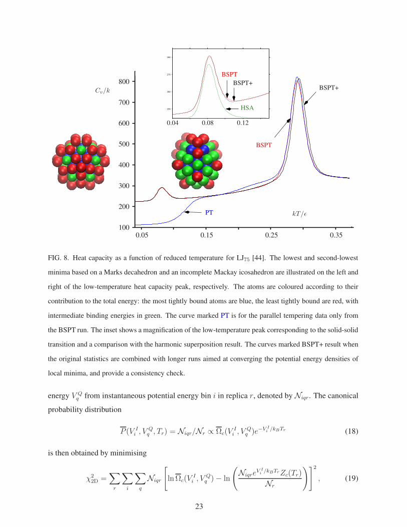
FIG. 8. Heat capacity as a function of reduced temperature for LJ75 [44]. The lowest and second-lowest

minima based on a Marks decahedron and an incomplete Mackay icosahedron are illustrated on the left and

right of the low-temperature heat capacity peak, respectively. The atoms are coloured according to their

contribution to the total energy: the most tightly bound atoms are blue, the least tightly bound are red, with

intermediate binding energies in green. The curve marked PT is for the parallel tempering data only from

the BSPT run. The inset shows a magnification of the low-temperature peak corresponding to the solid-solid

transition and a comparison with the harmonic superposition result. The curves marked BSPT+ result when

the original statistics are combined with longer runs aimed at converging the potential energy densities of

local minima, and provide a consistency check.

energy V Qq from instantaneous potential energy bin i in replica r, denoted by Niqr. The canonical

probability distribution

P (V Ii , V

Qq , Tr) = Niqr/Nr ∝ Ωc(V

Ii , V

Qq )e−V I

i /kBTr (18)

is then obtained by minimising

χ22D =

∑

r

∑

i

∑

q

Niqr

[lnΩc(V

Ii , V

Qq )− ln

(Niqre

V Ii /kBTrZc(Tr)

Nr

)]2, (19)

23

T

Q6

P (Q6, T )

F (Q6, T )

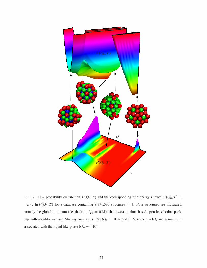
FIG. 9. LJ75 probability distribution P (Q6, T ) and the corresponding free energy surface F (Q6, T ) =

−kBT lnP (Q6, T ) for a database containing 8,391,630 structures [44]. Four structures are illustrated,

namely the global minimum (decahedron, Q6 = 0.31), the lowest minima based upon icosahedral pack-

ing with anti-Mackay and Mackay overlayers [92] (Q6 = 0.02 and 0.15, respectively), and a minimum

associated with the liquid-like phase (Q6 = 0.10).

24

V/ǫ0

10

20

30

40

50

60

−370−375−380−385−390−395

lnM st(V )

lnMPI(V )/2N !

FIG. 10. Calculated values for the lnM st(V ) and lnMPI(V )/2N ! as a function of potential energy for

LJ75 [44]. M st(V ) and MPI(V ) are the potential energy densities of distinct local minima structures and

permutation-inversion isomers, respectively.

where the variables are Ωc(VIi , V

Qq ) if we fix Zc(Tr) = Z∗

c (Tr) from an initial 1D fit to the parallel

tempering results for the distribution P (V, T ) ∝ Ωc(V )e−V/kBT . Here Ωc(V ) is again the config-

urational density of states. For each replica r with temperature Tr we count the number of visits,

Nir, to potential energy bins indexed as V Ii , providing the estimate for P (V I

i , Tr) as

P (V Ii , Tr) = Nir/Nr, (20)

where Nr =∑

i Nir is the total number of Monte Carlo steps for replica r. We then minimise

χ21D =

∑

r

∑

i

Nir

[ln Ωc(V

Ii )− ln

(Nire

V Ii /kBTrZc(Tr)

Nr

)]2, (21)

where the variables are Ωc(VIi ) andZc(Tr). The optimal values are denoted by Ω∗

c(VIi ) and Z∗

c (Tr).

In the present work, all the fitting was conducted by minimising χ22D or χ2

1D using the modified

limited memory Broyden-Fletcher-Goldfarb-Shanno (L-BFGS) algorithm [93, 94] from the GMIN

code [95].

25

To simplify the fitting a model anharmonic density of states was employed for each quench bin,

and an efficient representation was obtained using two fitting parameters, Aq and Bq, with

lnΩc(VIi , V

Qq ) = (κ′ + eAqViq) lnViq +Bq, (22)

where κ′ = κ/2 − 1 and Viq = V Ii − V Q

q , the difference between the instantaneous and quench

potential energies. Here we have built on previous work [40] that used the analytic density of states

for a Morse potential [96]. For Viq → 0 we recover the usual harmonic result: Ωc(VIi , V

Qq ) ∝

Vκ/2−1iq . Aq makes no contribution in this limit, and can therefore be identified with the effective

well anharmonicity, while Bq incorporates the landscape entropy in terms of the number of minima

included in quench bin q. This interpretation facilitates the calculation of distributions for the

potential energy density of minimum energy structures [44].

Optimal values for the two parameters in each bin were again obtained by fitting, and are

denoted A∗q and B∗

q . Then to exploit additional information corresponding to the low temperature

limit a normal mode analysis of the local minima obtained from basin-hopping global optimisation

was used. B∗q values were simply replaced up to a specified potential energy threshold using

the normal mode data, and the final configurational density of states, Ωc(VIi ), was obtained by

combining the results of the one- and two-dimensional fitting procedures as:

Ωc(VIi ) =

∑

q

[δqΩ

∗c(V

Ii )

Niq

Ni+ (1− δq)Ω

∗

c(VIi , V

Qq )

], (23)

where the mixing parameter δq = (i− iqmin)/(imaxq − imin

q ) depends on the optimal fitting range for

the q bins [44].

Extensive tests were conducted for both LJ31 and LJ75. Some results for the larger cluster are

illustrated in Figures 8, 9, and 10. Here Q6 is a bond-order parameter [97, 98], which takes larger

values of the decahedral global minimum than for minima based upon icosahedral packing. 32

temperature replicas were used, exponentially spaced in the temperature range 0.15 to 0.375. The

production run of 200×106 standard parallel tempering steps followed by 60×106 BSPT steps

(PT with quenches every 30 steps) required 22 hours of wall clock time. When the lowest 13

minima are used to replace the fitted B∗q values the resulting heat capacity curve appears to be well

converged (Figure 8, with the characteristic low temperature solid-solid peak well reproduced.

This result can be compared with previous simulations using an auxiliary harmonic superposition

reference [7], which required 3 × 109 steps. In contrast, even 1011 Monte Carlo steps are not

enough to converge the heat capacity using adaptive exchange parallel tempering [8, 91]. The

26

corresponding probability distribution P (Q6, T ) and free energy surface are shown in Figure 9,

where various features corresponding to different families of structures can be associated with

peaks that are separated in these two-dimensional projections. The calculated potential energy

distributions of distinct structures and permutation-inversion isomers are shown in Figure 10. Here

the effect of point group symmetry in reducing the number of permutation-inversion isomers is

visible at low energy. There is also an unexpected feature, namely a shallow minimum in the

distributions around V = −385 ǫ, which has been associated with regions of the potential energy

landscape that are relatively sparsely populated [44]. The total number of distinct local minimum

structures for this cluster is estimated at around 4 × 1025 [44]. The capability of basin-sampling

to yield estimates like this as a by-product of the sampling could be particularly interesting for

amorphous systems in future studies.

VIII. CONCLUSIONS

The idea of exploiting knowledge of low-lying local minima to enhance sampling [1, 5] recently

reached fruition in a variety of new techniques [7, 38, 44, 68, 89]. The foundation for each of

these methods is the superposition approach, in which the total partition function is decomposed

into contributions from distinct local minima [8, 14, 34–37]. The continuing development of

these methods provides important cross-validations of results for challenging systems that exhibit

broken ergodicity. These results are not only important in themselves, but also provide an essential

platform for optimising efficiency, which is likely to come from hybrid schemes, and may be

system dependent. Nevertheless, many general conclusions should hold for very diverse problems

in chemical physics, and important tests in molecular simulation and soft and condensed matter

problems should reveal that further progress is possible.

The authors gratefully acknowledge financial support from the EPSRC and the ERC. S.M ac-

knowledges financial support from the Gates Cambridge Scholarship. We also thank Gabor Csanyi

for helpful discussions.

[1] R. Zhou and B. J. Berne, J. Chem. Phys. 107, 9185 (1997).

[2] U. H. E. Hansmann and Y. Okamoto, Curr. Op. Struct. Biol. 9, 177 (1999).

[3] F. Wang and D. P. Landau, Phys. Rev. Lett. 86, 2050 (2001).

27

[4] W. Watanabe and W. P. Reinhardt, Phys. Rev. Lett. 65, 3301 (1990).

[5] I. Andricioaei, J. E. Straub and A. F. Voter, J. Chem. Phys. 114, 6994 (2001).

[6] J. Kim, J. E. Straub and T. Keyes, Phys. Rev. Lett. 97, 050601 (2006).

[7] V. A. Sharapov and V. A. Mandelshtam, J. Phys. Chem. A 111, 10284 (2007).

[8] V. A. Sharapov, D. Meluzzi and V. A. Mandelshtam, Phys. Rev. Lett. 98, 105701 (2007).

[9] J. Kim, T. Keyes and J. E. Straub, J. Chem. Phys. 135, 061103 (2011).

[10] J. Kim, J. E. Straub and T. Keyes, J. Phys. Chem. B 116, 8646 (2012).

[11] P. J. Ortoleva, T. Keyes and M. Tuckerman, J. Phys. Chem. B 116, 8335 (2012).

[12] G. A. Huber and S. Kim, Biophys. J. 70, 97 (1996).

[13] D. Bhatt, B. W. Zhang and D. M. Zuckerman, J. Chem. Phys. 133, 014110 (2010).

[14] D. J. Wales, Energy Landscapes, Cambridge University Press, Cambridge (2003).

[15] D. J. Wales, Curr. Op. Struct. Biol. 20, 3 (2010).

[16] D. J. Wales, Phil. Trans. Roy. Soc. A 370, 2877 (2012).

[17] D. Frenkel and B. Smit, Understanding molecular simulation, second edition, Academic Press, Lon-

don (2002).

[18] J. E. Jones and A. E. Ingham, Proc. R. Soc. A 107, 636 (1925).

[19] D. J. Wales and J. P. K. Doye, J. Phys. Chem. A 101, 5111 (1997).

[20] J. P. K. Doye, D. J. Wales and M. A. Miller, J. Chem. Phys. 109, 8143 (1998).

[21] J. P. K. Doye, M. A. Miller and D. J. Wales, J. Chem. Phys. 110, 6896 (1999).

[22] F. Calvo, J. P. Neirotti, D. L. Freeman and J. D. Doll, J. Chem. Phys. 112, 10350 (2000).

[23] J. P. Neirotti, F. Calvo, D. L. Freeman and J. D. Doll, J. Chem. Phys. 112, 10340 (2000).

[24] P. A. Frantsuzov and V. A. Mandelshtam, Phys. Rev. E 72, 037102 (2005).

[25] C. Predescu, P. A. Frantsuzov and V. A. Mandelshtam, J. Chem. Phys. 122, 154305 (2005).

[26] H. Liu and K. D. Jordan, J. Phys. Chem. A 107, 5703 (2003).

[27] L. T. Wille, in Annual Reviews of Computational Physics VII, edited by D. Stauffer, World Scientific,

Singapore (2000).

[28] D. J. Wales, Mol. Phys. 100, 3285 (2002).

[29] C. Dellago, P. G. Bolhuis and D. Chandler, J. Chem. Phys. 108, 9236 (1998).

[30] D. Passerone and M. Parrinello, Phys. Rev. Lett. 87, 108302 (2001).

[31] W. E, W. Ren and E. Vanden-Eijnden, Phys. Rev. B 66, 052301 (2002).

[32] P. G. Mezey, Theo. Chim. Acta 58, 309 (1981).

28

[33] P. G. Mezey, Potential Energy Hypersurfaces, Elsevier, Amsterdam (1987).

[34] F. H. Stillinger and T. A. Weber, Science 225, 983 (1984).

[35] D. J. Wales, Mol. Phys. 78, 151 (1993).

[36] F. H. Stillinger, Science 267, 1935 (1995).

[37] B. Strodel and D. J. Wales, Chem. Phys. Lett. 466, 105 (2008).

[38] T. V. Bogdan, D. J. Wales and F. Calvo, J. Chem. Phys. 124, 044102 (2006).

[39] F. Sciortino, W. Kob and P. Tartaglia, J. Phys.: Condens. Matt. 12, 6525 (2000).

[40] J. P. K. Doye and D. J. Wales, J. Chem. Phys. 102, 9659 (1995).

[41] J. P. K. Doye and D. J. Wales, J. Chem. Phys. 102, 9673 (1995).

[42] F. Calvo, J. P. K. Doye and D. J. Wales, J. Chem. Phys. 115, 9627 (2001).

[43] I. Georgescu and V. A. Mandelshtam, J. Chem. Phys. 137, 144106 (2012).

[44] D. J. Wales, Chem. Phys. Lett. 584, 1 (2013).

[45] F. G. Amar and R. S. Berry, J. Chem. Phys. 85, 5943 (1986).

[46] M. K. Gilson and K. K. Irikura, J. Phys. Chem. B 114, 16304 (2010).

[47] F. Calvo, J. P. K. Doye and D. J. Wales, Nanoscale 4, 1085 (2012).

[48] Z. Li and H. A. Scheraga, Proc. Natl. Acad. Sci. USA 84, 6611 (1987).

[49] D. J. Wales and H. A. Scheraga, Science 285, 1368 (1999).

[50] K. Klenin, B. Strodel, D. J. Wales and W. Wenzel, Biochimica et Biophysica Acta 1814, 977 (2011).

[51] B. Strodel, J. W. L. Lee, C. S. Whittleston and D. J. Wales, J. Am. Chem. Soc. 132, 13300 (2010).

[52] K. H. Hoffmann, A. Franz and P. Salamon, Phys. Rev. E 66, 046706 (2002).

[53] R. H. Leary and J. P. K. Doye, Phys. Rev. E 60, R6320 (1999).

[54] C. Shang and D. J. Wales, J. Chem. Phys. 141, (2014).

[55] C. Tsallis, J. Stat. Phys. 52, 479 (1988).

[56] C. Tsallis, Braz. J. Phys. 29, 1 (1999).

[57] J. P. K. Doye and D. J. Wales, Phys. Rev. Lett. 80, 1357 (1998).

[58] J. P. K. Doye, D. J. Wales and M. A. Miller, J. Chem. Phys. 109, 8143 (1998).

[59] R. H. Swendsen and J.-S. Wang, Phys. Rev. Lett. 57, 2607 (1986).

[60] D. Earl and M. W. Deem, Phys. Chem. Chem. Phys. 7, 3910 (2005).

[61] Y. Sugita and Y. Okamoto, Chem. Phys. Lett. 329, 261 (2000).

[62] Y. Sugita and Y. Okamoto, Chem. Phys. Lett. 314, 141 (1999).

[63] D. A. Kofke, J. Chem. Phys. 117, 6911 (2002).

29

[64] D. A. Kofke, J. Chem. Phys. 120, 10852 (2004).

[65] W. Nadler and U. H. E. Hansmann, Phys. Rev. E 75, 026109 (2007).

[66] W. Nadler and U. H. E. Hansmann, J. Phys. Chem. B 112, 10386 (2008).

[67] R. Denschlag, M. Lingenheil and P. Tavan, Chem. Phys. Lett. 473, 193 (2009).

[68] A. J. Ballard and D. J. Wales, submitted, (2014).

[69] S. Somani, B. J. Killian and M. K. Gilson, J. Chem. Phys. 130, 34102 (2009).

[70] J. G. Kirkwood and E. M. Boggs, J. Chem. Phys. 10, 402 (1942).

[71] J. Hansen and I. McDonald, Theory of Simple Liquids, Third Edition, Academic Press, 3rd edn. (1976).

[72] W. McGill, IEEE Trans. Information Theory 4, 93 (1954).

[73] R. M. Fano, Transmission of Information: A Statistical Theory of Communication, The MIT Press

(1961).

[74] B. J. Killian, M. K. Gilson and J. Y. Kravitz, J. Chem. Phys. 127, 24107 (2007).

[75] S. Somani, Conformational sampling and calculation of molecular free energy using superposition

approximations, Ph.D. thesis, University of Maryland, College Park (2011).

[76] S. Somani and M. K. Gilson, J. Chem. Phys. 134, 34107 (2011).

[77] C.-E. Chang, M. J. Potter and M. K. Gilson, J. Phys. Chem. B 107, 1048 (Jan. 2003).

[78] Drug Dev. Res. 72, 85 (Feb. 2011).

[79] S. Somani, Y. Okamoto, A. J. Ballard and D. J. Wales, submitted, (2014).

[80] H. M. Berman, J. Westbrook, Z. Feng, G. Gilliland, T. N. Bhat, H. Weissig, I. N. Shindyalov and P. E.

Bourne, The protein data bank, The Protein Data Bank home page is http://www.rcsb.org/pdb.

[81] F. H. Allen, Acta Cryst. 58, 380 (Jun 2002).

[82] J. Skilling, Bayesian Analysis 1, 833 (2006).

[83] S. J. Vigeland and M. Vallisneri, Mon. Not. R. Astron. Soc. 440, 1446 (2014).

[84] D. M. Kipping, D. Nesvorny, L. A. Buchhave, J. Hartman, G. A. Bakos and A. R. Schmitt, Astrophys-

ical J. 784, 28 (2014).

[85] N. Pullen and R. J. Morris, Plos One 9, e88419 (2014).

[86] L. B. Partay, A. P. Bartok and G. Csanyi, Phys. Rev. E 89, 022302 (2014).

[87] L. B. Partay, A. P. Bartok and G. Csanyi, J. Phys. Chem. B 114, 10502 (2010).

[88] B. J. Brewer, L. B. Partay and G. Csanyi, Statistics Computing 21, 649 (2011).

[89] S. Martiniani, J. D. Stevenson, D. J. Wales and D. Frenkel, Phys. Rev. X 4, 031034 (2014).

[90] H. Fukunishi, O. Watanabe and S. Takada, J. Chem. Phys. 116, 9058 (2002).

30

[91] V. A. Mandelshtam, P. A. Frantsuzov and F. Calvo, J. Phys. Chem. A 110, 5326 (2006).

[92] J. P. K. Doye, M. A. Miller and D. J. Wales, J. Chem. Phys. 111, 8417 (1999).

[93] J. Nocedal, Mathematics of Computation 35, 773 (1980).

[94] D. C. Liu and J. Nocedal, Math. Prog. 45, 503 (1989).

[95] D. J. Wales, Gmin: A program for basin-hopping global optimisation, basin-sampling, and parallel

tempering ().

[96] P. C. Haarhoff, Mol. Phys. 7, 101 (1963).

[97] P. J. Steinhardt, D. R. Nelson and M. Ronchetti, Phys. Rev. B 28, 784 (1983).

[98] J. S. van Duijneveldt and D. Frenkel, J. Chem. Phys. 96, 4655 (1992).

31