EXPLOITING ATTITUDE SENSING IN VISION-BASED ... - CORE
172
EXPLOITING ATTITUDE SENSING IN VISION-BASED NAVIGATION, MAPPING AND TRACKING INCLUDING RESULTS FROM AN AIRSHIP. PHD THESIS SUBMITTED TO THE DEPARTMENT OF ELECTRICAL AND COMPUTER ENGINEERING OF THE UNIVERSITY OF COIMBRA By Luiz Gustavo Bizarro Mirisola September 2008
-
Upload
khangminh22 -
Category
Documents
-
view
1 -
download
0
Transcript of EXPLOITING ATTITUDE SENSING IN VISION-BASED ... - CORE
EXPLOITING ATTITUDE SENSING IN VISION-BASED
NAVIGATION, MAPPING AND TRACKING
INCLUDING RESULTS FROM AN AIRSHIP.
PHD THESIS
SUBMITTED TO THE DEPARTMENT OF ELECTRICAL AND COMPUTER ENGINEERING
OF THE UNIVERSITY OF COIMBRA
By
Luiz Gustavo Bizarro Mirisola
September 2008
Mirisola
Rectangle

c© Copyright 2008 by Luiz Gustavo Bizarro Mirisola
All Rights Reserved
ii
Abstract
In this thesis, an attitude sensor is used to compensate for rotational motion, and togenerate virtual images to simulate a pure translation movement. The compensationof rotational motion is made possible by the combination of inertial and earth fieldmagnetic sensors within a package which provides an absolute orientation measure-ment, and by a calibration routine to determine the rotation between the camera andinertial sensor frames. The objective is to facilitate vision-based tasks such as navi-gation over smooth terrain, 3D point cloud registration, generation of image mosaicsand digital elevation maps, and plane segmentation. In the rotation-compensated,pure translation case, homographies are reduced to planar homologies, which areused to recover the relative pose between two views. In the particular case where theground plane is horizontal, the relative pose between two views can also be recoveredby directly finding a rigid transformation to register corresponding scene coordinates.These pure translation models perform fairly accurately especially regarding the esti-mation of the vertical motion component. The results include recovering trajectoriesof hundreds of meters for an airship UAV and comparison with GPS data. Theaccuracy of the height estimation was evaluated against ground truth through ex-periments in controlled environments. The rotational motion and the vertical andhorizontal components of translational motion are measured or estimated separately,which should facilitate the integration of other sensors in the future, although onlyorientation measurements and image pixel correspondences have been used in thisthesis. The rotation-compensated images and the pixel correspondences are furtherexploited to perform plane segmentation and to generate sparse Digital ElevationMaps and image mosaics. The visual odometry is also fused with GPS position fixes,improving the recovered trajectory locally. These gains are further exploited to im-prove the tracking accuracy of a target moving on the ground which is tracked in a 2Dframe of reference in actual metric units, in the airship and urban people surveillancescenarios. Orientation estimates are also used to rotate 3D point clouds obtained byranging devices such as stereo cameras or Laser Range Finders to a stabilized frameof reference, and the problem of registration of these point clouds is reduced to thedetermination of the remaining translation vector, taking into account the character-istics of the ranging device which generated the point clouds. The appendix presents
iii

iv
the technical characteristics of the UAV platform utilized for dataset recording, a re-motely piloted airship, as well as requirements towards future extension for automaticflight.
Resumo
Nesta tese, um sensor de orientação é usado para compensar o movimento rotacio-nal, e para gerar imagens virtuais, simulando um movimento de translação pura. Acompensação do movimento rotacional se torna possível devido à combinação de sen-sores inerciais e de campo magnético, de forma a fornecer uma medida de orientaçãoabsoluta, e à uma rotina de calibração para determinar a rotação entre os sistemasde cordenadas da câmera e do sensor inercial. O objetivo é facilitar tarefas basea-das em visão como navegação sobre superfícies planas, registro de nuvens de pontos3D, geração de mosaicos de imagens e mapas digitais de elevação, e segmentação deplanos. Com a rotação compensada, supondo-se um movimento de translação pura,homografias são reduzidas à homologias planares, que são usadas para recuperar apose relativa entre duas vistas. No caso particular onde o plano do chão é horizon-tal, a pose relativa entre duas vistas também pode ser recuperada pela estimação deuma transformação rígida que registre coordenadas correspondentes na cena. Estesmodelos considerando translação pura obtêm resultados mais precisos especialmenteao estimar a componente vertical da trajetória. Os resultados incluem a recuperaçãode trajetórias de centenas de metros para um UAV dirigível com comparação comdados de GPS. A estimação da altura foi avaliada também em ambientes controlados,onde a altura real é conhecida com precisão. O movimento rotacional e os compo-nentes horizontais e verticais do movimento translacional são medidos ou estimadosseparadamente, o que deve facilitar a integração de outros sensores no futuro, emboraapenas medidas de orientação e correspondências entre os pixels das imagens foramusadas nesta tese. As imagens com rotação compensada e as correspondências entreos pixels das imagens são exploradas ainda para realizar segmentação de planos epara gerar mapas de elevação digital esparsos e mosaicos de imagens. A odometriavisual é também fundida com leituras de posição do GPS, melhorando localmente atrajetória recuperada. Estas melhorias são ainda exploradas para aumentar a acurá-cia do seguimento de um alvo que se move no plano da terra, que é seguido emcoordenadas 2D considerando as unidades métricas reais, nos cenários do dirigível ede vigilância urbana de pessoas. As estimativas de orientação também são usadaspara rodar nuvens de pontos 3D, obtidas por sensores de mapeamento por medida dedistância como cameras estéreo e Laser Range Finders, em um sistema de coordena-
v

vi
das estabilizado. Então o problema de registro destas nuvens de pontos é reduzido àdeterminação de um vetor de translação, levando em consideração as característicasdo sensor que gerou as nuvens de pontos. O apêndice apresenta as características téc-nicas da plataforma UAV, um dirígivel pilotado remotamente, usada para gravar osdatasets utilizados, bem como requisitos para extender a plataforma para a realizaçãofutura de vôos automáticos.

Acknowledgments
As I started to think about who deserves a mention here, I quickly realized the listwould be too large to fit in this space, and any “selection of the most importantpeople” would be necessarily unfair. The process of my coming to this PhD defensedid not start in Coimbra, neither is restricted to the four years of work here. I haveto thank not just the people who made life more enjoyable - or more bearable? - withtheir friendship and companionship, but also the ones that subtly - or not so subtly- made me go forward in the worse downturns.
I also realized that this must be written mainly in English, because of my manyforeign friends from many countries. It was an interesting experience to be together,away from our countries and families. I hope that I have helped to receive and supportsome of you, but it is not enough to pay back the kindness of the ones who receivedme when I was in other country struggling with another language. E também aos queme receberam depois aqui em Portugal. Me despeço de Portugal, já com saudades dovinho, azeite, e bacalhau. As I will leave Europe I will miss the frequent opportunityto see “live” the history, a história, la historia, la storia, die geschichte, et la histoire.Back into Brazil where 200 years is very very amazingly old...
Um abraço para todos os outros brazucas perdidos, para os que voltam e para osque ficam. Espero que tenha lhes trazido doces do Brasil o suficiente para matar asaudade, mas não o suficiente para engordar muito. Saludo a los amigos españoles yde latinoamerica. ¡Viva la Sangria! Je salue aussi mes amis français et leurs familles.Je promets que je vais améliorer mon français ! Finally an english salute to all theothers, at least you understand this language.
To my advisor, Professor Jorge Dias, and to all colleagues in the Institute ofSystems and Robotics and in the Department of Electrical and Computer Engineeringof the University of Coimbra, especially of the Mobile Robotics Laboratory, where Irealized all my work, and to the other partners of the DIVA project, also in Lisbonand Minho, I thank for the advice and support, which allowed me to learn muchduring these years. My work depended on yours.
Finalmente aos meus pais obrigado por todo o apoio constante e incondicional.Agora já os dispenso do hábito de ir todo sabádo conectar no computador e conversar.Estive longe mas nunca sem notícias. E vamos lembrar da viagem por aqui.
vii

viii
Contents
1 Introduction 11.1 Motivation . . . . . . . . . . . . . . . . . . . . . . . . . . . . . . . . . 11.2 State of the Art . . . . . . . . . . . . . . . . . . . . . . . . . . . . . . 2
1.2.1 Visual navigation & 3D mapping . . . . . . . . . . . . . . . . 31.2.2 Image Mosaicing . . . . . . . . . . . . . . . . . . . . . . . . . 41.2.3 3D Depth map registration . . . . . . . . . . . . . . . . . . . . 51.2.4 Surveillance and Tracking . . . . . . . . . . . . . . . . . . . . 6
1.3 Objectives . . . . . . . . . . . . . . . . . . . . . . . . . . . . . . . . . 61.4 Experimental Platform . . . . . . . . . . . . . . . . . . . . . . . . . . 91.5 Thesis summary . . . . . . . . . . . . . . . . . . . . . . . . . . . . . . 101.6 Publications . . . . . . . . . . . . . . . . . . . . . . . . . . . . . . . . 11
2 Sensor Modeling 132.1 Projective Camera model . . . . . . . . . . . . . . . . . . . . . . . . . 13
2.1.1 Stereo Cameras . . . . . . . . . . . . . . . . . . . . . . . . . . 142.2 Image Features & Homographies . . . . . . . . . . . . . . . . . . . . . 15
2.2.1 Interest Point Matching . . . . . . . . . . . . . . . . . . . . . 152.2.2 Planar surfaces and homographies . . . . . . . . . . . . . . . . 162.2.3 Pure translation case . . . . . . . . . . . . . . . . . . . . . . . 18
2.3 Attitude Heading Reference System . . . . . . . . . . . . . . . . . . . 232.4 Laser Range Finder . . . . . . . . . . . . . . . . . . . . . . . . . . . . 242.5 Frames of reference . . . . . . . . . . . . . . . . . . . . . . . . . . . . 252.6 Calibration of Camera - Inertial System . . . . . . . . . . . . . . . . . 272.7 The virtual horizontal plane concept or an inertial stabilized plane . . 29
3 Inertial Aided Visual Trajectory Recovery 313.1 Introduction . . . . . . . . . . . . . . . . . . . . . . . . . . . . . . . . 313.2 Visual Navigation . . . . . . . . . . . . . . . . . . . . . . . . . . . . 31
3.2.1 Reprojecting the images on the virtual horizontal plane . . . . 313.2.2 Procrustes solution to register scene points. . . . . . . . . . . 35
ix
x CONTENTS
3.2.3 The homology model for a horizontal plane . . . . . . . . . . . 393.2.4 From the FOE and µ to the translation vector . . . . . . . . . 423.2.5 Filtering the translation measurements . . . . . . . . . . . . . 443.2.6 Fusing visual odometry and GPS . . . . . . . . . . . . . . . . 44
3.3 The case of planes in general position . . . . . . . . . . . . . . . . . . 453.3.1 The homology model for planes in general position . . . . . . 45
3.4 Trajectory recovery results . . . . . . . . . . . . . . . . . . . . . . . . 493.4.1 Relative height experiments with ground truth . . . . . . . . . 493.4.2 Overpass Experiment . . . . . . . . . . . . . . . . . . . . . . . 523.4.3 Screwdriver Table Experiment . . . . . . . . . . . . . . . . . . 543.4.4 Trajectory recovery for aerial vehicles with the MTB-9 AHRS 553.4.5 Trajectory recovery for aerial vehicles with the MTi AHRS . . 663.4.6 Combining GPS and Visual Odometry . . . . . . . . . . . . . 68
4 Inertial Aided Visual Mapping 734.1 Introduction . . . . . . . . . . . . . . . . . . . . . . . . . . . . . . . . 734.2 Image Mosaicing . . . . . . . . . . . . . . . . . . . . . . . . . . . . . 734.3 Plane Segmentation and DEM . . . . . . . . . . . . . . . . . . . . . . 79
4.3.1 Plane Segmentation Experiments . . . . . . . . . . . . . . . . 794.3.2 Calculating Height For Each Pixel Correspondence . . . . . . 814.3.3 Constructing a DEM . . . . . . . . . . . . . . . . . . . . . . . 834.3.4 Applications and Future Improvements . . . . . . . . . . . . . 84
4.4 3D Depth Map Registration . . . . . . . . . . . . . . . . . . . . . . . 864.4.1 Delimiting an image sequence . . . . . . . . . . . . . . . . . . 864.4.2 Rotating to a stabilized frame of reference . . . . . . . . . . . 874.4.3 Translation to a common frame. . . . . . . . . . . . . . . . . . 894.4.4 Subsuming other geometric constraints for outlier removal . . 924.4.5 Filtering out redundant points . . . . . . . . . . . . . . . . . . 944.4.6 Results . . . . . . . . . . . . . . . . . . . . . . . . . . . . . . . 97
5 Aerial Surveillance by Visual Tracking 1035.1 Introduction . . . . . . . . . . . . . . . . . . . . . . . . . . . . . . . . 1035.2 Tracking of moving targets . . . . . . . . . . . . . . . . . . . . . . . 104
5.2.1 Target Pose measurement: projecting from image to world frame1045.2.2 Filtering of target pose . . . . . . . . . . . . . . . . . . . . . . 105
5.3 Tracking of a Moving Target from Airship Observations . . . . . . . . 1065.3.1 Tracking after fusing GPS and Visual Odometry . . . . . . . . 107
5.4 Tracking people with a moving surveillance camera . . . . . . . . . . 109
6 Conclusions 113

CONTENTS xi
Bibliography 117
A Experimental Platform 125A.1 Technical Characteristics of the DIVA Airship . . . . . . . . . . . . . 125
A.1.1 Embedded System . . . . . . . . . . . . . . . . . . . . . . . . 125A.1.2 Ground Station . . . . . . . . . . . . . . . . . . . . . . . . . . 126
A.2 Requisites for autonomy . . . . . . . . . . . . . . . . . . . . . . . . . 127A.2.1 Embedded System . . . . . . . . . . . . . . . . . . . . . . . . 127A.2.2 Ground Station . . . . . . . . . . . . . . . . . . . . . . . . . . 128
A.3 Overview of architecture . . . . . . . . . . . . . . . . . . . . . . . . . 129A.3.1 Sensors and hardware components . . . . . . . . . . . . . . . . 129A.3.2 Embedded & Ground Station Software . . . . . . . . . . . . . 135
B Mathematical Proofs and formulae 139B.1 Recovering the scale of the recovered homography matrix . . . . . . . 139B.2 Calculating sigma points for the Unscented Transform . . . . . . . . . 142B.3 Jacobian formulae for the homology transformation. . . . . . . . . . . 143B.4 Jacobian formulae for the optimization in t. . . . . . . . . . . . . . . 145B.5 The discrete Wiener process acceleration model for the Kalman Filter 146B.6 The Procrustes Procedure . . . . . . . . . . . . . . . . . . . . . . . . 147

xii CONTENTS
List of Figures
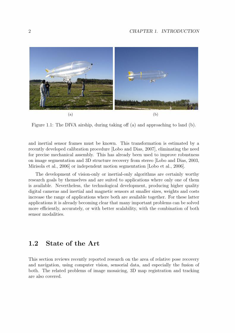
1.1 The DIVA airship, during taking off (a) and approaching to land (b). 21.2 The DIVA airship, with details showing the vision-AHRS system and
GPS receiver mounted on the gondola. . . . . . . . . . . . . . . . . . 9
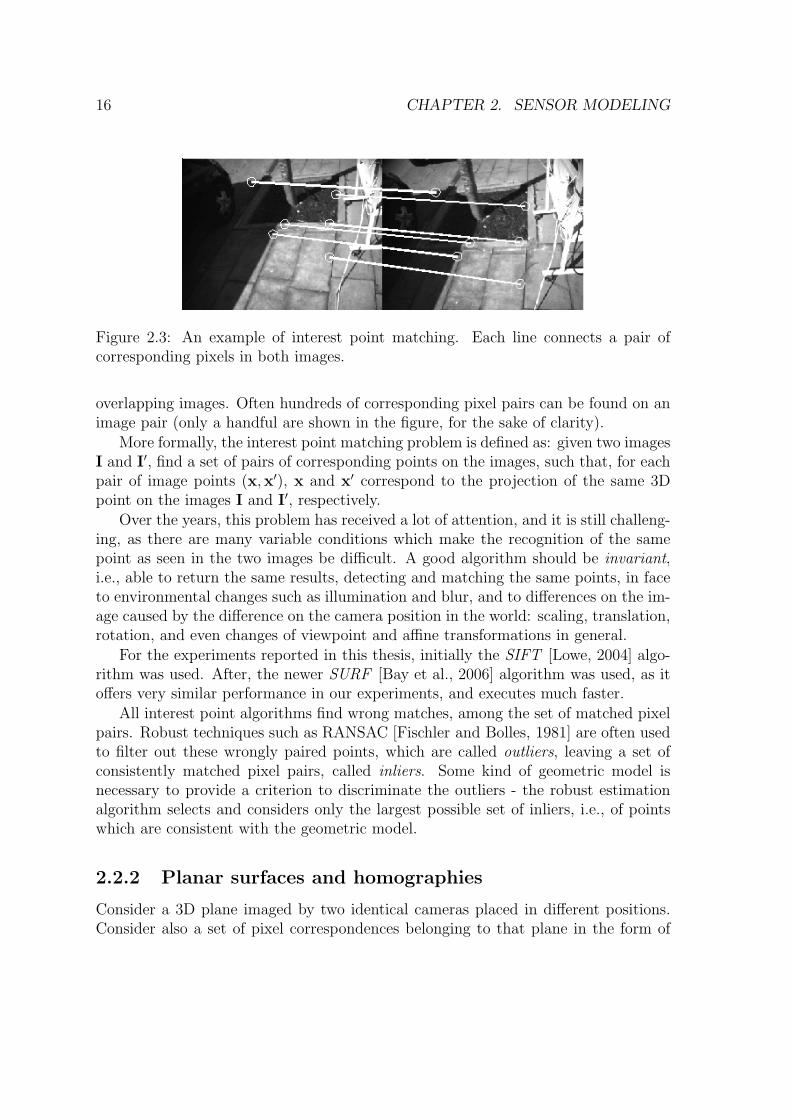
2.1 The pinhole camera model. . . . . . . . . . . . . . . . . . . . . . . . . 142.2 The ideal stereo model of disparity for binocular cameras. . . . . . . . 152.3 An example of interest point matching. Each line connects a pair of
corresponding pixels in both images. . . . . . . . . . . . . . . . . . . 162.4 A 3D plane imaged by a moving camera induces a homography. . . . 172.5 An example of a homology planar transformation with two correspond-
ing pairs of points in the plane. . . . . . . . . . . . . . . . . . . . . . 192.6 A camera images a pair of 3D points. The depth ratio is related with
a ratio of distances on the image (equation (2.8)). . . . . . . . . . . . 212.7 Relating absolute scene depth with ratios of distances on the image for
a pair of cameras and a pair of points. . . . . . . . . . . . . . . . . . 212.8 The module of the magnetic vector in different environments. . . . . . 242.9 Sensors utilized for mapping: AHRS, LRF, stereo and single cameras. 252.10 Definitions of frames of reference. . . . . . . . . . . . . . . . . . . . . 262.11 The calibration recovers the rotation between the camera and inertial
sensor frames. The camera and AHRS measure the gravity direction.Two example images with vertically placed chessboards used in thecalibration are shown in the right. . . . . . . . . . . . . . . . . . . . . 27
2.12 The virtual horizontal plane concept. . . . . . . . . . . . . . . . . . . 30
3.1 Example of reprojection in the virtual horizontal plane . . . . . . . . 323.2 An example of a reprojected image before and after cutting the low
latitude regions. The limit was set at 45◦. . . . . . . . . . . . . . . . 343.3 Deleting pixels projected on the virtual sphere in low latitude regions. 353.4 The relation between pixel coordinates and the angle of the projection
ray with the optical axis. . . . . . . . . . . . . . . . . . . . . . . . . . 35
xiii
xiv LIST OF FIGURES
3.5 Finding the translation between successive camera poses by 3D sceneregistration. . . . . . . . . . . . . . . . . . . . . . . . . . . . . . . . . 37
3.6 A pair of virtual cameras under pure translation imaging the same 3Dpoint. . . . . . . . . . . . . . . . . . . . . . . . . . . . . . . . . . . . 40
3.7 Finding the homology transformation between two images reprojectedon the stabilized plane. . . . . . . . . . . . . . . . . . . . . . . . . . . 43
3.8 Finding the scale of translation from the difference in height. . . . . . 443.9 The ratios Z/Z ′, d/d′, b/b′ are the same. . . . . . . . . . . . . . . . . 473.10 Finding the homology transformation between two images. . . . . . . 493.11 A tripod with a camera rigidly mounted with the AHRS, and an image
example. . . . . . . . . . . . . . . . . . . . . . . . . . . . . . . . . . . 503.12 Relative heights to the ground for the tripod experiment, with two
example images. Each unit on the abscissa corresponds to one image.Images were taken from 3 different heights. . . . . . . . . . . . . . . . 50
3.13 The camera mounted on a base, to be manually aligned with the walls,with an image example. . . . . . . . . . . . . . . . . . . . . . . . . . 51
3.14 Relative heights to the ground plane, with two image examples. Eachunit on the abscissa corresponds to one image. Images were taken from5 different heights. . . . . . . . . . . . . . . . . . . . . . . . . . . . . 52
3.15 Trajectories recovered by the homology and homography models forthe overpass dataset. . . . . . . . . . . . . . . . . . . . . . . . . . . . 53
3.16 Trajectories recovered by the Procrustes procedure for the overpassdataset, and by optimizing in t, with two distance metrics. . . . . . . 54
3.17 The screwdriver with its moving table and one example image (a) andthe recovered 3D camera trajectories (b). . . . . . . . . . . . . . . . . 56
3.18 Two views of the recovered trajectories with highlighted displacements. 563.19 Visual odometry based on homology compared with GPS altitude mea-
surements. . . . . . . . . . . . . . . . . . . . . . . . . . . . . . . . . . 573.20 The µ values for individual pixel correspondences. . . . . . . . . . . . 583.21 3D (a) and 2D (b) plots comparing the trajectory recovered by the
homology with GPS position fixes. The circles indicate some of theGPS eph values (i.e. one standard deviation). . . . . . . . . . . . . . 60
3.22 3D (a) and 2D (b) plots comparing the trajectory recovered by opti-mizing in the translation vector with GPS position fixes. The circlesindicate some of the GPS eph values (i.e. one standard deviation). . . 61
3.23 Data from GPS and visual odometry fused by a Kalman filter. . . . 623.24 2D plot of the trajectories recovered by the homography model with
different height measurements to scale it. Compare with figure 3.21. 633.25 2D plots comparing of the trajectory recovered by the homography
model and scene registration approaches. . . . . . . . . . . . . . . . . 64
LIST OF FIGURES xv
3.26 Comparison of average computation time per frame for some of meth-ods tested. All experiments in this chapter were executed in a PentiumD 3.2 [GHz]. . . . . . . . . . . . . . . . . . . . . . . . . . . . . . . . . 65
3.27 3D (a) and 2D (b) plots comparing visual odometry with GPS posi-tion fixes. The circles indicate some of the GPS eph values (i.e. onestandard deviation). . . . . . . . . . . . . . . . . . . . . . . . . . . . 69
3.28 Maps formed by reprojecting the images on the ground plane, withtrajectories superimposed. The circles indicate some of the GPS ephvalues (i.e. one standard deviation). . . . . . . . . . . . . . . . . . . . 70
3.29 A satellite image of the flight area, the Coimbra City Airfield. . . . . 703.30 Data from GPS and visual odometry fused by a Kalman filter. The
images are projected on the ground plane, forming a map. . . . . . . 71
4.1 Example of mosaic constructed from successive images. . . . . . . . . 744.2 Choosing the next base frame for the next mosaic. . . . . . . . . . . . 754.3 On the right, two mosaics, with their pixel correspondences; left, the
same mosaics registered and drawn together. . . . . . . . . . . . . . . 764.4 A mosaic from 61 registered images. . . . . . . . . . . . . . . . . . . . 784.5 The relative depths from two cameras used to order different planes by
they height. . . . . . . . . . . . . . . . . . . . . . . . . . . . . . . . . 804.6 The ground plane, and other parallel planes, segmented and ordered
by height. . . . . . . . . . . . . . . . . . . . . . . . . . . . . . . . . . 814.7 Calculating the height of a 3D point from an image pair under pure
translation. . . . . . . . . . . . . . . . . . . . . . . . . . . . . . . . . 824.8 Image ratios before (a) and after (b) compensation by fitting a plane.
The points on the building are the only ones above the ground plane. 834.9 2D and 3D plots of the DEM generated from the 10 frames mosaiced
on the left. The red stars indicate the vehicle trajectory. . . . . . . . 854.10 The data flow for the registration of each 3D point cloud. . . . . . . . 874.11 The process for the registration of 3D point clouds. The box “process
point cloud” corresponds to figure 4.10. . . . . . . . . . . . . . . . . . 874.12 Compensating the rotation: point clouds aligned on inertial stabilized
frame. . . . . . . . . . . . . . . . . . . . . . . . . . . . . . . . . . . . 884.13 The concept of a corresponding pair of 3D points with a translation
vector. . . . . . . . . . . . . . . . . . . . . . . . . . . . . . . . . . . . 904.14 An example of a translation vector set with outliers. . . . . . . . . . . 904.15 An example of the usage of RANSAC to detect outliers. . . . . . . . . 914.16 An example of an aggregated point cloud . . . . . . . . . . . . . . . . 954.17 From the garden dataset: (a) one point cloud; (b) two registered point
clouds. . . . . . . . . . . . . . . . . . . . . . . . . . . . . . . . . . . . 98
xvi LIST OF FIGURES
4.18 The result of registering point clouds for 26 successive frames. . . . . 984.19 From the jeep dataset: (a) one point cloud; (b) two registered point
clouds. . . . . . . . . . . . . . . . . . . . . . . . . . . . . . . . . . . . 994.20 The result of registering point clouds for 27 successive frames. . . . . 994.21 The sidewalk dataset . . . . . . . . . . . . . . . . . . . . . . . . . . . 1004.22 The result of registering point clouds for 27 successive frames. . . . . 1004.23 Registration of three point clouds taken by the LRF. . . . . . . . . . 102
5.1 Tracking an independently moving target with observations from amoving camera. . . . . . . . . . . . . . . . . . . . . . . . . . . . . . . 104
5.2 A block diagram of the tracking process. . . . . . . . . . . . . . . . . 1055.3 A 3D view of the recovered trajectories from Visual Odometry and
from GPS, for the target and airship. . . . . . . . . . . . . . . . . . 1075.4 Tracking a car from the airship with the pure translation and the image
only methods. The green circles are the tracked target trajectory withone standard deviation ellipses drawn in red. . . . . . . . . . . . . . 108
5.5 The airship trajectory from GPS and from the fusion of GPS and visualodometry, with the target observations shown in the ground plane. . 108
5.6 The target trajectory over a satellite image of the flight area. The carfollowed the dirty roads. In (a), the airship trajectory was taken fromGPS, in (b) a Kalman Filter estimated the airship trajectory by fusingGPS and visual odometry. . . . . . . . . . . . . . . . . . . . . . . . 109
5.7 A photo with highlighted trajectories of camera and target person (a).A 3D view of the recovered trajectories, using Procrustes and optimiz-ing in t to recover the camera trajectory (b). . . . . . . . . . . . . . . 110
5.8 A low pass filter is applied to the observed target trajectory. . . . . . 1115.9 A closer view of the target person tracked trajectory. . . . . . . . . . 112
A.1 The embedded system of the DIVA project. . . . . . . . . . . . . . . 129A.2 Hardware components of the DIVA prototype. . . . . . . . . . . . . . 130A.3 The Ground Station. . . . . . . . . . . . . . . . . . . . . . . . . . . . 132A.4 The MiniITX VIA EN 1500G CPU used in the DIVA on board com-
puter. . . . . . . . . . . . . . . . . . . . . . . . . . . . . . . . . . . . 133A.5 Ground Station Components . . . . . . . . . . . . . . . . . . . . . . . 136A.6 Monitoring GUI at the Ground Station laptop with a instruments panel
and a map of the flight area. . . . . . . . . . . . . . . . . . . . . . . . 137
B.1 A 3D plane imaged by a moving camera induces a homography. . . . 140

List of Tables
3.1 Results for relative depth of 3D plane parallel to virtual image planes. 513.2 Results for relative depth of 3D plane in general position. . . . . . . . 523.3 Comparison of trajectories recovered using the homography and the
pure translation models for the overpass dataset. . . . . . . . . . . . . 533.4 Comparison of displacements recovered using the homography and ho-
mology models for the screwdriver table dataset. All displacements aregiven in [cm]. . . . . . . . . . . . . . . . . . . . . . . . . . . . . . . . 55
3.5 Comparison of all trajectories presented with the GPS as a reference.Red and green cells represent the two worst and the two best values ineach column. The grayed lines represent the results of Kalman Filtersincluding the GPS position fixes which can not be fairly compared. Allerror values are given in meters. . . . . . . . . . . . . . . . . . . . . . 66
3.6 Comparison of visual odometry with the GPS reference. All errorvalues are given in meters. . . . . . . . . . . . . . . . . . . . . . . . . 67
3.7 Comparison of the execution time of visual odometry techniques. . . 67
A.1 Comparison between the PC104 and MiniITX standards. ’+’ indicatesan advantage, ’-’ a disadvantage. . . . . . . . . . . . . . . . . . . . . 133
A.2 The weight budget of a flight experiment. . . . . . . . . . . . . . . . . 134
xvii

xviii LIST OF TABLES

List of Algorithms
1 Finding pixels to delete from the image. . . . . . . . . . . . . . . . . 362 Filtering redundant 3D points from sequences of point clouds. . . . . 96
xix

xx LIST OF ALGORITHMS

Nomenclature
Acronyms (in alphabetical order):
AHRS Attitude Heading Reference SystemCCD Charge-Coupled DeviceDEM Digital Elevation MapDIVA Dirigível Instrumentado para Vigilância Aérea1
DOF Degree of Freedomeph expected horizontal error (GPS)epv expected vertical error (GPS)FOE Focus of ExpansionGPS Global Positioning SystemICP Iterative Closest PointLLA Latitude Longitude AltitudeLRF Laser Range FinderNED North East DownPWM Pulse Width ModulationRANSAC Random Sample ConsensusRGB Red, Green, BlueSIFT Scale Invariant Feature TransformSLAM Simultaneous Localization And MappingSURF Speed Up Robust FeaturesUAV Unmanned Aerial VehicleUUV Unmanned Undersea Vehicle
1Portuguese for “Instrumented Dirigeable for Aerial Surveillance”
xxi
xxii LIST OF ALGORITHMS
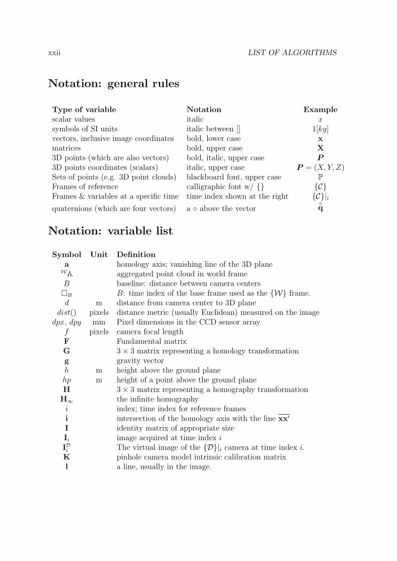
Notation: general rules
Type of variable Notation Examplescalar values italic xsymbols of SI units italic between [] 1[kg]vectors, inclusive image coordinates bold, lower case xmatrices bold, upper case X3D points (which are also vectors) bold, italic, upper case P3D points coordinates (scalars) italic, upper case P = (X, Y, Z)Sets of points (e.g. 3D point clouds) blackboard font, upper case PFrames of reference calligraphic font w/ {} {C}Frames & variables at a specific time time index shown at the right {C}|iquaternions (which are four vectors) a ◦ above the vector
◦q
Notation: variable list
Symbol Unit Definitiona homology axis; vanishing line of the 3D plane
WA aggregated point cloud in world frameB baseline: distance between camera centers�B B: time index of the base frame used as the {W} frame.d m distance from camera center to 3D plane
dist() pixels distance metric (usually Euclidean) measured on the imagedpx, dpy mm Pixel dimensions in the CCD sensor array
f pixels camera focal lengthF Fundamental matrixG 3× 3 matrix representing a homology transformationg gravity vectorh m height above the ground planehp m height of a point above the ground planeH 3× 3 matrix representing a homography transformation
H∞ the infinite homographyi index; time index for reference framesi intersection of the homology axis with the line xx′
I identity matrix of appropriate sizeIi image acquired at time index iIDi The virtual image of the {D}|i camera at time index i.K pinhole camera model intrinsic calibration matrixl a line, usually in the image.
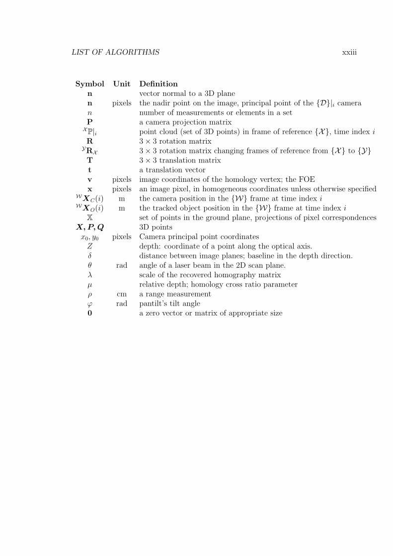
LIST OF ALGORITHMS xxiii
Symbol Unit Definitionn vector normal to a 3D planen pixels the nadir point on the image, principal point of the {D}|i cameran number of measurements or elements in a setP a camera projection matrix
XP|i point cloud (set of 3D points) in frame of reference {X}, time index iR 3× 3 rotation matrix
YRX 3× 3 rotation matrix changing frames of reference from {X} to {Y}T 3× 3 translation matrixt a translation vectorv pixels image coordinates of the homology vertex; the FOEx pixels an image pixel, in homogeneous coordinates unless otherwise specified
WXC(i) m the camera position in the {W} frame at time index iWXO(i) m the tracked object position in the {W} frame at time index i
X set of points in the ground plane, projections of pixel correspondencesX, P, Q 3D points
x0, y0 pixels Camera principal point coordinatesZ depth: coordinate of a point along the optical axis.δ distance between image planes; baseline in the depth direction.θ rad angle of a laser beam in the 2D scan plane.λ scale of the recovered homography matrixµ relative depth; homology cross ratio parameterρ cm a range measurementϕ rad pantilt’s tilt angle0 a zero vector or matrix of appropriate size

xxiv LIST OF ALGORITHMS
Chapter 1
Introduction
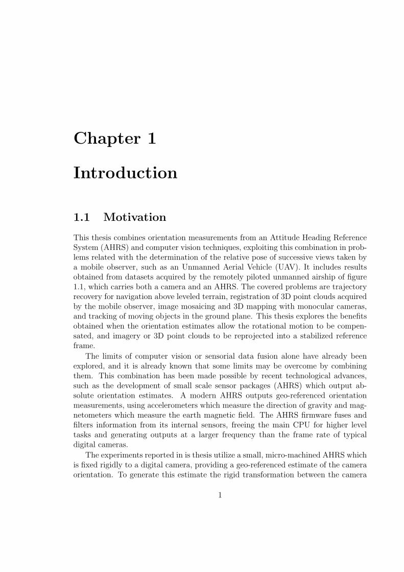
1.1 Motivation
This thesis combines orientation measurements from an Attitude Heading ReferenceSystem (AHRS) and computer vision techniques, exploiting this combination in prob-lems related with the determination of the relative pose of successive views taken bya mobile observer, such as an Unmanned Aerial Vehicle (UAV). It includes resultsobtained from datasets acquired by the remotely piloted unmanned airship of figure1.1, which carries both a camera and an AHRS. The covered problems are trajectoryrecovery for navigation above leveled terrain, registration of 3D point clouds acquiredby the mobile observer, image mosaicing and 3D mapping with monocular cameras,and tracking of moving objects in the ground plane. This thesis explores the benefitsobtained when the orientation estimates allow the rotational motion to be compen-sated, and imagery or 3D point clouds to be reprojected into a stabilized referenceframe.
The limits of computer vision or sensorial data fusion alone have already beenexplored, and it is already known that some limits may be overcome by combiningthem. This combination has been made possible by recent technological advances,such as the development of small scale sensor packages (AHRS) which output ab-solute orientation estimates. A modern AHRS outputs geo-referenced orientationmeasurements, using accelerometers which measure the direction of gravity and mag-netometers which measure the earth magnetic field. The AHRS firmware fuses andfilters information from its internal sensors, freeing the main CPU for higher leveltasks and generating outputs at a larger frequency than the frame rate of typicaldigital cameras.
The experiments reported in is thesis utilize a small, micro-machined AHRS whichis fixed rigidly to a digital camera, providing a geo-referenced estimate of the cameraorientation. To generate this estimate the rigid transformation between the camera
1
2 CHAPTER 1. INTRODUCTION
(a) (b)
Figure 1.1: The DIVA airship, during taking off (a) and approaching to land (b).
and inertial sensor frames must be known. This transformation is estimated by arecently developed calibration procedure [Lobo and Dias, 2007], eliminating the needfor precise mechanical assembly. This has already been used to improve robustnesson image segmentation and 3D structure recovery from stereo [Lobo and Dias, 2003,Mirisola et al., 2006] or independent motion segmentation [Lobo et al., 2006].
The development of vision-only or inertial-only algorithms are certainly worthyresearch goals by themselves and are suited to applications where only one of themis available. Nevertheless, the technological development, producing higher qualitydigital cameras and inertial and magnetic sensors at smaller sizes, weights and costsincrease the range of applications where both are available together. For these latterapplications it is already becoming clear that many important problems can be solvedmore efficiently, accurately, or with better scalability, with the combination of bothsensor modalities.
1.2 State of the Art
This section reviews recently reported research on the area of relative pose recoveryand navigation, using computer vision, sensorial data, and especially the fusion ofboth. The related problems of image mosaicing, 3D map registration and trackingare also covered.
1.2. STATE OF THE ART 3
1.2.1 Visual navigation & 3D mappingIn [Hygounenc et al., 2004], a stereovision-only approach is used to build a 3D map ofthe environment from stereo images taken by a remotely controlled airship, keepingestimates of the camera pose and the position of automatically detected landmarkson the ground. The landmarks are found by interest point algorithms applied on theaerial images. It was not their aim to integrate inertial measurements.
Again utilizing stereo images taken by a UAV, the trajectory can be recovered byregistering successive sets of triangulated 3D points calculated for each stereo frame.Trajectories of hundred of meters have been recovered [Kelly et al., 2007], althoughthe UAV height is limited to a few meters due to stereo baseline size. An earlier workfocused on estimating the height above the ground plane using efficient sparse stereotechniques [Corke et al., 2001].
Images from a moving camera can also be used to track a sparse set of 3D pointsin the environment using triangulation and interest points matched across the imagesequence and considered as natural landmarks. These estimates of observed land-marks, combined with measurements from inertial sensors, were used to estimate thelandmark poses and the camera trajectory for a ground vehicle carrying an omni-directional camera through a large trajectory [Strelow and Singh, 2004]. Matchedinteresting points in images with broad baseline were used to generate stochasticepipolar constraints which were used to minimize drift in the position estimate frominertial-based navigation [Diel, 2005].
Image mosaicing was performed for an unmanned submarine navigating above flatsea-bottom, using only images from a monocular camera as input for the calculationof relative poses [Gracias, 2002]. The most recent vehicle orientation estimate wasused to reproject the images onto a stabilized plane, avoiding using direct measuresfrom inertial sensors. The vehicle pose is estimated, and a mosaic of the sea-bottomis generated, which in turn is used for navigation. Although it involved elaborateoptimization steps, the registration converges only if the vehicle has restricted move-ment and shows minimal variation in roll and pitch angles. These results indicate alimitation for vision-only approaches.
A UAV trajectory can also be estimated by fusing GPS and on-board inertialdata and considering a dynamic vehicle model. Given accurate vehicle poses, im-ages taken from a high-flying airplane are reprojected onto the ground plane thusachieving one-pixel accuracy with no need for image-based registration techniques[Brown and Sullivan, 2002]. At high altitudes a relatively flat area can be safely as-sumed to be planar.
Combined inertial and vision data were used to keep pose estimates in an under-water environment, navigating a robot submarine above a large area [Eustice, 2005],with no access to a beacon-based localization system. Relative pose measurementsfrom the images were used to avoid divergence of the tracked vehicle pose, and an
4 CHAPTER 1. INTRODUCTION
image mosaic was generated as a byproduct.In the context of an aerial vehicle, even without utilizing the available GPS data,
inertial measurements and observations of artificial landmarks on images can be fusedtogether to provide a full 6-DOF pose estimate, performing localization and map-ping, and incorporating recent advances on filtering. Inertial sensors and barometricaltitude sensors can also compensate for inaccurate GPS altitude measurements orsatellite drop-outs [Kim, 2004].
The trajectory of a mobile observer can be recovered from images of a planarsurface using interest point matching and the well known planar homography model.Various geometric constraints have been proposed to recover the right motion amongthe four solutions of the homography matrix decomposition [Caballero et al., 2006].This has been already performed for an airship by using clustering and blob-basedinterest point matching algorithms, building an image mosaic which in turn is used asa map for navigation. The relative pose estimation involved homographies calculatedfrom images of a planar area taken by a UAV [Caballero et al., 2006] and imagesequences taken by various UAVs [Merino et al., 2006].
The trajectory of a UAV can also be recovered by tracking known fixed targetson the ground, which requires modifying the environment [Saripalli et al., 2003].
Another example of usage of inertial data to aid vision tasks are ego-motion al-gorithms without using pixel correspondences [Makadia and Daniilidis, 2005], wheregravity vector measurements compensate for two rotational degrees of freedom, de-creasing the dimensionality of the unknown parameter space.
Visual servoing schemes based on the relative pose obtained by decomposing ho-mographies could also be improved with the homology model [Suter et al., 2002],especially when depth ratios calculated from the homography matrix are directlyutilized.
Aerial vehicles have been utilized to produce 3D maps of the ground using a varietyof different sensors. Stereo images were used to build a dense 3D map of the groundsurface, in the form of a DEM (Digital Elevation Map), in the work already cited above[Hygounenc et al., 2004]. Stereo imagery has also been combined with other visiontechniques such as color segmentation [Huguet et al., 2003]. Airborne range sensingdevices such as laser range finders or radars have also been extensively used to build3D maps actually exploited in domains such as geology [Cunningham et al., 2006].
1.2.2 Image Mosaicing
Image mosaicing consists on registering a set of images of a surface in the world,producing a single, larger image of this surface. The mosaic ideally images the unionof the areas imaged by the individual images.
Many of the image mosaic results existing so far register images taken at the

1.2. STATE OF THE ART 5
same position, but with the camera looking at different directions, i.e., a pure ro-tational movement. In this case, the mosaicing surface is the plane at infinity, orthe sphere of directions. Disregarding differences on the camera intrinsic parameters,the transformation needed to register any pair of images is an infinite homography,as there is not translation. For the specific pure-rotation case, there are commercialsoftware products which take as input a set of images, and output a single mosaicedimage, which is called a panorama [Brown, 2006]. The solutions available take intoaccount differences on the camera intrinsic parameters [Brown and Lowe, 2003], illu-mination [Eden et al., 2006], and include optimization steps to reach a final registra-tion, plus processes to produce a visually clean image by eliminating misregisteredimages of the same object which appear repeated in the mosaic, called “ghosts”[Szeliski, 2005, Szeliski, 2004, Brown and Lowe, 2003].
Image mosaicing also can be done above a planar surface, allowing the camera tofreely translate, and there are also solutions available for this case, including bun-dle adjustment, N-view interest point matching, and automatically reprojecting theimages with an infinite homography in a direction that minimizes the projective dis-tortion [Capel, 2001]. The number of images registered on such mosaics range froma handful to less than a hundred images.
1.2.3 3D Depth map registration
3D mapping with color images and a rotating LRF was already performed[Ohno and Tadokoro, 2005], but without any calibration process to calibrate the ro-tation between the sensor frames, and using only ICP to register the point clouds.Rotating LRFs were also used to recover 3D range scans, that were matched to buildmaps, in room scale with small mobile robots [Kleiner et al., 2005].
Large terrestrial 3D mapping [Triebel et al., 2006] was performed using laser scan-ners mounted on a car, and registered on the world frame with the aid of fused infor-mation from on-board GPS, inertial systems and odometry. Before being integratedinto a new representation for the global map, local laser scans were registered togetherwith ICP algorithms, with no help from image or inertial data.
The ICP (Iterative Closest Point) algorithm [Besl and McKay, 1992], and its vari-ations, has been widely used for the registration of pairs of 3D point clouds. It isbased on picking a subset of 3D points from each point cloud, and associating eachsuch point to the closest point in the other point cloud. Then, a transformation isfound to register these corresponding pairs of points. The process is repeated untilno significant progress is made. This process is vulnerable to convergence into localminima, particularly when the initial position is far from the correct one. ApplyingICP after the processes defined in this thesis remain a possibility, depending on theapplication.

6 CHAPTER 1. INTRODUCTION
Results on visual odometry from stereo images associate 3D points obtained fromstereo images with interest points detected on the images. By matching the inter-est points on images taken successively, the sets of 3D points derived from theseimages are registered, recovering the full 6-DOF relative pose between two views[Cheng et al., 2006, Sünderhauf and Protzel, 2007]. The error on stereo triangulationis considered, leading to different weights to each constraint depending on the posi-tion of the 3D points relative to the cameras. The case of translation-only movementthe registration reduces to solve a weighted average [Matthies and Shafer, 1987].
The processes of interest point matching and stereo imaging are used in the reg-istration of point clouds, but they usually output wrong estimates for some pixels,which are called outliers. To detect and eliminate these outliers, robust estimationtechniques such as RANSAC [Fischler and Bolles, 1981] may be used, or geometricconstraints can be exploited, avoiding iterative techniques. An example are the twoconstraints proposed by [Hirschmüller et al., 2002], which exploit the fact that thetransformation is rigid. Given a pair of 3D points which have correspondences onthe other point cloud, the first constraint checks if the distance between the two 3Dpoints remains the same after the transformation. The second constraint checks if thepair of 3D points is rotated by an angle too large, given a maximum possible rotationbetween both point clouds.
A comprehensive comparison of different approaches for the registration of stereopoint clouds is still missing in the literature, as it was noted in a recent survey paper[Sünderhauf and Protzel, 2007].
1.2.4 Surveillance and TrackingThe Unscented Transform [Julier and Uhlmann, 1997] has been used to propagateuncertainty in the moving camera position and orientation, and from the target de-tected position in the image, to the target position on the ground plane. Then from aseries of successive observations of the same static target, a final estimate of its posi-tion was obtained, taking into account the anisotropic uncertainty of each observation[Merino et al., 2005].
Uncertainty in the camera orientation estimate is often the most important sourceof error in tracking of ground objects imaged by an airborne camera [Redding et al., 2006],and its projection in the 2D ground plane is usually anisotropic even if the originaldistribution is isotropic.
1.3 ObjectivesThis thesis aims to perform trajectory recovery from a sequence of images reprojectedin a stabilized frame where the rotation is compensated with the aid of AHRS ori-

1.3. OBJECTIVES 7
entation estimates. In the particular case where the ground plane is horizontal, therelative pose between two views can also be recovered by directly finding a rigid trans-formation to register corresponding scene coordinates. Additionally, for a sequence ofimages of a planar area, the transformation that relates corresponding pixel coordi-nates in two images is a planar homography, which is reduced to a planar homologyin the pure translation case. Some preliminary results using the homology modelhave already been obtained [Michaelsen et al., 2004], but a comprehensive evaluationof these pure translation models with aerial images is still missing in the literature.
In our experiments, the camera trajectory is recovered without recourse to artificiallandmarks and using only a monocular camera instead of depending on stereo imaging.The method depends on orientation measurements, which are obtained only from theAHRS sensor package, without considering any model of the vehicle dynamics. GPSis utilized only for comparison, and not on the trajectory recovery process itself,except in the experiments where both GPS and visual odometry are fused.
As it is shown in some of the works reviewed, incorporating GPS measurementsor considering a dynamic vehicle model in the estimation of the camera orientationcould improve the orientation estimate. Moreover, the models shown here has per-formed reasonably or at least better than image only approaches even with a relativelylow-cost and inaccurate AHRS. More expensive and accurate AHRS models shouldprovide more accurate estimates.
Differently of the UUV utilized to perform navigation and mosaicing [Gracias, 2002],the airship used in this thesis has large variations on roll and pitch during its flight,which is typical behavior for airships [de Paiva et al., 2006]. The orientation esti-mates compensate for these variations, and overcome that limitation of the visiononly approach.
Some of the works reviewed also utilize the reprojection of images into a virtualstabilized plane. Nevertheless, the homography model is still used. It may still benecessary to recover the residual rotation for some applications, but the pure trans-lation models presented here are certainly an option, and appear to be especiallysuitable to estimate the vertical motion component. Moreover, with the pure transla-tion models the extraction of the translation vector up to scale has a unique solution.In contrast, with the homography model, the recovered matrix must be algebraicallydecomposed into rotational and translational components, yielding four possible so-lutions, of which only one is the real relative pose [Ma et al., 2004].
Additionally, the homology model explicity separates the vertical and the hori-zontal components of the translation, facilitating the fusion of other measurements ofthese specific motion components in the future. For example, GPS north-east velocityor optical flow could be used to measure the direction of horizontal translation.
This work deals mainly with the calculation of relative pose between successivecamera poses, and the trajectory recovered is only a concatenation of the relative
8 CHAPTER 1. INTRODUCTION
poses, with Kalman Filters employed to reduce errors. It also includes results fromthe fusion of visual trajectory recovery and GPS position fixes. But this relative posemeasurement could be incorporated in localization and mapping schemes such as theones reviewed before, using artificial landmarks placed on the environment or naturallandmarks found by interest point matching.
This thesis also provides a method for obtaining 3D maps from the stabilizedimagery, using the images and a FOE estimate to estimate the height or the 3Dpoints imaged by some image pixels. This map is less accurate and much coarserthan the ones obtained by other sensors such as airborne LRFs and radars or stereoimagery, but it is very fast to obtain, and it requires only images from a monocularcamera.
While this thesis do not develop new algorithms in the image mosaicing domain, itquantifies the gains obtained with the usage of camera orientation estimates to repro-ject images on a virtual horizontal plane, and present an image mosaic as an example.These gains are related with the gains of affine invariant interest point algorithms,when compared with similar algorithms invariant only to rotation, translation, andillumination [Mikolajczyk and Schmid, 2004, Mikolajczyk et al., 2005]. Other navi-gation works have already used inertial data or image based measures in the sameway [Gracias, 2002, Brown and Sullivan, 2002, Eustice, 2005], but to our knowledgeit was not clearly quantified what is gained with the reprojection of images into astabilized plane.
In the 3D point cloud registration domain, it is necessary to find the relative posebetween successive camera poses. The rotational components of these relative posesmay be directly compensated by exploiting the AHRS orientation estimates. Fur-ther, the translational components may be more efficiently estimated when dealingwith rotation-compensated point clouds. This thesis leverage results in visual odom-etry and interest point matching and applies them into the registration of 3D mapsobtained by stereo cameras and laser range finders (LRF), always exploiting AHRSorientation estimates, and detailing the specific coordinate frames and sensor modelsutilized in each case. A comparison with ICP based algorithms is also provided forsome results, aiming to determine under which conditions it is advisable to employthe the method described here instead or together with ICP.
This thesis also showns that the improvements in trajectory recovery for the cam-era also translate into improvements in the accuracy of the tracking of a moving objectin the ground. The recovered target trajectory becomes smoother or more accurate,due to the improvements in the camera pose estimation and because the parametersof the filters involved in the tracking are defined in the actual metric units relatedto the target motion, which is also tracked in a metric frame. In contrast, when thetracking is performed directly on the image, in pixel coordinates, the scene suffersprojective distortion and the relation between pixel units and metric distances in the
1.4. EXPERIMENTAL PLATFORM 9
ground changes with the camera height and these distortions are often not taken intoaccount. Two scenarios are covered: aerial surveillance with the airship, and urbanpeople surveillance with a moving camera.
1.4 Experimental PlatformThe trajectory recovery algorithms were tested on data obtained from a remotelycontrolled blimp, the DIVA non-rigid airship. Figure 1.2 shows an image of theairship, which has a helium filled envelope with 18[m3] volume. It is 9.4[m] long, with1.9[m] diameter and the maximum speed attained is around 70[km/h]. Typically, themaximum height reached during our remotely piloted flights reached 200[m] abovethe ground, corresponding to an altitude of approximatelly 300[m].
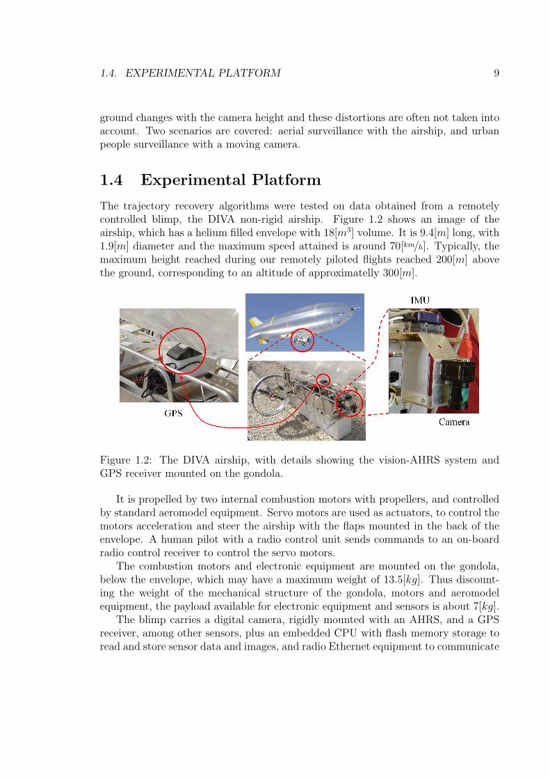
Figure 1.2: The DIVA airship, with details showing the vision-AHRS system andGPS receiver mounted on the gondola.
It is propelled by two internal combustion motors with propellers, and controlledby standard aeromodel equipment. Servo motors are used as actuators, to control themotors acceleration and steer the airship with the flaps mounted in the back of theenvelope. A human pilot with a radio control unit sends commands to an on-boardradio control receiver to control the servo motors.
The combustion motors and electronic equipment are mounted on the gondola,below the envelope, which may have a maximum weight of 13.5[kg]. Thus discount-ing the weight of the mechanical structure of the gondola, motors and aeromodelequipment, the payload available for electronic equipment and sensors is about 7[kg].
The blimp carries a digital camera, rigidly mounted with an AHRS, and a GPSreceiver, among other sensors, plus an embedded CPU with flash memory storage toread and store sensor data and images, and radio Ethernet equipment to communicate
10 CHAPTER 1. INTRODUCTION
with the ground. Figure 1.2 also shows details of the camera inertial system and theGPS receiver.
A ground station, consisting of a laptop connected to a wireless Ethernet accesspoint with a 7[dB] antenna, receives telemetry data during the flight, and displaysit to the operator, who is able to check the operation of all sensors before taking offand monitor the telemetry data during the flight.
The datasets used in the experiments of chapters 3 and 5 were acquired with thisplatform, remotely piloted. Appendix A provides a more detailed description of theonboard platform and the ground station, considering both software and hardwarecomponents.
The sensor specifications most relevant for the experiments of chapters 3 and 5are:
Digital Camera: Model Point Gray Flea [Point Grey Inc., 2007], a digital camerawith a bayer color CDD array with resolution of 1024x768 pixels and FirewireIEEE 1394 interface, weighting 40[g] without lens.
GPS receiver: Model GARMIN GPS35 [Garmin Int. Inc., 2007], a 12 channel GPSreceiver unit, which outputs 3D position and velocity at 1[Hz] rate, and weights130[g]. DGPS correction was not utilized in this thesis.
Inertial System: The last experiments used a XSens MTi, and the first ones aXSens MTB-9 [XSens Tech., 2007]. Both AHRS sensor suites have 3-axis ac-celerometer, inclinometer and gyroscope. They contain also a thermometer, andoutput calibrated and temperature-compensated sensor readings, plus filteredabsolute orientation at maximum 100[Hz] rate. The weights are 35[g] (MTB-9)and 50[g] (MTi). If the sensor is static, then the manufactures states that theerror in its orientation estimate has standard deviation of 3[◦] for the MTB-9and for the MTi of 0.5[◦] in the pitch and roll angles and of 1[◦] in the headingdirection. In dynamic conditions this error should be larger.
1.5 Thesis summaryThe next chapter reviews concepts, sensor models and frames of reference whichwill be needed in the rest of the thesis. It also reviews the calibration camera in-ertial utilized plus some important results in computer vision including the case oftranslation-only movement.
Chapter 3 presents models and results for trajectory recovery with rotation-compensated imagery, including experiments using the DIVA blimp. The chapteropens with the reprojection of the images on the virtual horizontal plane, a processthat will be used in the next chapters too.

1.6. PUBLICATIONS 11
Then, chapter 4 covers Image Mosaicing and Mapping. The mapping experimentsinclude point cloud registration with stereo cameras and LRFs, and mapping frommonocular cameras. The latter includes mapping from rotation-compensated imagerytaken by the DIVA UAV, and plane segmentation experiments.
The trajectory recovery results are extended to the tracking of an object inde-pendently moving on the ground plane which is observed by the moving camera, inchapter 5.
The conclusions and discussion of results are presented in chapter 6. After theconclusions, the appendix A present a more detailed view of the DIVA airship, in-cluding system characteristics and pre-requisites for future expansion, and hardwareand software architecture. Finally some mathematical proofs and formulae are left toappendix B.
1.6 PublicationsThe following publications resulted of the work leading to this thesis:
Book chapters
• Mirisola, L. G. B., Dias, J. “Tracking a Moving Target from a Moving Camerawith Rotation-Compensated Imagery” In “Intelligent Aerial Vehicles”, I-TechPublishing, Vienna, Austria, 2008A more complete version of the results in tracking of a moving object on theground after the camera trajectory is recovered are published in this paper,including the airship and people surveillance scenarios (chapter 5) and includingthe fusion of GPS and visual odometry.
• Moutinho, A, Mirisola, L. G. B., Azinheira, J., Dias, J. “Project DIVA: Guid-ance and Vision Surveillance Techniques for an Autonomous Airship” In “Re-search Trends in Robotics” (preliminary book title), NOVA Publishers, 2008.This book chapter covers part of the trajectory recovery and mapping resultsusing imagery taken by the DIVA airship, which appear in chapter 3 and section5.2.
Conference Papers
• Mirisola, L. G. B., Lobo, J., and Dias, J. “Stereo vision 3D map registrationfor airships using vision-inertial sensing.” The 12th IASTED Int. Conf. onRobotics and Applications (RA 2006), Honolulu, HI, USA, August 2006.This paper presents the 3D depth map registration using a stereo camera, aspresented in section 4.4.
12 CHAPTER 1. INTRODUCTION
• Mirisola, L. G. B. and Dias, J. M. M. “Exploiting inertial sensing in mosaicingand visual navigation.” 6th IFAC Symposium on Intelligent Autonomous Vehi-cles (IAV07), Toulouse, France, September 2007.In this paper were published, with less detail, the mosaicing results of section4.2, and the earliest experiments with the homology model: the tripod heightdetermination of section 3.4.1.1 and the recovery of altitude for the blimp flight(part of section 3.4.4).
• Mirisola, L. G. B., Lobo, J., and Dias, J. “3D Map Registration using Vi-sion/Laser and Inertial Sensing” European Conference on Mobile Robots (ECMR07),Freiburg, Germany, September 2007.The 3D map registration algorithm (section 4.4) was adapted and applied forthe LRF setup, with the introduction of the weighted averaging and comparisonwith ICP.
• Mirisola, L. G. B., Dias, J. M. M. and Traça de Almeida, A. “Trajectory Re-covery and 3D Mapping from Rotation-Compensated Imagery for an Airship.”In International Conference on Intelligent Robots and Systems (IROS 07), SanDiego, CA, USA, November 2007.The first version of the full trajectory recovery results for the DIVA UAV (sec-tion 3.4.4) was published here. This paper also includes the mapping results ofsection 4.3.3.
• Mirisola, L. G. B. and Dias, J. “Tracking a Moving Target from a MovingCamera with Rotation-Compensated Imagery” Israeli Conference in Robotics,Herzlia, Israel, November 2008A shorter version of the results in tracking of a moving object on the groundafter the camera trajectory is recovered are published in this paper, includingthe airship and people surveillance scenarios (chapter 5).
Chapter 2
Sensor Modeling
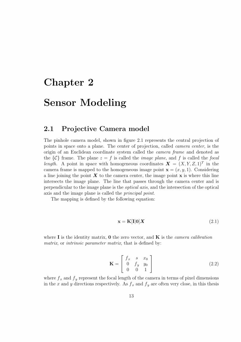
2.1 Projective Camera modelThe pinhole camera model, shown in figure 2.1 represents the central projection ofpoints in space onto a plane. The center of projection, called camera center, is theorigin of an Euclidean coordinate system called the camera frame and denoted asthe {C} frame. The plane z = f is called the image plane, and f is called the focallength. A point in space with homogeneous coordinates X = (X, Y, Z, 1)T in thecamera frame is mapped to the homogeneous image point x = (x, y, 1). Consideringa line joining the point X to the camera center, the image point x is where this lineintersects the image plane. The line that passes through the camera center and isperpendicular to the image plane is the optical axis, and the intersection of the opticalaxis and the image plane is called the principal point.
The mapping is defined by the following equation:
x = K[I|0]X (2.1)
where I is the identity matrix, 0 the zero vector, and K is the camera calibrationmatrix, or intrinsic parameter matrix, that is defined by:
K =
fx s x0
0 f y y0
0 0 1
(2.2)
where fx and f y represent the focal length of the camera in terms of pixel dimensionsin the x and y directions respectively. As fx and f y are often very close, in this thesis
13

14 CHAPTER 2. SENSOR MODELING
Figure 2.1: The pinhole camera model.
f is considered as the average of its two components, although this approximation isnot strictly necessary. The variables x0 and y0 are the principal point coordinates interms of pixel dimensions, and s is the skew parameter, very small for most cameras.In this thesis digital cameras with CCD sensors are used, where the image plane isconsidered as the plane of the CCD surface with its array of light sensors.
Each camera have its lens fixed and is calibrated, i.e., its intrinsic parameter matrixK is determined. Besides that, the calibration process finds the parameters whichdefine lens camera distortion - deviations from the camera projective model causedby the optical properties of the lens geometry. Through all this thesis, all camerasare calibrated, and all images are corrected for lens distortion. Single cameras werecalibrated by the Camera Calibration Toolkit [Bouguet, 2006], and stereo cameras bythe SVS Calibration Software [Konolige, 1997].
In this thesis all camera intrinsic parameters and the matrix K are given in pixelunits unless it is explicity defined otherwise. The dimension of each sensor on theCDD sensor array, i.e., the pixel size in millimeters, is given in the camera manual.In this thesis the pixel dimension is denoted as (dpx, dpy) and used to transformdistances in the image plane from pixels to a metric scale when needed. Alternatively,a calibration target with known dimensions can be used to calibrate the camera tofind the components of K in metric units.
2.1.1 Stereo Cameras
The stereo camera consists on two identical cameras rigidly mounted with near paralleloptical axes. The distance between the optical centers of both cameras is calledbaseline, denoted by B. When both cameras image the same 3D point P , this pointwill be projected on different positions on the two image planes, xL and xR, referringto the projections on the left and right camera, respectively, as shown in figure 2.2.The difference xL − xR is called disparity, and the depth of the point P is related tothe disparity by:
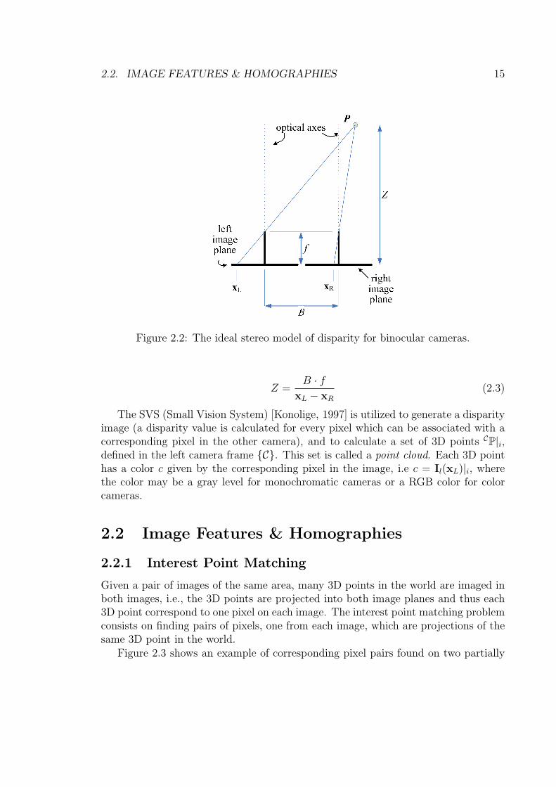
2.2. IMAGE FEATURES & HOMOGRAPHIES 15
Figure 2.2: The ideal stereo model of disparity for binocular cameras.
Z =B · f
xL − xR
(2.3)
The SVS (Small Vision System) [Konolige, 1997] is utilized to generate a disparityimage (a disparity value is calculated for every pixel which can be associated with acorresponding pixel in the other camera), and to calculate a set of 3D points CP|i,defined in the left camera frame {C}. This set is called a point cloud. Each 3D pointhas a color c given by the corresponding pixel in the image, i.e c = Il(xL)|i, wherethe color may be a gray level for monochromatic cameras or a RGB color for colorcameras.
2.2 Image Features & Homographies
2.2.1 Interest Point Matching
Given a pair of images of the same area, many 3D points in the world are imaged inboth images, i.e., the 3D points are projected into both image planes and thus each3D point correspond to one pixel on each image. The interest point matching problemconsists on finding pairs of pixels, one from each image, which are projections of thesame 3D point in the world.
Figure 2.3 shows an example of corresponding pixel pairs found on two partially
16 CHAPTER 2. SENSOR MODELING
Figure 2.3: An example of interest point matching. Each line connects a pair ofcorresponding pixels in both images.
overlapping images. Often hundreds of corresponding pixel pairs can be found on animage pair (only a handful are shown in the figure, for the sake of clarity).
More formally, the interest point matching problem is defined as: given two imagesI and I′, find a set of pairs of corresponding points on the images, such that, for eachpair of image points (x,x′), x and x′ correspond to the projection of the same 3Dpoint on the images I and I′, respectively.
Over the years, this problem has received a lot of attention, and it is still challeng-ing, as there are many variable conditions which make the recognition of the samepoint as seen in the two images be difficult. A good algorithm should be invariant,i.e., able to return the same results, detecting and matching the same points, in faceto environmental changes such as illumination and blur, and to differences on the im-age caused by the difference on the camera position in the world: scaling, translation,rotation, and even changes of viewpoint and affine transformations in general.
For the experiments reported in this thesis, initially the SIFT [Lowe, 2004] algo-rithm was used. After, the newer SURF [Bay et al., 2006] algorithm was used, as itoffers very similar performance in our experiments, and executes much faster.
All interest point algorithms find wrong matches, among the set of matched pixelpairs. Robust techniques such as RANSAC [Fischler and Bolles, 1981] are often usedto filter out these wrongly paired points, which are called outliers, leaving a set ofconsistently matched pixel pairs, called inliers. Some kind of geometric model isnecessary to provide a criterion to discriminate the outliers - the robust estimationalgorithm selects and considers only the largest possible set of inliers, i.e., of pointswhich are consistent with the geometric model.
2.2.2 Planar surfaces and homographies
Consider a 3D plane imaged by two identical cameras placed in different positions.Consider also a set of pixel correspondences belonging to that plane in the form of
2.2. IMAGE FEATURES & HOMOGRAPHIES 17
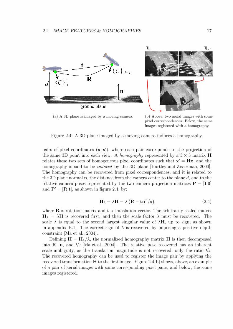
(a) A 3D plane is imaged by a moving camera. (b) Above, two aerial images with somepixel correspondences. Below, the sameimages registered with a homography.
Figure 2.4: A 3D plane imaged by a moving camera induces a homography.
pairs of pixel coordinates (x,x′), where each pair corresponds to the projection ofthe same 3D point into each view. A homography represented by a 3 × 3 matrix Hrelates these two sets of homogeneous pixel coordinates such that x′ = Hx, and thehomography is said to be induced by the 3D plane [Hartley and Zisserman, 2000].The homography can be recovered from pixel correspondences, and it is related tothe 3D plane normal n, the distance from the camera center to the plane d, and to therelative camera poses represented by the two camera projection matrices P = [I|0]and P′ = [R|t], as shown in figure 2.4, by:
Hλ = λH = λ(R− tnT /d
)(2.4)
where R is rotation matrix and t a translation vector. The arbitrarily scaled matrixHλ = λH is recovered first, and then the scale factor λ must be recovered. Thescale λ is equal to the second largest singular value of λH, up to sign, as shownin appendix B.1. The correct sign of λ is recovered by imposing a positive depthconstraint [Ma et al., 2004].
Defining H = Hλ/λ, the normalized homography matrix H is then decomposedinto R, n, and t/d [Ma et al., 2004]. The relative pose recovered has an inherentscale ambiguity, as the translation magnitude is not recovered, only the ratio t/d.The recovered homography can be used to register the image pair by applying therecovered transformation H to the first image. Figure 2.4(b) shows, above, an exampleof a pair of aerial images with some corresponding pixel pairs, and below, the sameimages registered.
18 CHAPTER 2. SENSOR MODELING
2.2.2.1 Pure rotation case
The infinite homography H∞ is a special case: it is the homography induced by theplane at infinity. It is also the homography between two images taken from twocameras at the same position (i.e., no translation, t = 0), but rotated by a rotationrepresented by the matrix R. The infinite homography can also be used to synthesizea virtual view from a non-existent virtual camera, at a desired orientation, given theappropriate rotation matrix.
The infinite homography is calculated by a limiting process where d approachesinfinity, or the translation t tends to zero. In both cases the ratio t/d tends to zero inequation (2.4):
H∞ = limt/d→0
H = limt/d→0
K(R +t
dnT )K−1 = KRK−1 (2.5)
2.2.3 Pure translation case
This section reviews computer vision results for the special case of pure translationmovement.
2.2.3.1 Planar Homologies
Equation (2.4) of section 2.2.2 is valid for general camera motion, involving the relativecamera rotation matrix R and translation vector t. In the translation-only case,R = I and the homography becomes a planar homology.
A planar homology G is a planar perspective transformation with the propertythat there is a line, called the axis, such that every point on this line is a fixedpoint1, and there is another fixed point not on the axis (the vertex ) . A 3D planeimaged under pure translation induces a planar homology, where the axis is theimage of the vanishing line of the plane (the intersection of the 3D plane and theplane at infinity), and the vertex is the epipole, or the FOE. Among the propertiesof homologies [Hartley and Zisserman, 2000, van Gool et al., 1998], we recall:
• Lines joining corresponding points intersect at the vertex, and correspondinglines (lines joining two pairs of corresponding points) intersect at the axis.
1A fixed point is a point x such that Gx = x, i.e., a point that is not changed by the transfor-mation
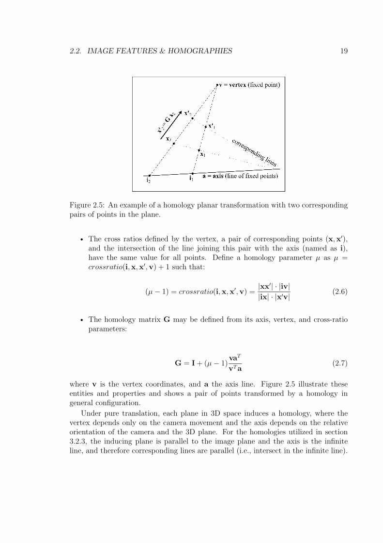
2.2. IMAGE FEATURES & HOMOGRAPHIES 19
Figure 2.5: An example of a homology planar transformation with two correspondingpairs of points in the plane.
• The cross ratios defined by the vertex, a pair of corresponding points (x,x′),and the intersection of the line joining this pair with the axis (named as i),have the same value for all points. Define a homology parameter µ as µ =crossratio(i,x,x′,v) + 1 such that:
(µ− 1) = crossratio(i,x,x′,v) =|xx′| · |iv||ix| · |x′v|
(2.6)
• The homology matrix G may be defined from its axis, vertex, and cross-ratioparameters:
G = I + (µ− 1)vaT
vTa(2.7)
where v is the vertex coordinates, and a the axis line. Figure 2.5 illustrate theseentities and properties and shows a pair of points transformed by a homology ingeneral configuration.
Under pure translation, each plane in 3D space induces a homology, where thevertex depends only on the camera movement and the axis depends on the relativeorientation of the camera and the 3D plane. For the homologies utilized in section3.2.3, the inducing plane is parallel to the image plane and the axis is the infiniteline, and therefore corresponding lines are parallel (i.e., intersect in the infinite line).
20 CHAPTER 2. SENSOR MODELING
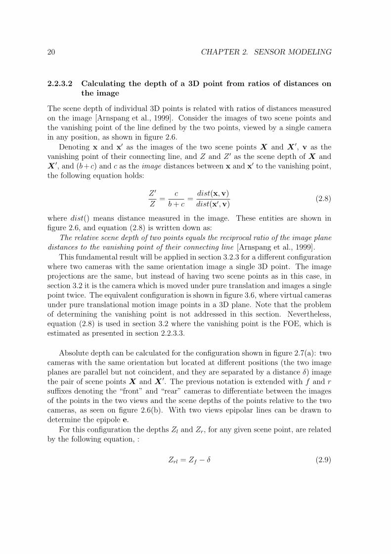
2.2.3.2 Calculating the depth of a 3D point from ratios of distances onthe image
The scene depth of individual 3D points is related with ratios of distances measuredon the image [Arnspang et al., 1999]. Consider the images of two scene points andthe vanishing point of the line defined by the two points, viewed by a single camerain any position, as shown in figure 2.6.
Denoting x and x′ as the images of the two scene points X and X ′, v as thevanishing point of their connecting line, and Z and Z ′ as the scene depth of X andX ′, and (b+ c) and c as the image distances between x and x′ to the vanishing point,the following equation holds:
Z ′
Z=
c
b + c=
dist(x,v)
dist(x′,v)(2.8)
where dist() means distance measured in the image. These entities are shown infigure 2.6, and equation (2.8) is written down as:
The relative scene depth of two points equals the reciprocal ratio of the image planedistances to the vanishing point of their connecting line [Arnspang et al., 1999].
This fundamental result will be applied in section 3.2.3 for a different configurationwhere two cameras with the same orientation image a single 3D point. The imageprojections are the same, but instead of having two scene points as in this case, insection 3.2 it is the camera which is moved under pure translation and images a singlepoint twice. The equivalent configuration is shown in figure 3.6, where virtual camerasunder pure translational motion image points in a 3D plane. Note that the problemof determining the vanishing point is not addressed in this section. Nevertheless,equation (2.8) is used in section 3.2 where the vanishing point is the FOE, which isestimated as presented in section 2.2.3.3.
Absolute depth can be calculated for the configuration shown in figure 2.7(a): twocameras with the same orientation but located at different positions (the two imageplanes are parallel but not coincident, and they are separated by a distance δ) imagethe pair of scene points X and X ′. The previous notation is extended with f and rsuffixes denoting the “front” and “rear” cameras to differentiate between the imagesof the points in the two views and the scene depths of the points relative to the twocameras, as seen on figure 2.6(b). With two views epipolar lines can be drawn todetermine the epipole e.
For this configuration the depths Zl and Zr, for any given scene point, are relatedby the following equation, :
Zrl = Zf − δ (2.9)
2.2. IMAGE FEATURES & HOMOGRAPHIES 21
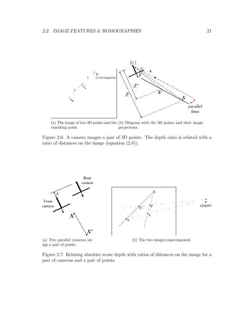
(a) The image of two 3D points and thevanishing point.
(b) Diagram with the 3D points and their imageprojections.
Figure 2.6: A camera images a pair of 3D points. The depth ratio is related with aratio of distances on the image (equation (2.8)).
(a) Two parallel cameras im-age a pair of points.
(b) The two images superimposed.
Figure 2.7: Relating absolute scene depth with ratios of distances on the image for apair of cameras and a pair of points.
22 CHAPTER 2. SENSOR MODELING
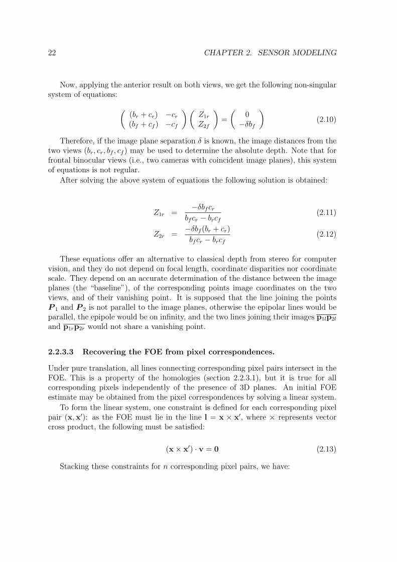
Now, applying the anterior result on both views, we get the following non-singularsystem of equations: (
(br + cr) −cr
(bf + cf ) −cf
)(Z1r
Z2f
)=
(0−δbf
)(2.10)
Therefore, if the image plane separation δ is known, the image distances from thetwo views (br, cr, bf , cf ) may be used to determine the absolute depth. Note that forfrontal binocular views (i.e., two cameras with coincident image planes), this systemof equations is not regular.
After solving the above system of equations the following solution is obtained:
Z1r =−δbfcr
bfcr − brcf
(2.11)
Z2r =−δbf (br + cr)
bfcr − brcf
(2.12)
These equations offer an alternative to classical depth from stereo for computervision, and they do not depend on focal length, coordinate disparities nor coordinatescale. They depend on an accurate determination of the distance between the imageplanes (the “baseline”), of the corresponding points image coordinates on the twoviews, and of their vanishing point. It is supposed that the line joining the pointsP 1 and P 2 is not parallel to the image planes, otherwise the epipolar lines would beparallel, the epipole would be on infinity, and the two lines joining their images p1lp2l
and p1rp2r would not share a vanishing point.
2.2.3.3 Recovering the FOE from pixel correspondences.
Under pure translation, all lines connecting corresponding pixel pairs intersect in theFOE. This is a property of the homologies (section 2.2.3.1), but it is true for allcorresponding pixels independently of the presence of 3D planes. An initial FOEestimate may be obtained from the pixel correspondences by solving a linear system.
To form the linear system, one constraint is defined for each corresponding pixelpair (x,x′): as the FOE must lie in the line l = x × x′, where × represents vectorcross product, the following must be satisfied:
(x× x′) · v = 0 (2.13)
Stacking these constraints for n corresponding pixel pairs, we have:
2.3. ATTITUDE HEADING REFERENCE SYSTEM 23
(x1 × x′1) · v = 0(x2 × x′2) · v = 0
...(xn × x′n) · v = 0
(2.14)
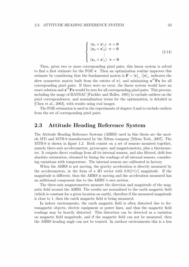
Then, given two or more corresponding pixel pairs, this linear system is solvedto find a first estimate for the FOE v. Then an optimization routine improves thisestimate by considering that the fundamental matrix is F = [v]× ([v]× indicates theskew symmetric matrix built from the entries of v), and minimizing x′TFx for allcorresponding pixel pairs. If there were no error, the linear system would have anexact solution and x′TFx would be zero for all corresponding pixel pairs. This process,including the usage of RANSAC [Fischler and Bolles, 1981] to exclude outliers on thepixel correspondences, and normalization terms for the optimization, is detailed in[Chen et al., 2003], with results using real images.
The FOE estimation is used in the experiments of chapter 3 and to exclude outliersfrom the set of corresponding pixel pairs.
2.3 Attitude Heading Reference SystemThe Attitude Heading Reference Systems (AHRS) used in this thesis are the mod-els MTi and MTB-9 manufactured by the XSens company [XSens Tech., 2007]. TheMTB-9 is shown in figure 1.2. Both consist on a set of sensors mounted together,namely three-axis accelerometers, gyroscopes, and magnetometers, plus a thermome-ter. It outputs direct readings from all its internal sensors, and also filtered, drift-lessabsolute orientation, obtained by fusing the readings of all internal sensors, consider-ing variations with temperature. The internal sensors are calibrated in factory.
When the AHRS is not moving, the gravity acceleration is directly measured bythe accelerometers, in the form of a 3D vector with 9.81[m/s2] magnitude. If themagnitude is different, then the AHRS is moving and the acceleration measured hasan additional component due to the AHRS´s own motion.
The three-axis magnetometers measure the direction and magnitude of the mag-netic field around the AHRS. The results are normalized to the earth magnetic field(which is constant for a given location on earth), therefore if the measured magnitudeis close to 1, then the earth magnetic field is being measured.
In indoor environments, the earth magnetic field is often distorted due to fer-romagnetic objects, electric equipment or power lines, and thus the magnetic fieldreadings may be heavily distorted. This distortion can be detected as a variationon magnetic field magnitude, and if the magnetic field can not be measured, thenthe AHRS heading angle can not be trusted. In outdoor environments this is a less
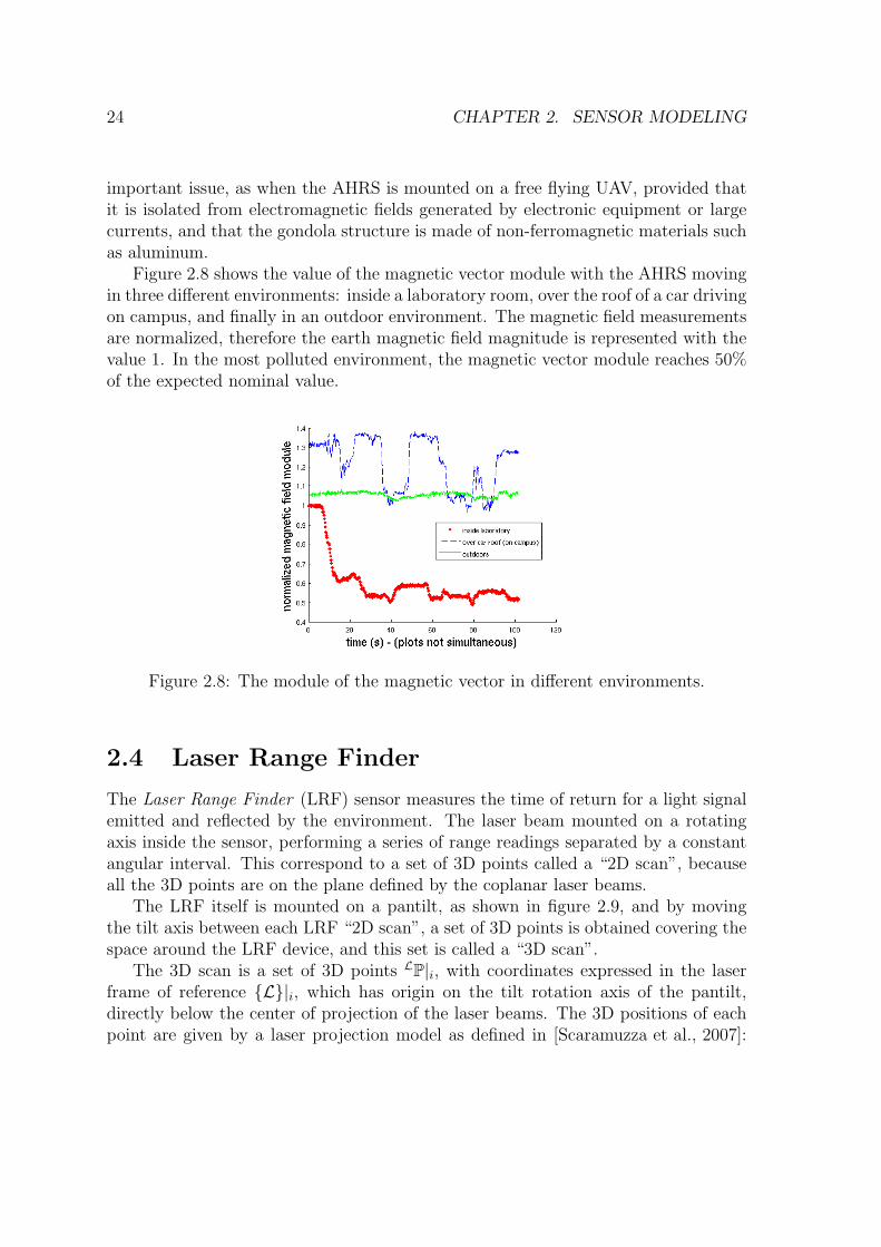
24 CHAPTER 2. SENSOR MODELING
important issue, as when the AHRS is mounted on a free flying UAV, provided thatit is isolated from electromagnetic fields generated by electronic equipment or largecurrents, and that the gondola structure is made of non-ferromagnetic materials suchas aluminum.
Figure 2.8 shows the value of the magnetic vector module with the AHRS movingin three different environments: inside a laboratory room, over the roof of a car drivingon campus, and finally in an outdoor environment. The magnetic field measurementsare normalized, therefore the earth magnetic field magnitude is represented with thevalue 1. In the most polluted environment, the magnetic vector module reaches 50%of the expected nominal value.
Figure 2.8: The module of the magnetic vector in different environments.
2.4 Laser Range FinderThe Laser Range Finder (LRF) sensor measures the time of return for a light signalemitted and reflected by the environment. The laser beam mounted on a rotatingaxis inside the sensor, performing a series of range readings separated by a constantangular interval. This correspond to a set of 3D points called a “2D scan”, becauseall the 3D points are on the plane defined by the coplanar laser beams.
The LRF itself is mounted on a pantilt, as shown in figure 2.9, and by movingthe tilt axis between each LRF “2D scan”, a set of 3D points is obtained covering thespace around the LRF device, and this set is called a “3D scan”.
The 3D scan is a set of 3D points LP|i, with coordinates expressed in the laserframe of reference {L}|i, which has origin on the tilt rotation axis of the pantilt,directly below the center of projection of the laser beams. The 3D positions of eachpoint are given by a laser projection model as defined in [Scaramuzza et al., 2007]:
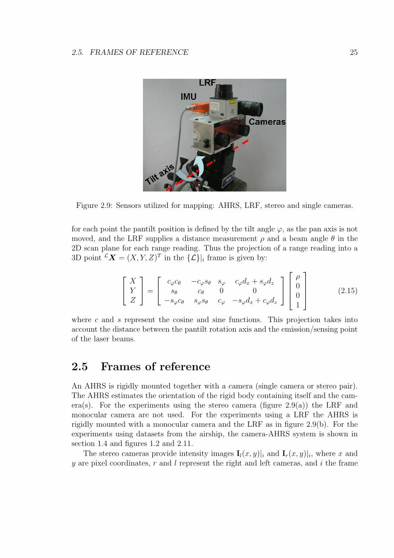
2.5. FRAMES OF REFERENCE 25
Figure 2.9: Sensors utilized for mapping: AHRS, LRF, stereo and single cameras.
for each point the pantilt position is defined by the tilt angle ϕ, as the pan axis is notmoved, and the LRF supplies a distance measurement ρ and a beam angle θ in the2D scan plane for each range reading. Thus the projection of a range reading into a3D point LX = (X, Y, Z)T in the {L}|i frame is given by:
XYZ
=
cϕcθ −cϕsθ sϕ cϕdx + sϕdz
sθ cθ 0 0−sϕcθ sϕsθ cϕ −sϕdx + cϕdz
ρ001
(2.15)
where c and s represent the cosine and sine functions. This projection takes intoaccount the distance between the pantilt rotation axis and the emission/sensing pointof the laser beams.
2.5 Frames of reference
An AHRS is rigidly mounted together with a camera (single camera or stereo pair).The AHRS estimates the orientation of the rigid body containing itself and the cam-era(s). For the experiments using the stereo camera (figure 2.9(a)) the LRF andmonocular camera are not used. For the experiments using a LRF the AHRS isrigidly mounted with a monocular camera and the LRF as in figure 2.9(b). For theexperiments using datasets from the airship, the camera-AHRS system is shown insection 1.4 and figures 1.2 and 2.11.
The stereo cameras provide intensity images Il(x, y)|i and Ir(x, y)|i, where x andy are pixel coordinates, r and l represent the right and left cameras, and i the frame
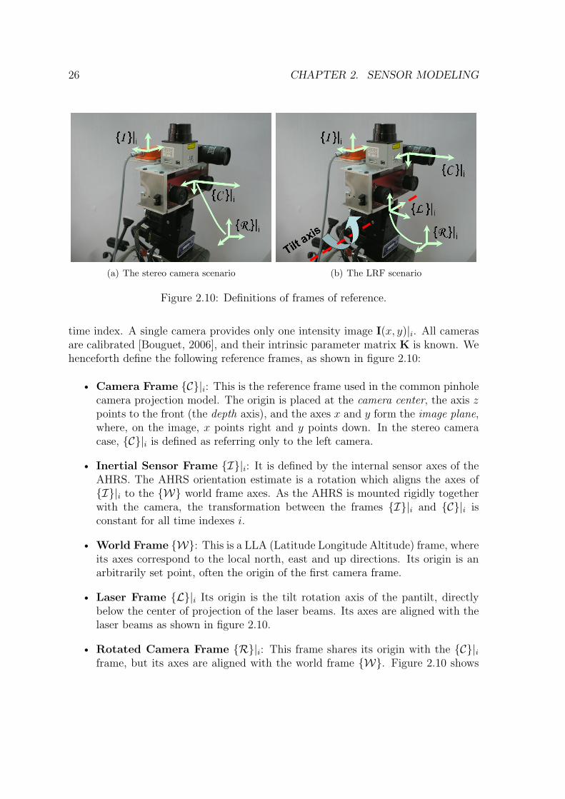
26 CHAPTER 2. SENSOR MODELING
(a) The stereo camera scenario (b) The LRF scenario
Figure 2.10: Definitions of frames of reference.
time index. A single camera provides only one intensity image I(x, y)|i. All camerasare calibrated [Bouguet, 2006], and their intrinsic parameter matrix K is known. Wehenceforth define the following reference frames, as shown in figure 2.10:
• Camera Frame {C}|i: This is the reference frame used in the common pinholecamera projection model. The origin is placed at the camera center, the axis zpoints to the front (the depth axis), and the axes x and y form the image plane,where, on the image, x points right and y points down. In the stereo cameracase, {C}|i is defined as referring only to the left camera.
• Inertial Sensor Frame {I}|i: It is defined by the internal sensor axes of theAHRS. The AHRS orientation estimate is a rotation which aligns the axes of{I}|i to the {W} world frame axes. As the AHRS is mounted rigidly togetherwith the camera, the transformation between the frames {I}|i and {C}|i isconstant for all time indexes i.
• World Frame {W}: This is a LLA (Latitude Longitude Altitude) frame, whereits axes correspond to the local north, east and up directions. Its origin is anarbitrarily set point, often the origin of the first camera frame.
• Laser Frame {L}|i Its origin is the tilt rotation axis of the pantilt, directlybelow the center of projection of the laser beams. Its axes are aligned with thelaser beams as shown in figure 2.10.
• Rotated Camera Frame {R}|i: This frame shares its origin with the {C}|iframe, but its axes are aligned with the world frame {W}. Figure 2.10 shows
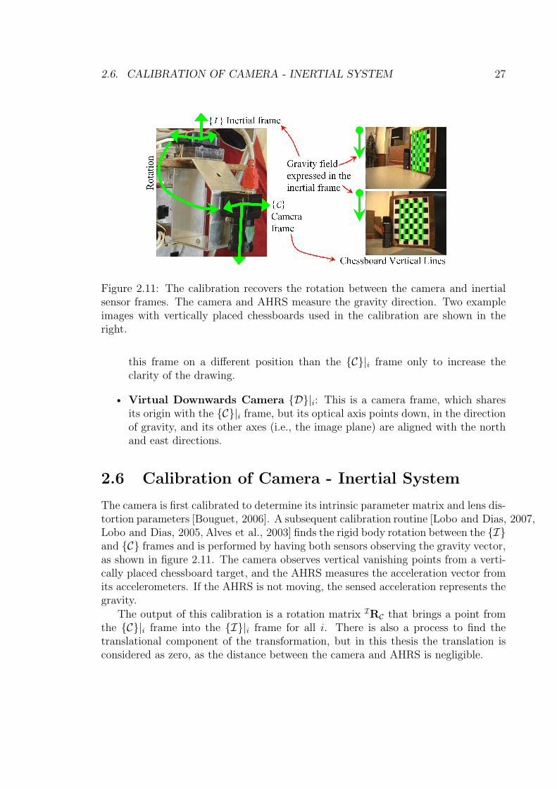
2.6. CALIBRATION OF CAMERA - INERTIAL SYSTEM 27
Figure 2.11: The calibration recovers the rotation between the camera and inertialsensor frames. The camera and AHRS measure the gravity direction. Two exampleimages with vertically placed chessboards used in the calibration are shown in theright.
this frame on a different position than the {C}|i frame only to increase theclarity of the drawing.
• Virtual Downwards Camera {D}|i: This is a camera frame, which sharesits origin with the {C}|i frame, but its optical axis points down, in the directionof gravity, and its other axes (i.e., the image plane) are aligned with the northand east directions.
2.6 Calibration of Camera - Inertial System
The camera is first calibrated to determine its intrinsic parameter matrix and lens dis-tortion parameters [Bouguet, 2006]. A subsequent calibration routine [Lobo and Dias, 2007,Lobo and Dias, 2005, Alves et al., 2003] finds the rigid body rotation between the {I}and {C} frames and is performed by having both sensors observing the gravity vector,as shown in figure 2.11. The camera observes vertical vanishing points from a verti-cally placed chessboard target, and the AHRS measures the acceleration vector fromits accelerometers. If the AHRS is not moving, the sensed acceleration represents thegravity.
The output of this calibration is a rotation matrix IRC that brings a point fromthe {C}|i frame into the {I}|i frame for all i. There is also a process to find thetranslational component of the transformation, but in this thesis the translation isconsidered as zero, as the distance between the camera and AHRS is negligible.
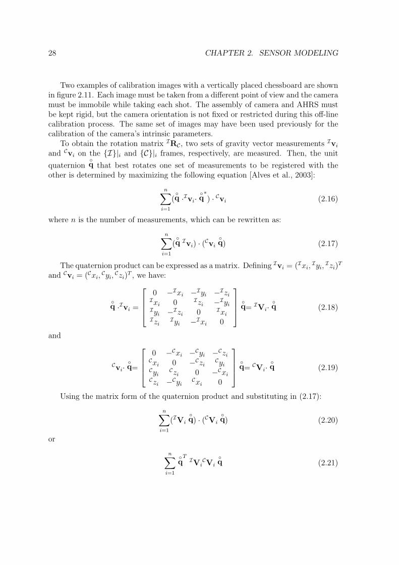
28 CHAPTER 2. SENSOR MODELING
Two examples of calibration images with a vertically placed chessboard are shownin figure 2.11. Each image must be taken from a different point of view and the cameramust be immobile while taking each shot. The assembly of camera and AHRS mustbe kept rigid, but the camera orientation is not fixed or restricted during this off-linecalibration process. The same set of images may have been used previously for thecalibration of the camera’s intrinsic parameters.
To obtain the rotation matrix IRC, two sets of gravity vector measurements Ivi
and Cvi on the {I}|i and {C}|i frames, respectively, are measured. Then, the unitquaternion
◦q that best rotates one set of measurements to be registered with the
other is determined by maximizing the following equation [Alves et al., 2003]:
n∑i=1
(◦q ·Ivi·
◦q∗) · Cvi (2.16)
where n is the number of measurements, which can be rewritten as:
n∑i=1
(◦q Ivi) · (Cvi
◦q) (2.17)
The quaternion product can be expressed as a matrix. Defining Ivi = (Ixi,Iyi,
Izi)T
and Cvi = (Cxi,Cyi,
Czi)T , we have:
◦q ·Ivi =
0 −Ixi −Iyi −IziIxi 0 Izi −IyiIyi −Izi 0 IxiIzi
Iyi −Ixi 0
◦q= IVi·
◦q (2.18)
and
Cvi·◦q=
0 −Cxi −Cyi −CziCxi 0 −Czi
CyiCyi
Czi 0 −CxiCzi −Cyi
Cxi 0
◦q= CVi·
◦q (2.19)
Using the matrix form of the quaternion product and substituting in (2.17):
n∑i=1
(IVi
◦q) · (CVi
◦q) (2.20)
or
n∑i=1
◦q
TIVi
CVi
◦q (2.21)
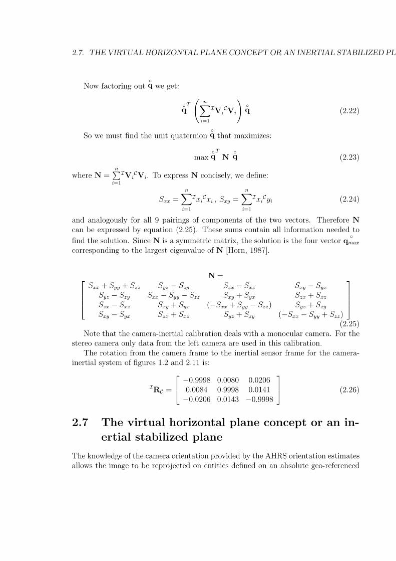
2.7. THE VIRTUAL HORIZONTAL PLANE CONCEPT OR AN INERTIAL STABILIZED PLANE29
Now factoring out◦q we get:
◦q
T(
n∑i=1
IViCVi
)◦q (2.22)
So we must find the unit quaternion◦q that maximizes:
max◦q
T
N◦q (2.23)
where N =n∑
i=1
IViCVi. To express N concisely, we define:
Sxx =n∑
i=1
IxiCxi , Sxy =
n∑i=1
IxiCyi (2.24)
and analogously for all 9 pairings of components of the two vectors. Therefore Ncan be expressed by equation (2.25). These sums contain all information needed tofind the solution. Since N is a symmetric matrix, the solution is the four vector
◦qmax
corresponding to the largest eigenvalue of N [Horn, 1987].
N =Sxx + Syy + Szz Syz − Szy Szx − Sxz Sxy − Syx
Syz − Szy Sxx − Syy − Szz Sxy + Syx Szx + Sxz
Szx − Sxz Sxy + Syx (−Sxx + Syy − Szz) Syz + Szy
Sxy − Syx Szx + Sxz Syz + Szy (−Sxx − Syy + Szz)
(2.25)
Note that the camera-inertial calibration deals with a monocular camera. For thestereo camera only data from the left camera are used in this calibration.
The rotation from the camera frame to the inertial sensor frame for the camera-inertial system of figures 1.2 and 2.11 is:
IRC =
−0.9998 0.0080 0.02060.0084 0.9998 0.0141−0.0206 0.0143 −0.9998
(2.26)
2.7 The virtual horizontal plane concept or an in-ertial stabilized plane
The knowledge of the camera orientation provided by the AHRS orientation estimatesallows the image to be reprojected on entities defined on an absolute geo-referenced

30 CHAPTER 2. SENSOR MODELING
Figure 2.12: The virtual horizontal plane concept.
frame, such as a virtual horizontal plane (with normal parallel to gravity), at a dis-tance f below the camera center, as shown in figure 2.12. Projection rays from 3Dpoints to the camera center intersect this plane, reprojecting the 3D point into theplane. This reprojection corresponds to the image of a virtual camera with the sameoptical center as the original camera, but with optical axis coincident with the gravityvector. Section 3.2.1 details how to perform this reprojection.
Chapter 3
Inertial Aided Visual TrajectoryRecovery
3.1 IntroductionIn this chapter, the trajectory of a mobile observer is recovered from a sequenceof images of a planar area. Orientation estimates from an AHRS compensate therotational degrees of freedom and allow the usage of a translation-only model.
Firstly, the knowledge of camera orientation allows the images to be reprojectedon a virtual horizontal plane, compensating the rotation, as presented in section 3.2.1.Then, the pure rotation models are introduced in sections 3.2.2 and 3.2.3. The caseof non-horizontal planes is covered in section 3.3.
The results are presented in section 3.4. As the vertical component is of specialimportance for aerial vehicles and is recovered separately by the homology algorithm,experiments with images taken from a tripod are presented to evaluate the algorithmsagainst hand measured ground truth. The chapter finishes by presenting trajectoryrecovery for the DIVA airship, and evaluating it by comparison with the commonhomography model and GPS. Visual odometry is also fused with GPS position fixes,and the maps generated when images are projected on the ground plane are alsocompared.
3.2 Visual Navigation
3.2.1 Reprojecting the images on the virtual horizontal plane
The first step of the processes of this chapter and of sections 4.2 and 5.2 is to re-project each image onto the virtual horizontal plane. In other words, a virtual viewis generated, to compensate differences due to heading and viewpoint. Each image
31
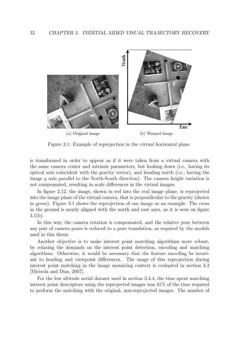
32 CHAPTER 3. INERTIAL AIDED VISUAL TRAJECTORY RECOVERY
(a) Original image (b) Warped image
Figure 3.1: Example of reprojection in the virtual horizontal plane
is transformed in order to appear as if it were taken from a virtual camera withthe same camera center and intrinsic parameters, but looking down (i.e., having itsoptical axis coincident with the gravity vector), and heading north (i.e., having theimage y axis parallel to the North-South direction). The camera height variation isnot compensated, resulting in scale differences in the virtual images.
In figure 2.12, the image, shown in red into the real image plane, is reprojectedinto the image plane of the virtual camera, that is perpendicular to the gravity (shownin green). Figure 3.1 shows the reprojection of one image as an example. The crossin the ground is nearly aligned with the north and east axes, as it is seen on figure3.1(b).
In this way, the camera rotation is compensated, and the relative pose betweenany pair of camera poses is reduced to a pure translation, as required by the modelsused in this thesis.
Another objective is to make interest point matching algorithms more robust,by relaxing the demands on the interest point detection, encoding and matchingalgorithms. Otherwise, it would be necessary that the feature encoding be invari-ant to heading and viewpoint differences. The usage of this reprojection duringinterest point matching in the image mosaicing context is evaluated in section 4.2[Mirisola and Dias, 2007].
For the low altitude aerial dataset used in section 3.4.4, the time spent matchinginterest point descriptors using the reprojected images was 41% of the time requiredto perform the matching with the original, non-reprojected images. The number of
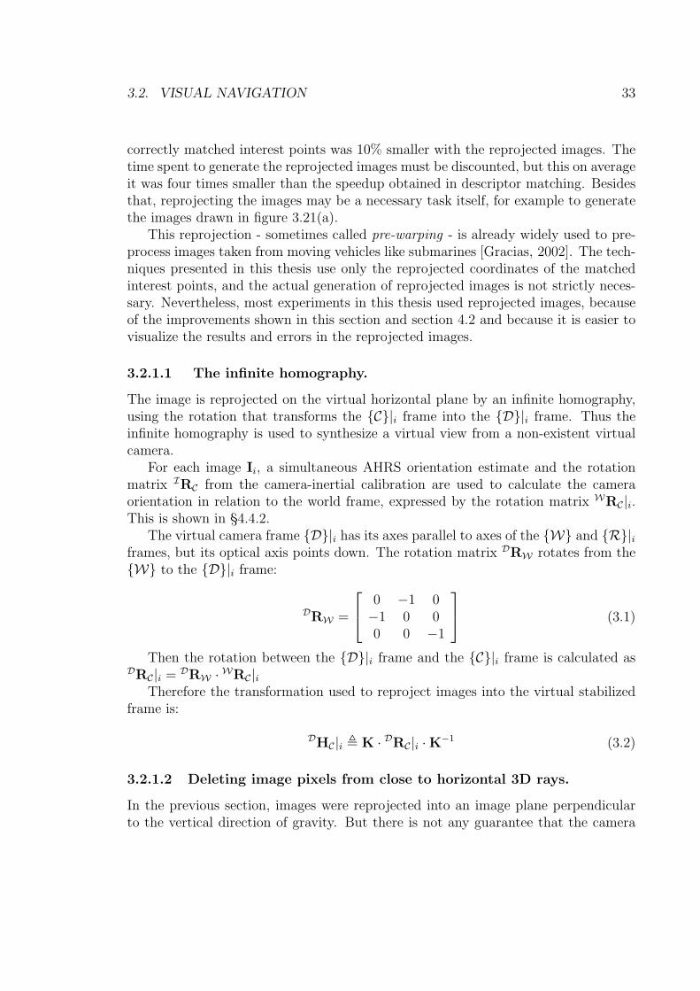
3.2. VISUAL NAVIGATION 33
correctly matched interest points was 10% smaller with the reprojected images. Thetime spent to generate the reprojected images must be discounted, but this on averageit was four times smaller than the speedup obtained in descriptor matching. Besidesthat, reprojecting the images may be a necessary task itself, for example to generatethe images drawn in figure 3.21(a).
This reprojection - sometimes called pre-warping - is already widely used to pre-process images taken from moving vehicles like submarines [Gracias, 2002]. The tech-niques presented in this thesis use only the reprojected coordinates of the matchedinterest points, and the actual generation of reprojected images is not strictly neces-sary. Nevertheless, most experiments in this thesis used reprojected images, becauseof the improvements shown in this section and section 4.2 and because it is easier tovisualize the results and errors in the reprojected images.
3.2.1.1 The infinite homography.
The image is reprojected on the virtual horizontal plane by an infinite homography,using the rotation that transforms the {C}|i frame into the {D}|i frame. Thus theinfinite homography is used to synthesize a virtual view from a non-existent virtualcamera.
For each image Ii, a simultaneous AHRS orientation estimate and the rotationmatrix IRC from the camera-inertial calibration are used to calculate the cameraorientation in relation to the world frame, expressed by the rotation matrix WRC|i.This is shown in §4.4.2.
The virtual camera frame {D}|i has its axes parallel to axes of the {W} and {R}|iframes, but its optical axis points down. The rotation matrix DRW rotates from the{W} to the {D}|i frame:
DRW =
0 −1 0−1 0 00 0 −1
(3.1)
Then the rotation between the {D}|i frame and the {C}|i frame is calculated asDRC|i = DRW · WRC|i
Therefore the transformation used to reproject images into the virtual stabilizedframe is:
DHC|i , K · DRC|i ·K−1 (3.2)
3.2.1.2 Deleting image pixels from close to horizontal 3D rays.
In the previous section, images were reprojected into an image plane perpendicularto the vertical direction of gravity. But there is not any guarantee that the camera
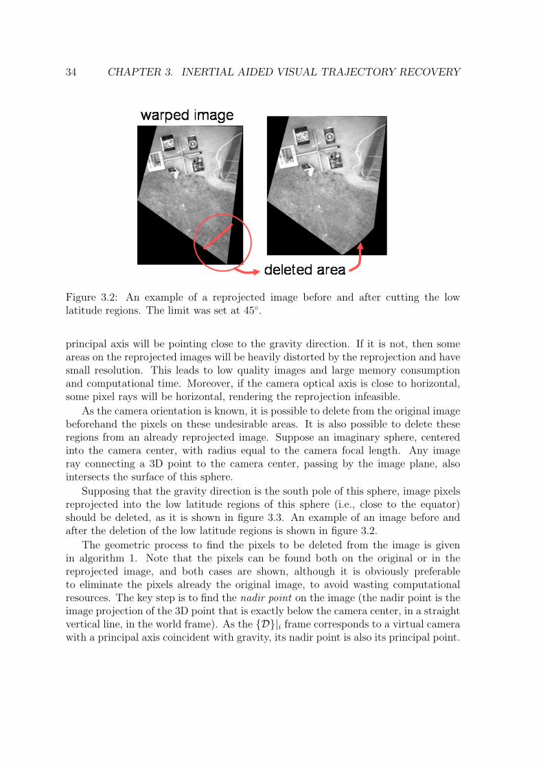
34 CHAPTER 3. INERTIAL AIDED VISUAL TRAJECTORY RECOVERY
Figure 3.2: An example of a reprojected image before and after cutting the lowlatitude regions. The limit was set at 45◦.
principal axis will be pointing close to the gravity direction. If it is not, then someareas on the reprojected images will be heavily distorted by the reprojection and havesmall resolution. This leads to low quality images and large memory consumptionand computational time. Moreover, if the camera optical axis is close to horizontal,some pixel rays will be horizontal, rendering the reprojection infeasible.
As the camera orientation is known, it is possible to delete from the original imagebeforehand the pixels on these undesirable areas. It is also possible to delete theseregions from an already reprojected image. Suppose an imaginary sphere, centeredinto the camera center, with radius equal to the camera focal length. Any imageray connecting a 3D point to the camera center, passing by the image plane, alsointersects the surface of this sphere.
Supposing that the gravity direction is the south pole of this sphere, image pixelsreprojected into the low latitude regions of this sphere (i.e., close to the equator)should be deleted, as it is shown in figure 3.3. An example of an image before andafter the deletion of the low latitude regions is shown in figure 3.2.
The geometric process to find the pixels to be deleted from the image is givenin algorithm 1. Note that the pixels can be found both on the original or in thereprojected image, and both cases are shown, although it is obviously preferableto eliminate the pixels already the original image, to avoid wasting computationalresources. The key step is to find the nadir point on the image (the nadir point is theimage projection of the 3D point that is exactly below the camera center, in a straightvertical line, in the world frame). As the {D}|i frame corresponds to a virtual camerawith a principal axis coincident with gravity, its nadir point is also its principal point.
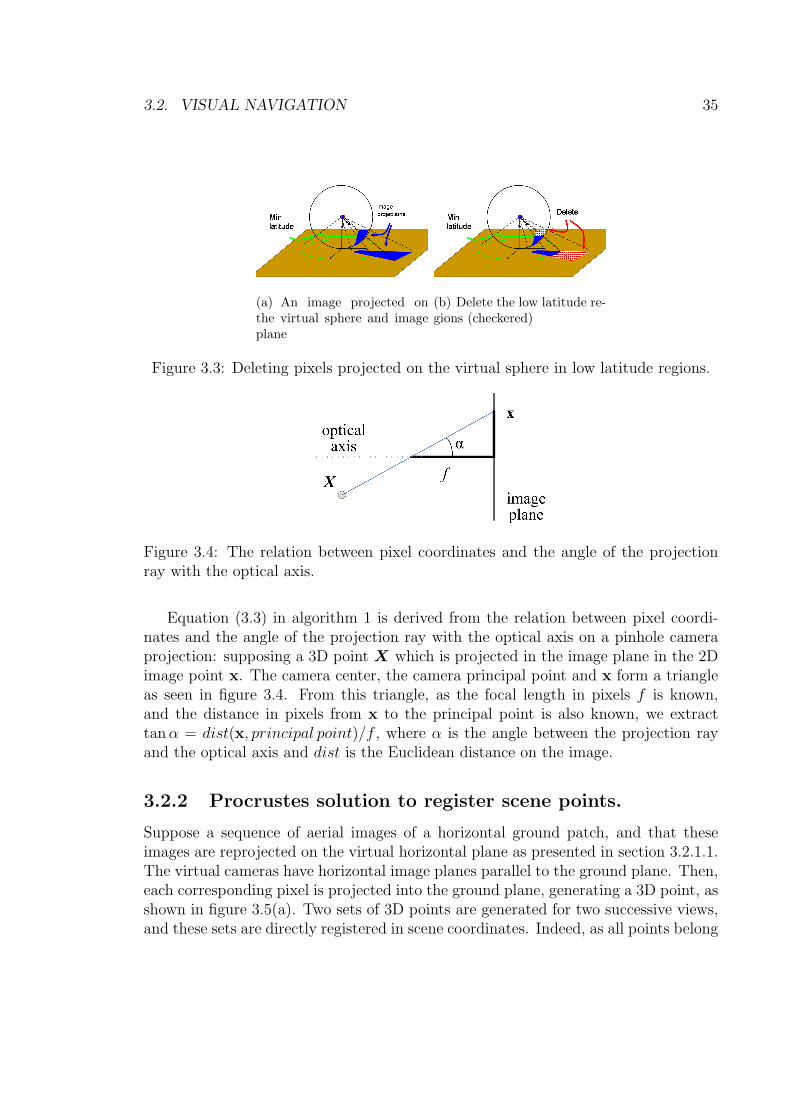
3.2. VISUAL NAVIGATION 35
(a) An image projected onthe virtual sphere and imageplane
(b) Delete the low latitude re-gions (checkered)
Figure 3.3: Deleting pixels projected on the virtual sphere in low latitude regions.
Figure 3.4: The relation between pixel coordinates and the angle of the projectionray with the optical axis.
Equation (3.3) in algorithm 1 is derived from the relation between pixel coordi-nates and the angle of the projection ray with the optical axis on a pinhole cameraprojection: supposing a 3D point X which is projected in the image plane in the 2Dimage point x. The camera center, the camera principal point and x form a triangleas seen in figure 3.4. From this triangle, as the focal length in pixels f is known,and the distance in pixels from x to the principal point is also known, we extracttan α = dist(x, principal point)/f , where α is the angle between the projection rayand the optical axis and dist is the Euclidean distance on the image.
3.2.2 Procrustes solution to register scene points.
Suppose a sequence of aerial images of a horizontal ground patch, and that theseimages are reprojected on the virtual horizontal plane as presented in section 3.2.1.1.The virtual cameras have horizontal image planes parallel to the ground plane. Then,each corresponding pixel is projected into the ground plane, generating a 3D point, asshown in figure 3.5(a). Two sets of 3D points are generated for two successive views,and these sets are directly registered in scene coordinates. Indeed, as all points belong
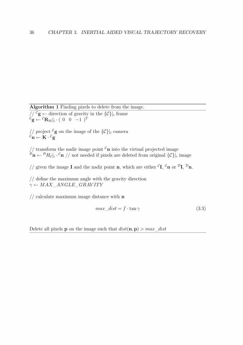
36 CHAPTER 3. INERTIAL AIDED VISUAL TRAJECTORY RECOVERY
Algorithm 1 Finding pixels to delete from the image.// Cg← direction of gravity in the {C}|i frameCg← CRW |i · ( 0 0 −1 )T
// project Cg on the image of the {C}|i cameraCn← K · Cg
// transform the nadir image point Cn into the virtual projected imageDn← DHC|i · Cn // not needed if pixels are deleted from original {C}|i image
// given the image I and the nadir point n, which are either CI, Cn or DI, Dn.
// define the maximum angle with the gravity directionγ ←MAX_ANGLE_GRAV ITY
// calculate maximum image distance with n
max_dist = f · tan γ (3.3)
Delete all pixels p on the image such that dist(n,p) > max_dist

3.2. VISUAL NAVIGATION 37
to the same ground plane, the registration is solved in 2D coordinates. Figure 3.5(b)shows a diagram of this process.
(a)
Figure 3.5: Finding the translation between successive camera poses by 3D sceneregistration.
Each corresponding pixel pair (x,x′) is projected by equation (3.4) yielding a pairof 3D points (X, X ′), defined in the {D}|i frame:
X =
(xx−nx)·hi
f(xy−ny)·hi
f
hi
, X ′(t) =
(x′x−nx)·(hi−tz/tw)
f+ tx
tw(x′y−ny)·(hi−tz/tw)
f+ ty
tw
hi − tz
(3.4)
where x = [xx, xy, 1]T , x′ =[x′x, x
′y, 1]T , again in inhomogeneous form, h is the
camera height above the ground plane, t is defined as a four element homogenousvector t = [tx, ty, tz, tw]T . The t value which turns X ′(t) = X is the translationwhich registers the {D}|i and {D}|i+1 frames, and which must be determined. If
38 CHAPTER 3. INERTIAL AIDED VISUAL TRAJECTORY RECOVERY
there are n corresponding pixel pairs, this projection yields two sets of 3D points,X = {Xk|k = 1 . . . n} and X′ = {X ′
k|k = 1 . . . n}An initial, inhomogeneous, value for t0 is calculated by the Procrustes registration
routine [Borg and Groenen, 1997, Gower and Dijksterhuis, 2004], which is describedin appendix B.6. It finds the 2D translation and scale factor which register the twopoint sets taken as 2D points, yielding estimates the x and y components of t0 andof the scale factor µ0. The inputs for the Procrustes routine are the configurations Xand X′(0).
From µ0 and the current estimate of the camera height an initial estimate thevertical component of t0 can be calculated, as µ0 = (hi− tz)/hi. Outliers in the pixelcorrespondences are removed by embedding the Procrustes routine in a RANSACprocedure. Then t0 is used as an initial estimate for an optimization routine whichminimizes the registration error between X and X′(t), estimating an updated andfinal value for t.
This optimization variables are the four elements of t, with equation (3.4) usedto update X′(t). The function to minimize is:
min(tx,ty ,tz ,tw)
∑k=1...n
dist (X ′k (t) , Xk) (3.5)
where dist is a distance metric. Appendix B.4 shows the partial derivatives of thisfunction with Euclidean distance as dist.
The same process could be performed with an inhomogeneous, three elementt. But, as it is the case with homography and homology estimation, the over-parameterization improves the accuracy of the final estimate and sometimes eventhe speed of convergence. In this case the extra dimension allows the length of thetranslation to change without changing its direction.
The optimization variables could also be (tx, ty, tw, µ), with the translation beinga 2D translation vector in homogeneous form, with µ as a scale factor and with theoptimization performed in the virtual plane 2D coordinates. For the aerial imagedataset, this second parameterization yielded worse results and was abandoned. Thesame remarks about overparameterization are again valid.
Nevertheless, for datasets such as the overpass dataset of section 3.4.2, where theactual camera orientation is almost constant, the error in the orientation estimate isless significant, and interest point matching is easier, not only both parameterizationsobtain good results even without over-parameterization or homogeneous variables,but also the algebraic Procrustes procedure obtains good results alone, with no op-timization at all, as it is shown in figure 3.16. Indeed, if the assumptions of havingboth image and ground planes parallel and horizontal are really true, with outliersremoved, and considering isotropic error in the corresponding pixel coordinates, thenit can be proved that the Procrustes solution is the best solution in a least squares
3.2. VISUAL NAVIGATION 39
sense. But the other methods should be more robust and resilient to errors, outliersand deviations from the model, and still exploit the available orientation estimate torecover the relative pose more accurately than an image-only method.
The FOE estimation of section 2.2.3.3 can also be used to find the initial estimatet0 instead of the Procrustes routine. But t0 can be calculated from the FOE onlyup to scale (section 3.2.4). To find the correct scale, an estimate of the cross-ratioparameter µ is obtained by measuring and averaging, for all corresponding pixelpairs, the ratios of image distances to the FOE as in equation (3.13). Then, giventhe estimate of the height of the first view h, tz is calculated as tz = (µ − 1)h, andthe horizontal components are calculated by equation (3.14).
3.2.3 The homology model for a horizontal planeSuppose again a sequence of aerial images of a horizontal ground area, and that theseimages are reprojected on the virtual horizontal plane as presented in section 3.2.1.This section shows another solution for the relative pose determination problem. Asthe virtual image planes and the ground plane are both horizontal, the camera heightabove the plane is equal to the plane depth in the virtual camera frame.
Although the homology (equation (2.7)) considers an inducing 3D plane in generalposition, in our experiments the relative pose estimation becomes less accurate if theplane axis also must be estimated, therefore it was necessary to restrict the inducingplane to be parallel to the virtual image planes. If a 3D plane is imaged by twocameras with image planes parallel to it, the image of vanishing line of the 3D plane,i.e., the homology axis, is the infinite line a = (0, 0, 1)T , and equation (2.7) becomes:
G =
1 0 (µ− 1) · vx
0 1 (µ− 1) · vy
0 0 µ
(3.6)
where vx, vy are the inhomogeneous1 image coordinates of the vertex v = (vx, vy, 1).The cross ratio parameter µ depends only of the depths of the 3D plane in thetwo views. To analyze the latter relation, we recall that the relative scene depth oftwo points equals the reciprocal ratio of the image plane distances to the vanishingpoint of their connecting line [Arnspang et al., 1999], as reviewed in section 2.2.3.2.Here, instead of having two parallel cameras as in section 2.2.3.2, the same principlesare applied to two images taken by a single moving camera, which keeps the sameorientation during its movement.
Take two images of the same 3D point X taken under pure translation, as in figure3.6(a), where the vanishing point is the FOE and the image is the superimposed image
1Without loss of generality as if v is known in homogeneous coordinates, it can be scaled into itsinhomogeneous form.
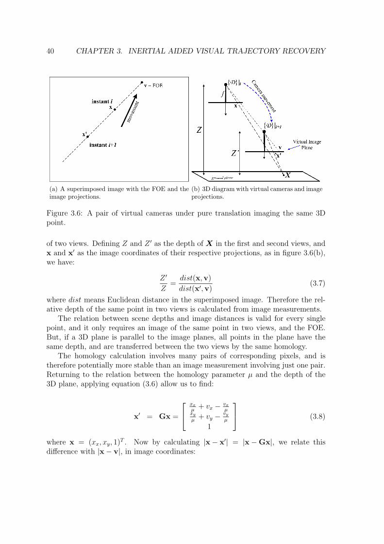
40 CHAPTER 3. INERTIAL AIDED VISUAL TRAJECTORY RECOVERY
(a) A superimposed image with the FOE and theimage projections.
(b) 3D diagram with virtual cameras and imageprojections.
Figure 3.6: A pair of virtual cameras under pure translation imaging the same 3Dpoint.
of two views. Defining Z and Z ′ as the depth of X in the first and second views, andx and x′ as the image coordinates of their respective projections, as in figure 3.6(b),we have:
Z ′
Z=
dist(x,v)
dist(x′,v)(3.7)
where dist means Euclidean distance in the superimposed image. Therefore the rel-ative depth of the same point in two views is calculated from image measurements.
The relation between scene depths and image distances is valid for every singlepoint, and it only requires an image of the same point in two views, and the FOE.But, if a 3D plane is parallel to the image planes, all points in the plane have thesame depth, and are transferred between the two views by the same homology.
The homology calculation involves many pairs of corresponding pixels, and istherefore potentially more stable than an image measurement involving just one pair.Returning to the relation between the homology parameter µ and the depth of the3D plane, applying equation (3.6) allow us to find:
x′ = Gx =
xx
µ+ vx − vx
µxy
µ+ vy − vy
µ
1
(3.8)
where x = (xx, xy, 1)T . Now by calculating |x− x′| = |x−Gx|, we relate thisdifference with |x− v|, in image coordinates:
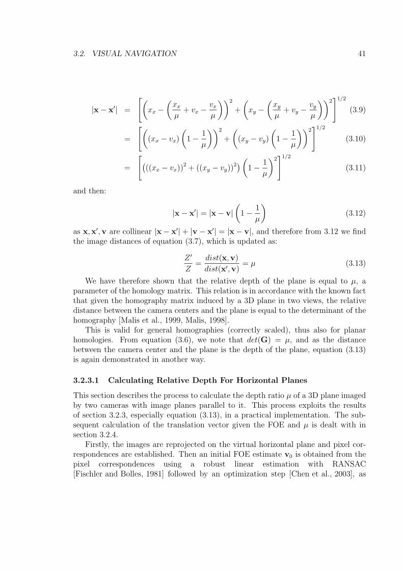
3.2. VISUAL NAVIGATION 41
|x− x′| =
[(xx −
(xx
µ+ vx −
vx
µ
))2
+
(xy −
(xy
µ+ vy −
vy
µ
))2]1/2
(3.9)
=
[((xx − vx)
(1− 1
µ
))2
+
((xy − vy)
(1− 1
µ
))2]1/2
(3.10)
=
[(((xx − vx))
2 + ((xy − vy))2)(1− 1
µ
)2]1/2
(3.11)
and then:
|x− x′| = |x− v|(
1− 1
µ
)(3.12)
as x,x′,v are collinear |x− x′| + |v − x′| = |x− v|, and therefore from 3.12 we findthe image distances of equation (3.7), which is updated as:
Z ′
Z=
dist(x,v)
dist(x′,v)= µ (3.13)
We have therefore shown that the relative depth of the plane is equal to µ, aparameter of the homology matrix. This relation is in accordance with the known factthat given the homography matrix induced by a 3D plane in two views, the relativedistance between the camera centers and the plane is equal to the determinant of thehomography [Malis et al., 1999, Malis, 1998].
This is valid for general homographies (correctly scaled), thus also for planarhomologies. From equation (3.6), we note that det(G) = µ, and as the distancebetween the camera center and the plane is the depth of the plane, equation (3.13)is again demonstrated in another way.
3.2.3.1 Calculating Relative Depth For Horizontal Planes
This section describes the process to calculate the depth ratio µ of a 3D plane imagedby two cameras with image planes parallel to it. This process exploits the resultsof section 3.2.3, especially equation (3.13), in a practical implementation. The sub-sequent calculation of the translation vector given the FOE and µ is dealt with insection 3.2.4.
Firstly, the images are reprojected on the virtual horizontal plane and pixel cor-respondences are established. Then an initial FOE estimate v0 is obtained from thepixel correspondences using a robust linear estimation with RANSAC[Fischler and Bolles, 1981] followed by an optimization step [Chen et al., 2003], as
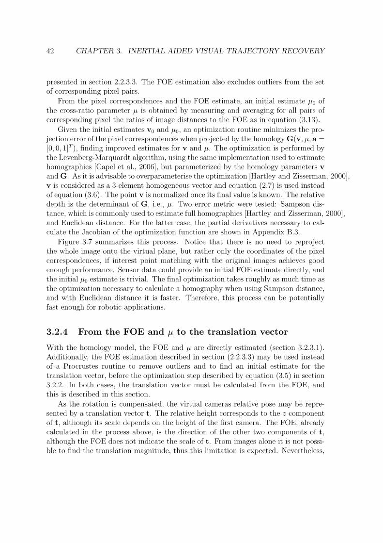
42 CHAPTER 3. INERTIAL AIDED VISUAL TRAJECTORY RECOVERY
presented in section 2.2.3.3. The FOE estimation also excludes outliers from the setof corresponding pixel pairs.
From the pixel correspondences and the FOE estimate, an initial estimate µ0 ofthe cross-ratio parameter µ is obtained by measuring and averaging for all pairs ofcorresponding pixel the ratios of image distances to the FOE as in equation (3.13).
Given the initial estimates v0 and µ0, an optimization routine minimizes the pro-jection error of the pixel correspondences when projected by the homology G(v, µ, a =[0, 0, 1]T ), finding improved estimates for v and µ. The optimization is performed bythe Levenberg-Marquardt algorithm, using the same implementation used to estimatehomographies [Capel et al., 2006], but parameterized by the homology parameters vand G. As it is advisable to overparameterise the optimization [Hartley and Zisserman, 2000],v is considered as a 3-element homogeneous vector and equation (2.7) is used insteadof equation (3.6). The point v is normalized once its final value is known. The relativedepth is the determinant of G, i.e., µ. Two error metric were tested: Sampson dis-tance, which is commonly used to estimate full homographies [Hartley and Zisserman, 2000],and Euclidean distance. For the latter case, the partial derivatives necessary to cal-culate the Jacobian of the optimization function are shown in Appendix B.3.
Figure 3.7 summarizes this process. Notice that there is no need to reprojectthe whole image onto the virtual plane, but rather only the coordinates of the pixelcorrespondences, if interest point matching with the original images achieves goodenough performance. Sensor data could provide an initial FOE estimate directly, andthe initial µ0 estimate is trivial. The final optimization takes roughly as much time asthe optimization necessary to calculate a homography when using Sampson distance,and with Euclidean distance it is faster. Therefore, this process can be potentiallyfast enough for robotic applications.
3.2.4 From the FOE and µ to the translation vector
With the homology model, the FOE and µ are directly estimated (section 3.2.3.1).Additionally, the FOE estimation described in section (2.2.3.3) may be used insteadof a Procrustes routine to remove outliers and to find an initial estimate for thetranslation vector, before the optimization step described by equation (3.5) in section3.2.2. In both cases, the translation vector must be calculated from the FOE, andthis is described in this section.
As the rotation is compensated, the virtual cameras relative pose may be repre-sented by a translation vector t. The relative height corresponds to the z componentof t, although its scale depends on the height of the first camera. The FOE, alreadycalculated in the process above, is the direction of the other two components of t,although the FOE does not indicate the scale of t. From images alone it is not possi-ble to find the translation magnitude, thus this limitation is expected. Nevertheless,
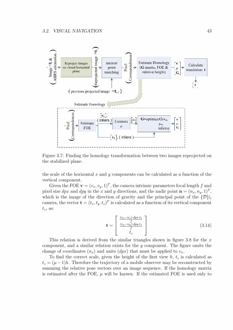
3.2. VISUAL NAVIGATION 43
Figure 3.7: Finding the homology transformation between two images reprojected onthe stabilized plane.
the scale of the horizontal x and y components can be calculated as a function of thevertical component.
Given the FOE v = (vx, vy, 1)T , the camera intrinsic parameters focal length f andpixel size dpx and dpy in the x and y directions, and the nadir point n = (nx, ny, 1)T ,which is the image of the direction of gravity and the principal point of the {D}|icamera, the vector t = (tx, ty, tz)
T is calculated as a function of its vertical componenttz, as:
t =
(vx−nx)·dpx·tz
f(vy−ny)·dpy·tz
f
tz
(3.14)
This relation is derived from the similar triangles shown in figure 3.8 for the xcomponent, and a similar relation exists for the y component. The figure omits thechange of coordinates (nx) and units (dpx) that must be applied to vx.
To find the correct scale, given the height of the first view h, tz is calculated astz = (µ− 1)h. Therefore the trajectory of a mobile observer may be reconstructed bysumming the relative pose vectors over an image sequence. If the homology matrixis estimated after the FOE, µ will be known. If the estimated FOE is used only to
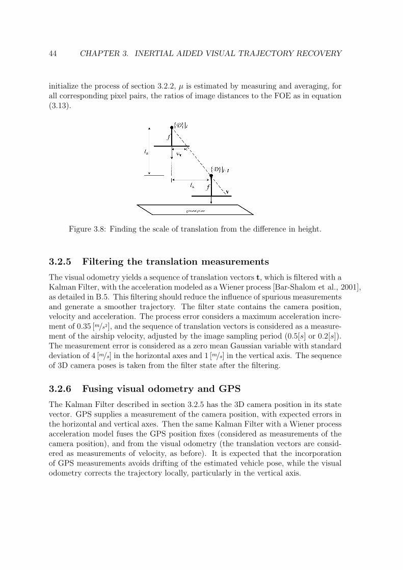
44 CHAPTER 3. INERTIAL AIDED VISUAL TRAJECTORY RECOVERY
initialize the process of section 3.2.2, µ is estimated by measuring and averaging, forall corresponding pixel pairs, the ratios of image distances to the FOE as in equation(3.13).
Figure 3.8: Finding the scale of translation from the difference in height.
3.2.5 Filtering the translation measurements
The visual odometry yields a sequence of translation vectors t, which is filtered with aKalman Filter, with the acceleration modeled as a Wiener process [Bar-Shalom et al., 2001],as detailed in B.5. This filtering should reduce the influence of spurious measurementsand generate a smoother trajectory. The filter state contains the camera position,velocity and acceleration. The process error considers a maximum acceleration incre-ment of 0.35 [m/s2], and the sequence of translation vectors is considered as a measure-ment of the airship velocity, adjusted by the image sampling period (0.5[s] or 0.2[s]).The measurement error is considered as a zero mean Gaussian variable with standarddeviation of 4 [m/s] in the horizontal axes and 1 [m/s] in the vertical axis. The sequenceof 3D camera poses is taken from the filter state after the filtering.
3.2.6 Fusing visual odometry and GPS
The Kalman Filter described in section 3.2.5 has the 3D camera position in its statevector. GPS supplies a measurement of the camera position, with expected errors inthe horizontal and vertical axes. Then the same Kalman Filter with a Wiener processacceleration model fuses the GPS position fixes (considered as measurements of thecamera position), and from the visual odometry (the translation vectors are consid-ered as measurements of velocity, as before). It is expected that the incorporationof GPS measurements avoids drifting of the estimated vehicle pose, while the visualodometry corrects the trajectory locally, particularly in the vertical axis.
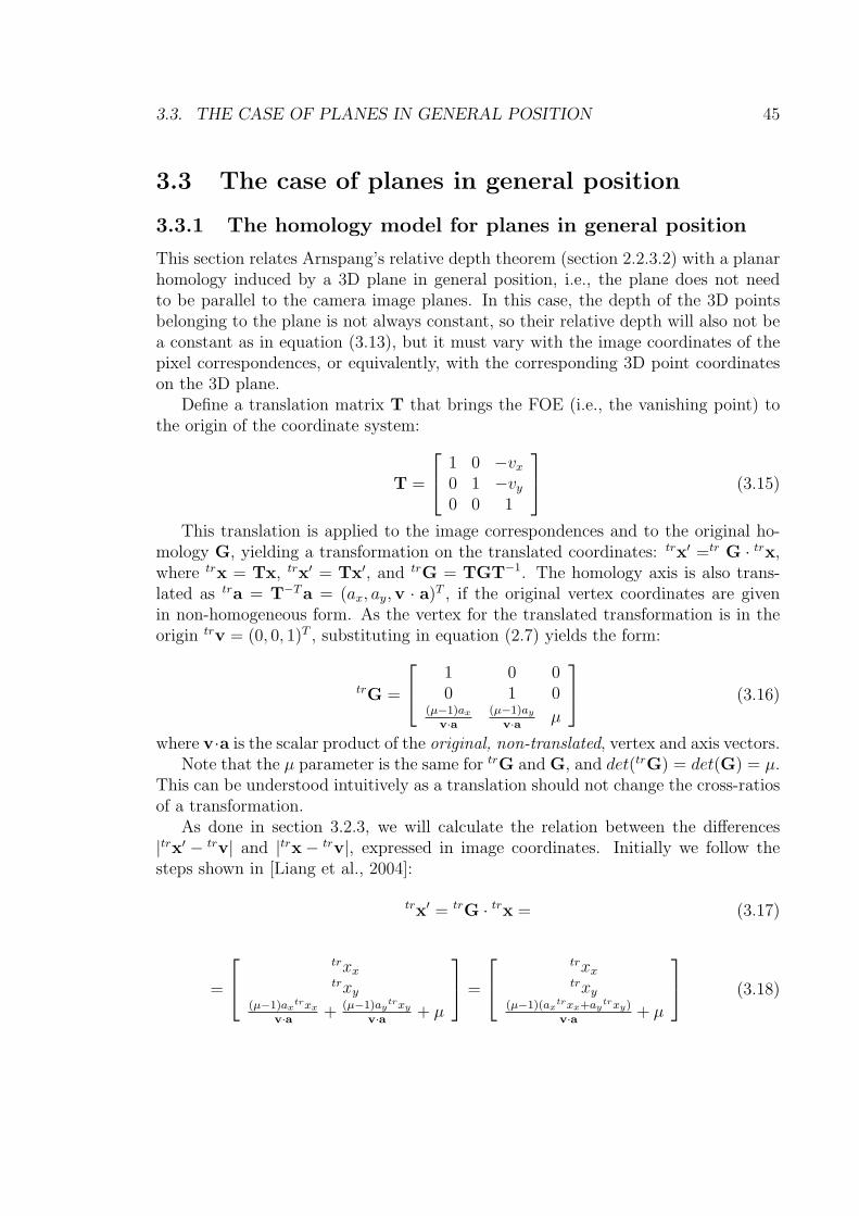
3.3. THE CASE OF PLANES IN GENERAL POSITION 45
3.3 The case of planes in general position
3.3.1 The homology model for planes in general positionThis section relates Arnspang’s relative depth theorem (section 2.2.3.2) with a planarhomology induced by a 3D plane in general position, i.e., the plane does not needto be parallel to the camera image planes. In this case, the depth of the 3D pointsbelonging to the plane is not always constant, so their relative depth will also not bea constant as in equation (3.13), but it must vary with the image coordinates of thepixel correspondences, or equivalently, with the corresponding 3D point coordinateson the 3D plane.
Define a translation matrix T that brings the FOE (i.e., the vanishing point) tothe origin of the coordinate system:
T =
1 0 −vx
0 1 −vy
0 0 1
(3.15)
This translation is applied to the image correspondences and to the original ho-mology G, yielding a transformation on the translated coordinates: trx′ =tr G · trx,where trx = Tx, trx′ = Tx′, and trG = TGT−1. The homology axis is also trans-lated as tra = T−Ta = (ax, ay,v · a)T , if the original vertex coordinates are givenin non-homogeneous form. As the vertex for the translated transformation is in theorigin trv = (0, 0, 1)T , substituting in equation (2.7) yields the form:
trG =
1 0 00 1 0
(µ−1)ax
v·a(µ−1)ay
v·a µ
(3.16)
where v·a is the scalar product of the original, non-translated, vertex and axis vectors.Note that the µ parameter is the same for trG and G, and det(trG) = det(G) = µ.
This can be understood intuitively as a translation should not change the cross-ratiosof a transformation.
As done in section 3.2.3, we will calculate the relation between the differences|trx′ − trv| and |trx− trv|, expressed in image coordinates. Initially we follow thesteps shown in [Liang et al., 2004]:
trx′ = trG · trx = (3.17)
=
trxxtrxy
(µ−1)axtrxx
v·a + (µ−1)aytrxy
v·a + µ
=
trxxtrxy
(µ−1)(axtrxx+ay
trxy)
v·a + µ
(3.18)
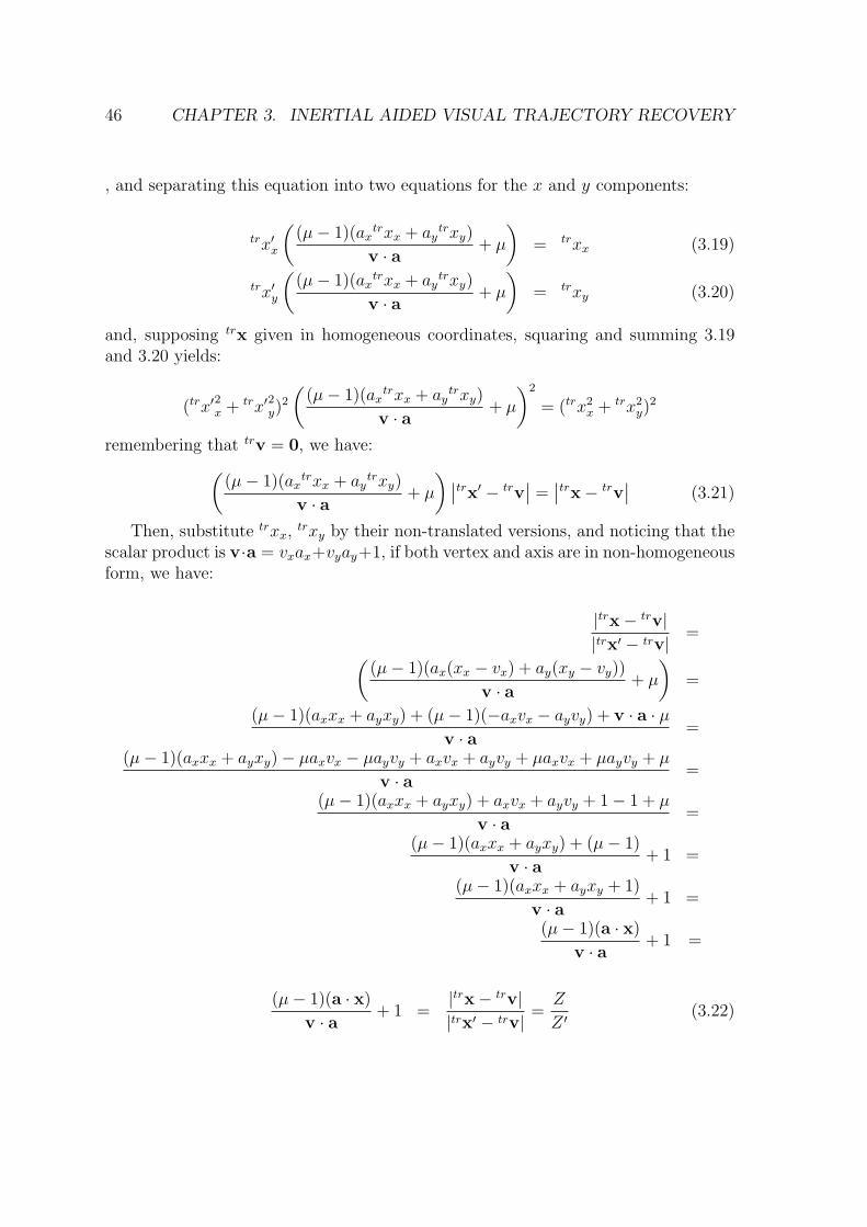
46 CHAPTER 3. INERTIAL AIDED VISUAL TRAJECTORY RECOVERY
, and separating this equation into two equations for the x and y components:
trx′x
((µ− 1)(ax
trxx + aytrxy)
v · a+ µ
)= trxx (3.19)
trx′y
((µ− 1)(ax
trxx + aytrxy)
v · a+ µ
)= trxy (3.20)
and, supposing trx given in homogeneous coordinates, squaring and summing 3.19and 3.20 yields:
(trx′2x + trx′
2y)
2
((µ− 1)(ax
trxx + aytrxy)
v · a+ µ
)2
= (trx2x + trx2
y)2
remembering that trv = 0, we have:((µ− 1)(ax
trxx + aytrxy)
v · a+ µ
) ∣∣trx′ − trv∣∣ =
∣∣trx− trv∣∣ (3.21)
Then, substitute trxx, trxy by their non-translated versions, and noticing that thescalar product is v·a = vxax+vyay+1, if both vertex and axis are in non-homogeneousform, we have:
|trx− trv||trx′ − trv|
=((µ− 1)(ax(xx − vx) + ay(xy − vy))
v · a+ µ
)=
(µ− 1)(axxx + ayxy) + (µ− 1)(−axvx − ayvy) + v · a · µv · a
=
(µ− 1)(axxx + ayxy)− µaxvx − µayvy + axvx + ayvy + µaxvx + µayvy + µ
v · a=
(µ− 1)(axxx + ayxy) + axvx + ayvy + 1− 1 + µ
v · a=
(µ− 1)(axxx + ayxy) + (µ− 1)
v · a+ 1 =
(µ− 1)(axxx + ayxy + 1)
v · a+ 1 =
(µ− 1)(a · x)
v · a+ 1 =
(µ− 1)(a · x)
v · a+ 1 =
|trx− trv||trx′ − trv|
=Z
Z ′ (3.22)
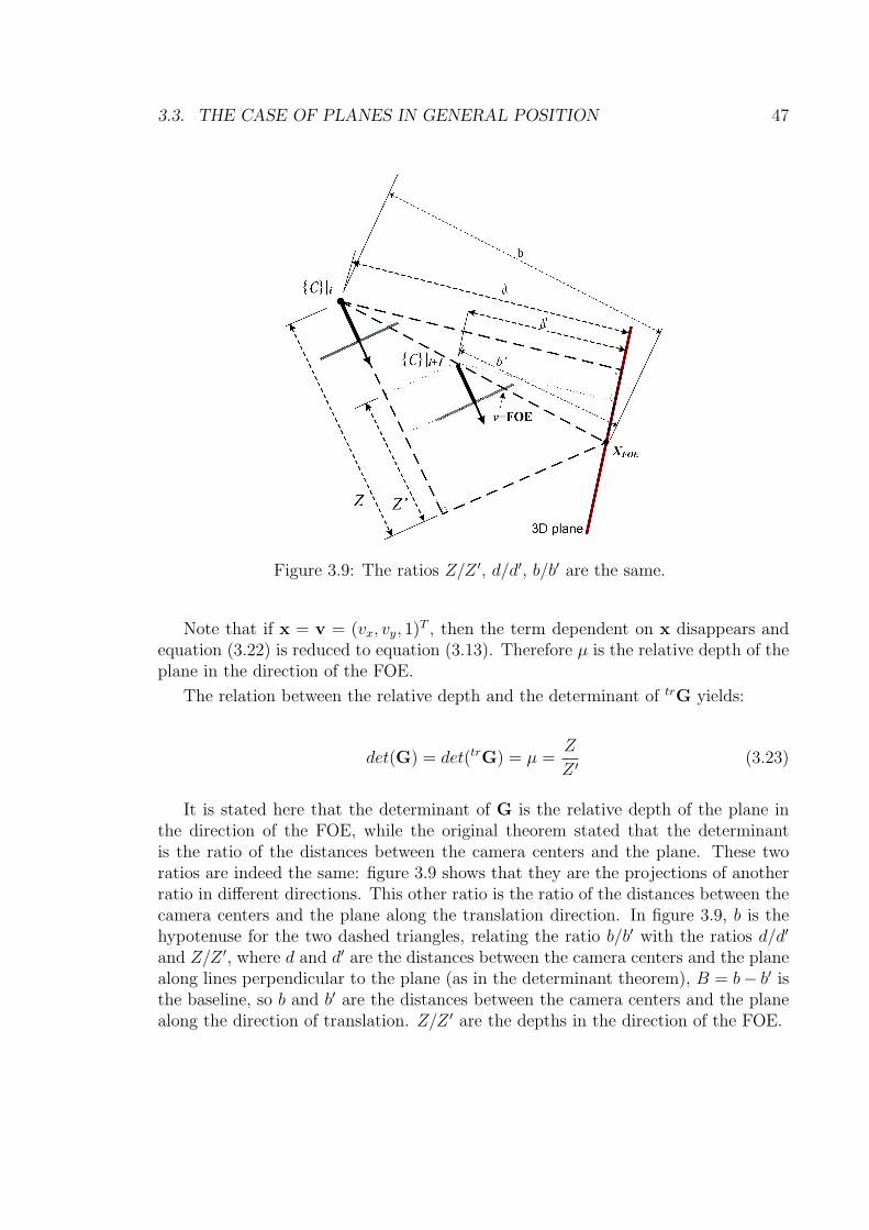
3.3. THE CASE OF PLANES IN GENERAL POSITION 47
Figure 3.9: The ratios Z/Z ′, d/d′, b/b′ are the same.
Note that if x = v = (vx, vy, 1)T , then the term dependent on x disappears andequation (3.22) is reduced to equation (3.13). Therefore µ is the relative depth of theplane in the direction of the FOE.
The relation between the relative depth and the determinant of trG yields:
det(G) = det(trG) = µ =Z
Z ′ (3.23)
It is stated here that the determinant of G is the relative depth of the plane inthe direction of the FOE, while the original theorem stated that the determinantis the ratio of the distances between the camera centers and the plane. These tworatios are indeed the same: figure 3.9 shows that they are the projections of anotherratio in different directions. This other ratio is the ratio of the distances between thecamera centers and the plane along the translation direction. In figure 3.9, b is thehypotenuse for the two dashed triangles, relating the ratio b/b′ with the ratios d/d′
and Z/Z ′, where d and d′ are the distances between the camera centers and the planealong lines perpendicular to the plane (as in the determinant theorem), B = b− b′ isthe baseline, so b and b′ are the distances between the camera centers and the planealong the direction of translation. Z/Z ′ are the depths in the direction of the FOE.
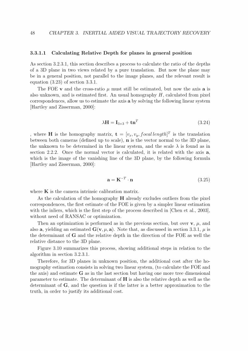
48 CHAPTER 3. INERTIAL AIDED VISUAL TRAJECTORY RECOVERY
3.3.1.1 Calculating Relative Depth for planes in general position
As section 3.2.3.1, this section describes a process to calculate the ratio of the depthsof a 3D plane in two views related by a pure translation. But now the plane maybe in a general position, not parallel to the image planes, and the relevant result isequation (3.23) of section 3.3.1.
The FOE v and the cross-ratio µ must still be estimated, but now the axis a isalso unknown, and is estimated first. An usual homography H, calculated from pixelcorrespondences, allow us to estimate the axis a by solving the following linear system[Hartley and Zisserman, 2000]:
λH = I3×3 + tnT (3.24)
, where H is the homography matrix, t = [vx, vy, focal length]T is the translationbetween both cameras (defined up to scale), n is the vector normal to the 3D plane,the unknown to be determined in the linear system, and the scale λ is found as insection 2.2.2. Once the normal vector is calculated, it is related with the axis a,which is the image of the vanishing line of the 3D plane, by the following formula[Hartley and Zisserman, 2000]:
a = K−T · n (3.25)
where K is the camera intrinsic calibration matrix.As the calculation of the homography H already excludes outliers from the pixel
correspondences, the first estimate of the FOE is given by a simpler linear estimationwith the inliers, which is the first step of the process described in [Chen et al., 2003],without need of RANSAC or optimization.
Then an optimization is performed as in the previous section, but over v, µ, andalso a, yielding an estimated G(v, µ, a). Note that, as discussed in section 3.3.1, µ isthe determinant of G and the relative depth in the direction of the FOE as well therelative distance to the 3D plane.
Figure 3.10 summarizes this process, showing additional steps in relation to thealgorithm in section 3.2.3.1.
Therefore, for 3D planes in unknown position, the additional cost after the ho-mography estimation consists in solving two linear system, (to calculate the FOE andthe axis) and estimate G as in the last section but having one more tree dimensionalparameter to estimate. The determinant of H is also the relative depth as well as thedeterminant of G, and the question is if the latter is a better approximation to thetruth, in order to justify its additional cost.
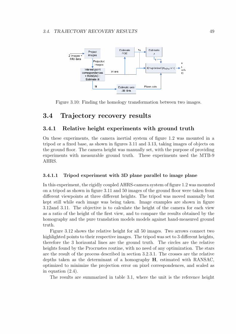
3.4. TRAJECTORY RECOVERY RESULTS 49
Figure 3.10: Finding the homology transformation between two images.
3.4 Trajectory recovery results
3.4.1 Relative height experiments with ground truth
On these experiments, the camera inertial system of figure 1.2 was mounted in atripod or a fixed base, as shown in figures 3.11 and 3.13, taking images of objects onthe ground floor. The camera height was manually set, with the purpose of providingexperiments with measurable ground truth. These experiments used the MTB-9AHRS.
3.4.1.1 Tripod experiment with 3D plane parallel to image plane
In this experiment, the rigidly coupled AHRS-camera system of figure 1.2 was mountedon a tripod as shown in figure 3.11 and 50 images of the ground floor were taken fromdifferent viewpoints at three different heights. The tripod was moved manually butkept still while each image was being taken. Image examples are shown in figure3.12and 3.11. The objective is to calculate the height of the camera for each viewas a ratio of the height of the first view, and to compare the results obtained by thehomography and the pure translation models models against hand-measured groundtruth.
Figure 3.12 shows the relative height for all 50 images. Two arrows connect twohighlighted points to their respective images. The tripod was set to 3 different heights,therefore the 3 horizontal lines are the ground truth. The circles are the relativeheights found by the Procrustes routine, with no need of any optimization. The starsare the result of the process described in section 3.2.3.1. The crosses are the relativedepths taken as the determinant of a homography H, estimated with RANSAC,optimized to minimize the projection error on pixel correspondences, and scaled asin equation (2.4).
The results are summarized in table 3.1, where the unit is the reference height
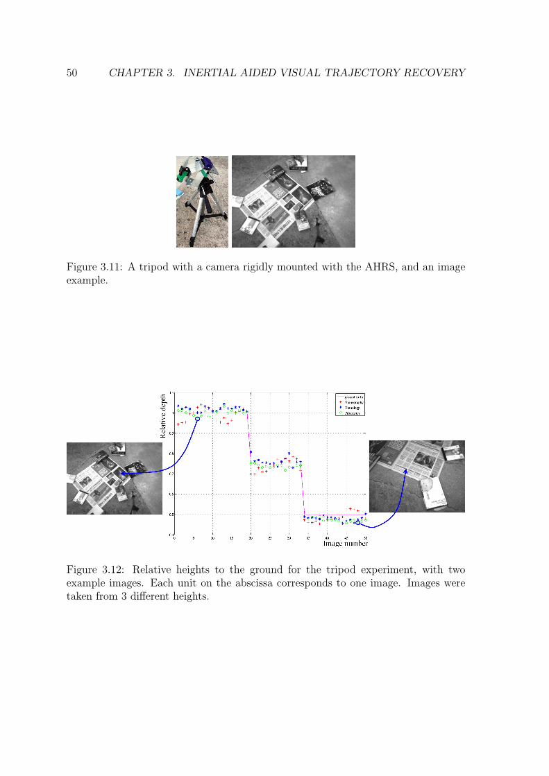
50 CHAPTER 3. INERTIAL AIDED VISUAL TRAJECTORY RECOVERY
Figure 3.11: A tripod with a camera rigidly mounted with the AHRS, and an imageexample.
Figure 3.12: Relative heights to the ground for the tripod experiment, with twoexample images. Each unit on the abscissa corresponds to one image. Images weretaken from 3 different heights.
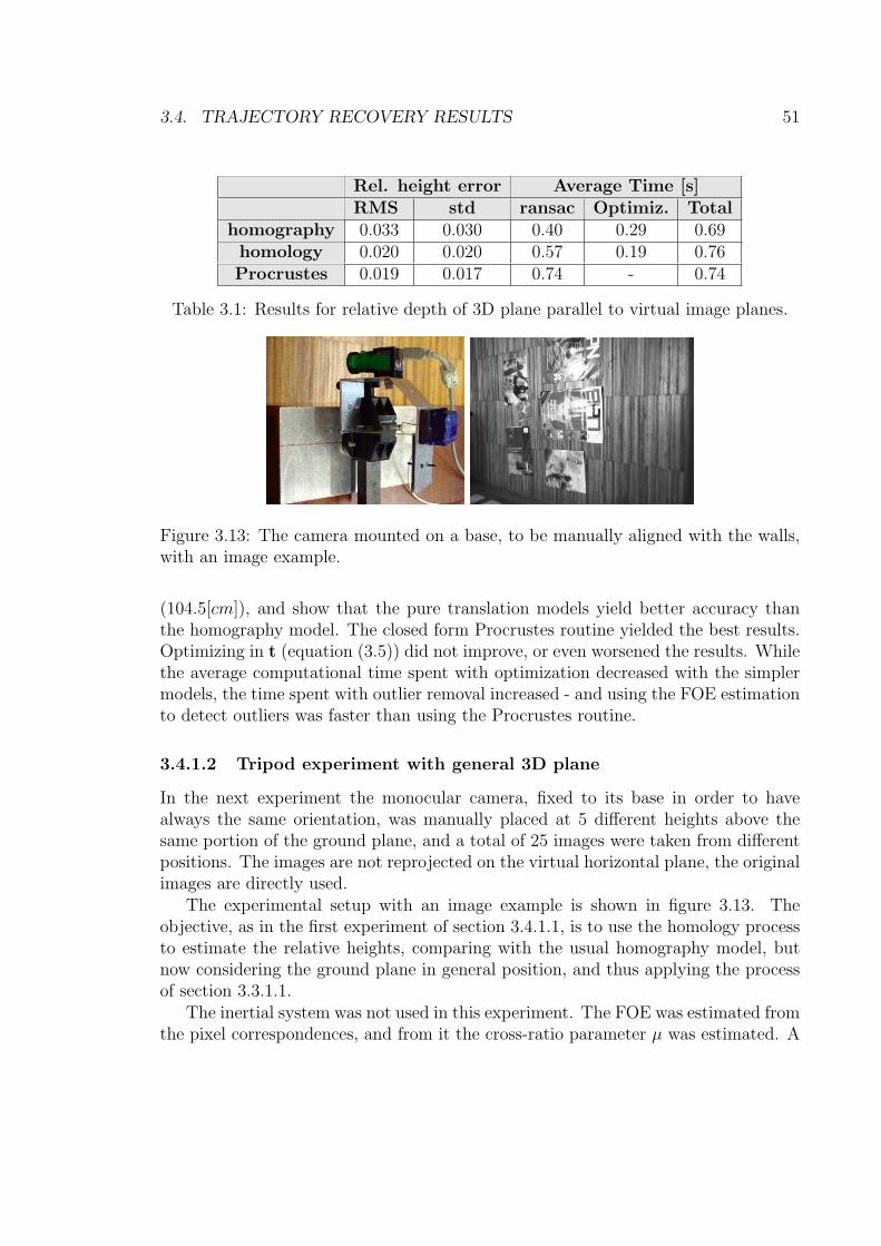
3.4. TRAJECTORY RECOVERY RESULTS 51
Rel. height error Average Time [s]RMS std ransac Optimiz. Total
homography 0.033 0.030 0.40 0.29 0.69homology 0.020 0.020 0.57 0.19 0.76Procrustes 0.019 0.017 0.74 - 0.74
Table 3.1: Results for relative depth of 3D plane parallel to virtual image planes.
Figure 3.13: The camera mounted on a base, to be manually aligned with the walls,with an image example.
(104.5[cm]), and show that the pure translation models yield better accuracy thanthe homography model. The closed form Procrustes routine yielded the best results.Optimizing in t (equation (3.5)) did not improve, or even worsened the results. Whilethe average computational time spent with optimization decreased with the simplermodels, the time spent with outlier removal increased - and using the FOE estimationto detect outliers was faster than using the Procrustes routine.
3.4.1.2 Tripod experiment with general 3D plane
In the next experiment the monocular camera, fixed to its base in order to havealways the same orientation, was manually placed at 5 different heights above thesame portion of the ground plane, and a total of 25 images were taken from differentpositions. The images are not reprojected on the virtual horizontal plane, the originalimages are directly used.
The experimental setup with an image example is shown in figure 3.13. Theobjective, as in the first experiment of section 3.4.1.1, is to use the homology processto estimate the relative heights, comparing with the usual homography model, butnow considering the ground plane in general position, and thus applying the processof section 3.3.1.1.
The inertial system was not used in this experiment. The FOE was estimated fromthe pixel correspondences, and from it the cross-ratio parameter µ was estimated. A
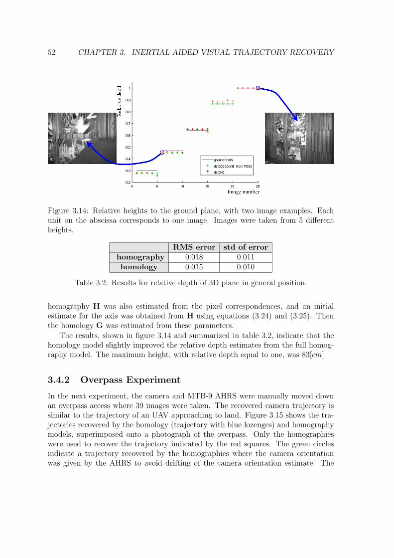
52 CHAPTER 3. INERTIAL AIDED VISUAL TRAJECTORY RECOVERY
Figure 3.14: Relative heights to the ground plane, with two image examples. Eachunit on the abscissa corresponds to one image. Images were taken from 5 differentheights.
RMS error std of errorhomography 0.018 0.011homology 0.015 0.010
Table 3.2: Results for relative depth of 3D plane in general position.
homography H was also estimated from the pixel correspondences, and an initialestimate for the axis was obtained from H using equations (3.24) and (3.25). Thenthe homology G was estimated from these parameters.
The results, shown in figure 3.14 and summarized in table 3.2, indicate that thehomology model slightly improved the relative depth estimates from the full homog-raphy model. The maximum height, with relative depth equal to one, was 83[cm]
3.4.2 Overpass Experiment
In the next experiment, the camera and MTB-9 AHRS were manually moved downan overpass access where 39 images were taken. The recovered camera trajectory issimilar to the trajectory of an UAV approaching to land. Figure 3.15 shows the tra-jectories recovered by the homology (trajectory with blue lozenges) and homographymodels, superimposed onto a photograph of the overpass. Only the homographieswere used to recover the trajectory indicated by the red squares. The green circlesindicate a trajectory recovered by the homographies where the camera orientationwas given by the AHRS to avoid drifting of the camera orientation estimate. The
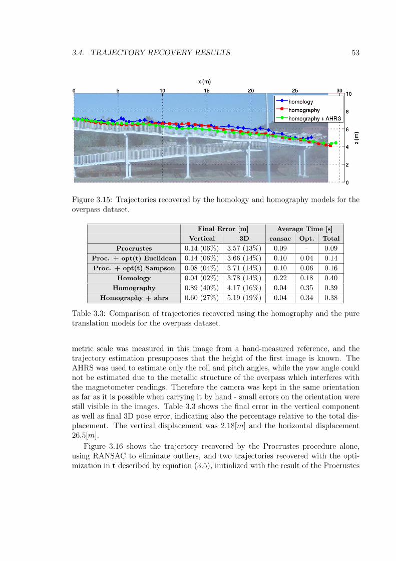
3.4. TRAJECTORY RECOVERY RESULTS 53
Figure 3.15: Trajectories recovered by the homology and homography models for theoverpass dataset.
Final Error [m] Average Time [s]Vertical 3D ransac Opt. Total
Procrustes 0.14 (06%) 3.57 (13%) 0.09 - 0.09Proc. + opt(t) Euclidean 0.14 (06%) 3.66 (14%) 0.10 0.04 0.14Proc. + opt(t) Sampson 0.08 (04%) 3.71 (14%) 0.10 0.06 0.16
Homology 0.04 (02%) 3.78 (14%) 0.22 0.18 0.40Homography 0.89 (40%) 4.17 (16%) 0.04 0.35 0.39
Homography + ahrs 0.60 (27%) 5.19 (19%) 0.04 0.34 0.38
Table 3.3: Comparison of trajectories recovered using the homography and the puretranslation models for the overpass dataset.
metric scale was measured in this image from a hand-measured reference, and thetrajectory estimation presupposes that the height of the first image is known. TheAHRS was used to estimate only the roll and pitch angles, while the yaw angle couldnot be estimated due to the metallic structure of the overpass which interferes withthe magnetometer readings. Therefore the camera was kept in the same orientationas far as it is possible when carrying it by hand - small errors on the orientation werestill visible in the images. Table 3.3 shows the final error in the vertical componentas well as final 3D pose error, indicating also the percentage relative to the total dis-placement. The vertical displacement was 2.18[m] and the horizontal displacement26.5[m].
Figure 3.16 shows the trajectory recovered by the Procrustes procedure alone,using RANSAC to eliminate outliers, and two trajectories recovered with the opti-mization in t described by equation (3.5), initialized with the result of the Procrustes

54 CHAPTER 3. INERTIAL AIDED VISUAL TRAJECTORY RECOVERY
Figure 3.16: Trajectories recovered by the Procrustes procedure for the overpassdataset, and by optimizing in t, with two distance metrics.
procedure, and using two distance metrics. For this dataset the projective modelsare not necessary, as the simpler Procrustes registration finds a good, non-iterativesolution, and even is able to remove outliers. The 10[cm] difference between the puretranslation models in the vertical displacement is not very significative.
3.4.3 Screwdriver Table Experiment
In this experiment, the camera was mounted on a moving table below the screwdriverof figure 3.17(a). The camera was fixed with its optical axis pointing approximatelydown - bubble levels were utilized to fix the camera enclosure at the right orientation.Therefore in this experiment reprojected images were not utilized, and the originalimages were always used. Although the AHRS is present, it was not utilized. Thescrewdriver moving table was moved by manually turning three mechanical screws,which allow independent movement for each axis. The objective of this experiment isto perform trajectory recovery with small errors in the camera orientation with mo-tion in a single axis, vertical or horizontal. Both cases represent extreme situations:for horizontal displacements, the direction of translation is almost parallel to the im-age plane, and the FOE is estimated as a large number (from 104 to 106 pixels in thisdataset), nevertheless the trajectory recovery proceeds normally. Large FOE coordi-nate values also can be found in the flight experiment of section 3.4.4, as the airshipmotion is often almost horizontal. On the other hand, during vertical displacementthe FOE is close to the camera principal point in the center of the image.
The screwdriver table was moved and the images used to recover its trajectoryas shown in figure 3.17(b). The horizontal (forward and lateral) displacements in-

3.4. TRAJECTORY RECOVERY RESULTS 55
Unit: [cm] forward1 forward2 lateral height2 height3ground truth 15.9 15.9 8.5 99.6 109.6
homology 16.4 15.9 7.9 100.1 110.5homology filtered 16.4 15.8 8.0 100.1 110.5
homography 15.4 13.6 9.1 98.8 108.1homography scaled 15.4 13.5 9.4 99.2 108.8by homology height
Table 3.4: Comparison of displacements recovered using the homography and homol-ogy models for the screwdriver table dataset. All displacements are given in [cm].
dicated in figures 3.18(a) and 3.18(b) are the maximum displacements allowed bythe mechanical devices, and were measured with metric tape. After each verticaldisplacement of the camera, its height in relation to the ground plane was also handmeasured. Therefore the distances indicated in figures 3.18(a) and 3.18(b) can becompared against ground truth as it is shown in table 3.4. One image was takenevery 0.6[s], including the moments when the camera was not moving, e.g. when itsheight was being measured. The initial height was also measured and it was 85.6[cm].Figure 3.17(a) also presents an example image.
3.4.4 Trajectory recovery for aerial vehicles with the MTB-9AHRS
This experiment uses images taken by the remotely controlled airship of figure 1.2,carrying the AHRS-camera system with the MTB-9 AHRS and a GPS receiver, flyingabove a planar area next to the Coimbra Aerodrome. The image frame rate is 2fps.
3.4.4.1 Visual Odometry: Heights For a UAV
The GPS measured height is shown in figure 3.19 compared against visual odometrybased on the µ value of homologies calculated for the sequence of images using theprocess described in section 3.2.3.1.
For the first image the height is visually guessed and manually set as h1 = 4[m],
and for the ith image the height is hi =
(i−1∏j=1
j+1µj
)· h1, where j+1µj represents the
cross-ratio parameter for the homology that transforms the jth image into the imagej+1. For a few image pairs the homology could not be calculated due to corrupted ormissing images, or because too few interest points were matched. In this case the lastvalid µ value is assumed to be the current one. Except by that, no other attempt was

56 CHAPTER 3. INERTIAL AIDED VISUAL TRAJECTORY RECOVERY
(a) (b)
Figure 3.17: The screwdriver with its moving table and one example image (a) andthe recovered 3D camera trajectories (b).
(a)
(b)
Figure 3.18: Two views of the recovered trajectories with highlighted displacements.
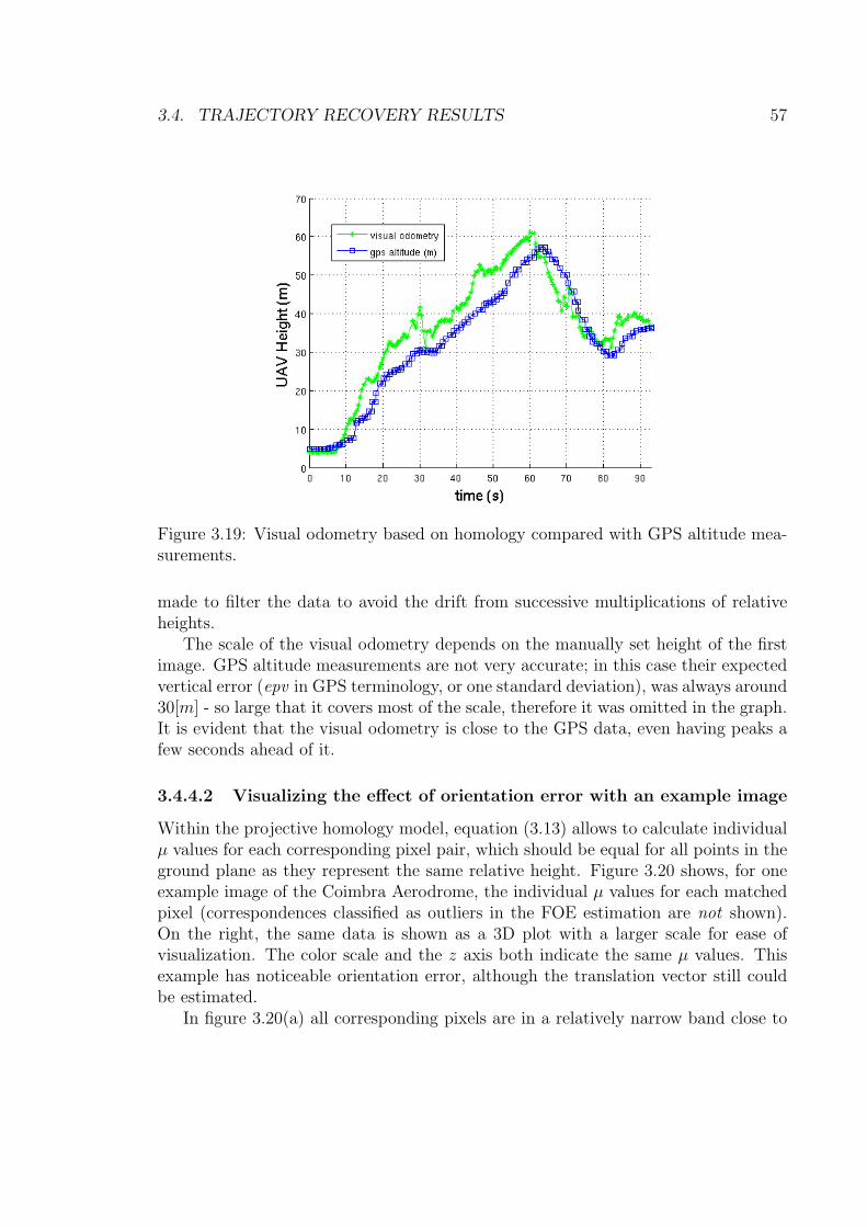
3.4. TRAJECTORY RECOVERY RESULTS 57
Figure 3.19: Visual odometry based on homology compared with GPS altitude mea-surements.
made to filter the data to avoid the drift from successive multiplications of relativeheights.
The scale of the visual odometry depends on the manually set height of the firstimage. GPS altitude measurements are not very accurate; in this case their expectedvertical error (epv in GPS terminology, or one standard deviation), was always around30[m] - so large that it covers most of the scale, therefore it was omitted in the graph.It is evident that the visual odometry is close to the GPS data, even having peaks afew seconds ahead of it.
3.4.4.2 Visualizing the effect of orientation error with an example image
Within the projective homology model, equation (3.13) allows to calculate individualµ values for each corresponding pixel pair, which should be equal for all points in theground plane as they represent the same relative height. Figure 3.20 shows, for oneexample image of the Coimbra Aerodrome, the individual µ values for each matchedpixel (correspondences classified as outliers in the FOE estimation are not shown).On the right, the same data is shown as a 3D plot with a larger scale for ease ofvisualization. The color scale and the z axis both indicate the same µ values. Thisexample has noticeable orientation error, although the translation vector still couldbe estimated.
In figure 3.20(a) all corresponding pixels are in a relatively narrow band close to
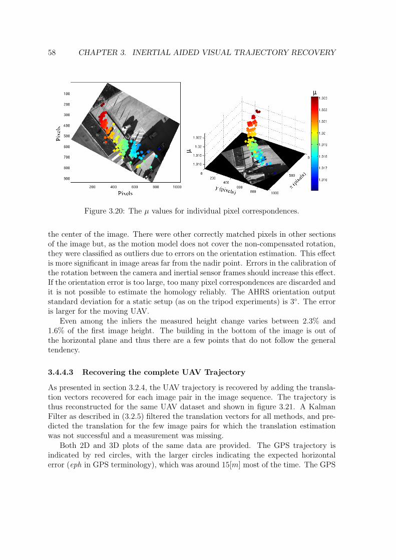
58 CHAPTER 3. INERTIAL AIDED VISUAL TRAJECTORY RECOVERY
Figure 3.20: The µ values for individual pixel correspondences.
the center of the image. There were other correctly matched pixels in other sectionsof the image but, as the motion model does not cover the non-compensated rotation,they were classified as outliers due to errors on the orientation estimation. This effectis more significant in image areas far from the nadir point. Errors in the calibration ofthe rotation between the camera and inertial sensor frames should increase this effect.If the orientation error is too large, too many pixel correspondences are discarded andit is not possible to estimate the homology reliably. The AHRS orientation outputstandard deviation for a static setup (as on the tripod experiments) is 3◦. The erroris larger for the moving UAV.
Even among the inliers the measured height change varies between 2.3% and1.6% of the first image height. The building in the bottom of the image is out ofthe horizontal plane and thus there are a few points that do not follow the generaltendency.
3.4.4.3 Recovering the complete UAV Trajectory
As presented in section 3.2.4, the UAV trajectory is recovered by adding the transla-tion vectors recovered for each image pair in the image sequence. The trajectory isthus reconstructed for the same UAV dataset and shown in figure 3.21. A KalmanFilter as described in (3.2.5) filtered the translation vectors for all methods, and pre-dicted the translation for the few image pairs for which the translation estimationwas not successful and a measurement was missing.
Both 2D and 3D plots of the same data are provided. The GPS trajectory isindicated by red circles, with the larger circles indicating the expected horizontalerror (eph in GPS terminology), which was around 15[m] most of the time. The GPS
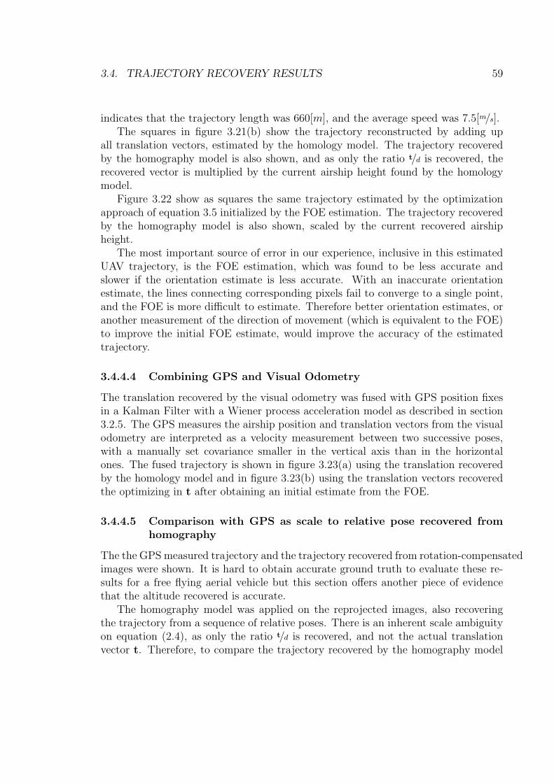
3.4. TRAJECTORY RECOVERY RESULTS 59
indicates that the trajectory length was 660[m], and the average speed was 7.5[m/s].The squares in figure 3.21(b) show the trajectory reconstructed by adding up
all translation vectors, estimated by the homology model. The trajectory recoveredby the homography model is also shown, and as only the ratio t/d is recovered, therecovered vector is multiplied by the current airship height found by the homologymodel.
Figure 3.22 show as squares the same trajectory estimated by the optimizationapproach of equation 3.5 initialized by the FOE estimation. The trajectory recoveredby the homography model is also shown, scaled by the current recovered airshipheight.
The most important source of error in our experience, inclusive in this estimatedUAV trajectory, is the FOE estimation, which was found to be less accurate andslower if the orientation estimate is less accurate. With an inaccurate orientationestimate, the lines connecting corresponding pixels fail to converge to a single point,and the FOE is more difficult to estimate. Therefore better orientation estimates, oranother measurement of the direction of movement (which is equivalent to the FOE)to improve the initial FOE estimate, would improve the accuracy of the estimatedtrajectory.
3.4.4.4 Combining GPS and Visual Odometry
The translation recovered by the visual odometry was fused with GPS position fixesin a Kalman Filter with a Wiener process acceleration model as described in section3.2.5. The GPS measures the airship position and translation vectors from the visualodometry are interpreted as a velocity measurement between two successive poses,with a manually set covariance smaller in the vertical axis than in the horizontalones. The fused trajectory is shown in figure 3.23(a) using the translation recoveredby the homology model and in figure 3.23(b) using the translation vectors recoveredthe optimizing in t after obtaining an initial estimate from the FOE.
3.4.4.5 Comparison with GPS as scale to relative pose recovered fromhomography
The the GPS measured trajectory and the trajectory recovered from rotation-compensatedimages were shown. It is hard to obtain accurate ground truth to evaluate these re-sults for a free flying aerial vehicle but this section offers another piece of evidencethat the altitude recovered is accurate.
The homography model was applied on the reprojected images, also recoveringthe trajectory from a sequence of relative poses. There is an inherent scale ambiguityon equation (2.4), as only the ratio t/d is recovered, and not the actual translationvector t. Therefore, to compare the trajectory recovered by the homography model
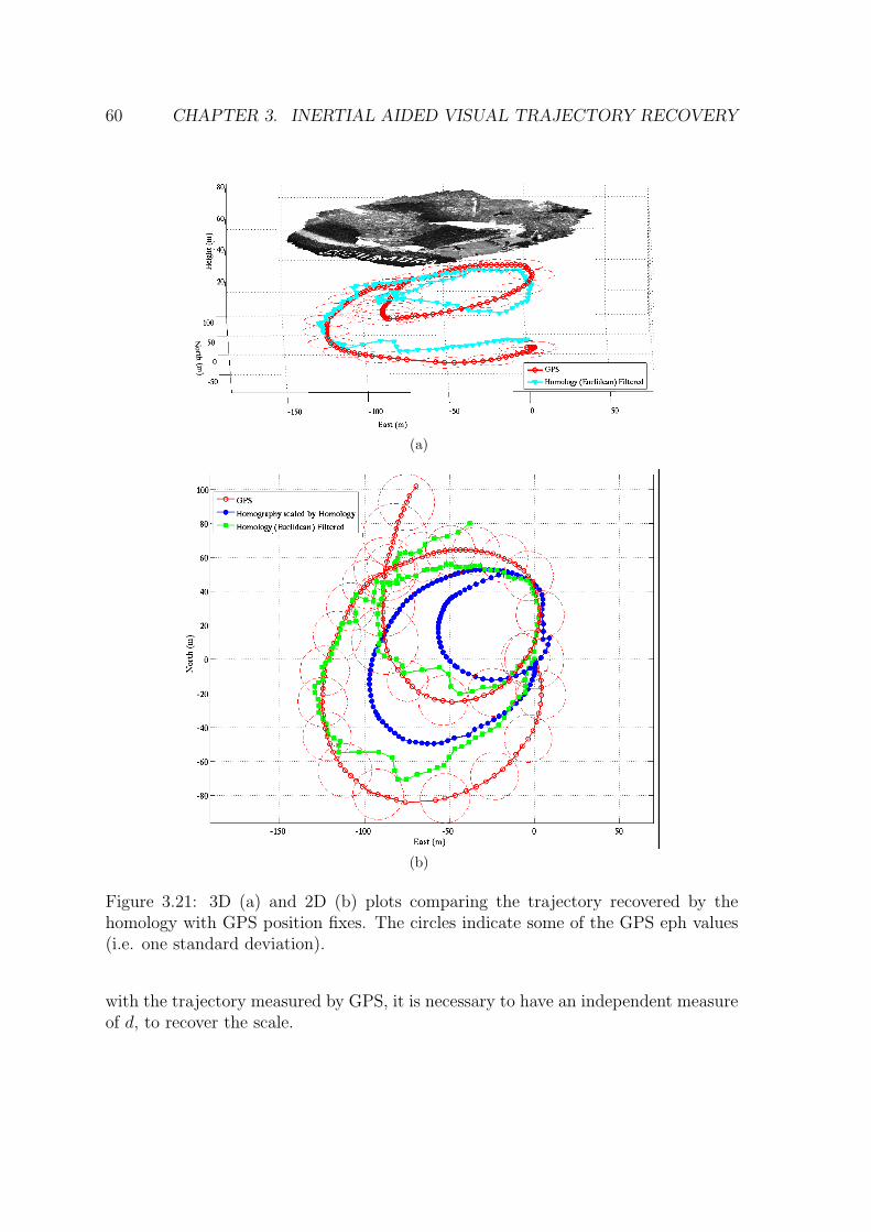
60 CHAPTER 3. INERTIAL AIDED VISUAL TRAJECTORY RECOVERY
(a)
(b)
Figure 3.21: 3D (a) and 2D (b) plots comparing the trajectory recovered by thehomology with GPS position fixes. The circles indicate some of the GPS eph values(i.e. one standard deviation).
with the trajectory measured by GPS, it is necessary to have an independent measureof d, to recover the scale.
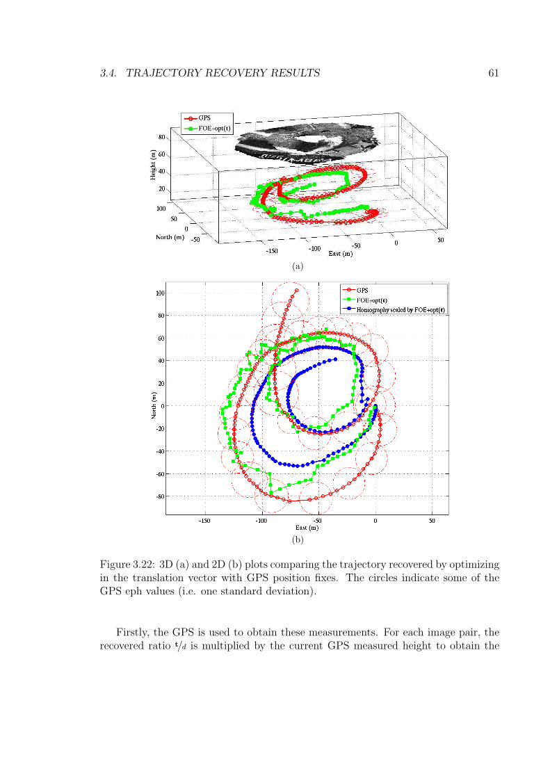
3.4. TRAJECTORY RECOVERY RESULTS 61
(a)
(b)
Figure 3.22: 3D (a) and 2D (b) plots comparing the trajectory recovered by optimizingin the translation vector with GPS position fixes. The circles indicate some of theGPS eph values (i.e. one standard deviation).
Firstly, the GPS is used to obtain these measurements. For each image pair, therecovered ratio t/d is multiplied by the current GPS measured height to obtain the
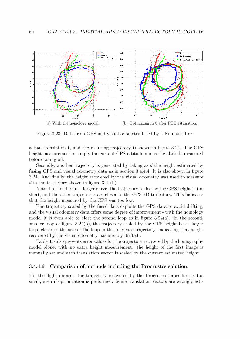
62 CHAPTER 3. INERTIAL AIDED VISUAL TRAJECTORY RECOVERY
(a) With the homology model. (b) Optimizing in t after FOE estimation.
Figure 3.23: Data from GPS and visual odometry fused by a Kalman filter.
actual translation t, and the resulting trajectory is shown in figure 3.24. The GPSheight measurement is simply the current GPS altitude minus the altitude measuredbefore taking off.
Secondly, another trajectory is generated by taking as d the height estimated byfusing GPS and visual odometry data as in section 3.4.4.4. It is also shown in figure3.24. And finally, the height recovered by the visual odometry was used to measured in the trajectory shown in figure 3.21(b).
Note that for the first, larger curve, the trajectory scaled by the GPS height is tooshort, and the other trajectories are closer to the GPS 2D trajectory. This indicatesthat the height measured by the GPS was too low.
The trajectory scaled by the fused data exploits the GPS data to avoid drifting,and the visual odometry data offers some degree of improvement - with the homologymodel it is even able to close the second loop as in figure 3.24(a). In the second,smaller loop of figure 3.24(b), the trajectory scaled by the GPS height has a largerloop, closer to the size of the loop in the reference trajectory, indicating that heightrecovered by the visual odometry has already drifted .
Table 3.5 also presents error values for the trajectory recovered by the homographymodel alone, with no extra height measurement: the height of the first image ismanually set and each translation vector is scaled by the current estimated height.
3.4.4.6 Comparison of methods including the Procrustes solution.
For the flight dataset, the trajectory recovered by the Procrustes procedure is toosmall, even if optimization is performed. Some translation vectors are wrongly esti-
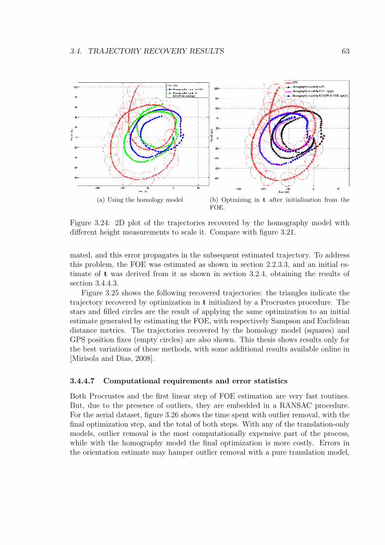
3.4. TRAJECTORY RECOVERY RESULTS 63
(a) Using the homology model (b) Optmizing in t after initialization from theFOE.
Figure 3.24: 2D plot of the trajectories recovered by the homography model withdifferent height measurements to scale it. Compare with figure 3.21.
mated, and this error propagates in the subsequent estimated trajectory. To addressthis problem, the FOE was estimated as shown in section 2.2.3.3, and an initial es-timate of t was derived from it as shown in section 3.2.4, obtaining the results ofsection 3.4.4.3.
Figure 3.25 shows the following recovered trajectories: the triangles indicate thetrajectory recovered by optimization in t initialized by a Procrustes procedure. Thestars and filled circles are the result of applying the same optimization to an initialestimate generated by estimating the FOE, with respectively Sampson and Euclideandistance metrics. The trajectories recovered by the homology model (squares) andGPS position fixes (empty circles) are also shown. This thesis shows results only forthe best variations of these methods, with some additional results available online in[Mirisola and Dias, 2008].
3.4.4.7 Computational requirements and error statistics
Both Procrustes and the first linear step of FOE estimation are very fast routines.But, due to the presence of outliers, they are embedded in a RANSAC procedure.For the aerial dataset, figure 3.26 shows the time spent with outlier removal, with thefinal optimization step, and the total of both steps. With any of the translation-onlymodels, outlier removal is the most computationally expensive part of the process,while with the homography model the final optimization is more costly. Errors inthe orientation estimate may hamper outlier removal with a pure translation model,
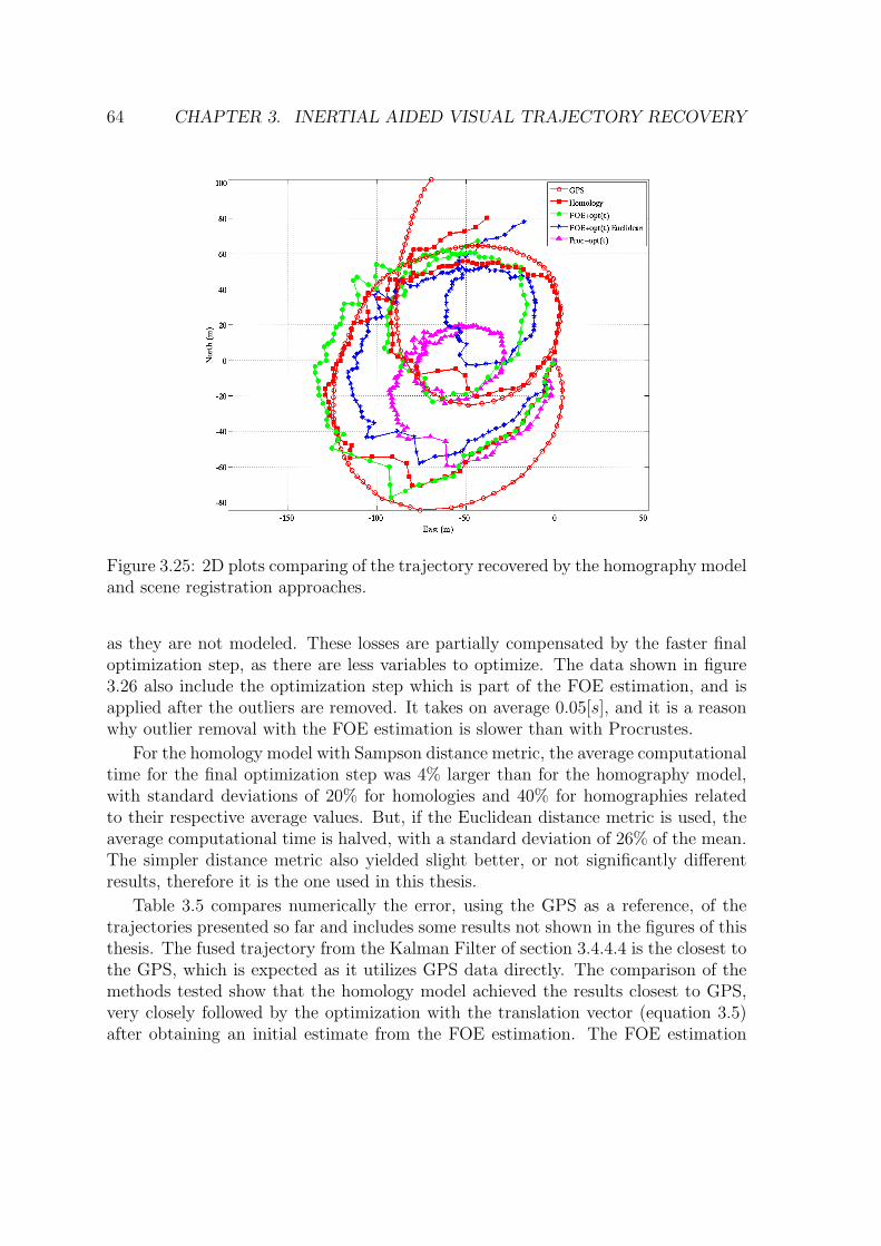
64 CHAPTER 3. INERTIAL AIDED VISUAL TRAJECTORY RECOVERY
Figure 3.25: 2D plots comparing of the trajectory recovered by the homography modeland scene registration approaches.
as they are not modeled. These losses are partially compensated by the faster finaloptimization step, as there are less variables to optimize. The data shown in figure3.26 also include the optimization step which is part of the FOE estimation, and isapplied after the outliers are removed. It takes on average 0.05[s], and it is a reasonwhy outlier removal with the FOE estimation is slower than with Procrustes.
For the homology model with Sampson distance metric, the average computationaltime for the final optimization step was 4% larger than for the homography model,with standard deviations of 20% for homologies and 40% for homographies relatedto their respective average values. But, if the Euclidean distance metric is used, theaverage computational time is halved, with a standard deviation of 26% of the mean.The simpler distance metric also yielded slight better, or not significantly differentresults, therefore it is the one used in this thesis.
Table 3.5 compares numerically the error, using the GPS as a reference, of thetrajectories presented so far and includes some results not shown in the figures of thisthesis. The fused trajectory from the Kalman Filter of section 3.4.4.4 is the closest tothe GPS, which is expected as it utilizes GPS data directly. The comparison of themethods tested show that the homology model achieved the results closest to GPS,very closely followed by the optimization with the translation vector (equation 3.5)after obtaining an initial estimate from the FOE estimation. The FOE estimation

3.4. TRAJECTORY RECOVERY RESULTS 65
Figure 3.26: Comparison of average computation time per frame for some of methodstested. All experiments in this chapter were executed in a Pentium D 3.2 [GHz].
was better than the Procrustes routine to find an initial estimate of t.
Different height measurements were used to scale the translation recovered by thehomography, including GPS data, the height component of the trajectory recoveredby the pure translation models, and the result of the Kalman Filter fusing both visualodometry and GPS. The visual odometry achieved better results than GPS, indicatinga more accurate height estimate in the fused trajectory. With the homology model,the result of the Kalman filter was better than either GPS or visual odometry aloneto scale the trajectory recovered by the homography model.
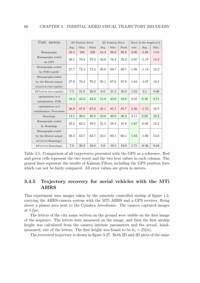
66 CHAPTER 3. INERTIAL AIDED VISUAL TRAJECTORY RECOVERY
Unit: meters 3D Position Error 2D Position Error Error in the length of t
Avg. Max. Final Avg. Max. Final rms Avg. Max.
Homography 48.5 100 100 44.3 98.6 98.6 3.00 -2.68 14.6Homography scaled
by GPS38.5 79.3 79.3 33.0 76.2 76.2 2.07 -1.19 14.3
Homography scaled
by FOE+opt(t)27.7 72.4 72.4 20.0 69.7 69.7 1.88 -1.14 13.2
Homography scaled
by the filtered output
kf(gps & foe+opt(t))
27.9 70.2 70.2 20.1 67.0 67.0 1.84 -1.07 13.2
KF(gps & foe+opt(t)) 7.5 21.6 20.0 6.0 21.5 20.0 1.62 0.1 8.06optimization in t
initialization: FOE16.4 43.3 43.3 15.8 43.0 43.0 2.03 0.16 8.71
optimization in t
initialization: Procrustes38.9 87.0 87.0 35.1 85.7 85.7 2.56 -1.73 10.5
Homology 12.1 39.8 38.9 10.6 39.0 38.2 2.11 0.09 10.3Homography scaled
by Homology35.2 62.5 49.5 31.5 58.2 45.8 1.67 -0.66 12.2
Homography scaled
by the filtered output
kf(gps & Homology)
30.3 63.7 63.7 24.1 60.1 60.1 1.83 -1.00 13.8
KF(gps & Homology) 7.0 20.3 19.6 5.0 19.5 19.0 1.71 -0.36 8.04
Table 3.5: Comparison of all trajectories presented with the GPS as a reference. Redand green cells represent the two worst and the two best values in each column. Thegrayed lines represent the results of Kalman Filters including the GPS position fixeswhich can not be fairly compared. All error values are given in meters.
3.4.5 Trajectory recovery for aerial vehicles with the MTiAHRS
This experiment uses images taken by the remotely controlled airship of figure 1.2,carrying the AHRS-camera system with the MTi AHRS and a GPS receiver, flyingabove a planar area next to the Coimbra Aerodrome. The camera captured imagesat 5 fps.
The letters of the city name written on the ground were visible on the first imageof the sequence. The letters were measured on the image, and then the first airshipheight was calculated from the camera intrinsic parameters and the actual, hand-measured, size of the letters. The first height was found to be h1 = 25[m].
The recovered trajectory is shown in figure 3.27. Both 2D and 3D plots of the same

3.4. TRAJECTORY RECOVERY RESULTS 67
data are provided. The GPS trajectory is indicated by small circles, with larger circlesindicating the GPS eph, which was around 8[m] in the horizontal axes and 15[m] in thevertical axis. The GPS indicates a trajectory length of 543[m], and average speed of9[m/s]. A Kalman Filter with a constant acceleration model [Bar-Shalom et al., 2001]filtered the translation vectors for all methods, and predicted the translation forthe few image pairs for which the translation estimation was not successful and ameasurement was missing.
The squares in figure 3.27 show the trajectory reconstructed by adding up alltranslation vectors, estimated by the optimization approach of equation 3.5 initializedby Procrustes. The recovered trajectory is very close to the one recovered by theProcrustes procedure alone, indicated by crosses. The trajectory recovered by thehomography model using only the images is also indicated with stars. As only theratio t/d is recovered by the homographies, the scale is recovered by multiplying therecovered vector by the current recovered airship height. Tables 3.6 and 3.7 show theerrors in the visual odometry, taking the GPS as a reference, and the execution times.
Unit: meters 3D Position Error 2D Position Error Error in the length of t
Avg. Max. Final Avg. Max. Final rms Avg. Max.
Homography 57.5 98.2 52.3 43.1 67.6 52.0 0.88 -0.63 1.24Visual Odometry:
Procrustes only16.5 43.6 43.6 15.3 43.3 43.3 0.73 -0.46 0.59
Visual Odometry:
optimization in t
initialization: Procrustes
16.0 41.6 41.6 14.9 41.3 41.3 0.70 -0.45 0.59
Table 3.6: Comparison of visual odometry with the GPS reference. All error valuesare given in meters.
Unit: seconds RANSAC Optimization Total
Avg. std. Avg. std.
Homography 0.05 0.02 0.43 0.19 0.48Visual Odometry:
Procrustes only0.18 0.08 - - 0.18
Visual Odometry:
optimization in t
initialization: Procrustes
0.18 0.08 0.18 0.10 0.36
Table 3.7: Comparison of the execution time of visual odometry techniques.
Another image sequence with a recovered trajectory is shown in figure 3.28. Theimages are reprojected on the ground plane forming a map by using equation (3.4) to
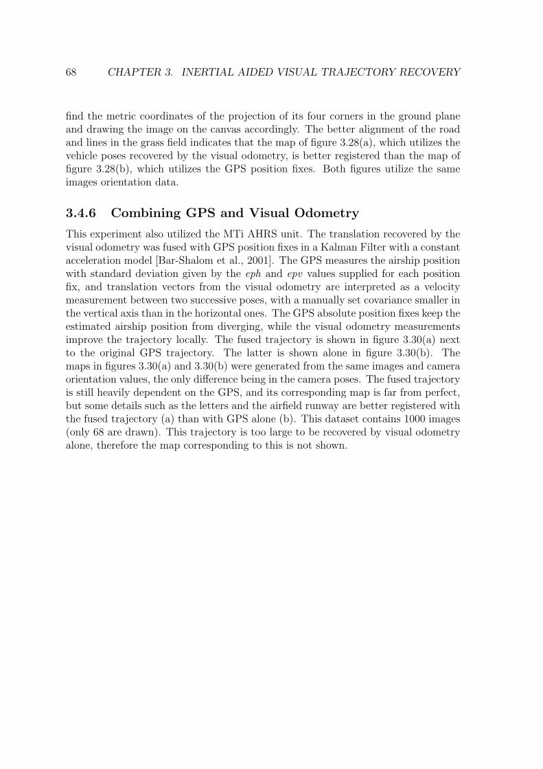
68 CHAPTER 3. INERTIAL AIDED VISUAL TRAJECTORY RECOVERY
find the metric coordinates of the projection of its four corners in the ground planeand drawing the image on the canvas accordingly. The better alignment of the roadand lines in the grass field indicates that the map of figure 3.28(a), which utilizes thevehicle poses recovered by the visual odometry, is better registered than the map offigure 3.28(b), which utilizes the GPS position fixes. Both figures utilize the sameimages orientation data.
3.4.6 Combining GPS and Visual OdometryThis experiment also utilized the MTi AHRS unit. The translation recovered by thevisual odometry was fused with GPS position fixes in a Kalman Filter with a constantacceleration model [Bar-Shalom et al., 2001]. The GPS measures the airship positionwith standard deviation given by the eph and epv values supplied for each positionfix, and translation vectors from the visual odometry are interpreted as a velocitymeasurement between two successive poses, with a manually set covariance smaller inthe vertical axis than in the horizontal ones. The GPS absolute position fixes keep theestimated airship position from diverging, while the visual odometry measurementsimprove the trajectory locally. The fused trajectory is shown in figure 3.30(a) nextto the original GPS trajectory. The latter is shown alone in figure 3.30(b). Themaps in figures 3.30(a) and 3.30(b) were generated from the same images and cameraorientation values, the only difference being in the camera poses. The fused trajectoryis still heavily dependent on the GPS, and its corresponding map is far from perfect,but some details such as the letters and the airfield runway are better registered withthe fused trajectory (a) than with GPS alone (b). This dataset contains 1000 images(only 68 are drawn). This trajectory is too large to be recovered by visual odometryalone, therefore the map corresponding to this is not shown.

3.4. TRAJECTORY RECOVERY RESULTS 69
(a)
(b)
Figure 3.27: 3D (a) and 2D (b) plots comparing visual odometry with GPS positionfixes. The circles indicate some of the GPS eph values (i.e. one standard deviation).
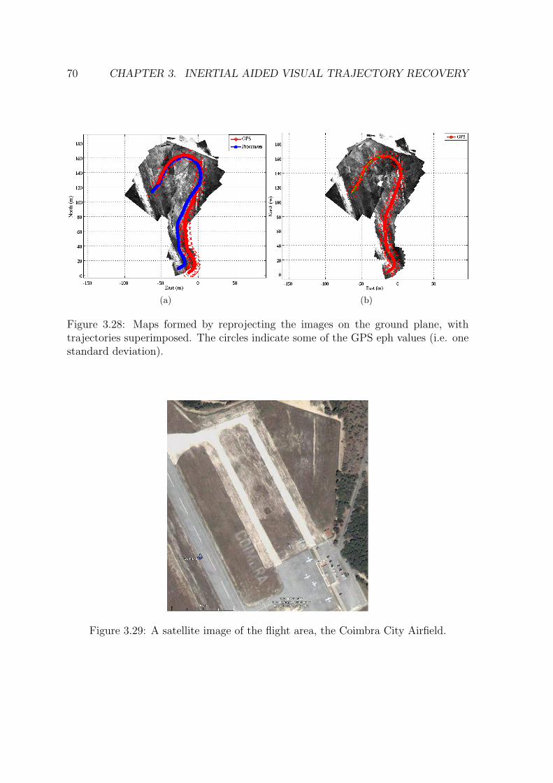
70 CHAPTER 3. INERTIAL AIDED VISUAL TRAJECTORY RECOVERY
(a) (b)
Figure 3.28: Maps formed by reprojecting the images on the ground plane, withtrajectories superimposed. The circles indicate some of the GPS eph values (i.e. onestandard deviation).
Figure 3.29: A satellite image of the flight area, the Coimbra City Airfield.
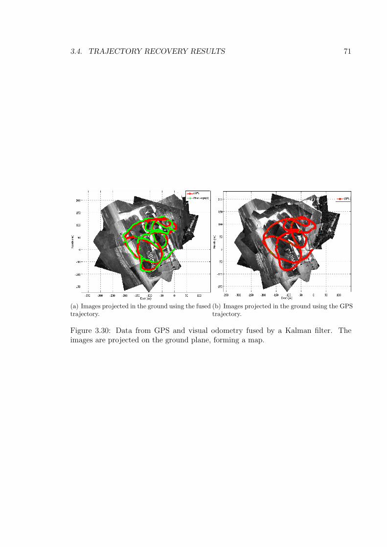
3.4. TRAJECTORY RECOVERY RESULTS 71
(a) Images projected in the ground using the fusedtrajectory.
(b) Images projected in the ground using the GPStrajectory.
Figure 3.30: Data from GPS and visual odometry fused by a Kalman filter. Theimages are projected on the ground plane, forming a map.

72 CHAPTER 3. INERTIAL AIDED VISUAL TRAJECTORY RECOVERY

Chapter 4
Inertial Aided Visual Mapping
4.1 IntroductionThe reprojection on the virtual horizontal plane introduced in section 2.7 and detailedin section 3.2.1 can be applied in other domains besides trajectory recovery. Thischapter considers other problems such as Image Mosaicing, Plane Segmentation and3D Mapping from a monocular camera image sequence and registration of point cloudstaken from a stereo camera or LRF.
4.2 Image Mosaicing
Building small mosaicsAll images are reprojected on the virtual horizontal plane as presented in sections 2.7and 3.2.1. These images of the virtual downwards camera are denoted by IDi . Interestpoint matching is used to establish point correspondences between each image IDiand an arbitrarily chosen reference image IDB. Wrong correspondences will appear asoutliers, that are detected by RANSAC, using the homography model.
In the sequence of images, the interest point matching algorithm tries to match thereference image IDB with the images following and preceding it until the image match isnot good enough, therefore delimiting an image sequence denoted by {ID1 . . . IDB . . . IDn }.
For an image match to be considered “good enough”, two conditions must besatisfied:
1. There must be a minimum number of corresponding pixel pairs, after excludingoutliers. (A minimum 20 pixel correspondences in this work);
2. The area covered by the corresponding pixels in the image must be large. Thisis relevant because the homography calculation is better conditioned when dif-
73

74 CHAPTER 4. INERTIAL AIDED VISUAL MAPPING
Figure 4.1: Example of mosaic constructed from successive images.
ferent portions of the image are constrained [Hartley and Zisserman, 2000]. Inthis work the area of the convex hull of all corresponding pixels must be largerthan 20% of the image area, in both images.
If any of these two conditions do not hold, the pair of images is considered badlymatched, the image sequence also stops.
Then for each image IDi , a homography BHi is calculated to register the image IDito the reference image IDB, and then the images are drawn together. Figure 4.1 showsan example of a mosaic built from a sequence of successive image frames.
It might be asked why the reprojected images were registered using homographiesinstead of homologies as used in chapter 3. Certainly homologies can be estimated,as it is done with the same kind of dataset in the tripod experiments of section 3.4.1,but the remaining uncompensated rotation is still significant enough to cause visiblemisalignments on an image pair when drawn together. It is still necessary to estimatehomographies with the reprojected images to obtain visually clean small mosaics.
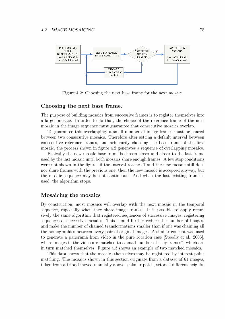
4.2. IMAGE MOSAICING 75
Figure 4.2: Choosing the next base frame for the next mosaic.
Choosing the next base frame.
The purpose of building mosaics from successive frames is to register themselves intoa larger mosaic. In order to do that, the choice of the reference frame of the nextmosaic in the image sequence must guarantee that consecutive mosaics overlap.
To guarantee this overlapping, a small number of image frames must be sharedbetween two consecutive mosaics. Therefore after setting a default interval betweenconsecutive reference frames, and arbitrarily choosing the base frame of the firstmosaic, the process shown in figure 4.2 generates a sequence of overlapping mosaics.
Basically the new mosaic base frame is chosen closer and closer to the last frameused by the last mosaic until both mosaics share enough frames. A few stop conditionswere not shown in the figure: if the interval reaches 1 and the new mosaic still doesnot share frames with the previous one, then the new mosaic is accepted anyway, butthe mosaic sequence may be not continuous. And when the last existing frame isused, the algorithm stops.
Mosaicing the mosaics
By construction, most mosaics will overlap with the next mosaic in the temporalsequence, especially when they share image frames. It is possible to apply recur-sively the same algorithm that registered sequences of successive images, registeringsequences of successive mosaics. This should further reduce the number of images,and make the number of chained transformations smaller than if one was chaining allthe homographies between every pair of original images. A similar concept was usedto generate a panorama from video in the pure rotation case [Steedly et al., 2005],where images in the video are matched to a small number of “key frames”, which arein turn matched themselves. Figure 4.3 shows an example of two matched mosaics.
This data shows that the mosaics themselves may be registered by interest pointmatching. The mosaics shown in this section originate from a dataset of 61 images,taken from a tripod moved manually above a planar patch, set at 2 different heights.
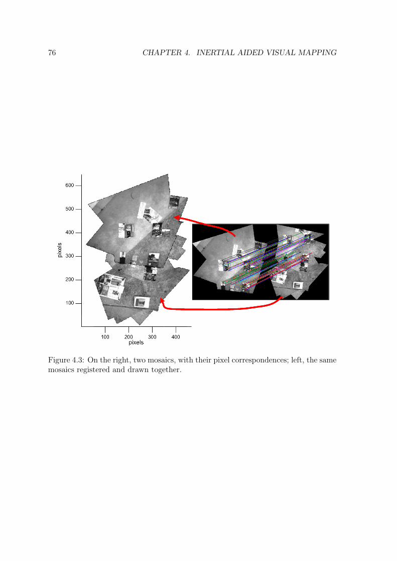
76 CHAPTER 4. INERTIAL AIDED VISUAL MAPPING
Figure 4.3: On the right, two mosaics, with their pixel correspondences; left, the samemosaics registered and drawn together.
4.2. IMAGE MOSAICING 77
This sequence generated 20 mosaics built from successive pairs of images. Then, asecond run over them generated 4 larger mosaics. A final run generated the mosaicof fig. 4.4. A feathering process was applied to smooth image transitions on the laststep, and this implied on some ghosting in the books in the middle.
The mosaic of figure 4.4 was obtained without deghosting and bundle adjustment,which usually must be applied to image-only mosaicing of this size[Szeliski, 2004, Capel, 2001]. These techniques still could be used to register largerdatasets. Also, some recent results in mosaicing suppose a rotation-only model (e.g[Brown and Lowe, 2003, Szeliski, 2004]), where the camera center is the same for allimages. But here the camera is freely translating and rotating.
For comparison, the same interest point matching algorithms were applied tosuccessive frames in the original image sequence as well as in the sequence reprojectedinto the virtual horizontal plane. The reprojection error (root mean square) on pixelcorrespondences was 20% less on the reprojected images.
The ratio of correct matches versus total number of interest points detected is bet-ter with images taken from the same viewpoint, therefore the algorithm parametersmay be tuned to detect less features, while keeping the same number of correct pixelcorrespondences. Therefore, interest point matching is faster (less features means lessdescriptor computation and faster matching) or more robust (more correct matcheswith the same number of detected interest points means greater probability of suc-cessful registration), which is a trade-off. For this dataset, the matching of interestpoint descriptors with the reprojected images was 50% faster, while still yielding a2% larger number of correct correspondences.
Otherwise, it would be necessary that the feature encoding be invariant to headingand viewpoint differences of the original images [Mikolajczyk and Schmid, 2004].
Note that the small mosaics are built from a small temporal sequence of over-lapping images, where the camera pose and viewpoint could not change too much.But during a larger movement, such as when the mosaics themselves are registered,the moving observer may revisit the same area from other points of view, includingchanges in scale, rotation, and luminosity, and thus interest point matching with themosaics is more difficult.
The gains obtained with the reprojection to the virtual horizontal plane should berelated to the gains of affine invariant interest point matching algorithms[Mikolajczyk et al., 2005], i.e., interest point algorithms invariant to affine transfor-mations of planar images - the transformation that a small patch of image sufferswhen seen under different viewpoints.
Some affine invariant interest point matching algorithms improve the matchingreliability under viewpoint change by reprojecting the region around each detectedinterest point to a viewpoint uniquely determined by the statistical characteristics ofthat image region [Mikolajczyk and Schmid, 2004]. In our case, the reprojection to
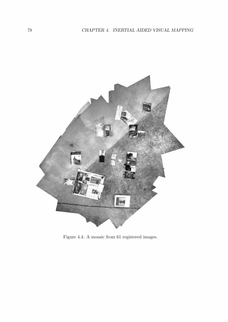
78 CHAPTER 4. INERTIAL AIDED VISUAL MAPPING
Figure 4.4: A mosaic from 61 registered images.
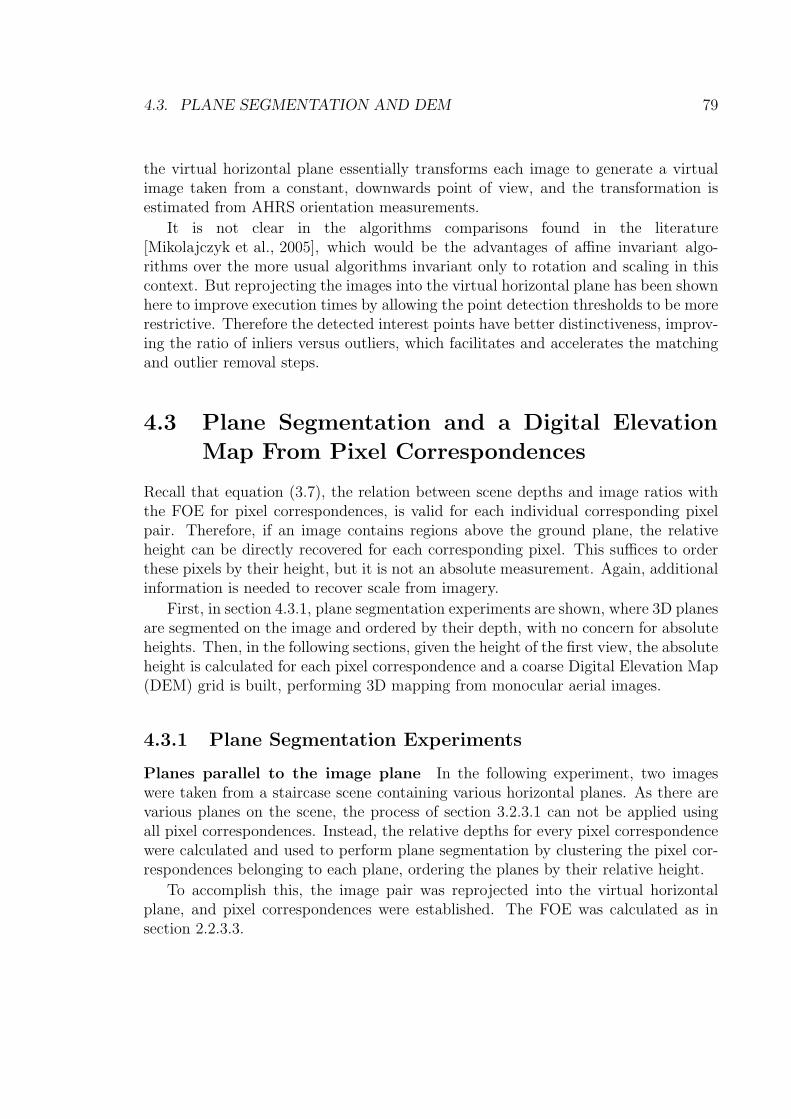
4.3. PLANE SEGMENTATION AND DEM 79
the virtual horizontal plane essentially transforms each image to generate a virtualimage taken from a constant, downwards point of view, and the transformation isestimated from AHRS orientation measurements.
It is not clear in the algorithms comparisons found in the literature[Mikolajczyk et al., 2005], which would be the advantages of affine invariant algo-rithms over the more usual algorithms invariant only to rotation and scaling in thiscontext. But reprojecting the images into the virtual horizontal plane has been shownhere to improve execution times by allowing the point detection thresholds to be morerestrictive. Therefore the detected interest points have better distinctiveness, improv-ing the ratio of inliers versus outliers, which facilitates and accelerates the matchingand outlier removal steps.
4.3 Plane Segmentation and a Digital ElevationMap From Pixel Correspondences
Recall that equation (3.7), the relation between scene depths and image ratios withthe FOE for pixel correspondences, is valid for each individual corresponding pixelpair. Therefore, if an image contains regions above the ground plane, the relativeheight can be directly recovered for each corresponding pixel. This suffices to orderthese pixels by their height, but it is not an absolute measurement. Again, additionalinformation is needed to recover scale from imagery.
First, in section 4.3.1, plane segmentation experiments are shown, where 3D planesare segmented on the image and ordered by their depth, with no concern for absoluteheights. Then, in the following sections, given the height of the first view, the absoluteheight is calculated for each pixel correspondence and a coarse Digital Elevation Map(DEM) grid is built, performing 3D mapping from monocular aerial images.
4.3.1 Plane Segmentation Experiments
Planes parallel to the image plane In the following experiment, two imageswere taken from a staircase scene containing various horizontal planes. As there arevarious planes on the scene, the process of section 3.2.3.1 can not be applied usingall pixel correspondences. Instead, the relative depths for every pixel correspondencewere calculated and used to perform plane segmentation by clustering the pixel cor-respondences belonging to each plane, ordering the planes by their relative height.
To accomplish this, the image pair was reprojected into the virtual horizontalplane, and pixel correspondences were established. The FOE was calculated as insection 2.2.3.3.
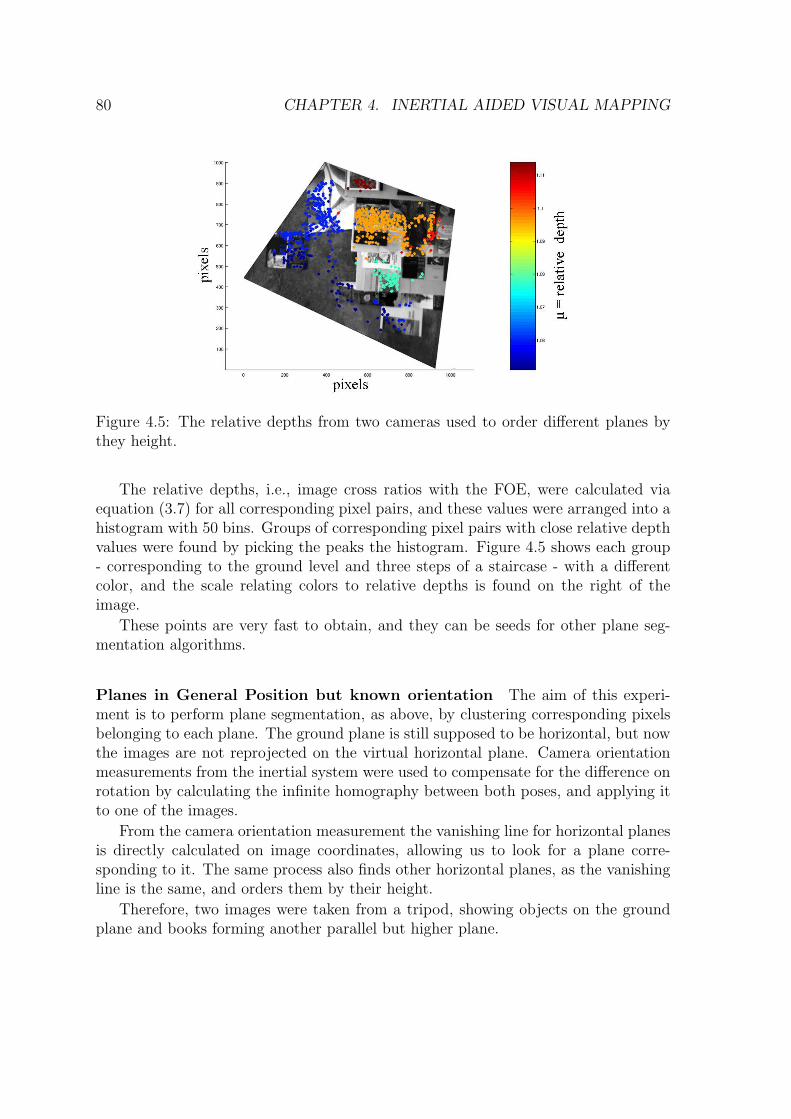
80 CHAPTER 4. INERTIAL AIDED VISUAL MAPPING
Figure 4.5: The relative depths from two cameras used to order different planes bythey height.
The relative depths, i.e., image cross ratios with the FOE, were calculated viaequation (3.7) for all corresponding pixel pairs, and these values were arranged into ahistogram with 50 bins. Groups of corresponding pixel pairs with close relative depthvalues were found by picking the peaks the histogram. Figure 4.5 shows each group- corresponding to the ground level and three steps of a staircase - with a differentcolor, and the scale relating colors to relative depths is found on the right of theimage.
These points are very fast to obtain, and they can be seeds for other plane seg-mentation algorithms.
Planes in General Position but known orientation The aim of this experi-ment is to perform plane segmentation, as above, by clustering corresponding pixelsbelonging to each plane. The ground plane is still supposed to be horizontal, but nowthe images are not reprojected on the virtual horizontal plane. Camera orientationmeasurements from the inertial system were used to compensate for the difference onrotation by calculating the infinite homography between both poses, and applying itto one of the images.
From the camera orientation measurement the vanishing line for horizontal planesis directly calculated on image coordinates, allowing us to look for a plane corre-sponding to it. The same process also finds other horizontal planes, as the vanishingline is the same, and orders them by their height.
Therefore, two images were taken from a tripod, showing objects on the groundplane and books forming another parallel but higher plane.
4.3. PLANE SEGMENTATION AND DEM 81
Figure 4.6: The ground plane, and other parallel planes, segmented and ordered byheight.
The FOE was robustly estimated from all pixel correspondences [Chen et al., 2003],and outliers were discarded in this step. The horizon line a, i.e., the vanishing line ofthe ground plane, is obtained via equation (3.25), with n being the vector normal tothe ground plane in the camera frame.
For each corresponding pixel pair (x,x′), the cross-ratio µ is calculated by:
µ =‖v,x‖ ‖x′, i‖‖v,x′‖ ‖x, i‖
(4.1)
where i is the intersection of the vanishing line a and the line |x,x′|. Again, ahistogram is calculated on the values of µ, and by picking the peaks of the histogramwe find groups of pixel correspondences corresponding to the same plane.
Figure 4.6 shows the value of the cross-ratio µ (corresponding to relative height)for groups of pixel correspondences.
4.3.2 Calculating Height For Each Pixel Correspondence
In the previous section, the relative height is directly recovered for each correspondingpixel. This sufficed to order these pixels by their height, but it is not an absolutemeasurement. Again, additional information is needed to recover scale from imagery.The absolute height of these points may be recovered if the absolute height on bothviews is known - case (a), or, equivalently, if the height of one view and relative heightcorresponding to the ground plane is known - case (b).
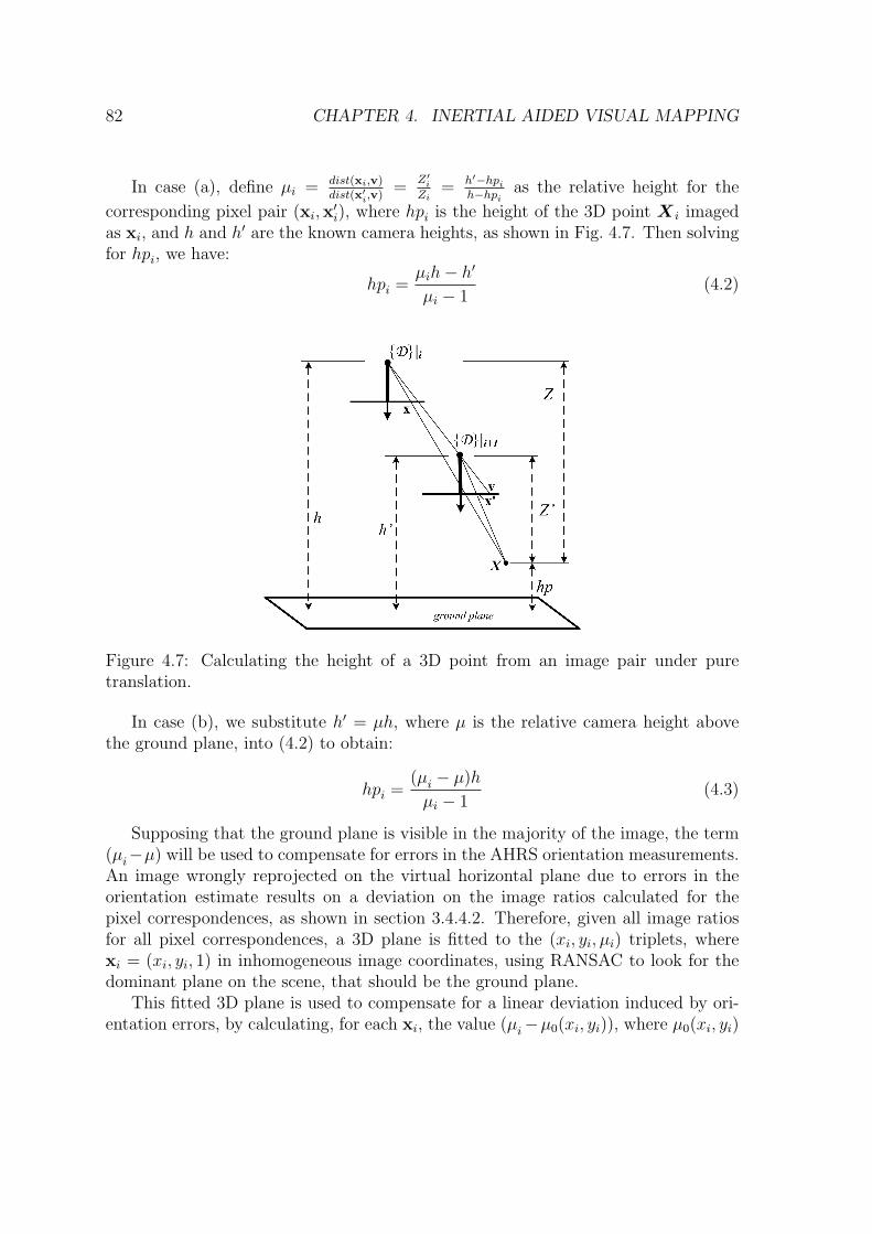
82 CHAPTER 4. INERTIAL AIDED VISUAL MAPPING
In case (a), define µi = dist(xi,v)dist(x′i,v)
=Z′
i
Zi= h′−hpi
h−hpias the relative height for the
corresponding pixel pair (xi,x′i), where hpi is the height of the 3D point X i imaged
as xi, and h and h′ are the known camera heights, as shown in Fig. 4.7. Then solvingfor hpi, we have:
hpi =µih− h′
µi − 1(4.2)
Figure 4.7: Calculating the height of a 3D point from an image pair under puretranslation.
In case (b), we substitute h′ = µh, where µ is the relative camera height abovethe ground plane, into (4.2) to obtain:
hpi =(µi − µ)h
µi − 1(4.3)
Supposing that the ground plane is visible in the majority of the image, the term(µi−µ) will be used to compensate for errors in the AHRS orientation measurements.An image wrongly reprojected on the virtual horizontal plane due to errors in theorientation estimate results on a deviation on the image ratios calculated for thepixel correspondences, as shown in section 3.4.4.2. Therefore, given all image ratiosfor all pixel correspondences, a 3D plane is fitted to the (xi, yi, µi) triplets, wherexi = (xi, yi, 1) in inhomogeneous image coordinates, using RANSAC to look for thedominant plane on the scene, that should be the ground plane.
This fitted 3D plane is used to compensate for a linear deviation induced by ori-entation errors, by calculating, for each xi, the value (µi−µ0(xi, yi)), where µ0(xi, yi)
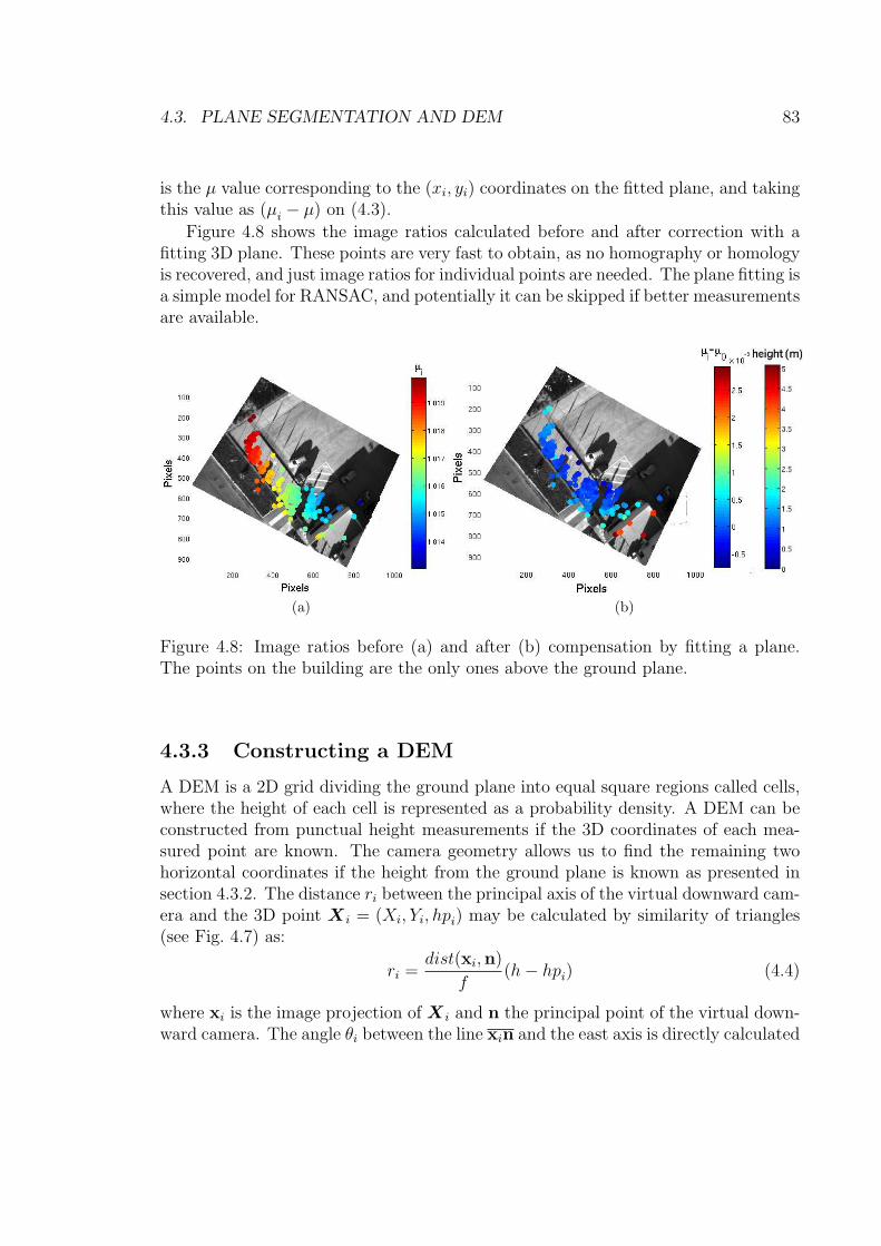
4.3. PLANE SEGMENTATION AND DEM 83
is the µ value corresponding to the (xi, yi) coordinates on the fitted plane, and takingthis value as (µi − µ) on (4.3).
Figure 4.8 shows the image ratios calculated before and after correction with afitting 3D plane. These points are very fast to obtain, as no homography or homologyis recovered, and just image ratios for individual points are needed. The plane fitting isa simple model for RANSAC, and potentially it can be skipped if better measurementsare available.
(a) (b)
Figure 4.8: Image ratios before (a) and after (b) compensation by fitting a plane.The points on the building are the only ones above the ground plane.
4.3.3 Constructing a DEM
A DEM is a 2D grid dividing the ground plane into equal square regions called cells,where the height of each cell is represented as a probability density. A DEM can beconstructed from punctual height measurements if the 3D coordinates of each mea-sured point are known. The camera geometry allows us to find the remaining twohorizontal coordinates if the height from the ground plane is known as presented insection 4.3.2. The distance ri between the principal axis of the virtual downward cam-era and the 3D point X i = (Xi, Yi, hpi) may be calculated by similarity of triangles(see Fig. 4.7) as:
ri =dist(xi,n)
f(h− hpi) (4.4)
where xi is the image projection of X i and n the principal point of the virtual down-ward camera. The angle θi between the line xin and the east axis is directly calculated

84 CHAPTER 4. INERTIAL AIDED VISUAL MAPPING
from their coordinates. Then, transforming (ri, θi) from polar to rectangular coor-dinates yields (Xi, Yi), the remaining two components of X i = (Xi, Yi, hpi), in the{D}|i frame. If the camera pose in the world frame is known, these coordinates maybe registered into the {W}|i frame, incorporating the height measurements in a globalDEM.
Each point X i represents a height measurement for an individual DEM cell. Theheight of each cell and the heights measurements are represented by random variableswith Gaussian distribution, and the cell update follows the Kalman Filter update rule.There is not an initialization and the cell takes its first value when incorporating itsfirst measurement.
The position of each point X i has also an uncertainty on the xy axes, i.e., itmay be uncertain which cell the measurement belongs to. Currently the influence ofmeasurements on neighboring cells is approximated by considering all measurementsexact on the North-East axes, and then smoothing each local DEM with a Gaussiankernel with variance similar to the measurements.
Figure 4.9 shows a DEM constructed from a 10 frame sequence (a 5[s] portion ofthe flight), with the GPS-measured vehicle localization shown as red stars. The cellsize is 3[m], and the Gaussian convolution kernel has standard deviation of 2[m]. Thehighest cells correspond to the building, and the smaller blue peaks correspond to theairplanes and vehicles. Points more than 1[m] below the ground plane are discardedas obvious outliers. The mosaic on the left - included just to allow the reader tocompare visually the covered area and the DEM grid - is built from homographiescalculated between each successive image pair as in section 4.2.
4.3.4 Applications and Future Improvements
In section 3.4 the complete UAV trajectory was reconstructed from rotation com-pensated imagery. In this section, a 3D map of the environment, in the form of asparse DEM, is built from punctual height measurements generated from a sequenceof images and the vehicle pose. These two techniques assume mutually exclusiveconditions: the trajectory recovery requires imaging a planar area, and the map-ping procedure is meaningful only if there are obstacles above the ground plane.Therefore, they could not make a complete SLAM (Simultaneous Localization andMapping) scheme on their own, but they may be complimentary methods to otherSLAM approaches. A SLAM scheme also needs to obtain, from the maps built at eachstep, another displacement measurement to constrain the vehicle pose estimation, bymatching local maps with the previous local map or with the global map built so far.A comparison of different approaches for matching 2D occupancy grids built fromsonar data indicates that both options are feasible [Schiele and Crowley, 1994], andthe DEM grids could be correlated this way.

4.3. PLANE SEGMENTATION AND DEM 85
Figure 4.9: 2D and 3D plots of the DEM generated from the 10 frames mosaiced onthe left. The red stars indicate the vehicle trajectory.
Figure 4.8 shows that all pixel correspondences are concentrated into one smallportion of the image. Outside this region, there are other correspondences foundby the interest point matching algorithm, but they are considered outliers during theFOE estimation and rejected, probably due to errors on the orientation measurement.For the estimation of the homology, and particularly of its cross ratio used on theheight component of the trajectory estimation, usually there are enough correspon-dences for a reliable estimation. But for the mapping problem, the area covered byheight measurements is quite smaller than the total area imaged (see Fig. 4.9), andthus the map becomes too sparse for a reliable correlation between the DEM gridmaps. This problem could be addressed by improving the accuracy of the orientationmeasurements, by increasing the image frame rate, or by developing models that take
86 CHAPTER 4. INERTIAL AIDED VISUAL MAPPING
into account small uncompensated rotations.
4.4 3D Depth Map RegistrationThis section describes the registration of 3D maps taken from a moving ranging device,which may be a calibrated stereo camera, or a LRF coupled with a single camera.There is also an AHRS rigidly coupled with the ranging device as before. The mapsconsist of sets of 3D points, or point clouds, defined in the frame corresponding tothe ranging device used, i.e., the {C}|i or {L}|i frames. These point clouds must beregistered in a common world frame {W}. The models to calculate these point cloudsfrom the raw sensor readings at each frame index i are given in sections 2.1.1 and 2.4,and they are denoted by CP|i or LP|i, where the left superscript represent the frameof reference and the right subscript represent the time index.
Each point cloud is associated to an image Ii captured at the same instant by adigital camera. This image is the left camera image in the stereo camera case. Inthe LRF case, the acquisition of the point cloud is not instantaneous, therefore thepantilt position at the moment of image acquisition must be known. For these resultsthe image was always acquired with the tilt and pan angles zeroed.
First, an image sequence is delimited, consisting of images that can be successfullymatched with an arbitrarily chosen reference image IB by interest point matchingalgorithms (section 4.4.1). Then for each point cloud, the rotational componentsare compensated using measurements of the camera orientation in section 4.4.2, andimage correspondences find the remaining translational component in section 4.4.3.
The output for each frame is a point cloud registered into a common frame, theframe {W} = {R}|B. The registered point clouds are not kept separately as in figure4.22(a) but are combined into an aggregated point cloud (figure 4.22(b)), discardingredundant points to save memory.
Figure 4.10 shows the data flow for the registration of each point cloud. Onthe left of the figure, the inputs are shown: for each time index i, the stereo pointcloud, the image from the left camera, and the inertial orientation measurement. Twoother inputs are constant for all frames: the image from the reference frame, and therotation matrix IRC, output of the camera-inertial calibration.
4.4.1 Delimiting an image sequenceTo delimit the subsequence to be registered, interest point matching is applied tomatch the reference image IB with the next images on the sequence until an imageis found that can not be successfully matched with the reference frame, as shown infigure 4.11 (actually, for the sake of clarity the figure omits that the loop is executedtwice, first matching frames in the forward direction and then backwards). An image

4.4. 3D DEPTH MAP REGISTRATION 87
Figure 4.10: The data flow for the registration of each 3D point cloud.
Figure 4.11: The process for the registration of 3D point clouds. The box “processpoint cloud” corresponds to figure 4.10.
match is deemed successful if the number of corresponding pixel pairs is bigger thana threshold. The frames on the delimited image sequence are numbered with a timeindex i = 1 . . . B . . . n. The inertial orientation measurement corresponding to eachtime index i is also available.
4.4.2 Rotating to a stabilized frame of reference
The measured inertial orientation for the time index i is expressed as a rotation matrixRRI |i which rotates the inertial sensor frame {I}|i into the stabilized frame {R}|i.
If stereo cameras are used as the ranging device, the point cloud CP|i is rotatedfrom the camera frame to the stabilized frame by the rotation RRC|i = RRI |i · IRC.As figure 4.12 shows for two point clouds, the purpose of this rotation is to alignall point clouds to the earth-referenced {R}|i frame, i.e., North, East and verticaldirections, as indicated by the inertial and magnetic orientation measurements.
For the LRF, a similar step is taken, but it is necessary to compensate for thepantilt position at the moment the inertial measurement was taken. The pantiltrotation is represented by R(ϕ, 0, 0), the rotation matrix equivalent to the Eulerangles ϕ, 0, 0 considering ϕ as the tilt angle and zero as the other two Euler angles.For each time index i = 1 . . . n, the rotation matrix WRL|i = WRI |i · IRL ·R(ϕ, 0, 0)brings a point from the laser frame {L}|i into the {R}|i frame, this rotation is applied
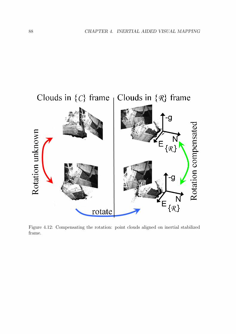
88 CHAPTER 4. INERTIAL AIDED VISUAL MAPPING
Figure 4.12: Compensating the rotation: point clouds aligned on inertial stabilizedframe.
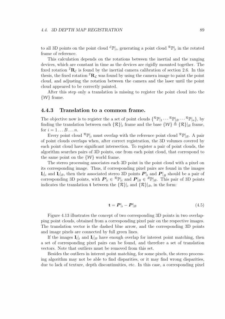
4.4. 3D DEPTH MAP REGISTRATION 89
to all 3D points on the point cloud LP|i, generating a point cloud RP|i in the rotatedframe of reference.
This calculation depends on the rotations between the inertial and the rangingdevices, which are constant in time as the devices are rigidly mounted together. Thefixed rotation IRC is found by the inertial camera calibration of section 2.6. In thisthesis, the fixed rotation IRL was found by using the camera image to paint the pointcloud, and adjusting the rotation between the camera and the laser until the pointcloud appeared to be correctly painted.
After this step only a translation is missing to register the point cloud into the{W} frame.
4.4.3 Translation to a common frame.The objective now is to register the a set of point clouds {RP|1 · · ·RP|B · · ·RP|n}, byfinding the translation between each {R}|i frame and the base {W} , {R}|B frame,for i = 1 . . . B . . . n.
Every point cloud RP|i must overlap with the reference point cloud RP|B. A pairof point clouds overlaps when, after correct registration, the 3D volumes covered byeach point cloud have significant intersection. To register a pair of point clouds, thealgorithm searches pairs of 3D points, one from each point cloud, that correspond tothe same point on the {W} world frame.
The stereo processing associates each 3D point in the point cloud with a pixel onits corresponding image. Thus, if corresponding pixel pairs are found in the imagesIl|i and Il|B, then their associated stereo 3D points P |i and P |B should be a pair ofcorresponding 3D points, with P |i ∈ RP|i and P |B ∈ RP|B. This pair of 3D pointsindicates the translation t between the {R}|i and {R}|B, in the form:
t = P |i − P |B (4.5)
Figure 4.13 illustrates the concept of two corresponding 3D points in two overlap-ping point clouds, obtained from a corresponding pixel pair on the respective images.The translation vector is the dashed blue arrow, and the corresponding 3D pointsand image pixels are connected by full green lines.
If the images Il|i and Il|B have enough overlap for interest point matching, thena set of corresponding pixel pairs can be found, and therefore a set of translationvectors. Note that outliers must be removed from this set.
Besides the outliers in interest point matching, for some pixels, the stereo process-ing algorithm may not be able to find disparities, or it may find wrong disparities,due to lack of texture, depth discontinuities, etc. In this case, a corresponding pixel
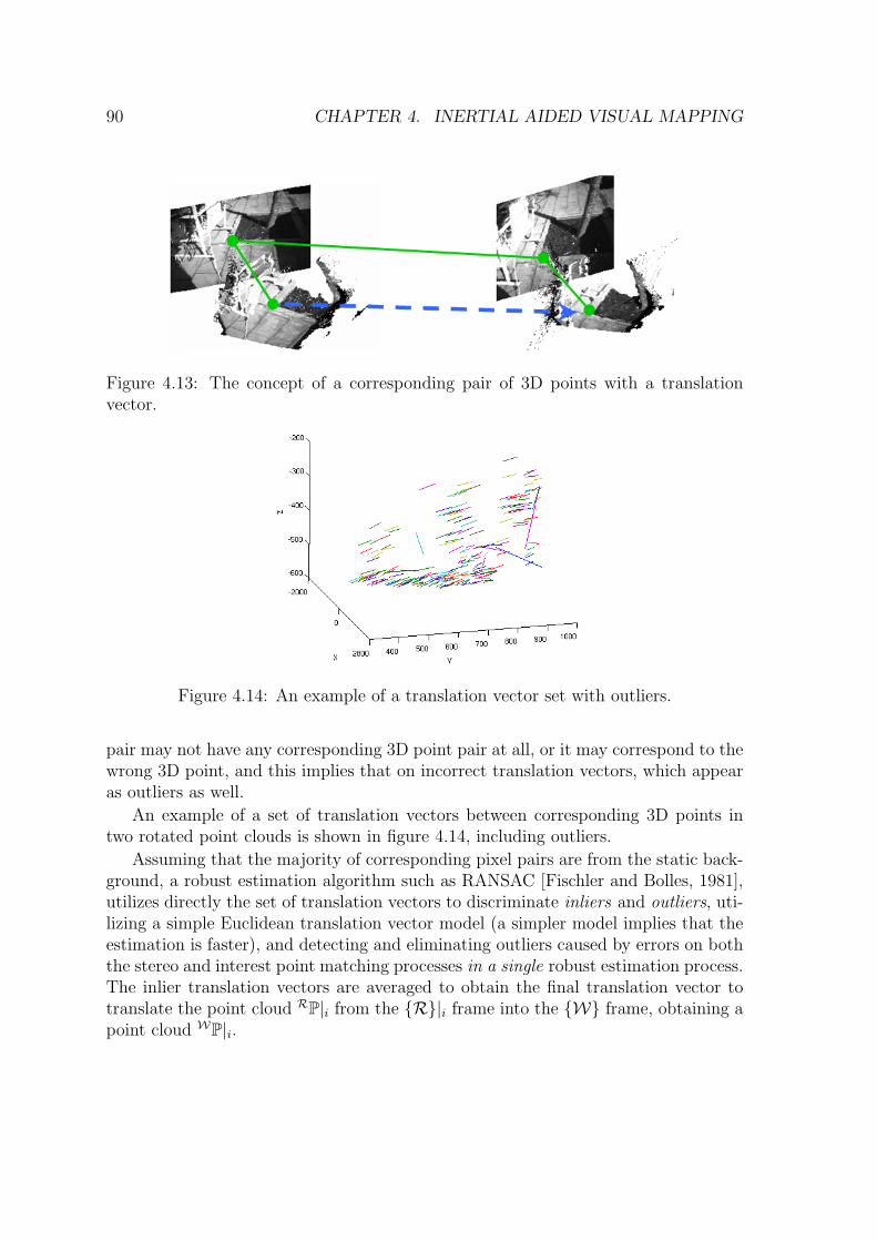
90 CHAPTER 4. INERTIAL AIDED VISUAL MAPPING
Figure 4.13: The concept of a corresponding pair of 3D points with a translationvector.
Figure 4.14: An example of a translation vector set with outliers.
pair may not have any corresponding 3D point pair at all, or it may correspond to thewrong 3D point, and this implies that on incorrect translation vectors, which appearas outliers as well.
An example of a set of translation vectors between corresponding 3D points intwo rotated point clouds is shown in figure 4.14, including outliers.
Assuming that the majority of corresponding pixel pairs are from the static back-ground, a robust estimation algorithm such as RANSAC [Fischler and Bolles, 1981],utilizes directly the set of translation vectors to discriminate inliers and outliers, uti-lizing a simple Euclidean translation vector model (a simpler model implies that theestimation is faster), and detecting and eliminating outliers caused by errors on boththe stereo and interest point matching processes in a single robust estimation process.The inlier translation vectors are averaged to obtain the final translation vector totranslate the point cloud RP|i from the {R}|i frame into the {W} frame, obtaining apoint cloud WP|i.
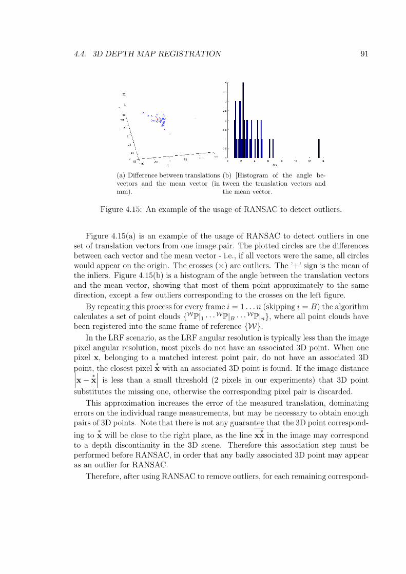
4.4. 3D DEPTH MAP REGISTRATION 91
(a) Difference between translationsvectors and the mean vector (inmm).
(b) [Histogram of the angle be-tween the translation vectors andthe mean vector.
Figure 4.15: An example of the usage of RANSAC to detect outliers.
Figure 4.15(a) is an example of the usage of RANSAC to detect outliers in oneset of translation vectors from one image pair. The plotted circles are the differencesbetween each vector and the mean vector - i.e., if all vectors were the same, all circleswould appear on the origin. The crosses (×) are outliers. The ’+’ sign is the mean ofthe inliers. Figure 4.15(b) is a histogram of the angle between the translation vectorsand the mean vector, showing that most of them point approximately to the samedirection, except a few outliers corresponding to the crosses on the left figure.
By repeating this process for every frame i = 1 . . . n (skipping i = B) the algorithmcalculates a set of point clouds {WP|1 · · ·WP|B · · ·WP|n}, where all point clouds havebeen registered into the same frame of reference {W}.
In the LRF scenario, as the LRF angular resolution is typically less than the imagepixel angular resolution, most pixels do not have an associated 3D point. When onepixel x, belonging to a matched interest point pair, do not have an associated 3Dpoint, the closest pixel
∗x with an associated 3D point is found. If the image distance∣∣∣x− ∗
x∣∣∣ is less than a small threshold (2 pixels in our experiments) that 3D point
substitutes the missing one, otherwise the corresponding pixel pair is discarded.This approximation increases the error of the measured translation, dominating
errors on the individual range measurements, but may be necessary to obtain enoughpairs of 3D points. Note that there is not any guarantee that the 3D point correspond-ing to
∗x will be close to the right place, as the line x
∗x in the image may correspond
to a depth discontinuity in the 3D scene. Therefore this association step must beperformed before RANSAC, in order that any badly associated 3D point may appearas an outlier for RANSAC.
Therefore, after using RANSAC to remove outliers, for each remaining correspond-
92 CHAPTER 4. INERTIAL AIDED VISUAL MAPPING
ing pixel pair (xk,x′k) in the images Ii and Ij, the value wk =
(∣∣∣xk −∗xk
∣∣∣+ ∣∣∣x′k − ∗x′k
∣∣∣)−1
is defined as a weight in the averaging of the resulting translation vector, as suggestedin [Matthies and Shafer, 1987], and therefore the translation vector is calculated by:
t =
( ∑for all k
wk
)−1( ∑for all k
wktk
)(4.6)
where tk = P k|i − P ′k|j, with P k|i and P ′
k|j being the pair of 3D points associatedwith the corresponding pixel pair (xk,x
′k). For the corresponding pixel pairs where
this approximation is not necessary, their weights should be set at some larger value,as equation (4.6) would yield wk = (0 + 0)−1 =∞. In the experiments in this thesisthey were set at 2.
In the stereo scenario, this approximation is not usually necessary, as many cor-responding pixel pairs have associated 3D points. A covariance for each 3D pointcan be calculated using stereo triangulation error models, and used as weights in theaveraging of translation as presented in [Matthies and Shafer, 1987].
4.4.4 Subsuming other geometric constraints for outlier re-moval
Other geometric constraints have been proposed to remove outliers from the set of cor-responding 3D points. In this section, the two constraints proposed in[Hirschmüller et al., 2002] are reviewed and it is shown that in the rotation com-pensated case they may be enforced more tightly and subsumed by the translationvector constraint proposed in section 4.4.3.
Consider two pairs of corresponding 3D points on the i and j frames, (P |i, P |j)and (Q|i, Q|j). The first constraint concerns the invariance of the length of theP |i −Q|i vector under a rigid transformation, i.e. ‖P |i −Q|i‖ = ‖P |i −Q|i‖ mustbe true.
The second constraint limits the angle between a vector formed by two 3D pointsbefore and after the motion. With the orientation measured, it can be more tightlyenforced with a statistically significant boundary if the error on orientation measure-ments is known.
Represent the rotation between the poses i and j by a rotation axis r and arotation angle φ. The angle between the vectors P |j −Q|j and P |i −Q|i must bebetween 0 and φ. It is zero if P |i − Q|i is parallel to r, and it is φ if P |i − Q|i isorthogonal to r.
Imposing the restriction φ < θ results in the inequality:
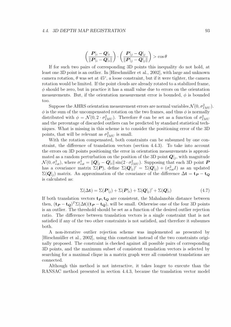
4.4. 3D DEPTH MAP REGISTRATION 93
(P |i −Q|i‖P |i −Q|i‖
)·(
P |j −Q|j‖P |j −Q|j‖
)> cos θ
If for such two pairs of corresponding 3D points this inequality do not hold, atleast one 3D point is an outlier. In [Hirschmüller et al., 2002], with large and unknowncamera rotation, θ was set at 45◦, a loose constraint, but if it were tighter, the camerarotation would be limited. If the point clouds are already rotated to a stabilized frame,φ should be zero, but in practice it has a small value due to errors on the orientationmeasurements. But, if the orientation measurement error is bounded, φ is boundedtoo.
Suppose the AHRS orientation measurement errors are normal variablesN (0, σ2IMU).
φ is the sum of the uncompensated rotation on the two frames, and thus φ is normallydistributed with φ = N (0, 2 · σ2
IMU). Therefore θ can be set as a function of σ2IMU
and the percentage of discarded outliers can be predicted by standard statistical tech-niques. What is missing in this scheme is to consider the positioning error of the 3Dpoints, that will be relevant as σ2
IMU is small.With the rotation compensated, both constraints can be subsumed by one con-
straint, the difference of translation vectors (section 4.4.3). To take into accountthe errors on 3D points positioning the error in orientation measurements is approxi-mated as a random perturbation on the position of the 3D point Q|j, with magnitudeN (0, σ2
rot), where σ2rot = ‖Q|j −Q|i‖ sin(2 · σ2
IMU). Supposing that each 3D point Phas a covariance matrix Σ(P ), define Σ(Q|j)′ = Σ(Q|j) + (σ2
rotI) as an updatedΣ(Q|j) matrix. An approximation of the covariance of the difference ∆t = tP − tQ
is calculated as:
Σ(∆t) = Σ(P |j) + Σ(P |i) + Σ(Q|j)′ + Σ(Q|i) (4.7)
If both translation vectors tP , tQ are consistent, the Mahalanobis distance betweenthen, (tP − tQ)T Σ(∆t)(tP − tQ), will be small. Otherwise one of the four 3D pointsis an outlier. The threshold should be set as a function of the desired outlier rejectionratio. The difference between translation vectors is a single constraint that is notsatisfied if any of the two other constraints is not satisfied, and therefore it subsumesboth.
A non-iterative outlier rejection scheme was implemented as presented by[Hirschmüller et al., 2002], using this constraint instead of the two constraints origi-nally proposed. The constraint is checked against all possible pairs of corresponding3D points, and the maximum subset of consistent translation vectors is selected bysearching for a maximal clique in a matrix graph were all consistent translations areconnected.
Although this method is not interactive, it takes longer to execute than theRANSAC method presented in section 4.4.3, because the translation vector model

94 CHAPTER 4. INERTIAL AIDED VISUAL MAPPING
is simple, allowing RANSAC to be executed very fast, without need to test everypossible pair of translation vectors. Therefore, RANSAC was used on the experi-ments of this thesis to exclude outliers, and the non-iterative method was abandoned.
Nevertheless, using equation (4.7) with typical values for the covariance of the3D points and the AHRS orientation error, yields an expected covariance for thedifference between translation vectors which may be used to define the threshold forinlier/outlier discrimination in the RANSAC outlier detection method.
4.4.5 Filtering out redundant points
The algorithm described on the last sections registers a set of overlapping point clouds{WP|1 · · ·WP|B · · ·WP|n} into the frame of reference {W}. The simple union of allpoint clouds in this set is a registered point cloud itself, but, due to overlapping, theremay be a many 3D points from different point clouds which are very close and areconsidered redundant. They should be eliminated to save memory and processingtime.
Additionally, the point clouds must be filtered, deleting points wrongly positioneddue to errors on stereo processing. Isolated, “floating” 3D points must be eliminated,generating a smoother point cloud. The outlier detection process of section 4.4.3deals only with the relatively small number of 3D points corresponding to the pixelsmatched by the interest point matching algorithm, and do not change the point cloudsthemselves.
The registered point clouds in the set {WP|1 · · ·WP|B · · ·WP|n} do not need toactually exist at the same time; Instead, they are calculated sequentially by theprocess described in the last sections, and aggregated into a final aggregated pointcloud WA. WA is initialized with WA = ∅, and as each point cloud WP|i is calculated,a subset of the points on WP|i is added into WA. Namely, the points of WP|i that arecloser than a threshold value dmin to any point already in WA are discarded.
The value of dmin determines the final resolution of WA. It may be close to theresolution of the original point clouds, or dmin may be set to a higher value, leadingto a coarser point cloud which occupies less memory.
As the number of points is typically large, it would be too slow to check linearlyall the stored points in WA to test if each new point in WP|i is redundant. We havechosen the well-known approach of keeping only the point cloud WA and a hash table,that indexes all its points by their x-y coordinates. The hash table is used to retrievea list of potentially close points for each point in WP|i, and the closest point is quicklysearched for.
The cloud WA could also be built by dividing the 3D space in voxels, markingeach voxel as occupied or free as new points are added. But as the number of voxelsincreases with the volume of the covered space, it is difficult to cover a large volume.

4.4. 3D DEPTH MAP REGISTRATION 95
(a) (b)
Figure 4.16: An example of an aggregated point cloud
Besides that, many voxels are empty, outside and inside the 3D surface visible on thescene.
With a moving camera with a fast frame rate, the same 3D point in the worldmay be imaged by a relatively large number of frames, being represented repeatedlyin various point clouds in the set {WP|1 · · ·WP|B · · ·WP|n} . Therefore, for each pointP ∈ WP|i the hash table bin corresponding to P is searched for a point Q ∈ W Asuch that Q is closer than dmin to P . If such Q is found, P is discarded, but a votecounter associated with Q is incremented.
In such a way, the 3D points in WA receive “votes” from each individual pointcloud. For every 3D point in WA, the software keeps a vote counter, and the timeindex i of the point cloud that last voted for it. A 3D point in W A is only allowed toreceive one “vote” at each time step i.
The most voted 3D points in WA correspond to 3D positions that were imagedand considered occupied by various successive stereo frames, and therefore may beconsidered as occupied with more confidence. The 3D points in WA with less “votes”correspond to random stereo errors to be eliminated, or to moving objects, which canalso be eliminated in this way [Lobo et al., 2006], although this is not the objectivehere.
Algorithm 2 summarizes in pseudo-code the process of filtering redundant 3Dpoints, where dist() calculates the Euclidean distance between two points and dmin,votemin are constant parameters.
Figure 4.16 shows an example of an aggregated point cloud, created from 200highly overlapping point clouds. Only 3D points with more than 35 votes were allowedto remain in the aggregated point cloud, and the hash table bins had 5[cm] × 5[cm]
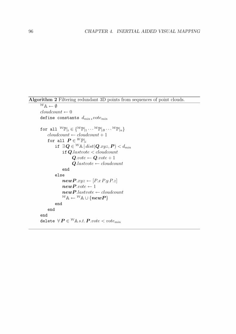
96 CHAPTER 4. INERTIAL AIDED VISUAL MAPPING
Algorithm 2 Filtering redundant 3D points from sequences of point clouds.WA← ∅cloudcount← 0define constants dmin,votemin
for all WP|i ∈ {WP|1 · · ·WP|B · · ·WP|n}cloudcount← cloudcount + 1for all P ∈ W P|i
if ∃Q ∈ WA | dist(Q.xyz, P ) < dmin
if Q.lastvote < cloudcountQ.vote← Q.vote + 1Q.lastvote← cloudcount
endelse
newP .xyz ← [P.x P.y P.z]newP .vote← 1newP .lastvote← cloudcountWA← WA ∪ {newP }
endend
enddelete ∀P ∈ WA s.t.P .vote < votemin
4.4. 3D DEPTH MAP REGISTRATION 97
in a 1[m]× 1[m]× 1[m] covered area - therefore each hash table bin contained about1/400 of the points in the point cloud. The threshold dmin was set to 1[cm]. Thepoint cloud looks sparse when plotted with a small point size (figure 4.16(a)), thegaps are filled when plotting with a larger point size, as in figure 4.16(b).
4.4.6 Results
Results with Stereo Cameras
Outdoor image sequences were used in the next experiments. Given one referenceframe {R}|B, corresponding to an image arbitrarily chosen as the reference image,SIFT correspondences were used to match each image with the reference image,finding a set of translation vectors to translate the point clouds into the {R}|B frame.
This set of translation vectors contains outliers, due to mismatched SIFTs andwrong stereo disparities, that are detected by the same RANSAC procedure.
As the model utilized on the RANSAC calculations is very simple, involving aver-aging and calculating differences between Euclidean 3D vectors, the RANSAC proce-dure runs very fast, on the order of a few tenths of seconds per frame in MATLABr.
As many backward and forward frames are matched as it is possible, by keepingtrying to match frames in the sequence until the number of inliers correspondencesfound by RANSAC falls below a threshold - probably because the camera has movedand the overlap region is too small.
The garden sequence was taken on an outdoor grass field, under indirect sunlight.There is a small light post. Figure 4.17(a) shows one point cloud from this data set,with its corresponding left camera image displayed on the back. Figure 4.17(b) showstwo registered point clouds, one in green, the other in the original gray level color.Figure 4.18 shows the resulting point cloud after registering together a sequence of26 successive frames, with points seen in less than 4 frames discarded.
The jeep sequence shows a jeep parked on the street under sunlight. Analogously,figures 4.19(a) and 4.21(a) show one point cloud from this data set, with its corre-sponding left camera image displayed on the back. Figures 4.19(b) and 4.21(b) showtwo registered point clouds, one in green, the other in the original gray level color,with their respective images displayed behind them. Figures 4.20 and 4.22 show, inthe left, a set of registered point clouds, and on the right, the resulting point cloudafter registering together a sequence of 27 (in both figures) successive point clouds,and filtering out points with less than four votes. In the left figure, only one everyfour point clouds is shown, to ease visualization.
The pyramids in figures 4.18, 4.20 and 4.22 represent the camera trajectory andorientation: there is one pyramid for every four camera poses, and camera pointstowards the base of the pyramid. The images on the graph sides are an approximatevisual reference, being stretched up to the extreme coordinates of their point clouds.
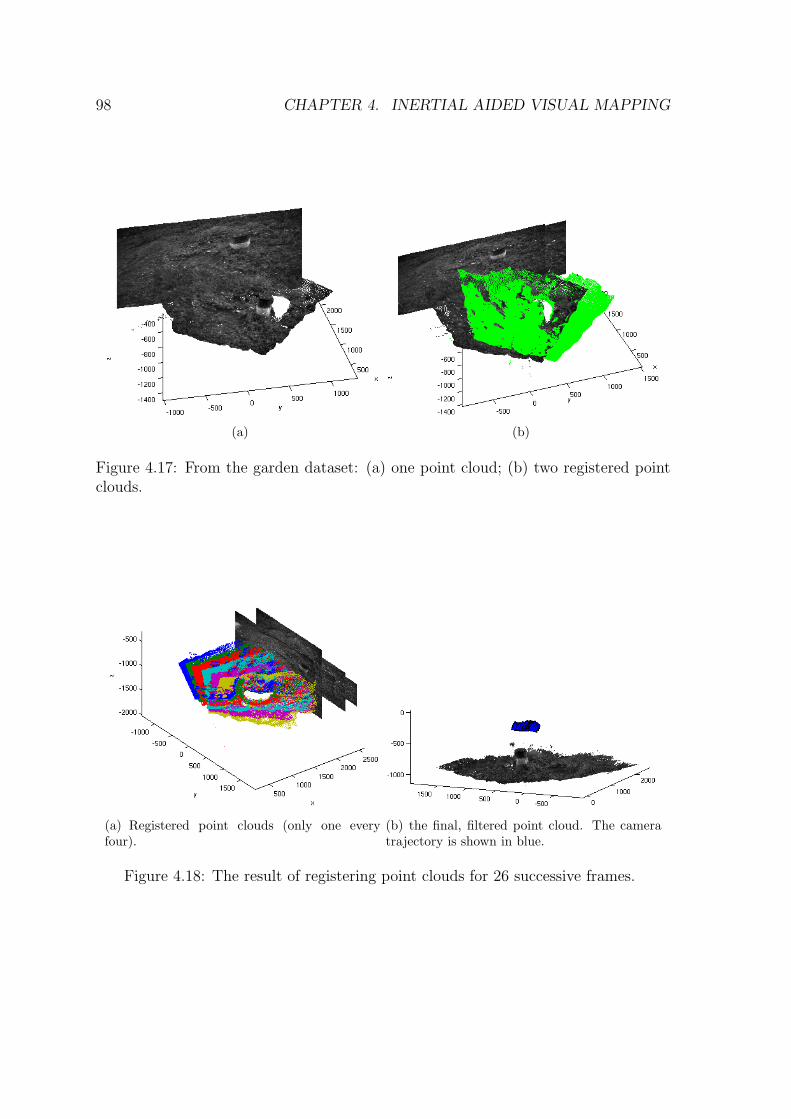
98 CHAPTER 4. INERTIAL AIDED VISUAL MAPPING
(a) (b)
Figure 4.17: From the garden dataset: (a) one point cloud; (b) two registered pointclouds.
(a) Registered point clouds (only one everyfour).
(b) the final, filtered point cloud. The cameratrajectory is shown in blue.
Figure 4.18: The result of registering point clouds for 26 successive frames.
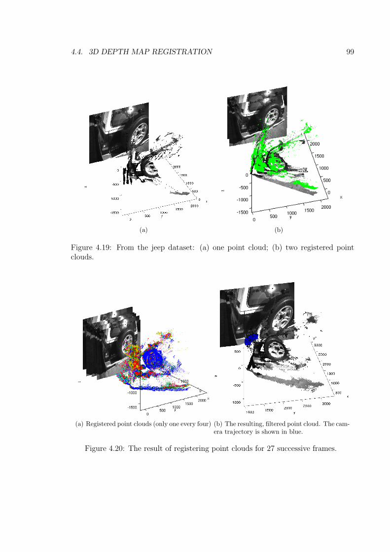
4.4. 3D DEPTH MAP REGISTRATION 99
(a) (b)
Figure 4.19: From the jeep dataset: (a) one point cloud; (b) two registered pointclouds.
(a) Registered point clouds (only one every four) (b) The resulting, filtered point cloud. The cam-era trajectory is shown in blue.
Figure 4.20: The result of registering point clouds for 27 successive frames.
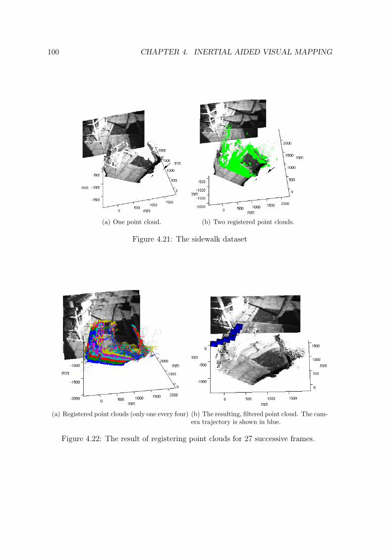
100 CHAPTER 4. INERTIAL AIDED VISUAL MAPPING
(a) One point cloud. (b) Two registered point clouds.
Figure 4.21: The sidewalk dataset
(a) Registered point clouds (only one every four) (b) The resulting, filtered point cloud. The cam-era trajectory is shown in blue.
Figure 4.22: The result of registering point clouds for 27 successive frames.
4.4. 3D DEPTH MAP REGISTRATION 101
The RANSAC threshold for membership in the inlier set was 5[cm] for bothdatasets. The minimum acceptable number of inliers was 20.
For each frame chosen as a reference frame, between 20 and 50 frames could beregistered, equivalent to approximately between 1.5 and 3 seconds at 15fps.
Results with LRF and monocular cameras
To generate a 3D point cloud, the LRF was mounted on a pantilt, and its tilt axiswas moved from −30◦ to 30◦, taking a scan every 1◦. One example is shown in figure4.23(a). Points in the area imaged by the camera are painted with the gray colorof their corresponding pixel, while points not imaged are in a uniform gray. Threesuch point clouds are shown registered in figure 4.23(b), with the other point cloudshighlighted in green and blue.
After the process shown in this section is completed, ICP can be used to fine tunethe registration. This was unnecessary with the outdoor sequence of figure 4.22. Butin indoor environments, often metallic structures or electric equipment interferes onthe magnetic field, and thus the AHRS compass output has larger errors. In suchconditions our method can only be used as a first approximation for other techniques.
Averaging the processing times for 10 different pairs of point clouds, after the datais acquired, it takes 1.5[s] to generate interest points on both images, plus 1.5[s] torun the process described here, against 7[s] to execute ICP.

102 CHAPTER 4. INERTIAL AIDED VISUAL MAPPING
(a) A point cloud taken by a LRF
(b) Three registered point clouds.
Figure 4.23: Registration of three point clouds taken by the LRF.
Chapter 5
Aerial Surveillance by VisualTracking
5.1 Introduction
As reported in chapter 3, orientation measurements from an AHRS compensated therotational degrees of freedom of the motion of the moving camera, including in the caseof the remotely controlled airship of figure 1.2. Firstly, the images were reprojectedin a geo-referenced virtual horizontal plane. Pure translation models were then usedto recover the camera trajectory from images of a horizontal planar area, and theywere found to be especially suitable for the estimation of the height component of thetrajectory.
In this chapter, the models which achieved the best results are used to recoverthe trajectory of the camera while it images a target independently moving in theground plane. The target position is marked in the reprojected images. The targettrajectory is then recovered and tracked using only the observations made from amoving camera, including the airship on-board camera, as it is shown in figure 5.1,and results in a urban people surveillance context with known ground truth.
GPS also can be utilized to recover the airship trajectory, but GPS position fixesare notoriously less accurate in the altitude than in the latitude and longitude axes,and this uncertainty is very significant for the low altitude dataset used in this chapter.
Uncertainty in the camera orientation estimate is the most important source of er-ror in tracking of ground objects imaged by an airborne camera [Redding et al., 2006],and its projection in the 2D ground plane is usually anisotropic even if the original dis-tribution is isotropic. The Unscented Transform [Julier and Uhlmann, 1997], whichhas been used to localize static targets on the ground [Merino et al., 2005], is thusused to project the uncertainty on the camera orientation estimate to the 2D groundplane, taking into account its anisotropic projection.
103
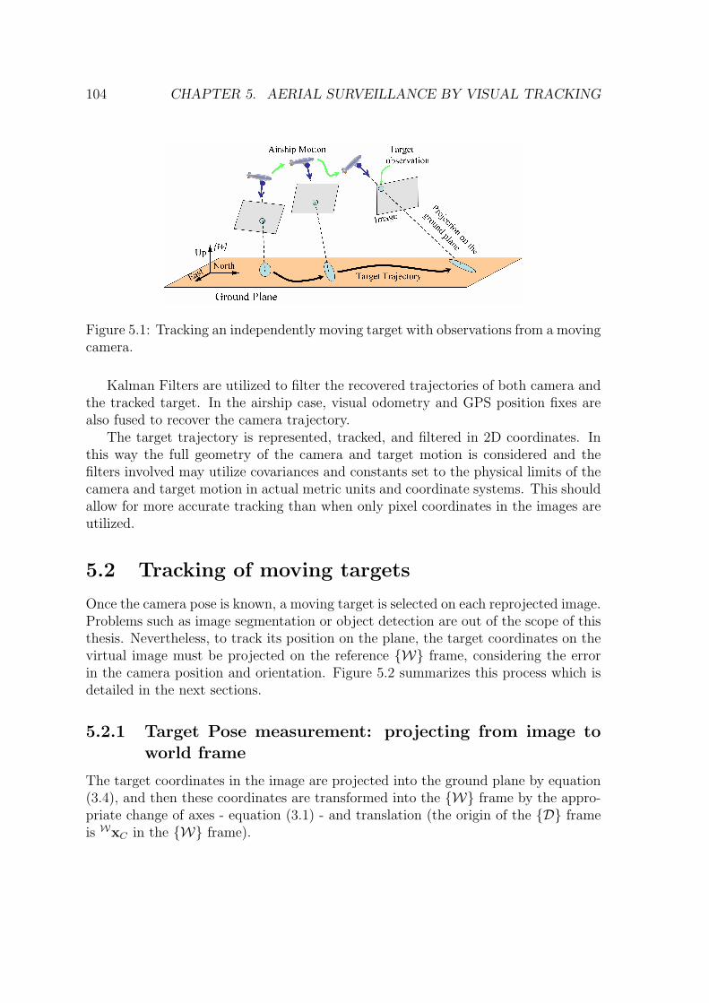
104 CHAPTER 5. AERIAL SURVEILLANCE BY VISUAL TRACKING
Figure 5.1: Tracking an independently moving target with observations from a movingcamera.
Kalman Filters are utilized to filter the recovered trajectories of both camera andthe tracked target. In the airship case, visual odometry and GPS position fixes arealso fused to recover the camera trajectory.
The target trajectory is represented, tracked, and filtered in 2D coordinates. Inthis way the full geometry of the camera and target motion is considered and thefilters involved may utilize covariances and constants set to the physical limits of thecamera and target motion in actual metric units and coordinate systems. This shouldallow for more accurate tracking than when only pixel coordinates in the images areutilized.
5.2 Tracking of moving targetsOnce the camera pose is known, a moving target is selected on each reprojected image.Problems such as image segmentation or object detection are out of the scope of thisthesis. Nevertheless, to track its position on the plane, the target coordinates on thevirtual image must be projected on the reference {W} frame, considering the errorin the camera position and orientation. Figure 5.2 summarizes this process which isdetailed in the next sections.
5.2.1 Target Pose measurement: projecting from image toworld frame
The target coordinates in the image are projected into the ground plane by equation(3.4), and then these coordinates are transformed into the {W} frame by the appro-priate change of axes - equation (3.1) - and translation (the origin of the {D} frameis WxC in the {W} frame).
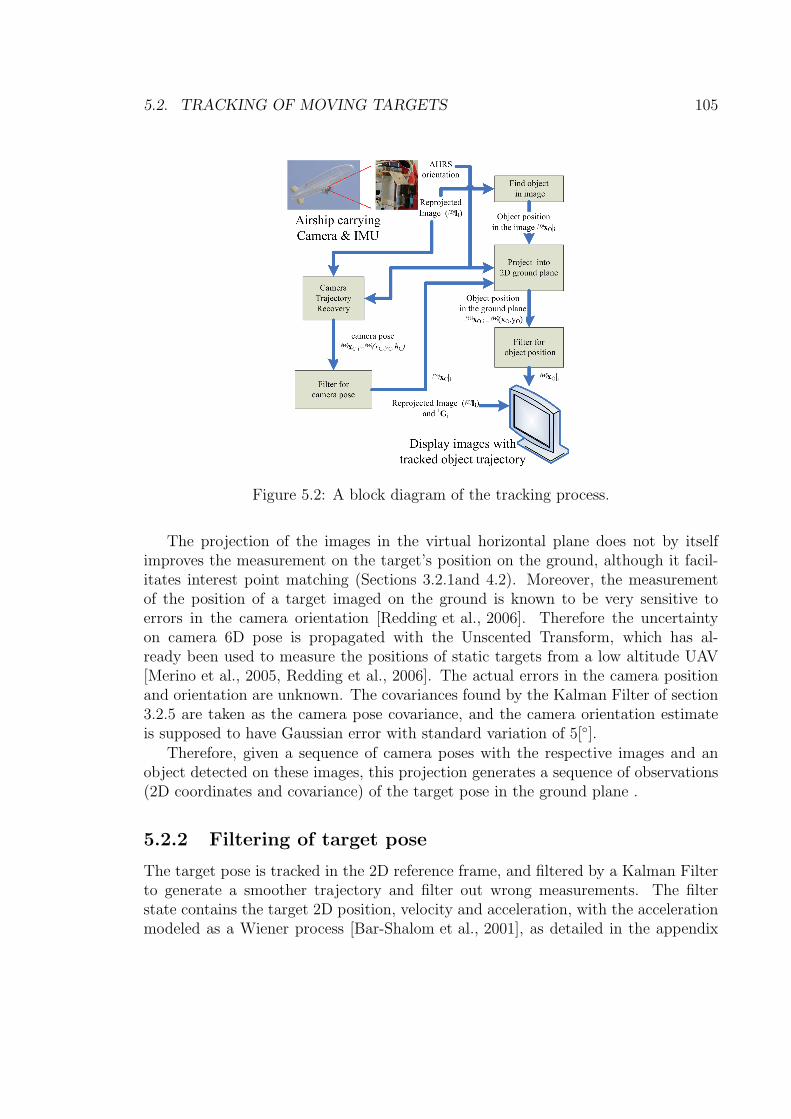
5.2. TRACKING OF MOVING TARGETS 105
Figure 5.2: A block diagram of the tracking process.
The projection of the images in the virtual horizontal plane does not by itselfimproves the measurement on the target’s position on the ground, although it facil-itates interest point matching (Sections 3.2.1and 4.2). Moreover, the measurementof the position of a target imaged on the ground is known to be very sensitive toerrors in the camera orientation [Redding et al., 2006]. Therefore the uncertaintyon camera 6D pose is propagated with the Unscented Transform, which has al-ready been used to measure the positions of static targets from a low altitude UAV[Merino et al., 2005, Redding et al., 2006]. The actual errors in the camera positionand orientation are unknown. The covariances found by the Kalman Filter of section3.2.5 are taken as the camera pose covariance, and the camera orientation estimateis supposed to have Gaussian error with standard variation of 5[◦].
Therefore, given a sequence of camera poses with the respective images and anobject detected on these images, this projection generates a sequence of observations(2D coordinates and covariance) of the target pose in the ground plane .
5.2.2 Filtering of target pose
The target pose is tracked in the 2D reference frame, and filtered by a Kalman Filterto generate a smoother trajectory and filter out wrong measurements. The filterstate contains the target 2D position, velocity and acceleration, with the accelerationmodeled as a Wiener process [Bar-Shalom et al., 2001], as detailed in the appendix
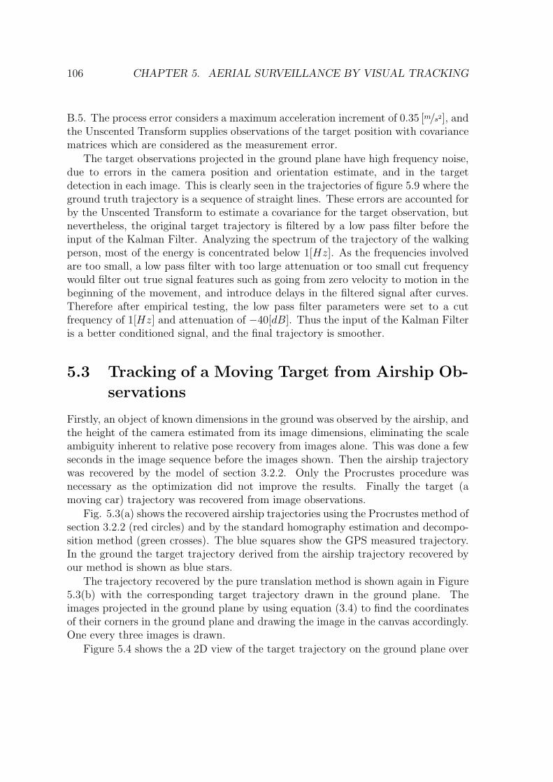
106 CHAPTER 5. AERIAL SURVEILLANCE BY VISUAL TRACKING
B.5. The process error considers a maximum acceleration increment of 0.35 [m/s2], andthe Unscented Transform supplies observations of the target position with covariancematrices which are considered as the measurement error.
The target observations projected in the ground plane have high frequency noise,due to errors in the camera position and orientation estimate, and in the targetdetection in each image. This is clearly seen in the trajectories of figure 5.9 where theground truth trajectory is a sequence of straight lines. These errors are accounted forby the Unscented Transform to estimate a covariance for the target observation, butnevertheless, the original target trajectory is filtered by a low pass filter before theinput of the Kalman Filter. Analyzing the spectrum of the trajectory of the walkingperson, most of the energy is concentrated below 1[Hz]. As the frequencies involvedare too small, a low pass filter with too large attenuation or too small cut frequencywould filter out true signal features such as going from zero velocity to motion in thebeginning of the movement, and introduce delays in the filtered signal after curves.Therefore after empirical testing, the low pass filter parameters were set to a cutfrequency of 1[Hz] and attenuation of −40[dB]. Thus the input of the Kalman Filteris a better conditioned signal, and the final trajectory is smoother.
5.3 Tracking of a Moving Target from Airship Ob-servations
Firstly, an object of known dimensions in the ground was observed by the airship, andthe height of the camera estimated from its image dimensions, eliminating the scaleambiguity inherent to relative pose recovery from images alone. This was done a fewseconds in the image sequence before the images shown. Then the airship trajectorywas recovered by the model of section 3.2.2. Only the Procrustes procedure wasnecessary as the optimization did not improve the results. Finally the target (amoving car) trajectory was recovered from image observations.
Fig. 5.3(a) shows the recovered airship trajectories using the Procrustes method ofsection 3.2.2 (red circles) and by the standard homography estimation and decompo-sition method (green crosses). The blue squares show the GPS measured trajectory.In the ground the target trajectory derived from the airship trajectory recovered byour method is shown as blue stars.
The trajectory recovered by the pure translation method is shown again in Figure5.3(b) with the corresponding target trajectory drawn in the ground plane. Theimages projected in the ground plane by using equation (3.4) to find the coordinatesof their corners in the ground plane and drawing the image in the canvas accordingly.One every three images is drawn.
Figure 5.4 shows the a 2D view of the target trajectory on the ground plane over

5.3. TRACKING OF A MOVING TARGET FROM AIRSHIP OBSERVATIONS107
(a) Airship trajectories from GPS, pure transla-tion and image-only method. Target trajectoryderived from pure translation airship trajectory.
(b) Trajectories recovered by the pure transla-tion method, with registered images.
Figure 5.3: A 3D view of the recovered trajectories from Visual Odometry and fromGPS, for the target and airship.
the corresponding images for the pure translation (a) and image-only (b) methods.The error in height estimation for the image only method is apparent in figure 5.4(b)as an exaggeration in the size of the last images. The same low pass and Kalmanfilters were used with both methods.
5.3.1 Tracking after fusing GPS and Visual Odometry
In this experiment the car has been driven in a closed loop in the ground while theairship was flying above it. The translation recovered by the visual odometry wasfused with GPS position fixes by a Kalman Filter with a constant acceleration model[Bar-Shalom et al., 2001]. The GPS outputs standard deviation values for its positionfixes (shown as the red ellipses and red points in Fig. 5.5), and the translationvectors from the visual odometry are interpreted as a velocity measurement, witha manually set covariance smaller in the vertical axis than in the horizontal ones.The GPS absolute position fixes keep the estimated airship position from diverging,while the visual odometry measurements improve the trajectory locally. The fusedairship trajectory is shown as green crosses in Fig. 5.5, while the target observationsare shown as blue points in the ground plane. The target could not be continouslyobserved, therefore the straight lines (for example the straight lines crossing the path)indicate where observations were missing and resumed at some other point of the path.
Figure 5.6(a) shows the target trajectory drawn over a satellite image of the flightarea. The airship trajectory was taken directly from GPS. Figure 5.6(b) shows thesame target trajectory obtained when the airship trajectory is recovered by a KalmanFilter fusing both visual odometry and GPS. In both figures, the squares show the
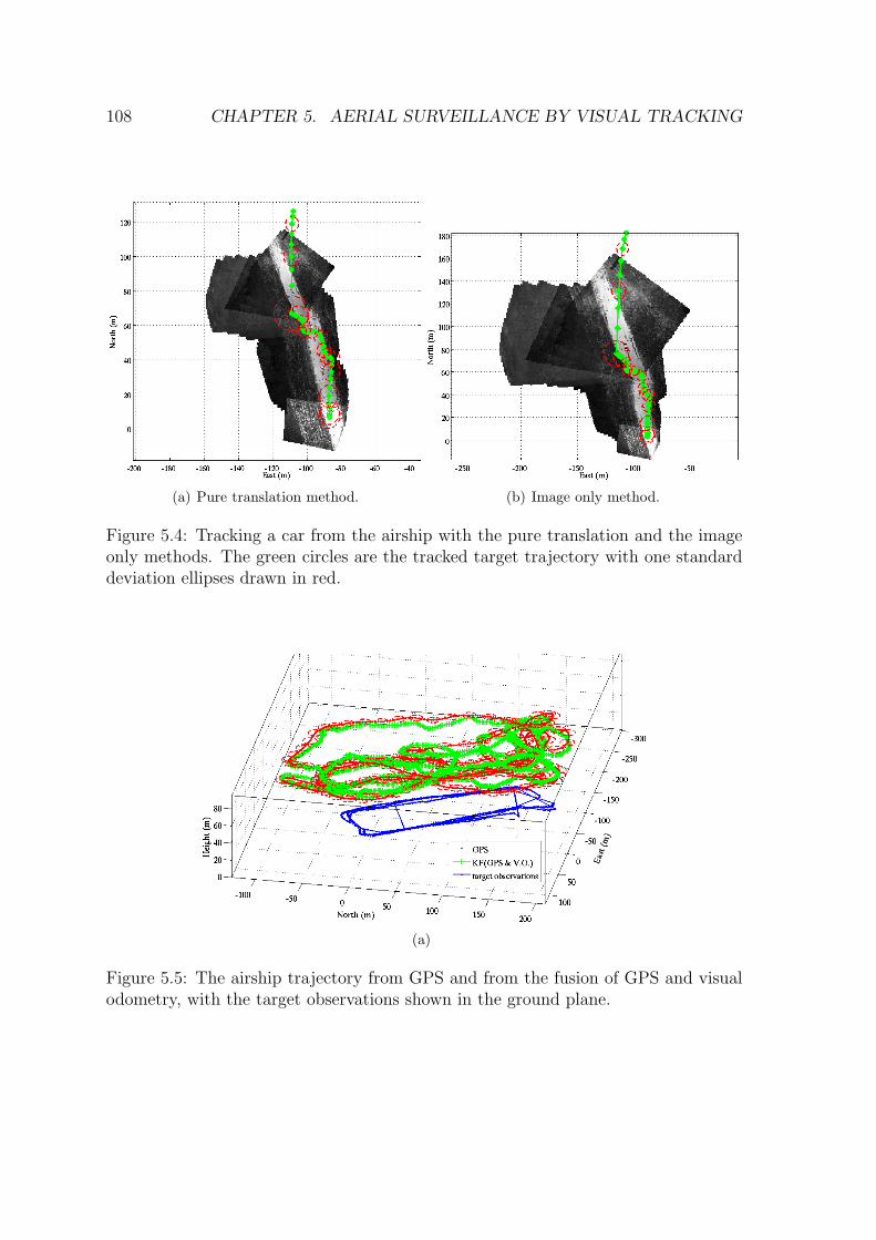
108 CHAPTER 5. AERIAL SURVEILLANCE BY VISUAL TRACKING
(a) Pure translation method. (b) Image only method.
Figure 5.4: Tracking a car from the airship with the pure translation and the imageonly methods. The green circles are the tracked target trajectory with one standarddeviation ellipses drawn in red.
(a)
Figure 5.5: The airship trajectory from GPS and from the fusion of GPS and visualodometry, with the target observations shown in the ground plane.
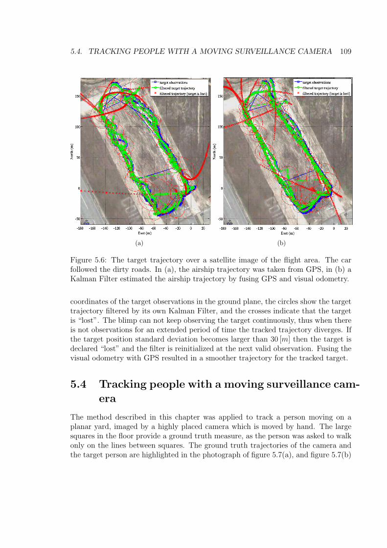
5.4. TRACKING PEOPLE WITH A MOVING SURVEILLANCE CAMERA 109
(a) (b)
Figure 5.6: The target trajectory over a satellite image of the flight area. The carfollowed the dirty roads. In (a), the airship trajectory was taken from GPS, in (b) aKalman Filter estimated the airship trajectory by fusing GPS and visual odometry.
coordinates of the target observations in the ground plane, the circles show the targettrajectory filtered by its own Kalman Filter, and the crosses indicate that the targetis “lost”. The blimp can not keep observing the target continuously, thus when thereis not observations for an extended period of time the tracked trajectory diverges. Ifthe target position standard deviation becomes larger than 30 [m] then the target isdeclared “lost” and the filter is reinitialized at the next valid observation. Fusing thevisual odometry with GPS resulted in a smoother trajectory for the tracked target.
5.4 Tracking people with a moving surveillance cam-era
The method described in this chapter was applied to track a person moving on aplanar yard, imaged by a highly placed camera which is moved by hand. The largesquares in the floor provide a ground truth measure, as the person was asked to walkonly on the lines between squares. The ground truth trajectories of the camera andthe target person are highlighted in the photograph of figure 5.7(a), and figure 5.7(b)
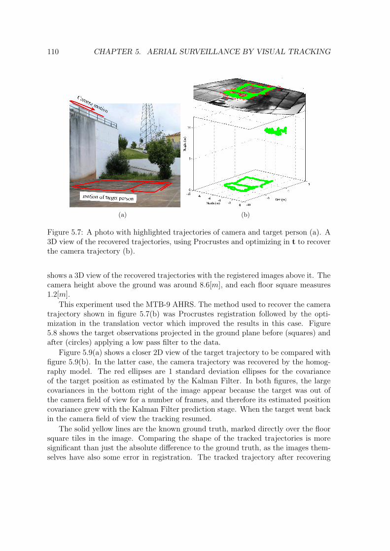
110 CHAPTER 5. AERIAL SURVEILLANCE BY VISUAL TRACKING
(a) (b)
Figure 5.7: A photo with highlighted trajectories of camera and target person (a). A3D view of the recovered trajectories, using Procrustes and optimizing in t to recoverthe camera trajectory (b).
shows a 3D view of the recovered trajectories with the registered images above it. Thecamera height above the ground was around 8.6[m], and each floor square measures1.2[m].
This experiment used the MTB-9 AHRS. The method used to recover the cameratrajectory shown in figure 5.7(b) was Procrustes registration followed by the opti-mization in the translation vector which improved the results in this case. Figure5.8 shows the target observations projected in the ground plane before (squares) andafter (circles) applying a low pass filter to the data.
Figure 5.9(a) shows a closer 2D view of the target trajectory to be compared withfigure 5.9(b). In the latter case, the camera trajectory was recovered by the homog-raphy model. The red ellipses are 1 standard deviation ellipses for the covarianceof the target position as estimated by the Kalman Filter. In both figures, the largecovariances in the bottom right of the image appear because the target was out ofthe camera field of view for a number of frames, and therefore its estimated positioncovariance grew with the Kalman Filter prediction stage. When the target went backin the camera field of view the tracking resumed.
The solid yellow lines are the known ground truth, marked directly over the floorsquare tiles in the image. Comparing the shape of the tracked trajectories is moresignificant than just the absolute difference to the ground truth, as the images them-selves have also some error in registration. The tracked trajectory after recovering

5.4. TRACKING PEOPLE WITH A MOVING SURVEILLANCE CAMERA 111
(a) Camera trajectory recovered by the ho-mography model.
Figure 5.8: A low pass filter is applied to the observed target trajectory.
the camera trajectory with the pure translation model appears more accurate thanwhen the homography model is used.
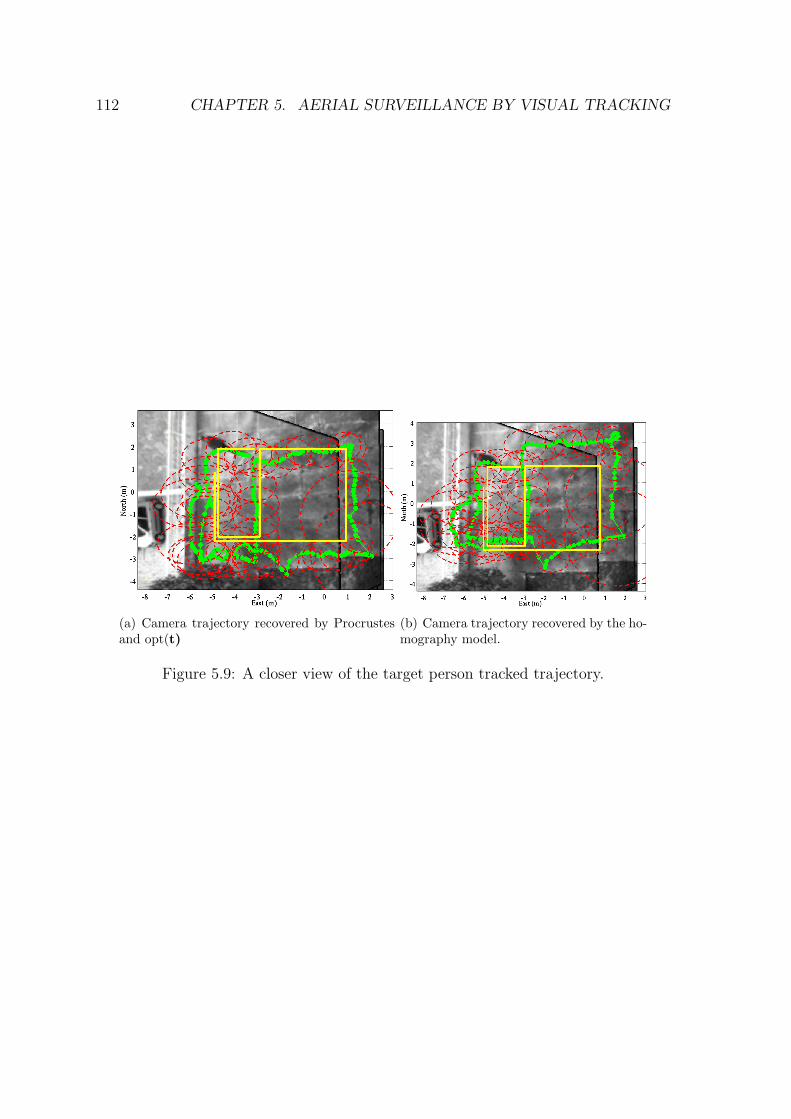
112 CHAPTER 5. AERIAL SURVEILLANCE BY VISUAL TRACKING
(a) Camera trajectory recovered by Procrustesand opt(t)
(b) Camera trajectory recovered by the ho-mography model.
Figure 5.9: A closer view of the target person tracked trajectory.
Chapter 6
Conclusions
In this thesis, pure translation models are used to recover an airship UAV trajectoryusing AHRS orientation estimates and aerial images of the horizontal ground plane.The sets of points projected in the ground plane may be directly registered. Theoreti-cally, this is an instance of the well-known Procrustes problem [Gower and Dijksterhuis, 2004],with closed-form solution, but with real datasets sometimes optimization approachesmay improve the results, for example taking the translation vector itself as the op-timization variable. The other alternative, the homology model, is derived fromprojective geometry, being the special case of the homography transformation underpure translation.
These models were also compared with the usual homography model againstground truth, by determining relative heights in the tripod experiments and re-covering the camera trajectory in the overpass experiment. The screwdriver tableexperiment showed that horizontal and vertical displacements can also be recoveredwith the homology model, even if the FOE is very close to the camera principal pointor very large, tending to infinite as the trajectory is parallel to the image plane.
The experiments with aerial image datasets show that the optimization proposedappears to be unnecessary with the more accurate AHRS, as faster non-iterative so-lutions are obtained by directly registering the correspondences, and the optimizationprovides very small or no improvement in the results. Optimization is also not neces-sary in the tripod and overpass experiment where the camera is static or moves onlyslowly.
Nevertheless, with the less accurate AHRS the best visual odometry results for theairship were obtained by a projective model (FOE estimation and planar homologies)which required an optimization step. Future work may explore the limit conditionswhere the Procrustes registration fails and other approaches are necessary.
The vehicle poses recovered by the visual odometry were compared with the vehicleposes estimated by GPS by generating maps of the ground plane, and the visual
113
114 CHAPTER 6. CONCLUSIONS
odometry results in locally more coherent image alignment. GPS and visual odometrydata were also fused by a Kalman Filter, and the map generated with the fusedtrajectory is more accurate than the map generated with the GPS alone, even if thetrajectory is too large to be recovered by visual odometry alone.
Over-parameterization is usually recommended in the case of homography es-timation (the nine elements of the matrix are estimated although it has only eightdegrees of freedom [Hartley and Zisserman, 2000]). In the pure translation case, over-parameterization with homogeneous variables was also found to be necessary.
The pure translation models have performed better than the image-only approachin the recovery of the vertical motion component. Vertical motion is more criticalbecause errors in the height estimation propagate not only in the vertical component,but also as an error in the scale of the horizontal components. The effect of erroraccumulation in vertical motion is visible in figure 3.21: the recovered trajectorieshave a relatively correct shape but a wrong scale.
Altitude estimation is important for aerial vehicles, and GPS altitude measure-ments are less accurate in the altitude axis than in the horizontal axes. During landingand taking off, GPS uncertainty may be very significant due to the small height, andthe restriction to horizontal ground planes is likely to be valid. Also in high altitudesthe ground plane can often be safely assumed as horizontal. Moreover, reasonablepose estimates were obtained even with the orientation estimates directly output bythe relatively inexpensive and inaccurate AHRS utilized, and under relatively largeroll and pitch variations.
Certainly, even under pure translation motion, image-based measurements are notsufficient to find the correct scale of the translation. Scale ambiguity is inherent to rel-ative pose retrieval from images, even when using homographies [Merino et al., 2006].However, as image-based visual odometry may be integrated with other measurements[Kelly et al., 2007], the fact that in the pure translation model rotational, vertical,and horizontal motion are explicitly separated should facilitate the data fusion neededto recover the actual scale and improve the overall relative pose estimate. For ex-ample, other sensors which measure the direction of movement, even if relativelyinaccurate, could contribute to the initial estimate before the final optimization.
The computer vision community has sporadically used planar homologies for atleast ten years, but not as widely as homographies. To our knowledge the puretranslation models have never been used successfully for trajectory recovery froma real aerial image sequence. Possible reasons include the relative difficulty andexpense of obtaining good orientation estimates until some years ago, or even lack ofcommunication between the robotics and computer vision communities.
Another reason may be that the estimation of the homology with unknown axis,vector and cross ratio, empirically appears to be less reliable and more vulnerable toconvergence into local minima than the homography estimation and decomposition
115
process which has already become usual in the computer vision community. Thefurther simplification of supposing the ground plane horizontal and therefore usingthe virtual camera with an image plane parallel to it, improves much the reliabilityof the estimation.
Future work can explore more elaborate error models, e.g., estimating an uncer-tainty for each pixel coordinate by propagating the uncertainty in the camera 6D pose.Procrustes problem variants with diverse uncertainty models have been solved, al-though for some cases there are only non-iterative solutions [Gower and Dijksterhuis, 2004].The FOE estimation algorithm could be adapted by taking into account these uncer-tainties when calculating epipolar distances.
Other constraints between the recovered vehicle poses could be extracted fromthe map formed by the reprojected images by matching other image pairs, thus aSLAM method could improve both the map and the vehicle poses. Such methodmust consider that when one vehicle pose is updated by a new constraint, the scaleof all subsequent translation vectors from the visual odometry must be also updated.
The tracking experiments further exploited the improvements in camera trajectoryrecovery, with the same rotation compensated images being used to track an indepen-dently moving target in the ground plane. Using the pure translation model to recoverthe camera trajectory resulted in a more accurate trajectory for the tracked objectthan using the homography model. In a low altitude setting recovering the trajectoryfrom the images represents a significant improvement, because GPS uncertainty isvery significant, particularly as uncertainty in its altitude estimate is projected asuncertainty in the tracked object position. The fusion of Visual Odometry and GPSposition fixes in the airship scenario improved the recovered airship trajectory, andthese improvements translate in a smoother recovered trajectory for the moving tar-get in the ground. The tracking can also be performed over an extended period oftime.
In the context of urban people surveillance, the camera could be carried by amobile robot to extend the coverage of a network of static cameras, being able tofocus the surveillance by moving towards a detected occurrence. In such context visualodometry can be fused with wheel odometry or beacon-based localization systems,and the surveillance of an horizontal plane at a lower level is a likely scenario.
In the domain of 3D point clouds registration, the inertial orientation measure-ments also permitted to deal with the rotational and translational components sepa-rately. The compensation of the rotational component is very fast (it just applies arotation to the points) and may accelerate considerably a posterior ICP registration,besides improving its reliability.
The second part of the method, the approximation of the translational compo-nent using the image correspondences, does not represent a large time saving if itsis necessary to apply ICP afterwards to fine-tune the registration. ICP quickly ap-

116 CHAPTER 6. CONCLUSIONS
proximates the remaining translation when its input are rotation-compensated pointclouds. Besides that, the time necessary to calculate the translational components isaround 30% to 50% of the time needed to run ICP in this case.
To decide if this technique should be applied, alone or as a first approximation toICP, the developer should consider the characteristics of its particular sensor setupand the application requisites in terms of accuracy and reliability. We highlight thefollowing points to consider:
1. The computational time spent in the calculation of the translational componentis dominated by the interest point detection and matching algorithm. If interestpoint matching is already being done for other purposes, then the additionalcost of RANSAC is very small.
2. Even with interest point matching, the total time spent by this method is con-siderably less than with ICP. Depending of the application, the approximationof the translational components may be good enough and the final ICP may bedismissed. For example in the stereo results of section 4.4.6, the point cloudsregistered using this method are visually indistinguishable from the same pointclouds registered using ICP. On the other hand, when using the LRF, the pointcloud is more sparse, the association of image pixels and 3D points is less accu-rate, and thus the results are not so accurate.
3. The approximation of the translational component represents a better startingpoint for ICP. In some cases, such as registration of point clouds with onlypartial overlap, this may allow ICP to avoid a wrong registration due to localminima. Therefore the larger computational cost may be paid off by increasedreliability. In the LRF case, as the time needed to tilt the LRF to collect a 3Dscan is significant, it is reasonable to think that in any robotic application thedistance traveled between two consecutive 3D scans will also be relatively large.Therefore in the LRF case it is more likely that this method would be useful toapproximate the translation before applying ICP.
Bibliography
[Alves et al., 2003] Alves, J., Lobo, J., and Dias, J. (2003). Camera-Inertial Sensormodelling and alignment for Visual Navigation. In Proceedings of the 11th Inter-national Conference on Advanced Robotics, pages 1693–1698, Coimbra, Portugal.
[Arnspang et al., 1999] Arnspang, J., Henriksen, K., and Bergholm, F. (1999). Re-lating scene depth to image ratios. In Solina, F. and Leonardis, A., editors, Proc. ofthe 8th Int. Conf. on Computer Analysis of Images and Patterns (CAIP’99), vol-ume 1689 of Lecture Notes in Comp. Science, pages 516–525, Ljubljana, Slovenia.Springer.
[Bar-Shalom et al., 2001] Bar-Shalom, Y., Li, X. R., and Kirubarajan, T. (2001).Estimation with Applications to Tracking and Navigation. John Willey & Sons,Inc.
[Bay et al., 2006] Bay, H., Tuytelaars, T., and van Gool, L. (2006). SURF: SpeededUp Robust Features. In the Ninth European Conference on Computer Vision, Graz,Austria.
[Besl and McKay, 1992] Besl, P. and McKay, N. (1992). A method for registration of3-d shapes [ICP]. IEEE Pattern Analysis and Machine Intelligence, 14(2):239–256.
[Borg and Groenen, 1997] Borg and Groenen (1997). Modern Multidimensional Scal-ing, Theory and Application. Springer Verlag.
[Bouguet, 2006] Bouguet, J. (2006). Camera Calibration Toolbox for Matlab.http://www.vision.caltech.edu/bouguetj/calib_doc/index.html.
[Bronshtein and Semendyayev, 1997] Bronshtein, I. N. and Semendyayev, K. A.(1997). Handbook of mathematics (3rd ed.). Springer-Verlag, London, UK.
[Brown and Sullivan, 2002] Brown, A. and Sullivan, D. (2002). Precision kinematicalignment using a low-cost GPS/INS system. In ION GPS, Portland, OR, USA.
117
118 BIBLIOGRAPHY
[Brown, 2006] Brown, M. (2006). Autostitch: Automated panorama creation.http://www.cs.ubc.ca/ mbrown/autostitch/autostitch.html.
[Brown and Lowe, 2003] Brown, M. and Lowe, D. G. (2003). Recognising panoramas.In 10th Int. Conf. on Computer Vision (ICCV), Nice, France.
[Caballero et al., 2006] Caballero, F., Merino, L., Ferruz, J., and Ollero, A. (2006).Improving vision-based planar motion estimation for unmanned aerial vehiclesthrough online mosaicing. In IEEE Int. Conf. on Robotics and Automation(ICRA06), pages 2860–2865, Orlando, FL, USA.
[Capel et al., 2006] Capel, D., Fitzgibbon, A., Kovesi, P., Werner, T., Wexler,Y., and Zisserman, A. (2006). Matlab functions for multiple view geometry.http://www.robots.ox.ac.uk/∼vgg/hzbook/code/.
[Capel, 2001] Capel, D. P. (2001). Image Mosaicing and Super-resolution. PhD thesis,University of Oxford, Oxford, UK.
[Chen et al., 2003] Chen, Z., Pears, N., McDermid, J., and Heseltine, T. (2003).Epipole estimation under pure camera translation. In Sun, C., Talbot, H., Ourselin,S., and Adriaansen, T., editors, Proc. of the 7th Int. Conf. on Digital Image Com-puting: Techniques and Applications, DICTA 2003, pages 849–858, Sydney, Aus-tralia. CSIRO Publishing.
[Cheng et al., 2006] Cheng, Y., Maimone, M. W., and Matthies, L. (2006). Visualodometry on the mars exploration rovers. IEEE Robotics and Automation Maga-zine, 13(2):54–62.
[Corke et al., 2001] Corke, P., Sikka, P., and Roberts, J. M. (2001). Height estimationfor an autonomous helicopter. In ISER ’00: Experimental Robotics VII, pages 101–110, London, UK. Springer-Verlag.
[Cunningham et al., 2006] Cunningham, D., Grebby, S., Tansey, K., and Gosar, A.(2006). Application of airborne LiDAR to mapping seismogenic faults in forestedmountainous terrain, southeastern Alps, Slovenia. Geophysical Research Letters,33.
[de Paiva et al., 2006] de Paiva, E. C., Azinheira, J. R., Ramos, J. J. G., Moutinho,A., and Bueno, S. S. (2006). Project AURORA: Infrastructure and flight controlexperiments for a robotic airship. Journal of Field Robotics, 23(3-4):201–222.
[Diel, 2005] Diel, D. D. (2005). Stochastic constraints for vision-aided inertial navi-gation. Master’s thesis, Dept. of Mechanical Engineering - Massachussetts Instituteof Technology, Cambridge, MA, USA.
BIBLIOGRAPHY 119
[Eden et al., 2006] Eden, A., Uyttendaele, M., and Szeliski, R. (2006). Seamlessimage stitching of scenes with large motions and exposure differences. In CVPR’06: Proceedings of the 2006 IEEE Computer Society Conference on ComputerVision and Pattern Recognition, pages 2498–2505, Washington, DC, USA. IEEEComputer Society.
[Eustice, 2005] Eustice, R. M. (2005). Large-Area Visually Augmented Navigation forAutonomous Underwater Vehicles. PhD thesis, Massachusetts Institute of Tech-nology / Woods Hole Oceanographic Institution - Joint Program in Applied OceanScience & Engineering.
[Fischler and Bolles, 1981] Fischler, M. A. and Bolles, R. C. (1981). Random sampleconsensus: A paradigm for model fitting with applications to image analysis andautomated cartography. Comm. of the ACM, 24:381–395.
[Garmin Int. Inc., 2007] Garmin Int. Inc. (2007). www.garmin.com.
[Gower and Dijksterhuis, 2004] Gower, J. C. and Dijksterhuis, G. B. (2004). Pro-crustes Problems. Oxford Statistical Science Series. Oxford University Press.
[Gracias, 2002] Gracias, N. R. E. (2002). Mosaic-based Visual Navigation for Au-tonomous Underwater Vehicles. PhD thesis, Universidade Técnica de Lisboa -Instituto Superior Técnico, Lisbon, Portugal.
[Hartley and Zisserman, 2000] Hartley, R. and Zisserman, A. (2000). Multiple ViewGeometry in Computer Vision. Cambridge University Press, Cambridge, UK.
[Hirschmüller et al., 2002] Hirschmüller, H., Innocent, P. R., and Garibaldi, J. (2002).Fast, unconstrained camera motion estimation from stereo without tracking androbust statistics. In 7th International Conference on Control, Automation, Roboticsand Vision, Singapore.
[Horn, 1987] Horn, B. (1987). Closed-Form Solution of Absolute Orientation UsingUnit Quaternions. Journal of the Optical Society of America, 4(4):629–462.
[Huguet et al., 2003] Huguet, A. B., Carceroni, R. L., and de A. Araújo, A. (2003).Towards automatic 3d reconstruction of urban scenes from low altitude aerial im-ages. In IEEE 12th Int. Conf. on Image Analysis and Processing (ICIAP’03),Mantova, Italy.
[Hygounenc et al., 2004] Hygounenc, E., Jung, I.-K., Soueres, P., and Lacroix, S.(2004). The Autonomous Blimp Project at LAAS/CNRS: Achievements in FlightControl and Terrain Mapping. Int. J. of Robotics Research, 23(4/5):473–512.
120 BIBLIOGRAPHY
[Julier and Uhlmann, 1997] Julier, S. J. and Uhlmann, J. K. (1997). A new extensionof the kalman filter to nonlinear systems. In Int. Symp. Aerospace/Defense Sensing,Simul. and Controls, Orlando, FL, USA.
[Kelly et al., 2007] Kelly, J., Saripalli, S., and Sukhatme, G. S. (2007). Combinedvisual and inertial navigation for an unmanned aerial vehicle. In Proc. 6th Int’lConf. Field and Service Robotics (FSR’07), Chamonix, France.
[Kim, 2004] Kim, J. (2004). Autonomous Navigation for Airborne Applications. PhDthesis, The University of Sydney, Sydney, NSW, Australia.
[Kleiner et al., 2005] Kleiner, A., Steder, B., Dornhege, C., Hoefler, D., Meyer-Delius,D., Prediger, J., Stueckler, J., Glogowski, K., Thurner, M., Luber, M., Schnell, M.,Kuemmerle, R., Burk, T., Braeuer, T., and Nebel, B. (2005). RoboCupRescue- RescueRobots Freiburg (Germany), Team Description Paper. In Rescue RobotLeague, Osaka, Japan.
[Konolige, 1997] Konolige, K. (1997). Small vision systems: Hardware and implemen-tation. In Eight International Symposium on Robotics Research, Hayama, Japan.
[Liang et al., 2004] Liang, B., Pears, N., and Chen, Z. (2004). Affine height land-scapes for monocular mobile robot obstacle avoidance. In Groen, F., Amato, N.,Bonarini, A., Yoshida, E., and Kröse, B., editors, Intelligent Autonomous Systems8, pages 863–872, Amsterdam, The Netherlands. IOS Press.
[Lobo and Dias, 2003] Lobo, J. and Dias, J. (2003). Vision and inertial sensor coop-eration using gravity as a vertical reference. IEEE Trans. on Pattern Analysis andMachine Intelligence, 25(12):1597–1608.
[Lobo and Dias, 2005] Lobo, J. and Dias, J. (2005). Relative pose calibration betweenvisual and inertial sensors. In ICRA Workshop on Integration of Vision and InertialSensors - 2nd InerVis, Barcelona, Spain.
[Lobo and Dias, 2007] Lobo, J. and Dias, J. (2007). Relative pose calibration betweenvisual and inertial sensors. International Journal of Robotics Research, 26(6):561–575.
[Lobo et al., 2006] Lobo, J., Ferreira, J. F., and Dias, J. (2006). Bioinspired visuo-vestibular artificial perception system for independent motion segmentation. InICVW06 (2nd Int. Cognitive Vision Workshop), Graz, Austria.
[Lowe, 2004] Lowe, D. G. (2004). Distinctive image features from scale-invariantkeypoints. International Journal of Computer Vision, 60(2):91–110.
BIBLIOGRAPHY 121
[Ma et al., 2004] Ma, Y., Soatto, S., Kosecka, J., and Sastry, S. (2004). An Invitationto 3D Vision. Springer.
[Makadia and Daniilidis, 2005] Makadia, A. and Daniilidis, K. (2005). Correspon-denceless ego-motion estimation using an imu. In Proceedings of the IEEE Inter-national Conferenece on Robotics and Automation.
[Malis, 1998] Malis, E. (1998). Contributions à la modélisation et à la commande enasservissement visuel. PhD thesis, L’Université de Rennes, École de Informatique,Traitement du Signal et Telecommunications, Rennes, France.
[Malis et al., 1999] Malis, E., Chaumette, F., and Boudet, S. (1999). 2-12-D Visual
Servoing . IEEE Trans. on Robotics and Automation, 15(2):238–250.
[Matthies and Shafer, 1987] Matthies, L. and Shafer, S. (1987). Error modeling instereo navigation. IEEE J. of Robotics and Automation, RA-3(3).
[Merino et al., 2005] Merino, L., Caballero, F., de Dios, J., and Ollero, A. (2005).Cooperative fire detection using unmanned aerial vehicles. In IEEE InternationalConference on Robotics and Automation, pages 1896–1901, Barcelona, Spain.
[Merino et al., 2006] Merino, L., Wiklund, J., Caballero, F., Moe, A., de Dios, J.R. M., Forssen, P.-E., Nordberg, K., and Ollero, A. (2006). Vision-based multi-UAV position estimation. Robotics & Automation Magazine, IEEE, 13(3):53–62.
[Michaelsen et al., 2004] Michaelsen, E., Kirchhof, M., and Stilla, U. (2004). Sen-sor pose inference from airborne videos by decomposing homography estimates.In XXth ISPRS Congress, Istambul, Turkey. The International Society for Pho-togrammetry and Remote Sensing.
[Mikolajczyk and Schmid, 2004] Mikolajczyk, K. and Schmid, C. (2004). Scale andaffine invariant interest point detectors. International Journal of Computer Vision,60(1).
[Mikolajczyk et al., 2005] Mikolajczyk, K., Tuytelaars, T., Schmid, C., Zisserman,A., Matas, J., Schaffalitzky, F., Kadir, T., and van Gool, L. (2005). A comparisonof affine region detectors. International Journal of Computer Vision, 65(7):43 – 72.
[Mirisola, 2001] Mirisola, L. G. B. (2001). Desenvolvimento da estação de terra doprojeto AURORA. Master’s thesis, Universidade Estadual de Campinas, Institutode Computação, Campinas, SP, Brazil.
[Mirisola and Dias, 2008] Mirisola, L. G. B. and Dias, J. (2008). Complemen-tary results and data to Exploiting inertial sensing in vision based navigation.http://paloma.isr.uc.pt/∼lgm/.
122 BIBLIOGRAPHY
[Mirisola and Dias, 2007] Mirisola, L. G. B. and Dias, J. M. M. (2007). Exploitinginertial sensing in mosaicing and visual navigation. In 6th IFAC Symposium onIntelligent Autonomous Vehicles (IAV07), Toulouse, France.
[Mirisola et al., 2006] Mirisola, L. G. B., Lobo, J., and Dias, J. (2006). Stereo vision3D map registration for airships using vision-inertial sensing. In The 12th IASTEDInt. Conf. on Robotics and Applications (RA 2006), Honolulu, HI, USA.
[Ohno and Tadokoro, 2005] Ohno, K. and Tadokoro, S. (2005). Dense 3D map build-ing based on LRF data and color image fusion. In IEEE Int. Conf. on IntelligentRobots and Systems (IROS 2005), pages 2792– 2797.
[OMG, 2007] OMG, O. M. G. (2007). OMG’s CORBA page. http://www.corba.org.
[Point Grey Inc., 2007] Point Grey Inc. (2007). www.ptgrey.com.
[Redding et al., 2006] Redding, J., McLain, T., Beard, R., and Taylor, C. (2006).Vision-based target localization from a fixed-wing miniature air vehicle. In Amer-ican Control Conference, Minneapolis, MN, USA.
[Saripalli et al., 2003] Saripalli, S., Montgomery, J., and Sukhatme, G. (2003).Visually-guided landing of an unmanned aerial vehicle. IEEE Transactions onRobotics and Automation, 19(3):371–381.
[Scaramuzza et al., 2007] Scaramuzza, D., Harati, A., and Siegwart, R. (2007). Ex-trinsic self calibration of a camera and a 3d laser range finder from natural scenes.In IEEE Int. Conf.on Intelligent Robots and Systems (IROS), San Diego, CA, USA.
[Schiele and Crowley, 1994] Schiele, B. and Crowley, J. L. (1994). A comparison ofposition estimation techniques using occupancy grids. In Int. Conf. on Roboticsand Automation (ICRA94), pages 1628– 1634, San Diego,CA, USA.
[Schmidt, 2007] Schmidt, D. C. (2007). TAO - The ACE ORB.http://www.cs.wustl.edu/∼schmidt/TAO.html.
[Steedly et al., 2005] Steedly, D., Pal, C., and Szeliski, R. (2005). Efficiently reg-istering video into panoramic mosaics. In IEEE Int. Conf. on Computer Vision(ICCV05), Beijing, China.
[Strelow and Singh, 2004] Strelow, D. and Singh, S. (2004). Motion estimation fromimage and inertial measurements. The International Journal of Robotics Research,23(12):1157 – 1195.
BIBLIOGRAPHY 123
[Suter et al., 2002] Suter, D., Hamel, T., and Mahony, R. (2002). Visual servo controlusing homography estimation for the stabilization of an x4-flyer. In 41st IEEE Conf.on Decision and Control, pages 2872–2877, Las Vegas, NV, USA.
[Szeliski, 2004] Szeliski, R. (2004). Image alignment and stitching: A tutorial. Tech-nical Report MSR-TR-2004-92, Microsoft Research.
[Szeliski, 2005] Szeliski, R. (2005). Image alignment and stitching, chapter 17, pages273–292. Handbook of Mathematical Models in Computer Vision. Springer.
[Sünderhauf and Protzel, 2007] Sünderhauf, N. and Protzel, P. (2007). Stereo odom-etry - a review of approaches. In IASTED Conference on Robotics and Applications,Würzburg, Germany.
[Triebel et al., 2006] Triebel, R., Pfaff, P., and Burgard, W. (2006). Multi-level sur-face maps for outdoor terrain mapping and loop closing. In Int. Conf. on IntelligentRobots and Systems (IROS), Beijing, China.
[van Gool et al., 1998] van Gool, L., Proesmans, M., and Zisserman, A. (1998). Pla-nar homologies for grouping and recognition. Image and Vision Computing, 16(21-26).
[XSens Tech., 2007] XSens Tech. (2007). www.xsens.com.

124 BIBLIOGRAPHY
Appendix A
Experimental Platform
This chapter provides a more detailed description of the DIVA airship, complementingthe overview of section 1.4. A high level view of the characteristics and capabilities ofthe current system is presented in section A.1. Then, section A.2 presents the requi-sites for an extension of this system towards automatic flight. Finally, the hardwarecomponents, sensors, and software architecture are shown in section A.3.
A.1 Technical Characteristics of the DIVA AirshipThis section details the technical characteristics of the system which collected thedata used on the experiments shown in chapter 3. They can be considered as therequisites to build an equivalent system. The system is composed by an embeddedsystem and a ground station, which communicate through a wireless link.
A.1.1 Embedded SystemOperational Requisites
• Periodically, the embedded system must read data from all sensors and trans-mit the data to the ground station, with a period compatible with the vehicledynamics.
• The embedded system must integrate at least one camera, capturing imageswith sufficient resolution and frame rate. A modern camera with automaticgain adjustment is necessary as illumination conditions change often during theflight.
• The embedded system must store all telemetry data, besides transmitting themto the ground station, to avoid losing data if the data link is lost. Cameraimages also are stored (the heaviest burden to the CPU and storage system).
125
126 APPENDIX A. EXPERIMENTAL PLATFORM
• If DGPS (Differential GPS) corrections are needed, the embedded system mustreceive DGPS data from the ground station via a reliable data link. GPSposition fixes when DGPS data is intermittent often “jump” between correctedand uncorrected states, which may be worse than having no DGPS correctionat all. A separate low speed link for DGPS data may be advisable.
• Payload weight is a severe limitation for airships. Thus, energy consumptionmust be minimized to decrease battery weight.
Safety Characteristics
• The embedded system must have a Remote Control (RC) receiver to allow ahuman pilot to manually pilot the airship. Figure A.3 shows a Radio ControlUnit (standard aero-modeling equipment), used to pilot the airship.
• There must be a device electrically independent of the CPU to read the servocommands from the RC receiver, able to continue working in case of CPUmalfunctioning. It receives commands from the RC receiver, and relays themto the servo motors and to the CPU to be read and stored.
• The embedded system must be sufficiently resistant to vibration and tilting toresist the flight and motor induced vibration. Vibration isolation (lightweight)may be necessary. Vibration-resistant data storage such as a flash disk is neededto store images.
A.1.2 Ground Station
This section presents the technical characteristics of the ground station.
Data Collection And Storage
• Although the embedded system stores all state variables, the data may not berecoverable due to accidents or malfunctioning. Therefore, the ground stationshould receive and store data from the embedded system.
• The ground station must be easily reconfigurable if there is a change in the dataformat sent by the embedded system (e.g., if a new sensor is added).
• The stored data must be easily converted to a format readable by commercialmathematical software such as MATLABr (e.g., an ASCII format).

A.2. REQUISITES FOR AUTONOMY 127
User Interface: Vehicle Safety And Monitoring The ground station mustmonitor the vehicle state not only to detect hazardous situations (safety issues),but also to avoid useless flights and waste of time in case of malfunctioning. Thehuman pilot and the algorithm developers should determine which variables shouldbe monitored.
• Monitor all critical state variables, i.e., the ones which are essential to the flightsafety or data recording, like tachometers, GPS, camera status, etc. The userinterface must show the state of the most critical variables clearly and contin-uously (but not necessarily the actual numeric value of all of them), indicatingcritical failures with alarms (red lights and/or sounds).
• This monitoring must be active before take-off, so that the ground station op-erator can abort the flight if a critical system is not operating.
Differential GPS
• If differential GPS correction is needed, the ground station should be connectedto a DGPS (Differential GPS) station and transmit its signals to the embeddedsystem.
A.2 Requisites for extension towards an autonomousairship prototype
This section details the requisites necessary to extend the current system towardsautomatic flight, in addition to the requisites already presented in section A.1.1. Anearly version of these requisites, without an on-board camera, is found on [Mirisola, 2001].
A.2.1 Embedded SystemOperational Requirements
• Periodically, the embedded system must also receive from the ground stationcommands and parameters related to the algorithms to be executed, transmitfeedback about their execution, and send commands to the actuators.
• To develop control algorithms based on inputs generated from images, the em-bedded system must also transmit camera images to the ground.
• If more than one camera is utilized to perform some of the tasks described inthis thesis, it is desirable to have synchronized cameras, i.e., cameras which,when connected in the same data bus, can take frames at the same time.

128 APPENDIX A. EXPERIMENTAL PLATFORM
Safety Requirements
• The human pilot must be able to take over the control at his will using a channelon his RC unit. The on-board electronics must detect this command and changeimmediately to manual mode.
• There must be a device electrically independent from the CPU to select be-tween manual and automatic control, able to continue working in case of CPUmalfunctioning. It should receive commands from both the embedded CPU andthe RC receiver, and relay one of them to the servo motors. The commands arealso relayed to the CPU to be stored.
A.2.2 Ground StationGround Station User Interface: Operational These requirements aim to in-crease the usefulness of each flight, reducing the number of flights needed to achievethe intended results.
• For image-based algorithms, the user interface must show the images beingreceived from the embedded system.
• The embedded system may be able to execute different types of mission, withdifferent parameters, e.g., controller gains, or camera parameters as brightness,saturation, etc. Parameter adjustments must be done online via the groundstation, during the flight. It is not desirable to have to land the airship and logon the embedded system to change the a parameter value.
• The operator must be informed about the execution of the mission. Missionrelated information must be displayed over a map of the vehicle trajectory.
Ground Station User Interface: Vehicle Safety And Monitoring
• The user interface must have an Instruments Panel displaying the value ofthe most important variables (e.g. tachometers, altitude, attitude). Underautomatic flight a sensor failure may represent a safety risk.
• The user interface must be able to show graphs of all state variables. They maybe important to evaluate the algorithms being tested and choose new values forparameters.
• To visualize the vehicle in a virtual 3D world is not useful if the virtual world isnot sufficiently detailed to provide visually recognizable references to the user.If the airship is always within visual range a virtual world visualization is alsoless important.
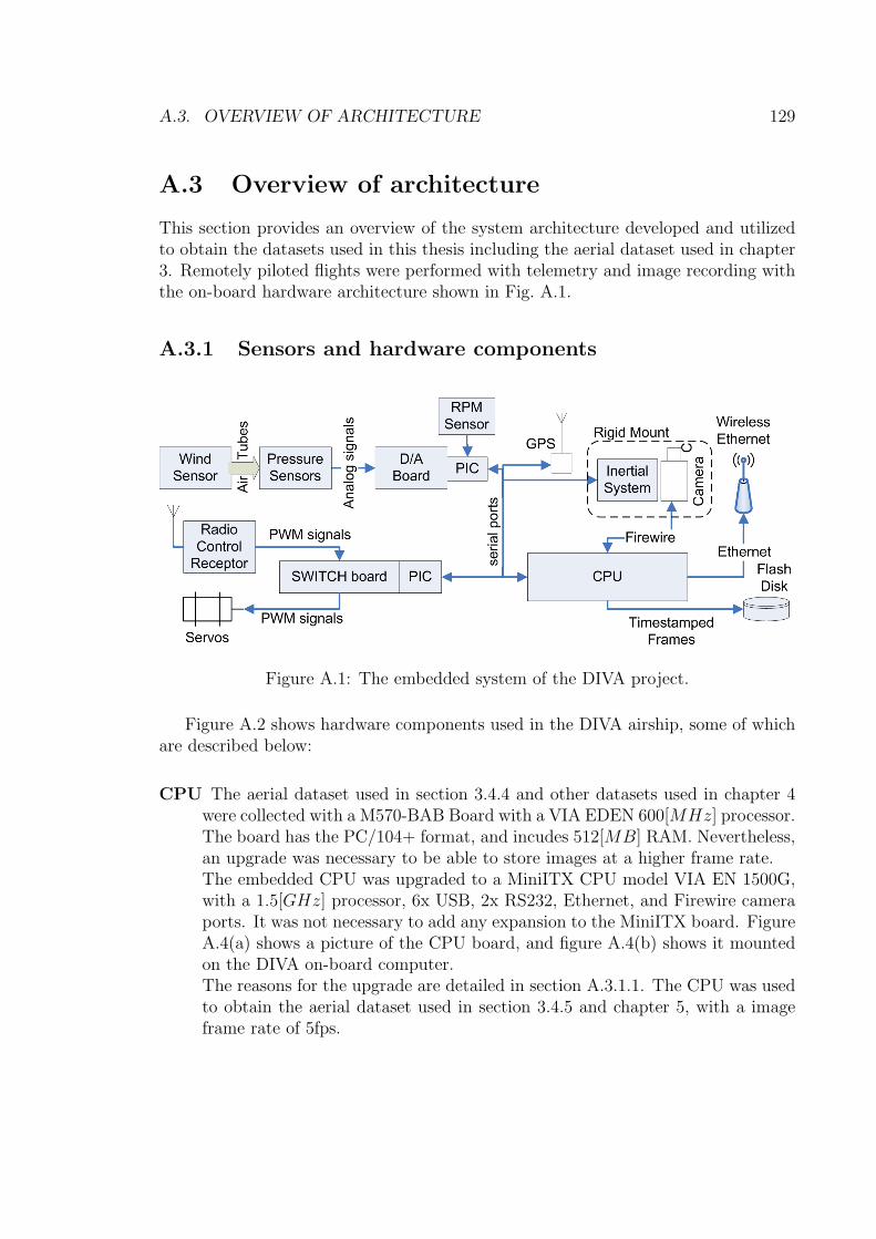
A.3. OVERVIEW OF ARCHITECTURE 129
A.3 Overview of architecture
This section provides an overview of the system architecture developed and utilizedto obtain the datasets used in this thesis including the aerial dataset used in chapter3. Remotely piloted flights were performed with telemetry and image recording withthe on-board hardware architecture shown in Fig. A.1.
A.3.1 Sensors and hardware components
Figure A.1: The embedded system of the DIVA project.
Figure A.2 shows hardware components used in the DIVA airship, some of whichare described below:
CPU The aerial dataset used in section 3.4.4 and other datasets used in chapter 4were collected with a M570-BAB Board with a VIA EDEN 600[MHz] processor.The board has the PC/104+ format, and incudes 512[MB] RAM. Nevertheless,an upgrade was necessary to be able to store images at a higher frame rate.The embedded CPU was upgraded to a MiniITX CPU model VIA EN 1500G,with a 1.5[GHz] processor, 6x USB, 2x RS232, Ethernet, and Firewire cameraports. It was not necessary to add any expansion to the MiniITX board. FigureA.4(a) shows a picture of the CPU board, and figure A.4(b) shows it mountedon the DIVA on-board computer.The reasons for the upgrade are detailed in section A.3.1.1. The CPU was usedto obtain the aerial dataset used in section 3.4.5 and chapter 5, with a imageframe rate of 5fps.
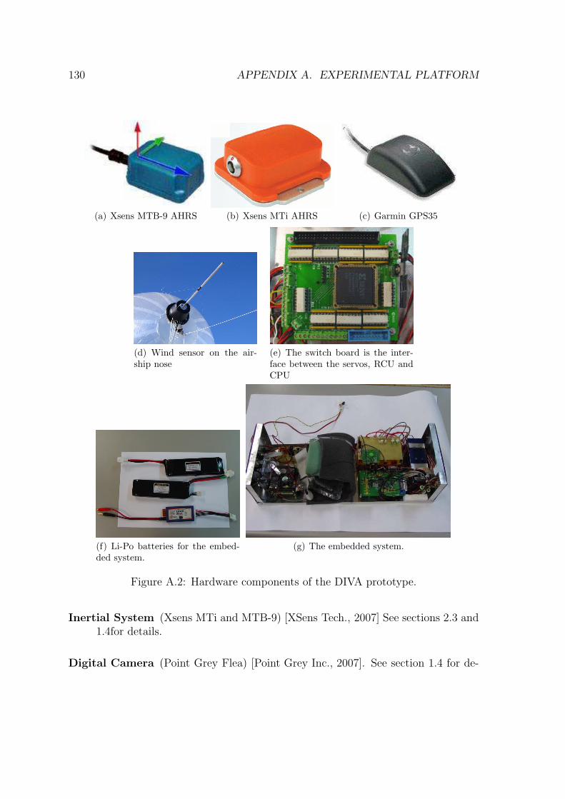
130 APPENDIX A. EXPERIMENTAL PLATFORM
(a) Xsens MTB-9 AHRS (b) Xsens MTi AHRS (c) Garmin GPS35
(d) Wind sensor on the air-ship nose
(e) The switch board is the inter-face between the servos, RCU andCPU
(f) Li-Po batteries for the embed-ded system.
(g) The embedded system.
Figure A.2: Hardware components of the DIVA prototype.
Inertial System (Xsens MTi and MTB-9) [XSens Tech., 2007] See sections 2.3 and1.4for details.
Digital Camera (Point Grey Flea) [Point Grey Inc., 2007]. See section 1.4 for de-

A.3. OVERVIEW OF ARCHITECTURE 131
tails. This camera automatically controls parameters such as gain to adapt toillumination changes. Images were captured during flight, with no need of anyparameter control external to the camera. Bayer images were converted intograyscale images by simple linear interpolation with OpenCV functions.
GPS Receptor (Garmin GPS35 12 channel GPS unit) Low weight GPS receptorand antenna integrated in a single mouse-sized package, with RS-232 commu-nication.
Wind Sensor It is mounted on the airship nose and measures barometric altitude,the angle of attack, sideslip angle and wind speed. It is not yet calibrated.
RPM Sensor Measures the rotation speed of the motors, by counting the number ofinterruptions on an Infra Red light signal that is cut by the propeller movement.
Switch Board The servo-motors on the flaps and motors accelerators are com-manded by Pulse Width Modulation (PWM) signals sent by the human pilotvia the Radio Control Unit. The Switch Board reads the signals from the Ra-dio Control Receiver, transmits their values in digital form (serial port) to theCPU, for recording, and retransmits PWM signals to the servo motors. In fu-ture automatic flights, the same board may switch to transmit commands sentfrom the CPU to the servo motors.As the switch board is responsible to send commands to the servos in both man-ual and automatic modes, a failure on it would render the airship unresponsiveto any command. For safety, it must be able to continue functioning even inthe case of CPU failure. Therefore, it is electrically isolated from the on-boardCPU and servo motors, with a separate battery for power.
Video Storage Vibration resistant storage for images is provided by a fast USB flashdisk. It must be tested by saving a file large enough to fill all buffers involvedin data writing (in the order of hundreds of megabytes), and then observingthe continuous data transfer speed. Actual continuous writing speed is oftenmuch less than the advertised value (respectively 5MB/s and 21MB/s with ourflashdisk).
Besides the on-board system, there is also support equipment on the ground (seeFig. A.3). The human pilot commands the airship with a standard aeromodel RemoteControl Unit, sending PWM signals to command the servo-motors on the flaps andmotor accelerators. Also, a laptop connected to a Wireless Access Point receives,stores and displays telemetry data from the airship.
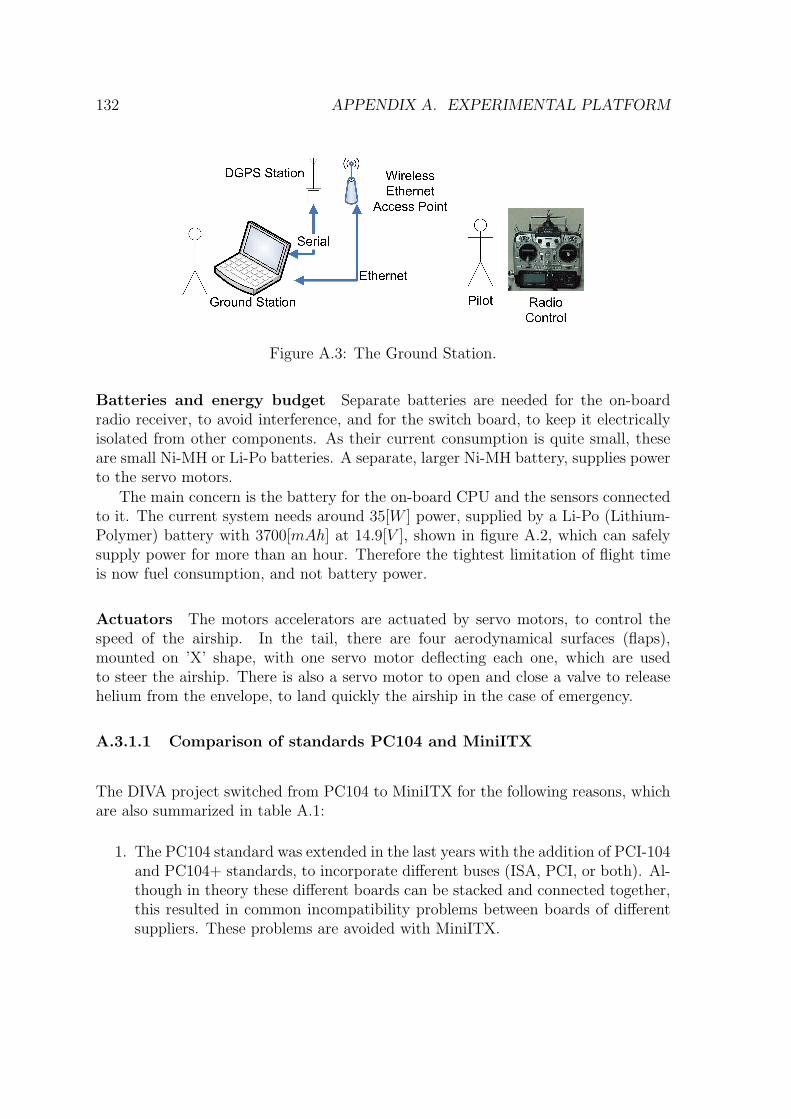
132 APPENDIX A. EXPERIMENTAL PLATFORM
Figure A.3: The Ground Station.
Batteries and energy budget Separate batteries are needed for the on-boardradio receiver, to avoid interference, and for the switch board, to keep it electricallyisolated from other components. As their current consumption is quite small, theseare small Ni-MH or Li-Po batteries. A separate, larger Ni-MH battery, supplies powerto the servo motors.
The main concern is the battery for the on-board CPU and the sensors connectedto it. The current system needs around 35[W ] power, supplied by a Li-Po (Lithium-Polymer) battery with 3700[mAh] at 14.9[V ], shown in figure A.2, which can safelysupply power for more than an hour. Therefore the tightest limitation of flight timeis now fuel consumption, and not battery power.
Actuators The motors accelerators are actuated by servo motors, to control thespeed of the airship. In the tail, there are four aerodynamical surfaces (flaps),mounted on ’X’ shape, with one servo motor deflecting each one, which are usedto steer the airship. There is also a servo motor to open and close a valve to releasehelium from the envelope, to land quickly the airship in the case of emergency.
A.3.1.1 Comparison of standards PC104 and MiniITX
The DIVA project switched from PC104 to MiniITX for the following reasons, whichare also summarized in table A.1:
1. The PC104 standard was extended in the last years with the addition of PCI-104and PC104+ standards, to incorporate different buses (ISA, PCI, or both). Al-though in theory these different boards can be stacked and connected together,this resulted in common incompatibility problems between boards of differentsuppliers. These problems are avoided with MiniITX.
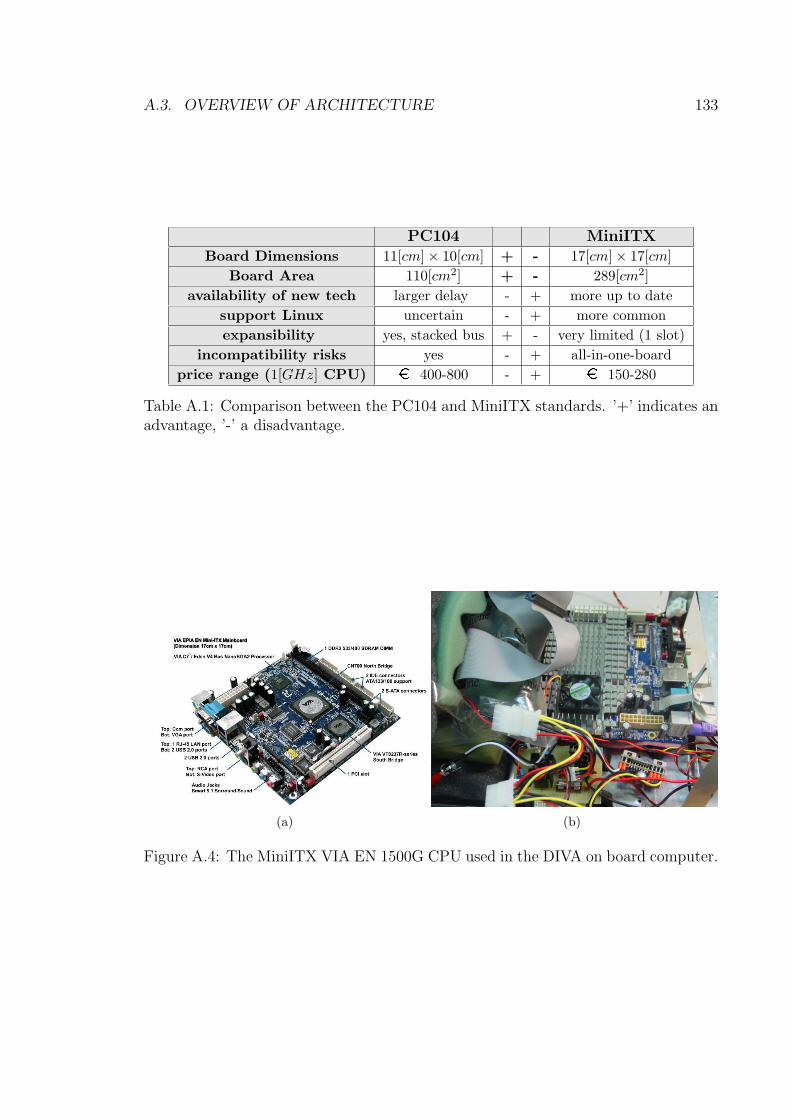
A.3. OVERVIEW OF ARCHITECTURE 133
PC104 MiniITXBoard Dimensions 11[cm]× 10[cm] + - 17[cm]× 17[cm]
Board Area 110[cm2] + - 289[cm2]availability of new tech larger delay - + more up to date
support Linux uncertain - + more commonexpansibility yes, stacked bus + - very limited (1 slot)
incompatibility risks yes - + all-in-one-boardprice range (1[GHz] CPU) � 400-800 - + � 150-280
Table A.1: Comparison between the PC104 and MiniITX standards. ’+’ indicates anadvantage, ’-’ a disadvantage.
(a) (b)
Figure A.4: The MiniITX VIA EN 1500G CPU used in the DIVA on board computer.
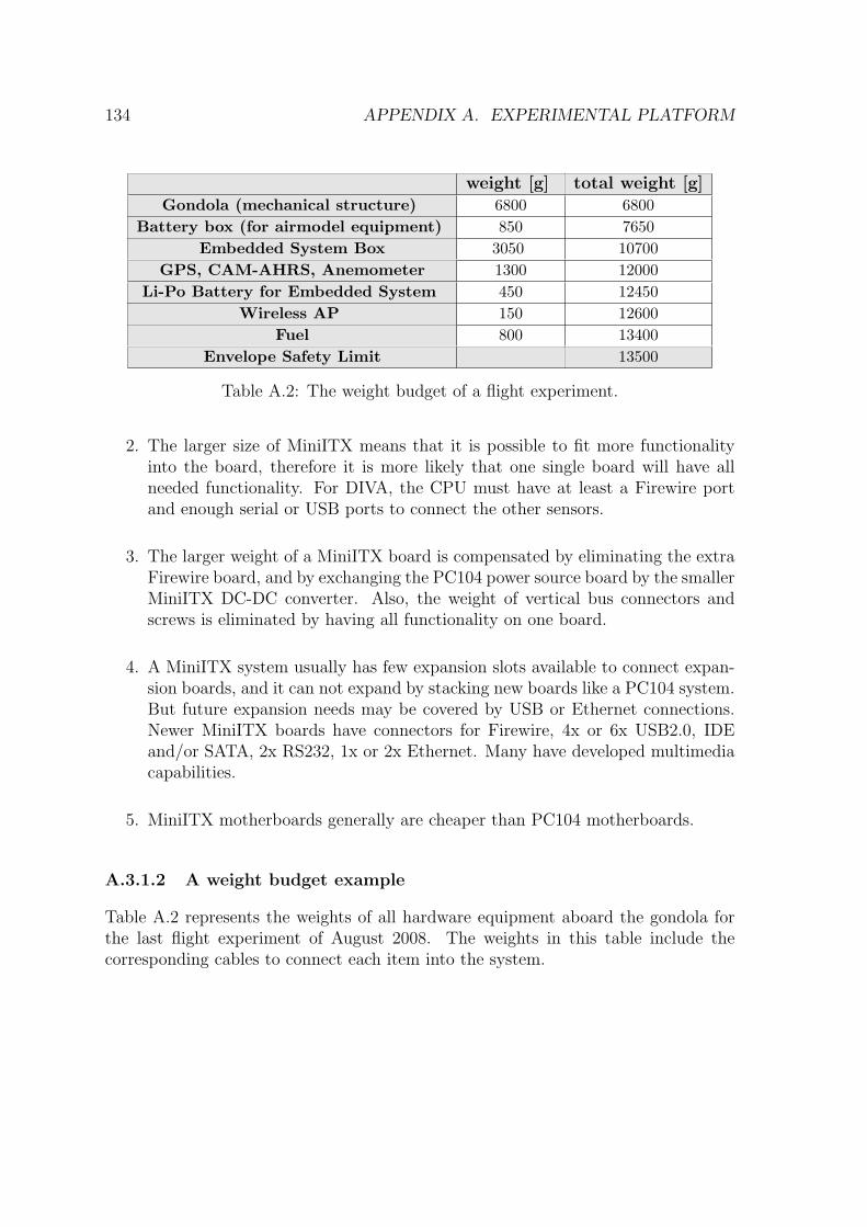
134 APPENDIX A. EXPERIMENTAL PLATFORM
weight [g] total weight [g]Gondola (mechanical structure) 6800 6800
Battery box (for airmodel equipment) 850 7650Embedded System Box 3050 10700
GPS, CAM-AHRS, Anemometer 1300 12000Li-Po Battery for Embedded System 450 12450
Wireless AP 150 12600Fuel 800 13400
Envelope Safety Limit 13500
Table A.2: The weight budget of a flight experiment.
2. The larger size of MiniITX means that it is possible to fit more functionalityinto the board, therefore it is more likely that one single board will have allneeded functionality. For DIVA, the CPU must have at least a Firewire portand enough serial or USB ports to connect the other sensors.
3. The larger weight of a MiniITX board is compensated by eliminating the extraFirewire board, and by exchanging the PC104 power source board by the smallerMiniITX DC-DC converter. Also, the weight of vertical bus connectors andscrews is eliminated by having all functionality on one board.
4. A MiniITX system usually has few expansion slots available to connect expan-sion boards, and it can not expand by stacking new boards like a PC104 system.But future expansion needs may be covered by USB or Ethernet connections.Newer MiniITX boards have connectors for Firewire, 4x or 6x USB2.0, IDEand/or SATA, 2x RS232, 1x or 2x Ethernet. Many have developed multimediacapabilities.
5. MiniITX motherboards generally are cheaper than PC104 motherboards.
A.3.1.2 A weight budget example
Table A.2 represents the weights of all hardware equipment aboard the gondola forthe last flight experiment of August 2008. The weights in this table include thecorresponding cables to connect each item into the system.
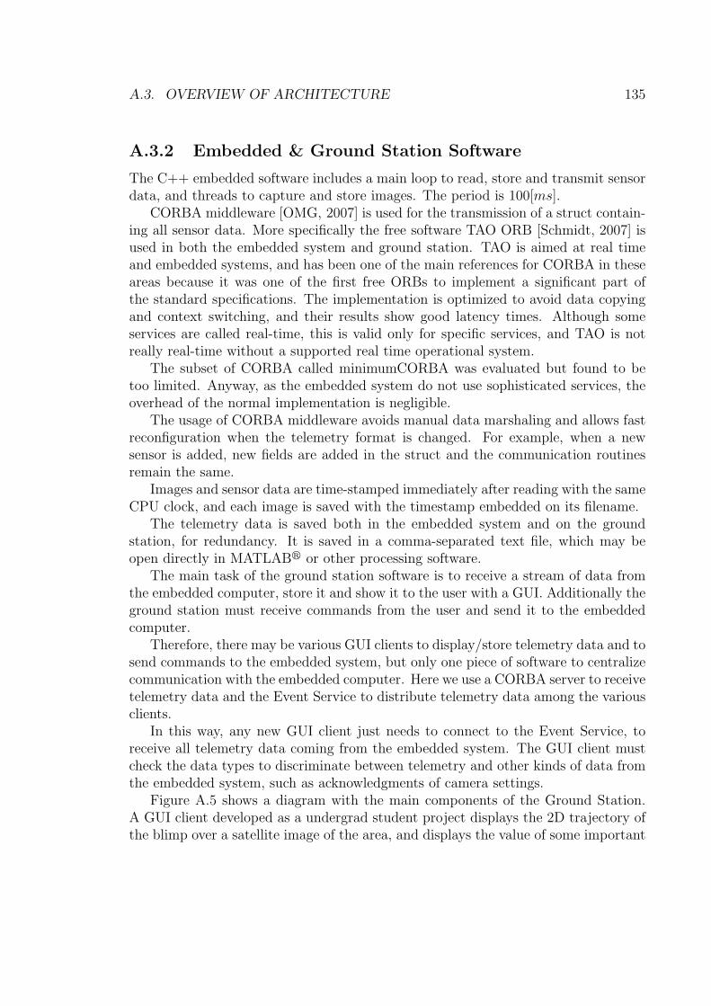
A.3. OVERVIEW OF ARCHITECTURE 135
A.3.2 Embedded & Ground Station SoftwareThe C++ embedded software includes a main loop to read, store and transmit sensordata, and threads to capture and store images. The period is 100[ms].
CORBA middleware [OMG, 2007] is used for the transmission of a struct contain-ing all sensor data. More specifically the free software TAO ORB [Schmidt, 2007] isused in both the embedded system and ground station. TAO is aimed at real timeand embedded systems, and has been one of the main references for CORBA in theseareas because it was one of the first free ORBs to implement a significant part ofthe standard specifications. The implementation is optimized to avoid data copyingand context switching, and their results show good latency times. Although someservices are called real-time, this is valid only for specific services, and TAO is notreally real-time without a supported real time operational system.
The subset of CORBA called minimumCORBA was evaluated but found to betoo limited. Anyway, as the embedded system do not use sophisticated services, theoverhead of the normal implementation is negligible.
The usage of CORBA middleware avoids manual data marshaling and allows fastreconfiguration when the telemetry format is changed. For example, when a newsensor is added, new fields are added in the struct and the communication routinesremain the same.
Images and sensor data are time-stamped immediately after reading with the sameCPU clock, and each image is saved with the timestamp embedded on its filename.
The telemetry data is saved both in the embedded system and on the groundstation, for redundancy. It is saved in a comma-separated text file, which may beopen directly in MATLABr or other processing software.
The main task of the ground station software is to receive a stream of data fromthe embedded computer, store it and show it to the user with a GUI. Additionally theground station must receive commands from the user and send it to the embeddedcomputer.
Therefore, there may be various GUI clients to display/store telemetry data and tosend commands to the embedded system, but only one piece of software to centralizecommunication with the embedded computer. Here we use a CORBA server to receivetelemetry data and the Event Service to distribute telemetry data among the variousclients.
In this way, any new GUI client just needs to connect to the Event Service, toreceive all telemetry data coming from the embedded system. The GUI client mustcheck the data types to discriminate between telemetry and other kinds of data fromthe embedded system, such as acknowledgments of camera settings.
Figure A.5 shows a diagram with the main components of the Ground Station.A GUI client developed as a undergrad student project displays the 2D trajectory ofthe blimp over a satellite image of the area, and displays the value of some important
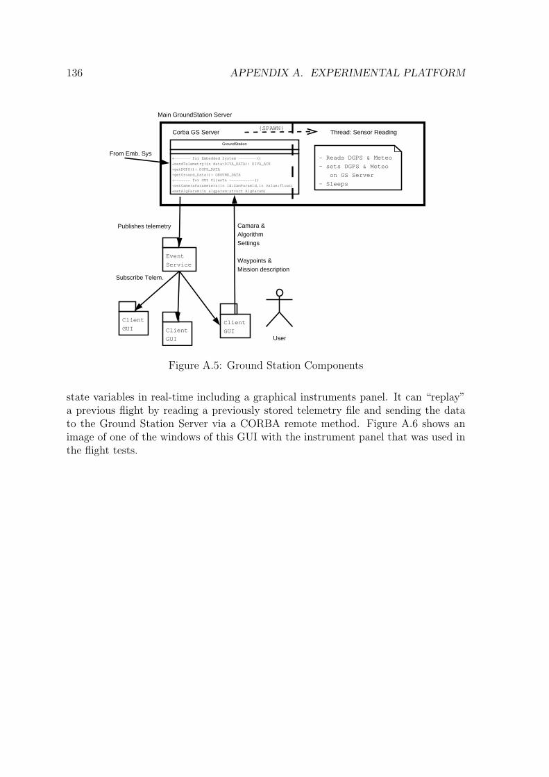
136 APPENDIX A. EXPERIMENTAL PLATFORM
GroundStation
+------- for Embedded System --------()
+sendTelemetry(in data:DIVA_DATA): DIVA_ACK
+getDGPS(): DGPS_DATA
+getGround_Data(): GROUND_DATA
+------- for GUI Clients -----------()
+setCameraParameters(in Id:CamParamId,in value:float)
+setAlgParam(in algparam:struct AlgParam)
Main GroundStation Server
Corba GS Server{SPAWN}
Thread: Sensor Reading
- Reads DGPS & Meteo
- sets DGPS & Meteo
on GS Server
- Sleeps
From Emb. Sys
Event
Service
Publishes telemetry
Client
GUI Client
GUI
Subscribe Telem.
Camara &AlgorithmSettings
Waypoints &Mission description
Client
GUIUser
Figure A.5: Ground Station Components
state variables in real-time including a graphical instruments panel. It can “replay”a previous flight by reading a previously stored telemetry file and sending the datato the Ground Station Server via a CORBA remote method. Figure A.6 shows animage of one of the windows of this GUI with the instrument panel that was used inthe flight tests.
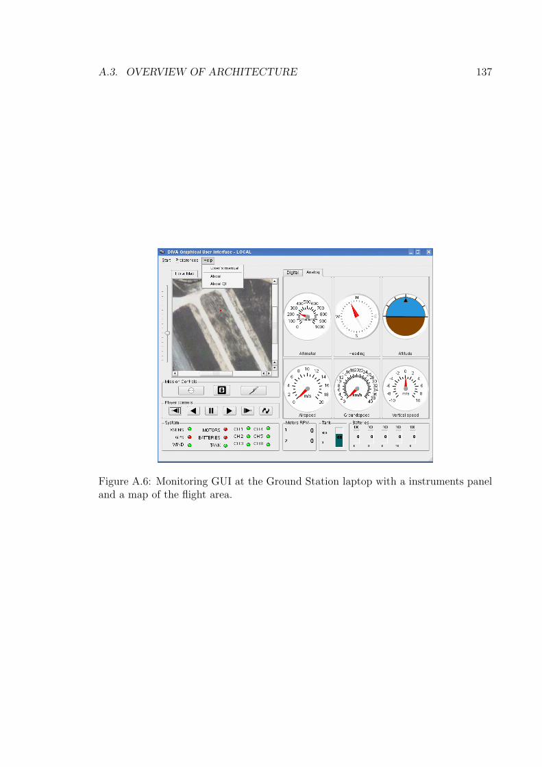
A.3. OVERVIEW OF ARCHITECTURE 137
Figure A.6: Monitoring GUI at the Ground Station laptop with a instruments paneland a map of the flight area.

138 APPENDIX A. EXPERIMENTAL PLATFORM
Appendix B
Mathematical Proofs and formulae
B.1 Recovering the scale of the recovered homog-raphy matrix
Given two images of the same 3D plane, a homography recovered from point cor-respondences is recovered only up to a scale factor λ (section 2.2.2), in the formHλ = λH = λ
(R− tnT /d
). The matrix R is a 3 × 3 rotation matrix, t ∈ R3 is a
translation vector, n ∈ R3 is the plane normal vector, and d ∈ R the distance fromthe camera center to the plane, as shown in figure B.1.
The matrix Hλ = λH is recovered only up to the scale factor λ ∈ R which mustbe recovered first. After λ is recovered, the translational and rotational componentsembedded in the matrix will be recovered. Therefore, the following proposition mustbe proved:
Proposition: For a matrix on the form Hλ = λ(R− tnT /d
), |λ| is the second
largest singular value of Hλ.Proof: This proof was taken from [Ma et al., 2004], and it is more explicitly de-
tailed here. For definitions in algebra we relied on [Bronshtein and Semendyayev, 1997].The notation x ∼ y denotes that the vectors x and y are proportional or parallel.
Let u = RT t/d ∈ R3. Then it can be shown that:
HTλHλ = λ2
(I + unT + nuT + ‖u‖2 nnT
)(B.1)
Denote u = (u1, u2, u3) ∈ R3, and
u =
0 −u3 u2
u3 0 −u1
−u2 u1 0
∈ R3×3 (B.2)
139
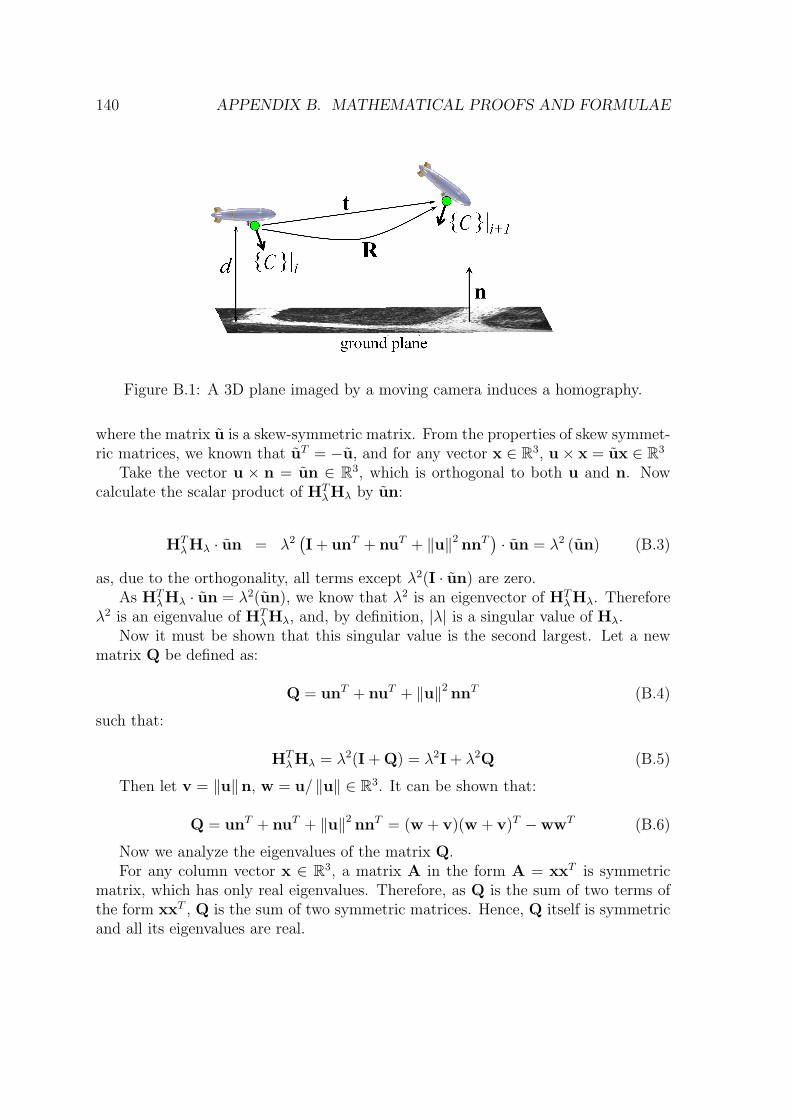
140 APPENDIX B. MATHEMATICAL PROOFS AND FORMULAE
Figure B.1: A 3D plane imaged by a moving camera induces a homography.
where the matrix u is a skew-symmetric matrix. From the properties of skew symmet-ric matrices, we known that uT = −u, and for any vector x ∈ R3, u× x = ux ∈ R3
Take the vector u × n = un ∈ R3, which is orthogonal to both u and n. Nowcalculate the scalar product of HT
λHλ by un:
HTλHλ · un = λ2
(I + unT + nuT + ‖u‖2 nnT
)· un = λ2 (un) (B.3)
as, due to the orthogonality, all terms except λ2(I · un) are zero.As HT
λHλ · un = λ2(un), we know that λ2 is an eigenvector of HTλHλ. Therefore
λ2 is an eigenvalue of HTλHλ, and, by definition, |λ| is a singular value of Hλ.
Now it must be shown that this singular value is the second largest. Let a newmatrix Q be defined as:
Q = unT + nuT + ‖u‖2 nnT (B.4)
such that:
HTλHλ = λ2(I + Q) = λ2I + λ2Q (B.5)
Then let v = ‖u‖n, w = u/ ‖u‖ ∈ R3. It can be shown that:
Q = unT + nuT + ‖u‖2 nnT = (w + v)(w + v)T −wwT (B.6)
Now we analyze the eigenvalues of the matrix Q.For any column vector x ∈ R3, a matrix A in the form A = xxT is symmetric
matrix, which has only real eigenvalues. Therefore, as Q is the sum of two terms ofthe form xxT , Q is the sum of two symmetric matrices. Hence, Q itself is symmetricand all its eigenvalues are real.
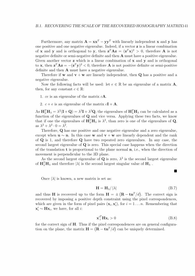
B.1. RECOVERING THE SCALE OF THE RECOVERED HOMOGRAPHY MATRIX141
Furthermore, any matrix A = xxT − yyT with linearly independent x and y hasone positive and one negative eigenvalue. Indeed, if a vector z is a linear combinationof x and y and is orthogonal to y, then zTAz = (zTx)2 > 0, therefore A is notnegative definite or semi-negative definite and then A must have a positive eigenvalue.Given another vector z which is a linear combination of x and y and is orthogonalto x, then zTAz = −(zTy)2 < 0, therefore A is not positive definite or semi-positivedefinite and then A must have a negative eigenvalue.
Therefore if w and v + w are linearly independent, then Q has a positive and anegative eigenvalue.
Now the following facts will be used: let e ∈ R be an eigenvalue of a matrix A,then, for any constant c ∈ R:
1. ce is an eigenvalue of the matrix cA.
2. c + e is an eigenvalue of the matrix cI + A.
As HTλHλ = λ2(I + Q) = λ2I + λ2Q, the eigenvalues of HT
λHλ can be calculated as afunction of the eigenvalues of Q and vice versa. Applying these two facts, we knowthat if one the eigenvalues of HT
λHλ is λ2, than zero is one of the eigenvalues of Q,as λ2 + λ2 · 0 = λ2.
Therefore, Q has one positive and one negative eigenvalue and a zero eigenvalue,except when u ∼ n. In this case w and v + w are linearly dependent and the rankof Q is 1, and therefore Q have two repeated zero eigenvalues. In any case, thesecond largest eigenvalue of Q is zero. This special case happens when the directionof the translation t is proportional to the plane normal n, i.e., when the direction ofmovement is perpendicular to the 3D plane.
As the second largest eigenvalue of Q is zero, λ2 is the second largest eigenvalueof HT
λHλ and therefore |λ| is the second largest singular value of Hλ .
�
Once |λ| is known, a new matrix is set as:
H = Hλ/ |λ| (B.7)
and thus H is recovered up to the form H = ±(R− tnT /d
). The correct sign is
recovered by imposing a positive depth constraint using the pixel correspondences,which are given in the form of pixel pairs (xi,x
′i), for i = 1 . . . n. Remembering that
x′i ∼ Hxi, we have, for all i:
x′Ti Hxi > 0 (B.8)
for the correct sign of H. Thus if the pixel correspondences are on general configura-tion on the plane, the matrix H =
(R− tnT /d
)can be uniquely determined.
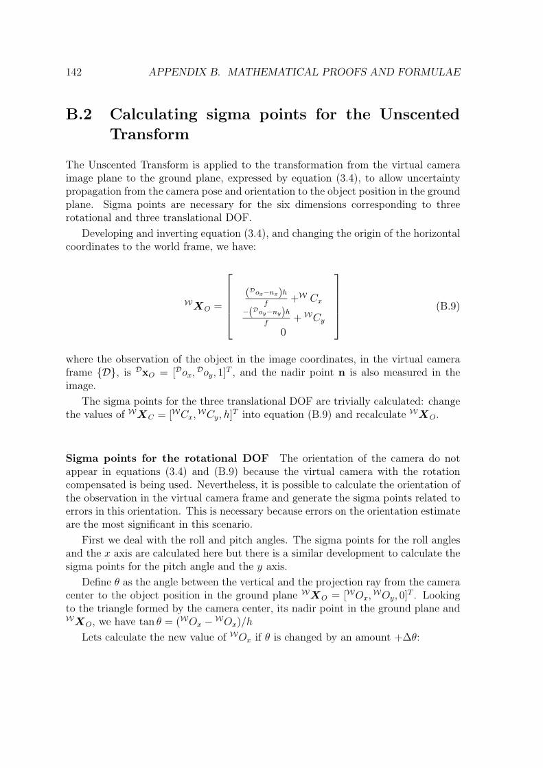
142 APPENDIX B. MATHEMATICAL PROOFS AND FORMULAE
B.2 Calculating sigma points for the UnscentedTransform
The Unscented Transform is applied to the transformation from the virtual cameraimage plane to the ground plane, expressed by equation (3.4), to allow uncertaintypropagation from the camera pose and orientation to the object position in the groundplane. Sigma points are necessary for the six dimensions corresponding to threerotational and three translational DOF.
Developing and inverting equation (3.4), and changing the origin of the horizontalcoordinates to the world frame, we have:
WXO =
(Dox−nx)h
f+W Cx
−(Doy−ny)h
f+ WCy
0
(B.9)
where the observation of the object in the image coordinates, in the virtual cameraframe {D}, is DxO = [Dox,
Doy, 1]T , and the nadir point n is also measured in theimage.
The sigma points for the three translational DOF are trivially calculated: changethe values of WXC = [WCx,
WCy, h]T into equation (B.9) and recalculate WXO.
Sigma points for the rotational DOF The orientation of the camera do notappear in equations (3.4) and (B.9) because the virtual camera with the rotationcompensated is being used. Nevertheless, it is possible to calculate the orientation ofthe observation in the virtual camera frame and generate the sigma points related toerrors in this orientation. This is necessary because errors on the orientation estimateare the most significant in this scenario.
First we deal with the roll and pitch angles. The sigma points for the roll anglesand the x axis are calculated here but there is a similar development to calculate thesigma points for the pitch angle and the y axis.
Define θ as the angle between the vertical and the projection ray from the cameracenter to the object position in the ground plane WXO = [WOx,
WOy, 0]T . Lookingto the triangle formed by the camera center, its nadir point in the ground plane andWXO, we have tan θ = (WOx − WOx)/h
Lets calculate the new value of WOx if θ is changed by an amount +∆θ:

B.3. JACOBIAN FORMULAE FOR THE HOMOLOGY TRANSFORMATION.143
χ+pitch = h tan (θ + ∆θ) + WCx (B.10)
= h
(tan (θ)
1− tan (θ) tan (∆θ)+
tan (∆θ)
1− tan (θ) tan (∆θ)
)+ WCx
and similarly for the negative sigma point:
χ−pitch = h tan (θ −∆θ) + WCy (B.11)
= h
(tan (θ)
1 + tan (θ) tan (∆θ)− tan (∆θ)
1 + tan (θ) tan (∆θ)
)+ Wcy
The sigma points for the yaw angle can be calculated by transforming the objectcoordinates from Cartesian to polar coordinates, changing the yaw angle, and trans-forming it back into Cartesian. A translation must be performed to place the originin the camera center, as in the following algorithm:
[θρ
]← cart2pol((WOx − WCx), (
WOy − WCy)) (B.12)
χ+yaw ← pol2cart((θ + ∆θ) , ρ) + [ WCx
WCy ]T (B.13)
χ−yaw ← pol2cart((θ −∆θ) , ρ) + [ WCxWCy ]T (B.14)
χ+yaw ←
[χ+
yaw
0
](B.15)
χ−yaw ←[
χ−yaw
0
](B.16)
where the last two lines just set the z coordinate to zero as the object is on theground plane, and cart2pol and pol2cart are the functions which transform Cartesiancoordinates into polar coordinates and vice-versa.
B.3 Jacobian formulae for the homology transfor-mation.
In section 3.2.3 the following equation is minimized to find the homology transforma-tion which register two images:
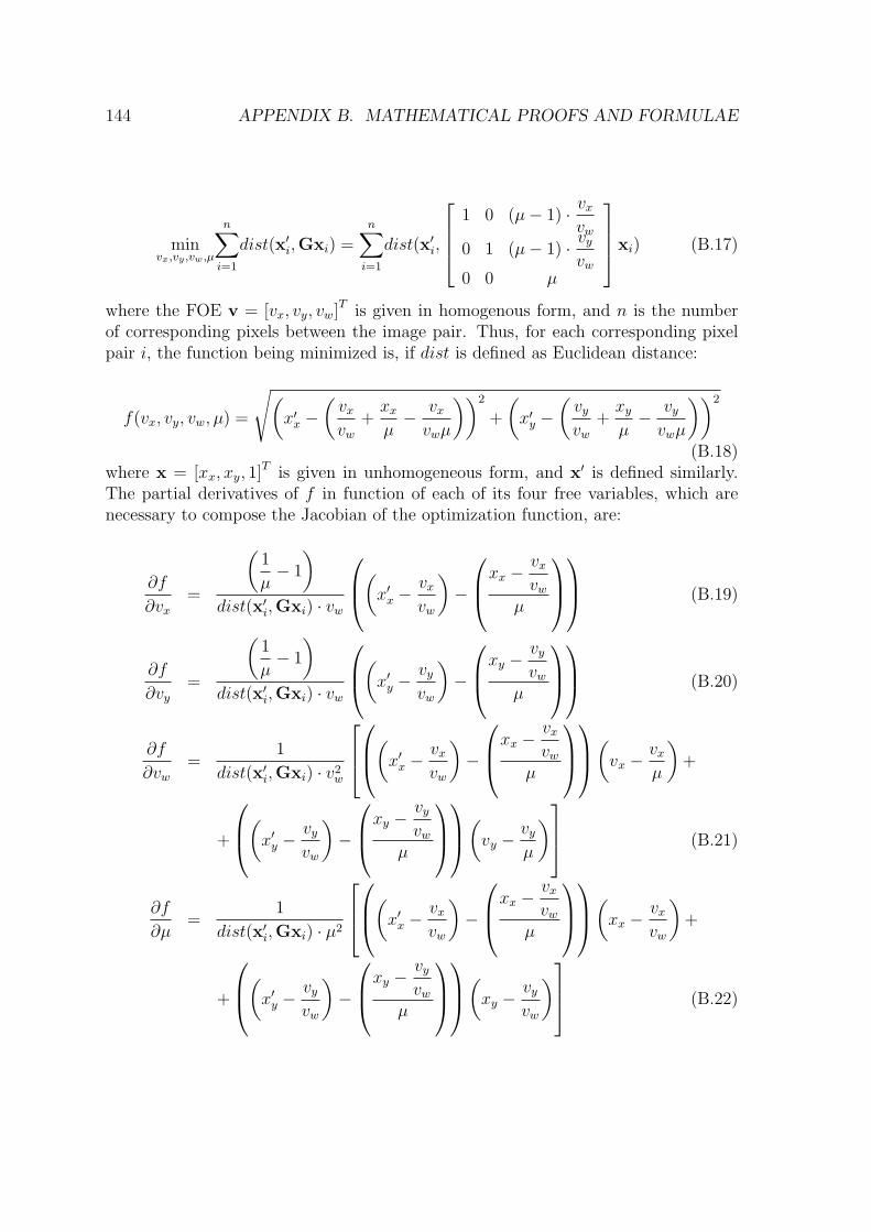
144 APPENDIX B. MATHEMATICAL PROOFS AND FORMULAE
minvx,vy ,vw,µ
n∑i=1
dist(x′i,Gxi) =n∑
i=1
dist(x′i,
1 0 (µ− 1) · vx
vw
0 1 (µ− 1) · vy
vw
0 0 µ
xi) (B.17)
where the FOE v = [vx, vy, vw]T is given in homogenous form, and n is the numberof corresponding pixels between the image pair. Thus, for each corresponding pixelpair i, the function being minimized is, if dist is defined as Euclidean distance:
f(vx, vy, vw, µ) =
√(x′x −
(vx
vw
+xx
µ− vx
vwµ
))2
+
(x′y −
(vy
vw
+xy
µ− vy
vwµ
))2
(B.18)where x = [xx, xy, 1]T is given in unhomogeneous form, and x′ is defined similarly.The partial derivatives of f in function of each of its four free variables, which arenecessary to compose the Jacobian of the optimization function, are:
∂f
∂vx
=
(1
µ− 1
)dist(x′i,Gxi) · vw
(x′x −vx
vw
)−
xx −vx
vw
µ
(B.19)
∂f
∂vy
=
(1
µ− 1
)dist(x′i,Gxi) · vw
(x′y −vy
vw
)−
xy −vy
vw
µ
(B.20)
∂f
∂vw
=1
dist(x′i,Gxi) · v2w
(x′x −
vx
vw
)−
xx −vx
vw
µ
(vx −
vx
µ
)+
+
(x′y −vy
vw
)−
xy −vy
vw
µ
(vy −
vy
µ
) (B.21)
∂f
∂µ=
1
dist(x′i,Gxi) · µ2
(x′x −
vx
vw
)−
xx −vx
vw
µ
(xx −
vx
vw
)+
+
(x′y −vy
vw
)−
xy −vy
vw
µ
(xy −
vy
vw
) (B.22)
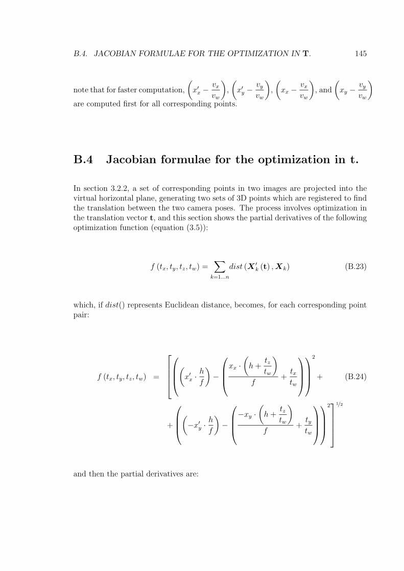
B.4. JACOBIAN FORMULAE FOR THE OPTIMIZATION IN T. 145
note that for faster computation,(
x′x −vx
vw
),(
x′y −vy
vw
),(
xx −vx
vw
), and
(xy −
vy
vw
)are computed first for all corresponding points.
B.4 Jacobian formulae for the optimization in t.
In section 3.2.2, a set of corresponding points in two images are projected into thevirtual horizontal plane, generating two sets of 3D points which are registered to findthe translation between the two camera poses. The process involves optimization inthe translation vector t, and this section shows the partial derivatives of the followingoptimization function (equation (3.5)):
f (tx, ty, tz, tw) =∑
k=1...n
dist (X ′k (t) , Xk) (B.23)
which, if dist() represents Euclidean distance, becomes, for each corresponding pointpair:
f (tx, ty, tz, tw) =
(x′x ·
h
f
)−
xx ·(
h +tztw
)f
+txtw
2
+ (B.24)
+
(−x′y ·h
f
)−
−xy ·(
h +tztw
)f
+tytw
2
1/2
and then the partial derivatives are:
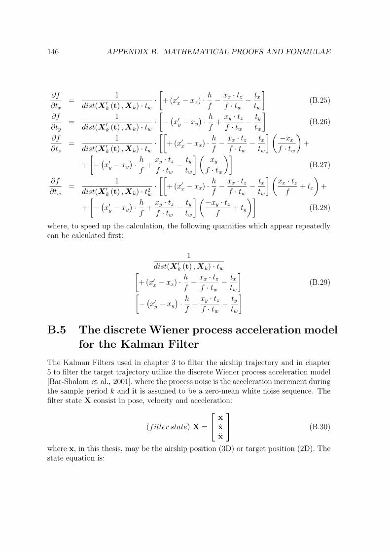
146 APPENDIX B. MATHEMATICAL PROOFS AND FORMULAE
∂f
∂tx=
1
dist(X ′k (t) , Xk) · tw
·[+ (x′x − xx) ·
h
f− xx · tz
f · tw− tx
tw
](B.25)
∂f
∂ty=
1
dist(X ′k (t) , Xk) · tw
·[−(x′y − xy
)· hf
+xy · tzf · tw
− tytw
](B.26)
∂f
∂tz=
1
dist(X ′k (t) , Xk) · tw
·[[
+ (x′x − xx) ·h
f− xx · tz
f · tw− tx
tw
](−xx
f · tw
)+
+
[−(x′y − xy
)· hf
+xy · tzf · tw
− tytw
](xy
f · tw
)](B.27)
∂f
∂tw=
1
dist(X ′k (t) , Xk) · t2w
·[[
+ (x′x − xx) ·h
f− xx · tz
f · tw− tx
tw
](xx · tz
f+ tx
)+
+
[−(x′y − xy
)· hf
+xy · tzf · tw
− tytw
](−xy · tz
f+ ty
)](B.28)
where, to speed up the calculation, the following quantities which appear repeatedlycan be calculated first:
1
dist(X ′k (t) , Xk) · tw[
+ (x′x − xx) ·h
f− xx · tz
f · tw− tx
tw
](B.29)[
−(x′y − xy
)· hf
+xy · tzf · tw
− tytw
]
B.5 The discrete Wiener process acceleration modelfor the Kalman Filter
The Kalman Filters used in chapter 3 to filter the airship trajectory and in chapter5 to filter the target trajectory utilize the discrete Wiener process acceleration model[Bar-Shalom et al., 2001], where the process noise is the acceleration increment duringthe sample period k and it is assumed to be a zero-mean white noise sequence. Thefilter state X consist in pose, velocity and acceleration:
(filter state) X =
xxx
(B.30)
where x, in this thesis, may be the airship position (3D) or target position (2D). Thestate equation is:
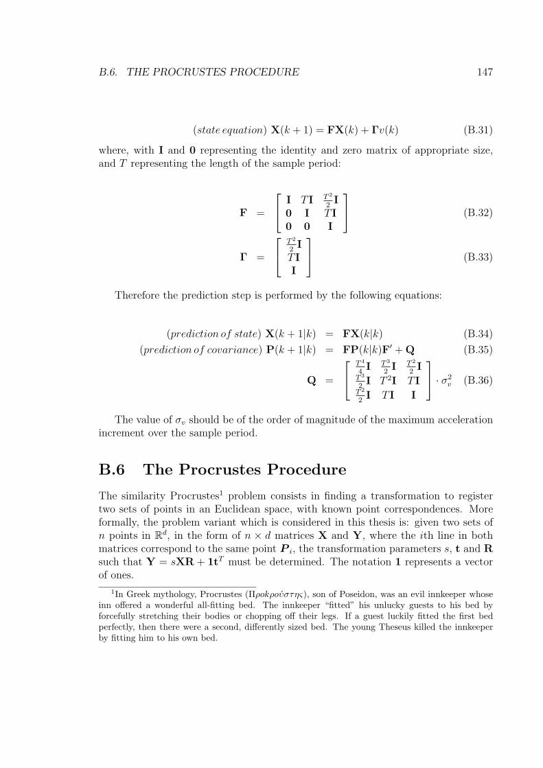
B.6. THE PROCRUSTES PROCEDURE 147
(state equation) X(k + 1) = FX(k) + Γv(k) (B.31)
where, with I and 0 representing the identity and zero matrix of appropriate size,and T representing the length of the sample period:
F =
I T I T 2
2I
0 I T I0 0 I
(B.32)
Γ =
T 2
2I
T II
(B.33)
Therefore the prediction step is performed by the following equations:
(prediction of state) X(k + 1|k) = FX(k|k) (B.34)(prediction of covariance) P(k + 1|k) = FP(k|k)F′ + Q (B.35)
Q =
T 4
4I T 3
2I T 2
2I
T 3
2I T 2I T I
T 2
2I T I I
· σ2v (B.36)
The value of σv should be of the order of magnitude of the maximum accelerationincrement over the sample period.
B.6 The Procrustes Procedure
The similarity Procrustes1 problem consists in finding a transformation to registertwo sets of points in an Euclidean space, with known point correspondences. Moreformally, the problem variant which is considered in this thesis is: given two sets ofn points in Rd, in the form of n × d matrices X and Y, where the ith line in bothmatrices correspond to the same point P i, the transformation parameters s, t and Rsuch that Y = sXR + 1tT must be determined. The notation 1 represents a vectorof ones.
1In Greek mythology, Procrustes (Πρokρoυστης), son of Poseidon, was an evil innkeeper whoseinn offered a wonderful all-fitting bed. The innkeeper “fitted” his unlucky guests to his bed byforcefully stretching their bodies or chopping off their legs. If a guest luckily fitted the first bedperfectly, then there were a second, differently sized bed. The young Theseus killed the innkeeperby fitting him to his own bed.
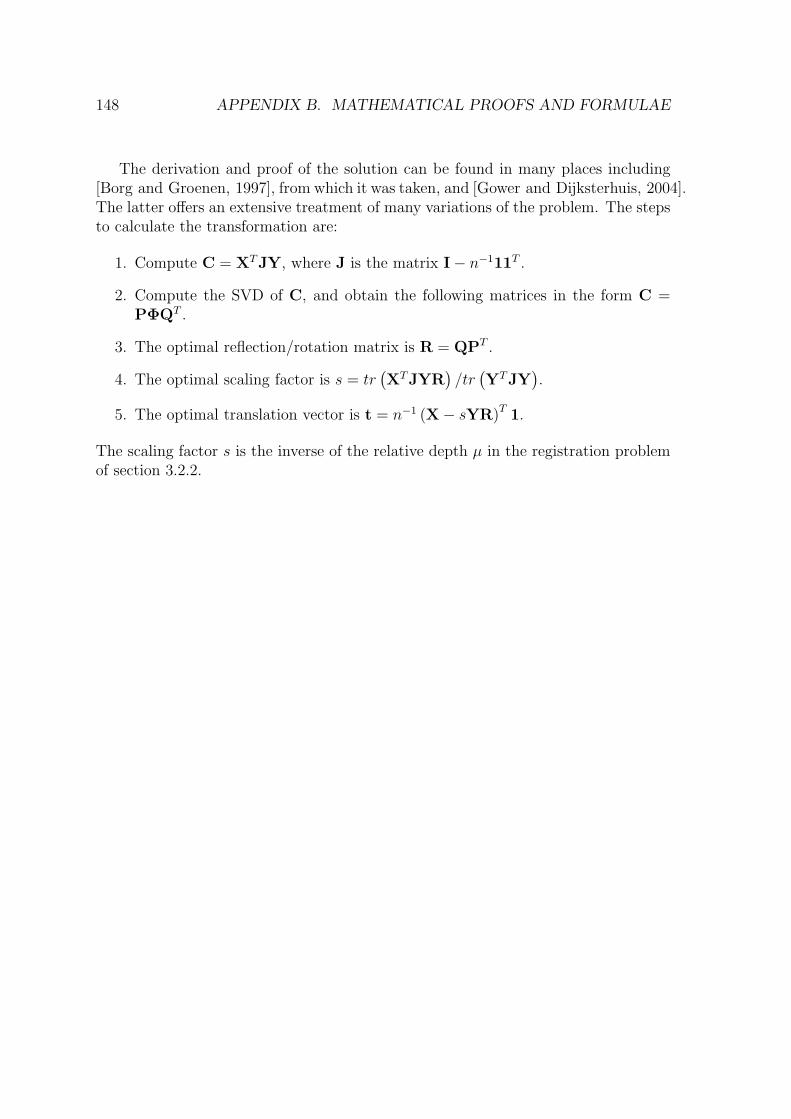
148 APPENDIX B. MATHEMATICAL PROOFS AND FORMULAE
The derivation and proof of the solution can be found in many places including[Borg and Groenen, 1997], from which it was taken, and [Gower and Dijksterhuis, 2004].The latter offers an extensive treatment of many variations of the problem. The stepsto calculate the transformation are:
1. Compute C = XTJY, where J is the matrix I− n−111T .
2. Compute the SVD of C, and obtain the following matrices in the form C =PΦQT .
3. The optimal reflection/rotation matrix is R = QPT .
4. The optimal scaling factor is s = tr(XTJYR
)/tr(YTJY
).
5. The optimal translation vector is t = n−1 (X− sYR)T 1.
The scaling factor s is the inverse of the relative depth µ in the registration problemof section 3.2.2.