Exploiting Long-term Co-integration between major Animal andAquatic Food Commodities and countries’ GDP for Robust

Forecasting

Kedir Nesha(1)

Tadayoshi Masuda(2)

Peter Goldsmith(3)

National Soybean Research Laboratory (NSRL)University of Illinois at Champaign-Urbana

1) Visiting Research Associate, the National Soybean Research Laboratory2) Post-Doctoral Researcher, National Soybean Research Laboratory3) Associate Professor, Soybean Industry Endowed Fellow, and Executive

Director, the National Soybean Research Laboratory

1

1. Introduction

World food consumption pattern has seen changes during the past

decades which largely attributed to the economic developments in

the world. Along with population growth, many developing

countries have shown increased purchasing power causing the

demand for more and high valued food (Gerbens-leenes and Nonhebl,

2006). The change is not only increase in the gross consumption

of food but also in the composition and quality of diet. As

income grows individual replace their diet with high value

products. For example, direct per capita consumption of cereal as

food has declined over the past three decades in the rapidly

growing economies of Japan, Korea, and Taiwan, while meat, fish,

and dairy consumption has increased dramatically (Huang and

Bouis, 2002). As per capita income rises, consumers in developing

countries will shift some consumption away from lower value

cereals to higher value livestock products (Regmi et al., 2001).

Secondary forces that closely associate with rise in incomes;

urbanization, development of more advanced marketing systems

(e.g. supermarkets), occupational changes, and leisure

consumptions also shift the structure of global food consumption

patterns (Coyle and et al. 1998). Another issue comes along with

income increase is the consumer health concern. Consumer’s

preference for healthy foods increase as income grows. Hence, the

consumption of protein food decline or reaches some climax in

this countries.

2

Many studies have investigated the impact of income growth on the

food commodity consumption (Gio, Mroz and Popkin, 2002; Sengul

and Sengul, 2006; Angulo, Gil and Gracia, 2001; and Keyzer et.

al, 2005). However, these studies are at micro level based on the

individual income and consumption survey data. Elasticities based

on individual consumption behavior varies among different income

level in the population as well as on the food consumption

culture in a region within a country. In addition, the

elasticities calculated from these studies vary based on the

model, data selection and assumptions. Above all, interpreting

the results from micro level demand study to macro level is not

straight forward (Anderson and Vahid, 1997). Hence, the challenge

remains unsettled in establishing the long-term relationship

between food consumption and income growth at macro level. This

is not only of interest for academicians, who want to understand

the relationship, but also for food industries and policy makers

as it affects the forecasts of future consumptions. So far,

projections of commodities consumption by large organizations

like FOA, IFPRI and USDA are expensive and forecasts are not

tailored to commodity level in many cases.

Few studies at macro level are on too broad category of food

consumption (for example see Selvanathan and Selvanathan, 2003;

Selvanathan and Selvanathan, 2006; Clements, Wu and Zhang, 2006).

However, the demand for the specific food is different from the

other depending on culture and lifestyle. For example, if income

3

elasticity of demand for meat is estimated the result is

cumbersome in that it does not reveal the demand for basic meat

commodities (for example; beef, fish or pork, etc.,)

specifically. It is necessary to distinguish the demand for the

specific food type at least at the basic commodity level so that

the information generated will be useful for forecasting of its

consumption.

A country experiences different income elasticity (coefficient)

of consumption for a commodity over time. Study conducted in

China at different periods (between 1989 and 1993) on the

consumption of major staple food shows that income elasticity of

food demand varies along the time period (Gio, Mroz and Popkin,

2000). This variation over time originates from the fact that the

relationship between nation’s income level and consumption

pattern of a particular commodity is not monotonous. The

relationship between per capita income and consumption is that,

for example, at the lower level of per capita income meat

consumption is hardly increasing and at higher income level the

consumption of meat reaches satiation level (Keyzer et al.,

2005). However, as income level increase from low to middle the

consumption of meat raises very steeply (Keyzer et al., 2005).

Therefore the responsiveness of consumption of meat to income

varies for different level of income. It is elastic at the low

income level and almost inelastic at the higher income level.

This has an implication for the temporal structural change in

4

income elasticity of a country as a country will be at different

stage of income at different times. In line with this, for

example, capita food consumption is becoming less responsive to

changes in income and appears to be reaching a ceiling in the

majority of EU countries and parts of Turkey abased on the

analysis conducted in the period from 1970 to 2000 (Sengul and

Sengul, 2006). As a result estimation income elasticity of food

consumption based on data aggregated over time or cross-sectional

data is not reliable reflection of this long term relationship.

Income elasticity estimation that does not take long-term

relationship in to account is misleading and may give wrong

forecast of the demand.

Generally, income elasticity of food consumption is more valuable

if it is specific to commodity and country. It improves

forecasting accuracy as the trend over time for is captured in

the long-run relationship estimations. Knowing how consumers

respond to rises and falls in income can help policymakers assess

future food demand and trade policy. An understanding the trends

of food demand across countries and enhanced ability to predict

potential shifts in demand for different food products is an

invaluable tool for stakeholders involved in the production and

supply chain of food commodities. In addition, it helps to

evaluate the driven demand for grain as feed for production of

animal food commodities. .

5

The study uses time series data of per capita GDP (as proxy for

income) and per capita consumption for commodities to determine

the long term relationship. Though a lots of factors play role

in determining the shift in consumption this study takes

simplistic approach as data and time are limited in estimation

and forecasting of commodity consumption. This simple

relationship between aggregate commodity consumption and GDP of a

country is meant to give cheap and robust way of projecting long

term consumption for stakeholders in the production and supply

chain.

The rest of this paper is organized as follows. Literature review

part provided the available research results and their

limitations. The mythology part outlines the data type and

source, the economic model on which the study is based and

econometric methods used for model selection and estimation. The

result and discussion part presents the elasticities of the

estimation along with interpretation and forecasted figures for

27 years. We will also discuss the driven demand for feed based

on biological experiment results from literature. The final

section provides with conclusions.

2. Literature review

In this section we will review relevant research paper to the

study. This provides us with existing research results and

research gap for our study.

6

Previously, the links between changes in the global economy (as

measured by per capita income) and consumption of food have been

explored by a relatively wide range of authors. Most of these

works are at very aggregate level where food is just a single

commodity in the demand system. Selvanathan and Selvanathan

(2003) analyzed aggregate income elasticity of food along other

seven commodities (housing, cloth, durable, medicine, recreation,

transport and other) for each 45 countries (both OECD and LCD)

using time series method. They found that food consumption

decline with increase in the GNP and poor countries allocate more

budgets to food than rich countries. Later, Selvanathan and

Selvanathan (2006) estimated cross country income elasticity of

food, tobacco, soft drinks, and alcohol in 43 developed and

developing countries. Based on the Selvanathan and Selvanathan

(2003) Clements, Wu and Zhang (2006) also analyzed cross country

(for 45 countries) income elasticity for eight commodity food

being a single commodity in the simple utility based demand

system. In result from their analysis shows that the income

elasticity of food for poor countries is high as compared to rich

countries. The lowest is for USA (0.44) and the highest is for

Sri Lanka (0.67). However, income elasticity obtained by

aggregating food as a single commodity in the demand system does

not provide information about which commodity is being more

consumed and which is less consumed as a result of income

changes.

7

More wider and more disaggregated income elasticity of food

commodities was estimated by Seale, Regmi and Bernstein (2003).

They analyzed and compared full cross-country demand system

internationally (across 114 countries) in two stages. In the

first stage, food is considered as a commodity among other non

food expenditure. In this estimation the income (expenditure)

elasticity of demand for food, beverages, and tobacco varies

greatly among countries. It is highest among low-income

countries; it varies from 0.80 for Tanzania to 0.68 for Georgia;

it ranges between 0.67 to 0.49 for middle-income countries and

from 0.48 to 0.10 for high income countries (Seale, Regmi and

Bernstein, 2003). At the second stage eight broadly defined food

categories were analyzed as sub demand system which gives better

understanding of consumption pattern. The income elasticity for

cereals ranges from 0.62 in Tanzania to 0.47 in Georgia, 0.28 in

Slovenia, and 0.05 in the United States (Seale, Regmi and

Bernstein, 2003). However, the study is not specific enough to

understand the demand for specific commodity in specific country.

The elasticity for these commodities cannot be aggregated in to

very general category, for instance cereal, because one cereal

commodity can be staple food and the other can be high valued

cereal depending on the cultural and geographical situation. For

example, Income elasticity of wheat is not the same as income

elasticity for maize within a certain country. Similarly in meat

category income elasticity for beef is not the same as income

elasticity for pork. Most religions forbid certain foods, for

8

example; pork meat in Judaism and Islam, pork and beef in

Hinduism and Buddhism (Sack, 2001: 218). Hence, though Seale,

Regmi and Bernstein (2003) they gave better detail of each food

category at the second stage, it is not detail enough to give

information at each commodity level which help for understanding

the current demand and forecasting future consumption.

Few studies also focus on countries that have shown to have

significant impact on the world food consumption due to economic

and population factors. China as world phenomena for economic and

food consumption change is the main focus of these studies. Fang

and Beghin (2002) uses urban household-level survey data (pseudo

panel) from 1992 to 1998 and provide estimates of final demand

for edible vegetable oils and animal fats in three regions of

China based on an incomplete demand system. The results of the

estimation indicate that the demand for the major staple oil is

price inelastic, the aggregate demand for non-staple and

condiment oil are more responsive to price changes and is elastic

in some cases (Fang and Beghin, 2002). The most detail income

elasticity of food consumption in china was estimated by Guo et

al. (1996). The study analyses the difference in income

elasticities for foods and nutrients across income levels and

over time (for 1989, 1991, and 1993). They point out that the

proportion of the diet that is coming from what were previously

viewed as superior grain and grain products (for example rice and

wheat) are being reduced and more pork and oil are being

9

consumed. The largest increases in pork consumption are taking

place among higher-income adults, and the larger increases in the

edible oils are happening among lower-income adults. There are

also few studies for USA consumer expenditure in similar fashion.

While these studies provide good insight at least for china and

USA, the number of country with significant impact on the traded

commodity on the globe are far more in number and vary across

food commodities. It is necessary to estimate these consumption

patterns at least for major consuming countries of commodities

under consideration.

Income elasticity of a single broadly defined commodity is also

estimated by many studies. For example; Keyzer et al. (2005)

analyzed consumption pattern shift towards meat which generates

indirect demand for cereals as livestock feed. He identifies

three income levels related consumption pattern shifts towards

meat. At the lower level of per capita income meat consumption is

hardly increasing and at higher income level the consumption of

meat reaches satiation level. However, as income level increase

from low to middle the consumption of meat rises very steeply.

York and Gossard (2004) also analyzed the demand for meat and

fish at worldwide level but from ecological resource requirement

point of view using simple demand model. This study concluded

that the liberalization of trade (global sourcing of food) untied

the consumption of meat and fish from local ecological

requirements for production. Rather economic developments,

10

urbanization and cultural (geographic) factors play major role in

stimulating demand for meat and fish. These studies emphasis the

shift in the world food consumption towards high values like

animal proteins as a result of income growth and try to show its

consequences on the cereal as livestock feed and environment.

However, these studies are crude in that they did not identify

which meat (beef, pork, chicken, etc) are more in demand and

impacting the demand for cereal. Keyzer et al. (2005) uses time

series data in non-linear consumption model to capture the

differences in countries income and the deference in

responsiveness of consumers at different income level. However he

did not analyse the individual commodity differences for each

country.

3. Methodology

3.1. The data

The two most important data used in this estimation are

consumption quantity per country per year and GDP of country over

years. Unlike the common research on consumption and demand, this

study prefers to use total yearly consumption and GDP than per

capita consumption and per capita GDP. Due to the fact that

results at micro level study cannot be directly interpreted to

macro level as discussed in the introduction part, this study

utilizes macro level data as it is rather than manipulating it to

create representative consumer.

11

These data are extracted from FAO and World Bank databases

respectively. Consumptions data of generic protein food

commodities were directly downloaded from FOAstat food balance

sheet database. Consumption of these 12 commodities is expressed

in tones per year in each country. FAO converts consumption of

the processed foods to generic food equivalents. The income data

is obtained from the World Bank’s World Development Indicators

Online (WDI). GDP of countries is stated in 1000 US dollar. The

available data ranges from 1961-2003 for consumption while GDP

can be obtained up to year 2007. Therefore, the study utilizes 43

years data except for Germany for which data is not available

from 1961 to 1971 (only 33 years data is used for Germany).

There are concerns in literature in GDP as income indicator. The

choice is between real GDP (in constant US dollar) and GDP with

Purchasing Power Parity (PPP). The choice depends on the goal of

the study and advantage and disadvantage of these options. The

disadvantage of using constant or current exchange rate is that

it has productivity biases which make rich countries richer and

poor countries poorer (Samuelson, 1964). This occurs because

international productivity differences in the production of

traded goods cause non-traded goods to be relatively more

expensive in rich countries and cheaper in poor countries

(Clements, Wu and Zhang, 2006). As non-traded goods prices are

not fully reflected in the prevailing exchange rate, the result

is artificial amplification of world income inequality (Clements,

12

Wu and Zhang, 2006). The second approach, PPP, have better appeal

in international comparison. However, the choice of base year and

price indexes used in calculating parities are not agreed up on

universally (Clements, Wu and Zhang, 2006). This paper follows

the first approach in estimating the elasticity as it does not

involve international comparison.

Given the significance of the contribution of countries to the

world total consumption of each food commodity, only five top

countries are selected for each four commodities. Based on 2003

FAO database these countries account for 76% of world

crustaceans’ consumption, 71% of freshwater fish consumption, 60%

of pig meat consumption and 53% of poultry meat consumption.

Therefore, the effect of the growth or decline of consumption of

these commodities in these countries will have substantial effect

on the stakeholders of the commodity supply chain.

3.2. The Economic Model

A large number of alternative functional forms are possible for

modeling the Engel curve, which is the relationship between food

demand and income levels. Double-log specification has been used

widely because of its simplicity and readily interpretable

properties. This can be written as follows:

13

lnCt=α+βlnYt+εt(1)

Where: lnCt is the log of quantity food commodity consumed in a

country, lnYt is the log of income (GDP) of a country, εt is

serially uncorrelated and homoscedastic error term, and t is time.

Equation (1) estimates the static elasticity of income of

consumption. Obviously, a static approach does not provide a

realistic description of how consumers behave in real life. In

fact, consumers very often react with some delay to income

changes, with the implication that an adjustment towards a new

equilibrium is spread over several time periods (Phlips, 1983).

Hence, not only current income but also the past income

influences the current consumption. In addition, it is long

established, in the work of Duesenbery (1949), Friedman (1957),

Stone (1954) and Houthakkar and Taylor (1970) that past

consumptions influence the current consumptions. Consumption

persists from the past can be explained by habit formation.

Formal treatment of this dynamic nature in the demand study is

also given in Deaton and Muellbauer (1980). In order to capture

such influences from past consumption habit we include lags of

the dependent variable in the model.

The question is how to incorporate this backward looking behavior

in the model. The autoregressive distributed lag (ARDL) model is

the most widely used model for estimating macroeconomic data (in

14

our case GDP and food commodity consumption) relationships in a

time-series context. This can be written as follows:

lnCt=α+βolnCt−1+β1lnYt+β2lnYt−1+εt

(2)

Where: β1 is the coefficient of current income, βo is coefficients

of lagged of consumption, β2 is the coefficients of lagged income

(lnYt-1).

Equation (2) represent an autoregressive distributed lag model

which describes the dynamic effect of change in Yt on current and

future values of Ct (Verbeek, 2004). Thus, it can be seen that

the ARDL model has an appealing separation of short- and long-run

effects of Yt on Ct. Alternatively, ARDL can be formulated as

error correction model by subtracting Ct-1 from both side of

equation (2) and after some rewriting as:

∆Ct=β1∆Yt+(1−θ ) [Ct−1−α−βYt−1 ]+εt

(3)

Where β=β1+β21−ϴ , and (1−θ )[Ct−1−α−βYt−1] is the error correction

term (1−θ) being an adjustment parameter.

15

This formulation is Error-Correction Model (ECM) which says that

the change in consumption (∆C¿¿t)¿is due to the current change in

income (∆Yt) plus an error correction parameter. If Ct−1 is above

the equilibrium value that corresponds toYt−1, that is, if the

equilibrium error in square brackets is positive, an additional

negative adjustment in Yt is generated. The adjustment direction

is in opposite direction if Ct−1 is below equilibrium. The speed

of adjustment depends on (1−θ ) under assumption that1−θ>0

(Verbeek, 2004).

3.3. Econometric Method

Both Equation (2) and (3) can be estimated by OLS assuming thatCt and Yt are stationary series so that the standard F and t-

test can be applied. However, if the series are not stationary

the OLS result is spurious regression in which two independent

nonstationary series are spuriously related because they are both

trended (verbeek, 2004). The spurious regression problem in

estimating OLS can be corrected for by including lagged values of

the series which is determined by testing for serial correlation

(verbeek, 2004). Here multicollinearity and simultaneity are a

constraint for inclusion of many lagged variables as required by

the model in OLS estimation. Moreover, if the two nonstationary

series are cointegrated, when the two nonstationary series share

common stochastic trend, the OLS estimator is super-consistent

because the OLS estimator on differenced-stationary series

16

converges at much faster rate than the normal asymptotic

(verbeek, 2004).

However, when both series are integrated of one (I (1)) there

exist a cointegrating vector which operates on the long-run

component of the two series and the nonstationarity in the two

series cancel out each other. The idea of cointegration is that

even if economic time series variables wonder around with

nonstationarity, there exists the possibility that a linear

combination of them could be stationary. Hence the error

correction equation can be estimated using cointegration methods.

The seminal work of Engle and Granger (1987) showed that the

long-run equilibrium relationship can be conveniently examined

using the cointegration technique, and the ECM describes the

short-run dynamic characteristics of economic activities. Using

the cointegration regression, both the long-run equilibrium

relationship and short-run dynamics can be examined. Secondly,

the spurious regression problem will not occur if the variables

in the regression are cointegrated.

3.4. Method of estimation

The first step in the estimation is to examine the stationarity

properties of the univariat time series. The series is can be

stationary at level, trend stationary or stationary after d times

differencing. The series is trend stationary if it becomes

stationary after detrending (including trend) at level. The

17

series is integrated of order d (denoted I(d) if it attains

stationarity after differencing d times. The processes is tested

using designed group of unit root tests which include the

Augmented Dickey-Fuller (ADF) test (1976), Phillips-Perron test

(PP) (1988). The ADF and PP tests state the null hypothesis of

non-stationarity or the presence of a unit root. The Monte Carlo

simulations by Schwert (1989) showed that the ADF tests have low

power and are sensitive to the choice of lag-length. The ADF unit

root tests are known to have low power problems in small samples,

particularly, if the series include structural breaks

(Kwiatkowski et al.1992; Leybourne & Newbold 2000). PP test is an

alternative (nonparametric) method of controlling for serial

correlation when testing for a unit root. Since no single unit

root test is without some statistical shortcomings, in terms of

size and power properties, both unit root tests are applied to

statistically determine the order of integration of the time-

series used in cointegration analyses.

The second step in the cointegration estimation is the

identification of the number of lags to be included in underlying

the VAR and identification of the rank of cointegration. The

identification of the rank of cointegration is sensitive to the

number of lags in the underlying VAR. The lag order is determined

using information criteria (IC) methods such as Final Prediction

Error (FPE), Akaike’s Information criteria (AIC), Schwarz’s

Bayesian Information Criteria (SBIC), and Hannan and Quinn

18

Information Criteria (HQIC). Lutkepohl (2005) demonstrates SBIC

an HQIC provides consistent estimates of true lag order while AIC

and FPE overestimate the lag number. Hence this study relies on

the SBIC and HQIC to determine number o0f lag order.

Following Engle and Granger (1987), several ways of testing for

the presence of cointegration have been proposed including

Johansen’s multivariate test (Johansen and Juselius, 1990). This

study uses Johansen’s test. The co integration rank is evaluated

based on the trace statistics, maximum eigenvalue statistics and

information criteria methods. Monte carlo simulation study shows

that Information criteria method of cointegration rank

determination is superior over residual based dickey-Fuller test

and system based trace statistics (Baltagi and Wang, 2007). Hence

this study determines the cointegration rank based on the three

methods while the result from information criteria is given more

weight when conflicting result obtained. Empirical application

of cointegration rank is also as it is sensitive to the

deterministic ( trend and constant).

If, applying these three tests indicates that there is no

cointegration, it’s said that the variables have no long run

equilibrium relationship. No cointegration might lead us to

estimate a VAR in differences. However, if the variables are

cointegrated, mistakenly estimating the VAR in differences means

not just throwing away information – it is misspecified. On the

19

other hand, if we assume as if there is cointegration between the

series when there is none, the model will also suffer from

misspecification and the estimation suffer from unpleasant

problems such as spurious regression. Hence, getting the

properties of the system right is an important matter in order to

get estimation and inference as correct as we possibly can.

Finally, the study uses the Johansen (1995) cointegration

framework which is log-likelihood estimation. The rank and the

number of lags as well as the inclusion of the trend and

intercept in the VECM model is determined according to the test

results of the previous steps. To give the cointegration

equation structural interpretation Johansen identification scheme

places constraint on the dependent variable parameter.

3.5. Model Specification

As discussed in the methodological part this study, the first

step in the analysis of the long-term relationship between the

animal protein commodity consumption and countries GDP is to

examine the stationarity of the individual variables. The

stationarity test is based on Dicky and fuller test statistics

and Philips Perron statistics. In annex-(1) it is shown that most

of the variables under discussion are not stationary. China pork

consumption, Indian crustacean consumption, USA GDP, Spain GDP

shows trend stationarity. Japan crustaceans, Italy GDP, Japan

GDP, and Mexico GDP are stationarity based on Dicky and Fuller as

20

well as Phillips Perron tests. However, the visual analysis of

the graphs of the serieses show rather quadratic trend. Further

examination of these series with augmented Dickey and fuller

statistics rejects the stationarity of the series. OLS estimation

of these variables would be spurious. The examination of the

number of lags values that affect the current value of the

estimation ranges from 1 to 4 in the underlying VAR while its 0

to 3 for the VEC (VAR lags minus one for the VEC estimation).

The cointegration rank test shows that that there is one

cointegration between the commodity consumption and GDP of the

country. The cointegration rank result is evaluated using trace,

maximum Eigen statistics and information criteria test. Trend and

intercept in the VEC are included or excluded based on the visual

analysis of the graph of the series in level and in difference.

The result from this estimation is interpreted as long term

relationship between consumption of food commodity and GDP of the

country. Elasticities are not expected to satisfy all demand

theories

3.6. Forecasting Reliability

Additional objective of the research is to enhance the predictability

of future total consumption of the food commodity of concern

based on the GDP which can be easily available from various

organizations. Studies by many researches indicate that

forecasting using structural model captures trend behavior than

univariate time series model. Engle and Yoo (1987) implied that

21

if variables are cointegrated the optimal forecasts using the

proper information set is tied together by the equilibrium

relationships. Forecast from univariate models do not enjoy using

the cointegration term. However, for the cointegration to enhance

the forecasting there must be granger causality in at least one

direction and one variable must be capable of helping to forecast

the others.

The Granger causality test result can be found in the last column

of appendix (1). The test result indicate that Brazil pork

consumption, Brazil poultry meat consumption China freshwater

fish consumption, Germany pork consumption, Japan poultry meat

consumption, Spain pork consumption, USA pork consumption and USA

poultry meat consumption have no statistically significant

Granger causality relationship with GDP. This result implies that

for those equations where there is no statistically significant

Granger causality, the forecast mainly rely on the underlying VAR

estimates. Therefore, the accuracy of the forecast is similar to

VAR based forecast.

4. Results and Discussion

In this section we will present and discuss the estimation

results for four commodities for each top five consuming

countries and dicuss the dynamic forecasting results based the co

integration equation. Finally, we will drive demand for animal

feed to meet the consumption of these countries.

22

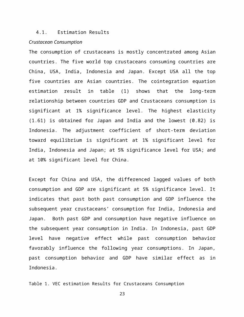
4.1. Estimation Results

Crustacean Consumption

The consumption of crustaceans is mostly concentrated among Asian

countries. The five world top crustaceans consuming countries are

China, USA, India, Indonesia and Japan. Except USA all the top

five countries are Asian countries. The cointegration equation

estimation result in table (1) shows that the long-term

relationship between countries GDP and Crustaceans consumption is

significant at 1% significance level. The highest elasticity

(1.61) is obtained for Japan and India and the lowest (0.82) is

Indonesia. The adjustment coefficient of short-term deviation

toward equilibrium is significant at 1% significant level for

India, Indonesia and Japan; at 5% significance level for USA; and

at 10% significant level for China.

Except for China and USA, the differenced lagged values of both

consumption and GDP are significant at 5% significance level. It

indicates that past both past consumption and GDP influence the

subsequent year crustaceans’ consumption for India, Indonesia and

Japan. Both past GDP and consumption have negative influence on

the subsequent year consumption in India. In Indonesia, past GDP

level have negative effect while past consumption behavior

favorably influence the following year consumptions. In Japan,

past consumption behavior and GDP have similar effect as in

Indonesia.

Table 1. VEC estimation Results for Crustaceans Consumption

23

Country Long-run elasticity

Adjustment estimates

VEC differenced Lag estimates

Chi-sq

R-sq

Variable

lag-1 lag-2

China 1.06(0.17)***

-0.03* Consmp 0.04 0.08 37*** 0.3gdp -0.13 0.09

India 1.61(0.32)***

-0.10*** Consmp -1.36***

24*** 0.4

gdp -3.70**Indonesia

0.82(0.14)***

-0.27*** Consmp 0.35** 35** 0.3gdp -2.09**

Japan 1.61(0.15)***

-0.42*** Consmp 0.34** -0.031**

115***

0.7

gdp -1.18** 0.22USA 1.15(0.16)

***0.04** Consmp 48*** 0.1

9gdpNote: Numbers in brackets are standard errors. ***, **, and * indicates 1%, 5% and 10%significance level respectively. Chi-sq indicates the statistical significance of theoverall cointegration equation and R-sq is for underlying VAR explanatory power.

Freshwater Fish Consumption

The five large total consumption of freshwater fish is in

Bangladesh, china, India, Indonesia and USA. The long-term

elasticity, short-term elasticity and adjustment coefficients are

depicted in table (2). The long-term relationship between GDP

and total consumption in these countries are statistically

significant at 1% significant level. Bangladesh, India and USA

have long-run elasticity of greater than one. One percent growth

in GDP in these countries yields a growth of freshwater fish

consumption by more than one percent. China has long-term

elasticity closer to one, one percent growth of GDP lead to 0.93

percent growth of freshwater fish consumption. The least

elasticity is for Indonesia fish. The adjustment coefficients are

24

statistically significant at 1% significance level for Bangladesh

and Indonesia and India where as it is insignificant for both

china and USA. The sign of the adjustment coefficient indicates

that the speed of adjustment for Indonesia and Bangladesh is very

fast. The adjustment speed is slower for India compared to other

countries. The direction of adjustment depends on the on weather

the past value is above or below the equilibrium relation value.

For Bangladesh, china, India, and Indonesia; where fish

consumption is part of the traditional diet; past GDP has

negative and statistically significant (at least at 10%

significance level) influence on the subsequent year consumption.

The influence of past consumption for these countries is

statistically insignificant, except china for which two year

lagged value is significant at 5% significance level and

positive. For USA past consumption is more important than GDP and

it negatively and significantly (at 5% significant level)

influence the following year consumption.

Table 2. VEC estimation Results for Freshwater Fish ConsumptionCountry Long-run

elasticityAdjustment estimates

differenced Lag estimates Chi-sq R-sq Variabl

e lag-1 lag-2 lag-

3

Bangladesh

1.02(0.01)***

-0.19***

Consmp 0.24 0.07 96*** 0.5gdp -

0.66**-0.28

China 0.93(0.10)***

0.01 Consmp 0.23 0.38**

0.18

85*** 0.8

gdp 0.46* -0.28 -

25

0.12India 1.04(0.03)

*** 0.40***

Consmp -0.13 1244***

0.7gdp -

0.56**Indonesia

0.44(0.09)***

-0.11***

Consmp -0.13 25*** 0.3gdp -

0.56**USA 1.08(0.40)

*** 0.04 Consmp -

0.54**-0.04 7*** 0.3

gdp -0.23 -0.25Note: Numbers in brackets are standard errors. ***, **, and * indicates 1%, 5% and 10%significance level respectively. Chi-sq indicates the statistical significance of theoverall cointegration equation and R-sq is for underlying VAR explanatory power.

Poultry Meat Consumption

The five top countries that consume poultry meat are Brazil,

china, Japan, Mexico and USA. The long-term elasticity of GDP to

poultry meat consumption is very large and statistically

significant at 1% significance level for china. One percent

growth in GDP leads 2.51% growth in total poultry meat

consumption, which is very remarkable in terms of total

consumption. The long-term elasticity for USA is greater than one

and statistically significant at 1% significant level. The long-

term elasticity of Brazil and Mexico are smaller relatively but

statistically significant at 1% significance level. The long term

elasticity for Japan is statistically insignificant and negative.

The adjustment coefficient for Brazil and china are negative in

sign which indicates the adjustment speed is very fast compared

to china, Mexico and USA.

26

Past consumption significantly (at 10%) and positively influence

the consumption of poultry meat in Brazil and China. Past GDP

significantly (at 1%) and positively influence the following year

poultry meat consumption in Mexico. China has tradition of

poultry meat consumption which enforced the current high growth

rate of consumption as income rises. In Mexico, where poultry

meat consumption is tradition, the increase in GDP further

enforces the consumption ion but with low growth rate.

Table 3. VEC estimation Results for Poultry Meat ConsumptionCountry

Long-runelasticity

Adjustmentestimates

Coefficients of differencedlag

Chi-sq R-sq

Variable

lag-1 lag-2 Lag-3

Brazil 0.41(0.11)***

-0.67*** Consmp 0.29* 0.29*

0.21

14*** 0.7

gdp 0.18 -0.16 -0.11

China 2.51(0.31)***

-0.10* Consmp 0.41** 68*** 0.8gdp 0.05

Japan -0.97(0.99) -0.05*** Consmp 0.19 -0.13 0.04 0.97 0.9gdp 0.39 -0.49 0.31

Mexico 0.38(0.15)***

0.36*** Consmp 0.15 7** 0.8gdp 0.70**

*USA 1.34(0.08)

***0.02 Consmp 0.023 0.24 0.0

1254*** 0.7

gdp 0.22 0.14 0.52

Note: Numbers in brackets are standard errors. ***, **, and * indicates 1%, 5% and 10%significance level respectively. Chi-sq indicates the statistical significance of theoverall cointegration equation and R-sq is for underlying VAR explanatory power.

Pig Meat Consumption

27

World pig meat consumption is dominated by china, Germany, Spain,

Italy and Brazil. As shown in table 4, long-term elasticity for

Brazil, china, are below one and significant at 1% significant

level. One percent growth in GDP yields 0.57% and 0.73% for

Brazil and china respectively. Italy and Spain have long-term

elasticity of greater than one and statistically significant at

1% significance level. The larger coefficients for these two

countries are not surprising that these countries are

traditionally pork consuming countries. The number one pork

producing country in Europe, German, has negative long term

elasticity which is statistically significant at 5% significance

level. The short-term deviation adjustment coefficients are

statistically significant at 1% and 5% significance level except

for Brazil which is insignificant. All countries total pork

consumptions adjustment coefficients towards equilibrium are

negative which indicates fast convergence of short term deviation

towards equilibrium value.

Only few of the included underlying VAR (differenced lagged

values of the variables) have influence on the current

consumption. China’s lagged consumption have statistically

significant (at1%) influence on the current consumption. German,

with negative elasticity of GDP to consumption, is statistically

significant (at 10%) negative past GDP influence. Probably this

can be attributed to high income at which consumers tend to shift

their diet from meat, growing health and environmental concern

among the citizens, and decreasing population. One year past

28

consumption has statistically significant (at 10%) influence on

the subsequent year consumption in Italy.

Table 4. VEC estimation Results for Pig Meat ConsumptionCountr

yLong-run elasticity

Adjustment estimates

Coefficient of differencedlag

Chi-sq R-sq

Variable

lag-1 lag-2

lag-3

Brazil 0.57(0.01)***

-0.03 Consmp 5933*** 0.08gdp

China 0.73(0.02)***

-0.48***

Consmp 0.36***

1561*** 0.8

gdp 0.09German -

0.89(0.33)**

-0.06** Consmp -0.05 -0.01

-0.19

7** 0.4

gdp -0.81* 0.48

-0.94*

Italy 1.57(0.30)***

-0.20** Consmp -0.26* 28*** 0.7gdp 0.18

Spain 1.27(0.21)***

-0.17***

Consmp -0.15 -0.12

0.01 36*** 0.6

gdp 0.22 -0.63

-0.94

Note: Numbers in brackets are standard errors. ***, **, and * indicates 1%, 5% and 10%significance level respectively. Chi-sq indicates the statistical significance of theoverall cointegration equation and R-sq is for underlying VAR explanatory power.

4.2. Forecasted Consumption

Based on the established country GDP and commodity consumption

relationships, the study forecasts the consumption of these four

commodities. Here we only present the result of the forecast for

interval years of 2010, 2015, 2020, and 2030. The observation of

29

year 2003 is also presented for comparison with initial

situation. The full result of the forecast is attached in the

appendix. Given the downward bias of the forecasting nature of

the cointegration the forecasted figures may give sense if we

look at future consumption from conservative assumptions such as

food prices increase, slowdown of world economic growth, slowdown

of population growth due to interventions, and technical and

environmental limitation satisfy the demand.

Table (5) depicts the forecast of crustacean consumption in five

countries. If the current economic growth rate continues which,

increase the middle class and expand urbanization, crustacean

consumption in the largest consuming country (China) boosts to

about 45 million tone per in 2030. The second large consuming

country Japan will more than double its consumption by 2030 but

the aging and declining population may halt growth of

consumption. In USA there will be only slight growth in

consumption.

Table 5. Countries’ Total Crustaceans Consumption Forecast Results forworld top five large consumers (in tones)

year China India Indonesia

Japan USA

2003 3,919,607

345,291.1

281,417.9

1,150,132

1,373,432

2010 6,837,885

508,892.5

418,452.6

1,481,800

1,680,446

2015 10,587,536

699,083.2

509,237.1

1,866,239

1,924,464

2020 16,753,186

983,142.2

581,634.8

2,385,712

2,189,196

2025 27,121,1 1,417,86 636,403. 3,047,6 2,474,53

30

11 2 5 40 22030 44,969,7

682,100,83

2676,379.

83,889,8

142,780,17

7

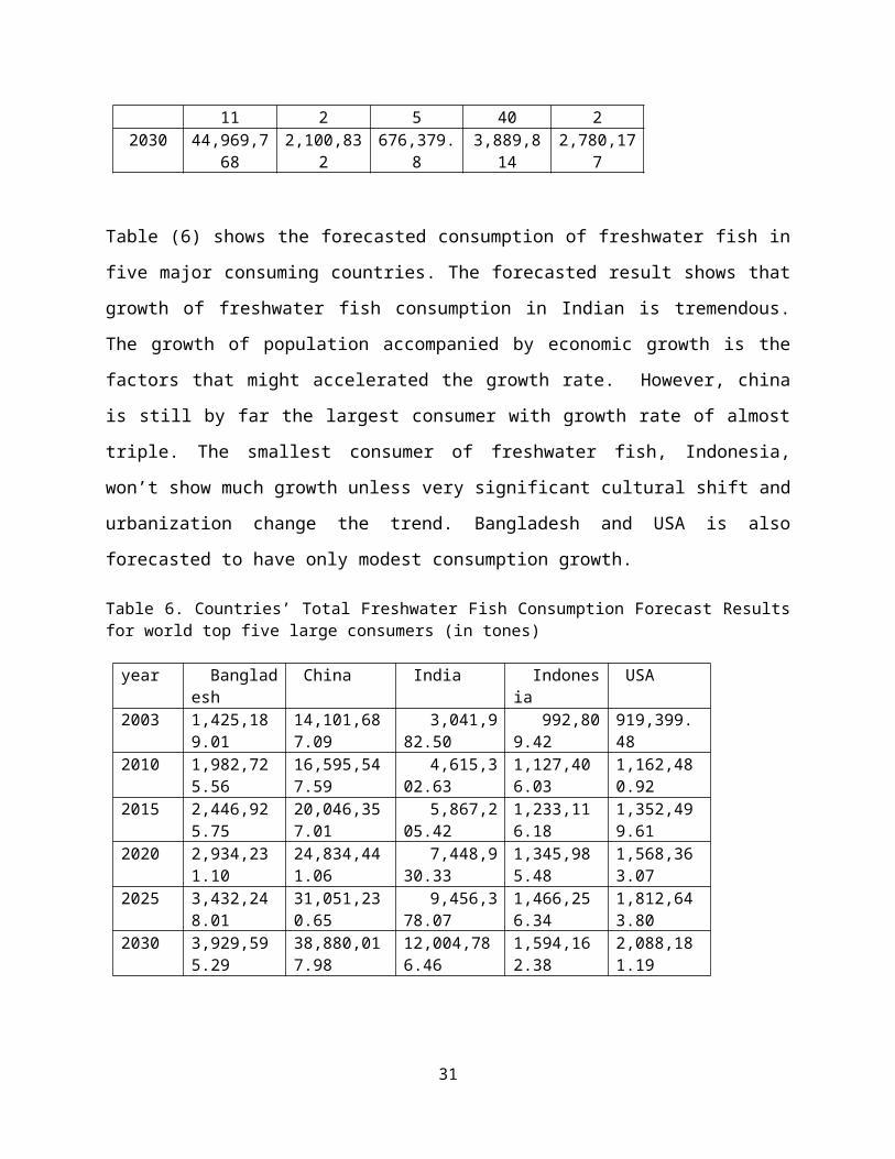
Table (6) shows the forecasted consumption of freshwater fish in

five major consuming countries. The forecasted result shows that

growth of freshwater fish consumption in Indian is tremendous.

The growth of population accompanied by economic growth is the

factors that might accelerated the growth rate. However, china

is still by far the largest consumer with growth rate of almost

triple. The smallest consumer of freshwater fish, Indonesia,

won’t show much growth unless very significant cultural shift and

urbanization change the trend. Bangladesh and USA is also

forecasted to have only modest consumption growth.

Table 6. Countries’ Total Freshwater Fish Consumption Forecast Resultsfor world top five large consumers (in tones)

year Bangladesh

China India Indonesia

USA

2003 1,425,189.01

14,101,687.09

3,041,982.50

992,809.42

919,399.48

2010 1,982,725.56

16,595,547.59

4,615,302.63

1,127,406.03

1,162,480.92

2015 2,446,925.75

20,046,357.01

5,867,205.42

1,233,116.18

1,352,499.61

2020 2,934,231.10

24,834,441.06

7,448,930.33

1,345,985.48

1,568,363.07

2025 3,432,248.01

31,051,230.65

9,456,378.07

1,466,256.34

1,812,643.80

2030 3,929,595.29

38,880,017.98

12,004,786.46

1,594,162.38

2,088,181.19

31

The forecast shows that poultry meat consumption increases

tremendously (about 114 million tons) by 2030. Though china is

leading in growth of many food consumption categories, the

forecast result shows poultry consumption is booming very much.

Consumption of poultry meat will also increase in Brazil, Mexico

and USA modestly. In Japan, poultry have small elasticity of GDP

and the forecast shows only slight increase in consumption in the

future. Give the declining population (especially young

population) in Japan it’s not surprising to see poultry

consumption will not increase much.

Table 6. Countries’ Total Poultry Meat Consumption Forecast Resultsfor world top five large consumers (in tones)

year Brazil China Japan Mexico USA 2003 5,891,6

40.27 14,319,359.63

2,013,419.34

2,646,903.44

14,766,756.06

2010 9,897,720.14

24,800,763.58

2,043,028.86

4,910,871.60

17,698,191.20

2015 13,411,418.11

36,412,438.82

2,013,991.23

7,370,624.53

20,022,375.88

2020 17,860,712.03

53,372,276.37

1,972,694.63

10,954,555.99

22,443,060.16

2025 23,152,191.52

78,245,353.08

1,915,074.34

16,229,789.99

24,956,378.53

2030 29,351,376.42

114,711,403.80

1,848,453.68

24,020,807.70

27,546,250.88

Table (7) depicts the forecast of pig meat by 2030. China with

already by far large consumer of pork is expected to grow its

consumption to more than 289 million tons by 2030. Spain also

more than triples its consumption by the time. Brazil pork

consumption experiences only slight growth over next decades

32

given the culture of pork consumption is not widespread among

rural population. However with current growth rate Brazil GDP and

diffusion of fast food culture it is inevitable that consumption

may increase at rate than expected. Germany and Italy relatively

maintains stable consumption.

Table 7. Countries’ Total Pig Meat Consumption Forecast Results forworld top five large consumers (in tones)

year Brazil China Germany Italy Spain 2003 2,424,22

8.7746,309,931

.534,465,639.56

2,503,799.66

2,730,712.17

2010 2,655,464.10

83,627,000.63

4,683,077.33

2,558,649.15

3,787,038.98

2015 2,803,468.62

113,983,812.42

4,658,536.96

2,582,049.44

4,609,251.33

2020 2,937,307.78

155,492,491.15

4,672,360.68

2,588,750.80

5,458,158.39

2025 3,057,478.15

212,121,546.31

4,699,962.09

2,580,923.92

6,312,743.97

2030 3,164,729.04

289,372,979.36

4,712,956.61

2,560,663.60

7,154,542.30

4.3. Driven Demand for Animal Feed

The production of these commodities is increasingly being

dependent on the feed industry which is basically cereals grain.

In this section we try to predict the driven demand for total

feed requirement and share of soybean. This gives the soybean

producers what they have to expect if the consumption growth

trend continues as current situation. It’s simple assumption that

we drive the amount of feed need to produce the forecasted

33

commodities consumption. We base our assumption of the facts from

FAO and other experimental results as follows.

From 1984 to 1990, world aquaculture production increased at an

average rate of about 14% annually, and the total production will

be dramatically increased at least by the year 2005 (Hardy 1999).

However, the world fish meal production is not expected to

increase further (Pauly et al. 2000). Therefore, in order to

develop economical aquaculture systems, alternate sources of high

quality proteins will have to be identified to replace high-cost

fish meal. The protein diet demand for aquaculture production has

to come from legume crops like soybean.

Aquaculture freshwater fish production contributes 27.3% of the

total world fish production (FAO database, 2007). According to

Speedy (2003) to produce one unit of fish it takes 1.42 unit of

feed (feed conversion ratio of 1:1.42). Based on experimental

results the protein requirement for fresh water fish is up to 50%

of the total feed (Lee, Cho & Kim, 2007). The experiment result

by Adrian And Shim (2000) indicate that soybean meal can be

included in the diet up to 37% as a substitute for fish meal,

replacing about 33% of fishmeal protein.

Similarly, aquaculture crustacean’s production (both marine and

fresh water) contributes 6.3% of the total world crustaceans’

production (FAO database, 2007). Most modern crustacean diets are

based on the work of the Japanese. A typical modern diet

34

(Deshimaru & Shigeno, 1972) contains the following ingredients:

squid meal, fish meal, whale meal, Mysid shrimp meal, yeasts,

soya-bean protein, active sludge, casein, gluten, starch, vitamin

mixture, mineral salt mixture. The food conversion ratio of

crustaceans in aquaculture is 1:1.5. To gain one gram of weight

it needs 1.5 gram of dry matter feed. Out of these the protein

percentage is experimentally determined to be about 30%

(Lochmann, McClain & Gatlin, 2007). Feed experiment conducted by

Paul, Sena and Brad (1996) shows that 20% soybean meal protein

can be replaced for fish meal in crustacean species feed for the

maximum weight gain.

Production of poultry and pig meat is assumed to come from

commercial farms based on the commercial feed. In one way or

other, both traditional and commercial production of these

commodities depends on the cereal grain for feed. Therefore, this

study does not assume certain portion of the production system

needs grain feed as the case for the aquaculture production.

According to Speedy (2003) broilers convert feed at 1:2 ratio and

swine converts at 1:3 ratio. We will take the assumption for all

poultry species included in the data. It is mentioned in Speedy

(2003) and Verstegen and Tamminga (2001) that 10.9% of soybean

meal is appropriate to get good weight of swine meat. In Araújo

et al. (2004) it’s experimentally shown that 24% soybean meal is

a good composition in the broilers feed. Accordingly, we

calculated the total feed requirement and portion of protein that

35

can be replaced by soybean meal for future production of these

two commodities to meet the demand of five top consuming

countries.

Based on the above backgrounds and assumptions we calculated the

quantity of total feed and soybean protein replacement that is

required to meet the demand of five top consuming countries of

each commodity. The full result is attached at appendix 7-10. In

this section, we present only results at five year intervals.

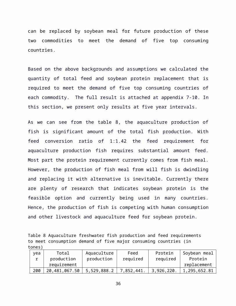
As we can see from the table 8, the aquaculture production of

fish is significant amount of the total fish production. With

feed conversion ratio of 1:1.42 the feed requirement for

aquaculture production fish requires substantial amount feed.

Most part the protein requirement currently comes from fish meal.

However, the production of fish meal from will fish is dwindling

and replacing it with alternative is inevitable. Currently there

are plenty of research that indicates soybean protein is the

feasible option and currently being used in many countries.

Hence, the production of fish is competing with human consumption

and other livestock and aquaculture feed for soybean protein.

Table 8 Aquaculture freshwater fish production and feed requirements to meet consumption demand of five major consuming countries (in tones)

year

Totalproductionrequirement

Aquacultureproduction

Feedrequired

Protein required

Soybean mealProtein

replacement200 20,481,067.50 5,529,888.2 7,852,441. 3,926,220. 1,295,652.81

36

3 3 28 642010

25,483,462.73 6,880,534.94

9,770,359.61

4,885,179.80

1,612,109.34

2015

30,946,103.97 8,355,448.07

11,864,736.26

5,932,368.13

1,957,681.48

2020

38,131,951.03 10,295,626.78

14,619,790.02

7,309,895.01

2,412,265.35

2025

47,218,756.86 12,749,064.35

18,103,671.38

9,051,835.69

2,987,105.78

2030

58,496,743.30 15,794,120.69

22,427,651.38

11,213,825.69

3,700,562.48

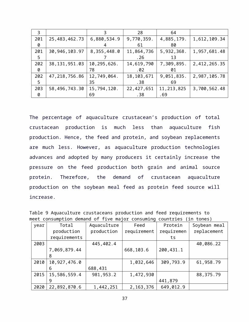
The percentage of aquaculture crustacean’s production of total

crustacean production is much less than aquaculture fish

production. Hence, the feed and protein, and soybean replacements

are much less. However, as aquaculture production technologies

advances and adopted by many producers it certainly increase the

pressure on the feed production both grain and animal source

protein. Therefore, the demand of crustacean aquaculture

production on the soybean meal feed as protein feed source will

increase.

Table 9 Aquaculture crustaceans production and feed requirements to meet consumption demand of five major consuming countries (in tones)year Total

productionrequirements

Aquacultureproduction

Feedrequirement

Proteinrequiremen

ts

Soybean meal replacement

2003 7,069,879.448

445,402.4 668,103.6

200,431.1

40,086.22

2010 10,927,476.06

688,431

1,032,646 309,793.9 61,958.79

2015 15,586,559.49

981,953.2 1,472,930 441,879

88,375.79

2020 22,892,870.6 1,442,251 2,163,376 649,012.9

37

129,802.62025 34,697,549.4

5 2,185,946 3,278,918 983,675.5

196,735.12030 54,416,970.7

3 3,428,269 5,142,404 1,542,721

308,544.2

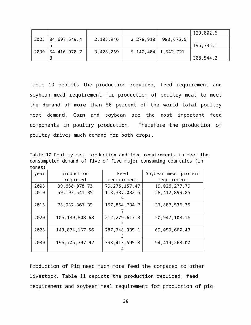
Table 10 depicts the production required, feed requirement and

soybean meal requirement for production of poultry meat to meet

the demand of more than 50 percent of the world total poultry

meat demand. Corn and soybean are the most important feed

components in poultry production. Therefore the production of

poultry drives much demand for both crops.

Table 10 Poultry meat production and feed requirements to meet the consumption demand of five of five major consuming countries (in tones)year production

required Feed

requirementSoybean meal protein

requirement 2003 39,638,078.73 79,276,157.47 19,026,277.792010 59,193,541.35 118,387,082.6

928,412,899.85

2015 78,932,367.39 157,864,734.77

37,887,536.35

2020 106,139,808.68 212,279,617.35

50,947,108.16

2025 143,874,167.56 287,748,335.13

69,059,600.43

2030 196,706,797.92 393,413,595.84

94,419,263.00

Production of Pig need much more feed the compared to other

livestock. Table 11 depicts the production required; feed

requirement and soybean meal requirement for production of pig

38

meat to meet the demand of more than 600 percent of the world

total pig meet demand. Soybean is important feed component in pig

feed composition. Therefore, the production of poultry drives

much demand for cereal crop.

Table 11 Pig meat production and feed requirements to meet theconsumption demand of five of five major consuming countries (intones)year Total production

requiredFeed

requirementSoybean meal protein

requirement2003 58,434,311.69 175,302,935.0

719,108,019.92

2010 97,311,230.19 291,933,690.56

31,820,772.27

2015 128,637,118.77 385,911,356.32

42,064,337.84

2020 171,149,068.80 513,447,206.40

55,965,745.50

2025 228,772,654.43 686,317,963.29

74,808,658.00

2030 306,965,870.91 920,897,612.74

100,377,839.79

5. Conclusions

The main objective of this study is to establish relationship

between some protein food consumption and country’s GDP in order

to enhance forecasting. The co integration rank evaluation shows

that there is long term relationship between consumption of these

commodities and country’s GDP. The model evaluation shows that

consumption also depends not only on present GDP but also on the

past consumption and past GDP, which fall back to up three years.

39

The estimated elasticities are all positive which indicates that

consumption grows with GDP. However, the magnitude and

statistical significance of the elasticity differs from country

to country and for each commodity. For developed countries

especially USA and Japan elaticities are less significant

compared to Developing countries like china and India where GDP

growth much more affects the consumption of the commodities in

positive way. The adjustment speed towards the equilibrium long-

term relationship is not significant in USA for all four

commodities. This shows that GDP may not shape the consumption of

this commodity significantly. In countries where the consumption

of these commodities are part traditional diet for long,

consumption is less elastic to GDP growth and the equilibrium

adjustment speed is faster. Past GDP has negative effect on the

current consumption for developing countries like India and

Indonesia. Past consumption is more important for countries like

USA and Japan.

The second objective of the study is to forecast the consumption

of these commodities for the next two decades. Our forecasting

starts at year 2004 since the data available on FAO website is

only limited to 2003. Therefore, as soon as FAO releases its data

for 2004 to 2008 we will evaluate the disparity between our

forecast and the observed data. The forecasted result shows that

generally consumption of these commodity increases if GDP should

continue to grow at the current rate. Consumption will increases

substantially in China for all commodities included in this

40

study. Consumption is not going to increase very much for

countries like Japan and USA.

In the same manner the demand for animal feed will also increase

with the increase in consumption of these commodities. This is

substantial for poultry and Pig meat production as their

production is entirely depend on the feed availability and

production. The aquaculture production of fish is also increasing

as the marine resource for captured fish dwindle in the world due

to environmental as well as fishing pressure. Therefore the

demand for animal feed for aquaculture production fish will

increase. The aquaculture production of crustaceans has not grown

very much till now and its pressure on the animal feed will not

be substantial for the next decades.

Soybean is important part of the protein diet for the production

of these commodities. Especially for aquaculture production as it

is largely replacing the fish meal protein in the diet. Soybean

and corn are the two most important components of poultry diets.

Therefore, Poultry is also much depend on the soybeans protein

which drive large demand for this commodity in the coming

decades.

41

References Adrian, Elangovan, & K. F. Shim (2000). The influence of replacing fish mealpartially in the diet with soybean meal on growth and body composition ofjuvenile tin foil barb (Barbodes altus), Aquaculture, Vol. 189 (1-2): 133-144.

Anderson, H. M. and Vahid, F. (1997). On the Correspondence between Individualand Aggregate Food Consumption Functions: Evidence from the USA and theNetherlands, Journal of Applied Econometrics, Vol. 12: 477-507.

A.M. Angulo, J.M. Gil and A. Gracia (2001). The demand for alcoholic beveragesin Spain, Agricultural Economics, Vol. 26 (1): 71–83.

Araújo, Lúcio Francelino, et al. (2004). Different criteria of feed formulation for broilers aged 43 to 49 days, Brazilian Journal of Poultry Science, vol. 6 (1):61-64.

Bonne, K. and Verbeke, W. (2008). Religious values informing halal meatproduction and the control and delivery of halal credence quality, Agricultureand Human Values, Vol. 25: 35–47.

Clements, K. W., Wu, Y., and Zhang, J. (2006). Comparing InternationalConsumption Patterns, Empirical Economics, Vol. 31: 1-30.

W. Coyle, M. Gehlhar, T. Hertel, Z. Wang and W. Yu, (1998). Understanding thedeterminants of structural change in world food markets. Am. J. Agr. Econ., Vol.80:1051–1061.

Caballero, B. and Popkin, B. M. (2002). The nutrition Transition: Diet and Disease in theDeveloping World. Amsterdam: Academics press.

Deaton, A. and Muellbauer, J. (1983) Economics and Consumer Behavior, New York:Cambridge university press.

Dernburg, Thomas F., "Consumer Response to Innova-tion: Television," in ThomasF. Dernburg, R. N. Rossett and H. W. Watts, Studies in Household Economic Behavior, Yale Studies in Economics, vol. 9 (New Haven: Yale University Press,1958), 3-49.

Dickey, D.A., 1976, Estimation and hypothesis testing in nonstationary time series, Ph.D. dissertation (Iowa State University, Ames, IA).

Dickey, D A., and W. A. Fuller (1979). Distribution of the estimators forautoregressive time series with a unit root. Journal of the American StatisticalAssociation, Vol. 74:427-431.

Engle, R. F., and B. S. Yoo (1987). Forecasting and Testing in Co-IntegratedSystems, Journal of Econometrics, Vol. 35:143-159.

42

Engle, R. F., and C. W. J. Granger (1987). Cointegration and Error Correction:Representation, Estimation and Testing. Econometrica, vol. 55:251-276.

Fang, C. and Beghin, J. C. (2002). Urban Demand for Edible Oils and Fats inChina: Evidence from Household Survey Data, Journal of Comparative Economics, Vol.30: 732–753.

Friedman, Milton (1957). The Permanent Income Hypothesis: Comment, American Economic Review, Vol. 48:990-91.

Gehlhar M., Regmi A. (2005): Factors Shaping Global Food Markets. In NewDirections in Global Food Markets. Edited by: Regmi A, Gehlhar M. United StatesDepartment of Agriculture (USDA), Agriculture Information Bulletin No. 794;:5-17.

Gerbens-Leenes, P. W. and Nonhebel, S. (2002). Analysis Consumption Patternsand their Effects on Land Required for Food, Ecological Economics, Vol. 42 (1-2):185–199.

Gracia, A., Albisu, L.M. (2001). Food consumption in the European Union: Maindeterminants and country differences, Agribusiness, Vol. 17 (4): 469-488.

Guo, X., Mrox, T. A., and Popkin, B. M. Zhai, F (2000). Structural Change inthe Impact of Income on Food Consumption in China, 1989-1993, EconomicDevelopment and Cultural Change, Vol. 48(4): 737-760.

Huang, J. and Bouis, H. (2002). Structural changes in the demand for food inAsia: empirical evidence from Taiwan, Agriculturul Economics, Vol. 26: 57-69.

Hardy, R.W. (1999) Collaborative opportunities between fish nutrition and other disciplines in aquaculture: an overview. Aquaculture, 177: 217-230.

Helland, S. J. and B. Grisdale-Helland (1998). Growth, feed utilization andbody composition of juvenile Atlantic halibut (Hippoglossus hippoglossus) feddiets differing in the ratio between the macronutrients. Aquaculture, Vol.166(1-2): 49-56.

Houthakker, H.S. and L.D. Taylor (1970). Consumer demand in the United States: analyses and projections, Harvard University Press : Cambridge.

Johansen, S. (1995). Likelihood-based Inference in Cointegrated Vector Autoregressive Models, Oxford University Press :Oxford.

Johansen, S., and K. Juselius (1990). Maximum likelihood estimation and inference on cointegration: With applications to the demand for money. Oxford Bulletin of Economics and Statistics (May): 169-210.

43

Keyzer, M. A., Mebrbis, M. D, Pavel, I. F. P. W, van Wesenbeeck, C. F. A.(2005). Diet Shifts Towards Meat and the Effects on Cereal Use: Can we feedthe animals in 2030? Ecological economics, Vol. 55: 187-202.

Lee, Sang-Min, Sung Hwoan Cho, and Kyoung-Duck Kim ( 2007). Effects of Dietary Protein and Energy Levels on Growth and Body Composition of Juvenile Flounder Paralichthys olivaceus, Journal of the World Aquaculture Society, Vol. 31(3): 306 – 315.

Kwiatkowski, D., Phillips, P. C. B., Schmidt, P. and Shin, Y. (1992). Testing for the Null of Stationarity Against the Alternative of a Unit Root, Journal of Econometrics, vol. 54:159-178.

Leybourne S.J. and P. Newbold (2000). Behaviour of the standard and symmetricDickey—Fuller-type tests when there is a break under the null hypothesis, Econometrics Journal,Vol. 3:1-15

Lochmann, R., W. R. MCClain and D. M. Gatlin (1992). Evaluation of practical feed formulations and dietary supplements for red swamp crayfish. Journal of the World Aquaculture Society, vol. 23 (3):217–227.

Lutkepohl, H. (2005). New Introduction to Multiple Time Series Analysis. New York: Springer

Pauly, D., Christensen, V., Froese, R. & Palomares, M.L. (2000). Fishing downaquatic food webs. Amer. Sci., 88: 46-51.

Paul, Sena  and Brad (1996). Effects of replacement of animal protein by soybean meal on growth and carcass composition in juvenile Australian freshwater crayfish, Aquaculture International, Vol. 4(4): 339-359

Phillips, P. C. B., and P. Perron (1988). Testing for a unit root in time series regression. Biometrika , Vol. 75:335-346

Regmi, A., et al. (2001). “Cross-Country Analysis of Food Consumption Patterns.” In :Changing Structure of Global Food Consumption and Trade. Ed. A.Regmi, Washington, D.C.: Economic Research Service/USDA, pp. 14-22.

Sack, D. (2001). Whitebread Protestants: Food and religion in American culture . New York : Palgrave

Seale, J. Jr., Regmi, A., and Bernstein, J. (2003). International Evidence on Food Consumption Patterns, USDA, Technical Bulletin No. 1904, www.ers.usda.govviewed August 27, 2008.

Selvanathan, E. A., Selvanathan, S. (2003). International Consumption Comparisons:OECD versus LDC. New Jersey: World Scientific Pub Co Inc.

44

Selvanathan, E. A., Selvanathan, S. (2006). Consumption patterns of food,tobacco and beverages: a cross-country analysis. Applied Economics, Vol. 38 (18):1567-1584.

Sengul, H. and Sengul, S. (2006). Food consumption and economic development inturkey and European Unioun countries, Applied Economics, Vol. 38: 2421-2431.

Speedy A. W. (2003). Global production and consumption of animal source foods.Journal of Nutrition, vol. 133:4048S–53S.

Stone, R. (1954) Linear expenditure systems and demand analysis: an application to the British demand, The Economic Journal, 64(255), 511–27.

Schwert, G.W. (1989). Tests for unit roots: A Monte Carlo investigation, Journal of Business and Economic Statistics, Vol. 7: 147-159.

York, R. and M. Gossard (2004). Cross-national meat and fish consumption: Exploring the effects of modernization and ecological context. Ecological Economics, Vol. 48: 293–302.

Yu, W., Hertel, T. W., Preckel, P. and Eales, J. (2004). Projecting World FoodDemand using Alternative Demand Systems. Economic Modelling, Vol. 21 (1): 99-129.

45

Appendixes

Appendix 1. Unit root test statistics of the variables Variables Dickey fuller test

statistics for variable in level

Philips Perron test for variables in level

Dickey-Fuller test statistics for variable in difference

Withouttrend

With trend

without trend

Bangladesh Fresh water fish

0.011 -0.926 -0.268 -4.820***

Brazil Pork -0.692 -2.118 -0.635 -6.369***Brazil Poultry -1.524 -2.258 -1.614 -6.245***China Crustacean 1.210 -1.722 1.129 -5.682***China Fresh water fish

1.210 -2.083 0.676 -4.302***

China Pork -3.475**

-5.426*** -2.731* -3.444***

China Poultry 2.130 -1.595 1.414 -3.969***Germany Pork -2.808 -1.148 -2.843* -5.537***India Crustacean -1.524 -3.720** -1.372 -9.732***India Fresh water fish

-1.659 -3.467* -1.703 -7.041***

Indonesia Crustacean

-0.849 -2.262 -0.952 -5.261***

Indonesia Fresh water fish

0.371 -1.526 0.503 -6.984***

Italy Pork -2.559 -1.023 -3.200** -7.164***Japan Crustacean -0.849 -0.596 -2.065 -4.996***Japan Poultry -

7.712***

-1.707 -6.635*** -2.832*

Mexico Poultry 0.907 -2.042 1.168 -6.174***Spain Pork -2.059 -1.165 -2.484 -6.720***USA Crustacean -0.400 -2.278 -0.320 -7.533***USA Fresh water fish

-0.069 -2.674 0.804 -10.780***

USA Poultry -0.366 -1.630 -0.366 -6.204***Bangladesh real GDP (US$)

1.319 -0.921 1.569 -6.090***

Brazil real GDP (US$)

-3.015**

-0.360 -2.305 -3.432**

China real GDP (US$)

1.123 -2.124 1.324 -5.392***

Germany real GDP (US$)

-1.623 -1.440 -1.507 -3.741***

46

India real GDP (US$)

1.759 -1.231 2.535 -6.826***

Indonesia real GDP(US$)

-0.494 -1.044 -0.473 -4.389***

Italy real GDP (US$)

-5.059***

-1.301 -5.750*** -4.364***

Japan real GDP (US$)

-8.207***

-1.938 -6.493*** -2.500

Mexico real GDP (US$)

-3.628**

-1.526 -3.367** -4.225***

Spain real GDP (US$)

-4.484***

-4.057** -3.114** -3.257**

USA real GDP (US$) -1.500 -3.358** -1.515 -4.942***Note: *** significant at 1%, **significant at 5% and * at 10%. Dickey-Fuller test critical value at 1%=-3.634, 5%=-2.952 and10%=-2.610; Dickey-Fuller test (with trend) critical value at 1%=-4.224, 5%=-3.532 and 10%=-3.199; Phillips-Perron test critical value at 1%=-3.702, 5%=-2.980 and 10%=-2.62; and Dickey-Fuller test(with differenced variables) critical value at 1%=-3.641, 5%=-2.955 and 10%=-2.611

47

Appendix 2. Cointegration equation specification and resultsDependent variables Long-term

elasticityCointegration rank

Model Granger causality

No. of lags inunderlying VAR

Trend and constant specification

Bangladesh Fresh waterfish & Bangladesh realGDP (US$)

1.02(0.014)***

1 3 Restricted constant

16.84***

Brazil Pork & Brazil real GDP (US$)

2.14(0.994)**

1 1 Restricted constant

2.66

Brazil Poultry & Brazil real GDP (US$)

0.41(0.11)***

1 4 unrestricted trend

1.47

China Crustacean & China real GDP (US$)

1.06(0.172)***

1 3 Restricted constant

9.60**

China Fresh water fish& China real GDP (US$)

0.93(0.100)***

1 4 Restricted constant

3.47

China Pork & China real GDP (US$)

0.70(0.027)***

1 2 Unrestricted constant

53.52***

China Poultry & China real GDP (US$)

2.51(0.31)***

1 2 Restricted trend

6.16*

Germany Pork & Germanyreal GDP (US$)

0.33(0.029)***

1 6 Unrestricted constant

4.31

India Crustacean & India real GDP (US$)

1.61(0.323)***

1 2 Restricted constant

21.67***

India Fresh water fishvs. India real GDP (US$)

1.04(0.029)***

1 1 Unrestricted trend

16.41***

Indonesia Crustacean vs. Indonesia real GDP(US$)

0.82(0.138)***

1 2 Restricted constant

14.84**

Indonesia Fresh water fish & Indonesia real GDP (US$)

0.44(0.088)***

1 2 Restricted constant

10.58**

Italy Pork & Italy real GDP (US$)

0.72(0.199)***

1 2 Restricted trend

11.67**

Japan Crustacean & Japan real GDP (US$)

1.61(0.150)***

1 3 Unrestricted trend

25.79***

Japan Poultry & Japan real GDP (US$)

-0.97 (0.99)

1 5 Restricted trend

1.55

Mexico Poultry & Mexico real GDP (US$)

0.38(0.145)***

1 2 restricted trend

10.50**

Spain Pork & Spain real GDP (US$)

1.82(1.091)*

1 2 Restricted trend

1.26

USA Crustacean & USA 1.15(0.166 1 4 Restricted 2.91

48

real GDP (US$) )*** constantUSA Fresh water fish &USA real GDP (US$)

1.08(0.403)***

1 3 Restricted constant

7.03**

USA Poultry & USA realGDP (US$)

1.32(0.055)***

1 4 Restricted constant

1.35

Note: *** significant at 1%, **significant at 5% and * at 10%.

49

Appendix- 3. Countries’ Total Freshwater Fish Consumption Forecast Results forworld top five large consumers (in tones)

year Bangladesh

China India Indonesia USA

2003 1,425,189.01

14,101,687.09

3,041,982.50

992,809.42

919,399.48

2004 1,470,161.77

14,432,006.91

3,311,023.78

1,009,417.51

974,062.74

2005 1,539,692.07

14,549,162.65

3,545,710.07

1,028,526.75

994,462.83

2006 1,629,803.48

14,750,506.81

3,762,563.26

1,047,820.66

1,027,750.51

2007 1,720,705.60

15,084,178.94

3,972,312.59

1,067,315.31

1,058,367.30

2008 1,807,651.42

15,543,793.73

4,181,748.42

1,087,071.56

1,093,400.37

2009 1,894,415.68

16,067,963.45

4,395,162.23

1,107,101.61

1,127,337.26

2010 1,982,725.56

16,595,547.59

4,615,302.63

1,127,406.03

1,162,480.92

2011 2,072,876.89

17,144,791.79

4,844,017.52

1,147,987.54

1,198,384.55

2012 2,164,658.13

17,763,831.32

5,082,633.04

1,168,846.59

1,235,513.21

2013 2,257,708.68

18,470,233.61

5,332,154.84

1,189,987.07

1,273,527.29

2014 2,351,824.58

19,240,904.24

5,593,422.99

1,211,409.36

1,312,519.33

2015 2,446,925.75

20,046,357.01

5,867,205.42

1,233,116.18

1,352,499.61

2016 2,542,938.86

20,884,378.56

6,154,216.41

1,255,109.03

1,393,530.48

2017 2,639,777.00

21,775,433.75

6,455,164.07

1,277,390.65

1,435,612.29

2018 2,737,339.44

22,735,064.90

6,770,767.46

1,299,962.53

1,478,763.76

2019 2,835,525.96

23,759,167.17

7,101,765.69

1,322,827.44

1,523,005.13

2020 2,934,231.10

24,834,441.06

7,448,930.33

1,345,985.48

1,568,363.07

2021 3,033,361.60

25,956,172.49

7,813,050.23

1,369,439.38

1,614,857.06

2022 3,132,819.64

27,132,368.97

8,194,960.91

1,393,191.90

1,662,509.89

2023 3,232,514.90

28,373,239.85

8,595,539.81

1,417,244.43

1,711,343.00

50

2024 3,332,355.60

29,680,980.16

9,015,690.44

1,441,599.76

1,761,379.73

2025 3,432,248.01

31,051,230.65

9,456,378.07

1,466,256.34

1,812,643.80

2026 3,532,110.06

32,481,199.40

9,918,616.46

1,491,219.80

1,865,155.53

2027 3,631,854.65

33,974,167.01

10,403,439.18

1,516,489.98

1,918,942.86

2028 3,731,403.52

35,536,361.58

10,911,960.07

1,542,069.65

1,974,026.65

2029 3,830,672.76

37,171,652.53

11,445,337.50

1,567,960.05

2,030,431.72

2030 3,929,595.29

38,880,017.98

12,004,786.46

1,594,162.38

2,088,181.19

51

Appendix-4. Countries’ Total Crustaceans Consumption Forecast Results forworld top five large consumers (in tones)

year China India Indonesia

Japan USA

2003 3919607 345291.1 281417.9 1150132 13734322004 4199697 348188.8 293632.7 1190286 14148412005 4518529 383152.7 312625.4 1250145 14570632006 4899041 400383.9 334127.9 1290858 15001002007 5316156 424466.3 355995 1322978 15439542008 5775694 451509.6 377439.7 1365670 15886282009 6281014 478663.9 398265.8 1420827 16341252010 6837885 508892.5 418452.6 1481800 16804462011 7450681 541329.3 437993.3 1546489 17275942012 8124632 576224.1 456868.6 1617014 17755682013 8866529 614034.3 475050.8 1694444 18243712014 9684546 654876.5 492512.9 1777832 18740022015 10587536 699083.2 509237.1 1866239 19244642016 11584899 746983.2 525211.3 1959626 19757532017 12687172 798918.3 540432.5 2058247 20278732018 13906487 855290.1 554903.8 2162136 20808192019 15256665 916535.4 568633.3 2271253 21345942020 16753186 983142.2 581634.8 2385712 21891962021 18413341 1055651 593924.8 2505761 22446202022 20256595 1134665 605523.7 2631688 23008702023 22305080 1220856 616453.4 2763764 23579402024 24583819 1314976 626738.1 2902300 24158292025 27121111 1417862 636403.5 3047640 24745322026 29948955 1530451 645476.4 3200149 25340492027 33103680 1653793 653983.2 3360220 25943772028 36626442 1789062 661951.1 3528241 26555092029 40564060 1937581 669408 3704626 27174432030 44969768 2100832 676379.8 3889814 2780177

52

Appendix-5. Countries’ Total Poultry Meat Consumption Forecast Results forworld top five large consumers (in tones)

year Brazil China Japan Mexico USA2003 5,891,640.

2714,319,359.

632,013,419

.34 2,646,903.

4414,766,756

.062004 6,404,836.

7215,513,823.

141,999,954

.52 2,872,657.

1615,188,650

.062005 7,059,628.

5916,930,308.

911,993,606

.76 3,164,649.

9315,518,896

.992006 7,671,954.

7718,394,200.

822,018,984

.06 3,478,278.

3415,910,884

.622007 8,280,244.

0519,857,771.

502,021,462

.87 3,804,320.

6816,414,981

.802008 8,843,851.

2421,369,324.

142,029,845

.01 4,148,627.

0216,799,589

.342009 9,367,014.

6923,001,408.

242,040,295

.08 4,516,513.

9317,266,987

.512010 9,897,720.

1424,800,763.

582,043,028

.86 4,910,871.

6017,698,191

.202011 10,465,482

.3026,779,092.

222,036,320

.38 5,333,984.

0818,168,556

.632012 11,097,717

.3428,929,372.

892,034,582

.10 5,788,455.

1518,637,346

.462013 11,806,325

.4431,245,908.

582,028,306

.97 6,277,234.

0319,088,125

.542014 12,583,097

.4633,734,614.

342,019,359

.62 6,803,501.

7419,558,215

.772015 13,411,418

.1136,412,438.

822,013,991

.23 7,370,624.

5320,022,375

.882016 14,271,127

.5339,301,293.

902,008,319

.78 7,982,203.

0320,502,635

.572017 15,146,862

.9142,422,693.

451,999,220

.67 8,642,089.

9220,981,276

.442018 16,033,165

.8445,795,848.

461,991,709

.75 9,354,424.

5221,463,384

.612019 16,934,237

.1949,439,240.

061,983,675

.51 10,123,651

.7321,952,004

.182020 17,860,712

.0353,372,276.

371,972,694

.63 10,954,555

.9922,443,060

.162021 18,824,673

.7357,616,929.

651,961,935

.41 11,852,317

.7822,940,259

.922022 19,835,007

.7062,198,223.

741,951,474.89

12,822,487.20

23,438,792.34

2023 20,895,136.78

67,143,387.33

1,939,186.28

13,871,043.17

23,941,334.50

2024 22,002,859 72,481,941. 1,926,867 15,004,489 24,447,267

53

.94 06 .14 .29 .282025 23,152,191

.5278,245,353.

081,915,074

.34 16,229,789

.9924,956,378

.532026 24,336,211

.8884,467,297.

031,902,193

.02 17,554,519

.5725,468,934

.182027 25,549,415

.5691,183,999.

901,888,929

.83 18,986,808

.3825,983,934

.472028 26,789,163

.0598,434,705.

701,876,036

.75 20,535,486

.5726,502,059

.372029 28,055,745

.51106,261,861

.801,862,477

.22 22,210,062

.2827,022,840

.212030 29,351,376

.42114,711,403

.801,848,453

.68 24,020,807

.7027,546,250

.88

54

Appendix-6. Countries’ Total Pig Meat Consumption Forecast Results for worldtop five large consumers (in tones)

year Brazil China Germany Italy Spain 2003 2,424,228

.7746,309,931.

534,465,639

.562,503,799

.662,730,712

.172004 2,458,957

.4152,413,984.

844,577,479

.152,502,490

.522,887,888

.012005 2,493,126

.2459,330,199.

454,527,353

.002,517,341

.653,045,047

.322006 2,526,733

.7065,327,915.

564,535,382

.582,526,180

.413,171,166

.312007 2,559,772

.6470,206,608.

314,608,762

.772,535,788

.013,314,230

.412008 2,592,242

.7974,529,158.

804,702,383

.192,544,106

.333,476,981

.192009 2,624,140

.5778,890,233.

904,713,574

.052,551,785

.843,633,798

.222010 2,655,464

.1083,627,000.

634,683,077

.332,558,649

.153,787,038

.982011 2,686,213

.1388,841,727.

334,650,540

.472,564,771

.633,948,115

.762012 2,716,386

.3394,517,163.

474,670,281

.942,570,153

.034,113,097

.702013 2,745,986

.64100,610,079

.054,692,588

.942,574,816

.944,276,741

.732014 2,775,013

.03107,097,158

.094,678,981

.432,578,774

.904,441,563

.452015 2,803,468

.62113,983,812

.424,658,536

.962,582,049

.444,609,251

.332016 2,831,357

.96121,295,466

.634,658,313

.362,584,656

.054,777,911

.102017 2,858,684

.18129,066,456

.974,672,641

.032,586,613

.374,946,772

.992018 2,885,445

.89137,332,836

.374,683,864

.152,587,935

.475,116,575

.882019 2,911,651

.49146,129,971

.584,678,419

.982,588,642

.075,287,250

.952020 2,937,307

.78155,492,491

.154,672,360

.682,588,750

.805,458,158

.392021 2,962,413

.90165,456,354

.674,684,224

.822,588,279

.695,629,172

.452022 2,986,978

.80176,059,400

.694,700,023

.192,587,244

.585,800,351

.052023 3,011,006

.60187,341,928

.544,705,346

.632,585,661

.675,971,477

.852024 3,034,505 199,347,083 4,702,322 2,583,550 6,142,307

55

.39 .17 .06 .05 .232025 3,057,478

.15212,121,546

.314,699,962

.092,580,923

.926,312,743

.972026 3,079,934

.84225,714,390

.694,705,492

.492,577,800

.316,482,676

.352027 3,101,883

.30240,178,510

.844,713,541

.062,574,196

.496,651,952

.642028 3,123,325

.94255,569,258

.164,714,681

.872,570,129

.906,820,429

.472029 3,144,272

.18271,946,251

.514,712,367

.532,565,613

.016,988,000

.352030 3,164,729

.04289,372,979

.364,712,956

.612,560,663

.607,154,542

.30

56

Appendix 7- Aquaculture freshwater fish production and feed requirements tomeet consumption demand of five major consuming countries (in tones)

year

Productionrequirement

aquacultureproduction

Feed required Protein feedrequired

soybean mealProtein

replacement2003

20,481,067.50 5,529,888.23 7,852,441.28 3,926,220.64 1,295,652.81

2004

21,196,672.72 5,723,101.63 8,126,804.32 4,063,402.16 1,340,922.71

2005

21,657,554.37 5,847,539.68 8,303,506.35 4,151,753.17 1,370,078.55

2006

22,218,444.71 5,998,980.07 8,518,551.70 4,259,275.85 1,405,561.03

2007

22,902,879.75 6,183,777.53 8,780,964.10 4,390,482.05 1,448,859.08

2008

23,713,665.50 6,402,689.68 9,091,819.35 4,545,909.68 1,500,150.19

2009

24,591,980.23 6,639,834.66 9,428,565.22 4,714,282.61 1,555,713.26

2010

25,483,462.73 6,880,534.94 9,770,359.61 4,885,179.80 1,612,109.34

2011

26,408,058.29 7,130,175.74 10,124,849.55 5,062,424.77 1,670,600.18

2012

27,415,482.30 7,402,180.22 10,511,095.91 5,255,547.96 1,734,330.83

2013

28,523,611.49 7,701,375.10 10,935,952.65 5,467,976.32 1,804,432.19

2014

29,710,080.50 8,021,721.73 11,390,844.86 5,695,422.43 1,879,489.40

2015

30,946,103.97 8,355,448.07 11,864,736.26 5,932,368.13 1,957,681.48

2016

32,230,173.33 8,702,146.80 12,357,048.45 6,178,524.23 2,038,913.00

2017

33,583,377.76 9,067,511.99 12,875,867.03 6,437,933.52 2,124,518.06

2018

35,021,898.09 9,455,912.49 13,427,395.73 6,713,697.86 2,215,520.30

2019

36,542,291.38 9,866,418.67 14,010,314.51 7,005,157.26 2,311,701.89

2020

38,131,951.03 10,295,626.78 14,619,790.02 7,309,895.01 2,412,265.35

2021

39,786,880.74 10,742,457.80 15,254,290.08 7,627,145.04 2,516,957.86

2022

41,515,851.30 11,209,279.85 15,917,177.39 7,958,588.69 2,626,334.27

202 43,329,881.99 11,699,068.14 16,612,676.75 8,306,338.38 2,741,091.66

57

32024

45,232,005.70 12,212,641.54 17,341,950.99 8,670,975.49 2,861,421.91

2025

47,218,756.86 12,749,064.35 18,103,671.38 9,051,835.69 2,987,105.78

2026

49,288,301.25 13,307,841.34 18,897,134.70 9,448,567.35 3,118,027.23

2027

51,444,893.69 13,890,121.30 19,723,972.24 9,861,986.12 3,254,455.42

2028

53,695,821.47 14,497,871.80 20,586,977.95 10,293,488.98

3,396,851.36

2029

56,046,054.56 15,132,434.73 21,488,057.32 10,744,028.66

3,545,529.46

2030

58,496,743.30 15,794,120.69 22,427,651.38 11,213,825.69

3,700,562.48

58

Appendix 8 Aquaculture crustaceans production and feed requirements to meetconsumption demand of five major consuming countries (in tones)

year productionrequirements

Aquaculture

production

Feedrequirement

Proteinrequirements

soybean meal replacement

2003 7069879.448 445402.4 668103.6 200431.1 40086.222004 7446645.926 469138.7 703708 211112.4 42222.482005 7921514.306 499055.4 748583.1 224574.9 44914.992006 8424510.492 530744.2 796116.2 238834.9 47766.972007 8963549.037 564703.6 847055.4 254116.6 50823.322008 9558941.322 602213.3 903320 270996 54199.22009 10212896.23 643412.5 965118.7 289535.6 57907.122010 10927476.06 688431 1032646 309793.9 61958.792011 11704086.59 737357.5 1106036 331810.9 66362.172012 12550307.21 790669.4 1186004 355801.2 71160.242013 13474429.35 848889 1273334 382000.1 76400.012014 14483769.69 912477.5 1368716 410614.9 82122.972015 15586559.49 981953.2 1472930 441879 88375.792016 16792471.9 1057926 1586889 476066.6 95213.322017 18112642.83 1141096 1711645 513493.4 102698.72018 19559635.52 1232257 1848386 554515.7 110903.12019 21147679.93 1332304 1998456 599536.7 119907.32020 22892870.6 1442251 2163376 649012.9 129802.62021 24813297.69 1563238 2344857 703457 140691.42022 26929342.39 1696549 2544823 763446.9 152689.42023 29264093.32 1843638 2765457 829637 165927.42024 31843661.24 2006151 3009226 902767.8 180553.62025 34697549.45 2185946 3278918 983675.5 196735.12026 37859080.99 2385122 3577683 1073305 2146612027 41366052.9 2606061 3909092 1172728 234545.52028 45261205.45 2851456 4277184 1283155 2566312029 49593118.55 3124366 4686550 1405965 2811932030 54416970.73 3428269 5142404 1542721 308544.2

59

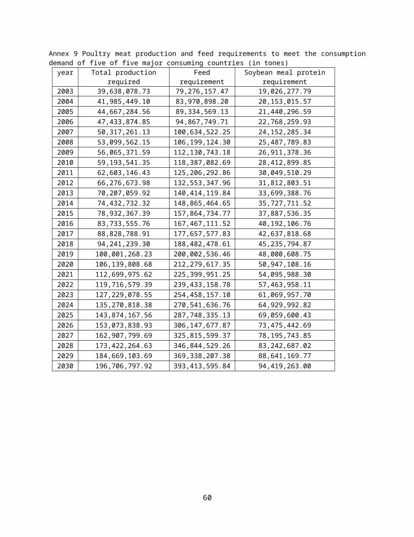
Annex 9 Poultry meat production and feed requirements to meet the consumptiondemand of five of five major consuming countries (in tones)

year Total productionrequired

Feedrequirement

Soybean meal proteinrequirement

2003 39,638,078.73 79,276,157.47 19,026,277.792004 41,985,449.10 83,970,898.20 20,153,015.572005 44,667,284.56 89,334,569.13 21,440,296.592006 47,433,874.85 94,867,749.71 22,768,259.932007 50,317,261.13 100,634,522.25 24,152,285.342008 53,099,562.15 106,199,124.30 25,487,789.832009 56,065,371.59 112,130,743.18 26,911,378.362010 59,193,541.35 118,387,082.69 28,412,899.852011 62,603,146.43 125,206,292.86 30,049,510.292012 66,276,673.98 132,553,347.96 31,812,803.512013 70,207,059.92 140,414,119.84 33,699,388.762014 74,432,732.32 148,865,464.65 35,727,711.522015 78,932,367.39 157,864,734.77 37,887,536.352016 83,733,555.76 167,467,111.52 40,192,106.762017 88,828,788.91 177,657,577.83 42,637,818.682018 94,241,239.30 188,482,478.61 45,235,794.872019 100,001,268.23 200,002,536.46 48,000,608.752020 106,139,808.68 212,279,617.35 50,947,108.162021 112,699,975.62 225,399,951.25 54,095,988.302022 119,716,579.39 239,433,158.78 57,463,958.112023 127,229,078.55 254,458,157.10 61,069,957.702024 135,270,818.38 270,541,636.76 64,929,992.822025 143,874,167.56 287,748,335.13 69,059,600.432026 153,073,838.93 306,147,677.87 73,475,442.692027 162,907,799.69 325,815,599.37 78,195,743.852028 173,422,264.63 346,844,529.26 83,242,687.022029 184,669,103.69 369,338,207.38 88,641,169.772030 196,706,797.92 393,413,595.84 94,419,263.00

60

Annex 10 pig meat production and feed requirements to meet the consumptiondemand of five of five major consuming countries (in tones)

year Total productionrequired

Feedrequirement

Soybean meal proteinrequirement

2003 58,434,311.69 175,302,935.07 19,108,019.922004 64,840,799.92 194,522,399.76 21,202,941.572005 71,913,067.66 215,739,202.99 23,515,573.132006 78,087,378.57 234,262,135.70 25,534,572.792007 83,225,162.14 249,675,486.42 27,214,628.022008 87,844,872.29 263,534,616.88 28,725,273.242009 92,413,532.58 277,240,597.74 30,219,225.152010 97,311,230.19 291,933,690.56 31,820,772.272011 102,691,368.32 308,074,104.95 33,580,077.442012 108,587,082.47 325,761,247.40 35,507,975.972013 114,900,213.30 344,700,639.91 37,572,369.752014 121,571,490.90 364,714,472.69 39,753,877.522015 128,637,118.77 385,911,356.32 42,064,337.842016 136,147,705.09 408,443,115.28 44,520,299.572017 144,131,168.54 432,393,505.61 47,130,892.112018 152,606,657.76 457,819,973.28 49,902,377.092019 161,595,936.08 484,787,808.24 52,841,871.102020 171,149,068.80 513,447,206.40 55,965,745.502021 181,320,445.53 543,961,336.58 59,291,785.692022 192,133,998.32 576,401,994.95 62,827,817.452023 203,615,421.28 610,846,263.85 66,582,242.762024 215,809,767.90 647,429,303.71 70,569,794.102025 228,772,654.43 686,317,963.29 74,808,658.002026 242,560,294.68 727,680,884.05 79,317,216.362027 257,220,084.32 771,660,252.97 84,110,967.572028 272,797,825.35 818,393,476.04 89,204,888.892029 289,356,504.58 868,069,513.75 94,619,577.002030 306,965,870.91 920,897,612.74 100,377,839.79

61