LBNL-41772TA-417

Presented at Thermal VII, Thermal Performance of the Exterior Envelopes of Buildings VII, Clearwater Beach,Florida, December 7-11, 1998, and published in the Proceedings.

This work was supported by the Assistant Secretary for Energy Efficiency and Renewable Energy, Office ofBuilding Technology, State and Community Programs, Office of Building Systems of the U.S. Department ofEnergy under Contract No. DE-AC03-76SF00098.

Experimental Techniques for Measuring Temperature and Velocity Fields toImprove the Use and Validation of Building Heat Transfer Models

Brent Griffith, Daniel Türler, Howdy Goudey,and Dariush Arasteh

Windows and Daylighting GroupBuilding Technologies Department

Environmental Energy Technologies DivisionErnest Orlando Lawrence Berkeley National Laboratory

University of California1 Cyclotron Road

Berkeley, CA 94720

April 1998

1

Experimental Techniques for Measuring Temperature and Velocity Fields to Improve theUse and Validation of Building Heat Transfer Models

Brent Griffith, Daniel Türler, Howdy Goudey, and Dariush Arasteh P.E., ASHRAE member *

Abstract

When modeling thermal performance of building components and envelopes, researchers havetraditionally relied on average surface heat-transfer coefficients that often do not accuratelyrepresent surface heat-transfer phenomena at any specific point on the component beingevaluated. The authors have developed new experimental techniques that measure localizedsurface heat-flow phenomena resulting from convection. The data gathered using these newexperimental procedures can be used to calculate local film coefficients and validate complexmodels of room and building envelope heat flows. These new techniques use a computer-controlled traversing system to measure both temperatures and air velocities in the boundarylayer near the surface of a building component, in conjunction with current methods that rely oninfrared (IR) thermography to measure surface temperatures. Measured data gathered usingthese new experimental procedures are presented here for two specimens: (1) a CalibratedTransfer Standard (CTS) that approximates a constant-heat-flux, flat plate; and (2) a dual-glazed,low-emittance (low-e), wood-frame window. The specimens were tested under steady-state heatflow conditions in laboratory thermal chambers. Air temperature and mean velocity data arepresented with high spatial resolution (0.25- to 25-mm density). Local surface heat-transfer filmcoefficients are derived from the experimental data by means of a method that calculates heatflux using a linear equation for air temperature in the inner region of the boundary layer. Localvalues for convection surface heat-transfer rate vary from 1 to 4.5 W/m2·K. Data for air velocityshow that convection in the warm-side thermal chamber is mixed forced/natural, but localvelocity maximums occur from 4 to 8 mm from the window glazing.

Introduction

Nearly everyone has felt an uncomfortable draft standing near a window or sliding glass doorduring cold weather. Even if no outdoor air makes its way inside, natural convection produces anoticeable, downward flow of low-temperature air. This phenomenon has obvious implications,not only for thermal comfort of building occupants; it is also an important component of buildingenvelope thermal performance, particularly for accurately determining surface temperatures orthe likelihood of moisture condensation on the interior surfaces.

* B. T. Griffith is Principal Research Associate, Christian Köhler is Visiting Researcher, DanielTürler is Senior Research Associate, and Dariush Arasteh is Staff Scientist, Lawrence BerkeleyNational Laboratory, Berkeley CA

2

Current methods for analyzing building thermal performance use film coefficients to estimatesurface heat-transfer rates. These coefficients are average values used to describe heat-transferrates for the entire surfaces where the building envelope surface meets relatively still room air.Because these values are averages, they are often not accurate for specific locations on thesurface. Although the growing use of computer simulations has allowed increasinglysophisticated analysis of the physical structure of building components, comparatively littleimprovement has been made in the analysis of surface heat-transfer phenomena. One way toimprove the analysis of surface heat-transfer rates is to account for localized variations in bothconvective and radiative heat flows. The work described in this paper allows researchers toinvestigate localized convective heat flow.

Schrey et. al. (1998) analyzed thermographic data for surface temperature and solved for localvalues of the convection portion of the film coefficient, hc, for flush-mounted glazing units. Incontrast to Schrey et al.'s research, which used an iterative approach that relied on computersimulations with film coefficient boundary conditions, we present techniques for gatheringexperimental data near an object's surface; these techniques may allow us to directly determinelocalized convection heat transfer coefficients, or local hc.

Noncontact surface temperature measurements using infrared thermography have been used tovalidate simulations (Sullivan et al. 1996). However, one limitation of thermographic data forsuch purposes is that it gives only surface temperatures but not film coefficients at the time of theexperimental measurements. Our current work is on developing expanded experimentaltechniques that allow measuring local convection effects during the testing of buildingassemblies in laboratory thermal chambers. These experimental techniques for mapping data forair temperature and velocity near the surface may be used to develop recommendations forlocalized values for natural convection. The data are also useful for validating conjugateCFD/heat-transfer simulations of building assemblies in laboratory chambers. Becauselaboratory thermal chambers use fans, one concern is whether pure natural convection theory canbe applied to predicting the performance of building assemblies tested in these chambers. Ourexperimental work may be used to test this assumption.

Two specimens were evaluated in the authors' infrared thermography laboratory: a CalibratedTransfer Standard (CTS) and a wood-frame window with low-emittance (low-e) dual glazing.Data were collected for a vertical plane oriented perpendicular to the specimen at its center.Surface temperature data were gathered using infrared thermography. An automated traversingsystem was used to gather air temperature and velocity data. These high-resolution spatial datafor temperature distributions are analyzed using fundamental equations from boundary-layertheory to predict local convection surface heat-transfer rates.

Experiment Measurements

Laboratory experiments were conducted at the authors' laboratory. Figure 1 shows theconfiguration of the thermal chambers. Two laboratory environmental chambers were used toestablish steady-state heat flow through the specimen in a fashion similar to that used in hot-boxtesting for winter heating conditions. However, the warm-side chamber where the measurements

3

took place is designed for unobstructed access to the specimen and therefore does not employ abaffle in the way that a hot box does. The chambers and related instrumentation are described byTürler et al. (1997).

Reference Emitter

Climate Chamber Measurement Chamber

Air Conditioning

CrossflowFan

Heater

Cooling Coil

TestSpecimen

Imager

(not to scale)

Traversing System

Figure 1 -- Laboratory Chambers

The cold-side chamber moves air up the back of the specimen in a plenum; velocity for theseexperiments was about 4.7 m/s at middle of the specimen's main face during measurements.Bulk air temperature was measured at –17.8°C with a four-wire platinum resistance thermometersituated about halfway up the specimen. The mean surface heat-transfer coefficient on the coldside was measured at 33.4 W/m2◊K using the Calibrated Transfer Standard (CTS) describedbelow.

On the warm side of the specimen, air slowly circulates through a subfloor where thetemperature is controlled. An air sink below the specimen removes cooled air. Thistemperature control scheme results in bulk air velocities of about 200 mm/s. Bulk airtemperature was measured at 21.1°C with a four-wire platinum resistance thermometer situatedat the top of the specimen about 250 mm from the surface. The mean surface heat-transfercoefficient on the specimen's warm side was measured at 8.4 W/m2◊K using the CTS describedbelow. Although a desiccant system can be used to decrease the humidity in the warm chamber,it was not used for these experiments; the humidity level was about 45%.

Specimens Evaluated

We evaluated two specimens: a CTS and a wood framed window with low-e dual glazing.

CTS. -- A CTS is a special thermal test assembly used to characterize mean surface heat-transfercoefficients in certain types of standardized hot-box testing (ASTM C-1199). The CTS used forthis experiment was constructed from expanded polystyrene foam board (EPS) that was 25.4 mm(1in) thick and sandwiched between 4.7-mm (3/16-inch) glass sheets. The 912-mm- (36-in-)

4

square CTS has a total thickness of 35 mm (1 3/8-inch) and is mounted flush on its warm side ina 39.4-mm-(1.5-in-) thick surrounding panel made of extruded expanded polystyrene foam(XEPS). Thermocouple arrays located at each interface between glass and EPS can be used todetermine heat-flow rates, surface temperatures, and mean film coefficients.

Dual-Glazed Window -- A wood casement window was obtained from a major manufacturer.The window was a fixed casement with a three-step frame profile. It had a low-e, dual-sealed,insulating glazing unit. The wood nailing flange and minor exterior trim sections were removed.Overall size was 916 mm (36 in) high by 611 mm (24 in) wide. Glazed area was 830 mm (32.7in) high by 525 mm (20.7 in) wide. The window's frame profile, dimensions, and mounting forthermal testing are diagrammed in Figure 2. The window was mounted in a 117-mm-(4.6-in-)thick XEPS surrounding panel that was approximately flush with the outer frame surfaces onboth the cold and warm sides.

29.0

12.7

16.2

25.4

12.7

17.5

16.5

4.7 4.7

42.9

115.1

18.6

25.9Dimensions in Millimeters

Not a Scale Drawing

830916

315

117

Frame Cross Section Test Mount

315

Figure 2 -- Wood-Frame Window Specimen and Mounting

Traversing System Air Measurements

A computer-controlled motion system was used to move sensors in the air space near thespecimens. This system collected air temperature and velocity data with high spatial resolution.Figure 3 depicts the traversing apparatus and shows the orientation of the plane (perpendicular tothe specimen face) in which data were collected for this paper. The traversing system offers fullcontrol in three axes although the data presented here are only two-dimensional.

5

Cold-Side Chamber

Test Specimen Assembly Traversing System

Plane ofDataCollection

Figure 3 -- Traversing System for Air Measurements, showing planein which data are collected

Because a specimen may not be perfectly flat and/or aligned to the traversing system, scanningthe air space very near the surface requires careful setup. Each specimen is first mounted in thethermal chambers and brought to steady-state conditions because it may bend or warp because ofthermal expansion/contraction. The surface profile (specimen coordinate system) ischaracterized with respect to the traversing system's alignment (traversing system coordinatesystem) by sweeping an electronic dial gauge across the surface. (See Figure 5 for orientation ofx and y coordinates.) The traversing system is then programmed to track the surface based onthe dial gauge data, with resolution to 0.01 mm and estimated accuracy of 0.05 mm. Thetraversing program dictates the grid of measurement locations. In the x direction, the grid variesto provide higher resolution near interesting features such as the beginning of a flat specimen orthe sill of a window. In the y direction, the data grid is varied to provide 0.25-mm resolution inthe first 2 or 3 mm near the surface; resolution gradually decreases until the grid has 5-mmresolution at distances greater than 20 mm from the surface. As it tracks the surface, the

6

traversing system corrects y locations at each x location so that the final data grid is orthogonal.A typical scanning experiment will measure 1,000 to 1,400 points in a grid that hasapproximately 40 points in the x direction and 30 points in the y direction.

The traversing system rests at each grid point to gather a measurement before moving on to thenext point. At the middle of the rest period, a trigger notifies the data-acquisition system torecord values. Experiments presented here used a 40-second rest time with the data collectedduring a period of 20 seconds toward the end of the rest period. A typical scanning experimentran for 10 to 15 hours, depending on the number of data points recorded.

Boundary-layer air temperatures were measured using a custom-built probe with a fine-wire,type T thermocouple. The probe is diagrammed in Figure 4. The 40-gauge wire has a diameterof 0.08 mm (0.003 in). The probe is read at 0.03∞C resolution with an estimated accuracy of ±0.3∞C. The 16-bit data-acquisition system sampled the probe at 240 times per second andperformed an initial average of every 40 values. These averaged data were then analyzed for aperiod of 20 seconds to determine the average value (variance of the data was also recorded).The probe and associated instrumentation were calibrated with a four-wire referencethermometer accurate to ±0.02∞C, by immersion in a temperature-controlled, stirred, fluid bath.

Air velocities were measured using a commercial, constant-temperature, hot-wire anemometer.The probe is diagrammed in Figure 4. The sensor wire has a diameter of 4 mm (0.00015 in).Overheat level is about 100∞C. The probe was calibrated for velocities from 0 to 400 mm/s usinga sled technique in which the traversing system moves the probe through still air at a measuredvelocity. Resolution of the velocity measurements is 1 mm/s, but the precision is estimated at±10 mm/s, and the bias in data could be as much as ±70 mm/s. The data-acquisition rates andanalysis are the same as for the temperature probe.

7

23

4057

Thermocouple Junction

Stainless Steel Tubing, 1mm OD

Air Temperature Probe

Air Velocity Probe

Bare Thermocouple Wire, 0.08 mm OD

Hot-Wire Probe Sensor, 4 mm OD

1.5 Dia.

4.6 Dia.3.2 Dia.

12.7

12.7

0.13

38

Dimensions in Millimeters

Figure 4 -- Sensors used in Traversing Experiments

Thermographic Surface-Temperature Measurements

Specimen surface temperatures were measured using infrared thermography and an externalreferencing technique. Detailed discussion of the equipment and techniques developed for thispurpose are presented elsewhere (Griffith et al. 1995; Türler et al.1997; Griffith et al. 1998). Thethermographic measurements presented here for the wood-frame window required morecomplicated procedures than needed for the flat specimen because the window frame surfaceswere not flush. The complexities caused by self-viewing surfaces were accounted for usingsmall mirrors in a multistage process that gathered background radiation values for each surface.These procedures are discussed briefly in previous research (Griffith 1998). More research isneeded on performing thermographic measurements of self-viewing surfaces, so the infrared datapresented for the window specimen should be regarded as preliminary. External referencing ofthe infrared data used a target with a glass surface that was controlled by circulating waterthrough a copper plate. Surface temperature data sets were generated with spatial resolutionranging from 1 to 3 mm. Temperature values have 0.1∞C resolution and estimated accuracy of±0.5∞C.

8

Potential Applications of the Experimental Data

The temperature and velocity measurements made using the traversing system can be used to (1)calculate local convection coefficients for building assemblies and to (2) validate computermodels of building heat transfer and air flow.

Local Convection Coefficients

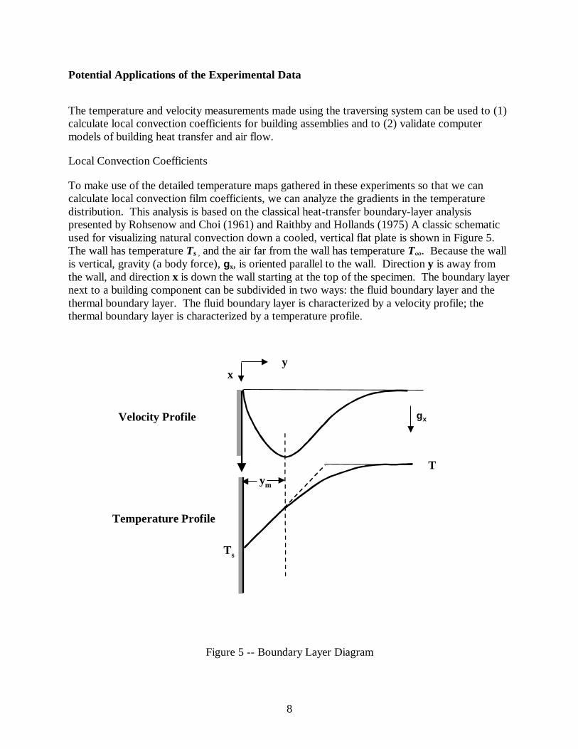
To make use of the detailed temperature maps gathered in these experiments so that we cancalculate local convection film coefficients, we can analyze the gradients in the temperaturedistribution. This analysis is based on the classical heat-transfer boundary-layer analysispresented by Rohsenow and Choi (1961) and Raithby and Hollands (1975) A classic schematicused for visualizing natural convection down a cooled, vertical flat plate is shown in Figure 5.The wall has temperature Ts , and the air far from the wall has temperature T• . Because the wallis vertical, gravity (a body force), gx, is oriented parallel to the wall. Direction y is away fromthe wall, and direction x is down the wall starting at the top of the specimen. The boundary layernext to a building component can be subdivided in two ways: the fluid boundary layer and thethermal boundary layer. The fluid boundary layer is characterized by a velocity profile; thethermal boundary layer is characterized by a temperature profile.

T•

Ts

gx

ym

yx

Velocity Profile

Temperature Profile

Figure 5 -- Boundary Layer Diagram

9

Fluid Boundary Layer. -- A thorough discussion of fluid boundary-layer theory is beyond thescope of this paper; our focus is on only one feature of this layer, referred to as the inner region.This is shown in Figure 5 as the region where y < ym. The value of ym corresponds to thedistance from the wall where the air velocity has a local maximum as a result of naturalconvection. As the boundary layer develops, or grows, in the x direction, the value of ym isexpected to increase slightly. Note that at the surface of the wall the velocity in both the x and ydirections is zero. In the inner boundary layer region there is no momentum transferperpendicular to the wall, and viscous, buoyancy, and acceleration forces are balanced. Thus,the y component of velocity is zero in the inner region. We can then argue that there is noenergy transport from mass transfer in this inner region. Therefore, the convection heat flow ispurely from conduction within/across the inner boundary layer, which permits us to use Fourier'sequation for heat conduction to characterize surface heat flows.

Identifying where the maximum velocity occurs should allow us to determine the extent of theinner boundary layer region in the y direction. This is shown in Figure 5 as the region y < ym. Ifwe are able to map the local air velocity maximum, we can be reasonably certain that we arewithin the inner boundary layer and thus that our temperature measurements were taken at apoint between that maximum and the building component being analyzed (see Figure 5).

Thermal Boundary Layer.-- The analysis presented by Raithby and Hollands (1975) makesextensive use of a linear approximation for the temperature profile in the inner boundary layerregion very near the surface of an object. This approximation is justified by and closely tied tothe pure conduction mode of heat flow in the y direction in the inner boundary layer. Becausethe measurements presented in this paper have such fine resolution and are close to the surface, itis possible to analyze local convection using only the simple principle of pure conduction.

Thus, we make use of the following equations adapted from the literature (Rohsenow 1961) todetermine values for natural convection. The temperature gradient in Equation 1 (DT/Dy) mustbe evaluated within the region where y < ym.

=

DyDT

kQc (1)

( )sc TT

h−

=∞

cQ(2)

whereQc = heat delivered to the surface by convection(W/m2)hc = convection film coefficient (W/m2◊K)k = thermal conductivity of still air (W/m◊K)T = air temperature (∞C)y = distance from plate (m)T• = air temperature (∞C)Ts = surface temperature (∞C).

10

Data Analysis: Local hc From Air Temperatures. -- Air-temperature data were collected atnumerous x and y locations. The spatial coordinates for the temperature data were transformedinto a flat coordinate system that corresponding to the one shown in Figure 5. (When the surfacewas not flat to within 0.1 mm, we accounted for this in the traversing measurements; the datawere transformed into a coordinate system that appears flat.) Data collected for air temperaturewere analyzed by fitting a linear equation for air temperature as a function of distance from theplate. For each x location, we fitted a line through eight points in the y direction within threemillimeters from the plate. The slope of this line became the value for DT/Dy at position x. Thethermal conductivity of the air, k, is evaluated the temperature at the middle of the line (betweenthe fourth and fifth data points -- about 2 mm from the surface depending on the experiment) byinterpolating between two literature values for k, 0.02408 W/m◊K at 0∞C and 0.02614 at 26.85∞C(Liley 1968). Surface-temperature data were gathered using infrared thermography with a highspatial resolution of about 1 mm and a fifth-order polynomial equation curve fit was used toconvert the data for Ts between coordinate systems. The CTS also has direct contact sensorsembedded in it, which provides six temperature points along the middle of the specimen; thesedata were also fit with a fifth-order polynomial equation to provide a second set of values for Ts

for the CTS.

Applications for Model Validation

The data gathered by the traversing system can also be used to validate sophisticated computersimulation tools that are used to analyze energy use and comfort in buildings. Two general typesof simulation programs that are used are those that focus on the details of heat flow throughcomponents of a building's thermal envelope and those that focus on the details of air flow insidea building's occupied spaces. The first type of program simulates heat transfer by conduction intwo or three dimensions using thermal models that extend between the interior and the exteriorsurfaces of the building thermal envelope. These programs can be used to generate ratings forfenestration products and are beginning to incorporate modeling of localized surface heat-transfer effects by means of improved radiation modeling algorithms and variable boundarycondition inputs. The second type of computer program used to analyzed buildings relies onComputational Fluid Dynamics (CFD) solution techniques to simulate air flows in occupiedspaces inside a building's thermal envelope (Chen 1997, Ladiende 1997). CFD programs canpredict the energy use and thermal comfort of complicated building spaces such as glazed atria(Schild 1996).

Building heat-transfer and CFD simulations are sometimes merged together in sophisticatedconjugate simulations that predict both heat and fluid flows (Chen 1995). Conjugate simulationscan account for localized radiation and convection effects although they are not often solvedbecause of the considerable computational effort that is required to model fluid motion.

Both types of simulation programs make predictions that are affected by surface heat-transferphenomena and could benefit from being able to use local values for film coefficients. Forexample, Griffith (1998) and Arasteh (1998) showed that element-to-element, radiation viewfactor modeling improves the accuracy of surface temperature results for projecting fenestrationproducts. This research also identified complicated convection phenomena as the cause ofdifferences between the experimental and simulated data. Accounting for local radiation and

11

convection effects would be especially useful for rating product performance for condensationresistance. Proposed voluntary Canadian fenestration standards suggest varying the convectioncoefficient by stepped amounts when simulating the condensation performance of the bottomedge of a window (Glover 1998). While this procedure is definitely an improvement over theuse of a constant film coefficient, basing such modeling guidelines on experimental resultswould improve their validity.

Computer simulations are often validated by comparison to experimental measurements. Heat-transfer simulations of building assemblies are usually compared to U-factors measured understeady-state conditions in laboratory thermal chambers (Elmahdy 1992). Though some detailedexperimental data are available for room air flows (Murakumi et al.1994), it is common to verifyCFD simulations in a two-step process that first compares results for a standard benchmark caseand then applies the simulation algorithms to the desired model (Curcija 1992).

Using a modern, computer-controlled traversing system to gather large sets of data with finespatial resolution offers a new way to test the accuracy of simulated data. Instead of extractingsmall parts of the temperature or flow field, entire matrices of data could be compared.Specimens with complicated surface geometry can also be evaluated, providing more rigoroustesting of a model than is possible with classic-flat-plate solutions.

Results

The traversing system was used to test two specimens. Chamber operation over the approximate12-hour time period of the experiments was fairly stable, with temperatures controlled to within± 0.1°C. Uncertainty in the traversed air temperature measurements is estimated at ±0.3°C.Uncertainty in the thermographic surface temperature measurements is estimated at ± 0.6°C.Bias error in the velocity measurements could be as high as 100 mm/s, but the velocity data isestimated to be precise to within ± 10 mm/s. Uncertainty in position is estimated at ± 0.2 mm inthe y direction and ± 0.4 in the x direction. The traversing system setup found that the glasssurfaces of both specimens deflected by distances of about 0.5 to 1 mm.

CTS

The experiments using the CTS focused on gathering temperature data. Figure 6 shows thecomplete set of temperature data including the air temperatures near the surface of the CTS andthe surface temperatures determined from infrared thermography. Figure 7 shows selected airtemperature profiles very near the CTS and linear curve fits of the type that could be used togenerate local convection film coefficients. Figure 8 shows the results for local convectioncoefficients obtained by analyzing the temperature gradient in the air within 3 mm of the CTS'ssurface.

Figure 6 -- CTS Temperature Map: Air Temperatures and Infrared Surface Temperatures

13

15

16

17

18

19

20

21

0 5 10 15

Y, Distance from CTS, mm

Air

Tem

pera

ture

, Deg

. C10 mm

515 mm

815 mm

line fit,10mm

line fit,515 mm

line fit,815 mm

Figure 7 -- Air Temperature Profiles Near the CTS at Three Locations: Showing Linear Fits usedfor Local Convection Coefficients

0

0.5

1

1.5

2

2.5

3

3.5

4

4.5

5

0 200 400 600 800

X, Distance From Top of CTS, mm

Loca

l Con

vect

ion

Film

Coe

ffic

ient

(W

/m2-

K)

Infrared SurfaceTemperaturesUsed

CTSthermocouplesurfacetemperaturesUsed

Figure 8--Local Convection Coefficients along the CTS from the top down, as analyzed from airtemperature gradients

14

Window

Both air temperature and velocity data were gathered for the wood-frame window with low-eglazing focusing on the glazing portion of the specimen. For the traversing experiments,humidity was not suppressed, and condensation was present on the lower 100 mm (x= 730 to830) of the glazing at the sill. The air dryer was used, however, during the thermographicmeasurements. Figure 9 shows the complete set of temperature data including the airtemperatures near the surface of the window glazing and the surface temperatures determinedfrom infrared thermography. Figure 10 shows the complete set of air velocity data near thesurface of the glazing. Figure 11 shows selected horizontal velocity profiles at three distancesfrom the top of the glazing. Figure 12 shows selected vertical velocity profiles at three differentdistances down the glazing. Figure 13 shows the results for local convection coefficientsobtained by analyzing the temperature gradient in the air within 3 mm of the specimen's surface.

Figure 9 -- Wood Window Glazing Temperature Map: Air

Temperatures and Infrared Surface Temperatures

Figure 10 -- Wood Window Glazing, Air Velocity Measurements

17

0

50

100

150

200

250

300

0 5 10 15 20 25 30 35 40 45 50

Y, Distance From Glass, mm

Air

Vel

ocity

, mm

/s

662 mm

212 mm

87 mm

Figure 11 -- Selected Horizontal Profiles of Air Velocity Near Window Glazing at ThreeDistances from the Top of the Glazing

0

50

100

150

200

250

300

0 200 400 600 800

X, Distance From Top of Glazing, mm

Air

Vel

ocity

, mm

/s

1 mm

6 mm

51 mm

Figure 12 -- Selected Vertical Profiles of Air Velocity Near Window Glazing at Three DistancesAway from the Glass

18

0

0.5

1

1.5

2

2.5

3

3.5

4

4.5

0 200 400 600 800

X, Distance From Top of Glazed Area, mm

Loca

l Con

vect

ion

Film

Coe

ffic

ient

(W

/m2-

K)

Figure 13 -- Local Convection Coefficients along Window Glazing from the Top Down asAnalyzed from Air-Temperature Gradients

Discussion

Mapping with high spatial resolution the air conditions near a thermal test specimen is a feasibletechnique for researching localized heat transfer phenomena. The large sets of data fortemperature and velocity that can be gathered with a computer-controlled traversing and dataacquisition system should prove useful for improving the analysis of building thermal envelopeheat flows. The combination of data for both thermal and fluid phenomena measured by thetraversing system are useful for validating steady-state, conjugate CFD simulations. Researchersinterested in obtaining our results are encouraged to contact the authors for electronic versions ofdata sets (see http://windows.lbl.gov).

Our temperature-distribution results show that air temperature can be considered linear in theinner region of the thermal boundary layer, as theory leads us to expect. The velocity profiles forthe window show that, although the flow is not purely natural convection, there is a localvelocity maximum that occurs as would be expected for pure natural convection. This maximumwas found to occur from 4 mm to 8 mm from the surface of the window (4 mm < ym < 8 mm),indicating that y < 3 mm is safely inside an inner boundary layer region. Thus, it appears that,although the fan mixing of air in the thermal chamber results in mixed forced and naturalconvection, local convection dominates sufficiently to allow determining local convection

19

coefficients by analyzing the temperature gradients in air and assuming pure conduction in thisregion.

The temperature gradients near the surface were analyzed to determine local surface heat transfercoefficients resulting from convection. The values obtained for local convection coefficientsappear to be reasonable, displaying the trends and magnitudes that are in accordance with theory.However, there is currently no independent method of verifying that the results are accurate.More testing of the procedure for determining local coefficients is needed.

Future Research

The techniques presented here will continue to be used as part of research efforts to develop bothimproved inputs for use in performing building simulations (e.g. local film coefficients) and animproved method for verifying the accuracy of simulated results. Subjects recommended forfuture study using these techniques are listed below.

1. Performing isothermal flat plate measurements. Measuring conditions near anisothermal flat plate in laboratory thermal chambers could provide a good opportunityto evaluate how well engineering theory can be applied to the problem of predictingthe performance levels of building assemblies in a hot box test.

2. Determining local coefficients from temperature boundary-condition modeling. Anindependent method of determining local convection coefficients is being developedthat uses thermographic data as modeling inputs.

3. Performing three-dimensional measurements. Software to control the traversingsystem is being developed to simplify setup and enable collection of data resolved inthree dimensions.

4. Characterizing turbulence intensity. Data collection routines are being refined toallow characterization of the velocity and temperature variations over time.

5. Investigating air humidity interactions. Brandli (1996) identified that radiationabsorption by moisture in the air can produce a measurable effect on the temperatureprofile and thus effect convective film coefficients. This phenomenon will beinvestigated.

Conclusions

The steady-state, thermal testing of building assemblies can be augmented by measuring withhigh spatial resolution temperatures and velocities using a traversing system. Data can beobtained within the thermal boundary in detail sufficient for determining local film coefficientsthat could be used to improve the boundary-condition inputs in heat transfer models. Thecomputer-controlled, motion/data-acquisition system allows collection of large and complicateddata sets that could be used to check the accuracy of sophisticated computer simulations ofconjugate problems of heat transfer and fluid dynamics in buildings.

20

Acknowledgments

The authors thank Nan Wishner for her assistance in editing this paper. This work wassupported by the Assistant Secretary for Energy Efficiency and Renewable Energy, Office ofBuilding Technology, State and Community Programs, Office of Building Systems of the U.S.Department of Energy under Contract No. DE-AC03-76SF00098.

References

Arasteh, D. et. al. 1998. THERM 2.0 : Program description. LBL Report 37371. Berkeley, CAArasteh, D. E. Finlayson, D. Curjica, J. Baker, and C. Huizenga. 1998. "Guidelines for Modeling

Projecting Fenestration Products," ASHRAE Transactions 104(1). Atlanta, GA. AmericanSociety of Heating, Refrigerating and Air-Conditioning Engineers Inc.

ASTM C 1199. 1995. Standard Test Method for Measuring the Steady-State ThermalTransmittance of Fenestration Systems Using Hot Box Methods. 1995 Annual Book ofASTM Standards, vol. 04.06, pp. 658-669, American Society for Testing and Materials.

Brandli, M., G. Schenker, and B. Keller. 1996. The interaction of the infrared radiation from theroom boundaries with the humidity content of the enclosed air. 5th Internationalconferences on Air Distribution in Rooms, ROOMVENT'96. July 17-19, 1996.

Chen, Q. 1997. "Computational fluid dynamics for HVAC: successes and failures," ASHRAETransactions, 103(1). Atlanta, GA. American Society of Heating, Refrigerating and Air-Conditioning Engineers Inc.

Chen, Q., Peng, X. and Paassen, A.H.C. van. 1995. "Prediction of room thermal response byCFD technique with conjugate heat transfer and radiation models," ASHRAETransactions 101(2). Atlanta, GA. American Society of Heating, Refrigerating and Air-Conditioning Engineers Inc.

Curcija, D. 1992. Three dimensional Finite Element model of overall nightime heat transferthrough fenestration systems. Ph.D dissertation. Amherst: University of Massachusetts.

Elmahdy, A.H. 1992. Testing and Simulation of High-Performance Windows -- Phase II of theCanadian/U.S. Joint Research Project on Window Performance. Thermal Performance ofthe Exterior Envelopes of Buildings V. December 1992. Atlanta, GA. American Societyof Heating, Refrigerating and Air-Conditioning Engineers Inc.

Glover, M. 1998. 1998. Proposed Change to CSA Standard A440 Condensation Resistance Test.January 11, 1998

Griffith, B.T. F. Beck, D. Arasteh, and D. Turler. 1995. Issues associated with the use of infraredthermography for experimental testing of insulated systems. Proceedings of the ThermalPerformance of the Exterior Envelopes of Buildings VI Conference. Atlanta,GA.:American Society of Heating, Refrigerating and Air-Conditioning Engineers.

Griffith, B.T., D. Türler, and D. Arasteh. 1996. Surface temperatures of insulated glazing units:infrared thermography laboratory measurements, ASHRAE Transactions 102(2). Atlanta,GA: American Society of Heating, Refrigerating and Air-Conditioning Engineers Inc.

Griffith, B.T., D. Curcija, D. Turler, and D. Arasteh. 1998. Improving Computer Simulations ofHeat Transfer for Projecting Fenestration Products: Using Radiation View-FactorModels, ASHRAE Transactions 104(1). Atlanta, GA. American Society of Heating,Refrigerating and Air-Conditioning Engineers Inc.

21

Ladeinde, F. and M.D. Nearon. 1997. CFD Applications in the HVAC&R Industry. ASHRAEJournal, January 1997.

Liley, P.E.. 1968. The Thermal Conductivity of 46 Gases at Atmospheric Pressure. Proceedingsof the Fourth Symposium on Thermophysical Properties, College Park, MD. AmericanSociety of Mechanical Engineers.

Murakami, S., H. Yoshino, S. Kato, T. Harada and T. Hiramatsu. 1994. Sample data for testingmodels of air and temperature prediction in large enclosures- time dependent data ofexperimental atrium. Institute of Industrial Science, University of Tokyo, Japan.

Raithby, G.D., and K.G.T. Hollands. 1975. A general method of obtaining approximate solutionsof laminar and turbulent free convection problems. Advances in Heat Transfer, 11:265-315. Academic Press.

Rohsenow, W.M. and H.Y. Choi. 1961. Heat, Mass, and Momentum Transfer. Englewood Cliffs,N.J.: Prentice-Hall.

Schild, P.G. 1996. CFD analysis of an atrium, using a conjugate heat transfer modelincorporating long-wave and solar radiation. 5th International Conference on AirDistribution in Rooms, ROOMVENT'96. July 17-19, 1996.

Schrey, A., R. A. Fraser, and P.F. de Abreu. Local Heat transfer Coefficents for a flush mountedGlazing Unit. ASHRAE Transactions 104(1). Atlanta, GA. American Society ofHeating, Refrigerating and Air-Conditioning Engineers Inc.

Sullivan, H.F., J.L. Wright, and R.A. Fraser. 1996. Overview of a project to determine thesurface temperature of insulated glazing units: thermographic measurements and 2-Dsimulations. ASHRAE Transactions 102(2). Atlanta, GA. American Society of Heating,Refrigerating and Air-Conditioning Engineers Inc.

Türler, D., B. Griffith, and D. Arasteh. 1997. “Laboratory procedures for using infraredthermography to validate heat transfer models.” Insulation Materials: Testing andApplications: Third Volume ASTM STP 1320. R. S. Graves and R. R. Zarr, Eds.,Philadelphia, PA: American Society for Testing and Materials.