Experimental study of a geostrophic vortex of gallium in a transverse magnetic field

ELSEVIER Physics of the Earth and Planetary Interiors 91 (1995) 77-98

PHYSICS OFTHE EARTH

AN D PLANI-!TARY INTERIORS

Experimental study of a geostrophic vortex of gallium in a transverse magnetic field

Daniel Brito *, Philippe Cardin, Henri-Claude Nataf, Guy Marolleau D~partement Terre Amosph~re Ocean, Ecole Normale Sup~rieure, URA 1316 du CNRS, 24, rue Lhomond, 75231 Paris Cedex 05,

France

Received 29 November 1994; accepted 27 March 1995

Abstract

We have built an experimental set-up to study the interaction between one single vertical vortex of liquid gallium, generated by a disk, and a transverse magnetic field. Magnetic Reynolds number of 0.1 has been reached. This experiment has been conducted on a rotating table. Therefore the dominant forces are Coriolis and Lorentz forces, as in the Earth's core. We measured pressure profiles at the top of the vortex, differences in electrical potentials between some points in the vortex, and the magnetic field induced by the flow. To understand the velocity flow of the vortex, we introduced a simple two-dimensional model which predicts well these three types of measurements. The Elsasser number (ratio of Lorentz to Coriolis forces) is the critical parameter for the dynamical aspect of the vortex. Under the influence of the magnetic field, the vortex is slowed down but remains two-dimensional or geostrophic, up to Elsasser number 0.2. On the other hand, the size of the vortex increases with the strength of the magnetic field. The induced magnetic field forms a horizontal dipole perpendicular to the imposed field, and has a significant vertical component associated with the geometry of electrical currents and insulating boundaries, and not with the helicity.

R~sum~

Nous avons EtudiE expErimentalement l'interaction entre un vortex vertical de gallium liquide (gEnErE par un disque) et un champ magnEtique horizontal. Des nombres de Reynolds magnEtique de l'ordre de 0.1 ont pu ~tre atteints. Comme cette experience a EtE realisEe sur une table tournante, les forces de Coriolis et de Lorentz Etaient dominantes dans rEcoulement, comme dans le noyau terrestre. Trois grandeurs ont EtE mesurEes: la pression ~ la surface du vortex, la difference de potentiel entre des points situEs sur la gEnEratrice du vortex, et le champ magnEtique induit par l'Ecoulement. Pour amEliorer notre comprehension du vortex, nous avons introduit un module de vitesse bidimensionnel simple, qui rend tr~s bien compte des trois types de mesures EffectuEes. Le nombre d'Elsasser (rapport entre les forces de Lorentz et les forces de Coriolis) est le param~tre critique contrElant la dynamique du vortex. Sous l'influence du champ magnEtique, le vortex est freinE mais reste bidimensionnel ou gEostrophique, jusqu'~t un hombre d'Elsasser de 0.2. En revanche, la taille du vortex augmente avec l'intensit~ du

* Corresponding author.

0031-9201/95/$09.50 © 1995 Elsevier Science B.V. All rights reserved SSDI 0031-9201(95 )03051-4

78 D. Brito et al. / Physics of the Earth and Planetary' Interiors 91 (1995) 77-98

champ magn6tique. Le champ magn6tique induit prend la forme d'un dip61e horizontal perpendiculaire au champ magn&ique impos6. Nous rnontrons que cela est df~ a la g6ometrie des courants 61ectriques et des parois isolantes, plut6t qu'~t l'h61icit6 de l'6coulement.

I. Introduction

The understanding and modeling of the Earth's dynamo, responsible for its magnetic field (Elsasser, 1946), remains one of the most chal- lenging problems in the Earth sciences. The major ingredients of this phenomenon are now well established: the engine of the dynamo lies in the convective motions linked with the solidification of the inner core; there is an equilibrium between diffusion and advection of the magnetic field (the magnetic Reynolds number, which is the ratio of advection to diffusion, is larger than unity); the flow is dominated by the Coriolis and Lorentz forces, which are of the same order (the Elsasser number, A, which is the ratio of the Lorentz forces to the Coriolis forces, is of order unity). The full modeling of the dynamo with these ingredients has not been attempted yet.

However, in recent years, following the pio- neer work of Busse (1970), considerable progress has been made in the understanding of convection in the core in the presence of rotation, without a magnetic field. Under these conditions, the Coriolis force is dominant and the flow is geostrophic. It takes the form of columnar vortices, with their axels aligned with the rotation axis (Busse, 1970). This organization of the flow remains in the turbulent regime, which sets in for more active convection (Cardin and Olson, 1994). The inference that this flow could adequately describe actual motions in the core is suggested by the equatorial symmetry of the flow at the surface of the core, as deduced from the inversion of the observed secular variation of the magnetic field (Le Moiiel et al., 1985; Hulot et al., 1990), and also by the alignment of the dipolar magnetic field with the rotation axis for all planets in the solar system (Busse, 1983; Sun et al. 1993; Manneville and Olson, 1995).

Although these observations suggest a strong control of rotation on the generation of the mag-

netic field, limitations of this approach are obvi- ous. First, the Lorentz forces cannot be ne- glected, as they should roughly balance the Corio- lis forces. Second, the diameter of the vortices expected in the core in the absence of a magnetic field is only a few tens of kilometers (Cardin and Olson, 1995), much smaller than the 'observed' vortices at the surface of the core. Nevertheless, the idea that vortices parallel to the rotation axis are the basic element of the flow is a powerful guide.

Within this frame, in which geostrophy is assumed, several workers have investigated the effect of an imposed magnetic field. These studies have shown that the magnetic field strongly en- larges the vortices, and decreases the threshold above which convection starts (Fearn, 1979; Cardin and Olson, 1995). It has also been demonstrated that dynamo action could be substained by such a flow (Busse, 1975).

Of course, the limitation of these studies is that geostrophy is assumed to hold, even in the presence of a strong magnetic field. For very large Elsasser numbers, geostrophy is replaced by magnetostrophy, with the flow following the field magnetic lines. Very few studies attempt to model convection in the core in 3-D geometry, with both the Coriolis and Lorentz forces present. Re- cently, Zhang (1992) and Glatzmaier and Olson (1993) have obtained results in this situation that seem to indicate that the equatorial symmetry of the flow, and its organization in vortices, would hold for Elsasser numbers of order unity.

In any case, the regime in which the Coriolis and Lorentz forces are comparable appears to be very rich, and relatively unexplored. Although several types of instabilities have been discovered (Braginsky and Meytlis, 1991; St. Pierre, 1994; Moffatt and Loper, 1994) we wish to concentrate on a simple problem.

In this paper, we present laboratory experiments that aim at clarifying the influence of the

D. Brito et al. /Physics of the Earth and Planetary Interiors 91 (1995) 77-98

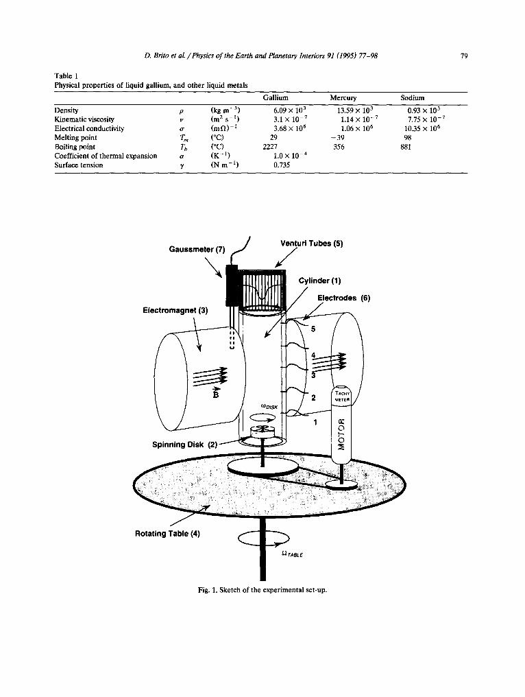
Table 1 Physical properties of liquid gallium, and other liquid metals

79

Gallium Mercury Sodium

Density p (kg m - 3 ) 6.09 × 10 3

Kinematic viscosity v (m 2 s-~) 3.1 × 10-7 Electrical conductivity tr (mE/)-I 3.68 )< 10 6

Melting point T,, (°C) 29 Boiling point Tb (°C) 2227 Coefficient of thermal expansion t~ (K- 1) 1.0 x 10 -4 Surface tension ~, (N m - 1) 0.735

13.59 × 103 0.93 x 103 1.14 × 10 -7 7.75 × 10 -7 1.06 × 106 10.35 × 106

- 39 98 356 881

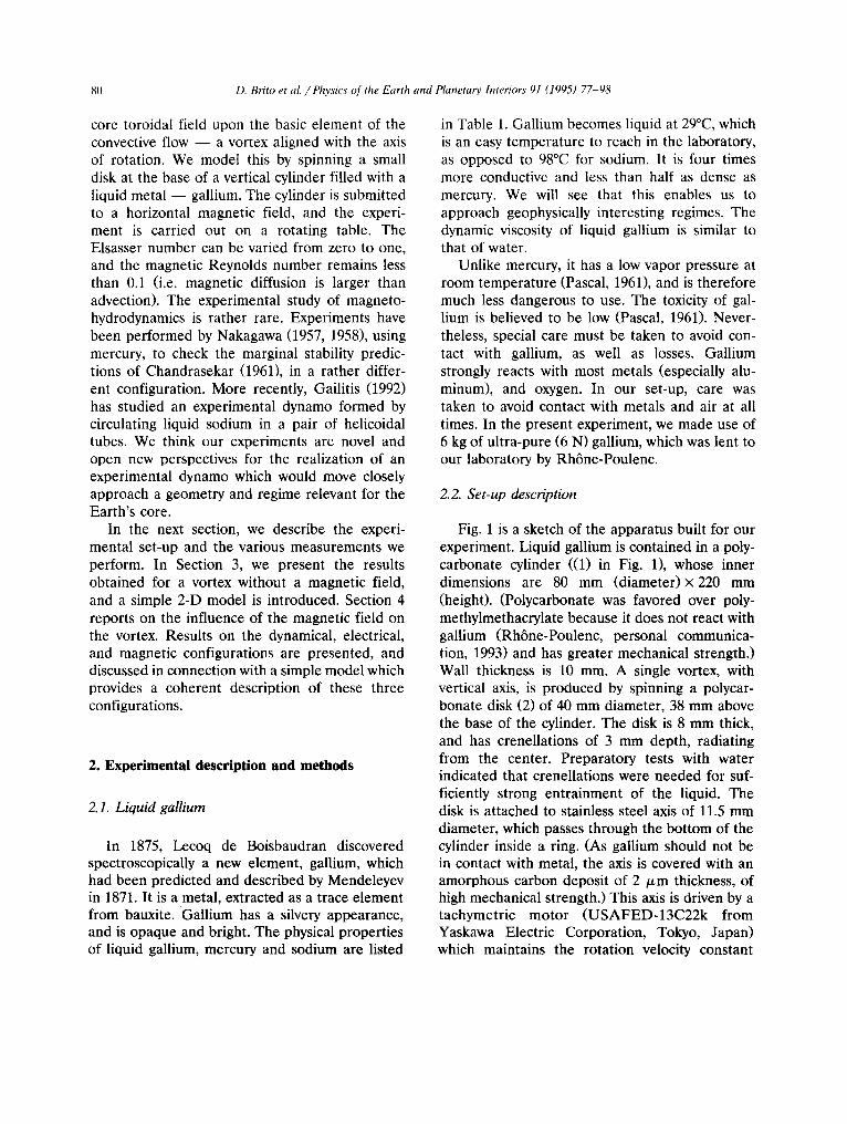
Gaussmeter (7)

Electromagnet (3)

Venturi Tubes (5)

/ Cylinder (1)

E l e c t r o d e s ( 6 )

Spinning Disk (2)

(I) DISK

Rotating Table (4)

~i,~ i~ i ̧~̧ ~!~iii!i! ~ !~:~ ~i?i! !i ii!iil/i~:~i~!:! i ii! ̧ ̧? !: '

~ TABLE

Fig. 1. Sketch of the experimental set-up.

80 D. Brito et al. /Physics of the Earth and Planetary. Interiors 91 (1995) 77-98

core toroidal field upon the basic element of the convective flow - - a vortex aligned with the axis of rotation. We model this by spinning a small disk at the base of a vertical cylinder filled with a liquid metal - - gallium. The cylinder is submitted to a horizontal magnetic field, and the experiment is carried out on a rotating table. The Elsasser number can be varied from zero to one, and the magnetic Reynolds number remains less than 0.1 (i.e. magnetic diffusion is larger than advection). The experimental study of magnetohydrodynamics is rather rare. Experiments have been performed by Nakagawa (1957, 1958), using mercury, to check the marginal stability predictions of Chandrasekar (1961), in a rather different configuration. More recently, Gailitis (1992) has studied an experimental dynamo formed by circulating liquid sodium in a pair of helicoidal tubes. We think our experiments are novel and open new perspectives for the realization of an experimental dynamo which would move closely approach a geometry and regime relevant for the Earth's core.

In the next section, we describe the experimental set-up and the various measurements we perform. In Section 3, we present the results obtained for a vortex without a magnetic field, and a simple 2-D model is introduced. Section 4 reports on the influence of the magnetic field on the vortex. Results on the dynamical, electrical, and magnetic configurations are presented, and discussed in connection with a simple model which provides a coherent description of these three configurations.

2. Experimental description and methods

2.1. Liquid gallium

In 1875, Lecoq de Boisbaudran discovered spectroscopically a new element, gallium, which had been predicted and described by Mendeleyev in 1871. It is a metal, extracted as a trace element from bauxite. Gallium has a silvery appearance, and is opaque and bright. The physical properties of liquid gallium, mercury and sodium are listed

in Table 1. Gallium becomes liquid at 29°C, which is an easy temperature to reach in the laboratory, as opposed to 98°C for sodium. It is four times more conductive and less than half as dense as mercury. We will see that this enables us to approach geophysically interesting regimes. The dynamic viscosity of liquid gallium is similar to that of water.

Unlike mercury, it has a low vapor pressure at room temperature (Pascal, 1961), and is therefore much less dangerous to use. The toxicity of gallium is believed to be low (Pascal, 1961). Never- theless, special care must be taken to avoid contact with gallium, as well as losses. Gallium strongly reacts with most metals (especially aluminum), and oxygen. In our set-up, care was taken to avoid contact with metals and air at all times. In the present experiment, we made use of 6 kg of ultra-pure (6 N) gallium, which was lent to our laboratory by Rh6ne-Poulenc.

2.2. Set-up description

Fig. 1 is a sketch of the apparatus built for our experiment. Liquid gallium is contained in a polycarbonate cylinder ((1) in Fig. 1), whose inner dimensions are 80 mm (d iamete r )x 220 mm (height). (Polycarbonate was favored over poly- methylmethacrylate because it does not react with gallium (Rh6ne-Poulenc, personal communication, 1993) and has greater mechanical strength.) Wall thickness is 10 mm. A single vortex, with vertical axis, is produced by spinning a polycarbonate disk (2) of 40 mm diameter, 38 mm above the base of the cylinder. The disk is 8 mm thick, and has crenellations of 3 mm depth, radiating from the center. Preparatory tests with water indicated that crenellations were needed for sufficiently strong entrainment of the liquid. The disk is attached to stainless steel axis of 11.5 mm diameter, which passes through the bottom of the cylinder inside a ring. (As gallium should not be in contact with metal, the axis is covered with an amorphous carbon deposit of 2 / z m thickness, of high mechanical strength.) This axis is driven by a tachymetric motor (USAFED-13C22k from Yaskawa Electric Corporation, Tokyo, Japan) which maintains the rotation velocity constant

D. Brito et al, / Physics of the Earth and Planetary Interiors 91 (1995) 77-98 81

within 10 -4 . The maximum rotation velocity is 700 rev min-1.

The cylinder is symmetrically placed between the poles, of 160 mm diameter, of an electromagnet (3), which produces a horizontal magnetic field whose intensity can reach 0.1 T. The current to the magnet is delivered by a power source, stabilized within 10 -4 . The temperature around the cylinder is kept at all times above 29°C (the melting temperature of gallium) by circulating hot water in the coils of the magnet and hot air around it.

All these components, weighing around 300 kg, are attached to a rotating table (4). This table was built by the Laboratoire des t~coulements G6ophysiques et Industriels in Grenoble, where the experiments took place, and consists of a duralumin plate of 1.5 m diameter, entrained by a tachymetric motor. The table has excellent horizontal stability during rotation. We could spin it up to 45 rev min-1 (75 rev min-1 for a lightened version), with a velocity control of 10 -3, and to 60 rev min-1 (90 rev min-1 for a lightened version) with a poorer velocity control of about 4%.

2.3. Description of experimental measurements

We try to retrieve as much information as possible on the kinematic, electrical, magnetic,

and dynamical state of our vortex. This is not an easy task, as gallium is opaque. We perform three types of measurements:

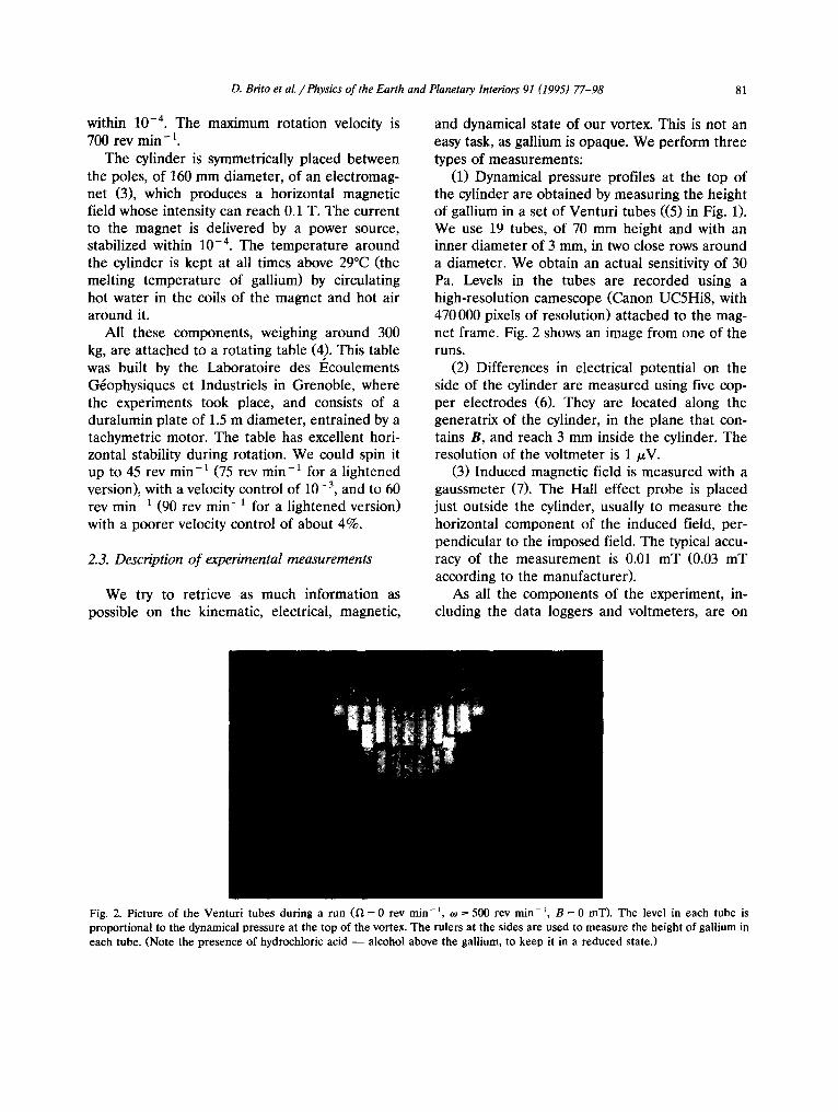
(1) Dynamical pressure profiles at the top of the cylinder are obtained by measuring the height of gallium in a set of Venturi tubes ((5) in Fig. 1). We use 19 tubes, of 70 mm height and with an inner diameter of 3 mm, in two close rows around a diameter. We obtain an actual sensitivity of 30 Pa. Levels in the tubes are recorded using a high-resolution camescope (Canon UC5Hi8, with 470 000 pixels of resolution) attached to the magnet frame. Fig. 2 shows an image from one of the runs.

(2) Differences in electrical potential on the side of the cylinder are measured using five cop- per electrodes (6). They are located along the generatrix of the cylinder, in the plane that contains B, and reach 3 mm inside the cylinder. The resolution of the voltmeter is 1 /xV.

(3) Induced magnetic field is measured with a gaussmeter (7). The Hall effect probe is placed just outside the cylinder, usually to measure the horizontal component of the induced field, perpendicular to the imposed field. The typical accu- racy of the measurement is 0.01 mT (0.03 mT according to the manufacturer).

As all the components of the experiment, in- cluding the data loggers and voltmeters, are on

Fig. 2. Picture of the Venturi tubes during a run (1) = 0 rev min - J, to = 500 rev min - t, B = 0 mT). The level in each tube is proportional to the dynamical pressure at the top of the vortex. The rulers at the sides are used to measure the height of gallium in each tube. (Note the presence of hydrochloric acid - - alcohol above the gallium, to keep it in a reduced state.)

82 D. Brito et al. / Physics of the Earth

the rapidly rotating table, we need a system that controls the experiment on the table, from the beginning to the end of a run. The system we built relies on a PC 486, placed on the table, and a stand-alone program, which is responsible for three tasks:

(1) it regularly checks that the experiment is behaving properly. An emergency stop of the disk and an alarm are triggered if any of the following dysfunctions is detected: (i) temperature drops below 30°C; (ii) gallium leaks from the cylinder; (iii) the torque on the disk drive is higher than a given threshold.

(2) It sets the rotation velocity of the disk to the programmed values.

(3) It triggers the data loggers, and records the measurements from the electrodes and the gaussmeter. All data and programs are written on a virtual disk in random access memory, to avoid accessing the hard disk during rotation. Coded sounds and lights inform the experimentalists of the progress of the run. We control the speed of the rotating table from the outside, as well as the intensity in the magnet, and the movie camera.

2.4. Chemical treatment o f gallium

To avoid the oxidation of gallium, the filling and emptying of the cylinder were performed under a nitrogen atmosphere. Even so, oxides were visible at the top of each column of gallium in the Venturi tubes, We therefore injected into each tube an identical quantity of alcohol mixed

and Planetary Interiors 91 (1995) 77-98

with hydrochloric acid (Fig. 2), which reacted completely with oxides, yielding a clean surface.

3. Equations and dimensionless numbers

We consider a vortex in an incompressible, conductive fluid, in a magnetic field, rotating on a table. The temperature and all material properties are constant. We can write the equation for conservation of mass, the third Maxwell equation, the equation for conservation of momentum, and the induction equation of the magnetic field:

V . U = O (1)

v . n : o (2) oU

p--~-+ p ( U ' V ) U + 2 p U × •

Inertial term Coriolis term = - V P + /zV2U + J × B (3)

Viscous term Lorentz term aB

vx(vxB) at

Magnetic advection term = AVEB (4)

Magnetic diffusion term where U is the fluid velocity vector in the rotating frame, B is the total magnetic field vector B = Bimpose d -1-Binduced, and J is the current density vector. P is the following scalar:

P = p + }~2r2 +p@

where p is the fluid pressure, the second term is the centrifugal force and @ is the gravity poten-

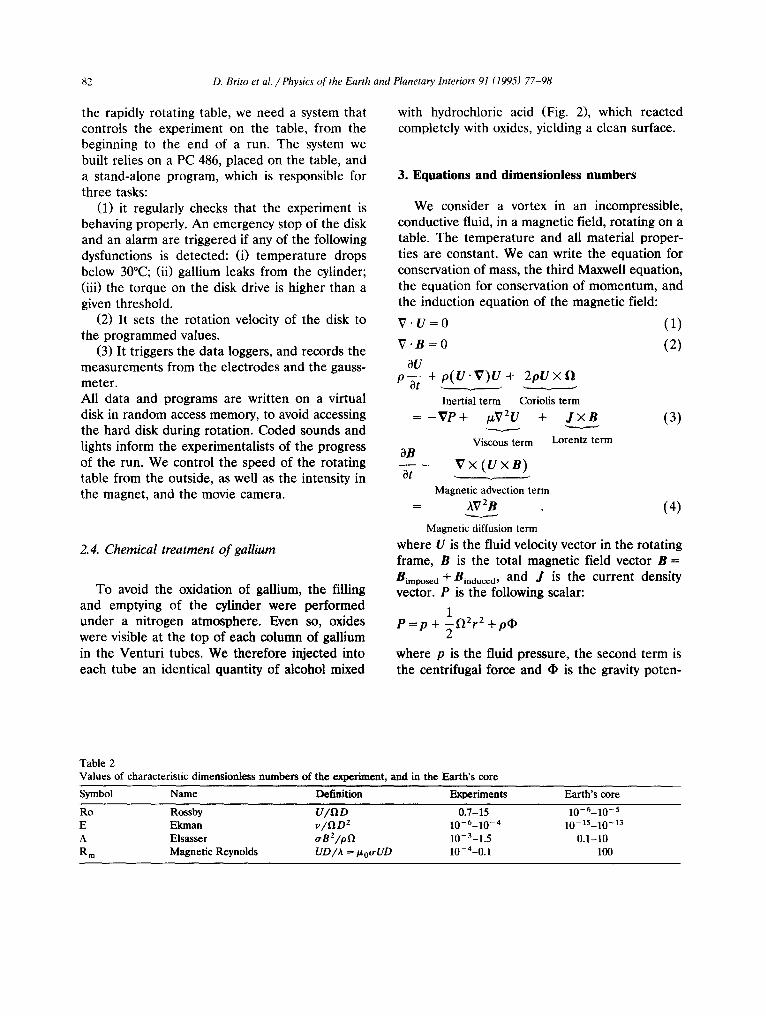
Table 2 Values of characteristic dimensionless numbers of the experiment, and in the Earth's core

Symbol Name Definition Experiments Earth's core

Re Rossby U/lID 0.7-15 10-6-10 -5 E Ekman v/l-lD 2 10 - 6-10- 4 10-15 10-13 A Elsasser o'B2/p~ 10-3-1.5 0.1-10 R m Magnetic Reynolds UD/A = I~o~rUD 10-4-0.1 100

D. Brito et aL / Physics of the Earth and Planetary Interiors 91 (1995) 77-98 83

tial. p is the fluid density,/z the dynamic viscosity, ~, = t z /p the kinematic viscosity, 11 the angular velocity vector of the table; A = 1//~0~r is the magnetic diffusivity, where ~r is the electrical conductivity and/~0 is the magnetic permeability of vacuum.

Eq. (3) is the classical Navier-Stokes equation in a rotating frame, with the Lorentz term added. We look for stationary solutions and therefore drop the first term of Eqs. (3) and (4). Nondimen- sional equations are obtained, using the following scales: the length scale D is the radius of the spinning disk; the velocity scale U is the imposed velocity at the edge of the disk; B is the intensity of the applied magnetic field. We derive the scale for current density, ~rUB, and pressure scale Po is the hydrostatic pressure at the depth of the disk. We write dimensionless vectors with a tilde, and dimensionless scalars with a circumflex. Eqs. (1) and (2) retain the same form, whereas Eqs. (3) and (4) become

Ro(0. ¢)0 + 20 × fi

P0 - ^ = p D U f I V P + E(V2U) + A ( f × / ~ )

Sem[V X ( U X B ) ] = V2/~

where four dimensionless numbers appear: the Rossby, Ekman, Elsasser and magnetic Reynolds numbers. Table 2 gives typical values of these four numbers in the Earth's core, and in our experiments.

4. Study of a vortex generated by a disk without magnetic field

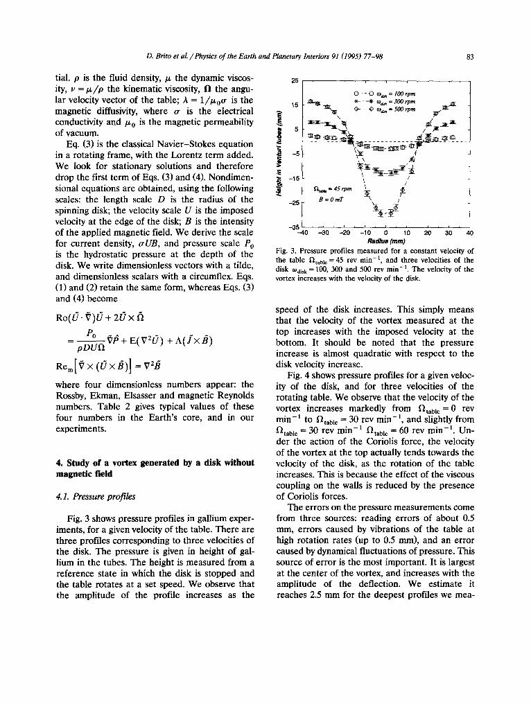
4.1. Pressure profiles

Fig. 3 shows pressure profiles in gallium experiments, for a given velocity of the table. There are three profiles corresponding to three velocities of the disk. The pressure is given in height of gallium in the tubes. The height is measured from a reference state in which the disk is stopped and the table rotates at a set speed. We observe that the amplitude of the profile increases as the

2 5 . , . , , , . , • , . , • , .

0 - - 0 ¢odi a = lOO rpm

-~-- - ---~ %~a = 3OO rpm

-15 \ /

B = O m T ~ /

% . . . . . . . . 'o 'o ' - 3 ~ 0 -30 --20 -10 0 1 2 30 40 Radius (mm)

Fig. 3. Pressure profiles measured for a constant velocity of the table fZtabl e = 45 rev rain - t , and three velocities of the disk O~disk = 100, 300 and 500 rev min - I . The velocity of the vortex increases with the velocity of the disk.

speed of the disk increases. This simply means that the velocity of the vortex measured at the top increases with the imposed velocity at the bottom. It should be noted that the pressure increase is almost quadratic with respect to the disk velocity increase.

Fig. 4 shows pressure profiles for a given velocity of the disk, and for three velocities of the rotating table. We observe that the velocity of the vortex increases markedly from l-ltabt e = 0 rev min - t t o ['~table = 30 rev min -1, and slightly from [ - ~ t a b l e = 30 rev min -1 l~tabl e = 60 rev min -1. Un- der the action of the Coriolis force, the velocity of the vortex at the top actually tends towards the velocity of the disk, as the rotation of the table increases. This is because the effect of the viscous coupling on the walls is reduced by the presence of Coriolis forces.

The errors on the pressure measurements come from three sources: reading errors of about 0.5 ram, errors caused by vibrations of the table at high rotation rates (up to 0.5 mm), and an error caused by dynamical fluctuations of pressure. This source of error is the most important. It is largest at the center of the vortex, and increases with the amplitude of the deflection. We estimate it reaches 2.5 mm for the deepest profiles we mea-

84 D. Brito et al. / Physics o[ the Earth and Planetary Interiors 91 (1995) 77-98

25

.:_ ~ ~ ,,:, ~ ) ,:,

-, ~ , ~ ,

.~ -15

.~ 0,,, : 500,i,,,, ~ ~ ~ ~

- 2 5 B = 0 m T ' , i !

-35 -40 -30 -20 -10 0 10 20 30 40

Radius (mm) Fig. 4. Pressure profiles measured for a constant velocity of the disk Wdisk = 500 rev min -1, and three velocities of the table ~tab le = 0, 30 and 60. With rapider rotation of the table, the vortex becomes increasingly geostrophic, and its angular velocity tends towards the velocity of the disk.

where in the cylinder, and pressure at the top is computed. The mathematical derivation is given in Appendix A. There are only two parameters in this model: Rsolid, the radius of the central region of solid body rotation, and WsoliO, its angular velocity.

From each experimental pressure profile, we derive these two parameters by least-squares inversion. Fig. 6 shows two examples. We see that the simple 2-D model provides a good fit to the measured profiles. The retrieved angular velocity is close to the imposed disk velocity. We will discuss in Section 5 the uncertainty on the inverted parameters.

sure. The resulting error bars are drawn in Fig. 3 and 4.

4.2. 2-D kinematic model

The present experiment was designed to investigate the effect of a simple magnetic field geometry on a simple hydrodynamic flow. The flow we study is simply a forced vortex in a cylinder. This is in fact already a rather complex flow (Spohn, 1991): it is turbulent and three-dimensional, and the viscous coupling with the crenellated disk is far from trivial. Despite all these complexities, the advantage of this flow is that the velocity field is clearly dominated by one componen t - - the azimuthal velocity. Furthermore, we expect little variation in the vertical direction, as a conse- quence of the Proudman-Taylor theorem under geostrophic or vortostrophic conditions.

To investigate the effect of a magnetic field, and to relate our various measurements, we need some simple kinematic model. The model we use is described in Fig. 5: rigid rotation in the central part of the vortex is matched with simple shear at the wall of the cylinder. There is no variation in the vertical direction. Velocity is deduced every-

Fig. 5. 2-D kinematic model of the vortex velocity field. The central cylinder of radius Rsoll d is rotating with a constant angular velocity tosoli d. The solid part is matched with simple shear at the wall of the cylinder. Each measured profile is inverted numerically for the two parameters of this model, Rsoli d and tOsoli d.

D. Br i to et aL / P h y s i c s o f t he E a r t h a n d P l a n e t a r y Inter iors 91 (1995) 7 7 - 9 8 85

4.3. Experimental test of the 2-D kinematic model

We have seen that our simple 2-D model provides a good fit to the observed pressure profiles. However, pressure is relatively insensitive to the precise velocity distribution. It is difficult to obtain more information on the velocity field in an opaque liquid such as gallium. To check the valid- ity of our model, we performed similar experiments with water, the rotating table being at rest.

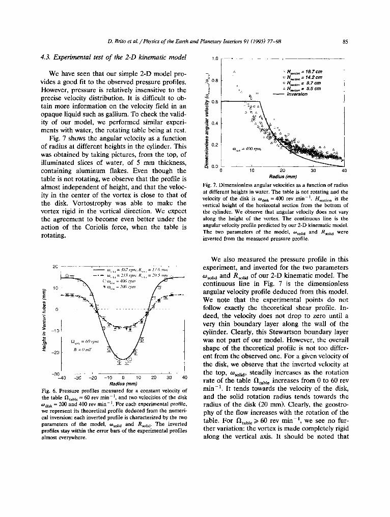
Fig. 7 shows the angular velocity as a function of radius at different heights in the cylinder. This was obtained by taking pictures, from the top, of illuminated slices of water, of 5 mm thickness, containing aluminum flakes. Even though the table is not rotating, we observe that the profile is almost independent of height, and that the velocity in the center of the vortex is close to that of the disk. Vortostrophy was able to make the vortex rigid in the vertical direction. We expect the agreement to become even better under the action of the Coriolis force, when the table is rotating.

1.0

0.8 h

~a .~, 0.6

0.4

m

0.2

Ib

0.0

• I a ~ Ho~tio, = 1 & 7 c m

[] [] H , ~ , o . = 1 4 . 2 c m o H,,~tio" = 9. 7 c m

% t, H.,,,,o, = 5 . 5 ¢ m i n v e r s i o n %

O ~ ZX

~ ~ o o1,,,,, = 400 rprn a ~ ~ a

10 20 30 R a d i u s ( r a m )

40

Fig. 7. Dimensionless angular velocities as a function of radius at different heights in water. The table is not rotating and the velocity of the disk is tOdisk = 400 rev r a in - i , asection is the vertical height of the horizontal section from the bot tom of the cylinder. We observe that angular velocity does not vary along the height of the vortex. The continuous line is the angular velocity profile predicted by our 2-D kinematic model. The two parameters of the model, tOsoli a and Rsoli d were inverted from the measured pressure profile.

20 ] ,° ,,;--~ .~sz,:r . , :e ,,, = }z/ , . , , , '

- - - -- (o ~ ~ = 215 rpm. R ~ ~ = 20.5 m.~g ,__ . .~

I ~ © ,o , , = 400 ,-1 ....

o

- lo ~" -T~ g

~: - 2 0 ~ : o .,r ~ N ~

, i , i , i , ~ 1 ~ 0 t i - 3 % 0 -30 -20 -10 0 20 30 40

R a d i u s ( m m )

Fig. 6. Pressure profiles measured for a constant velocity of the table ~table = 60 rev min -1, and two velocities of the disk tOdisk = 200 and 400 rev rain-1. For each experimental profile, we represent its theoretical profile deduced from the numerical inversion: each inverted profile is characterized by the two parameters of the model, tOsoli d and Rsoli a. The inverted profiles stay within the error bars of the experimental profiles almost everywhere.

We also measured the pressure profile in this experiment, and inverted for the two parameters tOsoli d and Rsoli d of our 2-D kinematic model. The continuous line in Fig. 7 is the dimensionless angular velocity profile deduced from this model. We note that the experimental points do not follow exactly the theoretical shear profile. In- deed, the velocity does not drop to zero until a very thin boundary layer along the wall of the cylinder. Clearly, this Stewartson boundary layer was not part of our model. However, the overall shape of the theoretical profile is not too different from the observed one. For a given velocity of the disk, we observe that the inverted velocity at the top, O)solid, steadily increases as the rotation rate of the table l'~tabl e increases from 0 to 60 rev min- t . It tends towards the velocity of the disk, and the solid rotation radius tends towards the radius of the disk (20 mm). Clearly, the geostrophy of the flow increases with the rotation of the table. For lltaUe >t 60 rev min -] , we see no further variation: the vortex is made completely rigid along the vertical axis. It should be noted that

86 D. Brito et al. / Physics o f the Earth and Planetary Interiors 91 (1995) 77-98

2 0 I , , , • r , , -

®. • t, /~ = 15 ,,7 ~-~ 10 - ' ~ " ,U~ ~" ,3"- ,0, B = 30 m/ ,~,

- l o

-20

t , 1 ~ t . t J ,

-30-40 -30 -20 -10 0 10 20 30 40 Radius (mm)

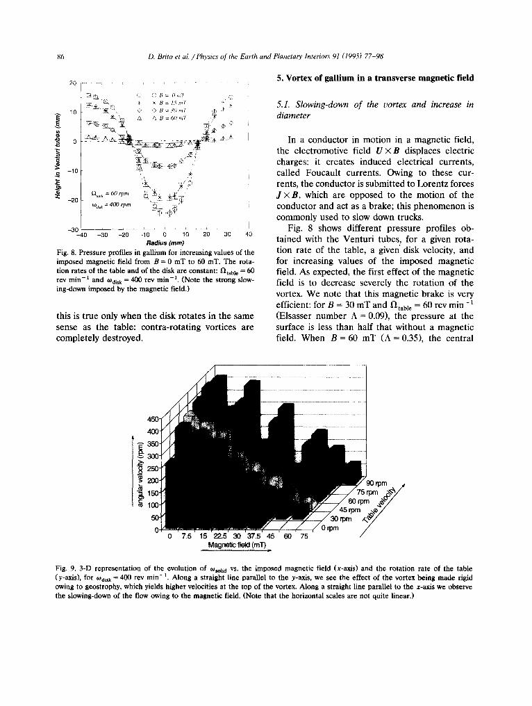
Fig. 8. Pressure profiles in gallium for increasing values of the imposed magnetic field from B = 0 mT to 60 roT. The rotation rates of the table and of the disk are c o n s t a n t : ~ ' tabl¢ = 60 rev rain- ~ and todisk = 400 rev min- ~. (Note the strong slowing-down imposed by the magnetic field.)

this is t rue only when the disk rotates in the same sense as the table: cont ra- ro ta t ing vortices are completely destroyed.

5. Vortex of gal l ium in a transverse magnet ic field

5.1. Slowing-down o f the vortex and increase in

diameter

In a conductor in mot ion in a magnet ic field, the electromotive field U × B displaces electric charges: it creates induced electrical currents , called Foucaul t currents . Owing to these currents, the conductor is submit ted to Lorentz forces J × B, which are opposed to the mot ion of the conductor and act as a brake; this p h e n o m e n o n is commonly used to slow down trucks.

Fig. 8 shows different pressure profiles ob- ta ined with the Ventur i tubes, for a given rota- t ion rate of the table, a given' disk velocity, and for increasing values of the imposed magnet ic field. As expected, the first effect of the magnet ic field is to decrease severely the ro ta t ion of the vortex. We note that this magnet ic brake is very

efficient: for B = 30 m T and ~ - ~ t a b l e = 60 rev m i n - 1 (Elsasser n u m b e r A = 0.09), the pressure at the surface is less than half that without a magnet ic field. W h e n B = 60 mT (A = 0.35), the central

0 7.5 15 22.5 30 37.5 45 60 75 Magnetic field (mT) .

~0 rpm _ _

/

Fig. 9. 3-D representation of the evolution of tOso,i d vs. the imposed magnetic field (x-axis) and the rotation rate of the table (y-axis), for tOdisk ~ 400 rev rain -1. Along a straight line parallel to the y-axis, we see the effect of the vortex being made rigid owing to geostrophy, which yields higher velocities at the top of the vortex. Along a straight line parallel to the x-axis we observe the slowing-down of the flow owing to the magnetic field. (Note that the horizontal scales are not quite linear.)

D. Brito et al. / Physics of the Earth and Planetary Interiors 91 (1995) 77-98 87

depression is only a few millimeters deep: the motion at the top of the vortex is very slow.

As the Lorentz force acts only upon the flow components that are not parallel to the magnetic field, one might expect the axisymmetry of the vortex to be broken by the magnetic field. This does not seem to be the case. Indeed, we performed a few experiments with a free surface and observed that the vortex depression remained axisymmetric as long as it was observable. We therefore use the same 2-D axisymmetric model to fit the observed pressure profiles.

Fig. 9 is a 3D representat ion of the inverted solid body angular velocities v s . ~'~table and B, from all the pressure profiles we have measured with tOdi~k = 400 rev ra in- 1. The evolution of tOsoli d along the lines of constant B clearly shows the effect of the Coriolis force: the inverted solid body angular velocity increases when the rotation speed of the table increases. When the magnetic field is zero, it tends towards the rotation rate of the disk (400 rev min-1). Looking now at the evolution of tOsoli d along the lines of constant

f~table, we see the strong slowing-down imposed by the magnetic field. It should also be noted that, when the table is at rest, the pressure profiles are not deep enough to be inverted for a magnetic field larger than 37.5 roT, whereas for twice this value the profile for l~tabl e = 90 rev min-1 yields a sufficiently deep profile. Our results confirm and quantify the effects of the Cori- olis force and the Lorentz force on the vortex velocity. We will propose a combined view of these two effects later in this section.

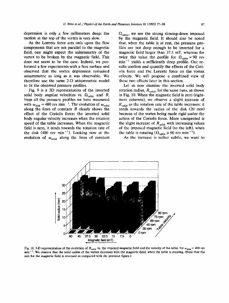
Let us now examine the inverted solid body rotation radius, RsoJid, for the same runs, as shown in Fig. 10. When the magnetic field is zero (right- most columns), we observe a slight increase of Rso~i d as the rotation rate of the table increases: it tends towards the radius of the disk (20 mm) because of the vortex being made rigid under the action of the Coriolis force. More unexpected is the slight increase of Rsoli d with increasing values of the imposed magnetic field (to the left), when the table is rotating (f~table >/60 rev min-1).

As the increase is rather subtle, we want to

45 37.5 30 22.5 15 7.5 0 / . Magnetic field (rnT)

Fig. 10. 3-D representation of the evolution of Rsoli d vs. the imposed magnetic field and the velocity of the table, for tOdisk = 400 rev min-i. We observe that the solid radius of the vortex increases with the magnetic field, when the table is rotating. (Note that the axis for the magnetic field is reversed as compared with the previous figure.)

8 8 D. Brito et al. / Physics of the Earth and Planetary Interiors 91 (1995) 77-98

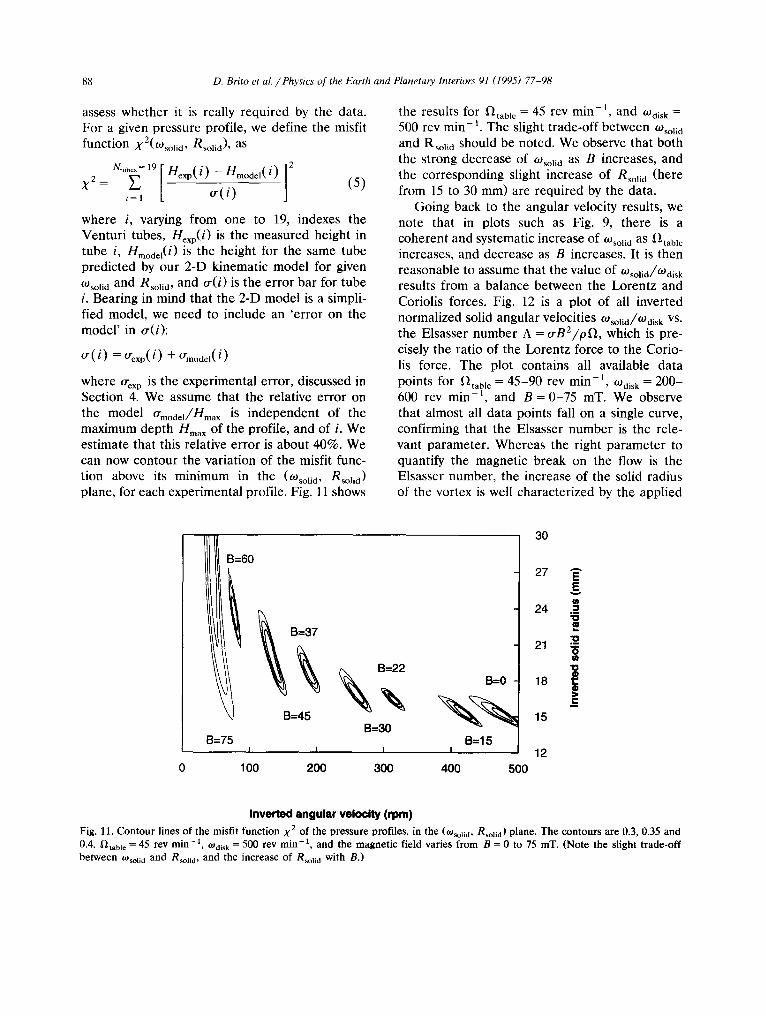
assess whether it is really required by the data. For a given pressure profile, we define the misfit function X2( tOso l id , Rsolid) , as

where i, varying from one to 19, indexes the Ventur i tubes, Hexp(i) is the measured height in tube i, H~nodel(i) is the height for the same tube predicted by our 2-D kinematic model for given OJsoli d and Rsolid, and tr(i) is the error bar for tube i. Bearing in mind that the 2-D model is a simpli- fied model, we need to include an 'e r ror on the model ' in ~r(i):

~r(i) = O'exp(i ) + ~mode,(i)

where Crux p is the experimental error, discussed in Section 4. We assume that the relative error on the model ~rmod~l/Hma ~ is independent of the maximum depth Hma x of the profile, and of i. We estimate that this relative error is about 40%. We can now contour the variation of the misfit function above its min imum in the ((-Osolid, R s o l i d ) plane, for each experimental profile. Fig. 11 shows

the results for ~C~tabl e = 45 rev min-~, and OJdisk ~---

500 rev m i n - i. The slight t rade-off between tOsoli d and Rsoli d should be noted. We observe that both the strong decrease of Wsoli d as B increases, and the corresponding slight increase of Rsoli d (here f rom 15 to 30 mm) are required by the data.

Going back to the angular velocity results, we note that in plots such as Fig. 9, there is a coherent and systematic increase of ¢.Osoli d a s ~table increases, and decrease as B increases. It is then reasonable to assume that the value of tOsol id / tOdisk results f rom a balance between the Lorentz and Coriolis forces. Fig. 12 is a plot of all inverted normalized solid angular velocities tOsolid/tOdisk VS. the Elsasser number A = trBZ/p[l, which is pre- cisely the ratio of the Lorentz force to the Corio- lis force. The plot contains all available data points for f~table = 45-90 rev m i n - l , tOdisk = 200- 600 rev min -1, and B = 0 -75 mT. We observe that almost all data points fall on a single curve, confirming that the Elsasser number is the relevant parameter . Whereas the right pa ramete r to quantify the magnet ic break on the flow is the Elsasser number , the increase of the solid radius of the vortex is well character ized by the applied

B=60

B=75

1 ~ B=3~ B=22

B=45 B=30

I I I

1 O0 200 300

B=O

B=15 I

400 500

30

27

24

21

18

15

12

A

E E

v

m O W

_=

Inverted angular velocity (rpm) Fig. 11. Contour lines of the misfit function X 2 of the pressure profiles, in the (tosolid, Rsoli d) plane. The contours are 0.3, 0.35 and 0,4. f~table = 45 rev min -I, tOdisk = 500 rev min -I, and the magnetic field varies from B = 0 to 75 mT. (Note the slight trade-off between tOsoli d and Rsolid, and the increase of Rsoli d with B.)

D. Bri to et al. / Physics o f the Ear th and Planetary Interiors 91 (1995) 7 7 - 9 8 89

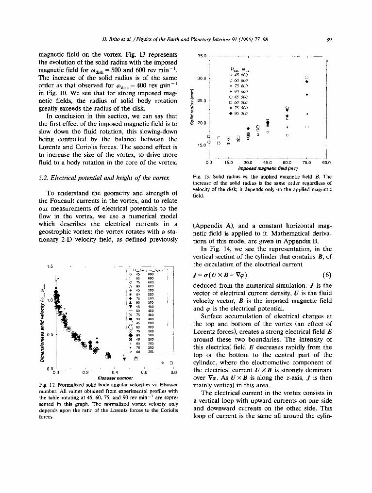
magnetic field on the vortex. Fig. 13 represents the evolution of the solid radius with the imposed magnetic field for tOdi~k = 500 and 600 rev min-1. The increase of the solid radius is of the same order as that observed for OJdi~k = 400 rev min- in Fig. 10. We see that for strong imposed magnetic fields, the radius of solid body rotation greatly exceeds the radius of the disk.

In conclusion in this section, we can say that the first effect of the imposed magnetic field is to slow down the fluid rotation, this slowing-down being controlled by the balance between the Lorentz and Coriolis forces. The second effect is to increase the size of the vortex, to drive more fluid to a body rotation in the core of the vortex.

5.2. Electrical potential and height of the vortex

To understand the geometry and strength of the Foucault currents in the vortex, and to relate our measurements of electrical potentials to the flow in the vortex, we use a numerical model which describes the electrical currents in a geostrophic vortex: the vortex rotates with a stationary 2-D velocity field, as defined previously

1.5

~.o

~ 0.5

0'00.0 0.2 i

0.4

f~,~ (rpm to~,,t(rpm) O 45 60O [ ] 60 600 'C' 75 600

90 600 Jr 45 500

60 500 • 75 500

• 90 5oo • 45 400

i °o ,oo 75 400

:: • 90 400

! I S 45 300 60 300

X 75 300

x ~ 90 3°° 45 200

: o 60 200 • 75 200 o 90 200

0 . . . . . . . . . . , ~

t

0.6 0.8 Elseseer number

Fig. 12. Normalized solid body angular velocities vs. Elsasser number. All values obtained from experimental profiles with the table rotating at 45, 60, 75, and 90 rev min-1 are represented in this graph. The normalized vortex velocity only depends upon the ratio of the Lorentz forces to the Coriolis forces.

35.0

30.0

25.0

20.0

15.0

0.0 15.0

o 45 600 60 600

* 75 6 0 0

* 90 600 0 45 500 ½ 60 500 ~¢ 75500 t 90 500

J o

D o []

30.0 45.0 60.0 75.0 I0.0 Imposed magnetic field (m 7")

Fig. 13. Solid radius vs. the applied magnetic field B. The increase of the solid radius is the same order regardless of velocity of the disk; it depends only on the applied magnetic field.

(Appendix A), and a constant horizontal magnetic field is applied to it. Mathematical deriva- tions of this model are given in Appendix B.

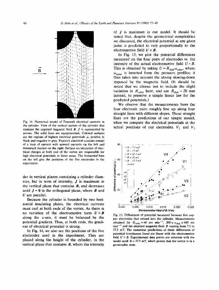
In Fig. 14, we see the representation, in the vertical section of the cylinder that contains B, of the circulation of the electrical current

J = c r ( U X B - V~) (6)

deduced from the numerical simulation. J is the vector of electrical current density, U is the fluid velocity vector, B is the imposed magnetic field and ~ is the electrical potential.

Surface accumulation of electrical charges at the top and bottom of the vortex (an effect of Lorentz forces), creates a strong electrical field E around these two boundaries. The intensity of this electrical field E decreases rapidly from the top or the bottom to the central part of the cylinder, where the electromotive component of the electrical current U × B is strongly dominant over Vq~. As U x B is along the z-axis, J is then mainly vertical in this area.

The electrical current in the vortex consists in a vertical loop with upward currents on one side and downward currents on the other side. This loop of current is the same all around the cylin-

90 D. Brito et aim /Physics of the Earth and Planetary Interiors 91 (1995) 77-98

B i ,

Fig. 14. Numerical model of Foucault electrical currents in the cylinder. View of the vertical section of the cylinder that contains the imposed magnetic field B. J is represented by arrows. The solid lines are equipotentials. Colored surfaces are the regions of highest electrical potentials ~0, positive in black and negative in grey. Foucault electrical currents consist of a loop of current with upward currents on the left and downward current on the right. Surface accumulation of electrical charges at both end of the vortex are responsible for high electrical potentials in these areas. The horizontal bars on the left give the positions of the five electrodes in the experiment.

der in vertical planes containing a cylinder diameter, but in term of intensity, J is maximum in the vertical plane that contains B, and decreases until J = 0 in the orthogonal plane, where B and U are parallel.

Because the cylinder is bounded by two horizontal insulating plates, the electrical currents must curl at both ends of the vortex. As there is no variation of the electromotive term U X B along the z-axis, it must be balanced by the potential gradient. Thus, at both ends, the gradient of electrical potential is strong.

In Fig. 14, we also see the positions of the five electrodes used in the experiment. They are placed along the height of the cylinder, in the vertical plane that contains B, where the intensity

of J is maximum in our model. It should be noted that, despite the geometrical complexities we discussed, the electrical potential at any given point is predicted to vary proportionally to the electromotive field U × B.

In Fig. 15, we plot the potential differences measured on the four pairs of electrodes vs. the intensity of the actual electromotive field U * B. This is obtained by taking U = Rdisk tOsol id , where tOsoli d is inverted from the pressure profiles; it thus takes into account the strong slowing-down imposed by the magnetic field. (It should be noted that we choose not to include the slight variation in Rsoli d here, and u s e Rdisk = 20 mm instead, to preserve a simple linear law for the predicted potentials.)

We observe that the measurements from the four electrode pairs roughly line up along four straight lines with different slopes. These straight lines are the predictions of our simple model, when we compute the electrical potentials at the actual positions of our electrodes. V 2 and V 3

80

60

0

~ 40 0

20

V B = 7 . 5 m T

] B = 1 5 m T

C' B = 2 2 . 5 m T

6) B = 3 0 m T

/'~ B = 3 7 . 5 m T

m o d e l

v4 i V3 v2 vl

/ , /

t3

t2

0 ~ ~ . . . . ~ , i . . . . . . . . . ±

O'OOO 0.005 0,010 0.015 0.020 0.025 Electromotive field U*B (V/m)

Fig. 15. Differences of potential measured between five cop- per electrodes that extend into the cylinder. Measurements obtained for [~ tab le = 60 rev min -1, 200 .<< ~Odisk < 600 rev min-1 and the imposed magnetic field B varying from 7.5 to 37.5 roT. The numerical predictions of these differences of potential (continuous lines) are linear with the electromotive field U x B. Experimental data points are coherent with the model until B = 37.5 mT, which proves that the vortex is in a geostrophic state.

D. Brito et aL / Physics o f the Earth and Planetary Interiors 91 (1995) 77-98 91

30 -~

2 0 / ~ - \

~ - V3 ', ~, ~ ~__ f2,,~,= 0 rpm - 2 0 ~ , - * V 2 ~J-,"

O- - ~0" V l ~_ °Jail, = 300 rpm

D • ~ n s v ~ s e - 3 0 - ' ~ ' ~ ' ~

0 15 3 0 4 5 6 0 7 5 9 0

Imposed magnetic field (m T)

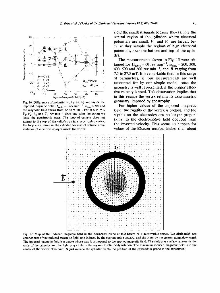
Fig. 16. Differences of potential Vt, II2, 113, V 4 and V T v s . the imposed magnetic field. ~ " ~ t a b l e = 0 rev min - 1, todi~k = 300 and the magnetic field varies from 7.5 to 90 mT. For B >/15 mT, V4, V 3, V 2 and 1I] rev min -1 drop one after the other: we leave the geostrophic state. The loop of current does not extend to the top of the cylinder as in a geostrophic vortex; the loop curls lower in the cylinder because of volume accumulation of electrical charges inside the vortex.

B

yield the smallest signals because they sample the central region of the cylinder, where electrical potentials are small. I/" l and I/4 are larger, because they sample the regions of high electrical potentials, near the bottom and top of the cylinder.

The measurements shown in Fig. 15 were obtained for ~ '~ tab le = 60 rev min-1, O)disk : 200, 300, 400, 500 and 600 rev min-1, and B varying from 7.5 to 37.5 mT. It is remarkable that, in this range of parameters, all our measurements are well accounted for by our simple model, once the geometry is well represented, if the proper effective velocity is used. This observation implies that in this regime the vortex retains its axisymmetric geometry, imposed by geostrophy.

For higher values of the imposed magnetic field, the rigidity of the vortex is broken, and the signals on the electrodes are no longer proportional to the electromotive field deduced from the inverted velocity. This seems to happen for values of the Elsasser number higher than about

. . . . . . . . . . . . . . . . . . . ° ° . . . . . . . . . . . . . . . . . .

. . . . . . . . . . . . . . . , i , , , , , t . . . . . . . . . . . . . . .

. . . . . . . . . . . . . , , s l ¢ 1 ~ , , , . . . . . . . . . . . . .

. . . . . . . . . . . . . , , , , f t t ~ , , , . . . . . . . . . . . . .

. . . . . . . . . . . . . . . . , . J l . , , . . . . . . . . . . . . . . .

. . . . . . . . . . . . . . . . , ¢ . ~ . . . . . . . . . . . . . . . . . .

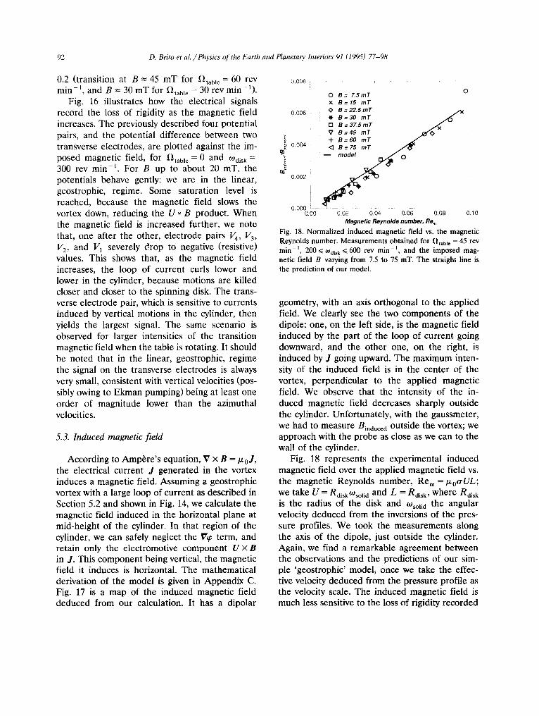
Fig. 17. Map of the induced magnetic field in the horizontal plane at mid-height of a geostrophic vortex. We distinguish two components of the induced magnetic field: one induced by the current going upward, and the other by the current going downward. The induced magnetic field is a dipole whose axis is orthogonal to the applied magnetic field. The dark gray surface represents the walls of the cylinder and the light gray circle is the region of solid body rotation. The maximum induced magnetic field is in the center of the vortex. The point G just outside the cylinder marks the position of the gaussmeter probe in the experiment.

92 D. Brito et al. / Physics of the Earth and Planetary Interiors 91 (1995) 77-98

0.2 (transition at B---45 mT for ~'~table = 60 rev min - t , and B = 30 mT for ~'~table = 30 rev min- l ) .

Fig. 16 illustrates how the electrical signals record the loss of rigidity as the magnetic field increases. The previously described four potential pairs, and the potential difference between two transverse electrodes, are plotted against the imposed magnetic field, for ~'~table = 0 and tOdisk = 300 rev min- t . For B up to about 20 mT, the potentials behave gently: we are in the linear, geostrophic, regime. Some saturation level is reached, because the magnetic field slows the vortex down, reducing the U * B product. When the magnetic field is increased further, we note that, one after the other, electrode pairs V4, I/3, I/2, and I/1 severely drop to negative (resistive) values. This shows that, as the magnetic field increases, the loop of current curls lower and lower in the cylinder, because motions are killed closer and closer to the spinning disk. The transverse electrode pair, which is sensitive to currents induced by vertical motions in the cylinder, then yields the largest signal. The same scenario is observed for larger intensities of the transition magnetic field when the table is rotating. It should be noted that in the linear, geostrophic, regime the signal on the transverse electrodes is always very small, consistent with vertical velocities (pos- sibly owing to Ekman pumping) being at least one order of magnitude lower than the azimuthal velocities.

5.3. Induced magnetic field

According to Amp~re's equation, V × B =/z0J, the electrical current J generated in the vortex induces a magnetic field. Assuming a geostrophic vortex with a large loop of current as described in Section 5.2 and shown in Fig. 14, we calculate the magnetic field induced in the horizontal plane at mid-height of the cylinder. In that region of the cylinder, we can safely neglect the V~ term, and retain only the electromotive component U × B in J. This component being vertical, the magnetic field it induces is horizontal. The mathematical derivation of the model is given in Appendix C. Fig. 17 is a map of the induced magnetic field deduced from our calculation. It has a dipolar

0.008 0

0 B= LSmT x B = 15 mT 0 B=22.5mT

0.008 ~ B=30 mT

[] B = 37.5 mT ~ x V B=45 mT ~ ' 0 + B=60 mT

o.oo4 < B= r5 mr / " ~ i y o ~ - 0.002

0.000 • ~ . . . . . 0 .00 0.02 0.04 0.06 0.08 0.10

Magnetic Reynolds number, Re ~

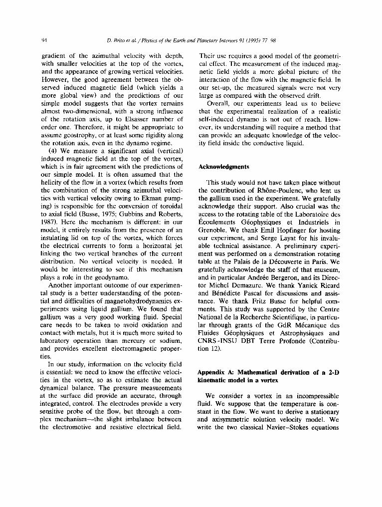
Fig. 18. Normalized induced magnetic field vs. the magnetic Reynolds number. Measurements obtained for ~'~table = 45 rev rain -1, 200 ~< tOdisk ~< 600 rev min -1, and the imposed magnetic field B varying from 7.5 to 75 mT. The straight line is the prediction of our model.

geometry, with an axis orthogonal to the applied field. We clearly see the two components of the dipole: one, on the left side, is the magnetic field induced by the part of the loop of current going downward, and the other one, on the right, is induced by J going upward. The maximum intensity of the induced field is in the center of the vortex, perpendicular to the applied magnetic field. We observe that the intensity of the induced magnetic field decreases sharply outside the cylinder. Unfortunately, with the gaussmeter, we had to measure Binduce d outside the vortex; we approach with the probe as close as we can to the wall of the cylinder.

Fig. 18 represents the experimental induced magnetic field over the applied magnetic field vs. the magnetic Reynolds number, Re m = lZotrUL; we take U = RdisktOsol i d and L = Rdisk, where R d i s k is the radius of the disk and tOsoli d the angular velocity deduced from the inversions of the pressure profiles. We took the measurements along the axis of the dipole, just outside the cylinder. Again, we find a remarkable agreement between the observations and the predictions of our simple 'geostrophic' model, once we take the effective velocity deduced from the pressure profile as the velocity scale. The induced magnetic field is much less sensitive to the loss of rigidity recorded

D. Brito et aL / Physics of the Earth and Planetary Interiors 91 (1995)77-98 93

l , .L ' •

-0 .01

k~

- 0 . 0 2

- 0 . 0 3 ~ /

0 C % , , = h ( X ) r p m . . . .

- - #llOd('l

- 0 . 0 4 . 1 . L . . . . ~ . - - J - . ~ •

0 1 0 2 0 3 0 4 0 5 0 6 0 7 0

radius (ram)

Fig. 19. Horizontal profile of the vertical induced magnetic field above the lid of the cylinder. The measurements were obtained for B = 30 roT, ~Oaisk = 600 rev rain -1, the table being at rest. The vertical dashed lines give the drift of the background field observed over the time of each measurement. The continuous line is the prediction from our simple model.

by the electrodes: B as high as 60 mT still yields the expected induced field. According to our model, the maximum intensity of the induced magnetic field, in the core of the vortex, is about seven times larger than that measured outside the cylinder, and represented in Fig. 17.

Fig. 19 shows the vertical induced magnetic field we measure above the top of the cylinder, along a radius perpendicular to the imposed magnetic field. It is compared with the prediction of our simple model. Here the vertical component of the induced magnetic field was computed by integration of the Biot and Savart law, using the current distribution over the entire volume of the cylinder. We observe that the measured maximum intensity, which is about half the horizontal induced field discussed previously, occurred outside the cylinder, in contrast with the model prediction. Nevertheless, the model produces the right amplitude. This is somewhat surprising because Ekman pumping is often considered to be the source of the axial induced magnetic field, and Ekman pumping is not included in our model. We conclude that the observed axial magnetic

field results from the horizontal electrical current beneath the insulating lid, with no evidence of contribution from vertical fluid motions.

6. Conclusion

Our experimental study of the effect of a horizontal magnetic field on a vortex with vertical axis yields four important results:

(1) the dynamical regime is controlled by the balance between the Coriolis and Lorentz forces: the normalized angular velocity at the top of the vortex only depends on the value of the Elsasser number, and not on the Ekman or Rossby number.

(2) The radius of the solid body rotation core of the vortex increases with the applied magnetic field. In our experiments, this increase is modest (at most a factor of two), because the vortex is strongly constrained by the cylinder. It is reminis- cent of the large increase of vortex diameter observed in numerical experiments on magneto- convection (Fearn, 1979; Glatzmaier and Olson, 1993; Cardin and Olson, 1995). Within the frame of our simple kinematic model, we could not derive an adequate explanation of this phenomenon. It should be noted that a related problem was treated by Parker (1966) and Gubbins and Roberts (1987); they looked at the effect of a magnetic field on a rapidly rotating solid conduct- ing cylinder, and found that the magnetic field is pushed out from the cylinder. Although their calculation assumes a fixed diameter, it gives the intuition that a natural vortex would contract, so as to minimize the field expulsion (P.H. Roberts, personal communication, 1992). This is the oppo- site to what we observe in our experiments. How- ever, their calculation is valid for Re m of order one, whereas Re m is always less than 0.1 in our experiments.

(3) We observe that geostrophy is preserved for Elsasser numbers up to 0.2. This is clearly demonstrated by the linearity of the electrical signals with the electromotive term. For higher Elsasser numbers the same signals, which are very sensitive to any geometric change, indicate a

94 D. Brito et al. / Physkw of the Earth and Planetary Interiors 91 (1995) 77-98

gradient of the azimuthal velocity with depth, with smaller velocities at the top of the vortex, and the appearance of growing vertical velocities. However, the good agreement between the observed induced magnetic field (which yields a more global view) and the predictions of our simple model suggests that the vortex remains almost two-dimensional, with a strong influence of the rotation axis, up to Elsasser number of order one. Therefore, it might be appropriate to assume geostrophy, or at least some rigidity along the rotation axis, even in the dynamo regime.

(4) We measure a significant axial (vertical) induced magnetic field at the top of the vortex, which is in fair agreement with the predictions of our simple model. It is often assumed that the helicity of the flow in a vortex (which results from the combination of the strong azimuthal velocities with vertical velocity owing to Ekman pumping) is responsible for the conversion of toroidal to axial field (Busse, 1975; Gubbins and Roberts, 1987). Here the mechanism is different: in our model, it entirely results from the presence of an insulating lid on top of the vortex, which forces the electrical currents to form a horizontal jet linking the two vertical branches of the current distribution. No vertical velocity is needed. It would be interesting to see if this mechanism plays a role in the geodynamo.

Another important outcome of our experimental study is a better understanding of the potential and difficulties of magnetohydrodynamics experiments using liquid gallium. We found that gallium was a very good working fluid. Special care needs to be taken to avoid oxidation and contact with metals, but it is much more suited to laboratory operation than mercury or sodium, and provides excellent electromagnetic properties.

In our study, information on the velocity field is essential: we need to know the effective velocities in the vortex, so as to estimate the actual dynamical balance. The pressure measurements at the surface did provide an accurate, through integrated, control. The electrodes provide a very sensitive probe of the flow, but through a complex mechanism-- the slight imbalance between the electromotive and resistive electrical field.

Their use requires a good model of the geometrical effect. The measurement of the induced magnetic field yields a more global picture of the interaction of the flow with the magnetic field. In our set-up, the measured signals were not very large as compared with the observed drift.

Overall, our experiments lead us to believe that the experimental realization of a realistic self-induced dynamo is not out of reach. How- ever, its understanding will require a method that can provide an adequate knowledge of the velocity field inside the conductive liquid.

Acknowledgments

This study would not have taken place without the contribution of Rh6ne-Poulenc, who lent us the gallium used in the experiment. We gratefully acknowledge their support. Also crucial was the access to the rotating table of the Laboratoire des lEcoulements G6ophysiques et Industriels in Grenoble. We thank Emil Hopfinger for hosting our experiment, and Serge Layat for his invalu- able technical assistance. A preliminary experiment was performed on a demonstration rotating table at the Palais de la D6couverte in Paris. We gratefully acknowledge the staff of that museum, and in particular Andr6e Bergeron, and its Direc- tor Michel Demazure. We thank Yanick Ricard and B6n6dicte Pascal for discussions and assistance. We thank Fritz Busse for helpful com- ments. This study was supported by the Centre National de la Recherche Scientifique, in particular through grants of the GdR M6canique des Fluides G6ophysiques et Astrophysiques and CNRS-INSU DBT Terre Profonde (Contribu- tion 12).

Appendix A: Mathematical derivation of a 2-D kinematic model in a vortex

We consider a vortex in an incompressible fluid. We suppose that the temperature is constant in the flow. We want to derive a stationary and axisymmetric solution velocity model. We write the two classical Navier-Stokes equations

D. Brito et aL /Physics o f the Earth and Planetary Interiors 91 (1995) 77-98 95

in a fixed frame with the cylindrical coordinates (r, O, z) (in these equations, the rotation of the table and consequently the Coriolis force do not appear; actually, we look for a 2-D solution because we are in a geostrophic flow, when the large influence of the Coriolis force is implicitly taken into account in the Navier-Stokes equations (A1) and (A2))

V. U = 0 (A1)

p ( u . v ) v = pg - vp + ,v2v (A2)

p is the fluid density, U the fluid velocity vector in a fixed frame, g the gravity vector, p the fluid pressure a n d / , the dynamic viscosity of the fluid.

We assume that the core of the vortex is in rigid rotation, characterized by

V ( r ) = rtosolide o for 0 <~ r ~ Rsoii o (A3)

with 0 < Rsoli d < Rcylinder, Rcylinder being the radius of the cylinder. The boundary condition on the wall is

U = 0 for r = Rcylinder (A4)

We suppose that there is no radial or axial motion: hence, U r = U z = 0 everywhere. The mass equation and the z-component of the momentum equations are automatically satisfied.

We are left with two equations to solve for Up:

op . (AS)

Or r

oiuo 1 ouo uo 3r 2 + (A6) r Or r 2

The right-hand term in Eq. (A5) is the centrifugal force. It is equilibrated by the pressure gradient.

We actually have to solve a 'Couette ' flow (A6), with the angular velocity to = 0 for r = Rcylinder and to = tosolid for r = Rsoli d. Writing the angular velocity to(r) = Uo(r)/r, the solution is

2 CRcylinder

to(r) = - C + r 2

for Rsoli d < r < Rcylinder (A7)

where

2 tosolid n solid

C = 2 2 ncylinder -- gsol i d

to ( r ) - tosolid for 0 < r < Rsoli d (A8)

By integrating Eq. (A5), we compute the pressure at the surface. Expressed as height of liquid H(r) in the Venturi tubes, we obtain

C2 [ ( 1 1 ) _ R solid 4 H ( r ) ~ q r 2 2 --Rcylinder r 2 2

Rsolid

+ 4Rcylinder l o g

2 2 tO Rsoli d + - -

2g for Rsoli d < r < Rcylinder

(A9)

t o2 r2 n ( r ) = - - for 0 < r < Rsoli d (A10)

2g

where H(r) is measured with respect to the position when to = 0.

According to this 2-D model, the solid body rotation radius is the radius of the parabolic part of the pressure profile. It should also be noted that in this model, density and viscosity do not appear explicitly. This means that whatever incompressible fluid we use, the shape of the pressure profile should be the same. In fact, we found a small difference for the same experimental conditions between the pressure profiles of water and gallium. We explained this by greater capil- larity tensions in tubes with water.

Appendix B: Model of electrical potential in a geostrophic vortex

A vortex of gallium is generated in a cylinder of radius Rcylinder , of height ncylinder , of volume V and boundaries aV. The vortex is submitted to a constant magnetic field B, orthogonal to the rotation axis of the vortex. To describe the electrical currents induced in the vortex by the interaction of the velocity field U with the magnetic field B,

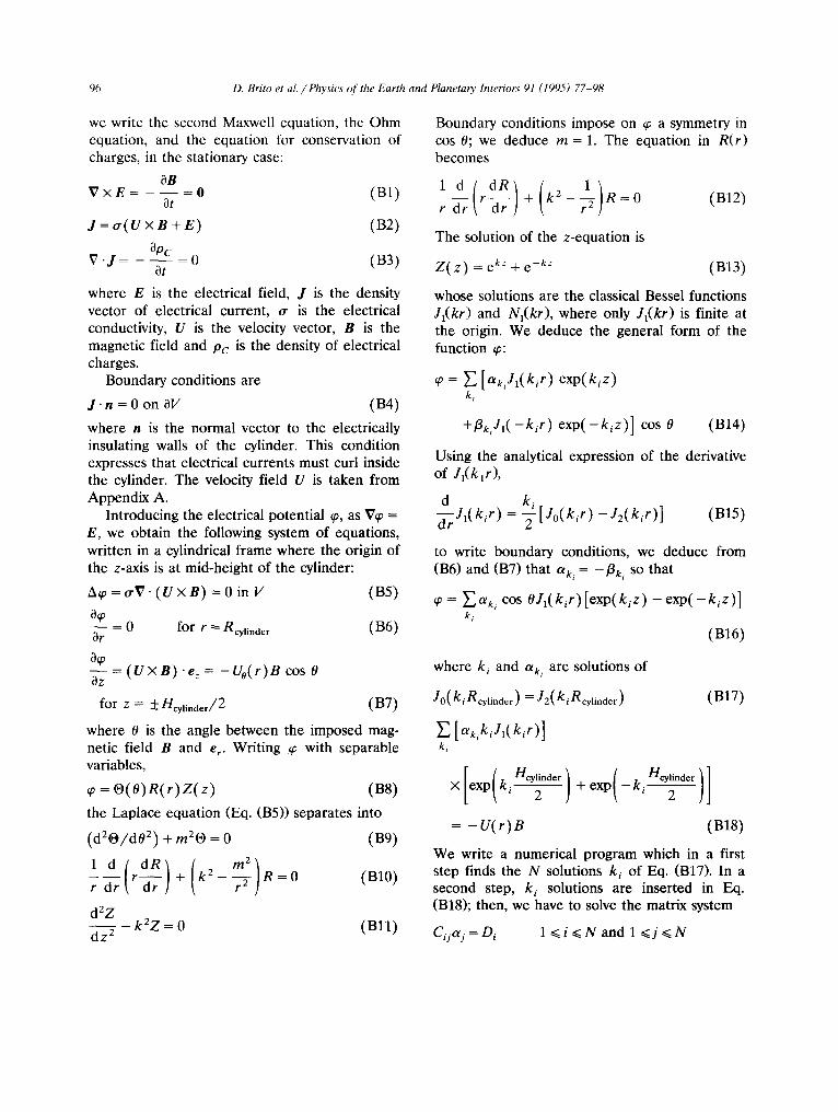
96 D. Brito et al. / Physics of the Earth and Planetary Interiors 91 (1995) 77-98

we write the second Maxwell equation, the Ohm equation, and the equation for conservation of charges, in the stationary case:

0B V × E 0 (B1)

0t

J = O r ( U × B + E) (B2)

Opc $7 . j = _ 0---~ = 0 (B3)

where E is the electrical field, J is the density vector of electrical current, or is the electrical conductivity, U is the velocity vector, B is the magnetic field and Pc is the density of electrical charges.

Boundary conditions are

J ' n = 0 on 0V (B4)

where n is the normal vector to the electrically insulating walls of the cylinder. This condition expresses that electrical currents must curl inside the cylinder. The velocity field U is taken from Appendix A.

Introducing the electrical potential q~, as Vq~ = E, we obtain the following system of equations, written in a cylindrical frame where the origin of the z-axis is at mid-height of the cylinder:

A~p = orV- (U X B) = 0 in V (B5)

0~ - - = 0 for r = Rcylinder (B6) Or 0~ Oz ( U × B ) e z - U o ( r ) B c o s O

for z = + n c y l i n d e r / 2 (B7)

where 0 is the angle between the imposed magnetic field B and e r. Writing ~ with separable variables,

q~ = O( O)R( r )Z ( z) (B8)

the Laplace equation (Eq. (B5)) separates into

(dZO/d0 2) + m20 = 0 (B9)

1 d dR k2 - r dr r ~ r + -77- R = 0 (B10)

d 2 Z dz--- $ - k 2 Z = 0 ( B l l )

Boundary conditions impose on ~p a symmetry in cos 0; we deduce m = 1. The equation in R(r) becomes

1 d r T r + k2 - r dr 7- ~ R---0 (B12)

The solution of the z-equation is

Z ( z ) = e *z + e -kz (B13)

whose solutions are the classical Bessel functions Jl(kr) and Nl(kr), where only Jl(kr) is finite at the origin. We deduce the general form of the function ~:

= E [°lkiJl(kir) exp(k iz ) ki

+f ie ,J1( -k ir ) e x p ( - k i z ) ] cos 0 (B14)

Using the analytical expression of the derivative of Jl(klr) ,

d k i -~rJl(kir) = -~[Jo(k , r ) - J2 (k i r ) ] (B15)

to write boundary conditions, we deduce from (B6) and (B7) that aki = -fig, so that

q~ = ~ ] a , , cos OJ,(kir)[exp(kiz ) - e x p ( - - k i z ) ] ki

(B16)

where ki and a~i are solutions of

J o ( k i R cylinder ) = J 2 ( k i R cylinder ) (B17)

E [ o% kiJ,( kir ) ] ki

X exp k i 2 + e x p - k i - - - - ~

= - U ( r ) B (B18)

We write a numerical program which in a first step finds the N solutions k i of Eq. (B17). In a second step, k~ solutions are inserted in Eq. (B18); then, we have to solve the matrix system

Ci ja j=D i 1 <~i < N and 1 <~j <~N

D. Brito et al. / Physics o f the Earth and Planetary Interiors 91 (1995) 77-98 97

where

)

D i = - BU( r i)

with r i varying from zero to Rcytinder

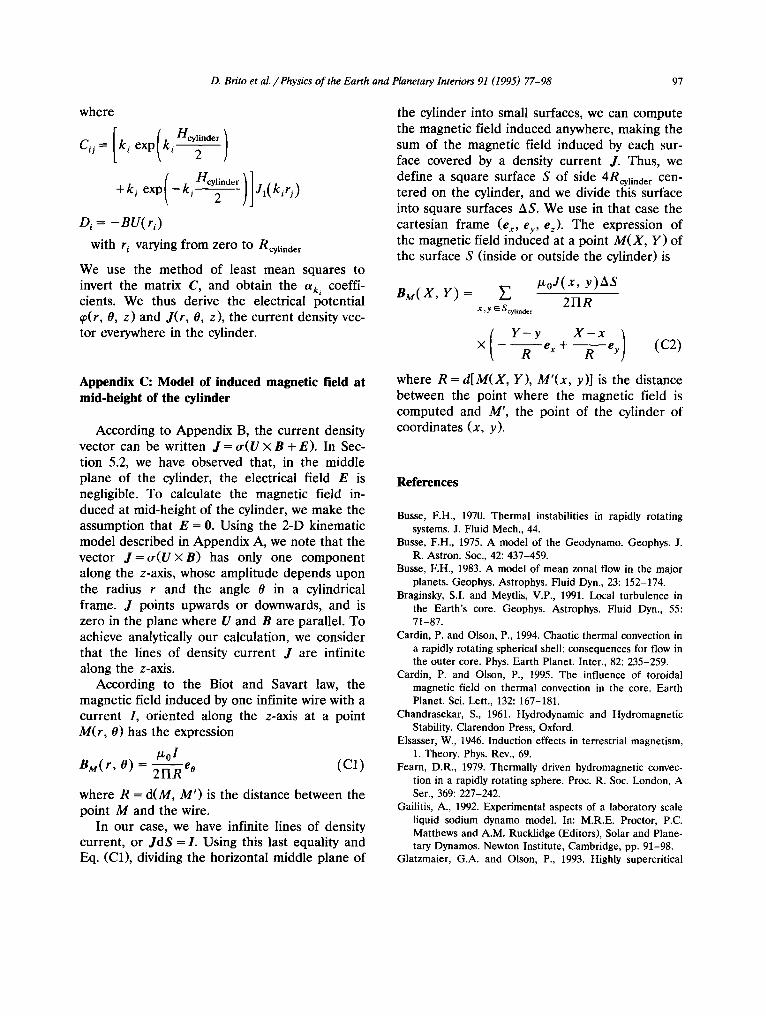
We use the method of least mean squares to invert the matrix C, and obtain the aki coeffi- cients. We thus derive the electrical potential qffr, 0, z) and J(r, O, z), the current density vector everywhere in the cylinder.

Appendix C: Model of induced magnetic field at mid-height of the cylinder

According to Appendix B, the current density vector can be written J = ~r(U × B + E). In Sec- tion 5.2, we have observed that, in the middle plane of the cylinder, the electrical field E is negligible. To calculate the magnetic field induced at mid-height of the cylinder, we make the assumption that E = 0. Using the 2-D kinematic model described in Appendix A, we note that the vector J=~r(U×B) has only one component along the z-axis, whose amplitude depends upon the radius r and the angle 0 in a cylindrical frame. J points upwards or downwards, and is zero in the plane where U and B are parallel. To achieve analytically our calculation, we consider that the lines of density current J are infinite along the z-axis.

According to the Biot and Savart law, the magnetic field induced by one infinite wire with a current I, oriented along the z-axis at a point

M(r, O) has the expression

/z0I SM(r, O) -- ~ - ~ e o (C1)

where R = d(M, M') is the distance between the point M and the wire.

In our case, we have infinite lines of density current, or JdS = I. Using this last equality and Eq. (C1), dividing the horizontal middle plane of

the cylinder into small surfaces, we can compute the magnetic field induced anywhere, making the sum of the magnetic field induced by each surface covered by a density current J. Thus, we define a square surface S of side 4Rcyji.der cen- tered on the cylinder, and we divide this surface into square surfaces AS. We use in that case the cartesian frame (ex, ey, ez). The expression of the magnetic field induced at a point M(X, Y) of the surface S (inside or outside the cylinder) is

iXoJ(x, y )AS nM(x, Y) = E

2IIR X, y ~ Scylindcr

× ( _ Y - y + X - x - - - ~ e x - - - - ~ e , } (C2)

where R = d[M(X, Y), M'(x, y)] is the distance between the point where the magnetic field is computed and M', the point of the cylinder of coordinates (x, y).

References

Busse, F.H., 1970. Thermal instabilities in rapidly rotating systems. J. Fluid Mech., 44.

Busse, F.H., 1975. A model of the Geodynamo. Geophys. J. R. Astron. Soe., 42: 437-459.

Busse, F.H., 1983. A model of mean zonal flow in the major planets. Geophys. Astrophys. Fluid Dyn., 23: 152-174.

Braginsky, S.I. and Meytlis, V.P., 1991. Local turbulence in the Earth's core. Geophys. Astrophys. Fluid Dyn., 55: 71-87.

Cardin, P. and Olson, P., 1994. Chaotic thermal convection in a rapidly rotating spherical shell: consequences for flow in the outer core. Phys. Earth Planet. Inter., 82: 235-259.

Cardin, P. and Olson, P., 1995. The influence of toroidal magnetic field on thermal convection in the core. Earth Planet. Sci. Lett., 132: 167-181.

Chandrasekar, S., 1961. Hydrodynamic and Hydromagnetic Stability. Clarendon Press, Oxford.

Elsasser, W., 1946. Induction effects in terrestrial magnetism, 1. Theory. Phys. Rev., 69.

Fearn, D.R., 1979. Thermally driven hydromagnetic convection in a rapidly rotating sphere. Proc. R. Soc. London, A Ser., 369: 227-242.

Gailitis, A., 1992. Experimental aspects of a laboratory scale liquid sodium dynamo model. In: M.R.E. Proctor, P.C. Matthews and A.M. Rucklidge (Editors), Solar and Plane- tary Dynamos. Newton Institute, Cambridge, pp. 91-98.

Glatzmaier, G.A. and Olson, P., 1993. Highly supercritical

98 D. Brito et aL / Physics of the Earth and Planetary Interiors 91 (1995) 77-98

thermal convection in a rotating spherical shell: centrifugal vs. radial gravity. Geophys. Astrophys. Fluid Dyn., 70: 113-136.

Gubbins, D. and Roberts, P.H., 1987. In: J.A. Jacobs (Editor), Geomagnetism, Vol. 2. Academic Press, New York, pp. 1-303.

Hulot, G., Le Moiiel, J-L. and Jault, D., 1990. The flow at the core-mantle boundary: symmetry properties. J. Geomagn. Geoelectr., 42: 857-874.

Le Moiiel, J.L., Gire, C. and Madden, T., 1985. Motions at the core surface in geostrophic approximation. Phys. Earth Planet. Inter., 39: 270-287.

Manneville, J.B. and Olson, P., 1995. Banded convection in a rotating fluid sphere. Nature, submitted.

Moffatt, D. and Loper, D.E., 1994. The magnetostrophic rise of buoyant parcel in the Earth's core. Geophys. J. Int., 117: 394-402.

Nakagawa, Y., 1957. Experiments on the instability of a layer of mercury heated from below and subject to the simulta- neous action of a magnetic field and rotation. Proc. R. Soc. London, Ser. A, 242: 81.

Nakagawa, Y., 1958. Experiments on the instability of a layer of mercury heated from below and subject to the simulta- neous action of a magnetic field and rotation II. Proc. R. Soc. London, Ser. A, 249: 138.

Parker, R.L., 1966. Reconnexion of lines of forces in rotating spheres and cylinders. Proc. R. Soc. London, Ser. A, 291: 60.

Pascal, P., 1961. Nouveau Traitd de Chimie Mindrale VI. Masson, Paris, pp. 669-774.

St. Pierre, M.G., 1994. The stability of buoyant structures in the outer core. Oral communication presented at the SEDI Symposium. Whistler Mountain, B.C., 7-12 August 1994.

Spohn, A., 1991. l~coulement et dclatement tourbillonaires engendr6s par un disque tournant dans une enceinte cylin- drique. Th~se de doctorat, I'Universit6 de Grenoble 1.

Sun, Z., Schubert, G. and Glatzmaier, G.A., 1993. Banded surface flow maintained by convection in a model of rapidly rotating giant planets. Science, 260: 661-664.

Zhang, K.K., 1992. Spiralling columnar convection in rapidly rotating spherical fluid shells. J. Fluid Mech., 236: 535-556.

Experimental study of a geostrophic vortex of gallium in a transverse magnetic field

Documents

Transcript of Experimental study of a geostrophic vortex of gallium in a transverse magnetic field