Experimental-Modelling Approach in CO2-Rock Interaction

Louisiana State University Louisiana State University

LSU Digital Commons LSU Digital Commons

LSU Doctoral Dissertations Graduate School

8-28-2017

Diagenesis and Formation Stress in Fracture Conductivity of Shaly Diagenesis and Formation Stress in Fracture Conductivity of Shaly

Rocks; Experimental-Modelling Approach in CO2-Rock Rocks; Experimental-Modelling Approach in CO2-Rock

Interactions Interactions

Abiola Olukola Olabode Louisiana State University and Agricultural and Mechanical College

Follow this and additional works at: https://digitalcommons.lsu.edu/gradschool_dissertations

Part of the Environmental Engineering Commons, Geotechnical Engineering Commons, and the

Petroleum Engineering Commons

Recommended Citation Recommended Citation Olabode, Abiola Olukola, "Diagenesis and Formation Stress in Fracture Conductivity of Shaly Rocks; Experimental-Modelling Approach in CO2-Rock Interactions" (2017). LSU Doctoral Dissertations. 4105. https://digitalcommons.lsu.edu/gradschool_dissertations/4105

This Dissertation is brought to you for free and open access by the Graduate School at LSU Digital Commons. It has been accepted for inclusion in LSU Doctoral Dissertations by an authorized graduate school editor of LSU Digital Commons. For more information, please [email protected].

https://digitalcommons.lsu.edu/

https://digitalcommons.lsu.edu/gradschool_dissertations

https://digitalcommons.lsu.edu/gradschool

https://digitalcommons.lsu.edu/gradschool_dissertations?utm_source=digitalcommons.lsu.edu%2Fgradschool_dissertations%2F4105&utm_medium=PDF&utm_campaign=PDFCoverPages

https://network.bepress.com/hgg/discipline/254?utm_source=digitalcommons.lsu.edu%2Fgradschool_dissertations%2F4105&utm_medium=PDF&utm_campaign=PDFCoverPages



https://digitalcommons.lsu.edu/gradschool_dissertations/4105?utm_source=digitalcommons.lsu.edu%2Fgradschool_dissertations%2F4105&utm_medium=PDF&utm_campaign=PDFCoverPages

mailto:[email protected]

1

DIAGENESIS AND FORMATION STRESS IN FRACTURE CONDUCTIVITY OF SHALY ROCKS; EXPERIMENTAL-MODELLING APPROACH IN CO2-ROCK INTERACTIONS

A Dissertation

Submitted to the Graduate Faculty of the Louisiana State University and

Agricultural and Mechanical College in partial fulfilment of the

requirements for the degree of Doctor of Philosophy

in

The Craft & Hawkins Department of Petroleum Engineering

by Abiola Olukola Olabode

B.S., Obafemi Awolowo University, 2008 M.S., Louisiana State University, 2012

December 2017

ii

To my mother, Adeyinka, who lived but for a while

iii

ACKNOWLEDGEMENTS

My sincere gratitude goes to the following; Dr. Craig M Harvey for graciously serving as chair of

my doctoral research committee; my committee members, Dr. Mayank Tyagi, Dr. Paulo Waltrich,

Dr. Dandina Rao and the graduate school Dean’s Representative Dr. Chao Sun for their invaluable

contributions and criticisms that have given shape to this work. I want to specially thank the Craft

and Hawkins Department of Petroleum Engineering for availing me the multi-year resources that

made this project a success. I appreciate Wanda LeBlanc, LSU AgCenter, Donmei Cao, and the

LSU SIF staff members for assisting with post experimental data analysis. I also thank George

Ohrberg for helping with computing needs in data acquisition and Fenelon Nunes for helping with

laboratory ware purchases and maintenance. The financial support of the SPE and the GDL

Foundation is kindly acknowledged. Thanks to LSU Graduate School for the Dissertation Year

Fellowship that saw me through my final semesters.

I am appreciative of colleagues with whom I shared and gained useful ideas. They include Nnamdi

Agbasimalo, Chukwudi Chukwudozie, Wei Wang, Gbola Afonja, Paulina Mwangi, Louise Smith,

Arome Oyibo, Darko Kupresan, Kolawole Bello, Ruixuan Guo and Hui Du to mention a few.

Special thanks to my wife, Omoefe Kio-Olabode, for her unrelenting support throughout my

graduate studies. Your children shall call you blessed. To our son, Mark Olayinka, thanks for

beaming light on to our world at this junction in our lives.

I deeply appreciate the fervent prayers and support of my father and siblings; Oladepo Olabode,

Titilola Akinyemi and Motunrola Olaiya. Thanks to my uncle, Jinmi Olabode and cousin, Tolu

Olabode for always checking on us all these years. Also, special thanks to the Chapel on Campus

for the edification of my inner man since I arrived at LSU.

iv

TABLE OF CONTENTS

ACKNOWLEDGEMENTS…………..……………………………………………………………………………………………..... iii

LIST OF TABLES ……………………………………………………………………………………………………………………….. vi

LIST OF FIGURES ……………………………………………………………………………………………………………..…….. viii

NOMENCLATURE …………………………………………………………………………………………………………..……..... xv

ABSTRACT ………………………………………………………………………………………………………………………..….... xvi

CHAPTER 1. INTRODUCTION …………………………………………………………………………………………………….. 1

1.1 Background on Carbon Sequestration ..................................................................................... 1

1.2 Diagenesis and Fractures ......................................................................................................... 8

1.3 Problem Definition ................................................................................................................. 12

1.4 Objective of Research ……….………………………………………………………………………………………………. 13

CHAPTER 2. LITERATURE REVIEW ………………………………………….………………………………………………… 15

2.1 Diagenesis of Sedimentary Rocks …………................................................................................ 15

2.2 A Brief on Properties of CO2 Saturated Brine ........................................................................ 16

2.3 Shale Caprock Geochemical Alteration and Subsurface CO2 Migration ................................. 20

2.4 Geomechanical Effects ……………………………………………….. ....................................................... 43

2.5 Previous Experimental and Modeling Works ….……………………............................................... 55

CHAPTER 3. EXPERIMENTAL SETUP AND PROCEDURE ……………………………………………….…………… 62

3.1 Experimental Methods and Sample Preparation ……………………….……………………………………… 62

3.2 Experimental Setup................................................................................................................ 66

3.3 Experimental Shale Rocks Geology ........................................................................................ 66

3.4 Mineralogical Composition of Shale Rock Samples................................................................ 67

3.5 Experimental CO2-brine Fluid…............................................................................................... 70

3.6 Techniques in Rock and Fluid Analysis .................................................................................... 71

3.7 Experimental Parameters ……………………………………………………………………………………..………….. 74

3.8 Experimental Matrix ……………………………………………………………………………………………..………….. 76

CHAPTER 4. RESULTS FROM SHALE ROCK/FLUID INTERACTIONS EXPERIMENTS …………………….. 81

4.1 pH Measurement ……………………………………………………………………………………………………………... 81

4.2 Inductively Coupled Plasma-Optical Emission Spectroscopy (ICP-OES) Analysis.................... 82

4.3 Total Carbon Analysis …………………………………………………………................................................. 94

4.4 X-Ray Diffraction (XRD) Analysis ……………………………………….……………….................................. 96

v

4.5 Electron Micro-Probe Analysis (EMPA) of Bulk Rock............................................................. 106

4.6 Micro-Indentation of Rock Samples .................................................................................... 120

4.7 Differential Pressure Analysis …………………………………………………………………………………………. 124

4.8 Fracture Conductivity Estimation ……………………………………………………………………………………. 128

CHAPTER 5. DISCUSSION OF RESULTS ROCK/FLUID INTERACTIONS EXPERIMENTS …..………….. 134

5.1 General Discussion of Experimental Results …………..………………………………………………………. 134

5.2 Integrated Experimental Observations ……………………….………..…………………………….…….……. 141

CHAPTER 6. CONCLUSIONS AND RECOMMENDATIONS …………………………………….……..……… 143

6.1 Conclusions ………………………………………………………………………………………………………….………… 143

6.2 Recommendations ……………………………………………………………………………………………….………… 146

REFERENCES............................................................................................................................... 147

APPENDICES …………………………………………………………………………………………………………………………. 166

A: EQUIPMENT AND MATERIALS USED FOR SHALE ROCK/CO2 BRINE EXPERIMENTS ……………… 166

B: EXPERIMENTAL PROCEDURE FOR ROCK-FLUID INTERACTION EXPERIMENTS ………………....... 172

C: pH DATA ……………………..………………………..…………………………..……………….………………….……..…. 175

D: INDUCTIVELY COUPLED PLASMA EMISSION SPECTROSCOPY (ICP-OES) DATA....................... 176

E: MICRO-INDENTATION OF SHALE ROCKS DATA ………………...................................................... 179

F: ADDITIONAL DATA FOR ELECTRON MICROPROBE ANALYSIS (EMPA).................................... 180

G: FLOW/PRESSURE DATA ......................................................................................................... 188

H: FRACTURE CONDUCTIVITY DATA AND CALCULATIONS ..……………….………………….................. 196

VITA ……………………………………………………………………………………………………………………….…..……….. 197

vi

LIST OF TABLES

1.1: Worldwide potential CO2 sequestration capacities and risks …………….………………..…..………… 2

2.1: Mineralogy of typical shale rock samples showing percentage composition ….………….….…. 22

2.2: Geochemical model for reaction of shale, sandstone and cement with CO2 and Na, Ca, Mg

Chloride brines ……………….………………………………………………………………………………….………………….. 26

3.1. Geological properties of shale rock samples used in the experiment ……………….….…………… 67

3.2: Mineralogical composition of shale samples in percentages as captured by the ternary

diagram of figure 3.5 …………………………….………………………………………………………………………………… 70

3.3: Experimental brine composition for Shale/CO2-brine flooding experiment based on flowback

fluid composition from hydraulically fractured shale ………………………………………………………………..71

3.4: Experimental Matrix for CO2-brine/shale interaction at conditions of 50°C temperature and

1,000 psi pressure stated in A above .…………………………………………………………………………..……… 76

3.5: Experimental Matrix for CO2-brine/shale interaction at conditions of 50°C temperature and

1,000 psi pressure stated in B above .……………………………..…………………………………….…..……. 77

3.6: Micro-indentation; Hardness and Young Modulus at different temperature and pressure

conditions of rock fluid interaction ………………………………………………….……………………….…………….. 78

3.7: Pre-injection and Post-injection analyses for each CO2-brine flooding experimental run

including rock and fluid sampling procedure ………………………….……………………………………………….. 79

4.1: Bulk rock compositional change for the shale rock samples. These values were computed

from the pre- and post-XRD quantitative analysis using the bulk and clay XRD methods. There

were slight changes in quartz, carbonates and clay contents ……………………….…………………..…... 104

4.2: Percentage composition of the mineralogical components of precipitates that were

recovered from the effluent during the shale/CO2-brine flooding experiment. The analysis

indicated diagenetic quartz and carbonates as new minerals that were formed …………...………. 105

B.1: Pre-injection and Post-injection analysis for each CO2-brine flooding run …………….……….. 172

vii

G.1: Data for differential pressure across 25µm fractured core for flow-through experiment using

Mancos shale ……………………………………………….………………………………………………………………………. 188


Marcellus shale …………………………………………………………………….……………………………………………….189


Pottsville shale…………………………………………………………….…………………………………………………………190


Wilcox shale ……………………………………………………………….……..…………………………………………………. 191

G.5: Data for differential pressure across 150µm fractured core for flow-through experiment

using Mancos shale ………………………………………………………………………………………………………………. 192


using Marcellus shale …………………………………………………………………………….………………………………193


using Pottsville shale ……………………………………………………………………………………………………………. 194


using Wilcox shale ……………………………………………………………………………………………………..…………. 195

H.1: Steps, equations and assumptions were made in calculating the fracture conductivity of the

cores used during the experiments …………………………………………………………..……………………………196

viii

LIST OF FIGURES

1.1: CO2 emission sources, potential utilization and sequestration sites …………………………………… 3

1.2: United States electric power generation by fuel over the next 25 years ……………………………. 4

1.3: Projected carbon dioxide (CO2) emission in the United States ……......……………..………………… 5

1.4: Schematic of CO2 diffusive loss and other leakages through caprock ………….……………………… 8

1.5: Representation of a possible CO2 migration pathway from the reservoir through the caprock

via fractures that have been opened during CO2 injection …….………………..…….……………….……….. 10

2.1: Phase diagram of CO2 showing the pressure and temperature envelope for most sedimentary

basins worldwide …………………………………………………………….……………………….……………………………. 17

2.2: the isothermal compressibility of CO2 at 35°C and 50°C ………………………..…………………………. 19

2.3: Quartz precipitation rate in micrometers per million years for a range of temperature from

25°C to 250°C. The three curves represent the range of expected growth rate in a fracture ...... 25

2.4: Mineral dissolution rate as function of pH, 1/T, 𝑎𝐴𝑙3+ , oxalate concentration, and f(ΔGr) ……32

2.5: Schematic drawing of pressure solution. Compaction by pressure solution reduces the

porosity and permeability of a rock …………………………………………………………….…………….……………..39

2.6: Schematic of precipitation/dissolution reaction in finite length single fracture ….…………….. 46

2.7: Fracture shape with precipitation of cemented minerals leading to aperture loss ………….. 46

2.8: Fracture production simulation illustrating the impact of conductivity on long-term

production ……………………………………………………………………………………………………………….………….… 48

2.9: illustration of the pressure solution and compaction mechanism. High stress at the contact

points increases the solubility of silica ………..…………………………………………….……………………………. 48

2.10: Modification of calculated steady-state effective permeability for a generic fracture pattern

showing reduction in effective permeabilities, kx and ky, caused by diagenetic cementation ….. 52

3.1: Detailed process flow diagram of the experimental setup showing critical devices ………….. 63

ix

3.2: Visual design of composite core made of kaolinite, cement and microtubings .………………… 64

3.3: Sample design of composite core made of kaolinite, cement and microtubings …………….… 64

3.4: Samples of composite core made of kaolinite, cement and microtubings mimic fractures …65

3.5: Initial mineralogical composition of four shale rock samples used in rock-fluid interaction

experiment. The ternary diagram shows carbonates, quartz, feldspar, pyrite and clay ..…………. 68

3.6: Initial mineralogical composition of four shale rock samples used in rock-fluid interaction

experiment when compared to other plays ……………………..………………………………………….…………..69

4.1: pH measurement of effluent for the four different shale rock samples used for the rock-fluid

interaction experiment …………………………………………………………………….……………………………………. 81

4.2: Dimensionless elemental concentration of the effluent fluids showing the fraction of Calcium

that were leached out from the shale rock samples …………..…………………………………………………… 83

4.3: Dimensionless cationic concentration of the effluent fluids showing the fraction of

Magnesium that were leached out from the shale rock samples …………….………..…………………….. 86

4.4: Dimensionless cationic concentration of the effluent fluids showing the fraction of Potassium

that were leached out from the shale rock samples ……………………….…….……………………………….. 86

4.5: Dimensionless cationic concentration of the effluent fluids showing the fraction of Selenium

that were leached out from the shale rock samples …………………………......……………………………….. 87

4.6: Dimensionless cationic concentration of the effluent fluids showing the fraction of Sulphur

that were leached out from the shale rock samples ….…………..…………...………………………………….. 87

4.7: Dimensionless cationic concentration of the effluent fluids showing the fraction of Silicon

that were leached out from the shale rock samples ………..………………………….………………………….. 88

4.8: Dimensionless cationic concentration of the effluent fluids showing the fraction of Aluminum

that were leached out from the shale rock samples ……………..……….…………………..…………………… 90

4.9: Dimensionless cationic concentration of the effluent fluids showing the fraction of Arsenic

that were leached out from the shale rock samples ……..…………..………..………………………………….. 91

x

4.10: Dimensionless cationic concentration of the effluent fluids showing the fraction of Boron

that were leached out from the shale rock samples ………………..……………..……………….……………… 91

4.11: Dimensionless cationic concentration of the effluent fluids showing the fraction of Iron that

were leached out from the shale rock samples ……………….……………..……………..……………………….. 92


Manganese that were leached out from the shale rock samples. ……………………….………….……….. 92

4.13: Dimensionless cationic concentration of the effluent fluids showing the fraction of Nickel

that were leached out from the shale rock samples ………….……....……………….………………………….. 93


Phosphorus that were leached out from the shale rock samples. ………………….….…………………….. 93

4.15: Dimensionless cationic concentration of the effluent fluids showing the fraction of Zinc that

were leached out from the shale rock samples …..………..…………...………………………………………….. 94

4.16: Total Carbon measurement of bulk shale rocks for the four different samples analyzed. It

shows major increase in carbon content for the Marcellus shale …………………………….……………... 95

4.17: XRD Analysis of bulk rock Mancos before and after CO2-brine flooding at moderate

temperature and pressure conditions along with the mineralogical composition of the associated

precipitates recovered from the effluent …………..…………………………………….……………………………. 97

4.18: XRD Analysis of bulk rock Marcellus before and after CO2-brine flooding along with the

mineralogical composition of the associated precipitates recovered from the effluent ………….. 98

4.19: XRD Analysis of bulk rock Pottsville before and after CO2-brine flooding at moderate


precipitates recovered from the effluent .…………………………………………………………………….……..... 99

4.20: XRD Analysis of bulk rock Wilcox before and after CO2-brine flooding at moderate


precipitates recovered from the effluent ……….………………………………..……………………………………. 99

4.21: XRD Analysis of clay components Mancos before and after CO2-brine flooding at moderate


precipitates recovered from the effluent …….....………………….……………………………………………..… 101

xi

4.22: XRD Analysis of clay components Marcellus before and after CO2-brine flooding at moderate


precipitates recovered from the effluent ……………………………….………………………………………..…… 101

4.23: XRD Analysis of clay components Pottsville before and after CO2-brine flooding at moderate


precipitates recovered from the effluent. Significantly higher clay content is present in

precipitates compared to previous samples ……………………..……………………………………………………102

4.24: XRD Analysis of clay components Wilcox before and after CO2-brine flooding at moderate


precipitates recovered from the effluent ………………………….……………………………………………………102

4.25: 20µm Electron Micro-Probe maps for Mancos shale showing the Calcium surface

geochemical profile of the CO2-reacted sample compared to control specimen .......….……….... 107

4.26: 20µm Electron Micro-Probe Analysis for Mancos shale showing Magnesium and Aluminum

surface geochemical profile of the CO2-reacted sample compared to control specimen …..…… 108

4.27: 20µm Electron Micro-Probe Analysis for Mancos shale showing Iron and silicon surface

geochemical profile of the CO2-reacted sample compared to control specimen …………………... 109

4.28: 20µm Electron Micro-Probe Analysis for Marcellus shale showing the Calcium surface

geochemical profile of the CO2-reacted sample compared to control specimen ………………..….. 110

4.29: 20µm Electron Micro-Probe Analysis for Marcellus shale showing Mg and Al surface

geochemical profile of the CO2-reacted sample compared to control specimen …………………….111

4.30: 20µm Electron Micro-Probe Analysis for Marcellus shale showing Iron and Silicon surface

geochemical profile of the CO2-reacted sample compared to control specimen …......……………. 112

4.31: 20µm Electron Micro-Probe Analysis for Pottsville shale showing the Calcium surface

geochemical profile of the CO2-reacted sample compared to control specimen ….……….…….... 114

4.32: 20µm Electron Micro-Probe Analysis for Pottsville shale showing Magnesium and Aluminum

surface geochemical profile of the CO2-reacted sample compared to control specimen ……..….115

4.33: 20µm Electron Micro-Probe Analysis for Pottsville shale showing Iron and Silicon surface

geochemical profile of the CO2-reacted sample compared to control specimen ………….………….116

xii

4.34: 20µm Electron Micro-Probe Analysis for Wilcox shale showing the Calcium surface

geochemical profile of the CO2-reacted sample compared to control specimen ……………………. 117

4.35: 20µm Electron Micro-Probe Analysis for Wilcox shale showing Magnesium and Aluminum

surface geochemical profile of the CO2-reacted sample compared to control specimen ………...118

4.36: 20µm Electron Micro-Probe Analysis for Wilcox shale showing Iron and Silicon surface

geochemical profile of the CO2-reacted sample compared to control specimen …………..….…... 119

4.37: the Vickers’ micro-hardness measurement taken on multiple samples of the experimental

shale rocks. The results indicated reduction in geomechanical hardness of the rocks …………… 121

4.38: Young’s Modulus plots showing across the board decreases in measured values for the shale

caprocks after flooding with CO2-brine at 50oC and 1,000psi ………..……………………..………………… 122

4.39: Combined Hardness and Young’s Modulus plots showing across the board decreases in

values for the caprocks after flooding with CO2-brine at 50oC and 1,000psi ………………………….. 122

4.40: A correlation between the hardness of the shale rock and quantifiable mineralogical change

in percentages. The graph shows that formation of diagenetic quartz can improve the hardness

of the shale rock as observed in the Pottsville shale ………..…………..……………………………..……….. 123

4.41: Average differential pressure profile across the 25µm composite core, with embedded

micro-tubings to mimic fractures. The injected fluid was directly from the outlet of the packed

bed of crushed shale rock samples ………………………..………………………………….…………………..………125

4.42: Average differential pressure profile across 150µm composite core, with embedded micro-

tubings to mimic fractures. The injected fluid was directly from the outlet of the packed bed of

crushed shale rock samples ……………………………………………..……………………………………………….….. 126

4.43: Average first derivative of differential pressure drop across the 25µm composite core, with

embedded micro-tubings to mimic fractures. The injected fluid was from directly from the outlet

of the packed bed of crushed shale rock samples …………………………………………………………………. 127

4.44: Average first derivative of differential pressure drop across the 150µm composite core, with

embedded micro-tubings to mimic fractures. The injected fluid was from directly from the outlet

of the packed bed of crushed shale rock samples …………………………..…………………………………….. 128

xiii

4.45: Calculated dimensionless fracture conductivity profile from experimental differential

pressure using fractured core parameters with 25µm micro-tubings embedded. The profile

indicated a rapid reduction in the conductivity of the artificial fractured core ………………….…. 132

4.46: Calculated dimensionless fracture conductivity profile from experimental differential

pressure (dP) data using fractured core parameters with 150µm micro-tubings embedded .…. 132

4.47: Comparison of calculated dimensionless fracture conductivity profile from experimental

differential pressure (dP) data using fractured core parameters with 25µm and 150µm embedded

micro-tubings …………………………………………………..………………………………………………………………….. 133

5.1. The integration schematics of the geochemical, geomechanical and micro-fracture

conductivity in shale rock-aqueous CO2 interactions ………………………………………………………..……142

A.1: Core flooding setup showing core holder and instrumentation…………………………………….… 166

A.2: Helium porosimetry unit for estimation of porosity of fractured cores…………………….……… 166

A.3: Core flooding control unit…………………………………………………………………………………………….… 166

A.4: Automated oven for temperature control………………………………………………………………………. 166

A.5: Piston pump………………………………………………….…………..…………………………………………………… 167

A.6: PEEK micro-tubing used in composite cores…………………………………………………………………..…167

A.7: Micro-indentation fixture…………………………………………………………………………………….………... 167

A.8: Example of shale fragment and the indentation points……………………….…………………….….... 167

A.9: Crushed shale samples, pre-flooding with CO2-brine; Mancos……………………………..……….… 168

A.10: Crushed shale samples, pre-flooding with CO2-brine; Marcellus …………………..………....… 168

A.11: Crushed shale samples, pre-flooding with CO2-brine; Pottsville…………………….………………. 168

A.12: Crushed shale samples, pre-flooding with CO2-brine; Wilcox………………………………….…….. 168

A.13: Crushed shale samples, post-flooding with CO2-brine; Mancos ……………..…………………….. 169

xiv

A.14: Crushed shale samples, post-flooding with CO2-brine; Marcellus ……………..………………..… 169

A.15: Crushed shale samples, post-flooding with CO2-brine; Pottsville …………………..……………… 169

A.16: Crushed shale samples, post-flooding with CO2-brine; Wilcox ………………………..……….…… 169

A.17: Recovered effluent precipitates, post-flooding with CO2-brine; Mancos …………..………..… 170

A.18: Recovered effluent precipitates, post-flooding with CO2-brine; Marcellus …………..….…… 170

A.19: Recovered effluent precipitates, post-flooding with CO2-brine; Pottsville …………..……….. 170

A.20: Recovered effluent precipitates, post-flooding with CO2-brine; Wilcox ……………………….. 170

A.21: Process schematics of experimental setup showing materials and equipment used for CO2-

brine flooding and composite core conductivity measurement ………………………….…………….….. 171

xv

NOMENCLATURE

Cr = Dimensionless Fracture Conductivity

Fcdn = Normalized Dimensionless Fracture Conductivity

wf = Fracture Width, µm

km = Matrix Permeability, D

kf = Fracture Permeability, D

Lf = Fracture Length

φ = Porosity, %

P = Pressure, psi

ΔP = Differential Pressure (psi)

T = Temperature, °C

q = Flow Rate, ml/min

RT = Flow Rate (ml/min) at Temperature T (°C)

kr = reaction rate, m/s

v = velocity, m/s

µ = Viscosity, cp

A = Cross-sectional Area

YM = Young’s Modulus

SD = Standard Deviation

HV = Vickers’ Hardness

xvi

ABSTRACT

In large scale subsurface injection of carbon dioxide (CO2) as obtainable in carbon sequestration

programs and in environmentally friendly hydraulic fracturing processes (using supercritical CO2),

long term rock-fluid interaction can affect reservoir and seal rocks properties which are essential

in monitoring the progress of these operations. The mineralogical components of sedimentary

rocks are geochemically active particularly under enormous earth stresses, which generate high

pressure and temperature conditions in the subsurface. While geomechanical properties such as

rock stiffness, Poisson’s ratio and fracture geometry largely govern fluid flow characteristics in

deep fractured formations, the effect of mineralization can lead to flow impedance in the

presence of favorable geochemical and thermodynamic conditions. Simulation results suggested

that influx-induced mineral dissolution/precipitation reactions within clay-based sedimentary

rocks can continuously close micro-fracture networks, though injection pressure and effective-

stress transformation first rapidly expand the fractures. This experimental modelling research

investigated the impact of in-situ geochemical precipitation at 50°C and 1,000 psi on conductivity

of fractures under geomechanical stress conditions. Geochemical analysis were performed on

different samples of shale rocks, effluent fluid and recovered precipitates both before and after

CO2-brine flooding of crushed shale rocks at high temperature and pressure conditions. Bulk rock

geomechanical hardness was determined using micro-indentation. Differential pressure drop

data across fractured composite core were also measured with respect to time over a five a day

period. This was used in estimating the conductivity of the fractured core. Three experimental

runs per sample type were carried out in order to check the validity of observed changes. The

results showed that most significant diagenetic changes in shale rocks after flooding with CO2-

xvii

brine reflect in the effluent fluid with calcium based minerals dissolving and precipitating under

experimental conditions. Major and trace elements in the effluent fluid (using ICP-OES analysis)

indicated that multiple geochemical reactions are occurring with almost all of the constituent

minerals participating. The geochemical composition of precipitates recovered after the

experiments showed diagenetic carbonates and opal (quartz) as the main constituents. The bulk

rock showed little changes in composition except for sharper peaks on XRD analysis, suggesting

that a significant portion of amorphous content of the rocks have been removed via dissolution

by the slightly acid CO2-brine fluid that was injected. However total carbon (TOC) analysis showed

a slight increase in carbon content of the bulk rock. Micro-indention results suggested a slight

reduction in the hardness of the shale rocks and this reduction appear dependent on quartz

content. The differential pressure drop, its 1st derivative and estimated fracture conductivity

suggests that reactive transport of dissolved minerals can possibly occlude fracture flow path at

varying degree depending on equivalent aperture width, thereby improving caprock integrity

with respect to leakage risks under CO2 sequestration conditions. An exponential-natural

logarithm fit of the fracture conductivity can be obtained and applied in discrete fracture network

modelling. The fit yielded lower and upper boundary limits for fracture conductivity closure.

Higher temperature and pressure conditions of experimental investigations may be needed to

determine the upper limit of shale rock seal integrity tolerance, under conditions that are similar

to sequestration of CO2 into deep and hot sedimentary rocks.

1

CHAPTER 1

INTRODUCTION

1.1 Background on Carbon Sequestration

Sequestration of anthropogenic carbon dioxide (CO2) into geologic subsurface sinks has gained

much attention from the science and engineering community in recent years. As fossil fuel is

expected to continue to play a significant role in meeting worldwide energy demand,

environmental considerations require some form of mitigation for the CO2 being emitted- a

prominent greenhouse gas [1-3]. Carbon cycle is one of the most complex geochemical cycles of

the Earth as it involves atmosphere, hydrosphere, biosphere and lithosphere. Among these

different geochemical spheres, mechanisms and reaction rates governing migration and fixation

of carbon (i.e. fluxes), such as the stability of the different carbonates minerals under specific

conditions in crustal reservoirs, are still matter of detailed studies [4].

Development of fossil fuels, emission of greenhouse gases, and changing climate have been at

the forefront of geopolitical discussions in recent years. The challenge is to produce enough

energy to maintain the current standard of living while simultaneously reducing greenhouse gas

(GHG) emissions. Considerable amount of experimental and simulation studies in carbon dioxide

sequestration have been carried out in investigating the geochemical and geomechanical stability

of porous subsurface storage reservoirs such as saline aquifers, depleted oil and gas reservoirs,

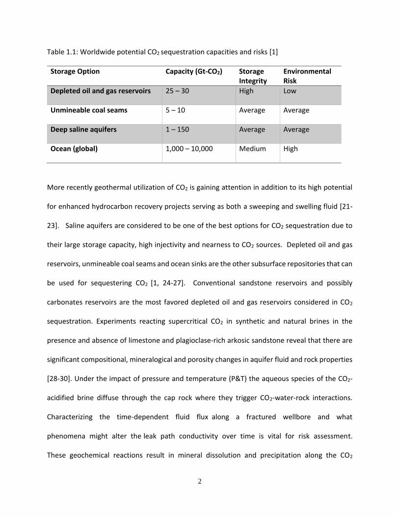
and coal bed seams for this purpose [5-20]. Table 1.1 below shows some estimates of the

capacities available for each of these repositories worldwide. These capacities assume that

variable solubility of CO2 due to depth is insignificant. A particular risk is for CO2 to migrate

from the storage and leak into an overlying formation or back to the atmosphere.

2

Table 1.1: Worldwide potential CO2 sequestration capacities and risks [1]

Storage Option Capacity (Gt-CO2) Storage Integrity

Environmental Risk

Depleted oil and gas reservoirs 25 – 30 High Low

Unmineable coal seams 5 – 10 Average Average

Deep saline aquifers 1 – 150 Average Average

Ocean (global) 1,000 – 10,000 Medium High

More recently geothermal utilization of CO2 is gaining attention in addition to its high potential

for enhanced hydrocarbon recovery projects serving as both a sweeping and swelling fluid [21-

23]. Saline aquifers are considered to be one of the best options for CO2 sequestration due to

their large storage capacity, high injectivity and nearness to CO2 sources. Depleted oil and gas

reservoirs, unmineable coal seams and ocean sinks are the other subsurface repositories that can

be used for sequestering CO2 [1, 24-27]. Conventional sandstone reservoirs and possibly

carbonates reservoirs are the most favored depleted oil and gas reservoirs considered in CO2

sequestration. Experiments reacting supercritical CO2 in synthetic and natural brines in the

presence and absence of limestone and plagioclase-rich arkosic sandstone reveal that there are

significant compositional, mineralogical and porosity changes in aquifer fluid and rock properties

[28-30]. Under the impact of pressure and temperature (P&T) the aqueous species of the CO2-

acidified brine diffuse through the cap rock where they trigger CO2-water-rock interactions.

Characterizing the time-dependent fluid flux along a fractured wellbore and what

phenomena might alter the leak path conductivity over time is vital for risk assessment.

These geochemical reactions result in mineral dissolution and precipitation along the CO2

3

migration path and are responsible for a change in porosity and therefore for the sealing capacity

of the cap rock [31, 32]. Figure 1.1 shows the network of potential sequestration sites and the

CO2 emitting industries that could be involved [14].

Figure 1.1: CO2 emission sources, potential utilization and sequestration sites (Courtesy of the

Department of Energy [14])

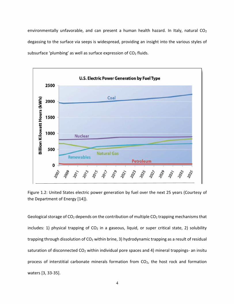
Meanwhile the emission of anthropogenic CO2 is expected to continue into the future at an

increasing volumetric rate. Figure 1.2 depicts the trend in CO2 emissions in the United States by

fuel type over the next 25 years and beyond. Figure 1.3 shows long term emission data for

anthropogenic CO2 in the United States. Industrialized societies which continue to use fossil fuel

energy sources are considering adoption of Carbon Capture and Storage (CCS) technology to

meet carbon emission reduction targets. Long-term security of performance of engineered CO2

storage is a principle concern, as seepage of injected CO2 to the surface is economically and

4

environmentally unfavorable, and can present a human health hazard. In Italy, natural CO2

degassing to the surface via seeps is widespread, providing an insight into the various styles of

subsurface ‘plumbing’ as well as surface expression of CO2 fluids.

Figure 1.2: United States electric power generation by fuel over the next 25 years (Courtesy of

the Department of Energy [14]).

Geological storage of CO2 depends on the contribution of multiple CO2 trapping mechanisms that

includes: 1) physical trapping of CO2 in a gaseous, liquid, or super critical state, 2) solubility

trapping through dissolution of CO2 within brine, 3) hydrodynamic trapping as a result of residual

saturation of disconnected CO2 within individual pore spaces and 4) mineral trappings- an insitu

process of interstitial carbonate minerals formation from CO2, the host rock and formation

waters [3, 33-35].

5

Figure 1.3: Projected carbon dioxide (CO2) emission in the United States. The model is based on

point source industries (Courtesy of the Department of Energy [14]).

The process of carbon capture and sequestration include monitoring, verification, accounting and

risk assessment of emission units and storage sites. At Sleipner in Norway, seismic monitoring

combined with seabed gravimetric technologies have been used to constrain reservoir simulation

models and to acquire insight into the flow behavior of CO2 plumes in the Utsira sandstone

reservoir [5, 6, 8, 36-38]. Extensive economic and cost analysis are required for projects that

involve commercial entities and government budgetary appropriations.

Successful implementation of geological CO2 sequestration depends on many factors including

the ability to predict the extent of underground CO2 movement and storage as a function of

specific target formation that will enable the identification of optimal sites and evaluate their

long term isolation performance while asserting the results through experimentation [1, 39, 40].

6

Geomechanical, geochemical and hydrological impact of engineered CO2 storage into these

geological storage options have been well researched with the conclusion that accurate

estimation of maximum sustainable injection pressure plays a significant role on wellbore

stability, wettability parameters, possible dormant fault reactivation among other concerns. The

presence of impurities in the CO2 stream raises the question of possible underground water and

aquatic life contamination. This requires factoring the effects of trace impurities from large

emission sources into CO2 transport, injection and storage modeling [41-43].

While appreciable efforts have been expended in the scientific evaluation of CO2 storage

feasibility in conventional underground repositories, significant experimental research efforts are

yet to be devoted to the seal rocks that cap most of these reservoirs. The reason might be their

complexity, not just in terms of mineralogy and fluid flow behavior but also due to the lengthy

laboratory measurements required for meaningful investigation. The rock-fluid interaction

processes that are observed in most conventional CO2 repositories with high permeability and

porosity are to a limited extent applicable to sedimentary caprocks. Most effective caprock

lithologies are fine-grained siliciclastics (clay-based rocks) and evaporites (anhydrites, gypsum,

halites). An effective caprock usually has capillary entry pressure that exceeds the upward

buoyancy pressure exerted by an underlying hydrocarbon or CO2 column [33, 44, 45]. The

capillary pressure of the caprock is largely a function of its pore sizes and this may be laterally

variable. The buoyancy pressure is determined by the density of the reservoir fluid and column

height. A caprock of extremely small pore size, in the order of nanometers, is required to prevent

the buoyant rise of an underlying gas column [39, 46, 47]. The injection of CO2 leads to CO2-

water-rock interactions that result in the precipitation and dissolution of minerals which in turn

7

result in a change in porosity and permeability of the cap rock. This change leads to the

improvement or deterioration of the sealing capacity of the cap rock. Mineral dissolution results

in an increase in porosity and enables the creation of pathways for CO2 migration. Mineral

precipitation leads to a decrease in porosity and increases the sealing effect [31, 48-50].

Geochemistry and geomechanics affect caprock effectiveness and loss of gas through caprock

may take place if the integrity of the caprock is breached, although transport processes are

usually not rapid and may be in the nano-darcy permeability range. Recent field tests such as in

Sleipner (Norway), showed that experience on in-situ caprock integrity characteristics can only

be obtained in decades. CO2 plume development and the required geophysical monitoring

methods (seismic, gravity, and satellite data) can only yield valuable geological information in

years as evident from the 15 years of operating the Sleipner project. Existing geologic

discontinuities, fractures and faults also add to the uncertainty that may compromise seal

effectiveness [37, 38]. The effectiveness of natural shale rock seals and other tight rocks are

dependent on the absence of discontinuities.

The quantitative assessment of leakage risks and leakage rates is a basic requirement for site

approval, public acceptance and the awarding of potential credits for sequestered CO2 quantities.

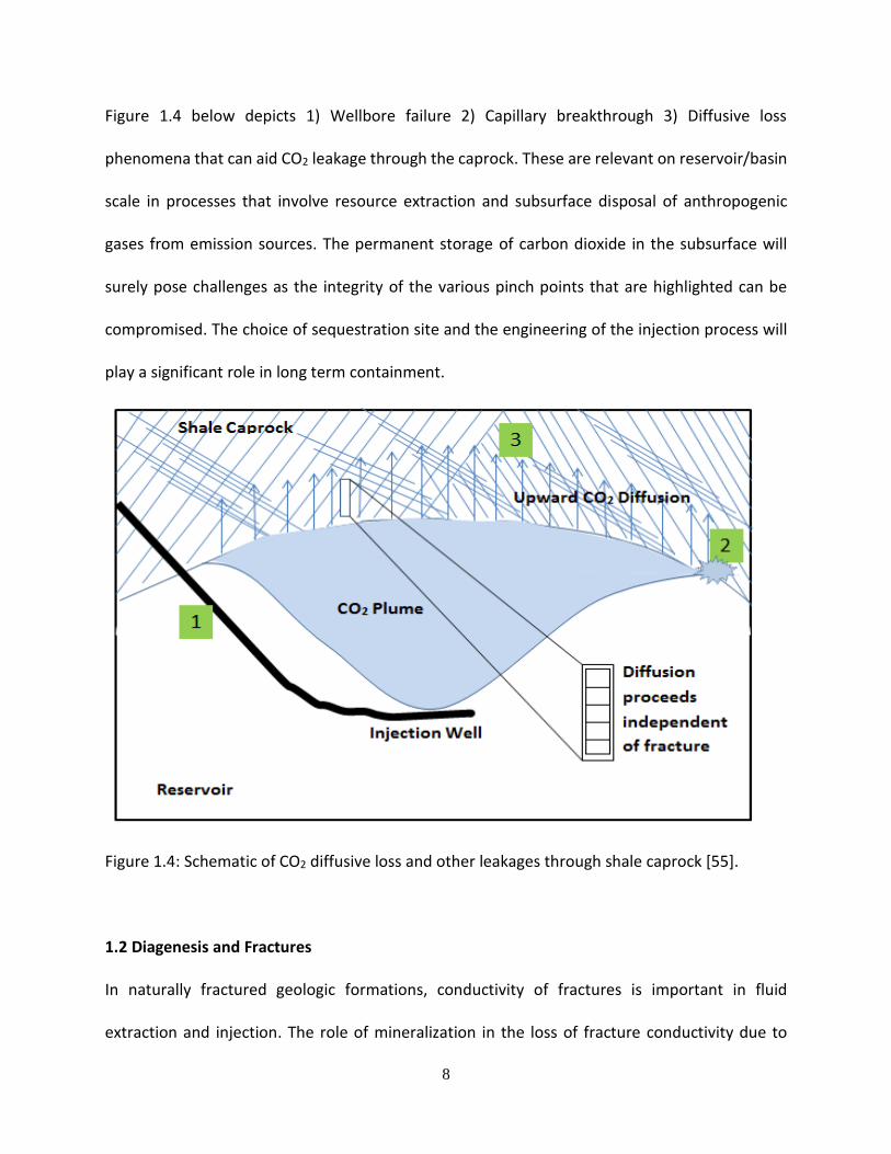
Leakage through caprocks may occur in three different ways [51-54]:

i.) rapid leakage by seal-breaching or wellbore failure (corrosion of pipes and cements),

resulting in gas flow through a micro-fracture network.

ii.) long-term leakage controlled by the capillary sealing efficiency and permeability (after

capillary breakthrough pressure is exceeded).

iii.) diffusive loss of dissolved gas through the water-saturated pore spaces.

8

Figure 1.4 below depicts 1) Wellbore failure 2) Capillary breakthrough 3) Diffusive loss

phenomena that can aid CO2 leakage through the caprock. These are relevant on reservoir/basin

scale in processes that involve resource extraction and subsurface disposal of anthropogenic

gases from emission sources. The permanent storage of carbon dioxide in the subsurface will

surely pose challenges as the integrity of the various pinch points that are highlighted can be

compromised. The choice of sequestration site and the engineering of the injection process will

play a significant role in long term containment.

Figure 1.4: Schematic of CO2 diffusive loss and other leakages through shale caprock [55].

1.2 Diagenesis and Fractures

In naturally fractured geologic formations, conductivity of fractures is important in fluid

extraction and injection. The role of mineralization in the loss of fracture conductivity due to

9

aqueous precipitation of insoluble substances has been discussed by several researchers [56-59].

It is generally thought that aside geomechanical properties of sedimentary rocks, the

geochemical properties of rocks and reservoir fluids can favorably or unfavorably lead to the

constriction of fractures in the subsurface given the right temperature, pressure and chemical

composition. This type of constrict is desired in CO2 sequestration and containment. Different

formation evaluation scales can be considered when describing tight shaly rocks (caprock): from

the pore or grain scale in petrophysics and geochemistry, to regional scale in geology and

geomechanics [60]. At small scale, the identification of geological facies and the origin of the low

porosity and permeability in terms of sedimentology and diagenesis is necessary.

For clayey caprocks, the amount and type of clay is critical in characterizing its petrophysics unlike

tight carbonate formation where dolomitisation is the key feature [38, 61]. Caprocks are

essentially defined as low (<10-18 m2) or very low (<10-21 m2) permeability formations, and

sometimes, but not necessarily, with low porosity (<15%) [62, 63]. They are generally viewed as

hermetic layers above the storage into which no CO2 should migrate. During the injection of CO2,

mechanical constraints are generated in both the storage and caprock formations, and the

bottom of the caprock can be affected by geochemical reactions. Geochemistry and

geomechanics affect caprock effectiveness and loss of gas through caprock may take place if the

integrity of the caprock is breached, although transport processes are usually not rapid and may

be in the nano-darcy permeability range. In order to better understand storage integrity and the

interplay between fluid-rock interactions and mechanical stability, the study of processes leading

to potential leakage are indispensable. Several studies have shown that in large scale carbon

sequestration, the CO2 migrates a few meters during one thousand years, and that the porosity

10

mostly decreases by precipitation, and increases very locally at the base of the caprock when

convective and hydraulic actions of CO2 plume movement in the subsurface is advanced by

multiple reactive and non-reactive dissolution [39, 65]. Naturally occurring fractures in shaly

Figure 1.5: Representation of a possible CO2 migration pathway from the reservoir through the

caprock via fractures that have been opened during CO2 injection. Black lines represent open

fractures and white lines represent closed fractures [64].

caprocks under CO2 sequestration and subsurface fluid extraction make significant contribution

to flow and any natural or artificial geologic process that can impact them should be adequately

researched [66]. Figure 1.5 shows a diagrammatic representation of natural fractures in shaly

caprocks. Areal footprints of current and future hydraulically fractured oil and gas reservoirs and

potential CO2 repository intervals often overlap in sedimentary basins [67]. Significant vertical

separations between prospective subsurface volumes, however, will limit their interaction,

particularly if the carbon-storage site is deeper than the hydrocarbon resource. Environmental

11

risks result mostly from abandoned wells and faults, poorly characterized for carbon storage, and

from defective well completions and surface spills during oil and gas production [68]. Future

deployment of geologic sequestration technology on a significant scale could result in water-

management challenges, ranging from increases in water demand for power plants to need of

disposal space for pressure management to possible water-contamination issues. An analysis of

the spatial adequacy of potential pressure-relief wells would enhance synergy between carbon

sequestration and other subsurface operations.

In natural systems multiple minerals and other phases (such as organic carbon), gradients in pore

size distributions and other components create potentially other complicating factors that

reduce our ability to discern what is occurring in these systems[69]. Nanopores may contain the

largest deviations from bulk-like reactivity, and at the same, may constitute the majority of pores

in a rock. A sometimes overlooked set of effects of precipitation in pores are geomechanical [69].

That is, when rocks, cements or other porous materials have fluids circulate through them that

induce crystallization, the precipitated material exerts a pressure on the rock itself and vice versa.

As advances in experimental and imaging techniques allow for improved characterization of

pore-scale processes, modeling approaches are being challenged to incorporate the textural and

mineralogical heterogeneity of natural porous media, in particular with regard to their treatment

of interfaces [69, 70]. The chemical transformation of iron-bearing minerals to form iron

carbonates could impact the geochemistry of carbon sequestration and the presence of

carbonate adsorbates does not impede the reduction of ferric iron to ferrous forming siderite.

Through leaching, the chemical constituent of shale can cause a slight increase in porosity that

may be available for sequestering CO2.

12

The geochemical composition of shale caprock plays a significant role in its ability to perform

effectively as a regional seal. The chemical reactivity of shale has been shown by several

researchers to affect its petrophysical characteristics though the multiple reaction mechanisms

and kinetic rates are not clearly defined and still needs to be investigated. Different mineral

compositions ranging from quartz, calcite, anorthites, and feldspar to muscovite, chlorite, illite,

kaolinite and smectite have been reported for shale. Mineral dissolution, re-precipitation and

redistribution could affect transport properties of shale. Post experimental fluid analysis in a

shale/water/CO2 batch mixing experiment showed that the aqueous concentration of major

elements such as Ca, Mg, Fe, Al and K increased and that the release rate of Fe and SiO2 were

more pronounced in solutions reacted with CO2-brine when compared to reactions with CO2-free

brine. The use of isotopic species have been suggested in tracing diagenetic changes in shale

caprock due to CO2 sequestration. But the cost implication of monitoring the isotope partition

coefficients effectively as a control tool is yet to be determined. For example in hydraulically

fractured shale for the oil and gas production purposes, tracer tests faced challenges of

dissolution and loss of concentration. This was for high flow paths which are different in carbon

sequestration cases of lower injectivity and with no flowback expected. Monitoring wells will be

difficult to maintain.

1.3 Problem Definition

Subsurface carbon dioxide leakage risk assessments to date tended to use risk scenarios, the

major ones being related to wellbores, large faults and an unspecified leaking caprock. Those

related to the caprock either ignore fracture networks or do not explicitly consider them in detail.

13

Shale caprocks are heterogeneous compaction of naturally occurring minerals and are important

caprocks in oil, gas and subsurface storage (e.g CO2 sequestration, nuclear waste disposal).

Recently these rocks have become valuable hydrocarbon reserves. Given the fact that shale rocks

are geochemically active minerals in the presence of aqueous fluids such as CO2 saturated brine

and high pH fracturing fluid and most shale rocks have natural fractures or are induced (hydraulic

fracturing). Mineralization can affect the conductivity of fractures. Digenetic processes involving

a host of sedimentary siliciclastic minerals can play significant role in enhancing or degrading

caprock integrity over the long term. Temperature and pressure play an enormous extrinsic

control on these subsurface processes. The geochemical interaction of these subtle fracture

networks with formation minerals has not been quantified under confining stress conditions. This

is needed in long term assessment of CO2 sequestration efficiency and possibly in loss of

conductivity in hydraulically fractured tight reservoirs [71]. This phenomenon is a multi-faceted

problem involving low pH fluid transport, geochemistry and geomechanics that needs be

investigated experimentally along with analytical, theoretical and geologic simulation modelling.

1.4 Objective of Research

As most effective tight lithologies are either fine-grain siliciclastics (clay-based rocks e.g. shale)

or evaporite (anhydrites, gypsum, halite), it important that they provide effective hydraulic

barriers in the subsurface for underground storage. Effective tight/caprocks have capillary entry

pressure or displacement pressure that exceeds the upward buoyancy pressure exerted by an

underlying hydrocarbon or CO2 column; assuming no inherent deformation with lithologies that

are varying in mineralogy, porosity, permeability, natural fracture distribution and wettability

14

parameters. Shale caprocks which are preferably of low ductility, lateral geologic continuity and

thick depth of burial were used in this experimental investigations. The aim of this research

project is to qualify and quantify how (micro-) fracture conductivity in shaly rocks can be

impacted by diagenesis, particularly with respect to CO2 sequestration and containment. The

objective is to investigate the impact of in-situ geochemical precipitation on conductivity of open

fractures under geomechanical stress conditions using laboratory and analytical modeling tools.

This will provide meaningful and predictive insight on long term storage of CO2 in shale capped

reservoirs with intrinsic natural fractures and or large scale injection induced fractures.

15

CHAPTER 2

LITERATURE REVIEW

2.1 Diagenesis of Sedimentary Rocks

Diagenesis is the process of physical and chemical changes in sediment, after deposition that

converts it to consolidated rock. Classical diagenesis is considered to be a slow process occurring

over centuries, but in fact, the reactions occur fairly rapidly, requiring fractions of years at

reservoir conditions [56, 57, 60]. The centuries of time normally associated with diagenesis is the

time required to bury sediment deep enough to reach the pressure and temperature conditions

conducive to diagenetic change. Common minerals, dissolved in or precipitated from an aqueous

phase can be grouped into those that are relatively reactive or inert in that their dissolution or

precipitation rates are fast or slow, respectively, relative to the flow rate of the aqueous phase

[72]. Multiple investigators have outlined the consequences of variations in reaction rates

relative to flow rate of the fluid in which the minerals are reacting [56, 57, 59, 60, 72]. These

minerals can be further grouped according to simple and complex stoichiometry. Those minerals

with complex stoichiometry are much less likely to reach the solubility equilibrium than those

with simple stoichiometry. For example, it is well known that simple ionic solids with high

solubilities (such as halite, mirabilite, and carnallite) will reach solubility equilibrium more quickly

than complex solids with a much more covalent character and low solubility [57]. Since calcite is

a reactive mineral and has simple stoichiometry, it is considered as an example of water-rock

reaction problem whenever it is present in substantial amounts. Calcium carbonate minerals can

become insoluble at high pH and exposure to acidic fluid can reverse it. Generally, diagenesis of

carbonate rocks includes all the processes on the sediments after their initial deposition [73].

16

High temperatures and pressures at the subsurface create minerals and structures by

metamorphism. Physical, chemical, and organic processes begin acting on carbonate sediments

after their deposition, leaving an influence on the mineral composition and structure [25,

39]. Diagenesis typically changes porosity, permeability and capillary pressure characteristics of

a typical rock volume [25].

2.2 A Brief on Properties of CO2 Saturated Brine

The distribution of CO2 injected into water - rock systems is closely related to the differences in

physical parameters between CO2 and formation water. Carbonic acid (aqueous CO2), which is a

weak acid, forms two kinds of salts, the carbonates and the bicarbonates. In geology, carbonic

acid causes limestone to dissolve producing calcium bicarbonate which leads to many limestone

features such as stalactites and stalagmites. Under normal atmospheric temperature and

pressure conditions, carbon dioxide is in the gas phase. According to the phase diagram of CO2,

solid CO2 (“dry ice”) is stable under low temperatures and somewhat elevated pressures [74]. As

liquid CO2 forms only at pressures above 0.5 MPa, increasing the temperature at low pressures

will change solid CO2 directly into gaseous CO2 through sublimation. It should be noted that

gaseous CO2 cannot be perceived by smell. This is one of the reasons why high concentration of

carbon dioxide can be lethal and care should be taken when handling large quantities in the

laboratory. Oxygen, carbon dioxide and carbon monoxide level detectors should always be used

for precautionary purposes. Supercritical form of carbon dioxide is usually used for EOR

operations where carefully conditioned and pure form of the gas in transported via pipeline. The

triple point of carbon dioxide (see figure 2.1), where the solid, liquid and gaseous phases can

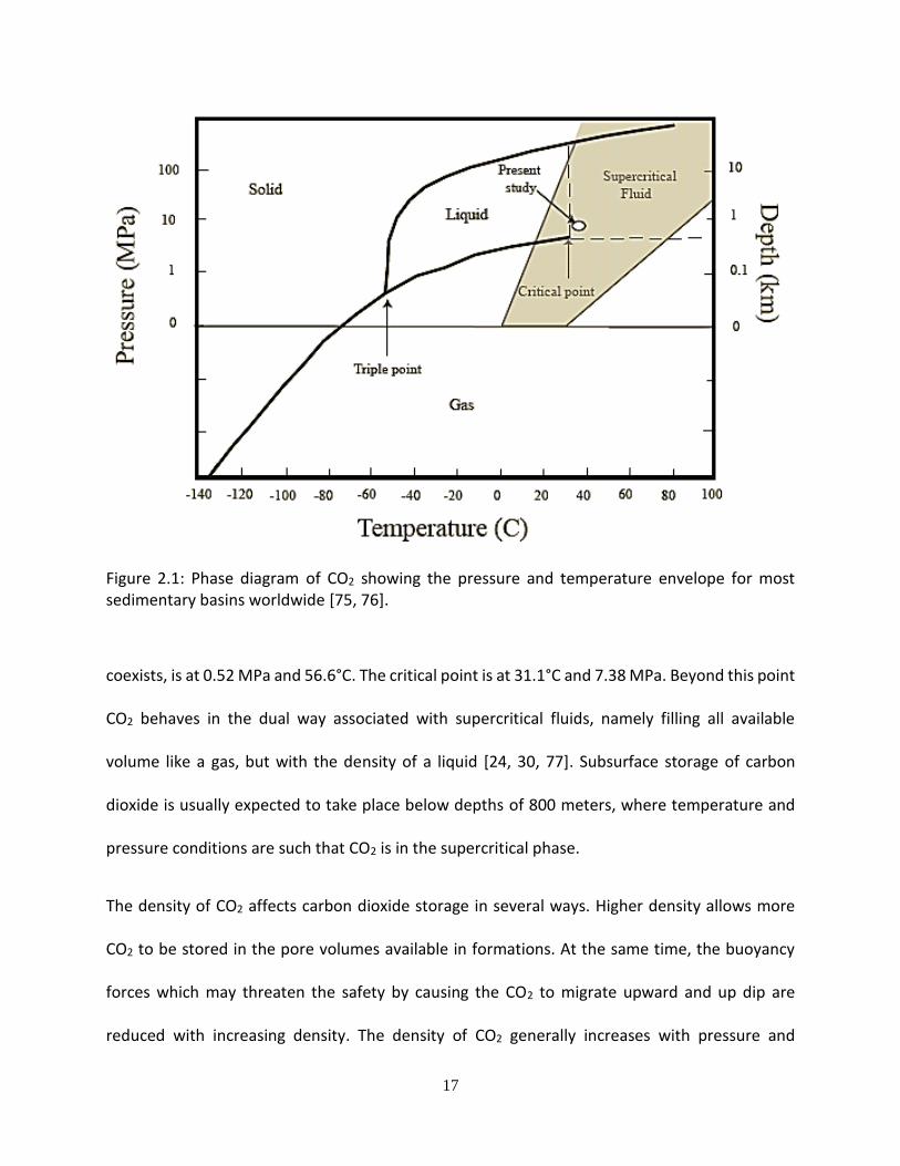
17

Figure 2.1: Phase diagram of CO2 showing the pressure and temperature envelope for most sedimentary basins worldwide [75, 76].

coexists, is at 0.52 MPa and 56.6°C. The critical point is at 31.1°C and 7.38 MPa. Beyond this point

CO2 behaves in the dual way associated with supercritical fluids, namely filling all available

volume like a gas, but with the density of a liquid [24, 30, 77]. Subsurface storage of carbon

dioxide is usually expected to take place below depths of 800 meters, where temperature and

pressure conditions are such that CO2 is in the supercritical phase.

The density of CO2 affects carbon dioxide storage in several ways. Higher density allows more

CO2 to be stored in the pore volumes available in formations. At the same time, the buoyancy

forces which may threaten the safety by causing the CO2 to migrate upward and up dip are

reduced with increasing density. The density of CO2 generally increases with pressure and

18

decreases with temperature. At depths considered for underground storage of CO2, the density

of CO2 typically varies between 0.6-0.8 g/cm3. At the pressure and temperature used in this study

(P~8.0 MPa and T=36°C) the density of CO2 is close to 0.6 g/cm3 (figure 2.1) [75]. The density of

formation waters depends on salinity, in addition to pressure and temperature. The density (ρb)

of 1 M NaCl solution at 8.0 MPa and 36°C can be estimated based on an empirically derived

expression by;

𝑝𝑏 = −3.033405 + 10.1288163𝑥 − 8.750567𝑥2 + 2.663107𝑥3 ………………………..……... Eq. 2.1

𝑥 = −9.9559𝑒−0.004539𝑚 + 7.0845𝑒−0.0001638𝑇 + 3.9093𝑒−0.00002551𝑃……………………….. Eq. 2.2

where P is pressure in bars, T is temperature in Celsius and m is NaCl molality. The calculated

density is 1.04 g/cm3, which is close to 75 % higher than the CO2 density.

Viscosity describes the resistance of fluids to flow and for CO2 it increases with pressure and

temperature. Under the relevant conditions, CO2 has a viscosity around 3.0 × 10-5 Pas. The

viscosity of water decreases with temperature, and increases with salinity and pressure.

Temperature is the main controlling factor, and under elevated pressure and temperature

conditions, the viscosity of water is more than ten times that of supercritical CO2 [78, 79].

The volume change of fluids in response to applied pressure is expressed as their compressibility.

Compared to water, supercritical CO2 has a very high compressibility, meaning that relatively

small pressure and temperature changes can significantly alter its density. Actually, the

compressibility of CO2 close to the critical point ((δρ/δP)T=Tc at P→Pc) approaches infinite values.

The changes in isothermal compressibility (ΔT=0) with pressure is significantly larger and more

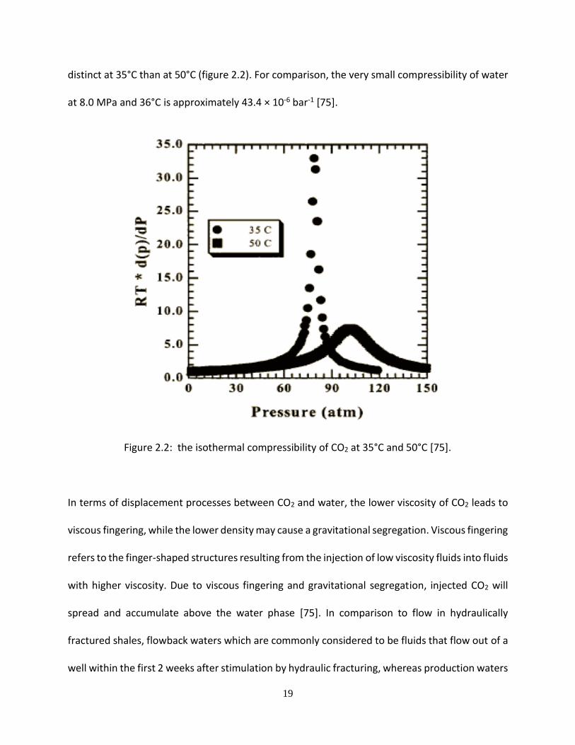
19

distinct at 35°C than at 50°C (figure 2.2). For comparison, the very small compressibility of water

at 8.0 MPa and 36°C is approximately 43.4 × 10-6 bar-1 [75].

Figure 2.2: the isothermal compressibility of CO2 at 35°C and 50°C [75].

In terms of displacement processes between CO2 and water, the lower viscosity of CO2 leads to

viscous fingering, while the lower density may cause a gravitational segregation. Viscous fingering

refers to the finger-shaped structures resulting from the injection of low viscosity fluids into fluids

with higher viscosity. Due to viscous fingering and gravitational segregation, injected CO2 will

spread and accumulate above the water phase [75]. In comparison to flow in hydraulically

fractured shales, flowback waters which are commonly considered to be fluids that flow out of a

well within the first 2 weeks after stimulation by hydraulic fracturing, whereas production waters

20

are the remaining fluid that flows from the well after the initial 2-week period [80]. Flowback is

driven by the release of the capped pressure and rock deformation induced by the flows from

the well after the initial 2-week period post-fracturing process [81, 82].

2.3 Shale Caprock Geochemical Alteration and Subsurface CO2 Migration

Shale caprock constitutes more than 60% of effective seals for geologic hydrocarbon bearing

formations and are therefore of considerable interest in underground CO2 storage into depleted

oil and gas formations [39]. Experimental studies of wettability, contact angle and interfacial

tension on shale using CO2-rich fluid have not been widely reported [77, 83, 84]. Porosity,

permeability, fractures and other petrophysical properties of the seal rock are of importance in

seal integrity analysis and can be experimentally determined. Organic-rich shale is considered to

have limited potential as membrane seals in CO2 containment [85]. Shale rocks are

predominantly composed of clays such as Illites, Kaolinites, Smectites and swelling

Montmorillonites [33, 35, 65, 86, 87]. They might also have other silica and carbonate based

minerals that contribute to their geomechanical strength. The mineralogical components of some

shale samples are shown in table 2.1.

Detritus formations in the subsurface are composed of transported and deposited rock grains,

minerals formed after deposition of the rock and organic material. The pore spaces between the

grains and minerals are occupied by water and some oil and gas. The rocks making up the

formation can be divided into cap rocks and reservoir rocks. The cap rocks are virtually

impermeable rocks which form a barrier above the reservoir rocks. CO2 injected into such

21

formations will interact with both cap rock and reservoir rock, in addition to the in situ formation

water or what is generally referred to as the connate aqueous medium [20, 48].

Different mechanisms for CO2 migration are possible, from small to large scales: (i) molecular

diffusion of dissolved CO2 in the pore water from the reservoir zone into the caprock formation,

(ii) CO2 diphasic flow after capillary breakthrough, (iii) CO2 flow through existing open fractures.

The following mechanisms can accelerate or slow down the migration: (i) chemical alteration of

the mineralogical assemblage of the caprock formation under the influence of acid water, (ii) re-

opening of pre-existing fractures or micro-cracks induced by overpressure of the reservoir below,

(iii) a combination of the above (including chemical alteration of the mineral filling the

fractures)[48, 88, 89].

Several simulation results have predicted that influx-triggered mineral dissolution/precipitation

reactions within typical shale cap rocks can continuously reduce micro-fracture apertures, while

pressure and effective-stress evolution first rapidly increase then slowly constrict them. The

extent of geochemical alteration is considered to be nearly independent of the injection rate

while that of geomechanical deformation is thought to be more pronounced during engineered

storage. The formation of wormholes in limestone or evaporate caprock core samples or

dissolution of calcite and dolomite cements around quartz framework grains in siliciclastic core

samples has been observed in batch or flow through reactions. Fracture evolution and

permeability reduction through fines movement in fractured carbonate cap-rock has also been

characterized. The potential effect on water chemistry or mineral trapping can be assessed; in

addition to identifying the reaction of minor amounts of minerals not resolvable by rock

characterization often necessitates identification through changes in water chemistry.

22

Table 2.1: Mineralogy of typical shale rock samples showing percentage composition [90].

Pierre Shale Arco-China

Shale

C1-Shale

X-Ray

Diffraction

%by weight % by weight % by weight

Quartz 19.0 51.0 14.0

Feldspar 4.0 12.0 2.0

Calcite 3.0 3.0 0.0

Dolomite 7.0 1.0 0.0

Pyrite 2.0 2.0 0.5

Siderite 1.0 0.0 0.0

*Total Clay 64.0 31.0 76.0

Chlorite 4.0 10.0 N/A

Kaolinite 11.0 14.0 39.0

Illite 19.0 44.0 N/A

Smectite 17.0 13.0 N/A

Mixed layer 49.0 20.0 N/A

*the percent composition of the total clay are broken down into chlorite, kaolinite, illite, smectite

and mixed layer.

There have been suggestions that ultimate restoration of pre-influx hydrodynamic seal

integrity—in both EOR-EGR/storage and natural accumulation settings—hinges on ultimate

geochemical counterbalancing of the resultant geomechanical effect [91, 92]. The geochemical

reactivity of caprock formations should be evaluated gradually, essentially in two steps: classical

batch experiments on crushed or small pieces of rock samples to evaluate reaction paths and

possibly the reaction kinetics, and flow tests on plugs to evaluate, among other important

quantities, the porosity and morphological variations.

23

In general, most researchers suggested that reaction trends are very difficult to identify at any

temperature. This is not to say that no reaction occurred but the complex natural mineralogical

composition envelops all reactions [65, 70]. In other experiments on the same formation and

using an image analysis technique, an illitization of the illite-smectite components was identified,

as well as the formation of gypsum. But similarly, these reaction paths are very difficult to identify

using standard bulk measurements such as X-ray diffraction (XRD). With such difficulties in

identifying reaction paths, the reaction kinetics is obviously out of reach [33, 61, 93].

Previous experimental research works have documented evidences of pore structure alteration

in CO2 flooded shale caprocks. The previous section (section 2.2) describes in detail some

properties of the injected fluid in these experiments.

2.3.1 Geochemical Dissolution/Precipitation.

The instability of clays in the presence of low-pH fluids has also been observed when using

hydraulic fracturing fluid. Low-pH fluids are capable of dissolving clays and silicates. As

temperature increases, the solubility of silici-clastic minerals is significantly increased especially

in low-pH environment [94, 95]. These findings are often observed when immersion tests are run

on cores in the laboratory. This type of fluid-mineral reactions is dynamic processes that involve

many effects: complex fluid flow, pore space changes, surface chemistry, and the mineral

composition. Several clays have been observed swelling rapidly in the presence of depressed pH

and elevated temperature including sloughing or disappearance of swelling clays [32, 94]. After

minerals are dissolved in the low-pH fluids, they can precipitate in the formation pores, restricting

fluid flow and leading to scaling and progressive geochemical aggregation [57, 69]. Clay soIubiIity

24

and geochemical precipitation in dry-gas, low permeability formations have a definite effect on

decreasing conductivity of proppant packs and fracture walls; formation matrix and surface

chemistry play a significant role in this as well as pH, ionic strength and adsorption processes. In

addition, fracturing fluids can interact with formations. Water from these fluids may exhibit

hydrogen bonding effects with formation clays and cause swelling and sloughing [96].

The mineral dissolution/precipitation with associated flow and reactive transport processes in

porous media can be described at different scales. Reactive transport modeling represents a

critical component in assessment of geochemical impact of CO2 water-rock interactions. The

following geochemical analytical model (equations 2.3 to 2.5) has been developed to generalize

precipitation-dissolution processes [75, 97, 98]:

𝑑𝑛

𝑑𝑡= −𝑆𝑘298.15𝑒

−𝐸𝑅

(1 𝑇

− 1

298.15)(1−

𝑄𝐾𝑒𝑞

)… … … … … … … … … . … … … … 𝐸𝑞. 2.3

𝑆 = 𝑆0 (𝐶

𝐶0)

2/3

(∅

∅0)

2/3

… … … … … … … … … … … … … … … . 𝐸𝑞. 2.4

𝐾 = 𝐾0 (∅

∅0)

𝑛

… … … … … … … … … … … … … … … … … … … … 𝐸𝑞. 2.5

Where S= specific surface area, k =permeability, Q = reaction rate, ɸ = porosity, Keq = equilibrium

rate constant, C = spherical grain size, n = heterogeneity exponent, R = gas constant, E = activation

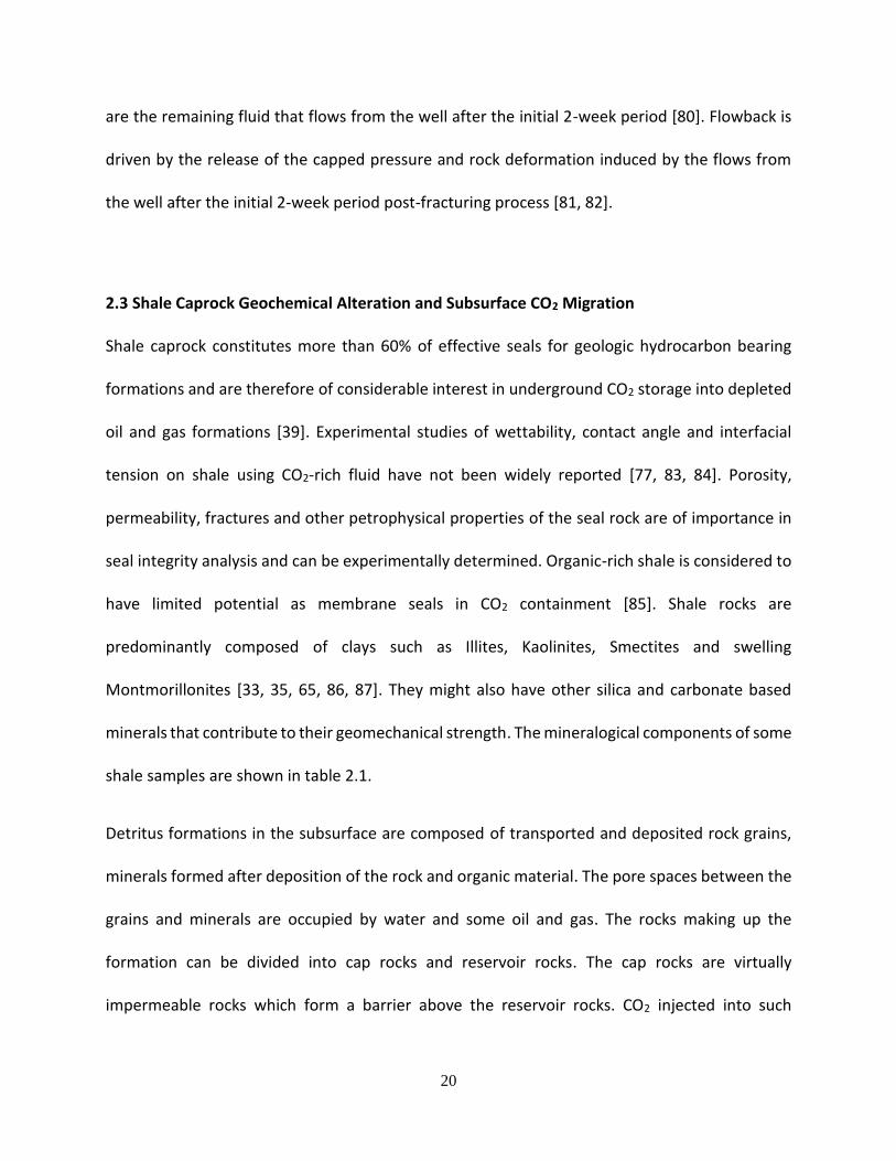
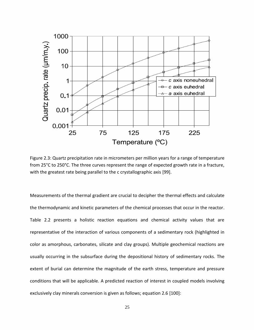
energy. An example of temperature-quartz precipitation relationship is presented in figure 2.3

[99]. The assumptions made for generating figure 2.3 included fixing the equilibrium constants.

25

Figure 2.3: Quartz precipitation rate in micrometers per million years for a range of temperature

from 25°C to 250°C. The three curves represent the range of expected growth rate in a fracture,

with the greatest rate being parallel to the c crystallographic axis [99].

Measurements of the thermal gradient are crucial to decipher the thermal effects and calculate

the thermodynamic and kinetic parameters of the chemical processes that occur in the reactor.

Table 2.2 presents a holistic reaction equations and chemical activity values that are

representative of the interaction of various components of a sedimentary rock (highlighted in

color as amorphous, carbonates, silicate and clay groups). Multiple geochemical reactions are

usually occurring in the subsurface during the depositional history of sedimentary rocks. The

extent of burial can determine the magnitude of the earth stress, temperature and pressure

conditions that will be applicable. A predicted reaction of interest in coupled models involving

exclusively clay minerals conversion is given as follows; equation 2.6 [100]:

26

KAlSi3O8 + 2.5Mg5Al2Si3O10(OH)8 + 12.5CO2(aq) KAl3Si3O10(OH)2 K-feldspar Mg-Chlorite Muscovite

+ 1.5Al2Si2O5(OH)4 + 12.5MgCO3 + 4.5SiO2 + 6H2O ……………………………………….……….Eq.2.6

Kaolinite Magnesite Silica

Table 2.2: Geochemical model for reaction of shale, sandstone and cement with CO2 and Na,

Ca, Mg Chloride brines [101, 102].

Phase Cement, Sandstone, and Shale Carbonation Mass Balance

Log K 95oC

Amorphous Al(OH)3 Al(OH)3 +3H+ ⇔ Al3+ + 3H2O 5.42

Amorphous Fe(OH)3 Fe(OH)3 +3H+ ⇔ Fe3+ + 3H2O 2.86

Boehmite AlO(OH) + 3H+ ⇔ Al3+ + 2H2O 3.75

Magnesite MgCO3 + H+ ⇔ Mg2+ + HCO3- 0.71

Siderite FeCO3 + H+ ⇔ Fe2+ + HCO3- -1.40

Calcite CaCO3 + H+ ⇔ Ca2+ + HCO3- 0.85

Dolomite CaMg(CO3)2 + 2H+ ⇔ Ca2+ + Mg2+ + 2HCO3- 1.41

Chalcedony SiO2 ⇔ SiO2,aq -2.88

Quartz SiO2 ⇔ SiO2,aq -3.10

Albite (Feldspar) NaAlSi3O8 + 4H+ ⇔ Al3+ + Na+ + 2H2O + 3SiO2 0.46

Kaolinite Al2Si2O5(OH)4 + 6H+ ⇔ 2Al3+ + 2SiO2 + 5H2O 1.35

Ripidolite 14Å Mg3Fe2Al2Si3O10(OH)8 +16 H+ ⇔ 2Al3+ + 3SiO2,aq

+ 3Mg2+ + 2Fe2+ + 12H2O

41.45

Illite K 0.6Mg0.25 Al2.3Si3.5O10(OH)2 + 8H+ ⇔ 0.25Mg2+ +

0.6K+ + 2.3Al3+ + 3.5SiO2 + 5H2O

2.56

Smectite

(Ca-Beidellite)

Ca0.165Al2.33Si3.67O10(OH)2 + 7.32H+ ⇔ + 0.165Ca2+

+ 2.33Al3+ + 4.66H2O + 3.67SiO2

-0.62

27

As already mentioned, CO2 will be in a supercritical phase at depths of geological formations

being considered for storage of carbon dioxide. Supercritical CO2 is less dense than water and will

rise until it reaches the overlying cap rock. This kind of physical trapping beneath stratigraphic or

structural barriers is the principle means to store CO2 in geological formations. With time CO2 will

dissolve into the formation water, removing buoyancy as a reason for migration. The dissolved

CO2 will instead migrate according to relatively slow regional-scale groundwater flows [103]. The

storing of CO2 dissolved in slow moving waters is referred to as hydrodynamic trapping. Finally,

CO2 can be locked up in carbonate minerals in mineral trapping. Some of the most probable

carbonate minerals forming are calcite (CaCO3), magnesite (MgCO3), siderite (FeCO3) and

dawsonite (NaAlCO3(OH)2). The advantages of mineral trapping are apparent, as the CO2 would

be stored in fairly stable minerals over very long timescales [86, 104, 105].

2.3.2 Dissolution Kinetics in Shale Caprock Minerals

Most of the knowledge on mineral dissolution kinetics acquired over the last fifty years comes

from the ability to accurately measure the variation in aqueous chemistry as a function of time

when a mineral (usually powder) and a solution are put together to react. This approach has been

used to produce adequate data to formulate empirically derived dissolution rate laws that

account for the effects of pH, temperature, aqueous Al, organic acids, solution saturation state,

and ionic strength on clay mineral dissolution rates. In the last two decades, additional micro-

and nanoscale data has come out from the improved capacity of new techniques such as atomic

force microscopy (AFM), interferometry techniques (VSI (vertical scanning interferometry) and

PSI (phase shifting interferometry)), and laser confocal microscopy with differential interference

28

contrast microscopy (LCM-DIM) to study the mineral-water interface [105]. Integration of both

strategies is leading to a remarkable level of understanding of the dissolution kinetics.

Rock mineral dissolution rate can be written by considering a general law (equation 2.7), as that

proposed by Lasaga in the late 90s:

𝑅𝑎𝑡𝑒 = 𝑘0. 𝐴𝑚𝑖𝑛. 𝑒𝐸𝑎𝑅𝑇 . 𝑎𝐻

𝑛𝐻 . ∏ 𝑎𝑖𝑛𝑖 . 𝑔(𝐼). 𝑓(∆𝐺𝑟) … … … … … … … … . . … … … . … … … 𝐸𝑞. 2.7

𝑖

Where ko is a constant, Amin is the reactive surface area of the mineral, Ea is the apparent

activation energy of the overall reaction, R is the gas constant, T is the temperature (K), aH is the

activity of protons in the solution, nH is the order of the reaction with respect to H+ and the term

involving the activities of other aqueous species, ai, incorporate other possible catalytic or

inhibitor effects on the overall rate [106]. The g(l) term indicates a possible dependence of the

rate on the ionic strength (l) in addition to that entering through the activities of specific ions.

The f(ΔGr) term accounts for the variation from equilibrium (ΔGr = 0; 0 < f(ΔGr) < 1). The

formulation of the rate equation above is very useful because it relates the reaction rate to

activities of ions in solution that may be obtained directly from the solution chemistry. However,

silicate dissolution is a surface process and therefore, it is more appropriate to express the

dependence of the rate on the concentrations (or activities) of ions adsorbed on the surface

rather than on the bulk activities in solution. Hence, the equation can be written in terms of

surface concentrations (Cs,i) (Eq. 2.8);

𝑅𝑎𝑡𝑒 = 𝑘0. 𝐴𝑚𝑖𝑛. 𝑒𝐸𝑎𝑅𝑇 . 𝐶𝑠,𝐻

𝑛𝐻,𝑎𝑑𝑠 . ∏ 𝑎𝑖𝑛𝑖,𝑎𝑑𝑠 . 𝑔(𝐼). 𝑓(∆𝐺𝑟) … … … . … … … … … . 𝐸𝑞. 2.8

𝑖

29

Where the coefficients nH,ads and ni,ads are the reaction orders with respect to the adsorbed

surface species. Given the above and based on the two rate equations, there is a diversity of rate

laws that account for the dissolution kinetics of different clays [107, 108].

In the last four decades, several mechanistic models have been developed to account for the

effect of deviation from equilibrium (f(ΔGr)) on mineral dissolution kinetics. Among others, these

mechanisms include: (1) the most widely extended one was derived from transition state theory

(TST) which was developed for elementary reactions and may be applied to overall reactions

governing the dissolution process and relates the variation in solution composition with mineral

dissolution and precipitation rates[108, 109]. TST may be applied only in cases in which defects

such as dislocations do not control the dissolution kinetics (2) at the start of the twenty-first

century, a different conceptual model took off. Researchers also proposed a model of mineral

dissolution that directly links the surface reactivity of minerals with their dissolution kinetics

[108]; (3) in a third approach, dissolution of some alumina-silicates can be understood through

the same mechanistic theory of nucleation developed for mineral growth. Another model

predicts that dissolution occurs via the formation of etch pits and the generation of dissolution

step-waves at the outskirts of the pit walls [110]. If the under-saturation of the solution is high

enough, i.e., ΔG < ΔGcrit (critical free energy), etch pits not only open up but they are the source

for trains of steps that travel across the surface. By moving away from the defect site and

lowering the silicate surface the propagation eventually controls the bulk dissolution rate. Several

studies using vertical scanning interferometry (VSI) have demonstrated this mechanism and

suggest that etch pits in combination with step movement control the dissolution process of

several minerals independent of their degree of structural complexity [111].

30

It has also been showed that mineral dissolution can be understood through the same

mechanistic theory of nucleation developed for mineral growth [108]. The derived dislocation

model can predict variation of the normal aluminosilicate dissolution rate (Rn) with degree of

under-saturation (σ). It is argued that two-dimensional nucleation dominates rates measured at

higher temperatures 150°C – 200°C. In contrast, the 80°C data for kaolinite is predicted by the

dislocation defect model. Nonetheless, this model has not been further developed for clay

minerals other than kaolinite.

Implementation of base case dissolution model has gained terrain as real-time microscopic

observations of reacted mineral surfaces offer new insights into the dissolution mechanisms

[108]. Also, the validity of the TST-based rate laws to be sufficient to explain mineral dissolution

kinetics as a function of distance from equilibrium has been questioned, mainly based on the fact

that TST allows a relation between the forward and reverse rate constants but only of an

elementary reaction [112, 113]. The adequacy of simple surface adsorption models to explain the

complexity of the three-dimensional lattice and its participation in the dissolution process is also

argued. Previous works showed that the use of a stochastic approach that treats crystal

dissolution as a many-body problem has led to the development of the step-wave model and

some in-depth exploration of the dissolution mechanism [114].

As it has been extensively discussed in the literature, most of the descriptions and interpretations

of the clay dissolution kinetics are at the moment, TST-based. Therefore, TST is further discussed.

The terms integrated in equation 2.8 above other than the f(ΔGr), account for the effect of

different environmental variables on clay dissolution rates.

31

In order to model the effects of pH, temperature, catalysis/inhibitors, ionic strength on clay

mineral dissolution rates, it is important to separate between direct and indirect effects of the

environmental variables involved. Direct effect means effect related to surface processes and

therefore, one that can be used to understand the reaction mechanism. As changes in most

environmental variables affect also the degree of saturation, their direct effect on the rate should

be measured in experiments that are carried out under far-from-equilibrium conditions.

2.3.2.1 Negative Logarithm of Hydrogen Ion (pH)

The effect of pH on the dissolution rates of oxides and silicates, and hence clay minerals has been

exhaustively examined in the last decade (figure 2.4). For the pH-dissolution rate dependence, in

the absence of catalysts/inhibitors, the dissolution rate (equation 2.9) has been classically

interpreted by three reaction mechanisms [108, 109]: proton promoted, hydroxyl-promoted and

water promoted, that dominate the reaction rate under acidic, alkaline, or neutral conditions,

respectively:

𝑅𝑎𝑡𝑒 = 𝑘𝐻ł . 𝑎𝐻ł

𝑛𝐻ł

+ 𝑘𝑊 + 𝑘𝑂𝐻. 𝑎𝑂𝐻𝑛𝑂𝐻 … … … … … … … … … 𝐸𝑞. 2.9

Where 𝑎𝐻ł is the proton activity; 𝑎𝑂𝐻 is the hydroxyl activity; 𝑘𝐻, 𝑘𝑊, and 𝑘𝑂𝐻 are the rate

constants under acidic, neutral, and basic conditions, respectively, and 𝑛𝐻ł and 𝑛𝑂𝐻ł are the

corresponding orders of reaction. The dissolution rates of most alumina-silicates as a function of

pH exhibit a U-shape figure. In some studies the pH dependence of dissolution rate is modelled

using a surface complexation model (equation 2.10) [108]:

𝑅𝑎𝑡𝑒 = 𝑘𝐻. 𝐶𝑆,𝐻 + 𝑘𝑊 + 𝑘𝑂𝐻. 𝐶𝑆,𝑂𝐻 … … … … … … … … . 𝐸𝑞. 2.10

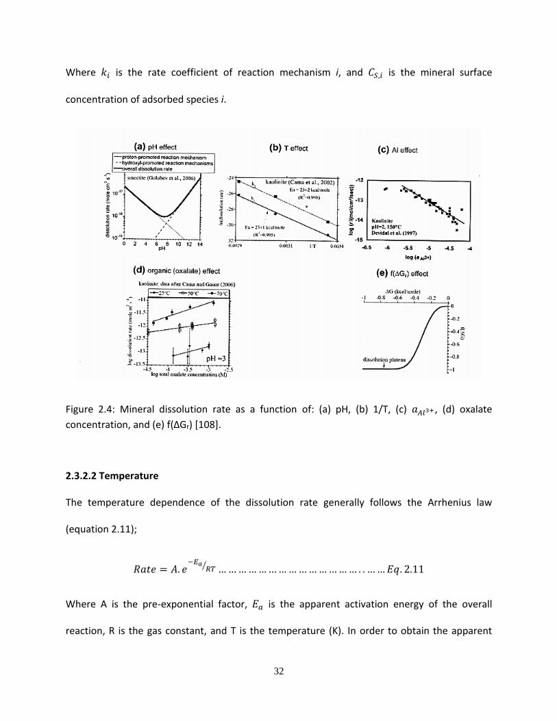
32

Where 𝑘𝑖 is the rate coefficient of reaction mechanism i, and 𝐶𝑆,𝑖 is the mineral surface

concentration of adsorbed species i.

Figure 2.4: Mineral dissolution rate as a function of: (a) pH, (b) 1/T, (c) 𝑎𝐴𝑙3+ , (d) oxalate

concentration, and (e) f(ΔGr) [108].

2.3.2.2 Temperature

The temperature dependence of the dissolution rate generally follows the Arrhenius law

(equation 2.11);

𝑅𝑎𝑡𝑒 = 𝐴. 𝑒−𝐸𝑎

𝑅𝑇⁄ … … … … … … … … … … … … … … . . … … 𝐸𝑞. 2.11

Where A is the pre-exponential factor, 𝐸𝑎 is the apparent activation energy of the overall

reaction, R is the gas constant, and T is the temperature (K). In order to obtain the apparent

33

activation energy experimentally, it is common to conduct several experiments at different

temperatures while all the other experimental variables (e.g., pH) are held constant. A critical

assumption in calculating activation energies using this method is that the pre-exponential factor,

A, is the same in all experiments. This pre-exponential factor includes other effects of the

experimental variables on the rate. As mineral dissolution is a surface process, the pH effect on

dissolution rate is controlled by protons adsorbed on the surface and not directly by the pH [115].

Therefore, conducting experiments under the same pH is not enough to keep the pre-exponential

factor constant but the surface concentration can be held constant [108].

Under non-equilibrium conditions, and keeping all parameters except pH and temperature

constant, the rate becomes (equation 2.12);

𝑅𝑎𝑡𝑒 = 𝑘. 𝑒−𝐸𝑎

𝑅𝑇⁄ . 𝑎𝐻ł

𝑛𝐻ł

… … … … … … … … … … … … … … … . . 𝐸𝑞. 2.12

Where k is a coefficient that is constant under these conditions.

2.3.2.3 Surface Area and Reactivity

Reactive surface area is one of the key parameters for studying the kinetics of mineral dissolution.

The determination of the reactive surface area is not trivial in clay minerals as they possess both

internal and external surface areas, and in which many cases the dissolution is controlled by the

chemical attach on the edge surface [116, 117]. The common practice in experimental kinetics is

to normalize dissolution rate to the surface area measured by the Brunauer–Emmett–Teller (BET)

method. As the BET method measures the total surface area, it was suggested that it is not a valid

proxy for reactive surface area of clays [108, 118, 119]. It is widely recognized that dissolution

34

and precipitation of clay minerals (and phyllosilicates) occur preferentially at the edge. Lack of

correlation between the total and the edge surface area of smectite makes the smectite BET

surface area an ineffective proxy for its reactive surface area. This conclusion may be

extrapolated to all clay minerals which form layered particles. Hence, it is suggested to use AFM

measurements of the specific edge surface area as an alternative proxy for the reactive surface

area of smectite and other clay minerals [116, 120-122]. However, the recent VSI and AFM

experiments with muscovite indicate that basal/edge surface area ratios are highly variable and

change continuously over the progression of the reaction, thus obviating their utility as

characteristic parameters defining mica reactivity [108].

2.3.2.4 Catalysis/Inhibitors

Aluminum (Al) and organic matter (OM) can be used as proxy for measuring catalytic and

inhibiting phenomenon in clay rich shaly rocks [108, 123]. It has been showed strong Al inhibition

of kaolinite dissolution reaction under very-far-from-equilibrium conditions at 150°C and pH = 2.

The reaction order of this inhibition was -1. It was proposed that Al-silicate dissolution is

controlled by a Si-rich precursor complex formed by the exchange of Al for protons at the surface

[116, 124]. Due to differences in the surface properties of different minerals, there is a significant

variability in their tendencies to adsorb organic matters. Among the naturally abundant minerals,

the most effective adsorbents are clay minerals and oxides [25, 110, 125]. Although both

inhibition and enhancement of clay mineral dissolution rates were observed, the latter effect is

much more common. Low molar mass organic acids (e.g., oxalate, malonate, citrate, salicylate,

o-phthalate, and gluconate) through ligand-promoted dissolution at mineral surfaces and

35

complexation of metal cations in solution have been shown to enhance dissolution of kaolinite

and montmorillonite [32, 115, 126]. It has equally been found that acetate, gluconate, alginate,

glucosamine, and glucoronate may also inhibit dissolution of montmorillonite [108, 127]. The

empirical rate laws that account for the effect of OM on silicate dissolution are of the form

(equation 2.13);

𝑅𝑎𝑡𝑒 = 𝑘𝑂𝑀. 𝐶𝑂𝑀𝑛 … … … … … … … … … … … … … … . 𝐸𝑞. 2.13

Where 𝑘𝑂𝑀 is the rate coefficient and 𝐶𝑂𝑀 is the OM concentration, and n is the reaction order

with respect to OM concentration [108].

Several studies have showed that steady-state kaolinite dissolution was stoichiometric with

respect to Al/Si ratio both in acid and alkaline solutions. To assess the possible initial in-

congruency of kaolinite dissolution experiments were performed using X-ray photo-electron

spectroscopy (XPS) for surface composition analyses [108]. The XPS of kaolinite surface

composition examined after acid and basic dissolution was found to be depleted in Al relative to

the initial mineral, suggesting an initial preferential Al release [115]. These data, together with

the stoichiometric nature of steady-state dissolution, imply that the slightly depleted Al surface

persists, following its initial development, throughout the duration of the experiments. This initial

Al preferential release may be related to the formation of a rate controlling precursor complex

[128]. Also, the pH of the solutions used to pre-treat the starting kaolinite samples may change

the relative concentration of Al and Si sites on the surface toward the stoichiometric ratio [129,

130]. Dissolution of kaolinite at pH = 2 and 150°C is specifically inhibited by Al. Addition of Al3+

into solution was found to inhibit the K+-montmorillonite dissolution reaction at pH≤3 and 25°C

36

but not at 50°C (≈ 10-6 M < [Al] < 10-4 M). The surface reaction mechanism consists of fast

adsorption of Al3+ on the mineral surface (crystal edge surface sites) followed by a slow hydrolysis

step [108].

2.3.2.5 Ionic Strength Effect

Transition State theory (TST) predicted that the rate constant depends on the activity coefficients

of aqueous species [108]. For not too high concentrated solutions (< 0.1M), the logarithm of the

rate constant of an elementary reaction involving ions depends on the square root of the ionic

strength of the solution [131, 132]. Early fast release rates of interlayer cations from clay

minerals, induced by ion exchange reactions between the solution and the interlayer sites, have

been observed in several studies, yielding to early non-stoichiometric dissolution of clay minerals,

which is pH dependent [108]. In most cases steady-state dissolution was stoichiometric. Non-

stoichiometric dissolution under steady state condition is mostly the result of precipitation of

secondary phases [133]. Similarly to silicates, the dissolution rates of clay minerals slow down

with increasing pH in the acidic range, become constant at an intermediate pH, and increase with

increasing pH in the basic range [134, 135]. This pattern of change with pH in the dissolution rate

of oxides and silicates was classically interpreted by three reaction mechanisms: proton-

promoted, hydroxyl-promoted, and water-promoted, that dominate the reaction rate under

acidic, basic, or near-neutral conditions, respectively [108]. The fractional reaction orders

calculated from the linear regression of plot of log RSi and/or RAl against pH are between 0.32

and 0.60 (Illite), 0.4 and 0.75 (Montmorillonite). The proton-dependent reaction order for

trioctahedral micas (phlogopite and biotite) ranged between 0.25 and 0.61 compared to 0.14-

37

0.20 for dioctahedral mica (muscovite). The fractional reaction orders for pH are between 0.44

and 0.45 (vermiculite) and 0.29 and 0.49 (chlorite) [110, 136]. Experimental works to study the

effect of ionic strength on kaolinite, montmorillonite, and illlite show that the kaolinite

dissolution rates were dependent on ionic strength. The dissolution rates of the other two clay

minerals were mainly controlled by solution pH, and no effect of ionic strength was observed on

the dissolution rates. In the case of illite dissolution, an increase in the release rates of Al3+ and

K+ occurred by increasing the ionic strength from 0.01 M to 0.25 M, however, no such effect was

observed on Si release rates [108].

2.3.3 Precipitation in Porous Media

The interpretation of mechanisms of reactions in rocks is based on studying the microstructural

development associated with the reaction [137]. The microstructure of a rock describes the

relationships between the mineral grains and organic material in the rock, their size, shape, and

orientation. When reactions involve fluids we look for microstructural and chemical evidence for

the presence of fluid and fluid pathways [137, 138]. In that sense the porosity can be considered

as an integral part of the microstructure, in that it is the space occupied by the fluid phase, and

the distribution of the fluid phase is just as important to the rock properties as the distribution

of the minerals. The individual mineral grains in a rock may also have a microstructure that

reflects the processes taking place within the crystalline structure as a result of the geological

history of the rock [20, 126, 137]. Examples would include ex-solution from an initial solid

solution, or transformation twinning, or the formation of dislocation arrays during deformation

[48, 139]. The rock and mineral microstructures can provide important information on how the

38

rock formed and its subsequent thermal and deformational history. The microstructure is thus a

direct result of the mechanisms of the processes that take place when a rock or mineral reacts to

lower the overall free energy of the system under the imposed physical and chemical conditions

[126, 138]. The microstructure formed during any process is always a balance between the

thermodynamics (reducing the free energy) and the kinetics (the time available and the rates of

the processes involved). As such, a microstructure may change over time, for example by

coarsening or recrystallization to reduce the surface energy [137]. When an aqueous fluid

interacts with a mineral with which it is not in equilibrium (i.e., is either under-saturated or

supersaturated with respect to that mineral) the mineral will either tend to dissolve or grow until

equilibrium is reached, i.e., until the fluid is saturated with respect to that mineral. The solubility

of a mineral can also be increased by applied stress and this leads to the phenomenon of pressure

solution whereby grains in contact with one another and under compression dissolve at these

pressure points (figure 2.5). The resulting fluid is then supersaturated with respect to a free

mineral surface and can re-precipitate in the pore spaces [120, 137]. The newly precipitated

phase may have the same major chemical composition as the dissolved phase, but can be

recognized as an overgrowth both texturally and from trace element and isotope geochemistry.

This mechanism of compaction reduces the porosity of a rock and leads to well-known

relationships between depth of burial, porosity and rock density [69, 140]. The re-precipitated

phase can also act as a cement to bind the particles during the lithification process [48, 141].

in structural geology and diagenesis, pressure solution or pressure dissolution is a deformation

mechanism that involves the dissolution of minerals at grain-to-grain contacts into an aqueous

pore fluid in areas of relatively high stress and either deposition in regions of relatively low stress

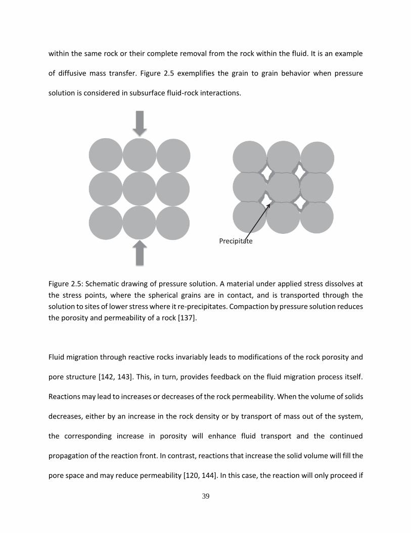
39

within the same rock or their complete removal from the rock within the fluid. It is an example

of diffusive mass transfer. Figure 2.5 exemplifies the grain to grain behavior when pressure

solution is considered in subsurface fluid-rock interactions.

Figure 2.5: Schematic drawing of pressure solution. A material under applied stress dissolves at

the stress points, where the spherical grains are in contact, and is transported through the

solution to sites of lower stress where it re-precipitates. Compaction by pressure solution reduces

the porosity and permeability of a rock [137].

Fluid migration through reactive rocks invariably leads to modifications of the rock porosity and

pore structure [142, 143]. This, in turn, provides feedback on the fluid migration process itself.

Reactions may lead to increases or decreases of the rock permeability. When the volume of solids

decreases, either by an increase in the rock density or by transport of mass out of the system,

the corresponding increase in porosity will enhance fluid transport and the continued

propagation of the reaction front. In contrast, reactions that increase the solid volume will fill the

pore space and may reduce permeability [120, 144]. In this case, the reaction will only proceed if

40

the stress generated by the volume increasing process is large enough to create a fracture

network that will enable continued fluid flow. Reaction-induced fracturing is particularly relevant

during fluid migration into high-grade metamorphic and slowly cooled magmatic rocks with very

low initial porosity, but may also be important during reactive transport in more porous rocks

where growth processes within the pore space exerts forces on the pore walls [20, 144] and

fracture propagation. Spheroidal weathering is an example of a process where reactions produce

pronounced fracturing under the low confining pressures that prevail near the Earth’s surface.

This kind of weathering has been described for most rock types in a wide range of climate zones.

Although spheroidal weathering, per definition, involves surface-parallel fracturing and spalling

of layers at the margin of rock blocks, which become progressively rounded (core stones), the

progress of this mode of weathering and the fracture patterns produced are sensitive to the initial

porosity of the rock type [145]. Fluid flow in fractures is assumed to be effectively instantaneous

compared to the rate of other relevant processes [146, 147]. In a natural system, the progress of

the fluid-driven, volume-increasing reactions, is controlled by two main parameters: rock

porosity, and the shape of the initial domain undergoing volatilization [148, 149]. For circular

domains, porosity variation will control both the relative rates of reaction kinetics and transport,

often expressed by the dimensionless Damkohler or Peclet-Damkohler Number, and the amount

of the mobile reactant that the rock can contain [70, 150]. Although reactions may produce

fractures and porosity, mineral growth in pores may also lead to clogging. This may significantly

decrease the permeability and therefore fluid migration through initially porous rocks, and

through rocks that are initially fractured due to tectonic and thermal processes. When fluid

consuming reactions occur synchronously with tectonic deformation, the externally imposed

41

stress may completely control the reaction rate and progress if permeability is generated at a

faster rate than the infilling of pores by reaction products. On the other hand, if the precipitation

rate is fast compared to the rate of fracturing and permeability generation, the progress of

reaction may be modest even in extensively fractured rocks [151].

Replacement reactions mediated by a fluid phase take place through a coupled dissolution–

precipitation reaction. When fluid comes into contact with the reactive mineral, dissolution takes

place at the mineral surface [138]. This immediately creates a supersaturated solution with

respect to the replacing mineral, which will then precipitate in the immediate vicinity of the

dissolving surface. A nanometer-scale confined fluid film between the parent and daughter

phases will allow the reaction to continue. If the supersaturation with respect to the precipitating

phase is high, there will be enough chemical energy available for the precipitating material to

exert a mechanical stress on the reacting grain, and cause fracturing, when precipitation is

confined within dissolution pits and wedges [151].

A well-established example of the use of the continuum approach for interfacial reactive

processes is that of reactive transport in fractures. In fractured media, there is a sharp contrast—

with a clear separation of scales—between the porosity in the fracture and in the rock matrix

[135]. As a result, the fracture is modeled as a fast flow path, where transport is dominated by

advection, and the rock matrix, where transport is dominated by diffusion. Heterogeneous

reactions take place within the porous rock matrix or the layer of precipitate that coats the

surface [152]. To simulate flow in discrete fractures in Darcy-scale models, the cubic law is often

used to obtain a fracture permeability under the assumption of parallel smooth walls [153].

However, this model does not typically provide an accurate estimation of fracture hydrodynamic

42

properties at realistic fracture roughness. Mineral rates measured in laboratory experiments are

often several orders of magnitude faster than those estimated from natural systems [154]. These

differences in rates have been attributed to a variety of factors including, among others, reactive

surface area accessibility in natural porous media, limitations on flow and transport in

heterogeneous material, or transport, rather than interface control of rates. Microfracture-scale

modeling can be used to address some of these hypotheses by explicitly accounting for the rate-

limiting effect of transport, and by incorporating mechanistic descriptions for the evolution of

reactive surface area [155, 156].

Applications of direct numerical simulation of pore-scale processes in subsurface materials are

growing in part due to the computational advantages of well-established computational fluid

dynamics (CFD) methods [70, 151]. Availability of high-level, open-source libraries such as

OpenFOAM or Chombo have also facilitated implementation of models into new simulation

capabilities [157]. In reactive systems, the ability to calculate the heterogeneous reaction rates

at the fluid–solid interfaces makes direct numerical simulation a suitable tool to mechanistically

model processes that are not captured by models at larger scales, especially when well-mixed

assumptions are made [158, 159]. In multiscale problems, direct numerical simulation has

typically been performed using continuum methods rather than strictly using pore-scale

methods. In these methods surface reactions and transport processes are not explicitly

calculated at the interface and are upscaled from the pore scale [160]. Upscaling of strongly

coupled non-linear processes is not straightforward and the solution of macro- and micro-scale

problems is coupled. It is ultimately the combination of new microscopic characterization,

experimental, and modeling approaches that presents the opportunity to provide mechanistic

43

explanations for many of the long-standing questions in geochemical processes in fractured

porous media [97, 138, 161].

2.4 Geomechanical Effects

2.4.1 Cap Rock Seal Integrity and Capillarity

CO2 injection may lead to pressure build up and temperature decrease, which may cause CO2

leakage through the cap rock by capillary leakage or rock fracturing. CO2 diffusion through the

cap rock is an extremely slow process, and is only considered important over geological time.

Capillary leakage occurs if the minimum pressure needed to displace the brine in the cap rock

(capillary breakthrough pressure, Pc) is exceeded [47, 162, 163].

Since cap rocks overlying gas and oil reservoirs have proven the ability to prevent upward

migration of hydrocarbons through geological time, it has been argued that they will be sufficient

seals also after CO2 injection. Recently however, it has been pointed out that since the interfacial

tension (IFT) is much lower in the CO2/water system than in the hydrocarbon/water system, the

sealing capacity of the cap rock is significantly reduced after CO2 injection. IFT (σ) is a result of

the attractive forces of molecules acting at the interface between fluids, and is closely related to

capillary breakthrough pressure [83, 164]. The cohesive forces among the liquid molecules are

responsible for this phenomenon of surface tension. Chiquet et al. experimentally examined the

contact angle on quartz and mica under varying CO2 pressures. They observed a 40°-50° increase

in the contact angle of mica and 15°-25° increase for quartz over the pressure interval 0-11 MPa.

This corresponds to lowering the sealing capacity by a factor of ~1.5. This wettability alteration

was primarily attributed to a decrease in brine pH caused by CO2 dissolution, as the electrostatic

44

repulsion between the negative surface charges on the mineral-brine and brine-CO2 interfaces

are reduced at low pHin the bulk of the liquid, each molecule is pulled equally in every direction

by neighbouring liquid molecules, resulting in a net force of zerothe two are connected through

the Laplace law (equation 2.14);

𝑃𝑐 =2𝜎𝑐𝑜𝑠𝜃

𝑟𝑝 … … … … … … … … … … … … … … … … … … … … … … … . 𝐸𝑞. 2.14

where σ is the IFT between CO2 and water, rp is the largest connected pore throat radius and θ is

the contact angle between the mineral - brine - CO2 - system. The general assumption has been

that brine is a good wetting fluid (small contact angle). Recently however, it has been pointed

out that the dense, supercritical CO2 reduces the wettability of water on shale minerals (e.g.

quartz, mica). It should be noted that the concept of interfacial tension in subsurface rock-fluid

interactions and phase behavior has been around for several decades, with applications in water

flooding operations for crude oil production.

Quantitatively, the differences in IFT between brine/CO2 and brine/hydrocarbons have been

addressed by several authors. Numerous other researchers have investigated IFT in (CO2 + CH4)

+ water systems, and it was observed that the relative amounts of CO2 and hydrocarbons affected

the IFT [165]. Other researchers also complemented their gas breakthrough experiments with a

review of existing experimental data [47, 84]. At pressures from 6 - 20 MPa and temperatures

below 71°C, the IFT levels in brine-CO2 are approximately half the values of water/hydrocarbon.

Among pressure, temperature and salinity of the brine, pressure exerts the main control on the

IFT. Combining the effects of reduced IFT and increased contact angle, the replacement of

hydrocarbons by CO2 can reduce the capillary breakthrough pressure by a factor of ~3.

45

Translating the breakthrough pressure into storage capacity for aquifers is relatively

straightforward. If the reservoir in which CO2 is stored has a thickness h, the buoyancy forces

driving CO2 upwards are the product of the gravitational constant, the thickness of the aquifer

and the difference between the density of brine and CO2 ((ρwater – ρCO2)×g×h). If the buoyancy

forces are greater than the cap rocks capillary pressure, CO2 will enter the cap rock. A certain

amount of work is required to move a water molecule from within the body of the liquid through

the interface. This is referred to as free surface energy of liquid. The maximum height of CO2 that

can be stored can therefore be obtained from the simple inequality expression (equation 2.15):

(𝜌𝑤𝑎𝑡𝑒𝑟 – 𝜌𝑐𝑜2). 𝑔. ℎ ≤=2𝜎𝑐𝑜𝑠𝜃

𝑟𝑝 and ℎ ≤=

2𝜎𝑐𝑜𝑠𝜃

𝑟𝑝.(𝜌𝑤𝑎𝑡𝑒𝑟− 𝜌𝑐𝑜2).𝑔 ………… Eq. 2.15

It should be mentioned that the density variations of CO2 and water in the reservoir is not

accounted for in these equations. The low viscosity and high diffusion coefficient of supercritical

CO2 has made it a preferred agent in supercritical fluid extraction (SFE). The ability to extract

organic matter from rocks could potentially influence the sealing performance of the organic-rich

claystone from the Troll East Field. Other researchers have treated siltstone from the field

injection test sites (total organic matter content 0.4 - 1.3 wt %) with supercritical CO2 to identify

potential cap rock alterations caused by SFE [166-168]. Even though the carbon and nitrogen

levels, porosity and pore size distribution remained virtually unchanged after 150 days of

treatment, significant permeability changes could not be excluded. If the minor amounts of

organic matter dissolving hold grains together, the resulting pore structure alteration could

drastically increase the permeability [27, 169, 170].

46

2.4.2 Fracture Conductivity and Formation Stress

A fracture has been recognized as a fluid conduit that has high permeability relative to that of

the surrounding rock matrix in a fractured reservoir [171, 172]. The reservoir quality of

sedimentary rocks is closely related to diagenesis, a process involving post-depositional

alteration of previously deposited sediments. Rock properties such as porosity, permeability,

pore-size distribution, reservoir heterogeneity and spatial correlation can be the product of

diagenetic modification of original properties [173, 174]. Figures 2.6 and 2.7 illustrate

hypothetical diagenetic changes in a single fracture factoring diffusion, convection and surface

reaction.

Figure 2.6: Schematic of precipitation/dissolution reaction in a finite length single fracture.

Figure 2.7: fracture shape with precipitation of cemented minerals leading to aperture loss.

47

One of the most important mechanisms of diagenetic processes is chemical reaction between

minerals and migrating fluids. The hydraulic isolation of a porous medium by a caprock layer

provides an environment amenable to several uses of the underlying porous formation. When

the porous medium is under artesian pressure, it serves as a ready source of water supply. With

sessile groundwater conditions, such porous formations are looked upon favorably for deep

geologic disposal of contaminants and other forms of hazardous waste in liquid form.

Hydrodynamic and stratigraphic trapping represents the primary phase of containment of the

fluidized CO2 and it is assumed that this will ensure longevity of the retention of CO2 in the storage

formation. This environment would enable the initiation of other time-dependent trapping

mechanisms, including solution, mineral and residual phase trapping that can occur at time scales

varying from the time of injection to a million years.

It is can be assumed that the caprock fracture is stationary and that its dimensions are

uninfluenced by the pressures of injected fluids. This is hardly the case in many oil and gas

operations that are related. Fractures are nearly ubiquitous in rocks that have experienced

even slight deformation and most of these are mineral filled [175]. Their presence indicates that:

(1) dilation of the rock took place for fractures to be both open and provide pathways for fluid

flow and (2) fluid was present and perhaps moving during and after the deformation event, and

it carried sufficient mass of fracture constituents in solution to precipitate in the observed

fracture void space [176, 177]. Pressure solution and compaction mechanism as a result of

enormous formation stress is a driver for the diagenetic loss of fracture conductivity and

adjoining formation permeability [59, 178, 179]. Pressure solution and compaction of quartz

materials have been extensively studied and models have been developed that relate the rate of

48

porosity loss to the applied stress, temperature, and formation grain size in hydraulically

fractured tight rocks (see figures 2.6, 2.7 and 2.9). These are for long term subsurface predictions.

Figure 2.8: fracture production (of light oil) simulation illustrating the impact of conductivity on

long-term production. Only the impact of a pressure-solution model was used as the damage

mechanism under constant and elevated temperature [59].

Figure 2.9: illustration of the pressure solution and compaction mechanism. High stress at the

contact points increases the solubility of silica, which diffuses into the pore spaces and

precipitates [59].

Grains Dissolution

49

A crystal growing in a pore will stop growing when the stress on the crystal surface approaches

the maximum crystallization pressure [137]. However, if the stress is sufficient to open a fracture,

the stress on the crystal surface will decrease, thus enabling further growth. When strain rates

are slow, as can be the case during precipitation in pores and cracks, fracture propagation takes

place through a kinetic process known as subcritical crack growth [167, 180]. Previous works have

demonstrated how to couple the rates of crystal growth and fracture propagation when a crystal

grows from a supersaturated solution inside the aperture of a fracture [181]. As long as there is

an unlimited supply of supersaturated solution, fracture propagation causes the stress on the

crystal surface to decrease and the rate of fracture propagation will accelerate until complete

failure takes place [182]. Few researchers have developed precipitation/dissolution models for

the flow in finite parallel plates that represent single fractures [183]. The idea behind such models

is to approximate the description of a variable fracture aperture, surface reaction, and diffusion

by a set of parameters and simple rules governing the alteration of fractures [184, 185]. Fracture

aperture can either grow or shrink as chemical reaction proceeds at the fracture surface. This

sometimes involves mass conservation equations for the components of aqueous and solid

phases simultaneously and shows the fracture aperture size distribution with time. Calcite

cementation is a form of precipitation that can be modelled and incorporated. It has been shown

that to replicate the lower permeability that typify tight gas shale requires the superimposition

of systematic cement filling that preferentially plugs fracture tips and other narrower parts of the

fracture pattern[15, 146, 186]. Additional challenge for natural fracture characterization is

quantifying the effective permeability of fracture networks. A benefit of the mechanics-based

analysis is that fracture aperture is an intrinsic part of the solution; a result of boundary

50

conditions imposed, propagation criteria, and the mechanical interaction between neighboring

fractures. Four different fracture patterns in sedimentary rocks could be identified; polygonal

pattern, cross-fractured pattern, and single set of nominally parallel fractures [187-189].

In subsurface fractures, crack-seal textures and other evidence suggest that cement may be

deposited simultaneously with fracture opening and propagation, partially filling and propping

the large aperture [173]. The highly heterogeneous quartz cement thicknesses found in partially

cemented fractures in mudrocks are a function of the processes that control quartz/clay crystal

growth rates. The mineral components in mudstones and shales respond to CO2 in several

ways. It has been reported that the interaction of water and CO2 causes montmorillonites

to expand, thereby increasing solid volume and leading to self-sealing of caprock fractures,

which is reducing the caprock permeability. Quartz or opal crystals show substantial

anisotropies in growth rate depending on the nucleation substrate [124, 190]. The fastest rates

of growth occur on irregular surfaces that are perpendicular to the crystallographic axis.

Geochemical precipitate growth rate is a strong function of temperature, which can be expressed

using the exponential Arrhenius expression (equation 2.16);

𝑞 = 𝐴𝑒−𝐸𝑎𝑛𝑐

𝑅𝑇 … … … … … … … … … … … … … … 𝐸𝑞. 2.16

where q is the rate of geochemical precipitation per unit area (mol/cm2s), A is a constant

(mol/cm2s), Eanc is the activation energy for geochemical precipitation on irregular surfaces

(J/mol), R is the real gas constant (8.314 J/mol°K), and T is the temperature (K).

The result developed for the flow rate through a single fracture located in the caprock can also

be used to examine the leakage through multiple vertically-aligned fractures. The global

51

permeability or hydraulic flow constant of diagenetic fractured grid blocks was computed as

given by equations 2.17 and 2.18; where km is the matrix permeability and kf is the intrinsic

fracture permeability. Δc is the grid-block dimension and d is the fracture aperture.

𝑘𝑓𝑟𝑎𝑐𝑑 = 𝑘𝑓 x 𝑑 + 𝑘𝑚 x(∆𝑐 − 𝑑)

∆𝑐 … … … … … … … … … . . 𝐸𝑞. 2.17

𝑘𝑓 =𝑑2

12 … … … … … … … … … … … … … … … … … … … … 𝐸𝑞. 2.18

the competition between diagenetic (quartz) precipitation rate and fracture opening rate

determines whether a fracture is completely filled with cement (no porosity), partially filled with

occasional aperture spanning bridges that prop it open, or mostly open with only a thin coating

of geochemical materials [191, 192]. Emergent threshold was described in many quartz-rich

mudrocks such that a kinematic aperture exists below which fractures are completely filled with

cement and occluded and above which they are only partially cemented and bridged or

completely open[193, 194]. The emergent threshold can be estimated by picking the slowest

precipitation rate which is indicative of the formation temperature during fracturing. Figure 2.10

shows the relationship among global permeability, emergent threshold and fracture porosity.

Significant changes in fracture pattern geometry and flow properties caused by minor changes in

deformational or diagenetic boundary conditions highlight the challenges of accurate

characterization of natural fractures caused by small strain events [51, 55, 195-197]. Only few

examples of coupled chemical transport-mechanical modelling studies are available, and most of

them focus on short timescales. This work by Noh and Lake are very useful in conceptual model

developments of rock-fluid-fracture interactions.

52

Figure 2.10: Modification of calculated steady-state effective permeability (left axis) for a generic

fracture pattern showing reduction in effective permeabilities, kx and ky, caused by diagenetic

cementation represented by the increasing emergent threshold. Fracture porosity is plotted on

the right axis [173].

2.4.3 Mechanisms of Natural CO2 Migration

There are three processes that can lead to the vertical migration of CO2 from a reservoir through

the caprock: migration through unfractured caprock by capillary flow, migration by fracturing the

caprock, and migration through faults. Migration of CO2 through mudrocks or shales will occur

when the pressure in the reservoir exceeds that of the capillary entry pressure of fractures or

pores in the seal. The small pore sizes of low permeability rocks require thousands of units of

53

capillary entry pressures to occur. The density and phase conditions of CO2 are dependent on

pressure and temperature, which is a direct function of the depth of the reservoir [143]. The

density contrast between CO2 and brine in the reservoir decreases with increasing depth, and

hence differential buoyancy pressure on the caprock also decreases with increasing depth. For

this reason shallow reservoirs (<1000 m depth) are inherently more likely to leak CO2 through an

unfractured caprock. Yet, there are no indications that leakage through the caprock by capillary

flow is a leaking mechanism in the studied shallow reservoirs [2, 198]. For leaking CO2 reservoirs

in Italy, it was shown that the observed surface CO2 seep rates greatly exceed the physical

possibility of leakage by capillary flow through intact mudrock from the area above the site. Thus

CO2 migration must be via fractures not matrix flow. It has also been shown that even after an

estimated 70 Ma, CO2 only infiltrated 12 m of sealing mudrocks directly over a CO2 rich oil field

in the UK North Sea. Hence, the time-scales required for CO2 migration through unfractured

caprocks are orders of magnitudes longer than those necessary for CO2 storage to effectively

mitigate climate change [199].

As burial depth increases, it becomes more likely that fluid pressures will be over pressured, that

is, pore pressures deviate from hydrostatic (or“normal”) pressures towards lithostatic pressures.

If pore pressure in the reservoir exceeds both the pore pressure in the caprock and the tensile

strength of the caprock (including any differences in confining stress due to different elastic

properties), hydraulic fracturing and/or frictional failure along optimally oriented pre-existing

fractures of the caprock occurs[30, 74, 79]. Both mechanisms can lead to migration of CO2 from

the reservoir through the caprock by fracture flow. This effect was induced at the CO2 injection

test site at in Salah. Fracturing to form dilatant joints (mode 1 fractures) induced by elevated fluid

54

pressure only occurs when the pressure exceeds the least principal stress of the caprock (this

direction of least principal stress is typically horizontal until depths exceed 1.5–2 km) [200-202].

The pore pressure required to cause such failure is much less than the pore pressure required to

overcome the capillary entry pressure of a mudstone caprock and so caprocks will transmit CO2

more readily by fracture flow than by capillary flow [203, 204]. Most sedimentary rocks are

fractured during burial and the fracture density depends on the geomechanical properties and

thickness of the rock and thus different rock layers fracture differently in response to the same

stress. Fracture density increases in the vicinity of faults and fractures provide permeability only

when open or connected [205]. There is no clear evidence for leakage through dilatant joints in

hydraulically fractured caprock in the examined sites [206, 207].

Strong evidence for CO2 migration through fault induced fractures exists at several insecure

reservoirs. CO2 seeps are frequently located close to active or extinct faults, which may exist prior

to CO2 migration [134]. Thus fractures and flow through fractures as part of a fault zone play a

significant role in permitting CO2 migration. This indicates that pre-existing faults are important

pathways for CO2 migration, possibly due to increased fracture permeability in the fault damage

zone [139, 208].

The subsurface is not a random collection of materials. Geological processes have led to

structured deposits with distinct material characteristics and geometrical relationships.

Processes have formed the geomechanical facies as a conceptual building block for the

subsurface [143]. A geomechanical facies has specific material characteristics defined by the

geology of the rocks and defined by the engineering use to which it will be put [2, 134]. Using the

55

geomechanical facies framework, the factors crucial to assessing the CO2 storage security of a

storage basin such as basin architecture, caprock architecture, reservoir quality, stress state,

mechanical characteristics, fractures, burial depth, geo-thermal gradient, risk of orogenic

modification, structural stability and preservation potential can all be taken into account [209,

210]. By examining the typical characteristics of the geomechanical facies within the different

tectonic settings, it is possible to compare and contrast the different tectonic settings to appraise

global CO2 storage opportunities and predict which tectonic settings will be most suitable for CO2

storage [211, 212].

It is important to note that the geomechanical facies approach for CO2 site selection is the first

step in what is a complex and iterative site specific assessment procedure, where uncertainty

decreases as the data requirement increases. However this first appraisal step is a crucial stage

in the identification and assessment of suitable CO2 storage sites and underpins the later

screening and ranking procedure of sedimentary basins for geological CO2 storage [213, 214].

2.5. Previous Experimental and Modeling Works

2.5.1 Similar Experimental Setups for CO2 Sequestration and Containment

Previous experimental investigations as reported in reported in unpublished thesis about a

decade ago [75], examined the deformation of limestone and sandstone caused by injection of

high and low PCO2 aqueous fluids. The experiments were performed in a triaxial cell where a

vertical stress of 16 MPa was imposed by a piston directly in contact with the sample. The

horizontal confining pressure was 10.2 MPa, the temperature 40°C and the salinity of the brine

56

0.01 M NaCl. The fluids were injected in the bottom of the sample at constant flux (0.005 ml/min)

using a high pressure liquid chromatography pump. The high pressure CO2/brine mixture (8 MPa)

was prepared in an autoclave. After filling the autoclave with CO2 ice, they injected saline solution

([NaCl] =5.8 g/l) until the desired pressure was obtained. The mixing of CO2 and water was

considered satisfactory after one week as the heavier water was injected at the top and the

autoclave was equipped with an impeller. Furthermore, the exchange kinetics over the interface

have previously been demonstrated to rapidly equilibrate supercritical CO2 and water [75].

The experimental setup used previously display some features similar to the setup used in this

study. Their reacting material was placed in a 100 cm high column inside a large heated pressure

vessel, with the confining pressure controlled by a syringe pump. CO2 and brine were equilibrated

at 70°C and 10 MPa using a second syringe pump which was also connected to the top of the

column. Fluid flow was controlled by a third syringe pump connected to the bottom of the

column. A 30 cm3 titanium floating piston pressure sampler inserted between the outlet of the

pressure vessel and the syringe pump applying the back-pressure, allowed fluid samples to be

taken. Analytically the solids were examined using SEM and gas sorption on clean surfaces to

determine the surface areas. In addition to pH measurements, the fluid samples were analyzed

for both major and trace cations using inductively coupled plasma-optical emission spectroscopy

(ICP-OES) and for anions using ion chromatography [75].

Fluids leaving triaxial from previous experiments reported were constantly collected, and

analyzed by ICP-OES every second day. As the pressure was reduced in the samples upon analysis,

nitric acid was added to prevent precipitation. A Triassic Arkosic sandstone was exposed to 70

57

days of high PCO2 (8.3 MPa) injection, followed by 50 days of no-flow. During fluid injection, the

aqueous concentrations of Ca, Si and Sr decreased, while Mg increased. After the 50 days without

flow, a second injection period was started with an injection rate 10 times the original one. This

rate was later lowered to 2 times the original rate, thereby completing an increase-decrease

sequence simulating uplift followed by burial. All the steady state concentrations decreased after

the injection rate was increased, whereas decreasing the injection rate again led to increasing

concentrations in a step-like manner. The overall higher concentrations of Mg and Ca compared

to Si were attributed to a well-known decrease in reactivity from dolomite and calcite to quartz

[65].

Furthermore, injected CO2 at 200°C and 20 MPa into an aquifer-aquitard system composed of

Arkosic sandstone and shale, respectively. The injection period lasted for 80 days, and the

purpose was to examine fluid-rock interactions with focus on carbonate mineral precipitation

[43, 149]. This was done by investigating reaction textures on aquifer and aquitard minerals,

carbonate minerals precipitated and changes in brine chemistry. In addition to precipitated

magnesite, amalcine mica and clay minerals, their results showed textures on silicate minerals

which indicated significant reactions. The arkosic sandstone serving as the aquifer was composed

of equal amounts of quartz, oligoclase and microcline. On the edges of pits and open fractures of

the quartz grains, abundant clay minerals were observed using SEM. Smectites not present on

the initial oligoclase were present in abundance on the surfaces and cleavages of the CO2 exposed

oligoclase grains. While it was observed that there were differential etching on the microcline

surfaces, the same phenomenon was not observed for the oligoclase. For the shale (mostly

composed of quartz and clay minerals), they saw clay coatings draping across surfaces and small

58

cavities. Halite crystals had accumulated on the shale surfaces, something which may have

resulted from brine trapping during quenching. The levels of major ions in the brine stabilized

within the first 670 hours after start of injection. Whereas the Na-and B-concentrations stayed

close to the initial concentrations, K-, Mg- and Cl-levels decreased by 15-20%. Ca increased by

approximately 30%, while Si increased from zero to a level just below what was calculated based

on quartz solubility. The concentrations of Sulphate and Iron did not stabilize and continued to

change throughout the duration of the experiment [75].

Previous works examined the cap rock effects of CO2 injection at Sleipner by reactive transport

modeling of dissolved CO2 in the cap rock [38]. As it is considered unlikely that capillary leakage

will occur through the Nordland Group shales overlying the Utsira sand at Sleipner, only reaction

kinetics and diffusive transport was included in the model [37, 215]. The Oseberg formation

water was equilibrated with the cap rock mineralogy by geochemical modeling as a starting point.

Under 37°C and approximately 10 MPa, two types of batch models were done; one assuming

instantaneous thermodynamic equilibrium and one incorporating the kinetics over 15,000 years

[6]. There are multiple complex reactions that are taking place during rock-fluid interactions and

only very few have been extensively described. In the experiments carried out by the authors of

the previously described procedure, it was shown that the latter far-from equilibrium geo-

reactions showed a fairly fast dissolution of calcite after the initial pH drop from 7.7 to 3.0. In the

thermodynamic batch model an unrealistically high reactivity was revealed by a significant

reduction in pure H2O levels. Overall smectites and illite dissolved, while chalcedony, kaolinite

and large amounts of carbonates (magnesite, dolomite, dawsonite and siderite) precipitated.

Relatively small amounts of calcite were needed to stabilize the pH at 4.5. In the long run,

59

kaolinite and calcite formed from the dissolution of albite combined with Ca2+ ions from the initial

dissolution of carbonates according to equation 2.19;

2NaAlSi3O8 + CO2 + 2H2O + Ca2+ ---------- 4SiO2 + CaCO3 + Al2Si2O5(OH)4 + 2Na+ ……….. Eq. 2.19

As the Ca2+ concentration decreased with time, the model predicted a shift from calcite to

dawsonite formation. However, the total amounts of carbonate minerals formed over the 15,000

years were minor, and the porosity of the cap rock remained virtually unaffected by the

dissolution/precipitation reactions. Replacing albite with the more reactive anorthite retarded

the CO2 migration as the CO2 rapidly reacted with the anorthite in the lower part of the cap rock

[216].

The main lesson learned from the diffusive transport model was that the process is very slow

particularly in tight caprocks, even when the effective diffusion coefficients were in the high end

of their calculated range [75].

2.5.2 Geomechanical Experiments

The axial displacement sensors in previous rock-fluid interaction experiments indicated that the

compaction response of the sandstone after injection start, was very rapid. After 1 day the

deformation rate was already at the limit of what could be measured. The rapid compaction was

believed to be caused by a sudden increase in pore fluid pressure. This pressure increase initiated

grain-grain rearrangement and grain-grain sliding, which led to the compaction. A porosity

increase in the sandstone of 1.7 % was estimated based on the amount of carbonates such as

dolomite and calcite cement dissolved in aqueous medium [75].

60

Capillary breakthrough pressure tests for supercritical CO2 have been performed with somewhat

different approaches. Researchers experimentally investigated the breakthrough pressure of

supercritical CO2 for Midale evaporites (Weyburn cap rock) [40, 215]. These rocks have very low

porosity and permeability. Using a constant backpressure of 7.3 MPa and the in-situ temperature

of 59°C, they increased the injection pressure in steps of 0.5 – 1.0 MPa. For samples with

porosities ranging from 0.3-0.7 %, they got breakthrough at differential pressures from 11.2-5.0

MPa. It was determined that capillary entry and breakthrough pressure of the Nordland shale

cap rock under reservoir conditions can be estimated. With a confining pressure of 15.3 MPa,

they started with equal pore pressure in the top and bottom of their samples (10.3 MPa). Next,

the downstream pressure was decreased in steps of approximately 0.3 MPa until upstream CO2

moved into the sample. This occurred after the downstream pressure had been reduced to 8.6

MPa, resulting in a breakthrough pressure of 1.7 MPa.

The laboratory tests on Vp and Vs performed two decades ago were motivated by the

discrepancies between theoretically derived and observed seismic velocities after CO2 injection

at the McElroy field, Texas. The higher velocities observed compared to the ones predicted using

the special theory of Gassmann, were attributed to a more significant pore pressure increase

following the CO2 injection than what was initially assumed. Therefore, they flooded eight

dolostone cores with CO2 under higher pressure and temperature conditions and examined the

velocities as functions of CO2 saturation and pore pressure. Their experimental data suggested

3.0 – 10.9 % decrease in Vp and 3.3 – 9.5 % decrease in Vs. The results obtained from the two

decades experiments indicated that while Vp is sensitive to changes in both CO2 saturation and

pore pressure, Vs is only sensitive to pore pressure changes. Based on this, they suggested that

61

S-wave velocities can be used to separate the effect of pore pressure increase from the combined

effect of pore pressure build up and increasing CO2 saturation. This can possibly be used to

separate between reservoir zones with CO2 and high pressure zones without CO2 [75].

62

CHAPTER 3

EXPERIMENTAL SETUP AND PROCEDURE

3.1 Experimental Methods and Sample Preparation

The approach to investigating the problem of the effects of diagenetic alterations in fracture

conductivity entails experimental and simulation design using artificially prepared composite

rocks with capillary tubing embedded to mimic fractures. The experimental and simulation

methods are described below in details. The experimental design entails flooding crushed

samples of four different shaly rocks with CO2-brine fluid and/or hydraulic fracturing fluid.

Temperature and pressure will be elevated throughout the system with adequate regulation of

flow rate at sub-unity level. The dissolved/precipitated minerals from this flooding process are

transported through the artificial composite rocks with real time monitoring of pressure drop

overtime across the composite core using the Core Flooding System (CFS 200) data acquisition

unit with advanced differential pressure transducers for real time analysis of responses. Detailed

effluent and crushed rock analysis will be carried out using various analytical techniques and tools

as indicated below. The proposed composite core will be made of kaolinite, cement and non-

corrosive PEEK polymer microtubings. Figures 3.1 to 3.4 show the schematics of the experimental

setup and the composite core respectively.

The equipment used in the flow-through experiments part of this research work are unique due

to highly scientific and precision driven instrumentation that were included. The overall

experimental work applied specific analytical techniques in investigating changes in

surface/near-surface properties of the shale rock after exposure (by flooding) to CO2-brine,

63

Figure 3.1: Detailed process flow diagram of the experimental setup showing critical devices and equipment for CO2-brine flooding and composite core conductivity measurement.

64

Figure 3.2: Visual design of composite core made of kaolinite, cement and micro-tubes (magnified) using SolidWorks©.

Figure 3.3: Visual sample design of composite core made of kaolinite, cement and polymer PEEK micro-tubes which are not evenly distributed as envisage through SolidWorks©.

Micro-tube (25µm/150µm in diameter)

Composite core

3in

1in

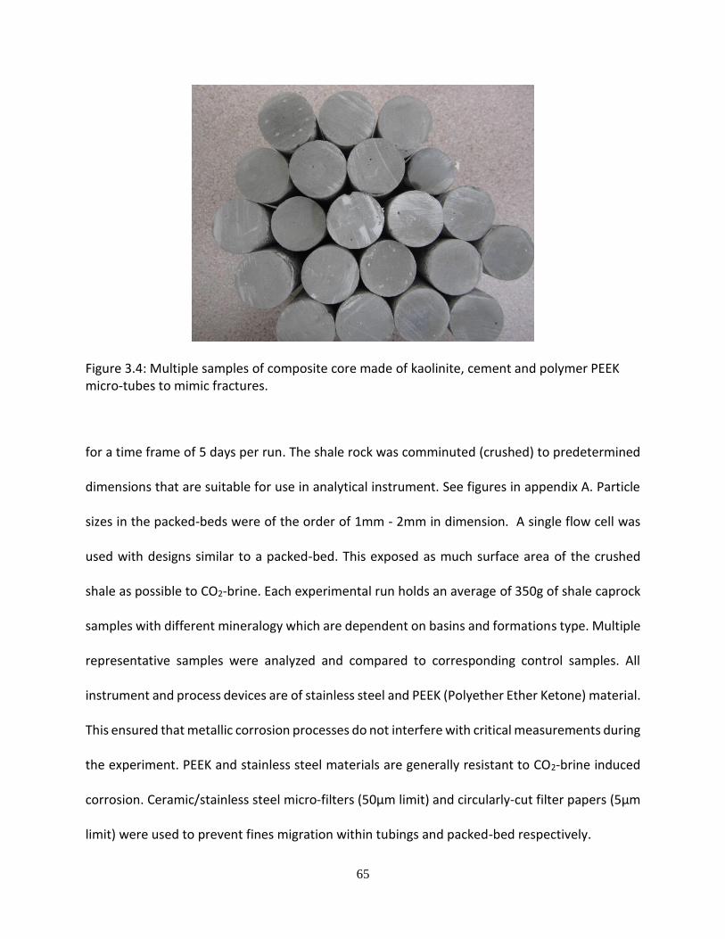
65

Figure 3.4: Multiple samples of composite core made of kaolinite, cement and polymer PEEK micro-tubes to mimic fractures.

for a time frame of 5 days per run. The shale rock was comminuted (crushed) to predetermined

dimensions that are suitable for use in analytical instrument. See figures in appendix A. Particle

sizes in the packed-beds were of the order of 1mm - 2mm in dimension. A single flow cell was

used with designs similar to a packed-bed. This exposed as much surface area of the crushed

shale as possible to CO2-brine. Each experimental run holds an average of 350g of shale caprock

samples with different mineralogy which are dependent on basins and formations type. Multiple

representative samples were analyzed and compared to corresponding control samples. All

instrument and process devices are of stainless steel and PEEK (Polyether Ether Ketone) material.

This ensured that metallic corrosion processes do not interfere with critical measurements during

the experiment. PEEK and stainless steel materials are generally resistant to CO2-brine induced

corrosion. Ceramic/stainless steel micro-filters (50µm limit) and circularly-cut filter papers (5µm

limit) were used to prevent fines migration within tubings and packed-bed respectively.

66

3.2 Experimental Setup

The experimental set-up consisted of a core flooding unit (CFS-200), an automated Oven, a

heating tape, a stainless steel pressure cell, a syringe pump (and a piston pump for backup), a

back pressure regulator (BPR), accumulators (glass beaker), multiple transducers, three pressure

gauges, PEEK and stainless steel tubings, National Instruments data acquisition device, two

ceramic filter to prevent fines carry over (larger than 50 μm) and a computer system. PEEK

polymers were used because it has high resistance to corrosion as a result of low pH or high

temperature and pressure conditions. Schematics of the CO2-brine flooding of shale caprock and

composite fractured core injection are shown in Figures 3.1 and 3.2. The packed-bed was

mounted vertically in the oven for temperature control with aqueous CO2 flowing from the top

to the bottom of the experimental fixture. This is to prevent particulate fluidization were it to be

the other way round i.e. bottom to top. Also the effect of gravity is assumed to be negligible. A

schematic of the experimental setup is shown in figure 3.3. Figure A.1 in Appendix A has pictures

of the physical components of the experimental setup among other equipment and consumable.

3.3 Experimental Shale Rocks Geology

The approach used in the design of experiments required multiple shale rock samples to be used

such that geographical and mineralogical variations are factored into the experimental matrix

configuration. Table 3.1 below shows the geological properties of the shale samples that were

used in the flooding experiment. This consist of Mancos, Marcellus, Pottsville and Wilcox shales.

These shales are found in different geographic regions of the United States with potentials for

energy fluid extraction or storage of carbon dioxide.

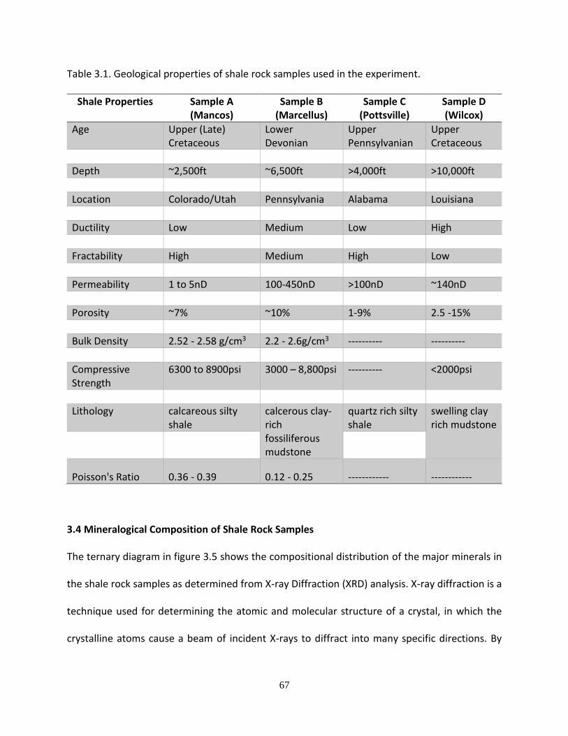
67

Table 3.1. Geological properties of shale rock samples used in the experiment.

Shale Properties Sample A (Mancos)

Sample B (Marcellus)

Sample C (Pottsville)

Sample D (Wilcox)

Age Upper (Late) Cretaceous

Lower Devonian

Upper Pennsylvanian

Upper Cretaceous

Depth ~2,500ft ~6,500ft >4,000ft >10,000ft

Location Colorado/Utah Pennsylvania Alabama Louisiana

Ductility Low Medium Low High

Fractability High Medium High Low

Permeability 1 to 5nD 100-450nD >100nD ~140nD

Porosity ~7% ~10% 1-9% 2.5 -15%

Bulk Density 2.52 - 2.58 g/cm3 2.2 - 2.6g/cm3 ---------- ----------

Compressive Strength

6300 to 8900psi 3000 – 8,800psi ---------- <2000psi

Lithology calcareous silty shale

calcerous clay-rich fossiliferous mudstone

quartz rich silty shale

swelling clay rich mudstone

Poisson's Ratio 0.36 - 0.39 0.12 - 0.25 ------------ ------------

3.4 Mineralogical Composition of Shale Rock Samples

The ternary diagram in figure 3.5 shows the compositional distribution of the major minerals in

the shale rock samples as determined from X-ray Diffraction (XRD) analysis. X-ray diffraction is a

technique used for determining the atomic and molecular structure of a crystal, in which the

crystalline atoms cause a beam of incident X-rays to diffract into many specific directions. By

68

measuring the angles and intensities of these diffracted beams, an XRD equipment can produce

quality geochemical data. Figure 3.6 compared the composition to other CO2 sequestration shale

caprock sites and hydraulically fractured shale for oil and gas production as provided by Bourg

[217]. Table 3.2 contains the details of the percentage composition of each mineral. The samples

consist on a broad scale quartz, feldspar, pyrite, calcite, dolomite, chlorite, illite, kaolinite and

montmorillonite. The relative abundance of these components in each shale rock type showed

the preponderance of quartz, carbonates and clay in general terms. The compositions presented

in this report have similar characteristics to data available in the literature. It affirms the fact that

shale rocks are heterogeneous compactions of multiple sedimentary minerals.

Figure 3.5: Initial mineralogical composition of four shale rock samples (from XRD Analysis) used

in rock-fluid interaction experiment. The ternary diagram shows carbonates, quartz, feldspar,

pyrite and clay as main components of the shale rocks used for the experiment.

Mancos

Marcellus

Pottsville

Wilcox

Quartz+Feldspar+Plagioclase+Pyrite

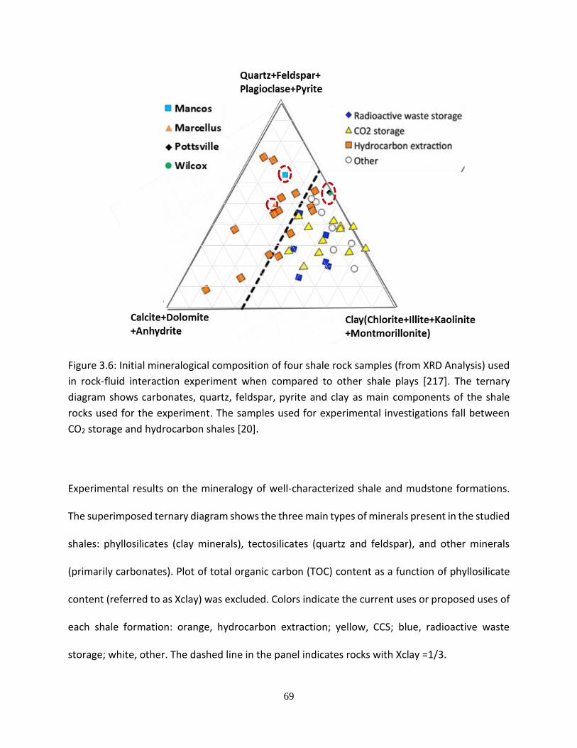
69

Figure 3.6: Initial mineralogical composition of four shale rock samples (from XRD Analysis) used

in rock-fluid interaction experiment when compared to other shale plays [217]. The ternary

diagram shows carbonates, quartz, feldspar, pyrite and clay as main components of the shale

rocks used for the experiment. The samples used for experimental investigations fall between

CO2 storage and hydrocarbon shales [20].

Experimental results on the mineralogy of well-characterized shale and mudstone formations.

The superimposed ternary diagram shows the three main types of minerals present in the studied

shales: phyllosilicates (clay minerals), tectosilicates (quartz and feldspar), and other minerals

(primarily carbonates). Plot of total organic carbon (TOC) content as a function of phyllosilicate

content (referred to as Xclay) was excluded. Colors indicate the current uses or proposed uses of

each shale formation: orange, hydrocarbon extraction; yellow, CCS; blue, radioactive waste

storage; white, other. The dashed line in the panel indicates rocks with Xclay =1/3.

70

Table 3.2: Mineralogical composition of the four shale samples in percentages as captured by the ternary diagram of figure 3.5.

Components

Mancos(%) Marcellus(%) Pottsville(%) Wilcox(%)

Quartz

60.47 43.43 49.77 46.09

K-Feldspar

0.88 0.8 0 1.43

Plagioclase

1.35 1.21 5.58 3.83

Calcite

7.92 25.25 0 0

Dolomite

8.14 2.44 0 0

Anhydrite

0 0.41 1.2 1.02

Pyrite

1.18 4.01 0 3.35

Clay

20.06 22.46 43.45 44.28

Chlorite 3.5 0 10.37 10.31

Illite 11.46 20.61 25.15 12.69

Kaolinite 5.1 1.85 7.93 14.24

Montmorillonite 0 0 0 7.04

3.5 Experimental CO2-brine Fluid

Carbon dioxide saturated brine solution was used for all experiments. Brine was prepared with

distilled water to ensure that unknown species were not present in the solution. The brine

composition was designed to simulate typical shale formation brine as observed in hydraulic

stimulation flowback water [218]. This brine contained Mg and CaCO3 in minor amounts. The

composition was then simplified to include only NaCl which contains trace amount of KCl

(<0.05%). As seen in the Table 3.3, the brine solution contained ~ 2% dissolved solids. After mixing

water and salts, the brine was filtered using filter paper to eliminate undissolved solid particles

71

that can plug the flow lines in the experimental set-up. A filter was also installed upstream of

injection to reduce the risk of plugging the flow lines. An accumulator (volume ~25 liters) was

used to hold the brine solution as CO2 was bubbled through at 40 psi for approximately 80 mins

resulting in average pH value of 3.7 over the course of the experiment. This method was selected

because of ease of preparation. A digital pH meter was used to record pH measurements every

morning and calibration was done with standard buffer solutions (pH= 4, 7, 10) each week. Figure

A.6 in Appendix A shows the setup for CO2-brine preparation.

Table 3.3. Experimental brine composition for Shale/CO2-brine flooding experiment based on

flowback fluid composition from stimulated shale. NaCl is the principal component [80, 218].

Salts Amount added to 1 L of De-ionized Water

Sodium Chloride (NaCl) 22.6g

3.6 Techniques in Rock and Fluid Analyses

Prior to and after the experiments, various material characterization techniques were employed

to assess the internal and external mineralogical and petrophysical alterations of the shale

caprock. The following discusses the specific analytical tools used for fluid and shale caprock

analysis. The analytical techniques that were used include:

1) XRD Analysis: X-Ray Diffraction (XRD) was used in the mineralogical analysis of the shale

caprock- the inorganic mineral composition. XRD is a bulk analysis technique, used to

determine the mineralogical content of a core sample, in which the section of interest is

powdered and placed inside the X-Ray diffractometer. X-rays are emitted and rotated

from 2 to 70 degrees at a step of 0.02 degree increments with Cu Kα1 (copper) radiation.

72

The X-ray source sends the signal and receives a response. Each mineral has a

characteristic response. Computer software determines the type of mineral and outputs

peak versus intensity plots for the minerals present in the core sample. Since XRD can

only determine crystalline substances, amorphous materials present cannot be identified

by XRD. XRD analyses were conducted on the control sample and the CO2-brine contacted

samples at the LSU’s Shared Instrumentation Facility (SIF) using a Siemens Kristalloflex

D5000 X-Ray Diffractometer. This technique was used in the mineralogical analysis of the

shale caprock- inorganic mineral composition.

2) SEM-FIB Imaging with EMPA: Scanning Electron Microscopy with Focused Ion Beam

(SEM-FIB) is a technique that was used to examine physical changes on the surface of the

shale particles providing useful information at high magnification and resolution. Portions

of CO2-brine contacted and uncontacted crushed shale caprock samples were imaged

using SEM for microstructural characterization. SEM was deployed to further investigate

the nature of altered surfaces at a much finer scale and under low vacuum conditions in

order to obtain clearer images during the analysis. Micro-porous spaces can be identified

from the captured images. The SEM images were obtained using an EDAX model electron

microscope at the Center for Material Characterization, in the LSU Mechanical

Engineering Department. Light microscopy images were obtained using a Leica

microscope at the LSU Sustainable Energy and Environmental Laboratory. These

techniques were used to examine physical changes on the surface of the shale particles

providing useful information on structural morphology at high magnification and

resolution. Thin sections slides are the appropriate samples to use.

73

3) Micro-indentation: This was a complimentary analysis that can provide useful

information on chemo-geomechanical changes in the flooded shaly rocks. The material

hardness characterization technique was used to analyze polished customized samples.

The micro-hardness test uses an established method where a diamond indenter tip with

a known geometry is driven into a specific site of the sample by applying an increasing

normal load. Nanovea® MicroHardness Tester, which was used, is based on the standards

for instrumented indentation, ASTM E2546 and ISO 14577. The indenter tip with a known

geometry (Vickers’ Diamond) is driven into the shale sample to be tested, by applying an

increasing normal load. When reaching a pre-set maximum value, the normal load is

reduced until partial or complete unloading of the sample occurs. For each

loading/unloading cycle, the applied load value is plotted with respect to the

corresponding position of the indenter. Six-spot indentation was done in a form of a 3-

line profile, on every sample ranging from outer pipe position to the inner region of the

shale specimen, covering its entire cross-section (more than 20 indentation points in

total). The following set of conditions was used in all the indentation experiments: the

maximum force used was 20 N; the loading and unloading rates were kept the same at 20

N/min; the pause at maximum load as 30 seconds; the contact load was 30 mN. The

hardness was obtained with computation method from Oliver and Pharr [219]. The

indenter type was Vickers diamond with the Poisson coefficient of 0.07.

4) ICP-OES Analysis of influent/effluent: Analysis of influent/effluent fluid included metallic

mineral evaluation of the influent and the effluent which established the expected

geochemical alterations in the rock with CO2-brine depletion. Inductively Coupled Plasma-

74

Optical Emission Spectroscopy (ICP-OES) is a method which was conducted to determine

metallic cation contents in the fluid. The fundamental characteristic of this process is that

each element emits energy at specific wavelengths peculiar to its atomic character. By

determining which wavelengths are emitted by a sample and their intensities, the analyst

can determine the elements from the given sample relative to a reference standard

qualitatively and quantitatively. The samples were analyzed in the LSU’s School of Plant,

Environmental and Soil Sciences. During the experiments, effluent brine samples were

monitored for pH and collected daily while samples were selected for ICP-OES analysis

depending on pH values. Metallic mineral analysis of the influent and the effluent were

used to correlate the expected geochemical alterations in the rock with CO2-brine pH

change and fracture conductivity loss.

3.7 Experimental Parameters

The following geochemical, geomechanical, and flow parameters were experimentally

determined using crushed shaly rocks samples and composite rock respectively. The reactive fluid

of interest is the CO2 saturated brine.

3.7.1 Geochemical Properties

1. Cationic assay of effluent (ICP-OES)

2. pH of effluent

3. Mineralogy of flooded crushed shale rocks (XRD, EDS, EMPA, XPS)

4. Morphology of crushed shale rocks (FIB-SEM)

5. Total organic carbon content of crushed shale rock

75

3.7.2 Geomechanical/Flow Properties

1. Composite fracture conductivity (PDLP/CFS)

2. Fracture porosity of composite rock (Helium porosimeter)

3. Hardness of crushed rocks (Nano-indentation)

Initial fracture conductivity was qualitatively estimated using equations 3.1 to 3.12 as an

approximation of capillary tubing bundles of fractures; tubing dimensions are assumed to be

fracture properties. R= micro-tubing radius, n= number of tubings, ∆p = differential pressure

drop, k= permeability, φ = tubing porosity. The assumption here is that the matrix contribution

to flow in negligible. These equations were only used for qualitative purposes.

𝜋𝑅4∆𝑝

8𝜇𝐿=

𝑘(𝜋𝑅2)∆𝑝

𝜇𝐿 𝐸𝑞. 3.1

𝑘 = 𝑅2

8 𝐸𝑞. 3.2

𝑘𝑡𝑜𝑡𝑎𝑙 = 𝑘1 + 𝑘2 = 𝑅2

1 + 𝑅22

8 𝐸𝑞. 3.3

𝑘𝑡𝑜𝑡𝑎𝑙 = ∑ 𝑘𝑛 =1

8 ∑ 𝑅2

𝑛 𝐸𝑞. 3.4

𝑘′𝑒𝑓𝑓 = ∅𝑘𝑡𝑜𝑡𝑎𝑙 = ∅ ∑ 𝑘𝑛 =∅

8 ∑ 𝑅2

𝑛 𝐸𝑞. 3.5

𝑤𝑓 𝑘′𝑒𝑓𝑓 = 𝜋𝐶𝑟𝑘𝐿𝑓 𝐸𝑞. 3.6

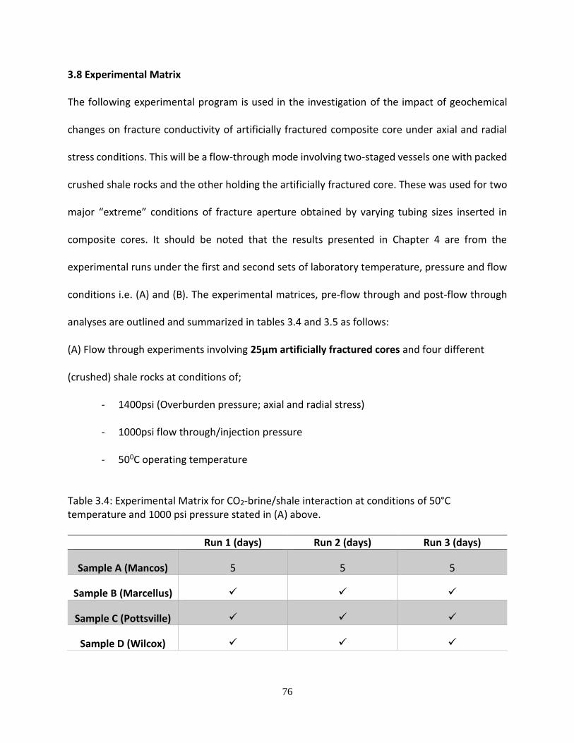
76

3.8 Experimental Matrix

The following experimental program is used in the investigation of the impact of geochemical

changes on fracture conductivity of artificially fractured composite core under axial and radial

stress conditions. This will be a flow-through mode involving two-staged vessels one with packed

crushed shale rocks and the other holding the artificially fractured core. These was used for two

major “extreme” conditions of fracture aperture obtained by varying tubing sizes inserted in

composite cores. It should be noted that the results presented in Chapter 4 are from the

experimental runs under the first and second sets of laboratory temperature, pressure and flow

conditions i.e. (A) and (B). The experimental matrices, pre-flow through and post-flow through

analyses are outlined and summarized in tables 3.4 and 3.5 as follows:

(A) Flow through experiments involving 25µm artificially fractured cores and four different

(crushed) shale rocks at conditions of;

- 1400psi (Overburden pressure; axial and radial stress)

- 1000psi flow through/injection pressure

- 500C operating temperature

Table 3.4: Experimental Matrix for CO2-brine/shale interaction at conditions of 50°C temperature and 1000 psi pressure stated in (A) above.

Run 1 (days) Run 2 (days) Run 3 (days)

Sample A (Mancos) 5 5 5

Sample B (Marcellus)


Sample D (Wilcox)

77

(B) Flow through experiments involving 150µm artificially fractured cores and four different

(crushed) shale rocks at conditions of;

- 1400psi (Overburden pressure; axial and radial stress)

- 1000psi flow through/injection pressure

- 500C operating temperature

Table 3.5: Experimental Matrix for CO2-brine/shale interaction at conditions of 50°C temperature and 1000 psi pressure stated in (B) above.

Samples Run 1 (days) Run 2 (days) Run 3 (days)

Sample A (Mancos) 5 5 5

Sample B(Marcellus)


Sample D (Wilcox)

3.8.1 Geochemical Analysis

i. Pre- and Post-flow through experiment (crushed rocks)

a. X-Ray Diffraction (XRD) Analysis

b. Total Organic Carbon Content (TOC) Analysis

c. Scanning Electron Microscopy/Energy Dispersive Spectroscopy (SEM/EDS)

d. Electron Micro-Probe (EMPA) Analysis

e. Micro-indentation

ii. Pre-flow through experiment (fluid)

a. pH

b. Inductively Coupled Plasma-Optical Emission Spectroscopy (ICP-OES)

78

3.8.2 Measurement of Hardness and Conductivity; Artificially fractured composite cores

This is done at 1000psi and 50⁰C operating conditions as outlined in table 3.6. The units of

measurements are conductivity (mdft; from differential pressure drop permeability) vs time

(days). Individual plots in mdft versus days for each rock formation sample was analyzed and a

combined plot generated to compare responses of the two micro-tubing sizes. Dimensionless

fracture conductivity was used for estimating the impact of geochemistry on flow characteristics.

Dimensionless fracture conductivity (Cr) is defined as fracture conductivity, kfw (md-ft), divided

by reservoir permeability (k) multiplied by the fracture half-length, xf (ft). It provides a means of

optimizing the amount of conductivity in a fracture for varying permeability and fracture length.

In the case of tight rocks, matrix permeability is assumed to be zero.

Each run of the flow through experiment as stated below will undergo rock and fluid analyses

pre-injection and post-injection of CO2-brine. The steps involved are presented in table 3.7.

Table 3.6: Micro/Nano-indentation; Hardness and Young Modulus at different temperature and pressure conditions of the rock-fluid interactions experiment.

No. of samples at 1000psi and 50⁰C (25µm cores)

No. of samples at 1000psi and 50⁰C (150µm cores)

Run 1

Run 2

Run 3

Total Run 1 Run 2 Run 3 Total

Pottsville 1 1 1 3 1 1 1 3

Marcellus 1 1 1 3 1 1 1 3

Mancos 1 1 1 3 1 1 1 3

Wilcox 1 1 1 3 1 1 1 3

79

Table 3.7: Pre-injection and Post-injection analyses for each CO2-brine flooding experimental run including rock and fluid sampling procedure.

Run No. Type of Analysis

Step 1 Flood crushed shale rock with CO2-brine and transport effluent to composite

core under varying axial and radial stress.

Step 2 Take real time measurement of differential pressure drop for changes in

conductivity. This will be automatically acquired during injection and transport

of CO2-brine.

Step 3 Analyze final effluent composition (pH, ICP-OES). Analyze crushed shale rock for

morphology, mineral composition, total organic carbon composition and

hardness characteristics (SEM, EDS, XRD, TOC, Micro-indentation).

Step 4 Calculate effective fracture aperture and fracture conductivity.

Step 5 Use geochemical results to bound overall chemo-flow modelling in aqueous

CO2-shale interaction under constant geomechanical conditions

3.8.3 Critical Experimental Conditions and Materials

-Artificial Cores Solids Fraction: made from cement (≈97%), kaolinite (≈3%) and PEEK polymer

micro-tubing (resistant to chemical corrosion)

-Crushed Shale Rocks: sizes <2mm (lots of fines)

-CO2-Brine Composition: 22.6g/l (22600 ppm) of NaCl solution

-Pressure Vessels and Flowlines: high temperature and pressure rated (max. of 350°F, 4000psi)

80

3.8.4 Experimental Process Parameters for Conditions A and B as Reported in Chapter 4

The following experimental conditions were used during the shale/CO2-brine flooding

a. Global flow rate: 0.5ml/min

b. Flow cell(s) back pressure: 1000psi

c. Flow cell(s) axial and radial pressure:1400psi

d. Operating temperature: 50°C

e. pH of CO2 – brine: 3.7 – 3.8

The raw data of most of the experimental results presented in Chapter 4 are included in the

Appendix section of this report.

81

CHAPTER 4

RESULTS FROM SHALE ROCK/FLUID INTERACTIONS EXPERIMENTS

4.1 pH Measurement

Measurements of the pH of the effluent for all the 24 experiments were taken and the averages

reported in figure 4.1. The pH values for each sample type were used for the computation of the

standard error (standard deviation). It can be observed from the pH profile that the alkaline

buffer strength of the shale rocks through reactive interaction with the CO2-brine fluid at the

experimental pressure and temperature conditions is significantly pronounced for the Mancos,

Marcellus and Pottsville shale rocks while that of the Wilcox shale is markedly lower.

Figure 4.1: pH measurement of effluent for the four different shale rock samples used for the

rock-fluid interaction experiment. It shows consistent increase in the pH values indicating

significant alkalinity buffer strength of the shale rocks in the presence of acid CO2 -brine fluid that

was injected. This buffer strength is expected to reduce over time under dynamic condition.

3

4

5

6

7

8

9

0 1 2 3 4 5

pH

of

Effl

uen

t Fl

uid

Time (days)

Sample A

Sample B

Sample C

Sample D

Initial

82

The profile showed a trend pointing towards a waning of the buffer strength by the 5th day. The

error bars are standard deviation values based on 3 measurements of pH values. These

observations are in agreement with previous experiments conducted in the laboratory and

reported by other researchers. This changes in pH is expected to control, to some degree, the

ability of the various rock minerals to exchange ions with one another.

4.2 Inductively Coupled Plasma-Optical Emission Spectroscopy (ICP-OES) Analysis

The inductively coupled plasma optical emission spectroscopy analysis of the effluent from

moderate temperature- moderate pressure runs using the four shale rock samples are shown in

figures 4.2 to 4.15. The dimensionless concentration of both the major and trace elements in the

effluent solution at the end of the experiments were analyzed using the initial composition of the

influent CO2 saturated brine as the normalizing quantity. The elemental concentration of the

influent is 1 on each of the graph. Sections 4.2.1 and 4.2.2 discusses the major and trace elements

present in the fluid in details and relating them to the mineralogical composition of the bulk rock

samples. Geochemical reactions of interest are also further discussed in Chapter 5.

4.2.1 Major Elemental Concentration in Effluent

Elemental Calcium concentration in the effluent collected at the outlet of the artificially fractured

cores are presented in figure 4.2. The ratios of Can/Cao are presented as data points on the chart.

Can represent the concentration of Calcium in part per million (ppm) for each day (n= time in

days). Cao is the original elemental concentration in the influent CO2 saturated brine. This

dimensionless entity represents the fractional increase or decrease in the elemental composition

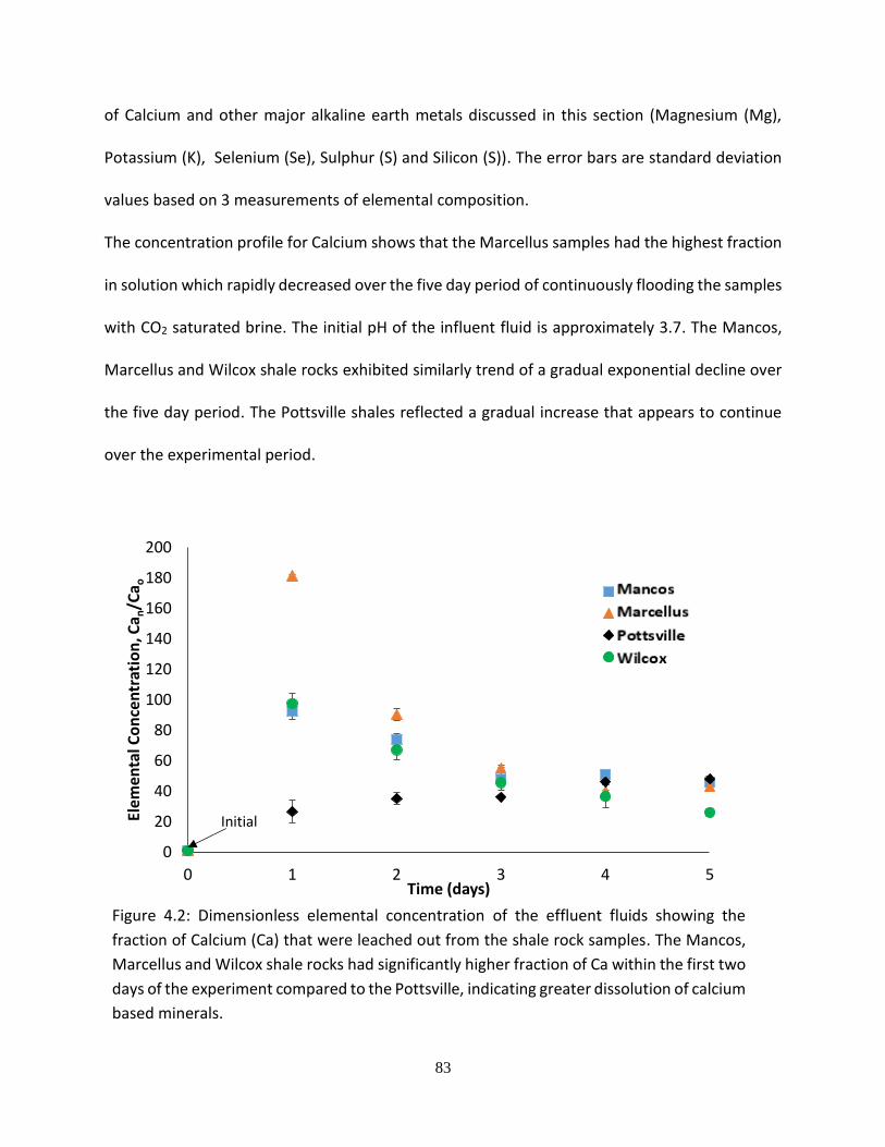
83

of Calcium and other major alkaline earth metals discussed in this section (Magnesium (Mg),

Potassium (K), Selenium (Se), Sulphur (S) and Silicon (S)). The error bars are standard deviation

values based on 3 measurements of elemental composition.

The concentration profile for Calcium shows that the Marcellus samples had the highest fraction

in solution which rapidly decreased over the five day period of continuously flooding the samples

with CO2 saturated brine. The initial pH of the influent fluid is approximately 3.7. The Mancos,

Marcellus and Wilcox shale rocks exhibited similarly trend of a gradual exponential decline over

the five day period. The Pottsville shales reflected a gradual increase that appears to continue

over the experimental period.

Figure 4.2: Dimensionless elemental concentration of the effluent fluids showing the

fraction of Calcium (Ca) that were leached out from the shale rock samples. The Mancos,

Marcellus and Wilcox shale rocks had significantly higher fraction of Ca within the first two

days of the experiment compared to the Pottsville, indicating greater dissolution of calcium

based minerals.

0

20

40

60

80

100

120

140

160

180

200

0 1 2 3 4 5

Elem

enta

l Co

nce

ntr

atio

n, C

a n/C

a o

Time (days)

Sample A

Sample B

Sample C

Sample D

Initial

84

While the elemental concentration of Calcium in the Mancos, Marcellus and Wilcox shales peaks

on the first day of the experiment, that of the Pottsville shale continued to increase over the five

day period but it also expected to peak and gradually decline with similar trend to the Mancos,

Marcellus and Wilcox shales. This resilient behavior of the Pottsville shale might suggest a slower

dissolution reaction of it calcium based minerals constituent compared to the Mancos, Marcellus

and Wilcox shales. The bulk rock XRD analysis indicated calcite and dolomite as the main calcium

bearing minerals in the Mancos, Marcellus and Wilcox shales while anhydrites are the main

calcium bearing minerals in the Pottsville.

Figure 4.3 presents the five day elemental concentration trend in the effluent for Magnesium.

The profile for the four samples are similar to that of calcium. It can be observed that the

fractional composition of magnesium in the effluent are about half of elemental calcium

presented in figure 4.2. The Mancos, Pottsville and Wilcox shale rocks appear to be plateauing

out after the five-day experimental period, while the Marcellus shale samples is rapidly

approaching zero concentration during the same period. The similarity of concentration profile

suggests that plausible geochemical dissolution reactions are occurring along with magnesium

based minerals in the shale rocks. This type of reactions are mostly associated with calcite,

dolomite and illitic (illite containing) clay minerals.

Elemental Potassium in solution (figure 4.4) exhibited a trend that showed a reduction in the free

potassium available in the influent fluid for the Marcellus and Wilcox shale rocks before

stabilizing after the five-day experimental period. This indicated a consumption of the potassium

element in the injected fluid via reactive rock-fluid interaction for the two samples. The Mancos

and Pottsville shale samples exhibited the general trend of initial increases in elemental

85

(potassium) concentration, in the effluent fluid, followed by a decreasing profile as the

experiment progresses. This is most-likely due to limited rock volume.

Concentrations of Selenium (figure 4.5) are most significant for the Mancos and Pottsville shale

rocks while the Marcellus and Wilcox shales had little to no selenium ions leached into the

effluent fluid. The presence of selenium in the effluent solution showed the extent of shale rock

samples’ heterogeneity as no known selenium bearing mineral was identified in the rocks by XRD

analysis. This suggests that these selenium bearing minerals only exist in trace amounts within

these sedimentary rocks matrix. The presence of free selenium in solution could act as catalysts

for faster reactive flow. Furthermore, Sulphur content (figure 4.6) was highest in the Wilcox shale

followed by the Mancos and Marcellus shale. This confirms that CO2 saturated-brine can

effectively dissolve stable minerals like pyrites and other sulphur bearing minerals. The Marcellus

and Wilcox shale samples had the highest content of pyrite mineral as identified by XRD analysis.

It appears that there is a preferential dissolution of pyrite in the Wilcox shale compared to the

Marcellus, even though it has a higher content of pyrite. It can be assumed that relative

abundance of these soluble minerals in the rock matrix would have influence on geochemical

speciation in the effluent. The convective transport of these geochemical species are important

in balancing the equilibrium conditions of the subsurface. The introduction of fluids such as

dissolved CO2 in brine can significantly alter the equilibrium landscape that can affect the natural

in-take or release of chemical species. The trend noticeable in these results suggest that massive

dissolution of calcites and dolomites might pose significant challenges in cases where there are

significant ingress of carbon dioxide in aqueous form into the shale caprock. This can lead to

increased percentage of flow paths within the rock.

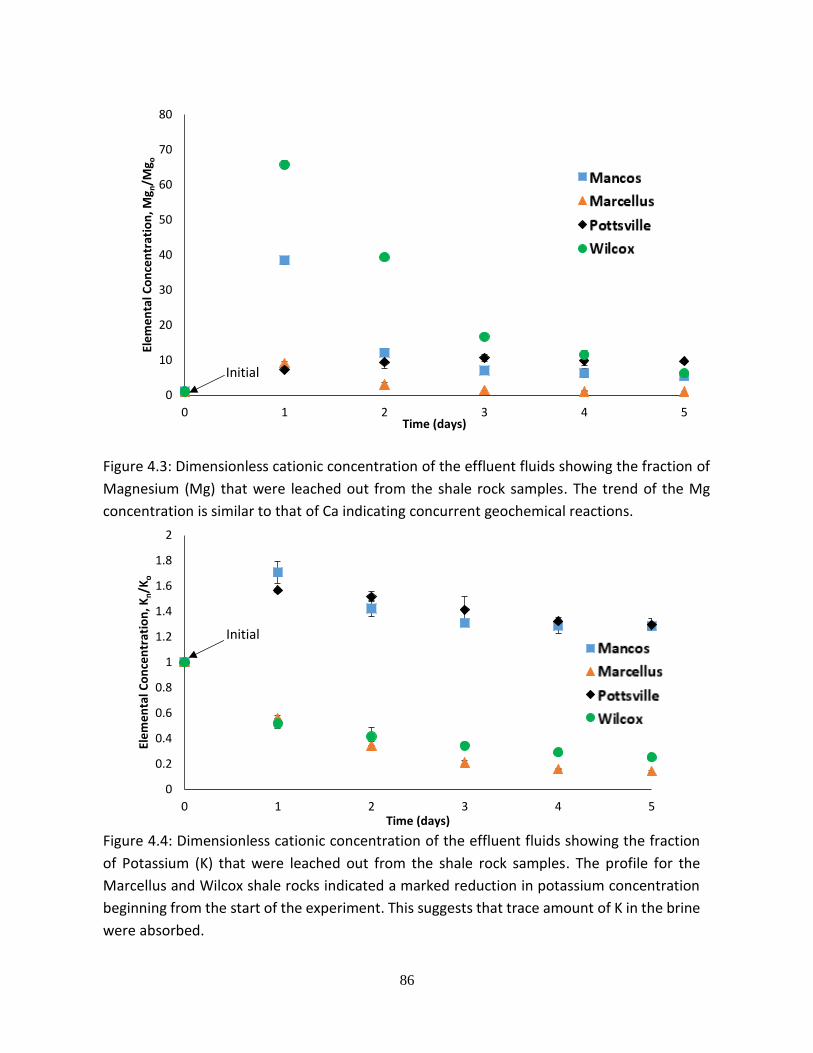
86

Figure 4.3: Dimensionless cationic concentration of the effluent fluids showing the fraction of

Magnesium (Mg) that were leached out from the shale rock samples. The trend of the Mg

concentration is similar to that of Ca indicating concurrent geochemical reactions.

Figure 4.4: Dimensionless cationic concentration of the effluent fluids showing the fraction

of Potassium (K) that were leached out from the shale rock samples. The profile for the

Marcellus and Wilcox shale rocks indicated a marked reduction in potassium concentration

beginning from the start of the experiment. This suggests that trace amount of K in the brine

were absorbed.

0

10

20

30

40

50

60

70

80

0 1 2 3 4 5

Ele

me

nta

l Co

nce

ntr

atio

n, M

g n/M

g o

Time (days)

Sample A

Sample B

Sample C

Sample D

Initial

0

0.2

0.4

0.6

0.8

1

1.2

1.4

1.6

1.8

2

0 1 2 3 4 5

Ele

me

nta

l Co

nce

ntr

atio

n, K

n/K

o

Time (days)

Sample A

Sample B

Sample C

Sample D

Initial

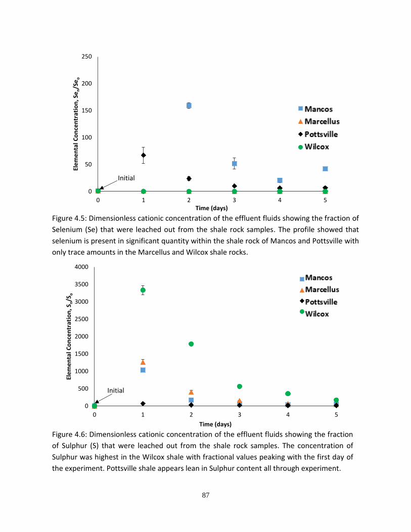
87


Selenium (Se) that were leached out from the shale rock samples. The profile showed that

selenium is present in significant quantity within the shale rock of Mancos and Pottsville with

only trace amounts in the Marcellus and Wilcox shale rocks.

Figure 4.6: Dimensionless cationic concentration of the effluent fluids showing the fraction

of Sulphur (S) that were leached out from the shale rock samples. The concentration of

Sulphur was highest in the Wilcox shale with fractional values peaking with the first day of

the experiment. Pottsville shale appears lean in Sulphur content all through experiment.

0

50

100

150

200

250

0 1 2 3 4 5

Ele

me

nta

l Co

nce

ntr

atio

n, S

en/S

eo

Time (days)

Sample A

Sample B

Sample C

Sample D

Initial

0

500

1000

1500

2000

2500

3000

3500

4000

0 1 2 3 4 5

Ele

me

nta

l Co

nce

ntr

atio

n, S

n/S

o

Time (days)

Sample A

Sample B

Sample C

Sample D

Initial

88


Silicon (Si) that were leached out from the shale rock samples. The fractional profile of silicon

indicated dissolution of silicon bearing minerals. It is possible that of early precipitation in form

of diagenetic quartz occurred as the concentration of Si remained fairly constant.

Elemental silicon concentration in the effluent analyzed showed that they are present in solution

in significant quantity compared to the initial CO2-brine fluid that was injected. Figure 4.7

documents these Si concentrations for all the shale samples. The presence of diagenetic quartz

in the precipitates recovered, indicated that most of the silicon in solution had crystalized out of

the solution to form a variant of opal mineral that is amorphous in shape.

4.2.2 Minor Elemental Concentration in Effluent

Trace concentration of certain elements in the effluent solution is discussed. These include

Aluminum (Al), Arsenic (As), Boron (B), Iron (Fe), Manganese (Mn), Nickel (Ni), Phosphorus (P)

and Zinc (Zn). They are described as occurring in trace amounts because the actual part per

million (ppm) concentrations are in the range 0.1 mg/l to 10mg/l which are significantly lower

0

5

10

15

20

25

30

35

40

0 1 2 3 4 5

Ele

me

mta

l Co

nce

ntr

atio

n, S

i n/S

i o

Time (days)

Sample A

Sample B

Sample C

Sample D

Initial

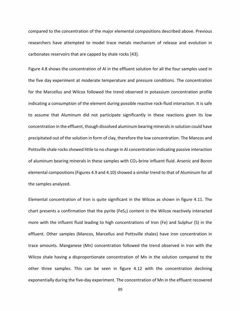
89

compared to the concentration of the major elemental compositions described above. Previous

researchers have attempted to model trace metals mechanism of release and evolution in

carbonates reservoirs that are capped by shale rocks [43].

Figure 4.8 shows the concentration of Al in the effluent solution for all the four samples used in

the five day experiment at moderate temperature and pressure conditions. The concentration

for the Marcellus and Wilcox followed the trend observed in potassium concentration profile

indicating a consumption of the element during possible reactive rock-fluid interaction. It is safe

to assume that Aluminum did not participate significantly in these reactions given its low

concentration in the effluent, though dissolved aluminum bearing minerals in solution could have

precipitated out of the solution in form of clay, therefore the low concentration. The Mancos and

Pottsville shale rocks showed little to no change in Al concentration indicating passive interaction

of aluminum bearing minerals in these samples with CO2-brine influent fluid. Arsenic and Boron

elemental compositions (Figures 4.9 and 4.10) showed a similar trend to that of Aluminum for all

the samples analyzed.

Elemental concentration of Iron is quite significant in the Wilcox as shown in figure 4.11. The

chart presents a confirmation that the pyrite (FeS2) content in the Wilcox reactively interacted

more with the influent fluid leading to high concentrations of Iron (Fe) and Sulphur (S) in the

effluent. Other samples (Mancos, Marcellus and Pottsville shales) have iron concentration in

trace amounts. Manganese (Mn) concentration followed the trend observed in Iron with the

Wilcox shale having a disproportionate concentration of Mn in the solution compared to the

other three samples. This can be seen in figure 4.12 with the concentration declining

exponentially during the five-day experiment. The concentration of Mn in the effluent recovered

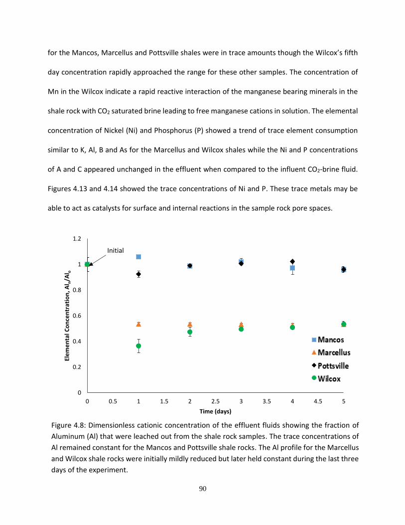
90

for the Mancos, Marcellus and Pottsville shales were in trace amounts though the Wilcox’s fifth

day concentration rapidly approached the range for these other samples. The concentration of

Mn in the Wilcox indicate a rapid reactive interaction of the manganese bearing minerals in the

shale rock with CO2 saturated brine leading to free manganese cations in solution. The elemental

concentration of Nickel (Ni) and Phosphorus (P) showed a trend of trace element consumption

similar to K, Al, B and As for the Marcellus and Wilcox shales while the Ni and P concentrations

of A and C appeared unchanged in the effluent when compared to the influent CO2-brine fluid.

Figures 4.13 and 4.14 showed the trace concentrations of Ni and P. These trace metals may be

able to act as catalysts for surface and internal reactions in the sample rock pore spaces.


Aluminum (Al) that were leached out from the shale rock samples. The trace concentrations of

Al remained constant for the Mancos and Pottsville shale rocks. The Al profile for the Marcellus

and Wilcox shale rocks were initially mildly reduced but later held constant during the last three

days of the experiment.

0

0.2

0.4

0.6

0.8

1

1.2

0 0.5 1 1.5 2 2.5 3 3.5 4 4.5 5

Ele

me

nta

l Co

nce

ntr

atio

n, A

l n/A

l o

Time (days)

Sample A

Sample B

Sample C

Sample D

Initial

91


Arsenic (As) that were leached out from the shale rock samples. The trace concentrations of

As in the effluent fluid from the Mancos and Pottsville shale rocks significantly diverged from

the Marcellus and Wilcox over the 5 day experiment plateauing out for all samples at end of

the experiment.


Boron (B) that were leached out from the shale rock samples. The minor concentrations of

Boron showed a common decreasing pattern for all the samples, stabilizing towards the end

of the experiment at values that are lower than the initial.

0

0.2

0.4

0.6

0.8

1

1.2

1.4

1.6

1.8

2

0 1 2 3 4 5

Ele

me

nta

l Co

nce

ntr

atio

n, A

s n/A

s o

Time (days)

Sample A

Sample B

Sample C

Sample D

Initial

0

0.2

0.4

0.6

0.8

1

1.2

1.4

1.6

0 1 2 3 4 5

Ele

me

nta

l Co

nce

ntr

atio

n, B

n/B

o

Time (days)

Sample A

Sample B

Sample C

Sample D

Initial

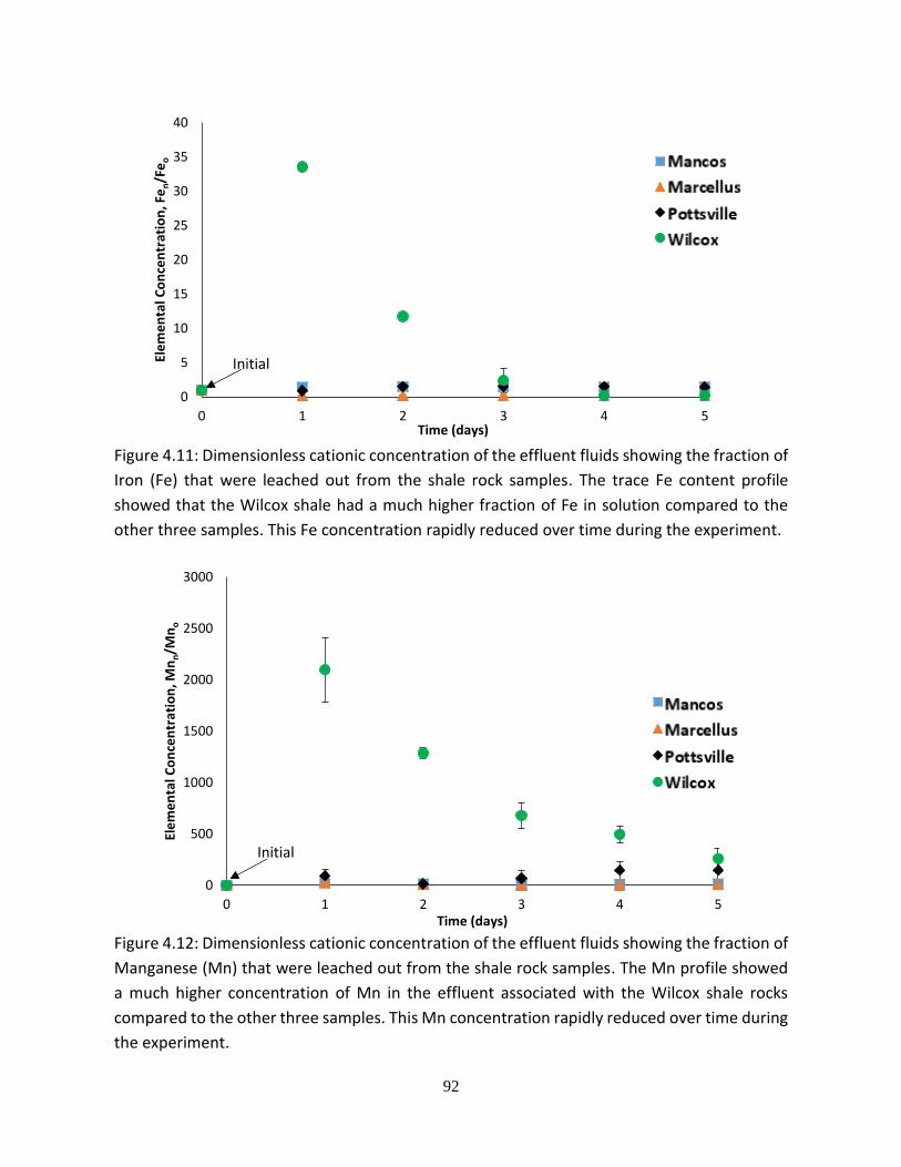
92


Iron (Fe) that were leached out from the shale rock samples. The trace Fe content profile

showed that the Wilcox shale had a much higher fraction of Fe in solution compared to the

other three samples. This Fe concentration rapidly reduced over time during the experiment.


Manganese (Mn) that were leached out from the shale rock samples. The Mn profile showed

a much higher concentration of Mn in the effluent associated with the Wilcox shale rocks

compared to the other three samples. This Mn concentration rapidly reduced over time during

the experiment.

0

5

10

15

20

25

30

35

40

0 1 2 3 4 5

Ele

me

nta

l Co

nce

ntr

atio

n, F

en/F

eo

Time (days)

Sample A

Sample B

Sample C

Sample D

Initial

0

500

1000

1500

2000

2500

3000

0 1 2 3 4 5

Ele

me

nta

l Co

nce

ntr

atio

n, M

nn/M

no

Time (days)

Sample A

Sample B

Sample C

Sample D

Initial

93


Nickel (Ni) that were leached out from the shale rock samples. The trace profile for Ni indicated

that the Marcellus and the Wilco shales had a mild decrease in the associated effluent

compared to the initial CO2-brine fluid. Nickel concentration remained constant for the Mancos

and Pottsville shale rocks.


Phosphorus (P) that were leached out from the shale rock samples. The trace profile for P

indicated that the Marcellus and Wilcox shale rocks had a mild decrease in the associated

effluent compared to the initial CO2-brine fluid. Phosphorus concentration remained fairly

constant for the Mancos and Pottsville shale rocks.

0

0.2

0.4

0.6

0.8

1

1.2

0 1 2 3 4 5 6

Ele

me

nta

l Co

nce

ntr

atio

n, N

i n/N

i o

Time (days)

Sample A

Sample B

Sample C

Sample D

Initial

0

0.2

0.4

0.6

0.8

1

1.2

1.4

0 1 2 3 4 5

Ele

me

nta

l Co

nce

ntr

atio

n, P

n/P

o

Time (days)

Sample A

Sample B

Sample C

Sample D

Initial

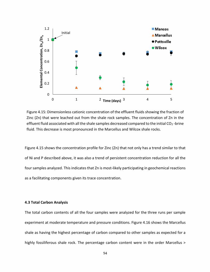
94


Zinc (Zn) that were leached out from the shale rock samples. The concentration of Zn in the

effluent fluid associated with all the shale samples decreased compared to the initial CO2 -brine

fluid. This decrease is most pronounced in the Marcellus and Wilcox shale rocks.

Figure 4.15 shows the concentration profile for Zinc (Zn) that not only has a trend similar to that

of Ni and P described above, it was also a trend of persistent concentration reduction for all the

four samples analyzed. This indicates that Zn is most-likely participating in geochemical reactions

as a facilitating components given its trace concentration.

4.3 Total Carbon Analysis

The total carbon contents of all the four samples were analyzed for the three runs per sample

experiment at moderate temperature and pressure conditions. Figure 4.16 shows the Marcellus

shale as having the highest percentage of carbon compared to other samples as expected for a

highly fossiliferous shale rock. The percentage carbon content were in the order Marcellus >

0

0.2

0.4

0.6

0.8

1

1.2

0 1 2 3 4 5

Elem

enta

l Co

nce

ntr

atio

n, Z

nn/Z

no

Time (days)

Sample A

Sample B

Sample C

Sample D

Initial

95

Wilcox > Mancos > Pottsville. This order of magnitude still holds after the CO2-brine flooding

experiment. It can be observed for the figure that were significant increases in the percentage

content of carbon in all the samples which can be indicative of both adhered carbon and

mineralized carbon in the these shale samples. This might be good for carbon sequestration.

Figure 4.16: Total Carbon measurement of bulk rock for the four different samples analyzed. It

shows major increase in carbon content for the Marcellus shale compared to the other three

samples. This increases can be associated with surface CO2 adsorption or carbon mineralization.

It suggests that shale caprock can act like repositories for CO2 when sufficient surface area are

available for rock fluid interaction. The surface area of the shale caprock exposed in these

experiments are equivalent of several thousand meter square. Subsurface CO2 plume movement

will be contact seal rocks in this manner and scope. Distinguishing between adhered carbon and

mineralized carbon content might shed more light on which process- adsorption or

mineralization- will be most significant for CO2 sequestration in shaly rocks over the long term.

0

0.5

1

1.5

2

2.5

3

3.5

4

0 5

Tota

l Car

bo

n (

TC),

%

Time (days)

Sample A

Sample B

Sample C

Sample D

96

The error bars are standard deviation (SD) values for the three runs per sample experiments. The

total carbon analysis is more qualitative than quantitative for conclusive interpretations.

4.4 X-Ray Diffraction (XRD) Analysis

X-ray diffraction (XRD) analysis were carried on the bulk rock and the precipitates that were

recovered from the effluent fluid. Both bulk and clay XRD analysis were performed in order to

decipher the minerals that are most active in rock-fluid interaction and their implication on

precipitates generation which can be transported in solution. These precipitates are of interest

as hydraulic paths (micro-fractures, worm holes etc.) may be possibly plugged if the right quantity

are generated from the bulk rock as dissolved substances. These dissolved minerals can then

precipitate given the right pH, pressure, temperature, compositional and other conditions. The

following sections (4.4.1 and 4.4.2) discuss the XRD analyses in details.

4.4.1 Bulk XRD Analysis

After the five days of flooding the shale rock samples continuously with CO2 saturated brine at

moderate temperature and pressure conditions, XRD analyses were carried out on the bulk

experimental shale rock samples and the precipitates that were recovered from the effluent fluid

with the aim of qualifying and quantifying geochemical changes that could have taken place as a

result of reactive rock-fluid interaction. These geochemical changes are expected to affect the

mineralogical composition and structure of the shale rocks. The results were compared to the

initial shale rock samples that were not flooded with CO2-brine. Figures 4.17 to 4.20 show the

profiles of the main mineralogical components in the shale rocks (pre- and post-flooding with

CO2-brine) and the recovered precipitates as identified by bulk XRD analysis for the Mancos,

Marcellus, Pottsville and Wilcox shale rocks respectively. The bulk shale rocks show little to no

97

change in mineralogical content pre- and post-flooding with CO2-brine within the limit of XRD

resolution. This was the observed trend in all the four samples. It can however be observed that

the mineralogy identification peaks were better resolved in the post-flooding samples. It suggests

that the amorphous content of the shale rocks have been largely removed by the acidic fluid. In

the data reported by expert researchers in the field of carbon sequestration, defects or inherent

errors in measuring equipment can affect the accuracy of XRD readings.

Amorphous content of rocks are usually responsible for suppressed peaks in XRD qualitative

analysis. The bulk XRD analysis of precipitates showed the appearance of diagenetic minerals that

were formed from the major mineralogical components of the shale rocks.

Figure 4.17: XRD Analysis of bulk rock (Mancos) before and after CO2-brine flooding at

moderate temperature and pressure conditions along with the mineralogical composition

of the associated precipitates recovered from the effluent. It showed higher amount of

diagenetic carbonates in the precipitates compared to the pre- and post-flooding samples.

0

5000

10000

15000

20000

25000

30000

35000

40000

0 10 20 30 40 50 60 70 80

Inte

nsi

ty (

Co

un

ts)

2-Theta (°)

Precipitates

Post-flooding

Pre-flooding

Calcite

Dolomite

Pyrite

Clay

Quartz

98

Precipitate recovered from the effluent of flooding the Mancos shale with CO2 saturated brine

showed quartz, plagioclase, calcite, dolomite and pyrite as main constituent. This is excluding the

clay fraction. Precipitates associated with the Marcellus shale included quartz aragonite and

calcite only with no clay detected using XRD analysis. Precipitates associated with the Pottsville

shale included quartz, albite and calcite while precipitates associated with the Wilcox shale

included quartz, plagioclase and pyrite, excluding clay fractions from both samples. It can be seen

from the bulk XRD output that mineral constituents of the original shale rocks are largely

responsibility for the diagenetic constituents of the associated precipitates which are dominated

by quartz, calcites and clays.

Figure 4.18: XRD Analysis of bulk rock (Marcellus) before and after CO2-brine flooding at

moderate temperature and pressure conditions along with the mineralogical composition of

the associated precipitates recovered from the effluent. It showed higher amount of diagenetic

carbonates in the precipitates compared to the pre- and post-flooding samples

0

2000

4000

6000

8000

10000

12000

14000

16000

18000

20000

0 10 20 30 40 50 60 70 80

Inte

nsi

ty (

Co

un

ts)

2-Theta (°)

Calcite

Dolomite

Pyrite

Clay

Quartz

Feldspar

99

Figure 4.19: XRD Analysis of bulk rock (Pottsville) before and after CO2-brine flooding at


the associated precipitates recovered from the effluent. It showed higher amount of

diagenetic quartz and clays in the precipitates versus the pre- and post-flooding samples.

Figure 4.20: XRD Analysis of bulk rock (Wilcox) before and after CO2-brine flooding at moderate

temperature and pressure conditions along with the mineralogical composition of the

associated precipitates recovered from the effluent. It showed higher amount of diagenetic

quartz and clays in the precipitates versus the pre- and post-flooding samples.

0

10000

20000

30000

40000

50000

60000

0 10 20 30 40 50 60 70 80

Inte

nsi

ty (

Co

un

ts)

2-Theta (°)

Precipitates

Post-flooding

Pre-floodingFeldspar

Clay

Quartz

0

10000

20000

30000

40000

50000

60000

0 10 20 30 40 50 60 70 80

Inte

nsi

ty (

Co

un

ts)

2-Theta (°)

Pyrite

Clay

Quartz

Feldspar

100

The quantitative assessment of the mineralogical changes in the both the bulk shale rock and the

precipitates are presented in section 4.4.3. The analysis of clay constituents in both the bulk rock

and precipitates are presented in section 4.4.2.

4.4.2 Clay XRD Analysis

Clay XRD analysis is performed by first removing all other non-clay mineralogical contents in the

shale rock. This is then followed by four stages of XRD analysis: a) Air dried analysis b) Glycolated

analysis c) 300 Celsius analysis d) 550 Celsius analysis. These staged analysis are specifically

important in quantitative clay content evaluation. The results of Ethylene glycolated samples are

discussed in this section as it is representative of all the other stages in clay mineral identification.

Figures 4.21 to 4.24 show the clay XRD analyses of the pre- and post-flooding samples as well as

the recovered precipitates for all the four samples used during the experiment. The results

showed sharper identification peaks for the clay minerals similar to the trend observed in bulk

XRD analysis in the precipitates. An indication of non-interference of amorphous substances in

mineral identification using XRD analysis.

The clay composition of the Mancos shale showed illite, chlorite and kaolinite as the main

component (figure 4.21). The precipitates has mainly chlorite and kaolinite with traces of illite.

Figure 4.22 indicated the presence of only lllitic clay and kaolinite in the bulk shale rock of the

Marcellus shale with no identifiable clay peak in the precipitates associated with it. Clay fraction

in Pottsville shale and the associated precipitates are presented in figure 4.23 showing the

multiple identification peaks of illites, chlorite and kaolinite in the shale bulk rock and the

associated precipitates recovered after the CO2 brine flooding experiment. The Wilcox shale rock

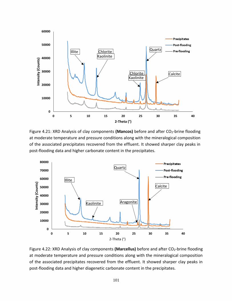
101

Figure 4.21: XRD Analysis of clay components (Mancos) before and after CO2-brine flooding

at moderate temperature and pressure conditions along with the mineralogical composition

of the associated precipitates recovered from the effluent. It showed sharper clay peaks in

post-flooding data and higher carbonate content in the precipitates.

Figure 4.22: XRD Analysis of clay components (Marcellus) before and after CO2-brine flooding


of the associated precipitates recovered from the effluent. It showed sharper clay peaks in

post-flooding data and higher diagenetic carbonate content in the precipitates.

0

10000

20000

30000

40000

50000

60000

0 5 10 15 20 25 30 35 40

Inte

nsi

ty (

Co

un

ts)

2-Theta (°)

Calcite

Illite

KaoliniteChlorite

Quartz

KaoliniteChlorite

0

10000

20000

30000

40000

50000

60000

70000

80000

0 5 10 15 20 25 30 35 40

Inte

nsi

ty (

Co

un

ts)

2-Theta (°)

Kaolinite

Calcite

Illite

Quartz

Aragonite

102

Figure 4.23: XRD Analysis of clay components (Pottsville) before and after CO2-brine flooding


of the associated precipitates recovered from the effluent. Significantly higher clay content is

present in precipitates compared to previous samples.

Figure 4.24: XRD Analysis of clay components (Wilcox) before and after CO2-brine flooding at


the associated precipitates recovered from the effluent. Significantly higher clay content is

present in precipitates compared to previous samples combined with pyrite.

0

20000

40000

60000

80000

100000

120000

0 5 10 15 20 25 30 35 40

Inte

nsi

ty (

Co

un

ts)

2-Theta (°)

Chlorite

Illite

ChloriteIllite

Quartz

Kaolinite

Kaolinite

0

10000

20000

30000

40000

50000

60000

70000

80000

90000

0 5 10 15 20 25 30 35 40

Inte

nsi

ty (

Co

un

ts)

2-Theta (°)

ChloriteKaolinite

Feldspar

Illite

QuartzChloriteKaolinite

Montmoriillonite

103

as shown in figure 4.24 indicated the presence of four distinct clay fractions which are

montmorillonite (a characteristic swelling clay), illite, chlorite and kaolinite. The dissolution and

re-precipitation of siliciclastic minerals such illitic clays and quartz show that acidified aqueous

media such as CO2-brine can effect disequilibrium conditions. the qualitative results from the

clay analysis of the shale bulk rock and the associated precipitates recovered from effluent fluid

after CO2-brine flooding indicated that the clay composition of the shale rocks are not

significantly diagenetically modified at the operating laboratory conditions of the moderately

high temperature and injection pressure (50 Celsius and 1000 psi).

4.4.3 Quantitative XRD Mineralogical Analysis

Quantitative evaluation of the changes in mineralogical content of the shale rocks are presented

in table 4.1. It can be seen that non-clay minerals that are compounds of alkaline earth metals

(Ca, Mg, Fe) such as calcite, dolomite, pyrite and feldspar are significantly altered, mostly a

reduction in percentage within the accuracy of quantitative XRD analysis.

Mancos shale had reductions in feldspar, dolomite, pyrite and total clay (particularly illite and

kaolinite). There was a slight increase in quartz, plagioclase, calcite, and chlorite in the Mancos

shale. The Marcellus shale had reductions in feldspar, plagioclase, calcite, dolomite, anhydrite

and kaolinite, while its quartz, chlorite and illite content increased. Furthermore, bulk shale rock

of Pottsville shale had reductions in anhydrite, chlorite and illite with associated increases in

quartz, feldspar, plagioclase and kaolinite. The Wilcox shale had mineralogical reductions in

feldspar, anhydrite, pyrite, chlorite and kaolinite with associated increases in quartz, plagioclase,

illites and swelling clay montmorillonite. It can be observed that significant reduction in total clay

component in most of the samples analyzed was accompanied with significant increases in quartz

104

fraction of the mineralogy. This was a strong indication of diagenetic alteration of shale rock

minerals due to aqueous CO2-shale rock interaction under laboratory temperature and pressure

conditions. The flow rate was set to a value that would replicate convective fluid transport in the

subsurface. This type of flow characteristics represent long term scenarios.

Table 4.1: Bulk rock compositional change (in percentages) for the shale rock samples. These

values were computed from the pre- and post-XRD quantitative analysis using the bulk and clay

XRD methods. There were slight changes in quartz, carbonates and clay contents.

Component


Quartz

1.25 0.61 11.19 5.57

K-Feldspar -0.07 -0.8 0.86 -0.12

Plagioclase 0.18 -0.15 3.3 1.13

Calcite

1.04 -8.29 0 0

Dolomite

-0.65 -0.57 0 0

Anhydrite 0 -0.41 -1.2 -1.02

Pyrite

-0.74 0.56 0 -1.79

Clay(total) -1.01 9.04 -14.15 -3.77

Chlorite 0.4 0.18 -4.64 -0.88

Illite -1.17 10.12 -9.83 1.82

Kaolinite -0.24 -1.26 0.32 -5.44

Montmorillonite 0 0 0 0.73

The mineralogical constituents of the precipitates that were recovered from the effluent during

the shale/CO2-brine flooding experiment are presented in table 4.2. The minerals were are

definitely derived from the bulk shale rocks showed diagenetic components that have elemental

105

compositions that indicated reactive dissolution-precipitation process occurred during the

experiment. Precipitates from CO2-brine flooding of the Mancos shale showed quartz, calcite and

fine clays in nearly equal proportion. Precipitates from the Marcellus shale showed aragonite and

calcite (both carbonates of calcium) as the sole component, indicating pronounced preferential

dissolution of carbonates in this organics rich shale rock. Precipitates associated with the

Pottsville and Wilcox shale rocks showed mainly clays and quartz with traces of calcite in that

were probably formed from the dissolution of minor amount anhydrite present in the rocks by

the CO2-brine. Further clay analyses confirmed this compositions.

Table 4.2: Percentage composition of the mineralogical components of precipitates that were

recovered from the effluent during the shale/CO2-brine flooding experiment. The analysis

indicated diagenetic quartz and carbonates as new minerals that were formed.

Minerals


Quartz

30.15 1.8 43.56 39.39

K-Feldspar

- - - -

Plagioclase

0.99 - - 2.36

Albite

- - 3.73 -

Aragonite

- 19.28 - -

Calcite

38.06 78.92 3.07 1.22

Dolomite

4.1 - - -

Anhydrite

- - - -

Pyrite

1.42 - - 2.37

Clays (total)

25.28 - 49.64 54.66

106

4.5 Electron Micro-Probe Analysis (EMPA) of Bulk Rock

The geochemical surface imaging of the shale rocks using Electron Microprobe Analyzer (EMPA)

technique revealed the nature of the changes to surface chemistry at micron scale and the

possible transport and re-crystallization of secondary mineralogical textures. Polished thin

sections of pre- and post- CO2 flooding samples of the shale rocks were studies in order to map

all the identifiable elemental component of the constituent minerals as applicable in sedimentary

petrology. Figures 4.25 to 4.36 present the unique elemental maps for each of the shale caprock

sample types.

Major element and select trace element compositions were determined by Electron Microprobe

Analysis (EMPA). EMPA is one of several particle-beam techniques. A beam of accelerated

electrons is focused on the surface of a specimen using a series of electromagnetic lenses, and

these energetic electrons produce characteristic X-rays within a small volume (typically 1 to 9

cubic microns) of the specimen. Two dimensional maps were obtained for multiple elements that

constitute the shale rocks, under operating conditions of accelerating voltage of 15 kV and beam

current of 200 nA. The electron microprobe was run in mapping mode allowing automated

analysis overnight. A total of four thin sections were mapped over a period of 4-5 hours each.

Maps depict relative abundances of elements of interest, allowing the determination of

compositional zones. The results showed the presence of Iron (Fe), Sodium (Na), Potassium (K),

Silicon (Si), Carbon (C), Oxygen (O), Chlorine (Cl), Manganese (Mn), Calcium (Ca), Magnesium

(Mg) and Aluminum (Al). They are present in rock minerals capable of exchanging ions with

carbonic acid or aqueous CO2. The elemental distribution of Ca and Mg in the reacted Mancos

and Marcellus shales were lower within grain facies as shown in figures 4.25 to 4.27 and figures

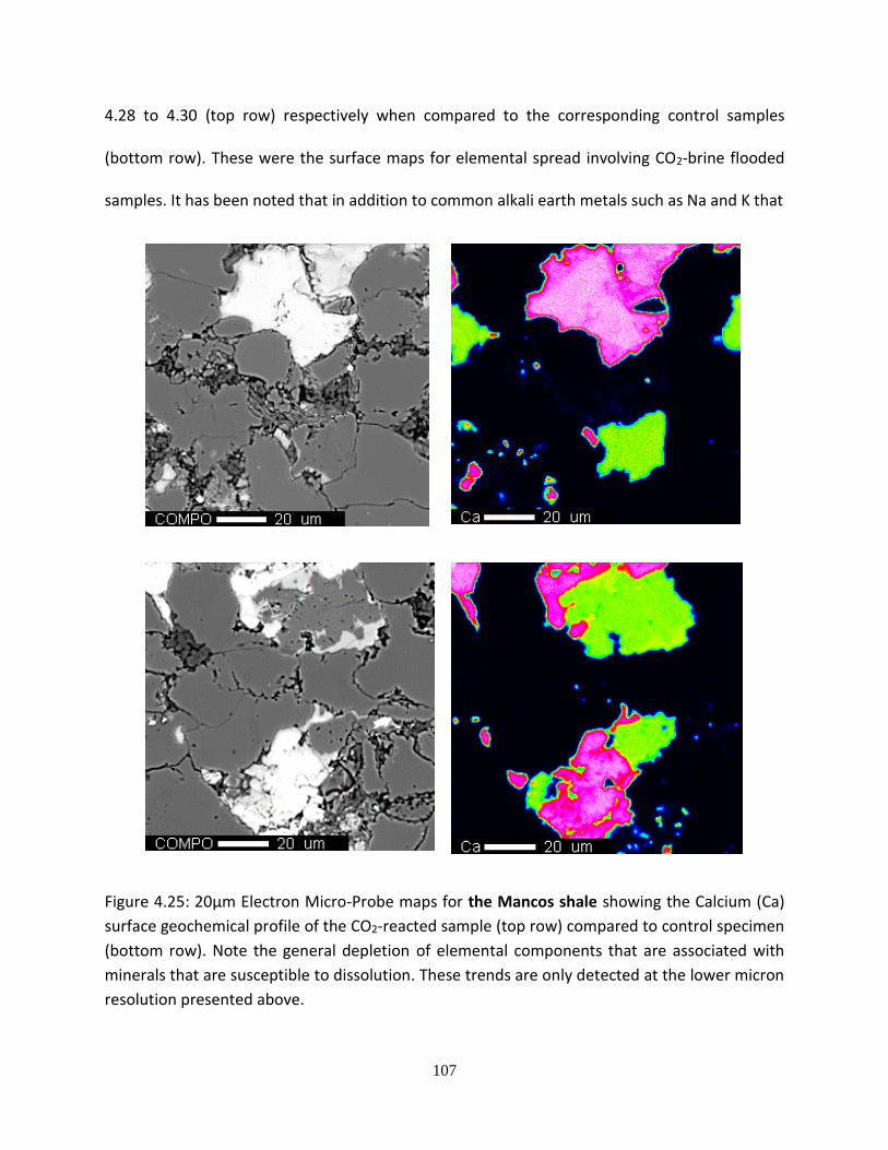
107

4.28 to 4.30 (top row) respectively when compared to the corresponding control samples

(bottom row). These were the surface maps for elemental spread involving CO2-brine flooded

samples. It has been noted that in addition to common alkali earth metals such as Na and K that

Figure 4.25: 20µm Electron Micro-Probe maps for the Mancos shale showing the Calcium (Ca)

surface geochemical profile of the CO2-reacted sample (top row) compared to control specimen

(bottom row). Note the general depletion of elemental components that are associated with

minerals that are susceptible to dissolution. These trends are only detected at the lower micron

resolution presented above.

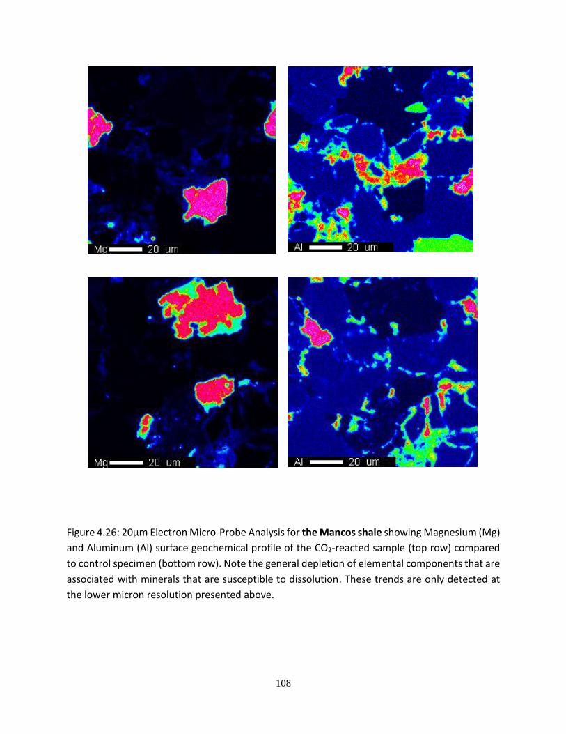
108

Figure 4.26: 20µm Electron Micro-Probe Analysis for the Mancos shale showing Magnesium (Mg)

and Aluminum (Al) surface geochemical profile of the CO2-reacted sample (top row) compared

to control specimen (bottom row). Note the general depletion of elemental components that are

associated with minerals that are susceptible to dissolution. These trends are only detected at

the lower micron resolution presented above.

109

Figure 4.27: 20µm Electron Micro-Probe Analysis for the Mancos shale showing Iron (Fe) and

silicon (Si) surface geochemical profile of the CO2-reacted sample (top row) compared to control

specimen (bottom row). Note the general depletion of elemental components that are



110

Figure 4.28: 20µm Electron Micro-Probe Analysis for the Marcellus shale showing the Calcium

(Ca) surface geochemical profile of the CO2-reacted sample (top row) compared to control




111

Figure 4.29: 20µm Electron Micro-Probe Analysis for the Marcellus shale showing Magnesium

(Mg) and Aluminum (Al) surface geochemical profile of the CO2-reacted sample (top row)

compared to control specimen (bottom row). Note the general depletion of elemental

components that are associated with minerals that are susceptible to dissolution. These trends

are only detected at the lower micron resolution presented above.

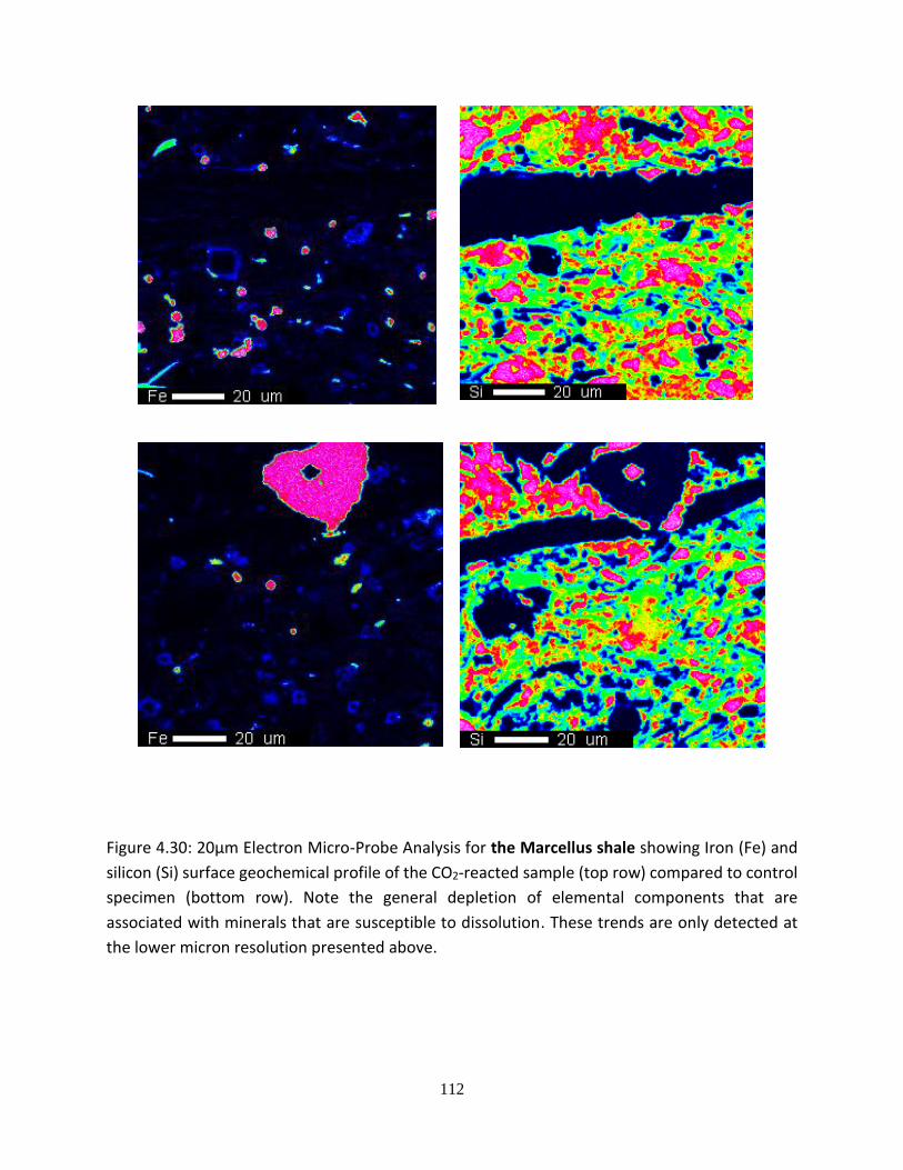
112

Figure 4.30: 20µm Electron Micro-Probe Analysis for the Marcellus shale showing Iron (Fe) and





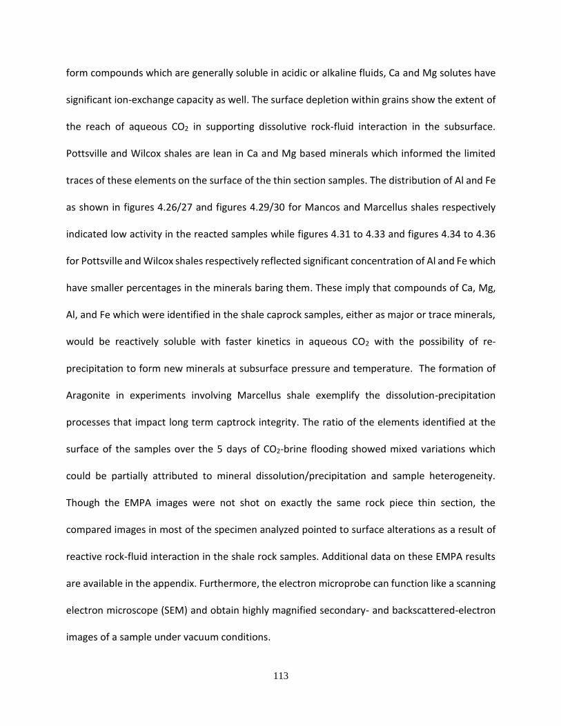
113

form compounds which are generally soluble in acidic or alkaline fluids, Ca and Mg solutes have

significant ion-exchange capacity as well. The surface depletion within grains show the extent of

the reach of aqueous CO2 in supporting dissolutive rock-fluid interaction in the subsurface.

Pottsville and Wilcox shales are lean in Ca and Mg based minerals which informed the limited

traces of these elements on the surface of the thin section samples. The distribution of Al and Fe

as shown in figures 4.26/27 and figures 4.29/30 for Mancos and Marcellus shales respectively

indicated low activity in the reacted samples while figures 4.31 to 4.33 and figures 4.34 to 4.36

for Pottsville and Wilcox shales respectively reflected significant concentration of Al and Fe which

have smaller percentages in the minerals baring them. These imply that compounds of Ca, Mg,

Al, and Fe which were identified in the shale caprock samples, either as major or trace minerals,

would be reactively soluble with faster kinetics in aqueous CO2 with the possibility of re-

precipitation to form new minerals at subsurface pressure and temperature. The formation of

Aragonite in experiments involving Marcellus shale exemplify the dissolution-precipitation

processes that impact long term captrock integrity. The ratio of the elements identified at the

surface of the samples over the 5 days of CO2-brine flooding showed mixed variations which

could be partially attributed to mineral dissolution/precipitation and sample heterogeneity.

Though the EMPA images were not shot on exactly the same rock piece thin section, the

compared images in most of the specimen analyzed pointed to surface alterations as a result of

reactive rock-fluid interaction in the shale rock samples. Additional data on these EMPA results

are available in the appendix. Furthermore, the electron microprobe can function like a scanning

electron microscope (SEM) and obtain highly magnified secondary- and backscattered-electron

images of a sample under vacuum conditions.

114

Figure 4.31: 20µm Electron Micro-Probe Analysis for the Pottsville shale showing the Calcium

(Ca) surface geochemical profile of the CO2-reacted sample (top row) compared to control




115

Figure 4.32: 20µm Electron Micro-Probe Analysis for the Pottsville shale showing Magnesium

(Mg) and Aluminum (Al) surface geochemical profile of the CO2-reacted sample (top row)

compared to control specimen (bottom row). Note the general depletion of elemental

components that are associated with minerals that are susceptible to dissolution. These trends

are only detected at the lower micron resolution presented above.

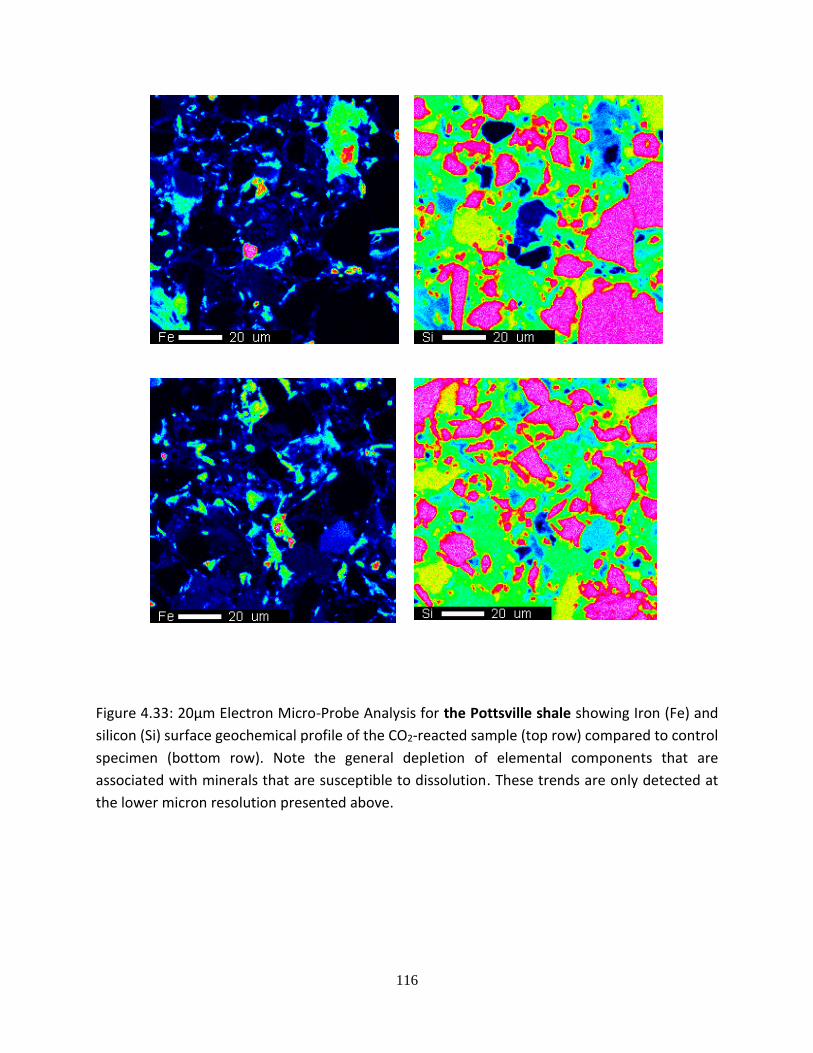
116

Figure 4.33: 20µm Electron Micro-Probe Analysis for the Pottsville shale showing Iron (Fe) and





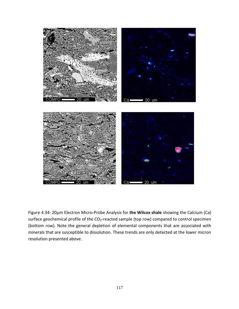
117

Figure 4.34: 20µm Electron Micro-Probe Analysis for the Wilcox shale showing the Calcium (Ca)

surface geochemical profile of the CO2-reacted sample (top row) compared to control specimen

(bottom row). Note the general depletion of elemental components that are associated with

minerals that are susceptible to dissolution. These trends are only detected at the lower micron

resolution presented above.

118

Figure 4.35: 20µm Electron Micro-Probe Analysis for the Wilcox shale showing Magnesium (Mg)

and Aluminum (Al) surface geochemical profile of the CO2-reacted sample (top row) compared

to control specimen (bottom row). Note the general depletion of elemental components that are



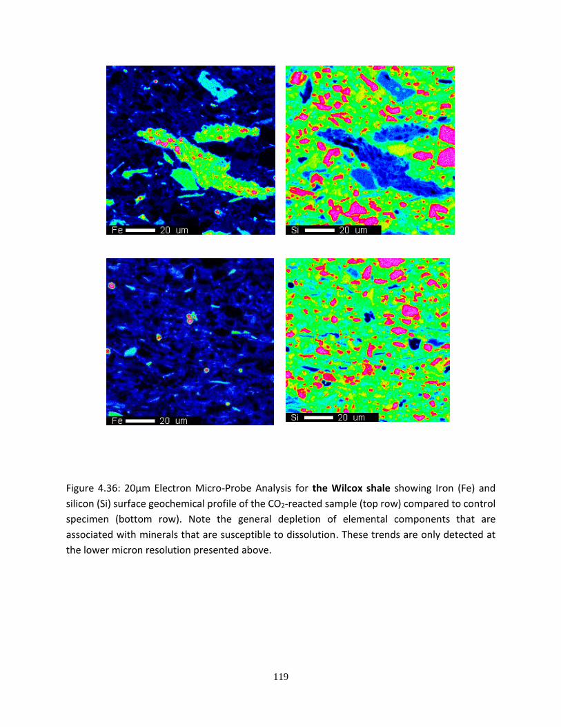
119

Figure 4.36: 20µm Electron Micro-Probe Analysis for the Wilcox shale showing Iron (Fe) and





120

4.6 Micro-Indentation of Rock Samples

Micro-indentation analyses were performed on polished samples of the shale rocks with the aim

of determining the extent of possible changes in hardness level of the rocks after the CO2-brine

flooding experiment. The following set of conditions were used in all the indentation

experiments: the maximum force used was 10 N; the loading and unloading rates were kept the

same at 10 N/min; the pause at maximum load was 30 seconds; the contact load was 30 mN. The

hardness was obtained with computational method from Oliver and Pharr [219]. The indenter

type was Vickers’ diamond with the Poisson coefficient of 0.07. There are scientific

documentation of using this method for nano-indentation of pure clay minerals [220].

Figure 4.37 shows the Vickers’ micro-hardness measurements acquired on the samples with the

error bar equivalent of standard deviation (SD) from three experimental runs per sample. There

was noticeable decrease in the hardness of the Mancos, Marcellus and Wilcox shale rocks in that

order with the Pottsville shale showing little to no change at the moderate temperature and

pressure conditions in which the experiments were performed.

This might indicate a weakening of the shale rocks under carbon sequestration conditions in the

case of pervasive CO2 intrusion into the overlaying caprock or most importantly at the seal rock-

reservoir rock interphase where the impact of the injected CO2 plume will be most significant.

The impact of higher temperature and pressure conditions is recommended to be investigated

in subsequent experimental research involving shale-aqueous CO2 interactions. Experimental set

up for the indentation is annotatively explained in the appendix A. Figures 4.38 shows the Young’s

Modulus equivalent of the Vickers’ hardness and figure 4.39 attempted to combine the two

parameters. YM and HV refers to Young’s Modulus and Vickers’ Hardness respectively. The

121

results show loss of geomechanical hardness particularly for the samples that are most

susceptible to dissolution i.e. The Mancos and Marcellus shale rocks. The significant difference

between the profiles of the Young Modulus and Vickers’ Hardness is explained in the

computation properties of the rock used. Vickers’ Hardness captured more variations in the

properties of the reacted samples when compared with the controls after the five days of the

experiment. These two properties have been shown in other data acquired on engineered

materials not to have any correlation. They were independently analyzed in this section for the

impact of geochemical changes at the surface. Heterogeneity in material composition is believed

to have significant effect on the trends that can be obtained for geomechanical properties.

Figure 4.37: the Vickers’ micro-hardness measurement taken on multiple samples of the

experimental shale rocks. The results indicated a mild reduction in geomechanical hardness of

the rock samples which are most significant in the Mancos, Marcellus and Wilcox shale rocks with

lower quartz contents. This implies that initial quartz composition of shaly caprocks might be

important in maintaining geomechanical integrity in long term CO2 sequestration.

0

10

20

30

40

50

60

70

0 5

Vic

ker

Har

dnes

s (H

V)

Time (days)

Mancos

Marcellus

Pottsville

Wilcox

122

Figure 4.38: Young’s Modulus (GPa) plots showing across the board decreases in measured

values for the shale caprocks after flooding with CO2-brine at 50oC and 1000psi.

Figure 4.39: Combined Hardness and Young’s Modulus plots showing across the board decreases

in measured values for the shale caprocks after flooding with CO2-brine at 50oC and 1000psi.

0

5

10

15

20

25

0 5

Young's

Modulu

s (G

Pa)

Time (days)

Mancos_YM

Marcellus_YM

Pottsville_YM

Wilcox_YM

0

5

10

15

20

25

0

10

20

30

40

50

60

70

0 5

Young's

Modulu

s (G

Pa)

Vic

ker

's H

ardnes

s (H

V)

Time (days)

Mancos_HV

Marcellus_HV

Pottsville_HV

Wilcox_HV

Mancos_YM

Marcellus_YM

Pottsville_YM

Wilcox_YM

123

Figure 4.40 shows a plot of magnitude change in Vickers’ hardness versus changes in the

mineralogical composition of the shale rocks with respect to quartz, clay and carbonates. It can

be suggested that formation of diagenetic quartz could improve the hardness of the shale rock

as observed in the Pottsville shale where the percentage change in quartz content exceeded 10%

which likely resulted from the clay fractions that were reduced by almost 15%. Significant

reduction in clay and carbonates fraction of the shale rock which did not necessarily transformed

to diagenetic quartz, as observed in the Mancos, Marcellus and Wilcox shale rocks, could shrink

the geomechanical hardness of the rock. Higher temperature and pressure experiment could be

used to confirm this observation.

Figure 4.40: A correlation between the hardness of the shale rock and quantifiable

mineralogical change in percentages. The graph shows that formation of diagenetic quartz can

improve the hardness of the shale rock as observed in Pottsville shale. Significant reduction in

clay and carbonates fraction of the shale rock, as observed in the Mancos, Marcellus and

Wilcox shale rocks, can shrink the geomechanical hardness of the rock.

-20

-15

-10

-5

0

5

10

15

Mancos Marcellus Pottsville Wilcox

Vic

ker

s' H

ardnes

s C

han

ge

(ΔH

V)

Shal

e M

iner

alogy C

han

ge

(Δ%

)

Hardness Quartz

Clay Carbonates

124

4.7 Differential Pressure Analysis

Differential pressure drop data acquired during the experimental runs were analyzed for flow

inferences and diagnostics. Each shale caprock type had associated experimental runs that

acquired multiple differential pressure data over a 5-day period. For example, three experimental

runs were performed on the Mancos shale using composite fractured cores (25µm and 150µm

micro-tubing embedded) with reaction effluent flowing through. This yielded thousands of

differential pressure data points at 20 secs interval that were averaged for diagnostic and flow

characteristic trends. These experimental runs were the same for other shale caprock types.

These flow experiments were repeated for composite fractured cores with 150µm micro-tubing

embedded for all the shale caprock types. The results of the averaged differential pressure data

(dP), the 1st derivative of the differential pressure (dP/dt) and the estimated fracture

conductivity are presented in figures 4.41 to 4.46. A comparison of the two fracture conductivity

profiles are presented in figure 4.47. The effective fracture width was first estimated which

formed a major input for the calculation of dimensionless fracture conductivity. The differential

pressure drop, dP, data acquired during the experiment are presented in figures 4.41 (for 25µm

micro-tubing embedded cores) and 4.42 (for 150µm micro-tubing embedded cores).these are

averaged data points of pressure measurement acquired per every 20 seconds.

Figures 4.43 and 4.44 show the 1st order derivative of the differential pressure data for all the

samples used in the experiment involving 25µm and 150µm micro-tubing embedded cores

respectively. The results showed a gradual increase in the differential pressure (dP) drop across

the composite core as dissolved precipitates laden fluid in flowed through it under equivalent

temperature and pressure conditions prevailing in the whole closed system. These dP

125

measurements were acquired to tract the possibility of micro-fracture occlusion as a result of

intra-fracture path precipitation. The differential pressure drop profiles (figures 4.41 and 4.42)

showed significant increases within the initial two days of the experiment which gradually

stabilized in the last three days. It will be noted that the stabilized value (or peak) of the pressure

drops for the 150µm fractured cores profile (figure 4.42) is about half of the stabilized peak for

25µm composite fractured cores (figure 4.41). These profiles are indicative of possible particulate

build up along conductive flow paths in the fractured composite cores.

Figure 4.41: Average differential pressure profile across the 25µm composite core, with

embedded micro-tubings to mimic fractures. The injected fluid was directly from the outlet of

the packed bed of crushed shale rock samples. Each data point represented a moving average

from the three experimental runs per shale rock samples.

0

20

40

60

80

100

120

140

160

180

200

0 1 2 3 4 5

Dif

fere

nti

al P

ress

ure

acr

oss

Co

mp

osi

te C

ore

, dP

(p

si)

Time (days)

Sample A

Sample B

Sample C

Sample D

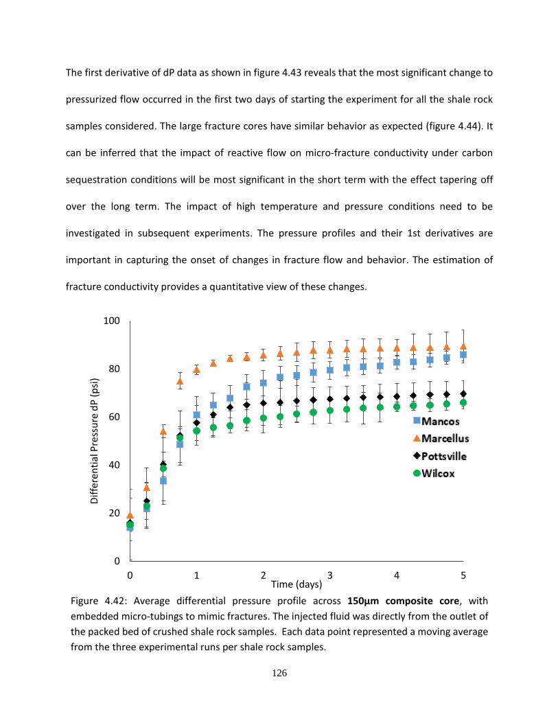
126

The first derivative of dP data as shown in figure 4.43 reveals that the most significant change to

pressurized flow occurred in the first two days of starting the experiment for all the shale rock

samples considered. The large fracture cores have similar behavior as expected (figure 4.44). It

can be inferred that the impact of reactive flow on micro-fracture conductivity under carbon

sequestration conditions will be most significant in the short term with the effect tapering off

over the long term. The impact of high temperature and pressure conditions need to be

investigated in subsequent experiments. The pressure profiles and their 1st derivatives are

important in capturing the onset of changes in fracture flow and behavior. The estimation of

fracture conductivity provides a quantitative view of these changes.

Figure 4.42: Average differential pressure profile across 150µm composite core, with

embedded micro-tubings to mimic fractures. The injected fluid was directly from the outlet of

the packed bed of crushed shale rock samples. Each data point represented a moving average

from the three experimental runs per shale rock samples.

0

20

40

60

80

100

0 1 2 3 4 5

Dif

fere

nti

al P

ress

ure

dP

(p

si)

Time (days)

Sample A

Sample B

Sample C

Sample D

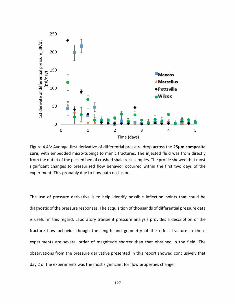
127

Figure 4.43: Average first derivative of differential pressure drop across the 25µm composite

core, with embedded micro-tubings to mimic fractures. The injected fluid was from directly

from the outlet of the packed bed of crushed shale rock samples. The profile showed that most

significant changes to pressurized flow behavior occurred within the first two days of the

experiment. This probably due to flow path occlusion.

The use of pressure derivative is to help identify possible inflection points that could be

diagnostic of the pressure responses. The acquisition of thousands of differential pressure data

is useful in this regard. Laboratory transient pressure analysis provides a description of the

fracture flow behavior though the length and geometry of the effect fracture in these

experiments are several order of magnitude shorter than that obtained in the field. The

observations from the pressure derivative presented in this report showed conclusively that

day 2 of the experiments was the most significant for flow properties change.

0

50

100

150

200

250

0 1 2 3 4 5

1st

der

ivat

e o

f d

iffe

ren

tial

pre

ssu

re, d

P/d

t (p

si/d

ay)

Time (days)

Sample A, derivative

Sample B, derivative

Sample C, derivative

Sample D, derivative

128

Figure 4.44: Average first derivative of differential pressure drop across the 150µm composite

core, with embedded micro-tubings to mimic fractures. The injected fluid was from directly

from the outlet of the packed bed of crushed shale rock samples. The profile showed that most

significant changes to pressurized flow behavior occurred within the first two days of the

experiment. This probably due to flow path occlusion.

4.8 Fracture Conductivity Estimation

The fracture conductivity of the multiple composite fractured cores were estimated using the

equations proposed by Dicman et al., [193, 221], and Warren and Root [222] for flow in fractures.

Each shale caprock type had associated experimental runs that acquired multiple differential

pressure data over a 5-day period. For example, three experimental runs were performed on the

Mancos shale using composite fractured cores (25µm micro-tubing embedded) with reaction

effluent flowing through. This yielded differential pressure data points at 20 secs interval that

were averaged for diagnostic and flow characteristic trends. These experimental runs were the

0

20

40

60

80

100

120

0 1 2 3 4 5

1st

der

ivat

ive,

dP/

dt

(psi

/day

)

Time (days)

Sample A

Sample B

Sample C

Sample D

129

same for other shale caprock types. These flow experiments were repeated for composite

fractured cores with 150µm micro-tubing embedded for all the shale caprock types. The results

of the estimated fracture conductivity are presented in figures 4.45 to 4.47. The effective fracture

width was first estimated which formed a major input for the calculation of dimensionless

fracture conductivity. The critical assumptions were i.) flow was primarily through fractures ii.)

bulk fracture flow properties are captured in the experimental differential pressure

measurements ii.) CO2-brine viscosity was constant throughout the experiment iii.) the length of

the core approximates the fracture length. Using equations 4.1 to 4.8;

𝑘𝑓 = 8.45 × 109 𝑤𝑓

2 𝐸𝑞. 4.1

𝑘𝑓 = 𝑘𝑎𝑣𝐴 − 𝑘𝑚(𝐴 − 𝑤𝑓𝑙)

𝑤𝑓𝑙 𝐸𝑞. 4.2

8.45 × 109 𝑤𝑓3𝑙 − 𝑘𝑎𝑣𝐴 + 𝑘𝑚(𝐴 − 𝑤𝑓𝑙) = 0 𝐸𝑞. 4.3

𝑞𝑚 = 𝑘𝑚𝐴∆𝑃

𝜇𝐿 𝐸𝑞. 4.4

𝑞𝑓 = 9.86 × 109 𝑤𝑓

3𝑙∆𝑃

12𝜇𝐿𝑓 𝐸𝑞. 4.5

𝑤𝑓𝑘𝑓 = 𝜋𝐶𝑟𝑘𝐿𝑓 𝐸𝑞. 4.6

𝑤𝑓 = √𝑞𝑓 × 12𝜇

9.86 × 109∆𝑃

3

𝐸𝑞. 4.7

𝐶𝑟 = 𝑤𝑓𝑘𝑓

𝜋𝐾𝑎𝑣𝐿𝑓 ≈

𝑤𝑓

𝜋𝐿𝑓 𝐸𝑞. 4.8

130

Where ΔP, wf, l, Lf, km, kf, kav, A, qm, qf, µ, and Cr represent differential pressure (atm), fracture

width (cm), core diameter (cm), fracture length (cm), matrix permeability (darcy), fracture

permeability (darcy), average permeability (darcy), cross sectional area (cm2), flow rate through

matrix (cm3/sec), flow rate through fracture (cm3/sec), viscosity (cp) and dimensionless fracture

conductivity respectively.

Figure 4.45 shows the dimensionless fracture conductivity for flow through the artificially

fractured composite cores (with 25µm micro-tubings embedded), calculated using equation 4.8.

The profile suggests that the conductivity of the fractures degenerated rapidly within the first

day of the experiment, tapering off at a constant rate towards the end of the experiment. The

data presented in figure 4.45 were based on three experimental runs per shale rock sample with

the error bar representing the standard deviation values. The fracture conductivity profile for the

experiments that were conducted using fractured composite cores with 150µm micro-tubing

embedded showed similar trend in rapid conductivity loss within the initial two days of the

experiments (figure 4.46). With the recovery of significant amount of precipitates from effluent

fluid, it can be inferred that in-situ geochemical precipitation was responsible for the loss of

fractured conductivity as differential pressure drop across the cores built up and later stabilized

during the experiments. It is estimated that only few micron size particulates are required to

completely occlude fracture flow paths. It also appears there is no direct linear correlations

between the fracture conductivity trends and the micro-tubings sizes that were used during the

experiment. Chapters 5 and 6 explored the attempts at fitting the experimental data of the

calculated fractured conductivity and reaction kinetics for some form of generalization.

131

Figure 4.47 compared the trends of the fracture conductivity of the 25µm cores with the 150µm

cores. The extent of conductivity reduction in about 30% lower for the bigger micro-fractures

(150µm). This indicates that there is significant limit to fracture aperture closure due to

geochemical effects. The data presented in figure 4.47 can be used for modelling the impact of

diagenetic alterations within subsets of naturally fractured shale caprocks. The availability of

more geochemical data and their impacts on flow properties in micro-fractures will help build

more robust numerical approximations that can be applied field-wide. The number of shale rock

samples used in these experimental reports fall within and outside those that have been reported

in the literature. The fact that the larger the potential micro-fracture defects in an intact rock the

less likely short-term diagenesis can seal them, implies that we can only depend to a limited

extent on the ability of rock-aqueous CO2 interactions to heal inherent anomalies in caprocks.

The field-wide effects of this can be investigated with discrete fracture network studies. In many

instances, modeling flow characteristics in fractured media can be through the use of the dual-

continuum algorithm whereby fractures and matrix are modeled as two separate kinds of

continua. These facsimile type of models usually do not replicate many commonly observed types

of fractured tight rock characteristics as they do not explicitly model the shape of discrete

fractures, geological inclusion features, and characteristic beddings that govern flow direction in

the subsurface. One of the perceived issues with using DFN models to address this short comings

is that the fractures in the model tend to be too uniform in length, area and spatial distribution

but these features describe the interpretative assumptions made in this experimental report.

132

Figure 4.45: Calculated dimensionless fracture conductivity profile from experimental

differential pressure (dP) data using fractured core parameters with 25µm micro-tubings

embedded. The profile indicated a rapid reduction in the conductivity of the artificial fractured

core within the first two days of the experiment. This reduction can only be attributed to in-

situ geochemical precipitation.

Figure 4.46: Calculated dimensionless fracture conductivity profile from experimental

differential pressure (dP) data using fractured core parameters with 150µm micro-tubings

embedded. The profile indicated a rapid reduction in the conductivity of the artificial fractured

core within the first two days of the experiment. This reduction can only be attributed to in-

situ geochemical precipitation.

3.5

4

4.5

5

5.5

6

6.5

7

7.5

0 1 2 3 4 5

Dim

ensi

on

less

Fra

ctu

re C

on

du

ctiv

ity

Cr

(x1

0-6

)

Time (days)

Core A, 25um

Core B, 25um

Core C, 25um

Core D, 25um

3.5

4.5

5.5

6.5

7.5

8.5

9.5

10.5

0 1 2 3 4 5

Dim

ensi

on

less

Fra

ctu

re

Co

nd

uct

ivit

y C

r (x

10

-6)

Time (days)

Core A, 150um

Core B, 150um

Core C, 150um

Core D, 150um

133

Figure 4.47: Comparison of calculated dimensionless fracture conductivity profile from

experimental differential pressure (dP) data using fractured core parameters with 25µm and

150µm embedded micro-tubings. The profile indicated a rapid reduction in the conductivity

of the artificial fractured core within the first two days of the experiment. The extent of

conductivity reduction in about 30% lower for the bigger micro-fractures (150µm). This

indicates that there is significant limit to fracture aperture closure due to geochemical effects.

3.5

4.5

5.5

6.5

7.5

8.5

9.5

10.5

0 1 2 3 4 5

Dim

ensi

on

less

Fra

ctu

re C

on

du

ctiv

ity

Cr

(x1

0-6

)

Time (days)

Core A, 25um

Core B, 25um

Core C, 25um

Core D, 25um

Core A, 150um

Core B, 150um

Core C, 150um

Core D, 150um

Closure reduction ≈30%

150µm

25µm

134

CHAPTER 5

DISCUSSION OF RESULTS OF SHALE ROCK/FLUID INTERACTIONS EXPERIMENTS

5.1 General Discussion of Experimental Results

The detailed discussion of experimental results is presented in this chapter. The discussion is

done under three sub-headings; (1) geochemical speciation in effluent fluid, (2) bulk

rock/precipitates analysis, (3) fracture flow characterization. The discussion covers in detail the

aqueous geochemistry of the resulting dissolved-mineral-saturated fluid (after rock-fluid

interactions experiments) and the impact of rock-fluid interactions on surface and bulk rock

geochemistry, including the precipitates that were recovered from the effluent. The effect of the

convective transport of the geochemically active effluent through fractured media is also

discussed; primarily differential pressure drop and micro-fracture conductivity. The impact of

these phenomena are captured by the various analytical methods and techniques that were used

for fluid, rock and fractured media characterization.

5.1.1 Geochemical Speciation in Experimental Effluent Fluid

The geochemical characterization of the effluent fluid showed the most pronounced

documentation of reactive rock-fluid interactions. The pH of the effluent fluid showed initial

resilience to acidic fluid medium. The shaly rocks acted as alkaline buffering media where by the

final effluent indicated geochemical reactions that brought acidity conditions up to and above

neutral scale. It can be observed from the pH profile (figure 4.1) that the alkaline buffer strength

of the shale rocks through reactive interaction with the CO2-brine fluid at the experimental

pressure and temperature conditions is significantly pronounced for the Mancos, Marcellus and

Pottsville shale rocks while that of the Wilcox shale is markedly lower. Many geochemical

135

reactions are dependent on the pH of the medium. It is expected that forward dissolution

reactions will be encouraged under acidic pH conditions of CO2 geo-sequestration. These

observations are in agreement with previous experiments conducted in the laboratory and

reported by other researchers. The changes in pH is expected to control, to some degree, the

ability of the various rock minerals to exchange ions with one another. The diffusion and

subsequent dissolution of free CO2 molecules in the connate water of the caprock is expected to

lead to localized ultra-low pH ranges that will catalyze pore and micro-fracture surface

dissolution. The idea that supercritical CO2 would sink to the deep bottom part of the reservoir

brings the idea of convective transport of super-saturated acidic fluid into the overlaying seal

rocks. This will have the same effect as gaseous CO2 diffusion in the tight hydraulically connected

spaces within the rock. The pH data reported suggest varying degrees of alkaline buffering

strength of the rocks; the higher the fraction of calcium based minerals, the higher the alkaline

buffering strength. This is consistent with literature reports.

The ICP-OES concentrations of both major and trace metals such as Ca2+, Mg2+, Se2+, Al3+ Si2+, and

Zn2+ indicated rapid dissolution of rock minerals that have alkaline earth metals in their crystalline

or amorphous matrices (figures 4.2 to 4.15). The concentration profile for Calcium shows that

the Marcellus samples had the highest fraction in solution which rapidly decreased over the five

day period of continuously flooding the samples with CO2 saturated brine. The initial pH of the

influent fluid is approximately 3.7. The Mancos, Marcellus and Wilcox shale rocks exhibited

similarly trend of a gradual exponential decline over the five day period. The Pottsville shales

reflected a gradual increase that appears to continue over the experimental period. While the

elemental concentration of Calcium in the Mancos, Marcellus and Wilcox shales peaks on the

136

first day of the experiment, that of the Pottsville shale continued to increase over the five day

period but it also expected to peak and gradually decline with similar trend to the Mancos,

Marcellus and Wilcox shales. This resilient behavior of the Pottsville shale might suggest a slower

dissolution reaction of it calcium based minerals constituent compared to the Mancos, Marcellus

and Wilcox shales. The bulk rock XRD analysis indicated calcite and dolomite as the main calcium

bearing minerals in the Mancos, Marcellus and Wilcox shales while anhydrites are the main

calcium bearing minerals in the Pottsville. These observations in the effluent are significant as

the cationic content of any fluid determines the extent to which sizeable amount of dissolved

solutes precipitates out of solution. This is evident in the Marcellus and Mancos samples where

large amount of carbonate precipitates were recovered. The precipitation of dissolved minerals

at normal temperature and pressure conditions shows that in the subsurface, changes in

geochemical and thermodynamic conditions can affect the speed at which aqueous precipitation

processes take place.

5.1.2 Bulk Rock/Precipitates Analysis

The XRD analysis of the bulk rocks yielded useful information about the possible changes in the

mineralogy of the shales. Figures 4.17 to 4.20 show the profiles of the main mineralogical

components in the shale rocks (pre- and post-flooding with CO2-brine) and the recovered

precipitates as identified by bulk XRD analysis for the Mancos, Marcellus, Pottsville and Wilcox

shale rocks respectively. Bulk XRD analysis reflected changes that are not significant enough in

their percentages in order to make affirmative conclusions. The clay XRD analysis also showed

that there are only subtle changes in the clay component of all the rock samples. But the

137

Marcellus shale showed far greater heterogeneity in both mineralogy and morphology. These

heterogeneities does not make the Marcellus shale a good candidate for seal rocks of CO2

sequestration sites. The Pottsville shale shows platy grain structures that are tightly packed and

efficient for preventing fluid movement. In terms of pre- and post-flooding minerology, it appears

the Pottsville shale is most stable followed by the Wilcox which is not tight in pore structure.

Furthermore, the recovery of amorphous precipitates in all of the associated effluent samples

showed the role that temperature plays in the ability of dissolved minerals to remain in solution

for an extended period. More than ninety percent of the precipitates were recovered within a

month after the experiments. These precipitates are of varying coloration; dark brown to light

pink (see Appendix A). While the bulk shale rock samples showed little changes at the surface,

the mineralogical analysis carried out on them revealed the removal of amorphous contents from

the rocks in significant amounts. These amorphous contents form the bulk of the precipitates

were recovered from the effluent. Amorphous content of rocks are usually responsible for

suppressed peaks in XRD qualitative analysis. The bulk XRD analysis of precipitates showed the

appearance of diagenetic minerals that were formed from the major mineralogical components

of the shale rocks. The quantitative XRD analysis performed on samples are largely qualitative

with minor evidence of changes in the mineralogy of the rock samples after the experiment. But

for the margin of changes reported in tables 4.1 and 4.2, it best to assume that the contents of

the precipitates are largely amorphous and crystalline forms of carbonates as seen in XRD.

The total carbon content of the shale rocks (figure 4.16) indicated that the higher the organic

content of the seal rock, the higher the potential for carbon absorption to the surface of the rock.

The Marcellus shale exemplified this behavior well when compared to other shale samples. The

138

percentage carbon content were in the order Marcellus > Wilcox > Mancos > Pottsville. This order

of magnitude still holds after the CO2-brine flooding experiment. It can be observed for the figure

that were significant increases in the percentage content of carbon in all the samples which can

be indicative of both adhered carbon and mineralized carbon in the these shale samples.

The electron microprobe analysis (EMPA) showed the presence of Iron (Fe), Sodium (Na),

Potassium (K), Silicon (Si), Carbon (C), Oxygen (O), Chlorine (Cl), Manganese (Mn), Calcium (Ca),

Magnesium (Mg) and Aluminum (Al). They are present in rock minerals capable of exchanging

ions with carbonic acid or aqueous CO2. The elemental distribution of Ca and Mg in the reacted

Mancos and Marcellus shales were lower within grain facies as shown in figures 4.25 to 4.27 and

figures 4.28 to 4.30 (top row) respectively when compared to the corresponding control samples

(bottom row). These were the surface maps for elemental spread involving CO2-brine flooded

samples. It has been noted that in addition to common alkali earth metals such as Na and K that

form compounds which are generally soluble in acidic or alkaline fluids, Ca and Mg solutes have

significant ion-exchange capacity as well. The surface depletion within grains show the extent of

the reach of aqueous CO2 in supporting dissolutive rock-fluid interaction in the subsurface.

Pottsville and Wilcox shales are lean in Ca and Mg based minerals which informed the limited

traces of these elements on the surface of the thin section samples. The distribution of Al and Fe

as shown in figures 4.26/27 and figures 4.29/30 for Mancos and Marcellus shales respectively

indicated low activity in the reacted samples while figures 4.31 to 4.33 and figures 4.34 to 4.36

for Pottsville and Wilcox shales respectively reflected significant concentration of Al and Fe which

have smaller percentages in the minerals baring them. These imply that compounds of Ca, Mg,

Al, and Fe which were identified in the shale caprock samples, either as major or trace minerals,

139

would be reactively soluble with faster kinetics in aqueous CO2 with the possibility of re-

precipitation to form new minerals at subsurface pressure and temperature. The formation of

Aragonite in experiments involving Marcellus shale exemplify the dissolution-precipitation

processes that impact long term caprock integrity.

The magnitude of the mechanical strength of the bulk shale rocks was reduced for most of the

samples analyzed (figures 4.37 and 4.38). This was measured in terms of Vickers’ Hardness. The

most impacted was the Wilcox shale which has the highest percentage of swelling clay

(Montmorillonite). The tablet of shale rocks used were polished using laboratory grinder which

could have altered some mechanical properties. These polishers are graded from fine to coarse

applications. The finest grade of polisher is used at the final stage of rock preparation for micro-

indentation. This is expected to have some effects on near-wellbore stability of shale caprock

sections for CO2 sequestration sites. Also, the correlation of changes in mineralogy to hardness

and Young’s Modulus (figures 4.39 and 4.40) suggested that the higher the diagenetic quartz

formed, the higher the mechanical properties. It implies that rock-fluid geochemical interactions

that can continuously convert clays and other minerals into opal will provide higher

geomechanical stability and tighter hydraulic barrier on the longer term.

5.1.3 Fracture Flow Characterization

The characterization of fracture flow properties showed that the formation of precipitates in the

super-saturated fluid can occlude hydraulic conductivity. This phenomenon is supported by the

experimental data presented in figures 4.41 to 4.47. These are in specific cases when soluble

alkaline earth metal minerals are present in large amount with the host rock as seen with

140

carbonates rich shale rocks. The next chapter attempts to integrate the geochemical and fracture

flow experimental data obtained and provide models to represent them. The applications of such

integrated models will be in numerical reservoir simulations where discrete fracture network

models can be used to describe and visualize long term behavior of sedimentary tight rocks under

carbon sequestration conditions. It is expected that deep fractured shale will exhibit greater

diagenesis when in contact with aqueous carbon dioxide. The experimental data reported

showed that 25µm sized fractures can be closed more rapidly with 150µm sized ones taking

longer time to close and are 30% less in fracture sizes. The first derivatives of the differential

pressures showed that most of the changes occurred during the first two days of the experiment

with the Marcellus sample reflecting the most changes in the rapid exponential decline. The use

of pressure derivative is to help identify possible inflection points that could be diagnostic of the

pressure responses. The acquisition of thousands of differential pressure data is useful in this

regard. Laboratory transient pressure analysis provides a description of the fracture flow

behavior though the length and geometry of the effect fracture in these experiments are several

order of magnitude shorter than that obtained in the field the Mancos and the Wilcox also

indicated a rapid loss of fracture conductivity. These losses are attributable to the generation of

significant amount of precipitates from the effluent fluid of shale rock-aqueous CO2 interactions.

These precipitates were crystalized at varying rates and this was thought to have been

responsible for the different initial gradients. The rapid precipitation of aragonites from the

effluent samples of the CO2-brine flooding Marcellus shales showed that the convective transport

of precipitate laden fluid at 50°C and 1000psi pressure, can lead to fast fracture conductivity

closure.

141

5.2 Integrated Experimental Observations

The integration of the sections described above leads to the flow diagram shown in figure 5.1.

The geochemical footprint in the effluent and the mineralogical/morphological characteristics of

the shale rocks is shown to have impacted the conductivity of micro-fractures. This is through the

formation of precipitates. The physics of geochemical-fracture flow in shale caprock can be

described analytically. The upper decline curve represents lower impact of the effects of

geochemical interactions under constant geomechanical conditions. The upper decline curve

represent higher impact of the effects of geochemical interactions. These effects can be

mathematically/analytically modelled as an exponential-natural logarithmic function. This

function can be used in used in complex discrete fracture networks representing natural flow

path deformities in shale caprock. This function is exclusively for corrections to flow

characteristics over time in re-activated or open micro-fracture networks inherent in shale

caprocks. The monitoring of leakages via caprock should account for geochemical changes and

not just geomechanical alterations which tend to first worsen seal integrity during the initial

phase of injection. The independent modelling of coupled geochemical effects and micro-

fracture conductivity can be described by the exponential-natural logarithm relationship, leaving

out complex reactions which are difficult to account for simultaneously. In the literature, the

effect of capillarity is highly emphasized as a determining factor for seal integrity but the

presence of scattered, randomly distributed micro-fractures lead to low or non-accounting of

carbon molecules that could be involved in rock-fluid interactions under CO2 sequestration and

containment conditions.

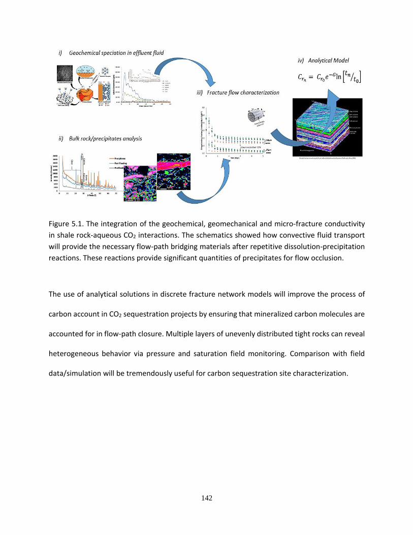
142

Figure 5.1. The integration of the geochemical, geomechanical and micro-fracture conductivity

in shale rock-aqueous CO2 interactions. The schematics showed how convective fluid transport

will provide the necessary flow-path bridging materials after repetitive dissolution-precipitation

reactions. These reactions provide significant quantities of precipitates for flow occlusion.

The use of analytical solutions in discrete fracture network models will improve the process of

carbon account in CO2 sequestration projects by ensuring that mineralized carbon molecules are

accounted for in flow-path closure. Multiple layers of unevenly distributed tight rocks can reveal

heterogeneous behavior via pressure and saturation field monitoring. Comparison with field

data/simulation will be tremendously useful for carbon sequestration site characterization.

143

CHAPTER 6

CONCLUSIONS AND RECOMMENDATIONS

6.1 Conclusions

The interaction of aqueous CO2 and shale caprocks that are representative of the geological seals

suitable for CO2 sequestration and containment projects have been experimentally studied under

laboratory conditions of stress (1400psi axial and radial stress), temperature (50°C) and injection

pressures (1000 psi). Four shale caprock samples from different geologic formations within the

United States were used. The effluent emanating from these closed system diagenetic rock-fluid

interactions were flowed through an artificially fractured media made of cylindrical cement cores

with PEEK polymer micro-tubings embedded. This was intended to mimic micro-fractures, which

are sometimes present in intact caprocks. Several experimental runs using the unique setup

described in Chapter 3 were carried out with two different sets of micro-tubing diameters (25µm

and 150 µm ID). Effluent fluid analysis were carried out using pH meters and ICP-OES techniques

for acidity/alkalinity measurements and ionic content analysis. Bulk shale rocks were analyzed

with XRD, SEM, EMPA, TOC and Micro-indentation techniques for changes in rock mineralogy,

morphology, elemental composition, inorganic carbon and geomechanical properties. The

measurement of differential pressure drop across the artificially fractured cores yielded

information on the impact of geochemical changes in the experimental fluid on effective micro-

fracture apertures and corresponding fracture conductivity.

The following major conclusions can be inferred from the laboratory experiment involving shale

rock interactions with CO2 saturated brine under dynamic flow conditions:

144

1. Moderately high temperature (50°C) and injection pressure (1000psi) in the core scale

experiment indicate rapid dissolution of shale rock minerals as shown by the analyses of

effluent fluid, bulk rock and precipitate analyses.

2. The effluent fluid indicated that alkaline earth metal based minerals particularly Calcium

and Magnesium in shale caprocks are the most susceptible to reactive dissolution at these

experimental conditions.

3. Reactive dissolution leads to the formation of new diagenetic minerals, notably in

carbonates-rich shale caprocks, which precipitated out of the effluent fluid in significant

quantity. These precipitates are capable of aggregating in saturated solutions.

4. The distribution of major elements on the surface of the bulk shale caprocks showed

minute morphological changes at the edges of distinct grains and the association of minor

elements with major minerals. This shows that significant heterogeneity within the tight

rocks are responsible for the release of environmentally unfriendly trace elements that

can compromise groundwater quality.

5. Reaction kinetic models indicated that there is significant increase in rates of diagenetic

rock fluid interactions as temperature is additively doubled. This implied that deep hot

shale rocks will experience higher rates of diagenetic rock-fluid interactions that could

possibly impact hydraulic fractures. This is applicable to large scale CO2 sequestration into

stimulated shale reservoirs with hydraulic fracture networks.

6. Micro-hardness property of the bulk rock showed significant reduction in geomechanical

strength for three samples; Mancos, Marcellus and Wilcox. Micro-hardness property of

145

the bulk rock is not significantly affected as observed in this 5-day experiment for

Pottsville shale samples with non-swelling clay and no carbonates.

7. The gradual rise of differential pressure drop across the fractured composite core is an

indication of loss of flow characteristics. Dimensionless fracture conductivity indicated

that the loss of flow characteristics was most pronounced within the first two days of the

experiment leading to aperture closure over time.

8. There is significant limit to the size of effective fracture apertures that can be closed by

diagenetic rock-fluid interactions. Experimental data showed approximately 30%

reduction in end-of-experiment conductivity loss when micro-tubings sizes where

changed from 25µm to 150µm.

9. The loss of fracture conductivity can be analytically modelled as an exponential-natural

logarithm function for two profiles of fracture conductivity that represent the extremes.

10. The modelling of discrete fracture networks in shale caprocks can be the key to the

accuracy of carbon accounting. It can be opined that given the potential of rock-fluid

interactions in generating significant amount of precipitates, the exact amount of carbon

from molecules of carbon dioxide injected and minerally sequestered can be estimated.

11. The data presented in this report can be used in incorporating the effect of short term

diagenesis on fracture flow characteristics by assigning physics based models

(exponential-natural logarithm function is developed) to discrete fracture network cases.

The integration of various models of geochemistry, geomechanics and micro-fracture

conductivity can provide a single model representation of caprock behavior/integrity

under carbon sequestration conditions.

146

6.2 Recommendations

The understanding of diagenetic rock-fluid interactions in tight shale caprocks require detailed

experimental data for successful theoretical and numerical modelling. Base on the additions to

the body of knowledge through this research works, the following recommendations are

proposed:

1. Experimental runs at higher temperature and pressure conditions could be carried out to

investigate rock-fluid interactions effect in the case of injection of CO2 into deep fractured

shale formations. For example the experimental conditions could be: Overburden stress

= 4000psi, Backpressure = 3600psi; Injection pressure = 3600 psi, Operating temperature

= 150°C. Temperature and pressure control will present the biggest challenge and more

sophisticated instrumentation can be deplored to achieve the desired conditions.

2. Acquire geochemical, geomechanical and flow parameters as were in the moderate

temperature and pressure experiments described in this report. Imaging analyses of

relevant samples will also be carried out to identify morphological changes.

3. Model the reaction rate and flow characteristics at multiple experimental conditions of

pressure and temperature at the core scale for possible scale up to numerical simulation.

4. Predict subsurface implication of the impact of diagenesis and stress on fracture

conductivity from core scale experiment and the associated models.

5. Additional shale rock samples could be explored to create a more robust statistically

useful data base for geostatistical and discrete fracture network predictions of long term

rock-fluid interaction effects on other geological basins of interests to CO2 sequestration

project managers.

147

REFERENCES

1. Shukla, R., et al., A Review of Studies on CO2 Sequestration and Caprock Integrity. Fuel, 2010. 89(10): p. 2651-2664.

2. Stevens, S.H., Natural CO2 Fields as Analogs for Geologic CO2 Storage. 2005. Volume

2(Carbon Dioxide Capture for Storage in Deep Geologic Formations – Results from the CO2 Capture Project Geologic Storage of Carbon Dioxide with Monitoring and Verification, Sally M. Benson, Lawrence Berkeley Laboratory, Berkeley, CA, USA): p. Pages 687-697.

3. Wollenweber, J., et al., Experimental Investigation of the CO2 Sealing Efficiency of

Caprocks. International Journal of Greenhouse Gas Control, 2010. 4(2): p. 231-241.

4. Bicocchi, G., et al., Chemical Alteration and Mineral Growth under High Pco2 Conditions: Insights from the Mineral Chemistry of Carbonate Phases in the Caprese Reservoir (Northern Apennines, central Italy). Chemical Geology, 2017. 450: p. 81-95.

5. Arts, R.C., O. Eiken, and N. Scott- Sylvain, Ten Years' Experience of Monitoring CO2

Injection in the Utsira Sand at Sleipner, Offshore Norway. First Break, 2008. 26: p. 65-72.

6. Akervoll, I., E. Lindeberg, and A. Lackner, Feasibility of Reproduction of Stored CO2

from the Utsira Formation at the Sleipner Gas Field. Energy Procedia, 2009. 1(1): p. 2557-2564.

7. Buttinelli, M., et al., the Geo-database of Caprock Quality and Deep Saline Aquifers

Distribution for Geological Storage of CO2 in Italy. Energy, 2011. 36(5): p. 2968-2983.

8. Chadwick, R.A., et al., Geological Characterization of CO2 Storage Sites: Lessons from Sleipner, Northern North Sea, in Greenhouse Gas Control Technologies - 6th International Conference, J. Gale and Y. Kaya, Editors. 2003, Pergamon: Oxford. p. 321-326.

9. Davis, E.J. and S.D. Marsic, Interpretation of CO2-Sequestration-Induced Surface

Deformation at Krechba, Algeria, in SPE International Conference on CO2 Capture, Storage, and Utilization. 2010: New Orleans, Louisiana, USA. doi:10.2118/147444-MS.

10. Farokhpoor, R., et al., Experimental and Numerical Simulation of CO2 Injection Into

Upper-Triassic Sandstones in Svalbard, Norway, in SPE International Conference on CO2 Capture, Storage, and Utilization. 2010: New Orleans, Louisiana, USA.

148

11. Giday-WoldeGabriel, M.F., et al., Textural and Geochemical Features along a Reservoir-Cap Rock Contact in the Sacroc Unit of West Texas, L.A.N.L. Earth and Environmental Sciences Division, Editor. 2007: Los Alamos, NM, 87545 USA.

12. Xu, T., et al., Reactive Transport Modeling to Study Changes in Water Chemistry

Induced By CO2 Injection at the Frio-I Brine Pilot. Chemical Geology, 2010. 271(3-4): p. 153-164.

13. Zhang, W., et al., Long-Term Variations of CO2 Trapped in different Mechanisms in

Deep Saline Formations: A Case Study of the Songliao Basin, China. International Journal of Greenhouse Gas Control, 2009. 3(2): p. 161-180.

14. Carbon Sequestration Atlas of the United States and Canada. National Energy

Technology Laboratory, Department of Energy 2010. Vol. 3: p. 162.

15. Ellis, B., et al. Alteration of Caprock Fracture Geometries During Flow of CO2-acidified Brine: Informing Basin-scale Leakage Models From Pore-scale modeling and Core-scale Experiments. in AGU Fall Meeting Abstracts. 2011.

16. Javadpour, F., CO2 Injection in Geological Formations: Determining Macroscale

Coefficients From Pore Scale Processes. Transport in Porous Media, 2009. 79(1): p. 87-105.

17. Renard, S., et al., Geochemical Study of the Reactivity of a Carbonate r=Rock in a

Geological Storage of CO2: Implications of co-injected Gases. Energy Procedia, 2011. 4: p. 5364-5369.

18. Salem, A.M. and S.A. Shedid, Variation of Petrophysical Properties due to Carbon

Dioxide (CO2) Storage in Carbonate Reservoirs. Journal of Petroleum and Gas, 2013. 4(4): p. 91-102.

19. Wei, N., et al., Geochemical Impact of Aquifer Storage for Impure CO2 containing O2

and N2: Tongliao field experiment. Applied Energy, 2015. 145: p. 198-210.

20. Bourg, I.C., L.E. Beckingham, and D.J. DePaolo, the Nanoscale Basis of CO2 Trapping for Geologic Storage. Environmental science & technology, 2015.

21. Hong, K.C. and J.W. Ault, Effects of Noncondensable Gas Injection on Oil Recovery by

Steamflooding. SPE Journal of Petroleum Technology, 1984. 36(12): p. 2160-2170.

22. Bagci, A.S. and F. Gumrah, Effects of CO2 and CH4 Addition to Steam on Recovery of West Kozluca Heavy Oil, in SPE International thermal Operations and Heavy Oil Symposium and Western Regional Meeting. 2004, Society of Petroleum Engineers: Bakersfield, California.

149

23. Smith, S.A., et al., Geomechanical Testing and Modeling of Reservoir and Cap Rock

Integrity in an Acid Gas EOR/Sequestration Project, Zama, Alberta, Canada. Energy Procedia, 2009. 1(1): p. 2169-2176.

24. Mohammad, S., R.L. Robinson, and K. Gasem, Multiphase Analysis for CO2:

Water/Mixed-Gas Adsorption on Coals, in SPE International Conference on CO2 Capture, Storage, and Utilization. 2010: New Orleans, Louisiana, USA.

25. Pitman, J.K., et al., Origin of Minerals in Joint and Cleat Systems of the Pottsville

Formation, Black Warrior Basin, Alabama: Implications for Coalbed Methane Generation and Production. AAPG Bulletin, 2003. 87(5): p. 713-731.

26. Pashin, J.C., et al., Carbon Sequestration and Enhanced Recovery Potential of Mature

Coalbed Methane Reservoirs in the Black Warrior Basin. AAPG Special Volume, 2009.

27. Goodman, A., et al., Methodology for Assessing CO2 Storage Potential of Organic-Rich Shale Formations. Energy Procedia, 2014. 63: p. 5178-5184.

28. Murphy, R., et al., Ferrihydrite Phase Transformation in the Presence of Aqueous

Sulfide and Supercritical CO2. Chemical Geology, 2010. 271(1-2): p. 26-30.

29. Alemu, B.L., et al., Caprock Interaction with CO2: A Laboratory Study of reactivity of shale with supercritical CO2 and brine. Applied Geochemistry, 2011. 26(12): p. 1975-1989.

30. Pentland, C.H., et al., Measurement of Supercritical Carbon Dioxide Capillary Trapping in Core Analysis, in SPE International Conference on CO2 Capture, Storage, and Utilization. 2010: New Orleans, Louisiana, USA. doi:10.2118/138476-MS.

31. Hemme, C. and W. van Berk, Change in Cap Rock Porosity triggered by Pressure and Temperature Dependent CO2–Water–Rock Interactions in CO2 Storage Systems. Petroleum, 2017. 3(1): p. 96-108.

32. Michels, L., et al., Intercalation and Retention of Carbon Dioxide in a Smectite Clay

promoted by Interlayer Cations. Scientific reports, 2015. 5: p. 8775.

33. Busch, A., et al., Effects of Physical Sorption and Chemical Reactions of CO2 in Shaly Caprocks. Energy Procedia, 2009. 1(1): p. 3229-3235.

34. Wollenweber, J., et al., Caprock and Overburden Processes in Geological CO2 Storage:

an Experimental Study on Sealing Efficiency and Mineral Alterations. Energy Procedia, 2009. 1(1): p. 3469-3476.

150

35. Busch, A., et al., Carbon Dioxide Storage Potential of Shales. International Journal of Greenhouse Gas Control, 2008. 2(3): p. 297-308.

36. Audigane, P., et al., Reactive Transport Modeling Using TOUGHREACT for the Long

Term CO2 Storage at Sleipner, North Sea. Carbon Capture and Sequestration, 2005. 2.

37. Eiken, O., et al., Lessons Learned From 14 Years of CCS Operations: Sleipner, In Salah and Snøhvit. Energy Procedia, 2011. 4: p. 5541-5548.

38. Gaus, I., M. Azaroual, and I. Czernichowski-Lauriol, Reactive Transport Modelling of

the Impact of CO2 Injection on the Clayey Cap Rock at Sleipner (North Sea). Chemical Geology, 2005. 217(3): p. 319-337.

39. Allen, P.A. and J.R. Allen, Basin Analysis - Principles and Applications (2nd Edition).

John Wiley & Sons.

40. Li, Z., et al., CO2 Sequestration in Depleted Oil and Gas Reservoirs--Caprock Characterization and Storage Capacity. Energy Conversion and Management, 2006. 47(11-12): p. 1372-1382.

41. Bryant, S. and L.W. Lake, Effect of Impurities on Subsurface CO2 Storage Processes, in

Carbon Dioxide Capture for Storage in Deep Geologic Formations. 2005, Elsevier Science: Amsterdam. p. 983-996.

42. Wang, J., et al., Effects of Impurities on CO2 Transport, Injection and Storage. Energy Procedia, 2011. 4: p. 3071-3078.

43. Marcon, V. and J.P. Kaszuba, Carbon Dioxide–Brine–Rock Interactions in a Carbonate

Reservoir Capped By Shale: Experimental Insights Regarding the Evolution of Trace Metals. Geochimica Et Cosmochimica Acta, 2015. 168: p. 22-42.

44. Busch, A., et al., Investigation of High-Pressure Selective Adsorption/Desorption

Behaviour of CO2 and CH4 on Coals: An Experimental Study. International Journal of Coal Geology, 2006. 66(1-2): p. 53-68.

45. Busch, A. and A. Amann-Hildenbrand, Predicting Capillarity of Mudrocks. Marine and

Petroleum Geology, 2013. 45: p. 208-223.

46. Bennett, R.H., W.R. Bryant, and M.H. Hulbert, the Microstructure of Fine-Grained Sediments, From Mud to Shale. 1991, New York: Springer-Verlag.

47. Hildenbrand, A., S. Schlömer, and B.M. Krooss, Gas Breakthrough Experiments on

Fine-Grained Sedimentary Rocks. Geofluids, 2002. 2(1): p. 3-23.

151

48. Emmanuel, S., L.M. Anovitz, and R.J. Day-Stirrat, Effects of Coupled Chemo-Mechanical Processes on the Evolution of Pore-Size Distributions in Geological Media. Rev Mineral Geochem, 2015. 80: p. 45-60.

49. Mouzakis, K.M., et al., Experimental Study of Porosity Changes in Shale Caprocks

Exposed to CO2-Saturated Brines I: Evolution of Mineralogy, Pore Connectivity, Pore Size Distribution, and Surface Area. Environmental Engineering Science.

50. Miller, Q.R., et al., Experimental Study of Porosity Changes in Shale Caprocks Exposed

to Carbon Dioxide-Saturated Brine II: Insights From Aqueous Geochemistry. Environmental Engineering Science. 33.10 (2016): p. 736-744.

51. Khan, S., et al., An Integrated Geomechanics Workflow for Caprock-Integrity Analysis

of a Potential Carbon Storage, in SPE International Conference on CO2 Capture, Storage, and Utilization. 2010: New Orleans, Louisiana, USA. doi:10.2118/139477-MS.

52. Vilarrasa, V., S. Olivella, and J. Carrera, Geomechanical Stability of the Caprock During

CO2 Sequestration in Deep Saline Aquifers. Energy Procedia, 2011. 4: p. 5306-5313.

53. Busch, A., et al., The Significance of Caprock Sealing Integrity for CO2 Storage, in SPE International Conference on CO2 Capture, Storage, and Utilization. 2010: New Orleans, Louisiana, USA. doi:10.2118/139588-MS.

54. Ellis, B.R., et al., Changes in Caprock Integrity Due to Vertical Migration of CO2-

Enriched Brine. Energy Procedia, 2011. 4: p. 5327-5334.

55. Mcpherson, B., Modeling Caprock Integrity: Assessment Objectives. IEA-GHG CO2 Geological Storage Modelling Workshop Orleans, France, 2009.

56. Armitage, P.J., et al., Diagenetic and Sedimentary Controls on Porosity in Lower Carboniferous Fine-Grained Lithologies, Krechba Field, Algeria: a Petrological Study of a Caprock to a Carbon Capture Site. Marine and Petroleum Geology, 2010. 27(7): p. 1395-1410.

57. Ali, S.A., et al., Diagenesis and Reservoir Quality. Oilfield Review, 2010. 22(2): p. 14-

27.

58. Duenckel, R., et al., Proppant Diagenesis--Integrated Analyses Provide New Insights Into Origin Occurrence and Implications for Proppant Performance. SPE Production & Operations, 2012. 27(02): p. 131-144.

59. Weaver, J.D., et al., Fracture-Related Diagenesis may Impact Conductivity. SPE

Journal, 2007. 12(03): p. 272-281.

152

60. Katsube, T.J. and M.A. Williamson, Effects of Diagenesis on Shale Nano-Pore Structure and Implications for Sealing Capacity. Clay Minerals, 1994. 29(4): p. 451-472.

61. Kohler, E., T. Parra, and O. Vidal, Clayey Cap-Rock Behavior in H2O-CO2 Media at Low

Pressure and Temperature Conditions: An Experimental Approach. Clays and Clay Minerals, 2009. 57(5): p. 616-637.

62. Nogues, J.P., et al., Permeability Evolution Due to Dissolution and Precipitation of

Carbonates Using Reactive Transport Modeling in Pore Networks. Water Resources Research, 2013. 49(9): p. 6006-6021.

63. Armitage, P., et al., Permeability of the Mercia Mudstone: Suitability As Caprock to

Carbon Capture and Storage Sites. Geofluids 16.1 (2016): p. 26-42.

64. Edlmann, K., S. Haszeldine, and C. Mcdermott, Experimental Investigation Into the Sealing Capability of Naturally Fractured Shale Caprocks to Supercritical Carbon Dioxide Flow. Environmental Earth Sciences, 2013. 70(7): p. 3393-3409.

65. Liu, F., et al., CO2–Brine–Caprock Interaction: Reactivity Experiments on Eau Claire

Shale and a Review of Relevant Literature. International Journal of Greenhouse Gas Control, 2012. 7: p. 153-167.

66. Elsworth, D. and H. Yasuhara, Mechanical and Transport Constitutive Models for

Fractures Subject to Dissolution and Precipitation. International Journal for Numerical and Analytical Methods in Geomechanics, 2010. 34(5): p. 533-549.

67. Reynolds, M. and J. Buendia. Permanently Sequester Anthropogenic Carbon Dioxide-

Through Hydraulic Fracturing. in SPE Unconventional Resources Conference. 2017. Society of Petroleum Engineers. doi:10.2118/185033-MS.

68. Nicot, J.p. and I.J. Duncan, Common attributes of Hydraulically Fractured Oil and Gas

Production and CO2 Geological Sequestration. Greenhouse Gases: Science and Technology, 2012. 2(5): p. 352-368.

69. Stack, A.G., Precipitation in Pores: A Geochemical Frontier. Rev Mineral Geochem,

2015. 80: p. 165-190.

70. Molins, S., Reactive Interfaces in Direct Numerical Simulation of Pore Scale Processes. Rev Mineral Geochem, 2015. 80: p. 461-481.

71. Vidic, R.D., et al., Impact of Shale Gas Development on Regional Water Quality.

Science, 2013. 340(6134).

153

72. Amthor, J.E. and J. Okkerman, Influence of Early Diagenesis on Reservoir Quality of Rotliegende Sandstones, Northern Netherlands. AAPG Bulletin, 1998. 82(12): p. 2246-2265.

73. Wendler, J., et al., Carbonate Diagenesis and Feldspar Alteration in Fracture-Related

Bleaching Zones (Buntsandstein, Central Germany): Possible Link to CO2-Influenced Fluid–Mineral Reactions. International Journal of Earth Sciences, 2012. 101(1): p. 159-176.

74. Altundas, B., et al., Retardation of CO2 Migration Due to Capillary Pressure Hysteresis:

a New CO2 Trapping Mechanism, in SPE International Conference on CO2 Capture, Storage, and Utilization. 2010: New Orleans, Louisiana, USA. doi:10.2118/139641-MS.

75. Soldal, M., Caprock Interaction with CO2: Geomechanical and Geochemical Effects, in

Department of Geosciences. 2008, University of Oslo: Oslo. p. 106.

76. Pashin, J.C. and M.R. Mcintyre, Temperature–Pressure Conditions in Coalbed Methane Reservoirs of the Black Warrior Basin: Implications for Carbon Sequestration and Enhanced Coalbed Methane Recovery. International Journal of Coal Geology, 2003. 54(3): p. 167-183.

77. Espinoza, D.N. and J.C. Santamarina, Water-CO2-Mineral Systems: Interfacial Tension,

Contact Angle, and Diffusion;Implications to CO2 Geological Storage. Water Resour. Res., 2010. 46(7): p. W07537.

78. Moultos, O.A., et al., Self-Diffusion Coefficients of the Binary H2O–CO2 Mixture at High

Temperatures and Pressures. the Journal of Chemical thermodynamics 93 (2016): p. 424-429.

79. Busch, A. and N. Müller, Determining CO2/Brine Relative Permeability and Capillary

Threshold Pressures for Reservoir Rocks and Caprocks: Recommendations for Development of Standard Laboratory Protocols. Energy Procedia, 2011. 4: p. 6053-6060.

80. Blauch, M.E. Developing Effective and Environmentally Suitable Fracturing Fluids

Using Hydraulic Fracturing Flowback Waters. in SPE Unconventional Gas Conference. 2010. Society of Petroleum Engineers. doi:10.2118/131784-MS

81. EPA, Characteristics of Coalbed Methane Production and Associated Hydraulic

Fracturing Practices. Evaluation of Impacts to Underground Sources of Drinking Water by Hydraulic Fracturing of Coalbed Methane Reservoirs, 2004: p. 32.

82. USGS, Summary of Studies Related to Hydraulic Fracturing Conducted by USGS Water

Science Centers. USGS, 2012. 5: p. 1 - 8.

154

83. Chalbaud, C., et al., Interfacial Tension Measurements and Wettability Evaluation for Geological CO2 Storage. Advances in Water Resources, 2009. 32(1): p. 98-109.

84. Hildenbrand, A., et al., Gas Breakthrough Experiments on Pelitic Rocks: Comparative

Study with N2, CO2 and CH4. Geofluids, 2004. 4(1): p. 61-80.

85. Bacon, D.H., et al., CO2 Storage by Sorption on Organic Matter and Clay in Gas Shale. Journal of Unconventional Oil and Gas Resources, 2015. 12: p. 123-133.

86. Xu, T., J.A. Apps, and K. Pruess, Mineral Sequestration of Carbon Dioxide in a

Sandstone–Shale System. Chemical Geology, 2005. 217(3): p. 295-318.

87. Schieber, J., Reverse Engineering Mother Nature—Shale Sedimentology From An Experimental Perspective. Sedimentary Geology, 2011. 238(1): p. 1-22.

88. Anovitz, L.M. and D.R. Cole, Characterization and Analysis of Porosity and Pore

Structures. Rev Mineral Geochem, 2015. 80: p. 61-164.

89. Bennion, D.B. and S. Bachu, Permeability and Relative Permeability Measurements at Reservoir Conditions for CO2-Water Systems in Ultra Low Permeability Confining Caprocks, in EUROPEC/EAGE Conference and Exhibition. 2007: London, U.K.

90. Al-Bazali, T.M., et al., Measurement of the Sealing Capacity of Shale Caprocks, in SPE

Annual Technical Conference and Exhibition. 2005: Dallas, Texas. doi:10.2118/96100-MS.

91. Johnson, J. W., J.J. Nitao and J.P. Morris, Environmental Sciences Division, Lawrence

Livermore National Laboratory, Livermore, CA, USA, Reactive Transport Modeling of Cap-Rock Integrity During Natural and Engineered CO2 Storage. Carbon Dioxide Capture for Storage in Deep Geologic Formations, 2005. Vol. 2.

92. Morris, J., S. Johnson, and S.J. Friedmann, Geomechanical Simulations of Caprock

Integrity Using the Livermore Distinict Element Method. 2008. Medium: ED; Size: PDF-File: 10 Pages; Size: 1 Mbytes.

93. Amann-Hildenbrand, A., et al., Experimental Investigation of the Sealing Capacity of

Generic Clay-Rich Caprocks. International Journal of Greenhouse Gas Control, 2013. 19: p. 620-641.

94. Hensen, E.J.M. and B. Smit, Why Clays Swell. the Journal of Physical Chemistry B, 2002.

106(49): p. 12664-12667.

95. Eke, P.E., A. Curtis, and S. Haszeldine, CO2-Brine Surface Dissolution and Injection: CO2 Storage Enhancement, in Offshore Europe. 2009: Aberdeen, UK.

155

96. Kampman, N., et al., Drilling and Sampling a Natural CO2 Reservoir: Implications for

Fluid Flow and CO2-Fluid–Rock Reactions During CO2 Migration Through the Overburden. Chemical Geology, 2013.

97. Ruiz-Agudo, E., C. Putnis, and A. Putnis, Coupled Dissolution and Precipitation at

Mineral–Fluid Interfaces. Chemical Geology, 2014. 383: p. 132-146.

98. Rimmelé, G., V. Barlet-Gouédard, and F. Renard, Evolution of the Petrophysical and Mineralogical Properties of Two Reservoir Rocks Under thermodynamic Conditions Relevant for CO2 Geological Storage at 3 Km Depth. Oil & Gas Science and Technology–Revue De l’Institut Français Du Pétrole, 2010. 65(4): p. 565-580.

99. Olson, J.E., S.E. Laubach, and R.H. Lander, Natural Fracture Characterization in Tight

Gas Sandstones: Integrating Mechanics and Diagenesis. AAPG Bulletin, 2009. 93(11): p. 1535-1549.

100. Johnson, J.W., J.J. Nitao, and C. I. Steefel, Fundamental Elements of Geologic CO2

Sequestration in Saline Aquifers, G.A.E.T. Division and L.L.N. Laboratory, Editors. 2006: Livermore, CA 94550.

101. Carroll, S.A., W.W. Mcnab, and S.C. Torres, Experimental Study of Cement-

Sandstone/Shale-Brine-CO2 Interactions. Geochemical Transactions, 2011. 12(1): p. 9.

102. Carroll, S., et al., Wellbore Integrity in Carbon Sequestration Environments: 1. Experimental Study of Cement-Sandstone/Shale-Brine-CO2. Energy Procedia, 2011. 4: p. 5186-5194.

103. De Lucia, M., et al., Modelling CO2-Induced Fluid–Rock Interactions in the

Altensalzwedel Gas Reservoir. Part I: From Experimental Data to a Reference Geochemical Model. Environmental Earth Sciences, 2012. 67(2): p. 563-572.

104. Peters, C., et al., Basin-Scale Leakage Risks From Geologic Carbon Sequestration:

Impact on Carbon Capture and Storage Energy Market Competitiveness. 2013, the Trustees of Princeton University DOE Award DE-FE0000749, Final Technical Report Number DOE/FE0000749-41.

105. Giammar, D.E., R.G. Bruant Jr, and C.A. Peters, Forsterite Dissolution and Magnesite

Precipitation at Conditions Relevant for Deep Saline Aquifer Storage and Sequestration of Carbon Dioxide. Chemical Geology, 2005. 217(3): p. 257-276.

106. Bergaya, F. and G. Lagaly, Chapter 1 General Introduction: Clays, Clay Minerals, and

Clay Science, in Developments in Clay Science, B.K.G.T. Faïza Bergaya and L. Gerhard, Editors. 2006, Elsevier. p. 1-18.

156

107. Lagaly, G., Chapter 5 Colloid Clay Science, in Developments in Clay Science, B.K.G.T.

Faïza Bergaya and L. Gerhard, Editors. 2006, Elsevier. p. 141-245.

108. Tournassat, C., et al., Natural and Engineered Clay Barriers. Vol. 6. 2015: Elsevier.

109. Landais, p. and J.-F. Aranyossy, Clays in Natural and Engineered Barriers for Radioactive Waste Confinement. Physics and Chemistry of the Earth, Parts A/B/C, 2011. 36(17): p. 1437.

110. Bildstein, O. and F. Claret, Chapter 5 - Stability of Clay Barriers Under Chemical

Perturbations, in Developments in Clay Science, C.I.S.I.C.B. Christophe Tournassat and B. Faȹza, Editors. 2015, Elsevier. p. 155-188.

111. Lagaly, G., M. Ogawa, and I. Dékány, Chapter 7.3 Clay Mineral Organic Interactions, in

Developments in Clay Science, B.K.G.T. Faïza Bergaya and L. Gerhard, Editors. 2006, Elsevier. p. 309-377.

112. Sterpenich, J., et al., Experimental Simulation of the Impact of a thermal Gradient on

a Clayey Caprock Submitted to the Combined Action of Water and CO2.

113. Steefel, C.I., L.E. Beckingham, and G. Landrot, Micro-Continuum Approaches for Modeling Pore-Scale Geochemical Processes. Rev Mineral Geochem, 2015. 80: p. 217-246.

114. Xu, T., et al., TOUGHREACT--A Simulation Program for Non-Isothermal Multiphase

Reactive Geochemical Transport in Variably Saturated Geologic Media: Applications to Geothermal Injectivity and CO2 Geological Sequestration. Computers & Geosciences, 2006. 32(2): p. 145-165.

115. Credoz, A., et al., Mixed-Layer Illite–Smectite Reactivity in Acidified Solutions:

Implications for Clayey Caprock Stability in CO2 Geological Storage. Applied Clay Science, 2011. 53(3): p. 402-408.

116. Beckingham, L.E., et al., Evaluation of Mineral Reactive Surface Area Estimates for

Prediction of Reactivity of a Multi-Mineral Sediment. Geochimica Et Cosmochimica Acta, 2016. 188: p. 310-329.

117. Schoonheydt, R.A. and C.T. Johnston, Chapter 3 Surface and Interface Chemistry of

Clay Minerals, in Developments in Clay Science, B.K.G.T. Faïza Bergaya and L. Gerhard, Editors. 2006, Elsevier. p. 87-113.

157

118. Olabode, A. and M. Radonjic, Characterization of Shale Cap-Rock Nano-Pores in Geologic CO2 Containment. Environmental & Engineering Geoscience, 2014. 20(4): p. 361-370.

119. Bertier, P., et al., on the Use and Abuse of N2 Physisorption for the Characterization of the Pore Structure of Shales. Clay Clay Miner, 2016.

120. Liu, C., et al., Pore-Scale Process Coupling and Effective Surface Reaction Rates in

Heterogeneous Subsurface Materials. Rev Mineral Geochem, 2015. 80: p. 191-216.

121. Hong, M. and H.H. Teng, Implications of Solution Chemistry Effects: Direction-Specific Restraints on the Step Kinetics of Calcite Growth. Geochimica Et Cosmochimica Acta, 2014. 141: p. 228-239.

122. Golubev, S.V., O.S. Pokrovsky, and J. Schott, Experimental Determination of the Effect

of Dissolved CO2 on the Dissolution Kinetics of Mg and Ca Silicates at 25°C. Chemical Geology, 2005. 217(3): p. 227-238.

123. Min, Y. and Y.-S. Jun, Anorthite Dissolution Under Conditions Relevant to Subsurface

CO2 Injection: Effects of Na+, Ca2+, and Al3+. Environmental Science & Technology, 2016.

124. Yang, L., et al., CO2-Induced Geochemical Reactions in Heterogeneous Sandstone and

Potential Conditions Causing the Tight Cementation. Applied Geochemistry, 2017.

125. Brigatti, M.F., E. Galan, and B.K.G. theng, Chapter 2 Structures and Mineralogy of Clay Minerals, in Developments in Clay Science, B.K.G.T. Faïza Bergaya and L. Gerhard, Editors. 2006, Elsevier. p. 19-86.

126. Tournassat, C. and C.I. Steefel, Ionic Transport in Nano-Porous Clays with

Consideration of Electrostatic Effects. Rev Mineral Geochem, 2015. 80: p. 287-329.

127. Giesting, P., et al., Interaction of Carbon Dioxide with Na-Exchanged Montmorillonite at Pressures to 640bars: Implications for CO2 Sequestration. International Journal of Greenhouse Gas Control, 2012. 8: p. 73-81.

128. Petro, M. Experimental Study of Rock-Fluid Interaction Using Automated

Multichannel System Operated Under Conditions of CO2-Based Geothermal Systems. in 38th Annual Workshop on Geothermal Reservoir Engineering, Stanford, CA, Feb. 11-13, 2013. 2014.

129. Wan, Y., et al., Experimental and Numerical Simulation Study of the Mineral

Sequestration Mechanism of the Shiqianfeng Saline Aquifers in the Ordos Basin, Northwest China. Environmental Earth Sciences, 2017. 76(1): p. 43.

158

130. Labus, K., et al., Preliminary Geochemical Modeling of Water–Rock–Gas Interactions Controlling CO2 Storage in the Badenian Aquifer within Czech Part of Vienna Basin. Environmental Earth Sciences, 2016. 75(14): p. 1-13.

131. Wigand, M., et al., Geochemical Effects of CO2 Sequestration on Fractured Wellbore Cement at the Cement/Caprock Interface. Chemical Geology, 2009. 265(1-2): p. 122-133.

132. Lima, V.D., et al., CO2 Geological Storage in Saline Aquifers: Paraná Basin Caprock and

Reservoir Chemical Reactivity. Energy Procedia, 2011. 4: p. 5377-5384.

133. Rosenbauer, R.J., T. Koksalan, and J.L. Palandri, Experimental Investigation of CO2-Brine-Rock Interactions at Elevated Temperature and Pressure: Implications for CO2 Sequestration in Deep-Saline Aquifers. Fuel Processing Technology, 2005. 86(14-15): p. 1581-1597.

134. Shipton, Z.K., et al., Natural Leaking CO2-Charged Systems As Analogs for Failed

Geologic Storage Reservoirs, in Carbon Dioxide Capture for Storage in Deep Geologic Formations. 2005, Elsevier Science: Amsterdam. p. 699-712.

135. Sathaye, K.J., et al., Constraints on the Magnitude and Rate of CO2 Dissolution at Bravo

Dome Natural Gas Field. Proceedings of the National Academy of Sciences, 2014. 111(43): p. 15332-15337.

136. Cantucci, B., et al., Geochemical Barriers in CO2 Capture and Storage Feasibility

Studies. Transport in Porous Media, 2015. 106(1): p. 107-143.

137. Putnis, A., Transient Porosity Resulting From Fluid–Mineral Interaction and Its Consequences. Rev Mineral Geochem, 2015. 80: p. 1-23.

138. Røyne, A. and B. Jamtveit, Pore-Scale Controls on Reaction-Driven Fracturing. Reviews

in Mineralogy and Geochemistry, 2015. 80(1): p. 25-44.

139. Zoback, M.D. and S.M. Gorelick, to Prevent Earthquake Triggering, Pressure Changes Due to CO2 Injection Need to Be Limited. Proceedings of the National Academy of Sciences, 2015. 112(33): p. E4510-E4510.

140. Navarre-Sitchler, A., S.L. Brantley, and G. Rother, How Porosity Increases during

Incipient Weathering of Crystalline Silicate Rocks. Rev Mineral Geochem, 2015. 80: p. 331-354.

141. Druhan, J.L., S.T. Brown, and C. Huber, Isotopic Gradients Across Fluid–Mineral

Boundaries. Reviews in Mineralogy and Geochemistry, 2015. 80(1): p. 355-391.

159

142. Frery, E., et al., Geochemical Transect through a Travertine Mount: A Detailed Record of CO2-Enriched Fluid Leakage from Late Pleistocene to Present-Day–Little Grand Wash Fault (Utah, USA). Quaternary International, 2016.

143. Mcdermott, C.I., et al., Natural Analogue Studies, in Geological Storage of CO2 in Deep

Saline Formations. 2017, Springer. p. 473-520.

144. Mehmani, Y. and M.T. Balhoff, Mesoscale and Hybrid Models of Fluid Flow and Solute Transport. Rev Mineral Geochem, 2015. 80: p. 433-459.

145. Johnson, J.W., J.J. Nitao, and K.G. Knauss, Reactive Transport Modeling of CO2 Storage

in Saline Aquifers to Elucidate Fundamental Processes, Trapping Mechanisms and Sequestration Partitioning. Geological Storage of Carbon Dioxide, 2004. 233: p. 107-128.

146. Ellis, B.R., et al., Dissolution-Driven Permeability Reduction of a Fractured Carbonate

Caprock. Environmental Engineering Science, 2013. 30(4): p. 187-193.

147. Keller, A.A., Single and Multiphase Flow and Transport in Fractured Porous Media. 1996, Stanford University.

148. Park, Y., et al., Sequestering Carbon Dioxide Into Complex Structures of Naturally

Occurring Gas Hydrates. Proceedings of the National Academy of Sciences, 2006. 103(34): p. 12690-12694.

149. Lo Ré, C., et al., Fluid–Rock Interactions in CO2-Saturated, Granite-Hosted Geothermal

Systems: Implications for Natural and Engineered Systems From Geochemical Experiments and Models. Geochimica et Cosmochimica Acta, 2014. 141: p. 160-178.

150. Noiriel, C., Resolving Time-Dependent Evolution of Pore-Scale Structure, Permeability

and Reactivity Using X-Ray Microtomography. Rev Mineral Geochem, 2015. 80: p. 247-285.

151. Yoon, H., Q. Kang, and A. Valocchi, Lattice Boltzmann-Based Approaches for Pore-

Scale Reactive Transport. Rev Mineral Geochem, 2015. 80: p. 393-431.

152. Kampman, N., et al., Observational Evidence Confirms Modelling of the Long-Term Integrity of CO2-Reservoir Caprocks. Nature Communications, 2016. 7.

153. Kim, T.H., J. Cho, and K.S. Lee, Evaluation of CO2 Injection in Shale Gas Reservoirs with Multi-Component Transport and Geomechanical Effects. Applied Energy, 2017. 190: p. 1195-1206.

160

154. Pawar, R.J., et al., Recent Advances in Risk Assessment and Risk Management of Geologic CO2 Storage. International Journal of Greenhouse Gas Control, 2015. 40: p. 292-311.

155. Goldberg, D.S., T. Takahashi, and A.L. Slagle, Carbon Dioxide Sequestration in Deep-

Sea Basalt. Proceedings of the National Academy of Sciences, 2008. 105(29): p. 9920-9925.

156. Jenkins, C.R., et al., Safe Storage and Effective Monitoring of CO2 in Depleted Gas

Fields. Proceedings of the National Academy of Sciences, 2012. 109(2): p. E35-E41.

157. Sadhukhan, S., P. Gouze, and T. Dutta, A Simulation Study of Reactive Flow in 2-D Involving Dissolution and Precipitation in Sedimentary Rocks. Journal of Hydrology, 2014.

158. Ahmad, N., et al., Reactive Transport Modeling of Leaking CO2-Saturated Brine Along

a Fractured Pathway. International Journal of Greenhouse Gas Control, 2015. 42: p. 672-689.

159. Algive, L., Et Al. Reactive Transport: Experiments and Pore Network Modelling. in

Paper SCA2007-10 Presented at the International Symposium of the Society of Core Analysts, Calgary, Canada. 2007.

160. Neunhauserer, L., et al., Flow and Transport Processes in Fractured Porous Media.

Computational Methods in Water Resources XII. Volume 2, 1998: p. 101-108.

161. Sarkar, S., M.N. Toksoz, and D.R. Burns, Fluid Flow Simulation in Fractured Reservoirs. 2002, Massachusetts Institute of Technology. Earth Resources Laboratory.

162. Rezaeyan, A., et al., A Laboratory Study on Capillary Sealing Efficiency of Iranian Shale

and Anhydrite Caprocks. Marine and Petroleum Geology, 2015.

163. Shah, V., D.F. Broseta, and G. Mouronval. Capillary Alteration of Caprocks by Acid Gases. in SPE Symposium on Improved Oil Recovery. 2008. Society of Petroleum Engineers.

164. Farokhpoor, R., Akervol I., Torsater O., Bjorkvik B.J.A. CO2 Capillary Entry Pressure Into

Flow Barrier and Caprock. in SCA Symposium. 2013. California.

165. Aggelopoulos, C.A., M. Robin, and O. Vizika, Interfacial Tension Between CO2 and Brine (Nacl + CaCl2) at Elevated Pressures and Temperatures: the Additive Effect of Different Salts. Advances in Water Resources, 2011. 34(4): p. 505-511.

161

166. Zhu, H.-Y., et Al. Multiscale Change Characteristics of Chinese Wufeng Shale Under Supercritical Carbon Dioxide. in SPE Annual Technical Conference and Exhibition. 2016. Society of Petroleum Engineers. doi:10.2118/181369-MS.

167. Dávila, G., et al., Interaction Between a Fractured Marl Caprock and CO2-Rich Sulfate

Solution Under Supercritical CO2 Conditions. International Journal of Greenhouse Gas Control 48 (2016): p. 105-119.

168. Schütt, H., M. Wigand, and E. Spangenberg, Geophysical and Geochemical Effects of Supercritical CO2 on Sandstones, in Carbon Dioxide Capture for Storage in Deep Geologic Formations. 2005, Elsevier Science: Amsterdam. p. 767-786.

169. Sidiq, H.H. and R. Amin, Supercritical CO2/Methane Relative Permeability

Investigation, in SPE International Conference on CO2 Capture, Storage, and Utilization. 2010: New Orleans, Louisiana, USA. doi:10.2118/137884-MS.

170. Ishiwatari, H.Y.A.R., Characterization of Organic Matter Generated From Green River

Shale by Infrared Laser Pyrolysis. Geochemical Journal, 2002. 36: p. 73-82.

171. Selvadurai, A.P.S., Fluid Leakage Through Fractures in An Impervious Caprock Embedded Between Two Geologic Aquifers. Advances in Water Resources, 2012. 41: p. 76-83.

172. Jung, H.B., et al., Wellbore Cement Fracture Evolution at the Cement–Basalt Caprock

Interface During Geologic Carbon Sequestration. Applied Geochemistry, 2014. 47: p. 1-16.

173. Noh, M.H. and L.W. Lake. Geochemical Modeling of Fracture Filling. in SPE/DOE

Improved Oil Recovery Symposium. 2002. Society of Petroleum Engineers.

174. Yu, D. and A. Ladd, A Numerical Simulation Method for Dissolution in Porous and Fractured Media. Journal of Computational Physics, 2010. 229(18): p. 6450-6465.

175. Chappell, B.A., Deformational Response of Differently Shaped and Sized Test Pieces of

Shale Rock. International Journal of Rock Mechanics and Mining Sciences & Geomechanics Abstracts, 1974. 11(1): p. 21-25.

176. Yasuhara, H., et al., Evolution of Fracture Permeability Through Reactive Flow at

Elevated Temperature. Trans. Geotherm. Res. Council, 2005. 29: p. 437-441.

177. Yasuhara, H. and D. Elsworth, A Numerical Model Simulating Reactive Transport and Evolution of Fracture Permeability. International Journal for Numerical and Analytical Methods in Geomechanics, 2006. 30(10): p. 1039-1062.

162

178. Weaver, J.D. and R.D. Rickman. Productivity Impact from Geochemical Degradation of Hydraulic Fractures. in SPE Deep Gas Conference and Exhibition. 2010. Society of Petroleum Engineers. doi:10.2118/130641-MS.

179. Weaver, J.D., R.D. Rickman, and H. Luo, Fracture-Conductivity Loss Caused by

Geochemical Interactions Between Man-Made Proppants and Formations. SPE Journal, 2010. 15(01): p. 116-124.

180. De Borst, R., J. Réthoré, and M.-A. Abellan, Two-Scale Approaches for Fracture in

Fluid-Saturated Porous Media. Interaction and Multiscale Mechanics: An International Journal, 2007. 1: p. 83-101.

181. De Borst, R., J. Rethore, and M.-A. Abellan, A Precis of Two-Scale Approaches for

Fracture in Porous Media, in Lecture Notes on Composite Materials. 2009, Springer. p. 149-171.

182. Edlmann, K., et al., Appraisal of Global CO2 Storage Opportunities Using the

Geomechanical Facies Approach. Environmental Earth Sciences: p. 1-22.

183. Kang, Q., D. Zhang, and S. Chen, Simulation of Dissolution and Precipitation in Porous Media. J. Geophys. Res., 2003. 108(B10): p. 2505.

184. Wilson-Lopez, R. and F. Rodriguez. A Network Model for Two-Phase Flow in

Microfractured Porous Media. in SPE International Petroleum Conference in Mexico. 2004. Society of Petroleum Engineers. doi:10.2118/92056-MS.

185. Rosen, B. and C. König, Calculation and Interpretation of Interaction Between Fluid

Flow and Deformation in Fractured Rock. http://www.delta-h.de/DELTAH/referenzen/ck_veroeffentlichungen/veroeff_fluid.pdf.

186. Yalcinkaya, T., Experimental Study on Single Cement Fracture Exposed to CO2

Saturated Brine Under Dynamic Conditions, in Petroleum Engineering. 2010, Unpublished Thesis, Loiusiana State University: Baton Rouge. p. 105.

187. White, J.A., et al., Geomechanical Behavior of the Reservoir and Caprock System at

the in Salah CO2 Storage Project. Proceedings of the National Academy of Sciences, 2014. 111(24): p. 8747-8752.

188. Ferronato, M., et al., Geomechanical Issues of Anthropogenic CO2 Sequestration in

Exploited Gas Fields. Energy Conversion and Management, 2010. 51(10): p. 1918-1928.

163

189. David, C. and M. Le Ravalec-Dupin, Rock Physics and Geomechanics in the Study of Reservoirs and Repositories. Geological Society, London, Special Publications, 2007. 284(1): p. 1-14.

190. Kjøller, C., et al., Novel Experimental/Numerical Approach to Evaluate the

Permeability of Cement-Caprock Systems. International Journal of Greenhouse Gas Control, 2016. 45: p. 86-93.

191. Bastian, P., et al., Numerical Simulation of Multiphase Flow in Fractured Porous

Media, in Numerical Treatment of Multiphase Flows in Porous Media. 2000, Springer. p. 50-68.

192. Bagherieh, A., et al., Drying Response and Effective Stress in a Double Porosity

Aggregated Soil. Engineering Geology, 2009. 105(1): p. 44-50.

193. Alfred, D., Modeling Fluid Flow Through Single Fracture Using Experimental, Stochastic, and Simulation Approaches. 2004, Unpublished Thesis, Texas A&M University.

194. Veer, E., S. Van Der Waldmann, and P. Fokker. A Coupled Geochemical-Transport-

Geomechanical Model to Address Caprock Integrity During Long-Term CO2 Storage. in 49th US Rock Mechanics/Geomechanics Symposium. 2015. American Rock Mechanics Association.

195. Smith, J., et al., Carbon Dioxide Storage Risk Assessment: Analysis of Caprock Fracture

Network Connectivity. International Journal of Greenhouse Gas Control, 2011. 5(2): p. 226-240.

196. Streit, J.E., A.F. Siggins, and B.J. Evans, Predicting and Monitoring Geomechanical

Effects of CO2 Injection, in Carbon Dioxide Capture for Storage in Deep Geologic Formations. 2005, Elsevier Science: Amsterdam. p. 751-766.

197. Moreno, F.J., R. Chalaturnyk, and J. Jimenez, Methodology for Assessing Integrity of

Bounding Seals (Wells and Caprock) for Geological Storage of CO2, in Greenhouse Gas Control Technologies 7, E.S. Rubin, et al., Editors. 2005, Elsevier Science Ltd: Oxford. p. 731-739.

198. Zhou, X., Z. Zeng, and H. Liu, Laboratory Testing on Pierre Shale for CO2 Sequestration

Under Clayey Caprock, in 44th U.S. Rock Mechanics Symposium and 5th U.S.-Canada Rock Mechanics Symposium. 2010, American Rock Mechanics Association: Salt Lake City, Utah.

164

199. Heath, J.E., et al., Pore-Lining Phases and Capillary Breakthrough Pressure of Mudstone Caprocks: Sealing Efficiency of Geologic CO2 Storage Sites. International Journal of Greenhouse Gas Control, 2012. 11: p. 204-220.

200. Wu, Y.-S., Numerical Simulation of Single-Phase and Multiphase Non-Darcy Flow in

Porous and Fractured Reservoirs. Transport in Porous Media, 2002. 49(2): p. 209-240.

201. Hangx, S.J.T., C.J. Spiers, and C.J. Peach, the Effect of Deformation on Permeability Development in Anhydrite and Implications for Caprock Integrity During Geological Storage of CO2. Geofluids, 2010. 10(3): p. 369-387.

202. Hangx, S., C. Spiers, and C. Peach, the Mechanical Behavior of Anhydrite and the Effect

of CO2 Injection. Energy Procedia, 2009. 1(1): p. 3485-3492.

203. Vernescu, B., Convergence Results for the Homogenization of Flow in Fractured Porous Media. Unpublished Thesis, University of Minnesota, 1990.

204. Diomampo, G.P., Relative Permeability Through Fractures, Technical Report,

Department of Energy and Department of Petroleum Engineering, Editor. 2001: Stanford, California.

205. Macquarrie, K.T.B. and K.U. Mayer, Reactive Transport Modeling in Fractured Rock: A

State-Of-the-Science Review. Earth-Science Reviews, 2005. 72(3-4): p. 189-227.

206. Chen, Z.M., et al., Appraising Carbon Geological Storage Potential in Unconventional Reservoirs Using Well-Testing Method: Engineering Parameters Analysis. Society of Petroleum Engineers. doi:NA

207. Li, P., et al., Assessment of the Effective CO2 Storage Capacity in the Beibuwan Basin,

Offshore of Southwestern P. R. China. International Journal of Greenhouse Gas Control, 2015. 37: p. 325-339.

208. Szulczewski, M.L., et al., Lifetime of Carbon Capture and Storage As a Climate-Change

Mitigation Technology. Proceedings of the National Academy of Sciences, 2012. 109(14): p. 5185-5189.

209. Zhang, R., et al., A Novel Computational Framework for thermal‐Hydrological‐

Mechanical‐Chemical Processes of CO2 Geological Sequestration Into a Layered Saline Aquifer and a Naturally Fractured Enhanced Geothermal System. Greenhouse Gases: Science and Technology, 2015.

210. Randolph, J.B. and M.O. Saar, Coupling Carbon Dioxide Sequestration with

Geothermal Energy Capture in Naturally Permeable, Porous Geologic Formations: Implications for CO2 Sequestration. Energy Procedia, 2011. 4: p. 2206-2213.

165

211. Sasaki, S., Characteristics of Microseismic Events Induced During Hydraulic Fracturing Experiments at the Hijiori Hot Dry Rock Geothermal Energy Site, Yamagata, Japan. Tectonophysics, 1998. 289(1): p. 171-188.

212. Lyon, T.A., et al., Integrated Study of a Faulted and Fractured Reservoir, in Abu Dhabi

International Petroleum Exhibition and Conference. 1998, Society of Petroleum Engineers: Abu Dhabi, United Arab Emirates. doi:10.2118/49453-MS

213. Goodarzi, S., et al., Thermal Aspects of Geomechanics and Induced Fracturing in CO2

Injection with Application to CO2 Sequestration in Ohio River Valley, in SPE International Conference on CO2 Capture, Storage, and Utilization. 2010: New Orleans, Louisiana, USA. doi:10.2118/139706-MS.

214. Mutschler, T., T. Triantafyllidis, and K. Balthasar, Geotechnical Investigations of Cap

Rocks above CO2-Resevoirs. Energy Procedia, 2009. 1(1): p. 3375-3382.

215. Verdon, J.P., et al., Comparison of Geomechanical Deformation Induced by Megatonne-Scale CO2 Storage at Sleipner, Weyburn, and in Salah. Proceedings of the National Academy of Sciences, 2013. 110(30): p. E2762-E2771.

216. Gaus, I., Role and Impact of CO2-Rock Interactions During CO2 Storage in Sedimentary

Rocks. International Journal of Greenhouse Gas Control, 2010. 4(1): p. 73-89.

217. Bourg, I.C., Sealing Shales Versus Brittle Shales: A Sharp Threshold in the Material Properties and Energy Technology Uses of Fine-Grained Sedimentary Rocks. Environmental Science & Technology Letters, 2015. 2(10): p. 255-259.

218. Haluszczak, L.O., A.W. Rose, and L.R. Kump, Geochemical Evaluation of Flowback Brine

from Marcellus Gas Wells in Pennsylvania, USA. Applied Geochemistry, 2013. 28: p. 55-61.

219. Oliver, W.C. and G.M. Pharr, Measurement of Hardness and Elastic Modulus by

Instrumented Indentation: Advances in Understanding and Refinements to Methodology. Journal of Materials Research, 2004. 19(01): p. 3-20.

220. Zhang, G., Z. Wei, and R.E. Ferrell, Elastic Modulus and Hardness of Muscovite and

Rectorite Determined by Nanoindentation. Applied Clay Science, 2009. 43(2): p. 271-281.

221. Dicman, A., E. Putra, and D.S. Schechter, Modeling Fluid Flow through Single Fractures

Using Experimental, Stochastic and Simulation Approaches. 2004, Society of Petroleum Engineers. doi:10.2118/89442-MS.

222. Lee, J. and R.A. Wattenbarger, Gas Reservoir Engineering. 1996.

166

APPENDIX A

EQUIPMENT AND MATERIALS USED FOR SHALE ROCK/CO2 BRINE EXPERIMENTS

Figure A.1: Core flooding setup showing core

holder and instrumentation

Figure A.2: Helium porosimetry unit for

estimation of porosity of fractured cores

Figure A.3: Core flooding control unit

Figure A.4: Automated oven for temperature

control

167

Figure A.5: Piston pump

Figure A.6: PEEK micro-tubing used in composite

Figure A.7: Micro-indentation Fixture

Figure A.8: Example of shale fragment and the indentation points

168

Figure A.9: Crushed shale samples, pre-

flooding with CO2-brine; Mancos


flooding with CO2-brine; Marcellus


flooding with CO2-brine; Pottsville


flooding with CO2-brine; Wilcox

169

Figure A.13: Crushed shale samples, post-

flooding with CO2-brine; Mancos


flooding with CO2-brine; Marcellus


flooding with CO2-brine; Pottsville


flooding with CO2-brine; Wilcox

170

Figure A.17: Recovered effluent precipitates,

post-flooding with CO2-brine; Mancos


post-flooding with CO2-brine; Marcellus


post-flooding with CO2-brine; Pottsville Figure A.20: Recovered effluent precipitates,

post-flooding with CO2-brine; Wilcox

171

Figure A.21: Process schematics of experimental setup showing materials and equipment used for CO2-brine flooding and composite core conductivity measurement.

172

APPENDIX B

EXPERIMENTAL PROCEDURE FOR ROCK-FLUID INTERACTION EXPERIMENTS

The following table and detailed description of steps summarizes the procedures used in conducting the shale rock – aqueous CO2 interactions:

Table B.1: Pre-injection and Post-injection analysis for each CO2-brine flooding run

Run X Type of Analysis

Step 1 Flood crushed shale rock with CO2-brine and transport effluent to composite

core under varying axial and radial stress.

Step 2 Take real time measurement of differential pressure drop for changes in

conductivity. This will be automatically acquired during injection and transport

of CO2-brine.

Step 3 Analyze final and intermediate effluent composition (pH, ICP-OES). Analyze

crushed shale rock for morphology, mineral composition, total organic carbon

composition and hardness (SEM, EDS, XRD, TOC, Micro-indentation).

Step 4 Measure effective fracture aperture and conductivity.

Step 5 Use geochemical results to bound overall chemo-fracture flow modelling in

aqueous CO2-shale interactions.

Description of a Single Experimental Run and the Associated Analyses

For a typical single run of the experiment, the two units of the experimental setup- the packed

bed vessel and high pressure coreholder are opened up. The packed bed vessel is filled with

sieved crushed shale rock samples up to 350g per experiment. The dimensions of the crushed

173

rock were about 2mm in diameter. The fractured core samples are placed in the high pressure

coreholder and the two vessels capped afterwards. The high pressure coreholder has a heating

tape around it for the maintenance of temperature and the packed bed vessel is placed in the

oven with regulated temperature. The experiments were run at constant temperature of 50°C.

The CO2-brine reservoir is then connected to the pump for steady injection at 0.5ml/min. The

injection pressure is gradually ramped up at 100psi/hr at the start. Minor trouble shootings such

as trapped air bleeding and leakage points tightening are done. pH measurements are taken

three times a day for each run. The stability of temperature is very important. Sometimes

adjustments are made to the heating tape temperature which sometimes shoots above or below

the set value. This is due to the analogue nature of the device. The differential pressure

measurement is acquired at 15 to 20 sec rate. This yielded a wealth of differential pressure data

points that can be averaged over the five day experimental period. These averaged data points

are reported in the results and discussion sections for fracture flow characterization. All the

effluent fluid is collected and stored for further analyses. Verification runs involving using only

brine and/or unfractured cores were carried out to know the source of geochemical species.

These runs confirmed that the unique geochemical responses are attributable to the shale rocks.

During the five days experimental run per shale type, one sample per day of the effluent fluid is

taken and sent for ICP-OES analysis. This is to be able to obtain geochemical species within the

fluid. The precipitates recovered from the effluents as well as the bulk rock were subjected to

XRD analysis. The precipitates were fully recovered via concentrated sedimentation and room

temperature dried. This is to ensure that no material damage was done to chemical components

of the precipitates. About 10g of the post-flooding bulk rock are analysed with bulk and clay XRD

174

techniques. For total carbon content, about 5g of the rock samples are analysed. Special samples

(1 inch cylindrical cuts of about 5mm thickness) which have been placed in the packed bed vessels

for indentation analyses are recovered. This special tablets (1 inch diameter) are polished to

reduce the impact of surface roughness on measured indentation values. Some of the cylindrical

samples are used for thin section slides. These slides were used in data acquisition of surface

morphology coupled with geochemical spread or maps (using EMPA technique).

175

APPENDIX C

pH DATA

Average= Average of six data points, SD= Standard Deviation

Time (days) Mancos_Average pH Mancos_SD

0 3.70 0.10 1 7.73 0.047 2 7.70 0.24 3 8.20 0.22 4 8.17 0.21 5 8.07 0.12

Time (days) Marcellus_Average pH Marcellus_SD 0 3.70 0.10 1 7.47 0.17 2 7.60 0.16 3 7.93 0.09 4 7.87 0.09 5 7.83 0.05

Time (days) Pottsville_Average pH Pottsville_SD 0 3.70 0.10 1 7.83 0.10 2 7.90 0.10 3 8.17 0.09 4 7.97 0.05 5 7.70 0.16

Time (days) Wilcox_Average pH Wilcox_SD 0 3.70 0.10 1 6.67 0.12 2 7.00 0.10 3 7.03 0.20 4 7.43 0.05 5 7.00 0.30

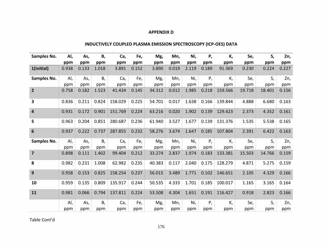
176

APPENDIX D

INDUCTIVELY COUPLED PLASMA EMISSION SPECTROSCOPY (ICP-OES) DATA

Samples No. Al, ppm

As, ppm

B, ppm

Ca, ppm

Fe, ppm

Mg, ppm

Mn, ppm

Ni, ppm

P, ppm

K, ppm

Se, ppm

S, ppm

Zn, ppm

1(initial) 0.938 0.133 1.018 3.891 0.152 3.890 0.019 2.119 0.189 91.369 0.230 0.224 0.227

Samples No. Al, ppm

As, ppm

B, ppm

Ca, ppm

Fe, ppm

Mg, ppm

Mn, ppm

Ni, ppm

P, ppm

K, ppm

Se, ppm

S, ppm

Zn, ppm

2 0.758 0.182 1.523 41.434 0.145 34.312 0.012 1.985 0.218 159.566 19.718 18.401 0.156

3 0.836 0.211 0.824 158.029 0.225 54.701 0.017 1.638 0.166 139.844 4.888 6.680 0.163

4 0.931 0.172 0.901 151.769 0.224 63.216 0.020 1.902 0.139 129.423 2.373 4.352 0.161

5 0.963 0.204 0.851 280.687 0.236 61.940 3.527 1.677 0.139 131.376 1.535 5.538 0.165

6 0.937 0.222 0.737 287.855 0.232 58.276 3.674 1.647 0.185 107.804 2.391 6.422 0.163

Samples No. Al, ppm

As, ppm

B, ppm

Ca, ppm

Fe, ppm

Mg, ppm

Mn, ppm

Ni, ppm

P, ppm

K, ppm

Se, ppm

S, ppm

Zn, ppm

7 0.898 0.111 1.402 99.404 0.212 33.274 2.837 1.974 0.183 133.381 15.503 14.766 0.159

8 0.982 0.231 1.008 62.982 0.235 40.383 0.117 2.040 0.175 128.279 4.871 5.275 0.159

9 0.958 0.153 0.825 158.254 0.237 56.015 3.489 1.771 0.102 146.651 2.105 4.329 0.166

10 0.959 0.135 0.809 135.917 0.244 50.535 4.333 1.701 0.185 100.017 1.165 3.165 0.164

11 0.981 0.066 0.794 137.811 0.224 53.508 4.304 1.651 0.191 116.427 0.918 2.823 0.166

Al, ppm

As, ppm

B, ppm

Ca, ppm

Fe, ppm

Mg, ppm

Mn, ppm

Ni, ppm

P, ppm

K, ppm

Se, ppm

S, ppm

Zn, ppm

Table Cont’d

177

12 0.943 0.212 0.783 170.567 0.064 16.609 2.381 1.911 0.197 136.113 11.133 12.307 0.165

13 0.969 0.138 0.838 190.773 0.231 14.309 0.721 1.925 0.158 146.863 6.718 9.065 0.169

14 0.943 0.120 0.727 110.283 0.228 4.929 0.331 1.926 0.134 110.789 2.503 4.009 0.179

15 0.955 0.063 0.622 121.485 0.218 2.533 0.506 1.940 0.138 131.005 1.592 3.148 0.173

16 0.784 0.202 0.885 136.905 0.226 1.423 0.488 1.891 0.187 130.773 1.307 3.024 0.189

Samples No. Al, ppm

As, ppm

B, ppm

Ca, ppm

Fe, ppm

Mg, ppm

Mn, ppm

Ni, ppm

P, ppm

K, ppm

Se, ppm

S, ppm

Zn, ppm

17 0.992 0.131 1.385 299.766 0.209 155.486 0.026 1.913 0.214 149.931 264.710 252.782 0.180

18 0.850 0.299 0.965 250.543 0.226 43.309 0.154 2.021 0.192 131.438 42.562 43.913 0.170

19 0.925 0.078 0.891 181.867 0.215 19.395 0.179 2.045 0.177 133.871 14.157 15.090 0.170

20 0.861 0.171 0.507 139.011 0.212 11.346 0.130 2.062 0.139 122.004 4.360 5.965 0.182

21 0.936 0.204 0.834 142.500 0.215 7.519 0.179 2.089 0.191 114.017 2.688 4.499 0.183

Samples No. Al, ppm

As, ppm

B, ppm

Ca, ppm

Fe, ppm

Mg, ppm

Mn, ppm

Ni, ppm

P, ppm

K, ppm

Se, ppm

S, ppm

Zn, ppm

22 0.982 0.117 1.331 341.123 0.216 129.537 0.569 1.964 0.152 133.875 214.068 204.079 0.180

23 0.971 0.105 0.669 280.464 0.241 54.869 0.276 2.021 0.139 143.070 44.862 46.500 0.174

24 0.963 0.160 0.709 124.545 0.234 29.227 0.026 2.076 0.176 113.514 8.541 9.695 0.170

25 0.903 0.113 0.760 231.745 0.222 26.108 0.239 1.966 0.170 133.517 3.840 7.110 0.170

26 0.974 0.223 0.672 224.777 0.230 25.617 0.222 2.043 0.128 127.760 2.930 5.811 0.165

Samples No. Al, ppm

As, ppm

B, ppm

Ca, ppm

Fe, ppm

Mg, ppm

Mn, ppm

Ni, ppm

P, ppm

K, ppm

Se, ppm

S, ppm

Zn, ppm

Table Cont’d

178

27 1.005 0.160 1.422 439.562 0.228 163.691 0.544 1.892 0.119 184.273 249.904 238.647 0.173

28 0.955 0.196 0.909 332.542 0.219 43.471 0.321 2.021 0.162 115.198 22.512 25.968 0.167

29 0.980 0.103 0.732 254.728 0.230 33.583 0.299 2.053 0.128 111.499 13.009 15.231 0.169

30 0.972 0.183 0.700 225.436 0.225 35.698 0.235 2.056 0.169 97.375 6.199 9.094 0.171

31 0.792 0.182 0.565 170.797 0.218 29.904 0.372 1.914 0.281 110.092 23.395 24.581 0.184

179

APPENDIX E

MICRO-INDENTATION OF SHALE ROCKS DATA

Properties Time(days) Mancos Marcellus Pottsville Wilcox

Vicker’s Hardness 0 48.74 58.47 34.77 11.59

5 30.56 54.61 36.18 7.39

Young’s Modulus 0 13.29 17.12 17.24 4.19

5 8.02 14.1 11.35 3.05

Rock Type Original SD_Original Runs_AV SD_Runs_AV

Mancos 48.74 3.19 30.56 4.28

Marcellus 58.47 3.27 54.61 4.39

Pottsville 34.77 1.18 36.18 6.33

Wilcox 11.59 1.01 7.39 1.16

180

APPENDIX F

ADDITIONAL DATA FOR ELECTRON MICROPROBE ANALYSIS (EMPA)

Figure G1: 20µm Electron Micro-Probe Analysis for Mancos shale showing Potassium (K) and

Manganese (Mn) surface geochemical profile of the CO2-reacted sample (top row) compared to

control specimen (bottom row). Note the general depletion of elemental components that are


the lower micron resolution presented above. The Scanning Electron Microscopy (SEM) back

scatter image for these profiles is in figure 4.25.

181

Figure G2: 20µm Electron Micro-Probe Analysis for Mancos shale showing Zinc (Zn) and Chlorine

(Cl) surface geochemical profile of the CO2-reacted sample (top row) compared to control





182

Figure G3: 20µm Electron Micro-Probe Analysis for Marcellus shale showing Potassium (K) and






183

Figure G4: 20µm Electron Micro-Probe Analysis for Marcellus shale showing Zinc (Zn) and

Chlorine (Cl) surface geochemical profile of the CO2-reacted sample (top row) compared to





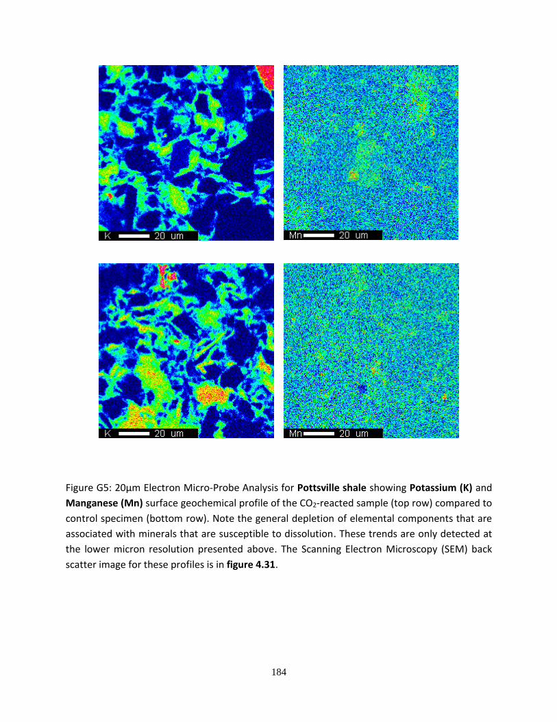
184

Figure G5: 20µm Electron Micro-Probe Analysis for Pottsville shale showing Potassium (K) and






185

Figure G6: 20µm Electron Micro-Probe Analysis for Pottsville shale showing Zinc (Zn) and

Chlorine (Cl) surface geochemical profile of the CO2-reacted sample (top row) compared to





186

Figure G7: 20µm Electron Micro-Probe Analysis for Wilcox shale showing Potassium (K) and






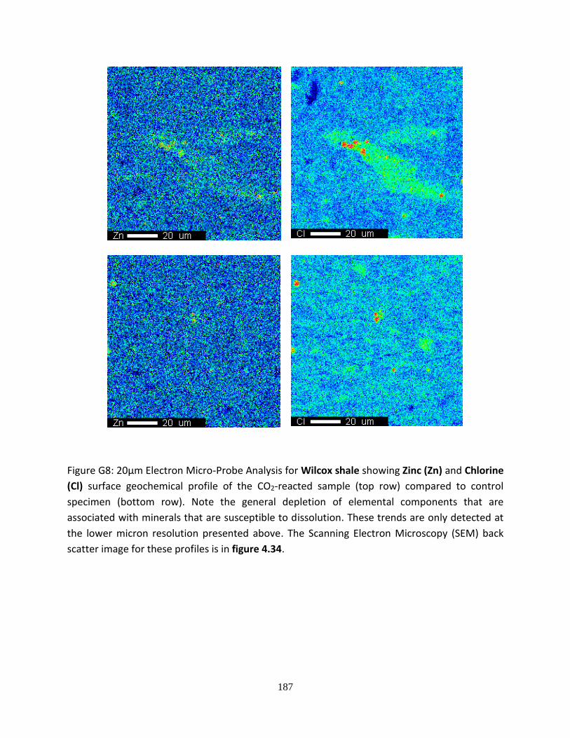
187

Figure G8: 20µm Electron Micro-Probe Analysis for Wilcox shale showing Zinc (Zn) and Chlorine

(Cl) surface geochemical profile of the CO2-reacted sample (top row) compared to control





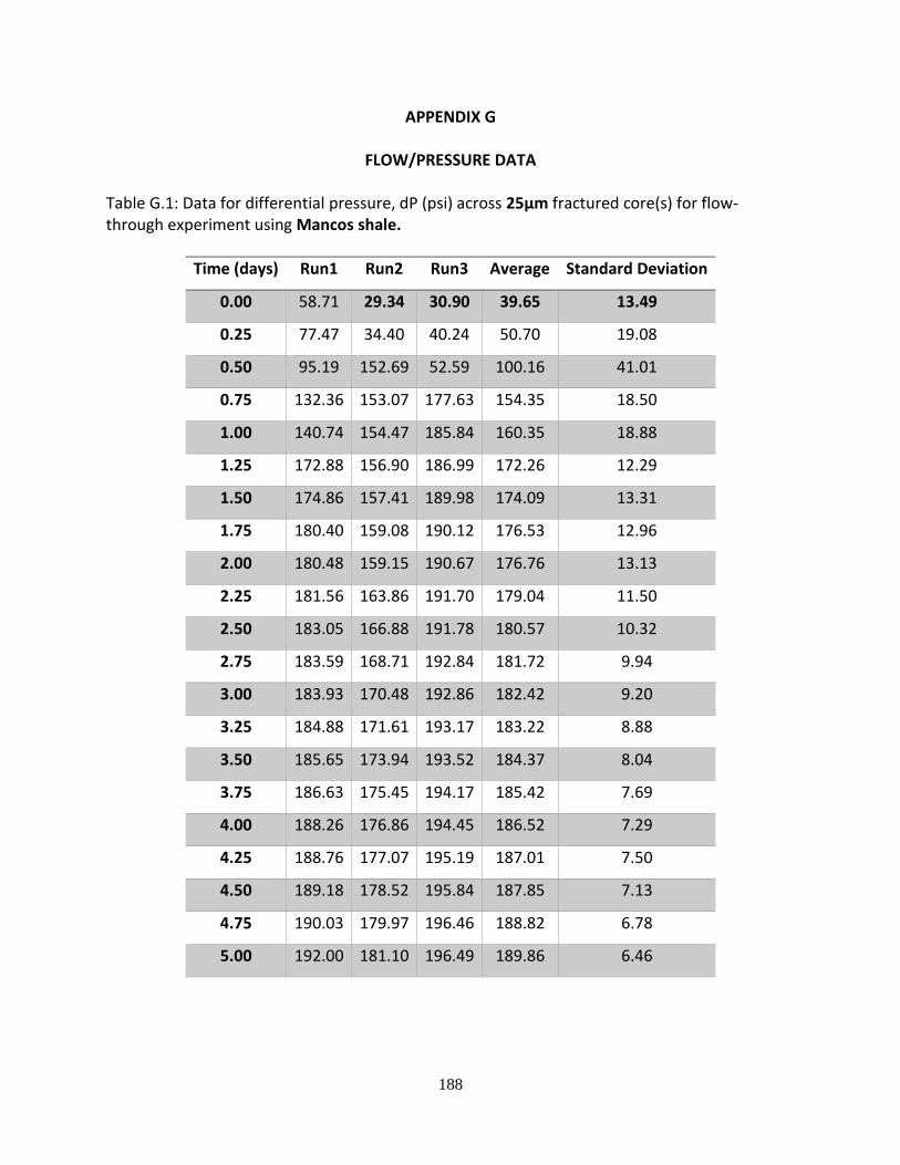
188

APPENDIX G

FLOW/PRESSURE DATA

Table G.1: Data for differential pressure, dP (psi) across 25µm fractured core(s) for flow-through experiment using Mancos shale.

Time (days) Run1 Run2 Run3 Average Standard Deviation

0.00 58.71 29.34 30.90 39.65 13.49

0.25 77.47 34.40 40.24 50.70 19.08

0.50 95.19 152.69 52.59 100.16 41.01

0.75 132.36 153.07 177.63 154.35 18.50

1.00 140.74 154.47 185.84 160.35 18.88

1.25 172.88 156.90 186.99 172.26 12.29

1.50 174.86 157.41 189.98 174.09 13.31

1.75 180.40 159.08 190.12 176.53 12.96

2.00 180.48 159.15 190.67 176.76 13.13

2.25 181.56 163.86 191.70 179.04 11.50

2.50 183.05 166.88 191.78 180.57 10.32

2.75 183.59 168.71 192.84 181.72 9.94

3.00 183.93 170.48 192.86 182.42 9.20

3.25 184.88 171.61 193.17 183.22 8.88

3.50 185.65 173.94 193.52 184.37 8.04

3.75 186.63 175.45 194.17 185.42 7.69

4.00 188.26 176.86 194.45 186.52 7.29

4.25 188.76 177.07 195.19 187.01 7.50

4.50 189.18 178.52 195.84 187.85 7.13

4.75 190.03 179.97 196.46 188.82 6.78

5.00 192.00 181.10 196.49 189.86 6.46

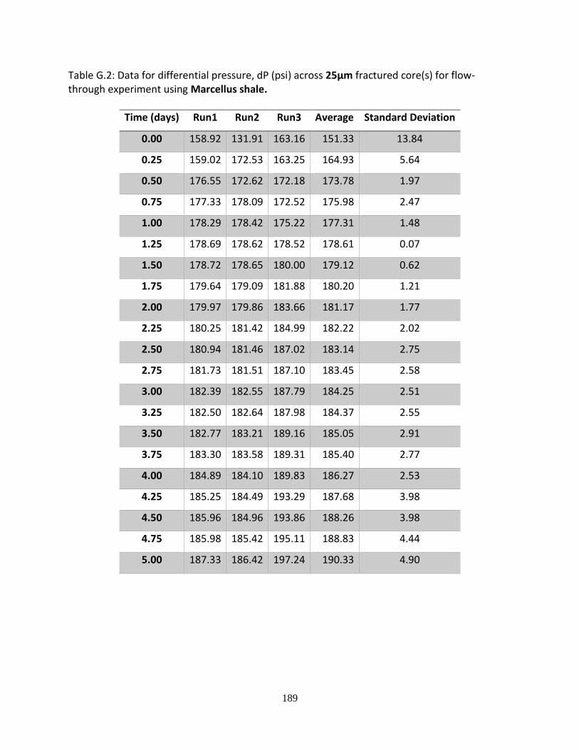
189

Table G.2: Data for differential pressure, dP (psi) across 25µm fractured core(s) for flow-through experiment using Marcellus shale.


0.00 158.92 131.91 163.16 151.33 13.84

0.25 159.02 172.53 163.25 164.93 5.64

0.50 176.55 172.62 172.18 173.78 1.97

0.75 177.33 178.09 172.52 175.98 2.47

1.00 178.29 178.42 175.22 177.31 1.48

1.25 178.69 178.62 178.52 178.61 0.07

1.50 178.72 178.65 180.00 179.12 0.62

1.75 179.64 179.09 181.88 180.20 1.21

2.00 179.97 179.86 183.66 181.17 1.77

2.25 180.25 181.42 184.99 182.22 2.02

2.50 180.94 181.46 187.02 183.14 2.75

2.75 181.73 181.51 187.10 183.45 2.58

3.00 182.39 182.55 187.79 184.25 2.51

3.25 182.50 182.64 187.98 184.37 2.55

3.50 182.77 183.21 189.16 185.05 2.91

3.75 183.30 183.58 189.31 185.40 2.77

4.00 184.89 184.10 189.83 186.27 2.53

4.25 185.25 184.49 193.29 187.68 3.98

4.50 185.96 184.96 193.86 188.26 3.98

4.75 185.98 185.42 195.11 188.83 4.44

5.00 187.33 186.42 197.24 190.33 4.90

190

Table G.3: Data for differential pressure, dP (psi) across 25µm fractured core(s) for flow-through experiment using Pottsville shale.


0.00 41.89 41.89 32.55 38.78 4.40

0.25 85.83 85.83 118.89 96.85 15.58

0.50 99.79 99.79 121.19 106.93 10.09

0.75 125.53 125.53 137.63 129.56 5.70

1.00 126.54 126.54 157.07 136.72 14.39

1.25 126.84 126.84 164.56 139.41 17.78

1.50 128.18 128.18 166.09 140.81 17.87

1.75 128.35 128.35 167.68 141.46 18.54

2.00 128.96 128.96 168.34 142.09 18.56

2.25 129.45 129.45 168.49 142.47 18.40

2.50 130.22 130.22 168.58 143.01 18.08

2.75 147.43 147.43 169.07 154.65 10.20

3.00 147.68 147.68 169.30 154.88 10.19

3.25 148.83 148.83 169.59 155.75 9.79

3.50 149.65 149.65 170.37 156.56 9.77

3.75 149.69 149.69 172.03 157.14 10.53

4.00 150.23 150.23 172.73 157.73 10.60

4.25 150.78 150.78 172.90 158.15 10.43

4.50 152.48 152.48 175.72 160.22 10.95

4.75 153.50 153.50 175.98 160.99 10.60

5.00 154.35 154.35 177.79 162.17 11.05

191

Table G.4: Data for differential pressure, dP (psi) across 25µm fractured core(s) for flow-through experiment using Wilcox shale.


0.00 33.00 65.00 95.35 64.45 25.46

0.25 55.57 92.51 132.29 93.46 31.33

0.50 70.02 93.07 132.40 98.50 25.75

0.75 88.35 94.76 132.48 105.20 19.47

1.00 108.34 126.32 132.56 122.41 10.27

1.25 116.50 126.89 132.67 125.35 6.69

1.50 120.75 131.84 132.77 128.45 5.46

1.75 121.69 140.15 132.87 131.57 7.59

2.00 124.95 150.25 132.99 136.06 10.55

2.25 143.06 152.59 133.41 143.02 7.83

2.50 143.51 153.17 139.45 145.38 5.75

2.75 157.23 158.46 139.91 151.87 8.47

3.00 163.60 158.99 141.91 154.84 9.33

3.25 164.59 160.21 143.64 156.15 9.02

3.50 164.90 170.15 143.90 159.65 11.34

3.75 166.16 171.86 147.42 161.81 10.44

4.00 167.47 173.48 165.33 168.76 3.45

4.25 167.75 173.74 166.63 169.37 3.12

4.50 172.22 178.07 166.82 172.37 4.59

4.75 176.49 180.72 169.39 175.53 4.68

5.00 179.42 180.83 170.63 176.96 4.51

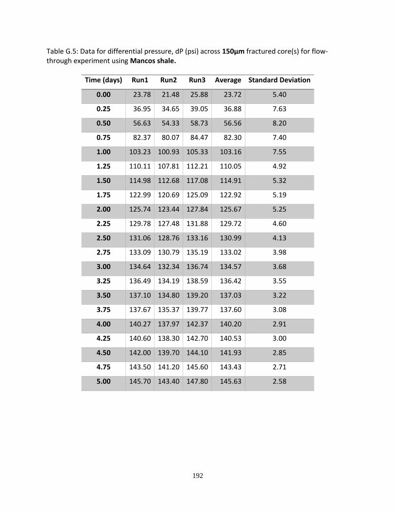
192

Table G.5: Data for differential pressure, dP (psi) across 150µm fractured core(s) for flow-through experiment using Mancos shale.


0.00 23.78 21.48 25.88 23.72 5.40

0.25 36.95 34.65 39.05 36.88 7.63

0.50 56.63 54.33 58.73 56.56 8.20

0.75 82.37 80.07 84.47 82.30 7.40

1.00 103.23 100.93 105.33 103.16 7.55

1.25 110.11 107.81 112.21 110.05 4.92

1.50 114.98 112.68 117.08 114.91 5.32

1.75 122.99 120.69 125.09 122.92 5.19

2.00 125.74 123.44 127.84 125.67 5.25

2.25 129.78 127.48 131.88 129.72 4.60

2.50 131.06 128.76 133.16 130.99 4.13

2.75 133.09 130.79 135.19 133.02 3.98

3.00 134.64 132.34 136.74 134.57 3.68

3.25 136.49 134.19 138.59 136.42 3.55

3.50 137.10 134.80 139.20 137.03 3.22

3.75 137.67 135.37 139.77 137.60 3.08

4.00 140.27 137.97 142.37 140.20 2.91

4.25 140.60 138.30 142.70 140.53 3.00

4.50 142.00 139.70 144.10 141.93 2.85

4.75 143.50 141.20 145.60 143.43 2.71

5.00 145.70 143.40 147.80 145.63 2.58

193

Table G.6: Data for differential pressure, dP (psi) across 150µm fractured core(s) for flow-through experiment using Marcellus shale.


0.00 32.81 30.92 34.52 32.75 6.92

0.25 52.25 50.36 53.96 52.19 7.90

0.50 91.80 89.91 93.51 91.74 2.75

0.75 127.10 125.21 128.81 127.04 3.45

1.00 135.08 133.19 136.79 135.02 2.07

1.25 139.68 137.79 141.39 139.62 1.28

1.50 143.17 141.28 144.88 143.11 1.29

1.75 144.10 142.21 145.81 144.04 1.69

2.00 145.30 143.41 147.01 145.24 2.47

2.25 146.70 144.81 148.41 146.64 2.83

2.50 147.20 145.31 148.91 147.14 3.86

2.75 148.90 147.01 150.61 148.84 3.61

3.00 149.10 147.21 150.81 149.04 3.51

3.25 149.80 147.91 151.51 149.74 3.57

3.50 149.90 148.01 151.61 149.84 4.08

3.75 150.30 148.41 152.01 150.24 3.87

4.00 150.50 148.61 152.21 150.44 3.55

4.25 150.60 148.71 152.31 150.54 5.57

4.50 150.90 149.01 152.61 150.84 5.58

4.75 151.30 149.41 153.01 151.24 6.22

5.00 151.60 149.71 153.31 151.54 6.86

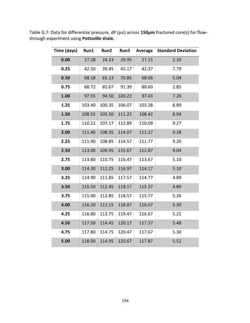
194

Table G.7: Data for differential pressure, dP (psi) across 150µm fractured core(s) for flow-through experiment using Pottsville shale.


0.00 27.28 24.23 29.95 27.15 2.20

0.25 42.50 39.45 45.17 42.37 7.79

0.50 68.18 65.13 70.85 68.06 5.04

0.75 88.72 85.67 91.39 88.60 2.85

1.00 97.55 94.50 100.22 97.43 7.20

1.25 103.40 100.35 106.07 103.28 8.89

1.50 108.55 105.50 111.22 108.42 8.94

1.75 110.22 107.17 112.89 110.09 9.27

2.00 111.40 108.35 114.07 111.27 9.28

2.25 111.90 108.85 114.57 111.77 9.20

2.50 113.00 109.95 115.67 112.87 9.04

2.75 113.80 110.75 116.47 113.67 5.10

3.00 114.30 111.25 116.97 114.17 5.10

3.25 114.90 111.85 117.57 114.77 4.89

3.50 115.50 112.45 118.17 115.37 4.89

3.75 115.90 112.85 118.57 115.77 5.26

4.00 116.20 113.15 118.87 116.07 5.30

4.25 116.80 113.75 119.47 116.67 5.21

4.50 117.50 114.45 120.17 117.37 5.48

4.75 117.80 114.75 120.47 117.67 5.30

5.00 118.00 114.95 120.67 117.87 5.52

195

Table G.8: Data for differential pressure, dP (psi) across 150µm fractured core(s) for flow-through experiment using Wilcox shale.


0.00 25.78 24.54 27.89 26.07 14.76

0.25 39.03 37.79 41.14 39.32 9.40

0.50 65.40 64.16 67.51 65.69 14.94

0.75 87.00 85.76 89.11 87.29 11.29

1.00 91.94 90.70 94.05 92.23 5.96

1.25 94.30 93.06 96.41 94.59 3.88

1.50 95.74 94.50 97.85 96.03 3.17

1.75 99.25 98.01 101.36 99.54 4.40

2.00 100.94 99.70 103.05 101.23 6.12

2.25 102.00 100.76 104.11 102.29 4.54

2.50 103.90 102.66 106.01 104.19 3.34

2.75 105.00 103.76 107.11 105.29 4.91

3.00 106.40 105.16 108.51 106.69 5.41

3.25 107.10 105.86 109.21 107.39 5.23

3.50 108.00 106.76 110.11 108.29 6.58

3.75 108.50 107.26 110.61 108.79 6.05

4.00 108.90 107.66 111.01 109.19 2.00

4.25 109.70 108.46 111.81 109.99 1.81

4.50 110.10 108.86 112.21 110.39 2.66

4.75 111.00 109.76 113.11 111.29 2.71

5.00 111.90 110.66 114.01 112.19 2.62

196

APPENDIX H

FRACTURE CONDUCTIVITY DATA AND CALCULATIONS

Table H.1: Steps, equations and assumptions were made in calculating the fracture conductivity of the cores used during the experiments.

Steps Equations Assumptions

1. Put averaged values of dP from three experiments /per core in tabular form. 2. Declare and specify parameters (in approximate units) such as viscosity, fracture length, flow rate 3. Calculate average fracture width from experimental data 4. Estimate dimensionless fracture conductivity over time from fracture width and fracture length using the relationship shown in the list of equations

𝑘𝑓 = 8.45 × 109 𝑤𝑓2

𝑘𝑓 = 𝑘𝑎𝑣𝐴 − 𝑘𝑚(𝐴 − 𝑤𝑓𝑙)

𝑤𝑓𝑙

8.45 × 109 𝑤𝑓3𝑙 − 𝑘𝑎𝑣𝐴

+ 𝑘𝑚(𝐴 − 𝑤𝑓𝑙) = 0

𝑞𝑚 = 𝑘𝑚𝐴∆𝑃

𝜇𝐿

𝑞𝑓 = 9.86 × 109 𝑤𝑓

3𝑙∆𝑃

12𝜇𝐿𝑓

𝑤𝑓𝑘𝑓 = 𝜋𝐶𝑟𝑘𝐿𝑓

𝑤𝑓 = √𝑞𝑓 × 12𝜇

9.86 × 109∆𝑃

3

𝐶𝑟 = 𝑤𝑓𝑘𝑓

𝜋𝐾𝑎𝑣𝐿𝑓 ≈

𝑤𝑓

𝜋𝐿𝑓

1. Flow is primarily through fractures 2. Bulk fracture flow properties are captured in the experimental differential pressure measurements 3. CO2-brine viscosity is constant throughout the experiment 4. Length of the core(s), for each experimental run, approximates the fracture length. 5. Tortuosity of fracture geometry is unity 6. Effect of fracture surface roughness is negligible 7. Microtubes are made of polymeric materials (PEEK), does not interfere at all with dissolution-precipitation process

197

VITA

Abiola Olabode is the third child of a family of three children. He attended Government College

Ibadan and Command Day Secondary School Odogbo for his secondary education. He later

proceeded to Obafemi Awolowo University, Ile Ife where in 2008, he earned a Bachelor’s degree

in Chemical Engineering with honors. Abiola worked with Pan Ocean Oil Corporation in Lagos,

Nigeria between 2008 and 2010 as a natural gas Process Engineer helping with the design of

multi-stage NGL recovery systems. He joined the graduate program of the Craft & Hawkins

Department of Petroleum Engineering in 2010 and obtained a Master of Science degree with

Thesis in December 2012. His doctoral program began in January of 2013. He has co-authored

several peer-reviewed research articles and conference papers during his graduate studies

(https://scholar.google.com/citations?user=TrkUbtQAAAAJ&hl=en).

Experimental-Modelling Approach in CO2-Rock Interaction

Documents

Transcript of Experimental-Modelling Approach in CO2-Rock Interaction