Experimental investigation of thermal and fluid dynamical ...
258
HAL Id: tel-00961231 https://tel.archives-ouvertes.fr/tel-00961231 Submitted on 19 Mar 2014 HAL is a multi-disciplinary open access archive for the deposit and dissemination of sci- entific research documents, whether they are pub- lished or not. The documents may come from teaching and research institutions in France or abroad, or from public or private research centers. L’archive ouverte pluridisciplinaire HAL, est destinée au dépôt et à la diffusion de documents scientifiques de niveau recherche, publiés ou non, émanant des établissements d’enseignement et de recherche français ou étrangers, des laboratoires publics ou privés. Experimental investigation of thermal and fluid dynamical behavior of flows in open-ended channels : Application to Building Integrated Photovoltaic (BiPV) Systems Estibaliz Sanvicente To cite this version: Estibaliz Sanvicente. Experimental investigation of thermal and fluid dynamical behavior of flows in open-ended channels : Application to Building Integrated Photovoltaic (BiPV) Systems. Other [cond-mat.other]. INSA de Lyon, 2013. English. NNT : 2013ISAL0061. tel-00961231
-
Upload
khangminh22 -
Category
Documents
-
view
3 -
download
0
Transcript of Experimental investigation of thermal and fluid dynamical ...
HAL Id: tel-00961231https://tel.archives-ouvertes.fr/tel-00961231
Submitted on 19 Mar 2014
HAL is a multi-disciplinary open accessarchive for the deposit and dissemination of sci-entific research documents, whether they are pub-lished or not. The documents may come fromteaching and research institutions in France orabroad, or from public or private research centers.
L’archive ouverte pluridisciplinaire HAL, estdestinée au dépôt et à la diffusion de documentsscientifiques de niveau recherche, publiés ou non,émanant des établissements d’enseignement et derecherche français ou étrangers, des laboratoirespublics ou privés.
Experimental investigation of thermal and fluiddynamical behavior of flows in open-ended channels :
Application to Building Integrated Photovoltaic (BiPV)Systems
Estibaliz Sanvicente
To cite this version:Estibaliz Sanvicente. Experimental investigation of thermal and fluid dynamical behavior of flowsin open-ended channels : Application to Building Integrated Photovoltaic (BiPV) Systems. Other[cond-mat.other]. INSA de Lyon, 2013. English. NNT : 2013ISAL0061. tel-00961231
N° d’ordre: 2013-ISAL-0061 Année 2013
Thèse
Experimental investigation of thermal and
fluid dynamical behavior of flows in open-
ended channels
--- APPLICATION TO BUILDING INTEGRATED PHOTOVOLTAIC
(BIPV) SYSTEMS
Présentée devant
L’institut national des sciences appliquées de Lyon
Pour obtenir
Le grade de docteur
Formation doctorale: Énergétique
École doctorale: Mécanique, Énergétique, Génie Civil, Acoustique
Par
Estibaliz Sanvicente Quintanilla
Soutenue le 03 Juillet 2013 devant la Commission d’examen
Jury MM.
Rapporteur S. FOHANNO Maître de Conférences HDR (Université de Reims)
Rapporteur M. FOSSA Professeur (Università degli study di Genova)
S. GIROUX-JULIEN Maître de Conférences (Université Claude Bernard Lyon 1)
S. LASSUE Professeur (Université d’Artois)
C. MENEZO Professeur (Chaire EDF-INSA de LYON)
J. REIZES Professeur emeritus (University of New South Wales)
V. TIMCHENKO Maître de Conférences HDR (University of New South Wales)
S. XIN Professeur (INSA de LYON)
Laboratoire de recherche : Centre Thermique de Lyon (CETHIL) / CFD Laboratory (UNSW)
Cette thèse est accessible à l'adresse : http://theses.insa-lyon.fr/publication/2013ISAL0061/these.pdf © [E. Sanvicente Quintanilla], [2013], INSA de Lyon, tous droits réservés

Cette thèse est accessible à l'adresse : http://theses.insa-lyon.fr/publication/2013ISAL0061/these.pdf © [E. Sanvicente Quintanilla], [2013], INSA de Lyon, tous droits réservés
i
INSA Direction de la Recherche - Ecoles Doctorales – Quinquennal 2011-2015
SIGLE ECOLE DOCTORALE NOM ET COORDONNEES DU RESPONSABLE
CHIMIE
CHIMIE DE LYON
http://www.edchimie-lyon.fr
Insa : R. GOURDON
M. Jean Marc LANCELIN Université de Lyon – Collège Doctoral Bât ESCPE
43 bd du 11 novembre 1918 69622 VILLEURBANNE Cedex
Tél : 04.72.43 13 95 [email protected]
E.E.A.
ELECTRONIQUE,
ELECTROTECHNIQUE, AUTOMATIQUE
http://edeea.ec-lyon.fr
Secrétariat : M.C. HAVGOUDOUKIAN
M. Gérard SCORLETTI Ecole Centrale de Lyon
36 avenue Guy de Collongue 69134 ECULLY
Tél : 04.72.18 65 55 Fax : 04 78 43 37 17 [email protected]
E2M2
EVOLUTION, ECOSYSTEME, MICROBIOLOGIE, MODELISATION
http://e2m2.universite-lyon.fr
Insa : H. CHARLES
Mme Gudrun BORNETTE CNRS UMR 5023 LEHNA
Université Claude Bernard Lyon 1 Bât Forel
43 bd du 11 novembre 1918
69622 VILLEURBANNE Cédex Tél : 06.07.53.89.13
e2m2@ univ-lyon1.fr
EDISS
INTERDISCIPLINAIRE SCIENCES-
SANTE
http://www.ediss-lyon.fr
Sec : Samia VUILLERMOZ
Insa : M. LAGARDE
M. Didier REVEL Hôpital Louis Pradel Bâtiment Central
28 Avenue Doyen Lépine 69677 BRON
Tél : 04.72.68.49.09 Fax :04 72 68 49 16 [email protected]
INFOMATHS
INFORMATIQUE ET MATHEMATIQUES
http://infomaths.univ-lyon1.fr
Sec :Renée EL MELHEM
Mme Sylvie CALABRETTO Université Claude Bernard Lyon 1
INFOMATHS Bâtiment Braconnier
43 bd du 11 novembre 1918 69622 VILLEURBANNE Cedex
Tél : 04.72. 44.82.94 Fax 04 72 43 16 87 [email protected]
Matériaux
MATERIAUX DE LYON
http://ed34.universite-lyon.fr
Secrétariat : M. LABOUNE
PM : 71.70 –Fax : 87.12
Bat. Saint Exupéry
M. Jean-Yves BUFFIERE INSA de Lyon
MATEIS Bâtiment Saint Exupéry
7 avenue Jean Capelle 69621 VILLEURBANNE Cedex
Tél : 04.72.43 83 18 Fax 04 72 43 85 28 [email protected]
MEGA
MECANIQUE, ENERGETIQUE, GENIE
CIVIL, ACOUSTIQUE
http://mega.ec-lyon.fr
Secrétariat : M. LABOUNE
PM : 71.70 –Fax : 87.12
Bat. Saint Exupéry [email protected]
M. Philippe BOISSE INSA de Lyon
Laboratoire LAMCOS Bâtiment Jacquard
25 bis avenue Jean Capelle 69621 VILLEURBANNE Cedex
Tél :04.72 .43.71.70 Fax : 04 72 43 72 37 [email protected]
ScSo
ScSo*
http://recherche.univ-lyon2.fr/scso/
Sec : Viviane POLSINELLI
Brigitte DUBOIS
Insa : J.Y. TOUSSAINT
M. OBADIA Lionel Université Lyon 2
86 rue Pasteur 69365 LYON Cedex 07
Tél : 04.78.77.23.86 Fax : 04.37.28.04.48 [email protected]
*ScSo : Histoire, Géographie, Aménagement, Urbanisme, Archéologie, Science politique, Sociologie, Anthropologie
Cette thèse est accessible à l'adresse : http://theses.insa-lyon.fr/publication/2013ISAL0061/these.pdf © [E. Sanvicente Quintanilla], [2013], INSA de Lyon, tous droits réservés

ii
Cette thèse est accessible à l'adresse : http://theses.insa-lyon.fr/publication/2013ISAL0061/these.pdf © [E. Sanvicente Quintanilla], [2013], INSA de Lyon, tous droits réservés

iii
A los míos, a mi gente, y en especial, a mis aitas.
Cette thèse est accessible à l'adresse : http://theses.insa-lyon.fr/publication/2013ISAL0061/these.pdf © [E. Sanvicente Quintanilla], [2013], INSA de Lyon, tous droits réservés

iv
Cette thèse est accessible à l'adresse : http://theses.insa-lyon.fr/publication/2013ISAL0061/these.pdf © [E. Sanvicente Quintanilla], [2013], INSA de Lyon, tous droits réservés
v
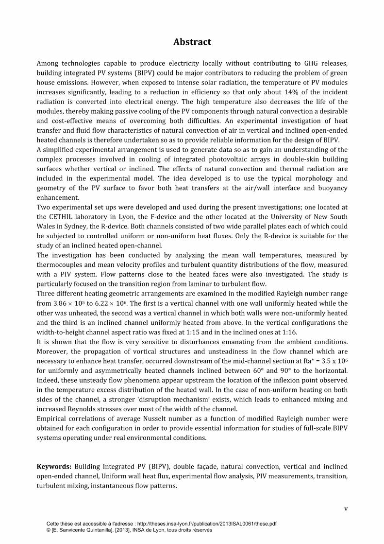
Abstract
Among technologies capable to produce electricity locally without contributing to GHG releases,
building integrated PV systems (BIPV) could be major contributors to reducing the problem of green
house emissions. However, when exposed to intense solar radiation, the temperature of PV modules
increases significantly, leading to a reduction in efficiency so that only about 14% of the incident
radiation is converted into electrical energy. The high temperature also decreases the life of the
modules, thereby making passive cooling of the PV components through natural convection a desirable
and cost-effective means of overcoming both difficulties. An experimental investigation of heat
transfer and fluid flow characteristics of natural convection of air in vertical and inclined open-ended
heated channels is therefore undertaken so as to provide reliable information for the design of BIPV.
A simplified experimental arrangement is used to generate data so as to gain an understanding of the
complex processes involved in cooling of integrated photovoltaic arrays in double-skin building
surfaces whether vertical or inclined. The effects of natural convection and thermal radiation are
included in the experimental model. The idea developed is to use the typical morphology and
geometry of the PV surface to favor both heat transfers at the air/wall interface and buoyancy
enhancement.
Two experimental set ups were developed and used during the present investigations; one located at
the CETHIL laboratory in Lyon, the F-device and the other located at the University of New South
Wales in Sydney, the R-device. Both channels consisted of two wide parallel plates each of which could
be subjected to controlled uniform or non-uniform heat fluxes. Only the R-device is suitable for the
study of an inclined heated open-channel.
The investigation has been conducted by analyzing the mean wall temperatures, measured by
thermocouples and mean velocity profiles and turbulent quantity distributions of the flow, measured
with a PIV system. Flow patterns close to the heated faces were also investigated. The study is
particularly focused on the transition region from laminar to turbulent flow.
Three different heating geometric arrangements are examined in the modified Rayleigh number range
from 3.86 105 to 6.22 106. The first is a vertical channel with one wall uniformly heated while the
other was unheated, the second was a vertical channel in which both walls were non-uniformly heated
and the third is an inclined channel uniformly heated from above. In the vertical configurations the
width-to-height channel aspect ratio was fixed at 1:15 and in the inclined ones at 1:16.
It is shown that the flow is very sensitive to disturbances emanating from the ambient conditions.
Moreover, the propagation of vortical structures and unsteadiness in the flow channel which are
necessary to enhance heat transfer, occurred downstream of the mid-channel section at Ra* = 3.5 x 10⁶
for uniformly and asymmetrically heated channels inclined between 60° and 90° to the horizontal.
Indeed, these unsteady flow phenomena appear upstream the location of the inflexion point observed
in the temperature excess distribution of the heated wall. In the case of non-uniform heating on both
sides of the channel, a stronger ‘disruption mechanism’ exists, which leads to enhanced mixing and
increased Reynolds stresses over most of the width of the channel.
Empirical correlations of average Nusselt number as a function of modified Rayleigh number were
obtained for each configuration in order to provide essential information for studies of full-scale BIPV
systems operating under real environmental conditions.
Keywords: Building Integrated PV (BIPV), double façade, natural convection, vertical and inclined
open-ended channel, Uniform wall heat flux, experimental flow analysis, PIV measurements, transition,
turbulent mixing, instantaneous flow patterns.
Cette thèse est accessible à l'adresse : http://theses.insa-lyon.fr/publication/2013ISAL0061/these.pdf © [E. Sanvicente Quintanilla], [2013], INSA de Lyon, tous droits réservés

vi
Cette thèse est accessible à l'adresse : http://theses.insa-lyon.fr/publication/2013ISAL0061/these.pdf © [E. Sanvicente Quintanilla], [2013], INSA de Lyon, tous droits réservés
vii
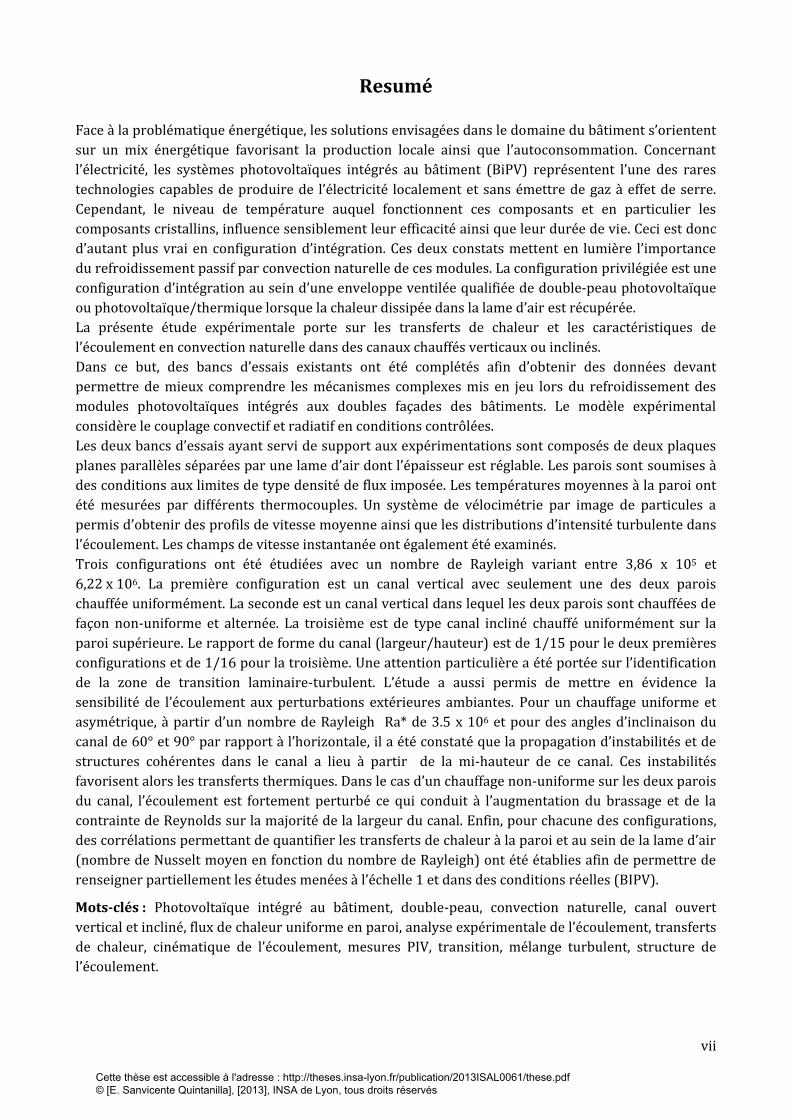
Resumé
Face à la problématique énergétique, les solutions envisagées dans le domaine du bâtiment s’orientent
sur un mix énergétique favorisant la production locale ainsi que l’autoconsommation. Concernant
l’électricité, les systèmes photovoltaïques intégrés au bâtiment (BiPV) représentent l’une des rares
technologies capables de produire de l’électricité localement et sans émettre de gaz à effet de serre.
Cependant, le niveau de température auquel fonctionnent ces composants et en particulier les
composants cristallins, influence sensiblement leur efficacité ainsi que leur durée de vie. Ceci est donc
d’autant plus vrai en configuration d’intégration. Ces deux constats mettent en lumière l’importance
du refroidissement passif par convection naturelle de ces modules. La configuration privilégiée est une
configuration d’intégration au sein d’une enveloppe ventilée qualifiée de double-peau photovoltaïque
ou photovoltaïque/thermique lorsque la chaleur dissipée dans la lame d’air est récupérée.
La présente étude expérimentale porte sur les transferts de chaleur et les caractéristiques de
l’écoulement en convection naturelle dans des canaux chauffés verticaux ou inclinés.
Dans ce but, des bancs d’essais existants ont été complétés afin d’obtenir des données devant
permettre de mieux comprendre les mécanismes complexes mis en jeu lors du refroidissement des
modules photovoltaïques intégrés aux doubles façades des bâtiments. Le modèle expérimental
considère le couplage convectif et radiatif en conditions contrôlées.
Les deux bancs d’essais ayant servi de support aux expérimentations sont composés de deux plaques
planes parallèles séparées par une lame d’air dont l’épaisseur est réglable. Les parois sont soumises à
des conditions aux limites de type densité de flux imposée. Les températures moyennes à la paroi ont
été mesurées par différents thermocouples. Un système de vélocimétrie par image de particules a
permis d’obtenir des profils de vitesse moyenne ainsi que les distributions d’intensité turbulente dans
l’écoulement. Les champs de vitesse instantanée ont également été examinés.
Trois configurations ont été étudiées avec un nombre de Rayleigh variant entre 3,86 x 10⁵ et
6,22 x 10⁶. La première configuration est un canal vertical avec seulement une des deux parois
chauffée uniformément. La seconde est un canal vertical dans lequel les deux parois sont chauffées de
façon non-uniforme et alternée. La troisième est de type canal incliné chauffé uniformément sur la
paroi supérieure. Le rapport de forme du canal (largeur/hauteur) est de 1/15 pour le deux premières
configurations et de 1/16 pour la troisième. Une attention particulière a été portée sur l’identification
de la zone de transition laminaire-turbulent. L’étude a aussi permis de mettre en évidence la
sensibilité de l’écoulement aux perturbations extérieures ambiantes. Pour un chauffage uniforme et
asymétrique, à partir d’un nombre de Rayleigh Ra* de 3.5 x 10⁶ et pour des angles d’inclinaison du
canal de 60° et 90° par rapport à l’horizontale, il a été constaté que la propagation d’instabilités et de
structures cohérentes dans le canal a lieu à partir de la mi-hauteur de ce canal. Ces instabilités
favorisent alors les transferts thermiques. Dans le cas d’un chauffage non-uniforme sur les deux parois
du canal, l’écoulement est fortement perturbé ce qui conduit à l’augmentation du brassage et de la
contrainte de Reynolds sur la majorité de la largeur du canal. Enfin, pour chacune des configurations,
des corrélations permettant de quantifier les transferts de chaleur à la paroi et au sein de la lame d’air
(nombre de Nusselt moyen en fonction du nombre de Rayleigh) ont été établies afin de permettre de
renseigner partiellement les études menées à l’échelle 1 et dans des conditions réelles (BIPV).
Mots-clés : Photovoltaïque intégré au bâtiment, double-peau, convection naturelle, canal ouvert
vertical et incliné, flux de chaleur uniforme en paroi, analyse expérimentale de l’écoulement, transferts
de chaleur, cinématique de l’écoulement, mesures PIV, transition, mélange turbulent, structure de
l’écoulement.
Cette thèse est accessible à l'adresse : http://theses.insa-lyon.fr/publication/2013ISAL0061/these.pdf © [E. Sanvicente Quintanilla], [2013], INSA de Lyon, tous droits réservés

viii
Cette thèse est accessible à l'adresse : http://theses.insa-lyon.fr/publication/2013ISAL0061/these.pdf © [E. Sanvicente Quintanilla], [2013], INSA de Lyon, tous droits réservés
ix
Nomenclature
Symbols
a discrete heat source height M
A cross sectional area of the channel (L x D) m2
Bq Buoyancy flux
c pressure loss coefficient
C mean number density of tracer particles particles. m-3
Ck correction coefficient applied to 1D Fourier law
Cp specific heat capacity at constant pressure J.kg-1.K-1
C* global thermal conductance
d diameter M
particle image diameter M
D wall separating distance, diameter of the bead M
Da diameter of aperture of the camera M
DH hydraulic diameter
E discrepancy between tests %
f friction factor along the height of channel
fc cut-off frequency Hz
fl focal length M
F flatness factor
h heat transfer coefficient, W.m-2.K-1
H channel height M
Cette thèse est accessible à l'adresse : http://theses.insa-lyon.fr/publication/2013ISAL0061/these.pdf © [E. Sanvicente Quintanilla], [2013], INSA de Lyon, tous droits réservés

x
k thermal conductivity W.m-1.K-1
Kf1 friction factor at the entrance of the channel
Kf2 friction factor at the exit of the channel
li size of the interrogation window M
L width of the plate M
mass flow rate kg.s-1
Ni mean number of particles / interrogation window
NuD Nusselt number based on the width of the channel
M magnification factor
Pelec local electric heat flux injected W.m-2
PS1 power injected in wall S1 W
PS2 power injected in wall S2 W
qs imposed heat current through the heat source W.m-1
Q volumetric flow rate m3.s-1
r0 thickness of the light sheet M
Ra* Average modified Rayleigh number
Ray Local Rayleigh number
S skewness factor
St stratification parameter
Cette thèse est accessible à l'adresse : http://theses.insa-lyon.fr/publication/2013ISAL0061/these.pdf © [E. Sanvicente Quintanilla], [2013], INSA de Lyon, tous droits réservés

xi
thf thickness of heating foil M
US velocity deviation between a tracer particle and fluid m.s-1
x horizontal coordinate, perpendicular to the channel walls
M
X position vector of the particle M
z horizontal coordinate, parallel to the channel walls M
Greek letters
thermal diffusivity, m2.s-1
coefficient of thermal expansion K-1
emissivity of the surface
Efficiency
inclination angle of the channel to the horizontal ˚
wavelength of light nm
kinematic viscosity m2.s-1
temperature efficiency degradation coefficient %/K
Density kg.m-3
relaxation time of the particles S
convective flux W.m-2
conductive flux in the x-direction W.m-2
conductive flux in the y-direction W.m-2
net radiative flux W.m-2
Cette thèse est accessible à l'adresse : http://theses.insa-lyon.fr/publication/2013ISAL0061/these.pdf © [E. Sanvicente Quintanilla], [2013], INSA de Lyon, tous droits réservés

xii
Subscrits
B Bead
Bf bulk region
C cold
cond conductive
conv convective
D reference length is D
diff diffraction
elec electric
F final
film film
f# f-number of the lens
F fluid
H hot
Hf heating foil
HZ heated zone
In initial
inj injected
inlet inlet of the channel
ins insulation
max maximum
P particle
rad radiative
Cette thèse est accessible à l'adresse : http://theses.insa-lyon.fr/publication/2013ISAL0061/these.pdf © [E. Sanvicente Quintanilla], [2013], INSA de Lyon, tous droits réservés

xiii
ref, reference, at the conditions of inlet air
S1,S2 channel sizes
X reference length is x
y reference length is y
Abbreviations
bfl back focal length
BIPV building integrated photovoltaics
GHG green house gases
LDA laser doppler anemometry
PIV particle image velocimetry
RTD resistance temperature detector
UHF uniform heat flux
UWT uniform wall temperature
Cette thèse est accessible à l'adresse : http://theses.insa-lyon.fr/publication/2013ISAL0061/these.pdf © [E. Sanvicente Quintanilla], [2013], INSA de Lyon, tous droits réservés

xiv
Cette thèse est accessible à l'adresse : http://theses.insa-lyon.fr/publication/2013ISAL0061/these.pdf © [E. Sanvicente Quintanilla], [2013], INSA de Lyon, tous droits réservés

xv
Table of Contents
TABLE OF CONTENTS .............................................................................................................................................. XV
LIST OF FIGURES ................................................................................................................................................... XIX
LIST OF TABLES .................................................................................................................................................... XXV
CHAPTER 1 INTRODUCTION AND EXPOSITION OF THE PROBLEM PROBLEM ..................................................... 27
1.1 CURRENT ENERGY ISSUE AND A ROADMAP FOR THE FUTURE .......................................................................................... 28 1.1.1 Trends in global CO2 emissions.................................................................................................................... 28
1.1.2 Europe’s energy development scenario ...................................................................................................... 29
1.1.3 Energy use in the building sector ................................................................................................................ 31
1.2 THE PHOTOVOLTAIC TECHNOLOGY ........................................................................................................................... 34 1.2.1 PV Roadmap 2050 ....................................................................................................................................... 35
1.2.2 The PV module and its electrical performance ............................................................................................ 35
1.2.3 Building-Integration .................................................................................................................................... 37
1.2.3.1 Thermal issues in BIPV applications ..................................................................................................................... 37 1.3 CONFIGURATION OF THE STUDY: BUILDING PHOTOVOLTAIC DOUBLE SKINS ....................................................................... 39
1.3.1 The BiPV double skin envelope .................................................................................................................... 39
1.3.2 Implied physical mechanisms governing the energy behavior in the BIPV cavity ....................................... 42
1.3.2.1 The energy transfers ............................................................................................................................................ 42 1.3.2.2 Chimney effect ..................................................................................................................................................... 43
1.4 POSITIONING OF THE STUDY ................................................................................................................................... 45 1.4.1 The multi-scale approach of CETHIL and UNSW for the study of PV double skins ...................................... 45
1.5 THE STATE OF THE ART IN NATURAL CONVECTION FLOW IN OPEN-ENDED CHANNELS ........................................................... 49 1.5.1 Introduction ................................................................................................................................................ 49
1.5.2 Key parameters affecting temperature profiles at the wall and fluid behavior .......................................... 50
1.5.2.1 Thermal performance in uniformly heated channels .......................................................................................... 50 1.5.2.2 Modified thermal boundary conditions in vertical channels in order to optimise thermal performance ........... 56
1.5.3 Dynamic thermal and flow structures ......................................................................................................... 60
1.5.3.1 Characterisation of the transition to turbulent flow in parallel plate channels ................................................... 60 1.5.3.2 Flow sensitivity to channel surrounding conditions ............................................................................................ 63 1.5.3.3 Flow reversals ...................................................................................................................................................... 64
1.5.4 Concluding remarks and motivation of the study ....................................................................................... 67
CHAPTER 2 RESEARCH DESIGN ........................................................................................................................ 71
2.1 EXPERIMENTAL FACILITIES AND SET UP ...................................................................................................................... 72 2.1.1 Vertical channel apparatus-the F.device ..................................................................................................... 72
Geometrical characteristics .................................................................................................................................................. 72 Characteristics of the test room and ambient conditions ................................................................................................... 73
2.1.2 Tilted channel apparatus-the R-device ....................................................................................................... 73
Geometrical characteristics .................................................................................................................................................. 73 Characteristics of the test room and ambient conditions ................................................................................................... 75
2.2 INSTRUMENTATION AND EXPERIMENTAL PROCEDURES ................................................................................................. 77 2.2.1 Temperature measurement techniques ...................................................................................................... 77
2.2.1.1 A theoretical analysis of the response of thermocouples.................................................................................... 77 2.2.1.2 Experimental arrangement for vertical configurations- the F-device .................................................................. 79 2.2.1.3 Experimental arrangement for tilted configurations- the R-device ..................................................................... 81
2.2.2 Fluid flow velocity measurements by PIV .................................................................................................... 85
2.2.2.1 Principle of operation of the PIV method ......................................................................................................... 85
Cette thèse est accessible à l'adresse : http://theses.insa-lyon.fr/publication/2013ISAL0061/these.pdf © [E. Sanvicente Quintanilla], [2013], INSA de Lyon, tous droits réservés

xvi
Data acquisition ..................................................................................................................................................................... 86 2.2.2.2 The PIV apparatus and measurement procedures .............................................................................................. 87 2.2.2.3 Image evaluation method and post-processing ............................................................................................. 100 2.2.2.4 Experimental error .......................................................................................................................................... 102
2.3 DATA PROCESSING METHODS ................................................................................................................................ 104 2.3.1 The heat balance method ......................................................................................................................... 104
2.3.2 Data reduction .......................................................................................................................................... 106
2.3.3 Statistical analysis techniques .................................................................................................................. 108
2.3.3.1 Convergence on mean velocity and turbulent quantities measurements ......................................................... 108 2.3.3.2 Quantification of the heterogeneity of a flow ................................................................................................... 110
2.4 STUDIED HEATING CONFIGURATIONS ...................................................................................................................... 112
CHAPTER 3 VERTICAL CHANNEL UNDER UNIFORM THERMAL BOUNDARY CONDITIONS ................................. 115
3.1 CONFIGURATION OF THE STUDIES .......................................................................................................................... 116 3.2 THERMAL BOUNDARY CONDITIONS AND WALL HEAT TRANSFER .................................................................................... 116
3.2.1 Thermal boundary conditions ................................................................................................................... 116
3.2.2 Temperature profiles and wall heat transfer ............................................................................................ 117
3.2.3 Study of repeatability on thermal characteristics ..................................................................................... 118
3.3 CHANNEL FLOW CHARACTERISTICS ......................................................................................................................... 120 3.3.1 Mean velocity and turbulent intensity in the channel flow ....................................................................... 121
3.3.2 Study of repeatability for mean velocity and fluctuation profiles ............................................................. 122
3.4 ANALYSIS OF THE FLOW UNSTEADINESS ................................................................................................................... 124 3.4.1 Boundary layer behavior ........................................................................................................................... 125
3.4.2 Flow reversal at the outlet of the channel ................................................................................................ 128
3.4.3 The quantification of the inhomogeneity of the fluid flow ....................................................................... 130
3.5 EFFECT OF THE RAYLEIGH NUMBER ........................................................................................................................ 132 3.5.1 Description of the temperature profiles at the walls ................................................................................ 132
3.5.2 Description of the velocity profiles and the fluid temperature through the width of the channel ............ 134
3.6 CONCLUSIONS ................................................................................................................................................... 137
CHAPTER 4 VERTICAL CHANNEL UNDER NON-UNIFORM THERMAL BOUNDARY CONDITIONS ......................... 141
4.1 CONFIGURATION STUDIES .................................................................................................................................... 142 4.2 THERMAL BOUNDARY CONDITIONS......................................................................................................................... 143 4.3 CHANNEL FLOW CHARACTERISTICS ......................................................................................................................... 147
4.3.1 Evolution of the time average velocity and turbulent quantities .............................................................. 147
4.3.2 Boundary layer behavior on both walls .................................................................................................... 151
4.3.3 Instantaneous velocity signals: single point analysis ................................................................................ 158
4.4 ANALYSIS OF GLOBAL CHARACTERISTICS .................................................................................................................. 163 4.4.1 Induced mass flow rate estimation ........................................................................................................... 163
4.4.2 Overall heat transfer characteristics ......................................................................................................... 163
4.5 CONCLUSIONS ............................................................................................................................................... 166
CHAPTER 5 INCLINED CHANNEL UNDER UNIFORM THERMAL BOUNDARY CONDITIONS ................................. 169
5.1 HEATING CONFIGURATIONS .................................................................................................................................. 170 5.2 THERMAL AND KINEMATICAL COMPARISON BETWEEN EXPERIMENTS IN LYON/SYDNEY ..................................................... 171 5.3 THERMAL BOUNDARY CONDITIONS......................................................................................................................... 174 5.4 ANALYSIS OF THE GLOBAL THERMAL AND KINEMATIC FEATURES ................................................................................... 175
5.4.1 Induced mass flow rate estimation ........................................................................................................... 175
5.4.2 Mean thermal characteristics ................................................................................................................... 177
5.4.2.1 Temperature correlations .................................................................................................................................. 177
Cette thèse est accessible à l'adresse : http://theses.insa-lyon.fr/publication/2013ISAL0061/these.pdf © [E. Sanvicente Quintanilla], [2013], INSA de Lyon, tous droits réservés

xvii
5.4.2.2 Heat transfer correlations.................................................................................................................................. 178 5.5 THERMAL AND KINEMATICAL DISTRIBUTIONS ALONG THE CHANNEL HEIGHT .................................................................... 183
5.5.1 Temperature and convective coefficient profiles ...................................................................................... 183
5.5.2 Vertical velocity and turbulence intensity profiles .................................................................................... 185
5.6 ANALYSIS OF THE FLOW UNSTEADINESS ................................................................................................................... 187 5.6.1 Boundary layer behavior at y/H = 0.54 ..................................................................................................... 187
5.6.2 Flow behavior at the outlet of the channel (y/H = 0.95) ........................................................................... 189
5.7 CONCLUSIONS ................................................................................................................................................... 194
CONCLUSIONS AND FURTHER WORK ................................................................................................................... 197
APPENDICES ........................................................................................................................................................ 209
BIBLIOGRAPHY .................................................................................................................................................... 245
Cette thèse est accessible à l'adresse : http://theses.insa-lyon.fr/publication/2013ISAL0061/these.pdf © [E. Sanvicente Quintanilla], [2013], INSA de Lyon, tous droits réservés

xviii
Cette thèse est accessible à l'adresse : http://theses.insa-lyon.fr/publication/2013ISAL0061/these.pdf © [E. Sanvicente Quintanilla], [2013], INSA de Lyon, tous droits réservés

xix
List of Figures Figure 1-1: GHG emissions by sector in 1990 and 2004 [1]. ..................................................................................... 28 Figure 1-2: CO2 emissions per country from fossil fuel and cement production in 1990, 2000 and 2011[2]. ........................................................................................................................................................................................... 29 Figure 1-3: CO2 emissions per capita in 1990, 2000 and 2011 in the top CO2 emitting countries [2] . ... 29 Figure 1-4: Energy dependence, Eu-27, by energy source. ........................................................................................ 30 Figure 1-5: Gross inland energy consumption, Eu-27 by fuel. ................................................................................. 30 Figure 1-6: Share of renewable energy in gross inland energy consumption, EU-27. ................................... 30 Figure 1-7 : Consumption of renewable energy in 2010, EU-27. ............................................................................ 30 Figure 1-8: EU-27 decarbonisation scenarios—2030 and 2050 range of fuel shares in primary energy consumption compared to 2005 outcome (%) ............................................................................................................... 31 Figure 1-9: Typical building energy use in 2010. .......................................................................................................... 33 Figure 1-10: Electricity consumption of households between 1990 and 2010. ............................................... 33 Figure 1-11: Cumulative installed grid connected and off-grid PV power in the IEA PVPS member countries. ........................................................................................................................................................................................ 34 Figure 1-12: PV-integration options in façade systems [13]..................................................................................... 37 Figure 1-13: Monthly irradiation of differently inclined surfaces in Stuttgart [14]. ....................................... 37 Figure 1-14: Temperature differences (TPV module – Tamb) versus Irradiance for four different installations [7]. ........................................................................................................................................................................... 38 Figure 1-15: Pompeu Fabra Library (Spain): (a) exterior view of the south PV ventilated double skin façade and (b) interior view of the PV façade showing the semitransparent PV contrasts. ........................ 40 Figure 1-16: Tourist information office at Alès (France): (a) exterior view of the south facing façade and (b) interior view of an office showing the semitransparent PV contrasts .................................................. 41 Figure 1-17: Alan Gilbert Building (University of Melbourne, Australia): (a) external view of the north (a) zoom of the PV modules integrated in the two top storeys and (c) internal view of the “service top floor” showing the appearance of the PV cells from inside and shadows cast on the floor. ........................ 41 Figure 1-18: Schematic view of a BIPV ventilated façade composed by PV modules separated by glass partitions. ....................................................................................................................................................................................... 42 Figure 1-19: Schema of the simplified interaction of the heat transfers in a BIPV double system [20].. 42 Figure 1-20: Natural convection air velocity in PV façade of Mataró (Spain) as a function of the irradiance as measured by [24]. ........................................................................................................................................... 44 Figure 1-21: Picture view of two outdoors full scale prototypes built in the RESSOURCES projet: (a) PV double skin façade (7m x 4m) in the Technal building (Toulouse ) and (b) double skin systems comprising façade and roof integrated in the ETNA experimental dwelling cells (EDF R&D, Les Renardières). ................................................................................................................................................................................. 46 Figure 1-22: Representation of the BiPV ventilated systems considered in the present study. ................ 47 Figure 1-23: Typical geometry of an open ended channel configuration. ........................................................... 50 Figure 1-24: Temperature (Twall –Tinlet) and velocity profiles reported by Eleenbas [54] for (a) narrow gaps and (b) wide gaps. ............................................................................................................................................................ 51 Figure 1-25: Effect on the channel depth on the heat transfer mode [71]. ......................................................... 52 Figure 1-26: Temperature profiles at y/H= 0.5 for different inclination angles [23]. .................................... 55 Figure 1-27: Sketch of a symmetrically heated channel with an unheated chimney added downstream [91]. ................................................................................................................................................................................................... 57 Figure 1-28: Discrete heating configuration in (a) flat plate (b) rectangular enclosure (c) open-top cavity (d) asymmetrically heated open channel (e) alternate symmetrical heated open channel. .......... 58 Figure 1-29: Experimental temperature excess distribution on the heated and adiabatic plates for q= 104 W/m2[73]. ............................................................................................................................................................................. 61 Figure 1-30: Experimental Reynolds shear stress profiles at four vertical elevations, D/H = 0.04 and q= 344 W/m2[100]. ........................................................................................................................................................................... 61 Figure 1-31: Experimental temperature excess distribution on the heated and adiabatic plates with and without bell mouthed entrance [112]. ....................................................................................................................... 64 Figure 1-32: Diagram relating the conditions of apparition of reverse flows based on temperature measurements [129]. ................................................................................................................................................................. 65
Cette thèse est accessible à l'adresse : http://theses.insa-lyon.fr/publication/2013ISAL0061/these.pdf © [E. Sanvicente Quintanilla], [2013], INSA de Lyon, tous droits réservés
xx
Figure 1-33: Maximum penetration depth of downflow, D/H= 0.0656. [60]. .................................................... 66 Figure 1-34: Influence of the aspect ratio on the recirculation length cell. [123]. ........................................... 67 Figure 2-1: Experimental set up (Cethil Lab, France). ................................................................................................. 72 Figure 2-2:Inlet and outlet boundary conditions in the F-device. .......................................................................... 72 Figure 2-3: View of the experimental apparatus in vertical position (UNSW, Australia). ............................ 74 Figure 2-4: View of the experimental apparatus tilted 45˚(UNSW, Australia). ................................................. 74 Figure 2-5: View of the L110 room where other experiments were simultaneously carried out. ............ 75 Figure 2-6: View of the curtains covering the experimental area. .......................................................................... 75 Figure 2-7: Evolution of the inlet temperature and the room temperature at three heights. ..................... 76 Figure 2-8: Schema of a thermocouple wire inserted through a hole drilled in insulation. ........................ 77 Figure 2-9: Schema of the thermocouple location at each wall surface [131]. .................................................. 80 Figure 2-10: Thermal instrumentation in the test room of the F-device [131]................................................. 80 Figure 2-11: Schema of the location of the thermocouple location at each wall surface of the R-device. ............................................................................................................................................................................................................. 82 Figure 2-12: Measurement method. .................................................................................................................................... 82 Figure 2-13: Torch and silver solder flux used to prepare the thermocouples. ................................................ 82 Figure 2-14: View of the National Instruments unit and the 3 slots used for data acquisition. ................. 82 Figure 2-15: Thermal instrumentation in the test room of the R-device. ............................................................ 83 Figure 2-16: Time Surface temperatures evolution to steady state for................................................................ 84 Figure 2-17: Approximation of the local velocity of particles by PIV method (idea original from[137]). ............................................................................................................................................................................................................. 86 Figure 2-18: PIV recording methods, (a) Single frame/Double exposure and (b) Double frame/single exposure (idea from [136]). .................................................................................................................................................... 87 Figure 2-19: Schema of the 2D-PIV set up used in the F-device: (a) view of the whole test (b) Laser sheet and illuminated particles (c) Laser head and light sheet optics (d) Mirror used to re-orientate the laser beam . .................................................................................................................................................................................... 88 Figure 2-20: Aerosol generator used to seed the flow. ................................................................................................ 90 Figure 2-21: Light scattering by a 1µm oil particle in air, λ= 532 nm [136]. ...................................................... 90 Figure 2-22: Schema of the diverging and converging system of cylindrical lenses used to generate the laser sheet for different working distances: (a) bfl= 452-812 mm (b) bfl= 526-1242 mm and (c) bfl= 1200-3000 mm. ............................................................................................................................................................................ 93 Figure 2-23: Events and timing Redlake ES1.0 camera (R-device) [141]. ......................................................... 95 Figure 2-24: PIV experiment conducted at an inclination angle of 60°. (a) View of the set up and the integrated transverse system supporting the camera and laser, (b) detail of the camera displacement support positioned in the inlet of the channel and (c) zoom of the protactor used for angle verification. ............................................................................................................................................................................................................. 99 Figure 2-25: Analysis of a double frame single exposure recording by the digital cross-correlation method field [136]. ...................................................................................................................................................................100 Figure 2-26: Example of a resulting cross-correlation field [136]. ......................................................................100 Figure 2-27: Schematic representation of the thermal energy exchanges in Type A and B configuration. ...........................................................................................................................................................................................................104 Figure 2-28: Time convergence on mean vertical velocity profiles at mid-height (a) and the outlet (b). 108 Figure 2-29: Time convergence on turbulent intensity profiles at mid-height (a) and the outlet (b). ..108 Figure 2-30: Time convergence on (a) mean vertical velocity (b) velocity profiles at the inlet, y/H = 0.18,
and for a channel tilt angle of 60º. .........................................................................................................................................109 Figure 2-31: Time convergence on (a) mean vertical velocity (b) velocity profiles at the outlet, y/H = 0.95, and for a channel tilt angle of 60º. ...........................................................................................................................109 Figure 2-32: Instantaneous flow field of a puff being ejected from the wall. ...................................................111 Figure 2-33: Schematic view of heating configuration modes: filled regions represent heated areas. 113 Figure 3-1 : Schematic view of the tested configuration and center of the PIV measurement. ................116 Figure 3-2 : Evolution of the thermal wall boundary conditions: Electrical flux and distribution of heat fluxes in the upward direction. ............................................................................................................................................117 Figure 3-3 : Evolution of wall surface temperature on both sides of the channel. ........................................117 Figure 3-4 : Local convective heat transfer characteristics: (a) Local convective heat transfer, and (b) Local
Nusselt Number. ..........................................................................................................................................................................118
Cette thèse est accessible à l'adresse : http://theses.insa-lyon.fr/publication/2013ISAL0061/these.pdf © [E. Sanvicente Quintanilla], [2013], INSA de Lyon, tous droits réservés
xxi
Figure 3-5 : Performed tests under the same injected flux conditions: (a) Injected convective heat flux at the heated wall, (b) Temperatures along the heated wall and (c) Temperatures along the non-heated wall. .................................................................................................................................................................................................119 Figure 3-6 : Streamwise time average velocity profiles in the upwards direction of the channel. ...................121 Figure 3-7 : Distribution of the turbulent intensity across the channel width and for 5 channel heights: (a)
streamwise turbulent intensity and (b) spanwise turbulent intensity. ..............................................................122 Figure 3-8 : Discrepancies between tests at the same height: (a) vertical mean velocity, (b) streamwise turbulent intensity and (c) spanwise turbulent intensity. .......................................................................................123 Figure 3-9 : Spatial-temporal evolution of the flow field (vertical velocity component) at 5 different heights in the channel: (a) Inlet of the channel, y/H=0.18, (b) H/4, y/H=0.36, (c) Mid-height of the channel, y/H=0.54, (d) 3H/4, y/H=0.8, and (e) Outlet of the channel, y/H=0.95. ...........................................125 Figure 3-10: Typical behavior of the boundary layer for different times (in seconds) at the same height (y/H = 0.54): (a, c, e) Velocity vectors coloured by their magnitude and (b, d, f) superposition of the streamlines and iso-vorticity contours. ...........................................................................................................................127 Figure 3-11 : Instantaneous Frequency Analysis at y/H=0.54 for different: (a) x/D = 0.15 and (b) x/D=0.85. ......................................................................................................................................................................................127 Figure 3-12 : Dynamical instabilities at the outlet of the channel: (a) Instantaneous velocity distribution (y/H=0.95), (b) Instantaneous velocity distribution (y/H=0.95) no reversal flow and (c) Instantaneous velocity distribution (y/H=0.95). .........................................................................................................128 Figure 3-13: Statistical analysis of instantaneous velocity signals, Case VREF, at x/D = 0.15 and x/D = 0.85 for: (a) y/H = 0.18, (b) y/H = 0.36,(c) y/H = 0.54, (d) y/H = 0.8, (e) and y/H = 0.95. ...........................131 Figure 3-14: Distribution of the Skewness and Flatness factors at five height of the channel for Ra* = 3.5 106.. ...........................................................................................................................................................................................131 Figure 3-15 : Distribution of (Twall-Tinlet) along the height of the channel for all cases of study: (a) heated wall and (b) non-heated wall. ...............................................................................................................................133 Figure 3-16 : Zoom of (Twall-Tinlet) along the non-heated wall (0 ≤ y/H ≤ 0.4) for Cases 1-5. .....................133 Figure 3-17 : Comparison of time average velocity profiles at y/H = 0.54 and for Cases 1-5. ..................134 Figure 3-18 : Comparison of velocity fluctuation distributions at y/H = 0.54 and for Cases 1-5. ............134 Figure 3-19 : Streamwise turbulent intensity distributions at y/H = 0.54 and for Cases 1-5. ..................135 Figure 3-20: Energy spectrum E(k) for all five cases of study. ...............................................................................136 Figure 3-21 : Comparison of mean axial temperature profiles at y/H = 0.54. .................................................137 Figure 3-22 : Comparison of the intensity of temperature fluctuations at y/H = 0.54. ................................137 Figure 4-1 : Different tested configuration and centreline of the PIV zone of measurement. ..................142 Figure 4-2: Distribution of the local and mean heat fluxes on the channel height in Case V1 (wall S1). ...........................................................................................................................................................................................................144 Figure 4-3: Distribution of the local and mean heat fluxes on the channel height in Case V2 (wall S1). ...........................................................................................................................................................................................................144 Figure 4-4 : Comparison of the evolution of the wall surface temperature with height for Case V1, Case V2 and Case VREF: (a) wall S1 and (b) wall S2. ............................................................................................................145 Figure 4-5: Local convective heat transfer characteristics for Case V1, Case V2 and case VREF. ...........146 Figure 4-6 : Streamwise time average velocity profiles for 5 channel heights:(a) Case 1, a/H = 1/15, 149 Figure 4-7 : Distribution of the streamwise turbulent intensity for 5 channel heights: :(a) Case 1, a/H = 1/15, ...............................................................................................................................................................................................149 Figure 4-8 : Distribution of the normal turbulent intensity for 5 channel heights: :(a) Case 1, a/H = 1/15, (b): Case 2, a/H = 4/15 and (c): Case Ref, a/H = 1. .........................................................................................149 Figure 4-9 : Comparison of Reynolds shear stress at five heights between Case v1-V2-VEF. ..................150 Figure 4-10 : Case V1; Typical behavior of the boundary layer for a/H = 1/15 and y/H = 0.54: (a-c-e-f) velocity vectors and (b-d-f-h) superposition of the streamlines and ..................................................................153 Figure 4-11 : Case V2; Typical behavior of the boundary layer for a/H = 4/15 and y/H = 0.54: (a-c-e-g) velocity vectors and (b-d-f-h) superposition of the streamlines and iso-vorticity contours. ...................154 Figure 4-12 : Typical behavior of the flow at y/H = 0.95: (a-b-c-d) Case V1 and (e-f-g-h) Case V2. .......155 Figure 4-13 : Recirculation motions and low velocity regions observed occasionally at y/H = 0.54 in: (a-b-c-d) Case V1 and (e-f-g-h) Case V2. ................................................................................................................................156 Figure 4-14 : Case V1; Frequency analysis at y/H = 0.54 for different: (a) x/D = 0.15 and (b) x/D = 0.85. ...........................................................................................................................................................................................................157
Cette thèse est accessible à l'adresse : http://theses.insa-lyon.fr/publication/2013ISAL0061/these.pdf © [E. Sanvicente Quintanilla], [2013], INSA de Lyon, tous droits réservés
xxii
Figure 4-15 : Case V2; Frequency analysis at y/H = 0.54 for different: (a) x/D = 0.15 and (b) x/D = 0.85. ...........................................................................................................................................................................................................157 Figure 4-16 : Energy spectrum E(k) for all cases of study. ......................................................................................158 Figure 4-17 : Comparison of skewness and flatness factors of velocity signals at x/D = 0.15 and 0.18 ≤ y/H ≤ 0.95, Cases V1-V2-VREF. ...........................................................................................................................................158 Figure 4-18 : Comparison of turbulent quantities at x/D = 0.15 and five different heights between Cases V1-V2-VREF: (a) Streamwise turbulent intensity and (b) Normal turbulent intensity. .................160 Figure 4-19 : Estimation of the turbulent production term at x/D = 0.15 and five different heights between Cases V1-V2-VREF. .................................................................................................................................................160 Figure 4-20 : Statistical analysis of instantaneous velocity signals , Case V1, at x/D = 0.15 and x/D = 0.85 for: (a) y/H = 0.18, (b) y/H = 0.36, (c) y/H = 0.54, (d) y/H = 0.8, and (e) y/H = 0.95. ..........................161 Figure 4-21 : Statistical analysis of instantaneous velocity signals, Case V2, at x/D = 0.15 and x/D = 0.85 for: (a) (a) y/H = 0.18, (b) y/H = 0.36, (c) y/H = 0.54, (d) y/H = 0.8 and (e) y/H = 0.95. ...................162 Figure 4-22 : Comparison of induced mass flow rate at y/H= 0.54 between Cases V1,V2 and VREF. ...163 Figure 4-23 : Average Nusselt number as a function of Ra*(D/a) for Cases V1 and V2. ...................164 Figure 4-24 : Average Nusselt number estimation and experimental data for Cases V1 and V2. ...........164 Figure 4-25 : Overall channel average Nusselt number as a function of Ra*d (d/a). .....................................164 Figure 4-26: Local Nusselt number estimation of equation (43). .........................................................................164 Figure 5-1: Schematic view of the tested configuration and centreline of the PIV measurement. .........170 Figure 5-2: Comparison between experimental temperature results of Lyon and Sydney: (a) heated wall and (b) non-heated wall. ..............................................................................................................................................171 Figure 5-3 : Comparison between PIV measurements of Lyon and Sydney at y/H = 0.18: (a) Time-averaged velocity distributions and (b) Turbulent intensity profiles. ................................................................173 Figure 5-4: Comparison between PIV measurements of Lyon and Sydney at y/H = 0.36: (a) Time-averaged velocity distributions and (b) Turbulent intensity profiles. ................................................................173 Figure 5-5: Comparison between PIV measurements of Lyon and Sydney at y/H = 0.95: (a) Time-averaged velocity distributions and (b) Turbulent intensity profiles. ................................................................173 Figure 5-6 : Evolution of the electrical flux and distribution of heat fluxes in the upward direction. ...174 Figure 5-7 : Comparison of mass flow rate at y/H = 0.54 in Cases i30-i60 and VREF for a mean electrical heat flux of 210 W/m2. ............................................................................................................................................................175 Figure 5-8 : Evolution of the average wall temperature Vs (Ra*sin ) for 3.86x10⁵ < Ra*sin θ < 6.2x 10⁶. ...................................................................................................................................................................................................178 Figure 5-9 : Estimation of relation (47) and experimental data for 3.86x10⁵ < Ra*sin θ < 6.22x10⁶. .....178 Figure 5-10 : Local Nusselt number,Nuy, as a function of local Rayleigh number, Ray, for all cases studied. ..........................................................................................................................................................................................179 Figure 5-11 : Local Nusselt number distribution: comparison of Cases i30-i45-i60-VREF with vertical flat plate relation. ......................................................................................................................................................................179 Figure 5-12 : Average Nusselt number as a function of Rayleigh number, Ra* sin θ, for Cases i30-i45-i60-VREF. ..............................................................................................................................................................................180 Figure 5-13 : Average Nusselt number estimation and experimental data for Cases i30-i45-i60-VREF. ...........................................................................................................................................................................................................180 Figure 5-14 : Average Nusselt number, as a function of Rayleigh number, Ra* sin θ, for 3.86x 10⁵ < Ra*sin θ < 6.22x10⁶. ...................................................................................................................................................................181 Figure 5-15 : Average Nusselt number estimation and experimental data for 3.86x10⁵ < Ra*sin θ < 6.22x10⁶. ........................................................................................................................................................................................181 Figure 5-16 : Comparison of average Nusselt number between present experimental data with available data from literature for the case of UHF. .....................................................................................................182 Figure 5-17 : Evolution of the heated wall surface temperature with height for all inclination angles: (a) heated wall and (b) nonheated wall. ..........................................................................................................................183 Figure 5-18 : Local convective heat transfer characteristics for all inclination angles. ...............................184 Figure 5-19 : Comparison of mean axial temperature profiles at y/H = 0.54. .................................................184 Figure 5-20 : Comparison of mean axial velocity profiles at different heights of the channel in Cases i30-i60 together with Case VREF. .......................................................................................................................................186 Figure 5-21 : Comparison of velocity fluctuation distributions at different heights of the channel in Cases i30-i60 together with Case VREF. ..........................................................................................................................186
Cette thèse est accessible à l'adresse : http://theses.insa-lyon.fr/publication/2013ISAL0061/these.pdf © [E. Sanvicente Quintanilla], [2013], INSA de Lyon, tous droits réservés

xxiii
Figure 5-22 : Typical behavior of the boundary layer at θ = 30° and y/H = 0.54: (a) velocity vectors (b) superposition of the streamlines and iso-vorticity contours (Case i30). ...........................................................188 Figure 5-23 : Typical behavior of the boundary layer at θ = 45° and y/H = 0.54: (a) velocity vectors (b) superposition of the streamlines and iso-vorticity contours (Case i45). ...........................................................188 Figure 5-24 : Typical behavior of the boundary layer at θ = 60° and y/H = 0.54: (a) velocity vectors (b) superposition of the streamlines and iso-vorticity contours.(Case i60). ...........................................................188 Figure 5-25: Maximum penetration length of reversal flow for various inclination angles and a fixed heat input. .....................................................................................................................................................................................189 Figure 5-26 : Dynamical instabilities at the outlet of the channel (Case i45, θ = 45°): Instantaneous velocity distribution (a) with reversal flow (c) no reversal flow and superposition of the streamlines and iso-vorticity contours (b) with reversal flow (d) no reversal flow. .............................................................191 Figure 5-27 : Dynamical instabilities at the outlet of the channel (Case i60, θ = 60°): Instantaneous velocity distribution (a) with reversal flow (c) no reversal flow and superposition of the streamlines and iso-vorticity contours (b) with reversal flow (d) no reversal flow. .............................................................191 Figure 5-28 : Flow visualization experiments carried out in the outlet of the channel (y/H> 1) and at (a) θ= 30° and (b) θ= 45°. ......................................................................................................................................................192 Figure 5-29 : Temporal PIV sequence, backflow phenomena at the channel outlet y/H > 1 and θ = 45°. ...........................................................................................................................................................................................................193
Cette thèse est accessible à l'adresse : http://theses.insa-lyon.fr/publication/2013ISAL0061/these.pdf © [E. Sanvicente Quintanilla], [2013], INSA de Lyon, tous droits réservés

xxiv
Cette thèse est accessible à l'adresse : http://theses.insa-lyon.fr/publication/2013ISAL0061/these.pdf © [E. Sanvicente Quintanilla], [2013], INSA de Lyon, tous droits réservés
xxv
List of Tables
Table 2-1: Summary of seeding procedure parameter. ............................................................................................... 91 Table 2-2: Details of the light generation system and light sheet optics (F-device and R-device). ........... 91 Table 2-3: Details of the PIV camera and lenses (F-device and R-device). .......................................................... 94 Table 2-4: PIV recording parameters for both experiments (F-device and R-device). .................................. 97 Table 2-5: Parameters of the PIV cross correlation image and interrogation algorithm (F-device and R-device). ...........................................................................................................................................................................................102 Table 2-6: Summary of the studied configurations and the parameters varied in each case. ..................113 Table 2-7: Summary of the measurements conducted in each case. ...................................................................113 Table 3-1 : Summary of the tested configurations in the Case Reference. ........................................................116 Table 3-2 : comparison of the inlet temperatures and the mean Nusselt numbers between tests. ........120 Table 3-3 : Comparison of the volumetric flow rate between tests. .....................................................................124 Table 3-4: Summary of the five cases tested on the Reference configuration and inlet temperatures. 132 Table 3-5: Inflection points in the distributions of the wall temperature profile and for Cases 1-5. .....133 Table 3-6 : Comparison of maximum velocity and velocity gradients at y/H = 0.54 for Cases 1-5. ........135 Table 3-7 : Comparison of maximum temperature and temperature gradients at y/H = 0.54 for Cases 1-5. .......................................................................................................................................................................................................137 Table 4-1 : Average electrical heat flux and injected heat power for Case V1, Case V2 and Case VREF. ...........................................................................................................................................................................................................143 Table 4-2: Summary of heat fluxes and average inlet temperature for all cases of study ..........................144 Table 4-3 : Summary of the average surface temperature and maximum temperature in the heated zone for all cases of study in wall. ......................................................................................................................................146 Table 4-4: Summary of maximum velocity magnitudes in the vicinity of wall S1 and wall S2 for Case V1, Case V2 and Case VREF. ..........................................................................................................................................................149 Table 5-1: Summary of heat fluxes and average inlet temperature for all cases of study. .........................174 Table 5-2 : Evaluation of the density of the air at y/H = 0.54 for all cases. .......................................................175 Table 5-3: Comparison between experimental data and numerical results of Lau et al. [165] of volumetric air flow rate at y/H = 0.9. ................................................................................................................................176 Table 5-4: Comparison of average wall temperature between Cases i30, i45, i60 and VREF. ..................177 Table 5-5 : Wall average heat transfer coefficient estimation and validity range in reviewed inclined configurations for the case of UHF applied at the top wall. .....................................................................................182
Cette thèse est accessible à l'adresse : http://theses.insa-lyon.fr/publication/2013ISAL0061/these.pdf © [E. Sanvicente Quintanilla], [2013], INSA de Lyon, tous droits réservés

26
Cette thèse est accessible à l'adresse : http://theses.insa-lyon.fr/publication/2013ISAL0061/these.pdf © [E. Sanvicente Quintanilla], [2013], INSA de Lyon, tous droits réservés
Chapter 1 Introduction and Exposition of the
problem problem
Chapter 1
Introduction and exposition of the problem
This chapter presents the energy and research contexts relevant to the present investigation. The
world's energy infrastructure is for the most part dependent upon the combustion of fossil fuels
(carbon, gas and oil), with electricity systems based on centralised production on a large scale, which
may be costly and damaging to the environment. In addition, with increasing global demand for finite
oil and natural gas reserves, energy security is becoming a major concern. Thus for interests of energy
efficiency, environment, and security, many countries are motivated to change their patterns of energy
consumption.
One of the fundamental factors motivating a new energy model is environment concerns and, more
specifically, the negative consequences that excessive green house gasses (GHG) emissions have on
world climate as highlighted by the international scientific community1. In order to keep a Planet
temperature increase under 2°C, it is necessary to limit the CO2 concentration increase under 400
ppm in 20502. As part of the Kyoto Protocol and in order to reach this factor 2 at the planet scale,
industrialized countries, such as the European Union, have agreed to reduce their emissions to a
quarter of 1990 levels by 2050. In the case of Australia, this engagement corresponds to a factor 53. It
follows that the reduction of GHG emissions cannot be done only with an energy consumption
reduction but effective energy policies promoting the use of renewable energies should be
implemented at the same time.
In the first section of the chapter, we have briefly introduced these long-term visions in the form of
two main commitment periods: the scenario twenty years after the agreement of the Kyoto protocol
(1990-2010) and the milestones 2020 and 2050. The building sector is a key factor for the factor 4/5
challenge. In France, 25% of the GHG emissions are coming from the buildings as they are responsible
for 43% of total energy consumption. Our current centralized style of electricity generation needs to
be changed from one where buildings are simply passive consumers of electricity to a more localized
system where buildings are active producers of electricity. Among technologies which are capable to
produce electricity locally, solar photovoltaics will play a major role in the power generation as well as
reducing CO2 emissions.
Our work is part of the research studies dedicated to the building integration of photovoltaic
components (BIPV). Since electricity consumption of buildings is increasing but the electrical yield of
the PV components is limited, it is clear that the overall envelope of the building should be seen as a
potential of integration, including both the façade and the roof of the building.
Every kind of integration should be investigated even if the orientation of the components relative to
the sun is not optimal. However, special attention has to be given to the operating temperature of BiPV
installations facing both photoconversion thermal dependency and the aging.
1 Global Climate Change, accessed January 2013, <http://climate.nasa.gov/key_indicators>. 2 Mitigation of ClimateChange, accessed December 2012, <http://www.ipcc.ch/publications_and_data> 3 Australian’s emissions reduction targets, accessed April 2013, ; <http:// http://www.climatechange.gov.au>.
Cette thèse est accessible à l'adresse : http://theses.insa-lyon.fr/publication/2013ISAL0061/these.pdf © [E. Sanvicente Quintanilla], [2013], INSA de Lyon, tous droits réservés
Chapter 1 – Introduction and exposition of the problem
28
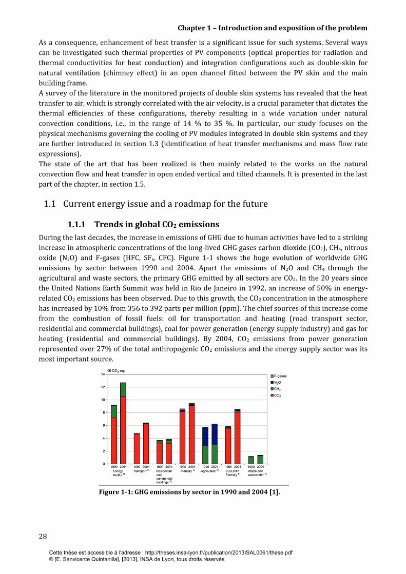
As a consequence, enhancement of heat transfer is a significant issue for such systems. Several ways
can be investigated such thermal properties of PV components (optical properties for radiation and
thermal conductivities for heat conduction) and integration configurations such as double-skin for
natural ventilation (chimney effect) in an open channel fitted between the PV skin and the main
building frame.
A survey of the literature in the monitored projects of double skin systems has revealed that the heat
transfer to air, which is strongly correlated with the air velocity, is a crucial parameter that dictates the
thermal efficiencies of these configurations, thereby resulting in a wide variation under natural
convection conditions, i.e., in the range of 14 % to 35 %. In particular, our study focuses on the
physical mechanisms governing the cooling of PV modules integrated in double skin systems and they
are further introduced in section 1.3 (identification of heat transfer mechanisms and mass flow rate
expressions).
The state of the art that has been realized is then mainly related to the works on the natural
convection flow and heat transfer in open ended vertical and tilted channels. It is presented in the last
part of the chapter, in section 1.5.
1.1 Current energy issue and a roadmap for the future
1.1.1 Trends in global CO2 emissions
During the last decades, the increase in emissions of GHG due to human activities have led to a striking
increase in atmospheric concentrations of the long-lived GHG gases carbon dioxide (CO2), CH4, nitrous
oxide (N2O) and F-gases (HFC, SF6, CFC). Figure 1-1 shows the huge evolution of worldwide GHG
emissions by sector between 1990 and 2004. Apart the emissions of N2O and CH4 through the
agricultural and waste sectors, the primary GHG emitted by all sectors are CO2. In the 20 years since
the United Nations Earth Summit was held in Rio de Janeiro in 1992, an increase of 50% in energy-
related CO2 emissions has been observed. Due to this growth, the CO2 concentration in the atmosphere
has increased by 10% from 356 to 392 parts per million (ppm). The chief sources of this increase come
from the combustion of fossil fuels: oil for transportation and heating (road transport sector,
residential and commercial buildings), coal for power generation (energy supply industry) and gas for
heating (residential and commercial buildings). By 2004, CO2 emissions from power generation
represented over 27% of the total anthropogenic CO2 emissions and the energy supply sector was its
most important source.
Figure 1-1: GHG emissions by sector in 1990 and 2004 [1].
Cette thèse est accessible à l'adresse : http://theses.insa-lyon.fr/publication/2013ISAL0061/these.pdf © [E. Sanvicente Quintanilla], [2013], INSA de Lyon, tous droits réservés

Chapter 1 – Introduction and exposition of the problem
29
The scientific community advises that limiting the average global temperature rise to two degrees
Celsius above pre-industrial levels (a target that was adopted during UN climate negotiations), is
possible if global cumulative emissions between 1990–2050 are reduced by a factor of 2.
Geographically, however, there are important differences between regions. Developed countries hold a
20% share in the world population but however account for 46.4% of global GHG emissions. In
contrast, the 80% of the world population living in developing countries accounts for 53.6% of GHG
emissions. Thus, to effectively reduce global GHG emissions by 2050, we must reduce energy-related
emissions of CO2, which will result in the urgently required reduction in fossil fuels consumption. For
instance, the European Union has agreed to reduce their CO2 emissions by a factor of 4 and Australia
by a factor of five within the next 40 years.
In 2011, the world’s five largest emitters were: China (29%), the United States (16%), the European
Union (EU-27) (11%), India (6%) and the Russian Federation (5%) (see Figure 1-2). The total
emissions in the EU-27 decreased by 3% in 2011, particularly in France that achieved a reduction of
5%, whereas CO2 emissions increased, for example, in Australia by 8% and Spain by 1%. These trends
reflect several factors including the impact of established energy policies, changes in national and
global economies, and the high fuel taxes during the recession. Trends in population should also be
considered, since population growth rates differ. The highest population growth rate since 1990 is
seen in Australia with a 32% increase until 2011, whereas the population of the EU and France
increased by much less: 7% and 10% respectively.
Figure 1-2: CO2 emissions per country from fossil fuel
and cement production in 1990, 2000 and 2011[2]. Figure 1-3: CO2 emissions per capita in 1990,
2000 and 2011 in the top CO2 emitting countries [2] .
As mentioned earlier, real trends in CO2 emissions are strongly related to the fuel energy consumption
during the last two decades as well as the energy policies established after the 1990’s. Specifically, the
European Union, although being one of the top emitters, it is also an example of an energy model in
transition, thereby it will be discussed in more detail in the next subsection.
1.1.2 Europe’s energy development scenario
Europe development 1990-2010
Europe’s development in the last 20 years can be characterized by an increasing consumption and an
increasing dependence of energy.
To meet its on own demands, it is obvious that the European continent does not have sufficient energy
resources so it depends heavily on imports. This dependence has grown more or less continuously
over the last ten years, with 53.9% of the energy used in the EU in 2009 being imported from around
the world. In Figure 1-4 the difference of the imported energy percentage between 1998 and 2009 in
various sectors of energy can be seen.
Cette thèse est accessible à l'adresse : http://theses.insa-lyon.fr/publication/2013ISAL0061/these.pdf © [E. Sanvicente Quintanilla], [2013], INSA de Lyon, tous droits réservés
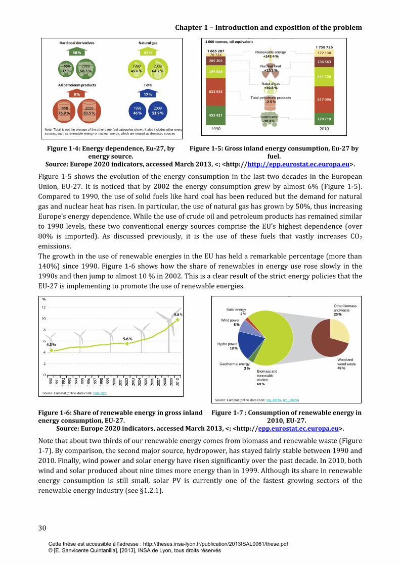
Chapter 1 – Introduction and exposition of the problem
30
Figure 1-4: Energy dependence, Eu-27, by energy source.
Figure 1-5: Gross inland energy consumption, Eu-27 by fuel.
Source: Europe 2020 indicators, accessed March 2013, <; <http://http://epp.eurostat.ec.europa.eu>.
Figure 1-5 shows the evolution of the energy consumption in the last two decades in the European
Union, EU-27. It is noticed that by 2002 the energy consumption grew by almost 6% (Figure 1-5).
Compared to 1990, the use of solid fuels like hard coal has been reduced but the demand for natural
gas and nuclear heat has risen. In particular, the use of natural gas has grown by 50%, thus increasing
Europe’s energy dependence. While the use of crude oil and petroleum products has remained similar
to 1990 levels, these two conventional energy sources comprise the EU’s highest dependence (over
80% is imported). As discussed previously, it is the use of these fuels that vastly increases CO2
emissions.
The growth in the use of renewable energies in the EU has held a remarkable percentage (more than
140%) since 1990. Figure 1-6 shows how the share of renewables in energy use rose slowly in the
1990s and then jump to almost 10 % in 2002. This is a clear result of the strict energy policies that the
EU-27 is implementing to promote the use of renewable energies.
Figure 1-6: Share of renewable energy in gross inland energy consumption, EU-27.
Figure 1-7 : Consumption of renewable energy in 2010, EU-27.
Source: Europe 2020 indicators, accessed March 2013, <; <http://epp.eurostat.ec.europa.eu>.
Note that about two thirds of our renewable energy comes from biomass and renewable waste (Figure
1-7). By comparison, the second major source, hydropower, has stayed fairly stable between 1990 and
2010. Finally, wind power and solar energy have risen significantly over the past decade. In 2010, both
wind and solar produced about nine times more energy than in 1999. Although its share in renewable
energy consumption is still small, solar PV is currently one of the fastest growing sectors of the
renewable energy industry (see §1.2.1).
Source: Eurostat (online data code: tsdcc310)
Energy dependence, EU-27
Hard coal derivatives Natural gas
All petroleum products Total
Note: ‘Total’ is not the average of the other three fuel categories shown. It also includes other energy
sources, such as renewable energy or nuclear energy, which are treated as domestic sources
Source: Eurostat (online data code: tsdcc320)
Gross inland energy consumption, by fuel, EU-271 000 tonnes, oil equivalent
Renewable energy
+143.4 %
Nuclear heat
+15.3 %
Natural gas
+49.8 %
Total petroleum products
-2.5 %
Solid fuels
-38.3 %
Source: Eurostat (online data code: tsdcc320)
Share of renewable energy in gross inland energy
consumption, EU-27%
Source: Eurostat (online data code: nrg_1071a, nrg_1072a)
Consumption of renewable energy, EU-27, 2010
Solar energy
2 %
Wind power
8 %
Hydro power
18 %
Geothermal energy
3 %Biomass and
renewable wastes
69 %
Wood and
wood waste 49 %
Other biomass
and waste 20 %
Cette thèse est accessible à l'adresse : http://theses.insa-lyon.fr/publication/2013ISAL0061/these.pdf © [E. Sanvicente Quintanilla], [2013], INSA de Lyon, tous droits réservés
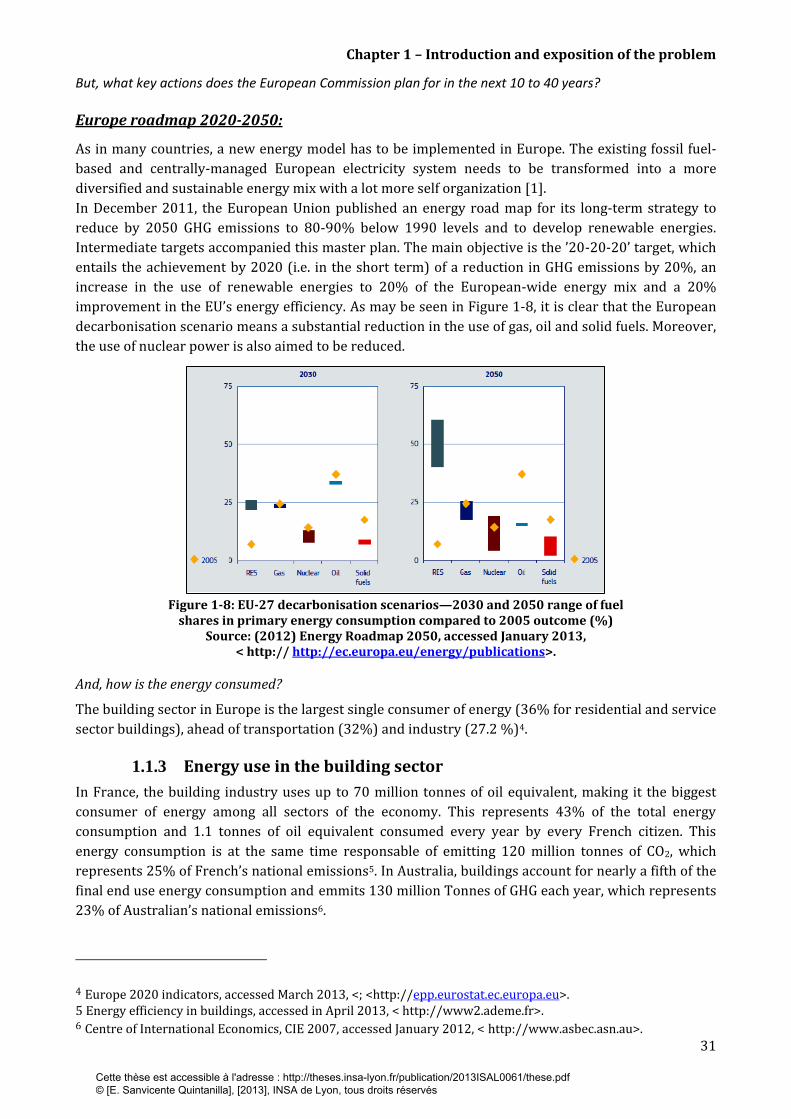
Chapter 1 – Introduction and exposition of the problem
31
But, what key actions does the European Commission plan for in the next 10 to 40 years?
Europe roadmap 2020-2050:
As in many countries, a new energy model has to be implemented in Europe. The existing fossil fuel-
based and centrally-managed European electricity system needs to be transformed into a more
diversified and sustainable energy mix with a lot more self organization [1].
In December 2011, the European Union published an energy road map for its long-term strategy to
reduce by 2050 GHG emissions to 80-90% below 1990 levels and to develop renewable energies.
Intermediate targets accompanied this master plan. The main objective is the ’20-20-20’ target, which
entails the achievement by 2020 (i.e. in the short term) of a reduction in GHG emissions by 20%, an
increase in the use of renewable energies to 20% of the European-wide energy mix and a 20%
improvement in the EU’s energy efficiency. As may be seen in Figure 1-8, it is clear that the European
decarbonisation scenario means a substantial reduction in the use of gas, oil and solid fuels. Moreover,
the use of nuclear power is also aimed to be reduced.
Figure 1-8: EU-27 decarbonisation scenarios—2030 and 2050 range of fuel
shares in primary energy consumption compared to 2005 outcome (%) Source: (2012) Energy Roadmap 2050, accessed January 2013,
< http:// http://ec.europa.eu/energy/publications>.
And, how is the energy consumed?
The building sector in Europe is the largest single consumer of energy (36% for residential and service
sector buildings), ahead of transportation (32%) and industry (27.2 %)4.
1.1.3 Energy use in the building sector
In France, the building industry uses up to 70 million tonnes of oil equivalent, making it the biggest
consumer of energy among all sectors of the economy. This represents 43% of the total energy
consumption and 1.1 tonnes of oil equivalent consumed every year by every French citizen. This
energy consumption is at the same time responsable of emitting 120 million tonnes of CO2, which
represents 25% of French’s national emissions5. In Australia, buildings account for nearly a fifth of the
final end use energy consumption and emmits 130 million Tonnes of GHG each year, which represents
23% of Australian’s national emissions6.
4 Europe 2020 indicators, accessed March 2013, <; <http://epp.eurostat.ec.europa.eu>. 5 Energy efficiency in buildings, accessed in April 2013, < http://www2.ademe.fr>. 6 Centre of International Economics, CIE 2007, accessed January 2012, < http://www.asbec.asn.au>.
Cette thèse est accessible à l'adresse : http://theses.insa-lyon.fr/publication/2013ISAL0061/these.pdf © [E. Sanvicente Quintanilla], [2013], INSA de Lyon, tous droits réservés
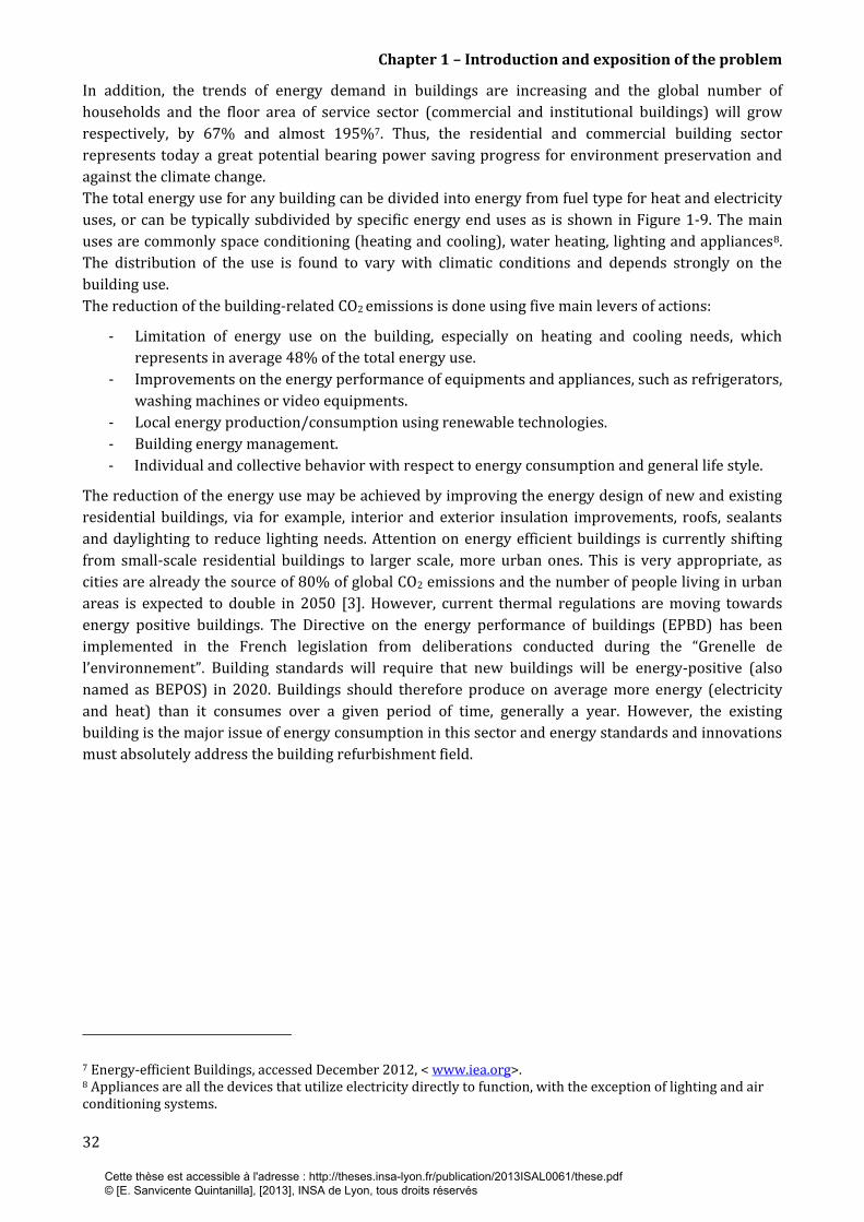
Chapter 1 – Introduction and exposition of the problem
32
In addition, the trends of energy demand in buildings are increasing and the global number of
households and the floor area of service sector (commercial and institutional buildings) will grow
respectively, by 67% and almost 195%7. Thus, the residential and commercial building sector
represents today a great potential bearing power saving progress for environment preservation and
against the climate change.
The total energy use for any building can be divided into energy from fuel type for heat and electricity
uses, or can be typically subdivided by specific energy end uses as is shown in Figure 1-9. The main
uses are commonly space conditioning (heating and cooling), water heating, lighting and appliances8.
The distribution of the use is found to vary with climatic conditions and depends strongly on the
building use.
The reduction of the building-related CO2 emissions is done using five main levers of actions:
- Limitation of energy use on the building, especially on heating and cooling needs, which
represents in average 48% of the total energy use.
- Improvements on the energy performance of equipments and appliances, such as refrigerators,
washing machines or video equipments.
- Local energy production/consumption using renewable technologies.
- Building energy management.
- Individual and collective behavior with respect to energy consumption and general life style.
The reduction of the energy use may be achieved by improving the energy design of new and existing
residential buildings, via for example, interior and exterior insulation improvements, roofs, sealants
and daylighting to reduce lighting needs. Attention on energy efficient buildings is currently shifting
from small-scale residential buildings to larger scale, more urban ones. This is very appropriate, as
cities are already the source of 80% of global CO2 emissions and the number of people living in urban
areas is expected to double in 2050 [3]. However, current thermal regulations are moving towards
energy positive buildings. The Directive on the energy performance of buildings (EPBD) has been
implemented in the French legislation from deliberations conducted during the “Grenelle de
l’environnement”. Building standards will require that new buildings will be energy-positive (also
named as BEPOS) in 2020. Buildings should therefore produce on average more energy (electricity
and heat) than it consumes over a given period of time, generally a year. However, the existing
building is the major issue of energy consumption in this sector and energy standards and innovations
must absolutely address the building refurbishment field.
7 Energy-efficient Buildings, accessed December 2012, < www.iea.org>. 8 Appliances are all the devices that utilize electricity directly to function, with the exception of lighting and air conditioning systems.
Cette thèse est accessible à l'adresse : http://theses.insa-lyon.fr/publication/2013ISAL0061/these.pdf © [E. Sanvicente Quintanilla], [2013], INSA de Lyon, tous droits réservés

Chapter 1 – Introduction and exposition of the problem
33
Figure 1-9: Typical building energy use in 2010. Source: Technology Roadmaps - Energy-efficient
Buildings, accessed February 2013, <; <http://www.iea.org>.
Figure 1-10: Electricity consumption of households between 1990 and 2010.
Source: Europe 2020 indicators, accessed February 2013, <; <http://epp.eurostat.ec.europa.eu>.
The energy consumption in buildings increased by 20% between 1990 and 2010. 13% of the growth
has been used for space conditioning and water heating and more than 70% was used for electric
appliances. The demand of heating and hot water may be satisfied by renewable heating sources
(geothermal, solar thermal, biomass) associated with storage and as previously mentioned, with
improved insulation. However, as may be seen in Figure 1-10, with the development of air
conditioning and the increased use of electronic devices (TV, radio, computer, video), the power
requirements in households has risen continuously by about 40 % over the past 20 years. In addition,
there are more and more households in developed countries with fewer and fewer people.
The solutions for local power generation are more limited. Different sources of energy are used, such
us wind turbines, diesel generators or fuel cells. However, the only available renewable source that
could satisfy this required local power consumption is photovoltaic solar energy (not completely at
that time). Solutions involve the integration of local energy generation systems, and in particular, the
use of photovoltaic components (BIPV) into the envelopes of buildings.
Source: Eurostat (online data code: tsdpc310)
Electricity consumption of householdsMillion tonnes of oil equivalent
Cette thèse est accessible à l'adresse : http://theses.insa-lyon.fr/publication/2013ISAL0061/these.pdf © [E. Sanvicente Quintanilla], [2013], INSA de Lyon, tous droits réservés

Chapter 1 – Introduction and exposition of the problem
34
1.2 The Photovoltaic technology
Photovoltaic (PV) refers to the direct conversion of short-wave solar irradiance into electricity. The PV
effect has been observed in 1839 by Alexander Edmond Becquerel but the first PV cells were not
commercialized until 1960’s [4]. The energy crisis after the oil embargo in 1973/1974 induced the
beginning of interest using solar photovoltaics, but the prohibitive prices (nearly 30 times higher than
current ones) made large-scale applications impractical.
PV power generating systems can be divided into independent PV systems and grid-connected PV
systems and are further related to the installation environment. As shown in Figure 1-11, until the
mid-1990s most systems were off-grid applications (stand alone), including rural household power
supply, beacons at sea or mountain, hydraulic pumping in developing countries, rural central power
plants and power supply for communication and lighting.
Today, on the contrary, more than 90% of the total PV market worldwide is grid conected systems. For
example, 91% of 2011 new systems in Australia were grid connected and in France they increased till
99.9%. Grid connected PV systems generally include building integrated PV (BIPV) systems and PV
power plants.
Figure 1-11: Cumulative installed grid connected and off-grid PV power
in the IEA PVPS member countries. Source:, Technology Roadmaps – Solar PV energy, accessed February
2013, <; <http://www.iea.org>.
There are several PV industries. Today’s solar cell market is dominated by crystalline silicon (c-Si)
technologies, with a market share of over 80-95% and by thin film technologies with a share of 10%-
15% of. Organic cells, advanced thin films and concentration technologies (CPV) are, on the other
hand, currently emerging technologies with significant potential for performance increase and cost
reduction.
Compared to all other power generation technologies, they have five fundamental characteristics that
set them apart:
As they are durably encapsulated and fixed on a support exposed to the sun, they are reliable,
they have no moving parts, need no fuel, and require essentially no maintenance during the
lifetime of over 20 years.
PV cells can be mass produced. For the past 30 years, their price has dropped on average by
more than 20% for every doubling of the production volume [5].
As the transformation of light into electricity occurs at microscopic levels, PV technologies are
scalable. They can be mounted in a small watch, on a roof or in a large plant with no efficiency
change and with cost differences due to different mechanical or electrical integration.
Cette thèse est accessible à l'adresse : http://theses.insa-lyon.fr/publication/2013ISAL0061/these.pdf © [E. Sanvicente Quintanilla], [2013], INSA de Lyon, tous droits réservés
Chapter 1 – Introduction and exposition of the problem
35
Innovation cycles for PV plants are up to ten times shorter than for conventional power plants.
Depending on the size they can be installed within weeks.
Local production possibilities that allow to limit energy loss du to transport.
There is a major difficulty without daylight, however, since there is no power generation. Moreover,
investment costs of PV systems are relatively high although they are decreasing rapidly, representing
today the most important barrier to PV deployment.
1.2.1 PV Roadmap 2050
PV has been one of the fastest growing sectors of the renewable energy industry until 2011. In
particular, the cumulative installed capacity of PV has grown from 0.1 GW in 1992 to 63.6 GW in 2011,
corresponding to an annual growth rate of 40% (Figure 1-11). In the last decade, Germany has been
the country pushing the majority of this growth, making up today for 39% of the worlwide total
installed capacity. In 2011, however, the Italian annual PV power installed was largest with 9.3 GW of
newly conected systems. Germany (7.5 GW) and China (2.5 GW) were followed by USA (1.8 GW),
France (1.7 GW) and Japan (1.2 GW). In Australia 0.83 GW were installed in 2011.
Today PV represents the 0.1% of total global electricity generation but is projected to provide 5% of
global electricity consumption in 2030, rising to 11% in 2050. In Europe, on the other hand, it is
expected to cover up to 25% after 20509.
1.2.2 The PV module and its electrical performance
As mentioned before, the major PV market cell is concerning crystalline silicon. The conversion
efficiencies of these PV cells, defined as the ratio between the produced electrical power and the
amount of incident solar energy per second, are typically under 25%. PV cells are interconnected and
need to be encapsulated in a polymer material and protected by glass to form a PV module. The range
of PV module power is typically 50-200 Watts Peak (Wp). The Wp corresponds to the power generated
under standard conditions (STC).
The performance of a PV module is indeed somewhat lower than of a PV cell. In particular, the
crystalline efficiency of silicon cells is in average of about 16% and the one of the module is about 13-
14 % [6]. This reduction in electrical efficiency is principally due to the additional reflection of solar
radiation caused by the glass cover (~ 0.70 %) and losses caused by the aluminum border area (~
1.4%). In addition, there are losses related to the cell interconnection (~ 0.75 %) since PV modules are
connected in series and the module operates at the performance of the least productive cell.
To provide the stated electrical efficiency of a PV panel, modules are tested at standard testing
conditions (STC), which generally involve an operational temperature of 25°C and an intensity of
radiation of 1kW/m2 [7]. This test is conducted in a chamber known as a flash simulator where PV
cells are flashed in only 50 miliseconds, allowing the electrical characteristics of the module to be
measured at this specific temperature.
In reality the standard testing conditions occur very rarely since cells heat up appreciably under
radiation and their temperature is usually above 25°C. For this reason a second test is usually
performed at a Standard Reference Environment (SRE) to specify the Nominal Operating Cell
Temperature (NOCT) [7]. This cell temperature is determined within an optimally tilted open-rack
mounted module, for an irradiance level of 800 W/m2, an ambient temperature of 20°C and a wind
velocity of 1m/s.
9 Technology Roadmaps – Solar PV energy, accessed February 2013, <; <http://www.iea.org>.
Cette thèse est accessible à l'adresse : http://theses.insa-lyon.fr/publication/2013ISAL0061/these.pdf © [E. Sanvicente Quintanilla], [2013], INSA de Lyon, tous droits réservés
Chapter 1 – Introduction and exposition of the problem
36
Besides, the maximum power output and electrical efficiency achievable by a PV module is extremely
dependent on the temperature of the PV cells within the panel.
As discussed above, crystalline silicon PV cells in real conditions convert aproximately 16% of the
solar energy into electricity. Because of this, 80% or more of the incident energy is converted passively
into heat, rising the operating temperature of the cell significantly and thus reducing by more the
efficiency from the active part converted into electricity [8-11].
Zondag [12] used the following correlation which expresses the adverse effect of an operating
temperature increase upon the PV module’s electrical efficiency:
(1)
in which generally, is the temperature degradation coefficient, T is the operating temperature (°C)
and η@T=25°C is the conversion efficiency indicated by the panel rating at STC. The temperature
coefficient depends on the PV material used and typical values of 0.4-0.6%/K for crystalline silicon,
and 0.2%/K for a-Si are found on literature10.
In order to illustrate the temperature effect, we can refer to a typical 80 Wp PV module output
(crystalline silicon), with a manufacturing tolerance of ± 5% and a derating due to dirtying of 5%
(typical in an urban environment). When its operating temperature is about 70 °C [8] and considering
a coefficient = 0.45%/K, the module output can reach only 57.5 W. With 13 % of absolute conversion
efficiency, for these types of modules a reduction by 20°C of the operating temperature will give rise to
an increase in efficiency between 1 and 1.5%.
Besides the module output degradation with the increase of temperature, the module lifetime is also
affected (module delamination, encapsulating material aging, deterioration of intercell welds). It is
therefore very important to take precautions so unnecessary ‘overheating’ of modules can be avoided.
In the context of BiPV for which the component is supposed to work rather at higher temperature than
for non-integrated configurations, the ventilation of the PV modules is presented as one of the key
points to limit both problems.
10 Technology Roadmaps – Solar PV energy, accessed February 2013, <; <http://www.iea.org>.
Cette thèse est accessible à l'adresse : http://theses.insa-lyon.fr/publication/2013ISAL0061/these.pdf © [E. Sanvicente Quintanilla], [2013], INSA de Lyon, tous droits réservés

Chapter 1 – Introduction and exposition of the problem
37
1.2.3 Building-Integration
Building-integrated photovoltaic systems offer a means to achieve multifunctional building envelopes
that provide energy. It is currently one of the fastest growing areas of the photovoltaic industry. Using
the photovoltaic modules as real components of building walls and rooftops, allows these surfaces to
generate electricity in addition to ensure other building envelope functions such as water tightness
and cover. In this context, BiPV plays a key role on the decarbonisation of the building sector,
particularly with respect to the local usage of renewable energy resources.
There is a wide range of design approaches and according to the integration option, a different
function is associated: they can be out of sight, for instance high on a roof, or where the absolute
maximum collection is needed. They can act as shading devices or they can be integrated in façades.
Figure 1-12 shows a classification of the different façades according to [13].
Figure 1-12: PV-integration options in façade systems [13].
1.2.3.1 Thermal issues in BIPV applications
A number of different circumstances occur when PV modules are applied as BIPV components in a
building, which is far from the Standard Reference Environment (§1.2.2). The most notable differences
are in level of irradiation and operating temperature.
For instance, the inclination for façade application is typically 90° and for roof application it depends
on the roof construction but is seldom optimized on existing buildings. As may be seen in Figure 1-13,
the choice of integration leads to different levels of irradiation and consequently annual outputs.
Indeed, these differences vary with weather conditions, thereby making for example more interesting
the integration of PV modules on façades for cold weather.
Figure 1-13: Monthly irradiation of differently inclined surfaces in Stuttgart [14].
Cette thèse est accessible à l'adresse : http://theses.insa-lyon.fr/publication/2013ISAL0061/these.pdf © [E. Sanvicente Quintanilla], [2013], INSA de Lyon, tous droits réservés

Chapter 1 – Introduction and exposition of the problem
38
On the other hand, in building integration PV modules are always mounted close to a surface, thereby
affecting in general the convective and radiation heat exchanges on the rear side of the PV module.
In particular, airflow is constrained around the module and heat loss by radiation is reduced because
of the presence of surrounding warm surfaces [15]. By way of illustration, Figure 1-14 reports
measurements on a full sunny day from four modules installed under four different conditions, namely
rack mounting, ventilated roof, an integrated roof and a fully insulated module. As may be seen, the
worst condition is when the PV module does not have convective or radiation thermal fluxes at the
rear side. Moreover, all BiPV applications are situated above the NOCT trend (free rack mounted
module).
Figure 1-14: Temperature differences (TPV module – Tamb) versus
Irradiance for four different installations [7].
It is therefore noted that the integration of PV modules in buildings affects both the energy yield and
life of the installation. As well, conversion from PV modules specifications at STC to BIPV system
design values is of highest priority as the integration of PV in buildings continues to emerge.
Cette thèse est accessible à l'adresse : http://theses.insa-lyon.fr/publication/2013ISAL0061/these.pdf © [E. Sanvicente Quintanilla], [2013], INSA de Lyon, tous droits réservés
Chapter 1 – Introduction and exposition of the problem
39
1.3 Configuration of the study: Building photovoltaic double skins
One approach to temperature regulation is free cooling, suitable for rooftop and façade integrated PV.
It involves fitting an air open channel between the PV laminate and the frame of the building, through
which the chimney effect develops. In the literature, the system analysis shows that the inclusion of
the channel behind the PV panels can decrease the operating temperature as much as 10-20 °C, which
depending on the channel geometry and radiation flux, may result in an absolute efficiency gain of 1-
2% [9].
The aim of the next section is to describe the BiPV double skin configuration selected as the case in
study.
1.3.1 The BiPV double skin envelope
Building photovoltaic double skin systems arise from the integration of PV modules, either opaque or
semitransparent, in the exterior skin of a double skin ventilated façade or roof.
Double skin ventilated systems (DSVS) are typically used in multi-storey buildings and consist of two
building skins separated by a ventilated cavity. Most commonly, the outdoor air flows into the bottom
of the cavity and exhausts from the top via natural or mechanical ventilation. Double-skin systems first
came into use in the 1970s in an attempt to help moderate façade thermal loads with high glazing
fractions. However, the potential of usage of DSVS for building ventilation purposes is very limited
though. Only a small proportion of solar heat is absorbed by the outer skin (ordinary glass, 10%)
compared to the heat transmitted to the cavity (80%), resulting in a poor buoyancy effect and a risk of
summertime overheating [16].
Building photovoltaic double skin systems is presented as a promising building configuration in terms
of both energy savings and generation for the following reasons:
Large available surfaces for roof and façade integration local production of electricity
(Figure 1-15 (a)).
PV modules (opaque or semi transparent) could act as shading devices, preventing from
overheating in summer periods while maintaining daylight penetration Contribution for
thermal comfort (Figure 1-15 (b)).
Effective ventilation of the back of PV arrays minimise efficiency loss while maintaining cell
temperature [4].
Heat absorption by the outer skin now becomes pronounced leading to a flow behavior similar
to that in solar chimney systems Building and façade cooling purposes are achieved [17].
In the beginning of the 2000s, the initial problem was how to cool the PV modules and how to enhance
the air circulation and the heat transfer between the skins. This quickly led to the idea that these ‘heat
losses’ could also be used in winter, e.g. for room heating or in summer to reduce cooling loads driving
natural ventilation. The logical step forward was research on how much heat was produced and how it
could be efficiently applied (BiPV systems with heat recovery).
The public library of Pompeu Fabra (Mataró, Spain) represents one example of a ventilated PVT façade
[18]. It was completed in 1996. This project has been extensively used in literature (as will be seen in
subsequent sections) to understand the thermal performance of PVT-façades. Moreover, it represents
in real scale one of the three configurations we are investigating.
It consists of a South ventilated façade 6 m high and 37.5 m wide giving a total area of 255 m2 for PV
integration (Figure 1-15 (a)). Multi-crystalline PV cells within a clear glass-glass laminate give a
semitransparent appearance to the outer skin of the façade (Figure 1-15 (b)).
Cette thèse est accessible à l'adresse : http://theses.insa-lyon.fr/publication/2013ISAL0061/these.pdf © [E. Sanvicente Quintanilla], [2013], INSA de Lyon, tous droits réservés
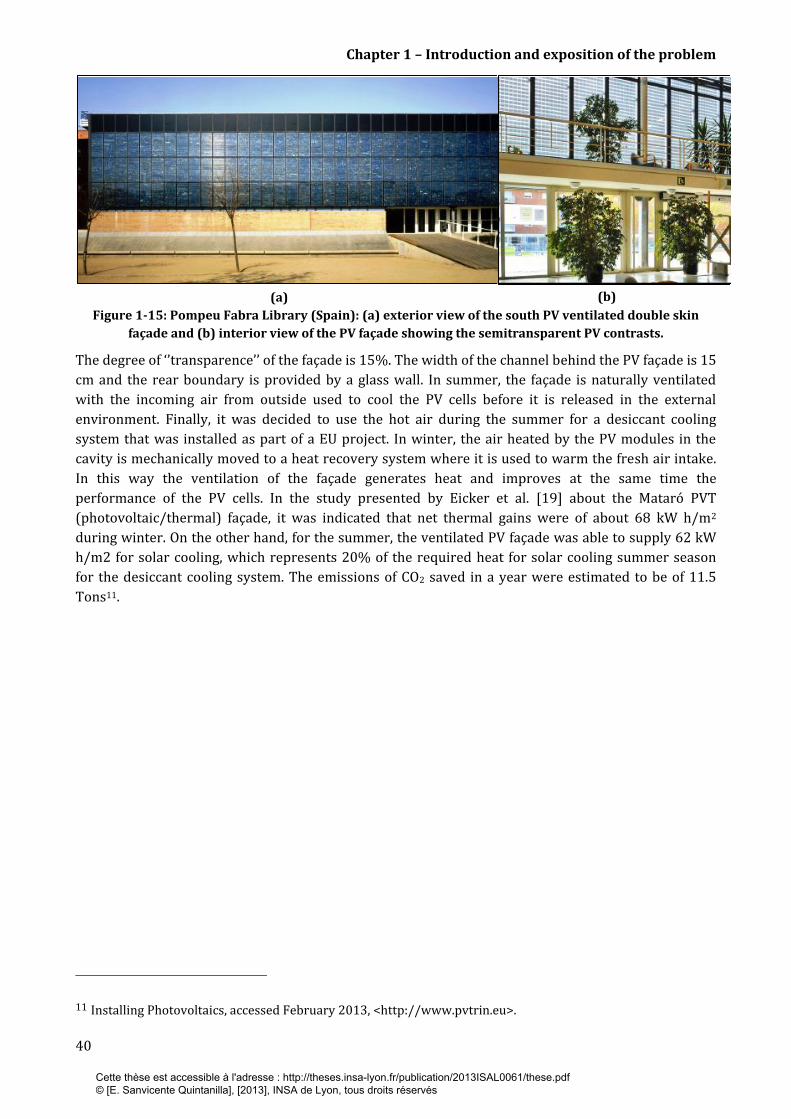
Chapter 1 – Introduction and exposition of the problem
40
(a)
(b)
Figure 1-15: Pompeu Fabra Library (Spain): (a) exterior view of the south PV ventilated double skin
façade and (b) interior view of the PV façade showing the semitransparent PV contrasts.
The degree of ‘’transparence’’ of the façade is 15%. The width of the channel behind the PV façade is 15
cm and the rear boundary is provided by a glass wall. In summer, the façade is naturally ventilated
with the incoming air from outside used to cool the PV cells before it is released in the external
environment. Finally, it was decided to use the hot air during the summer for a desiccant cooling
system that was installed as part of a EU project. In winter, the air heated by the PV modules in the
cavity is mechanically moved to a heat recovery system where it is used to warm the fresh air intake.
In this way the ventilation of the façade generates heat and improves at the same time the
performance of the PV cells. In the study presented by Eicker et al. [19] about the Mataró PVT
(photovoltaic/thermal) façade, it was indicated that net thermal gains were of about 68 kW h/m2
during winter. On the other hand, for the summer, the ventilated PV façade was able to supply 62 kW
h/m2 for solar cooling, which represents 20% of the required heat for solar cooling summer season
for the desiccant cooling system. The emissions of CO2 saved in a year were estimated to be of 11.5
Tons11.
11 Installing Photovoltaics, accessed February 2013, <http://www.pvtrin.eu>.
Cette thèse est accessible à l'adresse : http://theses.insa-lyon.fr/publication/2013ISAL0061/these.pdf © [E. Sanvicente Quintanilla], [2013], INSA de Lyon, tous droits réservés
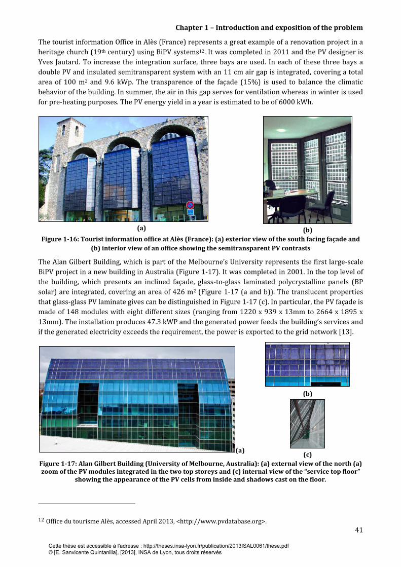
Chapter 1 – Introduction and exposition of the problem
41
The tourist information Office in Alès (France) represents a great example of a renovation project in a
heritage church (19th century) using BiPV systems12. It was completed in 2011 and the PV designer is
Yves Jautard. To increase the integration surface, three bays are used. In each of these three bays a
double PV and insulated semitransparent system with an 11 cm air gap is integrated, covering a total
area of 100 m2 and 9.6 kWp. The transparence of the façade (15%) is used to balance the climatic
behavior of the building. In summer, the air in this gap serves for ventilation whereas in winter is used
for pre-heating purposes. The PV energy yield in a year is estimated to be of 6000 kWh.
(a)
(b)
Figure 1-16: Tourist information office at Alès (France): (a) exterior view of the south facing façade and
(b) interior view of an office showing the semitransparent PV contrasts
The Alan Gilbert Building, which is part of the Melbourne’s University represents the first large-scale
BiPV project in a new building in Australia (Figure 1-17). It was completed in 2001. In the top level of
the building, which presents an inclined façade, glass-to-glass laminated polycrystalline panels (BP
solar) are integrated, covering an area of 426 m2 (Figure 1-17 (a and b)). The translucent properties
that glass-glass PV laminate gives can be distinguished in Figure 1-17 (c). In particular, the PV façade is
made of 148 modules with eight different sizes (ranging from 1220 x 939 x 13mm to 2664 x 1895 x
13mm). The installation produces 47.3 kWP and the generated power feeds the building’s services and
if the generated electricity exceeds the requirement, the power is exported to the grid network [13].
(a)
(b)
(c)
Figure 1-17: Alan Gilbert Building (University of Melbourne, Australia): (a) external view of the north (a) zoom of the PV modules integrated in the two top storeys and (c) internal view of the “service top floor”
showing the appearance of the PV cells from inside and shadows cast on the floor.
12 Office du tourisme Alès, accessed April 2013, <http://www.pvdatabase.org>.
Cette thèse est accessible à l'adresse : http://theses.insa-lyon.fr/publication/2013ISAL0061/these.pdf © [E. Sanvicente Quintanilla], [2013], INSA de Lyon, tous droits réservés
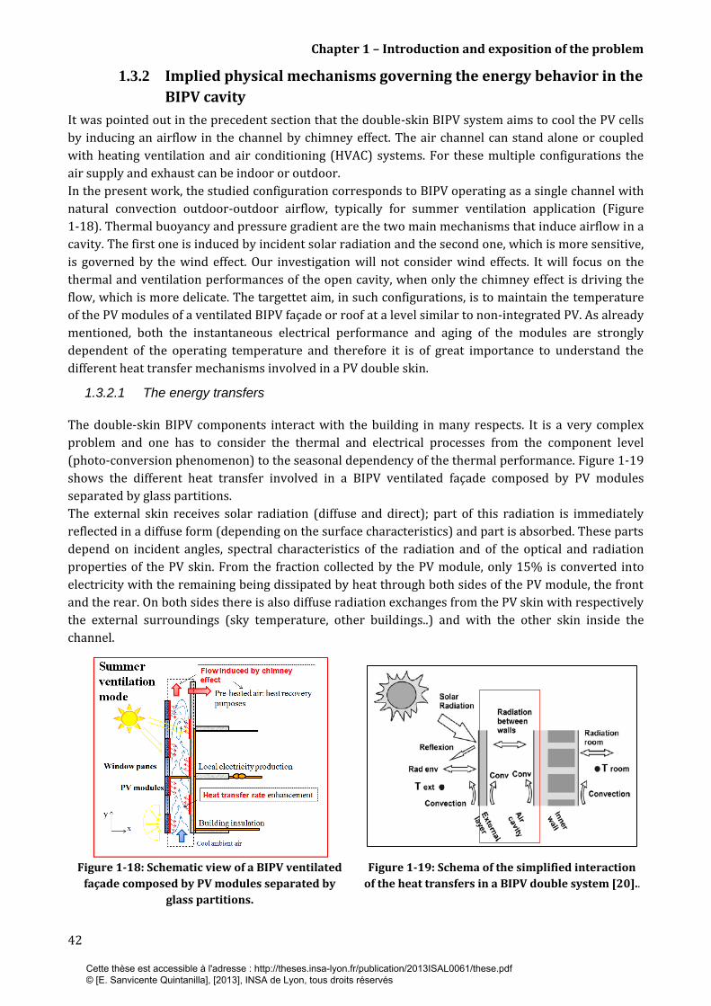
Chapter 1 – Introduction and exposition of the problem
42
1.3.2 Implied physical mechanisms governing the energy behavior in the
BIPV cavity
It was pointed out in the precedent section that the double-skin BIPV system aims to cool the PV cells
by inducing an airflow in the channel by chimney effect. The air channel can stand alone or coupled
with heating ventilation and air conditioning (HVAC) systems. For these multiple configurations the
air supply and exhaust can be indoor or outdoor.
In the present work, the studied configuration corresponds to BIPV operating as a single channel with
natural convection outdoor-outdoor airflow, typically for summer ventilation application (Figure
1-18). Thermal buoyancy and pressure gradient are the two main mechanisms that induce airflow in a
cavity. The first one is induced by incident solar radiation and the second one, which is more sensitive,
is governed by the wind effect. Our investigation will not consider wind effects. It will focus on the
thermal and ventilation performances of the open cavity, when only the chimney effect is driving the
flow, which is more delicate. The targettet aim, in such configurations, is to maintain the temperature
of the PV modules of a ventilated BIPV façade or roof at a level similar to non-integrated PV. As already
mentioned, both the instantaneous electrical performance and aging of the modules are strongly
dependent of the operating temperature and therefore it is of great importance to understand the
different heat transfer mechanisms involved in a PV double skin.
1.3.2.1 The energy transfers
The double-skin BIPV components interact with the building in many respects. It is a very complex
problem and one has to consider the thermal and electrical processes from the component level
(photo-conversion phenomenon) to the seasonal dependency of the thermal performance. Figure 1-19
shows the different heat transfer involved in a BIPV ventilated façade composed by PV modules
separated by glass partitions.
The external skin receives solar radiation (diffuse and direct); part of this radiation is immediately
reflected in a diffuse form (depending on the surface characteristics) and part is absorbed. These parts
depend on incident angles, spectral characteristics of the radiation and of the optical and radiation
properties of the PV skin. From the fraction collected by the PV module, only 15% is converted into
electricity with the remaining being dissipated by heat through both sides of the PV module, the front
and the rear. On both sides there is also diffuse radiation exchanges from the PV skin with respectively
the external surroundings (sky temperature, other buildings..) and with the other skin inside the
channel.
Figure 1-18: Schematic view of a BIPV ventilated
façade composed by PV modules separated by
glass partitions.
Figure 1-19: Schema of the simplified interaction
of the heat transfers in a BIPV double system [20]..
Cette thèse est accessible à l'adresse : http://theses.insa-lyon.fr/publication/2013ISAL0061/these.pdf © [E. Sanvicente Quintanilla], [2013], INSA de Lyon, tous droits réservés

Chapter 1 – Introduction and exposition of the problem
43
At the interior side, PV components are passively cooled by two major mechanisms: One part of the
heat dissipated on the rear side is transferred by convection to the air and transported away by the
induced airflow. On the other hand, thermal radiation heat transfer appears between the inward
surface of the cavity and the inner wall of the building. In some configurations such as ventilated
rooftop systems, as the chimney effect is hampered by the tilt, a coating of a suitable emissivity could
be applied at the back surface of the module, thereby increasing the heat transfer by thermal radiation
[9, 21, 22]. Moshfegh and Sandberg [23], for instance, reported that for a surface emissivity of ε = 0.9,
radiation heat transfer carried up to 30 % of the heat from the PV panel across the air gap to the
otherwise unheated wall. In the experimental model, the coupling of convection and radiation
transforms the originally single sided heated problem to a double sided heated problem. In addition,
the heat conduction, which is also present, tends to homogenize the temperature of both the PV
modules and the inner side of both walls.
In the case of an opaque PV double façade, similar phenomena would be present at the surface of the
main frame (inner wall), with noticeable lack of incident solar radiation flux and reflection. However,
for the case of a double skin composed of photovoltaic cells separated by glass partitions, solar
radiation is also transmitted to the inner wall surface, resulting in the heating of zones inside the air
gap. Thus in such an arrangement, solar radiation and reflection from the inner wall contribute to the
convection and the radiation heat exchanges within the cavity (see Figure 1-18).
1.3.2.2 Chimney effect
The cooling of PV cells using chimney effect has been used for BIPV façade systems as well as roof
systems. It follows that the wall/air heat transfer is a key point that dictates the thermal operating
conditions and thus the efficiency of the system. A survey of the literature in this subject reveals that
the heat transfer is strongly correlated with the air velocity, resulting in the wide variation of thermal
efficiencies under natural convection conditions, from 3% to 30%, as reported by [24, 25].
Consequently, much effort has been done in both the experiments and modelling of the airflow in the
double-skin channel.
Eicker and Gross [24] carried out experiments on the test façade for the PVT façade project of the
library of Pompeu Fabra (Figure 1-15) at the University of Stuttgart. Based on the measurements
obtained as shown in Figure 1-20, it was found that the air velocity increased from 0.05 m/s to 0.16
m/s and the thermal efficiency increased from 5% up to 30% as the irradiance increases from 200 to
1000 W/m2. Note the difficulty that naturally ventilated systems involve in comparison to the
mechanically driven systems. Indeed as shown by Figure 1-20, the airflow rate varies over time as a
function of the outside climate and the use of the building .The results of this figure may also indicate
that turbulence regime which intensifies as the irradiance increases is able to enhance the heat
transfer in the channel, thereby making it a desirable means to improve the thermal performance of
natural ventilated BIPV systems.
Cette thèse est accessible à l'adresse : http://theses.insa-lyon.fr/publication/2013ISAL0061/these.pdf © [E. Sanvicente Quintanilla], [2013], INSA de Lyon, tous droits réservés

Chapter 1 – Introduction and exposition of the problem
44
Figure 1-20: Natural convection air velocity in PV façade
of Mataró (Spain) as a function of the irradiance as
measured by [24].
It follows that the prediction of the performance of BIPV naturally ventilated systems is complex. In
systems such as solar chimneys, this performance is strictly related to the induced mass flow rate
whithin the chimney. Consequently, several empirical relations can be found on literature to predict
the mass flow rates as a function of geometrical parameters of the channel as well as a function of the
heat input. These relations are very useful in the design phase of the system as well as for comparison
of the obtained results.
The airflow induced is strongly dependent of two aspects: The first one is the stack pressure built up in
the chimney, which represents the driving forces and the second one is the pressure losses at the inlet,
outlet and along the channel, which represents the aerodynamic losses.
On the other hand, the thermal buoyancy mechanism, which is the motive force of the flow, is generally
represented by the Buoyancy flux:
in which g is the gravitational acceleration (m/s2), is the heat flux (W/m2), D and H are respectively
the width and height of the channel (m), is the air density at ambient temperature (kg/m3), is
the specific heat capacity (J/kg K) and Tinlet is the average inlet temperature of the channel (K). This
term is commonly used in solar chimney studies to predict airflow rates under given solar radiation
intensity and without wind [23, 26, 27].
An extensive experimental and numerical work has been carried out at the Cardiff University by
Brinkworth et al. [25] in naturally ventilated PV cladding for roofs and façades. Experiments were
carried out in a channel with height H = 5 m, width D = 0.12 m and a peak irradiance for vertical
surface of 620 W/m2 of a typical sunny day. Specifically, the average velocity was found to increase
from 0.2 m/s in a channel with H = 1 m, to a fixed value of 0.4 m/s in a channel with H > 30 m.
Brinkworth [28] calculates the natural convection flow rate from:
where Kf1 and Kf2 are the friction factors of the entrance and exit, St is a stratification parameter (S =
0.5 for a linear temperature increase). The friction factor, f, is based on experiments. This method has
been adopted by several other authors, such as Guiavarch and Peuportier [29] and Bazilian [30]. A
similar relation is provided by the authors to take into account the wind effects. The importance of
wind effects was also stressed by Infield [31], based on measurements of the library of Pompeu Fabra
(Figure 1-15).
(2)
(3)
Cette thèse est accessible à l'adresse : http://theses.insa-lyon.fr/publication/2013ISAL0061/these.pdf © [E. Sanvicente Quintanilla], [2013], INSA de Lyon, tous droits réservés
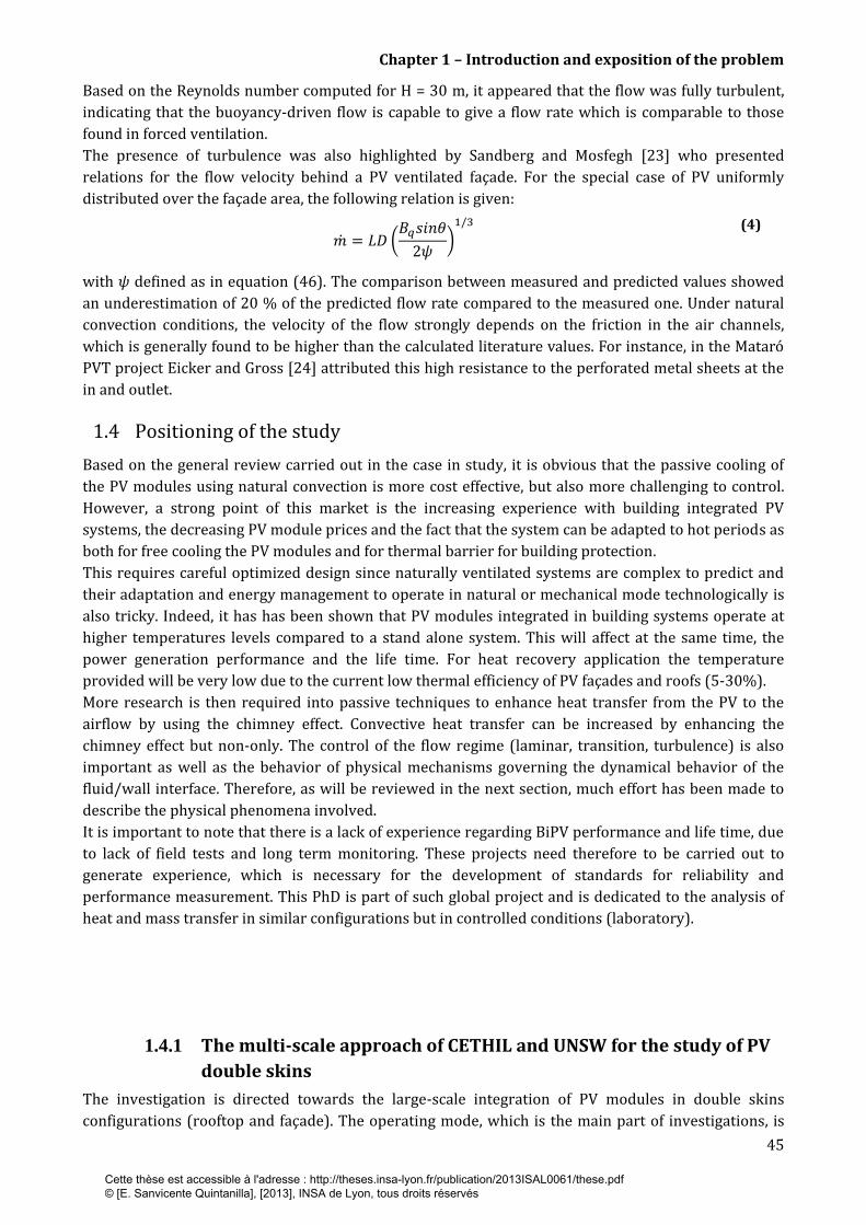
Chapter 1 – Introduction and exposition of the problem
45
Based on the Reynolds number computed for H = 30 m, it appeared that the flow was fully turbulent,
indicating that the buoyancy-driven flow is capable to give a flow rate which is comparable to those
found in forced ventilation.
The presence of turbulence was also highlighted by Sandberg and Mosfegh [23] who presented
relations for the flow velocity behind a PV ventilated façade. For the special case of PV uniformly
distributed over the façade area, the following relation is given:
with defined as in equation (46). The comparison between measured and predicted values showed
an underestimation of 20 % of the predicted flow rate compared to the measured one. Under natural
convection conditions, the velocity of the flow strongly depends on the friction in the air channels,
which is generally found to be higher than the calculated literature values. For instance, in the Mataró
PVT project Eicker and Gross [24] attributed this high resistance to the perforated metal sheets at the
in and outlet.
1.4 Positioning of the study
Based on the general review carried out in the case in study, it is obvious that the passive cooling of
the PV modules using natural convection is more cost effective, but also more challenging to control.
However, a strong point of this market is the increasing experience with building integrated PV
systems, the decreasing PV module prices and the fact that the system can be adapted to hot periods as
both for free cooling the PV modules and for thermal barrier for building protection.
This requires careful optimized design since naturally ventilated systems are complex to predict and
their adaptation and energy management to operate in natural or mechanical mode technologically is
also tricky. Indeed, it has has been shown that PV modules integrated in building systems operate at
higher temperatures levels compared to a stand alone system. This will affect at the same time, the
power generation performance and the life time. For heat recovery application the temperature
provided will be very low due to the current low thermal efficiency of PV façades and roofs (5-30%).
More research is then required into passive techniques to enhance heat transfer from the PV to the
airflow by using the chimney effect. Convective heat transfer can be increased by enhancing the
chimney effect but non-only. The control of the flow regime (laminar, transition, turbulence) is also
important as well as the behavior of physical mechanisms governing the dynamical behavior of the
fluid/wall interface. Therefore, as will be reviewed in the next section, much effort has been made to
describe the physical phenomena involved.
It is important to note that there is a lack of experience regarding BiPV performance and life time, due
to lack of field tests and long term monitoring. These projects need therefore to be carried out to
generate experience, which is necessary for the development of standards for reliability and
performance measurement. This PhD is part of such global project and is dedicated to the analysis of
heat and mass transfer in similar configurations but in controlled conditions (laboratory).
1.4.1 The multi-scale approach of CETHIL and UNSW for the study of PV
double skins
The investigation is directed towards the large-scale integration of PV modules in double skins
configurations (rooftop and façade). The operating mode, which is the main part of investigations, is
(4)
Cette thèse est accessible à l'adresse : http://theses.insa-lyon.fr/publication/2013ISAL0061/these.pdf © [E. Sanvicente Quintanilla], [2013], INSA de Lyon, tous droits réservés

Chapter 1 – Introduction and exposition of the problem
46
the most difficult to control in the naturally ventilated mode (in summer). The experimental challenge
is to attain a good compromise between the advantages of enhanced ventilation and natural cooling
(improved electrical performance of modules, slower the aging due to reduced operating
temperature), and esthetical (architectural) criteria. A strong point of this project comprises the multi
scale approach, from experimental studies under laboratory-controlled conditions to the full scale
experimental evaluation under real conditions. In addition, numerical models are developed and
adapted to these different scales. The simulations are compared to the empirical data collected in both
field and laboratory.
The originality of this investigation relies on the understanding of the physical mechanisms governing
the electrical, thermal and kinematic behavior of these systems. This includes the study of different
physical processes (photoconversion, chimney effect, radiation in semi-transparent media
propagation) and at different levels (component, façade, and building).
In particular, this PhD thesis is part of two ANR projects: The RESSOURCES project (French PREBAT
2007, French agreement ADEME-0705C0076) and the CERISES project (French ANR-08-JCJC-0018-
01). The RESSOURCES project is a research project coordinated by the Lyon Thermal Science Center
(CETHIL UM 5008), which focuses on the redefinition of the solar building envelope (rooftop and
façade). The project was launched in 2008 in collaboration with the architect Jacques Ferrier, Tenesol,
HBS-Technal and several research centers (Enerbat department of EDF R&D, LOCIE and LEEVAM).
Three full-scale prototypes were designed, constructed and instrumented: one on an existing tertiary
building (Figure 1-21(a)) and two on a detached house (Figure 1-21(b)). The architect (JFA), the
module manufacturer (Tenesol) and building façade specialists (HBS) have focused specially on the
inclusion of technological and aesthetic innovations on the active envelope.
(a)
(b)
Figure 1-21: Picture view of two outdoors full scale prototypes built in the RESSOURCES projet: (a) PV
double skin façade (7m x 4m) in the Technal building (Toulouse ) and (b) double skin systems
comprising façade and roof integrated in the ETNA experimental dwelling cells (EDF R&D, Les
Renardières).
The role of the research laboratories, on the other hand, is mainly to define the instrumentation
required for the field monitoring of the full scale prototypes and to provide analysis and expert tools to
the system designer based on both full scale experiments and laboratory experiments under
controlled conditions. This scientific approach (of which this PhD thesis is part), is complemented by
the CERISES project (ConvEction and Radiation In Solar Energy Systems) which focuses specifically on
Cette thèse est accessible à l'adresse : http://theses.insa-lyon.fr/publication/2013ISAL0061/these.pdf © [E. Sanvicente Quintanilla], [2013], INSA de Lyon, tous droits réservés
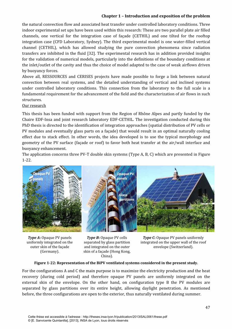
Chapter 1 – Introduction and exposition of the problem
47
the natural convection flow and associated heat transfer under controlled laboratory conditions. Three
indoor experimental set ups have been used within this research: These are two parallel plate air filled
channels, one vertical for the integration case of façade (CETHIL) and one tilted for the rooftop
integration case (CFD Laboratory, Sydney). The third experimental model is one water-filled vertical
channel (CETHIL), which has allowed studying the pure convection phenomena since radiation
transfers are inhibited in the fluid [32]. The experimental research has in addition provided insights
for the validation of numerical models, particularly into the definitions of the boundary conditions at
the inlet/outlet of the cavity and thus the choice of model adapted to the case of weak airflows driven
by buoyancy forces.
Above all, RESSOURCES and CERISES projects have made possible to forge a link between natural
convection between real systems, and the detailed understanding of vertical and inclined systems
under controlled laboratory conditions. This connection from the laboratory to the full scale is a
fundamental requirement for the advancement of the field and the characterization of air flows in such
structures.
Our research
This thesis has been funded with support from the Region of Rhône Alpes and partly funded by the
Chaire EDF-Insa and joint research laboratory EDF-CETHIL. The investigation conducted during this
PhD thesis is directed to the identification of integration approaches (spatial distribution of PV cells or
PV modules and eventually glass parts on a façade) that would result in an optimal naturally cooling
effect due to stack effect. In other words, the idea developed is to use the typical morphology and
geometry of the PV surface (façade or roof) to favor both heat transfer at the air/wall interface and
buoyancy enhancement.
The application concerns three PV-T double skin systems (Type A, B, C) which are presented in Figure
1-22.
Type A: Opaque PV panels uniformly integrated on the
outer skin of the façade (Germany).
Type B: Opaque PV cells separated by glass partition and integrated on the outer skin of a façade (Hong Kong,
China).
Type C: Opaque PV panels uniformly integrated on the upper wall of the roof
envelope (Switzerland).
Figure 1-22: Representation of the BiPV ventilated systems considered in the present study.
For the configurations A and C the main purpose is to maximize the electricity production and the heat
recovery (during cold period) and therefore opaque PV panels are uniformly integrated on the
external skin of the envelope. On the other hand, on configuration type B the PV modules are
separated by glass partitions over its entire height, allowing daylight penetration. As mentioned
before, the three configurations are open to the exterior, thus naturally ventilated during summer.
Cette thèse est accessible à l'adresse : http://theses.insa-lyon.fr/publication/2013ISAL0061/these.pdf © [E. Sanvicente Quintanilla], [2013], INSA de Lyon, tous droits réservés
Chapter 1 – Introduction and exposition of the problem
48
The experimental work has been conducted in the two air filled set ups subjected to imposed heat flux
conditions. The vertical configuration is investigated on the CETHIL Laboratory (Lyon) and the tilted
configuration on the CFD laboratory (Sydney). This study is an additional step in an extensive
collaboration conducted between three laboratories (CETHIL Lab, CFD Lab and DIPTEM Lab-Genova,
Italy) during the recent years on different aspects of PV air cooling via natural convection. Most of the
previous studies have dealt with the fluid/flow heat transfer characterization by means of both
experimental [25, 26, 39] and numerical investigations [21, 24, 39, 40]. Moreover, the kinematic aspect
of the problem has been only approached numerically and more recently experimentally in pure
convection mode [32].
The current investigation focuses on the local and detailed experimental analysis of the flow with
different thermal boundary conditions. Since the thermal performance of PV double skin systems
depends greatly on the buoyancy-driven flow occurring in the channel, past studies related to the
natural convective phenomena in open-ended channels are reviewed in this chapter.
Cette thèse est accessible à l'adresse : http://theses.insa-lyon.fr/publication/2013ISAL0061/these.pdf © [E. Sanvicente Quintanilla], [2013], INSA de Lyon, tous droits réservés
Chapter 1 – Introduction and exposition of the problem
49
1.5 The state of the art in natural convection flow in open-ended channels
1.5.1 Introduction
Natural convection flow is a mechanism in which the fluid motion is driven by buoyancy forces due to
the combined presence of a fluid density gradient and a body force that is proportional to density.
Unlike forced convection, natural or free convection is not caused by an externally imposed pressure,
such as a fan, for example. A density gradient could be the result of temperature gradient indicating a
non-isothermal flow, or other factors such as concentration gradients and centrifugal forces, which
occur in rotating fluid machinery and Coriolis forces, which are important in atmospheric rotational
motions.
The flows investigated in this thesis are non-isothermal flows in which the fluid density gradients are
due to temperature gradients and a gravitational body force: such motions are generally termed
natural convection if it is in a confined space, or free convection if the space is unconfined. The fluid
motion due to natural convection in open-ended channels is a low speed flow whereby the control of
the development is considered to be difficult. This is mainly due to its high sensitivity to the external
environmental conditions, which include temperature and pressure fluctuations and variations in the
external velocity field.
Apart from the passive cooling of ventilated PV air systems, the main applications of this kind of
configuration are found in electronic equipment cooling [33-43], in ventilation systems in buildings
such as Trombe walls and solar chimneys [8, 15, 26, 27, 44-50], PV double-skin façade and rooftop
systems [9, 23, 26, 27, 51-53].
Depending on the application, the objective could be either to:
maximize heat transfer from wall to fluid if cooling is the application. The optimization
criterion could then be based on minimizing the temperatures of the wall.
or to,
maximize the heat recovery at the outlet of the channel if preheating is the application. The
optimization criterion could be then based on mass flow rate and temperature differences
between the inlet and the outlet of the channel.
or
finding a compromise between the previous two conditions.
As it has been mentioned in section 1.3, PV double-skin façades or rooftops should have an optimized
operation in all seasons. Consequently, both the heat transfer and the heat recovery capacity need to
be investigated. Even if the main purpose of this work concerns the PV modules cooling in summer, it
is interesting to evaluate the heat recovery capacity at the outlet in natural regimes for all the
uniformly or non-uniformly boundary conditions at the walls. However for such a system the
preheating of the building during winter provided by the double skin is ensured by mixed or forced
convection. It is apparent that in natural convection in PV double-skin façades or rooftops, the number
of PV modules and their spatial distribution will have an impact on the temperature distribution
within the modules and the heat recovery efficiency and it is pertinent to find the appropriate
configuration which will make the best use of the available “free” energy.
The typical geometry of the problem is shown in Figure 1-23. The walls can be vertical or inclined. H
represents the height of the channel, D the space between the walls and D/H the channel aspect ratio.
The walls can be either isothermal for the uniform wall temperature, UWT, boundary condition or
uniformly heated for the uniform heat flux, UHF, boundary condition. Indeed, the channel can be
heated asymmetrically, which means that one wall is heated while the other one is non-heated, or
symmetrically, with both of the walls being heated.
Cette thèse est accessible à l'adresse : http://theses.insa-lyon.fr/publication/2013ISAL0061/these.pdf © [E. Sanvicente Quintanilla], [2013], INSA de Lyon, tous droits réservés
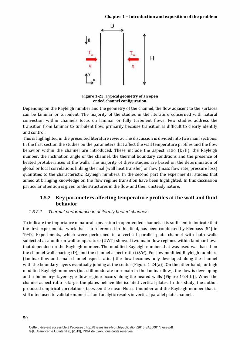
Chapter 1 – Introduction and exposition of the problem
50
Figure 1-23: Typical geometry of an open ended channel configuration.
Depending on the Rayleigh number and the geometry of the channel, the flow adjacent to the surfaces
can be laminar or turbulent. The majority of the studies in the literature concerned with natural
convection within channels focus on laminar or fully turbulent flows. Few studies address the
transition from laminar to turbulent flow, primarily because transition is difficult to clearly identify
and control.
This is highlighted in the presented literature review. The discussion is divided into two main sections:
In the first section the studies on the parameters that affect the wall temperature profiles and the flow
behavior within the channel are introduced. These include the aspect ratio (D/H), the Rayleigh
number, the inclination angle of the channel, the thermal boundary conditions and the presence of
heated protuberances at the walls. The majority of these studies are based on the determination of
global or local correlations linking thermal (wall heat transfer) or flow (mass flow rate, pressure loss)
quantities to the characteristic Rayleigh numbers. In the second part the experimental studies that
aimed at bringing knowledge on the flow regime transition have been highlighted. In this discussion
particular attention is given to the structures in the flow and their unsteady nature.
1.5.2 Key parameters affecting temperature profiles at the wall and fluid behavior
1.5.2.1 Thermal performance in uniformly heated channels
To indicate the importance of natural convection in open-ended channels it is sufficient to indicate that
the first experimental work that is a referenced in this field, has been conducted by Elenbass [54] in
1942. Experiments, which were performed in a vertical parallel plate channel with both walls
subjected at a uniform wall temperature (UWT) showed two main flow regimes within laminar flows
that depended on the Rayleigh number. The modified Rayleigh number that was used was based on
the channel wall spacing (D), and the channel aspect ratio (D/H). For low modified Rayleigh numbers
(laminar flow and small channel aspect ratios) the flow becomes fully developed along the channel
with the boundary layers eventually joining at the center (Figure 1-24(a)). On the other hand, for high
modified Rayleigh numbers (but still moderate to remain in the laminar flow), the flow is developing
and a boundary- layer type flow regime occurs along the heated walls (Figure 1-24(b)). When the
channel aspect ratio is large, the plates behave like isolated vertical plates. In this study, the author
proposed empirical correlations between the mean Nusselt number and the Rayleigh number that is
still often used to validate numerical and analytic results in vertical parallel plate channels.
Cette thèse est accessible à l'adresse : http://theses.insa-lyon.fr/publication/2013ISAL0061/these.pdf © [E. Sanvicente Quintanilla], [2013], INSA de Lyon, tous droits réservés

Chapter 1 – Introduction and exposition of the problem
51
(a)
(b)
Figure 1-24: Temperature (Twall –Tinlet) and velocity profiles reported by Eleenbas [54] for (a) narrow gaps and (b) wide gaps.
Pioneering on the analytical studies in this field, in 1962, Bodoia and Osterle [55] and in 1972, Aung
[56] and Aung et al. [57] solved the governing equations for a parallel plate channel by using a
parabolic model in developing [57] and fully developed laminar [56] type flow regime. Both
symmetrically and asymmetrically isothermal and isoflux plates were considered and maximum wall
temperatures and Nusselt numbers were correlated to the channel Rayleigh number. The results of
Bodoia and Osterle [55] showed a good agreement with the Elenbaas [54] data for intermediate
Rayleigh numbers, Ra*.
These studies represent the basis of the other studies conducted later on in laminar flows, as indicated
in the literature, e.g., (Sparrow and Baharami [58], Raythby and Hollands [59], Sparrow et al. [60],
Azevedo and Sparrow [61], Bar-Cohen and Roshenow [62], Ostrach [63] for uniform wall temperature,
UWT, boundary conditions and (Sobel et al. [64], Dalbert et al. [65], Wirtz and Stutzman [66], Webb
and Hill [67], Tanda [68]), for uniform heat flux, UHF, boundary conditions. In these studies,
correlations describing the local and mean heat transfer along the channel and the maximum wall
temperature as a function of geometrical and thermal parameters were also developed. A summary of
the correlations, which are most often used, can be found on the Appendix A.
Among these we can highlight the review on the formulas for the calculation of the heat transfer
presented by Rohsenow et al. [69] in 1984 and the up to date review on the subject, which includes as
well the formulas for the calculation of flow rate, presented by Olsson [70] in 2004.
As in the case of the above cited work and nearly all research in heat transfer, more recent studies on
heat transfer in an uniformly heated parallel-plate channel have generally been carried out by
analyzes of results of parametric studies which were based on varying the channel aspect ratio, the
inclination angle of the channel and the Rayleigh number.
In natural convection in channel, the channel aspect ratio is also found to govern the mode of heat
transfer. Apart from the two limits of laminar flow regimes (Figure 1-24), different heat transfer
mechanisms have been identified between very narrow and wide right rectangular channels.
Onur and Aktas [71] investigated experimentally a short vertical chimney 0.3 m height and 0.2 m
width asymmetrically heated with one of the walls maintained at a isothermal temperature while the
other was well insulated and assumed to be adiabatic. The remaining two sides of the channel were
not closed. Figure 1-25 below, extracted from this paper, presents the evolution of the Nusselt number,
based on the plate height, for different channel aspect ratio in terms of the heat transfer effectiveness.
This parameter was defined as the ratio of the Nusselt number for the channel, NuH, to the Nusselt
number for an isolated plate, NuH,single plate; both were based on the height H. A fixed Rayleigh number,
RaH of 3.107, also based on the channel height, was considered.
Cette thèse est accessible à l'adresse : http://theses.insa-lyon.fr/publication/2013ISAL0061/these.pdf © [E. Sanvicente Quintanilla], [2013], INSA de Lyon, tous droits réservés

Chapter 1 – Introduction and exposition of the problem
52
As may be seen in Figure 1-25, three heat transfer regimes were found for the UWT boundary
conditions. The regime in very narrow channels, D/H < 1/66, in which D is the separation between the
plates, was called the heat conduction regime as this mode dominated the heat transfer process. The
convection regime with joined boundary layers occurred in slightly wider channels, 1/50< D/H < 1/14
and the convection regime in which the boundary layers develop independently as if the two vertical
plates were isolated plates, was found in wide channels, D/H > ~1/10.
Figure 1-25: Effect on the channel depth on the heat
transfer mode [71].
For this UWT boundary conditions a maximum heat transfer is obtained at an aspect ratio of D/H =
1/20 with a ratio NuH/Nusingle plate close to 1.15. With larger inter-plate spacing, the interaction of the
walls becomes gradually weaker and boundary layers are found to develop independently along each
wall with a decrease in the Nusselt number that tends to the single plate case.
It is remarkable that Brinkworth & Sandberg [13], who study analytically and experimentally the
cooling of a PV duct, observed that for a wall on which an uniform heat flux (UHF) is imposed, the same
optimal channel aspect ratio D/H = 1/20 as in [71] led to minimum temperatures of the heated wall at
a Rayleigh number of about 106. They also proposed a design procedure. As shown in Table B-1 in
Appendix B, Fossa et al. [47] found an optimal ratio of D/H = 1/16 that lead to minimum wall
temperatures in assymetrically heated vertical channel with an UHF boundary conditions for
103 Ra* 107. However, despite the fact that it appears that the same optimum is obtained for both
UWT and UHF boundary conditions, it is shown in Table B-1 of Appendix B that the dependence of the
mass flow rate on the optimum aspect ratio D/H is more complex as large discrepancies are found in
the literature.
The induced mass flow rate increases with both the channel aspect channel ratio (D/H) and the
Rayleigh number (Ra) [15, 44, 45, 72, 73]. The correlations are typically of the form
(5)
with the exponent in the range of [0.57 - 0.44] for low Rayleigh numbers and [0.25 - 0.31] for the
highest Rayleigh numbers. Further details of the correlations are given in Table B-2 of Appendix B for
both imposed boundary conditions (UWT and UHF). Given the form of this expression, the mass flow
rate for UHF conditions presents an inflexion for a particular (D/H) but not a maximum except in the
work conducted by Bouchair et al. [46], in which a maximum air flow rate is said to have occurred but
this time for a quite large aspect ratio D/H ~ 1/10.
Cette thèse est accessible à l'adresse : http://theses.insa-lyon.fr/publication/2013ISAL0061/these.pdf © [E. Sanvicente Quintanilla], [2013], INSA de Lyon, tous droits réservés
Chapter 1 – Introduction and exposition of the problem
53
The inflexion of the mass flow rate found in the other cases is explained by a flow phenomenon that is
the occurrence of a flow reversal near the channel outlet depending on the aspect ratio. The
occurrence of flow reversal will be discussed in more detail in 1.5.3.3. Notice also that in all the
correlations presented in Table B-2 of Appendix B, the exponent of the Rayleigh number is consistent
with the theoretical exponents which are 1/2 in laminar flow and 1/3 – 1/4 in turbulent flow [74].
Based on numerical simulations, Zamora and Kaiser [48] also found an optimal aspect ratio, for UHF.
Moreover, since they searched for the optimum aspect ratio for both heat transfer and mass flow rates,
they showed that under the same heating conditions the channel aspect ratio that maximizes the mass
flow rate is not the same as the one that minimises the wall temperatures. Higher channel aspect ratios
were obtained for achieving maximum mass flow rates that those needed to minimize the
temperatures . The authors concluded that it is not feasible to simultaneously optimize both the
thermal and the flow performances through only channel aspect ratio variations.
More studies related to uniformly heated channels are presented in section 1.5.3. Indeed, the studies
that aim at bringing knowledge on the structure and regime of the flow are in the majority conducted
on vertical parallel-plate channels.
Effect of the channel inclination angle
Natural convection in tilted open-ended channels has attracted comparatively less attention than the
vertical ones since these investigations generally involve more experimental complication due to
lower chimney effect. Consequently, limited experimental data are found regarding the impact of the
angle of inclination on the induced mass flow rate and the thermal fields. However, the effect of the
inclination angle on the heat transfer rate from the upper surface is of major interest since PV modules
may also be integrated in ventilated rooftop systems. Indeed, this is a very attractive solution for us
since tilted configurations generally yield greater electrical energy output due to more favorable
angles of incidence to the incoming radiation.
Although the radiation gains can be increased due to tilt, the net result of channel inclination affects
adversely the cooling of the PV modules in the following way: In a tilted channel only the component of
the buoyancy force parallel to the wall drives the flow so that the induced mass flow rate is lower and
consequently the wall temperatures higher than it would be in the case of a vertical channel with the
same thermal input, as indicated in the literature [10, 23, 27, 52, 53].
Prior studies on laminar natural convection between inclined open-ended channels considered
isothermal plates (Azevedo and Sparrow [61], Straatman [75], Onur and Aktas [71], Said [76], Hirouki
et al. [77]). Correlations describing the average heat transfer characteristics were developed for
inclination angles with respect to the horizontal in the range of 85°-10°. In general, the angle effect is
included in the Rayleigh number definition by the inclusion of an additional term on the form of
in which is the angle of the channel to the horizontal. Such a relationship , RaD , has been found to
be able to correlate successfully natural convection flow in inclined channels when heated from above
[76].
Among these studies we can highlight the investigation conducted by Azevedo and Sparrow [61] in
1985. Heat transfer and flow visualization experiments were performed on an inclined isothermal
channel in which the overall heat transfer from the channel was investigated for a large set of data.
Three different heating modes (top wall heated, bottom wall heated, both walls heated) and various
aspect ratios and Rayleigh numbers were investigated. In particular, Nusselt numbers were evaluated
for 90o 45o and they were correlated within ±10%.
In early studies the data for inclined channels with uniform heat flux, UHF, boundary conditions was
however more limited [78-80]. Inaba [78] studied an inclined air channel heated from the bottom
surface.
Cette thèse est accessible à l'adresse : http://theses.insa-lyon.fr/publication/2013ISAL0061/these.pdf © [E. Sanvicente Quintanilla], [2013], INSA de Lyon, tous droits réservés

Chapter 1 – Introduction and exposition of the problem
54
As a result, a correlation for the average Nusselt number as a function of modified Rayleigh number
was proposed for channels with inclination angles between 30° and 90°. Symmetric and asymmetric
(top wall heated) heating were experimentally investigated in 1992 by Manca et al. [79, 80] for
inclination angles in the range of 90° to 30° [80] and 30° to 0° [79]. Average heat transfer coefficients
were evaluated and Nusselt numbers were correlated to the inclination angle and to a channel
Rayleigh number including the effect of the channel aspect ratio (D/H). Temperatures at the walls and
velocity and temperature distributions across the width of the channels were reported for the
symmetric heating condition and for constant heat fluxes, which varied between 14 W/m2 and 250
W/m2. It was shown that for = 30° the velocity distribution near the channel exit was skewed
towards the top wall in comparison with the symmetric velocity profile observed for the vertical
position. The asymmetric velocity distribution determined an overall chimney effect in the tilted
position smaller than that in the vertical one although the local maximum values of velocity were not
very different
Recent applications on tilted channels are related to roof solar collectors and solar chimneys attached
to the roofs, thereby low inclination angles (15°-45°) have been most often investigated in literature as
indicated in (Susanti et al. [53], Chami et al. [79], Candanedo et al. [10], Chungloo et al. [81],
Brinkworth [28]).
Chami and Zoughaib [52] proposed a correlation for mass flow rate from results obtained from natural
simulation of natural convection in tilted chimneys with 30o 45o in terms of various parameters
such as the inclination angle, inter-plate spacing, the chimney height and the ambient temperature.
Numerical results were validated with particle image velocimetry (PIV) measurements. An average
discrepancy of about 10 % in the mass flow rate was found between the PIV data and the numerical
results.
In the case of the work cited above, the impact of radiation exchange inside the channel was generally
minimized (by using very low surface emissivities, ε < 0.1) or ignored and therefore not considered.
However, in many engineering applications, the emissivity of the channel surface may range from 0.15
< ε < 0.95, thereby radiation effects may have a great impact on both the heat transfer and the natural
convection flow in the channel, specially when the channel is heated asymmetrically [23, 82, 83].
Indeed, for laminar air convection in channels, the radiative contribution may be significant as was
first shown by Carpenter et al. [84] in 1976. They investigated numerically a vertical parallel plate
channel with isoflux (UHF) asymmetric heating and showed that radiation significantly altered the
pure natural convection results by reducing the wall temperatures, especially the maximum value.
Combined natural convection and thermal radiation effects in inclined parallel plate channels was
experimentally investigated by Manca and Nardini [83] in 1994 for laminar air natural convection with
uniform, symmetric and asymmetric heat flux conditions. The tests were performed for two different
surface emissivities (ε = 0.05 and 0.8). Later in 1999, Manca et al. [85] proposed a large set of
composite correlations for inclined channels (90°-15°) by employing the experimental data from [83].
The surface radiative contribution was taken into account in both the modified Nusselt and Rayleigh
numbers. In 2001, the same authors [82] complemented the previous work by a graphical procedure
used to estimate the maximum wall temperature achieved at the walls and evaluate the optimum
spacing between the walls for ε = 0.05 and 0.8.
Recently, the coupling of convection and thermal radiation heat transfer mechanisms has been
explored in the literature as an effective passive mean for improving the thermal performance of
ventilated roofs.
Reflective foil or radiant barriers are typically disposed on the inner plate of the channels. It was found
that the increase of the emissivity of the walls not only reduces the temperature of the surface but also
increases the mass flow rate.
Cette thèse est accessible à l'adresse : http://theses.insa-lyon.fr/publication/2013ISAL0061/these.pdf © [E. Sanvicente Quintanilla], [2013], INSA de Lyon, tous droits réservés
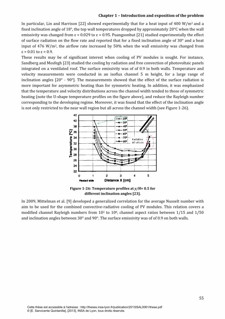
Chapter 1 – Introduction and exposition of the problem
55
In particular, Lin and Harrison [22] showed experimentally that for a heat input of 400 W/m2 and a
fixed inclination angle of 18°, the top wall temperatures dropped by approximately 20°C when the wall
emissivity was changed from ε = 0.029 to ε = 0.95. Puangsonbut [21] studied experimentally the effect
of surface radiation on the flow rate and reported that for a fixed inclination angle of 30° and a heat
input of 476 W/m2, the airflow rate increased by 50% when the wall emissivity was changed from
ε = 0.01 to ε = 0.9.
These results may be of significant interest when cooling of PV modules is sought. For instance,
Sandberg and Mosfegh [23] studied the cooling by radiation and free convection of photovoltaic panels
integrated on a ventilated roof. The surface emissivity was of of 0.9 in both walls. Temperature and
velocity measurements were conducted in an isoflux channel 5 m height, for a large range of
inclination angles [20° - 90°]. The measurements showed that the effect of the surface radiation is
more important for asymmetric heating than for symmetric heating. In addition, it was emphasized
that the temperature and velocity distributions across the channel width tended to those of symmetric
heating (note the U-shape temperature profiles on the figure above), and reduce the Rayleigh number
corresponding to the developing regime. Moreover, it was found that the effect of the inclination angle
is not only restricted to the near wall region but all across the channel width (see Figure 1-26).
Figure 1-26: Temperature profiles at y/H= 0.5 for
different inclination angles [23].
In 2009, Mittelman et al. [9] developed a generalized correlation for the average Nusselt number with
aim to be used for the combined convective-radiative cooling of PV modules. This relation covers a
modified channel Rayleigh numbers from 102 to 108, channel aspect ratios between 1/15 and 1/50
and inclination angles between 30° and 90°. The surface emissivity was of of 0.9 on both walls.
Cette thèse est accessible à l'adresse : http://theses.insa-lyon.fr/publication/2013ISAL0061/these.pdf © [E. Sanvicente Quintanilla], [2013], INSA de Lyon, tous droits réservés

Chapter 1 – Introduction and exposition of the problem
56
1.5.2.2 Modified thermal boundary conditions in vertical channels in order to optimise thermal
performance
Two different approaches have been used to enhance heat transfer from the walls in channel
configurations. The first method consists of some geometric arrangement in the channel which
modifies the aerodynamic characteristics of the flow. This includes among others, to induce an
increase in the flow rate or to produce physical disturbances in the laminar boundary layer, thereby
causing an earlier transition to turbulence and an enhancement of the chimney effect. The placement
of adiabatic extensions, the use of rough walls and the use of obstacles in the inlet section are some of
the attempts used in this approach [43, 86-89]. The second technique relies on altering the imposed
thermal boundary conditions. This is especially met in the cooling of electronic printed circuit boards.
When a global heat flux must be transferred from the plates, an appropriate arrangement of
dissipating components can contribute to reduce the maximum temperature reached in these
components and, consequently, their risk of being damaged. What is required is to determine the heat
flux distributions on a wall that minimize the maximum wall temperature for a given thermal load. The
use of arrays of discrete heat protrusions and heat sources are some examples of this approach [36,
37, 41, 47, 90].
Establishing under which conditions these particular configurations yield heat transfer enhancements
is of great importance in applications where the maximization of heat transfer rate is of prime
consideration. Moreover, since the interest of this type of investigations is cooling (electronics, PV
modules or nuclear engineering), most of the work dedicated has been based on heat transfer studies
from plane surfaces with mixed or forced convection fluid flows. However, since the work in the
present thesis is on natural convection, which requires no external energy input, the particular focus
of the literature survey will be on investigations that deal with natural convection flows.
It should also be noted that there are situations in which roughness, obstacles or non-uniform thermal
conditions occur naturally and are not added for the specific purpose of modifying heat transfer
performance. This may be the case in electronic circuit boards or even surfaces of buildings. In all
cases the understanding of the thermal behavior of these systems is essential for their design.
One of the simplest modified channel configurations employed to increase the heat transfer rate is the
channel-chimney system. This configuration is obtained by means of the placement of adiabatic
extensions upstream or downstream the heated channel. When a heated channel has an unheated
entry section, the flow is somewhat more developed hydro-dynamically upon reaching the heated
surface. This may cause the local heat transfer to increase slightly in the first section of the heated
channel. However, Wirtz and Haag [66] found experimentally that, except for very narrow ducts, the
influence of inlet extensions is negligible in an isothermal symmetrically heated channel.
The addition of adiabatic extensions downstream the heated channel, was found to induce larger total
heat transfer and flow rate than an unheated entry does [34, 67]. Both experimental [87, 91-93] and
numerical investigations [94, 95] have been carried out extensively in this field. A sketch showing the
possible geometry and the characteristic parameters of this type of configuration is presented in
Figure 1-27 below:
Cette thèse est accessible à l'adresse : http://theses.insa-lyon.fr/publication/2013ISAL0061/these.pdf © [E. Sanvicente Quintanilla], [2013], INSA de Lyon, tous droits réservés

Chapter 1 – Introduction and exposition of the problem
57
Figure 1-27: Sketch of a symmetrically heated channel with an unheated chimney added downstream [91].
In general, it was found that the average Nusselt number increased by 10-20% in a channel with long
adiabatic extensions, Lext ≥ 4Lh, and high chimney aspect ratio, B/b > 3 for 1.8102 < Rad* < 1.1106.
Similar observations have been found in symmetrically [86, 95] and asymmetrically [91, 92, 95] isoflux
heated channel walls.
The increase in the average Nusselt number is mainly the result of two phenomena. The first is the
enhanced chimney effect due to large adiabatic extensions, which implies an increase in the effective
height of the channel and a subsequent increment in the range of action of the buoyancy force. The
second is the pressure recovery in the unheated region and a smaller pressure drop in the exit region
of the heated channel due to the increment of the chimney gap (B). Note that for a fixed L/Lh, if the
chimney expansion ratio B/b is very large, a reverse flow may occur, thereby implying a weaker
chimney effect.
Additional modified configurations including auxiliary plates placed in the centerline [48, 88] or
discrete protrusions along the walls [43] have been studied in the field in order to obtain heat transfer
enhancement. The majority of these studies were carried out by numerical investigations [48, 88]. The
common aim was to use discrete obstacles as turbulence generators. It has been shown that the
magnitude of the mean Nusselt number and flow rate is lower for adiabatic protrusions than for
heated ones since heated obstacles induced both dynamic and thermal disturbances in the flow [43,
48]. Indeed, the length and width of the ribs and their location in the channel appeared to influence
strongly the thermal performance of a system. While increasing the length of the rib has only a limited
influence on the heat transfer, increasing its width may dramatically decrease the mass flow rate and
as a consequence the heat transfer rate. This is caused by the obstruction, resulting in an increased
pressure loss in the channel. Indeed, it is particularly pertinent when thick obstacles are placed in the
inlet section of a channel. Therefore, special attention should be taken when designing this type of
configurations.
To illustrate this phenomenon we can cite the complementary experimental work reported by Tanda
et al. [40] in 1997 and Ambrosini et al. [96] in 2004 in vertical channels with one surface roughened by
uniformly distributed transverse ribs. UWT conditions were imposed on the ribbed side while the
opposite surface remained smooth and unheated.
Cette thèse est accessible à l'adresse : http://theses.insa-lyon.fr/publication/2013ISAL0061/these.pdf © [E. Sanvicente Quintanilla], [2013], INSA de Lyon, tous droits réservés
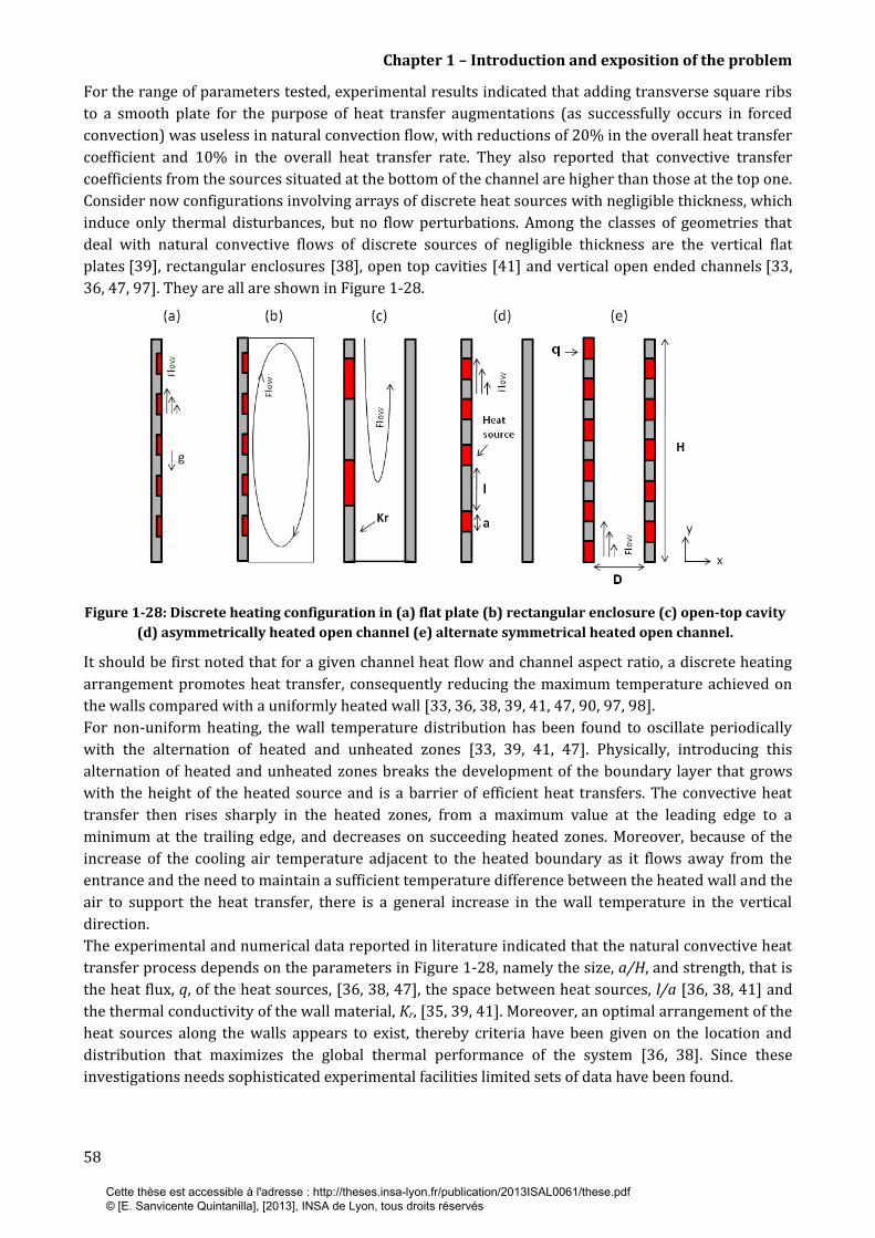
Chapter 1 – Introduction and exposition of the problem
58
For the range of parameters tested, experimental results indicated that adding transverse square ribs
to a smooth plate for the purpose of heat transfer augmentations (as successfully occurs in forced
convection) was useless in natural convection flow, with reductions of 20% in the overall heat transfer
coefficient and 10% in the overall heat transfer rate. They also reported that convective transfer
coefficients from the sources situated at the bottom of the channel are higher than those at the top one.
Consider now configurations involving arrays of discrete heat sources with negligible thickness, which
induce only thermal disturbances, but no flow perturbations. Among the classes of geometries that
deal with natural convective flows of discrete sources of negligible thickness are the vertical flat
plates [39], rectangular enclosures [38], open top cavities [41] and vertical open ended channels [33,
36, 47, 97]. They are all are shown in Figure 1-28.
Figure 1-28: Discrete heating configuration in (a) flat plate (b) rectangular enclosure (c) open-top cavity
(d) asymmetrically heated open channel (e) alternate symmetrical heated open channel.
It should be first noted that for a given channel heat flow and channel aspect ratio, a discrete heating
arrangement promotes heat transfer, consequently reducing the maximum temperature achieved on
the walls compared with a uniformly heated wall [33, 36, 38, 39, 41, 47, 90, 97, 98].
For non-uniform heating, the wall temperature distribution has been found to oscillate periodically
with the alternation of heated and unheated zones [33, 39, 41, 47]. Physically, introducing this
alternation of heated and unheated zones breaks the development of the boundary layer that grows
with the height of the heated source and is a barrier of efficient heat transfers. The convective heat
transfer then rises sharply in the heated zones, from a maximum value at the leading edge to a
minimum at the trailing edge, and decreases on succeeding heated zones. Moreover, because of the
increase of the cooling air temperature adjacent to the heated boundary as it flows away from the
entrance and the need to maintain a sufficient temperature difference between the heated wall and the
air to support the heat transfer, there is a general increase in the wall temperature in the vertical
direction.
The experimental and numerical data reported in literature indicated that the natural convective heat
transfer process depends on the parameters in Figure 1-28, namely the size, a/H, and strength, that is
the heat flux, q, of the heat sources, [36, 38, 47], the space between heat sources, l/a [36, 38, 41] and
the thermal conductivity of the wall material, Kr, [35, 39, 41]. Moreover, an optimal arrangement of the
heat sources along the walls appears to exist, thereby criteria have been given on the location and
distribution that maximizes the global thermal performance of the system [36, 38]. Since these
investigations needs sophisticated experimental facilities limited sets of data have been found.
Cette thèse est accessible à l'adresse : http://theses.insa-lyon.fr/publication/2013ISAL0061/these.pdf © [E. Sanvicente Quintanilla], [2013], INSA de Lyon, tous droits réservés
Chapter 1 – Introduction and exposition of the problem
59
An experimental investigation of the thermal impact of the size of the heat source (a/H) was carried
out by Fossa et al. [47]. Results were obtained for a 2 m high vertical air channel (see Figure 1-28 (e)),
a range of channel aspect ratios, 1/55 D/H 1/10, three different lengths of heated source, a/H: 0.1,
0.2, 1 and l/a = 1. It was shown that for a heat flux of 220 W/m2 averaged over the total surface area of
the plates, reducing the source length to a/H = 0.1 yielded the lowest wall temperatures, with values
decreasing by up to 15°C from the values obtained with the uniformly heated configuration, a/H = 1.
This observation supported the conclusions of Da Silva et al. [36] who attributed this to the thicker
boundary layers developed when heat sources are larger and the consequent larger resultant thermal
resistance.
Da Silva et al. [36] investigated analytically an asymmetrically discrete heated vertical open channel
cooled by natural convection and shown schematically in Figure 1-28 (d). For RaH numbers (based on
the height of the channel) in the range 102 < RaH < 104, the optimal location of discrete heat sources
was also determined. The criteria given was to maximize the global thermal conductance, C*, between
the discretely heated wall and the cold fluid defined as
(6)
where N is the number of heat sources, qs is the imposed heat current through the heat source (W/m),
k is the thermal conductivity, and Tmax -Tinlet is the maximum temperature difference between the wall
and the inlet air (K). This was equivalent to minimizing the maximum temperature of the hot spot that
occurs at some point on the wall.
For heat sources with fixed size and fixed heat flux the spatial optimal arrangement depends strongly
on the Rayleigh number and the heat flux [36]. For example, at low Rayleigh numbers (RaH ~ 102),
authors recommended that the heat sources should be concentrated and distributed near the inlet
region of the channel, where the boundary layer is thinner and thus the air thermal resistance is
smaller.
On the other hand, as the Rayleigh number increased (RaH > 103) the global thermal conductance
appeared to increase, indicating that the maximum temperature in the hot spot decreased, when the
last, downstream, heat source was moved toward the exit plane. This resulted in a non-uniform
distribution of heat sources with more energy being transferred in the lower section of the channel.
This observation supports the conclusion of Hernandez and Zamora [33] and Da Silva et al. [38] for
natural convection flows, Zhang and Dutta [90] for mixed convection flows and Da Silva et al. [37] for
forced convection flows. Furthermore, the separation distance between heat sources not only
influences the thermal field but also the flow field. This was shown numerically by Dehghan and
Behnia [41] for an array of two heat sources inside an open-top cavity with conductive walls similar to
the situation shown in Figure 1-28 (c). They showed that as the distance between the two heating
source, l/a, increases, the velocity with which the air approaches the upper heat source increases with
a consequent enhancement of the heat transfer coefficient of the upper heat source. However, as the
thermal conductivity of the walls increases, there is a mutual thermal interaction between both heat
sources due to conduction in the wall and convection. Moreover, the wall temperature in the case of
conductive walls is found to be distributed more uniformly than in the case of adiabatic walls, implying
that direct convection heat transfer from the chip to the air decreases while the indirect conduction
heat transfer through the unheated wall region increases.
This observation supports the results found by Chen et al. [39] for a flat plate in heated on one side as
shown in Figure 1-28 (a) and Mathews et al. [35] for an open channel with mixed convection flow (see
in Figure 1-28 (d)). In both studies the heat transfer process with coupled effects of conduction and
convection was investigated.
Cette thèse est accessible à l'adresse : http://theses.insa-lyon.fr/publication/2013ISAL0061/these.pdf © [E. Sanvicente Quintanilla], [2013], INSA de Lyon, tous droits réservés
Chapter 1 – Introduction and exposition of the problem
60
It follows from the above discussion that the cooling of the systems represented in Figure 1-28 cannot
be understood without the knowledge of the interactions between the instantaneous flow structures
and the thermal fields.
1.5.3 Dynamic thermal and flow structures
The study of heat and mass transfer related to natural convection flow in a channel would not be fully
completed without the investigation of instantaneous kinematical and thermal quantities as well as
the examination of flow patterns.
Although laminar natural convection in open-ended channels has been the subject of extensive
experimental and numerical investigations for several decades, there is only a limited literature on the
development of flow structures, transition to turbulence and the consequent thermal behavior in
natural convection in parallel plate channels. This is despite the possible interest that the phenomenon
might produce, as early transition could be a possible mechanism of heat transfer enhancement.
Indeed, since most engineering applications involve transition and turbulent flows, the understanding
of transition phenomena is of great practical importance. Further, turbulent flows produce flow
structures responsible for high levels of mixing [99] usually thought to be important in enhancing heat
transfer. Hence, in this section a detailed review of studies and models, which use this approach, is now
presented. The initial focus will be on studies which characterize the transition to turbulent flow in
parallel plate channels and then the unsteady nature of the flows involved will be highlighted. Both
approaches may help the understanding of the difficulties that numerical studies encounter in the
validation step.
1.5.3.1 Characterisation of the transition to turbulent flow in parallel plate channels
With a low level of external disturbance, natural convection flows along a parallel plate channel similar
to that on the present study would be expected to be laminar at the inlet, undergo transition and
finally become fully turbulent near the outlet depending upon the aspect ratio, D/H, and the Rayleigh
number, Ra. The identification of the transition from laminar flow to turbulent flow has been mostly
inferred from the characteristics of the surface temperature variation. Experimentally, the widely cited
work of Miyamoto [73] has contributed significantly to the understanding of turbulent natural
convection in asymmetrically heated vertical parallel plate channels. Experiments were carried out in a
five meters vertical air channel with an UHF imposed on one wall, the other being adiabatic. The
injected fluxes were 104 and 208 W/m2 and the channel aspect ratios (D/H) tested varied from 0.01 to
0.04. An inflexion point in the temperature excess distribution on the heated plate for a wall heat flux
of 104 W/m2 was observed. Presented in Figure 1-29 below are the corresponding experimental
results obtained for three different channel aspect ratios (D/H).
Cette thèse est accessible à l'adresse : http://theses.insa-lyon.fr/publication/2013ISAL0061/these.pdf © [E. Sanvicente Quintanilla], [2013], INSA de Lyon, tous droits réservés
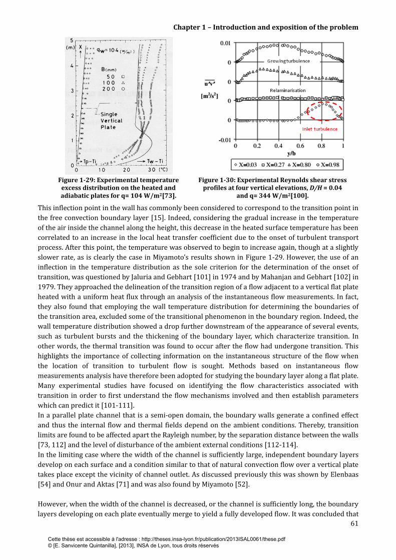
Chapter 1 – Introduction and exposition of the problem
61
Figure 1-29: Experimental temperature
excess distribution on the heated and adiabatic plates for q= 104 W/m2[73].
Figure 1-30: Experimental Reynolds shear stress profiles at four vertical elevations, D/H = 0.04
and q= 344 W/m2[100].
This inflection point in the wall has commonly been considered to correspond to the transition point in
the free convection boundary layer [15]. Indeed, considering the gradual increase in the temperature
of the air inside the channel along the height, this decrease in the heated surface temperature has been
correlated to an increase in the local heat transfer coefficient due to the onset of turbulent transport
process. After this point, the temperature was observed to begin to increase again, though at a slightly
slower rate, as is clearly the case in Miyamoto’s results shown in Figure 1-29. However, the use of an
inflection in the temperature distribution as the sole criterion for the determination of the onset of
transition, was questioned by Jaluria and Gebhart [101] in 1974 and by Mahanjan and Gebhart [102] in
1979. They approached the delineation of the transition region of a flow adjacent to a vertical flat plate
heated with a uniform heat flux through an analysis of the instantaneous flow measurements. In fact,
they also found that employing the wall temperature distribution for determining the boundaries of
the transition area, excluded some of the transitional phenomenon in the boundary region. Indeed, the
wall temperature distribution showed a drop further downstream of the appearance of several events,
such as turbulent bursts and the thickening of the boundary layer, which characterize transition. In
other words, the thermal transition was found to occur after the flow had undergone transition. This
highlights the importance of collecting information on the instantaneous structure of the flow when
the location of transition to turbulent flow is sought. Methods based on instantaneous flow
measurements analysis have therefore been adopted for studying the boundary layer along a flat plate.
Many experimental studies have focused on identifying the flow characteristics associated with
transition in order to first understand the flow mechanisms involved and then establish parameters
which can predict it [101-111].
In a parallel plate channel that is a semi-open domain, the boundary walls generate a confined effect
and thus the internal flow and thermal fields depend on the ambient conditions. Thereby, transition
limits are found to be affected apart the Rayleigh number, by the separation distance between the walls
[73, 112] and the level of disturbance of the ambient external conditions [112-114].
In the limiting case where the width of the channel is sufficiently large, independent boundary layers
develop on each surface and a condition similar to that of natural convection flow over a vertical plate
takes place except the vicinity of channel outlet. As discussed previously this was shown by Elenbaas
[54] and Onur and Aktas [71] and was also found by Miyamoto [52].
However, when the width of the channel is decreased, or the channel is sufficiently long, the boundary
layers developing on each plate eventually merge to yield a fully developed flow. It was concluded that
Cette thèse est accessible à l'adresse : http://theses.insa-lyon.fr/publication/2013ISAL0061/these.pdf © [E. Sanvicente Quintanilla], [2013], INSA de Lyon, tous droits réservés
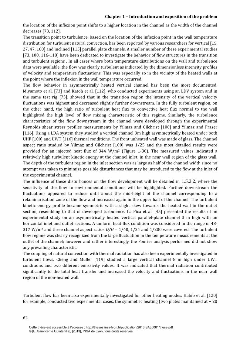
Chapter 1 – Introduction and exposition of the problem
62
the location of the inflexion point shifts to a higher location in the channel as the width of the channel
decreases [73, 112].
The transition point to turbulence, based on the location of the inflexion point in the wall temperature
distribution for turbulent natural convection, has been reported by various researchers for vertical [15,
27, 47, 100] and inclined [115] parallel plate channels. A smaller number of these experimental studies
[73, 100, 116-118] have been dedicated to investigate the behavior of flow structures in the transition
and turbulent regions . In all cases where both temperature distributions on the wall and turbulence
data were available, the flow was clearly turbulent as indicated by the dimensionless intensity profiles
of velocity and temperature fluctuations. This was especially so in the vicinity of the heated walls at
the point where the inflexion in the wall temperature occurred.
The flow behavior in asymmetrically heated vertical channel has been the most documented.
Miyamoto et al. [73] and Katoh et al. [112], who conducted experiments using an LDV system and in
the same test rig [73], showed that in the transition region the intensity of the vertical velocity
fluctuations was highest and decreased slightly further downstream. In the fully turbulent region, on
the other hand, the high ratio of turbulent heat flux to convective heat flux normal to the wall
highlighted the high level of flow mixing characteristic of this regime. Similarly, the turbulence
characteristics of the flow downstream in the channel were developed through the experimental
Reynolds shear stress profiles measurements by Yilmaz and Gilchrist [100] and Yilmaz and Fraser
[116]. Using a LDA system they studied a vertical channel 3m high asymmetrically heated under both
UHF [100] and UWT [116] thermal conditions. The front unheated wall was made of glass. The channel
aspect ratio studied by Yilmaz and Gilchrist [100] was 1/25 and the most detailed results were
provided for an injected heat flux of 344 W/m2 (Figure 1-30). The measured values indicated a
relatively high turbulent kinetic energy at the channel inlet, in the near wall region of the glass wall.
The depth of the turbulent region in the inlet section was as large as half of the channel width since no
attempt was taken to minimize possible disturbances that may be introduced to the flow at the inlet of
the experimental channel.
The influence of these disturbances on the flow development will be detailed in 1.5.3.2, where the
sensitivity of the flow to environmental conditions will be highlighted. Further downstream the
fluctuations appeared to reduce until about the mid-height of the channel corresponding to a
relaminarisation zone of the flow and increased again in the upper half of the channel. The turbulent
kinetic energy profile became symmetric with a slight skew towards the heated wall in the outlet
section, resembling to that of developed turbulence. La Pica et al. [45] presented the results of an
experimental study on an asymmetrically heated vertical parallel-plate channel 3 m high with an
horizontal inlet and outlet sections. A uniform heat flux condition was considered in the range of 48-
317 W/m2 and three channel aspect ratios D/H = 1/40, 1/24 and 1/200 were covered. The turbulent
flow regime was clearly recognized from the large fluctuation in the temperature measurements at the
outlet of the channel; however and rather interestingly, the Fourier analysis performed did not show
any prevailing characteristic.
The coupling of natural convection with thermal radiation has also been experimentally investigated in
turbulent flows. Cheng and Muller [119] studied a large vertical channel 8 m high under UWT
conditions and two different emissivity values. It was indicated that thermal radiation contributed
significantly to the total heat transfer and increased the velocity and fluctuations in the near wall
region of the non-heated wall.
Turbulent flow has been also experimentally investigated for other heating modes. Habib et al. [120]
for example, conducted two experimental cases, the symmetric heating (two plates maintained at + 20
Cette thèse est accessible à l'adresse : http://theses.insa-lyon.fr/publication/2013ISAL0061/these.pdf © [E. Sanvicente Quintanilla], [2013], INSA de Lyon, tous droits réservés

Chapter 1 – Introduction and exposition of the problem
63
°C) and asymmetric heating (one plate kept at + 10 °C while the other at - 10 °C). They performed flow
visualization studies and velocity measurements using an LDV system.
It was shown that the heating mode significantly influenced the flow patterns. This was characterized
for both heating modes by measured skewness and flatness factors at two different sections.
The more rapid change in the velocity gradient across the channel in the asymmetric case resulted in
higher skewness factors than in the symmetric case. Ayinde et al. [118] also investigated the symmetric
heating condition by using a PIV system in a vertical parallel plate channel. Turbulent flow was
present, particularly in the near wall regions as indicated the profile of root mean square (rms) values
of velocity fluctuations and the Reynolds stress. These maxima on both profiles were attributed to the
creation of eddies in the shear layer of considerable gradient close to the wall region. The maxima were
also found to diminish as a result of the diffusion of Reynolds stresses towards the center of the
channel.
1.5.3.2 Flow sensitivity to channel surrounding conditions
Experimental investigations carried out in open-ended channels have revealed that pressure,
temperature and disturbance conditions outside the channel may affect the location of the transition
from the laminar to turbulent flow as well as the average heat transfer and transport coefficients [112-
114]. If no measure is taken to minimize possible disturbances that may be introduced to the flow at
the inlet of the experimental channel, a high turbulent intensity level may be present in the inlet of the
channel as discussed above [100, 116]. An increase in the inlet disturbances is found to enhance the
mixing in the inlet zone and the local transition between laminar regime and turbulent regime
appeared to be less brusque. Indeed, it was observed that this increased fluctuations in the inlet may
move the transition point further upstream [112]. Based on a vertical flat plate subjected to a uniform
heat flux, transition is likely to occur for a Rayleigh number based on the channel height between
21013 and 11014. For the tested heat inputs between 200 and 600W, Chen et al. [27] analytically
estimated the starting point of transition at a height around 2 m. However, for a 1.5 m high solar
chimney channel (D/H = 1/20), transition was identified earlier (y/H ~ 0.9) through the inflection
point observed in the wall temperature profile along the heated wall. The authors concluded that this
early transition compared to the analytical prediction was due to the air disturbances in the chimney
inlet which they linked to the test room conditions. However, no information describing external
conditions was provided.
In an attempt to experimentally characterize the influence of inlet disturbances and subsequently to
control them, Katoh et al. [112] installed a bell-mouth entrance at the lower end of the vertical parallel
plate channel previously used by Miyamoto et al. [73]. Under the same experimental conditions (D/H
and injected heat fluxes) it was observed that the general characteristics of the time-averaged
temperature distributions and the time-mean vertical velocity between both experiments did not
appear to be very different However, the inflexion point in the temperature distribution appeared
clearer, indicating a more brusque transition process, and indeed it was shifted to a higher location
when inlet disturbances were controlled. Presented in Figure 1-31 below, among other information, is
a comparison between the experimental temperature distributions with and without the bell-mouth
for q = 202 W/m2 at a fixed channel aspect ratio of D/H = 1/50. Please note that the enhanced mixing
in the inlet zone without the bell-mouth resulting in a lower temperature of the heated surface
indicates the presence of disturbances.
Cette thèse est accessible à l'adresse : http://theses.insa-lyon.fr/publication/2013ISAL0061/these.pdf © [E. Sanvicente Quintanilla], [2013], INSA de Lyon, tous droits réservés
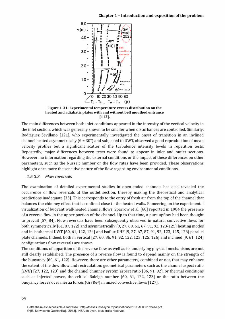
Chapter 1 – Introduction and exposition of the problem
64
Figure 1-31: Experimental temperature excess distribution on the
heated and adiabatic plates with and without bell mouthed entrance [112].
The main differences between both inlet conditions appeared in the intensity of the vertical velocity in
the inlet section, which was generally shown to be smaller when disturbances are controlled. Similarly,
Rodriguez Sevillano [121], who experimentally investigated the onset of transition in an inclined
channel heated asymmetrically (θ = 30°) and subjected to UWT, observed a good reproduction of mean
velocity profiles but a significant scatter of the turbulence intensity levels in repetition tests.
Repeatedly, major differences between tests were found to appear in inlet and outlet sections.
However, no information regarding the external conditions or the impact of these differences on other
parameters, such as the Nusselt number or the flow rates have been provided. These observations
highlight once more the sensitive nature of the flow regarding environmental conditions.
1.5.3.3 Flow reversals
The examination of detailed experimental studies in open-ended channels has also revealed the
occurrence of flow reversals at the outlet section, thereby making the theoretical and analytical
predictions inadequate [33]. This corresponds to the entry of fresh air from the top of the channel that
balances the chimney effect that is confined close to the heated walls. Pioneering on the experimental
visualization of buoyant wall-heated channel flows, Sparrow et al. [60] reported in 1984 the presence
of a reverse flow in the upper portion of the channel. Up to that time, a pure upflow had been thought
to prevail [57, 84]. Flow reversals have been subsequently observed in natural convective flows for
both symmetrically [61, 87, 122] and asymmetrically [9, 27, 60, 61, 67, 91, 92, 123-125] heating modes
and in isothermal UWT [60, 61, 122, 124] and isoflux UHF [9, 27, 67, 87, 91, 92, 123, 125, 126] parallel
plate channels. Indeed, both in vertical [27, 60, 86, 91, 92, 122, 123, 125, 126] and inclined [9, 61, 124]
configurations flow reversals are shown.
The conditions of apparition of the reverse flow as well as its underlying physical mechanisms are not
still clearly established. The presence of a reverse flow is found to depend mainly on the strength of
the buoyancy [60, 61, 122]. However, there are other parameters, combined or not, that may enhance
the extent of the downflow and recirculation: geometrical parameters such as the channel aspect ratio
(D/H) [27, 122, 123] and the channel chimney system aspect ratio [86, 91, 92], or thermal conditions
such as injected power, the critical Raleigh number [60, 61, 122, 123] or the ratio between the
buoyancy forces over inertia forces (Gr/Re2) in mixed convective flows [127].
Cette thèse est accessible à l'adresse : http://theses.insa-lyon.fr/publication/2013ISAL0061/these.pdf © [E. Sanvicente Quintanilla], [2013], INSA de Lyon, tous droits réservés

Chapter 1 – Introduction and exposition of the problem
65
Indeed, depending on the penetration length and the size of the recirculation cells, the total energy
transfer between the wall and the fluid may be affected [127] and the induced mass flow rate may be
consequently limited.
Recently, the measurements of the velocity fields inside an assymetrically heated vertical channel
(UHF) conducted by Dupont et al. [128] led to define three classes of outlet flow corresponding to the
absence, intermittence and permanence of the reverse flow. The principal discriminating parameters
used for this classification were the Rayleigh number and the channel aspect ratio. A third parameter,
the inclination, was also considered as a key parameter but no results were reported yet. Temperature
measurements conducted in a similar channel [129] but with one of the walls maintained at a uniform
wall temperature stated as well the three classes of reverse flows and reported a classification of them
in diagram using the Rayleigh number versus the channel aspect ratio coordinate system (see Figure
1-32).
Figure 1-32: Diagram relating the conditions of apparition
of reverse flows based on temperature measurements [129].
In general, the conditions marking the onset and extent of flow reversals are sought by systematic
variations of the independent parameters, particularly the Rayleigh number and the channel aspect
ratio.
We can first cite the experimental and analytical results of Sparrow et al. [60] and Azevedo et al. [61]
where the effect of both parameters in the onset and extent of the flow reversal were systematically
investigated for vertical [60] and inclined [61] channels. It should be noted that these investigations
have contributed significantly to the understanding of the physical mechanisms that lead to flow
reversals. Experiments in [60, 61] were performed in water (Pr = 5) in an asymmetrically heated
isothermal channel 12.5 cm height and with the aid of the thymol blue flow visualization technique.
They stated that this flow divides into two separate flows at the stagnation point and then merge into
the upcoming flow through the heated channel. These motions create spanwise vortices. This
phenomenon is accompanied by a separation of the ascending boundary layer type flow close to the
non-heated wall leaving a V-shaped region (see Figure 1-34(b)). Similar recirculation flow structures
have been highlighted by other authors [60, 91, 122] for UWT boundary conditions. On the other hand,
the penetration length of the reverse flow is the distance from the channel exit to the stagnation point
on the centerline.
In the vertical configuration three channel aspect ratios D/H = 1/23, 1/18 and 1/15 were examined
covering a range of 2.2x10⁴ < RaD < 6x10⁴ in the laminar flow regime. Under the particular conditions
Cette thèse est accessible à l'adresse : http://theses.insa-lyon.fr/publication/2013ISAL0061/these.pdf © [E. Sanvicente Quintanilla], [2013], INSA de Lyon, tous droits réservés

Chapter 1 – Introduction and exposition of the problem
66
tested, the onset of the flow reversal was identified at a RaD ~ 3.1x10⁴ - 3.5x10⁴ and the penetration
depth appears to increase more or less linearly with increasing Rayleigh number.
This is illustrated in Figure 1-33 where the penetration length is plotted in terms of modified Ra*
number, based on the channel width and the channel aspect ratio. Please note the identifiable
Rayleigh-number-related transition from no downflow to downflow is clearly identified.
Figure 1-33: Maximum penetration depth of downflow, D/H= 0.0656.
[60].
Similar flow patterns, transition values and penetration length trends were observed when the
channel was tilted 30° and 45° both heated from the top or symmetrically. However, when heat was
applied in the bottom wall, no backflow was observed.
Rather interestingly, the analysis of the measured Nusselt numbers indicates that the convection heat
transfer to the recirculating air from the wall is limited and the overall heat transfer is found to be
unaffected by the presence of the flow reversal. The limited influence of flow reversals on the wall heat
transfer is subsequently reported by several researchers such as Webb and Hill [67] , Kihm et al. [122]
and Mittelman [9]. Different arguments can provide explanation for this phenomenon. First, flow
reversals are generally confined to the unheated wall in the asymmetrically heated case [9, 67] or the
central part of the channel in the symmetrical heated case [61, 122], while Nusselt numbers pertain to
the heated walls. A second factor is that backflow phenomena occur at the outlet of the channel while
the overall heat transfer correlations calculated in these studies are an average of the entire heated
wall. In addition, heat transfer rates appear to be highest in the inlet section, thereby dampening the
response of Nus to the reversal flow. However, it should be noted that the aforementioned studies
consider the laminar flow regime.
To gain further insights on the dynamics involved in recirculating flows in vertical channels, Ospir et
al. [123] and Popa et al. [125] have recently investigated the detailed flow structure when the channel
aspect ratio and the Rayleigh number are varied. Experiments were carried out in a vertical parallel
plate short channel (H = 376 mm) with one of the walls composed of a heated central part (Hheated =
188 mm) subjected to a UHF condition.
Water was used as working fluid which leads to a negligible effect of heat transfer by radiation.
Moreover, flow visualisation techniques based on laser tomography using discrete and continuous
tracers were performed in the mid-plane of the channel (z/L = 0.5) along its entire height. Although
both the steady-state regime and the transitional phase just after the start of the heating were
investigated, we will particularly focus on the steady state regime.
It was shown that in particular the channel aspect ratio, D/H, significantly affects the penetration
length of such recirculation flow. Indeed, they demonstrated that an increase in the channel aspect
Cette thèse est accessible à l'adresse : http://theses.insa-lyon.fr/publication/2013ISAL0061/these.pdf © [E. Sanvicente Quintanilla], [2013], INSA de Lyon, tous droits réservés

Chapter 1 – Introduction and exposition of the problem
67
ratio (with increase in the channel gap) from D/H = 1/7 to D/H= 1/5 may result in twice an increase in
the recirculation length cell. Figure 1-34 (a) shows results of flow visualisation tests for a fixed
modified Rayleigh number of Ra* = 4.5 x 10⁶ and three different aspect ratios (varying the distance
between plates).
Figure 1-34: Influence of the aspect ratio on the recirculation length cell.
[123].
The reverse flow structure observed is characterized by two large recirculation cells, connecting by a
neck and forming an elongated eight-shaped structure. The penetration length of the reverse flow has
been indicated in Figure 1-34 (a) with dashed lines. These recirculation lengths are illustrated in
Figure 1-34 (c) for each case and are denoted Lup (upper recirculation cell length) and Llow (lower
recirculation cell length), respectively. In Figure 1-34(c) one can observe that an increase in the
channel aspect ratio (with increase in the channel gap) affects particularly the upper recirculation
length, the lower recirculation cell remaining stable regardless the channel aspect ratio. In this study
no information regarding the thermal fields was provided.
1.5.4 Concluding remarks and motivation of the study
The cooling of the PV modules integrated in double skin arrangements is the result of coupling
radiation and natural convection generating an airflow in the channel. Natural convection in open-
Cette thèse est accessible à l'adresse : http://theses.insa-lyon.fr/publication/2013ISAL0061/these.pdf © [E. Sanvicente Quintanilla], [2013], INSA de Lyon, tous droits réservés
Chapter 1 – Introduction and exposition of the problem
68
ended channels is driven on one hand, by the pressure gradient between the inlet and outlet and on
the other one, by buoyancy forces which are generated by density gradients. Buoyancy forces in air are
small for moderate differences in temperatures, so that in general induced fluid velocities are low and
therefore difficult to measure. As well, control of the flow is challenging because of the significant
impact that disturbances from the external environmental have on natural convection flows. The
influence of external conditions is also still not so obvious because of the thermal stratification, inlet-
outlet pressure difference and kinematical and thermal fluctuations that may dampen, neutralize or
enhance the chimney effect. In addition in the outlet of the channel, the effect of the intermittent
occurrence of flow reversals on heat transfer and flow rate is not clearly identified. As a result, existing
experimental data on buoyancy driven flows and temperature distributions in open-ended heated
channels is still very limited despite all the investigations that have been conducted. This is especially
highlighted in the transitional range from laminar flow to turbulent flow, which is possibly one of the
most important aspects of the cooling of these systems and is still not well understood. The flow
patterns and involved physical mechanisms remain as well an open problematic. In addition, in many
of the reviewed studies, radiation exchange has either been minimized or ignored, thereby introducing
some interpretation errors of the results that have been obtained. It follows that the control of the
energy transfers from the PV arrays could not be understood without a thorough experimental
investigation of all the phenomena involved.
Literature review has also indicated the importance of investigating the simple geometry of the
parallel plate channel when thermal optimization is sought. Under the criterion of maximizing cooling
and thus minimizing wall temperatures a fixed gap-to-height ratio, D/H of 1/15 has been selected for
the present investigation. This channel aspect ratio lies within the typical range considered in
buildings, 1/25 < D/H < 1/3 [130]. Regarding the inclination angle of the channel, it is implicit that the
impact of the inclination is highly dependent on the latitude of the location. Subsequently, the inclined
configurations will be experimentally investigated between 90o -30o, where latitudes of Sydney [~34
°], Lyon and Genoa (~ 45°) are also considered.
It is also found that heat transfer can be enhanced by specific wall geometrical arrangements of PV
modules. This would obviously depend on the requirements of the real design in terms of visual
comfort and aesthetic appearance. As a result, investigations of thermal boundary conditions related
to PV modules or PV cells arrangements which appear to be of prime importance as it has been shown
[40]. Regarding the requirements of the double façade, we will investigate an academic configuration
including a uniform distribution of discrete heat sources although it is seen that optimum
configurations includes a linear wall heat flux distribution with larger heat fluxes located in the inlet
section. As was indicated by Sandberg [26], if the PV covers only part of the façade, the ideal location of
the PV is at the lower end of the air channel, because this results in a higher column of heated air and
therefore a higher natural convection flow. However, we will use these observations for positioning
the first heated zone, that corresponds to the first PV module, at the bottom of the external wall of the
double façade.
It has also been shown that while configurations subjected to non-uniform heat flux distributions are
extensively investigated through thermal studies, there is lack of information regarding the flow fields
and the induced mass flow rate. This can be really useful for hybrid applications where both heating
and ventilating are sought.
As a consequence there are two mains objectives for the present work: the input of knowledge about
physical phenomena governing the chimney effect and associated heat transfers and the generation of
experimental data base for CFD modeling. Indeed, this study and the data collected may also help to
select a CFD model suitable for this type of flow, which is one of the recurring problems in numerical
Cette thèse est accessible à l'adresse : http://theses.insa-lyon.fr/publication/2013ISAL0061/these.pdf © [E. Sanvicente Quintanilla], [2013], INSA de Lyon, tous droits réservés

Chapter 1 – Introduction and exposition of the problem
69
simulations, to select appropriate boundaries of the computational domain and to define the kinematic
(pressure and velocity) inlet/outlet boundary. Moreover, concerning effective application, the
understanding of kinematical and thermal mechanisms involved is necessary if active control of the
temperature of PV modules is sought.
Cette thèse est accessible à l'adresse : http://theses.insa-lyon.fr/publication/2013ISAL0061/these.pdf © [E. Sanvicente Quintanilla], [2013], INSA de Lyon, tous droits réservés

Chapter 1 – Introduction and exposition of the problem
70
Cette thèse est accessible à l'adresse : http://theses.insa-lyon.fr/publication/2013ISAL0061/these.pdf © [E. Sanvicente Quintanilla], [2013], INSA de Lyon, tous droits réservés

Chapter 2 Research Design
Chapter 2
Research Design
This chapter on research design outlines the experimental set ups and measuring techniques used in
the present investigation to analyze natural convection flow in open-ended channels.
Two experimental apparatuses have been used during the investigation, one for the study of vertical
configurations and the second one for the study of the inclined ones. The experimental set up designed
to simulate the essential features of natural ventilated double façades, namely F-device, was built in
2007 during the previous PhD thesis at the CETHIL Laboratory (France). The second experimental
apparatus designed to simulate natural ventilated roofs, namely R-device, was built in 2006 at the
University of New South Wales (Australia). Related to the application, in both of them the thermal
boundary conditions at the wall are of uniform heat flux (UHF) type.
In the first section of the chapter the geometrical characteristics of the test rigs and the test room
conditions are presented. Their principle of operation and the differences between the inlet and outlet
conditions are outlined.
With regards to provide information on the natural convection flow and heat transfer characteristics,
we have conducted both temperature and velocity measurements. The temperature distribution of
each of the heated plates and the temperature at a number of points in the experimental room are
measured with thermocouples. On the other hand, the channel flow characteristics are investigated
using a 2D-PIV system and thermocouples immersed in the flow. The measuring techniques and the
experimental procedures carried out are discussed in detail in the second section of the chapter.
The methodology used to evaluate and analyze the data is presented in the third section. In particular,
the measurement of the wall temperatures has enabled the convective heat transfer coefficients to be
evaluated from the electrical power dissipated in each heater and from estimation of the conduction
and radiation losses to the environment. The convergence for time periods on the mean velocity and
turbulent quantities is presented as well. Finally, the flow heterogeneity is characterized through
statistical quantities such as the probability density function and the skewness and flatness factors.To
conclude, the configurations studied in the present investigation are detailed toguether with the
research criteria influencing the choice.
Cette thèse est accessible à l'adresse : http://theses.insa-lyon.fr/publication/2013ISAL0061/these.pdf © [E. Sanvicente Quintanilla], [2013], INSA de Lyon, tous droits réservés

Chapter 2 – Research Design
72
2.1 Experimental facilities and set up
2.1.1 Vertical channel apparatus-the F.device
Geometrical characteristics
The experimental set up employed for the study of vertical arrangements is located at the CETHIL
laboratory in Lyon (France). In this section the main geometrical characteristics are presented; a more
detailed description of the design procedure is referred to the section ‘Conception et instrumentation
du banc d’essai’ (pages 51-62) in [131].
The test rig presented in Figure 2-1 consists of two parallel vertical walls (H = 1.5 m height, D = 0.70 m
wide) separated by a fixed distance d adjustable in the range [5 cm- 60 cm]. Each wall is constituted by
an insulated material (polyurethane block, 12 cm thick) with a nominal thermal conductivity of
0.027 ± 0.00135 W/m.K embedded in a wooden frame. Moreover, the channel is closed on both sides
by two vertical Plexiglass sheets to avoid lateral infiltration of air and allow optical access to the
channel.
Horizontal Bakelite plates (40 cm long and 70 cm large) are fixed in the inlet and outlet of the channel
(see Figure 2-2). This ensures top/bottom geometrical symmetry and allows the use of the classical
and well-controlled wall boundary conditions for numerical simulations. During the first experiments,
recirculation zones were observed close to the first heated film [131] in the inlet section. In order to
drive streamlines and prevent fluid separation from the wall, the edges of the two plates at the inlet of
the channel have chamfers of 30°. Moreover, a distance of 75 cm is left between the floor and the
channel inlet. The top/bottom geometrical symmetry is also conserved by adding a horizontal plane at
the same distance from the channel outlet (seeFigure 2-2). The effect of the floor and ceiling distances
on the development of the flow was previously investigated while the experimental set up was being
designed. Calculation details can be found in [131].
Figure 2-1: Experimental set up (Cethil Lab,
France).
Figure 2-2: Inlet and outlet boundary conditions in
the F-device.
On the inner side of each wall, 15 independent rectangular film heaters have been placed in order to
allow different heating configurations. The dimension of each heater is 10 cm high and 83.75 cm wide.
The heater consists of a thin metal foil of stainless steel 50 µm thick, with a mean conductivity of k =
13 W/m.k and an emissivity of ε = 0.092. The characteristics of the heaters allow a uniform heat flux
(UHF) boundary condition to be imposed. The upper power limit of the heaters is 500 W/m².
Cette thèse est accessible à l'adresse : http://theses.insa-lyon.fr/publication/2013ISAL0061/these.pdf © [E. Sanvicente Quintanilla], [2013], INSA de Lyon, tous droits réservés
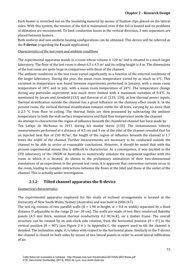
Chapter 2 – Research Design
73
Each heater is stretched out on the insulating material by means of fixation clips placed on the lateral
sides. With this system, the tension of the foil is maintained even if the foil is heated and no problems
of dilatation are encountered. To limit conduction losses in the vertical direction, 2 mm separators are
placed between heaters.
Both uniform and non-uniform heating configurations can be obtained. This device will be referred as
the F-device (regarding the Façade application).
Characteristics of the test room and ambient conditions
The experimental apparatus stands in a room whose volume is 120 m3 and is situated in a much larger
laboratory. The floor of the test room is about 6.5 x 4.5 m2 and its ceiling height is 4 m. The dimensions
of the test room are quite large in comparison with those of the channel.
The ambient conditions in the test room varied significantly as a function of the external conditions of
the larger laboratory. During the year, the mean room temperature varied by as much as 6°C. This
variation in temperature was found between experiments performed in January, with a mean room
temperature of 18°C and in July, with a mean room temperature of 24°C. The temperature change
during any particular experiment was much more limited with a maximum variation of 0.4°C. As
mentioned by Javam and Armfield [132] and Daverat et al. [133, 134], at low thermal power inputs,
thermal stratification outside the channel has a great influence on the chimney effect inside it. In the
present room, the vertical thermal stratification remains stable for all tests, varying by no more than
2-2.5 °C from floor to ceiling. The thermal fields are then presented by subtracting the ambient
temperature to both the wall surface temperatures and fluid flow temperature inside the channel.
An attempt to characterize the region of influence beneath the chamfered channel has been made by
Teo Lafaye de Micheaux in 2011 during his master thesis [135]. The instantaneous velocity
measurements performed at a distance of 4.5 cm and 9 cm of the inlet of the channel revealed that for
an injected heat flux of 230 W/m2, the length of the region of influence beneath the channel is 1.7
times the width of the channel. Further measurements are necessary to be conducted outside the
channel to be able to arrive at reasonable conclusions. However, it should be noted that with the
present experimental means this is difficult to characterize. As a consequence, it was decided in the
CFD laboratory of the UNSW in Australia to numerically simulate the equipment together with the
room in which it is located. As shown in the preliminary animations of their two-dimensional
simulations of an experiment in the present test room, it is apparent that convection currents occur in
the room, leading to complex interactions between the flows at the inlet and those at the outlet of the
channel. This is actually under investigation.
2.1.2 Tilted channel apparatus-the R-device
Geometrical characteristics
The experimental apparatus employed for the study of inclined arrangements is located at the
University of New South Wales, Sydney (Australia) and was built in 2006 [47].
The test rig consists of two parallel walls (H = 1.98 m height, w = 0.8 m width) separated by a fixed
distance D adjustable in the range [5 cm- 30 cm]. The walls are made of two fibre reinforced Bakelite
panels (4.5 mm thick, nominal thermal conductivity 0.2 W/m.K), on a timber frame. The overall
structure can be rotated by an anti-clock side rotation, from the horizontal position (θ = 0°) to the
vertical position (θ = 90°) (see Figure 2-4 ). In Appendix C, the support used to tilt the channel is
detailed. The inclination angle, θ, is taken with respect to the horizontal plane. Similarly to the F-device
the channel is closed on both sides by means of two lateral panels in order to avoid lateral infiltration
of air.
Cette thèse est accessible à l'adresse : http://theses.insa-lyon.fr/publication/2013ISAL0061/these.pdf © [E. Sanvicente Quintanilla], [2013], INSA de Lyon, tous droits réservés
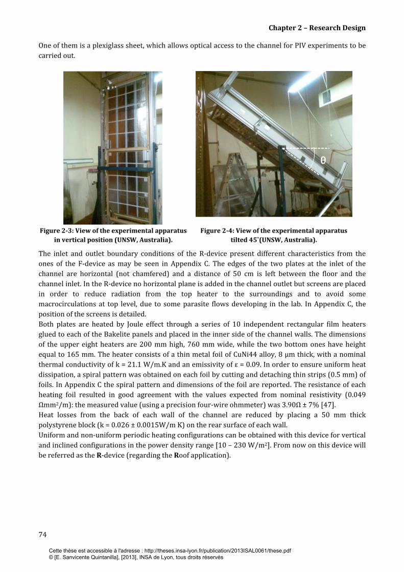
Chapter 2 – Research Design
74
One of them is a plexiglass sheet, which allows optical access to the channel for PIV experiments to be
carried out.
Figure 2-3: View of the experimental apparatus
in vertical position (UNSW, Australia).
Figure 2-4: View of the experimental apparatus
tilted 45˚(UNSW, Australia).
The inlet and outlet boundary conditions of the R-device present different characteristics from the
ones of the F-device as may be seen in Appendix C. The edges of the two plates at the inlet of the
channel are horizontal (not chamfered) and a distance of 50 cm is left between the floor and the
channel inlet. In the R-device no horizontal plane is added in the channel outlet but screens are placed
in order to reduce radiation from the top heater to the surroundings and to avoid some
macrocirculations at top level, due to some parasite flows developing in the lab. In Appendix C, the
position of the screens is detailed.
Both plates are heated by Joule effect through a series of 10 independent rectangular film heaters
glued to each of the Bakelite panels and placed in the inner side of the channel walls. The dimensions
of the upper eight heaters are 200 mm high, 760 mm wide, while the two bottom ones have height
equal to 165 mm. The heater consists of a thin metal foil of CuNi44 alloy, 8 µm thick, with a nominal
thermal conductivity of k = 21.1 W/m.K and an emissivity of ε = 0.09. In order to ensure uniform heat
dissipation, a spiral pattern was obtained on each foil by cutting and detaching thin strips (0.5 mm) of
foils. In Appendix C the spiral pattern and dimensions of the foil are reported. The resistance of each
heating foil resulted in good agreement with the values expected from nominal resistivity (0.049
Ωmm2/m): the measured value (using a precision four-wire ohmmeter) was 3.90Ω ± 7% [47].
Heat losses from the back of each wall of the channel are reduced by placing a 50 mm thick
polystyrene block (k = 0.026 ± 0.0015W/m K) on the rear surface of each wall.
Uniform and non-uniform periodic heating configurations can be obtained with this device for vertical
and inclined configurations in the power density range [10 – 230 W/m2]. From now on this device will
be referred as the R-device (regarding the Roof application).
Cette thèse est accessible à l'adresse : http://theses.insa-lyon.fr/publication/2013ISAL0061/these.pdf © [E. Sanvicente Quintanilla], [2013], INSA de Lyon, tous droits réservés
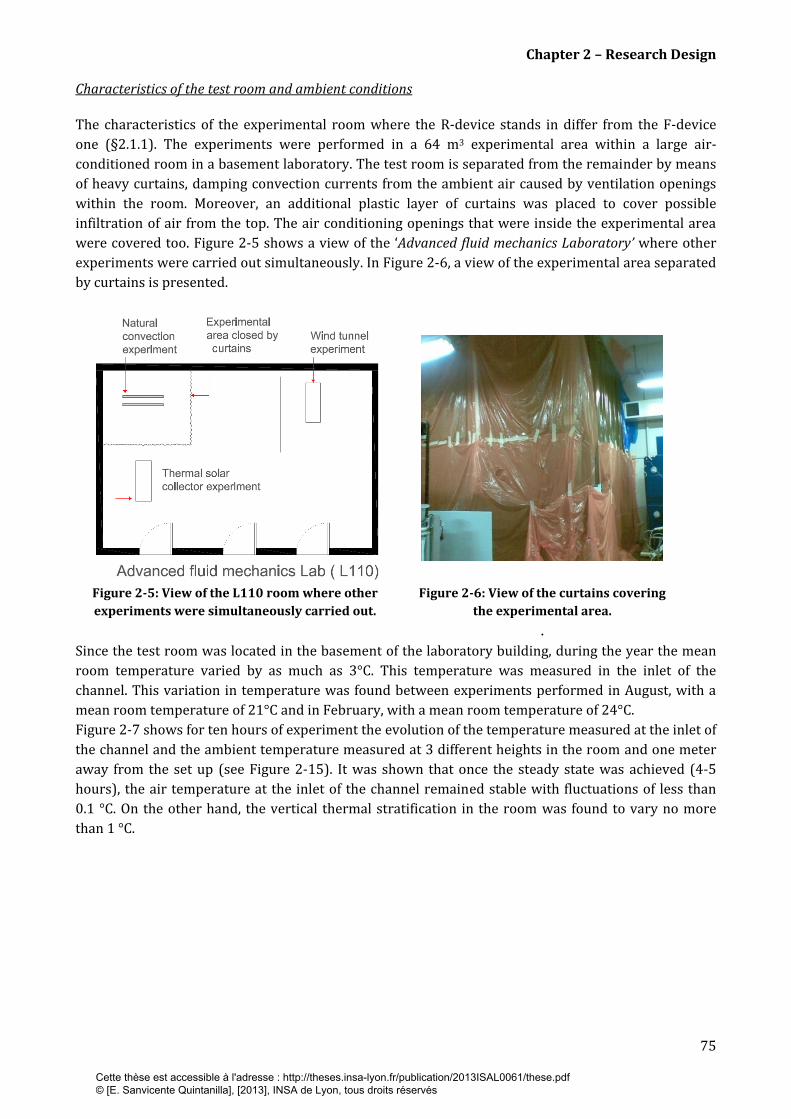
Chapter 2 – Research Design
75
Characteristics of the test room and ambient conditions
The characteristics of the experimental room where the R-device stands in differ from the F-device
one (§2.1.1). The experiments were performed in a 64 m3 experimental area within a large air-
conditioned room in a basement laboratory. The test room is separated from the remainder by means
of heavy curtains, damping convection currents from the ambient air caused by ventilation openings
within the room. Moreover, an additional plastic layer of curtains was placed to cover possible
infiltration of air from the top. The air conditioning openings that were inside the experimental area
were covered too. Figure 2-5 shows a view of the ‘Advanced fluid mechanics Laboratory’ where other
experiments were carried out simultaneously. In Figure 2-6, a view of the experimental area separated
by curtains is presented.
Figure 2-5: View of the L110 room where other
experiments were simultaneously carried out.
Figure 2-6: View of the curtains covering
the experimental area.
.
Since the test room was located in the basement of the laboratory building, during the year the mean
room temperature varied by as much as 3°C. This temperature was measured in the inlet of the
channel. This variation in temperature was found between experiments performed in August, with a
mean room temperature of 21°C and in February, with a mean room temperature of 24°C.
Figure 2-7 shows for ten hours of experiment the evolution of the temperature measured at the inlet of
the channel and the ambient temperature measured at 3 different heights in the room and one meter
away from the set up (see Figure 2-15). It was shown that once the steady state was achieved (4-5
hours), the air temperature at the inlet of the channel remained stable with fluctuations of less than
0.1 °C. On the other hand, the vertical thermal stratification in the room was found to vary no more
than 1 °C.
Cette thèse est accessible à l'adresse : http://theses.insa-lyon.fr/publication/2013ISAL0061/these.pdf © [E. Sanvicente Quintanilla], [2013], INSA de Lyon, tous droits réservés
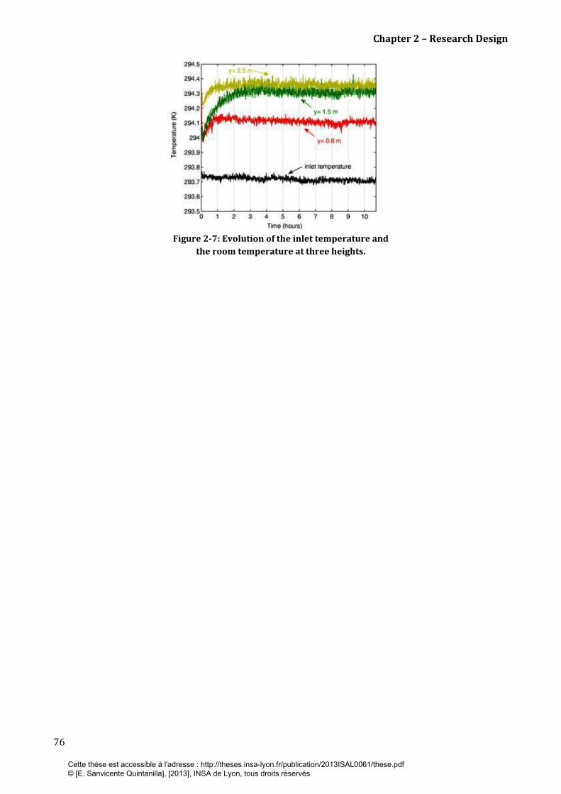
Chapter 2 – Research Design
76
Figure 2-7: Evolution of the inlet temperature and
the room temperature at three heights.
Cette thèse est accessible à l'adresse : http://theses.insa-lyon.fr/publication/2013ISAL0061/these.pdf © [E. Sanvicente Quintanilla], [2013], INSA de Lyon, tous droits réservés
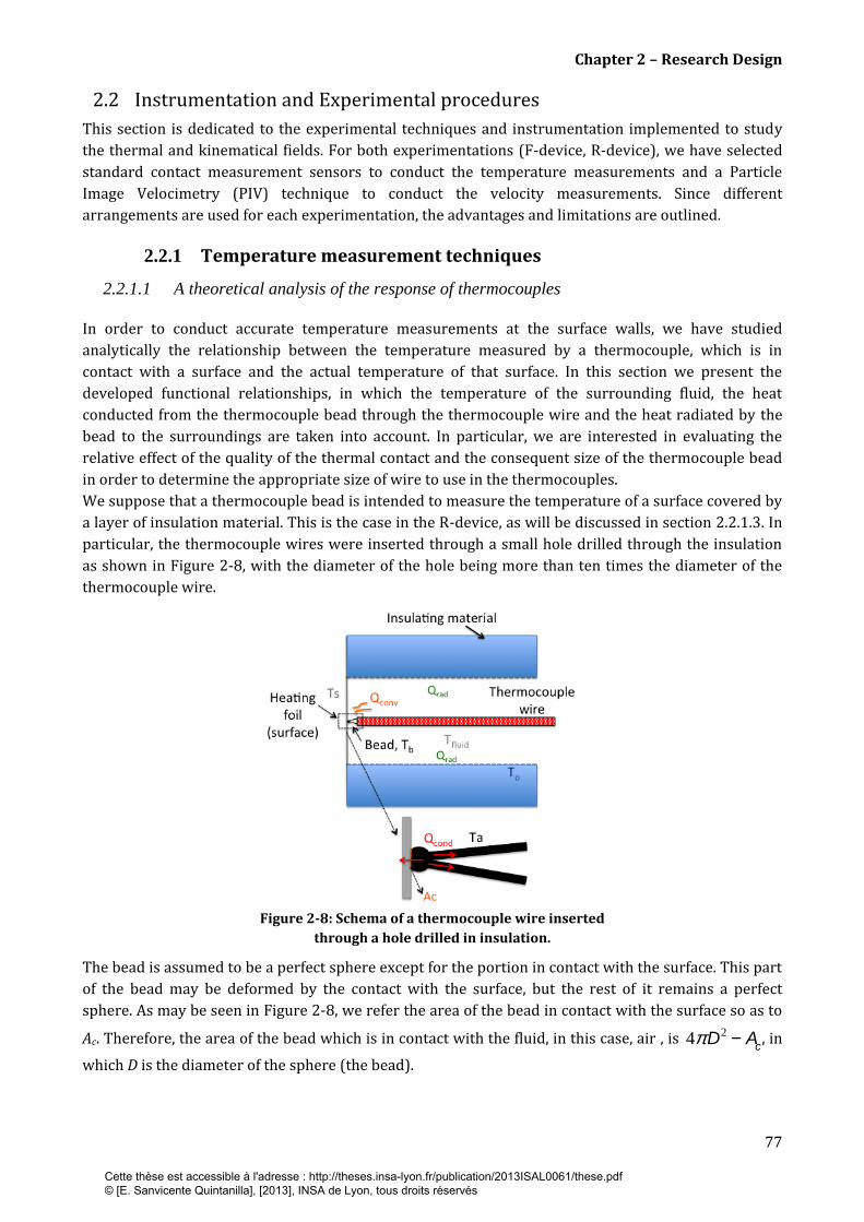
Chapter 2 – Research Design
77
2.2 Instrumentation and Experimental procedures
This section is dedicated to the experimental techniques and instrumentation implemented to study
the thermal and kinematical fields. For both experimentations (F-device, R-device), we have selected
standard contact measurement sensors to conduct the temperature measurements and a Particle
Image Velocimetry (PIV) technique to conduct the velocity measurements. Since different
arrangements are used for each experimentation, the advantages and limitations are outlined.
2.2.1 Temperature measurement techniques
2.2.1.1 A theoretical analysis of the response of thermocouples
In order to conduct accurate temperature measurements at the surface walls, we have studied
analytically the relationship between the temperature measured by a thermocouple, which is in
contact with a surface and the actual temperature of that surface. In this section we present the
developed functional relationships, in which the temperature of the surrounding fluid, the heat
conducted from the thermocouple bead through the thermocouple wire and the heat radiated by the
bead to the surroundings are taken into account. In particular, we are interested in evaluating the
relative effect of the quality of the thermal contact and the consequent size of the thermocouple bead
in order to determine the appropriate size of wire to use in the thermocouples.
We suppose that a thermocouple bead is intended to measure the temperature of a surface covered by
a layer of insulation material. This is the case in the R-device, as will be discussed in section 2.2.1.3. In
particular, the thermocouple wires were inserted through a small hole drilled through the insulation
as shown in Figure 2-8, with the diameter of the hole being more than ten times the diameter of the
thermocouple wire.
Figure 2-8: Schema of a thermocouple wire inserted
through a hole drilled in insulation.
The bead is assumed to be a perfect sphere except for the portion in contact with the surface. This part
of the bead may be deformed by the contact with the surface, but the rest of it remains a perfect
sphere. As may be seen in Figure 2-8, we refer the area of the bead in contact with the surface so as to
Ac. Therefore, the area of the bead which is in contact with the fluid, in this case, air , is , in
which D is the diameter of the sphere (the bead).
4p D2 - A
c
Cette thèse est accessible à l'adresse : http://theses.insa-lyon.fr/publication/2013ISAL0061/these.pdf © [E. Sanvicente Quintanilla], [2013], INSA de Lyon, tous droits réservés
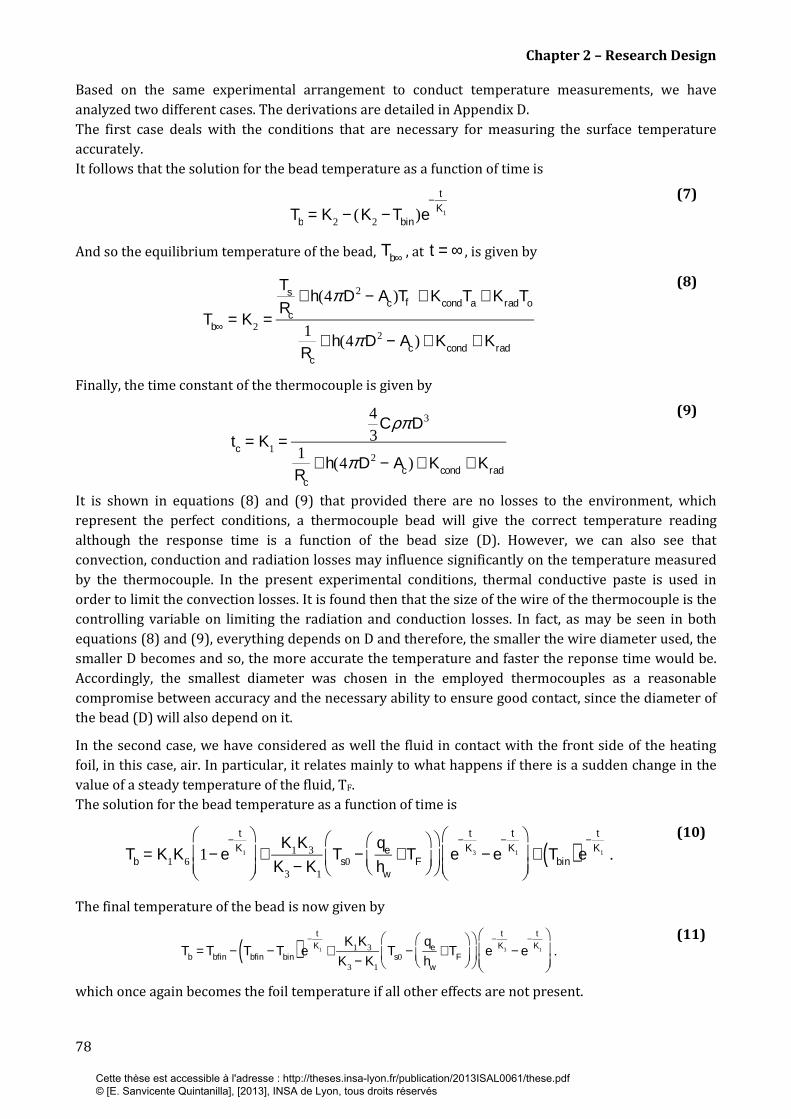
Chapter 2 – Research Design
78
Based on the same experimental arrangement to conduct temperature measurements, we have analyzed two different cases. The derivations are detailed in Appendix D. The first case deals with the conditions that are necessary for measuring the surface temperature accurately. It follows that the solution for the bead temperature as a function of time is
(7)
And so the equilibrium temperature of the bead, , at , is given by
(8)
Finally, the time constant of the thermocouple is given by
(9)
It is shown in equations (8) and (9) that provided there are no losses to the environment, which represent the perfect conditions, a thermocouple bead will give the correct temperature reading although the response time is a function of the bead size (D). However, we can also see that convection, conduction and radiation losses may influence significantly on the temperature measured by the thermocouple. In the present experimental conditions, thermal conductive paste is used in order to limit the convection losses. It is found then that the size of the wire of the thermocouple is the controlling variable on limiting the radiation and conduction losses. In fact, as may be seen in both equations (8) and (9), everything depends on D and therefore, the smaller the wire diameter used, the smaller D becomes and so, the more accurate the temperature and faster the reponse time would be. Accordingly, the smallest diameter was chosen in the employed thermocouples as a reasonable compromise between accuracy and the necessary ability to ensure good contact, since the diameter of the bead (D) will also depend on it.
In the second case, we have considered as well the fluid in contact with the front side of the heating foil, in this case, air. In particular, it relates mainly to what happens if there is a sudden change in the value of a steady temperature of the fluid, TF. The solution for the bead temperature as a function of time is
(10)
The final temperature of the bead is now given by
(11)
which once again becomes the foil temperature if all other effects are not present.
Tb = K2 − (K2 − Tbin)e− t
K1
Tb∞ t = ∞
Tb∞ = K2 =
Ts
Rc
+ h(4π D2 − Ac)Tf + KcondTa + KradTo
1Rc
+ h(4π D2 − Ac) + Kcond + Krad
tc = K1 =
43
Cρπ D3
1Rc
+ h(4π D2 − Ac) + Kcond + Krad
Tb = K1K6 1− e− t
K1
+K1K3
K3 − K1
Ts0 −qe
hw
+ TF
e
− tK3 − e
− tK1
+ Tbin( )e− t
K1 .
Tb = Tbfin − Tbfin − Tbin( )e− t
K1 +K1K3
K3 − K1
Ts0 −qe
hw
+ TF
e
− tK3 − e
− tK1
.
Cette thèse est accessible à l'adresse : http://theses.insa-lyon.fr/publication/2013ISAL0061/these.pdf © [E. Sanvicente Quintanilla], [2013], INSA de Lyon, tous droits réservés
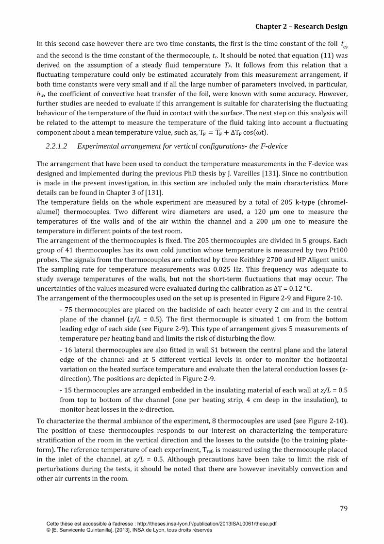
Chapter 2 – Research Design
79
In this second case however there are two time constants, the first is the time constant of the foil
and the second is the time constant of the thermocouple, tc. It should be noted that equation (11) was
derived on the assumption of a steady fluid temperature TF. It follows from this relation that a
fluctuating temperature could only be estimated accurately from this measurement arrangement, if
both time constants were very small and if all the large number of parameters involved, in particular,
hw, the coefficient of convective heat transfer of the foil, were known with some accuracy. However,
further studies are needed to evaluate if this arrangement is suitable for charaterising the fluctuating
behaviour of the temperature of the fluid in contact with the surface. The next step on this analysis will
be related to the attempt to measure the temperature of the fluid taking into account a fluctuating
component about a mean temperature value, such as,
2.2.1.2 Experimental arrangement for vertical configurations- the F-device
The arrangement that have been used to conduct the temperature measurements in the F-device was
designed and implemented during the previous PhD thesis by J. Vareilles [131]. Since no contribution
is made in the present investigation, in this section are included only the main characteristics. More
details can be found in Chapter 3 of [131].
The temperature fields on the whole experiment are measured by a total of 205 k-type (chromel-
alumel) thermocouples. Two different wire diameters are used, a 120 μm one to measure the
temperatures of the walls and of the air within the channel and a 200 μm one to measure the
temperature in different points of the test room.
The arrangement of the thermocouples is fixed. The 205 thermocouples are divided in 5 groups. Each
group of 41 thermocouples has its own cold junction whose temperature is measured by two Pt100
probes. The signals from the thermocouples are collected by three Keithley 2700 and HP Aligent units.
The sampling rate for temperature measurements was 0.025 Hz. This frequency was adequate to
study average temperatures of the walls, but not the short-term fluctuations that may occur. The
uncertainties of the values measured were evaluated during the calibration as ΔT = 0.12 °C.
The arrangement of the thermocouples used on the set up is presented in Figure 2-9 and Figure 2-10.
- 75 thermocouples are placed on the backside of each heater every 2 cm and in the central
plane of the channel (z/L = 0.5). The first thermocouple is situated 1 cm from the bottom
leading edge of each side (see Figure 2-9). This type of arrangement gives 5 measurements of
temperature per heating band and limits the risk of disturbing the flow.
- 16 lateral thermocouples are also fitted in wall S1 between the central plane and the lateral
edge of the channel and at 5 different vertical levels in order to monitor the hotizontal
variation on the heated surface temperature and evaluate then the lateral conduction losses (z-
direction). The positions are depicted in Figure 2-9.
- 15 thermocouples are arranged embedded in the insulating material of each wall at z/L = 0.5
from top to bottom of the channel (one per heating strip, 4 cm deep in the insulation), to
monitor heat losses in the x-direction.
To characterize the thermal ambiance of the experiment, 8 thermocouples are used (see Figure 2-10).
The position of these thermocouples responds to our interest on characterizing the temperature
stratification of the room in the vertical direction and the losses to the outside (to the training plate-
form). The reference temperature of each experiment, Tref, is measured using the thermocouple placed
in the inlet of the channel, at z/L = 0.5. Although precautions have been take to limit the risk of
perturbations during the tests, it should be noted that there are however inevitably convection and
other air currents in the room.
tcs
Cette thèse est accessible à l'adresse : http://theses.insa-lyon.fr/publication/2013ISAL0061/these.pdf © [E. Sanvicente Quintanilla], [2013], INSA de Lyon, tous droits réservés
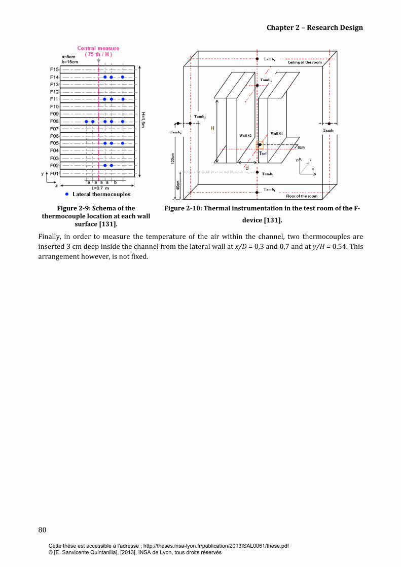
Chapter 2 – Research Design
80
Figure 2-9: Schema of the
thermocouple location at each wall surface [131].
Figure 2-10: Thermal instrumentation in the test room of the F-
device [131].
Finally, in order to measure the temperature of the air within the channel, two thermocouples are
inserted 3 cm deep inside the channel from the lateral wall at x/D = 0,3 and 0,7 and at y/H = 0.54. This
arrangement however, is not fixed.
Cette thèse est accessible à l'adresse : http://theses.insa-lyon.fr/publication/2013ISAL0061/these.pdf © [E. Sanvicente Quintanilla], [2013], INSA de Lyon, tous droits réservés
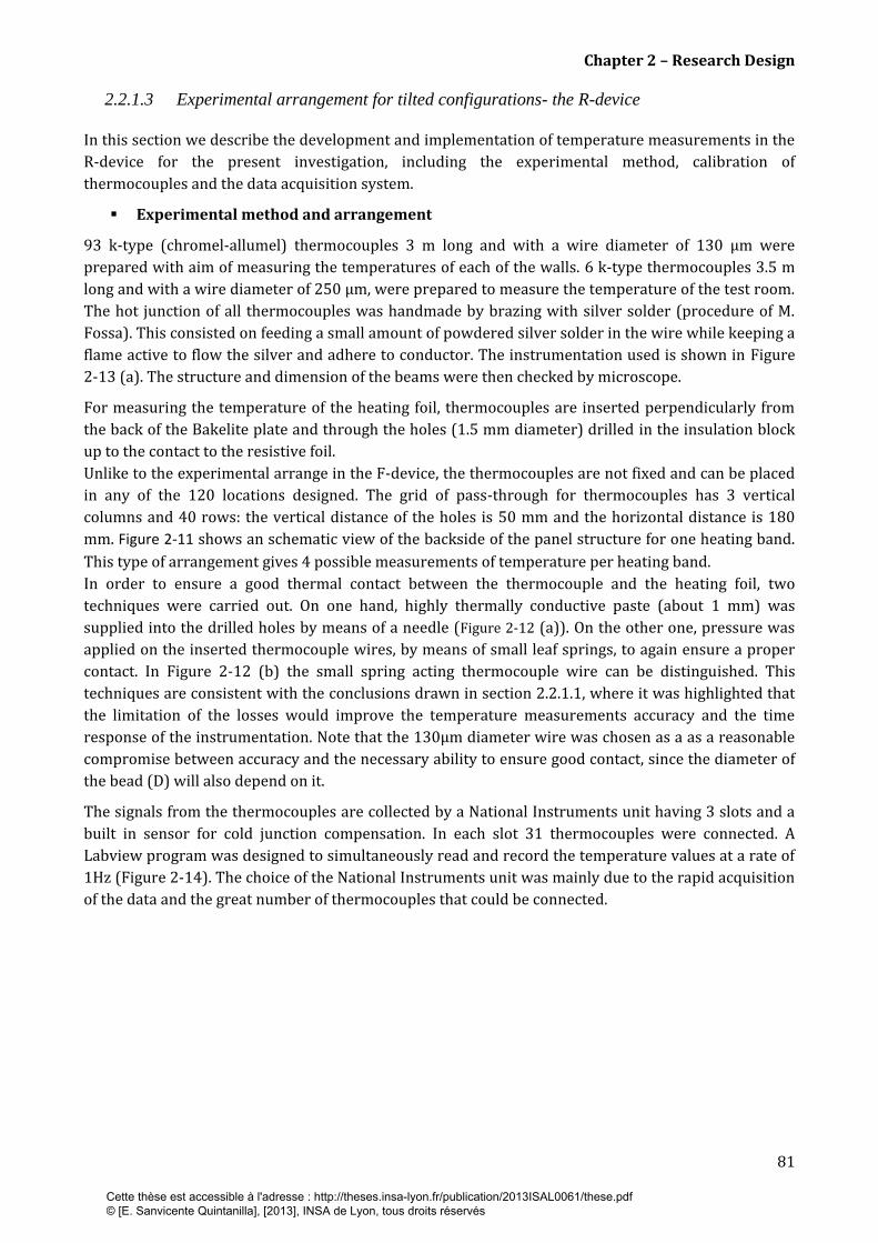
Chapter 2 – Research Design
81
2.2.1.3 Experimental arrangement for tilted configurations- the R-device
In this section we describe the development and implementation of temperature measurements in the
R-device for the present investigation, including the experimental method, calibration of
thermocouples and the data acquisition system.
Experimental method and arrangement
93 k-type (chromel-allumel) thermocouples 3 m long and with a wire diameter of 130 μm were
prepared with aim of measuring the temperatures of each of the walls. 6 k-type thermocouples 3.5 m
long and with a wire diameter of 250 μm, were prepared to measure the temperature of the test room.
The hot junction of all thermocouples was handmade by brazing with silver solder (procedure of M.
Fossa). This consisted on feeding a small amount of powdered silver solder in the wire while keeping a
flame active to flow the silver and adhere to conductor. The instrumentation used is shown in Figure
2-13 (a). The structure and dimension of the beams were then checked by microscope.
For measuring the temperature of the heating foil, thermocouples are inserted perpendicularly from
the back of the Bakelite plate and through the holes (1.5 mm diameter) drilled in the insulation block
up to the contact to the resistive foil.
Unlike to the experimental arrange in the F-device, the thermocouples are not fixed and can be placed
in any of the 120 locations designed. The grid of pass-through for thermocouples has 3 vertical
columns and 40 rows: the vertical distance of the holes is 50 mm and the horizontal distance is 180
mm. Figure 2-11 shows an schematic view of the backside of the panel structure for one heating band.
This type of arrangement gives 4 possible measurements of temperature per heating band.
In order to ensure a good thermal contact between the thermocouple and the heating foil, two
techniques were carried out. On one hand, highly thermally conductive paste (about 1 mm) was
supplied into the drilled holes by means of a needle (Figure 2-12 (a)). On the other one, pressure was
applied on the inserted thermocouple wires, by means of small leaf springs, to again ensure a proper
contact. In Figure 2-12 (b) the small spring acting thermocouple wire can be distinguished. This
techniques are consistent with the conclusions drawn in section 2.2.1.1, where it was highlighted that
the limitation of the losses would improve the temperature measurements accuracy and the time
response of the instrumentation. Note that the 130μm diameter wire was chosen as a as a reasonable
compromise between accuracy and the necessary ability to ensure good contact, since the diameter of
the bead (D) will also depend on it.
The signals from the thermocouples are collected by a National Instruments unit having 3 slots and a
built in sensor for cold junction compensation. In each slot 31 thermocouples were connected. A
Labview program was designed to simultaneously read and record the temperature values at a rate of
1Hz (Figure 2-14). The choice of the National Instruments unit was mainly due to the rapid acquisition
of the data and the great number of thermocouples that could be connected.
Cette thèse est accessible à l'adresse : http://theses.insa-lyon.fr/publication/2013ISAL0061/these.pdf © [E. Sanvicente Quintanilla], [2013], INSA de Lyon, tous droits réservés

Chapter 2 – Research Design
82
(a)
(b)
Figure 2-11: Schema of the location of the thermocouple location at each wall surface of the R-device.
Figure 2-12: Measurement method. (a) Thermal conductive paste and needle used to inject it and (b) Small leaf springs
acting on the thermocouple wires.
(a)
(b)
Figure 2-13: Torch and silver solder flux used to prepare the thermocouples.
Figure 2-14: View of the National Instruments unit and the 3 slots used for data acquisition.
Cette thèse est accessible à l'adresse : http://theses.insa-lyon.fr/publication/2013ISAL0061/these.pdf © [E. Sanvicente Quintanilla], [2013], INSA de Lyon, tous droits réservés
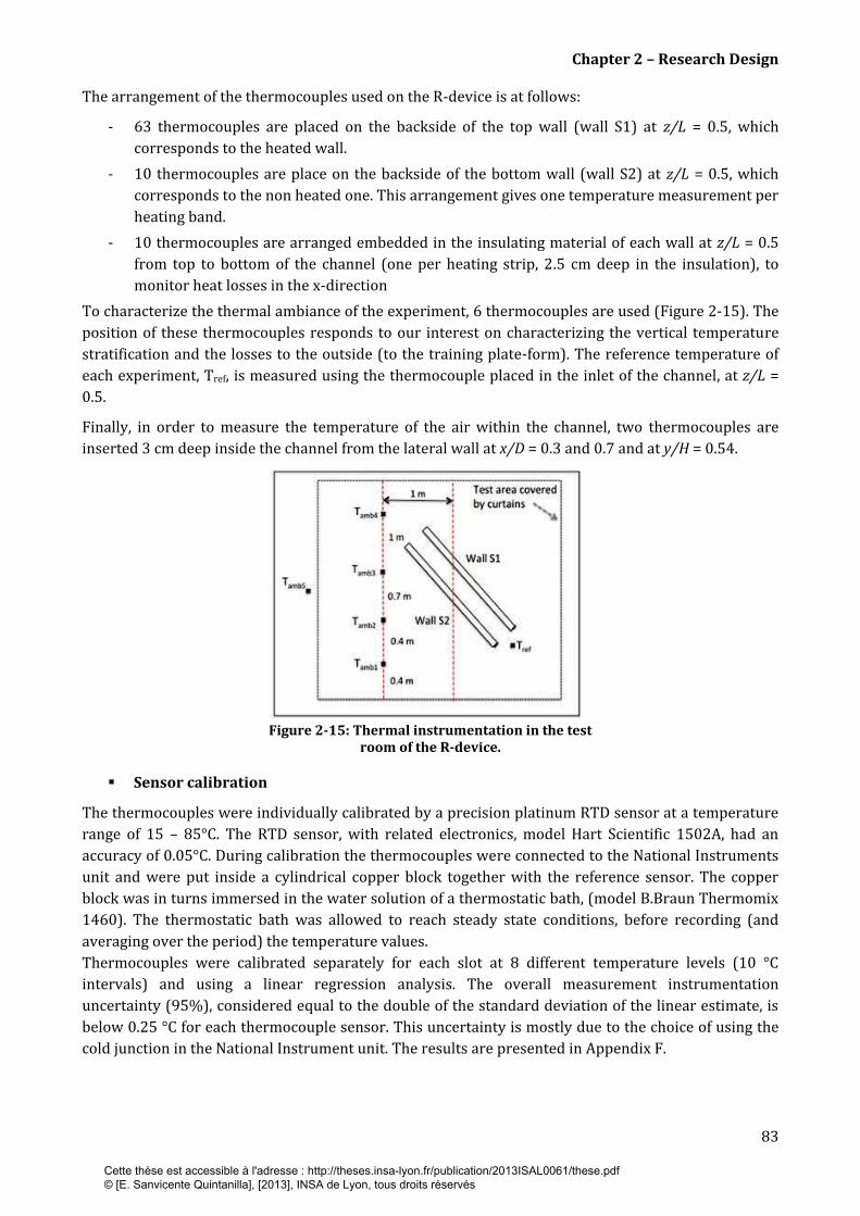
Chapter 2 – Research Design
83
The arrangement of the thermocouples used on the R-device is at follows:
- 63 thermocouples are placed on the backside of the top wall (wall S1) at z/L = 0.5, which
corresponds to the heated wall.
- 10 thermocouples are place on the backside of the bottom wall (wall S2) at z/L = 0.5, which
corresponds to the non heated one. This arrangement gives one temperature measurement per
heating band.
- 10 thermocouples are arranged embedded in the insulating material of each wall at z/L = 0.5
from top to bottom of the channel (one per heating strip, 2.5 cm deep in the insulation), to
monitor heat losses in the x-direction
To characterize the thermal ambiance of the experiment, 6 thermocouples are used (Figure 2-15). The
position of these thermocouples responds to our interest on characterizing the vertical temperature
stratification and the losses to the outside (to the training plate-form). The reference temperature of
each experiment, Tref, is measured using the thermocouple placed in the inlet of the channel, at z/L =
0.5.
Finally, in order to measure the temperature of the air within the channel, two thermocouples are
inserted 3 cm deep inside the channel from the lateral wall at x/D = 0.3 and 0.7 and at y/H = 0.54.
Figure 2-15: Thermal instrumentation in the test
room of the R-device.
Sensor calibration
The thermocouples were individually calibrated by a precision platinum RTD sensor at a temperature
range of 15 – 85°C. The RTD sensor, with related electronics, model Hart Scientific 1502A, had an
accuracy of 0.05°C. During calibration the thermocouples were connected to the National Instruments
unit and were put inside a cylindrical copper block together with the reference sensor. The copper
block was in turns immersed in the water solution of a thermostatic bath, (model B.Braun Thermomix
1460). The thermostatic bath was allowed to reach steady state conditions, before recording (and
averaging over the period) the temperature values.
Thermocouples were calibrated separately for each slot at 8 different temperature levels (10 °C
intervals) and using a linear regression analysis. The overall measurement instrumentation
uncertainty (95%), considered equal to the double of the standard deviation of the linear estimate, is
below 0.25 °C for each thermocouple sensor. This uncertainty is mostly due to the choice of using the
cold junction in the National Instrument unit. The results are presented in Appendix F.
Cette thèse est accessible à l'adresse : http://theses.insa-lyon.fr/publication/2013ISAL0061/these.pdf © [E. Sanvicente Quintanilla], [2013], INSA de Lyon, tous droits réservés
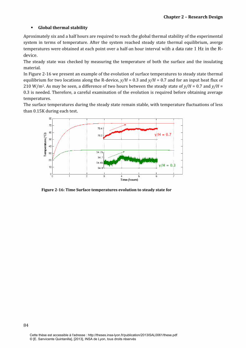
Chapter 2 – Research Design
84
Global thermal stability
Aproximately six and a half hours are required to reach the global thermal stability of the experimental
system in terms of temperature. After the system reached steady state thermal equilibrium, averge
temperatures were obtained at each point over a half-an hour interval with a data rate 1 Hz in the R-
device.
The steady state was checked by measuring the temperature of both the surface and the insulating
material.
In Figure 2-16 we present an example of the evolution of surface temperatures to steady state thermal
equilibrium for two locations along the R-device, y/H = 0.3 and y/H = 0.7 and for an input heat flux of
210 W/m2. As may be seen, a difference of two hours between the steady state of y/H = 0.7 and y/H =
0.3 is needed. Therefore, a careful examination of the evolution is required before obtaining average
temperatures.
The surface temperatures during the steady state remain stable, with temperature fluctuations of less
than 0.15K during each test.
Figure 2-16: Time Surface temperatures evolution to steady state for
Cette thèse est accessible à l'adresse : http://theses.insa-lyon.fr/publication/2013ISAL0061/these.pdf © [E. Sanvicente Quintanilla], [2013], INSA de Lyon, tous droits réservés
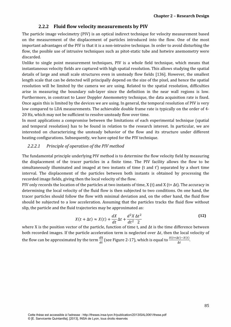
Chapter 2 – Research Design
85
2.2.2 Fluid flow velocity measurements by PIV
The particle image velocimetry (PIV) is an optical indirect technique for velocity measurement based
on the measurement of the displacement of particles introduced into the flow. One of the most
important advantages of the PIV is that it is a non-intrusive technique. In order to avoid disturbing the
flow, the posible use of intrusive techniques such as pitot-static tube and hotwire anemometry were
discarded.
Unlike to single point measurement techniques, PIV is a whole field technique, which means that
instantaneous velocity fields are captured with high spatial resolution. This allows studying the spatial
details of large and small scale structures even in unsteady flow fields [136]. However, the smallest
length scale that can be detected will principally depend on the size of the pixel, and hence the spatial
resolution will be limited by the camera we are using. Related to the spatial resolution, difficulties
arise in measuring the boundary sub-layer since the definition in the near wall regions is low.
Furthermore, in constrast to Laser Doppler Anemometry technique, the data acquisition rate is fixed.
Once again this is limited by the devices we are using. In general, the temporal resolution of PIV is very
low compared to LDA measurements. The achievable double frame rate is typically on the order of 4-
20 Hz, which may not be sufficient to resolve unsteady flow over time.
In most applications a compromise between the limitations of each experimental technique (spatial
and temporal resolution) has to be found in relation to the research interest. In particular, we are
interested on characterizing the unsteady behavior of the flow and its structure under different
heating configurations. Subsequently, we have opted for the PIV technique.
2.2.2.1 Principle of operation of the PIV method
The fundamental principle underlying PIV method is to determine the flow velocity field by measuring
the displacement of the tracer particles in a finite time. The PIV facility allows the flow to be
simultaneously illuminated and imaged at two instants of time (t and t’) separated by a short time
interval. The displacement of the particles between both instants is obtained by processing the
recorded image fields, giving then the local velocity of the flow.
PIV only records the location of the particles at two instants of time, X (t) and X (t+ Δt). The accuracy in
determining the local velocity of the fluid flow is then subjected to two conditions. On one hand, the
tracer particles should follow the flow with minimal deviation and, on the other hand, the fluid flow
should be subjected to a low acceleration. Assuming that the particles tracks the fluid flow without
slip, the particle and the fluid trajectories may be approximated as:
(12)
where X is the position vector of the particle, function of time t, and is the time difference between
both recorded images. If the particle acceleration term is neglected over , then the local velocity of
the flow can be approximated by the term
(see Figure 2-17), which is equal to
.
Cette thèse est accessible à l'adresse : http://theses.insa-lyon.fr/publication/2013ISAL0061/these.pdf © [E. Sanvicente Quintanilla], [2013], INSA de Lyon, tous droits réservés

Chapter 2 – Research Design
86
Figure 2-17: Approximation of the local velocity of particles by PIV method
(idea original from[137]).
It is important to notice that flow information is only obtained from the locations at which the tracer
particles are present. If the seeding concentration is very low, individual particles may be tracked. This
is often referred to as particle tracking velocimetry, or PTV. However, since these are distributed
randomly over the flow, the displacement of individual tracer particles constitutes a random sampling
of the displacement field. In the case where the characteristic length scales of the flow are smaller than
the typical space between neighboring tracer particles the measurement will be indeed inaccurate13.
It follows that to obtain a PIV vector map the concentration of tracers should be high, especially if the
experimental data is compared with the results of numerical calculations. In this mode, the high
concentration of image particles makes tracking individual tracers time consuming, and one measures
instead, the displacement of small groups of particles. This is accomplished by extracting small
samples of each image, called interrogation windows and analyzing them statistically. This statistical
approach will depend, as will be seen, on the recording technique.
Data acquisition
From now we assume the PIV recording case where the flow is imaged at two different times (t and t’),
with a time delay , which is adjustable between both illuminations. Typically, 2 different recording
modes are à priori possible to obtain images of the flow at t and .
The first technique consists on storing two exposures of the same particles on a single recording, and it
is named as single frame/double exposure (see Figure 2-18(a)). This technique is especially the case in
PIV when using photographic recording with high resolution. The advantage is that it only needs one
active frame.
All the information in t and is then contained on a single frame. The evaluation method
associated to this recording mode consists on calculating the autocorrelation function of each
interrogation area. The autocorrelation function is characterized by a central peak resulted from the
autocorrelation of the interrogation area with itself, and two peaks that describe the most probable
mean displacement of the particles within the interrogation area. These two peaks are symmetrically
located around the self-correlation peak and arise from the fact that the sign of the direction of the
particle motion within each interrogation area cannot be determined, since there is no way to decide
which particle image is due to the first and which one is due to the second illumination pulse. This is
an inconvenient when the flow under investigation, such as the present one, contains regions of
reverse flow. The elimination of the ambiguity of direction requires additional techniques to be
employed, such as the image shifting, which imposes a fixed displacement between the two exposures.
In chapter 4 of [136], the general aspects of this method can be found.
13 http://gpiv.sourceforge.net/gpiv_doc
Cette thèse est accessible à l'adresse : http://theses.insa-lyon.fr/publication/2013ISAL0061/these.pdf © [E. Sanvicente Quintanilla], [2013], INSA de Lyon, tous droits réservés

Chapter 2 – Research Design
87
Another inconvenient of the single frame/double exposure method that should be taken into account is
related to the measure of slow velocities. Precautions have to be made in this case since the two
correlation peaks linked to the displacement of the particles will be close to the central autocorrelation
one, which decreases the precision of the displacement estimation.
Figure 2-18: PIV recording methods, (a) Single frame/Double exposure and
(b) Double frame/single exposure (idea from [136]).
The second technique, namely double frame/single exposure, lies in the capacity of the acquisition
technology to record two instances of time (t and t’) on two separated frames (see Figure 2-18(b)). In
particular, this technique has been widely used since the implementation of digital cameras, such as
the CCD and CMOS-based PIV cameras. The evaluation method of this recording mode is typically
performed by cross-correlating frame I with frame II, which results in one peak of correlation that
corresponds to the average in-plane displacement of the particles within the interrogation area.
Due to the availability of a CCD camera and a double-pulsed laser (as will be detailed subsequently),
we have used in the present investigation the double frame-single exposure recording method. The
cross-correlation method and post-processing conducted will be detailed in section 2.2.2.3.
2.2.2.2 The PIV apparatus and measurement procedures
In this section we detail the 2D-PIV apparatus utilized in each experiment (F-device and R-device) and
the measurement procedures carried out.
The PIV apparatus used in the vertical configuration, the F-device, is shown in Figure 2-19. It consists
of two powerful lasers allowing two pulses of light to be created with a freely selectable time
separation. These light pulses are made coincident and pass through the optic system, generating a
plane sheet of light that illuminates the particles previously added in the flow. The light scattered by
the particles is captured in the coupled CCD camera that is located 90° to the sheet, so that its in-focus
object plane coincides with the illuminated slice of fluid. The camera and laser are synchronized using
a synchronization unit either as a computer card (as in the F-device PIV apparatus) or as an external
unit (as in the R-device PIV apparatus). The images of the flow are then transferred to the computer,
which runs a PIV software for evaluating the recorded data.
Cette thèse est accessible à l'adresse : http://theses.insa-lyon.fr/publication/2013ISAL0061/these.pdf © [E. Sanvicente Quintanilla], [2013], INSA de Lyon, tous droits réservés

Chapter 2 – Research Design
88
(a)
(b)
(c)
(d)
Figure 2-19: Schema of the 2D-PIV set up used in the F-device: (a) view of the whole test (b) Laser sheet and illuminated particles (c) Laser head and light sheet optics (d) Mirror used to re-orientate the laser beam .
Particle seeding
The choice of the particles
The particle seeding is particularly important in PIV since as we have above highlighted, the principle
of PIV is based on measuring the velocity of tracer particles instead of the fluid velocity. Thus, correct
choice of particles and seeding procedure are critical to increase the accuracy and minimize the
uncertainty of the measurements.
The seeding system selected for both experimentations comprises an aerosol generator using Laskin
Nozzles (Figure 2-20) and DEHS (liquid, Table 2-1) to generate the tracer particles. The principle of
operation of this type of device is to supply compressed air through two air inlets into a vegetable oil
container: the air becomes loaded of small oil droplets generating an aerosol, which is carried towards
the flow to seed.
Cette thèse est accessible à l'adresse : http://theses.insa-lyon.fr/publication/2013ISAL0061/these.pdf © [E. Sanvicente Quintanilla], [2013], INSA de Lyon, tous droits réservés

Chapter 2 – Research Design
89
A detail description of the operating mode is reported by Raffel and Mei [136, 138].
We have selected this seeding system since it is found to be one of the most useful devices for seeding
airflows. One of the principal problems that arise in applications in airflows is the difference in density
between the fluid and the tracer particles. Equation (13) reports an estimation of the velocity
deviation between a tracer particle and the fluid:
(13)
In which is the particle velocity, dP and are the particle diameter and density and , µF and a are
respectively the density, dynamic viscosity and acceleration of the fluid. In particular, DEHS particles
have a density of 912 kg/m3. From equation (13) it can be seen that due the particle weight relative to
the air, the diameter of the particles should be very small in order to ensure good tracking of the fluid
motion, thereby with minimal deviation. We have therefore selected for both experimentations
particles of a diameter < 1 µm. According to the manufacturer of the aerosol generator14, the particle
size distribution ranges between 0.15 µm to 1 µm, and the highest concentration is obtained for
particles of diameter between 0.3 µm to 0.5 µm (see Table 2-1). This was measured by a scanning
mobility particle sizer system by the manufacturer of the DEHS aerosol.
After the particles are injected into the flow, there is a characteristic time of response from the
particles to achieve velocity equilibrium with the fluid. This is known as the step response
characteristic or relaxation time (τs) of the particles and mainly depends on both the diameter and
density of the particle (see equation (14)). In the present case the time of response of the particles is
τ= 2.77 µsec. Indeed, to be able to measure turbulence, the particles must follow the local fluctuations
in the flow, so particle size and density also are the controlling variables on the highest cut-off
frequency at which the particles still follow the velocity oscillations [139]. For particle diameter of dp =
1x10⁻⁶ m and a assuming a slip velocity error of 0.1 % relative to the instantaneous local velocity, the
cut-off frequency is given at 8 kHz. This is calculated through equations (15), (16) and (17).
(14)
(15)
(16)
(17)
It follows that the physical characteristics of the tracer particles are suitable. In addition, these
particles are non-toxic, leave almost no deposit on the walls, stay in air at rest for hours and do not
change in size significantly under various conditions (large temperature and pressure gradients)
[140]. As reported by Raffel et al. [136], careful examination of this last property should be given if
measuring in air flows as the size and the distribution of the tracer particles may change during the
travel from the aerosol generator to the test section.
However, these particles should also have at the same time a sufficient light scattering capability as
PIV signals rely on the scattered light to take the velocity measurement. The particle image intensity is
found to be proportional to the square of the particle diameter and therefore it is generally
accomplished with larger particles. Considering the particles spherical with a diameter that is larger
than the wavelength of light (dp > λ), the Mie scattering theory can be applied to examine the optical
characteristics of the particles. Figure 2-21 shows the scattering efficiency for an oil particle diameter
(dp) of 1µm [136].
14 Topas ATM 225 manual, < http://www.topas-gmbh.de/dateien/prospekt/200/atmprspe.pdf>.
Cette thèse est accessible à l'adresse : http://theses.insa-lyon.fr/publication/2013ISAL0061/these.pdf © [E. Sanvicente Quintanilla], [2013], INSA de Lyon, tous droits réservés
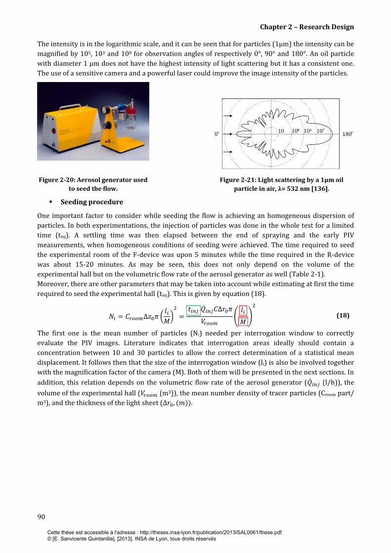
Chapter 2 – Research Design
90
The intensity is in the logarithmic scale, and it can be seen that for particles (1µm) the intensity can be
magnified by 105, 103 and 108 for observation angles of respectively 0°, 90° and 180°. An oil particle
with diameter 1 µm does not have the highest intensity of light scattering but it has a consistent one.
The use of a sensitive camera and a powerful laser could improve the image intensity of the particles.
Figure 2-20: Aerosol generator used
to seed the flow. Figure 2-21: Light scattering by a 1µm oil
particle in air, λ= 532 nm [136].
Seeding procedure
One important factor to consider while seeding the flow is achieving an homogeneous dispersion of
particles. In both experimentations, the injection of particles was done in the whole test for a limited
time (tinj). A settling time was then elapsed between the end of spraying and the early PIV
measurements, when homogeneous conditions of seeding were achieved. The time required to seed
the experimental room of the F-device was upon 5 minutes while the time required in the R-device
was about 15-20 minutes. As may be seen, this does not only depend on the volume of the
experimental hall but on the volumetric flow rate of the aerosol generator as well (Table 2-1).
Moreover, there are other parameters that may be taken into account while estimating at first the time
required to seed the experimental hall (tinj). This is given by equation (18).
(18)
The first one is the mean number of particles (Ni) needed per interrogation window to correctly
evaluate the PIV images. Literature indicates that interrogation areas ideally should contain a
concentration between 10 and 30 particles to allow the correct determination of a statistical mean
displacement. It follows then that the size of the interrogation window (li) is also be involved together
with the magnification factor of the camera (M). Both of them will be presented in the next sections. In
addition, this relation depends on the volumetric flow rate of the aerosol generator ( (l/h)), the
volume of the experimental hall ( (m3)), the mean number density of tracer particles (Croom part/
m3), and the thickness of the light sheet ( .
Cette thèse est accessible à l'adresse : http://theses.insa-lyon.fr/publication/2013ISAL0061/these.pdf © [E. Sanvicente Quintanilla], [2013], INSA de Lyon, tous droits réservés
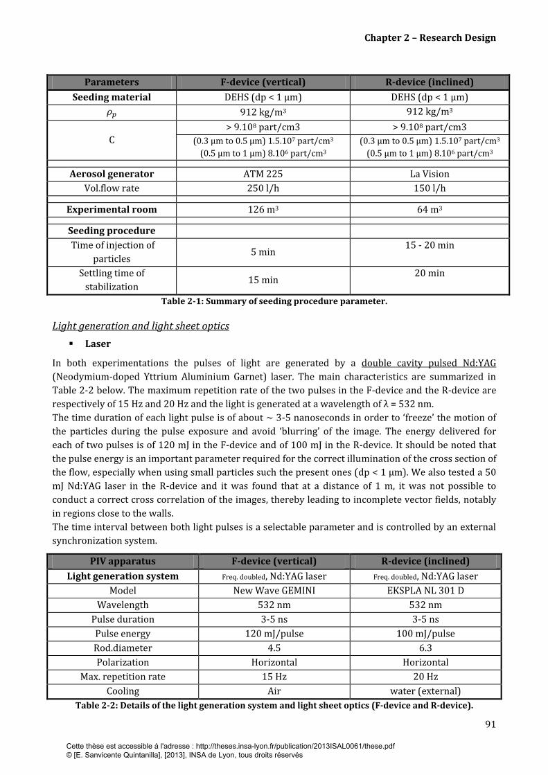
Chapter 2 – Research Design
91
Parameters F-device (vertical) R-device (inclined)
Seeding material DEHS (dp < 1 µm) DEHS (dp < 1 µm)
912 kg/m3 912 kg/m3
C
> 9.108 part/cm3 > 9.108 part/cm3
(0.3 µm to 0.5 µm) 1.5.107 part/cm3
(0.5 µm to 1 µm) 8.106 part/cm3
(0.3 µm to 0.5 µm) 1.5.107 part/cm3
(0.5 µm to 1 µm) 8.106 part/cm3
Aerosol generator ATM 225 La Vision
Vol.flow rate 250 l/h 150 l/h
Experimental room 126 m3 64 m3
Seeding procedure
Time of injection of
particles 5 min
15 - 20 min
Settling time of
stabilization 15 min
20 min
Table 2-1: Summary of seeding procedure parameter.
Light generation and light sheet optics
Laser
In both experimentations the pulses of light are generated by a double cavity pulsed Nd:YAG
(Neodymium-doped Yttrium Aluminium Garnet) laser. The main characteristics are summarized in
Table 2-2 below. The maximum repetition rate of the two pulses in the F-device and the R-device are
respectively of 15 Hz and 20 Hz and the light is generated at a wavelength of λ = 532 nm.
The time duration of each light pulse is of about ~ 3-5 nanoseconds in order to ‘freeze’ the motion of
the particles during the pulse exposure and avoid ‘blurring’ of the image. The energy delivered for
each of two pulses is of 120 mJ in the F-device and of 100 mJ in the R-device. It should be noted that
the pulse energy is an important parameter required for the correct illumination of the cross section of
the flow, especially when using small particles such the present ones (dp < 1 µm). We also tested a 50
mJ Nd:YAG laser in the R-device and it was found that at a distance of 1 m, it was not possible to
conduct a correct cross correlation of the images, thereby leading to incomplete vector fields, notably
in regions close to the walls.
The time interval between both light pulses is a selectable parameter and is controlled by an external
synchronization system.
PIV apparatus F-device (vertical) R-device (inclined)
Light generation system Freq. doubled, Nd:YAG laser Freq. doubled, Nd:YAG laser
Model New Wave GEMINI EKSPLA NL 301 D
Wavelength 532 nm 532 nm
Pulse duration 3-5 ns 3-5 ns
Pulse energy 120 mJ/pulse 100 mJ/pulse
Rod.diameter 4.5 6.3
Polarization Horizontal Horizontal
Max. repetition rate 15 Hz 20 Hz
Cooling Air water (external)
Table 2-2: Details of the light generation system and light sheet optics (F-device and R-device).
Cette thèse est accessible à l'adresse : http://theses.insa-lyon.fr/publication/2013ISAL0061/these.pdf © [E. Sanvicente Quintanilla], [2013], INSA de Lyon, tous droits réservés

Chapter 2 – Research Design
92
Design of the laser sheet
For both vertical and inclined configurations, the laser beam is injected from the low part of the
experimental set up (see Figure 2-19 (a and c). Afterwards, the laser beam is reoriented vertically by
means of a mirror, which is tilted at 45° and placed at 35 cm from the inlet of the channel (Figure 2-19
(d)). The mirror has a special coat so more than 99.8% of the incident laser light is reflected.
Both light pulses are made coincident and pass through an optic system, generating a light sheet that is
used to illuminate the cross section of the flow.
The laser sheet is designed to be 2 mm thick in all measuring locations so the effect of particles leaving
out-of-plane is minimized. The shaping optics combines a diverging and converging system of
cylindrical lenses with variable space between lenses (see Figure 2-22). The first group of lenses is
used to focus the laser beam at the desired working distance. In the present case the converging lenses
used have allowed to work in a back focal length ranging from 400 mm to 2500 mm. This group of
lenses was adapted according to the measuring location studied, i.e., the inlet, the mid-height or the
outlet of the channel. In total three configurations are used as shown in Figure 2-22 (a,b,c). The
diverging lenses are used to decrease the angle of the light sheet and therefore focus all the intensity of
light in the area we are measuring. Since the width of the channel is fixed to D = 100 mm, the light
sheet in the present investigation was designed to have at all measuring locations a maximum scan
area of 125 x 125 mm2
(a)
(b)
Cette thèse est accessible à l'adresse : http://theses.insa-lyon.fr/publication/2013ISAL0061/these.pdf © [E. Sanvicente Quintanilla], [2013], INSA de Lyon, tous droits réservés
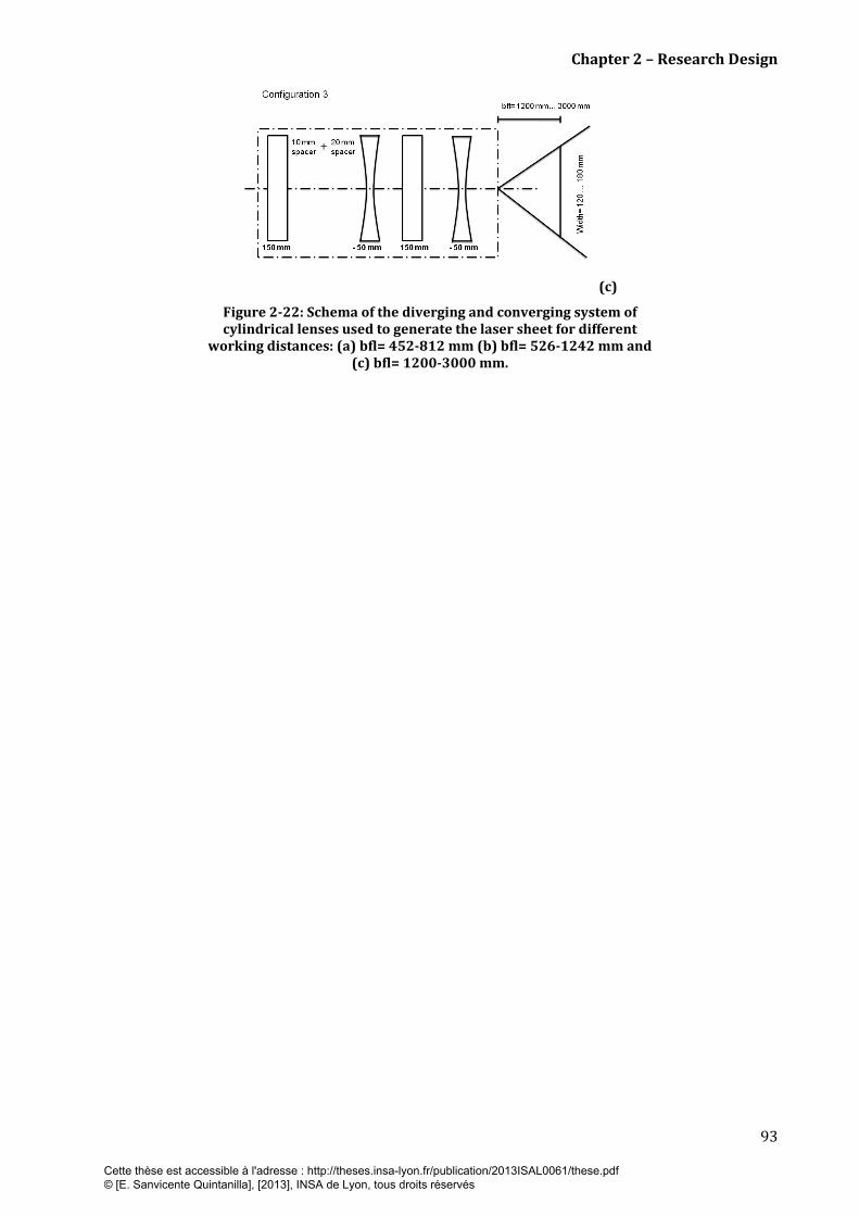
Chapter 2 – Research Design
93
(c)
Figure 2-22: Schema of the diverging and converging system of cylindrical lenses used to generate the laser sheet for different
working distances: (a) bfl= 452-812 mm (b) bfl= 526-1242 mm and (c) bfl= 1200-3000 mm.
Cette thèse est accessible à l'adresse : http://theses.insa-lyon.fr/publication/2013ISAL0061/these.pdf © [E. Sanvicente Quintanilla], [2013], INSA de Lyon, tous droits réservés
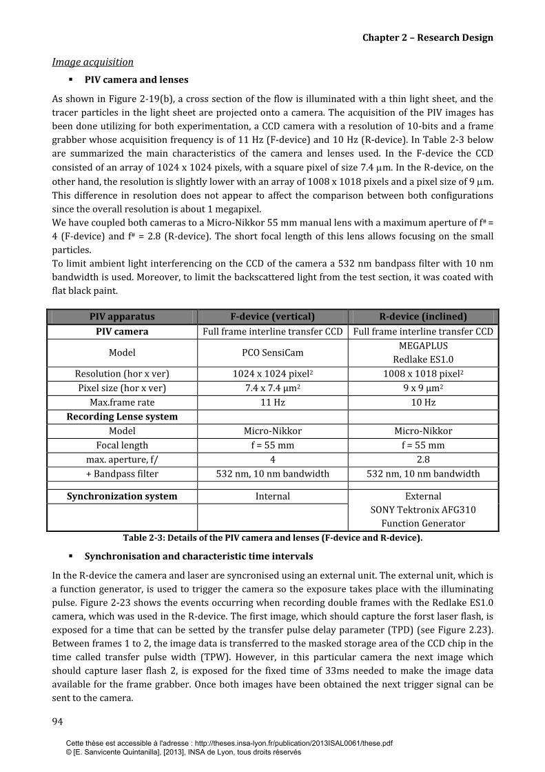
Chapter 2 – Research Design
94
Image acquisition
PIV camera and lenses
As shown in Figure 2-19(b), a cross section of the flow is illuminated with a thin light sheet, and the
tracer particles in the light sheet are projected onto a camera. The acquisition of the PIV images has
been done utilizing for both experimentation, a CCD camera with a resolution of 10-bits and a frame
grabber whose acquisition frequency is of 11 Hz (F-device) and 10 Hz (R-device). In Table 2-3 below
are summarized the main characteristics of the camera and lenses used. In the F-device the CCD
consisted of an array of 1024 x 1024 pixels, with a square pixel of size 7.4 m. In the R-device, on the
other hand, the resolution is slightly lower with an array of 1008 x 1018 pixels and a pixel size of 9 m.
This difference in resolution does not appear to affect the comparison between both configurations
since the overall resolution is about 1 megapixel.
We have coupled both cameras to a Micro-Nikkor 55 mm manual lens with a maximum aperture of f# =
4 (F-device) and f# = 2.8 (R-device). The short focal length of this lens allows focusing on the small
particles.
To limit ambient light interferencing on the CCD of the camera a 532 nm bandpass filter with 10 nm
bandwidth is used. Moreover, to limit the backscattered light from the test section, it was coated with
flat black paint.
Table 2-3: Details of the PIV camera and lenses (F-device and R-device).
Synchronisation and characteristic time intervals
In the R-device the camera and laser are syncronised using an external unit. The external unit, which is
a function generator, is used to trigger the camera so the exposure takes place with the illuminating
pulse. Figure 2-23 shows the events occurring when recording double frames with the Redlake ES1.0
camera, which was used in the R-device. The first image, which should capture the forst laser flash, is
exposed for a time that can be setted by the transfer pulse delay parameter (TPD) (see Figure 2.23).
Between frames 1 to 2, the image data is transferred to the masked storage area of the CCD chip in the
time called transfer pulse width (TPW). However, in this particular camera the next image which
should capture laser flash 2, is exposed for the fixed time of 33ms needed to make the image data
available for the frame grabber. Once both images have been obtained the next trigger signal can be
sent to the camera.
PIV apparatus F-device (vertical) R-device (inclined)
PIV camera Full frame interline transfer CCD Full frame interline transfer CCD
Model PCO SensiCam MEGAPLUS
Redlake ES1.0
Resolution (hor x ver) 1024 x 1024 pixel2 1008 x 1018 pixel2
Pixel size (hor x ver) 7.4 x 7.4 µm2 9 x 9 µm2
Max.frame rate 11 Hz 10 Hz
Recording Lense system
Model Micro-Nikkor Micro-Nikkor
Focal length f = 55 mm f = 55 mm
max. aperture, f/ 4 2.8
+ Bandpass filter 532 nm, 10 nm bandwidth 532 nm, 10 nm bandwidth
Synchronization system Internal External
SONY Tektronix AFG310
Function Generator
Cette thèse est accessible à l'adresse : http://theses.insa-lyon.fr/publication/2013ISAL0061/these.pdf © [E. Sanvicente Quintanilla], [2013], INSA de Lyon, tous droits réservés
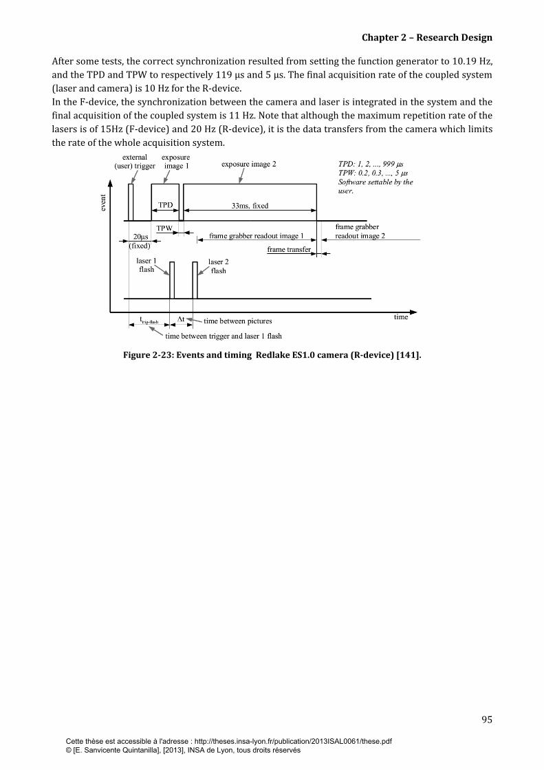
Chapter 2 – Research Design
95
After some tests, the correct synchronization resulted from setting the function generator to 10.19 Hz,
and the TPD and TPW to respectively 119 μs and 5 μs. The final acquisition rate of the coupled system
(laser and camera) is 10 Hz for the R-device.
In the F-device, the synchronization between the camera and laser is integrated in the system and the
final acquisition of the coupled system is 11 Hz. Note that although the maximum repetition rate of the
lasers is of 15Hz (F-device) and 20 Hz (R-device), it is the data transfers from the camera which limits
the rate of the whole acquisition system.
Figure 2-23: Events and timing Redlake ES1.0 camera (R-device) [141].
Cette thèse est accessible à l'adresse : http://theses.insa-lyon.fr/publication/2013ISAL0061/these.pdf © [E. Sanvicente Quintanilla], [2013], INSA de Lyon, tous droits réservés

Chapter 2 – Research Design
96
Camera calibration and acquisition procedure
In order to obtain accurate PIV results, the diameter of the particle image (the one projected in the
image) should size 2-3 pixels. This depends on one hand on the physical diameter of the particle, and
on the other one, on the camera calibration.
To estimate the particle image diameter , the following equation is generally used neglecting the
effects of lens aberrations:
where, = particle image diameter [m], = particle diameter [m], M = magnification factor and
= diffraction limited minimum object diameter [m] which is defined in the following equation:
(20)
The magnification factor of particle image (M) depends upon the position of the imaging lens
(equation (21)) and the f-number of the lens (f#) on the diameter of aperture (eq (22)).
(21)
(22)
Furthermore, as mentioned before, to obtain accurate results a mean number of 10-30 particles should
be contained in the interrogation window. This is represented by image density (Ni) parameter and
may be evaluated according to the equation proposed by Adrian [142]:
(23)
Equations (19), (20) and (23) reveal that we can optimize the measurement accuracy by carefully
selecting calibration parameters of the camera.
The dimensions of the cross section of the flow we are measuring (field of view) represent a
compromise between two requirements: On one hand, the field of view should cover the section area
of the flow we want to investigate. On the other one, we should consider the spatial resolution of the
image. In the present study we are interested in covering the width of the channel, which measures in
all experimentations 100 mm. Since it is not possible to scan the entire channel in only one image view,
the flow is investigated in 5 different sections along the height of the channel. An accurate
displacement support for the camera has been settled up to measure any desired section in the
channel flow. Moreover, according to the required recording time to reach convergence of the mean
values, the tests need to be conducted on several days. As a consequence, the reproductibility of the
measurements has been studied carefully. This issue is addressed in Chapter 3.
In the F-device, each field of view represents a section of the flow of 200 x 200 mm2, with the camera
located at a distance of 0.9 m of the object plane. In the R-device, however, the camera was located at
0.6 m of the object plane and the field of view obtained was of 115 x 115 mm2.
By changing the distance of the camera to the object plane from 0.9 m to 0.6 m, the height of the image
section of the flow is reduced from aproximately 200 mm to 115 mm, which leads in turns to a relation
of 5.2 px/mm in the F-device whereas of 10 px/mm in the R-device (Table 2-4).
(19)
Cette thèse est accessible à l'adresse : http://theses.insa-lyon.fr/publication/2013ISAL0061/these.pdf © [E. Sanvicente Quintanilla], [2013], INSA de Lyon, tous droits réservés
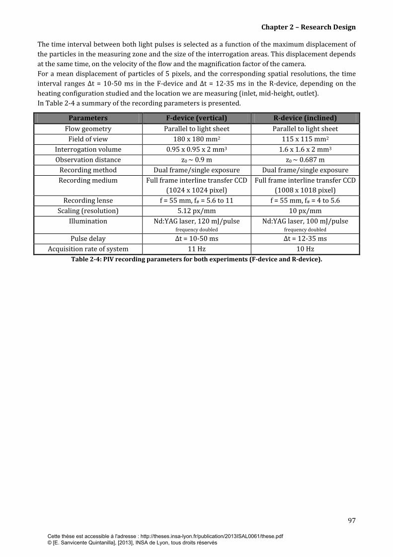
Chapter 2 – Research Design
97
The time interval between both light pulses is selected as a function of the maximum displacement of
the particles in the measuring zone and the size of the interrogation areas. This displacement depends
at the same time, on the velocity of the flow and the magnification factor of the camera.
For a mean displacement of particles of 5 pixels, and the corresponding spatial resolutions, the time
interval ranges ∆t = 10-50 ms in the F-device and ∆t = 12-35 ms in the R-device, depending on the
heating configuration studied and the location we are measuring (inlet, mid-height, outlet).
In Table 2-4 a summary of the recording parameters is presented.
Parameters F-device (vertical) R-device (inclined)
Flow geometry Parallel to light sheet Parallel to light sheet
Field of view 180 x 180 mm2 115 x 115 mm2
Interrogation volume 0.95 x 0.95 x 2 mm3 1.6 x 1.6 x 2 mm3
Observation distance z0 ~ 0.9 m z0 ~ 0.687 m
Recording method Dual frame/single exposure Dual frame/single exposure
Recording medium Full frame interline transfer CCD
(1024 x 1024 pixel)
Full frame interline transfer CCD
(1008 x 1018 pixel)
Recording lense f = 55 mm, f# = 5.6 to 11 f = 55 mm, f# = 4 to 5.6
Scaling (resolution) 5.12 px/mm 10 px/mm
Illumination Nd:YAG laser, 120 mJ/pulse frequency doubled
Nd:YAG laser, 100 mJ/pulse frequency doubled
Pulse delay ∆t = 10-50 ms ∆t = 12-35 ms
Acquisition rate of system 11 Hz 10 Hz
Table 2-4: PIV recording parameters for both experiments (F-device and R-device).
Cette thèse est accessible à l'adresse : http://theses.insa-lyon.fr/publication/2013ISAL0061/these.pdf © [E. Sanvicente Quintanilla], [2013], INSA de Lyon, tous droits réservés

Chapter 2 – Research Design
98
Transversing system
For each experimental apparatus an accurate displacement support for the camera and the laser was
designed and installed to measure any desired section in the channel flow.
The transverse system set up in the vertical configuration, the F-device, was shown in Figure 2-19. The
displacement support where the camera is fitted allows it to be repositioned with a maximum error of
2 mm. If transverse planes other than x/D = 0.5 were to be studied, the mirror- optics system box,
Figure 2-19 (c), was moved in the z-direction. This option was adopted because of security issues in
order to avoid moving the laser as well as the fact that repositing of the laser involved greater
uncertainty in the determination of position.
In the inclined configuration, the R-device, the design of the transverse system involved greater
difficulties. Firstly, when the inclination angle of the set up is varied, the inclination angle of the laser
sheet also needs to be adjusted, so as to maintain the laser sheet at 900 to the camera. Secondly, since
as the channel is inclined, the position of the inlet changes relative to the location of the laser, so that
the laser also needs to be moved. Different options were considered such as designing a system which
would control the mirror and camera. However, in order to avoid errors, such a system would have to
position both devices very accurately and it would have required a large device as the laser would
need to be moved quite some distance at low angles in order to remain correctly aligned with the
channel. The difficulties involved as it needed to support a 40 kg laser and the lack of sufficient room
in the laboratory, made this approach impractical.
The solution, as may be seen in Figure 2-24, consisted of integrating the traverse system with the
channel, so that when the channel was tilted, both the camera and laser were tilted accordingly. This
system avoided any reposition of any of the components in the measurement system, such as the
mirror, laser sheet and camera when varying the inclination angle as shown in Figure 2-24(a and b).
The displacement support system was designed and built so that the apparatus could be positioned
with a maximum error of ~0.5° with the inclination angle. The inclination angle was determined by
means of a protractor, which was placed on the supporting frame of the inclining device, as may be
seen in Figure Figure 2-24 (c).
Cette thèse est accessible à l'adresse : http://theses.insa-lyon.fr/publication/2013ISAL0061/these.pdf © [E. Sanvicente Quintanilla], [2013], INSA de Lyon, tous droits réservés
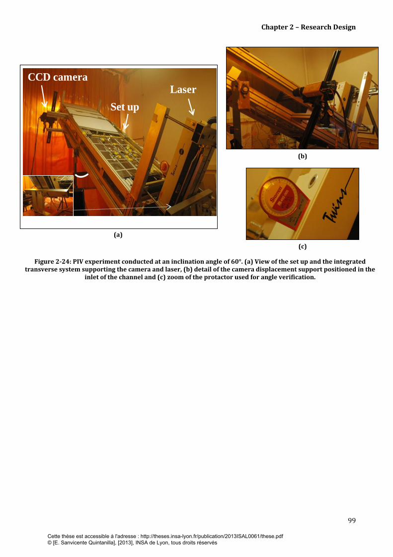
Chapter 2 – Research Design
99
(a)
(b)
(c)
Figure 2-24: PIV experiment conducted at an inclination angle of 60°. (a) View of the set up and the integrated transverse system supporting the camera and laser, (b) detail of the camera displacement support positioned in the
inlet of the channel and (c) zoom of the protactor used for angle verification.
LaserCCD camera
Set up
Cette thèse est accessible à l'adresse : http://theses.insa-lyon.fr/publication/2013ISAL0061/these.pdf © [E. Sanvicente Quintanilla], [2013], INSA de Lyon, tous droits réservés
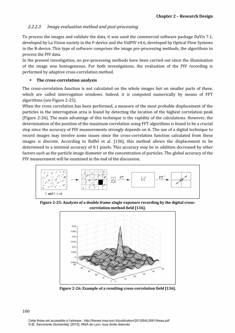
Chapter 2 – Research Design
100
2.2.2.3 Image evaluation method and post-processing
To process the images and validate the data, it was used the commercial software package DaVis 7.1,
developed by La Vision society in the F-device and the VidPIV v4.6, developed by Optical Flow Systems
in the R-device. This type of software comprises the image pre-processing methods, the algorithms to
process the PIV data.
In the present investigation, no pre-processing methods have been carried out since the illumination
of the image was homogeneous. For both investigations, the evaluation of the PIV recording is
performed by adaptive cross-correlation method.
The cross-correlation analysis
The cross-correlation function is not calculated on the whole images but on smaller parts of these,
which are called interrogation windows. Indeed, it is computed numerically by means of FFT
algorithms (see Figure 2-25).
When the cross correlation has been performed, a measure of the most probable displacement of the
particles in the interrogation area is found by detecting the location of the highest correlation peak
(Figure 2-26). The main advantage of this technique is the rapidity of the calculations. However, the
determination of the position of the maximum correlation using FFT algorithms is found to be a crucial
step since the accuracy of PIV measurements strongly depends on it. The use of a digital technique to
record images may involve some issues since the cross-correlation function calculated from these
images is discrete. According to Raffel et al. [136], this method allows the displacement to be
determined to a minimal accuracy of 0.1 pixels. This accuracy may be in addition decreased by other
factors such as the particle image diameter or the concentration of particles. The global accuracy of the
PIV measurement will be examined in the end of the discussion.
Figure 2-25: Analysis of a double frame single exposure recording by the digital cross-
correlation method field [136].
Figure 2-26: Example of a resulting cross-correlation field [136].
Cette thèse est accessible à l'adresse : http://theses.insa-lyon.fr/publication/2013ISAL0061/these.pdf © [E. Sanvicente Quintanilla], [2013], INSA de Lyon, tous droits réservés
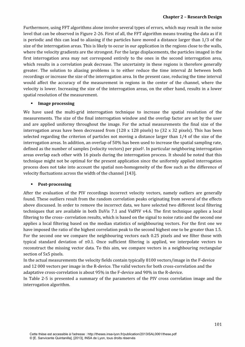
Chapter 2 – Research Design
101
Furthermore, using FFT algorithms alone involve several types of errors, which may result in the noise
level that can be observed in Figure 2-26. First of all, the FFT algorithm means treating the data as if it
is periodic and this can lead to aliasing if the particles have moved a distance larger than 1/3 of the
size of the interrogation areas. This is likely to occur in our application in the regions close to the walls,
where the velocity gradients are the strongest. For the large displacements, the particles imaged in the
first interrogation area may not correspond entirely to the ones in the second interrogation area,
which results in a correlation peak decrease. The uncertainty in these regions is therefore generally
greater. The solution to aliasing problems is to either reduce the time interval ∆t between both
recordings or increase the size of the interrogation area. In the present case, reducing the time interval
would affect the accuracy of the measurement in regions in the center of the channel, where the
velocity is lower. Increasing the size of the interrogation areas, on the other hand, results in a lower
spatial resolution of the measurement.
Image processing
We have used the multi-grid interrogation technique to increase the spatial resolution of the
measurements. The size of the final interrogation window and the overlap factor are set by the user
and are applied uniformy throughout the image. For the actual measurements the final size of the
interrogation areas have been decreased from (128 x 128 pixels) to (32 x 32 pixels). This has been
selected regarding the criterion of particles not moving a distance larger than 1/4 of the size of the
interrogation areas. In addition, an overlap of 50% has been used to increase the spatial sampling rate,
defined as the number of samples (velocity vectors) per pixel2. In particular neighboring interrogation
areas overlap each other with 16 pixels during the interrogation process. It should be noted that this
technique might not be optimal for the present application since the uniformly applied interrogation
process does not take into account the spatial non-homogeneity of the flow such as the difference of
velocity fluctuations across the width of the channel [143].
Post-processing
After the evaluation of the PIV recordings incorrect velocity vectors, namely outliers are generally
found. These outliers result from the random correlation peaks originating from several of the effects
above discussed. In order to remove the incorrect data, we have selected two different local filtering
techniques that are available in both DaVis 7.1 and VidPIV v4.6. The first technique applies a local
filtering to the cross- correlation results, which is based on the signal to noise ratio and the second one
applies a local filtering based on the median statistics of neighbouring vectors. For the first one we
have imposed the ratio of the highest correlation peak to the second highest one to be greater than 1.5.
For the second one we compare the neighbouring vectors each 0.25 pixels and we filter those with
typical standard deviation of ±0.1. Once sufficient filtering is applied, we interpolate vectors to
reconstruct the missing vector data. To this aim, we compare vectors in a neighbouring rectangular
section of 5x5 pixels.
In the actual measurements the velocity fields contain typically 8100 vectors/image in the F-device
and 12 000 vectors per image in the R-device. The valid vectors for both cross-correlation and the
adaptative cross-correlation is about 95% in the F-device and 90% in the R-device.
In Table 2-5 is presented a summary of the parameters of the PIV cross correlation image and the
interrogation algorithm.
Cette thèse est accessible à l'adresse : http://theses.insa-lyon.fr/publication/2013ISAL0061/these.pdf © [E. Sanvicente Quintanilla], [2013], INSA de Lyon, tous droits réservés
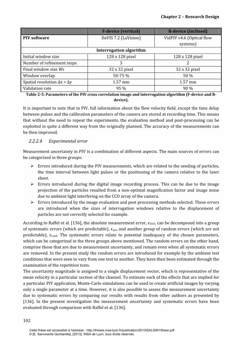
Chapter 2 – Research Design
102
Table 2-5: Parameters of the PIV cross correlation image and interrogation algorithm (F-device and R-
device).
It is important to note that in PIV, full information about the flow velocity field, except the time delay
between pulses and the calibration parameters of the camera are stored at recording time. This means
that without the need to repeat the experiments, the evaluation method and post-processing can be
exploited in quite a different way from the originally planned. The accuracy of the measurements can
be then improved.
2.2.2.4 Experimental error
Measurement uncertainty in PIV is a combination of different aspects. The main sources of errors can
be categorized in three groups:
Errors introduced during the PIV measurements, which are related to the seeding of particles,
the time interval between light pulses or the positioning of the camera relative to the laser
sheet.
Errors introduced during the digital image recording process. This can be due to the image
projection of the particles resulted from a non-optimal magnification factor and image noise
due to ambient light interfering on the CCD array of the camera.
Errors introduced by the image evaluation and post processing methods selected. These errors
are introduced when the sizes of interrogation windows relative to the displacement of
particles are not correctly selected for example.
According to Raffel et al. [136], the absolute measurement error, εTOT, can be decomposed into a group
of systematic errors (which are predictable), εsys, and another group of random errors (which are not
predictable), εrand. The systematic errors relate to potential inadequacy of the chosen parameters,
which can be categorized in the three groups above mentioned. The random errors on the other hand,
comprise those that are due to measurement uncertainty, and remain even when all systematic errors
are removed. In the present study the random errors are introduced for example by the ambient test
conditions that were seen to vary from one test to another. They have then been estimated through the
examination of the repetition tests.
The uncertainty magnitude is assigned to a single displacement vector, which is representative of the
mean velocity in a particular section of the channel. To estimate each of the effects that are implied for
a particular PIV application, Monte-Carlo simulations can be used to create artificial images by varying
only a single parameter at a time. However, it is also possible to assess the measurement uncertainty
due to systematic errors by comparing our results with results from other authors as presented by
[136]. In the present investigation the measurement uncertainty and systematic errors have been
evaluated through comparison with Raffel et al. [136].
F-device (vertical) R-device (inclined)
PIV software DaVIS 7.2 (LaVision) VidPIV v4.6 (Optical flow
systems)
Interrogation algorithm
Initial window size 128 x 128 pixel 128 x 128 pixel
Number of refinement steps 3 2
Final window size Ws 32 x 32 pixel 32 x 32 pixel
Window overlap 50-75 % 50 %
Spatial resolution Δx = Δy 1.57 mm 1.57 mm
Validation rate 95 % 90 %
Cette thèse est accessible à l'adresse : http://theses.insa-lyon.fr/publication/2013ISAL0061/these.pdf © [E. Sanvicente Quintanilla], [2013], INSA de Lyon, tous droits réservés

Chapter 2 – Research Design
103
The uncertainty of the mean displacement introduced by the systematic errors is estimated to be of
0.23 pixels for the F-device (see Table E-1 of Appendix E) and 0.21 pixels for the R-device (see Table E-
2 of Appendix E). For a mean displacement on the range of 4 to 8 pixels, the magnitude in the
uncertainty of the mean velocity due to instrumentation choice is between 3%-6%.
In the case of the F-device, where the repetition tests allowed to evaluate as well the random errors,
the total maximum uncertainty on the mean velocity, εTOT, is estimated to 15%.
In Appendix E the details of the calculations are included.
Cette thèse est accessible à l'adresse : http://theses.insa-lyon.fr/publication/2013ISAL0061/these.pdf © [E. Sanvicente Quintanilla], [2013], INSA de Lyon, tous droits réservés
Chapter 2 – Research Design
104
2.3 Data processing methods
In this section, the methodology used to evaluate and analyze the data is presented. We firstly
introduce the heat balance method, from which the convective heat transfer coefficient can be
determined and then the evaluation method used to estimate the induced mass flow rates within the
channel. The non-dimensional parameters characterizing the problem are also defined. Finally, the
statistical tools used to analyze both the temperature and velocity data are presented.
2.3.1 The heat balance method
In the first chapter we have identified the different heat transfer mechanisms involved in a BIPV
ventilated façade, which are the convection, conduction and radiation. In Figure 2-27 they are
schematically illustrated for a uniform heating configuration. In general, when an electrical power is
input to the heater plate ( ), a part of the heat is loss through conduction in the y and z directions of
the surface while the rest is transferred to the cavity air through convection and
radiation exchange. The buoyancy induced flow will exhaust from the top (Qout) while colder air
will continuously flow into the cavity through the inlet.
Figure 2-27: Schematic representation of the thermal energy exchanges in Type A and B
configuration.
Local convective heat transfer coefficients
Starting from the electrical power dissipated per heater, Pelec, the spatial distribution and
identification of each heat transfer rate have been determined. Conduction losses and radiation have
been evaluated in order to quantify the thermal convection flux.
The local convective flux is evaluated by using an indirect technique developed by Fossa et al. [47],
which consists on a global energy balance of the heating elements.
(24)
where Pin is the local specific electrical power, are the (local) heat flux lost by
conduction in respectively the x and y-directions and is the radiation heat flux to the
surroundings (including facing heaters).
Cette thèse est accessible à l'adresse : http://theses.insa-lyon.fr/publication/2013ISAL0061/these.pdf © [E. Sanvicente Quintanilla], [2013], INSA de Lyon, tous droits réservés

Chapter 2 – Research Design
105
The local heat flux lost by conduction in the y-direction, , is calculated by applying the one-
dimensional, steady state Fourier law:
(25)
where is the thermal conductivity of the heating foil and is its thickness. The determination of
is about the estimation of the second derivative of the local surface temperature, . This
can be approximated in turns by using a second-order scheme as shown in equation (25).
In the z-direction, the conductive part could be considered as negligible in comparison with the one in
the y-direction and therefore, has not been taken into account while evaluating the local
convective flux injected in the channel (equation (24)). It should be noted that the error in the
calculated local heat transfer coefficient due to possible large horizontal variations in the heated
surface temperature was previously examined according to the method proposed by Webb and Hill
[67] for a vertical channel subjected to a UHF condition. In their study they defined a parameter, ,
which compares the horizontal temperature variations in the heating foil with the temperature
difference between the surface and the inlet of the channel. They reported that if this ratio is smaller
than 1.5%, heat transfer in the channel may be assumed to be two-dimensional. In the present case, for
both devices and all heating configurations, this ratio is of the order of 0.8% for thermocouples
positioned 15 cm (F-device, Figure 2-9) and 18 cm (R-device, Figure 2-11).
The local conduction heat losses are evaluated in the x-direction by temperature
measurements in the insulated material. The one dimensional, steady state Fourier law is applied to
the insulation layer as shown in equation (26):
(26)
where is the thickness of the insulating material and its thermal conductivity. Note that in both
apparatus one thermocouple per heating band was arranged embedded in the insulating material
(section 2.2.1). The temperature, , is calculated based on a linear interpolation between each
measurement point made along the height of the channel in the insulating material.
To take into account the 2D effects at the heater edges, a correction coefficient Ck(y) inferred from
ANSYS, two dimensional numerical analysis of the conduction field in the insulating material, is
applied to equation (26). The basis of the method has been developed by Ménézo et al. [144].
Comparing the 1D solution with the 2D one, an estimation of the side effects that act close to the
heating trailing and leading edges in both uniform and non uniform heating configurations has been
proceded.
For a uniform heating condition, the correction coefficient is only applied in the inlet and outlet foils
within the channel. For the first and second thermocouples close to the edge heaters, Ck(y) is equal to
2.7 (y = 0.02m, y = 1.48m) and 1.3 (y = 0.04 m, y = 1.46m). In the remaining of the channel, Ck(y) = 1.
On the other hand, for non-uniform heating experiments, the correction coefficients are applied
similarly for each heated surface on both edge thermocouples.
The radiation heat transfer rate to the surroundings was determined from the emissivity and the surface
temperature field by solving a diffuse-grey enclosure problem [67, 82]. The basis of the method has been
previously applied on this configuration by Fossa et al. [47]. In the F-device, 152 different isothermal
surfaces (whose radiosities are the unknown variables of the algebraic system) are considered, which
correspond to the 75 measured temperatures in each wall (5 per heating band). In the R-device, 22
isothermal sources are considered, which correspond to the 20 heaters, that is, 10 heaters / panel.
Cette thèse est accessible à l'adresse : http://theses.insa-lyon.fr/publication/2013ISAL0061/these.pdf © [E. Sanvicente Quintanilla], [2013], INSA de Lyon, tous droits réservés
Chapter 2 – Research Design
106
The portions of the environment seen by the heaters, are supposed to behave as black bodies, at
temperature T∞.
For the asymmetrically heated configuration subjected to a uniform heat flux of 225 W/m2, the mean
conduction losses along the y-direction, the mean conduction losses through the insulation (x-
direction) and the mean radiation losses to the surroundings are respectively of the order of 0.9 %, 3.5
% and 8%.
The local heat transfer characteristics are evaluated then throught equation (27) as follows:
(27)
The uncertainty analysis was performed according the procedure described by Moffat [145]: The order of
magnitude of the overall uncertainty on the local convective heat transfer coefficient (due to the errors in
primary quantity measurements and in the estimation of heat losses) is estimated to be 12%. Details of
the uncertainty calculation of h for the reference case of study (uniform heat flux imposed at one wall, qs =
220 W/m2) are presented in Appendix E.
Evaluation of the induced mass flow rate
The mass flow rate of the channel is calculated on the basis of
(28)
in which is the density of the fluid at a mean temperature , S corresponds to the cross
sectional area of the flow, A= LxD and to the time-average bulk fluid velocity at z/L = 0.5 obtained
through integration of Vy over the width of the channel (D)[118].
The order of magnitude of the uncertainty on the induced mass flow rate is estimated to be 20%.
Details of the uncertainty calculation of , evaluated at at mid-height section of the channel (y/H = 0.54)
and for the reference case of study (uniform heat flux imposed at one wall, qs = 220 W/m2) are included
in Appendix E.
2.3.2 Data reduction
In the present study, the heat transfer properties of the buoyancy-induced flow in the channel have
been recast in terms of dimensionless quantities either on a local or on average basis. They are
evaluated particularly for a channel subjected to a uniform heat flux, UHF, boundary condition.
Firstly, the Rayleigh number is a parameter which describes the ratio between buoyancy and viscous
forces in a fluid. In the present investigation, the average modified Rayleigh number is evaluated for a
uniformly heated vertical channel based on the channel width and multiplied by the channel aspect
ratio as shown in equation (29):
(29)
in which is the thermal expansion coefficient, g is the gravitational acceleration, is the thermal
conductivity, is the kinematic viscosity and α is the thermal difussivity.
On the other hand, the local Rayleigh number is evaluated based on the local vertical coordinate from
the leading edge of the heated wall, as shown in equation (30):
(30)
Cette thèse est accessible à l'adresse : http://theses.insa-lyon.fr/publication/2013ISAL0061/these.pdf © [E. Sanvicente Quintanilla], [2013], INSA de Lyon, tous droits réservés
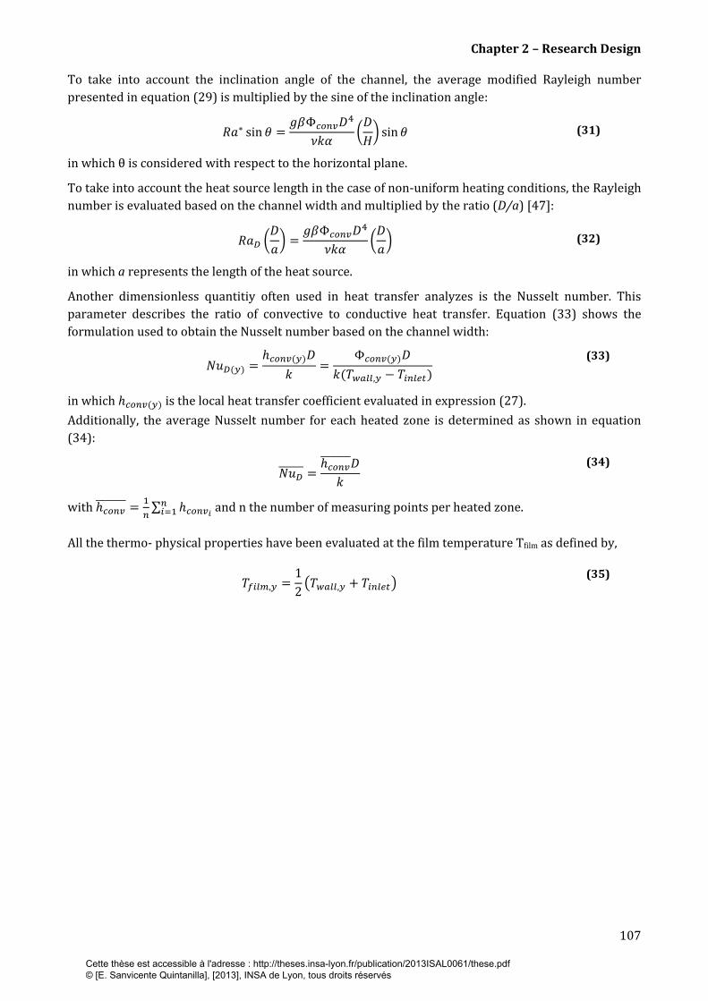
Chapter 2 – Research Design
107
To take into account the inclination angle of the channel, the average modified Rayleigh number
presented in equation (29) is multiplied by the sine of the inclination angle:
(31)
in which θ is considered with respect to the horizontal plane.
To take into account the heat source length in the case of non-uniform heating conditions, the Rayleigh
number is evaluated based on the channel width and multiplied by the ratio (D/a) [47]:
(32)
in which a represents the length of the heat source.
Another dimensionless quantitiy often used in heat transfer analyzes is the Nusselt number. This
parameter describes the ratio of convective to conductive heat transfer. Equation (33) shows the
formulation used to obtain the Nusselt number based on the channel width:
(33)
in which is the local heat transfer coefficient evaluated in expression (27).
Additionally, the average Nusselt number for each heated zone is determined as shown in equation
(34):
(34)
with
and n the number of measuring points per heated zone.
All the thermo- physical properties have been evaluated at the film temperature Tfilm as defined by,
(35)
Cette thèse est accessible à l'adresse : http://theses.insa-lyon.fr/publication/2013ISAL0061/these.pdf © [E. Sanvicente Quintanilla], [2013], INSA de Lyon, tous droits réservés
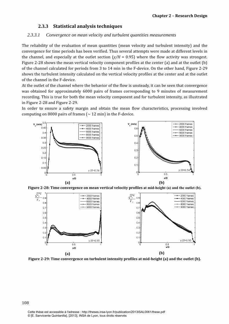
Chapter 2 – Research Design
108
2.3.3 Statistical analysis techniques
2.3.3.1 Convergence on mean velocity and turbulent quantities measurements
The reliability of the evaluation of mean quantities (mean velocity and turbulent intensity) and the
convergence for time periods has been verified. Thus several attempts were made at different levels in
the channel, and especially at the outlet section (y/H = 0.95) where the flow activity was strongest.
Figure 2-28 shows the mean vertical velocity component profiles at the center (a) and at the outlet (b)
of the channel calculated for periods from 3 to 14 min in the F-device. On the other hand, Figure 2-29
shows the turbulent intensity calculated on the vertical velocity profiles at the center and at the outlet
of the channel in the F-device.
At the outlet of the channel where the behavior of the flow is unsteady, it can be seen that convergence
was obtained for approximately 6000 pairs of frames corresponding to 9 minutes of measurement
recording. This is true for both the mean velocity component and for turbulent intensity, as illustrated
in Figure 2-28 and Figure 2-29.
In order to ensure a safety margin and obtain the mean flow characteristics, processing involved
computing on 8000 pairs of frames (~ 12 min) in the F-device.
(a)
(b)
Figure 2-28: Time convergence on mean vertical velocity profiles at mid-height (a) and the outlet (b).
(a)
(b)
Figure 2-29: Time convergence on turbulent intensity profiles at mid-height (a) and the outlet (b).
Cette thèse est accessible à l'adresse : http://theses.insa-lyon.fr/publication/2013ISAL0061/these.pdf © [E. Sanvicente Quintanilla], [2013], INSA de Lyon, tous droits réservés
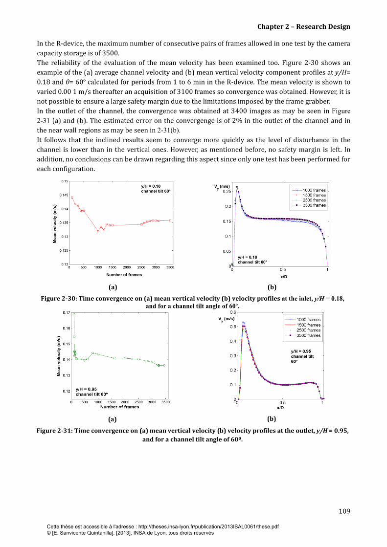
Chapter 2 – Research Design
109
In the R-device, the maximum number of consecutive pairs of frames allowed in one test by the camera
capacity storage is of 3500.
The reliability of the evaluation of the mean velocity has been examined too. Figure 2-30 shows an
example of the (a) average channel velocity and (b) mean vertical velocity component profiles at y/H=
0.18 and θ= 60º calculated for periods from 1 to 6 min in the R-device. The mean velocity is shown to
varied 0.00 1 m/s thereafter an acquisition of 3100 frames so convergence was obtained. However, it is
not possible to ensure a large safety margin due to the limitations imposed by the frame grabber.
In the outlet of the channel, the convergence was obtained at 3400 images as may be seen in Figure
2-31 (a) and (b). The estimated error on the convergenge is of 2% in the outlet of the channel and in
the near wall regions as may be seen in 2-31(b).
It follows that the inclined results seem to converge more quickly as the level of disturbance in the
channel is lower than in the vertical ones. However, as mentioned before, no safety margin is left. In
addition, no conclusions can be drawn regarding this aspect since only one test has been performed for
each configuration.
(a)
(b)
Figure 2-30: Time convergence on (a) mean vertical velocity (b) velocity profiles at the inlet, y/H = 0.18,
and for a channel tilt angle of 60º.
(a)
(b)
Figure 2-31: Time convergence on (a) mean vertical velocity (b) velocity profiles at the outlet, y/H = 0.95,
and for a channel tilt angle of 60º.
Cette thèse est accessible à l'adresse : http://theses.insa-lyon.fr/publication/2013ISAL0061/these.pdf © [E. Sanvicente Quintanilla], [2013], INSA de Lyon, tous droits réservés

Chapter 2 – Research Design
110
2.3.3.2 Quantification of the heterogeneity of a flow
In the present investigation we have quantified the heterogeneity of the flow by calculating the
probability density function (p.d.f.) of instantaneous velocity signals, which in its turns is characterized
by its skewness and flatness factors. The measure of inhomogeneities in the fluid flow needs to be
considered in theories of turbulent diffusion and therefore, the direct knowledge of the p.d.f. would be
very valuable for any CFD approach. Specifically, the effect of viscous dissipation, pressure fluctuations
and scalar dissipation in CFD simulations based on p.d.f. methods can be validated based on the
experimental results obtained [146].
The p.d.f. method is currently used in the study of turbulent natural convection flow in vertical
channels [147]and squares cavities [148]. Also it is used in the study of turbulent combustion and flow
with chemical reactions [146]. In particular, the results obtained can be used for instance, to
characterize experimentally the structure of the temperature and velocity fluctuations present in the
flow [148].
The probability distribution of some random variable, X, is usually represented by a p.d.f. which is
defined as follows. The probability that u lies in the range [a;b], which we write, P(a < X <b), is related
to the probability density fuction by,
(36)
with f(u)du representing the relative frequency that u lies in the range uu+du.
The skewness (S) and the flatness (F) factors, that are dimensionless, are defined by the following
relations:
(37)
(38)
with corresponding to the standard deviation.
The skewness gives a measure of the symmetry of the probability distribution of the random variable,
S = 0 corresponding to a perfect symmetric distribution. The flatness gives a measure of how fast the
probability distribution goes to zero.
When the flow is homogeneous, S = 0 and F = 3. The deviation of these quantities leads to non
homogeneous turbulent fields due to the non linearity of the equations. Existence of homogeneity in a
turbulent field is associated with randomness in turbulent motion while inhomogeneity may indicate
the presence of organized motions in the flow that may persist further downstream and play a role in
the transition process. In turbulent shear flows such motions are identified in the form of large-scale
vortex structures [99]. Moreover, large values of F relate a spotty character of the turbulent intensity
with alternates of long period fluctuations and rapid fluctuations of high intensity.
As mentioned by Papailiou et al. [149], the skewness factor of a velocity field is associated with the
convection of turbulent energy between regions of different intensity. For a turbulent temperature
field, negative values of the skewness factor calculated at a given location means that cooler eddies
than the mean temperature cross this point more often than hotter eddies and conversely for positive
values of the skewness. In the case of a thermal flow field over an horizontal heated plate, Vouros et al.
[150] attributed the positive sign of the skewness to the intermittent and localized hot plumes forming
in the conductive layer and erupting in the fluid above, a phenomena that we suspect to be linked to
sparse kinematical puffs that are ejected from the heated wall to the center of the channel (see Figure
2-32).
Cette thèse est accessible à l'adresse : http://theses.insa-lyon.fr/publication/2013ISAL0061/these.pdf © [E. Sanvicente Quintanilla], [2013], INSA de Lyon, tous droits réservés
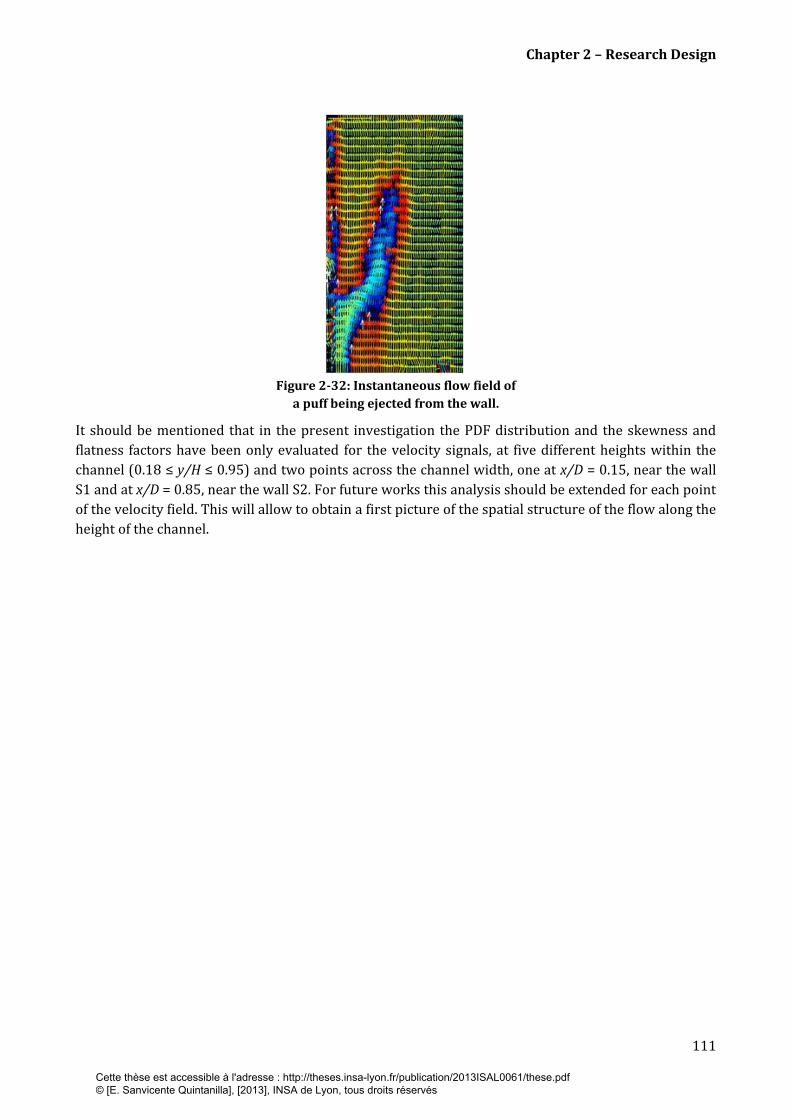
Chapter 2 – Research Design
111
Figure 2-32: Instantaneous flow field of
a puff being ejected from the wall.
It should be mentioned that in the present investigation the PDF distribution and the skewness and
flatness factors have been only evaluated for the velocity signals, at five different heights within the
channel (0.18 ≤ y/H ≤ 0.95) and two points across the channel width, one at x/D = 0.15, near the wall
S1 and at x/D = 0.85, near the wall S2. For future works this analysis should be extended for each point
of the velocity field. This will allow to obtain a first picture of the spatial structure of the flow along the
height of the channel.
Cette thèse est accessible à l'adresse : http://theses.insa-lyon.fr/publication/2013ISAL0061/these.pdf © [E. Sanvicente Quintanilla], [2013], INSA de Lyon, tous droits réservés
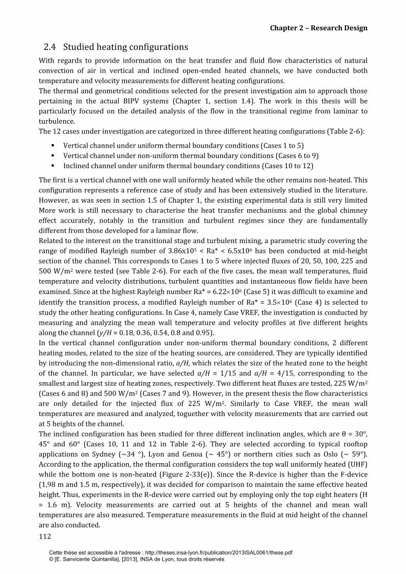
Chapter 2 – Research Design
112
2.4 Studied heating configurations
With regards to provide information on the heat transfer and fluid flow characteristics of natural
convection of air in vertical and inclined open-ended heated channels, we have conducted both
temperature and velocity measurements for different heating configurations.
The thermal and geometrical conditions selected for the present investigation aim to approach those
pertaining in the actual BIPV systems (Chapter 1, section 1.4). The work in this thesis will be
particularly focused on the detailed analysis of the flow in the transitional regime from laminar to
turbulence.
The 12 cases under investigation are categorized in three different heating configurations (Table 2-6):
Vertical channel under uniform thermal boundary conditions (Cases 1 to 5)
Vertical channel under non-uniform thermal boundary conditions (Cases 6 to 9)
Inclined channel under uniform thermal boundary conditions (Cases 10 to 12)
The first is a vertical channel with one wall uniformly heated while the other remains non-heated. This
configuration represents a reference case of study and has been extensively studied in the literature.
However, as was seen in section 1.5 of Chapter 1, the existing experimental data is still very limited
More work is still necessary to characterise the heat transfer mechanisms and the global chimney
effect accurately, notably in the transition and turbulent regimes since they are fundamentally
different from those developed for a laminar flow.
Related to the interest on the transitional stage and turbulent mixing, a parametric study covering the
range of modified Rayleigh number of 3.86x10⁵ < Ra* < 6.5x10⁶ has been conducted at mid-height
section of the channel. This corresponds to Cases 1 to 5 where injected fluxes of 20, 50, 100, 225 and
500 W/m2 were tested (see Table 2-6). For each of the five cases, the mean wall temperatures, fluid
temperature and velocity distributions, turbulent quantities and instantaneous flow fields have been
examined. Since at the highest Rayleigh number Ra* = 6.22106 (Case 5) it was difficult to examine and
identify the transition process, a modified Rayleigh number of Ra* = 3.5106 (Case 4) is selected to
study the other heating configurations. In Case 4, namely Case VREF, the investigation is conducted by
measuring and analyzing the mean wall temperature and velocity profiles at five different heights
along the channel (y/H = 0.18, 0.36, 0.54, 0.8 and 0.95).
In the vertical channel configuration under non-uniform thermal boundary conditions, 2 different
heating modes, related to the size of the heating sources, are considered. They are typically identified
by introducing the non-dimensional ratio, a/H, which relates the size of the heated zone to the height
of the channel. In particular, we have selected a/H = 1/15 and a/H = 4/15, corresponding to the
smallest and largest size of heating zones, respectively. Two different heat fluxes are tested, 225 W/m2
(Cases 6 and 8) and 500 W/m2 (Cases 7 and 9). However, in the present thesis the flow characteristics
are only detailed for the injected flux of 225 W/m2. Similarly to Case VREF, the mean wall
temperatures are measured and analyzed, toguether with velocity measurements that are carried out
at 5 heights of the channel.
The inclined configuration has been studied for three different inclination angles, which are θ = 30°,
45° and 60° (Cases 10, 11 and 12 in Table 2-6). They are selected according to typical rooftop
applications on Sydney (~34 °), Lyon and Genoa (~ 45°) or northern cities such as Oslo (~ 59°).
According to the application, the thermal configuration considers the top wall uniformly heated (UHF)
while the bottom one is non-heated (Figure 2-33(e)). Since the R-device is higher than the F-device
(1,98 m and 1.5 m, respectively), it was decided for comparison to maintain the same effective heated
height. Thus, experiments in the R-device were carried out by employing only the top eight heaters (H
= 1.6 m). Velocity measurements are carried out at 5 heights of the channel and mean wall
temperatures are also measured. Temperature measurements in the fluid at mid height of the channel
are also conducted.
Cette thèse est accessible à l'adresse : http://theses.insa-lyon.fr/publication/2013ISAL0061/these.pdf © [E. Sanvicente Quintanilla], [2013], INSA de Lyon, tous droits réservés
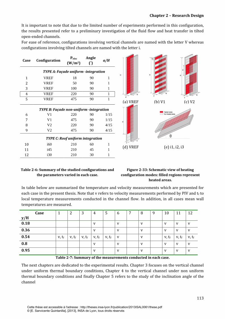
Chapter 2 – Research Design
113
It is important to note that due to the limited number of experiments performed in this configuration,
the results presented refer to a preliminary investigation of the fluid flow and heat transfer in tilted
open-ended channels.
For ease of reference, configurations involving vertical channels are named with the letter V whereas
configurations involving tilted channels are named with the letter i.
Case Configuration Pelec
(W/m2)
Angle
(˚) a/H
TYPE A: Façade uniform -integration
1 VREF 18 90 1
2 VREF 50 90 1
3 VREF 100 90 1
4 VREF 220 90 1
5 VREF 475 90 1
TYPE B: Façade non-uniform -integration
6 V1 220 90 1/15
7 V1 475 90 1/15
8 V2 220 90 4/15
9 V2 475
90 4/15
TYPE C: Roof uniform integration
10 i60 210 60 1
11 i45 210 45 1
12 i30 210 30 1
(a) VREF
(aV1 VREF
(b) V1 (c) V2
(d) VREF (e) i1, i2, i3
Table 2-6: Summary of the studied configurations and
the parameters varied in each case.
Table 2: Cases tested in the experimental set up
Figure 2-33: Schematic view of heating
configuration modes: filled regions represent
heated areas.
In table below are summarized the temperature and velocity measurements which are presented for
each case in the present thesis. Note that v refers to velocity measurements performed by PIV and tf to
local temperature measurements conducted in the channel flow. In addition, in all cases mean wall
temperatures are measured.
Case y/H
1 2 3 4 5 6 7 8 9 10 11 12
0.18 v v v v v v
0.36 v v v v v v
0.54 v, tf v, tf v, tf v, tf v, tf v v v, tf v, tf v, tf
0.8 v v v v v v
0.95 v v v v v v
Table 2-7: Summary of the measurements conducted in each case.
The next chapters are dedicated to the experimental results. Chapter 3 focuses on the vertical channel
under uniform thermal boundary conditions, Chapter 4 to the vertical channel under non uniform
thermal boundary conditions and finally Chapter 5 refers to the study of the inclination angle of the
channel
Cette thèse est accessible à l'adresse : http://theses.insa-lyon.fr/publication/2013ISAL0061/these.pdf © [E. Sanvicente Quintanilla], [2013], INSA de Lyon, tous droits réservés

Chapter 2 – Research Design
114
Cette thèse est accessible à l'adresse : http://theses.insa-lyon.fr/publication/2013ISAL0061/these.pdf © [E. Sanvicente Quintanilla], [2013], INSA de Lyon, tous droits réservés
Chapter 3 Vertical channel under uniform thermal
boundary conditions
Chapter 3
Vertical channel under uniform thermal boundary
conditions
The first chapter of experimental results refers to the study of natural convection flow in vertical open-
ended channels heated asymmetrically and subjected to uniform wall heat flux. This configuration has
been extensively studied for the last thirty years since it is relevant in many applications at different
scales. We may cite cooling of electronic component or nuclear equipment and in the building field,
solar chimneys, Trombe walls or solar collectors. Most of the studies reported in literature considered
boundary conditions of UWT type (uniform wall temperature imposed) and focused on the laminar
regime. Few studies are available in UHF type (uniform heat flux imposed).
Since for this heating configuration the boundary conditions are uniform, the application benefits may
concern the free cooling of opaque PV modules uniformly integrated in façades and ventilated by
natural convection in summer season. Moreover, we cannot avoid dealing with it, especially because it
constitutes a baseline and a reference, relatively to the configurations which will be treated further.
Indeed, in Chapter 4 the thermal boundary conditions are non-uniform (periodic and alternate
heating) and in Chapter 5 the channel is inclined relatively to the horizontal position.
However, this simple configuration involves complex physical phenomena such as a potentially change
in the flow regime, a reverse flow in the outlet of the channel, acceleration or deceleration and coupled
and interrelated heat and mass transfers (convection, radiation, conduction). More work is still
necessary to characterise accurately the heat transfer mechanisms and the global chimney effect,
notably in the transition and turbulent regimes since they are fundamentally different from those
developed for a laminar flow.
Concerning the previous works done on the experimental device available in the CETHIL laboratory,
Jérémie Vareilles [131] studied during the previous PhD thesis (2007) the thermal behavior of the
channel inner wall surfaces. He also designed and built the experimental set up.
The present work aims to provide novel information regarding the natural convective flow in the
channel through the studies on kinematic and thermal behaviours. Specifically, by exploring the
instantaneous flow structure and its associated thermal and kinematical changes, this work performed
herein shows that the flow in the channel is extremely sensitive to environmental conditions.
These questions are addressed in the first part through the study of discrepancies on both
temperature and velocity profiles (mean quantities and turbulent intensities) along the channel height
between several tests performed at a fixed Ra* = 3.5 x 10⁶ and under the same experimental
conditions. The analysis of the unsteadiness of the flow is reinforced through the examination of
instantaneous velocity fields, which has lead us to highlight several phenomena related to the
transition of the flow regime thereafter y/H =0.54 and to characterize the reverse flow occurring in the
outlet section.
Cette thèse est accessible à l'adresse : http://theses.insa-lyon.fr/publication/2013ISAL0061/these.pdf © [E. Sanvicente Quintanilla], [2013], INSA de Lyon, tous droits réservés
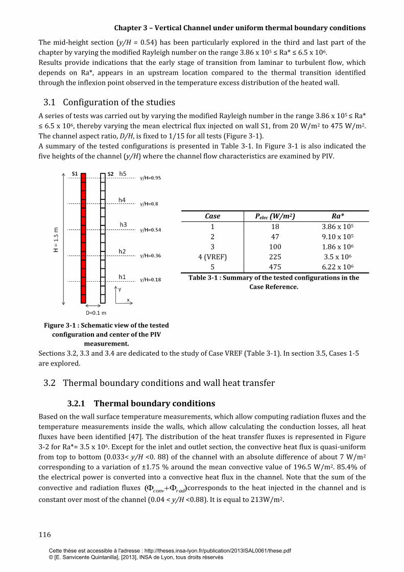
Chapter 3 – Vertical Channel under uniform thermal boundary conditions
116
The mid-height section (y/H = 0.54) has been particularly explored in the third and last part of the
chapter by varying the modified Rayleigh number on the range 3.86 x 10⁵ ≤ Ra* ≤ 6.5 x 10⁶.
Results provide indications that the early stage of transition from laminar to turbulent flow, which
depends on Ra*, appears in an upstream location compared to the thermal transition identified
through the inflexion point observed in the temperature excess distribution of the heated wall.
3.1 Configuration of the studies
A series of tests was carried out by varying the modified Rayleigh number in the range 3.86 x 10⁵ ≤ Ra*
≤ 6.5 x 10⁶, thereby varying the mean electrical flux injected on wall S1, from 20 W/m2 to 475 W/m2.
The channel aspect ratio, D/H, is fixed to 1/15 for all tests (Figure 3-1).
A summary of the tested configurations is presented in Table 3-1. In Figure 3-1 is also indicated the
five heights of the channel (y/H) where the channel flow characteristics are examined by PIV.
Table 3-1 : Summary of the tested configurations in the
Case Reference.
Case Pelec (W/m2) Ra*
1 18 3.86 x 10⁵
2 47 9.10 x 10⁵
3 100 1.86 x 10⁶
4 (VREF) 225 3.5 x 10⁶
5 475 6.22 x 10⁶
Figure 3-1 : Schematic view of the tested
configuration and center of the PIV
measurement.
Sections 3.2, 3.3 and 3.4 are dedicated to the study of Case VREF (Table 3-1). In section 3.5, Cases 1-5
are explored.
3.2 Thermal boundary conditions and wall heat transfer
3.2.1 Thermal boundary conditions
Based on the wall surface temperature measurements, which allow computing radiation fluxes and the
temperature measurements inside the walls, which allow calculating the conduction losses, all heat
fluxes have been identified [47]. The distribution of the heat transfer fluxes is represented in Figure
3-2 for Ra*= 3.5 x 10⁶. Except for the inlet and outlet section, the convective heat flux is quasi-uniform
from top to bottom (0.033< y/H <0. 88) of the channel with an absolute difference of about 7 W/m2
corresponding to a variation of ±1.75 % around the mean convective value of 196.5 W/m2. 85.4% of
the electrical power is converted into a convective heat flux in the channel. Note that the sum of the
convective and radiation fluxes corresponds to the heat injected in the channel and is
constant over most of the channel (0.04 < y/H <0.88). It is equal to 213W/m2.
)( radconv
Cette thèse est accessible à l'adresse : http://theses.insa-lyon.fr/publication/2013ISAL0061/these.pdf © [E. Sanvicente Quintanilla], [2013], INSA de Lyon, tous droits réservés
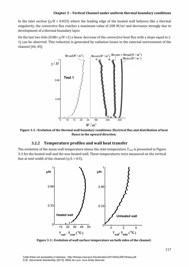
Chapter 3 – Vertical Channel under uniform thermal boundary conditions
117
In the inlet section (y/H < 0.033) where the leading edge of the heated wall behaves like a thermal
singularity, the convective flux reaches a maximum value of 208 W/m2 and decreases strongly due to
development of a thermal boundary layer.
On the last two foils (0.88< y/H <1) a linear decrease of the convective heat flux with a slope equal to (-
1) can be observed. This reduction is generated by radiation losses to the external environment of the
channel [44, 45].
Figure 3-2 : Evolution of the thermal wall boundary conditions: Electrical flux and distribution of heat
fluxes in the upward direction.
3.2.2 Temperature profiles and wall heat transfer
The evolution of the mean wall temperature minus the inlet temperature Tinlet is presented in Figure
3-3 for the heated wall and the non-heated wall. These temperatures were measured on the vertical
line at mid-width of the channel (z/L = 0.5).
Figure 3-3 : Evolution of wall surface temperature on both sides of the channel.
Cette thèse est accessible à l'adresse : http://theses.insa-lyon.fr/publication/2013ISAL0061/these.pdf © [E. Sanvicente Quintanilla], [2013], INSA de Lyon, tous droits réservés

Chapter 3 – Vertical Channel under uniform thermal boundary conditions
118
The temperature evolution along the heated wall is consistent with the convective heat flux shown in
Figure 3-2. Three typical trends according to the height can be observed. In the bottom part of the
channel (y/H <1/3), the wall temperature increases strongly and the maximum gradient is localized at
the leading edge of the heated wall, where the convective heat flux is singular.
This strong evolution of the convective heat coefficient can be seen in Figure 3-4(a). Between y/H =1/3
and y/H = 3/4 the temperature increases linearly as already mentioned by Dalbert et al. [65] and
Manca and Naso [151]. Finally, the temperature decreases from y/H > 3/4 up to the top of the channel.
These 2 inflections limits are also visible on the local Nusselt number as defined in equation (39).
(39)
(a)
(b)
Figure 3-4 : Local convective heat transfer characteristics: (a) Local convective heat transfer, and (b) Local
Nusselt Number.
The inflexion point close to the outlet of the channel has been identified by several authors, such as
Miyamoto [73], Fedorov and Viskanta [114] and Said et al. [115], as a primer signature in the process
of transition to turbulence. This can be verified by the flow dynamic analysis presented in section 3.3.1
in particular through the increase in the fluctuations of the vertical velocity component thus, resulting
in higher rates of heat transfer. This tendency is amplified when approaching the exit of the channel.
The emphasis in the temperature drop is also related to the increase in radiation exchanges and losses
with the environment, as already noted by Webb and Hill [67] and Manca et al. [152]. It is possible that
it is a combination of both.
On the opposite non-heated wall, the surface temperature evolves slightly, with a maximum difference
between the bottom and the top of the channel, ΔTmax= 3°C, compared to ΔTmax= 26°C observed for the
heated wall. This noticeable overheating stems from heat transfer via convection between the fluid and
the wall but mainly by the radiation heat transfer.
3.2.3 Study of repeatability on thermal characteristics
In this section are presented four tests, which have been performed strictly under the same thermal
boundary conditions and following the same experimental procedure.
Figure 3-5(a), Figure 3-5(b) and Figure 3-5(c) present respectively the convective flux along the
heated wall and the evolution of the wall temperatures minus Tinlet along sides S1 (uniformly heated)
and S2 (non-heated), respectively. It should be noted that inlet temperatures varied a maximum of
).(
.).()(
)(
inletwall
yconvconv
TTk
y
k
yyhyNu
Cette thèse est accessible à l'adresse : http://theses.insa-lyon.fr/publication/2013ISAL0061/these.pdf © [E. Sanvicente Quintanilla], [2013], INSA de Lyon, tous droits réservés

Chapter 3 – Vertical Channel under uniform thermal boundary conditions
119
4.5°C between experiments because tests were performed at different period of the year. Nevertheless,
thermal stratification in the test room remained no more than 2-2.5°C for all tests. Detailed
temperatures for each experiment are presented in Table 3-2.
The profiles of the convective heat flux (Figure 3-5(a)) and wall temperatures (Figure 3-5(b), Figure
3-5(c)) obtained from the 4 tests are similar. The differences in the convective flux (Figure 3-5(a)) and
the temperatures of the heated wall (Figure 3-5(b) reach their maxima around 3 W/m2 and 3.5°C at
the central part of the channel, with the profiles overlapping at the inlet and the outlet of the channel
with a deviation lower than 1.5°C. On the non-heated wall (S2), the greatest differences are on the
opposite observed in Figure 3-5(c) close to the bottom and the top of the sides. The non-heated wall
with a mean temperature close to that of the ambient oneis, as expected, more sensitive to the external
environment than is the heated wall. Relative discrepancies have been calculated at 3 levels in the
channel: inlet, mid-height and outlet. The maximum relative temperature discrepancy was at the mid-
height: 1.4% for the temperature on the heated wall, 0.4% for the temperature on the non-heated wall
and 2.8% for the convective heat flux. Discrepancies were less than 1% at the inlet and outlet for all
variables.
(a)
(b)
(c)
Figure 3-5 : Performed tests under the same injected flux conditions: (a) Injected convective heat flux at
Cette thèse est accessible à l'adresse : http://theses.insa-lyon.fr/publication/2013ISAL0061/these.pdf © [E. Sanvicente Quintanilla], [2013], INSA de Lyon, tous droits réservés

Chapter 3 – Vertical Channel under uniform thermal boundary conditions
120
the heated wall, (b) Temperatures along the heated wall and (c) Temperatures along the non-heated
wall.
In order to qualify the global thermal characteristics, the mean Nusselt number has been calculated for
each test. It is defined on the channel height by equation (40)):
(40)
The relative error between tests is evaluated by equation (41). The “reference” Nusselt number in the
error estimation is the mean of all the calculated mean Nusselt numbers for the four experiments. The
results obtained are presented in Table 3-2.
Test ENU
1 24.9 127.60 0.6%
2 21.6 125.9 2 %
3 25 126.31 1.7%
4 26.1 134 4.3%
Table 3-2 : comparison of the inlet temperatures and the mean Nusselt numbers between tests.
The global heat transfer rates are obtained from one test to another with good agreement, with the
relative difference not exceeding 4.3%.
(41)
According to the comparison between these four tests done under the same experimental conditions
and procedure, the repeatability of the thermal characteristics, the wall temperature profile as well as
the Nusselt number that is relative to the convective heat transfer, remains satisfactory.
3.3 Channel flow characteristics
Most studies of unsteady convection have focused on the average and turbulent intensities of
characteristic quantities like velocity, temperature and heat transfer coefficients. Very few have dealt
with the repeatability of these measured quantities and on instantaneous structures developing in the
flow. Based on the few studies dealing with the topic, we can cite a completely different configuration,
namely the horizontal plate subjected to a uniform heat flux, which was used by Aseada and Watanabe
[153] in their attempt to link the instantaneous thermal and kinematical characteristics of flow
structures. Nevertheless, this investigation showed that strong activity depending on space and time
was observed. This is relevant when focusing on local heat transfer at the wall/fluid interface. For
vertical channel configurations, the only studies that have approached the link between the
instantaneous thermal and kinematic characteristics of flows were carried out in mixed convection.
Even in mixed convection where kinematics and thermal effects are of the same order, the flow is very
unstable and very difficult to maintain as reported by Chen and Chung [154], whereas the mean wall
thermal characteristics remains roughly unchanged [155]. Therefore on the basis of what is observed
in mixed convection and according to the fact that natural convection flows are even more sensitive, it
may be expected that every disturbance could be amplified in the fluid flow and thus affects the
steadiness.
H
dyyNuH
Nu
0
).(1
reference
reference
NuNu
NuNuE
Cette thèse est accessible à l'adresse : http://theses.insa-lyon.fr/publication/2013ISAL0061/these.pdf © [E. Sanvicente Quintanilla], [2013], INSA de Lyon, tous droits réservés
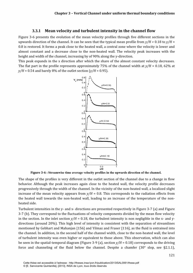
Chapter 3 – Vertical Channel under uniform thermal boundary conditions
121
3.3.1 Mean velocity and turbulent intensity in the channel flow
Figure 3-6 presents the evolution of the mean velocity profiles through five different sections in the
upwards direction of the channel. It can be seen that the typical mean profile from y/H = 0.18 to y/H =
0.8 is restored. It forms a peak close to the heated wall, a central zone where the velocity is lower and
almost constant and a decrease close to the non-heated wall. The velocity peak increases with the
height and width of the channel, increasing by of 90% along the y-direction.
This peak expands in the x direction after which the share of the almost constant velocity decreases.
The flat part in the profile represents approximately 75% of the channel width at y/H = 0.18, 62% at
y/H = 0.54 and barely 8% of the outlet section (y/H = 0.95).
Figure 3-6 : Streamwise time average velocity profiles in the upwards direction of the channel.
The shape of the profiles is very different in the outlet section of the channel due to a change in flow
behavior. Although the peak increases again close to the heated wall, the velocity profile decreases
progressively through the width of the channel. In the vicinity of the non-heated wall, a localized slight
increase of the mean velocity appears from y/H = 0.8. This corresponds to the radiation effects from
the heated wall towards the non-heated wall, leading to an increase of the temperature of the non-
heated side.
Turbulent intensities in the y- and x- directions are presented respectively in Figure 3-7 (a) and Figure
3-7 (b). They correspond to the fluctuations of velocity components divided by the mean flow velocity
in the section. In the inlet section y/H = 0.18, the turbulent intensity is non negligible in the x- and y-
directions (around 20%). This high level of intensity is consistent with the separation of streamlines
mentioned by Gebhart and Mahanjan [156] and Yilmaz and Fraser [116], as the fluid is entrained into
the channel. In addition, in the second half of the channel width, close to the non-heated wall, the level
of turbulent intensity was even higher or equivalent to those above. This observation, which can also
be seen in the spatial-temporal diagram (Figure 3-9 (a), section y/H = 0.18) corresponds to the driving
force and channeling of the fluid below the channel. Despite a chamfer (30° slop, see §2.1.1),
Cette thèse est accessible à l'adresse : http://theses.insa-lyon.fr/publication/2013ISAL0061/these.pdf © [E. Sanvicente Quintanilla], [2013], INSA de Lyon, tous droits réservés
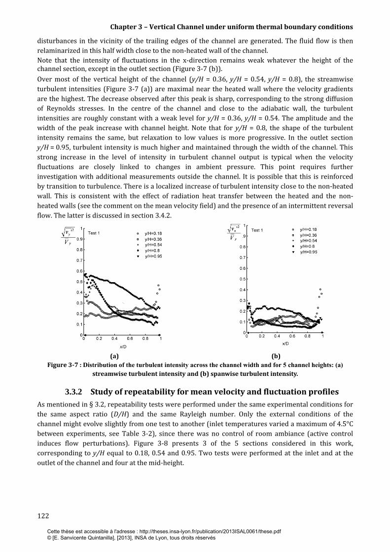
Chapter 3 – Vertical Channel under uniform thermal boundary conditions
122
disturbances in the vicinity of the trailing edges of the channel are generated. The fluid flow is then
relaminarized in this half width close to the non-heated wall of the channel.
Note that the intensity of fluctuations in the x-direction remains weak whatever the height of the channel section, except in the outlet section (Figure 3-7 (b)).
Over most of the vertical height of the channel (y/H = 0.36, y/H = 0.54, y/H = 0.8), the streamwise
turbulent intensities (Figure 3-7 (a)) are maximal near the heated wall where the velocity gradients
are the highest. The decrease observed after this peak is sharp, corresponding to the strong diffusion
of Reynolds stresses. In the centre of the channel and close to the adiabatic wall, the turbulent
intensities are roughly constant with a weak level for y/H = 0.36, y/H = 0.54. The amplitude and the
width of the peak increase with channel height. Note that for y/H = 0.8, the shape of the turbulent
intensity remains the same, but relaxation to low values is more progressive. In the outlet section
y/H = 0.95, turbulent intensity is much higher and maintained through the width of the channel. This
strong increase in the level of intensity in turbulent channel output is typical when the velocity
fluctuations are closely linked to changes in ambient pressure. This point requires further
investigation with additional measurements outside the channel. It is possible that this is reinforced
by transition to turbulence. There is a localized increase of turbulent intensity close to the non-heated
wall. This is consistent with the effect of radiation heat transfer between the heated and the non-
heated walls (see the comment on the mean velocity field) and the presence of an intermittent reversal
flow. The latter is discussed in section 3.4.2.
(a)
(b)
Figure 3-7 : Distribution of the turbulent intensity across the channel width and for 5 channel heights: (a)
streamwise turbulent intensity and (b) spanwise turbulent intensity.
3.3.2 Study of repeatability for mean velocity and fluctuation profiles
As mentioned in § 3.2, repeatability tests were performed under the same experimental conditions for
the same aspect ratio (D/H) and the same Rayleigh number. Only the external conditions of the
channel might evolve slightly from one test to another (inlet temperatures varied a maximum of 4.5°C
between experiments, see Table 3-2), since there was no control of room ambiance (active control
induces flow perturbations). Figure 3-8 presents 3 of the 5 sections considered in this work,
corresponding to y/H equal to 0.18, 0.54 and 0.95. Two tests were performed at the inlet and at the
outlet of the channel and four at the mid-height.
Cette thèse est accessible à l'adresse : http://theses.insa-lyon.fr/publication/2013ISAL0061/these.pdf © [E. Sanvicente Quintanilla], [2013], INSA de Lyon, tous droits réservés
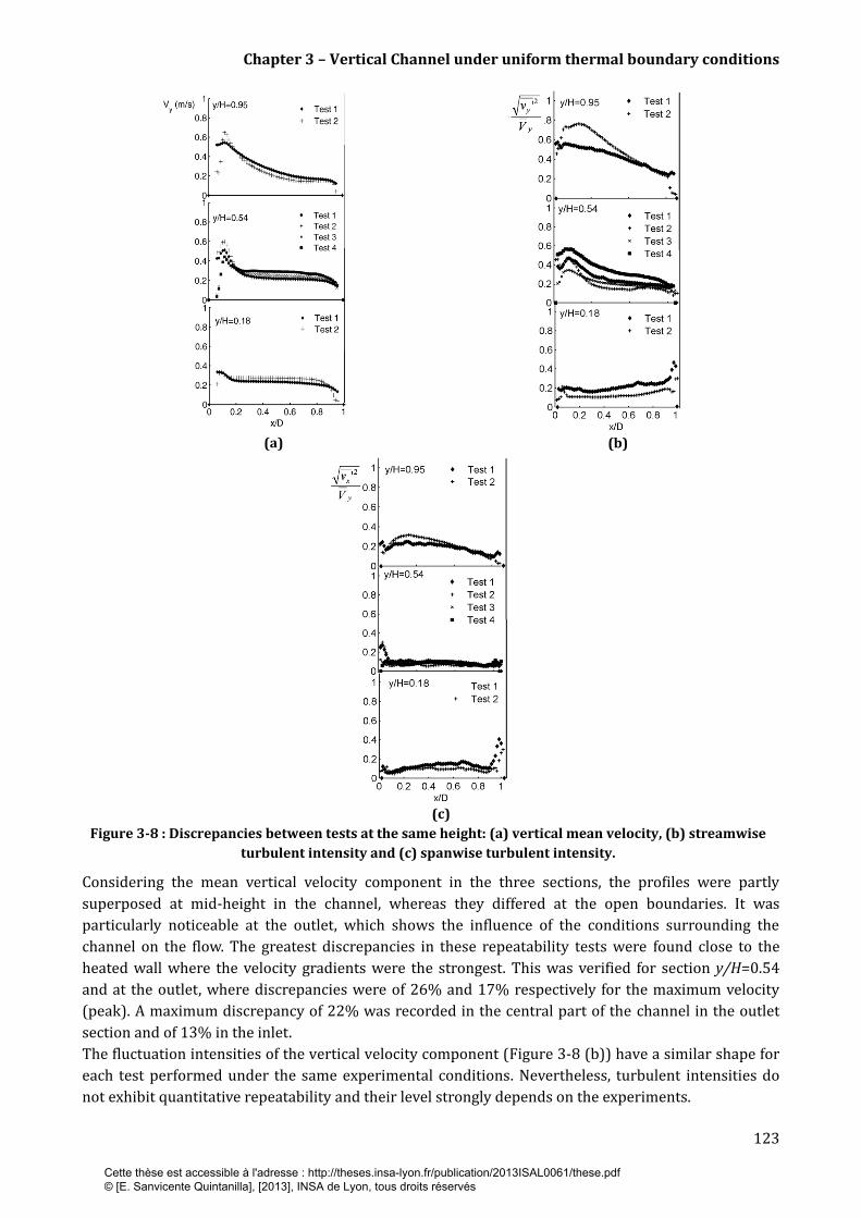
Chapter 3 – Vertical Channel under uniform thermal boundary conditions
123
(a)
(b)
(c)
Figure 3-8 : Discrepancies between tests at the same height: (a) vertical mean velocity, (b) streamwise
turbulent intensity and (c) spanwise turbulent intensity.
Considering the mean vertical velocity component in the three sections, the profiles were partly
superposed at mid-height in the channel, whereas they differed at the open boundaries. It was
particularly noticeable at the outlet, which shows the influence of the conditions surrounding the
channel on the flow. The greatest discrepancies in these repeatability tests were found close to the
heated wall where the velocity gradients were the strongest. This was verified for section y/H=0.54
and at the outlet, where discrepancies were of 26% and 17% respectively for the maximum velocity
(peak). A maximum discrepancy of 22% was recorded in the central part of the channel in the outlet
section and of 13% in the inlet.
The fluctuation intensities of the vertical velocity component (Figure 3-8 (b)) have a similar shape for
each test performed under the same experimental conditions. Nevertheless, turbulent intensities do
not exhibit quantitative repeatability and their level strongly depends on the experiments.
Cette thèse est accessible à l'adresse : http://theses.insa-lyon.fr/publication/2013ISAL0061/these.pdf © [E. Sanvicente Quintanilla], [2013], INSA de Lyon, tous droits réservés
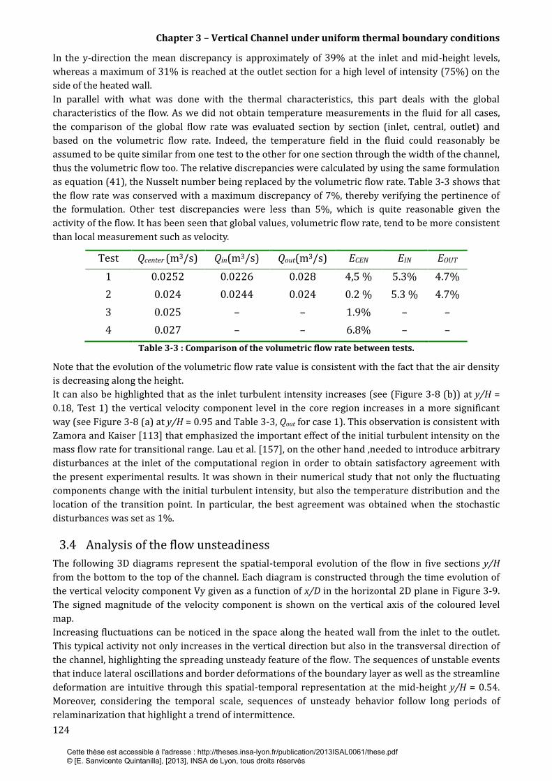
Chapter 3 – Vertical Channel under uniform thermal boundary conditions
124
In the y-direction the mean discrepancy is approximately of 39% at the inlet and mid-height levels,
whereas a maximum of 31% is reached at the outlet section for a high level of intensity (75%) on the
side of the heated wall.
In parallel with what was done with the thermal characteristics, this part deals with the global
characteristics of the flow. As we did not obtain temperature measurements in the fluid for all cases,
the comparison of the global flow rate was evaluated section by section (inlet, central, outlet) and
based on the volumetric flow rate. Indeed, the temperature field in the fluid could reasonably be
assumed to be quite similar from one test to the other for one section through the width of the channel,
thus the volumetric flow too. The relative discrepancies were calculated by using the same formulation
as equation (41), the Nusselt number being replaced by the volumetric flow rate. Table 3-3 shows that
the flow rate was conserved with a maximum discrepancy of 7%, thereby verifying the pertinence of
the formulation. Other test discrepancies were less than 5%, which is quite reasonable given the
activity of the flow. It has been seen that global values, volumetric flow rate, tend to be more consistent
than local measurement such as velocity.
Test Qcenter (m3/s) Qin(m3/s) Qout(m3/s) ECEN EIN EOUT
1 0.0252 0.0226 0.028 4,5 % 5.3% 4.7%
2 0.024 0.0244 0.024 0.2 % 5.3 % 4.7%
3 0.025 – – 1.9% – –
4 0.027 – – 6.8% – –
Table 3-3 : Comparison of the volumetric flow rate between tests.
Note that the evolution of the volumetric flow rate value is consistent with the fact that the air density
is decreasing along the height.
It can also be highlighted that as the inlet turbulent intensity increases (see (Figure 3-8 (b)) at y/H =
0.18, Test 1) the vertical velocity component level in the core region increases in a more significant
way (see Figure 3-8 (a) at y/H = 0.95 and Table 3-3, Qout for case 1). This observation is consistent with
Zamora and Kaiser [113] that emphasized the important effect of the initial turbulent intensity on the
mass flow rate for transitional range. Lau et al. [157], on the other hand ,needed to introduce arbitrary
disturbances at the inlet of the computational region in order to obtain satisfactory agreement with
the present experimental results. It was shown in their numerical study that not only the fluctuating
components change with the initial turbulent intensity, but also the temperature distribution and the
location of the transition point. In particular, the best agreement was obtained when the stochastic
disturbances was set as 1%.
3.4 Analysis of the flow unsteadiness
The following 3D diagrams represent the spatial-temporal evolution of the flow in five sections y/H
from the bottom to the top of the channel. Each diagram is constructed through the time evolution of
the vertical velocity component Vy given as a function of x/D in the horizontal 2D plane in Figure 3-9.
The signed magnitude of the velocity component is shown on the vertical axis of the coloured level
map.
Increasing fluctuations can be noticed in the space along the heated wall from the inlet to the outlet.
This typical activity not only increases in the vertical direction but also in the transversal direction of
the channel, highlighting the spreading unsteady feature of the flow. The sequences of unstable events
that induce lateral oscillations and border deformations of the boundary layer as well as the streamline
deformation are intuitive through this spatial-temporal representation at the mid-height y/H = 0.54.
Moreover, considering the temporal scale, sequences of unsteady behavior follow long periods of
relaminarization that highlight a trend of intermittence.
Cette thèse est accessible à l'adresse : http://theses.insa-lyon.fr/publication/2013ISAL0061/these.pdf © [E. Sanvicente Quintanilla], [2013], INSA de Lyon, tous droits réservés

Chapter 3 – Vertical Channel under uniform thermal boundary conditions
125
(a)
(b)
(c)
(d)
(e)
Figure 3-9 : Spatial-temporal evolution of the flow field (vertical velocity component) at 5 different heights in the channel: (a) Inlet of the channel, y/H=0.18, (b) H/4, y/H=0.36, (c) Mid-height of the channel,
y/H=0.54, (d) 3H/4, y/H=0.8, and (e) Outlet of the channel, y/H=0.95.
As seen on the spatial-temporal diagrams, unsteadiness results in an iterative process of
destabilization and relaminarization of the flow within the channel. The destabilization of the flow was
mainly due to shear instabilities in the boundary layer close to the heated wall and from the time and
space dependent reversal flow occurring in the outlet section. The latter are described and
characterized in the following subsections.
3.4.1 Boundary layer behavior
The main typologies that are observed in the boundary layer close to the heated wall are shown in
Figure 3-10 through velocity vectors coloured by their magnitude (cases a, c, e) and non-dimensional
2-D vorticity isocontours superimposed on the streamlines (cases b, d, f) at different times. Cases (a,b),
(c,d), (e,f) correspond to consecutive frames spaced within 10 seconds.
2-D vorticity is defined by the following expression (equation (42)):
Cette thèse est accessible à l'adresse : http://theses.insa-lyon.fr/publication/2013ISAL0061/these.pdf © [E. Sanvicente Quintanilla], [2013], INSA de Lyon, tous droits réservés

Chapter 3 – Vertical Channel under uniform thermal boundary conditions
126
(42)
The development of the boundary layer close to the heated wall has been observed from the leading
edge of the channel. The flow in the boundary layers is primarily driven by the ascendant buoyancy
force [50], the shear stress gradient and the diffusive terms, both latest phenomena being dominant in
the boundary sublayer. This boundary layer may become unstable during short intermittent period.
It has been observed at y/H = 0.54 long temporal sequences where the flow remains stable. The flow is
then characterized by a narrow layer of over-velocity (Figure 3-10 (a)) where vorticity appears most
concentrated and where the streamlines remain parallel to the vertical heated surface (Figure 3-10
(b)). Morever the thickness of the layer close to the heated wall remains steady.
These long temporal sequences are interrupted by short periods where the boundary layer becomes
unstable until the non-linear effects interact. These first results in spanwise oscillations where the
thickness of the boundary layer can double with time with the occurrence of wave deformations of the
streamlines (Figure 3-10 (c-d)). Since non-linear effects interact, the splitting of the boundary layer
(Figure 3-10 (c-d)) as well as maximum intensity vortices crossing the channel in the streamwise
direction may be observed (Figure 3-10 (e-f)).
These deformations are typically due to shear stress instabilities. The boundary layer splitting is
characterized by vorticity layers of opposite signs as shown in Figure 3-10 (d) which deforms under
constraints. The vortices that are consecutively generated are finally ejected toward the center of the
channel and damped through mean stretching (Figure 3-10 (f)).
The intensification of these events is observed at y/H = 0.8 and in the outlet section (y/H =0.95). The
flow is disturbed more frequently by sequences of vortices that are ejected from the heated wall to the
adiabatic one, as shown in Figure 3-10 (e-f).
(a) t = t0 (b) t= t0
Cette thèse est accessible à l'adresse : http://theses.insa-lyon.fr/publication/2013ISAL0061/these.pdf © [E. Sanvicente Quintanilla], [2013], INSA de Lyon, tous droits réservés

Chapter 3 – Vertical Channel under uniform thermal boundary conditions
127
(c) t = t0+6 (d) t = t0+6
© t = t0+8 (f) t = t0+8
Figure 3-10: Typical behavior of the boundary layer for different times (in seconds) at the same height (y/H = 0.54): (a, c, e) Velocity vectors coloured by their magnitude and (b, d, f) superposition of the
streamlines and iso-vorticity contours.
What is important at this stage is first to specify whether frequencies are associated with
laminar/unstable sequences, which in the experiments, develop without any constraints. The second
task is to link these unstable kinematic events with their energy contents and the heat transfer at the
wall, in order to control the thermal draining from the wall, both locally and dynamically.
For this purpose the power spectral density is evaluated. The results presented in Figure 3-11 were
obtained from the velocity measurements performed at y/H = 0.54, x/D = 0.15 (point A) and x/D = 0.85
(point B).
(a)
(b)
Figure 3-11 : Instantaneous Frequency Analysis at y/H=0.54 for different: (a) x/D = 0.15 and (b)
x/D=0.85.
The spectrum revealed low-frequency peaks [0.03-0.67 Hz] whose amplitude decreases with distance
from the wall (locations A, B). According to the PIV films, the highest frequencies, f2 ~ 0.1 Hz and f3 ~
0.25 Hz, seem to be inherently linked to the unstable boundary layer near the heated wall but not to
laminar/unstable sequences. Indeed the behavior of the boundary layer at mid-height, that seems to
be intermittent, requires detailed investigations with adequate analysis and adequate parameters
[105, 107, 109]. This could also be carried out by using the same approach as Tsuji and Nagano [158],
who observed intermittent fluctuations of temperature and velocities in a natural convection boundary
layer along a vertical flat plate.
Cette thèse est accessible à l'adresse : http://theses.insa-lyon.fr/publication/2013ISAL0061/these.pdf © [E. Sanvicente Quintanilla], [2013], INSA de Lyon, tous droits réservés

Chapter 3 – Vertical Channel under uniform thermal boundary conditions
128
3.4.2 Flow reversal at the outlet of the channel
The unsteady characteristics of the flow can lead to an intermittent unstable flow reversal. This
corresponds to the entry of fresh air from the top of the channel that balances the chimney effect that
is confined close to the heated wall. Most observations were performed for UWT boundary conditions,
corresponding to the majority of studies.
As stated by Azevedo et al. [61] in 1985 for a vertical channel under UWT boundary conditions, this
flow divides into two separate flows at a stagnation point and then merge into the upcoming flow
through the heated channel, thereby creating spanwise vortices This phenomenon is accompanied by a
separation of the ascending boundary layer type flow close to the non-heated wall leaving a V-shaped
region (see streamlines in Figure 3-12(b)).
(a)
(b)
(c)
Figure 3-12 : Dynamical instabilities at the outlet of the channel at different instants of time:
(a) Instantaneous velocity distribution (y/H=0.95), (b) Instantaneous velocity distribution (y/H=0.95)
no reversal flow and (c) Instantaneous velocity distribution (y/H=0.95).
As mentioned above, this phenomenon is not stationary but evolves in time and space. However, to
characterize it, we may evaluate the maximum penetration length defined as the distance from the
channel exit to the stagnation point. Figure 3-12 (a) and Figure 3-12 (c) clearly show the location of
the stagnation point, which changes through time. In Figure 3-12 (a), the penetration length is 7 cm,
whereas in Figure 3-12 (c), the length is about 20 cm. Therefore this reversed flow also induced flow
oscillations.
As discussed in section 1.5.3.3 of Chapter 1, the existence of downflows inside asymmetric heated
channels in laminar conditions has been reported by Sparrow et al. [61] in water experiments and by
Webb and Hill [67] in air ones. Several other studies have been performed in the field of solar
chimneys, such as that by Chen et al. [27]. Both the channel aspect ratio and the Rayleigh number are
found to be the most influential parameters on the existence of reversal flows [128]. Acording to the
observations reported by Dupont et al. [128], which were presented in Figure 1-32, the D/H and Ra*
parameters tested in the present study lead to the apparition of a reversal flow of the second type,
which is the intermittent mode. Recall that in the classification of reverse flows made by [128] the
absence and the steady existence modes were also considered.
In steady state conditions, Ospir [123] stated for UHF conditions that the structure of the reverse flow
using water is characterized by an elongated eight-shaped structure with two main recirculation cells.
Kihm et al. [122] also worked on the penetration length of such recirculation flow in the vertical
channel.
Cette thèse est accessible à l'adresse : http://theses.insa-lyon.fr/publication/2013ISAL0061/these.pdf © [E. Sanvicente Quintanilla], [2013], INSA de Lyon, tous droits réservés

Chapter 3 – Vertical Channel under uniform thermal boundary conditions
129
The sources of this phenomenon depend apparently on the internal conditions existing in the channel
(if the inlet section is considered as part of the channel) even if we have stressed through the
kinematical analysis presented above, that the increase of velocity fluctuations at the outlet of the
channel is linked to external pressure fluctuations. This has to be investigated further especially
regarding the aspect ratio (D/H) and injected power variations, i.e. for several modified Rayleigh
number.
It should be noted that penetration lengths on the vertical configuration will be compared in Chapter 5
to the ones observed in tilted configurations. Conclusions are drawn on Chapter 5 regarding all cases.
Cette thèse est accessible à l'adresse : http://theses.insa-lyon.fr/publication/2013ISAL0061/these.pdf © [E. Sanvicente Quintanilla], [2013], INSA de Lyon, tous droits réservés

Chapter 3 – Vertical Channel under uniform thermal boundary conditions
130
3.4.3 The quantification of the inhomogeneity of the fluid flow
In Figure 3-13, the time evolution of the vertical velocity Vy is examined at five different heights within
the channel (0.18 ≤ y/H ≤ 0.95), at the centerline (z/L = 0.5) and two points across the channel width,
one at x/D = 0.15, near the S1 wall and the other at x/D = 0.85 near the S2 wall. Since the behavior of
the flow is quite stable close to the non-heated face, the statistical characteristics of the velocity signal,
such as the PDF, the skewness (S) and flatness factors (F) will be only discussed for x/D = 0.15.
The fluid flow appears to be non-homogeneous from the leading edge to the trailing edge of the
channel with a skewness factor varying from 0.55 to 0.32 and a flatness factor varying from 13.37 to
3.27 (Figure 3-14). The skewness factor always positive increases from y/H = 0.18 to the mid-height of
the channel y/H = 0.54 and decreases in the second part of the channel. The flatness factor decreases
monotonously from the bottom to the top with a really large value at the inlet. This means, as
expected, that external perturbations of high intensity affect sparsely the inlet flow in the channel
(spotty character of the flow) even if ambient conditions and external noises are partly controlled in
the experimental room. These perturbations tend to be damped at y/H = 0.36, resulting in a sharp
decrease of the flatness factor and an increase of the skewness factor. Note that the flow becomes
more regular in this first quarter channel (relaminarization shift).
At y/H = 0.54, the skewness factor achieves its maximum value. This is related to large scale organized
motions corresponding as shown in section 3.4.1 to the destabilization of the boundary layer and
ejection of kinematical puffs. Above, S and F decrease towards the values 0 and 3, values that are not
reached at the outlet. Thereby, the random variable is not strictly in a Gaussian distribution and the
turbulent field appears to remain inhomogeneous through the entire height of the channel. This is
consistent with the intermittent reversal flow occurring in the outlet section. This analysis, which is
done only in five points at x/D = 0.15 close to the heated wall, needs to be completed for every point of
the fluid section to map the degree of homogeneity/inhomogeneity of the flow. This was done by Tian
et al [148] who distinguished several regions for the configuration of an air filled square cavity under
low turbulence regime.
(e)
(d)
Cette thèse est accessible à l'adresse : http://theses.insa-lyon.fr/publication/2013ISAL0061/these.pdf © [E. Sanvicente Quintanilla], [2013], INSA de Lyon, tous droits réservés
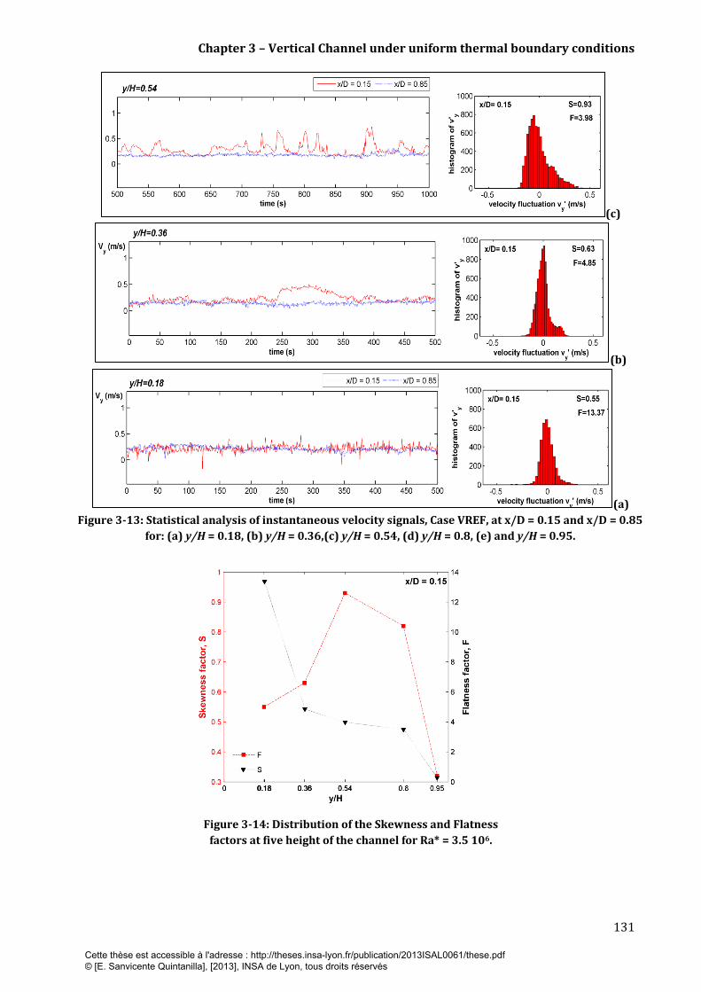
Chapter 3 – Vertical Channel under uniform thermal boundary conditions
131
(c)
(b)
(a)
Figure 3-13: Statistical analysis of instantaneous velocity signals, Case VREF, at x/D = 0.15 and x/D = 0.85
for: (a) y/H = 0.18, (b) y/H = 0.36,(c) y/H = 0.54, (d) y/H = 0.8, (e) and y/H = 0.95.
Figure 3-14: Distribution of the Skewness and Flatness
factors at five height of the channel for Ra* = 3.5 106.
Cette thèse est accessible à l'adresse : http://theses.insa-lyon.fr/publication/2013ISAL0061/these.pdf © [E. Sanvicente Quintanilla], [2013], INSA de Lyon, tous droits réservés

Chapter 3 – Vertical Channel under uniform thermal boundary conditions
132
3.5 Effect of the Rayleigh number
The effect of the Rayleigh number on the temperature and velocity fields is explored in this section by
varying the heat input on the heated wall S1. Experiments have been carried out for the vertical center
plane of the channel (z/L = 0.5), for a fixed aspect ratio of 1/15 and covering the range of modified
Rayleigh number Ra* from 3.86 x 10⁵ to 6.22 x 10⁶. Table 3-4 summarizes the cases tested in the
experimental set up for the present investigation, including the input wall heat flux range, the
corresponding Rayleigh numbers and the reference temperatures (inlet temperatures) for each
experiment. Note that inlet temperatures have varied a maximum of 6.5°C between experiments.
Case Pelec (W/m2) Ra* Tinlet (oC)
1 18 3.86 x 10⁵ 21.98
2 47 9.10 x 10⁵ 23.75
3 100 1.86 x 10⁶ 23.7
4 (VREF) 225 3.5 x 10⁶ 25
5 475 6.22 x 10⁶ 18.5
Table 3-4: Summary of the five cases tested on the Reference configuration and inlet temperatures.
3.5.1 Description of the temperature profiles at the walls
The wall temperature excess distributions (Twall -Tinlet) along the channel height for all five cases are
presented in Figure 3-15(a) for the heated wall and Figure 3-15(b) for the non-heated wall. Two
typical trends are observed in Figure 3-15, the first one, which corresponds to the two lowest Rayleigh
numbers (Cases 1 and 2) and the second one to the three highest ones (Cases 3, 4 and 5).
For the lowest Rayleigh numbers, the temperature profiles monotonically increase with the height of
the channel, the difference ΔToutlet-inlet at the heated wall, S1, being equal to 3.2°C for Case 1 and 6.1°C
for Case 2.
When the modified Rayleigh number is equal or greater than 1.86 x 10⁶ (or heat input is greater than
100 W/m2), the shape of the temperature profiles at the heated wall is similar to the one discussed in
subsection 3.2.2. Two inflection points delimits three regions characterized by a strong increase in the
inlet, following by a linear growth with a smooth slope and a decrease towards the outlet of the
channel. One should note that the linear increasing section gets shorter as the Rayleigh number
increases and consequently the second inflection point, which corresponds to the maximum value of
the wall temperature, shifts downwards the channel. Moreover, the temperature gradient (°C/m) is
greater as the Rayleigh number increases. Graph information regarding Cases 1 to 5 is summarized in
Table 3-5. Temperatures on the non-heated wall, S2, are found to increase slightly from the bottom to
the top of the channel (Figure 3-15(b)). In particular, for the lowest Ra*, ΔTinlet-outlet is 0.7°C and for Ra*
= 6.22 x 10⁶, this difference increases up to 6°C. This temperature increase on the non-heated wall may
be attributed to radiation heat transfer from the heated wall to the non-heated one. Despite the low
surface emissivity and the relatively low surface temperatures, radiation is expected to be an
important heat transfer mode at the highest Ra*. Similar observations were done by Webb and Hill
[67], Burek et al. [44] and Chen et al. [39] in vertical open ended channels with similar surface
emissivity. It should be noted that in addition, the non-heated wall, S2, with a mean temperature close
to that of the ambient one, is more sensitive to external environment as mentioned in §3.2.3. This is
illustrated in the first section of the channel (0 < y/H < 0.25) where one can expect the local wall
temperatures for Case 4 to be greater than those of Cases 2 and 3 (see the zoom in Figure 3-16). For
the highest Ra* = 6.22 x 10⁶, a decrease of the temperature distribution is observed thereafter y/H =
0.65 (Figure 3-15(b)). This location corresponds to the inflection point observed in the temperature
distribution of the heated wall (Table 3-5).
Cette thèse est accessible à l'adresse : http://theses.insa-lyon.fr/publication/2013ISAL0061/these.pdf © [E. Sanvicente Quintanilla], [2013], INSA de Lyon, tous droits réservés

Chapter 3 – Vertical Channel under uniform thermal boundary conditions
133
This clear reduction of temperature on both walls might be significant as a late stage of the transition.
Obviously, a frequency analysis is needed to support these arguments.
(a)
(b)
Figure 3-15 : Distribution of (Twall-Tinlet) along the height of the channel for all cases of
study: (a) heated wall and (b) non-heated wall.
Figure 3-16 : Zoom of (Twall-Tinlet) along the non-heated wall (0 ≤ y/H ≤ 0.4) for Cases 1-5.
Ra* ( oC)
First inflection point,
y/H
Second inflection
point, y/H
Increasing rate in
linear section (°C/m)
3.86 x 10⁵ 5.35 - - -
9.10 x 10⁵ 11.25 - - -
1.86 x 10⁶ 21.42 0.12 0.9 6.5
3.5 x 10⁶ 40 0.25 0.72 8.8
6.22 x 10⁶ 69.92 0.34 0.65 17
Table 3-5: Inflection points in the distributions of the wall temperature profile and for Cases 1-5.
Cette thèse est accessible à l'adresse : http://theses.insa-lyon.fr/publication/2013ISAL0061/these.pdf © [E. Sanvicente Quintanilla], [2013], INSA de Lyon, tous droits réservés

Chapter 3 – Vertical Channel under uniform thermal boundary conditions
134
If the thermal transition is identified by the presence of the second inflexion point on the temperature
excess distribution as reported by Miyamoto [73] and Moshfegh and Sandberg [15] in vertical
channels, we observe on Figure 3-15 that transition does not occur for the lowest Rayleigh numbers,
Ra*=3.86 105 and Ra*=9.1 105. On the other hand, for the three largest ones, Ra* = 1.86 106, 3.5 106 and
6.22 106, transition is found to occur lower in the channel, the higher the Rayleigh number is (see
Table 3-5 ).
3.5.2 Description of the velocity profiles and the fluid temperature
through the width of the channel
Velocity and temperature distributions across the width of the channel have been explored at mid-
height section (y/H = 0.54) for all five cases.
When examining the mean vertical velocity (Figure 3-17) and fluctuation distributions (Figure 3-18),
two groups of typical profiles may be distinguished. For the three lowest Rayleigh numbers (Cases 1-
3), we observe that the shape of the mean velocity profile remains similar, with a relatively small
variation between the maxima obtained close to the heated walls and the quasi-uniform velocity in the
bulk region, ΔVy/Vy (see Table 3-6). As expected, although the shapes of the profiles are similar in
Cases 1 and 2, the magnitude of the velocity at each point within the channel becomes higher as the
Rayleigh number increases. In parallel, the vertical velocity fluctuation profiles present similar trends,
with amplitude that increases with increasing Rayleigh number and that is maintained through the
width of the channel.
As can be seen in Figure 3-17, the shape of the velocity profile for the highest Rayleigh numbers Ra*
[3.5 x 10⁶; 6.22 x 10⁶] changes significantly, with the peak close to the heated wall becoming more
emphasized, the higher the Rayleigh number is (see Table 3-6). It is found that increasing Ra* by a
factor of 3 increased the magnitude of the deviation ΔVy/Vy by a factor of 4.7. A reduction of the
velocity in the core region is observed for Ra* = 3.5 x 10⁶ compared to the lower one Ra* = 1.86 x 10⁶.
Furthermore, as can be seen in Figure 3-17, the peak for Ra* = 6.22 x 10⁶ shifts to the center of the
channel as compared to Ra* = 3.5 x 10⁶ and Ra* = 1.86 106. This shows that the velocity boundary layer
thickness increases with Rayleigh number.
Figure 3-17 : Comparison of time average velocity
profiles at y/H = 0.54 and for Cases 1-5.
Figure 3-18 : Comparison of velocity fluctuation
distributions at y/H = 0.54 and for Cases 1-5.
Cette thèse est accessible à l'adresse : http://theses.insa-lyon.fr/publication/2013ISAL0061/these.pdf © [E. Sanvicente Quintanilla], [2013], INSA de Lyon, tous droits réservés
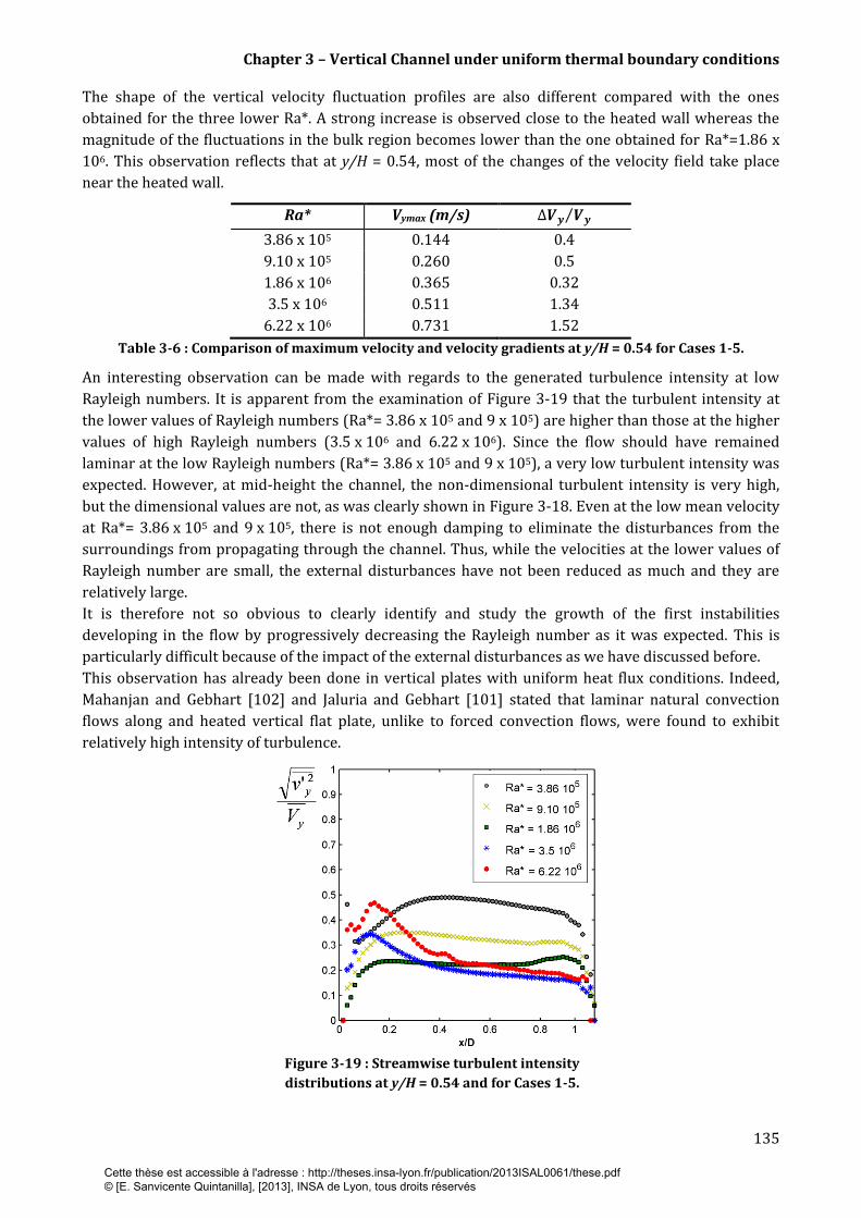
Chapter 3 – Vertical Channel under uniform thermal boundary conditions
135
The shape of the vertical velocity fluctuation profiles are also different compared with the ones
obtained for the three lower Ra*. A strong increase is observed close to the heated wall whereas the
magnitude of the fluctuations in the bulk region becomes lower than the one obtained for Ra*=1.86 x
106. This observation reflects that at y/H = 0.54, most of the changes of the velocity field take place
near the heated wall.
Ra* Vymax (m/s)
3.86 x 10⁵ 0.144 0.4
9.10 x 10⁵ 0.260 0.5
1.86 x 10⁶ 0.365 0.32
3.5 x 10⁶ 0.511 1.34
6.22 x 10⁶ 0.731 1.52
Table 3-6 : Comparison of maximum velocity and velocity gradients at y/H = 0.54 for Cases 1-5.
An interesting observation can be made with regards to the generated turbulence intensity at low
Rayleigh numbers. It is apparent from the examination of Figure 3-19 that the turbulent intensity at
the lower values of Rayleigh numbers (Ra*= 3.86 x 10⁵ and 9 x 10⁵) are higher than those at the higher
values of high Rayleigh numbers (3.5 x 10⁶ and 6.22 x 10⁶). Since the flow should have remained
laminar at the low Rayleigh numbers (Ra*= 3.86 x 10⁵ and 9 x 10⁵), a very low turbulent intensity was
expected. However, at mid-height the channel, the non-dimensional turbulent intensity is very high,
but the dimensional values are not, as was clearly shown in Figure 3-18. Even at the low mean velocity
at Ra*= 3.86 x 10⁵ and 9 x 10⁵, there is not enough damping to eliminate the disturbances from the
surroundings from propagating through the channel. Thus, while the velocities at the lower values of
Rayleigh number are small, the external disturbances have not been reduced as much and they are
relatively large.
It is therefore not so obvious to clearly identify and study the growth of the first instabilities
developing in the flow by progressively decreasing the Rayleigh number as it was expected. This is
particularly difficult because of the impact of the external disturbances as we have discussed before.
This observation has already been done in vertical plates with uniform heat flux conditions. Indeed,
Mahanjan and Gebhart [102] and Jaluria and Gebhart [101] stated that laminar natural convection
flows along and heated vertical flat plate, unlike to forced convection flows, were found to exhibit
relatively high intensity of turbulence.
Figure 3-19 : Streamwise turbulent intensity
distributions at y/H = 0.54 and for Cases 1-5.
Cette thèse est accessible à l'adresse : http://theses.insa-lyon.fr/publication/2013ISAL0061/these.pdf © [E. Sanvicente Quintanilla], [2013], INSA de Lyon, tous droits réservés
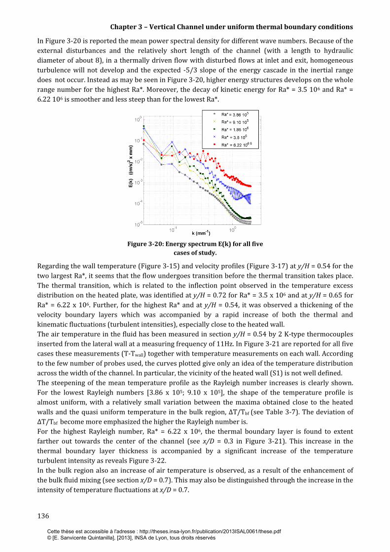
Chapter 3 – Vertical Channel under uniform thermal boundary conditions
136
In Figure 3-20 is reported the mean power spectral density for different wave numbers. Because of the
external disturbances and the relatively short length of the channel (with a length to hydraulic
diameter of about 8), in a thermally driven flow with disturbed flows at inlet and exit, homogeneous
turbulence will not develop and the expected -5/3 slope of the energy cascade in the inertial range
does not occur. Instead as may be seen in Figure 3-20, higher energy structures develops on the whole
range number for the highest Ra*. Moreover, the decay of kinetic energy for Ra* = 3.5 106 and Ra* =
6.22 106 is smoother and less steep than for the lowest Ra*.
Figure 3-20: Energy spectrum E(k) for all five
cases of study.
Regarding the wall temperature (Figure 3-15) and velocity profiles (Figure 3-17) at y/H = 0.54 for the
two largest Ra*, it seems that the flow undergoes transition before the thermal transition takes place.
The thermal transition, which is related to the inflection point observed in the temperature excess
distribution on the heated plate, was identified at y/H = 0.72 for Ra* = 3.5 x 10⁶ and at y/H = 0.65 for
Ra* = 6.22 x 10⁶. Further, for the highest Ra* and at y/H = 0.54, it was observed a thickening of the
velocity boundary layers which was accompanied by a rapid increase of both the thermal and
kinematic fluctuations (turbulent intensities), especially close to the heated wall.
The air temperature in the fluid has been measured in section y/H = 0.54 by 2 K-type thermocouples
inserted from the lateral wall at a measuring frequency of 11Hz. In Figure 3-21 are reported for all five
cases these measurements (T-Twall) together with temperature measurements on each wall. According
to the few number of probes used, the curves plotted give only an idea of the temperature distribution
across the width of the channel. In particular, the vicinity of the heated wall (S1) is not well defined.
The steepening of the mean temperature profile as the Rayleigh number increases is clearly shown.
For the lowest Rayleigh numbers [3.86 x 10⁵; 9.10 x 10⁵], the shape of the temperature profile is
almost uniform, with a relatively small variation between the maxima obtained close to the heated
walls and the quasi uniform temperature in the bulk region, ΔT/Tbf (see Table 3-7). The deviation of
ΔT/Tbf become more emphasized the higher the Rayleigh number is.
For the highest Rayleigh number, Ra* = 6.22 x 10⁶, the thermal boundary layer is found to extent
farther out towards the center of the channel (see x/D = 0.3 in Figure 3-21). This increase in the
thermal boundary layer thickness is accompanied by a significant increase of the temperature
turbulent intensity as reveals Figure 3-22.
In the bulk region also an increase of air temperature is observed, as a result of the enhancement of
the bulk fluid mixing (see section x/D = 0.7). This may also be distinguished through the increase in the
intensity of temperature fluctuations at x/D = 0.7.
Cette thèse est accessible à l'adresse : http://theses.insa-lyon.fr/publication/2013ISAL0061/these.pdf © [E. Sanvicente Quintanilla], [2013], INSA de Lyon, tous droits réservés

Chapter 3 – Vertical Channel under uniform thermal boundary conditions
137
The rise of the temperature close to the non-heated wall is due to radiation between both surfaces,
which is estimated to be 12 % of the heat input.
Figure 3-21 : Comparison of mean axial
temperature profiles at y/H = 0.54.
Figure 3-22 : Comparison of the intensity of
temperature fluctuations at y/H = 0.54.
Ra* Tmax (°C)
3.86 x 10⁵ 27.51 0.23
9.10 x 10⁵ 36.09 0.6
1.86 x 10⁶ 46.88 0.97
3.5 x 10⁶ 68.91 1.71
6.22x 10⁶ 99.77 2.61
Table 3-7 : Comparison of maximum temperature and temperature gradients at y/H = 0.54 for Cases 1-5.
3.6 Conclusions
This chapter was dedicated to study the flow and heat transfer characteristics within an open-ended
vertical channel with one side uniformly heated. This study completes the previous ones [97, 131]
based purely on wall thermal field analysis. The analysis led in this chapter will serve as a reference
base to conduct the analysis on both other configurations studied: vertical channel under non-uniform
boundary conditions (Chapter 4) and inclined channel (Chapter 5).
In reviewing the literature there is a lack of detailed experimental work, notably for transitional and
turbulent natural convection regime. Moreover, most of the studies that are concerned consider
uniform wall temperature as boundary conditions.
The study that we have performed under uniform heat flux conditions focuses on the local and
detailed analysis of the flow field in what we assume as a transitional flow regime.
The results obtained do not allow concluding on the turbulent feature of the flow for Ra* = 3.5 106;
rather it favors the assumption of an intermittent flow. Several indices such as boundary layer
structures release, reversal intermittent flow behaviors at the outlet section, turbulent intensity
profiles and the inflection of the local Nusselt number near the outlet of the channel highlight this
observation related to a change in the flow regime.
The repeatability tests, presented in the first part of the chapter, showed that the thermal
characteristics of the walls were measured with very good accuracy from one test to another.
However, agreement of the results on flow kinematic is less clear. The flow rate effect related to the
buoyancy is recovered with a quite satisfactory accuracy. However, mean kinematic characteristics of
the flow appear to be quite different from one test to the other. This is particularly the case for the
mean velocity and turbulent intensities near the heated wall, where the differences are significant.
Cette thèse est accessible à l'adresse : http://theses.insa-lyon.fr/publication/2013ISAL0061/these.pdf © [E. Sanvicente Quintanilla], [2013], INSA de Lyon, tous droits réservés
Chapter 3 – Vertical Channel under uniform thermal boundary conditions
138
Nevertheless, the frequency analysis carried out seems to highlight certain frequencies possibly
related to the intrinsic destabilization of the boundary layer.
On the other hand, the sensitivity of the flow development to the inlet turbulent intensity suggests the
possibility of controlling the development of natural convection flows and thus heat transfer at the
wall/ fluid interface.
Concerning the laminar/turbulent transition mechanisms, we observe for Ra* = 3.5 x 10⁶ and
6.22 x 10⁶ that the inflexion point of the wall temperature evolution along the height of the channel
appears downstream the point at which the flow undergoes transition to turbulence. This highlights
the importance of collecting information on the instantaneous structure of the flow when
characterizing the transition to turbulence. However, to confirm this result, the experimentations
should be completed for the five Rayleigh numbers with PIV measurements in the four sections y/H =
0.18, y/H = 0.36, y/H=0.8 and y/H = 0.95. To conclude, this work also contributes to the constitution of
a data-base of the fluctuating quantities measured, which will be very helpful in numerical simulations.
As referenced below, the same approach will be developed in the next chapters.
Cette thèse est accessible à l'adresse : http://theses.insa-lyon.fr/publication/2013ISAL0061/these.pdf © [E. Sanvicente Quintanilla], [2013], INSA de Lyon, tous droits réservés

139
Cette thèse est accessible à l'adresse : http://theses.insa-lyon.fr/publication/2013ISAL0061/these.pdf © [E. Sanvicente Quintanilla], [2013], INSA de Lyon, tous droits réservés

140
Cette thèse est accessible à l'adresse : http://theses.insa-lyon.fr/publication/2013ISAL0061/these.pdf © [E. Sanvicente Quintanilla], [2013], INSA de Lyon, tous droits réservés
Chapter 4 Vertical channel under non-uniform
thermal boundary conditions
Chapter 4
Vertical channel under non-uniform thermal
boundary conditions
The experimental results presented in this chapter refer to the study of the natural convection
flow in vertical open-ended channels subjected to non-uniform wall heat flux boundary
conditions. More precisely the imposed boundary conditions represent alternate heated and
unheated zones of equal size along the height of each of the walls. The heating zones are
arranged so that the heated zone on one wall is opposite an unheated zone on the other. The
application of the present investigation is a model of a PV-T double-skin façade with the external
wall consisting of alternate bands of PV cell arrays (localized heat sources) and semitransparent
window panes (unheated zones) over its entire height. This arrangement can be also found in
many applications such as electronic and microelectronic equipments. Indeed, it is of practical
interest in these particular applications to investigate the possibility of reducing the maximum
wall temperature in a channel by using an appropriate spatial distribution of the heat flux to be
transferred from the plates. Hence, the majority of the works on this subject has been focused on
wall thermal studies and often involved the use of mixed or forced convection flows.
The flow in natural convection in which there are alternate heated and unheated zones does not
necessarily undergo transition [47, 159]. In fact the continuous development of thermal
boundary layer is prevented by the insertion of unheated zones between heated zones. Near the
boundary, air leaves an unheated zone at a lower temperature than would have been the case
had heating been continued. This means that at the leading edge of the next downstream heated
zone, the low air temperature leads to a high heat transfer rate, which is manifested as a high
coefficient of convective heat transfer.
The thermal behavior of the walls in non-uniform heating conditions was characterized
experimentally in an earlier PhD thesis [131] for four configurations. It was shown that for the
same average heat flux injected in the channel and keeping the same channel aspect ratio, an
increase of the number of heated/unheated zones in each wall causes a reduction in the
maximum temperature of the heated areas. This is achieved by reducing the size of the heated
and cooled zones.
In the present investigation we have selected the cases previously tested that correspond to the
largest and the smallest size of heated zones and extended the analysis as the PIV measurement
of the air flow has now also been included. Thus in this chapter the local and detailed analysis of
the flow within the channel as well as the determination of global parameters and mean
correlations are presented. The flow is unsteady, in the transitional regime and in the range of
Rayleigh numbers attained in building applications.
Cette thèse est accessible à l'adresse : http://theses.insa-lyon.fr/publication/2013ISAL0061/these.pdf © [E. Sanvicente Quintanilla], [2013], INSA de Lyon, tous droits réservés

Chapter 4 – Vertical channel under non-uniform thermal boundary conditions
142
The points investigated are similar to those raised in the previous chapter: unsteady character of
the flow, structure of the flow pattern and characterization of the transition stage. Additionally,
the enhancement of the mixing in the flow, which might be expected in such configurations, is
also studied. These questions are addressed through the examination of the mean and turbulent
quantities of the flow obtained by PIV in five sections along the height of the channel.
The results indicate for each configuration that a noticeable change of the flow behavior occurs
at y/H = 0.54. Thereafter, the turbulent mixing appears to enhance till the top of the channel. The
analysis of the instantaneous velocity fields has allowed us to highlight several flow phenomena
related to the size of the heated zones. In particular, many structures with very high velocities
are observed at y/H=0.54 compared with the uniformly and differentially heated channel
(Chapter 3). In the case of smallest heated zones, the structures detaching from the heated areas
were predominantly found along the wall where they were developed, whereas in the case of the
largest heated zones, the structures were also attracted by the upper heated zone located in the
opposite wall.
The global quantities of the flow, such as the induced mass flow rate and the overall heat
transfer are discussed in the last part of the chapter. Conclusions are drawn regarding the
ventilation application and the useful generation of heat for this type of configuration.
4.1 Configuration studies
The effect of the non-uniformity of the wall heat flux distribution on the temperature and the
velocity fields, as well as the heat transfer efficiency is explored for a single aspect ratio,
D/H=1/15, and an average electrical heat input maintained at Pelec ~ 222 W/m2. The experiments
were conducted for two different periodical distributions of heated and non-heated zones,
characterized by the non-dimensional ratio a/H, which relates the size of the heated zones (a) to
the height of the channel (H). Moreover, results are compared to the reference configuration,
namely Case VREF, which corresponds to the vertical configuration subjected to an
asymmetrical and uniform heating (a/H = 1, Chapter 3).
Two periodicities, corresponding to a/H =1/15 and a/H=4/15 are investigated. The scheme of
each configuration is shown in Figure 4-1. As well are included the five heights marked
corresponding to the PIV measuring sections.
Figure 4-1 : Different tested configuration and centreline of the PIV zone of measurement.
Cette thèse est accessible à l'adresse : http://theses.insa-lyon.fr/publication/2013ISAL0061/these.pdf © [E. Sanvicente Quintanilla], [2013], INSA de Lyon, tous droits réservés
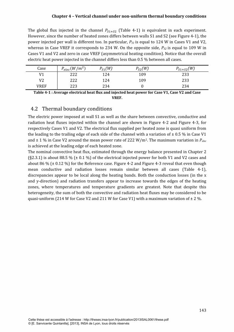
Chapter 4 – Vertical channel under non-uniform thermal boundary conditions
143
The global flux injected in the channel (Table 4-1) is equivalent in each experiment.
However, since the number of heated zones differs between walls S1 and S2 (see Figure 4-1), the
power injected per wall is different too. In particular, PS1 is equal to 124 W in Cases V1 and V2,
whereas in Case VREF it corresponds to 234 W. On the opposite side, PS2 is equal to 109 W in
Cases V1 and V2 and zero in case VREF (asymmetrical heating condition). Notice that the overall
electric heat power injected in the channel differs less than 0.5 % between all cases.
Case (W) (W) (W)
V1 222 124 109 233
V2 222 124 109 233
VREF 223 234 0 234
Table 4-1 : Average electrical heat flux and injected heat power for Case V1, Case V2 and Case
VREF.
4.2 Thermal boundary conditions
The electric power imposed at wall S1 as well as the share between convective, conductive and
radiation heat fluxes injected within the channel are shown in Figure 4-2 and Figure 4-3, for
respectively Cases V1 and V2. The electrical flux supplied per heated zone is quasi uniform from
the leading to the trailing edge of each side of the channel with a variation of ± 0.5 % in Case V1
and ± 1 % in Case V2 around the mean power rate of 222 W/m2. The maximum variation in Pelec
is achieved at the leading edge of each heated zone.
The nominal convective heat flux, estimated through the energy balance presented in Chapter 2
(§2.3.1) is about 88.5 % (± 0.1 %) of the electrical injected power for both V1 and V2 cases and
about 86 % (± 0.12 %) for the Reference case. Figure 4-2 and Figure 4-3 reveal that even though
mean conductive and radiation losses remain similar between all cases (Table 4-1),
discrepancies appear to be local along the heating bands. Both the conduction losses (in the x
and y-direction) and radiation transfers appear to increase towards the edges of the heating
zones, where temperatures and temperature gradients are greatest. Note that despite this
heterogeneity, the sum of both the convective and radiation heat fluxes may be considered to be
quasi-uniform (214 W for Case V2 and 211 W for Case V1) with a maximum variation of ± 2 %.
Cette thèse est accessible à l'adresse : http://theses.insa-lyon.fr/publication/2013ISAL0061/these.pdf © [E. Sanvicente Quintanilla], [2013], INSA de Lyon, tous droits réservés
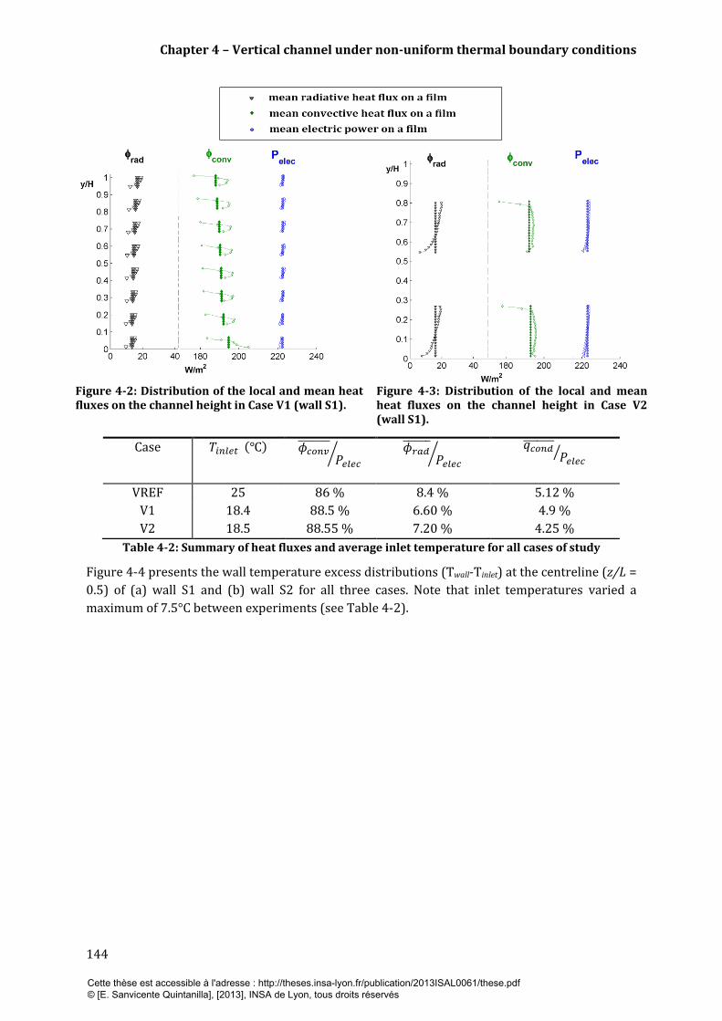
Chapter 4 – Vertical channel under non-uniform thermal boundary conditions
144
Figure 4-2: Distribution of the local and mean heat fluxes on the channel height in Case V1 (wall S1).
Figure 4-3: Distribution of the local and mean heat fluxes on the channel height in Case V2 (wall S1).
Table 4-2: Summary of heat fluxes and average inlet temperature for all cases of study
Figure 4-4 presents the wall temperature excess distributions (Twall-Tinlet) at the centreline (z/L =
0.5) of (a) wall S1 and (b) wall S2 for all three cases. Note that inlet temperatures varied a
maximum of 7.5°C between experiments (see Table 4-2).
Case
VREF 25 86 % 8.4 % 5.12 %
V1 18.4 88.5 % 6.60 % 4.9 %
V2 18.5 88.55 % 7.20 % 4.25 %
Cette thèse est accessible à l'adresse : http://theses.insa-lyon.fr/publication/2013ISAL0061/these.pdf © [E. Sanvicente Quintanilla], [2013], INSA de Lyon, tous droits réservés
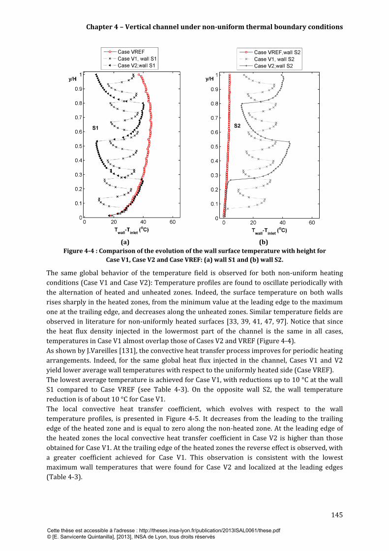
Chapter 4 – Vertical channel under non-uniform thermal boundary conditions
145
(a)
(b)
Figure 4-4 : Comparison of the evolution of the wall surface temperature with height for
Case V1, Case V2 and Case VREF: (a) wall S1 and (b) wall S2.
The same global behavior of the temperature field is observed for both non-uniform heating
conditions (Case V1 and Case V2): Temperature profiles are found to oscillate periodically with
the alternation of heated and unheated zones. Indeed, the surface temperature on both walls
rises sharply in the heated zones, from the minimum value at the leading edge to the maximum
one at the trailing edge, and decreases along the unheated zones. Similar temperature fields are
observed in literature for non-uniformly heated surfaces [33, 39, 41, 47, 97]. Notice that since
the heat flux density injected in the lowermost part of the channel is the same in all cases,
temperatures in Case V1 almost overlap those of Cases V2 and VREF (Figure 4-4).
As shown by J.Vareilles [131], the convective heat transfer process improves for periodic heating
arrangements. Indeed, for the same global heat flux injected in the channel, Cases V1 and V2
yield lower average wall temperatures with respect to the uniformly heated side (Case VREF).
The lowest average temperature is achieved for Case V1, with reductions up to 10 °C at the wall
S1 compared to Case VREF (see Table 4-3). On the opposite wall S2, the wall temperature
reduction is of about 10 °C for Case V1.
The local convective heat transfer coefficient, which evolves with respect to the wall
temperature profiles, is presented in Figure 4-5. It decreases from the leading to the trailing
edge of the heated zone and is equal to zero along the non-heated zone. At the leading edge of
the heated zones the local convective heat transfer coefficient in Case V2 is higher than those
obtained for Case V1. At the trailing edge of the heated zones the reverse effect is observed, with
a greater coefficient achieved for Case V1. This observation is consistent with the lowest
maximum wall temperatures that were found for Case V2 and localized at the leading edges
(Table 4-3).
Cette thèse est accessible à l'adresse : http://theses.insa-lyon.fr/publication/2013ISAL0061/these.pdf © [E. Sanvicente Quintanilla], [2013], INSA de Lyon, tous droits réservés
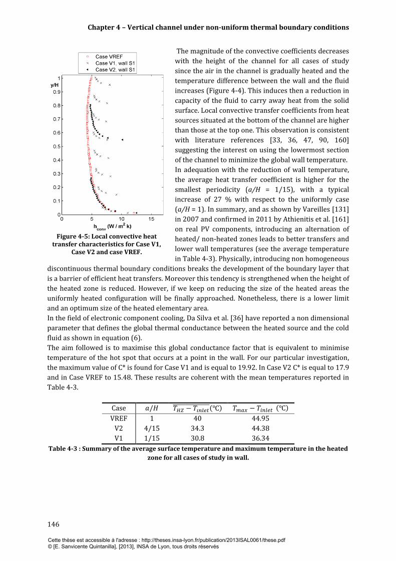
Chapter 4 – Vertical channel under non-uniform thermal boundary conditions
146
The magnitude of the convective coefficients decreases
with the height of the channel for all cases of study
since the air in the channel is gradually heated and the
temperature difference between the wall and the fluid
increases (Figure 4-4). This induces then a reduction in
capacity of the fluid to carry away heat from the solid
surface. Local convective transfer coefficients from heat
sources situated at the bottom of the channel are higher
than those at the top one. This observation is consistent
with literature references [33, 36, 47, 90, 160]
suggesting the interest on using the lowermost section
of the channel to minimize the global wall temperature.
In adequation with the reduction of wall temperature,
the average heat transfer coefficient is higher for the
smallest periodicity (a/H = 1/15), with a typical
increase of 27 % with respect to the uniformly case
(a/H = 1). In summary, and as shown by Vareilles [131]
in 2007 and confirmed in 2011 by Athienitis et al. [161]
on real PV components, introducing an alternation of
heated/ non-heated zones leads to better transfers and
lower wall temperatures (see the average temperature
in Table 4-3). Physically, introducing non homogeneous
discontinuous thermal boundary conditions breaks the development of the boundary layer that
is a barrier of efficient heat transfers. Moreover this tendency is strengthened when the height of
the heated zone is reduced. However, if we keep on reducing the size of the heated areas the
uniformly heated configuration will be finally approached. Nonetheless, there is a lower limit
and an optimum size of the heated elementary area.
In the field of electronic component cooling, Da Silva et al. [36] have reported a non dimensional
parameter that defines the global thermal conductance between the heated source and the cold
fluid as shown in equation (6).
The aim followed is to maximise this global conductance factor that is equivalent to minimise
temperature of the hot spot that occurs at a point in the wall. For our particular investigation,
the maximum value of C* is found for Case V1 and is equal to 19.92. In Case V2 C* is equal to 17.9
and in Case VREF to 15.48. These results are coherent with the mean temperatures reported in
Table 4-3.
Case
VREF 1 40 44.95
V2 4/15 34.3 44.38
V1 1/15 30.8 36.34
Table 4-3 : Summary of the average surface temperature and maximum temperature in the heated
zone for all cases of study in wall.
Figure 4-5: Local convective heat transfer characteristics for Case V1,
Case V2 and case VREF.
Cette thèse est accessible à l'adresse : http://theses.insa-lyon.fr/publication/2013ISAL0061/these.pdf © [E. Sanvicente Quintanilla], [2013], INSA de Lyon, tous droits réservés

Chapter 4 – Vertical channel under non-uniform thermal boundary conditions
147
4.3 Channel flow characteristics
In this section we investigate the effect of the periodical heating distribution in the kinematical
structure of the flow. The flow is first characterized through mean quantities; mean vertical
velocities and turbulent parameters are described and compared for Cases V1, V2 and VREF
along the height of the channel. In the second part, the discussion is completed with the analysis
of the instantaneous velocity fields obtained by PIV.
4.3.1 Evolution of the time average velocity and turbulent
quantities
Figure 4-6 shows a comparison of time-average velocity profiles for each case of study at five
different heights along the channel, y/H = 0.18, 0.36, 0.54, 0.8 and 0.95. Case V1 is presented in
Figure 4-6 (a), Case V2 in Figure 4-6 (b) and Case VREF in Figure 4-6 (c).
Similar behavior of velocity fields along the height of the channel is found in Cases V1 and V2.
For both a/H = 1/15 and 4/15, the time-average distributions of velocity near the inlet section
(y/H = 0.18) present a quasi flat shape across the channel width. The presence of localized small
peaks close to wall S1 is linked to the distribution of the heated zones (Figure 4-1). The similar
magnitudes of velocity in the vicinity of wall S1 are consistent with the temperature
distributions that were seen to overlap in the lowermost part of the channel, y/H ≤ 0.08 (Figure
4-4(a)). In the inlet section, the turbulent intensity of the streamwise velocity component is not
negligible (Figure 4-6 (a-b)), with magnitudes of 14 % for Case V1 and of 12 % for Case V2 at x/D
= 0.5. In Case VREF it is of 19%. As was shown in section §3.3.2, the flow is highly sensitive to
ambient conditions and natural disturbances may be introduced through the inlet section and
amplified in the channel.
As the flow moves upwards, the shape of the velocity profiles evolves with maximum values
achieved in the vicinity of each wall. For all cases, the velocity peaks are found to increase with
the height of the channel (y-direction) as reported in Table 4-4. In the outlet section an increase
of 22 % is observed in the maximum velocity value as a/H is increased from 1/15 to 1. Maximum
velocities, which are localized close to each wall are similar for both distributions of heated
sources, a/H = 1/15 and a/H = 4/15 (see Table 4-4).
The distributions of turbulent intensity in the inlet section, shown in Figure 4-7(a) and Figure
4-7(b), exhibit two peaks close to the walls in the region where velocity gradients are the
greatest. As may be seen, the intensity of fluctuations in the lower half of the channel (y/H ≤ 36)
remains uniform in the central region (0.15 ≤ x/D ≤ 0.8). At mid-height y/H = 0.54, the amplitude
of the turbulent intensity (along y and x) near the walls is significantly greater than in any other
section for both Cases V1 and V2.
A remarkable change in the flow behavior occurred between y/H = 0.36 and y/H = 0.54 for both
cases V1 and V2. Indeed, a significant reduction of the velocity particularly in the core region
(0.2 ≤ x/D ≤ 0.7) and a drastic increase of turbulent intensity close to the walls are observed
respectively in Figure 4-6 (a and b) and Figure 4-7 (a and b). It corresponds to a suction of fluid
into the core region that feeds the boundary layers close to the walls. This phenomenon will be
discussed in more detail in the following.
Cette thèse est accessible à l'adresse : http://theses.insa-lyon.fr/publication/2013ISAL0061/these.pdf © [E. Sanvicente Quintanilla], [2013], INSA de Lyon, tous droits réservés
Chapter 4 – Vertical channel under non-uniform thermal boundary conditions
148
Beyond y/H > 0.54, the streamwise mean velocity component increases again and the amplitude
of the fluctuations decreases significantly compared to the mid-height section of the channel.
Moreover, the distribution of the intensity of fluctuations becomes uniform across the channel
width, suggesting a homogenization of the flow. In the outlet section the maxima obtained for
both non-uniform cases (Vmax = 0.52 m/s for Case V1 and Vmax = 0.51 m/s for Case V2) is smaller
compared to the Reference case (Vmax= 0.64 m/s,Figure 4-6(c)) where the left side is uniformly
heated. This is consistent with the different power injected per wall between Cases V1 and V2
and Case VREF, as previously indicated at the beginning of this section.
Concerning the change in the flow behavior, the local reduction of velocity in the centre of the
channel has already been observed on the natural flow that is developing for a symmetrically
and uniformly heated vertical channel [65, 118, 162]. In particular, Litvak and Morrisson [162]
have studied experimentally and numerically the flow in a thermosyphon solar system and have
highlighted this phenomenon. The experimental set-up is a water loop with a cylindrical heated
pipe. Simulations were performed for simplification on the 2D vertical parallel plate channel
symmetrically heated. A fully developed laminar velocity profile was set as a boundary condition
in the inlet section. The velocity profiles obtained numerically presented the same reduction of
velocity magnitude in the core region, following in upper sections by an increase of the velocity
magnitude in the same central part of the channel. For a particular set of parameters (Rayleigh
number, Reynolds number and aspect ratio), these profiles even showed an inversion of the
velocity sign in the core region. Using a dye solution, they observed in their experiments a
blockage of the flow with a stable core of dye, which remained for more than one hour in the
central region. In the vicinity of the heated boundaries, an ascendant flow is maintained. Above
the heated section in the pipe, the central core becomes unstable. The authors related this
phenomenon to a competition between the shear forces and the gravity (buoyancy forces)
between regions of different temperatures and densities at different heights.
In our experiment where heated/unheated boundaries alternate from one wall to the other, only
a reduction of the velocity in the core region is observed between y/H = 0.36 and y/H = 0.54. No
blockage of the flow appears for the ratio a/H and the Rayleigh numbers studied. However, 3D
effects that may become significant as this process occurs have not been before examined.
Moreover, in these non-uniform heating cases, different flow mechanisms are involved at
different scales. Indeed, there is on one hand a global “chimney effect” governed by buoyancy
forces and pressure drop and on the other hand, there is a local successive acceleration/
deceleration of fluid particles (headquarters of significant fluctuations), which are induced by
the non-uniform boundary conditions.
Cette thèse est accessible à l'adresse : http://theses.insa-lyon.fr/publication/2013ISAL0061/these.pdf © [E. Sanvicente Quintanilla], [2013], INSA de Lyon, tous droits réservés
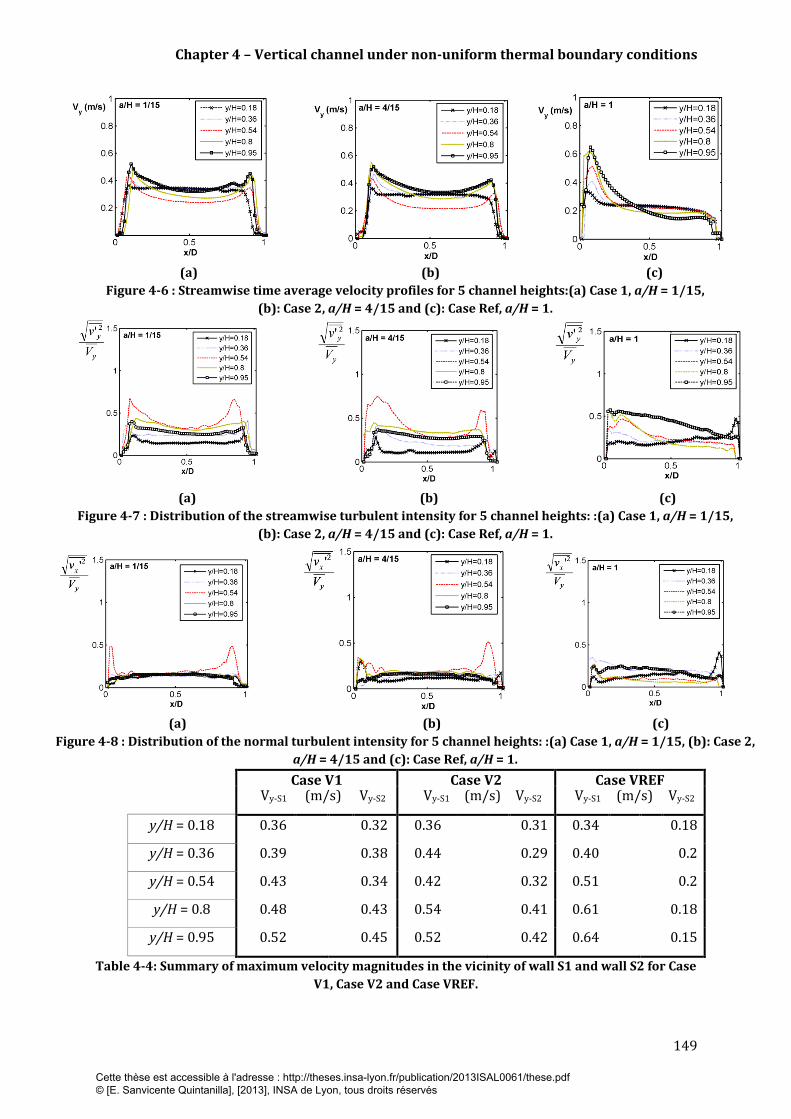
Chapter 4 – Vertical channel under non-uniform thermal boundary conditions
149
(a)
(b)
(c)
Figure 4-6 : Streamwise time average velocity profiles for 5 channel heights:(a) Case 1, a/H = 1/15,
(b): Case 2, a/H = 4/15 and (c): Case Ref, a/H = 1.
(a)
(b)
(c)
Figure 4-7 : Distribution of the streamwise turbulent intensity for 5 channel heights: :(a) Case 1, a/H = 1/15,
(b): Case 2, a/H = 4/15 and (c): Case Ref, a/H = 1.
(a)
(b)
(c)
Figure 4-8 : Distribution of the normal turbulent intensity for 5 channel heights: :(a) Case 1, a/H = 1/15, (b): Case 2,
a/H = 4/15 and (c): Case Ref, a/H = 1.
Case V1 Case V2 Case VREF Vy-S1 (m/s) Vy-S2 Vy-S1 (m/s) Vy-S2 Vy-S1 (m/s) Vy-S2
y/H = 0.18 0.36 0.32 0.36 0.31 0.34 0.18
y/H = 0.36 0.39 0.38 0.44 0.29 0.40 0.2
y/H = 0.54 0.43 0.34 0.42 0.32 0.51 0.2
y/H = 0.8 0.48 0.43 0.54 0.41 0.61 0.18
y/H = 0.95 0.52 0.45 0.52 0.42 0.64 0.15
Table 4-4: Summary of maximum velocity magnitudes in the vicinity of wall S1 and wall S2 for Case
V1, Case V2 and Case VREF.
Cette thèse est accessible à l'adresse : http://theses.insa-lyon.fr/publication/2013ISAL0061/these.pdf © [E. Sanvicente Quintanilla], [2013], INSA de Lyon, tous droits réservés

Chapter 4 – Vertical channel under non-uniform thermal boundary conditions
150
Figure 4-9 presents the profile of
in the five
different sections y/H and for the three Cases V1, V2
and VREF. It can be seen that in general the
production of turbulence by shear increases with the
height of the channel.
For the periodically heated configurations, the sign of
the Reynolds shear stress profiles is observed to vary
from positive for x/D ≤ 0.5 to negative for x/D ≥ 0.5
along the second half of the channel (Figure 4-9 (c-d-
e). This shape is typically found in symmetrically
heated configurations, as showed Ayinde et al. [118]
for isothermal walls and Daverat [32] for isoflux
walls.
For 0.18 ≤ y/H ≤ 0.8, the Reynolds stresses are larger
for both periodically heated configurations. In
particular at y/H = 0.8, they are as much as three
times the size of those found in the Case VREF.
Indeed, the Reynolds stress has a significant
magnitude over most of the cross-section of the
channel, emphasizing the enhanced mixing of the
bulk fluid produced by turbulent transport processes.
In the outlet of the channel (y/H = 0.95) however, a
very large magnitude of
is observed in Case
VREF close to wall S1 (heated wall). As discussed in
3.3, this may be resulted from an increase of the
intensity of velocity fluctuations linked to changes in
ambient pressure fluctuations or a change in the flow
regime. Possibly a combination of both aspects has
taken place.
(e)
(d)
(c)
(b)
(a)
Figure 4-9 : Comparison of Reynolds
shear stress at five heights between Case
V1-V2-VEF.
Cette thèse est accessible à l'adresse : http://theses.insa-lyon.fr/publication/2013ISAL0061/these.pdf © [E. Sanvicente Quintanilla], [2013], INSA de Lyon, tous droits réservés
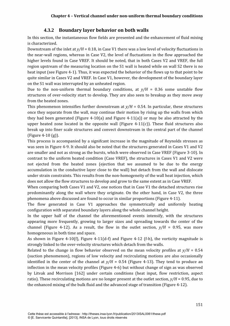
Chapter 4 – Vertical channel under non-uniform thermal boundary conditions
151
4.3.2 Boundary layer behavior on both walls
In this section, the instantaneous flow fields are presented and the enhancement of fluid mixing
is characterized.
Downstream of the inlet at y/H = 0.18, in Case V1 there was a low level of velocity fluctuations in
the near-wall regions, whereas in Case V2, the level of fluctuations in the flow approached the
higher levels found in Case VREF. It should be noted, that in both Cases V2 and VREF, the full
region upstream of the measuring location on the S1 wall is heated while on wall S2 there is no
heat input (see Figure 4-1). Thus, it was expected the behavior of the flows up to that point to be
quite similar in Cases V2 and VREF. In Case V1, however, the development of the boundary layer
on the S1 wall was interrupted by an unheated region.
Due to the non-uniform thermal boundary conditions, at y/H = 0.36 some unstable flow
structures of over-velocity start to develop. They are also seen to breakup as they move away
from the heated zones.
This phenomenon intensifies further downstream at y/H = 0.54. In particular, these structures
once they separate from the wall, may continue their motion by rising up the walls from which
they had been generated (Figure 4-10(a) and Figure 4-11(a)) or may be also attracted by the
upper heated zone located in the opposite wall (Figure 4-11(c)). These fluid structures also
break up into finer scale structures and convect downstream in the central part of the channel
(Figure 4-10 (g)).
This process is accompanied by a signifcant increase in the magnitude of Reynolds stresses as
was seen in Figure 4-9. It should also be noted that the structures generated in Cases V1 and V2
are smaller and not as strong as the bursts, which were observed in Case VREF (Figure 3-10). In
contrast to the uniform heated condition (Case VREF), the structures in Cases V1 and V2 were
not ejected from the heated zones (ejection that we assumed to be due to the energy
accumulation in the conductive layer close to the wall) but detach from the wall and dislocate
under strain constraints. This results from the non-homogeneity of the wall heat injection, which
does not allow the flow structures to develop and grow to the same extent as in Case VREF.
When comparing both Cases V1 and V2, one notices that in Case V1 the detached structures rise
predominantly along the wall where they originate. On the other hand, in Case V2, the three
phenomena above discussed are found to occur in similar proportions (Figure 4-11).
The flow generated in Case V1 approaches the symmetrically and uniformly heating
configuration with separated boundary layers along the whole channel height.
In the upper half of the channel the aforementioned events intensify, with the structures
appearing more frequently, growing to larger sizes and spreading towards the center of the
channel (Figure 4-12). As a result, the flow in the outlet section, y/H = 0.95, was more
homogeneous in both time and space.
As shown in Figure 4-10(f), Figure 4-11(d-f) and Figure 4-12 (f-h), the vorticity magnitude is
strongly linked to the over-velocity structures which detach from the walls.
Related to the change in flow behavior observed on the mean velocity profiles at y/H = 0.54
(suction phenomenon), regions of low velocity and recirculating motions are also occasionally
identified in the center of the channel at y/H = 0.54 (Figure 4-13). They tend to produce an
inflection in the mean velocity profiles (Figure 4-6) but without change of sign as was observed
by Litvak and Morrison [162] under certain conditions (heat input, flow restriction, aspect
ratio). These recirculating motions are no longer present at the outlet section, y/H = 0.95, due to
the enhanced mixing of the bulk fluid and the advanced stage of transition (Figure 4-12).
Cette thèse est accessible à l'adresse : http://theses.insa-lyon.fr/publication/2013ISAL0061/these.pdf © [E. Sanvicente Quintanilla], [2013], INSA de Lyon, tous droits réservés

Chapter 4 – Vertical channel under non-uniform thermal boundary conditions
152
Finally, because in Cases V1 and V2 both walls are heated, albeit in different asymmetric ways,
no flow reversals were identified at the uppermost location, y/H = 0.95 during the whole
experimental programme in which these arrangements were used.
Cette thèse est accessible à l'adresse : http://theses.insa-lyon.fr/publication/2013ISAL0061/these.pdf © [E. Sanvicente Quintanilla], [2013], INSA de Lyon, tous droits réservés
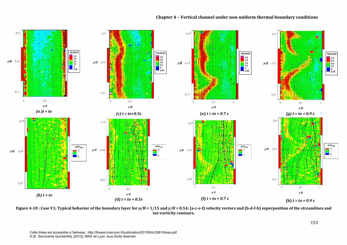
Chapter 4 – Vertical channel under non-uniform thermal boundary conditions
153
(a )t = to
(c) t = to+0.5s
(e) t = to + 0.7 s
(g) t = to + 0.9 s
(b) t = to (d) t = to + 0.5s (f) t = to + 0.7 s
(h) t = to + 0.9 s
Figure 4-10 : Case V1; Typical behavior of the boundary layer for a/H = 1/15 and y/H = 0.54: (a-c-e-f) velocity vectors and (b-d-f-h) superposition of the streamlines and iso-vorticity contours.
Cette thèse est accessible à l'adresse : http://theses.insa-lyon.fr/publication/2013ISAL0061/these.pdf © [E. Sanvicente Quintanilla], [2013], INSA de Lyon, tous droits réservés

Chapter 4 – Vertical channel under non-uniform thermal boundary conditions
154
(a) t = to
(c) t = to (e) t = t1 + 0.3.s
(g) t = t1 + 0.5s
(b) t = t1 (d) t = t1 (f) t = t1 + 0.5s
(h) t = to + 0.5s
Figure 4-11 : Case V2; Typical behavior of the boundary layer for a/H = 4/15 and y/H = 0.54: (a-c-e-g) velocity vectors and (b-d-f-h) superposition of the streamlines and iso-vorticity contours.
Cette thèse est accessible à l'adresse : http://theses.insa-lyon.fr/publication/2013ISAL0061/these.pdf © [E. Sanvicente Quintanilla], [2013], INSA de Lyon, tous droits réservés

Chapter 4 – Vertical channel under non-uniform thermal boundary conditions
155
(a)
(c)
(e)
(g)
(b)
(d)
(f)
(h)
Figure 4-12 : Typical behavior of the flow at y/H = 0.95: (a-b-c-d) Case V1 and (e-f-g-h) Case V2.
Cette thèse est accessible à l'adresse : http://theses.insa-lyon.fr/publication/2013ISAL0061/these.pdf © [E. Sanvicente Quintanilla], [2013], INSA de Lyon, tous droits réservés

Chapter 4 – Vertical channel under non-uniform thermal boundary conditions
156
(a)
(c)
(e)
(g)
(b)
(d) (f)
(h)
Figure 4-13 : Recirculation motions and low velocity regions observed occasionally at y/H = 0.54 in: (a-b-c-d) Case V1 and (e-f-g-h) Case V2.
Cette thèse est accessible à l'adresse : http://theses.insa-lyon.fr/publication/2013ISAL0061/these.pdf © [E. Sanvicente Quintanilla], [2013], INSA de Lyon, tous droits réservés

Chapter 4 – Vertical channel under non-uniform thermal boundary conditions
157
The power spectral density, evaluated at y/H = 0.54, x/D = 0.15 and x/D = 0.85, has revealed in
Cases V1 and V2 low frequency peaks [0.03-0.2 Hz] whose amplitudes are larger than in the Case
VREF discussed in §3.4.1. The results in Case V1 are shown in Figure 4-14 and in Case V2 in
Figure 4-15. Similarly to Case VREF, characteristic frequencies of ~ 0.03 Hz, 0.06 Hz and 0.1 Hz
are identified in both cases. Further investigations are needed to link these frequencies with the
complex structure of the flow pattern.
The motion in both periodic heating arrangements contains higher-energy structures over the
whole wave-number range than in the Case VREF (Figure 4-16), indicating probably a more
vigorous mixing in Case V1. Moreover, the decay of kinetic energy is smoother and less steep
than the one observed for Case VREF.
(a)
(b)
Figure 4-15 : Case V2; Frequency analysis at y/H = 0.54 for different: (a) x/D = 0.15 and (b) x/D = 0.85.
(a)
(b)
Figure 4-14 : Case V1; Frequency analysis at y/H = 0.54 for different: (a) x/D = 0.15 and (b) x/D = 0.85.
Cette thèse est accessible à l'adresse : http://theses.insa-lyon.fr/publication/2013ISAL0061/these.pdf © [E. Sanvicente Quintanilla], [2013], INSA de Lyon, tous droits réservés

Chapter 4 – Vertical channel under non-uniform thermal boundary conditions
158
Figure 4-16 : Energy spectrum E(k) for all cases of
study.
4.3.3 Instantaneous velocity signals: single point analysis
In this section instantaneous velocity measurements are examined at five different heights
within the channel (0.18 ≤ y/H ≤ 0.95), at the centerline (z/L = 0.5) and two points across the
channel width, one at x/D = 0.15, near the S1 wall and the other at x/D = 0.85 near the S2 wall.
Results are presented for Case V1 and V2 in respectively in Figure 4-20 andFigure 4-21.
In order to capture some of the statistical characteristics of the instantaneous velocity fields, the
probability density function and the values of the skewness and flatness factors have been
calculated for each configuration and measuring location. In the literature, results concerning
these aspects of the flow are scarce. The significance of the skewness and flatness factors was
introduced in section 2.3.3.2 of Chapter 2.
The instantaneous velocity field presents at each height similar statistical characteristics in both
locations, x/D = 0.15 and 0.85 (Figure 4-20 and Figure 4-21 ). This is consistent with the time-
averaged velocity and turbulent intensity distributions that were seen to be almost symmetric
across the channel width. Only the point x/D = 0.15 will be hereafter discussed.
The distribution of both the flatness and skewness factors along the channel height indicates
that the velocity field is inhomogeneous (S≠0, F≠3) along the height of the channel (Figure 4-17
Figure 4-17 : Comparison of skewness and flatness factors of velocity signals at x/D = 0.15 and
0.18 ≤ y/H ≤ 0.95, Cases V1-V2-VREF.
Cette thèse est accessible à l'adresse : http://theses.insa-lyon.fr/publication/2013ISAL0061/these.pdf © [E. Sanvicente Quintanilla], [2013], INSA de Lyon, tous droits réservés

Chapter 4 – Vertical channel under non-uniform thermal boundary conditions
159
For the periodic heating cases, the flatness factor drops below the value 3 in contrast to Case
VREF. The distribution appears flatter. However flatness factors remain of the same order as the
ones evaluated for Case VREF and decrease from the inlet to the outlet in all the three cases.
Thereby, the flow field does not achieve the homogeneity in the outlet of the channel in any of
the cases. Note that the flatness factors are very high in the inlet, with values equal to 15 and
9.95 for respectively Cases V1 and V2. As previously mentioned for Case VREF (F=13.37), this
shows the sensitivity of the flow to external perturbations.
The skewness factor is always positive. For Case V1 it seems to increase and to decrease
according to the location of the point of measurement and the periodicity of the boundary
conditions (heated/unheated zones). When the measured point is close to a heated source, the
skewness factor S appears to increase, whereas it decreases in the vicinity of a non-heated zone.
Note the very weak value of the skewness factor at y/H = 0.36, which corresponds to the first
quarter of the beginning of a non-heated zone (see zoom in Figure 4-17 ). As mentioned in the
previous section, in Case V1 coherent structures which develop on the heated zones intensify
since they dislocate sharply close to the following non-heated zone.
In Case V2, the skewness factor presents the same evolution as Case VREF. Indeed, the skewness
factor increases until y/H = 0.54 and decreases up to the outlet section. In this case, the coherent
structures have time to become stronger so they persist and maintain in the flow.
It is noted from the shape of the PDF’s obtained at the outlet section (Figure 4-20 and Figure
4-21 (e)) that we might have a problem of definition. Nevertheless, further processing in every
point of the velocity field are necessary to show how the non-homogeneous boundary conditions
influence the skewness factors evolution in both cases.
The intensity of vertical and horizontal velocity fluctuations for Cases V1 and V2 increases from
the inlet section of the channel to y/H = 0.54 and decreases until the outlet section (Figure 4-18).
The growth of the vertical intensity component is clearly higher than the horizontal one in the
bottom half of the channel. Concerning the horizontal intensity, it is always greater for Cases V1
and V2 than in Case VREF, except in the outlet section. The evolution of the intensity of
fluctuations is consistent with the suction phenomenom described in section 4.3.1.
The turbulent mixing of the flow is enhanced for periodically heated configurations. This is
illustrated by the rate of turbulent production, which increases gradually along the height of the
channel in Cases V1 and V2 (Figure 4-19 ). In the second half of the channel (y/H = 0.8, 0.95) the
flow tends to homogenize with values of S and F being reduced.
On the other hand, the rate of turbulence production in periodically heated configurations is
found to be greater than in Case VREF except for the outlet section of the channel. This might be
explained by the change in the flow regime, the ambient pressure fluctuations and the unsteady
flow reversals, which were identified close to the outlet section in Case VREF as previously
described in sections 3.3.1 and 3.4.1.
Cette thèse est accessible à l'adresse : http://theses.insa-lyon.fr/publication/2013ISAL0061/these.pdf © [E. Sanvicente Quintanilla], [2013], INSA de Lyon, tous droits réservés

Chapter 4 – Vertical channel under non-uniform thermal boundary conditions
160
(a) (b)
Figure 4-18 : Comparison of turbulent quantities at x/D = 0.15 and five different heights between
Cases V1-V2-VREF: (a) Streamwise turbulent intensity and (b) spanwise turbulent intensity.
Figure 4-19 : Estimation of the turbulent production term at x/D = 0.15 and five different heights
between Cases V1-V2-VREF.
Cette thèse est accessible à l'adresse : http://theses.insa-lyon.fr/publication/2013ISAL0061/these.pdf © [E. Sanvicente Quintanilla], [2013], INSA de Lyon, tous droits réservés

Chapter 4 – Vertical channel under non-uniform thermal boundary conditions
161
(e)
(d)
(c)
(b)
(a)
Figure 4-20 : Statistical analysis of instantaneous velocity signals , Case V1, at x/D = 0.15 and x/D = 0.85 for: (a)
y/H = 0.18, (b) y/H = 0.36, (c) y/H = 0.54, (d) y/H = 0.8, and (e) y/H = 0.95.
Cette thèse est accessible à l'adresse : http://theses.insa-lyon.fr/publication/2013ISAL0061/these.pdf © [E. Sanvicente Quintanilla], [2013], INSA de Lyon, tous droits réservés
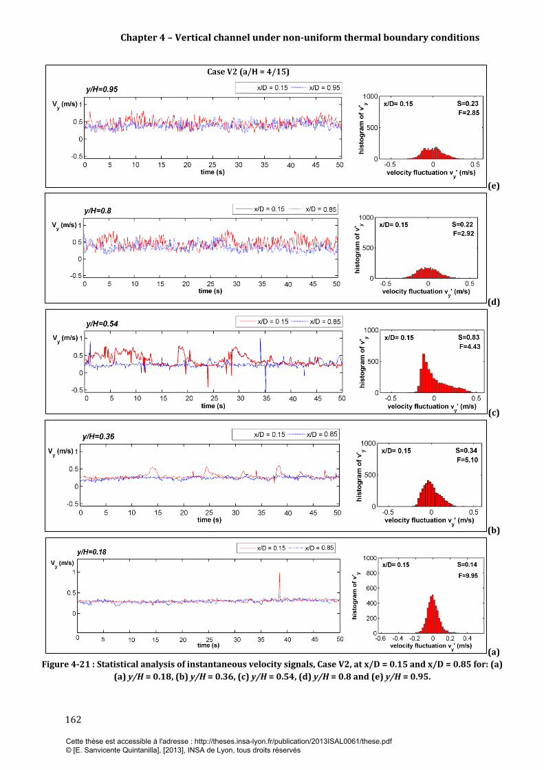
Chapter 4 – Vertical channel under non-uniform thermal boundary conditions
162
(e)
(d)
(c)
(b)
(a)
Figure 4-21 : Statistical analysis of instantaneous velocity signals, Case V2, at x/D = 0.15 and x/D = 0.85 for: (a)
(a) y/H = 0.18, (b) y/H = 0.36, (c) y/H = 0.54, (d) y/H = 0.8 and (e) y/H = 0.95.
Cette thèse est accessible à l'adresse : http://theses.insa-lyon.fr/publication/2013ISAL0061/these.pdf © [E. Sanvicente Quintanilla], [2013], INSA de Lyon, tous droits réservés

Chapter 4 – Vertical channel under non-uniform thermal boundary conditions
163
4.4 Analysis of global characteristics
4.4.1 Induced mass flow rate estimation
The mean mass flow rates per unit width of the channel (Kg/m.s) at y/H = 0.54 are presented in
Figure 4-22 . Please note that since no temperature measurements were carried out in the flow,
the density of the air was evaluated at the mean temperature between the twall temperatures of
S1 and S2. The method to evaluate the flow rate (m3/s) is detailed in §2.3.1.
As may be observed, the mass flow rate increases as a/H tends to 1/15. In particular, for
periodically heated configurations the mass flow rate achieved is enhanced by 12% compared to
the uniformly heated condition (Case VREF). It is apparent from the analysis of the induced mass
flow rate that a differentially heated channel has benefits on the ventilation process which
simultaneously improves the heat transfer process as was demonstrated in §4.2. This resulted
increased in chimney effect is not only an important outcome in terms cooling of PV components
but also for natural ventilation of the building as was discussed in Chapter 1.
In reviewing the literature, no experimental data regading mass flow rates were found for this
type of configurations.
Figure 4-22 : Comparison of induced mass flow rate at y/H= 0.54
between Cases V1, V2 and VREF.
4.4.2 Overall heat transfer characteristics
The effect of a periodical heating distribution on the overall average Nusselt number has also
been characterized. Figure 4-25 shows the plot of the average Nusselt number versus the
modified Rayleigh number multiplied by the ratio D/a [Ra (D/a)] (see equation (32)). This
relation, used to take into account the variation of the heat source length, was found in literature
regarding non-uniform thermal boundary conditions, as detailed Incropera et al. [47] for forced
flows and Fossa et al. [163] for natural convection flows. Recall that in this study a equals to 0.1
m in Case V1 and 0.4 m in Case V2. In addition to Cases V1 and V2 (220 W/m2), two more cases
obtained for an electrical heat input of 475 W/m2 are included.
As expected, the overall channel average Nusselt number increases for periodically heated
configurations. In particular, the overall heat transfer process at the same global heat input
improves by 34% in Case V1 and by 23% in Case V2 with respect to Case VREF.
Cette thèse est accessible à l'adresse : http://theses.insa-lyon.fr/publication/2013ISAL0061/these.pdf © [E. Sanvicente Quintanilla], [2013], INSA de Lyon, tous droits réservés

Chapter 4 – Vertical channel under non-uniform thermal boundary conditions
164
Figure 4-23 : Average Nusselt number as a
function of Ra (D/a) for Cases V1 and V2.
Figure 4-24 : Average Nusselt number
estimation and experimental data for Cases V1
and V2.
On the logarithmic graph shown in Figure 4-23 experimental data is found to collapse to a single
curve. The correlation, obtained from a linear regression (least square method) is given below:
(43)
The values given by the formula above proposed (equation (43)) against the measured ones are
shown in Figure 4-24 . The uncertainty does not exceed ± 1%. However, more measurements are
needed to complete these graphs and redefine the correlation given above.
It may be of practical interest for the particular integration in double façades to obtain a global
correlation regardless the size of alternated heated zones (opaque PV modules) and non heated
zones (transparent windows). In Figure 4-25 the above presented data is reported together with
experimental measurements (solid rhombus symbols) obtained on the uniform heated vertical
configuration in the F-device (§3.5) and for Rayleigh numbers, Ra* = 3.86 x 10⁵; 9.10 x 10⁵;
1.86 x 10⁶; 3.5 x 10⁶ and 6.22 x 10⁶.
Figure 4-25 : Overall channel average Nusselt
number as a function of Ra (D/a).
Figure 4-26: Local Nusselt number estimation
of equation (44).
Cette thèse est accessible à l'adresse : http://theses.insa-lyon.fr/publication/2013ISAL0061/these.pdf © [E. Sanvicente Quintanilla], [2013], INSA de Lyon, tous droits réservés

Chapter 4 – Vertical channel under non-uniform thermal boundary conditions
165
Two different slopes, coresponding respectively to the uniform and the non-uniform heated
configurations may be identified in Figure 4-25. This is consistent with the different flow
mechanisms involved in each case as was highlighted in sections 3.4.1 and 4.3.2, which leads to
different global thermal performances.
Despite these two different trends, an attempt was made to fit all data in a single correlation
(equation (44) able to account uniform (a/H = 1) and no uniform (a/H = 1/15, 4/15) heating
conditions and in a larger range of Ra*:
(44)
This second correlation allows an estimation of with a maximum error of ±15% with
respect to measured values (Figure 4-26).
In Figure 4-25 is also reported the experimental result obtained by Fossa et al. [47] in the R-
device for Case V2 ( 200 W/m2) and an aspect ratio of D/H = 1/16. The deviation with
the present data is of 12%.
Note that data in vertical channel under uniform heated configurations will be examined in
detail and compared with more literature work in Chapter 5, where the effect of the inclination
angle of the channel is studied.
Cette thèse est accessible à l'adresse : http://theses.insa-lyon.fr/publication/2013ISAL0061/these.pdf © [E. Sanvicente Quintanilla], [2013], INSA de Lyon, tous droits réservés
Chapter 4 – Vertical channel under non-uniform thermal boundary conditions
166
4.5 CONCLUSIONS
This chapter was dedicated to investigate the effect of the non-uniformity of the wall heat flux
distribution on the natural convection flow and heat transfer within an open-ended vertical
channel. Experiments were conducted for two different periodicities of heated/unheated zones,
a/H = 1/15 and 4/15, and two levels of heat inputs, q= 220 W/m2 and 420 W/m2. In all cases
D/H was 1/15.
It was shown that the introduction of alternating heated and unheated zones leads
simultaneously to the enhancement of convective heat transfer at the heated source level (lower
wall temperature) and to an increase of the chimney effect (induced mass flow rate). In
particular, for q = 220 W/m2, we have seen in Cases V1 and V2, a typical reduction of 10°C and
an increase of mass flow rate of 12 % with respect to the uniformly heated wall (Case VREF)
which remains weak. These results indicate that the maximum temperature achieved at the
walls is strongly related to the spatial distribution of the wall heat flux in the walls. Thereby, in
practical situations the choice of PV modules distribution on the façade appears to be of great
importance as regards the thermal behavior of the wall. As discussed on Chapter 1, this is an
important outcome since both the efficiency and lifetime of the PV modules are seriously
affected when the temperature of the cells are not regulated. On the other hand, even if the mass
flow rate, which is induced in the channel for the same heat injection configuration (uniform,
non uniform) is governed by the global heat flux that is injected in the channel, it is found that is
also depending of wall heat flux spatial distribution.
Two empirical correlations are reported from the present data to predict the heat transfer
efficiency. One for non-uniform cases with estimations within ±1% and the second one with
estimations within ±15% including the data of the vertical uniform heated case. They are of
interest from an application point of view since they apply from typical opaque PV façades to
semi-transparent PV façades.
The detailed examination of the flow fields has revealed at y/H = 0.54 the appearance of many
unsteady structures with high velocities. The fluid motion appeared disturbed because of the
flow passing heated and unheated zones. This strong ‘disruption’ mechanism of the flow led to
enhanced mixing and increased Reynolds stresses over most of the width of the channel. The
rate of turbulent production increased gradually with the height of the channel, especially after
y/H = 0.54. Towards the outlet section of the channel turbulent mixing is enhanced and the flow
tends to homogenize.
The enhancement of the mixing of the flow might be an important factor in increasing the
temperature of the air within the channel. This led us to consider the possibility that useful heat
may be generated and used for heating or cooling purposes. However, in order to estimate the
heat recovery options, local measurements of the temperature of the air in the cavity need to be
carried out at different heights.
Cette thèse est accessible à l'adresse : http://theses.insa-lyon.fr/publication/2013ISAL0061/these.pdf © [E. Sanvicente Quintanilla], [2013], INSA de Lyon, tous droits réservés

167
Cette thèse est accessible à l'adresse : http://theses.insa-lyon.fr/publication/2013ISAL0061/these.pdf © [E. Sanvicente Quintanilla], [2013], INSA de Lyon, tous droits réservés

168
Cette thèse est accessible à l'adresse : http://theses.insa-lyon.fr/publication/2013ISAL0061/these.pdf © [E. Sanvicente Quintanilla], [2013], INSA de Lyon, tous droits réservés
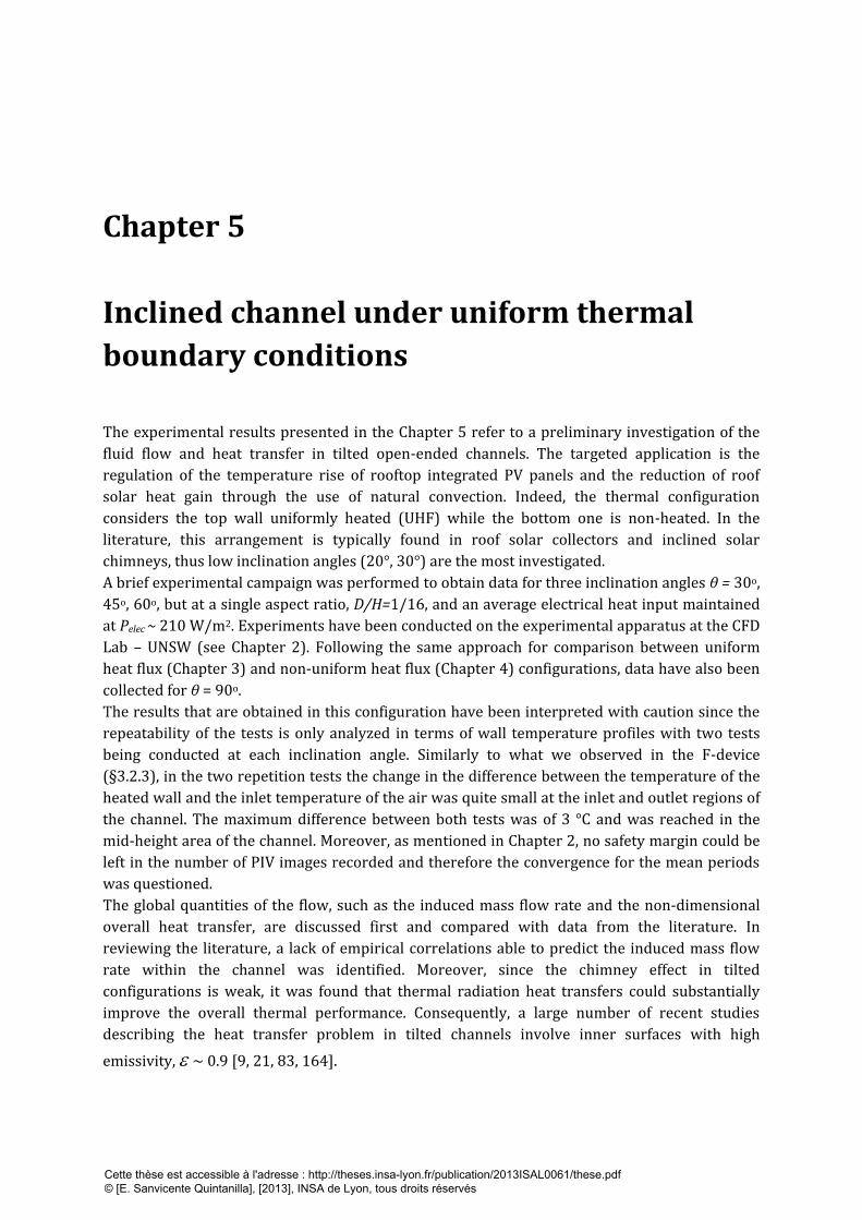
Chapter 5 Inclined channel under uniform thermal
boundary conditions
Chapter 5
Inclined channel under uniform thermal
boundary conditions
The experimental results presented in the Chapter 5 refer to a preliminary investigation of the
fluid flow and heat transfer in tilted open-ended channels. The targeted application is the
regulation of the temperature rise of rooftop integrated PV panels and the reduction of roof
solar heat gain through the use of natural convection. Indeed, the thermal configuration
considers the top wall uniformly heated (UHF) while the bottom one is non-heated. In the
literature, this arrangement is typically found in roof solar collectors and inclined solar
chimneys, thus low inclination angles (20°, 30°) are the most investigated.
A brief experimental campaign was performed to obtain data for three inclination angles θ = 30o,
45o, 60o, but at a single aspect ratio, D/H=1/16, and an average electrical heat input maintained
at Pelec ~ 210 W/m2. Experiments have been conducted on the experimental apparatus at the CFD
Lab – UNSW (see Chapter 2). Following the same approach for comparison between uniform
heat flux (Chapter 3) and non-uniform heat flux (Chapter 4) configurations, data have also been
collected for θ = 90o.
The results that are obtained in this configuration have been interpreted with caution since the
repeatability of the tests is only analyzed in terms of wall temperature profiles with two tests
being conducted at each inclination angle. Similarly to what we observed in the F-device
(§3.2.3), in the two repetition tests the change in the difference between the temperature of the
heated wall and the inlet temperature of the air was quite small at the inlet and outlet regions of
the channel. The maximum difference between both tests was of 3 °C and was reached in the
mid-height area of the channel. Moreover, as mentioned in Chapter 2, no safety margin could be
left in the number of PIV images recorded and therefore the convergence for the mean periods
was questioned.
The global quantities of the flow, such as the induced mass flow rate and the non-dimensional
overall heat transfer, are discussed first and compared with data from the literature. In
reviewing the literature, a lack of empirical correlations able to predict the induced mass flow
rate within the channel was identified. Moreover, since the chimney effect in tilted
configurations is weak, it was found that thermal radiation heat transfers could substantially
improve the overall thermal performance. Consequently, a large number of recent studies
describing the heat transfer problem in tilted channels involve inner surfaces with high
emissivity, ~ 0.9 [9, 21, 83, 164].
Cette thèse est accessible à l'adresse : http://theses.insa-lyon.fr/publication/2013ISAL0061/these.pdf © [E. Sanvicente Quintanilla], [2013], INSA de Lyon, tous droits réservés
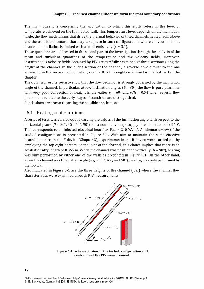
Chapter 5 – Inclined channel under uniform thermal boundary conditions
170
The main questions concerning the application to which this study refers is the level of
temperature achieved on the top heated wall. This temperature level depends on the inclination
angle, the flow mechanisms that drive the thermal behavior of tilted channels heated from above
and the transition scenario that may take place in such configurations where convection is not
favored and radiation is limited with a small emissivity (ε ~ 0.1).
These questions are addressed in the second part of the investigation through the analysis of the
mean and turbulent quantities of the temperature and the velocity fields. Moreover,
instantaneous velocity fields obtained by PIV are carefully examined at three sections along the
height of the channel. In the outlet section of the channel, a reverse flow, similar to the one
appearing in the vertical configuration, occurs. It is thoroughly examined in the last part of the
chapter.
The obtained results seem to show that the flow behavior is strongly governed by the inclination
angle of the channel. In particular, at low inclination angles (θ = 30o) the flow is purely laminar
with very poor convection of heat. It is thereafter θ = 60o and y/H = 0.54 when several flow
phenomena related to the early stages of transition are distinguished.
Conclusions are drawn regarding the possible applications.
5.1 Heating configurations
A series of tests was carried out by varying the values of the inclination angle with respect to the
horizontal plane (θ = 30°, 45°, 60°, 90°) for a nominal voltage supply of each heater of 23.6 V.
This corresponds to an injected electrical heat flux Pelec = 210 W/m2. A schematic view of the
studied configurations is presented in Figure 5-1. With aim to maintain the same effective
heated length as in the F-device (Chapter 3), experiments in the R-device were carried out by
employing the top eight heaters. At the inlet of the channel, this choice implies that there is an
adiabatic entry length of 0.365 m. When the channel was positioned vertically (θ = 90°), heating
was only performed by either one of the walls as presented in Figure 5-1. On the other hand,
when the channel was tilted at an angle (e.g. = 30°, 45°, and 60°), heating was only performed by
the top wall.
Also indicated in Figure 5-1 are the three heights of the channel (y/H) where the channel flow
characteristics were examined through PIV measurements.
Figure 5-1: Schematic view of the tested configuration and
centreline of the PIV measurement.
Cette thèse est accessible à l'adresse : http://theses.insa-lyon.fr/publication/2013ISAL0061/these.pdf © [E. Sanvicente Quintanilla], [2013], INSA de Lyon, tous droits réservés
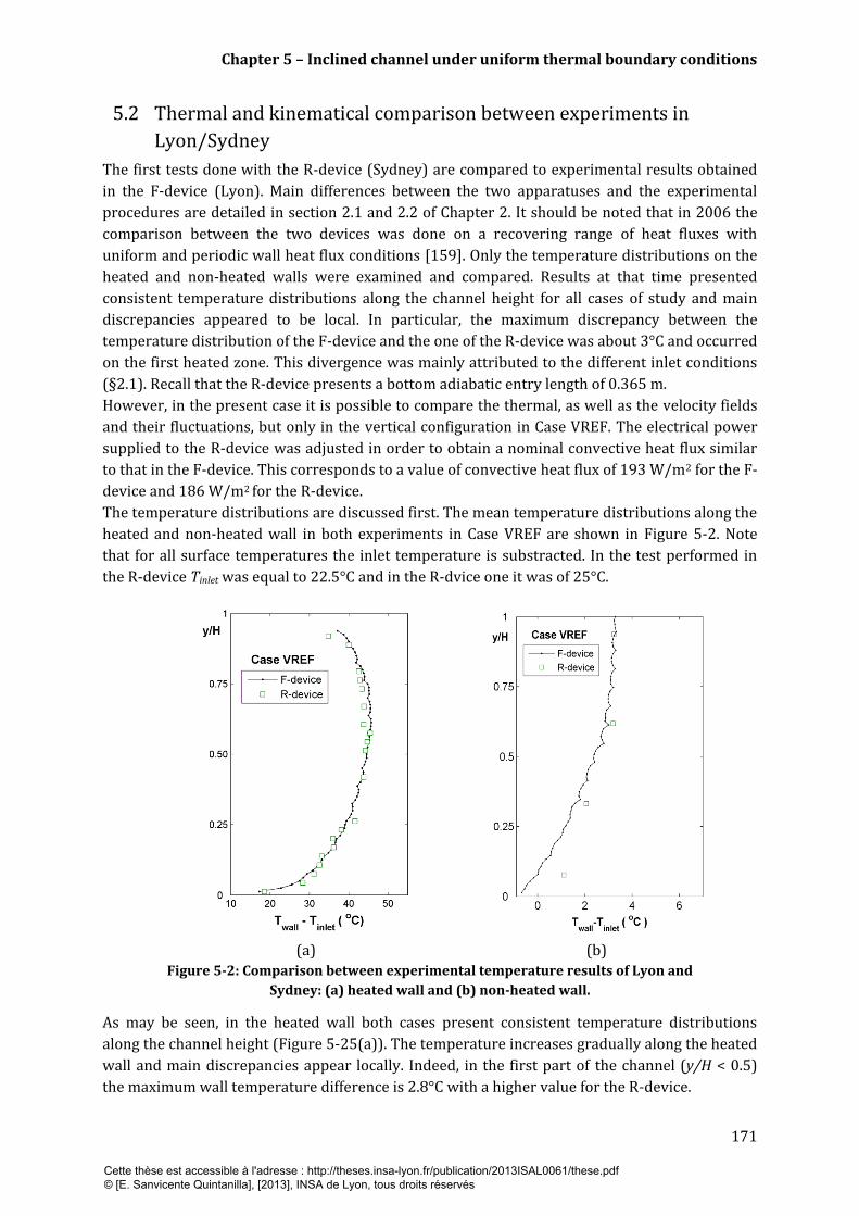
Chapter 5 – Inclined channel under uniform thermal boundary conditions
171
5.2 Thermal and kinematical comparison between experiments in
Lyon/Sydney
The first tests done with the R-device (Sydney) are compared to experimental results obtained
in the F-device (Lyon). Main differences between the two apparatuses and the experimental
procedures are detailed in section 2.1 and 2.2 of Chapter 2. It should be noted that in 2006 the
comparison between the two devices was done on a recovering range of heat fluxes with
uniform and periodic wall heat flux conditions [159]. Only the temperature distributions on the
heated and non-heated walls were examined and compared. Results at that time presented
consistent temperature distributions along the channel height for all cases of study and main
discrepancies appeared to be local. In particular, the maximum discrepancy between the
temperature distribution of the F-device and the one of the R-device was about 3°C and occurred
on the first heated zone. This divergence was mainly attributed to the different inlet conditions
(§2.1). Recall that the R-device presents a bottom adiabatic entry length of 0.365 m.
However, in the present case it is possible to compare the thermal, as well as the velocity fields
and their fluctuations, but only in the vertical configuration in Case VREF. The electrical power
supplied to the R-device was adjusted in order to obtain a nominal convective heat flux similar
to that in the F-device. This corresponds to a value of convective heat flux of 193 W/m2 for the F-
device and 186 W/m2 for the R-device.
The temperature distributions are discussed first. The mean temperature distributions along the
heated and non-heated wall in both experiments in Case VREF are shown in Figure 5-2. Note
that for all surface temperatures the inlet temperature is substracted. In the test performed in
the R-device Tinlet was equal to 22.5°C and in the R-dvice one it was of 25°C.
(a)
(b)
Figure 5-2: Comparison between experimental temperature results of Lyon and
Sydney: (a) heated wall and (b) non-heated wall.
As may be seen, in the heated wall both cases present consistent temperature distributions
along the channel height (Figure 5-25(a)). The temperature increases gradually along the heated
wall and main discrepancies appear locally. Indeed, in the first part of the channel (y/H < 0.5)
the maximum wall temperature difference is 2.8°C with a higher value for the R-device.
Cette thèse est accessible à l'adresse : http://theses.insa-lyon.fr/publication/2013ISAL0061/these.pdf © [E. Sanvicente Quintanilla], [2013], INSA de Lyon, tous droits réservés

Chapter 5 – Inclined channel under uniform thermal boundary conditions
172
Above y/H = 0.5, the wall temperatures measured in the R-device become lower than
temperatures obtained with the F-device with a maximum difference of 4°C. These discrepancies
may be explained by experimental differences in the inlet-outlet and ambient conditions, the
different constitution of the walls and obviously linked to the difference between injected power
which is around 6W/m2 (section 2.1). Mean conduction losses along the height of the channel
are estimated to 7.4% and 5.1% of the total heat input in respectively, the F-device and the R-
device. On the other hand, mean radiation transfers are estimated to 7.6% and 8.3% of the total
heat input in respectively, the F-device and the R-device.
The temperature distribution of the non-heated wall (Figure 5-25(b)) seems to be more
sensitive to exchanges and disturbances with the external environment than the heated one.
With the current available temperature measurements, the maximum wall temperature
difference is 1.2°C at y/H = 0.08. The adiabatic entry in the R-device may be responsible of the
higher level of temperature in its non-heated wall since radiation losses to the environment are
reduced.
Figure 5-3, Figure 5-4 and Figure 5-5 show the mean profiles of the vertical velocity component
and the streamwise fluctuation intensities between both tests at y/H = 0.18, 0.36 and 0.95,
respectively. As may be seen, the mean velocity profiles are pretty close from each other in both
sections. Maximum discrepancies appear principally close to the heated wall where the velocity
gradients are the strongest (18% at y/H = 0.18 and 13% at y/H = 0.95).
In the inlet section y/H = 0.18, for both tests, the turbulent intensity is not negligible across the
channel width and the intensity levels are consistent (20 % in 0.1 < x/D <0.9). Nonetheless, a
localized peak is observed in the R-device close to the heated wall whereas in the F-device it is
localized close to the non-heated wall. It is surprising that the level of turbulent intensities is
similar for both experiments since in the R-device we would expect that the adiabatic inlet
section (about 40 cm height) should dampen the external disturbances and canalize the air flow
with regular streamlines.
The mean discrepancy of turbulent intensities at y/H = 0.36 is approximately 35 % with larger
values in the R-devices. Spatial irregularities due to the gluing of foils on bakelite wall may be
sites generating perturbations amplified all along the channel height. However, as shown in
Chapter 3 levels of fluctuations depend strongly on tests, presenting a non-reproducible
character.
At y/H = 0.95, the discrepancy of turbulent intensities is approximately 40 % with larger values
in the F-device. The radiation screens placed at the outlet section of R-device may dampen the
external disturbances with respect to the F-device.
However, as mentioned before, no conclusions can be extracted since only one test was
conducted in the R-device.
Cette thèse est accessible à l'adresse : http://theses.insa-lyon.fr/publication/2013ISAL0061/these.pdf © [E. Sanvicente Quintanilla], [2013], INSA de Lyon, tous droits réservés
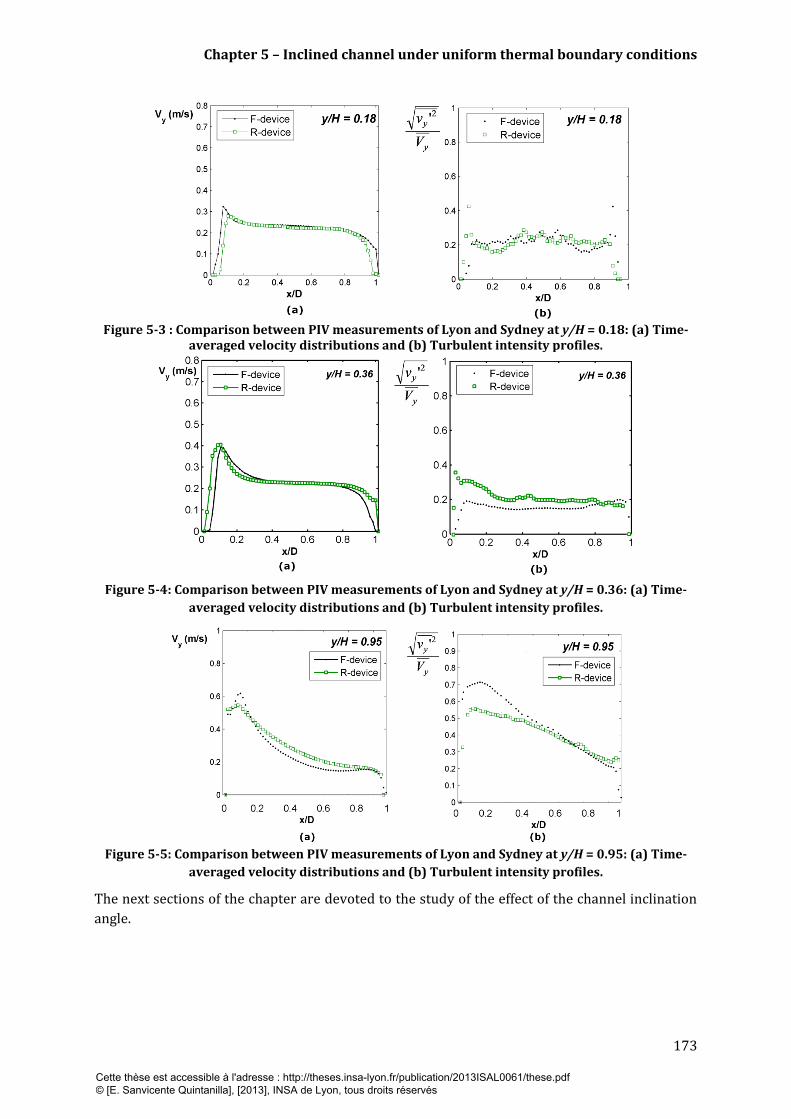
Chapter 5 – Inclined channel under uniform thermal boundary conditions
173
Figure 5-3 : Comparison between PIV measurements of Lyon and Sydney at y/H = 0.18: (a) Time-
averaged velocity distributions and (b) Turbulent intensity profiles.
Figure 5-4: Comparison between PIV measurements of Lyon and Sydney at y/H = 0.36: (a) Time-
averaged velocity distributions and (b) Turbulent intensity profiles.
Figure 5-5: Comparison between PIV measurements of Lyon and Sydney at y/H = 0.95: (a) Time-
averaged velocity distributions and (b) Turbulent intensity profiles.
The next sections of the chapter are devoted to the study of the effect of the channel inclination
angle.
Cette thèse est accessible à l'adresse : http://theses.insa-lyon.fr/publication/2013ISAL0061/these.pdf © [E. Sanvicente Quintanilla], [2013], INSA de Lyon, tous droits réservés

Chapter 5 – Inclined channel under uniform thermal boundary conditions
174
5.3 Thermal boundary conditions
The electrical power injected at the wall was quasi-uniform from the bottom to the top with an
absolute difference of 9W/m2 corresponding to a variation of ± 2% around the mean power rate
of 210 W/m2 (see Pelec evolution in Figure 5-6). These discrepancies were attributed to the
variation of the heater foil resistance value (§2.1.2).
The share of the mean wall conductive losses in the x-direction (see Figure 5-6) increases as the
channel is more inclined towards the horizontal plane: from 7.4% of the wall heat transfer for
Case VREF to 10.2% for Case i30. Likewise, the radiation flux increases from 7.6% to 12% as the
inclination angle decreases due to the increase of the temperature of the foil. Moreover, it is in
the exit section of the channel that both radiation heat transfers with the environment and
conduction losses to the polystyrene insulation are the strongest. This has been already noted by
other authors such as Webb and Hill [67] and Manca et al. [152] for vertical channels, and
Mittelman et al. [9] for tilted ones. The convective heat flux is less important as the inclination
angle decreases, with a maximum share of 85% for the vertical case (Case VREF) and a minimum
share of about 78% for Case i30 (see Table 5-1). The maximum deviation of the convective flux
along the height of the channel is about 1.1%.
Figure 5-6 : Evolution of the electrical flux and distribution of heat fluxes in the upward direction.
(°C)
VREF 22.5 85 % 8% 7 %
i60 19.3 81% 11 % 8 %
i45 19.4 79 % 12 % 9%
i30 19.5 78 % 12 % 10 %
Table 5-1: Summary of heat fluxes and average inlet temperature for all cases of study.
Cette thèse est accessible à l'adresse : http://theses.insa-lyon.fr/publication/2013ISAL0061/these.pdf © [E. Sanvicente Quintanilla], [2013], INSA de Lyon, tous droits réservés
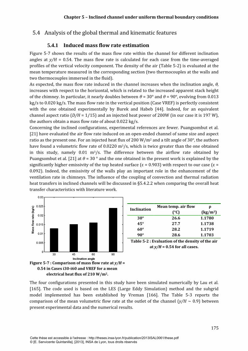
Chapter 5 – Inclined channel under uniform thermal boundary conditions
175
5.4 Analysis of the global thermal and kinematic features
5.4.1 Induced mass flow rate estimation
Figure 5-7 shows the results of the mass flow rate within the channel for different inclination
angles at y/H = 0.54. The mass flow rate is calculated for each case from the time-averaged
profiles of the vertical velocity component. The density of the air (Table 5-2) is evaluated at the
mean temperature measured in the corresponding section (two thermocouples at the walls and
two thermocouples immersed in the fluid).
As expected, the mass flow rate induced in the channel increases when the inclination angle, θ,
increases with respect to the horizontal, which is related to the increased apparent stack height
of the chimney. In particular, it nearly doubles between θ = 30° and θ = 90°, evolving from 0.013
kg/s to 0.020 kg/s. The mass flow rate in the vertical position (Case VREF) is perfectly consistent
with the one obtained experimentally by Burek and Habeb [44]. Indeed, for an equivalent
channel aspect ratio (D/H = 1/15) and an injected heat power of 200W (in our case it is 197 W),
the authors obtain a mass flow rate of about 0.022 kg/s.
Concerning the inclined configurations, experimental references are fewer. Puangsombut et al.
[21] have evaluated the air flow rate induced on an open-ended channel of same size and aspect
ratio as the present one. For an injected heat flux of 200 W/m2 and a tilt angle of 30°, the authors
have found a volumetric flow rate of 0.0220 m3/s, which is twice greater than the one obtained
in this study, namely 0.01 m3/s. The difference between the airflow rate obtained by
Puangsombut et al. [21] at θ = 30 ° and the one obtained in the present work is explained by the
significantly higher emissivity of the top heated surface (ε = 0.903) with respect to our case (ε =
0.092). Indeed, the emissivity of the walls play an important role in the enhancement of the
ventilation rate in chimneys. The influence of the coupling of convection and thermal radiation
heat transfers in inclined channels will be discussed in §5.4.2.2 when comparing the overall heat
transfer characteristics with literature work.
Table 5-2 : Evaluation of the density of the air
at y/H = 0.54 for all cases.
Inclination Mean temp. air flow
(°C)
ρ
(kg/m3)
30° 26.6 1.1780
45° 27.7 1.1738
60° 28.2 1.1719
90° 28.6 1.1703
Figure 5-7 : Comparison of mass flow rate at y/H =
0.54 in Cases i30-i60 and VREF for a mean
electrical heat flux of 210 W/m2.
The four configurations presented in this study have been simulated numerically by Lau et al.
[165]. The code used is based on the LES (Large Eddy Simulation) method and the subgrid
model implemented has been established by Vreman [166]. The Table 5-3 reports the
comparison of the mean volumetric flow rate at the outlet of the channel (y/H ~ 0.9) between
present experimental data and the numerical results.
Cette thèse est accessible à l'adresse : http://theses.insa-lyon.fr/publication/2013ISAL0061/these.pdf © [E. Sanvicente Quintanilla], [2013], INSA de Lyon, tous droits réservés
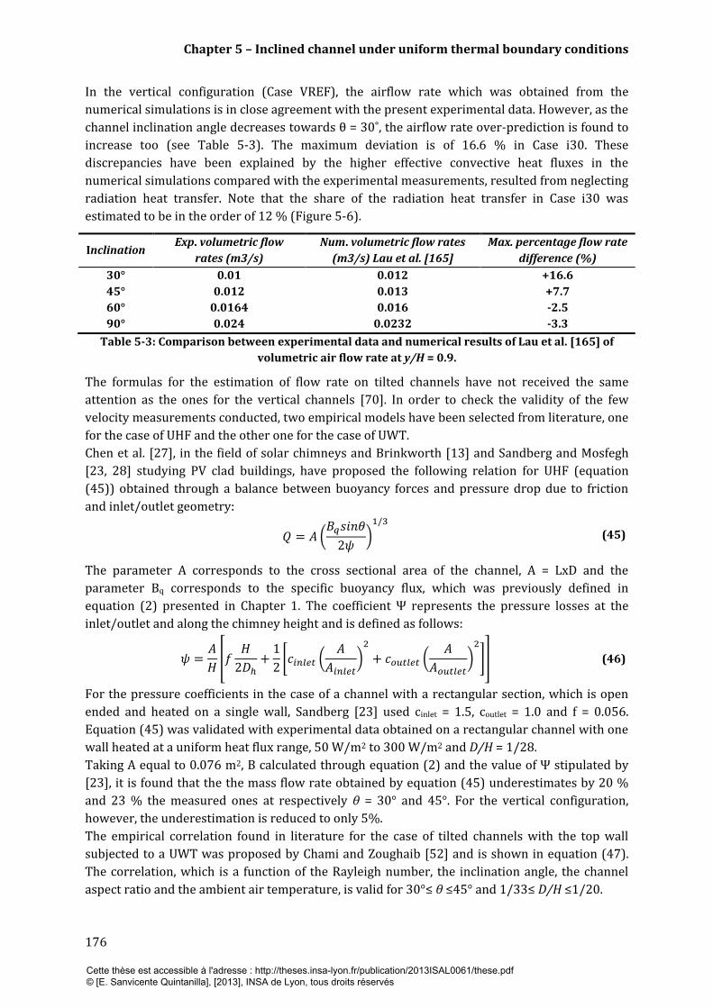
Chapter 5 – Inclined channel under uniform thermal boundary conditions
176
In the vertical configuration (Case VREF), the airflow rate which was obtained from the
numerical simulations is in close agreement with the present experimental data. However, as the
channel inclination angle decreases towards θ = 30˚, the airflow rate over-prediction is found to
increase too (see Table 5-3). The maximum deviation is of 16.6 % in Case i30. These
discrepancies have been explained by the higher effective convective heat fluxes in the
numerical simulations compared with the experimental measurements, resulted from neglecting
radiation heat transfer. Note that the share of the radiation heat transfer in Case i30 was
estimated to be in the order of 12 % (Figure 5-6).
Inclination Exp. volumetric flow
rates (m3/s)
Num. volumetric flow rates
(m3/s) Lau et al. [165]
Max. percentage flow rate
difference (%)
30° 0.01 0.012 +16.6
45° 0.012 0.013 +7.7
60° 0.0164 0.016 -2.5
90° 0.024 0.0232 -3.3
Table 5-3: Comparison between experimental data and numerical results of Lau et al. [165] of
volumetric air flow rate at y/H = 0.9.
The formulas for the estimation of flow rate on tilted channels have not received the same
attention as the ones for the vertical channels [70]. In order to check the validity of the few
velocity measurements conducted, two empirical models have been selected from literature, one
for the case of UHF and the other one for the case of UWT.
Chen et al. [27], in the field of solar chimneys and Brinkworth [13] and Sandberg and Mosfegh
[23, 28] studying PV clad buildings, have proposed the following relation for UHF (equation
(45)) obtained through a balance between buoyancy forces and pressure drop due to friction
and inlet/outlet geometry:
(45)
The parameter A corresponds to the cross sectional area of the channel, A = LxD and the
parameter Bq corresponds to the specific buoyancy flux, which was previously defined in
equation (2) presented in Chapter 1. The coefficient Ψ represents the pressure losses at the
inlet/outlet and along the chimney height and is defined as follows:
(46)
For the pressure coefficients in the case of a channel with a rectangular section, which is open
ended and heated on a single wall, Sandberg [23] used cinlet = 1.5, coutlet = 1.0 and f = 0.056.
Equation (45) was validated with experimental data obtained on a rectangular channel with one
wall heated at a uniform heat flux range, 50 W/m2 to 300 W/m2 and D/H = 1/28.
Taking A equal to 0.076 m2, B calculated through equation (2) and the value of Ψ stipulated by
[23], it is found that the the mass flow rate obtained by equation (45) underestimates by 20 %
and 23 % the measured ones at respectively θ = 30° and 45°. For the vertical configuration,
however, the underestimation is reduced to only 5%.
The empirical correlation found in literature for the case of tilted channels with the top wall
subjected to a UWT was proposed by Chami and Zoughaib [52] and is shown in equation (47).
The correlation, which is a function of the Rayleigh number, the inclination angle, the channel
aspect ratio and the ambient air temperature, is valid for 30°≤ θ ≤45° and 1/33≤ D/H ≤1/20.
Cette thèse est accessible à l'adresse : http://theses.insa-lyon.fr/publication/2013ISAL0061/these.pdf © [E. Sanvicente Quintanilla], [2013], INSA de Lyon, tous droits réservés
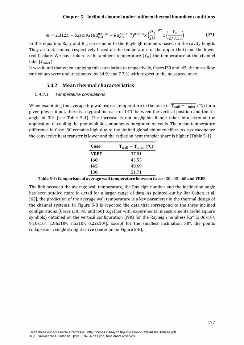
Chapter 5 – Inclined channel under uniform thermal boundary conditions
177
(47)
In this equation, RaH,h and RH,c correspond to the Rayleigh numbers based on the cavity length.
They are determined respectively based on the temperature of the upper (hot) and the lower
(cold) plate. We have taken as the ambient temperature ( ) the temperature at the channel
inlet ( .
It was found that when applying this correlation to respectively, Cases i30 and i45, the mass flow
rate values were underestimated by 34 % and 7.7 % with respect to the measured ones.
5.4.2 Mean thermal characteristics
5.4.2.1 Temperature correlations
When examining the average top wall excess temperature in the form of for a
given power input, there is a typical increase of 14°C between the vertical position and the tilt
angle of 30° (see Table 5-4). The increase is not negligible if one takes into account the
application of cooling the photovoltaic components integrated on roofs. The mean temperature
difference in Case i30 remains high due to the limited global chimney effect. As a consequence
the convective heat transfer is lower and the radiation heat transfer share is higher (Table 5-1).
VREF 37.81
i60 43.55
i45 48.69
i30 51.71
Table 5-4: Comparison of average wall temperature between Cases i30, i45, i60 and VREF.
The link between the average wall temperature, the Rayleigh number and the inclination angle
has been studied more in detail for a larger range of data. As pointed out by Bar-Cohen et al.
[62], the prediction of the average wall temperature is a key parameter in the thermal design of
the channel systems. In Figure 5-8 is reported the data that correspond to the three inclined
configurations (Cases i30, i45 and i60) together with experimental measurements (solid square
symbols) obtained on the vertical configuration (i90) for the Rayleigh numbers Ra* [3.86x10⁵,
9.10x10⁵, 1.86x10⁶, 3.5x10⁶, 6.22x10⁶]. Except for the smallest inclination 30°, the points
collapse on a single straight curve (see zoom in Figure 5-8).
Cette thèse est accessible à l'adresse : http://theses.insa-lyon.fr/publication/2013ISAL0061/these.pdf © [E. Sanvicente Quintanilla], [2013], INSA de Lyon, tous droits réservés

Chapter 5 – Inclined channel under uniform thermal boundary conditions
178
Figure 5-8 : Evolution of the average wall
temperature Vs (Ra*sin ) for 3.86 x 10⁵ < Ra*sin θ < 6.2 x 10⁶.
Figure 5-9 : Estimation of relation (48) and experimental data for
3.86x10⁵ < Ra*sin θ < 6.22 x 10⁶.
The data which corresponds to an inclination angle range, 45°≤ θ ≤90°, may be fitted to a single
correlation (equation (48)) able to predict the mean temperature of the wall within an
uncertainty of ±10% (Figure 5-9):
(48)
In addition, Tinlet appears to be explicit in the correlation, which leads to estimate the level of
temperature achieved at the top wall in different seasons in the year.
5.4.2.2 Heat transfer correlations
The link between the inclination angle and the local convective heat transfer along the height of
the top heated wall may be characterized through the local Nusselt number distributions.
The local Nusselt number, Nuy, as a function of the local Rayleigh number, Ray, for all four cases
is presented on Figure 5-10. As can be seen, the local Nusselt number distributions for all tilted
configurations overlap in the lowermost part of the channel y/H < 0.3 since the convective
injected heat flux density (W/m2) is the same for all cases. Downstream, the effect of the
inclination angle becomes more evident, resulting in a maximum deviation of the local Nusselt
numbers of nearly 29% between Case i30 and Case VREF (θ = 90°). The highest convective
transfers are achieved when the channel is vertical. As expected, the results obtained for Case
VREF are in agreement with the experimental results reported by Fossa et al [47] in 2006 in the
same experimental set up (Figure 5-10).
Cette thèse est accessible à l'adresse : http://theses.insa-lyon.fr/publication/2013ISAL0061/these.pdf © [E. Sanvicente Quintanilla], [2013], INSA de Lyon, tous droits réservés
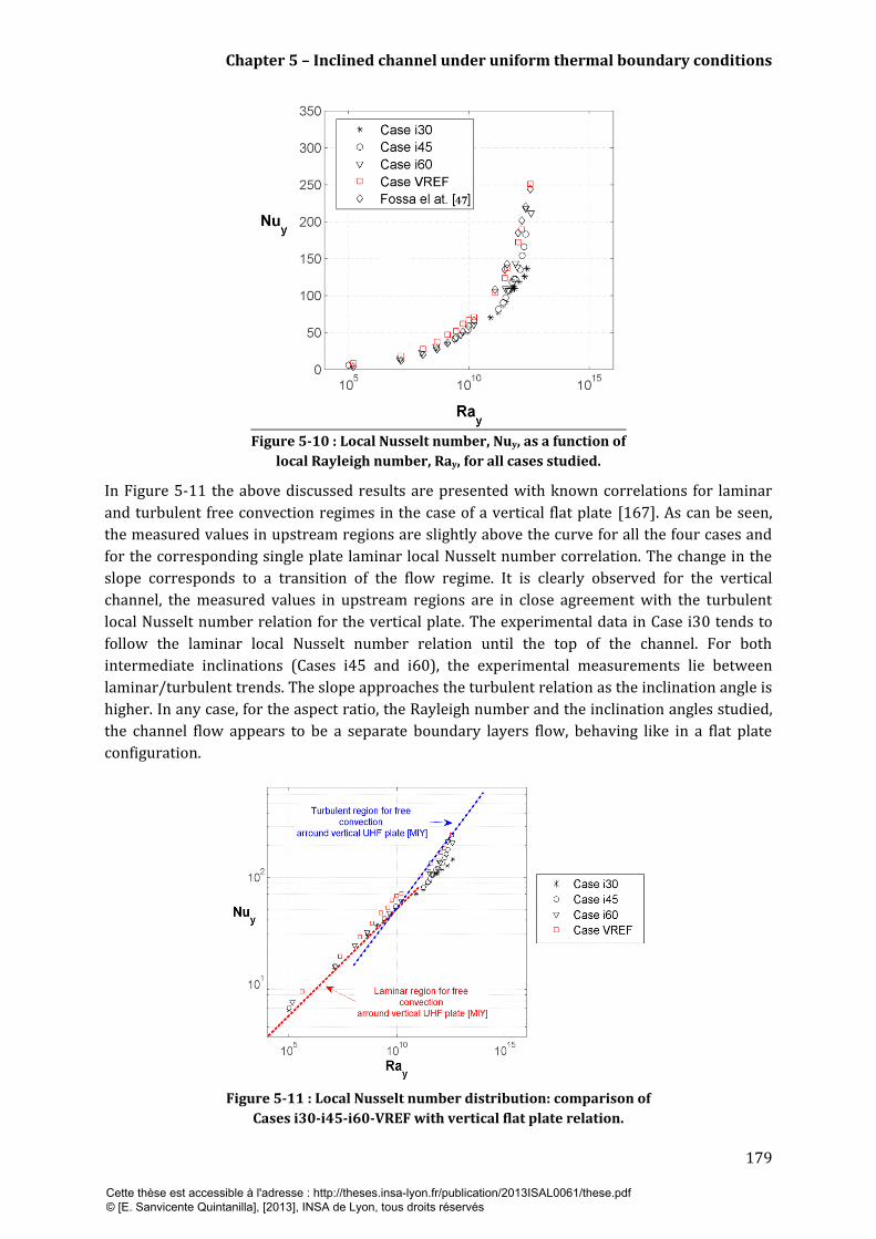
Chapter 5 – Inclined channel under uniform thermal boundary conditions
179
Figure 5-10 : Local Nusselt number, Nuy, as a function of
local Rayleigh number, Ray, for all cases studied.
In Figure 5-11 the above discussed results are presented with known correlations for laminar
and turbulent free convection regimes in the case of a vertical flat plate [167]. As can be seen,
the measured values in upstream regions are slightly above the curve for all the four cases and
for the corresponding single plate laminar local Nusselt number correlation. The change in the
slope corresponds to a transition of the flow regime. It is clearly observed for the vertical
channel, the measured values in upstream regions are in close agreement with the turbulent
local Nusselt number relation for the vertical plate. The experimental data in Case i30 tends to
follow the laminar local Nusselt number relation until the top of the channel. For both
intermediate inclinations (Cases i45 and i60), the experimental measurements lie between
laminar/turbulent trends. The slope approaches the turbulent relation as the inclination angle is
higher. In any case, for the aspect ratio, the Rayleigh number and the inclination angles studied,
the channel flow appears to be a separate boundary layers flow, behaving like in a flat plate
configuration.
Figure 5-11 : Local Nusselt number distribution: comparison of
Cases i30-i45-i60-VREF with vertical flat plate relation.
Cette thèse est accessible à l'adresse : http://theses.insa-lyon.fr/publication/2013ISAL0061/these.pdf © [E. Sanvicente Quintanilla], [2013], INSA de Lyon, tous droits réservés

Chapter 5 – Inclined channel under uniform thermal boundary conditions
180
Figure 5-12 shows for the four cases the average Nusselt number based on the width of the
channel, , as a function of the modified Rayleigh number in the form of Ra*sin θ (see
equation (31)) . This relation, used to take into account the variation of the inclination angle on
the thermal field, was found in literature as detailed [52, 60, 115]. As expected, the average
Nusselt number increases with the inclination angle, the Rayleigh number being kept constant.
Note the low value of the average Nusselt number for the tilt angle 30° compared with other
cases.
In addition, on the logarithmic graph the experimental data are found to collapse to a single
curve (Figure 5-13). The correlation, obtained from a linear regression (least square method) is
given below:
(49)
The experimental Nusselt number obtained versus the prevision of the data fitting formula (49)
is reported in Figure 5-13. The maximum uncertainty given by (49) in the the range, 30° ≤ θ ≤
90° and 1.32 x 10⁶ < Ra*sin <3.5 x 10⁶ , does not exceed ± 3%.
Figure 5-14 provides the data which corresponds to the three inclined configurations (Cases i30,
i45 and i60) together with experimental measurements obtained on the vertical configuration
(F-device) for the Rayleigh numbers (solid square symbols named as i90) Ra* [3.86x105,
9.10x10⁵, 1.86x10⁶, 3.5x10⁶, 6.22x10⁶] (section 3.5). In Figure 5-14, these results are referred as
i90 to differentiate it from Case VREF.
Figure 5-12 : Average Nusselt number
as a
function of Rayleigh number, Ra* sin θ, for Cases i30-
i45-i60-VREF.
Figure 5-13 : Average Nusselt number estimation
and experimental data for Cases i30-i45-i60-
VREF.
Cette thèse est accessible à l'adresse : http://theses.insa-lyon.fr/publication/2013ISAL0061/these.pdf © [E. Sanvicente Quintanilla], [2013], INSA de Lyon, tous droits réservés

Chapter 5 – Inclined channel under uniform thermal boundary conditions
181
An attempt was made to fit all data with a single correlation able to take into account a larger
range of Ra*sin . The correlation is given in equation (50):
(50)
This second correlation, valid for 30° ≤ θ ≤ 90° and 3.86x10⁵ < Ra*sin < 6.22x10⁶; allows to
estimate with a maximum uncertainty of ±10% with respect to measured values (Figure
5-15).
The results obtained are compared with recent literature relations for the case of UHF in vertical
and tilted open-ended channels. The inclined configurations selected for comparison correspond
to the arrangement of top wall heated with bottom wall non-heated and the comparison is
presented in Figure 5-16 below.
As can be observed in Figure 5-16, the present experimental data is closely limited by the
empirical correlations obtained on the vertical configurations (Fossa et al. [47], Webb and Hill
[67], Roshenov et al. [168]) and the one obtained numerically by Mittelman et al. [169] for the
inclined ones on the laminar and transition flow regimes. This last quoted correlation is valid for
an inclination angle range similar to the one of our study, 30° ≤ θ ≤ 90°, but for lower values of
Rayleigh number (≤ 106). Indeed, the maximum deviation is of 8 %. Note that the numerical
values predicted by Manca and Nardini [85] on a lowest Rayleigh number range matches the
correlation of Mittelman et al. [169]. If we look closely to the present data (zoom in Figure 5-16),
the slope obtained for the relation of the present work appears to be more pronounced than the
ones reported from the literature.
Despite the low tilt angles experimentally studied by Lin and Harrison [22] and Puangsonbut et
al. [21] (see Table 5-5), the trend of the average Nusselt number of [22] indicates a factor of two
with respect to our study. These differences can be explained by the high emissivity, in their
cases, of the top and bottom surfaces of the channel which was found to enhance significantly
radiation heat transfers between both walls. It induces a heating of the bottom wall and
consequently enhances free convection in inclined channels. In particular, in the study of Lin and
Harrison [22] it was shown that for a fixed inclination angle of 18°, the top wall temperatures
dropped by about 20 °C for a variation of the wall emissivity from ε = 0.029 to ε = 0. 95.
Figure 5-14 : Average Nusselt number, as a
function of Rayleigh number, Ra* sin θ, for 3.86x
105 < Ra*sin θ < 6.22x10⁶.
Figure 5-15 : Average Nusselt number
estimation and experimental data for 3.86x10⁵
< Ra*sin θ < 6.22x10⁶.
Cette thèse est accessible à l'adresse : http://theses.insa-lyon.fr/publication/2013ISAL0061/these.pdf © [E. Sanvicente Quintanilla], [2013], INSA de Lyon, tous droits réservés
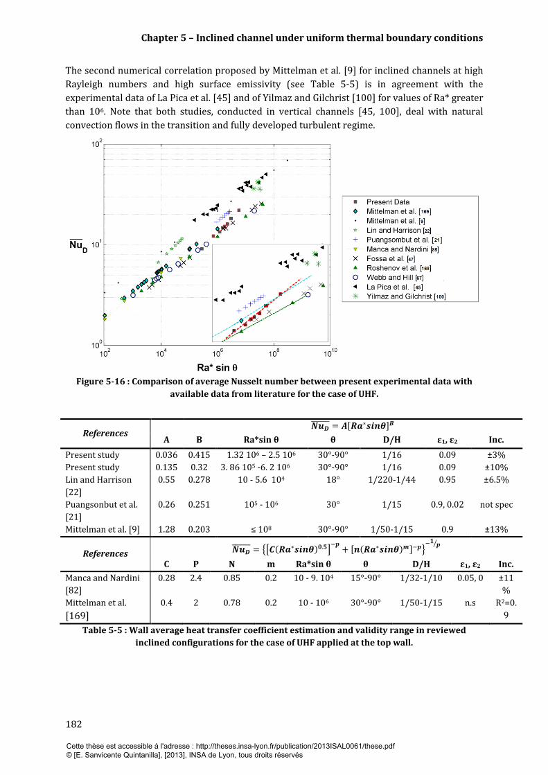
Chapter 5 – Inclined channel under uniform thermal boundary conditions
182
The second numerical correlation proposed by Mittelman et al. [9] for inclined channels at high
Rayleigh numbers and high surface emissivity (see Table 5-5) is in agreement with the
experimental data of La Pica et al. [45] and of Yilmaz and Gilchrist [100] for values of Ra* greater
than 106. Note that both studies, conducted in vertical channels [45, 100], deal with natural
convection flows in the transition and fully developed turbulent regime.
Figure 5-16 : Comparison of average Nusselt number between present experimental data with
available data from literature for the case of UHF.
References
A B Ra*sin θ θ D/H ε1, ε2 Inc.
Present study 0.036 0.415 1.32 106 – 2.5 106 30°-90° 1/16 0.09 ±3%
Present study 0.135 0.32 3. 86 105 -6. 2 106 30°-90° 1/16 0.09 ±10%
Lin and Harrison
[22]
0.55 0.278 10 - 5.6 104 18° 1/220-1/44 0.95 ±6.5%
Puangsonbut et al.
[21]
0.26 0.251 105 - 106 30° 1/15 0.9, 0.02 not spec
Mittelman et al. [9] 1.28 0.203 ≤ 108 30°-90° 1/50-1/15 0.9 ±13%
References
C P N m Ra*sin θ θ D/H ε1, ε2 Inc.
Manca and Nardini
[82]
0.28 2.4 0.85 0.2 10 - 9. 104 15°-90° 1/32-1/10 0.05, 0 ±11
%
Mittelman et al.
[169]
0.4 2 0.78 0.2 10 - 106 30°-90° 1/50-1/15 n.s R2=0.
9
Table 5-5 : Wall average heat transfer coefficient estimation and validity range in reviewed
inclined configurations for the case of UHF applied at the top wall.
Cette thèse est accessible à l'adresse : http://theses.insa-lyon.fr/publication/2013ISAL0061/these.pdf © [E. Sanvicente Quintanilla], [2013], INSA de Lyon, tous droits réservés

Chapter 5 – Inclined channel under uniform thermal boundary conditions
183
5.5 Thermal and kinematical distributions along the channel height
5.5.1 Temperature and convective coefficient profiles
The mean temperature distributions along the heated wall have similar profiles whatever the
inclination angle of the channel is (Figure 5-17(a)). In all the cases, the local temperatures
increase from the leading edge of the heated wall and decrease close to the outlet, presenting an
inflexion point. As can be seen, the local temperature differences in the form of (Twall – Tinlet) are
relatively low near the inlet region. In particular, for inclination angles between 30° and 60°, and
in view of error bars, the temperature profiles appear to overlap for y/H <0.25. Further
downstream, the different curves are distinguished and wall temperatures become increasingly
important when the tilt angle of the channel decreases from 90° to 30°. The position of the
inflection point (Figure 5-17 (a)) evolves linearly with the angle of inclination, shifting
downwards, the lower the tilt angle is. Thus, the lowest position of the inflexion point in the
channel is found for the vertical configuration. As previously mentioned in Chapter 3, the
inflexion on the temperature excess distribution close to the outlet section is, according to
literature work, due to radiative losses towards the environment [67, 152] or to transition from
laminar to turbulent flows [27, 73, 115]. It is possible that both phenomena may exist, which
results in higher heat transfer coefficients at the top of the channel.
The temperature on the non-heated wall increases very little from the bottom to the top of the
channel (Figure 5-17 (b)). The rate of increase is more pronounced the lower the inclination
angle is. In particular, ΔTinlet-outlet is 2.1°C for Case VREF and 3.5°C for Case i30.
Figure 5-17 : Evolution of the heated wall surface temperature with height for all
inclination angles: (a) heated wall and (b) nonheated wall.
Cette thèse est accessible à l'adresse : http://theses.insa-lyon.fr/publication/2013ISAL0061/these.pdf © [E. Sanvicente Quintanilla], [2013], INSA de Lyon, tous droits réservés
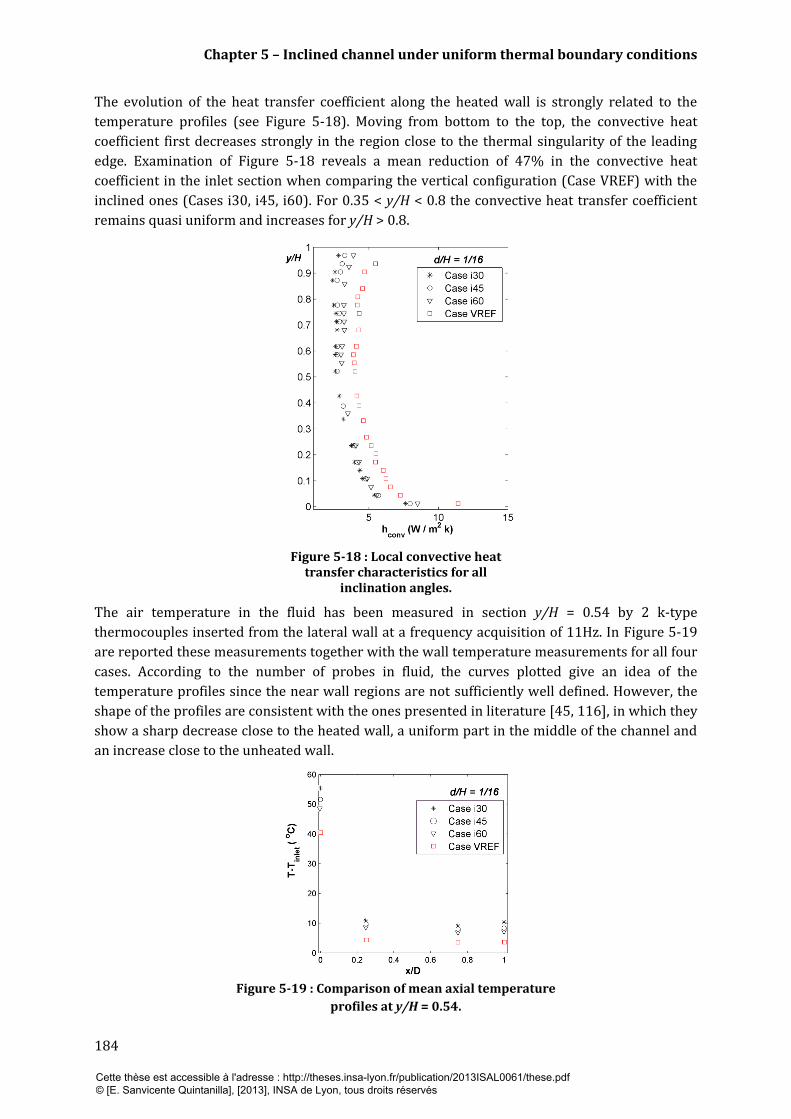
Chapter 5 – Inclined channel under uniform thermal boundary conditions
184
The evolution of the heat transfer coefficient along the heated wall is strongly related to the
temperature profiles (see Figure 5-18). Moving from bottom to the top, the convective heat
coefficient first decreases strongly in the region close to the thermal singularity of the leading
edge. Examination of Figure 5-18 reveals a mean reduction of 47% in the convective heat
coefficient in the inlet section when comparing the vertical configuration (Case VREF) with the
inclined ones (Cases i30, i45, i60). For 0.35 < y/H < 0.8 the convective heat transfer coefficient
remains quasi uniform and increases for y/H > 0.8.
Figure 5-18 : Local convective heat transfer characteristics for all
inclination angles.
The air temperature in the fluid has been measured in section y/H = 0.54 by 2 k-type
thermocouples inserted from the lateral wall at a frequency acquisition of 11Hz. In Figure 5-19
are reported these measurements together with the wall temperature measurements for all four
cases. According to the number of probes in fluid, the curves plotted give an idea of the
temperature profiles since the near wall regions are not sufficiently well defined. However, the
shape of the profiles are consistent with the ones presented in literature [45, 116], in which they
show a sharp decrease close to the heated wall, a uniform part in the middle of the channel and
an increase close to the unheated wall.
Figure 5-19 : Comparison of mean axial temperature
profiles at y/H = 0.54.
Cette thèse est accessible à l'adresse : http://theses.insa-lyon.fr/publication/2013ISAL0061/these.pdf © [E. Sanvicente Quintanilla], [2013], INSA de Lyon, tous droits réservés

Chapter 5 – Inclined channel under uniform thermal boundary conditions
185
The rise of the temperature close to the non-heated wall is due to radiation between both
surfaces. As may be seen, it is more pronounced for smaller inclination angles (see Case i30)
since temperatures of the heated walls are higher, thereby heating more the opposite wall. As
previously mentioned, mean radiative heat transfer is estimated to increase from 7 to 12 %
when the channel inclination angle θ, is decreased from 90° to 30° (Table 5-1). In particular, at
section y/H = 0.54, where the axial temperature profiles have been measured, thermal radiation
losses are estimated at 7% and 15% of the total heat input for respectively Case VREF and Case
i30. Similar observations were done by Sandberg and Moshfegh [26], Chen et al. [27] and
Mittelman et al. [9].
In the middle part of the channel ( 0.2 < x/D < 0.7) the temperature of the air is observed to
increase by a factor of 2 as the inclination angle, θ, is decreased from 90° to 30°. This indicates
that the decrease in the inclination angle involves non favorable conditions for ventilation but on
the contrary, it may be interesting if we are concerned by the heat recovered in winter or
intermediate seasons.
It should be however pointed out, that the four temperatures measurements conducted across
the width of the channel were mainly used to evaluate the density of the air for the mass flow
rate computation.
5.5.2 Vertical velocity and turbulence intensity profiles
Figure 5-20 shows the time-averaged velocity profiles for the different inclination angles at
three different heights along the channel, which are y/H = 0.18, 0.54 and 0.95. In section y/H =
0.18 the velocity profiles show a peak near the heated wall, a central zone where the velocity is
low and almost uniform and a rapid decrease to zero in the vicinity of the non-heated wall. The
velocity profiles quasi overlap for the inclinations 30°, 45° and 60°, with peak amplitudes
achieving respectively 0.21 m/s, 0.248 m/s and 0.26 m/s and a central portion corresponding to
a similar velocity 0.15 m/s. This result is consistent with the temperature profiles presented in
the previous section that are quasi superimposed in this area for these three inclination angles.
The vertical case appears distinct, with a peak amplitude of 0.28 m/s and a greater velocity in
the central region of 0.22 m/s.
In the case of the lowest tilt angle, θ = 30°, the velocity distribution slightly evolves over the
height of the channel with an increase in the maximum velocity peak limited to 18% between
sections y/H = 0.18 and y/H = 0.95 (Figure 5-20). The flow remains laminar although the
turbulent intensity becomes stronger, as will be seen in section 5.6.
On the other configurations, the amplitudes of the maximum velocity increase drastically
between sections y/H = 0.18 and y/H = 0.54. Particularly, a factor of 1.3, 2 and 2.1 was measured
respectively for Cases i45, i60 and VREF. The mean velocity in the central part of the channel
remains similar for θ = 45° and 60°. Notice the curvature of the velocity profile in the central
part for the tilt angle θ = 60°, a curvature which corresponds to a suction phenomenon for
feeding the boundary layer near the heated wall. Indeed, the peak amplitude becomes
comparable to the one obtained in the vertical configuration. This phenomenon appears to be
local at various levels in the channel. However, this observation remains to be explored in
repetition tests since only was test was conducted for each case in study.
Cette thèse est accessible à l'adresse : http://theses.insa-lyon.fr/publication/2013ISAL0061/these.pdf © [E. Sanvicente Quintanilla], [2013], INSA de Lyon, tous droits réservés
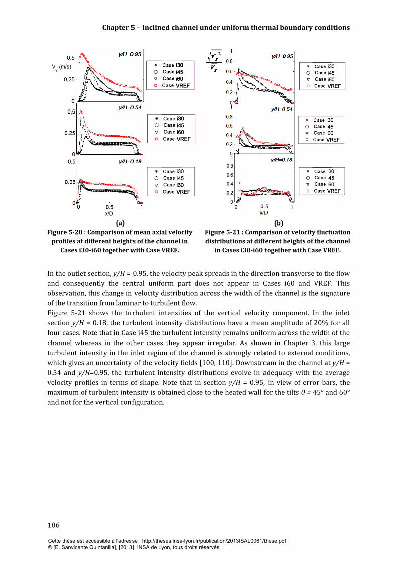
Chapter 5 – Inclined channel under uniform thermal boundary conditions
186
(a) (b)
Figure 5-20 : Comparison of mean axial velocity
profiles at different heights of the channel in
Cases i30-i60 together with Case VREF.
Figure 5-21 : Comparison of velocity fluctuation
distributions at different heights of the channel
in Cases i30-i60 together with Case VREF.
In the outlet section, y/H = 0.95, the velocity peak spreads in the direction transverse to the flow
and consequently the central uniform part does not appear in Cases i60 and VREF. This
observation, this change in velocity distribution across the width of the channel is the signature
of the transition from laminar to turbulent flow.
Figure 5-21 shows the turbulent intensities of the vertical velocity component. In the inlet
section y/H = 0.18, the turbulent intensity distributions have a mean amplitude of 20% for all
four cases. Note that in Case i45 the turbulent intensity remains uniform across the width of the
channel whereas in the other cases they appear irregular. As shown in Chapter 3, this large
turbulent intensity in the inlet region of the channel is strongly related to external conditions,
which gives an uncertainty of the velocity fields [100, 110]. Downstream in the channel at y/H =
0.54 and y/H=0.95, the turbulent intensity distributions evolve in adequacy with the average
velocity profiles in terms of shape. Note that in section y/H = 0.95, in view of error bars, the
maximum of turbulent intensity is obtained close to the heated wall for the tilts θ = 45° and 60°
and not for the vertical configuration.
Cette thèse est accessible à l'adresse : http://theses.insa-lyon.fr/publication/2013ISAL0061/these.pdf © [E. Sanvicente Quintanilla], [2013], INSA de Lyon, tous droits réservés

Chapter 5 – Inclined channel under uniform thermal boundary conditions
187
5.6 Analysis of the flow unsteadiness
The mean features of the flow behavior as well as the main structure developing in the flow for
Cases i30, i45 and i60 are illustrated in two different sections y/H = 0.54 and y/H = 0.95.
Instantaneous fields are presented through velocity vectors coloured by their magnitude (a) and
2-D vorticity isocontours superimposed on the streamlines (b).
5.6.1 Boundary layer behavior at y/H = 0.54
The flow developing in the channel for the tilt angle of 30° remained laminar during the entire
sequence recorded and some deformations of streamlines appeared to be local. As may be seen
in Figure 5-22, perturbations with small amplitude in terms of velocity and vorticity norms may
cross the channel and the streamlines may not be strictly regular from the bottom to the top of
the picture. Close to the heated wall (represented on the right hand side), the vorticity is
localized and depends on time (see Figure 5-22 (b)). These perturbations may be amplified and
contribute to a growth of fluctuations along the height of the channel but without bifurcation of
the flow behavior.
As θ increases to 45°, the flow is characterized by a narrow layer of over velocity in the near
region of the heated wall (right hand side) where vorticity appears concentrated and the
streamlines keep their regularity (Figure 5-23). The thickness of the layer close to the heated
wall remains quasi-constant and stable in both time and space due to the stronger shear stress.
For an inclination angle θ = 60° (Case i60), we observe a similar scenario likewise in the vertical
case (Case VREF) for y/H = 0.54 (section 3.4.1). In terms of illustration, Figure 5-24 (a) shows
plume-like structures of opposite vorticity signs that form in the vicinity of the heated wall (right
hand side) and shed in the mean flow. As in the vertical case, it leads to more vigorous activity
downstream in the channel as will be confirmed in the following subsection when examining the
outlet section.
Cette thèse est accessible à l'adresse : http://theses.insa-lyon.fr/publication/2013ISAL0061/these.pdf © [E. Sanvicente Quintanilla], [2013], INSA de Lyon, tous droits réservés
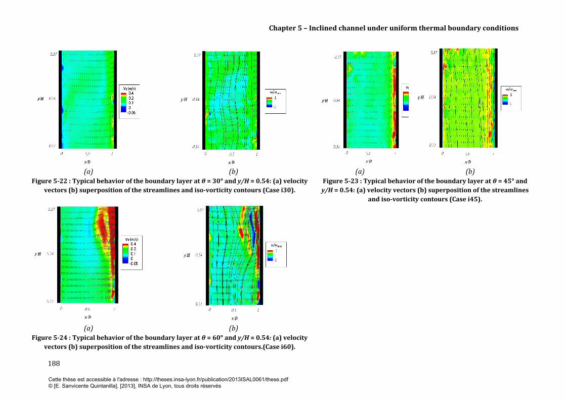
Chapter 5 – Inclined channel under uniform thermal boundary conditions
188
(a)
(b)
(a)
(b)
Figure 5-22 : Typical behavior of the boundary layer at θ = 30° and y/H = 0.54: (a) velocity
vectors (b) superposition of the streamlines and iso-vorticity contours (Case i30).
Figure 5-23 : Typical behavior of the boundary layer at θ = 45° and
y/H = 0.54: (a) velocity vectors (b) superposition of the streamlines
and iso-vorticity contours (Case i45).
(a)
(b)
Figure 5-24 : Typical behavior of the boundary layer at θ = 60° and y/H = 0.54: (a) velocity
vectors (b) superposition of the streamlines and iso-vorticity contours.(Case i60).
Cette thèse est accessible à l'adresse : http://theses.insa-lyon.fr/publication/2013ISAL0061/these.pdf © [E. Sanvicente Quintanilla], [2013], INSA de Lyon, tous droits réservés

Chapter 5 – Inclined channel under uniform thermal boundary conditions
189
5.6.2 Flow behavior at the outlet of the channel (y/H = 0.95)
The main typologies observed in the flow at the outlet of the channel (y/H = 0.95) are examined
in Figure 5-26 and Figure 5-27 for Cases i45 and i60, respectively. Note that the heated wall is
the one represented on the right hand side.
Since the flow at θ = 30° remains laminar along the entire height of the channel and no
additional information is provided, instantaneous flow fields at the outlet section in Case i30 are
not presented.
When examining the instantaneous patterns in the outlet section (y/H = 0.95) of the other cases,
one notices the intensification of the previous identified events (§5.6.1). Of particular interest is
θ = 60° (Case i60) where the change in the flow behavior is observed (see Figure 5-27). As may
be seen, for high inclination angles, unsteadiness and disturbances in the flow increase
substantially with respect to upstream locations, notably in the central part of the channel
(compare Figure 5-24 (b) and Figure 5-26 (d)). Indeed, the vortical activity localized in the
vicinity of the heated wall at y/H = 0.54 has intensified and the development, the amplification
and the ejection of the localized plume-like structures towards the center of the channel is more
and more frequent.
This stronger level of unsteadiness observed when approaching the vertical position increases
the mixing of the fluid and when combined with increased chimney effect, yields to overall lower
temperature of the heated wall as demonstrated in Figure 5-17. This is as well consistent with
the enhanced heat transfer from the wall to the fluid revealed in Figure 5-18.
Close to the non-heated wall the intermittent flow reversal is only observed for the greatest
inclinations, which are Case i60 (θ = 60°) and Case i45 (θ = 45°) as shown in Figure 5-26 (a) and
Figure 5-27 (a) respectively. It does not appear for Case i30 (θ = 30°). The occurrence frequency
of this phenomenon is all the more important than the vertical position is approached. This
phenomenon has been previously highlighted by Azevedo et al. [60] in water for inclination
angles of 45° and 60° and a Rayleigh number ranging 5.2 x 10³ < Ra*sin θ < 5.4 x 10⁴. In mixed
convection regime, Rheault and Bilgen [127] have shown that due to less favorable buoyancy
force, the flow reversal was weaker in the inclined channel than in the vertical one.
In addition, we note that the maximum length of penetration of the recirculation zone measured
at y/H = 0.95 increases with the inclination angle. In particular, the maximum penetration length
doubles between Case i45 and Case i90, rising from 8 cm to 16 cm (see Figure 5-25).
Figure 5-25: Maximum penetration length of reversal flow for
various inclination angles and a fixed heat input.
Cette thèse est accessible à l'adresse : http://theses.insa-lyon.fr/publication/2013ISAL0061/these.pdf © [E. Sanvicente Quintanilla], [2013], INSA de Lyon, tous droits réservés

Chapter 5 – Inclined channel under uniform thermal boundary conditions
190
This penetration length is particularly difficult to evaluate in this intermittent regime. Further
studies are necessary to characterize this phenomenon more precisely. However, as was
discussed in Chapter 1, this penetration length seems to depend on several parameters like the
aspect ratio [123, 128], the Rayleigh number [123, 128] and the inclination angle. In this way,
Brangeon [170] has simulated during his PHD the experiments reported by Samot et al. [171]
and Dupont el al. [172] on a vertical channel under UHF boundary conditions. He extended the
investigation of the reverse flow phenomena for inclination angles of 45°, 30° and 15°. In
particular, for Pelec = 100 W/m2 and D/H = 1/12.8, he provided penetration lengths of 40 cm, 35
cm and 20 cm, respectively for θ =90°, 45° and 30°. The penetration lengths appeared to
increase for these aspect ratio and Rayleigh number by a factor of 2 between θ = 30° to θ = 90°.
Cette thèse est accessible à l'adresse : http://theses.insa-lyon.fr/publication/2013ISAL0061/these.pdf © [E. Sanvicente Quintanilla], [2013], INSA de Lyon, tous droits réservés
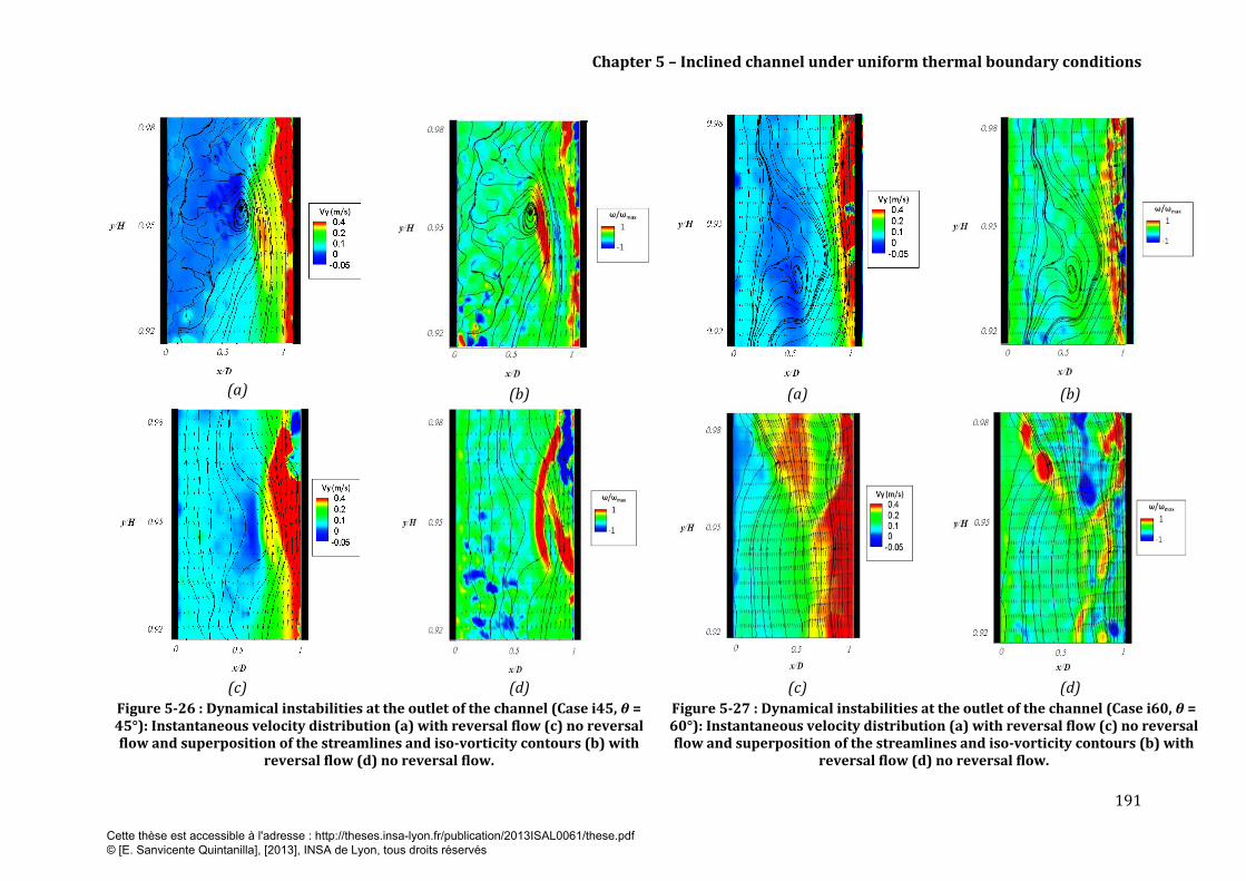
Chapter 5 – Inclined channel under uniform thermal boundary conditions
191
(a)
(b)
(a)
(b)
(c)
(d)
(c)
(d)
Figure 5-26 : Dynamical instabilities at the outlet of the channel (Case i45, θ = 45°): Instantaneous velocity distribution (a) with reversal flow (c) no reversal flow and superposition of the streamlines and iso-vorticity contours (b) with
reversal flow (d) no reversal flow.
Figure 5-27 : Dynamical instabilities at the outlet of the channel (Case i60, θ = 60°): Instantaneous velocity distribution (a) with reversal flow (c) no reversal flow and superposition of the streamlines and iso-vorticity contours (b) with
reversal flow (d) no reversal flow.
Cette thèse est accessible à l'adresse : http://theses.insa-lyon.fr/publication/2013ISAL0061/these.pdf © [E. Sanvicente Quintanilla], [2013], INSA de Lyon, tous droits réservés

Chapter 5 – Inclined channel under uniform thermal boundary conditions
192
From the observations carried out on both the vertical (Chapter 3) and inclined configuration, it
seems that during the flow reversal sequences there is a strong interaction between the
environment and the flow developed within the channel. The influence of the environment has
been identified through the observed increase in the intensity of velocity fluctuations at the
outlet section of the channel, which may be linked to changes in ambient pressure fluctuations.
To illustrate the interaction between the ambient air and the internal buoyancy induced flow,
flow visualization experiments and few PIV measurements were carried out on the R-device in
the outlet section at y/H > 1 on Sydney experimental set-up.
Tomography visualizations have been realized with a continuous and single plane laser sheet in
the mid-plane of the channel (z/L = 0.5). The lighting of the flow was obtained through a 300
mW maximum power green laser source (model LambdaPro Model LPS 300 DPSS) and it was
coupled to the cylindrical optical system designed for the PIV study in order to create the laser
sheet.
The typical dynamic structure of the flow obtained at (a) θ = 30° and (b) θ = 45° once the
thermal steady state was reached can be distinguished in Figure 5-28. Note that in Figure
5-28 (a) the flow field was obtained with smoke whereas in Figure 5-28 (b) DEHS particles were
used. The heated wall, which acts as a source of buoyancy, provides acceleration for the air in
the vicinity of the hot wall and consequently, in order to satisfy mass conservation, fluid is
drawn towards the heated wall. This flow mechanism, in a first stage, may cause a depletion of
up-moving fluid adjacent to the unheated wall, thereby resulting in an intermittent reduction of
the airflow rate (see Figure 5-28 (a)). Note that Figure 5-28 (a) shows Case i30 for which the
buoyancy effect is the weakest among all the cases. Indeed, the backflow was found to be limited
at the proximity of the channel outlet. With further increase of the inclination angle and
consequently buoyancy production, the reverse flow enhanced and was further down into the
channel (see Figure 5-28 (b)). This is consistent with the instantaneous flow fields previously
examined at y/H = 0.95 where flow reversals appeared merely at 45° < θ < 90° and not at
θ = 30°.
(a)
(b)
Figure 5-28 : Flow visualization experiments carried out in the outlet of the
channel (y/H> 1) and at (a) θ= 30° and (b) θ= 45°.
Unheated WallHeated Wall
Cette thèse est accessible à l'adresse : http://theses.insa-lyon.fr/publication/2013ISAL0061/these.pdf © [E. Sanvicente Quintanilla], [2013], INSA de Lyon, tous droits réservés

Chapter 5 – Inclined channel under uniform thermal boundary conditions
193
In Figure 5-29 a temporal sequence of 4 PIV images is shown for θ = 45°. As can be seen, the
inflow phenomenon brings cooler air from outside into the channel throught the region of the
non heated wall.
Figure 5-29 : Temporal PIV sequence, backflow phenomena at the channel outlet y/H > 1 and θ =
45°.
Cette thèse est accessible à l'adresse : http://theses.insa-lyon.fr/publication/2013ISAL0061/these.pdf © [E. Sanvicente Quintanilla], [2013], INSA de Lyon, tous droits réservés
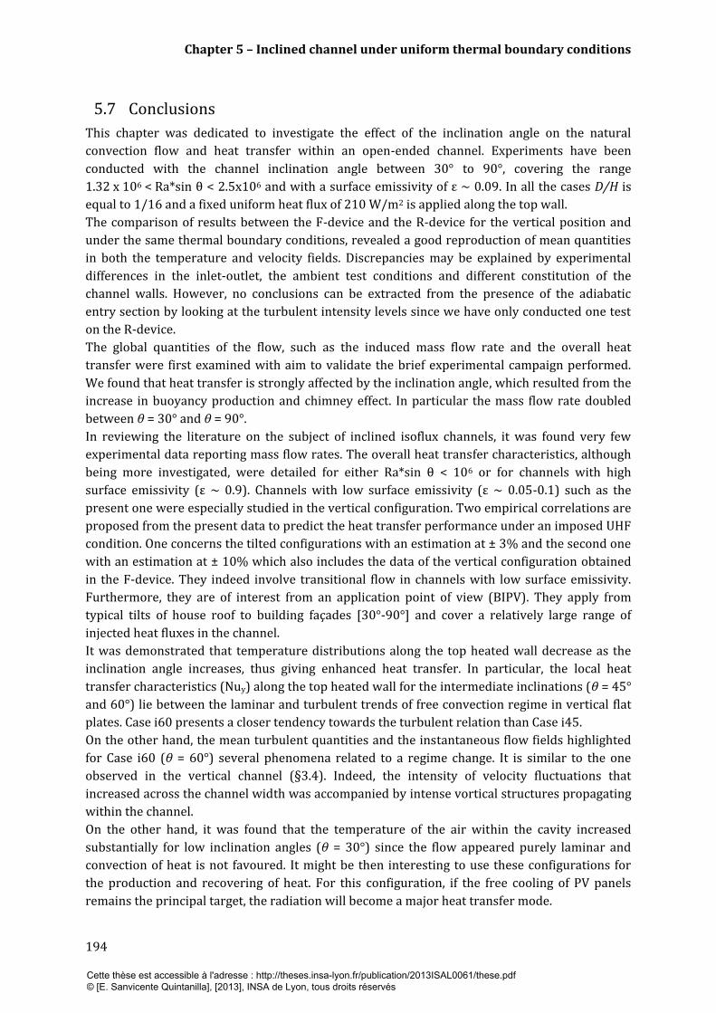
Chapter 5 – Inclined channel under uniform thermal boundary conditions
194
5.7 Conclusions
This chapter was dedicated to investigate the effect of the inclination angle on the natural
convection flow and heat transfer within an open-ended channel. Experiments have been
conducted with the channel inclination angle between 30° to 90°, covering the range
1.32 x 10⁶ < Ra*sin θ < 2.5x10⁶ and with a surface emissivity of ε ~ 0.09. In all the cases D/H is
equal to 1/16 and a fixed uniform heat flux of 210 W/m2 is applied along the top wall.
The comparison of results between the F-device and the R-device for the vertical position and
under the same thermal boundary conditions, revealed a good reproduction of mean quantities
in both the temperature and velocity fields. Discrepancies may be explained by experimental
differences in the inlet-outlet, the ambient test conditions and different constitution of the
channel walls. However, no conclusions can be extracted from the presence of the adiabatic
entry section by looking at the turbulent intensity levels since we have only conducted one test
on the R-device.
The global quantities of the flow, such as the induced mass flow rate and the overall heat
transfer were first examined with aim to validate the brief experimental campaign performed.
We found that heat transfer is strongly affected by the inclination angle, which resulted from the
increase in buoyancy production and chimney effect. In particular the mass flow rate doubled
between θ = 30° and θ = 90°.
In reviewing the literature on the subject of inclined isoflux channels, it was found very few
experimental data reporting mass flow rates. The overall heat transfer characteristics, although
being more investigated, were detailed for either Ra*sin θ < 106 or for channels with high
surface emissivity (ε ~ 0.9). Channels with low surface emissivity (ε ~ 0.05-0.1) such as the
present one were especially studied in the vertical configuration. Two empirical correlations are
proposed from the present data to predict the heat transfer performance under an imposed UHF
condition. One concerns the tilted configurations with an estimation at ± 3% and the second one
with an estimation at ± 10% which also includes the data of the vertical configuration obtained
in the F-device. They indeed involve transitional flow in channels with low surface emissivity.
Furthermore, they are of interest from an application point of view (BIPV). They apply from
typical tilts of house roof to building façades [30°-90°] and cover a relatively large range of
injected heat fluxes in the channel.
It was demonstrated that temperature distributions along the top heated wall decrease as the
inclination angle increases, thus giving enhanced heat transfer. In particular, the local heat
transfer characteristics (Nuy) along the top heated wall for the intermediate inclinations (θ = 45°
and 60°) lie between the laminar and turbulent trends of free convection regime in vertical flat
plates. Case i60 presents a closer tendency towards the turbulent relation than Case i45.
On the other hand, the mean turbulent quantities and the instantaneous flow fields highlighted
for Case i60 (θ = 60°) several phenomena related to a regime change. It is similar to the one
observed in the vertical channel (§3.4). Indeed, the intensity of velocity fluctuations that
increased across the channel width was accompanied by intense vortical structures propagating
within the channel.
On the other hand, it was found that the temperature of the air within the cavity increased
substantially for low inclination angles (θ = 30°) since the flow appeared purely laminar and
convection of heat is not favoured. It might be then interesting to use these configurations for
the production and recovering of heat. For this configuration, if the free cooling of PV panels
remains the principal target, the radiation will become a major heat transfer mode.
Cette thèse est accessible à l'adresse : http://theses.insa-lyon.fr/publication/2013ISAL0061/these.pdf © [E. Sanvicente Quintanilla], [2013], INSA de Lyon, tous droits réservés

Chapter 5 – Inclined channel under uniform thermal boundary conditions
195
The wall properties, especially at the inner side of the channel, will be the key parameters. This
will be considered in future work.
Cette thèse est accessible à l'adresse : http://theses.insa-lyon.fr/publication/2013ISAL0061/these.pdf © [E. Sanvicente Quintanilla], [2013], INSA de Lyon, tous droits réservés

196
Cette thèse est accessible à l'adresse : http://theses.insa-lyon.fr/publication/2013ISAL0061/these.pdf © [E. Sanvicente Quintanilla], [2013], INSA de Lyon, tous droits réservés

Conclusions and Further work
Conclusion and
Future work CONCLUSIONS
The experimental work discussed in the present thesis is an investigation on heat transfer and
fluid flow characteristics of natural convection of air in vertical and inclined open-ended heated
channels. A simplified experimental arrangement has been used to generate data so as to gain an
understanding of the complex processes involved in cooling of integrated photovoltaic arrays in
double-skin building surfaces whether vertical or inclined. In practice, the cooling of the PV
modules integrated in double skin arrangements is the result of coupling radiation and natural
convection generating airflow in the channel, and these were the mechanisms included in the
experimental model.
Two experimental set ups have been completed and used during the present investigations. One
is located at the CETHIL laboratory in Lyon (F-device) and the other is located at the University
of New South Wales in Sydney (R-device). The two sets of apparatus have been employed for the
study of the vertical configurations. Only the R-device is adapted to the study of an inclined
heated open-channel. Both channels consisted of two wide parallel plates (F-device (1,5m
height, 0,7m depth), R-device (1,8m height x 0,765m depth)). They could be subjected to a
controlled uniform heat flux. The channels are closed on both sides and each plate is insulated
for conduction heat losses limitation. The heating system consisted of adjacent bands of
resistance foil, each of which could be individually controlled, thereby allowing both uniform
and non-uniform heating configurations to be studied in both set ups. The upper power limit of
the F-device was 500 W/m² whereas in the R-device the power was restricted to 230 W/m². The
temperature distribution of each of the heated plates, the temperature of the air within the
channel and the temperature at a limited number of points in the experimental rooms are
measured.
Based on the wall surface temperature measurements that allow computing the radiation heat
fluxes and the temperature measurements inside the walls that allow calculating heat loss by
conduction, the convective heat flux can be determinate from the energy balance at the
wall/fluid interface where the electrical power is dissipated. The heat transfer coefficients are
inferred and recast in dimensionless form, either on a local or average basis. In both set ups, the
mean velocity field and velocity fluctuations at different levels of the channel height have been
measured with PIV systems.
The aim of the present work has been to identify and understand the impact of the distribution
of the wall heat flux and the impact of the inclination angle on both the fluid flow and heat
transfer characteristics in the natural convection of air in open-ended heated channels. The idea
developed was to use the typical morphology and geometry of the PV surface to favor both heat
transfer at the air/wall interface and buoyancy enhancement.
Cette thèse est accessible à l'adresse : http://theses.insa-lyon.fr/publication/2013ISAL0061/these.pdf © [E. Sanvicente Quintanilla], [2013], INSA de Lyon, tous droits réservés
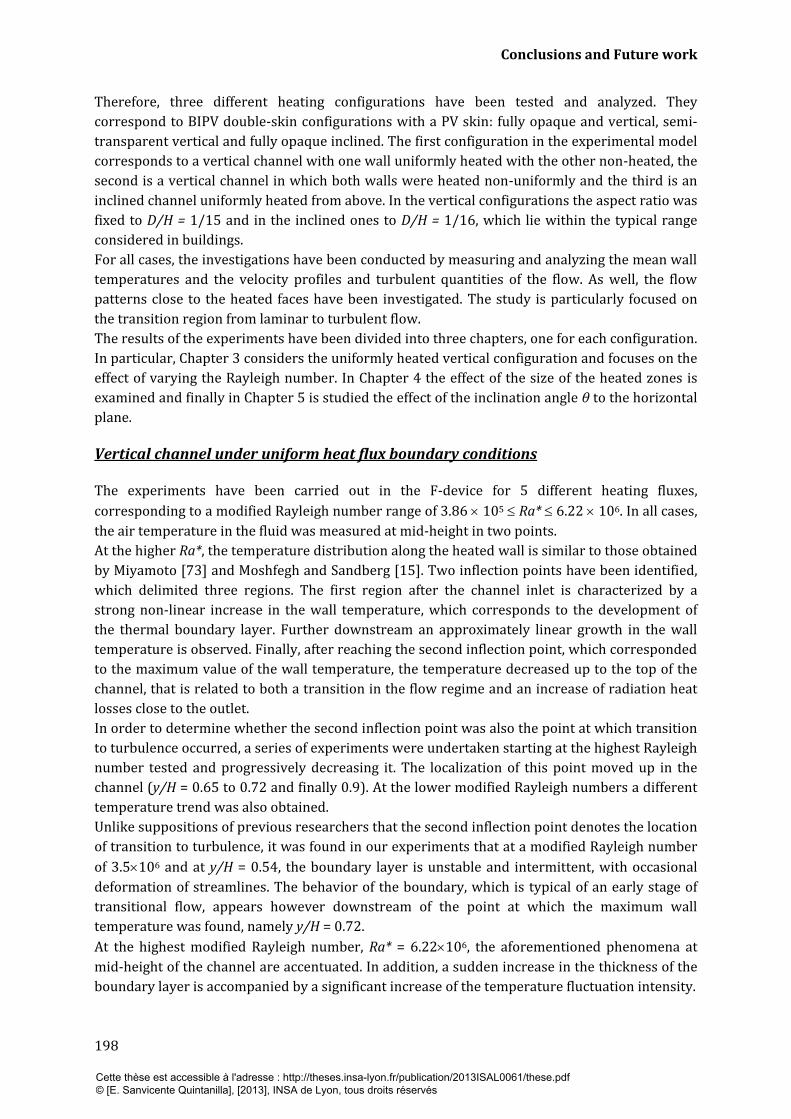
Conclusions and Future work
198
Therefore, three different heating configurations have been tested and analyzed. They
correspond to BIPV double-skin configurations with a PV skin: fully opaque and vertical, semi-
transparent vertical and fully opaque inclined. The first configuration in the experimental model
corresponds to a vertical channel with one wall uniformly heated with the other non-heated, the
second is a vertical channel in which both walls were heated non-uniformly and the third is an
inclined channel uniformly heated from above. In the vertical configurations the aspect ratio was
fixed to D/H = 1/15 and in the inclined ones to D/H = 1/16, which lie within the typical range
considered in buildings.
For all cases, the investigations have been conducted by measuring and analyzing the mean wall
temperatures and the velocity profiles and turbulent quantities of the flow. As well, the flow
patterns close to the heated faces have been investigated. The study is particularly focused on
the transition region from laminar to turbulent flow.
The results of the experiments have been divided into three chapters, one for each configuration.
In particular, Chapter 3 considers the uniformly heated vertical configuration and focuses on the
effect of varying the Rayleigh number. In Chapter 4 the effect of the size of the heated zones is
examined and finally in Chapter 5 is studied the effect of the inclination angle θ to the horizontal
plane.
Vertical channel under uniform heat flux boundary conditions
The experiments have been carried out in the F-device for 5 different heating fluxes,
corresponding to a modified Rayleigh number range of 3.86 105 Ra* 6.22 106. In all cases,
the air temperature in the fluid was measured at mid-height in two points.
At the higher Ra*, the temperature distribution along the heated wall is similar to those obtained
by Miyamoto [73] and Moshfegh and Sandberg [15]. Two inflection points have been identified,
which delimited three regions. The first region after the channel inlet is characterized by a
strong non-linear increase in the wall temperature, which corresponds to the development of
the thermal boundary layer. Further downstream an approximately linear growth in the wall
temperature is observed. Finally, after reaching the second inflection point, which corresponded
to the maximum value of the wall temperature, the temperature decreased up to the top of the
channel, that is related to both a transition in the flow regime and an increase of radiation heat
losses close to the outlet.
In order to determine whether the second inflection point was also the point at which transition
to turbulence occurred, a series of experiments were undertaken starting at the highest Rayleigh
number tested and progressively decreasing it. The localization of this point moved up in the
channel (y/H = 0.65 to 0.72 and finally 0.9). At the lower modified Rayleigh numbers a different
temperature trend was also obtained.
Unlike suppositions of previous researchers that the second inflection point denotes the location
of transition to turbulence, it was found in our experiments that at a modified Rayleigh number
of 3.5106 and at y/H = 0.54, the boundary layer is unstable and intermittent, with occasional
deformation of streamlines. The behavior of the boundary, which is typical of an early stage of
transitional flow, appears however downstream of the point at which the maximum wall
temperature was found, namely y/H = 0.72.
At the highest modified Rayleigh number, Ra* = 6.22106, the aforementioned phenomena at
mid-height of the channel are accentuated. In addition, a sudden increase in the thickness of the
boundary layer is accompanied by a significant increase of the temperature fluctuation intensity.
Cette thèse est accessible à l'adresse : http://theses.insa-lyon.fr/publication/2013ISAL0061/these.pdf © [E. Sanvicente Quintanilla], [2013], INSA de Lyon, tous droits réservés
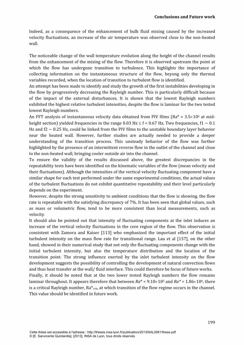
Conclusions and Future work
199
Indeed, as a consequence of the enhancement of bulk fluid mixing caused by the increased
velocity fluctuations, an increase of the air temperature was observed close to the non-heated
wall.
The noticeable change of the wall temperature evolution along the height of the channel results
from the enhancement of the mixing of the flow. Therefore it is observed upstream the point at
which the flow has undergone transition to turbulence. This highlights the importance of
collecting information on the instantaneous structure of the flow, beyong only the thermal
variables recorded, when the location of transition to turbulent flow is identified.
An attempt has been made to identify and study the growth of the first instabilities developing in
the flow by progressively decreasing the Rayleigh number. This is particularly difficult because
of the impact of the external disturbances. It is shown that the lowest Rayleigh numbers
exhibited the highest relative turbulent intensities, despite the flow is laminar for the two tested
lowest Rayleigh numbers.
An FFT analysis of instantaneous velocity data obtained from PIV films (Ra* = 3.5106 at mid-
height section) yielded frequencies in the range 0.03 Hz f < 0.67 Hz. Two frequencies, f1 ~ 0.1
Hz and f2 ~ 0.25 Hz, could be linked from the PIV films to the unstable boundary layer behavior
near the heated wall. However, further studies are actually needed to provide a deeper
understanding of the transition process. This unsteady behavior of the flow was further
highlighted by the presence of an intermittent reverse flow in the outlet of the channel and close
to the non-heated wall, bringing cooler outside air into the channel.
To ensure the validity of the results discussed above, the greatest discrepancies in the
repeatability tests have been identified on the kinematic variables of the flow (mean velocity and
their fluctuations). Although the intensities of the vertical velocity fluctuating component have a
similar shape for each test performed under the same experimental conditions, the actual values
of the turbulent fluctuations do not exhibit quantitative repeatability and their level particularly
depends on the experiment.
However, despite the strong sensitivity to ambient conditions that the flow is showing, the flow
rate is repeatable with the satisfying discrepancy of 7%. It has been seen that global values, such
as mass or volumetric flow, tend to be more consistent than local measurements, such as
velocity.
It should also be pointed out that intensity of fluctuating components at the inlet induces an
increase of the vertical velocity fluctuations in the core region of the flow. This observation is
consistent with Zamora and Kaiser [113] who emphasized the important effect of the initial
turbulent intensity on the mass flow rate for transitional range. Lau et al [157], on the other
hand, showed in their numerical study that not only the fluctuating components change with the
initial turbulent intensity, but also the temperature distribution and the location of the
transition point. The strong influence exerted by the inlet turbulent intensity on the flow
development suggests the possibility of controlling the development of natural convection flows
and thus heat transfer at the wall/ fluid interface. This could therefore be focus of future works.
Finally, it should be noted that at the two lower tested Rayleigh numbers the flow remains
laminar throughout. It appears therefore that between Ra* = 9.10105 and Ra* = 1.86106, there
is a critical Rayleigh number, Ra*crit, at which transition of the flow regime occurs in the channel.
This value should be identified in future work.
Cette thèse est accessible à l'adresse : http://theses.insa-lyon.fr/publication/2013ISAL0061/these.pdf © [E. Sanvicente Quintanilla], [2013], INSA de Lyon, tous droits réservés

Conclusions and Future work
200
Vertical channel under non-uniform spatial heat flux boundary conditions
The effect of non-uniform heating conditions has been investigated in the vertical channel with
the imposed boundary conditions representing alternated heated and unheated zones of equal
size along the height of each of the walls. The experiments were carried out for two sizes of
heated zones, corresponding respectively to 10 cm (Case V1) and 40 cm (Case V2).
In agreement with literature, the present investigation shows that the alternated heating
arrangements promote heat transfer, with a typical increase of the average heat transfer
coefficient of 27%. Consequently, for the same average heat flux injected in the channel, the
increase of the number of heated and unheated zones in each wall caused a reduction in the
maximum temperature of the heated areas up to 10°C. In fact, the continuous development of
the thermal boundary layer, which is a barrier of efficient heat transfers, is prevented by the
insertion of unheated zones between heated zones. Near the boundary, air leaves an unheated
zone at a lower temperature than would have been in the case of a continuous heating. This
means that at the leading edge of the next downstream heated zone, the lower temperature of
the air leads to a higher heat transfer rate, which is manifested in turns as a higher convective
heat transfer.
As a result, from a local point of view, the case with heated sections of 40 cm (Case V2) showed
the lowest wall temperatures at the beginning of the heated zones. A reverse effect is observed
along the heated zone for the reasons mentioned above and therefore in terms of average
convective heat tranfers per heated area, it is V1 the most interesting case. However, if we go on
this principle, it would led to very small heated and unheated zones and lead to a closer case of
the uniformly heated wall which is not optimum in terms of convective heat transfers. As a
consequence, an optimum for the ratio (a/H) remains to be found. As previously observed, the
heat sources situated at the bottom of the channel exhibit higher local convective coefficients
than those at the top one.
Two empirical correlations for average Nusselt numbers are obtained from the present data
with respect to modified Rayleigh numbers. The average Nusselt values are evaluated in the
heated areas and the modified Rayleigh numbers, Ra*D (D/a), were partly based on the width of
the channel (D) and on the ratio D/a, according to literature.
The flow in natural convection in which there are alternated heated and unheated zones at the
wall does not necessarily undergo transition. However, the appearance of many unsteady
structures with high velocities leads to a higher rate of turbulent production compared with the
uniformly heated channel.
A remarkable change in the flow behavior occurred before the mid-height in both non-uniform
heating cases. Indeed, a significant reduction of the velocity particularly in the core region and a
drastic increase of turbulent intensity close to the walls are also observed.
In the case of smallest heated zones, the structures detaching from the heated areas are
predominantly found along the wall where they are developing. In the case of the largest heated
zones, the structures are also attracted by the upper heated zone located in the opposite wall. It
is shown that the fluid motion is disturbed because of the flow passing heated and unheated
zones. As a consequence, there might not have actual transition but a a ‘disruption mechanism’
of the flow which leads to enhanced mixing and increased Reynolds stresses over most of the
width of the channel.
Results of the frequency analysis in the mid-height section highlights frequencies in the range
0.03 Hz < f < 0.2 Hz. However, further investigations are required to link these frequencies with
the complex structure of the flow pattern.
Cette thèse est accessible à l'adresse : http://theses.insa-lyon.fr/publication/2013ISAL0061/these.pdf © [E. Sanvicente Quintanilla], [2013], INSA de Lyon, tous droits réservés
Conclusions and Future work
201
On the second half of the channel, the flow is characterized by a gradual increase of the turbulent
mixing and a tendency to homogenization. This was measured by the rate of turbulent
production and the values of the skewness and flatness factors, which were calculated from the
instantaneous velocity measurements at two points across the channel width and were reduced
towards the outlet section. Unlike the uniformly heated channel, no flow reversals are identified
during the experiments. This is due to the fact that both walls are heated.
Finally, it is also shown that the alternated heating arrangements promote the chimney effect,
enhancing the mass flow rates up to 12% compared to the uniformly heated channel for the
same amount of injected heat flux in the channel. These results indicate that the maximum
temperature achieved at the walls is strongly related to the spatial distribution of the wall heat
flux in the walls. Even if the mass flow rate, which is induced in the channel for the same heat
injection configuration (uniform, non uniform) is governed by the global heat flux that is injected
in the channel, it is also depending of wall heat flux spatial distribution.
The enhancement of both the induced mass flow rate and the mixing of the flow might be an
important factor when considering the possibility that useful heat may be generated and used
for heating or cooling purposes. However, in order to estimate the heat recovery options, local
measurements of the temperature of the air in the cavity need to be carried out at different
heights in future works.
Inclined channel under uniform heat flux boundary conditions
The experiments have been conducted with the channel inclination angle between 30° to 90°,
covering the range 1.32x10⁶ < Ra*sin θ < 2.5x 10⁶ and with a surface emissivity of ε ~ 0.09 in
both walls.
The results obtained in this configuration have to be interpreted with caution since the
repeatability of the tests is only analyzed in terms of wall temperature profiles with two tests
being conducted at each inclination angle. Moreover, it should be noted that although the
number of PIV images obtained by test were seen to converge in the mean values, no safety
margin was left due to limitations in the instrumentation.
The average heat transfer in the channel is strongly affected by the inclination angle, resulted of
the increase in buoyancy production and chimney effect which doubled between θ = 30° and
θ = 90°. Consequently, the average temperature of the top heated wall in the vertical position
was reduced up to 14°C with respect to the channel tilt angle of 30°.
A comparison is done with literature Nusselt/Rayleigh correlations for the laminar and
turbulent free convection regimes in the case of a vertical flat plate. Two typical trends are
resulted. These results seem also to show that the flow behavior is strongly governed by the
inclination angle of the channel.
For a channel tilt angle of 30°, the local Nusselt number values tend to follow the laminar
relation until the top of the channel. Indeed, the flow is purely laminar with very poor
convection of heat due to the high level of pressure loss and low stack height of the channel. This
is indicated by the uniform velocity distribution, which is evolving slightly along the height of
the channel and also by the temperature of the air within the core section of the channel, which
is shown to increase by a factor 2 with respect to the vertical position.
In the inclination angle range 45° θ 90°, there is a change in the slope of the local Nusselt
values, indicating a transition of the flow regime.
In particular, for intermediate inclinations θ = 45° and 60°, the local Nusselt values lie between
the laminar and turbulent trends of free convection regime in vertical flat plates. It is the θ = 60°
Cette thèse est accessible à l'adresse : http://theses.insa-lyon.fr/publication/2013ISAL0061/these.pdf © [E. Sanvicente Quintanilla], [2013], INSA de Lyon, tous droits réservés

Conclusions and Future work
202
case which presents a closer tendency towards the turbulent relation. Indeed, it is at θ = 60o and
thereafter the mid-height section of the channel, when unsteady vortical structures related to
the early stages of the transition are distinguished. It thus amplifies the velocity fluctuations
downstream in the channel.
In agreement with some literature studies performed in inclined channels, a reverse flow is
intermittently observed in the outlet section and close to the bottom non-heated face for channel
tilt angles of 45° and 60°. No reverse flows are observed for θ = 30°. It is shown that the
maximum penetration length of the recirculation zone recorded at the outlet of the channel
increases from 8 cm to 16 cm between θ = 45° and θ = 90°.
In terms of convective heat transfer, two empirical correlations for average Nusselt numbers
with respect to modified Rayleigh numbers are proposed. The average Nusselt numbers are
evaluated in the top heated wall. The modified Rayleigh numbers, Ra*sin θ, are partly based on
the width of the channel and on the sinus of the angle θ with respect to the horizontal. One of the
correlations concerns solely the tilted configurations and allows to estimate NuD with a
maximum uncertainty of ± 3%. In the second one, the data for the vertical configuration
configuration is included and the maximum uncertainty increases to ± 10%. Comparisons with
literature relations of heat transfer are performed. However, very few experimental data
reporting mass flow rates are found. Furthermore, channels with low inner wall emissivities (ε ~
0.05-0.1) such as the one in the present study are especially studied for the vertical
configuration. Thus, the present investigation contributes to the constitution of an empirical
database concerning tilted channels.
SUGGESTIONS FOR FUTURE WORK
The scope for the advancement of this study is extensive, as we have seen through our
investigations. Two kinds of perspectives could be planned. One is related to the experimental
means and the other one to the analysis of heat and mass transfers and structure of the flow.
By experimental means we refer to the improvements that could be made to the existing set ups,
instrumentation and experimental procedures implemented.
Regarding the R-device, the stiffness of both panels needs to be improved. In particular, during
the R-device operation several bending issues were found in the Bakelite panels, which
encountered, in turns, many experimental difficulties. For further projects, it may be an option to
embed each panel in a rigid “box” like the one designed in Lyon for maintaining the insulation
block and the Bakelite plate connected (see Chapter 3 of J. Vareilles [131]).
Temperature measurements
Different improvements have been identified in terms of temperature acquisition and
thermocouple arrangements for each device.
The instrumentation used in the R-device needs to be completed by increasing the number of
thermocouples used to measure the surface temperature of each plate. This will allow to get a
more accurate distribution of the temperature in the walls, which as mentioned before, is
necessary to predict the location of the transition to turbulent flow.
Regarding the arrangement of thermocouples used, a fixed placement of thermocouples in for
example the centerline of the panels (z/L = 0.5), would have made easier the acquisition of
temperature in the R-device. However, it is very useful to have a number of non-fixed
thermocouples to measure different locations for different experiments. Based on the
Cette thèse est accessible à l'adresse : http://theses.insa-lyon.fr/publication/2013ISAL0061/these.pdf © [E. Sanvicente Quintanilla], [2013], INSA de Lyon, tous droits réservés
Conclusions and Future work
203
experience, a combination of both arrangements, fixed and not fixed, might be the best option
for future experiments.
For the F-device, the improvement required for future works is related to the frequency of the
wall temperature acquisition system, which is too low for studying the link between the wall/air
heat transfer and the kinematic structure of the flow. This is particularly important for the study
of the mechanisms driving the unsteady structures identified in the flow, which detached from
the walls thereafter the mid-height section of the channel. With the current temperature
acquisition system, however, it is not possible to complete this analysis.
For both devices, it will be as well necessary to test the sensitivity of this arrangement to the
temperature fluctuations in the fluid since measurements are carried out in the rear of the
heating foil and not in the face which is in contact with the fluid.
The arrangement of thermocouples used in both devices to measure the temperature of the air
within the channel (two thermocouples immersed in the fluid) has allowed us to obtain only a
‘rough’ average temperature of the air, which has been especially used for the estimation of the
density of the air. However, this number of thermocouples is not sufficient if the temperature
distribution of the flow aims to be obtained and analyzed. It follows that more thermocouples
need to be employed for future works, notably located in the near wall regions where the
temperature gradients are greatest. In such case, the wire diameter of the thermocouples could
be smaller, for example of 0.1 mm, to minimize disturbance of the airflow.
Velocity measurements
Regarding the velocity measurements, the PIV system has shown a main limitation close to the
walls (lack of data and accuracy). The strong velocity gradients which are present in these zones
are found to decrease the probability of detection of the displacement peak. Therefore the
uncertainty in these regions is greater (section 2.2.2.3 of Chapter 2). This is especially the case
when square interrogation areas are uniformly applied through the image section of the flow. On
one hand, our actual measurements can be improved by using in the near wall regions
rectangular interrogation windows (extending parallel to the wall) instead of squared ones.
With this, we keep inside the interrogation areas the largest displacements (which will be in the
vertical direction) and the smallest ones (which correspond to the horizontal displacements).
According to the literature [136], window deformation techniques for PIV evaluation are
actually improving the data quality in boundary layers and shear flows. As well, as detailed by
Theunissen et al. [143], it is possible to use a cross-correlation based PIV image interrogation
algorithm that adapts the number of interrogation windows and their size to the image
properties and to the flow conditions. In their experimental study for example, the position and
size of the interrogation windows were locally adapted to the image signal (i.e., seeding density)
and the local window spacing (commonly set by the overlap factor) was put in relation with the
spatial variation of the velocity field. They showed that with this technique the spatial resolution
in the wall regions was locally enhanced.
The 3D effects should be also carefully evaluated. Measurements of the kinematic characteristics
of the flow on the transversal planes parallel to the one already studied (0 < z/L < 1) are
therefore needed. Flow visualizations may be also performed placing the camera perpendicular
to the outlet section of the channel (y-direction) so as to image the cross section of the channel,
S= LxD.
Cette thèse est accessible à l'adresse : http://theses.insa-lyon.fr/publication/2013ISAL0061/these.pdf © [E. Sanvicente Quintanilla], [2013], INSA de Lyon, tous droits réservés

Conclusions and Future work
204
Further analysis and measurements
A primary necessity for the accurately characterization of the flow in a natural convection flow is
to control the conditions in the room while an experiment is in progress. Besides the
temperature measurements that were recorded in the room in the present work, measurements
on channel external conditions have to be completed. It should include measurements of the
instantaneous static pressures and temperatures at different locations during any tests to
evaluate both the temperature and pressure gradients.
A first attempt to characterize the possible air currents in the experimental room where the F-
device is now located has been performed by Teo Lafaye de Micheaux in 2011 during his master
thesis [135]. He used helium filled soap bubbles of 0.5 - 1 cm diameter as tracers and conducted
flow visualizations while the F-device was not in operation. Some circular motions of convection
currents could be identified in the room. During tests this could also be measured by regular
checks with hot wire anemometer probes. As well, instantaneous velocity measurements were
taken by PIV outside the channel and in the inlet region [135]. It was shown that for an injected
heat flux 230 W/m2, the length of the region of influence beneath the channel was 1.7 times the
length of the channel width and air velocities of the order of 0.15 m/s and 0,1 m/s were
measured respectively at a distance of 4.5 cm and 9 cm of the inlet of the channel. For future
works, more instantaneous velocity measurements should be taken in different locations outside
the channel and in the whole room and then cross correlate these measurements with velocities
inside the channel. This will, on one hand, allow assessing the influence of the external
conditions on the development of the flow.
On the other hand, the accurate characterization of the surrounding conditions may allow these
conditions to be taken into account in future numerical calculations. As reported by Lau et al.
[157], discrepancies between the numerical data and the present experimental results were in
part related to the lack of knowledge of the exact environmental conditions. Because the
experimental results are affected by fluctuations external to the apparatus, it was necessary for
Lau et al [157] to introduce arbitrary disturbances at the inlet of the computational region in
order to model the effect of external fluctuations on the flow in the channel. It was found that the
best agreement was achieved when the stochastic disturbances was set as 1%. Nevertheless,
when comparing the numerical results obtained in Lau et al [157] with the present experimental
ones, the transition location was found to be different. Furthermore, a compromise was made
between the accuracy of the results and simulation time. This suggests that the environmental
conditions of the room, e.g. the flow fluctuations as seen in the experimental data have to be
taken into consideration when imposing the boundary conditions at the inlet. As a consequence
of the results obtained in the present work and that of Lau et al [157], CFD calculations involving
the modeling of the whole room including the channel in operation have begun. They are
conducted by the CFD laboratory of the UNSW in Australia. The first results indicate that the
whole room is affected by the heating on the experimental device.
Regarding the unstable wall structures that repeatedly appeared close to the heated faces such
as the destabilization of the boundary layer and intermittent flow reversals, they need to be
characterized precisely and the research should be focused on determining their driving
mechanisms. This is consistent with the study of instantaneous mechanisms affecting the
behavior of turbulent flows.
First of all, the statistical quantities of the flow, such as the skewness and flatness factors should
be obtained in each point of the velocity field similarly as the analysis conducted in two single
points.
Cette thèse est accessible à l'adresse : http://theses.insa-lyon.fr/publication/2013ISAL0061/these.pdf © [E. Sanvicente Quintanilla], [2013], INSA de Lyon, tous droits réservés

Conclusions and Future work
205
Moreover, the intermittency factor could be obtained for each point by performing conditional
sampling on the present instantaneous velocity signals [173, 174]. This first investigation of the
actual measurements should provide a deeper understanding of the structure of the velocity
flow field and the influence of the Rayleigh number, the non-uniform heating conditions and the
inclination angle of the channel on it.
Furthermore, a post processing based on Proper Orthogonal Descomposition, namely POD, could
be applied to the actual PIV velocity field data in order to extract the main dominant, dynamical
and energetic features of the flow. The POD method was introduced in the context of turbulence
by Lumley [175] in the late 60’s to extract the spatial and temporal structures judged essential
and provide a rigorous mathematical frame work for their description. Currently, it deals with
active control studies [176, 177]. The most striking property of this decomposition is optimality
since it provides the most efficient way of capturing the dominant components of an infinite-
dimensional process with only a few functions. That is why the POD process is successfully
applied in different turbulent flows to analyze for example experimental PIV data [178, 179].
The proposed future work would involve the use of this method, not only for the analysis and
synthesis of the experimental data, but also for the construction, from the Navier-Stokes
equations, of a low order dynamical model (or reduced order model) that represents with a
satisfactory level of accuracy the original full-order model and requires less computational time
[180, 181]. This reduced order model could be in turns incorporated in thermo-aeraulic building
simulation codes or could be used for flow control of unsteady natural convection within open-
ended channels.
Regarding new measurements, in the regions where the unsteadiness of the natural flow seemed
to be markedly intermittent, the growth of the hydrodynamic instabilities and dominant features
can be studied experimentally by adequate mechanical or thermo-acoustic excitation of the flow.
For example, the first method could consist in stretching a fine metallic ribbon across the flow
close to the wall, which vibrates by passing an alternating current through it in the field of a
magnet, just the other side of the wall [182]. The second method consists on applying acoustic waves created by for example a loudspeaker placed outside the channel to obtain an active
control of the instabilities [183]. The resulted disturbance of the flow obtained with both
methods can be characterized downstream by means of for example PIV or hot wire
anemometer measurement techniques.
Finally, in order to evaluate the turbulent heat flux transported from the walls,
, it
will be necessary to develop a measurement technique to simultaneous measure velocities and
temperatures close to the walls. The employment of a fast response micro-thermocouple with a
displacement system of precision together with the PIV system will allow the calculation of the
cross correlations of velocity and temperature in the near wall regions. However, this type of
measurement in transitional and turbulent natural convection is quite delicate due its sensibility
to perturbations [184] and because the velocity and temperature must be measured
simultaneously at the same point. With the metrology employed (PIV and thermocouple) both
measurements cannot be carried out at the same location since the laser sheet would disturb the
measured temperature. The location of a single thermocouple with respect to the laser sheet as
well as the influence of the laser on the temperature measurements would need first to be
investigated similarly as was done by Ilie et al. [184] in an open-ended vertical channel.
The criterion used by the authors for finding the best location is the correlation coefficient
between the temperature and the velocity data and they demonstrated the feasibility of this kind
of measurements although the difficulty.
Cette thèse est accessible à l'adresse : http://theses.insa-lyon.fr/publication/2013ISAL0061/these.pdf © [E. Sanvicente Quintanilla], [2013], INSA de Lyon, tous droits réservés
Conclusions and Future work
206
Regarding the short-term prospects for the inclined configurations, an analysis of the
repeatability of the data on the thermal and kinematical measurements should be conducted in
order to ensure the validity of the results above discussed. In turns, this study will lead us to
deepen in the influence of the ambient conditions to the flow development in tilted channels. In
the long-term perspectives, if the free cooling of PV panels remains the principal target, the
radiation will become a major heat transfer mode. Future works will be conducted by varying
the inner wall properties, such as the emissivity of the surface.
From a global perspective in terms of application, it has been confirmed experimentally that
external effects have a significant impact on the performance of such devices so that, not only
wind but also surrounding buildings need to be taken into account in both experiments and
codes used to simulate the thermo-aeraulic behavior of BiPV double skin systems. According to
Athienitis et al. [161], wind speeds higher than 2 m/s with a strong fluctuating component
increase significantly the turbulence along these type of façades, particularly for low suction
velocities. This is consistent with our results regarding the effect of inlet turbulent intensity
upon the development of the flow and the buoyancy-induced mass flow rate. We should,
nonetheless, be aware that although the wind effect needs to be taken into account, it is a non
controlled parameter which in turns could also limit the buoyancy driven ventilation. This study
provides then information on the heat transfer and flow mechanisms involved which would be
useful and necessary for the control of the thermal performance of real double skin PV systems.
In addition, the observations made on the enhanced mixing of the flow existing in non-uniform
heating experiments bring new perspectives on the production of useful heat while
simultaneously generating electricity from the same building envelope surface. The effect of the
ratio of photovoltaic area coverage of the transparent façade, which according to Athienitis et al.
[161] is generally selected based on the fresh air heating needs of the building, the value of the
electricity generated and the available building surfaces, requires further study, particularly in
full scale systems. It has also been confirmed experimentally the occasional appearance of low
velocity and recirculation motions in the center of the channel during non uniform heating
experiments similarly to those observed by Litvak and Morrison [162]. These phenomena is
undesirable to occur for these type of installations since they cause a depletion of the up-moving
air in the center of the channel, thereby resulting in occasional reduction of the air flow rates.
This will need therefore to be evaluated for large installations.
Finally, the appearance of localized reverse flows in the outlet of the channel, which was
confirmed in our experiments for uniformly and asymmetrically heated vertical and inclined
configurations, would need to be evaluated in opaque PV double façades and ventilated roofs,
particularly regarding the area of the façade they are covering. Since the experimentally
measured penetration lengths are of order one tenth the channel height, one strategy to reduce
the effect of reverse flow in real building components could be to adapt this upper section of the
cavity such that is unheated, without PV modules, and either made of transparent material of
insulator. Such a configuration is consistent with laboratory studies of heated channels with
unheated sections added doanstream of the flow.
Cette thèse est accessible à l'adresse : http://theses.insa-lyon.fr/publication/2013ISAL0061/these.pdf © [E. Sanvicente Quintanilla], [2013], INSA de Lyon, tous droits réservés

207
Cette thèse est accessible à l'adresse : http://theses.insa-lyon.fr/publication/2013ISAL0061/these.pdf © [E. Sanvicente Quintanilla], [2013], INSA de Lyon, tous droits réservés

208
Cette thèse est accessible à l'adresse : http://theses.insa-lyon.fr/publication/2013ISAL0061/these.pdf © [E. Sanvicente Quintanilla], [2013], INSA de Lyon, tous droits réservés

209
Appendices
Appendix A HEAT TRANSFER CORRELATIONS
In this appendix is included a summary of correlations of average and local Nusselt numbers as a
function of Rayleigh number which are presented in the field of heat transfer between parallel plate
vertical channels.
These correlations are presented in two separated tables, which are based on the imposed
boundary conditions at the walls. Table A-1 summarizes the correlations for uniform heat flux,
UHF boundary conditions and Table A-2 to uniform temperature, UWT, boundary conditions.
Cette thèse est accessible à l'adresse : http://theses.insa-lyon.fr/publication/2013ISAL0061/these.pdf © [E. Sanvicente Quintanilla], [2013], INSA de Lyon, tous droits réservés
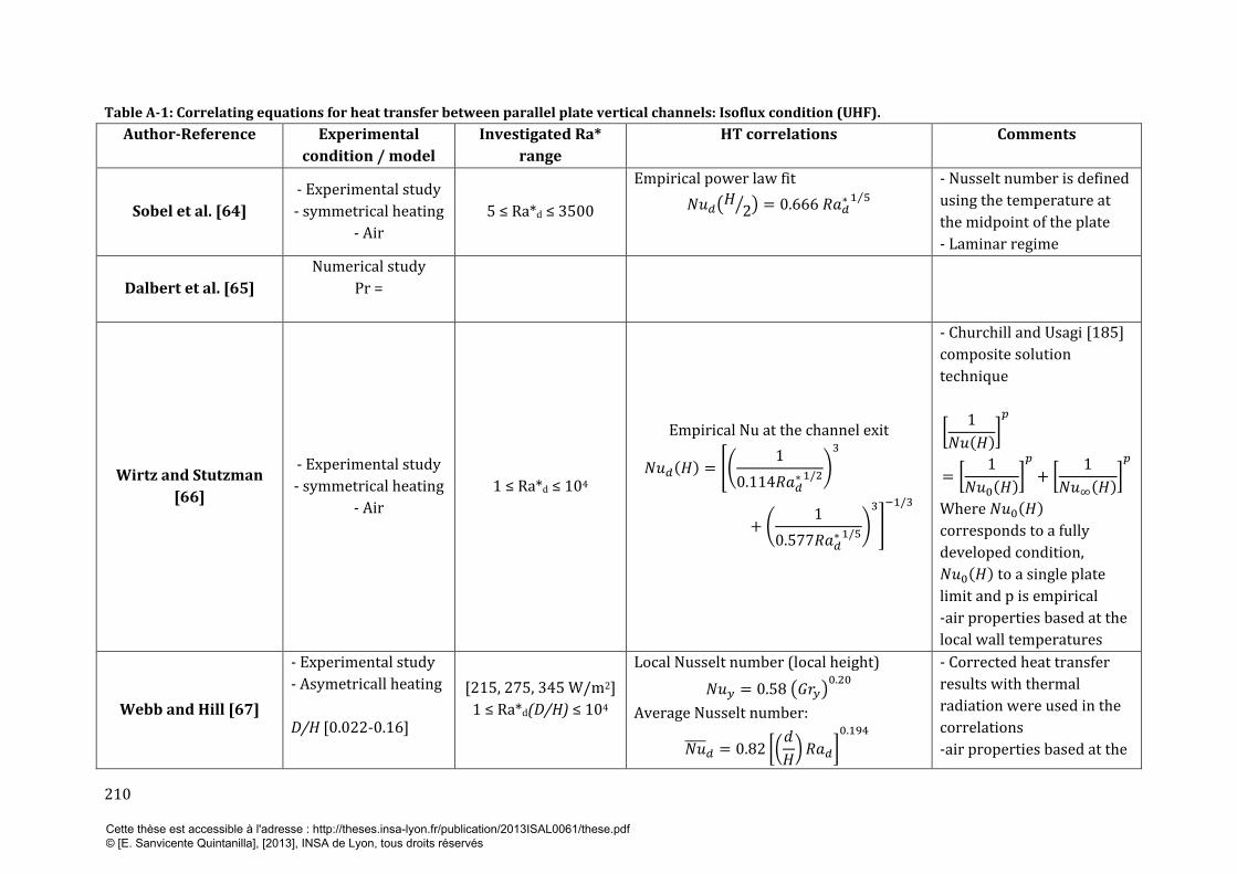
210
Table A-1: Correlating equations for heat transfer between parallel plate vertical channels: Isoflux condition (UHF).
Author-Reference Experimental
condition / model
Investigated Ra*
range
HT correlations Comments
Sobel et al. [64]
- Experimental study
- symmetrical heating
- Air
5 ≤ Ra*d ≤ 3500
Empirical power law fit
- Nusselt number is defined
using the temperature at
the midpoint of the plate
- Laminar regime
Dalbert et al. [65]
Numerical study
Pr =
Wirtz and Stutzman
[66]
- Experimental study
- symmetrical heating
- Air
1 ≤ Ra*d ≤ 104
Empirical Nu at the channel exit
- Churchill and Usagi [185]
composite solution
technique
Where
corresponds to a fully
developed condition,
to a single plate
limit and p is empirical
-air properties based at the
local wall temperatures
Webb and Hill [67]
- Experimental study
- Asymetricall heating
D/H [0.022-0.16]
[215, 275, 345 W/m2]
1 ≤ Ra*d(D/H) ≤ 104
Local Nusselt number (local height)
Average Nusselt number:
- Corrected heat transfer
results with thermal
radiation were used in the
correlations
-air properties based at the
Cette thèse est accessible à l'adresse : http://theses.insa-lyon.fr/publication/2013ISAL0061/these.pdf © [E. Sanvicente Quintanilla], [2013], INSA de Lyon, tous droits réservés
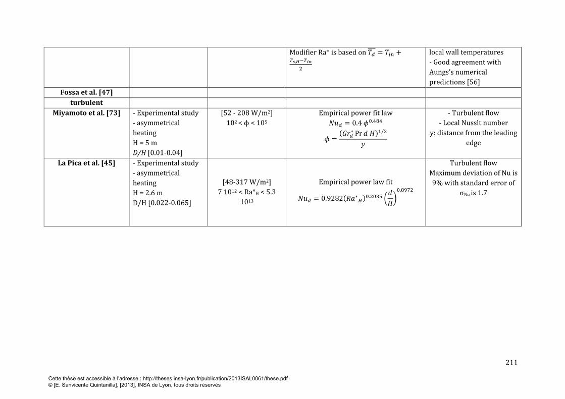
211
Modifier Ra* is based on
local wall temperatures
- Good agreement with
Aungs’s numerical
predictions [56]
Fossa et al. [47]
turbulent
Miyamoto et al. [73] - Experimental study
- asymmetrical
heating
H = 5 m
D/H [0.01-0.04]
[52 - 208 W/m2]
102 < ϕ < 105
Empirical power fit law
- Turbulent flow
- Local Nusslt number
y: distance from the leading
edge
La Pica et al. [45] - Experimental study
- asymmetrical
heating
H = 2.6 m
D/H [0.022-0.065]
[48-317 W/m2]
7 1012 < Ra*H < 5.3
1013
Empirical power law fit
Turbulent flow
Maximum deviation of Nu is
9% with standard error of
σNu is 1.7
Cette thèse est accessible à l'adresse : http://theses.insa-lyon.fr/publication/2013ISAL0061/these.pdf © [E. Sanvicente Quintanilla], [2013], INSA de Lyon, tous droits réservés
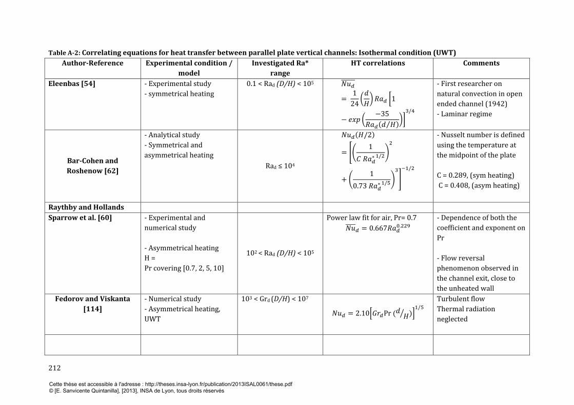
212
Table A-2: Correlating equations for heat transfer between parallel plate vertical channels: Isothermal condition (UWT)
Author-Reference Experimental condition /
model
Investigated Ra*
range
HT correlations Comments
Eleenbas [54] - Experimental study
- symmetrical heating
0.1 < Rad (D/H) < 105
- First researcher on
natural convection in open
ended channel (1942)
- Laminar regime
Bar-Cohen and
Roshenow [62]
- Analytical study
- Symmetrical and
asymmetrical heating
Rad ≤ 104
- Nusselt number is defined
using the temperature at
the midpoint of the plate
C = 0.289, (sym heating)
C = 0.408, (asym heating)
Raythby and Hollands
Sparrow et al. [60] - Experimental and
numerical study
- Asymmetrical heating
H =
Pr covering [0.7, 2, 5, 10]
102 < Rad (D/H) < 105
Power law fit for air, Pr= 0.7
- Dependence of both the
coefficient and exponent on
Pr
- Flow reversal
phenomenon observed in
the channel exit, close to
the unheated wall
Fedorov and Viskanta
[114]
- Numerical study
- Asymmetrical heating,
UWT
103 < Grd (D/H) < 107
Turbulent flow
Thermal radiation
neglected
Cette thèse est accessible à l'adresse : http://theses.insa-lyon.fr/publication/2013ISAL0061/these.pdf © [E. Sanvicente Quintanilla], [2013], INSA de Lyon, tous droits réservés
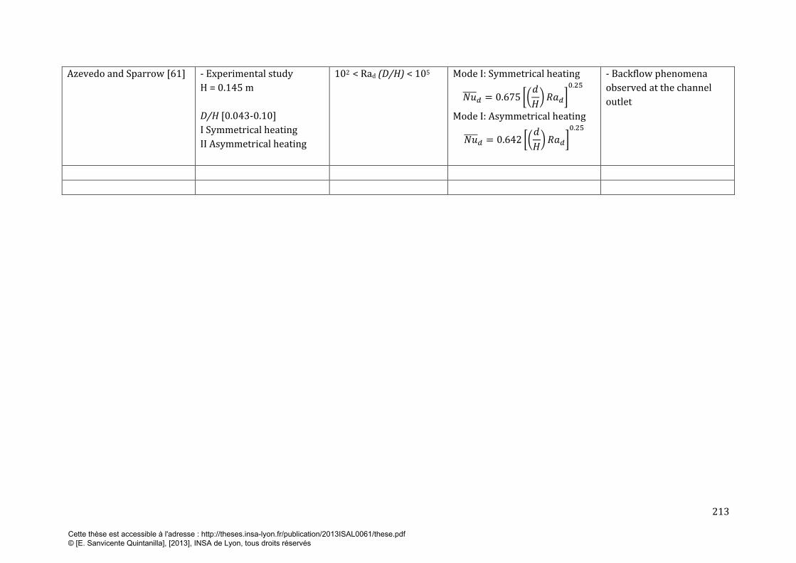
213
Azevedo and Sparrow [61] - Experimental study
H = 0.145 m
D/H [0.043-0.10]
I Symmetrical heating
II Asymmetrical heating
102 < Rad (D/H) < 105 Mode I: Symmetrical heating
Mode I: Asymmetrical heating
- Backflow phenomena
observed at the channel
outlet
Cette thèse est accessible à l'adresse : http://theses.insa-lyon.fr/publication/2013ISAL0061/these.pdf © [E. Sanvicente Quintanilla], [2013], INSA de Lyon, tous droits réservés

214
Cette thèse est accessible à l'adresse : http://theses.insa-lyon.fr/publication/2013ISAL0061/these.pdf © [E. Sanvicente Quintanilla], [2013], INSA de Lyon, tous droits réservés

215
Appendix B EMPIRICAL CORRELATIONS
In Table B1 is included a summary of the experimental studies conducted in open-ended channels where the optimum channel aspect ratio was investigated. Two main objectives are established corresponding to the application: Minimizing the temperatures at the walls and maximizing the induced mass flow rate.
Table B1-Summary of experimental investigations on the optimum channel aspect ratio.
Reference Experimental
conditions
Investigated
D/H range
*Criteria
**Objective
Optimum D/H?
Onur&Aktas
[71]
H = 0.3 m
Assym. Heating, UWT
∆T= 11.6 °C
RaH* = [107 - 108]
[0.015 - 0.22]
*Maximum wall
heat transfer
**Cooling of
electronic devices
0.05
Brinkworth&Sandberg
[8]
H = 5 m
Assym. Heating, UHF
200 W/m2 RaH* = 106
[--]
*Minimum wall
temperatures
**Cooling PV
modules
0.05
Chen et al.
[27]
H = 1.5 m
Assym. Heating, UHF
[200-600 W/m2]
[0.06 - 0.4]
*Maximum airflow
rate
**Ventilation
no
Burek et al.
[44]
H = 1.025 m
Assym. Heating, UHF
[200-1000 W/m2] RaH*=[10 10- 1013]
[0.019 - 0.11]
*Maximum airflow
rate
**Ventilation
no
La Pica et al.
[45]
H = 2.6 m
Assym. Heating, UHF
[48-317 W/m2] RaH*=1013
[0.022 - 0.065] *Ventilation
**Cooling no
Bouchair
[46]
H = 2 m
Assym. Heating, UHF
[--]
*Maximum airflow
rate
**Ventilation
~ 0.1
Fossa et al.
[47]
H = 1.98 m
Assym. Heating, UHF
[75 - 200 W/m2] RaD/H* = 103-107
[0.018 - 0.1]
*Minimum wall
temperatures
**Cooling of PV
modules
~ 0.06
Cette thèse est accessible à l'adresse : http://theses.insa-lyon.fr/publication/2013ISAL0061/these.pdf © [E. Sanvicente Quintanilla], [2013], INSA de Lyon, tous droits réservés

216
In Table B2 is included a summary of empirical correlations obtained in open ended channels, which relate the Rayleigh number and the induced mass flow rate. The flow conditions are highlighted for ach case in the the last column of the table.
Table B2-Summary of empirical correlations relating the Rayleigh number and mass flow rate.
Author-Reference Experimental conditions
Investigated Ra* range
Correlation Comments
Flow conditions
Burek et al. [44]
H = 1.025 m Assym. Heating, UHF d/H [0.019-0.11]
[200-1000 ]W/m2 Ra*=
Mass flow rate represented by Re number
Laminar Transition
La Pica et al. ç [45]
H = 2.6 m Assym. Heating, UHF d/H [0.022-0.065]
[48-317 W/m2] Ra*=
represented by Re number
Turbulent
Moshfeh&Sandberg [50]
H = 6.5 m Assym. Heating, UHF d/H [0.001-0.05]
[50-300 W/m2] Ra*=
(50-100 W/m2) (200-400 W/m2)
Laminar-
Turbulent
Chen et al. [27]
H = 1.5 m Assym. Heating, UHF d/H [0.06-0.4]
[200-600 W/m2]
no correlation given
-----
Ayinde et al. [118]
H = 0.68 m Sym. Heating, UWT d/H [0.08 -0.32]
Ra* [2.106 - 8.106]
represented by the dimensionless volume airflow rate
Turbulent
Yilmaz&Fraser [116]
H = 3 m Assym. Heating, UWT d/H [0.033]
Ra* []
Tw [60-130]
represented by the dimensionless volume airflow rate
Turbulent
Cette thèse est accessible à l'adresse : http://theses.insa-lyon.fr/publication/2013ISAL0061/these.pdf © [E. Sanvicente Quintanilla], [2013], INSA de Lyon, tous droits réservés

217
Appendix C SKETCHES OF THE R-DEVICE
Tilting support details
The method to support the framework when testing at non vertical angles is base on the use of
links of lengths, which are related to a given angle, to support the frame. In the present
investigation, three holes were made in the link corresponding to the angles θ = 30°, 45° and 60°
with respect to the horizontal plane. Figure bellow shows how the system will work.
Simple locking plates and retainer plates were also made to ensure that frame 2 can be easily
locked in place and prevent frame 2 from coming off the horizontal supports.
Figure B-1: Diagram showing how the link will control
the channel slope.
Main structure of the panels
Figure C-2 shows the geometry of a single wall, viewed from the back (non heated) side. All
dimensions are in millimetres and the drawing is in scale. Each bakelite panel has dimensions
800x1960 mm and it is mounted on two timber ribs (35x70x2300 mm) by screws and glue. Each
rib was equipped with 8 screwed (female) inserts, M8 screw on the back and with 6 M6 inserts
on the side, in order to allow standard mechanical fastening to other structures, including the
metal frame.
In Figure C-2 can also be seen the grid of pass-through for thermocouples has 3 vertical columns
and 40 rows: the vertical distance of the holes is 50mm and the horizontal distance is 180mm.
The drilled holes are 50mm depth and have a diameter of 1.5 mm (see schema of Figure C-3).
Each hole is in correspondence of the centre of the heating element of each run of the spiral
shaped heater. A drawing of the heater is presented in Figure C-4.
Cette thèse est accessible à l'adresse : http://theses.insa-lyon.fr/publication/2013ISAL0061/these.pdf © [E. Sanvicente Quintanilla], [2013], INSA de Lyon, tous droits réservés
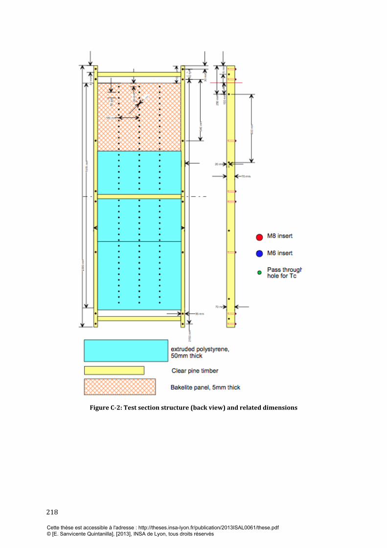
218
Figure C-2: Test section structure (back view) and related dimensions
Cette thèse est accessible à l'adresse : http://theses.insa-lyon.fr/publication/2013ISAL0061/these.pdf © [E. Sanvicente Quintanilla], [2013], INSA de Lyon, tous droits réservés

219
FigureC-3: Schema of the drilled holes in the insulation material and bakelite plate used to
insert the thermocouples. Detail of one heating band.
FigureC-4: Detail of Heater (yellow) and connector
(cyan) geometry.
Screens placed in the outlet of the channel
In Figure below is represented the position of the screens placed in the outlet of the channel in
order to reduce principally radiation from the top heater to the surroundings and to avoid some
macrocirculations at top level, due to some parasite flows developing in the lab.
Figure C-5: Detail of Heater (yellow) and connector (cyan) geometry.
Cette thèse est accessible à l'adresse : http://theses.insa-lyon.fr/publication/2013ISAL0061/these.pdf © [E. Sanvicente Quintanilla], [2013], INSA de Lyon, tous droits réservés

220
Cette thèse est accessible à l'adresse : http://theses.insa-lyon.fr/publication/2013ISAL0061/these.pdf © [E. Sanvicente Quintanilla], [2013], INSA de Lyon, tous droits réservés

221
Appendix D A THEORETICAL ANALYSIS OF THE RESPONSE
OF THERMOCOUPLES
In this section, we present the detail calculations of the functional relationships developed
between the temperature measured by a thermocouple, which is in contact with a surface and
the actual temperature of that surface. The temperature of the surrounding fluid, the heat
conducted from the thermocouple bead through the thermocouple wire and the heat radiated by
the bead to the surroundings are taken into account in this relation.
We suppose that a thermocouple bead is intended to measure the temperature of a surface
covered by a layer of insulation material.
The bead is assumed to be a perfect sphere except for the portion in contact with the surface.
This part of the bead may be deformed by the contact with the surface, but the rest of it remains
a perfect sphere.
As may be seen in Figure D-1, we refer the area of the bead in contact in contact with the surface
so as to Ac. Therefore, the area of the bead which is in contact with the fluid, in this case, air, is
, in which D is the diameter of the sphere (the bead).
Figure D-1: Schema of a thermocouple wire inserted
through a hole drilled in insulation.
The four modes by which heat can be transferred from the bead and to the bead are the
following:
conduction through the area that is in contact with the surface, Qc;
convection to the fluid in contact, Qconv ;
conduction through the thermocouple wires, Qcond
radiation from or to the surroundings, Qrad.
4p D2 - A
c
Cette thèse est accessible à l'adresse : http://theses.insa-lyon.fr/publication/2013ISAL0061/these.pdf © [E. Sanvicente Quintanilla], [2013], INSA de Lyon, tous droits réservés
222
Since the insulation had been removed, the temperature of the foil facing the hole would have dropped a little from its value when insulated. But, because the hole was small relative to the total area of the heating foil, and it was conducting, the effect on the temperature in the vicinity of the hole would have been quite small. Further, the foil was thin, 8 μm, so that the difference in temperature between the two surfaces would have been very small, so that, for all practical purposes the temperature of the surface being measured by the thermocouple is the temperature of the “front” heating foil in its vicinity. As a consequence, the discussion in this firs case is limited to the problem of accurately measuring the temperature of that surface.
On the assumption that the temperature of the bead, Tb, is uniform throughout the bead, then the rate of heat transfer from the surface at a temperature, Ts, is
, (1)
in which Rc is the thermal contact resistance between the bead and he surface. The convective heat transfer can be evaluated from the convective heat transfer coefficient h and the fluid temperature Tf by
. (2)
The heat losses by conduction along the thermocouple wires are dependent on the design of the thermocouple and the insulation thickness and material, but they can be expressed as,
, (3)
For simplicity, because the wires running between the thermocouple and the measuring device pass through a range of temperatures, Ta is taken as the mean temperature along the wires and that Kcond is a constant. Finally the radiation losses or gains for the conditions assumed here can be reasonably expressed by
(4)
In which Krad is a constant and T0 is the temperature of the surrounding surfaces. The bead could be radiating to several surfaces at different temperatures and each could be included in equation (4) and there would be a different Krad for each temperature. In fact each Krad is not a constant, but for small excursions in temperature they are nearly constant.
Qc =
Ts − Tb
Rc
Qconv = h(4π D2 − Ac)(Tf − Tb)
Qcond = Kcond(Ta − Tb)
Qrad = Krad (T0 − Tb)
Cette thèse est accessible à l'adresse : http://theses.insa-lyon.fr/publication/2013ISAL0061/these.pdf © [E. Sanvicente Quintanilla], [2013], INSA de Lyon, tous droits réservés
223
Thus, the total heat transferred to the bulb is
(5)
The substitution of Equations (1-4) in Equation (5), leads to
, (6)
The temperature change in the bead is related to the rate of heat transfer by
, (7)
in which C is the specific heat capacity of the material of the bead and ρ its density and t is time. It follows from equations (6) and (7) that
(8)
Equation (8) can be rewritten as
(8a)
Dividing both sides of equation (8a) by , leads to
.
(8b)
Q = Qc + Qconv + Qcond + Qrad
Q =
Ts − Tb
Rc
+ h(4π D2 − Ac)(Tf − Tb) + Kcond (Ta − Tb) + Krad (T0 − Tb)
Q = 4
3Cρπ D3 dTb
dt
4
3Cρπ D3 dTb
dt=
Ts − Tb
Rc
+ h(4π D2 − Ac)(Tf − Tb) + Kcond (Ta − Tb) + Krad (T0 − Tb).
4
3Cρπ D3 dTb
dt=
Ts
Rc
+ h(4π D2 − Ac)Tf + KcondTa + KradTo
−Tb
1
Rc
+ h(4π D2 − Ac) + Kcond + Krad
.
1
Rc
+ h(4π D2 − Ac) + Kcond + Krad
43
Cρπ D3
1Rc
+ h(4π D2 − Ac) + Kcond + Krad
dTb
dt=
Ts
Rc
+ h(4π D2 − Ac)Tf + KcondTa + KradTo
1Rc
+ h(4π D2 − Ac) + Kcond + Krad
− Tb
Cette thèse est accessible à l'adresse : http://theses.insa-lyon.fr/publication/2013ISAL0061/these.pdf © [E. Sanvicente Quintanilla], [2013], INSA de Lyon, tous droits réservés
224
Equations (8-8b) can be applied whether Ts, T0, Ta and Tf are constants or whether they depend of time. In the case in which a steady state has been established and the thermocouple is brought into contact with the surface, Ts, To, Ta and Tf are constants and equation (8b) can then be written as
, (8c)
in which are constants ,which are expressed as
(9)
and
. (10)
From equation (8c) it follows that
, (11)
in which Tbin is the initial temperature of the bead. The integration of Equation (11) yields,
. (12)
It follows that the solution for the bead temperature as a function of time is
. (13)
Then, the equilibrium temperature of the bead, , at , is given by
. (14)
K1
dTb
dt= K2 − Tb
K1andK2
K1 =
43
Cρπ D3
1Rc
+ h(4π D2 − Ac) + Kcond + Krad
K2 =
Ts
Rc
+ h(4π D2 − Ac)Tf + KcondTa + KradTo
1Rc
+ h(4π D2 − Ac) + Kcond + Krad
dTK2 − TTbin
Tb
∫ = dτK10
t
∫
ln
K2 − Tb
K2 − Tbin
= − t
K1
Tb = K2 − (K2 − Tbin)e− t
K1
Tb∞ t = ∞
Tb∞ = K2 =
Ts
Rc
+ h(4π D2 − Ac)Tf + KcondTa + KradTo
1Rc
+ h(4π D2 − Ac) + Kcond + Krad
Cette thèse est accessible à l'adresse : http://theses.insa-lyon.fr/publication/2013ISAL0061/these.pdf © [E. Sanvicente Quintanilla], [2013], INSA de Lyon, tous droits réservés
225
We can see from equation (14) that if there were no heat losses or gains by radiation, no losses through the thermocouple wires or if the fluid temperature Tf is equal to Ts, then the final temperature of the bead would be Ts. This represents the perfect conditions. However, if all heat transfer modes are present, the temperature reading given by the thermocouple will depend on all four temperatures Ts, To, Tf and Ta. The design of the thermocouples, the physical properties of the fluid and the surfaces of the surroundings, will also affect. For instance, when thermocouples are submerged in conductive liquids such as water, they are particularly susceptible to noise, which is a common source of error. This relation shows the conditions necessary for measuring the correct temperature and how careful one needs to be in order to get the correct temperature value. Relationships such as that equation (13) are often written as
, (15)
in which tc is the time constant. In this case the time constant is given by,
. (16)
Since all the terms in the denominator of equation (16) could be of the same order, the time constant would be significantly lower than if the bead were perfectly insulated except for the area of contact, that is when h, Kcond and Krad were zero. Finally, as would have been expected, the density and thermal conductivity of the material of the bead appear only in the time constant and affect only the rate at which the temperature of the bead changes, but not the its final value. Whilst, the magnitude of the terms representing convection, conduction through the thermocouple wires and radiation depend on the circumstances, it is clear that they have a major influence on the temperature that the thermocouple bead “feels” and therefore its temperature reading as well as the rate that it responds to changes.
Tb = K2 − (K2 − Tbin)e− t
tc
tc = K1 =
43
Cρπ D3
1Rc
+ h(4π D2 − Ac) + Kcond + Krad
Cette thèse est accessible à l'adresse : http://theses.insa-lyon.fr/publication/2013ISAL0061/these.pdf © [E. Sanvicente Quintanilla], [2013], INSA de Lyon, tous droits réservés

226
Temperature of the bulb starting from the fluid temperature. Suppose that the heat transfer through the foil is one-dimensional. If the foil is very thin the temperature of the foil is then uniform so that both sides of the foil are at the same temperature. The heat transfer from the fluid to the foil is then (17)
in which TF is the temperature of the fluid cooling the foil. On the assumption that the heat transfer at the rear of the foil is negligibly small, the rate of change of the temperature in the foil is given by
, (18)
in which w is the thickness of the foil and the subscript s refers to the foil and qe is the electrical energy per unit area (heat flux) supplied to the foil. By the same argument as above, it follows that
(19)
which can be rewritten as
(20a)
Now suppose that the foil has an initial temperature Ts0 and is then brought in contact with a fluid at a constant temperature TF and at the same time the heating is turned on. Assume further that hw and qe are constant. Equation (20) can be written as
(20b)
in which
(21)
and
(22)
Equation (20b) can be formulated as
(23)
which on integration yields
Qh = hwAc(Ts − TF ) ,
Qh = qeAc − ρsCsAcw
dTs
dt
hwAc(Ts − TF ) = qeAc − ρsCsAcw
dTs
dt
ρsCsw
dTs
dt= (qe + hwTF ) − hwTs .
K3
dTs
dt= K4 − Ts ,
K3 =
ρsCsw
hw
K4 =
qe
hw
+ TF .
dTT − K4Ts0
Ts
∫ = − dτK30
t
∫
Cette thèse est accessible à l'adresse : http://theses.insa-lyon.fr/publication/2013ISAL0061/these.pdf © [E. Sanvicente Quintanilla], [2013], INSA de Lyon, tous droits réservés
227
(24)
which becomes
(25)
so that
(26)
The final temperature of the surface, , given by
(27)
and is the time constant of the foil given by
(28)
Since equation (8) applies whether the surface temperature is constant or not, the substitution of equation (26) for the surface temperature in equation (5) yields,
(29)
Equation (29) can be rewritten as
(30)
ln
Ts − K4
Ts0 − K4
= − t
K3
Ts = K4 + Ts0 − K4( )e
− tK3
Ts = TF +
qe
hw
+ (Ts0 − TF ) −qe
hw
e
− ttcs
Tsfin
Tsfin = TF +
qe
hw
tcs
tcs = K3 =
ρsCsw
hw
.
43
Cρπ D3 dTb
dt=
TF +qe
hw
+ (Ts0 − TF ) −qe
hw
e
− ttcs − Tb
Rc
+ h(4π D2 − Ac)(Tf − Tb) + Kcond (Ta − Tb) + Krad (T0 − Tb).
dTb
dt+
31Rc
+ h(4π D2 − Ac) + Kcond + Krad
4Cρπ D3Tb =
3 TF +qe
hw
+ (Ts0 − TF ) −qe
hw
e
− ttcs
4RcCρπ D3+
3 h(4π D2 − Ac)Tf + KcondTa + KradT0
4Cρπ D3.
Cette thèse est accessible à l'adresse : http://theses.insa-lyon.fr/publication/2013ISAL0061/these.pdf © [E. Sanvicente Quintanilla], [2013], INSA de Lyon, tous droits réservés
228
Equation (30) can be simplified to
(31)
in which
(32)
and
(33)
Multiplying equation (31) by the integrating factor , that is by it becomes
(34)
The integration of equation (34) yields
(35)
The bulb temperature therefore becomes
(36)
When , so that
(37)
so that C is given by
(38)
dTb
dt+ K5Tb = K6 + Ts0 − K4( )e
− t
K3
K5 = 1
K1
=3
1Rc
+ h(4π D2 − Ac) + Kcond + Krad
4Cρπ D3
K6 =
3 TF +qe
hw
4RcCρπ D3+
3 h(4π D2 − Ac)Tf + KcondTa + KradT0
4Cρπ D3
eK5t e
− tK1
d Tbe1
K1
t
dt= K6e
1K1
t
+ Ts0 − K4( )e1K1
− 1K3
t
Tbe
1K1
t
= K1K6e1K1
t
+K1K3 Ts0 − K4( )
K3 − K1
e
1
K1
− 1
K3
t
+ C
Tb = K1K6 +
K1K3 Ts0 − K4( )K3 − K1
e− t
K3 + Ce− t
K1
t = 0 Tb = Tbin
Tbin = K
1K
6+
K1K
3Ts0
− K4( )
K3
− K1
+ C ,
C = Tbin − K1K6 −
K1K3 Ts0 − K4( )K3 − K1
.
Cette thèse est accessible à l'adresse : http://theses.insa-lyon.fr/publication/2013ISAL0061/these.pdf © [E. Sanvicente Quintanilla], [2013], INSA de Lyon, tous droits réservés
229
The bulb temperature is therefore,
(39a)
which can be rearranged to give
(39b)
The final temperature of the bulb is
(40)
which once again becomes the foil temperature if all the extraneous effects are not present. There are now two time constants, the first is the time constant of the foil and as may have
been expected the second is the time constant of the thermocouple . They interact in the
second term on the right hand side of equation (39b). Equation (40) can be written as
(41)
It should be noted that equation (41) was derived on the assumption of a steady fluid temperature TF. The only place in equation (41) that the fluid temperature, TF, appears in Tbfin, defined in equation (40), and in the last term on the right hand side of the equation. Therefore a fluctuating fluid temperature could only be estimated accurately, if both time constants were very small and if all the large number of parameters, in particular, hw, the coefficient of convective heat transfer, were known with some accuracy.
Tb = K1K6 +K1K3 Ts0 − K4( )
K3 − K1
e− t
K3 + Tbin − K1K6 −K1K3 Ts0 − K4( )
K3 − K1
e
− tK1 .
Tb = K1K6 1− e− t
K1
+K1K3
K3 − K1
Ts0 −qe
hw
+ TF
e
− tK3 − e
− tK1
+ Tbin( )e− t
K1 .
Tbfin = K1K6 =
1Rc
TF +qe
hw
+ h(4π D2 − Ac)Tf + KcondTa + KradT0
1Rc
+ h(4π D2 − Ac) + Kcond + Krad
,
tcs
tc
Tb = Tbfin − Tbfin − Tbin( )e− t
K1 +K1K3
K3 − K1
Ts0 −qe
hw
+ TF
e
− tK3 − e
− tK1
.
Cette thèse est accessible à l'adresse : http://theses.insa-lyon.fr/publication/2013ISAL0061/these.pdf © [E. Sanvicente Quintanilla], [2013], INSA de Lyon, tous droits réservés

230
Cette thèse est accessible à l'adresse : http://theses.insa-lyon.fr/publication/2013ISAL0061/these.pdf © [E. Sanvicente Quintanilla], [2013], INSA de Lyon, tous droits réservés

231
Appendix E Uncertainty calculation
The uncertainty analysis of the measurements presented in this work has been performed
according the procedure described by Moffat [145] and ASME15 codes. By international
agreement, uncertainties are estimated at the 95% confidence level for most work. In this
appendix are discussed and estimated the overall uncertainties in the velocity measurements, in
the mass flow rate calculations and in the local convective heat transfer coefficients.
The overall uncertainty assigned to a given measurement is the combination of fixed and
randoms errors. The fixed errors, namely systematic errors, are introduced by the
instrumentation used such as the thermocouples and the PIV system and have been estimated
experimentally and from manufacturer’s specifications. In the present study the random errors
are introduced by the ambient test conditions that were seen to vary from one test to another.
As demonstrated in Chapter 3, the initial turbulent intensity which depends on the experiment
had a strong influence on the development of the flow and discrepancies in the repeteability
tests of both the mean wall temperatures and flow velocities were found. According to ASME14,
treating these discrepancies as a fixed error may not be valid since they origin not because the
measurements are in error, but because the physical situation is different as we have seen in the
present study.
The overall uncertainty assigned to a given measurement R is then expressed as the root-sum-square combination of both sources of errors as follows:
(51)
When calculating the overall uncertainty in an experimental result, such as in the local
convective heat transfer coefficients (h) and in the induced mass flow rates ( , the contribution
of the systematic errors, , is evaluated in terms of the sensitivity coefficients of the result to
the measured quantities following the propagation equation of Kline and McClintock [186]
shown in relation (52),
(52)
In the above equation, represents the measured variable, such as the mass
flow rate; the uncertainty of the measured variable ; , each variable that effect the
measured quantity, such as in the case of mass flow rate, the velocity, density and cross section
of the channel; and the uncertainty in each of these variables. The partial derivaties are the
sensitivities of with respect to each .
15 Policy on reporting uncertainties in Experimental measurements and results, accessed December 2012, <http://heattransfer.asmedigitalcollection.asme.org>.
Cette thèse est accessible à l'adresse : http://theses.insa-lyon.fr/publication/2013ISAL0061/these.pdf © [E. Sanvicente Quintanilla], [2013], INSA de Lyon, tous droits réservés
232
The random errors introduced by the variability of the ambient conditions are calculated for the
measured quantities as shown equation below:
(53)
in which is an statistic function, namely student number, and is the standard deviation
of the set of repetitions tests. The value of the student number for four repetition tests is t = 4.60
as detailed in [187].
Uncertainty on PIV mean velocity
The systematic errors, , introduced in the PIV measurements are related to inadequacy of the
parameters selected. The factors contributing to the uncertainty are mainly categorized in three
groups:
1) Parameters related to the laser and seeding procedure: In this group we consider
inadequate time interval between the light pulses and the concentration of particles.
2) Parameters related to the calibration of the camera and the recording of images: In
this group we consider inadequate diameter of the image of the particle, which is directly
linked to the magnification factor of the camera selected, and the effect of background
noise in the images.
3) Parameters related to method for evaluating the data: In this group we mainly
consider the size of the interrogation windows.
The uncertainty magnitude is assigned to a single displacement vector which is representative of
the mean velocity in a particular section. The effect of these parameters, interrelated in most
cases, is analyzed for each PIV system (F-device and R-device) by comparing them with the
results obtained by Raffel et al. [136], which are presented below in Figures E-1 to E-6. Details of
the calculation are included in Table E-1 for the F-device and Table E-2 for the R-device.
The uncertainty on the mean displacement introduced by the systematic errors is estimated to
be 0.23 pixels for the F-device (see Table E-1) and 0.21 pixels for the R-device (see Table E-2).
For a mean displacement on the range of 4 to 6 pixels, the magnitude of the uncertainty in the
mean velocity due to the PIV instrumentation is estimated between 3.5%-6%.
The random errors associated to the PIV measurements due to the variability of the ambient
conditions are quantified only for the F-device, where repeteability was analyzed in terms of
velocity measurements. Four tests were conducted above mid-height, y/H = 0.54 (Chapter 3,
section 3.3.2) and the average velocity across the channel width was 0.254 m/s, 0.248 m/s,
0.249 m/s and 0.283 m/s for respectively, Tests 1, 2, 3 and 4. Using these values in equation (53)
we obtain a random error of magnitude, .
In the F-device, the magnitude of the overall uncertainty on the mean velocity, for an average
velocity of 0.259 m/s measured at mid height section (Chapter 3, section 3.3.2) and taking into
account the systematic and random errors as was shown in equation (51), is estimated to be of,
(54)
Note that the value of 0.015 m/s corresponds to the maximum uncertainty introduced by the
systematic errors which is of 6% of the average velocity of the four tests conducted at mid-
height section. As may be seen in the equation (54), the higher uncertainty in the velocity
measurements conducted in the F-device compared to the one estimated for the R-device (max.
Cette thèse est accessible à l'adresse : http://theses.insa-lyon.fr/publication/2013ISAL0061/these.pdf © [E. Sanvicente Quintanilla], [2013], INSA de Lyon, tous droits réservés
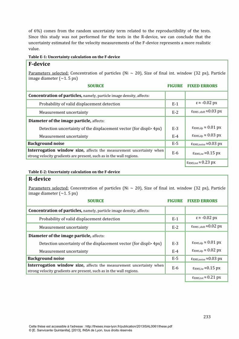
233
of 6%) comes from the random uncertainty term related to the reproductibility of the tests.
Since this study was not performed for the tests in the R-device, we can conclude that the
uncertainty estimated for the velocity measurements of the F-device represents a more realistic
value.
Table E-1: Uncertainty calculation on the F-device
F-device
Parameters selected: Concentration of particles (Ni ~ 20), Size of final int. window (32 px), Particle image diameter (~1. 5 px)
SOURCE FIGURE FIXED ERRORS
Concentration of particles, namely, particle image density, affects:
Probability of valid displacement detection E-1 ε ≈ -0.02 px
Measurement uncertainty E-2 εRMS ,shift ≈0.03 px
Diameter of the image particle, affects:
Detection uncertainty of the displacement vector (for displ> 4px) E-3 εRMS,dp ≈ 0.01 px
Measurement uncertainty E-4 εRMS,dp ≈ 0.03 px
Background noise E-5 εRMS,noise ≈0.03 px
Interrogation window size, affects the measurement uncertainty when
strong velocity gradients are present, such as in the wall regions. E-6 εRMS,iw ≈0.15 px
εRMS,tot ≈ 0.23 px
Table E-2: Uncertainty calculation on the F-device
R-device
Parameters selected: Concentration of particles (Ni ~ 20), Size of final int. window (32 px), Particle image diameter (~1. 5 px)
SOURCE FIGURE FIXED ERRORS
Concentration of particles, namely, particle image density, affects:
Probability of valid displacement detection E-1 ε ≈ -0.02 px
Measurement uncertainty E-2 εRMS ,shift ≈0.02 px
Diameter of the image particle, affects:
Detection uncertainty of the displacement vector (for displ> 4px) E-3 εRMS,dp ≈ 0.01 px
Measurement uncertainty E-4 εRMS,dp ≈ 0.02 px
Background noise E-5 εRMS,noise ≈0.03 px
Interrogation window size, affects the measurement uncertainty when
strong velocity gradients are present, such as in the wall regions. E-6 εRMS,iw ≈0.15 px
εRMS,tot ≈ 0.21 px
Cette thèse est accessible à l'adresse : http://theses.insa-lyon.fr/publication/2013ISAL0061/these.pdf © [E. Sanvicente Quintanilla], [2013], INSA de Lyon, tous droits réservés

234
Results presented by Raffel et al. [136] in Chapter 5:
Figure E-1: Simulation results showing the difference between actual and measured displacement bias (dp
= 2.0 px)
Figure E-2: Measurement uncertainty for single exposure/double frame PIV as a function of particle
image shift for various particle image densities Ni (dp = 2.2 px)
Figure E-3: Monte Carlo simulation results for the measurement uncertainty in digital cross correlation
PIV evaluation as a function of particle image displacement.
Figure E-4: Measurement uncertainty in digital cross-correlation PIV evaluation with respect to varying
particle image diameter.
Figure E-5: Measurement uncertainty as a function of
the displacement and various amounts of white background noise (dp = 2.2 px).
Figure E-6: Measurement uncertainty as a function of the displacement gradients for various particle
images densities and interrogation window size (dp = 2.0 px).
Cette thèse est accessible à l'adresse : http://theses.insa-lyon.fr/publication/2013ISAL0061/these.pdf © [E. Sanvicente Quintanilla], [2013], INSA de Lyon, tous droits réservés

235
Uncertainty on the evaluation of the mass flow rate
The mass flow rate is evaluated at mid-height section of the channel (y/H = 0.54) as shown in
equation (55):
(55)
in which is the density of the fluid at a mean temperature , S corresponds to the cross
sectional area of the flow, S= LxD and to the time-average bulk fluid velocity at z/L = 0.5
obtained through integration of Vy over the width of the channel (D).
The order of magnitude of the uncertainty assigned to the present experimental result, , is
given by equation (56):
(56)
where,
(57)
(58)
(59)
(60)
The term corresponds to the error committed when assuming that represents the mean
velocity on each point of the depth of the channel (D). This error can be estimated through
comparison of the time-average velocity profiles measured at 5 different planes in the z-
direction, namely z/L = 0.27, 0.34, 0.5, 0.66 and 0.82. The results at mid-height of the channel are
presented in Figure E-7. The maximum difference between the mean velocities is estimated to
about 10%.
Figure E-7: Comparison of time-average velocity profiles at y/H = 0.54 and qs= 225
W/m2 obtaied in five different parallel planes in the z-direction.
Cette thèse est accessible à l'adresse : http://theses.insa-lyon.fr/publication/2013ISAL0061/these.pdf © [E. Sanvicente Quintanilla], [2013], INSA de Lyon, tous droits réservés
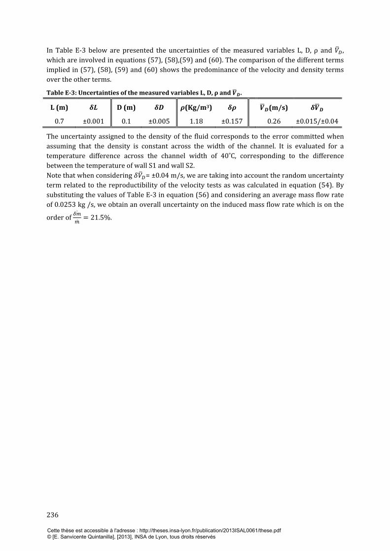
236
In Table E-3 below are presented the uncertainties of the measured variables L, D, ρ and ,
which are involved in equations (57), (58),(59) and (60). The comparison of the different terms
implied in (57), (58), (59) and (60) shows the predominance of the velocity and density terms
over the other terms.
Table E-3: Uncertainties of the measured variables L, D, ρ and .
L (m) D (m) (Kg/m3) (m/s)
0.7 ±0.001 0.1 ±0.005 1.18 ±0.157 0.26 ±0.015/±0.04
The uncertainty assigned to the density of the fluid corresponds to the error committed when
assuming that the density is constant across the width of the channel. It is evaluated for a
temperature difference across the channel width of 40˚C, corresponding to the difference
between the temperature of wall S1 and wall S2.
Note that when considering = ±0.04 m/s, we are taking into account the random uncertainty
term related to the reproductibility of the velocity tests as was calculated in equation (54). By
substituting the values of Table E-3 in equation (56) and considering an average mass flow rate
of 0.0253 kg /s, we obtain an overall uncertainty on the induced mass flow rate which is on the
order of
Cette thèse est accessible à l'adresse : http://theses.insa-lyon.fr/publication/2013ISAL0061/these.pdf © [E. Sanvicente Quintanilla], [2013], INSA de Lyon, tous droits réservés
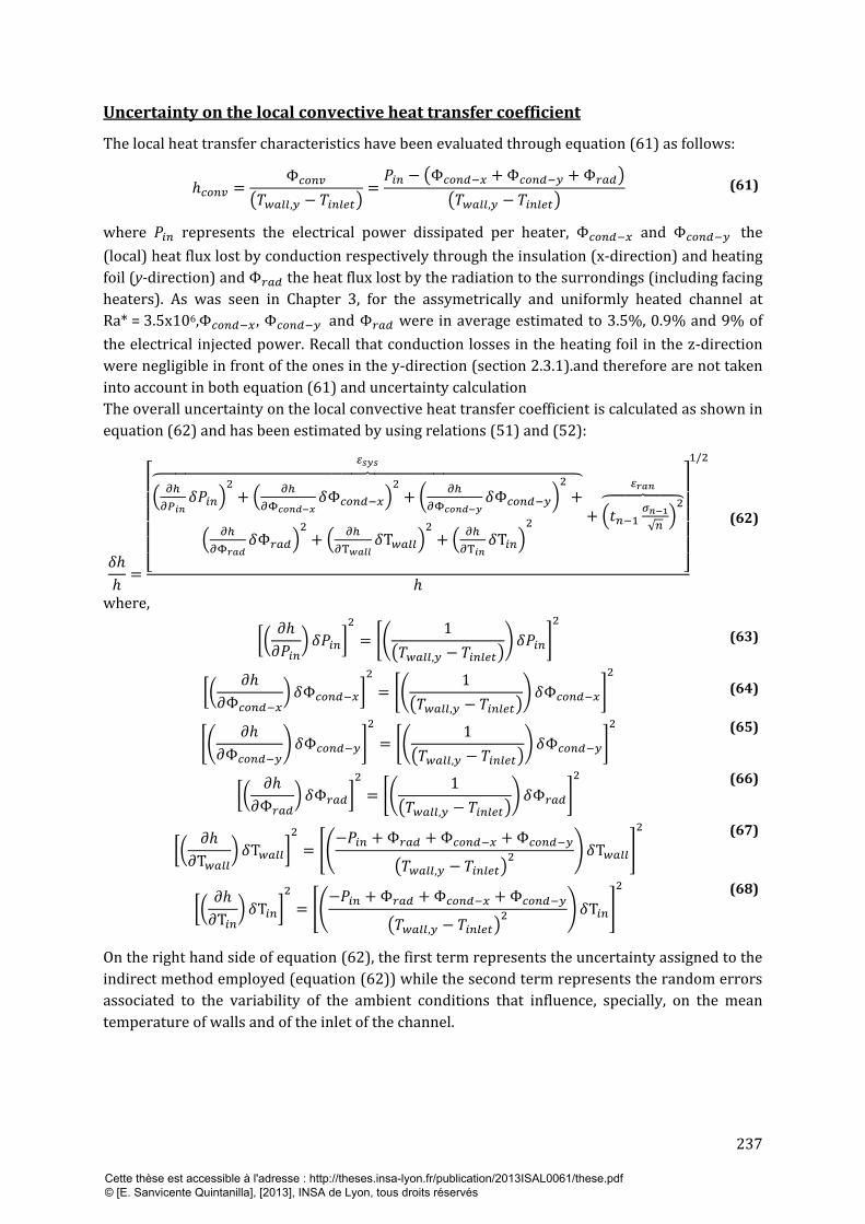
237
Uncertainty on the local convective heat transfer coefficient
The local heat transfer characteristics have been evaluated through equation (61) as follows:
(61)
where represents the electrical power dissipated per heater, and the
(local) heat flux lost by conduction respectively through the insulation (x-direction) and heating
foil (y-direction) and the heat flux lost by the radiation to the surrondings (including facing
heaters). As was seen in Chapter 3, for the assymetrically and uniformly heated channel at
Ra* = 3.5x10⁶, , and were in average estimated to 3.5%, 0.9% and 9% of
the electrical injected power. Recall that conduction losses in the heating foil in the z-direction
were negligible in front of the ones in the y-direction (section 2.3.1).and therefore are not taken
into account in both equation (61) and uncertainty calculation
The overall uncertainty on the local convective heat transfer coefficient is calculated as shown in
equation (62) and has been estimated by using relations (51) and (52):
(62)
where,
(63)
(64)
(65)
(66)
(67)
(68)
On the right hand side of equation (62), the first term represents the uncertainty assigned to the
indirect method employed (equation (62)) while the second term represents the random errors
associated to the variability of the ambient conditions that influence, specially, on the mean
temperature of walls and of the inlet of the channel.
Cette thèse est accessible à l'adresse : http://theses.insa-lyon.fr/publication/2013ISAL0061/these.pdf © [E. Sanvicente Quintanilla], [2013], INSA de Lyon, tous droits réservés
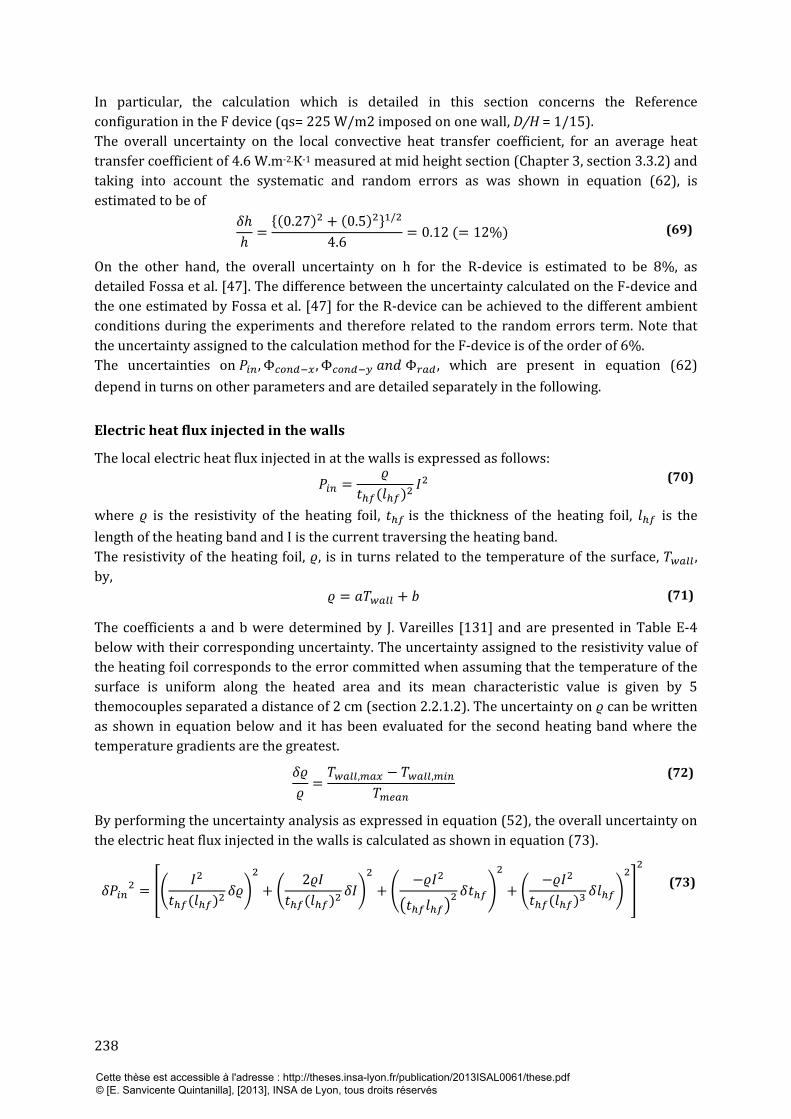
238
In particular, the calculation which is detailed in this section concerns the Reference
configuration in the F device (qs= 225 W/m2 imposed on one wall, D/H = 1/15).
The overall uncertainty on the local convective heat transfer coefficient, for an average heat
transfer coefficient of 4.6 W.m-2.K-1 measured at mid height section (Chapter 3, section 3.3.2) and
taking into account the systematic and random errors as was shown in equation (62), is
estimated to be of
(69)
On the other hand, the overall uncertainty on h for the R-device is estimated to be 8%, as
detailed Fossa et al. [47]. The difference between the uncertainty calculated on the F-device and
the one estimated by Fossa et al. [47] for the R-device can be achieved to the different ambient
conditions during the experiments and therefore related to the random errors term. Note that
the uncertainty assigned to the calculation method for the F-device is of the order of 6%.
The uncertainties on , which are present in equation (62)
depend in turns on other parameters and are detailed separately in the following.
Electric heat flux injected in the walls
The local electric heat flux injected in at the walls is expressed as follows:
(70)
where is the resistivity of the heating foil, is the thickness of the heating foil, is the
length of the heating band and I is the current traversing the heating band.
The resistivity of the heating foil, , is in turns related to the temperature of the surface, ,
by,
(71)
The coefficients a and b were determined by J. Vareilles [131] and are presented in Table E-4
below with their corresponding uncertainty. The uncertainty assigned to the resistivity value of
the heating foil corresponds to the error committed when assuming that the temperature of the
surface is uniform along the heated area and its mean characteristic value is given by 5
themocouples separated a distance of 2 cm (section 2.2.1.2). The uncertainty on can be written
as shown in equation below and it has been evaluated for the second heating band where the
temperature gradients are the greatest.
(72)
By performing the uncertainty analysis as expressed in equation (52), the overall uncertainty on
the electric heat flux injected in the walls is calculated as shown in equation (73).
(73)
Cette thèse est accessible à l'adresse : http://theses.insa-lyon.fr/publication/2013ISAL0061/these.pdf © [E. Sanvicente Quintanilla], [2013], INSA de Lyon, tous droits réservés
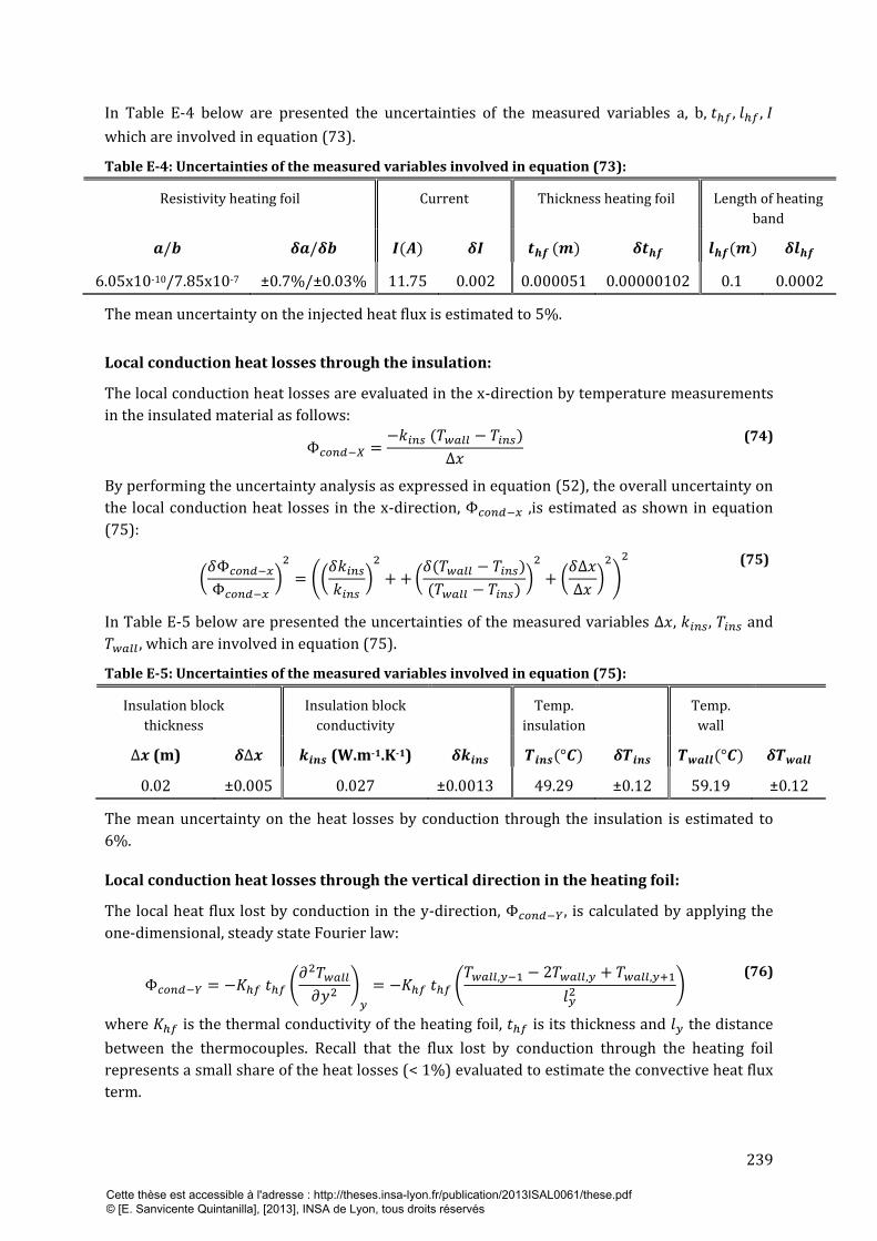
239
In Table E-4 below are presented the uncertainties of the measured variables a, b, , ,
which are involved in equation (73).
Table E-4: Uncertainties of the measured variables involved in equation (73):
Resistivity heating foil Current Thickness heating foil Length of heating
band
6.05x10⁻¹⁰/7.85x10-7 ±0.7%/±0.03% 11.75 0.002 0.000051 0.00000102 0.1 0.0002
The mean uncertainty on the injected heat flux is estimated to 5%.
Local conduction heat losses through the insulation:
The local conduction heat losses are evaluated in the x-direction by temperature measurements
in the insulated material as follows:
(74)
By performing the uncertainty analysis as expressed in equation (52), the overall uncertainty on
the local conduction heat losses in the x-direction, ,is estimated as shown in equation
(75):
(75)
In Table E-5 below are presented the uncertainties of the measured variables , , and
, which are involved in equation (75).
Table E-5: Uncertainties of the measured variables involved in equation (75):
Insulation block
thickness
Insulation block
conductivity
Temp.
insulation
Temp.
wall
(m) (W.m-1.K-1)
0.02 ±0.005 0.027 ±0.0013 49.29 ±0.12 59.19 ±0.12
The mean uncertainty on the heat losses by conduction through the insulation is estimated to
6%.
Local conduction heat losses through the vertical direction in the heating foil:
The local heat flux lost by conduction in the y-direction, , is calculated by applying the
one-dimensional, steady state Fourier law:
(76)
where is the thermal conductivity of the heating foil, is its thickness and the distance
between the thermocouples. Recall that the flux lost by conduction through the heating foil
represents a small share of the heat losses (< 1%) evaluated to estimate the convective heat flux
term.
Cette thèse est accessible à l'adresse : http://theses.insa-lyon.fr/publication/2013ISAL0061/these.pdf © [E. Sanvicente Quintanilla], [2013], INSA de Lyon, tous droits réservés
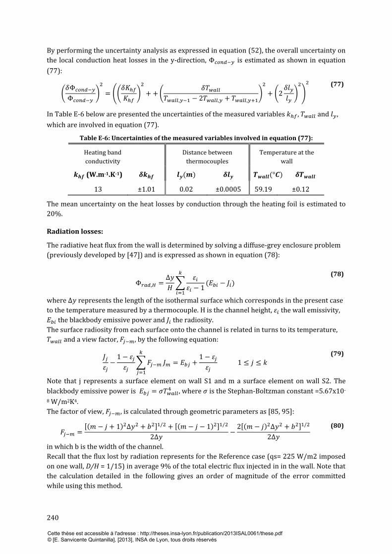
240
By performing the uncertainty analysis as expressed in equation (52), the overall uncertainty on
the local conduction heat losses in the y-direction, is estimated as shown in equation
(77):
(77)
In Table E-6 below are presented the uncertainties of the measured variables , and ,
which are involved in equation (77).
Table E-6: Uncertainties of the measured variables involved in equation (77):
Heating band
conductivity Distance between
thermocouples Temperature at the
wall
(W.m-1.K-1)
13 ±1.01 0.02 ±0.0005 59.19 ±0.12
The mean uncertainty on the heat losses by conduction through the heating foil is estimated to
20%.
Radiation losses:
The radiative heat flux from the wall is determined by solving a diffuse-grey enclosure problem
(previously developed by [47]) and is expressed as shown in equation (78):
(78)
where represents the length of the isothermal surface which corresponds in the present case
to the temperature measured by a thermocouple. H is the channel height, the wall emissivity,
the blackbody emissive power and the radiosity.
The surface radiosity from each surface onto the channel is related in turns to its temperature,
and a view factor, , by the following equation:
(79)
Note that j represents a surface element on wall S1 and m a surface element on wall S2. The
blackbody emissive power is , where is the Stephan-Boltzman constant =5.67x10-
8 W/m2K4.
The factor of view, , is calculated through geometric parameters as [85, 95]:
(80)
in which b is the width of the channel.
Recall that the flux lost by radiation represents for the Reference case (qs= 225 W/m2 imposed
on one wall, D/H = 1/15) in average 9% of the total electric flux injected in in the wall. Note that
the calculation detailed in the following gives an order of magnitude of the error committed
while using this method.
Cette thèse est accessible à l'adresse : http://theses.insa-lyon.fr/publication/2013ISAL0061/these.pdf © [E. Sanvicente Quintanilla], [2013], INSA de Lyon, tous droits réservés
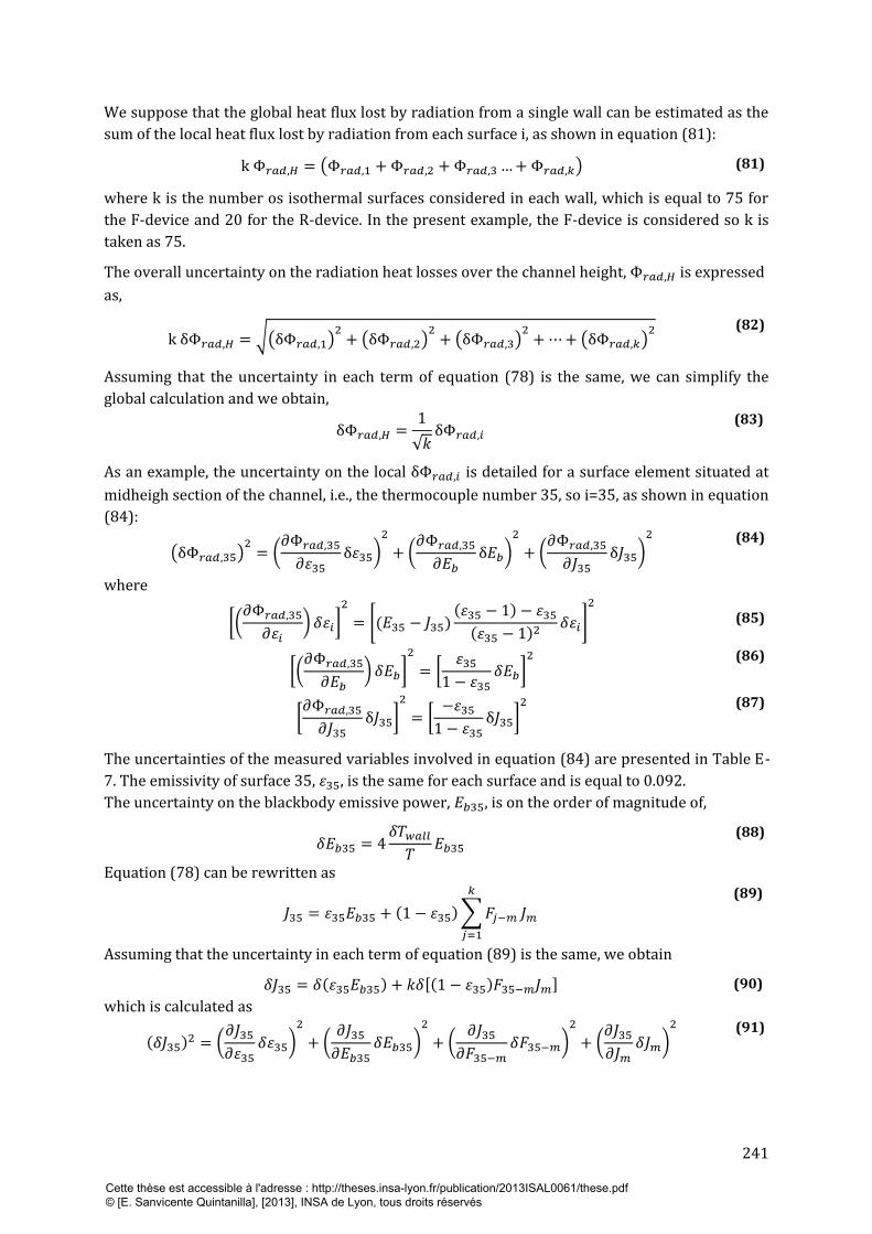
241
We suppose that the global heat flux lost by radiation from a single wall can be estimated as the
sum of the local heat flux lost by radiation from each surface i, as shown in equation (81):
(81)
where k is the number os isothermal surfaces considered in each wall, which is equal to 75 for
the F-device and 20 for the R-device. In the present example, the F-device is considered so k is
taken as 75.
The overall uncertainty on the radiation heat losses over the channel height, is expressed
as,
(82)
Assuming that the uncertainty in each term of equation (78) is the same, we can simplify the
global calculation and we obtain,
(83)
As an example, the uncertainty on the local is detailed for a surface element situated at
midheigh section of the channel, i.e., the thermocouple number 35, so i=35, as shown in equation
(84):
(84)
where
(85)
(86)
(87)
The uncertainties of the measured variables involved in equation (84) are presented in Table E-
7. The emissivity of surface 35, is the same for each surface and is equal to 0.092.
The uncertainty on the blackbody emissive power, , is on the order of magnitude of,
(88)
Equation (78) can be rewritten as
(89)
Assuming that the uncertainty in each term of equation (89) is the same, we obtain
(90)
which is calculated as
(91)
Cette thèse est accessible à l'adresse : http://theses.insa-lyon.fr/publication/2013ISAL0061/these.pdf © [E. Sanvicente Quintanilla], [2013], INSA de Lyon, tous droits réservés
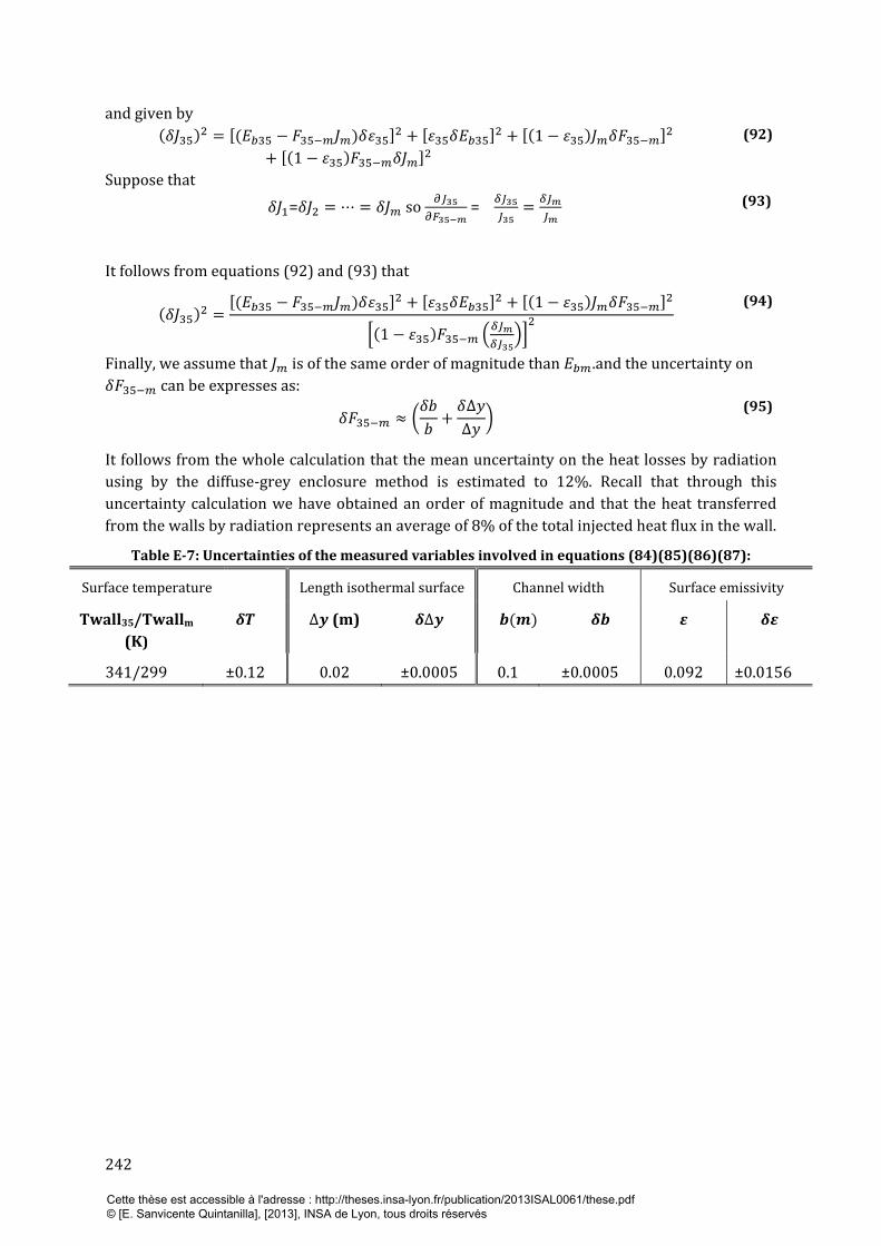
242
and given by
(92)
Suppose that
= so
=
(93)
It follows from equations (92) and (93) that
(94)
Finally, we assume that is of the same order of magnitude than .and the uncertainty on
can be expresses as:
(95)
It follows from the whole calculation that the mean uncertainty on the heat losses by radiation
using by the diffuse-grey enclosure method is estimated to 12%. Recall that through this
uncertainty calculation we have obtained an order of magnitude and that the heat transferred
from the walls by radiation represents an average of 8% of the total injected heat flux in the wall.
Table E-7: Uncertainties of the measured variables involved in equations (84)(85)(86)(87):
Surface temperature Length isothermal surface Channel width Surface emissivity
Twall35/Twallm
(K)
(m)
341/299 ±0.12 0.02 ±0.0005 0.1 ±0.0005 0.092 ±0.0156
Cette thèse est accessible à l'adresse : http://theses.insa-lyon.fr/publication/2013ISAL0061/these.pdf © [E. Sanvicente Quintanilla], [2013], INSA de Lyon, tous droits réservés

243
Appendix F CALIBRATION OF THERMOCOUPLES
In this appendix we include the thermocouple calibration data set of the experimental
arrangement used in the R-device to conduct temperature measurements. In particular, K-type
thermocouples with a wire diameter of 130µm were used.
Recall that the signals of these thermocouples were collected by a National Instrument Unit
having 3 slots and a built in sensor for cold junction compensation.
The thermocouples were calibrated by a precision platinium RTD sensor, model Hart Scientific
1502A, which had an accuracy of 0.05 ˚C. During the calibration the thermocouples were
connected to the National Instruments unit. Moreover, they were put inside a cylindrical copper
block, which was in turns immersed in the water solution of a thermostatic bath, together with
the reference sensor.
The calibration was conducted for 7 different temperature levels, with intervals of 10˚C, starting
from a temperature of 20 ˚C and finishing with a temperature of 80˚C. To avoid measurement
errors resulted from inmersing too many thermocouples in the thermostatic bath during the
calibration test, we have performed the calibration of all thermocouples in four different times.
In particular for each test 21 thermocouples were calibrated, with 7 thermocouples connected in
each slot.
The overall measurement instrumentation uncertainty (95%), considered equal to the double of
the standard deviation of the linear estimate according to the method proposed by [187], is
below 0.25 °C for each thermocouple sensor.
Table F-1 below shows an example of the constant coefficients a and b calculated after a
calibration test of 21 thermocouples. The uncertainty obtained at each level of temperature and
for each thermocouple of the example is reported in Figure F-1.
Figure F-1: Thermocouple temperature uncertainty
estimation at each temperature level and for each
thermocouple.
Note that in each slot were connected 7 thermocouples.
Cette thèse est accessible à l'adresse : http://theses.insa-lyon.fr/publication/2013ISAL0061/these.pdf © [E. Sanvicente Quintanilla], [2013], INSA de Lyon, tous droits réservés
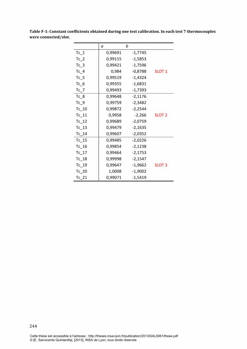
244
Table F-1: Constant coefficients obtained during one test calibration. In each test 7 thermocouples
were connected/slot.
a b
Tc_1 0,99691 -1,7745
Tc_2 0,99115 -1,5853
Tc_3 0,99421 -1,7596
Tc_4 0,984 -0,8788 SLOT 1
Tc_5 0,99519 -1,4324
Tc_6 0,99355 -1,6831
Tc_7 0,99493 -1,7393
Tc_8 0,99648 -2,1176
Tc_9 0,99759 -2,3482
Tc_10 0,99872 -2,2544
Tc_11 0,9958 -2,266 SLOT 2
Tc_12 0,99689 -2,0759
Tc_13 0,99479 -2,1635
Tc_14 0,99607 -2,0352
Tc_15 0,99485 -2,0226
Tc_16 0,99854 -2,1238
Tc_17 0,99464 -2,1753
Tc_18 0,99998 -2,1547
Tc_19 0,99647 -1,9662 SLOT 3
Tc_20 1,0008 -1,9002
Tc_21 0,99071 -1,5419
Cette thèse est accessible à l'adresse : http://theses.insa-lyon.fr/publication/2013ISAL0061/these.pdf © [E. Sanvicente Quintanilla], [2013], INSA de Lyon, tous droits réservés
245
Bibliography 1. B. Metz, et al., Contribution of Working Group III to the Fourth Assessment Report of the
Intergovernmental Panel on Climate Change, C.U. Press, Editor 2007, Cambridge: United
Kingdom and New York, NY, USA.
2. IEA, Energy Statistics of OECD Countries and NonOECD Countries, I. Energy and Agency,
Editors. 2011: Paris.
3. D. Pollard et al., The living planet report 2010. WWF International, Zoological Society of
London and Global Footprint Network, 2010.
4. H.A. Zondag, Flat-plate PV-Thermal collectors and systems: A review. Renewable and
Sustainable Energy Reviews. 2008. 12: p. 891-959.
5. R. Schleicher-Tappeser, How renewables will change electricity markets in the next five years.
Energy Policy, 2012. 48: p. 64-77.
6. I. Hädrich, From cell to module efficiency. 2012. Fraunhofer ISE.
7. J.J Bloem, , Evaluation of a PV-integrated building application in a well-controlled outdoor
test environment. Building and Environment, 2008. 43(2): p. 205-216.
8. B.J. Brinkworth and M. Sandberg, Design procedure for cooling ducts to minimise efficiency
loss due to temperature rise in PV arrays. Solar Energy, 2006. 80: p. 89-103.
9. G. Mittelman, A. Alshare, and J.H. Davidson, A model and heat transfer correlation for
rooftop integrated photovoltaics with a passive air cooling channel. Solar Energy, 2009. 83:
p. 1150-1160.
10. L.M. Candanedo, A.K. Athienitis, and K. Park, Convective Heat Transfer Coefficients in a
Building-Integrated Photovoltaic/Thermal System. Journal of Solar Energy Engineering, 2011.
133: p. 021002-1.
11. L. Liao, Y. Poissant, M. Collins, A.K. Athienitis, and K. Park, Numerical and Experimental
Study of Heat Transfer in a BIPV-Thermal System. Journal of Solar Energy Engineering,
2007. 129: p. 423-430.
12. H.A. Zondag, Flat-plate PV-Thermal collectors and systems: A review. Renewable and
Sustainable Energy Reviews, 2008. 12(4): p. 891-959.
13. S. Roberts and N. Guariento, Building integrated photovoltaics: a handbook 2009: Birkhauser
Architecture.
14. E. Ursula, Solar technologies for buildings, 2003, John Wiley & Sons Ltd.
15. B. Moshfegh, and M. Sandberg, Flow and heat transfer in the air gap behind photovoltaic
panels. Renewable and Sustainable Energy Reviews, 1998. 2: p. 287-301.
16. G. Gan, Simulation of buoyancy-induced flow in open cavities for natural ventilation. Energy
and Buildings, 2006. 38: p. 410-420.
17. G. Gan, Simulation of buoyancy-induced flow in open cavities for natural ventilation. Energy
and Buildings, 2006. 38: p. 410-420.
18. A. Lloret, et al. Lessons learned in the electrical system design, installation and operation of
the Mataró Public Library. Proceedings: 14th. European Photovoltaic Solar Energy
Conference, Barcelona. 1997.
19. U. Eicker, V. Fox, D.G. Infield, and L. Mei, Heating and cooling potential combined
photovoltaic-solar air collector façade. in Proceedings of 16th European Photovoltaic Solar
Energy Conference, Glasgow. 2000.
20. C. Sanjuan, M.J. Suarez, M. Gonzalez, J. Pistono, and E. Blanco, Energy performance of an
open joint ventilated facade compared with conventional sealed cavity facade. Solar Energy,
2011. 85(9): p. 1851-1863.
21. W. Puangsombut, J. Hirunlabh, J. Khedari, B. Zeghmati, and M.M. Win, Enhancement of
natural ventilation rate and attic heat gain reduction of roof solar collector using radiant
barrier. Building and Environment, 2007. 42(6): p. 2218-2226.
22. Q. Lin and S.J. Harrison, Experimental study of natural convection in an asymmetrically
heated inclined channel with radiation exchange, in ASME Summer Heat Transfer
Conference2003: Las Vegas, Nevada,USA.
Cette thèse est accessible à l'adresse : http://theses.insa-lyon.fr/publication/2013ISAL0061/these.pdf © [E. Sanvicente Quintanilla], [2013], INSA de Lyon, tous droits réservés

246
23. M. Sandberg, and B. Moshfegh, Ventilated-solar roof air flow and heat transfer investigation.
Renewable Energy, 1998. 15: p. 287-292.
24. U. Eicker, and M. Gross. PV curtain walls for air preheating. in 14th European Photovoltaic
Solar Energy Conference, Barcelona, Spain. 1997.
25. B.J. Brinkworth, B.M. Cross, R.H. Marshall, and H. Hang, Thermal regulation of photovoltaic
cladding. Solar Energy, 1997. 61(3): p. 169-178.
26. M. Sandberg and B. Moshfegh, Buoyancy-induced air flow in photovoltaic facades: Effect of
geometry of the air gap and location of solar cell modules. Building and Environment, 2002.
37: p. 211-218.
27. Z.D. Chen, P. Bandopadhayay, J. Halldorsson, C. Byrjalssen, P. Heiselberg, An experimental
investigation of a solar chimney model with uniform wall heat flux. Building and
Environment, 2003. 38: p. 893-906.
28. B.J. Brinkworth, R.H. Marshall, and Z. Ibarahim, A validated model of naturally ventilated PV
cladding. Solar Energy, 2000. 69(1): p. 67-81.
29. A. Guiavarch and B. Peuportier, Photovoltaic collectors efficiency according to their
integration in buildings. Solar Energy, 2006. 80(1): p. 65-77.
30. M.D. Bazilian, and D. Prasad, Modelling of a photovoltaic heat recovery system and its role in
a design decision support tool for building professionals. Renewable energy, 2002. 27(1): p.
57-68.
31. D. Infield, L. Mei, and U. Eicker, Thermal performance estimation for ventilated PV facades.
Solar Energy, 2004. 76: p. 93-98.
32. C. Daverat, Etude expérimentale de la convection naturelle en canal vertical à flux de chaleur
imposé: application au rafraîchissement passif de composants actifs de l'enveloppe des
bâtiments, 2012, PhD Thesis, INSA de Lyon.
33. J. Hernandez and B. Zamora, Effects of variable properties and non-uniform heating on
natural convection flows in vertical channels. int. J. Heat Mass Transfer, 2005. 48: p. 793-
807.
34. K.T. Lee, Natural convection heat and mass transfer in partially heated vertical parallel
plates. International Journal of Heat and Mass Transfer, 1999. 42(23): p. 4417-4425.
35. R.N. Mathews, C. Balaji, and T. Sundararajan, Computation of conjugate heat transfer in the
turbulent mixed convection regime in a vertical channel with multiple heat sources. Heat and
Mass Transfer, 2007. 43(10): p. 1063-1074.
36. A.K.D. Silva , G. Lorenzini, and A. Bejan, Distribution of heat sources in vertical open
channels with natural convection. Int.J.Heat Mass Transfer, 2005. 48: p. 1462-1469.
37. A.K. Da Silva, S. Lorente, and A. Bejan, Optimal distribution of discrete heat sources on a
plate with laminar forced convection. International Journal of Heat and Mass Transfer, 2004.
47(10): p. 2139-2148.
38. A.K. Da Silva, S. Lorente, and A. Bejan, Optimal distribution of discrete heat sources on a
wall with natural convection. International Journal of Heat and Mass Transfer, 2004. 47: p.
203-204.
39. L. Chen, H. Tian, Y. Li, D. Zhang, Experimental study on natural convective heat transfer
from vertical plate with discrete heat sources mounted on the back, Energy Conservation and
Management, 2006. 47: p. 3447-3455.
40. G. Tanda, Natural convection heat transfer in vertical channels with and without transverse
square ribs. Int. J. Heat Mass Transfer, 1997. 40(9): p. 2173-2185.
41. A. Dehghan and M. Benhnia, Numerical investigation of natural convection in a vertical slot
with two heat source elements. Int. J. Heat and Fluid Flow, 1996. 17: p. 474-482.
42. G. Cammarata, G. Desrayaud, A. Fichera, C. Fischetti, Numerical analysis of a symmetrically
heated vertical channel with obstruction. Heat and Mass Transfer / Waerme- und
Stoffuebertragung, 2000. 36(6): p. 481-486.
43. G. Desrayaud and A. Fichera, Laminar natural convection in a vertical isothermal channel
with symmetric surface-mounted rectangular ribs. International Journal of Heat and Fluid
Flow, 2002. 23(4): p. 519-529.
44. S.A.M. Burek and A. Habeb, Air flow and thermal efficiency characteristics in solar chimneys
and Trombe walls. Energy and Buildings, 2007. 39: p. 128-135.
Cette thèse est accessible à l'adresse : http://theses.insa-lyon.fr/publication/2013ISAL0061/these.pdf © [E. Sanvicente Quintanilla], [2013], INSA de Lyon, tous droits réservés

247
45. A. La Pica, G. Rodono, and R. Volpes, An experimental investigation on natural convection of
air on a vertical channel. Int. J. Heat Mass Transfer, 1993. 36(3): p. 611-616.
46. A. Bouchair , Solar chimney for promoting cooling ventilation in southern Algeria. Building
Services Engineering Research and Technology, 1994. 15(2): p. 81-93.
47. M. Fossa, C. Menezo, and E. Leonardi, Experimental natural convection on vertical surfaces
for building integrated photovoltaic (BIPV) applications. Experimental Thermal and Fluid
Science, 2008. 32: p. 980-990.
48. B. Zamora and A.S. Kaiser, Thermal and dynamic optimization of the convective flow in
Trombe Wall shaped channels by numerical investigation. Heat and Mass Transfer, 2009.
45(11): p. 1393-1407.
49. R. Khanal and C. Lei, Solar chimney -- A passive strategy for natural ventilation. Energy and
Buildings, 2011. 43: p. 1811-1819.
50. B. Moshfegh and S. Sandberg, Investigation of fluid flow and heat transfer in a vertical
channel heated from one side by PV elements, part II - Experimental study. Special Issue
World Renewable Energy Congress Renewable Energy, 1996. 8(1-4): p. 254–258.
51. E.P. Sakonidou, T.D. Karapantsios, A.L. Balouktsis, D. Chassapis, Modeling of the optimum
tilt of a solar chimney for maximum air flow. Solar Energy, 2008. 82(1): p. 80-94.
52. N. Chami and A. Zoughaib, Modeling natural convection in a pitched thermosyphon system in
building roofs and experimental validation using particle image velocimetry. Energy and
Buildings, 2010. 42(8): p. 1267-1274.
53. L. Susanti, H. Homma, H. Matsumoto, Y. Suzuki, M. Shimizu , A laboratory experiment on
natural ventilation through a roof cavity for reduction of solar heat gain. Energy and
Buildings, 2008. 2008: p. 2196-2206.
54. W. Elenbaas, Heat dissipation of parallel plates by free convection. Physica, 1942. 9(1): p. 1-
28.
55. J. Bodoia and J. Osterle, The development of free convection between heated vertical plates.
Journal of Heat Transfer (US), 1962. 84.
56. W. Aung, Fully Developed Laminar Free Convection Between Vertical Plates Heated
Asymmetrically. Int.J.Heat Mass Transfer, 1972. 15: p. 1577-1580.
57. W. Aung, L.S. Fletcher, and V. Sernas, Developing laminar free convection between vertical
flat plates with asymmetric heating. Int.J.Heat Mass Transfer, 1972. 15: p. 2293-2308.
58. E. Sparrow and P. Bahrami, Experiments on natural convection from vertical parallel plates
with either open or closed edges. Journal of Heat Transfer, 1980. 102: p. 221.
59. G. Raithby and K. Hollands, Natural convection. Handbook of heat transfer fundamentals,
1985. 2: p. 1-6.
60. E.M. Sparrow, G.M. Chrysler, and L.F. Azevedo, Observed flow reversals and measured-
predicted Nusselt numbers for natural convection in one-sided heated vertical channel. ASME
J. Heat Transfer 1984. 106: p. 325-332.
61. LFA. Azevedo and E. Sparrow, Natural convection in open-ended inclined channels. Journal
of Heat Transfer, 1985. 107: p. 893-901.
62. A. Bar-Cohen, and W. Rohsenow, Thermally optimum spacing of vertical, natural convection
cooled, parallel plates. Journal of Heat Transfer, 1984. 106(1): p. 116-123.
63. S. Ostrach, An analysis of laminar-free convection flow and heat transfer about a flat parallel
to the direction of the generating body force, Technical report 2635, NACA, 1952.
64. N. Sobel, F. Landis, and W.K.M. Mueller, Natural Convection Heat Transfer in Short Vertical
Channels Including the Effects of Stagger, in Proc. 3rd International Heat Transfer
Conference 1966. p. 121-125.
65. A.M. Dalbert, F. Penot, and J.L. Peube, Convection naturelle laminaire dans un canal vertical
chauffé à flux constant Int. J. Heat Mass Transfer, 1981. 24(9): p. 1463-1473.
66. R. Wirtz and R. Stutzman, Experiments on free convection between vertical plates with
symmetric heating. Journal of Heat Transfer, 1982. 104: p. 501.
67. B.W. Webb and D.P. Hill, High Rayleigh number laminar natural convection in an
asymmetrically vertical channel. Journal of Heat Transfer, 1989. 111: p. 649-656.
68. G. Tanda, Natural convection in partially heated vertical channels. Wärme- und
Stoffübertragung, 1988. 23(5): p. 307-312.
Cette thèse est accessible à l'adresse : http://theses.insa-lyon.fr/publication/2013ISAL0061/these.pdf © [E. Sanvicente Quintanilla], [2013], INSA de Lyon, tous droits réservés

248
69. W.M. Rohsenow, J.P. Hartnett, and Y.I. Cho, Handbook of heat transfer. Vol. 3. 1998:
McGraw-Hill New York.
70. C.O. Olsson, Prediction of Nusselt Number and Flow Rate of Buoyancy Driven Flow Between
Vertical Parallel Plates. ASME Journal of Heat Transfer, 2004. 126: p. 97-104.
71. N. Onur and M. Aktaş, An experimental study on the effect of opposing wall on natural
convection along an inclined hot plate facing downward. International Communications in
Heat and Mass Transfer, 1998. 25(3): p. 389-397.
72. B.J. Brinkworth, Optimun depth for PV cooling ducts. Solar Energy, 2006. 80: p. 1131-1134.
73. M. Miyamoto, Turbulent free convection heat transfer from vertical parallel plates. J. Heat
Transfer, 1986. 4: p. 1593-1598.
74. M. Mattsson, B. Moshfegh, B. Sandburgh, H. Stymnv, Integration of PV Elements in Building
Components. Interim Report for JRC Project, Contract No. EU 10544-94-11, F1PC ISP S.
KTH Report, 1995.
75. A.G. Straatman, D. Naylor, J.M. Floryan, J.D. Tarasuk, A study of natural convection between
inclined isothermal plates. A.G. Straatman, D. Naylor, J.M. Floryan, J.D. Tarasuk, 1994. 116:
p. 145-243.
76. S.A.M. Said, M.A. Habib, H.M. Badr, S. Anwar , Numerical investigation of natural
convection inside an inclined parallel-walled channel. International Journal for numerical
methods in fluids, 2005. 49: p. 569-582.
77. O. Hiroyuki, S. Hayatoshi, S.W. Churchill, Natural convection in an inclined square channel.
International Journal of Heat and Mass Transfer, 1974. 17(3): p. 401-406.
78. H. Inaba, Natural convection in an inclined rectangular channel heated from the bottom
surface. HEAT TRANSFER., 1986. 108(4): p. 764-769.
79. O. Manca, S. Nardini, and V. Naso, Experiments on natural convection in inclined channels.
ASME-PUBLICATIONS-HTD, 1993. 212: p. 41-41.
80. O. Manca, S. Nardini, and V. Naso, Experiments on natural convection in inclined
channels. Gen. Pap. Heat Transfer Heat transfer Hazard. Waste Process, 1992. 212: p. 41-46.
81. S. Chungloo, and B. Limmeechokchai, Application of passive cooling systems in the hot and
humid climate: The case study of solar chimney and wetted roof in Thailand. Building and
Environment, 2007. 42(9): p. 3341-3351.
82. O. Manca and S. Nardini, Thermal design of uniformly heated inclined channels in natural
convection with and without radiative effects. Heat Transfer Engineering, 2001. 22: p. 13-28.
83. O. Manca, S. Nardini, and V. Naso, Effect of radiation on natural convection in tilted
channels, in Thermal Management of Electronic Systems1994, Springer. p. 117-126.
84. J. Carpenter, D. Briggs, and V. Sernas, Combined radiation and developing laminar free
convection between vertical flat plates with asymmetric heating. Journal of Heat Transfer,
1976. 98: p. 95-100.
85. O. Manca and S. Nardini, Composite correlations for air natural convection in tilted channels.
Heat transfer engineering, 1999. 20(3): p. 64-72.
86. A. Auletta, and O. Manca, Heat and fluid flow resulting from the chimney effect in a
symmetrically heated vertical channel with adiabatic extensions. International Journal of
Thermal Sciences, 2002. 41: p. 1101-1111.
87. A. Auletta and O. Manca, Heat and fluid flow resulting from the chimney effect in a
symmetrically heated vertical channel with adiabatic extensions. International Journal of
Thermal Sciences, 2002. 41: p. 1101-1111.
88. A. Andreozzi, and O. Manca, Thermal and fluid dynamic behavior of symmetrically heated
vertical channels with auxiliary plate. International Journal of Heat and Fluid Flow, 2001.
22(4): p. 424-432.
89. G. Tanda, Natural convection in partially heated vertical channels. Wärme- und
Stoffübertragung, 1988. 23(5): p. 307-312.
90. X. Zhang and S. Dutta, Heat Transfer Analysis of Buoyancy-Assisted Mixed Convection With
Asymmetric Heating Conditions. Int. J. Heat Mass Transfer, 1998. 41(21): p. 3255-3264.
91. O. Manca, M. Musto, and V. Naso, Experimental investigation of natural convection in an
asymmetrically heated vertical channel with an asymmetric chimney. J. Heat Transfer, 2005.
127: p. 888-896.
Cette thèse est accessible à l'adresse : http://theses.insa-lyon.fr/publication/2013ISAL0061/these.pdf © [E. Sanvicente Quintanilla], [2013], INSA de Lyon, tous droits réservés
249
92. O. Manca, M. Musto, and V. Naso, Experimental analysis of asymmetrical isoflux channel-
chimney systems. International Journal of Thermal Sciences, 2003. 42: p. 837-846.
93. A. Auletta, O. Manca, B. Morrone, and V. Naso, Heat transfer enhancement by the chimney
effect in a vertical isoflux channel. Int.J.Heat Mass Transfer, 2001. 44: p. 4345-4357.
94. A. Andreozzi, B. Buonomo, and O. Manca, Transient natural convection in a symmetrically
heated vertical channel at uniform wall heat flux. Numerical Heat Transfer-Part A, 2009. 55:
p. 409-431.
95. A. Auletta, O. Manca, M. Musto, S. Nardini, Thermal design of symmetrically and
asymmetrically heated channel–chimney systems in natural convection. Applied Thermal
Engineering, 2003. 23(5): p. 605-621.
96. D. Ambrosini, D. Paoletti, and G. Tanda, Investigation of natural convection in vertical
channels by Schlieren and holographic interferometry. Journal of Flow Visualization and
Image Processing, 2004. 11(4).
97. S. Giroux-Julien, C. Menezo, J. Vareilles, H. Pabiou, M. Fossa, and E. Leonardi, Natural
convection in a nonuniformly heated channel with application to photovoltaic facades.
Computational thermal sciences, 2009. 1(3): p. 231-258.
98. P.M. Guimaraes and G.J. Menon, Combined free and forced convection in an inclined channel
with discrete heat sources. International Communication in Heat Mass Transfer, 2008. 35: p.
1267-1274.
99. S. B. Pope, Turbulent flows2000: Cambridge university press.
100. T. Yilmaz, and A. Gilchrist. , Temperature and velocity field characteristics of turbulent
natural convection in a vertical parallel-plate channel with asymetric heat flux. Heat and
Mass Transfer, 2007. 43: p. 707-719.
101. Y. Jaluria and B. Gebhart, On transition mechanisms in vertical natural convection flow.
Journal of Fluid Mechanics, 1974. 66: p. 309-337.
102. R. Mahajan and B. Gebhart, An experimental determination of transition limits in a vertical
natural convection flow adjacent to a surface. Journal of Fluid Mechanics, 1979. 91: p. 131-
154.
103. C.L Kuan and T. Wang, Investigtation of the intermittent behaviour of transitional boundary
layer using a conditional averaging technique. Experimental Thermal and Fluid Science 1990.
3: p. 157-173.
104. D.H. Zhang, Y.T. Chew, and S.H. Winoto, Investigation of intermittency measurement
methods for transitional boundary layer flows. Experimental Thermal and Fluid Science,
1996. 12: p. 433-443.
105. T.B. Hedley and J.F. Keffer, Turbulent /non turbulent decisions in an intermittent flow. J.Fluid
Mech, 1974. 64: p. 625-644.
106. O.N. Ramesh, J. Dey, and A. Prabhu, Transitional intermittency distribution in a three
dimensional constant pressure diverging flow. Experiments in fluids, 1996. 21: p. 259-263.
107. S.P. Schneider, Improved methods for measuring laminar-turbulent intermittency in boundary
layers. Experiments in fluids, 1995. 18: p. 370-375.
108. R. Cheesewright, and K. Doan, Space-time correlation measurements in a turbulent natural
convection boundary layer. International Journal of Heat and Mass Transfer, 1978. 21(7): p.
911-921.
109. Y.T. Chew, D.A. Shah, and J. Wan, An envelope method for detection of turbulence
intermittency in a transitional boundary layer. Fluid Dynamics Research, 1999. 24: p. 7-22.
110. B. Gebhart and F. Godaux, An experimental study of the transition of natural convection flow
adjacent to a vertical surface. International Journal of Heat and Mass Transfer, 1973. 17: p.
93-107.
111. B. Gebhart, Instability, transition, and turbulence in buoyancy induced flows. Annu.Rev.Fluid
Mech, 1973. 5: p. 213-246.
112. Y. Katoh, M. Miyamoto, J. Kurima, S. Kaneyasu Turbulent free convection heat transfer from
vertical parallel plates, effect of entrance Bell-Mouth shape. JSME International Journal,
1991. 34(4): p. 496-501.
Cette thèse est accessible à l'adresse : http://theses.insa-lyon.fr/publication/2013ISAL0061/these.pdf © [E. Sanvicente Quintanilla], [2013], INSA de Lyon, tous droits réservés
250
113. B. Zamora, A.S. Kaiser, and A.Viedma, On the effects of Rayleigh number and inlet
turbulence intensity upon the buoyancy-induced mass flow rate in sloping and convergent
channels. Int. J. Heat Mass Transfer, 2008. 51: p. 4985-5000.
114. A. Fedorov, R. Viskanta, and A. Mohamad, Turbulent Heat and Mass Transfer in an
Asymmetrically Heated, Vertical Parallel- plate Channel,. Int. J. Heat and Fluid Flow, 1997.
18: p. 307-315.
115. S.A.M. Said, M.A. Habib, H.M. Badr, S. Anwar, Turbulent natural convection between
inclined isothermal plates. Computers&Fluids, 2005. 34: p. 1025-1039.
116. T. Yilmaz and S.M. Fraser, Turbulent natural convection in a vertical parallel-plate channel
with asymmetric heating. Int. J. Heat Mass Transfer, 2007. 50(13-14): p. 2612-2623.
117. F. Taofeek, F. Ayinde, and S.A.M. Said, Turbulent natural convection flow in a vertical
channel with anti-symetric heating. Heat and Mass Transfer, 2008. 44: p. 1207-1216.
118. T.F. Ayinde, S.A.M. Said, and M.A. Habib, Experimental investigation of turbulent natural
convection flow in a channel. Heat and Mass Transfer, 2006. 42: p. 169-177.
119. X. Cheng and U. Muller, Turbulent natural convection coupled with thermal radiation in
large vertical channels with asymmetric heating. Int. J. Heat Mass Transfer, 1998. 41(12): p.
1681-1692.
120. M. Habib, S.A.M. Said, S.A. Ahmed, A. Asghar, Velocity characteristics of turbulent natural
convection in symmetrically and asymmetrically heated vertical channels. Experimental
Thermal and Fluid Science, 2002. 26(1): p. 77-87.
121. A. Rodríguez-Sevillano, I. Pérez-Grande, and J. Meseguer, On the onset of turbulence in
natural convection on inclined plates. Experimental Thermal and Fluid Science, 2011. 35: p.
68-72.
122. K.D. Kihm, J.H. Kim, and L.S. Fietchen, Onset of flow reversal and penetration lengths of
natural convective flow between isothermal vertical walls. J. Heat Transfer, 1995. 117(3): p.
776- 779.
123. D. Ospir, C. Popa, C. Chereches, G. Polidori, S. Fohanno, Flow visualization of natural
convection in a vertical channel with asymmetric heating. International Communications in
Heat and Mass Transfer, 2012. 39(4): p. 486-493.
124. S. Baskaya, M. Aktas, and N. Onur, Numerical simulation of the effects of plate separation
and inclination on heat transfer in buoyancy driven open channels. Heat and Mass Transfer,
1999. 35(4): p. 273-280.
125. C. Popa, D. Ospir, S. Fohanno, C. Chereches, Numerical simulation of dynamical aspects of
natural convection flow in a double-skin façade. Energy and Buildings, 2012.
126. D. Ospir, C. Chereches, C. Popa, S. Fohanno, C. Popovici, Flow dynamics in a double-skin
façade. in Proceedings of the 3rd WSEAS International Conference on Finite Differences–
Finite Elements–Finite Volumes–Boundary Elements. 2009.
127. S. Rheault, and E. Bilgen, Mixed convection heat transfer in open-ended inclined channels
with flow reversal. Heat and Mass Transfer, 1993. 29(2): p. 107-116.
128. F. Dupont, T. Fabien, B. Ruddy, S. Sandrine, Two-dimension experimental study of the
reverse flow in a free convection channel with active walls differentially heated. Experimental
Thermal and Fluid Science, 2013.
129. S. Samot, F. Dupont, and F. Penot, Mesure de température dans un écoulement renversé à la
sortie d’un thermosiphon vertical chauffé à flux constant. Actes du Congrès de la Société
Française de Thermique, 2010.
130. A. Zollner, E.R.F. Winter, and R. Viskanta, Experimental studies of combined heat transfer in
turbulent mixed convection fluid flows in double-skin facades. Heat and Mass Transfer, 2002.
45: p. 4401-4408.
131. J. Vareilles, Etude des transferts de chaleur dans un canal vertical différentiellement chauffé :
application aux enveloppes photovoltaïques-thermique, 2007, Lyon 1 University.
132. A. Javam, and S.W. Armfield, Stability and transition of stratified natural convection flow in
open cavities. J. Fluid Mech., 2001. 445: p. 285-303.
133. C. Daverat, H. Pabiou, H. Bouia, S. Xin, C. Menezo, Convection naturelle dans un canal
vertical en eau avec chauffage pariétal: influence de la stratification. 20ème Congrès Français
de Mécanique, 28 août/2 sept. 2011-25044 Besançon, France (FR), 2011.
Cette thèse est accessible à l'adresse : http://theses.insa-lyon.fr/publication/2013ISAL0061/these.pdf © [E. Sanvicente Quintanilla], [2013], INSA de Lyon, tous droits réservés
251
134. C. Daverat, H. Pabiou, C. Menezo, H. Bouia, S. Xin, Experimental investigation of turbulent
natural convection in a vertical water channel with symmetric heating: flow and heat transfer.
Experimental Thermal and Fluid Science, 2012. 44: p. 182-193.
135. T. Lafaye De Micheaux, Etude expérimentale de l'écoulement de convection naturelle dans un
canal vertical diférentiellement chauffé à flux imposé. Master Thesis, Insa de Lyon, 2011.
136. M. Raffel, C.E. Willert, S.T. Wereley, J. Kompenhans, Particle image velocimetry, a practical
guide, 2007: Springer.
137. A. Boillot and A. Prasad, Optimization procedure for pulse separation in cross-correlation
PIV. Experiments in Fluids, 1996. 21(2): p. 87-93.
138. R. Mei, Velocity fidelity of flow tracer particles. Experiments in Fluids, 1996. 22(1): p. 1-13.
139. H.E. Albrecht, Laser Doppler and phase Doppler measurement techniques, 2002: Springer.
140. C. Tropea, A.L. Yarin, and J.F. Foss, Springer handbook of experimental fluid mechanics.
Vol. 1. 2007: Springer.
141. P. Coray, Establishing a Particle Image Velocimetry (PIV) System for Studying Heat Transfer
Enhancements using Dimpled, in Master of engineerin Science2005, UNSW: Sydney.
142. R.J. Adrian, Particle-imaging techniques for experimental fluid mechanics. Annual review of
fluid mechanics, 1991. 23(1): p. 261-304.
143. R. Theunissen, F. Scarano, and M. Riethmuller, An adaptive sampling and windowing
interrogation method in PIV. Measurement Science and Technology, 2007. 18(1): p. 275.
144. C. Muresan, C. Menezo, R. Bennacer, and R. Vaillon, Numerical Simulation of a Vertical
Solar Collector Integrated in a Building Frame: Radiation and Turbulent Natural Convection
Coupling. Heat Transfer Engineering, 2006. 27(2): p. 29-42.
145. R.J. Moffat, Using uncertainty analysis in the planning of an experiment. ASME,
Transactions, Journal of Fluids Engineering(ISSN 0098-2202), 1985. 107: p. 173-178.
146. N. Qamar, Z.T. Alwahabi, Q.N. Chan, G.J. Nathan, D. Roekaerts, and K.D. King, Soot volume
fraction in a piloted turbulent jet non-premixed flame of natural gas. Combustion and Flame,
2009. 156(7): p. 1339-1347.
147. J. Pallares, A. Vernet, J.A. Ferre, and F.X. Grau, Turbulent large-scale structures in natural
convection vertical channel flow. International Journal of Heat and Mass Transfer, 2010.
53(19): p. 4168-4175.
148. Y. Tian, and T. Karayiannis, Low turbulence natural convection in an air filled square cavity:
Part II: the turbulence quantities. International Journal of Heat and Mass Transfer, 2000.
43(6): p. 867-884.
149. D.D. Papailiou, Statistical characteristics of a turbulent free-convection flow in the absence
and presence of a magnetic field. International Journal of Heat and Mass Transfer, 1980.
23(6): p. 889-895.
150. A. Vouros and T. Panidis. Turbulent free convection over a horizontal heated plate in an open
top cavity. in Journal of Physics: Conference Series. 2012. IOP Publishing.
151. O. Manca and V. Naso, Experimental analysis of natural convection and thermal radiation in
vertical channels. ASME Journal of Heat Transfer, 1990. 145: p. 13-21.
152. O. Manca, S. Nardini, and V. Naso, Effect on natural convection of the distance between an
inclined discretely heated plate and a parallel shroud below. Journal of Heat Transfer, 2003.
124(3): p. 441-451.
153. T. Aseada and K. Watanabe, The mechanism of heat transport in thermal convection at high
Rayleigh numbers. Phys. Fluids A, 1989. 1(5): p. 861-867.
154. Y.C. Chen and J.N. Chung, A direct numerical simulation of K- and H-type flow transition in
a heated vertical channel. Phys. Fluids, 2002. 14(9): p. 3327-3340.
155. G.J. Brereton and Y. Jiang, Convective heat transfer in unsteady laminar parallel flows. Phys.
Fluids 2006. 18(10): p. 103602-103602-15.
156. B. Gebhart and R. Mahajan, Characteristic disturbance frequency in vertical natural
convection flow. International Journal of Heat and Mass Transfer, 1975. 18(10): p. 1143-1148.
157. G.E. Lau, V. Timchenko, C. Menezo, S. Giroux-Julien, M. Fossa, E. Sanvicente, J. Reizes,
G.H. Yeoh, Numerical and experimental investigation of unsteady natural convection in an
open channel. Computational Thermal Sciences, 2012. 4: p. 443-456.
Cette thèse est accessible à l'adresse : http://theses.insa-lyon.fr/publication/2013ISAL0061/these.pdf © [E. Sanvicente Quintanilla], [2013], INSA de Lyon, tous droits réservés
252
158. T. Tsuji and Y. Nagano, Velocity and Temperature Measurements in a Natural Convection
Boundary Layer along a Vertical Flat Plate. Experimental Thermal and Fluid Science, 1989.
2: p. 208-215.
159. S. Giroux-Julien, C. Menezo, J. Vareilles, H. Pabiou, and M. Fossa, Numerical and
experimental investigation of natural convection in double facades, in ICHMT International
Symposium on Advances in Computational Heat Transfer 2008: Marrakech, Morocco.
160. H. Bhowmik and K.W. Tou, Experimental study of transient natural convection heat transfer
from simulated electronic chips. Experimental Thermal and Fluid Science, 2004. 29: p. 485-
492.
161. A. K. Athienitis, J. Bambara, B. O'Neill, J. Faille, A prototype photovoltaic/thermal system
integrated with transpired collector. Solar Energy, 2011. 85: p. 139 - 153.
162. A. Litvak and G.L. Morrison, Study of flow characteristics in thermosyphon flow
characteristics, in Eight Australasian Fluid Mechanics conference1983: University of
Newcastle, NSW
163. F.P. Incropera, J.S. Kerby, D.F. Moffatt, and S. Ramadhyani, Convection heat transfer from
discrete heat sources in a rectangular channel. Int. J. Heat Mass Transfer, 1986. 29: p. 1051-
1058.
164. Q. Lin and S.J. Harrison, Experimental Study on Natural Convection in an Asymmetrically
Heated Inclined Channel With Radiation Exchange. ASME conference proceedings, 2003. p.
41-45.
165. G. Lau, E. Sanvicente, G.H. Yeoh, V. Timchenko, M. Fossa, C. Menezo, S. Giroux-Julien,
Modelling of natural convection in vertical and tilted photovoltaic applications. Energy and
Buildings, 2012. 55: p. 810-822.
166. G. Lau, G.H. Yeoh, V. Timchenko, J.A. Reizes, Large-eddy simulation of turbulent natural
convection in vertical parallel-plate channels. Numerical Heat Transfer:Part B -
Fundamentals, 2011. 59: p. 259-287.
167. M. Miyamoto, Development of turbulence characteristics in a vertical free convection
boundary layer. Heat Transfer, 1982. 2.
168. W.M. Rohsenow, J.P. Hartnett, and Y.I. Cho, eds. Handbook of Heat Transfer. 1998,
McGraw-Hill: New York.
169. G. Mittelman, A. Alshare, and J.H. Davidson, Composite relation for laminar free convection
in inclined channels with uniform heat flux boundaries. International Journal of Heat and
Mass Transfer, 2009. 52(21): p. 4689-4694.
170. B. Brangeon, Contribution à l'étude numérique de la ventilation naturelle dans des cavités
ouvertes par la simulation des grandes échelles. Application au rafraîchissement passif des
bâtiments, 2012, PhD thesis: Université de la Réunion.
171. S. Samot, F. Dupont, F. Penot, Mesure de température dans un écoulement renversé à la
sortie d’un thermosiphon vertical chauffé à flux constant.
172. F. Dupont, T. Soubdhan, R. Blonbou, R. Calif, J.L. Tuhault, and F. Penot, Étude
expérimentale des conditions d'apparition d'écoulements inverses en sortie d'un thermosiphon
en convection naturelle d'air. in CONGRES FRANÇAIS DE THERMIQUE. 2008.
173. K. Nolan and T. Zaki. Conditional sampling and statistical analysis of transitional flows. in
Proceedings of the Summer Program. 2012.
174. R. Antonia, Conditional sampling in turbulence measurement. Annual review of fluid
mechanics, 1981. 13(1): p. 131-156.
175. J.L. Lumley, The structure of inhomogeneous turbulent flows. Atmospheric turbulence and
radio wave propagation, 1967: p. 166-178.
176. J. Baltzer, R. Adrian, and X. Wu. Turbulent boundary layer structure identification via pod. in
Proceedings of the Summer Program. 2010.
177. E. Liberge and A. Hamdouni, Reduced order modelling method via proper orthogonal
decomposition (POD) for flow around an oscillating cylinder. Journal of Fluids and
Structures, 2010. 26(2): p. 292-311.
178. V. Roussinova, A.-M. Shinneeb, and R. Balachandar, Investigation of fluid structures in a
smooth open-channel flow using proper orthogonal decomposition. Journal of Hydraulic
Engineering, 2009. 136(3): p. 143-154.
Cette thèse est accessible à l'adresse : http://theses.insa-lyon.fr/publication/2013ISAL0061/these.pdf © [E. Sanvicente Quintanilla], [2013], INSA de Lyon, tous droits réservés

253
179. J. Moreau, B. Patte-Rouland, and E. Rouland. Particle image velocimetry and proper
orthogonal decomposition. Euromech colloquium 411, 2000. Rouen, May 29-31.
180. P.J. Holmes, J.L. Lumley, G. Berkooz, J.C. Mattingly, R.W. Wittenberg, Low-dimensional
models of coherent structures in turbulence. Physics Reports, 1997. 287(4): p. 337-384.
181. G. Berkooz, P.J. Holmes, and J.L. Lumley, The proper orthogonal decomposition in the
analysis of turbulent flows. Annual review of fluid mechanics, 1993. 25(1): p. 539-575.
182. D.J. Tritton, Physical fluid dynamics. Oxford, Clarendon Press, 1988, 536 p., 1988. 1.
183. B. Patte-Rouland, A. Danlos, G. Lalizel, E. Rouland, and P. Paranthoen, Proper Orthogonal
Decomposition used for determination of the convection velocity of the initial zone of the
annular jet. Aerodynamic study and control of instabilities. International Journal of Fluid
Dynamics, 2008. 1: p. 1-10.
184. V.A. Ilie, D. Saury, D. Lemonnier, and P. Belleoud. Coupled temperature and velocity
measurements in turbulent natural convection flows. Journal of Physics: Conference Series
395. Eurotherm 2012. IOP Publishing.
185. S. Churchill and R. Usagi, A general expression for the correlation of rates of transfer and
other phenomena. AIChE Journal, 1972. 18(6): p. 1121-1128.
186. S.J. Kline and F. McClintock, Describing uncertainties in single-sample experiments.
Mechanical engineering, 1953. 75(1): p. 3-8.
187. J.R. Taylor, L. Reynaud, and P. Reynaud, Incertitudes et analyse des erreurs dans les mesures
physiques: avec exercices corrigés1999: Dunod.
Cette thèse est accessible à l'adresse : http://theses.insa-lyon.fr/publication/2013ISAL0061/these.pdf © [E. Sanvicente Quintanilla], [2013], INSA de Lyon, tous droits réservés

254
Cette thèse est accessible à l'adresse : http://theses.insa-lyon.fr/publication/2013ISAL0061/these.pdf © [E. Sanvicente Quintanilla], [2013], INSA de Lyon, tous droits réservés

255
Cette thèse est accessible à l'adresse : http://theses.insa-lyon.fr/publication/2013ISAL0061/these.pdf © [E. Sanvicente Quintanilla], [2013], INSA de Lyon, tous droits réservés