Effect of Thermal Radiation on Biomagnetic Fluid Flow and ...

CAMES, 28(2): 81–104, 2021, doi: 10.24423/cames.327Copyright © 2021 by Institute of Fundamental Technological ResearchPolish Academy of Sciences

Effect of Thermal Radiationon Biomagnetic Fluid Flow and Heat Transferover an Unsteady Stretching Sheet

Md. Jahangir ALAM1), Md. Ghulam MURTAZA1),Efstratios E. TZIRTZILAKIS2), Mohammad FERDOWS3)∗

1) Department of MathematicsComilla UniversityCumilla, Bangladesh

2) Department of Mechanical EngineeringUniversity of the PeloponneseTrípoli, Greece

3) Research Group of Fluid Flow Modeling and SimulationDepartment of Applied MathematicsUniversity of DhakaDhaka, Bangladesh∗Corresponding Author e-mail: [email protected]

This study examines the influence of thermal radiation on biomagnetic fluid, namelyblood that passes through a two-dimensional stretching sheet in the presence of magneticdipole. This analysis is conducted to observe the behavior of blood flow for an unsteadycase, which will help in developing new solutions to treat diseases and disorders related tohuman body. Our model is namely biomagnetic fluid dynamics (BFD), which is consistentwith two principles: ferrohydrodynamic (FHD) and magnetohydrodynamic (MHD), whereblood is treated as electrically conductive. It is assumed that the implemented magneticfield is sufficiently strong to saturate the ferrofluid, and the variation of magnetization withtemperature may be approximated with the aid of a function of temperature distinction.The governing partial differential equations (PDEs) converted into ordinary differentialequations (ODEs) using similarity transformation and numerical results are thus obtainedby using the bvp4c function technique in MATLAB software with considering applicableboundary conditions. With the help of graphs, we discuss the impact of various param-eters, namely radiation parameter, unsteady parameter, permeability parameter, suctionparameter, magnetic field parameter, ferromagnetic parameter, Prandtl number, velocityand thermal slip parameter on fluid (blood) flow and heat transfer in the boundary layer.The rate of heat transfer and skin friction coefficient is also computationally obtained forthe requirement of this study. The fluid velocity decreases with increasing values of themagnetic parameter, ferromagnetic interaction parameter, radiation parameter whereastemperature profile increases for the unsteady parameter, Prandtl number, and perme-

82 Md.J. Alam et al.

ability parameter. From the analysis, it is also observed that the skin friction coefficientdecreases and the rate of heat transfer increases respectively with increasing values ofthe ferromagnetic interaction parameter. The most important part of the present analy-sis is that we neither neglect the magnetization nor electrical conductivity of the bloodthroughout this study. To make the results more feasible, they are compared with thedata previously published in the literature and found to be in good accuracy.

Keywords: biomagnetic fluid, magnetohydrodynamic, ferrohydrodynamic, magneticdipole, thermal radiation, stretching sheet.

Notationa, b, c – constants,

x – horizontal coordinate [m],y – vertical coordinate [m],u – horizontal velocity [m/s],v – vertical velocity [m/s],t – time [s],T – fluid temperature inside boundary layer [K],Tw – temperature of the sheet [K],T∞ – fluid temperature far away from the sheet [K],M1 – magnetization [A/m],H – magnetic field of intensity [A/m],N – velocity slip factor,K – thermal slip factor,Cp – specific heat at constant pressure [J/(kg ·K)],Uw – stretching velocity,Vw – suction/injection velocity,Nu – local Nusselt number,Cf – skin friction coefficient,qw – wall heat flux,qr – radiative heat flux,Re – local Reynolds number,

B(t) – time-dependent magnetic field intensity,k1(t) – time-dependent magnetic permeability,k2 – constant permeability of the medium,k3 – non-dimensional permeability parameter,k∗ – mean absorption coefficient,d – distance between magnetic dipole to sheet,A – unsteady parameter,Pr – Prandtl number,M – magnetic field parameter,S – suction parameter,Nr – radiation parameter,Sf – velocity y-slip parameter,St – thermal l-slip parameter,f ′ – dimensionless velocity components along x direction,

f ′′(0) – skin friction.

Effect of thermal radiation on biomagnetic fluid flow. . . 83

Greek symbols:

η – similarity variable,θ – dimensionless temperature,

θ′(0) – wall heat transfer gradient,ψ – stream function [m2/s],ρ – density of the fluid [kg/m3],µ – dynamic viscosity [kg/ms],ϑ – kinematic viscosity [m2/s],µ0 – magnetic permeability [kg ·m/A2s2],σ – electrical conductivity of the fluid [S/m],κ – thermal conductivity [J/m · s ·K],σ∗ – Stefan–Boltzman constant,λ – viscous dissipation parameter,ε – dimensionless Curie temperature,β – ferromagnetic interaction parameter,α – dimensionless distance,τw – wall shear stress.

List of abbreviations:

BFD – biomagnetic fluid dynamic,FHD – ferrohydrodynamic,MHD – magnetohydrodynamic,PDE – partial differential equation,ODE – ordinary differential equation.

1. Introduction

Biological fluids (who are also a part of BFD) exist in living creatures withinthe presence of magnetic field generated from the action of a magnetic dipole. Themost prominent biomagnetic fluid is blood. It behaves as a magnetic fluid be-cause of the sophisticated interaction of the inter-cellular protein, cell membraneand hemoglobin that is a structure of iron oxides. In recent years, the study ofBFD has attracted considerable attention from theoretical as well as experi-mental researchers because of its increasing usefulness and practical relevancein biomedical engineering and medical sciences, which include magnetic devicesfor cell separation, decreasing bleeding during surgeries, targeted transport ofdrugs using magnetic particles to trigger drug release,treatment of most cancertumors causing magnetic hyperthermia, and magnetic resonance imaging (MRI)of specific parts of the human body [1–5].

Haik et al. [1] developed a biomagnetic fluid model based on the principleof FHD. Their study was additionally extended by another author in [6] byadopting principles of MHD and FHD and applying the developed model to in-vestigate the flow of blood under the influence of a magnetic field. In that study,


the author stated that the blood flow may be reduced up to 40% under a strongmagnetic field effect. Within the influence of magnetic dipole, a biomagneticmathematical model through a stretching sheet was studied in [7]. The incom-pressible three-dimensional biomagnetic fluid that is electrically nonconductingwas studied numerically in [8]. The authors assumed that the fluid magnetiza-tion varies with temperature and magnetic field strength. The significance ofFHD and MHD was studied and both principles were adopted to examine bio-magnetic blood flow model in [9]. The authors concluded that FHD and MHD(interaction parameters) both make significant impact on the flow field. Dualsolutions on biomagnetic flow model that passes through a nonlinear stretch-ing/shrinking sheet were presented in [10]. The flow of biomagnetic fluid withviscoelastic property over stretching sheet was studied numerically in [11]. Thestudy of biomagnetic fluid flow and heat transfer over a stretching sheet wasconducted by several researchers [12–16] with different conditions in presence ofexternal magnetic field.

Ali et al. [17] examined the analytical solution of MHD blood flow throughparallel plates when the lower plate exponentially expands. The impact of themagnetic dipole on ferrofluid over a stretched surface, taking into account the ther-mal radiation, was analyzed in [18]. Blood considered as electrical conductivephenomena under the influence of magnetic field was investigated in [19]. Theunsteady blood flow over a permeable stretching sheet was investigated numeri-cally in [20, 21] in the presence of a non-uniform heat source and sink. Theimpact of radiation and viscous dissipation on unsteady MHD free convectiveflow was analyzed in [22]. Convective flow over a porous stretch surface in theporous medium, in the presence of a heat source or sink, was studied in [23].Thermal radiation impact on boundary layer flow under different flow condi-tions has been reported by several investigators in [24–28]. Newtonian fluid withthe slip condition taken into consideration was studied in [29]. In [30], fluid flowand heat transfer on a stretched sheet were studied and variable viscosity withslip conditions was considered.

Moreover, an incompressible electrified Maxwell ferromagnetic liquid flowthrough a two-dimensional stretching sheet in the presence of a rotating mag-netic field along with heat generation/absorption was investigated in [31]. Theauthors found that velocity and temperature profile decreases and increases withincreasing values of the ferromagnetic parameter, respectively. The behavior offerrofluid over a cylindrical rotating disk with temperature-dependent viscositywas investigated in [32]. The flow and heat transfer of ferrofluid over a perme-able stretching sheet with the effects of suction/injection have been examined in[33]. The viscoelastic property of the fluid in MHD flow and heat transfer overa two-dimensional stretching sheet under slip velocity was studied in [34]. Theflow and convective heat transfer analysis of dusty ferrofluid over a stretching


surface have been presented in [35]. The authors noted that temperature profileincreases with enhanced values of the ferromagnetic parameter in both the fer-rofluid phase and dusty phase. It is also clear from that study that the ferrofluidphase is significantly more comprising than a dusty phase. The effects of thermalradiation on the ferrofluid flow and heat transfer over a stretching sheet werediscussed in [36].

The goal of the present analysis is to investigate the BFD flow and heattransfer of blood along a stretched sheet under the influence of thermal radiation.For the mathematical formulation, we adopt the version of BFD consistent withFHD and MHD principles. A similarity transformation is used to convert thenonlinear PDEs into nonlinear ODEs. The effects of various relevant parameterson the momentum and heat transfer have been investigated and the numericalresults are presented graphically and in tabular form. The aim is that the presentstudy will be used in the biotechnology and medical sciences.

2. Model descriptions

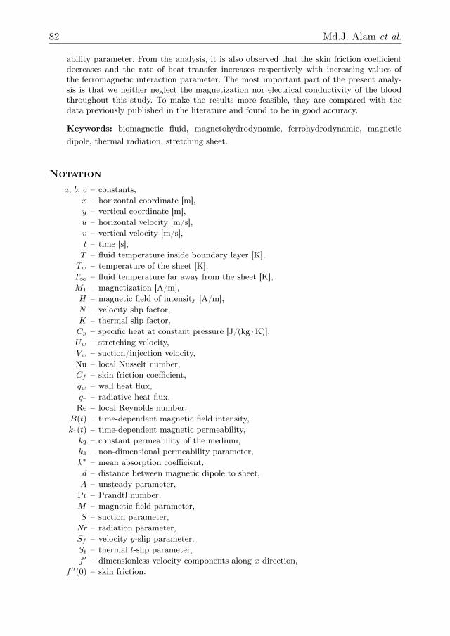
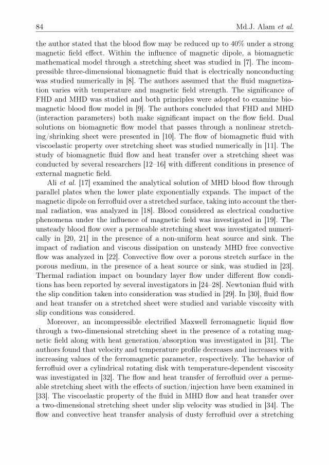
Consider an unsteady, two-dimensional boundary layer flow of an incom-pressible electrically conducting biomagnetic fluid, namely blood passing througha stretched sheet with velocity Uw(x, t) = ax

1−ct , where a and c are constant suchthat a > 0, c ≥ 0 and ct < 1 (Fig. 1). X – axes are taken along the sheetand Y – axes are chosen normal to it. It is assumed that the sheet is kept atconstant temperature Tw, and T∞ is the temperature of the ambient fluid where

Fig. 1. Schematic diagram of the flow problem.


Tw < T∞. A transverse magnetic field of strength B(t) = B0

(1−ct)1/2 is applied inthe Y – direction and at t = 0, B0 corresponds to the constant magnetic fieldstrength. A magnetic dipole generates a magnetic field of strength H, which issupposed to be located some distance d from the sheet. Under these assumptions,continuity, momentum and energy equations are taken in the following form [12].

Continuity equation:

∂u

∂x+∂v

∂y= 0. (1)

Momentum equation:

∂u

∂t+ u

∂u

∂x+ v

∂u

∂y= ϑ

∂2u

∂y2− σB2(t)

ρu− ϑ

k1 (t)u+

µ0ρM1

∂H

∂x. (2)

Energy (Heat) equation:

ρCp

(∂T

∂t+ u

∂T

∂x+ v

∂T

∂y

)+µ0T

∂M1

∂T

(u∂H

∂x+ v

∂H

∂y

)= κ

∂2T

∂y2− ∂qr∂y

, (3)

where u and v represents the velocity component along x- and y-direction, ρ andB(t) represents the biomagnetic fluid density and time-dependent magnetic fieldintensity, respectively, k1(t) = k2(1 − ct) is the time-dependent permeabilityparameter, k2 is initial permeability, κ and Cp denotes the thermal conductiv-ity and specific heat, respectively, ϑ is the kinematic coefficient, σ is electricalconductivity, qr implies radiative heat flux, M indicates magnetization, H ismagnetic field of strength, T is the temperature of field, and µ0 is magneticpermeability.

The associated boundary conditions for the given mathematical problem arein the following form [37, 38]:

y = 0 : u = Uw +Nµ∂u

∂y, v = Vw, T = Tw +K

∂T

∂y,

y →∞ : u→ 0, T → T∞,

(4)

where Vw specifies the injection/suction velocity and it is in the following form:

Vw = −√ϑUwx

f(0). (5)

Equation (5) expresses that mass transfer occurs with velocity Vw from thesurface of the wall, where Vw > 0 and Vw < 0 describe injection and suction,respectively. In Eq. (4), N = N0(1 − ct)1/2 and K = K0(1 − ct)1/2 are velocity


and thermal slip factor, respectively. The no-slip conditions can be recoveredinstead of putting N = K = 0. The temperature of the stretched sheet Tw(x, t)is assumed in the following form:

Tw(x, t) = T∞ +bx

1− ct, (6)

where b and c are positive constants such that b, c ≥ 0 having a dimension“time−1” and ct < 1.

The radiation heat flux qr is simulated according to the Rossel and approxi-mation [39] such that

qr =4σ∗

3k∗∂T 4

∂y, (7)

where σ∗ and k∗ are the Stefan–Boltzman constant and the mean absorption co-efficient. Following [39], we assumed that the temperature differences within theflow are such that the term T 4 may be expressed as a linear function of the tem-perature, we expand T 4 in a Taylor series about T∞ and neglecting the higher-order terms beyond the first degree in (T − T∞) we get

T 4 ∼= 4TT 3∞ − 3T 4

∞. (8)

Employing Eqs (7) and (8) in (3), the energy equation reduces to

ρCp

(∂T

∂t+ u

∂T

∂x+ v

∂T

∂y

)+ µ0T

∂M1

∂T

(u∂H

∂x+ v

∂H

∂y

)= κ

∂2T

∂y2+

16 σ∗ T 3∞

3k∗∂2T

∂y2. (9)

The partial part of µ0ρ M1∂H∂x in Eq. (2) denotes the ferromagnetic body force per

unit volume, while the term µ0T∂M1∂T

(u∂H∂x + v ∂H∂y

)in Eq. (3) indicates heating

due to adiabatic magnetization. According to the [40], we assumed that thecomponent Hx and Hy of the magnetic field H = (Hx, Hy) due to a magneticdipole that is located at a distance d below the sheet can be written in thefollowing form:

Hx(x, y) = −∂V∂x

=γ

2π

x2 − (y + d)2

[x2 + (y + d)2]2, (10)

Hy(x, y) = −∂V∂y

=γ

2π

2x(y + d)

[x2 + (y + d)2]2, (11)


where

V =α

2π

x

x2 + (y + d)2

depict the magnetic scalar potential in the region of a magnetic dipole, γ = αand α is a dimensionless distance defined as

α =

√Uwϑx

d.

Due to the magnetic body forces corresponding to the gradients of magnitude‖H‖ = H, we obtain

H(x, y) =[H2x +H2

y

]1/2=

γ

2π

[1

(y + d)2− x2

(y + d)4

]. (12)

Thus the corresponding horizontal and vertical components of the magnetic fieldare expressed in the form

∂H

∂x=

γ

2π

−2x

(y + d)4,

∂H

∂y=

γ

2π

[−2

(y + d)3+

4x2

(y + d)5

].

(13)

Following [41], we assume that the impact of magnetization M varies with tem-perature T defined by the expression in the following form:

M1 = K(T − T∞), (14)

where K is a pyromagnetic coefficient.

3. Transformation to non-dimensionalize

Equations (2) and (9) are made dimensionless with considering the followingtransformation [12]:

η =

√Uwϑx

y, ψ =√ϑxUwf(η), θ(η) =

T − T∞Tw − T∞

, (15)

where ψ, θ(η) and η are a stream function, dimensionless temperature function,and dimensionless similarity variable, respectively.

Continuity Eq. (1) is satisfied automatically by expressing the stream func-tion in the following form:

u =∂ψ

∂yand v = −∂ψ

∂x.


Using Eqs (10) to (15), we convert (2) and (7) into a set of following ODEs andboundary conditions:

f ′′′ − f ′2 + ff ′′ −A[f ′ +

1

2η f ′′

]−M2f ′ − 1

k3f ′ − 2βθ

(η + α)4= 0, (16)

(1 +Nr)

Prθ′′ −A

(θ +

1

2ηθ′)− f ′θ + fθ′ − 2βλ

(ε+ θ)

Pr (η + α)3f = 0, (17)

η = 0 : f = S, f ′ = 1 + Sff′′, θ = 1 + Stθ

′′, (18)

η →∞ : f ′ → θ → . (19)

In Eq. (18), S symbolizes suction and injection parameter if S > 0 and ifS < 0 respectively, which is used to control the strength of direction of flowat the boundary. In equations written above, primes denote derivatives withrespect to η.

Here the parameters that appears in Eqs (16)–(19) are expressed and de-fined as:

Pr =µCpκ

– Prandtl number,

A =c

a– unsteady parameter,

k3 =ak2ϑ

– permeability parameter,

Nr =16σ∗T 3

∞3κk∗

– radiation parameter,

λ =aµ2

ρk(1− ct)(Tw − T∞)– viscous dissipation parameter,

β =γ

2π

µ0K(Tw − T∞)ρ

µ2– ferromagnetic interaction parameter,

M = B0

√σ

ρa– magnetic field parameter,

ε =T∞

Tw − T∞– dimensionless Curie temperature,

α =

√Uwϑx

d – dimensionless distance,

Sf = N0ρ√aϑ – velocity-slip parameter,

St = K0

√a

ϑ– thermal-slip parameter.


The skin friction and local Nusselt number are interesting physical quantitieswhich mathematically are defined as:

Cf =2τwρU2

w

and Nu =xqw

κ(Tw − T∞).

The wall shear stress τw and the heat flux qw are determined in the followingway:

τw = µ

(∂u

∂y

)y=0

and qw = −κ(∂T

∂y

)y=0

.

Finally, the skin friction coefficient and Nusselt number are made dimensionlessand take the following form:

Cf = 2Re− 1/2f ′′(0), Nu = −Re1/2θ′(0),

where the local Reynolds number is defined as

Re =xUwϑ

.

4. Numerical method

In this section, we discuss the numerical method of the studied problem givenin (16) and (17) subject to the boundary conditions (18) and (19) that are builtin MATLAB software by using the bvp4c function technique. For this purpose,we convert the boundary conditions and the higher-order PDEs into a set of first-order differential equations by considering new variables. Let us define some newvariables as: f = y1, f ′ = y2, f ′′ = y3, θ = y4, θ′ = y5.

Then the system of first-order differential equations is given as follows:

f ′ = y2,

f ′′ = y′2 = y3,

f ′′′ = y′3 = A(y2 +

η

2y3) + y22 − y1y3 +

2βy4(η + α)4

+M2y2 + y2κ3,

θ′ = y5,

θ′′ = y′5 =

Pr

(1+Nr)

{A(y4+

η

2y5

)+ y2y4−y1y5

}+

1

(1+Nr)

2βλy1(ε+y4)

(η+α)3,

(20)

and the initial boundary conditions:

y1(0) = S, y2(0) = 1 + Sfy3(0), y4(0) = 1 + Sty5(0),

y2(∞) = 0, y4(∞) = 0.(21)


The initial boundary conditions (21) and Eq. (20) are integrated numericallyas an initial value problem to a given terminal point. All these simplificationshave been done using the MATLAB package.

5. Parameter estimated

In this work, we examine the influence of radiation on the blood flow thatpasses through the stretched sheet. To obtain the numerical answer, it is neces-sary to determine some unique values for the dimensionless parameters such asunsteadiness parameters, suction parameters, permeability parameters, velocityslip parameters, thermal slip parameter, Prandtl number, radiation parameter,magnetic field parameter, and ferromagnetic parameter, which all make a signi-ficant impact on the biomagnetic flow. Many scientists have been documentedin the scientific literature using different values of dimensionless parameters inhandling the flow problem. We assume that the fluid is blood, and take thefollowing values into account:

µ = 3.2× 10−3 kg/m · s, ρ = 1050 kg/m3, (22)

Cp = 14.65 J/kg ·K, κ = 2.2× 10−3 J/m · s ·K. (23)

Using these values, we have Pr =µCp

κ = 21.We assume that the human body temperature is Tw = 37◦C [43] and the

body Curie temperature is T∞ = 41◦C, hence the dimensionless temperature isε = 78.5◦C.

We use the value of the following parameters in Figs 2–27.The ferromagnetic interaction parameter β = 0 to 10 as in [9, 10]. Note

that β = 0 corresponds to the hydrodynamatic flow, unsteadiness parameterA = 0, 0.5, 1 as in [12], permeability parameter k3 = 0.2, 0.3, 0.4, 1 as in [12],radiation parameter Nr = 1, 2, 3 as in [12], Prandtl number Pr = 21, 23, 25as in [10, 12], values of dimensionless distance α = 1 as in [7], magnetic fieldparameter M = 1, 2, 3 as in [9, 12], velocity slip parameter Sf = 1, 1.5, 2.5as in [12], thermal slip parameter St = 0.5, 1, 1.5 as in [12], viscous dissipationparameter λ = 1.6× 10−14, and suction parameter S = 0.5, 1, 1.5 as in [12].

6. Results and discussion

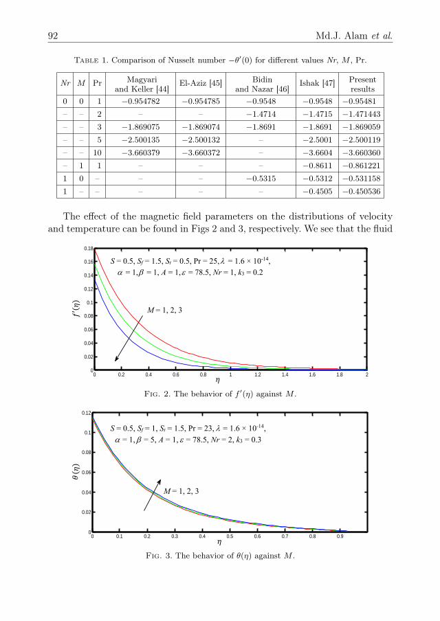
We compare the values of the local Nusselt number −θ′(0) with the workpresented in [44–47] to determine the validity of the numerical analysis by wayof replacing S = 0, Sf = 0, St = 0, β = 0, λ = 0, A = 0, k3 → ∞. Thecomparison shown in Table 1 suggests a very good agreement.


Table 1. Comparison of Nusselt number −θ′(0) for different values Nr, M , Pr.

Nr M Pr Magyariand Keller [44]

El-Aziz [45] Bidinand Nazar [46]

Ishak [47] Presentresults

0 0 1 −0.954782 −0.954785 −0.9548 −0.9548 −0.95481– – 2 – – −1.4714 −1.4715 −1.471443– – 3 −1.869075 −1.869074 −1.8691 −1.8691 −1.869059– – 5 −2.500135 −2.500132 – −2.5001 −2.500119– – 10 −3.660379 −3.660372 – −3.6604 −3.660360– 1 1 – – – −0.8611 −0.8612211 0 – – – −0.5315 −0.5312 −0.5311581 – – – – – −0.4505 −0.450536

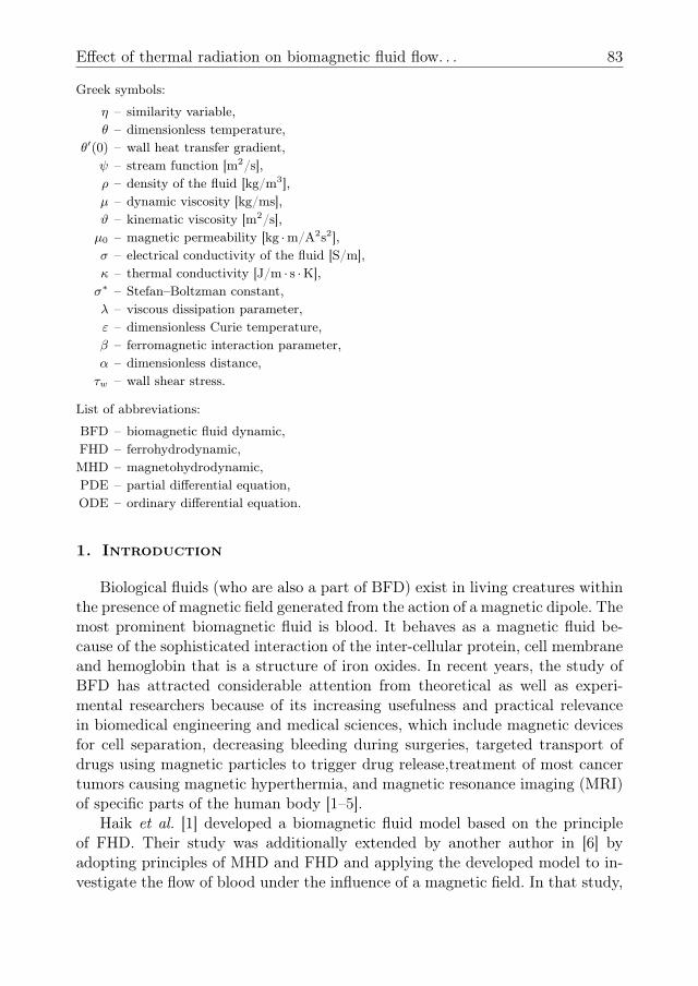
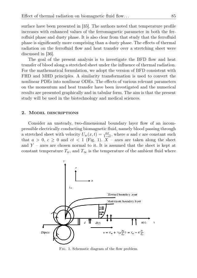
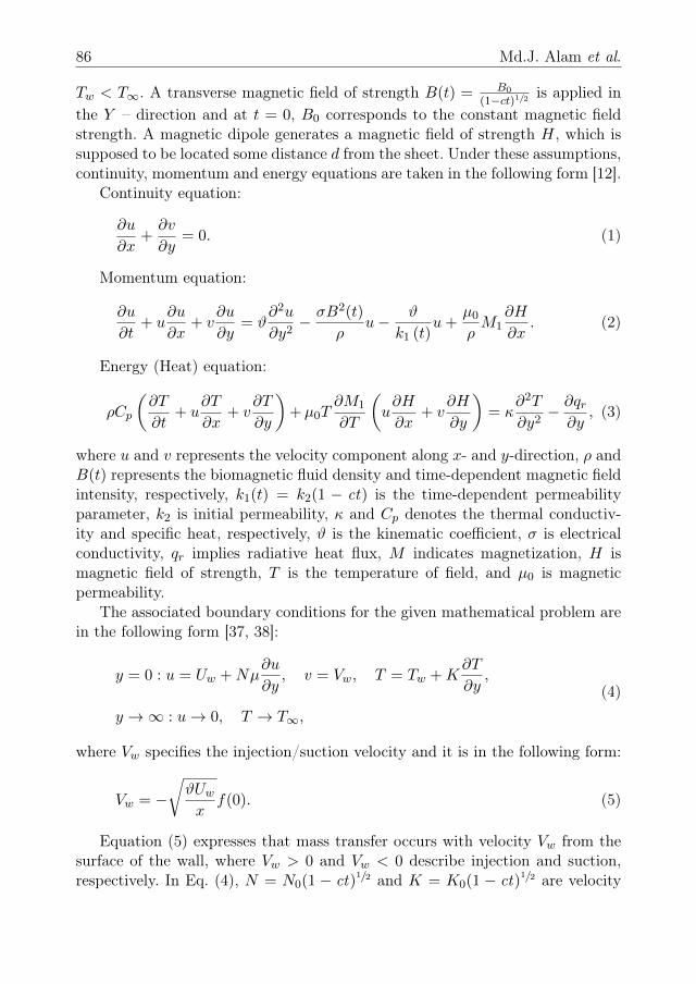
The effect of the magnetic field parameters on the distributions of velocityand temperature can be found in Figs 2 and 3, respectively. We see that the fluid

2/12

𝑓′(𝜂) 𝜂 M = 1, 2, 3S = 0.5, Sf = 1.5, St = 0.5, Pr = 25, = 1.6 × 10-14, = 1, = 1, A = 1, = 78.5, Nr = 1, k3 = 0.2

𝜃

0 0.2 0.4 0.6 0.8 1 1.2 1.4 1.6 1.8 20

0.02

0.04

0.06

0.08

0.1

0.12

0.14

0.16

0.18

0 0.1 0.2 0.3 0.4 0.5 0.6 0.7 0.8 0.90

0.02

0.04

0.06

0.08

0.1

0.12

M = 1, 2, 3

M = 1, 2, 3

S = 0.5, Sf = 1.5, St = 0.5, Pr = 25, λ = 1.6 × 10-14, α = 1, β = 1, A = 1, ε = 78.5, Nr = 1, k3 = 0.2

𝜂

𝑓′ ( 𝜂

)

S = 0.5, Sf = 1, St = 1.5, Pr = 23, λ = 1.6 × 10-14,α = 1, β = 5, A = 1, ε = 78.5, Nr = 2, k3 = 0.3

( 𝜂)

𝜂

Fig. 2. The behavior of f ′(η) against M .

2/12

𝑓′(𝜂) 𝜂 M = 1, 2, 3S = 0.5, Sf = 1.5, St = 0.5, Pr = 25, = 1.6 × 10-14, = 1, = 1, A = 1, = 78.5, Nr = 1, k3 = 0.2

𝜃

0 0.2 0.4 0.6 0.8 1 1.2 1.4 1.6 1.8 20

0.02

0.04

0.06

0.08

0.1

0.12

0.14

0.16

0.18

0 0.1 0.2 0.3 0.4 0.5 0.6 0.7 0.8 0.90

0.02

0.04

0.06

0.08

0.1

0.12

M = 1, 2, 3

M = 1, 2, 3

S = 0.5, Sf = 1.5, St = 0.5, Pr = 25, λ = 1.6 × 10-14, α = 1, β = 1, A = 1, ε = 78.5, Nr = 1, k3 = 0.2

𝜂

𝑓′ ( 𝜂

)

S = 0.5, Sf = 1, St = 1.5, Pr = 23, λ = 1.6 × 10-14,α = 1, β = 5, A = 1, ε = 78.5, Nr = 2, k3 = 0.3

( 𝜂)

𝜂

Fig. 3. The behavior of θ(η) against M .


velocity decreased with an improvement in the magnetic field parameter, and theboundary layer temperature increased with the same improvement. This showsspecifically that the transverse magnetic field opposes transport phenomena.We see that the fluid velocity decreased with an improvement in the magneticfield parameter, and the boundary layer temperature increased in the same case.Consequently, there is a tendency for the transverse magnetic field to createa drag force called the Lorentz force.

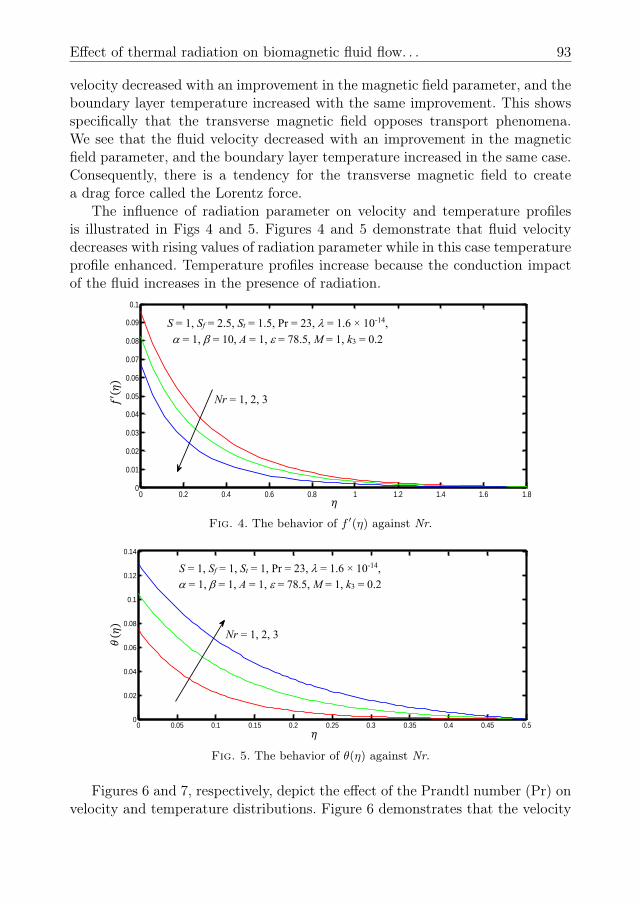
The influence of radiation parameter on velocity and temperature profilesis illustrated in Figs 4 and 5. Figures 4 and 5 demonstrate that fluid velocitydecreases with rising values of radiation parameter while in this case temperatureprofile enhanced. Temperature profiles increase because the conduction impactof the fluid increases in the presence of radiation.

3/12

Fig.4. The behavior of )(' f against Nr .

Fig.5. The behavior of θ(η) against Nr.

0 0.2 0.4 0.6 0.8 1 1.2 1.4 1.6 1.80

0.01

0.02

0.03

0.04

0.05

0.06

0.07

0.08

0.09

0.1

0 0.05 0.1 0.15 0.2 0.25 0.3 0.35 0.4 0.45 0.50

0.02

0.04

0.06

0.08

0.1

0.12

0.14

Nr = 1, 2, 3

Nr = 1, 2, 3

𝑓′ ( 𝜂

)𝜃

( 𝜂)

𝜂

𝜂

S = 1, Sf = 2.5, St = 1.5, Pr = 23, λ = 1.6 × 10-14,α = 1, β = 10, A = 1, ε = 78.5, M = 1, k3 = 0.2

S = 1, Sf = 1, St = 1, Pr = 23, λ = 1.6 × 10-14,α = 1, β = 1, A = 1, ε = 78.5, M = 1, k3 = 0.2

Fig. 4. The behavior of f ′(η) against Nr.

3/12

Fig.4. The behavior of )(' f against Nr .

Fig.5. The behavior of θ(η) against Nr.

0 0.2 0.4 0.6 0.8 1 1.2 1.4 1.6 1.80

0.01

0.02

0.03

0.04

0.05

0.06

0.07

0.08

0.09

0.1

0 0.05 0.1 0.15 0.2 0.25 0.3 0.35 0.4 0.45 0.50

0.02

0.04

0.06

0.08

0.1

0.12

0.14

Nr = 1, 2, 3

Nr = 1, 2, 3

𝑓′ ( 𝜂

)𝜃

( 𝜂)

𝜂

𝜂

S = 1, Sf = 2.5, St = 1.5, Pr = 23, λ = 1.6 × 10-14,α = 1, β = 10, A = 1, ε = 78.5, M = 1, k3 = 0.2

S = 1, Sf = 1, St = 1, Pr = 23, λ = 1.6 × 10-14,α = 1, β = 1, A = 1, ε = 78.5, M = 1, k3 = 0.2

Fig. 5. The behavior of θ(η) against Nr.

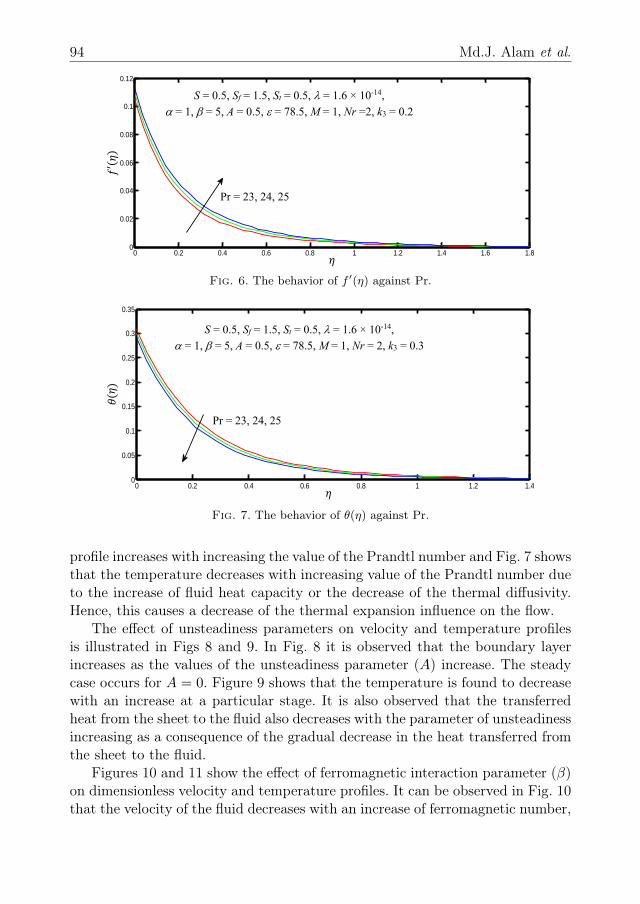
Figures 6 and 7, respectively, depict the effect of the Prandtl number (Pr) onvelocity and temperature distributions. Figure 6 demonstrates that the velocity


4/12

Fig.6. The behavior of f’(η)against Pr.

Fig.7. The behavior of θ(η)against Pr.

0 0.2 0.4 0.6 0.8 1 1.2 1.4 1.6 1.80

0.02

0.04

0.06

0.08

0.1

0.12

0 0.2 0.4 0.6 0.8 1 1.2 1.40

0.05

0.1

0.15

0.2

0.25

0.3

0.35

Pr = 23, 24, 25

Pr = 23, 24, 25

𝑓′ ( 𝜂

)𝜃

(𝜂)

𝜂

𝜂

S = 0.5, Sf = 1.5, St = 0.5, λ = 1.6 × 10-14,α = 1, β = 5, A = 0.5, ε = 78.5, M = 1, Nr =2, k3 = 0.2

S = 0.5, Sf = 1.5, St = 0.5, λ = 1.6 × 10-14,α = 1, β = 5, A = 0.5, ε = 78.5, M = 1, Nr = 2, k3 = 0.3

Fig. 6. The behavior of f ′(η) against Pr.

4/12

Fig.6. The behavior of f’(η)against Pr.

Fig.7. The behavior of θ(η)against Pr.

0 0.2 0.4 0.6 0.8 1 1.2 1.4 1.6 1.80

0.02

0.04

0.06

0.08

0.1

0.12

0 0.2 0.4 0.6 0.8 1 1.2 1.40

0.05

0.1

0.15

0.2

0.25

0.3

0.35

Pr = 23, 24, 25

Pr = 23, 24, 25

𝑓′ ( 𝜂

)𝜃

(𝜂)

𝜂

𝜂

S = 0.5, Sf = 1.5, St = 0.5, λ = 1.6 × 10-14,α = 1, β = 5, A = 0.5, ε = 78.5, M = 1, Nr =2, k3 = 0.2

S = 0.5, Sf = 1.5, St = 0.5, λ = 1.6 × 10-14,α = 1, β = 5, A = 0.5, ε = 78.5, M = 1, Nr = 2, k3 = 0.3

Fig. 7. The behavior of θ(η) against Pr.

profile increases with increasing the value of the Prandtl number and Fig. 7 showsthat the temperature decreases with increasing value of the Prandtl number dueto the increase of fluid heat capacity or the decrease of the thermal diffusivity.Hence, this causes a decrease of the thermal expansion influence on the flow.

The effect of unsteadiness parameters on velocity and temperature profilesis illustrated in Figs 8 and 9. In Fig. 8 it is observed that the boundary layerincreases as the values of the unsteadiness parameter (A) increase. The steadycase occurs for A = 0. Figure 9 shows that the temperature is found to decreasewith an increase at a particular stage. It is also observed that the transferredheat from the sheet to the fluid also decreases with the parameter of unsteadinessincreasing as a consequence of the gradual decrease in the heat transferred fromthe sheet to the fluid.

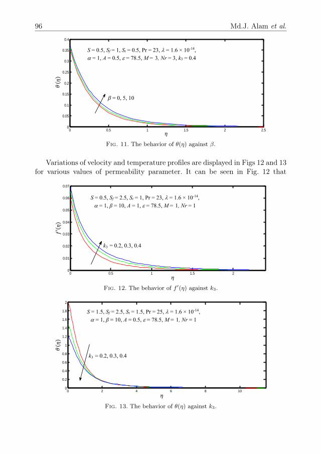
Figures 10 and 11 show the effect of ferromagnetic interaction parameter (β)on dimensionless velocity and temperature profiles. It can be observed in Fig. 10that the velocity of the fluid decreases with an increase of ferromagnetic number,


5/12

Fig.8 The behavior of f’(η) against A.

Fig.9. The behavior of θ(η) against A.

0 0.5 1 1.5 2 2.50

0.01

0.02

0.03

0.04

0.05

0.06

0.07

0 0.1 0.2 0.3 0.4 0.5 0.6 0.7 0.8 0.90

0.02

0.04

0.06

0.08

0.1

0.12

0.14

A = 0, 0.5, 1

A = 0, 0.5, 1

𝑓′ ( 𝜂

)𝜃

( 𝜂)

𝜂

𝜂

S = 0.5, Sf = 2.5, St = 1, Pr = 23, λ = 1.6 × 10-14, α = 1, β = 10, ε = 78.5, M = 1, Nr = 1, k3 = 0.4

S = 0.5, Sf = 1.5, St = 1, Pr = 23, λ = 1.6 × 10-14,α = 1, β = 5, ε = 78.5, M = 1, Nr = 1, k3 = 0.2

Fig. 8. The behavior of f ′(η) against A.

5/12

Fig.8 The behavior of f’(η) against A.

Fig.9. The behavior of θ(η) against A.

0 0.5 1 1.5 2 2.50

0.01

0.02

0.03

0.04

0.05

0.06

0.07

0 0.1 0.2 0.3 0.4 0.5 0.6 0.7 0.8 0.90

0.02

0.04

0.06

0.08

0.1

0.12

0.14

A = 0, 0.5, 1

A = 0, 0.5, 1

𝑓′ ( 𝜂

)𝜃

( 𝜂)

𝜂

𝜂

S = 0.5, Sf = 2.5, St = 1, Pr = 23, λ = 1.6 × 10-14, α = 1, β = 10, ε = 78.5, M = 1, Nr = 1, k3 = 0.4

S = 0.5, Sf = 1.5, St = 1, Pr = 23, λ = 1.6 × 10-14,α = 1, β = 5, ε = 78.5, M = 1, Nr = 1, k3 = 0.2

Fig. 9. The behavior of θ(η) against A.

6/12

ηFig.10. The behavior of f’(η) against β.

Fig.11. The behavior of θ(η) against β.

0 0.5 1 1.5 20

0.02

0.04

0.06

0.08

0.1

0.12

0.14

0.16

0.18

0.2

0 0.5 1 1.5 2 2.50

0.05

0.1

0.15

0.2

0.25

0.3

0.35

0.4

β = 0, 5, 10

β = 0, 5, 10

𝑓′ ( 𝜂

)𝜃

( 𝜂)

𝜂

𝜂

S = 1, Sf = 1.5, St = 0.5, Pr = 23, λ = 1.6 × 10-14,α = 1, A = 1, ε = 78.5, M = 1, Nr = 1, k3 = 0.3

S = 0.5, Sf = 1, St = 0.5, Pr = 23, λ = 1.6 × 10-14,α = 1, A = 0.5, ε = 78.5, M = 3, Nr = 3, k3 = 0.4

Fig. 10. The behavior of f ′(η) against β.

whereas Fig. 11 shows that the temperature profile increases in this case. Thisis because the ferromagnetic number is directly related to Kelvin force, which isalso known as drug force and it is the same as in Figs 2 and 3.


6/12

ηFig.10. The behavior of f’(η) against β.

Fig.11. The behavior of θ(η) against β.

0 0.5 1 1.5 20

0.02

0.04

0.06

0.08

0.1

0.12

0.14

0.16

0.18

0.2

0 0.5 1 1.5 2 2.50

0.05

0.1

0.15

0.2

0.25

0.3

0.35

0.4

β = 0, 5, 10

β = 0, 5, 10

𝑓′ ( 𝜂

)𝜃

( 𝜂)

𝜂

𝜂

S = 1, Sf = 1.5, St = 0.5, Pr = 23, λ = 1.6 × 10-14,α = 1, A = 1, ε = 78.5, M = 1, Nr = 1, k3 = 0.3

S = 0.5, Sf = 1, St = 0.5, Pr = 23, λ = 1.6 × 10-14,α = 1, A = 0.5, ε = 78.5, M = 3, Nr = 3, k3 = 0.4

Fig. 11. The behavior of θ(η) against β.

Variations of velocity and temperature profiles are displayed in Figs 12 and 13for various values of permeability parameter. It can be seen in Fig. 12 that

7/12

Fig.12. The behavior of f’(η)against k3.

Fig.13. The behavior of θ(η) against k3.

0 0.5 1 1.5 20

0.01

0.02

0.03

0.04

0.05

0.06

0.07

0 2 4 6 8 100

0.2

0.4

0.6

0.8

1

1.2

1.4

1.6

1.8

2

k3 = 0.2, 0.3, 0.4

k3 = 0.2, 0.3, 0.4

𝑓′ ( 𝜂

)𝜃

( 𝜂)

𝜂

𝜂

S = 0.5, Sf = 2.5, St = 1, Pr = 23, λ = 1.6 × 10-14,α = 1, β = 10, A = 1, ε = 78.5, M = 1, Nr = 1

S = 1.5, Sf = 2.5, St = 1.5, Pr = 25, λ = 1.6 × 10-14,α = 1, β = 10, A = 0.5, ε = 78.5, M = 1, Nr = 1

Fig. 12. The behavior of f ′(η) against k3.

7/12

Fig.12. The behavior of f’(η)against k3.

Fig.13. The behavior of θ(η) against k3.

0 0.5 1 1.5 20

0.01

0.02

0.03

0.04

0.05

0.06

0.07

0 2 4 6 8 100

0.2

0.4

0.6

0.8

1

1.2

1.4

1.6

1.8

2

k3 = 0.2, 0.3, 0.4

k3 = 0.2, 0.3, 0.4

𝑓′ ( 𝜂

)𝜃

( 𝜂)

𝜂

𝜂

S = 0.5, Sf = 2.5, St = 1, Pr = 23, λ = 1.6 × 10-14,α = 1, β = 10, A = 1, ε = 78.5, M = 1, Nr = 1

S = 1.5, Sf = 2.5, St = 1.5, Pr = 25, λ = 1.6 × 10-14,α = 1, β = 10, A = 0.5, ε = 78.5, M = 1, Nr = 1

Fig. 13. The behavior of θ(η) against k3.


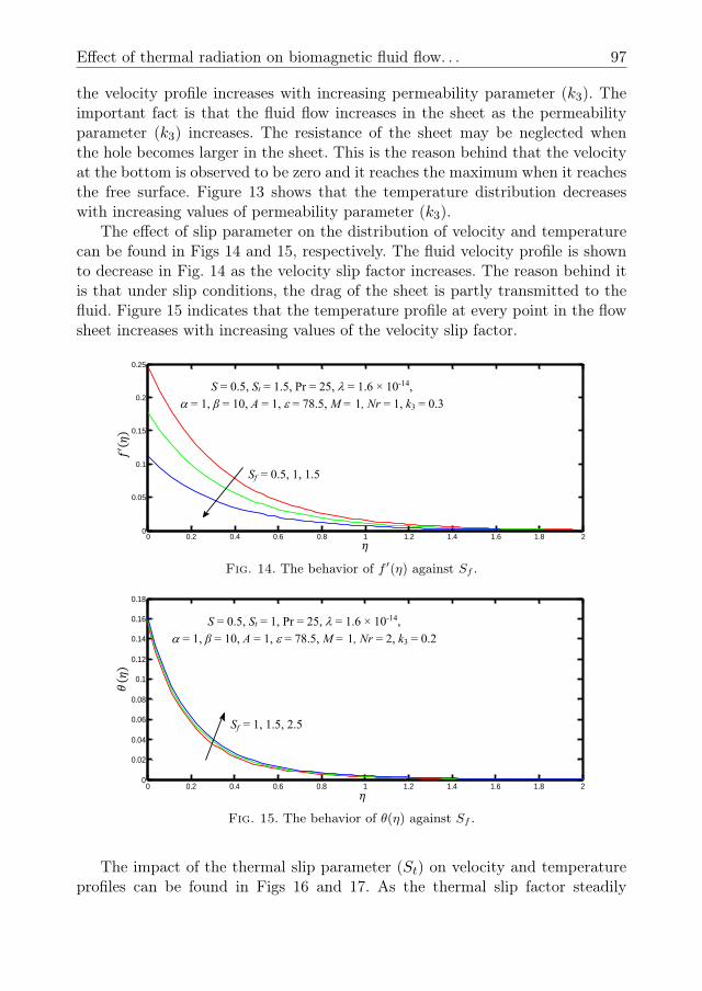
the velocity profile increases with increasing permeability parameter (k3). Theimportant fact is that the fluid flow increases in the sheet as the permeabilityparameter (k3) increases. The resistance of the sheet may be neglected whenthe hole becomes larger in the sheet. This is the reason behind that the velocityat the bottom is observed to be zero and it reaches the maximum when it reachesthe free surface. Figure 13 shows that the temperature distribution decreaseswith increasing values of permeability parameter (k3).

The effect of slip parameter on the distribution of velocity and temperaturecan be found in Figs 14 and 15, respectively. The fluid velocity profile is shownto decrease in Fig. 14 as the velocity slip factor increases. The reason behind itis that under slip conditions, the drag of the sheet is partly transmitted to thefluid. Figure 15 indicates that the temperature profile at every point in the flowsheet increases with increasing values of the velocity slip factor.

8/12

Fig.14. The behavior of f’(η)against Sf.

Fig.15. The behavior of θ(η)against Sf.

0 0.2 0.4 0.6 0.8 1 1.2 1.4 1.6 1.8 20

0.05

0.1

0.15

0.2

0.25

0 0.2 0.4 0.6 0.8 1 1.2 1.4 1.6 1.8 20

0.02

0.04

0.06

0.08

0.1

0.12

0.14

0.16

0.18

Sf = 0.5, 1, 1.5

Sf = 1, 1.5, 2.5

𝑓′ ( 𝜂

)𝜃

( 𝜂)

𝜂

𝜂

S = 0.5, St = 1.5, Pr = 25, λ = 1.6 × 10-14,α = 1, β = 10, A = 1, ε = 78.5, M = 1, Nr = 1, k3 = 0.3

S = 0.5, St = 1, Pr = 25, λ = 1.6 × 10-14,α = 1, β = 10, A = 1, ε = 78.5, M = 1, Nr = 2, k3 = 0.2

Fig. 14. The behavior of f ′(η) against Sf .

8/12

Fig.14. The behavior of f’(η)against Sf.

Fig.15. The behavior of θ(η)against Sf.

0 0.2 0.4 0.6 0.8 1 1.2 1.4 1.6 1.8 20

0.05

0.1

0.15

0.2

0.25

0 0.2 0.4 0.6 0.8 1 1.2 1.4 1.6 1.8 20

0.02

0.04

0.06

0.08

0.1

0.12

0.14

0.16

0.18

Sf = 0.5, 1, 1.5

Sf = 1, 1.5, 2.5

𝑓′ ( 𝜂

)𝜃

( 𝜂)

𝜂

𝜂

S = 0.5, St = 1.5, Pr = 25, λ = 1.6 × 10-14,α = 1, β = 10, A = 1, ε = 78.5, M = 1, Nr = 1, k3 = 0.3

S = 0.5, St = 1, Pr = 25, λ = 1.6 × 10-14,α = 1, β = 10, A = 1, ε = 78.5, M = 1, Nr = 2, k3 = 0.2

Fig. 15. The behavior of θ(η) against Sf .

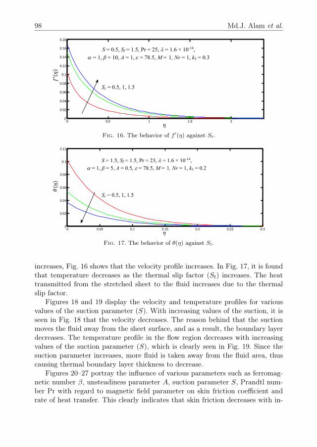
The impact of the thermal slip parameter (St) on velocity and temperatureprofiles can be found in Figs 16 and 17. As the thermal slip factor steadily


9/12

ηFig.16. The behavior of f’(η) against St.

ηFig.17. The behavior of θ(η) against St.

0 0.5 1 1.5 20

0.02

0.04

0.06

0.08

0.1

0.12

0.14

0.16

0.18

0 0.05 0.1 0.15 0.2 0.25 0.30

0.02

0.04

0.06

0.08

0.1

0.12

St = 0.5, 1, 1.5

St = 0.5, 1, 1.5

𝑓′ ( 𝜂

)𝜃

( 𝜂)

𝜂

𝜂

S = 0.5, Sf = 1.5, Pr = 25, λ = 1.6 × 10-14,α = 1, β = 10, A = 1, ε = 78.5, M = 1, Nr = 1, k3 = 0.3

S = 1.5, Sf = 1.5, Pr = 23, λ = 1.6 × 10-14,α = 1, β = 5, A = 0.5, ε = 78.5, M = 1, Nr = 1, k3 = 0.2

Fig. 16. The behavior of f ′(η) against St.

9/12

ηFig.16. The behavior of f’(η) against St.

ηFig.17. The behavior of θ(η) against St.

0 0.5 1 1.5 20

0.02

0.04

0.06

0.08

0.1

0.12

0.14

0.16

0.18

0 0.05 0.1 0.15 0.2 0.25 0.30

0.02

0.04

0.06

0.08

0.1

0.12

St = 0.5, 1, 1.5

St = 0.5, 1, 1.5

𝑓′ ( 𝜂

)𝜃

( 𝜂)

𝜂

𝜂

S = 0.5, Sf = 1.5, Pr = 25, λ = 1.6 × 10-14,α = 1, β = 10, A = 1, ε = 78.5, M = 1, Nr = 1, k3 = 0.3

S = 1.5, Sf = 1.5, Pr = 23, λ = 1.6 × 10-14,α = 1, β = 5, A = 0.5, ε = 78.5, M = 1, Nr = 1, k3 = 0.2

Fig. 17. The behavior of θ(η) against St.

increases, Fig. 16 shows that the velocity profile increases. In Fig. 17, it is foundthat temperature decreases as the thermal slip factor (St) increases. The heattransmitted from the stretched sheet to the fluid increases due to the thermalslip factor.

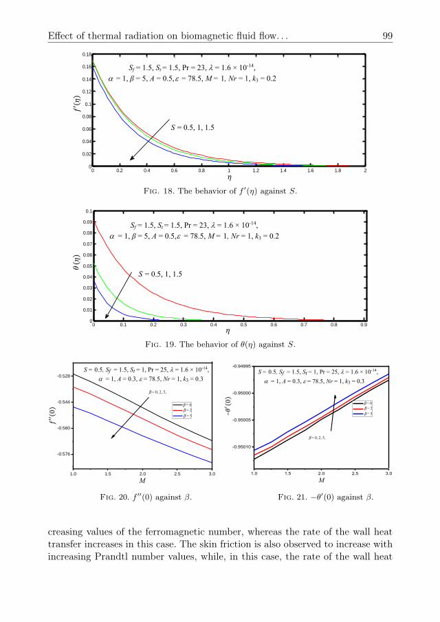
Figures 18 and 19 display the velocity and temperature profiles for variousvalues of the suction parameter (S). With increasing values of the suction, it isseen in Fig. 18 that the velocity decreases. The reason behind that the suctionmoves the fluid away from the sheet surface, and as a result, the boundary layerdecreases. The temperature profile in the flow region decreases with increasingvalues of the suction parameter (S), which is clearly seen in Fig. 19. Since thesuction parameter increases, more fluid is taken away from the fluid area, thuscausing thermal boundary layer thickness to decrease.

Figures 20–27 portray the influence of various parameters such as ferromag-netic number β, unsteadiness parameter A, suction parameter S, Prandtl num-ber Pr with regard to magnetic field parameter on skin friction coefficient andrate of heat transfer. This clearly indicates that skin friction decreases with in-


10/12

ηFig.18. The behavior of f’(η) against S.

Fig.19. The behavior of θ(η) against S.

0 0.2 0.4 0.6 0.8 1 1.2 1.4 1.6 1.8 20

0.02

0.04

0.06

0.08

0.1

0.12

0.14

0.16

0.18

0 0.1 0.2 0.3 0.4 0.5 0.6 0.7 0.8 0.90

0.01

0.02

0.03

0.04

0.05

0.06

0.07

0.08

0.09

0.1

S = 0.5, 1, 1.5

S = 0.5, 1, 1.5

𝑓′ ( 𝜂

)𝜃

( 𝜂)

𝜂

𝜂

Sf = 1.5, St = 1.5, Pr = 23, λ = 1.6 × 10-14,α = 1, β = 5, A = 0.5, ε = 78.5, M = 1, Nr = 1, k3 = 0.2


Fig. 18. The behavior of f ′(η) against S.

10/12

ηFig.18. The behavior of f’(η) against S.

Fig.19. The behavior of θ(η) against S.

0 0.2 0.4 0.6 0.8 1 1.2 1.4 1.6 1.8 20

0.02

0.04

0.06

0.08

0.1

0.12

0.14

0.16

0.18

0 0.1 0.2 0.3 0.4 0.5 0.6 0.7 0.8 0.90

0.01

0.02

0.03

0.04

0.05

0.06

0.07

0.08

0.09

0.1

S = 0.5, 1, 1.5

S = 0.5, 1, 1.5

𝑓′ ( 𝜂

)𝜃

( 𝜂)

𝜂

𝜂



Fig. 19. The behavior of θ(η) against S.

11/12

1.0 1.5 2.0 2.5 3.0

-0.576

-0.560

-0.544

-0.528

1.0 1.5 2.0 2.5 3.0

-0.95010

-0.95005

-0.95000

-0.94995

Fig.20. f''(0) against . Fig.21. –θ'(0) against β.

1.0 1.5 2.0 2.5 3.0

-0.370

-0.365

-0.360

-0.355 Pr=23

Pr=24

Pr=25

1.0 1.5 2.0 2.5 3.0

-0.64405

-0.64350

-0.64295

-0.64240 Pr=23

Pr=24

Pr=25

Fig.22. f''(0) against Pr. Fig.23 –θ'(0) against Pr.

1.0 1.5 2.0 2.5 3.0

-0.57

-0.56

-0.55

-0.54

-0.53

A=0

A=.5

A=1

1.0 1.5 2.0 2.5 3.0

-0.9505

-0.9500

-0.9495

-0.9490

A=0

A=.5

A=1

MFig.24. f''(0) against A.

Fig.25. –θ'(0) against A.

𝑓′′(0)

𝑓′′ (0 )

𝑓′′(0) –𝜃′ (0)

–𝜃 ( 0

)–𝜃′ (0)

M

M

M

M

M

M

S = 0.5, Sf = 1.5, St = 1, Pr = 25, λ� = 1.6 × 10-14,α� = 1, A = 0.3, ε = 78.5, Nr = 1, k3 = 0.3

S = 0.5, Sf = 1.5, St = 1, Pr = 25, λ� = 1.6 × 10-14,α� = 1, A = 0.3, ε = 78.5, Nr = 1, k3 = 0.3

S = 0.5, Sf = 2.5, St = 1.5, λ� = 1.6 × 10-14, α = 1,

β = 5, A = 0.3, ε = 78.5, Nr = 1, k3 = 0.3 S = 0.5, Sf = 2.5, St = 1.5, λ� = 1.6 × 10-14,

α = 1, β = 5, A = 0.3, ε = 78.5, Nr = 1, k3 = 0.3

S = 0.5, Sf = 1.5, St = 1, Pr = 25, λ� = 1.6 × 10-14, α = 1, β = 1, ε = 78.5, Nr = 1, k3 = 0.3

α = 1, β = 1, ε = 78.5, Nr = 1, k3 = 0.3 S = 0.5, Sf = 1.5, St = 1, Pr = 1, λ� = 1.6 × 10-14,

A = 0 A = 0.5 A = 1

A = 0A = 0.5A = 1

Pr = 23 Pr = 24 Pr = 25

Pr = 23 Pr = 24 Pr = 25

β = 0β = 2β = 5

β = 0, 2, 5

β = 0β = 2β = 5

β = 0, 2, 5

A = 0, 0.5, 1 A = 0, 0.5, 1

Pr = 23, 24, 25Pr = 23, 24, 25

11/12

1.0 1.5 2.0 2.5 3.0

-0.576

-0.560

-0.544

-0.528

1.0 1.5 2.0 2.5 3.0

-0.95010

-0.95005

-0.95000

-0.94995


1.0 1.5 2.0 2.5 3.0

-0.370

-0.365

-0.360

-0.355 Pr=23

Pr=24

Pr=25

1.0 1.5 2.0 2.5 3.0

-0.64405

-0.64350

-0.64295

-0.64240 Pr=23

Pr=24

Pr=25


1.0 1.5 2.0 2.5 3.0

-0.57

-0.56

-0.55

-0.54

-0.53

A=0

A=.5

A=1

1.0 1.5 2.0 2.5 3.0

-0.9505

-0.9500

-0.9495

-0.9490

A=0

A=.5

A=1



𝑓′′(0)

𝑓′′ (0 )

𝑓′′(0) –𝜃′ (0)

–𝜃 ( 0

)–𝜃′ (0)

M

M

M

M

M

M

S = 0.5, Sf = 1.5, St = 1, Pr = 25, λ� = 1.6 × 10-14,α� = 1, A = 0.3, ε = 78.5, Nr = 1, k3 = 0.3

S = 0.5, Sf = 1.5, St = 1, Pr = 25, λ� = 1.6 × 10-14,α� = 1, A = 0.3, ε = 78.5, Nr = 1, k3 = 0.3

S = 0.5, Sf = 2.5, St = 1.5, λ� = 1.6 × 10-14, α = 1,

β = 5, A = 0.3, ε = 78.5, Nr = 1, k3 = 0.3 S = 0.5, Sf = 2.5, St = 1.5, λ� = 1.6 × 10-14,

α = 1, β = 5, A = 0.3, ε = 78.5, Nr = 1, k3 = 0.3

S = 0.5, Sf = 1.5, St = 1, Pr = 25, λ� = 1.6 × 10-14, α = 1, β = 1, ε = 78.5, Nr = 1, k3 = 0.3

α = 1, β = 1, ε = 78.5, Nr = 1, k3 = 0.3 S = 0.5, Sf = 1.5, St = 1, Pr = 1, λ� = 1.6 × 10-14,

A = 0 A = 0.5 A = 1

A = 0A = 0.5A = 1

Pr = 23 Pr = 24 Pr = 25

Pr = 23 Pr = 24 Pr = 25

β = 0β = 2β = 5

β = 0, 2, 5

β = 0β = 2β = 5

β = 0, 2, 5

A = 0, 0.5, 1 A = 0, 0.5, 1

Pr = 23, 24, 25Pr = 23, 24, 25

Fig. 20. f ′′(0) against β. Fig. 21. −θ′(0) against β.

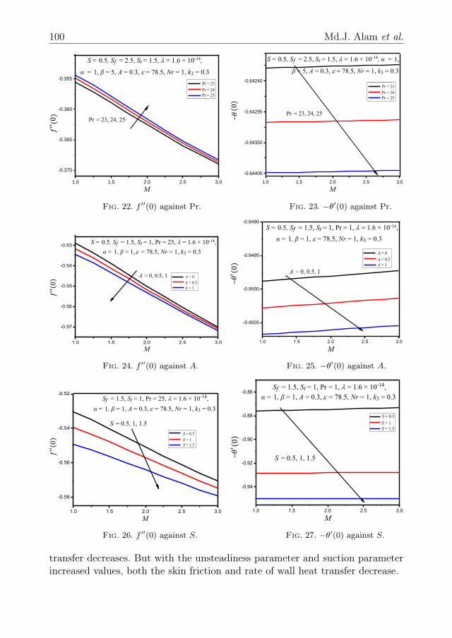
creasing values of the ferromagnetic number, whereas the rate of the wall heattransfer increases in this case. The skin friction is also observed to increase withincreasing Prandtl number values, while, in this case, the rate of the wall heat


11/12

1.0 1.5 2.0 2.5 3.0

-0.576

-0.560

-0.544

-0.528

1.0 1.5 2.0 2.5 3.0

-0.95010

-0.95005

-0.95000

-0.94995


1.0 1.5 2.0 2.5 3.0

-0.370

-0.365

-0.360

-0.355 Pr=23

Pr=24

Pr=25

1.0 1.5 2.0 2.5 3.0

-0.64405

-0.64350

-0.64295

-0.64240 Pr=23

Pr=24

Pr=25


1.0 1.5 2.0 2.5 3.0

-0.57

-0.56

-0.55

-0.54

-0.53

A=0

A=.5

A=1

1.0 1.5 2.0 2.5 3.0

-0.9505

-0.9500

-0.9495

-0.9490

A=0

A=.5

A=1



𝑓′′(0)

𝑓′′ (0 )

𝑓′′(0) –𝜃′ (0)

–𝜃 ( 0

)–𝜃′ (0)

M

M

M

M

M

M

S = 0.5, Sf = 1.5, St = 1, Pr = 25, λ� = 1.6 × 10-14,α� = 1, A = 0.3, ε = 78.5, Nr = 1, k3 = 0.3

S = 0.5, Sf = 1.5, St = 1, Pr = 25, λ� = 1.6 × 10-14,α� = 1, A = 0.3, ε = 78.5, Nr = 1, k3 = 0.3

S = 0.5, Sf = 2.5, St = 1.5, λ� = 1.6 × 10-14, α = 1,

β = 5, A = 0.3, ε = 78.5, Nr = 1, k3 = 0.3 S = 0.5, Sf = 2.5, St = 1.5, λ� = 1.6 × 10-14,

α = 1, β = 5, A = 0.3, ε = 78.5, Nr = 1, k3 = 0.3

S = 0.5, Sf = 1.5, St = 1, Pr = 25, λ� = 1.6 × 10-14, α = 1, β = 1, ε = 78.5, Nr = 1, k3 = 0.3

α = 1, β = 1, ε = 78.5, Nr = 1, k3 = 0.3 S = 0.5, Sf = 1.5, St = 1, Pr = 1, λ� = 1.6 × 10-14,

A = 0 A = 0.5 A = 1

A = 0A = 0.5A = 1

Pr = 23 Pr = 24 Pr = 25

Pr = 23 Pr = 24 Pr = 25

β = 0β = 2β = 5

β = 0, 2, 5

β = 0β = 2β = 5

β = 0, 2, 5

A = 0, 0.5, 1 A = 0, 0.5, 1

Pr = 23, 24, 25Pr = 23, 24, 25

11/12

1.0 1.5 2.0 2.5 3.0

-0.576

-0.560

-0.544

-0.528

1.0 1.5 2.0 2.5 3.0

-0.95010

-0.95005

-0.95000

-0.94995


1.0 1.5 2.0 2.5 3.0

-0.370

-0.365

-0.360

-0.355 Pr=23

Pr=24

Pr=25

1.0 1.5 2.0 2.5 3.0

-0.64405

-0.64350

-0.64295

-0.64240 Pr=23

Pr=24

Pr=25


1.0 1.5 2.0 2.5 3.0

-0.57

-0.56

-0.55

-0.54

-0.53

A=0

A=.5

A=1

1.0 1.5 2.0 2.5 3.0

-0.9505

-0.9500

-0.9495

-0.9490

A=0

A=.5

A=1



𝑓′′(0)

𝑓′′ (0 )

𝑓′′(0) –𝜃′ (0)

–𝜃 ( 0

)–𝜃′ (0)

M

M

M

M

M

M

S = 0.5, Sf = 1.5, St = 1, Pr = 25, λ� = 1.6 × 10-14,α� = 1, A = 0.3, ε = 78.5, Nr = 1, k3 = 0.3

S = 0.5, Sf = 1.5, St = 1, Pr = 25, λ� = 1.6 × 10-14,α� = 1, A = 0.3, ε = 78.5, Nr = 1, k3 = 0.3

S = 0.5, Sf = 2.5, St = 1.5, λ� = 1.6 × 10-14, α = 1,

β = 5, A = 0.3, ε = 78.5, Nr = 1, k3 = 0.3 S = 0.5, Sf = 2.5, St = 1.5, λ� = 1.6 × 10-14,

α = 1, β = 5, A = 0.3, ε = 78.5, Nr = 1, k3 = 0.3

S = 0.5, Sf = 1.5, St = 1, Pr = 25, λ� = 1.6 × 10-14, α = 1, β = 1, ε = 78.5, Nr = 1, k3 = 0.3

α = 1, β = 1, ε = 78.5, Nr = 1, k3 = 0.3 S = 0.5, Sf = 1.5, St = 1, Pr = 1, λ� = 1.6 × 10-14,

A = 0 A = 0.5 A = 1

A = 0A = 0.5A = 1

Pr = 23 Pr = 24 Pr = 25

Pr = 23 Pr = 24 Pr = 25

β = 0β = 2β = 5

β = 0, 2, 5

β = 0β = 2β = 5

β = 0, 2, 5

A = 0, 0.5, 1 A = 0, 0.5, 1

Pr = 23, 24, 25Pr = 23, 24, 25

Fig. 22. f ′′(0) against Pr. Fig. 23. −θ′(0) against Pr.

11/12

1.0 1.5 2.0 2.5 3.0

-0.576

-0.560

-0.544

-0.528

1.0 1.5 2.0 2.5 3.0

-0.95010

-0.95005

-0.95000

-0.94995


1.0 1.5 2.0 2.5 3.0

-0.370

-0.365

-0.360

-0.355 Pr=23

Pr=24

Pr=25

1.0 1.5 2.0 2.5 3.0

-0.64405

-0.64350

-0.64295

-0.64240 Pr=23

Pr=24

Pr=25


1.0 1.5 2.0 2.5 3.0

-0.57

-0.56

-0.55

-0.54

-0.53

A=0

A=.5

A=1

1.0 1.5 2.0 2.5 3.0

-0.9505

-0.9500

-0.9495

-0.9490

A=0

A=.5

A=1



𝑓′′(0)

𝑓′′ (0 )

𝑓′′(0) –𝜃′ (0)

–𝜃 ( 0

)–𝜃′ (0)

M

M

M

M

M

M

S = 0.5, Sf = 1.5, St = 1, Pr = 25, λ� = 1.6 × 10-14,α� = 1, A = 0.3, ε = 78.5, Nr = 1, k3 = 0.3

S = 0.5, Sf = 1.5, St = 1, Pr = 25, λ� = 1.6 × 10-14,α� = 1, A = 0.3, ε = 78.5, Nr = 1, k3 = 0.3

S = 0.5, Sf = 2.5, St = 1.5, λ� = 1.6 × 10-14, α = 1,

β = 5, A = 0.3, ε = 78.5, Nr = 1, k3 = 0.3 S = 0.5, Sf = 2.5, St = 1.5, λ� = 1.6 × 10-14,

α = 1, β = 5, A = 0.3, ε = 78.5, Nr = 1, k3 = 0.3

S = 0.5, Sf = 1.5, St = 1, Pr = 25, λ� = 1.6 × 10-14, α = 1, β = 1, ε = 78.5, Nr = 1, k3 = 0.3

α = 1, β = 1, ε = 78.5, Nr = 1, k3 = 0.3 S = 0.5, Sf = 1.5, St = 1, Pr = 1, λ� = 1.6 × 10-14,

A = 0 A = 0.5 A = 1

A = 0A = 0.5A = 1

Pr = 23 Pr = 24 Pr = 25

Pr = 23 Pr = 24 Pr = 25

β = 0β = 2β = 5

β = 0, 2, 5

β = 0β = 2β = 5

β = 0, 2, 5

A = 0, 0.5, 1 A = 0, 0.5, 1

Pr = 23, 24, 25Pr = 23, 24, 25

11/12

1.0 1.5 2.0 2.5 3.0

-0.576

-0.560

-0.544

-0.528

1.0 1.5 2.0 2.5 3.0

-0.95010

-0.95005

-0.95000

-0.94995


1.0 1.5 2.0 2.5 3.0

-0.370

-0.365

-0.360

-0.355 Pr=23

Pr=24

Pr=25

1.0 1.5 2.0 2.5 3.0

-0.64405

-0.64350

-0.64295

-0.64240 Pr=23

Pr=24

Pr=25


1.0 1.5 2.0 2.5 3.0

-0.57

-0.56

-0.55

-0.54

-0.53

A=0

A=.5

A=1

1.0 1.5 2.0 2.5 3.0

-0.9505

-0.9500

-0.9495

-0.9490

A=0

A=.5

A=1



𝑓′′(0)

𝑓′′ (0 )

𝑓′′(0) –𝜃′ (0)

–𝜃 ( 0

)–𝜃′ (0)

M

M

M

M

M

M

S = 0.5, Sf = 1.5, St = 1, Pr = 25, λ� = 1.6 × 10-14,α� = 1, A = 0.3, ε = 78.5, Nr = 1, k3 = 0.3

S = 0.5, Sf = 1.5, St = 1, Pr = 25, λ� = 1.6 × 10-14,α� = 1, A = 0.3, ε = 78.5, Nr = 1, k3 = 0.3

S = 0.5, Sf = 2.5, St = 1.5, λ� = 1.6 × 10-14, α = 1,

β = 5, A = 0.3, ε = 78.5, Nr = 1, k3 = 0.3 S = 0.5, Sf = 2.5, St = 1.5, λ� = 1.6 × 10-14,

α = 1, β = 5, A = 0.3, ε = 78.5, Nr = 1, k3 = 0.3

S = 0.5, Sf = 1.5, St = 1, Pr = 25, λ� = 1.6 × 10-14, α = 1, β = 1, ε = 78.5, Nr = 1, k3 = 0.3

α = 1, β = 1, ε = 78.5, Nr = 1, k3 = 0.3 S = 0.5, Sf = 1.5, St = 1, Pr = 1, λ� = 1.6 × 10-14,

A = 0 A = 0.5 A = 1

A = 0A = 0.5A = 1

Pr = 23 Pr = 24 Pr = 25

Pr = 23 Pr = 24 Pr = 25

β = 0β = 2β = 5

β = 0, 2, 5

β = 0β = 2β = 5

β = 0, 2, 5

A = 0, 0.5, 1 A = 0, 0.5, 1

Pr = 23, 24, 25Pr = 23, 24, 25

Fig. 24. f ′′(0) against A. Fig. 25. −θ′(0) against A.

12/12

1.0 1.5 2.0 2.5 3.0

-0.58

-0.56

-0.54

-0.52

1.0 1.5 2.0 2.5 3.0

-0.94

-0.92

-0.90

-0.88

-0.86

S = 0.5

Fig.26. f''(0) against S. Fig.27. –θ'(0) against S. M M

–𝜃′ (0)

𝑓′′(0)

Sf = 1.5, St = 1, Pr = 25, λ� = 1.6 × 10-14, α = 1, β = 1, A = 0.3, ε = 78.5, Nr = 1, k3 = 0.3

Sf = 1.5, St = 1, Pr = 1, λ� = 1.6 × 10-14, α = 1, β = 1, A = 0.3, ε = 78.5, Nr = 1, k3 = 0.3

S = 0.5, 1, 1.5

S = 0.5, 1, 1.5

S = 1 S = 1.5S = 0.5

S = 1S = 1.5

12/12

1.0 1.5 2.0 2.5 3.0

-0.58

-0.56

-0.54

-0.52

1.0 1.5 2.0 2.5 3.0

-0.94

-0.92

-0.90

-0.88

-0.86

S = 0.5

Fig.26. f''(0) against S. Fig.27. –θ'(0) against S. M M

–𝜃′ (0)

𝑓′′(0)

Sf = 1.5, St = 1, Pr = 25, λ� = 1.6 × 10-14, α = 1, β = 1, A = 0.3, ε = 78.5, Nr = 1, k3 = 0.3

Sf = 1.5, St = 1, Pr = 1, λ� = 1.6 × 10-14, α = 1, β = 1, A = 0.3, ε = 78.5, Nr = 1, k3 = 0.3

S = 0.5, 1, 1.5

S = 0.5, 1, 1.5

S = 1 S = 1.5S = 0.5

S = 1S = 1.5

Fig. 26. f ′′(0) against S. Fig. 27. −θ′(0) against S.

transfer decreases. But with the unsteadiness parameter and suction parameterincreased values, both the skin friction and rate of wall heat transfer decrease.


7. Conclusion

In this article, we examined the influence of thermal radiation on the BFDflow under the applied magnetic field action. The main findings are as follows:

1) The magnetic field parameter, radiation parameter, ferromagnetic interac-tion parameter, and velocity slip parameter lead to alleviated/lessened thefluid velocity, whereas temperature increased in all cases.

2) The fluid velocity increased with increasing values of the Prandtl num-ber, unsteadiness parameter, permeability parameter, and non-dimensionalthermal slip factor, while the temperature decreased in all cases.

3) An increase in the suction parameter reduced both fluid velocity and tem-perature.

4) With increasing values of ferromagnetic interaction parameters, the skinfriction decreased, while the rate of heat transfer increased.

5) The Prandtl number reduced the local Nusselt number where as theskin friction coefficient increased in this case.

6) The unsteadiness parameter and suction parameter reduced both the skinfriction coefficient and rate of heat transfer.

References

1. Y. Haik, J.C. Chen, V.M. Pai, Development of biomagnetic fluid dynamics, [in:] Proceed-ings of the IX International Symposium on Transport Properties in Thermal Fluid Engi-neering, Singapore, Pacific Center of Thermal Fluid Engineering, S.H. Winoto, Y.T. Chew,N.E. Wijeysundera [Eds], Hawaii, USA, June 25–28, pp. 121–126, 1996.

2. P.A. Voltairas, D.I. Fotiadis, L.K. Michalis, Hydrodynamics of magnetic drug targeting,Journal of Biomechanics, 35(6): 813–821, 2002, doi: 10.1016/S0021-9290(02)00034-9.

3. E.K. Ruuge, A.N. Rusetski, Magnetic fluid as drug carriers: Targeted transport of drugsby a magnetic field, Journal of Magnetism and Magnetic Materials, 122(1–3): 335–339,1993, doi: 10.1016/0304-8853(93)91104-F.

4. W.-L. Lin, J.-Y.Yen, Y.-Y. Chen, K.-W. Jin, M.-J. Shieh, Relationship between acousticaperture size and tumor conditions for external ultrasound hyperthermia,Medical Physics,26(5): 818–824, 1999, doi: 10.1118/1.598590.

5. J.C. Misra, A. Sinha, G.C. Shit, Flow of a biomagnetic viscoelastic fluid: Application toestimation of blood flow in arteries during electromagnetic hyperthermia, a therapeuticprocedure for cancer treatment, Applied Mathematics and Mechanics, 31(11): 1405–1420,2010, doi: 10.1007/s10483-010-1371-6.

6. E.E. Tzirtzilakis, A mathematical model for blood flow in magnetic field, Physics of Fluids,17(7): 077103-1-14, 2005, doi: 10.1063/1.1978807.

7. N.G. Kafoussias, E.E. Tzirtzilakis, Biomagnetic fluid flow over a stretching sheet withnonlinear temperature dependent magnetization, The Journal of Applied Mathematicsand Physics (ZAMP), 54: 551–565, 2003, doi: 10.1007/s00033-003-1100-5.


8. E.E. Tzirtzilakis, N.G. Kafoussias, Three-dimensional magnetic fluid boundary layer flowover a linearly stretching sheet, Journal of Heat Transfer, 132(1): 011702-1-8, 2010, doi:10.1115/1.3194765.

9. M.G. Murtaza, E.E. Tzirtzilakis, M. Ferdows, Effect of electrical conductivity and mag-netization on the biomagnetic fluid flow over a stretching sheet, The Journal of AppliedMathematics and Physics (ZAMP), 68: 93, 2017, doi: 10.1007/s00033-017-0839-z.

10. M. Ferdows, G. Murtaza, E.E. Tzirtzilakis, J.C. Misra, A. Alsenafi, Dual solutions inbiomagnetic fluid flow and heat transfer over a nonlinear stretching/shrinking sheet: Ap-plication of Lie group transformation method, Mathematical Biosciences and Engineering,17(5): 4852–4874, 2020, doi: 10.3934/mbe.2020264.

11. J.C. Misra, G.C. Shit, Biomagnetic viscoelastic fluid flow over a stretching sheet, AppliedMathematics and Computation, 210(2): 350–361, 2009, doi: 10.1016/j.amc.2008.12.088.

12. J.C. Misra, A. Sinha, Effect of thermal radiation on MHD flow of blood and heat transferin a permeable capillary in stretching motion, Heat and Mass Transfer, 49: 617–628, 2013,doi: 10.1007/s00231-012-1107-6.

13. N.G. Kafoussias, E.E. Tzirtzilakis, A. Raptis, Free forced convective boundary layer flowof a biomagnetic fluid under the action of a localized magnetic field, Canadian Journal ofPhysics, 86(3): 447–457, 2008, doi: 10.1139/p07-166.

14. M.G. Murtaza, E.E. Tzirtzilakis, M. Ferdows, Similarity solutions of nonlinear stretchedbiomagnetic fluid flow and heat transfer with signum function and temperature power lawgeometries, International Journal of Mathematical and Computational Sciences, 12(2):24–29, 2018, doi: 10.5281/zenodo-1315703.

15. M. Murtaza, E.E. Tzirtzilakis, M. Ferdows, Stability and convergence analysis of a bio-magnetic fluid flow over a stretching sheet in the presence of a magnetic dipole, Symmetry,12(2): 253, 2020, doi: 10.3390/sym12020253.

16. M.G. Murtaza, E.E. Tzirtzilakis, M. Ferdows, Numerical solution of three dimensionalunsteady biomagnetic flow and heat transfer through stretching/shrinking sheet usingtemperature dependent magnetization, Archives of Mechanics, 70(2): 161–185, 2018.

17. M. Ali, F. Ahmed, S. Hussain, Analytical solution of unsteady MHD blood flow andheat transfer through parallel plates when lower plate stretches exponentially, Journal ofApplied Environmental and Biological Sciences, 5(3): 1–8, 2015.

18. A. Zeeshan, A. Majed, R. Ellahi, Effect of magnetic dipole on viscous ferro-fluid pasta stretching surface with thermal radiation, Journal of Molecular Liquids, 215: 549–554,2016.

19. I.H. Isaac Chen, Subrata Sana, Analysis of an intensive magnetic field on blood flow:Part 2, Journal of Bioelectricity, 4(1): 55–62, 2009, doi: 10.3109/15368378509040360.

20. S. Srinivas, P.B.A. Reddy, B.S.R.V. Prasad, Effects of chemical reaction and thermalradiation on MHD flow over an inclined permeable stretching surface with non-uniformheat source/sink: An application to the dynamics of blood flow, Journal of Mechanics inMedicine and Biology, 14(5): 1450067, 2014, doi: 10.1142/S0219519414500675.

21. A. Sinha, J.C. Misra, G.C. Shit, Effect of heat transfer on unsteady MHD flow of bloodin a permeable vessel in the presence of non-uniform heat source, Alexandria EngineeringJournal, 55(3): 2023–2033, 2016, doi: 10.1016/j.aej.2016.07.010.


22. C. Israel-Cookey, A. Ogulu, V.B. Omubo-Pepple, Influence of viscous dissipation andradiation on unsteady MHD free-convection flow past an infinite heated vertical plate ina porous medium with time-dependent suction, International Journal of Heat and MassTransfer, 46(13): 2305–2311, 2003, doi: 10.1016/S0017-9310(02)00544-6.

23. E.M.A. Elbashbeshy, D.M.Yassmin, A.A. Dalia, Heat transfer over an unsteady porousstretching surface embedded in a porous medium with variable heat flux in the presenceof heat source or sink, African Journal of Mathematics and Computer Science Research,3(5): 68–73, 2010, doi:10.5897/AJMCSR.9000071.

24. P.B.A. Reddy, N.B. Reddy, Radiation effects on MHD combined convection and masstransfer flow past a vertical porous plate embedded in a porous medium with heat gener-ation, International Journal of Applied Mathematics and Mechanics, 6(18): 33–49, 2010.

25. S. Nadeem, S. Zaheer, T. Fang, Effects of thermal radiation on the boundary layer flowof a Jeffery fluid over an exponentially stretching surface, Numerical Algorithms, 57(2):187–205, 2011, doi: 10.1007/s11075-010-9423-8.

26. P.B.A. Reddy, N.B. Reddy, S. Suneetha, Radiation effects on MHD flow past an ex-ponentially accelerated isothermal vertical plate with uniform mass diffusion in thepresence of heat source, Journal of Applied Fluid Mechanics, 5(3): 119–126, 2012, doi:10.36884/jatm.5.03.19454.

27. A.A. Khan, S. Muhammad, R. Ellahi, Q.M.Z. Zia, Bionic study of variable viscosityon MHD peristaltic flow of pseudoplastic fluid in an asymmetric channel, Journal ofMagnetics, 21(2): 273–280, 2016, doi: 10.4283/JMAG.2016.21.2.273.

28. P. Sreenivasulu, T. Poornima, N. Bhaskar Reddy, Thermal radiation effects on MHDboundary layer slip flow past a permeable exponential stretching sheet in the presence ofjoule heating and viscous dissipation, Journal of Applied Fluid Mechanics, 29(1): 267–278,2016.

29. F.T. Akyildiz, D.A. Siginer, K. Vajravelu, J.R. Cannon, R.A. Van Gorder, Similaritysolutions of the boundary layer equations for a nonlinearly stretching sheet, MathematicalMethods in the Applied Sciences, 33(5): 601–606, 2010, doi: 10.1002/mma.1181.

30. K. Bhattacharyya, G.C. Layek, R.S.R. Gorla, Boundary layer slip flow and heat transferpast a stretching sheet with temperature dependent viscosity, Thermal Energy and PowerEngineering, 2(1): 38–43, 2013.

31. A. Majeed, A. Zeeshan, F.M. Noori, U. Masud, Influence of rotating magneticfield on Maxwell saturated ferrofluid flow over a heated stretching sheet withheat generation/absorption, Mechanics and Industry, 20(5): 502, 9 pp., 2019, doi:10.1051/meca/2019022.

32. P. Ram, V. Kumar, Heat transfer in FHD boundary layer flow with temperature dependentviscosity over a rotating disk, Fluid Dynamics and Materials Processing, 10(2): 179–196,2014.

33. G. Bognár, K. Hriczó, Ferrofluid flow in magnetic field above stretching sheet withsuction and injection, Mathematical Modeling and Analysis, 25(3): 461–472, 2020, doi:10.3846/mma.2020.10837.

34. A. Gizachew, B. Shanker, MHD flow of non-Newtonian viscoelastic fluid on stretchingsheet with the effects of slip velocity, International Journal of Engineer and ManufacturingScience, 8(1): 1–14, 2018.


35. A. Majeed, A. Zeeshan, R.S.R. Gorla, Convective heat transfer in a dusty ferromagneticfluid over a stretching surface with prescribed surface temperature/heat flux includingheat source/sink, Journal of the National Science Foundation of Sri Lanka, 46(3): 399–409, 2018, doi: 10.4038/jnsfsr.v46i3.8492.

36. L.S.R. Titus, A. Abraham, Heat transfer in ferrofluid flow over a stretching sheet withradiation, International Journal of Engineering Research and Technology, 3(6): 2198–2203,2014.

37. L. Wahidunnsia, K. Subbarayudu, S. Suneetha, A novel technique for unsteady Newtonianfluid flow over a permeable plate with viscous dissipation, non-uniform heat source/sinkand chemical reaction, International Journal of Research in Engineering Application andManagement, 4(10): 58–67, 2019.

38. S.R.R. Reddy, P.B.A. Reddy, S. Suneetha, Magnetohydrodynamic flow of blood in a per-meable inclined stretching surface with viscous dissipation, non-uniform heat source/sinkand chemical reaction, Frontiers in Heat and Mass Transfer, 10(22), 10 pp., 2018, doi:10.5098/hmt.10.22.

39. M.Q. Brewster, Thermal Radiative Transfer and Properties, John Wiley & Sons, NewYork, 1992.

40. E.E. Tzirtzilakis, A simple numerical methodology for BFD problems using stream func-tion vortices formulation, Communications in Numerical Methods in Engineering, 24(8):683–700, 2008, doi: 10.1002/cnm.981.

41. H.I. Anderson, O.A. Valens, Flow of a heated ferrofluid over a stretching sheet in the pres-ence of a magnetic dipole, Acta Mechanica, 128: 39–47, 1998, doi: 10.1007/BF01463158.

42. E.E. Tzirtzilakis, M.A. Xenos, Biomagnetic fluid flow in a driven cavity, Meccanica, 48(1):187–200, 2013, doi: 10.1007/s11012-012-9593-7.

43. V.C. Loukopoulos, E.E. Tzirtzilakis, Biomagnetic channel flow in a spatially varyingmagnetic field, International Journal of Engineering Sciences, 42: 571–590, 2014, doi:10.1016/j.ijengsci.2003.07.007.

44. E. Magyari, B. Keller, Heat and mass transfer in the boundary layers on an exponentiallystretching continuous surface, Journal of Physics D: Applied Physics, 32(5): 577–585,1999, doi: 10.1088/0022-3727/32/5/012.

45. M.A. El-Aziz, Viscous dissipation effect on mixed convection flow of a micropolar fluidover an exponentially stretching sheet, Canadian Journal of Physics, 87(4): 359–368, 2009,doi: 10.1139/P09-047.

46. B. Bidin, R. Nazar, Numerical solution of the boundary layer flow over an exponentiallystretching sheet with thermal radiation, European Journal Scientific Research, 33(4): 710–717, 2009.

47. A. Ishak, MHD boundary layer flow due to an exponentially stretching sheet with radiationeffect, Sains Malaysiana, 40(4): 391–395, 2011.

Received March 1, 2021; revised version May 24, 2021.

Effect of Thermal Radiation on Biomagnetic Fluid Flow and ...

Documents

Transcript of Effect of Thermal Radiation on Biomagnetic Fluid Flow and ...