Purdue UniversityPurdue e-Pubs

Open Access Dissertations Theses and Dissertations

Fall 2014

Coupled fluid-thermal analysis of low-pressuresublimation and condensation with application tofreeze-dryingArnab GangulyPurdue University

Follow this and additional works at: https://docs.lib.purdue.edu/open_access_dissertations

Part of the Aerospace Engineering Commons, Mechanical Engineering Commons, and thePharmacy and Pharmaceutical Sciences Commons

This document has been made available through Purdue e-Pubs, a service of the Purdue University Libraries. Please contact epubs@purdue.edu foradditional information.

Recommended CitationGanguly, Arnab, "Coupled fluid-thermal analysis of low-pressure sublimation and condensation with application to freeze-drying"(2014). Open Access Dissertations. 269.https://docs.lib.purdue.edu/open_access_dissertations/269

PURDUE UNIVERSITY GRADUATE SCHOOL

Thesis/Dissertation Acceptance

COUPLED FLUID-THERMAL ANALYSIS OF LOW-PRESSURE SUBLIMATION

AND CONDENSATION WITH APPLICATION TO FREEZE-DRYING

A Dissertation

Submitted to the Faculty

of

Purdue University

by

Arnab Ganguly

In Partial Fulfillment of the

Requirements for the Degree

of

Doctor of Philosophy

December 2014

Purdue University

West Lafayette, Indiana

ii

Dedicated to my family & all my teachers.

iii

ACKNOWLEDGMENTS

First of all, I sincerely thank my advisor Professor Alina Alexeenko for her

guidance, assistance, encouragement and patience, without whom this research

would not have been possible. Most of the knowledge and understanding gained

during my graduate school work has been through discussions I have had with

her. I have been fortunate to work with Dr Steven Nail and am extremely grate-

ful to him for his invaluable insight, time, suggestions and experimental data that

was provided during the work. I wish to acknowledge Prof Elizabeth Topp for her

valuable and thought provoking questions during our collaboration and Prof. John

Sullivan who has been an inspiration to me and thank him for his suggestions on

the experimental setup used during the study.

I thank Baxter Medical Products, AbbVie Inc. and IMA Life for supporting var-

ious phases of the research presented here. In particular, I am grateful to Steven

Schultz and Sherry Kim at AbbVie Inc and Frank DeMarco and Joe Brower at IMA

Life. The financial support from National Science Foundation, CBET/GOALI-

0829047, the National Institute for Pharmaceutical Technology and Education,

NIPTE-U01-PU002-2012 and from Purdue’s Center for Advanced Manufacturing

is also gratefully acknowledged.

I wish to thank Professor Michael Pikal and Professor Robin Bogner of Univer-

sity of Connecticut and Lisa Hardwick, Dr Wei Kuu, Dr Gregory Sacha and and

Dr Lindsay Wegiel of Baxter Medical Products (Bloomington, IN) for experimen-

tal data and extremely useful discussions all through our collaboration. I thank

all my research group colleagues and friends, in particular Andrew, Marat, Devon,

Cem and a special mention to Venkattraman for the guidance and good memories

iv

provided at various stages of the project. I thank all faculty and staff of the School

of Aeronautics and Astronautics, Purdue University for being extremely helpful

and especially Ms. Linda Flack.

I want to use this opportunity to thank all my teachers in school andmy friends

who have both, supported and guided me during this challenging phase of my

career. Last, but by no measure least, I thank each and every member of my family.

In particular, my parents (Somnath and Kamala) for their continuous support and

encouragement, brother (Amit), uncle and aunt (Jyotinath and Jhuma) and my

grandparents.

v

TABLE OF CONTENTS

Page

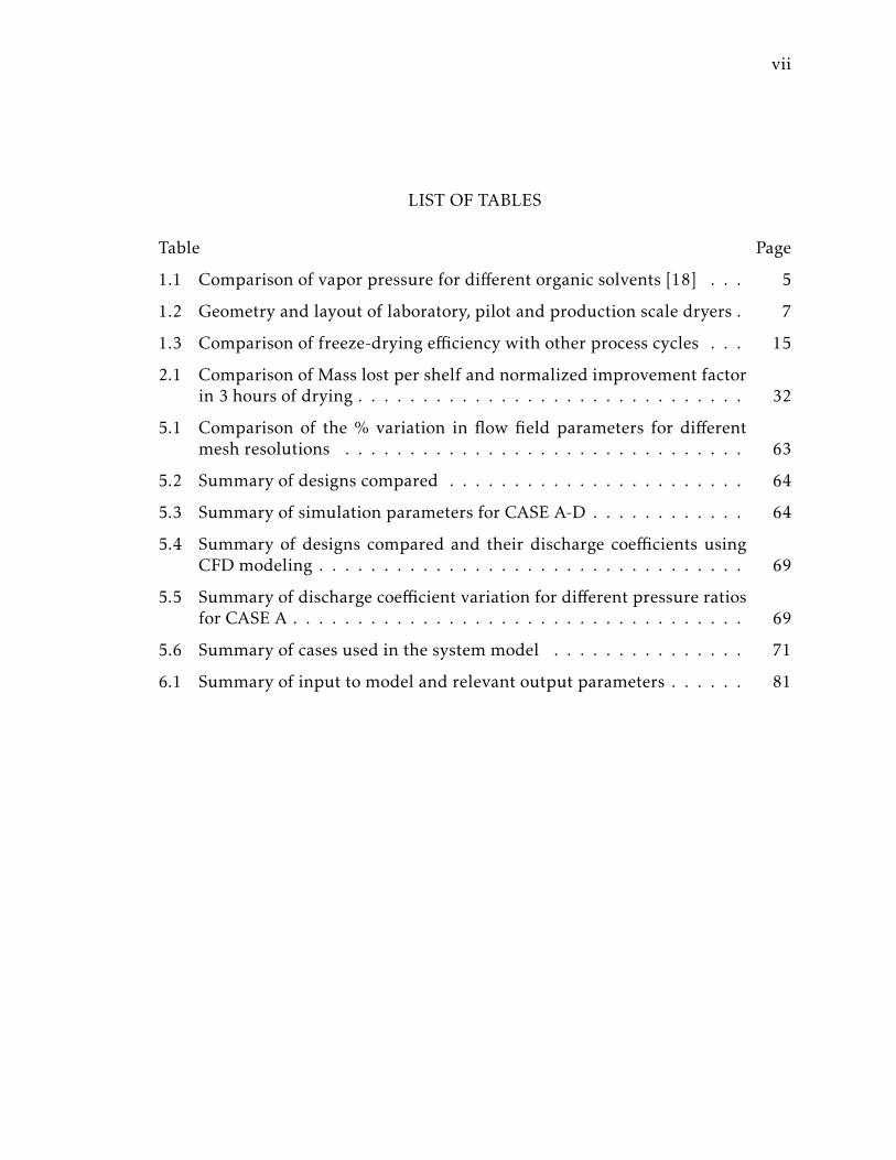
LIST OF TABLES . . . . . . . . . . . . . . . . . . . . . . . . . . . . . . . . . . vii

LIST OF FIGURES . . . . . . . . . . . . . . . . . . . . . . . . . . . . . . . . . viii

ABSTRACT . . . . . . . . . . . . . . . . . . . . . . . . . . . . . . . . . . . . . xi

1 INTRODUCTION . . . . . . . . . . . . . . . . . . . . . . . . . . . . . . . . 11.1 Background and Motivation . . . . . . . . . . . . . . . . . . . . . . . 1

1.1.1 Evaporation, Sublimation and Condensation Processes . . . 21.1.2 Low-pressure Sublimation Applied to Pharmaceutical Freeze-

Drying . . . . . . . . . . . . . . . . . . . . . . . . . . . . . . . 31.1.3 Thermodynamics and Heat Transfer Aspects of Freeze-drying 41.1.4 Vapor Flow in Freeze-drying . . . . . . . . . . . . . . . . . . 91.1.5 Current Challenges in Freeze-drying Technology . . . . . . 13

1.2 Research Goals and Objectives . . . . . . . . . . . . . . . . . . . . . 18

2 SUBLIMATION STUDIES: PROCESS FLUIDDYNAMICSANDHEATTRANS-FER . . . . . . . . . . . . . . . . . . . . . . . . . . . . . . . . . . . . . . . . 202.1 Heat Transfer Mechanisms Driving Sublimation . . . . . . . . . . . 202.2 Pressure Variation and Role of Convection . . . . . . . . . . . . . . 21

2.2.1 Measurements . . . . . . . . . . . . . . . . . . . . . . . . . . 222.2.2 Modeling . . . . . . . . . . . . . . . . . . . . . . . . . . . . . 232.2.3 Results . . . . . . . . . . . . . . . . . . . . . . . . . . . . . . . 24

2.3 Methods for Accelerating the Process . . . . . . . . . . . . . . . . . 282.3.1 Validation of Accelerated Sublimation through Top heating 30

2.4 Conclusions . . . . . . . . . . . . . . . . . . . . . . . . . . . . . . . . 31

3 CONDENSATION STUDIES: ICE ACCRETION ON AN ARBITRARY SU-PERCOOLED SURFACE . . . . . . . . . . . . . . . . . . . . . . . . . . . . 353.1 Ice Accretion Modeling . . . . . . . . . . . . . . . . . . . . . . . . . . 36

3.1.1 Simulation Parameters . . . . . . . . . . . . . . . . . . . . . . 373.1.2 Mesh Convergence . . . . . . . . . . . . . . . . . . . . . . . . 383.1.3 Verification of Ice Accretion Simulations . . . . . . . . . . . 39

3.2 Measurements of Ice Accretion in Low-pressure environment . . . 403.3 Effect of Non-condensable Gases on Ice Accretion Rate . . . . . . . 413.4 Validation of the Model . . . . . . . . . . . . . . . . . . . . . . . . . 43

3.4.1 Measurements . . . . . . . . . . . . . . . . . . . . . . . . . . 433.4.2 Comparison between Simulations and Measurements . . . 44

vi

Page3.5 Conclusions . . . . . . . . . . . . . . . . . . . . . . . . . . . . . . . . 47

4 SUBLIMATION-TRANSPORT-CONDENSATIONCOUPLED SIMULATIONFRAMEWORK . . . . . . . . . . . . . . . . . . . . . . . . . . . . . . . . . . 494.1 Introduction . . . . . . . . . . . . . . . . . . . . . . . . . . . . . . . . 504.2 Problem Description . . . . . . . . . . . . . . . . . . . . . . . . . . . 514.3 Measurements . . . . . . . . . . . . . . . . . . . . . . . . . . . . . . . 534.4 Modeling . . . . . . . . . . . . . . . . . . . . . . . . . . . . . . . . . . 53

4.4.1 Unsteady System-level Heat and Mass Transfer Model . . . 55

5 APPLICATION OF THE COUPLED MODEL TO ESTIMATE PRODUCT,EQUIPMENT AND PROCESS LIMIT . . . . . . . . . . . . . . . . . . . . . 625.1 Problem Description . . . . . . . . . . . . . . . . . . . . . . . . . . . 625.2 CFD Solution Verification . . . . . . . . . . . . . . . . . . . . . . . . 635.3 Simulation Parameters for Different Valve/Duct Configurations . . 635.4 Computed Flow Structure for Baseline Design . . . . . . . . . . . . 655.5 Effect of the Valve-Baffle Location and Design . . . . . . . . . . . . 665.6 Determination of Discharge Coefficient . . . . . . . . . . . . . . . . 675.7 Model Calibration . . . . . . . . . . . . . . . . . . . . . . . . . . . . . 685.8 Application of the Model for Predicting Equipment Performance . 73

5.8.1 Model Calibration at 150 L loading (Run-150-A) . . . . . . 735.8.2 Validation of the Model (Run-150-B) . . . . . . . . . . . . . 755.8.3 Effect of Hardware on Equipment Capability . . . . . . . . . 76

5.9 Conclusions . . . . . . . . . . . . . . . . . . . . . . . . . . . . . . . . 77

6 APPLICATION OF MODEL FOR GENERATING A 3-D DESIGN SPACE:PROCESS OPTIMIZATION . . . . . . . . . . . . . . . . . . . . . . . . . . 806.1 Process Optimization Through a Design Space Approach . . . . . . 82

6.1.1 Modeling the 2-D Space . . . . . . . . . . . . . . . . . . . . . 826.1.2 Construction of the Design Space: Experiments vs Modeling 84

6.2 The 3-D Design Space . . . . . . . . . . . . . . . . . . . . . . . . . . 866.2.1 Need for a 3-D Design Space . . . . . . . . . . . . . . . . . . 866.2.2 Developing the Three-dimensional Design Space . . . . . . 876.2.3 Application of Model to 5% Mannitol-5%Sucrose System . 89

6.3 Conclusions . . . . . . . . . . . . . . . . . . . . . . . . . . . . . . . . 93

7 SUMMARY AND RECOMMENDATIONS . . . . . . . . . . . . . . . . . . 95

REFERENCES . . . . . . . . . . . . . . . . . . . . . . . . . . . . . . . . . . . . 102

VITA . . . . . . . . . . . . . . . . . . . . . . . . . . . . . . . . . . . . . . . . . 107

vii

LIST OF TABLES

Table Page

1.1 Comparison of vapor pressure for different organic solvents [18] . . . 5

1.2 Geometry and layout of laboratory, pilot and production scale dryers . 7

1.3 Comparison of freeze-drying efficiency with other process cycles . . . 15

2.1 Comparison of Mass lost per shelf and normalized improvement factorin 3 hours of drying . . . . . . . . . . . . . . . . . . . . . . . . . . . . . . 32

5.1 Comparison of the % variation in flow field parameters for differentmesh resolutions . . . . . . . . . . . . . . . . . . . . . . . . . . . . . . . 63

5.2 Summary of designs compared . . . . . . . . . . . . . . . . . . . . . . . 64

5.3 Summary of simulation parameters for CASE A-D . . . . . . . . . . . . 64

5.4 Summary of designs compared and their discharge coefficients usingCFD modeling . . . . . . . . . . . . . . . . . . . . . . . . . . . . . . . . . 69

5.5 Summary of discharge coefficient variation for different pressure ratiosfor CASE A . . . . . . . . . . . . . . . . . . . . . . . . . . . . . . . . . . . 69

5.6 Summary of cases used in the system model . . . . . . . . . . . . . . . 71

6.1 Summary of input to model and relevant output parameters . . . . . . 81

viii

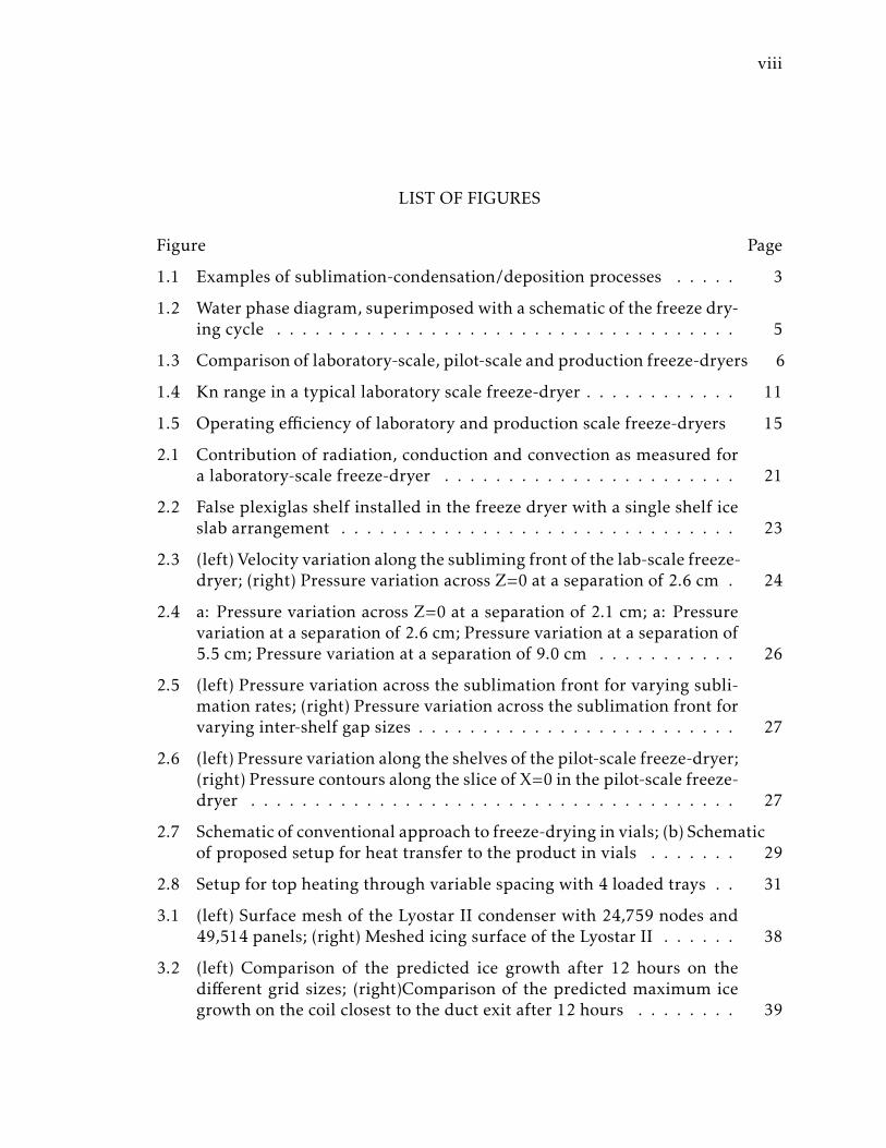
LIST OF FIGURES

Figure Page

1.1 Examples of sublimation-condensation/deposition processes . . . . . 3

1.2 Water phase diagram, superimposed with a schematic of the freeze dry-ing cycle . . . . . . . . . . . . . . . . . . . . . . . . . . . . . . . . . . . . 5

1.3 Comparison of laboratory-scale, pilot-scale and production freeze-dryers 6

1.4 Kn range in a typical laboratory scale freeze-dryer . . . . . . . . . . . . 11

1.5 Operating efficiency of laboratory and production scale freeze-dryers 15

2.1 Contribution of radiation, conduction and convection as measured fora laboratory-scale freeze-dryer . . . . . . . . . . . . . . . . . . . . . . . 21

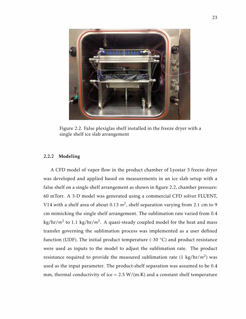
2.2 False plexiglas shelf installed in the freeze dryer with a single shelf iceslab arrangement . . . . . . . . . . . . . . . . . . . . . . . . . . . . . . . 23

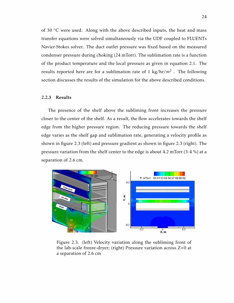
2.3 (left) Velocity variation along the subliming front of the lab-scale freeze-dryer; (right) Pressure variation across Z=0 at a separation of 2.6 cm . 24

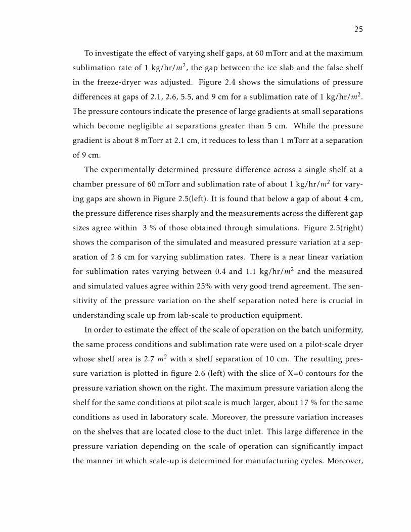
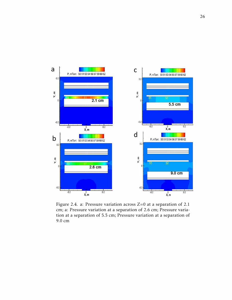
2.4 a: Pressure variation across Z=0 at a separation of 2.1 cm; a: Pressurevariation at a separation of 2.6 cm; Pressure variation at a separation of5.5 cm; Pressure variation at a separation of 9.0 cm . . . . . . . . . . . 26

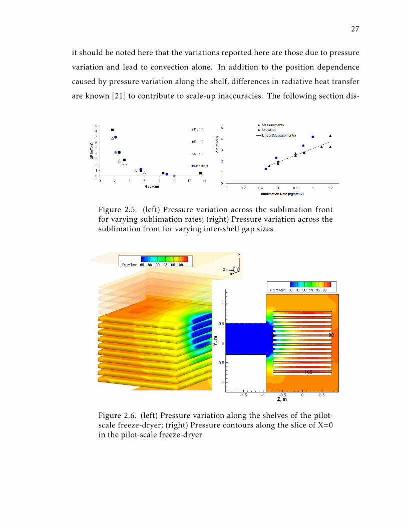
2.5 (left) Pressure variation across the sublimation front for varying subli-mation rates; (right) Pressure variation across the sublimation front forvarying inter-shelf gap sizes . . . . . . . . . . . . . . . . . . . . . . . . . 27

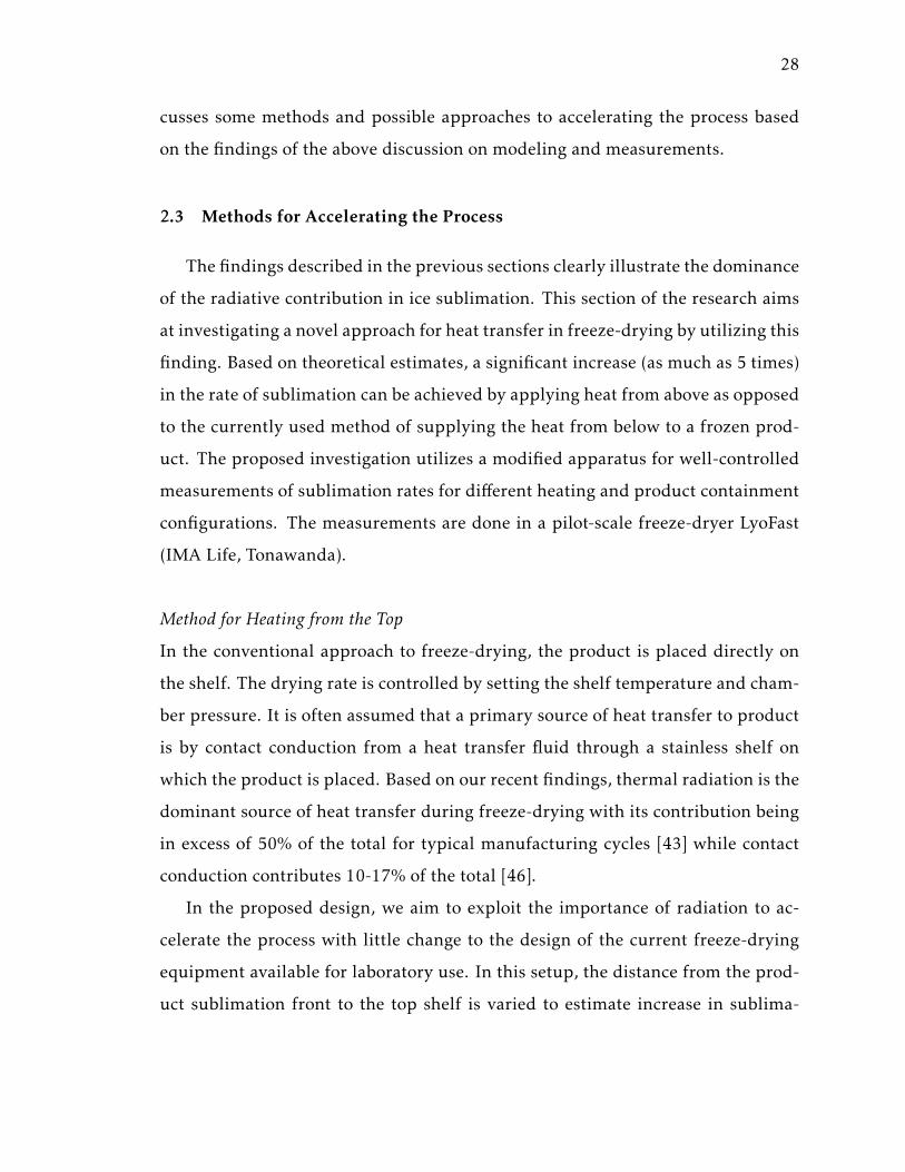
2.6 (left) Pressure variation along the shelves of the pilot-scale freeze-dryer;(right) Pressure contours along the slice of X=0 in the pilot-scale freeze-dryer . . . . . . . . . . . . . . . . . . . . . . . . . . . . . . . . . . . . . . 27

2.7 Schematic of conventional approach to freeze-drying in vials; (b) Schematicof proposed setup for heat transfer to the product in vials . . . . . . . 29

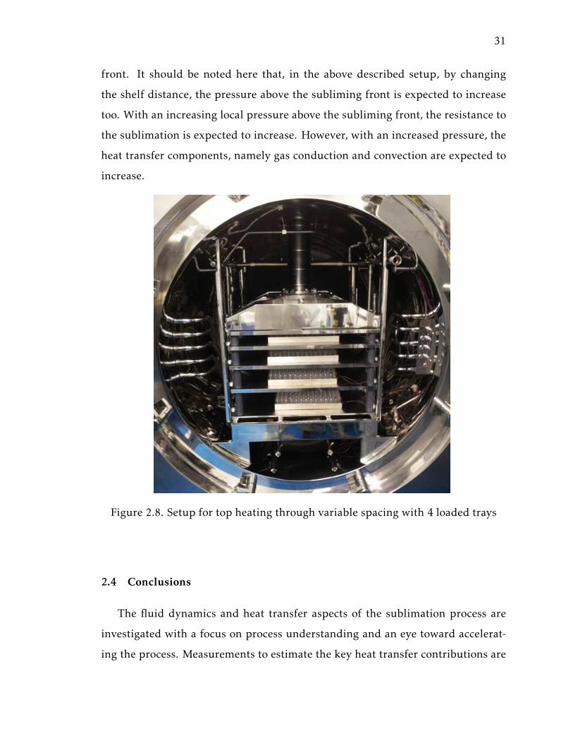
2.8 Setup for top heating through variable spacing with 4 loaded trays . . 31

3.1 (left) Surface mesh of the Lyostar II condenser with 24,759 nodes and49,514 panels; (right) Meshed icing surface of the Lyostar II . . . . . . 38

3.2 (left) Comparison of the predicted ice growth after 12 hours on thedifferent grid sizes; (right)Comparison of the predicted maximum icegrowth on the coil closest to the duct exit after 12 hours . . . . . . . . 39

ix

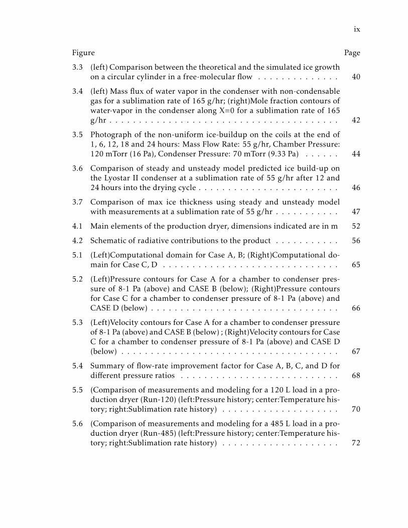
Figure Page

3.3 (left) Comparison between the theoretical and the simulated ice growthon a circular cylinder in a free-molecular flow . . . . . . . . . . . . . . 40

3.4 (left) Mass flux of water vapor in the condenser with non-condensablegas for a sublimation rate of 165 g/hr; (right)Mole fraction contours ofwater-vapor in the condenser along X=0 for a sublimation rate of 165g/hr . . . . . . . . . . . . . . . . . . . . . . . . . . . . . . . . . . . . . . . 42

3.5 Photograph of the non-uniform ice-buildup on the coils at the end of1, 6, 12, 18 and 24 hours: Mass Flow Rate: 55 g/hr, Chamber Pressure:120 mTorr (16 Pa), Condenser Pressure: 70 mTorr (9.33 Pa) . . . . . . 44

3.6 Comparison of steady and unsteady model predicted ice build-up onthe Lyostar II condenser at a sublimation rate of 55 g/hr after 12 and24 hours into the drying cycle . . . . . . . . . . . . . . . . . . . . . . . . 46

3.7 Comparison of max ice thickness using steady and unsteady modelwith measurements at a sublimation rate of 55 g/hr . . . . . . . . . . . 47

4.1 Main elements of the production dryer, dimensions indicated are in m 52

4.2 Schematic of radiative contributions to the product . . . . . . . . . . . 56

5.1 (Left)Computational domain for Case A, B; (Right)Computational do-main for Case C, D . . . . . . . . . . . . . . . . . . . . . . . . . . . . . . 65

5.2 (Left)Pressure contours for Case A for a chamber to condenser pres-sure of 8-1 Pa (above) and CASE B (below); (Right)Pressure contoursfor Case C for a chamber to condenser pressure of 8-1 Pa (above) andCASE D (below) . . . . . . . . . . . . . . . . . . . . . . . . . . . . . . . . 66

5.3 (Left)Velocity contours for Case A for a chamber to condenser pressureof 8-1 Pa (above) and CASE B (below) ; (Right)Velocity contours for CaseC for a chamber to condenser pressure of 8-1 Pa (above) and CASE D(below) . . . . . . . . . . . . . . . . . . . . . . . . . . . . . . . . . . . . . 67

5.4 Summary of flow-rate improvement factor for Case A, B, C, and D fordifferent pressure ratios . . . . . . . . . . . . . . . . . . . . . . . . . . . 68

5.5 (Comparison of measurements and modeling for a 120 L load in a pro-duction dryer (Run-120) (left:Pressure history; center:Temperature his-tory; right:Sublimation rate history) . . . . . . . . . . . . . . . . . . . . 70

5.6 (Comparison of measurements and modeling for a 485 L load in a pro-duction dryer (Run-485) (left:Pressure history; center:Temperature his-tory; right:Sublimation rate history) . . . . . . . . . . . . . . . . . . . . 72

x

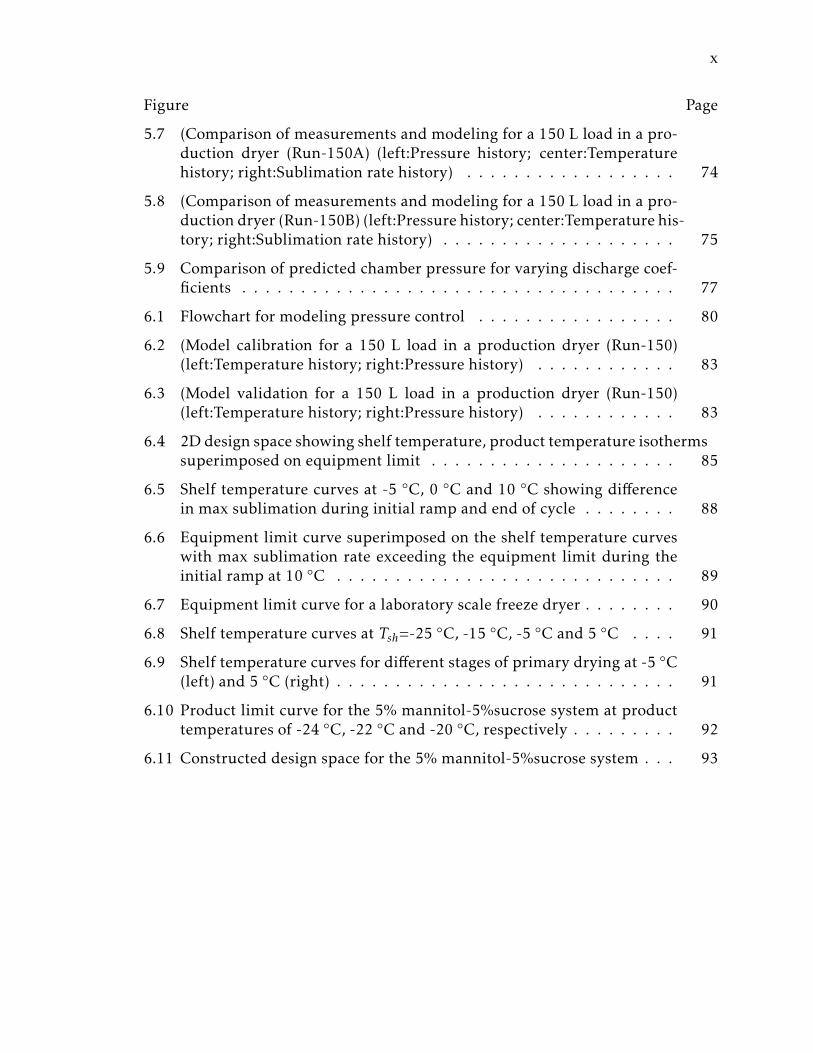
Figure Page

5.7 (Comparison of measurements and modeling for a 150 L load in a pro-duction dryer (Run-150A) (left:Pressure history; center:Temperaturehistory; right:Sublimation rate history) . . . . . . . . . . . . . . . . . . 74

5.8 (Comparison of measurements and modeling for a 150 L load in a pro-duction dryer (Run-150B) (left:Pressure history; center:Temperature his-tory; right:Sublimation rate history) . . . . . . . . . . . . . . . . . . . . 75

5.9 Comparison of predicted chamber pressure for varying discharge coef-ficients . . . . . . . . . . . . . . . . . . . . . . . . . . . . . . . . . . . . . 77

6.1 Flowchart for modeling pressure control . . . . . . . . . . . . . . . . . 80

6.2 (Model calibration for a 150 L load in a production dryer (Run-150)(left:Temperature history; right:Pressure history) . . . . . . . . . . . . 83

6.3 (Model validation for a 150 L load in a production dryer (Run-150)(left:Temperature history; right:Pressure history) . . . . . . . . . . . . 83

6.4 2D design space showing shelf temperature, product temperature isothermssuperimposed on equipment limit . . . . . . . . . . . . . . . . . . . . . 85

6.5 Shelf temperature curves at -5 ◦C, 0 ◦C and 10 ◦C showing differencein max sublimation during initial ramp and end of cycle . . . . . . . . 88

6.6 Equipment limit curve superimposed on the shelf temperature curveswith max sublimation rate exceeding the equipment limit during theinitial ramp at 10 ◦C . . . . . . . . . . . . . . . . . . . . . . . . . . . . . 89

6.7 Equipment limit curve for a laboratory scale freeze dryer . . . . . . . . 90

6.8 Shelf temperature curves at Tsh=-25◦C, -15 ◦C, -5 ◦C and 5 ◦C . . . . 91

6.9 Shelf temperature curves for different stages of primary drying at -5 ◦C(left) and 5 ◦C (right) . . . . . . . . . . . . . . . . . . . . . . . . . . . . . 91

6.10 Product limit curve for the 5% mannitol-5%sucrose system at producttemperatures of -24 ◦C, -22 ◦C and -20 ◦C, respectively . . . . . . . . . 92

6.11 Constructed design space for the 5% mannitol-5%sucrose system . . . 93

xi

ABSTRACT

Ganguly, Arnab. PhD, Purdue University, December 2014. Coupled Fluid-ThermalAnalysis of Low-Pressure Sublimation and Condensationwith Application to Freeze-Drying . Major Professor: Alina Alexeenko.

Freeze-drying is a low-pressure, low-temperature condensation pumping pro-

cess widely used in the manufacture of bio-pharmaceuticals for removal of sol-

vents by sublimation. The goal of the process is to provide a stable dosage form

by removing the solvent in such a way that the sensitive molecular structure of

the active substance is least disturbed. The vacuum environment presents unique

challenges for understanding and controlling heat and mass transfer in the pro-

cess. As a result, the design of equipment and associated processes has been largely

empirical, slow and inefficient.

A comprehensive simulation framework to predict both, process and equip-

ment performance is critical to improve current practice. A part of the dissertation

is aimed at performing coupled fluid-thermal analysis of low-pressure sublimation-

condensation processes typical of freeze-drying technologies. Both, experimen-

tal and computational models are used to first understand the key heat transfer

modes during the process. A modeling and computational framework, validated

with experiments for analysis of sublimation, water-vapor flow and condensation

in application to pharmaceutical freeze-drying is developed.

Augmentedwith computational fluid dynamicsmodeling, the simulation frame-

work presented here allows to predict for the first time, dynamic product/process

conditions taking into consideration specifics of equipment design. Moreover, by

applying the modeling framework to process design based on a design-space ap-

proach, it has demonstrated that there is a viable alternative to empiricism.

1

1. INTRODUCTION

1.1 Background and Motivation

Icing on the wings of an aircraft or sublimation of ice from the surface of

the moon during robotic explorations are examples involving phase change of

ice/water-vapor systems in nature. Each of these surface phenomena involve a

coupled, unsteady low-pressure heat and mass transfer problem, namely phase

change from its bulk form to a final deposit on a relatively cold surface. The un-

derlying physics governing these problems are common to most examples in a

low-pressure environment. Chemical vapor deposition (CVD) techniques are used

to grow carbon nanotubes from graphite rods on a catalyst substrate. Vaporizing

liquid microthrusters can be used for attitude control of small satellites by va-

porizing liquid in a thermal chamber and ejecting out of a micronozzle. Other

examples of low-pressure sublimation-deposition systems include manufacture of

organic small molecule light emitting diode (O-LED) for flexible electronics using

low-pressure organic vapor phase deposition of thin films and CIGS thin-film solar

cells. Manufacture of ceramic micro-particles and many bio-pharmaceuticals sim-

ilarly involve a controlled drying process referred to as freeze-drying. It involves

sublimation of the frozen/solid form of a product placed in a drying chamber and

deposition of the emanating solvent vapor on super-cooled surfaces. The section

below introduces some relevant research contributions involving sublimation and

condensation for a low-pressure environment.

2

1.1.1 Evaporation, Sublimation and Condensation Processes

Evaporation, sublimation and condensation are surface phase change phenom-

ena involving either molecular departure from or attachment to a surface. While

evaporation involves the phase change from liquid to vapor, sublimation is the

phase change from solid to vapor. Similarly, while condensation involves vapor to

liquid transition, deposition refers to change from vapor to solid. These processes

have been investigated by several researchers. For example, Hertz [1] in 1882 in-

troduced the kinetic theory for evaporation and later Knudsen’s work in 1915 [2]

on the evaporation of Mercury into vacuum are among the first known. The vapor

pressure of mercury was measured and the work led to the development of the

“Knudsen cell” source used commonly in molecular beam epitaxy as the source

evaporator. Later, Shankar and Marble [3] found that the net mass flow through

a surface depends on just one parameter, the difference between the saturation

pressure at the interface temperature and the local pressure, psat-p∞. In reality,

the net mass flow rate was found to be lower by a factor, often referred to as the

evaporation coefficient [4] [5]. Some of the many examples of such sublimation-

condensation processes are illustrated in figure 1.1 and in particular, the develop-

ments in ice/water vapor sublimation processes are briefly described next.

The existence of water on the moon has been debated for many years [6]. Ex-

planations for its origin were discussed in [7] and [8]. For latitudes between 75◦

north and 75◦south [9], the surface of the moon heat to temperatures at which

ice sublimes [10] [11] and [12]. Robotic missions in the past have attempted to

determine the source of hydrogen concentrations around lunar poles. However,

such robotic exploration typically include drilling or other mechanical operations

generating sufficient heat that may lead to subliming of the ice in the near-vacuum

conditions on the surface of the moon before its concentration is determined [13].

Models that can help predict the sublimation rate of the ice into vacuum are useful

tools [10], some of which are discussed next.

3

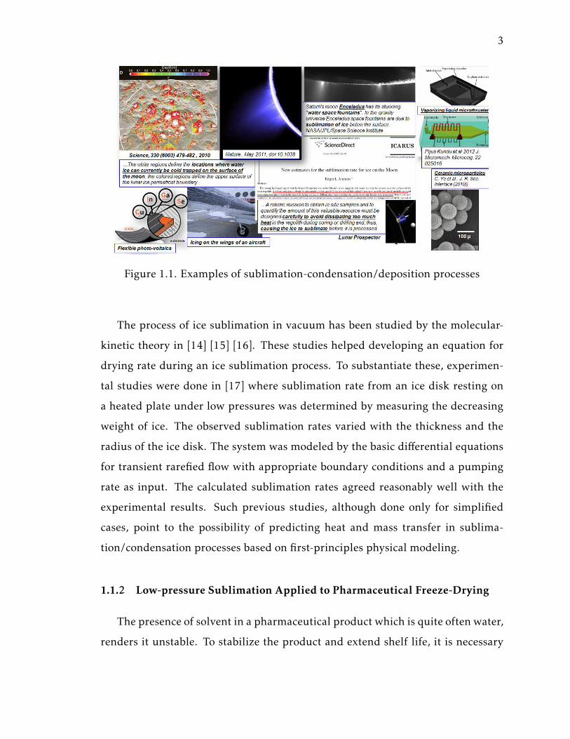
Figure 1.1. Examples of sublimation-condensation/deposition processes

The process of ice sublimation in vacuum has been studied by the molecular-

kinetic theory in [14] [15] [16]. These studies helped developing an equation for

drying rate during an ice sublimation process. To substantiate these, experimen-

tal studies were done in [17] where sublimation rate from an ice disk resting on

a heated plate under low pressures was determined by measuring the decreasing

weight of ice. The observed sublimation rates varied with the thickness and the

radius of the ice disk. The system was modeled by the basic differential equations

for transient rarefied flow with appropriate boundary conditions and a pumping

rate as input. The calculated sublimation rates agreed reasonably well with the

experimental results. Such previous studies, although done only for simplified

cases, point to the possibility of predicting heat and mass transfer in sublima-

tion/condensation processes based on first-principles physical modeling.

1.1.2 Low-pressure Sublimation Applied to Pharmaceutical Freeze-Drying

The presence of solvent in a pharmaceutical product which is quite often water,

renders it unstable. To stabilize the product and extend shelf life, it is necessary

4

to remove the solvent content. However, using conventional forms of drying can

be too aggressive, destroying its structure and properties. Hence, a more gentle

desiccation process, referred to as freeze-drying is required. The goal of freeze-

drying is to provide a stable dosage form by removing the solvent in such a way

that the sensitive molecular structure of the active substance is least disturbed.

The process path is controlled by the operating pressure and temperature. The

thermodynamics aspects and the operating ranges of pressure and temperature

are presented next.

1.1.3 Thermodynamics and Heat Transfer Aspects of Freeze-drying

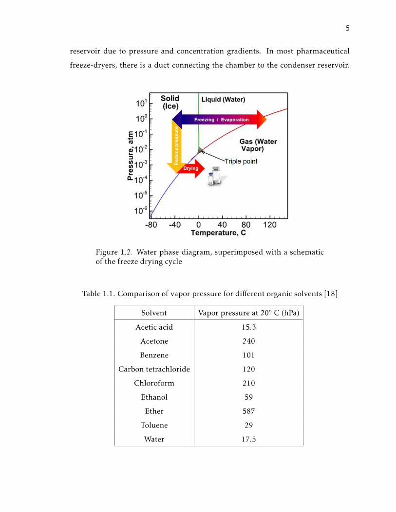
Freeze-drying is a three-stage process shown schematically in figure 1.2. The

initial stage is freezing, following which the pressure is reduced below the triple

point (0.000198 ◦C at 611.73 Pa for water). Heat is then provided for sublimation

of the ice during primary drying. If the first stage is reversed, with the addition

of heat, the water evaporates. Freeze-drying of aqueous solutions require a vac-

uum environment with typical pressures during primary drying below 0.001 atm.

The rate of sublimation is dependent on the ambient pressure and the saturation

pressure of the solvent at the product temperature. Table 1.1 compares the vapor

pressure in hPa of various organic solvents at room temperature in comparison to

water.

A typical laboratory-scale freeze-dryer is shown in figure 1.3 (left) with the op-

erating pressure and temperature ranges. The upper chamber contains the prod-

uct usually in glass vials or metallic trays that are most often positioned to be

in direct contact with shelves. The shelf temperature is controlled by a passage

of heat-transfer fluid. The rate of solvent vapor sublimation is dependent on the

shelf temperature and the chamber pressure [19]. The pressure is controlled by a

vacuum pump and by introducing a non-condensable gas such as nitrogen. The

solvent vapor and non-condensable gas flows from the chamber to the condenser

5

reservoir due to pressure and concentration gradients. In most pharmaceutical

freeze-dryers, there is a duct connecting the chamber to the condenser reservoir.

Figure 1.2. Water phase diagram, superimposed with a schematicof the freeze drying cycle

Table 1.1. Comparison of vapor pressure for different organic solvents [18]

Solvent Vapor pressure at 20◦ C (hPa)

Acetic acid 15.3

Acetone 240

Benzene 101

Carbon tetrachloride 120

Chloroform 210

Ethanol 59

Ether 587

Toluene 29

Water 17.5

6

The condenser reservoir contains an arrangement of coils or other condensing sur-

faces that are maintained at temperatures from -90 to -40 ◦C. The condenser reser-

voir is connected to a vacuum pump for removal of non-condensable gases. The

typical range of pressures encountered in the freeze-drying systems is from 10 to

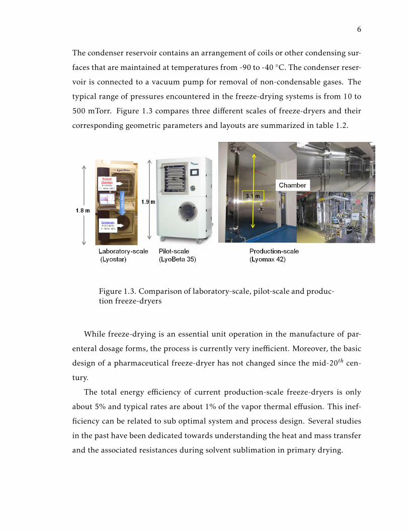
500 mTorr. Figure 1.3 compares three different scales of freeze-dryers and their

corresponding geometric parameters and layouts are summarized in table 1.2.

Figure 1.3. Comparison of laboratory-scale, pilot-scale and produc-tion freeze-dryers

While freeze-drying is an essential unit operation in the manufacture of par-

enteral dosage forms, the process is currently very inefficient. Moreover, the basic

design of a pharmaceutical freeze-dryer has not changed since the mid-20th cen-

tury.

The total energy efficiency of current production-scale freeze-dryers is only

about 5% and typical rates are about 1% of the vapor thermal effusion. This inef-

ficiency can be related to sub optimal system and process design. Several studies

in the past have been dedicated towards understanding the heat and mass transfer

and the associated resistances during solvent sublimation in primary drying.

7

Table 1.2. Geometry and layout of laboratory, pilot and production scale dryers

Design Shelves Shelf

Area,

m2

Shelf

Spacing, cm

Condenser

Area, m2

Power,

KW

Laboratory,

Lyostar

3 0.43 8.5 0.55 11

Pilot,

LyoBeta 35

7 1 6 - 19

Production,

Lyomax 42

15 42 12.5 44 53

Nail [19] identified poor thermal contact between the vial and the shelf as the

rate limiting resistance to heat transfer. Pikal [20] introduced the vial heat transfer

coefficient, Kv , as the following

Q = AvKv(Ts −Tb) (1.1)

where Q is the rate of heat flow from the shelf to a given vial, Av is the cross

sectional area of the vial based on the outer diameter, Ts is the temperature of the

surface of the shelf, and Tb is the temperature of the product at the bottom center

of the vial. The vial heat transfer coefficient was further defined as the sum of

three components:

Kv = Kc +Kr +Kg (1.2)

where Kc is the contribution resulting from conduction due to direct contact

between the shelf and the glass vial, Kr is the contribution from radiative heat

transfer, and Kg is the contribution of conduction through the gas between the

shelf and the vial bottom. Kc and Kr are independent of pressure. Kg varies from

being linearly dependent on pressure and independent of separation in the free-

8

molecular regime to being independent of pressure and inversely proportional to

the separation in the continuum regime.

Rambhatla and Pikal [21] examined the role of thermal radiation, with par-

ticular emphasis on the edge vial effect, that is enhanced heat transfer to vials at

the edges of an array of vials. Some vials were coated with gold to decrease the

thermal emissivity, and it was shown that gold-coating significantly decreased the

vial heat transfer coefficient, particularly at the edges of the array indicating that

radiation was responsible for higher sublimation rate observed at the edge of an

array of vials in a batch.

It is commonly accepted that, because of the low pressures used in freeze-

drying, convection plays no significant role in heat transfer. Since its magni-

tude scales as L3/2, its contribution can be crucial to determine the manner in

which scale-up from laboratory to production scale is established. Rambhatla and

Pikal [21] used a suspended vial experiment where vials were suspended about

11 cm from the surface of the shelf. Heat transfer coefficients for this configura-

tion were shown to be essentially independent of pressure, thus supporting the

conclusion that convection plays no significant role in the heat transfer. However,

Hottot and coworkers [22] investigated freeze-drying in pre-filled syringes, where

there was no direct contact between the shelf and the primary container. While

these investigators did conclude that the pressure dependent heat transfer mecha-

nism was convection in syringes suspended some distance off the shelf, there may

have been some pressure dependent gas conduction contribution, since the rel-

ative magnitudes of the heat transfer modes were not quantified. Furthermore,

Patel and Pikal [23] investigated freeze-drying in pre-filled syringes, where two

different holder systems were used to freeze-dry water, sucrose and mannitol. To

determine the role of convection, a physical barrier in the form of a skirt was intro-

duced to suppress convective flow between syringes. The difference in the subli-

mation rates showed a 6% variation in the presence of the barriers (at 60 mTorr). It

was concluded that this variation was within the experimental errors and convec-

9

tion was negligible relative to the other heat transfer mechanisms. However, the

variation in the contribution through convection for different chamber pressures

was not addressed explicitly.

Further investigations on the heat and mass transfer in lyophilization at pi-

lot scale were done by Rasetto and co-workers [24] where a means to couple the

fluid dynamics in the chamber with the heat and mass transfer in a vial using a

multi-dimensional model was presented. The model which incorporated the role

of the vial [25] was capable of predicting the evolution of the product temperature

during the cycle. It was concluded that at chamber pressures of about 80 mTorr,

the maximum pressure variation along the shelf could be as large as 15%. The

presence of such pressure gradients is one of the causes for bulk flow in the cham-

ber and hence convection. Some of the fluid dynamics aspects of the process are

addressed next.

1.1.4 Vapor Flow in Freeze-drying

Fluid dynamics in a freeze-dryer chamber determines product quality and dic-

tates drying rates and batch uniformity. Three main mechanisms determine the

bulk flow motion in a freeze-dryer chamber: 1)rarefied thermal creep due wall

temperature gradients and significant rarefaction; 2)free thermal convection and

3) pressure- and concentration-driven flow. The significance of each of these con-

tributions varies greatly depending on the operating pressure and temperature.

While thermal creep becomes comparable to free thermal and pressure driven con-

vection at Kn ∼1, its contribution is small compared to 2) and 3) for high chamber

pressures. The continuum thermal convection flows are generated by combined ef-

fect of temperature gradients and buoyancy. A classical example of such phenom-

ena is vertical thermal convection, or Rayleigh-Benard convection, in fluid layers

heated from below. A typical setup in a freeze-drying chamber involves heating

from below through stainless steel shelves, on top of which the product is placed

10

for drying. However, in addition to the vertical thermal gradients for laboratory-

scale dryers there is usually a significant gradient of the temperature in the hori-

zontal direction due to the absorption of thermal radiation through the glass door.

The industrial-scale dryers usually have a radiation shield to prevent the horizon-

tal temperature gradients and maintain uniformity of drying rates in a batch of

product vials. This, in principle, leads to distinctly different dynamic regimes of

thermal convection between the laboratory-scale and industrial-scale dryers. In

addition, pressure and concentration gradients are additional flow mechanisms

expected to play a significant role in the overall flow patterns and magnitudes in

the chambers. Since the drying rates are extremely sensitive to vapor pressure,

the pressure variation within the product chamber can lead to position dependent

variation in the drying rates. There also exists a large concentration gradient be-

tween the chamber and condenser due to the pumping effect of the metal surfaces

in the condenser cooled down to -50 ◦C -80 ◦C.

The fluid dynamics in the chamber is closely coupled with that in the con-

denser. The flow in the duct connecting the chamber and the condenser is essen-

tially driven by pressure and concentration gradients. Setting the product cham-

ber and condenser pressures usually controls the flow rate through the connecting

duct, which is most often a circular pipe. Above a critical pressure ratio, which

depends on the duct length-to-diameter ratio, a sonic velocity can be reached at

the duct exit. The mass flow rate cannot be increased without increasing chamber

pressure and the flow is said to be choked. Such choked flow may lead to a loss of

control over the pressure in the product chamber. Pressure fluctuations increase

heat transfer rates and the product temperature whichmay result in collapse of the

product and compromise quality. The critical pressure ratios depend on the ge-

ometry of the duct, such as the length-to-diameter ratio, the chamber temperature

and the water vapor and nitrogen mole fractions. The pressure at the exit of the

duct depends on the condensation rate and capacity of condenser, which depends

strongly on the geometric configuration. Oetjen and Jennings [26] [27] summa-

11

rized empirical guidelines for a freeze-dryer condenser design. It was concluded

that the surface area of the condenser should be less than or equal to the surface

area of the shelves in the freeze-drying chamber. In addition, the spacing between

coils should be such that the ice growth does not impede vapor flow through the

condenser. The following paragraph describes the different flow regimes for a typ-

ical freeze-drying process under such large variations in temperature and pressure

in the chamber and condenser.

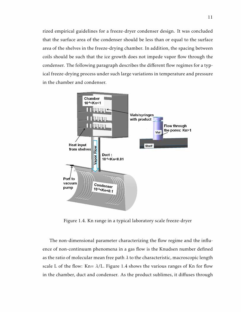
Figure 1.4. Kn range in a typical laboratory scale freeze-dryer

The non-dimensional parameter characterizing the flow regime and the influ-

ence of non-continuum phenomena in a gas flow is the Knudsen number defined

as the ratio of molecular mean free path λ to the characteristic, macroscopic length

scale L of the flow: Kn= λ/L. Figure 1.4 shows the various ranges of Kn for flow

in the chamber, duct and condenser. As the product sublimes, it diffuses through

12

the pores of the frozen product and solvent mixture and the flow in this region is

typically free molecular. The heat transfer between the vial bottom and the shelf is

also typically free molecular or at least in the transitional regime. The Kn of flow

in the product chamber, around the vials, the duct and in the condenser can vary

from 10−4 to 1.

The continuum hypothesis is valid for flows at small Knudsen numbers, typ-

ically Kn<0.01. In this case, fluid is close to the local thermodynamic equilib-

rium and the numerical modeling of such flows can be based on macroscopic

governing equations such as the Navier-Stokes equations for viscous flows. Flows

with Kn<0.1 can be modeled accurately by including the rarefaction effects as the

boundary conditions through a first-order velocity-slip and temperature jump con-

ditions [28]. The flows in this regime, 0.01 < Kn < 0.1 are referred to as slip flows.

At Knudsen numbers larger than 0.1, an approach based on gas kinetic theory is

required. The governing equation in this case is the Boltzmann equation for the

distribution function of gas molecules. For very large Knudsen numbers, typi-

cally Kn > 50, the intermolecular collision term in the Boltzmann equation can

be neglected. The corresponding flow regime is called free-molecular. The inter-

mediate range of Knudsen numbers correspond to the transitional regime of rar-

efaction. The conditions encountered in freeze-drying involve a range of rarefac-

tion regimes from slip flow to transitional. The intricate coexistence of different

thermally-driven and pressure-driven mechanisms creates conditions which are

difficult to understand based on simplified theories. As a result, the basic design

of freeze-drying equipment has changed little in several decades and is lagging

behind the growing demand. Some of the many resulting challenges are described

next.

13

1.1.5 Current Challenges in Freeze-drying Technology

Long cycle times, large exergy losses, scale-up inaccuracies and inter-vial and

batch-to-batch variability are some of the biggest challenges faced by the lyophiliz-

ing pharmaceutical manufacturers today. Drug shortages in the U.S. are at an all-

time high [29]. Many drugs on the shortage list, including generic cancer drugs

such as cisplatin, busulfan, doxorubicin, and others, require freeze-drying. Sev-

eral of the drugs listed on the shortage list suffer form manufacturing related is-

sues. The main goals of this dissertation are to develop, build and validate new

techniques for modeling sublimation and condensation at low-pressures with an

eye toward accelerated processing time with a simultaneous increase in energy ef-

ficiency. Though freeze-drying will be the first unit operation to be addressed, a

broad set of processes will benefit from the developed approach.

Drying Efficiency

The need for increased drying capacity has been the major driver in design of

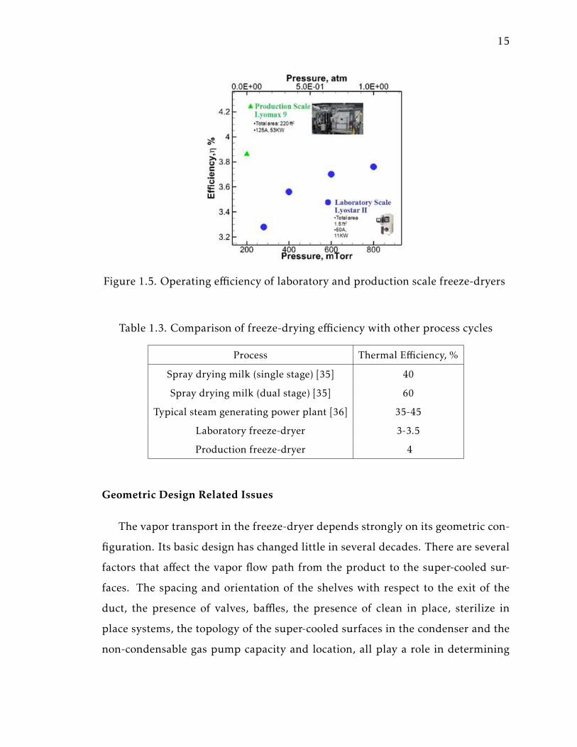
new freeze-drying systems. Figure 1.5 illustrates the cycle efficiency, of a typical

production dryer Lyomax 9 and a laboratory-scale dryer, Lyostar II. The efficiency

figures here were estimated using the following formula:

η =(Enthalpyofsublimation× Sublimationrate) + (Enthalpyoffreezing× freezingrate)

(Powerinput)(1.3)

These estimated efficiency figures are quite low which points to ample oppor-

tunities for improved designs. The enthalpy of sublimation and freezing used here

is 2,803 J/g and it is assumed that the sublimation and freezing rates are the same.

The rating for the laboratory scale dryer operating with 792 vials is 220 V and 50

A while that of the production dryer is 415 V and 125 A. It can be seen that the

efficiency of the laboratory-scale dryer increases with the chamber pressure and

reaches about 3 to 3.5%. The production dryers operate at efficiencies that are

14

marginally higher. Process-related manufacturing delays have led to the largest

drug shortage in the US in several decades. Thus, there is a need to accelerate

pharmaceutical freeze-drying by rethinking the conventional design and approach

used today. Improving the cycle efficiency and reducing cycle times can, in turn,

significantly reduce manufacturing costs for lyophilized bio/pharmaceuticals.

A systematic exergy analysis of the process was presented by Liapis and Brut-

tini [30]. It was shown that the maximum exergy input and losses occurred in the

primary drying stage followed by the vapor condensation processes. This clearly

points to the need for improving the efficiency of these two processes of freeze

drying to reduce cycle times and associated costs.

Because of a lack of predictive models, the design of freeze-drying equipment

and processes is largely empirical. Cycle times are a major concern in the industry.

The total energy efficiency of current production-scale freeze-dryers is only about

5% and typical rates are about 1% of the vapor thermal effusion. Each freeze-

drying cycle can last for several days and may consume millions of BTU of energy

[31]. The high energy expenditures lead to a cost that is 4 to 8 times higher than

other forms of drying [32] [33] [34]. Table 1.3 compares the thermal efficiency of

freeze-drying with other forms of drying. The spray drying efficiency is based on

the energy consumed to evaporate unit mass of water in a single and dual stage

spray dryer. The improved efficiency for the dual stage dryer spray dryer is due

to increased capacity and a simultaneous decrease in the outlet temperature of the

exhaust air, resulting in improved specific energy consumption. The efficiency of

the steam power plants is frequently used as a metric for comparison, based on

the amount of steam generated per unit work done in generating the same. The

process efficiency of freeze-drying is limited by the lengthy cycles. It clearly points

towards a need for improving efficiency.

15

Figure 1.5. Operating efficiency of laboratory and production scale freeze-dryers

Table 1.3. Comparison of freeze-drying efficiency with other process cycles

Process Thermal Efficiency, %

Spray drying milk (single stage) [35] 40

Spray drying milk (dual stage) [35] 60

Typical steam generating power plant [36] 35-45

Laboratory freeze-dryer 3-3.5

Production freeze-dryer 4

Geometric Design Related Issues

The vapor transport in the freeze-dryer depends strongly on its geometric con-

figuration. Its basic design has changed little in several decades. There are several

factors that affect the vapor flow path from the product to the super-cooled sur-

faces. The spacing and orientation of the shelves with respect to the exit of the

duct, the presence of valves, baffles, the presence of clean in place, sterilize in

place systems, the topology of the super-cooled surfaces in the condenser and the

non-condensable gas pump capacity and location, all play a role in determining

16

the vapor flow path and drying rate. The drying rate is affected by the rate lim-

iting heat transfer to the product. Furthermore, the rate at which the emanating

vapor can be removed from the product chamber depends on the design of the

chamber, the connecting duct and the topology of the cooling surfaces and the

vacuum pump. According to empirical guidelines [37], the geometry of the con-

denser should allow for bulk vapor transport with little disruption until it reaches

the condensing surface. In addition, the surface area of the condenser should be

less than or equal to the shelf area [27]. However, the effective coil surface area

available for condensation is dependent on the uniformity of ice accretion.

The heat transfer between the vapor and coil surface significantly affects the

pumping efficiency of the condenser. As the thickness of the ice layer increases,

the rate of heat transfer reduces. It was suggested in [27] that the thickness of

the ice layer should not exceed 1 cm. Additionally, the cooling capacity decreases

with decreasing temperature [38]. It is thus desirable to have a small tempera-

ture drop across the ice layer. However, this reduces the maximum thickness of

the ice, resulting in the need for a larger condensing surface area. Thus, while a

small condenser area reduces the energy consumption, it also increases the average

thickness of the ice formed on the cooled surfaces. Kobayashi showed that a lower

refrigerant temperature and presence of non-condensable gases led to an increase

in the non-uniformity of ice formation [39]. Thus, it is clear that there are several

design variables that can affect the vapor flow path and a good understanding of

the flow structure is needed to improve current designs.

Process Control and Scale-up

A key step in the development and scale-up of pharmaceutical lyophilization

processes is quantification of limits of the design space for a product-equipment

combination [40]. Once the design space has been established for laboratory-scale,

the scale-up parameters need to be determined for acceptable product quality in

17

production scale. This could often rely on trial and error techniques with limited

success [41]. Scale-up inaccuracies could arise from: a) degree of supercooling of

the product during the freezing stage [42] b) variations in the heat and mass trans-

fer mechanisms [43]; c) differences in the capability of the condenser [21] and d)

the dynamics of vapor flow in the freeze-dryer [24]. Amongst these, the dynam-

ics of vapor flow in the chamber and the contribution of convection has been the

hardest to quantify accurately. Though, recently the use of Tunable Diode Laser

Absorption Spectroscopy [44] has made it possible to measure the instantaneous

mass flow rate and velocity of flow in the duct, it has its limitations. Alexeenko

and co-workers [45] showed that the specifics of freeze-dryer design and the use

of simplified models could lead to inaccurate vapor flow characterization. The

low-pressure environment and the relatively small flow velocities in the product

chamber make it difficult to quantify the flow structure experimentally. Thus,

physics-based computationalmodels that provide detailed information on the flow

structure are valuable.

The performance of a freeze-dryer and the success of the cycle at various scales

of operation is governed by many parameters which couple the fluid dynamics in

the chamber, connecting duct and the condenser. An improved understanding of

the flowmechanisms and predictive physics-basedmodeling capability are needed

to develop optimal designs of this multiparametric heat and mass transfer system.

The analysis of the complex, 3D vapor-phase mass transfer in the freeze-drying

systems can be aided by application of computational fluid dynamics. In view

of the above challenges, the goals and objectives of the dissertation are presented

next.

18

1.2 Research Goals and Objectives

The major goal of the dissertation is to formulate a coupled heat and mass

transfer based model for predicting time-dependent sublimation rate based on

dynamic process conditions at low pressures applied to freeze-drying technology.

The model will incorporate dynamics of the product temperature and variation in

heat and mass transfer in the low-pressure environment accompanying the cou-

pling between the sublimation, transport and condensation processes. In this re-

gard, specific objectives that will drive the research towards the intended goals are

divided into three sections as:

I Sublimation Studies:

1 Formulate a one-way coupled, heat and mass transfer model for sublima-

tion in a low-pressure environment.

2 Quantify convection using both, simulation and experiments for low pres-

sures typically used in sublimation. This will be applied to a laboratory

scale freeze-dryer setup.

3 Propose alternate designs for more efficient heat transfer resulting in faster

sublimation with implementation and testing of the same in a laboratory

scale freeze-dryer.

II Condensation Studies:

Develop a model for predicting the condensation rate for a gas on a super-

cooled surface at low pressures. This will be applied to and validated with

measurements of icing rate on coils in a freeze-dryer condenser.

III Coupled Sublimation-Condensation Studies:

Develop a coupled unsteady sublimation-condensation model. A mass trans-

fer resistance model along with a heat transfer model will be incorporated to

help provide a realistic sublimation rate based on instantaneous temperature

19

and porosity of the subliming frozen material. This will provide a unified

sublimation-condensation model. The model will be validated with measure-

ments of sublimation rate in laboratory and production scale environment. Fi-

nally, the model will be applied for designing efficient, robust processes based

on a systematic 3-dimensional design space approach.

20

2. SUBLIMATION STUDIES: PROCESS FLUID DYNAMICS AND

HEAT TRANSFER

2.1 Heat Transfer Mechanisms Driving Sublimation

The goal of this section of the study was to examine quantitatively the relative

contributions of conduction, convection and radiation at low-pressures applied to

primary drying in vacuum freeze-drying. The shelf temperature, chamber pres-

sure and the separation distance between the vial and the shelf was systematically

varied during the study. In addition to facilitating analysis of heat transfer, the

investigation of configurations with no direct contact between the vials and the

freeze-dryer shelves is motivated by an interest in freeze-drying injectable phar-

maceutical products in pre-filled syringes. The analyses and results of this study

are briefly described next.

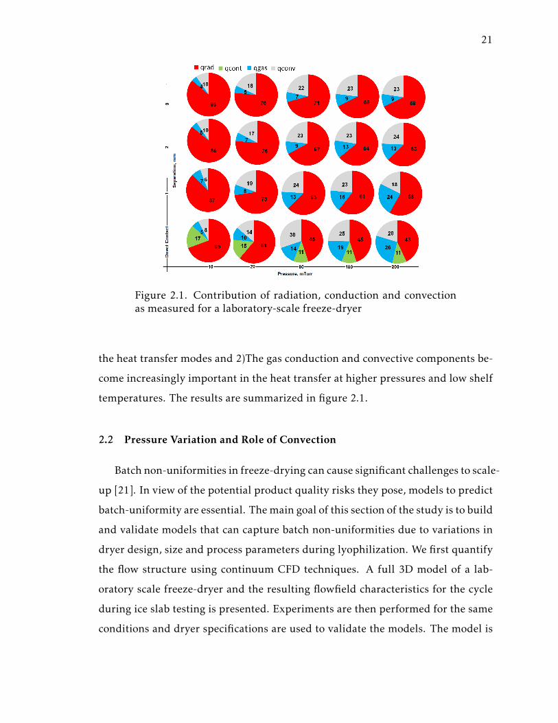
Sublimation rate measurements were performed in a laboratory scale Lyostar

II freeze-dryer using gravimetric means for both, vials in direct contact and sus-

pended vials. Once the individual sublimation rates were obtained, the heat flux

across an individual vial was calculated using the heat of sublimation. It was

found that while the contact conduction component contributed 11% to 17% of

the total heat transfer for the vial placed on the shelf, the radiative component

varied from 43% of the total heat transfer for the vial placed on the shelf to 86%

of the total heat transfer for the vial placed at a separation of 3 mm from the

shelf. The contribution from gas conduction at 100 mTorr for the vial placed on

the shelf amounts to 30% of the total heat transfer and the corresponding convec-

tive component amounts to 14% of the total heat transfer. This reduces to 6% and

8% respectively at a pressure of 10 mTorr [46]. The above conclusions are signif-

icant for two reasons, 1) The radiative component is clearly the dominant among

21

Figure 2.1. Contribution of radiation, conduction and convectionas measured for a laboratory-scale freeze-dryer

the heat transfer modes and 2)The gas conduction and convective components be-

come increasingly important in the heat transfer at higher pressures and low shelf

temperatures. The results are summarized in figure 2.1.

2.2 Pressure Variation and Role of Convection

Batch non-uniformities in freeze-drying can cause significant challenges to scale-

up [21]. In view of the potential product quality risks they pose, models to predict

batch-uniformity are essential. Themain goal of this section of the study is to build

and validate models that can capture batch non-uniformities due to variations in

dryer design, size and process parameters during lyophilization. We first quantify

the flow structure using continuum CFD techniques. A full 3D model of a lab-

oratory scale freeze-dryer and the resulting flowfield characteristics for the cycle

during ice slab testing is presented. Experiments are then performed for the same

conditions and dryer specifications are used to validate the models. The model is

22

then extended to predict the batch non-uniformity under the same conditions at

production scale.

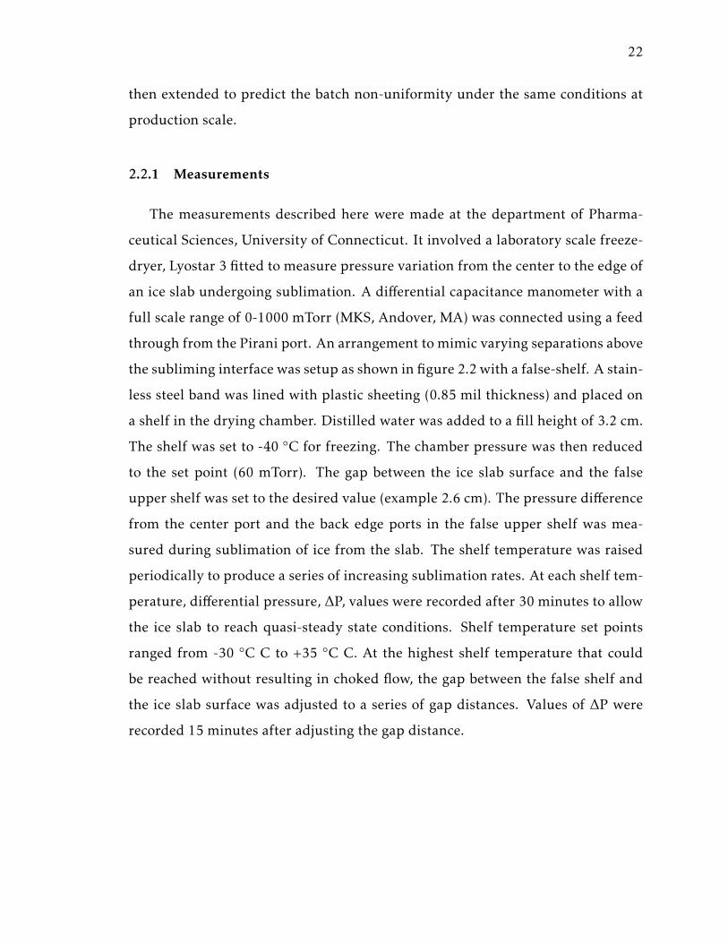
2.2.1 Measurements

The measurements described here were made at the department of Pharma-

ceutical Sciences, University of Connecticut. It involved a laboratory scale freeze-

dryer, Lyostar 3 fitted to measure pressure variation from the center to the edge of

an ice slab undergoing sublimation. A differential capacitance manometer with a

full scale range of 0-1000 mTorr (MKS, Andover, MA) was connected using a feed

through from the Pirani port. An arrangement to mimic varying separations above

the subliming interface was setup as shown in figure 2.2 with a false-shelf. A stain-

less steel band was lined with plastic sheeting (0.85 mil thickness) and placed on

a shelf in the drying chamber. Distilled water was added to a fill height of 3.2 cm.

The shelf was set to -40 ◦C for freezing. The chamber pressure was then reduced

to the set point (60 mTorr). The gap between the ice slab surface and the false

upper shelf was set to the desired value (example 2.6 cm). The pressure difference

from the center port and the back edge ports in the false upper shelf was mea-

sured during sublimation of ice from the slab. The shelf temperature was raised

periodically to produce a series of increasing sublimation rates. At each shelf tem-

perature, differential pressure, ∆P, values were recorded after 30 minutes to allow

the ice slab to reach quasi-steady state conditions. Shelf temperature set points

ranged from -30 ◦C C to +35 ◦C C. At the highest shelf temperature that could

be reached without resulting in choked flow, the gap between the false shelf and

the ice slab surface was adjusted to a series of gap distances. Values of ∆P were

recorded 15 minutes after adjusting the gap distance.

23

Figure 2.2. False plexiglas shelf installed in the freeze dryer with asingle shelf ice slab arrangement

2.2.2 Modeling

A CFD model of vapor flow in the product chamber of Lyostar 3 freeze-dryer

was developed and applied based on measurements in an ice slab setup with a

false shelf on a single shelf arrangement as shown in figure 2.2, chamber pressure:

60 mTorr. A 3-D model was generated using a commercial CFD solver FLUENT,

V14 with a shelf area of about 0.13 m2, shelf separation varying from 2.1 cm to 9

cm mimicking the single shelf arrangement. The sublimation rate varied from 0.4

kg/hr/m2 to 1.1 kg/hr/m2. A quasi-steady coupled model for the heat and mass

transfer governing the sublimation process was implemented as a user defined

function (UDF). The initial product temperature (-30 ◦C) and product resistance

were used as inputs to the model to adjust the sublimation rate. The product

resistance required to provide the measured sublimation rate (1 kg/hr/m2) was

used as the input parameter. The product-shelf separation was assumed to be 0.4

mm, thermal conductivity of ice = 2.5 W/(m.K) and a constant shelf temperature

24

of 30 ◦C were used. Along with the above described inputs, the heat and mass

transfer equations were solved simultaneously via the UDF coupled to FLUENTs

Navier-Stokes solver. The duct outlet pressure was fixed based on the measured

condenser pressure during choking (24 mTorr). The sublimation rate is a function

of the product temperature and the local pressure as given in equation 2.1. The

results reported here are for a sublimation rate of 1 kg/hr/m2 . The following

section discusses the results of the simulation for the above described conditions.

2.2.3 Results

The presence of the shelf above the subliming front increases the pressure

closer to the center of the shelf. As a result, the flow accelerates towards the shelf

edge from the higher pressure region. The reducing pressure towards the shelf

edge varies as the shelf gap and sublimation rate, generating a velocity profile as

shown in figure 2.3 (left) and pressure gradient as shown in figure 2.3 (right). The

pressure variation from the shelf center to the edge is about 4.2 mTorr (3-4 %) at a

separation of 2.6 cm.

Figure 2.3. (left) Velocity variation along the subliming front ofthe lab-scale freeze-dryer; (right) Pressure variation across Z=0 ata separation of 2.6 cm

25

To investigate the effect of varying shelf gaps, at 60 mTorr and at the maximum

sublimation rate of 1 kg/hr/m2, the gap between the ice slab and the false shelf

in the freeze-dryer was adjusted. Figure 2.4 shows the simulations of pressure

differences at gaps of 2.1, 2.6, 5.5, and 9 cm for a sublimation rate of 1 kg/hr/m2.

The pressure contours indicate the presence of large gradients at small separations

which become negligible at separations greater than 5 cm. While the pressure

gradient is about 8 mTorr at 2.1 cm, it reduces to less than 1 mTorr at a separation

of 9 cm.

The experimentally determined pressure difference across a single shelf at a

chamber pressure of 60 mTorr and sublimation rate of about 1 kg/hr/m2 for vary-

ing gaps are shown in Figure 2.5(left). It is found that below a gap of about 4 cm,

the pressure difference rises sharply and themeasurements across the different gap

sizes agree within 3 % of those obtained through simulations. Figure 2.5(right)

shows the comparison of the simulated and measured pressure variation at a sep-

aration of 2.6 cm for varying sublimation rates. There is a near linear variation

for sublimation rates varying between 0.4 and 1.1 kg/hr/m2 and the measured

and simulated values agree within 25% with very good trend agreement. The sen-

sitivity of the pressure variation on the shelf separation noted here is crucial in

understanding scale up from lab-scale to production equipment.

In order to estimate the effect of the scale of operation on the batch uniformity,

the same process conditions and sublimation rate were used on a pilot-scale dryer

whose shelf area is 2.7 m2 with a shelf separation of 10 cm. The resulting pres-

sure variation is plotted in figure 2.6 (left) with the slice of X=0 contours for the

pressure variation shown on the right. The maximum pressure variation along the

shelf for the same conditions at pilot scale is much larger, about 17 % for the same

conditions as used in laboratory scale. Moreover, the pressure variation increases

on the shelves that are located close to the duct inlet. This large difference in the

pressure variation depending on the scale of operation can significantly impact

the manner in which scale-up is determined for manufacturing cycles. Moreover,

26

Figure 2.4. a: Pressure variation across Z=0 at a separation of 2.1cm; a: Pressure variation at a separation of 2.6 cm; Pressure varia-tion at a separation of 5.5 cm; Pressure variation at a separation of9.0 cm

27

it should be noted here that the variations reported here are those due to pressure

variation and lead to convection alone. In addition to the position dependence

caused by pressure variation along the shelf, differences in radiative heat transfer

are known [21] to contribute to scale-up inaccuracies. The following section dis-

Figure 2.5. (left) Pressure variation across the sublimation frontfor varying sublimation rates; (right) Pressure variation across thesublimation front for varying inter-shelf gap sizes

Figure 2.6. (left) Pressure variation along the shelves of the pilot-scale freeze-dryer; (right) Pressure contours along the slice of X=0in the pilot-scale freeze-dryer

28

cusses some methods and possible approaches to accelerating the process based

on the findings of the above discussion on modeling and measurements.

2.3 Methods for Accelerating the Process

The findings described in the previous sections clearly illustrate the dominance

of the radiative contribution in ice sublimation. This section of the research aims

at investigating a novel approach for heat transfer in freeze-drying by utilizing this

finding. Based on theoretical estimates, a significant increase (as much as 5 times)

in the rate of sublimation can be achieved by applying heat from above as opposed

to the currently used method of supplying the heat from below to a frozen prod-

uct. The proposed investigation utilizes a modified apparatus for well-controlled

measurements of sublimation rates for different heating and product containment

configurations. The measurements are done in a pilot-scale freeze-dryer LyoFast

(IMA Life, Tonawanda).

Method for Heating from the Top

In the conventional approach to freeze-drying, the product is placed directly on

the shelf. The drying rate is controlled by setting the shelf temperature and cham-

ber pressure. It is often assumed that a primary source of heat transfer to product

is by contact conduction from a heat transfer fluid through a stainless shelf on

which the product is placed. Based on our recent findings, thermal radiation is the

dominant source of heat transfer during freeze-drying with its contribution being

in excess of 50% of the total for typical manufacturing cycles [43] while contact

conduction contributes 10-17% of the total [46].

In the proposed design, we aim to exploit the importance of radiation to ac-

celerate the process with little change to the design of the current freeze-drying

equipment available for laboratory use. In this setup, the distance from the prod-

uct sublimation front to the top shelf is varied to estimate increase in sublima-

29

tion rate. The product temperature decreases with distance from the shelf. As

the product dries, it forms a porous structure whose front moves from the free

surface downwards towards the vial bottom. Thus, during the process, the mass

transfer takes place through the evolving porous structure whose resistance Rp

increases with the thickness of the dried cake. Thus, in the conventional setup,

shown schematically in figure 2.7(left), the drying rate is a function of the lower

subliming front temperature Tpr = Tc. The drying rate, m is related to the sublim-

ing front temperature by the Clausius- Clapeyron equation as

m =dm

dt= −Apr(Psat −Plocal)/Rp (2.1)

Psat = Pref × exp(△Hs

R.Tpr −TrefTpr .Tref

) (2.2)

Here, Tref is the temperature at which the reference pressure Pref is calculated.

△Hs is the enthalpy of sublimation for ice, R is the gas constant and Plocal is the

local pressure in the vacuum chamber. Rp is the product resistance given by the

following relation [47]

Rp = R0 +K1Lcake

1+K2Lcake(2.3)

where R0, K1 and K2 are obtained through experiments.

In the modified design, schematically shown in Figure 2.7(right), a heated sur-

face placed above the product will be used. The source will heat the subliming

front directly leading to a higher temperature (Tpr = Th) at the subliming front,

Figure 2.7. Schematic of conventional approach to freeze-dryingin vials; (b) Schematic of proposed setup for heat transfer to theproduct in vials

30

and consequently lead to higher sublimation rates. For example, using a simpli-

fied model, for a 5 ◦C gradient in the product temperature (Tc= -38 ◦C and Th=

-33 ◦C), there is a 5 times increase in the sublimation rate. In reality, the increase

will be dependent on two factors, a) the heated surface temperature and b) the

separation between the product surface and the heated plate. The measurements

to validate this are described next.

2.3.1 Validation of Accelerated Sublimation through Top heating

To estimate the increase in drying rate under increased heat transfer from the

top, a setup using a modified shelf configuration on a LyoFast pilot scale 2.3m2

was used. The setup shown in figure 2.8 was used to mimic the position of a heat

source at varying distances from the product sublimation front. Four shelves were

used in the setup with three different product configurations, a)ice slab sublima-

tion with 1 L fill volume, b)3 mL water in unstoppered 6 mL vials and c)stoppered

6 mL vials with the same product fill height. Each of the product configurations

were placed at varying separations of 45 mm, 65 mm, 85 mm and 105 mm (top

to bottom shelf, respectively) from the shelf above. The sublimation rate was ob-

tained using a time averaged gravimetric analysis for estimating the difference for

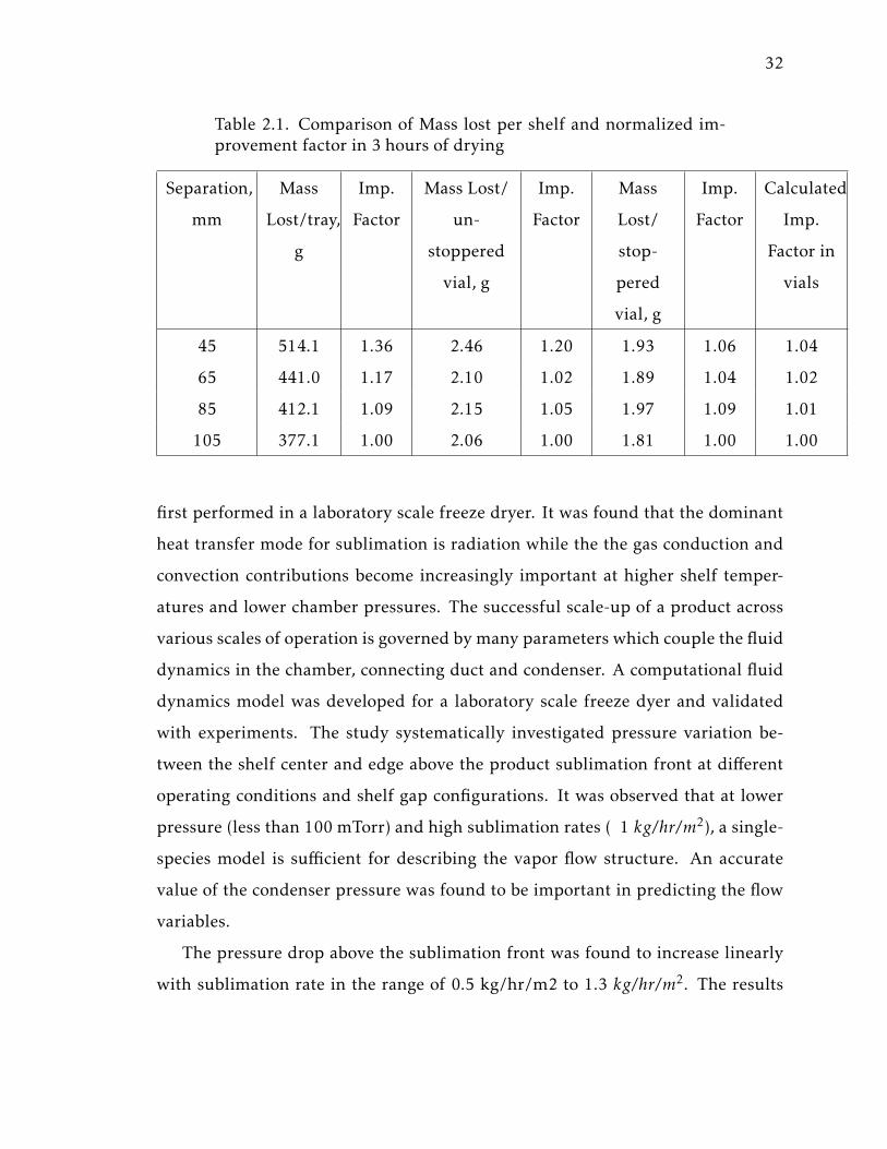
each configuration. The results of the analysis are summarized in table 5.1.

The results clearly indicate the influence of the view factor. While we see that

the largest improvement is in the open ice slabs with largest exposed surface area

of the product, the smallest improvement is in the stoppered vials. The improve-

ment varies from 36% for ice slabs with 45 mm separation, 20% at 45 mm for

unstoppered vials and reduces to 6% for the stoppered vials at the same separa-

tion. The results clearly indicate that while the process may be limited by the

heat transfer from the stopper above the vials, product configurations using bulk

drying may significantly benefit from higher radiation from above the subliming

31

front. It should be noted here that, in the above described setup, by changing

the shelf distance, the pressure above the subliming front is expected to increase

too. With an increasing local pressure above the subliming front, the resistance to

the sublimation is expected to increase. However, with an increased pressure, the

heat transfer components, namely gas conduction and convection are expected to

increase.

Figure 2.8. Setup for top heating through variable spacing with 4 loaded trays

2.4 Conclusions

The fluid dynamics and heat transfer aspects of the sublimation process are

investigated with a focus on process understanding and an eye toward accelerat-

ing the process. Measurements to estimate the key heat transfer contributions are

32

Table 2.1. Comparison of Mass lost per shelf and normalized im-provement factor in 3 hours of drying

Separation,

mm

Mass

Lost/tray,

g

Imp.

Factor

Mass Lost/

un-

stoppered

vial, g

Imp.

Factor

Mass

Lost/

stop-

pered

vial, g

Imp.

Factor

Calculated

Imp.

Factor in

vials

45 514.1 1.36 2.46 1.20 1.93 1.06 1.04

65 441.0 1.17 2.10 1.02 1.89 1.04 1.02

85 412.1 1.09 2.15 1.05 1.97 1.09 1.01

105 377.1 1.00 2.06 1.00 1.81 1.00 1.00

first performed in a laboratory scale freeze dryer. It was found that the dominant

heat transfer mode for sublimation is radiation while the the gas conduction and

convection contributions become increasingly important at higher shelf temper-

atures and lower chamber pressures. The successful scale-up of a product across

various scales of operation is governed by many parameters which couple the fluid

dynamics in the chamber, connecting duct and condenser. A computational fluid

dynamics model was developed for a laboratory scale freeze dyer and validated

with experiments. The study systematically investigated pressure variation be-

tween the shelf center and edge above the product sublimation front at different

operating conditions and shelf gap configurations. It was observed that at lower

pressure (less than 100 mTorr) and high sublimation rates ( 1 kg/hr/m2), a single-

species model is sufficient for describing the vapor flow structure. An accurate

value of the condenser pressure was found to be important in predicting the flow

variables.

The pressure drop above the sublimation front was found to increase linearly

with sublimation rate in the range of 0.5 kg/hr/m2 to 1.3 kg/hr/m2. The results

33

are found to agree within 10% of the measured pressure drop. While the pressure

drop was found to be small (less than 1 mTorr) at shelf gaps approaching 9 cm,

it increases to about 9 mTorr at gaps approaching 2.6 cm. The results were vali-

dated with experimental data and agree well across the range of shelf gaps inves-

tigated. The work presented here has proven that CFD approaches used to model

the flow physics in the chamber can accurately predict the process dynamics and

its impact on product uniformity within and across batches for a product. While

the findings presented here are substantial in quantifying the pressure variation

across the sublimation front for different process conditions and shelf configura-

tions, it is imperative that the impact of such variations on the drying uniformity

for different scales of operation be investigated for successful scale-up practice.

Furthermore, the findings of the previous section were used in understanding the

effect of re-distributing the heat transfer to the product. It was hypothesized that a

source of heat placed above and close to the subliming front would accelerate the

process. To estimate the increase in drying rate under increased heat transfer from

the top, a setup using a modified shelf configuration on a LyoFast pilot scale 2.3m2

was used. The setup with varying shelf separations to mimic a source of heat close

to the product was used in pilot scale freeze dryer. Four shelves were used in the

setup with three different product configurations were tested, a)ice slab sublima-

tion with 1 L fill volume, b)3 mL water in unstoppered 6 mL vials and c)stoppered

6 mL vials with the same product fill height. Each of the product configurations

were placed at varying separations of 45 mm, 65 mm, 85 mm and 105 mm (top

to bottom shelf, respectively) from the shelf above. The sublimation rate was ob-

tained using a time averaged gravimetric analysis for estimating the difference for

each configuration. It was found that the largest improvement was in the open ice

slabs with largest exposed surface area of the product, the smallest improvement

is in the stoppered vials. The improvement varies from 36% for ice slabs with 45

mm separation, 20% at 45 mm for unstoppered vials and reduces to 6% for the

stoppered vials at the same separation. The results presented here indicate that

34

there may be value in using additional radiative heat sources placed close to the

product in conventional bulk drying while those using stoppered vials may see a

small benefit.

35

3. CONDENSATION STUDIES: ICE ACCRETION ON AN

ARBITRARY SUPERCOOLED SURFACE

This section of the dissertation focuses on the development of a comprehensive

computational framework [48] [49] [50] for analysis of low-pressure heat andmass

transfer that enables, for the first time, obtaining detailed information on the va-

por flow structure as well as condensation rates on an arbitrary cooled surface.

This has been applied to visualize and examine various designs of freeze-dryers

and the performance of the condenser topology.

A freeze-drying cycle can last for several days. For a cycle with 100 vials sub-

liming at 0.5 g/hr, 3.6 kg of ice is formed. If the ice build-up is assumed to be uni-

form on the coils of a lab-scale condenser, a layer of ice about 1 cm thick is formed.

In reality, however, the coils closest to the duct exit receive majority of the conden-

sate whereas those farthest away from the duct may remain free of ice. Thus, it

is critical to understand factors that effect uniformity of ice growth. Here, we

use the direct simulation Monte Carlo (DSMC) technique to model gaseous trans-

port processes in a low-pressure environment encountered during freeze-drying.

The developing ice front on a supercooled surface is simulated based on the wa-

ter vapor mass flux computed by the DSMC. To validate the vapor flow and icing

simulations experimentally, measurements of ice accretion in a laboratory-scale

freeze-dryer are conducted with the use of time-lapse photography. The simu-

lations corresponding to the measured time-average water sublimation rate agree

well with the observed patterns and rates of ice accretion. The developed computa-

tional framework has been applied to investigate factors underlying the observed

non-uniformity of ice growth. Full 3D simulations of a laboratory-scale freeze-

dryer show that there is a trade-off between the total condensing surface area and

36

the ice thickness formed over a cycle. Moreover, uniformity of ice formation is

vital for the efficient usage of the condensing surfaces.

3.1 Ice Accretion Modeling

The DSMC solver SMILE (Statistical Modeling in Low-density Environment) is

used for all calculations [51]. The procedure for setting up a computation for 3D

flow in a low-pressure environment using the SMILE solver involves the follow-

ing. First, the 3D DSMC surface mesh is generated. Then the boundary conditions

are defined by assigning the surface properties such as the sticking coefficients for

water vapor and non-condensable gas, the inlet conditions such as the total mass

flow rate onto the deposition surface and the inlet temperature. Third, the molec-

ular models are specified for all chemical species in the simulation. More details

on the DSMC procedure can be found in [51] [52]. A number of modifications

to the gas-surface interaction procedure in the DSMC have been implemented to

simulate the ice accretion process. These are described below.

To predict the ice accretion on each coil during a cycle, a Gaussian weighted

approach is used. Each node in the surface mesh is a part of 1 or more panels. If

the distance between the node whose initial position is−→P tn and the centroid,

−−→Cti ,

of the triangular panel of which it is a part of, is d, to predict the position of the

node after time △t we use the following formula:

−−−−−→P t+∆tn =

−→P tn +

1

Npρice

Np∑

i=1

mi

−−−→niout Wi

−→P tn △ t (3.1)

where Np represents the number of panels connected to the point P,m· is the

steady state mass ux to the panel i,−−−→niout is the outward surface normal from the

panel and W represents the Gaussian weight given to the panel based on the dis-

tance d of the node point P from the panel centroid C. The weight is calculated

as

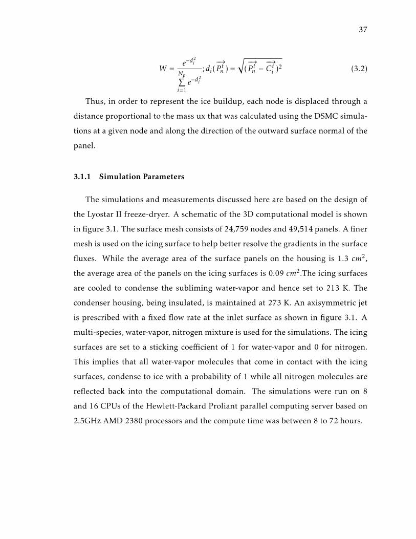
37

W =e−d

2i

Np∑

i=1e−d

2i

;di(−→P tn ) =

√

(−→P tn −−−→Cti )

2 (3.2)

Thus, in order to represent the ice buildup, each node is displaced through a

distance proportional to the mass ux that was calculated using the DSMC simula-

tions at a given node and along the direction of the outward surface normal of the

panel.

3.1.1 Simulation Parameters

The simulations and measurements discussed here are based on the design of

the Lyostar II freeze-dryer. A schematic of the 3D computational model is shown

in figure 3.1. The surface mesh consists of 24,759 nodes and 49,514 panels. A finer

mesh is used on the icing surface to help better resolve the gradients in the surface

fluxes. While the average area of the surface panels on the housing is 1.3 cm2,

the average area of the panels on the icing surfaces is 0.09 cm2.The icing surfaces

are cooled to condense the subliming water-vapor and hence set to 213 K. The

condenser housing, being insulated, is maintained at 273 K. An axisymmetric jet

is prescribed with a fixed flow rate at the inlet surface as shown in figure 3.1. A

multi-species, water-vapor, nitrogen mixture is used for the simulations. The icing

surfaces are set to a sticking coefficient of 1 for water-vapor and 0 for nitrogen.

This implies that all water-vapor molecules that come in contact with the icing

surfaces, condense to ice with a probability of 1 while all nitrogen molecules are

reflected back into the computational domain. The simulations were run on 8

and 16 CPUs of the Hewlett-Packard Proliant parallel computing server based on

2.5GHz AMD 2380 processors and the compute time was between 8 to 72 hours.

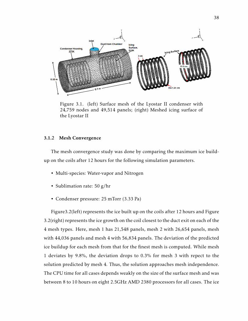
38

Figure 3.1. (left) Surface mesh of the Lyostar II condenser with24,759 nodes and 49,514 panels; (right) Meshed icing surface ofthe Lyostar II

3.1.2 Mesh Convergence

The mesh convergence study was done by comparing the maximum ice build-

up on the coils after 12 hours for the following simulation parameters.

• Multi-species: Water-vapor and Nitrogen

• Sublimation rate: 50 g/hr

• Condenser pressure: 25 mTorr (3.33 Pa)

Figure3.2(left) represents the ice built up on the coils after 12 hours and Figure

3.2(right) represents the ice growth on the coil closest to the duct exit on each of the

4 mesh types. Here, mesh 1 has 21,548 panels, mesh 2 with 26,654 panels, mesh

with 44,036 panels and mesh 4 with 56,834 panels. The deviation of the predicted

ice buildup for each mesh from that for the finest mesh is computed. While mesh

1 deviates by 9.8%, the deviation drops to 0.3% for mesh 3 with repect to the

solution predicted by mesh 4. Thus, the solution approaches mesh independence.

The CPU time for all cases depends weakly on the size of the surface mesh and was

between 8 to 10 hours on eight 2.5GHz AMD 2380 processors for all cases. The ice

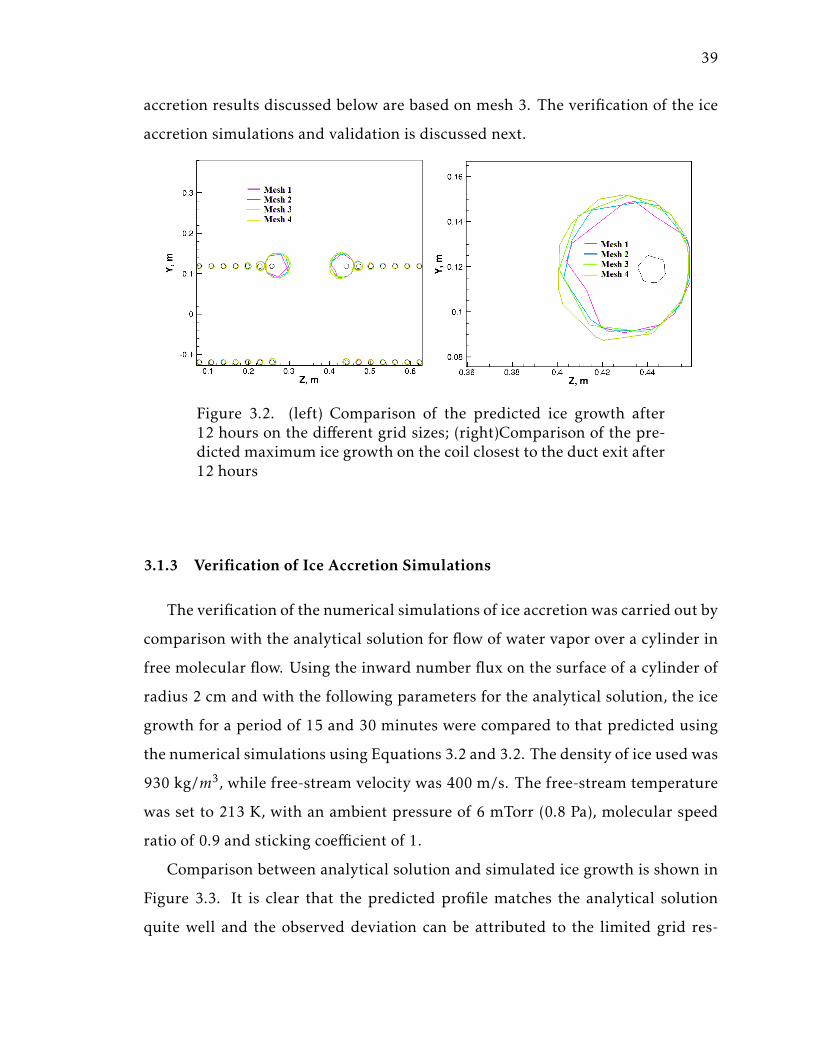
39

accretion results discussed below are based on mesh 3. The verification of the ice

accretion simulations and validation is discussed next.

Figure 3.2. (left) Comparison of the predicted ice growth after12 hours on the different grid sizes; (right)Comparison of the pre-dicted maximum ice growth on the coil closest to the duct exit after12 hours

3.1.3 Verification of Ice Accretion Simulations

The verification of the numerical simulations of ice accretion was carried out by

comparison with the analytical solution for flow of water vapor over a cylinder in

free molecular flow. Using the inward number flux on the surface of a cylinder of

radius 2 cm and with the following parameters for the analytical solution, the ice

growth for a period of 15 and 30 minutes were compared to that predicted using

the numerical simulations using Equations 3.2 and 3.2. The density of ice used was

930 kg/m3, while free-stream velocity was 400 m/s. The free-stream temperature

was set to 213 K, with an ambient pressure of 6 mTorr (0.8 Pa), molecular speed

ratio of 0.9 and sticking coefficient of 1.

Comparison between analytical solution and simulated ice growth is shown in

Figure 3.3. It is clear that the predicted profile matches the analytical solution

quite well and the observed deviation can be attributed to the limited grid res-

40

olution used. The maximum deviation between the analytical solution and the

simulation was 2.1%. The analytical solution was obtained using the relation for

the inward number flux shown in equation 3.3.

βNi

n= e−S

2cos2θ +

√ΠScosθ(1 + erf (Scosθ))

2√Π

(3.3)

Here, θ is the angle between the stream velocity, v, and the surface normal, β is

the inverse of the most probable molecular thermal speed, s is the molecular speed

ratio, n is the number density of molecules and Ni is the inward number flux of

molecules.

Figure 3.3. (left) Comparison between the theoretical and the sim-ulated ice growth on a circular cylinder in a free-molecular flow

3.2 Measurements of Ice Accretion in Low-pressure environment

Measurements of ice accretion patterns and rates in a freeze-drying condenser

have been obtained to provide a basis for experimental validation of the vapor

and icing flow modeling described above. The ice slab sublimation test was per-

formed on a laboratory-scale freeze-dryer Lyostar II (SP Scientific, Stone Ridge,

41

NY) at Baxter Medical Products laboratory in Bloomington, IN. A liter of water

each was loaded in three stainless steel trays. While the shelf temperature in the

product chamber was maintained at 0 C, the chamber pressure was maintained at

120 mTorr (16 Pa). The condenser pressure was 70 mtorr (9.33 Pa). After 24 hours

of freeze-drying the residual mass of water was measured. The time-average sub-

limation rate was determined to be 55 g/hr and was used as an input parameter in

the flow and ice accretion simulations.

In order to compare with the simulation results for icing growth rates, time-

lapse photographymeasurements were obtained using a Canon T2i cameramounted

on a tripod. A programmable timer-remote was used to capture images every 30

minutes for the duration of the cycle over the 24-hour period. In order to reduce

the reflection from the glass door, a lens hood was used. In addition, the inten-

sity of white light was minimized and a light emitting diode (LED) lamp with a

peak wavelength in the range of 390 to 410 nm was used to enhance contrast. The

captured images were post-processed using Matlab to extract the intensity plot

at a selected location corresponding to the coil closest to the duct exit. The ice

thickness as a function of time was determined with an accuracy of about 4%.

3.3 Effect of Non-condensable Gases on Ice Accretion Rate

Simulation Parameters

• Mass flow rate: 165 g/hr

• Multi species: Water vapor and Nitrogen

• Chamber surface temperature: 273 K

• Sticking coefficient of coils: 1 for water-vapor and 0 for N2

• Condenser pressure: 80 mTorr (10.66 Pa)

• Total simulated molecules: 2.1 million

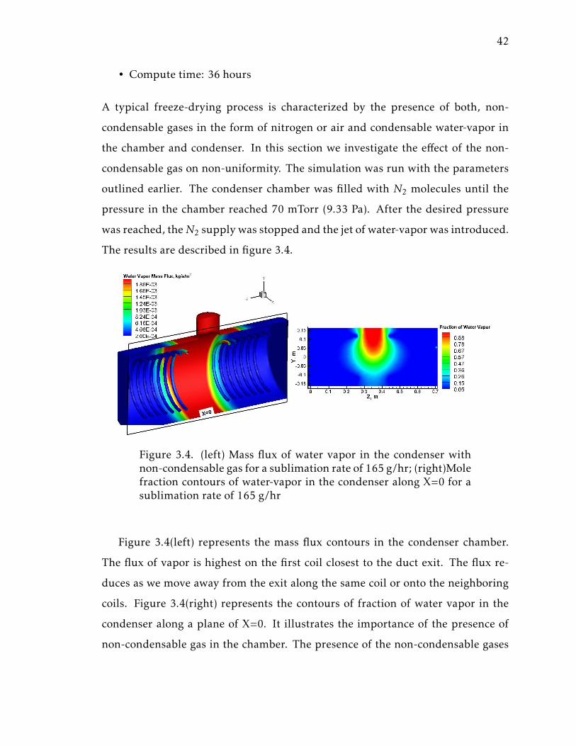
42

• Compute time: 36 hours

A typical freeze-drying process is characterized by the presence of both, non-

condensable gases in the form of nitrogen or air and condensable water-vapor in

the chamber and condenser. In this section we investigate the effect of the non-

condensable gas on non-uniformity. The simulation was run with the parameters

outlined earlier. The condenser chamber was filled with N2 molecules until the

pressure in the chamber reached 70 mTorr (9.33 Pa). After the desired pressure

was reached, theN2 supply was stopped and the jet of water-vapor was introduced.

The results are described in figure 3.4.

Figure 3.4. (left) Mass flux of water vapor in the condenser withnon-condensable gas for a sublimation rate of 165 g/hr; (right)Molefraction contours of water-vapor in the condenser along X=0 for asublimation rate of 165 g/hr

Figure 3.4(left) represents the mass flux contours in the condenser chamber.

The flux of vapor is highest on the first coil closest to the duct exit. The flux re-

duces as we move away from the exit along the same coil or onto the neighboring

coils. Figure 3.4(right) represents the contours of fraction of water vapor in the

condenser along a plane of X=0. It illustrates the importance of the presence of

non-condensable gas in the chamber. The presence of the non-condensable gases

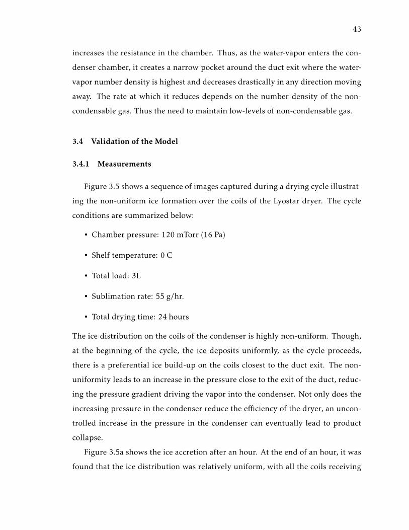
43

increases the resistance in the chamber. Thus, as the water-vapor enters the con-

denser chamber, it creates a narrow pocket around the duct exit where the water-

vapor number density is highest and decreases drastically in any direction moving

away. The rate at which it reduces depends on the number density of the non-

condensable gas. Thus the need to maintain low-levels of non-condensable gas.

3.4 Validation of the Model

3.4.1 Measurements

Figure 3.5 shows a sequence of images captured during a drying cycle illustrat-

ing the non-uniform ice formation over the coils of the Lyostar dryer. The cycle

conditions are summarized below:

• Chamber pressure: 120 mTorr (16 Pa)

• Shelf temperature: 0 C

• Total load: 3L

• Sublimation rate: 55 g/hr.

• Total drying time: 24 hours

The ice distribution on the coils of the condenser is highly non-uniform. Though,

at the beginning of the cycle, the ice deposits uniformly, as the cycle proceeds,

there is a preferential ice build-up on the coils closest to the duct exit. The non-

uniformity leads to an increase in the pressure close to the exit of the duct, reduc-

ing the pressure gradient driving the vapor into the condenser. Not only does the

increasing pressure in the condenser reduce the efficiency of the dryer, an uncon-

trolled increase in the pressure in the condenser can eventually lead to product

collapse.

Figure 3.5a shows the ice accretion after an hour. At the end of an hour, it was

found that the ice distribution was relatively uniform, with all the coils receiving

44

Figure 3.5. Photograph of the non-uniform ice-buildup on the coilsat the end of 1, 6, 12, 18 and 24 hours: Mass Flow Rate: 55 g/hr,Chamber Pressure: 120 mTorr (16 Pa), Condenser Pressure: 70mTorr (9.33 Pa)

about 1-3mm of ice growth. Figure 3.5b, c, d and e represent the ice accumulated

after 6, 12, 18 and 24 hours of drying, respectively. At the end of 24 hours, on

the coil closest to the duct exit, there is higher ice accumulation and reduces as we

move away in either direction. The thickness of the ice formed on the coil closest

to the duct exit is about 2.8 cm and reduces to a few mm on the coil farthest away

from it. The 3D icing model has been validated using the same conditions that

were used in the experiment and the results are discussed in the following section.

3.4.2 Comparison between Simulations and Measurements

The surfacemesh 3was used in the computations. The total number ofmolecules

at steady state ranged between 1.6-2 million with over 350,000 400,000 cells in

45

the domain. The simulations were run on 16 processors with total compute times

ranging between 48-72 hours for the 24 hour cycle. Figure 3.6 compares the ice

build-up on the coils as predicted by a steady and unsteady icing model. The

steady icing model predicts the ice thickness over a period of 24 hours based on

the steady state mass flux computed on the panels at time (t) = 0. The ice ac-

cretion profile obtained from the steady solution was found to over-predict the

measured maximum ice thickness by 14% at t=24 hrs. This was attributed to the

unsteady nature of the ice accretion, i.e. as the ice grows on the coils during the

drying cycle, there is a larger surface area available for the incoming water vapor

molecules to condense upon. Thus, there is a non-linear increase in the ice thick-

ness. Moreover, while the sublimation rate is highest at the beginning of the cycle

and reduces as the cycle progresses, the simulations use an average sublimation

rate over the entire drying cycle. Thus, the vapor trapping capability reduces as

the cycle proceeds. The measurements of the maximum ice thickness corroborate

this trend. An unsteady icing model was developed and implemented to capture

this trend.

The unsteady model is similar to the steady model in all aspects except that

it uses intermediate profile updates to predict the final ice front. For example, to

build the ice growth over 15 hours, the ice front can be updated every 5 hours. On

the new surface mesh obtained at the end of 5 hours (t=5), a DSMC calculation

is run to obtain the steady mass flux and the process is repeated for (t=10) going

up to the desired ice growth period (15 hours here). Figure 3.6 illustrates one

such example which uses 4 profile updates at 0, 6, 12 and 18 hours respectively to

predict the ice growth after 24 hours at a sublimation rate of 55 g/hr. The scale

indicates the maximum ice thickness at that time interval in cm. The red pointer

represents the steady model and the blue pointer represents the unsteady model

thickness prediction. By intermittently updating the surface mesh every 6 hours,

the non-linear behavior of the ice accretion was captured within an accuracy of 1%

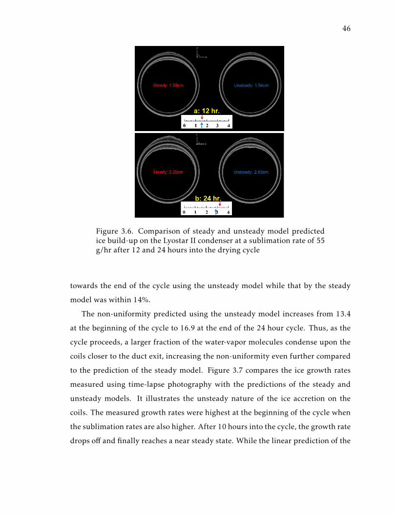
46

Figure 3.6. Comparison of steady and unsteady model predictedice build-up on the Lyostar II condenser at a sublimation rate of 55g/hr after 12 and 24 hours into the drying cycle

towards the end of the cycle using the unsteady model while that by the steady

model was within 14%.

The non-uniformity predicted using the unsteady model increases from 13.4

at the beginning of the cycle to 16.9 at the end of the 24 hour cycle. Thus, as the

cycle proceeds, a larger fraction of the water-vapor molecules condense upon the

coils closer to the duct exit, increasing the non-uniformity even further compared

to the prediction of the steady model. Figure 3.7 compares the ice growth rates

measured using time-lapse photography with the predictions of the steady and

unsteady models. It illustrates the unsteady nature of the ice accretion on the

coils. The measured growth rates were highest at the beginning of the cycle when

the sublimation rates are also higher. After 10 hours into the cycle, the growth rate

drops off and finally reaches a near steady state. While the linear prediction of the

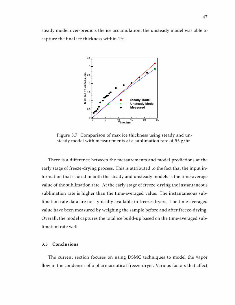
47

steady model over-predicts the ice accumulation, the unsteady model was able to

capture the final ice thickness within 1%.

Time, hrs

Max

. Ice

Th

ickn

ess,

cm

0 5 10 15 20 250

0.5

1

1.5

2

2.5

3

3.5

Steady ModelUnsteady ModelMeasured

Figure 3.7. Comparison of max ice thickness using steady and un-steady model with measurements at a sublimation rate of 55 g/hr

There is a difference between the measurements and model predictions at the

early stage of freeze-drying process. This is attributed to the fact that the input in-

formation that is used in both the steady and unsteady models is the time-average

value of the sublimation rate. At the early stage of freeze-drying the instantaneous

sublimation rate is higher than the time-averaged value. The instantaneous sub-

limation rate data are not typically available in freeze-dryers. The time-averaged

value have been measured by weighing the sample before and after freeze-drying.

Overall, the model captures the total ice build-up based on the time-averaged sub-

limation rate well.

3.5 Conclusions

The current section focuses on using DSMC techniques to model the vapor

flow in the condenser of a pharmaceutical freeze-dryer. Various factors that affect

48

non-uniformity of mass flux and hence ice-growth on an arbitrary cooled surface

were investigated. It was found that the presence of a duct connecting the product

chamber and condenser increased non-uniformity by 65% at a sublimation rate

of 5 g/hr. The non-uniformity of ice-growth also depends on the number density

of the non-condensable gas in the chamber. The presence of the non-condensable

gases increased the effective-resistance in the condenser, there-by preventing the

vapor from condensing on the coils away from the duct exit.

The computed steady state mass flux was used to predict the development of

the ice front on the condenser coils. To verify the algorithm used for the predic-

tion, a comparison was made with an analytical solution for the condensation of

vapor during free molecular flow around a circular cylinder. The model was then

extended to predict the ice accumulation on the coils of the Lyostar II condenser

and the predictions were validated with measurements. It was found that the coils

closest to the vapor inlet being subjected to the largest mass ux, had the largest

ice accumulation. The maximum thickness of the ice formed on the coil closest

to the duct exit at the end of 24 hours using the steady icing model was 3.2 cm.

This was 14% higher than the measurements made under the same drying condi-

tions. An unsteady icing model was developed and implemented to capture the

non-linear ice accretion rates. The model incorporated the unsteady behavior by

intermittently updating the surface mesh to track the ice growth. With an updated

geometry every 6 hours, the non-linear behavior of the ice accretion was captured

within 1% towards the end of the 24-hour freeze-drying process. It was shown

that as the cycle proceeds, a larger fraction of the water-vapor molecules condense

upon the coils closer to the duct exit, increasing the non-uniformity even further.

The unsteadymodel predicted a larger non-uniformity, of about 16.9, as compared

to 13.4 for steady-state model.

49

4. SUBLIMATION-TRANSPORT-CONDENSATION COUPLED

SIMULATION FRAMEWORK

Process understanding from the modeling effort described in the previous sections

have been applied to a unified framework and presented here. A physics-based

model for the sublimation-transport-condensation processes occurring in a low-

pressure environment as applied to freeze drying by coupling product attributes

and equipment capabilities into a unified simulation framework is presented. The

system-level model is used to determine the effect of operating conditions such

as shelf temperature, chamber pressure and the load size on occurrence of chok-

ing for a production-scale dryer. Several data sets corresponding to production-

scale runs with a load from 120 to 485 L have been compared with simulations.

A subset of data is used for calibration, whereas another data set correspond-

ing to a load of 150 L is used for model validation. The model predictions for

both the onset and extent of choking as well as for the measured product tem-

perature agree well with the production-scale measurements. Additionally, we

study the effect of resistance to vapor transport presented by the duct with a valve

and a baffle in the production-scale freeze-dryer. Computation Fluid Dynamics

(CFD) techniques augmented with a system-level unsteady heat and mass transfer

model allow to predict dynamic process conditions taking into consideration spe-

cific dryer design. CFD modeling of flow structure in the duct presented here for

a production-scale freeze-dryer quantifies the benefit of reducing the obstruction

to the flow through several design modifications. The comprehensive simulation

framework combining the system-level model and the detailed CFD computations

can provide a process analytical tool for more efficient and robust freeze-drying of

50

bio/pharmaceuticals. The problem description and model framework is presented

in this chapter while the results are discussed in the following chapters.

4.1 Introduction

Freeze-drying has been known to be a lengthy process. Traditionally, it has

been believed that the product requirements limit the maximum sublimation rate

and hence lower yield. However, there has been growing interest in allowing prod-

uct temperatures well above the collapse temperature in certain amorphous and

partially crystalline protein formulations [53] [54] [55]. Even though the cake

tends towards microscopic collapse at best under these conditions, the trend is

motivated by an interest in reducing cycle time. However, under aggressive drying

conditions, equipment based limitations could become the dominant factor. For

example, under such aggressive drying conditions, a typical freeze-dryer would

choke, leading to loss of pressure control and hence macroscopic collapse could

result. Patel and co-workers [56] studied the onset of choking in a laboratory-scale

Lyostar II freeze-dryer (SP Industries, NY). It was found that the pressure ratio

between the chamber and condenser (Pch/Pcd) was the critical factor that deter-

mined the onset of choked flow during primary drying. For the laboratory dryer

used for the study, the critical ratio leading to choked flow was about 2.5. Thus,

there is a need to advance current designs based on physics-based modeling such

that even under aggressive drying conditions, operating under equipment limita-

tions can be avoided.

A model describing the heat and mass transfer in lyophilization at pilot scale

was done by [24] where a means to couple the fluid dynamics in the chamber with

the heat and mass transfer in a vial using a multi-dimensional model was pre-

sented. The dual-scale model was capable of predicting the evolution of the prod-

uct temperature during primary drying for the prescribed process conditions. The

model results attributed some of the intra-batch differences in product character-

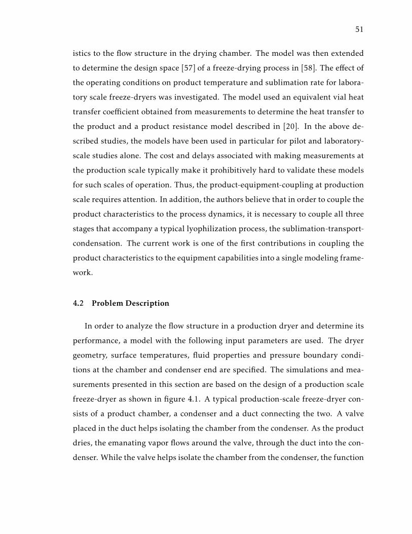
51

istics to the flow structure in the drying chamber. The model was then extended

to determine the design space [57] of a freeze-drying process in [58]. The effect of

the operating conditions on product temperature and sublimation rate for labora-

tory scale freeze-dryers was investigated. The model used an equivalent vial heat

transfer coefficient obtained from measurements to determine the heat transfer to

the product and a product resistance model described in [20]. In the above de-

scribed studies, the models have been used in particular for pilot and laboratory-

scale studies alone. The cost and delays associated with making measurements at

the production scale typically make it prohibitively hard to validate these models

for such scales of operation. Thus, the product-equipment-coupling at production

scale requires attention. In addition, the authors believe that in order to couple the

product characteristics to the process dynamics, it is necessary to couple all three

stages that accompany a typical lyophilization process, the sublimation-transport-

condensation. The current work is one of the first contributions in coupling the

product characteristics to the equipment capabilities into a single modeling frame-

work.

4.2 Problem Description

In order to analyze the flow structure in a production dryer and determine its

performance, a model with the following input parameters are used. The dryer

geometry, surface temperatures, fluid properties and pressure boundary condi-

tions at the chamber and condenser end are specified. The simulations and mea-

surements presented in this section are based on the design of a production scale

freeze-dryer as shown in figure 4.1. A typical production-scale freeze-dryer con-

sists of a product chamber, a condenser and a duct connecting the two. A valve

placed in the duct helps isolating the chamber from the condenser. As the product

dries, the emanating vapor flows around the valve, through the duct into the con-

denser. While the valve helps isolate the chamber from the condenser, the function

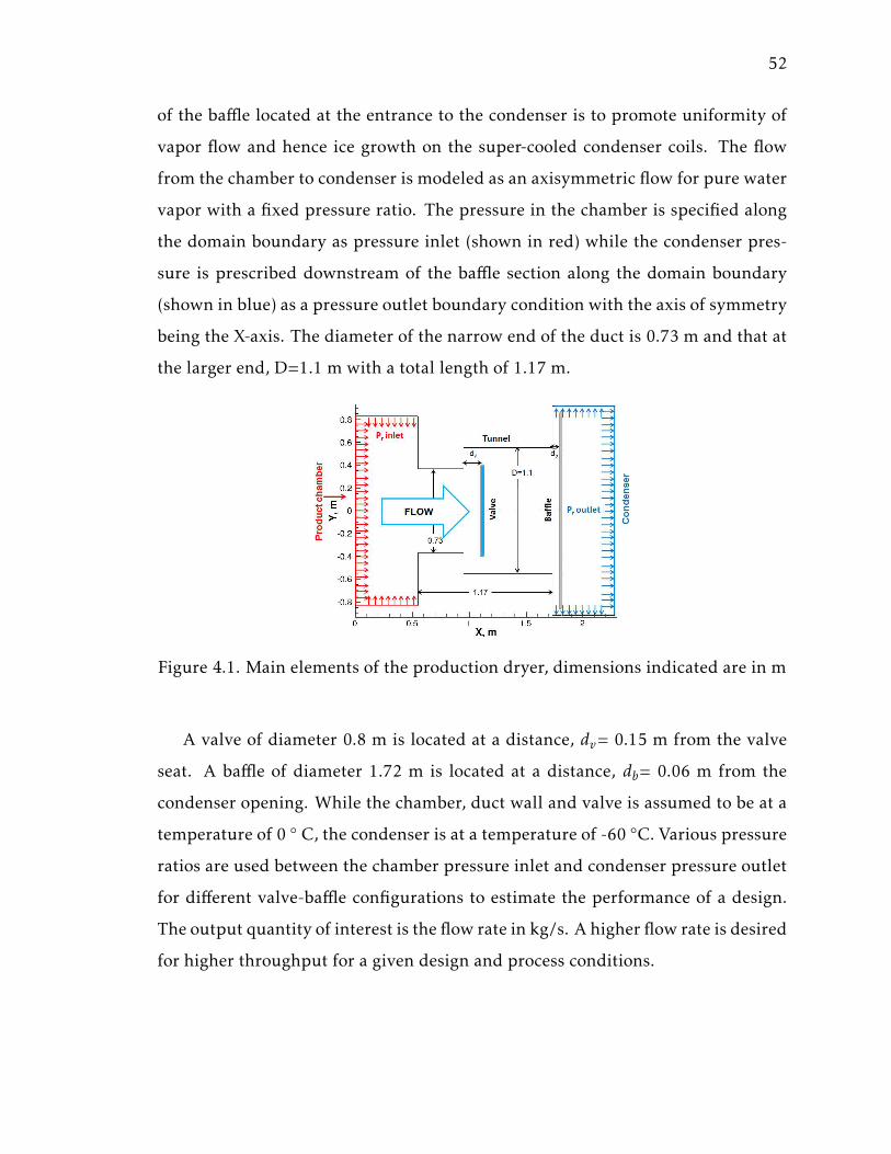
52

of the baffle located at the entrance to the condenser is to promote uniformity of

vapor flow and hence ice growth on the super-cooled condenser coils. The flow

from the chamber to condenser is modeled as an axisymmetric flow for pure water

vapor with a fixed pressure ratio. The pressure in the chamber is specified along

the domain boundary as pressure inlet (shown in red) while the condenser pres-

sure is prescribed downstream of the baffle section along the domain boundary

(shown in blue) as a pressure outlet boundary condition with the axis of symmetry

being the X-axis. The diameter of the narrow end of the duct is 0.73 m and that at

the larger end, D=1.1 m with a total length of 1.17 m.

Figure 4.1. Main elements of the production dryer, dimensions indicated are in m

A valve of diameter 0.8 m is located at a distance, dv= 0.15 m from the valve

seat. A baffle of diameter 1.72 m is located at a distance, db= 0.06 m from the

condenser opening. While the chamber, duct wall and valve is assumed to be at a

temperature of 0 ◦ C, the condenser is at a temperature of -60 ◦C. Various pressure

ratios are used between the chamber pressure inlet and condenser pressure outlet

for different valve-baffle configurations to estimate the performance of a design.

The output quantity of interest is the flow rate in kg/s. A higher flow rate is desired

for higher throughput for a given design and process conditions.

53

4.3 Measurements

Measurements were made in a production-scale freeze-dryer with thermocou-

ples to measure the shelf and product temperatures. Capacitance manometers and

Pirani gauges were used to measure the chamber and condenser pressures, respec-

tively. Varying loading and process conditions with product load between 120 L

to 485 L and chamber pressure between 8 Pa and 10 Pa were used. The product

was frozen first by maintaining a shelf temperature of about -45 ◦C and was then

ramped up to the higher temperatures, typically varying between 0 ◦C to 15 ◦C

during primary drying. Aggressive ramping rates in some of the cycles led to loss

of pressure control in the chamber. The average sublimation rate measured gravi-

metrically is used as ametric to compare themodeling results to themeasurements

for each of the cases discussed later.

4.4 Modeling

The modeling effort in this section consists of both, a computational fluid dy-

namics (CFD) model to simulate the flow structure in a production scale freeze-

dryer and a coupled, unsteady heat and mass transfer model developed and im-

plemented to couple the dryer hardware with the product characteristics.

Based on the continuum fluid hypothesis, fluid flow properties such as den-

sity and velocity can be defined as averages over volume elements that are large

enough in comparison to the microscopic structure of the fluid, but small enough

in comparison to the scale of macroscopic flow phenomena. A non-dimensional

parameter known as Knudsen number, Kn is often used to characterize the influ-

ence of non-continuum effects in a gas flow. The Knudsen number is defined as the

ratio of molecular mean free path to the characteristic, macroscopic length scale

L of the flow Kn=λ/L

The continuum hypothesis is valid for flows at small Knudsen numbers, typ-

ically less than 0.01. In this case, the fluid is close to the local thermodynamic

54

equilibrium and the numerical modeling of such flows can be based on solution

of Navier-Stokes equations for viscous flows. For Knudsen numbers larger than

0.01, the non-equilibrium rarefaction influences the flow near gas-solid interfaces.

These effects can be accounted for in the boundary conditions for Navier-Stokes

equations as the first-order approximations in Knudsen number for velocity slip

and temperature jump for Kn up to 0.1. For flows with larger Knudsen number,

the modeling has to be based on the Boltzmann equation, the principal equation

of the kinetic theory [52].

At large scales of operation as applied to production scale freeze-dryers, out-

side the product containment, the Kn is typically less than 0.008. The only region

where the Kn is typically greater than this is in the gap separating the vial and

the shelf and the flow in this region is in the transitional regime. In addition, the

flow through the pores of the product may be in the free molecular regime. Thus,

the modeling discussed in this work uses a 1-D temperature jump relation for the

heat transfer in the transitional regime [28] between the shelf and the product.

The mass transfer through the pores has been simplified using semi-analytical

equations for the mass transfer discussed later. CFD calculations are based on

the continuum based Navier-Stokes solver for the bulk flow in the freeze-dryer.

Since the change in sublimation rate (function of product temperature and cham-

ber pressure) is small compared to the time scale of the cycle, a quasi-steady state

is assumed.

In the current section, CFD modeling of water vapor flow in a production-

scale freeze-dryer is conducted using the solution of Navier-Stokes equations [59].

While previous CFD-basedmodeling efforts have dealt with addressing the sources

of heterogeneity in a batch during primary drying for a given dryer design [24], the

focus of this section is on coupling the equipment design to safe-process limits.

The CFD solver FLUENT is used for a water-vapor fluid with a power-law viscosity

model [45]. A steady, axisymmetric model with a second-order upwinding flux

scheme for the mass, momentum and energy is used.

55

4.4.1 Unsteady System-level Heat and Mass Transfer Model

The system level model describes the process dynamics in the entire freeze-

dryer, including chamber, duct and condenser. This is done by formulating the

corresponding mass conservation equations describing the sublimation, transport

and condensation processes. Below we describe the models and constitutive equa-

tions used for modeling each of the processes.

Model for Sublimation in Product Chamber

The heat transfer to the product during the drying cycle can be modeled as an

unsteady heat transfer problem whose input parameters are summarized below.

The sublimation process can be modeled as a one-dimensional unsteady cou-

pled heat and mass transfer problem for a control volume (shown in figure 4.2)

consisting of the frozen product and the dried cake. Amore detailed two-dimensional

modeling of heat and mass transfer during freeze-drying in glass vials has been

presented, for example, in [60]. As the product dries, the thickness of the frozen

product, Lpr reduces while that of the cake, Lcake increases. The sublimation rate is

controlled by the chamber pressure Pch, shelf temperature Tsh, product thickness

Lpr(t), product container surface area available for heat transfer and the product

area Apr and temperature Tsub.

The two fundamental equations that need to be solved are the energy and mass

conservation equations . The energy equation is given as:

˙Qext = −△Hsdm

dt+mCp

dTsubdt

(4.1)

Here, ˙Qext is the external heat supplied to sublime the product, △Hs is the en-

thalpy of sublimation, dm/dt is the sublimation rate as given in equation 2.1. m is

the mass of the product, Cp is the specific heat of the product at constant pressure

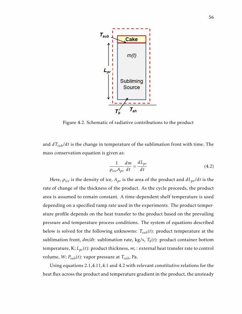
56

Figure 4.2. Schematic of radiative contributions to the product

and dTsub/dt is the change in temperature of the sublimation front with time. The

mass conservation equation is given as:

1

ρiceApr

dm

dt=dLpr

dt(4.2)

Here, ρice is the density of ice, Apr is the area of the product and dLpr /dt is the

rate of change of the thickness of the product. As the cycle proceeds, the product

area is assumed to remain constant. A time-dependent shelf temperature is used

depending on a specified ramp rate used in the experiments. The product temper-

ature profile depends on the heat transfer to the product based on the prevailing

pressure and temperature process conditions. The system of equations described

below is solved for the following unknowns: Tsub(t): product temperature at the

sublimation front, dm/dt: sublimation rate, kg/s, Tb(t): product container bottom

temperature, K; Lpr(t): product thickness,m; : external heat transfer rate to control

volume, W; Psub(t): vapor pressure at Tsub, Pa.

Using equations 2.1,4.11,4.1 and 4.2 with relevant constitutive relations for the

heat flux across the product and temperature gradient in the product, the unsteady

57

product temperature and sublimation rate can be obtained. The equation for the

external heat flow is given as:

˙Qext = qradArad + qg,condAg,cond (4.3)

where the radiative contribution is computed as

qrad =Atopqrad,top +Abot qrad,bottom

Atop +Abot(4.4)

qrad,top =σFsh−pr(T

4sh −T

4pr)

1/ǫss +1/ǫg − 1(4.5)

qrad,bottom =σFsh−b(T

4sh −T

4b )

1/ǫss +1/ǫg − 1(4.6)

Where σ is the Stefan-Boltzmann constant, F is the view factor between the shelf

and the subliming product, Tsh is the shelf temperature, Tsub is the subliming front

temperature and Tb is the product bottom temperature. ǫss and ǫg are the emissiv-

ities for steel and glass respectively (taken as 0.6 and 0.9).

The gas conduction contribution is given by [28]

qg,cond =Tsh −Tb

lK + 2

Pγ−1γ+1

√

π2R (√Th +√Tc)

(4.7)

where l is the shelf-vial bottom separation in m, K is the thermal conductivity

of water vapor [61] in W/(m.K), Pch is the chamber pressure in Pa, γ is the heat

ratio and R is the specific gas constant. Values of R=461.89 J/(kg.K) and γ =1.33

are used in the calculations. For values of l that are small, the above relation is

dominated by the contact conduction contribution of the heat transfer as:

qg,cond =K

l(Tsh −Tb) (4.8)

The external heat flux is related to the temperature gradient in the product as

Qext

Apr=

Tb −TprLpr /Kice

(4.9)

58

where the thermal conductivity of ice, kice=2.5 W/(m.K). The sublimation rate of

the product is given as [20]

dm

dt=

Apr

Rp +Rs(Psub −Pch) (4.10)

where the saturation pressure, Psub is

Psub = Pref × exp(△Hs

R.Tsub −TrefTsub.Tref

) (4.11)

where △Hs is the enthalpy of sublimation for ice (2503 J/g), R=8.314 J/(mol.K)

is the gas constant, Tref =233.15 K and Pref =12.848 Pa. The equivalent total resis-

tance to mass transfer shown in eq. 4.10 being an unknown, is used as a calibration

parameter with 3 coefficients, R0, K1 and K2 related to the dried cake thickness,

Lcake as [47].

Rp = R0 +K1Lcake

1+K2Lcake(4.12)

where R0, K1 and K2 are obtained through experiments. The above described sub-

limation model is coupled with the transport in the duct connecting the chamber-

condenser and the condensation process in the condenser. The following section

describes the transport and condensation modeling.

Transport and Condensation in Duct and Condenser

The flow through the duct is driven by the pressure and concentration gra-

dients existing between the chamber and the condenser. A small pressure ratio

between the chamber and condenser occurs in freeze-drying processes for formu-

lations requiring relatively large chamber pressures (10s of Pa). For such con-

ditions the vapor flow rate from chamber to condenser can be compared to the

fully-developed viscous flow through a long circular duct known as the Poiseuille

solution

˙mpois = ρAduct1

8µ

Pch −PcdLduct

(R2duct) (4.13)

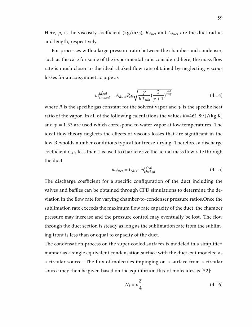
59

Here, µ, is the viscosity coefficient (kg/m/s), Rduct and Lduct are the duct radius

and length, respectively.

For processes with a large pressure ratio between the chamber and condenser,

such as the case for some of the experimental runs considered here, the mass flow

rate is much closer to the ideal choked flow rate obtained by neglecting viscous

losses for an axisymmetric pipe as

˙midealchoked = AductPch

√

γ

RTsub(

2

γ +1)γ+1γ−1 (4.14)

where R is the specific gas constant for the solvent vapor and γ is the specific heat

ratio of the vapor. In all of the following calculations the values R=461.89 J/(kg.K)

and γ = 1.33 are used which correspond to water vapor at low temperatures. The

ideal flow theory neglects the effects of viscous losses that are significant in the

low-Reynolds number conditions typical for freeze-drying. Therefore, a discharge

coefficient Cdis less than 1 is used to characterize the actual mass flow rate through

the duct

˙mduct = Cdis ·midealchoked (4.15)

The discharge coefficient for a specific configuration of the duct including the

valves and baffles can be obtained through CFD simulations to determine the de-

viation in the flow rate for varying chamber-to-condenser pressure ratios.Once the

sublimation rate exceeds the maximum flow rate capacity of the duct, the chamber

pressure may increase and the pressure control may eventually be lost. The flow

through the duct section is steady as long as the sublimation rate from the sublim-

ing front is less than or equal to capacity of the duct.

The condensation process on the super-cooled surfaces is modeled in a simplified

manner as a single equivalent condensation surface with the duct exit modeled as

a circular source. The flux of molecules impinging on a surface from a circular

source may then be given based on the equilibrium flux of molecules as [52]:

Ni = nc

4(4.16)

60

Here, the number flux of molecules impinging on the condensation surface will

depend on the number density of the gas, n and the mean molecular speed of the

gas, c which is given by:

c =

√

8kTsubπmmass

(4.17)

where, mmass is the molecular mass of the water vapor molecule. Combining the

sublimation, transport and condensation model, the rate of change of chamber

pressure for a given chamber geometry of volume, Vch can be related to the sub-

limation rate expressed in equation 4.10 and the flow rate through the duct as

shown below:

d

dt(PchVch

RTsub) = −m− ˙mduct (4.18)

where ˙mduct is the flow rate through the duct. The rate of increase of condenser

pressure can be given as

d

dt(Pcd) =

1

Vcd(

˙mduct

mmass−NiAcd)kTcd (4.19)

Here, Acd and Tcd are the equivalent area and temperature of the condenser sur-

face, respectively, while mmass is the molecular mass for water vapor. The basis

for the current condensation model is a simplified, condensation pumping mech-

anism for the condenser coils modeled as a single plate of equivalent area. It as-

sumes that the geometry of the coils (and ice thickness) do not change the vapor

trapping capability of the condenser during the cycle. Moreover, the model does

not include the changes in ice thickness variation during the cycle as this is ex-

pected to increase the compute time and deviates from the objective of the current

investigation. It assumes that the condenser pressure is likely to rise only when

the available condensing area is small compared to the flow rate at which the va-

por exits from the duct. The unknowns of the coupled sublimation-condensation

system-level model are the product temperature, the sublimation rate, chamber

pressure and the condenser pressure, given the geometry of the dryer, load and

61

product resistance. The condensation model can be applied to model the ice accre-

tion process on any super-cooled surface by receiving inputs from detailed CFD or

direct simulation Monte Carlo (DSMC) calculations. The sublimation rate model,

the duct flow model and the condensation model described in this section can be

coupled to provide a time-dependent sublimation rate that changes depending not

only on the chamber pressure but also the condenser pressure and duct-condenser

geometry. The following chapter will discuss its implementation and application

in determining the on-set and extent of choking for different designs and hard-

ware configurations.

62

5. APPLICATION OF THE COUPLEDMODEL TO ESTIMATE

PRODUCT, EQUIPMENT AND PROCESS LIMIT

5.1 Problem Description

The unsteady model described in the previous chapter is applied to predicting

the pressure variation, product temperature history and unsteady sublimation rate

for varying loading conditions from 120 L to 485 L in the production dryer for

different products. The following are main input parameters and assumptions

used in the system model:

• Equal chamber and condenser volume: 15 m3

• Total condensing surface area: 3.6 m2

• Duct radius and length: 0.365 m and 1.17 m

• Discharge coefficient (Cdis): Variable, dependent on connecting duct geome-

try and chamber to condenser pressure ratio, obtained from CFD results

• Constant condenser temperature, −60◦C

• The initial product thickness and product resistance are calibrated for a given

product to match the initial measured product temperature variation

• A first order explicit Euler method for time integration was used for all cal-

culations discussed in the manuscript with a time step of 100 s

• The output parameters of interest from the system are the extent, if any of

loss of pressure control in the cycle, the product temperature history, subli-

mation rate variation and time to dry the product

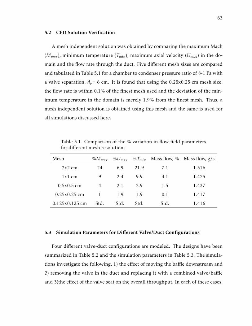
63

5.2 CFD Solution Verification

A mesh independent solution was obtained by comparing the maximum Mach

(Mmax), minimum temperature (Tmin), maximum axial velocity (Umax) in the do-

main and the flow rate through the duct. Five different mesh sizes are compared

and tabulated in Table 5.1 for a chamber to condenser pressure ratio of 8-1 Pa with

a valve separation, dv= 6 cm. It is found that using the 0.25x0.25 cm mesh size,

the flow rate is within 0.1% of the finest mesh used and the deviation of the min-

imum temperature in the domain is merely 1.9% from the finest mesh. Thus, a

mesh independent solution is obtained using this mesh and the same is used for

all simulations discussed here.

Table 5.1. Comparison of the % variation in flow field parametersfor different mesh resolutions

Mesh %Mmax %Umax %Tmin Mass flow, % Mass flow, g/s

2x2 cm 24 6.9 21.9 7.1 1.516

1x1 cm 9 2.4 9.9 4.1 1.475

0.5x0.5 cm 4 2.1 2.9 1.5 1.437

0.25x0.25 cm 1 1.9 1.9 0.1 1.417

0.125x0.125 cm Std. Std. Std. Std. 1.416

5.3 Simulation Parameters for Different Valve/Duct Configurations

Four different valve-duct configurations are modeled. The designs have been

summarized in Table 5.2 and the simulation parameters in Table 5.3. The simula-

tions investigate the following, 1) the effect of moving the baffle downstream and

2) removing the valve in the duct and replacing it with a combined valve/baffle

and 3)the effect of the valve seat on the overall throughput. In each of these cases,

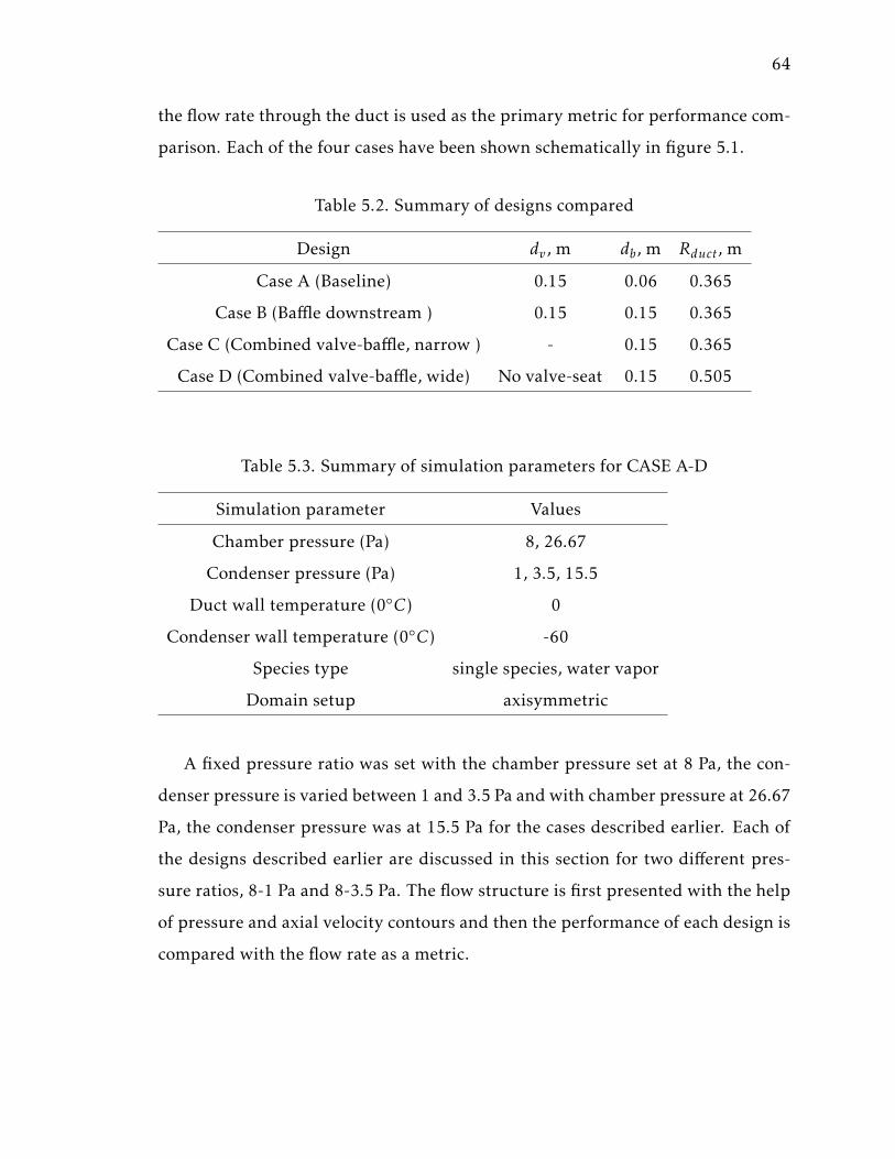
64

the flow rate through the duct is used as the primary metric for performance com-

parison. Each of the four cases have been shown schematically in figure 5.1.

Table 5.2. Summary of designs compared

Design dv , m db, m Rduct , m

Case A (Baseline) 0.15 0.06 0.365

Case B (Baffle downstream ) 0.15 0.15 0.365

Case C (Combined valve-baffle, narrow ) - 0.15 0.365

Case D (Combined valve-baffle, wide) No valve-seat 0.15 0.505

Table 5.3. Summary of simulation parameters for CASE A-D

Simulation parameter Values

Chamber pressure (Pa) 8, 26.67

Condenser pressure (Pa) 1, 3.5, 15.5

Duct wall temperature (0◦C) 0

Condenser wall temperature (0◦C) -60

Species type single species, water vapor

Domain setup axisymmetric

A fixed pressure ratio was set with the chamber pressure set at 8 Pa, the con-

denser pressure is varied between 1 and 3.5 Pa and with chamber pressure at 26.67

Pa, the condenser pressure was at 15.5 Pa for the cases described earlier. Each of

the designs described earlier are discussed in this section for two different pres-

sure ratios, 8-1 Pa and 8-3.5 Pa. The flow structure is first presented with the help

of pressure and axial velocity contours and then the performance of each design is

compared with the flow rate as a metric.

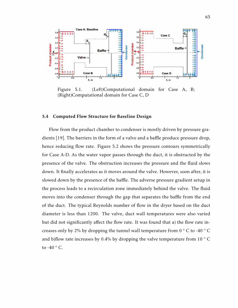
65

Figure 5.1. (Left)Computational domain for Case A, B;(Right)Computational domain for Case C, D

5.4 Computed Flow Structure for Baseline Design

Flow from the product chamber to condenser is mostly driven by pressure gra-

dients [19]. The barriers in the form of a valve and a baffle produce pressure drop,

hence reducing flow rate. Figure 5.2 shows the pressure contours symmetrically

for Case A-D. As the water vapor passes through the duct, it is obstructed by the

presence of the valve. The obstruction increases the pressure and the fluid slows

down. It finally accelerates as it moves around the valve. However, soon after, it is

slowed down by the presence of the baffle. The adverse pressure gradient setup in

the process leads to a recirculation zone immediately behind the valve. The fluid

moves into the condenser through the gap that separates the baffle from the end

of the duct. The typical Reynolds number of flow in the dryer based on the duct

diameter is less than 1200. The valve, duct wall temperatures were also varied

but did not significantly affect the flow rate. It was found that a) the flow rate in-

creases only by 2% by dropping the tunnel wall temperature from 0 ◦ C to -40 ◦ C

and b)flow rate increases by 0.4% by dropping the valve temperature from 10 ◦ C

to -40 ◦ C.

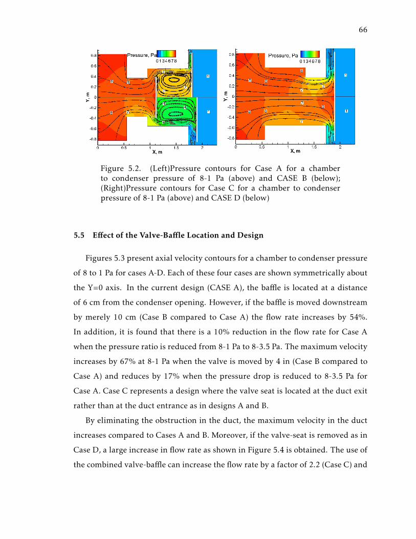
66

Figure 5.2. (Left)Pressure contours for Case A for a chamberto condenser pressure of 8-1 Pa (above) and CASE B (below);(Right)Pressure contours for Case C for a chamber to condenserpressure of 8-1 Pa (above) and CASE D (below)

5.5 Effect of the Valve-Baffle Location and Design

Figures 5.3 present axial velocity contours for a chamber to condenser pressure

of 8 to 1 Pa for cases A-D. Each of these four cases are shown symmetrically about

the Y=0 axis. In the current design (CASE A), the baffle is located at a distance

of 6 cm from the condenser opening. However, if the baffle is moved downstream

by merely 10 cm (Case B compared to Case A) the flow rate increases by 54%.

In addition, it is found that there is a 10% reduction in the flow rate for Case A

when the pressure ratio is reduced from 8-1 Pa to 8-3.5 Pa. The maximum velocity

increases by 67% at 8-1 Pa when the valve is moved by 4 in (Case B compared to

Case A) and reduces by 17% when the pressure drop is reduced to 8-3.5 Pa for

Case A. Case C represents a design where the valve seat is located at the duct exit

rather than at the duct entrance as in designs A and B.

By eliminating the obstruction in the duct, the maximum velocity in the duct

increases compared to Cases A and B. Moreover, if the valve-seat is removed as in

Case D, a large increase in flow rate as shown in Figure 5.4 is obtained. The use of

the combined valve-baffle can increase the flow rate by a factor of 2.2 (Case C) and

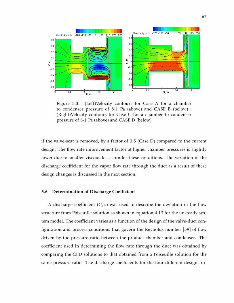
67

Figure 5.3. (Left)Velocity contours for Case A for a chamberto condenser pressure of 8-1 Pa (above) and CASE B (below) ;(Right)Velocity contours for Case C for a chamber to condenserpressure of 8-1 Pa (above) and CASE D (below)

if the valve-seat is removed, by a factor of 3.5 (Case D) compared to the current

design. The flow rate improvement factor at higher chamber pressures is slightly

lower due to smaller viscous losses under these conditions. The variation in the

discharge coefficient for the vapor flow rate through the duct as a result of these

design changes is discussed in the next section.

5.6 Determination of Discharge Coefficient

A discharge coefficient (Cdis) was used to describe the deviation in the flow

structure from Poiseuille solution as shown in equation 4.13 for the unsteady sys-

temmodel. The coefficient varies as a function of the design of the valve-duct con-

figuration and process conditions that govern the Reynolds number [59] of flow

driven by the pressure ratio between the product chamber and condenser. The

coefficient used in determining the flow rate through the duct was obtained by

comparing the CFD solutions to that obtained from a Poiseuille solution for the

same pressure ratio. The discharge coefficients for the four different designs in-

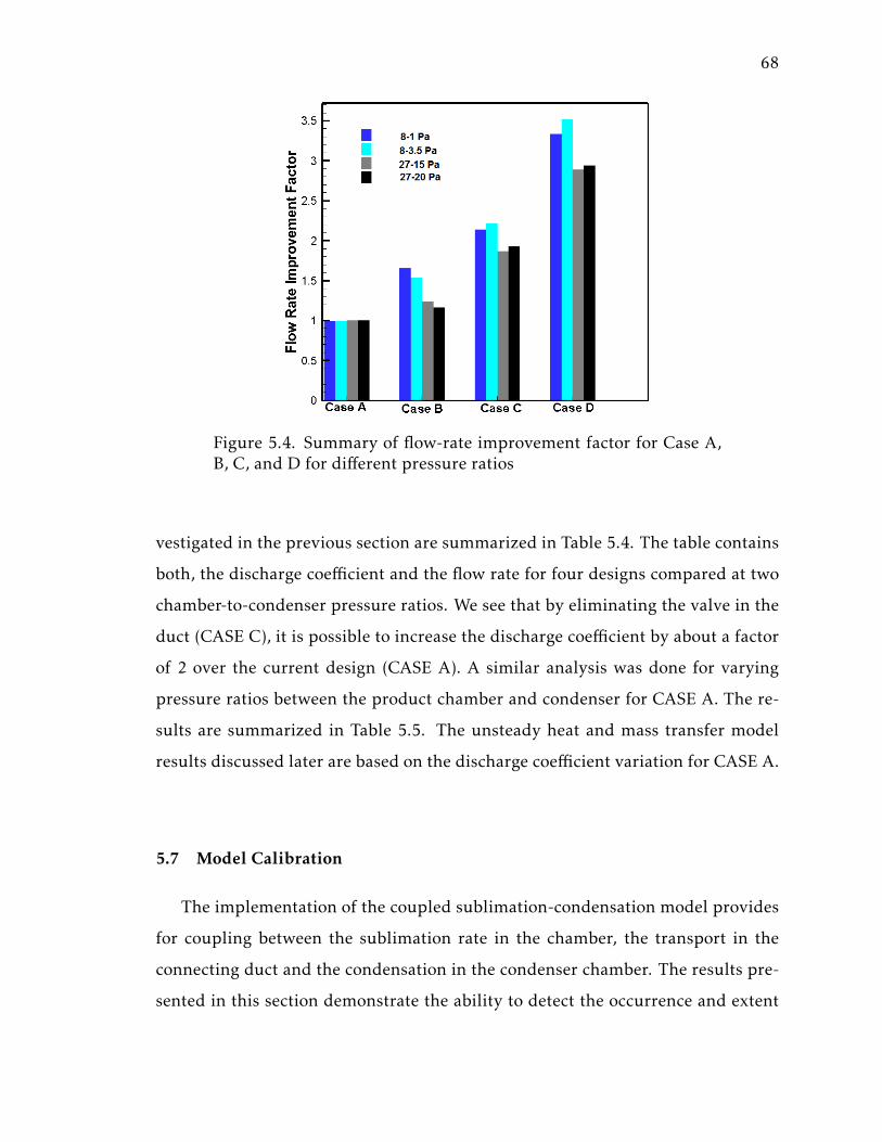
68

Figure 5.4. Summary of flow-rate improvement factor for Case A,B, C, and D for different pressure ratios

vestigated in the previous section are summarized in Table 5.4. The table contains

both, the discharge coefficient and the flow rate for four designs compared at two

chamber-to-condenser pressure ratios. We see that by eliminating the valve in the

duct (CASE C), it is possible to increase the discharge coefficient by about a factor

of 2 over the current design (CASE A). A similar analysis was done for varying

pressure ratios between the product chamber and condenser for CASE A. The re-

sults are summarized in Table 5.5. The unsteady heat and mass transfer model

results discussed later are based on the discharge coefficient variation for CASE A.

5.7 Model Calibration

The implementation of the coupled sublimation-condensation model provides

for coupling between the sublimation rate in the chamber, the transport in the

connecting duct and the condensation in the condenser chamber. The results pre-

sented in this section demonstrate the ability to detect the occurrence and extent

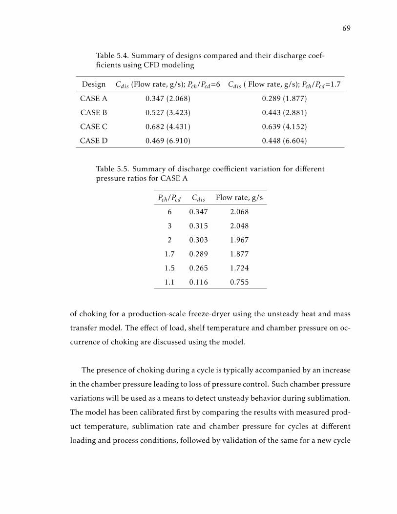
69

Table 5.4. Summary of designs compared and their discharge coef-ficients using CFD modeling

Design Cdis (Flow rate, g/s); Pch/Pcd=6 Cdis ( Flow rate, g/s); Pch/Pcd=1.7

CASE A 0.347 (2.068) 0.289 (1.877)

CASE B 0.527 (3.423) 0.443 (2.881)

CASE C 0.682 (4.431) 0.639 (4.152)

CASE D 0.469 (6.910) 0.448 (6.604)

Table 5.5. Summary of discharge coefficient variation for differentpressure ratios for CASE A

Pch/Pcd Cdis Flow rate, g/s

6 0.347 2.068

3 0.315 2.048

2 0.303 1.967

1.7 0.289 1.877

1.5 0.265 1.724

1.1 0.116 0.755

of choking for a production-scale freeze-dryer using the unsteady heat and mass

transfer model. The effect of load, shelf temperature and chamber pressure on oc-

currence of choking are discussed using the model.

The presence of choking during a cycle is typically accompanied by an increase

in the chamber pressure leading to loss of pressure control. Such chamber pressure

variations will be used as a means to detect unsteady behavior during sublimation.

The model has been calibrated first by comparing the results with measured prod-

uct temperature, sublimation rate and chamber pressure for cycles at different

loading and process conditions, followed by validation of the same for a new cycle

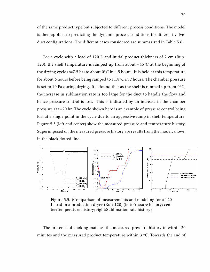
70

of the same product type but subjected to different process conditions. The model

is then applied to predicting the dynamic process conditions for different valve-

duct configurations. The different cases considered are summarized in Table 5.6.

For a cycle with a load of 120 L and initial product thickness of 2 cm (Run-

120), the shelf temperature is ramped up from about −45◦C at the beginning of

the drying cycle (t=7.5 hr) to about 0◦C in 4.5 hours. It is held at this temperature

for about 6 hours before being ramped to 11.8◦C in 2 hours. The chamber pressure

is set to 10 Pa during drying. It is found that as the shelf is ramped up from 0◦C,

the increase in sublimation rate is too large for the duct to handle the flow and

hence pressure control is lost. This is indicated by an increase in the chamber

pressure at t=20 hr. The cycle shown here is an example of pressure control being

lost at a single point in the cycle due to an aggressive ramp in shelf temperature.

Figure 5.5 (left and center) show the measured pressure and temperature history.

Superimposed on themeasured pressure history are results from themodel, shown

in the black dotted line.

Figure 5.5. (Comparison of measurements and modeling for a 120L load in a production dryer (Run-120) (left:Pressure history; cen-ter:Temperature history; right:Sublimation rate history)

The presence of choking matches the measured pressure history to within 20

minutes and the measured product temperature within 3 ◦C. Towards the end of

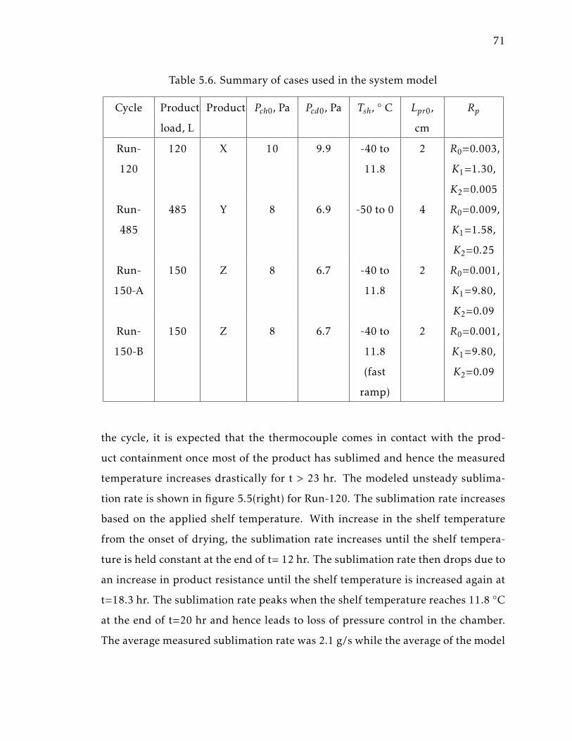
71

Table 5.6. Summary of cases used in the system model

Cycle Product

load, L

Product Pch0, Pa Pcd0, Pa Tsh,◦ C Lpr0,

cm

Rp

Run-

120

120 X 10 9.9 -40 to

11.8

2 R0=0.003,

K1=1.30,

K2=0.005

Run-

485

485 Y 8 6.9 -50 to 0 4 R0=0.009,

K1=1.58,

K2=0.25

Run-

150-A

150 Z 8 6.7 -40 to

11.8

2 R0=0.001,

K1=9.80,

K2=0.09

Run-

150-B

150 Z 8 6.7 -40 to

11.8

(fast

ramp)

2 R0=0.001,

K1=9.80,

K2=0.09

the cycle, it is expected that the thermocouple comes in contact with the prod-

uct containment once most of the product has sublimed and hence the measured

temperature increases drastically for t > 23 hr. The modeled unsteady sublima-

tion rate is shown in figure 5.5(right) for Run-120. The sublimation rate increases

based on the applied shelf temperature. With increase in the shelf temperature

from the onset of drying, the sublimation rate increases until the shelf tempera-

ture is held constant at the end of t= 12 hr. The sublimation rate then drops due to

an increase in product resistance until the shelf temperature is increased again at

t=18.3 hr. The sublimation rate peaks when the shelf temperature reaches 11.8 ◦C

at the end of t=20 hr and hence leads to loss of pressure control in the chamber.

The average measured sublimation rate was 2.1 g/s while the average of the model

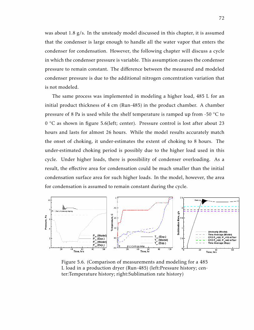
72

was about 1.8 g/s. In the unsteady model discussed in this chapter, it is assumed

that the condenser is large enough to handle all the water vapor that enters the

condenser for condensation. However, the following chapter will discuss a cycle

in which the condenser pressure is variable. This assumption causes the condenser

pressure to remain constant. The difference between the measured and modeled

condenser pressure is due to the additional nitrogen concentration variation that

is not modeled.

The same process was implemented in modeling a higher load, 485 L for an

initial product thickness of 4 cm (Run-485) in the product chamber. A chamber

pressure of 8 Pa is used while the shelf temperature is ramped up from -50 ◦C to

0 ◦C as shown in figure 5.6(left; center). Pressure control is lost after about 23

hours and lasts for almost 26 hours. While the model results accurately match

the onset of choking, it under-estimates the extent of choking to 8 hours. The

under-estimated choking period is possibly due to the higher load used in this

cycle. Under higher loads, there is possibility of condenser overloading. As a

result, the effective area for condensation could be much smaller than the initial

condensation surface area for such higher loads. In the model, however, the area

for condensation is assumed to remain constant during the cycle.

Figure 5.6. (Comparison of measurements and modeling for a 485L load in a production dryer (Run-485) (left:Pressure history; cen-ter:Temperature history; right:Sublimation rate history)

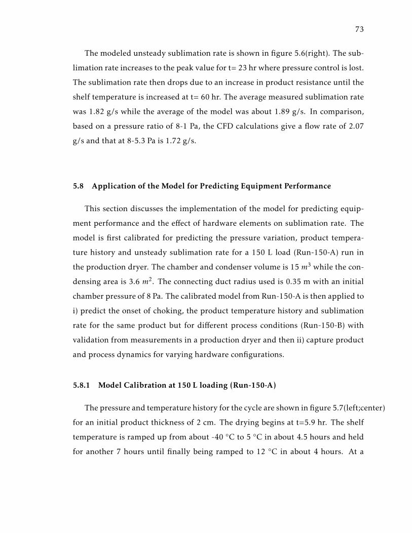
73

The modeled unsteady sublimation rate is shown in figure 5.6(right). The sub-

limation rate increases to the peak value for t= 23 hr where pressure control is lost.

The sublimation rate then drops due to an increase in product resistance until the

shelf temperature is increased at t= 60 hr. The average measured sublimation rate

was 1.82 g/s while the average of the model was about 1.89 g/s. In comparison,

based on a pressure ratio of 8-1 Pa, the CFD calculations give a flow rate of 2.07

g/s and that at 8-5.3 Pa is 1.72 g/s.

5.8 Application of the Model for Predicting Equipment Performance

This section discusses the implementation of the model for predicting equip-

ment performance and the effect of hardware elements on sublimation rate. The

model is first calibrated for predicting the pressure variation, product tempera-

ture history and unsteady sublimation rate for a 150 L load (Run-150-A) run in

the production dryer. The chamber and condenser volume is 15 m3 while the con-

densing area is 3.6 m2. The connecting duct radius used is 0.35 m with an initial

chamber pressure of 8 Pa. The calibrated model from Run-150-A is then applied to

i) predict the onset of choking, the product temperature history and sublimation

rate for the same product but for different process conditions (Run-150-B) with

validation from measurements in a production dryer and then ii) capture product

and process dynamics for varying hardware configurations.

5.8.1 Model Calibration at 150 L loading (Run-150-A)

The pressure and temperature history for the cycle are shown in figure 5.7(left;center)

for an initial product thickness of 2 cm. The drying begins at t=5.9 hr. The shelf

temperature is ramped up from about -40 ◦C to 5 ◦C in about 4.5 hours and held

for another 7 hours until finally being ramped to 12 ◦C in about 4 hours. At a

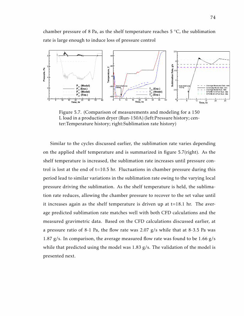
74

chamber pressure of 8 Pa, as the shelf temperature reaches 5 ◦C, the sublimation

rate is large enough to induce loss of pressure control

Figure 5.7. (Comparison of measurements and modeling for a 150L load in a production dryer (Run-150A) (left:Pressure history; cen-ter:Temperature history; right:Sublimation rate history)

Similar to the cycles discussed earlier, the sublimation rate varies depending

on the applied shelf temperature and is summarized in figure 5.7(right). As the

shelf temperature is increased, the sublimation rate increases until pressure con-

trol is lost at the end of t=10.5 hr. Fluctuations in chamber pressure during this

period lead to similar variations in the sublimation rate owing to the varying local

pressure driving the sublimation. As the shelf temperature is held, the sublima-

tion rate reduces, allowing the chamber pressure to recover to the set value until

it increases again as the shelf temperature is driven up at t=18.1 hr. The aver-

age predicted sublimation rate matches well with both CFD calculations and the

measured gravimetric data. Based on the CFD calculations discussed earlier, at

a pressure ratio of 8-1 Pa, the flow rate was 2.07 g/s while that at 8-3.5 Pa was

1.87 g/s. In comparison, the average measured flow rate was found to be 1.66 g/s

while that predicted using the model was 1.83 g/s. The validation of the model is

presented next.

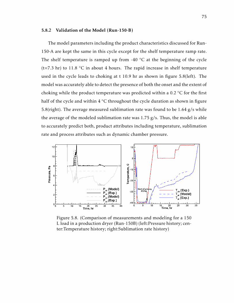
75

5.8.2 Validation of the Model (Run-150-B)

The model parameters including the product characteristics discussed for Run-

150-A are kept the same in this cycle except for the shelf temperature ramp rate.

The shelf temperature is ramped up from -40 ◦C at the beginning of the cycle

(t=7.3 hr) to 11.8 ◦C in about 4 hours. The rapid increase in shelf temperature

used in the cycle leads to choking at t 10.9 hr as shown in figure 5.8(left). The

model was accurately able to detect the presence of both the onset and the extent of

choking while the product temperature was predicted within a 0.2 ◦C for the first

half of the cycle and within 4 ◦C throughout the cycle duration as shown in figure

5.8(right). The average measured sublimation rate was found to be 1.64 g/s while

the average of the modeled sublimation rate was 1.75 g/s. Thus, the model is able

to accurately predict both, product attributes including temperature, sublimation

rate and process attributes such as dynamic chamber pressure.

Figure 5.8. (Comparison of measurements and modeling for a 150L load in a production dryer (Run-150B) (left:Pressure history; cen-ter:Temperature history; right:Sublimation rate history)

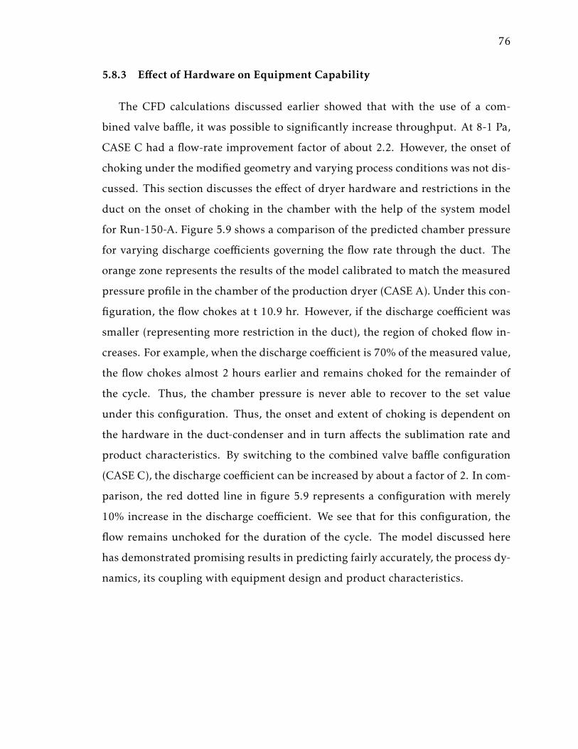
76

5.8.3 Effect of Hardware on Equipment Capability

The CFD calculations discussed earlier showed that with the use of a com-

bined valve baffle, it was possible to significantly increase throughput. At 8-1 Pa,

CASE C had a flow-rate improvement factor of about 2.2. However, the onset of

choking under the modified geometry and varying process conditions was not dis-

cussed. This section discusses the effect of dryer hardware and restrictions in the

duct on the onset of choking in the chamber with the help of the system model

for Run-150-A. Figure 5.9 shows a comparison of the predicted chamber pressure

for varying discharge coefficients governing the flow rate through the duct. The

orange zone represents the results of the model calibrated to match the measured

pressure profile in the chamber of the production dryer (CASE A). Under this con-

figuration, the flow chokes at t 10.9 hr. However, if the discharge coefficient was

smaller (representing more restriction in the duct), the region of choked flow in-

creases. For example, when the discharge coefficient is 70% of the measured value,

the flow chokes almost 2 hours earlier and remains choked for the remainder of

the cycle. Thus, the chamber pressure is never able to recover to the set value

under this configuration. Thus, the onset and extent of choking is dependent on

the hardware in the duct-condenser and in turn affects the sublimation rate and

product characteristics. By switching to the combined valve baffle configuration

(CASE C), the discharge coefficient can be increased by about a factor of 2. In com-

parison, the red dotted line in figure 5.9 represents a configuration with merely

10% increase in the discharge coefficient. We see that for this configuration, the

flow remains unchoked for the duration of the cycle. The model discussed here

has demonstrated promising results in predicting fairly accurately, the process dy-

namics, its coupling with equipment design and product characteristics.

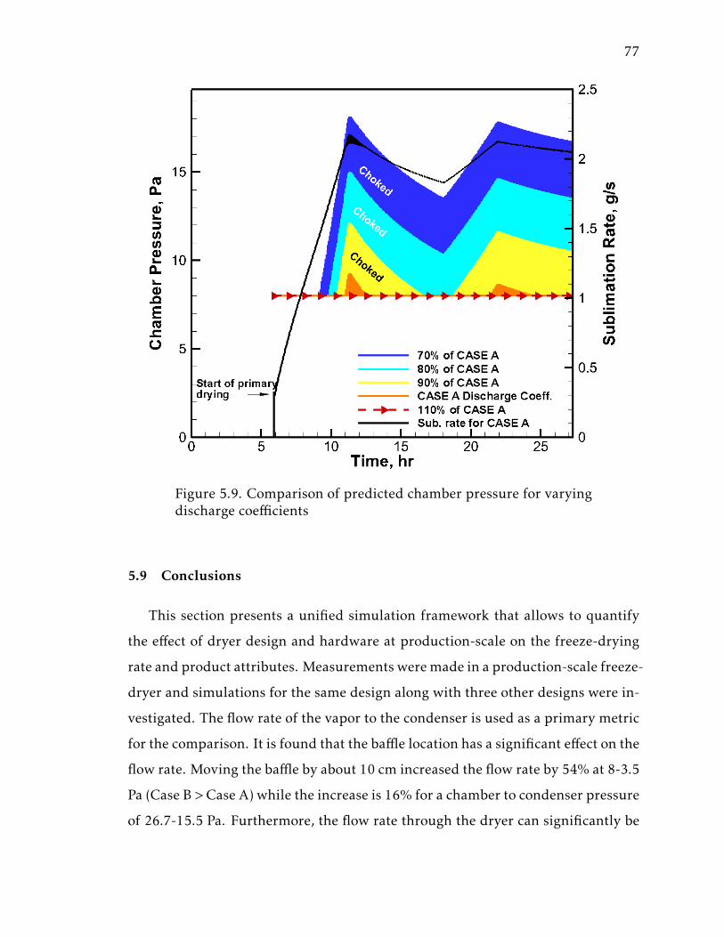
77

Figure 5.9. Comparison of predicted chamber pressure for varyingdischarge coefficients

5.9 Conclusions

This section presents a unified simulation framework that allows to quantify

the effect of dryer design and hardware at production-scale on the freeze-drying

rate and product attributes. Measurements weremade in a production-scale freeze-

dryer and simulations for the same design along with three other designs were in-

vestigated. The flow rate of the vapor to the condenser is used as a primary metric

for the comparison. It is found that the baffle location has a significant effect on the

flow rate. Moving the baffle by about 10 cm increased the flow rate by 54% at 8-3.5

Pa (Case B >Case A) while the increase is 16% for a chamber to condenser pressure

of 26.7-15.5 Pa. Furthermore, the flow rate through the dryer can significantly be

78

increased by eliminating the valve in the duct even with a valve-seat. There is a

44% increase in flow rate when valve is removed from the duct at 8-3.5 Pa (Case C

> Case B). The flow rate reduces with reducing pressure ratio and increases with

the chamber pressure. There was a 10% reduction in flow rate for Case A when

the pressure ratio is reduced from 8-1 Pa to 8-3.5 Pa. It is found that the use of

the combined valve-baffle can increase the flow rate by a factor of 2.2 (Case C) and

if the valve-seat is removed, by a factor of 3.5 (Case D) compared to the current

design.

A system-level coupled sublimation-condensation model was used to deter-

mine the effect of equipment design on the dynamic process/product character-

istics. The effect of load, shelf temperature and chamber pressure on occurrence

of choking are discussed using the model for a production-scale freeze-dryer. The

model was compared with the measurements of pressure and temperature history

for different loading and process conditions. It was found that while the model

was able to accurately predict the onset of choking in the product chamber, the

extent of choking was under-estimated at higher load conditions (485 L). At a load

of 150 L (Run-150-B) in the chamber, the model predicted both the occurrence

and extent of choking well and the measured product temperature within 4 ◦C.

Furthermore, the model was used to compare the predicted sublimation rate to

the gravimetrically measured value. While the measured average sublimation rate

was 1.64 g/s, the model estimate was found to be 1.75 g/s. The model was then

extended to determine the effect of dryer hardware and restrictions in the duct

on the onset of choking. It was found that by reducing the discharge coefficient

by 30% compared to the current design, the onset of choking in the chamber was

advanced by 2 hours and lasted the entire cycle for a 150 L product load. If on the

other hand, a combined valve baffle was used as represented by CASE C, choking

could be eliminated completely. Thus, with the use of the CFD calculations aug-

mented with capability of the system level model, it is possible to predict dynamic

process conditions as a function of dryer design. Such physics-based models can

79

become useful tools in understanding the coupling between equipment capability

and product characteristics in the future.

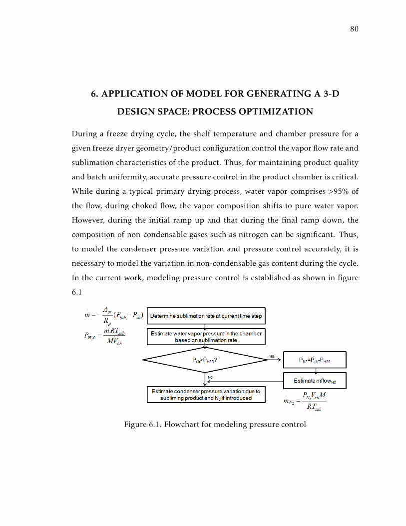
80

6. APPLICATION OFMODEL FOR GENERATING A 3-D

DESIGN SPACE: PROCESS OPTIMIZATION

During a freeze drying cycle, the shelf temperature and chamber pressure for a

given freeze dryer geometry/product configuration control the vapor flow rate and

sublimation characteristics of the product. Thus, for maintaining product quality

and batch uniformity, accurate pressure control in the product chamber is critical.

While during a typical primary drying process, water vapor comprises >95% of

the flow, during choked flow, the vapor composition shifts to pure water vapor.

However, during the initial ramp up and that during the final ramp down, the

composition of non-condensable gases such as nitrogen can be significant. Thus,

to model the condenser pressure variation and pressure control accurately, it is

necessary to model the variation in non-condensable gas content during the cycle.

In the current work, modeling pressure control is established as shown in figure

6.1

Figure 6.1. Flowchart for modeling pressure control

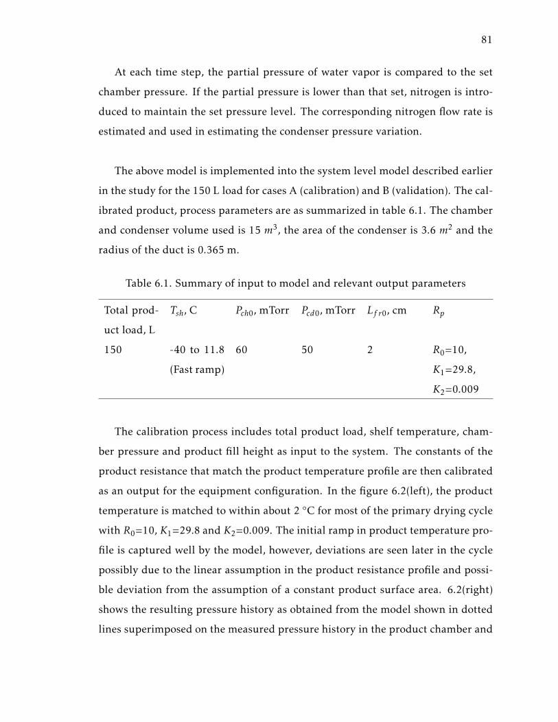
81

At each time step, the partial pressure of water vapor is compared to the set

chamber pressure. If the partial pressure is lower than that set, nitrogen is intro-

duced to maintain the set pressure level. The corresponding nitrogen flow rate is

estimated and used in estimating the condenser pressure variation.

The above model is implemented into the system level model described earlier

in the study for the 150 L load for cases A (calibration) and B (validation). The cal-

ibrated product, process parameters are as summarized in table 6.1. The chamber

and condenser volume used is 15 m3, the area of the condenser is 3.6 m2 and the

radius of the duct is 0.365 m.

Table 6.1. Summary of input to model and relevant output parameters

Total prod-

uct load, L

Tsh, C Pch0, mTorr Pcd0, mTorr Lf r0, cm Rp

150 -40 to 11.8

(Fast ramp)

60 50 2 R0=10,

K1=29.8,

K2=0.009

The calibration process includes total product load, shelf temperature, cham-

ber pressure and product fill height as input to the system. The constants of the

product resistance that match the product temperature profile are then calibrated

as an output for the equipment configuration. In the figure 6.2(left), the product

temperature is matched to within about 2 ◦C for most of the primary drying cycle

with R0=10, K1=29.8 and K2=0.009. The initial ramp in product temperature pro-

file is captured well by the model, however, deviations are seen later in the cycle

possibly due to the linear assumption in the product resistance profile and possi-

ble deviation from the assumption of a constant product surface area. 6.2(right)

shows the resulting pressure history as obtained from the model shown in dotted

lines superimposed on the measured pressure history in the product chamber and

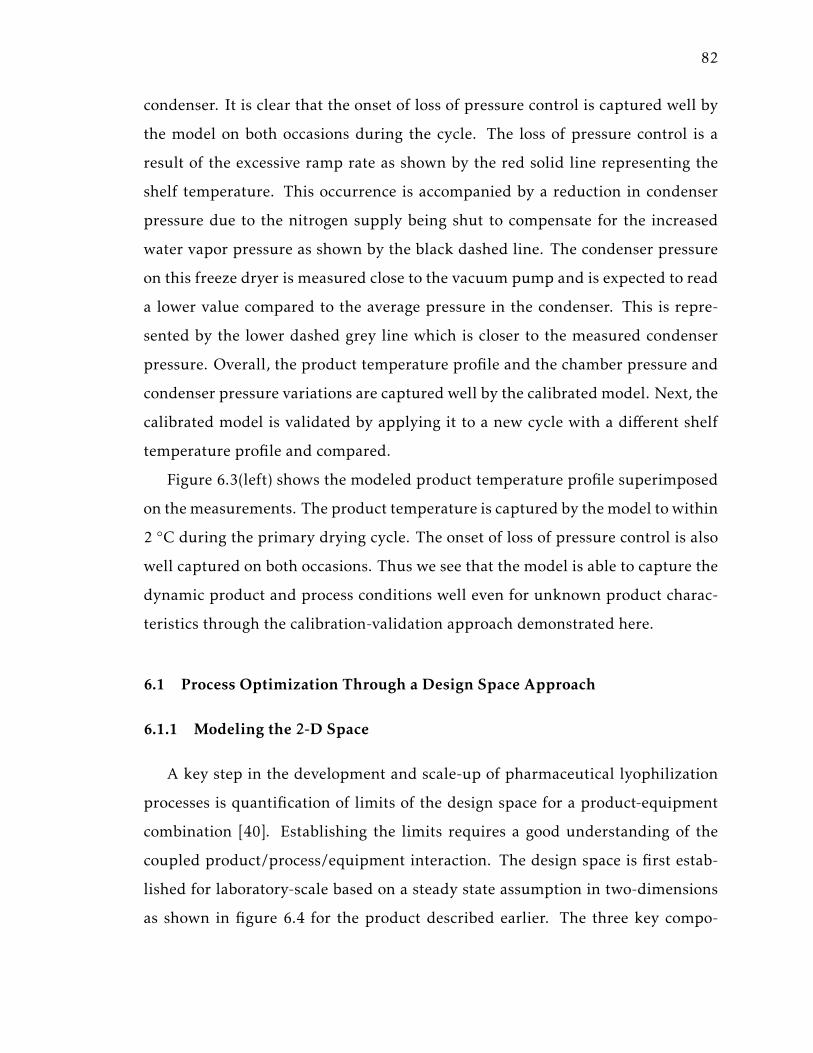
82

condenser. It is clear that the onset of loss of pressure control is captured well by

the model on both occasions during the cycle. The loss of pressure control is a

result of the excessive ramp rate as shown by the red solid line representing the

shelf temperature. This occurrence is accompanied by a reduction in condenser

pressure due to the nitrogen supply being shut to compensate for the increased

water vapor pressure as shown by the black dashed line. The condenser pressure

on this freeze dryer is measured close to the vacuum pump and is expected to read

a lower value compared to the average pressure in the condenser. This is repre-

sented by the lower dashed grey line which is closer to the measured condenser

pressure. Overall, the product temperature profile and the chamber pressure and

condenser pressure variations are captured well by the calibrated model. Next, the

calibrated model is validated by applying it to a new cycle with a different shelf

temperature profile and compared.

Figure 6.3(left) shows the modeled product temperature profile superimposed

on themeasurements. The product temperature is captured by themodel to within

2 ◦C during the primary drying cycle. The onset of loss of pressure control is also

well captured on both occasions. Thus we see that the model is able to capture the

dynamic product and process conditions well even for unknown product charac-

teristics through the calibration-validation approach demonstrated here.

6.1 Process Optimization Through a Design Space Approach

6.1.1 Modeling the 2-D Space

A key step in the development and scale-up of pharmaceutical lyophilization

processes is quantification of limits of the design space for a product-equipment

combination [40]. Establishing the limits requires a good understanding of the

coupled product/process/equipment interaction. The design space is first estab-

lished for laboratory-scale based on a steady state assumption in two-dimensions

as shown in figure 6.4 for the product described earlier. The three key compo-

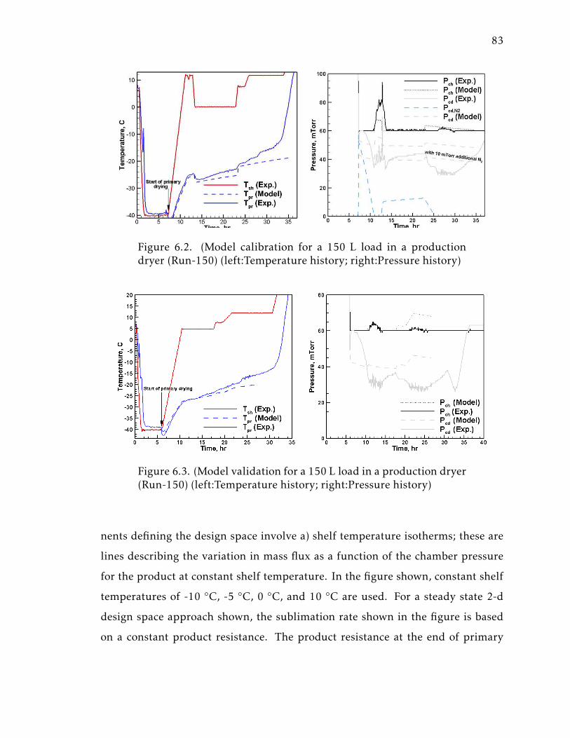
83

Figure 6.2. (Model calibration for a 150 L load in a productiondryer (Run-150) (left:Temperature history; right:Pressure history)

Figure 6.3. (Model validation for a 150 L load in a production dryer(Run-150) (left:Temperature history; right:Pressure history)

nents defining the design space involve a) shelf temperature isotherms; these are

lines describing the variation in mass flux as a function of the chamber pressure

for the product at constant shelf temperature. In the figure shown, constant shelf

temperatures of -10 ◦C, -5 ◦C, 0 ◦C, and 10 ◦C are used. For a steady state 2-d

design space approach shown, the sublimation rate shown in the figure is based

on a constant product resistance. The product resistance at the end of primary

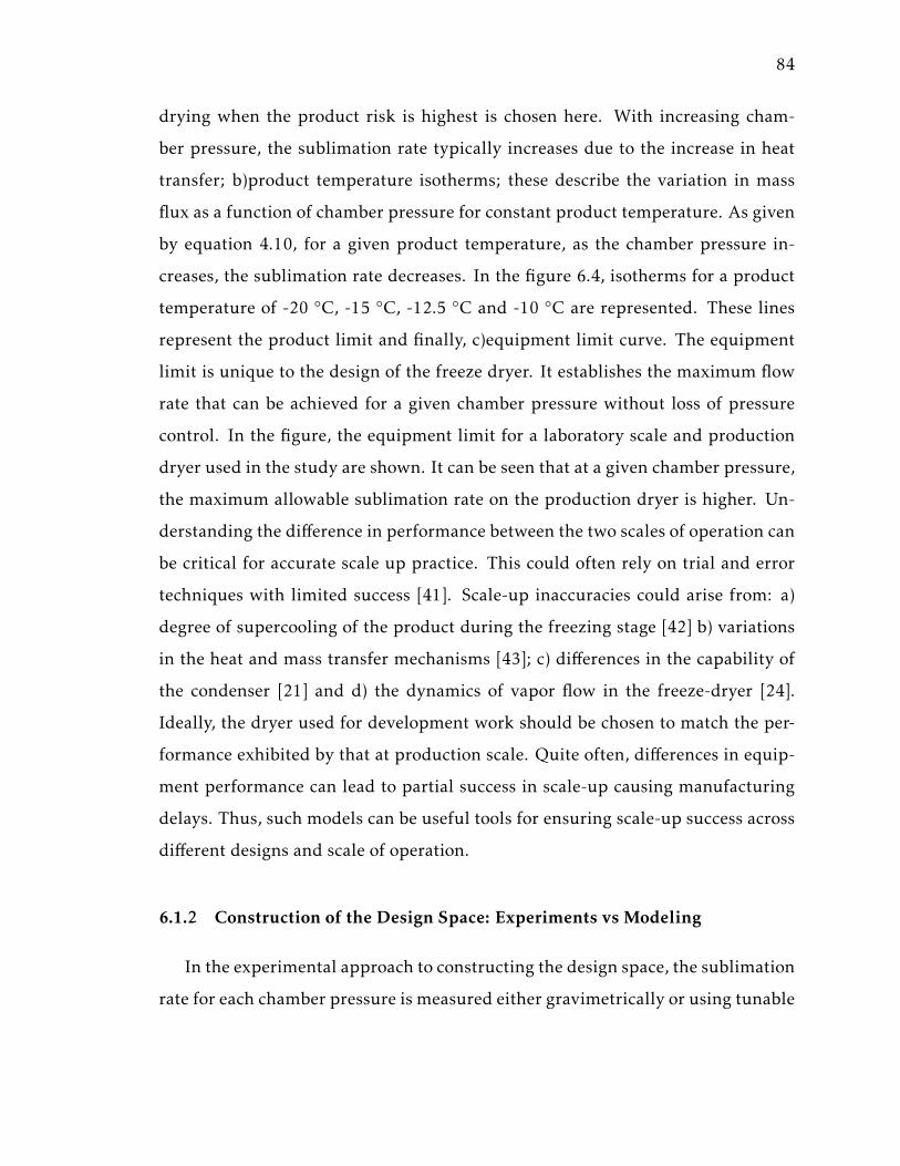
84

drying when the product risk is highest is chosen here. With increasing cham-

ber pressure, the sublimation rate typically increases due to the increase in heat

transfer; b)product temperature isotherms; these describe the variation in mass

flux as a function of chamber pressure for constant product temperature. As given

by equation 4.10, for a given product temperature, as the chamber pressure in-

creases, the sublimation rate decreases. In the figure 6.4, isotherms for a product

temperature of -20 ◦C, -15 ◦C, -12.5 ◦C and -10 ◦C are represented. These lines

represent the product limit and finally, c)equipment limit curve. The equipment

limit is unique to the design of the freeze dryer. It establishes the maximum flow

rate that can be achieved for a given chamber pressure without loss of pressure

control. In the figure, the equipment limit for a laboratory scale and production

dryer used in the study are shown. It can be seen that at a given chamber pressure,

the maximum allowable sublimation rate on the production dryer is higher. Un-

derstanding the difference in performance between the two scales of operation can

be critical for accurate scale up practice. This could often rely on trial and error

techniques with limited success [41]. Scale-up inaccuracies could arise from: a)

degree of supercooling of the product during the freezing stage [42] b) variations

in the heat and mass transfer mechanisms [43]; c) differences in the capability of

the condenser [21] and d) the dynamics of vapor flow in the freeze-dryer [24].

Ideally, the dryer used for development work should be chosen to match the per-

formance exhibited by that at production scale. Quite often, differences in equip-

ment performance can lead to partial success in scale-up causing manufacturing

delays. Thus, such models can be useful tools for ensuring scale-up success across

different designs and scale of operation.

6.1.2 Construction of the Design Space: Experiments vs Modeling

In the experimental approach to constructing the design space, the sublimation

rate for each chamber pressure is measured either gravimetrically or using tunable

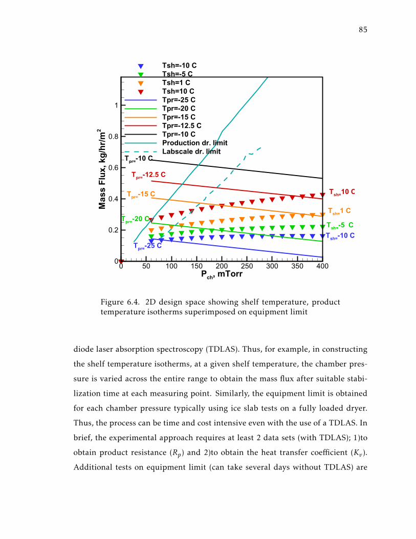
85

Pch, mTorr

Mas

s F

lux,

kg

/hr/

m2

0 50 100 150 200 250 300 350 4000

0.2

0.4

0.6

0.8

1

Tsh=-10 CTsh=-5 CTsh=1 CTsh=10 CTpr=-25 CTpr=-20 CTpr=-15 CTpr=-12.5 CTpr=-10 CProduction dr. limitLabscale dr. limit

Tsh=-5 CTsh=-10 C

Tsh=1 C

Tsh=10 C

Tpr=-10 C

Tpr=-25 C

Tpr=-12.5 C

Tpr=-15 C

Tpr=-20 C

Figure 6.4. 2D design space showing shelf temperature, producttemperature isotherms superimposed on equipment limit

diode laser absorption spectroscopy (TDLAS). Thus, for example, in constructing

the shelf temperature isotherms, at a given shelf temperature, the chamber pres-

sure is varied across the entire range to obtain the mass flux after suitable stabi-

lization time at each measuring point. Similarly, the equipment limit is obtained

for each chamber pressure typically using ice slab tests on a fully loaded dryer.

Thus, the process can be time and cost intensive even with the use of a TDLAS. In

brief, the experimental approach requires at least 2 data sets (with TDLAS); 1)to

obtain product resistance (Rp) and 2)to obtain the heat transfer coefficient (Kv).

Additional tests on equipment limit (can take several days without TDLAS) are

86

required. Thus, developing a robust modeling approach for constructing the de-

sign space helps reduce time and improves accuracy in establishing scale up.

In modeling the design space, the product calibration is first completed as de-

scribed earlier. The mass flux data based on 95% completion in primary drying

for different chamber pressures and constant shelf temperatures from the model

is then obtained. Next, at a constant product temperature, the chamber pressure is

varied to obtain the product temperature isotherms from equation 4.10. Finally, in

modeling the equipment limit curve, the geometry of the dryer including the duct

geometry, the chamber and condenser volume as used in equations are 4.13 and

4.14 for the maximum possible sublimation rate that can be achieved at a given

chamber pressure without loss of pressure control is used. In the figure 6.4, the

solid blue line shows the modeled equipment limit for a production scale freeze

dryer.

6.2 The 3-D Design Space

6.2.1 Need for a 3-D Design Space

Once the design space has been constructed, for developing a scalable opti-

mized cycle, the highest shelf temperature and lowest chamber pressure combi-

nation that lies within the product and equipment bounds leads to fastest cycle

times. However, inherent to the construction of the design space used today, the

following assumptions are made:

• Steady state heat and mass transfer equations are used based on end of pri-

mary drying and no product temperature variations are considered whose

validity is tested during the beginning and end of cycle

• Heat transfer coefficient obtained frommeasurements assumes variation only

with chamber pressure and not with shelf temperature. Moreover, measur-

87

ing vial heat transfer coefficient for each shelf temperature, chamber pres-

sure combination can be expensive.

• Assumes that equipment and product limit are tested at the same time in the

cycle and the developed space is based on maximum product risk.

Moreover, in reality, the shelf temperature and product resistance change dur-

ing the cycle. As a result, during the initial ramp, when the product resistance is

least, and the shelf temperature is ramped from the freezing temperature to pri-

mary drying temperature, the equipment limit can be exceeded if the cycle is de-

signed based on the end of drying parameters. Thus, a transient three-dimensional

design space approach is necessary to account for the variation in the shelf tem-

perature and product resistance.

6.2.2 Developing the Three-dimensional Design Space

The 3-d design space is modeled in a similar manner to the 2-d space account-

ing for variation in shelf temperature and product resistance during the cycle.

Thus, in defining the space, shelf temperature isotherms are replaced by curves

defined by the flux corresponding to the shelf temperature profile used during

the cycle. For example, for the 150 L product load described earlier, figure 6.5

shows the 3-d shelf temperature curves at -5 ◦C, 0 ◦C and 10 ◦C. ’A’ traces the edge

of the curve at the end of the cycle for a shelf temperature of 10 ◦C while curve

’B’ traces it during the initial ramp. There is about 16% difference in the maxi-

mum sublimation rate between the initial ramp and that at the end of the cycle. It

should be noted here that while the difference is 16% in the current product/cycle

configuration, it could vary significantly for another configuration. Thus, a cy-

cle designed based on A would under-predict the max sublimation rate and could

possibly lead to loss of pressure control during the initial ramp. This illustrates

the importance of using a 3-d design space approach. Lower shelf temperatures

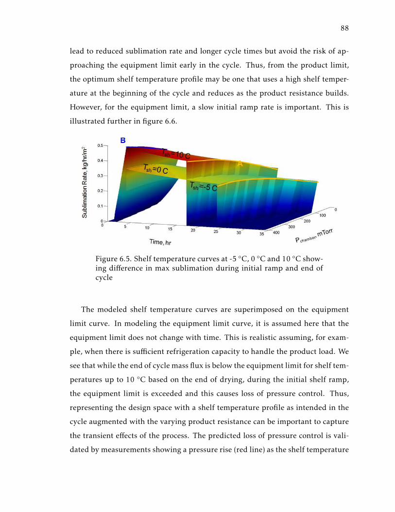
88

lead to reduced sublimation rate and longer cycle times but avoid the risk of ap-

proaching the equipment limit early in the cycle. Thus, from the product limit,

the optimum shelf temperature profile may be one that uses a high shelf temper-

ature at the beginning of the cycle and reduces as the product resistance builds.

However, for the equipment limit, a slow initial ramp rate is important. This is

illustrated further in figure 6.6.

Figure 6.5. Shelf temperature curves at -5 ◦C, 0 ◦C and 10 ◦C show-ing difference in max sublimation during initial ramp and end ofcycle

The modeled shelf temperature curves are superimposed on the equipment

limit curve. In modeling the equipment limit curve, it is assumed here that the

equipment limit does not change with time. This is realistic assuming, for exam-

ple, when there is sufficient refrigeration capacity to handle the product load. We

see that while the end of cycle mass flux is below the equipment limit for shelf tem-

peratures up to 10 ◦C based on the end of drying, during the initial shelf ramp,

the equipment limit is exceeded and this causes loss of pressure control. Thus,

representing the design space with a shelf temperature profile as intended in the

cycle augmented with the varying product resistance can be important to capture

the transient effects of the process. The predicted loss of pressure control is vali-

dated by measurements showing a pressure rise (red line) as the shelf temperature

89

is ramped up to 11 ◦C. This cycle is a typical example of a product that would fail

if designed based on the 2-d space at the end-of-drying.

Figure 6.6. Equipment limit curve superimposed on the shelf tem-perature curves with max sublimation rate exceeding the equip-ment limit during the initial ramp at 10 ◦C

6.2.3 Application of Model to 5%Mannitol-5%Sucrose System

As described for the 150 L load product in the previous section, the design

space consists of 1)the equipment limit curve 2)shelf temperature curves and 3)prod-

uct limit based on product temperature curves. The design space for the 5%

Mannitol-5%Sucrose system is described in this section for a laboratory scale freeze

dryer. The equipment limit curve assuming no variation as a function of time is

shown in figure 6.7. We see that the maximum mass flux increases with chamber

pressure.

Figure 6.8 shows the shelf temperature curves for primary drying temperatures

of -25 ◦C, -15 ◦C, -5 ◦C and 5 ◦C. The white dashed lines trace the curve at the end

of drying as would be predicted by a 2-d design space approach using the product

resistance based on the end of the cycle product characteristics. The black dashed

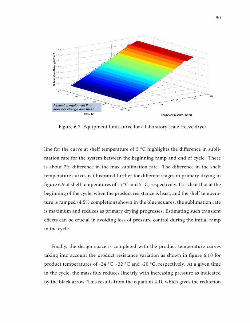
90

Figure 6.7. Equipment limit curve for a laboratory scale freeze dryer

line for the curve at shelf temperature of 5 ◦C highlights the difference in subli-

mation rate for the system between the beginning ramp and end of cycle. There

is about 7% difference in the max sublimation rate. The difference in the shelf

temperature curves is illustrated further for different stages in primary drying in

figure 6.9 at shelf temperatures of -5 ◦C and 5 ◦C, respectively. It is clear that at the

beginning of the cycle, when the product resistance is least, and the shelf tempera-

ture is ramped (4.5% completion) shown in the blue squares, the sublimation rate

is maximum and reduces as primary drying progresses. Estimating such transient

effects can be crucial in avoiding loss of pressure control during the initial ramp

in the cycle.

Finally, the design space is completed with the product temperature curves

taking into account the product resistance variation as shown in figure 6.10 for

product temperatures of -24 ◦C, -22 ◦C and -20 ◦C, respectively. At a given time

in the cycle, the mass flux reduces linearly with increasing pressure as indicated

by the black arrow. This results from the equation 4.10 which gives the reduction

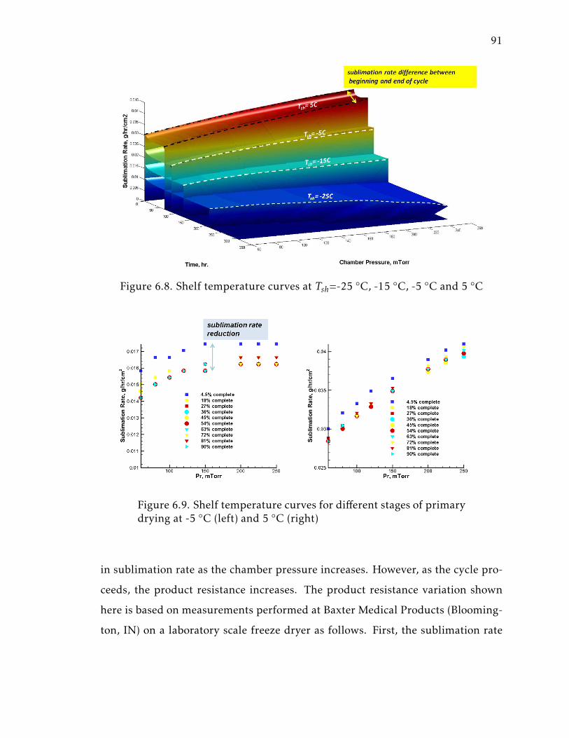
91

Figure 6.8. Shelf temperature curves at Tsh=-25◦C, -15 ◦C, -5 ◦C and 5 ◦C

Figure 6.9. Shelf temperature curves for different stages of primarydrying at -5 ◦C (left) and 5 ◦C (right)

in sublimation rate as the chamber pressure increases. However, as the cycle pro-

ceeds, the product resistance increases. The product resistance variation shown

here is based on measurements performed at Baxter Medical Products (Blooming-

ton, IN) on a laboratory scale freeze dryer as follows. First, the sublimation rate

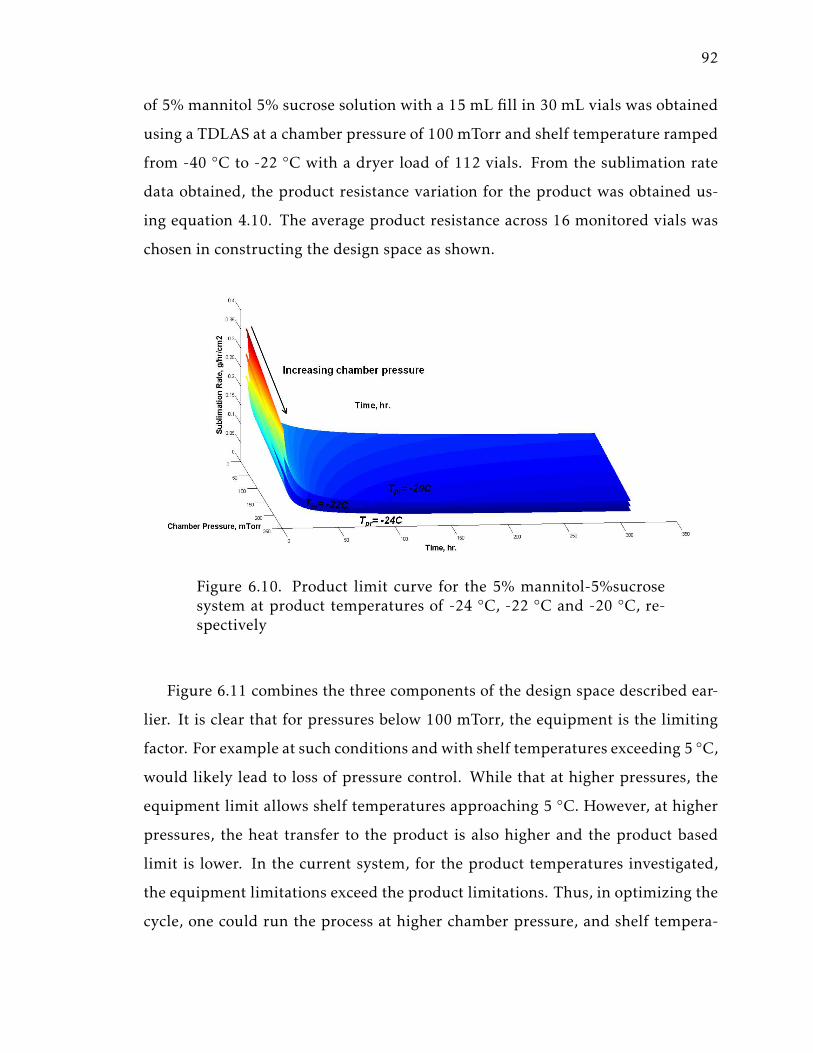
92

of 5% mannitol 5% sucrose solution with a 15 mL fill in 30 mL vials was obtained

using a TDLAS at a chamber pressure of 100 mTorr and shelf temperature ramped

from -40 ◦C to -22 ◦C with a dryer load of 112 vials. From the sublimation rate

data obtained, the product resistance variation for the product was obtained us-

ing equation 4.10. The average product resistance across 16 monitored vials was

chosen in constructing the design space as shown.

Figure 6.10. Product limit curve for the 5% mannitol-5%sucrosesystem at product temperatures of -24 ◦C, -22 ◦C and -20 ◦C, re-spectively

Figure 6.11 combines the three components of the design space described ear-

lier. It is clear that for pressures below 100 mTorr, the equipment is the limiting

factor. For example at such conditions andwith shelf temperatures exceeding 5 ◦C,

would likely lead to loss of pressure control. While that at higher pressures, the

equipment limit allows shelf temperatures approaching 5 ◦C. However, at higher

pressures, the heat transfer to the product is also higher and the product based

limit is lower. In the current system, for the product temperatures investigated,

the equipment limitations exceed the product limitations. Thus, in optimizing the

cycle, one could run the process at higher chamber pressure, and shelf tempera-

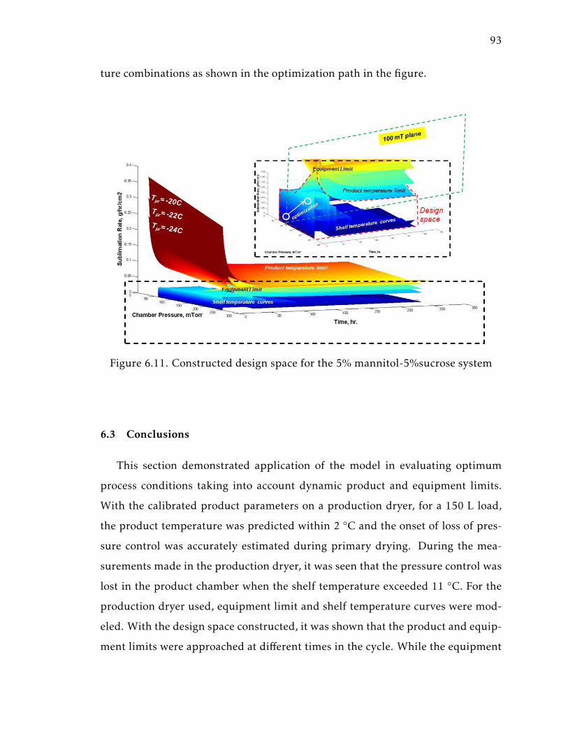
93

ture combinations as shown in the optimization path in the figure.

Figure 6.11. Constructed design space for the 5% mannitol-5%sucrose system

6.3 Conclusions

This section demonstrated application of the model in evaluating optimum

process conditions taking into account dynamic product and equipment limits.

With the calibrated product parameters on a production dryer, for a 150 L load,

the product temperature was predicted within 2 ◦C and the onset of loss of pres-

sure control was accurately estimated during primary drying. During the mea-

surements made in the production dryer, it was seen that the pressure control was

lost in the product chamber when the shelf temperature exceeded 11 ◦C. For the

production dryer used, equipment limit and shelf temperature curves were mod-

eled. With the design space constructed, it was shown that the product and equip-

ment limits were approached at different times in the cycle. While the equipment

94

limit was tested during the initial ramp, early in the cycle, the maximum product

risk was at the end of the cycle when the product temperature is highest. The 3-d

space demonstrated that the equipment limit of the dryer was exceeded when the

shelf temperature exceeded 10 ◦C at a chamber pressure of 60 mTorr which was

confirmed by findings from the measurements. If the process were designed us-

ing a 2-d approach based on end-of-cycle product characteristics, such predictions

would not be possible. The constructed design space was then used to demonstrate

the importance of understanding equipment limit across different scales of opera-

tion. It was shown that the production dryer had a higher limit than that could be

handled by laboratory scale freeze dryer. Thus, the need to carefully design devel-

opment batches before scale up is executed to larger manufacturing machines.

The model was then extended to construct the design space for a 5% mannitol-

5%sucrose system in a laboratory scale freeze dryer. Measurements were first

made to estimate the average batch product resistance. The product resistance,

along with the equipment characteristics were used to construct the shelf tem-

perature, product temperature and equipment limit curves. It was found that at

a shelf temperature of 5 ◦C, the max sublimation rate at the beginning and end

of cycle varied by 7%. Moreover, it was found that the system was restricted by

the equipment limit for chamber pressures lower than 100 mTorr. However, since

the product allowed aggressive drying conditions, the cycle could be optimized

by increasing the chamber pressure and shelf temperature while lying within the

equipment limit.

95

7. SUMMARY AND RECOMMENDATIONS

Low-pressure sublimation, transport and condensation processes involve an inter-

play of multiphase/multiscale heat andmass transfer phenomena. It covers a wide

range of temperature (-50 ◦C to +50 ◦C ) and pressure (down to < 0.1% of atmo-

spheric pressure) conditions. Considering the wide range of length and time-scales

the process involves, measurements to quantify the flow structure are insufficient,

making visualization difficult. The current work applies first-principles based

modeling for the low pressure heat and mass transfer governing sublimation-

transport-condensation applied to freeze-drying. Recent developments in indus-

trial processes involving heat and mass transfer have been made possible using

computational approaches through powerful computing resources. For exam-

ple, initial aircraft design and manufacturing cycles now are largely based on

CFD models. This has significantly reduced time needed for wind tunnel test-

ing. Regulatory bodies in the aircraft manufacturing industry can be analogous

in many ways to that in drug manufacturing. The strict guidelines for quality

can challenge the pace of new technology implementation. In the highly regu-

lated pharma/biopharmaceutical industry where not only the product, but also its

manufacturing process are subject to regulatory scrutiny, deviations from existing

technologies can be risky. As a result, rate of technological adaptations in manu-

facturing has been slow. However, recognizing this, recent initiatives at the U.S.

Food and Drug Administration (FDA), for in-process monitoring and through pro-

cess optimization initiatives, indicate that the agency is becoming more receptive

to process and technology innovation with long-overdue changes. In part because

of the low-pressure environment, and because of regulatory constraints outlined

above, such computational approaches to pharmaceutical manufacturing has not

been widely used for freeze-drying systems. The current work is the first sys-

96

tematic first principles modeling based on dynamic product, process and equip-

ment variables within a single simulation framework for sublimation-transport-

condensation processes applied to freeze drying.

In the present study, key heat transfer contributions driving sublimation were

first investigated to understand the relative role of radiation, gas and contact con-

duction and convection in the process. Sublimation rate measurements were per-

formed in a laboratory scale freeze-dryer using gravimetric means for both, vials

in direct contact and vials suspended off the shelf. It was found that while the

contact conduction component contributed 11% to 17% of the total heat transfer

for the vial placed on the shelf, the radiative component varied from 43% of the

total heat transfer for the vial placed on the shelf to 86% of the total heat transfer

for the vial placed at a separation of 3 mm from the shelf. The contribution from

gas conduction at 100 mTorr for the vial placed on the shelf amounts to 30% of

the total heat transfer and the corresponding convective component amounts to

14% of the total heat transfer. This reduces to 6% and 8% respectively at a pres-

sure of 10 mTorr. The above conclusions are significant for two reasons, 1) The

radiative component is clearly the dominant among the heat transfer modes and

2)The gas conduction and convective components become increasingly important

in the heat transfer at higher pressures and low shelf temperatures. Furthermore,

in understanding the role of convection across different scale of sublimation, the

current study for the first time includes validated CFD based analyses for pressure

variation and its effect on batch uniformity.

A CFD model was developed for quantifying the flow structure in a laboratory

scale freeze dyer and then validated with experiments. The study systematically

investigated the pressure variation between the shelf center and edge above the

sublimation front at different operating conditions and shelf gap configurations.

The pressure drop above the sublimation front was found to increase linearly with

sublimation rate in the range of 0.5 kg/hr/m2 to 1.3 kg/hr/m2. The results are

found to agree within 10% of the measured pressure drop. While the pressure

97

drop was found to be small (< 1 mTorr) at shelf gaps approaching 9 cm, it in-

creased to about 9 mTorr at gaps approaching 2.6 cm. The results were validated

with experimental data and agree well across the range of shelf gaps investigated.

The work presented here has proven that CFD approaches used to model the flow

physics in the chamber can accurately predict the process dynamics and its impact

on product uniformity within and across batches for a product.

The condensation studies presented in the work focus on using DSMC tech-

niques to model the vapor flow in a low-pressure environment and the resulting

ice accretion patterns on an arbitrary supercooled surface. The modeling frame-

work was extended to condensation studies in the freeze-drying environment. Var-

ious factors that affect the non-uniformity of mass flux and hence ice-growth were

investigated. It was found that the presence of a duct connecting the product

chamber and condenser increased non-uniformity by 65% at a sublimation rate of

5 g/hr. The non-uniformity of ice-growth also depended on the number density of

non-condensable gas in the chamber. The presence of the non-condensable gases

increased the effective-resistance in the condenser, there-by preventing vapor from

condensing on the coils away from the duct exit. The computed steady state mass

flux was used to predict development of the ice front on the condenser coils. To

verify the algorithm used for the prediction, a comparison was made with an an-

alytical solution for the condensation of vapor during free molecular flow around

a circular cylinder. The model was then extended to predict the ice accumula-

tion on the coils of a laboratory scale freeze-dryer condenser and the predictions

were validated with measurements. It was found that the coils closest to the vapor

inlet being subjected to the largest mass flux, had the highest ice accumulation.

The maximum thickness of ice formed on the coil closest to the duct exit at the

end of 24 hours using the steady icing model was 3.2 cm. This was 14% higher

than the measurements made under the same drying conditions. An unsteady ic-

ing model was developed and implemented to capture the non-linear ice accretion

rates. The model incorporated the unsteady behavior by intermittently updating

98

the surface mesh to track the ice growth. With an updated geometry every 6 hours,

the non-linear behavior of the ice accretion was captured within 1% towards the

end of the 24-hour freeze-drying process.The findings from the sublimation con-

densation studies were used to create a unified system level modeling framework

coupling dynamic product, process and equipment parameters.

First, a simulation framework that allowed to quantify the effect of dryer de-

sign and hardware configuration at production-scale on the freeze-drying rate and

product attributes was presented. Measurements were made in a production-scale

freeze-dryer and simulations for the same design along with three other configu-

rations were investigated. The flow rate of the vapor to the condenser was used as

a primary metric for the comparison. It was found that the baffle location had a

significant effect on the flow rate. Moving the baffle by about 10 cm increased the

flow rate by 54% at 8-3.5 Pa while the increase was 16% for a chamber to condenser

pressure of 26.7-15.5 Pa. Furthermore, the flow rate through the dryer could sig-

nificantly be increased by eliminating the valve in the duct even with a valve-seat.

Moreover, it was found that the use of the combined valve-baffle system increased

the flow rate by a factor of 2.2 and if the valve-seat was removed, by a factor of 3.5

compared to the current design.

The coupled model was used to model the effect of load, shelf temperature and

chamber pressure on occurrence of choking for a production-scale freeze-dryer.

The model was compared with the measurements of pressure and temperature

history for different loading and process conditions. It was found that while the

model was able to accurately predict the onset of choking in the product chamber,

the extent of choking was under-estimated at higher load conditions (485 L). At

a load of 150 L (Run-150-B) in the chamber, the model predicted both the occur-

rence and extent of choking well and the measured product temperature within

4 ◦C. Furthermore, the model results were compared to the gravimetrically mea-

sured value. While the measured average sublimation rate was 1.64 g/s, the model

estimate was found to be 1.75 g/s. The model was then extended to determine the

99

effect of dryer hardware and restrictions in the duct on the onset of choking. It

was found that by reducing the discharge coefficient by 30% compared to the cur-

rent design, the onset of choking in the chamber was advanced by 2 hours and

lasted the entire cycle for a 150 L product load. If on the other hand, a combined

valve baffle was used, choking could be eliminated completely. Thus, with the use

of the CFD calculations, augmented with capability of the system level model, it

was possible to predict dynamic process conditions as a function of dryer design.

Such physics-basedmodels can become useful tools in understanding the coupling

between equipment capability and product characteristics in the future.

The ultimate goal of the system-level modeling was to relate equipment and

process variables to product quality and drying characteristics. As a next step in

applying the model, a 3-d design space was constructed consisting of the equip-

ment, product and process driven limits. The 3-d design space was modeled in a

similar manner to the 2-d space accounting for the variation in shelf temperature

and product resistance during the cycle. With a 3-d design space constructed for

a 150 L product load was validated with measurements at production scale, it was

found that there was 16% difference in the maximum sublimation rate between

the beginning and end of the cycle. Thus, the equipment limit was exceeded in

the cycle during the initial ramp, leading to loss of pressure control. Thus, a cycle

designed based on the end of cycle as done on 2-d design space approach would

under-predict the max sublimation rate leading to loss of pressure control dur-

ing the initial ramp. This illustrated the importance of using a 3-d design space

approach.

While the work presented here has improved our understanding of the inher-

ent coupling that exists between the dynamics of the product-process parameters

with that of the equipment used for the process, there are some aspects that still

require attention. This section highlights some such areas.

In estimating the key heat transfer contributions driving sublimation, it was found

that the radiative contribution was the dominant mode while the role of gas con-

100

duction and convection increased for pressures exceeding about 100 mTorr, in par-

ticular at lower shelf temperatures. The conclusions of the study outlined above

were for small product loads, typically < 100 g. Since it was found that the pres-

sure variation from the shelf center to edge increased with product load, a study

designed based on this finding would bring closure to the topic. Moreover, such a

study would be beneficial if done in suspended vials or in syringes mounted in a

hexagonal-tray arrangement at full loads with a single shelf setup.

In themeasurements demonstrating accelerated sublimation through top-heating,

it was found that while the process may be limited by the heat transfer from the

stopper above the vials, product configurations using bulk drying may signifi-

cantly benefit from higher radiation from above the subliming front. However,

in the setup used, by changing the shelf distance, the pressure above the sublim-

ing front is expected to increase too. With an increasing local pressure above the

subliming front, the resistance to sublimation is expected to increase. To accu-

rately test the improvement factor for increasing heat transfer to the top of the

sublimation front, it may be necessary to eliminate heat transfer from the bottom,

maintain the same shelf separation, while simultaneously increasing the tempera-

ture of the heating source placed above the sublimation front.

The modeling framework presented here can be accurately used to solve a

wider-range of problems if extended to include a)sublimation model that does not

rely on measurements of product resistance but a more fundamental mass trans-

fer resistance parameter based on the product structure. This would reduce the

number of experiments needed for characterization even further; b)developing a

model that is capable of predicting the variation in batch uniformity based on

process and equipment parameters used. Though, this is possible in the current

framework, an accurate scale-up model would require further investigation; c)and

finally, implementing a temperature dependent sticking-coefficient for the con-

densation of water vapor on the super-cooled surfaces would help better predict

condenser pressure.

101

Overall, the developed computational framework has demonstrated the feasi-

bility of using first-principles based models to design new and optimized, robust

processes for freeze-drying that lie within the design space for acceptable product

quality attributes. The validation presented in the work demonstrates that there

is a viable alternative to empiricism in designing pharmaceutical manufacturing

systems.

REFERENCES

102

REFERENCES

[1] H. Hertz. Ueber die verdunstung der flussigkeiten, insbesondere des queck-silbers, im lufleeren raume. Ann. Phys. und Chemie, 17:177–200, 1882.

[2] M. Knudsen. Die maximale verdampfunggeschwindigkeit des quecksilbers.Ann. Phys. und Chemie, 47:697–708, 1915.

[3] P. N. Shankar and F. E. Marble. Kinetic theory of transient condensation andevaporation at a plane surface. Phys. Fluids, 14:510–516, 1971.

[4] A. F. Mills and R. A. Seban. The condensation coefficient of water. Int. J. HeatMass Transfer, 10:1815–1827, 1967.

[5] B. Paul. Compilation of evaporation coefficients. ARS J., 32:1321–1328, 1962.

[6] G.W Coakley. The disappearance of the water and atmosphere of the moon.Papers Am. Astron. Soc., 1:1–8, 1885.

[7] D.J. DesMarais, J.M. Hayes, and W.G. Meinschein. The distribution in lunarsoil of hydrogen released by pyrolysis. Geochim. Cosmochim. Acta (Suppl.),5:1811–1822, 1974.

[8] J.R. Arnold. Ice in the lunar polar regions. J. Geophys. Res., 84:5569–5668,1979.

[9] E.L. Andreas. New estimates for the sublimation rate for ice on the moon.Icarus, 186:24–30, 2007.

[10] K. Watson, B.C. Murray, and H. Brown. The behavior of volatiles on the lunarsurface. J. Geophys. Res., 66:3033–3045, 1961.

[11] R.R Hodges Jr. Helium and hydrogen in the lunar atmosphere. J. Geophys.Res., 78:8055–8064, 1973.

[12] A.R. Vasavada, D.A. Paige, and S.E. Wood. Near-surface temperatures onmer-cury and themoon and the stability of polar ice deposits. Icarus, 141:179–193,1999.

[13] P.A. Taylor, K. Baibakov, S. Brown, M.H. Hecht, T.L. Hudson, P.Y. Li, C.F.Lange, L. Prieto, and S. Savelyev. On the sublimation of ice particles onthe surface of mars; with applications to the 2007/8 phoenix scout mission.Icarus, 181:375–387, 2006.

[14] E. I. Guigo and D. Tsvetkov. An analytic study of the internal mass transferduring vacuum-sublimation drying. J. of Engg. Physics and Thermophysics,23:1422–1424, 1972.

103

[15] A.V. Luikov and D.P. Lebedev. Study of the ice sublimation process. Int. J.Heat Mass Transfer, 16:1087–1090, 1973.

[16] D.P. Lebedev and V.V. Samsonov. Temperature jumps and the mechanism ofexternal heat and mass transfer over a permeable surface in ice-water subli-mation into a vacuum. J. of Engg. Physics and Thermophysics, 21:1013–1018,1971.

[17] T. Tachiwaki, M. Muraoka, K. Sawada, and H. Uyeha. Estimation of sublima-tion rate from ice disk on heating plate at low pressures. Vacuum, 41:2038–2040, 1990.

[18] R. Christian. Solvents and Solvent Effects in Organic Chemistry. Wiley-VCHPublishers, New York, 3rd ed., 2003.

[19] S.L. Nail. The effect of chamber pressure on heat transfer in the freeze dryingof parenteral solutions. J. Parenteral Drug Assoc., 34:358–368, 1980.

[20] M. J. Pikal, M. L. Roy, and S. Shah. Mass and heat transfer in vial freeze-drying of pharmaceuticals: Role of the vial. J. Pharm. Sci., 73:1224–1237,1984.

[21] S. Rambhatla and M. J. Pikal. Heat and mass transfer scale-up issues duringfreeze-drying, i: Atypical radiation and the edge vial effect. AAPS Pharm-SciTech., 4(2):article 14, 2003.

[22] A. Hottot, J. Andrieu, V. Hoang, E.Y. Shalaev, L.A. Gatlin, and S. Ricketts.Experimental study and modeling of freeze-drying in syringe configuration.part ii: Mass and heat transfer parameters and sublimation end-points. Dry-ing Tech., 27:49–58, 2009.

[23] S.M. Patel and M.J. Pikal. Freeze-drying in novel container system: Charac-terization of heat and mass transfer in glass syringes. J. Pharm. Sci., 99:3188–3204, 2010.

[24] V. Rasetto, D. Marchisio, L. Fissore, and A.A. Barressi. On the use of a dual-scale model to improve understanding of a pharmaceutical freeze-dryingprocess. AAPS PharmSciTech., 99:4337–4350, 2010.

[25] V. Rasetto, D. L. Marchisio, D. Fissore, and A. A. Barresi. Model based- moni-toring of a non-uniform batch in a freeze-drying process. In In Proceedings ofthe 18th European Symp. on Computer-Aided Process Eng., Lyon, France, 2008.

[26] G. Oetjen, L. Rey, and J. C. eds. May. Freeze-drying/Lyophilization of Pharma-ceutical and Biological Products. Marcel Dekker, Inc, New York, NY, 1999.

[27] T. A. Jennings. Lyophilization: Introduction and Basic Principles. Inter-pharm/CRC, New York, NY, 2002.

[28] G. Karniadakis, A. Beskok, and N. Aluru. Microflows and Nanoflows: Funda-mentals and Simulation, chapter 2. Springer, New York, 2005.

[29] J. Kaiser. Shortages of cancer drugs put patients, trials at risk. Science, 332,2011.

104

[30] A.I. Liapis and R. Bruttini. Exergy analysis of freeze drying of pharmaceuti-cals in vials on trays. Int. J. Heat Mass Transfer, 51:3854–3868, 2008.

[31] F. Franks and T. Auffrett. Freeze-drying of Pharmaceuticals and Biopharmaceu-ticals. RSC, Cambridge, 2007.

[32] Y. Liu, Y. Zhao, and X. Feng. Exergy analysis for a freeze-drying process. Appl.Thermal Engr., 28:675–690, 2008.

[33] J. M. Flink. Energy analysis in dehydration processes. Food Tech., 31:77–84,1977.

[34] C. Ratti. Hot air and freeze-drying of high-value foods: A review. J. FoodEngr., 49:311–319, 2001.

[35] R Youngs. The improved energy efficiency of modern spray dryers. HeatRecovery Systems, 6:217–223, 1986.

[36] Weitzel P.S. Steam generator for advanced ultra-supercritical power plants700 to 760 c. In ASME 2011 Power Conference, Denver, Colorado, July 12-14,2011.

[37] G. Oetjen and P. Haseley. Freeze-Drying. Wiley-VCH, Wienhiem, Germany,2004.

[38] L. Rey. Glimpses into the realm of freeze-drying: Classical issues and newventures. Drugs and the pharmaceutical sciences, 96:1–30, 1999.

[39] M. Kobayashi. Development of a new refrigeration system and optimum ge-ometry of the vapor condenser for pharmaceutical freeze dryers. In In Pro-ceedings of the 4th International Drying Symposium, Kyoto, Japan, 1984.

[40] S.L. Nail and J.A. Searles. Elements of quality by design in development andscale-up of freeze-dried parenterals. BioPharm. Intl., 2008.

[41] S.M. Speaker and D.L. Teagarden. Practical considerations of scale-up andtechnology transfer of lyophilized drug products. American Pharm. Review,2008.

[42] S. Rambhatla, R. Ramot, C. Bhugra, and M.J. Pikal. Heat and mass transferscale-up issues during freeze-drying: Ii. control and characterization of thedegree of supercooling. AAPS PharmSciTech, 5::58, 2004.

[43] A. Ganguly, S. L. Nail, and A. A. Alexeenko. Experimental determinationof key heat transfer mechanisms in pharmaceutical freeze-drying. In 10thAIAA/ASME Joint Thermophysics and Heat Transfer Conference, Chicago, IL,June, 2010.

[44] H. Gieseler, W.J. Kessler, M. Finson, S.J. Davis, P.A. Mulhall, V. Bons, D. Debo,and M.J. Pikal. Evaluation of tunable diode laser absorption spectroscopyfor in-process water vapor mass flux measurements during freeze-drying. J.Pharm. Sci., 96:1776–1793, 2007.

[45] A. A. Alexeenko, A. Ganguly, and S. L. Nail. Computational analysis of fluiddynamics in pharmaceutical freeze-drying. J. Pharma. Sci., 246:1–12, 2002.

105

[46] A. Ganguly, S. L. Nail, and A. A. Alexeenko. Experimental determination ofthe key heat transfer mechanisms in pharmaceutical freeze drying. J. Pharm.Sci, Submitted June 2012.

[47] S. Rambhatla, S. Tchessalov, and M. J. Pikal. Heat and mass transfer scale-upissues during freeze-drying, iii: Control and characterization of dryer differ-ences via operational qualification tests. Int. J. Pharm., 7:E1–E10, 2006.

[48] A. Ganguly, A. Venkattraman, and A. A. Alexeenko. Simulations of vapor/icedynamics in a freeze-dryer condenser. 27th International Symposium on Rar-efied Gas Dynamics, 2010.

[49] A. Ganguly, A. A. Alexeenko, and S. L. Nail. Rarefied gas dynamics aspectsof pharmaceutical freeze-drying. Vacuum, 86:1739–1747, 2012.

[50] A. Ganguly and A. A. Alexeenko. Modeling and measurements of water-vapor flow and icing at low pressures with application to pharmaceuticalfreeze-drying. Int. J. Heat Mass Transfer, 55:5503–5513, 2012.

[51] M. S. Ivanov, A. V. Kashkovsky, G. N. Gimelshein, S. F .and Markelov, A. A.Alexeenko, YeA Bondar, G. A. Zhukova, S. B. Nikiforov, and P. V. Vaschenkov.Smile system for 2d/3d dsmc computations, proceedings of 25th interna-tional symposium on rarefied gas dynamics. In Proceedings of 25th Interna-tional Symposium on Rarefied Gas Dynamics, St. Petersburg, Russia, 2006.

[52] G.A. Bird. Molecular Gas Dynamics and the Direct Simulation of Gas Flows.Oxford Science Publications, 1994.

[53] S Jiang and S.L. Nail. Effect of process conditions on recovery of proteinactivity after freezing and freeze-drying. European J. of Pharm. and Biopharm.,45:249–257, 1998.

[54] K Schersch, o. Betz, P. Garidel, S. Muehlau, S. Bassarab, and G. Winter. Sys-tematic investigation of the effect of lyophilizate collapse on pharmaceuti-cally relevant proteins i: Stability after freeze-drying. J. Pharm. Sci., 99:2256–2278, 2010.

[55] R Johnson and L. Lewis. Freeze-drying protein formulations above theircollapse temperatures: Possible issues and concerns. American Pharm. Rev.,2011.

[56] S.M. Patel, S. Chaudhuri, and M.J. Pikal. Choked flow and importance ofmach i in freeze-drying process design. Chem. Engg. Sci., 65:5716–5727, 2010.

[57] L. N. Mockus, T. W. Paul, N. A. Pease, N. J. Harper, P. K. Basu, E. A. Oslos,G. A. Sacha, W. I. Kuu, L. M. Hardwick, J. J Karty, M. J. Pikal, E. Hee, M. A.Khan, and S. L. Nail. Quality by design in formulation and process devel-opment for a freeze-dried, small molecule parenteral product: a case study.Pharm. Dev. and Tech., 16 (6):549–576, 2011.

[58] D. Fissore, R. Pisano, and A.A. Barresi. Advanced approach to build the de-sign space for the primary drying of a pharmaceutical freeze-drying process.J. Pharm. Sci., 100(11):4922–4933, 2011.

106

[59] I. Currie. Fundamental Mechanics of Fluids. Mcgraw-Hill, 1993.

[60] A. Hottot, R. Peczalski, S. Vessot, and J. Andrieu. Freeze-drying of pharma-ceutical proteins in vials: Modeling of freezing and sublimation steps. DryingTechnology, 24(5):561–570, 2006.

[61] A. Wagner, W.and Pruss. The IAPWS formulation 1995 for the thermody-namic properties of ordinary water substance for general and scientific use.J. Phys. Chem. Ref. Data, 31:387–535, 2002.

VITA

107

VITA

ARNAB GANGULY

RESEARCH INTERESTS

Rarefied gas dynamics, heat transfer and icing modeling in low-pressure envi-

ronments applied to bio/pharmaceutical freeze-drying systems

EDUCATION

• Doctor of Philosophy in Aeronautics & Astronautics (PhD) Purdue University,

West Lafayette, IN, USA, Advisor: Alina A. Alexeenko August 2010-Present,

GPA 3.8; Major: Aerodynamics ; Minor: Structures

• Master of Science in Aeronautics & Astronautics (MSAA) Purdue University,

West Lafayette, IN, USA, Advisor: Alina A. Alexeenko , May 2010, Major:

Aerodynamics, Minor Structures, Advisor: Alina A. Alexeenko, GPA 3.9, The-

sis: Simulation and Experiments of Low-Pressure Water-Vapor Flows Applied

to Freeze-Drying

• Bacherlor of Engineering in Mechanical Engineering (B.E.), 2004-2008, M.S.

Ramaiah Institute of Technology, Bangalore, India, First Class with distinc-

tion.

HONORS AND AWARDS

• Recipient of 2012 Baxter Young Investigator Award, August 2012

108

• Recipient of a Student Participation Grant from NSF-CMMI Research and In-

novation Conference, 2012, 2011

• Recipient of ”Best Poster Interdisciplinary Research”, Office of Interdisci-

plinary Graduate Programs (OIGP) Annual Spring reception, Purdue Univer-

sity, April 2012.

• Selected as an ambassador for the Global Engineering Program (GEP), Purdue

University, 2011

• Co-Founder of Engineers for Social Impact, a fellowship program to connect

Engineers to social enterprises in India, 2008

• Winner of Best Undergraduate Achiever award, Department of Mechanical

Engineering, M. S. Ramaiah Institute of Technology, 2008

• Winner of Best Undergraduate Project,” 2008

• Elected Student Council member, M.S. Ramaiah Institute of Technology, 2004

- 2007

RESEARCH EXPERIENCE

• Graduate Research Assistant at Aero & Astro, Purdue University, Aug 2008-

July 2013

– Modeling the flow structure in 3D problems related to water vapor flows

using CFD techniques, Purdue University, 2008-2009

– Modeling and measurements of ice formation in pharmaceutical freeze-

dryers using DSMC simulations and time-lapse photography, Purdue Uni-

versity and Baxter BioPharma LLC, 2008-2011

– Guided summer undergraduate research fellows, Purdue University, ’09-

’12

109

• Undergraduate Researcher, Indian Institute of Science, May-December ’06:

Non-asbestos Brake Lining Composites and their application in Vehicular

braking

• Undergraduate Researcher, Jawaharlal Nehru Research Institute, November

’05 to April ’06: MoO3 nanoparticles and their application in Gas sensing

JOURNAL ARTICLES

1. A. Ganguly, A. Alexeenko, S. Kim, S. Schultz, Freeze-Drying Simulation Frame-

work Coupling Product Attributes and Equipment Capability, European Jour-

nal of Pharmaceutics and Biopharmaceutics, Vol. 85, pp. 223-235, 2013

2. A. Ganguly, S.L. Nail and A. Alexeenko, ”Experimental Determination of the

Key Heat Transfer Mechanisms in Pharmaceutical Freeze Drying”, J. Pharm.

Sci., Vol. 102(5), pp.1610-1625, 2013

3. A. Ganguly, A. Alexeenko, Modeling and Measurements of Water-Vapor Flow

and Icing at Low Pressures with Application to Pharmaceutical Freeze-Drying,

Int. J. Heat & Mass Transfer, Vol. 55, pp. 5503-5513, 2012.

4. A. Ganguly, A. Alexeenko and S. Nail, ”Rarefied Gas Dynamics Aspects of

Pharmaceutical Freeze-Drying”, Vacuum, Vol. 86, No. 11, pp. 17391747,

2012.

5. A. Alexeenko, A. Ganguly, S. Nail, ”Computational Analysis of Fluid Dynam-

ics in Pharmaceutical Freeze-Drying”, J. Pharm. Sci., Vol. 98 (9), pp. 3483-

3494, September 2009.

6. A. Ganguly and R. George, Asbestos Free Friction Composition for Brake Lin-

ings, Bulletin of Materials Science, Vol. 31, No.1, pp 15-18, 2008.

7. A. Ganguly and R. George, Synthesis, Characterization and Gas Sensitivity of

MoO3 Nanoparticles, Bulletin of Materials Science, vol. 30, pp. 183-186, 2007.

110

SELECT CONFERENCE PROCEEDINGS, PRESENTATIONS AND POSTERS (*

denotes the speaker/presenter)

1. (Invited talk) Arnab Ganguly*, Lindsay Weigel*, Steven L. Nail, Primary Dry-

ing Optimization Using a Three-Dimensional Design Space”, Freeze Drying of

Pharmaceuticals & Biologicals Conference, Garmisch-Partenkirchen 2014

2. (Invited talk) Arnab Ganguly*, Alina Alexeenko, Toward System-level mod-

eling and Control of Freeze-drying Process Dynamics”, Peptalk 2014, Palm

Springs, CA

3. (Invited talk) Arnab Ganguly*, Alina Alexeenko, Accelerating Freeze-drying

through Equipment Modifications: Simulation Framework Coupling Product

Attributes and Equipment Capability”, Peptalk 2013, Palm Springs, CA

4. (Invited talk) Arnab Ganguly*, Steven L. Nail and Alina Alexeenko, ”Exper-

imental Determination of Key Heat Transfer Mechanisms in Freeze-Drying:

Does Convection Matter in Scale-Up?”, Freeze Drying of Pharmaceuticals & Bi-

ologicals Conference, Breckenridge, CO August 2012

5. (Invited talk) Arnab Ganguly*, Alina Alexeenko and Frank DeMarco, Accel-

erating Pharmaceutical Technology through Computational Flow Modeling,

ACHEMA: World Exhibition Congress on Chemical Engineering, Environmental

Protection and Biotechnology. Frankfurt, Germany, June, 2012

6. Arnab Ganguly*, Alina Alexeenko and Steven L. Nail, Accelerating Phar-

maceutical Freeze-Drying through Physics-based Modeling, (Poster), OIGP

Spring Reception, April, 2012 (Best Poster award)

7. (Invited talk) Arnab Ganguly*, Alina Alexeenko and Steven Nail, ”Simula-

tions of Vapor Flow in Freeze-Drying: Does Convection Matter in Scale-Up?”,

Peptalk 2012, Coronado, CA.

8. Arnab Ganguly*, StevenNail, Alina Alexeenko, Modeling Low-Pressure Flows

and Heat Transfer in Pharmaceutical Freeze-Drying, NSF CMMI research and

innovation conference (Poster), January 4th- 7th 2011, Atlanta, GA.

111

9. Arnab Ganguly*, A. Venkattraman, and Alina A. Alexeenko, Simulations of

Vapor/Ice Dynamics in a Freeze-Dryer Condenser, 27th International Sympo-

sium on Rarefied Gas Dynamics, July 10th- 15th 2010, Pacific Grove, CA

10. Arnab Ganguly*, Steven L. Nail and Alina Alexeenko, Experimental Determi-

nation of the Key Heat Transfer Mechanisms in Pharmaceutical Freeze Dry-

ing, AIAA 2010-4654, Joint Thermophysics and Heat Transfer Conference, June

2010

PATENTS

Patent granted in the Indian Patent office, titled A Composition for Brake Lin-

ing and a Wear Sensor Made Therefrom, Inventors: Arnab Ganguly, Raji George,

2011.

TECHNICAL AND COMPUTING SKILLS

1. Scientific and Engineering Analysis Tools: ANSYS Fluent, Gambit, Gridgen,

Autocad, Catia, Abaqus, Tecplot

2. Programming and Scripting Languages: Python, C

PROFESSIONALMEMBERSHIP

1. International Society for Lyophilization and Freeze-Drying (ISLFD), commit-

tee member

2. International Society for Pharmaceutical Engineering (ISPE), member

3. American Institute of Aeronautics and Astronautics (AIAA), student member

4. Ambassador, Global Engineering Program (GEP), Purdue University