Experimental and Numerical Investigation of theAcoustic Response of Multi-slit Bunsen Burners

P. De Goey, V. Kornilov, R. Rook and J. Ten Thije Boonkkamp

Eindhoven Univesity of Technology, Den Dolech 2, 5600 MB Eindhoven, Netherlandsl.p.h.d.goey@tue.nl

Acoustics 08 Paris

2743

The design and construction of combustion systems like central heating boilers is obstructed by acousticproblems because these are largely misunderstood, despite our increase in knowledge over the lastdecades. Current models for the phase of the transfer function of Bunsen-type flames, based onthe kinematic behavior of the flame, completely miss the experimentally observed phase, unless themeasured flow field is used in the model. In this paper we analyze numerical results of the steadyflame form and flame transfer function obtained with detailed, two-dimensional numerical simulationsof flames on multi-slit burners. The numerical model is validated with experiments of the flame shape(using chemiluminescence) and the flame transfer function (using OH luminescence for the heat releasefluctuations and heated wire probe for the acoustic distortions). We subsequently study the influence ofchanges in mean flow velocity, slit width and distance between the slits on the transfer function, bothnumerically and experimentally. The experimentally observed effect of varying equivalence ratio on theflame transfer function is also analyzed. Good agreement is found which indicates the importance ofpredicting the influence of the flow on the flame and vice versa.

1 Introduction

Noise problems often arise in technical combustion sys-tems like domestic gas boilers or gas turbines. Theseproblems are related to the interaction of acoustic wavesin the complete system with the flame. Acoustic wavescould lead to fluctuations in the heat release of the flame,which could amplify the acoustic wave which leads againto an increase of the acoustic energy in the system, pro-vided the Rayleigh criterion is satisfied. If this happensnear eigenmodes of the system, this might lead to acous-tic instability, observed through noise and possibly evensystem failure if the velocity and pressure amplitudesare very high.

The feedback mechanism between the acoustic field andthe heat release fluctuations can have different origins.There are many ways to arrange this coupling depend-ing on the specific form and burner type. Here, we willconsider the response of fully premixed laminar Bunsen-type flames on multi-slit burners with fixed equivalenceratio to a fluctuating velocity field, resembling an acous-tic wave. It is expected that these small flames on multi-slit burners display (1) an oscillating heat release ratedue to flame surface area undulations, as in the case ofa Bunsen burner, and (2) on top of that an oscillatingheat loss rate to the burner near the flame foot arearesembling the case of a flat flame stabilized on a sur-face burner. Together these phenomena are responsiblefor a fluctuating heat release which is visible in termsof the flame transfer function (TF). Knowledge of such’generic’ flame structures might give new insight in thefield of turbulent flames as appearing for instance in gasturbines.

The acoustic response of Bunsen-type flames has beenstudied intensively over the years. Current state of theart is that there exists an essential discrepancy betweenexperimental and theoretical results. Putnam’s experi-ments [8] with many different systems in which a self-sustained acoustic instability can be observed forced himto conclude that there is a combustion process time lagand that this time delay is equal to a traveling time ofgas particles from the burner outlet to the mean po-sition in the flame zone. By nature this time lag is a’system time delay’, in other words, the flame effectivelyresponds to a flow perturbation some time τ0 after it isapplied at the burner outlet. This observation has beenverified in many experimental studies afterwards. Sev-eral models have been introduced to predict this behav-

ior. A very simple analytical model for predicting thekinematics of axi-symmetric premixed Bunsen flames ina tube has been derived by Fleifil et al. [1]. This model isbased on the dynamic G-equation. Compared to experi-ments, the global structure of the flame shape motion iscaptured but the resulting flame transfer function is un-satisfactory. The model predicts a phase for the trans-fer function which is asymptotically approaching π/2 forlarge frequencies, while experiments have shown a muchlarger phase. A number of improvements of the kine-matic models have been investigated over the years butthe experiment has not been reproduced unless a mea-sured velocity field is used to compute the flame motion[10].

In this paper we will investigate the response of Bunsen-type flames on multi-slit burners, both experimentallyand numerically. This configuration is chosen as it canbe easily modeled in a two-dimensional geometry. Akinematic flame surface model will not be used, butrather a more complex model which includes the Navier-Stokes and transport equations for a two-dimensionalflame on a burner, in which the full interaction betweenflame, flow and burner is taken into account. Resultsof the flame geometry (flame front motion), flow fieldpattern and acoustic transfer function of the flame arecompared with experimental results. The present pa-per contains results related to a parametric study ofthe flame TF (measured and simulated), accompaniedby examples of the comparison of the steady flame form.Results related to temporally and spatially resolved mo-tion of the flame front and flow field will be presentedelsewhere.

We have organized this paper as follows. The exper-imental configuration is presented in the next section,including the outline of the experiments performed. InSection 3, the model used in numerical simulations ispresented. The comparison of experimental and numer-ical results is presented in Section 4. This contributionends with a few conclusions.

2 Experimental method

The burner consists of a vessel with a flat perforated discinserted on top of it (see Fig. 1(a)). The disc containsa series of 12 mm long rectangular slits, each of widthd whereas l is the distance between adjecent slits. Thepitch then equals l + d and the porosity ξ = d/(d + l).

Acoustics 08 Paris

2744

The slits are perforated in a steel plate of 1.0 mm thick-ness. A mixture of methane and air at ambient condi-tions (p = 1.0 atm and T = 293K), with an equivalenceratio Φ and a velocity u (approaching bulk velocity be-low the plate, leading to an average velocity of V = u/ξin the slit) is used to stabilize the steady flames. Theburning velocity of the mixture is sL. The burner platereaches temperatures in the range of 100◦C−150◦C dueto the steady combustion. The gas flows are controlledwith mass flow controllers (MFC) installed far enoughfrom the burner to allow a perfect mixing and to avoida possible acoustic influence on Φ and/or uu. To imposea flow velocity perturbation u′, a loudspeaker operatedby a pure tone generator was installed upstream in themixture supply tube. To measure the flame heat releaserate, the chemoluminescence intensity of OH∗ was cho-sen as an appropriate indicator. To monitor the velocityoscillation a hot-wire anemometer was installed 10 mmupstream, just beneath a slit in the burner vessel (seeFig.1).

Methane + air mixturefrom MFC board

PIVcamera

laser sheet

Loudspeaker

PMT withfilterOH*

hot-wire probe

d l

12mm

~10mm

~1

50

mm

~50mm

T

V(t)

d/2

l/2

(a) (b)

15

mm

30

mm

thermocouple

Figure 1: Burner setup (a) and calculation domain (b)

The response of the flame to acoustic waves is character-ized in frequency domain by the so-called flame transferfunction (TF), which is defined as the ratio of the rela-tive heat release rate perturbation q′/q and the relativeflow velocity perturbation u′/u, i.e.,

TF(f) :=q′/q

u′/u, (1)

where f is the frequency of the velocity perturbation.The fluctuations q′ are a result of flame surface varia-tions due to flame front undulations and heat loss vari-ations to the burner. Raw experimental data consistof 0.5 s samples of u′(t) and I ′OH∗(t) time histories dig-itized with a sampling rate of 20 kHz. The gain of theTF was calculated as the ratio of the amplitude of theFourier transform of the I ′OH∗(t) signal and the ampli-tude of the Fourier transform of the acoustic velocitysignal u′(t). The phase difference between I ′OH∗(t) andu′(t) was restored by a cross-correlation analysis of thesesignals. The TF can be presented either in the form ofa frequency dependent gain G(f) and phase delay φ(f)or in a polar plot where G(f) presents the radial lengthand φ(f) presents the angle.

3 Numerical modeling

The code LAMFLA2D [4, 12] is used to simulate the re-sponse of methane-air flames to velocity perturbations.

The code solves the primitive variable formulation of theconservation laws for two-dimensional, low-Mach num-ber reacting flow. It is based on a one-step chemicalreaction model for the species CH4, O2, CO2, H2O andN2. LAMFLA2D uses the following numerical methods:a second order finite volume/complete flux scheme forspace discretisation, the implicit Euler method for timeintegration, a pressure-correction method to decouplethe pressure computation and a nonlinear multigridmethod and GMRES to solve the discretised system.For more details see [4, 12, 13].

Most important details of the physical and chemicalmodels used, are presented in the following. The diffu-sion fluxes are modeled using a Fick-like expression withthe mixture-averaged diffusion coefficients given by

Di,m = (1 − Yi)/

∑

j 6=i

Xj/Dij , (2)

where Xi and Yi are the mole and mass fractions, re-spectively, and Dij are the binary diffusion coefficients[11]. The transport equations are only solved for speciesCH4, O2, CO2 and H2O. The mass fraction of N2, theN -th abundant species, is computed from

∑N

i=1Yi = 1

to assure that sum of fluxes is 0. A semi-empirical for-mulation is applied for the conductivity, i.e.,

λ =1

2

(

N∑

i=1

Xiλi +(

N∑

i=1

Xi/λi

)−1)

, (3)

where λi is the thermal conductivity of the ith species.The transport coefficients Dij and λi are tabulated interms of polynomial coefficients, similar as in theCHEMKIN package [6]. The thermodynamic propertiesare also tabulated in polynomial form [7].

We apply a single-step overall irreversible reaction mech-anism in the numerical study:

CH4 + 2O2 → 2H2O + CO2, (4)

with the reaction rate of methane given by [5]:

ρCH4= −Aρm+nY m

CH4Y n

O2exp(−Ea/RT ). (5)

The overall reaction parameters were fit to experimentsto predict the correct relation between the burning ve-locity and flame temperature (for flat adiabatic andburner-stabilized flames) in the range 0.8 ≤ Φ ≤ 1.2 andoptimized for Φ = 0.8 [3], leading to m = 2.8, n = 1.2,

Ea = 138kJ/mol and A = 2.87×1015(

kg/m3)1−m−n

s−1.The effect of heat losses is incorporated in the fittingprocedure to make sure that flame stabilization due toheat transfer to the burner. It was shown in earlier stud-ies [3] that this model accurately describes the globalbehavior of steady burner-stabilized flames. In [9] it hasbeen shown that this mechanism is also well suited tomodel the response of one-dimensional lean methane-airflames to low-frequency acoustic distortions. In the cur-rent paper we restrict the modeling to premixed methane-air flames with Φ = 0.8.

Only a small part of the repetitive flame structure iscomputed (a numerical domain with half the pitch widthof (l + d)/2, using symmetry boundary conditions at

Acoustics 08 Paris

2745

both sides (see Fig.1b)). The inflow part below theburner-plate is also taken into account in the simula-tions using a flat velocity profile with perturbation, i.e.,u = u + u′ as inflow condition. This procedure ac-curately models the approaching acoustic wave at theinflow, since acoustic waves have infinite wave lengthand pressure fluctuations are not needed in the limit ofMach-numbers Ma → 0 (as used in this model). Theoutflow is simply modeled using zero derivatives of ve-locity and other combustion variables, which is also ac-curate in this case if the outflow boundary is sufficientlyfar away from the active region.

4 Results

Two types of results are considered in this section. First,the steady flame shape and flame TF is analyzed andcompared with numerical results for a flame with Φ =0.8, V = 100 cm/s, d = 2.0mm and l = 3.0mm (rep-resentative case). A parameter study is subsequentlypresented for the TF with varying Φ, V , d and l. Thetypical underlying flame form/size is analyzed and thechange in behavior of the flame TF is discussed.

To understand the general structure of the TF of themulti-slit burners presented in this section, it is instruc-tive to consider the flame TF’s for a Bunsen-type conicalflame and a flat burner-stabilized flame (see Fig.2). Asthe multi-slit flame contains parts which resemble boththese flame patterns, it is expected that the flame TF ofmulti-slit flames is a weighted sum of the two individualTF’s of a Bunsen-type flame cone (flame cone kinematicspart) and a flat burner-stabilized flame (flame to burnerdeck heat-exchange related part). It is well known [2]that the flame TF of a single Bunsen-type flame is char-acterized by (a) a low-pass filter behavior (amplitudedecreasing with frequency, with a cut-off frequency de-pendent on d), (b) a phase which shows a time delaybehavior in the low-frequency range (linearly increasingphase with frequency), which corresponds to a convec-tive wave traveling from the flame foot to the flame tipwhich takes a time τ0 ∝ H/V to arrive at the flame frontand (c) a slowly varying high-frequency offset behavior(constant gain and phase shift at high frequency). Onthe other hand, the flame TF of a flat burner-stabilizedflame also shows a low-pass filter behavior but shows alimited phase change φ(f) asymptotically approachingπ at high frequencies and displays a large gain G(f) atlow frequencies (resonance) [4].

Flame TF for the representative case

Fig.3 compares the steady flame shapes (c) and andTF’s (gain G(f) (a) and phase φ(f) (b)) for the par-ticular case. The experimental part shows a chemilumi-nescence photograph while the chemical source term isvisualized in the modeling results of Fig.3(c). The corre-spondence is reasonable despite that different quantitiesare visualized. The experimental flame has a height ofh = 4.7mm while the numerically computed flame isslightly smaller with height h = 4.5mm. Note also thatindividual flames stabilize on the slits and do not mergenear the foot area in both the experiment and the nu-

0 00 00 00 f, Hz1 2 3 400 5000.0

1

0.1

1

gai

n

(a)

1

0

3

6

9

21

-,

rad

f

(b)

0 00 00 00 f, Hz1 2 3 400 500

2

2

1

Figure 2: Experimental flame TF gain (a) and phase(b) for a single Bunsen flame on a tube (lines 1 forΦ = 0.9, V = 150 cm/s and d = 1.0 cm) and a flatflame stabilized on a burner perforated brass deck(lines 2 for Φ = 0.9, V =10 cm/s and T=260C).

merical simulation.

0 00 00 00 f, Hz1 2 3 400 5000.0

1

0.1

1

gai

n

(a)

0

3

6

9

21

-,

rad

f

(b)

0 00 00 00 f, Hz1 2 3 400 500

d=2mm

l=3mm

V=100sm/s

=0.8F

experimental

simulated

experimental

simulated mm

mm

(c)

luminescence,experimental

heat release rate,simulation

Figure 3: Comparison of experimental and numericalflame TF gain (a) and phase (b) for the representative

case including a direct comparison of the steadynumerical and experimental flame structure (c).Parameter values are: V = 100cm/s, d = 2.0mm,

l = 3.0mm, Φ = 0.8

The experimental and numerical flame TF’s are com-pared in Fig.3(a,b). The correspondence of gain andphase is reasonable. The experimental TF is found bymeasuring the flame response at a large number of dif-ferent frequencies, while the numerical result is com-puted during a single computation, i.e., by modelingthe flame response to a small but instantaneous veloc-ity change at the inlet. This perturbation contains thetransfer function for all frequencies which can be foundby Fourier analysis. It should be noted that the pertur-bations should be small enough to avoid nonlinear flame

Acoustics 08 Paris

2746

response. This is checked by varying velocity perturba-tion amplitudes.

A combination of both TF’s of a flat flame and a Bunsen-type flame is seen in the case of flames on multi-slitburners (Fig.3). The Bunsen flame (flame cone kine-matics) characteristics are very clear, and moreover, wesee a larger gain G(f) for low frequencies, correspondingto part of the TF of flat burner-stabilized flames. Theeffect of the resonant flame foot motion on top of theburner, as found for burner-stabilized flames is visiblein terms of a gain G > 1 near 100 Hz (see Fig. 3(a)).The fact that the numerical flame TF phase approachesa constant phase of around 4π for f > 450 Hz, whilethe experimental TF phase is still increasing is relatedto the high sensitivity of the TF phase saturation levelto small variations in the flame (mixture) parameters.

Effects of V , Φ, d and l on flame TF

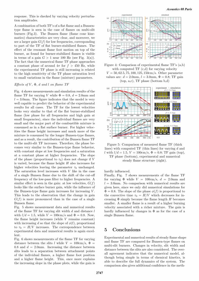
Fig. 4 shows measurements and simulation results of theflame TF for varying V while Φ = 0.8, d = 2.0mm andl = 3.0mm. The figure indicates that the model is verywell capable to predict the behavior of the experimentalresults for all cases. The TF for the lowest velocitieslooks very similar to that of the flat burner-stabilizedflame (low phase for all frequencies and high gain atsmall frequencies), since the individual flames are verysmall and the major part of the combustible mixture isconsumed as in a flat surface burner. For higher veloc-ities the flame height increases and much more of themixture is consumed by the longer Bunsen-type flames,and as a result, the contribution of the Bunsen flame TFto the multi-slit TF increases. Therefore, the phase be-comes very similar to the Bunsen-type flame behavior,with constant slope at low frequencies and a saturationat a constant phase at higher frequencies. The slopeof the phase (proportional to τ0) does not change if Vis varied, because the flame height H also increases forhigher velocities leaving the parameter τ0 unchanged.The saturation level increases with V like in the caseof a single Bunsen flame due to the shift of the cut-offfrequency of the low-pass filter to higher frequencies. Asimilar effect is seen in the gain: at low velocities, G(f)looks like the surface burner gain, while the influence ofthe Bunsen-type flame gain increases for increasing V .This leads to the observation that the change in gainG(f) is more pronounced than in the case of a singleBunsen flame.Fig. 5 shows measurement data and numerical resultsof the flame TF for varying slit width d and distance lwith l/d = 1.5, while V = 100cm/s and Φ = 0.8. Now,the flame height increases (while V remains constant)with increasing d so that the slope of φ(f), proportionalto τ0 = H/V increases. The correspondence betweenexperimental data and numerical results is again excel-lent.Fig. 6 shows measurements of the flame TF for varyingdistance between the slits l while V = 100cm/s, Φ =0.8 and d = 2.0mm. Increasing the distance betweenslits leads to a separation between attachment pointsof the individual flames, a higher flame foot positionand a higher flame height. This, once more explainsthe increasing slope in the phase plots, while the gain is

0 00 00 00 f, Hz1 2 3 400 5000.0

1 0

.1 1

gai

n

(a)

d=2mm

l=3mm

0 3

6

9

21

-, ra

df

(b)

0 00 00 00 f, Hz1 2 3 400 500

V= cm/s50

62.575 100 125

150

50

62.575

125

100

150

0 00 00 00 f, Hz1 2 3 400 5000.0

1 0

.1 1

gai

n

(c)

0 3

6

9

21

-, ra

df

(d)

0 00 00 00 f, Hz1 2 3 400 500

V= cm/s50

62.5

100

125

150

50

62.575

125

100 150

75

experimental simulated

Figure 4: Comparison of experimental flame TF’s (a,b)with computed TF (c,d) for varying velocity

V = 50, 62.5, 75, 100, 125, 150cm/s. Other parametervalues are: d = 2.0mm, l = 3.0mm, Φ = 0.8; TF gain

(top, a,c), TF phase (bottom b,d)

0 00 00 00 f, Hz1 2 3 400 5000.0

1 0

.1 1

gai

n 2

(a)

l/d=1.5

0 3

6

9

21

-, ra

df

(b)

d= mm1

d l

0 00 00 00 f, Hz1 2 3 400 500

d= mm1

1.5

22.5

mm

mm

mm

mm

d=1; l=1.5mm

experiment \ simulation

d=1.5; l=2.25mm

d=2; l=3mm

d=2.5; l=3.75mm

(c)

Figure 5: Comparison of measured flame TF (thicklines) with computed TF (thin lines) for varying d andl with l/d = 1.5, V = 100cm/s, Φ = 0.8; TF gain (top),

TF phase (bottom), experimental and numericalsteady flame structure (right).

hardly influenced.Finally, Fig. 7 shows measurements of the flame TFfor varying Φ while V = 100cm/s, d = 2.0mm andl = 3.0mm. No comparison with numerical results aregiven here, since we only did numerical simulations forΦ = 0.8. The slope of the phase φ(f) is proportional tothe convective time τ0 = H/V which decreases for in-creasing Φ simply because the flame length H becomessmaller. A smaller flame is a result of a higher burningvelocity associated with a richer mixture. The gain ishardly influenced by changes in Φ as for the case of asingle Bunsen flame.

5 Conclusions

Experimental and numerical results of steady flame shapeand flame TF are compared for Bunsen-type flames onmulti-slit burners. Changes in velocity, slit width anddistance between the slits are also considered. The over-all agreement indicates that the numerical model, al-though being simple in terms of chemical kinetics, isable to describe the full dynamics of the system. Thecomparison also gives additional confidence in the meth-

Acoustics 08 Paris

2747

0 00 00 00 f, Hz1 2 3 400 5000.0

1 0

.1 1

gai

n

3

(a)

d=2mm

0 3

6

9

21

-, ra

df

(b)

0 00 00 00 f, Hz1 2 3 400 500

3

l=2mm

4

l=2mm

4

Figure 6: Comparison of measured flame TF (thicklines) with computed TF (thin lines) for varying l andconstant d = 2.0mm with V = 100cm/s, Φ = 0.8; TF

gain (top), TF phase (bottom))

ods (i.e. chemiluminescence and heated wire techniques)used during the experimental research.

The results indicate that the TF of multi-slit flames is aweighted sum of the well-known TF’s of a Bunsen-typeconical flame and that of a flat flame stabilized on a flatburner. If the flames are short, the full multi-slit TFis similar to the TF of burner-stabilized flames becauseonly a small part of the mixture is consumed by thesmall Bunsen flames. The opposite is true in the case oflong Bunsen-type flames: the major part of the mixturethen is consumed by longer flames, leading to a TF verysimilar to that of the corresponding Bunsen-type flame.

References

[1] M. Fleifil, A.M. Annaswamy, Z.A. Ghoneim andA.F. Ghoniem, Response of a laminar premixedflame to flow oscillations, Combust. Flame 106,487-510 (1996).

[2] V.N. Kornilov, K.R.A.M. Schreel and L.P.H. deGoey, Experimental assessment of the acoustic re-sponse of laminar premixed Bunsen flames, Proc.Combust. Inst. 31, 1239-1246 (2007).

[3] H.C. de Lange and L.P.H. de Goey, Two-dimensional methane/air flames, Combust. Sci.Tech. 92, 423–427 (1993).

[4] R. Rook, Acoustics in Burner-Stabilised Flames,PhD Thesis, Eindhoven University of Technology(2001).

[5] W.E. Kaskan, The dependence of flame tempera-ture on mass burning velocity, Sixth Symp. (Int.)on Combustion, The Combustion Institute, NewHaven, pp. 134–143 (1956).

0 00 00 00 f, Hz1 2 3 400 5000.0

1 0

.1 1

gai

n

(a)

1

0 3

6

9

21

-, ra

df

(b)

F=0.8

2; 3mm

0 00 00 00 f, Hz1 2 3 400 500

0.9

F=0.8

0.9

1

Figure 7: Measured flame TF for varying equivalenceratio Φ with V = 100cm/s, d = 2.0mm, l = 3.0mm TF

gain (top), TF phase (bottom)

[6] R.J. Kee, G. Dixon-Lewis, J. Warnatz, M.E.Coltrin, and J.A. Miller, A Fortran computer codepackage for the evaluation of gas-phase multicom-ponent transport properties, Sandia National Labo-ratories, SAND86-8246 (1986).

[7] R.J. Kee, F.M. Rupley, and J.A. Miller, Thechemkin thermodynamic database, Sandia NationalLaboratories, SAND87-8215 (1991).

[8] A.A. Putnam, Combustion Driven Oscillations inIndustry, Elsevier, New York (1971).

[9] R. Rook, L.P.H. de Goey, K.R.A.M. Schreel, and R.Parchen, Response of burner-stabilized flat flamesto acoustic perturbations, Combust. Theory Mod-elling 6 (2), 223-242 (2002).

[10] T. Schuller, S. Ducruix. D. Durox and S. Candel,Modeling tools for the prediction of premixed flametransfer functions, Proc. Combust. Inst. 29 , 107-114 (2002)

[11] M.D. Smooke and V. Giovangigli, Formulationof the premixed and nonpremixed test problems,in: Reduced kinetic mechanisms and asymptoticapproximations for methane-air flames, ed. M.D.Smooke, pp. 1-28, Springer, Berlin (1991).

[12] B. van ’t Hof, Numerical Aspects of Laminar FlameSimulation, PhD Thesis, Eindhoven University ofTechnology (1998).

[13] B. van ’t Hof, J.H.M. ten Thije Boonkkamp andR.M.M. Mattheij, Pressure Correction for Laminarcombustion Simulation, Combust. Sci. Tech. 149,201–223 (1999).

Acoustics 08 Paris

2748