Experimental and computational techniques in carbon-13 NMR
200
W&M ScholarWorks W&M ScholarWorks Dissertations, Theses, and Masters Projects Theses, Dissertations, & Master Projects 1999 Experimental and computational techniques in carbon-13 NMR Experimental and computational techniques in carbon-13 NMR Samuel John Varner College of William & Mary - Arts & Sciences Follow this and additional works at: https://scholarworks.wm.edu/etd Part of the Condensed Matter Physics Commons Recommended Citation Recommended Citation Varner, Samuel John, "Experimental and computational techniques in carbon-13 NMR" (1999). Dissertations, Theses, and Masters Projects. Paper 1539623952. https://dx.doi.org/doi:10.21220/s2-9hyk-ky63 This Dissertation is brought to you for free and open access by the Theses, Dissertations, & Master Projects at W&M ScholarWorks. It has been accepted for inclusion in Dissertations, Theses, and Masters Projects by an authorized administrator of W&M ScholarWorks. For more information, please contact [email protected].
-
Upload
khangminh22 -
Category
Documents
-
view
3 -
download
0
Transcript of Experimental and computational techniques in carbon-13 NMR
W&M ScholarWorks W&M ScholarWorks
Dissertations, Theses, and Masters Projects Theses, Dissertations, & Master Projects
1999
Experimental and computational techniques in carbon-13 NMR Experimental and computational techniques in carbon-13 NMR
Samuel John Varner College of William & Mary - Arts & Sciences
Follow this and additional works at: https://scholarworks.wm.edu/etd
Part of the Condensed Matter Physics Commons
Recommended Citation Recommended Citation Varner, Samuel John, "Experimental and computational techniques in carbon-13 NMR" (1999). Dissertations, Theses, and Masters Projects. Paper 1539623952. https://dx.doi.org/doi:10.21220/s2-9hyk-ky63
This Dissertation is brought to you for free and open access by the Theses, Dissertations, & Master Projects at W&M ScholarWorks. It has been accepted for inclusion in Dissertations, Theses, and Masters Projects by an authorized administrator of W&M ScholarWorks. For more information, please contact [email protected].

INFORMATION TO USERS
This manuscript has been reproduced from the microfilm master. UMI films the
text directly from the original or copy submitted. Thus, some thesis and
dissertation copies are in typewriter face, while others may be from any type of
computer printer.
The quality of th is reproduction is dependent upon the quality o f th e copy
subm itted . Broken or indistinct print, colored or poor quality illustrations and
photographs, print bleedthrough, substandard margins, and improper alignment
can adversely affect reproduction.
In the unlikely event that the author did not send UMI a complete manuscript and
there are missing pages, these will be noted. Also, if unauthorized copyright
material had to be removed, a note will indicate the deletion.
Oversize materials (e.g., maps, drawings, charts) are reproduced by sectioning
the original, beginning at the upper left-hand comer and continuing from left to
right in equal sections with small overlaps. Each original is also photographed in
one exposure and is included in reduced form at the back of the book.
Photographs included in the original manuscript have been reproduced
xerographically in this copy. Higher quality 6” x 9” black and white photographic
prints are available for any photographs or illustrations appearing in this copy for
an additional charge. Contact UMI directly to order.
Bell & Howell Information and Learning 300 North Zeeb Road, Ann Arbor, Ml 48106-1346 USA
800-521-0600
Reproduced with permission of the copyright owner. Further reproduction prohibited without permission.

Reproduced with permission of the copyright owner. Further reproduction prohibited without permission.Reproduced with permission of the copyright owner. Further reproduction prohibited without permission.
EXPERIMENTAL AND COMPUTATIONAL TECHNIQUES IN
CARBON-13 NMR
A Dissertation
Presented to
The Faculty of the Physics Department
The College of William and Mary in Virginia
In Partial Fulfillment
Of the Requirements for the Degree of
Doctor of Philosophy
by
Samuel John Varner
May 1999
Reproduced with permission of the copyright owner. Further reproduction prohibited without permission.
UMI Number: 9942560
UMI Microform 9942560 Copyright 1999, by UMI Company. All rights reserved.
This microform edition is protected against unauthorized copying under Title 17, United States Code.
UMI300 North Zeeb Road Ann Arbor, MI 48103
Reproduced with permission of the copyright owner. Further reproduction prohibited without permission.

APPROVAL SHEET
Approved, May 1999
This dissertation is submitted in partial fulfillment
of the requirements for the degree of
Doctor of Philosophy
Samuel J. Varner
L.'tfoo&Dvv
Gina L. Hoatson, Advisor
Robert L. Void (Applied Science)
Harlan Schone
David Armstrong
s-n
CT
Brian Holloway (Applied Science)
Reproduced with permission of the copyright owner. Further reproduction prohibited without permission.

To Mom, Dad, and Paige
Reproduced with permission of the copyright owner. Further reproduction prohibited without permission.
Contents
A cknow ledgm ents iv
List o f Tables v
List o f Figures vi
A bstract v>*
1 C ondensed M atter P hysics 2
1.1 Branches of Physics ................................................................................................................... 3
1.2 Experimental Techniques ......................................................................................................... 5
1.3 Nuclear Magnetic R e so n a n c e ................................................................................................... 7
1.4 S u m m a ry ...................................................................................................................................... 8
2 N M R B ackground 10
2.1 Isotopes and s p i n ......................................................................................................................... 11
2.2 Theoretical Descriptions of N M R ............................................................................................ 12
2.2.1 Classical D escrip tion ...................................................................................................... 13
2.2.2 Quantum D e sc r ip tio n ................................................................................................... 15
2.2.3 The Density M a t r i x ...................................................................................................... 17
2.3 NMR in P ra c t ic e ......................................................................................................................... 21
iii
Reproduced with permission of the copyright owner. Further reproduction prohibited without permission.
2.3.1 Pulse Sequences .............................................................................................................. 21
2.3.2 Equipment ....................................................................................................................... 23
2.3.3 NMR S p e c tra .................................................................................................................... 28
2.4 Im portant In terac tio n s................................................................................................................ 31
2.4.1 The Zeeman In te ra c tio n ................................................................................................ 32
2.4.2 Chemical Shie ld ing .......................................................................................................... 32
2.4.3 The Dipolar In te ra c tio n ................................................................................................ 40
2.4.4 The Quadrupole In terac tion .......................................................................................... 42
2.5 Experimental Techniques ......................................................................................................... 44
2.5.1 Magic Angle S p in n in g .................................................................................................... 44
2.5.2 Cross P o la r iz a tio n .......................................................................................................... 46
2.5.3 Dipolar Dephasing and Short Contact T i m e s ......................................................... 50
2.5.4 Spin-Lattice Relaxation M easurem ents...................................................................... 50
2.5.5 Multi-Dimensional Techniques ................................................................................... 54
2.6 S u m m a ry ...................................................................................................................................... 63
3 Pow der P attern C alcu lations 64
3.1 Common Methods of Powder Pattern C alcu lation .............................................................. 65
3.2 Analytical D erivation................................................................................................................... 69
3.3 The SUMS M eth o d ...................................................................................................................... 72
3.4 A pplications................................................................................................................................... 80
3.4.1 Automated Fitting of Experimental D a t a ................................................................ 80
3.4.2 Lineshapes from Partially Ordered S a m p le s ............................................................ 83
3.4.3 Deuteron L ineshapes....................................................................................................... 86
3.4.4 Partially Relaxed L in esh ap e s ...................................................................................... 86
3.5 S u m m a ry ...................................................................................................................................... 88
iv
Reproduced with permission of the copyright owner. Further reproduction prohibited without permission.

4 R elaxation C alculations 90
4.1 In troduction.................................................................................................................................. 90
4.2 C alculations.................................................................................................................................. 95
4.2.1 Redfield Theory ............................................................................................................ 95
4.2.2 Spectral Densities of Spinning Sam ples..................................................................... 99
4.2.3 Comparison to Static Spectral D en sities................................................................. 103
4.2.4 Linear Combinations of Spectral D ensities.............................................................. 105
4.2.5 Properties of Calculated Anisotropies ..................................................................... 107
4.3 Carbon Relaxation Time Anisotropies in F errocene.......................................................... I l l
4.4 Deuteron Relaxation Time Anisotropies in F errocene....................................................... 117
4.5 Relaxation Time Anisotropies in 2D E xperim ents............................................................. 121
4.6 C onclusions................................................................................................................................. 122
5 C haracterization o f P olyim ides 127
5.1 In troduction .................................................................................................................................. 127
5.1.1 LaR C -SI............................................................................................................................ 129
5.1.2 13C and *H NMR Techniques for Characterizing Polyim ides............................. 130
5.2 M a te r ia ls ..................................................................................................................................... 132
5.3 R esults........................................................................................................................................... 133
5.3.1 Solid S tate Isotropic 13C Chemical S h i f t s .............................................................. 133
5.3.2 Solution State l3C NMR S p e c tra .............................................................................. 148
5.3.3 13C Anisotropic Chemical S h i f t s .............................................................................. 153
5.3.4 Cross Polarization D y n a m ic s .................................................................................... 156
5.3.5 l H FID E xperim ents..................................................................................................... 159
5.3.6 l H Wideiine Separation Experim ents........................................................................ 160
5.3.7 l H Dipolar Filter E x p e r im e n ts ................................................................................. 162
v
Reproduced with permission of the copyright owner. Further reproduction prohibited without permission.
5.3.8 l3C Dipolar Filter Cross Polarization E x p erim en ts................................................... 165
5.3.9 H yd ra tio n ........................................................................................................................ 167
5.4 C onclusions.................................................................................................................................. 170
6 Sum m ary 173
V ita 183
vi
Reproduced with permission of the copyright owner. Further reproduction prohibited without permission.

Acknowledgments
I wish to express my gratitude to Or. Gina Hoatson for her commitment to my academic and
scientific development. Thanks go to Dr. Hoatson and Dr. Robert Void for their guidance and for
fruitful collaborations, and to my entire dissertation committee for taking the time to read and
comment on my dissertation during a particularly busy time of the academic year. I would like
to thank Marco Brown and Tak Tse for showing me the ropes in the NMR lab, and the transient
postdocs, Jurgen Paff, Raju Subramanian, and Jargen Kristensen, for sharing their experience. I
am grateful to Dasha Malyarenko for her friendship and for doing a fantastic job of taking over
my responsibilities in the lab. I deeply appreciate the efforts of Dasha and Zhenya Malyarenko in
helping me to print out my dissertation from half way across the country.
Many people outside of the physics department deserve mentioning. Dr. Robert Bryant and
others at the NASA Langley Research Center have provided illuminating discussions about polyimide
structure and properties. Thanks go to the William and Mary Chemistry Department for the use of
their liquid state NMR spectrometer, and to the William and Mary Applied Science Department for
the use of their facilities for sample preparation. I would like to express my appreciation to the Free
Software Foundation and to contributors to free software for making available many of the computer
programs used to produce this dissertation.
Special thanks go to Paige for her patience, support, understanding and friendship. Most of all,
I want to thank my parents for encouraging and supporting me in whatever I have tried to do.
vii
Reproduced with permission of the copyright owner. Further reproduction prohibited without permission.

List of Tables
3.1 Comparison of Powder P attern Calculation Times In Seconds for Three Algorithms . 78
3.2 Best-Fit Chemical Shifts Determined by Non-Linear Fit Using SUMS for Carbonyl
Carbons in L3C Enriched Benzoic Acid and Glycine, and the Methyl Carbon in Natural
Abundance CgA -U IC................................................................................................................... 81
5.1 Isotropic Chemical Shifts of Polyimide Model C om p o u n d s................................. 139
5.1 Isotropic Chemical Shifts of Polyimide Model Compounds (continued) ............ 140
5.2 Isotropic Chemical Shifts of Polyimides ........................................................................... 144
5.3 Anisotropic Chemical Shifts of Polyimides and Model C o m p o u n d s ............................. 155
viii
Reproduced with permission of the copyright owner. Further reproduction prohibited without permission.
List o f Figures
2.1 The Cross Polarization Pulse Sequence................................................................................. 22
2.2 Spectrometer Block D ia g ra m ................................................................................................. 24
2.3 Circuit Diagram for a Double Resonance P r o b e ................................................................ 26
2.4 I3C Energy Level Diagram and CSA Powder P a t te rn ....................................................... 37
2.5 Chemical Shielding Tensor E llipso ids.................................................................................... 39
2.6 Energy Levels and Powder Pattern for a Dipolar Coupled 13C Nucleus ................... 41
2.7 Energy Levels and Powder Pattern for a D e u te ro n .......................................................... 43
2.8 The WISE Pulse Sequence........................................................................................................ 55
2.9 Two-Dimensional Separation of Proton L in esh ap es .......................................................... 56
2.10 two-dimensional Separation of chemical shielding anisotropy L in esh ap es ................... 58
2.11 Sampling of the two-dimensional Time Plane W ith V A C S Y ......................................... 60
3.1 A Simple Tiling Scheme for Calculating Powder Patterns ............................................. 6 6
3.2 The ASG Method for Calculating Powder P a t te rn s .......................................................... 67
3.3 A Non-uniform Chemical Shielding Distribution Arising from a Uniform Angular
Distribution..................................................................................................................................... 71
3.4 Construction of an Asymmetric Powder Lineshape from Axially Symmetric Subspectra 74
3.5 Comparison of a SUMS Lineshape to Those Calculated by Other M ethods................ 79
3.6 Automated Nonlinear Least-Squares Fits to Experimental D a ta ................................... 82
ix
Reproduced with permission of the copyright owner. Further reproduction prohibited without permission.
3.7 Calculated Lineshapes for a Non-uniform D is tr ib u tio n ................................................... 85
3.8 Simulated Partially Relaxed Deuteron Lineshapes for Deuterated F e rro cen e 87
4.1 Ferrocene Structure ................................................................................................................. 95
4.2 Calculated Powder Patterns for a Static and Spinning S am p le ...................................... 104
4.3 Calculated Spectral D e n sitie s ................................................................................................. 109
4.4 Calculated Anisotropies of Relaxation Time and A and B ............................................. 110
4.5 Static and Spinning l3C Relaxation Time Anisotropies for F erro cen e ......................... 113
4.6 Anisotropies of A and B for F erro cen e ................................................................................. 115
4.7 Deuteron Relaxation Time Anisotropies for Ferrocene-d t o ............................................. 118
4.8 Measured Spectral Density Anisotropies for F e rro c e n e ................................................... 120
4.9 C8A-UIC VACSY S p ec tru m .................................................................................................... 123
4.10 T iz Anisotropies for CgA-UIC ............................................................................................. 124
5.1 Molecular Structures and Assigned l3C Spectra of Model Compound I ...................... 134
5.2 Molecular Structures and Assigned Spectra of Model Compound I I .............................. 135
5.3 Molecular Structures and Assigned Spectra of Model Compound III ........................... 136
5.4 Molecular Structures and Assigned Spectra of Model Compound IV ........................... 137
5.5 Molecular Structures and Assigned Spectra of Model Compound V .............................. 138
5.6 Molecular Structures and Assigned Spectra of L a R C -T P I .............................................. 141
5.7 Molecular Structures and Assigned Spectra of L a R C -IA .................................................. 142
5.8 Molecular Structures and Assigned Spectra of LaRC-SI .................................................. 143
5.9 Spectra of Polyimides Formed W ith Different Proportions of ODPA and BPDA . . . 146
5.10 Spectra of Fresh and Heat Treated LaRC-SI and L aR C -IA ............................................ 147
5.11 Solution and Solid State Spectra of Model Compound I I I ............................................ 149
5.12 Solid and Solution State Carbon Spectra of L aR C -S I...................................................... 152
5.13 Two-Dimensional VACSY Spectrum of Model Compound H I ...................................... 154
x
Reproduced with permission of the copyright owner. Further reproduction prohibited without permission.
5.14 Anisotropic 13C Lineshapes and Fits for LaRC-IA ........................................................... 157
5.15 Cross Polarization Dynamics for L aR C -IA ........................................................................... 158
5.16 Comparison of a Slice of a Two-Dimensional WISE Spectrum and the Static Proton
Spectrum of LaRC-IA.................................................................................................................. 161
5.17 One-Pulse and Dipolar Filtered Proton S p e c tr a ................................................................. 164
5.18 Comparison of DFCP and CPMAS S p e c t r a ........................................................................ 166
5.19 Proton Spectrum of Hydrated LaRC-SI .............................................................................. 169
xi
Reproduced with permission of the copyright owner. Further reproduction prohibited without permission.
Abstract
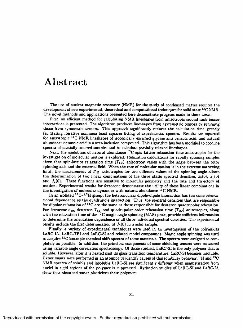
The use of nuclear magnetic resonance (NMR) for the study of condensed m atter requires the development of new experimental, theoretical and computational techniques for solid state l3C NMR. The novel methods and applications presented here demonstrate progress made in these areas-
First, an efficient method for calculating NMR lineshapes from anisotropic second rank tensor interactions is presented. The algorithm produces lineshapes from asymmetric tensors by summing those from symmetric tensors. This approach significantly reduces the calculation time, greatly facilitating iterative nonlinear least squares fitting of experimental spectra. Results are reported for anisotropic 13C NMR lineshapes of isotopically enriched glycine and benzoic acid, and natural abundance octanoic acid in a urea inclusion compound. This algorithm has been modified to produce spectra of partially ordered samples and to calculate partially relaxed lineshapes.
Next, the usefulness of natural abundance 13C spin-lattice relaxation time anisotropies for the investigation of molecular motion is explored. Relaxation calculations for rapidly spinning samples show that spin-lattice relaxation time (Tiz) anisotropy varies with the angle between the rotor spinning axis and the external field. When the rate of molecular motion is in the extreme narrowing limit, the measurement of T \z anisotropies for two different values of the spinning angle allows the determination of two linear combinations of the three static spectral densities, JQ(0), 7i(0) and TaCO). These functions are sensitive to molecular geometry and the rate and trajectory of motion. Experimental results for ferrocene demonstrate the utility of these linear combinations in the investigation of molecular dynamics with natural abundance 13 C NMR.
In an isolated 13C -I,2H group, the heteronuclear dipole-dipole interaction has the same orientational dependence as the quadrupole interaction. Thus, the spectral densities that are responsible for dipolar relaxation of 13C are the same as those responsible for deuteron quadrupolar relaxation. For ferrocene-dto, deuteron T\z and quadrupolar order relaxation time (7 \q ) anisotropies, along with the relaxation time of the 13 C magic angle spinning (MAS) peak, provide sufficient information to determine the orientation dependence of sill three individual spectral densities. The experimental results include the first determination of 7o(0) in a solid sample.
Finally, a variety of experimented techniques were used in an investigation of the polyimides LaRC-IA, LaRC-TPI and LaRC-SI and related model compounds. Magic angle spinning was used to acquire 13 C isotropic chemical shift spectra of these materials. The spectra were assigned as completely as possible. In addition, the principal components of some shielding tensors were measured using variable angle correlation spectroscopy. Of those studied, LaRC-SI is the only polymer that is soluble. However, after it is heated past its glass transition temperature, LaRC-SI becomes insoluble. Experiments were performed in an attem pt to identify causes of this solubility behavior. lH and 13C NMR spectra of soluble and insoluble LaRC-SI are significantly different when magnetization from nuclei in rigid regions of the polymer is suppressed. Hydration studies of LaRC-SI and LaRC-IA show that absorbed water plasticizes these polymers.
xii
Reproduced with permission of the copyright owner. Further reproduction prohibited without permission.
EXPERIMENTAL AND COMPUTATIONAL TECHNIQUES IN
CARBON-13 NMR
Reproduced with permission of the copyright owner. Further reproduction prohibited without permission.
Chapter 1
Condensed M atter Physics
The study of the nature of solid m atter is a relatively new discipline in physics. However, the
philosophy and science of solids, in a general sense, has a much longer history [1]. For millennia,
artists and artisans have noted properties of various materials for decorative and practical uses.
Centuries ago, alchemists sought to understand the changes that occurred in the physical properties
of materials as they were worked by craftspersons. The empirical knowledge gained from these
studies were the first steps toward modern chemistry. However, until the 20th century, physics had
largely ignored the problem of determining the microscopic origins of bulk properties of m atter. This
problem is the focus of the discipline now known as condensed m atter physics.
One reason for the late arrival of condensed m atter physics is that appropriate theoretical and
experimental methods were not available until other areas of physics matured. The analysis of exper
imental results requires knowledge not only of the materials being studied, but also of the particles
and waves that probe them. Thus, classical and quantum mechanics, classical electrodynamics, and
statistical mechanics are all im portant to the study of condensed m atter. In addition, technical ad
vances have made possible experimental methods that use such tools as x-rays, lasers, neutrons and
sophisticated electronics — tools that were unavailable throughout most of the history of physics.
This chapter is intended as an introduction to the goals and methods of condensed m atter physics.
2
Reproduced with permission of the copyright owner. Further reproduction prohibited without permission.
3
Some fundamental concepts that are im portant to the more detailed theoretical discussions in later
chapters will also be introduced. In order to show how the study of condensed m atter relates to the
study of physics as a whole, a brief survey of some of the major fields of physics, with an emphasis
on aspects that are relevant to condensed m atter, will be presented. Next, a few of the common
experimental techniques currently in use in condensed matter research will be described. Lastly,
the capabilities of the technique used in the investigations presented in this dissertation, nuclear
magnetic resonance (NMR), will be discussed.
1.1 Branches of Physics
The oldest branch of physics is classical mechanics. Classical mechanics describes the motion of
m atter in response to forces. The foundation of classical mechanics is formed by the laws of motion
first written in the 17th century by Sir Isaac Newton. These laws are expressed by the equation
?=% M l
where F is force and p is momentum. In classical mechanics, a rotating object can be considered
as a collection of tiny particles, each obeying Newton’s laws. However, it is worthwhile to consider
the analogs of Newton’s laws for rotating objects, especially considering the importance of angular
momentum in quantum mechanics. Substituting angular quantities for the linear ones in Eq. 1.1 we
get:
* = # ■ M l
Here, f is torque and L is angular momentum.
The laws of classical mechanics are suitable for describing the motions of planets, cannon balls
and falling apples. With molecular dynamics (MO) simulations, Newton’s laws are even applied to
molecules and condensed phases. In its original formulation, an MD simulation is accomplished by
treating the system as a collection of interacting particles with a number of degrees of freedom [2 j.
Reproduced with permission of the copyright owner. Further reproduction prohibited without permission.
4
The coupled Lagrange equations of motion for the system are solved numerically. The vast numbers
of interacting particles and extremely short time scales needed for an accurate simulation make the
technique expensive in terms of computer time. However, many variations and refinements on the
original idea have been made since the first simulations were performed in the 1950s. These have
served to extend the time and distance scales that can be modeled. Consequently, the technique
has become applicable in the investigation of a wide range of systems. MD simulations have been
particularly successful a t determining the elastic properties of inhomogeneous materials [2 ].
Early in the 20th century, classical mechanics was revealed to be merely an approximate descrip
tion of nature. The approximation breaks down for distance scales that are not much smaller than
those considered with MD simulations. A more general description is offered by quantum mechanics.
Atomic nuclei often exhibit counter-intuitive behavior due to quantum mechanical phenomena. Con
cepts such as quantization of angular momentum, the wave nature of particles and superposition of
states are im portant for accurate theoretical descriptions of condensed m atter and accurate analysis
of experimental data.
The experimental methods of condensed m atter physics are typically applied to macroscopic
samples; thus, the information gathered comes from vast numbers of atoms or molecules. It is
im portant, therefore, to understand the collective behavior of large numbers of weakly interacting
objects in order to interpret the results of condensed m atter experiments. The field of statistical
mechanics gives us the theoretical framework for describing such systems based on the description of
a single member. The pioneering work in statistical mechanics done in the 19th century has proven
to be essential for the study of solids in the 2 0 th century.
The 19th century also saw advances in the study of light and other forms of electromagnetic
radiation. Faraday noted the connection between electricity and magnetism. Maxwell consolidated
the field of electromagnetism by identifying its fundamental equations. In 1905 Einstein introduced
the concept of the photon to account for the photoelectric effect. Electromagnetic radiation with a
wavelength of A, or a frequency of ui, can be considered as a stream of photons, each with an energy
Reproduced with permission of the copyright owner. Further reproduction prohibited without permission.

5
given by
E = 2irhc/\ = huj. [1.3]
where ft is the Planck constant and c is the speed of light. Spectroscopic methods investigate m atter
by measuring the energies (or wavelengths, or frequencies) of electromagnetic radiation that are
absorbed or emitted by a sample. Energy is absorbed as the material absorbs a photon and moves
to a higher energy state. This could happen by an electron moving to a higher orbital in an atom, a
molecule changing its mode of vibration or, in the case of NMR, a nucleus changing spin states in a
magnetic field. Photons are reemited as the system returns to equilibrium. By observing absorption
and emission of photons of various energies, a wide range of interactions can be probed.
1.2 Experimental Techniques
The goal of condensed m atter research is to determine and understand the origins of the physical
properties of solids. These properties include color, density, electrical conductivity, thermal conduc
tivity, flexibility, tensile strength, and innumerable others. The origins of some of these properties
are well known in qualitative terms. An object’s color is determined by the wavelengths of ligbt that
it reflects. Conductivity depends on the presence of loosely bonded electrons that are free to travel
in response to an applied electric field. The flexibility of rubber is a result of long, entangled polymer
molecules. The diverse origins of the properties in these three examples illustrate the complexity of
the task of condensed m atter research.
An accurate determination of the nature of a solid requires consideration of a wide range of time
and distance scales. In some cases the structure of the individual molecules give rise to an important
property; in others, large domains of order and disorder that consist of thousands of molecules are
responsible. Motion, as well as structure, has an important role in determining bulk properties.
For example, the freedom of the chains in polycarbonate to move and dissipate energy results in
its remarkable impact resistance [3]. Molecular motion may be the slow reorientation of a large
Reproduced with permission of the copyright owner. Further reproduction prohibited without permission.
6
molecule o r the fast vibration of directly bonded atoms. This variety of sizes and rates necessitates
a wide variety of theoretical frameworks and experimental techniques.
Many techniques of solid state physics were originally developed to test the theoretical models
of physicists. Optical spectra have long been a proving ground for quantum mechanics. Diffraction
of electrons and neutrons was used to demonstrate the wave nature of m atter before it was used
to elucidate the structure of m atter. X-ray diffraction was performed in 1912 (17 years after the
effects of x-rays were first noticed by Rontgen) as an investigation of the nature of x-rays rather
than the nature of solids. As the application of the techniques became routine and interpretation of
experimental results became clear, these methods found broader application. Scattering, diffraction
and spectroscopic techniques are now indispensable tools in biology and chemistry as well as in
physics.
The spectrum of light absorbed or reflected by a substance has long been a valuable scientific
tool. The equipment is simple: a finely etched piece of glass, some lenses and a photographic plate
produce a record of the wavelengths present in reflected or transm itted light. Consequently, optical
spectroscopy is one of the oldest scientific methods for characterizing solids. Today a vast array
of spectroscopic techniques are used to measure electromagnetic fields with energies far above and
below the range of visible light.
Visible wavelengths are typically absorbed and emitted by electrons as they move from one
orbital to another. At the high energy end of the electromagnetic spectrum, Mdssbauer spectroscopy
measures the absorption of gamma rays. Below the energies of visible light, infrared radiation is
absorbed and em itted by vibrating molecules and crystals. Raman spectroscopies monitor molecular
and lattice inodes of vibration using scattered infrared light. Microwaves probe electron spin states
and gas-phase molecular rotation. At even lower energies, in the range of radio waves, NMR is used
to observe the absorption of energy by nuclei as they change spin states.
The interaction between nuclear magnetic moments and magnetic fields th a t makes NMR possible
was observed by Zeeman in the early years of the 20th century. However, an accurate theoretical
Reproduced with permission of the copyright owner. Further reproduction prohibited without permission.
7
description of this interaction must include the quantization of angular momentum, a concept that
was not introduced until the development of quantum theory in the 1930s. Calculations showed that
hydrogen nuclei in a magnetic field of less than one Tesla should absorb energy in the radio frequency
region of the electromagnetic spectrum. The first observations of this effect were made by Purcell,
Torrey and Pound [4], and independently by Bloch, Hansen and Packard [5], in 1946. Purcell and
Bloch were awarded the Nobel Prize in physics for this research in 1952. In the years since the first
signal was observed, solid state NMR has grown into a particularly versatile spectroscopic technique.
1.3 Nuclear M agnetic Resonance
NMR spectroscopy monitors the absorption of radio frequency photons (w ~ 10®-109 rad/s) by
nuclei as they change spin states in an static magnetic field. Therefore, the spectra are affected
by interactions that perturb the zeroth-order Zeeman energy levels. The effects of a number of
interactions are visible in NMR spectra. The dipolar interaction occurs when the magnetic field
from a nearby nucleus adds to (or subtracts horn) the static external field. Circulating electronic
currents induced by the external magnetic field reduce the magnitude of the applied field at the
nucleus, a phenomenon known as chemical shielding. A nucleus with a spin greater than ft/2 has a
non-spherical charge distribution, and thus, a nuclear electric quadrupole moment. The interaction
of the quadrupole moment with electric field gradients dominates the spectra of such nuclei. These
interactions provide information about crystal and molecular structure.
In the solid state, the im portant interactions depend on crystal orientation. NMR spectra of single
crystals are sometimes useful, but, more commonly, polycrystalline samples are used. The material
is ground to a fine powder to ensure that all crystal orientations are present. Many interesting
and im portant materials do not have crystal structures. Although these amorphous materials are
unsuitable for diffraction studies, they present no special challenge for NMR. Since the relevant spin
interactions are anisotropic, the random orientations found in a powder (or amorphous) sample lead
Reproduced with permission of the copyright owner. Further reproduction prohibited without permission.

8
to distributions of NMR frequencies and broad spectral lineshapes. These lineshapes provide a means
for resolving signals from different orientations of the principal axis systems of these interactions.
Since a change in molecular orientation results in a change in the strength of these interactions,
information about molecular motion can be gathered by measuring the time-dependence of NMR
spectra. For slow motional rates (~ 10~2-104 s~l ) two dimensional exchange and selective excitation
experiments provide details of molecular dynamics. Motion at rates that approach the strength
of the interactions that contribute to the width of the anisotropic lineshape are investigated using
lineshape analysis. For carbon, where the chemical shift is the dominant interaction, the intermediate
regime may begin at rates of 103 s -1 . In deuteron NMR, where the stronger quadrupole interaction
dominates, rates as high as 10 4 s -1 may still be considered slow.
Rates that are much higher them the interaction strengths motionally average the interactions
completely. In this regime, the NMR spectra show no sensitivity to the rate of motion. However, the
effects of dynamics can still be observed. The rapid fluctuations of the anisotropic interactions stim
ulate transitions among the Zeeman energy levels. These transitions help establish the equilibrium
population distributions, a process known as nuclear spin relaxation. Measuring the characteristic
time for relaxation at various points on a powder lineshape yields the relaxation time as a function of
orientation — the relaxation time anisotropy. Relaxation time anisotropies are calculated based on
hypothesized models of motion and compared to measured anisotropies to quantitatively determine
fast molecular dynamics in the solid state.
1.4 Summary
Through this brief introduction, the interdependence of condensed m atter and other areas of
physics has been illustrated. A few of the diverse branches of study within condensed m atter
physics have also been mentioned. Because of the interdisciplinary nature of NMR research, vast
communities of scientists exist that concentrate on particular types of problems or systems in physics,
Reproduced with permission of the copyright owner. Further reproduction prohibited without permission.

9
materials science, chemistry, molecular biology and medicine. Although the rest of this dissertation
is concerned with particular experimental and computational techniques of solid state NMR, the
relationship of this research to condensed m atter, physics, and science as a whole, should not be
forgotten.
Reproduced with permission of the copyright owner. Further reproduction prohibited without permission.
Chapter 2
N M R Background
Nuclear Magnetic Resonance (NMR) is a form of spectroscopy performed with radio-frequency
(RF) electromagnetic (EM) radiation. RF photons are absorbed and emitted by atomic nuclei with
spin angular momentum as they make transitions between spin states in an external, static magnetic
field. The Zeeman interaction between the spin angular momentum moment of a nucleus and the
applied magnetic field provides the largest contribution to the energies of the spin states. However,
sensitivity to tiny perturbations of the energy levels makes NMR an invaluable research tool in
a variety of scientific disciplines. The resonant frequencies of nuclei are influenced by a variety
of interactions tha t reflect molecular order, structure and motion. Effects of these perturbations
on NMR spectra are studied in order to develop and refine the theoretical framework that allows
quantitative interpretation of the spectra. Experimental techniques are constantly being invented
and existing ones improved in order to increase the quality and quantity of the information obtained
horn NMR spectra. These techniques are then used to further knowledge and understanding, not
only in physics, but in medicine, biology, materials science and other fields as well.
This chapter is presented as an introduction to the theory, techniques and vocabulary used
by NMR spectroscopists. The material is intended for an audience tha t is comfortable with the
fundamental concepts of physics, but familiarity with NMR is not assumed. The discussion will
10
Reproduced with permission of the copyright owner. Further reproduction prohibited without permission.
CHAPTER 2. NMR BACKGROUND 11
concentrate on m atters that are relevant to carbon-13 NMR. After a brief section concerning nuclear
isotopes, a simple NMR experiment is described using the language of classical physics. The same
experiment is then described quantum mechanically. This description is extended to large ensembles
of spins using the density m atrix formalism. Practical m atters, including details of the spectrometer,
are considered in the following section. Information about structure and dynamics is obtained
through interactions that affect NMR spectra. The interactions that significantly affect solid state
13C, 'H , and 2H NMR spectra are discussed. Finally, the experimental techniques that have been
used to obtain the data presented in this dissertation are introduced.
2.1 Isotopes and spin
NMR experiments can be performed on nuclear species that have intrinsic angular momentum,
or spin. A spinless ( / = 0) nucleus does not posses a magnetic moment and is invisible to NMR.
Nuclear angular momentum arises from the coupling of the spin and orbital angular momenta of
protons and neutrons. Each nucleon has a spin of ft/2 ; thus the total spin angular momentum of a
nucleus is a multiple of ft/2. Natural units are typically used in calculations of NMR phenomena.
Thus, the fundamental unit of angular momentum, the Planck constant (ft « 1.055 x 10~ 34 Js), is
set equal to one. A 13C atom has a spin of ft/2, and is described as a sp in -| nucleus. The deuteron,
an isotope of the hydrogen nucleus with one proton and one neutron, is a spin-1 nucleus.
Even if a particular nucleus is spinless, isotopes of that nucleus that have spin may be suitable
for NMR experiments. This is the case for carbon. The most abundant isotope of carbon is 12C with
a nucleus comprised of six protons and six neutrons. Carbon-12 has no spin angular momentum and
therefore cannot be detected with NMR. However, about one of every hundred carbon atoms has
an extra neutron. These 13 C atoms have the same chemical properties as 12 C atoms, but the extra
neutron gives the nucleus a spin of / = ft/2 .
An NMR experiment is typically performed to observe the resonance of one particular isotope.
Reproduced with permission of the copyright owner. Further reproduction prohibited without permission.

CHAPTER 2. NMR BACKGROUND 12
One speaks of a carbon-13 NMR experiment or a deuteron NMR experiment. A reason for this
specificity is that the difference between resonance frequencies of nuclei with different numbers of
nucleons is typically much greater than the range of frequencies produced by a single species. Also,
the range of frequencies of EM radiation produced by the spectrometer is limited. A pulse of EM
radiation is produced by gating an oscillating EM field. The excitation profile of this pulse is its
Fourier transform — a sine function (s in x /i) centered at the frequency of the oscillating field. The
frequency range over which excitation is reasonably uniform may be estimated as the inverse of the
pulse length. Because of the high power levels that must be used with short pulses, practical pulse
lengths are longer than a microsecond. Thus, the widest spectral width that can be achieved using a
single pulse is less than a megahertz. In the spectrometer that was used to collect the data shown in
later chapters deuterium nuclei resonate a t 46.06 MHz, carbon-13 nuclei a t 75.46 MHz and hydrogen
nuclei (protons) a t 300.07 MHz. Typical spectral widths for these isotopes are 200 kHz, 20 kHz and
70 kHz, respectively. Only a portion of the vast range of frequencies from all NMR-active nuclei can
be measured in a single experiment. However, the bandwidth is sufficient to measure all frequencies
of many isotopes.
2.2 Theoretical Descriptions of NM R
Nuclear magnetic resonance results from transitions between discrete energy states. For spin—
nuclei, the spin operator, / , has three orthogonal components, and thus transforms as a vector.
This fact allows NMR experiments with spin— nuclei, like 13 C and l H, to be described using the
vocabulary of classical mechanics. Although quantum mechanical descriptions are needed in order
to perform accurate calculations and to simulate NMR spectra, classical descriptions are useful for
providing qualitative descriptions th a t are easily visualized. A discussion of a simple one pulse
experiment from both the classical and quantum points of view is useful for introducing concepts
and terms used to describe NMR experiments.
Reproduced with permission of the copyright owner. Further reproduction prohibited without permission.

CHAPTER 2. NMR BACKGROUND 13
2.2.1 Classical Description
This derivation contains the highlights of the more detailed treatm ent of Gerstein and Dybowski
in Ref. [6 j. Consider a nucleus with spin placed in a static magnetic field, Bo. The direction of the
static magnetic field lines defines the positive z-direction of the laboratory coordinate system. The
magnetic moment of the nucleus is proportional to its angular momentum
M = ~r L , [2.lj
where 7 is the gyromagnetic ratio. If the magnetic moment (and its associated angular momentum
vector) is not parallel to the external field, the interaction between the magnetic moment of the
nucleus surd the field produces a torque that tends to align the moment along the field:
t = /I x Bo- [2.2]
This torque causes the angular momentum vector to change with time in accord with
Substituting Eq. 2.1 and 2.2 into 2.3 yields the differential equation that describes the precession of
the magnetization vector:
^ = 7 /1 x B0- [2.4)
Since the external field defines the laboratory z-direction, the cross product only has components
along the x and y axes. Thus, only the x and y components of the magnetization are time-dependent.
The solutions to Eq. 2.4 are:
= M*(0) cos-fBot + /Jty(Q)sixx~fBot [2.5]
(iy{t) = - p x(0)sin7f?o* + (iy{0) cos 'yBot
Pz(t) = Hz( 0)
The macroscopic magnetization measured in an NMR experiment is the vector sum of the nuclear
magnetic moments of the nuclei in the sample. Alignment of the nuclear moments along the external
Reproduced with permission of the copyright owner. Further reproduction prohibited without permission.
CHAPTER 2. NMR BACKGROUND 14
field is far from perfect. The moments are nearly randomly oriented with only a slight preference for
the r-direction. The components of these moments that are perpendicular to the external field do not
have a preferred direction. The absence of an NMR signal from a sample in thermal equilibrium leads
us to assume that the components of the nuclear magnetic moment in the xy-plane are randomly
oriented. For a large collection of nuclei the vector sum of these components is zero. Thus, at
equilibrium, the macroscopic magnetization is the sum of the z-components of the nuclear magnetic
moments:
individual nuclear magnetic moment, fi, given in Eq. 2.5. The projection of the macroscopic mag
netization vector onto the xy-plane precesses with a frequency of u/q = yBo, defined as the Larmor
frequency. Detection of such a rotating magnetic moment is straightforward. A coil of wire is placed
around the sample, with its axis perpendicular to the static magnetic field. The precessing moments
induce a tiny, but measurable, current in the sample coil due to the time-varying magnetic flux
through its windings. This analog signal is recorded, digitized, using two 32 bit analog-to-digital
converters, and processed to produce the spectrum.
The question of how the nuclear moment is placed in xy-plane remains. To simplify the problem,
we will ignore the external field for the moment. Running an electrical current through the sample
coil creates a magnetic field, Bi , perpendicular to the laboratory z-direction, around which the
nuclear moments will precess. This field is turned on and off to produce a pulse. The duration of
the pulse (the pulse length) and the intensity of the pulse determines how far the magnetization
vector is rotated. A pulse that rotates magnetization by 90° (called a 90° pulse, or a \ pulse) results
in the largest signed, since all of the magnetization is in the xy-plane.
In practice, the external field cannot simply be ignored. The constant field generated in the
superconducting magnet of a NMR spectrometer dwarfs any transient magnetic fields that can be
produced in the resistive sample coil. Any component of the magnetization vector that lies in the
[2 .6]
The time dependence of the macroscopic magnetization vector, M , is the same as that of an
Reproduced with permission of the copyright owner. Further reproduction prohibited without permission.

CHAPTER 2. NMR BACKGROUND 15
plane perpendicular to the external field precesses at the Larmor frequency. In order to simplify
visualization of the response of the magnetization vector to pulses, it is useful to imagine a reference
frame that rotates a t the Larmor frequency about the laboratory z-axis. In this rotating frame the
effect of the static magnetic field is nulled, and the magnetization vector appears to respond only to
the transient magnetic field generated in the coil. If the transient magnetic field, Bi , is stationary
in the rotating frame, then it follows that it is rotating a t the Larmor frequency in the laboratory
frame. However, producing a magnetic field rotating a t typical Larmor frequencies (10-500 MHz)
presents some technical problems. The solution is to produce a linearly oscillating field in the sample
coil by means of an alternating current. This oscillating field is the projection of a rotating field
onto a single axis. The direction in which the transient field points in the rotating frame depends
on the phase of the oscillation. An NMR spectrometer can produce pulses with arbitrary phases. It
is particularly convenient to produce transient fields in each of the z, y, - x or —y directions. With
control over the length and phase of the pulses, magnetization can be pointed in any direction in
the rotating frame.
2.2.2 Quantum Description
In the classical description, the sta te of a nucleus in a magnetic field is defined by the orientation
of its magnetic moment. In a quantum mechanical description, the state of a nucleus is defined by a
linear combination of eigenstates of the Zeeman Hamiltonian. For a spin- 5 nucleus this Hamiltonian
is
H = - 7 B0 • I [2.7]
where I is the nuclear angular momentum operator and A is set equal to one. As in the classical
discussion, the external field defines the laboratory z-direction. So the Hamiltonian becomes:
H = - 7 B0I Z. [2.8]
Reproduced with permission of the copyright owner. Further reproduction prohibited without permission.

CHAPTER 2. NMR BACKGROUND 16
In a matrix representation,
1 0
0 - 1
[2.9]
The eigenvectors of this matrix are:
and [2 . 10]
with eigenvalues 1/2 and —1/2, respectively. The nuclear states that correspond to these eigenvalues
are the spin-up and spin-down states, denoted 15 ) and | —j ) . The energy levels are the eigenvalues
of the Zeeman Hamiltonian:
t f |± i ) = i?± | ± i ) f [2.11]
where
E x = ± - 7Bq. [2 . 12]
In order to describe NMR quantum mechanically, we must identify the observable quantities. In
the classical picture it is the nuclear magnetic moment that is observed. This quantity is represented
in the quantum picture by the magnetization operator, M{t). Since the magnetic moment of a
nucleus is proportional to its angular momentum we make the identification
The expectation value of the magnetization operator is then:
[2.131
[2.14]
An arbitrary state ket, |^(t)>, is a linear combination of the spin-up and the spin-down eigenstates:
[2.15]
where the coefficients are normalized such that |CV(f) |2 + |C _(t) |2 = I for all t. The time dependence
of the wave function is found by applying the time evolution operator:
Reproduced with permission of the copyright owner. Further reproduction prohibited without permission.
CHAPTER 2. NMR BACKGROUND 17
|0(O) = exp(-ttfO |0(O )> [2.16]
= C+(0 )ex p ( - iH t ) | j ) + C _ (0 )ex p (-i/ft) | - j )
= C+(0) exp(iyBot/2) | I ) + C_(0) e x p (- i7 S 0 f/2) | - ± > .
The time evolution of the expectation value of the angular momentum operator is found by substi
tuting this expression for the state ket into Eq. 2.14. The angular momentum operator, I(t), can
be decomposed in order to determine the time dependence of three orthogonal components of the
expectation value of the magnetization operator:
/ = Ix x + I yy + Izz [2-17]
0 1 i 0 - 1 „ 1
y + 21 0
£ + 2T
1 0 1 0&
0 - 1
The resulting equations show that, for a sp in -j nucleus, the expectation value of the magnetization
operator has the same time dependence as the single particle classical magnetic moment, /I, given
in Eq. 2.5:
(.M*(t)) = (Afx(0)) cos 7 f?0t + (Mtf(0 )) s in 7 Bot [2.18]
(My(t)) = - {Mx {0)) sin-yBot + (M„(0)) cosyBot
(M t (t)) = (Afs (0)>,
where (Afx(0)) = 7 f?e[C+ (0)C!.(0)] and (A/„(0)> = - 7 /m(C+ (0)CI(0)].
2.2.3 The Density Matrix
A theoretical treatm ent of an NMR experiment requires th a t the time evolution of a large number
of spins must be described. In general, the state of each sp in -| nucleus in an ensemble is a linear
combination of the spin-up and spin-down states. For such mixed ensembles, the density matrix
formalism is useful. In a mixed ensemble the result of a measurement is given by the weighted
Reproduced with permission of the copyright owner. Further reproduction prohibited without permission.
CHAPTER 2. NMR BACKGROUND 18
average of expectation values [7]. Thus, the ensemble average of the magnetization operator is
(A/) = ^ 2 wi (^'1 M l^i) - [2.19]t
where the \i>,) represent states of the system and u;, is the fractional population of that state. These
states do not need to be orthogonal, and the number of states summed over is not necessarily the
same as the dimensionality of the ket space [7]. The fractional populations satisfy the normalization
condition, w, = I. The density operator is defined as
P = w. |t *> (tAil, [2.20]t
with matrix elements given by
{M>j\p\^k) = Y l Wi 0 *)- [2 .2 1 ]I
The closure relation can be used to expand Eq. 2.19:
(AT) = 2 Wi {1>i\ijjj) (tfi| Af tyr{) ( ^ | fr ) [2.22]t
t
Substitution of the expression for the matrix elements of the density matrix allows the ensemble
average to be written as
(Af) = Y l Mfcl P I M l^*> [2.23]
or
(M) = Tr(pM), [2.24]
where Tr denotes the trace. Since the trace of a matrix is independent of basis set, this result holds
regardless of the chosen representation.
The elements of the density m atrix have physical significance. In the Zeeman representation,
where the |t^,) are the eigenstates of the Zeeman Hamiltonian, the diagonal elements are the relative
populations of the eigenstates. Phase coherences of the spins in the ensemble are described by
Reproduced with permission of the copyright owner. Further reproduction prohibited without permission.

CHAPTER 2. NMR BACKGROUND 19
the off-diagonal elements. In an NMR experiment the signal observed after a pulse results from
single quantum coherences. These cire represented by non-zero elements whose indices differ by one,
i. e. Pij, where i = j ± 1. For a spin-1 system the density matrix is 2 x 2, so higher multiple
quantum coherences tire not possible. For nuclei with higher spin, multiple quantum coherences can
be created. However, they are not directly observable.
When a system is at thermal equilibrium in a static magnetic held, no signal is observed. This
demonstrates that no phase coherences exist among the spins at equilibrium. In this case, the
off-diagonal elements are zero, and the values of the diagonal elements are determined by thermal
energy partitioning [6 ]:
_ e x p ( - j I : B o /kBT) . .E * OW e x p ( - 7 / - f l 0/A:BT) \ x l>k) '
For temperatures above one kelvin, the high-temperature approximation, exp^—'y l .B o /ksT ) = 1 +
i h B o / k s T , is valid. Thus, the equilibrium density operator for a system particles with spin I is
9 = 2 7 T T (1 + (2-26l
Since the first term of this equation is simply a constant times the identity operator and has no time
dependence, it will be disregarded. From here on, the symbol p will refer to the reduced density
operator, which is the second term. As an example, consider a system of sp in -j particles in a static
magnetic field. The ensemble average of the magnetization is
(M ) = Tr(pM) [2.27]
Decomposition of the angular momentum operator allows the components of the ensemble average
magnetization to be written:
(Mx) = 0 [2.28]
(AT,) = 0
JTT-T I 2 Bo<"*> = 4S T '
Reproduced with permission of the copyright owner. Further reproduction prohibited without permission.

CHAPTER 2. NMR BACKGROUND 20
Thus, as discussed previously, no transverse magnetization exists a t equilibrium, and magnetization
in the z-direction, is proportional to Bq/ T , in agreement with the Curie-Weiss law [8 ].
The time evolution of the ensemble is contained in the density operator which evolves according
to the Liouville-von Neumann equation.
i % = -[«./»! [2291
This equation resembles the Heisenberg equation of motion. The only difference is the sign of the
right hand side. The discrepancy arises because the density matrix is not a Heisenberg-picture
operator. Rather, it a m atrix is made up of time dependent state vectors that evolve according to
the Schrodinger equation of motion [7J.
Calculations involving the density operator are further simplified by transformation to the in
teraction representation defined by the Zeeman Hamiltonian. The full Hamiltonian for an NMR
experiment can generally be expressed as the sum of the static Zeeman Hamiltonian, H z , and a
number of much smaller perturbing Hamiltonians. However, in the interaction representation, time
evolution under the Zeeman Hamiltonian is not present. This interaction representation is anal
ogous to a transformation to a reference frame rotating a t the Larmor frequency, as described in
the discussion of the classical picture of NMR. To describe the time evolution of a spin system, the
interaction representation density matrix is defined as
= exp( iHzt)pexp(—iH2 t)- [2.30]
The equation of motion in the interaction representation is
= [2-31]
where H\ is the interaction Hamiltonian:
H[ — exp(iHzt)'Hi exp( - i H z t ) . [2.32]
The density operator may be expanded in terms of a suitable basis set of operators. For spin- j
nuclei, Ix, Iy and I z are a natural choice, since, as shown earlier, these operators are proportional to
Reproduced with permission of the copyright owner. Further reproduction prohibited without permission.
CHAPTER 2. NMR BACKGROUND 21
the classical magnetization. Thus, a classical picture of magnetization vectors accurately describes
the evolution of a system of spin-1 particles in a static magnetic field. However, for nuclei with
higher spin the vector picture is inadequate because a larger basis set is needed. For deuterons,
which are spin-1 , a basis set of eight operators is needed.
2.3 NM R in Practice
The method most commonly used to acquire NMR spectra is pulsed Fourier transform NMR. The
signal is generated by irradiating the sample with a short, intense pulse of electromagnetic radiation.
The response of the sample to the pulse, called the free induction decay (FID), is the sum of the
responses of all the resonant nuclei in the sample. The Fourier transform of this time-domain FID
gives an NMR spectrum. The frequency of a peak in the NMR spectrum corresponds to a particular
value of the difference in energy for two spin states of the nucleus. The integrated intensity of a
peak is proportional to the number of nuclei resonating a t th a t particular frequency.
2.3.1 Pulse Sequences
The precision with which quantum mechanical states can be coherently manipulated is unique
to NMR. The relatively low (radio) frequencies allow pulses with precise phases, amplitudes and
durations to be generated. Fine control of the pulses allows the spins to be manipulated in a coherent
fashion, allowing fine control over quantum coherences. The ability to control the spins allows NMR
spectroscopists to improve and extend the single pulse Fourier transform NMR experiment described
in the previous section. Pulses of various lengths, intensities and phases are often used to prepare
the system in a particular state. The system is then allowed to evolve under the influence of
an interesting Hamiltonian. After evolution, observable single quantum coherences are created by
pulses applied during the mixing time. Finally, the signal is acquired during the detection time.
Such experiments can become quite complicated. A timeline for the events that occur in an NMR
Reproduced with permission of the copyright owner. Further reproduction prohibited without permission.
CHAPTER 2. NMR BACKGROUND 22
90x CP decou p leih n
CP t
13C
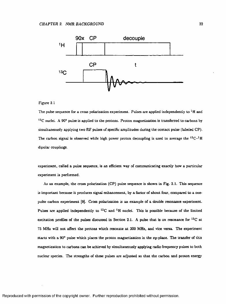
Figure 2.1
The pulse sequence for a cross polarization experiment. Pulses are applied independently to LH and
I3C nuclei. A 90° pulse is applied to the protons. Proton magnetization is transferred to carbons by
simultaneously applying two RF pulses of specific amplitudes during the contact pulse (labeled CP).
The carbon signal is observed while high power proton decoupling is used to average the 13C- 1 H
dipolar couplings.
experiment, called a pulse sequence, is an efficient way of communicating exactly how a particular
experiment is performed.
As an example, the cross polarization (CP) pulse sequence is shown in Fig. 2.1. This sequence
is im portant because it produces signal enhancement, by a factor of about four, compared to a one-
pulse carbon experiment [9]. Cross polarization is an example of a double resonance experiment.
Pulses are applied independently to 13C and lH nuclei. This is possible because of the limited
excitation profiles of the pulses discussed in Section 2.1. A pulse that is on resonance for 13C at
75 MHz will not affect the protons which resonate a t 300 MHz, and vice versa. The experiment
starts with a 90° pulse which places the proton magnetization in the xy-plane. The transfer of this
magnetization to carbons can be achieved by simultaneously applying radio frequency pulses to both
nuclear species. The strengths of these pulses are adjusted so that the carbon and proton energy
Reproduced with permission of the copyright owner. Further reproduction prohibited without permission.

CHAPTER 2. NMR BACKGROUND 23
levels are matched. When this Hartman-Hahn [10] condition is met, mutual carbon-proton spin flips
conserve energy. This technique is described in more detail in Section 2.5.2. After cross polarization,
the carbon magnetization is observed. During this acquisition time, the proton pulse is left on to
average the 13C -‘H dipolar interaction, thereby enhancing resolution in the l3C spectrum. This is
known as high-power proton decoupling.
Pulse sequences may be much more complicated than the cross polarization sequence shown here.
In general, pulse sequences have four time periods [11]: preparation, evolution, mixing and detection.
In the preparation time period, the system is placed in a non-equilibrium state. This state may have
phase coherences, or it may simply be a non-equilibrium distribution of populations. This state
is allowed to evolve under the influence of a particular Hamiltonian during the evolution period.
Preparation and evolution may take place without the creation of single quantum coherences. After
evolution, the detectable single quantum coherences are created in the mixing period. Finally, the
signal is acquired in the detection period.
In the cross polarization pulse sequence, the 90° pulse applied to the protons constitutes prepa
ration. The proton and carbon spin systems evolve during the contact pulse. Mixing also occurs
during the contact pulse; single quantum coherences in the carbons are produced through the dipolar
interaction with protons. Detection of the l3C NMR signal follows.
2.3.2 Equipment
A pulsed NMR spectrometer consists of devices for producing high-power radio frequency pulses,
a means for applying the pulses to the sample, a magnet for removing the degeneracy of the nuclear
energy levels and a means of collecting and processing the FID. The various hardware components
are controlled by precisely timed TTL logic signals sent from the pulse programmer according to
the pulse sequence that is loaded into its memory. A computer interface allows the user to specify
the pulse sequence and to digitize and manipulate the collected data. The fundamental components
of a spectrometer capable of being used for 13 C, l H double resonance experiments are shown in
Reproduced with permission of the copyright owner. Further reproduction prohibited without permission.
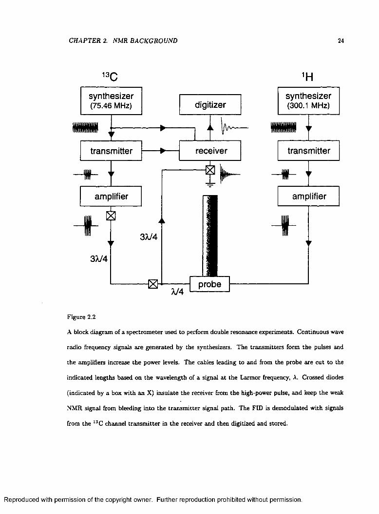
CHAPTER 2. NMR BACKGROUND 24
13Csynthesizer (75.46 MHz) digitizer
transmitter receiver
amplifier
1Hsynthesizer (300.1 MHz)
transmitter
amplifier
I1
Figure 2.2
A block diagram of a spectrometer used to perform double resonance experiments. Continuous wave
radio frequency signals are generated by the synthesizers. The transmitters form the pulses and
the amplifiers increase the power levels. The cables leading to and from the probe are cut to the
indicated lengths based on the wavelength of a signal a t the Larmor frequency, A. Crossed diodes
(indicated by a box with an X) insulate the receiver from the high-power pulse, and keep the weak
NMR signal from bleeding into the transm itter signal path. The FED is demodulated with signals
from the 13 C channel transm itter in the receiver and then digitized and stored.
Reproduced with permission of the copyright owner. Further reproduction prohibited without permission.

CHAPTER 2. NMR BACKGROUND 25
Fig. 2.2. Pulses are applied at both the carbon and proton resonance frequencies, 75 MHz and 300
MHz, respectively. Typically, only the carbon signal is detected.
An NMR signal can be observed using a modest magnetic field strength; however, the use of high
field strengths has some advantages. Perhaps the most im portant advantage is that a larger static
magnetic field results in larger energy level splittings. The Boltzmann distribution shows that a
larger energy difference leads to larger population differences, and thus a larger signal. The resistive
electromagnets used in early days of NMR were only capable of fields of about two Tesla. These
have largely been replaced by superconducting magnets, some of which produce fields in excess of
20 T. In both kinds of magnet the field is produced by a circulating electric current in a coil of wire.
However, the superconducting coil has no electrical resistance provided that the wire is kept below
its critical temperature; thus, it need not be connected to a power supply. The low temperature
is maintained by keeping the coil immersed in liquid helium, which has a boiling point of about 4
kelvins. The data presented here were acquired using a superconducting magnet with a field strength
of 7.048 T. This field is produced by a current of 36 Amperes Rowing through about a kilometer of
wire made of an alloy of niobium and titanium. In this magnet, carbons resonate at 75.46 MHz and
protons at 300.07 MHz.
To produce a radio frequency pulse, a continuous wave oscillating signal, produced by a precise
and stable frequency synthesizer, is gated by an electronic switch. This switch is controlled by TTL
signals from the pulse programmer. This switch, along with a device for controlling the phase of
the pulse, comprise the transm itter of an NMR spectrometer. The transm itter can produce pulses
of arbitrary phase with respect to the demodulating signal. This means that the transient field
produced in the sample coil can be made to point in any direction in the xy-plane of the rotating
reference frame. However, the most commonly used phases are x, y , —x and —y. The RF pulses
produced in the transm itter are amplified and sent to the probe. For double resonance experiments,
pulses of different frequencies must be produced independently. This requires that the spectrometer
have pairs of synthesizers, transm itters and amplifiers. For the 13 C and lH experiments, pulse power
Reproduced with permission of the copyright owner. Further reproduction prohibited without permission.

CHAPTER 2. NMR BACKGROUND 26
j sam p le j
rt7
Figure 2.3
Circuit diagram for a double resonance probe. The circuit consists of two resonance circuits. These
are independently tunable through choice of capacitor and inductor values, and by adjustment of
the variable capacitors. Both circuits share an inductor, the sample coil.
was a few hundred Watts. The wideline deuteron spectra necessitate short pulses, and power levels
in excess of a kilowatt.
The NMR probe positions the sample at the center of the magnet where the field is the strongest
and the most homogeneous. The probe also houses a resonant circuit that is tuned to match the
output impedance of the amplifier, and the impedance of the cables, a t the Larmor frequency. This
ensures the optimum power transfer for the pulses. Probes used for double resonance experiments
have two tuned circuits that share the sample coil (an inductor) [12], as shown in Fig. 2.3. This
arrangement allows pulses to be simultaneously applied to more than one nuclear species.
Three probes were used to collect the data presented in this dissertation, a single-tuned static
probe for the deuteron spectra, and two double-tuned magic angle spinning probes for the carbon
and proton spectra. In a magic angle spinning probe, the sample is contained in a hard cylindrical
rotor, usually made of silicon nitride or a ceramic material. The rotor fits into a cylindrical stator
in the probe. Air forced through small holes in the stator blows over flutes on the end of the rotor
Reproduced with permission of the copyright owner. Further reproduction prohibited without permission.
CHAPTER 2. NMR BACKGROUND 27
causing it to turn. Additional holes allow air to flow around the rotor to reduce friction between
the rotor and stator. For most of the carbon and proton spectra, a 5 mm (sample diameter) probe,
manufactured by Doty Scientific Inc., with a manually adjustable spinning angle was used. The
two-dimensional variable angle correlation spectroscopy (VACSY) experiments were performed with
a 7 mm probe that uses a computer-controlled stepper motor to change the spinning angle. Spin
rates were typically in the range of 3.5-4.0 kHz.
The coil in the probe which produces the time-dependent radio frequency fields is also used to
detect the precessing magnetization after the pulse. The NMR signal is the voltage induced in
the coil by the time-varying magnetization vector. This tiny analog signal has an amplitude on
the order of a microvolt; it must be highly amplified before it can be demodulated and digitized.
Demodulation of the NMR signal in the receiver shifts all of the frequencies from the RF range
(roughly 107-109 Hz) to the audio frequency range (roughly 0-105 Hz) using analog heterodyne
circuits. Audio frequency signals are much easier to amplify, filter and digitize. The phase difference
between the pulse and the demodulating signal determines where the transient magnetic field points
in the rotating frame. The final stage of demodulation (with a 30 MHz intermediate frequency)
produces two signals that tire 90° out of phase — the real and imaginary components of the complex
NMR signal. This is known as quadrature detection. A complex Fourier transform of this signal has
both positive frequencies (faster than the rotating frame) and negative frequencies (slower than the
rotating frame).
The demodulated NMR signal is an analog signal. To facilitate storage, signal averaging and
processing of the FID, this signal is digitized. T hat is, the voltage is sampled periodically and the
value is stored on a computer as a binary number. The time interval between samples, the dwell
time (td), determines the width of the spectrum. The highest frequency that can be accurately
represented is the Nyquist frequency, v s = 1/2t j . Frequencies higher them the Nyquist frequency
(or lower than - v n ) must be filtered out of the analog signal before digitization. Otherwise, they will
appear in the spectrum at another frequency, a phenomenon known as aliasing: a signal a t (i//v -I- v)
Reproduced with permission of the copyright owner. Further reproduction prohibited without permission.
CHAPTER 2. NMR BACKGROUND 28
appears as an aliased peak a t + v). The use of quadrature detection, to allow the acquisition
of signals with negative frequencies in the rotating frame, doubles the range of frequencies than can
be acquired using a particular dwell time. A typical l3C spectrum has a spectral width of ±10 kHz,
and thus, a dwell time of 50 fis is appropriate. Wideline deuteron spectra often require spectral
widths of greater than ±200 kHz, and, consequently, dwell times shorter than 2.5 fis.
2.3.3 NM R Spectra
A digitized signal, collected as described in the previous section, is processed to produce an
NMR spectrum. The frequencies in a spectrum correspond to the differences between spin energy
levels for which spectroscopic transitions are allowed. Nuclei that resonate at the same frequency
have identical magnetic environments. In simple experiments, the intensity observed at a particular
frequency is proportional to the number of nuclei that resonate at that frequency. An NMR spectrum
may consist of narrow peaks from motionally averaged interactions, characteristic lineshapes from
unaveraged anisotropic interactions, or featureless distributions when a range of interaction strengths
is present.
The intrinsic signal to noise ratio (S/N) of a single FID is rarely adequate for quantitative study.
Thousands of FIDs my be added to increase S/N . Since the NMR signal is coherent, its intensity
grows in proportion to the number of scans, n. However, the incoherent noise grows only as y/n.
Thus, S/N grows as y/n [13]. If one wishes to double S/N by coherently averaging, the penalty is a
four fold increase in the number of scans, and thus, in time.
As implied by its name, the free induction decay is a signal that becomes smaller as time goes on.
The NMR signal indicates th a t transverse magnetization is present, and therefore, the density matrix
has off-diagonal elements. This is a non-equilibrium configuration for the spin system. The system
will return to equilibrium by nuclear spin-spin relaxation. The relaxation of transverse magnetization
is generally exponential, with a time constant of T-j. An FID may also decay due to dephasing due
to the presence of a distribution of NMR frequencies. In this case, magnetization vectors spread
Reproduced with permission of the copyright owner. Further reproduction prohibited without permission.
CHAPTER 2. NMR BACKGROUND 29
out in the xy-plane of the rotating frame. This coherent dephasing process can be reversed using a
spin echo. For spin-j nuclei, a 180° pulse has the same effect as reversing the time evolution of the
Hamiltonian. However, random time-dependent processes, such as spin-spin relaxation, cannot be
reversed using pulses. In liquids, where fast, isotropic molecular motion averages the interactions
that influence the spectrum, spin-spin relaxation dominates the decay of the FID.
Another distinction to be made is that between homogeneously broadened and inhomogeneously
broadened lines. For a homogeneously broadened line, each nucleus makes a similar, broad contri
bution to the total lineshape. In the absence of decoupling, the contribution of each 13C nucleus in
the sample is broadened due to dipolar coupling to a large number of protons. The resulting peak is
homogeneously broadened. An inhomogeneously broadened line is made up contributions from many
narrow lines over a range of frequencies. An example of an inhomogeneously broadened line is the
powder pattern from an anisotropic interaction. For a powder sample, the random orientations of
the principal axis systems of the interaction lead to broad lines that consist of narrow contributions
from a large number of nuclei. Such inhomogeneously broadened lines resulting from chemical shift
anisotropy are the subject of the next chapter.
An FID that decays quickly yields a spectrum with broad lines; a long lasting FID yields narrow
lines. Narrow lines have the advantage of allowing the frequency resolution of closely spaced reso
nances. Also, the peak of a narrow line has a higher intensity than that of a wide line with the same
integrated intensity. Thus, fewer scans are needed to collect a spectrum with a signal to noise ratio
that is adequate for quantitative analysis when the lines are narrow. For these reasons, a number
of experimental techniques, such as magic angle spinning, high-power multiple-pulse decoupling,
dynamic-angle spinning (DAS) [14], and double rotation (DOR) [15], are aimed at sharpening the
resonances in NMR spectra. These techniques will be discussed in detail in a later section.
Spectral lines are sometimes artificially broadened in an effort to boost the signal to noise ratio.
In a process known as apodization, the FID is multiplied by a function [11], usually a decaying
exponential. As a result, the width of each line in the spectrum increases. This behavior is described
Reproduced with permission of the copyright owner. Further reproduction prohibited without permission.
CHAPTER 2. NMR BACKGROUND 30
by the convolution theorem of Fourier transforms [16]:
[2.33]
where T indicates the Fourier transform, and F(u>) and G(ui) are the Fourier transforms of /(f) and
g(t), respectively. The symbol * denotes convolution, defined as follows:
[2.34]
If / ( t ) is the FID and g(t) is a decaying exponential, then the apodized spectrum is the Fourier
transform of the FID convolved with a Lorentzian function. The effect of convolution is to distribute
spectrum is smoothed. The price paid is that every line in the spectrum is broadened. Some features
that are obscured by noise before apodization may show up clearly after convolution.
The amount of line broadening applied to a spectrum, usually expressed in Hertz, is the full
width at half maximum intensity of the Fourier transform of the apodizing function. The Fourier
transform of an exponential function, with time constant r , is a Lorentzian:
The apodization function written in terms of the amount of broadening in Hertz is given by
the intensity of each point in the spectrum. Thus, the jagged random noise th a t covers the entire
[2.35]
The maximum of the retd part of this function has the value r a t w = 0. The frequency where half
maximum occurs is found by solving for u in
r r[2.36]
I + w2t 2 2
The width of the Lorentzian is the difference between the two solutions:
[2.37]
= exp(—2w A ut /2). [2.38]
Reproduced with permission of the copyright owner. Further reproduction prohibited without permission.
CHAPTER 2. NMR BACKGROUND 31
To minimize the time spent collecting a spectrum, one would like to spend as little time as possible
between the recording of one FID and the generation of the next. However, the magnetization that
produces the signal is destroyed during detection. The magnetization returns to equilibrium through
spin-lattice relaxation; the time constant for this process is the spin-lattice relaxation time, T \ z ■ A
recycle delay is placed at the end of the pulse sequence to allow spin-lattice relaxation to occur
between scans. A balance must be struck when choosing the appropriate recycle delay. If the
recycle delay is much shorter than T iz then the magnetization along the external field is much
smaller than the equilibrium value, and little signal is detected with each scan. If the recycle delay
is much longer than T \z then time that could have been spent collecting signals has been wasted.
The optimum recycle delay is about 1.3 times the spin-lattice relaxation time.
2.4 Important Interactions
The nuclear energy levels are influenced by a number of interactions. For a l3C nucleus in a solid,
the dominant interactions are the Zeeman interaction between the nuclear magnetic moment and the
static magnetic field, chemical shielding, and the magnetic dipolar interaction. Chemical shielding is
the attenuation of static magnetic field by the local electron density. The dipolar interaction results
from the contribution to the magnetic field strength at the nucleus made by other nearby nuclei.
The total Hamiltonian is a sum of the Hamiltonians for each of these interactions:
H = H z + + H d [2.39]
where "Hz is the Hamiltonian for the Zeeman interaction, is for the chemical shift and 'Ho for
the dipolar interaction. The effects of these perturbing interactions can be measured in order to
obtain information about the environments of 13 C nuclei in the solid state.
Reproduced with permission of the copyright owner. Further reproduction prohibited without permission.

CHAPTER 2. NMR BACKGROUND 32
2.4.1 The Zeeman Interaction
As discussed previously, the Zeeman Hamiltonian describes the interaction between the nuclear
magnetic dipole moment and an applied static magnetic field. It has the form:
H z = - y B 0I z , [2.40]
where 7 is the gyromagnetic ratio — the ratio between the magnetic moment of a nucleus and its
spin angular momentum, and h has been set equal to one. For the applied field strengths typically
used in NMR experiments (Bq = 2-21 T), the strength of the Zeeman interaction can range from
10-900 MHz.
2.4.2 Chemical Shielding
When charges move through a magnetic field, they experience a force that deflects them so that
they travel in helical paths. The circulating charges establish a magnetic field tha t opposes the
external field. An analogous phenomenon occurs for electrons in molecules where the delocalized
current density circulates in response to the static external field. In most cases the induced magnetic
field opposes the applied field; thus, the electrons are said to shield the nucleus from the external
field. Chemical shielding depends on the electronic current density in the vicinity of the nucleus
of interest. This current density in turn depends on the electronic wave function which describes
an electron under the influence of the electrostatic potentials and the static magnetic field [17].
Chemical bonds have a large effect on the electronic wave functions because the formation of bonds
localizes electron density. Since NMR frequencies depend on the strength of the applied magnetic
field a t the nucleus, chemical shielding results in different resonant frequencies for each chemically
distinct nucleus in the sample. The range of chemical shieldings is particularly large for carbon.
This chemical specificity makes l3C NMR spectra useful for the determination of the molecular
structures of organic compounds in solution. For molecules whose structures are well known, the
chemical shielding interaction allows the signals from carbons at various sites in the molecule to be
Reproduced with permission of the copyright owner. Further reproduction prohibited without permission.
CHAPTER 2. NMR BACKGROUND 33
differentiated, allowing, for example, the measurement of relaxation times for each carbon site in a
molecule.
For a particular nucleus, the size of the chemical shielding interaction is proportional to the
strength of the applied static magnetic field. This complicates comparison of spectra acquired using
different static field strengths. To overcome this difficulty, frequencies are expressed in dimensionless
units as a ratio of frequencies. Since all chemical shielding frequencies scale by the same factor, the
ratio of two frequencies is independent of field strength. Frequencies in this scale, called chemical
shifts, are reported as parts per million (ppm) relative to the frequency of a reference compound.
The standard reference compound is tetramethylsilane (TMS) which has an usually high chemical
shielding. The chemical shift (J) in ppm is calculated by (18):
< 5 = " — U™ s x l O6 [2.41]UTMS
were u is a measured frequency in the spectrum and v t m s is the frequency of TMS for the same
field strength. Carbon chemical shifts span an unusually wide range, greater than 200 ppm. This
makes 13 C chemical shifts practically useful and theoretically interesting.
The process of determining which sites on a molecule are responsible for each peak in a spectrum
is called assignment. Calculations of the chemical shielding in molecules from first principles are
complicated by the many-body nature of the electrostatic interactions [17]. Nuclei that are as many
as four bonds away from the nucleus of interest can make significant contributions to the chemical
shielding [19]. Empirical rules based on patterns and tendencies in measured chemical shifts sure
commonly used to assign solution state spectra of complex molecules. However, these rules usually
fail for solid state spectra. The l3C spectra of some simple molecules can be completely assigned by
knowing the typical ranges of chemical shifts. In more complicated cases, a collection of published
chemical shifts, such as the one compiled by Duncan [20], is useful. Additional techniques are
needed to complete the assignment of many spectra. Placing 13C atoms a t a particular site on
the molecule, a process known as selective labeling, causes the peak from that site to stand out.
Reproduced with permission of the copyright owner. Further reproduction prohibited without permission.
CHAPTER 2. NMR BACKGROUND 34
However, many molecular isotopomers may need to be synthesized in order to assign all of the
peaks. Furthermore, labeled compounds are expensive. Pulse sequences that attenuate or enhance
the signals of protonated carbons can aid in assignment of l3C NMR spectra of natural abundance
samples. Two such techniques, short contact times and dipolar dephasing, are discussed later in this
chapter. A short contact time experiment produces a spectrum dominated by carbons with directly
bonded protons. Dipolar dephasing removes protonated carbon peaks from the spectrum. Thus,
these and other spectral editing pulse sequences [21] can allow the differentiation of carbons with
different numbers of attached protons. Even with these tools, some peaks in the spectra of complex
compounds may remain ambiguous.
The terms chemical shielding and chemical shift are often used interchangeably to describe the
effect of local electron density on the strength of the field experienced at the nucleus. At this
point, however, the distinction between shielding and shift should be emphasized. The chemical
shift (6) is a measured quantity — a ratio of frequencies expressed in parts per million. The greater
the chemical shift, the higher the observed NMR frequency. Chemical shielding (a) expresses the
physical phenomenon [18], the degree to which the static field is attenuated at the nucleus. The
greater the chemical shielding, the lower the chemical shift.
Chemical shielding is anisotropic; its magnitude and direction depend on the orientation of the
principal axis system of a second-rank tensor with respect to the external field. The magnitude
and direction of the induced magnetic field at the nucleus is described by the operator, cr. The
Hamiltonian for the interaction is:
U a = 7 1- <r{LAB) • S 0. [2.42]
The chemical shielding operator has components that transform as a scalar, as a first rank tensor,
and as a second rank tensor. The first rank component does not contribute to the spectrum [22]
and will not be considered further. Second rank tensors can be represented by 3 x 3 matrices. These
tensors are transformed from one coordinate system to another by operating on them with rotation
Reproduced with permission of the copyright owner. Further reproduction prohibited without permission.

CHAPTER 2. NMR BACKGROUND 35
matrices:
a ' = F T 'e rR .
For an Euler angle transformation, the Cartesian rotation m atrix is [23]:
[2.43]
/ \ cos a cos 0 cos 7 - sin a sin 7 sin a cos 0 cos 7 + cos a sin 7 — sin 0 cos 7
- cos a cos 0 sin 7 — sin a cos 7 - sin a cos 0 sin 7 + cos a cos 7 sin 0 sin 7
cos a sin 0 sin a sin 0 cos 0[2.44]
and its inverse is the transpose, R_l = Rf . The convention used here for the Euler angle trans
formation is that of Rose [23]; the axis system is rotated through a about the z-axis, 0 about the
y'-axis and 7 about the z"-axis.
The coordinate system in which the second rank tensor is diagonal is known as the principal axis
system (PAS). The axes of the PAS point in the same directions as the eigenvectors of the tensor.
By convention, the z-axis of the PAS points along the largest eigenvector of the chemical shielding
tensor and the x-axis points along the smallest eigenvector. The eigenvalues, o\ \ , cr22 and < 7 3 3 , are
the principal values of the tensor. The shielding tensor in the laboratory coordinate system (LAB)
is found by a rotation from the principal axis system [23]:
<t (LAB) = R - l (Q,/3, 7 )cr(PA S)R (a,/3, 7 ) [2-45]
where a , 0, and 7 are the Euler angles, R(a, /3,7 ) is the rotation operator and
I \<7il 0 0
[2.46]
simplifies to
<ru 0 0
* { P A S ) = 0 <722 0
. 0 0 <?33 t
field is taken to be the laboratory
( \<J*z
n a = —7 h i - *yz Bo.
K azz J
[2.47]
Reproduced with permission of the copyright owner. Further reproduction prohibited without permission.

CHAPTER 2. NMR BACKGROUND 36
Here elements of cr(LAB) are denoted by x, y, and z while in the PAS, numerical subscripts are
used. Since chemical shielding results in frequency shifts that are on the order of kilohertz, and
Zeeman splittings are 10-900 MHz, the chemical shielding Hamiltonian is a small perturbation of
the Zeeman Hamiltonian. Thus, to first order, the terms in the Hamiltonian that do not commute
with Iz , namely azz and ayz , may be ignored. Thus the expression for H a becomes
H = - y h I za zzB0. [2.48]
An expression for azz, in terms of the principal values of the shielding tensor and the Euler angles of
the principal axis system to laboratory transformation, is found by applying the rotation operators
to trpAS-
a zz = [R- l ( a ,^ ,7 )o ’P/tsR(a./3,7)].;
= (cti i cos2 7 + <722 sin2 7 ) sin2 0 + a33 cos2 0. [2.49]
The NMR frequency, u , of a nucleus subject to the Zeeman and chemical shielding interactions is
given, in this first-order approximation, by
w = u/o(l - (Tzz) [2.50]
where wo = 7 R0 is the Larmor frequency.
For a single crystal, where discrete molecular orientations are present, the NMR spectrum consists
of sharp peaks (disregarding other interactions). The frequencies of these peaks depend on the
orientation of the crystal with respect to the external field. By measuring these frequencies as a
function of crystal orientation the shielding tensor can be determined. However, for many samples
it is not possible to grow a crystal of an appropriate size for NMR. In addition, some materials, such
as glasses amorphous polymers, do not have a regular crystal structure. Instead, they contain a
distribution of orientations of the principal axis system of the chemical shielding anisotropy (CSA)
tensor. As a result, spectral lines from such substances are broadened by the distribution of resonance
frequencies. Although broad lines diminish resolution, the ability to probe all possible orientations
Reproduced with permission of the copyright owner. Further reproduction prohibited without permission.
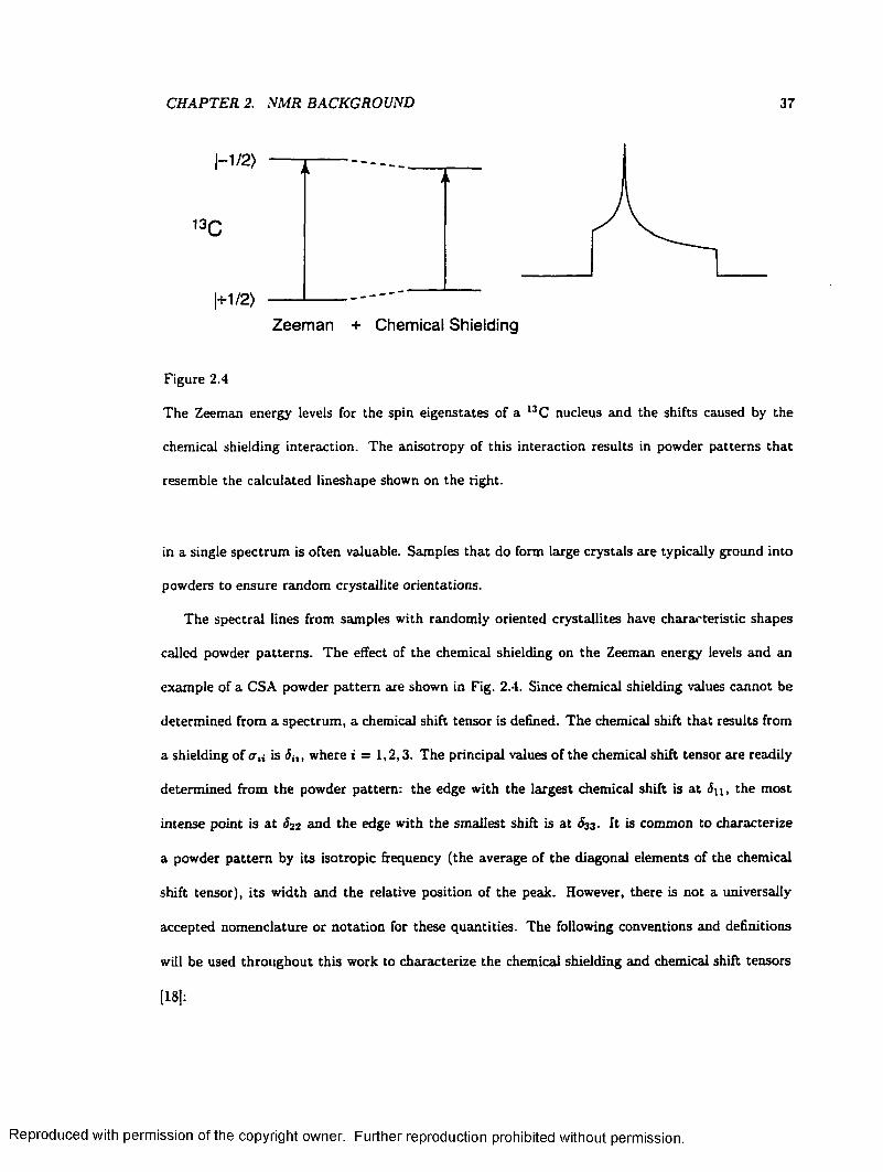
CHAPTER 2. NMR BACKGROUND 37
13C
1+ 1/2 )Zeeman + Chemical Shielding
Figure 2.4
The Zeeman energy levels for the spin eigenstates of a l3C nucleus and the shifts caused by the
chemical shielding interaction. The anisotropy of this interaction results in powder patterns that
resemble the calculated lineshape shown on the right.
in a single spectrum is often valuable. Samples that do form large crystals are typically ground into
powders to ensure random crystallite orientations.
The spectral lines from samples with randomly oriented crystallites have characteristic shapes
called powder patterns. The effect of the chemical shielding on the Zeeman energy levels and an
example of a CSA powder pattern are shown in Fig. 2.4. Since chemical shielding values cannot be
determined from a spectrum, a chemical shift tensor is defined. The chemical shift that results from
a shielding of an is <5;,, where t = 1,2,3. The principal values of the chemical shift tensor are readily
determined from the powder pattern: the edge with the largest chemical shift is at <Sn, the most
intense point is a t 622 and the edge with the smallest shift is a t £33 . It is common to characterize
a powder pattern by its isotropic frequency (the average of the diagonal elements of the chemical
shift tensor), its width and the relative position of the peak. However, there is not a universally
accepted nomenclature or notation for these quantities. The following conventions and definitions
will be used throughout this work to characterize the chemical shielding and chemical shift tensors
[18]:
Reproduced with permission of the copyright owner. Further reproduction prohibited without permission.
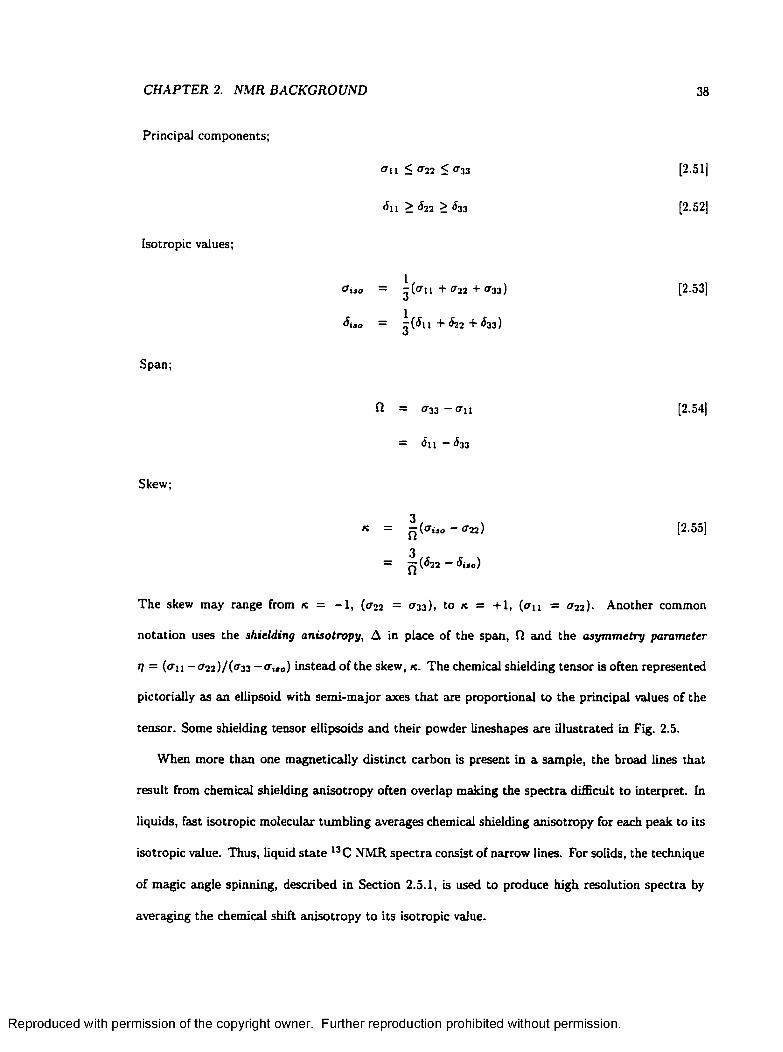
CHAPTER 2. NMR BACKGROUND 38
Principal components;
Isotropic values;
Span;
CTll S °22 < 033 [2.51]
dll > ^2 2 > ^33 [2.52]
° i s o — -jC^n + a ' 2 + ff33 [2.53]
di»o = -(d ll + ^22 + ^33)
fl = <X33 — O’! 1 [2.54]
= Su — 633
Skew;
3* = ^ { ( T i s o - t r 22 ) [2.55]
= j^(d2 2 -d»Jo)
The skew may range from k = - 1 , (a22 = <733), to it = +1, (a n = a 22 ). Another common
notation uses the shielding anisotropy, A in place of the span, Q and the asymmetry parameter
tj = (a n - a 22 ) / ( a 33 — a IIO) instead of the skew, k . The chemical shielding tensor is often represented
pictorially as an ellipsoid with semi-major axes that are proportional to the principal values of the
tensor. Some shielding tensor ellipsoids and their powder lineshapes are illustrated in Fig. 2.5.
When more than one magnetically distinct carbon is present in a sample, the broad lines that
result from chemical shielding anisotropy often overlap making the spectra difficult to interpret. In
liquids, fast isotropic molecular tumbling averages chemical shielding anisotropy for each peak to its
isotropic value. Thus, liquid state 13 C NMR spectra consist of narrow lines. For solids, the technique
of magic angle spinning, described in Section 2.5.1, is used to produce high resolution spectra by
averaging the chemical shift anisotropy to its isotropic value.
Reproduced with permission of the copyright owner. Further reproduction prohibited without permission.
CHAPTER 2. NMR BACKGROUND
■>33
k = 0.6
'11 ° 2 2 J33
K = -1.0
Figure 2.5
Chemical shielding tensor ellipsoids and the corresponding powder lineshapes for two shielding
sors with the same span, but different values of skew, it.
Reproduced with permission of the copyright owner. Further reproduction prohibited without permission.
CHAPTER 2. NMR BACKGROUND 40
2.4.3 The Dipolar Interaction
The strength of the magnetic field at the nucleus may be significantly affected by the fields
generated by other nearby magnetic nuclei. This dipolar interaction has a large effect on the resonant
frequencies o f 13 C nuclei that have directly attached protons. The dipolar Hamiltonian for an isolated
13C -l H, written in terms of second rank spherical irreducible tensor operators is [24]
Wo = E ( - i r - 4 - m ^ 21. [2.56]m= —2
where the spin operators are
4 a) = 7 S ( 3 / .S , - / “ •£ ) -4±! = + f± 5 : ) 4 22 = y ±S ± . [2.57]
Here, I and S are the angular momentum operators for the proton and carbon, respectively. The
spatial operators are
T0(2) = - V 6u d T™ = 0 = 0, [2.58]
where ujd — I c Th / t ch *s the dipolar coupling constant. Here, ~fc and 7H are the gyromagnetic
ratios of the coupled nuclei, and tch is the internuclear distance. Carbon-proton bond lengths are
typically about 1.1 A [25]. At this distance the dipolar coupling strength is about 24 kHz. As
with chemical shielding, and other second rank tensor interactions, the orientation dependence of
the dipolar interaction results in powder patterns in polycrystalline sample. Dipolar coupling to a
proton splits each of the 13C energy levels. (See Fig 2.6.) As a result, the size of the 13C transition
( |—j ) to 11)) depends on the state of the proton. Thus, for every orientation of the internuclear
vector, two peaks are present in the spectrum. For a powder sample, the lineshape is called a Pake
doublet; it resembles two overlapping chemical shielding anisotropy powder patterns, as shown in
Fig 2.6. The dipolar interaction is axially symmetric; thus, the dipolar tensor has a skew of one.
The width of the powder pattern depends on the dipolar coupling constant.
The effect of the dipolar interaction on 13C NMR spectra is further complicated by the fact that
many protons, a t a variety of distances, contribute to the appearance of the spectral line. Although
Reproduced with permission of the copyright owner. Further reproduction prohibited without permission.

CHAPTER 2. NMR BACKGROUND 41
13C
|+1/2>
|+1/2)1- 1/2 )
H
| - 1/2)1+ 1 /2 )
Zeeman + Dipolar
Figure 2.6
The Zeeman energy levels for the spin eigenstates of a 13C nucleus and the shifts caused by the dipolar
interaction with a single dipolar nucleus. The anisotropy of this interaction results in powder patterns
that resemble the calculated lineshape shown on the right. Because two unequal transitions are
present for each orientation, the powder pattern resembles two superimposed CSA powder patterns.
The axial symmetry of the dipolar interaction results in a skew equal to one.
Reproduced with permission of the copyright owner. Further reproduction prohibited without permission.
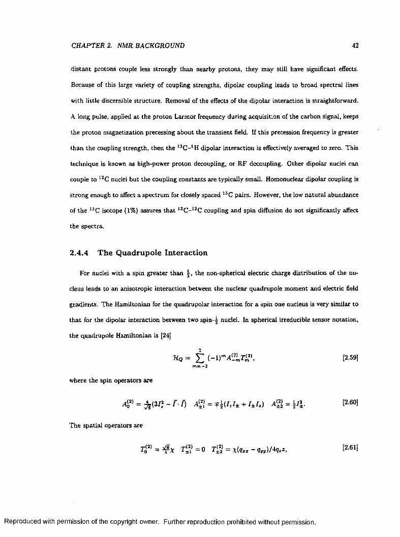
CHAPTER 2. NMR BACKGROUND 42
distant protons couple less strongly than nearby protons, they may still have significant effects.
Because of this large variety of coupling strengths, dipolar coupling leads to broad spectral lines
with little discernible structure. Removal of the effects of the dipolar interaction is straightforward.
A long pulse, applied at the proton Larmor frequency during acquisition of the carbon signal, keeps
the proton magnetization precessing about the transient field. If this precession frequency is greater
than the coupling strength, then the 13C - l H dipolar interaction is effectively averaged to zero. This
technique is known as high-power proton decoupling, or RF decoupling. Other dipolar nuclei can
couple to 13C nuclei but the coupling constants are typically small. Homonuclear dipolar coupling is
strong enough to affect a spectrum for closely spaced 13C pairs. However, the low natural abundance
of the 13C isotope ( 1%) assures that 13C -I3C coupling and spin diffusion do not significantly affect
the spectra.
2.4.4 The Quadrupole Interaction
For nuclei with a spin greater than j , the non-spherical electric charge distribution of the nu
cleus leads to an anisotropic interaction between the nuclear quadrupole moment and electric field
gradients. The Hamiltonian for the quadrupolar interaction for a spin one nucleus is very similar to
that for the dipolar interaction between two spin- 5 nuclei. In spherical irreducible tensor notation,
the quadrupole Hamiltonian is [24]
= E [2.59]m= —2
where the spin operators are
a o2) = 4 2! = T ^ ( I J ± + / * / , ) A ^ = i 4 . [2.601
The spatial operators are
to2) = *TX T±l = 0 T ™ = X{q~~qyy)HqzZ, t2-61!
Reproduced with permission of the copyright owner. Further reproduction prohibited without permission.

CHAPTER 2. NMR BACKGROUND 43
2H |o> Un
Zeeman + Quadrupolar
Figure 2.7
The Zeeman energy levels for the spin eigenstates of a deuteron and the shifts caused by the
quadrupole interaction. The anisotropy of this interaction results in powder patterns that resemble
the calculated lineshape shown on the right which has a skew of 0.9. Because two unequal transi
tions are present for each orientation, the powder pattern resembles two superimposed CSA powder
patterns.
where x = e2Q:zQ is the quadrupole coupling constant. Here, e is the electronic charge, and Q is
the quadrupole moment of the deuteron. The terms, qr * ,9yy and qss, are the principal components
of the electric held gradient tensor, with qzz being the largest. The quadrupole interaction breaks
the degeneracy of the two single quantum transitions, as indicated by the arrows in Fig 2.7. As with
the dipolar case, the presence of two unequal transitions leads to powder patterns that resemble
two overlapping CSA powder patterns. For a symmetric electric field gradient tensor (qzx = qvv),
the quadrupole Hamiltonian has the same orientation dependence as the dipolar Hamiltonian. The
anisotropy of the quadrupolar interaction dominates the NMR spectra of deuterons; the chemical
shielding and dipolar interactions do not normally make significant contributions.
Because deuterons have a low natural abundance, about 0.015%, the observation of a deuteron
NMR signal requires isotopic enrichment. For some quadrupolar nuclei, the powder patterns result
ing from the anisotropy of the quadrupole interaction can be several megahertz wide. The detection
Reproduced with permission of the copyright owner. Further reproduction prohibited without permission.

CHAPTER 2. NMR BACKGROUND 44
of such spectra presents a serious experimental challenge. The relatively modest anisotropy of the
quadrupole interaction in deuterons leads to powder patterns that are generally less than 250 kHz in
width, well within the capabilities of modern spectrometers. For deuterons in a C-D group, the skew
is typically greater than 0.9; however, averaging of the quadrupole interaction by fast, asymmetric
molecular motion can lead to lower skews.
2.5 Experimental Techniques
2.5.1 Magic Angle Spinning
In a liquid the fast random tumbling of the molecules averages the chemical shielding, dipolar
and quadrupole interactions. In solids, the effects of the u C - lH dipolar interaction can usually be
eliminated with high-power proton decoupling. Averaging of the chemical shielding anisotropy, on
the other hand, is usually performed by physically reorienting the sample during acquisition of the
signal. If a sample is spun rapidly about an axis at an angle of cos- l ( l / \ /3 ) « 54.7° to the external
magnetic field powder patterns are collapsed to narrow lines, giving liquid-like spectra (26j. Because
of this remarkable phenomenon, this angle is called the magic angle.
In order to perform a magic angle spinning (MAS) experiment, the sample is packed into a
cylindrical rotor machined from a hard material, such as ceramic, silicon nitride or zirconia. This
rotor is sealed with fluted end caps and placed in a stator in the probe. Air, nitrogen gas, or helium
gas is forced through small holes in the stator and blows past the fluted end caps causing the rotor
to spin. Spinning speeds used to collect the data presented in this dissertation ranged from 3-5
kHz. The sta to r has additional holes to admit the bearing gas which suspends the rotor to reduce
friction. MAS probes typically allow fine adjustment of the spinning angle for precise setting of the
magic angle. The spinning angle is initially adjusted using a l3C enriched sample so that a powder
pattern can be acquired in one scan. Since the spectral line is narrowest a t the magic angle, the
spinning angle is adjusted to make the FID last as long as possible. Once the spinning angle has
Reproduced with permission of the copyright owner. Further reproduction prohibited without permission.
CHAPTER 2. NMR BACKGROUND 45
been adjusted, high-resolution solid state l3C NMR spectra of natural abundance compounds can
be acquired.
The chemical shielding tensor for a spinning sample is calculated by transforming the coordinate
system from the principal axis system (PAS) to a frame fixed in the rotor (ROT). The tensor is then
averaged over all orientations about the spinning axis. The averaged tensor is then transformed to
the laboratory coordinate system (LAB). These transformations can be expressed pictorially as:
&PR Oftc(t)
PAS ------- > ROT > LAB.
The averaged tensor in the laboratory frame can be found applying the Cartesian rotation matrices:
r2*tr(LAB) = / B{aRi,&RL)R(ap(t,BpR)tTpAsH l {apR,0pR)P~l (aRL,0RL)d<XRL [2.62]
J o
The olrl angle is omitted from the transformation since it does not affect the representation of
<r{LAB). Only the zz component of (Ti a b needs to be calculated, as shown in Section 2.4.2.
azz{LAB) = <riJO + 4 o (/?rl)[(<tii cos2 a PR + a22 sin2 a PR) sin2 0 PR +- (r33 cos2 0 PR - <jxta\ [2.63]
For a spinning axis with an angle of cos_ 1( l / \ /3 ) with respect to the field, <${(3r l ) is zero, and
(3/2) sin2 0 rl = 1. Under this magic angle spinning condition the resonant frequency for a nucleus
is determined by a xto regardless of the orientation of the PAS.
The second term in the expression for a zz(LAB) strongly resembles the expression for the chem
ical shielding in a static sample (Eq. 2.49) scaled by < o (0r l )- The difference is that, in a spinning
sample, <rt z (L A B ) depends on 0 p R, the orientation of the principal axis system with respect to
the rotor axis rather than the laboratory z-axis. This difference has no effect on the shape of the
powder pattern since crystallites th a t are randomly oriented with respect to the laboratory z-axis
are also randomly oriented with respect to the rotor axis. Thus, for a sample spinning a t any angle,
the lineshape has the same shape as the static powder pattern; however, it scaled in frequency by
d £ W ) .
Reproduced with permission of the copyright owner. Further reproduction prohibited without permission.

CHAPTER 2. NMR BACKGROUND 46
The above derivation assumes that the sample spinning is fast enough to completely average
the chemical shielding interaction. To meet this condition, a rotor frequency of a t least twice the
width of the static powder pattern must be used. For powder patterns with widths that exceed five
kilohertz, this condition can be hard to meet. In a MAS experiment, incomplete averaging of the
chemical shielding tensor results in periodic frequency modulation. This periodicity is manifest in
the spectrum as a series of sharp spinning sidebands, a t multiples of the rotor frequency centered
about the isotropic peak.
For spectra with many peaks, the spinning sidebands are difficult to differentiate from the
isotropic peaks. Pulse sequences such as TOSS[27] and SELTICS[28] have been developed to ran
domize the phases of the sidebands and eliminate them from spectra [29]. Both methods are adequate
a t removing spinning sidebands. However, when SELTICS is used, small distortions of the baseline
occur.
2.5.2 Cross Polarization
As mentioned in the classical description of an NMR experiment the macroscopic magnetization
produced by the alignment of the spins of atomic nuclei inside a typical superconducting NMR
magnet is small. As a result, the signal to noise ratio (S/N) is often so low th a t the acquisition of
an acceptable spectrum may take hours. More elaborate experiments that require the acquisition
of many spectra may take days. The time spent collecting a spectrum may be reduced by either
increasing the S /N in each FID, or reducing the delay between scans. For rare spins, such as 13C,
both of these goals can often be achieved by cross polarization [9,26,30].
Cross polarization is the transfer of magnetization from an abundant nucleus, I , with a large
magnetic moment (or high 7 ) to a rare nucleus, S, that has a smaller magnetic moment. At thermal
equilibrium, the bulk nuclear magnetization is given by the Curie-Weiss law derived in Section 2.2.3.
Reproduced with permission of the copyright owner. Further reproduction prohibited without permission.

CHAPTER 2. NMR BACKGROUND 47
Thus, for spin- 5 nuclei, equilibrium 5 spin magnetization is given by
where Cs = 7 s/4fcfl. For the I spins,
Mas = [2-64]
Mot = [2-65]
where C/ = 7//4fce- For non-equilibrium spin configuration, the Curie-Weiss law holds for a tem
perature that differs from the lattice tem perature. This is known as the spin tem perature [31].
Spin-lattice relaxation can be viewed as the equilibration of the spin and lattice temperatures. For
cross polarization, we are concerned with the equilibration of the I and S spin temperatures.
For thermal equilibration of the I and 5 reservoirs to occur, the two spin systems must be placed
into thermal contact. This condition is satisfied when the energy levels for the / and 5 spins are
made equal. When the energy levels are matched, mutual / , S spin flips conserve energy. Thermal
contact can be achieved in the rotating frame where transient magnetic fields of different strengths
( B u and B is) can be applied to the two nuclear species. The requirement of energy conservation
leads to the Hartman-Hahn condition, 7 [ B n = 'ysB is [10]. The I spin magnetization is rotated
to the ry-plane by the initial 90° pulse in the pulse sequence. (See Fig. 2.1.) Therefore, the I
magnetization in the rotating frame is equal to the equilibrium magnetization:
= ^ = £2 66]
Since the 5 spins are rare, the I and 5 reservoirs equilibrate to a spin temperature that is very close
to 77; 5 magnetization after cross polarization is well approximated by
M is = [2-67]
By applying the Hartman-Hahn condition, B is = S 1/ 7 / / 7 S, we obtain
M is = • [2-68]T u 7s
Reproduced with permission of the copyright owner. Further reproduction prohibited without permission.
CHAPTER 2. NMR BACKGROUND 48
Rearrangement of Eq. 2.66 shows that T\[ = T B u /B q. Thus, 5 spin magnetization is
[2.69]
The signal enhancement is given by the ratio of cross polarized magnetization to equilibrium mag
netization in the 5 spins:
Conditions are favorable for signal enhancement of 13C NMR signals by cross polarization from
protons. In most organic compounds hydrogen atoms outnumber carbon atoms. Furthermore, only
about one in every 100 carbon atoms has a l3C nucleus. So the protons typically constitute a large
reservoir. Also, due to the ratios of the gyromagnetic ratios of l3C and ‘H, the carbon signal is
enhanced by nearly a factor of four. Another benefit of using cross polarization to collect13 C spectra
is the time between scans can be greatly reduced. In pulsed Fourier transform NMR, one must
wait for the spin-lattice relaxation of the observed nucleus between scans. In a cross polarization
experiment, it is the spin-lattice relaxation time (T i z ) of the polarizing nucleus, rather than the
observed nucleus, that limits the frequency of the scans. Since T iz values are typically 0.5-5 s for
protons, and 5-100 s for carbons, this effect is often more important than signed enhancement for
reducing the time needed to acquire a spectrum with an adequate signal-to-noise ratio.
The buildup and decay of magnetization in the S spins can often be described by three time
constants, the cross-relaxation time (77s), and the relaxation times of the protons and carbons in
the rotating frame, {Ti„f and Tips)- Solving the Solomon equations for relaxation of coupled spins
[32] one finds that magnetization as a function of contact time has the form [9,26]
Several factors, such as spin diffusion and interaction with multiple / spins, can distort the buildup
and decay curves. However, this bi-exponential function is usually a good approximation. The build
A f(t) oc i e x p ( - t / T i <, / ) [ l - e x p ( -A i/7 7 s ) ] . [2.71]
where
[2.72]
Reproduced with permission of the copyright owner. Further reproduction prohibited without permission.
CHAPTER 2. NMR BACKGROUND 49
up and decay of magnetization can be observed in a cross polarization dynamics experiment. A
set of spectra are collected using increasing contact pulse lengths. Peak intensities as a function of
contact time can be fitted to Eq.2.71 to determine 7 /s , Tlpi and Tips- Peaks from carbons that
have attached protons have short cross-relaxation times due to the strong dipolar coupling. These
peaks achieve maximum intensity at contact times of 30-50 ps. Non-protonated carbons typically
require 0.5-2 ms to reach maximum intensity. Because of these differences, relative intensities of
spectral lines are difficult to interpret in cross polarization spectra.
To achieve high sensitivity and high resolution, the majority of solid state l3C NMR spectra are
collected using cross polarization in conjunction with magic angle spinning (MAS) and high-power
proton decoupling. MAS tends to average all second-rank tensor interactions, including the l3C - l H
dipolar interaction that is necessary for cross polarization. However, the 13C - lH dipolar interaction
strength is about 24 kHz in most cases, and the 13C chemical shielding interaction is usually around
5 kHz. Thus, it is possible to spin at a speed that is high enough to average the chemical shielding
interaction without significantly affecting the dipolar interaction. This was first realized by Stejskal,
Schaefer and Waugh in 1977 (33). Since then, this combination of techniques (known as CPMAS)
has become the standard method for obtaining high resolution I3C NMR spectra of solids.
A variation on the cross polarization technique uses a dipolar filter pulse sequence to destroy
magnetization from protons that are strongly coupled to other protons. The dipolar filter pulse
sequence is a set of twelve 90° pulses separated by a short delay, usually ~ 10/js, designed to
destroy the magnetization from strongly coupled protons. The magnetization that survives is from
protons that experience weak homonuclear dipolar interactions because of motioned averaging or
large internuclear distances. This magnetization is then transferred, by cross polarization, to carbons
to take advantage of the chemical shielding specificity of 13CMAS spectra. Assignment of the peaks
that stand out in the dipolar filter-cross polarization (DFCP) spectra allow the sites with mobile
or isolated protons to be identified. In a rigid material, where most of the protons are strongly
coupled, the signal acquired using the DFCP technique is very much smaller than that from cross
Reproduced with permission of the copyright owner. Further reproduction prohibited without permission.

CHAPTER 2. NMR BACKGROUND 50
polarization, typically by a factor of 20-50.
2.5.3 Dipolar Dephasing and Short Contact Times
The technique of dipolar dephasing is used to simplify 13 C spectra and aid in assignment by
eliminating peaks from carbons with directly bonded protons. Between cross polarization and signal
acquisition, the decoupling pulse is turned off for 30-50 ps. During this time period, 13C -l H dipolar
coupling causes dephasing of the carbon magnetization. For non-protonated carbons, the amount of
dephasing is negligible. On the other hand, the peaks from protonated carbons are sufficiently de
phased to render them undetectable in the spectrum. Subtraction of the dipolar dephased spectrum
from the CPMAS spectrum, or a short CP time, produces a difference spectrum consisting only of
the peaks from protonated carbons. A short contact time (in the range of 30-50 /is) can also be
used to produce a spectrum dominated by protonated carbons.
Dipolar dephasing is a valuable assignment tool, especially when the spectrum is crowded. The
dephasing delay is easily incorporated into most pulse sequences, providing the ability to distinguish
protonated and non-protonated carbons in a variety of experiments. With TOSS, the decoupling
signal was turned off during one of the evolution periods between pulses. The evolution period
chosen lasts for 0.1226 times the rotor period. Typical rotor frequencies for these experiments were
3.5-4 kHz, resulting in dephasing times in the range of 25-30 /xs. This was adequate for unambiguous
differentiation of protonated and non-protonated carbons.
2.5.4 Spin-Lattice Relaxation Measurements
Before an NMR spectrum is acquired, the sample is placed in a strong magnetic field to remove
the degeneracy of the nuclear spin states. The populations of the lower energy states increases
and the sample becomes magnetized as the system approaches thermal equilibrium. The process of
equilibration is called spin-lattice relaxation. In most cases, systems approach equilibrium exponen
tially. Thus, relaxation is often quantified by the characteristic time constant of the exponential T\z-
Reproduced with permission of the copyright owner. Further reproduction prohibited without permission.
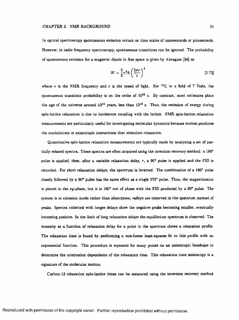
CHAPTER 2. NMR BACKGROUND 51
In optical spectroscopy spontaneous emission occurs on time scales of nanoseconds or picoseconds.
However, in radio frequency spectroscopy, spontaneous transitions can be ignored. The probability
of spontaneous emission for a magnetic dipole in free space is given by Abragam [34] as
where u is the NMR frequency and c is the speed of light. For 13C in a field of 7 Tesla, the
spontaneous transition probability is on the order of 1022 s. By contrast, most estimates place
the age of the universe around 1010 years, less than 1018 s. Thus, the emission of energy during
spin-lattice relaxation is due to incoherent coupling with the lattice. NMR spin-lattice relaxation
measurements are particularly useful for investigating molecular dynamics because motion produces
the modulations in anisotropic interactions that stimulate relaxation.
Quantitative spin-lattice relaxation measurements are typically made by analyzing a set of par
tially relaxed spectra. These spectra are often acquired using the inversion-recovery method: a 180°
pulse is applied, then, after a variable relaxation delay, r , a 90° pulse is applied and the FID is
recorded. For short relaxation delays, the spectrum is inverted. The combination of a 180° pulse
closely followed by a 90° pulse has the same effect as a single 270° pulse. Thus, the magnetization
is placed in the zy-plane, but it is 180° out of phase with the FID produced by a 90° pulse. The
system is in emission mode rather than absorption; valleys are observed in the spectrum instead of
peaks. Spectra collected with longer delays show the negative peaks becoming smaller, eventually
becoming positive. In the limit of long relaxation delays the equilibrium spectrum is observed. The
intensity as a function of relaxation delay for a point in the spectrum shows a relaxation profile.
The relaxation time is found by performing a non-linear least-squares fit to this profile with an
exponential function. This procedure is repeated for many points on an anisotropic lineshape to
determine the orientation dependence of the relaxation time. This relaxation time anisotropy is a
signature of the molecular motion.
Carbon-13 relaxation spin-lattice times can be measured using the inversion recovery method
Reproduced with permission of the copyright owner. Further reproduction prohibited without permission.
CHAPTER 2. NMR BACKGROUND 52
in a cross polarization experiment. Following polarization, a 90° pulse rotates the transverse mag
netization to the -z -ax is for the relaxation delay. The magnetization for short relaxation delays
would show the enhancement from cross polarization, but for long delays, the magnetization would
approach thermal equilibrium with the lattice. The equilibrium signal is typically about one-fourth
the intensity of the cross-polarized signal. However, since the precise ratio is not known, an ex
tra variable param eter is introduced into the fitting procedure. This source of systematic errors is
avoided by using the spin tem perature alternation technique [35]. On successive scans the magneti
zation is alternately placed along z and -z-axes prior to the relaxation delay by changing the phase
of the 90° pulse th a t follows cross polarization. When the magnetization is along - z , relaxation
causes if to grow to its equilibrium value, Meq:
M{t) = Mtq - (MCp + Af„) ex p (r/T l z ), [2 .7 4 ]
where Mc p is the magnetization produced by cross polarization. When placed along z the magne
tization decays from its enhanced value:
M (t) = + (MCp - M tq) exp( r / T l z ). [2.75]
Subtracting these two equations yields an exponential function th a t decays to zero:
M(t) = M c p e x p ( r /T iz ) . [2.76]
The subtraction is done during the experiment by changing the phase of the demodulating signal on
successive scans. The intensities in a set of spectra obtained using spin tem perature decay to zero
as a function of the relaxation delay.
M olecular M otion
Relaxation of a spin system to equilibrium in a static magnetic field is stimulated by incoher
ently fluctuating magnetic fields. Changes in The fluctuations are produced as molecular motion
modulates anisotropic interactions. The functions th a t describe the frequency distribution of the
Reproduced with permission of the copyright owner. Further reproduction prohibited without permission.
CHAPTER 2. NMR BACKGROUND 53
fluctuations are called spectral densities. Relaxation occurs most rapidly when the spectral densi
ties are large at the Larmor frequency. For systems with more than two energy levels, the spectral
densities at the frequencies of each of the transitions need to be considered. For dipolar relaxation,
the sum and difference of the Larmor frequencies of the interacting nuclei must be considered. For
deuterons, components a t uo and 2ui0 are important. Since molecular potentials in solids typi
cally consist of deep wells, motion is usually characterized as thermally activated jumps to discrete
orientations, or sites. At temperatures where molecular motion occurs at rates much slower than
the Larmor frequency, relaxation times are relatively long. As tem perature increases, the jump
raf e increases and relaxation occurs more quickly. As motional rates become greater than the Lar
mor frequency, relaxation times become shorter. For a thermally activated Markovian process, the
activation energy, £ a, can be found using the Arrhenius relation:
k = A exp(E a/k g T ) [2.77]
where E a is the activation energy, and k is the jum p rate. The pre-exponential factor, .4 is the
attem pt frequency, the jum p rate in the absence of a potential barrier [36]. The activation energy
and the attem pt frequency are found by plotting the logarithm of the jump rate versus inverse
tem perature. The slope of this graph is the activation energy, and the intercept is the attem pt
frequency.
In liquids, fast isotropic motion averages the anisotropy of the interactions. However, motion in
solids is typically restricted so that even the spectra of rapidly reorienting molecules retain some
orientation dependence. Relaxation time anisotropies depend sensitively on molecular geometry,
rate and trajectory of the motion. Molecular dynamics are characterized by comparing measured
anisotropies to those calculated for various molecular models.
Reproduced with permission of the copyright owner. Further reproduction prohibited without permission.

CHAPTER 2. NMR BACKGROUND 54
2.5.5 M ulti-Dimensional Techniques
The four time periods of a pulse sequence (preparation, evolution, mixing and detection) were
discussed in Section 2.3.1. Depending on the preparation of the spins, molecular motion, applied RF
fields or sample rotation, the Hamiltonian that governs the evolution of the spins in the evolution
time may be different from that during detection. In a two-dimensional experiment, the response
of the spins as a function of both the evolution and detection time is measured. This is typically
done by recording a number of FIDs, each with a different value of the evolution time. Each point
in this data set can be placed on a two-dimensional grid according to its value of evolution and
detection time. The spectrum is produced by a two-dimensional Fourier transform of the time
domain data. This idea can be extended to an arbitrary number of dimensions by putting multiple
variable evolution times into the pulse sequence.
Two types of multi-dimensional experiments can be classified as correlation and separation [11].
A correlation experiment allows resonances from nuclei that are coupled by an interaction to be
identified. Multi-dimensional correlation spectra provide information that cannot be obtained from
one-dimensional spectra. Separation techniques make use of one of the dimensions to enhance
resolution. This is done by spreading out overlapping resonances in the extra dimensions. The WISE
experiment discussed in the next section separates broad proton lines according to the chemical shifts
of the carbons to which they are strongly coupled. W ith the VACSY technique, the goal is to separate
l3C chemical shielding powder patterns on the basis of the isotropic chemical shift.
W ISE
Consider the pulse sequence for a wideline separation (WISE) [37,38,39] experiment shown in
Fig. 2.8. After the initial 90° pulse, the proton magnetization is allowed to evolve for a variable
evolution time, r . The magnetization that remains is then transferred to carbons by cross polariza
tion, and the carbon FID is collected with proton decoupling. If a series of FIDs is collected as a
function of the proton evolution time, the resulting d ata set contains NMR data as a function of two
Reproduced with permission of the copyright owner. Further reproduction prohibited without permission.
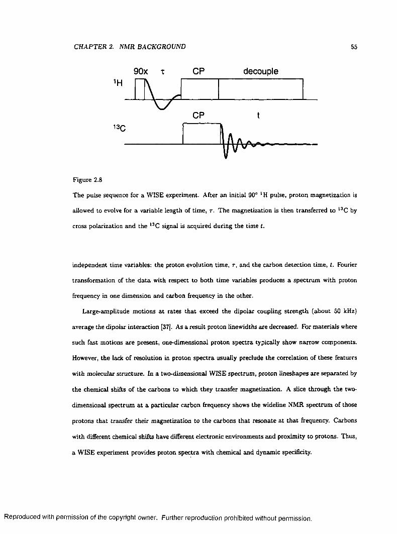
CHAPTER 2. NMR BACKGROUND 55
90x x CP decouple1H
CP t
13C
Figure 2.8
The pulse sequence for a WTSE experiment. After an initial 90° 1H pulse, proton magnetization is
cross polarization and the I3C signal is acquired during the time t.
independent time variables: the proton evolution time, r , and the carbon detection time, t. Fourier
transformation of the data with respect to both time variables produces a spectrum with proton
frequency in one dimension and carbon frequency in the other.
Large-amplitude motions at rates that exceed the dipolar coupling strength (about 50 kHz)
average the dipolar interaction [37]. As a result proton linewidths are decreased. For materials where
such fast motions are present, one-dimensional proton spectra typically show narrow components.
However, the lack of resolution in proton spectra usually preclude the correlation of these features
with molecular structure. In a two-dimensional WISE spectrum, proton lineshapes are separated by
the chemical shifts of the carbons to which they transfer magnetization. A slice through the two-
dimensional spectrum a t a particular carbon frequency shows the wideline NMR spectrum of those
protons that transfer their magnetization to the carbons that resonate at that frequency. Carbons
with different chemical shifts have different electronic environments and proximity to protons. Thus,
a WISE experiment provides proton spectra with chemical and dynamic specificity.
allowed to evolve for a variable length of time, r . The magnetization is then transferred to l3C by
Reproduced with permission of the copyright owner. Further reproduction prohibited without permission.
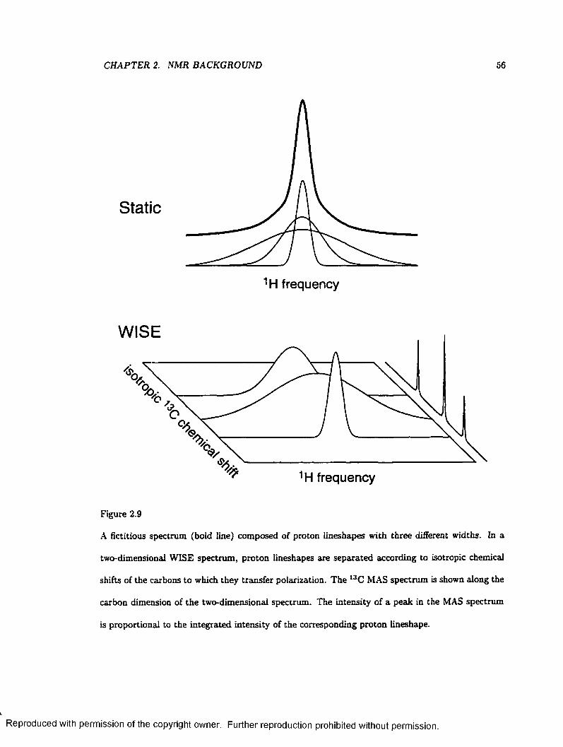
CHAPTER 2. NMR BACKGROUND 56
Static
1H frequency
WISE
1H frequency
Figure 2.9
A fictitious spectrum (bold line) composed of proton tineshapes with three different widths. In a
two-dimensional WISE spectrum, proton lineshapes are separated according to isotropic chemical
shifts of the carbons to which they transfer polarization. The 13 C MAS spectrum is shown along the
carbon dimension of the two-dimensional spectrum. The intensity of a peak in the MAS spectrum
is proportional to the integrated intensity of the corresponding proton lineshape.
Reproduced with permission of the copyright owner. Further reproduction prohibited without permission.

CHAPTER 2. NMR BACKGROUND 57
A variation on the WISE technique is designed to investigate spin diffusion. A l H -90° pulse
and a delay (usually 0.5-200 ms) are placed before CP. The pulse places the proton magnetization
along the laboratory z-axis so that dephasing will not occur in the delay that follows. Spin diffusion,
promoted by the strong homonuclear dipolar couplings, tends to equilibrate the proton magnetization
during this time. This is analogous to the process by which protons that are coupled to carbons
achieve a common spin tem perature during cross polarization. Proton spin diffusion in a WISE
experiment equalizes the proton linewidths in the two-dimensional spectrum. The rate at which
spin diffusion occurs indicates the proximity of the rigid and mobile domains in materials such as
phase separated polymers.
VACSY
The separation of overlapping I3C CSA powder patterns is a useful application of multi-dimensional
NMR. The lineshapes contain valuable information about orientation; however, the anisotropy is co
herently averaged when magic angle spinning is used. A two-dimensional spectrum, like that shown
in Fig. 2.10, that has the isotropic chemical shift in one dimension and the anisotropic powder
patterns in the other. This allows chemical shift anisotropies to be measured while retaining the
chemical shift resolution of a MAS experiment.
To produce a two-dimensional spectrum using the prescription stated a t the beginning of this
section, we would need to allow the system to evolve under the anisotropic (or isotropic) chemical
shielding interaction alone for a variable period of time and collect the signal during evolution under
the isotropic (or anisotropic) chemical shift. This is impossible because isotropic chemical shift
cannot be scaled independently of the components of the shift tensor. The VACSY technique uses
a different approach; the signal is collected as the system evolves under both the isotropic and
anisotropic chemical shielding interactions. The width of a powder pattern in spinning sample is
shown to depend on the angle between the spinning axis and the static field, 0 rl in Eq. 2.63. The
Reproduced with permission of the copyright owner. Further reproduction prohibited without permission.
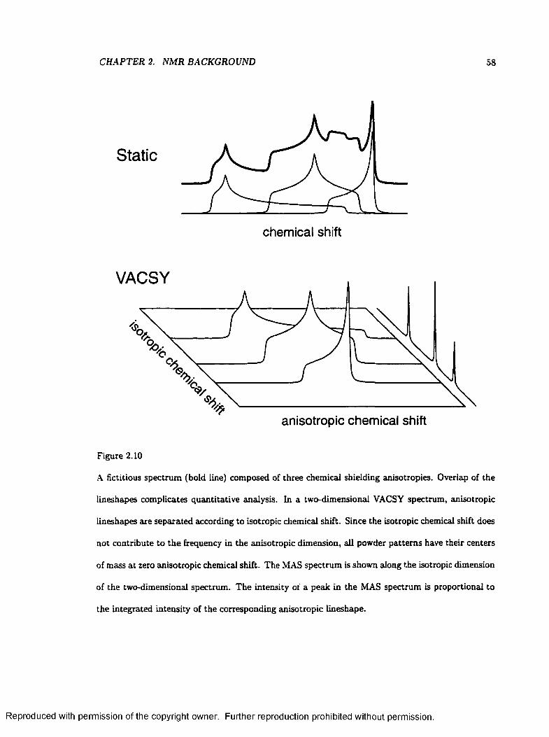
CHAPTER 2. NMR BACKGROUND 58
Static
chem ical shift
VACSY
anisotropic chem ical shift
Figure 2.10
A fictitious spectrum (bold line) composed of three chemical shielding anisotropies. Overlap of the
lineshapes complicates quantitative analysis. In a two-dimensional VACSY spectrum, anisotropic
lineshapes are separated according to isotropic chemical shift. Since the isotropic chemical shift does
not contribute to the frequency in the anisotropic dimension, all powder patterns have their centers
of mass at zero anisotropic chemical shift. The MAS spectrum is shown along the isotropic dimension
of the two-dimensional spectrum. The intensity of a peak in the MAS spectrum is proportional to
the integrated intensity of the corresponding anisotropic lineshape.
Reproduced with permission of the copyright owner. Further reproduction prohibited without permission.

CHAPTER 2. NMR BACKGROUND 59
expression is the sum of a constant term and a term that depends on the spinning angle:
<7 = <7«jo ■+■ dgo (/?a/,)<ronii0, [2.78]
where
^ a n u o = (<^L 1 COS2 Q p R + £T2 2 sin2 O p r ) Sin2 0 P R + (7 3 3 COS2 / J p f i - CT1JO [2.79]
and apR and 0 pr are the Euler angles for the principal axis to rotor frame transformation. One
can imagine these two terms arising from two different interactions: the isotropic chemical shift,
and the anisotropic chemical shift. The former leads to a sharp line in the spectrum, and the latter
results in a powder pattern. By varying the spinning axis, the strength of the anisotropic interaction
is changed. Thus, the rate a t which the system evolves in the anisotropic dimension is scaled by
(0r l ). Because the isotropic chemical shift is unaffected by the spinning angle, the rate at which
the system evolves in the isotropic dimension does not change. As a result, the FIDs collected for
the various spinning angles trace out rays in the two-dimensional time plane, as shown in Fig 2.11.
The irregular sampling of the two-dimensional time plane poses some problems with processing
the FIDs to produce artifact-free two-dimensional spectrum. The region near the origin of the time
plane are sampled very densely, while far away the sampling is sparse. It is fortunate, though, that
the sparsely sampled regions are those with large values of t ito and tan„0. Since the FID has its
maximum at t = 0 these regions contain little signal intensity. Discrete Fourier transform routines
require a grid of evenly spaced points. Such a grid can be produced interpolating the measured data.
A linear interpolation in the anisotropic time dimension is typically adequate.
Because of limitations in the values of <4qq (0rl ) that can be obtained, two triangular regions are
not sampled a t all. (See Fig. 2.11) The minimum value of c { 0 r l ) is - 1 /2 for 0 rl = 90°. The
maximum value is 1 for Prl = 0°; however, an NMR signal cannot be observed at this orientation
because the sample coil is parallel to the external field. Values of 0 rl less than about 35° are
impractical. Thus, < ^ { 0 r l ) usually ranges from -1 /2 to 1/2. Because the signal decays rapidly
in the anisotropic dimension, the large regions of the two-dimensional time plane that cannot be
Reproduced with permission of the copyright owner. Further reproduction prohibited without permission.
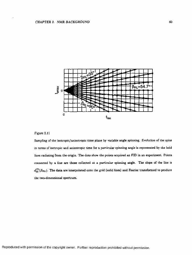
CHAPTER 2. NMR BACKGROUND 60
Figure 2.11
Sampling of the isotropic/anisotropic time plane by variable angle spinning. Evolution of the spins
in terms of isotropic and anisotropic time for a particular spinning angle is represented by the bold
lines radiating from the origin. The dots show the points acquired an FID in an experiment. Points
connected by a line are those collected a t a particular spinning angle. The slope of the line is
r l ). The da ta are interpolated onto the grid (solid lines) and Fourier transformed to produce
the two-dimensional spectrum.
Reproduced with permission of the copyright owner. Further reproduction prohibited without permission.

CHAPTER 2. NMR BACKGROUND 61
sampled contain little signal. In many cases, a reasonable spectrum is produced if the unsampled
regions are simply set to zero. There are, however, characteristic artifacts produced by this gridding
procedure. The unsampled regions produce diagonal ridges in the spectrum [40]. These ridges may
distort powder patterns of carbons with similar isotropic chemical shifts.
If necessary, the artifacts from the unsampled region can be lessened by extrapolating the data
into the unsampled region. One successful method of extrapolation is linear prediction with singular
value decomposition [41]. Linear prediction is so named because it involves solving a set of linear
equations. First the data are interpolated onto a rectangular grid. Every slice through the two-
dimensional time domain data set in the isotropic dimension shows evolution under the isotropic
Hamiltonian. Thus, these slices can be assumed to be the sum of oscillatory functions modulated by
decaying exponential envelopes. The linear prediction with singular value decomposition procedure
[41] uses matrix techniques to find the frequencies, amplitudes and decay rates that best fit the
d ata available in the slice. The user enters the number of peaks in the spectrum and the number of
d ata points to fit. Once the best-fit function is found, it is evaluated for the points that lie in the
unsampled region. Slices near t a n x,a = 0 that have only a few unsampled points can be accurately
extrapolated. However, the procedure tends to be unstable when the signal to be extrapolated is
noisy [41].
A second kind of artifact is produced by the non-uniform sampling of t i g0- t a n i , 0 plane. However,
the artifact is only noticeable in spectra with wide powder patterns and good a signal-to-noise ratio.
Small ridges radiate from each powder pattern in all directions. The cause is the decrease in the
density of data points in the anisotropic dimension as Us0 increases. If the spinning angles are chosen
such that the d ata points are spaced evenly in the anisotropic dimension, the anisotropic dwell time
is given by:
td .a m s o = — , [2.80]
where do is the smallest value of the spinning angle used, and N is the number of spinning angles.
For a typical VACSY experiment, 31 FIDs are collected for spinning angles ranging from 35° to
Reproduced with permission of the copyright owner. Further reproduction prohibited without permission.
CHAPTER 2. NMR BACKGROUND 62
90°. The anisotropic dwell time, td,0m»o = t.jo/30, corresponds to a spectral width of 1/2U,ani,0 or
15/ t„ 0. Thus, after only 15 ms the spectral width is down to 1 kHz. Although some FIDs can last
for more than 50 ms, the effect of this bandwidth limiting on the spectra is usually negligible because
the intensity of the NMR signal is greatest a t short times. When the data are interpolated onto a
regular grid, the spacing of the interpolated points determines the spectral width in the anisotropic
dimension. This spectral width can be chosen to be arbitrarily large. However, the interpolation
does not add any information about high frequency components. The remedy for these artifacts, if
needed, would be to collect FIDs at more angles. However, any improvement in the spectrum would
almost certainly not be worth the additional spectrometer time.
Other complications of the VACSY technique stem from the fact that the sample is physically
reoriented throughout the course of an experiment. This means that the sample occupies a different
volume inside the magnet for each of the different FIDs. As a result the contribution of field
homogeneity to linewidths is a function of spinning angle. As the spinning angle changes, the wires
that connect to the sample coil bend. Even a small change in the conformation of a wire in the
resonant circuit can significantly change the tuning of the probe. As a result, the variable capacitors
in the tuning circuit must be adjusted each time the spinning angle is changed. For the experiments
described in this dissertation, I fitted the probe with sliding contacts so that the spinning angle
could be changed without flexing any wires. W ith this modification, an entire VACSY experiment
can be performed without retuning.
Reorientation of the spinning angle results in reorientation of the time-dependent radio frequency
field B \ . Only the component of B\ in the laboratory xy-plane serves to rotate the nuclear mag
netization. To ensure th a t the 90° pulses in the sequence rotate the magnetization by 90° for each
spinning angle, the length of the pulse (fgo) is changed according to
• " « “ > - 12811
Although a number of technical challenges complicate the performance of a VACSY experiment,
Reproduced with permission of the copyright owner. Further reproduction prohibited without permission.
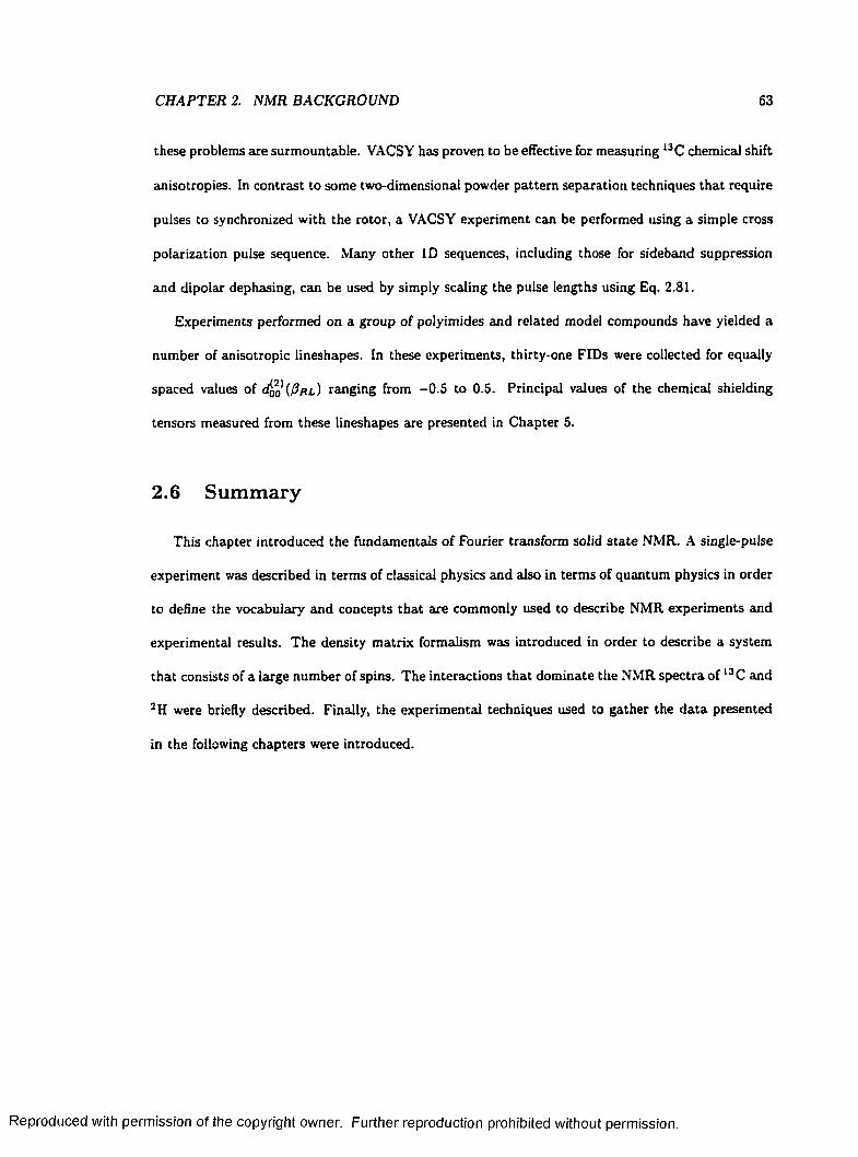
CHAPTER 2. NMR BACKGROUND 63
these problems are surmountable. VACSY has proven to be effective for measuring 13C chemical shift
anisotropies. In contrast to some two-dimensional powder pattern separation techniques that require
pulses to synchronized with the rotor, a VACSY experiment can be performed using a simple cross
polarization pulse sequence. Many other ID sequences, including those for sideband suppression
and dipolar dephasing, can be used by simply scaling the pulse lengths using Eq. 2.81.
Experiments performed on a group of polyimides and related model compounds have yielded a
number of anisotropic lineshapes. In these experiments, thirty-one FIDs were collected for equally
spaced values of d g l ranging from -0 .5 to 0.5. Principal values of the chemical shielding
tensors measured from these lineshapes are presented in Chapter 5.
2.6 Summary
This chapter introduced the fundamentals of Fourier transform solid sta te NMR. A single-pulse
experiment was described in terms of classical physics and also in terms of quantum physics in order
to define the vocabulary and concepts that are commonly used to describe NMR experiments and
experimental results. The density m atrix formalism was introduced in order to describe a system
that consists of a large number of spins. The interactions that dominate the NMR spectra o f 13 C and
2H were briefly described. Finally, the experimental techniques used to gather the data presented
in the following chapters were introduced.
Reproduced with permission of the copyright owner. Further reproduction prohibited without permission.
Chapter 3
Powder Pattern Calculations
In 13 C NMR spectra, shielding of the external magnetic field by local electrons results in different
resonance frequencies for every magnetically distinct 13 C nucleus. This interaction is called chemi
cal shielding; the resulting frequency change is the chemical shift. The anisotropy of the chemical
shielding interaction leads to powder patterns in polycrystalline or amorphous samples. This chapter
presents an original method for calculating the powder lineshapes that arise from chemical shielding
anisotropy and other second-rank tensor interactions. First, some of the common techniques for
calculating powder patterns are reviewed. Then the analytical expression for the intensity as a func
tion of frequency on a powder lineshape is derived. This expression is then modified to produce an
efficient algorithm for numerical calculation. Lastly, applications of this method are demonstrated.
These applications include non-linear least-squares fitting of experimental spectra, calculation of
lineshapes from partially oriented samples, and calculation of partially relaxed lineshapes. All of
the methods discussed here can be used to calculate powder patterns arising from any second-rank
interaction, such as the dipolar or quadrupolar interactions. However, in the interest of presenting
consistent notation, this discussion will focus on the chemical shielding interaction which was intro
duced in Section 2.4.2. Most of the material presented in this chapter was published in Journal of
Magnetic Resonance, Series A, 123 (1996).
64
Reproduced with permission of the copyright owner. Further reproduction prohibited without permission.
CHAPTER 3. POWDER PATTERN CALCULATIONS 65
3.1 Common M ethods of Powder Pattern Calculation
The analytical expression describing the intensity of a powder pattern as a function of frequency
involves an elliptic integral which must be evaluated at each point on the lineshape [6 ]. In gen
eral, elliptic integrals cannot be evaluated in closed form, and their series approximations converge
slowly. The difficulty of calculating powder patterns from the analytical expression has motivated
the development of alternative methods.
The most commonly used strategy for calculating powder lineshapes involves constructing a
histogram of NMR frequencies for a number of orientations of the principal axis system of the
chemical shielding tensor with respect to the static magnetic field. For the principal axis system of
a particular shielding tensor, the orientation of the external magnetic held is described by polar 0
and azimuthal angle 7 . Each orientation can be represented by a vector that indicates the direction
of the external held in the principal axis system of the interaction, as shown in Fig. 3.1. For each
orientation the resonance frequency is calculated from the Hamiltonian, and intensity is added to the
calculated spectrum a t that frequency. For a uniform distribution of orientations, the contribution
to the intensity of the pattern is the same for each orientation; however, non-uniform sampling is
more efficient [42,43]. To determine the intensity added to the spectrum for each orientation, the
unit sphere centered a t the origin of the principal axis system is partitioned into tiles such that each
orientation intersects one tile. The intensity added to the spectrum for a particular orientation is
proportional to the area of the tile that it intersects. Algorithms th a t use this strategy for calculating
powder patterns are called tiling schemes [42,43,44].
A simple tiling m ethod with uniform sampling of the polar and azimuthal is easily implemented
on a computer; however, this algorithm is not very efficient in terms of computation time. A large
number of angles must be considered in order to produce a sm ooth lineshape. Some refinements to
the simple tiling algorithm have been made in the interest of reducing computation time. One such
method, that tiles a unit octahedron ra ther than a sphere [44], is depicted in Fig. 3.2. The simplified
Reproduced with permission of the copyright owner. Further reproduction prohibited without permission.
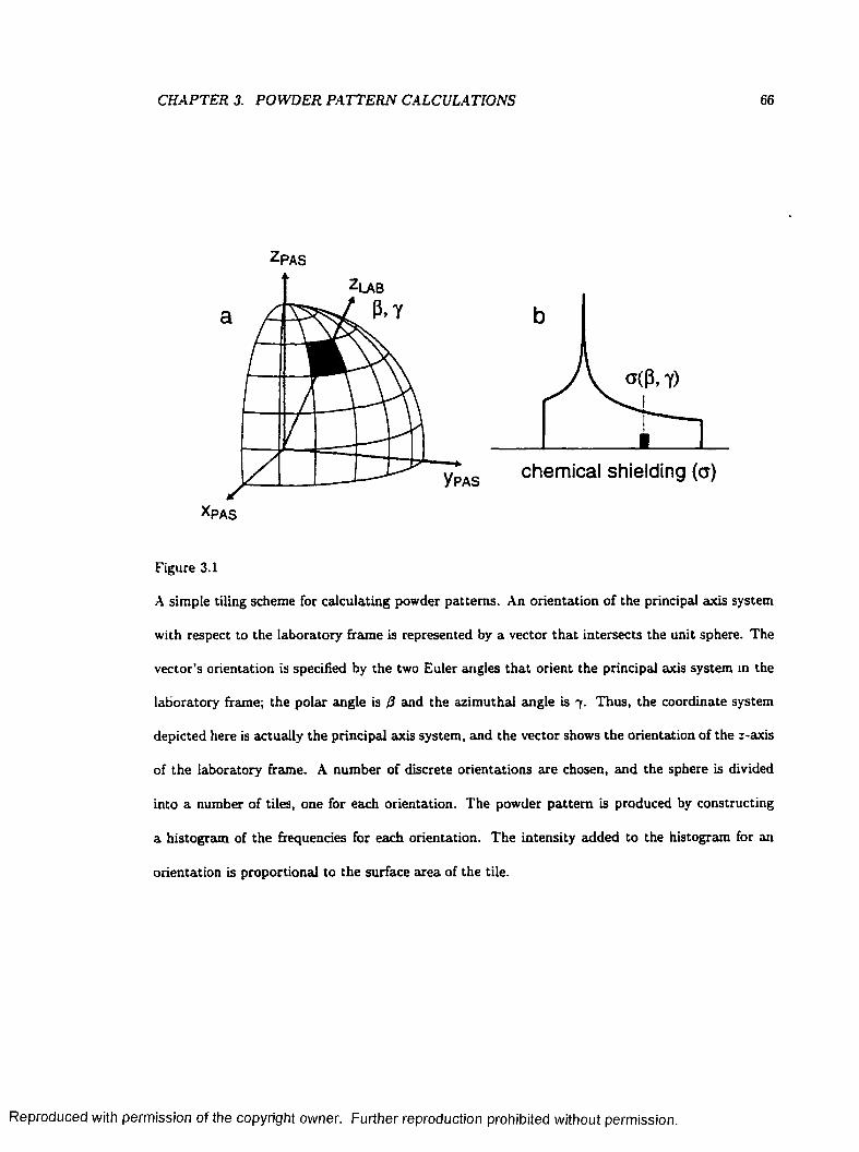
CHAPTER 3. POWDER PATTERN CALCULATIONS 66
ZPAS
chem ical shielding (a)
XPAS
Figure 3.1
A simple tiling scheme for calculating powder patterns. An orientation of the principal axis system
with respect to the laboratory frame is represented by a vector th a t intersects the unit sphere. The
vector’s orientation is specified by the two Euler angles that orient the principal axis system in the
laboratory frame; the polar angle is 0 and the azimuthal angle is 7 . Thus, the coordinate system
depicted here is actually the principal axis system, and the vector shows the orientation of the z-axis
of the laboratory frame. A number of discrete orientations are chosen, and the sphere is divided
into a number of tiles, one for each orientation. The powder pattern is produced by constructing
a histogram of the frequencies for each orientation. The intensity added to the histogram for an
orientation is proportioned to the surface area of the tile.
Reproduced with permission of the copyright owner. Further reproduction prohibited without permission.
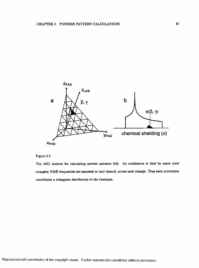
CHAPTER 3. POWDER PATTERS CALCULATIONS 67
ZpAS
chem ical shielding (a)
Figure 3.2
The ASG method for calculating powder patterns [44]. An octahedron is tiled by equal sized
triangles; NMR frequencies are assumed to vary linearly across each triangle. Thus each orientation
contributes a triangular distribution to the lineshape.
Reproduced with permission of the copyright owner. Further reproduction prohibited without permission.

CHAPTER 3. POWDER PATTERN CALCULATIONS 68
geometry eliminates the need to calculate trigonometric functions and allows the surface to be tiled
with triangles of equal size. The differences between the solid angles subtended by the tiles on
an octahedral face are accounted for by an approximate algebraic correction factor. In addition,
frequencies are assumed to vary linearly across each tile. Thus, each tile contributes a triangular
distribution of frequencies rather than a single frequency. The result is that many fewer tiles are
needed to produce a smooth lineshape. This method, published by Alderman, Solum, and Grant
[44], will be referred to as the ASG method throughout this work.
Calculation of the time domain signal due to an anisotropic second-rank interaction in a powder
sample can provide some performance advantages over the frequency domain methods [45]. Instead
of adding intensity to a histogram to form the lineshape, an oscillating signal (with a frequency
determined by the Hamiltonian and intensity determined by tiling] is added to the time domain
signal to form the FID. The number of trigonometric functions that need to be evaluated is greatly
reduced by the use of a propagator for time evolution under the Hamiltonian. Furthermore, line
broadening can be applied independently to each of the individual components. This feature is
essential for the calculation of lineshapes with orientation-dependent spin-spin relaxation times.
Other variations on the tiling scheme use optimized orientation distributions or sophisticated
interpolation methods to speed calculation [42,46,47,43]. The new algorithm presented here is not
a tiling scheme. Efficiency is achieved by making use of the fact that, for symmetric tensors, the
lineshape expression reduces to an algebraic formula. Asymmetric powder patterns are calculated as
sums of lineshapes from symmetric tensors. This approach exploits the computer’s ability to evaluate
algebraic expressions quickly. Also, there is no variable param eter th a t determines the quality of the
lineshape; the algorithm always produces a smooth powder pattern. The lineshapes that are added
to produce the powder pattern will be referred to as subspectra. The technique is called Simulation
Using Multiple Subspectra, or SUMS. Because many simulations can be performed in a short time,
autom ated nonlinear least-squares fitting of experimental lineshapes is feasible, yielding results that
do not rely upon subjective judgment of the quality of fit. As with the tiling methods, a modification
Reproduced with permission of the copyright owner. Further reproduction prohibited without permission.

CHAPTER 3. POWDER PATTERN CALCULATIONS 69
of the SUMS algorithm can be used to calculate partially relaxed or partially oriented lineshapes.
3.2 Analytical Derivation
This section contains a derivation of the analytical expression for the lineshape from the properties
of the chemical shielding Hamiltonian. The expression is modified in the method section to produce
the approximate form that will be used to calculate powder patterns numerically.
To calculate a lineshape that arises from chemical shielding anisotropy, we consider a Hamiltonian
that is the sum of Zeeman and chemical shielding terms:
H = Ht + Ha
= - y h f - Bq + yh l a ■ Bo- [3.1]
The resonant frequency of a nucleus subject to these interactions was shown, in Section 2.4.2, to be
u> = wo(l — <t) [3.2]
where
a - {ati cos2 7 + cr22 sin2 7 ) sin2 (3 + 033 cos2 0. [3.3]
The angles 0 and 7 are the Euler angles that describe the orientation of the principle axis system in
the laboratory system. The angle a describes a rotation about the direction of the static magnetic
field. Due to the cylindrical symmetry of the field, such rotations have no effect on the Hamiltonian.
The orientation-dependence of the chemical shielding interaction leads to powder patterns in the
NMR spectra of polycrystalline or amorphous samples.
A strategy for calculating powder lineshapes arises from the recognition that the intensity in an
NMR spectrum at a given frequency, / (cr), is proportional to the number of nuclei resonating at
that frequency. An equivalent statem ent is that / (cr) is proportional to the probability that a ran
domly chosen nucleus will resonate a t frequency <x. Thus, simulation of a powder lineshape requires
calculation of the probability th a t the principal axis system is oriented such that the frequency has
Reproduced with permission of the copyright owner. Further reproduction prohibited without permission.
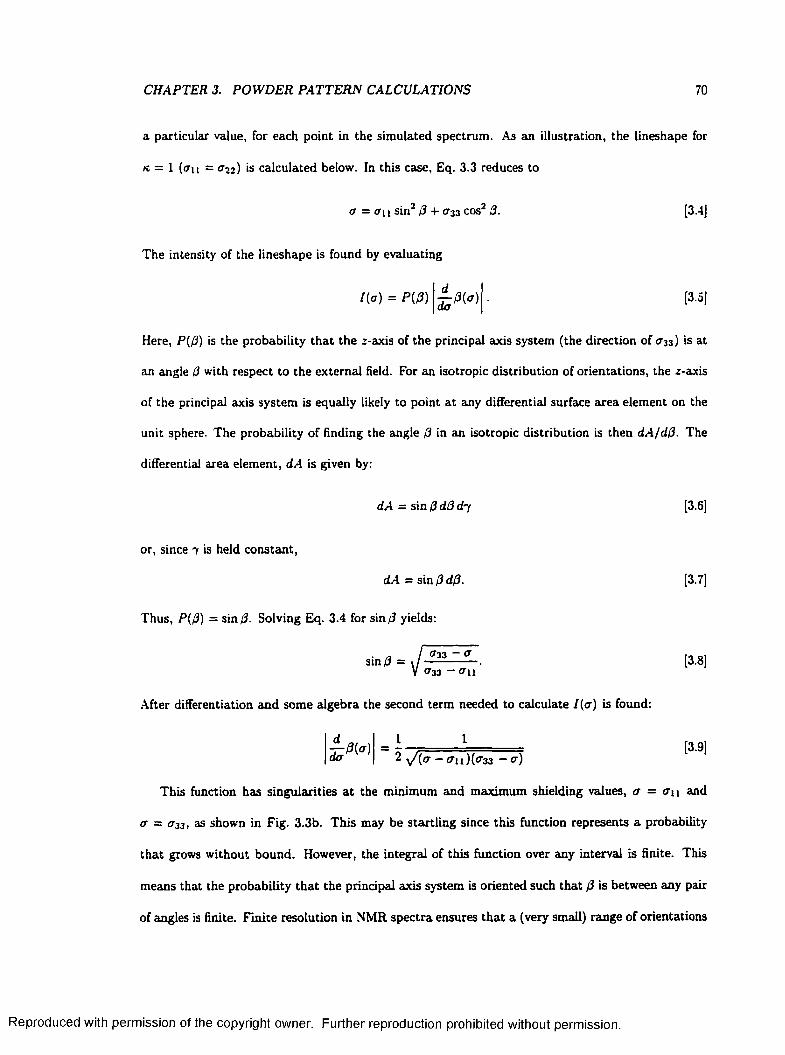
CHAPTER 3. POWDER PATTERN CALCULATIONS 70
a particular value, for each point in the simulated spectrum. As an illustration, the lineshape for
k — 1 (<7n — a 22) is calculated below. In this case, Eq. 3.3 reduces to
Here, P(0) is the probability that the z-axis of the principal axis system (the direction of <733) is at
an angle 0 with respect to the external field. For an isotropic distribution of orientations, the 2-axis
unit sphere. The probability of finding the angle 0 in an isotropic distribution is then dA/d0. The
differential area element, dA is given by:
This function has singularities a t the minimum and maximum shielding values, a = <7u and
a — <7-33, as shown in Fig. 3.3b. This may be startling since this function represents a probability
that grows without bound. However, the integral of this function over any interval is finite. This
means that the probability that the principal axis system is oriented such that 0 is between any pair
of angles is finite. Finite resolution in NMR spectra ensures that a (very small) range of orientations
<7 = <ru sin2 0 + <733 cos2 0. [3.4]
The intensity of the lineshape is found by evaluating
1(a) = P(0) ± 0 ( a ) . [3.5]
of the principal axis system is equally likely to point at any differential surface area element on the
dA = sin 0 d0 dry [3.6]
or, since 7 is held constant,
dA = sin 0 d0. [3.7]
Thus, P(0) = sin 0. Solving Eq. 3.4 for sin/J yields:
[3.8]
After differentiation and some algebra the second term needed to calculate /(cr) is found:
2 y/(a -< 7u)(<733 - cr)1 [3.9]
Reproduced with permission of the copyright owner. Further reproduction prohibited without permission.
CHAPTER 3. POWDER PATTERN CALCULATIONS 71
C O .
o'
30 60 900
C!
■o
8
4
2
0
P (degrees) o(P)
Figure 3.3
A non-uniform chemical shielding distribution arising from a uniform angular distribution for an
axially symmetric shielding tensor. Shielding as a function of the angle between the z-axis of the
principal axis system and the external field, <r(0), is shown in (a). The vertical lines depict a uniform
sampling of angles, 0. The horizontal lines show that o{0) is not sampled uniformly. The probability
that the principal axis system of a nucleus is oriented such that the nucleus experiences a shielding
of <r is proportional to the derivative of 0 with respect to a. This derivative, divided by the span
of the shielding tensor (fl = 033 - 0 a ), is plotted in (b). The graph shows that shieldings near the
principal values, cru and <733, are the most probable.
Reproduced with permission of the copyright owner. Further reproduction prohibited without permission.
CHAPTER 3. POWDER PATTERN CALCULATIONS 72
contribute to each point. In the method presented here, infinite values are avoided by integrating
over small frequency ranges to obtain the intensity for a point in the discrete spectrum.
The analytical form of the intensity for an axially symmetric powder pattern, normalized to an
integrated intensity of one, is found by substituting Eqs. 3.8 and 3.9 into Eq. 3.5:
= - Lu (3.101
The singularity in \d0/da\ at <733 is removed since P{0) goes as (<733 - cr) 1''2 and \d0/do\ goes as
(< 7 3 3 - a)~U2 near that point. The result shown in Eq. 3.10 also holds for skews other than ±1 if
the angle 7 is fixed and a u is replaced by (<7U cos3 7 + 022 sin2 7 ):
/ ( g ) = l - -------------------- 1 - [3.11](<733 - ffn COS2 7 - <722 sin3 7)(<7 - <7U COS2 7 - <722 sin2 7 )
To calculate the general form of a spin- 5 powder lineshape, Eq.3.11 is integrated with respect to
7 . The variable of integration, 7 , appears only as the argument of squared trigonometric functions.
Due to the symmetry of these functions, the integration can be restricted to the first quadrant. The
integrand is weighted by the probability th a t the nucleus has its shielding tensor oriented at Euler
angle 7 with respect to the lab frame, P(7 ). In a powder, all values of 7 are equally probable; thus,
P (7 ) = 2 /7r. The analytical expression for a powder lineshape can now be written:
dy1(a) = -R e7T / ’JO
(3.121y / ( a 3 2 - <7U COS2 7 - <722 sin2 7)(<7 - <7u cos2 7 - <722 sin2 7 )
W ith an appropriate change of variables, this expression can be put into the form of a complete
elliptic int r g r a l [6 ], Although this analytical result is compact and well-defined it does not lend itself
to efficient computational evaluation.
3.3 The SUMS M ethod
In devising a computer algorithm for calculating powder patterns, a logical first step would be
to change the integral in Eq. 3.12 to a summation over equally spaced values of 7 . However, because
Reproduced with permission of the copyright owner. Further reproduction prohibited without permission.
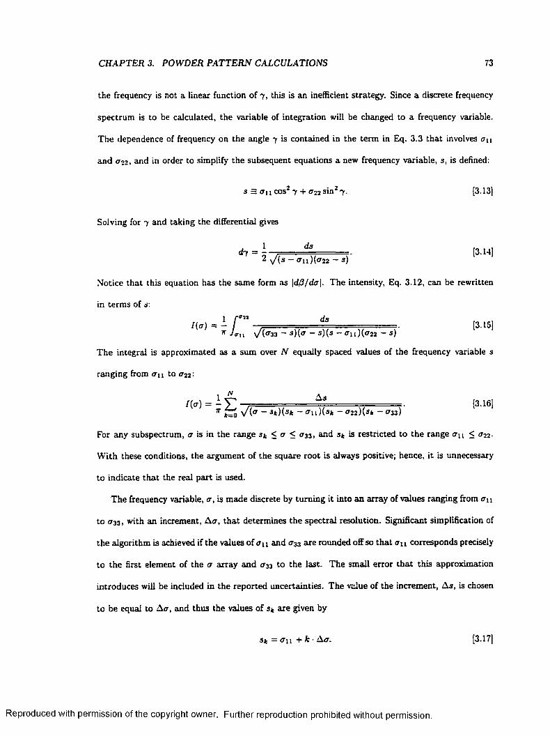
CHAPTER 3. POWDER PATTERN CALCULATIONS 73
the frequency is not a linear function of 7 , this is an inefficient strategy. Since a discrete frequency
spectrum is to be calculated, the variable of integration will be changed to a frequency variable.
The dependence of frequency on the angle 7 is contained in the term in Eq. 3.3 that involves <7U
and <722, and in order to simplify the subsequent equations a new frequency variable, s, is defined:
s = <7i 1 cos2 7 + <722 sin2 7 . [3.13]
Solving for 7 and taking the differential gives
d'r = \ , dS [3.14]2 y/(s — <7u )(<722 - s)
Notice that this equation has the same form as \d0/da\. The intensity, Eq. 3.12, can be rewritten
in terms of s:1 r a n d a
1(a) = - / . [3.15]K J*u y/(oz3 ~ a)(a - s)(s - <rn)(<722 - s)
The integral is approximated as a sum over N equally spaced values of the frequency variable s
ranging from <7u to <722:
1(a) = i £ ■V k^O V 1 ~ •Sfc)(3 fc ~ <7 u ) ( S f c “ * 22 ) ( « f c “ <7 3 3 )
[3.16]
For any subspectrum, a is in the range s t < <7 < < 7 3 3 , and s t is restricted to the range < 7 n < <722-
W ith these conditions, the argument of the square root is always positive; hence, it is unnecessary
to indicate that the real part is used.
The frequency variable, < 7 , is made discrete by turning it into an array of values ranging from <7u
to < 7 3 3 , with an increment, A < 7 , th a t determines the spectral resolution. Significant simplification of
the algorithm is achieved if the values of < 7 n and < 7 3 3 are rounded off so that < 7 u corresponds precisely
to the first element of the a array and < 733 to the last. The small error that this approximation
introduces will be included in the reported uncertainties. The value of the increment, As, is chosen
to be equal to A<7 , and thus the values of St are given by
S k = a n + k - A a . [3-17]
Reproduced with permission of the copyright owner. Further reproduction prohibited without permission.
CHAPTER 3. POWDER PATTERN CALCULATIONS 74
i0 20 40 60
points
Figure 3.4
Construction of an asymmetric lineshape with k = 0.3 from axially symmetric subspectra. A
spectrum with only 32 points is shown so that the 12 individual subspectra can be discerned.
It is im portant to note that N is the number of points from cru to cr22, not the total number of
points in the spectrum. Inspection of Eq. 3.16 shows th a t the calculated lineshape is composed of
N axially symmetric (k = 1 ) powder patterns, which will be referred to as subspectra, with various
widths and weighting factors. This can be seen more clearly if the weighting factors and constants
are absorbed into a single term, At:N
/ ( < r ) = 2 > fcBt [3.18]Jfc= 0
where
and
Afc = - ■■ Ag [3.19]v (s* -o'nK aik -<T22)(sfe - * 33)
B k = r - - ^ • [3.20]y ja - Sk
The subspectra and their sum are shown in Fig. 3.4, for a 32 point spectrum with a skew, k = 0.3.
Reproduced with permission of the copyright owner. Further reproduction prohibited without permission.

CHAPTER 3. POWDER PATTERN CALCULATIONS 75
It appears as though a subspectrum and a weighting function must be evaluated for each value
of the frequency variable, s, in order to generate the spectrum. However, all subspectra can be
generated by truncating the widest subspectrum and shifting the origin. To illustrate this, consider
the widest (k = 0) and narrowest (k = N) subspectra used in the calculation of a powder pattern.
In these cases Eq. 3.18 gives
/„(*) = - A° - - [3.21]y/a - ctu
/* (* ) = [3-22]y / ( T — ^ 2 2
To calculate a subspectrum, only values of the shielding such that s* < a < <733 need to be considered.
Values outside of this range are not achievable for any value of 0■ For the widest subspectrum, a
starts a t ctu and goes to ct33. Thus, a - a n has values that are multiples of Act in the range of zero
to CT33 — a n . The narrowest subspectrum starts at a33 and extends to C T 3 3 . The values cl a - a33 are
also multiples of A c t , but in a smaller range, zero to CT33 - < 7 2 2 - The denominators in Eq. 3.22 are a
subset of those in Eq. 3.21; they need not be calculated again. With this observation, the calculation
of an arbitrary powder pattern is reduced to the calculation of a single symmetric lineshape and N
weighting functions.
Because a discrete spectrum is calculated, the intensity of a point on a subspectrum is obtained
by integrating Eq. 3.18 over a frequency bin:
/(ct.) = f ’+1 I(a)do. [3.23]
If Ak is assumed to be constant, Eq. 3.18 becomes
y/Ui - St N ______________
= 2 ^ r Ak(y/crt+i — St — \ /a i - sk )• [3-24]k-0
This integration removes the singularity in the subspectra at s. Although the intensity at ct, = s*
is undefined, its integral over any interval, even one th a t includes s, is finite.
Reproduced with permission of the copyright owner. Further reproduction prohibited without permission.

CHAPTER 3. POWDER PATTERN CALCULATIONS 76
The value of the weighting function used for a given subspectrum is the average of .4* across the
bin that runs from s* to s*+i. Thus, the weighting factors must be integrated over successive values
of sk. Although this integration cannot be done in closed form, an approximation that is valid for
integration over small intervals can be made. Since sk ranges from a n to <732, the pole due to the
(<733 - sk) term is not encountered and the slope of ( 0 3 3 - sk)~ 1 2 remains fairly small. Regarding
(<733 - s * ) -1/2 as constant over one frequency bin allows th a t term to be removed from the integral:
A * = -1 Act 1 f , k dsk7T >/CT33 - Sk Act JSi y / (sk - CTu) (CT22 - 3* )
= I - - 1- tan - 1 . I 8* ' ,— ” " - ta n - 1 J SJl Z £ H ) . [3.25]* V 0 3 3 ~ S k \ V a n ~ S k - r l V <*22 ~ s k J
Since the average value of At is used as the weighting factor for a given subspectrum, it is reasonable
to choose the position of the pole for that bin to be halfway in between sk and sk+1:
Sk* = r +‘ 7 = ^ = [3.26]Ja. s/a - sk
2 [ \ / a x+i - sk - Act/2 - s /a t - sk - Act/2 ) .
The algebraic equation that will be evaluated in order to simulate a powder pattern is
N - 1
/(ct.) = £ A k B k , . [3.27]t=o
The number of square root and inverse tangent operations is minimized by calculating one array for
(cti - ctu)^ and one for ta n - l [(sfc - c tu )1 2 /(ct22 - sfc)1/2]. The difference term s in Eqs. 3.25 and
3.27 are then obtained by subtracting array elements.
Using the algorithm as described, the lineshapes produced contain some small distortions. The
distortions show up near the poles of the weighting factor array, A*, at a = ctu and a = a22, where
the approximation that A* is constant is invalid. The calculated value of the point at a — ctu is
underestimated by about 2 0 % and the point at ct = ct22 is too intense by approximately the same
amount. As a result, points near ctu and CT22 differ from the correct values by one or two percent.
These features can be removed by calculating a correction array that will be subtracted from the
Reproduced with permission of the copyright owner. Further reproduction prohibited without permission.
CHAPTER 3. POWDER PATTERN CALCULATIONS 77
portion of the spectrum between the discontinuities at era and (T22 . The correction to the first point
in each subspectrum is made by assuming that .4* varies linearly across each frequency bin. The
integrated intensity from the left hand edge to some position, a, of a subspectrum is
[ {a - Sfc)- da = 2a*. [3.28]J*h
To find the intensity of the first point of the kth subspectrum, this result is integrated over the bin
a x = sk, weighted by a linear extrapolation of .4t from the edge of the bin:
/(<r, = i f * ' ^ .4 , + a j da
[3.29]
The first term in Eq. 3.29 does not depend on the slope of the weighting function and is close to the
value that has already been calculated for the first point of a subspectrum. Thus, it is the second
term that will be used to calculate the correction array to be applied to the region of the spectrum
between <xu and ct22- As a result (033 — s*) is large for all s t and is approximated as the span of
the tensor, fi. The correction array has the form
C{Sk) = 1 ( 2 * - * n - O t a ) [3 301
l O T T ^ n [(<X22 - S fc ) (s fc - f f n ) ] s
Since the integrated intensity of a subspectrum is conserved, the intensity that is removed from the
first point is distributed among the other points. The second point receives most of this intensity.
A reasonable correction is made by assuming that 60% of the intensity lost by the first point in the
subspectrum is added to the second, and that the remaining intensity can be disregarded.
The assumption that the weighting function array is linear cannot be made near its poles, that
is, for the first and last subspectra. However, I {an) can be found analytically from the elliptic
integral expression, and is
l i p n ) = j \ . - - - [3-31]
Reproduced with permission of the copyright owner. Further reproduction prohibited without permission.

CHAPTER 3. POWDER PATTERN CALCULATIONS 78
Table 3.1
Comparison of Powder P attern Calculation Times In Seconds for Three Algorithms
128 points
a = 0
256 points 512 points 128 points
k = 0.5
256 points 512 points
ASG [44] 3.7 7.1 14.1 3.7 7.1 14.1
PPAT [45] 0.18 0.38 0.80 0.18 0.38 0.80
SUMS 0.046 0.10 0.30 0.022 0.066 0.17
Since only the first subspectrum contributes to /(ffn ), this is the correction to the first point of the
first subspectrum. Since intensity is added to this point, the intensity of the second point in this
subspectrum must be reduced. Because Ak has a pole at <722 that is of the same order as the one at
<7u> the correction is also applied to the last subspectrum.
The lineshapes produced by SUMS [48] were compared to those generated by other algorithms:
the Alderman, Solum, and G rant (ASG) tiling method [44] and PPAT, which is based on a semi-
analytic time domain calculation [45]. The ASG tiling method was implemented in the C program
ming language, and PPAT in FORTRAN. The quality of the output are be demonstrated in Fig. 3.5
where a SUMS lineshape, one produced by the ASG method, and the difference are plotted. The
ASG simulations were produced using 32 divisions of the octahedral edges. These parameters were
chosen because they give reasonably clean, although not perfect, spectra. The artifacts that remain
are generally removed by the amount of line broadening that is typically needed for comparison to
experimental data. For SUMS there is no variable parameter that determines the quality of the
output; the algorithm always produces clean spectra.
The calculation times for SUMS are compared to those of PPAT and ASG in Table 3.1. These
results demonstrate the greatest advantage of using SUMS — the speed with which calculations are
performed. The algorithm was implemented using the PV-WAVE software package [49] on a Silicon
Reproduced with permission of the copyright owner. Further reproduction prohibited without permission.
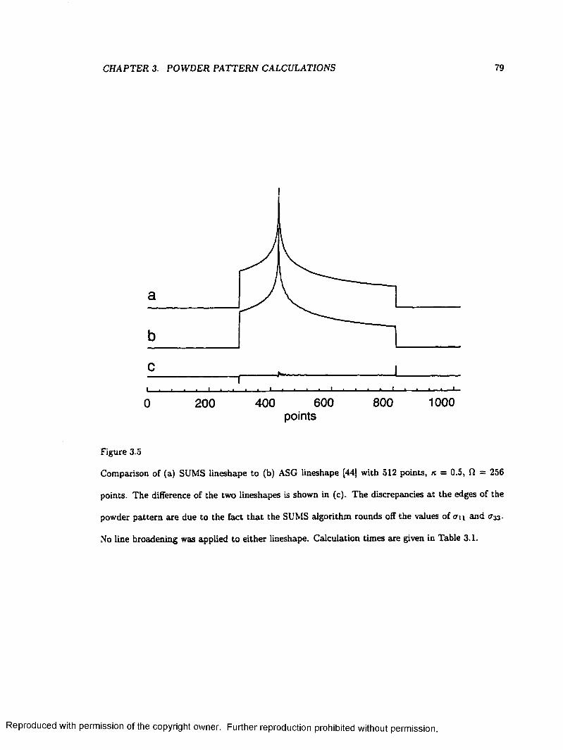
CHAPTER 3. POWDER PATTERN CALCULATIONS 79
c
0 200 400 600 800 1000points
Figure 3.5
Comparison of (a) SUMS lineshape to (b) ASG lineshape [44] with 512 points, k = 0.5, Q = 256
points. The difference of the two lineshapes is shown in (c). The discrepancies a t the edges of the
powder pattern are due to the fact th a t the SUMS algorithm rounds off the values of cru sod ° 33-
No line broadening was applied to either lineshape. Calculation times are given in Table 3.1.
Reproduced with permission of the copyright owner. Further reproduction prohibited without permission.

CHAPTER 3. POWDER PATTERN CALCULATIONS 80
Graphics Indigo2 workstation. The code was written in the WAVE programming language, which
uses loops and conditional structures that are similar to those of C or FORTRAN. In addition,
routines written in low-level compiled code are available to perform many common array operations.
The powder pattern calculation program will produce a simulation of a k = 0 spectrum with 256
points in 0.10 s, and with 512 points in 0.30 s. These times include line broadening and rescaling of
the intensity of the output. Calculation of spectra with other skew values takes less time since the
number of subspectra that need to be summed is smaller.
3.4 Applications
3.4.1 Automated Fitting of Experimental Data
Given the availability of fast computers it may seem unnecessary to seek out more efficient
algorithms for lineshape calculation. Indeed, if a single lineshape is to be calculated, it makes little
difference if the calculation takes a few milliseconds or a few seconds. However, an iterative least-
squares fitting routine may require the calculation of hundreds of lineshapes. The efficiency of the
SUMS algorithm makes fully automated least-squares fits to experimental d a ta feasible, even on
modest computer systems. Fitting of the experimental data presented here was done with a WAVE
routine that minimizes the sum of the squares of the differences of an array (experimental data)
and a user supplied function (simulation). The partial derivatives of the function with respect to
each of its param eters must also be supplied. The principal values of the shielding tensor are used
as the variable param eters of the function. Partial derivatives with respect to the principal values
are found by calculating a powder pattern with the current param eter values and subtracting the
pattern formed when one of the parameters is varied by a single point. The routine searches for a
minimum in the sum of the squares as the principal values are varied. Convergence is rapid and
stable provided that some broadening (a few percent of the span is sufficient) has been applied to
the calculated spectrum. Results obtained by the fitting procedure are not very sensitive to the
Reproduced with permission of the copyright owner. Further reproduction prohibited without permission.
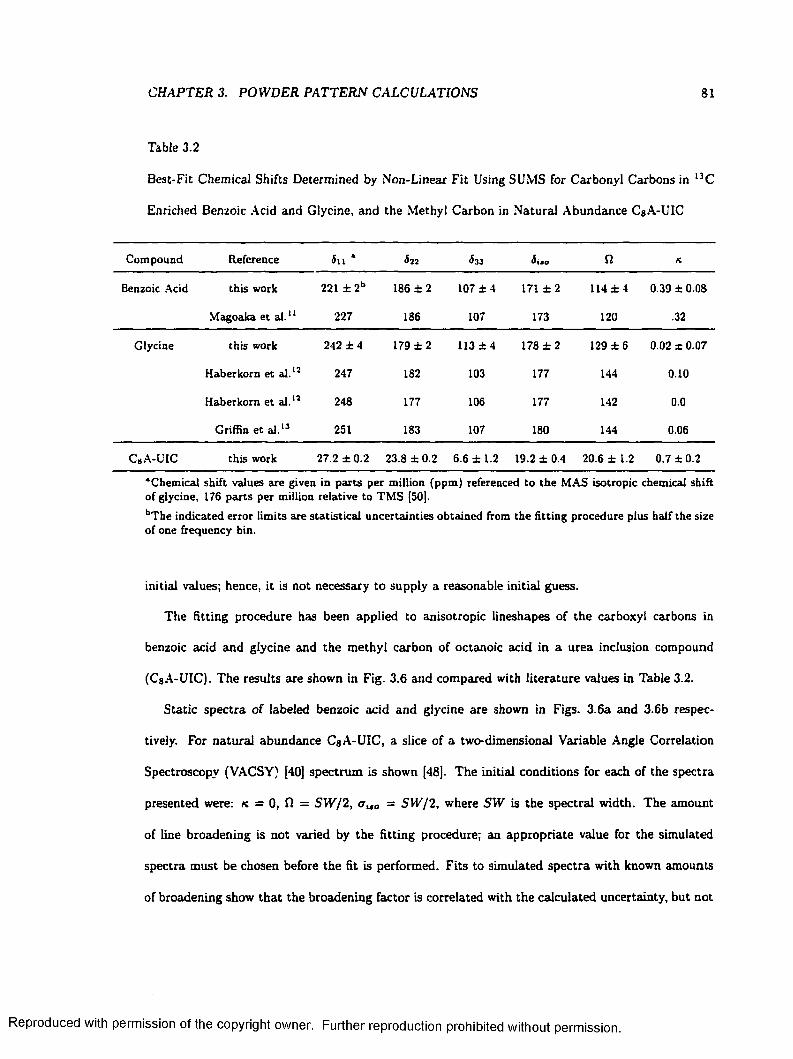
CHAPTER 3. POWDER PATTERN CALCULATIONS 81
Table 3.2
Best-Fit Chemical Shifts Determined by Non-Linear Fit Using SUMS for Carbonyl Carbons in 13C
Enriched Benzoic Acid and Glycine, and the Methyl Carbon in Natural Abundance CgA-UIC
Compound Reference i n * &n &Z3 <5ij o n K
Benzoic Acid this work 221 ± 2 b 186 ± 2 107 ± 4 171 ± 2 114 ± 4 0.39 ± 0.08
Magoaka et al.“ 227 186 107 173 120 .32
Glycine this work 242 ± 4 179 ± 2 113 ± 4 178 ± 2 129 ± 6 0.02 x 0.07
Haberkorn et al.12 247 182 103 177 144 0.10
Haberkorn et al.12 248 177 106 177 142 0.0
Griffin et al.13 251 183 107 180 144 0.06
CgA-UIC this work 27.2 ±0.2 23.8 ± 0.2 6.6 ±1.2 19.2 ± 0 .4 20.6 ± 1.2 0.7 ±0.2
‘ Chemical shift values are given in parts per million (ppm) referenced to the MAS isotropic chemical shift of glycine, 176 parts per million relative to TMS [50].bThe indicated error limits are statistical uncertainties obtained from the fitting procedure plus half the size of one frequency bin.
initial values; hence, it is not necessary to supply a reasonable initial guess.
The fitting procedure has been applied to anisotropic lineshapes of the carboxyl carbons in
benzoic acid and glycine and the methyl carbon of octanoic acid in a urea inclusion compound
(CsA-UIC). The results are shown in Fig. 3.6 and compared with literature values in Table 3.2.
S tatic spectra of labeled benzoic acid and glycine are shown in Figs. 3.6a and 3.6b respec
tively. For natural abundance C sA -U IC , a slice of a two-dimensional Variable Angle Correlation
Spectroscopy (VACSY) [40] spectrum is shown [48]. The initial conditions for each of the spectra
presented were: k = 0, fi = S W / 2, a ito = S W / 2, where S W is the spectral width. The amount
of line broadening is not varied by the fitting procedure; an appropriate value for the simulated
spectra must be chosen before the fit is performed. Fits to simulated spectra with known amounts
of broadening show tha t the broadening factor is correlated with the calculated uncertainty, but not
Reproduced with permission of the copyright owner. Further reproduction prohibited without permission.
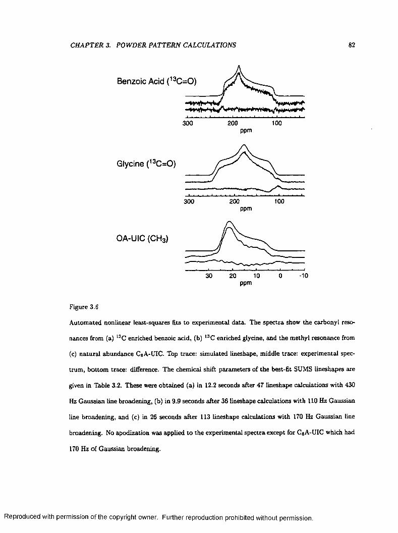
CHAPTER 3. POWDER PATTERN CALCULATIONS 82
Benzoic Acid (13C=
300
OA-UIC (CH3)
200 100 ppm
Glycine (13C=0)
300 200 100ppm
ppm-1030 20 10 0
Figure 3.6
Automated nonlinear least-squares fits to experimental data. The spectra show the carbonyl reso
nances from (a) i3C enriched benzoic acid, (b) l3 C enriched glycine, and the methyl resonance from
(c) natural abundance C sA -U IC . Top trace: simulated lineshape, middle trace: experimental spec
trum, bottom trace: difference. The chemical shift parameters of the best-fit SU M S lineshapes are
given in Table 3.2. These were obtained (a) in 12.2 seconds after 47 lineshape calculations with 430
Hz Gaussian line broadening, (b) in 9.9 seconds after 36 lineshape calculations with 110 Hz Gaussian
line broadening, and (c) in 26 seconds after 113 lineshape calculations with 170 Hz Gaussian line
broadening. No apodization was applied to the experimental spectra except for C sA -U IC which had
170 Hz of Gaussian broadening.
Reproduced with permission of the copyright owner. Further reproduction prohibited without permission.
CHAPTER 3. POWDER PATTERN CALCULATIONS 83
with the values of the best-fit chemical shifts.
For benzoic acid, the chemical shift parameters reported here are in close agreement with liter
ature values [51], except for <5n- For glycine, deviations from reported values [52,53] are somewhat
larger. The reason for the disagreements may lie in the fact th a t the results from the literature were
obtained from single crystal samples. Orientation dependence of the bulk magnetic susceptibility
of a single crystal may introduce systematic errors into the determ ination of the chemical shift pa
rameters [54]. This effect is averaged out in powder samples. The <$33 principal value for glycine
reported here is suspect due to the distortion at the upheld edge of the powder pattern. This may
be due to an impurity or a crystallographically inequivalent carbonyl carbon. In order to minimize
chi-squared, the fitting routine converges to a value of J 3 3 that is inside the drooping upheld edge.
No literature values are available for the methyl group in C sA -U IC , but the results are similar to
those quoted for other methyl carbons [2 0 ].
3.4.2 Lineshapes from Partially Ordered Samples
Another application to which S U M S is well suited is the calculation of powder patterns from
partially oriented samples. In m aterials such as drawn polymers or liquid crystals, a probability
distribution function, P { 0 , 7 ) describes the likelihood of finding the principal axis system a t a given
orientation with respect to some preferred axis. For a sample of randomly oriented crystallites,
P{@,~t) = ( l / 47r) sin/3. In general, we must consider distribution functions that are not separable
into functions of 0 only and 7 only. Thus, in order to simulate lineshapes of samples with non-
separable distribution functions, the value for 0 and 7 for every point in simulated spectrum must
be known. It is not obvious that this is possible since, in general, the equation that relates chemical
shielding to orientation (Eq. 3.3) can not be inverted to yield a unique value of 0 and 7 for a given
<t. However, the SU M S method presented above produces simulated lineshapes by adding up the
axially symmetric powder patterns th a t arise from distributions of 0 a t fixed values of 7 . When 7
Reproduced with permission of the copyright owner. Further reproduction prohibited without permission.

CHAPTER 3. POWDER PATTERN CALCULATIONS 84
is fixed,
a — s sin2 0 + 033 cos2 0. [3.32]
This expression is invertible, yielding a unique value of 0 for every value of cr:
0 = sin~l 11 17,3 g~ = cos-1 < / 3 [3.33]y ct33 - 3 y ffj3 - s
Since the principal square root is positive, both of these expressions yield a value of 0 in the first
quadrant. The correspondence between s and 7 is also one-to-one; thus, the weighting factor for
each axially symmetric powder pattern corresponds to a unique value of 7 . This value is found from
Eq. 3.13:
7 = sin-1 . / 8 gl-1— = cos-1 / g22 i T [3.34]V <722 — <7u V 0 2 2 - 0 1 1
As a result, each point in each axially symmetric powder pattern corresponds to a unique value of 0
and 7 in the first quadrant and can be weighted by the value of the probability distribution function
at those angles.
For the calculation of a powder pattern for a uniform orientation distribution, only values of 0
and 7 from 0° to 90° need to be considered. However, in a partially oriented sample, the orientation
distribution in a sample may not have this symmetry. In such cases, lineshapes for all necessary
quadrants are calculated and added together. The weighting functions for each of these powder
patterns is evaluated for 0 and 7 in the appropriate quadrant. The equations shown here for
determining 0 and 7 from a point on a subspectrum always return a value in the first quadrant.
Due to the symmetry of the equations th a t relate orientation to chemical shielding a{0) = a ( 0 ± n n )
and 3 (7 ) = 3 ( 7 ± nn) for n = 0 , 1 ,2 , To include all possible orientations, eight spectra must be
calculated, one for each octant of the unit sphere. The four octants that cover the upper (z > 0)
hemisphere correspond to 0 as determined from Eqs. 3.33. The lower hemisphere corresponds to
0 — i t / 2. W ithin each of these hemispheres, 2n ± 7 and n ± y are needed to cover the four octants.
As an example of a plausible non-uniform distribution function, consider the (unnormalized)
probability function shown in Fig. 3.7a. The most probable orientation is with the z-axis of the
Reproduced with permission of the copyright owner. Further reproduction prohibited without permission.

CHAPTER 3. POWDER PATTERN CALCULATIONS 85
co.5T 0.5
0 90 180
K=1
4000 200(3 (degrees) points
K=0
4000 200
K=-1
4000 200points points
Figure 3.7
Powder lineshapes for a non-uniform distribution of orientations of the principal axis system. The
distribution function (a) is P{0) = exp[(/3 - 7r / 2 )2], where 0 is expressed in radians. Powder patterns
resulting from this distribution (bold lines) are shown for k = 1 (b), k = 0 (c) and k = - 1 (d).
Powder patters from uniform distributions of orientations are shown in gray for comparison.
Reproduced with permission of the copyright owner. Further reproduction prohibited without permission.
CHAPTER 3. POWDER PATTERN CALCULATIONS 86
principal axis system perpendicular to the laboratory r-axis, although the distribution function is
not sharply peaked. This situation could correspond to a drawn polymer in which the polymer chains
tend to align with the draw axis. The carbon of interest would have its principal axis system oriented
perpendicular to the polymer backbone. Calculated lineshapes from this non-uniform distribution
of orientations are shown in Figures 3.7b, c and d.
3.4.3 Deuteron Lineshapes
Powder patterns from spin- 1 nuclei, such as deuterons, can be calculated with a small modification
to the SUMS algorithm. The deuteron has three energy levels in a magnetic field that correspond
to /- = 1, 0 and -1 . The dominant perturbation of these levels is the quadrupole interaction
between the electric quadrupole moment of the nucleus and the electric field gradient, as discussed
in Section 2.4.4. This interaction, like chemical shielding, is described by a second-rank tensor. The
energy differences between the two single-quantum transitions are shifted in opposite directions by
the perturbation. As a result, a pair of peaks appears for each orientation of the principal axis system
of the electric field gradient tensor with respect to the static field. For a powder or amorphous sample
the lineshape resembles a superposition of two chemical shift anisotropy lineshapes. Calculating a
deuteron powder pattern is as simple as calculating a carbon powder pattern, copying it, reflecting
it about its isotropic value and adding it to the original. The topmost powder pattern shown in
Fig. 3.8 is a typical static deuteron lineshape. Electric field gradient tensors tend to be nearly axially
symmetric, yielding lineshapes th a t resemble the superposition of two chemical shift anisotropy
powder patterns with | k | s s 1 . Calculation of such lineshapes is particularly fast since few subspectra
are needed.
3.4.4 Partially Relaxed Lineshapes
D ata from spin-lattice relaxation experiments provide detailed information about molecular mo
tion. The analysis of these data requires the calculation of powder patterns that are distorted by
Reproduced with permission of the copyright owner. Further reproduction prohibited without permission.
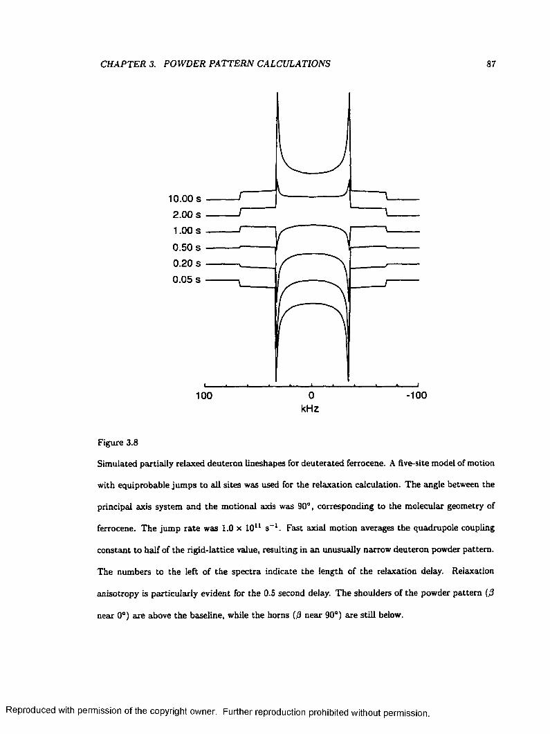
CHAPTER 3. POWDER PATTERN CALCULATIONS 87
10.00 s2.00 s1.00 s r
0.50 s 0.20 s 0.05 s
0 -1001 0 0
kHz
Figure 3.8
Simulated partially relaxed deuteron lineshapes for deuterated ferrocene. A five-site model of motion
with equiprobable jum ps to all sites was used for the relaxation calculation. The angle between the
principal axis system and the motional axis was 90°, corresponding to the molecular geometry of
ferrocene. The jump ra te was 1 .0 x 1011 s -1 . Fast axial motion averages the quadrupole coupling
constant to half of the rigid-lattice value, resulting in an unusually narrow deuteron powder pattern.
The numbers to the left of the spectra indicate the length of the relaxation delay. Relaxation
anisotropy is particularly evident for the 0-5 second delay. The shoulders of the powder pattern [0
near 0°) are above the baseline, while the horns (/3 near 90°) are still below.
Reproduced with permission of the copyright owner. Further reproduction prohibited without permission.

CHAPTER 3. POWDER PATTERN CALCULATIONS 88
relaxation anisotropy. Such partially relaxed lineshapes can be calculated using a method that is
similar to that used to calculate powder patterns from partially oriented samples. Intensities are
multiplied by a weighting factor th a t is calculated for each orientation determined by an external
routine. Except in special cases, relaxation times depend on transformations that have lower sym
metry than those that determine NMR frequency; thus, the calculation may need to be repeated
for 0 and 7 in all quadrants. Lineshapes from a simulated inversion recovery experiment are shown
in Fig. 3.8. The inversion recovery technique for measuring spin-lattice relaxation time, 7 \z , was
discussed in Section 2.5.4. The intensity of each point on the lineshape is given by
Meq(0, 7 ) + (M ,„„(/?,7 ) ~ A f„(/J,7 ))exp ~ }) [3-35]
where (>3,7 ) is the equilibrium intensity for a particular orientation. The time constant, T iz(/3,7 )
is calculated from molecular geometry and a model of motion, using an external routine. This
procedure was implemented to produce some of the calculated relaxation time anisotropies shown
in the next chapter.
An increase in the running time of the program is to be expected when calculating partially
oriented or partially relaxed lineshapes, due to the large number of operations that must be per
formed. The performance penalty depends largely on the complexity of the procedure that modifies
the intensity for each orientation. For a partially oriented sample with a simple distribution function
the calculation time increases by about a factor of six. Relaxation calculations require more than
a single function evaluation; thus, the generation of a partially relaxed lineshape can take much
longer.
3.5 Summary
SUMS has proven to be a valuable tool for the analysis of anisotropic lineshapes. The algorithm
produces high-quality powder lineshapes in less time than the more common methods. The methods
presented in this chapter have extended the usefulness of the algorithm to other applications and ar
Reproduced with permission of the copyright owner. Further reproduction prohibited without permission.
CHAPTER 3. POWDER PATTERN CALCULATIONS 89
eas of research. Calculated partially relaxed powder patterns were produced using SUMS to analyze
the molecular motion of ferrocene. The results of these studies tire presented in Chapter 4, Relax
ation Calculations. The non-linear least-squares fitting routine was used to determine the principal
values of l3C chemical shift tensors in polyimides in Chapter 5, Characterization of Polyimides.
Reproduced with permission of the copyright owner. Further reproduction prohibited without permission.
Chapter 4
Relaxation Calculations
4.1 Introduction
Molecular dynamics can have a great influence on the bulk properties of solids. Molecules in solids
undergo restricted motion due to the influence of neighboring molecules at nearby sites on the crystal
lattice. Thus, in solids, structure and motion on the molecular scale are strongly interrelated. Elates
and trajectories of motion give information about intermolecular potentials [55], thereby adding to
the knowledge of the microscopic origins of the bulk properties of solids.
Molecular motion affects NMR spectra through modulation of the anisotropic interactions de
scribed in Section 2.4. The orientation dependence of each these interactions is described by a
second rank tensor th a t is fixed in the molecular reference frame. Thus, as the molecule changes
orientation, the nuclei experience fluctuating magnetic fields. For fast motion (rates > 1 x 10s s~ l ),
these fields stim ulate the transitions that reestablish the equilibrium population distribution for the
spin energy levels. Thus, relaxation times reveal information about molecular motion.
In liquids, molecules undergo rapid isotropic reorientation. In a solid, molecular motion is usu
ally restricted by inter- and intramolecular potentials. The forms of these potentials, as functions of
orientation, typically consists of a number of deep wells. Motion in such a potential is often approx-
90
Reproduced with permission of the copyright owner. Further reproduction prohibited without permission.
91
imated with a Markov model in which the molecule jumps between discrete orientations. However,
for shallow potentials (or high temperatures), diffusive motion within the potential wells may need
to be included in the description of motion [56]. Since motion in solids is generally anisotropic,
relaxation times depend on the orientation of the crystal lattice with respect to the external mag
netic field. In polycrystalline samples the distribution of NMR frequencies leads to powder patterns.
By measuring the relaxation of points across the powder lineshape, the orientation dependence of
relaxation times is found. The precise form of this relaxation time anisotropy is a signature of the
rate and trajectory of molecular motion.
In order to quantitatively determine the rate and trajectory of molecular motion, relaxation time
anisotropies are calculated for various models of motion and compared to measured anisotropies.
Information about the time dependence of the anisotropic interactions is contained in the spectral
densities. In order to obtain as much information about molecular motion as possible, we seek to
measure the anisotropy of each spectral density. Since relaxation times are linear combinations of
the spectral densities, the spectral density anisotropies could be determined by measuring relaxation
times that depend on independent linear combinations of the spectral densities.
Determination of rates and trajectories of molecular motion using experimental and calculated
relaxation times anisotropies has been particularly successful using deuterons [24]. The relaxation
time anisotropy can be accurately determined from solid state deuteron NMR spectra. Inhomo-
geneous broadening by the quadrupolar interaction results in wide powder patterns that allow the
orientation of the principal axis system of the electric field gradient tensor, with respect to the static
magnetic field, to be determined from the spectral frequency with high precision. Furthermore,
isotopic labeling results in a high signal-to-noise ratio in deuteron spectra.
The deuteron has three energy levels in a static magnetic field, corresponding to the I- =
—1,0 and +1 eigenstates. Inverting the populations of these states results in a non-equilibrium
configuration of the spin system. Relaxation to equilibrium is described by the orientation-dependent
time constant Tiz- A non-equilibrium configuration with quadrupole order is created by inverting the
Reproduced with permission of the copyright owner. Further reproduction prohibited without permission.
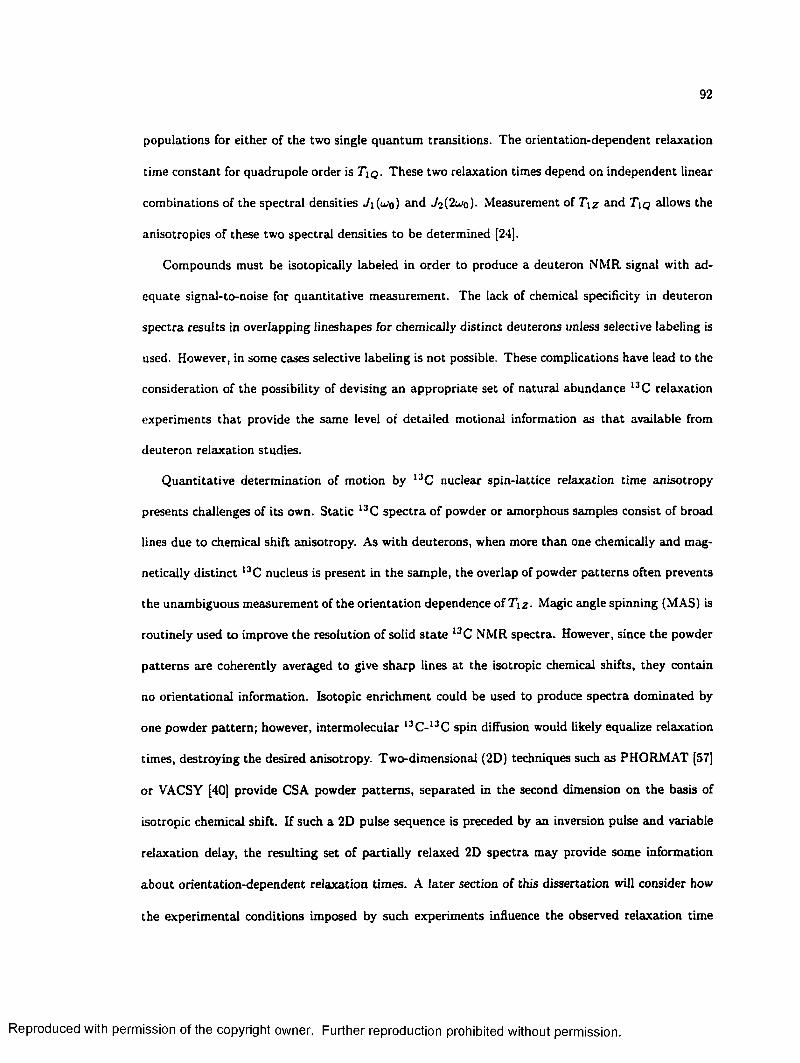
92
populations for either of the two single quantum transitions. The orientation-dependent relaxation
time constant for quadrupole order is T\q . These two relaxation times depend on independent linear
combinations of the spectral densities J\ ( ujq) and Jo(2wo). Measurement of T \ z and T\q allows the
anisotropies of these two spectral densities to be determined [24].
Compounds must be isotopically labeled in order to produce a deuteron NMR signal with ad
equate signal-to-noise for quantitative measurement. The lack of chemical specificity in deuteron
spectra results in overlapping lineshapes for chemically distinct deuterons unless selective labeling is
used. However, in some cases selective labeling is not possible. These complications have lead to the
consideration of the possibility of devising an appropriate set of natural abundance 13 C relaxation
experiments that provide the same level ot detailed motional information as that available from
deuteron relaxation studies.
Quantitative determination of motion by l3C nuclear spin-lattice relaxation time anisotropy
presents challenges of its own. Static 13C spectra of powder or amorphous samples consist of broad
lines due to chemical shift anisotropy. As with deuterons, when more than one chemically and mag
netically distinct l3C nucleus is present in the sample, the overlap of powder patterns often prevents
the unambiguous measurement of the orientation dependence o f T i z . Magic angle spinning (MAS) is
routinely used to improve the resolution of solid sta te 13 C NMR spectra. However, since the powder
patterns are coherently averaged to give sharp lines at the isotropic chemical shifts, they contain
no orientational information. Isotopic enrichment could be used to produce spectra dominated by
one powder pattern; however, intermolecular l3 C-l3C spin diffusion would likely equalize relaxation
times, destroying the desired anisotropy. Two-dimensional (2D) techniques such as PHORMAT [57]
or VACSY [40] provide CSA powder patterns, separated in the second dimension on the basis of
isotropic chemical shift. If such a 2D pulse sequence is preceded by an inversion pulse and variable
relaxation delay, the resulting set of partially relaxed 2D spectra may provide some information
about orientation-dependent relaxation times. A later section of this dissertation will consider how
the experimental conditions imposed by such experiments influence the observed relaxation time
Reproduced with permission of the copyright owner. Further reproduction prohibited without permission.

93
anisotropy.
A second problem is tha t a large number of spectral densities can contribute to carbon relax
ation. For deuterons, the only significant relaxation mechanism is the quadrupole interaction. Only
two spectral densities from the auto-correlation of this interaction, Ji(w) and contribute to
relaxation. For carbons, relaxation may be stimulated by motionally-induced fluctuations in the
dipolar, chemical shielding, or spin rotation interactions. Spectral densities that arise from the
auto-correlation of any of these interactions may contribute to relaxation. For a carbon that is
strongly coupled to more than one proton, spectral densities for each of the dipolar interactions
may need to be considered. Cross-correlations or interference between two different interactions can
also lead to relaxation [58]. Consider a time-dependent Hamiltonian with a dipolar and a chemical
shielding term:
= + [4.1]
The correlation function is
C (r) = { ( H D { t ) + H A m - H D ( t + T ) + H A t + T)y ) [4.2]
= (HD(t)H'D{t + r)) + (Ha ( i ) K ( t + r)) + (W0 ( t ) K ( ‘ + r)) + ( ^ ( t ) ^ o ( l + r)>
This function is the sum of two auto-correlation terms and two cross-correlation terms. The physical
situation, and the calculations, are much simpler when one of the interactions dominates. However,
even for the simple case of an isolated 13C -l H spin pair relaxed only by a time-dependent dipole-
dipole coupling, three spectral densities must be determined, J i {u>h - u / c ) , and Jzi^H +wc)>
where and ujq are the Larmor frequencies for lH and l3C, respectively.
For many motional processes, the anisotropies of different spectral densities have the opposite
sense and consequently the corresponding relaxation times show a reduced dependence on orienta
tion of the principal axis system with respect to the external magnetic field. It is therefore important
to measure as many different linear combinations of spectral densities as possible. Ideally, enough
independent measurements should be made to permit determination of the anisotropy of each indi
Reproduced with permission of the copyright owner. Further reproduction prohibited without permission.

94
vidual spectral density. In liquids, significant progress has been made towards this goal by designing
selective excitation pulse sequences to prepare the spins in appropriate initial states [58,59,60,61]
However, solid samples are far more challenging because extensive dipolar coupling and line broad
ening complicate such selective excitation [62].
For some systems, carbon and deuteron relaxation data are complementary. The dipolar interac
tion which dominates 13C relaxation in a l3C -l H group is axially symmetric. Vibrational averaging
can lead to an asymmetric averaged tensor; however, this effect is typically small. Quadrupole ten
sors for C - 'H groups are also very nearly symmetric. The dipolar and quadrupolar tensors have
their largest components oriented along the I3C -12H bond. Since these tensors have the same
orientations and nearly the same symmetry, fluctuations with approximately the same frequency
components occur when motion changes the internuclear vector. Thus, for an isolated l3C -1,2H
group, the spectral density anisotropies of the carbon and deuteron are identical.
In this chapter, expressions for the spectral densities for spinning samples are derived for motion
in the fast limit. These expressions are used to show how two independent linear combinations of
the spectral densities may be determined. In addition, a method is presented for measuring all three
spectral density anisotropies independently, by combining the deuteron T \ z and T \ q anisotropies
and the l3C MAS T\z- To test the calculations and experimental methods, experiments were
performed on natural abundance and deuterated ferrocene. The molecular structure for ferrocene
is shown in Fig. 4.1. Techniques for separating overlapping powder patterns are unnecessary for
this substance because only one chemically distinct carbon (or deuteron) site is present on the
ferrocene molecule. Calculations of l3C relaxation are simplified because the dipolar interaction
with directly bonded protons is the dominant relaxation mechanism. The orientation dependence of
each of the three individual spectral densities was determined by conducting experiments on natural
abundance 13 C and deuterated ferrocene. These experimental results are shown and compared with
calculated spectral densities. The possibility of using 2D techniques for measuring relaxation times
for chemically distinct carbons in complex spectra is explored. D ata from a VACSY experiment
Reproduced with permission of the copyright owner. Further reproduction prohibited without permission.
95
Figure 4.1
The molecular structure of ferrocene. The two cyclopentadienyl rings are free to move independently.
The staggered configuration, (shown) is energetically favorable to the eclipsed configuration which
minimizes the inter-ring carbon-carbon distance [63).
performed on octanoic acid in a urea inclusion compound (CsA-UIC) are presented. Much of the
material presented in this chapter was submitted to Journal of Magnetic Resonance.
4.2 Calculations
4.2.1 Redfield Theory
When molecular motion occurs a t a ra te that is much greater than the strengths of the inter
actions th a t contribute to the NMR spectrum, motionaliy averaged lineshapes are observed. In
this “fast” motion regime, relaxation times are accurately calculated using a formalism introduced
by Redfield [64]. The im portant steps in the derivation of the Redfield equation, drawing on the
discussions presented in References [17,3,36], are summarized in this section.
The state of an ensemble of spins is described by the density matrix. Calculation of the relaxation
of a system from a non-equilibrium configuration is done by determining the time evolution of the
Reproduced with permission of the copyright owner. Further reproduction prohibited without permission.
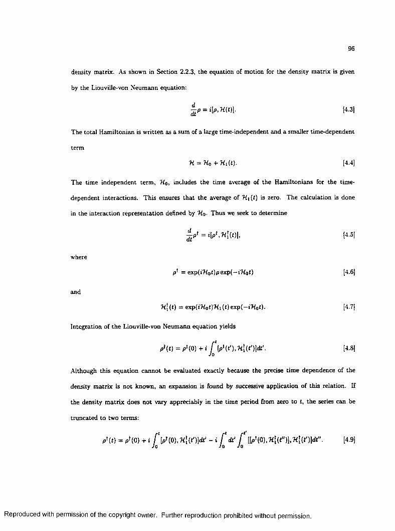
96
density matrix. As shown in Section 2.2.3, the equation of motion for the density matrix is given
by the Liouville-von Neumann equation:
± p = i[p,H(t)]. [4.3]
The total Hamiltonian is written as a sum of a large time-independent and a smaller time-dependent
term
H = H 0 + H 1{t). [4.4]
The time independent term, 'Ho, includes the time average of the Hamiltonians for the time-
dependent interactions. This ensures that the average of H i(t) is zero. The calculation is done
in the interaction representation defined by Ho- Thus we seek to determine
j t p ' = i[pf ,H [(t)], [4.5]
where
p 1 = exp(iH ot)pexp(-i'H ot) [4.6]
and
H [(t) = exp(t'Ho£)'Hi(Oexp(-iHoO. [4.7]
Integration of the Liouville-von Neumann equation yields
p'{t) = p>(0) + i A p t( t ') , -H l( t ')K . [4.81Jo
Although this equation cannot be evaluated exactly because the precise time dependence of the
density m atrix is not known, an expansion is found by successive application of this relation. If
the density m atrix does not vary appreciably in the time period from zero to t , the series can be
truncated to two terms:
P'(t) = pf(0) + i / V ( 0),:hI(j')]dt' - i f d t ' f [4.9]Jo Jo J 0
Reproduced with permission of the copyright owner. Further reproduction prohibited without permission.

97
Differentiation yields an approximation to the Liouville-von Neumann equation for the density ma
trix:
= 1^ ( 0 ) , 7£|(t)J - j \ [ p H o ) , n \ ( t % n \ ( t ) } d t ' . [4 .10]
The first term in this equation is zero since it is equal to dp*(0)/dt. Evaluation of the second term
[3] yields the Redfield equation [64]:
^ p ] k = 5 3 Ri klm exP[*(wi - - uj + u/m)t]. [4.11]l,m
This is a set of linear differential equations for the elements of the density matrix [3]. Because of
the exponential factor in this equation, the non-secular terms (terms where — w* ^ uij — u m) are
insignificant [17]. Thus, the Redfield equation can be simplified to
dt^Jk ~ RJklmPim- [4*12]l,m
The elements of the Redfield superoperator, Rjktmi are given by [55,17,3,36]
Rjklm = Jjtkm — UJi) + ~~ “ &km ^ *^nlnj (^n ) “ &jl ^ Jnknm&k ~~ ^n)» [4. 13]n n
where the spectral densities, Jijki, are the Fourier transforms of the correlation functions:
Jijki = r m n [ ( t ) |V>,) (V*| n \ ‘ (t) | t f , ) e " - r efT. [4.14]Jo
The time-dependent Hamiltonian can be written as the product of sphencal irreducible tensor
operators:
* I ( t ) = 5 3 ( - l ) m A {: l T ^ ^ L A B ) [4.151m
where the Am are the spin operators and the LAB ) are the time-dependent spatial operators
expressed in the laboratory coordinate system. For the heteronuclear dipolar interaction, the spin
operators are
4 2) = - I ■ S) A™ = ^ { I ZS ± + S XI±) A % = | / ± S ± [4-16]
Reproduced with permission of the copyright owner. Further reproduction prohibited without permission.

98
where I and 5 are the spin angular momentum operators of the interacting nuclei. The spatial
operators in the principal axis system are
Tq2 , (F .45) = \ / 6 * £ £ T ^ ( P A S ) = 0 T ^ P A S ) = 0, [417]
where 7 / and 7 s are the gyromagnetic ratios of the two nuclei and r / s is the internuclear distance.
The spatial operators in the laboratory frame are found by a transformation of coordinate systems
from the principal axis system (PAS), where the tensor is diagonal, to the laboratory coordinate
system through the Euler angles f2p t(t) = 7 p tW )- This transformation is time
dependent because of molecular motion. Since the time-dependence of the system is contained in
the spatial operators in the laboratory frame, we can ignore the spin operators when calculating
relaxation. Thus, the normalized reduced spectral densities are defined as the Fourier transforms of
the correlation functions for the spatial operators:
Here the angular brackets indicate that the average over the ensemble is taken. After a period of
time, the spatial operators at time t are effectively uncorrelated with those at t + t . No significant
contribution is made to the integral for r greater than this correlation time, rc; thus, the upper limit
of the integral may be reduced to r c.
Once the form of the Hamiltonian is known, the Redfield equation can be evaluated to find the
time-dependence of the density matrix. The diagonal elements of the density m atrix which describe
the populations of the energy state approach their equilibrium values exponentially with a time
constant, T^z- This time constant is a linear combination of the reduced spectral densities [3,55,65].
Henceforth, the reduced Jm(ui) will simply be called spectral densities. For spin-lattice relaxation
dominated by the dipole-dipole mechanism, the 13 C Zeeman relaxation rate is given by [65]
1 iir 2R i z — ■=,— = —r^-[^o(w/ — u/s) + 3Ji(w s) + 6J2(ui +u»s)], [4-19]
T iz 2
where /V is the number of / spins (protons, in this case) directly bonded to the relaxing S spin
Reproduced with permission of the copyright owner. Further reproduction prohibited without permission.

99
(carbon), and the dipolar couplings wq = 7 / 7 s f i ( l / r rs )• The singular brackets indicate that the
factor 1 / r j s is averaged over vibrational motions which are too fast to contribute appreciably to the
spectral densities. Cross correlation between different l3C-*H vectors is ignored in this calculation.
For deuterons, relaxation is induced by fluctuations in the quadrupole interaction. In this case the
relaxation rate of Zeeman order is given by [55|
3 t r 2Riz = —2~ X2 [* i (^o) + 4J2(2wo)]i [4-20J
where \ = e2lz:Q *s the quadrupole coupling constant in Hertz. As with dipolar relaxation rates,
the quadrupole coupling constant is averaged over fast vibrations. Relaxation of quadrupolar order
is described by a single spectral density:
97 T *R i q = - ^ - X 2 [*4-2 1 ]
The validity of Redfield theory depends on two conditions [17]. First, the correlation time, rc,
must be much shorter than At , the interval for which the density m atrix does not change appreciably.
Second, the Redfield superoperator elements must not change much during the time interval At . An
equivalent condition is that the relaxation times are much longer than the correlation time.
4.2.2 Spectral Densities of Spinning Samples
In this section, the normalized reduced spectral densities (Eq. 4.18), are evaluated to determine
the spectral densities in a spinning sample. The transformation from PAS to LAB is performed as
a series of rotations involving three intermediate coordinate systems: the molecule-fixed coordinate
system (MOL), the crystal-fixed coordinate system (CRYS) and the rotor-fixed coordinate system
(ROT). Breaking up the transformation in this way separates the time dependent and time inde
pendent steps. The successive transformations of the coordinate system from PAS to LAB may be
summarized as
OpAf O*rc( 0 ^ c f i
PAS -------► MOL ► CRYS ► ROT > LAB.
Reproduced with permission of the copyright owner. Further reproduction prohibited without permission.
100
The PAS is fixed in the molecule, so the PAS to MOL transformation, Qp m , is time independent.
The CRYS to ROT transformation, ftc« , is also time independent since the sample is station
ary with respect to the rotor. The time dependence of the system is contained in the remaining
transformations. The spinning rotor leads to a coherently time dependent ROT to LAB transfor
mation, f ( O i Pr l , 1 r l )), while random molecular motion is responsible for the time
dependence of the MOL to CRYS rotation, CIm c ~ (aM c(0>/3M c(i).7M c(t))- The transformation
O,vrc( 0 is of particular importance since its time dependence describes the fluctuating magnetic
fields that induce relaxation.
For spherical irreducible tensors, the successive transformations that take the dipolar tensor from
PAS to LAB are performed by summing over Wigner rotation m atrix elements. Thus, the spectral
densities are written
J ra(u,) = [t <2)(P A S )]"2 E E E Ea ,a ' = - 2 6 ,4 '= - 2 c,c ' = - 2 d.d' = - 2
jH ( d ™ (nRL(t))D{ m'(nRL(t + r))
D l l \ n CR ) D ™ '( n c R )
D%HnMc ( t ) ) D™' ( n Mc ( t + T))
^ 2c)( n p M ) ^ v ‘ ( n P„ )
Tj?){ P A S ) T £ )\ P A S ) } e ~ imuTdT. [4.22]
Since the dipolar tensor is a second rank tensor interaction, all summations over Wigner matrix
elements will be from —2 to 2. These limits will be omitted in subsequent equations.
Several assumptions can be made to simplify Eq. 4.22. For the axially symmetric dipolar in
teraction, only 1q2) (PAS) is non-zero. Two of the transformations are time independent so the
corresponding Wigner m atrix elements may be removed from the integral. Also, since molecular
motion is a stationary Markov process, the time t can be set to zero without loss of generality. With
Reproduced with permission of the copyright owner. Further reproduction prohibited without permission.

101
these modifications the spectral densities become
■A»m = E E E CincH)^'(ncn)C(«PM )^r(fipw)0 ,0 ' 6,6' c,c'
^ O° (D ^ (n f l t (0 ) ) £ ) i? i l ‘ (nfit (T ))O ^ (n M c (0 ))^ .26,, ’ (f iM c ( r ) ) } e - “ rdr.[4.23|
For most physically reasonable situations, the equations may be further simplified by recognizing
that the rotor period is long compared to the correlation time but short compared to typical 13C
relaxation times. For fast motion, correlation times are generally on the order of picoseconds, and
rotor periods are typically tenths of milliseconds. Thus, the rotor may be considered stationary
for the time period in which the integrand is non-zero. This fast motion approximation allows the
Wigner m atrix elements for the ft fit transformation to be taken outside of the integral. Carbon
relaxation times are generally longer than a few seconds; while the nuclei relax, the rotor undergoes
thousands of rotations. Thus, the relaxation times depend on spectral densities averaged over a
rotor cycle. For this situation the ROT to LAB transformation is determined completely by the
tingle between the rotor axis and the external field, 0 m - Thus, the following identity is valid:
{ D ™ (ftR t(O )) D ^ m ‘ ( f t f i t ( r ) ) ) = \ ^ ( 0 R L ) \ 2 <5a,0-. [4.24]
Assuming uniaxial motion about the molecule-fixed axis, the MOL to CRYS transformation is re
duced to a simple rotation about that axis. For this type of motion, the expression for the spectral
densities is simplified since
(ftM C(O)) D ™ ; ( f tMC( r ) ) ) = ( e - “ “ « c ( ° )e .6 'a « c ( r ) ) ^ ^ [4 .25]
Torchia and Szabo [65] denote the correlation function of the MOL to CRYS transformation by
r 6,6-(r) = ( e - ,6oMc(0)e,4'OMc(r)) . [4.26]
This function has been evaluated for a variety of axial motional models in Ref. 65.
For the ferrocene molecule, five-fold axial symmetry suggests that motion might be approximated
by a five-site jump model. Calculations by Campbell et al. [63] support this conjecture. The
Reproduced with permission of the copyright owner. Further reproduction prohibited without permission.

102
total potential function for a cyclopentadienyl ring is the sum of five-fold symmetric inter- and
intramolecular contributions. The intermolecular contribution favors a staggered relative orientation
of the two rings. This configuration is depicted in Fig 4.1. Attractive intramolecular interactions
between carbons on the two rings that favor an eclipsed configuration make a smaller contribution
to the total potential at room temperature.
For a model with five equally populated sites and jumps allowed only to neighboring sites, the
correlation function is
= ex p [-4 A:tsin2 (7r6 / 5 )]<5fc,6<, [4.27]
where k is the jump rate. If jumps to all sites are allowed, the correlation function becomes
r 6,6< = exp(-5*t)J*,».. [4.28]
If the potential barrier is small, free rotational diffusion may be a reasonable model of motion. The
correlation function for this model is
r M- = e x p ( - 6£>t)<SM.. [4.29]
Making the assumptions th a t the rotor period is much longer than the correlation time, and
much shorter than the relaxation time, and that molecular motion is axial, the expression for the
spectral densities in a spinning sample can be written as
J m { u ) = Y . T . V ^ R ^ D ^ ^ C R ) D ^ l \ ^ c R ) D ^ { S l p M ) D ^ \ n P M )a b,b‘
r b,„.(T)e-imuTdT. [4.30]JQ
For jum p models with five or more equally populated sites, is diagonal [65], and the spectral
densities become
J m(w) = t4-31!0 ,6
For this study, this equation has been evaluated numerically for a variety of molecular geometries and
models of molecular motion. Relaxation time anisotropies calculated horn these spectral densities
were studied and compared to measurements of ferrocene.
Reproduced with permission of the copyright owner. Further reproduction prohibited without permission.
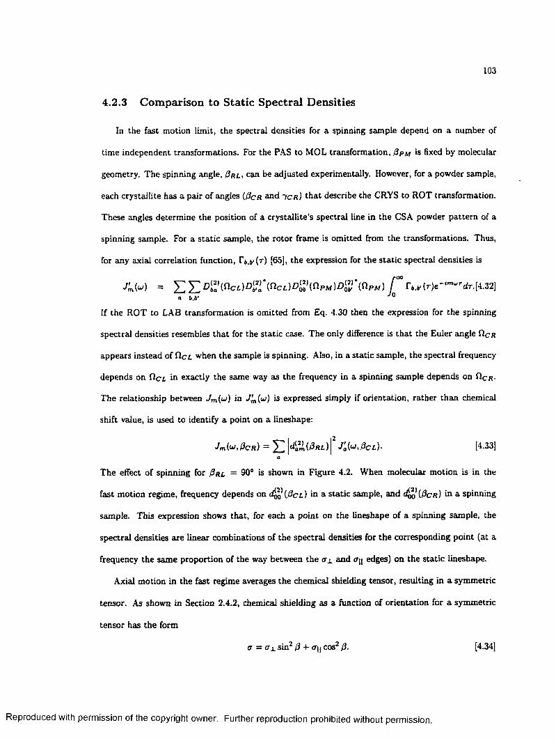
103
4.2.3 Comparison to Static Spectral Densities
In the fast motion limit, the spectral densities for a spinning sample depend on a number of
time independent transformations. For the PAS to MOL transformation, 0 p m is fixed by molecular
geometry. The spinning angle, 0 r l , can be adjusted experimentally. However, for a powder sample,
each crystallite has a pair of angles (0c r and 7 c r ) that describe the CRYS to ROT transformation.
These angles determine the position of a crystallite’s spectral line in the CSA powder pattern of a
spinning sample. For a static sample, the rotor frame is omitted from the transformations. Thus,
for any axial correlation function, [65], the expression for the static spectral densities is
J M = y , T D i l \ n CL)D[Va\n cL )D l ilHnPM)D(0f ( n p M ) f ° r M,( r ) e - m“rdr.[4.32]* t v J°
If the ROT to LAB transformation is omitted from Eq. 4.30 then the expression for the spinning
spectral densities resembles that for the static case. The only difference is that the Euler angle fIcr
appears instead of O c t when the sample is spinning. Also, in a static sample, the spectral frequency
depends on f i c t in exactly the same way as the frequency in a spinning sample depends on flcfi-
The relationship between Jm(u>) in J'm{u) is expressed simply if orientation, rather than chemical
shift value, is used to identify a point on a lineshape:
Jm(u,0CR) = £ \ & 0 R L ) \ 2 J ^ P C L ) . [4.33]a
The effect of spinning for 0 rl = 90° is shown in Figure 4.2. When molecular motion is in the
fast motion regime, frequency depends on < ^ { 0 c l ) in a static sample, and d $ { 0 c R ) in a spinning
sample. This expression shows that, for each a point on the lineshape of a spinning sample, the
spectral densities are linear combinations of the spectral densities for the corresponding point (at a
frequency the same proportion of the way between the cr± and <rj| edges) on the static lineshape.
Axial motion in the fast regime averages the chemical shielding tensor, resulting in a symmetric
tensor. As shown in Section 2.4.2, chemical shielding as a function of orientation for a symmetric
tensor has the form
a — <r± sin2 0 -I- <7 || cos2 0. [4-34]
Reproduced with permission of the copyright owner. Further reproduction prohibited without permission.
104
SpinningP r l = 9 0 °
a.a,
Figure 4.2
Calculated axially symmetric CSA powder patterns for (a) a static sample and (b) a sample spinning
a t 90° with respect to the external field. The spinning powder pattern is scaled in frequency by a
factor of -1 /2 , while the integrated intensity is held constant. The resonance frequency depends on
the angle between the z-axes of the crystal-fixed frame and the laboratory frame, 0 c l , for the static
lineshape. On the spinning lineshape, frequency depends on the angle between the molecule frame
and the rotor frame. For corresponding points on the powder patterns, 0 c l - 3 c r -
Reproduced with permission of the copyright owner. Further reproduction prohibited without permission.

105
Since chemical shielding depends on sin2 0 and cos2 0, the frequency for crystallites oriented at some
particular value of 0 c r is the same as that for 180° ± 0 c r and 360° - 0 c r - In general, spectral
densities do not have such high symmetry. Two values of 0 c r that give the same spectral frequency
may yield different spectral densities. If this is the case then relaxation is multi-exponential.
4.2.4 Linear Combinations of Spectral Densities
If the motional rate (jump rate or diffusion coefficient) is much higher than the relevant com
bination of Larmor frequencies, the spectral densities are effectively independent of frequency,
Jm { u ) ss J,n(0). When this extreme narrowing condition is met, the spinning spectral densities
can be written in terms of their static counterparts, 4 (0 ) , J{ (0) and 4 (0 )- In this case, the expres
sion for R \z in a spinning sample can be written in terms of the static spectral densities and the
spinning angle:
R \ z (0r l ) =N u 2d
\ (5 - 3cos2(/?r l )) 4 (0 )+
i (9 - 3cos2(0 r i) ) J[(0) + 3(1 + cos2(0r l )) 4 ( 0 ) ] . [4.35]
Thus, the relaxation rate is a linear combination of the static spectral densities with coefficients
determined by the spinning angle. This suggests a method for determining the static spectral
densities from spinning relaxation time anisotropies. By measuring relaxation time anisotropies for
a variety of spinning angles a set of equations could be constructed and solved to give the static
spectral densities. However, rearranging Eq. 4.35 yields a term that depends on the spinning angle
and a constant term,j v y .2
R i z (0r l ) = [A + B cos2(0r l )} [4.36]
where
and
A = ^ 4 (0) + \ j [ (0) + 3 4 (0 ) [4.37]
B = - | 4 ( 0 ) - § 4 ( 0 ) + 3 4 (0 ) [4.38]
Reproduced with permission of the copyright owner. Further reproduction prohibited without permission.
106
Thus, only two linearly independent combinations of the static spectral densities can be determined
from experiments performed with a variety of spinning angles.
These two linear combinations, .4 and B, are easily determined from experimental data by
recognizing that
A = R i z ( 9 0 ° ) - ^ r I4-39!
and
B = (fli*(0°) - * iz(90°)) [4.40]
It is impractical to perform a spinning experiment with Prl = 0° since this would place the coil of the
probe parallel to the external field and give no signal. However, evaluation of Eq. 4.33 for 0 rl = 0°
shows that, for this case, the spectral densities in a spinning sample are identical to those in a static
sample. Thus the linear combinations .4 and B can be determined by measuring the relaxation time
anisotropy for a static sample and for a sample spinning about an axis perpendicular to the external
field. If there is some overlap of powder patterns in the static spectrum it may be possible to choose
a different pair of rotor angles such that the CSA powder patterns are resolved but still wide enough
to allow determ ination of relaxation time anisotropies.
For a sample spun a t the magic angle (Pmagic = cos- 1( l / \ /3 ) ) , powder patterns are collapsed to
narrow lines a t their isotropic chemical shifts. All crystallite orientations contribute to a frequency
range that is narrower than the homogeneous linewidth. In this case it is impossible to measure
the relaxation of differently oriented crystallites from such a lineshape. If the correlation function,
F6,6' ( 0 > *s diagonal, relaxation times are not anisotropic in a sample spinning at the magic angle;
the MAS relaxation time is independent of orientation. Evaluation of Eq. 4.35 for B r l — f imagtc
yields
RiziPmag,c) = (0) + 2 J[ (0) + 2^(0 )]. [4.41]
This combination of spectral densities is not linearly independent of A and B , bu t it is experimentally
accessible even for complicated spectra.
Reproduced with permission of the copyright owner. Further reproduction prohibited without permission.

107
Since the spectral densities J i(w0) and J 2 (2wo) can be determined from deuteron spectra, the
relaxation time of the MAS peak can be used in conjunction with deuteron relaxation times to
determine all three spectral densities. Although this strategy requires isotopic labeling for the
deuteron experiments, it has the advantage tha t MAS enhances resolution and signal-to-noise ratio
in the carbon experiments. It should be stressed tha t the relaxation time anisotropy vanishes for
magic angle spinning only when the correlation function is diagonal, as it is for jum p motion with
five or more equivalent sites or for free rotational diffusion [65].
Although carbon dipolar relaxation and deuteron quadrupolar relaxation depend on the same
spectral densities (to the extent that they can be treated as axially symmetric), the relaxation rate
expressions involve different coupling strengths. The deuteron quadrupole coupling constant may
be determined, with reasonable accuracy, from the width of a low tem perature powder pattern.
However, determining the dipolar coupling between a 13C nucleus and a nearby proton is not so
straightforward. l3C -l H pairs are rarely sufficiently isolated that a dipolar powder pattern can be
measured. Since dipolar relaxation rates depend on the sixth power of the intemuclear distance,
r CH< t h e calculated rates depend sensitively on this value. A recent paper by Hardy et al. [6 6 ]
demonstrates tha t care must be taken when using published bond lengths, since measurements made
with different techniques are averaged differently by vibrations of the nuclei. Neutron scattering
yields a vibrationaily averaged bond length, (r). However, the average dipolar coupling, (u/o), is 1 /3
determined by an effective bond length of ( l / r c h ) In general, these two vibrational averages
differ from each other and from the equilibrium bond length, r e. For typical molecular potentials,
r e < (r) < ( l / r ^ ) ~ V 3 [66,67,68].
4.2.5 Properties of Calculated Anisotropies
Some interesting properties of the spectral densities of spinning samples may be found by studying
the calculated anisotropies. While the spectral density anisotropies depend strongly on the motional
rate, number of sites and orientation of the dipolar tensor, the calculated relaxation time (Tiz)
Reproduced with permission of the copyright owner. Further reproduction prohibited without permission.

108
anisotropies often show little sensitivity to the motional model. To illustrate this, the results of
calculations for two motional models are presented in Figures. 4.3 and 4.4.
The first rows in Figures 4.3 and 4.4, show the results for a five-site nearest neighbor jump
model with 0 p m = 90°. This model is appropriate for ferrocene. The results in the second rows
are for a three-site model with 0pm = 70.5°, typical of a methyl group. In both cases, the motion
is assumed to be in the extreme narrowing limit. Thus, the CSA powder patterns are axially
symmetric (k = ± 1) with the greatest intensity arising from perpendicularly oriented crystallites,
0 c r = 90°. The chemical shielding of this spectral position is denoted oj.- The weak shoulder of
the lineshape is from crystallites that have their 2-axes nearly parallel to the rotor axis (0cR % 0 °)
whose shielding is denoted Although spinning the sample scales the powder pattern by a factor
of d ^ ( 0 R i ) = (3cos2 0 r l - l ) / 2 , corresponding positions on the lineshapes have the same 0cR
value. Static samples are treated as samples spinning at 0 r l — 0° since spinning at this angle has
no effect on the spectrum; for this case 0 c r = 0 c l ■ For consistency, the angle that determines
the spectral frequency will be called 0 c r throughout the remainder of this chapter. The variable
a = IC^ll -° \ . )$ to {0 C R ) + <TiJO is used to denote frequency.
The calculated static spectral densities plotted as a function of a are quite distinct for these
two models, as illustrated in Figures 4.4a and 4.4b. In both cases the spectral densities, like the
NMR frequencies, are found to depend only on the angle 0 c r ■ The calculated spectral densities are
plotted as a function of this angle in Figure 4.3. The symmetry of the ferrocene spectral densities
is such that Jm(O,0cR) = / m(0,nl80° ± 0 c r ), where n = 0 , 1, 2 , — Thus, for every frequency
on the powder pattern, a unique set of three spectral densities and a unique relaxation time are
found. However, for the methyl spectral densities (shown in Figure 4.3b) the symmetry relation
is </m (9,0cr ) = J m(0 .” 180° + 0cr )- Although crystallites oriented a t 0 c r and (180° - 0c r )
have the same NMR frequencies, they have different spectral densities. This implies bi-exponential
relaxation. Even though the individual spectral densities for 0cr and (180° — 0c r ) are different,
the linear combination which determines the relaxation time, T \z , is the same for both orientations.
Reproduced with permission of the copyright owner. Further reproduction prohibited without permission.
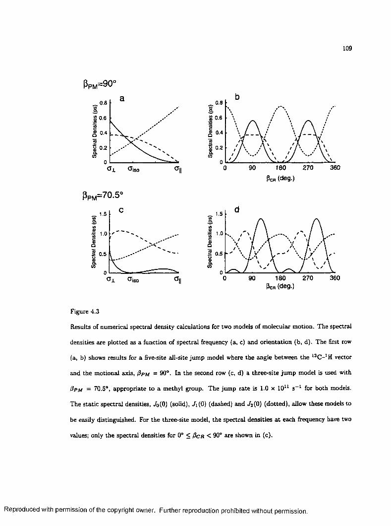
109
Ppm=90°
0.8
S 0.6<nI 0 .4
s| 0.2 Q.in
36090 180 2700
0.8
0.6
2 0.4
S 0.2
G\IIPcr (deg.)
Ppm=70.5°
1.5
1.0
X0.5
0360180 2700 90
S 0.5
<T|Pcr (deg.)
Figure 4.3
Results of numerical spectral density calculations for two models of molecular motion. The spectral
densities are plotted as a function of spectral frequency (a, c) and orientation (b, d). The first row
(a, b) shows results for a five-site all-site jum p model where the angle between the vector
and the motional axis, 0 p m = 90°. In the second row (c, d) a three-site jum p model is used with
0PM = 70.5°, appropriate to a methyl group. The jump rate is 1.0 x 10u s- 1 for both models.
The static spectral densities, ./o(O) (solid), Ji(0) (dashed) and ^ ( 0 ) (dotted), allow these models to
be easily distinguished. For the three-site model, the spectral densities a t each frequency have two
values; only the spectral densities for 0° < 0cR < 90° are shown in (c).
Reproduced with permission of the copyright owner. Further reproduction prohibited without permission.
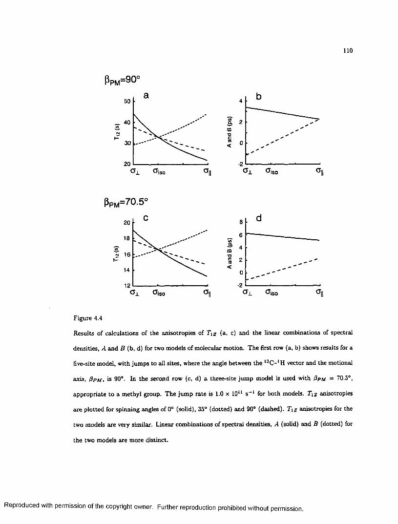
110
Ppm=90‘
(/)rsi
50
40
30
20a .II
a 2CD■acas n
C L CiISO
Ppm=70.5'
20
18
16
14
12a .
in
COT3Cas<
8
6
4
0
•2CT,II
Figure 4.4
Results of calculations of the anisotropies of T iz (a, c) and the linear combinations of spectral
densities, A and B (b, d) for two models of molecular motion. The first row (a, b) shows results for a
five-site model, with jumps to all sites, where the angle between the l3C-*H vector and the motional
axis, 0 p m , is 90°. In the second row (c, d) a three-site jum p model is used with 0pm = 70.5°,
appropriate to a methyl group. The jum p rate is 1 .0 x 10u s - 1 for both models. T \z anisotropies
are plotted for spinning angles of 0 ° (solid), 35° (dotted) and 90° (dashed). T \z anisotropies for the
two models are very similar. Linear combinations of spectral densities, A (solid) and B (dotted) for
the two models are more distinct.
Reproduced with permission of the copyright owner. Further reproduction prohibited without permission.

I l l
Thus, in the extreme narrowing limit, the relaxation of each point on a methyl powder pattern is a
single exponential function [65].
Although the linear combinations, A and B (defined in Eqs. 4.37 and 4.38) are not as distinctive as
the individual spectral densities, they do allow these two motional models to be easily distinguished,
as shown in Figures 4.4b and 4.4d. The most notable difference in the anisotropies is seen at the
parallel (0cR — 0°, a — CT||) edge of the CSA powder pattern. At this point A and B have the
same value for the ferrocene calculations, but are significantly different for the methyl spectrum. As
with the T \z anisotropies, A and B do not depend on the 0 c r quadrant for either model. While
it is unlikely that a relaxation experiment would be needed to distinguish methyl rotation from
five-site jumps, the differences in these particular linear combinations of spectral densities highlight
an im portant feature: the degree of separation between A and B at the parallel edge is sensitively
dependent on 0 p m , the angle between the l3C - l H vector and the motional axis. These curves are
also sensitive to the trajectory and rate of motion.
4.3 Carbon Relaxation Time Anisotropies in Ferrocene
For ferrocene, measurement of anisotropic relaxation times is straightforward because only one
chemically distinct carbon is present in the molecule. The natural abundance ferrocene sample
consisted of 103 mg of the material ground to a fine powder and packed into a 5 mm diameter ceramic
rotor. The precise values of the angles used in the off magic angle spinning (OMAS) experiments
were determined by comparing the widths of the spinning chemical shift powder patterns to the static
lineshape. The anisotropic lineshape parameters were determined by a least-squares fitting routine
that uses the SUMS powder pattern calculation algorithm [48]. A spin tem perature alternation
pulse sequence [35] was used to produce spectra that decay to zero a t long relaxation delays. The
cross-polarization (CP) contact time was 1 ms and a recycle delay of 40 s was used to allow for
proton relaxation. The proton 90° pulse length was 4 ps. Power in the proton channel was kept
Reproduced with permission of the copyright owner. Further reproduction prohibited without permission.
112
constant during cross polarization and acquisition of the carbon signals, resulting in a decoupling
field strength of 63 kHz. The relaxation delays used in the ferrocene T iz experiments were 0.1
s, 2 s, 4 s, 8 s, 16 s and 32 s. All relaxation experiments were performed a t room temperature,
296 ± 2 K. D ata analysis was performed on a Silicon Graphics 0 2 workstation with customized
PV-WAVE software. Relaxation times of each point on the powder lineshape were determined by a
two parameter non-linear least squares fit to the experimental data.
In spinning samples, one must be careful to compare relaxation times of identical crystallite
orientations, not measured chemical shift. Since spinning a t 0 m = 90° scales the powder pattern
by a factor of —1/2, the width of the experimental OMAS spectrum was scaled by a factor of - 2
to facilitate comparison with the static spectrum. The experimental T \ z anisotropies plotted in
Fig. 4.5 show the expected dependence on spinning angle, {0m,). For the static sample, relaxation
times are longest a t the a = <x± edge. When the sample is spun at 0 m — 90° the anisotropy is
reversed, with the longest relaxation times on the shoulder {a = cr||) of the powder pattern.
For carbons with directly bonded protons, the dominant relaxation mechanism is usually the
heteronuclear dipolar interaction. In order to ensure that the chemical shift anisotropy (CSA)
relaxation mechanism can be safely ignored in ferrocene, the relaxation time due to CSA alone was
estimated from the width of the static powder pattern. If this value of T \ z is much longer than the
measured relaxation rates then the assumption th a t the dipolar interaction dominates 13C relaxation
in ferrocene is justified. For an axially symmetric chemical shielding tensor the relaxation rate due
to chemical shift anisotropy is given by [69]
* iz (C S A ) = - O 2 1 ^ 2 - t4-42!
For our experiments, 'yBo = 27r x 75.46 x 10s s -1 . At room temperature, tne span of the ferrocene
powder pattern is f? = 80 ± 1 ppm. This lineshape is narrowed by a factor of two due to fast rotation
about the molecule’s Csv symmetry axis; thus, the static span, <T\\—a±_ = 160 ppm. The correlation
time is estim ated to be five times the largest calculated dipolar spectral density, 8 x 1 0 “ 13 s, at
Reproduced with permission of the copyright owner. Further reproduction prohibited without permission.

113
ISO
40
n 30
20
120 100 80 60 40 20 0ppm
Figure 4.5
For ferrocene, measured and calculated 13C T iz anisotropies for ferrocene. The filled diamonds
are the measured relaxation times for a static sample. Measured relaxation times for a sample
spinning at 90° with respect to the field are indicated with open squares. The width of the powder
pattern of the spinning sample was scaled by a factor of —2 before relaxation times were measured.
The solid line is the calculated anisotropy for the static sample. The calculated anisotropy for the
spinning sample is indicated with a dashed line. Experimental errors (±1 one standard deviation)
were determined by the fitting procedure. The rates used for the calculations are 1.1 ± 0.1 x 10u
s~l for the five-fold all-site jump model, 1.5 ± 0 .1 x 1011 s - 1 for the five site model with jumps only
to neighboring sites and 1.4 ± 0.1 x 10¹¹ s - 1 for rotational diffusion. These rates give the best fit of
the linear combinations of spectral densities (see text for details).
Reproduced with permission of the copyright owner. Further reproduction prohibited without permission.
114
the 3 c r = 0 ° edge of the static powder pattern. Substitution of these values into Eq. 4.42 yields a
relaxation rate of R iz (C S A ) = 3.1 x 10- 3 s _ l . The corresponding CSA spin-lattice relaxation time
is 330 s, significantly longer than the longest measured relaxation time of 40 s. For other orientations,
the estimated CSA relaxation times are even longer. Thus, the chemical shift anisotropy mechanism
makes a negligible contribution to the spin-lattice relaxation of ferrocene at room temperature.
For ferrocene, the experimental anisotropies of .4 and B are presented in Fig 4.6 along with
the results of calculations of A and B for the heteronuclear dipolar mechanism. The calculations
agree well with the experimental results. The experimental curves for A and B nearly overlap at
the parallel edge of the powder lineshape confirming that the angle between the 13C -l H vector and
the motional axis of ferrocene is very close to 90°. Neutron diffraction studies (70) have determined
that the C-H vectors are displaced out of the plane of the cyclopentadienyl rings, toward the iron
atom, by about 1.6°. Due to uncertainty in the experimental data, this deviation is too small to be
measured accurately by NMR.
In a sense, the molecular geometry of ferrocene is unfortunate. For 3 p m = 90° the expression
for the spectral densities (Eq. 4.31) simplifies further because d±2o(90°) = 3/8, efc?lo(90°) = 0 and
<4o(90°) = -1 /2 . Thus, the 6 = 1 terms vanish. The 6 = 0 terms are ignored because r 0,o does
not decay with time. Furthermore, for axial motion in the extreme narrowing limit, r 2,2 is simply a
constant, inversely proportional to the motional rate or diffusion coefficient. The spectral densities
for ferrocene are:
^ £ \d£L(PRL)\2 (0Cr )\2 + |d(_2>a(/3 c « )f} [4.43]a ^ *
where k is the jump rate and c is a number that depends on the motional model. For a five-
site model with jumps to all sites allowed, c = 5, if only jumps to nearest neighbor sites occur,
c = 4sin2(27r/5) ss 3.62, and for diffusive motion c = 4. Under these conditions, the spectral
densities for different models and rates differ only by the constant factor l / c k . As a result, for
this geometry, the subtleties of the motional trajectory cannot be differentiated. For ferrocene, the
Reproduced with permission of the copyright owner. Further reproduction prohibited without permission.

115
4
CO o3CQ-O C CO
< 0
-2
120 100 80 60 40 20 0ppm
Figure 4.6
For ferrocene, experimental (symbols) and best-fit values (lines) of the linear combinations of spectral
densities A and B determined from the static and spinning 13C T \z anisotropies. The rates used for
the calculations are 1.1 ± 0 .1 x 10u s - 1 for the five-fold all-site jum p model, 1.5 ± 0 .1 x 1011 s - 1 for
the five site model with jumps only to neighboring sites. The diffusion constant for the rotational
diffusion model is 1.4 ± 0.1 x 10u s'*1. The convergence of A and B a t the cry edge of the powder
pattern confirms that the angle between the vector and the axis of motion is close to 90°.
_ l —'ISO1---------------------T
a H~r
A
B
I I— 1 - I L - 1 . I ■ ‘ ■ I 1 ' ■ I ■ ■ ■ I ■ ■ ■
Reproduced with permission of the copyright owner. Further reproduction prohibited without permission.
116
best-fit rate for each model was determined by manually varying the rates used for the calculations
so as to minimize chi-squared of the calculated and measured A and B anisotropies.
If a UC - ‘H bond length of 1.08 A is used (vd — 2 rrup = 24.0 x 10⁵ kHz) then the A and B
anisotropies are best fit with a jump rate of Jfe = 1.1 ± 0 .1 x 10*1 s - 1 for the five-site model with
jumps to all sites allowed. The best-fit rates for the other models were found to be in agreement
with Eq. 4.43. Thus, the best-fit rate for the 5-site model with jumps to neighboring sites is
1.5 ± 0.1 x 10¹¹ s -1 and for diffusive motion the diffusion constant is 1.4 ± 0.1 x 10u s _ l. These
results are in reasonable agreement with neutron scattering measurements [71]. Assuming a five-site
nearest-neighbor jum p model, the neutron data give a rate of 1.1 ± 0 .2 x 1 0u s -1 , whereas the
experimental NMR data yield a best-fit value of 1.5 ± 0.1 x 10u s_ l .
The 13C -'H bond length of 1.08 A was determined by requiring that the motional rates measured
by carbon relaxation agree with the deuteron rates presented later in this chapter. Studies of the
dynamics of benzene [6 6 ] show that correlation times for the protonated and deuterated molecule
differ by only a few percent at room tem perature. Since the structure and dynamics of ferrocene
are similar to benzene’s, isotope effects in ferrocene are unlikely to be significant compared to
experimental uncertainties. The ferrocene bond length used, 1.08 A, is larger than published values
determined from neutron diffraction studies [70,72]. The values in these studies ranged from 0.903 A
to 1.056 A a t 298 K, depending on the refinement model used. The correction of the dipolar coupling
constant resulting from the use of an appropriately vibrationally averaged bond length, instead of
the equilibrium value, has been calculated [6 6 ] to be (1.080/1.106)3 or —7%. When the ferrocene
bond length used here is compared to the longest of the neutron diffraction values the vibrational
correction is also about —7%. As noted in Section 4.2.4, the vibrationally averaged bond length
measured by neutron diffraction is expected to be closer to the equilibrium value than the length
determined by the dipolar coupling strength.
The relaxation time of the ferrocene peak in a CPMAS experiment was measured to be T iz =
32.0 ± 0.4 s. The relaxation of this peak displays no apparent multi-exponential behavior. This is
Reproduced with permission of the copyright owner. Further reproduction prohibited without permission.
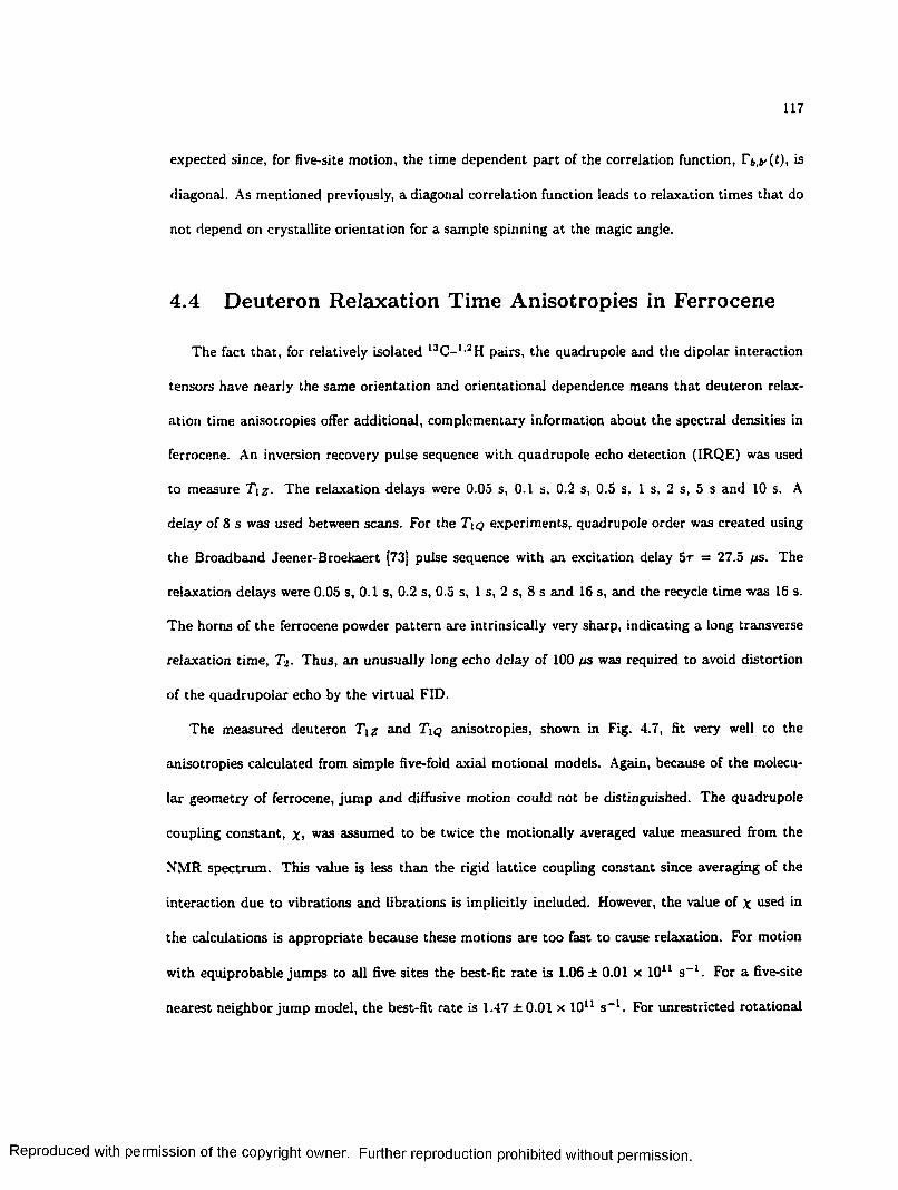
117
expected since, for five-site motion, the time dependent part of the correlation function, l \ y ( f ) , is
diagonal. As mentioned previously, a diagonal correlation function leads to relaxation times that do
not depend on crystallite orientation for a sample spinning at the magic angle.
4.4 Deuteron Relaxation Time Anisotropies in Ferrocene
The fact that, for relatively isolated 13C -l,2H pairs, the quadrupole and the dipolar interaction
tensors have nearly the same orientation and orientational dependence means that deuteron relax
ation time anisotropies offer additional, complementary information about the spectral densities in
ferrocene. An inversion recovery pulse sequence with quadrupole echo detection (IRQE) was used
to measure T \ z ■ The relaxation delays were 0.05 s, 0.1 s, 0.2 s, 0.5 s, 1 s, 2 s, 5 s and 10 s. A
delay of 8 s was used between scans. For the Tiq experiments, quadrupole order was created using
the Broadband Jeener-Broekaert [73] pulse sequence with an excitation delay 5 r = 27.5 ps. The
relaxation delays were 0.05 s, 0.1 s, 0.2 s, 0.5 s, 1 s, 2 s, 8 s and 16 s, and the recycle time was 16 s.
The horns of the ferrocene powder pattern are intrinsically very sharp, indicating a long transverse
relaxation time, T%. Thus, an unusually long echo delay of 100 (xs was required to avoid distortion
of the quadrupolar echo by the virtual FID.
The measured deuteron T \z and T iq anisotropies, shown in Fig. 4.7, fit very well to the
anisotropies calculated from simple five-fold axial motional models. Again, because of the molecu
lar geometry of ferrocene, jum p and diffusive motion could not be distinguished. The quadrupole
coupling constant, x> was assumed to be twice the motionally averaged value measured from the
NMR spectrum. This value is less than the rigid lattice coupling constant since averaging of the
interaction due to vibrations and librations is implicitly included. However, the value of x used in
the calculations is appropriate because these motions are too fast to cause relaxation. For motion
with equiprobable jum ps to all five sites the best-fit ra te is 1.06 ± 0.01 x 10¹¹ s-1 . For a five-site
nearest neighbor jump model, the best-fit rate is 1.47 ±0 .01 x 10u s -1 . For unrestricted rotational
Reproduced with permission of the copyright owner. Further reproduction prohibited without permission.
118
2.5
2.0
1.5
1.0
0.5
0.0-100 -50 0
kHz50 100
20
15
10
5
0 L- -100 50-50 0 100
kHz
Figure 4.7
Measured (symbols) and best-fit (lines) deuteron (a) T iz and (b) T \q anisotropies for ferrocene-
dio at 23° C. Calculated anisotropies correspond to a five-site jum p model with a jump rate of
1.06±0.01 x 10U s _ l , a five-site model with jumps to neighboring sites a t a rate of 1.47±0.01 x 10¹¹
s -1 or a free diffusion model with a diffusion constant of 1.33 ±0 .01 x 1011 s_1. The molecular
geometry of ferrocene prevents these models from being distinguished. Error bars representing
the experimental errors determined by the fitting procedure are plotted along with the measured
relaxation times. In some cases the error bars are smaller than the symbols.
Reproduced with permission of the copyright owner. Further reproduction prohibited without permission.
119
diffusion, the best-fit diffusion constant is 1.33 ± 0.01 x 10u s_ l . Within experimental error, these
rates agree with those determined from l3C relaxation. Since the calculated I3C relaxation time
anisotropies depend sensitively on the 13C -‘ H bond length, this agreement supports a ferrocene
bond length of 1.08 A.
From the deuteron relaxation data the individual spectral densities, J\ (uj0) and J 2 (2wo) can be
calculated as a function of quadrupolar frequency. In the extreme narrowing limit, these spectral
densities, combined with the relaxation time for the l3C CPMAS isotropic peak provided the in
formation needed to determine Jo(0). Although 7o(ui) has been measured in an oriented nematic
liquid crystal [74|, the ferrocene results are the first experimental determination of the orientation
dependence of Jo(0) in a polycrystalline solid. The experimental spectral densities closely match
the simulated data, as shown in Fig. 4.8. These results validate the assumption that, in ferrocene,
the spectral densities responsible for l3C dipolar relaxation are the same as those responsible for
deuteron quadrupolar relaxation.
Substitution of the spectral densities (Eq. 4.43) into the expressions for R \ z (Eqs. 4.19 and 4.20)
shows that R i z ( l3C) oc u>2D/ k for carbon, and R iz (2 H) oc X2/ k for deuterons. Since we require
that the rate of motion, k, be the same for both carbon and deuteron relaxation, the ratio of the
two relaxation rates is Wq / x 2- The quadrupole coupling constant has been determined; thus, an
expression for the dipolar coupling constant can be written:
/ « i z ( l3C)= * v r ^ F h T [ 1
This expression could be used to evaluate u>o and hence, ( l/r j~ tf). It also provides a means for
estimating the uncertainty in the 13C -l H bond length. The average uncertainty in R iz ( l3C) is
7.7%. For the deuteron da ta the average uncertainty is 1.4%. We estimate that the value used for
X is within one percent of the correct value. Propagation of these errors through Eq. 4.44 leads tom » /q
an uncertainty in ujd of 4.0%. The bond length, ) , determined in this study is
thus 1.08 ± 0 .0 2 A.
Reproduced with permission of the copyright owner. Further reproduction prohibited without permission.
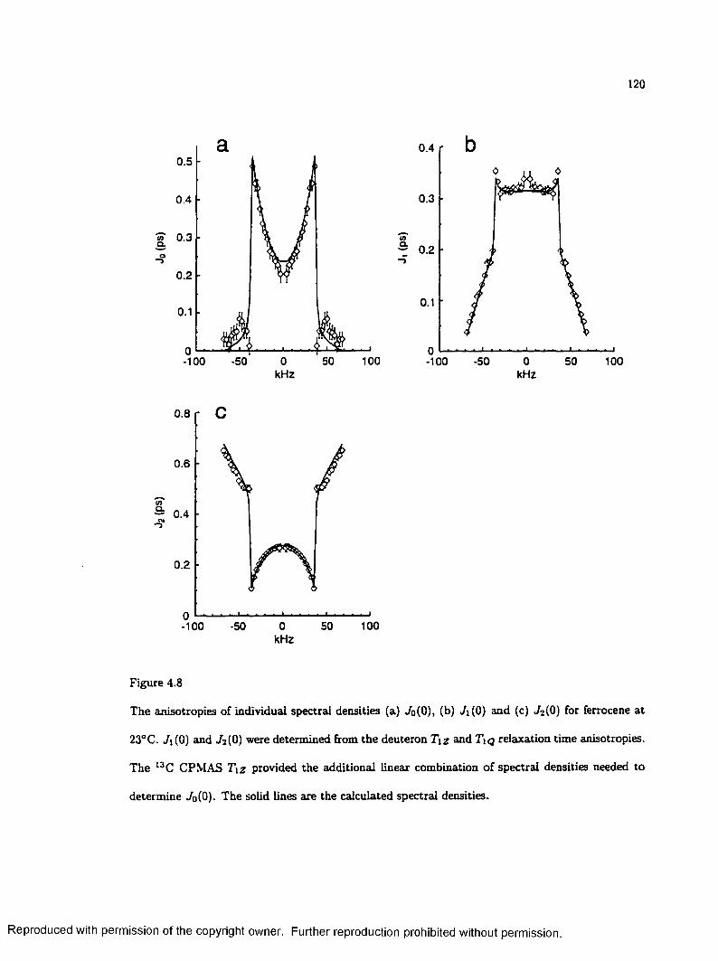
120
0.4
0.3
“ 0.2
0.1
-50 0 50 1 0 0-100
0.5
0.4
£ 0.3
0.2
0.1
0 ■— -100 0 50 100-50
kHz kHz
0.8
0.6
inQ. 0.4
0.2
100-50 0 50-100 kHz
Figure 4.8
The anisotropies of individual spectral densities (a) Jo(0), (b) Ji(Q) and (c) J 2 (0) for ferrocene at
23°C. Ji(0) and J 2 (0) were determined from the deuteron T iz and T iq relaxation time anisotropies.
The l3C CPMAS T \z provided the additional linear combination of spectral densities needed to
determine J o(0). The solid lines are the calculated spectral densities.
Reproduced with permission of the copyright owner. Further reproduction prohibited without permission.
121
4.5 Relaxation Tim e Anisotropies in 2D Experiments
When the overlap of 13 C powder patterns prevents accurate measurement of chemical shift
anisotropies, 2D techniques can often be used to separate the anisotropic lineshapes. A number
of experimental techniques are available for separating CSA powder patterns on the basis of their
isotropic chemical shift values [11]. This suggests that the incorporation of an inversion pulse and a
relaxation delay into these experiments would allow the measurement of relaxation time anisotropy of
each chemically distinct carbon. However, the effect of sample spinning on relaxation time anisotropy
must be kept in mind.
The fact that relaxation time anisotropy depends on spinning angle complicates the measurement
of partially relaxed powder patterns with variable angle correlation spectroscopy (VACSY). In a
VACSY experiment, the anisotropic chemical shift is scaled by varying the spinning angle. The
implicit assumption is that the only difference between the spectra taken at different spinning angles
is that the widths of the powder patterns are scaled. For partially relaxed spectra this assumption is
not valid. The relaxation time anisotropy in a VACSY powder pattern is not related in any simple
way to the anisotropies at each of the various spinning angles. However, for axial motional models,
simulations show that the anisotropies for 3 rl < 3magtc offset those for 3 rl > 3magic, yielding
virtually no relaxation anisotropy for the set of partially relaxed VACSY powder patterns.
A VACSY relaxation experiment has been performed for octanoic acid in a urea inclusion com
pound (CaA-UIC). The chemical structure of octanoic acid is shown in Fig. 4.9. In this material,
the linear octanoic acid guest molecules are restricted within narrow channels formed by the urea
host. Although the narrow channels greatly restrict the motion of the guest, the relaxation time
anisotropies, shown in Fig. 4.10, indicate that guest motion is not strictly axial. This observation
supports other evidence of non-axial motion. Deuteron NMR relaxation studies indicate that the
13C -‘H bonds of the methylene groups wobble about an axis perpendicular to the channel axis [75].
Carbon-13 MAS relaxation times for the methylene carbons depend on position in the molecule [76]
Reproduced with permission of the copyright owner. Further reproduction prohibited without permission.

122
and the asymmetry of measured chemical shift tensors (see Figure 4.9) also argue against a simple
axially symmetric model of motion.
Some 2D experiments are performed with MAS using rotor-synchronized pulses to disrupt the
averaging of the chemical shift [77]. If the sample is spun at the magic angle during the relaxation
delays, the measured relaxation anisotropy will reflect the averaging of the spectral densities that
occurs with MAS. For many motional trajectories no anisotropy would be observed. Even typical
magic angle turning frequencies (about 30 Hz) [57] yield rotor periods th a t are short compared
to most carbon relaxation times. The magic tingle hopping experiment [78] also suffers from this
problem since the rapid 1 20° jum ps also cause averaging of the spectral densities.
For spinning angles other than the magic angle, relaxation time anisotropies could be measured
by storing magnetization along the z-axis and quickly reorienting the rotor for the relaxation delay.
After which, the spinning axis would be returned to the magic angle and the pulse sequence for
measuring the 2D spectrum executed as usual. This technique is compatible with the magic angle
flipping 2D experiment [79] in which the spinning axis is reoriented to allow evolution under the
anisotropic chemical shift. By performing this modified magic angle flipping experiment twice, using
different spinning angles during relaxation, two linear combinations of the static spectral densities
could be determined for each carbon line in the spectrum. This technique appears to hold the most
promise for obtaining high-fidelity information about molecular motion in complex systems using
natural abundance l3C NMR.
4.6 Conclusions
NMR spin-lattice relaxation time anisotropies provide valuable and unique information about
molecular dynamics. This chapter describes a method for obtaining information about molecular
motion with a level of detail previously unavailable from natural abundance 13C NMR. For fast
motion, relaxation times are linear combinations of the spectral density functions which describe the
Reproduced with permission of the copyright owner. Further reproduction prohibited without permission.

123
- ch2 - ch2 - ch2 - ch2 - ch2 - ch2 - ch3HO 1 2 3 4 5 6 7 8
k = 0.84 a = 31.2 p p m
40
Ea
PPm
x = 0.76 12 = 2 1 . 2 p p m
20
4060-20
PPmppm
2654
Figure 4.9
2D VACSY spectrum for the methyl and methylene carbons in CgA-UIC. On the contour plot, the
vertical axis is isotropic chemical shift, and the horizontal axis is anisotropic chemical shift. Carbon
peaks are numbered according to position in the alkyl chain starting with the acid group. CSA
powder patterns for carbon 3 and the unresolved resonances of carbons 2 and 6 , found by taking
slices through the 2D spectrum at the indicated isotropic chemical shifts, are shown. The frequency
axes for the anisotropic lineshapes are corrected by shifting by the isotropic chemical shifts of the
carbons. The asymmetry of the chemical shift tensor (|/c| ^ 1) indicates deviations from axially
symmetric motion.
Reproduced with permission of the copyright owner. Further reproduction prohibited without permission.

124
OTT3Coo(Uc/>N
H
4
3
2
1
50 30 2040
A
1030 2040ppm ppm
Figure 4.10
T \2 anisotropies for (a) carbons 2 and 6 and (b) carbon 3 in CsA-UIC a t 23° C. (See Fig. 4.9 for
assignment.) The variation of T \z across lineshapes cannot be reproduced by axially symmetric
models of motion.
Reproduced with permission of the copyright owner. Further reproduction prohibited without permission.

125
time dependence of heteronuclear dipole interactions. In order to rigorously test models of molecular
motion, measurement of sill relevant spectral densities is sought. A variety of carbon and deuteron
relaxation time anisotropies were measured for ferrocene, in an attem pt to obtain as many linear
combinations of the spectral densities as possible, and thus provide the most complete motional
description.
The 13C results presented here dem onstrate theoretical and experimental methods for obtaining
the two linear combinations of the spectral densities responsible for 13C heteronuclear dipolar relax
ation. The method makes use of the observation that, in spinning samples, carbon T iz anisotropies
depend on the orientation of the spinning axis. In the extreme narrowing limit, where the spec
tral densities are independent of frequency, these anisotropies are linear combinations of the static
spectral densities with coefficients that depend on the spinning angle. Because of the functional
dependence of these coefficients on the spinning angle, only two independent linear combinations of
the static spectral densities can be determined. These linear combinations, A and B, are sensitive
to molecular geometry. In particular, the difference between A and B for Pc r = 0° is correlated
with the angle between the z-axes of the principal axis system and molecular frame. For ferrocene,
where Ppm = 90°, similar models of motion (five-fold jumps to all sites, five-fold jumps to neigh
boring sites and rotational diffusion) are not distinguishable from measurements of A and B. This
is a special case; for other molecular geometries, calculations show that the different trajectories are
distinguishable. Thus, natural abundance 13 C relaxation time measurements can provide detailed
motional information.
The measurement of the anisotropies of deuteron Zeeman and quadrupolar relaxation times, T iz
and T i q , allow the determination of two spectral densities, J i {uq) and Ji (2ljq). Motional rates
determined from these data are in good agreement with results of neutron scattering experiments
[71]. For fast uniaxial motional models, the combination of the deuteron results with carbon re
laxation experiments provides the additional constraint necessary for the determination of a third
spectral density, Jq(0). This chapter reports the first experimental measurement of the orientation
Reproduced with permission of the copyright owner. Further reproduction prohibited without permission.
126
dependence of Jo(0) in a polycrystalline solid. The combination of l3C and 2H relaxation data also
allowed the determination of the l3C - l H dipolar coupling strength, and thus, the l3C -‘H bond
length. For ferrocene, a bond length of 1.08 ± 0 .0 2 A was found.
The overlap of anisotropic lineshapes hampers quantitative analysis of l3C NMR spectra just
as it does for other nuclear species. Resonances from chemically distinct deuterons can sometimes
be measured with selectively deuterated samples. For carbon NMR, two dimensional separation of
powder patterns on the basis of isotropic chemical shift can provide selectivity. When applied with
care, 2D techniques should allow detailed motional information to be obtained for each chemically
distinct carbon in complex molecular systems. Such information is needed to characterize dynamics
accurately and to identify the microscopic physical phenomena th a t influence the bulk properties of
solids.
Reproduced with permission of the copyright owner. Further reproduction prohibited without permission.

Chapter 5
Characterization o f Polyim ides
5.1 Introduction
The characterization of materials is an im portant application of NMR. By probing the various
interactions experienced by atomic nuclei, much can be learned about structure, organization and
dynamics on a variety of distance scales. The goal of such research is to connect what is learned about
these microscopic properties with what is known about the material’s bulk properties. Once causal
connections are established, the synthesis of new materials can be directed toward meeting desired
physical specifications. Such connections are particularly difficult to make for polymers because of
their complex morphology [80]. The long chains of molecules have many degrees of freedom. Domains
of crystallinity often exist in an otherwise amorphous material. Conformations and dynamics will be
different in these distinct environments. For completely amorphous polymers, wide distributions of
conformations and distances makes precise characterization of microscopic structure and dynamics
difficult.
In some polymers the degree of heterogeneity requires that a wide range of distance scales be
considered. A number of techniques are available for probing distances from Angstroms to microns.
Direct dipolar coupling influences l3C NMR spectra when the nuclei are separated by less than about
127
Reproduced with permission of the copyright owner. Further reproduction prohibited without permission.
CHAPTER 5. CHARACTERIZATION OF POLYIMIDES 128
five Angstroms. In such cases, the cross relaxation rate, Tc h depends on the carbon-proton dipolar
interaction, and thus, on the internuclear distance. The effects of different cross relaxation rates are
seen in cross polarization dynamics, dipolar dephasing [81] and short contact (See Section 2.5.3.)
experiments. Precise distance measurements can be performed using the REDOR [82,83] or TEDOR
[84] techniques.
Over longer distances, homonuclear dipolar couplings among abundant nuclei promote the dif
fusion of nuclear polarization by energy-conserving spin flips. In polymer blends and other hetero
geneous materials, spin diffusion, detected through its effect on NMR spectra, can give information
about the miscibility of the polymer systems [80]. For heterogeneous systems, the size of the mor
phological domains can be determined by spin diffusion. When rigid crystalline and more mobile
amorphous regions are both present, the dipolar filter [85] or Goldman-Shen [8 6 ] pulse sequences
can be used to destroy the magnetization in the rigid region. Spin diffusion during an evolution time
redistributes the magnetization. Information about molecular order over distances in the range of
about 2 0 to 500 Angstroms are accessible by this kind of spin diffusion measurement [87]. Pulsed
field gradient NMR extends the range of spin diffusion techniques to the scale of microns [8 8 ].
Polyimides are a class of polymer with properties that make them suitable for applications in
punishing environments. They are remarkably strong due to the rigidity of the molecules in the
polymer chains. They resist chemical and thermal degradation, and the temperature a t which they
soften and sta rt to flow (the glass transition temperature) is particularly high compared to other
polymers. These properties have lead to the widespread use of polyimides as adhesives, matrix
resins for composite materials, and high strength films and coatings [89,90]. A significant drawback
of these materials is that they are notoriously insoluble, and therefore, difficult to process. Melt
processing these materials is made difficult by their high glass transition temperatures. Even at
temperatures above the glass transition, high viscosity complicates processing.
Great effort has been directed toward the synthesis of polyimides th a t are easier to process due
to improved solubility and lower melt viscosity [91]. Over twenty years ago it was recognized that
Reproduced with permission of the copyright owner. Further reproduction prohibited without permission.
CHAPTER 5. CHARACTERIZATION OF POLYIMIDES 129
introduction of meta- or ortho-substituted aromatic rings tends to improve solubility [92]. More
recently, polyimides have been prepared in which solubility in common aprotic solvents is greatly
enhanced by the introduction of flexible bridging ligands [93,94] or bulky substituents [95,96] at sites
on the polymer backbone. Although the ability to synthesize compounds that conform to a given set
of specifications is still many years away, the knowledge gained from the investigation of the effect
of structure on bulk properties has made possible the design of polyimides with specific properties
in mind. This has been demonstrated by the production of electroluminescent materials [97] and
molecules for use in liquid crystal displays [98].
5.1.1 LaRC-SI
Modification of the chemical structure to improve processability is done at the risk of degrad
ing desirable properties of polyimides. Improvements in solubility generally come at the expense
of thermoplastic properties. Given the compromises typically made in the production of soluble
polyimides, the recent synthesis [99] of a fully aromatic, soluble polyimide which has no substituents
is highly significant. This polyimide, LaRC-SI1, is a random copolymer composed of two dian
hydrides, 4,4'-oxydiphthalic anhydride (ODPA) and 3,4,3',4'-biphenyltetracarboxylic dianhydride
(BPDA), condensed with a single diamine, 3,4'-oxydianiline (ODA). The solubility is not strongly
dependent on the average molecular weight of the chains or on the relative proportions of the two
monomers. However, homopolymers formed from the diamine and either dianhydride alone are
insoluble [99].
LaRC-SI can be rendered insoluble by annealing at a tem perature above its glass transition tem
perature of 227°-253° C. This behavior is also not strongly dependent on the molecular weight of the
polymer [99]. It has been suggested [100] th a t the solubility of LaRC-SI is due to plasticization of the
polymer by trace quantities of solvent th a t remain after precipitation. Heat treatm ent increases the
1 LaRC stands for NASA’s Langley Research Center, where the polymer was first synthesized. SI stands for soluble
imide.
Reproduced with permission of the copyright owner. Further reproduction prohibited without permission.

CHAPTER 5. CHARACTERIZATION OF POLYIMIDES 130
mobility of the polymer chains, liberating trapped solvent molecules. Upon cooling the chains may
settle into a tighter arrangement that resists penetration of solvent molecules. Another possibility is
that the formation of crosslinks among the chains during heat treatment results in an arrangement
that excludes solvent molecules. These hypotheses will be considered in the analysis of the NMR
data.
The close similarity in structure between LaRC-SI and related, but insoluble, polyimides em
phasizes that much progress remains to be made in developing a quantitative understanding of the
relation between bulk properties and molecular structure, dynamics, and microscopic morphology
of polyimides.
5.1.2 l3C and NM R Techniques for Characterizing Polyimides
Sensitivity to structure and dynamics of amorphous materials makes NMR well suited to the
investigation of polymers. On the other hand, the broad distributions of quantities that contribute
to NMR spectra, including internuclear and interchain distances, conformations, and rates and
amplitudes of molecular motion, can make experimental results difficult to interpret.
In this chapter, the utility of solid state 13 C and l H NMR techniques for characterizing polymer
microstructure and dynamics is demonstrated by experiments on the polyimides LaRC-TPI, LaRC-
IA and LaRC-SI, and five related monomers. (See Figures 5.1-5.8 for molecular structures.) Much
of the material presented in this chapter was published in Solid State NMR, 12 (1998). The first
goal of this study was to add to the existing data base [101,102,103,104,105,106] of assigned solid
state 13 C CPMAS spectra of polyimides and model compounds. A large collection of measured
isotropic chemical shifts is useful because the 13 C NMR spectra of fully aromatic polyimides consist
of relatively broad, partially overlapping bands which cure difficult to assign without comparison to
previously interpreted spectra. Spectral assignments of solid samples are often made by comparison
to typical solution state chemical shift values. However, it is well known (and it is demonstrated in
this chapter) that isotropic chemical shift values for solids can be significantly different from those
Reproduced with permission of the copyright owner. Further reproduction prohibited without permission.

CHAPTER 5. CHARACTERIZATION OF POLYIMIDES 131
seen in liquids. This phenomenon may be of particular importance for polyimides, where interchain
charge transfer interactions [106] and ring currents [107] can contribute to the solid state chemical
shifts.
Solution state NMR experiments were performed on LaRC-SI and model compound III. These
were done, in part, to aid in the assignment of the solid state spectra. Also, it was hoped that
differences in the solid and solution chemical shifts would indicate non-equilibrium molecular con
formations or molecular packing arrangements in the solid.
It is possible that chemical shielding anisotropy can provide valuable information that is obscured
in the MAS spectra. Trends in the individual tensor components that are not apparent in the
isotropic values may be useful for elucidating the dependence of chemical shielding on structure.
The body of measured tensor components is much smaller than that of isotropic chemical shifts
since the tensor components are more difficult to measure than isotropic values. A larger collection
of measured anisotropic chemical shifts is needed to see if the analysis of chemical shift anisotropy
can provide unique insight. In order to add to this body of knowledge, the technique of variable
angle correlation spectroscopy (VACSY) [40] was used to measure anisotropic lineshapes of some of
the polymers and model compounds.
A number of solid state l3C and 1H NMR techniques were used to investigate the polyimides. It
was hoped that some of these techniques would shed some light on the solubility behavior of LaRC-
SI. The experiments performed include l H FID, two-dimensional wideline separation (WISE) [37,39],
‘H dipolar filter [85] experiments with either 13C cross polarization magic angle spinning (CPMAS)
or direct signal detection, and cross polarization dynamics. Some of these techniques were also
used in a preliminary investigation of water absorption by these materials, further illustrating the
ability of solid state NMR to provide insights into polyimide microstructure and dynamics.
Relaxation experiments are often a rich source of information about molecular dynamics. How
ever, due to the rigidity of the polymer chains in these materials, 13C relaxation times are quite long.
Preliminary experiments showed th a t the spin-lattice relaxation times in LaRC-SI are in the range
Reproduced with permission of the copyright owner. Further reproduction prohibited without permission.

CHAPTER 5. CHARACTERIZATION OF POLYIMIDES 132
of 45 seconds to a minute. Thousands of scans would be required to make an accurate measurement,
some with relaxation delays that are several times longer than the relaxation time. Acquisition of a
data set with a sufficient signal-to-noise ratio for quantitative analysis would take many days. Such
experiments were not performed because they were not seen as an effective use of spectrometer time.
5.2 Materials
Samples of LaRC-TPI, LaRC-IA, and LaRC-SI were obtained from Dr. Robert G. Bryant (NASA
Langley Research Center). LaRC-SI is synthesized by mixing the starting materials, ODPA, BPDA
and ODA, in stoichiometric amounts with phthalic anhydride (PA), an endcapping reagent. These
materials are mixed with the solvent n-methylpyrrolidinone and stirred overnight a t room tempera
ture to form a solution. Another solvent, toluene, is then added and the solution is heated to 165° C
for six hours to remove the water of reaction by azeotropic distillation. The reaction is cooled and
the polyimide is precipitated into water [99]. Heat treatment was performed by heating the samples
under vacuum to 1 0 0° C, 200° C and then 300° C for one hour periods.
Since phthalic anhydride terminates the polymer chains, the amount of this endcapping agent
added to the n-methylpyrrolidinone solution determines the average chain length and therefore,
the average molecular weight of the polymer. The weight-average molecular weight for LaRC-SI,
prepared in the same manner as the samples studied in this chapter, has been measured using gel
permeation chromatography/differential viscometry (GPC/DV) to be 41,100 g/m ol [108]. Since
the molecular weights of the ODPA-containing and BPDA-containing subunits are 474 and 458,
respectively, the average chain consists of about 8 8 subunits.
A series of five model compounds tha t have chemical structures similar to the repeat units of the
polymers was studied to support the chemical shift assignments. These materials were synthesized
by Dr. Jeffrey A. Hinckley (NASA Langley Research Center).
Reproduced with permission of the copyright owner. Further reproduction prohibited without permission.

CHAPTER 5. CHARACTERIZATION OF POLYIMIDES
5.3 Results
133
5.3.1 Solid State Isotropic 13C Chemical Shifts
Analysis of the CPMAS spectra has yielded tentative assignments of a group of monomers with
similar structures to the polymers. Dipolar dephasing experiments [81] simplified this task by elim
inating signals from carbons th a t have attached protons. (See discussion in section 2.5.3.) Assign
ment of the remaining non-protonated carbon peaks was fairly straightforward, but unambiguous
differentiation of the protonated carbon peaks is difficult.
The structures of these m aterials are shown, along with their assigned MAS, dipolar dephased,
and difference spectra in Figures 5.1-5.5. The isotropic chemical shifts of the assigned peaks are
reported in Table 5.2. Specific assignments were made by comparing the measured chemical shift
values to compiled solid and solution state chemical shift values [20]. Some ambiguous peaks were
assigned by comparing the structures and spectra of the various monomer model compounds under
investigation. However, the origin of many of the individual protonated carbon peaks remains
uncertain, and the assignments listed for these peaks in Table 5.1 must be regarded as tentative.
Assignment of the peaks in the spectra of polymers is especially difficult because the micro-
heterogeneous environment leads to spectral lines that are significantly broader than those of the
model compounds. Imide carbonyl and ether carbons remain well resolved, but considerable overlap
in the aromatic region prevents complete assignment of the spectra. Figures 5.6-5 .8 show the poly
mer molecular structures along with the assigned MAS, dipolar dephased, and difference spectra.
Dipolar dephasing reveals tha t the downfield portion of the remaining unresolved resonances is
predominantly from non-protonated carbons, although there is significant overlap of the protonated
and non-protonated carbon lines. T he aromatic C-C and the amine-imide C-N peaks are partially
resolved in the spectra of LaRC-IA and LaRC-SI. However, no resolvable structure is seen in spectra
of the protonated carbons of any of the polymers. The chemical shifts of the assigned peaks are
reported in Table 5.2.
Reproduced with permission of the copyright owner. Further reproduction prohibited without permission.
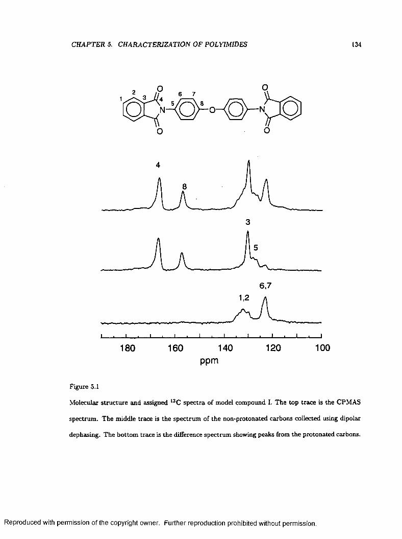
CHAPTER 5. CHARACTERIZATION OF POLYIMIDES 134
1 4
N
O
3
6,7
1 2 0 100180 160 140ppm
Figure 5.1
Molecular structure and assigned l3C spectra of model compound I. The top trace is the CPMAS
spectrum. The middle trace is the spectrum of the non-protonated carbons collected using dipolar
dephasing. The bottom trace is the difference spectrum showing peaks from the protonated carbons.
Reproduced with permission of the copyright owner. Further reproduction prohibited without permission.

CHAPTER 5. CHARACTERIZATION OF POLYIMIDES 135
411
N
12o o13
4
3
5,11
1,2 (-6,7,13-1
100120180 160 140ppm
Figure 5.2
Molecular structure and assigned l3C spectra of model compound II. The top trace is the CPMAS
spectrum. The middle trace is the spectrum of the non-protonated carbons collected using dipolar
dephasing. The bottom trace is the difference spectrum showing peaks from the protonated carbons.
Reproduced with permission of the copyright owner. Further reproduction prohibited without permission.

CHAPTER 5. CHARACTERIZATION OF POLYIMIDES 136
3,12
1,2,13,14 1-8,9,10
100180 160 1 2 0140ppm
Figure 5.3
Molecular structure and assigned 13 C spectra of model compound III. The top trace is the CPMAS
spectrum. The middle trace is the spectrum of the non-protonated carbons collected using dipolar
dephasing. The bottom trace is the difference spectrum showing peaks from the protonated carbons.
The peaks from the chemically equivalent aromatic ether carbons (7) are differentially shifted due
to intermolecular interactions.
Reproduced with permission of the copyright owner. Further reproduction prohibited without permission.

CHAPTER 5. CHARACTERIZATION OF POLYIMWES 137
O -C H
5 2
7
3,4,10
200 180 160 140 120 100 80 60 40 20ppm
Figure 5.4
Molecular structure and assigned 13C spectra of model compound IV. The top trace is the CPMAS
spectrum. The middle trace is the spectrum of the non-protonated carbons collected using dipolar
dephasing. The bottom trace is the difference spectrum showing peaks from the protonated carbons.
Reproduced with permission of the copyright owner. Further reproduction prohibited without permission.

CHAPTER 5. CHARACTERIZATION OF POLYIMIDES 138
N-HH-N
4 7
3,6
120 100160 140200 180ppm
Figure 5.5
Molecular structure and assigned l3C spectra of model compound V. The top trace is the CPMAS
spectrum. The middle trace is the spectrum of the non-protonated carbons collected using dipolar
dephasing. The bottom trace is the difference spectrum showing peaks from the protonated carbons.
Reproduced with permission of the copyright owner. Further reproduction prohibited without permission.
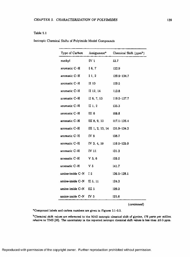
CHAPTER 5. CHARACTERIZATION OF POLYIMIDES 139
Table 5.1
Isotropic Chemical Shifts of Polyimide Model Compounds
Type of Carbon Assignment® Chemical Shift (ppmb)
methyl IV 1 53.7
aromatic C-H I 6 , 7 122.9
aromatic C-H I 1 , 2 129.9-134.7
aromatic C-H II 10 109.5
aromatic C-H II 12, 14 113.8
aromatic C-H II 6 , 7, 13 119.5-127.7
aromatic C-H II 1, 2 135.3
aromatic C-H III 6 108.8
aromatic C-H III 8 , 9, 10 117.1-126.4
aromatic C-H III 1, 2, 13, 14 131.9-134.3
aromatic C-H IV 8 108.7
aromatic C-H IV 3, 4, 10 116.0-125.9
aromatic C-H IV 11 131.3
aromatic C-H V 3, 6 125.5
aromatic C-H V 5 141.7
amine-imide C-N I 5 126.5-128.1
amine-imide C-N II 5, 11 124.3
amine-imide C-N III 5 129.3
amine-imide C-N IV a 121.6
(continued)
^Compound labels and carbon numbers are given in Figures 5.1-5.5.
b Chemical shift values are referenced to the MAS isotropic chemical shift of glycine, 176 parts per million relative to TMS [50]. The uncertainty in the reported isotropic chemical shift values is less than ±0.5 ppm.
Reproduced with permission of the copyright owner. Further reproduction prohibited without permission.

CHAPTER 5. CHARACTERIZATION OF POLYIMIDES
Table 5.1
Isotropic Chemical Shifts of Polyimide Model Compounds (continued)
Type of Carbon Assignment1 Chemical Shift (ppmb)
aromatic C-C 13 130.2
aromatic C-C II 3 128.1-130.5
aromatic C-C III 3, 12 131.6-133.9
aromatic C-C IV 7 130.2, 131.5
aromatic C-C V 7 133.5
aromatic C-C V 2 136.1
aromatic C-C V 4 145.4
ipso biphenyl IV 9 140.3
aromatic ether 18 157.3
aromatic ether II 8 152.4
aromatic ether II 9 153.9
aromatic ether III 7 152.9, 159.4
aromatic ether IV 2 158.8
imide carbonyl 14 166.6
imide carbonyl 114 166.9
imide carbonyl III 4, 11 163.8-166.7
imide carbonyl IV 5 166.5
imide carbonyl V 8 168.1
imide carbonyl V 1 172.2
aryl ketone carbonyl V 9 196.2
Reproduced with permission of the copyright owner. Further reproduction prohibited without permission.
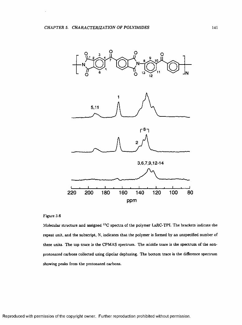
CHAPTER 5. CHARACTERIZATION OF POLYIMIDES 141
5,11
r 8 _ i
3,6,7,9,12-14
220 200 180 160 140 120 100 80ppm
Figure 5.6
Molecular structure and assigned 13C spectra of the polymer LaRC-TPI. The brackets indicate the
repeat unit, and the subscript, N, indicates that the polymer is formed by an unspecified number of
these units. The top trace is the CPMAS spectrum. The middle trace is the spectrum of the non-
protonated carbons collected using dipolar dephasing. The bottom trace is the difference spectrum
showing peaks from the protonated carbons.
Reproduced with permission of the copyright owner. Further reproduction prohibited without permission.
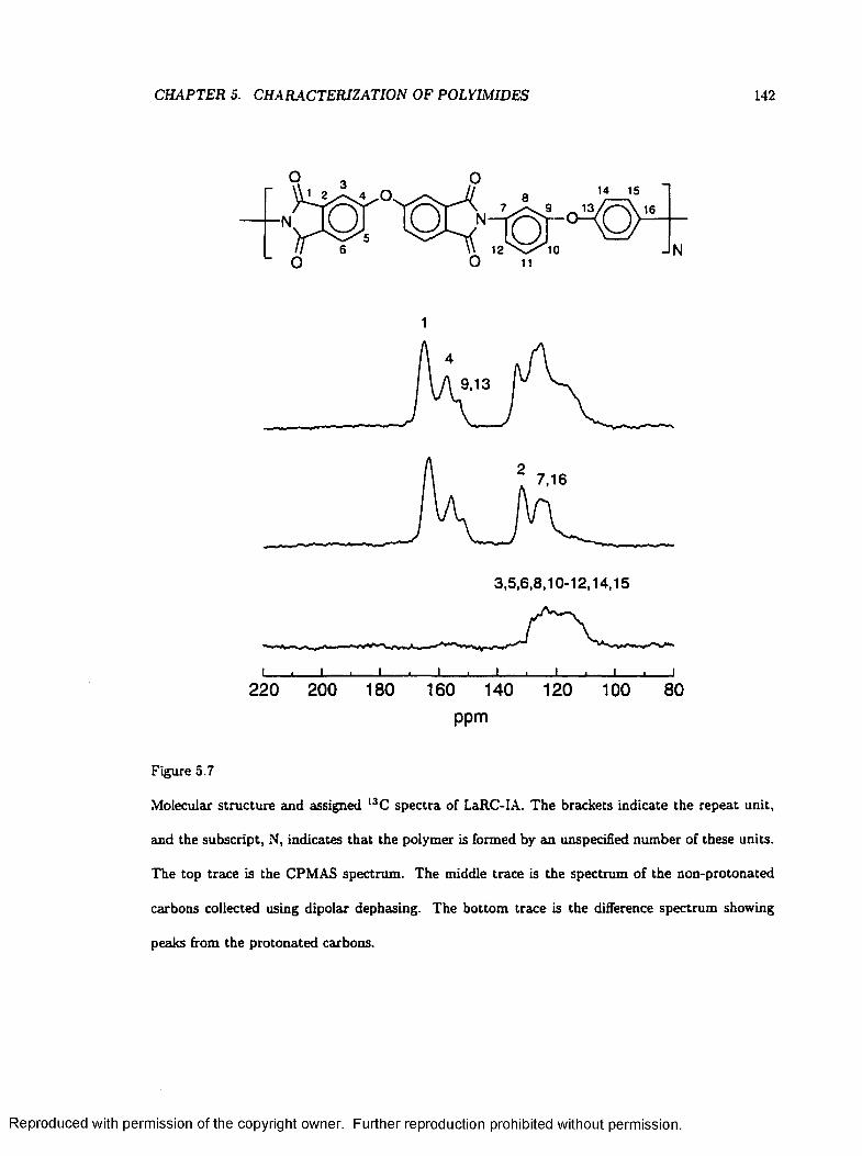
CHAPTER 5. CHARACTERIZATION OF POLYIMIDES 142
O
a 14 is
12 10 O 11
N
9,13
7,16
_L
3,5,6,8,10-12,14,15
X220 200 180 160 140
ppm120 100 80
Figure 5.7
Molecular structure and assigned l3C spectra of LaRC-IA. The brackets indicate the repeat unit,
and the subscript, N, indicates that the polymer is formed by an unspecified number of these units.
The top trace is the CPMAS spectrum. The middle trace is the spectrum of the non-protonated
carbons collected using dipolar dephasing. The bottom trace is the difference spectrum showing
peaks from the protonated carbons.
Reproduced with permission of the copyright owner. Further reproduction prohibited without permission.
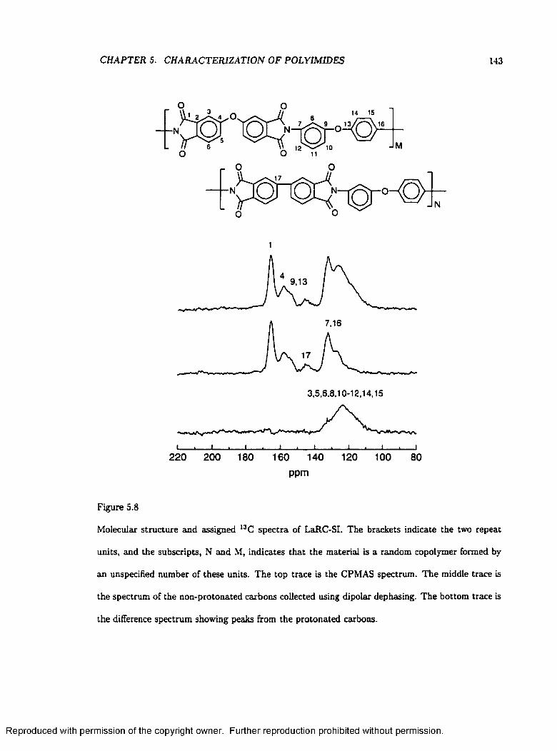
CHAPTER 5. CHARACTERIZATION OF POLYIMIDES 143
N
0 0
1
9,13
7,16
3,5,6.8.10-12,14,15
220 200 180 160 140 120 100 80ppm
Figure 5.8
Molecular structure and assigned l3C spectra of LaRC-SI. The brackets indicate the two repeat
units, and the subscripts, N and M, indicates that the material is a random copolymer formed by
an unspecified number of these units. The top trace is the CPMAS spectrum. The middle trace is
the spectrum of the non-protonated carbons collected using dipolar dephasing. The bottom trace is
the difference spectrum showing peaks from the protonated carbons.
Reproduced with permission of the copyright owner. Further reproduction prohibited without permission.

CHAPTER 5. CHARACTERIZATION OF POLYIMIDES 144
Table 5.2
Isotropic Chemical Shifts of Polyimides
Type of Carbon Assignment1 Chemical Shift (ppmb)
aromatic C-H T P I 3, 6 , 7, 9, 12-14 120-139
aromatic C-H IA 3, 5, 6 , 8 , 10-12, 14, 15 112-130
aromatic C-H SI 3, 5, 6 , 8 , 10-12, 14, 15 110-134
amine-imide C-N T P I 8 132-136
amine-imide C-N IA 7, 16 124-129
amine-imide C-N SI 7, 16 126
non-protonated aromatic T P I 2 140
non-protonated aromatic IA 2 133
non-protonated aromatic SI 2 132
ipso biphenyl SI 17 145
aromatic ether IA 9, 13 154
aromatic ether IA 4 158
aromatic ether SI 4, 9, 13 153-158
imide carbonyl T P I 1 165
imide carbonyl IA 1 166
imide carbonyl SI 1 166
aryl ketone carbonyl T P I 5, 11 189-194
^Compound labels and carbon numbers are given in Figures 5.6-5.8.
b Chemical shift values are referenced to the MAS isotropic chemical shift of glycine, 176 parts per million relative to TMS [50]. The uncertainty in the reported isotropic chemical shift values is less than ±1 ppm.
Reproduced with permission of the copyright owner. Further reproduction prohibited without permission.
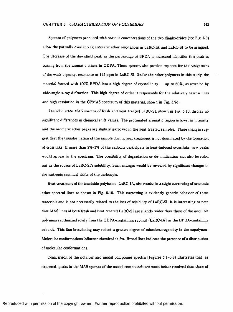
CHAPTER 5. CHARACTERIZATION OF POLYIMIDES 145
Spectra of polymers produced with various concentrations of the two dianhydrides (see Fig. 5.9)
allow the partially overlapping aromatic ether resonances in LaRC-fA and LaRC-SI to be assigned.
The decrease of the downfield peak as the percentage of BPDA is increased identifies this peak as
coming from the aromatic ethers in ODPA. These spectra also provide support for the assignment
of the weak biphenyl resonance a t 145 ppm in LaRC-SI. Unlike the other polymers in this study, the
material formed with 100% BPDA has a high degree of crystallinity — up to 60%, as revealed by
wide-angle x-ray diffraction. This high degree of order is responsible for the relatively narrow lines
and high resolution in the CPMAS spectrum of this material, shown in Fig. 5.9d.
The solid state MAS spectra of fresh and heat treated LaRC-SI, shown in Fig. 5.10, display no
significant differences in chemical shift values. The protonated aromatic region is lower in intensity
and the aromatic ether peaks are slightly narrower in the heat treated samples. These changes sug
gest that the transformation of the sample during heat treatment is not dominated by the formation
of crosslinks. If more than 2%-3% of the carbons participate in heat-induced crosslinks, new peaks
would appear in the spectrum. The possibility of degradation or de-imidization can also be ruled
out as the source of LaRC-SI’s solubility. Such changes would be revealed by significant changes in
the isotropic chemical shifts of the carbonyls.
Heat treatment of the insoluble polyimide, LaRC-IA, also results in a slight narrowing of aromatic
ether spectral lines as shown in Fig. 5.10. This narrowing is evidently generic behavior of these
materials and is not necessarily related to the loss of solubility of LaRC-SI. It is interesting to note
that MAS lines of both fresh and heat treated LaRC-SI are slightly wider than those of the insoluble
polymers synthesized solely from the ODPA-containing subunit (LaRC-IA) or the BPDA-containing
subunit. This line broadening may reflect a greater degree of microheterogeneity in the copolymer.
Molecular conformations influence chemical shifts. Broad lines indicate the presence of a distribution
of molecular conformations.
Comparison of the polymer and model compound spectra (Figures 5.1-5.8) illustrates that, as
expected, peaks in the MAS spectra of the model compounds are much better resolved than those of
Reproduced with permission of the copyright owner. Further reproduction prohibited without permission.

CHAPTER 5. CHARACTERIZATION OF POLYIMIDES 146
801 2 0200 160ppm
Figure 5.9
l3C CP MAS Spectra of polyimides formed with different proportions of the ODPA-containing and
BPDA-containing subunits. Spectra of samples with proportions of (a) 100% ODPA (LaRC-IA);
(b) 50% ODPA, 50% BPDA (LaRC-SI); (c) 25% ODPA, 75% BPDA; (d) 100% BPDA are shown.
These spectra allow the assignment of the aromatic ether resonances. Since the intensity of the two
aromatic peak at 158 ppm (See Fig. 5.8 and Table 5.2), depends on the relative concentrations of
the ODPA-containing subunit, this peak was assigned to carbon number 4 (see Fig 5.8), the ether
carbon that is present in the ODPA-containing subunit but not in the BPDA-containing subunit.
The vertical line indicates the position of this peak in the spectra.
Reproduced with permission of the copyright owner. Further reproduction prohibited without permission.
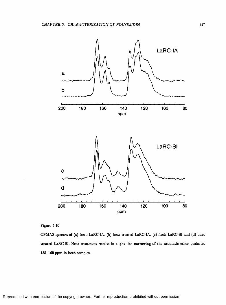
CHAPTER 5. CHARACTERIZATION OF POLYIMIDES 147
LaRC-IA
180 160 1 2 0 80200 140 1 0 0
ppm
LaRC-SI
180 100 80200 160 140 1 2 0
ppm
Figure 5.10
CPMAS spectra of (a) fresh LaRC-IA, (b) heat treated LaRC-IA, (c) fresh LaRC-SI and (d) heat
treated LaRC-SI. Heat treatment results in slight line narrowing of the aromatic ether peaks at
155-160 ppm in both samples.
Reproduced with permission of the copyright owner. Further reproduction prohibited without permission.

CHAPTER 5. CHARACTERIZATION OF POLYIMIDES 148
the polymers. The MAS spectrum of model compound III (Fig. 5.11a) has 14 peaks that are at least
partially resolved, although only a few of these can be assigned with certainty. Dipolar dephasing
[81) was used to simplify the spectrum by removing signals from protonated carbons. Despite some
unusual fine structure, the carbonyls and aromatic ether peaks are readily identified by their chemical
shift values. Model compound III has three other chemically distinct non-protonated carbon sites:
C3, C12 and C5 (see Fig. 5.3); however, C3 and C12 are not expected to be resolved in the CPMAS
spectrum. The resonance of C3 and C12 is distinguished from the resonance of C5 by comparison
with the MAS spectrum of model compound V, which has no carbons similar to C5 in compound
III. Comparison of the integrated intensities of these peaks supports this assignment.
5.3.2 Solution State I3C NM R Spectra
Solutions of LaRC-SI and model compound III were prepared so that the liquid state NMR
spectra of these materials could be studied. The LaRC-SI solution contained 33 mg of the polyimide
in 500 mg of m-cresol. A saturated solution of 220 mg of the model compound was made with 1 g of
dimethylsulfoxide. The samples were heated to 40°-60° C to speed up the dissolving process. The
William and Mary Chemistry D epartm ent’s General Electric QE300 spectrometer, equipped with
a Tecmag Aquarius pulse programmer, was used to acquire the solution state spectra. The carrier
frequency for these experiments was 75.57 MHz. A 6 ps 90° pulse was used with a 7 s recycle delay
for the model compound solution and 1.5 s recycle delay for the polymer solution.
In liquids, fast isotropic molecular motion averages the chemical shielding anisotropy. Magic angle
spinning is used to average the chemical shielding anisotropy in solid samples. Although liquid state
and magic angle spinning spectra both show isotropic values, components of the shielding tensors,
and thus the isotropic chemical shift values, may be different depending on whether the molecule is
in a solid or solution. In order to compare solid state isotropic chemical shifts with solution state
values, a solution s ta te 13 C NMR spectrum of model compound III in dimethylsulfoxide was recorded.
This solution state spectrum clearly shows the resonances expected from the ten chemically distinct
Reproduced with permission of the copyright owner. Further reproduction prohibited without permission.
CHAPTER 5. CHARACTERIZATION OF POLYIMIDES 149
4, 11 r 8 - 1 0 - i
r - 7 - i
3, 12
1,2, 13, 14
200 180 160 140 1 2 0 1 0 0 80ppm
Figure 5.11
Assigned 13 C spectra of model compound III, including solid state CPMAS spectra of (a) all carbons,
(b) non-protonated carbons, (c) protonated carbons, and (d) the solution state spectrum. The
molecular structure is shown in Fig. 5.3.
Reproduced with permission of the copyright owner. Further reproduction prohibited without permission.

CHAPTER 5. CHARACTERIZATION OF POLYIMIDES 150
carbons in the molecule. However, Fig. 5.11 shows that few of these resonances coincide with peaks
in the CPMAS spectrum.
The lack of a one-to-one correspondence between the spectral lines in the solid and solution
spectra demonstrates the influence that solid state effects can have on isotropic chemical shifts. One
notable difference between the solid and solution spectra is the 6 .6 ppm splitting of the aromatic
ether peak. In the solution spectrum a single ether carbon line, midway between the solid state
resonances, confirms that the molecule has only one chemically distinct aromatic ether carbon site.
The solid state spectrum also shows a splitting of the carbonyl line and a peak that is nine ppm
upfield of the lowest frequency line in the solution spectrum.
The solid state spectrum of model compound III differs from the solution spectrum for a variety
of reasons. The lack of fast rotation about the C-N bond removes the equivalence of C l and C14, C2
and C13, C3 and C12, and C4 and C ll . (See Fig. 5.3 for molecular structure.) Thus, the carbonyl
line is split slightly, the C3/C12 peak is broadened and splittings are observed in the protonated
carbon region of the spectrum. Crystallographic non-equivalence can result in small splittings if
there is more than one molecule per unit cell [109], but it is unclear if such effects are present in
this particular material. The splitting of the aromatic ether peak is too large to be accounted for by
crystallographic non-equivalence or by the existence of two distinct conformations of the molecule.
One possible source of the splitting is the formation of charge transfer complexes between aromatic
ether sites and aromatic rings on nearby molecules. Charge transfer has been implicated as the cause
of splittings of about 4 ppm in an investigation of other solid polyimides [106]. The circulation of
delocalized n electrons in aromatic rings in nearby molecules can be a significant source of chemical
shielding in solids. These ring currents are known to cause frequency shifts larger than those from
charge transfer [107]. Therefore, ring currents are a more likely cause of the observed splitting
of the aromatic ether peaks in compound III. The appearance of two peaks for the two chemically
equivalent aromatic ether carbons suggests that the molecules pack in such a way th a t approximately
half of the aromatic ether carbons lie close to the aromatic ring of a neighboring molecule.
Reproduced with permission of the copyright owner. Further reproduction prohibited without permission.
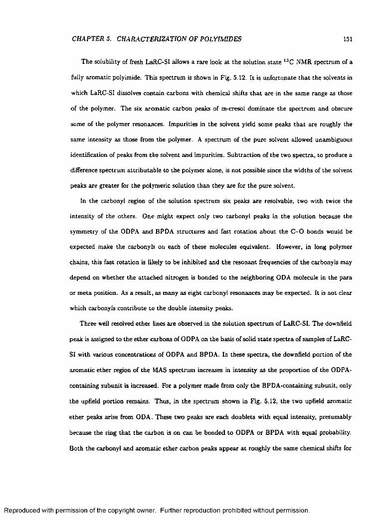
CHAPTER 5. CHARACTERIZATION OF POLYIMIDES 151
The solubility of fresh LaRC-SI allows a rare look at the solution state 13C NMR spectrum of a
fully aromatic polyimide. This spectrum is shown in Fig. 5.12. It is unfortunate that the solvents in
which LaRC-SI dissolves contain carbons with chemical shifts that are in the same range as those
of the polymer. The six aromatic carbon peaks of m-cresol dominate the spectrum and obscure
some of the polymer resonances. Impurities in the solvent yield some peaks that are roughly the
same intensity as those from the polymer. A spectrum of the pure solvent allowed unambiguous
identification of peaks from the solvent and impurities. Subtraction of the two spectra, to produce a
difference spectrum attributable to the polymer alone, is not possible since the widths of the solvent
peaks are greater for the polymeric solution than they are for the pure solvent.
In the carbonyl region of the solution spectrum six peaks are resolvable, two with twice the
intensity of the others. One might expect only two carbonyl peaks in the solution because the
symmetry of the ODPA and BPDA structures and fast rotation about the C -0 bonds would be
expected make the carbonyls on each of these molecules equivalent. However, in long polymer
chains, this fast rotation is likely to be inhibited and the resonant frequencies of the carbonyls may
depend on whether the attached nitrogen is bonded to the neighboring ODA molecule in the para
or meta position. As a result, as many as eight carbonyl resonances may be expected. It is not clear
which carbonyls contribute to the double intensity peaks.
Three well resolved ether lines are observed in the solution spectrum of LaRC-SI. The downfield
peak is assigned to the ether carbons of ODPA on the basis of solid state spectra of samples of LaRC-
SI with various concentrations of ODPA and BPDA. In these spectra, the downfield portion of the
aromatic ether region of the MAS spectrum increases in intensity as the proportion of the ODPA-
containing subunit is increased. For a polymer made from only the BPDA-containing subunit, only
the upheld portion remains. Thus, in the spectrum shown in Fig. 5.12, the two upheld aromatic
ether peaks arise from ODA. These two peaks are each doublets with equal intensity, presumably
because the ring that the carbon is on can be bonded to ODPA or BPDA with equal probability.
Both the carbonyl and aromatic ether carbon peaks appear a t roughly the same chemical shifts for
Reproduced with permission of the copyright owner. Further reproduction prohibited without permission.

CHAPTER 5. CHARACTERIZATION OF POLYIMIDES 152
♦ *
200 180 160 140ppm
100 801 2 0
X X XX X X X X X XX X
170 165 160 155ppm
Figure 5.12
Comparison of the (a) solid state and (b) m-cresol solution spectra of LaRC-SI. The carbonyl and
aromatic region of the solution spectrum is expanded in (c) to show the fine structure. Solvent peaks
are truncated and identified with asterisks.
Reproduced with permission of the copyright owner. Further reproduction prohibited without permission.

CHAPTER 5. CHARACTERIZATION OF POLYIMIDES 153
both the solid and solution. However, the centers of the solid state peaks are shifted slightly upheld.
Comparison of the solid and solution state spectra show that isotropic chemical shifts in the
solid state differ significantly from those measured in solution. Although solution state chemical
shift values can be useful guides for assigning solid state spectra, these values should not be used to
predict precise solid state values. In order to be certain of assignments of closely spaced peaks, other
evidence, such as accurate theoretical calculations or assigned spectra of closely related compounds,
is required.
5.3.3 13C Anisotropic Chemical Shifts
Two-dimensional variable angle correlation spectroscopy (VACSY) allows the chemical shift
anisotropy powder patterns to be measured, while retaining the resolution achieved by magic angle
spinning. VACSY experiments have been performed on the polymers LaRC-TPI, LaRC-IA, and
a homopolymer formed from the BPDA-containing subunit of LaRC-SI. VACSY experiments have
also been performed on model compounds II, III and V. Because of the amount of time needed to
acquire the 31 FIDs, VACSY experiments were not performed for all of the compounds in this study.
A two-dimensional contour plot of the VACSY spectrum of model compound III and two ani
sotropic lineshapes are presented in Fig. 5.13. For well resolved isotropic peaks, calculated powder
patterns have been fitted to the lineshapes in the anisotropic dimension in order to determine
the principal values of the corresponding shielding tensors. The fitting procedure uses the SUMS
[48] powder pattern calculation algorithm coupled with a nonlinear, least-squares fitting routine to
determine the principal values of the shielding tensor, as discussed in detail in C hapter 3. Principal
values of the chemical shift tensors are reported in Table 5.3. For the chemical shift values in the
isotropic dimension the uncertainty is less than ±1 ppm. The statistical uncertainties for the shift
tensor components, determined by the fitting procedure, were typically 5-10 ppm. Although the
VACSY experiment performed on model compound III yielded some measurable tensor components,
it is unfortunate that the signal-to-noise ratios of the aromatic ether lineshapes in this spectrum
Reproduced with permission of the copyright owner. Further reproduction prohibited without permission.

CHAPTER 5. CHARACTERIZATION OF POLYIMIDES 154
anisotropic pp
Figure 5.13
For model compound III, (a) contour plot of a two-dimensional VACSY spectrum and anisotropic
slices for (b) C4 and C l l a t 167 ppm and (c) C3 and C12 at 132 ppm. Best-fit calculated powder
patterns (dotted lines) are superimposed on the anisotropic spectra (solid lines). The best-fit pa
rameters are k = -0 .62, ft = 130 ppm for C4 and C l l (b) and k = 0.24, ft = 225 ppm for C3 and
C 12 (c). Measured anisotropic chemical shifts are given in Table 5.3.
Reproduced with permission of the copyright owner. Further reproduction prohibited without permission.
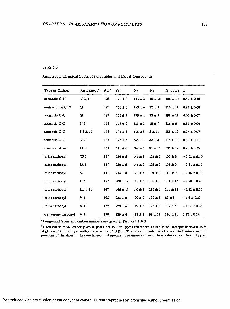
CHAPTER 5. CHARACTERIZATION OF POLYIMIDES 155
Table 5.3
Anisotropic Chemical Shifts of Polyimides and Model Compounds
Type of Carbon Assignment* <5,«b 6 J2 &33 n (ppm) K
aromatic C-H V 3, 6 125 176 ± 3 144 ± 3 49 ± 10 126 ± 10 0.50 ±0.12
amine-imide C-N SI 125 238 ± 6 153 ± 4 22 ± 9 215 ± 11 0.21 ±0.06
aromatic C-C SI 131 229 ± 7 139 ± 4 33 ± 9 195 ± 11 0.07 ± 0.07
aromatic C-C II 3 128 228 ± 5 131 ± 3 10 ± 7 218 ± 9 0.11 ±0.04
aromatic C-C III 3, 12 132 231 ± 6 146 ± 5 5 ± 11 255 ± 13 0.24 ± 0.07
aromatic C-C V 2 136 172 ± 3 135 ± 3 52 ± 8 119 ± 10 0.39 ±0.11
aromatic ether IA 4 159 211 ± 6 162 ± 5 81 ± 10 130 ± 12 0.23 ±0.15
imide carbonyl TPI 167 230 ± 8 144 ± 2 124 ± 2 105 ± 8 -0.62 ±0.10
imide carbonyl IA 1 167 230 ± 9 144 ± 2 125 ± 2 105 ± 9 -0.64 ±0.12
imide carbonyl SI 167 215 ± 8 139 ± 3 104 ± 3 110 ± 9 -0.36 ±0.10
imide carbonyl 1 1 2 167 260 ± 12 139 ± 3 109 ± 3 151 ± 1 2 -0.60 ±0.08
imide carbonyl III 4, 11 167 246 ± 16 140 ± 4 115 ± 4 130 ± 16 -0.62 ±0.14
imide carbonyl V 2 168 235 ± 0 139 ± 0 139 ± 8 87 ± 8 -1 .0 ±0.20
imide carbonyl V 3 172 229 ± 4 169 ± 2 122 ± 3 107 ± 5 -0.13 ±0.08
aryl ketone carbonyl V 9 196 239 ± 4 199 ± 3 99 ± 11 140 ± 11 0.43 ±0.14
*Compound labels and carbon numbers are given in Figures 5.1-5.8.bChemical shift values are given in parts per million (ppm) referenced to the MAS isotropic chemical shift of glycine, 176 parts per million relative to TMS [50]. The reported isotropic chemical shift values are the positions of the slices in the two-dimensional spectra. The uncertainties in these values is less than ±1 ppm.
Reproduced with permission of the copyright owner. Further reproduction prohibited without permission.
CHAPTER 5. CHARACTERIZATION OF POLYIMIDES 156
are too low to allow quantitative analysis of the powder patterns. However, it is apparent that the
largest and smallest principal values of the chemical shift tensor, <5u and £33, tire shifted in opposite
directions resulting in a larger span for the upheld peak.
Anisotropic lineshapes of the carbonyl carbons of the polymers and model compounds all yielded
good hts to calculated lineshapes. Some aromatic carbon lineshapes of the model compounds also
yielded reasonable Hts. Anisotropic lineshapes of aromatic carbons of the polymers, however, are
typically superpositions of several powder patterns due to the overlap of the isotropic peaks. With
a few exceptions, these lineshapes cannot be fitted to a single calculated powder pattern. Some
powder patterns from LaRC-IA are shown in Fig. 5.14.
5.3.4 Cross Polarization Dynamics
The intensities of several peaks in the LaRC-SI and LaRC-IA CPMAS spectrum were measured
as a function of contact pulse length. Cross polarization contact times ranged from 20 ps to 11 ms.
The intensities plotted as a function of contact time show the characteristic rise, as magnetization
is transferred from protons, and fall, as proton magnetization relaxes in the rotating frame. The
data for the carbonyl and protonated aromatic carbons in LaRC-IA are are shown in Fig. 5.15.
The carbons that have directly bonded protons reach maximum intensity in less than 100 (is. Non-
protonated carbons do not reach their maximum until about four milliseconds. These data emphasize
the difficulties in interpreting relative intensities of peaks in a cross polarization experiment.
The intensity of a carbon peak as a function of contact time depends on the cross relaxation
time, T is , and the rotating frame relaxation times, Tlp/ and Ti„s- For an isolated 13C -1H pair, the
buildup and decay of magnetization are described by a bi-exponential function [9,26], as shown in
Section 2.5.2:
M ( t ) oc ^ e x p ( - t / T i p/ ) [ l — ex p (-A f/T /s )]> [5.1]
Reproduced with permission of the copyright owner. Further reproduction prohibited without permission.

CHAPTER 5. CHARACTERIZATION OF POLYIMIDES 157
300 200 100 200300 1 0 0ppm ppm
200 100 0 200 100 0ppm ppm
Figure 5.14
Anisotropic 13C lineshapes for LaRC-IA. The powder patterns shown are for carbons with isotropic
frequencies of (a) 167 ppm, (b) 159 ppm, (c) 128 ppm, (d) 122 ppm. (See Fig. 5.7 for the magic
angle spinning spectrum.) The carbonyl and aromatic ether lineshapes (a and b, respectively) are
fitted well by calculated powder patterns. The best fit parameters are k = -0 .64 and 0 = 105
ppm and k = 0.23 and fi = 130 ppm for the two aromatic ether carbons. Because of overlap of the
isotropic peaks, the aromatic carbon lineshapes from the two-dimensional spectrum (c and d) are
superpositions or distributions of powder patterns. These lineshapes cannot be fitted with a single
calculated powder pattern.
Reproduced with permission of the copyright owner. Further reproduction prohibited without permission.

CHAPTER 5. CHARACTERIZATION OF POLYIMIDES 158
<D£ 0.4 m& 0.2
0.06 8 100 2 4
contact time (ms)
(0c0)
03
©CC
2 4 6 8 10contact time (ms)
Figure 5.15
Cross polarization dynamics for carbonyl (left) and protonated aromatic carbons (right). The exper
imental data have been scaled so that the highest intensity equals one. The solid line is the best-fit
bi-exponential function shown in Gq. 5.1. Strong coupling to attached protons results in more rapid
cross polarization for the protonated carbons. Spin diffusion and a distribution of 13C - l H coupling
strengths for each carbon are responsible for the significant deviations of the experimental from the
best-fit function.
Reproduced with permission of the copyright owner. Further reproduction prohibited without permission.
CHAPTER 5. CHARACTERIZATION OF POLYIMIDES 159
where
Tips T\„i[5.2]
The discrepancies between the cross polarization dynamics data and the best fit calculated curves
indicate that the carbons experience significant coupling to more than one proton. In addition, strong
homonuclear coupling among the protons promotes spin diffusion, which allows proton magnetization
to equilibrate. Since the carbons are in thermal contact with the protons during cross polarization,
proton spin diffusion promotes equilibration among the carbons. As a result, the protonated and
non-protonated carbons show similar cross polarization dynamics after about four milliseconds.
5.3.5 ‘H FID Experiments
Directly detected proton spectra were obtained using a single 4 fis 90° pulse. For all of the
polymers and model compounds in this study, the static proton spectra consist of broad and narrow
components. The spectra of LaRC-IA and LaRC-SI in Fig. 5.17 are typical. Relative intensities
of the components of the lineshapes were found by fitting the spectra to two Gaussian functions.
The intensities, widths and frequency offsets were varied manually, so as to minimize chi-squared.
The wide components of the proton spectra have flatter tops and steeper sides than the Gaussian
fitting functions. However, these differences are small; a Gaussian is a reasonable approximation to
the proton lineshape. The components of the polymer spectra are about 30 kHz and 3 kHz wide
(full width at half maximum intensity). The fraction of the total integrated intensity contained
in the narrow component is 4% for each of the polymer samples. For the model compounds, the
widths of the components are 40 kHz and 4 kHz. Much more variation of the intensity of the narrow
component is seen in the model compounds; model III has only 3% of its intensity in the narrow
component, while the narrow component accounts for almost 9% of the intensity in the spectrum of
model I.
The broad and narrow features can be seen in the spectra presented in Fig. 5.17. Such a super
position of broad and narrow peaks are frequently seen in the proton spectra of polymers. These
Reproduced with permission of the copyright owner. Further reproduction prohibited without permission.

CHAPTER 5. CHARACTERIZATION OF POLYIMIDES 160
components are generally attributed to crystalline and amorphous regions in the material. In the
amorphous regions, the chains are more mobile than in the ordered crystalline domains. This motion
averages the dipolar couplings, resulting in a narrow component in the lineshape. This interpretation
is not appropriate for these polyimide samples because, except for the homopolymer made from the
BPDA-containing monomer, they are completely amorphous. Differential scanning calorimetry and
wide angle x-ray scattering measurements show no evidence of crystallinity [100].
Another hypothesis about the origin of the narrow component is that it arises from protons that
are distant or isolated horn other protons. In LaRC-SI and L&RC-IA, protons bonded to C3 and
C8 might be sufficiently isolated from other protons to have significant smaller dipolar interactions.
These protons account for 21% of the total number of protons. Since the narrow component of
each of the polymer spectra contains only 4% of the total intensity, this interpretation requires the
assumption that a specific fraction (approximately 20%) of the C3 and C8 protons is distant from
protons on neighboring chains. This assumption is difficult to justify. Moreover, model compound
I, which has a larger narrow peak than any of the polymers, has none of these potentially isolated
protons.
Narrow peaks in the proton powder spectra of organic crystals often occur, and have been
ascribed to highly mobile molecules trapped in liquid-like pockets or defects [110]. This hypothesis
satisfactorily accounts for the present observations on the polyimide model compounds and on the
polymers themselves. Additional evidence for the existence of a small, highly mobile fraction of
polymer segments is presented in section 5.3.7.
5.3.6 lH Wideline Separation Experiments
Two dimensional wideline separation (WISE) experiments [37] were performed on LaRC-IA and
LaRC-SI in order to separate the proton spectrum by the chemical shift of the carbons. This
technique was discussed in Section 2.5.5. Experiments were performed with spin diffusion delay
times of zero and 50 ms. A set of 64 FIDs with different values of the proton evolution time was
Reproduced with permission of the copyright owner. Further reproduction prohibited without permission.

CHAPTER 5. CHARACTERIZATION OF POLYIMIDES 161
-30 -20 -10 0 10 20 30kHz
Figure 5.16
Comparison of a slice of a two-dimensional WISE spectrum (solid line) and the static proton spec
trum (dotted line) of LaRC-IA. The WISE peak is narrower than the proton spectrum due to partial
averaging of the homonuclear dipolar interaction by sample spinning. The best fit to the WISE peak
is achieved with a Gaussian with a full width at half maximum of 24 kHz. For the wide component
of the static spectrum, the best-fit Gaussian has a width of 30 kHz.
collected to sample the proton dimension. The dwell time in the proton dimension was 10 fis, giving
a spectral width of 50 kHz.
WISE experiments were performed on heat treated and fresh LaRC-SI and LaRC-IA. For all of
the WISE spectra, slices in the proton dimension yielded very similar proton lineshapes regardless
of position in the carbon dimension. The slice through the carbonyl peak of fresh LaRC-IA, shown
in Fig. 5.16, is typical. The proton lineshapes in the WISE spectrum show much smaller deviations
from a Gaussian shape than the static proton lineshapes do. The narrow component seen in the
Reproduced with permission of the copyright owner. Further reproduction prohibited without permission.
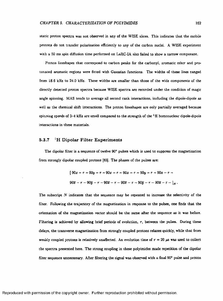
CHAPTER 5. CHARACTERIZATION OF POLYIMIDES 162
static proton spectra was not observed in any of the WISE slices. This indicates that the mobile
protons do not transfer polarization efficiently to any of the carbon nuclei. A WISE experiment
with a 50 ms spin diffusion time performed on LaRC-IA also failed to show a narrow component.
Proton lineshapes that correspond to carbon peaks for the carbonyl, aromatic ether and pro-
tonated aromatic regions were fitted with Gaussian functions. The widths of these lines ranged
from 18.6 kHz to 24.0 kHz. These widths are smaller than those of the wide components of the
directly detected proton spectra because WISE spectra are recorded under the condition of magic
angle spinning. MAS tends to average all second rank interactions, including the dipole-dipole as
well as the chemical shift interactions. The proton lineshapes are only partially averaged because
spinning speeds of 3-4 kHz are small compared to the strength of the 1H homonuciear dipole-dipole
interactions in these materials.
5.3.7 *H Dipolar Filter Experiments
The dipolar filter is a sequence of twelve 90° pulses which is used to suppress the magnetization
from strongly dipolar coupled protons [85]. The phases of the pulses are:
[ 90x — r — 90y — r - 90x — r — 90x — r — 90y — r — 90x — r -
90x — r — 90y — r — 90x — r — 90x — r — 90y — r — 90x — r — .
The subscript N indicates that the sequence may be repeated to increase the selectivity of the
filter. Following the trajectory of the magnetization in response to the pulses, one finds that the
orientation of the magnetization vector should be the same after the sequence as it was before.
Filtering is achieved by allowing brief periods of evolution, r , between the pulses. During these
delays, the transverse magnetization from strongly coupled protons relaxes quickly, while that from
weakly coupled protons is relatively unaffected. An evolution time of r = 20 ps was used to collect
the spectra presented here. The strong coupling in these polyimides made repetition of the dipolar
filter sequence unnecessary. After filtering the signal was observed with a final 90° pulse and proton
Reproduced with permission of the copyright owner. Further reproduction prohibited without permission.
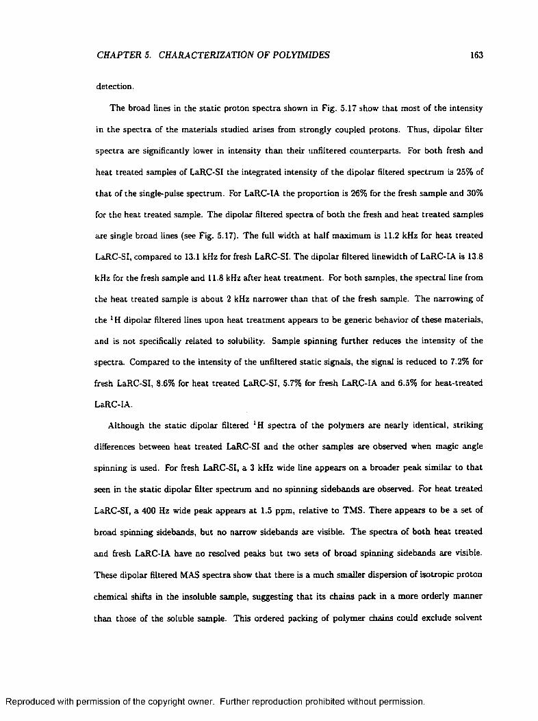
CHAPTER 5. CHARACTERIZATION OF POLYIMIDES 163
detection.
The broad lines in the static proton spectra shown in Fig. 5.17 show that most of the intensity
in the spectra of the materials studied arises from strongly coupled protons. Thus, dipolar filter
spectra are significantly lower in intensity than their unfiltered counterparts. For both fresh and
heat treated samples of LaRC-SI the integrated intensity of the dipolar filtered spectrum is 25% of
that of the single-pulse spectrum. For LaRC-IA the proportion is 26% for the fresh sample and 30%
for the heat treated sample. The dipolar filtered spectra of both the fresh and heat treated samples
are single broad lines (see Fig. 5.17). The full width at half maximum is 11.2 kHz for heat treated
LaRC-SI, compared to 13.1 kHz for fresh LaRC-SI. The dipolar filtered linewidth of LaRC-IA is 13.8
kHz for the fresh sample and 11.8 kHz after heat treatment. For both samples, the spectral line from
the heat treated sample is about 2 kHz narrower than that of the fresh sample. The narrowing of
the 1H dipolar filtered lines upon heat treatm ent appears to be generic behavior of these materials,
and is not specifically related to solubility. Sample spinning further reduces the intensity of the
spectra. Compared to the intensity of the unfiltered static signals, the signal is reduced to 7.2% for
fresh LaRC-SI, 8.6% for heat treated LaRC-SI, 5.7% for fresh LaRC-IA and 6.5% for heat-treated
LaRC-IA.
Although the static dipolar filtered ‘H spectra of the polymers are nearly identical, striking
differences between heat treated LaRC-SI and the other samples are observed when magic angle
spinning is used. For fresh LaRC-SI, a 3 kHz wide line appears on a broader peak similar to that
seen in the static dipolar filter spectrum and no spinning sidebands are observed. For heat treated
LaRC-SI, a 400 Hz wide peak appears a t 1.5 ppm, relative to TMS. There appears to be a set of
broad spinning sidebands, but no narrow sidebands are visible. The spectra of both heat treated
and fresh LaRC-IA have no resolved peaks but two sets of broad spinning sidebands are visible.
These dipolar filtered MAS spectra show that there is a much smaller dispersion of isotropic proton
chemical shifts in the insoluble sample, suggesting that its chains pack in a more orderly manner
than those of the soluble sample. This ordered packing of polymer chains could exclude solvent
Reproduced with permission of the copyright owner. Further reproduction prohibited without permission.
CHAPTER 5. CHARA CTERIZATION OF POLYIMIDES 164
20 0 -20 -40402040 0 -20 -40kHz kHz
40 20 0 -20 -40 -4040 20 0 -20kHz kHz
Figure 5.17
Proton spectra of (a) fresh LaRC-IA, (b) heat treated LaRC-L\, (c) fresh LaRC-SI and (d) heat
treated LaRC-SI. For each sample the widest lineshape is the static proton spectrum, the interme
diate lineshape is the static dipolar filtered spectrum and the narrowest lineshape is the dipolar
filtered MAS spectrum.
Reproduced with permission of the copyright owner. Further reproduction prohibited without permission.

CHAPTER 5. CHARACTERIZATION OF POLYIMIDES 165
molecules and render the material insoluble. The absence of narrow lines in the heat treated LaRC-
IA sample indicates that this narrowing upon heat treatment is not generic polyimide behavior and
could, therefore, be associated with the change in solubility of LaRC-SI.
5.3.8 13C Dipolar Filter Cross Polarization Experiments
Experiments were also performed in which dipolar filtered proton magnetization was transferred
to 13 C nuclei by cross polarization. The carbon signed was then observed with magic angle spinning
[85]. The resulting dipolar filter-cross polarization (DFCP) spectrum shows the isotropic chemical
shifts of those carbons that are cross polarized by protons that experience weak dipolar coupling. The
signal to noise per scan is poor in this experiment because the dipolar filter eliminates most of the
proton magnetization. If the proton-proton dipolar coupling is weak because of molecular motion,
the proton-carbon dipolar coupling will also be weak. As a result the transfer of magnetization
will occur more slowly and reduce the intensity of the spectrum further. DFCP experiments were
performed on fresh and heat treated LaRC-SI and fresh LaRC-IA. A typical DFCP spectrum with a
reasonable signal to noise ratio required over 70,000 scans and more than 38 hours of spectrometer
time.
For fresh LaRC-SI, all features of the CPMAS spectrum are present in the DFCP spectrum with
roughly the same relative intensities (Fig. 5.18b). This rules out the possibility that the narrow
component of the static lH spectrum originates from isolated protons, since they would not be able
to cross polarize all carbons on the polymer chain during the 2 ms contact time. On the other hand,
relative intensities of the DFCP peaks from insoluble samples (heat treated LaRC-SI, Fig. 5.18c and
LaRC-IA, Fig. 5.18a) show more differences when compared to their respective CPMAS spectra. The
DFCP spectra have all been normalized so that the CPMAS and DFCP spectra of the protonated
carbons near 120 ppm have the same intensity. This was done because carbons with directly bonded
protons are least sensitive to differences in cross polarization efficiency.
Although the differences between the CPMAS and DFCP spectra are small, and the spectra are
Reproduced with permission of the copyright owner. Further reproduction prohibited without permission.
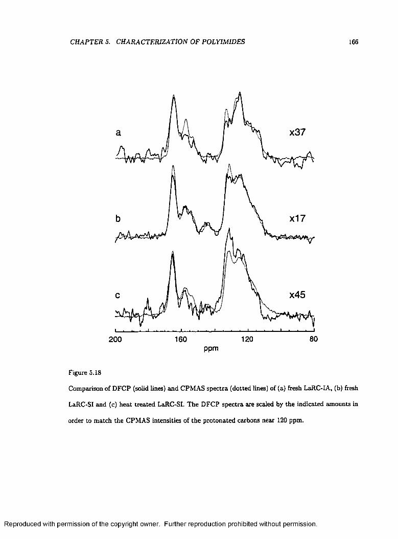
CHAPTER 5. CHARACTERIZATION OF POLYIMIDES 166
x37
x17
x45
80120160200ppm
Figure 5.18
Comparison of DFCP (solid lines) and CPMAS spectra (dotted lines) of (a) fresh LaRC-IA, (b) fresh
LaRC-SI and (c) heat treated LaRC-SI. The DFCP spectra are scaled by the indicated amounts in
order to match the CPMAS intensities of the protonated carbons near 120 ppm.
Reproduced with permission of the copyright owner. Further reproduction prohibited without permission.
CHAPTER 5. CHARACTERIZATION OF POLYIMIDES 167
noisy, some qualitative observations can be made. For heat treated LaRC-SI, the CPMAS and DFCP
spectra show some differences in the intensities of non-protonated carbon peaks. These differences
may reflect differences in conformational distributions for chains in mobile and rigid regions of these
materials. The range of conformations available to the relevant C-C and C -O -C bonds leads to a
broad distribution of distances to nearest protons. The changes in relative intensities of CPMAS
and DFCP spectra of fresh and heat treated LaRC-SI may then be due to significant changes in the
conformational distributions about biphenyl C -C and C -O -C bonds in the mobile chains selected
by the dipolar filter.
In order to quantify the absolute intensity reduction due to the dipolar filter, the integrated
intensities per scan of the CPMAS and DFCP spectra were compared. Fresh LaRC-SI suffered the
least attenuation. After correcting for the number of scans, the integrated intensity was found to be
5.9% of the intensity of the CPMAS spectrum. For LaRC-IA and heat treated LaRC-SI the DFCP
spectra were 2.7% and 2.2% of their respective CPMAS spectra.
5.3.9 Hydration
In the first hydration study performed as part of this investigation of polyimides, a small flask
containing 1.2 g of powdered LaRC-IA was placed in a seeded container containing a saturated
solution of NaClOa in H2O. After two weeks, the sample was removed and its mass was recorded.
After spectra were acquired the sample was heated at 115° C for five days in order to drive off
absorbed water. Again, the sample’s mass was measured. Comparison of the measured masses
places a lower limit on the weight percent of water in the hydrated sample a t 1.6%. For the ambient
humidity sample the value is 0.33%. The BPDA-containing monomer has a molecular weight of 474,
and the ODPA-containing monomer has a molecular weight of 458. Thus, for a sample of LaRC-SI
with equal parts of the two monomers, a weight percentage of 1.6% H2O (with a molecular weight
of 18) is a mole percentage of 72%. Each molecule of H2O has two protons and each molecule of
LaRC-SI has 28; thus the percentage of water protons present in the hydrated sample is 5.1%.
Reproduced with permission of the copyright owner. Further reproduction prohibited without permission.

CHAPTER 5. CHARACTERIZATION OF POLYIMIDES 168
The l H spectrum of LaRC-IA displayed a dram atic increase in the narrow component of the
lineshape. The intensity of the narrow component rose from 4% to 32% of the total integrated
intensity of the lineshape. This increase is too large to attribute solely to mobile water protons. The
spectra of the dry sample shows no appreciable difference in the intensity of the narrow component
compared to that of the ambient humidity sample.
To further investigate hydration of polyimides, hydration studies of LaRC-SI was performed. In
order to remove the possibility of water protons contributing to the spectrum, D jO rather than H2O
was used. Hydration of LaRC-SI was accomplished by first stirring 232 mg of the fresh, powdered
sample in a flask with 21 g of D2O for five days in order to displace any absorbed H2O. The
sample was then suction filtered and rinsed with pentane. A sealed container containing a saturated
solution, with excess NaC103 in D2O, was used to store the sample under 75% relative humidity.
This allowed D2 O on the surface of the sample to evaporate while preventing the absorption of H2O.
The sample was packed into a 5 mm rotor and stored in the container with the NaClOj solution
when experiments were not being performed. To allow comparison this procedure was repeated with
238 mg of LaRC-SI and 22 g of H20 .
After hydration of fresh LaRC-SI with H2O, the static proton lineshape shows a dramatic increase
in intensity and decrease in linewidth of the narrow component and a decrease in the intensity of the
broad component as shown in Fig. 5.19. The increase is more dramatic than tha t seen in LaRC-IA
because immersion of the sample allows for more thorough hydration. The fraction of total integrated
intensity in the narrow component grew from 4% to 79%. The full width a t half maximum of the
narrow component decreased from 3.5 kHz to 600 Hz. The width of the broad component increased
from 29.0 kHz to 33.5 kHz. The total integrated intensity of the spectrum of the hydrated sample
is 88% th a t of the ambient humidity sample.
The decrease in the intensity of the broad component argues that some of the polymer chains
that are normally in a fairly rigid region of the material are mobilized by absorbed water. The
proton spectrum of the sample of LaRC-SI that was hydrated with D2O shows a similar increase in
Reproduced with permission of the copyright owner. Further reproduction prohibited without permission.

CHAPTER 5. CHARACTERIZATION OF POLYIMIDES 169
x 1 0
40 20 0 -20 -40kHz
Figure 5.19
(a) Static proton spectra of LaRC-SI a t ambient humidity (dotted line) and hydrated LaRC-SI (solid
line), (b) The spectra are expanded vertically by a factor of ten to show that the broad component
of the ambient humidity spectrum is present in the hydrated sample, but at a much lower intensity.
Reproduced with permission of the copyright owner. Further reproduction prohibited without permission.

CHAPTER 5. CHARACTERIZATION OF POLYIMIDES 170
the narrow component and reduction of the broad component. Since very few protons were added
to the sample in the DjO hydration process (some exchange of deuterons with protons inevitably
occurs during brief periods of exposure to the atmosphere) the increase of the intensity of the narrow
component must be due to the mobilization of normally rigid polymer chains. Thus, the water that
is absorbed by the material acts as a plasticizer.
5.4 Conclusions
This study of LaRC-SI and related polymers and model compounds revealed details of these
materials in three main areas: cataloging of isotropic chemical shifts and tensor components, inves
tigation of the unusual solubility of LaRC-SI and investigation of the absorption of water of these
materials.
Analysis of the 13 C CPMAS data allowed assignment of the resolved peaks in LaRC-SI, LaRC-IA
and LaRC-TPI. Although the aromatic region of the spectra display only poorly resolved structure,
dipolar dephasing experiments show that the downfield portion of this region arises primarily from
non-protonated carbons, whereas the upheld portion is from protonated carbons. The spectra of
the model compounds showed better resolution due to the greater structural homogeneity of these
crystalline materials. These spectra were assigned more completely than those of the polymers,
however many of the protonated peaks remain ambiguous. These assignments, along with the
previous measurements cited earlier, should prove to be helpful in future structural investigations
of polyimides.
Two-dimensional VACSY experiments allow the analysis of anisotropic lineshapes to find the
principal values of chemical shift tensors, revealing information which is absent in MAS spectra.
At this time, such measurements are not routinely performed by many researchers. To my knowl
edge, the results of the VACSY experiments presented here are the only published measurements
of anisotropic chemical shifts in polyimides. These data should prove valuable when more results
Reproduced with permission of the copyright owner. Further reproduction prohibited without permission.

CHAPTER 5. CHARACTERIZATION OF POLYINIWES 171
become available.
Liquid state NMR spectra were collected for solutions of model compound III and LaRC-SI. In
solution, some of the isotropic chemical shifts of model compound III differ significantly from the
CPMAS chemical shifts. Hence, solution state chemical shift values were used only as a rough guide
for assigning the solid sta te spectra. The differences in the solution and solid state chemical shifts
point to effects of molecular packing and morphology. The dramatic frequency shifts seen in model
compound III indicate the presence of ring currents. W ith further study of a variety of systems, the
differences between solid and solution state spectra could elucidate the microstructure of important
materials.
Differences between fresh and heat treated LaRC-SI are not apparent in the NMR spectra unless
the magnetization from strongly coupled protons is suppressed with the dipolar filter pulse sequence.
The appearance of narrow lines in the ‘H dipolar filtered MAS spectra of heat treated LaRC-SI
indicates that heat treatm ent results in more uniform packing of the mobile chains. Conformational
changes may occur in response to a decrease in free volume as the chains settle into this tighter
packing arrangement. Also, this arrangement of polymer chains would hinder penetration by solvent
molecules. The spectra show no peaks attributable to residual solvent, which therefore cannot be
present in concentrations above 1-2 mole percent. Nevertheless, trace quantities could reside in
voids between loosely packed chains in fresh LaRC-SI. It is therefore possible that loss of solvent
actually triggers the heat-induced changes in chain packing.
Static proton NMR spectra show that the absorption of water plasticizes LaRC-IA and LaRC-SI.
The increase of the narrow component of the 1H lineshape and decrease of the broad component
reveals that regions of the material that are rigid at ambient humidity are mobile in the hydrated
sample. LaRC-LA has been shown to absorb a t least 1.6% of its own weight in water from atmosphere
at 75% relative humidity. The resulting change in dynamics displayed in the proton spectra suggests
that the physical properties of LaRC-IA and related materials should be investigated further in order
to better understand changes in the bulk properties of polyimides in high humidity environments.
Reproduced with permission of the copyright owner. Further reproduction prohibited without permission.
CHAPTER 5. CHARACTERIZATION OF POLYIMIDES 172
These results give an indication of the wealth of information about polyimide microstructure
provided by solid state NMR experiments. The wide range of information obtained in these studies
demonstrates the utility of solid state 13C and l H NMR for studying polymers.
Reproduced with permission of the copyright owner. Further reproduction prohibited without permission.
Chapter 6
Summary
The preceding chapters describe progress made in several aspects of NMR research. The results
presented have a bearing, not only on the field of solid state NMR, but also on condensed m atter
physics in general. Here, the im portant results, and their relevance to the study of solids, are
summarized.
The SUMS method is a new solution to the old problem of calculating the lineshapes for poly-
crystalline or amorphous sample. This novel algorithm is significantly more efficient than standard
methods. The speed with which anisotropic lineshapes can be computed allows automated, non
linear least-squares fits to experimental spectra to be performed quickly. This procedure removes
subjective judgment from the determination of the principal values of chemical shift tensors. The
versatility of the SUMS method is demonstrated in calculations of partially relaxed spectra and
lineshapes from partially ordered samples.
Chemical shifts contain valuable information about the electronic environments of nuclei. Chang
es in chemical shifts reflect changes in these environments. Isotropic chemical shifts are measured
routinely using magic angle spinning; however, characterization of the chemical shift tensor is less
common. The measurement of anisotropic lineshapes from many compounds is necessary to test
the results of chemical shielding calculations and to understand the effects of molecular structure
173
Reproduced with permission of the copyright owner. Further reproduction prohibited without permission.
CHAPTER 6. SUMMARY 174
and order on the electronic environment. The SUMS method, used with a non-linear least-squares
fitting routine should prove valuable for analyzing experimental da ta of this type.
Deuteron spin-Iattice relaxation times have long been used as a sensitive probe of molecular
motion in solids, liquid crystals and polymers. Similar studies using 13C NMR on natural abundance
samples are hampered by a number of technical challenges. Among these challenges are overlap
of anisotropic lineshapes and the number of spectral densities th a t need to be determined. In
experiments performed on ferrocene, fast sample spinning was shown to be a means for determining
two linear combinations of the spectral densities that contribute to relaxation by the heteronuclear
dipolar mechanism. This technique increases the fidelity of information about molecular dynamics
obtained using natural abundance 13 C NMR. The possibility of using two-dimensional techniques for
measuring relaxation time anisotropies for a variety of carbon sites in more complicated molecules
was explored. Like structure and order, rates and trajectories of molecular motion are correlated
with bulk properties of m atter. A description of solids is incomplete without accurate information
about dynamics.
The power of NMR is in the determination of structure, order and motion for new and fun
damentally interesting materials, or those that have practical applications. In part, this research
is done to identify the microscopic origins of bulk properties. The ultimate goal is to aid in the
production of materials with specific characteristics. A large number of 13C and 1H solid state NMR
techniques were used to investigate a group of related polyimides. One of these polyimides, LaRC-
SI, is remarkable because it is soluble, yet it retains the favorable properties that make polyimides
useful in extreme environments. LaRC-SI has been demonstrated to be an effective matrix resin, an
insulating coating for electrical wires, and as a backing for flexible and multi-layered printed circuits.
The NMR results suggest that loose packing of the polymer chains allow the penetration of solvent
molecules. Heat treatm ent renders LaRC-SI insoluble by allowing the chains to settle into a tighter
arrangement. This knowledge can add in the design of other soluble polymers.
Further study of the polyimides LaRC-IA and LaRC-SI has shown that a small amount of
Reproduced with permission of the copyright owner. Further reproduction prohibited without permission.
CHAPTER 6. SUMMARY 175
absorbed water has a dramatic effect on polymer chain dynamics. The dramatic increase in the
narrow component of the proton spectrum shows tha t absorbed water leads to fast, large-amplitude
molecular motion. Since the strength of these materials owes much to the rigidity of the polymer
chains, absorption of water may have detrimental effects on the structural integrity of these, and
similar, polyimides. In this case, NMR spectra have been used to identify a property of a material
that warrants further investigation.
The results presented here cover many aspects of NMR research from theory to experiment to
simulation to interpretation. The value of this research depends on the application of these tech
niques to a wide variety of im portant and interesting systems. NMR complements other techniques
for investigating solids, such as x-ray diffraction and infrared spectroscopy by allowing additional in
sight. The complex problem of characterizing order and dynamics and determining the microscopic
origin of physical properties requires investigations which use all of the diverse tools and techniques
of condensed m atter physics. The results of such fundamental research have benefits that extend to
an even wider range of academic disciplines and technologically oriented fields.

Bibliography
[1] Solid State Science, D. L. Weaire, C. G. Windsor, editors, (Adam Hilger, 1987).
[2] Computer Simulation in Materials Science, \1. Meyer, V. Pontkis, editors, (Kluwer, 1991).
[3] T. Y. Tse, Deuteron Nuclear Magnetic Resonance Studies of Molecular Motion in Solids, PhD
Thesis, College of William and Mary (1994) (unpublished).
[4] E. M. Purcell, H. C. Torrey, R. V. Pound, Phys. Rev., 69, 37 (1946).
[5] F. Bloch, W. W. Hansen, M. Packard, Phys. Rev., 69, 127 (1946).
[6] B. C. Gerstein, C. R. Dybowski, Transient Techniques in NMR of Solids, (Academic Press,
1985).
[7] J. J. Sakurai, Modem Quantum Mechanics, (Addison-Wesley, 1985).
[8] N. W. Ashcroft, N. D. Mermin, Solid State Physics, (Saunders College, 1976).
[9] D. Michel, F. Engeike, NMR Basic Principles and Progress, 32, 69 (1994).
[10] S. R. Hartman, E. L. Hahn, Phys. Rev., 128, 2042 (1962).
[11] R. R. Ernst, G. Bodenhausen, A. Wokaun, Principles o f Nuclear Magnetic Resonance in One
and Two Dimensions, (Oxford, 1987).
[12] F. D. Doty, R. R. Inners, P. D. Ellis, J. Magn. Reson., 43, 399 (1981).
176
Reproduced with permission of the copyright owner. Further reproduction prohibited without permission.
BIBLIOGRAPHY 177
[13] E. Fukushima, S. B. W. Roeder, Experimental Pulse NMR: A Nuts and Bolts Approach,
(Addison-Wesley, 1981).
[14] A. Llor, J Virlet, Chem. Phys. Lett., 152, 248 (1988).
[15] Y. Wu, B. Q. Sun, A. Pines, A. Samoson, E. Lippmaa, J. Magn. Reson., 89, 297 (1990).
[16] H. J. Weaver, Theory of Discrete and Continuous Fourier Analysis, (Wiley, 1989).
[17] C. P. Slichter, Principles of Magnetic Resonance, (Springer-Verlag, 1990).
[18] J. Mason, Solid State NMR, 2, 285 (1993).
[19] R. J. Abraham, J. Fisher, P. Loftus, Introduction to NMR Spectroscopy, (Wiley, 1988).
[20] T. M. Duncan, A Compilation o f Chemical Shift Anisotropies, (Farragut Press, 1990).
[21] X. Wu, S. T. Burns, K. W. Zilm, J. Magn. Reson. A, 111, 29 (1994).
[22] U. Haeberlen, High Resolution NM R in Solids: Selective Averaging, (Academic Press, 1976).
[23] M. E. Rose, Elementary Theory of Angular Momentum, (Wiley, 1957).
[24] G. L. Hoatson, R. L. Void, NM R Basic Principles and Progress, 32, 1 (1994).
[25] CRC Handbook of Chemistry and Physics, 79th edition, D. R. Linde, editor, (CRC Press,
1989).
[26] E. O. Stejskal, J. D. Memory, High Resolution NMR in the Solid State, (Oxford, 1994).
[27] W. T. Dixon, J. Shaefer, M. D. Sefcik, E. 0 . Stejskal, R. A. McKay, J. Magn. Reson., 49, 341
(1982).
[28] J. Hong, G. S. Harbison, J. Magn. Reson. A, 105, 128 (1993).
[29] O. A. Antzutkin, S. X. Feng, M. H. Levitt, J. Chem. Phys., 100, 130 (1994).
Reproduced with permission of the copyright owner. Further reproduction prohibited without permission.

BIBLIOGRAPHY 178
[30] A. Pines, M. G. Gibby, J. S. Waugh, J. Chem. Phys., 59, 569 (1973).
[31] M. Goldman, Spin Temperature and Nuclear Magnetic Resonance in Solids, (Oxford, 1970).
[32] I. Solomon, Phys. Rev., 99, 559 (1955).
[33] E. O. Stejskal, J. Schaefer, J . S. Waugh, J. Magn. Reson., 28, 105 (1977).
[34] A. Abragam, Principles of Nuclear Magnetism, (Oxford, 1961).
[35] D. A. Torchia, J. Magn. Reson., 30, 613 (1987).
[36] M. J. Brown, Selective Inversion in Solid State Deuteron NMR, PhD Thesis, College of William
and Mary (1996) (unpublished).
[37] K. Schmidt-Rohr, H. W. Spiess, Macromolecules, 25, 3273 (1992).
[38] K. Schmidt-Rohr, H. W. Spiess, Macromolecules, 25, 5208 (1992).
[39] K. Schmidt-Rohr, H. W. Spiess, Multidimensional Solid-State NMR of Polymers, (Academic
Press, 1994).
[40] L. Frydman, G. C. Chingas, Y. K. Lee, P. J. Grandinetti, M. A. Eastman, G. A. Barall,
A. Pines, J. Chem. Phys., 97, 4800 (1992).
[41] R. L. Void, G. L. Hoatson, Y. K. Lee, Y. Y. Lin, A. Pines, J. Magn. Reson. A, 112, 112
(1995).
[42] D. Wang, G. Hanson, J. Magn. Reson. A, 117, 1 (1995).
[43] M. J. Mombourquette, J. A. Weil, J. Magn. Reson., 99, 37 (1992).
[44] D. W. Alderman, M. S. Solum, D. M. Grant, J. Chem. Phys., 84, 3717 (1986).
[45] M. S. Greenfield, A. D. Ronemus, R. L. Void, P. D. Ellis, T . E. Raidy, J. Magn. Reson., 72,
89 (1987).
Reproduced with permission of the copyright owner. Further reproduction prohibited without permission.
BIBLIOGRAPHY 179
[46] G.van Veen, J. Magn. Reson., 30, 91 (1978).
[47] M. C. M. Gribnau, J. L. C.van Tits, E. J. Reijerse, J. Magn. Reson., 90, 474 (1990).
[48] S. J. Varner, R. L. Void, G. L. Hoatson, J. Magn. Reson. A, 123, 72 (1996).
[49] Visual Numerics, Inc. 9990 Richmond Ave. Suite 400, Houston, TX 77042, USA.
[50] R. M. Silverstein, G. C. Bassler, T. C. Morrill, Spectrometric Identification of Organic Com
pounds, (Wiley and Sons., 1981).
[51] S. Magaoka, T. Terao, F. Imashiro, A. Saika, N. Hirota, S. Hayashi, Chem. Phys. Lett., 80,
580 (1981).
[52] R. A. Haberkorn, R. E. Stark, H.van Willigen, R. G. Griffin, J. Am. Chem. Soc., 103, 2534
(1981).
[53] R. G. Griffin, A. Pines, J. S. Waugh, J. Chem. Phys., 63, 3676 (1975).
[54] Z. Olender, R. Poupko, Z. Luz, B. Tesche, H. Zimmermann, U. Haeberlen, J. Magn. Reson.
A, 114, 179 (1995).
[55] R. R. Void, R. L. Void, Advances in Magnetic and Optical Resonance, 16, 85 (1991).
[56] J. H. Kristensen, G. L. Hoatson, R. L. Void, J. Chem. Phys., 110, 4533 (1999).
[57] J. Z. Hu, W. Wang, F. Liu, M. S. Solum, D. W. Alderman, R. J . Pugmire, D. M. Grant, J.
Magn. Reson. A, 113, 210 (1995).
[58] V. A. Daragan, K. H. Mayo, Progress in NM R Spectroscopy, 31, 63 (1997).
[59] L. G. Werbelow, D. M. Grant, Advances in Magnetic Resonance, 9, 189 (1977).
[60] K. Elbayed, D. Canet, Mol. Phys., 68, 1033 (1989).
[61] P. Allard, T. Hard, J. Magn. Reson., 126, 48 (1997).
Reproduced with permission of the copyright owner. Further reproduction prohibited without permission.
BIBLIOGRAPHY 180
[62
[63
[64
[65
[66
[67
[68
[69
[70
[71
[72
[73
[74
[75
[76
[77
[78
D. Theimer, G. Bodenhausen, Appl. Magn. Reson., 3, 1071 (1992).
A. J. Campbell, C. A. Fyfe, D. Harold-Smith, K. R. Jeffery, Mol. Cryst. Liq. Cryst, 36, 1
(1976).
A. G. Redfield, Advances in Magnetic Resonance, 1, 1 (1965).
D. A. Torchia, A. Szabo, J. Magn. Reson., 49, 107 (1982).
E. H. Hardy, R. W itt, A. Dolle, M. D. Zeidler, J. Magn. Reson., 134, 300 (1998).
E. R. Henry, A. Szabo, J. Chem. Phys., 82, 4753 (1985).
S. Sykora, J. Vogt, H. Bosiger, P. Diehl, J. Magn. Reson., 36, 53 (1979).
T. C. Farrar, E. D. Becker, Pulse and Fourier Transform NMR, (Academic Press, 1971).
F. Takusagawa, T. F. Koetzle, Acta Cryst., B35, 1074 (1979).
A. B. Gardner, J. Howard, T. C. Waddington, R. M. Richardson, J. Tomkinson, Chem. Phys.,
57, 453 (1981).
C. P. Brock, Y. Fu, Acta Cryst., B53, 928 (1997).
G. L. Hoatson, J. Magn. Reson., 94, 152 (1991).
T . M. Barbara, R. R. Void, R. L. Void, J. Chem. Phys., 79, 6338 (1983).
R. L. Void, G. L. Hoatson, R. Subramanian, J. Chem. Phys., 17, 7305 (1998).
L. M. Keyt, 13 C NM R Spin Lattice Relaxation Times o f Octanoic Acid and Octane in a Urea
Inclusion Compound, B.S. Honors Thesis, College of William and Mary (1996). (unpublished).
R. Tycko, G. Dabbagh, P. A. Mirau, J. Magn. Reson., 85, 265 (1989).
A. Bax, N. M. Szeverenyi, G. E. Maciel, J. Magn. Reson., 52, 147 (1983).
Reproduced with permission of the copyright owner. Further reproduction prohibited without permission.

BIBLIOGRAPHY 181
[79] A. Bax, N. M. Szeverenyi, G. E. Maciel, J. Magn. Reson., 55, 494 (1983).
[80] V. J. McBrierty, K. J. Packer, Nuclear Magnetic Resonance in Solid Polymers, (Cambridge,
1993).
[81] L. B. Alemany, D. M. Grant, T. D. Alger, R. J. Pugmire, J. Am. Chem. Soc., 105, 6697
(1983).
[82] T. Gullion, J . Schaefer, Advances in Magnetic Resonance, 13, 57 (1989).
[83] T. Gullion, J. Schaefer, J. Magn. Reson., 81, 196 (1989).
[84] J. M. Goetz, J. H. Wu, A. F. Yee, J. Schaefer, Solid State NMR, 12, 87 (1998).
[85] N. Egger, K. Schmidt-Rohr, B. Blumich, B. Stapp, J. App. Poly. Sci., 44, 289 (1992).
[86] .VI. Goldman, L. Shen, Phys. Rev., 144, 321 (1966).
[87] D. L. VanderHart, G. B. McFadden, Solid State NMR, 7, 45 (1996).
[88] C. Yang, W. Wen, P. T. Inglefield A. A. Jones, Solid State NMR, 12, 153 (1998).
[89] D. Wilson, H. D. Stenzenberger, P. M. Hergenrother, Polyimides, (Blackie and Sons, 1990).
[90] M. P. Stevens, Polymer Chemistry: An Introduction, (University Press, 1990).
[91] K. C. Chuang, J. D. Kinder, D. L. Hull, D. B. McConville, W. J. Youngs, Macromolecules,
30, 7183 (1997).
[92] T. L. St. Clair, A. K. St. Clair, E. N. Smith, Polym. Prepr., 17, 359 (1976).
[93] W. A. Field, B. Ramalingam, F. W. Harris, J. Poly. Sci. Poly. Chem., 21, 319 (1983).
[94] S. H. Hsiao, C. P. Yang, C. Y. Yang, J. Poly. Sci. Poly. Chem. A, 35, 1487 (1997).
[95] H. J. Jeong, M. Kakimoto, Y. J . Imai, J. Poly. Sci. Poly. Chem. A, 30, 1027 (1992).
Reproduced with permission of the copyright owner. Further reproduction prohibited without permission.
BIBLIOGRAPHY 182
[96] D. J. Liaw, B. Y. Liaw, Polymer J., 28, 970 (1996).
[97] S. Fromine, C. Sanchez, L. Fromina, J. C. Alonso, T. Ogawa, Macromol. Chem. Phys., 197,
3667 (1996).
[98] S. Z. D. Cheng, F. Li, E. Savitski, F. W. Harris, Trends in Polym. Sci, 5, 51 (1997).
[99] R. G. Bryant, Patent Application NASA LAR 15205-1, 1994.
[100] R. G. Bryant, High Perform. Polym., 8, 607 (1996).
[101] S. A. Swanson, W. W. Fleming, D. C. Hofer, Macromolecules, 25, 582 (1992).
[102] A. C. Lind, C. G. Fry, R. L. Levy, T. L. Sandreczki, Final Report AFWAL/ML Contract
F33615-80-C-5170, 1986.( 3
[103] D. J. Patterson, C. M. Shields, A. Cholli, J. L. Koenig, Polym. Prepr., 35, 777 (1997).
[104] A. Milhourat-Hamadi, H. Chayrigues, R. Levoy, C. Merienne, A. Gaudemer, J. Polym. Sci.,
29, 1347 (1991).
[105] J. Grobelny, D. M. Rice, F. E. Karasz, W. J. MacKnight, Macromolecules, 23, 2139 (1989).
[106] F. J. Dinan, W. T. Schwartz, R. A. Wolfe, D. S. Hojniki, T. St. Clair, R. J. P ratt, J. Polym.
Sci. A, 30, 111 (1992).
[107] M. Okazaki, C. A. McDowell, J. Am. Chem. Soc., 106, 3185 (1984).
[108] E. J . Siochi, P. R. Young, R. G. Bryant, 40th International SAMPE Symposium, (1995).
(private communication).
[109] I. D. Gay, J. Magn. Reson., 51, 305 (1983).
[110] P. A. Beckmann, J. Chem. Soc. Faraday Trans. II, 82, 477 (1986).
Reproduced with permission of the copyright owner. Further reproduction prohibited without permission.
V ita
Samuel John Varner
The author was born on October 30, 1969 in Bellefonte, Pennsylvania and grew up in the town
of Clearfield, Pennsylvania. He graduated from Clearfield High School in 1987. After graduation the
author enrolled in the Indiana University of Pennsylvania (in the town of Indiana, Pennsylvania)
as a general fine arts major. After a year of indecision, the author became a physics major and
graduated cum laude with a B. S. in physics in 1991. The author entered the graduate program at
William and Mary in the fall of 1992 and began six productive and rewarding years in the NMR
laboratory of Dr. Gina Hoatson a year later. In th a t time he met Paige McKenzie. They were
married in 1996, and they currently live in Evanston, Illinois. The author continues to do research
in NMR in the lab of Dr. Lucio Frydman at the University of Illinois a t Chicago.
183
Reproduced with permission of the copyright owner. Further reproduction prohibited without permission.