Computational Techniques and Strategies for Monte Carlo Thermodynamic Calculations, with...

CHAPTER 1

Computational Techniques andStrategies for Monte CarloThermodynamic Calculations, withApplications to Nanoclusters

Robert Q. Topper,* David L. Freeman,{ Denise Bergin,*

and Keirnan R. LaMarche*

*Department of Chemistry, The Cooper Union for theAdvancement of Science and Art, 51 Astor Place, New York,New York 10003,** and {Department of Chemistry, Universityof Rhode Island, Kingston, Rhode Island 02881**Present address: Department of Chemistry, Medical Technology,andPhysics,MonmouthUniversity,WestLongBranch, NewJersey

INTRODUCTION

This chapter is written for the reader who would like to learn howMonte Carlo methods1 are used to calculate thermodynamic properties of sys-tems at the atomic level, or to determine which advanced Monte Carlo meth-ods might work best in their particular application. There are a number ofexcellent books and review articles on Monte Carlo methods, which are gen-erally focused on condensed phases, biomolecules or electronic structure the-ory.2–13 The purpose of this chapter is to explain and illustrate some of thespecial techniques that we and our colleagues have found to be particularly

Reviews in Computational Chemistry, Volume 19edited by Kenny B. Lipkowitz, Raima Larter, and Thomas R. Cundari

ISBN 0-471-23585-7 Copyright � 2003 Wiley-VCH, John Wiley & Sons, Inc.

1

well suited for simulations of nanodimensional atomic and molecular clusters.We want to help scientists and engineers who are doing their first work in thisarea to get off on the right foot, and also provide a pedagogical chapter forthose who are doing experimental work. By including examples of simulationsof some simple, yet representative systems, we provide the reader with somedata for direct comparison when writing their own code from scratch.

Although a number of Monte Carlo methods in current use will bereviewed, this chapter is not meant to be comprehensive in scope. Monte Carlois a remarkably flexible class of numerical methods. So many versions of thebasic algorithms have arisen that we believe a comprehensive review would beof limited pedagogical value. Instead, we intend to provide our readers withenough information and background to allow them to navigate successfullythrough the many different Monte Carlo techniques in the literature. Thisshould help our readers use existing Monte Carlo codes knowledgably, adaptexisting codes to their own purposes, or even write their own programs. Wealso provide a few general recommendations and guidelines for those who arejust getting started with Monte Carlo methods in teaching or in research.

This chapter has been written with the goal of describing methods thatare generally useful. However, many of our discussions focus on applicationsto atomic and molecular clusters (nanodimensional aggregates of a finite num-ber of atoms and/or molecules).14 We do this for two reasons:

1. A great deal of our own research has focused on such systems,15 par-ticularly the phase transitions and other structural transformations induced bychanges in a cluster’s temperature and size, keeping an eye on how variousproperties approach their bulk limits. The precise determination of thermody-namic properties (such as the heat capacity) of a cluster type as a function oftemperature and size presents challenges that must be addressed when usingMonte Carlo methods to study virtually any system. For example, analogousstructural transitions can also occur in phenomena as disparate as the dena-turation of proteins.16,17 The modeling of these transitions presents similarcomputational challenges to those encountered in cluster studies.

2. Although cluster systems can present some unique challenges, theirstudy is unencumbered by many of the technical issues regarding periodicboundary conditions that arise when solids, liquids, surface adsorbates, andsolvated biomolecules and polymers are studied. These issues are addressedwell elsewhere,7,11,12 and can be thoroughly appreciated and mastered oncea general background in Monte Carlo methods is obtained from this chapter.

It should be noted that ‘‘Monte Carlo’’ is a term used in many fields ofscience, engineering, statistics, and mathematics to mean entirely differentthings. The one (and only) thing that all Monte Carlo methods have in com-mon is that they all use random numbers to help calculate something. What wemean by ‘‘Monte Carlo’’ in this chapter is the use of random-walk processesto draw samples from a desired probability function, thereby allowing one to

2 Strategies for Monte Carlo Thermodynamic Calculations

calculate integrals of the formÐ

dqf ðqÞ rðqÞ. The quantity rðqÞ is a normalizedprobability density function that spans the space of a many-dimensionalvariable q, and f(q) is a function whose average is of thermodynamic impor-tance and interest. This integral, as well as all other integrals in this chapter,should be understood to be a definite integral that spans the entire domain ofq. Finally, we note that the inclusion of quantum effects through path-integralMonte Carlo methods is not discussed in this chapter. The reader interested inincluding quantum effects in Monte Carlo thermodynamic calculations isreferred elsewhere.15,18–22

METROPOLIS MONTE CARLO

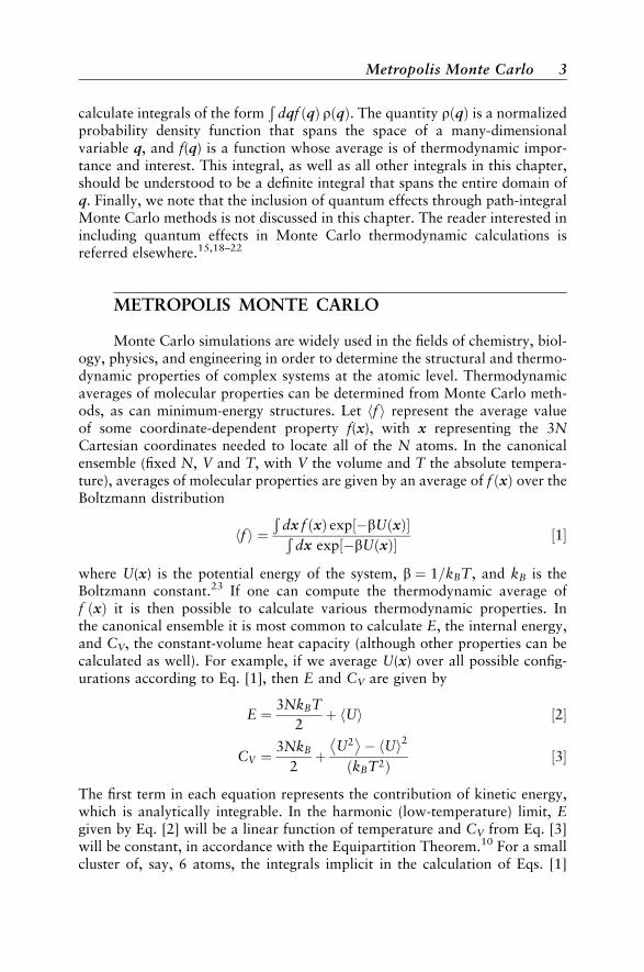
Monte Carlo simulations are widely used in the fields of chemistry, biol-ogy, physics, and engineering in order to determine the structural and thermo-dynamic properties of complex systems at the atomic level. Thermodynamicaverages of molecular properties can be determined from Monte Carlo meth-ods, as can minimum-energy structures. Let hf i represent the average valueof some coordinate-dependent property f(x), with x representing the 3NCartesian coordinates needed to locate all of the N atoms. In the canonicalensemble (fixed N, V and T, with V the volume and T the absolute tempera-ture), averages of molecular properties are given by an average of f ðxÞ over theBoltzmann distribution

hf i ¼Ð

dx f ðxÞ exp �bUðxÞ½ �Ðdx exp �bUðxÞ½ � ½1�

where U(x) is the potential energy of the system, b ¼ 1=kBT, and kB is theBoltzmann constant.23 If one can compute the thermodynamic average off ðxÞ it is then possible to calculate various thermodynamic properties. Inthe canonical ensemble it is most common to calculate E, the internal energy,and CV, the constant-volume heat capacity (although other properties can becalculated as well). For example, if we average U(x) over all possible config-urations according to Eq. [1], then E and CV are given by

E ¼ 3NkBT

2þ Uh i ½2�

CV ¼ 3NkB

2þ

U2� �

� Uh i2

kBT2ð Þ ½3�

The first term in each equation represents the contribution of kinetic energy,which is analytically integrable. In the harmonic (low-temperature) limit, Egiven by Eq. [2] will be a linear function of temperature and CV from Eq. [3]will be constant, in accordance with the Equipartition Theorem.10 For a smallcluster of, say, 6 atoms, the integrals implicit in the calculation of Eqs. [1]

Metropolis Monte Carlo 3

and [2] are already of such high dimension that they cannot be effectively com-puted using Simpson’s rule or other basic quadrature methods.2,24,25,26 Forlarger clusters, liquids, polymers or biological molecules the dimensionalityis obviously much higher, and one typically resorts to either Monte Carlo,molecular dynamics, or other related algorithms.

To calculate the desired thermodynamic averages, it is necessary to havesome method available for computation of the potential energy, either expli-citly (in the form of a function representing the interaction potential as inmolecular mechanics) or implicitly (in the form of direct quantum-mechanicalcalculations). Throughout this chapter we shall assume that U is known or canbe computed as needed, although this computation is typically the most com-putationally expensive part of the procedure (because U may need to be com-puted many, many times). For this reason, all possible measures should betaken to assure the maximum efficiency of the method used in the computationof U.

Also, it should be noted that constraining potentials (which keep thecluster components from straying too far from a cluster’s center of mass)are sometimes used.27 At finite temperature, clusters have finite vapor pres-sures, and particular cluster sizes are typically unstable to evaporation. Intro-ducing a constraining potential enables one to define clusters of desired sizes.Because the constraining potential is artificial, the dependence of calculatedthermodynamic properties on the form and the radius of the constrainingpotential must be investigated on a case-by-case basis. Rather than divertingthe discussion from our main focus (Monte Carlo methods), we refer theinterested reader elsewhere for more details and references on the use of con-straining potentials.15,19

Random-Number Generation: A Few Notes

Because generalized Metropolis Monte Carlo methods are based on‘‘random’’ sampling from probability distribution functions, it is necessaryto use a high-quality random-number generator algorithm to obtain reliableresults. A review of such methods is beyond the scope of this chapter,24,28

but a few general considerations merit discussion.Random-number generators do not actually produce random numbers.

Rather, they use an integer ‘‘seed’’ to initialize a particular ‘‘pseudorandom’’sequence of real numbers that, taken as a group, have properties that leavethem nearly indistinguishable from truly random numbers. These are conventi-onally floating-point numbers, distributed uniformly on the interval (0,1). Ifthere is a correlation between seeds, a correlation may be introduced betweenthe pseudorandom numbers produced by a particular generator. Thus, thegenerator should ideally be initialized only once (at the beginning of the ran-dom walk), and not re-initialized during the course of the walk. The seedshould be supplied either by the user or generated arbitrarily by the program


using, say, the number of seconds since midnight (or some other arcane for-mula). One should be cautious about using the ‘‘built-in’’ random-numbergenerator functions that come with a compiler for Monte Carlo integrationwork because some of them are known to be of very poor quality.26 Thereader should always be sure to consult the appropriate literature and obtain(and test) a high-quality random-number generator before attempting to writeand debug a Monte Carlo program.

The Generalized Metropolis Monte Carlo Algorithm

The Metropolis Monte Carlo (MMC) algorithm is the single most widelyused method for computing thermodynamic averages. It was originally devel-oped by Metropolis et al. and used by them to simulate the freezing transitionfor a two-dimensional hard-sphere fluid.1 However, Monte Carlo methods canbe used to estimate the values of multidimensional integrals in whatever con-text they may arise.29,30 Although Metropolis et al. did not present their algo-rithm as a general-utility method for numerical integration, it soon becameapparent that it could be generalized and applied to a variety of situations.The core of the MMC algorithm is the way in which it draws samples froma desired probability distribution function. The basic strategies used inMMC can be generalized so as to apply to many kinds of probability functionsand in combination with many kinds of sampling strategies. Some authorsrefer to the generalized MMC algorithm simply as ‘‘Metropolis sampling,’’31

while others have referred to it as the M(RT)2 method6 in honor of the fiveauthors of the original paper (Metropolis, the Rosenbluths, and the Tellers).1

We choose to call this the generalized Metropolis Monte Carlo (gMMC) meth-od, and we will always use the term MMC to refer strictly to the combinationof methods originally presented by Metropolis et al.1

In the literature of numerical analysis, gMMC is classified as an impor-tance sampling technique.6,24 Importance sampling methods generate config-urations that are distributed according to a desired probability function ratherthan simply picking them at random from a uniform distribution. The prob-ability function is chosen so as to obtain improved convergence of the proper-ties of interest. gMMC is a special type of importance sampling method whichasymptotically (i.e., in the limit that the number of configurations becomeslarge) generates states of a system according to the desired probability distri-bution.6,9 This probability function is usually (but not always6) the actualprobability distribution function for the physical system of interest. Nearlyall statistical-mechanical applications of Monte Carlo techniques require theuse of importance sampling, whether gMMC or another method is used (alter-natively, ‘‘stratified sampling’’ is sometimes an effective approach22,32).gMMC is certainly the most widely used importance sampling method.

In the gMMC algorithm successive configurations of the system aregenerated to build up a special kind of random walk called a Markov


chain.29,33,34 The random walk visits successive configurations, where eachconfiguration’s location depends on the configuration immediately precedingit in the chain. The gMMC algorithm establishes how this can be done so asto asymptotically generate a distribution of configurations corresponding tothe probability density function of interest, which we denote as rðqÞ.

We define Kðqi ! qjÞ to be the conditional probability that a configura-tion at qi will be brought to qj in the next step of the random walk. This con-ditional probability is sometimes called the ‘‘transition rate.’’ The probabilityof moving from q to q0 (where q and q0 are arbitrarily chosen configurationssomewhere in the available domain) is therefore given by Pðq ! q0Þ:

Pðq ! q0Þ ¼ Kðq ! q0Þ rðqÞ ½4�

For the system to evolve toward a unique limiting distribution, we must placea constraint on Pðq ! q0Þ. The gMMC algorithm achieves the desired limitingbehavior by requiring that, on the average, a point is just as likely to movefrom q to q0 as it is to move in the reverse direction, namely, thatPðq ! q0Þ ¼ Pðq0 ! qÞ. This likelihood can be achieved only if the walk isergodic (an ergodic walk eventually visits all configurations when startedfrom any given configuration) and if it is aperiodic (a situation in which nosingle number of steps will generate a return to the initial configuration).This latter requirement is known as the ‘‘detailed balance’’ or the ‘‘micro-scopic reversibility’’ condition:

Kðq ! q0Þ rðqÞ ¼ Kðq0 ! qÞ rðq0Þ ½5�

Satisfying the detailed balance condition ensures that the configurationsgenerated by the gMMC algorithm will asymptotically be distributed accord-ing to rðqÞ.

The transition rate may be written as a product of a trial probability �and an acceptance probability A

Kðqi ! qjÞ ¼ �ðqi ! qjÞAðqi ! qjÞ ½6�

where � can be taken to be any normalized distribution that asymptoticallyspans the space of all possible configurations, and A is constructed so thatEq. [5] is satisfied for a particular choice of �. The wonderful flexibilitywith which � can be chosen is one of the reasons so many Monte Carlo meth-ods are found in the literature. For example, Metropolis et al. used a uniformdistribution of points about xi to define the trial probability (we describe thisin greater detail in the next section),1 but a Gaussian distribution of points canalso be used profitably in certain situations.20 Many other distributions arepossible and even desirable in different contexts.


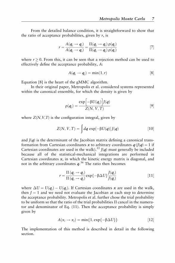
From the detailed balance condition, it is straightforward to show thatthe ratio of acceptance probabilities, given by r, is

r ¼Aðqi ! qjÞAðqj ! qiÞ

¼�ðqj ! qiÞ rðqjÞ�ðqi ! qjÞ rðqiÞ

½7�

where r � 0. From this, it can be seen that a rejection method can be used toeffectively define the acceptance probability, A:

Aðqi ! qjÞ ¼ minð1; rÞ ½8�

Equation [8] is the heart of the gMMC algorithm.In their original paper, Metropolis et al. considered systems represented

within the canonical ensemble, for which the density is given by

rðqjÞ ¼exp �bUðqjÞ

h iJðqÞ

ZðN;V;TÞ ½9�

where Z(N;V;T) is the configuration integral, given by

ZðN;V;TÞ ¼ð

dq exp �bUðqÞ½ � JðqÞ ½10�

and J(q) is the determinant of the Jacobian matrix defining a canonical trans-formation from Cartesian coordinates x to arbitrary coordinates q (J(q) ¼ 1 ifCartesian coordinates are used in the walk).35 J(q) must generally be includedbecause all of the statistical-mechanical integrations are performed inCartesian coordinates x, in which the kinetic energy matrix is diagonal, andnot in the arbitrary coordinates q.36 The ratio then becomes

r ¼� ðqj ! qiÞ� ðqi ! qjÞ

expf�b�UgJðqjÞJðqiÞ

½11�

where �U ¼ UðqjÞ � UðqiÞ. If Cartesian coordinates x are used in the walk,then J ¼ 1 and we need not evaluate the Jacobian at each step to determinethe acceptance probability. Metropolis et al. further chose the trial probabilityto be uniform so that the ratio of the trial probabilities � cancel in the numera-tor and denominator of Eq. (11). Then the acceptance probability is simplygiven by

Aðxi ! xjÞ ¼ min 1; exp �b�Uf gf g ½12�

The implementation of this method is described in detail in the followingsection.


Metropolis Monte Carlo: The ‘‘Classic’’ Algorithm

Having established the preceding important framework, we now turn tothe particulars of the original Metropolis Monte Carlo algorithm for samplingconfigurations from the canonical ensemble. As alluded to in the previous sec-tion, it is often most convenient to work in Cartesian coordinates for MMCcalculations (with some exceptions discussed later). In this case, Eqs. [6]–[12]reduce to the algorithm described by the flowchart in Figure 1. First, an initialconfiguration of the system is established. The initial configuration can be gen-erated randomly, although it is sometimes advantageous to start from anenergy-minimized structure,37 a crystalline lattice structure, or a structureobtained from experiment.

Next, a ‘‘trial move’’ is made to generate a new trial configuration,according to a rule that we call a ‘‘move strategy.’’ The simple move strategyintroduced by Metropolis et al.1 is still the most widely used method. One

Figure 1 Flowchart of the ‘‘classic’’ Metropolis Monte Carlo algorithm for samplingin the canonical ensemble.1 Note that samples of the property function f ðxÞ are alwaysaccumulated for averaging purposes, irrespective of whether a move is accepted orrejected.


preselects a maximum stepsize L and randomly moves each particle withina cube of length L centered on the atom’s original position (see Figure 2).This procedure defines the Metropolis transition probability, �M. For a one-dimensional system moving along a single coordinate x:

�M ¼ 1

L;

�L

2< x <

L

2¼ 0 elsewhere ½13�

The parameter L may have an optimum value for the particular type of atomof interest, as well as for the temperature and other variables studied. If L istoo small, most moves will be accepted and a very large number of attemptswill be required to move very far from the initial configuration. However, if Lis too big very few trial moves will be accepted and again, the walker willrequire many steps to move away from the starting point. For this reasonone generally chooses L so that between 30% and 70% of the moves areaccepted (50% is a happy medium).6,7 Each atom can be moved in sequence,

Figure 2 Single-particle Metropolis moves from the original MMC algorithm1 andmolecular rotation Barker–Watts moves41 for generation of a trial Monte Carlo move.


or an atom can be chosen randomly for each trial move, at the discretion ofthe programmer.

As noted previously, the Metropolis move strategy of ‘‘single-particlemoves’’ is still the most widely used in the literature. The use of single-particlemoves is often considered as being part and parcel of the MetropolisMonte Carlo method. However, a number of other move strategies in thecanonical ensemble are possible, some of which are outlined later in this chap-ter. Metropolis Monte Carlo simulations in other ensembles require the use ofother move strategies. For example, in the isothermal–isobaric ensemble (con-stant N,P,T), the volume and the configurations are perturbed.7,13,38,39 In thegrand canonical ensemble (constant chemical potential, V, and T) the numberof particles N fluctuates, so a move may include randomly deleting or adding aparticle.11,13,39 The use of the Gibbs ensemble for phase equilibrium studiesinvolves perturbations of volumes and configurations within each phase,as well as the transfer of particles between phases.10,13,39,40 In all of thesesituations, suitable move strategies must be employed to ensure that detailedbalance is satisfied for all variables involved.

Regardless how it is generated, the trial configuration does not automa-tically become the second step in the Markov chain. Within the canonicalensemble if the potential energy of the trial configuration is less than orequal to the potential energy of the previous configuration, that is, if�U � Uðx0Þ � UðxÞ � 0, the trial configuration is then ‘‘accepted.’’ However,if �U > 0 the trial move may still be conditionally accepted. A random num-ber � between 0 and 1 is chosen and compared to expð�b�UÞ. If � is less thanor equal to expð�b�UÞ the trial move is accepted; otherwise, the trial config-uration fails the ‘‘Boltzmann test,’’ the move is ‘‘rejected,’’ and the originalconfiguration becomes the second step in the Markov chain (see Figure 1).The procedure is then repeated many times until equilibration is achieved(equilibration is defined in a later section). After equilibration, the procedurecontinues as before, but now the values of U and U2 (and any other propertiesof interest, represented by f in Figure 1) are accumulated for each of theremaining n steps in the chain. Let n represent the number of samples usedin computing the averages of U and U2. The number of samples is chosento be sufficiently large for convergence of hUin and hU2in, the n-point averagesof U and U2, to their true values hUi and hU2i. In the case of U,

hUi ¼ limn!1

hUin ½14�

where

hUin � 1

n

Xn

j¼1

UðxjÞ ½15�


Similar formulas hold for hU2i and hU2in. It is important to emphasize thatconfigurations are not excluded for averaging purposes simply because theyhave been most recently accepted or rejected. Both accepted and rejectedconfigurations must be included in the average, or the potential energies willnot be Boltzmann-distributed.

The Barker–Watts Algorithm for Molecular Rotations

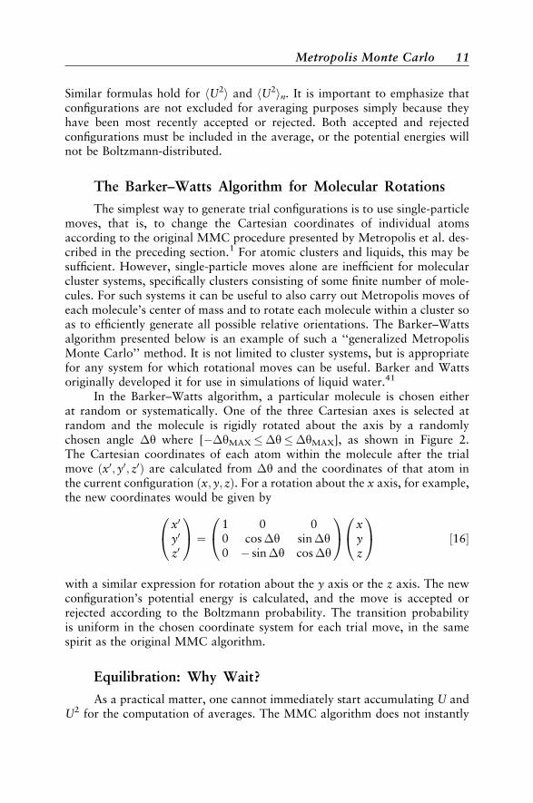
The simplest way to generate trial configurations is to use single-particlemoves, that is, to change the Cartesian coordinates of individual atomsaccording to the original MMC procedure presented by Metropolis et al. des-cribed in the preceding section.1 For atomic clusters and liquids, this may besufficient. However, single-particle moves alone are inefficient for molecularcluster systems, specifically clusters consisting of some finite number of mole-cules. For such systems it can be useful to also carry out Metropolis moves ofeach molecule’s center of mass and to rotate each molecule within a cluster soas to efficiently generate all possible relative orientations. The Barker–Wattsalgorithm presented below is an example of such a ‘‘generalized MetropolisMonte Carlo’’ method. It is not limited to cluster systems, but is appropriatefor any system for which rotational moves can be useful. Barker and Wattsoriginally developed it for use in simulations of liquid water.41

In the Barker–Watts algorithm, a particular molecule is chosen eitherat random or systematically. One of the three Cartesian axes is selected atrandom and the molecule is rigidly rotated about the axis by a randomlychosen angle �y where [��yMAX ��y��yMAX], as shown in Figure 2.The Cartesian coordinates of each atom within the molecule after the trialmove ðx0; y0; z0Þ are calculated from �y and the coordinates of that atom inthe current configuration ðx; y; zÞ. For a rotation about the x axis, for example,the new coordinates would be given by

x0

y0

z0

0@

1A ¼

1 0 00 cos�y sin�y0 � sin�y cos�y

0@

1A x

yz

0@

1A ½16�

with a similar expression for rotation about the y axis or the z axis. The newconfiguration’s potential energy is calculated, and the move is accepted orrejected according to the Boltzmann probability. The transition probabilityis uniform in the chosen coordinate system for each trial move, in the samespirit as the original MMC algorithm.

Equilibration: Why Wait?

As a practical matter, one cannot immediately start accumulating U andU2 for the computation of averages. The MMC algorithm does not instantly


sample configurations according to the Boltzmann distribution; the sampling isonly guaranteed to be correct in the asymptotic limit of large n. It is thereforealways necessary to allow the Markov walk to go through a large number ofsteps before beginning to accumulate samples to estimate U and U2. This pro-cedure is known as the ‘‘equilibration’’ of the walker.6,7,10 The walker shouldundergo a sufficiently large number of iterations for there to be no ‘‘memory’’of the system’s initial configuration. The index value j ¼ 1 in Eq. [15] refers tothe first configuration after the system has equilibrated by cycling through neq

steps; only states sampled after equilibration should be included in the aver-age. neq is often referred to as the ‘‘equilibration period.’’

One way to estimate neq is to calculate the running averages of U and U2

to make running estimates of E and CV ; these quantities are then plottedagainst m, the subtotal of all steps taken (m < n) at a few representative tem-peratures to determine when asymptotic, slowly varying behavior is attained.7

Since E is given by Eq. [3], the running average of U may be plotted instead ofE if desired. The running average of U is given by hUim

hUim � 1

m

Xm

j¼1

UðxjÞ ½17�

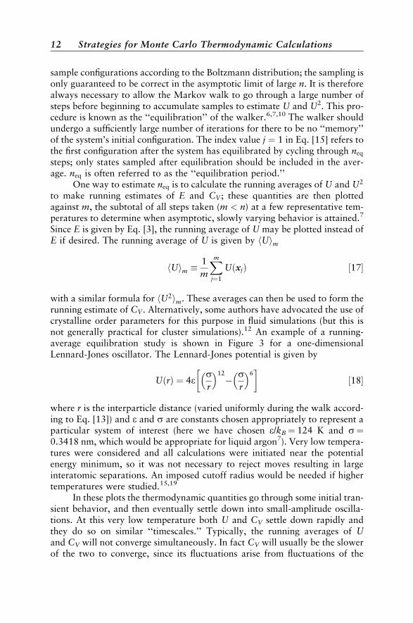
with a similar formula for hU2im. These averages can then be used to form therunning estimate of CV . Alternatively, some authors have advocated the use ofcrystalline order parameters for this purpose in fluid simulations (but this isnot generally practical for cluster simulations).12 An example of a running-average equilibration study is shown in Figure 3 for a one-dimensionalLennard-Jones oscillator. The Lennard-Jones potential is given by

UðrÞ ¼ 4esr

� 12� s

r

� 6� �

½18�

where r is the interparticle distance (varied uniformly during the walk accord-ing to Eq. [13]) and e and s are constants chosen appropriately to represent aparticular system of interest (here we have chosen e/kB ¼ 124 K and s¼0.3418 nm, which would be appropriate for liquid argon7). Very low tempera-tures were considered and all calculations were initiated near the potentialenergy minimum, so it was not necessary to reject moves resulting in largeinteratomic separations. An imposed cutoff radius would be needed if highertemperatures were studied.15,19

In these plots the thermodynamic quantities go through some initial tran-sient behavior, and then eventually settle down into small-amplitude oscilla-tions. At this very low temperature both U and CV settle down rapidly andthey do so on similar ‘‘timescales.’’ Typically, the running averages of Uand CV will not converge simultaneously. In fact CV will usually be the slowerof the two to converge, since its fluctuations arise from fluctuations of the


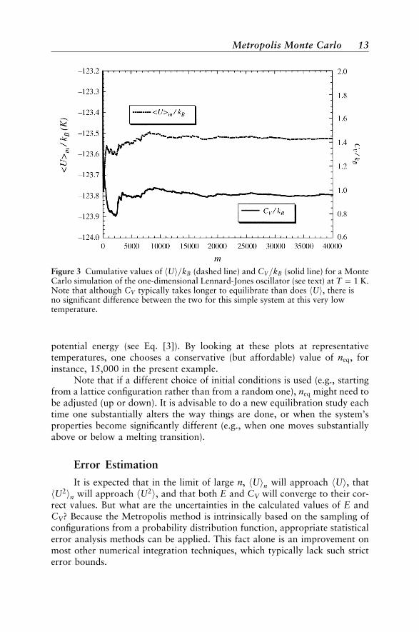
potential energy (see Eq. [3]). By looking at these plots at representativetemperatures, one chooses a conservative (but affordable) value of neq, forinstance, 15,000 in the present example.

Note that if a different choice of initial conditions is used (e.g., startingfrom a lattice configuration rather than from a random one), neq might need tobe adjusted (up or down). It is advisable to do a new equilibration study eachtime one substantially alters the way things are done, or when the system’sproperties become significantly different (e.g., when one moves substantiallyabove or below a melting transition).

Error Estimation

It is expected that in the limit of large n, hUin will approach hUi, thathU2in will approach hU2i, and that both E and CV will converge to their cor-rect values. But what are the uncertainties in the calculated values of E andCV? Because the Metropolis method is intrinsically based on the sampling ofconfigurations from a probability distribution function, appropriate statisticalerror analysis methods can be applied. This fact alone is an improvement onmost other numerical integration techniques, which typically lack such stricterror bounds.

Figure 3 Cumulative values of hUi=kB (dashed line) and CV=kB (solid line) for a MonteCarlo simulation of the one-dimensional Lennard-Jones oscillator (see text) at T ¼ 1 K.Note that although CV typically takes longer to equilibrate than does hUi, there isno significant difference between the two for this simple system at this very lowtemperature.


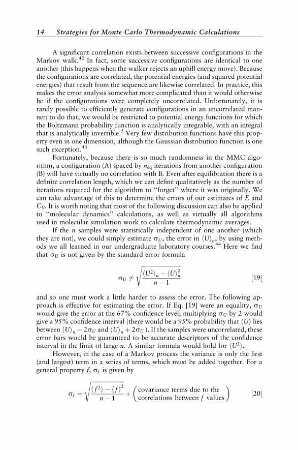
A significant correlation exists between successive configurations in theMarkov walk.42 In fact, some successive configurations are identical to oneanother (this happens when the walker rejects an uphill energy move). Becausethe configurations are correlated, the potential energies (and squared potentialenergies) that result from the sequence are likewise correlated. In practice, thismakes the error analysis somewhat more complicated than it would otherwisebe if the configurations were completely uncorrelated. Unfortunately, it israrely possible to efficiently generate configurations in an uncorrelated man-ner; to do that, we would be restricted to potential energy functions for whichthe Boltzmann probability function is analytically integrable, with an integralthat is analytically invertible.5 Very few distribution functions have this prop-erty even in one dimension, although the Gaussian distribution function is onesuch exception.43

Fortunately, because there is so much randomness in the MMC algo-rithm, a configuration (A) spaced by neq iterations from another configuration(B) will have virtually no correlation with B. Even after equilibration there is adefinite correlation length, which we can define qualitatively as the number ofiterations required for the algorithm to ‘‘forget’’ where it was originally. Wecan take advantage of this to determine the errors of our estimates of E andCV. It is worth noting that most of the following discussion can also be appliedto ‘‘molecular dynamics’’ calculations, as well as virtually all algorithmsused in molecular simulation work to calculate thermodynamic averages.

If the n samples were statistically independent of one another (whichthey are not), we could simply estimate sU, the error in hUin, by using meth-ods we all learned in our undergraduate laboratory courses.44 Here we findthat sU is not given by the standard error formula

sU 6¼

ffiffiffiffiffiffiffiffiffiffiffiffiffiffiffiffiffiffiffiffiffiffiffiffiffiffiffiffihU2in � hUi2

n

n � 1

s½19�

and so one must work a little harder to assess the error. The following ap-proach is effective for estimating the error. If Eq. [19] were an equality, sU

would give the error at the 67% confidence level; multiplying sU by 2 wouldgive a 95% confidence interval (there would be a 95% probability that hUi liesbetween hUin � 2sU and hUin þ 2sU ). If the samples were uncorrelated, theseerror bars would be guaranteed to be accurate descriptors of the confidenceinterval in the limit of large n. A similar formula would hold for hU2i.

However, in the case of a Markov process the variance is only the first(and largest) term in a series of terms, which must be added together. For ageneral property f, sf is given by

sf ¼

ffiffiffiffiffiffiffiffiffiffiffiffiffiffiffiffiffiffiffiffiffiffiffiffih f 2i � h f i2

n � 1

sþ covariance terms due to the

correlations between f values

� �½20�


where n is the number of steps after equilibration. These covariance termstypically converge slowly; details for treating these kinds of problems can befound elsewhere.45–48 Another commonly used method is ‘‘blocking.’’7,12,49

For definiteness, let n ¼ 1,000,000 samples. We divide these samples intoNB ¼ 100 blocks of s ¼ 10,000 samples each, with the first 10,000 samplesin block 1, the second 10,000 samples in block 2, and so forth. Within thelth block we form estimates of hUi [hUiflg

s ], and hU2i [hU2iflgs ]. A list of 100

‘‘block averages’’ for each property is thus established. The 100 block averagesof each property are statistically independent of one another if s is sub-stantially greater than the correlation length. This in turn means they can beanalyzed as if they were 100 statistically independent objects. Considering theuncertainty in hUin, we therefore have

sU ¼

ffiffiffiffiffiffiffiffiffiffiffiffiffiffiffiffiffiffiffiffiffiffiffiffiffiVar hUiflg

s

h iNB � 1

vuut½21�

where

Var hUiflgs

h i¼ 1

NB

XNB

l¼1

hUiflgs � hUin

h i2½22�

with similar formulas defining sU2 . Note that sU decreases asymptotically asthe inverse square root of the number of samples (even though only the num-ber of blocks is explicit), and that 2sU defines the 95% confidence interval forhUin. For published work we generally recommend that the 95% confidencelevel be reported. Since the thermodynamic energy E is given by Eq. [2] (whichis linear in hUi ), Eqs. [21] and [22] also happen to give directly the error in E.

It should be noted that in practice the parameters s and NB must gener-ally be determined empirically by trial and error, until convergence of the errorestimate is achieved at a single temperature. This is usually straightforward inpractice, and the prior determination of the equilibration period makes thistask considerably easier to achieve because the correlation length is likely tobe less than or equal to the equilibration period.

Similar equations and considerations hold for the average of the squaredpotential energy, but the propagation of the error through Eq. [3] is some-what more involved. It is simplest to compute NB values of ðCVÞf‘gs , the heatcapacity within each block, using Eq. [3], and then using Eq. [23] to obtain thestandard error in CV from the variance of the block heat capacities:

sCV¼

ffiffiffiffiffiffiffiffiffiffiffiffiffiffiffiffiffiffiffiffiffiffiffiffiffiffiffiffiVar ðCVÞf‘gs

h iNB � 1

vuut½23�


In Table 1 we show how the error in the average potential energy and the errorin CV (at the 95% confidence level) depend upon the number of blocks in asample of fixed size (500,000 samples after 20,000 equilibration cycles) forthe one-dimensional Lennard-Jones oscillator at 1 K. As noted previously,

Table 1 Convergence of Approximate 95% Confidence Level Error Estimates of aMetropolis Monte Carlo Estimate of hUi and CV with Respect to the Number of BlocksUsed for the One-Dimensional Lennard-Jones Oscillator at T ¼ 1 Ka,b

NB hUi/kB (K) 2sU/abs(hUi) CV/kB 2sCV=CV

2 �123.4958 3:3636 � 10�5 1. 0044 0.00724 — 4:2259 � 10�5 — 0.01095 — 1:8810 � 10�5 — 0.00558 — 3:5502 � 10�5 — 0.0118

10 — 3:3166 � 10�5 — 0.010216 — 2:9819 � 10�5 — 0.010620 — 2:8031 � 10�5 — 0.008825 — 2:6449 � 10�5 — 0.009332 — 2:6552 � 10�5 — 0.009340 — 2:3754 � 10�5 — 0.007650 — 2:2375 � 10�5 — 0.008380 — 2:5355 � 10�5 — 0.0087

aSee Eq. [18] and accompanying text.bAll calculations given are for a single Metropolis Monte Carlo calculation in which 20,000

equilibration cycles were followed by 500,000 data collection cycles. The stepsize was 0.01 nm,which produced an acceptance ratio of approximately 50%.

Table 2 Average Potential Energy, Heat Capacity, and Fractional 95% ConfidenceLevel Statistical Errors for the One-Dimensional Lennard-Jones Oscillatora,b

TðKÞ hUi=kBðKÞ 2sU/abs(hUi) CV /kB 2sCV=CV

0.1 �123:9499 5 � 10�6 0.999 0.010.5 �123:7495 2 � 10�5 1.002 0.011.0 �123:4938 4 � 10�5 1.008 0.011.5 �123:2367 5 � 10�5 1.020 0.012.0 �122:9741 9 � 10�5 1.022 0.022.5 �122:7207 8 � 10�5 1.027 0.013.0 �122:4455 2 � 10�4 1.043 0.023.5 �122:1789 2 � 10�4 1.048 0.024.0 �121:6182 3 � 10�4 1.053 0.024.5 �121:6182 3 � 10�4 1.063 0.025.0 �121:3596 3 � 10�4 1.060 0.025.5 �121:0521 4 � 10�4 1.076 0.026.0 �120:7361 5 � 10�4 1.100 0.036.5 �120:4725 5 � 10�4 1.104 0.03

aSee Eq. [18] and accompanying text.bAll calculations given are for Metropolis Monte Carlo calculations in which 20,000

equilibration cycles were followed by 500,000 data collection cycles. The stepsize was 0.01 nm,which produced an acceptance ratio of approximately 50%. Ten blocks were used to estimate thestatistical errors.


the relative error in CV is significantly larger than the error in E for the samevalue of n. This is because the heat capacity represents the mean-squaredfluctuations of the energy, and its error is proportional to the root meansquare (RMS) fluctuations of the energy’s fluctuations. In some cases theblocking technique may fail to effectively ‘‘break’’ the correlations; in sucha situation other methods may be employed to estimate the covariancedirectly.44–48

It is important to emphasize that different thermodynamic propertiesgenerally converge at different rates. Those rates also generally depend onthe temperature and can be quite strong functions of temperature in certaincases (for example, when phase transitions are possible). Table 2 shows howthe error in E and the error in CV vary with temperature for the Lennard-Jonesoscillator. For this simple system the temperature dependence of the error isweak, but the trend of gradual increases in the error is evident. Also notethat the average potential energy is approximately a linear function of tem-perature at low temperatures with a slope equal to kB/2 (Figure 4), and thatthe reduced heat capacity CV=kB approaches 1.0 as the temperatureapproaches zero (Figure 5), both in agreement with the EquipartitionTheorem.10

Figure 4 hUi=kB as a function of temperature (diamonds) for the one-dimensionalLennard-Jones oscillator (see text). The Equipartition Theorem requires that the slopeapproach the harmonic limit (¼ 1

2) as the temperature approaches zero (solid line).


QUASI-ERGODICITY: AN INSIDIOUS PROBLEM

While the methods discussed thus far are sufficiently powerful to allowthe simulation of many complex phenomena, there are circumstances wheretheir direct implementation must be modified for efficient sampling. In manyimportant cases the direct application of the preceding strategies with a (neces-sarily) finite set of points can give misleading or incorrect results.

In Monte Carlo computations of thermodynamic properties, it is oftendesirable that the sampling be ergodic.50 In the present context, we definean ergodic random walk as one that can eventually reach every possible statefrom every possible initial state. A simulation that samples ergodically is typi-cally characterized by low asymptotic variance and by rapid convergence.However, for systems for which there are wells in the potential energy surfacethat are separated by high barriers, sampling that is confined to a subset of thewells becomes problematic. This type of sampling is termed quasi-ergodicsampling.15,51 When a system is quasi-ergodic it usually appears to be ergodic,exhibiting low asymptotic variance and rapid convergence, thus making quasi-ergodicity particularly difficult to detect. This problem is not unique to MonteCarlo methods, but is also a feature of molecular dynamics calculations andvirtually all other molecular simulation methods.

Figure 5 CV=kB as a function of temperature for the one-dimensional Lennard-Jonesoscillator (see text). The Equipartition Theorem requires that the ratio of the heatcapacity to kB approach the harmonic limit (¼ 1) as the temperature approaches zero(solid line).


Cluster melting simulations are situations in which special effort must betaken to ensure ergodic sampling. The melting transitions typically occur overa range of temperatures, and clusters can often coexist in solid-like and liquid-like forms (or in several solidlike forms) within this range. The large energybarriers characteristic of ‘‘magic number clusters’’ lead to quasi-ergodicsampling.15

To illustrate the kinds of problems to which we refer, we make use of aclassical double-well potential that has proved to be useful52 for the study ofquasi-ergodicity:

UðxÞ ¼ 3x4

2a þ 1þ 4ða � 1Þx3

2a þ 1� 6ax2

2a þ 1þ 1 ½24�

This potential has a minimum of zero energy at x ¼ 1, a second minimum ofvariable energy at x ¼ �a and a barrier of unit height separating the minima atx ¼ 0. For 0 � a � 1 it is useful to define the relative well depth by

g ¼ Uð0Þ � Uð�aÞUð0Þ � Uð1Þ ¼ a3 a þ 2

2a þ 1½25�

For the case g ¼ 0:9 (a ¼ 0.961261), U(x) is shown in Figure 6. This modelpotential has many features generic to molecular potential surfaces, in particular

Figure 6 Asymmetricdouble-well potentialUðxÞ with g ¼ 0:9 (seeEqs. [24,25]).

Quasi-ergodicity: an Insidious Problem 19

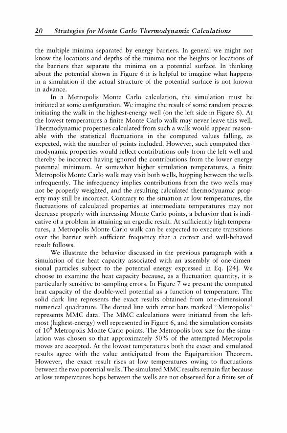
the multiple minima separated by energy barriers. In general we might notknow the locations and depths of the minima nor the heights or locations ofthe barriers that separate the minima on a potential surface. In thinkingabout the potential shown in Figure 6 it is helpful to imagine what happensin a simulation if the actual structure of the potential surface is not knownin advance.

In a Metropolis Monte Carlo calculation, the simulation must beinitiated at some configuration. We imagine the result of some random processinitiating the walk in the highest-energy well (on the left side in Figure 6). Atthe lowest temperatures a finite Monte Carlo walk may never leave this well.Thermodynamic properties calculated from such a walk would appear reason-able with the statistical fluctuations in the computed values falling, asexpected, with the number of points included. However, such computed ther-modynamic properties would reflect contributions only from the left well andthereby be incorrect having ignored the contributions from the lower energypotential minimum. At somewhat higher simulation temperatures, a finiteMetropolis Monte Carlo walk may visit both wells, hopping between the wellsinfrequently. The infrequency implies contributions from the two wells maynot be properly weighted, and the resulting calculated thermodynamic prop-erty may still be incorrect. Contrary to the situation at low temperatures, thefluctuations of calculated properties at intermediate temperatures may notdecrease properly with increasing Monte Carlo points, a behavior that is indi-cative of a problem in attaining an ergodic result. At sufficiently high tempera-tures, a Metropolis Monte Carlo walk can be expected to execute transitionsover the barrier with sufficient frequency that a correct and well-behavedresult follows.

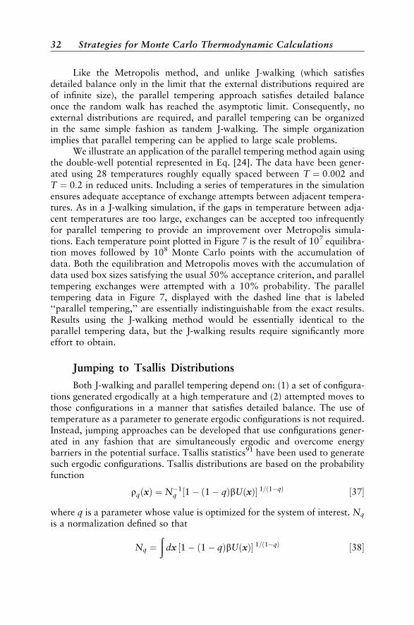
We illustrate the behavior discussed in the previous paragraph with asimulation of the heat capacity associated with an assembly of one-dimen-sional particles subject to the potential energy expressed in Eq. [24]. Wechoose to examine the heat capacity because, as a fluctuation quantity, it isparticularly sensitive to sampling errors. In Figure 7 we present the computedheat capacity of the double-well potential as a function of temperature. Thesolid dark line represents the exact results obtained from one-dimensionalnumerical quadrature. The dotted line with error bars marked ‘‘Metropolis’’represents MMC data. The MMC calculations were initiated from the left-most (highest-energy) well represented in Figure 6, and the simulation consistsof 108 Metropolis Monte Carlo points. The Metropolis box size for the simu-lation was chosen so that approximately 50% of the attempted Metropolismoves are accepted. At the lowest temperatures both the exact and simulatedresults agree with the value anticipated from the Equipartition Theorem.However, the exact result rises at low temperatures owing to fluctuationsbetween the two potential wells. The simulated MMC results remain flat becauseat low temperatures hops between the wells are not observed for a finite set of


Monte Carlo points. As the temperature is increased beyond the heat capacitymaximum in the exact result, the MMC simulated points begin to rise but theyare in poor agreement with the exact data. Additionally, the calculated errorbars increase, but are artificially large in this calculation and do not accuratelyreflect the true asymptotic fluctuations of the heat capacity. Finally, at thehighest calculated temperatures, both the Metropolis Monte Carlo and exactdata are in agreement.

Several methods have been developed to remove such difficulties fromMMC simulations. One obvious but not very useful method is to includemore Metropolis Monte Carlo points. In the limit of an infinite simulation

Figure 7 CV as a function of T for the asymmetric double-well potential shown inFigure 6. The ‘‘exact’’ result (solid line) is obtained by direct integration of theBoltzmann average. ‘‘Metropolis’’ Monte Carlo results (dotted line) are seen to be insharp disagreement with the exact result until temperatures are sampled that are wellabove the transition temperature for motion between the two potential energy wells.Parallel tempering Monte Carlo results (dashed line) are in all cases within the 95%confidence interval of the exact result.

Quasi-ergodicity: an Insidious Problem 21

adding more points is guaranteed to work, but in many cases this is imprac-tical. Another approach, which does work for the present one-dimensionalexample problem, is to simply extend the original Metropolis scheme. In theMetropolis method one usually chooses a single maximum displacement foreach Monte Carlo attempted move (the Metropolis step size). As in the exam-ple displayed in Figure 7, the step size is selected so that approximately 50% ofthe attempted moves are accepted. A simple modification to this procedure isto include two stepsizes. The first, used for most moves, has a size chosen tomeet the usual 50% criterion. The second maximum stepsize is chosen to betwo units of distance in length (the distance between the two minima inFigure 6). By using this magnified stepsize for a portion of the moves, the bar-rier between the wells is overcome even at low temperatures. It is not difficultto verify that the occasional inclusion of a magnified stepsize, which we call‘‘mag-walking,’’ satisfies detailed balance.52

Mag-walking is sufficiently simple that it can be useful for some many-particle applications where the locations of the barriers between the minimaare known in advance. Unfortunately this simple extension, based on two(or more) maximum stepsizes, fails for many important applications of MonteCarlo to interacting many-particle systems. For many-body applications thepotential minima are generally separated not just by a distance but also byone or more curvilinear directions. To move from one potential well toanother in a many-particle application, specifying the distance between thewells is insufficient. Because the locations of the wells are seldom known inadvance, more sophisticated approaches are usually necessary.

From the previous discussion, we see that the problem of adequatelysampling a potential energy surface can often be solved with a strategy havingtwo distinct parts. The first part concerns locating the relevant potential minimain the energy surface along with the transition state barriers that separate thoseminima. The second part concerns the development of a strategy to sample theimportant minima with the correct statistics. Simulation methods based onthis two-part separation strategy have limited utility in cluster studies becausethe number of minima on a potential surface grows extremely rapidly with thesize of the system studied (at a rate believed to be exponential). For example, acluster of 13 atoms interacting via Lennard-Jones forces is known to havemore than 1500 minima,53 while nanodimensional Lennard-Jones clusterscontaining 147 atoms are believed to have about 1060 minima.54 It is clearlyimpossible to enumerate all the minima for the latter cluster, even if a practicalprocedure were available to sample all such minima. Of course, we are reallyconcerned with only those minima that are actually accessible with a reason-able probability at a given temperature, but the number of such minima canalso be unreasonably large. The most successful approaches to proper sam-pling of complex potential surfaces involve methods that solve both parts ina single step.


OVERCOMING QUASI-ERGODICITY

Mag-Walking

As mentioned previously, the simplest method for addressing quasi-ergodicity is to occasionally magnify the stepsize in a Metropolis walk.52

A probability Pm is specified, and a magnified stepsize is used if Pm is greaterthan or equal to a random number x. The probability that a magnified move isaccepted is the same as that for a regular move. For example, if Pm is chosen tobe 0.1 then magnified steps are possible 10% of the time.

This very simple method has a chance of being effective only when themagnified stepsize corresponds to a displacement that is known to carry amolecule from one conformation to another. For example, we have foundmag-walking to be useful in certain contexts when applied to Barker–Wattsrotational moves; �yMAX may be equal to one radian for a regular rotationalstep, and p radians for a magnified step. We have used this method successfullyin simulations of order–disorder transitions in solid ammonium chloride,55

and in some preliminary investigations of cationic ammonium chlorideclusters.56 However, because one does not usually know a priori what kindof displacement will tend to generate new conformers, mag-walking is oflimited utility.

Subspace Sampling

The subspace sampling method developed by Shew and Mills uses tran-sitions among subspaces of the configuration space to overcome quasi-ergodicity.57 Configuration space is divided into subspaces based on the poten-tial energy surface. For example, for a double-well potential each well wouldbe a subspace defined by the location of the local maximum separating the twowells (subspaces A and B hereafter). A transfer probability PAB is specified anda transfer of the system from configuration i in subspace A to configuration jin subspace B is attempted if PAB is greater than a random number x. Thetransfer is accepted by the probability A(qi,A ! qj,B),

Aðqi;A ! qj;BÞ ¼ cVB

Vif Uðqi;AÞ < Uðqj;BÞ

¼ cVB

Vexp½�bðUðqi;AÞ � Uðqj;BÞÞ� if Uðqi;AÞ > Uðqj;BÞ ½26�

where V is the total volume, VB is the volume occupied by subspace B and c isan empirically chosen constant. As in mag-walking, the subspace sampling

Overcoming Quasi-ergodicity 23

method requires prior knowledge of the potential energy surface to divideconfiguration space into subspaces. Moreover, the determination of eachsubspace’s volume is only possible when definite rectilinear or sphericalboundaries can be drawn which separate and enclose all the subspaces (inwhich case the volume calculations are trivial). Identifying definite boundariesthat correctly separate the relevant subspaces can be challenging. Subspacesampling is therefore generally practical only for low-dimensional systems.

Jump Between Wells Method

The jump between wells (JBW) method developed by Senderowitz, Guar-nieri, and Still58 involves repeated sampling from known low energy confor-mers to generate a Markov chain. Each trial move is based on thetransformation of one low-energy conformer to another and subsequent per-turbation of the selected conformer. This method has been shown to workwell for relatively small organic molecules, but because it requires knowledgeof all low energy conformers, it may not be practical for larger molecules. Thislimitation applies especially to atomic and molecular clusters, since the loca-tion of all low energy conformers may itself be a significant computationalchallenge.

Atom-Exchange Method

The atom-exchange method was developed by Tsai, Abraham, andPound59 to speed barrier crossing in binary (two types of atoms) alloy clustersimulations. During the Metropolis walk two different types of atoms areperiodically chosen, and their positions are exchanged. The exchange isaccepted or rejected by the standard Metropolis acceptance probability. Theutility of this method is naturally limited to systems of this particular type,namely, binary atomic clusters and liquids.

Histogram Methods

The single histogram method17,60 involves constructing a histogram ofenergies h(U) that are obtained at an elevated sampling temperature Ts,with Ts > T. For continuous systems a large number of bins should be setup to discretize the energy. Because the probability distribution function isknown, it can be used to calculate ensemble averages at any temperature T

hf i ¼

PU

f ðUÞ hðUÞ exp½�Uðb� bsÞ�PU

hðUÞ exp½�Uðb� bsÞ�½27�


where bs is 1/kBTs. It is not necessary to actually save the histogram of energiesif the summations are carried out over configurations instead of energies:61

hf i ¼

Pi

f ðxiÞ= exp �bsUðxiÞ½ �f gð Þ exp ½�bUðxiÞ�Pi

1= exp �bsUðxiÞ½ �f gð Þ exp ½�bUðxiÞ�½28�

In addition to improving the simulation efficiency, the single-histogrammethod is designed to alleviate quasi-ergodicity by increasing the effectivesampling temperature. The square of the error is proportional to the numberof entries in the histogram, so the accuracy is greatest where h(U) is largest andthe error is greatest at the wings of the histogram.62 Thus the limitation of thismethod is that it may not be accurate for temperatures far below the samplingtemperature Ts, whereas Ts must be much higher than T for many cases toovercome quasi-ergodicity.

The accuracy of the histogram method can be improved and its limita-tions largely overcome by combining multiple histograms with overlappingtemperature ranges.60,63 The density is estimated from a linear combinationof the estimates from multiple histograms hi(U) measured at temperaturesTi. The weight assigned to each estimate is optimized to reduce error throughan iterative procedure. The simulated annealing–optimal histogram methodtakes a different approach wherein simulations at various temperatures areused to generate optimized sampling of energy bins.17 A more detailed discus-sion is beyond the scope of this chapter.

Umbrella Sampling

Umbrella sampling is a technique that facilitates barrier crossing byintroducing an artificial bias potential, called the ‘‘umbrella potential.’’4 Theumbrella potential optimally biases the sampling toward important regions ofconfiguration space that might otherwise be rarely visited. The probabilitydistribution of the physical system can then be extracted from the probabilitydistribution of the unphysical system. The probability distributions are oftenanalyzed along a ‘‘reaction coordinate’’ �, which can be one- or multidimen-sional and is expressed as a function of the coordinates of the system.64 Thereaction coordinate is often taken to be a distance or angle, or a linear combi-nation of distances or angles.

A modified potential energy function Umod ¼ U þ Euð�Þ is constructed,where U is the true potential energy of the system and Euð�Þ is the umbrellasampling potential [note that � ¼ �ðqÞ in general]. The Boltzmann average ofany property f can be computed by using Umod ¼ U þ Eu in place of U in theMetropolis algorithm and calculating the average as

hf i ¼f exp bEuð Þh iUmod

exp bEuð Þh iUmod

½29�

Overcoming Quasi-ergodicity 25

where hBiUmodis the average of B taken using the modified potential function in

a Markov walk where moves are accepted or rejected with probability

min 1; e�b�Umod� �

The efficiency of the method depends on the choice of umbrella potential. Thelimitation of the umbrella sampling method is that the umbrella potential mustbe appropriately chosen for each system of interest. There are many methodsof calculating an appropriate umbrella potential depending on the goals of thesimulation.65 A number of procedures have been developed to automaticallyand iteratively calculate an umbrella potential for certain types of situa-tions.66–70 We will also see in a later section that umbrella sampling is usedwithin the multicanonical ensemble. Finally, Valleau has recently reviewedthe thermodynamic-scaling Monte Carlo method, which uses umbrella sam-pling to guide a system between thermodynamic states.71

J-WALKING, PARALLEL TEMPERING,AND RELATED METHODS

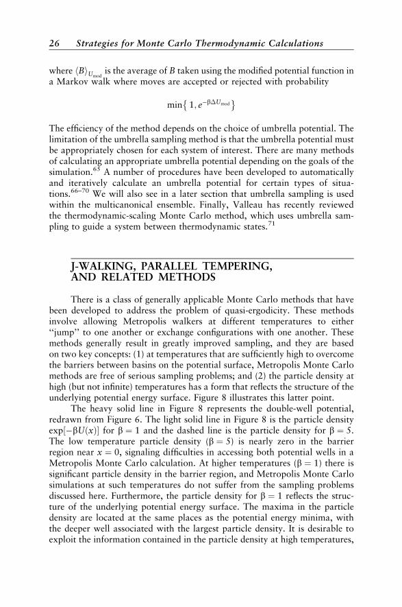
There is a class of generally applicable Monte Carlo methods that havebeen developed to address the problem of quasi-ergodicity. These methodsinvolve allowing Metropolis walkers at different temperatures to either‘‘jump’’ to one another or exchange configurations with one another. Thesemethods generally result in greatly improved sampling, and they are basedon two key concepts: (1) at temperatures that are sufficiently high to overcomethe barriers between basins on the potential surface, Metropolis Monte Carlomethods are free of serious sampling problems; and (2) the particle density athigh (but not infinite) temperatures has a form that reflects the structure of theunderlying potential energy surface. Figure 8 illustrates this latter point.

The heavy solid line in Figure 8 represents the double-well potential,redrawn from Figure 6. The light solid line in Figure 8 is the particle densityexp½�bUðxÞ� for b ¼ 1 and the dashed line is the particle density for b ¼ 5.The low temperature particle density (b ¼ 5) is nearly zero in the barrierregion near x ¼ 0, signaling difficulties in accessing both potential wells in aMetropolis Monte Carlo calculation. At higher temperatures (b ¼ 1) there issignificant particle density in the barrier region, and Metropolis Monte Carlosimulations at such temperatures do not suffer from the sampling problemsdiscussed here. Furthermore, the particle density for b ¼ 1 reflects the struc-ture of the underlying potential energy surface. The maxima in the particledensity are located at the same places as the potential energy minima, withthe deeper well associated with the largest particle density. It is desirable toexploit the information contained in the particle density at high temperatures,


which is easily generated from a Metropolis calculation, to enable an ergodicsimulation at low temperatures where the problems are more serious.

J-Walking

The first method to have been developed using the concepts discussed inthe previous paragraph is called J-walking, or alternatively, jump-walking.52

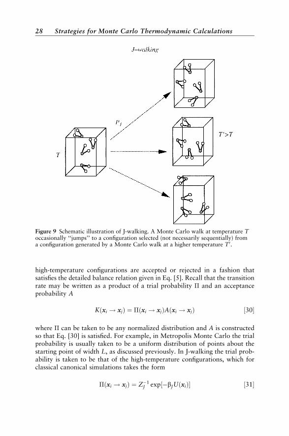
In the J-walking method a Metropolis calculation is performed at a tempera-ture sufficiently high to avoid ergodic sampling problems. A Monte Carlowalk is then performed at a low temperature that periodically makes movesto the configurations determined by the high-temperature walk. The configura-tions can be taken from either a walk carried out simultaneously (often calledtandem J-walking) or configurations that have been stored from a previoushigh-temperature walk. In the low temperature simulation, where achievingergodic sampling is problematic, moves are made periodically to the configura-tions from the high-temperature walk (see Figure 9). Attempts to jump to these

Figure 8 Boltzmann particle densities exp½�bUðxÞ� at b ¼ 1 (light, solid line) and b ¼ 5(dashed line) for the asymmetric double-well potential U(x) with g ¼ 0:9, which isalso shown (dark, solid line; see Figure 6).

J-Walking, Parallel Tempering, and Related Methods 27

high-temperature configurations are accepted or rejected in a fashion thatsatisfies the detailed balance relation given in Eq. [5]. Recall that the transitionrate may be written as a product of a trial probability � and an acceptanceprobability A

Kðxi ! xjÞ ¼ �ðxi ! xjÞAðxi ! xjÞ ½30�

where � can be taken to be any normalized distribution and A is constructedso that Eq. [30] is satisfied. For example, in Metropolis Monte Carlo the trialprobability is usually taken to be a uniform distribution of points about thestarting point of width L, as discussed previously. In J-walking the trial prob-ability is taken to be that of the high-temperature configurations, which forclassical canonical simulations takes the form

�ðxi ! xjÞ ¼ Z�1J exp½�bJUðxiÞ� ½31�

Figure 9 Schematic illustration of J-walking. A Monte Carlo walk at temperature Toccasionally ‘‘jumps’’ to a configuration selected (not necessarily sequentially) froma configuration generated by a Monte Carlo walk at a higher temperature T 0.


where ZJ is a normalization factor, bJ ¼ 1=kBTJ and TJ is the temperatureused to generate the high-temperature configurations. An acceptance prob-ability ensuring satisfaction of detailed balance is given by

Aðxi ! xjÞ ¼ min 1;rðxjÞ�ðxj ! xiÞrðxiÞ�ðxi ! xjÞ

� �½32�

which, for jumps to the high-temperature configurations in a classical canoni-cal simulation, takes the form

Aðxi ! xjÞ ¼ min 1; expð��b�UÞð Þ ½33�

where �b ¼ b� bJ and �U ¼ UðxjÞ � UðxiÞ. Again, b ¼ 1=kBT, where T isthe temperature of interest (associated with the low-temperature walk) andbJ is the inverse temperature used to generate the high-temperature externaldistribution.

The barriers that separate potential wells and make sampling difficult atlow temperatures are overcome by jumping periodically to the high-tempera-ture configurations. In this J-walking procedure detailed balance is satisfied tothe extent that the configurations in the high-temperature walk are an exactrepresentation of the actual high-temperature probability function (Eq. [31]).Such an exact representation of the actual probability function is possible onlyin the limit of an infinite external distribution, or when jumps to the tandemdistribution are taken after an infinite number of steps. Systematic errors aredifficult to remove in the tandem method, so most published applications haveused external distributions. In practice a large (but necessarily finite) high-temperature distribution is generated. In the low-temperature simulationmost Monte Carlo moves are generated using the Metropolis method withmoves to the external high-temperature distribution at some prescribedfrequency. In most applications these jump attempts are made about 10%of the simulation time, although higher jump attempt rates have been shownto be optimal in some cases.72 To ensure that the distribution is sufficientlylarge (so as to be an accurate representation of the true high-temperatureprobability function), the distribution size must be larger than the numberof jumps attempted in a simulation.

When using finite high-temperature external distributions, another issuearises when applying Eq. [33], because this equation assumes the exact prob-ability is used. This issue is the origin of tandem J-walking problems. Whengenerating the external high-temperature distribution using the Metropolismethod, it is important to not store every configuration from that Metropoliswalk. As noted previously, configurations generated using a Metropolis walkare correlated,6 and the correlations can introduce systematic errors whenmoves are accepted and rejected on the basis of the criterion of Eq. [33]. Toavoid these systematic errors it is necessary to store configurations from a


high-temperature Metropolis walk only after a sufficient number of MonteCarlo steps have been taken to break the correlations.

There is a final issue in J-walking that occurs in related simulation meth-ods as well. If the difference in temperature between that used to generate thejumping distribution TJ and the temperature of interest T is sufficiently large,the probability that an attempted jump is accepted can become vanishinglysmall. When (effectively) no attempted jumps are accepted, the J-walking algo-rithm is equivalent to a Metropolis walk. Rather than jumping from tempera-ture T to the distribution generated at temperature TJ, a series of temperaturesare chosen between T and TJ, and configurations are stored at each of the ser-ies of temperatures to circumvent this problem. The temperatures are chosento be sufficiently close to each other so that jump attempts between adjacenttemperatures are accepted with reasonable probability (e.g., at least 10%).J-walking between adjacent temperatures is used to ensure ergodic distribu-tions at each temperature.

To decrease the size of the external distributions needed in J-walking, analternative method known as ‘‘smart walking’’ has been developed.73 In smartwalking, the energy of each high-temperature configuration is minimizedbefore a jump is attempted. However, smart walking does not satisfy detailedbalance.74 A new technique called ‘‘smart darting’’ has recently been devel-oped that modifies the smart-walking procedure by including the use of‘‘darts,’’ which are displacement vectors connecting the minimum-energy con-figurations.74 Smart darting satisfies detailed balance, and it has been appliedsuccessfully to calculations of an 8-atom Lennard-Jones cluster and also forthe alanine dipeptide.

While J-walking has proved to be useful for many applications,75–82 theneed for a series of large external distributions limits its application to many-body systems having modest numbers of particles. The needed configurationsfor J-walking can require a prohibitively large portion of both computer mem-ory and disk space. In the next section we describe another approach thatobviates the need for external distributions.

Parallel Tempering

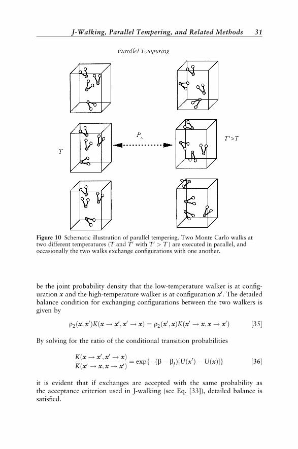
Like J-walking, parallel tempering83–90 addresses sampling problems byusing information about the underlying potential surface obtained from ahigh-temperature walk where sampling is not problematic to ensure propersampling by a lower-temperature simulation. While high-temperature config-urations are fed to a low-temperature walk in J-walking, parallel temperinguses configurations that are exchanged between the high- and low-temperaturewalkers (see Figure 10).

To understand the basis of parallel tempering, we let

r2ðx; x0Þ ¼ F�1 exp �bUðxÞ½ � exp½�bJUðx0Þ� ½34�


be the joint probability density that the low-temperature walker is at config-uration x and the high-temperature walker is at configuration x0. The detailedbalance condition for exchanging configurations between the two walkers isgiven by

r2ðx; x0ÞKðx ! x0; x0 ! xÞ ¼ r2ðx0; xÞKðx0 ! x; x ! x0Þ ½35�

By solving for the ratio of the conditional transition probabilities

Kðx ! x0; x0 ! xÞKðx0 ! x; x ! x0Þ ¼ expf�ðb� bJÞ Uðx0Þ � UðxÞ½ �g ½36�

it is evident that if exchanges are accepted with the same probability asthe acceptance criterion used in J-walking (see Eq. [33]), detailed balance issatisfied.

Figure 10 Schematic illustration of parallel tempering. Two Monte Carlo walks attwo different temperatures (T and T 0 with T 0 > T ) are executed in parallel, andoccasionally the two walks exchange configurations with one another.


Like the Metropolis method, and unlike J-walking (which satisfiesdetailed balance only in the limit that the external distributions required areof infinite size), the parallel tempering approach satisfies detailed balanceonce the random walk has reached the asymptotic limit. Consequently, noexternal distributions are required, and parallel tempering can be organizedin the same simple fashion as tandem J-walking. The simple organizationimplies that parallel tempering can be applied to large scale problems.

We illustrate an application of the parallel tempering method again usingthe double-well potential represented in Eq. [24]. The data have been gener-ated using 28 temperatures roughly equally spaced between T ¼ 0:002 andT ¼ 0:2 in reduced units. Including a series of temperatures in the simulationensures adequate acceptance of exchange attempts between adjacent tempera-tures. As in a J-walking simulation, if the gaps in temperature between adja-cent temperatures are too large, exchanges can be accepted too infrequentlyfor parallel tempering to provide an improvement over Metropolis simula-tions. Each temperature point plotted in Figure 7 is the result of 107 equilibra-tion moves followed by 108 Monte Carlo points with the accumulation ofdata. Both the equilibration and Metropolis moves with the accumulation ofdata used box sizes satisfying the usual 50% acceptance criterion, and paralleltempering exchanges were attempted with a 10% probability. The paralleltempering data in Figure 7, displayed with the dashed line that is labeled‘‘parallel tempering,’’ are essentially indistinguishable from the exact results.Results using the J-walking method would be essentially identical to theparallel tempering data, but the J-walking results require significantly moreeffort to obtain.

Jumping to Tsallis Distributions

Both J-walking and parallel tempering depend on: (1) a set of configura-tions generated ergodically at a high temperature and (2) attempted moves tothose configurations in a manner that satisfies detailed balance. The use oftemperature as a parameter to generate ergodic configurations is not required.Instead, jumping approaches can be developed that use configurations gener-ated in any fashion that are simultaneously ergodic and overcome energybarriers in the potential surface. Tsallis statistics91 have been used to generatesuch ergodic configurations. Tsallis distributions are based on the probabilityfunction

rqðxÞ ¼ N�1q 1 � ð1 � qÞbUðxÞ½ � 1=ð1�qÞ ½37�

where q is a parameter whose value is optimized for the system of interest. Nq

is a normalization defined so that

Nq ¼ð

dx 1 � ð1 � qÞbUðxÞ½ � 1=ð1�qÞ ½38�


The Tsallis probability distribution is equivalent to the classical Boltz-mann distribution in the limit q ! 1. As shown numerically elsewhere,92 forq > 1 the Tsallis distribution broadens, overcoming energy barriers, and likehigh-temperature Boltzmann particle densities, the Tsallis distribution hasmaxima at the coordinates of potential minima. The Tsallis distribution canbe used like high-temperature Boltzmann distributions if Tsallis configurationsare accepted or rejected with probability

min 1; e�b�UrqðxÞrqðx0Þ

" #q( )

Successful applications of jumps to Tsallis distributions have included clustersystems.92

Applications to Microcanonical Simulations

Monte Carlo methods can also be applied to systems in the microcano-nical ensemble,7,10 and the techniques just described can be extended to thisensemble as well. For a cluster of N atoms with the same mass m, microcano-nical averages of observables are obtained by calculating statistical expecta-tions using the density function

rEðxÞ ¼2pm=h2� �

3N=2 1= N! �ð3N=2Þ½ �f g�ðEÞ � E � UðxÞ½ � E � UðxÞ½ � ð3N=2Þ�1

½39�

where �ðyÞ is the gamma function, �ðyÞ is the Heaviside (step) function and�(E) is the classical density of states93

�ðEÞ ¼ 1

h3NN!

ðdx dp d E � Hðx; pÞ½ � ½40�

where p is the linear momentum vector, H the classical Hamiltonian, and d½y�the Dirac delta function.35 For example, the average kinetic energy K of asystem can be obtained from the expression

hKi ¼Ð

dx�ðE � UÞ ðE � UÞð3N=2Þ�1ðE � UÞÐdx�ðE � UÞ ðE � UÞð3N=2Þ�1

¼ hðE � UÞi ½41�

Either parallel tempering94,95 or J-walking82 in the microcanonical ensembleconsists of taking configurations from a walk at high energy Eh, rather than


from a high temperature. Exchanges or jumps are accepted or rejected withprobability

min 1;rEðx0ÞrEh

ðxÞrEðxÞrEh

ðx0Þ

( )

Microcanonical parallel tempering has been extended to the moleculardynamics ensemble by introducing the appropriate center of mass and angularmomentum constraints, the details of which can be found elsewhere.94

MULTICANONICAL ENSEMBLE /ENTROPY SAMPLING

Another class of methods that has been used to remove sampling diffi-culties is based on what is often called the multicanonical ensemble.96 Thesemethods have also been called ‘‘entropy sampling’’ methods,97 for reasons thatare made clear below.98 It is easiest to understand the multicanonical methodsby considering the full classical canonical coordinate–momentum distribution

rðx; pÞ ¼ M�1 exp �bHðx; pÞ½ � ½42�

where M is a normalization factor. The canonical density can also be ex-pressed as a function of the total energy E rather than the coordinates andmomenta

rðb;EÞ ¼ M�1�ðEÞ exp �bE½ � ½43�

As is discussed in many elementary treatments of statistical mechanics, �ðEÞ isa rapidly increasing function of the energy.99 Owing to the decay of the expo-nential factor in Eq. [42], rðb;EÞ is a sharp Gaussian distribution, and ispeaked about the mean energy associated with the inverse temperature b.

For a Metropolis walk using Eq. [42] the energy of each configurationgenerated can be tabulated to generate �ðEÞ. The sorting of configurationsinto energy bins is the basis of histogram sampling methods,17,60,100,101 which(as mentioned previously) are beyond the scope of this chapter. Accurate esti-mates of �ðEÞ can be achieved only for energies about the average energy of thetemperature used to generate the density of states. Consequently, to generate�ðEÞ accurately, calculations must be performed at a series of temperatures.The normalization for each energy distribution so generated must be chosencarefully such that the distributions created for each temperature match.The subtleties associated with this procedure are also beyond the scope ofthis chapter; for the purposes of this section, we only remark that �ðEÞ canbe constructed using a canonical Boltzmann Monte Carlo walk.17


Earlier we made clear that Monte Carlo walks can become trapped inregions of space owing to energy barriers that separate the disconnected con-figurations. In multicanonical methods the energy barriers are overcome byperforming a walk in a space with a uniform energy distribution. The energydistribution is defined by the relation

rMðEÞ ¼ M�1�ðEÞwðEÞ ¼ �kk ½44�

where �kk is a constant. We then sample with respect to the distribution

wðEÞ ¼ k�ðEÞ ½45�

where k ¼ �kkM. It is of interest to write

ln wðEÞ ¼ ln k� kB

kBln�ðEÞ

wðEÞ ¼ K exp �kB ln�ðEÞ½ �½46�

where K is a constant. Using the standard microcanonical expression for theentropy S ¼ kB ln �,99 w becomes

wðEÞ ¼ K exp½�SðEÞ� ½47�

Because of expression Eq. [47], multicanonical sampling is often called‘‘entropy sampling.’’

To calculate canonical averages of an observable f ðx; pÞ using theentropy distribution (Eq. [47]), we can implement umbrella sampling methods

hf i ¼Ð

dx dp f ðx; pÞ expð�bHÞÐdx dp expð�bHÞ ½48�

¼f ðx; pÞ expð�bHÞ

w

D ES

expð�bHÞw

D ES

½49�

where the subscript S below each average in Eq. [49] implies sampling withrespect to the distribution w.

J-walking ideas have also been used in multicanonical approaches102 asan alternative to calculating expectation values using Eq. [49]. In the multi-canonical J-walking approach, periodic jumps are made to the distributionof configurations associated with the entropy distribution w rather than peri-odic jumps to a set of high-temperature ergodic configurations. To satisfydetailed balance, such jumps are accepted with probability

min 1;exp �bH x0; p0ð Þ½ �w Hðx; pÞ½ �exp �bHðx; pÞ½ �w H x0; p0ð Þ½ �

" #

Multicanonical Ensemble / Entropy Sampling 35

From an operational point of view, an important issue when using multi-canonical methods is the generation of the multicanonical weight w. Becausew is not in general known analytically, w must be generated numerically.Some of the most successful methods for generating w are based on iterativemethods, the discussion of which can be found elsewhere.103 These iterativeprocedures suffer from oscillatory convergence characteristics, but theseconvergence problems have been solved using other J-walking based appro-aches.104 In practice, the generated multicanonical weights are accuratelydescribed at intermediate energies but often provide poor representations atlow energies. Consequently, multicanonical methods can be deficient forsystems having important low temperature structures that are difficult toaccess.88

CONCLUSIONS

As you perhaps may have noticed, many Monte Carlo methods can befound in the literature. We have not described all of the Monte Carlo methodsdeveloped to date. Indeed, new methods are being developed every day, andmethods better than those that now exist can be expected to appear in thefuture. Nonetheless we can make a few definite recommendations to thereaders interested in writing their own Monte Carlo programs (especiallyfor studying atomic and molecular clusters) based on existing methodology.

First, it is often useful to study a simple potential such as that given inEq. [29], and use it as a minimal proving ground for testing and implementa-tion of new Monte Carlo algorithms. Such potentials contain some (but notall) of the features of more realistic and complex problems. However, somemethods will work well for an asymmetric double-well potential but failwhen applied to more complex systems. We therefore warn the reader: letthe buyer of a ‘‘foolproof’’ Monte Carlo algorithm beware!

Second, it is advisable to carry out ordinary Metropolis Monte Carlo cal-culations using Metropolis sampling1 (with Barker–Watts rotational sampling41

and center-of-mass moves in addition to single-particle moves if the clustercontains molecules) as a function of temperature before moving to more com-plex methods. This will help identify the temperature range of greatest impor-tance and indicate how high the temperature must be for quasi-ergodicsampling problems to be avoided. This information can then be used in paralleltempering, J-walking, and other calculations.

Parallel tempering works, and works well in a wide variety of contexts(although the reader should be warned that we are even now finding particu-larly nasty examples where even parallel tempering converges at an unaccep-tably slow rate). In our experience, parallel tempering is much simpler to


implement than many of the alternatives. Thus, our final recommendation isthat parallel tempering is strongly recommended whenever quasi-ergodicityproblems are possible. Parallel tempering can be extremely useful in MonteCarlo studies of atomic and molecular clusters. It also can be used to excellenteffect in molecular dynamics simulations, and thus it constitutes an extremelygeneral and powerful technique. We are hopeful that the reader who uses thischapter as a starting point to develop new and improved Monte Carlo meth-ods will find the work as rewarding and interesting as we have.

ACKNOWLEDGMENTS

We are grateful for the efforts of all of our colleagues and students who have helped usunderstand and use the Monte Carlo method, and other stochastic methods, in our studies of clus-ters and condensed phases. Our sincere thanks to Sarah Kopel-Fink for assisting with some of thecalculations presented here, and to Gayle G. Topper for her help with the literature search. RQTand KRL’s work on this chapter was supported in part by the Petroleum Research Fund of theAmerican Chemical Society under grant PRF 33601-B6. DLF’s work on this chapter has been sup-ported in part by NSF grant CHE-0095053. DB acknowledges fellowship support from the EndersMemorial Fund, as well from as the Supercomputer Research Institute (SCRI) at Florida State Uni-versity for a travel grant to attend the 1999 SCRI Monte Carlo Workshop.

REFERENCES

1. N. Metropolis, A. W. Rosenbluth, M. N. Rosenbuth, A. H. Teller, and E. Teller, J. Chem.Phys., 21, 1087 (1953). Equation of State Calculations by Fast Computing Machines.

2. J. M. Hammersley and D. C. Handscomb, Monte Carlo Methods, Methuen, London, 1964.

3. J. P. Valleau and S. G. Whittington, in Statistical Mechanics Part A: Equilibrium Techniques,B. J. Berne, Ed., Plenum Press, New York, 1977, pp. 137–168. A Guide to Monte Carlo forStatistical Mechanics: 1. Highways.

4. J. P. Valleau and G. M. Torrie, in Statistical Mechanics Part A: Equilibrium Techniques; B. J.Berne, Ed., Plenum Press, New York, 1977, pp. 169–191. A Guide to Monte Carlo forStatistical Mechanics: 2. Byways.

5. K. Binder, in Monte Carlo Methods in Statistical Physics, K. Binder. Ed., Springer-Verlag,Berlin, 1979, pp. 1–45. Introduction: Theory and ‘‘Technical’’ Aspects of Monte CarloSimulations.

6. M. H. Kalos and P. A. Whitlock, Monte Carlo Methods, Wiley, New York, 1986.

7. M. P. Allen and D. J. Tildesley, Computer Simulation of Liquids, Clarendon Press, Oxford,1992.

8. J. M. Lluch, M. Moreno, and J. Bertran, in Computational Chemistry: Structure, Interaction,and Reactivity; S. Fraga, Ed., Elsevier Science Publishers, Amsterdam, 1992, p. 311. MonteCarlo Simulations for Solutions.

9. D. J. Tildesley, NATO ASI Ser., Ser. C (Computer Simulations in Chemical Physics) 397, 1(1993). The Monte Carlo Method.

10. R. L. Rowley, Statistical Mechanics for Thermophysical Property Calculations, PTR Prentice-Hall, Englewood Cliffs, NJ, 1994.

11. D. Frenkel and B. Smit, Understanding Molecular Simulation: From Algorithms to Applica-tions, Academic Press, San Diego, 1996.

References 37

12. A. R. Leach, Molecular Modelling: Principles and Applications, Longman, London, 1996.

13. J. I. Siepmann, Adv. Chem. Phys., 105, 1–12 (1999). An Introduction to the Monte CarloMethod for Particle Simulations.

14. G. Benedek, T. P. Martin, and G. Pacchioni, Eds., Elemental and Molecular Clusters: Proc.13th International School, Springer-Verlag, Berlin, 1988.

15. D. L. Freeman and J. D. Doll, Ann. Rev. Phys. Chem., 47, 43–80 (1996). ComputationalStudies of Clusters: Methods and Results.

16. D. Eisenberg and D. Crothers, Physical Chemistry with Applications to the Life Sciences,Benjamin/Cummings, Menlo Park, CA, 1979.

17. D. M. Ferguson and D. G. Garrett, Adv. Chem. Phys., 105, 311 (1999). Simulated Anneal-ing—Optimal Histogram Methods.

18. B. J. Berne and D. Thirumalai, Ann. Rev. Phys. Chem., 37, 401–424 (1986). On theSimulation of Quantum Systems: Path Integral Methods.

19. D. L. Freeman and J. D. Doll, Adv. Chem. Phys., 70B, 139 (1988). The Quantum Mechanicsof Clusters.

20. J. D. Doll, D. L. Freeman, and T. L. Beck, Adv. Chem. Phys., 78, 61–128 (1990). Equilibriumand Dynamical Fourier Path Integral Methods.

21. G. A. Voth, Adv. Chem. Phys., 93, 135–218 (1996). Path Integral Centroid Methods inQuantum Statistical Mechanics and Dynamics.

22. R. Q. Topper, Adv. Chem. Phys., 105, 117–170 (1999). Adaptive Path-Integral Monte CarloMethods for Accurate Computation of Molecular Thermodynamic Properties.

23. J. W. Gibbs, Elementary Principles in Statistical Mechanics, Yale Univ. Press, New Haven,CT, 1902.

24. J. H. Halton, SIAM Rev., 12, 1 (1970). A Retrospective and Prospective Survey of the MonteCarlo Method.

25. F. James, Rep. Prog. Phys., 43, 73 (1980). Monte Carlo Theory and Practice.

26. W. H. Press, S. A. Teukolsky, W. T. Vetterling, and B. P. Flannery, Numerical Recipes inFORTRAN: The Art of Scientific Computing, 2nd ed., Cambridge Univ. Press, CambridgeUK, 1992.

27. J. K. Lee, J. A. Barker, and F. F. Abraham, J. Chem. Phys., 58, 3166 (1973). Theory and MonteCarlo Simulation of Physical Clusters in the Imperfect Vapor.

28. A. Srinivasan, D. M. Ceperley, and M. Mascagni, Adv. Chem. Phys., 105, 13–36 (1999).Random Number Generators for Parallel Applications.

29. R. W. Wilde and S. Singh, Statistical Mechanics: Fundamentals and Modern Applications,Wiley, New York, 1998.

30. W. L. McMillan, Phys. Rev., 138, 442 (1965). Ground State of Liquid 4He.

31. J. B. Anderson, in Reviews in Computational Chemistry, K. B. Lipkowitz and D. B. Boyd, Eds.,Wiley-VCH, New York, 1999, Vol. 13, pp. 133–182. Quantum Monte Carlo: Atoms,Molecules, Clusters, Liquids, and Solids.

32. A. Riganelli, W. Wang, and A. J. C. Varandas, J. Phys. Chem. A, 103, 8303 (1999). MonteCarlo Approach to Internal Partition Functions for Van der Waals Molecules.

33. U. Grenander, Ark. Matemat., 1, 195 (1950). Stochastic Processes and Statistical Inference.

34. W. K. Hastings, Biometrika, 5, 97 (1970). Monte Carlo Sampling Methods Using MarkovChains and Their Applications.

35. H. Goldstein, Classical Mechanics, 2nd ed., Addison-Wesley, Reading MA, 1980.

36. D. A. McQuarrie, Statistical Mechanics, HarperCollins, New York, 1976.

37. D. D. Frantz, D. L. Freeman, and J. D. Doll, J. Chem. Phys., 93, 2769 (1990). Reducing Quasi-Ergodic Behavior in Monte Carlo Simulations by J-Walking: Applications to AtomicClusters.


38. I. R. McDonald, Molec. Phys., 23, 41 (1972). NpT-Ensemble Monte Carlo Calculations forBinary Liquid Mixtures.

39. J. I. Siepmann, Adv. Chem. Phys., 105, 443 (1999). Monte Carlo Methods for SimulatingPhase Equilibria of Complex Fluids.

40. A. Z. Panagiotopoulos, Molec. Phys., 61, 813 (1987). Direct Determination of PhaseCoexistence Properties of Fluids by Monte Carlo Simulation in a New Ensemble.

41. J. A. Barker and R. O. Watts, Chem. Phys. Lett., 3, 144 (1969). Structure of Water: A MonteCarlo Calculation.

42. W. J. Dixon, Ann. Math. Stat., 15, 119 (1944). Further Contributions to the Problem of SerialCorrelation.

43. G. E. P. Box and M. E. Muller, Ann. Math. Statist., 29, 610 (1958). A Note on the Generationof Random Normal Deviates.

44. J. R. Taylor, An Introduction to Error Analysis: The Study of Uncertainties in PhysicalMeasurements, University Science, Mill Valley, CA, 1982.

45. E. B. Smith and B. H. Wells, Molec. Phys., 53, 701 (1984). Estimating Errors in MolecularSimulation Calculations.

46. T. P. Straatsma, H. J. C. Berendsen, and A. J. Stam, Molec. Phys., 57, 89 (1986). Estimation ofStatistical Errors in Molecular Simulation Calculations.

47. R. Q. Topper and D. G. Truhlar, J. Chem. Phys., 97, 3647 (1992). Quantum Free-EnergyCalculations: Optimized Fourier Path-Integral Monte Carlo Computation of CoupledVibrational Partition Functions.

48. J. D. Doll and D. L. Freeman, Chem. Phys. Lett., 227, 436 (1994). Decisions, Decisions: Noiseand Its Effect on Integral Monte Carlo Algorithms.

49. J. M. Haile, Molecular Dynamics Simulation: Elementary Methods, Wiley, New York,1992.

50. R. W. Wilde and S. Singh, Statistical Mechanics: Fundamentals and Modern Applications,Wiley, New York, 1998.

51. J. I. Siepmann and I. R. McDonald, Molec. Phys., 75, 255 (1992). Monte Carlo Simulations ofMixed Monolayers.

52. D. D. Frantz, D. L. Freeman, and J. D. Doll, J. Chem. Phys., 93, 2769 (1990). Reducing Quasi-Ergodic Behavior in Monte Carlo Simulations by J-Walking: Applications to AtomicClusters.

53. D. B. Faken, A. F. Voter, D. L. Freeman, and J. D. Doll, J. Phys. Chem., 103, 9521 (1999).Dimensional Strategies and the Minimization Problem: Barrier-Avoiding Algorithms.

54. D. J. Wales and J. P. K. Doye, J. Phys. Chem., 101, 5111 (1997). Global Optimization byBasin-Hopping and the Lowest Energy Structures of Lennard-Jones Clusters Containing upto 110 Atoms.

55. R. Q. Topper and D. L. Freeman, Los Alamos Chemical Physics Preprint Database,#9403002, http://xxx.lanl.gov/archive/physics (1994). Monte Carlo Studies of the Orienta-tional Order-Disorder Phase Transition in Solid Ammonium Chloride.

56. D. Bergin, P. Sweeney, S. Fink, and R. Q. Topper, work in progress.

57. C.-Y. Shew and P. Mills, J. Phys. Chem., 97, 13824 (1993). A Monte Carlo Method toSimulate Systems with Barriers: Subspace Sampling.

58. H. Senderowitz, F. Guarnieri, and W. C. Still, J. Am. Chem. Soc., 117, 8211 (1995). A SmartMonte-Carlo Technique for Free-Energy Simulations of Multiconformational Molecules:Direct Calculations of the Conformational Populations of Organic Molecules.

59. N.-H. Tsai, F. F. Abraham, and G. M. Pound, Surf. Sci., 77, 465 (1978). The Structure andThermodynamics of Binary Microclusters: A Monte Carlo Simulation.

60. A. M. Ferrenberg and R. H. Swendsen, Phys. Rev. Lett., 61, 2635 (1988). New Monte CarloTechnique for Studying Phase Transitions.

References 39

61. C. J. Tsai and K. D. Jordan, J. Chem. Phys., 99, 6957 (1993). Use of the Histogram and Jump-Walking Methods for Overcoming Slow Barrier Crossing Behavior in Monte Carlo Simula-tions: Applications to the Phase Transitions in the (Ar)13 and (H2O)8 Clusters.

62. R. H. Swendsen, Physica A, 194, 53 (1993). Modern Methods of Analyzing Monte CarloComputer Simulations.

63. P. Labastie and R. L. Whetten, Phys. Rev. Lett., 65, 1567 (1990). Statistical Thermodynamicsof the Cluster Solid-Liquid Transition.

64. O. Engkvist and G. Karlstrom, Chem. Phys., 63, 213 (1996). A Method to Calculate theProbability Distribution for Systems with Large Energy Barriers.

65. T. C. Beutler and W. F. van Gunsteren, J. Chem. Phys., 100, 1492 (1994). The Computation ofa Potential of Mean Force: Choice of the Biasing Potential in the Umbrella SamplingTechnique.

66. M. Mezei, J. Comput. Phys., 68, 237 (1987). Adaptive Umbrella Sampling: Self-ConsistentDetermination of the Non-Boltzmann Bias.

67. J. E. Hunter III and W. P. Reinhardt, J. Chem. Phys., 103, 8627 (1995). Finite-Size-ScalingBehavior of the Free-Energy Barrier between Coexisting Phases—Determination of theCritical Temperature and Interfacial Tension of the Lennard-Jones Fluid.

68. R. W. W. Hooft, B. P. van Eijck, and J. Kroon, J. Chem. Phys., 97, 6690 (1992). An AdaptiveUmbrella Sampling Procedure in Conformational Analysis Using Molecular Dynamics andIts Application to Glycol.

69. C. Bartels and M. Karplus, J. Comput. Chem., 18, 1450 (1997). Multidimensional AdaptiveUmbrella Sampling: Applications to Main Chain and Side Chain Peptide Conformations.

70. C. Bartels and M. Karplus, J. Phys. Chem. B, 102, 865 (1998). Probability Distributions forComplex Systems: Adaptive Umbrella Sampling of the Potential Energy.

71. J. P. Valleau, Adv. Chem. Phys., 105, 369 (1999). Thermodynamic-Scaling Methods in MonteCarlo and Their Application to Phase Equilibria.

72. M. Eleftheriou, D. Kim, J. D. Doll, and D. L. Freeman, Chem. Phys. Lett., 276, 353 (1997).Information Theory and the Optimization of Monte Carlo Simulations.

73. R. Zhou and B. J. Berne, J. Chem. Phys., 107, 9185 (1997). Smart Walking: A New Methodfor Boltzmann Sampling of Protein Conformations.

74. I. Andricioaei, J. E. Straub, and A. F. Voter, J. Chem. Phys., 114, 6994 (2001). Smart DartingMonte Carlo.

75. M. A. Strozak, G. E. Lopez, and D. L. Freeman, J. Chem. Phys., 97, 4445 (1992). Gibbs Free-Energy Changes for the Growth of Argon Clusters Adsorbed on Graphite.

76. G. E. Lopez and D. L. Freeman, J. Chem. Phys., 98, 1428 (1993). A Study of Low TemperatureHeat Capacity Anomalies in Bimetallic Alloy Clusters Using J-Walking Monte CarloMethods.

77. D. D. Frantz, J. Chem. Phys., 102, 3747 (1995). Magic Numbers for Classical Lennard-JonesCluster Heat-Capacities.

78. C. J. Tsai and K. D. Jordan, J. Chem. Phys., 99, 6957 (1993). Use of the Histogram and Jump-Walking Methods for Overcoming Slow Barrier Crossing Behavior in Monte Carlo Simula-tions: Applications to the Phase Transitions in the (Ar)13 and (H2O)8 Clusters.

79. A. Matro, D. L. Freeman, and R. Q. Topper, J. Chem. Phys., 104, 8690 (1996). Computa-tional Study of the Structures and Thermodynamic Properties of Ammonium ChlorideClusters Using a Parallel Jump-Walking Approach.

80. A. J. Acevedo, L. M. Caballero, and G. E. Lopez, J. Chem. Phys., 106, 7257 (1997). PhaseTransitions in Molecular Clusters.

81. N. Y. Matos and G. E. Lopez, J. Chem. Phys., 109, 1141 (1998). Classical Monte Carlo Studyof Phase Transitions in Rare-Gas Clusters Adsorbed on Model Surfaces.

82. E. Curotto, D. L. Freeman, and J. D. Doll, J. Chem. Phys., 109, 1643 (1998). A J-WalkingAlgorithm for Microcanonical Simulations: Applications to Lennard-Jones Clusters.


83. E. Marinari and G. Parisi, Europhys. Lett., 19, 451 (1992). Simulated Tempering: A NewMonte Carlo Scheme.

84. C. J. Geyer and E. A. Thompson, J. Am. Stat. Assoc., 90, 909 (1995). Annealing Markov-Chain Monte-Carlo with Applications to Ancestral Inference.

85. M. C. Tesi, E. J. Janse van Rensburg, E. Orlandini, and S. G. Whittington, J. Stat. Phys., 82,155 (1996). Monte Carlo Study of the Interacting Self-Avoiding Walk Model in ThreeDimensions.

86. M. Falcioni and M. W. Deem, J. Chem. Phys., 110, 1754 (1999). A Biased Monte CarloScheme for Zeolite Structure Solution.

87. Q. Yan and J. J. de Pablo, J. Chem. Phys., 111, 9509 (1999). Hyper-Parallel Tempering MonteCarlo: Application to the Lennard-Jones Fluid and the Restricted Primitive Model.

88. J. P. Neirotti, F. Calvo, D. L. Freeman, and J. D. Doll, J. Chem. Phys., 112, 10340 (2000).Phase Changes in 38-Atom Lennard-Jones Clusters. I. A Parallel Tempering Study in theCanonical Ensemble.

89. M. R. Ghayal and E. Curotto, J. Chem. Phys., 113, 4298 (2000). The Melting of Ar54–HF: ACanonical Parallel Tempering Simulation.

90. D. D. Frantz, J. Chem. Phys., 115, 6136 (2001). Magic Number Behavior for Heat Capacitiesof Medium-Sized Classical Lennard-Jones Clusters.

91. C. Tsallis, J. Stat. Phys., 52, 479 (1988). Possible Generalization of Boltzmann-Gibbs Statistics.

92. I. Andricioaei and J. E. Straub, J. Chem. Phys., 107, 9117 (1997). On Monte Carlo andMolecular Dynamics Methods Inspired by Tsallis Statistics: Methodology, Optimization,and Application to Atomic Clusters.

93. J. I. Steinfeld, J. S. Francisco, and W. L. Hase, Chemical Kinetics and Dynamics, Prentice-Hall,Englewood Cliffs NJ, 1989.

94. F. Calvo, J. P. Neirotti, D. L. Freeman, and J. D. Doll, J. Chem. Phys., 112, 10350 (2000).Phase Changes in 38-Atom Lennard-Jones Clusters. II. A Parallel Tempering Study ofEquilibrium and Dynamic Properties in the Molecular Dynamics and MicrocanonicalEnsembles.

95. E. Curotto, J. Chem. Phys., 114, 4533 (2001). The HF Stretch Red Shift as a Function ofInternal Energy in Arn � HF (n ¼ 12,54): Comparisons in the Microcanonical Ensemble.

96. B. A. Berg and T. Neuhaus, Phys. Lett. B, 267, 249 (1991). Multicanonical Algorithms forFirst Order Phase Transitions.

97. J. Lee, Phys. Rev. Lett., 71, 211 (1993). New Monte Carlo Algorithm: Entropic Sampling.

98. B. A. Berg, U. H. E. Hansmann, and Y. Okamoto, J. Phys. Chem., 99, 2236 (1995). Commenton ‘‘Monte Carlo Simulation of a First-order Transition for Protein Folding.’’

99. R. S. Berry, S. A. Rice, and J. Ross, Matter in Equilibrium: Statistical Mechanics andThermodynamics, 2nd ed., Oxford Univ. Press, New York, 2002.

100. R. H. Swendsen and J. S. Wang, Phys. Rev. Lett., 58, 86 (1987). Nonuniversal CriticalDynamics in Monte Carlo Simulations.

101. P. Labastie and R. L. Whetten, Phys. Rev. Lett., 65, 1567 (1990). Statistical Thermodynamicsof the Cluster Solid-Liquid Transition.

102. H. Xu and B. J. Berne, J. Chem. Phys., 110, 10299 (1999). Multicanonical Jump Walking: AMethod for Efficiently Sampling Rough Energy Landscapes.

103. Y. Okamoto and U. H. E. Hansmann, J. Phys. Chem., 99, 11276 (1995). Thermodynamics ofHelix-Coil Transitions Studied by Multicanonical Algorithms.

104. M-H. Hao and H. A. Scheraga, J. Phys. Chem., 98, 9882 (1994). Statistical Thermodynamicsof Protein-Folding Sequence Dependence.

References 41

Computational Techniques and Strategies for Monte Carlo Thermodynamic Calculations, with...

Documents

Transcript of Computational Techniques and Strategies for Monte Carlo Thermodynamic Calculations, with...