experimental analysis of electric - MacSphere
241
EXPERIMENTAL ANALYSIS OF ELECTRIC DOUBLE LAYER AND LITHIUM-ION CAPACITORS FOR ENERGY STORAGE SYSTEMS AND THEIR APPLICATION IN A SIMULATED DC METRO RAILWAY SYSTEM
-
Upload
khangminh22 -
Category
Documents
-
view
0 -
download
0
Transcript of experimental analysis of electric - MacSphere

EXPERIMENTAL ANALYSIS OF ELECTRIC DOUBLE LAYER AND LITHIUM-ION
CAPACITORS FOR ENERGY STORAGE SYSTEMS AND THEIR APPLICATION IN A
SIMULATED DC METRO RAILWAY SYSTEM

EXPERIMENTAL ANALYSIS OF ELECTRIC DOUBLE LAYER AND LITHIUM-ION CAPACITORS FOR ENERGY STORAGE SYSTEMS
AND THEIR APPLICATION IN A SIMULATED DC METRO RAILWAY SYSTEM
By MACKENZIE WOOTTON, B.Sc
A Thesis Submitted to the School of Graduate Studies in Partial Fulfillment of the
Requirements for the Degree of Master of Applied Science.
McMaster University
© Copyright by Mackenzie Wootton, September 2018

ii
Master of Applied Science (2018) McMaster University
(Electrical & Computer Engineering) Hamilton, Ontario, Canada
Title: Experimental Analysis of Electric Double Layer and Lithium-ion Capacitors for
Energy Storage Systems and their Application in a Simulated DC Metro Railway
System
Author: Mackenzie Wootton B.Sc, Electrical Engineering Queen’s University Kingston, ON Canada
Supervisor: Dr. Ali Emadi
Number of Pages: xxiii, 240

iii
Abstract This works begins by providing motivation for additional research and political interest in the use of
passenger railway systems as a method of ‘green’ transportation. Additional motivation for the adoption
of energy saving methods within new and existing railway systems is also provided. This motivation
stems from the relatively small carbon dioxide emissions per passenger kilometer and large quantity of
electrical energy used in association with passenger railway systems. In specific cases, both theoretical
analyses and experimental implementations of energy storage in railway systems have shown a
reduction in electrical energy use and/or vehicle performance gains. Current railway energy storage
systems (ESS) commonly make use of battery or electric double layer capacitor (EDLC) cells. A review of
select energy storage technologies and their application in railway systems is provided. For example, the
developing Qatar Education City People Mover System makes use of energy dense batteries and power
dense EDLCs to provide the range and power needed to operate without a conventional railway power
source between stations, formally called catenary free operation.
As an alternative to combining two distinct energy storage technologies, this work looks at
experimentally characterizing the performance of commercially available lithium ion capacitors (LiCs); a
relatively new energy storage cell that combines characteristics of batteries and EDLCs into one cell. The
custom cell testing apparatus and lab safety systems used by this work, and others, is discussed. A
series of five tests were performed on two EDLC cells and five LiC cells to evaluate their characteristics
under various electrical load conditions at multiple temperatures. The general conclusion is that, in
comparison to the EDLC cells tested, the LiC cells tested offer a superior energy density however, their
power capabilities are relatively limited, especially in cold environments, due to larger equivalent series
resistance values.

iv
The second topic explored in this work is the development of a MATLAB based DC powered passenger
vehicle railway simulation tool. The simulation tool is connected to the experimental analysis of EDLC
and LiC cells by comparing the volume and mass of an energy storage system needed for catenary free
(no conventional DC power supply) operation between train stations using either energy storage
technology. A backward facing modelling approach is used to quantify the drive cycle electrical power
demands as a function of multiple vehicle parameters and driving parameters (eg. acceleration rate,
travel distance and time).
Additional modelling methods are provided as a resource to further develop the simulation tool to
include multiple vehicles and their interactions with the DC power supply. Completion of the multi-
vehicle simulation tool with energy storage systems remains a task for future work.

v
Acknowledgements I would first like to thank Dr. Emadi for his continuing drive to develop and improve opportunities for
students, such as myself, to explore their interests in transportation electrification through student
design teams, industry driven projects and self-motivated work. I attribute Dr. Emadi’s alternative
approaches to engineering education, strategic planning and passion to see students “go up” as the
catalysts for success in developing an environment that fosters higher education in Ontario. Even with
such a large research group, Dr. Emadi provided individual mentorship and support in my academic
work, career development and personal life.
Dr. Phillip Kollmeyer has, without a doubt, provided the most genuine, helpful and passion-driven
support and advice possible; something unparalleled by other post-doctorate research fellows. Phil’s
hands-on research approach, dedication to the success of others, self-motivation, and wealth of
knowledge obtained from his extensive education and diverse work experiences has earned him the
utmost respect and endless appreciation from industry professionals, academics and students. I am
extremely confident that Dr. Kollmeyer has, and will continue to, play an influential role in advancing
transportation electrification research while enriching educational experiences for others. I am
honoured to have the opportunity to work with Phil and learn from his highly regarded continuous
outpouring of technical knowledge, support and guidance. “Thank you” is simply not enough.
I owe great appreciation to several students, especially John Reimers, Alison Bayzat, Melissa He, Mike
Haussmann and Mrudang Kadakia, who have enriched my educational experience through the
McMaster Engineering EcoCAR 3 team, other projects at the McMaster Automotive Resource Centre
(MARC) and lunch breaks. Similarly, the staff at MARC, especially Theresa Mitchell and Cam Fisher, play
a large role in enabling the research activities of several students, including myself.

vi
Finally, I must thank my family and my love. Thank you to my parents, Todd, Katherine, and Angela, for
their support throughout my undergraduate and graduate school experiences. Most importantly, thank
you to Kelli for the patience, encouragement, excitement, support and love she provided throughout six
years of university as my friend, girlfriend and fiancée.
Mackenzie Wootton
August 26th, 2018

vii
Contents
Abstract........................................................................................................................................................ iii
Acknowledgements ...................................................................................................................................... v
Contents....................................................................................................................................................... vii
List of Tables ................................................................................................................................................ xii
List of Figures .............................................................................................................................................. xiv
Abbreviations ............................................................................................................................................... xx
Declaration of Interest, Funding Sources and Disclaimer ......................................................................... xxii
1. Introduction ........................................................................................................................................ 24
1.1. Background and Motivation ....................................................................................................... 24
1.2. Contributions .............................................................................................................................. 33
1.3. Thesis Outline ............................................................................................................................. 35
2. Capacitor and Battery Energy Storage: Overview, Current Status, and Future Trends ..................... 36
2.1. Overview of Conventional Capacitor Energy Storage Methods ................................................. 36
2.2. Overview of Lithium Ion Battery Energy Storage ....................................................................... 38
2.3. Performance Comparison of EDLC and LiB Cells ........................................................................ 40
2.4. Hybrid Energy Storage Systems .................................................................................................. 42
2.5. Lithium Ion Capacitors ................................................................................................................ 47
2.6. Literature Review of Lithium Ion Capacitor Studies ................................................................... 49
3. DC Railway Electrification with Energy Storage: Overview, Current Status, and Future Trends ....... 52

viii
3.1. High Level Railway System Architecture and Power Flow .......................................................... 52
3.2. Why Use Energy Storage Systems? ............................................................................................ 57
3.2.1. Supply Voltage Support ...................................................................................................... 57
3.2.2. Capture Regenerative Braking Energy and Peak Shaving ................................................... 57
3.2.3. Catenary Free Operation and Emergency Backup Power .................................................. 58
3.3. Lithium-Ion Capacitors in Railway Energy Storage Systems ....................................................... 59
4. Development of Testing Facilities to Compare EDLC and LiC Cells for Energy Storage Systems ....... 60
4.1.1. Custom MARC Cell Cycler ................................................................................................... 63
4.1.2. Lab Safety Systems ............................................................................................................. 79
5. Experimental Performance Comparison of EDLC and LiC Cells for Energy Storage Applications ...... 86
5.1. Chapter Overview and Research Contributions ......................................................................... 86
5.2. Device Under Test – Cell Selection, Specifications and Sources of Experimental Error ............. 88
5.3. Cell Testing Fixture Design .......................................................................................................... 95
5.4. Overview of Testing Profile Creation, Data Logging and Analysis Workflow ............................. 98
5.5. Test 1 – Constant Loss Thermal Cycling .................................................................................... 100
5.5.1. Test 1 Method ................................................................................................................... 100
5.5.2. Test 1 Analysis – Energy Loss ............................................................................................ 101
5.5.3. Test 1 Analysis – Temperature Rise .................................................................................. 108
5.5.4. Test 1 Conclusions ............................................................................................................ 112
5.6. Test 2 – Constant Current Capacity and Energy ....................................................................... 114

ix
5.6.1. Test 2 Method ................................................................................................................... 114
5.6.2. Test 2 Analysis – 2A Charge and Discharge Voltage Profile .............................................. 115
5.6.3. Test 2 Analysis – Multi-Temperature and Multi-Constant Current Useful Capacity and
Energy Measurement ....................................................................................................................... 120
5.6.4. Test 2 Conclusions ............................................................................................................ 123
5.7. Test 3 – Hybrid Pulse Power Characterization (HPPC) ............................................................. 124
5.7.1. Test 3 Method ................................................................................................................... 125
5.7.2. Test 3 Analysis – 25oC and Negative 10oC Charge and Discharge ESR vs SOC .................. 131
5.7.3. Test 3 Analysis – Multi-Temperature Charge and Discharge ESR vs SOC ......................... 132
5.7.4. Test 3 Analysis – Average and Normalized ESR Change vs Testing Temperature ............ 134
5.7.5. Test 3 Analysis – Current Dependent ESR ........................................................................ 135
5.7.6. Test 3 Conclusions ............................................................................................................ 141
5.8. Test 4 – Drive Cycle Model Validation ...................................................................................... 142
5.8.1. Test 4 Method ................................................................................................................... 143
5.8.2. Test 4 Results – 25oC and 0oC Drive Cycles ....................................................................... 145
5.8.3. Cell Modelling Method ..................................................................................................... 151
5.8.4. Test 4 and Modelling Analysis – Drive Cycle Comparison ................................................ 152
5.8.5. Test 4 Conclusions ............................................................................................................ 158
5.9. Test 5 – Self Discharge .............................................................................................................. 159
5.9.1. Test 4 Method ................................................................................................................... 159
5.9.2. Test 4 Analysis................................................................................................................... 160

x
5.9.3. Test 4 Conclusions ............................................................................................................ 161
5.10. Conclusion to Compare EDLC and LiC Cell Performance ...................................................... 161
6. Towards the Development of a DC Metro Railway System Modelling Tool .................................... 164
6.1. Modelling Approach ................................................................................................................. 164
6.2. Block 5 - Drive Cycle Development ........................................................................................... 166
6.2.1. Station-To-Station Drive Cycle Generation ....................................................................... 167
6.2.2. One Way and Round-Trip Drive Cycle Generation – Proposed ........................................ 171
6.2.3. Multi Vehicle Drive Cycle - Proposed ................................................................................ 174
6.3. Block 7 - Power Profile Development ....................................................................................... 178
6.3.1. Propulsion Resistance / Drag Power................................................................................. 179
6.3.2. Grade Power - Proposed ................................................................................................... 181
6.3.3. Acceleration Power in the Translational Frame ............................................................... 182
6.3.4. Auxiliary Load and Total Train Power Requirements ....................................................... 184
6.4. Block 10 - Modelling the DC Network with Modified Node Analysis – Proposed .................... 185
6.4.1. DC Substation Modelling .................................................................................................. 185
6.4.2. 3rd Rail Power Supply Modelling and Circuit Simplifications - Proposed .......................... 187
6.4.3. Block 9 -Train Electrical Power Consumption Modelling – Proposed .............................. 191
6.4.4. Admittance Matrix Stamps – Proposed ............................................................................ 191
6.4.5. Development of NETLIST Input - Proposed ...................................................................... 196
7. Evaluation of Vehicle Power Requirements and On-board Energy Storage for Catenary Free
Operation .................................................................................................................................................. 197

xi
7.1. Chapter Overview ..................................................................................................................... 197
7.2. Collection of Modelling Parameters ......................................................................................... 198
7.3. Station-to-Station Drive Cycle Power Demands and Parameter Sensitivity............................. 200
7.4. Power Based Cell and Pack Modelling with Operating Limits .................................................. 208
7.5. On-board ESS Sizing for EDLC and LiC Pack .............................................................................. 209
8. Conclusions ....................................................................................................................................... 217
8.1. Summary and Conclusions ........................................................................................................ 217
8.2. Future Work .............................................................................................................................. 218
References ................................................................................................................................................ 222

xii
List of Tables Table 1: Comparison of EDLC, LiB and lead acid battery technology. Adapted from Table 7.3 of [57]. .... 41
Table 2: Review of select research contributions from six Li-ion capacitor focused papers ..................... 51
Table 3: Key testing hardware available in the energy storage lab at the McMaster Automotive Resource
Centre ......................................................................................................................................................... 61
Table 4: Voltage, current and temperature measurement hardware for custom MARC cell cycler ......... 68
Table 5: Select datasheet values and experimental results used to compare cell specifications. ............. 91
Table 6: Overview of the five time-domain tests performed on each capacitor cell ................................. 99
Table 7: Calculated energy loss and equivalent series resistance from Test 1. ....................................... 105
Table 8: Select data from Test 1 for Cell A ............................................................................................... 106
Table 9: Select data from Test 1 for Cell B ................................................................................................ 107
Table 10: Temperature rise, ESR and calculated case to ambient thermal resistance results ................. 112
Table 11: Comparison of the 2A discharge (left number) and charge (right number) measured capacity at
-10oC and 35oC. ......................................................................................................................................... 120
Table 12: Two specific test conditions with the measured capacity and energy normalized by the cell’s
25oC 2A constant current discharge capacity/energy. The normalized values are obtained from data in
Figure 34. .................................................................................................................................................. 123
Table 13: RMS of cell terminal voltage modelling error for UDDS and US06 drive cycle at 25oC ............ 158
Table 14: Self discharge test results obtained over approximately 7.8 days of voltage measurements. 161
Table 15: Railway system simulation parameters gathered from literature. Some values are an
alternative representation (change of units) of the original values published ........................................ 199
Table 16: Collection of Davis equation coefficients from literature used to represent the vehicle’s
resistance to motion. ................................................................................................................................ 200
Table 17: Modelling values used for a station-to-station catenary free ESS sizing exercise .................... 201

xiii
Table 18: Eight catenary free station-to station drive cycles simulated with an EDLC or LiC based on-
board ESS in 250C and 00C conditions ....................................................................................................... 212

xiv
List of Figures Figure 1: Select hybrid energy storage system topologies including a) passive, b) fully active, c) semi
active (battery on DC link) and d) semi active (capacitor on DC link). ....................................................... 44
Figure 2: Simplification of a combined electrostatic positive electrode and electrochemical negative
electrode to form a lithium ion capacitor. Figure based on [72]. .............................................................. 48
Figure 3: High level representation of a railway system with two trains. A) Both trains propelling. B) One
train braking and one train propelling. C) Both trains braking. This figure is based on the work presented
in a webinar from Pablo Arboleya [79]. ...................................................................................................... 53
Figure 4: D&V Electronics BST240 battery pack testing equipment located in the mezzanine above the
energy storage lab. ..................................................................................................................................... 62
Figure 5: Inside the energy storage lab testing room – right side. ............................................................. 62
Figure 6: Inside the energy storage lab testing room – left side. ............................................................... 63
Figure 7: Control room outside the energy storage lab testing room........................................................ 63
Figure 8: Custom MARC cell cycler test stand and Envirotronics SH16 thermal chamber ......................... 64
Figure 9: Kepco power supply protection limits shown on the power supply LCD screen ........................ 65
Figure 10: Custom cell cycler power cables and remote voltage sense cable ........................................... 66
Figure 11: Custom MARC cell cycler power supply, computer monitor and control/data acquisition box68
Figure 12: Control and data acquisition box indicator LEDs. ...................................................................... 69
Figure 13: Back of the control and data acquisition box (top). Back of the Kepco power supply (bottom)
.................................................................................................................................................................... 70
Figure 14: Inside the control and data acquisition box .............................................................................. 71
Figure 15: Simplified e-stop schematic for the control and data acquisition box ...................................... 74
Figure 16: Inside the Envirotronics SH16 thermal chamber ....................................................................... 76
Figure 17: Top of the Envirotronics SH16 thermal chamber ...................................................................... 77

xv
Figure 18: Additional cable passage port added at the back-left corner of the Envirotronics SH16 thermal
chamber ...................................................................................................................................................... 77
Figure 19: Example interface from RealTerm software showing a command to read the Envirotronics
SH16 thermal chamber present temperature value. ................................................................................. 78
Figure 20: Photo taken using the interior thermal chamber webcam that shows ice forming on the heat
exchanger. .................................................................................................................................................. 79
Figure 21: CO2 pressurized fire suppression system located in the energy storage lab testing room ....... 81
Figure 22: Energy storage lab shutdown relay control box ........................................................................ 84
Figure 23: Energy storage lab emergency stop button and CO2 fire suppression system pull station ...... 85
Figure 24: Volumetric (left) and gravimetric (right) Ragone plots using data from Table 5. Power density
values are from cell datasheets while energy density values are calculated from the measured cell
mass/volume and measured energy content. The Cell IDs are located next to the corresponding data
point. The data for Cell H, which is a lithium ion battery, was obtained from [95]. .................................. 92
Figure 25: Cell testing fixtures with cell identification covered by blue boxes. ......................................... 97
Figure 26: Energy loss from repeated charge and discharge cycles – Cells A and B ................................ 103
Figure 27: Energy loss from repeated charge and discharge cycles – Cells C thru F ................................ 104
Figure 28: Cell temperature rise from repeated charge / discharge cycles – Cells A and B ..................... 110
Figure 29: Cell temperature rise from repeated charge / discharge cycles – Cells C thru F .................... 111
Figure 30: Cell terminal voltage vs capacity measured using a 2A constant current charge and discharge
profile at 25oC ........................................................................................................................................... 116
Figure 31: Cell terminal voltage vs state of charge measured using a 2A constant current charge profile
and normalized by the measured charging capacity at 25oC ................................................................... 117
Figure 32: Cell terminal voltage vs state of charge measured using a 2A constant current discharge
profile and normalized by the measured discharging capacity at 25oC ................................................... 117

xvi
Figure 33: Charge and discharge terminal voltage vs capacity characteristics for each cell tested at -10 oC,
0 oC, 10 oC, 25 oC, and 35 oC. ...................................................................................................................... 120
Figure 34: Measured useful capacity and energy from constant current charge and discharge profiles as
a function of testing current and temperature ........................................................................................ 122
Figure 35: Example HPPC pulse response for Cells A thru F using a 50A discharge pulse at 45% SOC at
25oC. .......................................................................................................................................................... 128
Figure 36: Charging and discharging ESR vs SOC for all seven cells tested at 25oC (Subplot A) and negative
10oC (Subplot B) determined using 25A charge and discharge pulses with a 3 second post-pulse
relaxation period and 5% SOC breakpoints. ............................................................................................. 132
Figure 37: Charge and discharge ESR of each cell determined at five testing temperatures with 25A
current pulses and a 3 second post-pulse relaxation period. .................................................................. 134
Figure 38: Average (Subplot A) and normalized (Subplot B) ESR as a function of the testing temperature.
Data collected using 25A charge and discharge HPPC current pulses with a 3 second post-pulse
relaxation time.......................................................................................................................................... 135
Figure 39: ESR vs SOC determined using 10A, 25A and 50A charge and discharge pulses at 25oC and -
10oC. .......................................................................................................................................................... 140
Figure 40: Cells A thru F mounted inside the Thermotron SE-3000 thermal chamber for simultaneous
testing with the Digatron multiple cell tester. ......................................................................................... 144
Figure 41: Cell A - UDDS and US06 measured drive cycle power, current and cell voltage at 25oC and 0oC
.................................................................................................................................................................. 146
Figure 42: Cell B - UDDS and US06 measured drive cycle power, current and cell voltage at 25oC and 0oC
.................................................................................................................................................................. 147
Figure 43: Cell C - UDDS and US06 measured drive cycle power, current and cell voltage at 25oC and 0oC
.................................................................................................................................................................. 148

xvii
Figure 44: Cell D - UDDS and US06 measured drive cycle power, current and cell voltage at 25oC and 0oC
.................................................................................................................................................................. 149
Figure 45: Cell F - UDDS and US06 measured drive cycle power, current and cell voltage at 25oC and 0oC
.................................................................................................................................................................. 150
Figure 46: Equivalent circuit model used to simulate capacitor cell behaviour ....................................... 151
Figure 47: Cell A – measured and modelled terminal voltage for the UDDS and US06 drive cycles at 25oC
.................................................................................................................................................................. 153
Figure 48: Cell B – measured and modelled terminal voltage for the UDDS and US06 drive cycles at 25oC
.................................................................................................................................................................. 154
Figure 49: Cell C – measured and modelled terminal voltage for the UDDS and US06 drive cycles at 25oC
.................................................................................................................................................................. 155
Figure 50: Cell D – measured and modelled terminal voltage for the UDDS and US06 drive cycles at 25oC
.................................................................................................................................................................. 156
Figure 51: Cell F – measured and modelled terminal voltage for the UDDS and US06 drive cycles at 25oC
.................................................................................................................................................................. 157
Figure 52: Change in cell voltage during an approximate 8-day self discharge test performed at room
temperature ............................................................................................................................................. 160
Figure 53: Simplified vehicle model workflow using the backward-facing (top) and forward-facing
(bottom) methods .................................................................................................................................... 165
Figure 54: Modelling workflow used to develop the railway simulation tool .......................................... 166
Figure 55: Simplified metro train station-to-station velocity profile ....................................................... 168
Figure 56: Example mini station-to-station drive cycle for a subway train with station spacing of 500m,
travel time of 80s, acceleration of 0.6m/s2 and braking acceleration of 1.2 m/s2 ................................... 171

xviii
Figure 57: Simulated railway system track configuration, naming conventions and train locations relative
to starting station ..................................................................................................................................... 172
Figure 58: Example forward trip drive cycle. The trip parameters are listed in the plot title. ................. 173
Figure 59: Example forward, return and round-trip drive cycle for a railway system with ten stations. 174
Figure 60: Return trip drive cycle for a multi vehicle railway system. The first three and final vehicle trip
are shown in succession with the same drive profile repeated but with a start delay equal to an integer
multiple of the headway time. ................................................................................................................. 176
Figure 61: Example of a multi train schedule showing the location of all trains in service. This schedule
corresponds to the drive cycles shown in Figure 60. ............................................................................... 177
Figure 62: Simplification of the forces acting on a railway vehicle. ......................................................... 178
Figure 63: Multi car rail vehicle travelling over a change in elevation. Cars that require additional power
for an elevation gain are notes in red while cars that assist in moving the train forward are in green. . 182
Figure 64: Circuit representation of a DC powered railway system ......................................................... 185
Figure 65: Lossless substation model with an ideal voltage source and equivalent series resistance .... 187
Figure 66: Example DC circuit showing the similarity in vehicle supply voltage using two transmission line
modelling methods ................................................................................................................................... 190
Figure 67: Example DC railway circuit with node voltages and voltage source current values determined
using MNA ................................................................................................................................................ 194
Figure 68: Element stamps and associated notation for voltage sources, current sources and resistors in
three configurations relative to ground (node 0). Unknown values are recorded in parentheses ........ 195
Figure 69: Driving resistance power for 2017 Chevrolet Bolt EV and London Underground subway
(operating above ground) calculated using Equation 27 and A, B, C coefficients from Table 16 ............ 201
Figure 70: Maximum electrical power and electrical energy required to complete a 1 km drive using
railway vehicle parameters from Table 17. Parameter sensitivity performed by changing the travel time

xix
(100, 150 seconds), the vehicle mass (100%, 70%), acceleration rate (0.4 to 0.9 m/s2) and vehicle
efficiency (65 to 100%) ............................................................................................................................. 204
Figure 71: Multiple drive cycles showing how the acceleration rate changes the velocity, power and
electrical energy consumption profile ...................................................................................................... 207
Figure 72: Vehicle power delivery architecture with an on-board energy storage system ..................... 209
Figure 73: ESS characteristics and performance for case 1 (top row, EDLC cell A) and case 3 (bottom row,
LiC cell D) from Table 18. Left - ESS pack specifications. Middle - ESS voltage, current and power. Right -
drive cycle mechanical, electrical and ESS power and energy ................................................................. 214

xx
Abbreviations ALSS Aluminum Stainless Steel (normally related to 3rd rail conductor material)
AWG American Wire Gauge
CC Constant Current
CCCV Constant Current Constant Voltage
CER Community of European Railway and Infrastructure Companies
DAQ Data Acquisition (normally related to NI hardware)
DPDT Double Pole Double Throw
DUT Device Under Test
EDLC Electric Double Layer Capacitor
EIS Electrochemical Impedance Spectroscopy
EMU Electric Multiple Unit
EPA Environmental Protection Agency
ESR Equivalent Series Resistance
ESS Energy Storage System
E-stop Emergency stop
HESS Hybrid Energy Storage System
HIL Hardware in the Loop
HPPC Hybrid Pulse Power Characterization
HWFET Highway Fuel Economy Test
IEA International Energy Agency
LiB Lithium Ion Battery
LiC Lithium Ion Capacitor
|| LiC Parallel / Symmetrical Lithium Ion Capacitor

xxi
MARC McMaster Automotive Resource Centre
MCT Multi Cell Tester
MNA Modified Node Analysis
N/C Normally Closed
N/O Normally Open
NI National Instruments
OCV Open Circuit Voltage
PLC Programmable Logic Controller
P/N Part Number
SEPTA Southeastern Pennsylvania Transportation Authority
SOC State of Charge
T.C Thermal Chamber
THESL Toronto Hydro-Electric Systems Limited
TTC Toronto Transit Commission
UDDS Urban Dynamometer Driving Schedule
UPX Union-Pearson Express
UIC International Railway Association
UITP Union Internationale des Transports Publics
US06 A specific velocity drive cycle profile often used for emission standards testing

xxii
Declaration of Interest, Funding Sources and Disclaimer This body of work was conducted as per the author’s interests without influence from external non-
academic sources or funding groups.
The energy storage lab used for the experimental portion of this work was funded, in part, by the
Canada Excellence Research Chair (CERC) in Hybrid Powertrain program lead by Dr. Ali Emadi, the Centre
for Mechatronics and Hybrid Technologies (CMHT) lead by Dr. Saeid Habibi, and the Leadership in
Automotive Powertrain (LEAP) project that includes funding from Fiat Chrysler Automobiles (FCA) and
NSERC Automotive Partnership Canada.
Six of the seven capacitor cells studied in this work were purchased at the author’s discretion without
incentives from the capacitor manufacturers nor sales offices. The remaining cell was provided by a
former student design team. The cell characterization results are intended to compare the performance
of EDLC and LiC cell technology rather than the performance of products offered by various
manufacturers. Therefore, considerable effort was made to conceal the identity of the cell
manufacturers while still providing information necessary for comparison. The experimental results are
prone to systematic and measurement error and therefore the author makes no public guarantee for
the accuracy of this work nor its representation of EDLC and LiC technology as a whole.
The railway simulation tool described in this work is based on a review of publicly available work and
general vehicle and circuit modelling methods. The simulation results were not compared to real world
measured values and therefore the simulation tool contains unquantified errors.

xxiii
Considerable effort was made to properly recognize the contributions of others towards this work,
including material from other resources. In the event of a reference omission or lack of
acknowledgement, the author is not intentionally trying to claim credit for the respective work.
The author shall not be held responsible for the use of this work, and/or resulting outcomes, by others.
Business decisions should not be made based on this work.

M.A.Sc Thesis – M. Wootton McMaster University – Electrical Engineering
24
1. Introduction
1.1. Background and Motivation A joint publication by the International Railway Association (UIC) and the Community of
European Railway and Infrastructure Companies (CER) states that “[r]ail is the most emissions-
efficient major mode of transport” [1, p. 3]. Similarily, a report from the European Rail Research
Advisory Council says that “Rail transport is recognised as the most environmentally friendly
form of mass transport” [2, p. 11]. For comparison, [3, p. 5] lists the carbon dioxide emissions for
rail, road and air passenger transportation to be 28.39 gCO2/pkm, 101.61 gCO2/pkm and 244.09
gCO2/pkm, respectively, where ‘pkm’ represents the distance, measure in kilometers, travelled
by each passenger. The 2016 Railway Handbook published by the International Energy Agency
(IEA) and IUC suggest that the total carbon dioxide emissions from passenger rail service has
decreased by 60% between 1975 and 2013 [4, p. 18]. With the worldwide increase in railway
electrification (163% increase between 1975 and 2013 [4, p. 18]) and increase in renewable
energy powering railway systems (7.6% to 20% from 1990 to 2013 in EU28 [4, p. 28]), the author
predicts that passenger rail transportation carbon dioxide emissions per passenger kilometer are
likely to decrease in the future. However, the electrical power to operate electrified rail systems
is considerable.
According to the International Association of Public Transport, properly called the Union
Internationale des Transports Publics or UITP, the energy consumed for urban rail passenger
transportation within Europe in 2013 was 0.12 kWh/pkm, which is “7x less than the average car
in [an] urban context” [5, p. 2]. Even with a reduced energy demand per passenger kilometer,
compared to many modes of transportation, “[t]he total urban rail energy consumption [within
Europe, 2013] is ~11.000 GWh per year, which is comparable to the residential energy

M.A.Sc Thesis – M. Wootton McMaster University – Electrical Engineering
25
consumption of the Brussels region (approximately 1 million people)” [5, p. 2]. As another
example, the Toronto Transit Commission (TTC) estimates that a six car Toronto Rocket subway
train replaces the necessity for approximately 980 passenger cars during a typical morning rush
hour [6]. In 2016, the TTC reported an annual “passenger trip” count of approximately 538
million, with approximately 47% of transportation trips by bus and 41% by subway trains [6].
When averaging data from [7], [8] and [9], the TTC’s average annual electricity consumption is
approximately 441.7 million kWh, of which approximately 75-77% (~335.7 million kWh) of the
energy is used for traction applications (not specified what percentage is for streetcar and
subway services) [7] [8] [10]. In 2010 Toronto Hydro-Electric Systems Limited (THESL), the
electricity distribution company for the City of Toronto, reported an annual distribution of “24.7
terawatt-hours of electricity representing approximately 19 percent of the electricity consumed
in the province of Ontario” [11]. Using these values, it is estimated that the TTC’s electrical
traction energy consumption could represent approximately 1.4% of Toronto’s annual electricity
consumption and approximately 0.26% of Ontario’s electricity consumption. Although this is a
rather small percentage, with an annual electricity cost of approximately $40 million [8], it is
estimated that the TTC annual traction electricity expense is approximately $30.4 million (CAD).
A large ridership and electrical energy consumption can also be seen in other transportation
systems. For example, the Southeastern Pennsylvania Transportation Authority (SEPTA) reported
a 2016 annual combined ridership of approximately 100 million trips on the Norristown High
Speed Line (NHSL), Market-Frankford Subway-Elevated Line (MFSE) and Broad Street Subway
(BSS) [12, p. 3]. The total energy consumed by these three services in 2016 amounted to
approximately 143 million kWh [12, p. 6].

M.A.Sc Thesis – M. Wootton McMaster University – Electrical Engineering
26
Considering the high ridership counts and relatively low carbon dioxide emissions from
passenger railway transportation, the author suggests additional research and political emphasis
on the implementation of energy efficient electrified passenger railway systems powered by
renewable energy. Unfortunately, the cost to develop passenger railway systems, including non-
electrically powered systems, can be a barrier to adoption. For example, the 23.3 km [13] Union-
Pearson Express (UPX) train in Toronto, which entered service in June 2015 [13], cost $456
million CAD to build and started with one way fares of $27.50 CAD [14]. The proposed 350 km
high speed electrified passenger rail system between Windsor, ON and Toronto, ON is estimated
to cost $21 billion CAD ($60 million CAD per kilometer). The recent 8.6 km [15] subway
extension on the TTC subway system, which adds 6 subway stations, cost approximately $3.2
billion CAD [16]. These local examples show that the cost to implement new passenger railway
systems, including surface rail (UPX), high speed rail (Windsor-Toronto) and subways is
considerable. Although new passenger railway systems may be infeasible, the author believes
that there may be a potential to reduce the electrical energy consumption from existing
electrified rail systems and further reduce the environmental impact and electricity cost for
passenger rail transportation.
The 2012 SEPTA Energy Action Plan identified eighteen initiatives aimed at reducing the entire
SEPTA system CO2 emissions by approximately 12% and subsequently save roughly $2.2 million
USD annually (2011 pricing) due to energy use reductions [17, pp. 2-3]. The electricity initiatives
from Table 14 of [17, pp. 23-26] include improvements in the utilization of regenerative braking
energy (projects 2A-1 and 2B-1 – combined savings of approximately 15,285,889 kWh and $1.36
million USD per year, evaluated at $0.089/kWh) and using wayside energy storage (projects 2B-
2, 2C-1 – combined savings of approximately 18,091,787 kWh and $1.6 million USD per year)

M.A.Sc Thesis – M. Wootton McMaster University – Electrical Engineering
27
[17]. With approximately 40 metro networks and 180 light rail and tram networks in Europe [5,
p. 2] the author believes that implementing energy saving devices or methods within existing
passenger rail systems may be an alternative approach to reducing passenger rail energy
consumption and carbon dioxide emissions rather than building new expensive rail systems.
Additionally, if a linear relationship between energy reduction and cost savings is assumed, in
the case of the TTC (see above) an electrical energy savings of even 1% may result in savings of
$400,000 CAD annually (based on 1% of $40 million CAD). Aging infrastructure and rollingstock
may present a considerable opportunity for energy savings, especially if there is an increase in
ridership.
When evaluating energy consumption reducing measures in passenger railway systems it is
important to look at the entire railway system and several variables. For example, [18] provides
an excellent review of energy consumption related to vehicle motion as well as energy saving
methods in railway systems. Figure 5 from [18] classifies twenty-one energy saving methods for
urban rail systems based on the technology type and implementation area; being either the
whole rail system, infrastructure or rollingstock (the train vehicles). Notable examples include
timetable optimization (whole system), wayside energy storage (infrastructure), drive cycle
modifications, and lighting improvements on rolling stock.
When looking at systems with regenerative braking capabilities, such as the TTC, which, in 2008
had 94% of subway trains and 100% of street cars with regenerative braking capabilities [7, p.
17], one future direction is to look at making that regenerated power available for other loads
such as auxiliary systems, other nearby rail vehicles or station infrastructure loads. Typically, the
use of regenerative braking energy by other vehicles is dependent on the power demands and

M.A.Sc Thesis – M. Wootton McMaster University – Electrical Engineering
28
proximity of other nearby vehicles, commonly called network receptivity. The movement of
electrical energy from the braking train to the DC railway power supply can result in an increase
in the line voltage due to the voltage supply resistance. To prevent electrical component
damage, the supply voltage, which is typically 600V, 750V, 1500V or 3000V DC, must be within
the voltage limits (approximately 20% more than the nominal voltage) outlined in various
standards such as EN 50163 [19, p. 33] [20] and IEC 60850 [21, p. 3]. For example, Section 9 of
[22], which documents parameters for the interworking of a 750V DC 3rd rail system, says that
“Regeneration voltage shall not exceed 900V at the collector shoe” [22]. Low network receptivity
and rising DC transmission voltages results in the need for dissipating regenerative braking
energy into braking resistors [18, p. 513]. The network receptivity can be increased by
introducing grid tied inverters that regenerate energy to the high voltage three phase grid
supply, commonly called reversible substations. However, the regeneration of energy to the
utility supply may not be an attractive energy saving option due to losses when transmitting
power to the grid tied inverters and electrical utility policies that either restrict bi-directional
power flow to the grid or offer minimal monetary value for regenerated electricity [23]. The
main alternative to bi-directional grid power flow is to consider energy storage systems either on
the rollingstock, formally called on-board ESS, or beside the tracks, formally called way-side
energy storage. The energy storage may be achieved using various methods such as mechanical
flywheels [24] [25], batteries [26] [27] [28], capacitors [29] [30] [31] [32] [33], or a combination
of technologies [34]. However, there are compelling arguments regarding the financial benefits
of reversible substations and energy storage systems when considering system lifetime,
operating costs and capital costs. For example, Gelman, author of an article titled Energy Storage
That May Be Too Good to be True, says that “The energy savings achieved by adding ESSs to
diode rectifier substations provide a payback time of well over 30 years” [35]. Although this

M.A.Sc Thesis – M. Wootton McMaster University – Electrical Engineering
29
article raises a concern regarding cost, we can look to energy storage examples from large
businesses as a source of motivation and a confirmation of the energy saving influence provided
by the experimental systems.
With the potential of reducing electricity consumption, providing line voltage support, load
shifting, catenary free operation (no 3rd rail or over head DC supply), increasing back up energy
storage and income from frequency regulation, multiple transit authorities and research groups,
such as those in [7] [17] [23] [36] and [37] are exploring the use of energy storage systems. One
of the most interesting upcoming projects is the Qatar Education City People Mover System
which uses a catenary free track between stations with onboard hybrid energy storage systems
(batteries and capacitors) that are charged at rail stations/stops [38] [39]. We can also look to
large manufacturers and the results from railway energy storage pilot projects for motivation to
study this topic. When discussing a rail-based hybrid energy storage system in Portugal, Siemens
suggests that “The recovery and storage of braking energy results in 20% less energy
consumption” [39, p. 21]. Bombardier suggests that the energy released from its capacitor based
EnerGstor wayside energy storage system can “reduce the network energy
consumption/demand by up to 20 per cent” [40, p. 2]. ABB’s “ENVILINE ESS is a wayside energy
storage system that stores and recycles this surplus energy, helping reduce the energy
consumption up to 30 percent*” [41]. Similarly, Toshiba’s traction energy storage system (TESS)
used in the Suesyoshi Substation field test showed that “daily traction energy consumption was
reduced to 575kWh/day (-17%) during weekday and 883kWh/day (-32%) during weekend…”
operation [42]. It is important to note that the energy and monetary savings from academic
literature and large manufacturers often state performance gains “up to” a certain value. As

M.A.Sc Thesis – M. Wootton McMaster University – Electrical Engineering
30
noted by the asterisk above in the quote discussing ABB’s ENVILINE ESS system, “The level of
savings will depend on the operating conditions of the train system” [41].
Considering the wide range of passenger railway systems, it is important to identify railway
configurations that would likely benefit the most from energy storage systems. From a high-level
perspective, energy storage systems may be most beneficial for rail systems with frequent
acceleration and braking cycles of multiple heavy vehicles that are powered by a relatively lossy
transmission line system along a track with varying altitude [43]. In an excellent review paper by
González-Gil et al., the authors state that “Typical values for infra-structure energy losses [,
which includes substation and distribution losses,] can be as high as 22%, 18%, 10% and 6% for
600 V, 750 V, 1500 V and 3000 V-DC networks, respectively” [18]. Therefore, the author predicts
that SNCF’s Atlantic high speed TGV passenger trains powered by a 2 x 25kV 50 Hz
autotransformer supply [44] is less ideal for energy storage systems compared to the TTC’s
subway system which has a weekday headway of a few minutes [45] and is powered by 600V DC
via the third rail [46]. Considering the large number of variables that impact the railway vehicle
system, including drive cycle characteristics and tractive supply power flow, the author suggests
that each railway system be analyzed individually to estimate the energy and monetary saving
benefits of adding energy storage systems.
Although the previous discussion has focused largely on energy savings by using energy storage
devices, the key ESS application studied in this work is for catenary free operation, similar to the
Qatar Education City People Mover System. Catenary free operation is an attractive solution for
developing city centres that want to eliminate the use of over-head wires while providing safe
public rail transit in dense urban areas. On-board ESSs can be used as the only power source to

M.A.Sc Thesis – M. Wootton McMaster University – Electrical Engineering
31
the vehicle as well as provide energy saving benefits, such as those described previously, when
operated with the DC power supply system (further analysis beyond this work is necessary).
In another excellent review paper (2013) by González-Gil et al. [23], the authors show multiple
tables that review the energy storage devices, study type (theoretical vs experimental) and main
results for on-board and stationary ESS systems for urban rail transportation. These tables,
which review publications and commercial products, show that stationary and onboard rail
energy storage systems primarily make use of electric double layer capacitors as the energy
storage technology. However, Figure 6 of [47] shows seventeen battery-based energy storage
systems for railway applications in Japan. The authors of [47] note that the energy storage
systems provide several functions such as voltage line support, emergency power backup and
energy saving. Select Japanese battery-based energy storage systems are discussed in more
detail in [48]. Section 10.3 of [49] discusses four German electric accumulator coaches that made
use of on-board lead acid batteries stored beneath the locomotive hood (vehicle ETA 177) and
under the cars (vehicles ETA 176 and ETA 150). Some of these vehicles entered service in 1908
[49]. The ETA 150 train was equipped with a 400 kWh battery that offered a 250 km range [49].
The 1928 Class E 8 locomotive commissioned by DRG featured a 417 kWh lead acid battery pack
[49]. It is interesting to see how the implementation of energy storage in railway systems began
with on-board lead acid battery packs and has transitioned to mainly EDLC-based systems.
When looking at large manufacturers, we can see both battery and capacitor-based energy
storage systems for railway applications. For example, Kawasaki has installed multiple battery
based energy storage systems each exceeding 200 kWh [50] and Bombardier developed a
battery powered tram using lithium ion battery packs from AKASOL [51] that completed a 41.6

M.A.Sc Thesis – M. Wootton McMaster University – Electrical Engineering
32
km trip without a conventional DC power supply [52]. On the other hand, Bombardier also offers
their EnerGstor technology that makes uses of capacitor energy storage for wayside rail
applications [40]. These examples, and many others, show that battery energy storage is
primarily used for situations that need large amounts of energy, such as catenary free driving,
and capacitors are primarily used for more power demanding applications such as regenerative
braking energy recovery. However, as mentioned earlier, Siemen’s is using the combination of
energy dense batteries and power dense electric double layer capacitors to form a hybrid energy
storage system (HESS) for the Qatar Education City People Mover System which features a
catenary free track between stations [38] [39]. A more detailed discussion on HESS technology is
provided in Section 2.4.
Lithium ion capacitors (LiCs) are an emerging energy storage technology that combine
characteristics of electric double layer capacitors and lithium ion batteries to form an
asymmetric hybrid cell. Lithium ion capacitors may be an alternative energy storage device for
specific railway applications that require a longer driving range than EDLC cells can provide or
more power than a battery pack of a given size can offer. The relatively limited academic
research investigating the performance of LiCs for energy storage in tractive applications,
specifically railway systems, is primarily documented in publications by Flavio Ciccarelli. Further
investigation into understanding the performance differences between EDLC cells and LiC cells
will assist in evaluating their use in railway applications.
In summary, this section provided motivation to further study the use of passenger rail
transportation; primarily due to the relatively low carbon diode emissions and opportunities to
further reduce electrical energy consumption for existing electrified rail systems. A brief

M.A.Sc Thesis – M. Wootton McMaster University – Electrical Engineering
33
overview of energy saving methods in passenger rail was provided and emphasis was placed on
the use of on-board energy storage systems for catenary free operation. A discussion on
different energy storage technologies, such as capacitors, batteries and a hybrid combination of
them, was provide with emphasis on railway energy consumption or catenary free operation. A
short discussion on a relatively new energy storage technology, lithium ion capacitors, was
provides to briefly highlight how their capacitor-battery hybrid characteristics may be
advantageous for tractive applications. The need for additional performance comparison
between EDLC and LiC cells was identified. Academic study and industry examples of energy
storage technology in railway applications have shown a considerable range of performance
benefits, primarily dependant on the railway system configuration and operating parameters (ie,
supply voltage and drive cycle characteristics). The author suggests further investigation into the
parameters that make railway energy storage systems a good solution to help reduce total
energy use in rail networks.
1.2. Contributions This thesis discusses the tools developed and results obtained in studying two main topics:
a) An experimental performance comparison of electric double layer capacitors and
lithium-ion capacitors for energy storage applications, and
b) The development of a railway simulation tool used to compare the mass and volume of
an EDLC and LiC based on-board ESS used for catenary free operation from one station
to another
These two topics are related by introducing experimental cell characterization results from a)
into the railway simulation tool of b). The author’s key contributions are outlined below:
• Documentation of design considerations for developing a custom cell testing device and
future improvements for other students to build upon.

M.A.Sc Thesis – M. Wootton McMaster University – Electrical Engineering
34
• Documentation of the processes and safety systems established to enable unattended
and automated capacitor cell testing in a university-based energy storage lab
• Development of a systematic experimental capacitor cell testing procedure
accompanied by a MATLAB based automated data analysis tool.
• High level specification comparison of two EDLCs and five lithium ion capacitors. The
capacitors studied in this work were obtained from four manufactures. This cell
selection broadens experimental work from literature by testing cells from more than
one manufacturer.
• Identification of endothermic charging for LiC cells (for the specified test currents used)
• Identification and comparison of how the equivalent series resistance of EDLC and LiC
cells changes with state of charge, temperature and testing current.
• Identification of a current dependant equivalent series resistance for LiC cells in cold
temperatures.
• Documentation of an approach to model a railway drive cycle, drive cycle power
demand and DC power transmission system using a circuit simplification and modified
node analysis.
• The parameters needed to model a passenger railway system were more difficult to
obtain than originally expected. A collection of publicly available modelling parameters
was established.
• Analysis on how the rail vehicle mass and acceleration impact the peak power
demanded and maximum electrical energy required for driving between two stations
• Comparison between the mass and volume of the cells for a LiC and EDLC based on-
board ESS used to power a specific catenary free drive cycle. Eight test cases are
explored.

M.A.Sc Thesis – M. Wootton McMaster University – Electrical Engineering
35
1.3. Thesis Outline This thesis is organized into eight chapters. The first chapter provided motivation for the study of
energy saving methods and catenary free operation in passenger railway systems and lithium ion
capacitors as an alternative energy storage technology. Chapter 2 provides an overview and
comparison of battery, EDLC and lithium ion capacitor energy storage devices with a focus on
their performance differences. In Chapter 3, DC railway power distribution is discussed in more
detail and a literature review of railway energy storage work is provided. Chapter 4 describes the
work performed to develop the custom cell testing device and related lab safety equipment used
to characterize the EDLC and lithium ion capacitors tested in Chapter 5. Chapter 5 compares the
performance of two EDLCs and five lithium ion capacitors based on five different time domain
characterization tests. Chapter 6 outlines the modelling methods used to represent railway
vehicle drive cycles, power demands and associated DC power flow (future work). Chapter 7
provides a collection of railway modelling parameters from literature that are used as the
starting point for a sensitivity analysis to evaluate on-board ESS sizing for catenary free
operation. Chapter 7 relates back to the experimental work from Chapter 5 by making use of the
experimental cell characterization results in the ESS sizing exercise. A conclusion is presented in
Chapter 8 and references follow.

M.A.Sc Thesis – M. Wootton McMaster University – Electrical Engineering
36
2. Capacitor and Battery Energy Storage: Overview, Current Status, and Future Trends
2.1. Overview of Conventional Capacitor Energy Storage Methods
In general, capacitors derive their energy storage capability from the electrostatic interactions
between two electrodes and an insulating/dielectric medium or electrolyte that separates them.
A dielectric medium is an electrically non-conductive material that polarizes when in the
presence of an electric field. This results in the movement of positive and negative charges from
their usual position to develop a localization of positive and negative charges. An electrolyte is a
gel or liquid that can be decomposed into oppositely charged ions called cations (positively
charged) and anions (negatively charged). Both dielectric and electrolyte materials/liquids are
useful in capacitors due to their interactions with the presence of negative and positive charges
on the electrodes. A collection of positive charges on the positive electrode results in the
attraction of negative charges from the dielectric or electrolyte. The collection of positive and
negative charges on the respective electrodes is developed by the presence of the electromotive
force from an applied voltage source (charging). On the other hand, the repulsive nature of
similar charges on a material (eg. negative charges on negative electrode) and attractive forces
between opposite charges (eg. ionized electrolyte) results in an electromotive force (voltage
sustained while charged) that wants to depolarize (discharge) the capacitor. Variations in
electrodes, insulating/dielectric materials or electrolytes and cell geometry result in the
development of various capacitor technologies and performance characteristics. Generally
speaking, a capacitor’s capacitance, C, can be represented by Equation 1 where A is the
electrode active area, ε is the dielectric constant, and d is the distance between the parallel
electrode plates.

M.A.Sc Thesis – M. Wootton McMaster University – Electrical Engineering
37
𝐶 = 𝐴𝜀
𝑑 [𝐹𝑎𝑟𝑎𝑑 𝑜𝑟 𝑐𝑜𝑢𝑙𝑜𝑚𝑏/𝑣𝑜𝑙𝑡]
Equation 1: Capacitance determined by the electrode active area, dielectric constant and distance between electrode plates.
Non-polar electrostatic capacitors, such as ceramic and film capacitors, typically use two
oppositely charged parallel metallic current collectors separated by a solid dielectric medium to
store energy in an electric field. Ceramic and film electrostatic capacitors are typically rated in
picofarads or microfarads and up to tens of kilovolts per cell. Polar electrolytic capacitors, such
as aluminum and tantalum capacitors, use the formation of a metal oxide on the metallic anode
as the dielectric to develop an electric field with the solid or liquid electrolyte cathode.
Aluminum electrolytic capacitors are typically rated in microfarads and up to several hundred
volts per cell. Although electrostatic and electrolytic capacitors are used extensively, their
relatively low energy density (0.024 Wh/kg and 0.019 Wh/kg, respectively [53, p. 10]) is
unfavourable for vehicle energy storage systems.
Pseudocapacitors are symmetrical electrochemical capacitors [53, p. 30] that use special
electrodes, such as ruthenium dioxide or conductive polymers [53, pp. 337,341] [54, p. 1] to
store energy electrostatically and electrochemically/faradaically through electrosorption,
intercalation or fast surface redox reactions [55, pp. 45-46] [54, p. 642]. Despite the use of
faradaic energy storage methods, which typically produce a relatively constant electrode
potential (flat open circuit voltage (OCV) vs. state of charge (SOC) relationship),
pseudocapacitors are characterized by a relatively constant differential capacitance (dq/dV ≈
constant) that creates a near linear OCV vs. SOC relationship [54, p. 641], similar to an EDLC.
Although the use of faradaic energy storage increases energy density compared to EDLC cells,
the cycle life is typically less than EDLC cells but remains greater than battery cells [53, p. 337]
[55, p. 46]. The wide-spread use of pseudocapacitors has been limited by high manufacturing

M.A.Sc Thesis – M. Wootton McMaster University – Electrical Engineering
38
costs and/or low cycle life [53, p. 340]. A more detailed discussion on pseudocapacitors and a
comparison to EDLCs can be found in Table 2 of [54] and Table 1 of [56].
Electric double layer capacitors are symmetrical polar capacitors that make use of highly porous
electrodes, such as activated carbon, and a liquid electrolyte to develop a high surface area
Helmholtz double layer at both electrode/electrolyte interfaces. The electrolyte is polarized to
develop two electrostatic energy storage interfaces within one cell without ion exchange. The
electrolyte polarization and development of two capacitor interfaces within an EDLC cell is
shown in Figure 2 on pg. 48. Partially due to the lack of chemical reactions, EDLC cells have a
high charge-discharge cycle life, often rated at one million cycles, with minimal cell degradation.
The combination of porous electrodes with a significant surface area (in the range of 1000 m2/g)
[55, p. 45] and a liquid electrolyte that fills the porous electrode structure results in a very high
area/distance ratio with a magnitude of 1012 [53, p. 24] and capacitance values measured in
Farads. However, the EDLC cell terminal voltage is limited by the decomposition voltage of the
liquid electrolyte and is typically limited to a few volts, therefore requiring multiple cells in series
for high voltage applications [53, p. 20].
2.2. Overview of Lithium Ion Battery Energy Storage Batteries are electrochemical energy storage devices that make use of oxidization (losing
electrons) and reduction (gain of electrons) reactions that facilitate the movement of electrons.
From an electrochemistry perspective, the anode is defined as the location where oxidation
occurs and the cathode is the location where reduction occurs. Therefore, depending on if a
battery cell is being charged (electrolytic cell – converting electrical energy into chemical energy)
or discharged (galvanic cell – converting chemical energy into electrical energy) the battery

M.A.Sc Thesis – M. Wootton McMaster University – Electrical Engineering
39
positive and negative electrodes can both act at the cathode and anode [57, p. 245]. However, it
is common practice in rechargeable battery work to use only galvanic cell notation (equivalent to
discharging the battery) and therefore call the negative terminal the anode and the positive
terminal the cathode.
The authors of [58] show an example of the chemical reactions that occur at the positive and
negative electrode for a rechargeable LiCoO2 lithium ion battery. During discharge, the positively
charged lithium atoms intercalated (inserted between the layers of a crystal lattice) in the
graphite layers of the negative terminal are removed (deintercalated) and move into the
electrolyte as a lithium ion while leaving an electron in the graphite. At the positive electrode,
the lithium ions combine with electrons delivered though the external circuit, to form lithium
atoms that are deposited into the metal oxide host [58] (see Figure 2 on pg. 48). Due to the
shuffling of lithium ions between the positive and negative electrodes, the electrolyte primarily
acts as an ionic conductor and is therefore not consumed during charge/discharge cycles [58].
Unlike a lead-acid battery, which involves reactions between the electrodes and electrolyte,
lithium ion batteries are not dependant on electrolyte reactants and therefore the quantity of
electrolyte can be relatively low while still enabling ionic conductivity [58]. The limited quantity
of electrolyte reduces the cell mass compared to lead-acid batteries.
The terminal voltage of a battery is dependant on the sum of reduction potentials related to the
half cell reactions at each electrode. Half cell reduction tables, such as shown in [59], show that
lithium has the most negative reduction potential (voltage). For comparison, [57, p. 251] shows
the half cell reactions for a LiCoO2 cell to have a resulting cell voltage of 3.7V while [57, p. 247]
shows the half cell reactions of a lead acid battery to have a resulting voltage of 2.04V. The

M.A.Sc Thesis – M. Wootton McMaster University – Electrical Engineering
40
increased terminal voltage and reduced mass (low electrolyte quantity) of lithium ion batteries
(LiBs) make their energy density superior to many other battery types.
Although the increased negative potential related to lithium is beneficial for increasing the cell
terminal voltage, lithium can be problematic when exposed to water (strong reducing agent).
This concern introduces the need for a nonaqueous electrolyte that then introduces
flammability concerns [58]. Additional safety concerns extend from the potential formation of
dendrites/whiskers (sharp metallic growths) that may pierce through the separator and cause a
short circuit within the cell. For example, over charging or quickly charging the lithium ion
battery may result in lithium metal plating onto the anode rather than fully integrating into the
anode though intercalation [60] [61]. On the other hand, over discharging the cell can cause the
copper current collector on the anode to dissolve into electrolyte [60]. Upon recharging, the
copper can reform in undesirable shapes and locations that may present a short circuit concern
[60]. A more detailed explanation of battery energy storage fundamentals can be found in [57].
2.3. Performance Comparison of EDLC and LiB Cells A very general and high-level comparison of EDLC and LiB cells is provided in Table 1. The values
in Table 1 should only be considered rough guidelines as cell specifications can change drastically
depending on the cell, even for cells within the same energy storage device category. The key
take-away from Table 1 is that EDLC cells typically have a larger power density, larger cycle life
and smaller energy density compared to lithium ion batteries. Of the energy storage devices
shown in Table 1, EDLC cells would most likely be a good energy storage device for high power
and low energy applications while LiB cells would most likely be best for lower power and high
energy applications.

M.A.Sc Thesis – M. Wootton McMaster University – Electrical Engineering
41
Energy Storage Device
Energy Density [Wh/kg]
Energy Density [Wh/L]
Power Density [W/kg]
Power Density [W/L]
Cycle life [cycles]
Electric Double Layer Capacitor (EDLC)
2.5-15 10-30 500-5000 100,000 10,000-100,000
Lithium-ion Battery (LiB)
100-265 250-730 250-340 100-210 400-1,200
Lead Acid-Battery
30-50 50-80 75-300 10-400 100-2,000
Table 1: Comparison of EDLC, LiB and lead acid battery technology. Adapted from Table 7.3 of [57].
As shown by Equation 2, the key components that dictate the output power capability of a cell
are the cell’s terminal voltage and equivalent series resistance (ESR). The equivalent series
resistance is a simplified term that represents the decrease or increase in cell terminal voltage
while under load compared to a no-load condition for a given state of charge. Simple battery and
capacitor modelling methods use the equivalent series resistance term to represent cell
characteristics such as the resistance of terminal posts/tabs, the resistance of current collectors,
the ionic resistance of electrolyte and simplified electrode kinetics, if applicable.
𝑃𝑑𝑖𝑠𝑐ℎ𝑎𝑟𝑔𝑒 = 𝑉𝑡𝑒𝑟𝑚𝑖𝑛𝑎𝑙 ∗ 𝐼𝑑𝑖𝑠𝑐ℎ𝑎𝑟𝑔𝑒
𝑃𝑑𝑖𝑠𝑐ℎ𝑎𝑟𝑔𝑒 = (𝑉𝑂𝐶𝑉 − 𝑅𝐸𝑆𝑅 ∗ 𝐼𝑑𝑖𝑠𝑐ℎ𝑎𝑟𝑔𝑒) ∗ 𝐼𝑑𝑖𝑠𝑐ℎ𝑎𝑟𝑔𝑒
𝑃𝑑𝑖𝑠𝑐ℎ𝑎𝑟𝑔𝑒 = (𝑉𝑂𝐶𝑉 ∗ 𝐼𝑑𝑖𝑠𝑐ℎ𝑎𝑟𝑔𝑒) − (𝑅𝐸𝑆𝑅 ∗ 𝐼𝑑𝑖𝑠𝑐ℎ𝑎𝑟𝑔𝑒2 )
𝑃𝑑𝑖𝑠𝑐ℎ𝑎𝑟𝑔𝑒 = 𝑁𝑜𝑚𝑖𝑛𝑎𝑙 𝑃𝑜𝑤𝑒𝑟 − 𝐿𝑜𝑠𝑠𝑒𝑠
Equation 2: Discharge power from a battery or capacitor energy storage system
However, due to electrode kinetics, thermal concerns and other factors, the discharge current of
a cell is not limitless. The cell terminal voltage (including when under load) and current must
remain within the datasheet specified values. Therefore, the maximum discharge current can be
defined using Equation 3, provided cell thermal limits are respected.

M.A.Sc Thesis – M. Wootton McMaster University – Electrical Engineering
42
𝐼𝑑𝑖𝑠𝑐ℎ𝑎𝑟𝑔𝑒 = max (𝑉𝑂𝐶𝑉 − 𝑉𝑚𝑖𝑛
𝑅𝐸𝑆𝑅, 𝐼𝑑𝑖𝑠𝑐ℎ𝑎𝑟𝑔𝑒, 𝑑𝑎𝑡𝑎𝑠ℎ𝑒𝑒𝑡)
Equation 3: Discharge power from a battery or capacitor energy storage system
Equation 2 and Equation 3 show that it is ideal to have a low equivalent series resistance to not
only minimize losses but also prolong cell discharge time under high current loads (minimizes
voltage drop that would result in hitting the minimum cell voltage early) and increase the
maximum discharge current. A similar representation of Equation 2 and Equation 3 can be made
for charging current and charging power capability.
The open circuit voltage and equivalent series resistance of a cell are not constant and may
change as a function of several parameters, such as state of charge, temperature, current
magnitude, current direction (charging or discharging) and cell age. Therefore, in order to fully
define the power capability of a cell, assuming thermal limits are respected, it is necessary to
understand how these parameters influence the open circuit voltage and equivalent series
resistance. As a general trend, the equivalent series resistance of EDLC cells does not typically
change with temperature, while the ESR of lithium ion batteries does.
2.4. Hybrid Energy Storage Systems Conventional energy storage systems for tractive applications consist of one energy storage
technology. However, as shown by Section 2.3, there are considerable power and energy density
differences between EDLC and LiBs. Combining EDLC and LiBs to form a hybrid energy storage
system (HESS) gives the opportunity to take advantage of the characteristics of both energy
storage devices. A HESS may offer the following performance gains:
• Reduction of battery pack current spikes [62], resulting in decreased battery pack heat
generation, battery degradation [63] and risk of battery thermal runaway

M.A.Sc Thesis – M. Wootton McMaster University – Electrical Engineering
43
• Increase energy storage system and vehicle efficiency, therefore increasing driving range
[64]
• Reduce the amplitude and frequency of battery micro cycles due to dynamic driving
conditions, therefore increasing battery pack lifespan [65], and
• Increase the capability to capture regenerative braking energy due to the ultra-
capacitor’s favorable power capability, therefore increasing vehicle efficiency
An experimental study conducted at Xi’an Jiaotong University showed a driving range increase of
42.1% when using an ultra-capacitor and lead acid battery HESS when compared to a system
utilizing exclusively lead acid batteries [64]. When using a lithium ion battery pack rather than a
lead acid pack, as in [64], more modest improvements in range are expected as compared to a
battery only system, in the range of 1-5% at 25°C or as high as 50% at low temperatures where
the battery cannot accept regenerative braking energy [66]. The hybrid energy storage system
and optimal power flow control strategy modelled in [67] show a driving range increase of
approximately 25% and total energy storage system loss reduction of approximately 40% when
compared to the battery only energy storage system using the US06 drive cycle.
The combination of two energy storage devices can be completed using several methods, such
as the four HESS topologies shown in Figure 1. An additional eight HESS topologies are available
in [68].

M.A.Sc Thesis – M. Wootton McMaster University – Electrical Engineering
44
Figure 1: Select hybrid energy storage system topologies including a) passive, b) fully active, c) semi active (battery on DC link) and d) semi active (capacitor on DC link).
The relatively simple passive HESS configuration shown in Figure 1 a) does not contain any
power electronic converters and therefore eliminates the need for a potentially expensive
hardware component. Both the battery and capacitor pack are available to provide current to
the load and therefore the current split is determined by the storage device characteristics
without any influence from the user. This simplicity eliminates the need to develop a power flow
control strategy and therefore simplifies the implementation. However, the direct coupling
requires the battery and capacitor packs to have a similar voltage which will prevent fully
discharging the energy available in the lower voltage range of the capacitor pack.
The fully active HESS topology shown in Figure 1 b) makes use of two DC/DC converters, one for
each energy source, connected in parallel to the DC link. This configuration allows for a

M.A.Sc Thesis – M. Wootton McMaster University – Electrical Engineering
45
mismatch between the voltages on the individual energy storage systems and provides the most
control for selecting what energy source provides power when. However, two DC/DC converters
introduces additional cost and controls complexity.
The semi active HESS topology shown in Figure 1 c) has the battery pack connected across the
DC link and the capacitor pack is located ‘behind’ the DC/DC converter. This topology allows for
the capacitor pack to operate at a different voltage range than the battery pack and be
completely discharged because it no longer has to sustain the DC link voltage. The DC/DC
converter must handle the full power and current rating intended for the capacitor pack.
The semi active HESS topology shown in Figure 1 d) has the capacitor pack connected across the
DC link and the battery back is located ‘behind’ the DC/DC converter. Depending on the power
split control strategy used to control the DC/DC converter, the DC link voltage may vary
considerably due to the small amount of energy storage in the capacitor pack. However, the
DC/DC converter is rated for the battery pack power level and therefore should be less
expensive than a converter that transfers power from a capacitor pack.
Although there are performance gains from combining energy source it is important to look at
the whole system, including cost, volume and weight. For example, academic literature, such as
[67], often present performance gains by comparing a battery only energy storage system to a
HESS that has a capacitor pack added to the original battery pack. However, the additional cost,
weight and volume needed for the capacitor pack and DC/DC converter, if applicable, may
outweigh the performance benefits. For example, the DC/DC converter used in [67] cost 42.4%
of the total HESS budget while the battery pack was 28.6% and the lithium ion capacitor pack

M.A.Sc Thesis – M. Wootton McMaster University – Electrical Engineering
46
was 19.7%. The capacitor pack occupied almost 1.5 times the volume of the battery pack while
only holding approximately 4.1% of the HESS energy content. An argument could be made that
doubling the existing battery pack would be less expensive than the HESS while providing
approximately twice the driving range and a 120kW peak power rating instead of 180kW. The
power rating could be increased by using less energy dense battery cells (more space available in
vehicle with capacitor pack removed) that would allow for the additional output power while
still eliminating the DC/DC converter expense and increasing the driving range beyond what the
HESS can offer.
As shown by the vehicle in [67], there are several considerations to make in identifying situations
where a hybrid energy storage system would be beneficial. Just because a vehicle has high
power requirements does not mean that it needs a capacitor ESS or HESS. For example, the Tesla
Model S P100D, which has two electric motors for a combined max output of approximately 500
kW, makes use of a battery only energy storage system. This is possible because the large cell
count results in a reasonable power demand from each cell. However, in applications that
require more power but do not have a large energy storage reservoir, such as hybrid vehicles,
the need for battery cells with increased power capability becomes a priority. A similar case may
be true for a railway vehicle that needs to travel a relatively short distance, maybe 1km,
between stations where the 3rd rail power does not exist.
Rather than developing two separate energy storage systems and coupling then to form a HESS,
there is an alternative to look at relatively new energy storage cells that combine characteristics
of batteries and capacitors.

M.A.Sc Thesis – M. Wootton McMaster University – Electrical Engineering
47
2.5. Lithium Ion Capacitors As shown in Equation 4 the energy stored within a capacitor increases linearly with capacitance
and squared with voltage. With the goal of increasing energy density and power density, it is
ideal to increase the terminal voltage while maintaining a low equivalent series resistance. This
can be partially achieved by combining an electrostatic electrode (similar to an EDLC) with an
electrochemical electrode (similar to a battery) to develop an asymmetrical hybrid capacitor (see
Figure 2). The introduction of an electrochemical anode (negative terminal) that enables lithium-
ion intercalation and is pre-doped with lithium-ions lowers the anode potential [69], therefore
increasing the cell terminal voltage [70, p. 282] to produce a lithium-ion capacitor. The pre-
lithiation process increases the minimum cell terminal voltage [70, p. 282], in the approximate
range of 2.2V-3.2V, compared to the minimum cell voltage of 0V for EDLC cells. Although the
electrochemical anode limits cell discharge to a non-zero minimum voltage, it can be shown that
80% of an EDLC cell’s stored energy corresponds to the upper 55.3% of the voltage range and
therefore the lower voltage range contains little useful energy. The increase in cell terminal
voltage is advantageous as the high currents needed to extract higher power levels from a low
voltage energy storage system can be a source for considerable losses and heat generation. As
shown by the charge and discharge cycle of a LiC in [70, p. 282], the Li/graphite anode potential
is relatively constant (between 0.07V and 0.2V) while the activated carbon cathode potential
cycled between 3.2V and 4.2V, all compared to a Li/Li+ reference electrode. Therefore, the cell
terminal voltage of the LiC under test in [70, p. 282] was shown to primarily follow the linear
voltage dependency on state of charge exemplified by the active carbon cathode and perform
similarly to the linear discharge curve of EDLCs. A similar result was obtained in [71, p. 2503]
such that the anode potential is relatively consistent compared to the cathode potential across a
-40oC to +60oC range.

M.A.Sc Thesis – M. Wootton McMaster University – Electrical Engineering
48
𝐸𝑛𝑒𝑟𝑔𝑦 = 0.5𝐶𝑉𝑚𝑎𝑥2 − 0.5𝐶𝑉𝑚𝑖𝑛
2
Equation 4: Energy stored in a capacitor
Figure 2: Simplification of a combined electrostatic positive electrode and electrochemical negative electrode to form a lithium ion capacitor. Figure based on [72].

M.A.Sc Thesis – M. Wootton McMaster University – Electrical Engineering
49
2.6. Literature Review of Lithium Ion Capacitor Studies Table 2 provides an overview of six research papers that discuss modelling and cell
characterization of lithium-ion capacitors. Any accidental misrepresentation of the following
publications is not intended.

M.A.Sc Thesis – M. Wootton McMaster University – Electrical Engineering
50
Reference, Publication Year
Cell(s) Tested Title, Some contributions and comment on the work
[73] 2017
2200F laminated LiC 2300F prismatic LiC Manufacturer name omitted
A Novel Current Dependent Lithium Ion Capacitor Model: Analysis and Experimental Driving Cycle Test Validation Development of a LiC model that makes use of four parameters – C, R and one RC branch. All four parameters are a function of current (not cell voltage) and the main capacitance is a function of voltage. Unclear what testing temperature is used. Model parameters obtained from multiple charge and discharge cycles of different current magnitudes. Very close match between simulated and experimentally determined cell voltage for both cells when exposed to NEDC and SC03 drive cycles.
[74] 2014
CLQ1100S1A laminated LiC CLQ2200S2A laminated LiC Manufactured by JSR Micro
Modeling and Parameter Identification of Lithium-Ion Capacitor Modules Goal to estimate the parameters, with cell voltage dependency, for a LiC model using frequency-based testing (galvanostatic electrochemical impedance spectroscopy - GEIS) in the 10 mHz to 1 kHz range. Individual cell testing performed in a 30oC thermal chamber with dc polarization voltages of 2.2 to 3.8V (5 voltage breakpoints). The cell model with experimental parameters is compared to cell experimental performance using select multi current pulses. Additional experimental testing using charge and discharge cycles of 36 series connected CLQ1100S1A LiC cells at room temperature was performed. A considerable difference between the experimental pack voltage and simulated pack voltage was observed. This difference is attributed to cell balancing.
[75] 2018
CLQ1100S1A laminated LiC Manufactured by JSR Micro
A lithium-ion capacitor model working on a wide temperature range Extension of modelling work in [74] to include testing at multiple temperatures. Use of GEIS testing to characterize five cell modelling parameters, including their dependency on cell voltage and temperature within the range of 0oC to 60 oC. Comparison of cell voltage model using GEIS obtained parameters to experimental voltages obtained form current pulse testing. Identification of current dependant cell impedance characteristics at 0oC initiated additional GEIS testing at -10 oC and -20 oC.

M.A.Sc Thesis – M. Wootton McMaster University – Electrical Engineering
51
[76] 2015
Prismatic 3300F LiC cell Manufactured by JM Energy (affiliated with JSR micro)
Lithium-ion capacitor – Characterization and development of new electrical model Identification of a change in cell useful capacity as a function of discharge current and ambient temperature. Identification of 8 cell model parameters expressed as a function cell voltage and testing temperature between -10 oC and 60 oC using frequency-based testing methods. Identification of model parameters as a function of SOC and current for a 2nd and 3rd order cell model using HPPC time domain testing. Classification of the Nyquist plots obtained from frequency domain testing to suggest a cell model structure that represents chemical reactions within the cell. Quantified current dependant charge transfer ohmic resistance as a function of charge and discharge current at -10 oC, 0
oC and 10 oC.
[77] 2015
1100F LiC cell Manufactured by JM Energy
Development of an Electrical Model for Lithium-Ion Ultracapacitors Use of AC and DC current test methods to develop a LiC model. Identification of differential capacitance as a function of the open circuit voltage. Testing performed in a controlled environment in the range of -15 oC to 65oC. Coulombic efficiency of approximately 99% for tests with 10A up to 60A currents in -15 oC to 65oC. Cell energy efficiency changes with testing current and temperature – lower efficiency at high current and low temperature. Comparison of simulated and experimental terminal voltage for a LiC pack with 120 series connected cells tested using DC current pulses.
[78] 2010
2700F EDLC Manufactured by Maxwell 2200F laminated LiC Manufacturer name omitted
Comparison of Supercapacitor and Lithium-Ion Capacitor Technologies for Power Electronics Applications Comparison between one ELDC and one LiC based on published specification, DC response analysis and frequency response analysis. Tests performed on three cells of each cell type and average values were used to minimize measurement differences due to manufacturing tolerances. Larger ESR for LiC cells than EDLC cells when obtained from step current change to initiate constant current discharge cycles. States that the inductive impedance of the cell cannot be obtained from the voltage drop determined using DC current pulses. Therefore, AC impedance testing is used obtain a true equivalent series resistance based on where the Nyquist plot crosses the real axis. The AC ESR was 37% and 15% lower that the DC pulse ESR for the EDLC and LiC cells, respectively – indicates that inductance of EDLC may be larger than in LiC.
Table 2: Review of select research contributions from six Li-ion capacitor focused papers
A discussion regarding how the experimental work in this thesis expands upon the work in literature is available in Section 5.1.

M.A.Sc Thesis – M. Wootton McMaster University – Electrical Engineering
52
3. DC Railway Electrification with Energy Storage: Overview, Current Status, and Future Trends
The purpose of this chapter is to:
• Provide the reader with a very brief overview of railway system terminology and
operation
• Identify different vehicle operating condition and how they influence power flow within
the DC power delivery system
• Identify sources of power loss
• Identify reasons to use energy storage systems or reversible substations
• Provide reference to literature that supports the use of energy storage systems or
reversible substations
3.1. High Level Railway System Architecture and Power Flow Figure 3 a) shows a high-level interpretation of a DC powered passenger railway system.

M.A.Sc Thesis – M. Wootton McMaster University – Electrical Engineering
53
Figure 3: High level representation of a railway system with two trains. A) Both trains propelling. B) One train braking and one train propelling. C) Both trains braking. This figure is based on the work presented in a webinar from Pablo
Arboleya [79].
The vehicle, or train, is typically of the electric multiple unit (EMU) type and therefore includes
multiple train cars each outfitted with electric propulsion devices. Electric multiple unit type
vehicles do not have one locomotive that pulls/pushes the remaining cars as done by many
freight trains. The DC supply system is powered by multiple DC power supplies in parallel that

M.A.Sc Thesis – M. Wootton McMaster University – Electrical Engineering
54
are distributed along the tracks. The DC power supplies typically use 6 pulse or 12 pulse diode
rectifiers, depending on the desired voltage ripple and operation requirements for connecting to
the high voltage AC three phase supply. Switched rectification systems are also in use but appear
to be less common than diode-based rectifiers. The vehicle’s connection to the DC voltage
supply positive terminal typically makes use of either a 3rd rail system or a over head contact
wire supported by the catenary. A 3rd rail system introduces a third rail, similar to the running
rail, that is located beside or between the running rails. A contact or pick up shoe that extends
from the vehicle makes contact with the positive terminal and provides power to the vehicle.
The second approach is a catenary system in which an over head cable runs along the tracks and
contact is made with the vehicle via the pantograph. The two running rails serve two functions,
firstly to provide a surface for travelling and directing vehicle motion, and secondly, to act as a
DC current return system to the negative terminal of the DC supplies. The running rails are not
used as the positive and negative supply terminals due to the need to insulate the wheels and
bearings. Additionally, the wooden sleepers used to hold the running rails are not sufficient
insulators where as the 3rd rail is mechanically supported using insulating materials. The
proximity of the 3rd rail and running rails introduces a considerable safety concern for
passengers. You will typically see the 3rd rail covered to minimize contact surface area or missing
in locations that passengers may be, such as passenger track crossings in rural train stations. The
author highly suggests reading “Overview of Electric Railway Systems and the Calculation of
Train Performance” by M. Chymera and C.J. Goodman [80] for additional information.
The railway system can be modelled as moving loads connected in parallel to the DC
transmission system. The resistance of the running rail and 3rd rail, which are commonly
expressed in the units of mΩ/km, can introduce a considerable voltage drop between the
nominal no load DC supply voltage and the voltage available to the train. The position of the

M.A.Sc Thesis – M. Wootton McMaster University – Electrical Engineering
55
train relative to the substations and other vehicles influences the resistance of the transmission
system. The high power demanded by the vehicles introduces a considerable amount of current
travelling through the DC transmission system, especially if the DC voltage is low (eg. 600V), and
therefore introduces losses within the transmission system. To give an idea of reasonable values,
details from a webinar offered by Pablo Arboleya [79] are provided. For example, Case 1 from
[79], which is very similar to Figure 3 a), has two trains that consume 650 kW and 350 kW,
respectively. The first train is powered by two DC substations that have an underload voltage of
622V and 590V, however, the voltage at the train is only 550 V. The positive voltage supply
connection has a resistance of 51 mΩ/km and the return rails are rated at 14 mΩ/km. With 2 km
from substation one, the resistance between the vehicle and substation one is 130 mΩ. With a
current draw of approximately 558A (307 kW / 550 V = 558 A) and resistance of 130 mΩ, the
voltage available to the train is only 550V (622 V – 558 A*130 mΩ ≈ 550 V). The transmission of
power from substation one to the train results in an approximate power loss of 40 kW (558
A*(622 V-550 V) ≈ 40 kW or (558 A)2* 130 mΩ ≈ 40 kW). The power loss within the DC
distribution system is highly dependant on the vehicle power demand and the resistance of the
3rd rail and running rails.
Figure 3 shows three train operation conditions for a simple two vehicle and three substation
railway system. Figure 3 a) shows two trains that are in propulsion mode that are both
consuming power from the DC supply system. In this case, the voltage at both trains is lower
than the under load supply voltage from the substations. Figure 3 b) shows a case in which one
train is braking (regenerating power back to the DC supply system) and the other train is
consuming power. The voltage of the supply system at the braking train increases beyond the
substation output voltage and therefore the substation no longer supplies power (unidirectional

M.A.Sc Thesis – M. Wootton McMaster University – Electrical Engineering
56
diode bridge), as noted by the X. The regenerative braking power from the first train is
transmitted to the second train and a voltage drop across the transmission system is shown. The
movement of power from one train to the other train is dependant on the power required by
other vehicles and their proximity. Figure 3 c) shows a case where both trains are braking and
attempting to push power into the DC supply system. The supply voltage increases beyond the
output voltage of the unidirectional subway stations and the vehicles cannot inject current into a
system that does not have any load. Therefore, depending on the voltage of the supply system,
resistor banks are used to dissipate the excess regenerative braking power. In this case, the
regenerative braking power is wasted energy and the total system efficiency decreases.
Additionally, the heat produced by the braking resistors may be transmitted to the open air or
partially confined spaces on a subway system. The increase in temperature inside subway
systems introduces additional power requirements for ventilation and air conditioning systems
that moderate the station temperature.
In cases where regenerative braking cannot be used or used efficiently (far transmission that
results in high transmission losses), an alternative solution is to capture the braking energy into
on-board energy storage systems, way side energy storage systems or transmit power back to
the AC supply using inverters to form a bidirectional substation when combined with the
rectifier. On-board energy storage systems travel with the train and therefore the losses of
transmitting power to another location are minimized. Wayside energy storage systems, which
are commonly located in places where regenerative braking occurs, such as stations, reduce the
need for retrofitting each vehicle. Bi-directional substations enable moving energy from the DC
supply system to the AC supply. However, the possibility for bi-directional power flow to the AC
supply may be determined by the local electrical utility supplier.

M.A.Sc Thesis – M. Wootton McMaster University – Electrical Engineering
57
3.2. Why Use Energy Storage Systems? The following discussion aims to outline performance gains from using energy storage in railway
systems with reference to academic and industrial work.
3.2.1. Supply Voltage Support As the need for public transportation increases there is a general trend to operate larger vehicles
with existing infrastructure. Larger and/or more vehicles in operation increases the power
demanded from existing infrastructure that may not be sized for future growth. As noted in [81],
larger railway vehicles, such as jumbo trams, may decrease the supply voltage available to other
nearby vehicles to the extent that the minimum operation voltage is hit. In this case the other
vehicle(s) cannot operate due to the minimum voltage protection systems. In [48] the authors
discuss the use of wayside energy storage (“battery posts”) to support the electrical system in
Japanese railway systems in the early 1900’s. In [81] the authors use a railway system model to
determine the weight, size and location of EDLC based wayside energy storage systems that act
to increase the voltage of the supply system. The addition of 9.6 kWh of EDLC energy storage
distributed in three locations reduced the voltage drop to be 32% of the original voltage drop at
the desired location within the simulated network.
3.2.2. Capture Regenerative Braking Energy and Peak Shaving Onboard and wayside energy storage systems can be used to capture excess regenerative
braking energy that would otherwise be dissipated into resistors. The simulation tool of [82]
showed the greatest energy savings in low traffic situations with a maximum energy saving of
approximately 36% for both onboard and wayside energy storage systems when compared to
systems without energy storage [82]. Another example comes from [83] in which the energy
used by the prototype rail vehicle was reduced by up to 30% over the approximate two-year trial
period. The captured regenerative braking energy can be used during the next acceleration

M.A.Sc Thesis – M. Wootton McMaster University – Electrical Engineering
58
phase to reduce the peak power consumed by the vehicle and therefore reduce the system peak
power and peak losses. Figure 2 from [83] shows that the peak power demanded from the
supply line during acceleration is reduced from approximately 100kW to 60kW by using the 860
Wh EDLC based on-board energy storage system. Figure 3 from [83] shows that the supply line
current and voltage drop was reduced by approximately 50% when compared to operation
without the energy storage system. Besides a reduction in energy consumption, peak shaving
may result in financial savings by also reducing electricity demand charges [84] [85].
3.2.3. Catenary Free Operation and Emergency Backup Power Rather than using an energy storage system as a secondary energy source or sink, the ESS can be
used as the primary power supply when the DC supply is unavailable. For example, in locations
where it is unsafe or aesthetically unpleasant to have the 3rd rail or over head catenary cables,
an onboard energy storage system or alternative power delivery method would be necessary.
The on-board energy storage system may be sized for traversing a small track portion, from one
station to another, up 41.6 km for example [52]. Chapter 7 discusses the sizing of an on-board
ESS for catenary free operation in more detail. Other catenary free power delivery methods exist
besides energy storage systems. For example, the innovative APS (Alimentation Par le Sol)
system developed for the Bordeaux tramway makes use of an underground ‘3rd rail’ power
supply that is only activated when the tram is travelling over the segmented rails [86]. However,
an energy storage system also offers a source of emergency power in the event of an
infrastructure fault or power outage and can be used for energy saving applications when
connected to the DC supply. In the event of a power failure the ESS may be used to further
propel the vehicle to a safe location. This is important for tracks located in tunnels where an
energized 3rd rail may exist [87] or for elevated tracks where there is a height safety concern.

M.A.Sc Thesis – M. Wootton McMaster University – Electrical Engineering
59
3.3. Lithium-Ion Capacitors in Railway Energy Storage Systems The relatively limited academic research investigating the performance of LiCs for energy
storage in tractive applications, specifically railway systems, is primarily documented in
publications by Flavio Ciccarelli. In [88] Ciccarelli at al. discuss a LiC based wayside ESS that uses
a power flow control strategy based on the braking vehicle’s kinetic energy. Additional wayside
LiC ESS control strategies by Ciccarelli et al. are presented in [89] and [90].
Although several authors have contributed to the research topic of energy storage systems for
railway applications, the author identifies the work of Dr. Pietro Tricoli (Birmingham, UK), Dr.
Ricardo Barrero (Belgium) and Dr. Flavio Ciccarelli (Naples, Italy) to be prominent.
The work presented in Chapter 7 focuses on the use of on-board Li-ion and electric double layer
capacitor-based energy storage systems for catenary free operation.

M.A.Sc Thesis – M. Wootton McMaster University – Electrical Engineering
60
4. Development of Testing Facilities to Compare EDLC and LiC Cells for Energy Storage Systems
The energy storage lab located at the McMaster Automotive Resource Centre received
considerable attention and updates over the past two years; largely motivated by the author, Dr.
Kollmeyer, other students studying ESS systems, and industry projects. The key testing hardware
available in the energy storage lab is listed in Table 3 and is shown in Figure 4 to Figure 8. At the
start of this work the Digaton multi cell tester (MCT) device was not available and therefore the
custom McMaster Automotive Resource Centre cell cycler test stand, as shown in Figure 8, was
developed to enable most of this experimental work in Chapter 5. The custom MARC cell cycler
was a collaborative effort between the author, Dr. Kollmeyer, and Cam Fisher to further develop
the custom cell tester work originally done by Dr. Habibi’s student Ali Delbari. The author was
primarily responsible for hardware work while Dr. Kollmeyer was responsible for the custom
LabView cell testing software. Mr. Fisher provided access to funding and helped define system
safety requirements. In addition to the hardware in Table 3 , the lab was equipped with a gas
sensing shut down system and CO2 fire suppression system that were installed by an external
company. The installation of these extra safety systems was necessary to enable unattended and
automated cell testing. Considering the necessity to modify testing profiles, re-run test
sequences, and adjust thermal chamber temperatures it is estimated that the custom MARC cell
cycler was operated for over 1,100 hours for this work. Due to the large testing time, this
research would be incomplete if the lab safety systems that enabled unattended and automated
testing were not available. Due to the author’s dependency on lab updates, the custom MARC
cell cycler and other lab work that the author contributed to will be discussed in the following
sections. The author’s key contributions come from the hardware work associated with
developing the custom cell testing device (eg. control and data acquisition box, sensor interface

M.A.Sc Thesis – M. Wootton McMaster University – Electrical Engineering
61
box, device under test connection cables), communication with the Envirotronics SH16 thermal
chamber, lab procedures (eg. equipment use, cell fixture and testing profile approval form), and
designing / assembling a lab shut down system that connects the fire suppression system, gas
sensing system and all testing equipment.
Device ID #
Equipment Name Description
1 D&V Electronics BST240
Battery pack cycler 2 x 400A, 500V, 120 kW testing channels Independent, series, or parallel channel configuration
2 Digatron Multiple Cell Tester (MCT)
8 x 75A, 0-5V testing channels Independent or parallel channel configuration (up to 600A)
3 Custom MARC Cell Cycler
1 x +/- 125A, +/- 6V testing channel Custom developed – enables more advanced and user configured testing methods such as electrochemical impedance spectroscopy (EIS), multiple temperature measurement points, multiple current sensors…
4 Thermotron SE-3000 Thermal Chamber
Interior volume 2945L (104 ft3) Temperature range: -70oC to 180oC Controlled by device #1
5 Envirotronics ET8-2-1.5 Thermal Chamber
Interior volume 227L (8 ft3) Temperature range: -63oC to 177oC Controlled by device #2
6 Envirotronics SH16 Thermal Chamber
Interior volume 453L (16 ft3) Temperature range: -30oC to 177oC Controlled by device #3
Table 3: Key testing hardware available in the energy storage lab at the McMaster Automotive Resource Centre

M.A.Sc Thesis – M. Wootton McMaster University – Electrical Engineering
62
Figure 4: D&V Electronics BST240 battery pack testing equipment located in the mezzanine above the energy storage lab.
Figure 5: Inside the energy storage lab testing room – right side.
Envirotronics SH16 thermal chamber
Digatron MCT
Envirotronics ET8-2-1.5 thermal chamber
Custom MARC cell cycler (not visible)

M.A.Sc Thesis – M. Wootton McMaster University – Electrical Engineering
63
Figure 6: Inside the energy storage lab testing room – left side.
Figure 7: Control room outside the energy storage lab testing room.
4.1.1. Custom MARC Cell Cycler The custom MARC cell cycler testing system is shown in Figure 8 and is discussed in the following
subsections.
Thermotron SE-3000 thermal chamber
Research battery pack
D&V Electronics BST240 testing channel power cables
Digatron MCT control computer and remote access to custom cell cycler computer
D&V Electronics BST240 pack tester control computer
Cell storage
Arc flash PPE
High voltage tool box with insulated tools
Testing approval forms
Lab emergency stop button and fire suppression system pull station

M.A.Sc Thesis – M. Wootton McMaster University – Electrical Engineering
64
Figure 8: Custom MARC cell cycler test stand and Envirotronics SH16 thermal chamber
4.1.1.1. Cell Cycling Power Supply The cell under test is charged and discharged using a bi-directional 1 kW Kepco BOP 6-125 MG
power supply that can provide +/- 125A in the +/- 6V range. The cell testing current is limited to
+/- 125A because the testing device is only a single channel. Additional Kepco BOP 6-125 MG
power supplies could be added in future work to increase the current capability, however there
is no need as the multichannel Digatron MCT can be used up to a maximum of 600A. Constant
current constant voltage (CCCV) charging is achieved using the power supply’s current supply
mode of operation only, and therefore the voltage supply mode of operation is not used for cell
testing. However, with software modifications, the voltage supply mode may be enabled to form
a low voltage high current DC voltage supply for testing other electrical components.
National Instruments (NI) data acquisition (DAQ) modules within the control and data
acquisition control box send the Kepco power supply an analog voltage signal that corresponds
Equipment rack
Computer screen
Control and data acquisition box
Kepco power supply/load
Envirotronics SH16 thermal chamber
Power and sensor cables
Webcam USB cable
Custom tester desktop PC (not visible in this photo)

M.A.Sc Thesis – M. Wootton McMaster University – Electrical Engineering
65
to a commanded current value (+ or -). Although the cell testing software is limited to enter a
protection mode of operation based on the software controller settings, the power supply has
its own software limits for current and voltage that act as a second level of protection. Although
it sounds ideal to limit the output voltage of the power supply to be equal with the cell
maximum voltage, this created an issue. When the output voltage was limited to the maximum
cell voltage, the voltage difference between the power supply output and cell under test was not
great enough to charge the cells at 125A. To prevent the charging/discharging current from
tapering off near the maximum and minimum cell voltage, respectively, the voltage limits on the
power supply were set beyond the cell voltage limits, as shown in Figure 9.
Figure 9: Kepco power supply protection limits shown on the power supply LCD screen
4.1.1.2. Power Cables and Remote Sensing The device under test (DUT), normally a battery or capacitor cell, is connected to the output
terminals of the Kepco power supply using two cable sets; one for power to charge/discharge
the cells and one for remote voltage sensing. The 2 AWG power cables extend from the Kepco
power supply output terminals into the control and data acquisition box where the positive
cable is switched using an automotive grade contactor (see Figure 14). The power cables then
extend into the Envirotronics SH16 thermal chamber and are terminated with an SB 120

M.A.Sc Thesis – M. Wootton McMaster University – Electrical Engineering
66
Anderson connector, as shown in Figure 10, that mates with another SB 120 connector on the
DUT.
The power supply remote voltage sense cable extends from the DUT to the control and data
acquisition box where the positive cable is switched using a small automotive grade contactor.
The switched remote sense voltage cables terminate at the remote voltage sense leads on the
back of the Kepco power supply. The power cable and remote sense cable contactors are
switched together based on software commands. However, when the remote voltage sense lead
contactor is open the power supply is unable to self regulate the output voltage due to the lack
of a feedback reference. This issue was solved by bridging a resistor between the local voltage
output terminal to the remote voltage sense input terminal.
Figure 10: Custom cell cycler power cables and remote voltage sense cable
4.1.1.3. Control and Data Acquisition Box The control and data acquisition box, shown in Figure 11 to Figure 15, provides six key functions:
1. Send commands from the NI DAQ system, specifically NI module 9264, to control the
Kepco power supply
2. House the NI DAQ modules that are used for data acquisition and provide a means
of connecting re-usable sensor cables to the measurement modules, specifically NI
Power supply remote voltage sense cable with two conductors
SB 120 connector attached to power cables extending from the DUT
Rubber covers for SB 120 connectors to be used when connector is not mated
SB 120 connector terminated on cables connected to the power supply output
Voltage sense lead from power supply connector. Not a recommended voltage measurement point

M.A.Sc Thesis – M. Wootton McMaster University – Electrical Engineering
67
modules 9205 (temperature measurement) and 9239 (voltage and current
measurement). See Figure 14.
3. House switching devices such as the DUT power cable contactor, voltage sense
contactor, watchdog relay and 8-channel relay module. See Figure 14.
4. House the LEM current sensor, current sensor load resistor and voltage divider
perforated circuit board used for temperature measurements.
5. Power distribution for the NI DAQ, switching devices and measurement devices. See
Figure 14.
6. Provide feedback to the user regarding the status of switching devices and power
supply functionality using status LEDs. See Figure 12.
Figure 11 to Figure 15 include several notes that assist in explaining the control and data
acquisition box functionality and internal components. Table 4 describes the hardware, and
associated measurement error, used to measure/calculate the cell surface temperature, thermal
chamber ambient temperature, testing current and cell terminal voltage.
Measurement Type (Measurement Range)
Measurement Device and Associated Error
Cell Terminal Voltage (0V to 4.1V)
NI 9239 module Gain error of +/- 0.3% (Max exposure 4.1V) Offset error of +/- 0.11% (range of 10.52V) Voltage measurement error +/- 0.024V
Cycling Current (-125A to 125A)
LEM IT 200-S Ultrastab current sensor Output error of 83.1 ppm (200mA output range) Secondary current output error +/- 0.017 mA 61.55 Ω bleed resistor Error associated with measuring 61.55 Ω resistor: +/- 0.034 Ω TCR +/- 300ppm/oC (62 Ω rating, assume +/- 10 oC) Resistance error +/- 0.22 Ω Bleed resistor voltage measurement with Ni 9239 Gain error of +/- 0.3% (Max exposure 7.72V) Offset error of +/- 0.11% Voltage measurement error +/-0.035V

M.A.Sc Thesis – M. Wootton McMaster University – Electrical Engineering
68
Temperature (-15oC to 45oC)
Murata 10K NTC thermistor (P/N NXFT15XH103FA2B100) Connected to GND Resistance tolerance +/- 1% B value tolerance +/- 1% 10KΩ 1% resistor for voltage divider Connected to 5V supply with reference voltage measurement AC/DC power supply, 5V output (P/N PMT-D1V100W1AA) Output voltage tolerance 1% 5V reference measured with Ni 9239 Voltage measurement with NI 9205 module Residual gain error of 135 ppm Residual offset error of 20 ppm (range of +/- 5V)
Table 4: Voltage, current and temperature measurement hardware for custom MARC cell cycler
Figure 11: Custom MARC cell cycler power supply, computer monitor and control/data acquisition box
Power supply master power switch
Control box “Hold to Start” button. Press for minimum of 1 second during start up procedure
Control box indicator LED lights
Control box master RUN/OFF switch
Custom LabView cell testing software. Main interface screen
Control and data acquisition box
Kepco power supply

M.A.Sc Thesis – M. Wootton McMaster University – Electrical Engineering
69
Figure 12: Control and data acquisition box indicator LEDs.
Control box master RUN/OFF switch
Must have all four power supply LEDs and all 5 Estop check LEDs on for the system to work
LED status indicators to show if testing power cable contactor coil is powered and if the DUT is being charged or discharged

M.A.Sc Thesis – M. Wootton McMaster University – Electrical Engineering
70
Figure 13: Back of the control and data acquisition box (top). Back of the Kepco power supply (bottom)
120V power switch for control box
120V AC input power cable connection
Cable used to send analog signals to the power supply for commanded current, protection limits and to read the power supply’s internal current measurement
Voltage sensor connections
Thermistor sensor connections
5V E-stop connection that goes to gas sensing shut down system relay panel
Kepco power supply shut down cables
Kepco power supply input power cable
Power supply remote voltage sense leads. The positive cable is switched via the small control box contactor. The positive sense lead on the power supply has a resistor added to the local sense lead so that the output voltage can be regulated when the contactor is open.
Power supply output terminals covered with moisture electrical tape
Cable used to send analog signals to the power supply for commanded current, protection limits and to read the power supply’s internal current measurement
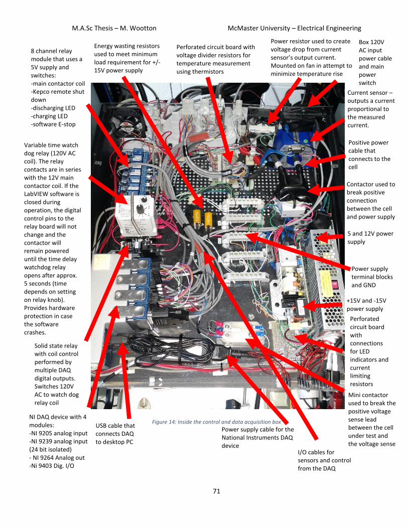
M.A.Sc Thesis – M. Wootton McMaster University – Electrical Engineering
71
Figure 14: Inside the control and data acquisition box
Box 120V AC input power cable and main power switch
Current sensor – outputs a current proportional to the measured current.
Positive power cable that connects to the cell
Contactor used to break positive connection between the cell and power supply
5 and 12V power supply
+15V and -15V power supply
Perforated circuit board with connections for LED indicators and current limiting resistors
Mini contactor used to break the positive voltage sense lead between the cell under test and the voltage sense input of the power supply
Power supply cable for the National Instruments DAQ device
USB cable that connects DAQ to desktop PC
NI DAQ device with 4 modules: -NI 9205 analog input -NI 9239 analog input (24 bit isolated) - NI 9264 Analog out -Ni 9403 Dig. I/O
Power supply terminal blocks and GND
Variable time watch dog relay (120V AC coil). The relay contacts are in series with the 12V main contactor coil. If the LabVIEW software is closed during operation, the digital control pins to the relay board will not change and the contactor will remain powered until the time delay watchdog relay opens after approx. 5 seconds (time depends on setting on relay knob). Provides hardware protection in case the software crashes.
Solid state relay with coil control performed by multiple DAQ digital outputs. Switches 120V AC to watch dog relay coil
8 channel relay module that uses a 5V supply and switches: -main contactor coil -Kepco remote shut down -discharging LED -charging LED -software E-stop
Energy wasting resistors used to meet minimum load requirement for +/- 15V power supply
Perforated circuit board with voltage divider resistors for temperature measurement using thermistors
Power resistor used to create voltage drop from current sensor’s output current. Mounted on fan in attempt to minimize temperature rise
I/O cables for sensors and control from the DAQ

M.A.Sc Thesis – M. Wootton McMaster University – Electrical Engineering
72
The control box has an E-stop system made up of switches in series, as shown by Figure 15. The
indicator LEDs on the front of the control box are connected to voltage tap points along the
series set of switches to show where the circuit has opened. The first switch is a relay contact
located in the lab’s gas sense/e-stop shut down system box that is mounted on the lab wall. The
second switch is a set of two normally closed thermal switches that are mounted on the device
under test and open at a temperature of 75 degrees C. The third switch is the red master switch
located on the front of the control box (see Figure 12). The last switch is one of the relay
contacts on the 8-channel relay board (see Figure 14). The relay board needs a 5V supply and
then uses digital inputs (GND = energize a relay, 5V = do not energize a relay) to control opto-
isolators that switch the coil of individual relays using the 5V board input supply for the coils.
This 5V board supply is taken from the “software e-stop” relay contacts. Before testing begins,
the relay board is not powered because the “software e-stop” relay is not energized and
therefore none of the other relays, including the power supply enable and main contactor relays,
are energized either. Even if a digital input from the DAQ is commanding the software e-stop
relay to be energized, it won’t be because the relay board is lacking a 5V supply for driving relay
coils. To overcome this, the green momentary “Hold to Start” button is connected across the
“software e-stop” relay contacts. Pushing the momentary N/O switch will provide 5V to the relay
board 5V input and then the DAQ’s control pin will command the “software e-stop” relay to
close via the opto-isolator. The “software e-stop” relay is wired to be a latching relay and will
remain energized until the coil 5V power supply is removed. This latching wiring method was
used so that the tester cannot be started remotely without the need to push the momentary
start button. This encourages the user to check over the testing hardware while in the energy
storage testing room before starting tests remotely. Provided the software e-stop relay control
pin stays low (GND) then the user can pause and restart the testing remotely. There is no need

M.A.Sc Thesis – M. Wootton McMaster University – Electrical Engineering
73
to press the momentary start button when the software goes into protection mode because the
“software e-stop relay” control pin is not controlled by the software protection state – it is only
controlled by the user clicking a software button. This allows the user to shut down the power
supply output and open the main contactor from home if he/she feels the need. In this event, if
anyone else tried to remote login to the computer and start a test, it will not work because the
momentary “Hold to Start” button must be pressed, therefore forcing someone to visit the lab
and presumably check for any issues. The lab gas sense system shutdown relay shown in Figure
15 is non-latching and therefore the latching nature of the custom MARC cell cycler e-stop
system ensures that the cell cycler will not restart without momentary input from someone in
the lab space.

M.A.Sc Thesis – M. Wootton McMaster University – Electrical Engineering
74
Figure 15: Simplified e-stop schematic for the control and data acquisition box
4.1.1.4. Sensor Interface Box The sensor interface box, shown in Figure 16, acts as a sensor cable breakout box and extension
to the back end of the control and data acquisition box. The sensor interface box provides a
convenient location for shorter sensor cables to connect to the cell testing device rather than
running multiple long cables through the thermal chamber and to the back of the control and
data acquisition box. The sensor interface box provides connectors for ten thermistors, three
voltage measurement points, and two E-stop thermal switches (see Figure 15).
4.1.1.5. Desktop Computer and LabView Software As noted in Figure 8, the custom MARC cell cycler computer is located at the bottom of the
mobile equipment rack. Custom LabView based cell testing software that was developed by Dr.

M.A.Sc Thesis – M. Wootton McMaster University – Electrical Engineering
75
Kollmeyer runs on the desktop computer and communicates to the NI DAQ hardware located in
the control and data acquisition box using a USB cable. An example of the software interface is
shown in Figure 11 and the NI hardware is shown in Figure 14. The feature rich software offers a
variety of functions such as:
• Constant current (CC) charge and CC discharge commands
• Constant voltage charge command
• Current waveform command - used for making drive cycle current profiles
• Impedance spectroscopy commands
• Autocycler - automatically executes a sequence of testing commands and counts cell
cycles
• Data logging to specified Excel worksheets at specified data logging rates (up to 10 Hz).
• Cell voltage, testing current and multiple temperature measurements
4.1.1.6. Thermal Chamber The Envirotronics SH16 thermal chamber was used for all testing performed with the custom cell
cycler. Figure 16 shows inside the thermal chamber prepared with the DUT connected to the
power cables and sensor interface box. Figure 16 also shows part of the lab gas sensing system
and CO2 fire suppression system which are discussed in Section 4.1.2. Figure 17 shows the
thermal chamber foam insert modifications performed by other ESS students. In the event of a
cell explosion, it is intended that the foam inserts will be blown out the top of the chamber,
rather than breaking the thermal chamber door latch and blowing the door open. The rubber
flaps that cover holes in the foam (approximately 4-inch diameter) are intended to act as a
pressure release when the CO2 fire suppression system discharges into the thermal chamber.
The rubber flap is intended to close, as shown in Figure 17, when the pressure wave equalizes.
The rubber flap is the preferred CO2 pressure release method rather than blowing out the foam
inserts because it is desirable to contain the cold carbon diode in the thermal chamber to assist

M.A.Sc Thesis – M. Wootton McMaster University – Electrical Engineering
76
in cooling the DUT and prolong the release of CO2 into the lab testing room. Due to the rather
small opening available to pass cables through the thermal chamber side wall, the author
modified the thermal chamber to add a second, and much larger, cable passage port as shown in
Figure 18.
Figure 16: Inside the Envirotronics SH16 thermal chamber
Sensor interface box
Circulator fans
Device under test. Blue cover in place to maintain anonymity
Cell cycler power and remote voltage sense cables
Webcam
Fire suppression system temperature sensor
CO2 fire suppression system discharge nozzle
Gas sensors Bottom of left side foam insert

M.A.Sc Thesis – M. Wootton McMaster University – Electrical Engineering
77
Figure 17: Top of the Envirotronics SH16 thermal chamber
Figure 18: Additional cable passage port added at the back-left corner of the Envirotronics SH16 thermal chamber
Due to very limited LCD screen functionality, the Envirotronics SH16 thermal chamber was
originally hard to control using keypad inputs. An update was made so that the custom cell
cycler desktop computer communicates with the thermal chamber via ASCII commands using a
USB to serial converter and RealTerm software (see Figure 19). Due to the limited frequency that
the thermal chamber temperature setpoint and circulator fan settings were changed, the ASCII
Foam inserts
Rubber flaps
3 phase power cable
Wiring from gas sensors inside of thermal chamber
Additional cable passage port with foam insert
CO2 fire suppression system flexible discharge hose

M.A.Sc Thesis – M. Wootton McMaster University – Electrical Engineering
78
commands are not linked to the LabView cell testing software. Although the RealTerm remote
commands provided most functionality needed to operate the thermal chamber, the remote key
pad and was used to access programmable logic controller (PLC) memory bits for diagnostic
purposes. The memory bits helped identify pressure switch issues that prevented the thermal
chamber from operating a couple times.
Figure 19: Example interface from RealTerm software showing a command to read the Envirotronics SH16 thermal chamber present temperature value.
The desktop computer interfaces with a computer webcam mounted inside the thermal
chamber using a USB connection. The image quality was reduced to enable high data rate
communication with the NI DAQ hardware. Although one would not expect any movement
inside the thermal chamber, the webcam was useful to remotely detect the presence of ice that
would accumulate on the internal heat exchanger (see Figure 20). The presence of ice would
restrict the thermal chamber from maintaining temperatures below 0oC and would therefore
require a manual thermal cycle to melt the ice.

M.A.Sc Thesis – M. Wootton McMaster University – Electrical Engineering
79
Figure 20: Photo taken using the interior thermal chamber webcam that shows ice forming on the heat exchanger.
4.1.2. Lab Safety Systems The development of the custom MARC cell cycler enabled cell testing a few months before the
Digatron cell testing equipment was commissioned. However, additional safety measures were
necessary before unattended testing could begin. The following list outlines the multitude of
safety systems developed and their operation sequence as a line of defence to minimize damage
from a device under test catching fire:
1. Testing approval form and fixture review
2. Cell / pack cycler software and hardware limits on voltage, temperature and current
3. All testing performed in thermal chambers equipped with gas sensing hardware and
pressure release ports
4. Activation of lab shut down system that turns off all cell/pack testing equipment and
thermal chambers
5. Automated CO2 fire suppression system plumbed into all three thermal chambers
The author integrated a master lab emergency stop (e-stop) button and select hardware from
items 3 and 5 to develop an automated lab shut down system. The following subsections
documents some of the work completed to enable unattended testing and therefore enable the
experimental work of this study.
Formation of ice on the heat exchanger
Shelf where DUT is secured during automated testing
Normal appearance of the heat exchanger without ice formation

M.A.Sc Thesis – M. Wootton McMaster University – Electrical Engineering
80
4.1.2.1. Testing Approval Form and Fixture Review Along with Dr. Kollmeyer and other ESS students, the author initiated the development of a
testing approval and cell fixture review process. This process requires students to review the
safe operating area limits for the DUT, such as voltage and current limits, and document the
software safety limits used on the testing hardware. This paperwork outlines the anticipated
testing duration, equipment in use, device under test, and emergency contact information for
the equipment user. The lab manager signs off on the paperwork once satisfied with the
cell/pack testing methods, safety settings and cell testing fixture design. By affixing the testing
approval form to the lab testing room door (see Figure 7), the lab manger and other students are
made aware of any testing underway.
4.1.2.2. Gas Sensing System and Automated CO2 Fire Suppression System Tyco Integrated Fire and Security installed a thermal chamber gas sensing system and
automated CO2 fire suppression system. Each thermal chamber was fit with two Oldham iTrans2
gas sensors to detect CO2 (sensor with P/N 7703-6321) and combustible gasses such as CH4 and
H2 (sensor with P/N 7702-2606). Figure 16 shows two gas sensors installed in the Envirotronics
SH16 thermal chamber. The gas sensing system is intended to detect battery cell/pack off
gassing before the DUT catches fire. In combination with the lab shut down system, the gas
sensors may prevent further cell testing that provokes a cell/pack fire. If the gas sensors and
equipment shut down are unsuccessful in eliminating the fire hazard, the fire suppression
system can be triggered automatically using temperature sensors in the thermal chambers (see
Figure 16), manually using the manual pull station shown in Figure 23 or manually by pulling the
firing plunger in Figure 21. The fire suppression system control panel is integrated with the
building fire alarm system.

M.A.Sc Thesis – M. Wootton McMaster University – Electrical Engineering
81
Figure 21: CO2 pressurized fire suppression system located in the energy storage lab testing room
4.1.2.3. Lab Shut Down System The author was responsible for designing and implementing a system that shuts down the
equipment listed in Table 3 under any of the following three conditions:
1) The lab CO2 fire suppression system is activated (activates the building fire alarm)
• Latching condition until fire alarm panel is reset
2) The gas sensing system is activated due to the presence of an undesirable gas
• Non-latching system
3) A master lab wide emergency stop button is pushed.
• E-stop button reset by twisting the button plunger
This requirement was achieved by developing the shutdown relay control box shown in Figure
22 and the lab master e-stop button shown in Figure 23.
Pressurized CO2 fire suppressant bottle
Manual firing plunger used to activate the fire suppression system
Hard pipe that routes the CO2 to all three thermal chambers CO2 fire suppression
system control panel

M.A.Sc Thesis – M. Wootton McMaster University – Electrical Engineering
82
The energy storage lab shutdown relay control box primarily consists of four double pole double
throw (DPDT) relays with normally open contacts wired in series. These contacts control the
power delivered to the 24V switched power terminal strip (yellow terminal blocks in Figure 22)
that provides coil power to a shut down relay installed in each testing device listed in Table 3.
Due to space constraints, the custom cell cycler shut down relay is installed inside the shutdown
relay control box. The coils of the four series connected relays are independently controlled by
the lab master E-stop button (see Figure 23), CO2 fire suppression system alarm panel, relays
within the gas sensors that signify a sensor fault and finally, relay contacts within the gas sensors
to signify that a concerning gas was detected.
The non-latching relays from the gas sensors were initially of concern as the lab equipment
could re-start after the concerning gas dissipated and the gas sensors retuned to a normal
operating state. This issue was corrected by implementing a latching system that uses the relays
from the gas sensors to add a parallel load of resistors that increases the load on the 24V supply
and therefore blows fuse Z (see Figure 22). Fuse Z is in series with the gas sensor alarm relay,
therefore causing the switched 24V bus to de-energize and remain de-energized until fuse Z is
replaced by someone in the lab space that would presumably investigate the concern.
The lab master emergency stop button shown in Figure 23 is installed next to the lab’s CO2 fire
suppression system trigger point located in the lab control room shown in Figure 7. The second
set of contacts on the four series connected main lab shut down system relays are used to
indicate the status of each relay via the LED lights on the E-stop button box (Figure 23). A red
LED indicates the relay is not energized and therefore the corresponding safety system, such as
the gas sensor fault relays, indicates a condition to shut down the lab equipment. A sequence of

M.A.Sc Thesis – M. Wootton McMaster University – Electrical Engineering
83
five green LEDs indicates that the lab safety systems do not detect an unsafe condition and the
lab equipment should be in a “ready” state. If neither light per row on the e-stop button box is
illuminated, this indicates either a wiring concern, a loss of power or a faulty LED light. These
status LEDs are located on the e-stop box relay so that students can see what issue is present
before entering the lab testing room.

M.A.Sc Thesis – M. Wootton McMaster University – Electrical Engineering
84
Figure 22: Energy storage lab shutdown relay control box
Terminal block for connecting blue cables that run to the e-stop box and power the e-stop box LEDs
E-stop relay
CO2 fire suppression system alarm panel relay
Gas sensor fault relay
Current limiting resistors for E-stop box LEDs
Fuse Z – this fuse should blow if any of the three gas sensor systems trigger a low gas alarm
E-stop button connection – continues the e-stop relay coil power through the e-stop button
Panel mount LEDs to show if 24V power supply is present and if fuse Z is not blown (LED = green)
Mechanical switch to shut off 24V input (after fuse 0) to the rest of the panel.
24V supply ground bus bar – all black terminal blocks connected via red jumper.
Custom cycler shut down relay that switches the custom cycler’s 5V E-stop line.
Thee separate resistor banks used to intentionally blow fuse Z when any of the size gas sensors in the lab are triggered. Blowing fuse Z should de-energising the gas sensor low alarm relay coil and therefore de-energize the 24V supply that powers the coil for the equipment shut down relays
Gas sensor alarm relay
Yellow terminal block for the switched 24V supply that powers the coils of shutdown relays installed in each piece of testing equipment.
Terminal block for all cables coming from the three gas sensing systems.

M.A.Sc Thesis – M. Wootton McMaster University – Electrical Engineering
85
Figure 23: Energy storage lab emergency stop button and CO2 fire suppression system pull station

M.A.Sc Thesis – M. Wootton McMaster University – Electrical Engineering
86
5. Experimental Performance Comparison of EDLC and LiC Cells for Energy Storage Applications
5.1. Chapter Overview and Research Contributions This chapter presents the experimental methods, select raw data, and analysis of over 881 hours
of experimental testing used to characterize and compare the performance of two electric
double layer capacitors, four asymmetric Li-ion capacitors and one unique symmetric/parallel Li-
ion capacitor (||LiC) for energy storage applications. The study of seven cells, including five
lithium-ion capacitors from four different manufacturers, extends the work of [74], [75], [76]
and [91] which study lithium-ion capacitor(s) from one well known manufacturer. Section 5.2
extends the high-level supercapacitor performance comparison in [92] by showing datasheet
and experimentally determined cell specifications that are used to develop a volumetric and
gravimetric Ragone plot. Unfortunately, the information available from publicly available EDLC,
LiC and LiB cell data sheets is rather limited. For example, most manufacturers will provide only
one equivalent series resistance value. Often, it is unknown if the published value is an average
of the experimental results from multiple testing conditions or one selected condition. As shown
by this work, the equivalent series resistance of a LiC cell changes with state of charge (minor
change), current direction and testing temperature. Therefore, additional experimental work is
necessary to extend one’s knowledge of the cell behaviour under testing conditions that are not
discussed on the datasheet. Additionally, some of the datasheets acquired for the LiC cells in this
work did not show a charge and discharge terminal voltage vs capacitor or state of charge
relationship. Although limited datasheet values and several assumptions can be used to model a
cell, the author’s experimental work extensively builds upon datasheet values to show how cell
behaviour changes under multiple conditions.

M.A.Sc Thesis – M. Wootton McMaster University – Electrical Engineering
87
The custom cell testing fixtures and related hardware are discussed in Section 5.3. Section 5.4
outlines the five time-domain experimental methods used to electrically and partially thermally
characterize the capacitor cells. Section 5.5 examines the cell charge/discharge cycling energy
loss and temperature rise to estimate the cell internal resistance and case-to-ambient thermal
resistance. Section 5.6 discusses the cell charge/discharge voltage vs. SOC profiles and
associated hysteresis at various temperatures. To build upon the work in [76] and [91], Section
5.6.3 documents the impact of temperature and current on both discharge and charge capacity
(measured in Ah) as well as useful energy stored/discharged (measured in Wh) in both EDLC and
lithium-ion capacitors. Section 5.7 extends the work in [91] by showing how the cells’ charge and
discharge equivalent series resistance changes across 5% SOC breakpoints. This information is
also presented as an average cell ESR and normalized average cell ESR. Section 5.7.5 addresses
the need for a multi-temperature current dependant ESR model, as described in [75], by
evaluating the internal resistance with time domain based HPPC testing using three different
current rates for both charging and discharging pulses at 5% SOC increments. Cell performance
during the US06 and UDDS drive cycles at 25oC and 0oC are compared in Section 5.8.
Additionally, Section 5.8 presents a simple cell model and select cell characterization data
validation using the drive cycle data at 25oC. Section 5.9 shows the change in cell terminal
voltage and approximate self discharge current over a nearly eight-day self discharge test.
Research results and discussion are documented within each section while Section 5.10 provides
a chapter conclusion.
The author’s contributions to the experimental work in this chapter include, but are not limited
to, the following:
• Selecting and acquiring the cells to test

M.A.Sc Thesis – M. Wootton McMaster University – Electrical Engineering
88
• Development of seven cell testing fixtures
• Selecting the five experimental tests performed and all conditions / parameters
associated with the testing (eg. thermal chamber temperatures, current
amplitudes…)
• Developing the cell testing profiles loaded onto the custom cell cycler
• Development of a drive cycle power profile for test #4 using a vehicle modeling and
power profile tool develop by Dr. Kollmeyer
• Operating the testing equipment and running the tests both locally and remotely
• Correcting most issues experienced with the testing equipment
• Developing a MATLAB based data analysis and plotting tool
5.2. Device Under Test – Cell Selection, Specifications and Sources of Experimental Error
The majority of commercially available EDLC cells with capacitance ≥2000 F are limited to an
upper voltage of 2.7V to 2.85V. EDLC Cell A was chosen because of it’s relatively high maximum
voltage of 3V. EDLC Cell B was chosen as a “standard” 2.7V EDLC benchmark and has the same
cylindrical form factor as Cell A. LiC Cell C was selected because of the unique prismatic form
that offers a better packing factor compared to cylindrical cells. LiC Cell D was chosen because it
has the same cylindrical form factor as cell A and B but greater than six times the energy density
when measured in Wh/kg. LiC Cell E was chosen due to it’s high energy density while LiC Cell F
was selected for it’s relatively high cycle life compared to the other LiC cells. Finally, ||LiC Cell G
was selected due to it’s relatively high gravimetric power density and unique symmetric/parallel
capacitor design. The author focused on testing a larger quantity of LiC cells than EDLC cells due
to the considerable amount of EDLC testing work publicly available in sources such as [92], [93],
and [94]. The capacitors were selected and purchased at the authors discretion without an
incentive from the manufacturers / suppliers.

M.A.Sc Thesis – M. Wootton McMaster University – Electrical Engineering
89
The author did not test any battery cells for a few reasons. The author originally though that the
LiC cells would behave more closely to EDLC cells and therefore a comparison to EDLC cells was
of more interest. This assumption was based on the linear LiC cell discharge curve (terminal
voltage vs capacity), the cell naming method and small datasheet capacity values. Additionally,
the time required to experimentally characterize LiB cells can be considerably longer than EDLC
and LiC cells. This increase in time comes from the increased capacity that requires additional
time to fully charge and discharge. For example, compare the testing time row in Table 5 for Cell
D and Cell F. As discussed in Section 5.7.1, the use of coulomb counting to change the cell state
of charge, which would be necessary for LiB testing, can extend the testing time considerably if
testing protection limits are hit. The ability to test LiC and EDLC cells faster than LiB cells allowed
the author to test more cells than normally studied in academic literature. The experimental
study of seven cells is a large quantity of work considering that a majority of experimental cell
comparison literature tests one or two cells. The time invested into establishing the lab facilities,
acquiring the cells and running tests was considerable. The time between acquiring the first cell
and the end of cell testing was approximately 9 months (Sept. 2017 to May 2018). Although it
would be ideal to also test LiB cells, the time necessary was beyond the scope of this work. An
alternative would be to test less LiC cells and introduce a LiB cells, however, the author
preferred to publish more data on various LiC cells to provide a larger representation of LiC
technology than what is publicly available to date.
Table 5 contains a combination of cell specifications obtained from datasheets and experimental
testing. The cell volumetric and gravimetric energy density are determined by dividing the
average measured energy by the measured volume or mass, respectively. The power density
values are calculated using Equation 5 and Equation 6. Although the experimental ESR results

M.A.Sc Thesis – M. Wootton McMaster University – Electrical Engineering
90
obtained in Section 5.7 are considerably larger than the datasheet values for select cells, the
author does not think a single power density number can accurately represent the power
capability of the cell. For example, although EDLC Cells A and B have the smallest ESR values, the
cell output power capability is relatively low near the 0V minimum cell voltage. This output
power is considerably different from values determined using the maximum cell voltage. To
accurately represent the power density of the cell for a given temperature, a plot of maximum
output power as a function of cell temperature, ESR and SOC would be necessary. This level of
detail is not helpful in comparing cells via a Ragone plot and is therefore beyond the scope of
this work. Figure 24 compares the cells’ energy and power density using two Ragone plots, one
for volumetric densities and one for gravimetric densities, using a combination of datasheet and
measured values. Figure 24 also includes one data point on each Ragone plot that corresponds
to A123’s AMP20M1HD-A lithium ion pouch cell, noted as Cell H. The data for Cell H was
obtained from the manufacturer datasheet [95].
𝑃𝑜𝑤𝑒𝑟 𝐷𝑒𝑛𝑠𝑖𝑡𝑦 [𝑊ℎ/𝐿] = 0.12 ∗ 𝑉𝑀𝑎𝑥
2
𝐸𝑆𝑅𝐷𝑎𝑡𝑎𝑠ℎ𝑒𝑒𝑡 ∗ 𝑉𝑜𝑙𝑢𝑚𝑒
Equation 5: Cell volumetric power density calculated using the datasheet ESR

M.A.Sc Thesis – M. Wootton McMaster University – Electrical Engineering
91
𝑃𝑜𝑤𝑒𝑟 𝐷𝑒𝑛𝑠𝑖𝑡𝑦 [𝑊ℎ/𝑘𝑔] = 0.12 ∗ 𝑉𝑀𝑎𝑥
2
𝐸𝑆𝑅𝐷𝑎𝑡𝑎𝑠ℎ𝑒𝑒𝑡 ∗ 𝑀𝑎𝑠𝑠
Equation 6: Cell gravimetric power density calculated using the datasheet ESR
Cell ID A B C D E F G
Cell Type EDLC EDLC LiC LiC LiC LiC ||LiC
Format Cyl. Cyl. Prismatic Cyl. Pouch Pouch Pouch
Test Fixture Compression No No No No No Yes Yes
Capacitance [F] 3,0001 3,0001 3,3001 28,0001 14,0001 1,1001 3,4675
Max Cell Voltage [V] 31 2.71 3.81 4.051 4.051 3.81 2.71
Min Cell Voltage [V] 02 02 2.21 2.81 2.81 2.21 1.351
Capacity [Ah] 2.54 2.254 1.474 9.724 4.864 0.494 1.31
Measured Capacity [Ah]7 (Charge / Discharge)
2.3213,8
2.2913,8 2.1803,8
2.1293,8 1.4653
1.4613 10.7743
10.7253 5.6073
5.6253 0.4883
0.4833 1.668 1.528
Energy [Wh] 3.754 3.044 4.404 33.304 16.654 1.474 3.154
Measured Energy [Wh] 7
(Charge / Discharge) 3.79 3,8 3.64 3,8
3.213,8 3.033,8
4.443
4.403 37.593
37.123 19.583
19.453 1.483
1.453 3.733 3.273
Datasheet ESR [mΩ] 0.271 0.231 11 0.351 0.81 ≤51 11
Experimental DC ESR [mΩ]* 0.33 0.20 1.19 1.04 2.42 4.66 6.00
Mass [kg] 0.521 0.5033 0.3483 0.8301 0.3213 0.1023 0.0873
Volume [L] 10 0.3915 0.3925 0.2175 0.3945 0.1425 0.0555 0.0465
Max Operation Temp. [oC] 651 651 701 551 551 651 551
Min Operation Temp. [oC] 11 -401 -401 -301 -251 -251 -301 -401
Cycle Life [cycles] 1 M1 1 M1 Unknown 50 k1 (1 M1 for 2.8V – 3.8V)
>50 k1
>100 k1 10 k1
Testing Time [h] 60.07 49.40 52.53 362.72 177.74 41.57 137.25
Energy density [Wh/kg] 7.146,9 6.205,9 12.705,9 45.006,9 60.795,9 14.365,9 40.235,9
Energy density [Wh/L] 9.505,9 7.965,9 20.375,9 94.815,9 137.435,9 26.645,9 76.095,9
Power density [kW/kg] 7.696 7.566 4.986 6.786 7.666 3.406 10.066
Power density [kW/L] 10.236 9.706 7.996 14.276 17.336 6.306 19.026
Table 5: Select datasheet values and experimental results used to compare cell specifications.
1 Datasheet or manufacturer provided 2 Assumed value 3 Measured value 4 Calculated from datasheet/assumed values 5 Calculated from measured values 6 Calculated from datasheet/assumed and measured values 7 Top value - 2A constant current (CC) charge, bottom value - 2A CC discharge, 25oC 8 Use minimum voltage of 0.05V, not 0V * Data replicated from Figure 8 a) – average discharge ESR determined at 25 oC using 25A discharge current pulses with 3 second relaxation time 9 Calculated using average of measured energy values 10 Volume measured for active cell area only, excludes terminals 11 Some manufacturers advise against charging the cells below 0oC

M.A.Sc Thesis – M. Wootton McMaster University – Electrical Engineering
92
Figure 24: Volumetric (left) and gravimetric (right) Ragone plots using data from Table 5. Power density values are from cell datasheets while energy density values are calculated from the measured cell mass/volume and measured
energy content. The Cell IDs are located next to the corresponding data point. The data for Cell H, which is a lithium ion battery, was obtained from [95].
Although the purpose of this chapter is to compare the performance trends between EDLC and
LiC cells, the results shown only apply to the specific cells tested and may not be representative
of all EDLC nor LiC cells. Due to the extensive amount of time necessary for testing, only one
sample of each cell was tested and therefore the results may not represent average
specifications. This chapter is not intended to reflect upon the work of the cell manufacturers /
suppliers and therefore the cells are described using unique identifiers “A” though “G”, as shown
in Table 5. As shown in Table 5 there are some discrepancies between datasheet listed values
and those obtained from the experimental work explained in this chapter. These discrepancies
may be the result of:
• Inconsistent cell testing methods between the manufacturer and the experimental
work presented. For example, the manufacturer may determine the cell equivalent
series resistance using an AC current sine wave rather than DC current pulses; which
can significantly change the ESR value. Using [96] as an example, Cell SCA0500 has a
rated DC ESR of 0.40mΩ while the rated 100 Hz AC 10ms ESR is 0.29mΩ. The author
attempted to mitigate the concern regarding different testing methods as a source
G
D
E
F
C
A
A B
E
G
D
A
B
C
F H H

M.A.Sc Thesis – M. Wootton McMaster University – Electrical Engineering
93
of data comparison by testing all the cells using the same, or very similar, testing
profiles.
• The electrical connection between the bus bars and cells with tab terminals may
introduce a source of resistance that is measured as a cell resistance. The author
attempted to mitigate this issue by using the manufacturer provided cell testing
fixture for Cell G and by securing two bus bars to each cell tab using bolted
connections for Cells E and F. Due to packaging and short circuit issues when
compressing a cell, the author made multiple bolted tab connections on Cell E and
Cell F using plastic bolts and metal hardware. The experimental and datasheet ESR
values for Cell E in Table 5 are very different, however, the experimental and
datasheet ESR values for Cell F are close. The datasheet and experimental ESR values
are close for Cells A, B and C which all have threaded connections. However, Cell D,
which also has a threaded connection, shows a large discrepancy between the
datasheet and experimental ESR value in Table 5. These cell connection methods
and related comparisons to datasheet values show that the author’s cell testing
fixtures may have an influence on the results. However, these results may also show
that the manufacturer datasheets are claiming performance values under ideal
conditions. One of the LiC cell manufacturers provided the author with incorrect
datasheet specifications and therefore there is a concern regarding the validity of
certain datasheet values.
• Tolerances in cell specifications, such as the capacitance, may result in a difference
between nominal datasheet values and experimental values. For example, the
measured capacity for Cell A is less than the value calculated from the nominal
datasheet capacitance and voltage limits. On the other hand, the measured capacity

M.A.Sc Thesis – M. Wootton McMaster University – Electrical Engineering
94
for Cell D was larger than the value calculated from the nominal datasheet
capacitance and voltage limits.
The following conclusions are made using data available in Table 5 and Figure 24.
• The measured charge and discharge capacity (Ah) of all cells aligns well with the
theoretical values, falling within -7.2% (Cell A) and +28% (Cell G).
• For all cells, the measured discharge capacity (Ah) is a fraction of the measured charge
capacity (Ah) within a range of 87.7% (Cell G) to 99.3% (Cell E). With the exception of
Cell G, the other cells have an energy (Wh) cycle efficiency greater than 94% under the
2A constant current charge/discharge testing performed.
• Both EDLC cells are rated for 1 million cycles while the largest LiC cycle life is >100k
cycles. However, the datasheet for Cell D lists 1 million cycles when operated at a limited
maximum cell voltage of 3.8V. Generally speaking, the LiC cells have a significantly lower
rated cycle life.
• Figure 24 shows that the LiC cells all have a volumetric and gravimetric energy density
larger than the EDLCs. However, neither cell type is strictly more power dense when
calculated using manufacturer provided ESR values.
• Li-ion capacitor Cell E and Cell G appear to have the best combination of power density
and energy density (points E and G are furthest from the origins in Figure 24) when
calculated with datasheet ESR values. This result would change if the power densities
were calculated using measured ESR values as the measured ESR values for Cell E and G
(see Table 5) are multiple times larger than the datasheet values.

M.A.Sc Thesis – M. Wootton McMaster University – Electrical Engineering
95
5.3. Cell Testing Fixture Design The author assembled a custom testing fixture for each cell that provides a power connection for
cycling, a terminal voltage measurement connection and multiple thermistor extension cable
connections. All cells and cell testing equipment in the energy storage lab use Anderson SB 120
connectors for the power cable and mini Anderson connectors for voltage sensing. This standard
lab practice allows for cells to quickly and easily be transferred between the custom cell cycler
and Digatron MCT. Considering that the cells are always energized, with the exception of EDLC
cells discharged to zero volts, all of the testing fixtures feature two fuses; one on the positive
power cable and one on the positive terminal voltage sensing cable. A variety of Littelfuse MEGA
fuses and fuse holders were used for the power cable fuse due to the variety of current ratings
available and ease of use. The cell voltage measurement cables are connected to the cell
terminals directly or using a Kelvin connection where possible. This voltage measurement
method is used to reduce any voltage change that results from the voltage drop across the
power cable and power cable fuse during high current testing. The voltage sensing fuse may
introduce a considerable resistance to the voltage measurement cable, however, the voltage
drop across the fuse is negligible due to the NI 9293 module input impedance of 1 MΩ. The
terminal voltage measurement fuse is primarily used to protect the voltage sense wires from an
external short circuit within the control and data acquisition box or during storage. Note that
rubber covers are to be used on the SB 120 power connector and mini Anderson voltage sense
connector when not in use.
As noted in Table 5, Cell F and Cell G require a compression force applied to the larger pouch
surfaces. The author made a custom compression fixture for Cell F and made modifications to a
manufacturer developed cell compression text fixture for Cell G. The manufacturer developed

M.A.Sc Thesis – M. Wootton McMaster University – Electrical Engineering
96
testing fixture required modifications to decrease the risk of unintentionally short circuiting the
cell and to develop better electrical contact with the cell tabs.
To ensure the cell surface temperature sensors would not move during thermal cycles, the
thermistors were attached to the cells using Kapton tape. The compression text fixture on Cell F
was designed so that the temperature sensors remain in contact with the cell surface without
being compressed and pushed into the cell surface. However, the manufacturer developed
compression fixture for Cell G was difficult to modify in an equivalent way and therefore the
thermistors were mounted closer to the cell tabs and not on the cell surface. For this reason, the
thermal cycling data in Section 5.5.3. does not include Cell G. Thermal cycling data for Cell F is
included in Section 5.5.3, however the author encourages the reader to consider the
inconsistent thermal packaging from the compression fixture that may influence the cell’s
temperature rise.
For illustrative purposes, Figure 25 shows the seven cell testing fixtures with any cell
identification covered with blue boxes.

M.A.Sc Thesis – M. Wootton McMaster University – Electrical Engineering
97
Figure 25: Cell testing fixtures with cell identification covered by blue boxes.
SB 120 power connector with positive and negative cables. Connects to power lead from cell tester. Labels indicate when the cell was received, mass without fixture, and lab serial number.
SB 120 power connector rubber cover. The connection points are always energized.
Main power fuse mounted in enclosure on positive power cable
Thermistor extension cables and connectors
Wire and mini Anderson connectors for cell voltage measurement. A rubber cover is in place while the cell is in storage.
Cell under test (covered by blue boxes)
Cells with threaded terminal connections
Cells with tab terminals that require a testing fixture with tab compression bus bars
Inline fuse on cell voltage measurement wire
Cell G)
Cell F) Cell E)
Cell C)
Cell B) Cell A) Cell D)

M.A.Sc Thesis – M. Wootton McMaster University – Electrical Engineering
98
5.4. Overview of Testing Profile Creation, Data Logging and Analysis Workflow
The custom cell cycler offers an autocycler function that automatically executes a series of
battery/capacitor testing commands from a text file and logs user selected data to Excel
worksheets. To ensure the use of consistent testing and data logging methods, the author
developed a universal Excel file that automatically updates the autocycler profile based on cell
specifications, naming conventions and the desired thermal chamber temperature. The
autocycler profile includes operations to sequentially complete tests 1) thru 3) from Table 6.
With the exception of very few noted cases, all seven cells were exposed to very similar testing
conditions as defined by the autocycler commands. In examining the capacitor cell datasheets
from multiple manufacturers, it became very evident that the method used to characterize the
cells varied. The author’s testing was based on commonly-used time domain testing methods
such as continuous charge/discharge cycling, constant current capacity tests [97], hybrid pulse
power characterization [97], self discharge tests [97] and drive cycle model validations, but
made use of custom testing durations, configurations and current amplitudes to fit the cell
limitations and testing time constraints. For example, rather than charging and discharging cells
based on C-rates, the author used fixed current values. Due to the large range in cell capacity,
from approximately 0.5Ah to 10Ah, and testing equipment limit of 125A, there would be a
limited amount of higher current testing performed on small capacity cells if consistent C-rates
were used. For example, with a capacity of 10Ah, the maximum C-rate would be 12.5C, which is
rather small for high power capacitor applications. The equivalent 12.5 C-rate for a 0.5Ah cell
would correspond to 6.25A max. With a range of 0-6.25A, the cell is not exposed to a large
enough current range to compare how current impacts the cell characteristics. Additionally, by
only testing the cell to 6.25A, the maximum testing capabilities would not be used, and the data
would be rather unhelpful. On the other hand, the 0.5Ah cell could be the base value for a

M.A.Sc Thesis – M. Wootton McMaster University – Electrical Engineering
99
maximum C-rate of 250C using 125A testing equipment. Assuming the cells are tested at five C-
rates at equal intervals (50C, 100C, 150C, 200C, 250C), the 10Ah cell would have a minimum test
current of 500A which is beyond the equipment and cell performance limitations.
Test ID & Name Test Description / Process
Testing Temperature(s) Testing Current(s) 12 Data log frequency
1) Constant loss thermal cycling
Charge the cell using a constant current until the maximum voltage minus 50 mV is hit. After a one second pause, discharge the cell to the minimum voltage plus 50 mV using a constant current. Repeat for approximately 3.5 hours. The charging and discharging current are chosen to give approximately 2.15W of I2R losses for the EDLC cells and approximately 1W of I2R losses for the LiC cells based on the datasheet listed internal resistance (R).
25 [oC] Unique to each cell 0.5 [Hz]
2) Constant current capacity
Starting with a fully discharged cell, use a constant current to charge the cell until the maximum voltage is hit. Then do a CCCV charge to bring the cell to 100% state of charge (SOC). Use constant current to discharge the cell until the minimum voltage is hit. Discharge the cell to 0% SOC and then repeat this cycle for each test current.
-10, 0, 10, 25, 35 [oC] +/- (2, 25, 50, 75, 100, 120) [A] 5 [Hz]
3) Hybrid pulse power characterization (HPPC)
Charge the cell to a SOC breakpoint (eg. 5%), perform a 2.5 or 1.5 second discharge/charge current pulse and allow the cell to relax. Continue this process, charging the cell in increments of 5% SOC. Fully discharge the cell and repeat with a charging pulse of the same magnitude. Repeat the charging and discharging HPPC sweep for all three current magnitudes.
-10, 0, 10, 25, 35 [oC] +/- (10, 25, 50) [A] 10 [Hz]
4) Self discharge Connect the cell to a single ended voltage measurement port on a NI 9205 module (input resistance of >10 GΩ || 100 pF) and log the cell voltage for approximately 8 days.
Room temperature No supply/load current 1/60 [Hz]
5) Drive cycle validation
Connect each cell to a unique cell testing channel on the Digatron MCT. Fully charge the cells using a CCCV profile and then start a power demand based US06 drive cycle profile. Upon completion fully charge the cell and perform a power demand based UDDS drive cycle profile. When the cell is incapable of meeting the power demand, the cycling current is minimized.
0, 25 [oC] US06, UDDS drive cycle 10 [Hz] Table 6: Overview of the five time-domain tests performed on each capacitor cell
12 Positive current values correspond to discharging and negative current values correspond to charging
The Excel based autocycler commands were designed to save select testing data to specific
worksheets within the same Excel file. For example, the testing data to obtain the cell capacity
using a constant current 2A charge and 10A charge are saved on separate Excel worksheets. This
method was used to ensure the cell specifications, autocycler commands and data were all
contained within one file. Additionally, separating specific test data into consistent worksheets
eliminated the need to filter through hours of useless data and made the comparison of data
from different tests much easier. A new Excel file is created for every testing temperature for

M.A.Sc Thesis – M. Wootton McMaster University – Electrical Engineering
100
each cell, therefore resulting in a total of 35 Excel files (seven cells tested at five temperatures)
with 141 worksheets each.
Rather than analyzing the 35 Excel files (1.4 Gb of data) manually, the data was imported into
Matlab and assigned variable names based on the structured and consistent data saving method
discussed earlier. The majority of the cell testing involved repeating very similar multi-day long
testing profiles at multiple temperatures for each cell. This repetitive nature lends itself nicely to
scripted data analysis that can simply be expanded to include new data as it becomes available.
Scripted data analysis allowed for easy detection of missing or inconsistent data. Additionally,
the scripted analysis provided a much faster method to compare data from different cells that
was originally stored in different Excel files.
5.5. Test 1 – Constant Loss Thermal Cycling The purpose of Test 1 is to evaluate the energy loss and temperature rise from repeated
constant current charge and discharge cycles that persist for approximately 3.5 hours. An
approximate power loss is determined from the average energy loss over the cycling time. An
approximate equivalent series resistance is estimated from the approximate power loss and
known testing current. The cell’s equivalent series resistance will also be evaluated in Section 5.7
using a hybrid pulse power characterization method. The same cell cycling data used to estimate
the energy loss can be used to evaluate the cell temperature rise and an approximate case-to-
ambient thermal resistance. The following subsections will describe the testing method, provide
analysis of the test results and end with a conclusion to compare the EDLC, LiC and ||LiC cell
technologies based on Test 1.
5.5.1. Test 1 Method The cell is connected to the custom cycler and left inside the thermal chamber for several hours.
This thermal saturation period is intended to make the capacitor cell reach the same

M.A.Sc Thesis – M. Wootton McMaster University – Electrical Engineering
101
temperature as the testing environment. Unlike Tests 2 thru 4, this test is only performed at a
desired temperature of 25oC. However, Cell B is also tested under supervision at room
temperature with the thermal chamber foam inserts removed. This additional testing condition
is used to show how the thermal chamber temperature-controlled environment with turbulent
airflow impacts the cell temperature rise.
The testing begins by fully discharging the cell and performing an amp hour counter reset to
0Ah. The cell is charged at a constant current that would result in an I2R loss equivalent to 2.15W
for EDLC cells and approximately 1W for LiC based cells based on the datasheet listed internal
resistance (R). The constant current is terminated to 0A when the cell voltage reaches the
maximum cell voltage minus 50mV. After a commanded 1 or 2 second pause the cell is then
discharged using a constant current selected to match the charging current I2R losses until the
cell voltage reaches the minimum cell voltage plus 50mV. The 50mV buffer was introduced to
prevent the cells from violating cell voltage limits set in the cell testing software.
The charge and discharge cycles, which are separated by one second testing pauses, are
repeated for approximately 3.5 hours. The number of charge/discharge cycles that occur within
3.5 hours is dependant on the testing current and cell capacity. Therefore, the number for
charge/discharge cycles was determined beforehand and the Excel based autocycler profile was
manually changed. The cell was left to rest with zero testing current for 2.5 hours after the
approximate 3.5 hours of cycling is complete.
5.5.2. Test 1 Analysis – Energy Loss Figure 26 and Figure 27 show the energy cycled through the capacitors during the repeated
charge and discharge cycles. Note that Test 1 is repeated twice for Cell B to evaluate the thermal

M.A.Sc Thesis – M. Wootton McMaster University – Electrical Engineering
102
chamber’s impact on the cell energy loss and temperature rise in comparison to testing in a
room without active thermal control active. Therefore, Figure 26 contains two plots for Cell B.

M.A.Sc Thesis – M. Wootton McMaster University – Electrical Engineering
103
Figure 26: Energy loss from repeated charge and discharge cycles – Cells A and B
A) Cell A
B) Cell B C) Cell B without thermal chamber operation

M.A.Sc Thesis – M. Wootton McMaster University – Electrical Engineering
104
Figure 27: Energy loss from repeated charge and discharge cycles – Cells C thru F
A) Cell C B) Cell D
C) Cell E D) Cell F

M.A.Sc Thesis – M. Wootton McMaster University – Electrical Engineering
105
Recall that the cell starts fully discharged and therefore, the first energy change corresponds to a
charge cycle which is noted by the negative energy value. As listed in the footnotes of Table 6, a
positive current corresponds to discharging the DUT and a negative current corresponds to
charging the DUT. Using Subplot C from Figure 27 as an example, we can see that Cell E
experienced thirteen charge and discharge cycles that started and ended in the discharged state.
As shown by the orange trend lines on all subplots in Figure 26 and Figure 27, the amount of
energy discharged is less than the energy charged and therefore we see a general trend of
energy loss (negative slope) over repeated charge/discharge cycles. This trend indicates a cyclic
energy efficiency of less than 100% and therefore an opportunity to identify the power loss as a
variable for comparison. The power loss associated with this test, 𝑃𝑐𝑦𝑐𝑙𝑖𝑛𝑔, is represented by the
rate of energy loss and is determined from the slope of the orange line. Using Equation 7, an
equivalent series resistance associated with Test 1 is determined and recorded in Table 7.
𝑅𝐸𝑆𝑅, 𝑇𝑒𝑠𝑡1[𝛺] = 𝑃𝑐𝑦𝑐𝑙𝑖𝑛𝑔[𝑊]
𝐼𝑐𝑦𝑐𝑙𝑖𝑛𝑔, 𝑅𝑀𝑆2 [𝐴]
Equation 7: Test 1 ESR calculated from cell cycling energy loss
Cell ID A EDLC
B EDLC
B No T.C13
EDLC C LiC
D LiC
E LiC
F LiC
G ||LiC
Number of cycles 63 75 75 38 10 13 50 N/A
Cycling Energy Slope [Wh/s] -1.07E-3 -8.58E-4 -8.39E-4 -4.90E-4 -9.97E-4 -1.06E-3 -3.32E-4 N/A
Cycling Energy Slope [W] -3.87 -3.09 -3.02 -1.76 -3.59 -3.83 -1.19 N/A
Intercept [Wh] -1.30 -1.11 -1.13 -1.89 -15.64 -8.48 -0.59 N/A
IRMS Cycling [A]14 87.24 94.06 94.11 31.49 53.80 35.30 13.65 N/A
Commanded Cycling Current
[A]
90 97 97 32 54 35.5 14 N/A
Datasheet ESR [mOhm] 0.27 0.23 0.23 1 0.35 0.8 5 1
𝑅𝐸𝑆𝑅, 𝑇𝑒𝑠𝑡1 [mOhm]15 0.51 0.35 0.34 1.78 1.24 3.07 6.41 N/A
Theoretical Loss16 [W] 2.05 2.03 2.04 0.99 1.01 1.00 0.93 N/A
Table 7: Calculated energy loss and equivalent series resistance from Test 1.
13 Test on Cell B repeated without the thermal chamber (T.C) operating to maintain the ambient temperature. Starting ambient temperature ~ 23.50C, ending ambient temperature ~ 280C 14 RMS cycling current from time zero until end of cycling (approx. 3.5 hours), does not include zero current from the 2.5-hour cell cool down phase 15 ESR calculated using the change in energy over time during continuous cycling. Uses Equation 7. 16 Theoretical loss = IRMS Cycling * IRMS Cycling * Datasheet ESR

M.A.Sc Thesis – M. Wootton McMaster University – Electrical Engineering
106
Recall from Section 5.4 that the cells were cycled using a current value that would result in
approximately 2.15W of I2R losses for EDLC cells and approximately 1W of I2R losses for LiC cells.
Table 7 show that the theoretical loss values calculated using the RMS cycling current and
datasheet listed ESR closely match the desired 1W for LiC cells but are approximately 0.1W less
than desired for the EDLC cells. The discrepancy for EDLC cells extends from the difference
between the commanded cycling current and RMS cycling current. The cycling profile for EDLC
Cell A used a commanded 2 second pause between the transition from charging to discharging
and vice versa while all other cells used a commanded 1 second pause. It should be noted that
although the data for Test 1 was logged at 0.5 Hz (one sample every two seconds), Cell A has a
near zero current value for three sample points (6 seconds) and the other cells have a near zero
current value for two sample points (4 seconds). The additional near zero current sample point is
a result of the power supply transitioning from the desired testing current to zero amps while in
a “Constant Current” command. This result is shown in Table 8 and Table 9 as an example.
Time [s] Command Cell Voltage
[V]
Testing Current
[A]
174 Constant Current 0.245209 90.00004
176 Constant Current 0.169335 90.00119
178 Constant Current 0.09343 89.99842
180 Constant Current 0.068855 -0.8652
182 Standby 0.072267 0
184 Standby 0.074342 0
186 Constant Current 0.145592 -93.3157
188 Constant Current 0.22628 -89.7248
190 Constant Current 0.306062 -89.6011
192 Constant Current 0.385065 -89.6712
Table 8: Select data from Test 1 for Cell A

M.A.Sc Thesis – M. Wootton McMaster University – Electrical Engineering
107
Time [s] Command Cell Voltage
[V]
Testing Current [A]
310 Constant Current 0.214418 96.999118
312 Constant Current 0.136686 96.999108
314 Constant Current 0.059022 96.998888
316 Constant Current 0.06024 -0.292485
318 Standby 0.062642 0
320 Constant Current 0.118551 -96.446569
322 Constant Current 0.201176 -97.030718
324 Constant Current 0.282879 -97.039925
326 Constant Current 0.363739 -97.032034
Table 9: Select data from Test 1 for Cell B
The RMS cycling current is determined by taking the RMS value of all current values during the
approximate 3.5 hour cycling period and not the relaxation period. Considering that the number
of cycles were xecuted in integer values the actual cycling time for each cell varies slightly.
Therefore, the time used to calculate the RMS current and energy loss slope is modified for each
cell. However, the author believes that the discrepancy between the RMS cycling current and
commanded current is largest for cells with high cycle counts due to the introduction of
additional near zero amp data log points. For example, the cycling period for Cell A occupied
5805 samples (11610 seconds) with approximately 327 samples (654 seconds) within the range
of -2A to +2A. In the case of Cell A, the near non zero amp samples represent approximately
5.6% of sample points and therefore the RMS current value is shown to be considerably less,
approximately 3%, than the commanded current value. In the case of Cell C, the near non-zero
amp samples within the range of -2A to +2A represent approximately 2.9% of all samples and
the RMS current value is shown to be similar, within 1.6%, of the commanded value. Although
the discrepancy between the desired current command and RMS testing current exists, the
author continued to use this method to analyze the energy loss and 𝑅𝐸𝑆𝑅, 𝑇𝑒𝑠𝑡1 for the following
reasons:

M.A.Sc Thesis – M. Wootton McMaster University – Electrical Engineering
108
• The theoretical loss values from Table 7 are within a maximum error of approximately
7% compared to the respective desired loss values of 2.15W and 1 W.
• The energy loss slope and RMS current are calculated over the entire cycling period and
therefore the energy loss slope and RMS current both consider the near zero current
data entries.
• Test 1 is an atypical method to determine a cell’s DC ESR and therefore a considerable
difference between the datasheet and experimentally determined values may exist.
• The purpose of this chapter is to provide a high-level comparison between the EDLC and
LiC based cell performance. Considering that all of the cells are compared using a very
similar testing profile in Test 1, the author believes a comparison between the cells using
this data is reasonable. Therefore, the 𝑅𝐸𝑆𝑅, 𝑇𝑒𝑠𝑡1 values in Table 7 should be compared
between cells but not to the datasheet values.
5.5.3. Test 1 Analysis – Temperature Rise Figure 28 and Figure 29 show the cycling current in orange, the thermal chamber temperature in
solid blue and multiple cell surface temperature measurements in blue patterns. These plots
show the cell temperature rises to a near steady state range via a repeating temperature rise
and fall profile that aligns with the changes in current direction (charge vs. discharge) and
resembles plots in [98]. Subplots A and B of Figure 28 show the cell surface cooling during a
relaxation period when the cycling current is 0A. However, Subplot C, which displays data for
testing Cell B without the thermal chamber maintaining the ambient temperature, hits the
programmed maximum cell temperature limit and therefore data recording is stopped during
the relaxation period. The temperature change from the start of charge/discharge cycling and
the average cell surface temperature when the relaxation begins is recorded in Table 10 as ∆T
[oC]. This temperature change is used in Table 10 to determine a case to ambient thermal

M.A.Sc Thesis – M. Wootton McMaster University – Electrical Engineering
109
resistance, 𝑅𝐶𝐴[/𝑊], based on the datasheet ESR and 𝑅𝐸𝑆𝑅, 𝑇𝑒𝑠𝑡1[𝛺]. The results are
recorded in Table 10.

M.A.Sc Thesis – M. Wootton McMaster University – Electrical Engineering
110
Figure 28: Cell temperature rise from repeated charge / discharge cycles – Cells A and B
A) Cell A
B) Cell B C) Cell B without thermal chamber operation

M.A.Sc Thesis – M. Wootton McMaster University – Electrical Engineering
111
Figure 29: Cell temperature rise from repeated charge / discharge cycles – Cells C thru F
A) Cell C B) Cell D
C) Cell E D) Cell F

M.A.Sc Thesis – M. Wootton McMaster University – Electrical Engineering
112
𝑅𝐶𝐴[ /𝑊] = ∆𝑇 []
𝐼𝑐𝑦𝑐𝑙𝑖𝑛𝑔, 𝑅𝑀𝑆2 [𝐴] ∗ 𝐸𝑆𝑅[𝛺]
Equation 8: Cell case to ambient thermal resistance determined using the change in temperature, ESR and cycling current
Table 10: Temperature rise, ESR and calculated case to ambient thermal resistance results
15 ESR calculated using the change in energy over time during continuous cycling. Uses Equation 7. 17 Temperature change from start of cycling test to the average temperature of the highest reading thermistor at the end of cycling. 18 Thermal resistance from case to ambient calculated using calculated ESR from cycling energy loss (row with note 15) 19 Thermal resistance from case to ambient calculated using ESR from datasheet 20 During a positive cycling current (discharging) the cell temperature will increase or decrease until the current becomes negative (charging) 21 Due to programmed temperature limits, this test was stopped and the cell does not reach a steady state temperature.
5.5.4. Test 1 Conclusions
The following conclusions are made using data available in Table 7, Table 10 and Figure 26 thru Figure 29.
• As shown by Cell B in Figure 28 Subplots B and C, the temperature change from cycling is
highly dependant on the thermal chamber turbulent air acting as a forced air-cooling
system. The cell temperature increased approximately 5.99oC with the thermal chamber
in operation at a setpoint of 25 oC. However, without the thermal chamber in operation,
the cell temperature increased by 18.9oC at which point the testing ended due to hitting
the cell maximum testing temperature programmed in the custom tester. Figure 28
Subplot C shows an increase in the thermal chamber temperature while Subplot B does
not. This shows that the thermal chamber is removing heat from the cell while in
Cell ID A EDLC
B EDLC
B No T.C13
EDLC C LiC
D LiC
E LiC
F LiC
G ||LiC
IRMS Cycling [A]14 87.24 94.06 94.11 31.49 53.80 35.30 13.65 N/A
𝑅𝐸𝑆𝑅, 𝑇𝑒𝑠𝑡1 [mOhm]15 0.51 0.35 0.34 1.78 1.24 3.07 6.41 N/A
Datasheet ESR [mOhm] 0.27 0.23 0.23 1 0.35 0.8 5 1
∆T [oC]17 6.57 5.99 18.921 1.9 4.1 2.8 1.5 N/A
RCA, RESR,Test1 [oC/W]18 1.69 1.93 6.28 1.08 1.14 0.73 1.26 N/A
RCA, Datasheet ESR [oC/W]19 3.20 2.94 9.28 1.92 4.05 2.81 1.61 N/A
∆Temp During Discharge20 Decrease Decrease Decrease Increase Increase Increase Increase N/A
∆Temp During Charge20 Increase Increase Increase Decrease Decrease Decrease Decrease N/A

M.A.Sc Thesis – M. Wootton McMaster University – Electrical Engineering
113
operation because the thermal chamber temperature does not rise while the cell expels
heat losses.
• However, the cycling energy slope for Cell B in Figure 26 Subplot C (thermal chamber
circulation fans off) is 97.7% the result in Subplot A (thermal chamber circulation fans
on). This result suggests that the energy loss in cell cycling has very little dependency on
the cooling system, assuming the ESR is not highly temperature dependant, and
therefore 𝑅𝐸𝑆𝑅, 𝑇𝑒𝑠𝑡1 calculations are less affected by active cooling than RCA
calculations.
• 𝑅𝐸𝑆𝑅, 𝑇𝑒𝑠𝑡1 values are consistently larger than the datasheet ESR, in the range of 128.2%
to 383.8%, therefore suggesting further investigation into quantifying the ESR using
other testing methods.
• Cell E has the lowest RCA, RESR,Test1 which may be the result of a large pouch cell surface
area without a compression fixture. Otherwise, there is no clear trend to compare the
thermal case to ambient resistance for the cells.
• The LiC cells experienced a surface temperature decrease while charging and a surface
temperature increase while discharging. This result aligns with the endothermic charging
results obtained in [99].
• The EDLC cells experienced a surface temperature increase while charging and a surface
temperature decrease while discharging, which aligns with the exothermic charging and
endothermic discharging results obtained in [98].
• The difference between the LiC cells charging endothermically and the EDLC cells
charging exothermically may be the result of the different desired I2R losses. Both cells
may exhibit endothermic (temp. decrease) charging at low currents but the EDLC losses
(2.15W) may exceed the endothermic effects. Additional analysis with different cycling

M.A.Sc Thesis – M. Wootton McMaster University – Electrical Engineering
114
currents is needed to determine if the EDLC cells charge exothermically and LiC cells
charge endothermically at all charging currents.
5.6. Test 2 – Constant Current Capacity and Energy The purpose of test 2 is to evaluate how the useful charge and discharge capacity of each cell
changes with the testing current and temperature. In Test 2 each capacitor cell was charged and
discharged using a variety of constant current tests, in the range of 2A to 120A, while subjected
to multiple operating temperatures in the range of -10oC to 35oC. A 2A charge and discharge
profile were used to identify the cell’s low current terminal voltage vs state of charge
characteristics. The results below discuss how the useful capacity and energy that can be stored
or discharged from the cells changes with temperature.
5.6.1. Test 2 Method Test 2 was performed after the completion of the 2.5 hour resting period from Test 1. However,
if the testing temperature was not set at 25oC then the testing procedure began at Test 2 with a
several hour-long thermal saturation period to change the capacitor temperature. The cell was
discharged to the minimum testing voltage using several low current discharge phases until the
cell reaches a discharged state using a 0.25 A discharge current. The capacity counter was reset
to 0Ah and the cell was considered to be at 0% SOC. The cell was then charged using a constant
current that is dependent on the testing conditions. This charging process continued until the
cell terminal voltage reaches the maximum cell voltage as listed in Table 5. The capacity,
measured in Ah, and energy, measured in Wh, used to charge the cell is noted as the useful
charging capacity/energy for the given test current and testing temperature. Considering the
voltage increase above the cell’s open circuit voltage during charging, the cell may have not
reached a complete charge during the constant current charging phase. For this reason, the cell
was charged using a CCCV charging profile until the maximum cell voltage is achieved and the
charging current reduced below a cut-off condition of 100mA or less. Upon completion of the

M.A.Sc Thesis – M. Wootton McMaster University – Electrical Engineering
115
full charge and an additional 15 second pause, the capacity counter was reset to 0Ah and a
constant current discharge is initiated. The constant current discharge terminated when the cell
hit the minimum testing voltage from Table 5. Considering that the cell was nearly fully
discharged, the next charge and discharge cycle began with a cell discharge process to reset the
cell at 0% SOC. This process was repeated using constant current charge and discharge currents
of 2A, 25A, 50A, 75A, 100A and 120A, where allowed by the cell testing limits. Upon the
completion of all constant current charge and discharge cycles, the autocycler proceeded to
perform Test 3.
5.6.2. Test 2 Analysis – 2A Charge and Discharge Voltage Profile The open circuit voltage (OCV) vs state of charge (SOC) profile for battery cells is typically
derived using a relatively small constant current in the approximate range of 1/20 C to 1/25 C.
This corresponds to a full charge and discharge cycle that requires approximately 40 to 50 hours
to complete. Considering the large quantity of cells characterized in this work the time required
to complete five 50-hour charge and discharge cycles per cell was unrealistic. As an alternative,
the author used a 2A charge and discharge current to examine the cell voltage vs state of charge
characteristics. While this method is not representative of a typical open circuit voltage vs SOC
that use 1/25 C rates, the 2A test provided insight into the cell voltage characteristics regarding
linearity and hysteresis.
The 25oC 2A charge and discharge voltage profiles vs capacity for all seven cells are shown in
Figure 30. The legend in Figure 30 show the charging/discharging C-rate using the capacity
measured from each charge/discharge test that is equivalent to a test current of 2A. As shown
in Figure 30 and Table 5, Cell G has a charging capacity (1.668 Ah) that is considerably larger than
the discharging capacity (1.528 Ah). Therefore, the charging C-rate is smaller (1.2C) than the
discharging C-rate (1.31C).

M.A.Sc Thesis – M. Wootton McMaster University – Electrical Engineering
116
As an extension to Figure 30, the data in Figure 31 and Figure 32 shows the 25oC 2A charge and
discharge terminal voltage vs state of charge relationships, respectively. The capacity data from
Figure 30 is normalized by the respective measured charged and discharged capacity to present
the data as a function of state of charge instead of capacity. It should be noted that the
normalizing capacities used for each cell in Figure 31 and Figure 32 are not necessarily equal.
Therefore, Cell G shows a voltage profile to 100% SOC in both plots even though the normalizing
capacities are unequal.
Figure 30: Cell terminal voltage vs capacity measured using a 2A constant current charge and discharge profile at 25oC

M.A.Sc Thesis – M. Wootton McMaster University – Electrical Engineering
117
Figure 31: Cell terminal voltage vs state of charge measured using a 2A constant current charge profile and normalized by the measured charging capacity at 25oC
Figure 32: Cell terminal voltage vs state of charge measured using a 2A constant current discharge profile and normalized by the measured discharging capacity at 25oC
Figure 30 to Figure 32 show the 2A charge and/or discharge profile for all seven cells when
tested at 25oC. Figure 33 shows the 2A charge and discharge terminal voltage vs capacity profile
for each cell when tested at -10oC, 0oC, 10oC, 25oC, and 35oC. The charging profiles are noted by
dashed lines on the left-side plots while the discharging profiles are noted by solid lines on the
right-side plots. Although unconventional, the subplots in Figure 33 include titles that contain

M.A.Sc Thesis – M. Wootton McMaster University – Electrical Engineering
118
the equivalent C-rate used for charging / discharging. Table 11 compares the 2A measured
charge and discharge capacity of each cell at 10oC and 35oC.
A) B)
C) D)
F) E)

M.A.Sc Thesis – M. Wootton McMaster University – Electrical Engineering
119
G)
I)
H)
J)
K) L)

M.A.Sc Thesis – M. Wootton McMaster University – Electrical Engineering
120
Figure 33: Charge and discharge terminal voltage vs capacity characteristics for each cell tested at -10 oC, 0 oC, 10 oC, 25 oC, and 35 oC.
Discharge / Charge capacity [Ah]
A EDLC
B EDLC
C LiC
D LiC
E LiC
F LiC
G ||LiC
@ Neg 10oC [Ah] 2.269 / -2.268 2.102 / -2.100 1.425 / -1.440 9.753 / -9.741 4.880 / -4.783 0.446 / -0.458 1.154 / -1.053
@ 35oC [Ah] 2.292 / -2.284 2.119 / -2.113 1.461 / -1.467 10.696 / -10.731
5.702 / -5.767 0.486 / -0.30222 1.581 / -1.720
𝐴ℎ @ 𝑁𝑒𝑔 10𝑜𝐶
𝐴ℎ @ 35𝑜𝐶∗ 100% [%]
99.0 / 99.3 99.2 / 99.4 97.5 / 98.2 91.2 / 90.8 85.6 / 82.9 91.6 / 152.722 73.0 / 61.2
Table 11: Comparison of the 2A discharge (left number) and charge (right number) measured capacity at -10oC and 35oC.
22The charge capacity of 0.302 Ah at @ 35oC is inconsistent with other results and therefore should not be used for comparison
5.6.3. Test 2 Analysis – Multi-Temperature and Multi-Constant Current Useful Capacity and Energy Measurement
Section 5.6.2 focused on displaying the 2A charge/discharge voltage profile and their
dependency, or lack of, on temperature. This section further analyzes the multi-current and
variable temperature capacity and energy measurements from Test 2 by displaying the total
useful capacity and energy measured vs. the cycling current. The test results are displayed in
Figure 34. Left-side plots show the cell’s normalized charge/discharge capacity [%, base unit of
Ah] while the right-side plots show the normalized charge/discharge energy [%, base unit of
Wh]. Similar to Figure 33, the subplots in Figure 34 contain titles that identify the cell and
normalizing capacity/energy. Due to current and charging temperature limits some plots contain
less testing data. Table 12 provides a comparison of the normalized usable capacity and energy
for each cell under two specific testing cases.
M) N)

M.A.Sc Thesis – M. Wootton McMaster University – Electrical Engineering
121
A B
C D
E F
G H

M.A.Sc Thesis – M. Wootton McMaster University – Electrical Engineering
122
Figure 34: Measured useful capacity and energy from constant current charge and discharge profiles as a function of
testing current and temperature
I J
K L
M N

M.A.Sc Thesis – M. Wootton McMaster University – Electrical Engineering
123
Test Condition
Normalized Measurement
A EDLC
B EDLC
C LiC
D LiC
E LiC
F LiC
G ||LiC
100A, 0oC, Discharge
Capacity [%] 96.7 97.0 57.4 79.4 66.4 39.2 N/A
Energy [%] 94.5 96.0 52.1 75.3 59.1 33.7 N/A
50A, 10oC Charge
Capacity [%] 97.7 97.8 90.6 86.6 76.7 66.4 51.8
Energy [%] 100 100 93.0 89.6 81.2 71.0 60.9 Table 12: Two specific test conditions with the measured capacity and energy normalized by the cell’s 25oC 2A constant
current discharge capacity/energy. The normalized values are obtained from data in Figure 34.
5.6.4. Test 2 Conclusions The following conclusions are made using information from Section 5.6.2.
• Figure 30 shows that EDLC Cells A and B have a linear 2A charge and discharge profile
with little to no hysteresis. LiC Cells C, D, E and F have a near linear 2A charge and
discharge profile with a small amount of hysteresis. However, ||LiC Cell G has a very
non-linear 2A charge and discharge voltage profile with a unique “knee” in the discharge
profile near 85% depth of discharge and considerable hysteresis near the minimum cell
voltage.
• Table 11 shows that the 2A charge/discharge capacity (Ah) for EDLC Cells A and B barely
changed with temperature (minimum 99%) while LiC Cells C, D, E and F experienced
minor capacity change (between 82.9% and 98.2% retained). However, ||LiC Cell G
experienced a large capacity change from -10oC to 35 oC (between 62.2% and 73%
retained). Figure 33 Subplots M and N shows a considerable change in Cell G’s terminal
voltage curve as a function of temperature for both the charge and discharge cycles.
Figure 33 Subplots M and N further highlight the unique discharge “knee” and
considerable hysteresis near the minimum cell voltage. The discharge voltage “knee”
appears to decrease in size as the temperature is reduced. Cell G’s charge/discharge
profile temperature dependency may require additional testing to evaluate if the cell
voltage changes while submitted to thermal cycles during storage (no intentional
capacity change). Additionally, this temperature dependency may introduce the need for
an advanced temperature dependent open circuit vs. SOC model for Cell G.

M.A.Sc Thesis – M. Wootton McMaster University – Electrical Engineering
124
The following conclusions are made from information in Section 5.6.3.
• For all seven cells the charging energy is typically larger in magnitude than the discharge
energy at a given temperature and cycling current. This indicates a cyclic energy
efficiency of less than 100% for all cells.
• In Figure 34 EDLC Cells A and B, show a worst-case normalized capacity and energy all
greater than 92% (Subplot B). In general, the worst-case normalized capacity and energy
for Subplots E thru N, which correspond to LiC Cells C thru F and ||LiC Cell G, show a
significantly lower normalized capacity and energy; in the approximate range of 5% to
65%.
• The two specific test cases in Table 12 show that the EDLC cells have the largest
normalized capacity and energy (least affected by high current testing at low
temperatures), followed by the LiC cells and then the ||LiC cell which is the lowest.
Comparatively speaking, the useful energy stored for the EDLC cells is minimally affected
by temperature, while the LiC cells and ||LiC are considerably affected by temperature.
This trend will be further explored in Section 5.7.4 by analysing the cell’s internal
resistance as a function of temperature.
5.7. Test 3 – Hybrid Pulse Power Characterization (HPPC) This section makes use of a modified version of the hybrid pulse power characterization testing
method described in [97] to identify the cell’s equivalent series resistance as a function of state
of charge, temperature and pulse current magnitude. Rather than identifying a single equivalent
series resistance value using an energy loss model, as done in Section 5.5, Test 3 aims to expose
each cell to a large variety of feasible operating conditions to explore how the ESR changes with
state of charge, temperature and testing current. The large quantity of ESR data points are
averaged to produce a representative ESR for specific conditions.

M.A.Sc Thesis – M. Wootton McMaster University – Electrical Engineering
125
5.7.1. Test 3 Method The custom cycler testing commands are programmed as part of the Excel based autocycler
profile discussed in Section 5.4 and were executed upon the completion of Test 2. If applicable,
Tests 1, 2, and 3 were executed sequentially all at one testing temperature. Upon completion of
Test 3 the thermal chamber temperature was changed to the next testing temperature and the
set of tests performed on the custom MARC cell cycler were repeated.
Hybrid power pulse characterization, commonly called HPPC, consists of a series of short charge
and discharge current pulses performed under different operating conditions to create an
opportunity for a change in the cell behaviour. For example, the short pulses may be executed at
increments of 10% SOC to see how the cell behaves in response to charging and discharging
pulses depending on the state of charge. The main purpose of HPPC testing is to use the change
in cell voltage during the current pulse, which should cause a negligible change in SOC, to
determine the cell’s equivalent series resistance (ESR) under the operating conditions studied.
The ESR is typically calculated using an equation similar to Equation 9, however the way in which
∆𝑉 and ∆𝐼 are defined can vary by the study.
𝐸𝑆𝑅𝐻𝑃𝑃𝐶[Ω] = 𝑎𝑏𝑠 (∆𝑉
∆𝐼)
Equation 9: Simple formulation to calculate the HPPC ESR
Figure 35 shows the change in cell terminal voltage for Cells A thru F from a 50A discharge pulse
when charged to 45% and operating in a controlled 25oC environment. The data from Cell F (pink
lines) in Figure 35 will be used to explain a variety of methods to determine the ESR based on
how ∆𝑉 and ∆𝐼 are defined. Note that the left side vertical axis shows the change in cell voltage
rather than the actual cell voltage. Considering the variety in terminal voltages among the cells
that represent 45% SOC, the left side vertical axis was modified to better show how the cell
voltage changes from a common SOC reference. The cell terminal voltage is noted with “+”

M.A.Sc Thesis – M. Wootton McMaster University – Electrical Engineering
126
marks while the discharging current is identified by “x” marks and corresponds to the right side
vertical axis. In this work, the time before the current pulse starts is referred to as the pre-pulse
relaxation time. The pre-pulse relaxation time is necessary to ensure that the cell voltage has
stabilized and is representative of the desired SOC operating condition. During the current pulse,
from approximately -1.5 to 0 seconds, the cell voltage decreases. This decrease is noted by the
combination of ∆𝑉1 and ∆𝑉2. ∆𝑉1 typically represents the initial voltage change due to current
collector resistance, electrolyte conductivity and separator resistance. Considering the very
small time step during the ∆𝑉1 phase, the current discharging the cell has a negligible impact on
the SOC and therefore the open circuit voltage. It is therefore assumed that the change in cell
voltage noted by ∆𝑉1 may represent the cell’s equivalent series resistance for that operating
point. However, depending on the energy storage device, especially batteries with additional
chemical reactions, the time duration used to define ∆𝑉1 becomes more difficult to select as the
cell voltage changes in a more continuous and curved manner rather than the sharp change
shown in Figure 35. For this reason, the ∆𝑉1 value is not used to represent ∆𝑉 from Equation 9 in
this work. The next logical approach would be to look at the combined voltage change from
∆𝑉1 + ∆𝑉2. Recall that the HPPC pulse currents should stimulate the cell to cause a voltage
change while minimizing the change in SOC during the charging/discharging pulse. For example,
a 50A discharge pulse with a duration of 2.5 seconds would discharge the cell by approximately
0.0347 Ah. While this capacity change is relatively small, it represents approximately 7% the
capacity of Cell F, which has the smallest capacity (approximately 0.5Ah) of all the cells tested.
This can be shown in Figure 35 such that the largest change in cell voltage during the ∆𝑉2 phase
occurs on the pink line that represents Cell F. It should be noted that the voltage change profile
during the ∆𝑉2 phase is rather non-linear. This non-linearity may be the result of electrode
kinetics within the lithium doped anode. As a contrast, the voltage profile for the equivalent ∆𝑉2

M.A.Sc Thesis – M. Wootton McMaster University – Electrical Engineering
127
phase on EDLC Cell A and B, which are represented by the red and orange lines, respectively, are
very linear. The author expected the linear profile for both EDLC cells due to the lack of
electrochemical reactions within the cell that would eliminate the development of cell over
potentials from electrode kinetics. When examining batteries, the non-linear behaviour that may
result from electrode kinetics is commonly modelled as a parallel resistor and capacitor to form
an RC pair in a second order equivalent circuit battery model. However, due to the desire for a
simple equivalent series capacitor model that allows for easy cell comparison, this work does not
explore second order equivalent circuit modelling. For this reason, the voltage change in ∆𝑉2 is
not of interest for modelling purposes. The remaining option, and the option used in this work, is
to represent ∆𝑉 using ∆𝑉3. The starting voltage for the ∆𝑉3 voltage range is easily defined as the
cell voltage when the pulse current is commanded to 0A. The ending voltage that defines ∆𝑉3 is
more difficult to identify. During the post-pulse relaxation period the cell voltage may change,
and in the case of a discharge pulse, increase over time. When testing battery cells with complex
chemical reactions it may be desirable to define the ending voltage at a post relaxation period of
several minutes to an hour. However, the capacitors studied in this work showed very little
voltage change beyond three seconds into the post-relaxation period. Additionally, a shorter
post-pulse relaxation period is advantageous for HPPC testing on multiple cells at several
operating conditions due to the time saved in not waiting for a very minimal no-load cell voltage
change. The ESR calculation method used in this work was further refined to Equation 10. Both
voltage and current values in Equation 10 are extracted from a total of two data log times; first
from time 0, the last sample point where the commanded pulse current is at the desired value,
and than again three seconds later. See Figure 35 for clarification.

M.A.Sc Thesis – M. Wootton McMaster University – Electrical Engineering
128
Figure 35: Example HPPC pulse response for Cells A thru F using a 50A discharge pulse at 45% SOC at 25oC.
𝐸𝑆𝑅𝐻𝑃𝑃𝐶[Ω] = 𝑎𝑏𝑠 (∆𝑉
∆𝐼) = 𝑎𝑏𝑠 (
𝑉𝐸𝑛𝑑 𝑜𝑓 𝐶𝑢𝑟𝑟𝑒𝑛𝑡 𝑃𝑢𝑙𝑠𝑒 − 𝑉𝐸𝑛𝑑 𝑜𝑓 𝑃𝑜𝑠𝑡 𝑃𝑢𝑙𝑠𝑒 𝑅𝑒𝑙𝑎𝑥𝑎𝑡𝑖𝑜𝑛
𝐼𝐸𝑛𝑑 𝑜𝑓 𝐶𝑢𝑟𝑟𝑒𝑛𝑡 𝑃𝑢𝑙𝑠𝑒 − 𝐼𝐸𝑛𝑑 𝑜𝑓 𝑃𝑜𝑠𝑡 𝑃𝑢𝑙𝑠𝑒 𝑅𝑒𝑙𝑎𝑥𝑎𝑡𝑖𝑜𝑛 )
Equation 10: Refined formulation to calculate the HPPC ESR
The author selected to perform HPPC charge and discharge pulses at increments of 5% SOC
rather than 10% increments as commonly seen in literature. However, recall that a 50A pulse
with duration of 2.5 seconds would charge Cell G by approximately 7%, which is larger than the
5% SOC increments. Therefore, as shown in Figure 35, the current pulse duration for all HPPC
testing on Cell F was limited to 1.5 second current pulses rather than the 2.5 second pulses that
are used on Cells A thru E. It should be noted that voltage and current values used in Equation
10 are not collected at exact 5% SOC increments due to charging/discharging that occurs during
the current pulse. Therefore, the 5% SOC breakpoints are used as approximate values and a
minor degree of modelling uncertainty is introduced. Equation 11 provides an example of
Equation 10 using data available from Cell F in Figure 35.
Pre-pulse relaxation Current pulse Post-pulse relaxation
∆𝑉3
∆𝐼
∆𝑉1
∆𝑉2

M.A.Sc Thesis – M. Wootton McMaster University – Electrical Engineering
129
𝐸𝑆𝑅𝐻𝑃𝑃𝐶[Ω] = 𝑎𝑏𝑠 (∆𝑉
∆𝐼) = 𝑎𝑏𝑠 (
(−0.3284) − (−0.09136)
50.34 − 0 ) =
0.23704
50.34= 4.7 [𝑚Ω]
Equation 11: Refined formulation to calculate the HPPC ESR
The typical method used to change the cell state of charge in preparation for HPPC current
pulses involves performing a CC charge or discharge until a specified capacity is
charged/discharged based on coulomb counting. This approach aims to create HPPC testing
points at equal SOC breakpoints. However, the capacity charged or discharged from a HPPC
pulse can introduce an offset and therefore make the SOC breakpoint spacing uneven. One
approach to over come this issue is to perform a charge pulse followed by a reasonable post-
pulse relaxation period and then perform a very similar discharge current pulse and relaxation
period. By performing an equal charge and discharge pulse near the same SOC breakpoint, it is
intended that the net SOC change is nearly zero and therefore moving between SOC breakpoints
based on coulomb counting is rather successful. However, the coulomb counting approach to
establishing SOC breakpoints can present additional concerns, specifically when using the
custom cell cycler. For example, performing a 50A discharge pulse at 10% SOC in a cold
environment often results in an ESR voltage drop that extends below the minimum cell voltage.
In this case the custom cycler enters protection mode and must be reset. The main concern is
that the coulomb or amp hour counter is reset to zero when entering protection mode.
Therefore, performing a manual reset to test at the next SOC breakpoint requires the cell to be
fully discharged from the previous SOC breakpoint, reset the Ah counter and then proceed to
charge the cell to the desired SOC breakpoint. Depending on the cell and testing conditions, this
time consuming full discharge and partial recharge process may need to be repeated several
times before reasonable ESR data can be obtained without hitting voltage protection limits. To
mitigate this issue, the author defined the SOC breakpoints by performing CCCV charging to
selected cell terminal voltages. Recall from Section 5.6.2 that the 2A charge and discharge

M.A.Sc Thesis – M. Wootton McMaster University – Electrical Engineering
130
terminal voltage vs capacity relationship was very linear, unlike the open circuit voltage vs
capacity relationship for batteries. The author divided the voltage range of Cells A thru F into
voltage breakpoints that represent 5% SOC breakpoints. Even through the cells would still hit
protection limits, the need to fully discharge and recharge the cells was eliminated as the testing
profile could be continued using the next testing command to perform a CCCV charge to the
next voltage breakpoint. Due to the non-linearity of the 2A terminal voltage vs capacity profile of
Cell G, as shown in Figure 33 Sublot M and N, Cell G was tested using capacity breakpoints based
on coulomb counting rather than cell voltage. This modification resulted in the development of a
new autocycle testing profile specifically for Cell G.
In general, the HPPC testing profile consisted of multiple “passes”. During one pass the cell
would be fully discharged and then charged using a CCCV profile to the lowest desired voltage
breakpoint. Due to the inability to perform discharge HPPC pulses at 0% SOC, the discharge
pulses started at the voltage corresponding to 5% SOC. Once the desired voltage was achieved
the custom tester would perform a 10A discharge pulse for 2.5 seconds (1.5 seconds for Cell F).
The tester would enter a paused state with zero output current and the cell would be allowed to
rest for 120 seconds. This formed the post-pulse relaxation phase. The cell would then be
charged to the next desired cell voltage and a similar discharge pulse was performed. This
process would repeat until the cell reached the maximum cell voltage and the final discharge
pulse and post-pulse relaxation were complete. This concludes the completion of one HPPC
“pass”. The HPPC pass would be repeated by discharging to the minimum cell voltage and
starting over. However, the next pass would use charging pulses of equal magnitude from
voltage breakpoints that correspond to 0% SOC up to 95% SOC. These two HPPC “passes”, one

M.A.Sc Thesis – M. Wootton McMaster University – Electrical Engineering
131
charging and one discharging, were repeated three times using pulse currents of 10A, 25A and
50A for a total of 120 HPPC current pulses for each cell at all five testing temperatures.
5.7.2. Test 3 Analysis – 25oC and Negative 10oC Charge and Discharge ESR vs SOC
Figure 36 presents the ESR data collected from 25A charge and discharge HPPC current pulses in
a controlled 25oC and negative 10oC environment. Note that due to the custom cell tester’s
inability to perform CCCV profiles below 0.6V, Figure 36 excludes ESR data for Cells A and B
below approximately 20% SOC.

M.A.Sc Thesis – M. Wootton McMaster University – Electrical Engineering
132
Figure 36: Charging and discharging ESR vs SOC for all seven cells tested at 25oC (Subplot A) and negative 10oC (Subplot B) determined using 25A charge and discharge pulses with a 3 second post-pulse relaxation period and 5%
SOC breakpoints.
5.7.3. Test 3 Analysis – Multi-Temperature Charge and Discharge ESR vs SOC
In Figure 37, each subplot presents the charge and discharge ESR values (25A HPPC current
pulses, 3 second post-pulse relaxation period) at five testing temperatures for one cell. It is
important to note that the vertical axis is not consistent among the subplots. For example,
A)
B)

M.A.Sc Thesis – M. Wootton McMaster University – Electrical Engineering
133
Subplot A shows a relatively small range from 0.3 mΩ to 0.48 mΩ while Subplot F shows a
relatively large range from 0 mΩ to 18 mΩ. Note that due the custom cell testers inability to
perform CCCV profiles below 0.6V, Figure 37 excludes ESR data for Cells A and B below
approximately 20% SOC.
A) Cell A B) Cell B
C) Cell C D) Cell D

M.A.Sc Thesis – M. Wootton McMaster University – Electrical Engineering
134
Figure 37: Charge and discharge ESR of each cell determined at five testing temperatures with 25A current pulses and a 3 second post-pulse relaxation period.
5.7.4. Test 3 Analysis – Average and Normalized ESR Change vs Testing Temperature
Figure 38 Subplot A presents the average charge and discharge ESR at each testing temperature
for all cells. The average charge and discharge resistance are calculated using all of the ESR data
points available using a 25A pulse current where the cell has not hit protection limits. For
example, the average ESR value for a cell that hit protection limits with charging pulses near the
upper SOC range will have less data points to form the average value than a cell that did not hit
protection limits. Figure 38 Subplot B shows the average ESR values from Subplot A normalized
by the average ESR from testing at 25OC. In comparison to Subplot A, Subplot B provides a
E) Cell E F) Cell F
G) Cell G

M.A.Sc Thesis – M. Wootton McMaster University – Electrical Engineering
135
normalized comparison metric to evaluate how the average ESR changes with temperature.
Note that Subplot B shows a normalized ESR of 100% for all cells when tested at 25OC.
Figure 38: Average (Subplot A) and normalized (Subplot B) ESR as a function of the testing temperature. Data collected using 25A charge and discharge HPPC current pulses with a 3 second post-pulse relaxation time.
5.7.5. Test 3 Analysis – Current Dependent ESR As discussed in [100] and [101], the use of a temperature insensitive energy storage device in
combination with lithium-based batteries can increase the energy storage system power
capabilities in cold temperatures as a whole. Compared to EDLC cells, the increased energy
A)
B)

M.A.Sc Thesis – M. Wootton McMaster University – Electrical Engineering
136
density of LiCs is attractive for hybrid energy storage applications and pure capacitor-based
energy storage systems. However, the performance of each energy storage device in cold
temperatures must be analysed. Although Sections 5.7.3 and 5.7.4 have addressed EDLC, LiC and
||LiC cell performance changes from -10oC to 35oC, the ESR data presented was collected using
25A charge and discharge HPPC current pulses. However, as discussed in [100], [102], and [103],
the cell’s internal resistance, and/or over potential of lithium based batteries may be a function
of the current, especially in cold temperatures. This characteristic is similar to the
electrochemical Butler-Volmer effect. Considering the presence of lithium in LiC and ||LiC cells,
the ESR’s dependency on current will be addressed and compared to EDLC cell performance.
Figure 39, shows HPPC ESR data for all cells determined from 10A, 25A and 50A charge and
discharge pulses at 25oC and -10oC.

M.A.Sc Thesis – M. Wootton McMaster University – Electrical Engineering
137
25oC, Charge Pulses 25oC, Discharge Pulses -10oC, Discharge Pulses -10oC, Charge Pulses C
ell A
C
ell B

M.A.Sc Thesis – M. Wootton McMaster University – Electrical Engineering
138
25oC, Charge Pulses 25oC, Discharge Pulses -10oC, Discharge Pulses -10oC, Charge Pulses
Cel
l C
Cel
l D

M.A.Sc Thesis – M. Wootton McMaster University – Electrical Engineering
139
25oC, Charge Pulses 25oC, Discharge Pulses -10oC, Discharge Pulses -10oC, Charge Pulses
Cel
l E
Cel
l F
Data not available due to
charging temperature
limitations

M.A.Sc Thesis – M. Wootton McMaster University – Electrical Engineering
140
Figure 39: ESR vs SOC determined using 10A, 25A and 50A charge and discharge pulses at 25oC and -10oC.
25oC, Charge Pulses 25oC, Discharge Pulses -10oC, Discharge Pulses -10oC, Charge Pulses C
ell F

M.A.Sc Thesis – M. Wootton McMaster University – Electrical Engineering
141
5.7.6. Test 3 Conclusions The following conclusions are made using data available in Section 5.7.2 and Figure 36.
• Both subplots in Figure 36 show that EDLC Cells A and B have the lowest ESR. The EDLC
and LiC cells have a near linear ESR vs. SOC relationship, while Cell G (||LiC) has a unique
ESR vs. SOC relationship. Additionally, Figure 36 shows that Cells C-G (LiCs and ||LiC) all
have a considerably larger ESR when tested at -10oC compared to 25oC.
The following conclusions were made using data available in Section 5.7.3 and Figure 37.
• Figure 37 further shows that the ESR of EDLC Cells A and B are barely affected by
temperature (e.g. Cell A plot vertical axis between 0.3 to 0.48 mOhms) while the LiC cells
are significantly impacted by temperature (e.g. Cell E plot vertical axis between 0
mOhms and 25 mOhms).
• The EDLC and LiC cells have ESR charging and discharging characteristics that are
relatively similar for a given cell. The ESR vs. SOC trends for Cells A-F are relatively
consistent with a near vertical shift in response to temperature change. However, ||LiC
Cell G features a vertical, horizontal and minor curve shape change in the ESR plot in
response to temperature change. For example, the plot for Cell G in Figure 37 has a
maximum charge ESR (~14.84 mOhms) at 40% SOC when at -10oC and maximum charge
ESR (~9.08 mOhms) at 75% SOC when at 10oC.
The following conclusions were made using data available in Section 5.7.4 and Figure 38.
• Figure 38 shows that the average ESR for EDLC Cells A and B does not increase
significantly at -10oC. Of all the lithium-ion capacitors, ||LiC Cell G featured the lowest
increase in average ESR at -10oC of ~227%.
The following conclusions were made using data available in Section 5.7.5 and Figure 39.

M.A.Sc Thesis – M. Wootton McMaster University – Electrical Engineering
142
• The EDLC and LiC cells show a charging and discharging ESR with very little dependency
on current when tested at 25oC. The ||LiC Cell G ESR shows a small current dependency
at low SOC at 25oC with charging pulses, but the current dependency is reduced for
discharging pulses.
• EDLC Cells A and B show a relatively insignificant ESR current dependency for charging
and discharging pulses at -10oC. Note that the y-axis for each subplot in Figure 39 is
unique.
• LiC Cells C, D, E and F show a considerable ESR current dependency for charging and
discharging pulses at -10oC. The ESR is largest for the 10A pulses and smallest for the 50A
pulses. Using Cell C as an example, at -10oC the 10A charging 10% SOC ESR is ~7.35
mOhms and the 50A charging 10% SOC ESR is ~6.25 mOhms.
• ||LiC Cell G shows a large ESR current dependency for charging and discharging pulses at
-10oC. The ESR is largest for the 10A pulses and smallest for the 50A pulses. For example,
at -10oC the 10A discharging 60% SOC ESR is ~16.76 mOhms and the 50A discharging
60% SOC ESR is ~8.83 mOhms (nearly half the 10A ESR).
• The author advises against modelling current dependant ESR or overpotentials for EDLC
cells due to the increase in modelling complexity. The author encourages the use of a
current dependant ESR for LiC cells when operating in cold temperatures. Considerations
should be made for a current dependant ESR for ||LiC cells, especially in cold
temperatures. However, the ||LiC sample size was very small and the need for a
detailed current dependant model may not be necessary for other cells.
5.8. Test 4 – Drive Cycle Model Validation The purpose of Test 4 was twofold: to compare cell performance from drive cycle testing in 0oC
and 25oC environments as well as validate select cell characterization data obtained from Test 2

M.A.Sc Thesis – M. Wootton McMaster University – Electrical Engineering
143
and 3. Rather than performing rather simple constant current charge/discharge cycles or current
pulses, the cells were exposed to a scaled version of the power profile that corresponds to a Fiat
500e driving the US06 and UDDS drive cycles in both 0oC and 25oC environments. The cells were
modelled using the characterization data from Tests 2/3 and the error between the models is
discussed as a source of model validation.
5.8.1. Test 4 Method As shown in Figure 40, Cells A thru F were mounted on a rack inside the Thermotron SE-3000
thermal chamber and connected to individual testing channels from the Digatron multiple cell
tester. The cells and identifying labels are covered with blue boxes to maintain anonymity. The
original SB 120 power connectors and mini Anderson voltage sense connectors were compatible
with the Digatron tester and therefore they were re-used for this test. However, the Digatron
tester does not interface with the thermistors used on the custom cycler and therefore the
author assembled multiple compatible temperature sensors.

M.A.Sc Thesis – M. Wootton McMaster University – Electrical Engineering
144
Figure 40: Cells A thru F mounted inside the Thermotron SE-3000 thermal chamber for simultaneous testing with the Digatron multiple cell tester.
Using a tool developed by Dr. Kollmeyer, the power profile used to test each cell was
determined by scaling the power required for a Fiat 500e vehicle to drive both the US06 and
UDDS drive cycles. The Fiat 500e vehicle was modelled using Davis equation coefficients (see
Section 6.4 for more detail) available from the American Environmental Protection Agency [104].
The vehicle power profile was scaled to ensure that the maximum cell testing current would not
exceed the Digatron’s 75A per channel limit. The scaled UDDS and US06 drive cycles consume
more energy than the cells can hold and therefore the desired drive cycle power requirements
are not met. The Digatron testing equipment adheres to the cell voltage limits and reduces the
actual charging / discharging current during infeasible conditions. For this reason, the cells with
small energy content often show relatively uneventful drive cycle data because the cells are
discharged for most of the test duration.
Gas sensors Six sets of Digatron cell testing cables. Includes wires for cycling the cell, terminal voltage measurement and interfacing with the Digatron compatible temperature sensors
SB 120 connector used to connect the cell testing fixture to the Digatron cell testing power cable
Cell fixture thermistor cables coiled and stored due to incompatibility with the Digatron tester
Wires for the Digatron compatible temperature sensors

M.A.Sc Thesis – M. Wootton McMaster University – Electrical Engineering
145
5.8.2. Test 4 Results – 25oC and 0oC Drive Cycles Figure 41 to Figure 45 show the measured drive cycle testing power (upper subplots), current
(lower subplots) and cell terminal voltage (middle subplots) for Cells A to D and F at 25oC and
0oC. Drive cycle data is not available for Cells E and G. Figure 41 and Figure 42, which
correspond to EDLC Cells A and B, appear to only show data collected at 0oC (blue lines).
However, as shown in Section 5.7.2 and 5.8.2, temperature has little to no impact on the EDLC
cell performance and therefore the data for 0oC and 25oC testing are very similar and overlap in
the plots. A discrepancy between the cell terminal voltage in 0oC and 25oC is first evident in the
terminal voltage subplot for LiC Cell C in Figure 43. Note that the y-axis ranges are not equal in
Figure 41 to Figure 45.

M.A.Sc Thesis – M. Wootton McMaster University – Electrical Engineering
146
Figure 41: Cell A - UDDS and US06 measured drive cycle power, current and cell voltage at 25oC and 0oC

M.A.Sc Thesis – M. Wootton McMaster University – Electrical Engineering
147
Figure 42: Cell B - UDDS and US06 measured drive cycle power, current and cell voltage at 25oC and 0oC

M.A.Sc Thesis – M. Wootton McMaster University – Electrical Engineering
148
Figure 43: Cell C - UDDS and US06 measured drive cycle power, current and cell voltage at 25oC and 0oC

M.A.Sc Thesis – M. Wootton McMaster University – Electrical Engineering
149
Figure 44: Cell D - UDDS and US06 measured drive cycle power, current and cell voltage at 25oC and 0oC

M.A.Sc Thesis – M. Wootton McMaster University – Electrical Engineering
150
Figure 45: Cell F - UDDS and US06 measured drive cycle power, current and cell voltage at 25oC and 0oC

M.A.Sc Thesis – M. Wootton McMaster University – Electrical Engineering
151
5.8.3. Cell Modelling Method The capacitor cells were modelled using the circuit model shown in Figure 46. The circuit model
makes use of a capacity / state of charge dependant ideal voltage source based on the 25oC 2A
constant current charge voltage profile from Section 5.6.2. The cell impedance is modelled by a
current direction and state of charge dependant resistor. The cell model examines the current
direction (charging or discharging) and extracts the equivalent series resistance from either a
charging or discharging ESR look up table filled with data from Test 3 using 25A current pulses at
25oC (see Figure 37). Where ESR data is unavailable due to cell voltage limits or hardware
limitations, typically near the minimum and maximum state of charge, the ESR from the next
available SOC breakpoint was used. For example, due to limitations of the custom cell testing
device the EDLC cells did not undergo HPPC testing below 0.6V, which represents approximately
0% to 20% SOC. Therefore, the ESR values that correspond to this SOC range were approximated
by the ESR value obtained at the next available breakpoint; commonly 25% SOC. In the range
where ESR data is available, interpolation was used between the 5% SOC breakpoints. This
modelling effect is expressed in Figure 46 as the charge and discharge resistances connected to
ideal diodes. The ideal diodes represent the selection of resistance based on current direction
without any additional voltage increase/decrease.
Figure 46: Equivalent circuit model used to simulate capacitor cell behaviour

M.A.Sc Thesis – M. Wootton McMaster University – Electrical Engineering
152
The model accepts an array of current values and cell parameters. The cell model can be
modified to accept a power input; however, this additional work is not necessary to validate
select experimentally determined cell characteristics and is therefore beyond the scope of work
for this chapter. Similarly, the model parameters could be updated to be a function of testing
temperature, including a current dependent ESR, but is beyond the scope of this work.
5.8.4. Test 4 and Modelling Analysis – Drive Cycle Comparison Figure 47 to Figure 51 show the measured cell terminal voltage, measured testing current and
simulated cell terminal voltage for Cells A thru D and F at 25oC for the UDDS and US06 drive
cycles. The simulated terminal voltage is determined using the measured testing current as the
input. Note that the vertical axis range is not consistent on Figure 47 to Figure 51. Table 13
quantifies the RMS error between the measured and modelled cell terminal voltage for Figure
47 to Figure 51 using Equation 12.
𝑅𝑀𝑆 𝐸𝑟𝑟𝑜𝑟 = 𝑅𝑀𝑆(𝑉𝑡𝑒𝑟𝑚𝑖𝑛𝑎𝑙, 𝑚𝑒𝑎𝑠𝑢𝑟𝑒𝑑 − 𝑉𝑡𝑒𝑟𝑚𝑖𝑛𝑎𝑙, 𝑠𝑖𝑚𝑢𝑙𝑎𝑡𝑒𝑑 )
Equation 12: Determining the RMC error between the measured drive cycle terminal voltage and modelled/simulated voltage

M.A.Sc Thesis – M. Wootton McMaster University – Electrical Engineering
153
Figure 47: Cell A – measured and modelled terminal voltage for the UDDS and US06 drive cycles at 25oC

M.A.Sc Thesis – M. Wootton McMaster University – Electrical Engineering
154
Figure 48: Cell B – measured and modelled terminal voltage for the UDDS and US06 drive cycles at 25oC

M.A.Sc Thesis – M. Wootton McMaster University – Electrical Engineering
155
Figure 49: Cell C – measured and modelled terminal voltage for the UDDS and US06 drive cycles at 25oC

M.A.Sc Thesis – M. Wootton McMaster University – Electrical Engineering
156
Figure 50: Cell D – measured and modelled terminal voltage for the UDDS and US06 drive cycles at 25oC

M.A.Sc Thesis – M. Wootton McMaster University – Electrical Engineering
157
Figure 51: Cell F – measured and modelled terminal voltage for the UDDS and US06 drive cycles at 25oC

M.A.Sc Thesis – M. Wootton McMaster University – Electrical Engineering
158
Drive Cycle Temp [oC] A EDLC
B EDLC
C LiC
D LiC
E LiC
F LiC
G ||LiC
UDDS 25 0.0515 0.056423 0.0204 0.0079 N/A 0.0293 N/A
US06 25 0.0494 0.048823 0.0258 0.0227 N/A 0.0473 N/A Table 13: RMS of cell terminal voltage modelling error for UDDS and US06 drive cycle at 25oC
23Open circuit voltage modelled using 2A charge cycle from 35oC testing, not 25oC testing
5.8.5. Test 4 Conclusions The following conclusions are made using data available from Figure 41 to Figure 51 and Table
13.
• The RMS value of the difference between the cell terminal voltage measured from drive
cycle tests at 25oC and 0oC should not be used as a comparison metric to measure how
much the cell performance is limited by cold temperature. This conclusion is made
because the testing power levels, and therefore the testing current, are not necessarily
equal for both temperatures due to cell voltage limitations that are hit sooner into the
drive cycle in the 0oC environment.
• An alternative method to compare the cell drive cycle performance at 25oC and 0oC
would be to look at the power cycle for both tests and visually evaluate any
performance limiting that exists in cold temperatures. It is very important to recall that
the testing current is limited to 75A and therefore the voltage increase/decrease due to
the cell ESR can be considerably small. Larger testing currents would make the power
difference between both testing temperatures more evident as the increase in ESR at
cold temperatures would result in a larger terminal voltage change and therefore
increase the need for additional testing current to achieve the desired power level.
• The 25oC and 0oC measured drive cycle data in Figure 41 to Figure 45 show very little cell
performance difference for EDLC Cells A and B. However, LiC Cell C (Figure 43) and
especially LiC Cell D (Figure 44) show considerable power limiting at 0oC compared to the

M.A.Sc Thesis – M. Wootton McMaster University – Electrical Engineering
159
25oC data. Recall from Figure 38 that LiC Cell D showed the average 0oC ESR to be
approximately 700% the average ESR at 25oC. This ESR increase is shown in Figure 44 by
the additional terminal voltage variations presented by the 0oC test results.
• The results in Table 13 show that the capacitor cell model and experimentally
determined cell characterization data from 25oC tests match the US06 and UDDS drive
cycle data rather well with a maximum RMS terminal voltage error of 0.0564 V. The
author considers this RMS error to be small and therefore justifies that the 25oC cell
characterization data is useful for future cell modelling projects.
5.9. Test 5 – Self Discharge The purpose of Test 5 was to quantify an approximate cell self discharge for each cell. This
information is useful as it provides the energy storage system designer with a starting point to
estimate how the ESS cells discharge without any load over an extended period. For example, it
may be useful to know that an ESS discharges 20% of it’s energy over one month without any
load connected so that someone relying on an ESS in storage can estimate the useful energy
content in the future. A self discharge test was performed my measuring the terminal voltage of
each cell stored at room temperature over approximately 8 days. While this period is relatively
short, the results reveal a considerable self discharge performance difference between the cells.
5.9.1. Test 4 Method Cells A thru F were mounted inside the Thermotron SE-3000 thermal chamber and connected to
individual channels on the Digatron cell tester, as shown in Figure 40. The cells were fully
charged simultaneously in a 25oC environment. The original intention was to perform the self
discharge testing from all cells at 100% SOC. However, due to the necessity to redo select drive
cycle testing, the lack of availability for six Digatron testing channels simultaneously, and the
author’s absence, the self discharge was completed with the cells starting at different states of
charge. The cells remained connected to the storage rack shown in Figure 40 and the Digatron

M.A.Sc Thesis – M. Wootton McMaster University – Electrical Engineering
160
power cables were removed. Instead, cell terminal voltage extension cables were connected and
routed to a NI 9205 module with input resistance of >10 GΩ || 100 pF. The cells were left at
room temperature for approximately eight days while cell terminal voltage data was collected.
5.9.2. Test 4 Analysis Figure 52 shows the change in cell terminal voltage for Cell A thru D and Cell F during the
approximate 8 day self discharge test. Cell E is not included in this test due to issues experienced
during the self discharge test. Cell G is not included in the test because the cell was unavailable
due to additional time needed to complete Test 3 with a modified autocycler testing profile.
Note that the vertical axis in Figure 52 shows the change in cell voltage relative to the voltage at
the start of the self discharge test. The self discharge trends shown in Figure 52 are represented
by five linear fit relationships and the key linear trend information is listed in Table 14. The
approximate capacity change values in Table 14 were obtained by matching the starting and
ending voltage from the self discharge tests to the 25oC 2A discharge profiles in Figure 30.
Figure 52: Change in cell voltage during an approximate 8-day self discharge test performed at room temperature

M.A.Sc Thesis – M. Wootton McMaster University – Electrical Engineering
161
A EDLC
B EDLC
C LiC
D LiC
E LiC
F LiC
G ||LiC
Starting Voltage [V] 1.780069 1.59764 2.797601 3.05397 N/A 3.223916 N/A
Ending Voltage [V] 1.717774 1.558425 2.789436 3.044893 N/A 3.222360 N/A
Voltage Change [∆V] 0.062295 0.039215 8.165e-3 9.077e-3 N/A 1.556e-3 N/A
Linear Fit - Slope [V / Days] -0.00795 -0.00503 -0.00105 -0.00117 N/A -0.00019 N/A
Slope R2 0.997 0.998 0.938 0.941 N/A 0.641 N/A
Y Intercept [∆V] -0.0022 -0.0010 -7.152e-05 0.0002 N/A 5.655e-06 N/A
Approx. Capacity Change [∆mAh] 24
50.22 32.89 7.00 67.11 N/A 0.44 N/A
Approx. Capacity Change [% SOC]24
2.19 1.54 0.48 0.63 N/A 0.09 N/A
Approx. Self Discharge [mAh/day]
6.442 4.219 0.898 8.609 N/A 0.057 N/A
Approx. Self Discharge Current [mA]
0.268 0.176 0.037 0.359 N/A 0.002 N/A
Table 14: Self discharge test results obtained over approximately 7.8 days of voltage measurements.
24 Compared to measured discharge capacity from Table 5
5.9.3. Test 4 Conclusions The following conclusions are made using data available in Figure 52 and Table 14.
• EDLC Cells A and B experienced the largest cell voltage decrease and approximate
change in SOC.
• LiC Cells C and F have the smallest approximate self discharge current. However, LiC Cell
D showed the largest approximate self discharge current (mA) while having a relatively
small voltage change. Recall that Cell D has the largest capacity and therefore a small
voltage change corresponds to a large capacity change (2nd largest capacity change was
from EDLC Cell A).
5.10. Conclusion to Compare EDLC and LiC Cell Performance This chapter presented select analysis of over 881 hours of performance testing for two EDLC
cells, four LiC cells and one ||LiC cell. Section 5.2 provided a cell specification comparison and
Ragone plots, both containing datasheet and experimentally derived data. This section
concluded that the ||LiC and LiC cells exceeded the volumetric and gravimetric energy density of
the EDLC cells, however, there was no superior power density trend between the LiC and EDLC

M.A.Sc Thesis – M. Wootton McMaster University – Electrical Engineering
162
cells. Section 5.3 explained the custom cell testing fixtures developed for the capacitor cells.
Section 5.4 provided an overview of the cell testing methods and data analysis workflow. Section
5.5 discussed Test 1 which examined constant loss thermal cycling and the impact on cell energy
loss and temperature rise. This section concluded that the ambient temperature considerably
impacts the calculated thermal case to ambient resistant (RCA). However, estimating the ESR
using energy loss values for constant cycling showed very little dependence on the ambient
temperature. During charging the LiC cells decreased in temperature while the EDLC cells
increased for the given testing conditions. Section 5.6 discussed Test 2 which analysed the 2A
constant current charge and discharge voltage vs. SOC profile for all cells. The EDLC and LiC cells
had a near linear charge and discharge profile with very little hysteresis. However, ||LiC Cell G
demonstrated a very non-linear 2A constant current voltage profile with considerable hysteresis.
The 2A constant current voltage profile for the EDLC and LiC cells showed very little dependency
on cell temperature while the ||LiC cell’s unique 2A constant current voltage profile changed
considerably with temperature. Section 5.6.3 evaluated the usable constant current
charge/discharge capacity and energy of each cell for a variety of currents and temperatures. It
was concluded that all cells had a larger charging energy than discharging energy which indicates
a cyclic energy efficiency of <100%. In comparison to test results at 25oC, the EDLC cells
experienced the smallest performance change in usable charge/discharge energy and capacity
when used in cold temperatures; followed by the LiC cells and then the ||LiC cell, which showed
the largest performance change. This result was explored further in Section 5.7.2 which analyzed
the cells’ ESR dependency on SOC and temperature. These results concluded that the EDLC cells
had the lowest average ESR which was relatively consistent across the SOC range with very little
dependency on temperature. The ||LiC and LiC cells showed a considerable ESR increase when
tested in cold temperatures. The ||LiC ESR vs. SOC profile was uniquely non-linear and changed

M.A.Sc Thesis – M. Wootton McMaster University – Electrical Engineering
163
shape based on the cell temperature. Section 5.7.5 analyzed the ESR dependency on current to
evaluate if a Butler-Volmer type of relationship existed. The ESR for EDLC cells showed very little
dependency on the charge/discharge current magnitude. However, LiC Cells C thru F showed
considerable ESR dependency on the testing current, especially at cold temperatures and ||LiC
Cell G demonstrated the largest ESR current dependency. In general, the lithium based capacitor
cells demonstrated a larger ESR at low test current pulses. Section 5.8 presented modified US06
and UDDS drive cycle testing results at 0oC and 25oC as well as cell modelling results compared
to drive cycle tests at only 25oC. Similar to Section 5.6.3 and 5.7, the experimental drive cycle
work in Section 5.8 confirmed that the EDLC cells have little performance degradation in cold
temperatures while the lithium based capacitors do show a performance difference. The
minimal RMS error between the 25oC measured and modelled cell terminal voltage confirmed
that select cell characterization data can be used to model certain cells with reasonable
accuracy. Section 5.9 evaluated the cell self discharge of six cells over approximately 8 days. This
section concluded that although the EDLC cells experienced the largest cell voltage change and
approximate change in SOC, LiC Cell D showed the largest approximate self discharge current.
In general, the ||LiC and LiC cells showed a considerable increase in energy density compared to
the EDLC cells. However, the lithium-based capacitors exhibit a relatively large ESR (lower power
output capability) that shows considerable dependency on temperature. Depending on the
application, lithium-based capacitors may be an alternative to EDLC cells in volume and mass
restricted applications that operate at room temperature or slightly warmer. Considering these
temperature dependencies and the limited cycle life compared to EDLC cells, additional
consideration should be made to explore the use of high power battery chemistries, such as
lithium titanite, for higher power applications.

M.A.Sc Thesis – M. Wootton McMaster University – Electrical Engineering
164
6. Towards the Development of a DC Metro Railway System Modelling Tool
6.1. Modelling Approach The railway vehicle model presented in this chapter makes use of a backward-facing modelling
approach such that the power flow is calculated “backwards” from the drive cycle velocity
profile through to the energy supply. In a backward-facing modeling approach the velocity
profile is used as an input to a vehicle model that then determines the power required to meet
the desired velocity profile. The power demand is used as the input to the torque producing
device; whether it be the internal combustion engine, electric motor or any combination.
Efficiency maps are typically used to determine the power required from the energy source
(gasoline fuel system, electrical energy storage and/or the electrical supply system) to power the
torque producing device. Backward-facing models generally assume that the vehicle can provide
the power required for the drive cycle and therefore act as a useful resource for component
sizing. However, if the vehicle components are undersized in terms of power performance then a
backwards-facing model will typically not limit the vehicle performance and may provide a false
sense of performance. The inability to meet a drive cycle based on backward-facing models is
evident when the supplied components are not specified to produce the required power levels
as determined from the backward-facing model. A general layout for a backward-facing model is
shown in Figure 53.
The main alternative to backward-facing modelling methods is to use forward-facing modelling.
This modeling method is generally based on the vehicle trying to achieve the desired drive cycle
using a driver model and performance limitations of powertrain components. The drive model
typically uses one or more controllers to request propulsion or braking torque to the wheels in

M.A.Sc Thesis – M. Wootton McMaster University – Electrical Engineering
165
attempt to meet the desired drive cycle. If the powertrain components are undersized then the
vehicle will provide insufficient power levels and the actual drive cycle will not closely match the
desired drive cycle. The forward-facing modelling approach is typically more useful to determine
vehicle performance once powertrain components are selected. Additionally, it is typically less
difficult to develop vehicle control strategies and perform hardware in the loop (HIL) testing
using the forward-facing modelling method. However, considering the limited availability of
powertrain component modelling resources for DC powered metro systems, the forward-facing
method would be rather difficult to implement. Similarly, considering that the focus of this work
is to look at the net vehicle power and energy consumption, the need for vehicle controls
development and HIL testing is non-existent. A general model layout for a forward-facing model
is shown in Figure 53. Additional comparison between forward-facing, backward-facing, and
backward/forward combined modelling methods can be found in [105] [106] and [107].
Figure 53: Simplified vehicle model workflow using the backward-facing (top) and forward-facing (bottom) methods

M.A.Sc Thesis – M. Wootton McMaster University – Electrical Engineering
166
The backward-facing modelling workflow used to develop the railway simulation tool is broken
down into the blocks shown in Figure 54. The red blocks represent a collection of data that could
be used as input parameters to the vehicle simulation tool. The green blocks primarily represent
kinematic and mechanical power calculations while the yellow blocks primarily represent
electrical calculations.
Figure 54: Modelling workflow used to develop the railway simulation tool
The following subsections will explore the relationships used to model the inner workings of
most blocks within Figure 54. Select input data from blocks 1) thru 4), 6) and 8) will be discussed
as a collection of parameters in Chapter 7. Chapter 7 makes use of blocks 1 thru 9 to compare
the mass and volume of cells for a LiC and EDLC based ESS for a catenary free station to station
drive cycle for one vehicle. As a guide for future work, additional discussion on proposed
modelling methods for a multi vehicle railway simulation tool, including blocks 10) and 11) is
included in this chapter.
6.2. Block 5 - Drive Cycle Development A shown in Figure 53, the first input to the backward-facing modelling method is the velocity vs
time drive cycle. Standardized velocity drive cycles, such as US06, UDDS, and HWFET, are
commonly used for automotive modelling. However, these standardized drive cycles are not
representative of railway velocity vs time profiles and therefore a modular metro drive cycle

M.A.Sc Thesis – M. Wootton McMaster University – Electrical Engineering
167
creation function was developed in this work. This section describes the modelling methods
used to generate the output from block 5) in Figure 54.
6.2.1. Station-To-Station Drive Cycle Generation The drive cycle for one subway train consists of several smaller drive cycles between the subway
stations. Therefore, the first step in developing the subway train drive cycle is to develop the
miniature drive cycle between each subway station. The development of mini station-to-station
drive cycles must consider the following:
• Not all stations have an equal travel distance between them
• The subway train must drive the exact distance between the subway stations without
overshooting or undershooting the station platforms
• The subway train has a maximum acceleration and braking rate
• The subway train has a maximum travelling speed that may be limited by the
rollingstock or track configuration
As shown by Figure 5 in [33, p. 670], which displays the DC supply line power and speed for an
MVV Verkehr AG prototype light rail vehicle, the velocity profile for passenger rail can have a
trapezoidal shape consisting of an acceleration phase, constant speed phase and braking phase.
The velocity profile for passenger trains, including metro/subway trains, may be more
complicated than shown in [33, p. 670] by introducing coasting phases and/or or speed limited
regions used to navigate specific track sections. However, due to simplicity, the velocity profile
between stations will be defined using the simplified trapezoidal velocity vs time relationship
shown in Figure 55.

M.A.Sc Thesis – M. Wootton McMaster University – Electrical Engineering
168
Figure 55: Simplified metro train station-to-station velocity profile
In knowing the desired train acceleration, braking acceleration, travel distance and travel time,
the station-to-station velocity profile can be defined using the following relationships in
Equation 14 to Equation 22.
𝑥𝑡𝑟𝑎𝑣𝑒𝑙 = 𝑣 ∗ 𝑡
Equation 13: Distance travelled when moving at a constant velocity (v) for duration of (t)
𝑥𝑡𝑟𝑎𝑣𝑒𝑙 = 𝑣𝑜𝑡 +1
2𝑎𝑡2
Equation 14: Distance travelled, (xtravel), when accelerating at a constant rate (a) from a starting velocity (vo) for a duration of (t)
With reference to Figure 55, Equation 13 and Equation 14, the train’s total distance travelled can
be represented as the sum of the distances travelled during the acceleration, constant speed
and braking times. The distances travelled can be represented by the sum of the areas A thru C
under the velocity profile.
𝑥𝑠𝑡𝑎𝑡𝑖𝑜𝑛−𝑡𝑜−𝑠𝑡𝑎𝑡𝑖𝑜𝑛 = 𝐴𝐴 + 𝐴𝐵 + 𝐴𝐶
Equation 15: Distance travelled between stations, (xstation-to-station), represented as the sum of areas A, B and C

M.A.Sc Thesis – M. Wootton McMaster University – Electrical Engineering
169
𝑥𝑠𝑡𝑎𝑡𝑖𝑜𝑛−𝑡𝑜−𝑠𝑡𝑎𝑡𝑖𝑜𝑛 = (1
2𝑣𝑡𝑟𝑎𝑣𝑒𝑙𝑡𝑎𝑐𝑐𝑒𝑙𝑒𝑟𝑎𝑡𝑖𝑜𝑛) + (𝑣𝑡𝑟𝑎𝑣𝑒𝑙𝑡𝑐𝑜𝑛𝑠𝑡𝑎𝑛𝑡 𝑠𝑝𝑒𝑒𝑑) + (
1
2𝑣𝑡𝑟𝑎𝑣𝑒𝑙𝑡𝑏𝑟𝑎𝑘𝑖𝑛𝑔)
Equation 16: Distance travelled between stations, (xstation-to-station), represented as the sum of areas A, B and C using kinematic representations
The acceleration and braking times can be represented by the related acceleration rates and the
train travel speed.
𝑣𝑡𝑟𝑎𝑣𝑒𝑙 = 𝑣𝑜 + 𝑎𝑡 𝑣𝑡𝑟𝑎𝑣𝑒𝑙 = 𝑎𝑝𝑟𝑜𝑝𝑢𝑙𝑠𝑖𝑜𝑛𝑡𝑎𝑐𝑐𝑒𝑙𝑒𝑟𝑎𝑡𝑖𝑜𝑛 𝑣𝑡𝑟𝑎𝑣𝑒𝑙 = 𝑎𝑏𝑟𝑎𝑘𝑖𝑛𝑔𝑡𝑏𝑟𝑎𝑘𝑖𝑛𝑔
𝑡𝑎𝑐𝑐𝑒𝑙𝑒𝑟𝑎𝑡𝑖𝑜𝑛 = 𝑣𝑡𝑟𝑎𝑣𝑒𝑙
𝑎𝑝𝑟𝑜𝑝𝑢𝑙𝑠𝑖𝑜𝑛 𝑡𝑏𝑟𝑎𝑘𝑖𝑛𝑔 =
𝑣𝑡𝑟𝑎𝑣𝑒𝑙
𝑎𝑏𝑟𝑎𝑘𝑖𝑛𝑔
Equation 17: Relate the acceleration time (tacceleration) and braking time (tbraking) to the respective acceleration values and train travel speed (vtravel)
Equation 16 can be updated using the relationships in Equation 17 to form Equation 18.
𝑥𝑠𝑡𝑎𝑡𝑖𝑜𝑛−𝑡𝑜−𝑠𝑡𝑎𝑡𝑖𝑜𝑛 = (1
2𝑣𝑡𝑟𝑎𝑣𝑒𝑙
𝑣𝑡𝑟𝑎𝑣𝑒𝑙
𝑎𝑝𝑟𝑜𝑝𝑢𝑙𝑠𝑖𝑜𝑛
) + (𝑣𝑡𝑟𝑎𝑣𝑒𝑙𝑡𝑐𝑜𝑛𝑠𝑡𝑎𝑛𝑡 𝑠𝑝𝑒𝑒𝑑) + (1
2𝑣𝑡𝑟𝑎𝑣𝑒𝑙
𝑣𝑡𝑟𝑎𝑣𝑒𝑙
𝑎𝑏𝑟𝑎𝑘𝑖𝑛𝑔
)
𝑥𝑠𝑡𝑎𝑡𝑖𝑜𝑛−𝑡𝑜−𝑠𝑡𝑎𝑡𝑖𝑜𝑛 = (𝑣𝑡𝑟𝑎𝑣𝑒𝑙
2
2 ∗ 𝑎𝑝𝑟𝑜𝑝𝑢𝑙𝑠𝑖𝑜𝑛
) + (𝑣𝑡𝑟𝑎𝑣𝑒𝑙𝑡𝑐𝑜𝑛𝑠𝑡𝑎𝑛𝑡 𝑠𝑝𝑒𝑒𝑑) + (𝑣𝑡𝑟𝑎𝑣𝑒𝑙
2
2 ∗ 𝑎𝑏𝑟𝑎𝑘𝑖𝑛𝑔
)
Equation 18: Relate the acceleration time (tacceleration) and braking time (tbraking) to the respective acceleration values and train travel speed (vtravel)
The total travel time between stations can be represented as the sum of the acceleration,
constant speed travel and braking times.
𝑡𝑐𝑜𝑛𝑠𝑡𝑎𝑛𝑡 𝑠𝑝𝑒𝑒𝑑 = 𝑡𝑡𝑜𝑡𝑎𝑙 − 𝑡𝑎𝑐𝑐𝑒𝑙𝑒𝑟𝑎𝑡𝑖𝑜𝑛 − 𝑡𝑏𝑟𝑎𝑘𝑖𝑛𝑔
𝑡𝑐𝑜𝑛𝑠𝑡𝑎𝑛𝑡 𝑠𝑝𝑒𝑒𝑑 = 𝑡𝑡𝑜𝑡𝑎𝑙 −𝑣𝑡𝑟𝑎𝑣𝑒𝑙
𝑎𝑝𝑟𝑜𝑝𝑢𝑙𝑠𝑖𝑜𝑛
−𝑣𝑡𝑟𝑎𝑣𝑒𝑙
𝑎𝑏𝑟𝑎𝑘𝑖𝑛𝑔
Equation 19: Relate the acceleration time (tacceleration) and braking time (tbraking) to the respective acceleration values and train travel speed (vtravel)
Equation 18 can now be updated with Equation 19 to eliminate the constant speed travel time
variable.

M.A.Sc Thesis – M. Wootton McMaster University – Electrical Engineering
170
𝑥𝑠𝑡𝑎𝑡𝑖𝑜𝑛−𝑡𝑜−𝑠𝑡𝑎𝑡𝑖𝑜𝑛 = (𝑣𝑡𝑟𝑎𝑣𝑒𝑙
2
2 ∗ 𝑎𝑝𝑟𝑜𝑝𝑢𝑙𝑠𝑖𝑜𝑛
) + (𝑣𝑡𝑟𝑎𝑣𝑒𝑙(𝑡𝑡𝑜𝑡𝑎𝑙 −𝑣𝑡𝑟𝑎𝑣𝑒𝑙
𝑎𝑝𝑟𝑜𝑝𝑢𝑙𝑠𝑖𝑜𝑛
−𝑣𝑡𝑟𝑎𝑣𝑒𝑙
𝑎𝑏𝑟𝑎𝑘𝑖𝑛𝑔
)) + (𝑣𝑡𝑟𝑎𝑣𝑒𝑙
2
2 ∗ 𝑎𝑏𝑟𝑎𝑘𝑖𝑛𝑔
)
𝑥𝑠𝑡𝑎𝑡𝑖𝑜𝑛−𝑡𝑜−𝑠𝑡𝑎𝑡𝑖𝑜𝑛 = (𝑣𝑡𝑟𝑎𝑣𝑒𝑙
2
2 ∗ 𝑎𝑝𝑟𝑜𝑝𝑢𝑙𝑠𝑖𝑜𝑛
) + 𝑡𝑡𝑜𝑡𝑎𝑙𝑣𝑡𝑟𝑎𝑣𝑒𝑙 −𝑣𝑡𝑟𝑎𝑣𝑒𝑙
2
𝑎𝑝𝑟𝑜𝑝𝑢𝑙𝑠𝑖𝑜𝑛
−𝑣𝑡𝑟𝑎𝑣𝑒𝑙
2
𝑎𝑏𝑟𝑎𝑘𝑖𝑛𝑔
+ (𝑣𝑡𝑟𝑎𝑣𝑒𝑙
2
2 ∗ 𝑎𝑏𝑟𝑎𝑘𝑖𝑛𝑔
)
𝑥𝑠𝑡𝑎𝑡𝑖𝑜𝑛−𝑡𝑜−𝑠𝑡𝑎𝑡𝑖𝑜𝑛 = (−𝑣𝑡𝑟𝑎𝑣𝑒𝑙
2
2 ∗ 𝑎𝑝𝑟𝑜𝑝𝑢𝑙𝑠𝑖𝑜𝑛
) + 𝑡𝑡𝑜𝑡𝑎𝑙𝑣𝑡𝑟𝑎𝑣𝑒𝑙 + (−𝑣𝑡𝑟𝑎𝑣𝑒𝑙
2
2 ∗ 𝑎𝑏𝑟𝑎𝑘𝑖𝑛𝑔
)
Equation 20: Distance between stations (xstation-to-station) represented in terms of the constant travel speed (vtravel), total travel time (ttotal), acceleration rate (apropulsion) and braking rate (abraking).
Equation 20 is a quadratic equation that can be modified to find the quadratic roots.
0 = (−𝑣𝑡𝑟𝑎𝑣𝑒𝑙
2
2 ∗ 𝑎𝑝𝑟𝑜𝑝𝑢𝑙𝑠𝑖𝑜𝑛
) + 𝑡𝑡𝑜𝑡𝑎𝑙𝑣𝑡𝑟𝑎𝑣𝑒𝑙 + (−𝑣𝑡𝑟𝑎𝑣𝑒𝑙
2
2 ∗ 𝑎𝑏𝑟𝑎𝑘𝑖𝑛𝑔
) − 𝑥𝑠𝑡𝑎𝑡𝑖𝑜𝑛−𝑡𝑜−𝑠𝑡𝑎𝑡𝑖𝑜𝑛
0 = 𝑣𝑡𝑟𝑎𝑣𝑒𝑙2 (−
1
2∗ (
1
𝑎𝑝𝑟𝑜𝑝𝑢𝑙𝑠𝑖𝑜𝑛
+1
𝑎𝑏𝑟𝑎𝑘𝑖𝑛𝑔
)) + 𝑣𝑡𝑟𝑎𝑣𝑒𝑙𝑡𝑡𝑜𝑡𝑎𝑙 − 𝑥𝑠𝑡𝑎𝑡𝑖𝑜𝑛−𝑡𝑜−𝑠𝑡𝑎𝑡𝑖𝑜𝑛
0 = 𝑣𝑡𝑟𝑎𝑣𝑒𝑙2 (−
1
2∗ (
1
𝑎𝑝𝑟𝑜𝑝𝑢𝑙𝑠𝑖𝑜𝑛
+1
𝑎𝑏𝑟𝑎𝑘𝑖𝑛𝑔
)) + 𝑣𝑡𝑟𝑎𝑣𝑒𝑙𝑡𝑡𝑜𝑡𝑎𝑙 − 𝑥𝑠𝑡𝑎𝑡𝑖𝑜𝑛−𝑡𝑜−𝑠𝑡𝑎𝑡𝑖𝑜𝑛
0 = (𝑥2 ∗ 𝑎) + (𝑥 ∗ 𝑏) − 𝑐
𝑥 = 𝑣𝑡𝑟𝑎𝑣𝑒𝑙 𝑎 = −1
2∗ (
1
𝑎𝑝𝑟𝑜𝑝𝑢𝑙𝑠𝑖𝑜𝑛+
1
𝑎𝑏𝑟𝑎𝑘𝑖𝑛𝑔) 𝑏 = 𝑡𝑡𝑜𝑡𝑎𝑙 𝑐 = −𝑥𝑠𝑡𝑎𝑡𝑖𝑜𝑛−𝑡𝑜−𝑠𝑡𝑎𝑡𝑖𝑜𝑛
𝑣𝑡𝑟𝑎𝑣𝑒𝑙 = 𝑥 =−𝑏 ± √𝑏2 − 4𝑎𝑐
2𝑎
Equation 21: Formulation of the quadratic equation coefficients (a, b, and c) used to determine the travel velocity (vtravel)
The quadratic roots that come of Equation 21 provide significant insight into the viability of the
drive cycle for the given propulsion and braking acceleration rates, travel time and distance
between the stations. One or more complex roots indicate that the drive cycle is not possible
with the given drive cycle parameters. Two real roots indicate that the drive cycle is possible.
However, the larger constant speed travel time root typically corresponds to a negative constant
speed driving time, which is not practical, and therefore the minimum driving speed should be
used.

M.A.Sc Thesis – M. Wootton McMaster University – Electrical Engineering
171
𝑖𝑓 𝑟𝑜𝑜𝑡𝑠[𝑎 𝑏 𝑐] == 𝑟𝑒𝑎𝑙
𝑣𝑡𝑟𝑎𝑣𝑒𝑙 = min(𝑟𝑜𝑜𝑡𝑠[𝑎 𝑏 𝑐])
𝑒𝑙𝑠𝑒
𝑣𝑡𝑟𝑎𝑣𝑒𝑙 = 𝑖𝑚𝑝𝑟𝑎𝑐𝑡𝑖𝑐𝑎𝑙
Equation 22: Constant speed travel time determined from the maximum real
The mini station-to-station drive cycle can now be fully defined using the given total travel time
(𝑡𝑡𝑜𝑡𝑎𝑙), travel distance (𝑥𝑠𝑡𝑎𝑡𝑖𝑜𝑛−𝑡𝑜−𝑠𝑡𝑎𝑡𝑖𝑜𝑛), propulsion acceleration (𝑎𝑝𝑟𝑜𝑝𝑢𝑙𝑠𝑖𝑜𝑛) and braking
acceleration (𝑎𝑏𝑟𝑎𝑘𝑖𝑛𝑔). The travel velocity (𝑣𝑡𝑟𝑎𝑣𝑒𝑙), which is determined using Equation 21 and
Equation 22, can be used to determine the accelerating time (𝑡𝑎𝑐𝑐𝑒𝑙𝑒𝑟𝑎𝑡𝑖𝑜𝑛) and braking time
(𝑡𝑏𝑟𝑎𝑘𝑖𝑛𝑔) using Equation 17. The final drive cycle parameter, the constant speed travel time
(𝑡𝑐𝑜𝑛𝑠𝑡𝑎𝑛𝑡 𝑠𝑝𝑒𝑒𝑑), can be determined using Equation 19. Figure 56 shows an example mini
station-to-station drive cycle that was produced using the MakeMiniDriveCycle MATLAB
function (shown below) that makes use of Equation 13 to Equation 22.
function [DriveProfile, DCKeySpecs, FailFlag] =
MakeMiniDriveCycle(Distance, Time, TimeStep, MaxAllowedVelocity,
PosAccel, NegAccel)
Figure 56: Example mini station-to-station drive cycle for a subway train with station spacing of 500m, travel time of 80s, acceleration of 0.6m/s2 and braking acceleration of 1.2 m/s2
6.2.2. One Way and Round-Trip Drive Cycle Generation – Proposed The catenary free ESS sizing exercise in Chapter 7 relies on a station-to-station drive cycle for
one vehicle. The details within this subsection are provided as an aid for future work.

M.A.Sc Thesis – M. Wootton McMaster University – Electrical Engineering
172
It is proposed that the railway simulation tool record the location of each train relative to the
first station at a location of 0m. The trip travelling from the starting station to the end station is
referred to as the forward trip. Similarly, travelling from the end station to the starting station is
called the return trip. The combination of an initial rest at the starting station followed by the
forward trip, a turn around delay, and the return trip form one “round-trip” (see Figure 57).
Figure 57: Simulated railway system track configuration, naming conventions and train locations relative to starting station
The forward trip drive cycle is developed by concatenating a series of mini station-to-station
drive cycles separated by station stop times. Considering that the subway stations are not
equally spaced apart, and the time required to travel between them may vary, the MATLAB
function MakeLargeDriveCycle, shown below, calls the MakeMiniDriveCycle several
times with unique inputs. The time delay between mini station-to-station drive cycles is
determined according to the StopTimes input variable that represents the time needed to
unload and reload passengers at the start of the trip between stations. Figure 58 shows an
example of a forward trip drive cycle developed using the MakeLargeDriveCycle function
with three subway stations.
function [LargeDriveProfile, LargeDCKeySpecs, LargeDCFailFlag] =
MakeLargeDriveCycle(StationLocations, TravelTimes, StopTimes, TimeStep,
MaxAllowedVelocity, PosAccel, NegAccel)

M.A.Sc Thesis – M. Wootton McMaster University – Electrical Engineering
173
Figure 58: Example forward trip drive cycle. The trip parameters are listed in the plot title.
The round-trip drive cycle is developed using the MakeFullDC function shown below. The
MakeFullDC function calls the MakeLargeDriveCycle function twice; once for the forward
trip and once for the return trip. The return trip is determined separately from the forward trip
using the original station locations, travel times and stop times but rearranged in a different
order. The return trip cannot simply be represented as the forward trip driven in reverse as the
propulsion and braking accelerations would be incorrectly switched and not represent the
vehicle’s driving behaviour. The time required to turn the train around between the forward and
return trips, noted by UTurnTime, is inserted between the two trips. It is assumed that the
train is travelling at a very slow speed during the track change and therefore the power required
during this time will not be modelled. Figure 59 shows an example return trip developed using
the MakeFullDC function. Note that the positive acceleration values are smaller in magnitude
compared to the braking, regardless of the travelling direction.
function [MetroDC, MetroDCFwd, MetroDCRev] =
MakeFullDC(StationLocations, TravelTimes, StopTimes, TimeStep,
UTurnTime, DelayTime, MaxAllowedVelocity, PosAccel, NegAccel)

M.A.Sc Thesis – M. Wootton McMaster University – Electrical Engineering
174
Figure 59: Example forward, return and round-trip drive cycle for a railway system with ten stations.
6.2.3. Multi Vehicle Drive Cycle - Proposed The catenary free ESS sizing exercise in Chapter 7 only relies on a station-to-station drive cycle
for one vehicle. The details within this subsection are provided as an aid for future work.
Considering that the DC supply micro-grid provides power to multiple rail vehicles
simultaneously, it is necessary to model the power, and therefore the drive cycle, required by all
vehicles in operation. A multi vehicle drive cycle is developed using the
MakeMultiTrainFullDC function (shown below) that calls the MakeFullDC function for
each vehicle. The number of trains required to provide transit service for the duration
Half way point where the vehicle changes tracks and begins the return trip.

M.A.Sc Thesis – M. Wootton McMaster University – Electrical Engineering
175
ApproxRunningTime is determined based on the return trip time and headway. The headway
defines the time between trains arriving at a desired station. The vehicles are delayed at the
starting station in integer intervals of the headway time. In repeating the same round-trip drive
cycle for each vehicle, a new vehicle will arrive at the stops within the headway period after the
previous vehicle departed. The effect of placing vehicles into service with delays that are integer
multiples of the headway results in a very repetitive trip schedule, as shown in Figure 60 and
Figure 61.
function [MetroDC, NumTrips, NumTrains, ActualRunningTime,
CollissionData] = MakeMultiTrainFullDC(ApproxRunningTime, Headway,
StationLocations, TravelTimes, StopTimes, TimeStep, UTurnTime,
MaxAllowedVelocity, PosAccel, NegAccel, TrainLength)

M.A.Sc Thesis – M. Wootton McMaster University – Electrical Engineering
176
Figure 60: Return trip drive cycle for a multi vehicle railway system. The first three and final vehicle trip are shown in succession with the same drive profile repeated but with a start delay equal to an integer multiple of the headway
time.
Figure 61 provides an alternative representation of the drive cycle data in Figure 60 by showing
the vehicle locations for all trips during the service time.

M.A.Sc Thesis – M. Wootton McMaster University – Electrical Engineering
177
Figure 61: Example of a multi train schedule showing the location of all trains in service. This schedule corresponds to the drive cycles shown in Figure 60.
Each line in Figure 61 represents a different round trip required to provide transit service for the
specified duration. The horizontal lines in each trip represent the vehicles stopping to change
passengers or change travel directions. Although there may be ‘X’ number of trips necessary to
meet the transit requirements, the number of trains may be less than or equal to ‘X’. For
example, in Figure 61 round trip #1 returns to the starting station (distance of 0 meters) at
approximately 1182 seconds. Round trip #11 starts at approximately 1203 seconds. The 21
second difference between these trips may be sufficient to move the vehicle from the return
tracks to the forward tracks.
The circled area on Figure 61 highlights a concern regarding a collision between vehicles. The
MakeMultiTrainFullDC function makes use of the input variable TrainLength to
determine if the vehicles travelling round-trip #1 and #2 remain a minimum distance apart equal
to the train length. If not, then the simulation tool will identify when and where the collision
would occur, with respect to the reference starting station. If the proposed multi vehicle drive
Round trip #1
Round trip #2
End station
Starting station
Station #2
Station #3
Station #4
Station #5
Round trip #11
Concern for vehicle collision

M.A.Sc Thesis – M. Wootton McMaster University – Electrical Engineering
178
cycle is infeasible due to a collision, then the MakeMultiTrainFullDC function inputs should
be modified. For the case shown in Figure 61, the collision concern could be reduced by
minimizing the stop time at station #4 or by increasing the headway time which introduces a
larger time delay between the trips.
In summary, the MakeMultiTrainFullDC function provides the multi vehicle drive cycle
information needed as the output of block 5) and input to block 7) from Figure 54. Section 6.3
explores how the power profile for each trip is developed using the drive cycle data as an input.
6.3. Block 7 - Power Profile Development This section primarily describes the kinematic and mechanical power equations used to
determine the power required by a vehicle to achieve the desired trip velocity profile. With
reference to Figure 54, this section explains the inner workings of block 7) which provides the
position dependant power levels needed by block 9). The major forces acting on a simplified
railway vehicle are summarized by Figure 62, Equation 23 and Equation 24.
Figure 62: Simplification of the forces acting on a railway vehicle.
𝑃𝑡𝑟𝑎𝑖𝑛,𝑚𝑒𝑐ℎ = 𝐹𝑝 ∗ 𝑣𝑡𝑟𝑎𝑖𝑛
Equation 23: Mechanical power required to move the railway vehicle
𝐹𝑝 = 𝐹𝑏 + 𝐹𝑡𝑖 + 𝐹𝑟𝑖 + 𝐹𝑔 + 𝐹𝑟𝑟
Equation 24: Sum of forces acting on the railway vehicle as shown in Figure 62.

M.A.Sc Thesis – M. Wootton McMaster University – Electrical Engineering
179
6.3.1. Propulsion Resistance / Drag Power The difficulty to decouple, quantify and model the individual rolling resistance forces (Frr) acting
on a railway vehicle (shown in Figure 62) introduces the need for experimentally derived
relationships. In Rochard and Schmid’s review of train resistance measurement and calculation
methods [108], the authors state that “all railway undertakings base their calculations of train
resistance to motion on run-down tests for given types of rolling stock” [108, p. 191]. Run-down
testing, or commonly called coast-down testing, typically involves driving a vehicle to a desired
speed and then allowing it to naturally slow down on a level straight surface without the drive
system enabled. The vehicle velocity vs time profile is differentiated to obtain an acceleration vs
time profile. The vehicle’s equivalent mass, velocity profile and acceleration profile are
multiplied to obtain a coast down drag power vs velocity relationship. The cost down drag power
vs velocity relationship typically follows a 3rd order polynomial relationship. The third order
nature of the drag power vs velocity function aligns well with the cubic representation for the air
drag power shown in Equation 25.
𝑃𝑎𝑖𝑟 𝑟𝑒𝑠𝑖𝑠𝑡𝑎𝑛𝑐𝑒 = 𝐹𝑎𝑖𝑟 𝑟𝑒𝑠𝑖𝑠𝑡𝑎𝑛𝑐𝑒 ∗ 𝑣𝑣𝑒ℎ𝑖𝑐𝑙𝑒
𝑃𝑎𝑖𝑟 𝑟𝑒𝑠𝑖𝑠𝑡𝑎𝑛𝑐𝑒 =1
2𝑝𝐴𝑣𝑣𝑒ℎ𝑖𝑐𝑙𝑒
2 𝐶𝑑 ∗ 𝑣𝑣𝑒ℎ𝑖𝑐𝑙𝑒 =1
2𝑝𝐴𝐶𝑑𝑣𝑣𝑒ℎ𝑖𝑐𝑙𝑒
3 𝐶𝑑
Equation 25: General representation of the power required to overcome air resistance
In automotive and railway applications the coast down power vs velocity profile represents
several drag forces that are not necessarily related to velocity squared. Therefore, the drag
power vs velocity profile is fit using a 3rd order polynomial with three unique cost down
coefficients A, B and C as shown in Equation 26. The coast down force representation in
Equation 26 is commonly referred to as the Davis equation. The power required to over come
the forces from the Davis equation, and therefore drive at a constant speed on a level surface,
can be represented by Equation 27. A detailed explanation and example of experimentally

M.A.Sc Thesis – M. Wootton McMaster University – Electrical Engineering
180
determined coast down coefficients for an electric passenger truck are described by Dr.
Kollmeyer in Section 3.2 of [109].
𝐹𝑑𝑟𝑎𝑔 = 𝐴 + 𝐵𝑣𝑣𝑒ℎ𝑖𝑐𝑙𝑒 + 𝐶𝑣𝑣𝑒ℎ𝑖𝑐𝑙𝑒2 (Davis equation)
Equation 26: General 3rd order polynomial representation of a vehicle’s coast down drag forces as a function of velocity
𝑃𝑑𝑟𝑎𝑔 = 𝐴𝑣𝑣𝑒ℎ𝑖𝑐𝑙𝑒 + 𝐵𝑣𝑣𝑒ℎ𝑖𝑐𝑙𝑒2 + 𝐶𝑣𝑣𝑒ℎ𝑖𝑐𝑙𝑒
3
Equation 27: General 3rd order polynomial representation of a vehicle’s coast down power as a function of velocity
The Davis equation approach to modelling the mechanical power required to propel a railway
vehicle is used in the railway simulation tool. Due to several difficulties in obtaining experimental
coast down results, including instrumentation costs, lack of readily available railway vehicles,
and considerable time, the coast down coefficients A, B and C were obtained from literature.
For railway applications, the A coefficient, which can be measured in Newtons [N], is typically
used to collectively represent mass dependent resistive forces such as bearing/journal resistance
and track resistance. As the weight of the train cars pushes the wheels against the track, the rail
may experience deflection and create a small “uphill” resistive force of up to 1.5 lb/ton [110, p.
71].
The B coefficient, which can be measured in [N/(m/s)], is typically used to represent speed
dependent forces such as flanging resistance. Railway wheels have a unique conical shape with a
larger inner diameter that is complemented by an inner flange. Depending on the slack between
the track gauge and wheel flange separation, the train’s trajectory follows a lateral path, almost
“bouncing” from rail to rail in a motion commonly called hunting [110, p. 73]. The flanging
resistance that results from hunting typically increases with speed [110, p. 73]. In addition to the
B coefficient, the flange contributes to a separate term; the flanging curve resistance (Fc) which
can be modeled in many ways [49, p. 39]. Two simple formulations for the flanging curve

M.A.Sc Thesis – M. Wootton McMaster University – Electrical Engineering
181
resistance are shown in Equation 28 where Fc1 is in [N/tonne of wagon mass], Fc2 is in [kN/t], R is
the curve radius in [m] and k is dimensionless and varies from 500 to 1200 (800 average)
depending on the vehicle [108, p. 188]. The railway simulation tool developed in this work
assumes the rail vehicles are travelling straight and therefore the flanging curve resistance is
omitted.
𝐹𝑐1 =6116
𝑅 [111, p. 143]
𝐹𝑐2 = 0.01 𝑘
𝑅 [108, p. 188]
Equation 28: Two representations for the force resulting from the curve resistance.
The C coefficient, which can be measured in [N/(m/s)2], represents resistance forces that vary
with the velocity squared; such as air resistance. In subway applications the air pressure wave
from travelling in tunnels should be considered [49, p. 38] [80, p. 9] [112, pp. 11-15]. As shown in
[113, p. 6] and [114, p. 35] the C variable used to represent travelling in a tunnel is
approximately two to three times the C value used for surface (not in a tunnel) trips. The railway
simulation tool presented in this work makes use of the input variable C which can be modified
to represent surface or tunnel driving conditions. However, a more advanced simulation tool
could make use of a varying C coefficient that is determined based on the proportion of the rail
vehicle that is travelling above ground and in tunnels.
6.3.2. Grade Power - Proposed Considering the extended vehicle length, the gradient resistance (Fg) and gravitational potential
energy of each independent car should be modelled each time step as the train moves over
geographic features [111, p. 144]. Figure 63 demonstrates how the independent inertial masses
of each train car can contribute to or reduce the power required to drive over an elevation
change. The author suggests using a quasi-dynamic longitudinal vehicle model that represents
the train cars as multiple independent inertial loads/cars connected by longitudinally rigid

M.A.Sc Thesis – M. Wootton McMaster University – Electrical Engineering
182
couplers [115, p. 344]. This modelling methods simplifies car-to-car coupler interactions and
therefore assumes that all train cars move at the same velocity. Therefore, the power required
to travel on a grade can be represented by the sum of power required to traverse a grade for
each train car, as shown in Equation 29. Equation 29 requires the car mass, passenger mass and
location dependant track grade (𝜃) for each train car. The gravitational constant 𝑔 and vehicle
speed remain constant for all train cars.
𝑃𝑔, 𝑣𝑒ℎ𝑖𝑐𝑙𝑒 = ∑ 𝑚𝑐𝑎𝑟 ∗ 𝑔 ∗ sin (𝜃)𝑁𝑢𝑚𝐶𝑎𝑟𝑠
1∗ 𝑣𝑣𝑒ℎ𝑖𝑐𝑙𝑒
Equation 29: Power required for a train to travel over a grade represented by the sum of power required by individual train cars
Figure 63: Multi car rail vehicle travelling over a change in elevation. Cars that require additional power for an elevation gain are notes in red while cars that assist in moving the train forward are in green.
The railway simulation tool developed in this work simplifies the proposed grade power
simulation method discussed above by lumping the train and passenger mass into one location
independent mass. The previous discussion was provided as a guide for future improvements to
the simulation tool.
6.3.3. Acceleration Power in the Translational Frame The power required to accelerate the rollingstock and passenger mass in the linear fame can be
represented by Equation 30. Although the rollingstock mass is nearly constant over the vehicle

M.A.Sc Thesis – M. Wootton McMaster University – Electrical Engineering
183
lifetime, the passenger mass can change between stations. The simplified railway simulation tool
in this work assumes the passenger mass remains constant in attempt to simplify the modelling.
𝑃𝑎𝑐𝑐𝑒𝑙 = 𝐹𝑡𝑖 ∗ 𝑣𝑣𝑒ℎ𝑖𝑐𝑙𝑒
𝑃𝑎𝑐𝑐𝑒𝑙 = (𝑚𝑟𝑜𝑙𝑙𝑖𝑛𝑔 𝑠𝑡𝑜𝑐𝑘 + 𝑚𝑝𝑎𝑠𝑠𝑒𝑛𝑔𝑒𝑟𝑠) ∗ 𝑎𝑣𝑒ℎ𝑖𝑐𝑙𝑒 ∗ 𝑣𝑣𝑒ℎ𝑖𝑐𝑙𝑒
Equation 30: Power to accelerate rollingstock and passenger mass in the translational frame
The power required to accelerate a vehicle should also consider the force and power associated
with accelerating the wheels, axles and other rotating parts – noted as Fri and Pri, respectively.
Rather than modelling the power needed to accelerate rotational components independently, a
simpler modelling approach can be used by transferring an equivalent mass to the translational
frame.
As derived in [66], the equivalent translational mass for a rotating component can be
determined using Equation 31. The rotational inertia of the component studied is noted by
Jcomponent. The gear ratio may be determined using the product of a transmission gear ratio and
the differential ratio.
𝑚𝑟𝑜𝑡,𝑒𝑞𝑢𝑖𝑣 = 𝐽𝑐𝑜𝑚𝑝𝑜𝑛𝑒𝑛𝑡 (𝐺𝑒𝑎𝑟 𝑟𝑎𝑡𝑖𝑜
𝑟𝑤ℎ𝑒𝑒𝑙)
2
Equation 31: Equivalent mass of a rotating component transferred to the translational frame
Subway trains often have six cars with approximately eight heavy wheels each. Therefore, the
rotational inertia of each wheel when transferred to the translational frame may add a
considerable effective mass. For example, Table 1 from [116, p. 378] lists specifications for a
full-size bogie wheelset from a BR Mk4 passenger coach (not a subway vehicle). The wheelset is
listed to have a diameter of 0.914m and rotational inertia of 174 kg m2, which represents an
equivalent translational mass of approximately 833 kg as noted in Equation 32. With a total of
four wheelsets per coach the total additional translational equivalent mass is approximately

M.A.Sc Thesis – M. Wootton McMaster University – Electrical Engineering
184
3332 kg or about 3.3 metric tonnes. The equivalent translational mass for the four wheelsets
contributes approximately an additional mass 8.25% of the coach mass (approximately 40 metric
tonnes [117]).
𝑚𝑟𝑜𝑡,𝑒𝑞𝑢𝑖𝑣 = 174 𝑘𝑔 𝑚2 (1
0.457 𝑚)
2
= 833𝑘𝑔
Equation 32: Equivalent translational mass for a BR Mk4 passenger coach wheelset
The rail simulation tool developed in this work models the additional translational mass that
represents rotating components by modifying Equation 30 to include an equivalent mass term as
shown in Equation 33.
𝑃𝑎𝑐𝑐𝑒𝑙 = (𝑚𝑟𝑜𝑙𝑙𝑖𝑛𝑔 𝑠𝑡𝑜𝑐𝑘 + 𝑚𝑝𝑎𝑠𝑠𝑒𝑛𝑔𝑒𝑟𝑠 + 𝑚𝑟𝑜𝑡,𝑒𝑞𝑢𝑖𝑣) ∗ 𝑎𝑣𝑒ℎ𝑖𝑐𝑙𝑒 ∗ 𝑣𝑣𝑒ℎ𝑖𝑐𝑙𝑒
Equation 33: Power required to accelerate a train including considerations for the equivalent mass from rotating components
6.3.4. Auxiliary Load and Total Train Power Requirements The last power consuming aspect of the train model comes from auxiliary loads such as power
outlets for passengers, climate control systems and lighting. The total power required to operate
the train is modelled using Equation 34 where 𝑢𝐷𝑇 is the net drivetrain efficiency that considers
losses within the motor drives, electric motors, and mechanical systems such as gear boxes.
𝑃𝑡𝑟𝑎𝑖𝑛 represents the total power required from the electrical supply to operate the train.
𝑃𝑡𝑟𝑎𝑖𝑛 = 𝜇𝐷𝑇(𝑃𝑑𝑟𝑎𝑔 + 𝑃𝑔𝑟𝑎𝑑𝑒 + 𝑃𝑎𝑐𝑐𝑒𝑙) + 𝑃𝑎𝑢𝑥
𝑃𝑡𝑟𝑎𝑖𝑛 = 𝑢𝐷𝑇 ((𝐴𝑣𝑣𝑒ℎ𝑖𝑐𝑙𝑒 + 𝐵𝑣𝑣𝑒ℎ𝑖𝑐𝑙𝑒2 + 𝐶𝑣𝑣𝑒ℎ𝑖𝑐𝑙𝑒
3 ) + (𝑚𝑐𝑎𝑟𝑔 ∗ sin(𝜃) ∗ 𝑣𝑣𝑒ℎ𝑖𝑐𝑙𝑒)
+ (𝑚𝑟𝑜𝑙𝑙𝑖𝑛𝑔 𝑠𝑡𝑜𝑐𝑘 + 𝑚𝑝𝑎𝑠𝑠𝑒𝑛𝑔𝑒𝑟𝑠 + 𝑚𝑟𝑜𝑡,𝑒𝑞𝑢𝑖𝑣) ∗ 𝑎𝑣𝑒ℎ𝑖𝑐𝑙𝑒 ∗ 𝑣𝑣𝑒ℎ𝑖𝑐𝑙𝑒)) + 𝑃𝑎𝑢𝑥
Equation 34: Model to represent the power required to operate a vehicle including considerations for drag, the grade, acceleration of translational and rotational parts and finally, auxiliary loads.

M.A.Sc Thesis – M. Wootton McMaster University – Electrical Engineering
185
6.4. Block 10 - Modelling the DC Network with Modified Node Analysis – Proposed
The catenary free ESS sizing exercise in Chapter 7 does not depend on the vehicle’s interaction
with the DC power supply. However, the following discussion is provided as an aid for future
work.
The next step in developing a multi vehicle train simulation tool is to explore how the individual
trains consume power from the DC network and how this power flow influences the supply
voltage along the 3rd rail. Figure 64 shows an example of a simple railway system with three DC
substations and three trains.
Figure 64: Circuit representation of a DC powered railway system
6.4.1. DC Substation Modelling The DC electrical distribution system is powered by multiple DC power sources, formally called
substations, that are spaced along the tracks. Common DC supply voltages include 750V, 1500V
and 3000V [118]. The DC supply voltages can be produced using a three-phase step-down
transformer followed by a multi-pulse rectifier. Although the simplest, the use of a three-phase
diode bridge to create a six pulse rectifier results in considerable DC voltage ripple and
significant 5th and 7th harmonics of AC line current that may interfere with railway signalling
components [118]. However, a more complex diode rectifier system that uses a phase shifting

M.A.Sc Thesis – M. Wootton McMaster University – Electrical Engineering
186
transformer and multiple series connected three phase diode bridges can reduce the DC ripple
while eliminating select AC supply harmonics and improve the overall power factor [119]. As
discussed in [120], “[t]he most common rectifier configuration […] is the parallel 12-pulse, which
features low harmonic distor[t]ion of AC line current and DC voltage, together with acceptable
structure complexity and cost. The rectifiers are normally equipped with diodes and voltage
regulation is not performed”. Considering the trend to minimize DC voltage ripple, the DC
substations are modelled, in part, by an ideal voltage source without any voltage ripple. Due to
the lack of voltage regulation, the output voltage of the rectifier can vary based on the DC
current. Figure 1 of [120] shows an example of the output DC voltage vs DC current for a 5400
kW, 3600V, 1500A rated 12-pulse diode rectifier from the Italian State Railways. The slope of the
near linear voltage vs current relationship is dependant on the substation transformer’s
commutation reactance [120]. This near linear relationship may be expressed as an equivalent
series resistance for DC circuit modelling simplification. Therefore, similar to the work in [121]
[122] and [123], the substations are modelled as ideal voltage sources with an equivalent
resistance. However, due to the reactive impedance of the transformer the voltage drop across
the transformer’s modelled equivalent series resistance does not result entirely in real power
loss. In attempt to determine the real power losses in the substation, the substation could be
modelled using a more complex model, such as Equation 38 in [122]. However, it is rather
difficult to differentiate between the voltage drop from reactive components and real power
loss when looking at experimental results. Therefore, this work proposes to model the
substations as lossless voltage sources as shown in Figure 65. The substation’s unidirectional
current flow is modelled using an ideal diode. However, when using nodal analysis to solve for
the DC network power flow, the non-linearity of an ideal diode is not trivial to model. Therefore,
it is suggested to change the series resistance to be nearly infinite when nodal analysis

M.A.Sc Thesis – M. Wootton McMaster University – Electrical Engineering
187
determines the DC substation to be a load (ie. not providing power). This method of changing
the resistance requires the nodal analysis calculation to be repeated as the power originally
injected into the DC substation must be diverted elsewhere. Although the current through the
nearly infinite resistor is non-zero, this modelling method error is considered negligible.
Figure 65: Lossless substation model with an ideal voltage source and equivalent series resistance
6.4.2. 3rd Rail Power Supply Modelling and Circuit Simplifications - Proposed
Subway systems generally use a 3rd rail power delivery system. The use of a 3rd rail is
advantageous for subway systems that have restricted space allowance for over head cables.
The positive DC voltage supply from the traction substations are typically connected to a 3rd rail,
commonly called the conductor rail, that runs beside or between the two train tracks/rails that
the wheels roll on, formally called running rails. The 3rd rail does not need to support the weight
of the rollingstock and therefore can be made of a less strong but more conductive material
compared to the running rails. For example, a stainless-steel rail/track may be covered in an
aluminum cap to decrease the rail resistance [124] . For example, [125] lists the resistance of
150 lbs steel conductor rail to be 0.0117 mΩ/km while 6000A ALSS (aluminium/stainless steel)
conductor rail is 0.00463 mΩ/km.
The running rail(s) complete the tractive power supply circuit by acting as the return path
connecting to the substation negative terminal. As noted in Section A.10 of [22], the return

M.A.Sc Thesis – M. Wootton McMaster University – Electrical Engineering
188
circuit may consist of only one running rail and therefore have a higher resistance than systems
with two conducting running rails. The segmented running rails are electrically connected
together using bonding wires to ensure a continuous current return path.
Due to the proximity, within a reasonable walking step, between the running rails (negative
terminal) and 3rd rail (positive terminal), 3rd rail systems often cover the positive conductor and
provide power to the rolling stock on the bottom of the rail. The rollingstock typically make
sliding contact with the 3rd rail using a contact or pick-up shoe. Where the rails may pose a safety
hazard, such as at a road crossing or passenger crossing, the 3rd rail is discontinued. The rolling
stock may obtain electrical power from contact shoes on other cars that are still connected to
the 3rd rail at a different location. However, for 3rd rail gaps that exceed the length of the
rollingstock the vehicle must propel itself across the gap or risk getting stuck. Similarly, a loss of
power can occur when travelling at higher speeds as the contact shoe(s) may loose physical
contact with the 3rd rail due to rollingstock movement.
The railway simulation tool proposed in this work assumes that the 3rd rail and running rails are
continuous. Therefore, the electrical model of the DC transmission system will not have any
discontinuities. Additionally, it is assumed that the vehicle will contact the 3rd rail and running
rail(s) at only at the leading car. This simplifies modelling as each train can be presented by only
one connection to the DC supply.
The transmission system in Figure 64 can be simplified by combining the resistance of the 3rd rail
and return rails into one resistor value. It is assumed that the length of 3rd rail and return rails
are equivalent and therefore a net transmission line resistance per unit length can be assigned.

M.A.Sc Thesis – M. Wootton McMaster University – Electrical Engineering
189
Rather than evaluating the voltage change across the 3rd rail and return rails independently, the
return rail is modelled to be at 0V and the combined voltage drop occurs on the positive lead.
The net supply voltage supplied to the vehicle remains the same in both modelling methods.
However, the simplification of a single transmission line resistance per unit length value
drastically reduces the number of nodes within the circuit. Figure 66 shows an example of a
simple railway DC transmission system with two substations and two trains (modelled as
resistors). The top circuit represents both the 3rd rail (positive) and return rails (negative) using
an equivalent resistance. The lower circuit represents the 3rd rail and return rails as one common
resistor. The key objective of Figure 66 is to show that the voltage across the train loads, which
are resistors in this case, are equal for both transmission line modelling methods. For example,
the voltage across R8 and R16 is the same at approximately 4.23V.

M.A.Sc Thesis – M. Wootton McMaster University – Electrical Engineering
190
Figure 66: Example DC circuit showing the similarity in vehicle supply voltage using two transmission line modelling methods

M.A.Sc Thesis – M. Wootton McMaster University – Electrical Engineering
191
6.4.3. Block 9 -Train Electrical Power Consumption Modelling – Proposed The catenary free ESS sizing exercise in Chapter 7 does not depend on the vehicle’s interaction
with the DC power supply. However, the following discussion is provided as an aid for future
work.
The power required by each vehicle can be calculated each time step using Equation 34 from
Section 6.3. Ideally, each vehicle would be modelled as a power source/load. However, the
recursive nature required to determine the current required from the variable voltage power
supply is beyond the scope of this work. The author explored modelling each vehicle as a voltage
controlled current source where the current source/load could be determined by a gain ratio
relating the desired power and the 3rd rail supply voltage at the vehicles’ current location. The
voltage reference and current values are related using the conductance term Gm in Equation 35.
However, as shown in Equation 35, the conductance term Gm and power are not equivalently
nor inversely related through voltage and current. Therefore, as shown in Figure 64, each vehicle
is modelled using an independent current source/load rather than a voltage controlled current
source. The current value at each timestep is determined using the present time desired power
value and the supply voltage from the previous time step.
𝐼 = 𝐺𝑚𝑉
𝐺𝑚 = 𝐼/𝑉
𝑃 = 𝐼𝑉
Equation 35: Relating current and voltage through conductance for a voltage controlled current source
6.4.4. Admittance Matrix Stamps – Proposed The catenary free ESS sizing exercise in Chapter 7 does not depend on the vehicle’s interaction
with the DC power supply. However, the following discussion is provided as an aid for future
work.

M.A.Sc Thesis – M. Wootton McMaster University – Electrical Engineering
192
The DC rail network power flow can be determined using modified node analysis (MNA). As
discussed in [126] and [127], MNA involves the construction of two matrices that contain the
linear equations used to describe a circuit using Kirchhoff’s current and voltage laws. The general
matrix formulation for MNA can be shown as Ax = z. When working with linear loads and
independent sources, the matrix A generally contains known conductance values (inverse of
resistance) and binary values that represent the node numbers for voltage and current sources.
Generally speaking, matrix x is a column vector that contains unknown values such as node
voltage (top values in column) and the current through voltage sources (lower values) [126]. The
z matrix is a column vector that contains known values related to the current through current
sources and the supply voltage from voltage sources [126].
Rather than developing and solving linear circuit equations manually, an algorithm can be used
to form matrices A, x and z and also solve for the unknown quantities in the matrix x [126].
Matrices A and z are formed using what are called element ‘stamps’ where the contributions to
A and/or z are dependant on the nodes surrounding the circuit element, the element type and
it’s value. The first step in developing the matrices using matrix stamps is to define the node
numbers in the circuit. When working with linear components and independent sources, Matrix
A is of size (n+m)*(n+m) where n is the number of nodes and m is the number of independent
voltage sources [126]. It is beneficial to reduce the number of nodes to make the matrix smaller
and therefore reduce memory demands and computation time. Recall from Figure 66 that
simplifying the railway DC power delivery system to use one equivalent per unit resistance for
the 3rd rail and return rail(s) combined reduced the number of nodes in the relatively small
circuit. The first node, Node 0, is generally used to mark the ground point of 0V and the

M.A.Sc Thesis – M. Wootton McMaster University – Electrical Engineering
193
remaining nodes are numbered in any increasing order. The element stamp method is applied to
all circuit elements; resistors, current sources, and voltage sources. The stamps from all
elements are combined to form the complete A, x and z matrices. Table 3 of [128] provides an
excellent overview of circuit element stamps for various components and their respective
equations. The element stamps for resistors, current sources and voltage sources used in this
work are shown in Figure 68. Matrix element stamps exist for other components such as
switching components [129], capacitors [130], diodes [131], op amps [132] and dependant
sources such as voltage controlled current sources and current controlled voltage sources.
The author’s MNA function, shown below, is used to identify the unknown node voltages and
voltage supply currents based on the NetList input variable. The NetList matrix contains a
row for each component and identifies the component type, connection node numbers and
component value. The netlist provided below represents the example circuit shown in Figure 67.
The netlist is annotated to identify the data within each column as well as the circuit element
that each row represents. The node voltages and voltage source current values shown on Figure
67 were determined using the author’s MNA function and the results align with values from
another circuit simulation tool.
function [NodeVoltages,VoltageSupplyCurrents] = MNA(NetList)
% Component Types: % 1 = Voltage supply % 2 = Current supply % 3 = Resistor
Row structure = [Component Type, From(-) Node, To(+) Node,
ComponentValue] NetList = [ 1 0 1 600;... -> V1 1 0 2 600;... -> V2 1 0 3 600;... -> V3 2 4 0 300;... -> I4 2 5 0 300;... -> I1 2 6 0 250;... -> I2 2 7 0 500;... -> I3 3 1 8 0.1;... -> R1 3 2 9 0.1;... -> R2 3 3 10 0.1;... -> R3

M.A.Sc Thesis – M. Wootton McMaster University – Electrical Engineering
194
3 4 8 0.1;... -> R4 3 8 5 0.1;... -> R5 3 5 6 0.1;... -> R6 3 6 9 0.1;... -> R7 3 9 7 0.1;... -> R8 3 7 10 0.1]; -> R9
Figure 67: Example DC railway circuit with node voltages and voltage source current values determined using MNA

M.A.Sc Thesis – M. Wootton McMaster University – Electrical Engineering
195
Figure 68: Element stamps and associated notation for voltage sources, current sources and resistors in three configurations relative to ground (node 0). Unknown values are recorded in parentheses

M.A.Sc Thesis – M. Wootton McMaster University – Electrical Engineering
196
6.4.5. Development of NETLIST Input - Proposed The final part required to fulfill block 10 from Figure 54 is to develop the NETLIST input variable
based on the location of each railway vehicle and the associated power requirements. It is
proposed that a standardized node numbering method be applied to simplify the process of
saving and manipulating MNA function output variables. The position of each railway vehicle
should be used to determine the resistance between adjacent nodes, which may be other
vehicles or substations. The current required by each substation may be modelled based on the
present power demanded by each vehicle and the supply voltage at the vehicle from the
previous time step. The current value can be determined using the power-based modelling
method described in Section 7.4. The completion of a function that develops the NETLIST
variable at each time step and connects the vehicles to the DC supply remains a task for future
work. However, the completion of drive cycle modeling and vehicle power modelling is sufficient
for ESS sizing exercises for catenary free operation, as discussed in Chapter 7.

M.A.Sc Thesis – M. Wootton McMaster University – Electrical Engineering
197
7. Evaluation of Vehicle Power Requirements and On-board Energy Storage for Catenary Free Operation
7.1. Chapter Overview The purpose of this chapter is to perform a sizing exercise for an on-board energy storage
system used to propel a rail vehicle from one station to another without the 3rd rail or catenary
supply. The experimental data and cell model from Chapter 5 are used to model the rail vehicle
energy storage system. Due to the lack of information available from capacitor datasheets (ie.
only one ESR value at one temperature and one current), the experimental work of Chapter 5
provides additional information to model the cell outside of the specific test case presented by
the datasheet. The comparison of the railway vehicle onboard energy storage system cell mass
and cell volume for a LiC and EDLC based system will be presented. This comparison is achieved
by:
• Creating a collection of railway vehicle and system modelling parameters based on
literature. These values serve as a guideline to define typical model parameters
• Using one set of modelling parameters to evaluate the power required for a train to
travel from one station to another. The drive cycle parameters and vehicle efficiency
parameters will be modified to perform a parameter sensitivity analysis. For example,
depending on efficiency values, the vehicle may consume less power by accelerating
quickly and then travelling at a low speed rather than accelerating slowly and travelling
at a higher speed to achieve the same travel distance and time.
• Expanding the cell modelling method from Section 5.8.3 to use a power command as the
input variable rather than a current value. A cell model is scaled to represent a capacitor
pack of series and parallel connected cells that will meet the power and energy demands

M.A.Sc Thesis – M. Wootton McMaster University – Electrical Engineering
198
for the drive cycle. Pack current and voltage limitations will be respected. It is assumed
that the ESS system remains within the operating thermal limits.
• A comparison of the LiC ESS system operation at 35oC and -10oC will be presented
7.2. Collection of Modelling Parameters Table 15 shows a collection of railway system simulation parameters collected from over ten
publications. The values are categorized into vehicle related and DC network related parameters.
Table 16 provides a collection of Davis equation parameters that are used to represent the
vehicle’s resistance to motion (see Equation 26 and Equation 27). Although a complete set of
model parameters is not available, the purpose of Table 15 and Table 16 is to provide insight
into reasonable values that may be used to develop a full set of modelling parameters. In
addition to these tables, Table 2.4 from [49, p. 41] indicates an approximate equivalent
translational mass for rotation components of various rail vehicle types as a ratio to the vehicle
weight. For example, 8-12% of the vehicle mass for electric coaches and 15-30% for electric
locomotives [49, p. 41]. Although considerable attention was made to replicate the published
parameters, the author encourages readers to confirm values with the original publications
before using this information for other work.

M.A.Sc Thesis – M. Wootton McMaster University – Electrical Engineering
199
Pap
er a
nd
A
uth
or Reference [133]
[134] [135] [82] [136] [137] [138] [81] [113] [139] [140] [141] [122] [120]
Select author25 Barrero Tricoli Barrero Ciccarelli Ciccarelli & Tricoli
Tricoli Barrero Tricoli Barrero
Veh
icle
Par
amet
ers
Type Bombardier Flexity tram T3000
Ansaldo Breda Sirio tram
Metro Metro Metro
Weight (unloaded) [Tons] 38.6 4 x 30.4 = 121.6
60 114.8 154 186
Weight (loaded) [Tons] 56.1 58 4 * 45.1 = 180.4 46 500 277.8
Motor power [kW] 4*105 = 420 kW
2*106 212 kW
8* Nom. 264 = 2112 8* peak. 420 = 3,360
800 prop. 400 braking
4*250 = 1,000
Max 9800 4* 275 = 1,100
Max 1700
12*250 = 3,000
Auxiliary power [kW] 300 120
Max speed [km/h] 70 80 72 80 85 115 80
Acceleration (propulsion) [m/s2] 1 1.33 0.7 1.2 0.7 1 1 1.2
Acceleration (braking) [m/s2] 1 1.7 0.8 1.1 1 1.1 1.1
Rolling resistance coefficient 0.006 0.005
Aerodynamic drag coefficient 0.6 0.6
A [N] 1.2 N/ kN 26 2541
B [N/(m/s)] 1.6x10⁻³ N/(kN*km/h) 26
77.616
C [N/(m/s)2] 15*10-4 N/(kN*km/h)2 26
14.5696
Gearbox or mechanical efficiency [%] 93 98 98 93 93 98
Motor efficiency [%] 90 86 27 91 90 86 27
Motor drive efficiency [%] 91 90 95 91
ESS DC/DC converter efficiency [%] 91 95 91
Net
wo
rk P
aram
eter
s
Overhead line or 3rd rail resistance [mΩ/km]
170 125 (contact wire)
24.6 156 (contact wire)
27.6 62 ≈27.7 21 24.6 3rd rail
27.6
Return rail(s) resistance [mΩ/km]
17.2 17.2 16 ≈4.4 15 (parallel rails)
17.2
Substation internal resistance [mΩ] 30 100 13 20 10 13 20 22.5 13 10 24 28 12.7 to 15.8 28
Substation power [kVA or kW]
1150 kVA 3500 kVA 5400 kW 3500 kVA
Distance between substations [km] 1.5 1 1
Substation no load voltage [V] 700 750 876 750 1500 3000 1500 1590 876 1500
Table 15: Railway system simulation parameters gathered from literature. Some values are an alternative representation (change of units) of the original values published
25 Title as Dr. removed to occupy less cell area 26 Force per kN of vehicle weight
27 Combined motor and inverter efficiency 28 Approximate values determined from slope of experimental rectifier voltage vs current plot

M.A.Sc Thesis – M. Wootton McMaster University – Electrical Engineering
200
Vehicle Type A B C Translational Mass Additional details
London Underground subway above ground [114]
2900 [N] 1.9 [kg/h] 6.84 [N/(m/s)] 29
1.9 [N/(km/h)] 29
0.61 [kg/km] 7.9056 [N/(m/s)2] 29
0.61 [N/(km/h)2] 29
Empty train: 156 [tonnes] Rotational equivalent mass 13.5 [tonnes] (8.6%) Passengers: 60 [tonnes] Total translational mass: 229.5 [tonnes]
Acceleration: 1.2 [m/s2]
Train has 16 motors with 17.4 kN (not power) for a total of 278 kN force.
London Underground subway in small tunnel29 [114]
2900 [N] 8.7 [kg/h] 31.32 [N/(m/s)] 29
8.7 [N/(km/h)] 29
2.3 [kg/km] 29.808 [N/(m/s)2] 29
2.3 [N/(km/h)2] 29
Same as above Same as above
“Tramway” [142]
1,552 [N] 40.320 [N/(m/s)] 11.2 [N/(km/h)] 29
8.025 [N/(m/s)2] 0.619 [N/(km/h)2] 29
52,480 [kg]
“Suburban train” [142]
3,182 [N] 118.940 [N/(m/s)] 33 [N/(km/h)] 29
11.700 [N/(m/s)2] 0.9028 [N/(km/h)2] 29
293,700 [kg]
“High-Speed train” [142]
2,500 [N] 118.800 [N/(m/s)] 33 [N/(km/h)] 29
6.610 [N/(m/s)2] 0.5100 [N/(km/h)2] 29
416,000 [kg]
2017 Chevrolet Bolt EV30 [104]
28.4 lbf 126.33 [N] 29
0.2018 lbf/mph 2.01 [N/(m/s)] 29
0.558 [N/(km/h)] 29
0.01948 lbf/mph2
0.43 [N/(m/s)2] 29
0.0332 [N/(km/h)] 29
1616 [kg] – does not include rotational inertia equivalent translational mass
Table 16: Collection of Davis equation coefficients from literature used to represent the vehicle’s resistance to motion.
28 45% of London Underground system is in tunnels [143] 29 Alternative units from original publication 30 Provided for comparison with a passenger electric vehicle
7.3. Station-to-Station Drive Cycle Power Demands and Parameter Sensitivity
The railway vehicle and drive cycle studied in the remainder of this chapter make use of the
modelling parameters in Table 17. These parameters are primarily based on the values for the
London Underground train operating above ground from [114], which are repeated in Table 16.

M.A.Sc Thesis – M. Wootton McMaster University – Electrical Engineering
201
Table 17: Modelling values used for a station-to-station catenary free ESS sizing exercise
Figure 69 shows the driving resistance power for a 2017 Chevrolet Bolt EV and London
Underground subway (operating above ground) calculated using Equation 27 and A, B, C
coefficients from Table 16. Figure 69 shows that the train requires considerably more power
than the passenger electric vehicle to overcome driving resistance, especially as speed increases.
Figure 69: Driving resistance power for 2017 Chevrolet Bolt EV and London Underground subway (operating above ground) calculated using Equation 27 and A, B, C coefficients from Table 16
Parameter Value Notes
Distance 1000 [m]
Travel time 100 [s]
Time step 0.1 [s]
Davis equation coefficient A 2900 [N] Surface travelling, no tunnel
Davis equation coefficient B 6.84 [N/(m/s)] Surface travelling, no tunnel
Davis equation coefficient C 7.9056 [N/(m/s)2] Surface travelling, no tunnel
Translational mass 229.5 [tonnes] 156 [tonnes] -> Vehicle 13.5 [tonnes] -> Rot. Equiv. 60 [tonnes] -> Passengers
Grade 0%
Auxiliary power load 50 kW
Wind velocity 0 m/s
Mechanical <-> electrical efficiency
80% Included mechanical drive system, electric motors, motor drives and ESS DC/DC converter

M.A.Sc Thesis – M. Wootton McMaster University – Electrical Engineering
202
The railway vehicle is quite heavy compared to conventional electric cars and therefore requires
additional power, especially during acceleration. For comparison, the 229.5 tonne railway
vehicle (including rotational equivalent mass) is approximately 142 times the mass of a 2017
Chevrolet Bolt EV (1616 kg – excludes rotating components, 60 kWh, peak power 150 kW) [144].
To accelerate at 0.4 m/s2 at 20 km/h (≈ 5.55 m/s), the Bolt EV would require approximately 3.57
kW while the train would require approximately 510 kW (approx. 142x). The auxiliary loads for a
railway and passenger vehicle are considerably different as well. For example, the Chevy Bolt EV
auxiliary power draw is approximately 0.5 to 1 kW (climate control off) while the train auxiliary
power may be >100 kW (based on Table 15)
The total electrical energy required to power the railway vehicle from one station to another is
dependant on the driving profile and other modelling parameters. The electrical power
requirements are determined using an efficiency number that represents all losses from the
wheel power to the electrical power (see Equation 36). This includes mechanical losses within
gear boxes, losses within the electric motors, losses within the motor drives and losses within
the power electronics that interface between the onboard energy storage system and the DC
link.
𝑃𝐸𝑙𝑒𝑐 =𝑃𝑚𝑒𝑐ℎ
𝜂𝑣𝑒ℎ𝑖𝑐𝑙𝑒
Equation 36: Relating mechanical power to electrical power
Recall from Section 6.3.1 and Figure 55 that the railway vehicle drive cycle is modelled using a
trapezoidal shape. Table 17 defines a travel distance of 1000 m and travel time of 100 s. These
requirements can be met using multiple drive cycles that vary in the acceleration rates and
travel speed. For this exercise it is assumed that the railway vehicle accelerates and brakes at the
same rate without any power or rail adhesion concerns. It is also assumed that the traction

M.A.Sc Thesis – M. Wootton McMaster University – Electrical Engineering
203
motors can provide the propulsion and braking power required without the use of mechanical
brakes. A parameter sensitivity analysis was performed to see how the vehicle mass, efficiency,
travel time and acceleration rate impacts both the maximum electrical power demand (occurs at
transition from accelerating to travel speed) and maximum electrical energy consumption
(occurs at transition from travel speed to braking). Figure 70 shows the parameter sensitivity
analysis results. These values provide key benchmarks for the peak power and energy required
from the onboard energy storage system.

M.A.Sc Thesis – M. Wootton McMaster University – Electrical Engineering
204
Figure 70: Maximum electrical power and electrical energy required to complete a 1 km drive using railway vehicle parameters from Table 17. Parameter sensitivity performed by changing the travel time (100, 150 seconds), the vehicle mass (100%, 70%), acceleration rate (0.4 to 0.9 m/s2) and vehicle efficiency (65 to 100%)

M.A.Sc Thesis – M. Wootton McMaster University – Electrical Engineering
205
The following conclusions are made from the parameter sensitivity analysis in Figure 70:
• Increasing the travel time and decreasing the vehicle mass decreases both the maximum
power and energy requirements – this is expected
• For the drive cycles with a travel time of 150 seconds, the maximum power required
increases nearly linearly with acceleration. Although the maximum electrical energy
decreases nearly linearly with acceleration, the acceleration has a relatively small impact
on the max energy required (ie. small slope). For drive cycles with a 150 second travel
time it may be favourable to use a small acceleration rate to take advantage of the
smaller peak power requirement while only requiring a small increase in total energy
consumption. For example, with a 150 second travel time, mass factor of 0.7 (70% the
full train mass) and efficiency of 80 % (green lines), a +/-0.4 m/s2 drive cycle requires a
peak of approx. 705.4 kW and approx. 4.985 kWh. However, for the same conditions,
accelerating at +/- 0.9 m/s2 requires approx. 1361 kW and 4.984 kWh. Considering that
the energy requirements are nearly the same (this does not consider losses within the
ESS), it is beneficial to accelerate slowly to decrease the peak electrical power and ESS
losses.
• The peak electrical power and energy requirements change non-linearly with
acceleration for the drive cycles with a 100 second travel time. For both the 100% and
70% vehicle mass plots in Figure 70, the minimum peak power required occurs with an
acceleration of approximately 0.45 m/s2. However, the minimum energy required occurs
at the maximum acceleration of 0.9 m/s2. This presents a trade off between minimizing
the peak power requirement and minimizing the energy storage requirement.
The non-linear results presented in Figure 70 with a drive time of 100 seconds and full vehicle
mass are presented below. A series of drive cycle profiles, energy storage requirements and

M.A.Sc Thesis – M. Wootton McMaster University – Electrical Engineering
206
power requirements at 80% vehicle efficiency for a variety of acceleration rates are shown in
Figure 71.

M.A.Sc Thesis – M. Wootton McMaster University – Electrical Engineering
207
Figure 71: Multiple drive cycles showing how the acceleration rate changes the velocity, power and electrical energy consumption profile

M.A.Sc Thesis – M. Wootton McMaster University – Electrical Engineering
208
Figure 71 shows that as the acceleration rate increases the amount of time at the travel speed
increases. For example, at 0.4 m/s2 the vehicle does not reach a travel speed and transitions
from accelerating to braking. However, at 0.9 m/s2, the vehicle spends most of the time at the
travelling speed.
7.4. Power Based Cell and Pack Modelling with Operating Limits The cell model from Section 5.8.3 is insufficient for an ESS sizing exercise and needs to be
improved to accept a power command instead of a current command. The improved modelling
method makes use of Equation 2 (quadratic equation) to solve for the discharge current needed
to achieve the desired power level. The current value is then passed into the model from Section
5.8.3 to determine the cell terminal voltage. The capacitor cell models are scaled to represent
capacitor packs with cells in series and parallel. It is assumed that the cells within a pack have
the same performance and remain balanced.
It is assumed that a high-power bi-directional DC/DC converter is available to connect the on-
board energy storage system to the railway vehicle DC bus. A simplified vehicle power delivery
configuration is shown in Figure 72 and is similar to Figure 3 of [145] and Figure 2 of [146]. The
DC/DC converter serves as a method to charge the on-board energy storage system as well as
boost the ESS output voltage to match the requirements of the traction inverter. Further
literature review is necessary to validate whether a DC/DC converter of the power magnitude
needed in this chapter (approx. 2 MW) is commercially available and financially viable.
Additionally, further investigation is required to determine a reasonable and practical voltage
boost ratio that will primarily influence the minimum allowed pack voltage for an EDLC based
on-board ESS. The use of an ESS with a higher minimum terminal voltage than EDLC cells may be
useful for a direct connection to the traction inverter, provided a connection to the DC power

M.A.Sc Thesis – M. Wootton McMaster University – Electrical Engineering
209
distribution system is eliminated. A direct parallel connection between the energy storage
system and DC distribution system could result in a very large and catastrophic current flow into
the ESS if the voltage between both systems do not match. The ESS could be charged from the
DC power distribution system using a lower power DC/DC converter.
Figure 72: Vehicle power delivery architecture with an on-board energy storage system
7.5. On-board ESS Sizing for EDLC and LiC Pack The purpose of this section is to compare the minimum number of cells, mass and volume of an
energy storage system required to fulfill the drive cycle requirements of Table 17. Eight
individual cases are simulated (see Table 18) with variations between the acceleration rate,
operation temperature and cell type. When using the full vehicle mass (mass factor = 1) we can
see that there is a trade off between the maximum power required from the ESS and the total
energy required. This is shown in Figure 70. Therefore, the two accelerations studied are 0.45
m/s2, which has the lowest peak power requirement, and 0.7 m/s2. Recall from Section 5.7.4 that
the ESR for EDLC cells was relatively unaffected by temperature while the ESR for LiC cells was
significantly affected. Therefore, the eight test cases look at cells operating at 25oC and 0oC. For
this analysis, it is assumed that the cell temperature remains constant. Although this is not the
most reasonable assumption considering the large currents through the ESS, modelling the

M.A.Sc Thesis – M. Wootton McMaster University – Electrical Engineering
210
temperature rise within the cell is beyond the scope of this work. Additionally, the ESR of each
cell is modelled using a current direction dependant resistance but not a current magnitude
dependant resistance. This introduces modelling inaccuracy at low temperature for LiC cells due
to the current dependant ESR trend evaluated in Section 5.7.5. Section 5.7.5 showed that the
ESR for LiC cells in cold temperatures decreased as the test current increased. Considering that
the test currents per cell in the railway simulation are much larger than 50A additional work is
necessary to evaluate how the current dependant ESR changes with currents greater than 50A.
EDLC A and LiC Cell D were chosen for the eight test cases. These cells have the same cylindrical
form factor and could replace each other inside of an ESS made for cylindrical cells. Therefore, a
comparison between the volume of the cells and mass of the cells would provide a good relative
comparison for an ESS that includes all pack level hardware such as bus bars, an enclosure, and
energy management system. For example, if the volume of EDLC cells required was 50% more
than LiC cells, then it is assumed that the EDLC ESS volume would be 50% more than the LiC ESS
volume. However, this does not consider differences in equipment sizing for thermal
management, which is beyond the scope of this work. The last two columns in Table 18 show the
mass, in [kg], and volume, in [L], of the energy storage cells required to meet the drive cycle
requirements. The modelling methods within this work provide a high-level modelling approach
and are not overly detailed. The additional mass of adding an on-board ESS (approx. 2 tonnes for
the cells) is considered negligible compared to the vehicle mass (approx. 230 tonnes). Although
the ESS mass only includes the cells at this point, the author assumes that the power required to
accelerate the additional ESS mass is negligible compared to the train. A more correct modelling
method would be iterative and revaluate the train power demands with the additional ESS mass
added. Additionally, the on-board ESS may occupy space that the passengers occupy (accounted

M.A.Sc Thesis – M. Wootton McMaster University – Electrical Engineering
211
to be 60 tonnes) and therefore reduce the passenger mass. Additional analysis on the influence
of the additional ESS mass is beyond the scope of this work.
The energy storage systems presented in Table 18 were designed to meet the power and energy
requirements for the rail vehicle to move from one station to another. The number of cells in
series was selected to have a maximum voltage equal to, or approximately equal to, the nominal
DC supply voltage for the London Underground, which is 630V. From there, the number of
parallel cells was modified to identify the minimum number of cells that would satisfy the drive
cycle power and energy requirements without hitting a cell voltage limit nor current limit.
Although the minimum number of parallel cells was often a non-integer value, the next largest
integer value was used. For cases 1, 3, 5 and 7 in Table 18, which use EDLC cell A, the minimum
number of parallel cells was determined by the presence of a complex valued (not a real
number) current. Recall that the current value is determined from a quadratic equation that
used the cell ESR, OCV and desired power level. The complex current value consistently occurred
as the EDLC ESS was reaching the minimum cell voltage. At this point, it is unclear if the complex
current solution is a result of the modelling methods or if an ESS with less cells in parallel than
presented in Table 18 is feasible.
Recall from the footnotes of Table 5 that some, but not all, manufacturers of the LiCs studied in
this work suggest using a minimal charging current below 0oC. Therefore, it is assumed that Cell
D can charge at the rated maximum current of 280A. It is unknown how charging at this current
will impact the life of the cell. An alternative approach would be to assume the LiC cell cannot be
charged at or below 0oC, therefore making the LiC based ESS for cases 4 and 8 in Table 18
infeasible.

M.A.Sc Thesis – M. Wootton McMaster University – Electrical Engineering
212
Case Num
Accel. [m/s2]
Peak Elec Pwr. [kW]
Max Elec Energy [kWh]
Cell Temp. [oC]
Num Series
Num Parallel
Num Cells
Current limits, assuming thermal and voltage limits respected (cell, pack) [A]
Volt Limits (cell, pack) [V]
Avg Discharge ESR 33 (cell, pack) [mΩ]
Discharging Energy (2A) (cell [Wh], pack [kWh])
Num Parallel Cell Reason
Cell Mass (cell, Pack) [kg]
Cell Volume (cell, pack) [L]
1
0.4
5
20
86
.46
11
.29
A
EDLC 25
210 15 3150
(+/- 2,200) (+/- 33,000) (0,3)
(0, 630)
0.33, 4.62
3.64 Wh, 11.466 kWh
Complex current
0.520, 1638
0.391 1232
2 A
EDLC 0 16 3360
(+/- 2,200) (+/- 35,200)
0.35, 4.59
3.63 Wh, 12.197 kWh
Complex current
0.520, 1747
0.391 1314
3 D
LiC 25
156
14 2184 (+/- 280) (+/- 3,920) (2.8 4.05)
(436.8, 631.8)
1.04, 11.59
37.12 Wh, 81.070 kWh
Current limit
0.830, 1813
0.394 860.5
4 D
LiC 0 33 5148
(+/- 280) 31 (+/- 9240) 31
7.33, 34.65
35.40 Wh, 182.24 kWh
Min volt limit
0.830, 4273
0.394 2028
5
0.7
25
42
.41
8.5
1
A EDLC
25 210
12 2520 (+/- 2,200) (+/- 26,400) (0,3)
(0, 630)
0.33 5.76
3.64 Wh, 9.173 kWh
Complex current
0.520, 1310
0.391 985
6 A
EDLC 0 12 2520
(+/- 2,200) (+/- 26,400)
0.35, 6.13
3.63 Wh, 9.147 kWh
Complex current
0.520, 1310
0.391 985
7 D
LiC 25
156
16 32 2496 (+/- 280) (+/- 4480) (2.8 4.05)
(436.8, 631.8)
1.04, 10.14
37.12 Wh, 92.651 kWh
Current limit
0.830, 2072
0.394 983.4
8 D
LiC 0 40 32 6240
(+/- 280) 31 (+/- 11,200) 31
7.33 28.59
35.40 Wh, 220.90 kWh
Min volt limit
0.830, 5179
0.394 2459
Table 18: Eight catenary free station-to station drive cycles simulated with an EDLC or LiC based on-board ESS in 250C and 00C conditions
31 Unknown impact on life time when charging with high current in cold temperatures. 32 Cannot start at 100% SOC due to hitting upper voltage limit during braking phase. Larger charging resistance than discharging resistance 33 Determined using 25 A current pulses

M.A.Sc Thesis – M. Wootton McMaster University – Electrical Engineering
213
Figure 73 shows the ESS current, terminal voltage, power and energy throughput for case 1
(EDLC A) and case 3 (LiC D). These cases are shown graphically as they are one of two
comparisons that show a desirable characteristic (minimize mass or volume) for the LiC pack.
The LiC cells in case 3 are about 111% the weight and about 70% the volume of the EDLC cells in
case 1. The other favourable LiC comparison exists between case 5 and 7. The cells for case 5
and 7 have a very similar volume but the LiC ESS weights approximately 158% the EDLC ESS
mass.

M.A.Sc Thesis – M. Wootton McMaster University – Electrical Engineering
214
Figure 73: ESS characteristics and performance for case 1 (top row, EDLC cell A) and case 3 (bottom row, LiC cell D) from Table 18. Left - ESS pack specifications. Middle - ESS voltage, current and power. Right - drive cycle mechanical, electrical and ESS power and energy
3618 A, approaching 3920 A limit
Approaching 0V limit Large cell voltage change results in non-linear current 630.6 V,
exceeds 630V limit, cannot start drive cycle at 100% SOC
ESS power matches demanded elec. power
ESS power matches demanded elec. power

M.A.Sc Thesis – M. Wootton McMaster University – Electrical Engineering
215
Although a comparison of case 1 and case 3 show a favourable LiC ESS due to a cell volume
reduction, the increased mass and other considerations may make the EDLC pack more
favourable. For example, the relatively small variation in cell performance for EDLCs in cold
temperatures is favourable considering that rail vehicles are operated year around. However,
recall that the modelling for cases 4 and 8, which are at 0oC, does not consider the current
dependant ESR or self heating of the LiC cells and therefore the results in Table 18 may not be
representative of a real-world scenario.
Additionally, as noted by the arrows in Figure 73, the LiC cells are operating near the maximum
discharge current while the ELDC cells operate at a max pack current of 9135A, which is far from
the 33,000A pack limit (based on cell limits only, does not consider park hardware limitations).
Although not discussed in this work, the author predicts that operating near the maximum LiC
cell current may further reduce the relatively limited cycle life of the LiC cells.
The LiC ESS in case 3 requires 2184 cells while the EDLC ESS in case 1 requires 3150 cells. The
authors expense to acquire one LiC Cell D was approximately 316% the cost of one EDLC Cell A.
Although this price difference may not be accurate when purchased in large quantities, a simple
comparison with this pricing shows that the LiC cells for case 3 would cost about 219% the cost
of EDLC cells for case 1.
The drive cycle in cases 1 and 3 requires approximately 11.29 kWh of electrical energy. The EDLC
ESS provides approximately 11.47 kWh (102% the needed amount) while the LiC ESS provides
approximately 81.07 kWh (718% the needed amount). The number of EDLC cells in parallel is

M.A.Sc Thesis – M. Wootton McMaster University – Electrical Engineering
216
primarily defined by energy storage content while the number of LiC cells in parallel is primarily
defined by the cell current limits.
As shown in Figure 73, the terminal voltage of the EDLC pack decreases significantly. The large
voltage change in the EDLC pack results in large currents that may be impractical for a DC/DC
converter. The LiC ESS may be favourable from a power electronics perspective due to the lower
current and boost ratio required. However, if the drive cycle were modified to reduce the peak
power and increasing the driving range, a LiC based on-board ESS may be favourable compared
to an EDLC on-board ESS. A detailed analysis of each drive cycle is necessary to make a
comparison between the favourable use of each energy storage technology studied in this work.

M.A.Sc Thesis – M. Wootton McMaster University – Electrical Engineering
217
8. Conclusions
8.1. Summary and Conclusions This work looked at two key topics:
a) Experimental performance characterization of two EDLC and five LiC cells using five time
domain testing methods.
b) Modelling an EDLC and LiC based ESS used to power a metro railway vehicle from one
station to another in catenary free operation
Discussion on the development of a custom cell cycling device and related energy storage lab
safety systems was presented. The workflow and testing methods used to characterize the cells
was discussed in detail. Select experimental results were presented and the following
conclusions were made. Generally speaking, LiC cells offer a superior energy density compared
to EDLC cells, but at the expense of a reduced cycle life, reduced operating current and
increased equivalent series resistance. The EDLC performance was nearly unaffected by
temperature change in the -10oC to 35oC range. However, the performance of LiC cells changed
significantly, for the worse, in cold operating conditions. The need for a current dependant
equivalent series resistance for LiC cells was identified.
The modelling methods and a collection of reasonable modelling parameters were presented for
the development of a railway vehicle velocity and power profile development tool. The tool was
used to analyze how drive cycle parameters, such as vehicle acceleration, impact the peak power
demand and energy requirements. These values were used for an on-board energy storage
system sizing exercise that compares the mass and volume of a LiC (using Cell D) and EDLC (using
Cell A) based ESS for a given drive cycle. Of the eight test cases modelled, the LiC ESS was only
beneficial on one application due to a reduced cell volume but the cell mass remained larger

M.A.Sc Thesis – M. Wootton McMaster University – Electrical Engineering
218
than the EDLC ESS. Additional discussion regarding the influence of temperature, cycle life, cost,
and operating conditions suggest that the EDLC energy storage system is a better solution for all
test cases presented, assuming that a suitable DC/DC converter is available, and the converter
cost is neglected. However, the use of LiC technology may be beneficial for catenary free
operating conditions where the peak power is reduced, and the desired vehicle range is
increased. Additionally, the use of an LiC ESS that maintains a higher terminal voltage during
discharge compared to an EDLC ESS may be beneficial due to the reduced current and reduced
boost ratio needed when developing/selecting a DC/DC converter. The author cannot provide a
specific conclusion on whether LiC or EDLC cells are a better technology for on-board railway
energy storage systems for catenary free operation. Both cells offer benefits and drawbacks and
it is suggested that each specific application be studied before selecting a cell technology.
Additional railway vehicle modelling methods were presented for future development of a multi-
vehicle railway simulation tool that can be used to analyze the impact of on-board and wayside
energy storage systems when interacting with a DC power supply. The full implementation of
the simulation tool remains a task for future work.
8.2. Future Work The authors suggest the following topics of study for future work. Some of these topics build
upon the experimental LiC and EDLC testing results to further develop an understanding of cell
performance under conditions not explored in this work. As noted throughout Chapter 6, several
modelling methods were proposed to further develop the railway simulation tool to model
multiple vehicles and their interaction with the DC supply system. There is extensive work that
can be studied with a more complex simulation tool. Suggested future work includes:

M.A.Sc Thesis – M. Wootton McMaster University – Electrical Engineering
219
• Additional experimental testing to determine the maximum current that the LiCs can be
charged at and still exhibit endothermic characteristics (cooling while charging). It is
assumed that the endothermic charging characteristics will eventually be overcome by
I2R losses that result in cell heating. This is of interest as the LiCs may be a good
candidate for fast charging applications that require minimal thermal management.
• Additional experimental testing with HPPC pulses in cold conditions with current pulse
amplitudes greater than 50A to evaluate if the ESR for LiCs continues to decrease as the
current increases beyond 50A. This modelling improvement may show that a smaller LiC
ESS is necessary for the catenary free operation cases in Chapter 7 because the pack
would be less limited by the voltage change due to a large internal resistance.
• As discussed in Chapter 7, the LiC pack in certain modelling cases must operate near the
maximum rated discharge current. It is unknown how the high currents will impact the
already limited cycle life of LiCs. Therefore, experimental work that quantifies the impact
of high current charging and discharging on LiC cycle life is of interest.
• Additional modifications to a station-to-station drive cycle may result in situations where
a LiC ESS is beneficial compared to an EDLC ESS. Additional exploration into modifying
the drive cycle to identify opportunities for LiC technology is of interest.
• Further development of the railway simulation tool to model multiple vehicles and their
interactions with the DC power supply. A tool of this capability can be used to identify
how the headway, vehicle acceleration and other drive cycle characteristics impact the
vehicle power requirements. A multi-vehicle tool will show how power is transferred
from a braking vehicle to other vehicles. Situations that result in the use of resistive
braking can be identified as opportunities for energy storage system use.

M.A.Sc Thesis – M. Wootton McMaster University – Electrical Engineering
220
• Using a multi-vehicle railway simulation tool to evaluate the optimal location(s) and size
of a wayside energy storage system, or multiple ESSs, for the purpose of reducing
voltage droop in the DC supply and/or recovering regenerative braking energy. There is
a wide variety of control strategies that can be explored to determine how the wayside
ESS interacts with the DC supply. For example, a 3rd rail voltage-based control strategy or
vehicle speed controller are some methods to explore. Although a large majority of the
discussion in this work focuses on capturing braking energy, the ESS is also useful for
peak power shaving to reduce the power required from the DC supply system during
acceleration.
• Using a multi-vehicle railway simulation tool to evaluate the impact of on-board ESS size
and control strategies on net energy savings. For example, future work could assess the
use of small ESSs on multiple trains or larger ESSs on fewer trains. Additional work can
be done to evaluate how the DC/DC converter connecting the on-board ESS should be
controlled. For example, there is minimal benefit to maintain a high ESS SOC before
braking so that the braking resistors must be used. Therefore, it is suggested to find an
optimal operating condition to use the on-board ESS for peak shaving while discharging
the ESS enough to fully capture excess regenerative braking energy.
• Using a multi-vehicle railway simulation tool to evaluate the energy savings and
performance gains when using on-board ESSs or wayside ESS with the same financial
limits. A detailed cost analysis would be necessary to determine the expense for
retrofitting existing rollingstock and adding wayside energy storage stations.
• Using a multi-vehicle railway simulation tool to evaluate the use of reversible
substations and energy storage systems to compare the capital cost, revenue

M.A.Sc Thesis – M. Wootton McMaster University – Electrical Engineering
221
generation, total operating costs and return on investment to determine what energy
saving technology is more financially viable.
The future work possible in studying energy storage systems for railway applications is vast.
However, the majority of research work is primarily done with simulation tools. If possible, the
author highly suggests experimental work in partnership with a passenger rail system operator
and rollingstock engineering corporation to evaluate simulated work and make the results
public. The author assumes that experimental work of this scale is not only expensive but also
difficult to complete due to the desire for minimal service interruptions on busy public transit
systems.

M.A.Sc Thesis – M. Wootton McMaster University – Electrical Engineering
222
References [1] International Railway Association (UIC), Community of European Railway and Infrastructure
Companies, "Rail transport and environment: facts and figures," September 2015. [Online].
Available:
http://www.cer.be/sites/default/files/publication/Facts%20and%20figures%202014.pdf.
[Accessed 8 December 2017].
[2] The European Rail Research Advisory Council, "Rail 2050 vision, rail - the backbone of Europe's
mobility," 15 December 2017. [Online]. Available:
http://www.cer.be/sites/default/files/publication/122017_ERRAC%20RAIL%202050.pdf.
[Accessed 14 August 2018].
[3] Community of European Railway and Infrastructure Companies (CER), "Who we are," 21 February
2018. [Online]. Available:
http://www.cer.be/sites/default/files/publication/CER_WhoWeAre_2018.pdf. [Accessed 14
August 2018].
[4] International Energy Agency, International Union of Railways, "Railway handbook 2016, energy
consumption and CO2 emissions," 2015. [Online]. Available: https://uic.org/IMG/pdf/iea-
uic_railway_handbook_2016.pdf. [Accessed 12 August 2018].
[5] Union Internationale des Transports Publics, "Energy efficiency contribution of urban rail
systems," [Online]. Available: http://www.uitp.org/sites/default/files/cck-focus-papers-
files/Energy%20Efficiency%20-%20Contribution%20of%20Urban%20Rail%20Systems.pdf.
[Accessed 12 August 2018].
[6] Toronto Transit Commission, "Section one system quick facts," [Online]. Available:
https://ttc.ca/About_the_TTC/Operating_Statistics/2016/section_one.jsp. [Accessed 8 12 2017].

M.A.Sc Thesis – M. Wootton McMaster University – Electrical Engineering
223
[7] S. R. Tanaka, "TTC environmental Plan - initatives and implementation," 4 July 2008. [Online].
Available: https://www.toronto.ca/legdocs/mmis/2008/pe/bgrd/backgroundfile-14566.pdf.
[Accessed 8 December 2017].
[8] Toronto Transit Commission, "Staff response to commission inquiry - energy efficiency and cost
savings," 27 February 2007. [Online]. Available:
https://www.ttc.ca/About_the_TTC/Commission_reports_and_information/Commission_meetin
gs/2007/Feb_27_2007/Other/Energy_Efficiency_an.jsp. [Accessed 8 December 2017].
[9] Toronto Transit Commission, "TTC environmental plan - initiatives and implementation," 6
December 2007. [Online]. Available:
http://www.ttc.ca/About_the_TTC/Commission_reports_and_information/Commission_meeting
s/2007/Dec_6_2007/Other/TTC_Environmental_Pl.pdf. [Accessed 8 December 2017].
[10] Toronto Transit Comission, "Produrement authorization - electrical power purchase agreement,"
21 January 2002. [Online]. Available:
https://www.ttc.ca/About_the_TTC/Commission_reports_and_information/Commission_meetin
gs/2002/Jan_21_2002/Other/Electrical_Power_Pur.jsp. [Accessed 8 December 2017].
[11] Toronto Hydro-Electric System Limited, "Electricity distirbution license ED-2002-0497," 2003.
[Online]. Available:
http://www.torontohydro.com/sites/electricsystem/Documents/2012EDR/B1.pdf.
[12] SEPTA, "SEPTA operating facts fiscal year 2016," [Online]. Available: https://septa.org/strategic-
plan/reports/2016-opfacts.pdf. [Accessed 11 December 2017].
[13] Railway Technology, "Union pearson express air rail link," [Online]. Available:
https://www.railway-technology.com/projects/air-rail-link/. [Accessed 11 August 2018].

M.A.Sc Thesis – M. Wootton McMaster University – Electrical Engineering
224
[14] M. Siu, "How Toronto got a 'world-class', gold plated, half-billion-dollar empty train," The Globe
and Mail, February 2016. [Online]. Available:
https://www.theglobeandmail.com/opinion/editorials/how-toronto-got-a-world-class-gold-
plated-half-billion-dollar-empty-train/article28708468/. [Accessed 11 August 2018].
[15] Toronto Transit Commission, "Line 1 extension now open!," 18 December 2017. [Online].
Available:
https://www.ttc.ca/Spadina/Project_News/News_Events/News_by_Date/2017/December/Subw
ayOpens.jsp. [Accessed 11 August 2018].
[16] C. Mulligan, "Exclusive: TTC, contractors behind the scenes fighting over York-Spadina subway
costs," CityNews, 14 December 2017. [Online]. Available:
https://toronto.citynews.ca/2017/12/14/exclusive-real-cost-york-spadina-extension-still-
unknown/. [Accessed 11 August 2018].
[17] Southeastern Pennsylvania Transportation Authority, "SEPTA energy action plan: a strategy to
achieve performance targets for energy and GHG emission," November 2012. [Online]. Available:
http://www.septa.org/sustain/pdf/energyaction12.pdf. [Accessed 8 December 2017].
[18] A. Gonzalez-Gil, R. Palacin, P. Batty and P. J.P, "A systems approach to reduce urban rail energy
consumption," Energy Conversion and Management, no. 80, pp. 509-524, 2014.
[19] F. Kiessling, R. Puschmann and A. Schmieder, Contact lines for electric railways: planning, design,
implementation, Publicis, 2001.
[20] "Part 2 DC railway electrification supply system," in IET Professional Development Course on
Electric Traction Systems, London, 2010.

M.A.Sc Thesis – M. Wootton McMaster University – Electrical Engineering
225
[21] S. S. Fazel, S. Firouxian and B. K. Shandiz, "Energy-efficient emplacement of reversible DC traction
power substations in urban rail transport through regenerative energy recovery," International
Journal Of Railway Research, pp. 1-11, 2015.
[22] Railtrack PLC, "Classic 750V d.c. 3rd rail electrification system and T&RS paramaters to ensure
interworking," June 1995. [Online]. Available:
https://www.rssb.co.uk/rgs/standards/GMRT1001%20Iss%201.pdf. [Accessed 10 August 2018].
[23] A. Gonzalez-Gil, P. Roberto and P. Batty, "Sustainable urban rail systems: strategies and
technologies for optimal management of regenerative braking energy," Energy Conversion and
Management, vol. 75, pp. 374-388, 2013.
[24] P. Radcliffe, J. Wallace and L. Shu, "Stationary applications of energy storage technologies for
transit systems," in IEEE Electrical Power and Energy Conference, 201.
[25] X. Dong and S. Zhuang, "Performance study of combined test rig for metro train traction," Journal
of Modern Transportation, vol. 19, no. 3, pp. 163-167, 2011.
[26] Kawasaki, "First test of BPS for international railways a success," 27 July 2010. [Online]. Available:
http://global.kawasaki.com/en/corp/newsroom/news/detail/20100727_1.html. [Accessed 11
December 2017].
[27] M. Ogasa and Y. Taguchi, "Power electronics technology for a lithium ion battery tram," in Fourth
Power Conversion Conference-NAGOYA, PCC-NAGOYA 2007, Nagoya, 2007.
[28] S. Akiyama, K. Tsutsumi and S. Matsuki, "The development of low floor battery-driven LRV
"SWIMO"," [Online]. Available: https://uic.org/cdrom/2008/11_wcrr2008/pdf/R.2.2.3.2.pdf.
[Accessed 11 December 2017].
[29] T. Konishi, S.-i. Hase and Y. Nakamicki, "Verification tests of energy storage system for DC
electrified railways using EDLC," Quarterly Report of RTRI, vol. 48, no. 2, pp. 71-77, 2007.

M.A.Sc Thesis – M. Wootton McMaster University – Electrical Engineering
226
[30] L. Hanmin, K. Gildong, L. Changmu and J. Euijin, "Field tests of DC 1500V stationary energy
storage system," International Journal of Railway, vol. 5, no. 3, pp. 124-128, 202.
[31] G. Morita, T. Konishi, S. Hase, Y. Nakamichi, N. H. and T. Uemura, "Verification tests of electrical
double layer capacitors for static energy storage system in DC electrified railway," in SPEEDAM
2008 - International Symposium on Power Electronics, Electrical Drives, Automation and Motion,
2008.
[32] H. M. Lee, "A study on development of ESS installed in DC railway systems," in International
Conference on Control, Automation and Systems 2019, Gyeonggi-do, 2010.
[33] M. Steiner and J. Scholten, "Energy storage on board of DC fed railway vehicles," in 2004 35th
Annual IEEE Power Electronics Specialists Conference, Aachen, 2004.
[34] Siemens, "Siemens' energy storage system reduces emission by up to 80 metric tons of CO2 per
year and enables trams to operate without an overhead contact line," 30 March 2009. [Online].
Available:
https://www.siemens.com/press/pool/de/pressemitteilungen/2009/mobility/IMO200903024e.p
df. [Accessed 11 December 2017].
[35] V. Gelman, "Energy storage that may be too good to be true," IEEE Vehicular Technology
Magazine, pp. 70-80, December 2013.
[36] M. Ogasa, "Application of energy storage technologies for electric railway vehicles - examples
with hybrid electric railway vehicles," IEEJ Transactions on Electrical and Electronic Engineering,
vol. 5, no. 3, pp. 304-311, 2010.
[37] T. Ratniyomchai and S. T. P. Hillmansen, "Recent developments and applications of energy
storage devices in electrified railways," IET Electrical Systems in Transportation, vol. 4, no. 1, pp.
9-20, 2014.

M.A.Sc Thesis – M. Wootton McMaster University – Electrical Engineering
227
[38] Siemens, "Quatar Education City people mover system," [Online]. Available:
https://www.siemens.com/press/pool/de/events/2015/mobility/2015-06-uitp/presentation-
qatar-e.pdf. [Accessed 11 December 2017].
[39] M. Meinert, "Hybrid energy storage systems at Siemens mobility division," [Online]. Available:
http://www.cii-resource.com/cet/FBC-05-04/Presentations/ECAP/Meinert_Michael.pdf.
[Accessed 11 December 2017].
[40] Bombarier Transport, "EnerGstor wayside energy storage," [Online]. Available:
http://www.bombardier.com/content/dam/Websites/bombardiercom/supporting-
documents/BT/Bombardier-Transportation-ECO4-EnerGstor-EN.pdf. [Accessed 11 December
2017].
[41] ABB, "Enviline ESS energy storage system for DC rail transportation," [Online]. Available:
https://library.e.abb.com/public/ec0423115ec94942a4960192c3f0c6d0/ENVILINE%20ESS%20EN.
pdf. [Accessed 11 August 2018].
[42] Toshiba, "Traction energy storage system with SCiB For DC railway power supply systems,"
[Online]. Available:
http://www.toshiba.co.jp/sis/railwaysystem/en/products/catalog/pdf/c10TESS.pdf. [Accessed 11
December 2017].
[43] M. Frohlich, M. Klohr and S. Pagiela, "Energy storage system with ultracaps on board of railway
vehicles," [Online]. Available: https://uic.org/cdrom/2008/11_wcrr2008/pdf/R.3.4.3.2.pdf.
[Accessed 11 August 2018].
[44] H. Roussel, "Power supply for the atlantic TGV high speed line," in 1989 International Conference
on Main Line Railway Electrification, York, 1989.

M.A.Sc Thesis – M. Wootton McMaster University – Electrical Engineering
228
[45] Toronto Transit Commission, "Schedules and maps," [Online]. Available:
http://www.ttc.ca/Routes/index.jsp. [Accessed 11 December 2017].
[46] Railway Technology, "Toronto transit subway system," [Online]. Available: http://www.railway-
technology.com/projects/toronto-transit/. [Accessed 11 December 2017].
[47] T. Suzuki, H. Hayashiya, T. Yamanoi and K. Kawahara, "Application examples of energy saving
measures in japanese DC feeding system," in International Power Electronics Conference,
Hiroshima, 2014.
[48] A. Okui, S. Hase, H. Shigeeda, T. Konishi and T. Yoshi, "Application of energy storage system for
railway transportation in Japan," in International Power Electronics Conference, Sapporo, 2010.
[49] A. Steimel, Electric traction: motive power and energy supply 2nd ed., Stylus Publishing, 2014.
[50] Kawasaki, "Battery power system (BPS) for railways," [Online]. Available:
http://global.kawasaki.com/en/energy/solutions/battery_energy/applications/bps.html.
[Accessed 11 August 2018].
[51] "Bombardier battery-powered tram makes record test run," Charged Electric Vehicle Magazine,
12 November 2015. [Online]. Available: https://chargedevs.com/newswire/bombardier-battery-
powered-tram-makes-record-test-run/. [Accessed 11 August 2018].
[52] Bombardier, "Bombardier's battery powered tram sets range record," 3 November 2015.
[Online]. Available: https://www.bombardier.com/en/media/newsList/details.BT-20151103-
Bombardiers-Battery-Powered-Tram-Sets-Range-Record-01.bombardiercom.html. [Accessed 11
August 2018].
[53] R. Deshpande, Ultracapacitors, New Delhi: McGraw-Hill Education (India) Private Limited, 2015.

M.A.Sc Thesis – M. Wootton McMaster University – Electrical Engineering
229
[54] B. Conway and W. Pell, "Double-layer and pseudocapactitance types of electrochemical
capacitors and their applications to the development of hybrid devices," Journal of Solid State
Electrochemistry, vol. 7, pp. 637-644, 2003.
[55] H. Abruna, Y. Kiya and J. Henderson, "Batteries and electrochemical capacitors," Physics Today,
vol. 61, no. 12, pp. 43-47, 2008.
[56] B. Conway, "Transition from "Supercapacitor" to "Battery" Behaviour in Electrochemical Energy
Storage," Journal of the Electrocehmical Society, vol. 138, no. 6, pp. 1539-1548, 1991.
[57] P. Malysz, L. Gauchia and H. Yang, "Fundamentals of electric energy storage systems," in
Advanced Electric Drive Vehicles, Boca Raton, CRC Press Taylor & Francis Group, 2015, pp. 237-
282.
[58] T. Kazda and P. vanysek, "The chalkboard: lithium batteries as electrochemical sources of
energy," The Electrochemical Society Interface, vol. 25, no. 3, pp. 47-49, Fall 2016.
[59] S.-C. S. Wang, "Advanced secondary batteries and their applications for hybrid and electric
vehicles," 5 December 2011. [Online]. Available: http://sites.ieee.org/clas-
sysc/files/2012/05/Wang-Battery-and-EV.pdf. [Accessed 18 August 2018].
[60] P. Voelker, "Trace degredation analysis of lithium-Ion battery components," April 2014. [Online].
Available: https://www.thermofisher.com/content/dam/tfs/ATG/CMD/cmd-documents/sci-
res/pub/comm/env/AR-Lithium-Ion-Battery-Degradation-RandD-Mag-042214.pdf. [Accessed 18
August 2018].
[61] Q. Liu, C. Du, B. Shen, P. Zuo, X. Cheng, Y. Ma, G. Yin and Y. Gao, "Understanding undesirable
anode lithium plating issues in lithium-ion batteries," RSC Advances, vol. 6, pp. 88683-88700,
2016.

M.A.Sc Thesis – M. Wootton McMaster University – Electrical Engineering
230
[62] H. Borhan and A. Vahidi, "Model predictive control of a power-split hybrid electric vehicle with
combined battery and ultracapacitor energy storage," in 2010 American Control Conference (ACC
2010), Baltimore, 2013.
[63] R. Gu, P. Malysz and A. Emadi, "A novel battery/ultracapacitor hybrid energy storage system
analysis based on physics-based lithium-Ion battery modeling," in Transportation Electrification
Conference and Expo (ITEC), Hamilton, 2015.
[64] J. Cao, C. Binggang, B. Zhifend and W. Chen, "Energy-regenerative fuzzy sliding mode controller
design for ultracapacitor-battery hybrid power of electric vehicle," in International Conference on
Mechatronics and Automation, Xi'an, 2007.
[65] E. Chemali, L. McCurlie, B. Howey, T. Stiene, M. M. P. M. Rahman, R. Ahmed and A. Emadi,
"Minimizing battery wear in a hybrid energy storage system using a linear quadratic regulator," in
IECON, 2015.
[66] P. Kollmeyer, "Development and implementation of a battery-electric light-duty class 2a truck
including hybrid energy storage," University of Wisconsin - Madison, Madison, 2015.
[67] P. Kollmeyer, M. Wootton, J. Riemers, T. Stiene, E. Chemali, M. Wood and A. Emadi, "Optimal
performance of a full scale li-ion battery and li-ion capacitor hybrid energy storage system for a
plug-in hybrid vehicle," in IEEE Energy Conversion Congress and Exposition (ECCE), Cincinnati,
2017.
[68] O. Onar and A. Khaligh, "Hybrid energy storage systems," in Advanced Electric Drive Vehicles,
Boca Raton, CRC Press Taylor & Francis Group, 2015, pp. 283-316.
[69] Green Car Congress, "JM Energy Introduces Lithium-ion Capacitor," 28 July 2008. [Online].
Available: http://www.greencarcongress.com/2008/07/jm-energy-intro.html. [Accessed 28
march 2018].

M.A.Sc Thesis – M. Wootton McMaster University – Electrical Engineering
231
[70] S. Sivakkumar and A. Pandlolfo, "Evaluation of lithium-ion cpaacitors assembled with pre-lithiated
graphite anode and activated carbon cathode," Electrochimica Acta, vol. 65, pp. 280-287, 2012.
[71] X. Sun, X. Zhang, K. Wang, N. Xu and Y. Ma, "Temperature effect on electrochemical
performances of Li-ion hybrid capacitors," Journal of Solid State Electrochemistry, vol. 19, no. 8,
pp. 2501-2506, 2015.
[72] JSR Micro, "The concept of lithium ion capacitor," [Online]. Available:
https://www.jsrmicro.be/emerging-technologies/lithium-ion-capacitor/concept-lithium-ion-
capacitor. [Accessed 18 August 2018].
[73] S. Barcellona, S. Grillo and L. Piegari, "A novel current dependent lithium ion capacitor model:
analysis and experimental drive cycle test validation," in 6th International Conference on Clean
Electrical Power, Santa Margherita Ligure, 2017.
[74] S. Barcellona, F. Ciccarelli, D. Iannuzzi and L. Piegari, "Modeling and paramater identification of
lithium-ion capacitor modules," IEEE Transactions on Sustainable Energy, vol. 5, no. 3, pp. 785-
794, 2014.
[75] S. Barcellona and L. Piegari, "A lithium-ion capacitor model working on a wide temperature
range," Journal of Power Sources, vol. 342, no. 241-251, 2017.
[76] Y. Firouz, N. Omar, J. Timmermans, P. Van den Bossche and J. Van Mierlo, "Lithium-ion capacitor -
characterization and development of new electrical model," Energy, vol. 83, pp. 597-613, 2015.
[77] E. Manla, G. Mandic and A. Nasiri, "Development of an electrical model for lithium-ion
ultracapacitors," IEEE Journal of Emerging and Selected Topics in Power Electronics, vol. 3, no. 2,
pp. 395-404, 2015.

M.A.Sc Thesis – M. Wootton McMaster University – Electrical Engineering
232
[78] S. Lambert, V. Pickert, J. Holden, X. He and W. Li, "Comparison of supercapacitor and lithium-ion
capacitor technologies for power electornics applications," in 5th IET International Conference on
Power Electronics, Machines and Drives, Brighton, 2010.
[79] P. Arboleya, On-board energy storage and another technological solutions for catenary free light
trains and trams, University of Oviedo, 2018.
[80] C. Goodman and M. Chymera, "Overview of electric railway systems and the calculation of train
performance," in the 9th Institution of Engineering and Technology Professional Development
Course on Electric Traction Systems, Manchester, 2006.
[81] D. Iannuzzi, E. Pagano and P. Tricoli, "The use of energy storage systems for supporting the
voltage needs of urban and suburban railway contact lines," Energies, vol. 6, pp. 1802-1820,
2013.
[82] R. Barrero, X. Tackoen and J. v. Mierlo, "Stationary or onboard energy storage systems for energy
consumption reduction in a metro network," Proceedings of the Insitution of Mechanical
Engineers, Part F: Journal of Rail and Rapid Transit, vol. 244, pp. 207-225, 2010.
[83] M. Steiner and J. Scholten, "Energy storage on board of railway vehicles," in European Conference
on Power Electronics and Applications, Dresden, 2005.
[84] J. Poulin, "An energy storage system which reduces costs and generates revenue for the transit
authority," November 2014. [Online]. Available:
https://www.polisnetwork.eu/uploads/Modules/PublicDocuments/2b-
poulin_energy_system_system_which_reduces_costs2.pdf. [Accessed 18 August 2018].
[85] D. Roch-Dupre, A. Lopez-Lopez, R. Pecharroman, A. Cucala and A. Fernandex-Cardador, "Analysis
of the demand charge in DC railway systems and reduction of its economic impact with energy
storage systems," Electrical Power and Energy Systems, vol. 93, pp. 459-467, 2017.

M.A.Sc Thesis – M. Wootton McMaster University – Electrical Engineering
233
[86] Alstom, "APS: Service-proven catenary-free tramway operations," [Online]. Available:
https://www.alstom.com/aps-service-proven-catenary-free-tramway-operations. [Accessed 16
August 2018].
[87] CBC, "TTC reviews safety protocols after rail left live during subway evacuation," 14 November
2014. [Online]. Available: https://www.cbc.ca/news/canada/toronto/ttc-reviews-safety-
protocols-after-rail-left-live-during-subway-evacuation-1.2836116. [Accessed 21 August 2018].
[88] F. Ciccarelli, A. Del Pizzo and D. Iannuzzi, "Improvement of energy efficiency in light railway
vehicles based on power management control of wayside lithium-ion capacitor storage," IEEE
Transactions on Power Electronics, vol. 29, no. 1, pp. 275-286, 2014.
[89] F. Ciccarelli, D. Iannuzzi, D. Lauria and P. Natale, "Optimal control of stationary lithium-ion
capacitor-based storage device for light electrical transportation network," IEEE Transactions on
Transportation Electrification, vol. 3, no. 3, pp. 618-631, 2017.
[90] F. Ciccarelli and D. Iannuzzi, "A novel energy management control of wayside Li-ion capacitors-
based storage for urban mass transit systems," in International Symposium on Power Electronics,
Electrical Drives, Automation and Motion, Sorrento, 2012.
[91] P. Smith, T. Tran and T. C. J. Jiang, "Li-ion capacitors: electrochemical performance and thermal
behavior," Journal Of Power Sources, vol. 243, pp. 982-992, 2003.
[92] M. Yassine and D. Fabris, "Performance of commercially available supercapacitors," Energies, vol.
10, no. 9, 2017.
[93] A. Chu and P. Braatz, "Comparison of commercial supercapacitors and high-power lithium ion
batteries for power-assist applications in hybrid electric vehicles I. initial characterization,"
Journal of Power Sources, vol. 112, no. 1, pp. 236-246, 2002.

M.A.Sc Thesis – M. Wootton McMaster University – Electrical Engineering
234
[94] A. Burke and M. Z. H. Miller, "Ultracapacitors in hybrid vehicle applications: testing of new high
power devices and prospects for increased energy density," in EVS26 International Battery,
Hybrid and Fuel Cell Electric Vehicle Symposium, Los Angeles, 2012.
[95] A123 Systems, "Nanophosphate(R) lithium ion prismatic pouch cell AMP20M1HD-A," [Online].
Available: http://liionbms.com/pdf/a123/AMP20M1HD-A.pdf. [Accessed 23 August 2018].
[96] Skeleton Technologies, "Data sheet SkelCap ultracapacitor," [Online]. Available:
https://www.skeletontech.com/hubfs/170525-1C-DataSheet-SCA.pdf?hsCtaTracking=9dad2c8b-
c8b1-4a0e-acba-913103f71ac2%7C1b0ce536-e940-43b8-b00a-9d371a854c27. [Accessed 7
August 2018].
[97] FreedomCAR Program Electrochemical Energy Storage Team, "FreedomCAR battery test manaual
for power-assist hybrid electric vehicles," October 2003. [Online]. Available:
https://avt.inl.gov/sites/default/files/pdf/battery/freedomcar_manual_04_15_03.pdf. [Accessed
Sept 2018].
[98] H. Gualous, H. Louahlia and R. Gallay, "Supercapacitor characterization and thermal modelling
with reversible and irreversible heat effect," IEEE Transactions on Power Electronics, vol. 26, no.
11, pp. 3402-3409, 2011.
[99] National Renewable Energy Laboratory, "Battery thermal modeling and testing," May 2011.
[Online]. Available: https://www.nrel.gov/transportation/assets/pdfs/50916.pdf. [Accessed 6
June 2018].
[100] P. Kollmeyer, A. Shridar and T. Jahns, "Modeling of low-temperature operation of a hybrid energy
storage system with a butler-volmer equation based battery model," in IEEE Energy Conversion
Congress and Exposition (ECCE), Milwaukee, 2016.

M.A.Sc Thesis – M. Wootton McMaster University – Electrical Engineering
235
[101] P. Keil and A. Jossen, "Improving the low-temperature performance of electric vehicles by hybrid
energy storage systems," in IEEE Vehicle Power and Propulsion Conference, Coimbra, 2014.
[102] L. Juang, P. Kollmeyer, T. Jahns and R. Lorenz, "Improved modeling of lithium-based batteries
using temperature-dependent resistance and overpotential," in IEEE Transportation
Electrification Conference and Expo, Dearborn, 2014.
[103] S. Liu, J. Jiang, W. Shi, Z. Ma, L. Y. Wang and H. Guo, "Butler-volmer-equation-based electrical
model for high-power lithium titanate batteries used in electric vehicles," IEEE Transactions on
Inductrial Electronics, vol. 62, no. 12, pp. 7557-7568, 2015.
[104] "Annual certification data for vehicles, engines, and equipment," Enivronmental Protection
Agency, [Online]. Available: https://www.epa.gov/compliance-and-fuel-economy-data/annual-
certification-data-vehicles-engines-and-equipment.
[105] G. Mohan, F. Assadian and S. Longo, "Comparative analysis of forward-facing models vs
backward-facing models in powertrain component sizing," in EIT 4th Hybrid and Electric Vehicle
Conference, London, 2013.
[106] K. Wipke, M. Cuddy and S. Burch, "ADVISOR 2.1: A user-friendly advanced powertrain simulation
using a combined backward/forward approach," IEEE Transactions on Vehicular Technology, vol.
48, no. 6, pp. 1751-1761, 1999.
[107] D. Choi, L. Seong, B.-H. Cho and Y. Yoon, "Development of design tool for hybrid power systems
of hybrid electric military combat vehicles," in IEEE Vehicle Power and Propulsion Conference,
Lille, 2010.
[108] B. Rochard and F. Schmid, "A review of methods to measure and calculate train resistances,"
Proceedings of the Institution of Mechanical Engineers, Part F: Journal of Rail and Rapid Transit,
no. 214, pp. 158-199, 2000.

M.A.Sc Thesis – M. Wootton McMaster University – Electrical Engineering
236
[109] Kollmeyer and Phillip, "Electromechanical modeling and analysis of a corbin sparrow electric
vehicle using on the road data," University of Wisconsin - Madison, Madison, 2011.
[110] W. W. Hay, Raiload engineering, John Wiley & Sons, Inc., 1982.
[111] M. Spiryagin, C. Cole, Y. Q. Sun, M. McClanachan, V. Spiryagin and T. McSweeney, Design and
simulation of rail vehicles, CRC Press, 2014.
[112] M. U. Nawaz, "Estimation of running resistance in train tunnels," Norwegian University of Science
and Technology, 2015.
[113] D. Seimbille, "Design of power supply system in DC electrified transit railways - influence of the
high voltage network," KTH Royal Institute of Technology, Stockholm, 2014.
[114] T. Nicholson, "DC & AC traction motors," in IET Professional Development Course on Electric
Traction Systems, Manchester, 2008.
[115] V. Garg and R. Dukkipati, Dynamics of railway vehicle systems, Don Mills: Academic Press Canada,
1984.
[116] A. Jaschinski, H. Chollet, S. Iwnicki, A. Wickens and J. Wurzen, "The application of roller rigs to
railway vehicle dynamics," Vehicle System Dynamics, vol. 31, pp. 345-395, 1999.
[117] Anonymous, "Would electrically-driven trains benefit from batteries to handle regenerative
braking," [Online]. Available: https://anonw.com/tag/mark-4-coach/. [Accessed 10 August 2018].
[118] F. Bennell, "Rectifiers for railway-traction substations," Electrical Power Applications, vol. 2, no. 1,
pp. 22-26, 1979.
[119] B. Wu, High-power converters and AC drives, Hoboken: John Wiley & Sons, 2006.

M.A.Sc Thesis – M. Wootton McMaster University – Electrical Engineering
237
[120] M. Fracchia, M. Galaverna, P. Pozzobon and L. Puglisi, "Voltage regulation in electrical supply
substations for DC traction systems," WIT Transactions on the Built Environment, vol. 7, pp. 387-
394, 1994.
[121] Z. Tian, S. Hillmansen, C. Roberts, P. Weston, L. Chen, N. Xhao, S. Su and T. Xin, "Modeling and
simulation of DC rail traction systems for energy saving," in IEEE International Conference on
Intelligent Transportation Systems, Qingdao, 2014.
[122] R. Barrero, O. Hegazy, T. Lataire, T. Coosemans and J. Van Mierlo, "An accurate multi-train
simulation tool for energy recovery evaulation in DC rail networks," International Review on
Modelling and Simulations, vol. 4, no. 6, pp. 2985-3003, 2011.
[123] T. Kulworawanichpong, "Multi-train modeling and simulation integrated with traction power
supply solver using simplified Newton-Raphson method," Journal of Modern Transportation, vol.
23, no. 4, pp. 241-251, 2015.
[124] Conductix, "Welded cap conductor rail," [Online]. Available:
https://www.conductix.us/sites/default/files/downloads/Brochure_-
_Welded_Cap_Conductor_for_Third_Rail.pdf. [Accessed 11 August 2018].
[125] K. Forman, "Aluminium/stainless steel conductor technology: A case for its adoption in the US,"
in Proceedings of the 2013 Joint Rail Conference, Knoxville, 2013.
[126] E. Cheever, "Modified node analysis," [Online]. Available:
https://www.swarthmore.edu/NatSci/echeeve1/Ref/mna/MNA2.html#Introduction. [Accessed
10 August 2018].
[127] C.-W. Ho, A. Ruehli and P. Brennan, "The modified nodal approach to network analysis," IEEE
Transactions on Circuits and Systems, vol. 22, no. 6, pp. 504-509, 1975.

M.A.Sc Thesis – M. Wootton McMaster University – Electrical Engineering
238
[128] F. Al-Naima and B. Al-Jewad, Element stamp algorithm for matrix formulation of symbolic circuits,
New York: Nova Science Publishers Inc, 2010.
[129] A. Yildiz, "A MNA-based unified ideal switch model for analysis of switching circuitrs," Journal of
Circuits, Systems, and Computers, vol. 22, no. 6, 2013.
[130] C, Circuit oriented electromagnetic modeling using the PEEC techniques, first edition, John Wiley
& Sons, 2017.
[131] L. Pillage, R. Rohrer and C. Visweswariah, Electronic circuit and system simulation methods,
McGraw-Hill, 1995.
[132] V. Litovski and M. Zwonlinski, VLSI circuit simulation and optimization, Springer, 1996.
[133] R. Barrero, X. Tackoen and J. V. Mierlo, "Supercapacitors on-board light rail vehicles: enhanced
energy storage systems for improved efficiency," in IEEE/ASME Joint Rail Conference, Wilmington,
2008.
[134] R. Barrero, Energy savings in public transportation, IEEE Vehicular Technology Magazine, 2008.
[135] D. Iannuzzi, P. Pighetti and P. Tricoli, "A study on stationary supercapacitor sets for voltage
droops compensation of streetcar feeder lines," in Electrical Systems for Aircraft, Railway and
Ship Propulsion, Bologna, 2010.
[136] D. Iannuzzi, F. Ciccarelli and D. Lauria, "Stationary ultracapacitors storage device for improving
energy savings and voltage profile of light transportation networks," Transportation Research
Part C: Emerging Technologies, vol. 21, no. 1, pp. 321-337, 2012.
[137] F. Ciccarelli, D. Iannuzzi and P. Tricoli, "Control of metro-trains equipped with onboard
supercapacitors for energy saving and reduction of power peak demand," Transportation
Research Part C: Emerging Technologies, vol. 24, pp. 36-49, 2012.

M.A.Sc Thesis – M. Wootton McMaster University – Electrical Engineering
239
[138] G. Graber, V. Calderaro, V. Galdi, A. Piccolo, R. Lamedica and A. Ruvio, "Techno-economic sizing
of auxilary-battery-based substation in DC railway systems," IEEE Transaction on Transportation
Electrification, vol. 4, no. 2, pp. 616-625, 2018.
[139] H. Ohsaki, N. Matsushita, T. Koseki and M. Tomita, "Characteristic analysis of DC electric railway
systems with superconducting power cables connecting power substations," in European
Conference on Applied Superconductivity, 2014.
[140] R. Barrero, X. Tackoen and J. V. Mierlo, "Improving energy efficiency in public transport:
stationary supercapacitor based energy storage systems for a metro network," in IEEE Vehicle
Power and Propulsion conference, Harbin, 2008.
[141] D. Iannuzzi and P. Tricoli, "Speed-based state-of-charge tracking control for metro trains with
onboard supercapacitors," IEEE Transactions on Power Electronics, vol. 24, no. 4, pp. 2129-2140,
2012.
[142] B. Robyns, C. Saudemont, D. Hissel, R. Xavier, B. Sareni and J. Pouget, Electrical energy storage in
transportation systems, Wiley, 2016.
[143] J. Attwooll, "150 London Underground facts," The Telegraph, 9 January 2017. [Online]. Available:
https://www.telegraph.co.uk/travel/destinations/europe/united-
kingdom/england/london/articles/London-Underground-150-fascinating-Tube-facts/. [Accessed
23 August 2018].
[144] General Motors Chevrolet, "Bolt EV 2017," [Online]. Available:
https://www.chevrolet.ca/content/dam/Chevrolet/northamerica/ca/nscwebsite/en/home/vehicl
es/cars/2017_bolt_ev/pdfs/CH-CAT-BOL-10674238_MY17_CDN_Bolt_EV_Catalog_FINAL_EN.pdf.
[Accessed 24 August 2017].

M.A.Sc Thesis – M. Wootton McMaster University – Electrical Engineering
240
[145] H. M. T. S. Al-Ezee, I. Taylor, S. D. and S. J., "An on-board energy storage system for catenary free
operation of a tram," in International Conference on Renewable Energies and Power Quality,
Malaga, 2017.
[146] H. Al-Ezee, S. Tennakoon, I. Taylor and D. Scheidecker, "Aspects of catenary free operation of DC
traction systems," in International Universities Power Engineering Conference, Stoke on Trent,
2015.